[R] Base Reference Stata Manual V13
User Manual:
Open the PDF directly: View PDF ![]() .
.
Page Count: 2556 [warning: Documents this large are best viewed by clicking the View PDF Link!]
- Contents
- [IG] Installation Guide
- Simple installation
- Installing Stata for Windows
- Installing Stata for Mac
- Installing Stata for Unix
- Installation overview
- Find your installation DVD and paper license
- Obtain superuser access
- Create a directory for Stata
- Upgrading
- Install Stata
- Initialize the license
- Set the message of the day (optional)
- Verify that Stata is working
- Modify shell start-up script
- Update Stata if necessary
- Starting Stata
- Exiting Stata
- Troubleshooting Unix installation
- Troubleshooting Unix start-up
- Stata(console) starts but Stata(GUI) does not
- Platforms and flavors
- Documentation
- [GS] Getting Started
- [GSM] Mac
- Contents
- 1 Introducing Stata---sample session
- 2 The Stata user interface
- 3 Using the Viewer
- The Viewer's purpose
- Viewer buttons
- Viewer's function
- Viewing local text files, including SMCL files
- Viewing remote files over the Internet
- Navigating within the Viewer
- Printing
- Tabs in the Viewer
- Right-clicking on the Viewer window
- Searching for help in the Viewer
- Commands in the Viewer
- Using the Viewer from the Command window
- 4 Getting help
- 5 Opening and saving Stata datasets
- 6 Using the Data Editor
- 7 Using the Variables Manager
- 8 Importing data
- 9 Labeling data
- 10 Listing data and basic command syntax
- 11 Creating new variables
- 12 Deleting variables and observations
- 13 Using the Do-file Editor---automating Stata
- 14 Graphing data
- 15 Editing graphs
- 16 Saving and printing results by using logs
- 17 Setting font and window preferences
- 18 Learning more about Stata
- 19 Updating and extending Stata---Internet functionality
- A Troubleshooting Stata
- B Advanced Stata usage
- C More on Stata for Mac
- Subject index
- [GSU] Unix
- Contents
- 1 Introducing Stata---sample session
- 2 The Stata user interface
- 3 Using the Viewer
- The Viewer in Stata(GUI)
- The Viewer's purpose
- Viewer buttons
- Viewer's function
- Viewing local text files, including SMCL files
- Viewing remote files over the Internet
- Navigating within the Viewer
- Printing
- Tabs in the Viewer
- Right-clicking on the Viewer window
- Searching for help in the Viewer
- Commands in the Viewer
- Using the Viewer from the Command window
- 4 Getting help
- 5 Opening and saving Stata datasets
- 6 Using the Data Editor
- 7 Using the Variables Manager
- 8 Importing data
- 9 Labeling data
- 10 Listing data and basic command syntax
- 11 Creating new variables
- 12 Deleting variables and observations
- 13 Using the Do-file Editor---automating Stata
- 14 Graphing data
- 15 Editing graphs
- 16 Saving and printing results by using logs
- 17 Setting font and window preferences
- 18 Learning more about Stata
- 19 Updating and extending Stata---Internet functionality
- A Troubleshooting Stata
- B Advanced Stata usage
- C Stata manual pages for Unix
- conren
- stata
- Subject index
- [GSW] Windows
- Contents
- 1 Introducing Stata---sample session
- 2 The Stata user interface
- 3 Using the Viewer
- The Viewer's purpose
- Viewer buttons
- Viewer's function
- Viewing local text files, including SMCL files
- Viewing remote files over the Internet
- Navigating within the Viewer
- Printing
- Tabs in the Viewer
- Right-clicking on the Viewer window
- Searching for help in the Viewer
- Commands in the Viewer
- Using the Viewer from the Command window
- 4 Getting help
- 5 Opening and saving Stata datasets
- 6 Using the Data Editor
- 7 Using the Variables Manager
- 8 Importing data
- 9 Labeling data
- 10 Listing data and basic command syntax
- 11 Creating new variables
- 12 Deleting variables and observations
- 13 Using the Do-file Editor---automating Stata
- 14 Graphing data
- 15 Editing graphs
- 16 Saving and printing results by using logs
- 17 Setting font and window preferences
- 18 Learning more about Stata
- 19 Updating and extending Stata---Internet functionality
- A Troubleshooting Stata
- B Advanced Stata usage
- C More on Stata for Windows
- Subject index
- [GSM] Mac
- [U] User's Guide
- Contents
- Stata basics
- Elements of Stata
- 11 Language syntax
- 12 Data
- 13 Functions and expressions
- 13.1 Overview
- 13.2 Operators
- 13.3 Functions
- 13.4 System variables (_variables)
- 13.5 Accessing coefficients and standard errors
- 13.6 Accessing results from Stata commands
- 13.7 Explicit subscripting
- 13.8 Indicator values for levels of factor variables
- 13.9 Time-series operators
- 13.10 Label values
- 13.11 Precision and problems therein
- 13.12 References
- 14 Matrix expressions
- 14.1 Overview
- 14.2 Row and column names
- 14.3 Vectors and scalars
- 14.4 Inputting matrices by hand
- 14.5 Accessing matrices created by Stata commands
- 14.6 Creating matrices by accumulating data
- 14.7 Matrix operators
- 14.8 Matrix functions
- 14.9 Subscripting
- 14.10 Using matrices in scalar expressions
- 14.11 Reference
- 15 Saving and printing output---log files
- 16 Do-files
- 17 Ado-files
- 17.1 Description
- 17.2 What is an ado-file?
- 17.3 How can I tell if a command is built in or an ado-file?
- 17.4 How can I look at an ado-file?
- 17.5 Where does Stata look for ado-files?
- 17.6 How do I install an addition?
- 17.7 How do I add my own ado-files?
- 17.8 How do I install official updates?
- 17.9 How do I install updates to user-written additions?
- 17.10 Reference
- 18 Programming Stata
- 18.1 Description
- 18.2 Relationship between a program and a do-file
- 18.3 Macros
- 18.4 Program arguments
- 18.5 Scalars and matrices
- 18.6 Temporarily destroying the data in memory
- 18.7 Temporary objects
- 18.8 Accessing results calculated by other programs
- 18.9 Accessing results calculated by estimation commands
- 18.10 Storing results
- 18.11 Ado-files
- 18.12 Tools for interacting with programs outside Stata and with other languages
- 18.13 A compendium of useful commands for programmers
- 18.14 References
- 19 Immediate commands
- 20 Estimation and postestimation commands
- 20.1 All estimation commands work the same way
- 20.2 Standard syntax
- 20.3 Replaying prior results
- 20.4 Cataloging estimation results
- 20.5 Saving estimation results
- 20.6 Specifying the estimation subsample
- 20.7 Specifying the width of confidence intervals
- 20.8 Formatting the coefficient table
- 20.9 Obtaining the variance--covariance matrix
- 20.10 Obtaining predicted values
- 20.11 Accessing estimated coefficients
- 20.12 Performing hypothesis tests on the coefficients
- 20.13 Obtaining linear combinations of coefficients
- 20.14 Obtaining nonlinear combinations of coefficients
- 20.15 Obtaining marginal means, adjusted predictions, and predictive margins
- 20.16 Obtaining conditional and average marginal effects
- 20.17 Obtaining pairwise comparisons
- 20.18 Obtaining contrasts, tests of interactions, and main effects
- 20.19 Graphing margins, marginal effects, and contrasts
- 20.20 Dynamic forecasts and simulations
- 20.21 Obtaining robust variance estimates
- 20.22 Obtaining scores
- 20.23 Weighted estimation
- 20.24 A list of postestimation commands
- 20.25 References
- Advice
- 21 Entering and importing data
- 22 Combining datasets
- 23 Working with strings
- 24 Working with dates and times
- 25 Working with categorical data and factor variables
- 26 Overview of Stata estimation commands
- 26.1 Introduction
- 26.2 Means, proportions, and related statistics
- 26.3 Linear regression with simple error structures
- 26.4 Structural equation modeling (SEM)
- 26.5 ANOVA, ANCOVA, MANOVA, and MANCOVA
- 26.6 Generalized linear models
- 26.7 Binary-outcome qualitative dependent-variable models
- 26.8 ROC analysis
- 26.9 Conditional logistic regression
- 26.10 Multiple-outcome qualitative dependent-variable models
- 26.11 Count dependent-variable models
- 26.12 Exact estimators
- 26.13 Linear regression with heteroskedastic errors
- 26.14 Stochastic frontier models
- 26.15 Regression with systems of equations
- 26.16 Models with endogenous sample selection
- 26.17 Models with time-series data
- 26.18 Panel-data models
- 26.19 Multilevel mixed-effects models
- 26.20 Survival-time (failure-time) models
- 26.21 Treatment-effect models
- 26.22 Generalized method of moments (GMM)
- 26.23 Estimation with correlated errors
- 26.24 Survey data
- 26.25 Multiple imputation
- 26.26 Multivariate and cluster analysis
- 26.27 Pharmacokinetic data
- 26.28 Specification search tools
- 26.29 Power and sample-size analysis
- 26.30 Obtaining new estimation commands
- 26.31 References
- 27 Commands everyone should know
- 28 Using the Internet to keep up to date
- Subject and author index
- [D] Data Management
- Contents
- intro
- data management
- append
- assert
- bcal
- by
- cd
- cf
- changeeol
- checksum
- clear
- clonevar
- codebook
- collapse
- compare
- compress
- contract
- copy
- corr2data
- count
- cross
- data types
- datasignature
- datetime
- Syntax
- Types of dates and their human readable forms (HRFs)
- Stata internal form (SIF)
- HRF-to-SIF conversion functions
- Displaying SIFs in HRF
- Building SIFs from components
- SIF-to-SIF conversion
- Extracting time-of-day components from SIFs
- Extracting date components from SIFs
- Conveniently typing SIF values
- Obtaining and working with durations
- Using dates and times from other software
- Description
- Remarks and examples
- References
- Also see
- Syntax
- datetime business calendars
- datetime business calendars creation
- Syntax
- Description
- Remarks and examples
- Introduction
- Concepts
- The preliminary commands
- The omit commands: from/to and if
- The omit commands: and
- The omit commands: omit date
- The omit commands: omit dayofweek
- The omit commands: omit dowinmonth
- Creating stbcal-files with bcal create
- Where to place stbcal-files
- How to debug stbcal-files
- Ideas for calendars that may not occur to you
- Also see
- datetime display formats
- datetime translation
- Syntax
- Description
- Remarks and examples
- Introduction
- Specifying the mask
- How the HRF-to-SIF functions interpret the mask
- Working with two-digit years
- Working with incomplete dates and times
- Translating run-together dates, such as 20060125
- Valid times
- The clock() and Clock() functions
- Why there are two SIF datetime encodings
- Advice on using datetime/c and datetime/C
- Determining when leap seconds occurred
- The date() function
- The other translation functions
- Also see
- describe
- destring
- dir
- drawnorm
- drop
- ds
- duplicates
- edit
- egen
- encode
- erase
- expand
- expandcl
- export
- filefilter
- fillin
- format
- functions
- Description
- Mathematical functions
- Probability distributions and density functions
- Beta and noncentral beta distributions
- ibeta()
- betaden()
- ibetatail()
- invibeta()
- invibetatail()
- nibeta()
- invnibeta()
- Binomial distribution
- binomial()
- binomialp()
- binomialtail()
- invbinomial()
- invbinomialtail()
- Chi-squared and noncentral chi-squared distributions
- chi2()
- chi2den()
- chi2tail()
- invchi2()
- invchi2tail()
- nchi2()
- nchi2den()
- nchi2tail()
- invnchi2()
- invnchi2tail()
- npnchi2()
- Dunnett's multiple range distribution
- dunnettprob()
- invdunnettprob()
- F and noncentral F distributions
- F()
- Fden()
- Ftail()
- invF()
- invFtail()
- nF()
- nFtail()
- invnFtail()
- npnF()
- Gamma distribution
- gammap()
- gammaden()
- gammaptail()
- invgammap()
- invgammaptail()
- dgammapda()
- dgammapdada()
- dgammapdadx()
- dgammapdx()
- dgammapdxdx()
- Hypergeometric distribution
- hypergeometric()
- hypergeometricp()
- Negative binomial distribution
- nbinomial()
- nbinomialp()
- nbinomialtail()
- invnbinomial()
- invnbinomiailtail()
- Normal (Gaussian), log of the normal, and binormal distributions
- binormal()
- normal()
- normalden()
- invnormal()
- lnnormal()
- Poisson distribution
- poisson()
- poissonp()
- poissontail()
- invpoisson()
- invpoissontail()
- Student's t and noncentral Student's t distributions
- t()
- tden()
- ttail()
- invt()
- invttail()
- nt()
- ntden()
- nttail()
- invnttail()
- npnt()
- Tukey's Studentized range distribution
- tukeyprob()
- invtukeyprob()
- Random-number functions
- String functions
- abbrev()
- char()
- indexnot()
- itrim()
- length()
- lower()
- ltrim()
- plural()
- proper()
- real()
- regexm()
- regexr()
- regexs()
- reverse()
- rtrim()
- soundex()
- soundex_nara()
- strcat()
- strdup()
- string()
- strlen()
- strlower()
- strltrim()
- strmatch()
- strofreal()
- strpos()
- strproper()
- strreverse()
- strrtrim()
- strtoname()
- strtrim()
- strupper()
- subinstr()
- subinword()
- substr()
- trim()
- upper()
- word()
- wordcount()
- Programming functions
- autocode()
- byteorder()
- c()
- _caller()
- chop()
- clip()
- cond()
- e()
- e(sample)
- epsdouble()
- epsfloat()
- fileexists()
- fileread()
- filereaderror()
- filewrite()
- float()
- fmtwidth()
- has_eprop()
- inlist()
- inrange()
- irecode()
- matrix()
- maxbyte()
- maxdouble()
- maxfloat()
- maxint()
- maxlong()
- mi()
- minbyte()
- mindouble()
- minfloat()
- minint()
- minlong()
- missing()
- r()
- recode()
- replay()
- return()
- s()
- scalar()
- smallestdouble()
- Date and time functions
- bofd()
- Cdhms()
- clock()
- Cmdyhms()
- Cofc()
- cofC()
- Cofd()
- cofd()
- daily()
- date()
- day()
- dhms()
- dofb()
- dofC()
- dofc()
- dofh()
- dofm()
- dofq()
- dofw()
- dofy()
- dow()
- doy()
- halfyear()
- halfyearly()
- hh()
- hhC()
- hms()
- hofd()
- hours()
- mdy()
- mdyhms()
- minutes()
- mm()
- mmC()
- mofd()
- month()
- monthly()
- msofhours()
- msofminutes()
- msofseconds()
- qofd()
- quarter()
- quarterly()
- seconds()
- ss()
- ssC()
- tC()
- tc()
- td()
- th()
- tm()
- tq()
- tw()
- week()
- weekly()
- wofd()
- year()
- yearly()
- yh()
- ym()
- yofd()
- yq()
- yw()
- Selecting time spans
- Matrix functions returning a matrix
- Matrix functions returning a scalar
- Acknowledgments
- References
- Also see
- Description
- generate
- gsort
- hexdump
- icd9
- import
- import delimited
- import excel
- import haver
- import sasxport
- infile (fixed format)
- infile (free format)
- infix (fixed format)
- input
- inspect
- ipolate
- isid
- joinby
- label
- label language
- labelbook
- list
- lookfor
- memory
- merge
- missing values
- mkdir
- mvencode
- notes
- obs
- odbc
- order
- outfile
- pctile
- putmata
- range
- recast
- recode
- rename
- rename group
- reshape
- Syntax
- Menu
- Description
- Options
- Remarks and examples
- Description of basic syntax
- Wide and long data forms
- Avoiding and correcting mistakes
- reshape long and reshape wide without arguments
- Missing variables
- Advanced issues with basic syntax: i()
- Advanced issues with basic syntax: j()
- Advanced issues with basic syntax: xij
- Advanced issues with basic syntax: String identifiers for j()
- Advanced issues with basic syntax: Second-level nesting
- Description of advanced syntax
- Stored results
- Acknowledgment
- References
- Also see
- rmdir
- sample
- save
- separate
- shell
- snapshot
- sort
- split
- stack
- statsby
- sysuse
- type
- use
- varmanage
- webuse
- xmlsave
- xpose
- zipfile
- Subject and author index
- [G] Graphics
- Contents
- Introduction
- Commands
- graph
- graph bar
- Syntax
- Menu
- Description
- Options
- Remarks and examples
- Introduction
- Examples of syntax
- Treatment of bars
- Treatment of data
- Obtaining frequencies
- Multiple bars (overlapping the bars)
- Controlling the text of the legend
- Multiple over()s (repeating the bars)
- Nested over()s
- Charts with many categories
- How bars are ordered
- Reordering the bars
- Putting the bars in a prespecified order
- Putting the bars in height order
- Putting the bars in a derived order
- Reordering the bars, example
- Use with by()
- Video example
- History
- References
- Also see
- graph box
- graph combine
- graph copy
- graph describe
- graph dir
- graph display
- graph dot
- graph drop
- graph export
- graph manipulation
- graph matrix
- graph other
- graph pie
- graph play
- graph print
- graph query
- graph rename
- graph save
- graph set
- graph twoway
- graph twoway area
- graph twoway bar
- graph twoway connected
- graph twoway contour
- graph twoway contourline
- graph twoway dot
- graph twoway dropline
- graph twoway fpfit
- graph twoway fpfitci
- graph twoway function
- graph twoway histogram
- graph twoway kdensity
- graph twoway lfit
- graph twoway lfitci
- graph twoway line
- graph twoway lowess
- graph twoway lpoly
- graph twoway lpolyci
- graph twoway mband
- graph twoway mspline
- graph twoway pcarrow
- graph twoway pcarrowi
- graph twoway pccapsym
- graph twoway pci
- graph twoway pcscatter
- graph twoway pcspike
- graph twoway qfit
- graph twoway qfitci
- graph twoway rarea
- graph twoway rbar
- graph twoway rcap
- graph twoway rcapsym
- graph twoway rconnected
- graph twoway rline
- graph twoway rscatter
- graph twoway rspike
- graph twoway scatter
- Syntax
- Menu
- Description
- Options
- Remarks and examples
- Typical use
- Scatter syntax
- The overall look for the graph
- The size and aspect ratio of the graph
- Titles
- Axis titles
- Axis labels and ticking
- Grid lines
- Added lines
- Axis range
- Log scales
- Multiple axes
- Markers
- Weighted markers
- Jittered markers
- Connected lines
- Graphs by groups
- Saving graphs
- Video example
- Appendix: Styles and composite styles
- References
- Also see
- graph twoway scatteri
- graph twoway spike
- graph twoway tsline
- graph use
- palette
- set graphics
- set printcolor
- set scheme
- Options
- added_line_options
- added_text_options
- addplot_option
- advanced_options
- area_options
- aspect_option
- axis_choice_options
- Syntax
- Description
- Options
- Remarks and examples
- Usual case: one set of axes
- Special case: multiple axes due to multiple scales
- yaxis(1) and xaxis(1) are the defaults
- Notation style is irrelevant
- yaxis() and xaxis() are plot options
- Specifying the other axes options with multiple axes
- Each plot may have at most one x scale and one y scale
- Special case: Multiple axes with a shared scale
- Reference
- Also see
- axis_label_options
- axis_options
- axis_scale_options
- axis_title_options
- barlook_options
- blabel_option
- by_option
- cat_axis_label_options
- cat_axis_line_options
- clegend_option
- cline_options
- connect_options
- eps_options
- fcline_options
- fitarea_options
- legend_options
- line_options
- marker_label_options
- marker_options
- name_option
- nodraw_option
- play_option
- png_options
- pr_options
- ps_options
- rcap_options
- region_options
- rspike_options
- saving_option
- scale_option
- scheme_option
- std_options
- textbox_options
- tif_options
- title_options
- twoway_options
- Styles/concepts/schemes
- addedlinestyle
- alignmentstyle
- anglestyle
- areastyle
- axisstyle
- bystyle
- clockposstyle
- colorstyle
- compassdirstyle
- concept: gph files
- concept: lines
- concept: repeated options
- connectstyle
- gridstyle
- intensitystyle
- justificationstyle
- legendstyle
- linepatternstyle
- linestyle
- linewidthstyle
- marginstyle
- markerlabelstyle
- markersizestyle
- markerstyle
- orientationstyle
- plotregionstyle
- pstyle
- relativesize
- ringposstyle
- schemes intro
- scheme economist
- scheme s1
- scheme s2
- scheme sj
- shadestyle
- stylelists
- symbolstyle
- text
- textboxstyle
- textsizestyle
- textstyle
- ticksetstyle
- tickstyle
- Subject and author index
- [ME] Multilevel Mixed Effects
- Contents
- me
- mecloglog
- mecloglog postestimation
- meglm
- meglm postestimation
- melogit
- melogit postestimation
- menbreg
- menbreg postestimation
- meologit
- meologit postestimation
- meoprobit
- meoprobit postestimation
- mepoisson
- mepoisson postestimation
- meprobit
- meprobit postestimation
- meqrlogit
- meqrlogit postestimation
- meqrpoisson
- meqrpoisson postestimation
- mixed
- Syntax
- Menu
- Description
- Options
- Remarks and examples
- Introduction
- Two-level models
- Covariance structures
- Likelihood versus restricted likelihood
- Three-level models
- Blocked-diagonal covariance structures
- Heteroskedastic random effects
- Heteroskedastic residual errors
- Other residual-error structures
- Crossed-effects models
- Diagnosing convergence problems
- Survey data
- Stored results
- Methods and formulas
- Acknowledgments
- References
- Also see
- mixed postestimation
- Glossary
- Subject and author index
- [MI] Multiple Imputation
- Contents
- intro substantive
- intro
- estimation
- mi add
- mi append
- mi convert
- mi copy
- mi describe
- mi erase
- mi estimate
- Syntax
- Menu
- Description
- Options
- Remarks and examples
- Using mi estimate
- Example 1: Completed-data logistic analysis
- Example 2: Completed-data linear regression analysis
- Example 3: Completed-data survival analysis
- Example 4: Panel data and multilevel models
- Example 5: Estimating transformations
- Example 6: Monte Carlo error estimates
- Potential problems that can arise when using mi estimate
- Stored results
- Methods and formulas
- Acknowledgments
- References
- Also see
- mi estimate using
- mi estimate postestimation
- mi expand
- mi export
- mi export ice
- mi export nhanes1
- mi extract
- mi import
- mi import flong
- mi import flongsep
- mi import ice
- mi import nhanes1
- mi import wide
- mi impute
- Syntax
- Menu
- Description
- Options
- Remarks and examples
- Stored results
- Methods and formulas
- References
- Also see
- mi impute chained
- mi impute intreg
- mi impute logit
- mi impute mlogit
- mi impute monotone
- mi impute mvn
- mi impute nbreg
- mi impute ologit
- mi impute pmm
- mi impute poisson
- mi impute regress
- mi impute truncreg
- mi merge
- mi misstable
- mi passive
- mi predict
- Syntax
- Menu
- Description
- Options
- Remarks and examples
- Introduction
- Using mi predict and mi predictnl
- Example 1: Obtain MI linear predictions and other statistics
- Example 2: Obtain MI linear predictions for the estimation sample
- Example 3: Obtain MI estimates of probabilities
- Example 4: Obtain other MI predictions
- Example 5: Obtain MI predictions after multiple-equation commands
- Methods and formulas
- References
- Also see
- mi ptrace
- mi rename
- mi replace0
- mi reset
- mi reshape
- mi select
- mi set
- mi stsplit
- mi test
- mi update
- mi varying
- mi xeq
- mi XXXset
- noupdate option
- styles
- technical
- Description
- Remarks and examples
- Notation
- Definition of styles
- Adding new commands to mi
- Outline for new commands
- Utility routines
- u_mi_assert_set
- u_mi_certify_data
- u_mi_no_sys_vars and u_mi_no_wide_vars
- u_mi_zap_chars
- u_mi_xeq_on_tmp_flongsep
- u_mi_get_flongsep_tmpname
- mata: u_mi_flongsep_erase()
- u_mi_sortback
- u_mi_save and u_mi_use
- mata: u_mi_wide_swapvars()
- u_mi_fixchars
- mata: u_mi_cpchars_get() and mata: u_mi_cpchars_put()
- mata: u_mi_get_mata_instanced_var()
- mata: u_mi_ptrace_*()
- How to write other set commands to work with mi
- Also see
- workflow
- Glossary
- Subject and author index
- [MV] Multivariate Statistics
- Contents
- intro
- multivariate
- alpha
- biplot
- ca
- ca postestimation
- ca postestimation plots
- candisc
- canon
- canon postestimation
- cluster
- Syntax
- Description
- Remarks and examples
- Introduction to cluster analysis
- Stata's cluster-analysis system
- Data transformations and variable selection
- Similarity and dissimilarity measures
- Partition cluster-analysis methods
- Hierarchical cluster-analysis methods
- Hierarchical cluster analysis applied to a dissimilarity matrix
- Postclustering commands
- Cluster-management tools
- References
- Also see
- clustermat
- cluster dendrogram
- cluster generate
- cluster kmeans and kmedians
- cluster linkage
- cluster notes
- cluster programming subroutines
- cluster programming utilities
- cluster stop
- cluster utility
- discrim
- discrim estat
- discrim knn
- discrim knn postestimation
- discrim lda
- discrim lda postestimation
- discrim logistic
- discrim logistic postestimation
- discrim qda
- discrim qda postestimation
- factor
- factor postestimation
- hotelling
- manova
- manova postestimation
- matrix dissimilarity
- mca
- mca postestimation
- mca postestimation plots
- mds
- mds postestimation
- mds postestimation plots
- mdslong
- mdsmat
- measure_option
- mvreg
- mvreg postestimation
- mvtest
- mvtest correlations
- mvtest covariances
- mvtest means
- mvtest normality
- pca
- pca postestimation
- procrustes
- procrustes postestimation
- rotate
- rotatemat
- scoreplot
- screeplot
- Glossary
- Subject and author index
- [PSS] Power and Sample Size
- Contents
- intro
- GUI
- power
- power, graph
- power, table
- power onemean
- power twomeans
- power pairedmeans
- power oneproportion
- power twoproportions
- power pairedproportions
- power onevariance
- power twovariances
- power onecorrelation
- power twocorrelations
- power oneway
- power twoway
- power repeated
- unbalanced designs
- Glossary
- Subject and author index
- [R] Base Reference
- Contents
- Introduction
- A
- about
- adoupdate
- ameans
- anova
- anova postestimation
- areg
- areg postestimation
- asclogit
- asclogit postestimation
- asmprobit
- asmprobit postestimation
- asroprobit
- asroprobit postestimation
- B
- C
- centile
- ci
- clogit
- clogit postestimation
- cloglog
- cloglog postestimation
- cls
- cnsreg
- cnsreg postestimation
- constraint
- contrast
- Syntax
- Menu
- Description
- Options
- Remarks and examples
- Stored results
- Methods and formulas
- References
- Also see
- contrast postestimation
- copyright
- copyright apache
- copyright boost
- copyright freetype
- copyright icu
- copyright jagpdf
- copyright lapack
- copyright libpng
- copyright miglayout
- copyright scintilla
- copyright ttf2pt1
- copyright zlib
- correlate
- cumul
- cusum
- D
- E
- eform_option
- eivreg
- eivreg postestimation
- error messages
- esize
- estat
- estat classification
- estat gof
- estat ic
- estat summarize
- estat vce
- estimates
- estimates describe
- estimates for
- estimates notes
- estimates replay
- estimates save
- estimates stats
- estimates store
- estimates table
- estimates title
- estimation options
- exit
- exlogistic
- exlogistic postestimation
- expoisson
- expoisson postestimation
- F
- G
- gllamm
- glm
- glm postestimation
- glogit
- glogit postestimation
- gmm
- Syntax
- Menu
- Description
- Options
- Remarks and examples
- Introduction
- Substitutable expressions
- The weight matrix and two-step estimation
- Obtaining standard errors
- Exponential (Poisson) regression models
- Specifying derivatives
- Exponential regression models with panel data
- Rational-expectations models
- System estimators
- Dynamic panel-data models
- Details of moment-evaluator programs
- Stored results
- Methods and formulas
- References
- Also see
- gmm postestimation
- grmeanby
- H
- hausman
- heckman
- heckman postestimation
- heckoprobit
- heckoprobit postestimation
- heckprobit
- heckprobit postestimation
- help
- hetprobit
- hetprobit postestimation
- histogram
- I
- icc
- inequality
- intreg
- intreg postestimation
- ivpoisson
- ivpoisson postestimation
- ivprobit
- ivprobit postestimation
- ivregress
- ivregress postestimation
- ivtobit
- ivtobit postestimation
- J
- K
- L
- ladder
- level
- limits
- lincom
- linktest
- lnskew0
- log
- logistic
- logistic postestimation
- Description
- Syntax for predict
- Menu for predict
- Options for predict
- Remarks and examples
- predict without options
- predict with the xb and stdp options
- predict with the residuals option
- predict with the number option
- predict with the deviance option
- predict with the rstandard option
- predict with the hat option
- predict with the dx2 option
- predict with the ddeviance option
- predict with the dbeta option
- Methods and formulas
- References
- Also see
- logit
- logit postestimation
- loneway
- lowess
- lpoly
- lroc
- lrtest
- lsens
- lv
- M
- margins
- Syntax
- Menu
- Description
- Options
- Remarks and examples
- Introduction
- Obtaining margins of responses
- Example 1: A simple case after regress
- Example 2: A simple case after logistic
- Example 3: Average response versus response at average
- Example 4: Multiple margins from one command
- Example 5: Margins with interaction terms
- Example 6: Margins with continuous variables
- Example 7: Margins of continuous variables
- Example 8: Margins of interactions
- Example 9: Decomposing margins
- Example 10: Testing margins---contrasts of margins
- Example 11: Margins of a specified prediction
- Example 12: Margins of a specified expression
- Example 13: Margins with multiple outcomes (responses)
- Example 14: Margins with multiple equations
- Example 15: Margins evaluated out of sample
- Obtaining margins of derivatives of responses (a.k.a. marginal effects)
- Do not specify marginlist when you mean over()
- Use at() freely, especially with continuous variables
- Expressing derivatives as elasticities
- Derivatives versus discrete differences
- Example 16: Average marginal effect (partial effects)
- Example 17: Average marginal effect of all covariates
- Example 18: Evaluating marginal effects over the response surface
- Obtaining margins with survey data and representative samples
- Standardizing margins
- Obtaining margins as though the data were balanced
- Obtaining margins with nested designs
- Special topics
- Video examples
- Glossary
- Stored results
- Methods and formulas
- References
- Also see
- margins postestimation
- margins, contrast
- margins, pwcompare
- marginsplot
- Syntax
- Menu
- Description
- Options
- Remarks and examples
- Introduction
- Dataset
- Profile plots
- Interaction plots
- Contrasts of margins---effects (discrete marginal effects)
- Three-way interactions
- Continuous covariates
- Plots at every value of a continuous covariate
- Contrasts of at() groups---discrete effects
- Controlling the graph's dimensions
- Pairwise comparisons
- Horizontal is sometimes better
- Marginal effects
- Plotting a subset of the results from margins
- Advanced usage
- Video examples
- Addendum: Advanced uses of dimlist
- Acknowledgments
- References
- Also see
- matsize
- maximize
- mean
- mean postestimation
- meta
- mfp
- mfp postestimation
- misstable
- mkspline
- ml
- Syntax
- Description
- Options
- Options for use with ml model in interactive or noninteractive mode
- Options for use with ml model in noninteractive mode
- Options for use when specifying equations
- Options for use with ml search
- Option for use with ml plot
- Options for use with ml init
- Options for use with ml maximize
- Option for use with ml graph
- Options for use with ml display
- Options for use with mleval
- Option for use with mlsum
- Option for use with mlvecsum
- Option for use with mlmatsum
- Options for use with mlmatbysum
- Options for use with ml score
- Remarks and examples
- Stored results
- Methods and formulas
- References
- Also see
- mlexp
- mlexp postestimation
- mlogit
- mlogit postestimation
- more
- mprobit
- mprobit postestimation
- margins
- N
- nbreg
- nbreg postestimation
- nestreg
- net
- Syntax
- Description
- Options
- Remarks and examples
- Definition of a package
- The purpose of the net and ado commands
- Content pages
- Package-description pages
- Where packages are installed
- A summary of the net command
- A summary of the ado command
- Relationship of net and ado to the point-and-click interface
- Creating your own site
- Format of content and package-description files
- Example 1
- Example 2
- Additional package directives
- SMCL in content and package-description files
- Error-free file delivery
- References
- Also see
- net search
- netio
- news
- nl
- nl postestimation
- nlcom
- nlogit
- nlogit postestimation
- nlsur
- nlsur postestimation
- nptrend
- O
- P
- pcorr
- permute
- pk
- pkcollapse
- pkcross
- pkequiv
- pkexamine
- pkshape
- pksumm
- poisson
- poisson postestimation
- predict
- predictnl
- probit
- probit postestimation
- proportion
- proportion postestimation
- prtest
- pwcompare
- Syntax
- Menu
- Description
- Options
- Remarks and examples
- Stored results
- Methods and formulas
- References
- Also see
- pwcompare postestimation
- pwmean
- pwmean postestimation
- Q
- R
- ranksum
- ratio
- ratio postestimation
- reg3
- reg3 postestimation
- regress
- regress postestimation
- Description
- Predictions
- DFBETA influence statistics
- Tests for violation of assumptions
- Syntax for estat hettest
- Menu for estat
- Description for estat hettest
- Options for estat hettest
- Syntax for estat imtest
- Menu for estat
- Description for estat imtest
- Options for estat imtest
- Syntax for estat ovtest
- Menu for estat
- Description for estat ovtest
- Option for estat ovtest
- Syntax for estat szroeter
- Menu for estat
- Description for estat szroeter
- Options for estat szroeter
- Remarks and examples for estat hettest, estat imtest, estat ovtest, and estat szroeter
- Stored results for estat hettest, estat imtest, and estat ovtest
- Variance inflation factors
- Measures of effect size
- Methods and formulas
- Acknowledgments
- References
- Also see
- regress postestimation diagnostic plots
- regress postestimation time series
- #review
- roc
- roccomp
- rocfit
- rocfit postestimation
- rocreg
- rocreg postestimation
- rocregplot
- roctab
- rologit
- rologit postestimation
- rreg
- rreg postestimation
- runtest
- S
- T
- U
- V
- W
- X
- Z
- Author index
- Subject index
- [SEM] Structural Equation Modeling
- Contents
- Acknowledgments
- intro 1
- intro 2
- Description
- Remarks and examples
- Using path diagrams to specify standard linear SEMs
- Specifying correlation
- Using the command language to specify standard linear SEMs
- Specifying generalized SEMs: Family and link
- Specifying generalized SEMs: Family and link, multinomial logistic regression
- Specifying generalized SEMs: Family and link, paths from response variables
- Specifying generalized SEMs: Multilevel mixed effects (2 levels)
- Specifying generalized SEMs: Multilevel mixed effects (3 levels)
- Specifying generalized SEMs: Multilevel mixed effects (4+ levels)
- Specifying generalized SEMs: Multilevel mixed effects with random intercepts
- Specifying generalized SEMs: Multilevel mixed effects with random slopes
- Reference
- Also see
- intro 3
- intro 4
- Description
- Remarks and examples
- Differences in assumptions between sem and gsem
- sem: Choice of estimation method
- gsem: Choice of estimation method
- Treatment of missing values
- Variable types: Observed, latent, endogenous, exogenous, and error
- Constraining parameters
- Identification 1: Substantive issues
- Identification 2: Normalization constraints (anchoring)
- References
- Also see
- intro 5
- Description
- Remarks and examples
- Single-factor measurement models
- Item--response theory (IRT) models
- Multiple-factor measurement models
- Confirmatory factor analysis (CFA) models
- Structural models 1: Linear regression
- Structural models 2: Gamma regression
- Structural models 3: Binary-outcome models
- Structural models 4: Count models
- Structural models 5: Ordinal models
- Structural models 6: Multinomial logistic regression
- Structural models 7: Dependencies between response variables
- Structural models 8: Unobserved inputs, outputs, or both
- Structural models 9: MIMIC models
- Structural models 10: Seemingly unrelated regression (SUR)
- Structural models 11: Multivariate regression
- Structural models 12: Mediation models
- Correlations
- Higher-order CFA models
- Correlated uniqueness model
- Latent growth models
- Models with reliability
- Multilevel mixed-effects models
- References
- Also see
- intro 6
- Description
- Remarks and examples
- The generic SEM model
- Fitting the model for different groups of the data
- Which parameters vary by default, and which do not
- Specifying which parameters are allowed to vary in broad, sweeping terms
- Adding constraints for path coefficients across groups
- Adding constraints for means, variances, or covariances across groups
- Adding constraints for some groups but not others
- Adding paths for some groups but not others
- Relaxing constraints
- Reference
- Also see
- intro 7
- Description
- Remarks and examples
- Replaying the model (sem and gsem)
- Displaying odds ratios, incidence-rate ratios, etc. (gsem only)
- Obtaining goodness-of-fit statistics (sem and gsem)
- Performing tests for including omitted paths and relaxing constraints (sem only)
- Performing tests of model simplification (sem and gsem)
- Displaying other results, statistics, and tests (sem and gsem)
- Obtaining predicted values (sem)
- Obtaining predicted values (gsem)
- Using contrast, pwcompare, and margins (sem and gsem)
- Accessing stored results
- Also see
- intro 8
- intro 9
- intro 10
- intro 11
- intro 12
- Description
- Remarks and examples
- Is your model identified?
- Convergence solutions generically described
- Temporarily eliminate option reliability()
- Use default normalization constraints
- Temporarily eliminate feedback loops
- Temporarily simplify the model
- Try other numerical integration methods (gsem only)
- Get better starting values (sem and gsem)
- Get better starting values (gsem)
- Also see
- Builder
- Builder, generalized
- estat eform
- estat eqgof
- estat eqtest
- estat framework
- estat ggof
- estat ginvariant
- estat gof
- estat mindices
- estat residuals
- estat scoretests
- estat stable
- estat stdize
- estat summarize
- estat teffects
- example 1
- example 2
- example 3
- example 4
- example 5
- example 6
- example 7
- example 8
- example 9
- example 10
- example 11
- example 12
- example 13
- example 14
- example 15
- example 16
- example 17
- example 18
- example 19
- example 20
- example 21
- example 22
- example 23
- example 24
- example 25
- example 26
- example 27g
- example 28g
- example 29g
- example 30g
- example 31g
- example 32g
- example 33g
- example 34g
- example 35g
- example 36g
- example 37g
- example 38g
- Description
- Remarks and examples
- Random-intercept model, single-equation formulation
- Random-intercept model, within-and-between formulation
- Random-slope model, single-equation formulation
- Random-slope model, within-and-between formulation
- Fitting the random-intercept model with the Builder
- Fitting the random-slope model with the Builder
- Reference
- Also see
- example 39g
- example 40g
- example 41g
- example 42g
- example 43g
- example 44g
- example 45g
- example 46g
- gsem
- gsem estimation options
- gsem family-and-link options
- gsem model description options
- gsem path notation extensions
- gsem postestimation
- gsem reporting options
- lincom
- lrtest
- methods and formulas for gsem
- methods and formulas for sem
- nlcom
- predict after gsem
- predict after sem
- sem
- sem and gsem option constraints()
- sem and gsem option covstructure()
- sem and gsem option from()
- sem and gsem option reliability()
- sem and gsem path notation
- sem and gsem syntax options
- sem estimation options
- sem group options
- sem model description options
- sem option method()
- sem option noxconditional
- sem option select()
- sem path notation extensions
- sem postestimation
- sem reporting options
- sem ssd options
- ssd
- test
- testnl
- Glossary
- Subject and author index
- [ST] Survival Analysis
- Contents
- intro
- survival analysis
- Description
- Remarks and examples
- Introduction
- Declaring and converting count data
- Converting snapshot data
- Declaring and summarizing survival-time data
- Manipulating survival-time data
- Obtaining summary statistics, confidence intervals, tables, etc.
- Fitting regression models
- Sample size and power determination for survival analysis
- Converting survival-time data
- Programmer's utilities
- Epidemiological tables
- Reference
- Also see
- ct
- ctset
- cttost
- discrete
- epitab
- Syntax
- Menu
- Description
- Options
- Remarks and examples
- Incidence-rate data
- Stratified incidence-rate data
- Standardized estimates with stratified incidence-rate data
- Cumulative incidence data
- Stratified cumulative incidence data
- Standardized estimates with stratified cumulative incidence data
- Case--control data
- Stratified case--control data
- Case--control data with multiple levels of exposure
- Case--control data with confounders and possibly multiple levels of exposure
- Standardized estimates with stratified case--control data
- Matched case--control data
- Video examples
- Stored results
- Methods and formulas
- Unstratified incidence-rate data (ir and iri)
- Unstratified cumulative incidence data (cs and csi)
- Unstratified case--control data (cc and cci)
- Unstratified matched case--control data (mcc and mcci)
- Stratified incidence-rate data (ir with the by() option)
- Stratified cumulative incidence data (cs with the by() option)
- Stratified case--control data (cc with by() option, mhodds, tabodds)
- Acknowledgments
- References
- Also see
- ltable
- snapspan
- st
- st_is
- stbase
- stci
- stcox
- Syntax
- Menu
- Description
- Options
- Remarks and examples
- Cox regression with uncensored data
- Cox regression with censored data
- Treatment of tied failure times
- Cox regression with discrete time-varying covariates
- Cox regression with continuous time-varying covariates
- Robust estimate of variance
- Cox regression with multiple-failure data
- Stratified estimation
- Cox regression as Poisson regression
- Cox regression with shared frailty
- Stored results
- Methods and formulas
- Acknowledgment
- References
- Also see
- stcox PH-assumption tests
- stcox postestimation
- stcrreg
- stcrreg postestimation
- stcurve
- stdescribe
- stfill
- stgen
- stir
- stpower
- stpower cox
- stpower exponential
- Syntax
- Menu
- Description
- Options
- Remarks and examples
- Introduction
- Other ways of specifying the effect size
- Sample-size determination by using different approximations
- Sample-size determination in the presence of censoring
- Nonuniform accrual and exponential losses to follow-up
- The conditional versus unconditional approaches
- Link to the sample-size and power computation for the log-rank test
- Power determination
- Stored results
- Methods and formulas
- References
- Also see
- stpower logrank
- stptime
- strate
- streg
- streg postestimation
- sts
- sts generate
- sts graph
- sts list
- sts test
- stset
- Syntax
- Menu
- Description
- Options for use with stset and streset
- Options unique to streset
- Options for st
- Remarks and examples
- What are survival-time data?
- Key concepts
- Survival-time datasets
- Using stset
- Two concepts of time
- The substantive meaning of analysis time
- Setting the failure event
- Setting multiple failures
- First entry times
- Final exit times
- Intermediate exit and reentry times (gaps)
- if() versus if exp
- Past and future records
- Using streset
- Performance and multiple-record-per-subject datasets
- Sequencing of events within t
- Weights
- Data warnings and errors flagged by stset
- Using survival-time data in Stata
- References
- Also see
- stsplit
- stsum
- sttocc
- sttoct
- stvary
- Glossary
- Subject and author index
- [SVY] Survey Data
- Contents
- intro
- survey
- bootstrap_options
- brr_options
- direct standardization
- estat
- jackknife_options
- ml for svy
- poststratification
- sdr_options
- subpopulation estimation
- svy
- svy bootstrap
- svy brr
- svy estimation
- svy jackknife
- svy postestimation
- svy sdr
- svy: tabulate oneway
- svy: tabulate twoway
- svydescribe
- svymarkout
- svyset
- variance estimation
- Glossary
- Subject and author index
- [TE] Treatment Effects
- Contents
- treatment effects
- etpoisson
- etpoisson postestimation
- etregress
- etregress postestimation
- teffects
- teffects intro
- teffects intro advanced
- Description
- Remarks and examples
- Introduction
- Defining treatment effects
- The potential-outcome model
- Assumptions needed for estimation
- Comparing the ATE and ATET
- Overview of treatment-effect estimators
- RA estimators
- IPW estimators
- AIPW estimators
- IPWRA estimators
- Nearest-neighbor matching estimators
- Propensity-score matching estimators
- Choosing among estimators
- Model choice
- Acknowledgments
- References
- Also see
- teffects aipw
- teffects ipw
- teffects ipwra
- teffects multivalued
- teffects nnmatch
- teffects overlap
- teffects postestimation
- teffects psmatch
- teffects ra
- Glossary
- Subject and author index
- [TS] Time Series
- Contents
- intro
- time series
- arch
- arch postestimation
- arfima
- arfima postestimation
- arima
- arima postestimation
- corrgram
- cumsp
- dfactor
- dfactor postestimation
- dfgls
- dfuller
- estat acplot
- estat aroots
- fcast compute
- fcast graph
- forecast
- forecast adjust
- forecast clear
- forecast coefvector
- forecast create
- forecast describe
- forecast drop
- forecast estimates
- forecast exogenous
- forecast identity
- forecast list
- forecast query
- forecast solve
- irf
- irf add
- irf cgraph
- irf create
- Syntax
- Menu
- Description
- Options
- Remarks and examples
- Methods and formulas
- Impulse--response function formulas for VARs
- Dynamic-multiplier function formulas for VARs
- Forecast-error variance decomposition formulas for VARs
- Impulse{--}response function formulas for VECMs
- Algorithms for bootstrapping the VAR IRF and FEVD standard errors
- Impulse--response function formulas for ARIMA and ARFIMA
- References
- Also see
- irf ctable
- irf describe
- irf drop
- irf graph
- irf ograph
- irf rename
- irf set
- irf table
- mgarch
- mgarch ccc
- mgarch ccc postestimation
- mgarch dcc
- mgarch dcc postestimation
- mgarch dvech
- mgarch dvech postestimation
- mgarch vcc
- mgarch vcc postestimation
- newey
- newey postestimation
- pergram
- pperron
- prais
- prais postestimation
- psdensity
- rolling
- sspace
- sspace postestimation
- tsappend
- tsfill
- tsfilter
- Syntax
- Description
- Remarks and examples
- An example dataset
- A baseline method: Symmetric moving-average (SMA) filters
- An overview of filtering in the frequency domain
- SMA revisited: The Baxter--King filter
- Filtering a random walk: The Christiano--Fitzgerald filter
- A one-parameter high-pass filter: The Hodrick--Prescott filter
- A two-parameter high-pass filter: The Butterworth filter
- Methods and formulas
- Acknowledgments
- References
- Also see
- tsfilter bk
- tsfilter bw
- tsfilter cf
- tsfilter hp
- tsline
- tsreport
- tsrevar
- tsset
- tssmooth
- tssmooth dexponential
- tssmooth exponential
- tssmooth hwinters
- tssmooth ma
- tssmooth nl
- tssmooth shwinters
- ucm
- ucm postestimation
- var intro
- var
- var postestimation
- var svar
- var svar postestimation
- varbasic
- varbasic postestimation
- vargranger
- varlmar
- varnorm
- varsoc
- varstable
- varwle
- vec intro
- vec
- vec postestimation
- veclmar
- vecnorm
- vecrank
- vecstable
- wntestb
- wntestq
- xcorr
- Glossary
- Subject and author index
- [XT] Longitudinal Data/Panel Data
- Contents
- intro
- xt
- quadchk
- vce_options
- xtabond
- xtabond postestimation
- xtcloglog
- xtcloglog postestimation
- xtdata
- xtdescribe
- xtdpd
- xtdpd postestimation
- xtdpdsys
- xtdpdsys postestimation
- xtfrontier
- xtfrontier postestimation
- xtgee
- xtgee postestimation
- xtgls
- xtgls postestimation
- xthtaylor
- xthtaylor postestimation
- xtintreg
- xtintreg postestimation
- xtivreg
- xtivreg postestimation
- xtline
- xtlogit
- xtlogit postestimation
- xtnbreg
- xtnbreg postestimation
- xtologit
- xtologit postestimation
- xtoprobit
- xtoprobit postestimation
- xtpcse
- xtpcse postestimation
- xtpoisson
- xtpoisson postestimation
- xtprobit
- xtprobit postestimation
- xtrc
- xtrc postestimation
- xtreg
- xtreg postestimation
- xtregar
- xtregar postestimation
- xtset
- xtsum
- xttab
- xttobit
- xttobit postestimation
- xtunitroot
- Glossary
- Subject and author index
- [P] Programming
- Contents
- Combined subject table of contents
- intro
- automation
- break
- byable
- capture
- char
- class
- Description
- Remarks and examples
- 1. Introduction
- 2. Definitions
- 3. Version control
- 4. Member variables
- 5. Inheritance
- 6. Member programs' return values
- 7. Assignment
- 8. Built-ins
- 9. Prefix operators
- 10. Using object values
- 11. Object destruction
- 12. Advanced topics
- Appendix A. Finding, loading, and clearing class definitions
- Appendix B. Jargon
- Appendix C. Syntax diagrams
- Also see
- class exit
- classutil
- comments
- confirm
- continue
- creturn
- _datasignature
- #delimit
- dialog programming
- Description
- Remarks and examples
- 1. Introduction
- 2. Concepts
- 3. Commands
- 3.1 VERSION
- 3.2 INCLUDE
- 3.3 DEFINE
- 3.4 POSITION
- 3.5 LIST
- 3.6 DIALOG
- 3.6.1 CHECKBOX on/off input control
- 3.6.2 RADIO on/off input control
- 3.6.3 SPINNER numeric input control
- 3.6.4 EDIT string input control
- 3.6.5 VARLIST and VARNAME string input controls
- 3.6.6 FILE string input control
- 3.6.7 LISTBOX list input control
- 3.6.8 COMBOBOX list input control
- 3.6.9 BUTTON special input control
- 3.6.10 TEXT static control
- 3.6.11 TEXTBOX static control
- 3.6.12 GROUPBOX static control
- 3.6.13 FRAME static control
- 3.6.14 COLOR input control
- 3.6.15 EXP expression input control
- 3.6.16 HLINK hyperlink input control
- 3.7 OK, SUBMIT, CANCEL, and COPY u-action buttons
- 3.8 HELP and RESET helper buttons
- 3.9 Special dialog directives
- 4. SCRIPT
- 5. PROGRAM
- 5.1 Concepts
- 5.1.1 Vnames
- 5.1.2 Enames
- 5.1.3 rstrings: cmdstring and optstring
- 5.1.4 Adding to an rstring
- 5.2 Flow-control commands
- 5.2.1 if
- 5.2.2 while
- 5.2.3 call
- 5.2.4 exit
- 5.2.5 close
- 5.3 Error-checking and presentation commands
- 5.3.1 require
- 5.3.2 stopbox
- 5.4 Command-construction commands
- 5.4.1 by
- 5.4.2 bysort
- 5.4.3 put
- 5.4.4 varlist
- 5.4.5 ifexp
- 5.4.6 inrange
- 5.4.7 weight
- 5.4.8 beginoptions and endoptions
- 5.4.8.1 option
- 5.4.8.2 optionarg
- 5.5 Command-execution commands
- 5.5.1 stata
- 5.5.2 clear
- 5.6 Special scripts and programs
- 6. Properties
- 7. Child dialogs
- 7.1 Referencing the parent
- 8. Example
- Appendix A: Jargon
- Appendix B: Class definition of dialog boxes
- Appendix C: Interface guidelines for dialog boxes
- Frequently asked questions
- Also see
- discard
- display
- ereturn
- error
- estat programming
- _estimates
- exit
- file
- Syntax
- Description
- Options
- Remarks and examples
- Use of file
- Use of file with tempfiles
- Writing ASCII text files
- Reading ASCII text files
- Use of seek when writing or reading ASCII text files
- Writing and reading binary files
- Writing binary files
- Reading binary files
- Use of seek when writing or reading binary files
- Appendix A.1 $mskip hinmuskip $ Useful commands and functions for use with file
- Appendix A.2 $mskip hinmuskip $ Actions of binary output formats with out-of-range values
- Stored results
- Reference
- Also see
- file formats .dta
- findfile
- foreach
- Syntax
- Description
- Remarks and examples
- Introduction
- foreach { elax $mathsurround hbox {$Z$}@ mathinner {ldotp ldotp ldotp }mskip hinmuskip $} of local and foreach { elax $mathsurround hbox {$Z$}@ mathinner {ldotp ldotp ldotp }mskip hinmuskip $} of global
- foreach { elax $mathsurround hbox {$Z$}@ mathinner {ldotp ldotp ldotp }mskip hinmuskip $} of varlist
- foreach { elax $mathsurround hbox {$Z$}@ mathinner {ldotp ldotp ldotp }mskip hinmuskip $} of newlist
- foreach { elax $mathsurround hbox {$Z$}@ mathinner {ldotp ldotp ldotp }mskip hinmuskip $} of numlist
- Use of foreach with continue
- The unprocessed list elements
- Also see
- forvalues
- fvexpand
- gettoken
- if
- include
- java
- javacall
- levelsof
- macro
- Syntax
- Description
- Remarks and examples
- Formal definition of a macro
- Global and local macro names
- Macro assignment
- Macro extended functions
- Macro extended function for extracting program properties
- Macro extended functions for extracting data attributes
- Macro extended function for naming variables
- Macro extended functions for filenames and file paths
- Macro extended function for accessing operating-system parameters
- Macro extended functions for names of stored results
- Macro extended function for formatting results
- Macro extended function for manipulating lists
- Macro extended functions related to matrices
- Macro extended function related to time-series operators
- Macro extended function for copying a macro
- Macro extended functions for parsing
- Macro expansion operators and function
- The tempvar, tempname, and tempfile commands
- Manipulation of macros
- Macros as arguments
- Also see
- macro lists
- makecns
- mark
- matlist
- matrix
- matrix accum
- matrix define
- matrix dissimilarity
- matrix eigenvalues
- matrix get
- matrix mkmat
- matrix rownames
- matrix score
- matrix svd
- matrix symeigen
- matrix utility
- more
- nopreserve option
- numlist
- pause
- plugin
- postfile
- _predict
- preserve
- program
- program properties
- Project Manager
- putexcel
- quietly
- _return
- return
- _rmcoll
- rmsg
- _robust
- scalar
- serset
- signestimationsample
- sleep
- smcl
- Description
- Remarks and examples
- Introduction
- SMCL modes
- Command summary---general syntax
- Help file preprocessor directive for substituting repeated material
- Formatting directives for use in line and paragraph modes
- Link directives for use in line and paragraph modes
- Formatting directives for use in line mode
- Formatting directives for use in paragraph mode
- Directive for entering the as-is mode
- Directive for entering the Stata 6 help mode
- Inserting values from constant and current-value class
- Displaying characters using ASCII code
- Advice on using display
- Advice on formatting help files
- Also see
- sortpreserve
- syntax
- sysdir
- tabdisp
- timer
- tokenize
- trace
- unab
- unabcmd
- varabbrev
- version
- viewsource
- while
- window programming
- window fopen
- window manage
- Syntax
- Description
- Remarks and examples
- Also see
- window menu
- Syntax
- Description
- Remarks and examples
- Overview
- Clear previously defined menu additions
- Define submenus
- Define menu items
- Define separator bars
- Activate menu changes
- Add files to the Open Recent menu
- Keyboard shortcuts (Windows only)
- Examples
- Advanced features: Dialogs and built-in actions
- Advanced features: Creating checked menu items
- Putting it all together
- Also see
- window push
- window stopbox
- Subject and author index
- [M] Mata
- Contents
- Introduction to the Mata manual
- Introduction and advice
- intro
- ado
- first
- Description
- Remarks and examples
- Invoking Mata
- Using Mata
- Making mistakes: Interpreting error messages
- Working with real numbers, complex numbers, and strings
- Working with scalars, vectors, and matrices
- Working with functions
- Distinguishing real and complex values
- Working with matrix and scalar functions
- Performing element-by-element calculations: Colon operators
- Writing programs
- More functions
- Mata environment commands
- Exiting Mata
- Also see
- help
- how
- interactive
- Description
- Remarks and examples
- 1. Start in Stata; load the data
- 2. Create any time-series variables
- 3. Create a constant variable
- 4. Drop unnecessary variables
- 5. Drop observations with missing values
- 6. Put variables on roughly the same numeric scale
- 7. Enter Mata
- 8. Use Mata's st_view() function to access your data
- 9. Perform your matrix calculations
- Review
- Reference
- Also see
- LAPACK
- limits
- naming
- permutation
- returnedargs
- source
- tolerance
- Language definition
- intro
- break
- class
- Syntax
- Description
- Remarks and examples
- Notation and jargon
- Declaring and defining a class
- Saving classes in files
- Workflow recommendation
- When you need to recompile
- Obtaining instances of a class
- Constructors and destructors
- Setting member variable and member function exposure
- Making a member final
- Making a member static
- Virtual functions
- Referring to the current class using this
- Using super to access the parent's concept
- Casting back to a parent
- Accessing external functions from member functions
- Pointers to classes
- Also see
- comments
- continue
- declarations
- do
- errors
- exp
- for
- ftof
- goto
- if
- op_arith
- op_assignment
- op_colon
- op_conditional
- op_increment
- op_join
- op_kronecker
- op_logical
- op_range
- op_transpose
- optargs
- pointers
- pragma
- reswords
- return
- semicolons
- struct
- Syntax
- Description
- Remarks and examples
- Introduction
- Structures and functions must have different names
- Structure variables must be explicitly declared
- Declare structure variables to be scalars whenever possible
- Vectors and matrices of structures
- Structures of structures
- Pointers to structures
- Operators and functions for use with structure members
- Operators and functions for use with entire structures
- Listing structures
- Use of transmorphics as passthrus
- Saving compiled structure definitions
- Saving structure variables
- Reference
- Also see
- subscripts
- syntax
- version
- void
- while
- Commands for controlling Mata
- Index and guide to functions
- Mata functions
- intro
- abbrev()
- abs()
- adosubdir()
- all()
- args()
- asarray()
- ascii()
- assert()
- blockdiag()
- bufio()
- byteorder()
- C()
- c()
- callersversion()
- cat()
- chdir()
- cholesky()
- cholinv()
- cholsolve()
- comb()
- cond()
- conj()
- corr()
- cross()
- crossdev()
- cvpermute()
- date()
- deriv()
- designmatrix()
- det()
- _diag()
- diag()
- diag0cnt()
- diagonal()
- dir()
- direxists()
- direxternal()
- display()
- displayas()
- displayflush()
- Dmatrix()
- _docx*()
- dsign()
- e()
- editmissing()
- edittoint()
- edittozero()
- editvalue()
- eigensystem()
- eigensystemselect()
- eltype()
- epsilon()
- _equilrc()
- error()
- errprintf()
- exit()
- exp()
- factorial()
- favorspeed()
- ferrortext()
- fft()
- fileexists()
- _fillmissing()
- findexternal()
- findfile()
- floatround()
- fmtwidth()
- fopen()
- fullsvd()
- geigensystem()
- ghessenbergd()
- ghk()
- ghkfast()
- gschurd()
- halton()
- hash1()
- hessenbergd()
- Hilbert()
- I()
- inbase()
- indexnot()
- invorder()
- invsym()
- invtokens()
- isdiagonal()
- isfleeting()
- isreal()
- isrealvalues()
- issymmetric()
- isview()
- J()
- Kmatrix()
- lapack()
- liststruct()
- Lmatrix()
- logit()
- lowertriangle()
- lud()
- luinv()
- lusolve()
- makesymmetric()
- matexpsym()
- matpowersym()
- mean()
- mindouble()
- minindex()
- minmax()
- missing()
- missingof()
- mod()
- moptimize()
- Syntax
- Step 1: Initialization
- Step 2: Definition of maximization or minimization problem
- Step 3: Perform optimization or perform a single function evaluation
- Step 4: Post, display, or obtain results
- Utility functions for use in all steps
- Definition of M
- Setting the sample
- Specifying dependent variables
- Specifying independent variables
- Specifying constraints
- Specifying weights or survey data
- Specifying clusters and panels
- Specifying optimization technique
- Specifying initial values
- Performing one evaluation of the objective function
- Performing optimization of the objective function
- Tracing optimization
- Specifying convergence criteria
- Accessing results
- Stata evaluators
- Advanced functions
- Syntax of evaluators
- Syntax of type lf evaluators
- Syntax of type d evaluators
- Syntax of type lf* evaluators
- Syntax of type gf evaluators
- Syntax of type q evaluators
- Passing extra information to evaluators
- Utility functions
- Description
- Remarks and examples
- Conformability
- Diagnostics
- References
- Also see
- Syntax
- more()
- _negate()
- norm()
- normal()
- optimize()
- panelsetup()
- pathjoin()
- pinv()
- polyeval()
- printf()
- qrd()
- qrinv()
- qrsolve()
- quadcross()
- range()
- rank()
- Re()
- reldif()
- rows()
- rowshape()
- runiform()
- runningsum()
- schurd()
- select()
- setbreakintr()
- sign()
- sin()
- sizeof()
- solve_tol()
- solvelower()
- solvenl()
- sort()
- soundex()
- spline3()
- sqrt()
- st_addobs()
- st_addvar()
- st_data()
- st_dir()
- st_dropvar()
- st_global()
- st_isfmt()
- st_isname()
- st_local()
- st_macroexpand()
- st_matrix()
- st_numscalar()
- st_nvar()
- st_rclear()
- st_store()
- st_subview()
- st_tempname()
- st_tsrevar()
- st_updata()
- st_varformat()
- st_varindex()
- st_varname()
- st_varrename()
- st_vartype()
- st_view()
- st_viewvars()
- st_vlexists()
- stata()
- stataversion()
- strdup()
- strlen()
- strmatch()
- strofreal()
- strpos()
- strreverse()
- strtoname()
- strtoreal()
- strtrim()
- strupper()
- subinstr()
- sublowertriangle()
- _substr()
- substr()
- sum()
- svd()
- svsolve()
- swap()
- Toeplitz()
- tokenget()
- tokens()
- trace()
- _transpose()
- transposeonly()
- trunc()
- uniqrows()
- unitcircle()
- unlink()
- valofexternal()
- Vandermonde()
- vec()
- xl()
- Mata glossary of common terms
- Subject and author index
- [I] Index
- Subject index

STATA BASE REFERENCE MANUAL
RELEASE 13
®
A Stata Press Publication
StataCorp LP
College Station, Texas

®
Copyright c
1985–2013 StataCorp LP
All rights reserved
Version 13
Published by Stata Press, 4905 Lakeway Drive, College Station, Texas 77845
Typeset in T
E
X
ISBN-10: 1-59718-116-1
ISBN-13: 978-1-59718-116-7
This manual is protected by copyright. All rights are reserved. No part of this manual may be reproduced, stored
in a retrieval system, or transcribed, in any form or by any means—electronic, mechanical, photocopy, recording, or
otherwise—without the prior written permission of StataCorp LP unless permitted subject to the terms and conditions
of a license granted to you by StataCorp LP to use the software and documentation. No license, express or implied,
by estoppel or otherwise, to any intellectual property rights is granted by this document.
StataCorp provides this manual “as is” without warranty of any kind, either expressed or implied, including, but
not limited to, the implied warranties of merchantability and fitness for a particular purpose. StataCorp may make
improvements and/or changes in the product(s) and the program(s) described in this manual at any time and without
notice.
The software described in this manual is furnished under a license agreement or nondisclosure agreement. The software
may be copied only in accordance with the terms of the agreement. It is against the law to copy the software onto
DVD, CD, disk, diskette, tape, or any other medium for any purpose other than backup or archival purposes.
The automobile dataset appearing on the accompanying media is Copyright c
1979 by Consumers Union of U.S.,
Inc., Yonkers, NY 10703-1057 and is reproduced by permission from CONSUMER REPORTS, April 1979.
Stata, , Stata Press, Mata, , and NetCourse are registered trademarks of StataCorp LP.
Stata and Stata Press are registered trademarks with the World Intellectual Property Organization of the United Nations.
NetCourseNow is a trademark of StataCorp LP.
Other brand and product names are registered trademarks or trademarks of their respective companies.
For copyright information about the software, type help copyright within Stata.
The suggested citation for this software is
StataCorp. 2013. Stata: Release 13 . Statistical Software. College Station, TX: StataCorp LP.
Contents
intro ........................................ Introductionto base referencemanual 1
about ....................................... Displayinformation about yourStata 7
adoupdate ........................................... Updateuser-writtenado-files 8
ameans . . . . . . . . . . . . . . . . . . . . . . . . . . . . . . . . . Arithmetic, geometric, and harmonic means 12
anova ........................................ Analysis ofvarianceandcovariance 16
anova postestimation ................................. Postestimationtools for anova 57
areg . . . . . . . . . . . . . . . . . . . . . . . . . . . . . Linear regression with a large dummy-variable set 74
areg postestimation ................................... Postestimationtools for areg 80
asclogit . . . . . . . . . . . . . . . . Alternative-specific conditional logit (McFadden’s choice) model 84
asclogit postestimation . . . . . . . . . . . . . . . . . . . . . . . . . . . . . . Postestimation tools for asclogit 94
asmprobit . . . . . . . . . . . . . . . . . . . . . . . . . . Alternative-specific multinomial probit regression 101
asmprobit postestimation . . . . . . . . . . . . . . . . . . . . . . . . . . Postestimation tools for asmprobit 126
asroprobit . . . . . . . . . . . . . . . . . . . . . . . . . . Alternative-specific rank-ordered probit regression 136
asroprobit postestimation . . . . . . . . . . . . . . . . . . . . . . . . . . Postestimation tools for asroprobit 149
BIC note ........................................ Calculating and interpretingBIC 157
binreg . . . . . . . . . . . . . . . . . . . Generalized linear models: Extensions to the binomial family 162
binreg postestimation . . . . . . . . . . . . . . . . . . . . . . . . . . . . . . . . Postestimation tools for binreg 175
biprobit ............................................... Bivariateprobit regression 178
biprobit postestimation . . . . . . . . . . . . . . . . . . . . . . . . . . . . . . Postestimation tools for biprobit 185
bitest ................................................... Binomialprobability test 188
bootstrap ....................................... Bootstrapsampling and estimation 193
bootstrap postestimation . . . . . . . . . . . . . . . . . . . . . . . . . . . Postestimation tools for bootstrap 215
boxcox .............................................. Box–Cox regression models 219
boxcox postestimation . . . . . . . . . . . . . . . . . . . . . . . . . . . . . . . Postestimation tools for boxcox 230
brier .................................................. Brierscore decomposition 235
bsample .............................................. Samplingwith replacement 241
bstat .................................................... Reportbootstrap results 249
centile ....................................... Reportcentile and confidenceinterval 256
ci . . . . . . . . . . . . . . . . . . . . . . . . . . . Confidence intervals for means, proportions, and counts 262
clogit . . . . . . . . . . . . . . . . . . . . . . . . . . . . . . . . . Conditional (fixed-effects) logistic regression 274
clogit postestimation . . . . . . . . . . . . . . . . . . . . . . . . . . . . . . . . . Postestimation tools for clogit 290
cloglog ......................................... Complementarylog-log regression 295
cloglog postestimation . . . . . . . . . . . . . . . . . . . . . . . . . . . . . . Postestimation tools for cloglog 304
cls ....................................................... ClearResults window 307
cnsreg .............................................. Constrained linear regression 308
cnsreg postestimation . . . . . . . . . . . . . . . . . . . . . . . . . . . . . . . . Postestimation tools for cnsreg 314
constraint .............................................. Defineand list constraints 317
contrast . . . . . . . . . . . . . . . . . . . . . . . . . . Contrasts and linear hypothesis tests after estimation 320
contrast postestimation . . . . . . . . . . . . . . . . . . . . . . . . . . . . . . Postestimation tools for contrast 383
copyright .......................................... Display copyright information 385
copyright apache ..................................... Apache copyright notification 386
copyright boost ....................................... Boost copyright notification 390
copyright freetype .................................. FreeTypecopyrightnotification 391
copyright icu .......................................... ICU copyright notification 394
copyright jagpdf ..................................... JagPDFcopyrightnotification 395
i

ii Contents
copyright lapack ................................... LAPACK copyright notification 396
copyright libpng ...................................... libpngcopyrightnotification 397
copyright miglayout . . . . . . . . . . . . . . . . . . . . . . . . . . . . . . MiG Layout copyright notification 399
copyright scintilla ................................... Scintilla copyright notification 400
copyright ttf2pt1 ...................................... ttf2pt1copyrightnotification 401
copyright zlib .......................................... zlib copyright notification 403
correlate . . . . . . . . . . . . . . . . . . . . . . . . Correlations (covariances) of variables or coefficients 404
cumul ................................................... Cumulative distribution 412
cusum . . . . . . . . . . . . . . . . . . . . . . . . . . . . . . . . . . . Cusum plots and tests for binary variables 416
db ............................................................. Launch dialog 420
diagnostic plots ..................................... Distributional diagnostic plots 422
display ........................................... Substitutefor a handcalculator 434
do ................................................ Execute commands froma file 435
doedit ............................................ Editdo-files and othertextfiles 436
dotplot ................................................. Comparative scatterplots 437
dstdize ......................................... Directand indirect standardization 444
dydx . . . . . . . . . . . . . . . . . . . . . . . . . . . . . . . . . . . . Calculate numeric derivatives and integrals 463
eform option . . . . . . . . . . . . . . . . . . . . . . . . . . . . . . . . . Displaying exponentiated coefficients 469
eivreg .............................................. Errors-in-variablesregression 471
eivreg postestimation . . . . . . . . . . . . . . . . . . . . . . . . . . . . . . . . . Postestimation tools for eivreg 476
error messages .................................... Error messagesand return codes 478
esize ....................................... Effect size basedon mean comparison 479
estat .................................................... Postestimationstatistics 490
estat classification . . . . . . . . . . . . . . . . . . . . . . . . . . . . . . . . . Classification statistics and table 491
estat gof . . . . . . . . . . . . . . . . . . . . . . . . . . Pearson or Hosmer–Lemeshow goodness-of-fit test 494
estat ic .............................................. Display information criteria 503
estat summarize ...................................... Summarize estimationsample 507
estat vce ...................................... Display covariance matrix estimates 510
estimates . . . . . . . . . . . . . . . . . . . . . . . . . . . . . . . . . . . Save and manipulate estimation results 513
estimates describe ...................................... Describeestimation results 517
estimates for . . . . . . . . . . . . . . . . . . . . . . . . . Repeat postestimation command across models 519
estimates notes .................................... Add notes toestimation results 521
estimates replay ....................................... Redisplay estimation results 523
estimates save ..................................... Save and useestimation results 526
estimates stats .......................................... Model-selection statistics 530
estimates store . . . . . . . . . . . . . . . . . . . . . . . . . . . . . . . . . . Store and restore estimation results 532
estimates table ......................................... Compare estimationresults 535
estimates title ........................................ Settitle for estimationresults 541
estimation options ............................................. Estimation options 542
exit ................................................................ Exit Stata 545
exlogistic ............................................... Exact logistic regression 546
exlogistic postestimation . . . . . . . . . . . . . . . . . . . . . . . . . . . Postestimation tools for exlogistic 564
expoisson ............................................... Exact Poisson regression 569
expoisson postestimation . . . . . . . . . . . . . . . . . . . . . . . . . . . Postestimation tools for expoisson 581
fp .............................................. Fractional polynomialregression 583
fp postestimation ....................................... Postestimationtools for fp 607
frontier ................................................ Stochasticfrontier models 616
frontier postestimation . . . . . . . . . . . . . . . . . . . . . . . . . . . . . . Postestimation tools for frontier 631
fvrevar . . . . . . . . . . . . . . . . . . . . . . . . . . . . . Factor-variables operator programming command 635

Contents iii
fvset .............................................. Declarefactor-variable settings 638
gllamm . . . . . . . . . . . . . . . . . . . . . . . . . . . . . . . . . Generalized linear and latent mixed models 643
glm ................................................... Generalizedlinear models 645
glm postestimation .................................... Postestimationtools for glm 679
glogit . . . . . . . . . . . . . . . . . . . . . . . . . . . . . . . . . Logit and probit regression for grouped data 685
glogit postestimation . . . . . . . . . . Postestimation tools for glogit, gprobit, blogit, and bprobit 696
gmm . . . . . . . . . . . . . . . . . . . . . . . . . . . . . . . . . . . Generalized method of moments estimation 698
gmm postestimation .................................. Postestimationtools for gmm 760
grmeanby . . . . . . . . . . . . . . . . . . . . . . . . . Graph means and medians by categorical variables 764
hausman .............................................. Hausman specification test 767
heckman ............................................... Heckmanselection model 776
heckman postestimation . . . . . . . . . . . . . . . . . . . . . . . . . . . . Postestimation tools for heckman 794
heckoprobit . . . . . . . . . . . . . . . . . . . . . . . . . . . . . Ordered probit model with sample selection 800
heckoprobit postestimation . . . . . . . . . . . . . . . . . . . . . . . Postestimation tools for heckoprobit 809
heckprobit ..................................... Probitmodel with sampleselection 814
heckprobit postestimation . . . . . . . . . . . . . . . . . . . . . . . . . Postestimation tools for heckprobit 822
help ...................................................... Displayhelp in Stata 827
hetprobit ............................................ Heteroskedastic probitmodel 829
hetprobit postestimation . . . . . . . . . . . . . . . . . . . . . . . . . . . . Postestimation tools for hetprobit 836
histogram . . . . . . . . . . . . . . . . . . . . . . . . Histograms for continuous and categorical variables 839
icc .............................................. Intraclass correlation coefficients 850
inequality ................................................... Inequalitymeasures 872
intreg ....................................................... Interval regression 875
intreg postestimation . . . . . . . . . . . . . . . . . . . . . . . . . . . . . . . . . Postestimation tools for intreg 885
ivpoisson . . . . . . . . . . . . . . . . . . . . . . . . . . . . . Poisson regression with endogenous regressors 890
ivpoisson postestimation . . . . . . . . . . . . . . . . . . . . . . . . . . . Postestimation tools for ivpoisson 905
ivprobit . . . . . . . . . . . . . . . . . . . . . . . . . . Probit model with continuous endogenous regressors 910
ivprobit postestimation . . . . . . . . . . . . . . . . . . . . . . . . . . . . . . Postestimation tools for ivprobit 923
ivregress . . . . . . . . . . . . . . . . . . . . . . . . . . . . Single-equation instrumental-variables regression 927
ivregress postestimation . . . . . . . . . . . . . . . . . . . . . . . . . . . . Postestimation tools for ivregress 943
ivtobit . . . . . . . . . . . . . . . . . . . . . . . . . . . Tobit model with continuous endogenous regressors 961
ivtobit postestimation . . . . . . . . . . . . . . . . . . . . . . . . . . . . . . . . Postestimation tools for ivtobit 971
jackknife .................................................. Jackknife estimation 975
jackknife postestimation . . . . . . . . . . . . . . . . . . . . . . . . . . . Postestimation tools for jackknife 987
kappa ...................................................... Interrateragreement 988
kdensity ...................................... Univariate kernel density estimation1002
ksmirnov . . . . . . . . . . . . . . . . . . . . . . . . . Kolmogorov–Smirnov equality-of-distributions test 1012
kwallis . . . . . . . . . . . . . . . . . . . . . . . . . . . . . Kruskal–Wallis equality-of-populations rank test 1016
ladder ........................................................ Ladderof powers1019
level ................................................ Set default confidencelevel1026
limits ................................................. Quickreference for limits1028
lincom ......................................... Linearcombinations of estimators1033
linktest . . . . . . . . . . . . . . . . . . . . . . . . . . . . . Specification link test for single-equation models 1041
lnskew0 . . . . . . . . . . . . . . . . . . . . . . . . . . . . . Find zero-skewness log or Box–Cox transform 1047
log ................................................. Echocopyof session tofile1051
logistic . . . . . . . . . . . . . . . . . . . . . . . . . . . . . . . . . . . Logistic regression, reporting odds ratios 1055
logistic postestimation . . . . . . . . . . . . . . . . . . . . . . . . . . . . . . . Postestimation tools for logistic 1067
logit . . . . . . . . . . . . . . . . . . . . . . . . . . . . . . . . . . . . . Logistic regression, reporting coefficients 1077

iv Contents
logit postestimation ................................... Postestimation toolsfor logit1090
loneway . . . . . . . . . . . . . . . . . . . . . . Large one-way ANOVA, random effects, and reliability 1096
lowess ...................................................... Lowess smoothing1102
lpoly . . . . . . . . . . . . . . . . . . . . . . . . . . . . . . . . . . Kernel-weighted local polynomial smoothing 1108
lroc . . . . . . . . . . . . . . . . . . . . . . . . . . . . Compute area under ROC curve and graph the curve 1118
lrtest ......................................... Likelihood-ratio testafter estimation1124
lsens . . . . . . . . . . . . . . . . . . . . . . . . Graph sensitivity and specificity versus probability cutoff 1134
lv ........................................................ Letter-value displays1139
margins . . . . . . . . . . . . . . . . . . . . . Marginal means, predictive margins, and marginal effects 1145
margins postestimation . . . . . . . . . . . . . . . . . . . . . . . . . . . . . Postestimation tools for margins 1200
margins, contrast ............................................ Contrasts ofmargins1202
margins, pwcompare . . . . . . . . . . . . . . . . . . . . . . . . . . . . . . . Pairwise comparisons of margins 1219
marginsplot . . . . . . . . . . . . . . . . . . . . . . . . . . Graph results from margins (profile plots, etc.) 1224
matsize . . . . . . . . . . . . . . . . . . . . . . . . . . . . Set the maximum number of variables in a model 1259
maximize ........................................ Detailsof iterative maximization1261
mean .......................................................... Estimatemeans1268
mean postestimation .................................. Postestimationtools for mean1279
meta ............................................................ Meta-analysis1281
mfp . . . . . . . . . . . . . . . . . . . . . . . . . . . . . . . . . . . . . Multivariable fractional polynomial models 1283
mfp postestimation .................................... Postestimationtools for mfp1295
misstable ................................................ Tabulate missing values1300
mkspline . . . . . . . . . . . . . . . . . . . . . . . . . . . . . . Linear and restricted cubic spline construction 1308
ml ............................................... Maximumlikelihoodestimation1314
mlexp . . . . . . . . . . . . . . . . . . . . Maximum likelihood estimation of user-specified expressions 1341
mlexp postestimation ................................. Postestimation tools formlexp1353
mlogit . . . . . . . . . . . . . . . . . . . . . . . . . . . . . . . . . Multinomial (polytomous) logistic regression 1355
mlogit postestimation . . . . . . . . . . . . . . . . . . . . . . . . . . . . . . . . Postestimation tools for mlogit 1369
more ................................................... The —more— message1379
mprobit ............................................. Multinomialprobit regression1381
mprobit postestimation . . . . . . . . . . . . . . . . . . . . . . . . . . . . . . Postestimation tools for mprobit 1388
nbreg .............................................. Negative binomialregression1391
nbreg postestimation . . . . . . . . . . . . . . . . . . . . . . . Postestimation tools for nbreg and gnbreg 1403
nestreg .................................................. Nested model statistics1407
net . . . . . . . . . . . . . . . . . . . . . . . Install and manage user-written additions from the Internet 1413
net search . . . . . . . . . . . . . . . . . . . . . . . . . . . . . . . Search the Internet for installable packages 1431
netio ................................................ ControlInternet connections1435
news ........................................................ Report Stata news1438
nl ............................................. Nonlinearleast-squares estimation1440
nl postestimation ....................................... Postestimation toolsfor nl1460
nlcom ....................................... Nonlinearcombinations of estimators1464
nlogit ................................................... Nestedlogit regression1475
nlogit postestimation ................................. Postestimation toolsfor nlogit1497
nlsur . . . . . . . . . . . . . . . . . . . . . . . . . . . . . . . . . . Estimation of nonlinear systems of equations 1502
nlsur postestimation .................................. Postestimation tools for nlsur1524
nptrend ....................................... Test for trend acrossordered groups1527
ologit ................................................ Orderedlogistic regression1531
ologit postestimation ................................. Postestimation toolsfor ologit1540
oneway ............................................. One-way analysis ofvariance1544
oprobit ................................................ Orderedprobit regression1555

Contents v
oprobit postestimation . . . . . . . . . . . . . . . . . . . . . . . . . . . . . . . Postestimation tools for oprobit 1560
orthog . . . . . . . . . . . . . . . . . . . Orthogonalize variables and compute orthogonal polynomials 1564
pcorr . . . . . . . . . . . . . . . . . . . . . . . . . . . . . . . . . Partial and semipartial correlation coefficients 1570
permute ........................................... MonteCarlo permutation tests1573
pk . . . . . . . . . . . . . . . . . . . . . . . . . . . . . . . . . . . . . . . Pharmacokinetic (biopharmaceutical) data 1583
pkcollapse . . . . . . . . . . . . . . . . . . . . . . . . . . . Generate pharmacokinetic measurement dataset 1591
pkcross ............................................ Analyzecrossover experiments1594
pkequiv ............................................. Perform bioequivalence tests1603
pkexamine . . . . . . . . . . . . . . . . . . . . . . . . . . . . . . . . . . . . Calculate pharmacokinetic measures 1610
pkshape . . . . . . . . . . . . . . . . . . . . . . . . . . . . . . . Reshape (pharmacokinetic) Latin-square data 1616
pksumm ......................................... Summarizepharmacokinetic data1624
poisson ...................................................... Poissonregression1629
poisson postestimation . . . . . . . . . . . . . . . . . . . . . . . . . . . . . . Postestimation tools for poisson 1639
predict . . . . . . . . . . . . . . . . . . . . . . . . . . . . Obtain predictions, residuals, etc., after estimation 1645
predictnl . . . . . . . . . . . . . Obtain nonlinear predictions, standard errors, etc., after estimation 1656
probit ........................................................ Probitregression1668
probit postestimation ................................. Postestimation tools forprobit1681
proportion ................................................. Estimateproportions1685
proportion postestimation . . . . . . . . . . . . . . . . . . . . . . . . . Postestimation tools for proportion 1691
prtest ...................................................... Tests of proportions1693
pwcompare ................................................ Pairwise comparisons1698
pwcompare postestimation . . . . . . . . . . . . . . . . . . . . . . . . Postestimation tools for pwcompare 1730
pwmean .......................................... Pairwise comparisons ofmeans1732
pwmean postestimation . . . . . . . . . . . . . . . . . . . . . . . . . . . . . Postestimation tools for pwmean 1744
qc ....................................................... Qualitycontrol charts1746
qreg ....................................................... Quantile regression1761
qreg postestimation . . . . . . . . . . . . . . Postestimation tools for qreg, iqreg, sqreg, and bsqreg 1791
query ................................................ Displaysystem parameters1795
ranksum ......................................... Equalitytests on unmatcheddata1802
ratio ........................................................... Estimateratios1809
ratio postestimation ................................... Postestimation toolsfor ratio1818
reg3 . . . . . . . . . . . . . . . . . . . . Three-stage estimation for systems of simultaneous equations 1819
reg3 postestimation ................................... Postestimation toolsfor reg31840
regress ....................................................... Linear regression1845
regress postestimation . . . . . . . . . . . . . . . . . . . . . . . . . . . . . . . Postestimation tools for regress 1870
regress postestimation diagnostic plots . . . . . . . . . . . . . . . . . Postestimation plots for regress 1905
regress postestimation time series . . . . . . . Postestimation tools for regress with time series 1924
#review .............................................. Review previous commands1934
roc . . . . . . . . . . . . . . . . . . . . . . . . . . . . . . . . Receiver operating characteristic (ROC) analysis 1935
roccomp .......................................... Tests of equality ofROCareas1937
rocfit ................................................... Parametric ROC models1949
rocfit postestimation .................................. Postestimationtools for rocfit1956
rocreg . . . . . . . . . . . . . . . . . . . . . . . . . . . . Receiver operating characteristic (ROC) regression 1960
rocreg postestimation . . . . . . . . . . . . . . . . . . . . . . . . . . . . . . . . Postestimation tools for rocreg 2013
rocregplot . . . . . . . . . . . . . . . . . Plot marginal and covariate-specific ROC curves after rocreg 2028
roctab .............................................. NonparametricROCanalysis2048
rologit ............................................ Rank-orderedlogistic regression2058
rologit postestimation . . . . . . . . . . . . . . . . . . . . . . . . . . . . . . . . Postestimation tools for rologit 2075
rreg .......................................................... Robustregression2077

vi Contents
rreg postestimation .................................... Postestimationtools for rreg2084
runtest ................................................... Testfor random order2086
scobit ................................................ Skewedlogistic regression2092
scobit postestimation ................................. Postestimation tools forscobit2101
sdtest ................................................. Variance-comparisontests2104
search . . . . . . . . . . . . . . . . . . . . . . . . . . . . . . . Search Stata documentation and other resources 2110
serrbar ............................................ Graphstandard error barchart2116
set ............................................... Overview ofsystem parameters2119
set cformat . . . . . . . . . . . . . . . . . . . . . . . . . . . . . . . . . . . . Format settings for coefficient tables 2131
set defaults . . . . . . . . . . . . . . . . . . . . . . . . Reset system parameters to original Stata defaults 2134
set emptycells . . . . . . . . . . . . . . . . . . . . . . . . Set what to do with empty cells in interactions 2136
set seed . . . . . . . . . . . . . . . . . . . . . . . . . . . . . . . Specify initial value of random-number seed 2137
set showbaselevels . . . . . . . . . . . . . . . . . . . . . . . . . . . . . Display settings for coefficient tables 2142
signrank ........................................... Equalitytests on matcheddata2151
simulate ................................................ MonteCarlo simulations2157
sj . . . . . . . . . . . . . . . . . . . . . . . . . . . . . . . . . . . . Stata Journal and STB installation instructions 2164
sktest . . . . . . . . . . . . . . . . . . . . . . . . . . . . . . . . . . . . . Skewness and kurtosis test for normality 2167
slogit .............................................. Stereotypelogistic regression2172
slogit postestimation ................................. Postestimationtools for slogit2185
smooth ............................................... Robust nonlinear smoother2189
spearman . . . . . . . . . . . . . . . . . . . . . . . . . . . . . . . . . . . . Spearman’s and Kendall’s correlations 2197
spikeplot ............................................. Spike plots androotograms2206
ssc ....................................... Installand uninstall packagesfrom SSC2210
stem .................................................... Stem-and-leafdisplays2218
stepwise .................................................... Stepwiseestimation2222
stored results ..................................................... Storedresults2232
suest ............................................. Seeminglyunrelated estimation2237
summarize ................................................... Summarystatistics2255
sunflower ...................................... Density-distribution sunflowerplots2265
sureg . . . . . . . . . . . . . . . . . . . . . . . . . . . . . . . . . . . . . . Zellner’s seemingly unrelated regression 2271
sureg postestimation .................................. Postestimationtools for sureg2279
swilk . . . . . . . . . . . . . . . . . . . . . . . . . . Shapiro–Wilk and Shapiro–Francia tests for normality 2282
symmetry . . . . . . . . . . . . . . . . . . . . . . . . . . . . . . . . Symmetry and marginal homogeneity tests 2286
table .......................................... Flexible table ofsummary statistics2294
tabstat ........................................ Compacttable of summarystatistics2305
tabulate oneway ...................................... One-waytable of frequencies2310
tabulate twoway ...................................... Two-way table of frequencies2318
tabulate, summarize() . . . . . . . . . . . . . . . . . . One- and two-way tables of summary statistics 2335
test ........................................ Test linear hypotheses after estimation2340
testnl . . . . . . . . . . . . . . . . . . . . . . . . . . . . . . . . . . . . Test nonlinear hypotheses after estimation 2359
tetrachoric . . . . . . . . . . . . . . . . . . . . . . . . . . . . . . Tetrachoric correlations for binary variables 2368
tnbreg . . . . . . . . . . . . . . . . . . . . . . . . . . . . . . . . . . . . . . Truncated negative binomial regression 2378
tnbreg postestimation . . . . . . . . . . . . . . . . . . . . . . . . . . . . . . . . Postestimation tools for tnbreg 2387
tobit .......................................................... Tobit regression2391
tobit postestimation ................................... Postestimation toolsfor tobit2398
total ........................................................... Estimatetotals2403
total postestimation ................................... Postestimation toolsfor total2409
tpoisson ............................................ TruncatedPoisson regression2410
tpoisson postestimation . . . . . . . . . . . . . . . . . . . . . . . . . . . . . Postestimation tools for tpoisson 2418
translate ................................................. Printand translate logs2421

Contents vii
truncreg ................................................... Truncated regression2431
truncreg postestimation . . . . . . . . . . . . . . . . . . . . . . . . . . . . . Postestimation tools for truncreg 2438
ttest .............................................. ttests (mean-comparison tests) 2441
update ................................................. Checkfor officialupdates2451
vce option .................................................. Variance estimators2454
view ....................................................... Viewfiles and logs2459
vwls ............................................. Variance-weightedleast squares2462
vwls postestimation ................................... Postestimation tools forvwls2468
which . . . . . . . . . . . . . . . . . . . . . . . . . . . . . . . . . . Display location and version for an ado-file 2470
xi ........................................................ Interactionexpansion2472
zinb . . . . . . . . . . . . . . . . . . . . . . . . . . . . . . . . . . . . Zero-inflated negative binomial regression 2482
zinb postestimation ................................... Postestimationtools for zinb2489
zip .............................................. Zero-inflatedPoisson regression2492
zip postestimation ..................................... Postestimationtools for zip2499
Author index ................................................................ 2503
Subject index ................................................................ 2519
Cross-referencing the documentation
When reading this manual, you will find references to other Stata manuals. For example,
[U] 26 Overview of Stata estimation commands
[XT]xtabond
[D]reshape
The first example is a reference to chapter 26, Overview of Stata estimation commands, in the User’s
Guide; the second is a reference to the xtabond entry in the Longitudinal-Data/Panel-Data Reference
Manual; and the third is a reference to the reshape entry in the Data Management Reference Manual.
All the manuals in the Stata Documentation have a shorthand notation:
[GSM]Getting Started with Stata for Mac
[GSU]Getting Started with Stata for Unix
[GSW]Getting Started with Stata for Windows
[U]Stata User’s Guide
[R]Stata Base Reference Manual
[D]Stata Data Management Reference Manual
[G]Stata Graphics Reference Manual
[XT]Stata Longitudinal-Data/Panel-Data Reference Manual
[ME]Stata Multilevel Mixed-Effects Reference Manual
[MI]Stata Multiple-Imputation Reference Manual
[MV]Stata Multivariate Statistics Reference Manual
[PSS]Stata Power and Sample-Size Reference Manual
[P]Stata Programming Reference Manual
[SEM]Stata Structural Equation Modeling Reference Manual
[SVY]Stata Survey Data Reference Manual
[ST]Stata Survival Analysis and Epidemiological Tables Reference Manual
[TS]Stata Time-Series Reference Manual
[TE]Stata Treatment-Effects Reference Manual:
Potential Outcomes/Counterfactual Outcomes
[I]Stata Glossary and Index
[M]Mata Reference Manual
ix

Title
intro — Introduction to base reference manual
Description Remarks and examples Also see
Description
This entry describes the organization of the reference manuals.
Remarks and examples
The complete list of reference manuals is as follows:
[R]Stata Base Reference Manual
[D]Stata Data Management Reference Manual
[G]Stata Graphics Reference Manual
[XT]Stata Longitudinal-Data/Panel-Data Reference Manual
[ME]Stata Multilevel Mixed-Effects Reference Manual
[MI]Stata Multiple-Imputation Reference Manual
[MV]Stata Multivariate Statistics Reference Manual
[PSS]Stata Power and Sample-Size Reference Manual
[P]Stata Programming Reference Manual
[SEM]Stata Structural Equation Modeling Reference Manual
[SVY]Stata Survey Data Reference Manual
[ST]Stata Survival Analysis and Epidemiological Tables Reference Manual
[TS]Stata Time-Series Reference Manual
[TE]Stata Treatment-Effects Reference Manual:
Potential Outcomes/Counterfactual Outcomes
[I]Stata Glossary and Index
[M]Mata Reference Manual
When we refer to “reference manuals”, we mean all manuals listed above.
When we refer to the specialty manuals, we mean all the manuals listed above except [R] and [I].
1

2intro — Introduction to base reference manual
Arrangement of the reference manuals
Each manual contains the following sections:
•Contents.
A table of contents can be found at the beginning of each manual.
•Cross-referencing the documentation.
This entry lists all the manuals and explains how they are cross-referenced.
•Introduction.
This entry—usually called intro—provides an overview of the manual. In the specialty manuals,
this introduction suggests entries that you might want to read first and provides information about
new features.
Each specialty manual contains an overview of the commands described in it.
•Entries.
Entries are arranged in alphabetical order. Most entries describe Stata commands, but some entries
discuss concepts, and others provide overviews.
Entries that describe estimation commands are followed by an entry discussing postestimation
commands that are available for use after the estimation command. For example, the xtlogit entry
in the [XT] manual is followed by the xtlogit postestimation entry.
•Index.
An index can be found at the end of each manual.
The Glossary and Index, [I], contains a subject table of contents for all the reference manuals and
the User’s Guide, a combined acronym glossary, a combined glossary, a vignette index, a combined
author index, and a combined subject index for all the manuals.
To find information and commands quickly, use Stata’s search command; see [R]search (see the
entry search in the [R] manual).
Arrangement of each entry
Entries in the Stata reference manuals, except the [M] and [SEM] manuals, generally contain the
following sections, which are explained below:
Syntax
Menu
Description
Options
Remarks and examples
Stored results
Methods and formulas
References
Also see
Syntax
A command’s syntax diagram shows how to type the command, indicates all possible options, and
gives the minimal allowed abbreviations for all the items in the command. For instance, the syntax
diagram for the summarize command is

intro — Introduction to base reference manual 3
summarize varlist if in weight ,options
options Description
Main
detail display additional statistics
meanonly suppress the display; calculate only the mean; programmer’s option
format use variable’s display format
separator(#)draw separator line after every #variables; default is separator(5)
display options control spacing and base and empty cells
varlist may contain factor variables; see [U] 11.4.3 Factor variables.
varlist may contain time-series operators; see [U] 11.4.4 Time-series varlists.
by is allowed; see [D] by.
aweights, fweights, and iweights are allowed. However, iweights may not be used with the detail option; see
[U] 11.1.6 weight.
Items in the typewriter-style font should be typed exactly as they appear in the diagram,
although they may be abbreviated. Underlining indicates the shortest abbreviations where abbre-
viations are allowed. For instance, summarize may be abbreviated su,sum,summ, etc., or it may be
spelled out completely. Items in the typewriter font that are not underlined may not be abbreviated.
Square brackets denote optional items. In the syntax diagram above, varlist,if,in,weight, and the
options are optional.
The options are listed in a table immediately following the diagram, along with a brief description
of each.
Items typed in italics represent arguments for which you are to substitute variable names, observation
numbers, and the like.
The diagrams use the following symbols:
#Indicates a literal number, for example, 5; see [U] 12.2 Numbers.
Anything enclosed in brackets is optional.
At least one of the items enclosed in braces must appear.
|The vertical bar separates alternatives.
%fmt Any Stata format, for example, %8.2f; see [U] 12.5 Formats: Controlling how data are
displayed.
depvar The dependent variable in an estimation command; see [U] 20 Estimation and postesti-
mation commands.
exp Any algebraic expression, for example, (5+myvar)/2; see [U] 13 Functions and ex-
pressions.
filename Any filename; see [U] 11.6 Filenaming conventions.
indepvars The independent variables in an estimation command; see [U] 20 Estimation and
postestimation commands.
newvar A variable that will be created by the current command; see [U] 11.4.2 Lists of new
variables.
numlist A list of numbers; see [U] 11.1.8 numlist.
oldvar A previously created variable; see [U] 11.4.1 Lists of existing variables.
options A list of options; see [U] 11.1.7 options.

4intro — Introduction to base reference manual
range An observation range, for example, 5/20; see [U] 11.1.4 in range.
"string"Any string of characters enclosed in double quotes; see [U] 12.4 Strings.
varlist A list of variable names; see [U] 11.4 varlists. If varlist allows factor variables, a note to
that effect will be shown below the syntax diagram; see [U] 11.4.3 Factor variables. If
varlist allows time-series operators, a note to that effect will be shown below the syntax
diagram; see [U] 11.4.4 Time-series varlists.
varname A variable name; see [U] 11.3 Naming conventions.
weight A[wgttype=exp]modifier; see [U] 11.1.6 weight and [U] 20.23 Weighted estimation.
xvar The variable to be displayed on the horizontal axis.
yvar The variable to be displayed on the vertical axis.
The Syntax section will indicate whether factor variables or time-series operators may be used
with a command. summarize allows factor variables and time-series operators.
If a command allows prefix commands, this will be indicated immediately following the table of
options. summarize allows by.
If a command allows weights, the types of weights allowed will be specified, with the default
weight listed first. summarize allows aweights, fweights, and iweights, and if the type of weight
is not specified, the default is aweights.
Menu
A menu indicates how the dialog box for the command may be accessed using the menu system.
Description
Following the syntax diagram is a brief description of the purpose of the command.
Options
If the command allows any options, they are explained here, and for dialog users the location of
the options in the dialog is indicated. For instance, in the logistic entry in this manual, the Options
section looks like this:
Model
. . .
SE/Robust
. . .
Reporting
. . .
Maximization
. . .

intro — Introduction to base reference manual 5
Remarks and examples
The explanations under Description and Options are exceedingly brief and technical; they are
designed to provide a quick summary. The remarks explain in English what the preceding technical
jargon means. Examples are used to illustrate the command.
Stored results
Commands are classified as e-class, r-class, s-class, or n-class, according to whether they store
calculated results in e(),r(),s(), or not at all. These results can then be used in subroutines by
other programs (ado-files). Such stored results are documented here; see [U] 18.8 Accessing results
calculated by other programs and [U] 18.9 Accessing results calculated by estimation commands.
Methods and formulas
The techniques and formulas used in obtaining the results are described here as tersely and
technically as possible.
References
Published sources are listed that either were directly referenced in the preceding text or might be
of interest.
Also see
Other manual entries relating to this entry are listed that might also interest you.
Elizabeth L. (“Betty”) Scott (1917–1988) was an astronomer and mathematician trained at the
University of California at Berkeley. She published her first paper when she was just 22 years
old, and her work was focused on comets for much of her early academic career.
During World War II, Scott began working at the statistical laboratory at Berkeley, which
had recently been established by Jerzy Neyman, sparking what would be a long and fruitful
collaboration with him. After the war, she shifted her focus toward mathematics and statistics,
partly because of limited career opportunities as an astronomer, though she still applied her
research to astronomical topics. For example, in 1949 she published a paper using statistical
techniques to analyze the distribution of binary star systems. She also published papers examining
the distribution of galaxies, and she is the name behind the “Scott effect”, which helps determine
the distances to galaxies. Later in her career, Scott applied her statistical knowledge to problems
associated with ozone depletion and its effects on the incidence of skin cancer as well as weather
modification. She was also a champion of equality for women graduate students and faculty.
Among Scott’s many awards and accomplishments, she was elected an honorary fellow of the
Royal Statistical Society and was a fellow of the American Association for the Advancement of
Science. In 1992, the Committee of Presidents of Statistical Societies established the Elizabeth
L. Scott Award, a biannual award to recognize those who have strived to enhance the status of
women within the statistics profession.


Title
about — Display information about your Stata
Syntax Menu Description Remarks and examples Also see
Syntax
about
Menu
Help >About Stata
Description
about displays information about your version of Stata.
Remarks and examples
If you are running Stata for Windows, information about memory is also displayed:
. about
Stata/MP 13 for Windows (64-bit x86-64)
Revision date
Copyright 1985-2013 StataCorp LP
Total physical memory: 8388608 KB
Available physical memory: 937932 KB
10-user 32-core Stata network perpetual license:
Serial number: 5013041234
Licensed to: Alan R. Riley
StataCorp
Also see
[R]which — Display location and version for an ado-file
[U] 3 Resources for learning and using Stata
[U] 5 Flavors of Stata
7

Title
adoupdate — Update user-written ado-files
Syntax Description Options Remarks and examples
Stored results Also see
Syntax
adoupdate pkglist ,options
options Description
update perform update; default is to list packages that have updates, but not to
update them
all include packages that might have updates; default is to list or update
only packages that are known to have updates
ssconly check only packages obtained from SSC; default is to check all installed packages
dir(dir)check packages installed in dir; default is to check those installed in PLUS
verbose provide output to assist in debugging network problems
Description
User-written additions to Stata are called packages. These packages can add remarkable abilities
to Stata. Packages are found and installed by using ssc,search, and net; see [R]ssc,[R]search,
and [R]net.
User-written packages are updated by their developers, just as official Stata software is updated
by StataCorp.
To determine whether your official Stata software is up to date, and to update it if it is not, you
use update; see [R]update.
To determine whether your user-written additions are up to date, and to update them if they are
not, you use adoupdate.
Options
update specifies that packages with updates be updated. The default is simply to list the packages
that could be updated without actually performing the update.
The first time you adoupdate, do not specify this option. Once you see adoupdate work, you
will be more comfortable with it. Then type
. adoupdate, update
The packages that can be updated will be listed and updated.
all is rarely specified. Sometimes, adoupdate cannot determine whether a package you previously
installed has been updated. adoupdate can determine that the package is still available over the
web but is unsure whether the package has changed. Usually, the package has not changed, but
if you want to be certain that you are using the latest version, reinstall from the source.
8

adoupdate — Update user-written ado-files 9
Specifying all does this. Typing
. adoupdate, all
adds such packages to the displayed list as needing updating but does not update them. Typing
. adoupdate, update all
lists such packages and updates them.
ssconly is a popular option. Many packages are available from the Statistical Software Components
(SSC) archive—often called the Boston College Archive—which is provided at http://repec.org.
Many users find most of what they want there. See [R]ssc for more information on the SSC.
ssconly specifies that adoupdate check only packages obtained from that source. Specifying
this option is popular because SSC always provides distribution dates, and so adoupdate can be
certain whether an update exists.
dir(dir)specifies which installed packages be checked. The default is dir(PLUS), and that is
probably correct. If you are responsible for maintaining a large system, however, you may have
previously installed packages in dir(SITE), where they are shared across users. See [P]sysdir
for an explanation of these directory codewords. You may also specify an actual directory name,
such as C:\mydir.
verbose is specified when you suspect network problems. It provides more detailed output that may
help you diagnose the problem.
Remarks and examples
Do not confuse adoupdate with update. Use adoupdate to update user-written files. Use update
to update the components (including ado-files) of the official Stata software. To use either command,
you must be connected to the Internet.
Remarks are presented under the following headings:
Using adoupdate
Possible problem the first time you run adoupdate and the solution
Notes for developers
Using adoupdate
The first time you try adoupdate, type
. adoupdate
That is, do not specify the update option. adoupdate without update produces a report but does
not update any files. The first time you run adoupdate, you may see messages such as
. adoupdate
(note: package utx was installed more than once; older copy removed)
(remaining output omitted)
Having the same packages installed multiple times is common; adoupdate cleans that up.
The second time you run adoupdate, pick one package to update. Suppose that the report indicates
that package st0008 has an update available. Type
. adoupdate st0008, update
You can specify one or many packages after the adoupdate command. You can even use wildcards
such as st* to mean all packages that start with st or st*8 to mean all packages that start with st
and end with 8. You can do that with or without the update option.

10 adoupdate — Update user-written ado-files
Finally, you can let adoupdate update all your user-written additions:
. adoupdate, update
Possible problem the first time you run adoupdate and the solution
The first time you run adoupdate, you might get many duplicate messages:
. adoupdate
(note: package ___ installed more than once; older copy removed)
(note: package ___ installed more than once; older copy removed)
(note: package ___ installed more than once; older copy removed)
...
(note: package ___ installed more than once; older copy removed)
(remaining output omitted)
Some users have hundreds of duplicates. You might even see the same package name repeated
more than once:
(note: package stylus installed more than once; older copy removed)
(note: package stylus installed more than once; older copy removed)
That means that the package was duplicated twice.
Stata tolerates duplicates, and you did nothing wrong when you previously installed and updated
packages. adoupdate, however, needs the duplicates removed, mainly so that it does not keep
checking the same files.
The solution is to just let adoupdate run. adoupdate will run faster next time, when there are
no (or just a few) duplicates.
Notes for developers
adoupdate reports whether an installed package is up to date by comparing its distribution date
with that of the package available over the web.
If you are distributing software, include the line
d Distribution-Date: date
somewhere in your .pkg file. The capitalization of Distribution-Date does not matter, but include
the hyphen and the colon as shown. Code the date in either of two formats:
all numeric: yyyymmdd, for example, 20120701
Stata standard: ddMONyyyy, for example, 01jul2012
Stored results
adoupdate stores the following in r():
Macros
r(pkglist) a space-separated list of package names that need updating (update not specified) or that
were updated (update specified)


Title
ameans — Arithmetic, geometric, and harmonic means
Syntax Menu Description Options
Remarks and examples Stored results Methods and formulas Acknowledgments
References Also see
Syntax
ameans varlist if in weight ,options
options Description
Main
add(#)add #to each variable in varlist
only add #only to variables with nonpositive values
level(#)set confidence level; default is level(95)
by is allowed; see [D] by.
aweights and fweights are allowed; see [U] 11.1.6 weight.
Menu
Statistics >Summaries, tables, and tests >Summary and descriptive statistics >Arith./geometric/harmonic means
Description
ameans computes the arithmetic, geometric, and harmonic means, with their corresponding
confidence intervals, for each variable in varlist or for all the variables in the data if varlist is
not specified. gmeans and hmeans are synonyms for ameans.
If you simply want arithmetic means and corresponding confidence intervals, see [R]ci.
Options
Main
add(#)adds the value #to each variable in varlist before computing the means and confidence
intervals. This option is useful when analyzing variables with nonpositive values.
only modifies the action of the add(#)option so that it adds #only to variables with at least one
nonpositive value.
level(#)specifies the confidence level, as a percentage, for confidence intervals. The default is
level(95) or as set by set level; see [U] 20.7 Specifying the width of confidence intervals.
12

ameans — Arithmetic, geometric, and harmonic means 13
Remarks and examples
Example 1
We have a dataset containing 8 observations on a variable named x. The eight values are 5, 4,
−4, −5, 0, 0, missing, and 7.
. ameans x
Variable Type Obs Mean [95% Conf. Interval]
x Arithmetic 7 1 -3.204405 5.204405
Geometric 3 5.192494 2.57899 10.45448
Harmonic 3 5.060241 3.023008 15.5179
. ameans x, add(5)
Variable Type Obs Mean [95% Conf. Interval]
x Arithmetic 7 6 1.795595 10.2044 *
Geometric 6 5.477226 2.1096 14.22071 *
Harmonic 6 3.540984 . . *
(*) 5 was added to the variables prior to calculating the results.
Missing values in confidence intervals for harmonic mean indicate
that confidence interval is undefined for corresponding variables.
Consult Reference Manual for details.
The number of observations displayed for the arithmetic mean is the number of nonmissing observations.
The number of observations displayed for the geometric and harmonic means is the number of
nonmissing, positive observations. Specifying the add(5) option produces 3 more positive observations.
The confidence interval for the harmonic mean is not reported; see Methods and formulas below.
Video example
Descriptive statistics in Stata
Stored results
ameans stores the following in r():
Scalars
r(N) number of nonmissing observations; used for arithmetic mean
r(N pos) number of nonmissing positive observations; used for geometric and harmonic means
r(mean) arithmetic mean
r(lb) lower bound of confidence interval for arithmetic mean
r(ub) upper bound of confidence interval for arithmetic mean
r(Var) variance of untransformed data
r(mean g) geometric mean
r(lb g) lower bound of confidence interval for geometric mean
r(ub g) upper bound of confidence interval for geometric mean
r(Var g) variance of lnxi
r(mean h) harmonic mean
r(lb h) lower bound of confidence interval for harmonic mean
r(ub h) upper bound of confidence interval for harmonic mean
r(Var h) variance of 1/xi

14 ameans — Arithmetic, geometric, and harmonic means
Methods and formulas
See Armitage, Berry, and Matthews (2002)orSnedecor and Cochran (1989). For a history of the
concept of the mean, see Plackett (1958).
When restricted to the same set of values (that is, to positive values), the arithmetic mean (x) is
greater than or equal to the geometric mean, which in turn is greater than or equal to the harmonic
mean. Equality holds only if all values within a sample are equal to a positive constant.
The arithmetic mean and its confidence interval are identical to those provided by ci; see [R]ci.
To compute the geometric mean, ameans first creates uj=lnxjfor all positive xj. The arithmetic
mean of the ujand its confidence interval are then computed as in ci. Let ube the resulting mean,
and let [L, U ]be the corresponding confidence interval. The geometric mean is then exp(u), and
its confidence interval is [ exp(L),exp(U) ].
The same procedure is followed for the harmonic mean, except that then uj=1/xj. The harmonic
mean is then 1/u, and its confidence interval is [1/U, 1/L ]if Lis greater than zero. If Lis not
greater than zero, this confidence interval is not defined, and missing values are reported.
When weights are specified, ameans applies the weights to the transformed values, uj=lnxj
and uj=1/xj, respectively, when computing the geometric and harmonic means. For details on
how the weights are used to compute the mean and variance of the uj, see [R]summarize. Without
weights, the formula for the geometric mean reduces to
expn1
nX
j
ln(xj)o
Without weights, the formula for the harmonic mean is
n
X
j
1
xj
Acknowledgments
This improved version of ameans is based on the gmci command (Carlin, Vidmar, and Ramal-
heira 1998) and was written by John Carlin of the Murdoch Children’s Research Institute and the
University of Melbourne; Suzanna Vidmar of the University of Melbourne; and Carlos Ramalheira
of Coimbra University Hospital, Portugal.
References
Armitage, P., G. Berry, and J. N. S. Matthews. 2002. Statistical Methods in Medical Research. 4th ed. Oxford:
Blackwell.
Carlin, J. B., S. Vidmar, and C. Ramalheira. 1998. sg75: Geometric means and confidence intervals.Stata Technical
Bulletin 41: 23–25. Reprinted in Stata Technical Bulletin Reprints, vol. 7, pp. 197–199. College Station, TX: Stata
Press.
Keynes, J. M. 1911. The principal averages and the laws of error which lead to them. Journal of the Royal Statistical
Society 74: 322–331.
Plackett, R. L. 1958. Studies in the history of probability and statistics: VII. The principle of the arithmetic mean.
Biometrika 45: 130–135.
Snedecor, G. W., and W. G. Cochran. 1989. Statistical Methods. 8th ed. Ames, IA: Iowa State University Press.
Stigler, S. M. 1985. Arithmetric means. In Vol. 1 of Encyclopedia of Statistical Sciences, ed. S. Kotz and N. L.
Johnson, 126–129. New York: Wiley.


Title
anova — Analysis of variance and covariance
Syntax Menu Description Options
Remarks and examples Stored results References Also see
Syntax
anova varname termlist if in weight ,options
where termlist is a factor-variable list (see [U] 11.4.3 Factor variables) with the following additional
features:
•Variables are assumed to be categorical; use the c. factor-variable operator to override this.
•The |symbol (indicating nesting) may be used in place of the #symbol (indicating interaction).
•The /symbol is allowed after a term and indicates that the following term is the error term
for the preceding terms.
options Description
Model
repeated(varlist)variables in terms that are repeated-measures variables
partial use partial (or marginal) sums of squares
sequential use sequential sums of squares
noconstant suppress constant term
dropemptycells drop empty cells from the design matrix
Adv. model
bse(term)between-subjects error term in repeated-measures ANOVA
bseunit(varname)variable representing lowest unit in the between-subjects error term
grouping(varname)grouping variable for computing pooled covariance matrix
bootstrap,by,fp,jackknife, and statsby are allowed; see [U] 11.1.10 Prefix commands.
Weights are not allowed with the bootstrap prefix; see [R] bootstrap.
aweights are not allowed with the jackknife prefix; see [R] jackknife.
aweights and fweights are allowed; see [U] 11.1.6 weight.
See [U] 20 Estimation and postestimation commands for more capabilities of estimation commands.
Menu
Statistics >Linear models and related >ANOVA/MANOVA >Analysis of variance and covariance
Description
The anova command fits analysis-of-variance (ANOVA) and analysis-of-covariance (ANCOVA) models
for balanced and unbalanced designs, including designs with missing cells; for repeated-measures
ANOVA; and for factorial, nested, or mixed designs.
16

anova — Analysis of variance and covariance 17
The regress command (see [R]regress) will display the coefficients, standard errors, etc., of the
regression model underlying the last run of anova.
If you want to fit one-way ANOVA models, you may find the oneway or loneway command more
convenient; see [R]oneway and [R]loneway. If you are interested in MANOVA or MANCOVA, see
[MV]manova.
Options
Model
repeated(varlist)indicates the names of the categorical variables in the terms that are to be treated
as repeated-measures variables in a repeated-measures ANOVA or ANCOVA.
partial presents the ANOVA table using partial (or marginal) sums of squares. This setting is the
default. Also see the sequential option.
sequential presents the ANOVA table using sequential sums of squares.
noconstant suppresses the constant term (intercept) from the ANOVA or regression model.
dropemptycells drops empty cells from the design matrix. If c(emptycells) is set to keep (see
[R]set emptycells), this option temporarily resets it to drop before running the ANOVA model. If
c(emptycells) is already set to drop, this option does nothing.
Adv. model
bse(term)indicates the between-subjects error term in a repeated-measures ANOVA. This option
is needed only in the rare case when the anova command cannot automatically determine the
between-subjects error term.
bseunit(varname)indicates the variable representing the lowest unit in the between-subjects error
term in a repeated-measures ANOVA. This option is rarely needed because the anova command
automatically selects the first variable listed in the between-subjects error term as the default for
this option.
grouping(varname)indicates a variable that determines which observations are grouped together in
computing the covariance matrices that will be pooled and used in a repeated-measures ANOVA.
This option is rarely needed because the anova command automatically selects the combination
of all variables except the first (or as specified in the bseunit() option) in the between-subjects
error term as the default for grouping observations.
Remarks and examples
Remarks are presented under the following headings:
Introduction
One-way ANOVA
Two-way ANOVA
N-way ANOVA
Weighted data
ANCOVA
Nested designs
Mixed designs
Latin-square designs
Repeated-measures ANOVA
Video examples

18 anova — Analysis of variance and covariance
Introduction
anova uses least squares to fit the linear models known as ANOVA or ANCOVA (henceforth referred
to simply as ANOVA models).
If your interest is in one-way ANOVA, you may find the oneway command to be more convenient;
see [R]oneway.
Structural equation modeling provides a more general framework for fitting ANOVA models; see
the Stata Structural Equation Modeling Reference Manual.
ANOVA was pioneered by Fisher. It features prominently in his texts on statistical methods and his
design of experiments (1925,1935). Many books discuss ANOVA; see, for instance, Altman (1991); van
Belle et al. (2004); Cobb (1998); Snedecor and Cochran (1989); or Winer, Brown, and Michels (1991).
For a classic source, see Scheff´
e(1959). Kennedy and Gentle (1980) discuss ANOVA’s computing
problems. Edwards (1985) is concerned primarily with the relationship between multiple regression
and ANOVA.Acock (2014, chap. 9) illustrates his discussion with Stata output. Repeated-measures
ANOVA is discussed in Winer, Brown, and Michels (1991); Kuehl (2000); and Milliken and John-
son (2009). Pioneering work in repeated-measures ANOVA can be found in Box (1954); Geisser and
Greenhouse (1958); Huynh and Feldt (1976); and Huynh (1978). For a Stata-specific discussion of
ANOVA contrasts, see Mitchell (2012, chap. 7–9).
One-way ANOVA
anova, entered without options, performs and reports standard ANOVA. For instance, to perform a
one-way layout of a variable called endog on exog, you would type anova endog exog.
Example 1: One-way ANOVA
We run an experiment varying the amount of fertilizer used in growing apple trees. We test four
concentrations, using each concentration in three groves of 12 trees each. Later in the year, we
measure the average weight of the fruit.
If all had gone well, we would have had 3 observations on the average weight for each of the
four concentrations. Instead, two of the groves were mistakenly leveled by a confused man on a large
bulldozer. We are left with the following data:
. use http://www.stata-press.com/data/r13/apple
(Apple trees)
. list, abbrev(10) sepby(treatment)
treatment weight
1. 1 117.5
2. 1 113.8
3. 1 104.4
4. 2 48.9
5. 2 50.4
6. 2 58.9
7. 3 70.4
8. 3 86.9
9. 4 87.7
10. 4 67.3

anova — Analysis of variance and covariance 19
To obtain one-way ANOVA results, we type
. anova weight treatment
Number of obs = 10 R-squared = 0.9147
Root MSE = 9.07002 Adj R-squared = 0.8721
Source Partial SS df MS F Prob > F
Model 5295.54433 3 1765.18144 21.46 0.0013
treatment 5295.54433 3 1765.18144 21.46 0.0013
Residual 493.591667 6 82.2652778
Total 5789.136 9 643.237333
We find significant (at better than the 1% level) differences among the four concentrations.
Although the output is a usual ANOVA table, let’s run through it anyway. Above the table is a
summary of the underlying regression. The model was fit on 10 observations, and the root mean
squared error (Root MSE) is 9.07. The R2for the model is 0.9147, and the adjusted R2is 0.8721.
The first line of the table summarizes the model. The sum of squares (Partial SS) for the model is
5295.5 with 3 degrees of freedom (df). This line results in a mean square (MS) of 5295.5/3≈1765.2.
The corresponding Fstatistic is 21.46 and has a significance level of 0.0013. Thus the model appears
to be significant at the 0.13% level.
The next line summarizes the first (and only) term in the model, treatment. Because there is
only one term, the line is identical to that for the overall model.
The third line summarizes the residual. The residual sum of squares is 493.59 with 6 degrees of
freedom, resulting in a mean squared error of 82.27. The square root of this latter number is reported
as the Root MSE.
The model plus the residual sum of squares equals the total sum of squares, which is reported as
5789.1 in the last line of the table. This is the total sum of squares of weight after removal of the
mean. Similarly, the model plus the residual degrees of freedom sum to the total degrees of freedom,
9. Remember that there are 10 observations. Subtracting 1 for the mean, we are left with 9 total
degrees of freedom.
Technical note
Rather than using the anova command, we could have performed this analysis by using the
oneway command. Example 1 in [R]oneway repeats this same analysis. You may wish to compare
the output.
Type regress to see the underlying regression model corresponding to an ANOVA model fit using
the anova command.
Example 2: Regression table from a one-way ANOVA
Returning to the apple tree experiment, we found that the fertilizer concentration appears to
significantly affect the average weight of the fruit. Although that finding is interesting, we next want
to know which concentration appears to grow the heaviest fruit. One way to find out is by examining
the underlying regression coefficients.

20 anova — Analysis of variance and covariance
. regress, baselevels
Source SS df MS Number of obs = 10
F( 3, 6) = 21.46
Model 5295.54433 3 1765.18144 Prob > F = 0.0013
Residual 493.591667 6 82.2652778 R-squared = 0.9147
Adj R-squared = 0.8721
Total 5789.136 9 643.237333 Root MSE = 9.07
weight Coef. Std. Err. t P>|t| [95% Conf. Interval]
treatment
1 0 (base)
2 -59.16667 7.405641 -7.99 0.000 -77.28762 -41.04572
3 -33.25 8.279758 -4.02 0.007 -53.50984 -12.99016
4 -34.4 8.279758 -4.15 0.006 -54.65984 -14.14016
_cons 111.9 5.236579 21.37 0.000 99.08655 124.7134
See [R]regress for an explanation of how to read this table. The baselevels option of regress
displays a row indicating the base category for our categorical variable, treatment. In summary,
we find that concentration 1, the base (omitted) group, produces significantly heavier fruits than
concentration 2, 3, and 4; concentration 2 produces the lightest fruits; and concentrations 3 and 4
appear to be roughly equivalent.
Example 3: ANOVA replay
We previously typed anova weight treatment to produce and display the ANOVA table for our
apple tree experiment. Typing regress displays the regression coefficients. We can redisplay the
ANOVA table by typing anova without arguments:
. anova
Number of obs = 10 R-squared = 0.9147
Root MSE = 9.07002 Adj R-squared = 0.8721
Source Partial SS df MS F Prob > F
Model 5295.54433 3 1765.18144 21.46 0.0013
treatment 5295.54433 3 1765.18144 21.46 0.0013
Residual 493.591667 6 82.2652778
Total 5789.136 9 643.237333
Two-way ANOVA
You can include multiple explanatory variables with the anova command, and you can specify
interactions by placing ‘#’ between the variable names. For instance, typing anova y a b performs a
two-way layout of yon aand b. Typing anova y a b a#b performs a full two-way factorial layout.
The shorthand anova y a##b does the same.
With the default partial sums of squares, when you specify interacted terms, the order of the terms
does not matter. Typing anova y a b a#b is the same as typing anova y b a b#a.

anova — Analysis of variance and covariance 21
Example 4: Two-way factorial ANOVA
The classic two-way factorial ANOVA problem, at least as far as computer manuals are concerned,
is a two-way ANOVA design from Afifi and Azen (1979).
Fifty-eight patients, each suffering from one of three different diseases, were randomly assigned
to one of four different drug treatments, and the change in their systolic blood pressure was recorded.
Here are the data:
Disease 1 Disease 2 Disease 3
Drug 1 42, 44, 36 33, 26, 33 31, –3, 25
13, 19, 22 21 25, 24
Drug 2 28, 23, 34 34, 33, 31 3, 26, 28
42, 13 36 32, 4, 16
Drug 3 1, 29, 19 11, 9, 7 21, 1, 9
1, –6 3
Drug 4 24, 9, 22 27, 12, 12 22, 7, 25
–2, 15 –5, 16, 15 5, 12
Let’s assume that we have entered these data into Stata and stored the data as systolic.dta.
Below we use the data, list the first 10 observations, summarize the variables, and tabulate the
control variables:
. use http://www.stata-press.com/data/r13/systolic
(Systolic Blood Pressure Data)
. list in 1/10
drug disease systolic
1. 1 1 42
2. 1 1 44
3. 1 1 36
4. 1 1 13
5. 1 1 19
6. 1 1 22
7. 1 2 33
8. 1 2 26
9. 1 2 33
10. 1 2 21
. summarize
Variable Obs Mean Std. Dev. Min Max
drug 58 2.5 1.158493 1 4
disease 58 2.017241 .8269873 1 3
systolic 58 18.87931 12.80087 -6 44
. tabulate drug disease
Patient’s Disease
Drug Used 1 2 3 Total
1 6 4 5 15
2 5 4 6 15
3 3 5 4 12
4 5 6 5 16
Total 19 19 20 58

22 anova — Analysis of variance and covariance
Each observation in our data corresponds to one patient, and for each patient we record drug,
disease, and the increase in the systolic blood pressure, systolic. The tabulation reveals that the
data are not balanced—there are not equal numbers of patients in each drug–disease cell. Stata
does not require that the data be balanced. We can perform a two-way factorial ANOVA by typing
. anova systolic drug disease drug#disease
Number of obs = 58 R-squared = 0.4560
Root MSE = 10.5096 Adj R-squared = 0.3259
Source Partial SS df MS F Prob > F
Model 4259.33851 11 387.212591 3.51 0.0013
drug 2997.47186 3 999.157287 9.05 0.0001
disease 415.873046 2 207.936523 1.88 0.1637
drug#disease 707.266259 6 117.87771 1.07 0.3958
Residual 5080.81667 46 110.452536
Total 9340.15517 57 163.862371
Although Stata’s table command does not perform ANOVA, it can produce useful summary tables
of your data (see [R]table):
. table drug disease, c(mean systolic) row col f(%8.2f)
Patient’s Disease
Drug Used 1 2 3 Total
1 29.33 28.25 20.40 26.07
2 28.00 33.50 18.17 25.53
3 16.33 4.40 8.50 8.75
4 13.60 12.83 14.20 13.50
Total 22.79 18.21 15.80 18.88
These are simple means and are not influenced by our anova model. More useful is the margins
command (see [R]margins) that provides marginal means and adjusted predictions. Because drug
is the only significant factor in our ANOVA, we now examine the adjusted marginal means for drug.
. margins drug, asbalanced
Adjusted predictions Number of obs = 58
Expression : Linear prediction, predict()
at : drug (asbalanced)
disease (asbalanced)
Delta-method
Margin Std. Err. t P>|t| [95% Conf. Interval]
drug
1 25.99444 2.751008 9.45 0.000 20.45695 31.53194
2 26.55556 2.751008 9.65 0.000 21.01806 32.09305
3 9.744444 3.100558 3.14 0.003 3.503344 15.98554
4 13.54444 2.637123 5.14 0.000 8.236191 18.8527
These adjusted marginal predictions are not equal to the simple drug means (see the total column from
the table command); they are based upon predictions from our ANOVA model. The asbalanced
option of margins corresponds with the interpretation of the Fstatistic produced by ANOVA—each
cell is given equal weight regardless of its sample size (see the following three technical notes). You
anova — Analysis of variance and covariance 23
can omit the asbalanced option and obtain predictive margins that take into account the unequal
sample sizes of the cells.
. margins drug
Predictive margins Number of obs = 58
Expression : Linear prediction, predict()
Delta-method
Margin Std. Err. t P>|t| [95% Conf. Interval]
drug
1 25.89799 2.750533 9.42 0.000 20.36145 31.43452
2 26.41092 2.742762 9.63 0.000 20.89003 31.93181
3 9.722989 3.099185 3.14 0.003 3.484652 15.96132
4 13.55575 2.640602 5.13 0.000 8.24049 18.871
Technical note
How do you interpret the significance of terms like drug and disease in unbalanced data? If you
are familiar with SAS, the sums of squares and the Fstatistic reported by Stata correspond to SAS
type III sums of squares. (Stata can also calculate sequential sums of squares, but we will postpone
that topic for now.)
Let’s think in terms of the following table:
Disease 1 Disease 2 Disease 3
Drug 1 µ11 µ12 µ13 µ1·
Drug 2 µ21 µ22 µ23 µ2·
Drug 3 µ31 µ32 µ33 µ3·
Drug 4 µ41 µ42 µ43 µ4·
µ·1µ·2µ·3µ··
In this table, µij is the mean increase in systolic blood pressure associated with drug iand disease
j, while µi·is the mean for drug i,µ·jis the mean for disease j, and µ·· is the overall mean.
If the data are balanced, meaning that there are equal numbers of observations going into the
calculation of each mean µij , the row means, µi·, are given by
µi·=µi1+µi2+µi3
3
In our case, the data are not balanced, but we define the µi·according to that formula anyway. The
test for the main effect of drug is the test that
µ1·=µ2·=µ3·=µ4·
To be absolutely clear, the Ftest of the term drug, called the main effect of drug, is formally
equivalent to the test of the three constraints:

24 anova — Analysis of variance and covariance
µ11 +µ12 +µ13
3=µ21 +µ22 +µ23
3
µ11 +µ12 +µ13
3=µ31 +µ32 +µ33
3
µ11 +µ12 +µ13
3=µ41 +µ42 +µ43
3
In our data, we obtain a significant Fstatistic of 9.05 and thus reject those constraints.
Technical note
Stata can display the symbolic form underlying the test statistics it presents, as well as display other
test statistics and their symbolic forms; see Obtaining symbolic forms in [R]anova postestimation.
Here is the result of requesting the symbolic form for the main effect of drug in our data:
. test drug, symbolic
drug
1 -(r2+r3+r4)
2 r2
3 r3
4 r4
disease
1 0
2 0
3 0
drug#disease
1 1 -1/3 (r2+r3+r4)
1 2 -1/3 (r2+r3+r4)
1 3 -1/3 (r2+r3+r4)
2 1 1/3 r2
2 2 1/3 r2
2 3 1/3 r2
3 1 1/3 r3
3 2 1/3 r3
3 3 1/3 r3
4 1 1/3 r4
4 2 1/3 r4
4 3 1/3 r4
_cons 0
This says exactly what we said in the previous technical note.
Technical note
Saying that there is no main effect of a variable is not the same as saying that it has no effect at
all. Stata’s ability to perform ANOVA on unbalanced data can easily be put to ill use.
For example, consider the following table of the probability of surviving a bout with one of two
diseases according to the drug administered to you:

anova — Analysis of variance and covariance 25
Disease 1 Disease 2
Drug 1 1 0
Drug 2 0 1
If you have disease 1 and are administered drug 1, you live. If you have disease 2 and are
administered drug 2, you live. In all other cases, you die.
This table has no main effects of either drug or disease, although there is a large interaction effect.
You might now be tempted to reason that because there is only an interaction effect, you would
be indifferent between the two drugs in the absence of knowledge about which disease infects you.
Given an equal chance of having either disease, you reason that it does not matter which drug is
administered to you—either way, your chances of surviving are 0.5.
You may not, however, have an equal chance of having either disease. If you knew that disease 1
was 100 times more likely to occur in the population, and if you knew that you had one of the two
diseases, you would express a strong preference for receiving drug 1.
When you calculate the significance of main effects on unbalanced data, you must ask yourself
why the data are unbalanced. If the data are unbalanced for random reasons and you are making
predictions for a balanced population, the test of the main effect makes perfect sense. If, however,
the data are unbalanced because the underlying populations are unbalanced and you are making
predictions for such unbalanced populations, the test of the main effect may be practically—if not
statistically—meaningless.
Example 5: ANOVA with missing cells
Stata can perform ANOVA not only on unbalanced populations, but also on populations that are
so unbalanced that entire cells are missing. For instance, using our systolic blood pressure data, let’s
refit the model eliminating the drug 1–disease 1 cell. Because anova follows the same syntax as all
other Stata commands, we can explicitly specify the data to be used by typing the if qualifier at the
end of the anova command. Here we want to use the data that are not for drug 1 and disease 1:
. anova systolic drug##disease if !(drug==1 & disease==1)
Number of obs = 52 R-squared = 0.4545
Root MSE = 10.1615 Adj R-squared = 0.3215
Source Partial SS df MS F Prob > F
Model 3527.95897 10 352.795897 3.42 0.0025
drug 2686.57832 3 895.526107 8.67 0.0001
disease 327.792598 2 163.896299 1.59 0.2168
drug#disease 703.007602 5 140.60152 1.36 0.2586
Residual 4233.48333 41 103.255691
Total 7761.44231 51 152.185143
Here we used drug##disease as a shorthand for drug disease drug#disease.

26 anova — Analysis of variance and covariance
Technical note
The test of the main effect of drug in the presence of missing cells is more complicated than that
for unbalanced data. Our underlying tableau now has the following form:
Disease 1 Disease 2 Disease 3
Drug 1 µ12 µ13
Drug 2 µ21 µ22 µ23 µ2·
Drug 3 µ31 µ32 µ33 µ3·
Drug 4 µ41 µ42 µ43 µ4·
µ·2µ·3
The hole in the drug 1–disease 1 cell indicates that the mean is unobserved. Considering the main
effect of drug, the test is unchanged for the rows in which all the cells are defined:
µ2·=µ3·=µ4·
The first row, however, requires special attention. Here we want the average outcome for drug 1,
which is averaged only over diseases 2 and 3, to be equal to the average values of all other drugs
averaged over those same two diseases:
µ12 +µ13
2=µ22 +µ23/2 + µ32 +µ33/2 + µ42 +µ43/2
3
Thus the test contains three constraints:
µ21 +µ22 +µ23
3=µ31 +µ32 +µ33
3
µ21 +µ22 +µ23
3=µ41 +µ42 +µ43
3
µ12 +µ13
2=µ22 +µ23 +µ32 +µ33 +µ42 +µ43
6
Stata can calculate two types of sums of squares, partial and sequential. If you do not specify
which sums of squares to calculate, Stata calculates partial sums of squares. The technical notes
above have gone into great detail about the definition and use of partial sums of squares. Use the
sequential option to obtain sequential sums of squares.
Technical note
Before we illustrate sequential sums of squares, consider one more feature of the partial sums. If
you know how such things are calculated, you may worry that the terms must be specified in some
particular order, that Stata would balk or, even worse, produce different results if you typed, say,
anova drug#disease drug disease rather than anova drug disease drug#disease. We assure
you that is not the case.
When you type a model, Stata internally reorganizes the terms, forms the cross-product matrix,
inverts it, converts the result to an upper-Hermite form, and then performs the hypothesis tests. As a
final touch, Stata reports the results in the same order that you typed the terms.

anova — Analysis of variance and covariance 27
Example 6: Sequential sums of squares
We wish to estimate the effects on systolic blood pressure of drug and disease by using sequential
sums of squares. We want to introduce disease first, then drug, and finally, the interaction of drug
and disease:
. anova systolic disease drug disease#drug, sequential
Number of obs = 58 R-squared = 0.4560
Root MSE = 10.5096 Adj R-squared = 0.3259
Source Seq. SS df MS F Prob > F
Model 4259.33851 11 387.212591 3.51 0.0013
disease 488.639383 2 244.319691 2.21 0.1210
drug 3063.43286 3 1021.14429 9.25 0.0001
disease#drug 707.266259 6 117.87771 1.07 0.3958
Residual 5080.81667 46 110.452536
Total 9340.15517 57 163.862371
The Fstatistic on disease is now 2.21. When we fit this same model by using partial sums of
squares, the statistic was 1.88.
N-way ANOVA
You may include high-order interaction terms, such as a third-order interaction between the variables
A,B, and C, by typing A#B#C.
Example 7: Three-way factorial ANOVA
We wish to determine the operating conditions that maximize yield for a manufacturing process.
There are three temperature settings, two chemical supply companies, and two mixing methods under
investigation. Three observations are obtained for each combination of these three factors.
. use http://www.stata-press.com/data/r13/manuf
(manufacturing process data)
. describe
Contains data from http://www.stata-press.com/data/r13/manuf.dta
obs: 36 manufacturing process data
vars: 4 2 Jan 2013 13:28
size: 144
storage display value
variable name type format label variable label
temperature byte %9.0g temp machine temperature setting
chemical byte %9.0g supplier chemical supplier
method byte %9.0g meth mixing method
yield byte %9.0g product yield
Sorted by:

28 anova — Analysis of variance and covariance
We wish to perform a three-way factorial ANOVA. We could type
. anova yield temp chem temp#chem meth temp#meth chem#meth temp#chem#meth
but prefer to use the ## factor-variable operator for brevity.
. anova yield temp##chem##meth
Number of obs = 36 R-squared = 0.5474
Root MSE = 2.62996 Adj R-squared = 0.3399
Source Partial SS df MS F Prob > F
Model 200.75 11 18.25 2.64 0.0227
temperature 30.5 2 15.25 2.20 0.1321
chemical 12.25 1 12.25 1.77 0.1958
temperature#chemical 24.5 2 12.25 1.77 0.1917
method 42.25 1 42.25 6.11 0.0209
temperature#method 87.5 2 43.75 6.33 0.0062
chemical#method .25 1 .25 0.04 0.8508
temperature#chemical#
method 3.5 2 1.75 0.25 0.7785
Residual 166 24 6.91666667
Total 366.75 35 10.4785714
The interaction between temperature and method appears to be the important story in these data.
A table of means for this interaction is given below.
. table method temp, c(mean yield) row col f(%8.2f)
mixing machine temperature setting
method low medium high Total
stir 7.50 6.00 6.00 6.50
fold 5.50 9.00 11.50 8.67
Total 6.50 7.50 8.75 7.58
Here our ANOVA is balanced (each cell has the same number of observations), and we obtain the
same values as in the table above (but with additional information such as confidence intervals) by
using the margins command. Because our ANOVA is balanced, using the asbalanced option with
margins would not produce different results. We request the predictive margins for the two terms
that appear significant in our ANOVA:temperature#method and method.

anova — Analysis of variance and covariance 29
. margins temperature#method method
Predictive margins Number of obs = 36
Expression : Linear prediction, predict()
Delta-method
Margin Std. Err. t P>|t| [95% Conf. Interval]
temperature#
method
low#stir 7.5 1.073675 6.99 0.000 5.284044 9.715956
low#fold 5.5 1.073675 5.12 0.000 3.284044 7.715956
medium#stir 6 1.073675 5.59 0.000 3.784044 8.215956
medium#fold 9 1.073675 8.38 0.000 6.784044 11.21596
high#stir 6 1.073675 5.59 0.000 3.784044 8.215956
high#fold 11.5 1.073675 10.71 0.000 9.284044 13.71596
method
stir 6.5 .6198865 10.49 0.000 5.220617 7.779383
fold 8.666667 .6198865 13.98 0.000 7.387284 9.946049
We decide to use the folding method of mixing and a high temperature in our manufacturing
process.
Weighted data
Like all estimation commands, anova can produce estimates on weighted data. See [U] 11.1.6 weight
for details on specifying the weight.
Example 8: Three-way factorial ANOVA on grouped data
We wish to investigate the prevalence of byssinosis, a form of pneumoconiosis that can afflict
workers exposed to cotton dust. We have data on 5,419 workers in a large cotton mill. We know
whether each worker smokes, his or her race, and the dustiness of the work area. The variables are
smokes smoker or nonsmoker in the last five years
race white or other
workplace 1 (most dusty), 2 (less dusty), 3 (least dusty)
We wish to fit an ANOVA model explaining the prevalence of byssinosis according to a full factorial
model of smokes,race, and workplace.
The data are unbalanced. Moreover, although we have data on 5,419 workers, the data are grouped
according to the explanatory variables, along with some other variables, resulting in 72 observations.
For each observation, we know the number of workers in the group (pop), the prevalence of byssinosis
(prob), and the values of the three explanatory variables. Thus we wish to fit a three-way factorial
model on grouped data.
We begin by showing a bit of the data, which are from Higgins and Koch (1977).

30 anova — Analysis of variance and covariance
. use http://www.stata-press.com/data/r13/byssin
(Byssinosis incidence)
. describe
Contains data from http://www.stata-press.com/data/r13/byssin.dta
obs: 72 Byssinosis incidence
vars: 5 19 Dec 2012 07:04
size: 864
storage display value
variable name type format label variable label
smokes int %8.0g smokes Smokes
race int %8.0g race Race
workplace int %8.0g workplace
Dustiness of workplace
pop int %8.0g Population size
prob float %9.0g Prevalence of byssinosis
Sorted by:
. list in 1/5, abbrev(10) divider
smokes race workplace pop prob
1. yes white most 40 .075
2. yes white less 74 0
3. yes white least 260 .0076923
4. yes other most 164 .152439
5. yes other less 88 0
The first observation in the data represents a group of 40 white workers who smoke and work
in a “most” dusty work area. Of those 40 workers, 7.5% have byssinosis. The second observation
represents a group of 74 white workers who also smoke but who work in a “less” dusty environment.
None of those workers has byssinosis.
Almost every Stata command allows weights. Here we want to weight the data by pop. We can,
for instance, make a table of the number of workers by their smoking status and race:
. tabulate smokes race [fw=pop]
Race
Smokes other white Total
no 799 1,431 2,230
yes 1,104 2,085 3,189
Total 1,903 3,516 5,419
The [fw=pop] at the end of the tabulate command tells Stata to count each observation as representing
pop persons. When making the tally, tabulate treats the first observation as representing 40 workers,
the second as representing 74 workers, and so on.
Similarly, we can make a table of the dustiness of the workplace:

anova — Analysis of variance and covariance 31
. tabulate workplace [fw=pop]
Dustiness
of
workplace Freq. Percent Cum.
least 3,450 63.66 63.66
less 1,300 23.99 87.65
most 669 12.35 100.00
Total 5,419 100.00
We can discover the average incidence of byssinosis among these workers by typing
. summarize prob [fw=pop]
Variable Obs Mean Std. Dev. Min Max
prob 5419 .0304484 .0567373 0 .287037
We discover that 3.04% of these workers have byssinosis. Across all cells, the byssinosis rates vary
from 0 to 28.7%. Just to prove that there might be something here, let’s obtain the average incidence
rates according to the dustiness of the workplace:
. table workplace smokes race [fw=pop], c(mean prob)
Dustiness Race and Smokes
of other white
workplace no yes no yes
least .0107527 .0101523 .0081549 .0162774
less .02 .0081633 .0136612 .0143149
most .0820896 .1679105 .0833333 .2295082
Let’s now fit the ANOVA model.
. anova prob workplace smokes race workplace#smokes workplace#race smokes#race
> workplace#smokes#race [aweight=pop]
(sum of wgt is 5.4190e+03)
Number of obs = 65 R-squared = 0.8300
Root MSE = .025902 Adj R-squared = 0.7948
Source Partial SS df MS F Prob > F
Model .173646538 11 .015786049 23.53 0.0000
workplace .097625175 2 .048812588 72.76 0.0000
smokes .013030812 1 .013030812 19.42 0.0001
race .001094723 1 .001094723 1.63 0.2070
workplace#smokes .019690342 2 .009845171 14.67 0.0000
workplace#race .001352516 2 .000676258 1.01 0.3718
smokes#race .001662874 1 .001662874 2.48 0.1214
workplace#smokes#race .000950841 2 .00047542 0.71 0.4969
Residual .035557766 53 .000670901
Total .209204304 64 .003268817
Of course, if we want to see the underlying regression, we could type regress.
Above we examined simple means of the cells of workplace#smokes#race. Our ANOVA shows
workplace,smokes, and their interaction as being the only significant factors in our model. We now
examine the predictive marginal mean byssinosis rates for these terms.

32 anova — Analysis of variance and covariance
. margins workplace#smokes workplace smokes
Predictive margins Number of obs = 65
Expression : Linear prediction, predict()
Delta-method
Margin Std. Err. t P>|t| [95% Conf. Interval]
workplace#
smokes
least#no .0090672 .0062319 1.45 0.152 -.0034323 .0215667
least#yes .0141264 .0053231 2.65 0.010 .0034497 .0248032
less#no .0158872 .009941 1.60 0.116 -.0040518 .0358263
less#yes .0121546 .0087353 1.39 0.170 -.0053662 .0296755
most#no .0828966 .0182151 4.55 0.000 .0463617 .1194314
most#yes .2078768 .012426 16.73 0.000 .1829533 .2328003
workplace
least .0120701 .0040471 2.98 0.004 .0039526 .0201875
less .0137273 .0065685 2.09 0.041 .0005526 .0269019
most .1566225 .0104602 14.97 0.000 .1356419 .177603
smokes
no .0196915 .0050298 3.91 0.000 .0096029 .02978
yes .0358626 .0041949 8.55 0.000 .0274488 .0442765
Smoking combined with the most dusty workplace produces the highest byssinosis rates.
Ronald Aylmer Fisher (1890–1962) (Sir Ronald from 1952) studied mathematics at Cambridge.
Even before he finished his studies, he had published on statistics. He worked as a statistician at
Rothamsted Experimental Station (1919–1933), as professor of eugenics at University College
London (1933–1943), as professor of genetics at Cambridge (1943–1957), and in retirement at
the CSIRO Division of Mathematical Statistics in Adelaide. His many fundamental and applied
contributions to statistics and genetics mark him as one of the greatest statisticians of all time,
including original work on tests of significance, distribution theory, theory of estimation, fiducial
inference, and design of experiments.
ANCOVA
You can include multiple explanatory variables with the anova command, but unless you explicitly
state otherwise by using the c. factor-variable operator, all the variables are interpreted as categorical
variables. Using the c. operator, you can designate variables as continuous and thus perform ANCOVA.
Example 9: ANCOVA (ANOVA with a continuous covariate)
We have census data recording the death rate (drate) and median age (age) for each state. The
dataset also includes the region of the country in which each state is located (region):
anova — Analysis of variance and covariance 33
. use http://www.stata-press.com/data/r13/census2
(1980 Census data by state)
. summarize drate age region
Variable Obs Mean Std. Dev. Min Max
drate 50 84.3 13.07318 40 107
age 50 29.5 1.752549 24 35
region 50 2.66 1.061574 1 4
age is coded in integral years from 24 to 35, and region is coded from 1 to 4, with 1 standing for
the Northeast, 2 for the North Central, 3 for the South, and 4 for the West.
When we examine the data more closely, we discover large differences in the death rate across
regions of the country:
. tabulate region, summarize(drate)
Census Summary of Death Rate
region Mean Std. Dev. Freq.
NE 93.444444 7.0553368 9
N Cntrl 88.916667 5.5833899 12
South 88.3125 8.5457104 16
West 68.769231 13.342625 13
Total 84.3 13.073185 50
Naturally, we wonder if these differences might not be explained by differences in the median ages
of the populations. To find out, we fit a regression model (via anova) of drate on region and age.
In the anova example below, we treat age as a categorical variable.
. anova drate region age
Number of obs = 50 R-squared = 0.7927
Root MSE = 6.7583 Adj R-squared = 0.7328
Source Partial SS df MS F Prob > F
Model 6638.86529 11 603.533208 13.21 0.0000
region 1320.00973 3 440.003244 9.63 0.0001
age 2237.24937 8 279.656171 6.12 0.0000
Residual 1735.63471 38 45.6745977
Total 8374.5 49 170.908163
We have the answer to our question: differences in median ages do not eliminate the differences in
death rates across the four regions. The ANOVA table summarizes the two terms in the model, region
and age. The region term contains 3 degrees of freedom, and the age term contains 8 degrees of
freedom. Both are significant at better than the 1% level.
The age term contains 8 degrees of freedom. Because we did not explicitly indicate that age was
to be treated as a continuous variable, it was treated as categorical, meaning that unique coefficients
were estimated for each level of age. The only clue of this labeling is that the number of degrees of
freedom associated with the age term exceeds 1. The labeling becomes more obvious if we review
the regression coefficients:

34 anova — Analysis of variance and covariance
. regress, baselevels
Source SS df MS Number of obs = 50
F( 11, 38) = 13.21
Model 6638.86529 11 603.533208 Prob > F = 0.0000
Residual 1735.63471 38 45.6745977 R-squared = 0.7927
Adj R-squared = 0.7328
Total 8374.5 49 170.908163 Root MSE = 6.7583
drate Coef. Std. Err. t P>|t| [95% Conf. Interval]
region
NE 0 (base)
N Cntrl .4428387 3.983664 0.11 0.912 -7.621668 8.507345
South -.2964637 3.934766 -0.08 0.940 -8.261981 7.669054
West -13.37147 4.195344 -3.19 0.003 -21.8645 -4.878439
age
24 0 (base)
26 -15 9.557677 -1.57 0.125 -34.34851 4.348506
27 14.30833 7.857378 1.82 0.076 -1.598099 30.21476
28 12.66011 7.495513 1.69 0.099 -2.51376 27.83399
29 18.861 7.28918 2.59 0.014 4.104825 33.61717
30 20.87003 7.210148 2.89 0.006 6.273847 35.46621
31 29.91307 8.242741 3.63 0.001 13.22652 46.59963
32 27.02853 8.509432 3.18 0.003 9.802089 44.25498
35 38.925 9.944825 3.91 0.000 18.79275 59.05724
_cons 68.37147 7.95459 8.60 0.000 52.26824 84.47469
The regress command displayed the anova model as a regression table. We used the baselevels
option to display the dropped level (or base) for each term.
If we want to treat age as a continuous variable, we must prepend c. to age in our anova.
. anova drate region c.age
Number of obs = 50 R-squared = 0.7203
Root MSE = 7.21483 Adj R-squared = 0.6954
Source Partial SS df MS F Prob > F
Model 6032.08254 4 1508.02064 28.97 0.0000
region 1645.66228 3 548.554092 10.54 0.0000
age 1630.46662 1 1630.46662 31.32 0.0000
Residual 2342.41746 45 52.0537213
Total 8374.5 49 170.908163
The age term now has 1 degree of freedom. The regression coefficients are

anova — Analysis of variance and covariance 35
. regress, baselevels
Source SS df MS Number of obs = 50
F( 4, 45) = 28.97
Model 6032.08254 4 1508.02064 Prob > F = 0.0000
Residual 2342.41746 45 52.0537213 R-squared = 0.7203
Adj R-squared = 0.6954
Total 8374.5 49 170.908163 Root MSE = 7.2148
drate Coef. Std. Err. t P>|t| [95% Conf. Interval]
region
NE 0 (base)
N Cntrl 1.792526 3.375925 0.53 0.598 -5.006935 8.591988
South .6979912 3.18154 0.22 0.827 -5.70996 7.105942
West -13.37578 3.723447 -3.59 0.001 -20.87519 -5.876377
age 3.922947 .7009425 5.60 0.000 2.511177 5.334718
_cons -28.60281 21.93931 -1.30 0.199 -72.79085 15.58524
Although we started analyzing these data to explain the regional differences in death rate, let’s focus
on the effect of age for a moment. In our first model, each level of age had a unique death rate
associated with it. For instance, the predicted death rate in a north central state with a median age
of 28 was
0.44 + 12.66 + 68.37 ≈81.47
whereas the predicted death rate from our current model is
1.79 + 3.92 ×28 −28.60 ≈82.95
Our previous model had an R2of 0.7927, whereas our current model has an R2of 0.7203. This
“small” loss of predictive power accompanies a gain of 7 degrees of freedom, so we suspect that the
continuous-age model is as good as the discrete-age model.
Technical note
There is enough information in the two ANOVA tables to attach a statistical significance to our
suspicion that the loss of predictive power is offset by the savings in degrees of freedom. Because
the continuous-age model is nested within the discrete-age model, we can perform a standard Chow
test. For those of us who know such formulas off the top of our heads, the Fstatistic is
(2342.41746 −1735.63471)/7
45.6745977 = 1.90
There is, however, a better way.
We can find out whether our continuous model is as good as our discrete model by putting age
in the model twice: once as a continuous variable and once as a categorical variable. The categorical
variable will then measure deviations around the straight line implied by the continuous variable, and
the Ftest for the significance of the categorical variable will test whether those deviations are jointly
zero.
36 anova — Analysis of variance and covariance
. anova drate region c.age age
Number of obs = 50 R-squared = 0.7927
Root MSE = 6.7583 Adj R-squared = 0.7328
Source Partial SS df MS F Prob > F
Model 6638.86529 11 603.533208 13.21 0.0000
region 1320.00973 3 440.003244 9.63 0.0001
age 699.74137 1 699.74137 15.32 0.0004
age 606.782747 7 86.6832496 1.90 0.0970
Residual 1735.63471 38 45.6745977
Total 8374.5 49 170.908163
We find that the Ftest for the significance of the (categorical) age variable is 1.90, just as we
calculated above. It is significant at the 9.7% level. If we hold to a 5% significance level, we cannot
reject the null hypothesis that the effect of age is linear.
Example 10: Interaction of continuous and categorical variables
In our census data, we still find significant differences across the regions after controlling for the
median age of the population. We might now wonder whether the regional differences are differences
in level — independent of age—or are instead differences in the regional effects of age. Just as we
can interact categorical variables with other categorical variables, we can interact categorical variables
with continuous variables.
. anova drate region c.age region#c.age
Number of obs = 50 R-squared = 0.7365
Root MSE = 7.24852 Adj R-squared = 0.6926
Source Partial SS df MS F Prob > F
Model 6167.7737 7 881.110529 16.77 0.0000
region 188.713602 3 62.9045339 1.20 0.3225
age 873.425599 1 873.425599 16.62 0.0002
region#age 135.691162 3 45.2303874 0.86 0.4689
Residual 2206.7263 42 52.5411023
Total 8374.5 49 170.908163
The region#c.age term in our model measures the differences in slopes across the regions. We cannot
reject the null hypothesis that there are no such differences. The region effect is now “insignificant”.
This status does not mean that there are no regional differences in death rates because each test is a
marginal or partial test. Here, with region#c.age included in the model, region is being tested at
the point where age is zero. Apart from this value not existing in the dataset, it is also a long way
from the mean value of age, so the test of region at this point is meaningless (although it is valid
if you acknowledge what is being tested).
To obtain a more sensible test of region, we can subtract the mean from the age variable and
use this in the model.
. quietly summarize age
. generate mage = age - r(mean)

anova — Analysis of variance and covariance 37
. anova drate region c.mage region#c.mage
Number of obs = 50 R-squared = 0.7365
Root MSE = 7.24852 Adj R-squared = 0.6926
Source Partial SS df MS F Prob > F
Model 6167.7737 7 881.110529 16.77 0.0000
region 1166.14735 3 388.715783 7.40 0.0004
mage 873.425599 1 873.425599 16.62 0.0002
region#mage 135.691162 3 45.2303874 0.86 0.4689
Residual 2206.7263 42 52.5411023
Total 8374.5 49 170.908163
region is significant when tested at the mean of the age variable.
Remember that we can specify interactions by typing varname#varname. We have seen examples
of interacting categorical variables with categorical variables and, in the examples above, a categorical
variable (region) with a continuous variable (age or mage).
We can also interact continuous variables with continuous variables. To include an age2term
in our model, we could type c.age#c.age. If we also wanted to interact the categorical variable
region with the age2term, we could type region#c.age#c.age (or even c.age#region#c.age).
Nested designs
In addition to specifying interaction terms, nested terms can also be specified in an ANOVA. A
vertical bar is used to indicate nesting: A|B is read as Anested within B.A|B|C is read as Anested
within B, which is nested within C.A|B#C is read as Ais nested within the interaction of Band C.
A#B|C is read as the interaction of Aand B, which is nested within C.
Different error terms can be specified for different parts of the model. The forward slash is used
to indicate that the next term in the model is the error term for what precedes it. For instance,
anova y A / B|A indicates that the Ftest for Ais to be tested by using the mean square from B|A
in the denominator. Error terms (terms following the slash) are generally not tested unless they are
themselves followed by a slash. Residual error is the default error term.
For example, consider A/B/C, where A,B, and Cmay be arbitrarily complex terms. Then
anova will report Atested by Band Btested by C. If we add one more slash on the end to form
A/B/C/, then anova will also report Ctested by the residual error.
Example 11: Simple nested ANOVA
We have collected data from a manufacturer that is evaluating which of five different brands
of machinery to buy to perform a particular function in an assembly line. Twenty assembly-line
employees were selected at random for training on these machines, with four employees assigned
to learn a particular machine. The output from each employee (operator) on the brand of machine
for which he trained was measured during four trial periods. In this example, the operator is nested
within machine. Because of sickness and employee resignations, the final data are not balanced. The
following table gives the mean output and sample size for each machine and operator combination.
. use http://www.stata-press.com/data/r13/machine, clear
(machine data)

38 anova — Analysis of variance and covariance
. table machine operator, c(mean output n output) col f(%8.2f)
five
brands of operator nested in machine
machine 1 2 3 4 Total
1 9.15 9.48 8.27 8.20 8.75
2 4 3 4 13
2 15.03 11.55 11.45 11.52 12.47
3 2 2 4 11
3 11.27 10.13 11.13 10.84
3 3 3 9
4 16.10 18.97 15.35 16.60 16.65
3 3 4 3 13
5 15.30 14.35 10.43 13.63
4 4 3 11
Assuming that operator is random (that is, we wish to infer to the larger population of possible
operators) and machine is fixed (that is, only these five machines are of interest), the typical test for
machine uses operator nested within machine as the error term. operator nested within machine
can be tested by residual error. Our earlier warning concerning designs with either unplanned missing
cells or unbalanced cell sizes, or both, also applies to interpreting the ANOVA results from this
unbalanced nested example.
. anova output machine / operator|machine /
Number of obs = 57 R-squared = 0.8661
Root MSE = 1.47089 Adj R-squared = 0.8077
Source Partial SS df MS F Prob > F
Model 545.822288 17 32.1071934 14.84 0.0000
machine 430.980792 4 107.745198 13.82 0.0001
operator|machine 101.353804 13 7.79644648
operator|machine 101.353804 13 7.79644648 3.60 0.0009
Residual 84.3766582 39 2.16350406
Total 630.198947 56 11.2535526
operator|machine is preceded by a slash, indicating that it is the error term for the terms before
it (here machine). operator|machine is also followed by a slash that indicates it should be tested
with residual error. The output lists the operator|machine term twice, once as the error term for
machine, and again as a term tested by residual error. A line is placed in the ANOVA table to separate
the two. In general, a dividing line is placed in the output to separate the terms into groups that are
tested with the same error term. The overall model is tested by residual error and is separated from
the rest of the table by a blank line at the top of the table.
The results indicate that the machines are not all equal and that there are significant differences
between operators.

anova — Analysis of variance and covariance 39
Example 12: ANOVA with multiple levels of nesting
Your company builds and operates sewage treatment facilities. You want to compare two particulate
solutions during the particulate reduction step of the sewage treatment process. For each solution,
two area managers are randomly selected to implement and oversee the change to the new treatment
process in two of their randomly chosen facilities. Two workers at each of these facilities are trained
to operate the new process. A measure of particulate reduction is recorded at various times during
the month at each facility for each worker. The data are described below.
. use http://www.stata-press.com/data/r13/sewage
(Sewage treatment)
. describe
Contains data from http://www.stata-press.com/data/r13/sewage.dta
obs: 64 Sewage treatment
vars: 5 9 May 2013 12:43
size: 320
storage display value
variable name type format label variable label
particulate byte %9.0g particulate reduction
solution byte %9.0g 2 particulate solutions
manager byte %9.0g 2 managers per solution
facility byte %9.0g 2 facilities per manager
worker byte %9.0g 2 workers per facility
Sorted by: solution manager facility worker
You want to determine if the two particulate solutions provide significantly different particulate
reduction. You would also like to know if manager,facility, and worker are significant effects.
solution is a fixed factor, whereas manager,facility, and worker are random factors.
In the following anova command, we use abbreviations for the variable names, which can sometimes
make long ANOVA model statements easier to read.
. anova particulate s / m|s / f|m|s / w|f|m|s /, dropemptycells
Number of obs = 64 R-squared = 0.6338
Root MSE = 12.7445 Adj R-squared = 0.5194
Source Partial SS df MS F Prob > F
Model 13493.6094 15 899.573958 5.54 0.0000
solution 7203.76563 1 7203.76563 17.19 0.0536
manager|solution 838.28125 2 419.140625
manager|solution 838.28125 2 419.140625 0.55 0.6166
facility|manager|
solution 3064.9375 4 766.234375
facility|manager|
solution 3064.9375 4 766.234375 2.57 0.1193
worker|facility|
manager|solution 2386.625 8 298.328125
worker|facility|
manager|solution 2386.625 8 298.328125 1.84 0.0931
Residual 7796.25 48 162.421875
Total 21289.8594 63 337.934276

40 anova — Analysis of variance and covariance
While solution is not declared significant at the 5% significance level, it is near enough to
that threshold to warrant further investigation (see example 3 in [R]anova postestimation for a
continuation of the analysis of these data).
Technical note
Why did we use the dropemptycells option with the previous anova? By default, Stata retains
empty cells when building the design matrix and currently treats |and #the same in how it
determines the possible number of cells. Retaining empty cells in an ANOVA with nested terms can
cause your design matrix to become too large. In example 12, there are 1024 =2×4×8×16
cells that are considered possible for the worker|facility|manager|solution term because the
worker,facility, and manager variables are uniquely numbered. With the dropemptycells
option, the worker|facility|manager|solution term requires just 16 columns in the design
matrix (corresponding to the 16 unique workers).
Why did we not use the dropemptycells option in example 11, where operator is nested in
machine? If you look at the table presented at the beginning of that example, you will see that
operator is compactly instead of uniquely numbered (you need both operator number and machine
number to determine the operator). Here the dropemptycells option would have only reduced
our design matrix from 26 columns down to 24 columns (because there were only 3 operators instead
of 4 for machines 3 and 5).
We suggest that you specify dropemptycells when there are nested terms in your ANOVA. You
could also use the set emptycells drop command to accomplish the same thing; see [R]set.
Mixed designs
An ANOVA can consist of both nested and crossed terms. A split-plot ANOVA design provides an
example.
Example 13: Split-plot ANOVA
Two reading programs and three skill-enhancement techniques are under investigation. Ten classes
of first-grade students were randomly assigned so that five classes were taught with one reading
program and another five classes were taught with the other. The 30 students in each class were
divided into six groups with 5 students each. Within each class, the six groups were divided randomly
so that each of the three skill-enhancement techniques was taught to two of the groups within each
class. At the end of the school year, a reading assessment test was administered to all the students.
In this split-plot ANOVA, the whole-plot treatment is the two reading programs, and the split-plot
treatment is the three skill-enhancement techniques.
. use http://www.stata-press.com/data/r13/reading
(Reading experiment data)

anova — Analysis of variance and covariance 41
. describe
Contains data from http://www.stata-press.com/data/r13/reading.dta
obs: 300 Reading experiment data
vars: 5 9 Mar 2013 18:57
size: 1,500 (_dta has notes)
storage display value
variable name type format label variable label
score byte %9.0g reading score
program byte %9.0g reading program
class byte %9.0g class nested in program
skill byte %9.0g skill enhancement technique
group byte %9.0g group nested in class and skill
Sorted by:
In this split-plot ANOVA, the error term for program is class nested within program. The error
term for skill and the program by skill interaction is the class by skill interaction nested
within program. Other terms are also involved in the model and can be seen below.
Our anova command is too long to fit on one line of this manual. Where we have chosen to break
the command into multiple lines is arbitrary. If we were typing this command into Stata, we would
just type along and let Stata automatically wrap across lines, as necessary.
. anova score prog / class|prog skill prog#skill / class#skill|prog /
> group|class#skill|prog /, dropemptycells
Number of obs = 300 R-squared = 0.3738
Root MSE = 14.6268 Adj R-squared = 0.2199
Source Partial SS df MS F Prob > F
Model 30656.5167 59 519.601977 2.43 0.0000
program 4493.07 1 4493.07 8.73 0.0183
class|program 4116.61333 8 514.576667
skill 1122.64667 2 561.323333 1.54 0.2450
program#skill 5694.62 2 2847.31 7.80 0.0043
class#skill|program 5841.46667 16 365.091667
class#skill|program 5841.46667 16 365.091667 1.17 0.3463
group|class#skill|
program 9388.1 30 312.936667
group|class#skill|
program 9388.1 30 312.936667 1.46 0.0636
Residual 51346.4 240 213.943333
Total 82002.9167 299 274.257246
The program#skill term is significant, as is the program term. Let’s look at the predictive margins
for these two terms and at a marginsplot for the first term.
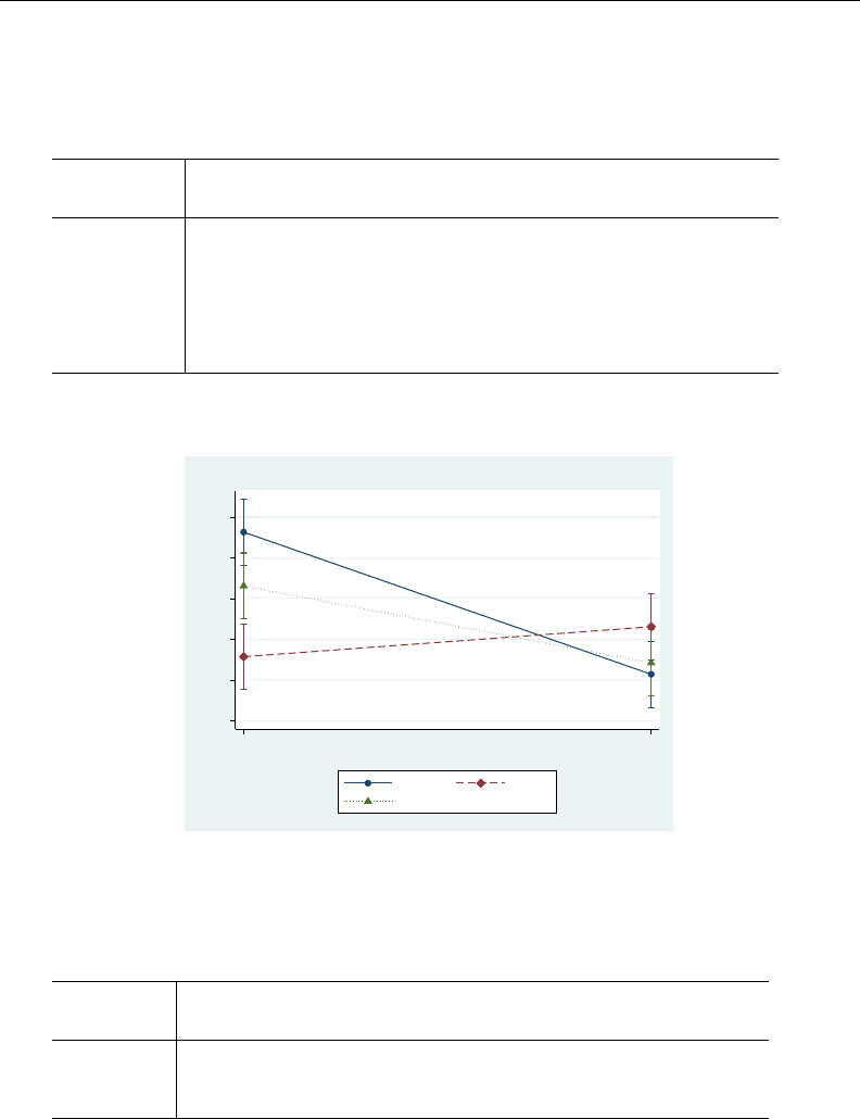
42 anova — Analysis of variance and covariance
. margins, within(program skill)
Predictive margins Number of obs = 300
Expression : Linear prediction, predict()
within : program skill
Empty cells : reweight
Delta-method
Margin Std. Err. t P>|t| [95% Conf. Interval]
program#skill
1 1 68.16 2.068542 32.95 0.000 64.08518 72.23482
1 2 52.86 2.068542 25.55 0.000 48.78518 56.93482
1 3 61.54 2.068542 29.75 0.000 57.46518 65.61482
2 1 50.7 2.068542 24.51 0.000 46.62518 54.77482
2 2 56.54 2.068542 27.33 0.000 52.46518 60.61482
2 3 52.1 2.068542 25.19 0.000 48.02518 56.17482
. marginsplot, plot2opts(lp(dash) m(D)) plot3opts(lp(dot) m(T))
Variables that uniquely identify margins: program skill
45 50 55 60 65 70
Linear Prediction
1 2
reading program
skill=1 skill=2
skill=3
Predictive Margins with 95% CIs
. margins, within(program)
Predictive margins Number of obs = 300
Expression : Linear prediction, predict()
within : program
Empty cells : reweight
Delta-method
Margin Std. Err. t P>|t| [95% Conf. Interval]
program
1 60.85333 1.194273 50.95 0.000 58.50074 63.20593
2 53.11333 1.194273 44.47 0.000 50.76074 55.46593
Because our ANOVA involves nested terms, we used the within() option of margins; see
[R]margins.
skill 2 produces a low score when combined with program 1 and a high score when combined
with program 2, demonstrating the interaction between the reading program and the skill-enhancement

anova — Analysis of variance and covariance 43
technique. You might conclude that the first reading program and the first skill-enhancement technique
perform best when combined. However, notice the overlapping confidence interval for the first reading
program and the third skill-enhancement technique.
Technical note
There are several valid ways to write complicated anova terms. In the reading experiment
example (example 13), we had a term group|class#skill|program. This term can be read
as group nested within both class and skill and further nested within program. You can
also write this term as group|class#skill#program or group|program#class#skill or
group|skill#class|program, etc. All variations will produce the same result. Some people prefer
having only one ‘|’ in a term and would use group|class#skill#program, which is read as group
nested within class,skill, and program.
Gertrude Mary Cox (1900–1978) was born on a farm near Dayton, Iowa. Initially intending to
become superintendent of an orphanage, she enrolled at Iowa State College. There she majored
in mathematics and attained the college’s first Master’s degree in statistics. After working on
her PhD in psychological statistics for two years at the University of California–Berkeley, she
decided to go back to Iowa State to work with George W. Snedecor. There she pursued her
interest in and taught a course in design of experiments. That work led to her collaboration with
W. G. Cochran, which produced a classic text. In 1940, when Snedecor shared with her his list
of men he was nominating to head the statistics department at North Carolina State College, she
wanted to know why she had not been included. He added her name, she won the position, and
she built an outstanding department at North Carolina State. Cox retired early so she could work
at the Research Triangle Institute in North Carolina. She consulted widely, served as editor of
Biometrics, and was elected to the National Academy of Sciences.
Latin-square designs
You can use anova to analyze a Latin-square design. Consider the following example, published
in Snedecor and Cochran (1989).
Example 14: Latin-square ANOVA
Data from a Latin-square design are as follows:
Row Column 1 Column 2 Column 3 Column 4 Column 5
1 257(B) 230(E) 279(A) 287(C) 202(D)
2 245(D) 283(A) 245(E) 280(B) 260(C)
3 182(E) 252(B) 280(C) 246(D) 250(A)
4 203(A) 204(C) 227(D) 193(E) 259(B)
5 231(C) 271(D) 266(B) 334(A) 338(E)

44 anova — Analysis of variance and covariance
In Stata, the data might appear as follows:
. use http://www.stata-press.com/data/r13/latinsq
. list
row c1 c2 c3 c4 c5
1. 1 257 230 279 287 202
2. 2 245 283 245 280 260
3. 3 182 252 280 246 250
4. 4 203 204 227 193 259
5. 5 231 271 266 334 338
Before anova can be used on these data, the data must be organized so that the outcome
measurement is in one column. reshape is inadequate for this task because there is information
about the treatments in the sequence of these observations. pkshape is designed to reshape this type
of data; see [R]pkshape.
. pkshape row row c1-c5, order(beacd daebc ebcda acdeb cdbae)
. list
sequence outcome treat carry period
1. 1 257 1 0 1
2. 2 245 5 0 1
3. 3 182 2 0 1
4. 4 203 3 0 1
5. 5 231 4 0 1
6. 1 230 2 1 2
7. 2 283 3 5 2
8. 3 252 1 2 2
9. 4 204 4 3 2
10. 5 271 5 4 2
11. 1 279 3 2 3
12. 2 245 2 3 3
13. 3 280 4 1 3
14. 4 227 5 4 3
15. 5 266 1 5 3
16. 1 287 4 3 4
17. 2 280 1 2 4
18. 3 246 5 4 4
19. 4 193 2 5 4
20. 5 334 3 1 4
21. 1 202 5 4 5
22. 2 260 4 1 5
23. 3 250 3 5 5
24. 4 259 1 2 5
25. 5 338 2 3 5

anova — Analysis of variance and covariance 45
. anova outcome sequence period treat
Number of obs = 25 R-squared = 0.6536
Root MSE = 32.4901 Adj R-squared = 0.3073
Source Partial SS df MS F Prob > F
Model 23904.08 12 1992.00667 1.89 0.1426
sequence 13601.36 4 3400.34 3.22 0.0516
period 6146.16 4 1536.54 1.46 0.2758
treat 4156.56 4 1039.14 0.98 0.4523
Residual 12667.28 12 1055.60667
Total 36571.36 24 1523.80667
These methods will work with any type of Latin-square design, including those with replicated
measurements. For more information, see [R]pk,[R]pkcross, and [R]pkshape.
Repeated-measures ANOVA
One approach for analyzing repeated-measures data is to use multivariate ANOVA (MANOVA); see
[MV]manova. In this approach, the data are placed in wide form (see [D]reshape), and the repeated
measures enter the MANOVA as dependent variables.
A second approach for analyzing repeated measures is to use anova. However, one of the underlying
assumptions for the Ftests in ANOVA is independence of observations. In a repeated-measures design,
this assumption is almost certainly violated or is at least suspect. In a repeated-measures ANOVA,
the subjects (or whatever the experimental units are called) are observed for each level of one or
more of the other categorical variables in the model. These variables are called the repeated-measure
variables. Observations from the same subject are likely to be correlated.
The approach used in repeated-measures ANOVA to correct for this lack of independence is to
apply a correction to the degrees of freedom of the Ftest for terms in the model that involve
repeated measures. This correction factor, , lies between the reciprocal of the degrees of freedom
for the repeated term and 1. Box (1954) provided the pioneering work in this area. Milliken and
Johnson (2009) refer to the lower bound of this correction factor as Box’s conservative correction
factor. Winer, Brown, and Michels (1991) call it simply the conservative correction factor.
Geisser and Greenhouse (1958) provide an estimate for the correction factor called the Greenhouse–
Geisser . This value is estimated from the data. Huynh and Feldt (1976) show that the Greenhouse–
Geisser tends to be conservatively biased. They provide a revised correction factor called the
Huynh–Feldt . When the Huynh–Feldt exceeds 1, it is set to 1. Thus there is a natural ordering
for these correction factors:
Box’s conservative ≤Greenhouse–Geisser ≤Huynh–Feldt ≤1
A correction factor of 1 is the same as no correction.
anova with the repeated() option computes these correction factors and displays the revised
test results in a table that follows the standard ANOVA table. In the resulting table, H-F stands for
Huynh–Feldt, G-G stands for Greenhouse–Geisser, and Box stands for Box’s conservative .

46 anova — Analysis of variance and covariance
Example 15: Repeated-measures ANOVA
This example is taken from table 4.3 of Winer, Brown, and Michels (1991). The reaction time for
five subjects each tested with four drugs was recorded in the variable score. Here is a table of the
data (see [P]tabdisp if you are unfamiliar with tabdisp):
. use http://www.stata-press.com/data/r13/t43, clear
(T4.3 -- Winer, Brown, Michels)
. tabdisp person drug, cellvar(score)
drug
person 1 2 3 4
1 30 28 16 34
2 14 18 10 22
3 24 20 18 30
4 38 34 20 44
5 26 28 14 30
drug is the repeated variable in this simple repeated-measures ANOVA example. The ANOVA is
specified as follows:
. anova score person drug, repeated(drug)
Number of obs = 20 R-squared = 0.9244
Root MSE = 3.06594 Adj R-squared = 0.8803
Source Partial SS df MS F Prob > F
Model 1379 7 197 20.96 0.0000
person 680.8 4 170.2 18.11 0.0001
drug 698.2 3 232.733333 24.76 0.0000
Residual 112.8 12 9.4
Total 1491.8 19 78.5157895
Between-subjects error term: person
Levels: 5 (4 df)
Lowest b.s.e. variable: person
Repeated variable: drug
Huynh-Feldt epsilon = 1.0789
*Huynh-Feldt epsilon reset to 1.0000
Greenhouse-Geisser epsilon = 0.6049
Box’s conservative epsilon = 0.3333
Prob > F
Source df F Regular H-F G-G Box
drug 3 24.76 0.0000 0.0000 0.0006 0.0076
Residual 12
Here the Huynh–Feldt is 1.0789, which is larger than 1. It is reset to 1, which is the same as making
no adjustment to the standard test computed in the main ANOVA table. The Greenhouse–Geisser is
0.6049, and its associated p-value is computed from an Fratio of 24.76 using 1.8147 (=3) and
7.2588 (=12) degrees of freedom. Box’s conservative is set equal to the reciprocal of the degrees
of freedom for the repeated term. Here it is 1/3, so Box’s conservative test is computed using 1 and
4 degrees of freedom for the observed Fratio of 24.76.
anova — Analysis of variance and covariance 47
Even for Box’s conservative ,drug is significant with a p-value of 0.0076. The following table
gives the predictive marginal mean score (that is, response time) for each of the four drugs:
. margins drug
Predictive margins Number of obs = 20
Expression : Linear prediction, predict()
Delta-method
Margin Std. Err. t P>|t| [95% Conf. Interval]
drug
1 26.4 1.371131 19.25 0.000 23.41256 29.38744
2 25.6 1.371131 18.67 0.000 22.61256 28.58744
3 15.6 1.371131 11.38 0.000 12.61256 18.58744
4 32 1.371131 23.34 0.000 29.01256 34.98744
The ANOVA table for this example provides an Ftest for person, but you should ignore it. An
appropriate test for person would require replication (that is, multiple measurements for person
and drug combinations). Also, without replication there is no test available for investigating the
interaction between person and drug.
Example 16: Repeated-measures ANOVA with nesting
Table 7.7 of Winer, Brown, and Michels (1991) provides another repeated-measures ANOVA example.
There are four dial shapes and two methods for calibrating dials. Subjects are nested within calibration
method, and an accuracy score is obtained. The data are shown below.
. use http://www.stata-press.com/data/r13/t77
(T7.7 -- Winer, Brown, Michels)
. tabdisp shape subject calib, cell(score)
2 methods for calibrating dials and
subject nested in calib
4 dial 1 2
shapes 1 2 3 1 2 3
1 0 3 4 4 5 7
2 0 1 3 2 4 5
3 5 5 6 7 6 8
4 3 4 2 8 6 9
The calibration method and dial shapes are fixed factors, whereas subjects are random. The
appropriate test for calibration method uses the nested subject term as the error term. Both the dial
shape and the interaction between dial shape and calibration method are tested with the dial shape
by subject interaction nested within calibration method. Here we drop this term from the anova
command, and it becomes residual error. The dial shape is the repeated variable because each subject
is tested with all four dial shapes. Here is the anova command that produces the desired results:

48 anova — Analysis of variance and covariance
. anova score calib / subject|calib shape calib#shape, repeated(shape)
Number of obs = 24 R-squared = 0.8925
Root MSE = 1.11181 Adj R-squared = 0.7939
Source Partial SS df MS F Prob > F
Model 123.125 11 11.1931818 9.06 0.0003
calib 51.0416667 1 51.0416667 11.89 0.0261
subject|calib 17.1666667 4 4.29166667
shape 47.4583333 3 15.8194444 12.80 0.0005
calib#shape 7.45833333 3 2.48611111 2.01 0.1662
Residual 14.8333333 12 1.23611111
Total 137.958333 23 5.99818841
Between-subjects error term: subject|calib
Levels: 6 (4 df)
Lowest b.s.e. variable: subject
Covariance pooled over: calib (for repeated variable)
Repeated variable: shape
Huynh-Feldt epsilon = 0.8483
Greenhouse-Geisser epsilon = 0.4751
Box’s conservative epsilon = 0.3333
Prob > F
Source df F Regular H-F G-G Box
shape 3 12.80 0.0005 0.0011 0.0099 0.0232
calib#shape 3 2.01 0.1662 0.1791 0.2152 0.2291
Residual 12
The repeated-measure corrections are applied to any terms that are tested in the main ANOVA
table and have the repeated variable in the term. These corrections are given in a table below the
main ANOVA table. Here the repeated-measures tests for shape and calib#shape are presented.
Calibration method is significant, as is dial shape. The interaction between calibration method and
dial shape is not significant. The repeated-measure corrections do not change these conclusions, but
they do change the significance level for the tests on shape and calib#shape. Here, though, unlike
in the example 15, the Huynh–Feldt is less than 1.
Here are the predictive marginal mean scores for calibration method and dial shapes. Because the
interaction was not significant, we request only the calib and shape predictive margins.
. margins, within(calib)
Predictive margins Number of obs = 24
Expression : Linear prediction, predict()
within : calib
Empty cells : reweight
Delta-method
Margin Std. Err. t P>|t| [95% Conf. Interval]
calib
1 3 .3209506 9.35 0.000 2.300709 3.699291
2 5.916667 .3209506 18.43 0.000 5.217375 6.615958

anova — Analysis of variance and covariance 49
. margins, within(shape)
Predictive margins Number of obs = 24
Expression : Linear prediction, predict()
within : shape
Empty cells : reweight
Delta-method
Margin Std. Err. t P>|t| [95% Conf. Interval]
shape
1 3.833333 .4538926 8.45 0.000 2.844386 4.82228
2 2.5 .4538926 5.51 0.000 1.511053 3.488947
3 6.166667 .4538926 13.59 0.000 5.17772 7.155614
4 5.333333 .4538926 11.75 0.000 4.344386 6.32228
Technical note
The computation of the Greenhouse–Geisser and Huynh–Feldt epsilons in a repeated-measures
ANOVA requires the number of levels and degrees of freedom for the between-subjects error term, as
well as a value computed from a pooled covariance matrix. The observations are grouped based on
all but the lowest-level variable in the between-subjects error term. The covariance over the repeated
variables is computed for each resulting group, and then these covariance matrices are pooled. The
dimension of the pooled covariance matrix is the number of levels of the repeated variable (or
combination of levels for multiple repeated variables). In example 16, there are four levels of the
repeated variable (shape), so the resulting covariance matrix is 4 ×4.
The anova command automatically attempts to determine the between-subjects error term and the
lowest-level variable in the between-subjects error term to group the observations for computation of
the pooled covariance matrix. anova issues an error message indicating that the bse() or bseunit()
option is required when anova cannot determine them. You may override the default selections of
anova by specifying the bse(),bseunit(), or grouping() option. The term specified in the bse()
option must be a term in the ANOVA model.
The default selection for the between-subjects error term (the bse() option) is the interaction of the
nonrepeated categorical variables in the ANOVA model. The first variable listed in the between-subjects
error term is automatically selected as the lowest-level variable in the between-subjects error term
but can be overridden with the bseunit(varname)option. varname is often a term, such as subject
or subsample within subject, and is most often listed first in the term because of the nesting notation
of ANOVA. This term makes sense in most repeated-measures ANOVA designs when the terms of
the model are written in standard form. For instance, in example 16, there were three categorical
variables (subject,calib, and shape), with shape being the repeated variable. Here anova looked
for a term involving only subject and calib to determine the between-subjects error term. It found
subject|calib as the term with six levels and 4 degrees of freedom. anova then picked subject
as the default for the bseunit() option (the lowest variable in the between-subjects error term)
because it was listed first in the term.
The grouping of observations proceeds, based on the different combinations of values of the
variables in the between-subjects error term, excluding the lowest level variable (as found by default
or as specified with the bseunit() option). You may specify the grouping() option to change the
default grouping used in computing the pooled covariance matrix.
The between-subjects error term, number of levels, degrees of freedom, lowest variable in the
term, and grouping information are presented after the main ANOVA table and before the rest of the
repeated-measures output.

50 anova — Analysis of variance and covariance
Example 17: Repeated-measures ANOVA with two repeated variables
Data with two repeated variables are given in table 7.13 of Winer, Brown, and Michels (1991).
The accuracy scores of subjects making adjustments to three dials during three different periods are
recorded. Three subjects are exposed to a certain noise background level, whereas a different set of
three subjects is exposed to a different noise background level. Here is a table of accuracy scores for
the noise,subject,period, and dial variables:
. use http://www.stata-press.com/data/r13/t713
(T7.13 -- Winer, Brown, Michels)
. tabdisp subject dial period, by(noise) cell(score) stubwidth(11)
noise
background
and subject 10 minute time periods and dial
nested in 1 2 3
noise 1 2 3 1 2 3 1 2 3
1
1 45 53 60 40 52 57 28 37 46
2 35 41 50 30 37 47 25 32 41
3 60 65 75 58 54 70 40 47 50
2
1 50 48 61 25 34 51 16 23 35
2 42 45 55 30 37 43 22 27 37
3 56 60 77 40 39 57 31 29 46
noise,period, and dial are fixed, whereas subject is random. Both period and dial are
repeated variables. The ANOVA for this example is specified next.

anova — Analysis of variance and covariance 51
. anova score noise / subject|noise period noise#period /
> period#subject|noise dial noise#dial /
> dial#subject|noise period#dial noise#period#dial, repeated(period dial)
Number of obs = 54 R-squared = 0.9872
Root MSE = 2.81859 Adj R-squared = 0.9576
Source Partial SS df MS F Prob > F
Model 9797.72222 37 264.803303 33.33 0.0000
noise 468.166667 1 468.166667 0.75 0.4348
subject|noise 2491.11111 4 622.777778
period 3722.33333 2 1861.16667 63.39 0.0000
noise#period 333 2 166.5 5.67 0.0293
period#subject|noise 234.888889 8 29.3611111
dial 2370.33333 2 1185.16667 89.82 0.0000
noise#dial 50.3333333 2 25.1666667 1.91 0.2102
dial#subject|noise 105.555556 8 13.1944444
period#dial 10.6666667 4 2.66666667 0.34 0.8499
noise#period#dial 11.3333333 4 2.83333333 0.36 0.8357
Residual 127.111111 16 7.94444444
Total 9924.83333 53 187.261006
Between-subjects error term: subject|noise
Levels: 6 (4 df)
Lowest b.s.e. variable: subject
Covariance pooled over: noise (for repeated variables)
Repeated variable: period
Huynh-Feldt epsilon = 1.0668
*Huynh-Feldt epsilon reset to 1.0000
Greenhouse-Geisser epsilon = 0.6476
Box’s conservative epsilon = 0.5000
Prob > F
Source df F Regular H-F G-G Box
period 2 63.39 0.0000 0.0000 0.0003 0.0013
noise#period 2 5.67 0.0293 0.0293 0.0569 0.0759
period#subject|noise 8
Repeated variable: dial
Huynh-Feldt epsilon = 2.0788
*Huynh-Feldt epsilon reset to 1.0000
Greenhouse-Geisser epsilon = 0.9171
Box’s conservative epsilon = 0.5000
Prob > F
Source df F Regular H-F G-G Box
dial 2 89.82 0.0000 0.0000 0.0000 0.0007
noise#dial 2 1.91 0.2102 0.2102 0.2152 0.2394
dial#subject|noise 8

52 anova — Analysis of variance and covariance
Repeated variables: period#dial
Huynh-Feldt epsilon = 1.3258
*Huynh-Feldt epsilon reset to 1.0000
Greenhouse-Geisser epsilon = 0.5134
Box’s conservative epsilon = 0.2500
Prob > F
Source df F Regular H-F G-G Box
period#dial 4 0.34 0.8499 0.8499 0.7295 0.5934
noise#period#dial 4 0.36 0.8357 0.8357 0.7156 0.5825
Residual 16
For each repeated variable and for each combination of interactions of repeated variables, there are
different correction values. The anova command produces tables for each applicable combination.
The two most significant factors in this model appear to be dial and period. The noise by
period interaction may also be significant, depending on the correction factor you use. Below is a
table of predictive margins for the accuracy score for dial, period, and noise by period.
. margins, within(dial)
Predictive margins Number of obs = 54
Expression : Linear prediction, predict()
within : dial
Empty cells : reweight
Delta-method
Margin Std. Err. t P>|t| [95% Conf. Interval]
dial
1 37.38889 .6643478 56.28 0.000 35.98053 38.79724
2 42.22222 .6643478 63.55 0.000 40.81387 43.63058
3 53.22222 .6643478 80.11 0.000 51.81387 54.63058
. margins, within(period)
Predictive margins Number of obs = 54
Expression : Linear prediction, predict()
within : period
Empty cells : reweight
Delta-method
Margin Std. Err. t P>|t| [95% Conf. Interval]
period
1 54.33333 .6643478 81.78 0.000 52.92498 55.74169
2 44.5 .6643478 66.98 0.000 43.09165 45.90835
3 34 .6643478 51.18 0.000 32.59165 35.40835

anova — Analysis of variance and covariance 53
. margins, within(noise period)
Predictive margins Number of obs = 54
Expression : Linear prediction, predict()
within : noise period
Empty cells : reweight
Delta-method
Margin Std. Err. t P>|t| [95% Conf. Interval]
noise#period
1 1 53.77778 .9395297 57.24 0.000 51.78606 55.76949
1 2 49.44444 .9395297 52.63 0.000 47.45273 51.43616
1 3 38.44444 .9395297 40.92 0.000 36.45273 40.43616
2 1 54.88889 .9395297 58.42 0.000 52.89717 56.8806
2 2 39.55556 .9395297 42.10 0.000 37.56384 41.54727
2 3 29.55556 .9395297 31.46 0.000 27.56384 31.54727
Dial shape 3 produces the highest score, and scores decrease over the periods.
Example 17 had two repeated-measurement variables. Up to four repeated-measurement variables
may be specified in the anova command.
Video examples
Analysis of covariance in Stata
Two-way ANOVA in Stata

54 anova — Analysis of variance and covariance
Stored results
anova stores the following in e():
Scalars
e(N) number of observations
e(mss) model sum of squares
e(df m) model degrees of freedom
e(rss) residual sum of squares
e(df r) residual degrees of freedom
e(r2) R-squared
e(r2 a) adjusted R-squared
e(F) Fstatistic
e(rmse) root mean squared error
e(ll) log likelihood
e(ll 0) log likelihood, constant-only model
e(ss #)sum of squares for term #
e(df #)numerator degrees of freedom for term #
e(ssdenom #)denominator sum of squares for term #(when using nonresidual error)
e(dfdenom #)denominator degrees of freedom for term #(when using nonresidual error)
e(F #)Fstatistic for term #(if computed)
e(N bse) number of levels of the between-subjects error term
e(df bse) degrees of freedom for the between-subjects error term
e(box#)Box’s conservative epsilon for a particular combination of repeated variables
(repeated() only)
e(gg#)Greenhouse–Geisser epsilon for a particular combination of repeated variables
(repeated() only)
e(hf#)Huynh–Feldt epsilon for a particular combination of repeated variables
(repeated() only)
e(rank) rank of e(V)
Macros
e(cmd) anova
e(cmdline) command as typed
e(depvar) name of dependent variable
e(varnames) names of the right-hand-side variables
e(term #)term #
e(errorterm #)error term for term #(when using nonresidual error)
e(sstype) type of sum of squares; sequential or partial
e(repvars) names of repeated variables (repeated() only)
e(repvar#)names of repeated variables for a particular combination (repeated() only)
e(model) ols
e(wtype) weight type
e(wexp) weight expression
e(properties) b V
e(estat cmd) program used to implement estat
e(predict) program used to implement predict
e(asbalanced) factor variables fvset as asbalanced
e(asobserved) factor variables fvset as asobserved
Matrices
e(b) coefficient vector
e(V) variance–covariance matrix of the estimators
e(Srep) covariance matrix based on repeated measures (repeated() only)
Functions
e(sample) marks estimation sample
References
Acock, A. C. 2014. A Gentle Introduction to Stata. 4th ed. College Station, TX: Stata Press.
Afifi, A. A., and S. P. Azen. 1979. Statistical Analysis: A Computer Oriented Approach. 2nd ed. New York: Academic
Press.

anova — Analysis of variance and covariance 55
Altman, D. G. 1991. Practical Statistics for Medical Research. London: Chapman & Hall/CRC.
Anderson, R. L. 1990. Gertrude Mary Cox 1900–1978. Biographical Memoirs, National Academy of Sciences 59:
116–132.
Box, G. E. P. 1954. Some theorems on quadratic forms applied in the study of analysis of variance problems, I.
Effect of inequality of variance in the one-way classification. Annals of Mathematical Statistics 25: 290–302.
Box, J. F. 1978. R. A. Fisher: The Life of a Scientist. New York: Wiley.
Chatfield, M., and A. P. Mander. 2009. The Skillings–Mack test (Friedman test when there are missing data).Stata
Journal 9: 299–305.
Cobb, G. W. 1998. Introduction to Design and Analysis of Experiments. New York: Springer.
Edwards, A. L. 1985. Multiple Regression and the Analysis of Variance and Covariance. 2nd ed. New York: Freeman.
Fisher, R. A. 1925. Statistical Methods for Research Workers. Edinburgh: Oliver & Boyd.
. 1935. The Design of Experiments. Edinburgh: Oliver & Boyd.
. 1990. Statistical Methods, Experimental Design, and Scientific Inference. Oxford: Oxford University Press.
Geisser, S., and S. W. Greenhouse. 1958. An extension of Box’s results on the use of the F distribution in multivariate
analysis. Annals of Mathematical Statistics 29: 885–891.
Gleason, J. R. 1999. sg103: Within subjects (repeated measures) ANOVA, including between subjects factors.Stata
Technical Bulletin 47: 40–45. Reprinted in Stata Technical Bulletin Reprints, vol. 8, pp. 236–243. College Station,
TX: Stata Press.
. 2000. sg132: Analysis of variance from summary statistics.Stata Technical Bulletin 54: 42–46. Reprinted in
Stata Technical Bulletin Reprints, vol. 9, pp. 328–332. College Station, TX: Stata Press.
Hall, N. S. 2010. Ronald Fisher and Gertrude Cox: Two statistical pioneers sometimes cooperate and sometimes
collide. American Statistician 64: 212–220.
Higgins, J. E., and G. G. Koch. 1977. Variable selection and generalized chi-square analysis of categorical data
applied to a large cross-sectional occupational health survey. International Statistical Review 45: 51–62.
Huynh, H. 1978. Some approximate tests for repeated measurement designs. Psychometrika 43: 161–175.
Huynh, H., and L. S. Feldt. 1976. Estimation of the Box correction for degrees of freedom from sample data in
randomized block and split-plot designs. Journal of Educational Statistics 1: 69–82.
Kennedy, W. J., Jr., and J. E. Gentle. 1980. Statistical Computing. New York: Dekker.
Kuehl, R. O. 2000. Design of Experiments: Statistical Principles of Research Design and Analysis. 2nd ed. Belmont,
CA: Duxbury.
Marchenko, Y. V. 2006. Estimating variance components in Stata.Stata Journal 6: 1–21.
Milliken, G. A., and D. E. Johnson. 2009. Analysis of Messy Data, Volume 1: Designed Experiments. 2nd ed. Boca
Raton, FL: CRC Press.
Mitchell, M. N. 2012. Interpreting and Visualizing Regression Models Using Stata. College Station, TX: Stata Press.
Scheff´
e, H. 1959. The Analysis of Variance. New York: Wiley.
Snedecor, G. W., and W. G. Cochran. 1989. Statistical Methods. 8th ed. Ames, IA: Iowa State University Press.
van Belle, G., L. D. Fisher, P. J. Heagerty, and T. S. Lumley. 2004. Biostatistics: A Methodology for the Health
Sciences. 2nd ed. New York: Wiley.
Winer, B. J., D. R. Brown, and K. M. Michels. 1991. Statistical Principles in Experimental Design. 3rd ed. New
York: McGraw–Hill.

56 anova — Analysis of variance and covariance
Also see
[R]anova postestimation — Postestimation tools for anova
[R]contrast — Contrasts and linear hypothesis tests after estimation
[R]icc — Intraclass correlation coefficients
[R]loneway — Large one-way ANOVA, random effects, and reliability
[R]oneway — One-way analysis of variance
[R]regress — Linear regression
[MV]manova — Multivariate analysis of variance and covariance
[PSS]power oneway — Power analysis for one-way analysis of variance
[PSS]power repeated — Power analysis for repeated-measures analysis of variance
[PSS]power twoway — Power analysis for two-way analysis of variance
Stata Structural Equation Modeling Reference Manual

Title
anova postestimation — Postestimation tools for anova
Description Syntax for predict Syntax for test after anova
Menu for test after anova Options for test after anova Remarks and examples
References Also see
Description
The following postestimation commands are of special interest after anova:
Command Description
dfbeta DFBETA influence statistics
estat hettest tests for heteroskedasticity
estat imtest information matrix test
estat ovtest Ramsey regression specification-error test for omitted variables
estat szroeter Szroeter’s rank test for heteroskedasticity
estat vif variance inflation factors for the independent variables
estat esize η2and ω2effect sizes
rvfplot residual-versus-fitted plot
avplot added-variable plot
avplots all added-variables plots in one image
cprplot component-plus-residual plot
acprplot augmented component-plus-residual plot
rvpplot residual-versus-predictor plot
lvr2plot leverage-versus-squared-residual plot
57

58 anova postestimation — Postestimation tools for anova
The following standard postestimation commands are also available:
Command Description
contrast contrasts and ANOVA-style joint tests of estimates
estat ic Akaike’s and Schwarz’s Bayesian information criteria (AIC and BIC)
estat summarize summary statistics for the estimation sample
estat vce variance–covariance matrix of the estimators (VCE)
estimates cataloging estimation results
hausman Hausman’s specification test
lincom point estimates, standard errors, testing, and inference for linear
combinations of coefficients
linktest link test for model specification
lrtest likelihood-ratio test
margins marginal means, predictive margins, marginal effects, and average marginal
effects
marginsplot graph the results from margins (profile plots, interaction plots, etc.)
nlcom point estimates, standard errors, testing, and inference for nonlinear
combinations of coefficients
predict predictions, residuals, influence statistics, and other diagnostic measures
predictnl point estimates, standard errors, testing, and inference for generalized predictions
pwcompare pairwise comparisons of estimates
suest seemingly unrelated estimation
test Wald tests of simple and composite linear hypotheses
testnl Wald tests of nonlinear hypotheses
Special-interest postestimation commands
In addition to the common estat commands (see [R]estat), estat hettest,estat imtest,
estat ovtest,estat szroeter, and estat vif are also available. dfbeta is also available.
The syntax for dfbeta and these estat commands is the same as after regress; see [R]regress
postestimation.
For information on the plot commands, see [R]regress postestimation diagnostic plots.
In addition to the standard syntax of test (see [R]test), test after anova has three additionally
allowed syntaxes; see below. test performs Wald tests of expressions involving the coefficients of
the underlying regression model. Simple and composite linear hypotheses are possible.
Syntax for predict
predict after anova follows the same syntax as predict after regress and can provide
predictions, residuals, standardized residuals, Studentized residuals, the standard error of the residuals,
the standard error of the prediction, the diagonal elements of the projection (hat) matrix, and Cook’s D.
See [R]regress postestimation for details.

anova postestimation — Postestimation tools for anova 59
Syntax for test after anova
In addition to the standard syntax of test (see [R]test), test after anova also allows the
following:
test, test(matname)mtest(opt)matvlc(matname)syntax a
test, showorder syntax b
test term term . . . /term term . . . , symbolic syntax c
syntax a test expression involving the coefficients of the underlying regression model;
you provide information as a matrix
syntax b show underlying order of design matrix, which is useful when constructing
matname argument of the test() option
syntax c test effects and show symbolic forms
Menu for test after anova
Statistics >Linear models and related >ANOVA/MANOVA >Test linear hypotheses after anova
Options for test after anova
test(matname)is required with syntax a of test. The rows of matname specify linear combinations
of the underlying design matrix of the ANOVA that are to be jointly tested. The columns correspond
to the underlying design matrix (including the constant if it has not been suppressed). The column
and row names of matname are ignored.
A listing of the constraints imposed by the test() option is presented before the table containing
the tests. You should examine this table to verify that you have applied the linear combinations
you desired. Typing test, showorder allows you to examine the ordering of the columns for
the design matrix from the ANOVA.
mtest(opt)specifies that tests are performed for each condition separately. opt specifies the method
for adjusting p-values for multiple testing. Valid values for opt are
bonferroni Bonferroni’s method
holm Holm’s method
sidak ˇ
Sid´
ak’s method
noadjust no adjustment is to be made
Specifying mtest with no argument is equivalent to mtest(noadjust).
matvlc(matname), a programmer’s option, saves the variance–covariance matrix of the linear
combinations involved in the suite of tests. For the test Lb =c, what is returned in matname is
LVL0, where Vis the estimated variance–covariance matrix of b.
showorder causes test to list the definition of each column in the design matrix. showorder is
not allowed with any other option.
symbolic requests the symbolic form of the test rather than the test statistic. When this option
is specified with no terms (test, symbolic), the symbolic form of the estimable functions is
displayed.

60 anova postestimation — Postestimation tools for anova
Remarks and examples
Remarks are presented under the following headings:
Testing effects
Obtaining symbolic forms
Testing coefficients and contrasts of margins
Video example
See examples 4,7,8,13,15,16, and 17 in [R]anova for examples that use the margins command.
Testing effects
After fitting a model using anova, you can test for the significance of effects in the ANOVA table,
as well as for effects that are not reported in the ANOVA table, by using the test or contrast
command. You follow test or contrast by the list of effects that you wish to test. By default, these
commands use the residual mean squared error in the denominator of the Fratio. You can specify
other error terms by using the slash notation, just as you would with anova. See [R]contrast for
details on this command.
Example 1: Testing effects
Recall our byssinosis example (example 8) in [R]anova:
. anova prob workplace smokes race workplace#smokes workplace#race smokes#race
> workplace#smokes#race [aweight=pop]
(sum of wgt is 5.4190e+03)
Number of obs = 65 R-squared = 0.8300
Root MSE = .025902 Adj R-squared = 0.7948
Source Partial SS df MS F Prob > F
Model .173646538 11 .015786049 23.53 0.0000
workplace .097625175 2 .048812588 72.76 0.0000
smokes .013030812 1 .013030812 19.42 0.0001
race .001094723 1 .001094723 1.63 0.2070
workplace#smokes .019690342 2 .009845171 14.67 0.0000
workplace#race .001352516 2 .000676258 1.01 0.3718
smokes#race .001662874 1 .001662874 2.48 0.1214
workplace#smokes#race .000950841 2 .00047542 0.71 0.4969
Residual .035557766 53 .000670901
Total .209204304 64 .003268817
We can easily obtain a test on a particular term from the ANOVA table. Here are two examples:
. test smokes
Source Partial SS df MS F Prob > F
smokes .013030812 1 .013030812 19.42 0.0001
Residual .035557766 53 .000670901
. test smokes#race
Source Partial SS df MS F Prob > F
smokes#race .001662874 1 .001662874 2.48 0.1214
Residual .035557766 53 .000670901
Both of these tests use residual error by default and agree with the ANOVA table produced earlier.

anova postestimation — Postestimation tools for anova 61
We could have performed these same tests with contrast:
. contrast smokes
Contrasts of marginal linear predictions
Margins : asbalanced
df F P>F
smokes 1 19.42 0.0001
Denominator 53
. contrast smokes#race
Contrasts of marginal linear predictions
Margins : asbalanced
df F P>F
smokes#race 1 2.48 0.1214
Denominator 53
Technical note
After anova, you can use the ‘/’ syntax in test or contrast to perform tests with a variety of
non-σ2Ierror structures. However, in most unbalanced models, the mean squares are not independent
and do not have equal expectations under the null hypothesis. Also, be warned that you assume
responsibility for the validity of the test statistic.
Example 2: Testing effects with different error terms
We return to the nested ANOVA example (example 11)in[R]anova, where five brands of machinery
were compared in an assembly line. We can obtain appropriate tests for the nested terms using test,
even if we had run the anova command without initially indicating the proper error terms.
. use http://www.stata-press.com/data/r13/machine
(machine data)
. anova output machine / operator|machine /
Number of obs = 57 R-squared = 0.8661
Root MSE = 1.47089 Adj R-squared = 0.8077
Source Partial SS df MS F Prob > F
Model 545.822288 17 32.1071934 14.84 0.0000
machine 430.980792 4 107.745198 13.82 0.0001
operator|machine 101.353804 13 7.79644648
operator|machine 101.353804 13 7.79644648 3.60 0.0009
Residual 84.3766582 39 2.16350406
Total 630.198947 56 11.2535526

62 anova postestimation — Postestimation tools for anova
In this ANOVA table, machine is tested with residual error. With this particular nested design, the
appropriate error term for testing machine is operator nested within machine, which is easily
obtained from test.
. test machine / operator|machine
Source Partial SS df MS F Prob > F
machine 430.980792 4 107.745198 13.82 0.0001
operator|machine 101.353804 13 7.79644648
This result from test matches what we obtained from our anova command.
Example 3: Pooling terms when testing effects
The other nested ANOVA example (example 12)in[R]anova was based on the sewage data. The
ANOVA table is presented here again. As before, we will use abbreviations of variable names in typing
the commands.
. use http://www.stata-press.com/data/r13/sewage
(Sewage treatment)
. anova particulate s / m|s / f|m|s / w|f|m|s /, dropemptycells
Number of obs = 64 R-squared = 0.6338
Root MSE = 12.7445 Adj R-squared = 0.5194
Source Partial SS df MS F Prob > F
Model 13493.6094 15 899.573958 5.54 0.0000
solution 7203.76563 1 7203.76563 17.19 0.0536
manager|solution 838.28125 2 419.140625
manager|solution 838.28125 2 419.140625 0.55 0.6166
facility|manager|
solution 3064.9375 4 766.234375
facility|manager|
solution 3064.9375 4 766.234375 2.57 0.1193
worker|facility|
manager|solution 2386.625 8 298.328125
worker|facility|
manager|solution 2386.625 8 298.328125 1.84 0.0931
Residual 7796.25 48 162.421875
Total 21289.8594 63 337.934276
In practice, it is often beneficial to pool nonsignificant nested terms to increase the power of
tests on remaining terms. One rule of thumb is to allow the pooling of a term whose p-value is
larger than 0.25. In this sewage example, the p-value for the test of manager is 0.6166. This value
indicates that the manager effect is negligible and might be ignored. Currently, solution is tested by
manager|solution, which has only 2 degrees of freedom. If we pool the manager and facility
terms and use this pooled estimate as the error term for solution, we would have a term with 6
degrees of freedom.
Below are two tests: a test of solution with the pooled manager and facility terms and a
test of this pooled term by worker.

anova postestimation — Postestimation tools for anova 63
. test s / m|s f|m|s
Source Partial SS df MS F Prob > F
solution 7203.76563 1 7203.76563 11.07 0.0159
manager|solution
facility|manager|
solution 3903.21875 6 650.536458
. test m|s f|m|s / w|f|m|s
Source Partial SS df MS F Prob > F
manager|solution
facility|manager|
solution 3903.21875 6 650.536458 2.18 0.1520
worker|facility|manager|
solution 2386.625 8 298.328125
In the first test, we included two terms after the forward slash (m|s and f|m|s). test after anova
allows multiple terms both before and after the slash. The terms before the slash are combined and
are then tested by the combined terms that follow the slash (or residual error if no slash is present).
The p-value for solution using the pooled term is 0.0159. Originally, it was 0.0536. The increase
in the power of the test is due to the increase in degrees of freedom for the pooled error term.
We can get identical results if we drop manager from the anova model. (This dataset has unique
numbers for each facility so that there is no confusion of facilities when manager is dropped.)
. anova particulate s / f|s / w|f|s /, dropemptycells
Number of obs = 64 R-squared = 0.6338
Root MSE = 12.7445 Adj R-squared = 0.5194
Source Partial SS df MS F Prob > F
Model 13493.6094 15 899.573958 5.54 0.0000
solution 7203.76563 1 7203.76563 11.07 0.0159
facility|solution 3903.21875 6 650.536458
facility|solution 3903.21875 6 650.536458 2.18 0.1520
worker|facility|
solution 2386.625 8 298.328125
worker|facility|
solution 2386.625 8 298.328125 1.84 0.0931
Residual 7796.25 48 162.421875
Total 21289.8594 63 337.934276
This output agrees with our earlier test results.
In the following example, two terms from the anova are jointly tested (pooled).
64 anova postestimation — Postestimation tools for anova
Example 4: Obtaining overall significance of a term using contrast
In example 10 of [R]anova, we fit the model anova drate region c.mage region#c.mage.
Now we use the contrast command to test for the overall significance of region.
. contrast region region#c.mage, overall
Contrasts of marginal linear predictions
Margins : asbalanced
df F P>F
region 3 7.40 0.0004
region#c.mage 3 0.86 0.4689
Overall 6 5.65 0.0002
Denominator 42
The overall Fstatistic associated with the region and region#c.mage terms is 5.65, and it is
significant at the 0.02% level.
In the ANOVA output, the region term, by itself, had a sum of squares of 1166.15, which, based
on 3 degrees of freedom, yielded an Fstatistic of 7.40 and a significance level of 0.0004. This is
the same test that is reported by contrast in the row labeled region. Likewise, the test from the
ANOVA output for the region#c.mage term is reproduced in the second row of the contrast output.
Obtaining symbolic forms
test can produce the symbolic form of the estimable functions and symbolic forms for particular
tests.
Example 5: Symbolic form of the estimable functions
After fitting an ANOVA model, we type test, symbolic to obtain the symbolic form of the
estimable functions. For instance, returning to our blood pressure data introduced in example 4 of
[R]anova, let’s begin by reestimating systolic on drug,disease, and drug#disease:
. use http://www.stata-press.com/data/r13/systolic, clear
(Systolic Blood Pressure Data)
. anova systolic drug disease drug#disease
Number of obs = 58 R-squared = 0.4560
Root MSE = 10.5096 Adj R-squared = 0.3259
Source Partial SS df MS F Prob > F
Model 4259.33851 11 387.212591 3.51 0.0013
drug 2997.47186 3 999.157287 9.05 0.0001
disease 415.873046 2 207.936523 1.88 0.1637
drug#disease 707.266259 6 117.87771 1.07 0.3958
Residual 5080.81667 46 110.452536
Total 9340.15517 57 163.862371

anova postestimation — Postestimation tools for anova 65
To obtain the symbolic form of the estimable functions, type
. test, symbolic
drug
1 -(r2+r3+r4-r0)
2 r2
3 r3
4 r4
disease
1 -(r6+r7-r0)
2 r6
3 r7
drug#disease
1 1 -(r2+r3+r4+r6+r7-r12-r13-r15-r16-r18-r19-r0)
1 2 r6 - (r12+r15+r18)
1 3 r7 - (r13+r16+r19)
2 1 r2 - (r12+r13)
2 2 r12
2 3 r13
3 1 r3 - (r15+r16)
3 2 r15
3 3 r16
4 1 r4 - (r18+r19)
4 2 r18
4 3 r19
_cons r0
Example 6: Symbolic form for a particular test
To obtain the symbolic form for a particular test, we type test term [term . . . ], symbolic. For
instance, the symbolic form for the test of the main effect of drug is
. test drug, symbolic
drug
1 -(r2+r3+r4)
2 r2
3 r3
4 r4
disease
1 0
2 0
3 0
drug#disease
1 1 -1/3 (r2+r3+r4)
1 2 -1/3 (r2+r3+r4)
1 3 -1/3 (r2+r3+r4)
2 1 1/3 r2
2 2 1/3 r2
2 3 1/3 r2
3 1 1/3 r3
3 2 1/3 r3
3 3 1/3 r3
4 1 1/3 r4
4 2 1/3 r4
4 3 1/3 r4
_cons 0

66 anova postestimation — Postestimation tools for anova
If we omit the symbolic option, we instead see the result of the test:
. test drug
Source Partial SS df MS F Prob > F
drug 2997.47186 3 999.157287 9.05 0.0001
Residual 5080.81667 46 110.452536
Testing coefficients and contrasts of margins
The test command allows you to perform tests directly on the coefficients of the underly-
ing regression model. For instance, the coefficient on the third drug and the second disease
is referred to as 3.drug#2.disease. This could also be written as i3.drug#i2.disease, or
b[3.drug#2.disease], or even coef[i3.drug#i2.disease]; see [U] 13.5 Accessing coeffi-
cients and standard errors.
Example 7: Testing linear combinations of coefficients
Let’s begin by testing whether the coefficient on the third drug is equal to the coefficient on the
fourth in our blood pressure data. We have already fit the model anova systolic drug##disease
(equivalent to anova systolic drug disease drug#disease), and you can see the results of that
estimation in example 5. Even though we have performed many tasks since we fit the model, Stata
still remembers, and we can perform tests at any time.
. test 3.drug = 4.drug
( 1) 3.drug - 4.drug = 0
F( 1, 46) = 0.13
Prob > F = 0.7234
We find that the two coefficients are not significantly different, at least at any significance level smaller
than 73%.
For more complex tests, the contrast command often provides a more concise way to specify
the test we are interested in and prevents us from having to write the tests in terms of the regression
coefficients. With contrast, we instead specify our tests in terms of differences in the marginal
means for the levels of a particular factor. For example, if we want to compare the third and fourth
drugs, we can test the difference in the mean impact on systolic blood pressure separately for each
disease using the @operator. We also use the reverse adjacent operator, ar., to compare the fourth
level of drug with the previous level.

anova postestimation — Postestimation tools for anova 67
. contrast ar4.drug@disease
Contrasts of marginal linear predictions
Margins : asbalanced
df F P>F
drug@disease
(4 vs 3) 1 1 0.13 0.7234
(4 vs 3) 2 1 1.76 0.1917
(4 vs 3) 3 1 0.65 0.4230
Joint 3 0.85 0.4761
Denominator 46
Contrast Std. Err. [95% Conf. Interval]
drug@disease
(4 vs 3) 1 -2.733333 7.675156 -18.18262 12.71595
(4 vs 3) 2 8.433333 6.363903 -4.376539 21.24321
(4 vs 3) 3 5.7 7.050081 -8.491077 19.89108
None of the individual contrasts shows significant differences between the third drug and the
fourth drug. Likewise, the overall Fstatistic is 0.85, which is hardly significant. We cannot reject
the hypothesis that the third drug has the same effect as the fourth drug.
Technical note
Alternatively, we could have specified these tests based on the coefficients of the underlying
regression model using the test command. We would have needed to perform tests on the coefficients
for drug and for the coefficients on drug interacted with disease in order to test for differences in
the means mentioned above. To do this, we start with our previous test command:
. test 3.drug = 4.drug
Notice that the Fstatistic for this test is equivalent to the test labeled (4 vs 3) 1 in the contrast
output. Let’s now add the constraint that the coefficient on the third drug interacted with the third
disease is equal to the coefficient on the fourth drug, again interacted with the third disease. We do
that by typing the new constraint and adding the accumulate option:
. test 3.drug#3.disease = 4.drug#3.disease, accumulate
( 1) 3.drug - 4.drug = 0
( 2) 3.drug#3.disease - 4.drug#3.disease = 0
F( 2, 46) = 0.39
Prob > F = 0.6791
So far, our test includes the equality of the two drug coefficients, along with the equality of the
two drug coefficients when interacted with the third disease. Now we add two more equations, one
for each of the remaining two diseases:

68 anova postestimation — Postestimation tools for anova
. test 3.drug#2.disease = 4.drug#2.disease, accumulate
( 1) 3.drug - 4.drug = 0
( 2) 3.drug#3.disease - 4.drug#3.disease = 0
( 3) 3.drug#2.disease - 4.drug#2.disease = 0
F( 3, 46) = 0.85
Prob > F = 0.4761
. test 3.drug#1.disease = 4.drug#1.disease, accumulate
( 1) 3.drug - 4.drug = 0
( 2) 3.drug#3.disease - 4.drug#3.disease = 0
( 3) 3.drug#2.disease - 4.drug#2.disease = 0
( 4) 3o.drug#1b.disease - 4o.drug#1b.disease = 0
Constraint 4 dropped
F( 3, 46) = 0.85
Prob > F = 0.4761
The overall Fstatistic reproduces the one from the joint test in the contrast output.
You may notice that we also got the message “Constraint 4 dropped”. For the technically inclined,
this constraint was unnecessary, given the normalization of the model. If we specify all the constraints
involved in our test or use contrast, we need not worry about the normalization because Stata
handles this automatically.
The test() option of test provides another alternative for testing coefficients. Instead of spelling
out each coefficient involved in the test, a matrix representing the test provides the needed information.
test, showorder shows the order of the terms in the ANOVA corresponding to the order of the
columns for the matrix argument of test().
Example 8: Another way to test linear combinations of coefficients
We repeat the last test of example 7 above with the test() option. First, we view the definition
and order of the columns underlying the ANOVA performed on the systolic data.

anova postestimation — Postestimation tools for anova 69
. test, showorder
Order of columns in the design matrix
1: (drug==1)
2: (drug==2)
3: (drug==3)
4: (drug==4)
5: (disease==1)
6: (disease==2)
7: (disease==3)
8: (drug==1)*(disease==1)
9: (drug==1)*(disease==2)
10: (drug==1)*(disease==3)
11: (drug==2)*(disease==1)
12: (drug==2)*(disease==2)
13: (drug==2)*(disease==3)
14: (drug==3)*(disease==1)
15: (drug==3)*(disease==2)
16: (drug==3)*(disease==3)
17: (drug==4)*(disease==1)
18: (drug==4)*(disease==2)
19: (drug==4)*(disease==3)
20: _cons
Columns 1–4 correspond to the four levels of drug. Columns 5–7 correspond to the three levels
of disease. Columns 8–19 correspond to the interaction of drug and disease. The last column
corresponds to cons, the constant in the model.
We construct the matrix dr3vs4 with the same four constraints as the last test shown in example 7
and then use the test(dr3vs4) option to perform the test.
. matrix dr3vs4 = (0,0,1,-1, 0,0,0, 0,0,0,0,0,0,0,0,0, 0, 0, 0, 0 \
> 0,0,0, 0, 0,0,0, 0,0,0,0,0,0,0,0,1, 0, 0,-1, 0 \
> 0,0,0, 0, 0,0,0, 0,0,0,0,0,0,0,1,0, 0,-1, 0, 0 \
> 0,0,0, 0, 0,0,0, 0,0,0,0,0,0,1,0,0,-1, 0, 0, 0)
. test, test(dr3vs4)
( 1) 3.drug - 4.drug = 0
( 2) 3.drug#3.disease - 4.drug#3.disease = 0
( 3) 3.drug#2.disease - 4.drug#2.disease = 0
( 4) 3o.drug#1b.disease - 4o.drug#1b.disease = 0
Constraint 4 dropped
F( 3, 46) = 0.85
Prob > F = 0.4761
Here the effort involved with spelling out the coefficients is similar to that of constructing a matrix
and using it in the test() option. When the test involving coefficients is more complicated, the
test() option may be more convenient than specifying the coefficients directly in test. However,
as previously demonstrated, contrast may provide an even simpler method for testing the same
hypothesis.
After fitting an ANOVA model, various contrasts (1-degree-of-freedom tests comparing different
levels of a categorical variable) are often of interest. contrast can perform each 1-degree-of-freedom
test in addition to the combined test, even in cases in which the contrasts do not correspond to one
of the contrast operators.

70 anova postestimation — Postestimation tools for anova
Example 9: Testing particular contrasts of interest
Rencher and Schaalje (2008) illustrate 1-degree-of-freedom contrasts for an ANOVA comparing the
net weight of cans filled by five machines (labeled A–E). The data were originally obtained from
Ostle and Mensing (1975). Rencher and Schaalje use a cell-means ANOVA model approach for this
problem. We could do the same by using the noconstant option of anova; see [R]anova. Instead,
we obtain the same results by using the standard overparameterized ANOVA approach (that is, we
keep the constant in the model).
. use http://www.stata-press.com/data/r13/canfill
(Can Fill Data)
. list, sepby(machine)
machine weight
1. A 11.95
2. A 12.00
3. A 12.25
4. A 12.10
5. B 12.18
6. B 12.11
7. C 12.16
8. C 12.15
9. C 12.08
10. D 12.25
11. D 12.30
12. D 12.10
13. E 12.10
14. E 12.04
15. E 12.02
16. E 12.02
. anova weight machine
Number of obs = 16 R-squared = 0.4123
Root MSE = .087758 Adj R-squared = 0.1986
Source Partial SS df MS F Prob > F
Model .059426993 4 .014856748 1.93 0.1757
machine .059426993 4 .014856748 1.93 0.1757
Residual .084716701 11 .007701518
Total .144143694 15 .00960958
The four 1-degree-of-freedom tests of interest among the five machines are Aand Dversus B,C,
and E;Band Eversus C;Aversus D; and Bversus E. We can specify these tests as user-defined
contrasts by placing the corresponding contrast coefficients into positions related to the five levels of
machine as described in User-defined contrasts of [R]contrast.

anova postestimation — Postestimation tools for anova 71
. contrast {machine 3 -2 -2 3 -2}
> {machine 0 1 -2 0 1}
> {machine 1 0 0 -1 0}
> {machine 0 1 0 0 -1}, noeffects
Contrasts of marginal linear predictions
Margins : asbalanced
df F P>F
machine
(1) 1 0.75 0.4055
(2) 1 0.31 0.5916
(3) 1 4.47 0.0582
(4) 1 1.73 0.2150
Joint 4 1.93 0.1757
Denominator 11
contrast produces a 1-degree-of-freedom test for each of the specified contrasts as well as a
joint test. We included the noeffects option so that the table displaying the values of the individual
contrasts with their confidence intervals was suppressed.
The significance values above are not adjusted for multiple comparisons. We could have produced
the Bonferroni-adjusted significance values by using the mcompare(bonferroni) option.
. contrast {machine 3 -2 -2 3 -2}
> {machine 0 1 -2 0 1}
> {machine 1 0 0 -1 0}
> {machine 0 1 0 0 -1}, mcompare(bonferroni) noeffects
Contrasts of marginal linear predictions
Margins : asbalanced
Bonferroni
df F P>F P>F
machine
(1) 1 0.75 0.4055 1.0000
(2) 1 0.31 0.5916 1.0000
(3) 1 4.47 0.0582 0.2329
(4) 1 1.73 0.2150 0.8601
Joint 4 1.93 0.1757
Denominator 11
Note: Bonferroni-adjusted p-values are reported for tests
on individual contrasts only.
Example 10: Linear and quadratic contrasts
Here there are two factors, Aand B, each with three levels. The levels are quantitative so that
linear and quadratic contrasts are of interest.

72 anova postestimation — Postestimation tools for anova
. use http://www.stata-press.com/data/r13/twowaytrend
. anova Y A B A#B
Number of obs = 36 R-squared = 0.9304
Root MSE = 2.6736 Adj R-squared = 0.9097
Source Partial SS df MS F Prob > F
Model 2578.55556 8 322.319444 45.09 0.0000
A 2026.72222 2 1013.36111 141.77 0.0000
B 383.722222 2 191.861111 26.84 0.0000
A#B 168.111111 4 42.0277778 5.88 0.0015
Residual 193 27 7.14814815
Total 2771.55556 35 79.1873016
We can use the p. contrast operator to obtain the 1-degree-of-freedom tests for the linear and
quadratic effects of Aand B.
. contrast p.A p.B, noeffects
Contrasts of marginal linear predictions
Margins : asbalanced
df F P>F
A
(linear) 1 212.65 0.0000
(quadratic) 1 70.88 0.0000
Joint 2 141.77 0.0000
B
(linear) 1 26.17 0.0000
(quadratic) 1 27.51 0.0000
Joint 2 26.84 0.0000
Denominator 27
All the above tests appear to be significant. In addition to presenting the 1-degree-of-freedom tests,
the combined tests for Aand Bare produced and agree with the original ANOVA results.
Now we explore the interaction between Aand B.
. contrast p.A#p1.B, noeffects
Contrasts of marginal linear predictions
Margins : asbalanced
df F P>F
A#B
(linear) (linear) 1 17.71 0.0003
(quadratic) (linear) 1 0.07 0.7893
Joint 2 8.89 0.0011
Denominator 27
The 2-degrees-of-freedom test of the interaction of Awith the linear components of Bis significant
at the 0.0011 level. But, when we examine the two 1-degree-of-freedom tests that compose this result,

anova postestimation — Postestimation tools for anova 73
the significance is due to the linear Aby linear Bcontrast (significance level of 0.0003). A significance
value of 0.7893 for the quadratic Aby linear Bindicates that this factor is not significant for these
data.
. contrast p.A#p2.B, noeffects
Contrasts of marginal linear predictions
Margins : asbalanced
df F P>F
A#B
(linear) (quadratic) 1 2.80 0.1058
(quadratic) (quadratic) 1 2.94 0.0979
Joint 2 2.87 0.0741
Denominator 27
The test of Awith the quadratic components of Bdoes not fall below the 0.05 significance level.
Video example
Introduction to contrasts in Stata: One-way ANOVA
References
Mitchell, M. N. 2012. Interpreting and Visualizing Regression Models Using Stata. College Station, TX: Stata Press.
Ostle, B., and R. W. Mensing. 1975. Statistics in Research. 3rd ed. Ames, IA: Iowa State University Press.
Rencher, A. C., and G. B. Schaalje. 2008. Linear Models in Statistics. 2nd ed. New York: Wiley.
Also see
[R]anova — Analysis of variance and covariance
[R]regress postestimation — Postestimation tools for regress
[R]regress postestimation diagnostic plots — Postestimation plots for regress
[U] 20 Estimation and postestimation commands

Title
areg — Linear regression with a large dummy-variable set
Syntax Menu Description Options
Remarks and examples Stored results Methods and formulas References
Also see
Syntax
areg depvar indepvars if in weight , absorb(varname)options
options Description
Model
∗absorb(varname)categorical variable to be absorbed
SE/Robust
vce(vcetype)vcetype may be ols,robust,cluster clustvar,bootstrap,
or jackknife
Reporting
level(#)set confidence level; default is level(95)
display options control column formats, row spacing, line width, display of omitted
variables and base and empty cells, and factor-variable labeling
coeflegend display legend instead of statistics
∗absorb(varname)is required.
indepvars may contain factor variables; see [U] 11.4.3 Factor variables.
depvar and indepvars may contain time-series operators; see [U] 11.4.4 Time-series varlists.
bootstrap,by,fp,jackknife,mi estimate,rolling, and statsby are allowed; see [U] 11.1.10 Prefix commands.
vce(bootstrap) and vce(jackknife) are not allowed with the mi estimate prefix; see [MI] mi estimate.
Weights are not allowed with the bootstrap prefix; see [R] bootstrap.
aweights are not allowed with the jackknife prefix; see [R] jackknife.
aweights, fweights, and pweights are allowed; see [U] 11.1.6 weight.
coeflegend does not appear in the dialog box.
See [U] 20 Estimation and postestimation commands for more capabilities of estimation commands.
Menu
Statistics >Linear models and related >Other >Linear regression absorbing one cat. variable
Description
areg fits a linear regression absorbing one categorical factor. areg is designed for datasets with
many groups, but not a number of groups that increases with the sample size. See the xtreg, fe
command in [XT]xtreg for an estimator that handles the case in which the number of groups increases
with the sample size.
74

areg — Linear regression with a large dummy-variable set 75
Options
Model
absorb(varname)specifies the categorical variable, which is to be included in the regression as if
it were specified by dummy variables. absorb() is required.
SE/Robust
vce(vcetype)specifies the type of standard error reported, which includes types that are derived
from asymptotic theory (ols), that are robust to some kinds of misspecification (robust), that
allow for intragroup correlation (cluster clustvar), and that use bootstrap or jackknife methods
(bootstrap,jackknife); see [R]vce option.
vce(ols), the default, uses the standard variance estimator for ordinary least-squares regression.
Exercise caution when using the vce(cluster clustvar)option with areg. The effective number
of degrees of freedom for the robust variance estimator is ng−1, where ngis the number of
clusters. Thus the number of levels of the absorb() variable should not exceed the number of
clusters.
Reporting
level(#); see [R]estimation options.
display options:noomitted,vsquish,noemptycells,baselevels,allbaselevels,nofvla-
bel,fvwrap(#),fvwrapon(style),cformat(%fmt),pformat(% fmt),sformat(% fmt), and
nolstretch; see [R]estimation options.
The following option is available with areg but is not shown in the dialog box:
coeflegend; see [R]estimation options.
Remarks and examples
Suppose that you have a regression model that includes among the explanatory variables a large
number, k, of mutually exclusive and exhaustive dummies:
y=Xβ+d1γ1+d2γ2+··· +dkγk+
For instance, the dummy variables, di, might indicate countries in the world or states of the United
States. One solution would be to fit the model with regress, but this solution is possible only if k
is small enough so that the total number of variables (the number of columns of Xplus the number
of di’s plus one for y) is sufficiently small—meaning less than matsize (see [R]matsize). For
problems with more variables than the largest possible value of matsize (100 for Small Stata, 800
for Stata/IC, and 11,000 for Stata/SE and Stata/MP), regress will not work. areg provides a way
of obtaining estimates of β—but not the γi’s—in these cases. The effects of the dummy variables
are said to be absorbed.
Example 1
So that we can compare the results produced by areg with Stata’s other regression commands,
we will fit a model in which kis small. areg’s real use, however, is when kis large.
In our automobile data, we have a variable called rep78 that is coded 1, 2, 3, 4, and 5, where 1
means poor and 5 means excellent. Let’s assume that we wish to fit a regression of mpg on weight,
gear ratio, and rep78 (parameterized as a set of dummies).

76 areg — Linear regression with a large dummy-variable set
. use http://www.stata-press.com/data/r13/auto2
(1978 Automobile Data)
. regress mpg weight gear_ratio b5.rep78
Source SS df MS Number of obs = 69
F( 6, 62) = 21.31
Model 1575.97621 6 262.662702 Prob > F = 0.0000
Residual 764.226686 62 12.3262369 R-squared = 0.6734
Adj R-squared = 0.6418
Total 2340.2029 68 34.4147485 Root MSE = 3.5109
mpg Coef. Std. Err. t P>|t| [95% Conf. Interval]
weight -.0051031 .0009206 -5.54 0.000 -.0069433 -.003263
gear_ratio .901478 1.565552 0.58 0.567 -2.228015 4.030971
rep78
Poor -2.036937 2.740728 -0.74 0.460 -7.515574 3.4417
Fair -2.419822 1.764338 -1.37 0.175 -5.946682 1.107039
Average -2.557432 1.370912 -1.87 0.067 -5.297846 .1829814
Good -2.788389 1.395259 -2.00 0.050 -5.577473 .0006939
_cons 36.23782 7.01057 5.17 0.000 22.22389 50.25175
To fit the areg equivalent, we type
. areg mpg weight gear_ratio, absorb(rep78)
Linear regression, absorbing indicators Number of obs = 69
F( 2, 62) = 41.64
Prob > F = 0.0000
R-squared = 0.6734
Adj R-squared = 0.6418
Root MSE = 3.5109
mpg Coef. Std. Err. t P>|t| [95% Conf. Interval]
weight -.0051031 .0009206 -5.54 0.000 -.0069433 -.003263
gear_ratio .901478 1.565552 0.58 0.567 -2.228015 4.030971
_cons 34.05889 7.056383 4.83 0.000 19.95338 48.1644
rep78 F(4, 62) = 1.117 0.356 (5 categories)
Both regress and areg display the same R2values, root mean squared error, and—for weight
and gear ratio—the same parameter estimates, standard errors, tstatistics, significance levels, and
confidence intervals. areg, however, does not report the coefficients for rep78, and, in fact, they
are not even calculated. This computational trick makes the problem manageable when kis large.
areg reports a test that the coefficients associated with rep78 are jointly zero. Here this test has a
significance level of 35.6%. This Ftest for rep78 is the same that we would obtain after regress
if we were to specify test 1.rep78 2.rep78 3.rep78 4.rep78; see [R]test.
The model Ftests reported by regress and areg also differ. The regress command reports a
test that all coefficients except that of the constant are equal to zero; thus, the dummies are included
in this test. The areg output shows a test that all coefficients excluding the dummies and the constant
are equal to zero. This is the same test that can be obtained after regress by typing test weight
gear ratio.

areg — Linear regression with a large dummy-variable set 77
Technical note
areg is designed for datasets with many groups, but not a number that grows with the sample
size. Consider two different samples from the U.S. population. In the first sample, we have 10,000
individuals and we want to include an indicator for each of the 50 states, whereas in the second
sample we have 3 observations on each of 10,000 individuals and we want to include an indicator for
each individual. areg was designed for datasets similar to the first sample in which we have a fixed
number of groups, the 50 states. In the second sample, the number of groups, which is the number of
individuals, grows as we include more individuals in the sample. For an estimator designed to handle
the case in which the number of groups grows with the sample size, see the xtreg, fe command
in [XT]xtreg.
Although the point estimates produced by areg and xtreg, fe are the same, the estimated VCEs
differ when vce(cluster clustvar)is specified because the commands make different assumptions
about whether the number of groups increases with the sample size.
Technical note
The intercept reported by areg deserves some explanation because, given kmutually exclusive
and exhaustive dummies, it is arbitrary. areg identifies the model by choosing the intercept that
makes the prediction calculated at the means of the independent variables equal to the mean of the
dependent variable: y=xb
β.
. predict yhat
(option xb assumed; fitted values)
. summarize mpg yhat if rep78 != .
Variable Obs Mean Std. Dev. Min Max
mpg 69 21.28986 5.866408 12 41
yhat 69 21.28986 4.383224 11.58643 28.07367
We had to include if rep78 < . in our summarize command because we have missing values in
our data. areg automatically dropped those missing values (as it should) in forming the estimates,
but predict with the xb option will make predictions for cases with missing rep78 because it does
not know that rep78 is really part of our model.
These predicted values do not include the absorbed effects (that is, the diγi). For predicted values
that include these effects, use the xbd option of predict (see [R]areg postestimation) or see
[XT]xtreg.
Example 2
areg, vce(robust) is a Huberized version of areg; see [P]robust. Just as areg is equivalent to
using regress with dummies, areg, vce(robust) is equivalent to using regress, vce(robust)
with dummies. You can use areg, vce(robust) when you expect heteroskedastic or nonnormal
errors. areg, vce(robust), like ordinary regression, assumes that the observations are independent,
unless the vce(cluster clustvar)option is specified. If the vce(cluster clustvar)option is
specified, this independence assumption is relaxed and only the clusters identified by equal values of
clustvar are assumed to be independent.

78 areg — Linear regression with a large dummy-variable set
Assume that we were to collect data by randomly sampling 10,000 doctors (from 100 hospitals)
and then sampling 10 patients of each doctor, yielding a total dataset of 100,000 patients in a cluster
sample. If in some regression we wished to include effects of the hospitals to which the doctors
belonged, we would want to include a dummy variable for each hospital, adding 100 variables to our
model. areg could fit this model by
. areg depvar patient vars, absorb(hospital) vce(cluster doctor)
Stored results
areg stores the following in e():
Scalars
e(N) number of observations
e(tss) total sum of squares
e(df m) model degrees of freedom
e(rss) residual sum of squares
e(df r) residual degrees of freedom
e(r2) R-squared
e(r2 a) adjusted R-squared
e(df a) degrees of freedom for absorbed effect
e(rmse) root mean squared error
e(ll) log likelihood
e(ll 0) log likelihood, constant-only model
e(N clust) number of clusters
e(F) Fstatistic
e(F absorb) Fstatistic for absorbed effect (when vce(robust) is not specified)
e(rank) rank of e(V)
Macros
e(cmd) areg
e(cmdline) command as typed
e(depvar) name of dependent variable
e(absvar) name of absorb variable
e(wtype) weight type
e(wexp) weight expression
e(title) title in estimation output
e(clustvar) name of cluster variable
e(vce) vcetype specified in vce()
e(vcetype) title used to label Std. Err.
e(datasignature) the checksum
e(datasignaturevars) variables used in calculation of checksum
e(properties) b V
e(predict) program used to implement predict
e(footnote) program used to implement the footnote display
e(marginsnotok) predictions disallowed by margins
e(asbalanced) factor variables fvset as asbalanced
e(asobserved) factor variables fvset as asobserved
Matrices
e(b) coefficient vector
e(Cns) constraints matrix
e(V) variance–covariance matrix of the estimators
e(V modelbased) model-based variance
Functions
e(sample) marks estimation sample

areg — Linear regression with a large dummy-variable set 79
Methods and formulas
areg begins by recalculating depvar and indepvars to have mean 0 within the groups specified
by absorb(). The overall mean of each variable is then added back in. The adjusted depvar is then
regressed on the adjusted indepvars with regress, yielding the coefficient estimates. The degrees
of freedom of the variance–covariance matrix of the coefficients is then adjusted to account for the
absorbed variables—this calculation yields the same results (up to numerical roundoff error) as if the
matrix had been calculated directly by the formulas given in [R]regress.
areg with vce(robust) or vce(cluster clustvar)works similarly, calling robust after
regress to produce the Huber/White/sandwich estimator of the variance or its clustered version. See
[P]robust, particularly Introduction and Methods and formulas. The model Ftest uses the robust
variance estimates. There is, however, no simple computational means of obtaining a robust test of the
absorbed dummies; thus this test is not displayed when the vce(robust) or vce(cluster clustvar)
option is specified.
The number of groups specified in absorb() are included in the degrees of freedom used in
the finite-sample adjustment of the cluster–robust VCE estimator. This statement is only valid if the
number of groups is small relative to the sample size. (Technically, the number of groups must remain
fixed as the sample size grows.) For an estimator that allows the number of groups to grow with the
sample size, see the xtreg, fe command in [XT]xtreg.
References
Blackwell, J. L., III. 2005. Estimation and testing of fixed-effect panel-data systems.Stata Journal 5: 202–207.
McCaffrey, D. F., K. Mihaly, J. R. Lockwood, and T. R. Sass. 2012. A review of Stata commands for fixed-effects
estimation in normal linear models.Stata Journal 12: 406–432.
Also see
[R]areg postestimation — Postestimation tools for areg
[R]regress — Linear regression
[MI]estimation — Estimation commands for use with mi estimate
[XT]xtreg — Fixed-, between-, and random-effects and population-averaged linear models
[U] 20 Estimation and postestimation commands

Title
areg postestimation — Postestimation tools for areg
Description Syntax for predict Menu for predict Options for predict
Remarks and examples References Also see
Description
The following postestimation commands are available after areg:
Command Description
contrast contrasts and ANOVA-style joint tests of estimates
estat ic Akaike’s and Schwarz’s Bayesian information criteria (AIC and BIC)
estat summarize summary statistics for the estimation sample
estat vce variance–covariance matrix of the estimators (VCE)
estimates cataloging estimation results
forecast1dynamic forecasts and simulations
lincom point estimates, standard errors, testing, and inference for linear
combinations of coefficients
linktest link test for model specification
lrtest likelihood-ratio test
margins marginal means, predictive margins, marginal effects, and average marginal
effects
marginsplot graph the results from margins (profile plots, interaction plots, etc.)
nlcom point estimates, standard errors, testing, and inference for nonlinear
combinations of coefficients
predict predictions, residuals, influence statistics, and other diagnostic measures
predictnl point estimates, standard errors, testing, and inference for generalized predictions
pwcompare pairwise comparisons of estimates
test Wald tests of simple and composite linear hypotheses
testnl Wald tests of nonlinear hypotheses
1forecast is not appropriate with mi estimation results.
80

areg postestimation — Postestimation tools for areg 81
Syntax for predict
predict type newvar if in ,statistic
where yj=xjb+dabsorbvar +ejand statistic is
statistic Description
Main
xb xjb, fitted values; the default
stdp standard error of the prediction
dresiduals dabsorbvar +ej=yj−xjb
∗xbd xjb+dabsorbvar
∗ddabsorbvar
∗residuals residual
∗score score; equivalent to residuals
Unstarred statistics are available both in and out of sample; type predict . . . if e(sample) . . . if wanted only for
the estimation sample. Starred statistics are calculated only for the estimation sample, even when if e(sample)
is not specified.
Menu for predict
Statistics >Postestimation >Predictions, residuals, etc.
Options for predict
Main
xb, the default, calculates the prediction of xjb, the fitted values, by using the average effect of the
absorbed variable. Also see xbd below.
stdp calculates the standard error of xjb.
dresiduals calculates yj−xjb, which are the residuals plus the effect of the absorbed variable.
xbd calculates xjb+dabsorbvar, which are the fitted values including the individual effects of the
absorbed variable.
dcalculates dabsorbvar, the individual coefficients for the absorbed variable.
residuals calculates the residuals, that is, yj−(xjb+dabsorbvar).
score is a synonym for residuals.
Remarks and examples
Example 1
Continuing with example 1 of [R]areg, we refit the model with robust standard errors and then
obtain linear predictions and standard errors for those linear predictions.
. use http://www.stata-press.com/data/r13/auto2
(1978 Automobile Data)

82 areg postestimation — Postestimation tools for areg
. areg mpg weight gear_ratio, absorb(rep78) vce(robust)
(output omitted )
. predict xb_ar
(option xb assumed; fitted values)
. predict stdp_ar, stdp
We can obtain the same linear predictions by fitting the model with xtreg, fe, but we would
first need to specify the panel structure by using xtset.
. xtset rep78
panel variable: rep78 (unbalanced)
. xtreg mpg weight gear_ratio, fe vce(robust)
(output omitted )
. predict xb_xt
(option xb assumed; fitted values)
. predict stdp_xt, stdp
. summarize xb_ar xb_xt stdp*
Variable Obs Mean Std. Dev. Min Max
xb_ar 74 21.36805 4.286788 11.58643 28.07367
xb_xt 74 21.36805 4.286788 11.58643 28.07367
stdp_ar 74 .7105649 .1933936 .4270821 1.245179
stdp_xt 74 .8155919 .4826332 .0826999 1.709786
The predicted xb values above are the same for areg and xtreg, fe, but the standard errors
for those linear predictions are different. The assumptions for these two estimators lead to different
formulations for their standard errors. The robust variance estimates with areg are equivalent to the
robust variance estimates using regress, including the panel dummies. The consistent robust variance
estimates with xtreg are equivalent to those obtained by specifying vce(cluster panelvar)with that
estimation command. For a theoretical discussion, see Wooldridge (2013), Stock and Watson (2008),
and Arellano (2003); also see the technical note after example 3 of [XT]xtreg.
Example 2
We would like to use linktest to check whether the dependent variable for our model is correctly
specified:
. use http://www.stata-press.com/data/r13/auto2, clear
(1978 Automobile Data)
. areg mpg weight gear_ratio, absorb(rep78)
(output omitted )
. linktest, absorb(rep78)
Linear regression, absorbing indicators Number of obs = 69
F( 2, 62) = 46.50
Prob > F = 0.0000
R-squared = 0.6939
Adj R-squared = 0.6643
Root MSE = 3.3990
mpg Coef. Std. Err. t P>|t| [95% Conf. Interval]
_hat -.9305602 .9537856 -0.98 0.333 -2.83715 .9760302
_hatsq .0462785 .0227219 2.04 0.046 .0008582 .0916989
_cons 19.24899 9.725618 1.98 0.052 -.1922457 38.69022
rep78 F(4, 62) = 1.278 0.288 (5 categories)

areg postestimation — Postestimation tools for areg 83
The squared residuals are significant in the regression for mpg on the linear and squared residuals;
therefore, the test indicates that our dependent variable does not seem to be well specified. Let’s
transform the dependent variable into energy consumption, gallons per mile, fit the alternative model,
and check the link test again.
. generate gpm = 1/mpg
. areg gpm weight gear_ratio, absorb(rep78)
(output omitted )
. linktest, absorb(rep78)
Linear regression, absorbing indicators Number of obs = 69
F( 2, 62) = 72.60
Prob > F = 0.0000
R-squared = 0.7436
Adj R-squared = 0.7187
Root MSE = 0.0068
gpm Coef. Std. Err. t P>|t| [95% Conf. Interval]
_hat .2842582 .7109124 0.40 0.691 -1.136835 1.705352
_hatsq 6.956965 6.862439 1.01 0.315 -6.760855 20.67478
_cons .0175457 .0178251 0.98 0.329 -.0180862 .0531777
rep78 F(4, 62) = 0.065 0.992 (5 categories)
The link test supports the use of the transformed dependent variable.
References
Arellano, M. 2003. Panel Data Econometrics. Oxford: Oxford University Press.
Stock, J. H., and M. W. Watson. 2008. Heteroskedasticity-robust standard errors for fixed effects panel data regression.
Econometrica 76: 155–174.
Wooldridge, J. M. 2013. Introductory Econometrics: A Modern Approach. 5th ed. Mason, OH: South-Western.
Also see
[R]areg — Linear regression with a large dummy-variable set
[U] 20 Estimation and postestimation commands

Title
asclogit — Alternative-specific conditional logit (McFadden’s choice) model
Syntax Menu Description Options
Remarks and examples Stored results Methods and formulas References
Also see
Syntax
asclogit depvar indepvars if in weight , case(varname)
alternatives(varname)options
options Description
Model
∗case(varname)use varname to identify cases
∗alternatives(varname)use varname to identify the alternatives available for each case
casevars(varlist)case-specific variables
basealternative(#|lbl |str)alternative to normalize location
noconstant suppress alternative-specific constant terms
altwise use alternativewise deletion instead of casewise deletion
offset(varname)include varname in model with coefficient constrained to 1
constraints(constraints)apply specified linear constraints
collinear keep collinear variables
SE/Robust
vce(vcetype)vcetype may be oim,robust,cluster clustvar,bootstrap,
or jackknife
Reporting
level(#)set confidence level; default is level(95)
or report odds ratios
noheader do not display the header on the coefficient table
nocnsreport do not display constraints
display options control column formats and line width
Maximization
maximize options control the maximization process; seldom used
coeflegend display legend instead of statistics
∗case(varname)and alternatives(varname)are required.
bootstrap,by,fp,jackknife,statsby, and xi are allowed; see [U] 11.1.10 Prefix commands.
Weights are not allowed with the bootstrap prefix; see [R] bootstrap.
fweights, iweights, and pweights are allowed (see [U] 11.1.6 weight), but they are interpreted to apply to cases
as a whole, not to individual observations. See Use of weights in [R] clogit.
coeflegend does not appear in the dialog box.
See [U] 20 Estimation and postestimation commands for more capabilities of estimation commands.
84

asclogit — Alternative-specific conditional logit (McFadden’s choice) model 85
Menu
Statistics >Categorical outcomes >Alternative-specific conditional logit
Description
asclogit fits McFadden’s choice model, which is a specific case of the more general conditional
logistic regression model (McFadden 1974). asclogit requires multiple observations for each case
(individual or decision), where each observation represents an alternative that may be chosen. The cases
are identified by the variable specified in the case() option, whereas the alternatives are identified by
the variable specified in the alternatives() option. The outcome or chosen alternative is identified
by a value of 1 in depvar, whereas zeros indicate the alternatives that were not chosen. There can be
multiple alternatives chosen for each case.
asclogit allows two types of independent variables: alternative-specific variables and case-specific
variables. Alternative-specific variables vary across both cases and alternatives and are specified in
indepvars. Case-specific variables vary only across cases and are specified in the casevars() option.
See [R]clogit for a more general application of conditional logistic regression. For example,
clogit would be used when you have grouped data where each observation in a group may be
a different individual, but all individuals in a group have a common characteristic. You may use
clogit to obtain the same estimates as asclogit by specifying the case() variable as the group()
variable in clogit and generating variables that interact the casevars() in asclogit with each
alternative (in the form of an indicator variable), excluding the interaction variable associated with the
base alternative. asclogit takes care of this data management burden for you. Also, for clogit,
each record (row in your data) is an observation, whereas in asclogit each case, consisting of
several records (the alternatives) in your data, is an observation. This last point is important because
asclogit will drop observations, by default, in a casewise fashion. That is, if there is at least one
missing value in any of the variables for each record of a case, the entire case is dropped from
estimation. To use alternativewise deletion, specify the altwise option and only the records with
missing values will be dropped from estimation.
Options
Model
case(varname)specifies the numeric variable that identifies each case. case() is required and must
be integer valued.
alternatives(varname)specifies the variable that identifies the alternatives for each case. The
number of alternatives can vary with each case; the maximum number of alternatives cannot exceed
the limits of tabulate oneway; see [R]tabulate oneway.alternatives() is required and may
be a numeric or a string variable.
casevars(varlist)specifies the case-specific numeric variables. These are variables that are constant
for each case. If there are a maximum of Jalternatives, there will be J−1 sets of coefficients
associated with the casevars().
basealternative(#|lbl |str)specifies the alternative that normalizes the latent-variable location
(the level of utility). The base alternative may be specified as a number, label, or string depending
on the storage type of the variable indicating alternatives. The default is the alternative with the
highest frequency.
If vce(bootstrap) or vce(jackknife) is specified, you must specify the base alternative. This
is to ensure that the same model is fit with each call to asclogit.

86 asclogit — Alternative-specific conditional logit (McFadden’s choice) model
noconstant suppresses the J−1 alternative-specific constant terms.
altwise specifies that alternativewise deletion be used when marking out observations due to missing
values in your variables. The default is to use casewise deletion; that is, the entire group of
observations making up a case is deleted if any missing values are encountered. This option does
not apply to observations that are marked out by the if or in qualifier or the by prefix.
offset(varname),constraints(numlist |matname),collinear; see [R]estimation options.
SE/Robust
vce(vcetype)specifies the type of standard error reported, which includes types that are derived
from asymptotic theory (oim), that are robust to some kinds of misspecification (robust), that
allow for intragroup correlation (cluster clustvar), and that use bootstrap or jackknife methods
(bootstrap,jackknife); see [R]vce option.
Reporting
level(#); see [R]estimation options.
or reports the estimated coefficients transformed to odds ratios, that is, ebrather than b. Standard errors
and confidence intervals are similarly transformed. This option affects how results are displayed,
not how they are estimated. or may be specified at estimation or when replaying previously
estimated results.
noheader prevents the coefficient table header from being displayed.
nocnsreport; see [R]estimation options.
display options:cformat(%fmt),pformat(% fmt),sformat(% fmt), and nolstretch; see [R]es-
timation options.
Maximization
maximize options:difficult,technique(algorithm spec),iterate(#),nolog,trace,
gradient,showstep,hessian,showtolerance,tolerance(#),ltolerance(#),
nrtolerance(#),nonrtolerance, and from(init specs); see [R]maximize. These options are
seldom used.
technique(bhhh) is not allowed.
The initial estimates must be specified as from(matname , copy ), where matname is the
matrix containing the initial estimates and the copy option specifies that only the position of each
element in matname is relevant. If copy is not specified, the column stripe of matname identifies
the estimates.
The following option is available with asclogit but is not shown in the dialog box:
coeflegend; see [R]estimation options.
Remarks and examples
asclogit fits McFadden’s choice model (McFadden [1974]; for a brief introduction, see Greene
[2012, sec. 18.2] or Cameron and Trivedi [2010, sec. 15.5]). In this model, we have a set of unordered
alternatives indexed by 1,2, . . . , J. Let yij ,j=1, . . . , J, be an indicator variable for the alternative
actually chosen by the ith individual (case). That is, yij = 1 if individual ichose alternative j
and yij =0 otherwise. The independent variables come in two forms: alternative specific and case

asclogit — Alternative-specific conditional logit (McFadden’s choice) model 87
specific. Alternative-specific variables vary among the alternatives (as well as cases), and case-specific
variables vary only among cases. Assume that we have palternative-specific variables so that for
case iwe have a J×pmatrix, Xi. Further, assume that we have qcase-specific variables so that
we have a 1 ×qvector zifor case i. Our random-utility model can then be expressed as
ui=Xiβ+ (ziA)0+i
Here βis a p×1 vector of alternative-specific regression coefficients and A= (α1,...,αJ)is a q×J
matrix of case-specific regression coefficients. The elements of the J×1 vector iare independent
Type I (Gumbel-type) extreme-value random variables with mean γ(the Euler–Mascheroni constant,
approximately 0.577) and variance π2/6. We must fix one of the αjto the constant vector to normalize
the location. We set αk=0, where kis specified by the basealternative() option. The vector
uiquantifies the utility that the individual gains from the Jalternatives. The alternative chosen by
individual iis the one that maximizes utility.
Example 1
We have data on 295 consumers and their choice of automobile. Each consumer chose among an
American, Japanese, or European car; the variable car indicates the nationality of the car for each
alternative. We want to explore the relationship between the choice of car to the consumer’s sex
(variable sex) and income (variable income in thousands of dollars). We also have information on
the number of dealerships of each nationality in the consumer’s city in the variable dealer that we
want to include as a regressor. We assume that consumers’ preferences are influenced by the number
of dealerships in an area but that the number of dealerships is not influenced by consumer preferences
(which we admit is a rather strong assumption). The variable dealer is an alternative-specific variable
(Xiis a 3 ×1 vector in our previous notation), and sex and income are case-specific variables (zi
is a 1 ×2 vector). Each consumer’s chosen car is indicated by the variable choice.
Let’s list some of the data.
. use http://www.stata-press.com/data/r13/choice
. list id car choice dealer sex income in 1/12, sepby(id)
id car choice dealer sex income
1. 1 American 0 18 male 46.7
2. 1 Japan 0 8 male 46.7
3. 1 Europe 1 5 male 46.7
4. 2 American 1 17 male 26.1
5. 2 Japan 0 6 male 26.1
6. 2 Europe 0 2 male 26.1
7. 3 American 1 12 male 32.7
8. 3 Japan 0 6 male 32.7
9. 3 Europe 0 2 male 32.7
10. 4 American 0 18 female 49.2
11. 4 Japan 1 7 female 49.2
12. 4 Europe 0 4 female 49.2
We see, for example, that the first consumer, a male earning $46,700 per year, chose to purchase a
European car even though there are more American and Japanese car dealers in his area. The fourth
consumer, a female earning $49,200 per year, purchased a Japanese car.

88 asclogit — Alternative-specific conditional logit (McFadden’s choice) model
We now fit our model.
. asclogit choice dealer, case(id) alternatives(car) casevars(sex income)
Iteration 0: log likelihood = -273.55685
Iteration 1: log likelihood = -252.75109
Iteration 2: log likelihood = -250.78555
Iteration 3: log likelihood = -250.7794
Iteration 4: log likelihood = -250.7794
Alternative-specific conditional logit Number of obs = 885
Case variable: id Number of cases = 295
Alternative variable: car Alts per case: min = 3
avg = 3.0
max = 3
Wald chi2(5) = 15.86
Log likelihood = -250.7794 Prob > chi2 = 0.0072
choice Coef. Std. Err. z P>|z| [95% Conf. Interval]
car
dealer .0680938 .0344465 1.98 0.048 .00058 .1356076
American (base alternative)
Japan
sex -.5346039 .3141564 -1.70 0.089 -1.150339 .0811314
income .0325318 .012824 2.54 0.011 .0073973 .0576663
_cons -1.352189 .6911829 -1.96 0.050 -2.706882 .0025049
Europe
sex .5704109 .4540247 1.26 0.209 -.3194612 1.460283
income .032042 .0138676 2.31 0.021 .004862 .0592219
_cons -2.355249 .8526681 -2.76 0.006 -4.026448 -.6840501
Displaying the results as odds ratios makes interpretation easier.
. asclogit, or noheader
choice Odds Ratio Std. Err. z P>|z| [95% Conf. Interval]
car
dealer 1.070466 .0368737 1.98 0.048 1.00058 1.145232
American (base alternative)
Japan
sex .5859013 .1840647 -1.70 0.089 .3165294 1.084513
income 1.033067 .013248 2.54 0.011 1.007425 1.059361
_cons .2586735 .1787907 -1.96 0.050 .0667446 1.002508
Europe
sex 1.768994 .8031669 1.26 0.209 .7265404 4.307178
income 1.032561 .0143191 2.31 0.021 1.004874 1.061011
_cons .0948699 .0808925 -2.76 0.006 .0178376 .5045693
These results indicate that men (sex =1) are less likely to pick a Japanese car over an American
car than women (odds ratio 0.59) but that men are more likely to choose a European car over an
American car (odds ratio 1.77). Raising a person’s income increases the likelihood that he or she

asclogit — Alternative-specific conditional logit (McFadden’s choice) model 89
purchases a Japanese or European car; interestingly, the effect of higher income is about the same
for these two types of cars.
Daniel Little McFadden was born in 1937 in North Carolina. He studied physics, psychology,
and economics at the University of Minnesota and has taught economics at Pittsburgh, Berkeley,
MIT, and the University of Southern California. His contributions to logit models were triggered
by a student’s project on freeway routing decisions, and his work consistently links economic
theory and applied problems. In 2000, he shared the Nobel Prize in Economics with James J.
Heckman.
Technical note
McFadden’s choice model is related to multinomial logistic regression (see [R]mlogit). If all the
independent variables are case specific, then the two models are identical. We verify this supposition
by running the previous example without the alternative-specific variable, dealer.
. asclogit choice, case(id) alternatives(car) casevars(sex income) nolog
Alternative-specific conditional logit Number of obs = 885
Case variable: id Number of cases = 295
Alternative variable: car Alts per case: min = 3
avg = 3.0
max = 3
Wald chi2(4) = 12.53
Log likelihood = -252.72012 Prob > chi2 = 0.0138
choice Coef. Std. Err. z P>|z| [95% Conf. Interval]
American (base alternative)
Japan
sex -.4694799 .3114939 -1.51 0.132 -1.079997 .141037
income .0276854 .0123666 2.24 0.025 .0034472 .0519236
_cons -1.962652 .6216804 -3.16 0.002 -3.181123 -.7441807
Europe
sex .5388441 .4525279 1.19 0.234 -.3480942 1.425782
income .0273669 .013787 1.98 0.047 .000345 .0543889
_cons -3.180029 .7546837 -4.21 0.000 -4.659182 -1.700876
To run mlogit, we must rearrange the dataset. mlogit requires a dependent variable that indicates
the choice—1, 2, or 3—for each individual. We will use car as our dependent variable for those
observations that represent the choice actually chosen.

90 asclogit — Alternative-specific conditional logit (McFadden’s choice) model
. keep if choice == 1
(590 observations deleted)
. mlogit car sex income
Iteration 0: log likelihood = -259.1712
Iteration 1: log likelihood = -252.81165
Iteration 2: log likelihood = -252.72014
Iteration 3: log likelihood = -252.72012
Multinomial logistic regression Number of obs = 295
LR chi2(4) = 12.90
Prob > chi2 = 0.0118
Log likelihood = -252.72012 Pseudo R2 = 0.0249
car Coef. Std. Err. z P>|z| [95% Conf. Interval]
American (base outcome)
Japan
sex -.4694798 .3114939 -1.51 0.132 -1.079997 .1410371
income .0276854 .0123666 2.24 0.025 .0034472 .0519236
_cons -1.962651 .6216803 -3.16 0.002 -3.181122 -.7441801
Europe
sex .5388443 .4525278 1.19 0.234 -.348094 1.425783
income .027367 .013787 1.98 0.047 .000345 .0543889
_cons -3.18003 .7546837 -4.21 0.000 -4.659182 -1.700877
The results are the same except for the model statistic: asclogit uses a Wald test and mlogit
uses a likelihood-ratio test. If you prefer the likelihood-ratio test, you can fit the constant-only model
for asclogit followed by the full model and use [R]lrtest. The following example will carry this
out.
. use http://www.stata-press.com/data/r13/choice, clear
. asclogit choice, case(id) alternatives(car)
. estimates store null
. asclogit choice, case(id) alternatives(car) casevars(sex income)
. lrtest null .
Technical note
We force you to explicitly identify the case-specific variables in the casevars() option to ensure
that the program behaves as you expect. For example, an if or in qualifier may drop observations in
such a way that (what was expected to be) an alternative-specific variable turns into a case-specific
variable. Here you would probably want asclogit to terminate instead of interacting the variable with
the alternative indicators. This situation could also occur if asclogit drops cases, or observations
if you use the altwise option, because of missing values.

asclogit — Alternative-specific conditional logit (McFadden’s choice) model 91
Stored results
asclogit stores the following in e():
Scalars
e(N) number of observations
e(N case) number of cases
e(k) number of parameters
e(k alt) number of alternatives
e(k indvars) number of alternative-specific variables
e(k casevars) number of case-specific variables
e(k eq) number of equations in e(b)
e(k eq model) number of equations in overall model test
e(df m) model degrees of freedom
e(ll) log likelihood
e(N clust) number of clusters
e(const) constant indicator
e(i base) base alternative index
e(chi2) χ2
e(F) Fstatistic
e(p) significance
e(alt min) minimum number of alternatives
e(alt avg) average number of alternatives
e(alt max) maximum number of alternatives
e(rank) rank of e(V)
e(ic) number of iterations
e(rc) return code
e(converged) 1 if converged, 0otherwise
Macros
e(cmd) asclogit
e(cmdline) command as typed
e(depvar) name of dependent variable
e(indvars) alternative-specific independent variable
e(casevars) case-specific variables
e(case) variable defining cases
e(altvar) variable defining alternatives
e(alteqs) alternative equation names
e(alt#)alternative labels
e(wtype) weight type
e(wexp) weight expression
e(title) title in estimation output
e(clustvar) name of cluster variable
e(offset) linear offset variable
e(chi2type) Wald, type of model χ2test
e(vce) vcetype specified in vce()
e(vcetype) title used to label Std. Err.
e(opt) type of optimization
e(which) max or min; whether optimizer is to perform maximization or minimization
e(ml method) type of ml method
e(user) name of likelihood-evaluator program
e(technique) maximization technique
e(datasignature) the checksum
e(datasignaturevars) variables used in calculation of checksum
e(properties) b V
e(estat cmd) program used to implement estat
e(predict) program used to implement predict
e(marginsnotok) predictions disallowed by margins

92 asclogit — Alternative-specific conditional logit (McFadden’s choice) model
Matrices
e(b) coefficient vector
e(stats) alternative statistics
e(altvals) alternative values
e(altfreq) alternative frequencies
e(alt casevars) indicators for estimated case-specific coefficients—e(k alt)×e(k casevars)
e(ilog) iteration log (up to 20 iterations)
e(gradient) gradient vector
e(V) variance–covariance matrix of the estimators
e(V modelbased) model-based variance
Functions
e(sample) marks estimation sample
Methods and formulas
In this model, we have a set of unordered alternatives indexed by 1,2, . . . , J. Let yij ,j=1, . . . , J,
be an indicator variable for the alternative actually chosen by the ith individual (case). That is, yij = 1
if individual ichose alternative jand yij =0 otherwise. The independent variables come in two
forms: alternative specific and case specific. Alternative-specific variables vary among the alternatives
(as well as cases), and case-specific variables vary only among cases. Assume that we have p
alternative-specific variables so that for case iwe have a J×pmatrix, Xi. Further, assume that
we have qcase-specific variables so that we have a 1 ×qvector zifor case i. The deterministic
component of the random-utility model can then be expressed as
ηi=Xiβ+ (ziA)0
=Xiβ+ (zi⊗IJ)vec(A0)
= (Xi,zi⊗IJ)β
vec(A0)
=X∗
iβ∗
As before, βis a p×1 vector of alternative-specific regression coefficients, and A= (α1,...,αJ)
is a q×Jmatrix of case-specific regression coefficients; remember that we must fix one of the αj
to the constant vector to normalize the location. Here IJis the J×Jidentity matrix, vec() is the
vector function that creates a vector from a matrix by placing each column of the matrix on top of
the other (see [M-5]vec( )), and ⊗is the Kronecker product (see [M-2]op kronecker).
We have rewritten the linear equation so that it is a form that can be used by clogit, namely,
X∗
iβ∗, where
X∗
i= (Xi,zi⊗IJ)
β∗=β
vec(A0)
With this in mind, see Methods and formulas in [R]clogit for the computational details of the
conditional logit model.
This command supports the clustered version of the Huber/White/sandwich estimator of the
variance using vce(robust) and vce(cluster clustvar). See [P]robust, particularly Maximum
likelihood estimators and Methods and formulas. Specifying vce(robust) is equivalent to specifying
vce(cluster casevar), where casevar is the variable that identifies the cases.

asclogit — Alternative-specific conditional logit (McFadden’s choice) model 93
References
Cameron, A. C., and P. K. Trivedi. 2010. Microeconometrics Using Stata. Rev. ed. College Station, TX: Stata Press.
Greene, W. H. 2012. Econometric Analysis. 7th ed. Upper Saddle River, NJ: Prentice Hall.
McFadden, D. L. 1974. Conditional logit analysis of qualitative choice behavior. In Frontiers in Econometrics, ed.
P. Zarembka, 105–142. New York: Academic Press.
Also see
[R]asclogit postestimation — Postestimation tools for asclogit
[R]asmprobit — Alternative-specific multinomial probit regression
[R]asroprobit — Alternative-specific rank-ordered probit regression
[R]clogit — Conditional (fixed-effects) logistic regression
[R]logistic — Logistic regression, reporting odds ratios
[R]logit — Logistic regression, reporting coefficients
[R]nlogit — Nested logit regression
[R]ologit — Ordered logistic regression
[U] 20 Estimation and postestimation commands

Title
asclogit postestimation — Postestimation tools for asclogit
Description Syntax for predict Menu for predict
Options for predict Syntax for estat Menu for estat
Options for estat mfx Remarks and examples Stored results
Methods and formulas Also see
Description
The following postestimation commands are of special interest after asclogit:
Commands Description
estat alternatives alternative summary statistics
estat mfx marginal effects
The following standard postestimation commands are also available:
Commands Description
estat ic Akaike’s and Schwarz’s Bayesian information criteria (AIC and BIC)
estat summarize summary statistics for the estimation sample
estat vce variance–covariance matrix of the estimators (VCE)
estimates cataloging estimation results
hausman Hausman’s specification test
lincom point estimates, standard errors, testing, and inference for linear
combinations of coefficients
lrtest likelihood-ratio test
nlcom point estimates, standard errors, testing, and inference for nonlinear
combinations of coefficients
predict predicted probabilities, estimated linear predictor and its standard error
predictnl point estimates, standard errors, testing, and inference for generalized
predictions
test Wald tests of simple and composite linear hypotheses
testnl Wald tests of nonlinear hypotheses
Special-interest postestimation commands
estat alternatives displays summary statistics about the alternatives in the estimation sample.
estat mfx computes probability marginal effects.
94

asclogit postestimation — Postestimation tools for asclogit 95
Syntax for predict
predict type newvar if in ,statistic options
predict type stub*|newvarlist if in , scores
statistic Description
Main
pr probability that each alternative is chosen; the default
xb linear prediction
stdp standard error of the linear prediction
options Description
Main
∗k(#|observed) condition on #alternatives per case or on observed number of alternatives
altwise use alternativewise deletion instead of casewise deletion when computing
probabilities
nooffset ignore the offset() variable specified in asclogit
∗k(#|observed) may be used only with pr.
These statistics are available both in and out of sample; type predict . . . if e(sample) . . . if wanted
only for the estimation sample.
Menu for predict
Statistics >Postestimation >Predictions, residuals, etc.
Options for predict
Main
pr computes the probability of choosing each alternative conditioned on each case choosing k()
alternatives. This is the default statistic with default k(1); one alternative per case is chosen.
xb computes the linear prediction.
stdp computes the standard error of the linear prediction.
k(#|observed) conditions the probability on #alternatives per case or on the observed number of
alternatives. The default is k(1). This option may be used only with the pr option.
altwise specifies that alternativewise deletion be used when marking out observations due to missing
values in your variables. The default is to use casewise deletion. The xb and stdp options always
use alternativewise deletion.
nooffset is relevant only if you specified offset(varname)for asclogit. It modifies the calcu-
lations made by predict so that they ignore the offset variable; the linear prediction is treated as
xβrather than as xβ+offset.
scores calculates the scores for each coefficient in e(b). This option requires a new variable list of
length equal to the number of columns in e(b). Otherwise, use the stub*option to have predict
generate enumerated variables with prefix stub.

96 asclogit postestimation — Postestimation tools for asclogit
Syntax for estat
Alternative summary statistics
estat alternatives
Marginal effects
estat mfx if in ,options
options Description
Main
varlist(varlist)display marginal effects for varlist
at(mean atlist |median atlist )calculate marginal effects at these values
k(#)condition on the number of alternatives chosen to be #
Options
level(#)set confidence interval level; default is level(95)
nodiscrete treat indicator variables as continuous
noesample do not restrict calculation of means and medians to the
estimation sample
nowght ignore weights when calculating means and medians
Menu for estat
Statistics >Postestimation >Reports and statistics
Options for estat mfx
Main
varlist(varlist)specifies the variables for which to display marginal effects. The default is all
variables.
at(mean atlist |median atlist )specifies the values at which the marginal effects are to be
calculated. atlist is
alternative:variable =# variable =# alternative:offset =# . . .
The default is to calculate the marginal effects at the means of the independent variables by using
the estimation sample, at(mean). If offset() is used during estimation, the means of the offsets
(by alternative) are computed by default.
After specifying the summary statistic, you can specify a series of specific values for variables.
You can specify values for alternative-specific variables by alternative, or you can specify one
value for all alternatives. You can specify only one value for case-specific variables. You specify
values for the offset() variable (if present) the same way as for alternative-specific variables. For
example, in the choice dataset (car choice), income is a case-specific variable, whereas dealer
is an alternative-specific variable. The following would be a legal syntax for estat mfx:
. estat mfx, at(mean American:dealer=18 income=40)

asclogit postestimation — Postestimation tools for asclogit 97
When nodiscrete is not specified, at(mean atlist )or at(median atlist )has no effect on
computing marginal effects for indicator variables, which are calculated as the discrete change in
the simulated probability as the indicator variable changes from 0 to 1.
The mean and median computations respect any if or in qualifiers, so you can restrict the data over
which the statistic is computed. You can even restrict the values to a specific case, for example,
. estat mfx if case==21
k(#)computes the probabilities conditioned on #alternatives chosen. The default is one alternative
chosen.
Options
level(#)sets the confidence level; default is level(95).
nodiscrete specifies that indicator variables be treated as continuous variables. An indicator variable
is one that takes on the value 0or 1in the estimation sample. By default, the discrete change in
the simulated probability is computed as the indicator variable changes from 0to 1.
noesample specifies that the whole dataset be considered instead of only those marked in the
e(sample) defined by the asclogit command.
nowght specifies that weights be ignored when calculating the medians.
Remarks and examples
Remarks are presented under the following headings:
Predicted probabilities
Obtaining estimation statistics
Predicted probabilities
After fitting a McFadden’s choice model with alternative-specific conditional logistic regression,
you can use predict to obtain the estimated probability of alternative choices given case profiles.
Example 1
In example 1 of [R]asclogit, we fit a model of consumer choice of automobile. The alternatives are
nationality of the automobile manufacturer: American, Japanese, or European. There is one alternative-
specific variable in the model, dealer, which contains the number of dealerships of each nationality
in the consumer’s city. The case-specific variables are sex, the consumer’s sex, and income, the
consumer’s income in thousands of dollars.
. use http://www.stata-press.com/data/r13/choice
. asclogit choice dealer, case(id) alternatives(car) casevars(sex income)
(output omitted )
. predict p
(option pr assumed; Pr(car))
. predict p2, k(2)
(option pr assumed; Pr(car))
. format p p2 %6.4f

98 asclogit postestimation — Postestimation tools for asclogit
. list car choice dealer sex income p p2 in 1/9, sepby(id)
car choice dealer sex income p p2
1. American 0 18 male 46.7 0.6025 0.8589
2. Japan 0 8 male 46.7 0.2112 0.5974
3. Europe 1 5 male 46.7 0.1863 0.5437
4. American 1 17 male 26.1 0.7651 0.9293
5. Japan 0 6 male 26.1 0.1282 0.5778
6. Europe 0 2 male 26.1 0.1067 0.4929
7. American 1 12 male 32.7 0.6519 0.8831
8. Japan 0 6 male 32.7 0.1902 0.5995
9. Europe 0 2 male 32.7 0.1579 0.5174
Obtaining estimation statistics
Here we will demonstrate the specialized estat subcommands after asclogit. Use estat
alternatives to obtain a table of alternative statistics. The table will contain the alternative values,
labels (if any), the number of cases in which each alternative is present, the frequency that the
alternative is selected, and the percent selected.
Use estat mfx to obtain marginal effects after asclogit.
Example 2
We will continue with the automobile choice example, where we first list the alternative statistics
and then compute the marginal effects at the mean income in our sample, assuming that there are
five automobile dealers for each nationality. We will evaluate the probabilities for females because
sex is coded 0 for females, and we will be obtaining the discrete change from 0 to 1.
. estat alternatives
Alternatives summary for car
Alternative Cases Frequency Percent
index value label present selected selected
1 1 American 295 192 65.08
2 2 Japan 295 64 21.69
3 3 Europe 295 39 13.22
. estat mfx, at(dealer=0 sex=0) varlist(sex income)
Pr(choice = American|1 selected) = .41964329
variable dp/dx Std. Err. z P>|z| [ 95% C.I. ] X
casevars
sex* .026238 .068311 0.38 0.701 -.107649 .160124 0
income -.007891 .002674 -2.95 0.003 -.013132 -.00265 42.097
(*) dp/dx is for discrete change of indicator variable from 0 to 1

asclogit postestimation — Postestimation tools for asclogit 99
Pr(choice = Japan|1 selected) = .42696187
variable dp/dx Std. Err. z P>|z| [ 95% C.I. ] X
casevars
sex* -.161164 .079238 -2.03 0.042 -.316468 -.005859 0
income .005861 .002997 1.96 0.051 -.000014 .011735 42.097
(*) dp/dx is for discrete change of indicator variable from 0 to 1
Pr(choice = Europe|1 selected) = .15339484
variable dp/dx Std. Err. z P>|z| [ 95% C.I. ] X
casevars
sex* .134926 .076556 1.76 0.078 -.015122 .284973 0
income .00203 .001785 1.14 0.255 -.001469 .00553 42.097
(*) dp/dx is for discrete change of indicator variable from 0 to 1
The marginal effect of income indicates that there is a lower chance for a consumer to buy American
automobiles with an increase in income. There is an indication that men have a higher preference
for European automobiles than women but a lower preference for Japanese automobiles. We did not
include the marginal effects for dealer because we view these as nuisance parameters, so we adjusted
the probabilities by fixing dealer to a constant, 0.
Stored results
estat mfx stores the following in r():
Scalars
r(pr alt)scalars containing the computed probability of each alternative evaluated at the value that is
labeled X in the table output. Here alt are the labels in the macro e(alteqs).
Matrices
r(alt)matrices containing the computed marginal effects and associated statistics. There is one matrix
for each alternative, where alt are the labels in the macro e(alteqs). Column 1 of each
matrix contains the marginal effects; column 2, their standard errors; column 3, their z
statistics; and columns 4 and 5, the confidence intervals. Column 6 contains the values
of the independent variables used to compute the probabilities r(pr alt).
Methods and formulas
The deterministic component of the random-utility model can be expressed as
η=Xβ+ (zA)0
=Xβ+ (z⊗IJ)vec(A0)
= (X,z⊗IJ)β
vec(A0)
=X∗β∗
where Xis the J×pmatrix containing the alternative-specific covariates, zis a 1 ×qvector
of case-specific variables, βis a p×1 vector of alternative-specific regression coefficients, and
A= (α1,...,αJ)is a q×Jmatrix of case-specific regression coefficients (with one of the αj
fixed to the constant). Here IJis the J×Jidentity matrix, vec() is the vector function that creates
a vector from a matrix by placing each column of the matrix on top of the other (see [M-5]vec( )),
and ⊗is the Kronecker product (see [M-2]op kronecker).

100 asclogit postestimation — Postestimation tools for asclogit
We have rewritten the linear equation so that it is a form that we all recognize, namely, η=X∗β∗,
where
X∗= (X,z⊗IJ)
β∗=β
vec(A0)
To compute the marginal effects, we use the derivative of the log likelihood ∂`(y|η)/∂η, where
`(y|η) = log Pr(y|η)is the log of the probability of the choice indicator vector ygiven the linear
predictor vector η. Namely,
∂Pr(y|η)
∂vec(X∗)0= Pr(y|η)∂`(y|η)
∂η0
∂η
∂vec(X∗)0
= Pr(y|η)∂`(y|η)
∂η0β∗0 ⊗IJ
The standard errors of the marginal effects are computed using the delta method.
Also see
[R]asclogit — Alternative-specific conditional logit (McFadden’s choice) model
[U] 20 Estimation and postestimation commands

Title
asmprobit — Alternative-specific multinomial probit regression
Syntax Menu Description Options
Remarks and examples Stored results Methods and formulas References
Also see
Syntax
asmprobit depvar indepvars if in weight , case(varname)
alternatives(varname)options
options Description
Model
∗case(varname)use varname to identify cases
∗alternatives(varname)use varname to identify the alternatives available for each case
casevars(varlist)case-specific variables
constraints(constraints)apply specified linear constraints
collinear keep collinear variables
Model 2
correlation(correlation)correlation structure of the latent-variable errors
stddev(stddev)variance structure of the latent-variable errors
structural use the structural covariance parameterization; default is the
differenced covariance parameterization
factor(#)use the factor covariance structure with dimension #
noconstant suppress the alternative-specific constant terms
basealternative(#|lbl |str)alternative used for normalizing location
scalealternative(#|lbl |str)alternative used for normalizing scale
altwise use alternativewise deletion instead of casewise deletion
SE/Robust
vce(vcetype)vcetype may be oim,robust,cluster clustvar,opg,
bootstrap, or jackknife
Reporting
level(#)set confidence level; default is level(95)
notransform do not transform variance–covariance estimates to the standard
deviation and correlation metric
nocnsreport do not display constraints
display options control column formats and line width
101

102 asmprobit — Alternative-specific multinomial probit regression
Integration
intmethod(seqtype)type of quasi- or pseudouniform point set
intpoints(#)number of points in each sequence
intburn(#)starting index in the Hammersley or Halton sequence
intseed(code |#)pseudouniform random-number seed
antithetics use antithetic draws
nopivot do not use integration interval pivoting
initbhhh(#)use the BHHH optimization algorithm for the first #iterations
favor(speed |space) favor speed or space when generating integration points
Maximization
maximize options control the maximization process
coeflegend display legend instead of statistics
correlation Description
unstructured one correlation parameter for each pair of alternatives; correlations
with the basealternative() are zero; the default
exchangeable one correlation parameter common to all pairs of alternatives;
correlations with the basealternative() are zero
independent constrain all correlation parameters to zero
pattern matname user-specified matrix identifying the correlation pattern
fixed matname user-specified matrix identifying the fixed and free correlation
parameters
stddev Description
heteroskedastic estimate standard deviation for each alternative; standard deviations
for basealternative() and scalealternative() set to one
homoskedastic all standard deviations are one
pattern matname user-specified matrix identifying the standard deviation pattern
fixed matname user-specified matrix identifying the fixed and free standard
deviations
seqtype Description
hammersley Hammersley point set
halton Halton point set
random uniform pseudorandom point set
∗case(varname)and alternatives(varname)are required.
bootstrap,by,jackknife,statsby, and xi are allowed; see [U] 11.1.10 Prefix commands.
Weights are not allowed with the bootstrap prefix; see [R] bootstrap.
fweights, iweights, and pweights are allowed; see [U] 11.1.6 weight.
coeflegend does not appear in the dialog box.
See [U] 20 Estimation and postestimation commands for more capabilities of estimation commands.

asmprobit — Alternative-specific multinomial probit regression 103
Menu
Statistics >Categorical outcomes >Alternative-specific multinomial probit
Description
asmprobit fits multinomial probit (MNP) models by using maximum simulated likelihood (MSL)
implemented by the Geweke–Hajivassiliou–Keane (GHK) algorithm. By estimating the variance–
covariance parameters of the latent-variable errors, the model allows you to relax the independence
of irrelevant alternatives (IIA) property that is characteristic of the multinomial logistic model.
asmprobit requires multiple observations for each case (decision), where each observation rep-
resents an alternative that may be chosen. The cases are identified by the variable specified in the
case() option, whereas the alternatives are identified by the variable specified in the alternative()
option. The outcome (chosen alternative) is identified by a value of 1 in depvar, with 0 indicating
the alternatives that were not chosen; only one alternative may be chosen for each case.
asmprobit allows two types of independent variables: alternative-specific variables and case-
specific variables. Alternative-specific variables vary across both cases and alternatives and are specified
in indepvars. Case-specific variables vary only across cases and are specified in the casevars()
option.
Options
Model
case(varname)specifies the variable that identifies each case. This variable identifies the individuals
or entities making a choice. case() is required.
alternatives(varname)specifies the variable that identifies the alternatives for each case. The
number of alternatives can vary with each case; the maximum number of alternatives is 20.
alternatives() is required.
casevars(varlist)specifies the case-specific variables that are constant for each case(). If there are
a maximum of Jalternatives, there will be J−1 sets of coefficients associated with casevars().
constraints(constraints),collinear; see [R]estimation options.
Model 2
correlation(correlation)specifies the correlation structure of the latent-variable errors.
correlation(unstructured) is the most general and has J(J−3)/2+1 unique correlation
parameters. This is the default unless stdev() or structural are specified.
correlation(exchangeable) provides for one correlation coefficient common to all latent
variables, except the latent variable associated with the basealternative() option.
correlation(independent) assumes that all correlations are zero.
correlation(pattern matname)and correlation(fixed matname)give you more flexibil-
ity in defining the correlation structure. See Variance structures later in this entry for more
information.
stddev(stddev)specifies the variance structure of the latent-variable errors.

104 asmprobit — Alternative-specific multinomial probit regression
stddev(heteroskedastic) is the most general and has J−2 estimable parameters. The standard
deviations of the latent-variable errors for the alternatives specified in basealternative()
and scalealternative() are fixed to one.
stddev(homoskedastic) constrains all the standard deviations to equal one.
stddev(pattern matname)and stddev(fixed matname)give you added flexibility in defining
the standard deviation parameters. See Variance structures later in this entry for more information.
structural requests the J×Jstructural covariance parameterization instead of the default J−1×J−1
differenced covariance parameterization (the covariance of the latent errors differenced with that
of the base alternative). The differenced covariance parameterization will achieve the same MSL
regardless of the choice of basealternative() and scalealternative(). On the other hand,
the structural covariance parameterization imposes more normalizations that may bound the model
away from its maximum likelihood and thus prevent convergence with some datasets or choices
of basealternative() and scalealternative().
factor(#)requests that the factor covariance structure of dimension #be used. The factor() option
can be used with the structural option but cannot be used with stddev() or correlation().
A#×J(or #×J−1)matrix, C, is used to factor the covariance matrix as I+C0C, where
Iis the identity matrix of dimension J(or J−1). The column dimension of Cdepends on
whether the covariance is structural or differenced. The row dimension of C,#, must be less than
or equal to floor((J(J−1)/2−1)/(J−2)), because there are only J(J−1)/2−1 identifiable
variance–covariance parameters. This covariance parameterization may be useful for reducing the
number of covariance parameters that need to be estimated.
If the covariance is structural, the column of Ccorresponding to the base alternative contains zeros.
The column corresponding to the scale alternative has a one in the first row and zeros elsewhere.
If the covariance is differenced, the column corresponding to the scale alternative (differenced with
the base) has a one in the first row and zeros elsewhere.
noconstant suppresses the J−1 alternative-specific constant terms.
basealternative(#|lbl |str)specifies the alternative used to normalize the latent-variable location
(also referred to as the level of utility). The base alternative may be specified as a number, label,
or string. The standard deviation for the latent-variable error associated with the base alternative
is fixed to one, and its correlations with all other latent-variable errors are set to zero. The default
is the first alternative when sorted. If a fixed or pattern matrix is given in the stddev()
and correlation() options, the basealternative() will be implied by the fixed standard
deviations and correlations in the matrix specifications. basealternative() cannot be equal to
scalealternative().
scalealternative(#|lbl |str)specifies the alternative used to normalize the latent-variable scale
(also referred to as the scale of utility). The scale alternative may be specified as a number,
label, or string. The default is to use the second alternative when sorted. If a fixed or pattern
matrix is given in the stddev() option, the scalealternative() will be implied by the
fixed standard deviations in the matrix specification. scalealternative() cannot be equal to
basealternative().
If a fixed or pattern matrix is given for the stddev() option, the base alternative and scale
alternative are implied by the standard deviations and correlations in the matrix specifications, and
they need not be specified in the basealternative() and scalealternative() options.
altwise specifies that alternativewise deletion be used when marking out observations due to missing
values in your variables. The default is to use casewise deletion; that is, the entire group of
observations making up a case is deleted if any missing values are encountered. This option does
not apply to observations that are marked out by the if or in qualifier or the by prefix.

asmprobit — Alternative-specific multinomial probit regression 105
SE/Robust
vce(vcetype)specifies the type of standard error reported, which includes types that are derived from
asymptotic theory (oim,opg), that are robust to some kinds of misspecification (robust), that
allow for intragroup correlation (cluster clustvar), and that use bootstrap or jackknife methods
(bootstrap,jackknife); see [R]vce option.
If specifying vce(bootstrap) or vce(jackknife), you must also specify basealternative()
and scalealternative().
Reporting
level(#); see [R]estimation options.
notransform prevents retransforming the Cholesky-factored variance–covariance estimates to the
correlation and standard deviation metric.
This option has no effect if structural is not specified because the default differenced variance–
covariance estimates have no interesting interpretation as correlations and standard deviations.
notransform also has no effect if the correlation() and stddev() options are specified with
anything other than their default values. Here it is generally not possible to factor the variance–
covariance matrix, so optimization is already performed using the standard deviation and correlation
representations.
nocnsreport; see [R]estimation options.
display options:cformat(%fmt),pformat(% fmt),sformat(% fmt), and nolstretch; see [R]es-
timation options.
Integration
intmethod(hammersley |halton |random) specifies the method of generating the point sets used in
the quasi–Monte Carlo integration of the multivariate normal density. intmethod(hammersley),
the default, uses the Hammersley sequence; intmethod(halton) uses the Halton sequence; and
intmethod(random) uses a sequence of uniform random numbers.
intpoints(#)specifies the number of points to use in the quasi–Monte Carlo integration. If
this option is not specified, the number of points is 50 ×Jif intmethod(hammersley) or
intmethod(halton) is used and 100 ×Jif intmethod(random) is used. Larger values of
intpoints() provide better approximations of the log likelihood, but at the cost of added
computation time.
intburn(#)specifies where in the Hammersley or Halton sequence to start, which helps reduce the
correlation between the sequences of each dimension. The default is 0. This option may not be
specified with intmethod(random).
intseed(code |#)specifies the seed to use for generating the uniform pseudorandom sequence. This
option may be specified only with intmethod(random).code refers to a string that records the
state of the random-number generator runiform(); see [R]set seed. An integer value #may
be used also. The default is to use the current seed value from Stata’s uniform random-number
generator, which can be obtained from c(seed).
antithetics specifies that antithetic draws be used. The antithetic draw for the J−1 vector
uniform-random variables, x, is 1 −x.
nopivot turns off integration interval pivoting. By default, asmprobit will pivot the wider intervals
of integration to the interior of the multivariate integration. This improves the accuracy of the
quadrature estimate. However, discontinuities may result in the computation of numerical second-
order derivatives using finite differencing (for the Newton–Raphson optimize technique, tech(nr))

106 asmprobit — Alternative-specific multinomial probit regression
when few simulation points are used, resulting in a non–positive-definite Hessian. asmprobit
uses the Broyden–Fletcher–Goldfarb–Shanno optimization algorithm, by default, which does not
require computing the Hessian numerically using finite differencing.
initbhhh(#)specifies that the Berndt–Hall–Hall–Hausman (BHHH) algorithm be used for the initial
#optimization steps. This option is the only way to use the BHHH algorithm along with other
optimization techniques. The algorithm switching feature of ml’s technique() option cannot
include bhhh.
favor(speed |space) instructs asmprobit to favor either speed or space when generating the
integration points. favor(speed) is the default. When favoring speed, the integration points are
generated once and stored in memory, thus increasing the speed of evaluating the likelihood. This
speed increase can be seen when there are many cases or when the user specifies a large number
of integration points, intpoints(#). When favoring space, the integration points are generated
repeatedly with each likelihood evaluation.
For unbalanced data, where the number of alternatives varies with each case, the estimates computed
using intmethod(random) will vary slightly between favor(speed) and favor(space). This
is because the uniform sequences will not be identical, even when initiating the sequences using the
same uniform seed, intseed(code |#). For favor(speed),ncase blocks of intpoints(#)×
J−2 uniform points are generated, where Jis the maximum number of alternatives. For
favor(space), the column dimension of the matrices of points varies with the number of
alternatives that each case has.
Maximization
maximize options:difficult,technique(algorithm spec),iterate(#),nolog,trace,
gradient,showstep,hessian,showtolerance,tolerance(#),ltolerance(#),
nrtolerance(#),nonrtolerance, and from(init specs); see [R]maximize.
The following options may be particularly useful in obtaining convergence with asmprobit:
difficult,technique(algorithm spec),nrtolerance(#),nonrtolerance, and
from(init specs).
If technique() contains more than one algorithm specification, bhhh cannot be one of them. To
use the BHHH algorithm with another algorithm, use the initbhhh() option and specify the other
algorithm in technique().
Setting the optimization type to technique(bhhh) resets the default vcetype to vce(opg).
The following option is available with asmprobit but is not shown in the dialog box:
coeflegend; see [R]estimation options.
Remarks and examples
Remarks are presented under the following headings:
Introduction
Variance structures

asmprobit — Alternative-specific multinomial probit regression 107
Introduction
The MNP model is used with discrete dependent variables that take on more than two outcomes
that do not have a natural ordering. The stochastic error terms are assumed to have a multivariate
normal distribution that is heteroskedastic and correlated. Say that you have a set of Junordered
alternatives that are modeled by a regression of both case-specific and alternative-specific covariates.
A “case” refers to the information on one decision maker. Underlying the model is the set of Jlatent
variables (utilities),
ηij =xij β+ziαj+ξij (1)
where idenotes cases and jdenotes alternatives. xij is a 1 ×pvector of alternative-specific variables,
βis a p×1 vector of parameters, ziis a 1×qvector of case-specific variables, αjis a q×1vector
of parameters for the jth alternative, and ξi= (ξi1, . . . , ξiJ )is distributed multivariate normal with
mean zero and covariance matrix Ω. The decision maker selects the alternative whose latent variable
is highest.
Because the MNP model allows for a general covariance structure in ξij , it does not impose the
IIA property inherent in multinomial logistic and conditional logistic models. That is, the MNP model
permits the odds of choosing one alternative over another to depend on the remaining alternatives. For
example, consider the choice of travel mode between two cities: air, train, bus, or car, as a function
of the travel mode cost, travel time (alternative-specific variables), and an individual’s income (a
case-specific variable). The odds of choosing air travel over a bus may not be independent of the train
alternative because both bus and train travel are public ground transportation. That is, the probability
of choosing air travel is Pr(ηair > ηbus, ηair > ηtrain, ηair > ηcar), and the two events ηair > ηbus
and ηair > ηtrain may be correlated.
An alternative to MNP that will allow a nested correlation structure in ξij is the nested logit model
(see [R]nlogit).
The added flexibility of the MNP model does impose a significant computation burden because of
the need to evaluate probabilities from the multivariate normal distribution. These probabilities are
evaluated using simulation techniques because a closed-form solution does not exist. See Methods
and formulas for more information.
Not all the Jsets of regression coefficients αjare identifiable, nor are all J(J+1)/2 elements
of the variance–covariance matrix Ω. As described by Train (2009, sec. 2.5), the model requires
normalization because both the location (level) and scale of the latent variable are irrelevant. Increasing
the latent variables by a constant does not change which ηij is the maximum for decision maker i,
nor does multiplying them by a constant. To normalize location, we choose an alternative, indexed
by k, say, and take the difference between the latent variable kand the J−1 others,
vijk =ηij −ηik
= (xij −xik)β+zi(αj−αk) + ξij −ξik
=δij0β+ziγj0+ij0
=λij0+ij0
(2)
where j0=jif j < k and j0=j−1if j > k, so that j0= 1, . . . , J −1. One can now work with
the (J−1)×(J−1)covariance matrix Σ(k)for 0
i= (i1, . . . , i,J−1). The kth alternative here
is the basealternative() in asmprobit. From (2), the probability that decision maker ichooses
alternative k, for example, is
Pr(ichooses k) = Pr(vi1k≤0, . . . , vi,J−1,k ≤0)
= Pr(i1≤ −λi1, . . . , i,J−1≤ −λi,J−1)

108 asmprobit — Alternative-specific multinomial probit regression
To normalize for scale, one of the diagonal elements of Σ(k)must be fixed to a constant. In
asmprobit, this is the error variance for the alternative specified by scalealternative(). Thus
there are a total of, at most, J(J−1)/2−1 identifiable variance–covariance parameters. See Variance
structures below for more on this issue.
In fact, the model is slightly more general in that not all cases need to have faced all Jalternatives.
The model allows for situations in which some cases chose among all possible alternatives, whereas
other cases were given a choice among a subset of them, and perhaps other cases were given a
choice among a different subset. The number of observations for each case is equal to the number
of alternatives faced.
The MNP model is often motivated using a random-utility consumer-choice framework. Equation
(1) represents the utility that consumer ireceives from good j. The consumer purchases the good for
which the utility is highest. Because utility is ordinal, all that matters is the ranking of the utilities
from the alternatives. Thus one must normalize for location and scale.
Example 1
Application of MNP models is common in the analysis of transportation data. Greene (2012,
sec. 18.2.9) uses travel-mode choice data between Sydney and Melbourne to demonstrate estimating
parameters of various discrete-choice models. The data contain information on 210 individuals’
choices of travel mode. The four alternatives are air, train, bus, and car, with indices 1, 2, 3, and 4,
respectively. One alternative-specific variable is travelcost, a measure of generalized cost of travel
that is equal to the sum of in-vehicle cost and a wagelike measure times the amount of time spent
traveling. A second alternative-specific variable is the terminal time, termtime, which is zero for car
transportation. Household income, income, is a case-specific variable.
. use http://www.stata-press.com/data/r13/travel
. list id mode choice travelcost termtime income in 1/12, sepby(id)
id mode choice travel~t termtime income
1. 1 air 0 70 69 35
2. 1 train 0 71 34 35
3. 1 bus 0 70 35 35
4. 1 car 1 30 0 35
5. 2 air 0 68 64 30
6. 2 train 0 84 44 30
7. 2 bus 0 85 53 30
8. 2 car 1 50 0 30
9. 3 air 0 129 69 40
10. 3 train 0 195 34 40
11. 3 bus 0 149 35 40
12. 3 car 1 101 0 40
The model of travel choice is
ηij =β1travelcostij +β2termtimeij +α1jincomei+α0j+ξij
The alternatives can be grouped as air and ground travel. With this in mind, we set the air alternative
to be the basealternative() and choose train as the scaling alternative. Because these are the
first and second alternatives in the mode variable, they are also the defaults.

asmprobit — Alternative-specific multinomial probit regression 109
. asmprobit choice travelcost termtime, case(id) alternatives(mode)
> casevars(income)
(output omitted )
Alternative-specific multinomial probit Number of obs = 840
Case variable: id Number of cases = 210
Alternative variable: mode Alts per case: min = 4
avg = 4.0
max = 4
Integration sequence: Hammersley
Integration points: 200 Wald chi2(5) = 32.05
Log simulated-likelihood = -190.09418 Prob > chi2 = 0.0000
choice Coef. Std. Err. z P>|z| [95% Conf. Interval]
mode
travelcost -.00977 .0027834 -3.51 0.000 -.0152253 -.0043146
termtime -.0377095 .0094088 -4.01 0.000 -.0561504 -.0192686
air (base alternative)
train
income -.0291971 .0089246 -3.27 0.001 -.046689 -.0117052
_cons .5616376 .3946551 1.42 0.155 -.2118721 1.335147
bus
income -.0127503 .0079267 -1.61 0.108 -.0282863 .0027857
_cons -.0571364 .4791861 -0.12 0.905 -.9963239 .882051
car
income -.0049086 .0077486 -0.63 0.526 -.0200957 .0102784
_cons -1.833393 .8186156 -2.24 0.025 -3.43785 -.2289357
/lnl2_2 -.5502039 .3905204 -1.41 0.159 -1.31561 .2152021
/lnl3_3 -.6005552 .3353292 -1.79 0.073 -1.257788 .0566779
/l2_1 1.131518 .2124817 5.33 0.000 .7150612 1.547974
/l3_1 .9720669 .2352116 4.13 0.000 .5110606 1.433073
/l3_2 .5197214 .2861552 1.82 0.069 -.0411325 1.080575
(mode=air is the alternative normalizing location)
(mode=train is the alternative normalizing scale)
. estimates store full
By default, the differenced covariance parameterization is used, so the covariance matrix for this
model is 3 ×3. There are two free variances to estimate and three correlations. To help ensure that the
covariance matrix remains positive definite, asmprobit uses the square root transformation, where it
optimizes on the Cholesky-factored variance–covariance. To ensure that the diagonal elements of the
Cholesky estimates remain positive, we use the log transformation. The estimates labeled /lnl2 2
and /lnl3 3 in the coefficient table are the log-transformed diagonal elements of the Cholesky
matrix. The estimates labeled /l2 1,/l3 1, and /l3 2 are the off-diagonal entries for elements
(2,1),(3,1), and (3,2)of the Cholesky matrix.
Although the transformed parameters of the differenced covariance parameterization are difficult
to interpret, you can view them untransformed by using the estat command. Typing

110 asmprobit — Alternative-specific multinomial probit regression
. estat correlation
train bus car
train 1.0000
bus 0.8909 1.0000
car 0.7895 0.8951 1.0000
Note: correlations are for alternatives differenced with air
gives the correlations, and typing
. estat covariance
train bus car
train 2
bus 1.600208 1.613068
car 1.37471 1.399703 1.515884
Note: covariances are for alternatives differenced with air
gives the (co)variances.
We can reduce the number of covariance parameters in the model by using the factor model by
Cameron and Trivedi (2005). For large models with many alternatives, the parameter reduction can
be dramatic, but for our example we will use factor(1), a one-dimension factor model, to reduce
by 3 the number of parameters associated with the covariance matrix.

asmprobit — Alternative-specific multinomial probit regression 111
. asmprobit choice travelcost termtime, case(id) alternatives(mode)
> casevars(income) factor(1)
(output omitted )
Alternative-specific multinomial probit Number of obs = 840
Case variable: id Number of cases = 210
Alternative variable: mode Alts per case: min = 4
avg = 4.0
max = 4
Integration sequence: Hammersley
Integration points: 200 Wald chi2(5) = 107.85
Log simulated-likelihood = -196.85094 Prob > chi2 = 0.0000
choice Coef. Std. Err. z P>|z| [95% Conf. Interval]
mode
travelcost -.0093696 .0036329 -2.58 0.010 -.01649 -.0022492
termtime -.0593173 .0064585 -9.18 0.000 -.0719757 -.0466589
air (base alternative)
train
income -.0373511 .0098219 -3.80 0.000 -.0566018 -.0181004
_cons .1092322 .3949529 0.28 0.782 -.6648613 .8833257
bus
income -.0158793 .0112239 -1.41 0.157 -.0378777 .0061191
_cons -1.082181 .4678732 -2.31 0.021 -1.999196 -.1651666
car
income .0042677 .0092601 0.46 0.645 -.0138817 .0224171
_cons -3.765445 .5540636 -6.80 0.000 -4.851389 -2.6795
/c1_2 1.182805 .3060299 3.86 0.000 .5829972 1.782612
/c1_3 1.227705 .3401237 3.61 0.000 .5610747 1.894335
(mode=air is the alternative normalizing location)
(mode=train is the alternative normalizing scale)
The estimates labeled /c1 2 and /c1 3 in the coefficient table are the factor loadings. These factor
loadings produce the following differenced covariance estimates:
. estat covariance
train bus car
train 2
bus 1.182805 2.399027
car 1.227705 1.452135 2.507259
Note: covariances are for alternatives differenced with air
Variance structures
The matrix Ωhas J(J+1)/2 distinct elements because it is symmetric. Selecting a base alternative,
normalizing its error variance to one, and constraining the correlations between its error and the other
errors reduces the number of estimable parameters by J. Moreover, selecting a scale alternative and
normalizing its error variance to one reduces the number by one, as well. Hence, there are at most
m=J(J−1)/2−1 estimable parameters in Ω.

112 asmprobit — Alternative-specific multinomial probit regression
In practice, estimating all mparameters can be difficult, so one must often place more restrictions on
the parameters. The asmprobit command provides the correlation() option to specify restrictions
on the J(J−3)/2+1 correlation parameters not already restricted as a result of choosing the base
alternatives, and it provides stddev() to specify restrictions on the J−2 standard deviations not
already restricted as a result of choosing the base and scale alternatives.
When the structural option is used, asmprobit fits the model by assuming that all m
parameters can be estimated, which is equivalent to specifying correlation(unstructured) and
stddev(heteroskedastic). The unstructured correlation structure means that all J(J−3)/2+1
of the remaining correlation parameters will be estimated, and the heteroskedastic specification means
that all J−2 standard deviations will be estimated. With these default settings, the log likelihood is
maximized with respect to the Cholesky decomposition of Ω, and then the parameters are transformed
to the standard deviation and correlation form.
The correlation(exchangeable) option forces the J(J−3)/2+1 correlation parameters
to be equal, and correlation(independent) forces all the correlations to be zero. Using the
stddev(homoskedastic) option forces all Jstandard deviations to be one. These options may help
in obtaining convergence for a model if the default options do not produce satisfactory results. In
fact, when fitting a complex model, it may be advantageous to first fit a simple one and then proceed
with removing the restrictions one at a time.
Advanced users may wish to specify alternative variance structures of their own choosing, and the
next few paragraphs explain how to do so.
correlation(pattern matname)allows you to give the name of a J×Jmatrix that identifies
a correlation structure. Sequential positive integers starting at 1 are used to identify each correlation
parameter: if there are three correlation parameters, they are identified by 1, 2, and 3. The integers
can be repeated to indicate that correlations with the same number should be constrained to be equal.
A zero or a missing value (.) indicates that the correlation is to be set to zero. asmprobit considers
only the elements of the matrix below the main diagonal.
Suppose that you have a model with four alternatives, numbered 1–4, and alternative 1 is the
base. The unstructured and exchangeable correlation structures identified in the 4 ×4 lower triangular
matrices are unstructured exchangeable
1234
1·
2 0 ·
3 0 1 ·
4 0 2 3 ·
1234
1·
2 0 ·
3 0 1 ·
4 0 1 1 ·
asmprobit labels these correlation structures unstructured and exchangeable, even though the correla-
tions corresponding to the base alternative are set to zero. More formally: these terms are appropriate
when considering the (J−1)×(J−1)submatrix Σ(k)defined in the Introduction above.
You can also use the correlation(fixed matname)option to specify a matrix that specifies
fixed and free parameters. Here the free parameters (those that are to be estimated) are identified by
a missing value, and nonmissing values represent correlations that are to be taken as given. Below
is a correlation structure that would set the correlations of alternative 1 to be 0.5:
1 2 3 4
1·
2 0.5 ·
3 0.5 · ·
4 0.5 ···

asmprobit — Alternative-specific multinomial probit regression 113
The order of the elements of the pattern or fixed matrices must be the same as the numeric
order of the alternative levels.
To specify the structure of the standard deviations—the diagonal elements of Ω—you can use the
stddev(pattern matname)option, where matname is a 1 ×Jmatrix. Sequential positive integers
starting at 1 are used to identify each standard deviation parameter. The integers can be repeated to
indicate that standard deviations with the same number are to be constrained to be equal. A missing
value indicates that the corresponding standard deviation is to be set to one. In the four-alternative
example mentioned above, suppose that you wish to set the first and second standard deviations to
one and that you wish to constrain the third and fourth standard deviations to be equal; the following
pattern matrix will do that:
(
1234
1· · 1 1 )
Using the stddev(fixed matname)option allows you to identify the fixed and free standard
deviations. Fixed standard deviations are entered as positive real numbers, and free parameters are
identified with missing values. For example, to constrain the first and second standard deviations to
equal one and to allow the third and fourth to be estimated, you would use this fixed matrix:
(
1234
1 1 1 · · )
When supplying either the pattern or the fixed matrices, you must ensure that the model is
properly scaled. At least two standard deviations must be constant for the model to be scaled. A
warning is issued if asmprobit detects that the model is not scaled.
The order of the elements of the pattern or fixed matrices must be the same as the numeric
order of the alternative levels.
Example 2
In example 1, we used the differenced covariance parameterization, the default. We now use
the structural option to view the J−2 standard deviation estimates and the (J−1)(J−2)/2
correlation estimates. Here we will fix the standard deviations for the air and train alternatives to
1 and the correlations between air and the rest of the alternatives to 0.

114 asmprobit — Alternative-specific multinomial probit regression
. asmprobit choice travelcost termtime, case(id) alternatives(mode)
> casevars(income) structural
(output omitted )
Alternative-specific multinomial probit Number of obs = 840
Case variable: id Number of cases = 210
Alternative variable: mode Alts per case: min = 4
avg = 4.0
max = 4
Integration sequence: Hammersley
Integration points: 200 Wald chi2(5) = 32.05
Log simulated-likelihood = -190.09418 Prob > chi2 = 0.0000
choice Coef. Std. Err. z P>|z| [95% Conf. Interval]
mode
travelcost -.0097703 .0027834 -3.51 0.000 -.0152257 -.0043149
termtime -.0377103 .0094092 -4.01 0.000 -.056152 -.0192687
air (base alternative)
train
income -.0291975 .0089246 -3.27 0.001 -.0466895 -.0117055
_cons .5616448 .3946529 1.42 0.155 -.2118607 1.33515
bus
income -.01275 .0079266 -1.61 0.108 -.0282858 .0027858
_cons -.0571664 .4791996 -0.12 0.905 -.9963803 .8820476
car
income -.0049085 .0077486 -0.63 0.526 -.0200955 .0102785
_cons -1.833444 .8186343 -2.24 0.025 -3.437938 -.22895
/lnsigma3 -.2447428 .4953363 -0.49 0.621 -1.215584 .7260985
/lnsigma4 -.3309429 .6494493 -0.51 0.610 -1.60384 .9419543
/atanhr3_2 1.01193 .3890994 2.60 0.009 .249309 1.774551
/atanhr4_2 .5786576 .3940461 1.47 0.142 -.1936586 1.350974
/atanhr4_3 .8885204 .5600561 1.59 0.113 -.2091693 1.98621
sigma1 1 (base alternative)
sigma2 1 (scale alternative)
sigma3 .7829059 .3878017 .2965368 2.067
sigma4 .7182462 .4664645 .2011227 2.564989
rho3_2 .766559 .1604596 .244269 .9441061
rho4_2 .5216891 .2868027 -.1912734 .874283
rho4_3 .7106622 .277205 -.2061713 .9630403
(mode=air is the alternative normalizing location)
(mode=train is the alternative normalizing scale)
When comparing this output to that of example 1, we see that we have achieved the same log
likelihood. That is, the structural parameterization using air as the base alternative and train as
the scale alternative applied no restrictions on the model. This will not always be the case. We leave
it up to you to try different base and scale alternatives, and you will see that not all the different
combinations will achieve the same log likelihood. This is not true for the differenced covariance
parameterization: it will always achieve the same log likelihood (and the maximum possible likelihood)
regardless of the base and scale alternatives. This is why it is the default parameterization.

asmprobit — Alternative-specific multinomial probit regression 115
For an exercise, we can compute the differenced covariance displayed in example 1 by using the
following ado-code.
. estat covariance
air train bus car
air 1
train 0 1
bus 0 .6001436 .6129416
car 0 .3747012 .399619 .5158776
. return list
matrices:
r(cov) : 4 x 4
. matrix cov = r(cov)
. matrix M = (1,-1,0,0 \ 1,0,-1,0 \ 1,0,0,-1)
. matrix cov1 = M*cov*M’
. matrix list cov1
symmetric cov1[3,3]
r1 r2 r3
r1 2
r2 1.6001436 1.6129416
r3 1.3747012 1.399619 1.5158776
The slight difference in the regression coefficients between the example 1 and example 2 coefficient
tables reflects the accuracy of the [M-5]ghk( ) algorithm using 200 points from the Hammersley
sequence.
We now fit the model using the exchangeable correlation matrix and compare the models with a
likelihood-ratio test.

116 asmprobit — Alternative-specific multinomial probit regression
. asmprobit choice travelcost termtime, case(id) alternatives(mode)
> casevars(income) correlation(exchangeable)
(output omitted )
Alternative-specific multinomial probit Number of obs = 840
Case variable: id Number of cases = 210
Alternative variable: mode Alts per case: min = 4
avg = 4.0
max = 4
Integration sequence: Hammersley
Integration points: 200 Wald chi2(5) = 53.60
Log simulated-likelihood = -190.4679 Prob > chi2 = 0.0000
choice Coef. Std. Err. z P>|z| [95% Conf. Interval]
mode
travelcost -.0084636 .0020452 -4.14 0.000 -.012472 -.0044551
termtime -.0345394 .0072812 -4.74 0.000 -.0488103 -.0202684
air (base alternative)
train
income -.0290357 .0083226 -3.49 0.000 -.0453477 -.0127237
_cons .5517445 .3719913 1.48 0.138 -.177345 1.280834
bus
income -.0132562 .0074133 -1.79 0.074 -.0277859 .0012735
_cons -.0052517 .4337932 -0.01 0.990 -.8554708 .8449673
car
income -.0060878 .006638 -0.92 0.359 -.0190981 .0069224
_cons -1.565918 .6633007 -2.36 0.018 -2.865964 -.265873
/lnsigmaP1 -.3557589 .1972809 -1.80 0.071 -.7424222 .0309045
/lnsigmaP2 -1.308596 .8872957 -1.47 0.140 -3.047663 .4304719
/atanhrP1 1.116589 .3765488 2.97 0.003 .3785667 1.854611
sigma1 1 (base alternative)
sigma2 1 (scale alternative)
sigma3 .7006416 .1382232 .4759596 1.031387
sigma4 .2701992 .2397466 .0474697 1.537983
rho3_2 .8063791 .131699 .3614621 .9521783
rho4_2 .8063791 .131699 .3614621 .9521783
rho4_3 .8063791 .131699 .3614621 .9521783
(mode=air is the alternative normalizing location)
(mode=train is the alternative normalizing scale)
. lrtest full .
Likelihood-ratio test LR chi2(2) = 0.75
(Assumption: . nested in full) Prob > chi2 = 0.6882
The likelihood-ratio test suggests that a common correlation is a plausible hypothesis, but this could
be an artifact of the small sample size. The labeling of the standard deviation and correlation estimates
has changed from /lnsigma and /atanhr, in the previous example, to /lnsigmaP and /atanhrP.
The “P” identifies the parameter’s index in the pattern matrices used by asmprobit. The pattern
matrices are stored in e(stdpattern) and e(corpattern).

asmprobit — Alternative-specific multinomial probit regression 117
Technical note
Another way to fit the model with the exchangeable correlation structure in example 2 is to use
the constraint command to define the constraints on the rho parameters manually and then apply
those.
. constraint 1 [atanhr3_2]_cons = [atanhr4_2]_cons
. constraint 2 [atanhr3_2]_cons = [atanhr4_3]_cons
. asmprobit choice travelcost termtime, case(id) alternatives(mode)
> casevars(income) constraints(1 2) structural
With this method, however, we must keep track of what parameterization of the rhos is used in
estimation, and that depends on the options specified.
Example 3
In the last example, we used the correlation(exchangeable) option, reducing the number
of correlation parameters from three to one. We can explore a two–correlation parameter model
by specifying a pattern matrix in the correlation() option. Suppose that we wish to have the
correlation between train and bus be equal to the correlation between bus and car and to have the
standard deviations for the bus and car equations be equal. We will use air as the base category and
train as the scale category.

118 asmprobit — Alternative-specific multinomial probit regression
. matrix define corpat = J(4, 4, .)
. matrix corpat[3,2] = 1
. matrix corpat[4,3] = 1
. matrix corpat[4,2] = 2
. matrix define stdpat = J(1, 4, .)
. matrix stdpat[1,3] = 1
. matrix stdpat[1,4] = 1
. asmprobit choice travelcost termtime, case(id) alternatives(mode)
> casevars(income) correlation(pattern corpat) stddev(pattern stdpat)
(output omitted )
Alternative-specific multinomial probit Number of obs = 840
Case variable: id Number of cases = 210
Alternative variable: mode Alts per case: min = 4
avg = 4.0
max = 4
Integration sequence: Hammersley
Integration points: 200 Wald chi2(5) = 41.67
Log simulated-likelihood = -190.12871 Prob > chi2 = 0.0000
choice Coef. Std. Err. z P>|z| [95% Conf. Interval]
mode
travelcost -.0100335 .0026203 -3.83 0.000 -.0151692 -.0048979
termtime -.0385731 .008608 -4.48 0.000 -.0554445 -.0217018
air (base alternative)
train
income -.029271 .0089739 -3.26 0.001 -.0468595 -.0116824
_cons .56528 .4008037 1.41 0.158 -.2202809 1.350841
bus
income -.0124658 .0080043 -1.56 0.119 -.0281539 .0032223
_cons -.0741685 .4763422 -0.16 0.876 -1.007782 .859445
car
income -.0046905 .0079934 -0.59 0.557 -.0203573 .0109763
_cons -1.897931 .7912106 -2.40 0.016 -3.448675 -.3471867
/lnsigmaP1 -.197697 .2751269 -0.72 0.472 -.7369359 .3415418
/atanhrP1 .9704403 .3286981 2.95 0.003 .3262038 1.614677
/atanhrP2 .5830923 .3690419 1.58 0.114 -.1402165 1.306401
sigma1 1 (base alternative)
sigma2 1 (scale alternative)
sigma3 .8206185 .2257742 .4785781 1.407115
sigma4 .8206185 .2257742 .4785781 1.407115
rho3_2 .7488977 .1443485 .3151056 .9238482
rho4_2 .5249094 .2673598 -.1393048 .863362
rho4_3 .7488977 .1443485 .3151056 .9238482
(mode=air is the alternative normalizing location)
(mode=train is the alternative normalizing scale)
In the call to asmprobit, we did not need to specify the basealternative() and scalealter-
native() options because they are implied by the specifications of the pattern matrices.

asmprobit — Alternative-specific multinomial probit regression 119
Technical note
If you experience convergence problems, try specifying nopivot, increasing intpoints(),
specifying antithetics, specifying technique(nr) with difficult, or specifying a switching
algorithm in the technique() option. As a last resort, you can use the nrtolerance() and
showtolerance options. Changing the base and scale alternative in the model specification can also
affect convergence if the structural option is used.
Because simulation methods are used to obtain multivariate normal probabilities, the estimates
obtained have a limited degree of precision. Moreover, the solutions are particularly sensitive to the
starting values used. Experimenting with different starting values may help in obtaining convergence,
and doing so is a good way to verify previous results.
If you wish to use the BHHH algorithm along with another maximization algorithm, you must
specify the initbhhh(#)option, where #is the number of BHHH iterations to use before switching
to the algorithm specified in technique(). The BHHH algorithm uses an outer-product-of-gradients
approximation for the Hessian, and asmprobit must perform the gradient calculations differently
than for the other algorithms.
Technical note
If there are no alternative-specific variables in your model, the variance–covariance matrix pa-
rameters are not identifiable. For such a model to converge, you would therefore need to use cor-
relation(independent) and stddev(homoskedastic). A better alternative is to use mprobit,
which is geared specifically toward models with only case-specific variables. See [R]mprobit.

120 asmprobit — Alternative-specific multinomial probit regression
Stored results
asmprobit stores the following in e():
Scalars
e(N) number of observations
e(N case) number of cases
e(k) number of parameters
e(k alt) number of alternatives
e(k indvars) number of alternative-specific variables
e(k casevars) number of case-specific variables
e(k sigma) number of variance estimates
e(k rho) number of correlation estimates
e(k eq) number of equations in e(b)
e(k eq model) number of equations in overall model test
e(df m) model degrees of freedom
e(ll) log simulated-likelihood
e(N clust) number of clusters
e(const) constant indicator
e(i base) base alternative index
e(i scale) scale alternative index
e(mc points) number of Monte Carlo replications
e(mc burn) starting sequence index
e(mc antithetics) antithetics indicator
e(chi2) χ2
e(p) significance
e(fullcov) unstructured covariance indicator
e(structcov) 1 if structured covariance; 0otherwise
e(cholesky) Cholesky-factored covariance indicator
e(alt min) minimum number of alternatives
e(alt avg) average number of alternatives
e(alt max) maximum number of alternatives
e(rank) rank of e(V)
e(ic) number of iterations
e(rc) return code
e(converged) 1 if converged, 0otherwise

asmprobit — Alternative-specific multinomial probit regression 121
Macros
e(cmd) asmprobit
e(cmdline) command as typed
e(depvar) name of dependent variable
e(indvars) alternative-specific independent variable
e(casevars) case-specific variables
e(case) variable defining cases
e(altvar) variable defining alternatives
e(alteqs) alternative equation names
e(alt#)alternative labels
e(wtype) weight type
e(wexp) weight expression
e(title) title in estimation output
e(clustvar) name of cluster variable
e(correlation) correlation structure
e(stddev) variance structure
e(cov class) class of the covariance structure
e(chi2type) Wald, type of model χ2test
e(vce) vcetype specified in vce()
e(vcetype) title used to label Std. Err.
e(opt) type of optimization
e(which) max or min; whether optimizer is to perform maximization or minimization
e(ml method) type of ml method
e(mc method) technique used to generate sequences
e(mc seed) random-number generator seed
e(user) name of likelihood-evaluator program
e(technique) maximization technique
e(datasignature) the checksum
e(datasignaturevars) variables used in calculation of checksum
e(properties) b V
e(estat cmd) program used to implement estat
e(mfx dlg) program used to implement estat mfx dialog
e(predict) program used to implement predict
e(marginsnotok) predictions disallowed by margins
Matrices
e(b) coefficient vector
e(Cns) constraints matrix
e(stats) alternative statistics
e(stdpattern) variance pattern
e(stdfixed) fixed and free standard deviations
e(altvals) alternative values
e(altfreq) alternative frequencies
e(alt casevars) indicators for estimated case-specific coefficients—e(k alt)×e(k casevars)
e(corpattern) correlation structure
e(corfixed) fixed and free correlations
e(ilog) iteration log (up to 20 iterations)
e(gradient) gradient vector
e(V) variance–covariance matrix of the estimators
e(V modelbased) model-based variance
Functions
e(sample) marks estimation sample
Methods and formulas
The simulated maximum likelihood estimates for the MNP are obtained using ml; see [R]ml.
The likelihood evaluator implements the GHK algorithm to approximate the multivariate distribution
function (Geweke 1989;Hajivassiliou and McFadden 1998;Keane and Wolpin 1994). The technique
is also described in detail by Genz (1992), but Genz describes a more general algorithm where both

122 asmprobit — Alternative-specific multinomial probit regression
lower and upper bounds of integration are finite. We briefly describe the GHK simulator and refer you
to Bolduc (1999) for the score computations.
As discussed earlier, the latent variables for a J-alternative model are ηij =xij β+ziαj+ξij ,
for j=1, . . . , J,i=1, . . . , n, and ξ0
i= (ξi,1, . . . , ξi,J)∼MVN(0,Ω). The experimenter observes
alternative kfor the ith observation if k=arg max(ηij , j =1, . . . , J). Let
vij0=ηij −ηik
= (xij −xik)β+zi(αj−αk) + ξij −ξik
=δij0β+ziγj0+ij0
where j0=jif j < k and j0=j−1 if j > k, so that j0=1, . . . , J −1. Further, i=
(i1, . . . , i,J−1)∼MVN(0,Σ(k)).Σis indexed by kbecause it depends on the choice made. We
denote the deterministic part of the model as λij0=δij0β+zjγj0, and the probability of this event
is
Pr(yi=k) = Pr(vi1≤0, . . . , vi,J−1≤0)
= Pr(i1≤ −λi1, . . . , i,J−1≤ −λi,J−1)
= (2π)−(J−1)/2|Σ(k)|−1/2Z−λi1
−∞ ···Z−λi,J−1
−∞
exp −1
2z0Σ−1
(k)zdz
(3)
Simulated likelihood
For clarity in the discussion that follows, we drop the index denoting case so that for an arbitrary
observation υ0= (v1, . . . , vJ−1),λ0= (λ1, . . . , λJ−1), and 0= (1, . . . , J−1).
The Cholesky-factored variance–covariance, Σ=LL0, is lower triangular,
L=
l11 0. . . 0
l21 l22 . . . 0
.
.
..
.
..
.
.
lJ−1,1lJ−1,2. . . lJ−1,J−1
and the correlated latent-variable errors can be expressed as linear functions of uncorrelated normal
variates, =Lζ, where ζ0= (ζ1, . . . , ζJ−1)and ζj∼iid N(0,1). We now have υ=λ+Lζ, and
by defining
zj=
−λ1
l11
for j=1
−λj+Pj−1
i=1 ljiζi
ljj
for j=2, . . . , J −1
(4)
we can express the probability statement (3) as the product of conditional probabilities
Pr(yi=k) = Pr (ζ1≤z1) Pr (ζ2≤z2|ζ1≤z1)···
Pr (ζJ−1≤zJ−1|ζ1≤z1, . . . , ζJ−2≤zJ−2)

asmprobit — Alternative-specific multinomial probit regression 123
because
Pr(v1≤0) = Pr(λ1+l11ζ1≤0)
= Pr ζ1≤ −λ1
l11
Pr(v2≤0) = Pr(λ2+l21ζ1+l22ζ2≤0)
= Pr ζ2≤ −λ2+l21ζ1
l22 |ζ1≤ −λ1
l11
. . .
The Monte Carlo algorithm then must make draws from the truncated standard normal distribution.
It does so by generating J−1 uniform variates, δj, j =1, . . . , J −1, and computing
e
ζj=
Φ−1δ1Φ−λ1
l11 for j=1
Φ−1(δjΦ −λj−Pj−1
i=1 lji e
ζi
ljj !) for j=2, . . . , J −1
Define ezjby replacing e
ζifor ζiin (4) so that the simulated probability for the lth draw is
pl=
J−1
Y
j=1
Φ(ezj)
To increase accuracy, the bounds of integration, λj, are ordered so that the largest integration intervals
are on the inside. The rows and columns of the variance–covariance matrix are pivoted accordingly
(Genz 1992).
For a more detailed description of the GHK algorithm in Stata, see Gates (2006).
Repeated draws are made, say, N, and the simulated likelihood for the ith case, denoted b
Li, is
computed as
b
Li=1
N
N
X
l=1
pl
The overall simulated log likelihood is Pilog b
Li.
If the true likelihood is Li, the error bound on the approximation can be expressed as
|b
Li−Li| ≤ V(Li)DN{(δi)}
where V(Li)is the total variation of Liand DNis the discrepancy, or nonuniformity, of the set of ab-
scissas. For the uniform pseudorandom sequence, δi, the discrepancy is of order O{(log log N/N)1/2}.
The order of discrepancy can be improved by using quasirandom sequences.
Quasi–Monte Carlo integration is carried out by asmprobit by replacing the uniform deviates
with either the Halton or the Hammersley sequences. These sequences spread the points more evenly
than the uniform random sequence and have a smaller order of discrepancy, O{(log N)J−1}/N
and O{(log N)J−2}/N, respectively. The Halton sequence of dimension J−1 is generated from
the first J−1primes, pk, so that on draw lwe have hl={rp1(l), rp2(l), . . . , rpJ−1(l)}, where

124 asmprobit — Alternative-specific multinomial probit regression
rpk(l) =
q
X
j=0
bjk(l)p−j−1
k∈(0,1)
is the radical inverse function of lwith base pkso that Pq
j=0 bjk(l)pj
k=l, where pq
k≤l < pq+1
k
(Fang and Wang 1994).
This function is demonstrated with base p3=5 and l=33, which generates r5(33). Here q=2,
b0,3(33) = 3, b1,5(33) = 1, and b2,5(33) = 1, so that r5(33) = 3/5+1/25 +1/625.
The Hammersley sequence uses an evenly spaced set of points with the first J−2 components
of the Halton sequence
hl=2l−1
2N, rp1(l), rp2(l), . . . , rpJ−2(l)
for l=1, . . . , N.
For a more detailed description of the Halton and Hammersley sequences, see Drukker and
Gates (2006).
Computations for the derivatives of the simulated likelihood are taken from Bolduc (1999). Bolduc
gives the analytical first-order derivatives for the log of the simulated likelihood with respect to
the regression coefficients and the parameters of the Cholesky-factored variance–covariance matrix.
asmprobit uses these analytical first-order derivatives and numerical second-order derivatives.
This command supports the clustered version of the Huber/White/sandwich estimator of the
variance using vce(robust) and vce(cluster clustvar). See [P]robust, particularly Maximum
likelihood estimators and Methods and formulas. Specifying vce(robust) is equivalent to specifying
vce(cluster casevar), where casevar is the variable that identifies the cases.
References
Bolduc, D. 1999. A practical technique to estimate multinomial probit models in transportation. Transportation Research
Part B 33: 63–79.
Bunch, D. S. 1991. Estimability of the multinomial probit model. Transportation Research Part B 25: 1–12.
Cameron, A. C., and P. K. Trivedi. 2005. Microeconometrics: Methods and Applications. New York: Cambridge
University Press.
Cappellari, L., and S. P. Jenkins. 2003. Multivariate probit regression using simulated maximum likelihood.Stata
Journal 3: 278–294.
Drukker, D. M., and R. Gates. 2006. Generating Halton sequences using Mata.Stata Journal 6: 214–228.
Fang, K.-T., and Y. Wang. 1994. Number-theoretic Methods in Statistics. London: Chapman & Hall.
Gates, R. 2006. A Mata Geweke–Hajivassiliou–Keane multivariate normal simulator.Stata Journal 6: 190–213.
Genz, A. 1992. Numerical computation of multivariate normal probabilities. Journal of Computational and Graphical
Statistics 1: 141–149.
Geweke, J. 1989. Bayesian inference in econometric models using Monte Carlo integration. Econometrica 57:
1317–1339.
Geweke, J., and M. P. Keane. 2001. Computationally intensive methods for integration in econometrics. In Vol. 5 of
Handbook of Econometrics, ed. J. Heckman and E. Leamer, 3463–3568. Amsterdam: Elsevier.
Greene, W. H. 2012. Econometric Analysis. 7th ed. Upper Saddle River, NJ: Prentice Hall.
Haan, P., and A. Uhlendorff. 2006. Estimation of multinomial logit models with unobserved heterogeneity using
maximum simulated likelihood.Stata Journal 6: 229–245.

asmprobit — Alternative-specific multinomial probit regression 125
Hajivassiliou, V. A., and D. L. McFadden. 1998. The method of simulated scores for the estimation of LDV models.
Econometrica 66: 863–896.
Hole, A. R. 2007. Fitting mixed logit models by using maximum simulated likelihood.Stata Journal 7: 388–401.
Keane, M. P., and K. I. Wolpin. 1994. The solution and estimation of discrete choice dynamic programming models
by simulation and interpolation: Monte Carlo evidence. Review of Economics and Statistics 76: 648–672.
Train, K. E. 2009. Discrete Choice Methods with Simulation. 2nd ed. New York: Cambridge University Press.
Also see
[R]asmprobit postestimation — Postestimation tools for asmprobit
[R]asclogit — Alternative-specific conditional logit (McFadden’s choice) model
[R]asroprobit — Alternative-specific rank-ordered probit regression
[R]mlogit — Multinomial (polytomous) logistic regression
[R]mprobit — Multinomial probit regression
[U] 20 Estimation and postestimation commands

Title
asmprobit postestimation — Postestimation tools for asmprobit
Description Syntax for predict Menu for predict Options for predict
Syntax for estat Menu for estat Options for estat Remarks and examples
Stored results Methods and formulas Also see
Description
The following postestimation commands are of special interest after asmprobit:
Command Description
estat alternatives alternative summary statistics
estat covariance covariance matrix of the latent-variable errors for the alternatives
estat correlation correlation matrix of the latent-variable errors for the alternatives
estat facweights covariance factor weights matrix
estat mfx marginal effects
The following standard postestimation commands are also available:
Command Description
estat ic Akaike’s and Schwarz’s Bayesian information criteria (AIC and BIC)
estat summarize summary statistics for the estimation sample
estat vce variance–covariance matrix of the estimators (VCE)
estimates cataloging estimation results
lincom point estimates, standard errors, testing, and inference for linear
combinations of coefficients
lrtest likelihood-ratio test
nlcom point estimates, standard errors, testing, and inference for nonlinear
combinations of coefficients
predict predicted probabilities, estimated linear predictor and its standard error
predictnl point estimates, standard errors, testing, and inference for generalized
predictions
test Wald tests of simple and composite linear hypotheses
testnl Wald tests of nonlinear hypotheses
Special-interest postestimation commands
estat alternatives displays summary statistics about the alternatives in the estimation sample
and provides a mapping between the index numbers that label the covariance parameters of the model
and their associated values and labels for the alternative variable.
estat covariance computes the estimated variance–covariance matrix of the latent-variable
errors for the alternatives. The estimates are displayed, and the variance–covariance matrix is stored
in r(cov).
126

asmprobit postestimation — Postestimation tools for asmprobit 127
estat correlation computes the estimated correlation matrix of the latent-variable errors for
the alternatives. The estimates are displayed, and the correlation matrix is stored in r(cor).
estat facweights displays the covariance factor weights matrix and stores it in r(C).
estat mfx computes the simulated probability marginal effects.
Syntax for predict
predict type newvar if in ,statistic altwise
predict type stub*|newvarlist if in , scores
statistic Description
Main
pr probability alternative is chosen; the default
xb linear prediction
stdp standard error of the linear prediction
These statistics are available both in and out of sample; type predict . . . if e(sample) . . . if wanted
only for the estimation sample.
Menu for predict
Statistics >Postestimation >Predictions, residuals, etc.
Options for predict
Main
pr, the default, calculates the probability that alternative jis chosen in case i.
xb calculates the linear prediction xij β+ziαjfor alternative jand case i.
stdp calculates the standard error of the linear predictor.
altwise specifies that alternativewise deletion be used when marking out observations due to missing
values in your variables. The default is to use casewise deletion. The xb and stdp options always
use alternativewise deletion.
scores calculates the scores for each coefficient in e(b). This option requires a new variable list of
length equal to the number of columns in e(b). Otherwise, use the stub*option to have predict
generate enumerated variables with prefix stub.

128 asmprobit postestimation — Postestimation tools for asmprobit
Syntax for estat
Alternative summary statistics
estat alternatives
Covariance matrix of the latent-variable errors for the alternatives
estat covariance , format(%fmt) border(bspec) left(#)
Correlation matrix of the latent-variable errors for the alternatives
estat correlation , format(%fmt) border(bspec) left(#)
Covariance factor weights matrix
estat facweights , format(%fmt) border(bspec) left(#)
Marginal effects
estat mfx if in ,estat mfx options
estat mfx options Description
Main
varlist(varlist)display marginal effects for varlist
at(mean atlist |median atlist )calculate marginal effects at these values
Options
level(#)set confidence interval level; default is level(95)
nodiscrete treat indicator variables as continuous
noesample do not restrict calculation of means and medians to the
estimation sample
nowght ignore weights when calculating means and medians
Menu for estat
Statistics >Postestimation >Reports and statistics
Options for estat
Options for estat are presented under the following headings:
Options for estat covariance, estat correlation, and estat facweights
Options for estat mfx

asmprobit postestimation — Postestimation tools for asmprobit 129
Options for estat covariance, estat correlation, and estat facweights
format(%fmt)sets the matrix display format. The default for estat covariance and estat
facweights is format(%9.0g); the default for estat correlation is format(%9.4f).
border(bspec)sets the matrix display border style. The default is border(all). See [P]matlist.
left(#)sets the matrix display left indent. The default is left(2). See [P]matlist.
Options for estat mfx
Main
varlist(varlist)specifies the variables for which to display marginal effects. The default is all
variables.
at(mean atlist |median atlist )specifies the values at which the marginal effects are to be
calculated. atlist is
alternative:variable =# variable =# . . .
The default is to calculate the marginal effects at the means of the independent variables at the
estimation sample, at(mean).
After specifying the summary statistic, you can specify a series of specific values for variables.
You can specify values for alternative-specific variables by alternative, or you can specify one
value for all alternatives. You can specify only one value for case-specific variables. For example,
in travel.dta,income is a case-specific variable, whereas termtime and travelcost are
alternative-specific variables. The following would be a legal syntax for estat mfx:
. estat mfx, at(mean air:termtime=50 travelcost=100 income=60)
When nodiscrete is not specified, at(mean atlist )or at(median atlist )has no effect on
computing marginal effects for indicator variables, which are calculated as the discrete change in
the simulated probability as the indicator variable changes from 0 to 1.
The mean and median computations respect any if and in qualifiers, so you can restrict the data
over which the means or medians are computed. You can even restrict the values to a specific
case; for example,
. estat mfx if case==21
Options
level(#)specifies the confidence level, as a percentage, for confidence intervals. The default is
level(95) or as set by set level; see [U] 20.7 Specifying the width of confidence intervals.
nodiscrete specifies that indicator variables be treated as continuous variables. An indicator variable
is one that takes on the value 0 or 1 in the estimation sample. By default, the discrete change in
the simulated probability is computed as the indicator variable changes from 0 to 1.
noesample specifies that the whole dataset be considered instead of only those marked in the
e(sample) defined by the asmprobit command.
nowght specifies that weights be ignored when calculating the means or medians.
Remarks and examples
Remarks are presented under the following headings:
Predicted probabilities
Obtaining estimation statistics
Obtaining marginal effects

130 asmprobit postestimation — Postestimation tools for asmprobit
Predicted probabilities
After fitting an alternative-specific multinomial probit model, you can use predict to obtain the
simulated probabilities that an individual will choose each of the alternatives. When evaluating the
multivariate normal probabilities via Monte Carlo simulation, predict uses the same method to
generate the random sequence of numbers as the previous call to asmprobit. For example, if you
specified intmethod(Halton) when fitting the model, predict also uses the Halton sequence.
Example 1
In example 1 of [R]asmprobit, we fit a model of individuals’ travel-mode choices. We can obtain
the simulated probabilities that an individual chooses each alternative by using predict:
. use http://www.stata-press.com/data/r13/travel
. asmprobit choice travelcost termtime, case(id) alternatives(mode)
> casevars(income)
(output omitted )
. predict prob
(option pr assumed; Pr(mode))
. list id mode prob choice in 1/12, sepby(id)
id mode prob choice
1. 1 air .1494137 0
2. 1 train .329167 0
3. 1 bus .1320298 0
4. 1 car .3898562 1
5. 2 air .2565875 0
6. 2 train .2761054 0
7. 2 bus .0116135 0
8. 2 car .4556921 1
9. 3 air .2098406 0
10. 3 train .1081824 0
11. 3 bus .1671841 0
12. 3 car .5147822 1
Obtaining estimation statistics
Once you have fit a multinomial probit model, you can obtain the estimated variance or correlation
matrices for the model alternatives by using the estat command.
Example 2
To display the correlations of the errors in the latent-variable equations, we type
. estat correlation
train bus car
train 1.0000
bus 0.8909 1.0000
car 0.7895 0.8951 1.0000
Note: correlations are for alternatives differenced with air

asmprobit postestimation — Postestimation tools for asmprobit 131
The covariance matrix can be displayed by typing
. estat covariance
train bus car
train 2
bus 1.600208 1.613068
car 1.37471 1.399703 1.515884
Note: covariances are for alternatives differenced with air
Obtaining marginal effects
The marginal effects are computed as the derivative of the simulated probability for an alternative
with respect to an independent variable. A table of marginal effects is displayed for each alternative,
with the table containing the marginal effect for each case-specific variable and the alternative for
each alternative-specific variable.
By default, the marginal effects are computed at the means of each continuous independent variable
over the estimation sample. For indicator variables, the difference in the simulated probability evaluated
at 0 and 1 is computed by default. Indicator variables will be treated as continuous variables if the
nodiscrete option is used.
Example 3
Continuing with our model from example 1, we obtain the marginal effects for alternatives air,
train,bus, and car evaluated at the mean values of each independent variable. Recall that the
travelcost and termtime variables are alternative specific, taking on different values for each
alternative, so they have a separate marginal effect for each alternative.

132 asmprobit postestimation — Postestimation tools for asmprobit
. estat mfx
Pr(choice = air) = .29434926
variable dp/dx Std. Err. z P>|z| [ 95% C.I. ] X
travelcost
air -.002688 .000677 -3.97 0.000 -.004015 -.001362 102.65
train .0009 .000436 2.07 0.039 .000046 .001755 130.2
bus .000376 .000271 1.39 0.166 -.000155 .000908 115.26
car .001412 .00051 2.77 0.006 .000412 .002412 95.414
termtime
air -.010376 .002711 -3.83 0.000 -.015689 -.005063 61.01
train .003475 .001639 2.12 0.034 .000264 .006687 35.69
bus .001452 .001008 1.44 0.150 -.000523 .003427 41.657
car .005449 .002164 2.52 0.012 .001209 .00969 0
casevars
income .003891 .001847 2.11 0.035 .000271 .007511 34.548
Pr(choice = train) = .29531182
variable dp/dx Std. Err. z P>|z| [ 95% C.I. ] X
travelcost
air .000899 .000436 2.06 0.039 .000045 .001753 102.65
train -.004081 .001466 -2.78 0.005 -.006953 -.001208 130.2
bus .001278 .00063 2.03 0.042 .000043 .002513 115.26
car .001904 .000887 2.15 0.032 .000166 .003641 95.414
termtime
air .003469 .001638 2.12 0.034 .000258 .00668 61.01
train -.01575 .00247 -6.38 0.000 -.020591 -.010909 35.69
bus .004934 .001593 3.10 0.002 .001812 .008056 41.657
car .007348 .002228 3.30 0.001 .00298 .011715 0
casevars
income -.00957 .002223 -4.31 0.000 -.013927 -.005214 34.548
Pr(choice = bus) = .08880039
variable dp/dx Std. Err. z P>|z| [ 95% C.I. ] X
travelcost
air .00038 .000274 1.39 0.165 -.000157 .000916 102.65
train .001279 .00063 2.03 0.042 .000044 .002514 130.2
bus -.003182 .001175 -2.71 0.007 -.005485 -.00088 115.26
car .001523 .000675 2.26 0.024 .0002 .002847 95.414
termtime
air .001466 .001017 1.44 0.149 -.000526 .003459 61.01
train .004937 .001591 3.10 0.002 .001819 .008055 35.69
bus -.012283 .002804 -4.38 0.000 -.017778 -.006788 41.657
car .00588 .002255 2.61 0.009 .001461 .010299 0
casevars
income .000435 .001461 0.30 0.766 -.002428 .003298 34.548

asmprobit postestimation — Postestimation tools for asmprobit 133
Pr(choice = car) = .32168607
variable dp/dx Std. Err. z P>|z| [ 95% C.I. ] X
travelcost
air .00141 .000509 2.77 0.006 .000411 .002408 102.65
train .001903 .000886 2.15 0.032 .000166 .003641 130.2
bus .001523 .000675 2.25 0.024 .000199 .002847 115.26
car -.004836 .001539 -3.14 0.002 -.007853 -.001819 95.414
termtime
air .005441 .002161 2.52 0.012 .001205 .009677 61.01
train .007346 .002228 3.30 0.001 .00298 .011713 35.69
bus .005879 .002256 2.61 0.009 .001456 .010301 41.657
car -.018666 .003938 -4.74 0.000 -.026385 -.010948 0
casevars
income .005246 .002166 2.42 0.015 .001002 .00949 34.548
First, we note that there is a separate marginal effects table for each alternative and that table
begins by reporting the overall probability of choosing the alternative, for example, 0.2944 for air
travel. We see in the first table that a unit increase in terminal time for air travel from 61.01 minutes
will result in a decrease in probability of choosing air travel (when the probability is evaluated at the
mean of all variables) by approximately 0.01, with a 95% confidence interval of about −0.016 to
−0.005. Travel cost has a less negative effect of choosing air travel (at the average cost of 102.65).
Alternatively, an increase in terminal time and travel cost for train, bus, or car from these mean values
will increase the chance for air travel to be chosen. Also, with an increase in income from 34.5, it
would appear that an individual would be more likely to choose air or automobile travel over bus or
train. (While the marginal effect for bus travel is positive, it is not significant.)
Example 4
Plotting the simulated probability marginal effect evaluated over a range of values for an independent
variable may be more revealing than a table of values. Below are the commands for generating the
simulated probability marginal effect of air travel for increasing air travel terminal time. We fix all
other independent variables at their medians.
. qui gen meff = .
. qui gen tt = .
. qui gen lb = .
. qui gen ub = .
. forvalues i=0/19 {
2. local termtime = 5+5*‘i’
3. qui replace tt = ‘termtime’ if _n == ‘i’+1
4. qui estat mfx, at(median air:termtime=‘termtime’) var(termtime)
5. mat air = r(air)
6. qui replace meff = air[1,1] if _n == ‘i’+1
7. qui replace lb = air[1,5] if _n == ‘i’+1
8. qui replace ub = air[1,6] if _n == ‘i’+1
9. qui replace prob = r(pr_air) if _n == ‘i’+1
10. }
. label variable tt "terminal time"
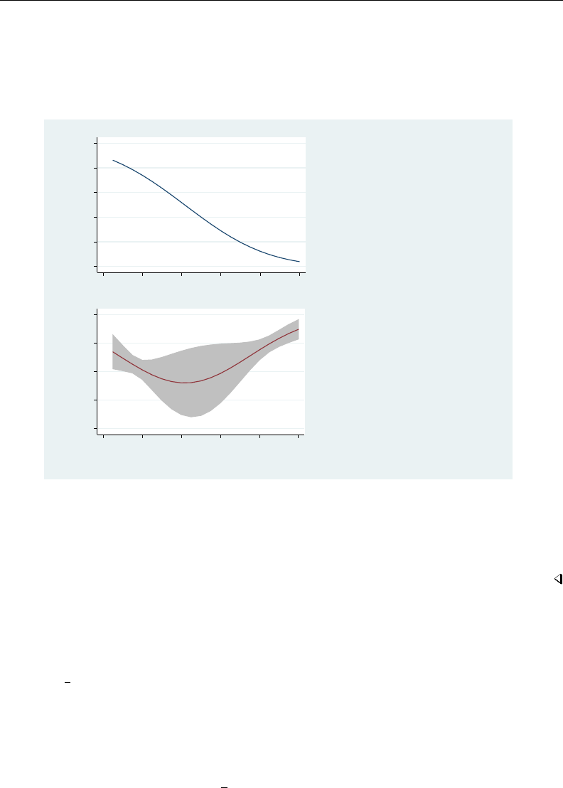
134 asmprobit postestimation — Postestimation tools for asmprobit
. twoway (rarea lb ub tt, pstyle(ci)) (line meff tt, lpattern(solid)), name(meff)
> legend(off) title(" marginal effect of air travel" "terminal time and"
> "95% confidence interval", position(3))
. twoway line prob tt, name(prob) title(" probability of choosing" "air travel",
> position(3)) graphregion(margin(r+9)) ytitle("") xtitle("")
. graph combine prob meff, cols(1) graphregion(margin(l+5 r+5))
0 .2 .4 .6 .8 1
0 20 40 60 80 100
probability of choosing
air travel
−.02 −.015 −.01 −.005 0
0 20 40 60 80 100
terminal time
marginal effect of air travel
terminal time and
95% confidence interval
From the graphs, we see that the simulated probability of choosing air travel decreases in an
sigmoid fashion. The marginal effects display the rate of change in the simulated probability as a
function of the air travel terminal time. The rate of change in the probability of choosing air travel
decreases until the air travel terminal time reaches about 45; thereafter, it increases.
Stored results
estat mfx stores the following in r():
Scalars
r(pr alt)scalars containing the computed probability of each alternative evaluated at the value that is
labeled X in the table output. Here alt are the labels in the macro e(alteqs).
Matrices
r(alt)matrices containing the computed marginal effects and associated statistics. There is one matrix
for each alternative, where alt are the labels in the macro e(alteqs). Column 1 of each
matrix contains the marginal effects; column 2, their standard errors; columns 3 and 4,
their zstatistics and the p-values for the zstatistics; and columns 5 and 6, the confidence
intervals. Column 7 contains the values of the independent variables used to compute the
probabilities r(pr alt).

asmprobit postestimation — Postestimation tools for asmprobit 135
Methods and formulas
Marginal effects
The marginal effects are computed as the derivative of the simulated probability with respect to each
independent variable. A set of marginal effects is computed for each alternative; thus, for Jalternatives,
there will be Jtables. Moreover, the alternative-specific variables will have Jentries, one for each
alternative in each table. The details of computing the effects are different for alternative-specific
variables and case-specific variables, as well as for continuous and indicator variables.
We use the latent-variable notation of asmprobit (see [R]asmprobit) for a J-alternative model
and, for notational convenience, we will drop any subscripts involving observations. We then have
the following linear functions ηj=xjβ+zαj, for j=1, . . . , J. Let kindex the alternative of
interest, and then
vj0=ηj−ηk
= (xj−xk)β+z(αj−αk) + j0
where j0=jif j < k and j0=j−1 if j > k, so that j0=1, . . . , J −1 and j0∼MVN(0,Σ).
Denote pk=Pr(v1≤0, . . . , vJ−1≤0)as the simulated probability of choosing alternative k
given profile xkand z. The marginal effects are then ∂pk/∂xk,∂pk/∂xj, and ∂pk/∂z, where
k= 1, . . . , J,j6=k.asmprobit analytically computes the first-order derivatives of the simulated
probability with respect to the v’s, and the marginal effects for x’s and zare obtained via the chain
rule. The standard errors for the marginal effects are computed using the delta method.
Also see
[R]asmprobit — Alternative-specific multinomial probit regression
[U] 20 Estimation and postestimation commands

Title
asroprobit — Alternative-specific rank-ordered probit regression
Syntax Menu Description Options
Remarks and examples Stored results Methods and formulas Reference
Also see
Syntax
asroprobit depvar indepvars if in weight , case(varname)
alternatives(varname)options
options Description
Model
∗case(varname)use varname to identify cases
∗alternatives(varname)use varname to identify the alternatives available for each case
casevars(varlist)case-specific variables
constraints(constraints)apply specified linear constraints
collinear keep collinear variables
Model 2
correlation(correlation)correlation structure of the latent-variable errors
stddev(stddev)variance structure of the latent-variable errors
structural use the structural covariance parameterization; default is the
differenced covariance parameterization
factor(#)use the factor covariance structure with dimension #
noconstant suppress the alternative-specific constant terms
basealternative(#|lbl |str)alternative used for normalizing location
scalealternative(#|lbl |str)alternative used for normalizing scale
altwise use alternativewise deletion instead of casewise deletion
reverse interpret the lowest rank in depvar as the best; the default is the
highest rank is the best
SE/Robust
vce(vcetype)vcetype may be oim,robust,cluster clustvar,opg,
bootstrap, or jackknife
Reporting
level(#)set confidence level; default is level(95)
notransform do not transform variance–covariance estimates to the standard
deviation and correlation metric
nocnsreport do not display constraints
display options control column formats and line width
136

asroprobit — Alternative-specific rank-ordered probit regression 137
Integration
intmethod(seqtype)type of quasi- or pseudouniform sequence
intpoints(#)number of points in each sequence
intburn(#)starting index in the Hammersley or Halton sequence
intseed(code |#)pseudouniform random-number seed
antithetics use antithetic draws
nopivot do not use integration interval pivoting
initbhhh(#)use the BHHH optimization algorithm for the first #iterations
favor(speed |space) favor speed or space when generating integration points
Maximization
maximize options control the maximization process
coeflegend display legend instead of statistics
correlation Description
unstructured one correlation parameter for each pair of alternatives; correlations
with the basealternative() are zero; the default
exchangeable one correlation parameter common to all pairs of alternatives;
correlations with the basealternative() are zero
independent constrain all correlation parameters to zero
pattern matname user-specified matrix identifying the correlation pattern
fixed matname user-specified matrix identifying the fixed and free correlation
parameters
stddev Description
heteroskedastic estimate standard deviation for each alternative; standard deviations
for basealternative() and scalealternative() set to one
homoskedastic all standard deviations are one
pattern matname user-specified matrix identifying the standard deviation pattern
fixed matname user-specified matrix identifying the fixed and free standard
deviations
seqtype Description
hammersley Hammersley point set
halton Halton point set
random uniform pseudorandom point set
∗case(varname)and alternatives(varname)are required.
bootstrap,by,jackknife,statsby, and xi are allowed; see [U] 11.1.10 Prefix commands.
Weights are not allowed with the bootstrap prefix; see [R] bootstrap.
fweights, iweights, and pweights are allowed; see [U] 11.1.6 weight.
coeflegend does not appear in the dialog box.
See [U] 20 Estimation and postestimation commands for more capabilities of estimation commands.

138 asroprobit — Alternative-specific rank-ordered probit regression
Menu
Statistics >Ordinal outcomes >Rank-ordered probit regression
Description
asroprobit fits rank-ordered probit (ROP) models by using maximum simulated likelihood (MSL).
The model allows you to relax the independence of irrelevant alternatives (IIA) property that is
characteristic of the rank-ordered logistic model by estimating the variance–covariance parameters
of the latent-variable errors. Each unique identifier in the case() variable has multiple alternatives
identified in the alternatives() variable, and depvar contains the ranked alternatives made by each
case. Only the order in the ranks, not the magnitude of their differences, is assumed to be relevant.
By default, the largest rank indicates the more desirable alternative. Use the reverse option if the
lowest rank should be interpreted as the more desirable alternative. Tied ranks are allowed, but they
increase the computation time because all permutations of the tied ranks are used in computing the
likelihood for each case. asroprobit allows two types of independent variables: alternative-specific
variables, in which the values of each variable vary with each alternative, and case-specific variables,
which vary with each case.
The estimation technique of asroprobit is nearly identical to that of asmprobit, and the two
routines share many of the same options; see [R]asmprobit.
Options
Model
case(varname)specifies the variable that identifies each case. This variable identifies the individuals
or entities making a choice. case() is required.
alternatives(varname)specifies the variable that identifies the alternatives available for each case.
The number of alternatives can vary with each case; the maximum number of alternatives is 20.
alternatives() is required.
casevars(varlist)specifies the case-specific variables that are constant for each case(). If there are
a maximum of Jalternatives, there will be J−1 sets of coefficients associated with casevars().
constraints(constraints),collinear; see [R]estimation options.
Model 2
correlation(correlation)specifies the correlation structure of the latent-variable errors.
correlation(unstructured) is the most general and has J(J−3)/2+1 unique correlation
parameters. This is the default unless stddev() or structural are specified.
correlation(exchangeable) provides for one correlation coefficient common to all latent
variables, except the latent variable associated with the basealternative().
correlation(independent) assumes that all correlations are zero.
correlation(pattern matname)and correlation(fixed matname)give you more flexibil-
ity in defining the correlation structure. See Variance structures in [R]asmprobit for more
information.
stddev(stddev)specifies the variance structure of the latent-variable errors.
stddev(heteroskedastic) is the most general and has J−2 estimable parameters. The standard
deviations of the latent-variable errors for the alternatives specified in basealternative()
and scalealternative() are fixed to one.

asroprobit — Alternative-specific rank-ordered probit regression 139
stddev(homoskedastic) constrains all the standard deviations to equal one.
stddev(pattern matname)and stddev(fixed matname)give you added flexibility in defining
the standard deviation parameters. See Variance structures in [R]asmprobit for more information.
structural requests the J×Jstructural covariance parameterization instead of the default J−1×J−1
differenced covariance parameterization (the covariance of the latent errors differenced with that of
the base alternative). The differenced covariance parameterization will achieve the same maximum
simulated likelihood regardless of the choice of basealternative() and scalealternative().
On the other hand, the structural covariance parameterization imposes more normalizations that
may bound the model away from its maximum likelihood and thus prevent convergence with some
datasets or choices of basealternative() and scalealternative().
factor(#)requests that the factor covariance structure of dimension #be used. The factor() option
can be used with the structural option but cannot be used with stddev() or correlation().
A#×J(or #×J−1)matrix, C, is used to factor the covariance matrix as I+C0C, where
Iis the identity matrix of dimension J(or J−1). The column dimension of Cdepends on
whether the covariance is structural or differenced. The row dimension of C,#, must be less than
or equal to floor((J(J−1)/2−1)/(J−2)), because there are only J(J−1)/2−1 identifiable
variance–covariance parameters. This covariance parameterization may be useful for reducing the
number of covariance parameters that need to be estimated.
If the covariance is structural, the column of Ccorresponding to the base alternative contains zeros.
The column corresponding to the scale alternative has a one in the first row and zeros elsewhere.
If the covariance is differenced, the column corresponding to the scale alternative (differenced with
the base) has a one in the first row and zeros elsewhere.
noconstant suppresses the J−1 alternative-specific constant terms.
basealternative(#|lbl |str)specifies the alternative used to normalize the latent-variable location
(also referred to as the level of utility). The base alternative may be specified as a number, label,
or string. The standard deviation for the latent-variable error associated with the base alternative
is fixed to one, and its correlations with all other latent-variable errors are set to zero. The default
is the first alternative when sorted. If a fixed or pattern matrix is given in the stddev()
and correlation() options, the basealternative() will be implied by the fixed standard
deviations and correlations in the matrix specifications. basealternative() cannot be equal to
scalealternative().
scalealternative(#|lbl |str)specifies the alternative used to normalize the latent-variable scale
(also referred to as the scale of utility). The scale alternative may be specified as a number,
label, or string. The default is to use the second alternative when sorted. If a fixed or pattern
matrix is given in the stddev() option, the scalealternative() will be implied by the
fixed standard deviations in the matrix specification. scalealternative() cannot be equal to
basealternative().
If a fixed or pattern matrix is given for the stddev() option, the base alternative and scale
alternative are implied by the standard deviations and correlations in the matrix specifications, and
they need not be specified in the basealternative() and scalealternative() options.
altwise specifies that alternativewise deletion be used when marking out observations due to missing
values in your variables. The default is to use casewise deletion; that is, the entire group of
observations making up a case is deleted if any missing values are encountered. This option does
not apply to observations that are marked out by the if or in qualifier or the by prefix.
reverse directs asroprobit to interpret the rank in depvar that is smallest in value as the preferred
alternative. By default, the rank that is largest in value is the favored alternative.

140 asroprobit — Alternative-specific rank-ordered probit regression
SE/Robust
vce(vcetype)specifies the type of standard error reported, which includes types that are derived from
asymptotic theory (oim,opg), that are robust to some kinds of misspecification (robust), that
allow for intragroup correlation (cluster clustvar), and that use bootstrap or jackknife methods
(bootstrap,jackknife); see [R]vce option.
If specifying vce(bootstrap) or vce(jackknife), you must also specify basealternative()
and scalealternative().
Reporting
level(#); see [R]estimation options.
notransform prevents retransforming the Cholesky-factored variance–covariance estimates to the
correlation and standard deviation metric.
This option has no effect if structural is not specified because the default differenced variance–
covariance estimates have no interesting interpretation as correlations and standard deviations.
notransform also has no effect if the correlation() and stddev() options are specified with
anything other than their default values. Here it is generally not possible to factor the variance–
covariance matrix, so optimization is already performed using the standard deviation and correlation
representations.
nocnsreport; see [R]estimation options.
display options:cformat(%fmt),pformat(% fmt),sformat(% fmt), and nolstretch; see [R]es-
timation options.
Integration
intmethod(hammersley |halton |random) specifies the method of generating the point sets used in
the quasi–Monte Carlo integration of the multivariate normal density. intmethod(hammersley),
the default, uses the Hammersley sequence; intmethod(halton) uses the Halton sequence; and
intmethod(random) uses a sequence of uniform random numbers.
intpoints(#)specifies the number of points to use in the quasi–Monte Carlo integration. If
this option is not specified, the number of points is 50 ×Jif intmethod(hammersley) or
intmethod(halton) is used and 100 ×Jif intmethod(random) is used. Larger values of
intpoints() provide better approximations of the log likelihood, but at the cost of added
computation time.
intburn(#)specifies where in the Hammersley or Halton sequence to start, which helps reduce the
correlation between the sequences of each dimension. The default is 0. This option may not be
specified with intmethod(random).
intseed(code |#)specifies the seed to use for generating the uniform pseudorandom sequence. This
option may be specified only with intmethod(random).code refers to a string that records the
state of the random-number generator runiform(); see [R]set seed. An integer value #may
be used also. The default is to use the current seed value from Stata’s uniform random-number
generator, which can be obtained from c(seed).
antithetics specifies that antithetic draws be used. The antithetic draw for the J−1 vector
uniform-random variables, x, is 1 −x.
nopivot turns off integration interval pivoting. By default, asroprobit will pivot the wider intervals
of integration to the interior of the multivariate integration. This improves the accuracy of the
quadrature estimate. However, discontinuities may result in the computation of numerical second-
order derivatives using finite differencing (for the Newton–Raphson optimize technique, tech(nr))

asroprobit — Alternative-specific rank-ordered probit regression 141
when few simulation points are used, resulting in a non–positive-definite Hessian. asroprobit
uses the Broyden–Fletcher–Goldfarb–Shanno optimization algorithm, by default, which does not
require computing the Hessian numerically using finite differencing.
initbhhh(#)specifies that the Berndt–Hall–Hall–Hausman (BHHH) algorithm be used for the initial
#optimization steps. This option is the only way to use the BHHH algorithm along with other
optimization techniques. The algorithm switching feature of ml’s technique() option cannot
include bhhh.
favor(speed |space) instructs asroprobit to favor either speed or space when generating the
integration points. favor(speed) is the default. When favoring speed, the integration points are
generated once and stored in memory, thus increasing the speed of evaluating the likelihood. This
speed increase can be seen when there are many cases or when the user specifies a large number
of integration points, intpoints(#). When favoring space, the integration points are generated
repeatedly with each likelihood evaluation.
For unbalanced data, where the number of alternatives varies with each case, the estimates computed
using intmethod(random) will vary slightly between favor(speed) and favor(space). This
is because the uniform sequences will not be identical, even when initiating the sequences using the
same uniform seed, intseed(code |#). For favor(speed),ncase blocks of intpoints(#)×
J−2 uniform points are generated, where Jis the maximum number of alternatives. For
favor(space), the column dimension of the matrices of points varies with the number of
alternatives that each case has.
Maximization
maximize options:difficult,technique(algorithm spec),iterate(#),nolog,trace,
gradient,showstep,hessian,showtolerance,tolerance(#),ltolerance(#),
nrtolerance(#),nonrtolerance, and from(init specs); see [R]maximize.
The following options may be particularly useful in obtaining convergence with asroprobit:
difficult,technique(algorithm spec),nrtolerance(#),nonrtolerance, and
from(init specs).
If technique() contains more than one algorithm specification, bhhh cannot be one of them. To
use the BHHH algorithm with another algorithm, use the initbhhh() option and specify the other
algorithm in technique().
Setting the optimization type to technique(bhhh) resets the default vcetype to vce(opg).
When specifying from(matname , copy ), the values in matname associated with the latent-
variable error variances must be for the log-transformed standard deviations and inverse-hyperbolic
tangent-transformed correlations. This option makes using the coefficient vector from a previously
fitted asroprobit model convenient as a starting point.
The following option is available with asroprobit but is not shown in the dialog box:
coeflegend; see [R]estimation options.
Remarks and examples
The mathematical description and numerical computations of the rank-ordered probit model are
similar to that of the multinomial probit model. The only difference is that the dependent variable
of the rank-ordered probit model is ordinal, showing preferences among alternatives, as opposed to
the binary dependent variable of the multinomial probit model, indicating a chosen alternative. We
will describe how the likelihood of a ranking is computed using the latent-variable framework here,

142 asroprobit — Alternative-specific rank-ordered probit regression
but for details of the latent-variable parameterization of these models and the method of maximum
simulated likelihood, see [R]asmprobit.
Consider the latent-variable parameterization of a Jalternative rank-ordered probit model. Using
the notation from asmprobit, we have variables ηij ,j=1, . . . , J, such that
ηij =xij β+ziαj+ξij
Here the xij are the alternative-specific independent variables, the ziare the case-specific variables,
and the ξij are multivariate normal with mean zero and covariance Ω. Without loss of generality,
assume that individual iranks the alternatives in order of the alternative indices j=1,2, . . . , J,
so the alternative Jis the preferred alternative and alternative 1is the least preferred alternative.
The probability of this ranking given βand αjis the probability that ηi,J −1−ηi,J ≤0 and
ηi,J−2−ηi,J−1≤0, . . . , and ηi,1−ηi,2≤0.
Example 1
Long and Freese (2014, 477) provide an example of a rank-ordered logit model with alternative-
specific variables. We use this dataset to demonstrate asroprobit. The data come from the Wisconsin
Longitudinal Study. This is a study of 1957 Wisconsin high school graduates that were asked to rate
their relative preference of four job characteristics: esteem, a job other people regard highly; variety,
a job that is not repetitive and allows you to do a variety of things; autonomy, a job where your
supervisor does not check on you frequently; and security, a job with a low risk of being laid off. The
case-specific covariates are gender, female, an indicator variable for females, and score, a score
on a general mental ability test measured in standard deviations. The alternative-specific variables
are high and low, which indicate whether the respondent’s current job is high or low in esteem,
variety, autonomy, or security. This approach provides three states for a respondent’s current job
status for each alternative, (1,0),(0,1), and (0,0), using the notation (high,low). The score (1,1)
is omitted because the respondent’s current job cannot be considered both high and low in one of the
job characteristics. The (0,0)score would indicate that the respondent’s current job does not rank
high or low (is neutral) in a job characteristic. The alternatives are ranked such that 1 is the preferred
alternative and 4 is the least preferred.
. use http://www.stata-press.com/data/r13/wlsrank
(1992 Wisconsin Longitudinal Study data on job values)
. list id jobchar rank female score high low in 1/12, sepby(id)
id jobchar rank female score high low
1. 1 security 1 1 .0492111 0 0
2. 1 autonomy 4 1 .0492111 0 0
3. 1 variety 1 1 .0492111 0 0
4. 1 esteem 3 1 .0492111 0 0
5. 5 security 2 1 2.115012 1 0
6. 5 variety 2 1 2.115012 1 0
7. 5 esteem 2 1 2.115012 1 0
8. 5 autonomy 1 1 2.115012 0 0
9. 7 autonomy 1 0 1.701852 1 0
10. 7 variety 1 0 1.701852 0 1
11. 7 esteem 4 0 1.701852 0 0
12. 7 security 1 0 1.701852 0 0

asroprobit — Alternative-specific rank-ordered probit regression 143
The three cases listed have tied ranks. asroprobit will allow ties, but at the cost of increased
computation time. To evaluate the likelihood of the first observation, asroprobit must compute
Pr(esteem = 3,variety = 1,autonomy = 4,security = 2)+
Pr(esteem = 3,variety = 2,autonomy = 4,security = 1)
and both of these probabilities are estimated using simulation. In fact, the full dataset contains 7,237
tied ranks and asroprobit takes a great deal of time to estimate the parameters. For exposition, we
estimate the rank-ordered probit model by using the cases without ties. These cases are marked in
the variable noties.
The model of job preference is
ηij =β1highij +β2lowij +α1jfemalei+α2jscorei+α0j+ξij
for j=1,2,3,4. The base alternative will be esteem, so α01 =α11 =α21 =0.

144 asroprobit — Alternative-specific rank-ordered probit regression
. asroprobit rank high low if noties, case(id) alternatives(jobchar)
> casevars(female score) reverse
note: variable high has 107 cases that are not alternative-specific: there is
no within-case variability
note: variable low has 193 cases that are not alternative-specific: there is
no within-case variability
Iteration 0: log simulated-likelihood = -1103.2768
Iteration 1: log simulated-likelihood = -1089.3361 (backed up)
(output omitted )
Alternative-specific rank-ordered probit Number of obs = 1660
Case variable: id Number of cases = 415
Alternative variable: jobchar Alts per case: min = 4
avg = 4.0
max = 4
Integration sequence: Hammersley
Integration points: 200 Wald chi2(8) = 34.01
Log simulated-likelihood = -1080.2206 Prob > chi2 = 0.0000
rank Coef. Std. Err. z P>|z| [95% Conf. Interval]
jobchar
high .3741029 .0925685 4.04 0.000 .192672 .5555337
low -.0697443 .1093317 -0.64 0.524 -.2840305 .1445419
esteem (base alternative)
variety
female .1351487 .1843088 0.73 0.463 -.2260899 .4963873
score .1405482 .0977567 1.44 0.151 -.0510515 .3321479
_cons 1.735016 .1451343 11.95 0.000 1.450558 2.019474
autonomy
female .2561828 .1679565 1.53 0.127 -.0730059 .5853715
score .1898853 .0875668 2.17 0.030 .0182575 .361513
_cons .7009797 .1227336 5.71 0.000 .4604262 .9415333
security
female .232622 .2057547 1.13 0.258 -.1706497 .6358938
score -.1780076 .1102115 -1.62 0.106 -.3940181 .038003
_cons 1.343766 .1600059 8.40 0.000 1.030161 1.657372
/lnl2_2 .1805151 .0757296 2.38 0.017 .0320878 .3289424
/lnl3_3 .4843091 .0793343 6.10 0.000 .3288168 .6398014
/l2_1 .6062037 .1169368 5.18 0.000 .3770117 .8353957
/l3_1 .4509217 .1431183 3.15 0.002 .1704151 .7314283
/l3_2 .2289447 .1226081 1.87 0.062 -.0113627 .4692521
(jobchar=esteem is the alternative normalizing location)
(jobchar=variety is the alternative normalizing scale)
We specified the reverse option because a rank of 1 is the highest preference. The variance–
covariance estimates are for the Cholesky-factored variance–covariance for the latent-variable errors
differenced with that of alternative esteem. We can view the estimated correlations by entering

asroprobit — Alternative-specific rank-ordered probit regression 145
. estat correlation
variety autonomy security
variety 1.0000
autonomy 0.4516 1.0000
security 0.2652 0.2399 1.0000
Note: correlations are for alternatives differenced with esteem
and typing
. estat covariance
variety autonomy security
variety 2
autonomy .8573015 1.80229
security .6376996 .5475882 2.890048
Note: covariances are for alternatives differenced with esteem
gives the (co)variances. [R]mprobit explains that if the latent-variable errors are independent, then
the correlations in the differenced parameterization should be ∼0.5 and the variances should be ∼2.0,
which seems to be the case here.
The coefficient estimates for the probit models can be difficult to interpret because of the
normalization for location and scale. The regression estimates for the case-specific variables will be
relative to the base alternative and the regression estimates for both the case-specific and alternative-
specific variables are affected by the scale normalization. The more pronounced the heteroskedasticity
and correlations, the more pronounced the resulting estimate differences when choosing alternatives
to normalize for location and scale. However, when using the differenced covariance structure, you
will obtain the same model likelihood regardless of which alternatives you choose as the base and
scale alternatives. For model interpretation, you can examine the estimated probabilities and marginal
effects by using postestimation routines predict and estat mfx. See [R]asroprobit postestimation.

146 asroprobit — Alternative-specific rank-ordered probit regression
Stored results
asroprobit stores the following in e():
Scalars
e(N) number of observations
e(N case) number of cases
e(N ties) number of ties
e(k) number of parameters
e(k alt) number of alternatives
e(k indvars) number of alternative-specific variables
e(k casevars) number of case-specific variables
e(k sigma) number of variance estimates
e(k rho) number of correlation estimates
e(k eq) number of equations in e(b)
e(k eq model) number of equations in overall model test
e(df m) model degrees of freedom
e(ll) log simulated-likelihood
e(N clust) number of clusters
e(const) constant indicator
e(i base) base alternative index
e(i scale) scale alternative index
e(mc points) number of Monte Carlo replications
e(mc burn) starting sequence index
e(mc antithetics) antithetics indicator
e(reverse) 1 if minimum rank is best, 0if maximum rank is best
e(chi2) χ2
e(p) significance
e(fullcov) unstructured covariance indicator
e(structcov) 1 if structured covariance; 0otherwise
e(cholesky) Cholesky-factored covariance indicator
e(alt min) minimum number of alternatives
e(alt avg) average number of alternatives
e(alt max) maximum number of alternatives
e(rank) rank of e(V)
e(ic) number of iterations
e(rc) return code
e(converged) 1 if converged, 0otherwise

asroprobit — Alternative-specific rank-ordered probit regression 147
Macros
e(cmd) asroprobit
e(cmdline) command as typed
e(depvar) name of dependent variable
e(indvars) alternative-specific independent variable
e(casevars) case-specific variables
e(case) variable defining cases
e(altvar) variable defining alternatives
e(alteqs) alternative equation names
e(alt#)alternative labels
e(wtype) weight type
e(wexp) weight expression
e(title) title in estimation output
e(clustvar) name of cluster variable
e(correlation) correlation structure
e(stddev) variance structure
e(chi2type) Wald, type of model χ2test
e(vce) vcetype specified in vce()
e(vcetype) title used to label Std. Err.
e(opt) type of optimization
e(which) max or min; whether optimizer is to perform maximization or minimization
e(ml method) type of ml method
e(mc method) Hammersley,Halton, or uniform random; technique to generate sequences
e(mc seed) random-number generator seed
e(user) name of likelihood-evaluator program
e(technique) maximization technique
e(datasignature) the checksum
e(datasignaturevars) variables used in calculation of checksum
e(properties) b V
e(estat cmd) program used to implement estat
e(mfx dlg) program used to implement estat mfx dialog
e(predict) program used to implement predict
e(marginsnotok) predictions disallowed by margins
Matrices
e(b) coefficient vector
e(Cns) constraints matrix
e(stats) alternative statistics
e(stdpattern) variance pattern
e(stdfixed) fixed and free standard deviations
e(altvals) alternative values
e(altfreq) alternative frequencies
e(alt casevars) indicators for estimated case-specific coefficients—e(k alt)×e(k casevars)
e(corpattern) correlation structure
e(corfixed) fixed and free correlations
e(ilog) iteration log (up to 20 iterations)
e(gradient) gradient vector
e(V) variance–covariance matrix of the estimators
e(V modelbased) model-based variance
Functions
e(sample) marks estimation sample
Methods and formulas
From a computational perspective, asroprobit is similar to asmprobit and the two programs
share many numerical tools. Therefore, we will use the notation from Methods and formulas in
[R]asmprobit to discuss the rank-ordered probit probability model.
The latent variables for a J-alternative model are ηij =xij β+ziαj+ξij , for j=1, . . . , J,
i=1, . . . , n, and ξ0
i= (ξi,1, . . . , ξi,J)∼MVN(0,Ω). Without loss of generality, assume for

148 asroprobit — Alternative-specific rank-ordered probit regression
the ith observation that an individual ranks the alternatives in the order of their numeric indices,
yi= (J, J −1,...,1), so the first alternative is the most preferred and the last alternative is the
least preferred. We can then difference the latent variables such that
vik =ηi,k+1 −ηi,k
= (xi,k+1 −xi,k)β+zi(αk+1 −αk) + ξi,k+1 −ξik
=δikβ+ziγk+ik
for k=1, . . . , J −1 and where i= (i1, . . . , i,J−1)∼MVN(0,Σ(i)).Σis indexed by ibecause
it is specific to the ranking of individual i. We denote the deterministic part of the model as
λik =δikβ+zjγk, and the probability of this event is
Pr(yi) = Pr(vi1≤0, . . . , vi,J−1≤0)
= Pr(i1≤ −λi1, . . . , i,J−1≤ −λi,J−1)
= (2π)−(J−1)/2|Σ(i)|−1/2Z−λi1
−∞ ···Z−λi,J−1
−∞
exp −1
2z0Σ−1
(i)zdz
The integral has the same form as (3) of Methods and formulas in [R]asmprobit. See [R]asmprobit
for details on evaluating this integral numerically by using simulation.
asroprobit handles tied ranks by enumeration. For ktied ranks, it will generate k!rankings,
where !is the factorial operator k! = k(k−1)(k−2)···(2)(1). For two sets of tied ranks of size k1
and k2,asroprobit will generate k1!k2!rankings. The total probability is the sum of the probability
of each ranking. For example, if there are two tied ranks such that yi= (J, J, J −2,...,1), then
asroprobit will evaluate Pr(yi) = Pr(y(1)
i) + Pr(y(2)
i), where y(1)
i= (J, J −1, J −2,...,1)
and y(2)
i= (J−1, J, J −2,...,1).
This command supports the clustered version of the Huber/White/sandwich estimator of the
variance using vce(robust) and vce(cluster clustvar). See [P]robust, particularly Maximum
likelihood estimators and Methods and formulas. Specifying vce(robust) is equivalent to specifying
vce(cluster casevar), where casevar is the variable that identifies the cases.
Reference
Long, J. S., and J. Freese. 2014. Regression Models for Categorical Dependent Variables Using Stata. 3rd ed. College
Station, TX: Stata Press.
Also see
[R]asroprobit postestimation — Postestimation tools for asroprobit
[R]asmprobit — Alternative-specific multinomial probit regression
[R]mlogit — Multinomial (polytomous) logistic regression
[R]mprobit — Multinomial probit regression
[R]oprobit — Ordered probit regression
[U] 20 Estimation and postestimation commands

Title
asroprobit postestimation — Postestimation tools for asroprobit
Description Syntax for predict Menu for predict Options for predict
Syntax for estat Menu for estat Options for estat Remarks and examples
Stored results Also see
Description
The following postestimation commands are of special interest after asroprobit:
Command Description
estat alternatives alternative summary statistics
estat covariance covariance matrix of the latent-variable errors for the alternatives
estat correlation correlation matrix of the latent-variable errors for the alternatives
estat facweights covariance factor weights matrix
estat mfx marginal effects
The following standard postestimation commands are also available:
Command Description
estat ic Akaike’s and Schwarz’s Bayesian information criteria (AIC and BIC)
estat summarize summary statistics for the estimation sample
estat vce variance–covariance matrix of the estimators (VCE)
estimates cataloging estimation results
lincom point estimates, standard errors, testing, and inference for linear
combinations of coefficients
lrtest likelihood-ratio test
nlcom point estimates, standard errors, testing, and inference for nonlinear
combinations of coefficients
predict predicted probabilities, estimated linear predictor and its standard error
predictnl point estimates, standard errors, testing, and inference for generalized
predictions
test Wald tests of simple and composite linear hypotheses
testnl Wald tests of nonlinear hypotheses
Special-interest postestimation commands
estat alternatives displays summary statistics about the alternatives in the estimation sample.
The command also provides a mapping between the index numbers that label the covariance parameters
of the model and their associated values and labels for the alternative variable.
estat covariance computes the estimated variance–covariance matrix of the latent-variable
errors for the alternatives. The estimates are displayed, and the variance–covariance matrix is stored
in r(cov).
149

150 asroprobit postestimation — Postestimation tools for asroprobit
estat correlation computes the estimated correlation matrix of the latent-variable errors for
the alternatives. The estimates are displayed, and the correlation matrix is stored in r(cor).
estat facweights displays the covariance factor weights matrix and stores it in r(C).
estat mfx computes marginal effects of a simulated probability of a set of ranked alternatives.
The probability is stored in r(pr), the matrix of rankings is stored in r(ranks), and the matrix of
marginal-effect statistics is stored in r(mfx).
Syntax for predict
predict type newvar if in ,statistic altwise
predict type stub*|newvarlist if in , scores
statistic Description
Main
pr probability of each ranking, by case; the default
pr1 probability that each alternative is preferred
xb linear prediction
stdp standard error of the linear prediction
These statistics are available both in and out of sample; type predict . . . if e(sample) . . . if wanted
only for the estimation sample.
Menu for predict
Statistics >Postestimation >Predictions, residuals, etc.
Options for predict
Main
pr, the default, calculates the probability of each ranking. For each case, one probability is computed
for the ranks in e(depvar).
pr1 calculates the probability that each alternative is preferred.
xb calculates the linear prediction xij β+ziαjfor alternative jand case i.
stdp calculates the standard error of the linear predictor.
altwise specifies that alternativewise deletion be used when marking out observations due to missing
values in your variables. The default is to use casewise deletion. The xb and stdp options always
use alternativewise deletion.
scores calculates the scores for each coefficient in e(b). This option requires a new variable list of
length equal to the number of columns in e(b). Otherwise, use the stub*option to have predict
generate enumerated variables with prefix stub.

asroprobit postestimation — Postestimation tools for asroprobit 151
Syntax for estat
Alternative summary statistics
estat alternatives
Covariance matrix of the latent-variable errors for the alternatives
estat covariance , format(%fmt) border(bspec) left(#)
Correlation matrix of the latent-variable errors for the alternatives
estat correlation , format(%fmt) border(bspec) left(#)
Covariance factor weights matrix
estat facweights , format(%fmt) border(bspec) left(#)
Marginal effects
estat mfx if in ,estat mfx options
estat mfx options Description
Main
varlist(varlist)display marginal effects for varlist
at(median atlist )calculate marginal effects at these values
rank(ranklist)calculate marginal effects for the simulated probability of these ranked
alternatives
Options
level(#)set confidence interval level; default is level(95)
nodiscrete treat indicator variables as continuous
noesample do not restrict calculation of the medians to the estimation sample
nowght ignore weights when calculating medians
Menu for estat
Statistics >Postestimation >Reports and statistics
Options for estat
Options for estat are presented under the following headings:
Options for estat covariance, estat correlation, and estat facweights
Options for estat mfx

152 asroprobit postestimation — Postestimation tools for asroprobit
Options for estat covariance, estat correlation, and estat facweights
format(%fmt)sets the matrix display format. The default for estat covariance and estat
facweights is format(%9.0g). The default for estat correlation is format(%9.4f).
border(bspec)sets the matrix display border style. The default is border(all). See [P]matlist.
left(#)sets the matrix display left indent. The default is left(2). See [P]matlist.
Options for estat mfx
Main
varlist(varlist)specifies the variables for which to display marginal effects. The default is all
variables.
at(median atlist )specifies the values at which the marginal effects are to be calculated. atlist is
alternative:variable =# variable =# . . . )
The marginal effects are calculated at the medians of the independent variables.
After specifying the summary statistic, you can specify specific values for variables. You can
specify values for alternative-specific variables by alternative, or you can specify one value for
all alternatives. You can specify only one value for case-specific variables. For example, in the
wlsrank dataset, female and score are case-specific variables, whereas high and low are
alternative-specific variables. The following would be a legal syntax for estat mfx:
. estat mfx, at(median high=0 esteem:high=1 low=0 security:low=1 female=1)
When nodiscrete is not specified, at(median atlist )has no effect on computing marginal
effects for indicator variables, which are calculated as the discrete change in the simulated probability
as the indicator variable changes from 0 to 1.
The median computations respect any if or in qualifiers, so you can restrict the data over which
the medians are computed. You can even restrict the values to a specific case, for example,
. estat mfx if case==13
rank(ranklist)specifies the ranks for the alternatives. ranklist is
alternative =# alternative =#. . . )
The default is to rank the calculated latent variables. Alternatives excluded from rank() are
omitted from the analysis. You must therefore specify at least two alternatives in rank(). You
may have tied ranks in the rank specification. Only the order in the ranks is relevant.
Options
level(#)specifies the confidence level, as a percentage, for confidence intervals. The default is
level(95) or as set by set level; see [U] 20.7 Specifying the width of confidence intervals.
nodiscrete specifies that indicator variables be treated as continuous variables. An indicator variable
is one that takes on the value 0 or 1 in the estimation sample. By default, the discrete change in
the simulated probability is computed as the indicator variable changes from 0 to 1.
noesample specifies that the whole dataset be considered instead of only those marked in the
e(sample) defined by the asroprobit command.
nowght specifies that weights be ignored when calculating the medians.

asroprobit postestimation — Postestimation tools for asroprobit 153
Remarks and examples
Remarks are presented under the following headings:
Predicted probabilities
Obtaining estimation statistics
Predicted probabilities
After fitting an alternative-specific rank-ordered probit model, you can use predict to obtain the
probabilities of alternative rankings or the probabilities of each alternative being preferred. When
evaluating the multivariate normal probabilities via (quasi) Monte Carlo, predict uses the same
method to generate the (quasi) random sequence of numbers as the previous call to asroprobit. For
example, if you specified intmethod(halton) when fitting the model, predict also uses Halton
sequences.
Example 1
In example 1 of [R]asroprobit, we fit a model of job characteristic preferences. This is a study
of 1957 Wisconsin high school graduates that were asked to rate their relative preference of four
job characteristics: esteem, a job other people regard highly; variety, a job that is not repetitive and
allows you to do a variety of things; autonomy, a job where your supervisor does not check on you
frequently; and security, a job with a low risk of being laid off. The case-specific covariates are
gender, female, an indicator variable for females, and score, a score on a general mental ability test
measured in standard deviations. The alternative-specific variables are high and low, which indicate
whether the respondent’s current job is high or low in esteem, variety, autonomy, or security. This
approach provides three states for a respondent’s current job status for each alternative, (1,0),(0,1),
and (0,0), using the notation (high,low). The score (1,1)is omitted because the respondent’s
current job cannot be considered both high and low in one of the job characteristics. The (0,0)
score would indicate that the respondent’s current job does not rank high or low (is neutral) in a job
characteristic. The alternatives are ranked such that 1 is the preferred alternative and 4 is the least
preferred.
We can obtain the probabilities of the observed alternative rankings, the pr option, and the
probability of each alternative being preferred, the pr1 option, by using predict:

154 asroprobit postestimation — Postestimation tools for asroprobit
. use http://www.stata-press.com/data/r13/wlsrank
(1992 Wisconsin Longitudinal Study data on job values)
. asroprobit rank high low if noties, case(id) alternatives(jobchar)
> casevars(female score) reverse
(output omitted )
. keep if e(sample)
(11244 observations deleted)
. predict prob, pr
. predict prob1, pr1
. list id jobchar prob prob1 rank female score high low in 1/12
id jobchar prob prob1 rank female score high low
1. 13 security .0421807 .2784269 3 0 .3246512 0 1
2. 13 autonomy .0421807 .1029036 1 0 .3246512 0 0
3. 13 variety .0421807 .6026725 2 0 .3246512 1 0
4. 13 esteem .0421807 .0160111 4 0 .3246512 0 1
5. 19 autonomy .0942025 .1232488 4 1 .0492111 0 0
6. 19 esteem .0942025 .0140261 3 1 .0492111 0 0
7. 19 security .0942025 .4601368 1 1 .0492111 1 0
8. 19 variety .0942025 .4025715 2 1 .0492111 0 0
9. 22 esteem .1414177 .0255264 4 1 1.426412 1 0
10. 22 variety .1414177 .4549441 1 1 1.426412 0 0
11. 22 security .1414177 .2629494 3 1 1.426412 0 0
12. 22 autonomy .1414177 .2566032 2 1 1.426412 1 0
The prob variable is constant for each case because it contains the probability of the ranking in
the rank variable. On the other hand, the prob1 variable contains the estimated probability of each
alternative being preferred. For each case, the sum of the values in prob1 will be approximately 1.0.
They do not add up to exactly 1.0 because of approximations due to the GHK algorithm.
Obtaining estimation statistics
For examples of the specialized estat subcommands covariance and correlation, see [R]asm-
probit postestimation. The entry also has a good example of computing marginal effects after asm-
probit that is applicable to asroprobit. Below we will elaborate further on marginal effects after
asroprobit where we manipulate the rank() option.
Example 2
We will continue with the preferred job characteristics example where we first compute the marginal
effects for case id =13.

asroprobit postestimation — Postestimation tools for asroprobit 155
. estat mfx if id==13, rank(security=3 autonomy=1 variety=2 esteem=4)
Pr(esteem=4 variety=2 autonomy=1 security=3) = .04218068
variable dp/dx Std. Err. z P>|z| [ 95% C.I. ] X
high*
esteem -.008713 .001964 -4.44 0.000 -.012562 -.004864 0
variety -.009102 .003127 -2.91 0.004 -.015231 -.002973 1
autonomy .025535 .007029 3.63 0.000 .011758 .039313 0
security -.003745 .001394 -2.69 0.007 -.006477 -.001013 0
low*
esteem .001614 .002646 0.61 0.542 -.003572 .0068 1
variety .001809 .003012 0.60 0.548 -.004094 .007712 0
autonomy -.003849 .006104 -0.63 0.528 -.015813 .008115 0
security .000582 .000985 0.59 0.554 -.001348 .002513 1
casevars
female* .009767 .009064 1.08 0.281 -.007998 .027533 0
score .008587 .004488 1.91 0.056 -.00021 .017384 .32465
(*) dp/dx is for discrete change of indicator variable from 0 to 1
Next we compute the marginal effects for the probability that autonomy is preferred given the profile
of case id =13.
. estat mfx if id==13, rank(security=2 autonomy=1 variety=2 esteem=2)
Pr(esteem=3 variety=4 autonomy=1 security=2) +
Pr(esteem=4 variety=3 autonomy=1 security=2) +
Pr(esteem=2 variety=4 autonomy=1 security=3) +
Pr(esteem=4 variety=2 autonomy=1 security=3) +
Pr(esteem=2 variety=3 autonomy=1 security=4) +
Pr(esteem=3 variety=2 autonomy=1 security=4) = .10276103
variable dp/dx Std. Err. z P>|z| [ 95% C.I. ] X
high*
esteem -.003524 .001258 -2.80 0.005 -.005989 -.001059 0
variety -.036203 .00894 -4.05 0.000 -.053724 -.018681 1
autonomy .057279 .013801 4.15 0.000 .030231 .084328 0
security -.0128 .002665 -4.80 0.000 -.018024 -.007576 0
low*
esteem .000518 .000833 0.62 0.534 -.001116 .002151 1
variety .006409 .010588 0.61 0.545 -.014343 .027161 0
autonomy -.008818 .013766 -0.64 0.522 -.035799 .018163 0
security .002314 .003697 0.63 0.531 -.004932 .009561 1
casevars
female* .013839 .021607 0.64 0.522 -.028509 .056188 0
score .017917 .011062 1.62 0.105 -.003764 .039598 .32465
(*) dp/dx is for discrete change of indicator variable from 0 to 1
The probability computed by estat mfx matches the probability computed by predict, pr1 only
within three digits. This outcome is because of how the computation is carried out and the numeric
inaccuracy of the GHK simulator using a Hammersley point set of length 200. The computation
carried out by estat mfx literally computes all six probabilities listed in the header of the MFX
table and sums them. The computation by predict, pr1 is the same as predict after asmprobit
(multinomial probit): it computes the probability that autonomy is chosen, thus requiring only one

156 asroprobit postestimation — Postestimation tools for asroprobit
call to the GHK simulator. Hence, there is a difference in the reported values even though the two
probability statements are equivalent.
Stored results
estat mfx stores the following in r():
Scalars
r(pr) scalar containing the computed probability of the ranked alternatives.
Matrices
r(ranks) column vector containing the alternative ranks. The rownames identify the alternatives.
r(mfx) matrix containing the computed marginal effects and associated statistics. Column 1 of the
matrix contains the marginal effects; column 2, their standard errors; column 3, their z
statistics; and columns 4 and 5, the confidence intervals. Column 6 contains the values of
the independent variables used to compute the probabilities r(pr).
Also see
[R]asroprobit — Alternative-specific rank-ordered probit regression
[R]asmprobit — Alternative-specific multinomial probit regression
[U] 20 Estimation and postestimation commands

Title
BIC note — Calculating and interpreting BIC
Description Remarks and examples Methods and formulas References
Also see
Description
This entry discusses a statistical issue that arises when using the Bayesian information criterion
(BIC) to compare models.
Stata calculates BIC, assuming N=e(N)—we will explain—but sometimes it would be better if
a different Nwere used. Commands that calculate BIC have an n() option, allowing you to specify
the Nto be used.
In summary,
1. If you are comparing results estimated by the same estimation command, using the default
BIC calculation is probably fine. There is an issue, but most researchers would ignore it.
2. If you are comparing results estimated by different estimation commands, you need to be
on your guard.
a. If the different estimation commands share the same definitions of observations,
independence, and the like, you are back in case 1.
b. If they differ in these regards, you need to think about the value of Nthat should
be used. For example, logit and xtlogit differ in that the former assumes
independent observations and the latter, independent panels.
c. If estimation commands differ in the events being used over which the likelihood
function is calculated, the information criteria may not be comparable at all. We
say information criteria because this would apply equally to the Akaike information
criterion (AIC), as well as to BIC. For instance, streg and stcox produce such
incomparable results. The events used by streg are the actual survival times,
whereas the events used by stcox are failures within risk pools, conditional on
the times at which failures occurred.
Remarks and examples
Remarks are presented under the following headings:
Background
The problem of determining N
The problem of conformable likelihoods
The first problem does not arise with AIC; the second problem does
Calculating BIC correctly
157

158 BIC note — Calculating and interpreting BIC
Background
The AIC and the BIC are two popular measures for comparing maximum likelihood models. AIC
and BIC are defined as
AIC =−2×ln(likelihood)+2×k
BIC =−2×ln(likelihood) + ln(N)×k
where
k=number of parameters estimated
N=number of observations
We are going to discuss AIC along with BIC because AIC has some of the problems that BIC has,
but not all.
AIC and BIC can be viewed as measures that combine fit and complexity. Fit is measured negatively
by −2×ln(likelihood); the larger the value, the worse the fit. Complexity is measured positively,
either by 2 ×k(AIC) or ln(N)×k(BIC).
Given two models fit on the same data, the model with the smaller value of the information
criterion is considered to be better.
There is substantial literature on these measures: see Akaike (1974); Raftery (1995); Sakamoto,
Ishiguro, and Kitagawa (1986); and Schwarz (1978).
When Stata calculates the above measures, it uses the rank of e(V) for kand it uses e(N) for
N.e(V) and e(N) are Stata notation for results stored by the estimation command. e(V) is the
variance–covariance matrix of the estimated parameters, and e(N) is the number of observations in
the dataset used in calculating the result.
The problem of determining N
The difference between AIC and BIC is that AIC uses the constant 2 to weight k, whereas BIC uses
ln(N).
Determining what value of Nshould be used is problematic. Despite appearances, the definition
“Nis the number of observations” is not easy to make operational. Ndoes not appear in the likelihood
function itself, Nis not the output of a standard statistical formula, and what is an observation is
often subjective.
Example 1
Often what is meant by Nis obvious. Consider a simple logit model. What is meant by Nis the
number of observations that are statistically independent and that corresponds to M, the number of
observations in the dataset used in the calculation. We will write N=M.
But now assume that the same dataset has a grouping variable and the data are thought to be
clustered within group. To keep the problem simple, let’s pretend that there are Ggroups and m
observations within group, so that M=G×m. Because you are worried about intragroup correlation,
you fit your model with xtlogit, grouping on the grouping variable. Now you wish to calculate
BIC. What is the Nthat should be used? N=Mor N=G?

BIC note — Calculating and interpreting BIC 159
That is a deep question. If the observations really are independent, then you should use N=M.
If the observations within group are not just correlated but are duplicates of one another, and they
had to be so, then you should use M=G. Between those two extremes, you should probably
use a number between Nand G, but determining what that number should be from measured
correlations is difficult. Using N=Mis conservative in that, if anything, it overweights complexity.
Conservativeness, however, is subjective, too: using N=Gcould be considered more conservative
in that fewer constraints are being placed on the data.
When the estimated correlation is high, our reaction would be that using N=Gis probably more
reasonable. Our first reaction, however, would be that using BIC to compare models is probably a
misuse of the measure.
Stata uses N=M. An informal survey of web-based literature suggests that N=Mis the
popular choice.
There is another reason, not so good, to choose N=M. It makes across-model comparisons more
likely to be valid when performed without thinking about the issue. Say that you wish to compare
the logit and xtlogit results. Thus you need to calculate
BICp=−2×ln(likelihoodp) + ln(Np)×k
BICx=−2×ln(likelihoodx) + ln(Nx)×k
Whatever Nyou use, you must use the same Nin both formulas. Stata’s choice of N=Mat
least meets that test.
Example 2
In the above example, using N=Mis reasonable. Now let’s look at when using N=Mis
wrong, even if popular.
Consider a model fit by stcox. Using N=Mis certainly wrong if for no other reason than
Mis not even a well-defined number. The same data can be represented by different datasets with
different numbers of observations. For example, in one dataset, there might be 1 observation per
subject. In another, the same subjects could have two records each, the first recording the first half
of the time at risk and the second recording the remaining part. All statistics calculated by Stata on
either dataset would be the same, but Mwould be different.
Deciding on the right definition, however, is difficult. Viewed one way, Nin the Cox regression
case should be the number of risk pools, R, because the Cox regression calculation is made on the
basis of the independent risk pools. Viewed another way, Nshould be the number of subjects, Nsubj,
because, even though the likelihood function is based on risk pools, the parameters estimated are at
the subject level.
You can decide which argument you prefer.
For parametric survival models, in single-record data, N=Mis unambiguously correct. For
multirecord data, there is an argument for N=Mand for N=Nsubj.

160 BIC note — Calculating and interpreting BIC
The problem of conformable likelihoods
The problem of conformable likelihoods does not concern N. Researchers sometimes use infor-
mation criteria such as BIC and AIC to make comparisons across models. For that to be valid, the
likelihoods must be conformable; that is, the likelihoods must all measure the same thing.
It is common to think of the likelihood function as the Pr(data |parameters), but in fact, the
likelihood is
Pr(particular events in the data |parameters)
You must ensure that the events are the same.
For instance, they are not the same in the semiparametric Cox regression and the various parametric
survival models. In Cox regression, the events are, at each failure time, that the subjects observed to
fail in fact failed, given that failures occurred at those times. In the parametric models, the events
are that each subject failed exactly when the subject was observed to fail.
The formula for AIC and BIC is
measure =−2×ln(likelihood) + complexity
When you are comparing models, if the likelihoods are measuring different events, even if the
models obtain estimates of the same parameters, differences in the information measures are irrelevant.
The first problem does not arise with AIC; the second problem does
Regardless of model, the problem of defining Nnever arises with AIC because Nis not used in
the AIC calculation. AIC uses a constant 2 to weight complexity as measured by k, rather than ln(N).
For both AIC and BIC, however, the likelihood functions must be conformable; that is, they must
be measuring the same event.
Calculating BIC correctly
When using BIC to compare results, and especially when using BIC to compare results from different
models, you should think carefully about how Nshould be defined. Then specify that number by
using the n() option:
. estimates stats full sub, n(74)
Akaike’s information criterion and Bayesian information criterion
Model Obs ll(null) ll(model) df AIC BIC
full 74 -45.03321 -20.59083 4 49.18167 58.39793
sub 74 -45.03321 -27.17516 3 60.35031 67.26251
Note: N=74 used in calculating BIC
Both estimates stats and estat ic allow the n() option; see [R]estimates stats and [R]estat
ic.

BIC note — Calculating and interpreting BIC 161
Methods and formulas
AIC and BIC are defined as
AIC =−2×ln(likelihood)+2×k
BIC =−2×ln(likelihood) + ln(N)×k
where kis the model degrees of freedom calculated as the rank of variance–covariance matrix of
the parameters e(V) and Nis the number of observations used in estimation or, more precisely, the
number of independent terms in the likelihood. Operationally, Nis defined as e(N) unless the n()
option is specified.
References
Akaike, H. 1974. A new look at the statistical model identification. IEEE Transactions on Automatic Control 19:
716–723.
Raftery, A. E. 1995. Bayesian model selection in social research. In Vol. 25 of Sociological Methodology, ed. P. V.
Marsden, 111–163. Oxford: Blackwell.
Sakamoto, Y., M. Ishiguro, and G. Kitagawa. 1986. Akaike Information Criterion Statistics. Dordrecht, The Netherlands:
Reidel.
Schwarz, G. 1978. Estimating the dimension of a model. Annals of Statistics 6: 461–464.
Also see
[R]estat ic — Display information criteria
[R]estimates stats — Model-selection statistics

Title
binreg — Generalized linear models: Extensions to the binomial family
Syntax Menu Description Options
Remarks and examples Stored results Methods and formulas References
Also see
Syntax
binreg depvar indepvars if in weight ,options
options Description
Model
noconstant suppress constant term
or use logit link and report odds ratios
rr use log link and report risk ratios
hr use log-complement link and report health ratios
rd use identity link and report risk differences
n(#|varname)use #or varname for number of trials
exposure(varname)include ln(varname) in model with coefficient constrained to 1
offset(varname)include varname in model with coefficient constrained to 1
constraints(constraints)apply specified linear constraints
collinear keep collinear variables
mu(varname)use varname as the initial estimate for the mean of depvar
init(varname)synonym for mu(varname)
SE/Robust
vce(vcetype)vcetype may be eim,robust,cluster clustvar,oim,opg,
bootstrap,jackknife,hac kernel,jackknife1, or unbiased
t(varname)variable name corresponding to time
vfactor(#)multiply variance matrix by scalar #
disp(#)quasi-likelihood multiplier
scale(x2 |dev |#)set the scale parameter; default is scale(1)
Reporting
level(#)set confidence level; default is level(95)
coefficients report nonexponentiated coefficients
nocnsreport do not display constraints
display options control column formats, row spacing, line width, display of omitted
variables and base and empty cells, and factor-variable labeling
162

binreg — Generalized linear models: Extensions to the binomial family 163
Maximization
irls use iterated, reweighted least-squares optimization; the default
ml use maximum likelihood optimization
maximize options control the maximization process; seldom used
fisher(#)Fisher scoring steps
search search for good starting values
coeflegend display legend instead of statistics
indepvars may contain factor variables; see [U] 11.4.3 Factor variables.
depvar and indepvars may contain time-series operators; see [U] 11.4.4 Time-series varlists.
bootstrap,by,fp,jackknife,mi estimate,rolling, and statsby are allowed; see [U] 11.1.10 Prefix commands.
vce(bootstrap),vce(jackknife), and vce(jackknife1) are not allowed with the mi estimate prefix; see
[MI] mi estimate.
Weights are not allowed with the bootstrap prefix; see [R] bootstrap.
aweights are not allowed with the jackknife prefix; see [R] jackknife.
fweights, aweights, iweights, and pweights are allowed; see [U] 11.1.6 weight.
coeflegend does not appear in the dialog box.
See [U] 20 Estimation and postestimation commands for more capabilities of estimation commands.
Menu
Statistics >Generalized linear models >GLM for the binomial family
Description
binreg fits generalized linear models for the binomial family. It estimates odds ratios, risk ratios,
health ratios, and risk differences. The available links are
Option Implied link Parameter
or logit odds ratios = exp(β)
rr log risk ratios = exp(β)
hr log complement health ratios = exp(β)
rd identity risk differences = β
Estimates of odds, risk, and health ratios are obtained by exponentiating the appropriate coefficients.
The or option produces the same results as Stata’s logistic command, and or coefficients
yields the same results as the logit command. When no link is specified, or is assumed.
Options
Model
noconstant; see [R]estimation options.
or requests the logit link and results in odds ratios if coefficients is not specified.
rr requests the log link and results in risk ratios if coefficients is not specified.
hr requests the log-complement link and results in health ratios if coefficients is not specified.
rd requests the identity link and results in risk differences.

164 binreg — Generalized linear models: Extensions to the binomial family
n(#|varname)specifies either a constant integer to use as the denominator for the binomial family
or a variable that holds the denominator for each observation.
exposure(varname),offset(varname),constraints(constraints),collinear; see [R]estima-
tion options.constraints(constraints)and collinear are not allowed with irls.
mu(varname)specifies varname containing an initial estimate for the mean of depvar. This option
can be useful if you encounter convergence difficulties. init(varname)is a synonym.
SE/Robust
vce(vcetype)specifies the type of standard error reported, which includes types that are robust to
some kinds of misspecification (robust), that allow for intragroup correlation (cluster clustvar),
that are derived from asymptotic theory (oim,opg), and that use bootstrap or jackknife methods
(bootstrap,jackknife); see [R]vce option.
vce(eim), the default, uses the expected information matrix (EIM) for the variance estimator.
binreg also allows the following:
vce(hac kernel #)specifies that a heteroskedasticity- and autocorrelation-consistent (HAC)
variance estimate be used. HAC refers to the general form for combining weighted matrices to
form the variance estimate. There are three kernels built into binreg.kernel is a user-written
program or one of
nwest |gallant |anderson
If #is not specified, N−2 is assumed.
vce(jackknife1) specifies that the one-step jackknife estimate of variance be used.
vce(unbiased) specifies that the unbiased sandwich estimate of variance be used.
t(varname)specifies the variable name corresponding to time; see [TS]tsset.binreg does not
always need to know t(), though it does if vce(hac . . . )is specified. Then you can either
specify the time variable with t(), or you can tsset your data before calling binreg. When the
time variable is required, binreg assumes that the observations are spaced equally over time.
vfactor(#)specifies a scalar by which to multiply the resulting variance matrix. This option
allows users to match output with other packages, which may apply degrees of freedom or other
small-sample corrections to estimates of variance.
disp(#)multiplies the variance of depvar by #and divides the deviance by #. The resulting
distributions are members of the quasilikelihood family.
scale(x2 |dev |#)overrides the default scale parameter. This option is allowed only with Hessian
(information matrix) variance estimates.
By default, scale(1) is assumed for the discrete distributions (binomial, Poisson, and negative
binomial), and scale(x2) is assumed for the continuous distributions (Gaussian, gamma, and
inverse Gaussian).
scale(x2) specifies that the scale parameter be set to the Pearson chi-squared (or generalized
chi-squared) statistic divided by the residual degrees of freedom, which was recommended by
McCullagh and Nelder (1989) as a good general choice for continuous distributions.
scale(dev) sets the scale parameter to the deviance divided by the residual degrees of freedom.
This option provides an alternative to scale(x2) for continuous distributions and overdispersed
or underdispersed discrete distributions.
scale(#)sets the scale parameter to #.

binreg — Generalized linear models: Extensions to the binomial family 165
Reporting
level(#),noconstant; see [R]estimation options.
coefficients displays the nonexponentiated coefficients and corresponding standard errors and
confidence intervals. This option has no effect when the rd option is specified, because it always
presents the nonexponentiated coefficients.
nocnsreport; see [R]estimation options.
display options:noomitted,vsquish,noemptycells,baselevels,allbaselevels,nofvla-
bel,fvwrap(#),fvwrapon(style),cformat(%fmt),pformat(% fmt),sformat(% fmt), and
nolstretch; see [R]estimation options.
Maximization
irls requests iterated, reweighted least-squares (IRLS) optimization of the deviance instead of
Newton–Raphson optimization of the log likelihood. This option is the default.
ml requests that optimization be carried out by using Stata’s ml command; see [R]ml.
maximize options:technique(algorithm spec),nolog,trace,gradient,showstep,hessian,
showtolerance,difficult,iterate(#),tolerance(#),ltolerance(#),
nrtolerance(#),nonrtolerance, and from(init specs); see [R]maximize. These options are
seldom used.
Setting the optimization method to ml, with technique() set to something other than BHHH,
changes the vcetype to vce(oim). Specifying technique(bhhh) changes vcetype to vce(opg).
fisher(#)specifies the number of Newton–Raphson steps that should use the Fisher scoring Hessian
or EIM before switching to the observed information matrix (OIM). This option is available only
if ml is specified and is useful only for Newton–Raphson optimization.
search specifies that the command search for good starting values. This option is available only if
ml is specified and is useful only for Newton–Raphson optimization.
The following option is available with binreg but is not shown in the dialog box:
coeflegend; see [R]estimation options.
Remarks and examples
Wacholder (1986) suggests methods for estimating risk ratios and risk differences from prospective
binomial data. These estimates are obtained by selecting the proper link functions in the generalized
linear-model framework. (See Methods and formulas for details; also see [R]glm.)
Example 1
Wacholder (1986) presents an example, using data from Wright et al. (1983), of an investigation
of the relationship between alcohol consumption and the risk of a low-birthweight baby. Covariates
examined included whether the mother smoked (yes or no), mother’s social class (three levels), and
drinking frequency (light, moderate, or heavy). The data for the 18 possible categories determined
by the covariates are illustrated below.
Let’s first describe the data and list a few observations.

166 binreg — Generalized linear models: Extensions to the binomial family
. use http://www.stata-press.com/data/r13/binreg
. list
category n_lbw_~s n_women alcohol smokes social
1. 1 11 84 heavy nonsmoker 1
2. 2 5 79 moderate nonsmoker 1
3. 3 11 169 light nonsmoker 1
4. 4 6 28 heavy smoker 1
5. 5 3 13 moderate smoker 1
6. 6 1 26 light smoker 1
7. 7 4 22 heavy nonsmoker 2
8. 8 3 25 moderate nonsmoker 2
9. 9 12 162 light nonsmoker 2
10. 10 4 17 heavy smoker 2
11. 11 2 7 moderate smoker 2
12. 12 6 38 light smoker 2
13. 13 0 14 heavy nonsmoker 3
14. 14 1 18 moderate nonsmoker 3
15. 15 12 91 light nonsmoker 3
16. 16 7 19 heavy smoker 3
17. 17 2 18 moderate smoker 3
18. 18 8 70 light smoker 3
Each observation corresponds to one of the 18 covariate structures. The number of low-birthweight
babies from n women in each category is given by the n lbw babies variable.

binreg — Generalized linear models: Extensions to the binomial family 167
We begin by estimating risk ratios:
. binreg n_lbw_babies i.soc i.alc i.smo, n(n_women) rr
Iteration 1: deviance = 14.2879
Iteration 2: deviance = 13.607
Iteration 3: deviance = 13.60503
Iteration 4: deviance = 13.60503
Generalized linear models No. of obs = 18
Optimization : MQL Fisher scoring Residual df = 12
(IRLS EIM) Scale parameter = 1
Deviance = 13.6050268 (1/df) Deviance = 1.133752
Pearson = 11.51517095 (1/df) Pearson = .9595976
Variance function: V(u) = u*(1-u/n_women) [Binomial]
Link function : g(u) = ln(u/n_women) [Log]
BIC = -21.07943
EIM
n_lbw_babies Risk Ratio Std. Err. z P>|z| [95% Conf. Interval]
social
2 1.340001 .3127382 1.25 0.210 .848098 2.11721
3 1.349487 .3291488 1.23 0.219 .8366715 2.176619
alcohol
moderate 1.191157 .3265354 0.64 0.523 .6960276 2.038503
heavy 1.974078 .4261751 3.15 0.002 1.293011 3.013884
smokes
smoker 1.648444 .332875 2.48 0.013 1.109657 2.448836
_cons .0630341 .0128061 -13.61 0.000 .0423297 .0938656
By default, Stata reports the risk ratios (the exponentiated regression coefficients) estimated by the
model. We can see that the risk ratio comparing heavy drinkers with light drinkers, after adjusting
for smoking and social class, is 1.974078. That is, mothers who drink heavily during their pregnancy
have approximately twice the risk of delivering low-birthweight babies as mothers who are light
drinkers.

168 binreg — Generalized linear models: Extensions to the binomial family
The nonexponentiated coefficients can be obtained with the coefficients option:
. binreg n_lbw_babies i.soc i.alc i.smo, n(n_women) rr coefficients
Iteration 1: deviance = 14.2879
Iteration 2: deviance = 13.607
Iteration 3: deviance = 13.60503
Iteration 4: deviance = 13.60503
Generalized linear models No. of obs = 18
Optimization : MQL Fisher scoring Residual df = 12
(IRLS EIM) Scale parameter = 1
Deviance = 13.6050268 (1/df) Deviance = 1.133752
Pearson = 11.51517095 (1/df) Pearson = .9595976
Variance function: V(u) = u*(1-u/n_women) [Binomial]
Link function : g(u) = ln(u/n_women) [Log]
BIC = -21.07943
EIM
n_lbw_babies Coef. Std. Err. z P>|z| [95% Conf. Interval]
social
2 .2926702 .2333866 1.25 0.210 -.1647591 .7500994
3 .2997244 .2439066 1.23 0.219 -.1783238 .7777726
alcohol
moderate .1749248 .274133 0.64 0.523 -.362366 .7122156
heavy .6801017 .2158856 3.15 0.002 .2569737 1.10323
smokes
smoker .4998317 .2019329 2.48 0.013 .1040505 .8956129
_cons -2.764079 .2031606 -13.61 0.000 -3.162266 -2.365891

binreg — Generalized linear models: Extensions to the binomial family 169
Risk differences are obtained with the rd option:
. binreg n_lbw_babies i.soc i.alc i.smo, n(n_women) rd
Iteration 1: deviance = 18.67277
Iteration 2: deviance = 14.94364
Iteration 3: deviance = 14.9185
Iteration 4: deviance = 14.91762
Iteration 5: deviance = 14.91758
Iteration 6: deviance = 14.91758
Iteration 7: deviance = 14.91758
Generalized linear models No. of obs = 18
Optimization : MQL Fisher scoring Residual df = 12
(IRLS EIM) Scale parameter = 1
Deviance = 14.91758277 (1/df) Deviance = 1.243132
Pearson = 12.60353235 (1/df) Pearson = 1.050294
Variance function: V(u) = u*(1-u/n_women) [Binomial]
Link function : g(u) = u/n_women [Identity]
BIC = -19.76688
EIM
n_lbw_babies Risk Diff. Std. Err. z P>|z| [95% Conf. Interval]
social
2 .0263817 .0232124 1.14 0.256 -.0191137 .0718771
3 .0365553 .0268668 1.36 0.174 -.0161026 .0892132
alcohol
moderate .0122539 .0257713 0.48 0.634 -.0382569 .0627647
heavy .0801291 .0302878 2.65 0.008 .020766 .1394921
smokes
smoker .0542415 .0270838 2.00 0.045 .0011582 .1073248
_cons .059028 .0160693 3.67 0.000 .0275327 .0905232
The risk difference between heavy drinkers and light drinkers is 0.0801291. Because the risk differences
are obtained directly from the coefficients estimated by using the identity link, the coefficients
option has no effect here.

170 binreg — Generalized linear models: Extensions to the binomial family
Health ratios are obtained with the hr option. The health ratios (exponentiated coefficients for the
log-complement link) are reported directly.
. binreg n_lbw_babies i.soc i.alc i.smo, n(n_women) hr
Iteration 1: deviance = 21.15233
Iteration 2: deviance = 15.16467
Iteration 3: deviance = 15.13205
Iteration 4: deviance = 15.13114
Iteration 5: deviance = 15.13111
Iteration 6: deviance = 15.13111
Iteration 7: deviance = 15.13111
Generalized linear models No. of obs = 18
Optimization : MQL Fisher scoring Residual df = 12
(IRLS EIM) Scale parameter = 1
Deviance = 15.13110545 (1/df) Deviance = 1.260925
Pearson = 12.84203917 (1/df) Pearson = 1.07017
Variance function: V(u) = u*(1-u/n_women) [Binomial]
Link function : g(u) = ln(1-u/n_women) [Log complement]
BIC = -19.55336
EIM
n_lbw_babies HR Std. Err. z P>|z| [95% Conf. Interval]
social
2 .9720541 .024858 -1.11 0.268 .9245342 1.022017
3 .9597182 .0290412 -1.36 0.174 .9044535 1.01836
alcohol
moderate .9871517 .0278852 -0.46 0.647 .9339831 1.043347
heavy .9134243 .0325726 -2.54 0.011 .8517631 .9795493
smokes
smoker .9409983 .0296125 -1.93 0.053 .8847125 1.000865
_cons .9409945 .0163084 -3.51 0.000 .9095674 .9735075
(HR) Health ratios
To see the nonexponentiated coefficients, we can specify the coefficients option.

binreg — Generalized linear models: Extensions to the binomial family 171
Stored results
binreg, irls stores the following in e():
Scalars
e(N) number of observations
e(k) number of parameters
e(k eq model) number of equations in overall model test
e(df m) model degrees of freedom
e(df) residual degrees of freedom
e(phi) model scale parameter
e(disp) dispersion parameter
e(bic) model BIC
e(N clust) number of clusters
e(deviance) deviance
e(deviance s) scaled deviance
e(deviance p) Pearson deviance
e(deviance ps) scaled Pearson deviance
e(dispers) dispersion
e(dispers s) scaled dispersion
e(dispers p) Pearson dispersion
e(dispers ps) scaled Pearson dispersion
e(vf) factor set by vfactor(),1if not set
e(rank) rank of e(V)
e(rc) return code
Macros
e(cmd) binreg
e(cmdline) command as typed
e(depvar) name of dependent variable
e(eform) eform() option implied by or,rr,hr, or rd
e(varfunc) program to calculate variance function
e(varfunct) variance title
e(varfuncf) variance function
e(link) program to calculate link function
e(linkt) link title
e(linkf) link function
e(m) number of binomial trials
e(wtype) weight type
e(wexp) weight expression
e(title fl) family–link title
e(clustvar) name of cluster variable
e(offset) linear offset variable
e(cons) noconstant or not set
e(hac kernel) HAC kernel
e(hac lag) HAC lag
e(vce) vcetype specified in vce()
e(vcetype) title used to label Std. Err.
e(opt) type of optimization
e(opt1) optimization title, line 1
e(opt2) optimization title, line 2
e(properties) b V
e(predict) program used to implement predict
e(marginsok) predictions allowed by margins
e(marginsnotok) predictions disallowed by margins
e(asbalanced) factor variables fvset as asbalanced
e(asobserved) factor variables fvset as asobserved

172 binreg — Generalized linear models: Extensions to the binomial family
Matrices
e(b) coefficient vector
e(Cns) constraints matrix
e(V) variance–covariance matrix of the estimators
e(V modelbased) model-based variance
Functions
e(sample) marks estimation sample
binreg, ml stores the following in e():
Scalars
e(N) number of observations
e(k) number of parameters
e(k eq) number of equations in e(b)
e(k eq model) number of equations in overall model test
e(k dv) number of dependent variables
e(df m) model degrees of freedom
e(df) residual degrees of freedom
e(phi) model scale parameter
e(aic) model AIC, if ml
e(bic) model BIC
e(ll) log likelihood, if ml
e(N clust) number of clusters
e(chi2) χ2
e(p) significance of model test
e(deviance) deviance
e(deviance s) scaled deviance
e(deviance p) Pearson deviance
e(deviance ps) scaled Pearson deviance
e(dispers) dispersion
e(dispers s) scaled dispersion
e(dispers p) Pearson dispersion
e(dispers ps) scaled Pearson dispersion
e(vf) factor set by vfactor(),1if not set
e(rank) rank of e(V)
e(ic) number of iterations
e(rc) return code
e(converged) 1 if converged, 0otherwise
Macros
e(cmd) binreg
e(cmdline) command as typed
e(depvar) name of dependent variable
e(eform) eform() option implied by or,rr,hr, or rd
e(varfunc) program to calculate variance function
e(varfunct) variance title
e(varfuncf) variance function
e(link) program to calculate link function
e(linkt) link title
e(linkf) link function
e(m) number of binomial trials
e(wtype) weight type
e(wexp) weight expression
e(title) title in estimation output
e(title fl) family–link title
e(clustvar) name of cluster variable
e(offset) linear offset variable
e(cons) noconstant or not set
e(hac kernel) HAC kernel
e(hac lag) HAC lag
e(chi2type) Wald; type of model χ2test
e(vce) vcetype specified in vce()

binreg — Generalized linear models: Extensions to the binomial family 173
e(vcetype) title used to label Std. Err.
e(opt) type of optimization
e(opt1) optimization title, line 1
e(which) max or min; whether optimizer is to perform maximization or minimization
e(ml method) type of ml method
e(user) name of likelihood-evaluator program
e(technique) maximization technique
e(properties) b V
e(predict) program used to implement predict
e(marginsok) predictions allowed by margins
e(marginsnotok) predictions disallowed by margins
e(asbalanced) factor variables fvset as asbalanced
e(asobserved) factor variables fvset as asobserved
Matrices
e(b) coefficient vector
e(Cns) constraints matrix
e(ilog) iteration log (up to 20 iterations)
e(gradient) gradient vector
e(V) variance–covariance matrix of the estimators
e(V modelbased) model-based variance
Functions
e(sample) marks estimation sample
Methods and formulas
Let πibe the probability of success for the ith observation, i=1, . . . , N, and let Xβ be the linear
predictor. The link function relates the covariates of each observation to its respective probability
through the linear predictor.
In logistic regression, the logit link is used:
lnπ
1−π=Xβ
The regression coefficient βkrepresents the change in the logarithm of the odds associated with a
one-unit change in the value of the Xkcovariate; thus exp(βk)is the ratio of the odds associated
with a change of one unit in Xk.
For risk differences, the identity link π=Xβ is used. The regression coefficient βkrepresents
the risk difference associated with a change of one unit in Xk. When using the identity link, you can
obtain fitted probabilities outside the interval (0,1). As suggested by Wacholder, at each iteration,
fitted probabilities are checked for range conditions (and put back in range if necessary). For example,
if the identity link results in a fitted probability that is smaller than 1e–4, the probability is replaced
with 1e–4 before the link function is calculated.
A similar adjustment is made for the logarithmic link, which is used for estimating the risk ratio,
ln(π) = Xβ, where exp(βk)is the risk ratio associated with a change of one unit in Xk, and for
the log-complement link used to estimate the probability of no disease or health, where exp(βk)
represents the “health ratio” associated with a change of one unit in Xk.
This command supports the Huber/White/sandwich estimator of the variance and its clustered
version using vce(robust) and vce(cluster clustvar), respectively. See [P]robust, particularly
Maximum likelihood estimators and Methods and formulas.

174 binreg — Generalized linear models: Extensions to the binomial family
References
Cummings, P. 2009. Methods for estimating adjusted risk ratios.Stata Journal 9: 175–196.
Hardin, J. W., and M. A. Cleves. 1999. sbe29: Generalized linear models: Extensions to the binomial family.Stata
Technical Bulletin 50: 21–25. Reprinted in Stata Technical Bulletin Reprints, vol. 9, pp. 140–146. College Station,
TX: Stata Press.
Kleinbaum, D. G., and M. Klein. 2010. Logistic Regression: A Self-Learning Text. 3rd ed. New York: Springer.
McCullagh, P., and J. A. Nelder. 1989. Generalized Linear Models. 2nd ed. London: Chapman & Hall/CRC.
Wacholder, S. 1986. Binomial regression in GLIM: Estimating risk ratios and risk differences. American Journal of
Epidemiology 123: 174–184.
Wright, J. T., I. G. Barrison, I. G. Lewis, K. D. MacRae, E. J. Waterson, P. J. Toplis, M. G. Gordon, N. F. Morris,
and I. M. Murray-Lyon. 1983. Alcohol consumption, pregnancy and low birthweight. Lancet 1: 663–665.
Also see
[R]binreg postestimation — Postestimation tools for binreg
[R]glm — Generalized linear models
[ME]mecloglog — Multilevel mixed-effects complementary log-log regression
[ME]meglm — Multilevel mixed-effects generalized linear model
[ME]melogit — Multilevel mixed-effects logistic regression
[ME]meprobit — Multilevel mixed-effects probit regression
[MI]estimation — Estimation commands for use with mi estimate
[U] 20 Estimation and postestimation commands

Title
binreg postestimation — Postestimation tools for binreg
Description Syntax for predict Menu for predict Options for predict
References Also see
Description
The following postestimation commands are available after binreg:
Command Description
contrast contrasts and ANOVA-style joint tests of estimates
estat ic Akaike’s and Schwarz’s Bayesian information criteria (AIC and BIC)
estat summarize summary statistics for the estimation sample
estat vce variance–covariance matrix of the estimators (VCE)
estimates cataloging estimation results
forecast1dynamic forecasts and simulations
lincom point estimates, standard errors, testing, and inference for linear combinations
of coefficients
linktest link test for model specification
margins marginal means, predictive margins, marginal effects, and average marginal
effects
marginsplot graph the results from margins (profile plots, interaction plots, etc.)
nlcom point estimates, standard errors, testing, and inference for nonlinear combinations
of coefficients
predict predictions, residuals, influence statistics, and other diagnostic measures
predictnl point estimates, standard errors, testing, and inference for generalized predictions
pwcompare pairwise comparisons of estimates
test Wald tests of simple and composite linear hypotheses
testnl Wald tests of nonlinear hypotheses
1forecast may not be used with mi estimation results.
175

176 binreg postestimation — Postestimation tools for binreg
Syntax for predict
predict type newvar if in ,statistic options
statistic Description
Main
mu expected value of y; the default
xb linear prediction η=xb
β
eta synonym for xb
stdp standard error of the linear prediction
anscombe Anscombe (1953) residuals
cooksd Cook’s distance
deviance deviance residuals
hat diagonals of the “hat” matrix
likelihood weighted average of the standardized deviance and standard Pearson residuals
pearson Pearson residuals
response differences between the observed and fitted outcomes
score first derivative of the log likelihood with respect to xjβ
working working residuals
options Description
Options
nooffset modify calculations to ignore the offset variable
adjusted adjust deviance residual to speed up convergence
standardized multiply residual by the factor (1−h)1/2
studentized multiply residual by one over the square root of the estimated scale parameter
modified modify denominator of residual to be a reasonable estimate of the variance of
depvar
These statistics are available both in and out of sample; type predict . . . if e(sample) . . . if wanted only for
the estimation sample.
Menu for predict
Statistics >Postestimation >Predictions, residuals, etc.
Options for predict
Main
mu, the default, specifies that predict calculate the expected value of y, equal to g−1(xb
β)[ng−1(xb
β)
for the binomial family].
xb calculates the linear prediction η=xb
β.
eta is a synonym for xb.
stdp calculates the standard error of the linear prediction.

binreg postestimation — Postestimation tools for binreg 177
anscombe calculates the Anscombe (1953) residuals to produce residuals that closely follow a normal
distribution.
cooksd calculates Cook’s distance, which measures the aggregate change in the estimated coefficients
when each observation is left out of the estimation.
deviance calculates the deviance residuals, which are recommended by McCullagh and Nelder (1989)
and others as having the best properties for examining goodness of fit of a GLM. They are
approximately normally distributed if the model is correct and may be plotted against the fitted
values or against a covariate to inspect the model’s fit. Also see the pearson option below.
hat calculates the diagonals of the “hat” matrix, analogous to linear regression.
likelihood calculates a weighted average of the standardized deviance and standardized Pearson
(described below) residuals.
pearson calculates the Pearson residuals, which often have markedly skewed distributions for
nonnormal family distributions. Also see the deviance option above.
response calculates the differences between the observed and fitted outcomes.
score calculates the equation-level score, ∂ln L/∂(xjβ).
working calculates the working residuals, which are response residuals weighted according to the
derivative of the link function.
Options
nooffset is relevant only if you specified offset(varname)for binreg. It modifies the calculations
made by predict so that they ignore the offset variable; the linear prediction is treated as xjb
rather than as xjb+offsetj.
adjusted adjusts the deviance residual to make the convergence to the limiting normal distribution
faster. The adjustment deals with adding to the deviance residual a higher-order term depending
on the variance function family. This option is allowed only when deviance is specified.
standardized requests that the residual be multiplied by the factor (1−h)−1/2, where his the
diagonal of the hat matrix. This step is done to take into account the correlation between depvar
and its predicted value.
studentized requests that the residual be multiplied by one over the square root of the estimated
scale parameter.
modified requests that the denominator of the residual be modified to be a reasonable estimate
of the variance of depvar. The base residual is multiplied by the factor (k/w)−1/2, where kis
either one or the user-specified dispersion parameter and wis the specified weight (or one if left
unspecified).
References
Anscombe, F. J. 1953. Contribution of discussion paper by H. Hotelling “New light on the correlation coefficient and
its transforms”. Journal of the Royal Statistical Society, Series B 15: 229–230.
McCullagh, P., and J. A. Nelder. 1989. Generalized Linear Models. 2nd ed. London: Chapman & Hall/CRC.
Also see
[R]binreg — Generalized linear models: Extensions to the binomial family
[U] 20 Estimation and postestimation commands

Title
biprobit — Bivariate probit regression
Syntax Menu Description Options
Remarks and examples Stored results Methods and formulas References
Also see
Syntax
Bivariate probit regression
biprobit depvar1depvar2indepvars if in weight ,options
Seemingly unrelated bivariate probit regression
biprobit equation1equation2if in weight ,su options
where equation1and equation2are specified as
(eqname:depvar = indepvars , noconstant offset(varname))
options Description
Model
noconstant suppress constant term
partial fit partial observability model
offset1(varname)offset variable for first equation
offset2(varname)offset variable for second equation
constraints(constraints)apply specified linear constraints
collinear keep collinear variables
SE/Robust
vce(vcetype)vcetype may be oim,robust,cluster clustvar,opg,bootstrap,
or jackknife
Reporting
level(#)set confidence level; default is level(95)
noskip perform likelihood-ratio test
nocnsreport do not display constraints
display options control column formats, row spacing, line width, display of omitted
variables and base and empty cells, and factor-variable labeling
Maximization
maximize options control the maximization process; seldom used
coeflegend display legend instead of statistics
178

biprobit — Bivariate probit regression 179
su options Description
Model
partial fit partial observability model
constraints(constraints)apply specified linear constraints
collinear keep collinear variables
SE/Robust
vce(vcetype)vcetype may be oim,robust,cluster clustvar,opg,bootstrap,
or jackknife
Reporting
level(#)set confidence level; default is level(95)
noskip perform likelihood-ratio test
nocnsreport do not display constraints
display options control column formats, row spacing, line width, display of omitted
variables and base and empty cells, and factor-variable labeling
Maximization
maximize options control the maximization process; seldom used
coeflegend display legend instead of statistics
indepvars may contain factor variables; see [U] 11.4.3 Factor variables.
depvar1,depvar2,indepvars, and depvar may contain time-series operators; see [U] 11.4.4 Time-series varlists.
bootstrap,by,fp,jackknife,rolling,statsby, and svy are allowed; see [U] 11.1.10 Prefix commands.
Weights are not allowed with the bootstrap prefix; see [R] bootstrap.
vce(),noskip, and weights are not allowed with the svy prefix; see [SVY] svy.
pweights, fweights, and iweights are allowed; see [U] 11.1.6 weight.
coeflegend does not appear in the dialog box.
See [U] 20 Estimation and postestimation commands for more capabilities of estimation commands.
Menu
biprobit
Statistics >Binary outcomes >Bivariate probit regression
seemingly unrelated biprobit
Statistics >Binary outcomes >Seemingly unrelated bivariate probit regression
Description
biprobit fits maximum-likelihood two-equation probit models—either a bivariate probit or a
seemingly unrelated probit (limited to two equations).

180 biprobit — Bivariate probit regression
Options
Model
noconstant; see [R]estimation options.
partial specifies that the partial observability model be fit. This particular model commonly has
poor convergence properties, so we recommend that you use the difficult option if you want
to fit the Poirier partial observability model; see [R]maximize.
This model computes the product of the two dependent variables so that you do not have to replace
each with the product.
offset1(varname),offset2(varname),constraints(constraints),collinear; see [R]estima-
tion options.
SE/Robust
vce(vcetype)specifies the type of standard error reported, which includes types that are derived from
asymptotic theory (oim,opg), that are robust to some kinds of misspecification (robust), that
allow for intragroup correlation (cluster clustvar), and that use bootstrap or jackknife methods
(bootstrap,jackknife); see [R]vce option.
Reporting
level(#); see [R]estimation options.
noskip specifies that a full maximum-likelihood model with only a constant for the regression equation
be fit. This model is not displayed but is used as the base model to compute a likelihood-ratio test
for the model test statistic displayed in the estimation header. By default, the overall model test
statistic is an asymptotically equivalent Wald test of all the parameters in the regression equation
being zero (except the constant). For many models, this option can substantially increase estimation
time.
nocnsreport; see [R]estimation options.
display options:noomitted,vsquish,noemptycells,baselevels,allbaselevels,nofvla-
bel,fvwrap(#),fvwrapon(style),cformat(%fmt),pformat(% fmt),sformat(% fmt), and
nolstretch; see [R]estimation options.
Maximization
maximize options:difficult,technique(algorithm spec),iterate(#),nolog,trace,
gradient,showstep,hessian,showtolerance,tolerance(#),ltolerance(#),
nrtolerance(#),nonrtolerance, and from(init specs); see [R]maximize. These options are
seldom used.
Setting the optimization type to technique(bhhh) resets the default vcetype to vce(opg).
The following option is available with biprobit but is not shown in the dialog box:
coeflegend; see [R]estimation options.
Remarks and examples
For a good introduction to the bivariate probit models, see Greene (2012, 738–752) and Pindyck
and Rubinfeld (1998). Poirier (1980) explains the partial observability model. Van de Ven and Van
Pragg (1981) explain the probit model with sample selection; see [R]heckprobit for details.

biprobit — Bivariate probit regression 181
Example 1
We use the data from Pindyck and Rubinfeld (1998, 332). In this dataset, the variables are
whether children attend private school (private), number of years the family has been at the present
residence (years), log of property tax (logptax), log of income (loginc), and whether the head of
the household voted for an increase in property taxes (vote).
We wish to model the bivariate outcomes of whether children attend private school and whether
the head of the household voted for an increase in property tax based on the other covariates.
. use http://www.stata-press.com/data/r13/school
. biprobit private vote years logptax loginc
Fitting comparison equation 1:
Iteration 0: log likelihood = -31.967097
Iteration 1: log likelihood = -31.452424
Iteration 2: log likelihood = -31.448958
Iteration 3: log likelihood = -31.448958
Fitting comparison equation 2:
Iteration 0: log likelihood = -63.036914
Iteration 1: log likelihood = -58.534843
Iteration 2: log likelihood = -58.497292
Iteration 3: log likelihood = -58.497288
Comparison: log likelihood = -89.946246
Fitting full model:
Iteration 0: log likelihood = -89.946246
Iteration 1: log likelihood = -89.258897
Iteration 2: log likelihood = -89.254028
Iteration 3: log likelihood = -89.254028
Bivariate probit regression Number of obs = 95
Wald chi2(6) = 9.59
Log likelihood = -89.254028 Prob > chi2 = 0.1431
Coef. Std. Err. z P>|z| [95% Conf. Interval]
private
years -.0118884 .0256778 -0.46 0.643 -.0622159 .0384391
logptax -.1066962 .6669782 -0.16 0.873 -1.413949 1.200557
loginc .3762037 .5306484 0.71 0.478 -.663848 1.416255
_cons -4.184694 4.837817 -0.86 0.387 -13.66664 5.297253
vote
years -.0168561 .0147834 -1.14 0.254 -.0458309 .0121188
logptax -1.288707 .5752266 -2.24 0.025 -2.416131 -.1612839
loginc .998286 .4403565 2.27 0.023 .1352031 1.861369
_cons -.5360573 4.068509 -0.13 0.895 -8.510188 7.438073
/athrho -.2764525 .2412099 -1.15 0.252 -.7492153 .1963102
rho -.2696186 .2236753 -.6346806 .1938267
Likelihood-ratio test of rho=0: chi2(1) = 1.38444 Prob > chi2 = 0.2393
The output shows several iteration logs. The first iteration log corresponds to running the univariate
probit model for the first equation, and the second log corresponds to running the univariate probit
for the second model. If ρ=0, the sum of the log likelihoods from these two models will equal the
log likelihood of the bivariate probit model; this sum is printed in the iteration log as the comparison
log likelihood.

182 biprobit — Bivariate probit regression
The final iteration log is for fitting the full bivariate probit model. A likelihood-ratio test of the
log likelihood for this model and the comparison log likelihood is presented at the end of the output.
If we had specified the vce(robust) option, this test would be presented as a Wald test instead of
as a likelihood-ratio test.
We could have fit the same model by using the seemingly unrelated syntax as
. biprobit (private=years logptax loginc) (vote=years logptax loginc)
Stored results
biprobit stores the following in e():
Scalars
e(N) number of observations
e(k) number of parameters
e(k eq) number of equations in e(b)
e(k aux) number of auxiliary parameters
e(k eq model) number of equations in overall model test
e(k dv) number of dependent variables
e(df m) model degrees of freedom
e(ll) log likelihood
e(ll 0) log likelihood, constant-only model (noskip only)
e(ll c) log likelihood, comparison model
e(N clust) number of clusters
e(chi2) χ2
e(chi2 c) χ2for comparison test
e(p) significance
e(rho) ρ
e(rank) rank of e(V)
e(rank0) rank of e(V) for constant-only model
e(ic) number of iterations
e(rc) return code
e(converged) 1 if converged, 0otherwise
Macros
e(cmd) biprobit
e(cmdline) command as typed
e(depvar) names of dependent variables
e(wtype) weight type
e(wexp) weight expression
e(title) title in estimation output
e(clustvar) name of cluster variable
e(offset1) offset for first equation
e(offset2) offset for second equation
e(chi2type) Wald or LR; type of model χ2test
e(chi2 ct) Wald or LR; type of model χ2test corresponding to e(chi2 c)
e(vce) vcetype specified in vce()
e(vcetype) title used to label Std. Err.
e(opt) type of optimization
e(which) max or min; whether optimizer is to perform maximization or minimization
e(ml method) type of ml method
e(user) name of likelihood-evaluator program
e(technique) maximization technique
e(properties) b V
d(predict) program used to implement predict
e(asbalanced) factor variables fvset as asbalanced
e(asobserved) factor variables fvset as asobserved

biprobit — Bivariate probit regression 183
Matrices
e(b) coefficient vector
e(Cns) constraints matrix
e(ilog) iteration log (up to 20 iterations)
e(gradient) gradient vector
e(V) variance–covariance matrix of the estimators
e(V modelbased) model-based variance
Functions
e(sample) marks estimation sample
Methods and formulas
The log likelihood, lnL, is given by
ξβ
j=xjβ+ offsetβ
j
ξγ
j=zjγ+ offsetγ
j
q1j=n1if y1j6= 0
−1otherwise
q2j=n1if y2j6= 0
−1otherwise
ρ∗
j=q1jq2jρ
lnL=
n
X
j=1
wjlnΦ2q1jξβ
j, q2jξγ
j, ρ∗
j
where Φ2() is the cumulative bivariate normal distribution function (with mean [ 0 0 ]0) and wjis
an optional weight for observation j. This derivation assumes that
y∗
1j=xjβ+1j+ offsetβ
j
y∗
2j=zjγ+2j+ offsetγ
j
E(1) = E(2) = 0
Var(1) = Var(2)=1
Cov(1, 2) = ρ
where y∗
1jand y∗
2jare the unobserved latent variables; instead, we observe only yij =1 if y∗
ij >0
and yij =0 otherwise (for i=1,2).
In the maximum likelihood estimation, ρis not directly estimated, but atanh ρis
atanh ρ=1
2ln1 + ρ
1−ρ
From the form of the likelihood, if ρ=0, then the log likelihood for the bivariate probit models
is equal to the sum of the log likelihoods of the two univariate probit models. A likelihood-ratio test
may therefore be performed by comparing the likelihood of the full bivariate model with the sum of
the log likelihoods for the univariate probit models.

184 biprobit — Bivariate probit regression
This command supports the Huber/White/sandwich estimator of the variance and its clustered
version using vce(robust) and vce(cluster clustvar), respectively. See [P]robust, particularly
Maximum likelihood estimators and Methods and formulas.
biprobit also supports estimation with survey data. For details on VCEs with survey data, see
[SVY]variance estimation.
References
De Luca, G. 2008. SNP and SML estimation of univariate and bivariate binary-choice models.Stata Journal 8:
190–220.
Greene, W. H. 2012. Econometric Analysis. 7th ed. Upper Saddle River, NJ: Prentice Hall.
Hardin, J. W. 1996. sg61: Bivariate probit models.Stata Technical Bulletin 33: 15–20. Reprinted in Stata Technical
Bulletin Reprints, vol. 6, pp. 152–158. College Station, TX: Stata Press.
Heckman, J. 1979. Sample selection bias as a specification error. Econometrica 47: 153–161.
Lokshin, M., and Z. Sajaia. 2011. Impact of interventions on discrete outcomes: Maximum likelihood estimation of
the binary choice models with binary endogenous regressors.Stata Journal 11: 368–385.
Pindyck, R. S., and D. L. Rubinfeld. 1998. Econometric Models and Economic Forecasts. 4th ed. New York:
McGraw–Hill.
Poirier, D. J. 1980. Partial observability in bivariate probit models. Journal of Econometrics 12: 209–217.
Van de Ven, W. P. M. M., and B. M. S. Van Pragg. 1981. The demand for deductibles in private health insurance:
A probit model with sample selection. Journal of Econometrics 17: 229–252.
Also see
[R]biprobit postestimation — Postestimation tools for biprobit
[R]mprobit — Multinomial probit regression
[R]probit — Probit regression
[SVY]svy estimation — Estimation commands for survey data
[U] 20 Estimation and postestimation commands

Title
biprobit postestimation — Postestimation tools for biprobit
Description Syntax for predict Menu for predict Options for predict Also see
Description
The following postestimation commands are available after biprobit:
Command Description
contrast contrasts and ANOVA-style joint tests of estimates
estat ic Akaike’s and Schwarz’s Bayesian information criteria (AIC and BIC)
estat summarize summary statistics for the estimation sample
estat vce variance–covariance matrix of the estimators (VCE)
estat (svy) postestimation statistics for survey data
estimates cataloging estimation results
lincom point estimates, standard errors, testing, and inference for linear combinations
of coefficients
lrtest1likelihood-ratio test
margins marginal means, predictive margins, marginal effects, and average marginal
effects
marginsplot graph the results from margins (profile plots, interaction plots, etc.)
nlcom point estimates, standard errors, testing, and inference for nonlinear combinations
of coefficients
predict predictions, residuals, influence statistics, and other diagnostic measures
predictnl point estimates, standard errors, testing, and inference for generalized predictions
pwcompare pairwise comparisons of estimates
suest seemingly unrelated estimation
test Wald tests of simple and composite linear hypotheses
testnl Wald tests of nonlinear hypotheses
1lrtest is not appropriate with svy estimation results.
185

186 biprobit postestimation — Postestimation tools for biprobit
Syntax for predict
predict type newvar if in ,statistic nooffset
predict type stub*|newvareq1 newvareq2 newvarathrho if in , scores
statistic Description
Main
p11 Φ2(xjb,zjg, ρ), predicted probability Pr(y1j= 1, y2j= 1); the default
p10 Φ2(xjb,−zjg,−ρ), predicted probability Pr(y1j= 1, y2j= 0)
p01 Φ2(−xjb,zjg,−ρ), predicted probability Pr(y1j= 0, y2j= 1)
p00 Φ2(−xjb,−zjg, ρ), predicted probability Pr(y1j= 0, y2j= 0)
pmarg1 Φ(xjb), marginal success probability for equation 1
pmarg2 Φ(zjg), marginal success probability for equation 2
pcond1 Φ2(xjb,zjg, ρ)/Φ(zjg), conditional probability of success for equation 1
pcond2 Φ2(xjb,zjg, ρ)/Φ(xjb), conditional probability of success for equation 2
xb1 xjb, linear prediction for equation 1
xb2 zjg, linear prediction for equation 2
stdp1 standard error of the linear prediction for equation 1
stdp2 standard error of the linear prediction for equation 2
where Φ() is the standard normal-distribution function and Φ2() is the bivariate standard
normal-distribution function.
These statistics are available both in and out of sample; type predict . . . if e(sample) . . . if wanted only for
the estimation sample.
Menu for predict
Statistics >Postestimation >Predictions, residuals, etc.
Options for predict
Main
p11, the default, calculates the bivariate predicted probability Pr(y1j= 1, y2j=1).
p10 calculates the bivariate predicted probability Pr(y1j= 1, y2j=0).
p01 calculates the bivariate predicted probability Pr(y1j= 0, y2j=1).
p00 calculates the bivariate predicted probability Pr(y1j= 0, y2j=0).
pmarg1 calculates the univariate (marginal) predicted probability of success Pr(y1j=1).
pmarg2 calculates the univariate (marginal) predicted probability of success Pr(y2j=1).
pcond1 calculates the conditional (on success in equation 2) predicted probability of success
Pr(y1j=1, y2j=1)/Pr(y2j=1).
pcond2 calculates the conditional (on success in equation 1) predicted probability of success
Pr(y1j=1, y2j=1)/Pr(y1j=1).

biprobit postestimation — Postestimation tools for biprobit 187
xb1 calculates the probit linear prediction xjb.
xb2 calculates the probit linear prediction zjg.
stdp1 calculates the standard error of the linear prediction for equation 1.
stdp2 calculates the standard error of the linear prediction for equation 2.
nooffset is relevant only if you specified offset1(varname)or offset2(varname)for biprobit.
It modifies the calculations made by predict so that they ignore the offset variables; the linear
predictions are treated as xjbrather than as xjb+offset1j and zjγrather than as zjγ+offset2j.
scores calculates equation-level score variables.
The first new variable will contain ∂ln L/∂(xjβ).
The second new variable will contain ∂ln L/∂(zjγ).
The third new variable will contain ∂ln L/∂(atanh ρ).
Also see
[R]biprobit — Bivariate probit regression
[U] 20 Estimation and postestimation commands

Title
bitest — Binomial probability test
Syntax Menu Description Option
Remarks and examples Stored results Methods and formulas References
Also see
Syntax
Binomial probability test
bitest varname== #pif in weight , detail
Immediate form of binomial probability test
bitesti #N#succ #p, detail
by is allowed with bitest; see [D] by.
fweights are allowed with bitest; see [U] 11.1.6 weight.
Menu
bitest
Statistics >Summaries, tables, and tests >Classical tests of hypotheses >Binomial probability test
bitesti
Statistics >Summaries, tables, and tests >Classical tests of hypotheses >Binomial probability test calculator
Description
bitest performs exact hypothesis tests for binomial random variables. The null hypothesis is that
the probability of a success on a trial is #p. The total number of trials is the number of nonmissing
values of varname (in bitest) or #N(in bitesti). The number of observed successes is the number
of 1s in varname (in bitest) or #succ (in bitesti). varname must contain only 0s, 1s, and missing.
bitesti is the immediate form of bitest; see [U] 19 Immediate commands for a general
introduction to immediate commands.
Option
Advanced
detail shows the probability of the observed number of successes, kobs; the probability of the
number of successes on the opposite tail of the distribution that is used to compute the two-sided
p-value, kopp; and the probability of the point next to kopp. This information can be safely ignored.
See the technical note below for details.
188
bitest — Binomial probability test 189
Remarks and examples
Remarks are presented under the following headings:
bitest
bitesti
bitest
Example 1
We test 15 university students for high levels of one measure of visual quickness which, from
other evidence, we believe is present in 30% of the nonuniversity population. Included in our data is
quick, taking on the values 1 (“success”) or 0 (“failure”) depending on the outcome of the test.
. use http://www.stata-press.com/data/r13/quick
. bitest quick == 0.3
Variable N Observed k Expected k Assumed p Observed p
quick 15 7 4.5 0.30000 0.46667
Pr(k >= 7) = 0.131143 (one-sided test)
Pr(k <= 7) = 0.949987 (one-sided test)
Pr(k <= 1 or k >= 7) = 0.166410 (two-sided test)
The first part of the output reveals that, assuming a true probability of success of 0.3, the expected
number of successes is 4.5 and that we observed seven. Said differently, the assumed frequency under
the null hypothesis H0is 0.3, and the observed frequency is 0.47.
The first line under the table is a one-sided test; it is the probability of observing seven or
more successes conditional on p=0.3. It is a test of H0:p=0.3 versus the alternative hypothesis
HA:p > 0.3. Said in English, the alternative hypothesis is that more than 30% of university students
score at high levels on this test of visual quickness. The p-value for this hypothesis test is 0.13.
The second line under the table is a one-sided test of H0versus the opposite alternative hypothesis
HA:p < 0.3.
The third line is the two-sided test. It is a test of H0versus the alternative hypothesis HA:p6=0.3.
Technical note
The p-value of a hypothesis test is the probability (calculated assuming H0is true) of observing
any outcome as extreme or more extreme than the observed outcome, with extreme meaning in the
direction of the alternative hypothesis. In example 1, the outcomes k=8, 9, . . . , 15 are clearly
“more extreme” than the observed outcome kobs =7 when considering the alternative hypothesis
HA:p6=0.3. However, outcomes with only a few successes are also in the direction of this alternative
hypothesis. For two-sided hypotheses, outcomes with ksuccesses are considered “as extreme or more
extreme” than the observed outcome kobs if Pr(k)≤Pr(kobs). Here Pr(k=0)and Pr(k=1)are
both less than Pr(k=7), so they are included in the two-sided p-value.
The detail option allows you to see the probability (assuming that H0is true) of the observed
successes (k=7) and the probability of the boundary point (k=1) of the opposite tail used for the
two-sided p-value.

190 bitest — Binomial probability test
. bitest quick == 0.3, detail
Variable N Observed k Expected k Assumed p Observed p
quick 15 7 4.5 0.30000 0.46667
Pr(k >= 7) = 0.131143 (one-sided test)
Pr(k <= 7) = 0.949987 (one-sided test)
Pr(k <= 1 or k >= 7) = 0.166410 (two-sided test)
Pr(k == 7) = 0.081130 (observed)
Pr(k == 2) = 0.091560
Pr(k == 1) = 0.030520 (opposite extreme)
Also shown is the probability of the point next to the boundary point. This probability, namely,
Pr(k=2) = 0.092, is certainly close to the probability of the observed outcome Pr(k=7) = 0.081,
so some people might argue that k=2 should be included in the two-sided p-value. Statisticians
(at least some we know) would reply that the p-value is a precisely defined concept and that this
is an arbitrary “fuzzification” of its definition. When you compute exact p-values according to the
precise definition of a p-value, your type I error is never more than what you say it is — so no one
can criticize you for being anticonservative. Including the point k=2 is being overly conservative
because it makes the p-value larger yet. But it is your choice; being overly conservative, at least in
statistics, is always safe. Know that bitest and bitesti always keep to the precise definition of
ap-value, so if you wish to include this extra point, you must do so by hand or by using the r()
stored results; see Stored results below.
bitesti
Example 2
The binomial test is a function of two statistics and one parameter: N, the number of observations;
kobs, the number of observed successes; and p, the assumed probability of a success on a trial. For
instance, in a city of N=2,500,000, we observe kobs =36 cases of a particular disease when the
population rate for the disease is p=0.00001.
. bitesti 2500000 36 .00001
N Observed k Expected k Assumed p Observed p
2500000 36 25 0.00001 0.00001
Pr(k >= 36) = 0.022458 (one-sided test)
Pr(k <= 36) = 0.985448 (one-sided test)
Pr(k <= 14 or k >= 36) = 0.034859 (two-sided test)
Example 3
Boice and Monson (1977) present data on breast cancer cases and person-years of observations
for women with tuberculosis who were repeatedly exposed to multiple x-ray fluoroscopies and for
women with tuberculosis who were not. The data are
Exposed Not exposed Total
Breast cancer 41 15 56
Person-years 28,010 19,017 47,027

bitest — Binomial probability test 191
We can thus test whether x-ray fluoroscopic examinations are associated with breast cancer; the
assumed rate of exposure is p=28010/47027.
. bitesti 56 41 28010/47027
N Observed k Expected k Assumed p Observed p
56 41 33.35446 0.59562 0.73214
Pr(k >= 41) = 0.023830 (one-sided test)
Pr(k <= 41) = 0.988373 (one-sided test)
Pr(k <= 25 or k >= 41) = 0.040852 (two-sided test)
Stored results
bitest and bitesti store the following in r():
Scalars
r(N) number Nof trials r(k opp) opposite extreme k
r(P p) assumed probability pof success r(P k) probability of observed k(detail only)
r(k) observed number kof successes r(P oppk) probability of opposite extreme k(detail
only)
r(p l) lower one-sided p-value r(k nopp) knext to opposite extreme (detail only)
r(p u) upper one-sided p-value r(P noppk) probability of knext to opposite extreme
r(p) two-sided p-value (detail only)
Methods and formulas
Let N,kobs, and pbe, respectively, the number of observations, the observed number of successes,
and the assumed probability of success on a trial. The expected number of successes is Np, and the
observed probability of success on a trial is kobs/N.
bitest and bitesti compute exact p-values based on the binomial distribution. The upper
one-sided p-value is
Pr(k≥kobs) =
N
X
m=kobs N
mpm(1 −p)N−m
The lower one-sided p-value is
Pr(k≤kobs) =
kobs
X
m=0 N
mpm(1 −p)N−m
If kobs ≥Np, the two-sided p-value is
Pr(k≤kopp or k≥kobs)
where kopp is the largest number ≤Np such that Pr(k=kopp)≤Pr(k=kobs). If kobs < N p,
the two-sided p-value is
Pr(k≤kobs or k≥kopp)
where kopp is the smallest number ≥Np such that Pr(k=kopp)≤Pr(k=kobs).

192 bitest — Binomial probability test
References
Boice, J. D., Jr., and R. R. Monson. 1977. Breast cancer in women after repeated fluoroscopic examinations of the
chest. Journal of the National Cancer Institute 59: 823–832.
Hoel, P. G. 1984. Introduction to Mathematical Statistics. 5th ed. New York: Wiley.
Also see
[R]ci — Confidence intervals for means, proportions, and counts
[R]prtest — Tests of proportions

Title
bootstrap — Bootstrap sampling and estimation
Syntax Menu Description Options
Remarks and examples Stored results Methods and formulas References
Also see
Syntax
bootstrap exp list ,options eform option :command
options Description
Main
reps(#)perform #bootstrap replications; default is reps(50)
Options
strata(varlist)variables identifying strata
size(#)draw samples of size #; default is N
cluster(varlist)variables identifying resampling clusters
idcluster(newvar)create new cluster ID variable
saving( filename,. . .)save results to filename; save statistics in double precision;
save results to filename every #replications
bca compute acceleration for BCaconfidence intervals
ties adjust BC/BCa confidence intervals for ties
mse use MSE formula for variance estimation
Reporting
level(#)set confidence level; default is level(95)
notable suppress table of results
noheader suppress table header
nolegend suppress table legend
verbose display the full table legend
nodots suppress replication dots
noisily display any output from command
trace trace command
title(text)use text as title for bootstrap results
display options control column formats, row spacing, line width, display of omitted
variables and base and empty cells, and factor-variable labeling
eform option display coefficient table in exponentiated form
Advanced
nodrop do not drop observations
nowarn do not warn when e(sample) is not set
force do not check for weights or svy commands; seldom used
193

194 bootstrap — Bootstrap sampling and estimation
reject(exp)identify invalid results
seed(#)set random-number seed to #
group(varname)ID variable for groups within cluster()
jackknifeopts(jkopts)options for jackknife; see [R]jackknife
coeflegend display legend instead of statistics
weights are not allowed in command.
group(),jackknifeopts(), and coeflegend do not appear in the dialog box.
See [U] 20 Estimation and postestimation commands for more capabilities of estimation commands.
exp list contains (name:elist)
elist
eexp
elist contains newvar = (exp)
(exp)
eexp is specname
[eqno]specname
specname is b
b[]
se
se[]
eqno is ##
name
exp is a standard Stata expression; see [U] 13 Functions and expressions.
Distinguish between [ ], which are to be typed, and , which indicate optional arguments.
Menu
Statistics >Resampling >Bootstrap estimation
Description
bootstrap performs bootstrap estimation. Typing
. bootstrap exp list, reps(#): command
executes command multiple times, bootstrapping the statistics in exp list by resampling observations
(with replacement) from the data in memory #times. This method is commonly referred to as the
nonparametric bootstrap.
command defines the statistical command to be executed. Most Stata commands and user-written
programs can be used with bootstrap, as long as they follow standard Stata syntax; see [U] 11 Lan-
guage syntax. If the bca option is supplied, command must also work with jackknife; see
[R]jackknife. The by prefix may not be part of command.
exp list specifies the statistics to be collected from the execution of command. If command changes
the contents in e(b),exp list is optional and defaults to b.

bootstrap — Bootstrap sampling and estimation 195
Because bootstrapping is a random process, if you want to be able to reproduce results, set the
random-number seed by specifying the seed(#)option or by typing
. set seed #
where #is a seed of your choosing, before running bootstrap; see [R]set seed.
Many estimation commands allow the vce(bootstrap) option. For those commands, we rec-
ommend using vce(bootstrap) over bootstrap because the estimation command already handles
clustering and other model-specific details for you. The bootstrap prefix command is intended
for use with nonestimation commands, such as summarize, user-written commands, or functions of
coefficients.
bs and bstrap are synonyms for bootstrap.
Options
Main
reps(#)specifies the number of bootstrap replications to be performed. The default is 50. A total of
50–200 replications are generally adequate for estimates of standard error and thus are adequate
for normal-approximation confidence intervals; see Mooney and Duval (1993, 11). Estimates of
confidence intervals using the percentile or bias-corrected methods typically require 1,000 or more
replications.
Options
strata(varlist)specifies the variables that identify strata. If this option is specified, bootstrap samples
are taken independently within each stratum.
size(#)specifies the size of the samples to be drawn. The default is N, meaning to draw samples of
the same size as the data. If specified, #must be less than or equal to the number of observations
within strata().
If cluster() is specified, the default size is the number of clusters in the original dataset. For
unbalanced clusters, resulting sample sizes will differ from replication to replication. For cluster
sampling, #must be less than or equal to the number of clusters within strata().
cluster(varlist)specifies the variables that identify resampling clusters. If this option is specified,
the sample drawn during each replication is a bootstrap sample of clusters.
idcluster(newvar)creates a new variable containing a unique identifier for each resampled cluster.
This option requires that cluster() also be specified.
saving( filename,suboptions )creates a Stata data file (.dta file) consisting of (for each statistic
in exp list) a variable containing the replicates.
double specifies that the results for each replication be saved as doubles, meaning 8-byte reals.
By default, they are saved as floats, meaning 4-byte reals. This option may be used without
the saving() option to compute the variance estimates by using double precision.
every(#)specifies that results be written to disk every #th replication. every() should be specified
only in conjunction with saving() when command takes a long time for each replication. This
option will allow recovery of partial results should some other software crash your computer.
See [P]postfile.
replace specifies that filename be overwritten if it exists. This option does not appear in the
dialog box.

196 bootstrap — Bootstrap sampling and estimation
bca specifies that bootstrap estimate the acceleration of each statistic in exp list. This estimate
is used to construct BCaconfidence intervals. Type estat bootstrap, bca to display the BCa
confidence interval generated by the bootstrap command.
ties specifies that bootstrap adjust for ties in the replicate values when computing the median
bias used to construct BC and BCa confidence intervals.
mse specifies that bootstrap compute the variance by using deviations of the replicates from the
observed value of the statistics based on the entire dataset. By default, bootstrap computes the
variance by using deviations from the average of the replicates.
Reporting
level(#); see [R]estimation options.
notable suppresses the display of the table of results.
noheader suppresses the display of the table header. This option implies nolegend. This option
may also be specified when replaying estimation results.
nolegend suppresses the display of the table legend. This option may also be specified when replaying
estimation results.
verbose specifies that the full table legend be displayed. By default, coefficients and standard errors
are not displayed. This option may also be specified when replaying estimation results.
nodots suppresses display of the replication dots. By default, one dot character is displayed for each
successful replication. A red ‘x’ is displayed if command returns an error or if one of the values
in exp list is missing.
noisily specifies that any output from command be displayed. This option implies the nodots
option.
trace causes a trace of the execution of command to be displayed. This option implies the noisily
option.
title(text)specifies a title to be displayed above the table of bootstrap results. The default title is the
title stored in e(title) by an estimation command, or if e(title) is not filled in, Bootstrap
results is used. title() may also be specified when replaying estimation results.
display options:noomitted,vsquish,noemptycells,baselevels,allbaselevels,nofvla-
bel,fvwrap(#),fvwrapon(style),cformat(%fmt),pformat(% fmt),sformat(% fmt), and
nolstretch; see [R]estimation options.
eform option causes the coefficient table to be displayed in exponentiated form; see [R]eform option.
command determines which of the following are allowed (eform(string)and eform are always
allowed):
eform option Description
eform(string)use string for the column title
eform exponentiated coefficient, string is exp(b)
hr hazard ratio, string is Haz. Ratio
shr subhazard ratio, string is SHR
irr incidence-rate ratio, string is IRR
or odds ratio, string is Odds Ratio
rrr relative-risk ratio, string is RRR

bootstrap — Bootstrap sampling and estimation 197
Advanced
nodrop prevents observations outside e(sample) and the if and in qualifiers from being dropped
before the data are resampled.
nowarn suppresses the display of a warning message when command does not set e(sample).
force suppresses the restriction that command not specify weights or be a svy command. This is a
rarely used option. Use it only if you know what you are doing.
reject(exp)identifies an expression that indicates when results should be rejected. When exp is
true, the resulting values are reset to missing values.
seed(#)sets the random-number seed. Specifying this option is equivalent to typing the following
command prior to calling bootstrap:
. set seed #
The following options are available with bootstrap but are not shown in the dialog box:
group(varname)re-creates varname containing a unique identifier for each group across the resampled
clusters. This option requires that idcluster() also be specified.
This option is useful for maintaining unique group identifiers when sampling clusters with replace-
ment. Suppose that cluster 1 contains 3 groups. If the idcluster(newclid) option is specified
and cluster 1 is sampled multiple times, newclid uniquely identifies each copy of cluster 1. If
group(newgroupid) is also specified, newgroupid uniquely identifies each copy of each group.
jackknifeopts(jkopts)identifies options that are to be passed to jackknife when it computes the
acceleration values for the BCaconfidence intervals; see [R]jackknife. This option requires the
bca option and is mostly used for passing the eclass,rclass, or n(#)option to jackknife.
coeflegend; see [R]estimation options.
Remarks and examples
Remarks are presented under the following headings:
Introduction
Regression coefficients
Expressions
Combining bootstrap datasets
A note about macros
Achieved significance level
Bootstrapping a ratio
Warning messages and e(sample)
Bootstrapping statistics from data with a complex structure
Introduction
With few assumptions, bootstrapping provides a way of estimating standard errors and other measures
of statistical precision (Efron 1979;Efron and Stein 1981;Efron 1982;Efron and Tibshirani 1986;
Efron and Tibshirani 1993; also see Davison and Hinkley [1997]; Guan [2003]; Mooney and Duval
[1993]; Poi [2004]; and Stine [1990]). It provides a way to obtain such measures when no formula
is otherwise available or when available formulas make inappropriate assumptions. Cameron and
Trivedi (2010, chap. 13) discuss many bootstrapping topics and demonstrate how to do them in Stata.

198 bootstrap — Bootstrap sampling and estimation
To illustrate bootstrapping, suppose that you have a dataset containing Nobservations and an
estimator that, when applied to the data, produces certain statistics. You draw, with replacement, N
observations from the N-observation dataset. In this random drawing, some of the original observations
will appear once, some more than once, and some not at all. Using the resampled dataset, you apply
the estimator and collect the statistics. This process is repeated many times; each time, a new random
sample is drawn and the statistics are recalculated.
This process builds a dataset of replicated statistics. From these data, you can calculate the standard
error by using the standard formula for the sample standard deviation
bse = 1
k−1X(b
θi−θ)21/2
where b
θiis the statistic calculated using the ith bootstrap sample and kis the number of replications.
This formula gives an estimate of the standard error of the statistic, according to Hall and Wilson (1991).
Although the average, θ, of the bootstrapped estimates is used in calculating the standard deviation,
it is not used as the estimated value of the statistic itself. Instead, the original observed value of the
statistic, b
θ, is used, meaning the value of the statistic computed using the original Nobservations.
You might think that θis a better estimate of the parameter than b
θ, but it is not. If the statistic is
biased, bootstrapping exaggerates the bias. In fact, the bias can be estimated as θ−b
θ(Efron 1982, 33).
Knowing this, you might be tempted to subtract this estimate of bias from b
θto produce an unbiased
statistic. The bootstrap bias estimate has an indeterminate amount of random error, so this unbiased
estimator may have greater mean squared error than the biased estimator (Mooney and Duval 1993;
Hinkley 1978). Thus b
θis the best point estimate of the statistic.
The logic behind the bootstrap is that all measures of precision come from a statistic’s sampling
distribution. When the statistic is estimated on a sample of size Nfrom some population, the sampling
distribution tells you the relative frequencies of the values of the statistic. The sampling distribution,
in turn, is determined by the distribution of the population and the formula used to estimate the
statistic.
Sometimes the sampling distribution can be derived analytically. For instance, if the underlying
population is distributed normally and you calculate means, the sampling distribution for the mean is
also normal but has a smaller variance than that of the population. In other cases, deriving the sampling
distribution is difficult, as when means are calculated from nonnormal populations. Sometimes, as in
the case of means, it is not too difficult to derive the sampling distribution as the sample size goes
to infinity (N→ ∞). However, such asymptotic distributions may not perform well when applied to
finite samples.
If you knew the population distribution, you could obtain the sampling distribution by simulation:
you could draw random samples of size N, calculate the statistic, and make a tally. Bootstrapping
does precisely this, but it uses the observed distribution of the sample in place of the true population
distribution. Thus the bootstrap procedure hinges on the assumption that the observed distribution
is a good estimate of the underlying population distribution. In return, the bootstrap produces an
estimate, called the bootstrap distribution, of the sampling distribution. From this, you can estimate
the standard error of the statistic, produce confidence intervals, etc.
The accuracy with which the bootstrap distribution estimates the sampling distribution depends on
the number of observations in the original sample and the number of replications in the bootstrap. A
crudely estimated sampling distribution is adequate if you are only going to extract, say, a standard
error. A better estimate is needed if you want to use the 2.5th and 97.5th percentiles of the distribution
to produce a 95% confidence interval. To extract many features simultaneously about the distribution,

bootstrap — Bootstrap sampling and estimation 199
an even better estimate is needed. Generally, replications on the order of 1,000 produce very good
estimates, but only 50–200 replications are needed for estimates of standard errors. See Poi (2004)
for a method to choose the number of bootstrap replications.
Regression coefficients
Example 1
Let’s say that we wish to compute bootstrap estimates for the standard errors of the coefficients
from the following regression:
. use http://www.stata-press.com/data/r13/auto
(1978 Automobile Data)
. regress mpg weight gear foreign
Source SS df MS Number of obs = 74
F( 3, 70) = 46.73
Model 1629.67805 3 543.226016 Prob > F = 0.0000
Residual 813.781411 70 11.6254487 R-squared = 0.6670
Adj R-squared = 0.6527
Total 2443.45946 73 33.4720474 Root MSE = 3.4096
mpg Coef. Std. Err. t P>|t| [95% Conf. Interval]
weight -.006139 .0007949 -7.72 0.000 -.0077245 -.0045536
gear_ratio 1.457113 1.541286 0.95 0.348 -1.616884 4.53111
foreign -2.221682 1.234961 -1.80 0.076 -4.684735 .2413715
_cons 36.10135 6.285984 5.74 0.000 23.56435 48.63835
To run the bootstrap, we simply prefix the above regression command with the bootstrap command
(specifying its options before the colon separator). We must set the random-number seed before calling
bootstrap.
. bootstrap, reps(100) seed(1): regress mpg weight gear foreign
(running regress on estimation sample)
Bootstrap replications (100)
12345
.................................................. 50
.................................................. 100
Linear regression Number of obs = 74
Replications = 100
Wald chi2(3) = 111.96
Prob > chi2 = 0.0000
R-squared = 0.6670
Adj R-squared = 0.6527
Root MSE = 3.4096
Observed Bootstrap Normal-based
mpg Coef. Std. Err. z P>|z| [95% Conf. Interval]
weight -.006139 .0006498 -9.45 0.000 -.0074127 -.0048654
gear_ratio 1.457113 1.297786 1.12 0.262 -1.086501 4.000727
foreign -2.221682 1.162728 -1.91 0.056 -4.500587 .0572236
_cons 36.10135 4.71779 7.65 0.000 26.85465 45.34805

200 bootstrap — Bootstrap sampling and estimation
The displayed confidence interval is based on the assumption that the sampling (and hence bootstrap)
distribution is approximately normal (see Methods and formulas below). Because this confidence
interval is based on the standard error, it is a reasonable estimate if normality is approximately true,
even for a few replications. Other types of confidence intervals are available after bootstrap; see
[R]bootstrap postestimation.
We could instead supply names to our expressions when we run bootstrap. For example,
. bootstrap diff=(_b[weight]-_b[gear]): regress mpg weight gear foreign
would bootstrap a statistic, named diff, equal to the difference between the coefficients on weight
and gear ratio.
Expressions
Example 2
When we use bootstrap, the list of statistics can contain complex expressions, as long as each
expression is enclosed in parentheses. For example, to bootstrap the range of a variable x, we could
type
. bootstrap range=(r(max)-r(min)), reps(1000): summarize x
Of course, we could also bootstrap the minimum and maximum and later compute the range.
. bootstrap max=r(max) min=r(min), reps(1000) saving(mybs): summarize x
. use mybs, clear
(bootstrap: summarize)
. generate range = max - min
. bstat range, stat(19.5637501)
The difference between the maximum and minimum of xin the sample is 19.5637501.
The stat() option to bstat specifies the observed value of the statistic (range) to be summarized.
This option is useful when, as shown above, the statistic of ultimate interest is not specified directly
to bootstrap but instead is calculated by other means.
Here the observed values of r(max) and r(min) are stored as characteristics of the dataset created
by bootstrap and are thus available for retrieval by bstat; see [R]bstat. The observed range,
however, is unknown to bstat, so it must be specified.
Combining bootstrap datasets
You can combine two datasets from separate runs of bootstrap by using append (see [D]append)
and then get the bootstrap statistics for the combined datasets by running bstat. The runs must
have been performed independently (having different starting random-number seeds), and the original
dataset, command, and bootstrap statistics must have been all the same.

bootstrap — Bootstrap sampling and estimation 201
A note about macros
In example 2, we executed the command
. bootstrap max=r(max) min=r(min), reps(1000) saving(mybs): summarize x
We did not enclose r(max) and r(min) in single quotes, as we would in most other contexts, because
it would not produce what was intended:
. bootstrap ‘r(max)’ ‘r(min)’, reps(1000) saving(mybs): summarize x
To understand why, note that ‘r(max)’, like any reference to a local macro, will evaluate to a literal
string containing the contents of r(max) before bootstrap is even executed. Typing the command
above would appear to Stata as if we had typed
. bootstrap 14.5441234 33.4393293, reps(1000) saving(mybs): summarize x
Even worse, the current contents of r(min) and r(max) could be empty, producing an even more
confusing result. To avoid this outcome, refer to statistics by name (for example, r(max)) and not
by value (for example, ‘r(max)’).
Achieved significance level
Example 3
Suppose that we wish to estimate the achieved significance level (ASL) of a test statistic by using
the bootstrap. ASL is another name for p-value. An example is
ASL = Pr b
θ∗≥b
θ|H0
for an upper-tailed, alternative hypothesis, where H0denotes the null hypothesis, b
θis the observed
value of the test statistic, and b
θ∗is the random variable corresponding to the test statistic, assuming
that H0is true.
Here we will compare the mean miles per gallon (mpg) between foreign and domestic cars by
using the two-sample ttest with unequal variances. The following results indicate the p-value to be
0.0034 for the two-sided test using Satterthwaite’s approximation. Thus assuming that mean mpg is
the same for foreign and domestic cars, we would expect to observe a tstatistic more extreme (in
absolute value) than 3.1797 in about 0.3% of all possible samples of the type that we observed.
Thus we have evidence to reject the null hypothesis that the means are equal.

202 bootstrap — Bootstrap sampling and estimation
. use http://www.stata-press.com/data/r13/auto
(1978 Automobile Data)
. ttest mpg, by(foreign) unequal
Two-sample t test with unequal variances
Group Obs Mean Std. Err. Std. Dev. [95% Conf. Interval]
Domestic 52 19.82692 .657777 4.743297 18.50638 21.14747
Foreign 22 24.77273 1.40951 6.611187 21.84149 27.70396
combined 74 21.2973 .6725511 5.785503 19.9569 22.63769
diff -4.945804 1.555438 -8.120053 -1.771556
diff = mean(Domestic) - mean(Foreign) t = -3.1797
Ho: diff = 0 Satterthwaite’s degrees of freedom = 30.5463
Ha: diff < 0 Ha: diff != 0 Ha: diff > 0
Pr(T < t) = 0.0017 Pr(|T| > |t|) = 0.0034 Pr(T > t) = 0.9983
We also place the value of the test statistic in a scalar for later use.
. scalar tobs = r(t)
Efron and Tibshirani (1993, 224) describe an alternative to Satterthwaite’s approximation that
estimates the ASL by bootstrapping the statistic from the test of equal means. Their idea is to recenter
the two samples to the combined sample mean so that the data now conform to the null hypothesis
but that the variances within the samples remain unchanged.
. summarize mpg, meanonly
. scalar omean = r(mean)
. summarize mpg if foreign==0, meanonly
. replace mpg = mpg - r(mean) + scalar(omean) if foreign==0
mpg was int now float
(52 real changes made)
. summarize mpg if foreign==1, meanonly
. replace mpg = mpg - r(mean) + scalar(omean) if foreign==1
(22 real changes made)
. sort foreign
. by foreign: summarize mpg
-> foreign = Domestic
Variable Obs Mean Std. Dev. Min Max
mpg 52 21.2973 4.743297 13.47037 35.47038
-> foreign = Foreign
Variable Obs Mean Std. Dev. Min Max
mpg 22 21.2973 6.611187 10.52457 37.52457
Each sample (foreign and domestic) is a stratum, so the bootstrapped samples must have the same
number of foreign and domestic cars as the original dataset. This requirement is facilitated by the
strata() option to bootstrap. By typing the following, we bootstrap the test statistic using the
modified dataset and save the values in bsauto2.dta:

bootstrap — Bootstrap sampling and estimation 203
. keep mpg foreign
. set seed 1
. bootstrap t=r(t), rep(1000) strata(foreign) saving(bsauto2) nodots: ttest mpg,
> by(foreign) unequal
Warning: Because is not an estimation command or does not set
, has no way to determine which observations are
used in calculating the statistics and so assumes that all
observations are used. This means that no observations will be
excluded from the resampling because of missing values or other
reasons.
If the assumption is not true, press Break, save the data, and drop
the observations that are to be excluded. Be sure that the dataset
in memory contains only the relevant data.
Bootstrap results
Number of strata = 2 Number of obs = 74
Replications = 1000
command: ttest mpg, by(foreign) unequal
t: r(t)
Observed Bootstrap Normal-based
Coef. Std. Err. z P>|z| [95% Conf. Interval]
t 1.75e-07 1.036437 0.00 1.000 -2.031379 2.031379
We can use the data in bsauto2.dta to estimate ASL via the fraction of bootstrap test statistics
that are more extreme than 3.1797.
. use bsauto2, clear
(bootstrap: ttest)
. generate indicator = abs(t)>=abs(scalar(tobs))
. summarize indicator, meanonly
. display "ASLboot = " r(mean)
ASLboot = .005
The result is ASLboot =0.005. Assuming that the mean mpg is the same between foreign and
domestic cars, we would expect to observe a tstatistic more extreme (in absolute value) than 3.1797
in about 0.5% of all possible samples of the type we observed. This finding is still strong evidence
to reject the hypothesis that the means are equal.
Bootstrapping a ratio
Example 4
Suppose that we wish to produce a bootstrap estimate of the ratio of two means. Because summarize
stores results for only one variable, we must call summarize twice to compute the means. Actually,
we could use collapse to compute the means in one call, but calling summarize twice is much
faster. Thus we will have to write a small program that will return the results we want.

204 bootstrap — Bootstrap sampling and estimation
We write the program below and save it to a file called ratio.ado (see [U] 17 Ado-files). Our
program takes two variable names as input and saves them in the local macros y(first variable)
and x(second variable). It then computes one statistic: the mean of ‘y’ divided by the mean of
‘x’. This value is returned as a scalar in r(ratio).ratio also returns the ratio of the number of
observations used to the mean for each variable.
program myratio, rclass
version 13
args y x
confirm var ‘y’
confirm var ‘x’
tempname ymean yn
summarize ‘y’, meanonly
scalar ‘ymean’ = r(mean)
return scalar n_‘y’ = r(N)
summarize ‘x’, meanonly
return scalar n_‘x’ = r(N)
return scalar ratio = ‘ymean’/r(mean)
end
Remember to test any newly written commands before using them with bootstrap.
. use http://www.stata-press.com/data/r13/auto, clear
(1978 Automobile Data)
. summarize price
Variable Obs Mean Std. Dev. Min Max
price 74 6165.257 2949.496 3291 15906
. scalar mean1=r(mean)
. summarize weight
Variable Obs Mean Std. Dev. Min Max
weight 74 3019.459 777.1936 1760 4840
. scalar mean2=r(mean)
. di scalar(mean1)/scalar(mean2)
2.0418412
. myratio price weight
. return list
scalars:
r(ratio) = 2.041841210168278
r(n_weight) = 74
r(n_price) = 74

bootstrap — Bootstrap sampling and estimation 205
The results of running bootstrap on our program are
. use http://www.stata-press.com/data/r13/auto
(1978 Automobile Data)
. set seed 1
. bootstrap ratio=r(ratio), reps(1000) nowarn nodots: myratio price weight
Bootstrap results Number of obs = 74
Replications = 1000
command: myratio price weight
ratio: r(ratio)
Observed Bootstrap Normal-based
Coef. Std. Err. z P>|z| [95% Conf. Interval]
ratio 2.041841 .0942932 21.65 0.000 1.85703 2.226652
As mentioned previously, we should specify the saving() option if we wish to save the bootstrap
dataset.
Warning messages and e(sample)
bootstrap is not meant to be used with weighted calculations. bootstrap determines the presence
of weights by parsing the prefixed command with standard syntax. However, commands like stcox
and streg require that weights be specified in stset, and some user commands may allow weights
to be specified by using an option instead of the standard syntax. Both cases pose a problem for
bootstrap because it cannot determine the presence of weights under these circumstances. In these
cases, we can only assume that you know what you are doing.
bootstrap does not know which variables of the dataset in memory matter to the calculation at
hand. You can speed their execution by dropping unnecessary variables because, otherwise, they are
included in each bootstrap sample.
You should thus drop observations with missing values. Leaving in missing values causes no
problem in one sense because all Stata commands deal with missing values gracefully. It does,
however, cause a statistical problem. Bootstrap sampling is defined as drawing, with replacement,
samples of size Nfrom a set of Nobservations. bootstrap determines Nby counting the number
of observations in memory, not counting the number of nonmissing values on the relevant variables.
The result is that too many observations are resampled; the resulting bootstrap samples, because they
are drawn from a population with missing values, are of unequal sizes.
If the number of missing values relative to the sample size is small, this will make little difference.
If you have many missing values, however, you should first drop the observations that contain them.
Example 5
To illustrate, we use the previous example but replace some of the values of price with missing
values. The number of values of price used to compute the mean for each bootstrap is not constant.
This is the purpose of the Warning message.

206 bootstrap — Bootstrap sampling and estimation
. use http://www.stata-press.com/data/r13/auto
(1978 Automobile Data)
. replace price = . if inlist(_n,1,3,5,7)
(4 real changes made, 4 to missing)
. set seed 1
. bootstrap ratio=r(ratio) np=r(n_price) nw=r(n_weight), reps(100) nodots:
> myratio price weight
Warning: Because is not an estimation command or does not set
, has no way to determine which observations are
used in calculating the statistics and so assumes that all
observations are used. This means that no observations will be
excluded from the resampling because of missing values or other
reasons.
If the assumption is not true, press Break, save the data, and drop
the observations that are to be excluded. Be sure that the dataset
in memory contains only the relevant data.
Bootstrap results Number of obs = 74
Replications = 100
command: myratio price weight
ratio: r(ratio)
np: r(n_price)
nw: r(n_weight)
Observed Bootstrap Normal-based
Coef. Std. Err. z P>|z| [95% Conf. Interval]
ratio 2.063051 .0893669 23.09 0.000 1.887896 2.238207
np 70 1.872178 37.39 0.000 66.3306 73.6694
nw 74 . . . . .
Bootstrapping statistics from data with a complex structure
Here we describe how to bootstrap statistics from data with a complex structure, for example,
longitudinal or panel data, or matched data. bootstrap, however, is not designed to work with
complex survey data. It is important to include all necessary information about the structure of the
data in the bootstrap syntax to obtain correct bootstrap estimates for standard errors and confidence
intervals.
bootstrap offers several options identifying the specifics of the data. These options are strata(),
cluster(),idcluster(), and group(). The usage of strata() was described in example 3 above.
Below we demonstrate several examples that require specifying the other three options.
Example 6
Suppose that the auto data in example 1 above are clustered by rep78. We want to obtain
bootstrap estimates for the standard errors of the difference between the coefficients on weight and
gear ratio, taking into account clustering.
We supply the cluster(rep78) option to bootstrap to request resampling from clusters rather
than from observations in the dataset.

bootstrap — Bootstrap sampling and estimation 207
. use http://www.stata-press.com/data/r13/auto, clear
(1978 Automobile Data)
. keep if rep78<.
(5 observations deleted)
. bootstrap diff=(_b[weight]-_b[gear]), seed(1) cluster(rep78): regress mpg
> weight gear foreign
(running regress on estimation sample)
Bootstrap replications (50)
12345
.................................................. 50
Linear regression Number of obs = 69
Replications = 50
command: regress mpg weight gear foreign
diff: _b[weight]-_b[gear]
(Replications based on 5 clusters in rep78)
Observed Bootstrap Normal-based
Coef. Std. Err. z P>|z| [95% Conf. Interval]
diff -1.910396 1.876778 -1.02 0.309 -5.588812 1.768021
We drop missing values in rep78 before issuing the command because bootstrap does not allow
missing values in cluster(). See the section above about using bootstrap when variables contain
missing values.
We can also obtain these same results by using the following syntax:
. bootstrap diff=(_b[weight]-_b[gear]), seed(1): regress mpg weight gear foreign,
> vce(cluster rep78)
When only clustered information is provided to the command, bootstrap can pick up the
vce(cluster clustvar)option from the main command and use it to resample from clusters.
Example 7
Suppose now that we have matched data and want to use bootstrap to obtain estimates of the
standard errors of the exponentiated difference between two coefficients (or, equivalently, the ratio
of two odds ratios) estimated by clogit. Consider the example of matched case–control data on
birthweight of infants described in example 2 of [R]clogit.
The infants are paired by being matched on mother’s age. All groups, defined by the pairid
variable, have 1:1 matching. clogit requires that the matching information, pairid, be supplied to
the group() (or, equivalently, strata()) option to be used in computing the parameter estimates.
Because the data are matched, we need to resample from groups rather than from the whole
dataset. However, simply supplying the grouping variable pairid in cluster() is not enough with
bootstrap, as it is with clustered data.

208 bootstrap — Bootstrap sampling and estimation
. use http://www.stata-press.com/data/r13/lowbirth2, clear
(Applied Logistic Regression, Hosmer & Lemeshow)
. bootstrap ratio=exp(_b[smoke]-_b[ptd]), seed(1) cluster(pairid): clogit low
> lwt smoke ptd ht ui i.race, group(pairid)
(running clogit on estimation sample)
Bootstrap replications (50)
12345
.................................................. 50
Bootstrap results Number of obs = 112
Replications = 50
command: clogit low lwt smoke ptd ht ui i.race, group(pairid)
ratio: exp(_b[smoke]-_b[ptd])
(Replications based on 56 clusters in pairid)
Observed Bootstrap Normal-based
Coef. Std. Err. z P>|z| [95% Conf. Interval]
ratio .6654095 17.71791 0.04 0.970 -34.06106 35.39187
For the syntax above, imagine that the first pair was sampled twice during a replication. Then the
bootstrap sample has four subjects with pairid equal to one, which clearly violates the original 1:1
matching design. As a result, the estimates of the coefficients obtained from this bootstrap sample
will be incorrect.
Therefore, in addition to resampling from groups, we need to ensure that resampled groups are
uniquely identified in each of the bootstrap samples. The idcluster(newcluster)option is designed
for this. It requests that at each replication bootstrap create the new variable, newcluster, containing
unique identifiers for all resampled groups. Thus, to make sure that the correct matching is preserved
during each replication, we need to specify the grouping variable in cluster(), supply a variable
name to idcluster(), and use this variable as the grouping variable with clogit, as we demonstrate
below.
. bootstrap ratio=exp(_b[smoke]-_b[ptd]), seed(1) cluster(pairid)
> idcluster(newpairid): clogit low lwt smoke ptd ht ui i.race, group(newpairid)
(running clogit on estimation sample)
Bootstrap replications (50)
12345
.................................................. 50
Bootstrap results Number of obs = 112
Replications = 50
command: clogit low lwt smoke ptd ht ui i.race, group(newpairid)
ratio: exp(_b[smoke]-_b[ptd])
(Replications based on 56 clusters in pairid)
Observed Bootstrap Normal-based
Coef. Std. Err. z P>|z| [95% Conf. Interval]
ratio .6654095 7.919441 0.08 0.933 -14.85641 16.18723
Note the difference between the estimates of the bootstrap standard error for the two specifications
of the bootstrap syntax.

bootstrap — Bootstrap sampling and estimation 209
Technical note
Similarly, when you have panel (longitudinal) data, all resampled panels must be unique
in each of the bootstrap samples to obtain correct bootstrap estimates of statistics. Therefore,
both cluster(panelvar)and idcluster(newpanelvar)must be specified with bootstrap, and
i(newpanelvar)must be used with the main command. Moreover, you must clear the current xtset
settings by typing xtset, clear before calling bootstrap.
Example 8
Continuing with our birthweight data, suppose that we have more information about doctors
supervising women’s pregnancies. We believe that the data on the pairs of infants from the same
doctor may be correlated and want to adjust standard errors for possible correlation among the pairs.
clogit offers the vce(cluster clustvar)option to do this.
Let’s add a cluster variable to our dataset. One thing to keep in mind is that to use vce(cluster
clustvar), groups in group() must be nested within clusters.
. use http://www.stata-press.com/data/r13/lowbirth2, clear
(Applied Logistic Regression, Hosmer & Lemeshow)
. set seed 12345
. by pairid, sort: egen byte doctor = total(int(2*runiform()+1)*(_n == 1))
. clogit low lwt smoke ptd ht ui i.race, group(pairid) vce(cluster doctor)
Iteration 0: log pseudolikelihood = -26.768693
Iteration 1: log pseudolikelihood = -25.810476
Iteration 2: log pseudolikelihood = -25.794296
Iteration 3: log pseudolikelihood = -25.794271
Iteration 4: log pseudolikelihood = -25.794271
Conditional (fixed-effects) logistic regression Number of obs = 112
Wald chi2(1) = .
Prob > chi2 = .
Log pseudolikelihood = -25.794271 Pseudo R2 = 0.3355
(Std. Err. adjusted for 2 clusters in doctor)
Robust
low Coef. Std. Err. z P>|z| [95% Conf. Interval]
lwt -.0183757 .0217802 -0.84 0.399 -.0610641 .0243128
smoke 1.400656 .0085545 163.73 0.000 1.38389 1.417423
ptd 1.808009 .938173 1.93 0.054 -.0307765 3.646794
ht 2.361152 1.587013 1.49 0.137 -.7493362 5.47164
ui 1.401929 .8568119 1.64 0.102 -.2773913 3.08125
race
black .5713643 .0672593 8.49 0.000 .4395385 .7031902
other -.0253148 .9149785 -0.03 0.978 -1.81864 1.76801
To obtain correct bootstrap standard errors of the exponentiated difference between the two
coefficients in this example, we need to make sure that both resampled clusters and groups within
resampled clusters are unique in each of the bootstrap samples. To achieve this, bootstrap needs
the information about clusters in cluster(), the variable name of the new identifier for clusters
in idcluster(), and the information about groups in group(). We demonstrate the corresponding
syntax of bootstrap below.

210 bootstrap — Bootstrap sampling and estimation
. bootstrap ratio=exp(_b[smoke]-_b[ptd]), seed(1) cluster(doctor)
> idcluster(uidoctor) group(pairid): clogit low lwt smoke ptd ht ui i.race,
> group(pairid)
(running clogit on estimation sample)
Bootstrap replications (50)
12345
.................................................. 50
Bootstrap results Number of obs = 112
Replications = 50
command: clogit low lwt smoke ptd ht ui i.race, group(pairid)
ratio: exp(_b[smoke]-_b[ptd])
(Replications based on 2 clusters in doctor)
Observed Bootstrap Normal-based
Coef. Std. Err. z P>|z| [95% Conf. Interval]
ratio .6654095 .3156251 2.11 0.035 .0467956 1.284023
In the above syntax, although we specify group(pairid) with clogit, it is not the group identifiers
of the original pairid variable that are used to compute parameter estimates from bootstrap samples.
The way bootstrap works is that, at each replication, the clusters defined by doctor are resampled
and the new variable, uidoctor, uniquely identifying resampled clusters is created. After that, another
new variable uniquely identifying the (uidoctor,group) combination is created and renamed to
have the same name as the grouping variable, pairid. This newly defined grouping variable is then
used by clogit to obtain the parameter estimates from this bootstrap sample of clusters. After all
replications are performed, the original values of the grouping variable are restored.
Technical note
The same logic must be used when running bootstrap with commands designed for panel (longi-
tudinal) data that allow specifying the cluster(clustervar)option. To ensure that the combination of
(clustervar,panelvar) values are unique in each of the bootstrap samples, cluster(clustervar),id-
cluster(newclustervar), and group(panelvar)must be specified with bootstrap, and i(panelvar)
must be used with the main command.
Bradley Efron was born in 1938 in Minnesota and studied mathematics and statistics at Caltech
and Stanford; he has lived in northern California since 1960. He has worked on empirical Bayes,
survival analysis, exponential families, bootstrap and jackknife methods, and confidence intervals,
in conjunction with applied work in biostatistics, astronomy, and physics.
Efron is a member of the U.S. National Academy of Sciences and was awarded the U.S. National
Medal of Science in 2005. He is by any standards one of the world’s leading statisticians:
his work ranges from deep and elegant contributions in theoretical statistics to pathbreaking
involvement in a variety of practical applications.

bootstrap — Bootstrap sampling and estimation 211
Stored results
bootstrap stores the following in e():
Scalars
e(N) sample size
e(N reps) number of complete replications
e(N misreps) number of incomplete replications
e(N strata) number of strata
e(N clust) number of clusters
e(k eq) number of equations in e(b)
e(k exp) number of standard expressions
e(k eexp) number of extended expressions (i.e., b)
e(k extra) number of extra equations beyond the original ones from e(b)
e(level) confidence level for bootstrap CIs
e(bs version) version for bootstrap results
e(rank) rank of e(V)
Macros
e(cmdname) command name from command
e(cmd) same as e(cmdname) or bootstrap
e(command) command
e(cmdline) command as typed
e(prefix) bootstrap
e(title) title in estimation output
e(strata) strata variables
e(cluster) cluster variables
e(seed) initial random-number seed
e(size) from the size(#)option
e(exp#)expression for the #th statistic
e(ties) ties, if specified
e(mse) mse, if specified
e(vce) bootstrap
e(vcetype) title used to label Std. Err.
e(properties) b V
Matrices
e(b) observed statistics
e(b bs) bootstrap estimates
e(reps) number of nonmissing results
e(bias) estimated biases
e(se) estimated standard errors
e(z0) median biases
e(accel) estimated accelerations
e(ci normal) normal-approximation CIs
e(ci percentile) percentile CIs
e(ci bc) bias-corrected CIs
e(ci bca) bias-corrected and accelerated CIs
e(V) bootstrap variance–covariance matrix
e(V modelbased) model-based variance
When exp list is b,bootstrap will also carry forward most of the results already in e() from
command.
Methods and formulas
Let b
θbe the observed value of the statistic, that is, the value of the statistic calculated with the
original dataset. Let i=1,2, . . . , k denote the bootstrap samples, and let b
θibe the value of the
statistic from the ith bootstrap sample.

212 bootstrap — Bootstrap sampling and estimation
When the mse option is specified, the standard error is estimated as
bseMSE =1
k
k
X
i=1
(b
θi−b
θ)21/2
Otherwise, the standard error is estimated as
bse = 1
k−1
k
X
i=1
(b
θi−θ)21/2
where
θ=1
k
k
X
i=1 b
θi
The variance–covariance matrix is similarly computed. The bias is estimated as
d
bias = θ−b
θ
Confidence intervals with nominal coverage rates 1 −αare calculated according to the following
formulas. The normal-approximation method yields the confidence intervals
b
θ−z1−α/2bse,b
θ+z1−α/2bse
where z1−α/2is the (1−α/2)th quantile of the standard normal distribution. If the mse option is
specified, bootstrap will report the normal confidence interval using bseMSE instead of bse.estat
bootstrap only uses bse in the normal confidence interval.
The percentile method yields the confidence intervals
θ∗
α/2, θ∗
1−α/2
where θ∗
pis the pth quantile (the 100pth percentile) of the bootstrap distribution (b
θ1,...,b
θk).
Let
z0= Φ−1{#(b
θi≤b
θ)/k}
where #(b
θi≤b
θ)is the number of elements of the bootstrap distribution that are less than or equal
to the observed statistic and Φis the standard cumulative normal. z0is known as the median bias of
b
θ. When the ties option is specified, z0is estimated as #(b
θi<b
θ) + #(b
θi=b
θ)/2, which is the
number of elements of the bootstrap distribution that are less than the observed statistic plus half the
number of elements that are equal to the observed statistic.
Let
a=Pn
i=1(θ(·)−b
θ(i))3
6Pn
i=1(θ(·)−b
θ(i))23/2
where b
θ(i)are the leave-one-out (jackknife) estimates of b
θand θ(·)is their mean. This expression is
known as the jackknife estimate of acceleration for b
θ. Let
p1= Φ z0+z0−z1−α/2
1−a(z0−z1−α/2)
p2= Φ z0+z0+z1−α/2
1−a(z0+z1−α/2)

bootstrap — Bootstrap sampling and estimation 213
where z1−α/2is the (1−α/2)th quantile of the normal distribution. The bias-corrected and accelerated
(BCa) method yields confidence intervals
θ∗
p1, θ∗
p2
where θ∗
pis the pth quantile of the bootstrap distribution as defined previously. The bias-corrected
(but not accelerated) method is a special case of BCawith a= 0.
References
¨
Angquist, L. 2010. Stata tip 92: Manual implementation of permutations and bootstraps.Stata Journal 10: 686–688.
Cameron, A. C., and P. K. Trivedi. 2010. Microeconometrics Using Stata. Rev. ed. College Station, TX: Stata Press.
Davison, A. C., and D. V. Hinkley. 1997. Bootstrap Methods and Their Application. Cambridge: Cambridge University
Press.
Efron, B. 1979. Bootstrap methods: Another look at the jackknife. Annals of Statistics 7: 1–26.
. 1982. The Jackknife, the Bootstrap and Other Resampling Plans. Philadelphia: Society for Industrial and Applied
Mathematics.
Efron, B., and C. Stein. 1981. The jackknife estimate of variance. Annals of Statistics 9: 586–596.
Efron, B., and R. J. Tibshirani. 1986. Bootstrap methods for standard errors, confidence intervals, and other measures
of statistical accuracy. Statistical Science 1: 54–77.
. 1993. An Introduction to the Bootstrap. New York: Chapman & Hall/CRC.
Field, C. A., and A. H. Welsh. 2007. Bootstrapping clustered data. Journal of the Royal Statistical Society, Series B
69: 369–390.
Gleason, J. R. 1997. ip18: A command for randomly resampling a dataset.Stata Technical Bulletin 37: 17–22.
Reprinted in Stata Technical Bulletin Reprints, vol. 7, pp. 77–83. College Station, TX: Stata Press.
. 1999. ip18.1: Update to resample.Stata Technical Bulletin 52: 9–10. Reprinted in Stata Technical Bulletin
Reprints, vol. 9, p. 119. College Station, TX: Stata Press.
Gould, W. W. 1994. ssi6.2: Faster and easier bootstrap estimation.Stata Technical Bulletin 21: 24–33. Reprinted in
Stata Technical Bulletin Reprints, vol. 4, pp. 211–223. College Station, TX: Stata Press.
Guan, W. 2003. From the help desk: Bootstrapped standard errors.Stata Journal 3: 71–80.
Hall, P., and S. R. Wilson. 1991. Two guidelines for bootstrap hypothesis testing. Biometrics 47: 757–762.
Hamilton, L. C. 1991. ssi2: Bootstrap programming.Stata Technical Bulletin 4: 18–27. Reprinted in Stata Technical
Bulletin Reprints, vol. 1, pp. 208–220. College Station, TX: Stata Press.
. 1992. Regression with Graphics: A Second Course in Applied Statistics. Belmont, CA: Duxbury.
. 2013. Statistics with Stata: Updated for Version 12. 8th ed. Boston: Brooks/Cole.
Hinkley, D. V. 1978. Improving the jackknife with special reference to correlation estimation. Biometrika 65: 13–22.
Holmes, S., C. Morris, and R. J. Tibshirani. 2003. Bradley Efron: A conversation with good friends. Statistical Science
18: 268–281.
Mooney, C. Z., and R. D. Duval. 1993. Bootstrapping: A Nonparametric Approach to Statistical Inference. Newbury
Park, CA: Sage.
Ng, E. S.-W., R. Grieve, and J. R. Carpenter. 2013. Two-stage nonparametric bootstrap sampling with shrinkage
correction for clustered data.Stata Journal 13: 141–164.
Poi, B. P. 2004. From the help desk: Some bootstrapping techniques.Stata Journal 4: 312–328.
Royston, P., and W. Sauerbrei. 2009. Bootstrap assessment of the stability of multivariable models.Stata Journal 9:
547–570.
Stine, R. 1990. An introduction to bootstrap methods: Examples and ideas. In Modern Methods of Data Analysis,
ed. J. Fox and J. S. Long, 353–373. Newbury Park, CA: Sage.

214 bootstrap — Bootstrap sampling and estimation
Also see
[R]bootstrap postestimation — Postestimation tools for bootstrap
[R]jackknife — Jackknife estimation
[R]permute — Monte Carlo permutation tests
[R]simulate — Monte Carlo simulations
[SVY]svy bootstrap — Bootstrap for survey data
[U] 13.5 Accessing coefficients and standard errors
[U] 13.6 Accessing results from Stata commands
[U] 20 Estimation and postestimation commands

Title
bootstrap postestimation — Postestimation tools for bootstrap
Description Syntax for predict Syntax for estat bootstrap
Menu for estat Options for estat bootstrap Remarks and examples
Also see
Description
The following postestimation command is of special interest after bootstrap:
Command Description
estat bootstrap percentile-based and bias-corrected CI tables
The following standard postestimation commands are also available:
Command Description
∗contrast contrasts and ANOVA-style joint tests of estimates
estat ic Akaike’s and Schwarz’s Bayesian information criteria (AIC and BIC)
estat summarize summary statistics for the estimation sample
estat vce variance–covariance matrix of the estimators (VCE)
estimates cataloging estimation results
∗hausman Hausman’s specification test
∗lincom point estimates, standard errors, testing, and inference for linear combinations
of coefficients
∗margins marginal means, predictive margins, marginal effects, and average marginal
effects
∗marginsplot graph the results from margins (profile plots, interaction plots, etc.)
∗nlcom point estimates, standard errors, testing, and inference for nonlinear
combinations of coefficients
∗predict predictions, residuals, influence statistics, and other diagnostic measures
∗predictnl point estimates, standard errors, testing, and inference for generalized
predictions
∗pwcompare pairwise comparisons of estimates
∗test Wald tests of simple and composite linear hypotheses
∗testnl Wald tests of nonlinear hypotheses
∗This postestimation command is allowed if it may be used after command.
215

216 bootstrap postestimation — Postestimation tools for bootstrap
Special-interest postestimation command
estat bootstrap displays a table of confidence intervals for each statistic from a bootstrap
analysis.
Syntax for predict
The syntax of predict (and even if predict is allowed) following bootstrap depends upon
the command used with bootstrap. If predict is not allowed, neither is predictnl.
Syntax for estat bootstrap
estat bootstrap ,options
options Description
bc bias-corrected CIs; the default
bca bias-corrected and accelerated (BCa)CIs
normal normal-based CIs
percentile percentile CIs
all all available CIs
noheader suppress table header
nolegend suppress table legend
verbose display the full table legend
bc,bca,normal, and percentile may be used together.
Menu for estat
Statistics >Postestimation >Reports and statistics
Options for estat bootstrap
bc is the default and displays bias-corrected confidence intervals.
bca displays bias-corrected and accelerated confidence intervals. This option assumes that you also
specified the bca option on the bootstrap prefix command.
normal displays normal approximation confidence intervals.
percentile displays percentile confidence intervals.
all displays all available confidence intervals.
noheader suppresses display of the table header. This option implies nolegend.
nolegend suppresses display of the table legend, which identifies the rows of the table with the
expressions they represent.
verbose requests that the full table legend be displayed.

bootstrap postestimation — Postestimation tools for bootstrap 217
Remarks and examples
Example 1
The estat bootstrap postestimation command produces a table containing the observed value
of the statistic, an estimate of its bias, the bootstrap standard error, and up to four different confidence
intervals.
If we were interested merely in getting bootstrap standard errors for the model coefficients, we
could use the bootstrap prefix with our estimation command. If we were interested in performing
a thorough bootstrap analysis of the model coefficients, we could use the estat bootstrap
postestimation command after fitting the model with the bootstrap prefix.
Using example 1 from [R]bootstrap, we need many more replications for the confidence interval
types other than the normal based, so let’s rerun the estimation command. We will reset the random-
number seed—in case we wish to reproduce the results—increase the number of replications, and
save the bootstrap distribution as a dataset called bsauto.dta.
. use http://www.stata-press.com/data/r13/auto
(1978 Automobile Data)
. set seed 1
. bootstrap _b, reps(1000) saving(bsauto) bca: regress mpg weight gear foreign
(output omitted )
. estat bootstrap, all
Linear regression Number of obs = 74
Replications = 1000
Observed Bootstrap
mpg Coef. Bias Std. Err. [95% Conf. Interval]
weight -.00613903 .0000567 .000628 -.0073699 -.0049082 (N)
-.0073044 -.0048548 (P)
-.0074355 -.004928 (BC)
-.0075282 -.0050258 (BCa)
gear_ratio 1.4571134 .1051696 1.4554785 -1.395572 4.309799 (N)
-1.262111 4.585372 (P)
-1.523927 4.174376 (BC)
-1.492223 4.231356 (BCa)
foreign -2.2216815 -.0196361 1.2023286 -4.578202 .1348393 (N)
-4.442199 .2677989 (P)
-4.155504 .6170642 (BC)
-4.216531 .5743973 (BCa)
_cons 36.101353 -.502281 5.4089441 25.50002 46.70269 (N)
24.48569 46.07086 (P)
25.59799 46.63227 (BC)
25.85658 47.02108 (BCa)
(N) normal confidence interval
(P) percentile confidence interval
(BC) bias-corrected confidence interval
(BCa) bias-corrected and accelerated confidence interval
The estimated standard errors here differ from our previous estimates using only 100 replications
by, respectively, 8%, 3%, 11%, and 6%; see example 1 of [R]bootstrap. So much for our advice
that 50–200 replications are good enough to estimate standard errors. Well, the more replications the
better—that advice you should believe.

218 bootstrap postestimation — Postestimation tools for bootstrap
Which of the methods to compute confidence intervals should we use? If the statistic is unbiased,
the percentile (P) and bias-corrected (BC) methods should give similar results. The bias-corrected
confidence interval will be the same as the percentile confidence interval when the observed value of
the statistic is equal to the median of the bootstrap distribution. Thus, for unbiased statistics, the two
methods should give similar results as the number of replications becomes large. For biased statistics,
the bias-corrected method should yield confidence intervals with better coverage probability (closer
to the nominal value of 95% or whatever was specified) than the percentile method. For statistics
with variances that vary as a function of the parameter of interest, the bias-corrected and accelerated
method (BCa) will typically have better coverage probability than the others.
When the bootstrap distribution is approximately normal, all of these methods should give similar
confidence intervals as the number of replications becomes large. If we examine the normality of
these bootstrap distributions using, say, the pnorm command (see [R]diagnostic plots), we see that
they closely follow a normal distribution. Thus here, the normal approximation would also be a valid
choice. The chief advantage of the normal-approximation method is that it (supposedly) requires fewer
replications than the other methods. Of course, it should be used only when the bootstrap distribution
exhibits normality.
We can load bsauto.dta containing the bootstrap distributions for these coefficients:
. use bsauto
(bootstrap: regress)
. describe *
storage display value
variable name type format label variable label
_b_weight float %9.0g _b[weight]
_b_gear_ratio float %9.0g _b[gear_ratio]
_b_foreign float %9.0g _b[foreign]
_b_cons float %9.0g _b[_cons]
We can now run other commands, such as pnorm, on the bootstrap distributions. As with all
standard estimation commands, we can use the bootstrap command to replay its output table. The
default variable names assigned to the statistics in exp list are bs 1,bs 2,. . . , and each variable
is labeled with the associated expression. The naming convention for the extended expressions b
and se is to prepend band se , respectively, onto the name of each element of the coefficient
vector. Here the first coefficient is b[weight], so bootstrap named it b weight.
Also see
[R]bootstrap — Bootstrap sampling and estimation
[U] 20 Estimation and postestimation commands

Title
boxcox — Box–Cox regression models
Syntax Menu Description Options
Remarks and examples Stored results Methods and formulas References
Also see
Syntax
boxcox depvar indepvars if in weight ,options
options Description
Model
noconstant suppress constant term
model(lhsonly) left-hand-side Box–Cox model; the default
model(rhsonly) right-hand-side Box–Cox model
model(lambda) both sides Box–Cox model with same parameter
model(theta) both sides Box–Cox model with different parameters
notrans(varlist)nontransformed independent variables
Reporting
level(#)set confidence level; default is level(95)
lrtest perform likelihood-ratio test
Maximization
nolog suppress full-model iteration log
nologlr suppress restricted-model lrtest iteration log
maximize options control the maximization process; seldom used
depvar and indepvars may contain time-series operators; see [U] 11.4.4 Time-series varlists.
bootstrap,by,jackknife,rolling,statsby, and xi are allowed; see [U] 11.1.10 Prefix commands.
Weights are not allowed with the bootstrap prefix; see [R] bootstrap.
fweights and iweights are allowed; see [U] 11.1.6 weight.
See [U] 20 Estimation and postestimation commands for more capabilities of estimation commands.
Menu
Statistics >Linear models and related >Box-Cox regression
Description
boxcox finds the maximum likelihood estimates of the parameters of the Box–Cox transform, the
coefficients on the independent variables, and the standard deviation of the normally distributed errors
for a model in which depvar is regressed on indepvars. You can fit the following models:
219

220 boxcox — Box–Cox regression models
Option Estimates
lhsonly y(θ)
j=β1x1j+β2x2j+··· +βkxkj +j
rhsonly yj=β1x(λ)
1j+β2x(λ)
2j+··· +βkx(λ)
kj +j
rhsonly notrans() yj=β1x(λ)
1j+β2x(λ)
2j+··· +βkx(λ)
kj +γ1z1j+··· +γlzlj +j
lambda y(λ)
j=β1x(λ)
1j+β2x(λ)
2j+··· +βkx(λ)
kj +j
lambda notrans() y(λ)
j=β1x(λ)
1j+β2x(λ)
2j+··· +βkx(λ)
kj +γ1z1j+··· +γlzlj +j
theta y(θ)
j=β1x(λ)
1j+β2x(λ)
2j+··· +βkx(λ)
kj +j
theta notrans() y(θ)
j=β1x(λ)
1j+β2x(λ)
2j+··· +βkx(λ)
kj +γ1z1j+··· +γlzlj +j
Any variable to be transformed must be strictly positive.
Options
Model
noconstant; see [R]estimation options.
model( lhsonly |rhsonly |lambda |theta ) specifies which of the four models to fit.
model(lhsonly) applies the Box–Cox transform to depvar only. model(lhsonly) is the default.
model(rhsonly) applies the transform to the indepvars only.
model(lambda) applies the transform to both depvar and indepvars, and they are transformed by
the same parameter.
model(theta) applies the transform to both depvar and indepvars, but this time, each side is
transformed by a separate parameter.
notrans(varlist)specifies that the variables in varlist be included as nontransformed independent
variables.
Reporting
level(#); see [R]estimation options.
lrtest specifies that a likelihood-ratio test of significance be performed and reported for each
independent variable.
Maximization
nolog suppresses the iteration log when fitting the full model.
nologlr suppresses the iteration log when fitting the restricted models required by the lrtest option.
maximize options:iterate(#)and from(init specs); see [R]maximize.
Model Initial value specification
lhsonly from(θ0, copy)
rhsonly from(λ0, copy)
lambda from(λ0, copy)
theta from(λ0θ0, copy)

boxcox — Box–Cox regression models 221
Remarks and examples
Remarks are presented under the following headings:
Introduction
Theta model
Lambda model
Left-hand-side-only model
Right-hand-side-only model
Introduction
The Box–Cox transform
y(λ)=yλ−1
λ
has been widely used in applied data analysis. Box and Cox (1964) developed the transformation and
argued that the transformation could make the residuals more closely normal and less heteroskedastic.
Cook and Weisberg (1982) discuss the transform in this light. Because the transform embeds several
popular functional forms, it has received some attention as a method for testing functional forms, in
particular,
y(λ)=
y−1if λ= 1
ln(y)if λ= 0
1−1/y if λ=−1
Davidson and MacKinnon (1993) discuss this use of the transform. Atkinson (1985) also gives a good
general treatment.
Theta model
boxcox obtains the maximum likelihood estimates of the parameters for four different models.
The most general of the models, the theta model, is
y(θ)
j=β0+β1x(λ)
1j+β2x(λ)
2j+··· +βkx(λ)
kj +γ1z1j+γ2z2j+··· +γlzlj +j
where ∼N(0, σ2). Here the dependent variable, y, is subject to a Box–Cox transform with
parameter θ. Each of the indepvars,x1, x2, . . . , xk, is transformed by a Box–Cox transform with
parameter λ. The z1, z2, . . . , zlspecified in the notrans() option are independent variables that are
not transformed.
Box and Cox (1964) argued that this transformation would leave behind residuals that more closely
follow a normal distribution than those produced by a simple linear regression model. Bear in mind
that the normality of is assumed and that boxcox obtains maximum likelihood estimates of the
k+l+4 parameters under this assumption. boxcox does not choose λand θso that the residuals are
approximately normally distributed. If you are interested in this type of transformation to normality,
see the official Stata commands lnskew0 and bcskew0 in [R]lnskew0. However, those commands
work on a more restrictive model in which none of the independent variables is transformed.

222 boxcox — Box–Cox regression models
Example 1
Below we fit a theta model to a nonrepresentative extract of the Second National Health and
Nutrition Examination Survey (NHANES II) dataset discussed in McDowell et al. (1981).
We model individual-level diastolic blood pressure (bpdiast) as a function of the transformed
variables body mass index (bmi) and cholesterol level (tcresult) and of the untransformed variables
age (age) and sex (sex).
. use http://www.stata-press.com/data/r13/nhanes2
. boxcox bpdiast bmi tcresult, notrans(age sex) model(theta) lrtest
Fitting comparison model
Iteration 0: log likelihood = -41178.61
Iteration 1: log likelihood = -41032.51
Iteration 2: log likelihood = -41032.488
Iteration 3: log likelihood = -41032.488
Fitting full model
Iteration 0: log likelihood = -39928.606
Iteration 1: log likelihood = -39775.026
Iteration 2: log likelihood = -39774.987
Iteration 3: log likelihood = -39774.987
Fitting comparison models for LR tests
Iteration 0: log likelihood = -39947.144
Iteration 1: log likelihood = -39934.55
Iteration 2: log likelihood = -39934.516
Iteration 3: log likelihood = -39934.516
Iteration 0: log likelihood = -39906.96
Iteration 1: log likelihood = -39896.63
Iteration 2: log likelihood = -39896.629
Iteration 0: log likelihood = -40464.599
Iteration 1: log likelihood = -40459.752
Iteration 2: log likelihood = -40459.604
Iteration 3: log likelihood = -40459.604
Iteration 0: log likelihood = -39829.859
Iteration 1: log likelihood = -39815.576
Iteration 2: log likelihood = -39815.575
Number of obs = 10351
LR chi2(5) = 2515.00
Log likelihood = -39774.987 Prob > chi2 = 0.000
bpdiast Coef. Std. Err. z P>|z| [95% Conf. Interval]
/lambda .6383286 .1577601 4.05 0.000 .3291245 .9475327
/theta .1988197 .0454088 4.38 0.000 .1098201 .2878193

boxcox — Box–Cox regression models 223
Estimates of scale-variant parameters
Coef. chi2(df) P>chi2(df) df of chi2
Notrans
age .003811 319.060 0.000 1
sex -.1054887 243.284 0.000 1
_cons 5.835555
Trans
bmi .0872041 1369.235 0.000 1
tcresult .004734 81.177 0.000 1
/sigma .3348267
Test Restricted
H0: log likelihood chi2 Prob > chi2
theta=lambda = -1 -40162.898 775.82 0.000
theta=lambda = 0 -39790.945 31.92 0.000
theta=lambda = 1 -39928.606 307.24 0.000
The output is composed of the iteration logs and three distinct tables. The first table contains
a standard header for a maximum likelihood estimator and a standard output table for the Box–
Cox transform parameters. The second table contains the estimates of the scale-variant parameters.
The third table contains the output from likelihood-ratio tests on three standard functional form
specifications.
The right-hand-side and the left-hand-side transformations each add to the regression fit at the 1%
significance level and are both positive but less than 1. All the variables have significant impacts on
diastolic blood pressure, bpdiast. As expected, the transformed variables—the body mass index,
bmi, and cholesterol level, tcresult—contribute to higher blood pressure. The last output table
shows that the linear, multiplicative inverse, and log specifications are strongly rejected.
Technical note
Spitzer (1984) showed that the Wald tests of the joint significance of the coefficients of the
right-hand-side variables, either transformed or untransformed, are not invariant to changes in the
scale of the transformed dependent variable. Davidson and MacKinnon (1993) also discuss this point.
This problem demonstrates that Wald statistics can be manipulated in nonlinear models. Lafontaine
and White (1986) analyze this problem numerically, and Phillips and Park (1988) analyze it by using
Edgeworth expansions. See Drukker (2000b) for a more detailed discussion of this issue. Because the
parameter estimates and their Wald tests are not scale invariant, no Wald tests or confidence intervals
are reported for these parameters. However, when the lrtest option is specified, likelihood-ratio
tests are performed and reported. Schlesselman (1971) showed that, if a constant is included in the
model, the parameter estimates of the Box–Cox transforms are scale invariant. For this reason, we
strongly recommend that you not use the noconstant option.
The lrtest option does not perform a likelihood-ratio test on the constant, so no value for this
statistic is reported. Unless the data are properly scaled, the restricted model does not often converge.
For this reason, no likelihood-ratio test on the constant is performed by the lrtest option. However,
if you have a special interest in performing this test, you can do so by fitting the constrained model
separately. If problems with convergence are encountered, rescaling the data by their means may help.

224 boxcox — Box–Cox regression models
Lambda model
A less general model than the one above is called the lambda model. It specifies that the same
parameter be used in both the left-hand-side and right-hand-side transformations. Specifically,
y(λ)
j=β0+β1x(λ)
1j+β2x(λ)
2j+··· +βkx(λ)
kj +γ1z1j+γ2z2j+··· +γlzlj +j
where ∼N(0, σ2). Here the depvar variable, y, and each of the indepvars,x1, x2, . . . , xk, is
transformed by a Box–Cox transform with the common parameter λ. Again the z1, z2, . . . , zlare
independent variables that are not transformed.
Left-hand-side-only model
Even more restrictive than a common transformation parameter is transforming the dependent
variable only. Because the dependent variable is on the left-hand side of the equation, this model is
known as the lhsonly model. Here you are estimating the parameters of the model
y(θ)
j=β0+β1x1j+β2x2j+··· +βkxkj +j
where ∼N(0, σ2). Here only the depvar,y, is transformed by a Box–Cox transform with the
parameter θ.

boxcox — Box–Cox regression models 225
Example 2
In this example, we model the transform of diastolic blood pressure as a linear combination of
the untransformed body mass index, cholesterol level, age, and sex.
. boxcox bpdiast bmi tcresult age sex, model(lhsonly) lrtest nolog nologlr
Fitting comparison model
Fitting full model
Fitting comparison models for LR tests
Number of obs = 10351
LR chi2(4) = 2509.56
Log likelihood = -39777.709 Prob > chi2 = 0.000
bpdiast Coef. Std. Err. z P>|z| [95% Conf. Interval]
/theta .2073268 .0452895 4.58 0.000 .1185611 .2960926
Estimates of scale-variant parameters
Coef. chi2(df) P>chi2(df) df of chi2
Notrans
bmi .0272628 1375.841 0.000 1
tcresult .0006929 82.380 0.000 1
age .0040141 334.117 0.000 1
sex -.1122274 263.219 0.000 1
_cons 6.302855
/sigma .3476615
Test Restricted LR statistic P-value
H0: log likelihood chi2 Prob > chi2
theta = -1 -40146.678 737.94 0.000
theta = 0 -39788.241 21.06 0.000
theta = 1 -39928.606 301.79 0.000
The maximum likelihood estimate of the transformation parameter for this model is positive and
significant. Once again, all the scale-variant parameters are significant, and we find a positive impact
of body mass index (bmi) and cholesterol levels (tcresult) on the transformed diastolic blood
pressure (bpdiast). This model rejects the linear, multiplicative inverse, and log specifications.
Right-hand-side-only model
The fourth model leaves the depvar alone and transforms a subset of the indepvars using the
parameter λ. This is the rhsonly model. In this model, the depvar,y, is given by
yj=β0+β1x(λ)
1j+β2x(λ)
2j+··· +βkx(λ)
kj +γ1z1j+γ2z2j+··· +γlzlj +j
where ∼N(0, σ2). Here each of the indepvars,x1, x2, . . . , xk, is transformed by a Box–Cox
transform with the parameter λ. Again the z1, z2, . . . , zlare independent variables that are not
transformed.

226 boxcox — Box–Cox regression models
Example 3
Now we consider a rhsonly model in which the regressors sex and age are not transformed.
. boxcox bpdiast bmi tcresult, notrans(sex age) model(rhsonly) lrtest nolog
> nologlr
Fitting full model
Fitting comparison models for LR tests
Number of obs = 10351
LR chi2(5) = 2500.79
Log likelihood = -39928.212 Prob > chi2 = 0.000
bpdiast Coef. Std. Err. z P>|z| [95% Conf. Interval]
/lambda .8658841 .1522387 5.69 0.000 .5675018 1.164266
Estimates of scale-variant parameters
Coef. chi2(df) P>chi2(df) df of chi2
Notrans
sex -3.544042 235.020 0.000 1
age .128809 311.754 0.000 1
_cons 50.01498
Trans
bmi 1.418215 1396.709 0.000 1
tcresult .0462964 78.500 0.000 1
/sigma 11.4557
Test Restricted LR statistic P-value
H0: log likelihood chi2 Prob > chi2
lambda = -1 -39989.331 122.24 0.000
lambda = 0 -39942.945 29.47 0.000
lambda = 1 -39928.606 0.79 0.375
The maximum likelihood estimate of the transformation parameter in this model is positive and
significant at the 1% level. The transformed bmi coefficient behaves as expected, and the remaining
scale-variant parameters are significant at the 1% level. This model rejects the multiplicative inverse
and log specifications strongly. However, we cannot reject the hypothesis that the model is linear.

boxcox — Box–Cox regression models 227
Stored results
boxcox stores the following in e():
Scalars
e(N) number of observations
e(ll) log likelihood
e(chi2) LR statistic of full vs. comparison
e(df m) full model degrees of freedom
e(ll0) log likelihood of the restricted model
e(df r) restricted model degrees of freedom
e(ll t1) log likelihood of model λ=θ=1
e(chi2 t1) LR of λ=θ=1 vs. full model
e(p t1) p-value of λ=θ=1 vs. full model
e(ll tm1) log likelihood of model λ=θ=−1
e(chi2 tm1) LR of λ=θ=−1vs. full model
e(p tm1) p-value of λ=θ=−1vs. full model
e(ll t0) log likelihood of model λ=θ=0
e(chi2 t0) LR of λ=θ=0 vs. full model
e(p t0) p-value of λ=θ=0 vs. full model
e(rank) rank of e(V)
e(ic) number of iterations
e(rc) return code
Macros
e(cmd) boxcox
e(cmdline) command as typed
e(depvar) name of dependent variable
e(model) lhsonly,rhsonly,lambda, or theta
e(wtype) weight type
e(wexp) weight expression
e(ntrans) yes if nontransformed indepvars
e(chi2type) LR; type of model χ2test
e(lrtest) lrtest, if requested
e(properties) b V
e(predict) program used to implement predict
e(marginsnotok) predictions disallowed by margins
Matrices
e(b) coefficient vector
e(V) variance–covariance matrix of the estimators (see note below)
e(pm) p-values for LR tests on indepvars
e(df) degrees of freedom of LR tests on indepvars
e(chi2m) LR statistics for tests on indepvars
Functions
e(sample) marks estimation sample
e(V) contains all zeros, except for the elements that correspond to the parameters of the Box–Cox
transform.

228 boxcox — Box–Cox regression models
Methods and formulas
In the internal computations,
y(λ)=
yλ−1
λif |λ|>10−10
ln(y)otherwise
The unconcentrated log likelihood for the theta model is
lnL=−N
2ln(2π) + ln(σ2)+ (θ−1)
N
X
i=1
ln(yi)−1
2σ2SSR
where
SSR =
N
X
i=1
(y(θ)
i−β0+β1x(λ)
i1+β2x(λ)
i2+··· +βkx(λ)
ik +γ1zi1+γ2zi2+··· +γlzil)2
Writing the SSR in matrix form,
SSR = (y(θ)−X(λ)b0−Zg0)0(y(θ)−X(λ)b0−Zg0)
where y(θ)is an N×1 vector of elementwise transformed data, X(λ)is an N×kmatrix of
elementwise transformed data, Zis an N×lmatrix of untransformed data, bis a 1 ×kvector of
coefficients, and gis a 1 ×lvector of coefficients. Letting
Wλ=X(λ)Z
be the horizontal concatenation of X(λ)and Zand
d0=b0
g0
be the vertical concatenation of the coefficients yields
SSR = (y(θ)−Wλd0)0(y(θ)−Wλd0)
For given values of λand θ, the solutions for d0and σ2are
b
d0= (W0
λWλ)−1W0
λy(θ)
and
bσ2=1
Ny(θ)−Wλb
d00y(θ)−Wλb
d0
Substituting these solutions into the log-likelihood function yields the concentrated log-likelihood
function
lnLc=−N
2ln(2π) + 1 + ln(bσ2)+ (θ−1)
N
X
i=1
ln(yi)

boxcox — Box–Cox regression models 229
Similar calculations yield the concentrated log-likelihood function for the lambda model,
lnLc=−N
2ln(2π) + 1 + ln(bσ2)+ (λ−1)
N
X
i=1
ln(yi)
the lhsonly model,
lnLc=−N
2ln(2π) + 1 + ln(bσ2)+ (θ−1)
N
X
i=1
ln(yi)
and the rhsonly model,
lnLc=−N
2ln(2π) + 1 + ln(bσ2)
where bσ2is specific to each model and is defined analogously to that in the theta model.
References
Atkinson, A. C. 1985. Plots, Transformations, and Regression: An Introduction to Graphical Methods of Diagnostic
Regression Analysis. Oxford: Oxford University Press.
Box, G. E. P., and D. R. Cox. 1964. An analysis of transformations. Journal of the Royal Statistical Society, Series
B26: 211–252.
Carroll, R. J., and D. Ruppert. 1988. Transformation and Weighting in Regression. New York: Chapman & Hall.
Cook, R. D., and S. Weisberg. 1982. Residuals and Influence in Regression. New York: Chapman & Hall/CRC.
Davidson, R., and J. G. MacKinnon. 1993. Estimation and Inference in Econometrics. New York: Oxford University
Press.
Drukker, D. M. 2000a. sg130: Box–Cox regression models.Stata Technical Bulletin 54: 27–36. Reprinted in Stata
Technical Bulletin Reprints, vol. 9, pp. 307–319. College Station, TX: Stata Press.
. 2000b. sg131: On the manipulability of Wald tests in Box–Cox regression models.Stata Technical Bulletin 54:
36–42. Reprinted in Stata Technical Bulletin Reprints, vol. 9, pp. 319–327. College Station, TX: Stata Press.
Lafontaine, F., and K. J. White. 1986. Obtaining any Wald statistic you want. Economics Letters 21: 35–40.
Lindsey, C., and S. J. Sheather. 2010a. Power transformation via multivariate Box–Cox.Stata Journal 10: 69–81.
. 2010b. Optimal power transformation via inverse response plots.Stata Journal 10: 200–214.
McDowell, A., A. Engel, J. T. Massey, and K. Maurer. 1981. Plan and operation of the Second National Health and
Nutrition Examination Survey, 1976–1980. Vital and Health Statistics 1(15): 1–144.
Phillips, P. C. B., and J. Y. Park. 1988. On the formulation of Wald tests of nonlinear restrictions. Econometrica 56:
1065–1083.
Schlesselman, J. J. 1971. Power families: A note on the Box and Cox transformation. Journal of the Royal Statistical
Society, Series B 33: 307–311.
Spitzer, J. J. 1984. Variance estimates in models with the Box–Cox transformation: Implications for estimation and
hypothesis testing. Review of Economics and Statistics 66: 645–652.
Also see
[R]boxcox postestimation — Postestimation tools for boxcox
[R]lnskew0 — Find zero-skewness log or Box–Cox transform
[R]regress — Linear regression
[U] 20 Estimation and postestimation commands

Title
boxcox postestimation — Postestimation tools for boxcox
Description Syntax for predict Menu for predict Options for predict
Remarks and examples Methods and formulas References Also see
Description
The following postestimation commands are available after boxcox:
Command Description
estat ic Akaike’s and Schwarz’s Bayesian information criteria (AIC and BIC)
estat summarize summary statistics for the estimation sample
estat vce variance–covariance matrix of the estimators (VCE)
estimates cataloging estimation results
∗lincom point estimates, standard errors, testing, and inference for linear combinations
of coefficients
∗nlcom point estimates, standard errors, testing, and inference for nonlinear combinations
of coefficients
predict predictions, residuals, influence statistics, and other diagnostic measures
∗test Wald tests of simple and composite linear hypotheses
∗testnl Wald tests of nonlinear hypotheses
∗Inference is valid only for hypotheses concerning λand θ.
Syntax for predict
predict type newvar if in ,statistic options
statistic Description
Main
yhat predicted value of y; the default
residuals residuals
options Description
Options
smearing compute statistic using smearing method; the default
btransform compute statistic using back-transform method
These statistics are available both in and out of sample; type predict . . . if e(sample) . . . if wanted
only for the estimation sample.
230

boxcox postestimation — Postestimation tools for boxcox 231
Menu for predict
Statistics >Postestimation >Predictions, residuals, etc.
Options for predict
Main
yhat, the default, calculates the predicted value of the dependent variable.
residuals calculates the residuals, that is, the observed value minus the predicted value.
Options
smearing calculates the statistics yhat and residuals using the smearing method proposed by
Duan (1983) (see Methods and formulas for a description of this method). smearing is the default.
btransform calculates the statistics yhat and residuals using the back-transform method (see
Methods and formulas for a description of this method).
Remarks and examples
Below we present two examples that illustrate how to use the smearing and btransform options.
Example 1: Predictions with the smearing option
In this example, we calculate the predicted values of diastolic blood pressure, bpdiast, that arise
from the theta model calculated in example 1 of [R]boxcox.
. use http://www.stata-press.com/data/r13/nhanes2
. boxcox bpdiast bmi tcresult, notrans(age sex) model(theta) lrtest
(output omitted )
. predict yhat
(statistic and option are assumed)
In the expression above, yhat is the name we gave to the estimates of the conditional expectation.
Given that we did not specify any statistic or option, the corresponding defaults yhat and smearing
were assumed.
As the summary table below illustrates, the mean of the dependent variable is close to the mean
of the predicted value yhat. This indicates that the theta model does a good job approximating the
true value of diastolic blood pressure, bpdiast.
. summarize bpdiast yhat
Variable Obs Mean Std. Dev. Min Max
bpdiast 10351 81.715 12.92722 35 150
yhat 10351 81.71406 5.983486 66.93709 110.5283
232 boxcox postestimation — Postestimation tools for boxcox
Similarly, we could have asked that residuals be calculated. Here we again use the default smearing
option:
. predict resid, residuals
(option assumed to compute residuals)
Example 2: Predictions with the btransform option
In this example, we illustrate the tradeoffs involved by using the btransform option as opposed
to the default smearing option. Continuing with example 1, we compute the predicted values using
the back-transform method.
. predict yhatb, btransform
(statistic assumed)
We now compute the predicted values using the smearing option and summarize both computations.
. predict yhats
(statistic and option are assumed)
. summarize bpdiast yhats yhatb
Variable Obs Mean Std. Dev. Min Max
bpdiast 10351 81.715 12.92722 35 150
yhats 10351 81.71406 5.983486 66.93709 110.5283
yhatb 10351 81.08018 5.95549 66.37479 109.7671
As can be seen from the mean and the standard deviation of the summary table, the predicted
values using the back-transform method give biased estimates but are less variable than those coming
from the smearing method. However, the efficiency loss is small compared with the bias reduction.
Technical note
boxcox estimates variances only for the λand θparameters (see the technical note in [R]boxcox),
so the extent to which postestimation commands can be used following boxcox is limited. Formulas
used in lincom,nlcom,test, and testnl are dependent on the estimated variances. Therefore,
the use of these commands is limited and generally applicable only to inferences on the λand θ
coefficients.
Methods and formulas
The computation of the expected value of the dependent variable conditional on the regressors for
the Box–Cox model does not follow the logic of the standard linear regression model because the
random disturbance does not vanish from the conditional expectation and must be accounted for. To
show this, we will revisit the lhsonly model described by
y(λ)
j=β0+β1x1j+β2x2j+··· +β(k−1)x(k−1)j+j
where
y(λ)=yλ−1
λ

boxcox postestimation — Postestimation tools for boxcox 233
and
y(λ)=
y−1if λ= 1
ln(y)if λ= 0
1−1/y if λ=−1
For the presentation below, let y(λ)be an N×1 vector of elementwise transformed data, Xbe
an N×kmatrix of regressors, βbe a k×1 vector of parameters, and ιbe an n×1 vector of ones.
If we were interested in E(y(λ)|X), then the conventional logic would follow, and we would
obtain predictions as y(b
λ)=Xb
β, where b
βis the estimate of β. However, to estimate the conditional
expectation of y, we need to isolate it on the left-hand side of the model. In the case of the lhsonly
model, this yields
y=nλ(Xb
β+) + ιo1/λ
The conditional expectation is then defined by
E(y|X) = Z{λ(Xβ+) + ι}1/λ dF (|X)
In the expression above, dF (|X)corresponds to the cdf of conditional on the regressors. It is
also clear that the random disturbance does not vanish.
To address this issue, the default methodology used by predict computes this integral using the
smearing method proposed by Duan (1983) to implement a two-step estimator, as was suggested by
Abrevaya (2002).
In the first step, we get an estimate for defined as
b=y(b
λ)−Xb
β
In the second step, for each jwe compute our predicted values as the sum:
byj=1
N
N
X
i=1{b
λ(xjb
β+bi)+1}1/b
λ
In the expression above, xjis the jth row of the matrix X(in other words, the values of the
covariates for individual j), and biis the residual for individual i. The result of this summation gives
us the conditional expectation of the dependent variable for individual j. Given that this operation is
performed for each individual j, the methodology is computationally intensive.
The back-transform method can be understood as a na¨
ıve estimate that disregards the random
disturbance. The predictions using this approach are given by
byj=b
λxjb
β+ 11/b
λ

234 boxcox postestimation — Postestimation tools for boxcox
References
Abrevaya, J. 2002. Computing marginal effects in the Box–Cox model. Econometric Reviews 21: 383–393.
Duan, N. 1983. Smearing estimate: A nonparametric retransformation method. Journal of the American Statistical
Association 78: 605–610.
Also see
[R]boxcox — Box–Cox regression models
[U] 20 Estimation and postestimation commands

Title
brier — Brier score decomposition
Syntax Menu Description Option
Remarks and examples Stored results Methods and formulas Acknowledgment
References Also see
Syntax
brier outcomevar forecastvar if in , group(#)
by is allowed; see [D] by.
Menu
Statistics >Epidemiology and related >Other >Brier score decomposition
Description
brier computes the Yates, Sanders, and Murphy decompositions of the Brier Mean Probability
Score. outcomevar contains 0/1 values reflecting the actual outcome of the experiment, and forecastvar
contains the corresponding probabilities as predicted by, say, logit, probit, or a human forecaster.
Option
Main
group(#)specifies the number of groups that will be used to compute the decomposition. group(10)
is the default.
Remarks and examples
You have a binary (0/1) response and a formula that predicts the corresponding probabilities of
having observed a positive outcome (1). If the probabilities were obtained from logistic regression,
there are many methods that assess goodness of fit (see, for instance, [R]estat gof). However, the
probabilities might be computed from a published formula or from a model fit on another sample,
both completely unrelated to the data at hand, or perhaps the forecasts are not from a formula at
all. In any case, you now have a test dataset consisting of the forecast probabilities and observed
outcomes. Your test dataset might, for instance, record predictions made by a meteorologist on the
probability of rain along with a variable recording whether it actually rained.
The Brier score is an aggregate measure of disagreement between the observed outcome and a
prediction—the average squared error difference. The Brier score decomposition is a partition of the
Brier score into components that suggest reasons for discrepancy. These reasons fall roughly into
three groups: 1) lack of overall calibration between the average predicted probability and the actual
probability of the event in your data, 2) misfit of the data in groups defined within your sample, and
3) inability to match actual 0 and 1 responses.
235

236 brier — Brier score decomposition
Problem 1 refers to simply overstating or understating the probabilities.
Problem 2 refers to what is standardly called a goodness-of-fit test: the data are grouped, and the
predictions for the group are compared with the outcomes.
Problem 3 refers to an individual-level measure of fit. Imagine that the grouped outcomes are predicted
on average correctly but that within the group, the outcomes are poorly predicted.
Using logit or probit analysis to fit your data will guarantee that there is no lack of fit due to problem
1, and a good model fitter will be able to avoid problem 2. Problem 3 is inherent in any prediction
exercise.
Example 1
We have data on the outcomes of 20 basketball games (win) and the probability of victory predicted
by a local pundit (for).
. use http://www.stata-press.com/data/r13/bball
. summarize win for
Variable Obs Mean Std. Dev. Min Max
win 20 .65 .4893605 0 1
for 20 .4785 .2147526 .15 .9
. brier win for, group(5)
Mean probability of outcome 0.6500
of forecast 0.4785
Correlation 0.5907
ROC area 0.8791 p = 0.0030
Brier score 0.1828
Spiegelhalter’s z-statistic -0.6339 p = 0.7369
Sanders-modified Brier score 0.1861
Sanders resolution 0.1400
Outcome index variance 0.2275
Murphy resolution 0.0875
Reliability-in-the-small 0.0461
Forecast variance 0.0438
Excess forecast variance 0.0285
Minimum forecast variance 0.0153
Reliability-in-the-large 0.0294
2*Forecast-Outcome-Covar 0.1179
The mean probabilities of forecast and outcome are simply the mean of the predicted probabilities
and the actual outcomes (wins/losses). The correlation is the product-moment correlation between
them.
The Brier score measures the total difference between the event (winning) and the forecast
probability of that event as an average squared difference. As a benchmark, a perfect forecaster would
have a Brier score of 0, a perfect misforecaster (predicts probability of win is 1 when loses and 0
when wins) would have a Brier score of 1, and a fence-sitter (forecasts every game as 50/50) would
have a Brier score of 0.25. Our pundit is doing reasonably well.
Spiegelhalter’s zstatistic is a standard normal test statistic for testing whether an individual Brier
score is extreme. The ROC area is the area under the receiver operating curve, and the associated test
is a test of whether it is greater than 0.5. The more accurate the forecast probabilities, the larger the
ROC area.
The Sanders-modified Brier score measures the difference between a grouped forecast measure
and the event, where the data are grouped by sorting the sample on the forecast and dividing it into

brier — Brier score decomposition 237
approximately equally sized groups. The difference between the modified and the unmodified score
is typically minimal. For this and the other statistics that require grouping—the Sanders and Murphy
resolutions and reliability-in-the-small—to be well-defined, group boundaries are chosen so as not
to allocate observations with the same forecast probability to different groups. This task is done by
grouping on the forecast using xtile, n(#), with #being the number of groups; see [D]pctile.
The Sanders resolution measures error that arises from statistical considerations in evaluating
the forecast for a group. A group with all positive or all negative outcomes would have a Sanders
resolution of 0; it would most certainly be feasible to predict exactly what happened to each member
of the group. If the group had 40% positive responses, on the other hand, a forecast that assigned
p=0.4 to each member of the group would be a good one, and yet, there would be “errors” in
the squared difference sense. The “error” would be (1−0.4)2or (0−0.4)2for each member. The
Sanders resolution is the average across groups of such “expected” errors. The 0.1400 value in our
data from an overall Brier score of 0.1828 or 0.1861 suggests that a substantial portion of the “error”
in our data is inherent.
Outcome index variance is just the variance of the outcome variable. This is the expected value of
the Brier score if all the forecast probabilities were merely the average observed outcome. Remember
that a fence-sitter has an expected Brier score of 0.25; a smarter fence sitter (who would guess
p=0.65 for these data) would have a Brier score of 0.2275.
The Murphy resolution measures the variation in the average outcomes across groups. If all groups
have the same frequency of positive outcomes, little information in any forecast is possible, and the
Murphy resolution is 0. If groups differ markedly, the Murphy resolution is as large as 0.25. The
0.0875 means that there is some variation but not a lot, and 0.0875 is probably higher than in most
real cases. If you had groups in your data that varied between 40% and 60% positive outcomes, the
Murphy resolution would be 0.01; between 30% and 70%, it would be 0.04.
Reliability-in-the-small measures the error that comes from the average forecast within group not
measuring the average outcome within group—a classical goodness-of-fit measure, with 0 meaning a
perfect fit and 1 meaning a complete lack of fit. The calculated value of 0.0461 shows some amount
of lack of fit. Remember, the number is squared, and we are saying that probabilities could be just
more than √0.0461 =0.215 or 21.5% off.
Forecast variance measures the amount of discrimination being attempted — that is, the variation in
the forecasted probabilities. A small number indicates a fence-sitter making constant predictions. If
the forecasts were from a logistic regression model, forecast variance would tend to increase with the
amount of information available. Our pundit shows considerable forecast variance of 0.0438 (standard
deviation √0.0438 =0.2093), which is in line with the reliability-in-the-small, suggesting that the
forecaster is attempting as much variation as is available in these data.
Excess forecast variance is the amount of actual forecast variance over a theoretical minimum.
The theoretical minimum—called the minimum forecast variance—corresponds to forecasts of p0
for observations ultimately observed to be negative responses and p1for observations ultimately
observed to be positive outcomes. Moreover, p0and p1are set to the average forecasts made for the
ultimate negative and positive outcomes. These predictions would be just as good as the predictions
the forecaster did make, and any variation in the actual forecast probabilities above this is useless.
If this number is large, above 1%–2%, then the forecaster may be attempting more than is possible.
The 0.0285 in our data suggests this possibility.
Reliability-in-the-large measures the discrepancy between the mean forecast and the observed
fraction of positive outcomes. This discrepancy will be 0 for forecasts made by most statistical
models—at least when measured on the same sample used for estimation—because they, by design,
reproduce sample means. For our human pundit, the 0.0294 says that there is a √0.0294, or 17-
percentage-point, difference. (This difference can also be found by calculating the difference in the

238 brier — Brier score decomposition
averages of the observed outcomes and forecast probabilities: 0.65 −0.4785 =0.17.) That difference,
however, is not significant, as we would see if we typed ttest win=for; see [R]ttest. If these data
were larger and the bias persisted, this difference would be a critical shortcoming of the forecast.
Twice the forecast-outcome covariance is a measure of how accurately the forecast corresponds to
the outcome. The concept is similar to that of R-squared in linear regression.
Stored results
brier stores the following in r():
Scalars
r(p roc) significance of ROC area r(murphy) Murphy resolution
r(roc area) ROC area r(relinsm) reliability-in-the-small
r(z) Spiegelhalter’s zstatistic r(Var f) forecast variance
r(p) significance of zstatistic r(Var fex) excess forecast variance
r(brier) Brier score r(Var fmin) minimum forecast variance
r(brier s) Sanders-modified Brier score r(relinla) reliability-in-the-large
r(sanders) Sanders resolution r(cov 2f) 2×forecast-outcome-covariance
r(oiv) outcome index variance
Methods and formulas
See Wilks (2011) or Schmidt and Griffith (2005) for a discussion of the Brier score.
Let dj,j=1, . . . , N, be the observed outcomes with dj=0 or dj=1, and let fjbe the
corresponding forecasted probabilities that djis 1, 0 ≤fj≤1. Assume that the data are ordered so
that fj+1 ≥fj(brier sorts the data to obtain this order). Divide the data into Knearly equally
sized groups, with group 1 containing observations 1 through j2−1, group 2 containing observations
j2through j3−1, and so on.
Define
f0=average fjamong dj=0
f1=average fjamong dj=1
f=average fj
d=average dj
e
fk=average fjin group k
e
dk=average djin group k
enk=number of observations in group k
The Brier score is Pj(dj−fj)2/N.
The Sanders-modified Brier score is Pj(dj−e
fk(j))2/N.
Let pjdenote the true but unknown probability that dj=1. Under the null hypothesis that pj=
fjfor all j,Spiegelhalter (1986) determined that the expectation and variance of the Brier score is
given by the following:

brier — Brier score decomposition 239
E(Brier) =1
N
N
X
j=1
fj(1 −fj)
Var(Brier) =1
N2
N
X
j=1
fj(1 −fj)(1 −2fj)2
Denoting the observed value of the Brier score by O(Brier), Spiegelhalter’s zstatistic is given by
Z=O(Brier)−E(Brier)
pVar(Brier)
The corresponding p-value is given by the upper-tail probability of Zunder the standard normal
distribution.
The area under the ROC curve is estimated by applying the trapezoidal rule to the empirical ROC
curve. This area is Wilcoxon’s test statistic, so the corresponding p-value is just that of a one-sided
Wilcoxon test of the null hypothesis that the distribution of predictions is constant across the two
outcomes.
The Sanders resolution is Pkenk{e
dk(1−e
dk)}/N.
The outcome index variance is d(1−d).
The Murphy resolution is Pkenk(e
dk−d)2/N.
Reliability-in-the-small is Pkenk(e
dk−e
fk)2/N.
The forecast variance is Pj(fj−f)2/N.
The minimum forecast variance is Pj∈F(fj−f0)2+Pj∈S(fj−f1)2/N , where Fis the
set of observations for which dj=0 and Sis the complement.
The excess forecast variance is the difference between the forecast variance and the minimum
forecast variance.
Reliability-in-the-large is (f−d)2.
Twice the outcome covariance is 2(f1−f0)d(1−d).
Glenn Wilson Brier (1913–1998) was an American meteorological statistician who, after obtaining
degrees in physics and statistics, was for many years head of meteorological statistics at the
U.S. Weather Bureau in Washington, DC. In the latter part of his career, he was associated with
Colorado State University. Brier worked especially on verification and evaluation of predictions
and forecasts, statistical decision making, the statistical theory of turbulence, the analysis of
weather modification experiments, and the application of permutation techniques.

240 brier — Brier score decomposition
Acknowledgment
We thank Richard Goldstein for his contributions to this improved version of brier.
References
Brier, G. W. 1950. Verification of forecasts expressed in terms of probability. Monthly Weather Review 78: 1–3.
Goldstein, R. 1996. sg55: Extensions to the brier command.Stata Technical Bulletin 32: 21–22. Reprinted in Stata
Technical Bulletin Reprints, vol. 6, pp. 133–134. College Station, TX: Stata Press.
Hadorn, D. C., E. B. Keeler, W. H. Rogers, and R. H. Brook. 1993. Assessing the Performance of Mortality Prediction
Models. Santa Monica, CA: Rand.
Holloway, L., and P. W. Mielke, Jr. 1998. Glenn Wilson Brier 1913–1998. Bulletin of the American Meteorological
Society 79: 1438–1439.
Jolliffe, I. T., and D. B. Stephenson, ed. 2012. Forecast Verification: A Practitioner’s Guide in Atmospheric Science.
2nd ed. Chichester, UK: Wiley.
Murphy, A. H. 1973. A new vector partition of the probability score. Journal of Applied Meteorology 12: 595–600.
. 1997. Forecast verification. In Economic Value of Weather and Climate Forecasts, ed. R. W. Katz and A. H.
Murphy, 19–74. Cambridge: Cambridge University Press.
Redelmeier, D. A., D. A. Bloch, and D. H. Hickam. 1991. Assessing predictive accuracy: How to compare Brier
scores. Journal of Clinical Epidemiology 44: 1141–1146.
Rogers, W. H. 1992. sbe9: Brier score decomposition.Stata Technical Bulletin 10: 20–22. Reprinted in Stata Technical
Bulletin Reprints, vol. 2, pp. 92–94. College Station, TX: Stata Press.
Sanders, F. 1963. On subjective probability forecasting. Journal of Applied Meteorology 2: 191–201.
Schmidt, C. H., and J. L. Griffith. 2005. Multivariate classification rules: Calibration and discrimination. In Vol. 2 of
Encyclopedia of Biostatistics, ed. P. Armitage and T. Colton, 3492–3494. Chichester, UK: Wiley.
Spiegelhalter, D. J. 1986. Probabilistic prediction in patient management and clinical trials. Statistics in Medicine 5:
421–433.
Von Storch, H., and F. W. Zwiers. 1999. Statistical Analysis in Climate Research. Cambridge: Cambridge University
Press.
Wilks, D. S. 2011. Statistical Methods in the Atmospheric Sciences. 3rd ed. Waltham, MA: Academic Press.
Yates, J. F. 1982. External correspondence: Decompositions of the mean probability score. Organizational Behavior
and Human Performance 30: 132–156.
Also see
[R]logistic — Logistic regression, reporting odds ratios
[R]logit — Logistic regression, reporting coefficients
[R]probit — Probit regression

Title
bsample — Sampling with replacement
Syntax Menu Description Options
Remarks and examples References Also see
Syntax
bsample exp if in ,options
where exp is a standard Stata expression; see [U] 13 Functions and expressions.
options Description
strata(varlist)variables identifying strata
cluster(varlist)variables identifying resampling clusters
idcluster(newvar)create new cluster ID variable
weight(varname)replace varname with frequency weights
Menu
Statistics >Resampling >Draw bootstrap sample
Description
bsample draws bootstrap samples (random samples with replacement) from the data in memory.
exp specifies the size of the sample, which must be less than or equal to the number of sampling
units in the data. The observed number of units is the default when exp is not specified.
For bootstrap sampling of the observations, exp must be less than or equal to N(the number of
observations in the data; see [U] 13.4 System variables ( variables)).
For stratified bootstrap sampling, exp must be less than or equal to Nwithin the strata identified
by the strata() option.
For clustered bootstrap sampling, exp must be less than or equal to Nc(the number of clusters
identified by the cluster() option).
For stratified bootstrap sampling of clusters, exp must be less than or equal to Ncwithin the strata
identified by the strata() option.
Observations that do not meet the optional if and in criteria are dropped (not sampled).
Options
strata(varlist)specifies the variables identifying strata. If strata() is specified, bootstrap samples
are selected within each stratum.
cluster(varlist)specifies the variables identifying resampling clusters. If cluster() is specified,
the sample drawn during each replication is a bootstrap sample of clusters.
241

242 bsample — Sampling with replacement
idcluster(newvar)creates a new variable containing a unique identifier for each resampled cluster.
weight(varname)specifies a variable in which the sampling frequencies will be placed. varname
must be an existing variable, which will be replaced. After bsample,varname can be used as
an fweight in any Stata command that accepts fweights, which can speed up resampling for
commands like regress and summarize. This option cannot be combined with idcluster().
By default, bsample replaces the data in memory with the sampled observations; however,
specifying the weight() option causes only the specified varname to be changed.
Remarks and examples
Below is a series of examples illustrating how bsample is used with various sampling schemes.
Example 1: Bootstrap sampling
We have data on the characteristics of hospital patients and wish to draw a bootstrap sample of
200 patients. We type
. use http://www.stata-press.com/data/r13/bsample1
. bsample 200
. count
200
Example 2: Stratified samples with equal sizes
Among the variables in our dataset is female, an indicator for the female patients. To get a
bootstrap sample of 200 female patients and 200 male patients, we type
. use http://www.stata-press.com/data/r13/bsample1, clear
. bsample 200, strata(female)
. tabulate female
female Freq. Percent Cum.
male 200 50.00 50.00
female 200 50.00 100.00
Total 400 100.00

bsample — Sampling with replacement 243
Example 3: Stratified samples with unequal sizes
To sample 300 females and 200 males, we must generate a variable that is 300 for females and
200 for males and then use this variable in exp when we call bsample.
. use http://www.stata-press.com/data/r13/bsample1, clear
. generate nsamp = cond(female,300,200)
. bsample nsamp, strata(female)
. tabulate female
female Freq. Percent Cum.
male 200 40.00 40.00
female 300 60.00 100.00
Total 500 100.00
Example 4: Stratified samples with proportional sizes
Our original dataset has 2,392 males and 3,418 females.
. use http://www.stata-press.com/data/r13/bsample1, clear
. tabulate female
female Freq. Percent Cum.
male 2,392 41.17 41.17
female 3,418 58.83 100.00
Total 5,810 100.00
To sample 10% from females and males, we type
. bsample round(0.1*_N), strata(female)
bsample requires that the specified size of the sample be an integer, so we use the round()
function to obtain the nearest integer to 0.1 ×2392 and 0.1 ×3418. Our sample now has 239 males
and 342 females:
. tabulate female
female Freq. Percent Cum.
male 239 41.14 41.14
female 342 58.86 100.00
Total 581 100.00
Example 5: Samples satisfying a condition
For a bootstrap sample of 200 female patients, we type
. use http://www.stata-press.com/data/r13/bsample1, clear
. bsample 200 if female
. tabulate female
female Freq. Percent Cum.
female 200 100.00 100.00
Total 200 100.00

244 bsample — Sampling with replacement
Example 6: Generating frequency weights
To identify the sampled observations using frequency weights instead of dropping unsampled
observations, we use the weight() option (we will need to supply it an existing variable name) and
type
. use http://www.stata-press.com/data/r13/bsample1, clear
. set seed 1234
. generate fw = .
(5810 missing values generated)
. bsample 200 if female, weight(fw)
. tabulate fw female
female
fw male female Total
0 2,392 3,221 5,613
1 0 194 194
2 0 3 3
Total 2,392 3,418 5,810
Note that (194 ×1)+(3×2) = 200.
Example 7: Oversampling observations
bsample requires the expression in exp to evaluate to a number that is less than or equal to the
number of observations. To sample twice as many male and female patients as there are already in
memory, we must expand the data before using bsample. For example,
. use http://www.stata-press.com/data/r13/bsample1, clear
. set seed 1234
. expand 2
(5810 observations created)
. bsample, strata(female)
. tabulate female
female Freq. Percent Cum.
male 4,784 41.17 41.17
female 6,836 58.83 100.00
Total 11,620 100.00
bsample — Sampling with replacement 245
Example 8: Stratified oversampling with unequal sizes
To sample twice as many female patients as male patients, we must expand the records for the
female patients because there are less than twice as many of them as there are male patients, but first
put the number of observed male patients in a local macro. After expanding the female records, we
generate a variable that contains the number of observations to sample within the two groups.
. use http://www.stata-press.com/data/r13/bsample1, clear
. set seed 1234
. count if !female
2392
. local nmale = r(N)
. expand 2 if female
(3418 observations created)
. generate nsamp = cond(female,2*‘nmale’,‘nmale’)
. bsample nsamp, strata(female)
. tabulate female
female Freq. Percent Cum.
male 2,392 33.33 33.33
female 4,784 66.67 100.00
Total 7,176 100.00
Example 9: Oversampling of clusters
For clustered data, sampling more clusters than are present in the original dataset requires more
than just expanding the data. To illustrate, suppose we wanted a bootstrap sample of eight clusters
from a dataset consisting of five clusters of observations.
. use http://www.stata-press.com/data/r13/bsample2, clear
. tabstat x, stat(n mean) by(group)
Summary for variables: x
by categories of: group
group N mean
A 15 -.3073028
B 10 -.00984
C 11 .0810985
D 11 -.1989179
E 29 -.095203
Total 76 -.1153269
bsample will complain if we simply expand the dataset.
. use http://www.stata-press.com/data/r13/bsample2
. expand 3
(152 observations created)
. bsample 8, cluster(group)
resample size must not be greater than number of clusters
r(498);

246 bsample — Sampling with replacement
Expanding the data will only partly solve the problem. We also need a new variable that uniquely
identifies the copied clusters. We use the expandcl command to accomplish both these tasks; see
[D]expandcl.
. use http://www.stata-press.com/data/r13/bsample2, clear
. set seed 1234
. expandcl 2, generate(expgroup) cluster(group)
(76 observations created)
. tabstat x, stat(n mean) by(expgroup)
Summary for variables: x
by categories of: expgroup
expgroup N mean
1 15 -.3073028
2 15 -.3073028
3 10 -.00984
4 10 -.00984
5 11 .0810985
6 11 .0810985
7 11 -.1989179
8 11 -.1989179
9 29 -.095203
10 29 -.095203
Total 152 -.1153269
. generate fw = .
(152 missing values generated)
. bsample 8, cluster(expgroup) weight(fw)
. tabulate fw group
group
fw A B C D E Total
0 15 10 0 0 29 54
1 15 10 22 22 0 69
2 0 0 0 0 29 29
Total 30 20 22 22 58 152
The results from tabulate on the generated frequency weight variable versus the original cluster ID
(group) show us that the bootstrap sample contains one copy of cluster A, one copy of cluster B, two
copies of cluster C, two copies of cluster D, and two copies of cluster E(1 +1+2+2+2=8).

bsample — Sampling with replacement 247
Example 10: Stratified oversampling of clusters
Suppose that we have a dataset containing two strata with five clusters in each stratum, but the
cluster identifiers are not unique between the strata. To get a stratified bootstrap sample with eight
clusters in each stratum, we first use expandcl to expand the data and get a new cluster ID variable.
We use cluster(strid group) in the call to expandcl; this action will uniquely identify the
2∗5=10 clusters across the strata.
. use http://www.stata-press.com/data/r13/bsample2, clear
. set seed 1234
. tabulate group strid
strid
group 1 2 Total
A 7 8 15
B 5 5 10
C 5 6 11
D 5 6 11
E 14 15 29
Total 36 40 76
. expandcl 2, generate(expgroup) cluster(strid group)
(76 observations created)
Now we can use bsample with the expanded data, stratum ID variable, and new cluster ID variable.
. generate fw = .
(152 missing values generated)
. bsample 8, cluster(expgroup) str(strid) weight(fw)
. by strid, sort: tabulate fw group
-> strid = 1
group
fw A B C D E Total
0 0 5 0 5 14 24
1 14 5 10 5 0 34
2 0 0 0 0 14 14
Total 14 10 10 10 28 72
-> strid = 2
group
fw A B C D E Total
0 8 10 0 6 0 24
1 8 0 6 6 15 35
2 0 0 6 0 15 21
Total 16 10 12 12 30 80
The results from by strid: tabulate on the generated frequency weight variable versus the original
cluster ID (group) show us how many times each cluster was sampled for each stratum. For stratum
1, the bootstrap sample contains two copies of cluster A, one copy of cluster B, two copies of cluster
C, one copy of cluster D, and two copies of cluster E(2 +1+2+1+2=8). For stratum 2, the
bootstrap sample contains one copy of cluster A, zero copies of cluster B, three copies of cluster C,
one copy of cluster D, and three copies of cluster E(1 +0+3+1+3=8).

248 bsample — Sampling with replacement
References
Gould, W. W. 2012a. Using Stata’s random-number generators, part 2: Drawing without replacement. The Stata Blog:
Not Elsewhere Classified.
http://blog.stata.com/2012/08/03/using-statas-random-number-generators-part-2-drawing-without-replacement/.
. 2012b. Using Stata’s random-number generators, part 3: Drawing with replacement. The Stata Blog:
Not Elsewhere Classified. http://blog.stata.com/2012/08/29/using-statas-random-number-generators-part-3-drawing-
with-replacement/.
Also see
[R]bootstrap — Bootstrap sampling and estimation
[R]bstat — Report bootstrap results
[R]simulate — Monte Carlo simulations
[D]sample — Draw random sample

Title
bstat — Report bootstrap results
Syntax Menu Description Options
Remarks and examples Stored results References Also see
Syntax
Bootstrap statistics from variables
bstat varlist if in ,options
Bootstrap statistics from file
bstat namelist using filename if in ,options
options Description
Main
stat(vector)observed values for each statistic
accel(vector)acceleration values for each statistic
ties adjust BC/BCa confidence intervals for ties
mse use MSE formula for variance estimation
Reporting
level(#)set confidence level; default is level(95)
n(#)#of observations from which bootstrap samples were taken
notable suppress table of results
noheader suppress table header
nolegend suppress table legend
verbose display the full table legend
title(text)use text as title for bootstrap results
display options control column formats and line width
See [U] 20 Estimation and postestimation commands for more capabilities of estimation commands.
Menu
Statistics >Resampling >Report bootstrap results
Description
bstat is a programmer’s command that computes and displays estimation results from bootstrap
statistics.
For each variable in varlist (the default is all variables), then bstat computes a covariance
matrix, estimates bias, and constructs several different confidence intervals (CIs). The following CIs
are constructed by bstat:
249

250 bstat — Report bootstrap results
1. Normal CIs (using the normal approximation)
2. Percentile CIs
3. Bias-corrected (BC)CIs
4. Bias-corrected and accelerated (BCa)CIs (optional)
estat bootstrap displays a table of one or more of the above confidence intervals; see
[R]bootstrap postestimation.
If there are bootstrap estimation results in e(),bstat replays them. If given the using modifier,
bstat uses the data in filename to compute the bootstrap statistics while preserving the data currently
in memory. Otherwise, bstat uses the data in memory to compute the bootstrap statistics.
The following options may be used to replay estimation results from bstat:
level(#) notable noheader nolegend verbose title(text)
For all other options and the qualifiers using,if, and in,bstat requires a bootstrap dataset.
Options
Main
stat(vector)specifies the observed value of each statistic (that is, the value of the statistic using
the original dataset).
accel(vector)specifies the acceleration of each statistic, which is used to construct BCaCIs.
ties specifies that bstat adjust for ties in the replicate values when computing the median bias
used to construct BC and BCaCIs.
mse specifies that bstat compute the variance by using deviations of the replicates from the observed
value of the statistics. By default, bstat computes the variance by using deviations from the
average of the replicates.
Reporting
level(#); see [R]estimation options.
n(#)specifies the number of observations from which bootstrap samples were taken. This value is
used in no calculations but improves the table header when this information is not saved in the
bootstrap dataset.
notable suppresses the display of the output table.
noheader suppresses the display of the table header. This option implies nolegend.
nolegend suppresses the display of the table legend.
verbose specifies that the full table legend be displayed. By default, coefficients and standard errors
are not displayed.
title(text)specifies a title to be displayed above the table of bootstrap results; the default title is
Bootstrap results.
display options:cformat(%fmt),pformat(% fmt),sformat(% fmt), and nolstretch; see [R]es-
timation options.

bstat — Report bootstrap results 251
Remarks and examples
Remarks are presented under the following headings:
Bootstrap datasets
Creating a bootstrap dataset
Bootstrap datasets
Although bstat allows you to specify the observed value and acceleration of each bootstrap
statistic via the stat() and accel() options, programmers may be interested in what bstat uses
when these options are not supplied.
When working from a bootstrap dataset, bstat first checks the data characteristics (see [P]char)
that it understands:
dta[bs version] identifies the version of the bootstrap dataset. This characteristic may be empty
(not defined), 2, or 3; otherwise, bstat will quit and display an error message. This version
tells bstat which other characteristics to look for in the bootstrap dataset.
bstat uses the following characteristics from version 3 bootstrap datasets:
dta[N]
dta[N strata]
dta[N cluster]
dta[command]
varname[observed]
varname[acceleration]
varname[expression]
bstat uses the following characteristics from version 2 bootstrap datasets:
dta[N]
dta[N strata]
dta[N cluster]
varname[observed]
varname[acceleration]
An empty bootstrap dataset version implies that the dataset was created by the bstrap
command in a version of Stata earlier than Stata 8. Here bstat expects varname[bstrap]
to contain the observed value of the statistic identified by varname (varname[observed]
in version 2). All other characteristics are ignored.
dta[N] is the number of observations in the observed dataset. This characteristic may be overruled
by specifying the n() option.
dta[N strata] is the number of strata in the observed dataset.
dta[N cluster] is the number of clusters in the observed dataset.
dta[command] is the command used to compute the observed values of the statistics.
varname[observed] is the observed value of the statistic identified by varname. To specify a different
value, use the stat() option.
varname[acceleration] is the estimate of acceleration for the statistic identified by varname. To
specify a different value, use the accel() option.
varname[expression] is the expression or label that describes the statistic identified by varname.

252 bstat — Report bootstrap results
Creating a bootstrap dataset
Suppose that we are interested in obtaining bootstrap statistics by resampling the residuals from
a regression (which is not possible with the bootstrap command). After loading some data, we
run a regression, save some results relevant to the bstat command, and save the residuals in a new
variable, res.
. use http://www.stata-press.com/data/r13/auto
(1978 Automobile Data)
. regress mpg weight length
Source SS df MS Number of obs = 74
F( 2, 71) = 69.34
Model 1616.08062 2 808.040312 Prob > F = 0.0000
Residual 827.378835 71 11.653223 R-squared = 0.6614
Adj R-squared = 0.6519
Total 2443.45946 73 33.4720474 Root MSE = 3.4137
mpg Coef. Std. Err. t P>|t| [95% Conf. Interval]
weight -.0038515 .001586 -2.43 0.018 -.0070138 -.0006891
length -.0795935 .0553577 -1.44 0.155 -.1899736 .0307867
_cons 47.88487 6.08787 7.87 0.000 35.746 60.02374
. matrix b = e(b)
. local n = e(N)
. predict res, residuals
We can resample the residual values in res by generating a random observation ID (rid), generate
a new response variable (y), and run the original regression with the new response variables.
. set seed 54321
. generate rid = int(_N*runiform())+1
. matrix score double y = b
. replace y = y + res[rid]
(74 real changes made)
. regress y weight length
Source SS df MS Number of obs = 74
F( 2, 71) = 103.41
Model 1773.23548 2 886.617741 Prob > F = 0.0000
Residual 608.747732 71 8.57391172 R-squared = 0.7444
Adj R-squared = 0.7372
Total 2381.98321 73 32.629907 Root MSE = 2.9281
y Coef. Std. Err. t P>|t| [95% Conf. Interval]
weight -.0059938 .0013604 -4.41 0.000 -.0087064 -.0032813
length -.0127875 .0474837 -0.27 0.788 -.1074673 .0818924
_cons 42.23195 5.22194 8.09 0.000 31.8197 52.6442
Instead of programming this resampling inside a loop, it is much more convenient to write a short
program and use the simulate command; see [R]simulate. In the following, mysim r requires
the user to specify a coefficient vector and a residual variable. mysim r then retrieves the list of
predictor variables (removing cons from the list), generates a new temporary response variable with
the resampled residuals, and regresses the new response variable on the predictors.

bstat — Report bootstrap results 253
program mysim_r
version 13
syntax name(name=bvector), res(varname)
tempvar y rid
local xvars : colnames ‘bvector’
local cons _cons
local xvars : list xvars - cons
matrix score double ‘y’ = ‘bvector’
gen long ‘rid’ = int(_N*runiform()) + 1
replace ‘y’ = ‘y’ + ‘res’[‘rid’]
regress ‘y’ ‘xvars’
end
We can now give mysim r a test run, but we first set the random-number seed (to reproduce
results).
. set seed 54321
. mysim_r b, res(res)
(74 real changes made)
Source SS df MS Number of obs = 74
F( 2, 71) = 103.41
Model 1773.23548 2 886.617741 Prob > F = 0.0000
Residual 608.747732 71 8.57391172 R-squared = 0.7444
Adj R-squared = 0.7372
Total 2381.98321 73 32.629907 Root MSE = 2.9281
__000000 Coef. Std. Err. t P>|t| [95% Conf. Interval]
weight -.0059938 .0013604 -4.41 0.000 -.0087064 -.0032813
length -.0127875 .0474837 -0.27 0.788 -.1074673 .0818924
_cons 42.23195 5.22194 8.09 0.000 31.8197 52.6442
Now that we have a program that will compute the results we want, we can use simulate to
generate a bootstrap dataset and bstat to display the results.
. set seed 54321
. simulate, reps(200) nodots: mysim_r b, res(res)
command: mysim_r b, res(res)
. bstat, stat(b) n(‘n’)
Bootstrap results Number of obs = 74
Replications = 200
Observed Bootstrap Normal-based
Coef. Std. Err. z P>|z| [95% Conf. Interval]
_b_weight -.0038515 .0015715 -2.45 0.014 -.0069316 -.0007713
_b_length -.0795935 .0552415 -1.44 0.150 -.1878649 .0286779
_b_cons 47.88487 6.150069 7.79 0.000 35.83096 59.93879
Finally, we see that simulate created some of the data characteristics recognized by bstat. All
we need to do is correctly specify the version of the bootstrap dataset, and bstat will automatically
use the relevant data characteristics.

254 bstat — Report bootstrap results
. char list
_dta[seed]: X681014b5c43f462544a474abacbdd93d00042842
_dta[command]: mysim_r b, res(res)
_b_weight[is_eexp]: 1
_b_weight[colname]: weight
_b_weight[coleq]: _
_b_weight[expression]: _b[weight]
_b_length[is_eexp]: 1
_b_length[colname]: length
_b_length[coleq]: _
_b_length[expression]: _b[length]
_b_cons[is_eexp]: 1
_b_cons[colname]: _cons
_b_cons[coleq]: _
_b_cons[expression]: _b[_cons]
. char _dta[bs_version] 3
. bstat, stat(b) n(‘n’)
Bootstrap results Number of obs = 74
Replications = 200
command: mysim_r b, res(res)
Observed Bootstrap Normal-based
Coef. Std. Err. z P>|z| [95% Conf. Interval]
weight -.0038515 .0015715 -2.45 0.014 -.0069316 -.0007713
length -.0795935 .0552415 -1.44 0.150 -.1878649 .0286779
_cons 47.88487 6.150069 7.79 0.000 35.83096 59.93879
See Poi (2004) for another example of residual resampling.

bstat — Report bootstrap results 255
Stored results
bstat stores the following in e():
Scalars
e(N) sample size
e(N reps) number of complete replications
e(N misreps) number of incomplete replications
e(N strata) number of strata
e(N clust) number of clusters
e(k aux) number of auxiliary parameters
e(k eq) number of equations in e(b)
e(k exp) number of standard expressions
e(k eexp) number of extended expressions (i.e., b)
e(k extra) number of extra equations beyond the original ones from e(b)
e(level) confidence level for bootstrap CIs
e(bs version) version for bootstrap results
e(rank) rank of e(V)
Macros
e(cmd) bstat
e(command) from dta[command]
e(cmdline) command as typed
e(title) title in estimation output
e(exp#)expression for the #th statistic
e(prefix) bootstrap
e(ties) ties, if specified
e(mse) mse, if specified
e(vce) bootstrap
e(vcetype) title used to label Std. Err.
e(properties) b V
Matrices
e(b) observed statistics
e(b bs) bootstrap estimates
e(reps) number of nonmissing results
e(bias) estimated biases
e(se) estimated standard errors
e(z0) median biases
e(accel) estimated accelerations
e(ci normal) normal-approximation CIs
e(ci percentile) percentile CIs
e(ci bc) bias-corrected CIs
e(ci bca) bias-corrected and accelerated CIs
e(V) bootstrap variance–covariance matrix
References
Ng, E. S.-W., R. Grieve, and J. R. Carpenter. 2013. Two-stage nonparametric bootstrap sampling with shrinkage
correction for clustered data.Stata Journal 13: 141–164.
Poi, B. P. 2004. From the help desk: Some bootstrapping techniques.Stata Journal 4: 312–328.
Also see
[R]bootstrap postestimation — Postestimation tools for bootstrap
[R]bootstrap — Bootstrap sampling and estimation
[R]bsample — Sampling with replacement

Title
centile — Report centile and confidence interval
Syntax Menu Description Options
Remarks and examples Stored results Methods and formulas Acknowledgment
References Also see
Syntax
centile varlist if in ,options
options Description
Main
centile(numlist)report specified centiles; default is centile(50)
Options
cci binomial exact; conservative confidence interval
normal normal, based on observed centiles
meansd normal, based on mean and standard deviation
level(#)set confidence level; default is level(95)
by is allowed; see [D] by.
Menu
Statistics >Summaries, tables, and tests >Summary and descriptive statistics >Centiles with CIs
Description
centile estimates specified centiles and calculates confidence intervals. If no varlist is specified,
centile calculates centiles for all the variables in the dataset. If centile() is not specified, medians
(centile(50)) are reported.
By default, centile uses a binomial method for obtaining confidence intervals that makes no
assumptions about the underlying distribution of the variable.
Options
Main
centile(numlist)specifies the centiles to be reported. The default is to display the 50th centile.
Specifying centile(5) requests that the fifth centile be reported. Specifying centile(5 50
95) requests that the 5th, 50th, and 95th centiles be reported. Specifying centile(10(10)90)
requests that the 10th, 20th, . . . , 90th centiles be reported; see [U] 11.1.8 numlist.
Options
cci (conservative confidence interval) forces the confidence limits to fall exactly on sample values.
Confidence intervals displayed with the cci option are slightly wider than those with the default
(nocci) option.
256

centile — Report centile and confidence interval 257
normal causes the confidence interval to be calculated by using a formula for the standard error
of a normal-distribution quantile given by Kendall and Stuart (1969, 237). The normal option is
useful when you want empirical centiles—that is, centiles based on sample order statistics rather
than on the mean and standard deviation—and are willing to assume normality.
meansd causes the centile and confidence interval to be calculated based on the sample mean and
standard deviation, and it assumes normality.
level(#)specifies the confidence level, as a percentage, for confidence intervals. The default is
level(95) or as set by set level; see [R]level.
Remarks and examples
The qth centile of a continuous random variable, X, is defined as the value of Cq, which fulfills
the condition Pr(X≤Cq) = q/100. The value of qmust be in the range 0 < q < 100, though q
is not necessarily an integer. By default, centile estimates Cqfor the variables in varlist and for
the values of qgiven in centile(numlist). It makes no assumptions about the distribution of X,
and, if necessary, uses linear interpolation between neighboring sample values. Extreme centiles (for
example, the 99th centile in samples smaller than 100) are fixed at the minimum or maximum sample
value. An “exact” confidence interval for Cqis also given, using the binomial-based method described
below in Methods and formulas and in Conover (1999, 143–148). Again linear interpolation is used
to improve the accuracy of the estimated confidence limits, but extremes are fixed at the minimum
or maximum sample value.
You can prevent centile from interpolating when calculating binomial-based confidence intervals
by specifying cci. The resulting intervals are generally wider than with the default; that is, the
coverage (confidence level) tends to be greater than the nominal value (given as usual by level(#),
by default 95%).
If the data are believed to be normally distributed (a common case), there are two alternative
methods for estimating centiles. If normal is specified, Cqis calculated, as just described, but its
confidence interval is based on a formula for the standard error (se) of a normal-distribution quantile
given by Kendall and Stuart (1969, 237). If meansd is alternatively specified, Cqis estimated as
x+zq×s, where xand sare the sample mean and standard deviation, and zqis the qth centile of
the standard normal distribution (for example, z95 =1.645). The confidence interval is derived from
the se of the estimate of Cq.
Example 1
Using auto.dta, we estimate the 5th, 50th, and 95th centiles of the price variable:
. use http://www.stata-press.com/data/r13/auto
(1978 Automobile Data)
. format price %8.2fc
. centile price, centile(5 50 95)
Binom. Interp.
Variable Obs Percentile Centile [95% Conf. Interval]
price 74 5 3,727.75 3,291.23 3,914.16
50 5,006.50 4,593.57 5,717.90
95 13,498.00 11,061.53 15,865.30
summarize produces somewhat different results from centile; see Methods and formulas.

258 centile — Report centile and confidence interval
. summarize price, detail
Price
Percentiles Smallest
1% 3291 3291
5% 3748 3299
10% 3895 3667 Obs 74
25% 4195 3748 Sum of Wgt. 74
50% 5006.5 Mean 6165.257
Largest Std. Dev. 2949.496
75% 6342 13466
90% 11385 13594 Variance 8699526
95% 13466 14500 Skewness 1.653434
99% 15906 15906 Kurtosis 4.819188
The confidence limits produced by using the cci option are slightly wider than those produced
without this option:
. centile price, c(5 50 95) cci
Binomial Exact
Variable Obs Percentile Centile [95% Conf. Interval]
price 74 5 3,727.75 3,291.00 3,955.00
50 5,006.50 4,589.00 5,719.00
95 13,498.00 10,372.00 15,906.00
If we are willing to assume that price is normally distributed, we could include either the normal
or the meansd option:
. centile price, c(5 50 95) normal
Normal, based on observed centiles
Variable Obs Percentile Centile [95% Conf. Interval]
price 74 5 3,727.75 3,211.19 4,244.31
50 5,006.50 4,096.68 5,916.32
95 13,498.00 5,426.81 21,569.19
. centile price, c(5 50 95) meansd
Normal, based on mean and std. dev.
Variable Obs Percentile Centile [95% Conf. Interval]
price 74 5 1,313.77 278.93 2,348.61
50 6,165.26 5,493.24 6,837.27
95 11,016.75 9,981.90 12,051.59
With the normal option, the centile estimates are, by definition, the same as before. The confidence
intervals for the 5th and 50th centiles are similar to the previous ones, but the interval for the
95th centile is different. The results using the meansd option also differ from both previous sets of
estimates.
We can use sktest (see [R]sktest) to check the correctness of the normality assumption:
. sktest price
Skewness/Kurtosis tests for Normality
joint
Variable Obs Pr(Skewness) Pr(Kurtosis) adj chi2(2) Prob>chi2
price 74 0.0000 0.0127 21.77 0.0000

centile — Report centile and confidence interval 259
sktest reveals that price is definitely not normally distributed, so the normal assumption is not
reasonable, and the normal and meansd options are not appropriate for these data. We should rely
on the results from the default choice, which does not assume normality. If the data are normally
distributed, however, the precision of the estimated centiles and their confidence intervals will be
ordered (best) meansd >normal >[default] (worst). The normal option is useful when we really
do want empirical centiles (that is, centiles based on sample order statistics rather than on the mean
and standard deviation) but are willing to assume normality.
Stored results
centile stores the following in r():
Scalars
r(N) number of observations
r(n cent) number of centiles requested
r(c #)value of #centile
r(lb #)#-requested centile lower confidence bound
r(ub #)#-requested centile upper confidence bound
Macros
r(centiles) centiles requested
Methods and formulas
Methods and formulas are presented under the following headings:
Default case
Normal case
meansd case
Default case
The calculation is based on the method of Mood and Graybill (1963, 408). Let x1≤x2≤ ··· ≤ xn
be a sample of size narranged in ascending order. Denote the estimated qth centile of the x’s as
cq. We require that 0 < q < 100. Let R= (n+1)q/100 have integer part rand fractional part f;
that is, r=int(R)and f=R−r. (If Ris itself an integer, then r=Rand f=0.) Note that
0≤r≤n. For convenience, define x0=x1and xn+1 =xn.Cqis estimated by
cq=xr+f×(xr+1 −xr)
that is, cqis a weighted average of xrand xr+1. Loosely speaking, a (conservative) p% confidence
interval for Cqinvolves finding the observations ranked tand u, which correspond, respectively, to
the α= (100 −p)/200 and 1 −αquantiles of a binomial distribution with parameters nand q/100,
that is, B(n, q/100). More precisely, define the ith value (i=0, . . . , n) of the cumulative binomial
distribution function as Fi= Pr(S≤i), where Shas distribution B(n, q/100). For convenience,
let F−1=0 and Fn+1 =1. tis found such that Ft≤αand Ft+1 > α, and uis found such that
1−Fu≤αand 1 −Fu−1> α.
With the cci option in force, the (conservative) confidence interval is (xt+1, xu+1), and its actual
coverage probability is Fu−Ft.

260 centile — Report centile and confidence interval
The default case uses linear interpolation on the Fias follows. Let
g= (α−Ft)/(Ft+1 −Ft)
h={α−(1 −Fu)}/{(1 −Fu−1)−(1 −Fu)}
= (α−1 + Fu)/(Fu−Fu−1)
The interpolated lower and upper confidence limits (cqL, cqU )for Cqare
cqL =xt+1 +g×(xt+2 −xt+1)
cqU =xu+1 −h×(xu+1 −xu)
Suppose that we want a 95% confidence interval for the median of a sample of size 13. n=13,
q=50, p=95, α=0.025, R=14 ×50/100 =7, and f=0. Therefore, the median is the 7th
observation. Some example data, xi, and the values of Fiare as follows:
i Fi1−Fixii Fi1−Fixi
0 0.0001 0.9999 – 7 0.7095 0.2905 33
1 0.0017 0.9983 5 8 0.8666 0.1334 37
2 0.0112 0.9888 7 9 0.9539 0.0461 45
3 0.0461 0.9539 10 10 0.9888 0.0112 59
4 0.1334 0.8666 15 11 0.9983 0.0017 77
5 0.2905 0.7095 23 12 0.9999 0.0001 104
6 0.5000 0.5000 28 13 1.0000 0.0000 211
The median is x7=33. Also, F2≤0.025 and F3>0.025, so t=2; 1 −F10 ≤0.025 and
1−F9>0.025, so u=10. The conservative confidence interval is therefore
(c50L, c50U)=(xt+1, xu+1)=(x3, x11) = (10,77)
with actual coverage F10 −F2=0.9888−0.0112 =0.9776 (97.8% confidence). For the interpolation
calculation, we have
g= (0.025 −0.0112)/(0.0461 −0.0112) = 0.395
h= (0.025 −1+0.9888)/(0.9888 −0.9539) = 0.395
So,
c50L=x3+ 0.395 ×(x4−x3) = 10 + 0.395 ×5 = 11.98
c50U=x11 −0.395 ×(x11 −x10) = 77 −0.395 ×18 = 69.89
Normal case
The value of cqis as above. Its se is given by the formula
sq=pq(100 −q)n100√nZ(cq;x, s)o
where xand sare the mean and standard deviation of the xi, and
Z(Y;µ, σ) = 1√2πσ2e−(Y−µ)2/2σ2
is the density function of a normally distributed variable Ywith mean µand standard deviation σ.
The confidence interval for Cqis (cq−z100(1−α)sq, cq+z100(1−α)sq).

centile — Report centile and confidence interval 261
meansd case
The value of cqis x+zq×s. Its se is given by the formula
s?
q=sq1/n +z2
q/(2n−2)
The confidence interval for Cqis (cq−z100(1−α)×s?
q, cq+z100(1−α)×s?
q).
Acknowledgment
centile was written by Patrick Royston of the MRC Clinical Trials Unit, London, and coauthor
of the Stata Press book Flexible Parametric Survival Analysis Using Stata: Beyond the Cox Model.
References
Conover, W. J. 1999. Practical Nonparametric Statistics. 3rd ed. New York: Wiley.
Kendall, M. G., and A. Stuart. 1969. The Advanced Theory of Statistics, Vol. 1: Distribution Theory. 3rd ed. London:
Griffin.
Mood, A. M., and F. A. Graybill. 1963. Introduction to the Theory of Statistics. 2nd ed. New York: McGraw–Hill.
Newson, R. B. 2000. snp16: Robust confidence intervals for median and other percentile differences between two
groups.Stata Technical Bulletin 58: 30–35. Reprinted in Stata Technical Bulletin Reprints, vol. 10, pp. 324–331.
College Station, TX: Stata Press.
Royston, P. 1992. sg7: Centile estimation command.Stata Technical Bulletin 8: 12–15. Reprinted in Stata Technical
Bulletin Reprints, vol. 2, pp. 122–125. College Station, TX: Stata Press.
Stuart, A., and J. K. Ord. 1994. Kendall’s Advanced Theory of Statistics: Distribution Theory, Vol I. 6th ed. London:
Arnold.
Also see
[R]ci — Confidence intervals for means, proportions, and counts
[R]summarize — Summary statistics
[D]pctile — Create variable containing percentiles

Title
ci — Confidence intervals for means, proportions, and counts
Syntax Menu Description Options
Remarks and examples Stored results Methods and formulas Acknowledgment
References Also see
Syntax
Syntax for ci
ci varlist if in weight ,options
Immediate command for variable distributed as normal
cii #obs #mean #sd ,ciin option
Immediate command for variable distributed as binomial
cii #obs #succ ,ciib options
Immediate command for variable distributed as Poisson
cii #exposure #events , poisson ciip options
options Description
Main
binomial binomial 0/1 variables; compute exact confidence intervals
poisson Poisson variables; compute exact confidence intervals
exposure(varname)exposure variable; implies poisson
exact calculate exact confidence intervals; the default
wald calculate Wald confidence intervals
wilson calculate Wilson confidence intervals
agresti calculate Agresti–Coull confidence intervals
jeffreys calculate Jeffreys confidence intervals
total add output for all groups combined (for use with by only)
separator(#)draw separator line after every #variables; default is separator(5)
level(#)set confidence level; default is level(95)
by is allowed with ci; see [D] by.
aweights and fweights are allowed, but aweights may not be specified with the binomial or poisson options;
see [U] 11.1.6 weight.
ciin option Description
level(#)set confidence level; default is level(95)
262

ci — Confidence intervals for means, proportions, and counts 263
ciib options Description
level(#)set confidence level; default is level(95)
exact calculate exact confidence intervals; the default
wald calculate Wald confidence intervals
wilson calculate Wilson confidence intervals
agresti calculate Agresti–Coull confidence intervals
jeffreys calculate Jeffreys confidence intervals
ciip options Description
∗poisson numbers are Poisson-distributed counts
level(#)set confidence level; default is level(95)
∗poisson is required.
Menu
ci
Statistics >Summaries, tables, and tests >Summary and descriptive statistics >Confidence intervals
cii for variable distributed as normal
Statistics >Summaries, tables, and tests >Summary and descriptive statistics >Normal CI calculator
cii for variable distributed as binomial
Statistics >Summaries, tables, and tests >Summary and descriptive statistics >Binomial CI calculator
cii for variable distributed as Poisson
Statistics >Summaries, tables, and tests >Summary and descriptive statistics >Poisson CI calculator
Description
ci computes standard errors and confidence intervals for each of the variables in varlist.
cii is the immediate form of ci; see [U] 19 Immediate commands for a general discussion of
immediate commands.
In the binomial and Poisson variants of cii, the second number specified (#succ or #events) must
be an integer or between 0 and 1. If the number is between 0 and 1, Stata interprets it as the fraction
of successes or events and converts it to an integer number representing the number of successes or
events. The computation then proceeds as if two integers had been specified.
Options
Main
binomial tells ci that the variables are 0/1 variables and that binomial confidence intervals will be
calculated. (cii produces binomial confidence intervals when only two numbers are specified.)
poisson specifies that the variables (or numbers for cii) are Poisson-distributed counts; exact Poisson
confidence intervals will be calculated.

264 ci — Confidence intervals for means, proportions, and counts
exposure(varname)is used only with poisson. You do not need to specify poisson if you specify
exposure();poisson is assumed. varname contains the total exposure (typically a time or an
area) during which the number of events recorded in varlist were observed.
exact,wald,wilson,agresti, and jeffreys specify that variables are 0/1 and specify how
binomial confidence intervals are to be calculated.
exact is the default and specifies exact (also known in the literature as Clopper–Pearson [1934])
binomial confidence intervals.
wald specifies calculation of Wald confidence intervals.
wilson specifies calculation of Wilson confidence intervals.
agresti specifies calculation of Agresti–Coull confidence intervals.
jeffreys specifies calculation of Jeffreys confidence intervals.
See Brown, Cai, and DasGupta (2001) for a discussion and comparison of the different binomial
confidence intervals.
total is for use with the by prefix. It requests that, in addition to output for each by-group, output
be added for all groups combined.
separator(#)specifies how often separation lines should be inserted into the output. The default is
separator(5), meaning that a line is drawn after every five variables. separator(10) would
draw the line after every 10 variables. separator(0) suppresses the separation line.
level(#)specifies the confidence level, as a percentage, for confidence intervals. The default is
level(95) or as set by set level; see [R]level.
Remarks and examples
Remarks are presented under the following headings:
Ordinary confidence intervals
Binomial confidence intervals
Poisson confidence intervals
Immediate form
Video examples
Ordinary confidence intervals
Example 1
Without the binomial or poisson options, ci produces “ordinary” confidence intervals, meaning
those that are correct if the variable is distributed normally, and asymptotically correct for all other
distributions satisfying the conditions of the central limit theorem.
. use http://www.stata-press.com/data/r13/auto
(1978 Automobile Data)
. ci mpg price
Variable Obs Mean Std. Err. [95% Conf. Interval]
mpg 74 21.2973 .6725511 19.9569 22.63769
price 74 6165.257 342.8719 5481.914 6848.6

ci — Confidence intervals for means, proportions, and counts 265
The standard error of the mean of mpg is 0.67, and the 95% confidence interval is [19.96,22.64 ].
We can obtain wider confidence intervals, 99%, by typing
. ci mpg price, level(99)
Variable Obs Mean Std. Err. [99% Conf. Interval]
mpg 74 21.2973 .6725511 19.51849 23.07611
price 74 6165.257 342.8719 5258.405 7072.108
Example 2
by() breaks out the confidence intervals according to by-group; total adds an overall summary.
For instance,
. ci mpg, by(foreign) total
-> foreign = Domestic
Variable Obs Mean Std. Err. [95% Conf. Interval]
mpg 52 19.82692 .657777 18.50638 21.14747
-> foreign = Foreign
Variable Obs Mean Std. Err. [95% Conf. Interval]
mpg 22 24.77273 1.40951 21.84149 27.70396
-> Total
Variable Obs Mean Std. Err. [95% Conf. Interval]
mpg 74 21.2973 .6725511 19.9569 22.63769
Technical note
You can control the formatting of the numbers in the output by specifying a display format for
the variable; see [U] 12.5 Formats: Controlling how data are displayed. For instance,
. format mpg %9.2f
. ci mpg
Variable Obs Mean Std. Err. [95% Conf. Interval]
mpg 74 21.30 0.67 19.96 22.64
Binomial confidence intervals
Example 3
We have data on employees, including a variable marking whether the employee was promoted
last year.

266 ci — Confidence intervals for means, proportions, and counts
. use http://www.stata-press.com/data/r13/promo
. ci promoted, binomial
Binomial Exact
Variable Obs Mean Std. Err. [95% Conf. Interval]
promoted 20 .1 .067082 .0123485 .3169827
The above interval is the default for binomial data, known equivalently as both the exact binomial
and the Clopper–Pearson interval.
Nominally, the interpretation of a 95% confidence interval is that under repeated samples or
experiments, 95% of the resultant intervals would contain the unknown parameter in question.
However, for binomial data, the actual coverage probability, regardless of method, usually differs from
that interpretation. This result occurs because of the discreteness of the binomial distribution, which
produces only a finite set of outcomes, meaning that coverage probabilities are subject to discrete
jumps and the exact nominal level cannot always be achieved. Therefore, the term exact confidence
interval refers to its being derived from the binomial distribution, the distribution exactly generating
the data, rather than resulting in exactly the nominal coverage.
For the Clopper–Pearson interval, the actual coverage probability is guaranteed to be greater
than or equal to the nominal confidence level, here 95%. Because of the way it is calculated—see
Methods and formulas—it may also be interpreted as follows: If the true probability of being promoted
were 0.012, the chances of observing a result as extreme or more extreme than the result observed
(20 ×0.1 =2 or more promotions) would be 2.5%. If the true probability of being promoted were
0.317, the chances of observing a result as extreme or more extreme than the result observed (two
or fewer promotions) would be 2.5%.
Example 4
The Clopper–Pearson interval is desirable because it guarantees nominal coverage; however, by
dropping this restriction, you may obtain accurate intervals that are not as conservative. In this vein,
you might opt for the Wilson (1927) interval,
. ci promoted, binomial wilson
Wilson
Variable Obs Mean Std. Err. [95% Conf. Interval]
promoted 20 .1 .067082 .0278665 .3010336
the Agresti–Coull (1998) interval,
. ci promoted, binomial agresti
Agresti-Coull
Variable Obs Mean Std. Err. [95% Conf. Interval]
promoted 20 .1 .067082 .0156562 .3132439
or the Bayesian-derived Jeffreys interval (Brown, Cai, and DasGupta 2001),
. ci promoted, binomial jeffreys
Jeffreys
Variable Obs Mean Std. Err. [95% Conf. Interval]
promoted 20 .1 .067082 .0213725 .2838533
ci — Confidence intervals for means, proportions, and counts 267
Picking the best interval is a matter of balancing accuracy (coverage) against precision (average
interval length) and depends on sample size and success probability. Brown, Cai, and DasGupta (2001)
recommend the Wilson or Jeffreys interval for small sample sizes (≤40) yet favor the Agresti–Coull
interval for its simplicity, decent performance for sample sizes less than or equal to 40, and performance
comparable to Wilson/Jeffreys for sample sizes greater than 40. They also deem the Clopper–Pearson
interval to be “wastefully conservative and [. . . ] not a good choice for practical use”, unless of course
one requires, at a minimum, the nominal coverage level.
Finally, the binomial Wald confidence interval is obtained by specifying the binomial and wald
options. The Wald interval is the one taught in most introductory statistics courses and for the above
is simply, for level 1 −α,Mean±zα(Std. Err.), where zαis the 1 −α/2 quantile of the standard
normal. Because its overall poor performance makes it impractical, the Wald interval is available
mainly for pedagogical purposes. The binomial Wald interval is also similar to the interval produced
by treating binary data as normal data and using ci without the binomial option, with two exceptions.
First, when binomial is specified, the calculation of the standard error uses denominator nrather
than n−1, used for normal data. Second, confidence intervals for normal data are based on the
tdistribution rather than the standard normal. Of course, both discrepancies vanish as sample size
increases.
Technical note
Let’s repeat example 3, but this time with data in which there are no promotions over the observed
period:
. use http://www.stata-press.com/data/r13/promonone
. ci promoted, binomial
Binomial Exact
Variable Obs Mean Std. Err. [95% Conf. Interval]
promoted 20 0 0 0 .1684335*
(*) one-sided, 97.5% confidence interval
The confidence interval is [0,0.168 ], and this is the confidence interval that most books publish. It
is not, however, a true 95% confidence interval because the lower tail has vanished. As Stata notes,
it is a one-sided, 97.5% confidence interval. If you wanted to put 5% in the right tail, you could type
ci promoted, binomial level(90).
Technical note
ci with the binomial option ignores any variables that do not take on the values 0 and 1
exclusively. For instance, with our automobile dataset,
. use http://www.stata-press.com/data/r13/auto
(1978 Automobile Data)
. ci mpg foreign, binomial
Binomial Exact
Variable Obs Mean Std. Err. [95% Conf. Interval]
foreign 74 .2972973 .0531331 .196584 .4148353
We also requested the confidence interval for mpg, but Stata ignored us. It does that so you can type
ci, binomial and obtain correct confidence intervals for all the variables that are 0/1 in your data.
268 ci — Confidence intervals for means, proportions, and counts
Poisson confidence intervals
Example 5
We have data on the number of bacterial colonies on a Petri dish. The dish has been divided into
36 small squares, and the number of colonies in each square has been counted. Each observation in
our dataset represents a square on the dish. The variable count records the number of colonies in
each square counted, which varies from 0 to 5.
. use http://www.stata-press.com/data/r13/petri
. ci count, poisson
Poisson Exact
Variable Exposure Mean Std. Err. [95% Conf. Interval]
count 36 2.333333 .2545875 1.861158 2.888825
ci reports that the average number of colonies per square is 2.33. If the expected number of colonies
per square were as low as 1.86, the probability of observing 2.33 or more colonies per square would
be 2.5%. If the expected number were as large as 2.89, the probability of observing 2.33 or fewer
colonies per square would be 2.5%.
Technical note
The number of “observations”—how finely the Petri dish is divided—makes no difference. The
Poisson distribution is a function only of the count. In example 4, we observed a total of 2.33×36 =84
colonies and a confidence interval of [1.86 ×36,2.89 ×36 ] = [ 67,104 ]. We would obtain the same
[67,104 ]confidence interval if our dish were divided into, say, 49 squares, rather than 36.
For the counts, it is not even important that all the squares be of the same size. For rates, however,
such differences do matter, but in an easy-to-calculate way. Rates are obtained from counts by dividing
by exposure, which is typically a number multiplied by either time or an area. For our Petri dishes,
we divide by an area to obtain a rate, but if our example were cast in terms of being infected by a
disease, we might divide by person-years to obtain the rate. Rates are convenient because they are
easier to compare: we might have 2.3 colonies per square inch or 0.0005 infections per person-year.
So, let’s assume that we wish to obtain the number of colonies per square inch, and, moreover,
that not all the “squares” on our dish are of equal size. We have a variable called area that records
the area of each “square”:
. ci count, exposure(area)
Poisson Exact
Variable Exposure Mean Std. Err. [95% Conf. Interval]
count 3 28 3.055051 22.3339 34.66591
The rates are now in more familiar terms. In our sample, there are 28 colonies per square inch and
the 95% confidence interval is [22.3,34.7 ]. When we did not specify exposure(),ci assumed that
each observation contributed 1 to exposure.
ci — Confidence intervals for means, proportions, and counts 269
Technical note
As with the binomial option, if there were no colonies on our dish, ci would calculate a one-sided
confidence interval:
. use http://www.stata-press.com/data/r13/petrinone
. ci count, poisson
Poisson Exact
Variable Exposure Mean Std. Err. [95% Conf. Interval]
count 36 0 0 0 .1024689*
(*) one-sided, 97.5% confidence interval
Immediate form
Example 6
We are reading a soon-to-be-published paper by a colleague. In it is a table showing the number of
observations, mean, and standard deviation of 1980 median family income for the Northeast and West.
We correctly think that the paper would be much improved if it included the confidence intervals.
The paper claims that for 166 cities in the Northeast, the average of median family income is $19,509
with a standard deviation of $4,379:
For the Northeast:
. cii 166 19509 4379
Variable Obs Mean Std. Err. [95% Conf. Interval]
166 19509 339.8763 18837.93 20180.07
For the West:
. cii 256 22557 5003
Variable Obs Mean Std. Err. [95% Conf. Interval]
256 22557 312.6875 21941.22 23172.78
Example 7
We flip a coin 10 times, and it comes up heads only once. We are shocked and decide to obtain
a 99% confidence interval for this coin:
. cii 10 1, level(99)
Binomial Exact
Variable Obs Mean Std. Err. [99% Conf. Interval]
10 .1 .0948683 .0005011 .5442871

270 ci — Confidence intervals for means, proportions, and counts
Example 8
The number of reported traffic accidents in Santa Monica over a 24-hour period is 27. We need
know nothing else:
. cii 1 27, poisson
Poisson Exact
Variable Exposure Mean Std. Err. [95% Conf. Interval]
1 27 5.196152 17.79317 39.28358
Video examples
Immediate commands in Stata: Confidence intervals for Poisson data
Immediate commands in Stata: Confidence intervals for binomial data
Immediate commands in Stata: Confidence intervals for normal data
Stored results
ci and cii store the following in r():
Scalars
r(N) number of observations or exposure r(lb) lower bound of confidence interval
r(mean) mean r(ub) upper bound of confidence interval
r(se) estimate of standard error
Methods and formulas
Methods and formulas are presented under the following headings:
Ordinary
Binomial
Poisson
Ordinary
Define n,x, and s2as, respectively, the number of observations, (weighted) average, and (unbiased)
estimated variance of the variable in question; see [R]summarize.
The standard error of the mean, sµ, is defined as ps2/n.
Let αbe 1 −l/100, where lis the significance level specified by the user. Define tαas the
two-sided tstatistic corresponding to a significance level of αwith n−1 degrees of freedom; tα
is obtained from Stata as invttail(n-1,0.5*α). The lower and upper confidence bounds are,
respectively, x−sµtαand x+sµtα.

ci — Confidence intervals for means, proportions, and counts 271
Binomial
Given ksuccesses of ntrials, the estimated probability is bp=k/n with standard error pbp(1−bp)/n.
ci calculates the exact (Clopper–Pearson) confidence interval [p1, p2]such that
Pr(K≥k|p=p1) = α/2
and
Pr(K≤k|p=p2) = α/2
where Kis distributed as binomial(n, p). The endpoints may be obtained directly by using Stata’s
invbinomial() function. If k=0 or k=n, the calculation of the appropriate tail is skipped.
The Wald interval is bp±zαpbp(1−bp)/n, where zαis the 1−α/2quantile of the standard
normal. The interval is obtained by inverting the acceptance region of the large-sample Wald test of
H0:p=p0versus the two-sided alternative. That is, the confidence interval is the set of all p0such
that bp−p0
pn−1bp(1−bp)≤zα
The Wilson interval is a variation on the Wald interval, using the null standard error pn−1p0(1−p0)
in place of the estimated standard error pn−1bp(1−bp)in the above expression. Inverting this
acceptance region is more complicated yet results in the closed form
k+z2
α/2
n+z2
α±zαn1/2
n+z2
α/2bp(1 −bp) + z2
α
4n1/2
The Agresti–Coull interval is basically a Wald interval that borrows its center from the Wilson
interval. Defining e
k=k+z2
α/2,en=n+z2
α, and (hence) ep=e
k/en, the Agresti–Coull interval is
ep±zαpep(1−ep)/en
When α= 0.05,zαis near enough to 2 that epcan be thought of as a typical estimate of proportion
where two successes and two failures have been added to the sample (Agresti and Coull 1998).
This typical estimate of proportion makes the Agresti–Coull interval an easy-to-present alternative
for introductory statistics students.
The Jeffreys interval is a Bayesian interval and is based on the Jeffreys prior, which is the
Beta(1/2,1/2)distribution. Assigning this prior to presults in a posterior distribution for pthat is
Beta with parameters k+1/2 and n−k+1/2. The Jeffreys interval is then taken to be the 1−αcentral
posterior probability interval, namely, the α/2 and 1−α/2 quantiles of the Beta(k+1/2, n−k+1/2)
distribution. These quantiles may be obtained directly by using Stata’s invibeta() function.
Poisson
Given the total cases, k, the estimate of the expected count λis k, and its standard error is √k.
ci calculates the exact confidence interval [λ1, λ2]such that
Pr(K≥k|λ=λ1) = α/2

272 ci — Confidence intervals for means, proportions, and counts
and
Pr(K≤k|λ=λ2) = α/2
where Kis Poisson with mean λ. Solution is by Newton’s method. If k=0, the calculation of λ1
is skipped. All values are then reported as rates, which are the above numbers divided by the total
exposure.
Harold Jeffreys (1891–1989) was born near Durham, England, and spent more than 75 years
studying and working at the University of Cambridge, principally on theoretical and observational
problems in geophysics, astronomy, mathematics, and statistics. He developed a systematic
Bayesian approach to inference in his monograph Theory of Probability.
Edwin Bidwell (E. B.) Wilson (1879–1964) majored in mathematics at Harvard and studied and
taught at Yale and MIT before returning to Harvard in 1922. He worked in mathematics, physics,
and statistics. His method for binomial intervals can be considered a precursor, for a particular
problem, of Neyman’s concept of confidence intervals.
Jerzy Neyman (1894–1981) was born in Bendery, Russia, now Moldavia. He studied and then
taught at Kharkov University, moving from physics to mathematics. In 1921, Neyman moved
to Poland, where he worked in statistics at Bydgoszcz and then Warsaw. Neyman received a
Rockefeller Fellowship to work with Karl Pearson at University College London. There, he
collaborated with Egon Pearson, Karl’s son, on the theory of hypothesis testing. Life in Poland
became progressively more difficult, and Neyman returned to UCL to work there from 1934 to 1938.
At this time, he published on the theory of confidence intervals. He then was offered a post in
California at Berkeley, where he settled. Neyman established an outstanding statistics department
and remained highly active in research, including applications in astronomy, meteorology, and
medicine. He was one of the great statisticians of the 20th century.
Acknowledgment
We thank Nicholas J. Cox of the Department of Geography at Durham University, UK, and coeditor
of the Stata Journal for his assistance with the jeffreys and wilson options.
References
Agresti, A., and B. A. Coull. 1998. Approximate is better than “exact” for interval estimation of binomial proportions.
American Statistician 52: 119–126.
Brown, L. D., T. T. Cai, and A. DasGupta. 2001. Interval estimation for a binomial proportion. Statistical Science
16: 101–133.
Campbell, M. J., D. Machin, and S. J. Walters. 2007. Medical Statistics: A Textbook for the Health Sciences. 4th
ed. Chichester, UK: Wiley.
Clopper, C. J., and E. S. Pearson. 1934. The use of confidence or fiducial limits illustrated in the case of the binomial.
Biometrika 26: 404–413.
Cook, A. 1990. Sir Harold Jeffreys. 2 April 1891–18 March 1989. Biographical Memoirs of Fellows of the Royal
Society 36: 303–333.
Gleason, J. R. 1999. sg119: Improved confidence intervals for binomial proportions.Stata Technical Bulletin 52:
16–18. Reprinted in Stata Technical Bulletin Reprints, vol. 9, pp. 208–211. College Station, TX: Stata Press.
Jeffreys, H. 1946. An invariant form for the prior probability in estimation problems. Proceedings of the Royal Society
of London, Series A 186: 453–461.

ci — Confidence intervals for means, proportions, and counts 273
Lindley, D. V. 2001. Harold Jeffreys. In Statisticians of the Centuries, ed. C. C. Heyde and E. Seneta, 402–405. New
York: Springer.
Reid, C. 1982. Neyman—from Life. New York: Springer.
Rothman, K. J., S. Greenland, and T. L. Lash. 2008. Modern Epidemiology. 3rd ed. Philadelphia: Lippincott Williams
& Wilkins.
Seed, P. T. 2001. sg159: Confidence intervals for correlations.Stata Technical Bulletin 59: 27–28. Reprinted in Stata
Technical Bulletin Reprints, vol. 10, pp. 267–269. College Station, TX: Stata Press.
Stigler, S. M. 1997. Wilson, Edwin Bidwell. In Leading Personalities in Statistical Sciences: From the Seventeenth
Century to the Present, ed. N. L. Johnson and S. Kotz, 344–346. New York: Wiley.
Utts, J. M. 2005. Seeing Through Statistics. 3rd ed. Belmont, CA: Brooks/Cole.
Wang, D. 2000. sg154: Confidence intervals for the ratio of two binomial proportions by Koopman’s method.Stata
Technical Bulletin 58: 16–19. Reprinted in Stata Technical Bulletin Reprints, vol. 10, pp. 244–247. College Station,
TX: Stata Press.
Wilson, E. B. 1927. Probable inference, the law of succession, and statistical inference. Journal of the American
Statistical Association 22: 209–212.
Also see
[R]ameans — Arithmetic, geometric, and harmonic means
[R]bitest — Binomial probability test
[R]centile — Report centile and confidence interval
[D]pctile — Create variable containing percentiles
[R]prtest — Tests of proportions
[R]summarize — Summary statistics
[R]ttest —ttests (mean-comparison tests)

Title
clogit — Conditional (fixed-effects) logistic regression
Syntax Menu Description Options
Remarks and examples Stored results Methods and formulas References
Also see
Syntax
clogit depvar indepvars if in weight , group(varname)options
options Description
Model
∗group(varname)matched group variable
offset(varname)include varname in model with coefficient constrained to 1
constraints(constraints)apply specified linear constraints
collinear keep collinear variables
SE/Robust
vce(vcetype)vcetype may be oim,robust,cluster clustvar,opg,bootstrap,
or jackknife
nonest do not check that panels are nested within clusters
Reporting
level(#)set confidence level; default is level(95)
or report odds ratios
nocnsreport do not display constraints
display options control column formats, row spacing, line width, display of omitted
variables and base and empty cells, and factor-variable labeling
Maximization
maximize options control the maximization process; seldom used
coeflegend display legend instead of statistics
∗group(varname)is required.
indepvars may contain factor variables; see [U] 11.4.3 Factor variables.
bootstrap,by,fp,jackknife,mfp,mi estimate,nestreg,rolling,statsby,stepwise, and svy are allowed;
see [U] 11.1.10 Prefix commands.
vce(bootstrap) and vce(jackknife) are not allowed with the mi estimate prefix; see [MI] mi estimate.
Weights are not allowed with the bootstrap prefix; see [R] bootstrap.
vce(),nonest, and weights are not allowed with the svy prefix; see [SVY] svy.
fweights, iweights, and pweights are allowed (see [U] 11.1.6 weight), but they are interpreted to apply to groups
as a whole, not to individual observations. See Use of weights below.
coeflegend does not appear in the dialog box.
See [U] 20 Estimation and postestimation commands for more capabilities of estimation commands.
274

clogit — Conditional (fixed-effects) logistic regression 275
Menu
Statistics >Categorical outcomes >Conditional logistic regression
Description
clogit fits what biostatisticians and epidemiologists call conditional logistic regression for matched
case–control groups (see, for example, Hosmer, Lemeshow, and Sturdivant [2013, chap. 7]) and what
economists and other social scientists call fixed-effects logit for panel data (see, for example,
Chamberlain [1980]). Computationally, these models are the same. depvar equal to nonzero and
nonmissing (typically depvar equal to one) indicates a positive outcome, whereas depvar equal to
zero indicates a negative outcome.
See [R]asclogit if you want to fit McFadden’s choice model (McFadden 1974). Also see [R]logistic
for a list of related estimation commands.
Options
Model
group(varname)is required; it specifies an identifier variable (numeric or string) for the matched
groups. strata(varname)is a synonym for group().
offset(varname),constraints(constraints),collinear; see [R]estimation options.
SE/Robust
vce(vcetype)specifies the type of standard error reported, which includes types that are derived from
asymptotic theory (oim,opg), that are robust to some kinds of misspecification (robust), that
allow for intragroup correlation (cluster clustvar), and that use bootstrap or jackknife methods
(bootstrap,jackknife); see [R]vce option.
nonest, available only with vce(cluster clustvar), prevents checking that matched groups are
nested within clusters. It is the user’s responsibility to verify that the standard errors are theoretically
correct.
Reporting
level(#); see [R]estimation options.
or reports the estimated coefficients transformed to odds ratios, that is, ebrather than b. Standard errors
and confidence intervals are similarly transformed. This option affects how results are displayed,
not how they are estimated. or may be specified at estimation or when replaying previously
estimated results.
nocnsreport; see [R]estimation options.
display options:noomitted,vsquish,noemptycells,baselevels,allbaselevels,nofvla-
bel,fvwrap(#),fvwrapon(style),cformat(%fmt),pformat(% fmt),sformat(% fmt), and
nolstretch; see [R]estimation options.
Maximization
maximize options:difficult,technique(algorithm spec),iterate(#),nolog,trace,
gradient,showstep,hessian,showtolerance,tolerance(#),ltolerance(#),
nrtolerance(#),nonrtolerance, and from(init specs); see [R]maximize. These options are
seldom used.
Setting the optimization type to technique(bhhh) resets the default vcetype to vce(opg).

276 clogit — Conditional (fixed-effects) logistic regression
The following option is available with clogit but is not shown in the dialog box:
coeflegend; see [R]estimation options.
Remarks and examples
Remarks are presented under the following headings:
Introduction
Matched case–control data
Use of weights
Fixed-effects logit
Introduction
clogit fits maximum likelihood models with a dichotomous dependent variable coded as 0/1
(more precisely, clogit interprets 0 and not 0 to indicate the dichotomy). Conditional logistic analysis
differs from regular logistic regression in that the data are grouped and the likelihood is calculated
relative to each group; that is, a conditional likelihood is used. See Methods and formulas at the end
of this entry.
Biostatisticians and epidemiologists fit these models when analyzing matched case–control studies
with 1 :1 matching, 1 :k2imatching, or k1i:k2imatching, where idenotes the ith matched group
for i=1,2, . . . , n, where nis the total number of groups. clogit fits a model appropriate for
all of these matching schemes or for any mix of the schemes because the matching k1i:k2ican
vary from group to group. clogit always uses the true conditional likelihood, not an approximation.
Biostatisticians and epidemiologists sometimes refer to the matched groups as “strata”, but we will
stick to the more generic term “group”.
Economists and other social scientists fitting fixed-effects logit models have data that look exactly
like the data biostatisticians and epidemiologists call k1i:k2imatched case–control data. In terms
of how the data are arranged, k1i:k2imatching means that in the ith group, the dependent variable
is 1 a total of k1itimes and 0 a total of k2itimes. There are a total of Ti=k1i+k2iobservations
for the ith group. This data arrangement is what economists and other social scientists call “panel
data”, “longitudinal data”, or “cross-sectional time-series data”.
So no matter what terminology you use, the computation and the use of the clogit command is
the same. The following example shows how your data should be arranged to use clogit.
Example 1
Suppose that we have grouped data with the variable id containing a unique identifier for each
group. Our outcome variable, y, contains 0s and 1s. If we were biostatisticians, y=1 would indicate
a case, y=0 would be a control, and id would be an identifier variable that indicates the groups of
matched case–control subjects.
If we were economists, y=1 might indicate that a person was unemployed at any time during
a year and y=0, that a person was employed all year, and id would be an identifier variable for
persons.

clogit — Conditional (fixed-effects) logistic regression 277
If we list the first few observations of this dataset, it looks like
. use http://www.stata-press.com/data/r13/clogitid
. list y x1 x2 id in 1/11
y x1 x2 id
1. 0 0 4 1014
2. 0 1 4 1014
3. 0 1 6 1014
4. 1 1 8 1014
5. 0 0 1 1017
6. 0 0 7 1017
7. 1 1 10 1017
8. 0 0 1 1019
9. 0 1 7 1019
10. 1 1 7 1019
11. 1 1 9 1019
Pretending that we are biostatisticians, we describe our data as follows. The first group (id =1014)
consists of four matched persons: 1 case (y=1) and three controls (y=0), that is, 1 :3 matching.
The second group has 1:2 matching, and the third 2 :2.
Pretending that we are economists, we describe our data as follows. The first group consists of
4 observations (one per year) for person 1014. This person had a period of unemployment during 1
year of 4. The second person had a period of unemployment during 1 year of 3, and the third had a
period of 2 years of 4.
Our independent variables are x1 and x2. To fit the conditional (fixed-effects) logistic model, we
type
. clogit y x1 x2, group(id)
note: multiple positive outcomes within groups encountered.
Iteration 0: log likelihood = -123.42828
Iteration 1: log likelihood = -123.41386
Iteration 2: log likelihood = -123.41386
Conditional (fixed-effects) logistic regression Number of obs = 369
LR chi2(2) = 9.07
Prob > chi2 = 0.0107
Log likelihood = -123.41386 Pseudo R2 = 0.0355
y Coef. Std. Err. z P>|z| [95% Conf. Interval]
x1 .653363 .2875215 2.27 0.023 .0898312 1.216895
x2 .0659169 .0449555 1.47 0.143 -.0221943 .1540281
Technical note
The message “note: multiple positive outcomes within groups encountered” at the top of the
clogit output for the previous example merely informs us that we have k1i:k2imatching with
k1i>1for at least one group. If your data should be 1 : k2imatched, this message tells you that
there is an error in the data somewhere.
We can see the distribution of k1iand Ti=k1i+k2ifor the data of the example 1 by using the
following steps:
278 clogit — Conditional (fixed-effects) logistic regression
. by id, sort: gen k1 = sum(y)
. by id: replace k1 = . if _n < _N
(303 real changes made, 303 to missing)
. by id: gen T = sum(y<.)
. by id: replace T = . if _n < _N
(303 real changes made, 303 to missing)
. tabulate k1
k1 Freq. Percent Cum.
1 48 72.73 72.73
2 12 18.18 90.91
3 4 6.06 96.97
4 2 3.03 100.00
Total 66 100.00
. tabulate T
T Freq. Percent Cum.
2 5 7.58 7.58
3 5 7.58 15.15
4 12 18.18 33.33
5 11 16.67 50.00
6 13 19.70 69.70
7 8 12.12 81.82
8 3 4.55 86.36
9 7 10.61 96.97
10 2 3.03 100.00
Total 66 100.00
We see that k1iranges from 1 to 4 and Tiranges from 2 to 10 for these data.
Technical note
For k1i:k2imatching (and hence in the general case of fixed-effects logit), clogit uses a recursive
algorithm to compute the likelihood, which means that there are no limits on the size of Ti. However,
computation time is proportional to PTimin(k1i, k2i), so clogit will take roughly 10 times longer
to fit a model with 10:10 matching than one with 1 :10 matching. But clogit is fast, so computation
time becomes an issue only when min(k1i, k2i)is around 100 or more. See Methods and formulas
for details.
Matched case–control data
Here we give a more detailed example of matched case–control data.
Example 2
Hosmer, Lemeshow, and Sturdivant (2013, 24) present data on matched pairs of infants, each pair
having one with low birthweight and another with regular birthweight. The data are matched on age
of the mother. Several possible maternal exposures are considered: race (three categories), smoking
status, presence of hypertension, presence of uterine irritability, previous preterm delivery, and weight
at the last menstrual period.

clogit — Conditional (fixed-effects) logistic regression 279
. use http://www.stata-press.com/data/r13/lowbirth2, clear
(Applied Logistic Regression, Hosmer & Lemeshow)
. describe
Contains data from http://www.stata-press.com/data/r13/lowbirth2.dta
obs: 112 Applied Logistic Regression,
Hosmer & Lemeshow
vars: 9 30 Jan 2013 08:46
size: 1,120
storage display value
variable name type format label variable label
pairid byte %8.0g Case-control pair ID
low byte %8.0g Baby has low birthweight
age byte %8.0g Age of mother
lwt int %8.0g Mother’s last menstrual weight
smoke byte %8.0g Mother smoked during pregnancy
ptd byte %8.0g Mother had previous preterm baby
ht byte %8.0g Mother has hypertension
ui byte %8.0g Uterine irritability
race byte %9.0g race race of mother: 1=white, 2=black,
3=other
Sorted by:
We list the case – control indicator variable, low; the match identifier variable, pairid; and two of
the covariates, lwt and smoke, for the first 10 observations.
. list low lwt smoke pairid in 1/10
low lwt smoke pairid
1. 0 135 0 1
2. 1 101 1 1
3. 0 98 0 2
4. 1 115 0 2
5. 0 95 0 3
6. 1 130 0 3
7. 0 103 0 4
8. 1 130 1 4
9. 0 122 1 5
10. 1 110 1 5
We fit a conditional logistic model of low birthweight on mother’s weight, race, smoking behavior,
and history.

280 clogit — Conditional (fixed-effects) logistic regression
. clogit low lwt smoke ptd ht ui i.race, group(pairid) nolog
Conditional (fixed-effects) logistic regression Number of obs = 112
LR chi2(7) = 26.04
Prob > chi2 = 0.0005
Log likelihood = -25.794271 Pseudo R2 = 0.3355
low Coef. Std. Err. z P>|z| [95% Conf. Interval]
lwt -.0183757 .0100806 -1.82 0.068 -.0381333 .0013819
smoke 1.400656 .6278396 2.23 0.026 .1701131 2.631199
ptd 1.808009 .7886502 2.29 0.022 .2622828 3.353735
ht 2.361152 1.086128 2.17 0.030 .2323796 4.489924
ui 1.401929 .6961585 2.01 0.044 .0374836 2.766375
race
black .5713643 .689645 0.83 0.407 -.7803149 1.923044
other -.0253148 .6992044 -0.04 0.971 -1.39573 1.345101
We might prefer to see results presented as odds ratios. We could have specified the or option when
we first fit the model, or we can now redisplay results and specify or:
. clogit, or
Conditional (fixed-effects) logistic regression Number of obs = 112
LR chi2(7) = 26.04
Prob > chi2 = 0.0005
Log likelihood = -25.794271 Pseudo R2 = 0.3355
low Odds Ratio Std. Err. z P>|z| [95% Conf. Interval]
lwt .9817921 .009897 -1.82 0.068 .9625847 1.001383
smoke 4.057862 2.547686 2.23 0.026 1.185439 13.89042
ptd 6.098293 4.80942 2.29 0.022 1.299894 28.60938
ht 10.60316 11.51639 2.17 0.030 1.261599 89.11467
ui 4.06303 2.828513 2.01 0.044 1.038195 15.90088
race
black 1.770681 1.221141 0.83 0.407 .4582617 6.84175
other .975003 .6817263 -0.04 0.971 .2476522 3.838573
Smoking, previous preterm delivery, hypertension, uterine irritability, and possibly the mother’s
weight all contribute to low birthweight. Race of black and race of other are statistically insignificant
when compared with the race of white omitted group, although the race of black effect is large. We
can test the joint statistical significance of race being black (2.race) and race being other (3.race)
by using test:
. test 2.race 3.race
( 1) [low]2.race = 0
( 2) [low]3.race = 0
chi2( 2) = 0.88
Prob > chi2 = 0.6436
For a more complete description of test, see [R]test.test presents results in coefficients rather
than odds ratios. Jointly testing that the coefficients on 2.race and 3.race are 0 is equivalent to
jointly testing that the odds ratios are 1.
Here one case was matched to one control, that is, 1:1 matching. From clogit’s point of view,
that was not important—k1cases could have been matched to k2controls (k1:k2matching), and
we would have fit the model in the same way. Furthermore, the matching can change from group

clogit — Conditional (fixed-effects) logistic regression 281
to group, which we have denoted as k1i:k2imatching, where idenotes the group. clogit does
not care. To fit the conditional logistic regression model, we specified the group(varname)option,
group(pairid). The case and control are stored in separate observations. clogit knew that they
were linked (in the same group) because the related observations share the same value of pairid.
Technical note
clogit provides a way to extend McNemar’s test to multiple controls per case (1:k2imatching)
and to multiple controls matched with multiple cases (k1i:k2imatching).
In Stata, McNemar’s test is calculated by the mcc command; see [ST]epitab. The mcc command,
however, requires that the matched case and control appear in one observation, so the data will need to
be manipulated from 1 to 2 observations per stratum before using clogit. Alternatively, if you begin
with clogit’s 2-observations-per-group organization, you will have to change it to 1 observation
per group if you wish to use mcc. In either case, reshape provides an easy way to change the
organization of the data. We will demonstrate its use below, but we direct you to [D]reshape for a
more thorough discussion.
In example 2, we used clogit to analyze the relationship between low birthweight and various
characteristics of the mother. Assume that we now want to assess the relationship between low
birthweight and smoking, ignoring the mother’s other characteristics. Using clogit, we obtain the
following results:
. clogit low smoke, group(pairid) or
Iteration 0: log likelihood = -35.425931
Iteration 1: log likelihood = -35.419283
Iteration 2: log likelihood = -35.419282
Conditional (fixed-effects) logistic regression Number of obs = 112
LR chi2(1) = 6.79
Prob > chi2 = 0.0091
Log likelihood = -35.419282 Pseudo R2 = 0.0875
low Odds Ratio Std. Err. z P>|z| [95% Conf. Interval]
smoke 2.75 1.135369 2.45 0.014 1.224347 6.176763
Let’s compare our estimated odds ratio and 95% confidence interval with that produced by mcc.
We begin by reshaping the data:
. keep low smoke pairid
. reshape wide smoke, i(pairid) j(low 0 1)
Data long -> wide
Number of obs. 112 -> 56
Number of variables 3 -> 3
j variable (2 values) low -> (dropped)
xij variables:
smoke -> smoke0 smoke1
We now have the variables smoke0 (formed from smoke and low =0), recording 1 if the control
mother smoked and 0 otherwise; and smoke1 (formed from smoke and low =1), recording 1 if the
case mother smoked and 0 otherwise. We can now use mcc:

282 clogit — Conditional (fixed-effects) logistic regression
. mcc smoke1 smoke0
Controls
Cases Exposed Unexposed Total
Exposed 8 22 30
Unexposed 8 18 26
Total 16 40 56
McNemar’s chi2(1) = 6.53 Prob > chi2 = 0.0106
Exact McNemar significance probability = 0.0161
Proportion with factor
Cases .5357143
Controls .2857143 [95% Conf. Interval]
difference .25 .0519726 .4480274
ratio 1.875 1.148685 3.060565
rel. diff. .35 .1336258 .5663742
odds ratio 2.75 1.179154 7.143667 (exact)
Both methods estimated the same odds ratio, and the 95% confidence intervals are similar. clogit
produced a confidence interval of [1.22,6.18 ], whereas mcc produced a confidence interval of
[1.18,7.14 ].
Use of weights
With clogit, weights apply to groups as a whole, not to individual observations. For example,
if there is a group in your dataset with a frequency weight of 3, there are a total of three groups
in your sample with the same values of the dependent and independent variables as this one group.
Weights must have the same value for all observations belonging to the same group; otherwise, an
error message will be displayed.
Example 3
We use the example from the above discussion of the mcc command. Here we have a total of 56
matched case–control groups, each with one case matched to one control. We had 8 matched pairs
in which both the case and the control are exposed, 22 pairs in which the case is exposed and the
control is unexposed, 8 pairs in which the case is unexposed and the control is exposed, and 18 pairs
in which they are both unexposed.
With weights, it is easy to enter these data into Stata and run clogit.

clogit — Conditional (fixed-effects) logistic regression 283
. clear
. input id case exposed weight
id case exposed weight
1. 1 1 1 8
2. 1 0 1 8
3. 2 1 1 22
4. 2 0 0 22
5. 3 1 0 8
6. 3 0 1 8
7. 4 1 0 18
8. 4 0 0 18
9. end
. clogit case exposed [w=weight], group(id) or
(frequency weights assumed)
Iteration 0: log likelihood = -35.425931
Iteration 1: log likelihood = -35.419283
Iteration 2: log likelihood = -35.419282
Conditional (fixed-effects) logistic regression Number of obs = 112
LR chi2(1) = 6.79
Prob > chi2 = 0.0091
Log likelihood = -35.419282 Pseudo R2 = 0.0875
case Odds Ratio Std. Err. z P>|z| [95% Conf. Interval]
exposed 2.75 1.135369 2.45 0.014 1.224347 6.176763
Fixed-effects logit
The fixed-effects logit model can be written as
Pr(yit = 1 |xit) = F(αi+xitβ)
where Fis the cumulative logistic distribution
F(z) = exp(z)
1 + exp(z)
i=1,2, . . . , n denotes the independent units (called “groups” by clogit), and t=1,2, . . . , Ti
denotes the observations for the ith unit (group).
Fitting this model by using a full maximum-likelihood approach leads to difficulties, however.
When Tiis fixed, the maximum likelihood estimates for αiand βare inconsistent (Andersen 1970;
Chamberlain 1980). This difficulty can be circumvented by looking at the probability of yi=
(yi1, . . . , yiTi)conditional on PTi
t=1 yit. This conditional probability does not involve the αi, so they
are never estimated when the resulting conditional likelihood is used. See Hamerle and Ronning (1995)
for a succinct and lucid development. See Methods and formulas for the estimation equation.

284 clogit — Conditional (fixed-effects) logistic regression
Example 4
We are studying unionization of women in the United States by using the union dataset; see
[XT]xt. We fit the fixed-effects logit model:
. use http://www.stata-press.com/data/r13/union, clear
(NLS Women 14-24 in 1968)
. clogit union age grade not_smsa south black, group(idcode)
note: multiple positive outcomes within groups encountered.
note: 2744 groups (14165 obs) dropped because of all positive or
all negative outcomes.
note: black omitted because of no within-group variance.
Iteration 0: log likelihood = -4521.3385
Iteration 1: log likelihood = -4516.1404
Iteration 2: log likelihood = -4516.1385
Iteration 3: log likelihood = -4516.1385
Conditional (fixed-effects) logistic regression Number of obs = 12035
LR chi2(4) = 68.09
Prob > chi2 = 0.0000
Log likelihood = -4516.1385 Pseudo R2 = 0.0075
union Coef. Std. Err. z P>|z| [95% Conf. Interval]
age .0170301 .004146 4.11 0.000 .0089042 .0251561
grade .0853572 .0418781 2.04 0.042 .0032777 .1674368
not_smsa .0083678 .1127963 0.07 0.941 -.2127088 .2294445
south -.748023 .1251752 -5.98 0.000 -.9933619 -.5026842
black 0 (omitted)
We received three messages at the top of the output. The first one, “multiple positive outcomes within
groups encountered”, we expected. Our data do indeed have multiple positive outcomes (union =1)
in many groups. (Here a group consists of all the observations for a particular individual.)
The second message tells us that 2,744 groups were “dropped” by clogit. When either union =0
or union =1 for all observations for an individual, this individual’s contribution to the log-likelihood
is zero. Although these are perfectly valid observations in every sense, they have no effect on the
estimation, so they are not included in the total “Number of obs”. Hence, the reported “Number of
obs” gives the effective sample size of the estimation. Here it is 12,035 observations—only 46% of
the total 26,200.
We can easily check that there are indeed 2,744 groups with union either all 0 or all 1. We will
generate a variable that contains the fraction of observations for each individual who has union =1.

clogit — Conditional (fixed-effects) logistic regression 285
. by idcode, sort: generate fraction = sum(union)/sum(union < .)
. by idcode: replace fraction = . if _n < _N
(21766 real changes made, 21766 to missing)
. tabulate fraction
fraction Freq. Percent Cum.
0 2,481 55.95 55.95
.0833333 30 0.68 56.63
.0909091 33 0.74 57.37
.1 53 1.20 58.57
(output omitted )
.9 10 0.23 93.59
.9090909 11 0.25 93.84
.9166667 10 0.23 94.07
1 263 5.93 100.00
Total 4,434 100.00
Because 2481 +263 =2744, we confirm what clogit did.
The third warning message from clogit said “black omitted because of no within-group variance”.
Obviously, race stays constant for an individual across time. Any such variables are collinear with
the αi(that is, the fixed effects), and just as the αidrop out of the conditional likelihood, so do
all variables that are unchanging within groups. Thus they cannot be estimated with the conditional
fixed-effects model.
There are several other estimators implemented in Stata that we could use with these data:
cloglog . . . , vce(cluster idcode)
logit . . . , vce(cluster idcode)
probit . . . , vce(cluster idcode)
scobit . . . , vce(cluster idcode)
xtcloglog . . .
xtgee . . . , family(binomial) link(logit) corr(exchangeable)
xtlogit . . .
xtprobit . . .
See [R]cloglog,[R]logit,[R]probit,[R]scobit,[XT]xtcloglog,[XT]xtgee,[XT]xtlogit, and
[XT]xtprobit for details.

286 clogit — Conditional (fixed-effects) logistic regression
Stored results
clogit stores the following in e():
Scalars
e(N) number of observations
e(N drop) number of observations dropped because of all positive or all negative outcomes
e(N group drop) number of groups dropped because of all positive or all negative outcomes
e(k) number of parameters
e(k eq) number of equations in e(b)
e(k eq model) number of equations in overall model test
e(k dv) number of dependent variables
e(df m) model degrees of freedom
e(r2 p) pseudo-R-squared
e(ll) log likelihood
e(ll 0) log likelihood, constant-only model
e(N clust) number of clusters
e(chi2) χ2
e(p) significance
e(rank) rank of e(V)
e(ic) number of iterations
e(rc) return code
e(converged) 1 if converged, 0otherwise
Macros
e(cmd) clogit
e(cmdline) command as typed
e(depvar) name of dependent variable
e(group) name of group() variable
e(multiple) multiple if multiple positive outcomes within group
e(wtype) weight type
e(wexp) weight expression
e(title) title in estimation output
e(clustvar) name of cluster variable
e(offset) linear offset variable
e(chi2type) Wald or LR; type of model χ2test
e(vce) vcetype specified in vce()
e(vcetype) title used to label Std. Err.
e(opt) type of optimization
e(which) max or min; whether optimizer is to perform maximization or minimization
e(ml method) type of ml method
e(user) name of likelihood-evaluator program
e(technique) maximization technique
e(properties) b V
e(predict) program used to implement predict
e(marginsok) predictions allowed by margins
e(marginsnotok) predictions disallowed by margins
e(asbalanced) factor variables fvset as asbalanced
e(asobserved) factor variables fvset as asobserved

clogit — Conditional (fixed-effects) logistic regression 287
Matrices
e(b) coefficient vector
e(Cns) constraints matrix
e(ilog) iteration log (up to 20 iterations)
e(gradient) gradient vector
e(V) variance–covariance matrix of the estimators
e(V modelbased) model-based variance
Functions
e(sample) marks estimation sample
Methods and formulas
Breslow and Day (1980, 247–279), Collett (2003, 251–267), and Hosmer, Lemeshow, and Sturdi-
vant (2013, 243–268) provide a biostatistical point of view on conditional logistic regression. Hamerle
and Ronning (1995) give a succinct and lucid review of fixed-effects logit; Chamberlain (1980) is
a standard reference for this model. Greene (2012, chap. 17) provides a straightforward textbook
description of conditional logistic regression from an economist’s point of view, as well as a brief
description of choice models.
Let i=1,2, . . . , n denote the groups and let t=1,2, . . . , Tidenote the observations for the ith
group. Let yit be the dependent variable taking on values 0 or 1. Let yi= (yi1, . . . , yiTi)be the
outcomes for the ith group as a whole. Let xit be a row vector of covariates. Let
k1i=
Ti
X
t=1
yit
be the observed number of ones for the dependent variable in the ith group. Biostatisticians would
say that there are k1icases matched to k2i=Ti−k1icontrols in the ith group.
We consider the probability of a possible value of yiconditional on PTi
t=1 yit =k1i(Hamerle
and Ronning 1995, eq. 8.33; Hosmer, Lemeshow, and Sturdivant 2013, eq. 7.4),
Pryi|PTi
t=1 yit =k1i=expPTi
t=1 yitxitβ
Pdi∈SiexpPTi
t=1 ditxitβ
where dit is equal to 0 or 1 with PTi
t=1 dit =k1i, and Siis the set of all possible combinations of
k1iones and k2izeros. Clearly, there are Ti
k1isuch combinations, but we need not count all of these
combinations to compute the denominator of the above equation. It can be computed recursively.
Denote the denominator by
fi(Ti, k1i) = X
di∈Si
expTi
X
t=1
ditxitβ
Consider, computationally, how fichanges as we go from a total of 1 observation in the group to 2
observations to 3, etc. Doing this, we derive the recursive formula
fi(T, k) = fi(T−1, k) + fi(T−1, k −1) exp(xiT β)
where we define fi(T, k) = 0 if T < k and fi(T, 0) = 1.

288 clogit — Conditional (fixed-effects) logistic regression
The conditional log-likelihood is
lnL=
n
X
i=1 (Ti
X
t=1
yitxitβ−log fi(Ti, k1i))
The derivatives of the conditional log-likelihood can also be computed recursively by taking derivatives
of the recursive formula for fi.
Computation time is roughly proportional to
p2
n
X
i=1
Timin(k1i, k2i)
where pis the number of independent variables in the model. If min(k1i, k2i)is small, computation
time is not an issue. But if it is large—say, 100 or more—patience may be required.
If Tiis large for all groups, the bias of the unconditional fixed-effects estimator is not a concern,
and we can confidently use logit with an indicator variable for each group (provided, of course,
that the number of groups does not exceed matsize; see [R]matsize).
This command supports the clustered version of the Huber/White/sandwich estimator of the
variance using vce(robust) and vce(cluster clustvar). See [P]robust, particularly Maximum
likelihood estimators and Methods and formulas. Specifying vce(robust) is equivalent to specifying
vce(cluster groupvar), where groupvar is the variable for the matched groups.
clogit also supports estimation with survey data. For details on VCEs with survey data, see
[SVY]variance estimation.
References
Andersen, E. B. 1970. Asymptotic properties of conditional maximum likelihood estimators. Journal of the Royal
Statistical Society, Series B 32: 283–301.
Breslow, N. E., and N. E. Day. 1980. Statistical Methods in Cancer Research: Vol. 1—The Analysis of Case–Control
Studies. Lyon: IARC.
Chamberlain, G. 1980. Analysis of covariance with qualitative data. Review of Economic Studies 47: 225–238.
Collett, D. 2003. Modelling Binary Data. 2nd ed. London: Chapman & Hall/CRC.
Greene, W. H. 2012. Econometric Analysis. 7th ed. Upper Saddle River, NJ: Prentice Hall.
Hamerle, A., and G. Ronning. 1995. Panel analysis for qualitative variables. In Handbook of Statistical Modeling for
the Social and Behavioral Sciences, ed. G. Arminger, C. C. Clogg, and M. E. Sobel, 401–451. New York: Plenum.
Hole, A. R. 2007. Fitting mixed logit models by using maximum simulated likelihood.Stata Journal 7: 388–401.
Hosmer, D. W., Jr., S. A. Lemeshow, and R. X. Sturdivant. 2013. Applied Logistic Regression. 3rd ed. Hoboken,
NJ: Wiley.
Kleinbaum, D. G., and M. Klein. 2010. Logistic Regression: A Self-Learning Text. 3rd ed. New York: Springer.
Long, J. S., and J. Freese. 2014. Regression Models for Categorical Dependent Variables Using Stata. 3rd ed. College
Station, TX: Stata Press.
McFadden, D. L. 1974. Conditional logit analysis of qualitative choice behavior. In Frontiers in Econometrics, ed.
P. Zarembka, 105–142. New York: Academic Press.

clogit — Conditional (fixed-effects) logistic regression 289
Also see
[R]clogit postestimation — Postestimation tools for clogit
[R]asclogit — Alternative-specific conditional logit (McFadden’s choice) model
[R]logistic — Logistic regression, reporting odds ratios
[R]mlogit — Multinomial (polytomous) logistic regression
[R]nlogit — Nested logit regression
[R]ologit — Ordered logistic regression
[R]scobit — Skewed logistic regression
[MI]estimation — Estimation commands for use with mi estimate
[SVY]svy estimation — Estimation commands for survey data
[XT]xtgee — Fit population-averaged panel-data models by using GEE
[XT]xtlogit — Fixed-effects, random-effects, and population-averaged logit models
[U] 20 Estimation and postestimation commands

Title
clogit postestimation — Postestimation tools for clogit
Description Syntax for predict Menu for predict Options for predict
Remarks and examples Methods and formulas Reference Also see
Description
The following standard postestimation commands are available after clogit:
Command Description
contrast contrasts and ANOVA-style joint tests of estimates
estat ic Akaike’s and Schwarz’s Bayesian information criteria (AIC and BIC)
estat summarize summary statistics for the estimation sample
estat vce variance–covariance matrix of the estimators (VCE)
estat (svy) postestimation statistics for survey data
estimates cataloging estimation results
hausman Hausman’s specification test
lincom point estimates, standard errors, testing, and inference for linear combinations
of coefficients
linktest link test for model specification
lrtest1likelihood-ratio test
margins2marginal means, predictive margins, marginal effects, and average marginal
effects
marginsplot graph the results from margins (profile plots, interaction plots, etc.)
nlcom point estimates, standard errors, testing, and inference for nonlinear combinations
of coefficients
predict predictions, residuals, influence statistics, and other diagnostic measures
predictnl point estimates, standard errors, testing, and inference for generalized predictions
pwcompare pairwise comparisons of estimates
suest seemingly unrelated estimation
test Wald tests of simple and composite linear hypotheses
testnl Wald tests of nonlinear hypotheses
1lrtest is not appropriate with svy estimation results.
2The default prediction statistic pc1 cannot be correctly handled by margins; however, margins can be used
after clogit with options predict(pu0) and predict(xb).
290

clogit postestimation — Postestimation tools for clogit 291
Syntax for predict
predict type newvar if in ,statistic nooffset
statistic Description
Main
pc1 probability of a positive outcome; the default
pu0 probability of a positive outcome, assuming fixed effect is zero
xb linear prediction
stdp standard error of the linear prediction
∗dbeta Delta-βinfluence statistic
∗dx2 Delta-χ2lack-of-fit statistic
∗gdbeta Delta-βinfluence statistic for each group
∗gdx2 Delta-χ2lack-of-fit statistic for each group
∗hat Hosmer and Lemeshow leverage
∗residuals Pearson residuals
∗rstandard standardized Pearson residuals
score first derivative of the log likelihood with respect to xjβ
Unstarred statistics are available both in and out of sample; type predict . . . if e(sample) . . . if wanted only for
the estimation sample. Starred statistics are calculated only for the estimation sample, even when if e(sample)
is not specified.
Starred statistics are available for multiple controls per case-matching design only. They are not available if vce(robust),
vce(cluster clustvar), or pweights were specified with clogit.
dbeta,dx2,gdbeta,gdx2,hat, and rstandard are not available if constraints() was specified with clogit.
Menu for predict
Statistics >Postestimation >Predictions, residuals, etc.
Options for predict
Main
pc1, the default, calculates the probability of a positive outcome conditional on one positive outcome
within group.
pu0 calculates the probability of a positive outcome, assuming that the fixed effect is zero.
xb calculates the linear prediction.
stdp calculates the standard error of the linear prediction.
dbeta calculates the Delta-βinfluence statistic, a standardized measure of the difference in the
coefficient vector that is due to deletion of the observation.
dx2 calculates the Delta-χ2influence statistic, reflecting the decrease in the Pearson chi-squared that
is due to deletion of the observation.
gdbeta calculates the approximation to the Pregibon stratum-specific Delta-βinfluence statistic, a
standardized measure of the difference in the coefficient vector that is due to deletion of the entire
stratum.

292 clogit postestimation — Postestimation tools for clogit
gdx2 calculates the approximation to the Pregibon stratum-specific Delta-χ2influence statistic,
reflecting the decrease in the Pearson chi-squared that is due to deletion of the entire stratum.
hat calculates the Hosmer and Lemeshow leverage or the diagonal element of the hat matrix.
residuals calculates the Pearson residuals.
rstandard calculates the standardized Pearson residuals.
score calculates the equation-level score, ∂ln L/∂(xitβ).
nooffset is relevant only if you specified offset(varname)for clogit. It modifies the calculations
made by predict so that they ignore the offset variable; the linear prediction is treated as xjb
rather than as xjb+offsetj. This option cannot be specified with dbeta,dx2,gdbeta,gdx2,
hat, and rstandard.
Remarks and examples
predict may be used after clogit to obtain predicted values of the index xitβ. Predicted
probabilities for conditional logistic regression must be interpreted carefully. Probabilities are estimated
for each group as a whole, not for individual observations. Furthermore, the probabilities are conditional
on the number of positive outcomes in the group (that is, the number of cases and the number of
controls), or it is assumed that the fixed effect is zero. predict may also be used to obtain influence
and lack of fit statistics for an individual observation and for the whole group, to compute Pearson,
standardized Pearson residuals, and leverage values.
predict may be used for both within-sample and out-of-sample predictions.
Example 1
Suppose that we have 1:k2imatched data and that we have previously fit the following model:
. use http://www.stata-press.com/data/r13/clogitid
. clogit y x1 x2, group(id)
(output omitted )
To obtain the predicted values of the index, we could type predict idx, xb to create a new
variable called idx. From idx, we could then calculate the predicted probabilities. Easier, however,
would be to type
. predict phat
(option pc1 assumed; probability of success given one success within group)
phat would then contain the predicted probabilities.
As noted previously, the predicted probabilities are really predicted probabilities for the group as
a whole (that is, they are the predicted probability of observing yit =1and yit0=0 for all t06=t).
Thus, if we want to obtain the predicted probabilities for the estimation sample, it is important that,
when we make the calculation, predictions be restricted to the same sample on which we estimated
the data. We cannot predict the probabilities and then just keep the relevant ones because the entire
sample determines each probability. Thus, assuming that we are not attempting to make out-of-sample
predictions, we type
. predict phat2 if e(sample)
(option pc1 assumed; probability of success given one success within group)

clogit postestimation — Postestimation tools for clogit 293
Methods and formulas
Recall that i=1, . . . , n denote the groups and t=1, . . . , Tidenote the observations for the ith
group.
predict produces probabilities of a positive outcome within group conditional on there being one
positive outcome (pc1),
Pr yit = 1
Ti
X
t=1
yit = 1!=exp(xitβ)
PTi
t=1 exp(xitβ)
or predict calculates the unconditional pu0:
Pr(yit = 1) = exp(xitβ)
1 + exp(xitβ)
Let N=Pn
j=1 Tjdenote the total number of observations, pdenote the number of covariates,
and b
θit denote the conditional predicted probabilities of a positive outcome (pc1).
For the multiple control per case (1 :k2i) matching, Hosmer, Lemeshow, and Sturdivant (2013,
248–251) propose the following diagnostics:
The Pearson residual is
rit =(yit −b
θit)
qb
θit
The leverage (hat) value is defined as
hit =b
θite
xT
it(e
XTUe
X)−1e
xit
where e
xit =xit −PTi
j=1 xij b
θij is the 1 ×prow vector of centered by a weighted stratum-specific
mean covariate values, UN=diag{b
θit}, and the rows of e
XN×pare composed of e
xit values.
The standardized Pearson residual is
rsit =rit
√1−hit
The lack of fit and influence diagnostics for an individual observation are (respectively) computed
as
∆χ2
it =r2
sit
and
∆b
βit = ∆χ2
it
hit
1−hit
The lack of fit and influence diagnostics for the groups are the group-specific totals of the respective
individual diagnostics shown above.


Title
cloglog — Complementary log-log regression
Syntax Menu Description Options
Remarks and examples Stored results Methods and formulas Acknowledgment
References Also see
Syntax
cloglog depvar indepvars if in weight ,options
options Description
Model
noconstant suppress constant term
offset(varname)include varname in model with coefficient constrained to 1
asis retain perfect predictor variables
constraints(constraints)apply specified linear constraints
collinear keep collinear variables
SE/Robust
vce(vcetype)vcetype may be oim,robust,cluster clustvar,opg,bootstrap,
or jackknife
Reporting
level(#)set confidence level; default is level(95)
eform report exponentiated coefficients
nocnsreport do not display constraints
display options control column formats, row spacing, line width, display of omitted
variables and base and empty cells, and factor-variable labeling
Maximization
maximize options control the maximization process; seldom used
coeflegend display legend instead of statistics
indepvars may contain factor variables; see [U] 11.4.3 Factor variables.
depvar and indepvars may contain time-series operators; see [U] 11.4.4 Time-series varlists.
bootstrap,by,fp,jackknife,mi estimate,nestreg,rolling,statsby,stepwise, and svy are allowed; see
[U] 11.1.10 Prefix commands.
vce(bootstrap) and vce(jackknife) are not allowed with the mi estimate prefix; see [MI] mi estimate.
Weights are not allowed with the bootstrap prefix; see [R] bootstrap.
vce() and weights are not allowed with the svy prefix; see [SVY] svy.
fweights, iweights, and pweights are allowed; see [U] 11.1.6 weight.
coeflegend does not appear in the dialog box.
See [U] 20 Estimation and postestimation commands for more capabilities of estimation commands.
295

296 cloglog — Complementary log-log regression
Menu
Statistics >Binary outcomes >Complementary log-log regression
Description
cloglog fits maximum-likelihood complementary log-log models.
See [R]logistic for a list of related estimation commands.
Options
Model
noconstant,offset(varname); see [R]estimation options.
asis forces retention of perfect predictor variables and their associated perfectly predicted observations
and may produce instabilities in maximization; see [R]probit.
constraints(constraints),collinear; see [R]estimation options.
SE/Robust
vce(vcetype)specifies the type of standard error reported, which includes types that are derived from
asymptotic theory (oim,opg), that are robust to some kinds of misspecification (robust), that
allow for intragroup correlation (cluster clustvar), and that use bootstrap or jackknife methods
(bootstrap,jackknife); see [R]vce option.
Reporting
level(#); see [R]estimation options.
eform displays the exponentiated coefficients and corresponding standard errors and confidence
intervals.
nocnsreport; see [R]estimation options.
display options:noomitted,vsquish,noemptycells,baselevels,allbaselevels,nofvla-
bel,fvwrap(#),fvwrapon(style),cformat(%fmt),pformat(% fmt),sformat(% fmt), and
nolstretch; see [R]estimation options.
Maximization
maximize options:difficult,technique(algorithm spec),iterate(#),nolog,trace,
gradient,showstep,hessian,showtolerance,tolerance(#),ltolerance(#),
nrtolerance(#),nonrtolerance, and from(init specs); see [R]maximize. These options are
seldom used.
Setting the optimization type to technique(bhhh) resets the default vcetype to vce(opg).
The following option is available with cloglog but is not shown in the dialog box:
coeflegend; see [R]estimation options.

cloglog — Complementary log-log regression 297
Remarks and examples
Remarks are presented under the following headings:
Introduction to complementary log-log regression
Robust standard errors
Introduction to complementary log-log regression
cloglog fits maximum likelihood models with dichotomous dependent variables coded as 0/1 (or,
more precisely, coded as 0 and not 0).
Example 1
We have data on the make, weight, and mileage rating of 22 foreign and 52 domestic automobiles.
We wish to fit a model explaining whether a car is foreign based on its weight and mileage. Here is
an overview of our data:
. use http://www.stata-press.com/data/r13/auto
(1978 Automobile Data)
. keep make mpg weight foreign
. describe
Contains data from http://www.stata-press.com/data/r13/auto.dta
obs: 74 1978 Automobile Data
vars: 4 13 Apr 2013 17:45
size: 1,702 (_dta has notes)
storage display value
variable name type format label variable label
make str18 %-18s Make and Model
mpg int %8.0g Mileage (mpg)
weight int %8.0gc Weight (lbs.)
foreign byte %8.0g origin Car type
Sorted by: foreign
Note: dataset has changed since last saved
. inspect foreign
foreign: Car type Number of Observations
Total Integers Nonintegers
# Negative - - -
# Zero 52 52 -
# Positive 22 22 -
#
# # Total 74 74 -
# # Missing -
0 1 74
(2 unique values)
foreign is labeled and all values are documented in the label.
The variable foreign takes on two unique values, 0 and 1. The value 0 denotes a domestic car,
and 1 denotes a foreign car.

298 cloglog — Complementary log-log regression
The model that we wish to fit is
Pr(foreign = 1) = F(β0+β1weight +β2mpg)
where F(z) = 1−exp −exp(z).
To fit this model, we type
. cloglog foreign weight mpg
Iteration 0: log likelihood = -34.054593
Iteration 1: log likelihood = -27.869915
Iteration 2: log likelihood = -27.742997
Iteration 3: log likelihood = -27.742769
Iteration 4: log likelihood = -27.742769
Complementary log-log regression Number of obs = 74
Zero outcomes = 52
Nonzero outcomes = 22
LR chi2(2) = 34.58
Log likelihood = -27.742769 Prob > chi2 = 0.0000
foreign Coef. Std. Err. z P>|z| [95% Conf. Interval]
weight -.0029153 .0006974 -4.18 0.000 -.0042823 -.0015483
mpg -.1422911 .076387 -1.86 0.062 -.2920069 .0074247
_cons 10.09694 3.351841 3.01 0.003 3.527448 16.66642
We find that heavier cars are less likely to be foreign and that cars yielding better gas mileage are
also less likely to be foreign, at least when holding the weight of the car constant.
See [R]maximize for an explanation of the output.
Technical note
Stata interprets a value of 0 as a negative outcome (failure) and treats all other values (except
missing) as positive outcomes (successes). Thus, if your dependent variable takes on the values 0 and
1, 0 is interpreted as failure and 1 as success. If your dependent variable takes on the values 0, 1,
and 2, 0 is still interpreted as failure, but both 1 and 2 are treated as successes.
If you prefer a more formal mathematical statement, when you type cloglog y x, Stata fits the
model
Pr(yj6= 0 |xj)=1−expn−exp(xjβ)o
Robust standard errors
If you specify the vce(robust) option, cloglog reports robust standard errors, as described in
[U] 20.21 Obtaining robust variance estimates. For the model of foreign on weight and mpg, the
robust calculation increases the standard error of the coefficient on mpg by 44%:

cloglog — Complementary log-log regression 299
. cloglog foreign weight mpg, vce(robust)
Iteration 0: log pseudolikelihood = -34.054593
Iteration 1: log pseudolikelihood = -27.869915
Iteration 2: log pseudolikelihood = -27.742997
Iteration 3: log pseudolikelihood = -27.742769
Iteration 4: log pseudolikelihood = -27.742769
Complementary log-log regression Number of obs = 74
Zero outcomes = 52
Nonzero outcomes = 22
Wald chi2(2) = 29.74
Log pseudolikelihood = -27.742769 Prob > chi2 = 0.0000
Robust
foreign Coef. Std. Err. z P>|z| [95% Conf. Interval]
weight -.0029153 .0007484 -3.90 0.000 -.0043822 -.0014484
mpg -.1422911 .1102466 -1.29 0.197 -.3583704 .0737882
_cons 10.09694 4.317305 2.34 0.019 1.635174 18.5587
Without vce(robust), the standard error for the coefficient on mpg was reported to be 0.076, with
a resulting confidence interval of [−0.29,0.01 ].
The vce(cluster clustvar)option can relax the independence assumption required by the
complementary log-log estimator to being just independence between clusters. To demonstrate this
ability, we will switch to a different dataset.
We are studying unionization of women in the United States by using the union dataset; see
[XT]xt. We fit the following model, ignoring that women are observed an average of 5.9 times each
in this dataset:
. use http://www.stata-press.com/data/r13/union, clear
(NLS Women 14-24 in 1968)
. cloglog union age grade not_smsa south##c.year
Iteration 0: log likelihood = -13606.373
Iteration 1: log likelihood = -13540.726
Iteration 2: log likelihood = -13540.607
Iteration 3: log likelihood = -13540.607
Complementary log-log regression Number of obs = 26200
Zero outcomes = 20389
Nonzero outcomes = 5811
LR chi2(6) = 647.24
Log likelihood = -13540.607 Prob > chi2 = 0.0000
union Coef. Std. Err. z P>|z| [95% Conf. Interval]
age .0185346 .0043616 4.25 0.000 .009986 .0270833
grade .0452772 .0057125 7.93 0.000 .0340809 .0564736
not_smsa -.1886592 .0317801 -5.94 0.000 -.2509471 -.1263712
1.south -1.422292 .3949381 -3.60 0.000 -2.196356 -.648227
year -.0133007 .0049576 -2.68 0.007 -.0230174 -.0035839
south#c.year
1 .0105659 .0049234 2.15 0.032 .0009161 .0202157
_cons -1.219801 .2952374 -4.13 0.000 -1.798455 -.6411462

300 cloglog — Complementary log-log regression
The reported standard errors in this model are probably meaningless. Women are observed repeatedly,
and so the observations are not independent. Looking at the coefficients, we find a large southern
effect against unionization and a different time trend for the south. The vce(cluster clustvar)
option provides a way to fit this model and obtains correct standard errors:
. cloglog union age grade not_smsa south##c.year, vce(cluster id) nolog
Complementary log-log regression Number of obs = 26200
Zero outcomes = 20389
Nonzero outcomes = 5811
Wald chi2(6) = 160.76
Log pseudolikelihood = -13540.607 Prob > chi2 = 0.0000
(Std. Err. adjusted for 4434 clusters in idcode)
Robust
union Coef. Std. Err. z P>|z| [95% Conf. Interval]
age .0185346 .0084873 2.18 0.029 .0018999 .0351694
grade .0452772 .0125776 3.60 0.000 .0206255 .069929
not_smsa -.1886592 .0642068 -2.94 0.003 -.3145021 -.0628162
1.south -1.422292 .506517 -2.81 0.005 -2.415047 -.4295365
year -.0133007 .0090628 -1.47 0.142 -.0310633 .004462
south#c.year
1 .0105659 .0063175 1.67 0.094 -.0018162 .022948
_cons -1.219801 .5175129 -2.36 0.018 -2.234107 -.2054942
These standard errors are larger than those reported by the inappropriate conventional calculation.
By comparison, another way we could fit this model is with an equal-correlation population-averaged
complementary log-log model:
. xtcloglog union age grade not_smsa south##c.year, pa nolog
GEE population-averaged model Number of obs = 26200
Group variable: idcode Number of groups = 4434
Link: cloglog Obs per group: min = 1
Family: binomial avg = 5.9
Correlation: exchangeable max = 12
Wald chi2(6) = 234.66
Scale parameter: 1 Prob > chi2 = 0.0000
union Coef. Std. Err. z P>|z| [95% Conf. Interval]
age .0153737 .0081156 1.89 0.058 -.0005326 .03128
grade .0549518 .0095093 5.78 0.000 .0363139 .0735897
not_smsa -.1045232 .0431082 -2.42 0.015 -.1890138 -.0200326
1.south -1.714868 .3384558 -5.07 0.000 -2.378229 -1.051507
year -.0115881 .0084125 -1.38 0.168 -.0280763 .0049001
south#c.year
1 .0149796 .0041687 3.59 0.000 .0068091 .0231501
_cons -1.488278 .4468005 -3.33 0.001 -2.363991 -.6125652
The coefficient estimates are similar, but these standard errors are smaller than those produced by
cloglog, vce(cluster clustvar). This finding is as we would expect. If the within-panel correlation
assumptions are valid, the population-averaged estimator should be more efficient.

cloglog — Complementary log-log regression 301
In addition to this estimator, we may use the xtgee command to fit a panel estimator (with
complementary log-log link) and any number of assumptions on the within-idcode correlation.
cloglog, vce(cluster clustvar)is robust to assumptions about within-cluster correlation. That
is, it inefficiently sums within cluster for the standard-error calculation rather than attempting to exploit
what might be assumed about the within-cluster correlation (as do the xtgee population-averaged
models).
Stored results
cloglog stores the following in e():
Scalars
e(N) number of observations
e(k) number of parameters
e(k eq) number of equations in e(b)
e(k eq model) number of equations in overall model test
e(k dv) number of dependent variables
e(N f) number of zero outcomes
e(N s) number of nonzero outcomes
e(df m) model degrees of freedom
e(ll) log likelihood
e(ll 0) log likelihood, constant-only model
e(N clust) number of clusters
e(chi2) χ2
e(p) significance
e(rank) rank of e(V)
e(ic) number of iterations
e(rc) return code
e(converged) 1 if converged, 0otherwise
Macros
e(cmd) cloglog
e(cmdline) command as typed
e(depvar) name of dependent variable
e(wtype) weight type
e(wexp) weight expression
e(title) title in estimation output
e(clustvar) name of cluster variable
e(offset) linear offset variable
e(chi2type) Wald or LR; type of model χ2test
e(vce) vcetype specified in vce()
e(vcetype) title used to label Std. Err.
e(opt) type of optimization
e(which) max or min; whether optimizer is to perform maximization or minimization
e(ml method) type of ml method
e(user) name of likelihood-evaluator program
e(technique) maximization technique
e(properties) b V
e(predict) program used to implement predict
e(asbalanced) factor variables fvset as asbalanced
e(asobserved) factor variables fvset as asobserved
Matrices
e(b) coefficient vector
e(Cns) constraints matrix
e(ilog) iteration log (up to 20 iterations)
e(gradient) gradient vector
e(V) variance–covariance matrix of the estimators
e(V modelbased) model-based variance
Functions
e(sample) marks estimation sample

302 cloglog — Complementary log-log regression
Methods and formulas
Complementary log-log analysis (related to the gompit model, so named because of its relationship
to the Gompertz distribution) is an alternative to logit and probit analysis, but it is unlike these other
estimators in that the transformation is not symmetric. Typically, this model is used when the positive
(or negative) outcome is rare.
The log-likelihood function for complementary log-log is
lnL=X
j∈S
wjlnF(xjb) + X
j6∈S
wjlnn1−F(xjb)o
where Sis the set of all observations jsuch that yj6=0, F(z) = 1−exp −exp(z), and wj
denotes the optional weights. lnLis maximized as described in [R]maximize.
We can fit a gompit model by reversing the success–failure sense of the dependent variable and
using cloglog.
This command supports the Huber/White/sandwich estimator of the variance and its clustered
version using vce(robust) and vce(cluster clustvar), respectively. See [P]robust, particularly
Maximum likelihood estimators and Methods and formulas. The scores are calculated as uj=
[exp(xjb) exp −exp(xjb)/F (xjb)]xjfor the positive outcomes and {−exp(xjb)}xjfor the
negative outcomes.
cloglog also supports estimation with survey data. For details on VCEs with survey data, see
[SVY]variance estimation.
Acknowledgment
We thank Joseph Hilbe of Arizona State University for providing the inspiration for the cloglog
command (Hilbe 1996,1998).
References
Clayton, D. G., and M. Hills. 1993. Statistical Models in Epidemiology. Oxford: Oxford University Press.
Hilbe, J. M. 1996. sg53: Maximum-likelihood complementary log-log regression.Stata Technical Bulletin 32: 19–20.
Reprinted in Stata Technical Bulletin Reprints, vol. 6, pp. 129–131. College Station, TX: Stata Press.
. 1998. sg53.2: Stata-like commands for complementary log-log regression.Stata Technical Bulletin 41: 23.
Reprinted in Stata Technical Bulletin Reprints, vol. 7, pp. 166–167. College Station, TX: Stata Press.
Long, J. S. 1997. Regression Models for Categorical and Limited Dependent Variables. Thousand Oaks, CA: Sage.
Long, J. S., and J. Freese. 2014. Regression Models for Categorical Dependent Variables Using Stata. 3rd ed. College
Station, TX: Stata Press.
Xu, J., and J. S. Long. 2005. Confidence intervals for predicted outcomes in regression models for categorical
outcomes.Stata Journal 5: 537–559.

cloglog — Complementary log-log regression 303
Also see
[R]cloglog postestimation — Postestimation tools for cloglog
[R]clogit — Conditional (fixed-effects) logistic regression
[R]glm — Generalized linear models
[R]logistic — Logistic regression, reporting odds ratios
[R]scobit — Skewed logistic regression
[ME]mecloglog — Multilevel mixed-effects complementary log-log regression
[MI]estimation — Estimation commands for use with mi estimate
[SVY]svy estimation — Estimation commands for survey data
[XT]xtcloglog — Random-effects and population-averaged cloglog models
[U] 20 Estimation and postestimation commands

Title
cloglog postestimation — Postestimation tools for cloglog
Description Syntax for predict Menu for predict Options for predict
Remarks and examples Also see
Description
The following postestimation commands are available after cloglog:
Command Description
contrast contrasts and ANOVA-style joint tests of estimates
estat ic Akaike’s and Schwarz’s Bayesian information criteria (AIC and BIC)
estat summarize summary statistics for the estimation sample
estat vce variance–covariance matrix of the estimators (VCE)
estat (svy) postestimation statistics for survey data
estimates cataloging estimation results
forecast1dynamic forecasts and simulations
lincom point estimates, standard errors, testing, and inference for linear
combinations of coefficients
linktest link test for model specification
lrtest2likelihood-ratio test
margins marginal means, predictive margins, marginal effects, and average marginal
effects
marginsplot graph the results from margins (profile plots, interaction plots, etc.)
nlcom point estimates, standard errors, testing, and inference for nonlinear
combinations of coefficients
predict predictions, residuals, influence statistics, and other diagnostic measures
predictnl point estimates, standard errors, testing, and inference for generalized predictions
pwcompare pairwise comparisons of estimates
suest seemingly unrelated estimation
test Wald tests of simple and composite linear hypotheses
testnl Wald tests of nonlinear hypotheses
1forecast is not appropriate with mi or svy estimation results.
2lrtest is not appropriate with svy estimation results.
304

cloglog postestimation — Postestimation tools for cloglog 305
Syntax for predict
predict type newvar if in ,statistic nooffset
statistic Description
Main
pr probability of a positive outcome; the default
xb linear prediction
stdp standard error of the linear prediction
score first derivative of the log likelihood with respect to xjβ
These statistics are available both in and out of sample; type predict . . . if e(sample) . . . if wanted only for
the estimation sample.
Menu for predict
Statistics >Postestimation >Predictions, residuals, etc.
Options for predict
Main
pr, the default, calculates the probability of a positive outcome.
xb calculates the linear prediction.
stdp calculates the standard error of the linear prediction.
score calculates the equation-level score, ∂ln L/∂(xjβ).
nooffset is relevant only if you specified offset(varname)for cloglog. It modifies the calculations
made by predict so that they ignore the offset variable; the linear prediction is treated as xjb
rather than as xjb+offsetj.
Remarks and examples
Once you have fit a model, you can obtain the predicted probabilities by using the predict
command for both the estimation sample and other samples; see [U] 20 Estimation and postestimation
commands and [R]predict. Here we will make only a few comments.
predict without arguments calculates the predicted probability of a positive outcome. With the
xb option, it calculates the linear combination xjb, where xjare the independent variables in the
jth observation and bis the estimated parameter vector.
With the stdp option, predict calculates the standard error of the linear prediction, which is not
adjusted for replicated covariate patterns in the data.
Example 1
In example 1 in [R]cloglog, we fit the complementary log-log model cloglog foreign weight
mpg. To obtain predicted probabilities,

306 cloglog postestimation — Postestimation tools for cloglog
. use http://www.stata-press.com/data/r13/auto
(1978 Automobile Data)
. cloglog foreign weight mpg
(output omitted )
. predict p
(option pr assumed; Pr(foreign))
. summarize foreign p
Variable Obs Mean Std. Dev. Min Max
foreign 74 .2972973 .4601885 0 1
p 74 .2928348 .29732 .0032726 .9446067
Also see
[R]cloglog — Complementary log-log regression
[U] 20 Estimation and postestimation commands


Title
cnsreg — Constrained linear regression
Syntax Menu Description Options
Remarks and examples Stored results Methods and formulas References
Also see
Syntax
cnsreg depvar indepvars if in weight , constraints(constraints)options
options Description
Model
∗constraints(constraints)apply specified linear constraints
collinear keep collinear variables
noconstant suppress constant term
SE/Robust
vce(vcetype)vcetype may be ols,robust,cluster clustvar,bootstrap,
or jackknife
Reporting
level(#)set confidence level; default is level(95)
nocnsreport do not display constraints
display options control column formats, row spacing, line width, display of omitted
variables and base and empty cells, and factor-variable labeling
mse1 force MSE to be 1
coeflegend display legend instead of statistics
∗constraints(constraints)is required.
indepvars may contain factor variables; see [U] 11.4.3 Factor variables.
depvar and indepvars may contain time-series operators; see [U] 11.4.4 Time-series varlists.
bootstrap,by,fp,jackknife,mi estimate,rolling,statsby, and svy are allowed; see [U] 11.1.10 Prefix
commands.
vce(bootstrap) and vce(jackknife) are not allowed with the mi estimate prefix; see [MI] mi estimate.
With the fp prefix (see [R] fp), constraints cannot be specified for the variable containing fractional polynomial terms.
Weights are not allowed with the bootstrap prefix; see [R] bootstrap.
aweights are not allowed with the jackknife prefix; see [R] jackknife.
vce(),mse1, and weights are not allowed with the svy prefix; see [SVY] svy.
aweights, fweights, iweights, and pweights are allowed; see [U] 11.1.6 weight.
mse1 and coeflegend do not appear in the dialog.
See [U] 20 Estimation and postestimation commands for more capabilities of estimation commands.
308

cnsreg — Constrained linear regression 309
Menu
Statistics >Linear models and related >Constrained linear regression
Description
cnsreg fits constrained linear regression models.
Options
Model
constraints(constraints),collinear,noconstant; see [R]estimation options.
SE/Robust
vce(vcetype)specifies the type of standard error reported, which includes types that are derived
from asymptotic theory (ols), that are robust to some kinds of misspecification (robust), that
allow for intragroup correlation (cluster clustvar), and that use bootstrap or jackknife methods
(bootstrap,jackknife); see [R]vce option.
vce(ols), the default, uses the standard variance estimator for ordinary least-squares regression.
Reporting
level(#); see [R]estimation options.
nocnsreport; see [R]estimation options.
display options:noomitted,vsquish,noemptycells,baselevels,allbaselevels,nofvla-
bel,fvwrap(#),fvwrapon(style),cformat(%fmt),pformat(% fmt),sformat(% fmt), and
nolstretch; see [R]estimation options.
The following options are available with cnsreg but are not shown in the dialog box:
mse1 is used only in programs and ado-files that use cnsreg to fit models other than constrained linear
regression. mse1 sets the mean squared error to 1, thus forcing the variance–covariance matrix of
the estimators to be (X0DX)−1(see Methods and formulas in [R]regress) and affecting calculated
standard errors. Degrees of freedom for tstatistics are calculated as nrather than n−p+c, where
pis the total number of parameters (prior to restrictions and including the constant) and cis the
number of constraints.
mse1 is not allowed with the svy prefix.
coeflegend; see [R]estimation options.
Remarks and examples
For a discussion of constrained linear regression, see Greene (2012, 121–122); Hill, Griffiths, and
Lim (2011, 231–233); or Davidson and MacKinnon (1993, 17).

310 cnsreg — Constrained linear regression
Example 1: One constraint
In principle, we can obtain constrained linear regression estimates by modifying the list of
independent variables. For instance, if we wanted to fit the model
mpg =β0+β1price +β2weight +u
and constrain β1=β2, we could write
mpg =β0+β1(price +weight) + u
and run a regression of mpg on price +weight. The estimated coefficient on the sum would be the
constrained estimate of β1and β2. Using cnsreg, however, is easier:
. use http://www.stata-press.com/data/r13/auto
(1978 Automobile Data)
. constraint 1 price = weight
. cnsreg mpg price weight, constraint(1)
Constrained linear regression Number of obs = 74
F( 1, 72) = 37.59
Prob > F = 0.0000
Root MSE = 4.7220
( 1) price - weight = 0
mpg Coef. Std. Err. t P>|t| [95% Conf. Interval]
price -.0009875 .0001611 -6.13 0.000 -.0013086 -.0006664
weight -.0009875 .0001611 -6.13 0.000 -.0013086 -.0006664
_cons 30.36718 1.577958 19.24 0.000 27.22158 33.51278
We define constraints by using the constraint command; see [R]constraint. We fit the model with
cnsreg and specify the constraint number or numbers in the constraints() option.
Just to show that the results above are correct, here is the result of applying the constraint by hand:
. generate x = price + weight
. regress mpg x
Source SS df MS Number of obs = 74
F( 1, 72) = 37.59
Model 838.065767 1 838.065767 Prob > F = 0.0000
Residual 1605.39369 72 22.2971346 R-squared = 0.3430
Adj R-squared = 0.3339
Total 2443.45946 73 33.4720474 Root MSE = 4.722
mpg Coef. Std. Err. t P>|t| [95% Conf. Interval]
x -.0009875 .0001611 -6.13 0.000 -.0013086 -.0006664
_cons 30.36718 1.577958 19.24 0.000 27.22158 33.51278

cnsreg — Constrained linear regression 311
Example 2: Multiple constraints
Models can be fit subject to multiple simultaneous constraints. We simply define the constraints
and then include the constraint numbers in the constraints() option. For instance, say that we
wish to fit the model
mpg =β0+β1price +β2weight +β3displ +β4gear ratio +β5foreign +
β6length +u
subject to the constraints
β1=β2=β3=β6
β4=−β5=β0/20
(This model, like the one in example 1, is admittedly senseless.) We fit the model by typing
. constraint 1 price=weight
. constraint 2 displ=weight
. constraint 3 length=weight
. constraint 5 gear_ratio = -foreign
. constraint 6 gear_ratio = _cons/20
. cnsreg mpg price weight displ gear_ratio foreign length, c(1-3,5-6)
Constrained linear regression Number of obs = 74
F( 2, 72) = 785.20
Prob > F = 0.0000
Root MSE = 4.6823
( 1) price - weight = 0
( 2) - weight + displacement = 0
( 3) - weight + length = 0
( 4) gear_ratio + foreign = 0
( 5) gear_ratio - .05*_cons = 0
mpg Coef. Std. Err. t P>|t| [95% Conf. Interval]
price -.000923 .0001534 -6.02 0.000 -.0012288 -.0006172
weight -.000923 .0001534 -6.02 0.000 -.0012288 -.0006172
displacement -.000923 .0001534 -6.02 0.000 -.0012288 -.0006172
gear_ratio 1.326114 .0687589 19.29 0.000 1.189046 1.463183
foreign -1.326114 .0687589 -19.29 0.000 -1.463183 -1.189046
length -.000923 .0001534 -6.02 0.000 -.0012288 -.0006172
_cons 26.52229 1.375178 19.29 0.000 23.78092 29.26365
There are many ways we could have specified the constraints() option (which we abbreviated
c() above). We typed c(1-3,5-6), meaning that we want constraints 1 through 3 and 5 and 6; those
numbers correspond to the constraints we defined. The only reason we did not use the number 4
was to emphasize that constraints do not have to be consecutively numbered. We typed c(1-3,5-6),
but we could have typed c(1,2,3,5,6) or c(1-3,5,6) or c(1-2,3,5,6) or even c(1-6), which
would have worked as long as constraint 4 was not defined. If we had previously defined a constraint
4, then c(1-6) would have included it.

312 cnsreg — Constrained linear regression
Stored results
cnsreg stores the following in e():
Scalars
e(N) number of observations
e(df m) model degrees of freedom
e(df r) residual degrees of freedom
e(F) Fstatistic
e(rmse) root mean squared error
e(ll) log likelihood
e(N clust) number of clusters
e(rank) rank of e(V)
Macros
e(cmd) cnsreg
e(cmdline) command as typed
e(depvar) name of dependent variable
e(wtype) weight type
e(wexp) weight expression
e(title) title in estimation output
e(clustvar) name of cluster variable
e(vce) vcetype specified in vce()
e(vcetype) title used to label Std. Err.
e(properties) b V
e(predict) program used to implement predict
e(asbalanced) factor variables fvset as asbalanced
e(asobserved) factor variables fvset as asobserved
Matrices
e(b) coefficient vector
e(Cns) constraints matrix
e(V) variance–covariance matrix of the estimators
e(V modelbased) model-based variance
Functions
e(sample) marks estimation sample
Methods and formulas
Let nbe the number of observations, pbe the total number of parameters (prior to restrictions
and including the constant), and cbe the number of constraints. The coefficients are calculated as
b0=T(T0X0WXT)−1(T0X0Wy −T0X0WXa0)+a0, where Tand aare as defined in
[P]makecns.W=Iif no weights are specified. If weights are specified, let v: 1 ×nbe the
specified weights. If fweight frequency weights are specified, W=diag(v). If aweight analytic
weights are specified, then W=diag[v/(10v)(101)], meaning that the weights are normalized to
sum to the number of observations.
The mean squared error is s2= (y0Wy −2b0X0Wy +b0X0WXb)/(n−p+c). The variance–
covariance matrix is s2T(T0X0WXT)−1T0.
This command supports the Huber/White/sandwich estimator of the variance and its clustered
version using vce(robust) and vce(cluster clustvar), respectively. See [P]robust, particularly
Introduction and Methods and formulas.
cnsreg also supports estimation with survey data. For details on VCEs with survey data, see
[SVY]variance estimation.

cnsreg — Constrained linear regression 313
References
Davidson, R., and J. G. MacKinnon. 1993. Estimation and Inference in Econometrics. New York: Oxford University
Press.
Greene, W. H. 2012. Econometric Analysis. 7th ed. Upper Saddle River, NJ: Prentice Hall.
Hill, R. C., W. E. Griffiths, and G. C. Lim. 2011. Principles of Econometrics. 4th ed. Hoboken, NJ: Wiley.
Also see
[R]cnsreg postestimation — Postestimation tools for cnsreg
[R]regress — Linear regression
[MI]estimation — Estimation commands for use with mi estimate
[SVY]svy estimation — Estimation commands for survey data
[U] 20 Estimation and postestimation commands

Title
cnsreg postestimation — Postestimation tools for cnsreg
Description Syntax for predict Menu for predict Options for predict Also see
Description
The following postestimation commands are available after cnsreg:
Command Description
contrast contrasts and ANOVA-style joint tests of estimates
estat ic Akaike’s and Schwarz’s Bayesian information criteria (AIC and BIC)
estat summarize summary statistics for the estimation sample
estat vce variance–covariance matrix of the estimators (VCE)
estat (svy) postestimation statistics for survey data
estimates cataloging estimation results
forecast1dynamic forecasts and simulations
lincom point estimates, standard errors, testing, and inference for linear combinations
of coefficients
linktest link test for model specification
lrtest2likelihood-ratio test
margins marginal means, predictive margins, marginal effects, and average marginal
effects
marginsplot graph the results from margins (profile plots, interaction plots, etc.)
nlcom point estimates, standard errors, testing, and inference for nonlinear combinations
of coefficients
predict predictions, residuals, influence statistics, and other diagnostic measures
predictnl point estimates, standard errors, testing, and inference for generalized predictions
pwcompare pairwise comparisons of estimates
suest seemingly unrelated estimation
test Wald tests of simple and composite linear hypotheses
testnl Wald tests of nonlinear hypotheses
1forecast is not appropriate with mi or svy estimation results.
2lrtest is not appropriate with svy estimation results.
314

cnsreg postestimation — Postestimation tools for cnsreg 315
Syntax for predict
predict type newvar if in ,statistic
statistic Description
Main
xb linear prediction; the default
residuals residuals
stdp standard error of the prediction
stdf standard error of the forecast
pr(a,b)Pr(a< yj<b)
e(a,b)E(yj|a< yj<b)
ystar(a,b)E(y∗
j),y∗
j=max{a, min(yj, b)}
score equivalent to residuals
These statistics are available both in and out of sample; type predict . . . if e(sample) . . . if wanted only for
the estimation sample.
stdf is not allowed with svy estimation results.
where aand bmay be numbers or variables; amissing (a≥.) means −∞, and bmissing (b≥.)
means +∞; see [U] 12.2.1 Missing values.
Menu for predict
Statistics >Postestimation >Predictions, residuals, etc.
Options for predict
Main
xb, the default, calculates the linear prediction.
residuals calculates the residuals, that is, yj−xjb.
stdp calculates the standard error of the prediction, which can be thought of as the standard error of
the predicted expected value or mean for the observation’s covariate pattern. The standard error
of the prediction is also referred to as the standard error of the fitted value.
stdf calculates the standard error of the forecast, which is the standard error of the point prediction
for 1 observation. It is commonly referred to as the standard error of the future or forecast value.
By construction, the standard errors produced by stdf are always larger than those produced by
stdp; see Methods and formulas in [R]regress postestimation.
pr(a,b)calculates Pr(a<xjb+uj<b), the probability that yj|xjwould be observed in the
interval (a,b).
aand bmay be specified as numbers or variable names; lb and ub are variable names;
pr(20,30) calculates Pr(20 <xjb+uj<30);
pr(lb,ub)calculates Pr(lb <xjb+uj<ub); and
pr(20,ub)calculates Pr(20 <xjb+uj<ub).
amissing (a≥.) means −∞;pr(.,30) calculates Pr(−∞ <xjb+uj<30);
pr(lb,30) calculates Pr(−∞ <xjb+uj<30)in observations for which lb ≥.
and calculates Pr(lb < xjb+uj<30)elsewhere.

316 cnsreg postestimation — Postestimation tools for cnsreg
bmissing (b≥.) means +∞;pr(20,.) calculates Pr(+∞>xjb+uj>20);
pr(20,ub)calculates Pr(+∞>xjb+uj>20)in observations for which ub ≥.
and calculates Pr(20 <xjb+uj<ub)elsewhere.
e(a,b)calculates E(xjb+uj|a<xjb+uj<b), the expected value of yj|xjconditional on
yj|xjbeing in the interval (a,b), meaning that yj|xjis truncated. aand bare specified as they
are for pr().
ystar(a,b)calculates E(y∗
j), where y∗
j=aif xjb+uj≤a,y∗
j=bif xjb+uj≥b, and
y∗
j=xjb+ujotherwise, meaning that y∗
jis censored. aand bare specified as they are for pr().
score is equivalent to residuals for linear regression models.
Also see
[R]cnsreg — Constrained linear regression
[U] 20 Estimation and postestimation commands

Title
constraint — Define and list constraints
Syntax Menu Description Remarks and examples
References Also see
Syntax
Define constraints
constraint define #exp=exp |coeflist
List constraints
constraint dir numlist |all
constraint list numlist |all
Drop constraints
constraint drop numlist |all
Programmer’s commands
constraint get #
constraint free
where coeflist is as defined in [R]test and #is restricted to the range 1–1,999, inclusive.
Menu
Statistics >Other >Manage constraints
Description
constraint defines, lists, and drops linear constraints. Constraints are for use by models that
allow constrained estimation.
Constraints are defined by the constraint command. The currently defined constraints can be
listed by either constraint list or constraint dir; both do the same thing. Existing constraints
can be eliminated by constraint drop.
constraint get and constraint free are programmer’s commands. constraint get returns
the contents of the specified constraint in macro r(contents) and returns in scalar r(defined) 0
or 1—1 being returned if the constraint was defined. constraint free returns the number of a free
(unused) constraint in macro r(free).
317

318 constraint — Define and list constraints
Remarks and examples
Using constraints is discussed in [R]cnsreg,[R]mlogit, and [R]reg3; this entry is concerned only
with practical aspects of defining and manipulating constraints.
Example 1
Constraints are numbered from 1 to 1,999, and we assign the number when we define the constraint:
. use http://www.stata-press.com/data/r13/sysdsn1
(Health insurance data)
. constraint 2 [indemnity]2.site = 0
The currently defined constraints can be listed by constraint list:
. constraint list
2: [indemnity]2.site = 0
constraint drop drops constraints:
. constraint drop 2
. constraint list
The empty list after constraint list indicates that no constraints are defined. Below we demonstrate
the various syntaxes allowed by constraint:
. constraint 1 [Indemnity]
. constraint 10 [Indemnity]: 1.site 2.site
. constraint 11 [Indemnity]: 3.site
. constraint 21 [Prepaid=Uninsure]: nonwhite
. constraint 30 [Prepaid]
. constraint 31 [Insure]
. constraint list
1: [Indemnity]
10: [Indemnity]: 1.site 2.site
11: [Indemnity]: 3.site
21: [Prepaid=Uninsure]: nonwhite
30: [Prepaid]
31: [Insure]
. constraint drop 21-25, 31
. constraint list
1: [Indemnity]
10: [Indemnity]: 1.site 2.site
11: [Indemnity]: 3.site
30: [Prepaid]
. constraint drop _all
. constraint list
Technical note
The constraint command does not check the syntax of the constraint itself because a constraint
can be interpreted only in the context of a model. Thus constraint is willing to define constraints
that later will not make sense. Any errors in the constraints will be detected and mentioned at the
time of estimation.

constraint — Define and list constraints 319
References
Buis, M. L. 2012. Stata tip 108: On adding and constraining.Stata Journal 12: 342–344.
Weesie, J. 1999. sg100: Two-stage linear constrained estimation.Stata Technical Bulletin 47: 24–30. Reprinted in
Stata Technical Bulletin Reprints, vol. 8, pp. 217–225. College Station, TX: Stata Press.
Also see
[R]cnsreg — Constrained linear regression

Title
contrast — Contrasts and linear hypothesis tests after estimation
Syntax Menu Description Options
Remarks and examples Stored results Methods and formulas References
Also see
Syntax
contrast termlist ,options
where termlist is a list of factor variables or interactions that appear in the current estimation results.
The variables may be typed with or without contrast operators, and you may use any factor-variable
syntax:
See the operators (op.) table below for the list of contrast operators.
options Description
Main
overall add a joint hypothesis test for all specified contrasts
asobserved treat all factor variables as observed
lincom treat user-defined contrasts as linear combinations
Equations
equation(eqspec)perform contrasts in termlist for equation eqspec
atequations perform contrasts in termlist within each equation
Advanced
emptycells(empspec)treatment of empty cells for balanced factors
noestimcheck suppress estimability checks
Reporting
level(#)confidence level; default is level(95)
mcompare(method)adjust for multiple comparisons; default is mcompare(noadjust)
noeffects suppress table of individual contrasts
cieffects show effects table with confidence intervals
pveffects show effects table with p-values
effects show effects table with confidence intervals and p-values
nowald suppress table of Wald tests
noatlevels report only the overall Wald test for terms that use the within @
or nested |operator
nosvyadjust compute unadjusted Wald tests for survey results
sort sort the individual contrast values in each term
post post contrasts and their VCEs as estimation results
display options control column formats, row spacing, line width, and factor-variable labeling
eform option report exponentiated contrasts
df(#)use tdistribution with #degrees of freedom for computing p-values
and confidence intervals
df(#)does not appear in the dialog box.
320

contrast — Contrasts and linear hypothesis tests after estimation 321
Term Description
Main effects
Ajoint test of the main effects of A
r.A individual contrasts that decompose Ausing r.
Interaction effects
A#B joint test of the two-way interaction effects of Aand B
A#B#C joint test of the three-way interaction effects of A,B, and C
r.A#g.B individual contrasts for each interaction of Aand Bdefined by r.and g.
Partial interaction effects
r.A#B joint tests of interactions of Aand Bwithin each contrast defined by r.A
A#r.B joint tests of interactions of Aand Bwithin each contrast defined by r.B
Simple effects
A@B joint tests of the effects of Awithin each level of B
A@B#C joint tests of the effects of Awithin each combination of the levels of Band C
r.A@B individual contrasts of Athat decompose A@B using r.
r.A@B#C individual contrasts of Athat decompose A@B#C using r.
Other conditional effects
A#B@C joint tests of the interaction effects of Aand Bwithin each level of C
A#B@C#D joint tests of the interaction effects of Aand Bwithin each combination of
the levels of Cand D
r.A#g.B@C individual contrasts for each interaction of Aand Bthat decompose A#B@C
using r.and g.
Nested effects
A|B joint tests of the effects of Anested in each level of B
A|B#C joint tests of the effects of Anested in each combination of the levels of Band C
A#B|C joint tests of the interaction effects of Aand Bnested in each level of C
A#B|C#D joint tests of the interaction effects of Aand Bnested in each
combination of the levels of Cand D
r.A|B individual contrasts of Athat decompose A|B using r.
r.A|B#C individual contrasts of Athat decompose A|B#C using r.
r.A#g.B|C individual contrasts for each interaction of Aand Bdefined by r.and g.
nested in each level of C
Slope effects
A#c.x joint test of the effects of Aon the slopes of x
A#c.x#c.y joint test of the effects of Aon the slopes of the product (interaction) of xand y
A#B#c.x joint test of the interaction effects of Aand Bon the slopes of x
A#B#c.x#c.y joint test of the interaction effects of Aand Bon the slopes of the product
(interaction) of xand y
r.A#c.x individual contrasts of A’s effects on the slopes of xusing r.
Denominators
... / term2 use term2 as the denominator in the Ftests of the preceding terms
... / use the residual as the denominator in the Ftests of the preceding terms
(the default if no other /s are specified)

322 contrast — Contrasts and linear hypothesis tests after estimation
A,B,C, and Drepresent any factor variable in the current estimation results.
xand yrepresent any continuous variable in the current estimation results.
r.and g.represent any contrast operator. See the table below.
c. specifies that a variable be treated as continuous; see [U] 11.4.3 Factor variables.
Operators are allowed on any factor variable that does not appear to the right of @or |. Operators
decompose the effects of the associated factor variable into one-degree-of-freedom effects (contrasts).
Higher-level interactions are allowed anywhere an interaction operator (#) appears in the table.
Time-series operators are allowed if they were used in the estimation.
eqns designates the equations in manova,mlogit,mprobit, and mvreg and can be specified
anywhere a factor variable appears.
/is allowed only after anova,cnsreg,manova,mvreg, or regress.
operators (op.) Description
r. differences from the reference (base) level; the default
a. differences from the next level (adjacent contrasts)
ar. differences from the previous level (reverse adjacent contrasts)
As-balanced operators
g. differences from the balanced grand mean
h. differences from the balanced mean of subsequent levels (Helmert contrasts)
j. differences from the balanced mean of previous levels (reverse Helmert
contrasts)
p. orthogonal polynomial in the level values
q. orthogonal polynomial in the level sequence
As-observed operators
gw. differences from the observation-weighted grand mean
hw. differences from the observation-weighted mean of subsequent levels
jw. differences from the observation-weighted mean of previous levels
pw. observation-weighted orthogonal polynomial in the level values
qw. observation-weighted orthogonal polynomial in the level sequence
One or more individual contrasts may be selected by using the op#.or op(numlist). syntax. For
example, a3.A selects the adjacent contrast for level 3 of A, and p(1/2).B selects the linear and
quadratic effects of B. Also see Orthogonal polynomial contrasts and Beyond linear models.
Custom contrasts Description
{A numlist}user-defined contrast on the levels of factor A
{A#B numlist}user-defined contrast on the levels of the interaction between Aand B
Custom contrasts may be part of a term, such as {A numlist}#B,{A numlist}@B,{A numlist}|B,{A#B
numlist}, and {A numlist}#{B numlist}. The same is true of higher-order custom contrasts, such
as {A#B numlist}@C,{A#B numlist}#r.C, and {A#B numlist}#c.x.
Higher-order interactions with at most eight factor variables are allowed with custom contrasts.

contrast — Contrasts and linear hypothesis tests after estimation 323
method Description
noadjust do not adjust for multiple comparisons; the default
bonferroni adjustall Bonferroni’s method; adjust across all terms
sidak adjustall ˇ
Sid´
ak’s method; adjust across all terms
scheffe Scheff´
e’s method
Menu
Statistics >Postestimation >Contrasts
Description
contrast tests linear hypotheses and forms contrasts involving factor variables and their interactions
from the most recently fit model. The tests include ANOVA-style tests of main effects, simple effects,
interactions, and nested effects. contrast can use named contrasts to decompose these effects into
comparisons against reference categories, comparisons of adjacent levels, comparisons against the
grand mean, orthogonal polynomials, and such. Custom contrasts may also be specified.
contrast can be used with svy estimation results; see [SVY]svy postestimation.
Contrasts can also be computed for margins of linear and nonlinear responses; see [R]margins,
contrast.
Options
Main
overall specifies that a joint hypothesis test over all terms be performed.
asobserved specifies that factor covariates be evaluated using the cell frequencies observed in the
estimation sample. The default is to treat all factor covariates as though there were an equal number
of observations in each level.
lincom specifies that user-defined contrasts be treated as linear combinations. The default is to require
that all user-defined contrasts sum to zero. (Summing to zero is part of the definition of a contrast.)
Equations
equation(eqspec)specifies the equation from which contrasts are to be computed. The default is
to compute contrasts from the first equation.
atequations specifies that the contrasts be computed within each equation.
Advanced
emptycells(empspec)specifies how empty cells are handled in interactions involving factor variables
that are being treated as balanced.
emptycells(strict) is the default; it specifies that contrasts involving empty cells be treated
as not estimable.
emptycells(reweight) specifies that the effects of the observed cells be increased to accommodate
any missing cells. This makes the contrast estimable but changes its interpretation.

324 contrast — Contrasts and linear hypothesis tests after estimation
noestimcheck specifies that contrast not check for estimability. By default, the requested contrasts
are checked and those found not estimable are reported as such. Nonestimability is usually caused
by empty cells. If noestimcheck is specified, estimates are computed in the usual way and
reported even though the resulting estimates are manipulable, which is to say they can differ across
equivalent models having different parameterizations.
Reporting
level(#)specifies the confidence level, as a percentage, for confidence intervals. The default is
level(95) or as set by set level; see [U] 20.7 Specifying the width of confidence intervals.
mcompare(method)specifies the method for computing p-values and confidence intervals that account
for multiple comparisons within a factor-variable term.
Most methods adjust the comparisonwise error rate, αc, to achieve a prespecified experimentwise
error rate, αe.
mcompare(noadjust) is the default; it specifies no adjustment.
αc=αe
mcompare(bonferroni) adjusts the comparisonwise error rate based on the upper limit of the
Bonferroni inequality
αe≤mαc
where mis the number of comparisons within the term.
The adjusted comparisonwise error rate is
αc=αe/m
mcompare(sidak) adjusts the comparisonwise error rate based on the upper limit of the probability
inequality
αe≤1−(1 −αc)m
where mis the number of comparisons within the term.
The adjusted comparisonwise error rate is
αc= 1 −(1 −αe)1/m
This adjustment is exact when the mcomparisons are independent.
mcompare(scheffe) controls the experimentwise error rate using the For χ2distribution with
degrees of freedom equal to the rank of the term.
mcompare(method adjustall) specifies that the multiple-comparison adjustments count all
comparisons across all terms rather than performing multiple comparisons term by term. This
leads to more conservative adjustments when multiple variables or terms are specified in
marginslist. This option is compatible only with the bonferroni and sidak methods.
noeffects suppresses the table of individual contrasts with confidence intervals. This table is
produced by default when the mcompare() option is specified or when a term in termlist implies
all individual contrasts.
cieffects specifies that a table containing a confidence interval for each individual contrast be
reported.
pveffects specifies that a table containing a p-value for each individual contrast be reported.
effects specifies that a single table containing a confidence interval and p-value for each individual
contrast be reported.

contrast — Contrasts and linear hypothesis tests after estimation 325
nowald suppresses the table of Wald tests.
noatlevels indicates that only the overall Wald test be reported for each term containing within or
nested (@or |) operators.
nosvyadjust is for use with svy estimation commands. It specifies that the Wald test be carried out
without the default adjustment for the design degrees of freedom. That is to say the test is carried
out as W/k ∼F(k, d)rather than as (d−k+1)W/(kd)∼F(k, d −k+1), where kis the
dimension of the test and dis the total number of sampled PSUs minus the total number of strata.
sort specifies that the table of individual contrasts be sorted by the contrast values within each term.
post causes contrast to behave like a Stata estimation (e-class) command. contrast posts the
vector of estimated contrasts along with the estimated variance–covariance matrix to e(), so you
can treat the estimated contrasts just as you would results from any other estimation command.
For example, you could use test to perform simultaneous tests of hypotheses on the contrasts,
or you could use lincom to create linear combinations.
display options:vsquish,nofvlabel,fvwrap(#),fvwrapon(style),cformat(%fmt),
pformat(% fmt),sformat(% fmt), and nolstretch.
vsquish specifies that the blank space separating factor-variable terms or time-series–operated
variables from other variables in the model be suppressed.
nofvlabel displays factor-variable level values rather than attached value labels. This option
overrides the fvlabel setting; see [R]set showbaselevels.
fvwrap(#)specifies how many lines to allow when long value labels must be wrapped. Labels
requiring more than #lines are truncated. This option overrides the fvwrap setting; see [R]set
showbaselevels.
fvwrapon(style)specifies whether value labels that wrap will break at word boundaries or break
based on available space.
fvwrapon(word), the default, specifies that value labels break at word boundaries.
fvwrapon(width) specifies that value labels break based on available space.
This option overrides the fvwrapon setting; see [R]set showbaselevels.
cformat(% fmt)specifies how to format contrasts, standard errors, and confidence limits in the
table of estimated contrasts.
pformat(% fmt)specifies how to format p-values in the table of estimated contrasts.
sformat(% fmt)specifies how to format test statistics in the table of estimated contrasts.
nolstretch specifies that the width of the table of estimated contrasts not be automatically
widened to accommodate longer variable names. The default, lstretch, is to automatically
widen the table of estimated contrasts up to the width of the Results window. To change the
default, use set lstretch off.nolstretch is not shown in the dialog box.
eform option specifies that the contrasts table be displayed in exponentiated form. econtrast is
displayed rather than contrast. Standard errors and confidence intervals are also transformed. See
[R]eform option for the list of available options.
The following option is available with contrast but is not shown in the dialog box:
df(#)specifies that the tdistribution with #degrees of freedom be used for computing p-values and
confidence intervals. The default is to use e(df r) degrees of freedom or the standard normal
distribution if e(df r) is missing.

326 contrast — Contrasts and linear hypothesis tests after estimation
Remarks and examples
Remarks are presented under the following headings:
Introduction
One-way models
Estimated cell means
Testing equality of cell means
Reference category contrasts
Reverse adjacent contrasts
Orthogonal polynomial contrasts
Two-way models
Estimated interaction cell means
Simple effects
Interaction effects
Main effects
Partial interaction effects
Three-way and higher-order models
Contrast operators
Differences from a reference level (r.)
Differences from the next level (a.)
Differences from the previous level (ar.)
Differences from the grand mean (g.)
Differences from the mean of subsequent levels (h.)
Differences from the mean of previous levels (j.)
Orthogonal polynomials (p. and q.)
User-defined contrasts
Empty cells
Empty cells, ANOVA style
Nested effects
Multiple comparisons
Unbalanced data
Using observed cell frequencies
Weighted contrast operators
Testing factor effects on slopes
Chow tests
Beyond linear models
Multiple equations
Video example
Introduction
contrast performs ANOVA-style tests of main effects, interactions, simple effects, and nested
effects. It can easily decompose these tests into constituent contrasts using either named contrasts
(codings) or user-specified contrasts. Comparing levels of factor variables—whether as main effects,
interactions, or simple effects—is as easy as adding a contrast operator to the variable. The operators
can compare each level with the previous level, each level with a reference level, each level with the
mean of previous levels, and more.
contrast tests and estimates contrasts. A contrast of the parameters µ1, µ2, . . . , µpis a linear
combination Piciµiwhose cisum to zero. A difference of population means that µ1−µ2is a contrast,
as are most other comparisons of population or model quantities (Coster 2005). Some contrasts may
be estimated with lincom, but contrast is much more powerful. contrast can handle multiple
contrasts simultaneously, and the command’s contrast operators make it easy to specify complicated
linear combinations.
Both the contrast operation and the creation of the margins for comparison can be performed as
though the data were balanced (typical for experimental designs) or using the observed frequencies
in the estimation sample (typical for observational studies). contrast can perform these analyses on
the results of almost all of Stata’s estimators, not just the linear-models estimators.

contrast — Contrasts and linear hypothesis tests after estimation 327
Most of contrast’s computations can be considered comparisons of estimated cell means from
a model fit. Tests of interactions are tests of whether the cell means for the interaction are all equal.
Tests of main effects are tests of whether the marginal cell means for the factor are all equal. More
focused comparisons of cell means (for example, is level 2 equal to level 1) are specified using
contrast operators. More formally, all of contrast’s computations are comparisons of conditional
expectations; cell means are one type of conditional expectation.
All contrasts can also easily be graphed; see [R]marginsplot.
For a discussion of contrasts and testing for linear models, see Searle (1971) and Searle (1997).
For discussions specifically related to experimental design, see Kuehl (2000), Winer, Brown, and
Michels (1991), and Milliken and Johnson (2009). Rosenthal, Rosnow, and Rubin (2000) focus on
contrasts with applications in behavioral sciences. Mitchell (2012) focuses on contrasts in Stata.
contrast is a flexible tool for understanding the effects of categorical covariates. If your model
contains categorical covariates, and especially if it contains interactions, you will want to use contrast.
One-way models
Suppose we have collected data on cholesterol levels for individuals from five age groups. To study
the effect of age group on cholesterol, we can begin by fitting a one-way model using regress:
. use http://www.stata-press.com/data/r13/cholesterol
(Artificial cholesterol data)
. label list ages
ages:
1 10-19
2 20-29
3 30-39
4 40-59
5 60-79
. regress chol i.agegrp
Source SS df MS Number of obs = 75
F( 4, 70) = 35.02
Model 14943.3997 4 3735.84993 Prob > F = 0.0000
Residual 7468.21971 70 106.688853 R-squared = 0.6668
Adj R-squared = 0.6477
Total 22411.6194 74 302.859722 Root MSE = 10.329
chol Coef. Std. Err. t P>|t| [95% Conf. Interval]
agegrp
20-29 8.203575 3.771628 2.18 0.033 .6812991 15.72585
30-39 21.54105 3.771628 5.71 0.000 14.01878 29.06333
40-59 30.15067 3.771628 7.99 0.000 22.6284 37.67295
60-79 38.76221 3.771628 10.28 0.000 31.23993 46.28448
_cons 180.5198 2.666944 67.69 0.000 175.2007 185.8388

328 contrast — Contrasts and linear hypothesis tests after estimation
Estimated cell means
margins will show us the estimated cell means for each age group based on our fitted model:
. margins agegrp
Adjusted predictions Number of obs = 75
Model VCE : OLS
Expression : Linear prediction, predict()
Delta-method
Margin Std. Err. t P>|t| [95% Conf. Interval]
agegrp
10-19 180.5198 2.666944 67.69 0.000 175.2007 185.8388
20-29 188.7233 2.666944 70.76 0.000 183.4043 194.0424
30-39 202.0608 2.666944 75.76 0.000 196.7418 207.3799
40-59 210.6704 2.666944 78.99 0.000 205.3514 215.9895
60-79 219.282 2.666944 82.22 0.000 213.9629 224.601
We can graph those means with marginsplot:
. marginsplot
Variables that uniquely identify margins: agegrp
180 200 220
Linear Prediction
10−19 20−29 30−39 40−59 60−79
agegrp
Adjusted Predictions of agegrp with 95% CIs

contrast — Contrasts and linear hypothesis tests after estimation 329
Testing equality of cell means
Are all the means equal? That is to say is there an effect of age group on cholesterol level? We can
answer that by asking contrast to test whether the means of the age groups are identical.
. contrast agegrp
Contrasts of marginal linear predictions
Margins : asbalanced
df F P>F
agegrp 4 35.02 0.0000
Denominator 70
The means are clearly different. We could have obtained this same test directly had we fit our model
using anova rather than regress.
. anova chol agegrp
Number of obs = 75 R-squared = 0.6668
Root MSE = 10.329 Adj R-squared = 0.6477
Source Partial SS df MS F Prob > F
Model 14943.3997 4 3735.84993 35.02 0.0000
agegrp 14943.3997 4 3735.84993 35.02 0.0000
Residual 7468.21971 70 106.688853
Total 22411.6194 74 302.859722
Achieving a more direct test result is why we recommend using anova instead of regress for
models where our focus is on the categorical covariates. The models fit by anova and regress are
identical; they merely parameterize the effects differently. The results of contrast will be identical
regardless of which command is used to fit the model. If, however, we were fitting models whose
responses are nonlinear functions of the covariates, such as logistic regression, then there would be
no analogue to anova, and we would appreciate contrast’s ability to quickly test main effects and
interactions.

330 contrast — Contrasts and linear hypothesis tests after estimation
Reference category contrasts
Now that we know that the overall effect of age group is statistically significant, we can explore
the effects of each age group. One way to do that is to use the reference category operator, r.:
. contrast r.agegrp
Contrasts of marginal linear predictions
Margins : asbalanced
df F P>F
agegrp
(20-29 vs 10-19) 1 4.73 0.0330
(30-39 vs 10-19) 1 32.62 0.0000
(40-59 vs 10-19) 1 63.91 0.0000
(60-79 vs 10-19) 1 105.62 0.0000
Joint 4 35.02 0.0000
Denominator 70
Contrast Std. Err. [95% Conf. Interval]
agegrp
(20-29 vs 10-19) 8.203575 3.771628 .6812991 15.72585
(30-39 vs 10-19) 21.54105 3.771628 14.01878 29.06333
(40-59 vs 10-19) 30.15067 3.771628 22.6284 37.67295
(60-79 vs 10-19) 38.76221 3.771628 31.23993 46.28448
The cell mean of each age group is compared against the base age group (ages 10–19). The first
table shows that each difference is significant. The second table gives an estimate and confidence
interval for each contrast. These are the comparisons that linear regression gives with a factor covariate
and no interactions. The contrasts are identical to the coefficients from our linear regression.
Reverse adjacent contrasts
We have far more flexibility with contrast. Age group is ordinal, so it is interesting to compare
each age group with the preceding age group (rather than against one reference group). We specify
that analysis by using the reverse adjacent operator, ar.:
. contrast ar.agegrp
Contrasts of marginal linear predictions
Margins : asbalanced
df F P>F
agegrp
(20-29 vs 10-19) 1 4.73 0.0330
(30-39 vs 20-29) 1 12.51 0.0007
(40-59 vs 30-39) 1 5.21 0.0255
(60-79 vs 40-59) 1 5.21 0.0255
Joint 4 35.02 0.0000
Denominator 70

contrast — Contrasts and linear hypothesis tests after estimation 331
Contrast Std. Err. [95% Conf. Interval]
agegrp
(20-29 vs 10-19) 8.203575 3.771628 .6812991 15.72585
(30-39 vs 20-29) 13.33748 3.771628 5.815204 20.85976
(40-59 vs 30-39) 8.60962 3.771628 1.087345 16.1319
(60-79 vs 40-59) 8.611533 3.771628 1.089257 16.13381
The 20–29 age group’s cholesterol level is 8.2 points higher than the 10–19 age group’s cholesterol
level; the 30–39 age group’s level is 13.3 points higher than the 20–29 age group’s level; and so on.
Each age group is statistically different from the preceding age group at the 5% level.
Orthogonal polynomial contrasts
The relationship between age group and cholesterol level looked almost linear in our graph. We
can examine that relationship further by using the orthogonal polynomial operator, p.:
. contrast p.agegrp, noeffects
Contrasts of marginal linear predictions
Margins : asbalanced
df F P>F
agegrp
(linear) 1 139.11 0.0000
(quadratic) 1 0.15 0.6962
(cubic) 1 0.37 0.5448
(quartic) 1 0.43 0.5153
Joint 4 35.02 0.0000
Denominator 70
Only the linear effect is statistically significant.
We can even perform the joint test that all effects beyond linear are zero. We do that by selecting
all polynomial contrasts above linear—that is, polynomial contrasts 2, 3, and 4.
. contrast p(2 3 4).agegrp, noeffects
Contrasts of marginal linear predictions
Margins : asbalanced
df F P>F
agegrp
(quadratic) 1 0.15 0.6962
(cubic) 1 0.37 0.5448
(quartic) 1 0.43 0.5153
Joint 3 0.32 0.8129
Denominator 70
The joint test has three degrees of freedom and is clearly insignificant. A linear effect of age group
seems adequate for this model.

332 contrast — Contrasts and linear hypothesis tests after estimation
Two-way models
Suppose we are investigating the effects of different dosages of a blood pressure medication and
believe that the effects may be different for men and women. We can fit the following ANOVA model
for bpchange, the change in diastolic blood pressure. Change is defined as the after measurement
minus the before measurement, so that negative values of bpchange correspond to decreases in blood
pressure.
. use http://www.stata-press.com/data/r13/bpchange
(Artificial blood pressure data)
. label list gender
gender:
1 male
2 female
. anova bpchange dose##gender
Number of obs = 30 R-squared = 0.9647
Root MSE = 1.4677 Adj R-squared = 0.9573
Source Partial SS df MS F Prob > F
Model 1411.9087 5 282.381741 131.09 0.0000
dose 963.481795 2 481.740897 223.64 0.0000
gender 355.118817 1 355.118817 164.85 0.0000
dose#gender 93.3080926 2 46.6540463 21.66 0.0000
Residual 51.699253 24 2.15413554
Total 1463.60796 29 50.4692399
Estimated interaction cell means
Everything is significant, including the interaction. So increasing dosage is effective and differs by
gender. Let’s explore the effects. First, let’s look at the estimated cell mean of blood pressure change
for each combination of gender and dosage.
. margins dose#gender
Adjusted predictions Number of obs = 30
Expression : Linear prediction, predict()
Delta-method
Margin Std. Err. t P>|t| [95% Conf. Interval]
dose#gender
250#male -7.35384 .6563742 -11.20 0.000 -8.708529 -5.99915
250#female 3.706567 .6563742 5.65 0.000 2.351877 5.061257
500#male -13.73386 .6563742 -20.92 0.000 -15.08855 -12.37917
500#female -6.584167 .6563742 -10.03 0.000 -7.938857 -5.229477
750#male -16.82108 .6563742 -25.63 0.000 -18.17576 -15.46639
750#female -14.38795 .6563742 -21.92 0.000 -15.74264 -13.03326
Our data are balanced, so these results will not be affected by the many different ways that
margins can compute cell means. Moreover, because our model consists of only dose and gender,
these are also the point estimates for each combination.
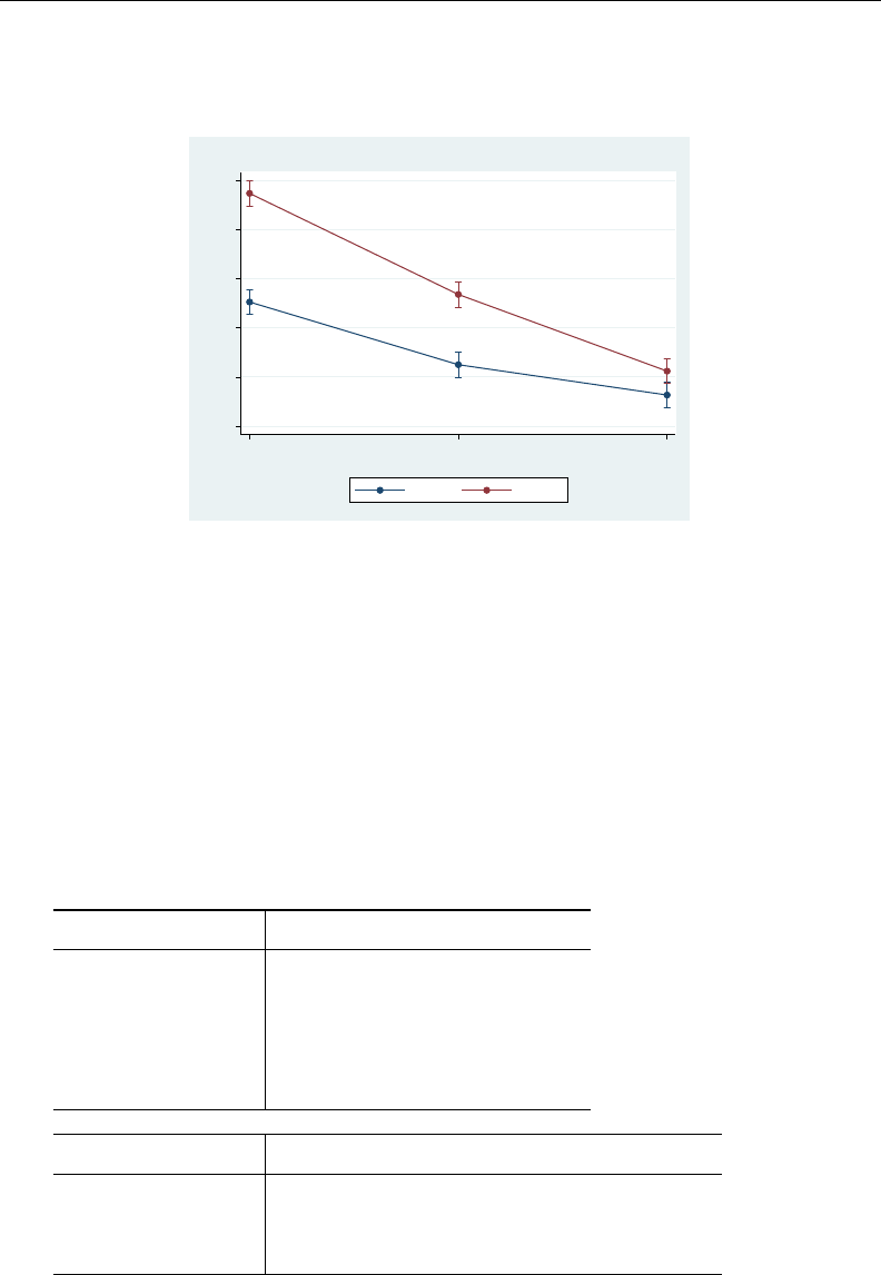
contrast — Contrasts and linear hypothesis tests after estimation 333
We can graph the results:
. marginsplot
Variables that uniquely identify margins: dose gender
−20 −15 −10 −5 0 5
Linear Prediction
250 500 750
dosage in milligrams per day
male female
Adjusted Predictions of dose#gender with 95% CIs
The lines are not parallel, which we expected because the interaction term is significant. Males
experience a greater decline in blood pressure at every dosage level, but the effect of increasing
dosage is greater for females. In fact, it is not clear if we can tell the difference between male and
female response at the maximum dosage.
Simple effects
We can contrast the male and female responses within dosage to see the simple effects of gender.
Because there are only two levels in gender, the choice of contrast operator is largely irrelevant.
Aside from orthogonal polynomials, all operators produce the same estimates, although the effects
can change signs.
. contrast r.gender@dose
Contrasts of marginal linear predictions
Margins : asbalanced
df F P>F
gender@dose
(female vs male) 250 1 141.97 0.0000
(female vs male) 500 1 59.33 0.0000
(female vs male) 750 1 6.87 0.0150
Joint 3 69.39 0.0000
Denominator 24
Contrast Std. Err. [95% Conf. Interval]
gender@dose
(female vs male) 250 11.06041 .9282533 9.144586 12.97623
(female vs male) 500 7.149691 .9282533 5.23387 9.065512
(female vs male) 750 2.433124 .9282533 .5173031 4.348944

334 contrast — Contrasts and linear hypothesis tests after estimation
The effect for males is about 11 points higher than for females at a dosage of 250, and that shrinks
to 2.4 points higher at the maximum dosage of 750.
We can form the simple effects the other way by contrasting the effect of dose at each level of
gender:
. contrast ar.dose@gender
Contrasts of marginal linear predictions
Margins : asbalanced
df F P>F
dose@gender
(500 vs 250) male 1 47.24 0.0000
(500 vs 250) female 1 122.90 0.0000
(750 vs 500) male 1 11.06 0.0028
(750 vs 500) female 1 70.68 0.0000
Joint 4 122.65 0.0000
Denominator 24
Contrast Std. Err. [95% Conf. Interval]
dose@gender
(500 vs 250) male -6.380018 .9282533 -8.295839 -4.464198
(500 vs 250) female -10.29073 .9282533 -12.20655 -8.374914
(750 vs 500) male -3.087217 .9282533 -5.003038 -1.171396
(750 vs 500) female -7.803784 .9282533 -9.719605 -5.887963
Here we use the ar. reverse adjacent contrast operator so that first we are comparing a dosage
of 500 with a dosage of 250, and then we are comparing 750 with 500. We see that increasing the
dosage has a larger effect on females—10.3 points when going from 250 to 500 compared with 6.4
points for males, and 7.8 points when going from 500 to 750 versus 3.1 points for males.
Interaction effects
By specifying contrast operators on both factors, we can decompose the interaction effect into
separate interaction contrasts.
. contrast ar.dose#r.gender
Contrasts of marginal linear predictions
Margins : asbalanced
df F P>F
dose#gender
(500 vs 250) (female vs male) 1 8.87 0.0065
(750 vs 500) (female vs male) 1 12.91 0.0015
Joint 2 21.66 0.0000
Denominator 24

contrast — Contrasts and linear hypothesis tests after estimation 335
Contrast Std. Err. [95% Conf. Interval]
dose#gender
(500 vs 250)
(female vs male) -3.910716 1.312748 -6.620095 -1.201336
(750 vs 500)
(female vs male) -4.716567 1.312748 -7.425947 -2.007187
Look for departures from zero to indicate an interaction effect between dose and gender. Both
contrasts are significantly different from zero. Of course, we already knew the overall interaction
was significant from our ANOVA results. The effect of increasing dose from 250 to 500 is 3.9 points
greater in females than in males, and the effect of increasing dose from 500 to 750 is 4.7 points
greater in females than in males. The confidence intervals for both estimates easily exclude zero,
meaning that there is an interaction effect.
The joint test of these two interaction effects reproduces the test of interaction effects in the anova
output. We can see that the Fstatistic of 21.66 matches the statistic from our original ANOVA results.
Main effects
We can perform tests of the main effects by listing each variable individually in contrast.
. contrast dose gender
Contrasts of marginal linear predictions
Margins : asbalanced
df F P>F
dose 2 223.64 0.0000
gender 1 164.85 0.0000
Denominator 24
The Ftests are equivalent to the tests of main effects in the anova output. This is true only for
linear models. contrast provides an easy way to obtain main effects and other ANOVA-style tests
for models whose responses are not linear in the parameters—logistic,probit,glm, etc.
If we include contrast operators on the variables, we can also decompose the main effects into
individual contrasts:
. contrast ar.dose r.gender
Contrasts of marginal linear predictions
Margins : asbalanced
df F P>F
dose
(500 vs 250) 1 161.27 0.0000
(750 vs 500) 1 68.83 0.0000
Joint 2 223.64 0.0000
gender 1 164.85 0.0000
Denominator 24

336 contrast — Contrasts and linear hypothesis tests after estimation
Contrast Std. Err. [95% Conf. Interval]
dose
(500 vs 250) -8.335376 .6563742 -9.690066 -6.980687
(750 vs 500) -5.4455 .6563742 -6.80019 -4.090811
gender
(female vs male) 6.881074 .5359273 5.774974 7.987173
By specifying the ar. operator on dose, we decompose the main effect for dose into two one-degree-
of-freedom contrasts, comparing the marginal mean of blood pressure change for each dosage level
with that of the previous level. Because gender has only two levels, we cannot decompose this main
effect any further. However, specifying a contrast operator on gender allowed us to calculate the
difference in the marginal means for women and men.
Partial interaction effects
At this point, we have looked at the total interaction effects and at the main effects of each variable.
The partial interaction effects are a midpoint between these two types of effects where we collect the
individual interaction effects along the levels of one of the variables and perform a joint test of those
interactions. If we think of the interaction effects as forming a table, with the levels of one factor
variable forming the rows and the levels of the other forming the columns, partial interaction effects
are joint tests of the interactions in a row or a column. To perform these tests, we specify a contrast
operator on only one of the variables in our interaction. For this particular model, these are not very
interesting because our variables have only two and three levels. Therefore, the tests of the partial
interaction effects reproduce the tests that we obtained for the total interaction effects. We specify a
contrast operator only on dose to decompose the overall test for interaction effects into joint tests
for each ar.dose contrast:
. contrast ar.dose#gender
Contrasts of marginal linear predictions
Margins : asbalanced
df F P>F
dose#gender
(500 vs 250) (joint) 1 8.87 0.0065
(750 vs 500) (joint) 1 12.91 0.0015
Joint 2 21.66 0.0000
Denominator 24
The first row is a joint test of all the interaction effects involving the (500 vs 250) comparison
of dosages. The second row is a joint test of all the interaction effects involving the (750 vs 500)
comparison. If we look back at our output in Interaction effects, we can see that there was only one of
each of these interaction effects. Therefore, each test labeled (joint) has only one degree-of-freedom.
We could have instead included a contrast operator on gender to compute the partial interaction
effects along the other dimension:

contrast — Contrasts and linear hypothesis tests after estimation 337
. contrast dose#r.gender
Contrasts of marginal linear predictions
Margins : asbalanced
df F P>F
dose#gender 2 21.66 0.0000
Denominator 24
Here we obtain a joint test of all the interaction effects involving the (female vs male) comparison
for gender. Because gender has only two levels, the (female vs male) contrast is the only reference
category contrast possible. Therefore, we obtain a single joint test of all the interaction effects.
Clearly, the partial interaction effects are not interesting for this particular model. However, if our
factors had more levels, the partial interaction effects would produce tests that are not available in
the total interaction effects. For example, if our model included factors for four dosage levels and
three races, then typing
. contrast ar.dose#race
would produce three joint tests, one for each of the reverse adjacent contrasts for dosage. Each of
these tests would be a two-degree-of-freedom test because race has three levels.
Three-way and higher-order models
All the contrasts and tests that we reviewed above for two-way models can be used with models
that have more terms. For instance, we could fit a three-way full factorial model by using the anova
command:
. use http://www.stata-press.com/data/r13/cont3way
. anova y race##sex##group
We could then test the simple effects of race within each level of the interaction between sex
and group:
. contrast race@sex#group
To see the reference category contrasts that decompose these simple effects, type
. contrast r.race@sex#group
We could test the three-way interaction effects by typing
. contrast race#sex#group
or the interaction effects for the interaction of race and sex by typing
. contrast race#sex
To see the individual reference category contrasts that decompose this interaction effect, type
. contrast r.race#r.sex

338 contrast — Contrasts and linear hypothesis tests after estimation
We could even obtain joint tests for the interaction of race and sex within each level of group
by typing
. contrast race#sex@group
For tests of the main effects of each factor, we can type
. contrast race sex group
We can calculate the individual reference category contrasts that decompose these main effects:
. contrast r.race r.sex r.group
For the partial interaction effects, we could type
. contrast r.race#group
to obtain a joint test of the two-way interaction effects of race and group for each of the individual
r.race contrasts.
We could type
. contrast r.race#sex#group
to obtain a joint test of all the three-way interaction terms for each of the individual r.race contrasts.
Contrast operators
contrast recognizes a set of contrast operators that are used to specify commonly used contrasts.
When these operators are used, contrast will report a test for each individual contrast in addition
to the joint test for the term. We have already seen a few of these, like r. and ar., in the previous
examples. Here we will take a closer look at each of the unweighted operators.
Here we use the cholesterol dataset and the one-way ANOVA model from the example in One-way
models:
. use http://www.stata-press.com/data/r13/cholesterol
(Artificial cholesterol data)
. anova chol agegrp
(output omitted )
The margins command reports the estimated cell means, bµ1,. . . ,bµ5, for each of the five age
groups.
. margins agegrp
Adjusted predictions Number of obs = 75
Expression : Linear prediction, predict()
Delta-method
Margin Std. Err. t P>|t| [95% Conf. Interval]
agegrp
10-19 180.5198 2.666944 67.69 0.000 175.2007 185.8388
20-29 188.7233 2.666944 70.76 0.000 183.4043 194.0424
30-39 202.0608 2.666944 75.76 0.000 196.7418 207.3799
40-59 210.6704 2.666944 78.99 0.000 205.3514 215.9895
60-79 219.282 2.666944 82.22 0.000 213.9629 224.601

contrast — Contrasts and linear hypothesis tests after estimation 339
Contrast operators provide an easy way to make certain types of comparisons of these cell means.
We use the ordinal factor agegrp to demonstrate these operators because some types of contrasts are
only meaningful when the levels of the factor have a natural ordering. We demonstrate these contrast
operators using a one-way model; however, they are equally applicable to main effects, simple effects,
and interactions for more complicated models.
Differences from a reference level (r.)
The r. operator specifies that each level of the attached factor variable be compared with a
reference level. These are referred to as reference-level or reference-category contrasts (or effects),
and r. is the reference-level operator.
In the following, we use the r. operator to test the effect of each category of age group when
that category is compared with a reference category.
. contrast r.agegrp
Contrasts of marginal linear predictions
Margins : asbalanced
df F P>F
agegrp
(20-29 vs 10-19) 1 4.73 0.0330
(30-39 vs 10-19) 1 32.62 0.0000
(40-59 vs 10-19) 1 63.91 0.0000
(60-79 vs 10-19) 1 105.62 0.0000
Joint 4 35.02 0.0000
Denominator 70
Contrast Std. Err. [95% Conf. Interval]
agegrp
(20-29 vs 10-19) 8.203575 3.771628 .6812991 15.72585
(30-39 vs 10-19) 21.54105 3.771628 14.01878 29.06333
(40-59 vs 10-19) 30.15067 3.771628 22.6284 37.67295
(60-79 vs 10-19) 38.76221 3.771628 31.23993 46.28448
In the first table, the row labeled (20-29 vs 10-19) is a test of µ2=µ1, a test that the mean
cholesterol levels for the 10–19 age group and the 20–29 age group are equal. The tests in the
next three rows are defined similarly. The row labeled Joint provides the joint test for these four
hypotheses, which is just the test of the main effects of age group.
The second table provides the contrasts of each category with the reference category along with
confidence intervals. The contrast in the row labeled (20-29 vs 10-19) is the difference in the cell
means of the second age group and the first age group, bµ2−bµ1.
The first level of a factor is the default reference level, but we can specify a different reference
level by using the b. operator; see [U] 11.4.3.2 Base levels. Here we use the last age group, (60-79),
instead of the first as the reference category. We also include the nowald option so that only the
table of contrasts and their confidence intervals is produced.

340 contrast — Contrasts and linear hypothesis tests after estimation
. contrast rb5.agegrp, nowald
Contrasts of marginal linear predictions
Margins : asbalanced
Contrast Std. Err. [95% Conf. Interval]
agegrp
(10-19 vs 60-79) -38.76221 3.771628 -46.28448 -31.23993
(20-29 vs 60-79) -30.55863 3.771628 -38.08091 -23.03636
(30-39 vs 60-79) -17.22115 3.771628 -24.74343 -9.698877
(40-59 vs 60-79) -8.611533 3.771628 -16.13381 -1.089257
Now the first row is labeled (10-19 vs 60-79) and is the difference in the cell means of the first
and fifth age groups.
Differences from the next level (a.)
The a. operator specifies that each level of the attached factor variable be compared with the next
level. These are referred to as adjacent contrasts (or effects), and a. is the adjacent operator. This
operator is only meaningful with factor variables that have a natural ordering in the levels.
We can use the a. operator to perform tests that each level of age group differs from the next
adjacent level.
. contrast a.agegrp
Contrasts of marginal linear predictions
Margins : asbalanced
df F P>F
agegrp
(10-19 vs 20-29) 1 4.73 0.0330
(20-29 vs 30-39) 1 12.51 0.0007
(30-39 vs 40-59) 1 5.21 0.0255
(40-59 vs 60-79) 1 5.21 0.0255
Joint 4 35.02 0.0000
Denominator 70
Contrast Std. Err. [95% Conf. Interval]
agegrp
(10-19 vs 20-29) -8.203575 3.771628 -15.72585 -.6812991
(20-29 vs 30-39) -13.33748 3.771628 -20.85976 -5.815204
(30-39 vs 40-59) -8.60962 3.771628 -16.1319 -1.087345
(40-59 vs 60-79) -8.611533 3.771628 -16.13381 -1.089257
In the first table, the row labeled (10-19 vs 20-29) tests the effect of belonging to the 10–19 age
group instead of the 20–29 age group. Likewise, the rows labeled (20-29 vs 30-39),(30-39 vs
40-59), and (40-59 vs 60-79) are tests for the effects of being in the younger of the two age
groups instead of the older one.
In the second table, the contrast in the row labeled (10-19 vs 20-29) is the difference in the
cell means of the first and second age groups, bµ1−bµ2. The contrasts in the other rows are defined
similarly.

contrast — Contrasts and linear hypothesis tests after estimation 341
Differences from the previous level (ar.)
The ar. operator specifies that each level of the attached factor variable be compared with the
previous level. These are referred to as reverse adjacent contrasts (or effects), and ar. is the reverse
adjacent operator. As with the a. operator, this operator is only meaningful with factor variables that
have a natural ordering in the levels.
In the following, we use the ar. operator to report tests for the individual reverse adjacent effects
of agegrp.
. contrast ar.agegrp
Contrasts of marginal linear predictions
Margins : asbalanced
df F P>F
agegrp
(20-29 vs 10-19) 1 4.73 0.0330
(30-39 vs 20-29) 1 12.51 0.0007
(40-59 vs 30-39) 1 5.21 0.0255
(60-79 vs 40-59) 1 5.21 0.0255
Joint 4 35.02 0.0000
Denominator 70
Contrast Std. Err. [95% Conf. Interval]
agegrp
(20-29 vs 10-19) 8.203575 3.771628 .6812991 15.72585
(30-39 vs 20-29) 13.33748 3.771628 5.815204 20.85976
(40-59 vs 30-39) 8.60962 3.771628 1.087345 16.1319
(60-79 vs 40-59) 8.611533 3.771628 1.089257 16.13381
Here the Wald tests in the first table for the individual reverse adjacent effects are equivalent to the
tests for the adjacent effects in the previous example. However, if we compare values of the contrasts
in the bottom tables, we see the difference between the r. and the ar. operators. This time, the
contrast in the first row is labeled (20-29 vs 10-19) and is the difference in the cell means of the
second and first age groups, bµ2−bµ1. This is the estimated effect of belonging to the 20–29 age
group instead of the 10–19 age group. The remaining rows make similar comparisons to the previous
level.
Differences from the grand mean (g.)
The g. operator specifies that each level of a factor variable be compared with the grand mean of
all levels. For this operator, the grand mean is computed using a simple average of the cell means.

342 contrast — Contrasts and linear hypothesis tests after estimation
Here are the grand mean effects of agegrp:
. contrast g.agegrp
Contrasts of marginal linear predictions
Margins : asbalanced
df F P>F
agegrp
(10-19 vs mean) 1 68.42 0.0000
(20-29 vs mean) 1 23.36 0.0000
(30-39 vs mean) 1 0.58 0.4506
(40-59 vs mean) 1 19.08 0.0000
(60-79 vs mean) 1 63.65 0.0000
Joint 4 35.02 0.0000
Denominator 70
Contrast Std. Err. [95% Conf. Interval]
agegrp
(10-19 vs mean) -19.7315 2.385387 -24.48901 -14.974
(20-29 vs mean) -11.52793 2.385387 -16.28543 -6.770423
(30-39 vs mean) 1.809552 2.385387 -2.947953 6.567057
(40-59 vs mean) 10.41917 2.385387 5.661668 15.17668
(60-79 vs mean) 19.0307 2.385387 14.2732 23.78821
There are five age groups in our estimation sample. Thus the row labeled (10-19 vs mean) tests µ1=
(µ1+µ2+µ3+µ4+µ5)/5. The row labeled (20-29 vs mean) tests µ2= (µ1+µ2+µ3+µ4+µ5)/5.
The remaining rows perform similar tests for the third, fourth, and fifth age groups. In our example,
the means for all age groups except the 30–39 age group are statistically different from the grand
mean.
Differences from the mean of subsequent levels (h.)
The h. operator specifies that each level of the attached factor variable be compared with the mean
of subsequent levels. These are referred to as Helmert contrasts (or effects), and h. is the Helmert
operator. For this operator, the mean is computed using a simple average of the cell means. This
operator is only meaningful with factor variables that have a natural ordering in the levels.
Here are the Helmert contrasts for agegrp:
. contrast h.agegrp
Contrasts of marginal linear predictions
Margins : asbalanced
df F P>F
agegrp
(10-19 vs >10-19) 1 68.42 0.0000
(20-29 vs >20-29) 1 50.79 0.0000
(30-39 vs >30-39) 1 15.63 0.0002
(40-59 vs 60-79) 1 5.21 0.0255
Joint 4 35.02 0.0000
Denominator 70

contrast — Contrasts and linear hypothesis tests after estimation 343
Contrast Std. Err. [95% Conf. Interval]
agegrp
(10-19 vs >10-19) -24.66438 2.981734 -30.61126 -18.7175
(20-29 vs >20-29) -21.94774 3.079522 -28.08965 -15.80583
(30-39 vs >30-39) -12.91539 3.266326 -19.42987 -6.400905
(40-59 vs 60-79) -8.611533 3.771628 -16.13381 -1.089257
The row labeled (10-19 vs >10-19) tests µ1= (µ2+µ3+µ4+µ5)/4, that is, that the cell mean
for the youngest age group is equal to the average of the cell means for the older age groups. The
row labeled (20-29 vs >20-29) tests µ2= (µ3+µ4+µ5)/3. The tests in the other rows are
defined similarly.
Differences from the mean of previous levels (j.)
The j. operator specifies that each level of the attached factor variable be compared with the
mean of the previous levels. These are referred to as reverse Helmert contrasts (or effects), and j.
is the reverse Helmert operator. For this operator, the mean is computed using a simple average of
the cell means. This operator is only meaningful with factor variables that have a natural ordering in
the levels.
Here are the reverse Helmert contrasts of agegrp:
. contrast j.agegrp
Contrasts of marginal linear predictions
Margins : asbalanced
df F P>F
agegrp
(20-29 vs 10-19) 1 4.73 0.0330
(30-39 vs <30-39) 1 28.51 0.0000
(40-59 vs <40-59) 1 43.18 0.0000
(60-79 vs <60-79) 1 63.65 0.0000
Joint 4 35.02 0.0000
Denominator 70
Contrast Std. Err. [95% Conf. Interval]
agegrp
(20-29 vs 10-19) 8.203575 3.771628 .6812991 15.72585
(30-39 vs <30-39) 17.43927 3.266326 10.92479 23.95375
(40-59 vs <40-59) 20.2358 3.079522 14.09389 26.37771
(60-79 vs <60-79) 23.78838 2.981734 17.8415 29.73526
The row labeled (20-29 vs 10-19) tests µ2=µ1, that is, that the cell means for the 20–29 and the
10–19 age groups are equal. The row labeled (30-39 vs <30-29) tests µ3= (µ1+µ2)/2, that is,
that the cell mean for the 30–39 age group is equal to the average of the cell means for the 10–19
and 20–29 age groups. The tests in the remaining rows are defined similarly.

344 contrast — Contrasts and linear hypothesis tests after estimation
Orthogonal polynomials (p. and q.)
The p. and q. operators specify that orthogonal polynomials be applied to the attached factor
variable. Orthogonal polynomial contrasts allow us to partition the effects of a factor variable into
linear, quadratic, cubic, and higher-order polynomial components. The p. operator applies orthogonal
polynomials using the values of the factor variable. The q. operator applies orthogonal polynomials
using the level indices. If the level values of the factor variable are equally spaced, as with our agegrp
variable, then the p. and q. operators yield the same result. These operators are only meaningful
with factor variables that have a natural ordering in the levels.
Because agegrp has five levels, contrast can test the linear, quadratic, cubic, and quartic effects
of agegrp.
. contrast p.agegrp, noeffects
Contrasts of marginal linear predictions
Margins : asbalanced
df F P>F
agegrp
(linear) 1 139.11 0.0000
(quadratic) 1 0.15 0.6962
(cubic) 1 0.37 0.5448
(quartic) 1 0.43 0.5153
Joint 4 35.02 0.0000
Denominator 70
The row labeled (linear) tests the linear effect of agegrp, the only effect that appears to be
significant in this case.
The labels for our agegrp variable show the age ranges that correspond to each level.
. label list ages
ages:
1 10-19
2 20-29
3 30-39
4 40-59
5 60-79
Notice that these groups do not have equal widths. Now let’s refit our model using the agemidpt
variable. The values of agemidpt indicate the midpoint of each age group that was defined by the
agegrp variable and are, therefore, not equally spaced.
. anova chol agemidpt
Number of obs = 75 R-squared = 0.6668
Root MSE = 10.329 Adj R-squared = 0.6477
Source Partial SS df MS F Prob > F
Model 14943.3997 4 3735.84993 35.02 0.0000
agemidpt 14943.3997 4 3735.84993 35.02 0.0000
Residual 7468.21971 70 106.688853
Total 22411.6194 74 302.859722

contrast — Contrasts and linear hypothesis tests after estimation 345
Now if we use the q. operator, we will obtain the same results as above because the level indices
of agemidpt are equivalent to the values of agegrp.
. contrast q.agemidpt, noeffects
Contrasts of marginal linear predictions
Margins : asbalanced
df F P>F
agemidpt
(linear) 1 139.11 0.0000
(quadratic) 1 0.15 0.6962
(cubic) 1 0.37 0.5448
(quartic) 1 0.43 0.5153
Joint 4 35.02 0.0000
Denominator 70
However, if we use the p. operator, we will instead fit an orthogonal polynomial to the midpoint
values.
. contrast p.agemidpt, noeffects
Contrasts of marginal linear predictions
Margins : asbalanced
df F P>F
agemidpt
(linear) 1 133.45 0.0000
(quadratic) 1 5.40 0.0230
(cubic) 1 0.05 0.8198
(quartic) 1 1.16 0.2850
Joint 4 35.02 0.0000
Denominator 70
Using the values of the midpoints, the quadratic effect is also significant at the 5% level.
Technical note
We used the noeffects option when working with orthogonal polynomial contrasts. Apart from
perhaps the sign of the contrast, the values of the individual contrasts are not meaningful for orthogonal
polynomial contrasts. In addition, many textbooks provide tables with contrast coefficients that can be
used to compute orthogonal polynomial contrasts where the levels of a factor are equally spaced. If
we use these coefficients and calculate the contrasts manually with user-defined contrasts, as described
below, the Wald tests for the polynomial terms will be equivalent, but the values of the individual
contrasts will not necessarily match those that we obtain when using the polynomial contrast operator.
When we use one of these contrast operators, an algorithm is used to calculate the coefficients of the
polynomial contrast that will allow for unequal spacing in the levels of the factor as well as in the
weights for the cell frequencies (when using pw. or qw.), as described in Methods and formulas.

346 contrast — Contrasts and linear hypothesis tests after estimation
User-defined contrasts
In the previous examples, we performed tests using contrast operators. When there is not a contrast
operator available to calculate the contrast in which we are interested, we can specify custom contrasts.
Here we fit a one-way model for cholesterol on the factor race, which has three levels:
. label list race
race:
1 black
2 white
3 other
. anova chol race
Number of obs = 75 R-squared = 0.0299
Root MSE = 17.3775 Adj R-squared = 0.0029
Source Partial SS df MS F Prob > F
Model 669.278235 2 334.639117 1.11 0.3357
race 669.278235 2 334.639117 1.11 0.3357
Residual 21742.3412 72 301.976961
Total 22411.6194 74 302.859722
margins calculates the estimated cell mean cholesterol level for each race:
. margins race
Adjusted predictions Number of obs = 75
Expression : Linear prediction, predict()
Delta-method
Margin Std. Err. t P>|t| [95% Conf. Interval]
race
black 204.4279 3.475497 58.82 0.000 197.4996 211.3562
white 197.6132 3.475497 56.86 0.000 190.6849 204.5415
other 198.7127 3.475497 57.18 0.000 191.7844 205.6409
Suppose we want to test the following linear combination:
3
X
i=1
ciµi
where µiis the cell mean of chol when race is equal to its ith level (the means estimated using
margins above). Assuming the cielements sum to zero, this linear combination is a contrast. We
can specify this type of custom contrast by using the following syntax:
{race c1c2c3}
The null hypothesis for the test of the main effects of race is
H0race:µ1=µ2=µ3

contrast — Contrasts and linear hypothesis tests after estimation 347
Although H0race can be tested using any of several different contrasts on the cell means, we will test
it by comparing the second and third cell means with the first. To test that the cell means for blacks
and whites are equal, µ1=µ2, we can specify the contrast
{race -1 1 0}
To test that the cell means for blacks and other races are equal, µ1=µ3, we can specify the contrast
{race -1 0 1}
We can use both in a single call to contrast.
. contrast {race -1 1 0} {race -1 0 1}
Contrasts of marginal linear predictions
Margins : asbalanced
df F P>F
race
(1) 1 1.92 0.1699
(2) 1 1.35 0.2488
Joint 2 1.11 0.3357
Denominator 72
Contrast Std. Err. [95% Conf. Interval]
race
(1) -6.814717 4.915095 -16.61278 2.983345
(2) -5.715261 4.915095 -15.51332 4.082801
The row labeled (1) is the test for µ1=µ2, the first specified contrast. The row labeled (2) is the
test for µ1=µ3, the second specified contrast. The row labeled Joint is the overall test for the
main effects of race.
Now let’s fit a model with two factors, race and age group:
. anova chol race##agegrp
Number of obs = 75 R-squared = 0.7524
Root MSE = 9.61785 Adj R-squared = 0.6946
Source Partial SS df MS F Prob > F
Model 16861.438 14 1204.38843 13.02 0.0000
race 669.278235 2 334.639117 3.62 0.0329
agegrp 14943.3997 4 3735.84993 40.39 0.0000
race#agegrp 1248.76005 8 156.095006 1.69 0.1201
Residual 5550.18143 60 92.5030238
Total 22411.6194 74 302.859722
The null hypothesis for the test of the main effects of race is now
H0race:µ1·=µ2·=µ3·
where µi·is the marginal mean of chol when race is equal to its ith level.

348 contrast — Contrasts and linear hypothesis tests after estimation
We can use the same syntax as above to perform this test by specifying contrasts on the marginal
means of race:
. contrast {race -1 1 0} {race -1 0 1}
Contrasts of marginal linear predictions
Margins : asbalanced
df F P>F
race
(1) 1 6.28 0.0150
(2) 1 4.41 0.0399
Joint 2 3.62 0.0329
Denominator 60
Contrast Std. Err. [95% Conf. Interval]
race
(1) -6.814717 2.720339 -12.2562 -1.37323
(2) -5.715261 2.720339 -11.15675 -.2737739
Custom contrasts may be specified on the cell means of interactions, too. Here we use margins
to calculate the mean of chol for each cell in the interaction of race and agegrp:
. margins race#agegrp
Adjusted predictions Number of obs = 75
Expression : Linear prediction, predict()
Delta-method
Margin Std. Err. t P>|t| [95% Conf. Interval]
race#agegrp
black#10-19 179.2309 4.301233 41.67 0.000 170.6271 187.8346
black#20-29 196.4777 4.301233 45.68 0.000 187.874 205.0814
black#30-39 210.6694 4.301233 48.98 0.000 202.0656 219.2731
black#40-59 214.097 4.301233 49.78 0.000 205.4933 222.7008
black#60-79 221.6646 4.301233 51.54 0.000 213.0609 230.2684
white#10-19 186.0727 4.301233 43.26 0.000 177.469 194.6765
white#20-29 184.6714 4.301233 42.93 0.000 176.0676 193.2751
white#30-39 196.2633 4.301233 45.63 0.000 187.6595 204.867
white#40-59 209.9953 4.301233 48.82 0.000 201.3916 218.5991
white#60-79 211.0633 4.301233 49.07 0.000 202.4595 219.667
other#10-19 176.2556 4.301233 40.98 0.000 167.6519 184.8594
other#20-29 185.0209 4.301233 43.02 0.000 176.4172 193.6247
other#30-39 199.2498 4.301233 46.32 0.000 190.646 207.8535
other#40-59 207.9189 4.301233 48.34 0.000 199.3152 216.5227
other#60-79 225.118 4.301233 52.34 0.000 216.5143 233.7218
Now we are interested in testing the following linear combination of these cell means:
3
X
i=1
5
X
j=1
cij µij

contrast — Contrasts and linear hypothesis tests after estimation 349
We can specify this type of custom contrast using the following syntax:
{race#agegrp c11 c12 . . . c15 c21 c22 . . . c25 c31 c32 . . . c35}
Because the marginal means of chol for each level of race are linear combinations of the cell
means, we can compose the test for the main effects of race in terms of the cell means directly.
The constraint that the marginal means for blacks and whites are equal, µ1·=µ2·, translates to the
following constraint on the cell means:
1
5(µ11 +µ12 +µ13 +µ14 +µ15) = 1
5(µ21 +µ22 +µ23 +µ24 +µ25)
Ignoring the common factor, we can specify this contrast as
{race#agegrp -1 -1 -1 -1 -1 1 1 1 1 1 0 0 0 0 0}
contrast will fill in the trailing zeros for us if we neglect to specify them, so
{race#agegrp -1 -1 -1 -1 -1 1 1 1 1 1}
is also allowed. The other constraint, µ1·=µ3·, translates to
1
5(µ11 +µ12 +µ13 +µ14 +µ15) = 1
5(µ31 +µ32 +µ33 +µ34 +µ35)
This can be specified to contrast as
{race#agegrp -1 -1 -1 -1 -1 0 0 0 0 0 1 1 1 1 1}
The following call to contrast yields the same test results as above.
. contrast {race#agegrp -1 -1 -1 -1 -1 1 1 1 1 1}
> {race#agegrp -1 -1 -1 -1 -1 0 0 0 0 0 1 1 1 1 1}, noeffects
Contrasts of marginal linear predictions
Margins : asbalanced
df F P>F
race#agegrp
(1) (1) 1 6.28 0.0150
(2) (2) 1 4.41 0.0399
Joint 2 3.62 0.0329
Denominator 60
The row labeled (1) (1) is the test for
µ11 +µ12 +µ13 +µ14 +µ15 =µ21 +µ22 +µ23 +µ24 +µ25
It was the first specified contrast. The row labeled (2) (2) is the test for
µ11 +µ12 +µ13 +µ14 +µ15 =µ31 +µ32 +µ33 +µ34 +µ35
It was the second specified contrast. The row labeled Joint tests (1) (1) and (2) (2) simultaneously.

350 contrast — Contrasts and linear hypothesis tests after estimation
We used the noeffects option above to suppress the table of contrasts. We can omit the 1/5
from the equations for µ1·=µ2·and µ1·=µ3·and still obtain the appropriate tests. However, if
we want to calculate the differences in the marginal means, we must include the 1/5=0.2 on each
of the contrast coefficients as follows:
. contrast {race#agegrp -0.2 -0.2 -0.2 -0.2 -0.2
0.2 0.2 0.2 0.2 0.2}
{race#agegrp -0.2 -0.2 -0.2 -0.2 -0.2
00000
0.2 0.2 0.2 0.2 0.2}
So far, we have reproduced the reference category contrasts by specifying user-defined contrasts
on the marginal means and then on the cell means. For this test, it would have been easier to use the
r. contrast operator:
. contrast r.race, noeffects
Contrasts of marginal linear predictions
Margins : asbalanced
df F P>F
race
(white vs black) 1 6.28 0.0150
(other vs black) 1 4.41 0.0399
Joint 2 3.62 0.0329
Denominator 60
In most cases, we can use contrast operators to perform tests. However, if we want to compare,
for instance, the second and third age groups with the fourth and fifth age groups with the test
1
2(µ·2+µ·3) = 1
2(µ·4+µ·5)
there is not a contrast operator that corresponds to this particular contrast. A custom contrast is
necessary.
. contrast {agegrp 0 -0.5 -0.5 0.5 0.5}
Contrasts of marginal linear predictions
Margins : asbalanced
df F P>F
agegrp 1 62.19 0.0000
Denominator 60
Contrast Std. Err. [95% Conf. Interval]
agegrp
(1) 19.58413 2.483318 14.61675 24.5515

contrast — Contrasts and linear hypothesis tests after estimation 351
Empty cells
An empty cell is a combination of the levels of factor variables that is not observed in the estimation
sample. In the previous examples, we have seen data with three levels of race, five levels of agegrp,
and all level combinations of race and agegrp present. Suppose there are no observations for white
individuals in the second age group (ages 20–29).
. use http://www.stata-press.com/data/r13/cholesterol2
(Artificial cholesterol data, empty cells)
. label list
ages:
1 10-19
2 20-29
3 30-39
4 40-59
5 60-79
race:
1 black
2 white
3 other
. regress chol race##agegrp
note: 2.race#2.agegrp identifies no observations in the sample
Source SS df MS Number of obs = 70
F( 13, 56) = 13.51
Model 15751.6113 13 1211.66241 Prob > F = 0.0000
Residual 5022.71559 56 89.6913498 R-squared = 0.7582
Adj R-squared = 0.7021
Total 20774.3269 69 301.077201 Root MSE = 9.4706
chol Coef. Std. Err. t P>|t| [95% Conf. Interval]
race
white 12.84185 5.989703 2.14 0.036 .8430383 24.84067
other -.167627 5.989703 -0.03 0.978 -12.16644 11.83119
agegrp
20-29 17.24681 5.989703 2.88 0.006 5.247991 29.24562
30-39 31.43847 5.989703 5.25 0.000 19.43966 43.43729
40-59 34.86613 5.989703 5.82 0.000 22.86732 46.86495
60-79 44.43374 5.989703 7.42 0.000 32.43492 56.43256
race#agegrp
white#20-29 0 (empty)
white#30-39 -22.83983 8.470719 -2.70 0.009 -39.80872 -5.870939
white#40-59 -14.67558 8.470719 -1.73 0.089 -31.64447 2.293306
white#60-79 -10.51115 8.470719 -1.24 0.220 -27.48004 6.457735
other#20-29 -6.054425 8.470719 -0.71 0.478 -23.02331 10.91446
other#30-39 -11.48083 8.470719 -1.36 0.181 -28.44971 5.488063
other#40-59 -.6796112 8.470719 -0.08 0.936 -17.6485 16.28928
other#60-79 -1.578052 8.470719 -0.19 0.853 -18.54694 15.39084
_cons 175.2309 4.235359 41.37 0.000 166.7464 183.7153

352 contrast — Contrasts and linear hypothesis tests after estimation
Now let’s use contrast to test the main effects of race:
. contrast race
Contrasts of marginal linear predictions
Margins : asbalanced
df F P>F
race (not testable)
Denominator 56
By “not testable”, contrast means that it cannot form a test for the main effects of race based
on estimable functions of the model coefficients. agegrp has five levels, so contrast constructs an
estimate of the ith margin for race as
bµi·=1
5
5
X
j=1 bµij =bµ0+bαi+1
5
5
X
j=1 nb
βj+ ( c
αβ)ij o
but (c
αβ)22 was constrained to zero because of the empty cell, so bµ2·is not an estimable function
of the model coefficients.
See Estimable functions in Methods and formulas of [R]margins for a technical description of
estimable functions. The emptycells(reweight) option causes contrast to estimate µ2·by
bµ2·=bµ21 +bµ23 +bµ24 +bµ25
4
which is an estimable function of the model coefficients.
. contrast race, emptycells(reweight)
Contrasts of marginal linear predictions
Margins : asbalanced
Empty cells : reweight
df F P>F
race 2 3.17 0.0498
Denominator 56

contrast — Contrasts and linear hypothesis tests after estimation 353
We can reconstruct the effect of the emptycells(reweight) option by using custom contrasts.
. contrast {race#agegrp -4 -4 -4 -4 -4 5 0 5 5 5}
> {race#agegrp -1 -1 -1 -1 -1 0 0 0 0 0 1 1 1 1 1}, noeffects
Contrasts of marginal linear predictions
Margins : asbalanced
df F P>F
race#agegrp
(1) (1) 1 1.06 0.3080
(2) (2) 1 2.37 0.1291
Joint 2 3.17 0.0498
Denominator 56
The row labeled (1) (1) is the test for
1
5(µ11 +µ12 +µ13 +µ14 +µ15) = 1
4(µ21 +µ23 +µ24 +µ25)
It was the first specified contrast. The row labeled (2) (2) is the test for
µ11 +µ12 +µ13 +µ14 +µ15 =µ31 +µ32 +µ33 +µ34 +µ35
It was the second specified contrast. The row labeled Joint is the overall test of the main effects of
race.
Empty cells, ANOVA style
Let’s refit the linear model from the previous example with anova to compare with contrast’s
test for the main effects of race.
. anova chol race##agegrp
Number of obs = 70 R-squared = 0.7582
Root MSE = 9.47055 Adj R-squared = 0.7021
Source Partial SS df MS F Prob > F
Model 15751.6113 13 1211.66241 13.51 0.0000
race 305.49046 2 152.74523 1.70 0.1914
agegrp 14387.8559 4 3596.96397 40.10 0.0000
race#agegrp 795.807574 7 113.686796 1.27 0.2831
Residual 5022.71559 56 89.6913498
Total 20774.3269 69 301.077201
contrast and anova handled the empty cell differently; the Fstatistic reported by contrast
was 3.17, but anova reported 1.70. To see how they differ, consider the following table of the cell
means and margins for our situation.

354 contrast — Contrasts and linear hypothesis tests after estimation
agegrp
1 2 3 4 5
1µ11 µ12 µ13 µ14 µ15 µ1·
race 2µ21 µ23 µ24 µ25
3µ31 µ32 µ33 µ34 µ35 µ3·
µ·1µ·3µ·4µ·5
For testing the main effects of race, we know that we will be testing the equality of the marginal
means for rows 1 and 3, that is, µ1·=µ3·. This translates into the following constraint:
µ11 +µ12 +µ13 +µ14 +µ15 =µ31 +µ32 +µ33 +µ34 +µ35
Because row 2 contains an empty cell in column 2, anova dropped column 2 and tested the equality
of the marginal mean for row 2 with the average of the marginal means from rows 1 and 3, using
only the remaining cell means. This translates into the following constraint:
2(µ21 +µ23 +µ24 +µ25) = µ11 +µ13 +µ14 +µ15 +µ31 +µ33 +µ34 +µ35 (1)
Now that we know the constraints that anova used to test for the main effects of race, we can use
custom contrasts to reproduce the anova test result.
. contrast {race#agegrp -1 -1 -1 -1 -1 0 0 0 0 0 1 1 1 1 1}
> {race#agegrp 1 0 1 1 1 -2 0 -2 -2 -2 1 0 1 1 1}, noeffects
Contrasts of marginal linear predictions
Margins : asbalanced
df F P>F
race#agegrp
(1) (1) 1 2.37 0.1291
(2) (2) 1 1.03 0.3138
Joint 2 1.70 0.1914
Denominator 56
The row labeled (1) (1) is the test for µ1·=µ3·; it was the first specified contrast. The row labeled
(2) (2) is the test for the constraint in (1); it was the second specified contrast. The row labeled
Joint is an overall test for the main effects of race.
Nested effects
contrast has the |operator for computing simple effects when the levels of one factor are nested
within the levels of another. Here is a fictional example where we are interested in the effect of
five methods of teaching algebra on students’ scores for the math portion of the SAT. Suppose three
algebra classes are randomly sampled from classes using each of the five methods so that class is
nested in method as demonstrated in the following tabulation.

contrast — Contrasts and linear hypothesis tests after estimation 355
. use http://www.stata-press.com/data/r13/sat
(Artificial SAT data)
. tabulate class method
method
class 1 2 3 4 5 Total
1 5 0 0 0 0 5
2 5 0 0 0 0 5
3 5 0 0 0 0 5
4 0 5 0 0 0 5
5 0 5 0 0 0 5
6 0 5 0 0 0 5
7 0 0 5 0 0 5
8 0 0 5 0 0 5
9 0 0 5 0 0 5
10 0 0 0 5 0 5
11 0 0 0 5 0 5
12 0 0 0 5 0 5
13 0 0 0 0 5 5
14 0 0 0 0 5 5
15 0 0 0 0 5 5
Total 15 15 15 15 15 75
We will consider method as fixed and class nested in method as random. To use class nested
in method as the error term for method, we can specify the following anova model:
. anova score method / class|method /
Number of obs = 75 R-squared = 0.7599
Root MSE = 71.8517 Adj R-squared = 0.7039
Source Partial SS df MS F Prob > F
Model 980312 14 70022.2857 13.56 0.0000
method 905872 4 226468 30.42 0.0000
class|method 74440 10 7444
class|method 74440 10 7444 1.44 0.1845
Residual 309760 60 5162.66667
Total 1290072 74 17433.4054
Like anova,contrast allows the |operator, which specifies that one variable is nested in the
levels of another. We can use contrast to test the main effects of method and the simple effects
of class within method.

356 contrast — Contrasts and linear hypothesis tests after estimation
. contrast method class|method
Contrasts of marginal linear predictions
Margins : asbalanced
df F P>F
method (not testable)
class|method
1 2 2.80 0.0687
2 2 0.91 0.4089
3 2 1.10 0.3390
4 2 0.22 0.8025
5 2 2.18 0.1221
Joint 10 1.44 0.1845
Denominator 60
Although contrast was able to perform the individual tests for the simple effects of class within
method, empty cells in the interaction between method and class prevented contrast from testing
for a main effect of method. Here we add the emptycells(reweight) option so that contrast
can take the empty cells into account when computing the marginal means for method.
. contrast method class|method, emptycells(reweight)
Contrasts of marginal linear predictions
Margins : asbalanced
Empty cells : reweight
df F P>F
method 4 43.87 0.0000
class|method
1 2 2.80 0.0687
2 2 0.91 0.4089
3 2 1.10 0.3390
4 2 0.22 0.8025
52 2.18 0.1221
Joint 10 1.44 0.1845
Denominator 60
Now contrast does report a test for the main effects of method. However, if we compare this with
the anova results, we will see that the results are different. They are different because contrast
uses the residual error term to compute the Ftest by default. Using notation similar to anova, we
can use the /operator to specify a different error term for the test. Therefore, we can reproduce the
test of main effects from our anova command by typing

contrast — Contrasts and linear hypothesis tests after estimation 357
. contrast method / class|method /, emptycells(reweight)
Contrasts of marginal linear predictions
Margins : asbalanced
Empty cells : reweight
df F P>F
method 4 30.42 0.0000
class|method 10 (denominator)
class|method
1 2 2.80 0.0687
2 2 0.91 0.4089
3 2 1.10 0.3390
4 2 0.22 0.8025
5 2 2.18 0.1221
Joint 10 1.44 0.1845
Denominator 60
Multiple comparisons
We have seen that contrast can report the individual linear combinations that make up the
requested effects. Depending upon the specified option, contrast will report confidence intervals,
p-values, or both in the effects table. By default, the reported confidence intervals and p-values are
not adjusted for multiple comparisons. Use the mcompare() option to adjust the confidence intervals
and p-values for multiple comparisons of the individual effects.
Let’s compute the grand mean effects of race using the g. operator. We also specify the mcom-
pare(bonferroni) option to compute p-values and confidence intervals using Bonferroni’s adjust-
ment.
. use http://www.stata-press.com/data/r13/cholesterol
(Artificial cholesterol data)
. anova chol race##agegrp
(output omitted )
. contrast g.race, mcompare(bonferroni)
Contrasts of marginal linear predictions
Margins : asbalanced
Bonferroni
df F P>F P>F
race
(black vs mean) 1 7.07 0.0100 0.0301
(white vs mean) 1 2.82 0.0982 0.2947
(other vs mean) 1 0.96 0.3312 0.9936
Joint 2 3.62 0.0329
Denominator 60
Note: Bonferroni-adjusted p-values are reported for tests on
individual contrasts only.

358 contrast — Contrasts and linear hypothesis tests after estimation
Number of
Comparisons
race 3
Bonferroni
Contrast Std. Err. [95% Conf. Interval]
race
(black vs mean) 4.17666 1.570588 .3083743 8.044945
(white vs mean) -2.638058 1.570588 -6.506343 1.230227
(other vs mean) -1.538602 1.570588 -5.406887 2.329684
The last table reports a Bonferroni-adjusted confidence interval for each individual contrast. (Use
the effects option to add p-values to the last table.) The first table includes a Bonferroni-adjusted
p-value for each test that is not a joint test.
Joint tests are never adjusted for multiple comparisons. For example,
. contrast race@agegrp, mcompare(bonferroni)
Contrasts of marginal linear predictions
Margins : asbalanced
df F P>F
race@agegrp
10-19 2 1.37 0.2620
20-29 2 2.44 0.0958
30-39 2 3.12 0.0512
40-59 2 0.53 0.5889
60-79 2 2.90 0.0628
Joint 10 2.07 0.0409
Denominator 60
Note: Bonferroni-adjusted p-values are reported
for tests on individual contrasts only.
Number of
Comparisons
race@agegrp 10

contrast — Contrasts and linear hypothesis tests after estimation 359
Bonferroni
Contrast Std. Err. [95% Conf. Interval]
race@agegrp
(white vs base) 10-19 6.841855 6.082862 -10.88697 24.57068
(white vs base) 20-29 -11.80631 6.082862 -29.53513 5.922513
(white vs base) 30-39 -14.40607 6.082862 -32.13489 3.322751
(white vs base) 40-59 -4.101691 6.082862 -21.83051 13.62713
(white vs base) 60-79 -10.60137 6.082862 -28.33019 7.127448
(other vs base) 10-19 -2.975244 6.082862 -20.70407 14.75358
(other vs base) 20-29 -11.45679 6.082862 -29.18561 6.272031
(other vs base) 30-39 -11.41958 6.082862 -29.1484 6.309244
(other vs base) 40-59 -6.17807 6.082862 -23.90689 11.55075
(other vs base) 60-79 3.453375 6.082862 -14.27545 21.1822
Here we have five tests of simple effects with two degrees of freedom each. No Bonferroni-adjusted
p-values are available for these tests, but the confidence intervals for the individual contrasts are
adjusted.
Unbalanced data
By default, contrast treats all factors as balanced when computing marginal means. By balanced,
we mean that contrast assumes an equal number of observations in each level of each factor and
an equal number of observations in each cell of each interaction. If our data are balanced, there
is no issue. If, however, our data are not balanced, we might prefer that contrast use the actual
cell frequencies from our data in computing marginal means. We instruct contrast to use observed
frequencies by adding the asobserved option.
Even if our data are unbalanced, we might still want contrast to compute balanced marginal
means. It depends on what we want to test and what our data represent. If we have data from a designed
experiment that started with an equal number of males and females but the data became unbalanced
because the data from a few males were unusable, we might still want our margins computed as
though the data were balanced. If, however, we have a representative sample of individuals from Los
Angeles with 40% of European descent, 34% African-American, 25% Hispanic, and 1% Australian,
we probably want our margins computed using these representative frequencies. We do not want
Australians receiving the same weight as Europeans.
The following examples will use an unbalanced version of our dataset.
. use http://www.stata-press.com/data/r13/cholesterol3
(Artificial cholesterol data, unbalanced)
. tab race agegrp
agegrp
race 10-19 20-29 30-39 40-59 60-79 Total
black 1 5 5 4 3 18
white 4 5 7 4 4 24
other 3 7 6 5 4 25
Total 8 17 18 13 11 67
The row labeled Total gives observed cell frequencies for age group. These can be obtained
by summing frequencies from the cells in the corresponding column. In this respect, we can also
refer to them as marginal frequencies. We use the terms marginal frequencies and cell frequencies
interchangeably below.

360 contrast — Contrasts and linear hypothesis tests after estimation
We begin by fitting the two-factor model with an interaction.
. anova chol race##agegrp
Number of obs = 67 R-squared = 0.8179
Root MSE = 8.37496 Adj R-squared = 0.7689
Source Partial SS df MS F Prob > F
Model 16379.9926 14 1169.99947 16.68 0.0000
race 230.754396 2 115.377198 1.64 0.2029
agegrp 13857.9877 4 3464.49693 49.39 0.0000
race#agegrp 857.815209 8 107.226901 1.53 0.1701
Residual 3647.2774 52 70.13995
Total 20027.27 66 303.443485
Using observed cell frequencies
Recall that the marginal means are computed from the cell means. Treating the factors as balanced
yields the following marginal means for race:
η1·=1
5(µ11 +µ12 +µ13 +µ14 +µ15)
η2·=1
5(µ21 +µ22 +µ23 +µ24 +µ25)
η3·=1
5(µ31 +µ32 +µ33 +µ34 +µ35)
If we have a fixed population and unbalanced cells, then the ηi·do not represent population means. If,
however, our data are representative of the population, we can use the frequencies from our estimation
sample to estimate the population marginal means, denoted µi·.
Here are the results of testing for a main effect of race, treating all the factors as balanced.
. contrast r.race
Contrasts of marginal linear predictions
Margins : asbalanced
df F P>F
race
(white vs black) 1 3.28 0.0757
(other vs black) 1 1.50 0.2263
Joint 2 1.64 0.2029
Denominator 52
Contrast Std. Err. [95% Conf. Interval]
race
(white vs black) -5.324254 2.93778 -11.21934 .5708338
(other vs black) -3.596867 2.93778 -9.491955 2.298221

contrast — Contrasts and linear hypothesis tests after estimation 361
The row labeled (white vs black) is the test for η2·=η1·. The row labeled (other vs black)
is the test for η3·=η1·.
If the observed marginal frequencies are representative of the distribution of the levels of agegrp,
we can use them to form the marginal means of chol for each of the levels of race from the cell
means.
µ1·=1
67(8µ11 + 17µ12 + 18µ13 + 13µ14 + 11µ15)
µ2·=1
67(8µ21 + 17µ22 + 18µ23 + 13µ24 + 11µ25)
µ3·=1
67(8µ31 + 17µ32 + 18µ33 + 13µ34 + 11µ35)
Here are the results of testing for the main effects of race, using the observed marginal frequencies:
. contrast r.race, asobserved
Contrasts of marginal linear predictions
Margins : asobserved
df F P>F
race
(white vs black) 1 7.25 0.0095
(other vs black) 1 3.89 0.0538
Joint 2 3.74 0.0304
Denominator 52
Contrast Std. Err. [95% Conf. Interval]
race
(white vs black) -7.232433 2.686089 -12.62246 -1.842402
(other vs black) -5.231198 2.651203 -10.55123 .0888295
The row labeled (white vs black) is the test for µ2·=µ1·. The row labeled (other vs black)
is the test for µ3·=µ1·. Both tests were insignificant when we tested the cell means resulting from
balanced frequencies; however, when we tested the cell means from observed frequencies, the first
test is significant beyond the 5% level (and the second test is nearly so).
Here we reproduce the results of the asobserved option with custom contrasts. Because we are
modifying the way that the marginal means are constructed from the cell means, we will specify the
contrasts on the predicted cell means. We use macro expansion, =exp, to evaluate the fractions instead
of approximating them with decimals. Macro expansion guarantees that the contrast coefficients sum
to zero. For more information, see Macro expansion operators and function in [P]macro.

362 contrast — Contrasts and linear hypothesis tests after estimation
. contrast {race#agegrp -‘=8/67’ -‘=17/67’ -‘=18/67’ -‘=13/67’ -‘=11/67’
> ‘=8/67’ ‘=17/67’ ‘=18/67’ ‘=13/67’ ‘=11/67’}
> {race#agegrp -‘=8/67’ -‘=17/67’ -‘=18/67’ -‘=13/67’ -‘=11/67’
> 0 0 0 0 0
> ‘=8/67’ ‘=17/67’ ‘=18/67’ ‘=13/67’ ‘=11/67’}
Contrasts of marginal linear predictions
Margins : asbalanced
df F P>F
race#agegrp
(1) (1) 1 7.25 0.0095
(2) (2) 1 3.89 0.0538
Joint 2 3.74 0.0304
Denominator 52
Contrast Std. Err. [95% Conf. Interval]
race#agegrp
(1) (1) -7.232433 2.686089 -12.62246 -1.842402
(2) (2) -5.231198 2.651203 -10.55123 .0888295
Weighted contrast operators
contrast provides observation-weighted versions of five of the contrast operators—gw.,hw.,
jw.,pw., and qw.. The first three of these operators perform comparisons of means across cells, and
like the marginal means just discussed, these means can be computed in two ways: 1) as though the
cell frequencies were equal or 2) using the observed cell frequencies from the estimation sample. The
weighted operators provide versions of the standard (as balanced) operators that weight these means
by their cell frequencies. The two orthogonal polynomial operators involve similar adjustments for
weighting.
Let’s examine what this means by using the gw. operator. The gw. operator is a weighted version
of the g. operator. The gw. operator computes the grand mean using the cell frequencies for race
obtained from the model fit.
Here we test the effects of race, comparing each level with the weighted grand mean but otherwise
treating the factors as balanced in the marginal mean calculations.
. contrast gw.race
Contrasts of marginal linear predictions
Margins : asbalanced
df F P>F
race
(black vs mean) 1 2.78 0.1014
(white vs mean) 1 2.06 0.1573
(other vs mean) 1 0.06 0.8068
Joint 2 1.64 0.2029
Denominator 52

contrast — Contrasts and linear hypothesis tests after estimation 363
Contrast Std. Err. [95% Conf. Interval]
race
(black vs mean) 3.24931 1.948468 -.6605779 7.159198
(white vs mean) -2.074944 1.44618 -4.976915 .8270276
(other vs mean) -.347557 1.414182 -3.18532 2.490206
The observed marginal frequencies of race are 18, 24, and 25. Thus the row labeled (black vs
mean) tests η1·= (18η1·+24η2·+25η3·)/67; the row labeled (white vs mean) tests η2·= (18η1·+
24η2·+25η3·)/67; and the row labeled (other vs mean) tests η3·= (18η1·+24η2·+25η3·)/67.
Now we reproduce the above results using custom contrasts. We are weighting the calculation
of the grand mean from the marginal means for each of the races, but we are not weighting the
calculation of the marginal means themselves. Therefore, we can specify the custom contrast on the
marginal means for race instead of on the cell means.
. contrast {race ‘=49/67’ -‘=24/67’ -‘=25/67’}
> {race -‘=18/67’ ‘=43/67’ -‘=25/67’}
> {race -‘=18/67’ -‘=24/67’ ‘=42/67’}
Contrasts of marginal linear predictions
Margins : asbalanced
df F P>F
race
(1) 1 2.78 0.1014
(2) 1 2.06 0.1573
(3) 1 0.06 0.8068
Joint 2 1.64 0.2029
Denominator 52
Contrast Std. Err. [95% Conf. Interval]
race
(1) 3.24931 1.948468 -.6605779 7.159198
(2) -2.074944 1.44618 -4.976915 .8270276
(3) -.347557 1.414182 -3.18532 2.490206
Now we will test for each race the difference between the marginal mean and the weighted grand
mean, treating the factors as observed in the marginal mean calculations.

364 contrast — Contrasts and linear hypothesis tests after estimation
. contrast gw.race, asobserved wald ci
Contrasts of marginal linear predictions
Margins : asobserved
df F P>F
race
(black vs mean) 1 6.81 0.0118
(white vs mean) 1 3.74 0.0587
(other vs mean) 1 0.26 0.6099
Joint 2 3.74 0.0304
Denominator 52
Contrast Std. Err. [95% Conf. Interval]
race
(black vs mean) 4.542662 1.740331 1.050432 8.034891
(white vs mean) -2.689771 1.39142 -5.481859 .1023172
(other vs mean) -.6885363 1.341261 -3.379973 2.002901
The row labeled (black vs mean) tests µ1·= (18µ1·+24µ2·+25µ3·)/67; the row labeled (white
vs mean) tests µ2·= (18µ1·+24µ2·+25µ3·)/67; and the row labeled (other vs mean) tests
µ3·= (18µ1·+24µ2·+25µ3·)/67.
Here we use a custom contrast to reproduce the above result testing µ1·= (18µ1·+24µ2·+
25µ3·)/67. Because both the calculation of the marginal means and the calculation of the grand mean
are adjusted, we specify the custom contrast on the cell means.
. contrast {race#agegrp ‘=49/67*8/67’ ‘=49/67*17/67’ ‘=49/67*18/67’
> ‘=49/67*13/67’ ‘=49/67*11/67’
> -‘=24/67*8/67’ -‘=24/67*17/67’ -‘=24/67*18/67’
> -‘=24/67*13/67’ -‘=24/67*11/67’
> -‘=25/67*8/67’ -‘=25/67*17/67’ -‘=25/67*18/67’
> -‘=25/67*13/67’ -‘=25/67*11/67’}, nowald
Contrasts of marginal linear predictions
Margins : asbalanced
Contrast Std. Err. [95% Conf. Interval]
race#agegrp
(1) (1) 4.542662 1.740331 1.050432 8.034891
The Helmert and reverse Helmert contrasts also involve calculating averages of the marginal means;
therefore, weighted versions of these parameters are available as well. The hw. operator is a weighted
version of the h. operator that computes the mean of the subsequent levels using the cell frequencies
obtained from the model fit. The jw. operator is a weighted version of the j. operator that computes
the mean of the previous levels using the cell frequencies obtained from the model fit.
For orthogonal polynomials, we can use the pw. and qw. operators, which are the weighted
versions of the p. and q. operators. In this case, the cell frequencies from the model fit are used in
the calculation of the orthogonal polynomial contrast coefficients.

contrast — Contrasts and linear hypothesis tests after estimation 365
Testing factor effects on slopes
For linear models where the independent variables are all factor variables, the linear prediction
at fixed levels of the factor variables turns out to be a cell mean. With these models, contrast
computes and tests the effects of the factor variables on the expected mean of the dependent variable.
When factor variables are interacted with continuous variables, contrast distinguishes factor effects
on the intercept from factor effects on the slope.
Here we have 1980 census data including information on the birth rate (brate), the median age
(medage), and the region of the country (region) for each of the 50 states. We can fit an ANCOVA
model for brate using main effects of the factor variable region and the continuous variable medage.
. use http://www.stata-press.com/data/r13/census3
(1980 Census data by state)
. label list cenreg
cenreg:
1 NE
2 NCentral
3 South
4 West
. anova brate i.region c.medage
Number of obs = 50 R-squared = 0.8264
Root MSE = 12.7575 Adj R-squared = 0.8110
Source Partial SS df MS F Prob > F
Model 34872.8589 4 8718.21473 53.57 0.0000
region 2197.75453 3 732.584844 4.50 0.0076
medage 15327.423 1 15327.423 94.18 0.0000
Residual 7323.96108 45 162.754691
Total 42196.82 49 861.159592
For those more comfortable with linear regression, this is equivalent to the regression model
. regress brate i.region c.medage
You may use either.
We can use contrast to compute reference category effects for region. These contrasts compare
the adjusted means of NCentral,South, and West regions with the adjusted mean of the NE region.
. contrast r.region
Contrasts of marginal linear predictions
Margins : asbalanced
df F P>F
region
(NCentral vs NE) 1 2.24 0.1417
(South vs NE) 1 0.78 0.3805
(West vs NE) 1 10.33 0.0024
Joint 3 4.50 0.0076
Denominator 45

366 contrast — Contrasts and linear hypothesis tests after estimation
Contrast Std. Err. [95% Conf. Interval]
region
(NCentral vs NE) 9.061063 6.057484 -3.139337 21.26146
(South vs NE) 5.06991 5.72396 -6.458738 16.59856
(West vs NE) 21.71328 6.755616 8.106774 35.31979
Let’s add the interaction between region and medage to the model.
. anova brate region##c.medage
Number of obs = 50 R-squared = 0.9000
Root MSE = 10.0244 Adj R-squared = 0.8833
Source Partial SS df MS F Prob > F
Model 37976.3149 7 5425.18784 53.99 0.0000
region 3405.07044 3 1135.02348 11.30 0.0000
medage 5279.71448 1 5279.71448 52.54 0.0000
region#medage 3103.45597 3 1034.48532 10.29 0.0000
Residual 4220.5051 42 100.488217
Total 42196.82 49 861.159592
The parameterization for the expected value of brate as a function of region and medage is given
by
E(brate|region =i, medage) = α0+αi+β0medage +βimedage
where α0is the intercept and β0is the slope of medage. We are modeling the effects of region
in two different ways. The αiparameters measure the effect of region on the intercept, and the βi
parameters measure the effect of region on the slope of medage.
contrast computes and tests effects on slopes separately from effects on intercepts. First, we
will compute the reference category effects of region on the intercept:
. contrast r.region
Contrasts of marginal linear predictions
Margins : asbalanced
df F P>F
region
(NCentral vs NE) 1 0.09 0.7691
(South vs NE) 1 0.01 0.9389
(West vs NE) 1 8.50 0.0057
Joint 3 11.30 0.0000
Denominator 42
Contrast Std. Err. [95% Conf. Interval]
region
(NCentral vs NE) -49.38396 167.1281 -386.6622 287.8942
(South vs NE) -9.058983 117.424 -246.0302 227.9123
(West vs NE) 343.0024 117.6547 105.5656 580.4393

contrast — Contrasts and linear hypothesis tests after estimation 367
Now we will compute the reference category effects of region on the slope of medage:
. contrast r.region#c.medage
Contrasts of marginal linear predictions
Margins : asbalanced
df F P>F
region#c.medage
(NCentral vs NE) 1 0.16 0.6917
(South vs NE) 1 0.03 0.8558
(West vs NE) 1 8.18 0.0066
Joint 3 10.29 0.0000
Denominator 42
Contrast Std. Err. [95% Conf. Interval]
region#c.medage
(NCentral vs NE) 2.208539 5.530981 -8.953432 13.37051
(South vs NE) .6928008 3.788735 -6.953175 8.338777
(West vs NE) -10.94649 3.827357 -18.67041 -3.22257
At the 5% level, the slope of medage for the West region differs from that of the NE region, but at
that level of significance, we cannot say that the slope for the NCentral or the South region differs
from that of the NE region.
This model is simple enough that the reference category contrasts reproduce the coefficients for
region and for the interactions in an equivalent model fit by regress.
. regress brate region##c.medage
Source SS df MS Number of obs = 50
F( 7, 42) = 53.99
Model 37976.3149 7 5425.18784 Prob > F = 0.0000
Residual 4220.5051 42 100.488217 R-squared = 0.9000
Adj R-squared = 0.8833
Total 42196.82 49 861.159592 Root MSE = 10.024
brate Coef. Std. Err. t P>|t| [95% Conf. Interval]
region
NCentral -49.38396 167.1281 -0.30 0.769 -386.6622 287.8942
South -9.058983 117.424 -0.08 0.939 -246.0302 227.9123
West 343.0024 117.6547 2.92 0.006 105.5656 580.4393
medage -8.802707 3.462865 -2.54 0.015 -15.79105 -1.814362
region#
c.medage
NCentral 2.208539 5.530981 0.40 0.692 -8.953432 13.37051
South .6928008 3.788735 0.18 0.856 -6.953175 8.338777
West -10.94649 3.827357 -2.86 0.007 -18.67041 -3.22257
_cons 411.8268 108.2084 3.81 0.000 193.4533 630.2002
This will not be the case for models that are more complicated.

368 contrast — Contrasts and linear hypothesis tests after estimation
Chow tests
Now let’s suppose we are fitting a model for birth rates on median age and marriage rate. We are
also interested in whether the regression coefficients differ for states in the east versus states in the
west. We use census divisions to create a new variable, west, that indicates which states are in the
western half of the United States.
. generate west = inlist(division, 4, 7, 8, 9)
We fit a model that includes a separate intercept for west as well as an interaction between west
and each of the other variables in our model.
. regress brate i.west##c.medage i.west##c.mrgrate
Source SS df MS Number of obs = 50
F( 5, 44) = 92.09
Model 38516.2172 5 7703.24344 Prob > F = 0.0000
Residual 3680.60281 44 83.6500639 R-squared = 0.9128
Adj R-squared = 0.9029
Total 42196.82 49 861.159592 Root MSE = 9.146
brate Coef. Std. Err. t P>|t| [95% Conf. Interval]
1.west 327.8733 58.71793 5.58 0.000 209.5351 446.2115
medage -7.532304 1.387624 -5.43 0.000 -10.32888 -4.735731
west#
c.medage
1 -10.11443 1.849103 -5.47 0.000 -13.84105 -6.387808
mrgrate 828.6813 643.3443 1.29 0.204 -467.8939 2125.257
west#
c.mrgrate
1 -800.8036 645.488 -1.24 0.221 -2101.699 500.092
_cons 366.5325 47.08904 7.78 0.000 271.6308 461.4343
We can test the effects of west on the intercept and on the slopes of medage and mrgrate. We will
specify all of these effects in a single contrast command and include the overall option to obtain
a joint test of effects, that is, a test that the coefficients for eastern states and for western states are
equal.
. contrast west west#c.medage west#c.mrgrate, overall
Contrasts of marginal linear predictions
Margins : asbalanced
df F P>F
west 1 31.18 0.0000
west#c.medage 1 29.92 0.0000
west#c.mrgrate 1 1.54 0.2213
Overall 3 22.82 0.0000
Denominator 44
This overall test is referred to as a Chow test in econometrics (Chow 1960).

contrast — Contrasts and linear hypothesis tests after estimation 369
Beyond linear models
contrast may be used after almost any estimation command, with the added benefit that contrast
provides direct support for testing main and interaction effects that is not available in most estimation
commands. To illustrate, we will use contrast with results from a logistic regression. Stata’s logit
command fits logistic regression models, reporting the fitted regression coefficients. The logistic
command fits the same models but reports odds ratios. Although contrast can report odds ratios for
the computed effects, the tests are all computed from linear combinations of the model coefficients
regardless of which estimation command we used.
Suppose we have data on patient satisfaction for three hospitals in a city. Let’s begin by fitting a
model for satisfied, whether the patient was satisfied with his or her treatment, using the main
effects of hospital:
. use http://www.stata-press.com/data/r13/hospital, clear
(Artificial hospital satisfaction data)
. logit satisfied i.hospital
Iteration 0: log likelihood = -393.72216
Iteration 1: log likelihood = -387.55736
Iteration 2: log likelihood = -387.4768
Iteration 3: log likelihood = -387.47679
Logistic regression Number of obs = 802
LR chi2(2) = 12.49
Prob > chi2 = 0.0019
Log likelihood = -387.47679 Pseudo R2 = 0.0159
satisfied Coef. Std. Err. z P>|z| [95% Conf. Interval]
hospital
2 .5348129 .2136021 2.50 0.012 .1161604 .9534654
3 .7354519 .2221929 3.31 0.001 .2999618 1.170942
_cons 1.034708 .1391469 7.44 0.000 .7619855 1.307431
Because there are no other independent variables in this model, the reference category effects of
hospital computed by contrast will match the fitted model coefficients, assuming a common
reference level.
. contrast r.hospital
Contrasts of marginal linear predictions
Margins : asbalanced
df chi2 P>chi2
hospital
(2 vs 1) 1 6.27 0.0123
(3 vs 1) 1 10.96 0.0009
Joint 2 12.55 0.0019
Contrast Std. Err. [95% Conf. Interval]
hospital
(2 vs 1) .5348129 .2136021 .1161604 .9534654
(3 vs 1) .7354519 .2221929 .2999618 1.170942

370 contrast — Contrasts and linear hypothesis tests after estimation
We see that the reference category effects are equal to the fitted coefficients. They also have the same
interpretation, the difference in log odds from the reference category. The top table also provides a
joint test of these effects, a test of the main effects of hospital.
We also have information on the condition for which each patient is being treated in the variable
illness. Here we fit a logistic regression using a two-way crossed model of hospital and illness.
. label list illness
illness:
1 heart attack
2 stroke
3 pneumonia
4 lung disease
5 kidney failure
. logistic satisfied hospital##illness
Logistic regression Number of obs = 802
LR chi2(14) = 38.51
Prob > chi2 = 0.0004
Log likelihood = -374.46865 Pseudo R2 = 0.0489
satisfied Odds Ratio Std. Err. z P>|z| [95% Conf. Interval]
hospital
2 1.226496 .5492177 0.46 0.648 .509921 2.950049
3 1.711111 .8061016 1.14 0.254 .6796395 4.308021
illness
stroke 1.328704 .6044214 0.62 0.532 .544779 3.240678
pneumonia .7993827 .3408305 -0.53 0.599 .3466015 1.843653
lung dise.. 1.231481 .5627958 0.46 0.649 .5028318 3.016012
kidney fa.. 1.25 .5489438 0.51 0.611 .5285676 2.956102
hospital#
illness
2#stroke 2.434061 1.768427 1.22 0.221 .5860099 10.11016
2#pneumonia 4.045805 2.868559 1.97 0.049 1.008058 16.23769
2 #
lung dise.. .54713 .3469342 -0.95 0.342 .1578866 1.89599
2 #
kidney fa.. 1.594425 1.081104 0.69 0.491 .4221288 6.022312
3#stroke .5416535 .3590089 -0.93 0.355 .1477555 1.985635
3#pneumonia 1.579502 1.042504 0.69 0.489 .4332209 5.758783
3 #
lung dise.. 3.137388 2.595748 1.38 0.167 .6198955 15.87881
3 #
kidney fa.. 1.672727 1.226149 0.70 0.483 .3976256 7.036812
_cons 2.571429 .8099239 3.00 0.003 1.386983 4.767358
Using contrast, we can obtain an ANOVA-style table of tests for the main effects and interaction
effects of hospital and illness.

contrast — Contrasts and linear hypothesis tests after estimation 371
. contrast hospital##illness
Contrasts of marginal linear predictions
Margins : asbalanced
df chi2 P>chi2
hospital 2 14.92 0.0006
illness 4 4.09 0.3937
hospital#illness 8 20.45 0.0088
Our interaction effect is significant, so we decide to evaluate the simple reference category effects of
hospital within illness. We are particularly interested in patient satisfaction when being treated
for a heart attack or stroke, so we will use the i. operator to limit our output to simple effects within
the first two illnesses.
. contrast r.hospital@i(1 2).illness, nowald
Contrasts of marginal linear predictions
Margins : asbalanced
Contrast Std. Err. [95% Conf. Interval]
hospital@illness
(2 vs 1) heart attack .2041611 .4477942 -.6734995 1.081822
(2 vs 1) stroke 1.093722 .5721288 -.0276296 2.215074
(3 vs 1) heart attack .5371429 .4710983 -.3861928 1.460479
(3 vs 1) stroke -.0759859 .4662325 -.9897847 .8378129
The row labeled (2 vs 1) heart attack estimates simple effects on the log odds when comparing
hospital 2 with hospital 1 for patients having heart attacks. These effects are differences in the cell
means of the linear predictions.
We can add the or option to report an odds ratio for each of these simple effects:
. contrast r.hospital@i(1 2).illness, nowald or
Contrasts of marginal linear predictions
Margins : asbalanced
Odds Ratio Std. Err. [95% Conf. Interval]
hospital@illness
(2 vs 1) heart attack 1.226496 .5492177 .509921 2.950049
(2 vs 1) stroke 2.985366 1.708014 .9727486 9.162089
(3 vs 1) heart attack 1.711111 .8061016 .6796395 4.308021
(3 vs 1) stroke .9268293 .4321179 .3716567 2.311306
These odds ratios are just the exponentiated version of the contrasts in the previous table.
For contrasts of the margins of nonlinear predictions, such as predicted probabilities, see [R]margins,
contrast.

372 contrast — Contrasts and linear hypothesis tests after estimation
Multiple equations
contrast works with models containing multiple equations. Commands such as intreg and
gnbreg allow their ancillary parameters to be modeled as functions of independent variables, and
contrast can compute and test effects within these equations. In addition, contrast allows a special
pseudofactor for equation—called eqns—when working with results from manova,mvreg,mlogit,
and mprobit.
In example 4 of [MV]manova, we fit a two-way MANOVA model using data from Woodard (1931).
Here we will fit this model using mvreg. The data represent patients with jaw fractures. y1 is the
patient’s age, y2 is blood lymphocytes, and y3 is blood polymorphonuclears. Two factor variables,
gender and fracture, are used as independent variables.
. use http://www.stata-press.com/data/r13/jaw
(Table 4.6 Two-Way Unbalanced Data for Fractures of the Jaw -- Rencher (1998))
. mvreg y1 y2 y3 = gender##fracture, vsquish nofvlabel
Equation Obs Parms RMSE "R-sq" F P
y1 27 6 10.21777 0.4086 2.902124 0.0382
y2 27 6 5.268768 0.4743 3.78967 0.0133
y3 27 6 4.993647 0.4518 3.460938 0.0195
Coef. Std. Err. t P>|t| [95% Conf. Interval]
y1
2.gender -17.5 11.03645 -1.59 0.128 -40.45156 5.451555
fracture
2 -12.625 5.518225 -2.29 0.033 -24.10078 -1.149222
3 5.666667 5.899231 0.96 0.348 -6.601456 17.93479
gender#
fracture
2 2 21.375 12.68678 1.68 0.107 -5.008595 47.75859
2 3 8.833333 13.83492 0.64 0.530 -19.93796 37.60463
_cons 39.5 4.171386 9.47 0.000 30.82513 48.17487
y2
2.gender 20.5 5.69092 3.60 0.002 8.665083 32.33492
fracture
2 -3.125 2.84546 -1.10 0.285 -9.042458 2.792458
3 .6666667 3.041925 0.22 0.829 -5.659362 6.992696
gender#
fracture
2 2 -19.625 6.541907 -3.00 0.007 -33.22964 -6.02036
2 3 -23.66667 7.133946 -3.32 0.003 -38.50252 -8.830813
_cons 35.5 2.150966 16.50 0.000 31.02682 39.97318
y3
2.gender -18.16667 5.393755 -3.37 0.003 -29.38359 -6.949739
fracture
2 1.083333 2.696877 0.40 0.692 -4.52513 6.691797
3 -3 2.883083 -1.04 0.310 -8.9957 2.9957
gender#
fracture
2 2 19.91667 6.200305 3.21 0.004 7.022426 32.81091
2 3 23.5 6.76143 3.48 0.002 9.438837 37.56116
_cons 61.16667 2.038648 30.00 0.000 56.92707 65.40627
contrast computes Wald tests using the coefficients from the first equation by default.

contrast — Contrasts and linear hypothesis tests after estimation 373
. contrast gender##fracture
Contrasts of marginal linear predictions
Margins : asbalanced
df F P>F
y1
gender 1 2.16 0.1569
fracture 2 2.74 0.0880
gender#fracture 2 1.69 0.2085
Denominator 21
Here we use the equation() option to compute the Wald tests in the y2 equation:
. contrast gender##fracture, equation(y2)
Contrasts of marginal linear predictions
Margins : asbalanced
df F P>F
y2
gender 1 5.41 0.0301
fracture 2 7.97 0.0027
gender#fracture 2 5.97 0.0088
Denominator 21
Here we use the equation index to compute the Wald tests in the third equation:
. contrast gender##fracture, equation(#3)
Contrasts of marginal linear predictions
Margins : asbalanced
df F P>F
y3
gender 1 2.23 0.1502
fracture 2 6.36 0.0069
gender#fracture 2 6.66 0.0058
Denominator 21
Here we use the atequations option to compute Wald tests for each equation in the model. We
also use the vsquish option to suppress the extra blank lines between terms.

374 contrast — Contrasts and linear hypothesis tests after estimation
. contrast gender##fracture, atequations vsquish
Contrasts of marginal linear predictions
Margins : asbalanced
df F P>F
y1
gender 1 2.16 0.1569
fracture 2 2.74 0.0880
gender#fracture 2 1.69 0.2085
y2
gender 1 5.41 0.0301
fracture 2 7.97 0.0027
gender#fracture 2 5.97 0.0088
y3
gender 1 2.23 0.1502
fracture 2 6.36 0.0069
gender#fracture 2 6.66 0.0058
Denominator 21
Because we are investigating the results from mvreg, we can use the special eqns factor to test
for a marginal effect on the means among the dependent variables:
. contrast _eqns
Contrasts of marginal linear predictions
Margins : asbalanced
df F P>F
_eqns 2 49.19 0.0000
Denominator 21
Here we test whether the main effects of gender differ among the dependent variables:
. contrast gender#_eqns
Contrasts of marginal linear predictions
Margins : asbalanced
df F P>F
gender#_eqns 2 3.61 0.0448
Denominator 21

contrast — Contrasts and linear hypothesis tests after estimation 375
Although it is not terribly interesting in this case, we can even calculate contrasts across equations:
. contrast gender#r._eqns
Contrasts of marginal linear predictions
Margins : asbalanced
df F P>F
gender#_eqns
(joint) (2 vs 1) 1 5.82 0.0251
(joint) (3 vs 1) 1 0.40 0.5352
Joint 2 3.61 0.0448
Denominator 21
Video example
Introduction to contrasts in Stata: One-way ANOVA
Stored results
contrast stores the following in r():
Scalars
r(df r) variance degrees of freedom
r(k terms) number of terms in termlist
r(level) confidence level of confidence intervals
Macros
r(cmd) contrast
r(cmdline) command as typed
r(est cmd) e(cmd) from original estimation results
r(est cmdline) e(cmdline) from original estimation results
r(title) title in output
r(overall) overall or empty
r(emptycells) empspec from emptycells()
r(mcmethod) method from mcompare()
r(mctitle) title for method from mcompare()
r(mcadjustall) adjustall or empty
r(margin method) asbalanced or asobserved
Matrices
r(b) contrast estimates
r(V) variance–covariance matrix of the contrast estimates
r(error) contrast estimability codes;
0means estimable,
8means not estimable
r(L) matrix of contrasts applied to the model coefficients
r(table) matrix containing the contrasts with their standard errors,
test statistics, p-values, and confidence intervals
r(F) vector of Fstatistics; r(df r) present
r(chi2) vector of χ2statistics; r(df r) not present
r(p) vector of p-values corresponding to r(F) or r(chi2)
r(df) vector of degrees of freedom corresponding to r(p)
r(df2) vector of denominator degrees of freedom corresponding to r(F)

376 contrast — Contrasts and linear hypothesis tests after estimation
contrast with the post option stores the following in e():
Scalars
e(df r) variance degrees of freedom
e(k terms) number of terms in termlist
Macros
e(cmd) contrast
e(cmdline) command as typed
e(est cmd) e(cmd) from original estimation results
e(est cmdline) e(cmdline) from original estimation results
e(title) title in output
e(overall) overall or empty
e(emptycells) empspec from emptycells()
e(margin method) asbalanced or asobserved
e(properties) b V
Matrices
e(b) contrast estimates
e(V) variance–covariance matrix of the contrast estimates
e(error) contrast estimability codes;
0means estimable,
8means not estimable
e(L) matrix of contrasts applied to the model coefficients
e(F) vector of unadjusted Fstatistics; e(df r) present
e(chi2) vector of χ2statistics; e(df r) not present
e(p) vector of unadjusted p-values corresponding to e(F) or e(chi2)
e(df) vector of degrees of freedom corresponding to e(p)
e(df2) vector of denominator degrees of freedom corresponding to e(F)
Methods and formulas
Methods and formulas are presented under the following headings:
Marginal linear predictions
Contrast operators
Reference level contrasts
Adjacent contrasts
Grand mean contrasts
Helmert contrasts
Reverse Helmert contrasts
Orthogonal polynomial contrasts
Contrasts within interactions
Multiple comparisons
Marginal linear predictions
contrast treats intercept effects separately from slope effects. To illustrate, consider the following
parameterization for a quadratic regression of yon xthat also models the effects of two factor variables
Aand B, where the levels of Aare indexed by i=1, . . . , kaand the levels of Bare indexed by
j=1, . . . , kb.
E(y|A=i, B =j, x) = η0ij +η1ij x+η2ij x2
η0ij =η0+α0i+β0j+ (αβ)0ij

contrast — Contrasts and linear hypothesis tests after estimation 377
η1ij =η1+α1i+β1j+ (αβ)1ij
η2ij =η2+α2i+β2j+ (αβ)2ij
We have partitioned the coefficients into three groups of parameters: η0ij is a cell prediction for the
intercept, η1ij is a cell prediction for the slope on x, and η2ij is a cell prediction for the slope on
x2. For the intercept parameters, η0is the intercept, α0irepresents a main effect for factor Aat its
ith level, β0jrepresents a main effect for factor Bat its jth level, and (αβ)0ij represents an effect
for the interaction of Aand Bat the ijth level. The individual coefficients in η1ij and η2ij have
similar interpretations, but the effects are on the slopes of xand x2, respectively.
The marginal intercepts for Aare given by
η0i. =
kb
X
j=1
fij η0ij
where fij is a marginal relative frequency of the jth level of Band is controlled by the asobserved
and emptycells(reweight) options according to
fij =
1/kb,default
w.j /w..,asobserved
1/(kb−ei.),emptycells(reweight)
wij /wi.,emptycells(reweight) and asobserved
Above, wij is the number of individuals with Aat its ith level and Bat its jth,
wi. =
kb
X
j=1
wij
w.j =
ka
X
i=1
wij
w.. =
ka
X
i=1
kb
X
j=1
wij
and ei. is the number of empty cells where Ais at its ith level. The marginal intercepts for Band
marginal slopes on xand x2are similarly defined.
Estimates for the cell intercepts and slopes are computed using the corresponding linear combination
of the coefficients from the fitted model. For example, the estimated cell intercepts are computed
using
bη0ij =bη0+bα0i+b
β0j+ ( c
αβ)0ij
and the estimated marginal intercepts for Aare computed as

378 contrast — Contrasts and linear hypothesis tests after estimation
bη0i. =
kb
X
j=1
fij bη0ij
Contrast operators
contrast performs Wald tests using linear combinations of marginal linear predictions. For
example, the following linear combination can be used to test for a specific effect of factor Aon the
marginal intercepts.
ka
X
i=1
ciη0i.
If the cielements sum to zero, the linear combination is called a contrast. If the factor Ais represented
by a variable named A, then we specify this contrast using the following syntax:
{A c1c2... cka}
Similarly, the following linear combination can be used to test for a specific interaction effect of
factors Aand Bon the marginal slope of x.
ka
X
i=1
kb
X
j=1
cij η1ij
If the factor Bis represented by a variable named B, then we specify this contrast using the following
syntax:
{A#B c11 c12 ... c1kbc21 ... ckakb}
contrast has variable operators for several commonly used contrasts. Each contrast operator
specifies a matrix of linear combinations that yield the requested set of contrasts to be applied to the
marginal linear predictions associated with the attached factor variable.
Reference level contrasts
The r. operator compares each level with a reference level. Let Rbe the corresponding contrast
matrix for factor A, and then Ris a (ka−1)×kamatrix with elements
Rij =
−1,if jis the reference level
1,if i=jand jis less than the reference level
1,if i+ 1 = jand jis greater than the reference level
0,otherwise

contrast — Contrasts and linear hypothesis tests after estimation 379
If ka=5 and the reference level is the third level of A(specified as rb(#3).A), then
R=
1 0 −100
0 1 −100
0 0 −110
0 0 −101
Adjacent contrasts
The a. operator compares each level with the next level. Let Abe the corresponding contrast
matrix for factor A, and then Ais a (ka−1)×kamatrix with elements
Aij =(1,if i=j
−1,if i+ 1 = j
0,otherwise
If ka=5, then
A=
1−1 0 0 0
0 1 −100
001−1 0
0 0 0 1 −1
The ar. operator compares each level with the previous level. If Ais the contrast matrix for the
a. operator, then −Ais the corresponding contrast matrix for the ar. operator.
Grand mean contrasts
The g. operator compares each level with the mean of all the levels. Let Gbe the corresponding
contrast matrix for factor A, and then Gis a ka×kamatrix with elements
Gij =1−1/ka,if i=j
−1/ka,if i6=j
If ka=5, then
G=
4/5−1/5−1/5−1/5−1/5
−1/5 4/5−1/5−1/5−1/5
−1/5−1/5 4/5−1/5−1/5
−1/5−1/5−1/5 4/5−1/5
−1/5−1/5−1/5−1/5 4/5
The gw. operator compares each level with the weighted mean of all the levels. The weights are
taken from the observed weighted cell frequencies in the estimation sample of the fitted model. Let
Gwbe the corresponding contrast matrix for factor A, and then Gwis a ka×kamatrix with elements

380 contrast — Contrasts and linear hypothesis tests after estimation
Gij =1−wi/w·,if i=j
−wj/w·,if i6=j
where wiis a marginal weight representing the number of individuals with Aat its ith level and
w·=Piwi.
Helmert contrasts
The h. operator compares each level with the mean of the subsequent levels. Let Hbe the
corresponding contrast matrix for factor A, and then His a (ka−1)×kamatrix with elements
Hij =(1,if i=j
−1/(ka−i),if i<j
0,otherwise
If ka=5, then
H=
1−1/4−1/4−1/4−1/4
0 1 −1/3−1/3−1/3
0 0 1 −1/2−1/2
0 0 0 1 −1
The hw. operator compares each level with the weighted mean of the subsequent levels. Let Hw
be the corresponding contrast matrix for factor A, and then Hwis a (ka−1)×kamatrix with
elements
Hwij =(1,if i=j
−wj/Pka
l=jwl,if i<j
0,otherwise
Reverse Helmert contrasts
The j. operator compares each level with the mean of the previous levels. Let Jbe the corresponding
contrast matrix for factor A, and then Jis a (ka−1)×kamatrix with elements
Jij =(1,if i+ 1 = j
−1/i, if j≤i
0,otherwise
If ka=5, then
H=
−11000
−1/2−1/2 1 0 0
−1/3−1/3−1/3 1 0
−1/4−1/4−1/4−1/4 1

contrast — Contrasts and linear hypothesis tests after estimation 381
The jw. operator compares each level with the weighted mean of the previous levels. Let Jwbe
the corresponding contrast matrix for factor A, and then Jwis a (ka−1)×kamatrix with elements
Jwij =(1,if i+ 1 = j
−wj/Pi
l=1 wl,if i≤j
0,otherwise
Orthogonal polynomial contrasts
The p. operator applies orthogonal polynomial contrasts using the level values of the attached
factor variable. The q. operator applies orthogonal polynomial contrasts using the level indices of
the attached factor variable. These two operators are equivalent when the level values of the attached
factor are equally spaced. The pw. and qw. operators are weighted versions of p. and q., where
the weights are taken from the observed weighted cell frequencies in the estimation sample of the
fitted model. contrast uses the Christoffel–Darboux recurrence formula for computing orthogonal
polynomial contrasts (Abramowitz and Stegun 1972). The elements of the contrasts are normalized
such that
Q0WQ =1
w·
I
where Wis a diagonal matrix of the marginal cell weights w1, w2, . . . , wkof the attached factor
variable (all 1 for p. and q.), and w·is the sum of the weights (the number of levels kfor p. and
q.).
Contrasts within interactions
Contrast operators are allowed to be specified on factor variables participating in interactions. In
such cases, contrast applies the proper matrix product of the contrast matrices to the cell margins
of the interacted factor variables.
For example, consider the contrasts implied by specifying r.A#h.B. Let Mbe the matrix of
estimated cell margins for the levels of Aand B, where the rows of Mare indexed by the levels of
Aand the columns are indexed by the levels of B.contrast puts the estimated cell margins in the
following vector form:
v= vec(M0) =
M11
M12
.
.
.
M1kb
M21
M22
.
.
.
M2kb
.
.
.
Mkakb

382 contrast — Contrasts and linear hypothesis tests after estimation
The individual contrasts are then given by the elements of
(R⊗H)v
where ⊗denotes the Kronecker direct product.
Multiple comparisons
See [R]pwcompare for details on the methods and formulas used to adjust p-values and confidence
intervals for multiple comparisons. The formulas for Bonferroni’s method and ˇ
Sid´
ak’s method are
presented with m=k(k−1)/2, the number of pairwise comparisons for a factor term with k
levels. For contrasts, mis instead the number of contrasts being performed on the factor term; often,
m=k−1 for a term with klevels.
References
Abramowitz, M., and I. A. Stegun, ed. 1972. Handbook of Mathematical Functions with Formulas, Graphs, and
Mathematical Tables. 10th ed. Washington, DC: National Bureau of Standards.
Chow, G. C. 1960. Tests of equality between sets of coefficients in two linear regressions. Econometrica 28: 591–605.
Coster, D. 2005. Contrasts. In Vol. 2 of Encyclopedia of Biostatistics, ed. P. Armitage and T. Colton, 1153–1157.
Chichester, UK: Wiley.
Kuehl, R. O. 2000. Design of Experiments: Statistical Principles of Research Design and Analysis. 2nd ed. Belmont,
CA: Duxbury.
Milliken, G. A., and D. E. Johnson. 2009. Analysis of Messy Data, Volume 1: Designed Experiments. 2nd ed. Boca
Raton, FL: CRC Press.
Mitchell, M. N. 2012. Interpreting and Visualizing Regression Models Using Stata. College Station, TX: Stata Press.
Rosenthal, R., R. L. Rosnow, and D. B. Rubin. 2000. Contrasts and Effect Sizes in Behavioral Research: A Correlational
Approach. Cambridge: Cambridge University Press.
Searle, S. R. 1971. Linear Models. New York: Wiley.
. 1997. Linear Models for Unbalanced Data. New York: Wiley.
Winer, B. J., D. R. Brown, and K. M. Michels. 1991. Statistical Principles in Experimental Design. 3rd ed. New
York: McGraw–Hill.
Woodard, D. E. 1931. Healing time of fractures of the jaw in relation to delay before reduction, infection, syphilis
and blood calcium and phosphorus content. Journal of the American Dental Association 18: 419–442.
Also see
[R]contrast postestimation — Postestimation tools for contrast
[R]lincom — Linear combinations of estimators
[R]margins — Marginal means, predictive margins, and marginal effects
[R]margins, contrast — Contrasts of margins
[R]pwcompare — Pairwise comparisons
[R]test — Test linear hypotheses after estimation
[U] 20 Estimation and postestimation commands

Title
contrast postestimation — Postestimation tools for contrast
Description Remarks and examples Also see
Description
The following postestimation commands are available after contrast, post:
Command Description
estat vce variance–covariance matrix of the estimators (VCE)
estat (svy) postestimation statistics for survey data
estimates cataloging estimation results
lincom point estimates, standard errors, testing, and inference for linear combinations
of coefficients
nlcom point estimates, standard errors, testing, and inference for nonlinear combinations
of coefficients
test Wald tests of simple and composite linear hypotheses
testnl Wald tests of nonlinear hypotheses
Remarks and examples
In Orthogonal polynomial contrasts in [R]contrast, we used the p. operator to test the orthogonal
polynomial effects of age group.
. contrast p.agegrp, noeffects
We then used a second contrast command,
. contrast p(2 3 4).agegrp, noeffects
selecting levels to test whether the quadratic, cubic, and quartic contrasts were jointly significant.
We can perform the same joint test by using the test command after specifying the post option
with our first contrast command.
383

384 contrast postestimation — Postestimation tools for contrast
. use http://www.stata-press.com/data/r13/cholesterol
(Artificial cholesterol data)
. anova chol agegrp
(output omitted )
. contrast p.agegrp, noeffects post
Contrasts of marginal linear predictions
Margins : asbalanced
df F P>F
agegrp
(linear) 1 139.11 0.0000
(quadratic) 1 0.15 0.6962
(cubic) 1 0.37 0.5448
(quartic) 1 0.43 0.5153
Joint 4 35.02 0.0000
Denominator 70
. test p2.agegrp p3.agegrp p4.agegrp
( 1) p2.agegrp = 0
( 2) p3.agegrp = 0
( 3) p4.agegrp = 0
F( 3, 70) = 0.32
Prob > F = 0.8129
Also see
[R]contrast — Contrasts and linear hypothesis tests after estimation
[U] 20 Estimation and postestimation commands

Title
copyright — Display copyright information
Syntax Description Remarks and examples Also see
Syntax
copyright
Description
copyright presents copyright notifications concerning tools, libraries, etc., used in the construction
of Stata.
Remarks and examples
The correct form for a copyright notice is
Copyright dates by author/owner
The word “Copyright” is spelled out. You can use the c
symbol, but “(C)” has never been given
legal recognition. The phrase “All Rights Reserved” was historically required but is no longer needed.
Currently, most works are copyrighted from the moment they are written, and no copyright notice
is required. Copyright concerns the protection of the expression and structure of facts and ideas, not
the facts and ideas themselves. Copyright concerns the ownership of the expression and not the name
given to the expression, which is covered under trademark law.
Copyright law as it exists today began in England in 1710 with the Statute of Anne, An Act for
the Encouragement of Learning, by Vesting the Copies of Printed Books in the Authors or Purchases
of Such Copies, during the Times therein mentioned. In 1672, Massachusetts introduced the first
copyright law in what was to become the United States. After the Revolutionary War, copyright was
introduced into the U.S. Constitution in 1787 and went into effect on May 31, 1790. On June 9,
1790, the first copyright in the United States was registered for The Philadelphia Spelling Book by
John Barry.
There are significant differences in the understanding of copyright in the English- and non–English-
speaking world. The Napoleonic or Civil Code, the dominant legal system in the non–English-speaking
world, splits the rights into two classes: the author’s economic rights and the author’s moral rights.
Moral rights are available only to “natural persons”. Legal persons (corporations) have economic
rights but not moral rights.
Also see
Copyright page of this book
385

Title
copyright apache — Apache copyright notification
Description Also see
Description
Stata uses portions of the Apache Commons Java components library, Apache log4j Java library,
and the docx4j Java library with the express permission of the authors under the Apache License,
version 2.0, pursuant to the following notice:
Apache License
Version 2.0, January 2004
http://www.apache.org/licenses/
TERMS AND CONDITIONS FOR USE, REPRODUCTION, AND DISTRIBUTION
1. Definitions.
“License” shall mean the terms and conditions for use, reproduction, and distribution as
defined by Sections 1 through 9 of this document.
“Licensor” shall mean the copyright owner or entity authorized by the copyright owner
that is granting the License.
“Legal Entity” shall mean the union of the acting entity and all other entities that control,
are controlled by, or are under common control with that entity. For the purposes of this
definition, “control” means (i) the power, direct or indirect, to cause the direction or
management of such entity, whether by contract or otherwise, or (ii) ownership of fifty
percent (50%) or more of the outstanding shares, or (iii) beneficial ownership of such
entity.
“You” (or “Your”) shall mean an individual or Legal Entity exercising permissions granted
by this License.
“Source” form shall mean the preferred form for making modifications, including but not
limited to software source code, documentation source, and configuration files.
“Object” form shall mean any form resulting from mechanical transformation or trans-
lation of a Source form, including but not limited to compiled object code, generated
documentation, and conversions to other media types.
“Work” shall mean the work of authorship, whether in Source or Object form, made
available under the License, as indicated by a copyright notice that is included in or
attached to the work (an example is provided in the Appendix below).
“Derivative Works” shall mean any work, whether in Source or Object form, that is
based on (or derived from) the Work and for which the editorial revisions, annotations,
elaborations, or other modifications represent, as a whole, an original work of authorship.
For the purposes of this License, Derivative Works shall not include works that remain
separable from, or merely link (or bind by name) to the interfaces of, the Work and
Derivative Works thereof.
386

copyright apache — Apache copyright notification 387
“Contribution” shall mean any work of authorship, including the original version of the
Work and any modifications or additions to that Work or Derivative Works thereof, that
is intentionally submitted to Licensor for inclusion in the Work by the copyright owner
or by an individual or Legal Entity authorized to submit on behalf of the copyright
owner. For the purposes of this definition, “submitted” means any form of electronic,
verbal, or written communication sent to the Licensor or its representatives, including but
not limited to communication on electronic mailing lists, source code control systems,
and issue tracking systems that are managed by, or on behalf of, the Licensor for the
purpose of discussing and improving the Work, but excluding communication that is
conspicuously marked or otherwise designated in writing by the copyright owner as “Not
a Contribution.”
“Contributor” shall mean Licensor and any individual or Legal Entity on behalf of whom
a Contribution has been received by Licensor and subsequently incorporated within the
Work.
2. Grant of Copyright License. Subject to the terms and conditions of this License, each
Contributor hereby grants to You a perpetual, worldwide, non-exclusive, no-charge, royalty-
free, irrevocable copyright license to reproduce, prepare Derivative Works of, publicly
display, publicly perform, sublicense, and distribute the Work and such Derivative Works
in Source or Object form.
3. Grant of Patent License. Subject to the terms and conditions of this License, each
Contributor hereby grants to You a perpetual, worldwide, non-exclusive, no-charge,
royalty-free, irrevocable (except as stated in this section) patent license to make, have
made, use, offer to sell, sell, import, and otherwise transfer the Work, where such license
applies only to those patent claims licensable by such Contributor that are necessarily
infringed by their Contribution(s) alone or by combination of their Contribution(s) with
the Work to which such Contribution(s) was submitted. If You institute patent litigation
against any entity (including a cross-claim or counterclaim in a lawsuit) alleging that the
Work or a Contribution incorporated within the Work constitutes direct or contributory
patent infringement, then any patent licenses granted to You under this License for that
Work shall terminate as of the date such litigation is filed.
4. Redistribution. You may reproduce and distribute copies of the Work or Derivative
Works thereof in any medium, with or without modifications, and in Source or Object
form, provided that You meet the following conditions:
You must give any other recipients of the Work or Derivative Works a copy of this
License; and
You must cause any modified files to carry prominent notices stating that You changed
the files; and
You must retain, in the Source form of any Derivative Works that You distribute, all
copyright, patent, trademark, and attribution notices from the Source form of the Work,
excluding those notices that do not pertain to any part of the Derivative Works; and
If the Work includes a “NOTICE” text file as part of its distribution, then any Derivative
Works that You distribute must include a readable copy of the attribution notices contained
within such NOTICE file, excluding those notices that do not pertain to any part of the
Derivative Works, in at least one of the following places: within a NOTICE text file
distributed as part of the Derivative Works; within the Source form or documentation, if
provided along with the Derivative Works; or, within a display generated by the Derivative
Works, if and wherever such third-party notices normally appear. The contents of the
NOTICE file are for informational purposes only and do not modify the License. You may

388 copyright apache — Apache copyright notification
add Your own attribution notices within Derivative Works that You distribute, alongside
or as an addendum to the NOTICE text from the Work, provided that such additional
attribution notices cannot be construed as modifying the License. You may add Your own
copyright statement to Your modifications and may provide additional or different license
terms and conditions for use, reproduction, or distribution of Your modifications, or for
any such Derivative Works as a whole, provided Your use, reproduction, and distribution
of the Work otherwise complies with the conditions stated in this License.
5. Submission of Contributions. Unless You explicitly state otherwise, any Contribution
intentionally submitted for inclusion in the Work by You to the Licensor shall be under the
terms and conditions of this License, without any additional terms or conditions. Notwith-
standing the above, nothing herein shall supersede or modify the terms of any separate
license agreement you may have executed with Licensor regarding such Contributions.
6. Trademarks. This License does not grant permission to use the trade names, trademarks,
service marks, or product names of the Licensor, except as required for reasonable and
customary use in describing the origin of the Work and reproducing the content of the
NOTICE file.
7. Disclaimer of Warranty. Unless required by applicable law or agreed to in writing,
Licensor provides the Work (and each Contributor provides its Contributions) on an
“AS IS” BASIS, WITHOUT WARRANTIES OR CONDITIONS OF ANY KIND, either
express or implied, including, without limitation, any warranties or conditions of TITLE,
NON-INFRINGEMENT, MERCHANTABILITY, or FITNESS FOR A PARTICULAR
PURPOSE. You are solely responsible for determining the appropriateness of using or
redistributing the Work and assume any risks associated with Your exercise of permissions
under this License.
8. Limitation of Liability. In no event and under no legal theory, whether in tort (including
negligence), contract, or otherwise, unless required by applicable law (such as deliberate
and grossly negligent acts) or agreed to in writing, shall any Contributor be liable to You
for damages, including any direct, indirect, special, incidental, or consequential damages
of any character arising as a result of this License or out of the use or inability to use
the Work (including but not limited to damages for loss of goodwill, work stoppage,
computer failure or malfunction, or any and all other commercial damages or losses),
even if such Contributor has been advised of the possibility of such damages.
9. Accepting Warranty or Additional Liability. While redistributing the Work or Derivative
Works thereof, You may choose to offer, and charge a fee for, acceptance of support,
warranty, indemnity, or other liability obligations and/or rights consistent with this License.
However, in accepting such obligations, You may act only on Your own behalf and on
Your sole responsibility, not on behalf of any other Contributor, and only if You agree to
indemnify, defend, and hold each Contributor harmless for any liability incurred by, or
claims asserted against, such Contributor by reason of your accepting any such warranty
or additional liability.
END OF TERMS AND CONDITIONS
APPENDIX: How to apply the Apache License to your work
To apply the Apache License to your work, attach the following boilerplate notice, with
the fields enclosed by brackets “[]” replaced with your own identifying information.
(Don’t include the brackets!) The text should be enclosed in the appropriate comment
syntax for the file format. We also recommend that a file or class name and description
of purpose be included on the same “printed page” as the copyright notice for easier
identification within third-party archives.

copyright apache — Apache copyright notification 389
Copyright [yyyy] [name of copyright owner]
Licensed under the Apache License, Version 2.0 (the “License”); you may not use this file
except in compliance with the License. You may obtain a copy of the License at
http://www.apache.org/licenses/LICENSE-2.0
Unless required by applicable law or agreed to in writing, software distributed under the
License is distributed on an “AS IS” BASIS, WITHOUT WARRANTIES OR CONDITIONS
OF ANY KIND, either express or implied. See the License for the specific language governing
permissions and limitations under the License.
Also see
[R]copyright — Display copyright information

Title
copyright boost — Boost copyright notification
Description Also see
Description
Stata uses portions of Boost with the express permission of the authors pursuant to the following
notice:
Boost Software License - Version 1.0 - August 17, 2003
Permission is hereby granted, free of charge, to any person or organization obtaining
a copy of the software and accompanying documentation covered by this license (the
“Software”) to use, reproduce, display, distribute, execute, and transmit the Software,
and to prepare derivative works of the Software, and to permit third-parties to whom
the Software is furnished to do so, all subject to the following:
The copyright notices in the Software and this entire statement, including the above
license grant, this restriction and the following disclaimer, must be included in all
copies of the Software, in whole or in part, and all derivative works of the Software,
unless such copies or derivative works are solely in the form of machine-executable
object code generated by a source language processor.
THE SOFTWARE IS PROVIDED “AS IS”, WITHOUT WARRANTY OF ANY KIND,
EXPRESS OR IMPLIED, INCLUDING BUT NOT LIMITED TO THE WARRANTIES
OF MERCHANTABILITY, FITNESS FOR A PARTICULAR PURPOSE, TITLE AND
NON-INFRINGEMENT. IN NO EVENT SHALL THE COPYRIGHT HOLDERS OR
ANYONE DISTRIBUTING THE SOFTWARE BE LIABLE FOR ANY DAMAGES
OR OTHER LIABILITY, WHETHER IN CONTRACT, TORT OR OTHERWISE,
ARISING FROM, OUT OF OR IN CONNECTION WITH THE SOFTWARE OR
THE USE OR OTHER DEALINGS IN THE SOFTWARE.
Also see
[R]copyright — Display copyright information
390

Title
copyright freetype — FreeType copyright notification
Description Legal Terms Also see
Description
Stata uses portions of FreeType, a library used by JagPDF, which helps create PDF files, with the
express permission of the authors.
StataCorp thanks and acknowledges the authors of FreeType for producing FreeType and allowing
its use in Stata and other software.
For more information about FreeType, visit http://www.freetype.org/.
The full FreeType copyright notice is
Legal Terms
0. Definitions
Throughout this license, the terms ‘package’, ‘FreeType Project’, and ‘FreeType archive’
refer to the set of files originally distributed by the authors (David Turner, Robert Wilhelm,
and Werner Lemberg) as the ‘FreeType Project’, be they named as alpha, beta or final
release.
‘You’ refers to the licensee, or person using the project, where ‘using’ is a generic term
including compiling the project’s source code as well as linking it to form a ‘program’
or ‘executable’. This program is referred to as ‘a program using the FreeType engine’.
This license applies to all files distributed in the original FreeType Project, including all
source code, binaries and documentation, unless otherwise stated in the file in its original,
unmodified form as distributed in the original archive. If you are unsure whether or not
a particular file is covered by this license, you must contact us to verify this.
The FreeType Project is copyright c
1996–2000 by David Turner, Robert Wilhelm, and
Werner Lemberg. All rights reserved except as specified below.
1. No Warranty
THE FREETYPE PROJECT IS PROVIDED ‘AS IS’ WITHOUT WARRANTY OF ANY
KIND, EITHER EXPRESS OR IMPLIED, INCLUDING, BUT NOT LIMITED TO, WAR-
RANTIES OF MERCHANTABILITY AND FITNESS FOR A PARTICULAR PURPOSE.
IN NO EVENT WILL ANY OF THE AUTHORS OR COPYRIGHT HOLDERS BE
LIABLE FOR ANY DAMAGES CAUSED BY THE USE OR THE INABILITY TO
USE, OF THE FREETYPE PROJECT.
391

392 copyright freetype — FreeType copyright notification
2. Redistribution
This license grants a worldwide, royalty-free, perpetual and irrevocable right and license
to use, execute, perform, compile, display, copy, create derivative works of, distribute and
sublicense the FreeType Project (in both source and object code forms) and derivative
works thereof for any purpose; and to authorize others to exercise some or all of the
rights granted herein, subject to the following conditions:
•Redistribution of source code must retain this license file (‘FTL.TXT’) unaltered;
any additions, deletions or changes to the original files must be clearly indicated in
accompanying documentation. The copyright notices of the unaltered, original files
must be preserved in all copies of source files.
•Redistribution in binary form must provide a disclaimer that states that the software is
based in part of the work of the FreeType Team, in the distribution documentation. We
also encourage you to put an URL to the FreeType web page in your documentation,
though this isn’t mandatory.
These conditions apply to any software derived from or based on the FreeType Project,
not just the unmodified files. If you use our work, you must acknowledge us. However,
no fee need be paid to us.
3. Advertising
Neither the FreeType authors and contributors nor you shall use the name of the other for
commercial, advertising, or promotional purposes without specific prior written permission.
We suggest, but do not require, that you use one or more of the following phrases to
refer to this software in your documentation or advertising materials: ‘FreeType Project’,
‘FreeType Engine’, ‘FreeType library’, or ‘FreeType Distribution’.
As you have not signed this license, you are not required to accept it. However, as the
FreeType Project is copyrighted material, only this license, or another one contracted with
the authors, grants you the right to use, distribute, and modify it. Therefore, by using,
distributing, or modifying the FreeType Project, you indicate that you understand and
accept all the terms of this license.
4. Contacts
There are two mailing lists related to FreeType:
•freetype@nongnu.org
Discusses general use and applications of FreeType, as well as future and wanted
additions to the library and distribution. If you are looking for support, start in this
list if you haven’t found anything to help you in the documentation.
•freetype-devel@nongnu.org
Discusses bugs, as well as engine internals, design issues, specific licenses, porting,
etc.
Our home page can be found at
http://www.freetype.org


Title
copyright icu — ICU copyright notification
Description Also see
Description
Stata uses portions of ICU, a library used by JagPDF, which helps create PDF files, with the express
permission of the authors pursuant to the following notice:
COPYRIGHT AND PERMISSION NOTICE
Copyright c
1995–2011 International Business Machines Corporation and others
All Rights Reserved
Permission is hereby granted, free of charge, to any person obtaining a copy of this
software and associated documentation files (the “Software”), to deal in the Software
without restriction, including without limitation the rights to use, copy, modify, merge,
publish, distribute, and/or sell copies of the Software, and to permit persons to whom
the Software is furnished to do so, provided that the above copyright notice(s) and
this permission notice appear in all copies of the Software and that both the above
copyright notice(s) and this permission notice appear in supporting documentation.
THE SOFTWARE IS PROVIDED “AS IS”, WITHOUT WARRANTY OF ANY
KIND, EXPRESS OR IMPLIED, INCLUDING BUT NOT LIMITED TO THE WAR-
RANTIES OF MERCHANTABILITY, FITNESS FOR A PARTICULAR PURPOSE
AND NONINFRINGEMENT OF THIRD PARTY RIGHTS. IN NO EVENT SHALL
THE COPYRIGHT HOLDER OR HOLDERS INCLUDED IN THIS NOTICE BE LI-
ABLE FOR ANY CLAIM, OR ANY SPECIAL INDIRECT OR CONSEQUENTIAL
DAMAGES, OR ANY DAMAGES WHATSOEVER RESULTING FROM LOSS OF
USE, DATA OR PROFITS, WHETHER IN AN ACTION OF CONTRACT, NEGLI-
GENCE OR OTHER TORTIOUS ACTION, ARISING OUT OF OR IN CONNECTION
WITH THE USE OR PERFORMANCE OF THIS SOFTWARE.
Except as contained in this notice, the name of a copyright holder shall not be used
in advertising or otherwise to promote the sale, use or other dealings in this Software
without prior written authorization of the copyright holder.
All trademarks and registered trademarks mentioned herein are the property of their
respective owners.
Also see
[R]copyright — Display copyright information
394

Title
copyright jagpdf — JagPDF copyright notification
Description Also see
Description
Stata uses portions of JagPDF, a library for creating PDF files, with the express permission of the
author pursuant to the following notice:
The JagPDF Library is
Copyright c
2005–2009 Jaroslav Greˇ
sula
Permission is hereby granted, free of charge, to any person obtaining a copy of this
software and associated documentation files (the ”Software”), to deal in the Software
without restriction, including without limitation the rights to use, copy, modify, merge,
publish, distribute, sublicense, and/or sell copies of the Software, and to permit persons
to whom the Software is furnished to do so, subject to the following conditions:
The above copyright notice and this permission notice shall be included in all copies
or substantial portions of the Software.
THE SOFTWARE IS PROVIDED ”AS IS”, WITHOUT WARRANTY OF ANY
KIND, EXPRESS OR IMPLIED, INCLUDING BUT NOT LIMITED TO THE WAR-
RANTIES OF MERCHANTABILITY, FITNESS FOR A PARTICULAR PURPOSE
AND NONINFRINGEMENT. IN NO EVENT SHALL THE AUTHORS OR COPY-
RIGHT HOLDERS BE LIABLE FOR ANY CLAIM, DAMAGES OR OTHER LI-
ABILITY, WHETHER IN AN ACTION OF CONTRACT, TORT OR OTHERWISE,
ARISING FROM, OUT OF OR IN CONNECTION WITH THE SOFTWARE OR
THE USE OR OTHER DEALINGS IN THE SOFTWARE.
Also see
[R]copyright — Display copyright information
395

Title
copyright lapack — LAPACK copyright notification
Description Also see
Description
Stata uses portions of LAPACK, a linear algebra package, with the express permission of the authors
pursuant to the following notice:
Copyright c
1992–2008 The University of Tennessee. All rights reserved.
•Redistributions of source code must retain the above copyright notice, this list of
conditions, and the following disclaimer.
•Redistributions in binary form must reproduce the above copyright notice, this list of
conditions, and the following disclaimer, listed in this license in the documentation
or other materials provided with the distribution or both.
•Neither the names of the copyright holders nor the names of its contributors may
be used to endorse or promote products derived from this software without specific
prior written permission.
THIS SOFTWARE IS PROVIDED BY THE COPYRIGHT HOLDERS AND CON-
TRIBUTORS “AS IS” AND ANY EXPRESS OR IMPLIED WARRANTIES, IN-
CLUDING, BUT NOT LIMITED TO, THE IMPLIED WARRANTIES OF MER-
CHANTABILITY AND FITNESS FOR A PARTICULAR PURPOSE ARE DIS-
CLAIMED. IN NO EVENT SHALL THE COPYRIGHT OWNER OR CONTRIB-
UTORS BE LIABLE FOR ANY DIRECT, INDIRECT, INCIDENTAL, SPECIAL,
EXEMPLARY, OR CONSEQUENTIAL DAMAGES (INCLUDING, BUT NOT LIM-
ITED TO, PROCUREMENT OF SUBSTITUTE GOODS OR SERVICES; LOSS OF
USE, DATA, OR PROFITS; OR BUSINESS INTERRUPTION) HOWEVER CAUSED
AND ON ANY THEORY OF LIABILITY, WHETHER IN CONTRACT, STRICT
LIABILITY, OR TORT (INCLUDING NEGLIGENCE OR OTHERWISE) ARISING
IN ANY WAY OUT OF THE USE OF THIS SOFTWARE, EVEN IF ADVISED OF
THE POSSIBILITY OF SUCH DAMAGE.
Also see
[R]copyright — Display copyright information
396

Title
copyright libpng — libpng copyright notification
Description Also see
Description
Stata uses portions of libpng, a library used by JagPDF, which helps create PDF files, with the
express permission of the authors.
For the purposes of this acknowledgment, “Contributing Authors” is as defined by the copyright
notice below.
StataCorp thanks and acknowledges the Contributing Authors of libpng and Group 42, Inc. for
producing libpng and allowing its use in Stata and other software.
For more information about libpng, visit http://www.libpng.org/.
The full libpng copyright notice is
COPYRIGHT NOTICE, DISCLAIMER, and LICENSE:
If you modify libpng you may insert additional notices immediately following this
sentence.
This code is released under the libpng license.
libpng versions 1.2.6, August 15, 2004, through 1.5.2, March 31, 2011, are Copyright
c
2004, 2006–2011 Glenn Randers-Pehrson, and are distributed according to the
same disclaimer and license as libpng-1.2.5 with the following individual added to the
list of Contributing Authors
Cosmin Truta
libpng versions 1.0.7, July 1, 2000, through 1.2.5 - October 3, 2002, are Copyright
c
2000–2002 Glenn Randers-Pehrson, and are distributed according to the same
disclaimer and license as libpng-1.0.6 with the following individuals added to the list
of Contributing Authors
Simon-Pierre Cadieux
Eric S. Raymond
Gilles Vollant
and with the following additions to the disclaimer:
There is no warranty against interference with your enjoyment of the library or against
infringement. There is no warranty that our efforts or the library will fulfill any of
your particular purposes or needs. This library is provided with all faults, and the
entire risk of satisfactory quality, performance, accuracy, and effort is with the user.
libpng versions 0.97, January 1998, through 1.0.6, March 20, 2000, are Copyright
c
1998, 1999 Glenn Randers-Pehrson, and are distributed according to the same
disclaimer and license as libpng-0.96, with the following individuals added to the list
of Contributing Authors:
397

398 copyright libpng — libpng copyright notification
Tom Lane
Glenn Randers-Pehrson
Willem van Schaik
libpng versions 0.89, June 1996, through 0.96, May 1997, are Copyright c
1996,
1997 Andreas Dilger Distributed according to the same disclaimer and license as
libpng-0.88, with the following individuals added to the list of Contributing Authors:
John Bowler
Kevin Bracey
Sam Bushell
Magnus Holmgren
Greg Roelofs
Tom Tanner
libpng versions 0.5, May 1995, through 0.88, January 1996, are Copyright c
1995,
1996 Guy Eric Schalnat, Group 42, Inc.
For the purposes of this copyright and license, “Contributing Authors” is defined as
the following set of individuals:
Andreas Dilger
Dave Martindale
Guy Eric Schalnat
Paul Schmidt
Tim Wegner
The PNG Reference Library is supplied “AS IS”. The Contributing Authors and Group 42,
Inc. disclaim all warranties, expressed or implied, including, without limitation, the
warranties of merchantability and of fitness for any purpose. The Contributing Authors
and Group 42, Inc. assume no liability for direct, indirect, incidental, special, exemplary,
or consequential damages, which may result from the use of the PNG Reference Library,
even if advised of the possibility of such damage.
Permission is hereby granted to use, copy, modify, and distribute this source code, or
portions hereof, for any purpose, without fee, subject to the following restrictions:
1. The origin of this source code must not be misrepresented.
2. Altered versions must be plainly marked as such and must not be misrepresented
as being the original source.
3. This Copyright notice may not be removed or altered from any source or altered
source distribution.
The Contributing Authors and Group 42, Inc. specifically permit, without fee, and
encourage the use of this source code as a component to supporting the PNG file format
in commercial products. If you use this source code in a product, acknowledgment is
not required but would be appreciated.
Also see
[R]copyright — Display copyright information

Title
copyright miglayout — MiG Layout copyright notification
Description Also see
Description
Stata uses portions of MiG Layout with the express permission of the author, pursuant to the
following notice:
Copyright (c) 2004, Mikael Grev, MiG InfoCom AB. (miglayout (at) miginfocom (dot)
com) All rights reserved.
Redistribution and use in source and binary forms, with or without modification, are
permitted provided that the following conditions are met: Redistributions of source
code must retain the above copyright notice, this list of conditions and the following
disclaimer. Redistributions in binary form must reproduce the above copyright notice,
this list of conditions and the following disclaimer in the documentation and/or other
materials provided with the distribution. Neither the name of the MiG InfoCom AB
nor the names of its contributors may be used to endorse or promote products derived
from this software without specific prior written permission.
THIS SOFTWARE IS PROVIDED BY THE COPYRIGHT HOLDERS AND CON-
TRIBUTORS “AS IS” AND ANY EXPRESS OR IMPLIED WARRANTIES, IN-
CLUDING, BUT NOT LIMITED TO, THE IMPLIED WARRANTIES OF MER-
CHANTABILITY AND FITNESS FOR A PARTICULAR PURPOSE ARE DIS-
CLAIMED. IN NO EVENT SHALL THE COPYRIGHT OWNER OR CONTRIB-
UTORS BE LIABLE FOR ANY DIRECT, INDIRECT, INCIDENTAL, SPECIAL,
EXEMPLARY, OR CONSEQUENTIAL DAMAGES (INCLUDING, BUT NOT LIM-
ITED TO, PROCUREMENT OF SUBSTITUTE GOODS OR SERVICES; LOSS OF
USE, DATA, OR PROFITS; OR BUSINESS INTERRUPTION) HOWEVER CAUSED
AND ON ANY THEORY OF LIABILITY, WHETHER IN CONTRACT, STRICT
LIABILITY, OR TORT (INCLUDING NEGLIGENCE OR OTHERWISE) ARISING
IN ANY WAY OUT OF THE USE OF THIS SOFTWARE, EVEN IF ADVISED OF
THE POSSIBILITY OF SUCH DAMAGE.
Also see
[R]copyright — Display copyright information
399

Title
copyright scintilla — Scintilla copyright notification
Description Also see
Description
Stata uses portions of Scintilla with the express permission of the author, pursuant to the following
notice:
Copyright c
1998–2002 by Neil Hodgson <neilh@scintilla.org>
All Rights Reserved
Permission to use, copy, modify, and distribute this software and its documentation
for any purpose and without fee is hereby granted, provided that the above copyright
notice appear in all copies and that both that copyright notice and this permission
notice appear in supporting documentation.
NEIL HODGSON DISCLAIMS ALL WARRANTIES WITH REGARD TO THIS
SOFTWARE, INCLUDING ALL IMPLIED WARRANTIES OF MERCHANTABIL-
ITY AND FITNESS, IN NO EVENT SHALL NEIL HODGSON BE LIABLE FOR
ANY SPECIAL, INDIRECT OR CONSEQUENTIAL DAMAGES OR ANY DAM-
AGES WHATSOEVER RESULTING FROM LOSS OF USE, DATA OR PROFITS,
WHETHER IN AN ACTION OF CONTRACT, NEGLIGENCE OR OTHER TOR-
TIOUS ACTION, ARISING OUT OF OR IN CONNECTION WITH THE USE OR
PERFORMANCE OF THIS SOFTWARE.
Also see
[R]copyright — Display copyright information
400

Title
copyright ttf2pt1 — ttf2pt1 copyright notification
Description Also see
Description
Stata uses portions of ttf2pt1 to convert TrueType fonts to PostScript fonts, with express permission
of the authors, pursuant to the following notice:
Copyright c
1997–2003 by the AUTHORS:
Andrew Weeks <ccsaw@bath.ac.uk>
Frank M. Siegert <fms@this.net>
Mark Heath <mheath@netspace.net.au>
Thomas Henlich <thenlich@rcs.urz.tu-dresden.de>
Sergey Babkin <babkin@users.sourceforge.net>,<sab123@hotmail.com>
Turgut Uyar <uyar@cs.itu.edu.tr>
Rihardas Hepas <rch@WriteMe.Com>
Szalay Tamas <tomek@elender.hu>
Johan Vromans <jvromans@squirrel.nl>
Petr Titera <P.Titera@sh.cvut.cz>
Lei Wang <lwang@amath8.amt.ac.cn>
Chen Xiangyang <chenxy@sun.ihep.ac.cn>
Zvezdan Petkovic <z.petkovic@computer.org>
Rigel <rigel863@yahoo.com>
All rights reserved.
Redistribution and use in source and binary forms, with or without modification, are permitted provided
that the following conditions are met:
1. Redistributions of source code must retain the above copyright notice, this list of conditions and
the following disclaimer.
2. Redistributions in binary form must reproduce the above copyright notice, this list of conditions
and the following disclaimer in the documentation and/or other materials provided with the
distribution.
3. All advertising materials mentioning features or use of this software must display the following
acknowledgment: This product includes software developed by the TTF2PT1 Project and its
contributors.
401

402 copyright ttf2pt1 — ttf2pt1 copyright notification
THIS SOFTWARE IS PROVIDED BY THE AUTHORS AND CONTRIBUTORS “AS IS” AND
ANY EXPRESS OR IMPLIED WARRANTIES, INCLUDING, BUT NOT LIMITED TO, THE IM-
PLIED WARRANTIES OF MERCHANTABILITY AND FITNESS FOR A PARTICULAR PURPOSE
ARE DISCLAIMED. IN NO EVENT SHALL THE AUTHORS OR CONTRIBUTORS BE LIABLE
FOR ANY DIRECT, INDIRECT, INCIDENTAL, SPECIAL, EXEMPLARY, OR CONSEQUENTIAL
DAMAGES (INCLUDING, BUT NOT LIMITED TO, PROCUREMENT OF SUBSTITUTE GOODS
OR SERVICES; LOSS OF USE, DATA, OR PROFITS; OR BUSINESS INTERRUPTION) HOW-
EVER CAUSED AND ON ANY THEORY OF LIABILITY, WHETHER IN CONTRACT, STRICT
LIABILITY, OR TORT (INCLUDING NEGLIGENCE OR OTHERWISE) ARISING IN ANY WAY
OUT OF THE USE OF THIS SOFTWARE, EVEN IF ADVISED OF THE POSSIBILITY OF SUCH
DAMAGE.
Also see
[R]copyright — Display copyright information

Title
copyright zlib — zlib copyright notification
Description Also see
Description
Stata uses portions of zlib, a library used by JagPDF, which helps create PDF files, with the express
permission of the authors.
StataCorp thanks and acknowledges the authors of zlib, Jean-loup Gailly and Mark Adler, for
producing zlib and allowing its use in Stata and other software.
For more information about zlib, visit http://www.zlib.net/.
The full zlib copyright notice is
Copyright c
1995–2013 Jean-loup Gailly and Mark Adler
This software is provided ’as-is’, without any express or implied warranty. In no event
will the authors be held liable for any damages arising from the use of this software.
Permission is granted to anyone to use this software for any purpose, including
commercial applications, and to alter it and redistribute it freely, subject to the
following restrictions:
1. The origin of this software must not be misrepresented; you must not claim
that you wrote the original software. If you use this software in a product, an
acknowledgment in the product documentation would be appreciated but is not
required.
2. Altered source versions must be plainly marked as such, and must not be misrep-
resented as being the original software.
3. This notice may not be removed or altered from any source distribution.
Jean-loup Gailly
Mark Adler
Also see
[R]copyright — Display copyright information
403

Title
correlate — Correlations (covariances) of variables or coefficients
Syntax Menu Description Options for correlate
Options for pwcorr Remarks and examples Stored results Methods and formulas
References Also see
Syntax
Display correlation matrix or covariance matrix
correlate varlist if in weight ,correlate options
Display all pairwise correlation coefficients
pwcorr varlist if in weight ,pwcorr options
correlate options Description
Options
means display means, standard deviations, minimums, and maximums with matrix
noformat ignore display format associated with variables
covariance display covariances
wrap allow wide matrices to wrap
pwcorr options Description
Main
obs print number of observations for each entry
sig print significance level for each entry
listwise use listwise deletion to handle missing values
casewise synonym for listwise
print(#)significance level for displaying coefficients
star(#)significance level for displaying with a star
bonferroni use Bonferroni-adjusted significance level
sidak use ˇ
Sid´
ak-adjusted significance level
varlist may contain time-series operators; see [U] 11.4.4 Time-series varlists.
by is allowed with correlate and pwcorr; see [D] by.
aweights and fweights are allowed; see [U] 11.1.6 weight.
404

correlate — Correlations (covariances) of variables or coefficients 405
Menu
correlate
Statistics >Summaries, tables, and tests >Summary and descriptive statistics >Correlations and covariances
pwcorr
Statistics >Summaries, tables, and tests >Summary and descriptive statistics >Pairwise correlations
Description
The correlate command displays the correlation matrix or covariance matrix for a group of
variables. If varlist is not specified, the matrix is displayed for all variables in the dataset. Also see
the estat vce command in [R]estat vce.
pwcorr displays all the pairwise correlation coefficients between the variables in varlist or, if
varlist is not specified, all the variables in the dataset.
Options for correlate
Options
means displays summary statistics (means, standard deviations, minimums, and maximums) with the
matrix.
noformat displays the summary statistics requested by the means option in gformat, regardless of
the display formats associated with the variables.
covariance displays the covariances rather than the correlation coefficients.
wrap requests that no action be taken on wide correlation matrices to make them readable. It prevents
Stata from breaking wide matrices into pieces to enhance readability. You might want to specify
this option if you are displaying results in a window wider than 80 characters. Then you may need
to set linesize to however many characters you can display across a line; see [R]log.
Options for pwcorr
Main
obs adds a line to each row of the matrix reporting the number of observations used to calculate the
correlation coefficient.
sig adds a line to each row of the matrix reporting the significance level of each correlation coefficient.
listwise handles missing values through listwise deletion, meaning that the entire observation is
omitted from the estimation sample if any of the variables in varlist is missing for that observation.
By default, pwcorr handles missing values by pairwise deletion; all available observations are
used to calculate each pairwise correlation without regard to whether variables outside that pair
are missing.
correlate uses listwise deletion. Thus listwise allows users of pwcorr to mimic correlate’s
treatment of missing values while retaining access to pwcorr’s features.
casewise is a synonym for listwise.

406 correlate — Correlations (covariances) of variables or coefficients
print(#)specifies the significance level of correlation coefficients to be printed. Correlation coeffi-
cients with larger significance levels are left blank in the matrix. Typing pwcorr, print(.10)
would list only correlation coefficients significant at the 10% level or better.
star(#)specifies the significance level of correlation coefficients to be starred. Typing pwcorr,
star(.05) would star all correlation coefficients significant at the 5% level or better.
bonferroni makes the Bonferroni adjustment to calculated significance levels. This option affects
printed significance levels and the print() and star() options. Thus pwcorr, print(.05)
bonferroni prints coefficients with Bonferroni-adjusted significance levels of 0.05 or less.
sidak makes the ˇ
Sid´
ak adjustment to calculated significance levels. This option affects printed
significance levels and the print() and star() options. Thus pwcorr, print(.05) sidak
prints coefficients with ˇ
Sid´
ak-adjusted significance levels of 0.05 or less.
Remarks and examples
Remarks are presented under the following headings:
correlate
pwcorr
Video example
correlate
Typing correlate by itself produces a correlation matrix for all variables in the dataset. If you
specify the varlist, a correlation matrix for just those variables is displayed.
Example 1
We have state data on demographic characteristics of the population. To obtain a correlation matrix,
we type
. use http://www.stata-press.com/data/r13/census13
(1980 Census data by state)
. correlate
(obs=50)
state brate pop medage division region mrgrate
state 1.0000
brate 0.0208 1.0000
pop -0.0540 -0.2830 1.0000
medage -0.0624 -0.8800 0.3294 1.0000
division -0.1345 0.6356 -0.1081 -0.5207 1.0000
region -0.1339 0.6086 -0.1515 -0.5292 0.9688 1.0000
mrgrate 0.0509 0.0677 -0.1502 -0.0177 0.2280 0.2490 1.0000
dvcrate -0.0655 0.3508 -0.2064 -0.2229 0.5522 0.5682 0.7700
medagesq -0.0621 -0.8609 0.3324 0.9984 -0.5162 -0.5239 -0.0202
dvcrate medagesq
dvcrate 1.0000
medagesq -0.2192 1.0000
Because we did not specify the wrap option, Stata did its best to make the result readable by breaking
the table into two parts.
correlate — Correlations (covariances) of variables or coefficients 407
To obtain the correlations between mrgrate,dvcrate, and medage, we type
. correlate mrgrate dvcrate medage
(obs=50)
mrgrate dvcrate medage
mrgrate 1.0000
dvcrate 0.7700 1.0000
medage -0.0177 -0.2229 1.0000
Example 2
The pop variable in example 1 represents the total population of the state. Thus, to obtain
population-weighted correlations among mrgrate,dvcrate, and medage, we type
. correlate mrgrate dvcrate medage [w=pop]
(analytic weights assumed)
(sum of wgt is 2.2591e+08)
(obs=50)
mrgrate dvcrate medage
mrgrate 1.0000
dvcrate 0.5854 1.0000
medage -0.1316 -0.2833 1.0000
With the covariance option, correlate can be used to obtain covariance matrices, as well as
correlation matrices, for both weighted and unweighted data.
Example 3
To obtain the matrix of covariances between mrgrate,dvcrate, and medage, we type correlate
mrgrate dvcrate medage, covariance:
. correlate mrgrate dvcrate medage, covariance
(obs=50)
mrgrate dvcrate medage
mrgrate .000662
dvcrate .000063 1.0e-05
medage -.000769 -.001191 2.86775
We could have obtained the pop-weighted covariance matrix by typing correlate mrgrate
dvcrate medage [w=pop], covariance.

408 correlate — Correlations (covariances) of variables or coefficients
pwcorr
correlate calculates correlation coefficients by using casewise deletion; when you request
correlations of variables x1,x2,. . . ,xk, any observation for which any of x1,x2,. . . ,xkis missing
is not used. Thus if x3and x4have no missing values, but x2is missing for half the data, the
correlation between x3and x4is calculated using only the half of the data for which x2is not
missing. Of course, you can obtain the correlation between x3and x4by using all the data by typing
correlate x3x4.
pwcorr makes obtaining such pairwise correlation coefficients easier.
Example 4
Using auto.dta, we investigate the correlation between several of the variables.
. use http://www.stata-press.com/data/r13/auto1
(Automobile Models)
. pwcorr mpg price rep78 foreign, obs sig
mpg price rep78 foreign
mpg 1.0000
74
price -0.4594 1.0000
0.0000
74 74
rep78 0.3739 0.0066 1.0000
0.0016 0.9574
69 69 69
foreign 0.3613 0.0487 0.5922 1.0000
0.0016 0.6802 0.0000
74 74 69 74
. pwcorr mpg price headroom rear_seat trunk rep78 foreign, print(.05) star(.01)
mpg price headroom rear_s~t trunk rep78 foreign
mpg 1.0000
price -0.4594* 1.0000
headroom -0.4220* 1.0000
rear_seat -0.5213* 0.4194* 0.5238* 1.0000
trunk -0.5703* 0.3143* 0.6620* 0.6480* 1.0000
rep78 0.3739* 1.0000
foreign 0.3613* -0.2939 -0.2409 -0.3594* 0.5922* 1.0000
. pwcorr mpg price headroom rear_seat trunk rep78 foreign, print(.05) bon
mpg price headroom rear_s~t trunk rep78 foreign
mpg 1.0000
price -0.4594 1.0000
headroom -0.4220 1.0000
rear_seat -0.5213 0.4194 0.5238 1.0000
trunk -0.5703 0.6620 0.6480 1.0000
rep78 0.3739 1.0000
foreign 0.3613 -0.3594 0.5922 1.0000

correlate — Correlations (covariances) of variables or coefficients 409
Technical note
The correlate command will report the correlation matrix of the data, but there are occasions
when you need the matrix stored as a Stata matrix so that you can further manipulate it. You can
obtain the matrix by typing
. matrix accum R = varlist, noconstant deviations
. matrix R = corr(R)
The first line places the cross-product matrix of the data in matrix R. The second line converts that
to a correlation matrix. Also see [P]matrix define and [P]matrix accum.
Video example
Pearson’s correlation coefficient in Stata
Stored results
correlate stores the following in r():
Scalars
r(N) number of observations
r(rho) ρ(first and second variables)
r(cov 12) covariance (covariance only)
r(Var 1) variance of first variable (covariance only)
r(Var 2) variance of second variable (covariance only)
Matrices
r(C) correlation or covariance matrix
pwcorr will leave in its wake only the results of the last call that it makes internally to correlate
for the correlation between the last variable and itself. Only rarely is this feature useful.
Methods and formulas
For a discussion of correlation, see, for instance, Snedecor and Cochran (1989, 177–195); for an
introductory explanation using Stata examples, see Acock (2014, 200–206).
According to Snedecor and Cochran (1989, 180), the term “co-relation” was first proposed by
Galton (1888). The product-moment correlation coefficient is often called the Pearson product-moment
correlation coefficient because Pearson (1896) and Pearson and Filon (1898) were partially responsible
for popularizing its use. See Stigler (1986) for information on the history of correlation.
The estimate of the product-moment correlation coefficient, ρ, is
bρ=Pn
i=1 wi(xi−x)(yi−y)
pPn
i=1 wi(xi−x)2pPn
i=1 wi(yi−y)2
where wiare the weights, if specified, or wi=1 if weights are not specified. x= (Pwixi)/(Pwi)
is the mean of x, and ¯yis similarly defined.
The unadjusted significance level is calculated by pwcorr as
p= 2 ∗ttail(n−2,|bρ|√n−2/p1−bρ2)

410 correlate — Correlations (covariances) of variables or coefficients
Let vbe the number of variables specified so that k=v(v−1)/2 correlation coefficients are to be
estimated. If bonferroni is specified, the adjusted significance level is p0= min(1, kp). If sidak
is specified, p0= min 1,1−(1−p)k. In both cases, see Methods and formulas in [R]oneway
for a more complete description of the logic behind these adjustments.
Carlo Emilio Bonferroni (1892–1960) studied in Turin and taught there and in Bari and Florence.
He published on actuarial mathematics, probability, statistics, analysis, geometry, and mechanics.
His work on probability inequalities has been applied to simultaneous statistical inference, although
the method known as Bonferroni adjustment usually relies only on an inequality established
earlier by Boole.
Florence Nightingale David (1909–1993) was born in Ivington, England, to parents who were
friends with Florence Nightingale, David’s namesake. She began her studies in statistics under
the direction of Karl Pearson at University College London and continued her studies under the
direction of Jerzy Neyman. After receiving her doctorate in statistics in 1938, David became a
senior statistician for various departments within the British military. She developed statistical
models to forecast the toll on life and infrastructure that would occur if a large city were bombed.
In 1938, she also published her book Tables of the Correlation Coefficient, dealing with the
distributions of correlation coefficients. After the war, she returned to University College London,
serving as a lecturer until her promotion to professor in 1962. In 1967, David joined the University
of California–Riverside, eventually becoming chair of the Department of Statistics. One of her
most well-known works is the book Games, Gods and Gambling: The Origins and History
of Probability and Statistical Ideas from the Earliest Times to the Newtonian Era, a history
of statistics. David published over 100 papers on topics including combinatorics, symmetric
functions, the history of statistics, and applications of statistics, including ecological diversity.
She published under the name F. N. David to avoid revealing her gender in a male-dominated
profession.
Karl Pearson (1857–1936) studied mathematics at Cambridge. He was professor of applied math-
ematics (1884–1911) and eugenics (1911–1933) at University College London. His publications
include literary, historical, philosophical, and religious topics. Statistics became his main interest
in the early 1890s after he learned about its application to biological problems. His work centered
on distribution theory, the method of moments, correlation, and regression. Pearson introduced
the chi-squared test and the terms coefficient of variation, contingency table, heteroskedastic,
histogram, homoskedastic, kurtosis, mode, random sampling, random walk, skewness, standard
deviation, and truncation. Despite many strong qualities, he also fell into prolonged disagreements
with others, most notably, William Bateson and R. A. Fisher.
Zbynˇ
ek ˇ
Sid´
ak (1933–1999) was a notable Czech statistician and probabilist. He worked on
Markov chains, rank tests, multivariate distribution theory and multiple-comparison methods, and
he served as the chief editor of Applications of Mathematics.

correlate — Correlations (covariances) of variables or coefficients 411
References
Acock, A. C. 2014. A Gentle Introduction to Stata. 4th ed. College Station, TX: Stata Press.
Dewey, M. E., and E. Seneta. 2001. Carlo Emilio Bonferroni. In Statisticians of the Centuries, ed. C. C. Heyde and
E. Seneta, 411–414. New York: Springer.
Eisenhart, C. 1974. Pearson, Karl. In Vol. 10 of Dictionary of Scientific Biography, ed. C. C. Gillispie, 447–473.
New York: Charles Scribner’s Sons.
Galton, F. 1888. Co-relations and their measurement, chiefly from anthropometric data. Proceedings of the Royal
Society of London 45: 135–145.
Gleason, J. R. 1996. sg51: Inference about correlations using the Fisher z-transform.Stata Technical Bulletin 32:
13–18. Reprinted in Stata Technical Bulletin Reprints, vol. 6, pp. 121–128. College Station, TX: Stata Press.
Goldstein, R. 1996. sg52: Testing dependent correlation coefficients.Stata Technical Bulletin 32: 18. Reprinted in
Stata Technical Bulletin Reprints, vol. 6, pp. 128–129. College Station, TX: Stata Press.
Pearson, K. 1896. Mathematical contributions to the theory of evolution—III. Regression, heredity, and panmixia.
Philosophical Transactions of the Royal Society of London, Series A 187: 253–318.
Pearson, K., and L. N. G. Filon. 1898. Mathematical contributions to the theory of evolution. IV. On the probable
errors of frequency constants and on the influence of random selection on variation and correlation. Philosophical
Transactions of the Royal Society of London, Series A 191: 229–311.
Porter, T. M. 2004. Karl Pearson: The Scientific Life in a Statistical Age. Princeton, NJ: Princeton University Press.
Rodgers, J. L., and W. A. Nicewander. 1988. Thirteen ways to look at the correlation coefficient. American Statistician
42: 59–66.
Rovine, M. J., and A. von Eye. 1997. A 14th way to look at the correlation coefficient: Correlation as the proportion
of matches. American Statistician 51: 42–46.
Seed, P. T. 2001. sg159: Confidence intervals for correlations.Stata Technical Bulletin 59: 27–28. Reprinted in Stata
Technical Bulletin Reprints, vol. 10, pp. 267–269. College Station, TX: Stata Press.
Seidler, J., J. Vondr´
aˇ
cek, and I. Saxl. 2000. The life and work of Zbynˇ
ek ˇ
Sid´
ak (1933–1999). Applications of
Mathematics 45: 321–336.
Snedecor, G. W., and W. G. Cochran. 1989. Statistical Methods. 8th ed. Ames, IA: Iowa State University Press.
Stigler, S. M. 1986. The History of Statistics: The Measurement of Uncertainty before 1900. Cambridge, MA: Belknap
Press.
Verardi, V., and C. Dehon. 2010. Multivariate outlier detection in Stata.Stata Journal 10: 259–266.
Weber, S. 2010. bacon: An effective way to detect outliers in multivariate data using Stata (and Mata).Stata Journal
10: 331–338.
Wolfe, F. 1997. sg64: pwcorrs: Enhanced correlation display.Stata Technical Bulletin 35: 22–25. Reprinted in Stata
Technical Bulletin Reprints, vol. 6, pp. 163–167. College Station, TX: Stata Press.
. 1999. sg64.1: Update to pwcorrs.Stata Technical Bulletin 49: 17. Reprinted in Stata Technical Bulletin Reprints,
vol. 9, p. 159. College Station, TX: Stata Press.
Also see
[R]esize — Effect size based on mean comparison
[R]icc — Intraclass correlation coefficients
[R]pcorr — Partial and semipartial correlation coefficients
[R]spearman — Spearman’s and Kendall’s correlations
[R]summarize — Summary statistics
[R]tetrachoric — Tetrachoric correlations for binary variables

Title
cumul — Cumulative distribution
Syntax Menu Description Options
Remarks and examples Acknowledgment References Also see
Syntax
cumul varname if in weight , generate(newvar)options
options Description
Main
∗generate(newvar)create variable newvar
freq use frequency units for cumulative
equal generate equal cumulatives for tied values
∗generate(newvar)is required.
by is allowed; see [D] by.
fweights and aweights are allowed; see [U] 11.1.6 weight.
Menu
Statistics >Summaries, tables, and tests >Distributional plots and tests >Generate cumulative distribution
Description
cumul creates newvar, defined as the empirical cumulative distribution function of varname.
Options
Main
generate(newvar)is required. It specifies the name of the new variable to be created.
freq specifies that the cumulative be in frequency units; otherwise, it is normalized so that newvar
is 1 for the largest value of varname.
equal requests that observations with equal values in varname get the same cumulative value in
newvar.
412
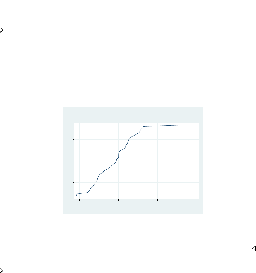
cumul — Cumulative distribution 413
Remarks and examples
Example 1
cumul is most often used with graph to graph the empirical cumulative distribution. For instance,
we have data on the median family income of 957 U.S. cities:
. use http://www.stata-press.com/data/r13/hsng
(1980 Census housing data)
. cumul faminc, gen(cum)
. sort cum
. line cum faminc, ylab(, grid) ytitle("") xlab(, grid)
> title("Cumulative of median family income")
> subtitle("1980 Census, 957 U.S. Cities")
0 .2 .4 .6 .8 1
15000.00 20000.00 25000.00 30000.00
Median family inc., 1979
1980 Census, 957 U.S. Cities
Cumulative of median family income
It would have been enough to type line cum faminc, but we wanted to make the graph look better;
see [G-2]graph twoway line.
If we had wanted a weighted cumulative, we would have typed cumul faminc [w=pop] at the
first step.
Example 2
To graph two (or more) cumulatives on the same graph, use cumul and stack; see [D]stack. For
instance, we have data on the average January and July temperatures of 956 U.S. cities:
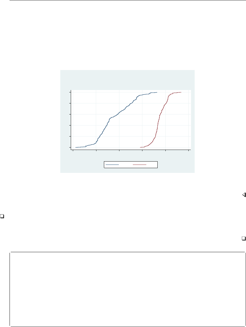
414 cumul — Cumulative distribution
. use http://www.stata-press.com/data/r13/citytemp, clear
(City Temperature Data)
. cumul tempjan, gen(cjan)
. cumul tempjuly, gen(cjuly)
. stack cjan tempjan cjuly tempjuly, into(c temp) wide clear
. line cjan cjuly temp, sort ylab(, grid) ytitle("") xlab(, grid)
> xtitle("Temperature (F)")
> title("Cumulatives:" "Average January and July Temperatures")
> subtitle("956 U.S. Cities")
0 .2 .4 .6 .8 1
0 20 40 60 80 100
Temperature (F)
cjan cjuly
956 U.S. Cities
Cumulatives:
Average January and July Temperatures
As before, it would have been enough to type line cjan cjuly temp, sort. See [D]stack for an
explanation of how the stack command works.
Technical note
According to Beniger and Robyn (1978), Fourier (1821) published the first graph of a cumulative
frequency distribution, which was later given the name “ogive” by Galton (1875).
Jean Baptiste Joseph Fourier (1768–1830) was born in Auxerre in France. As a young man,
Fourier became entangled in the complications of the French Revolution. As a result, he was
arrested and put into prison, where he feared he might meet his end at the guillotine. When
he was not in prison, he was studying, researching, and teaching mathematics. Later, he served
Napolean’s army in Egypt as a scientific adviser. Upon his return to France in 1801, he was
appointed Prefect of the Department of Is`
ere. While prefect, Fourier worked on the mathematical
basis of the theory of heat, which is based on what are now called Fourier series. This work
was published in 1822, despite the skepticism of Lagrange, Laplace, Legendre, and others—who
found the work lacking in generality and even rigor—and disagreements of both priority and
substance with Biot and Poisson.

cumul — Cumulative distribution 415
Acknowledgment
The equal option was added by Nicholas J. Cox of the Department of Geography at Durham
University, UK, and coeditor of the Stata Journal.
References
Beniger, J. R., and D. L. Robyn. 1978. Quantitative graphics in statistics: A brief history. American Statistician 32:
1–11.
Clayton, D. G., and M. Hills. 1999. gr37: Cumulative distribution function plots.Stata Technical Bulletin 49: 10–12.
Reprinted in Stata Technical Bulletin Reprints, vol. 9, pp. 96–98. College Station, TX: Stata Press.
Cox, N. J. 1999. gr41: Distribution function plots.Stata Technical Bulletin 51: 12–16. Reprinted in Stata Technical
Bulletin Reprints, vol. 9, pp. 108–112. College Station, TX: Stata Press.
Fourier, J. B. J. 1821. Notions g´
en´
erales, sur la population. Recherches Statistiques sur la Ville de Paris et le
D´
epartement de la Seine 1: 1–70.
Galton, F. 1875. Statistics by intercomparison, with remarks on the law of frequency of error. Philosophical Magazine
49: 33–46.
Wilk, M. B., and R. Gnanadesikan. 1968. Probability plotting methods for the analysis of data. Biometrika 55: 1–17.
Also see
[R]diagnostic plots — Distributional diagnostic plots
[R]kdensity — Univariate kernel density estimation
[D]stack — Stack data

Title
cusum — Cusum plots and tests for binary variables
Syntax Menu Description Options
Remarks and examples Stored results Acknowledgment References
Also see
Syntax
cusum yvar xvar if in ,options
options Description
Main
generate(newvar)save cumulative sum in newvar
yfit(fitvar)calculate cumulative sum against fitvar
nograph suppress the plot
nocalc suppress cusum test statistics
Cusum plot
connect options affect the rendition of the plotted line
Add plots
addplot(plot)add plots to the generated graph
Y axis, X axis, Titles, Legend, Overall
twoway options any options other than by() documented in [G-3]twoway options
Menu
Statistics >Other >Quality control >Cusum plots and tests for binary variables
Description
cusum graphs the cumulative sum (cusum) of a binary (0/1) variable, yvar, against a (usually)
continuous variable, xvar.
Options
Main
generate(newvar)saves the cusum in newvar.
yfit(fitvar)calculates a cusum against fitvar, that is, the running sums of the “residuals” fitvar
minus yvar. Typically, fitvar is the predicted probability of a positive outcome obtained from a
logistic regression analysis.
nograph suppresses the plot.
nocalc suppresses calculation of the cusum test statistics.
416

cusum — Cusum plots and tests for binary variables 417
Cusum plot
connect options affect the rendition of the plotted line; see [G-3]connect options.
Add plots
addplot(plot)provides a way to add other plots to the generated graph. See [G-3]addplot option.
Y axis, X axis, Titles, Legend, Overall
twoway options are any of the options documented in [G-3]twoway options, excluding by(). These
include options for titling the graph (see [G-3]title options) and for saving the graph to disk (see
[G-3]saving option).
Remarks and examples
The cusum is the running sum of the proportion of ones in the sample, a constant number, minus
yvar,
cj=
j
X
k=1
f−yvar(k),1≤j≤N
where f= (Pyvar)/N and yvar(k)refers to the corresponding value of yvar when xvar is placed in
ascending order: xvar(k+1) ≥xvar(k). Tied values of xvar are broken at random. If you want them
broken the same way in two runs, you must set the random-number seed to the same value before
giving the cusum command; see [R]set seed.
A U-shaped or inverted U-shaped cusum indicates, respectively, a negative or a positive trend of
yvar with xvar. A sinusoidal shape is evidence of a nonmonotonic (for example, quadratic) trend.
cusum displays the maximum absolute cusum for monotonic and nonmonotonic trends of yvar on
xvar. These are nonparametric tests of departure from randomness of yvar with respect to xvar.
Approximate values for the tests are given.
Example 1
For the automobile dataset, auto.dta, we wish to investigate the relationship between foreign
(0 =domestic, 1 =foreign) and car weight as follows:
. use http://www.stata-press.com/data/r13/auto
(1978 Automobile Data)
. cusum foreign weight
Variable Obs Pr(1) CusumL zL Pr>zL CusumQ zQ Pr>zQ
foreign 74 0.2973 10.30 3.963 0.000 3.32 0.469 0.320
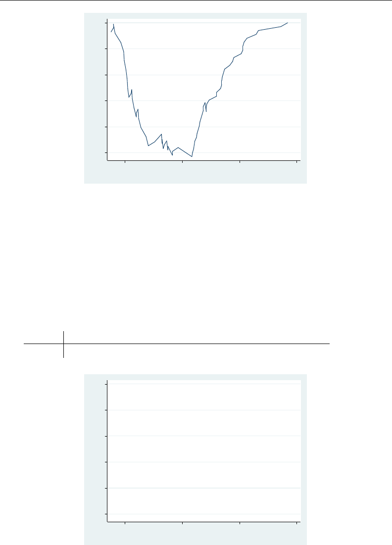
418 cusum — Cusum plots and tests for binary variables
−10 −8 −6 −4 −2 0
Cusum (Car type)
2000 3000 4000 5000
Weight (lbs.)
The resulting plot, which is U-shaped, suggests a negative monotonic relationship. The trend is
confirmed by a highly significant linear cusum statistic, labeled CusumL in the output above.
Some 29.73% of the cars are foreign (coded 1). The proportion of foreign cars diminishes with
increasing weight. The domestic cars are crudely heavier than the foreign ones. We could have
discovered that by typing table foreign, stats(mean weight), but such an approach does not
give the full picture of the relationship. The quadratic cusum (CusumQ) is not significant, so we
do not suspect any tendency for the very heavy cars to be foreign rather than domestic. A slightly
enhanced version of the plot shows the preponderance of domestic (coded 0) cars at the heavy end
of the weight axis:
. label values foreign
. cusum foreign weight, s(none) recast(scatter) mlabel(foreign) mlabp(0)
Variable Obs Pr(1) CusumL zL Pr>zL CusumQ zQ Pr>zQ
foreign 74 0.2973 10.30 3.963 0.000 2.92 0.064 0.475
10
0
1
1
1
1
1
1
1
10
0
1
1
1
0
0
1
1
1
1000
1
0
1
00
1
0
1
00
1
0
0
0
0
0
0
0
0
0
0
0
0
0
0
1
0
000
00
0
0
0
0
000
00
0
0
000000
−10 −8 −6 −4 −2 0
Cusum (Car type)
2000 3000 4000 5000
Weight (lbs.)

cusum — Cusum plots and tests for binary variables 419
The example is, of course, artificial, because we would not really try to model the probability of a
car being foreign given its weight.
Stored results
cusum stores the following in r():
Scalars
r(N) number of observations r(P zl) p-value for test (linear)
r(prop1) proportion of positive outcomes r(cusumq) quadratic cusum
r(cusuml) cusum r(zq) test (quadratic)
r(zl) test (linear) r(P zq) p-value for test (quadratic)
Acknowledgment
cusum was written by Patrick Royston of the MRC Clinical Trials Unit, London, and coauthor of
the Stata Press book Flexible Parametric Survival Analysis Using Stata: Beyond the Cox Model.
References
Royston, P. 1992. The use of cusums and other techniques in modelling continuous covariates in logistic regression.
Statistics in Medicine 11: 1115–1129.
. 1993. sqv7: Cusum plots and tests for binary variables.Stata Technical Bulletin 12: 16–17. Reprinted in Stata
Technical Bulletin Reprints, vol. 2, pp. 175–177. College Station, TX: Stata Press.
Also see
[R]logistic — Logistic regression, reporting odds ratios
[R]logit — Logistic regression, reporting coefficients
[R]probit — Probit regression

Title
db — Launch dialog
Syntax Description Options Remarks and examples Also see
Syntax
Syntax for db
db commandname
For programmers
db commandname , message(string) debug dryrun
Set system parameter
set maxdb #, permanently
where #must be between 5 and 1,000.
Description
db is the command-line way to launch a dialog for a Stata command.
The second syntax (which is the same but includes options) is for use by programmers.
If you wish to allow the launching of dialogs from a help file, see [P]smcl for information on the
dialog SMCL directive.
set maxdb sets the maximum number of dialog boxes whose contents are remembered from one
invocation to the next during a session. The default value of maxdb is 50.
Options
message(string)specifies that string be passed to the dialog box, where it can be referred to from
the MESSAGE STRING property.
debug specifies that the underlying dialog box be loaded with debug messaging turned on.
dryrun specifies that, rather than launching the dialog, db show the commands it would issue to
launch the dialog.
permanently specifies that, in addition to making the change right now, the maxdb setting be
remembered and become the default setting when you invoke Stata.
Remarks and examples
The usual way to launch a dialog is to open the Data,Graphics, or Statistics menu and to make
your selection from there. When you know the name of the command that you want to run, however,
db provides a way to invoke the dialog from the command line.
420

db — Launch dialog 421
db follows the same abbreviation rules that Stata’s command-line interface follows. So, to launch
the dialog for regress, you can type
. db regress
or
. db reg
Say that you use the dialog box for regress, either by selecting
Statistics > Linear models and related > Linear regression
or by typing
. db regress
You fit a regression.
Much later during the session, you return to the regress dialog box. It will have the contents
as you left them if 1) you have not typed clear all between the first and second invocations; 2)
you have not typed discard between the two invocations; and 3) you have not used more than 50
different dialog boxes—regardless of how many times you have used each—between the first and
second invocations of regress. If you use 51 or more, the contents of the regress dialog box will
be forgotten.
set maxdb determines how many different dialog boxes are remembered. A dialog box takes, on
average, about 20 KB of memory, so the 50 default corresponds to allowing dialog boxes to consume
about 1 MB of memory.
Also see
[R]query — Display system parameters

Title
diagnostic plots — Distributional diagnostic plots
Syntax Menu
Description Options for symplot, quantile, and qqplot
Options for qnorm and pnorm Options for qchi and pchi
Remarks and examples Methods and formulas
Acknowledgments References
Also see
Syntax
Symmetry plot
symplot varname if in ,options1
Ordered values of varname against quantiles of uniform distribution
quantile varname if in ,options1
Quantiles of varname1against quantiles of varname2
qqplot varname1varname2if in ,options1
Quantiles of varname against quantiles of normal distribution
qnorm varname if in ,options2
Standardized normal probability plot
pnorm varname if in ,options2
Quantiles of varname against quantiles of χ2distribution
qchi varname if in ,options3
χ2probability plot
pchi varname if in ,options3
422

diagnostic plots — Distributional diagnostic plots 423
options1Description
Plot
marker options change look of markers (color, size, etc.)
marker label options add marker labels; change look or position
Reference line
rlopts(cline options)affect rendition of the reference line
Add plots
addplot(plot)add other plots to the generated graph
Y axis, X axis, Titles, Legend, Overall
twoway options any options other than by() documented in [G-3]twoway options
options2Description
Main
grid add grid lines
Plot
marker options change look of markers (color, size, etc.)
marker label options add marker labels; change look or position
Reference line
rlopts(cline options)affect rendition of the reference line
Add plots
addplot(plot)add other plots to the generated graph
Y axis, X axis, Titles, Legend, Overall
twoway options any options other than by() documented in [G-3]twoway options
options3Description
Main
grid add grid lines
df(#)degrees of freedom of χ2distribution; default is df(1)
Plot
marker options change look of markers (color, size, etc.)
marker label options add marker labels; change look or position
Reference line
rlopts(cline options)affect rendition of the reference line
Add plots
addplot(plot)add other plots to the generated graph
Y axis, X axis, Titles, Legend, Overall
twoway options any options other than by() documented in [G-3]twoway options

424 diagnostic plots — Distributional diagnostic plots
Menu
symplot
Statistics >Summaries, tables, and tests >Distributional plots and tests >Symmetry plot
quantile
Statistics >Summaries, tables, and tests >Distributional plots and tests >Quantiles plot
qqplot
Statistics >Summaries, tables, and tests >Distributional plots and tests >Quantile-quantile plot
qnorm
Statistics >Summaries, tables, and tests >Distributional plots and tests >Normal quantile plot
pnorm
Statistics >Summaries, tables, and tests >Distributional plots and tests >Normal probability plot, standardized
qchi
Statistics >Summaries, tables, and tests >Distributional plots and tests >Chi-squared quantile plot
pchi
Statistics >Summaries, tables, and tests >Distributional plots and tests >Chi-squared probability plot
Description
symplot graphs a symmetry plot of varname.
quantile plots the ordered values of varname against the quantiles of a uniform distribution.
qqplot plots the quantiles of varname1against the quantiles of varname2(Q–Q plot).
qnorm plots the quantiles of varname against the quantiles of the normal distribution (Q–Q plot).
pnorm graphs a standardized normal probability plot (P–P plot).
qchi plots the quantiles of varname against the quantiles of a χ2distribution (Q–Q plot).
pchi graphs a χ2probability plot (P–P plot).
See [R]regress postestimation diagnostic plots for regression diagnostic plots and [R]logistic
postestimation for logistic regression diagnostic plots.
Options for symplot, quantile, and qqplot
Plot
marker options affect the rendition of markers drawn at the plotted points, including their shape,
size, color, and outline; see [G-3]marker options.
marker label options specify if and how the markers are to be labeled; see [G-3]marker label options.
Reference line
rlopts(cline options)affect the rendition of the reference line; see [G-3]cline options.
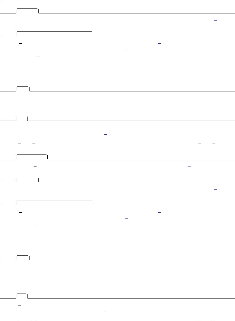
diagnostic plots — Distributional diagnostic plots 425
Add plots
addplot(plot)provides a way to add other plots to the generated graph; see [G-3]addplot option.
Y axis, X axis, Titles, Legend, Overall
twoway options are any of the options documented in [G-3]twoway options, excluding by(). These
include options for titling the graph (see [G-3]title options) and for saving the graph to disk (see
[G-3]saving option).
Options for qnorm and pnorm
Main
grid adds grid lines at the 0.05, 0.10, 0.25, 0.50, 0.75, 0.90, and 0.95 quantiles when specified with
qnorm. With pnorm,grid is equivalent to yline(.25,.5,.75) xline(.25,.5,.75).
Plot
marker options affect the rendition of markers drawn at the plotted points, including their shape,
size, color, and outline; see [G-3]marker options.
marker label options specify if and how the markers are to be labeled; see [G-3]marker label options.
Reference line
rlopts(cline options)affect the rendition of the reference line; see [G-3]cline options.
Add plots
addplot(plot)provides a way to add other plots to the generated graph; see [G-3]addplot option.
Y axis, X axis, Titles, Legend, Overall
twoway options are any of the options documented in [G-3]twoway options, excluding by(). These
include options for titling the graph (see [G-3]title options) and for saving the graph to disk (see
[G-3]saving option).
Options for qchi and pchi
Main
grid adds grid lines at the 0.05, 0.10, 0.25, 0.50, 0.75, 0.90, and .95 quantiles when specified with
qchi. With pchi,grid is equivalent to yline(.25,.5,.75) xline(.25,.5,.75).
df(#)specifies the degrees of freedom of the χ2distribution. The default is df(1).
Plot
marker options affect the rendition of markers drawn at the plotted points, including their shape,
size, color, and outline; see [G-3]marker options.
marker label options specify if and how the markers are to be labeled; see [G-3]marker label options.
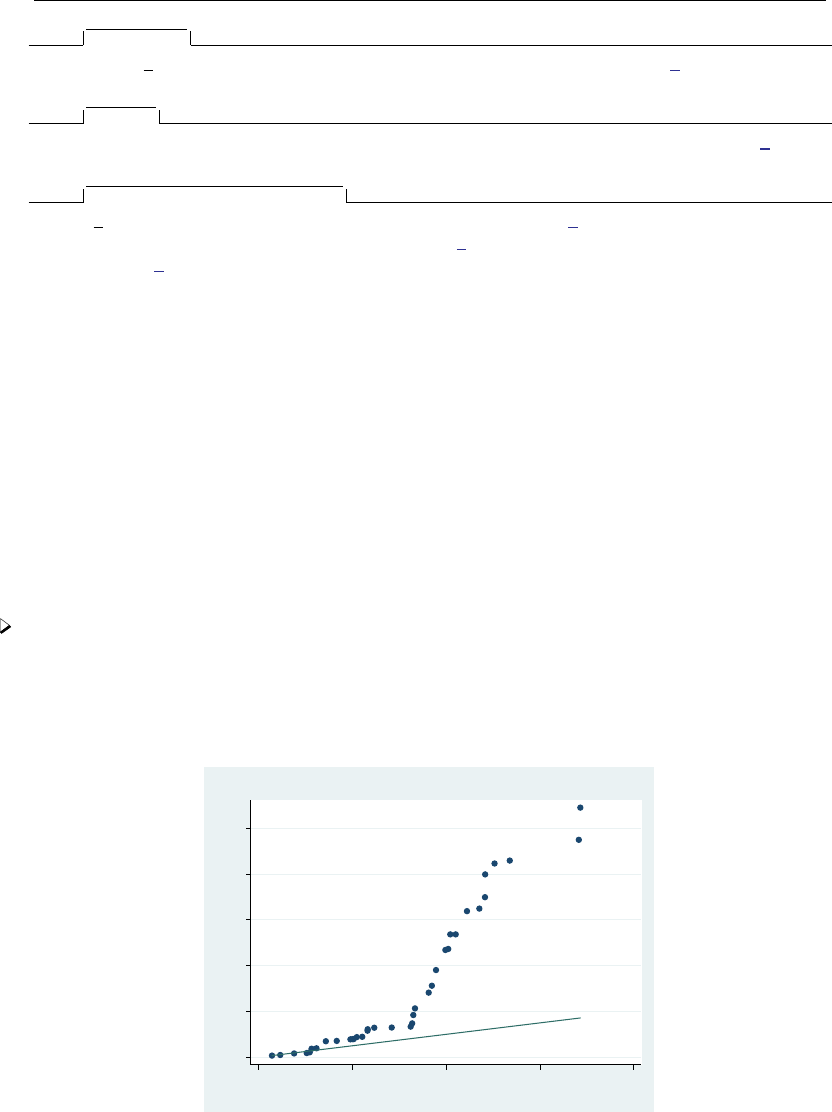
426 diagnostic plots — Distributional diagnostic plots
Reference line
rlopts(cline options)affect the rendition of the reference line; see [G-3]cline options.
Add plots
addplot(plot)provides a way to add other plots to the generated graph; see [G-3]addplot option.
Y axis, X axis, Titles, Legend, Overall
twoway options are any of the options documented in [G-3]twoway options, excluding by(). These
include options for titling the graph (see [G-3]title options) and for saving the graph to disk (see
[G-3]saving option).
Remarks and examples
Remarks are presented under the following headings:
symplot
quantile
qqplot
qnorm
pnorm
qchi
pchi
symplot
Example 1
We have data on 74 automobiles. To make a symmetry plot of the variable price, we type
. use http://www.stata-press.com/data/r13/auto
(1978 Automobile Data)
. symplot price
0 2000 4000 6000 8000 10000
Distance above median
0 500 1000 1500 2000
Distance below median
Price

diagnostic plots — Distributional diagnostic plots 427
All points would lie along the reference line (defined as y=x) if car prices were symmetrically
distributed. The points in this plot lie above the reference line, indicating that the distribution of car
prices is skewed to the right—the most expensive cars are far more expensive than the least expensive
cars are inexpensive.
The logic works as follows: a variable, z, is distributed symmetrically if
median −z(i)=z(N+1−i)−median
where z(i)indicates the ith-order statistic of z.symplot graphs yi=median −z(i)versus xi=
z(N+1−i)−median.
For instance, consider the largest and smallest values of price in the example above. The most
expensive car costs $15,906 and the least expensive, $3,291. Let’s compare these two cars with the
typical car in the data and see how much more it costs to buy the most expensive car, and compare
that with how much less it costs to buy the least expensive car. If the automobile price distribution
is symmetric, the price differences would be the same.
Before we can make this comparison, we must agree on a definition for the word “typical”. Let’s
agree that “typical” means median. The price of the median car is $5,006.50, so the most expensive
car costs $10,899.50 more than the median car, and the least expensive car costs $1,715.50 less than
the median car. We now have one piece of evidence that the car price distribution is not symmetric.
We can repeat the experiment for the second-most-expensive car and the second-least-expensive car.
We find that the second-most-expensive car costs $9,494.50 more than the median car, and the
second-least-expensive car costs $1,707.50 less than the median car. We now have more evidence.
We can continue doing this with the third most expensive and the third least expensive, and so on.
Once we have all of these numbers, we want to compare each pair and ask how similar, on average,
they are. The easiest way to do that is to plot all the pairs.
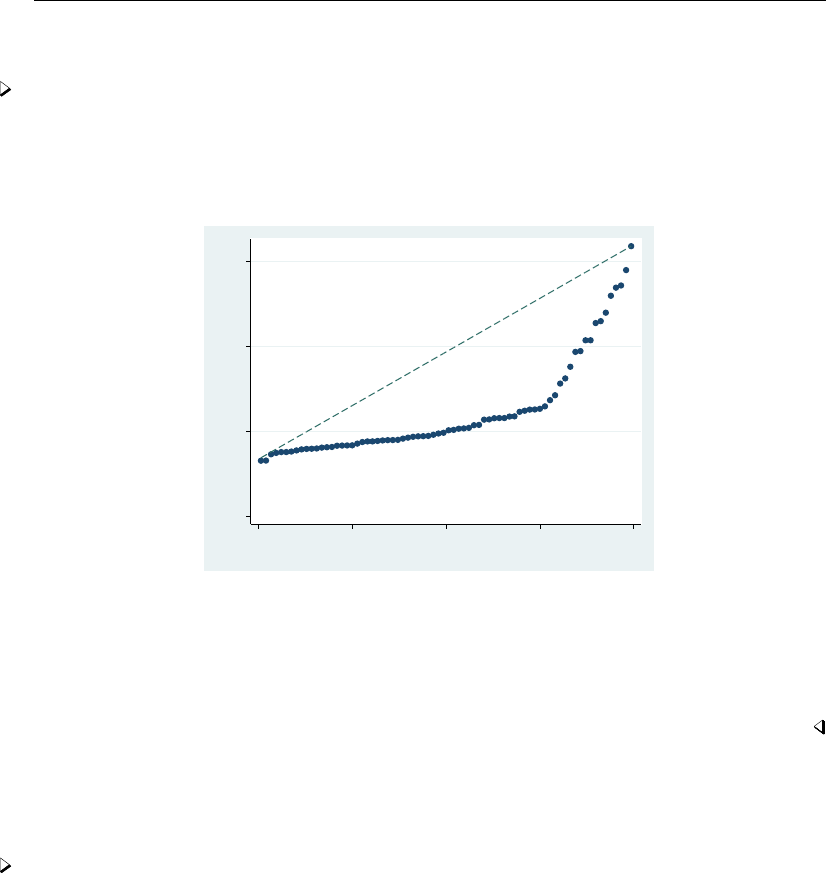
428 diagnostic plots — Distributional diagnostic plots
quantile
Example 2
We have data on the prices of 74 automobiles. To make a quantile plot of price, we type
. use http://www.stata-press.com/data/r13/auto, clear
(1978 Automobile Data)
. quantile price, rlopts(clpattern(dash))
0 5000 10000 15000
Quantiles of Price
0 .25 .5 .75 1
Fraction of the data
We changed the pattern of the reference line by specifying rlopts(clpattern(dash)).
In a quantile plot, each value of the variable is plotted against the fraction of the data that
have values less than that fraction. The diagonal line is a reference line. If automobile prices were
rectangularly distributed, all the data would be plotted along the line. Because all the points are below
the reference line, we know that the price distribution is skewed right.
qqplot
Example 3
We have data on the weight and country of manufacture of 74 automobiles. We wish to compare
the distributions of weights for domestic and foreign automobiles:
. use http://www.stata-press.com/data/r13/auto
(1978 Automobile Data)
. generate weightd=weight if !foreign
(22 missing values generated)
. generate weightf=weight if foreign
(52 missing values generated)
. qqplot weightd weightf
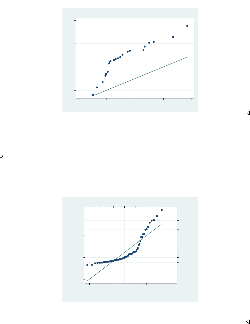
diagnostic plots — Distributional diagnostic plots 429
2000 3000 4000 5000
weightd
1500 2000 2500 3000 3500
weightf
Quantile−Quantile Plot
qnorm
Example 4
Continuing with our price data on 74 automobiles, we now wish to compare the distribution of
price with the normal distribution:
. qnorm price, grid ylabel(, angle(horizontal) axis(1))
> ylabel(, angle(horizontal) axis(2))
3,748
5,006.5
13,466
0
5,000
10,000
15,000
Price
6,165.3 11,0171,313.8
0 5,000 10,000 15,000
Inverse Normal
Grid lines are 5, 10, 25, 50, 75, 90, and 95 percentiles
The result shows that the distributions are different.
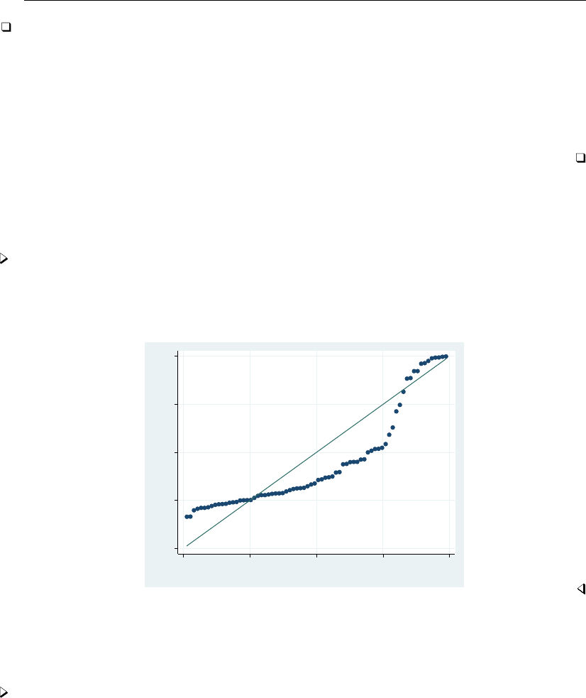
430 diagnostic plots — Distributional diagnostic plots
Technical note
The idea behind qnorm is recommended strongly by Miller (1997): he calls it probit plotting. His
recommendations from much practical experience should interest many users. “My recommendation
for detecting nonnormality is probit plotting” (Miller 1997, 10). “If a deviation from normality cannot
be spotted by eye on probit paper, it is not worth worrying about. I never use the Kolmogorov–Smirnov
test (or one of its cousins) or the χ2test as a preliminary test of normality. They do not tell you how
the sample is differing from normality, and I have a feeling they are more likely to detect irregularities
in the middle of the distribution than in the tails” (Miller 1997, 13–14).
pnorm
Example 5
Quantile–normal plots emphasize the tails of the distribution. Normal probability plots put the
focus on the center of the distribution:
. pnorm price, grid
0.00 0.25 0.50 0.75 1.00
Normal F[(price−m)/s]
0.00 0.25 0.50 0.75 1.00
Empirical P[i] = i/(N+1)
qchi
Example 6
Suppose that we want to examine the distribution of the sum of squares of price and mpg,
standardized for their variances.
. egen c1 = std(price)
. egen c2 = std(mpg)
. generate ch = c1^2 + c2^2
. qchi ch, df(2) grid ylabel(, alt axis(2)) xlabel(, alt axis(2))
diagnostic plots — Distributional diagnostic plots 431
.1598352
.7587778
8.926035
0 5 10 15
ch
.1025866
1.386294
5.991465
0 2 4 6 8
Expected χ2 d.f. = 2
Grid lines are 5, 10, 25, 50, 75, 90, and 95 percentiles
The quadratic form is clearly not χ2with 2 degrees of freedom.
pchi
Example 7
We can focus on the center of the distribution by doing a probability plot:
. pchi ch, df(2) grid
0.00 0.25 0.50 0.75 1.00
χ2(ch) d.f. = 2
0.00 0.25 0.50 0.75 1.00
Empirical P[i] = i/(N+1)

432 diagnostic plots — Distributional diagnostic plots
Methods and formulas
Let x(1),x(2),. . . ,x(N)be the data sorted in ascending order.
If a continuous variable, x, has a cumulative distribution function F(x) = P(X≤x) = p, the
quantiles xpiare such that F(xpi) = pi. For example, if pi=0.5, then x0.5is the median. When
we plot data, the probabilities, pi, are often referred to as plotting positions. There are many different
conventions for choice of plotting positions, given x(1) ≤ ··· ≤ x(N). Most belong to the family
(i−a)/(N−2a+1).a=0.5 (suggested by Hazen) and a=0 (suggested by Weibull) are popular
choices.
For a wider discussion of the calculation of plotting positions, see Cox (2002).
symplot plots median −x(i)versus x(N+1−i)−median.
quantile plots x(i)versus (i−0.5)/N (the Hazen position).
qnorm plots x(i)against qi, where qi= Φ−1(pi),Φis the cumulative normal distribution, and
pi=i/(N+1)(the Weibull position).
pnorm plots Φ(xi−bµ)/bσversus pi=i/(N+1), where bµis the mean of the data and bσis
the standard deviation.
qchi and pchi are similar to qnorm and pnorm; the cumulative χ2distribution is used in place
of the cumulative normal distribution.
qqplot is just a two-way scatterplot of one variable against the other after both variables have been
sorted into ascending order, and both variables have the same number of nonmissing observations. If
the variables have unequal numbers of nonmissing observations, interpolated values of the variable
with more data are plotted against the variable with fewer data.
Ramanathan Gnanadesikan (1932– ) was born in Madras. He obtained degrees from the Univer-
sities of Madras and North Carolina. He worked in industry at Procter & Gamble, Bell Labs, and
Bellcore, as well as in universities, retiring from Rutgers in 1998. Among many contributions
to statistics he is especially well known for work on probability plotting, robustness, outlier
detection, clustering, classification, and pattern recognition.
Martin Bradbury Wilk (1922–2013) was born in Montreal. He obtained degrees in chemical
engineering and statistics from McGill and Iowa State Universities. After holding several statistics-
related posts in industry and at universities (including periods at Princeton, Bell Labs, and Rutgers),
Wilk was appointed Chief Statistician at Statistics Canada (1980–1986). He is especially well
known for his work with Gnanadesikan on probability plotting and with Shapiro on tests for
normality.
Acknowledgments
We thank Peter A. Lachenbruch of the Department of Public Health at Oregon State University
for writing the original versions of qchi and pchi. Patrick Royston of the MRC Clinical Trials
Unit, London, and coauthor of the Stata Press book Flexible Parametric Survival Analysis Using
Stata: Beyond the Cox Model also published a similar command in the Stata Technical Bulletin
(Royston 1996).

diagnostic plots — Distributional diagnostic plots 433
References
Chambers, J. M., W. S. Cleveland, B. Kleiner, and P. A. Tukey. 1983. Graphical Methods for Data Analysis. Belmont,
CA: Wadsworth.
Cox, N. J. 1999. gr42: Quantile plots, generalized.Stata Technical Bulletin 51: 16–18. Reprinted in Stata Technical
Bulletin Reprints, vol. 9, pp. 113–116. College Station, TX: Stata Press.
. 2001. gr42.1: Quantile plots, generalized: Update to Stata 7.Stata Technical Bulletin 61: 10. Reprinted in Stata
Technical Bulletin Reprints, vol. 10, pp. 55–56. College Station, TX: Stata Press.
. 2002. Speaking Stata: On getting functions to do the work.Stata Journal 2: 411–427.
. 2004a. Speaking Stata: Graphing distributions.Stata Journal 4: 66–88.
. 2004b. gr42 2: Software update: Quantile plots, generalized.Stata Journal 4: 97.
. 2005a. Speaking Stata: Density probability plots.Stata Journal 5: 259–273.
. 2005b. Speaking Stata: The protean quantile plot.Stata Journal 5: 442–460.
. 2005c. Speaking Stata: Smoothing in various directions.Stata Journal 5: 574–593.
. 2007. Stata tip 47: Quantile–quantile plots without programming.Stata Journal 7: 275–279.
. 2012. Speaking Stata: Axis practice, or what goes where on a graph.Stata Journal 12: 549–561.
Daniel, C., and F. S. Wood. 1980. Fitting Equations to Data: Computer Analysis of Multifactor Data. 2nd ed. New
York: Wiley.
Gan, F. F., K. J. Koehler, and J. C. Thompson. 1991. Probability plots and distribution curves for assessing the fit
of probability models. American Statistician 45: 14–21.
Genest, C., and G. J. Brackstone. 2013. Obituary: Martin B. Wilk, 1922–2013. IMS Bulletin 42(4): 7–8.
Hamilton, L. C. 1992. Regression with Graphics: A Second Course in Applied Statistics. Belmont, CA: Duxbury.
. 2013. Statistics with Stata: Updated for Version 12. 8th ed. Boston: Brooks/Cole.
Hoaglin, D. C. 1985. Using quantiles to study shape. In Exploring Data Tables, Trends, and Shapes, ed. D. C.
Hoaglin, C. F. Mosteller, and J. W. Tukey, 417–460. New York: Wiley.
Kettenring, J. R. 2001. A conversation with Ramanathan Gnanadesikan. Statistical Science 16: 295–309.
Miller, R. G., Jr. 1997. Beyond ANOVA: Basics of Applied Statistics. London: Chapman & Hall.
Nolan, D., and T. Speed. 2000. Stat Labs: Mathematical Statistics Through Applications. New York: Springer.
Royston, P. 1996. sg47: A plot and a test for the χ2distribution.Stata Technical Bulletin 29: 26–27. Reprinted in
Stata Technical Bulletin Reprints, vol. 5, pp. 142–144. College Station, TX: Stata Press.
Scotto, M. G. 2000. sg140: The Gumbel quantile plot and a test for choice of extreme models.Stata Technical Bulletin
55: 23–25. Reprinted in Stata Technical Bulletin Reprints, vol. 10, pp. 156–159. College Station, TX: Stata Press.
Wilk, M. B., and R. Gnanadesikan. 1968. Probability plotting methods for the analysis of data. Biometrika 55: 1–17.
Also see
[R]cumul — Cumulative distribution
[R]kdensity — Univariate kernel density estimation
[R]logistic postestimation — Postestimation tools for logistic
[R]lv — Letter-value displays
[R]regress postestimation diagnostic plots — Postestimation plots for regress

Title
display — Substitute for a hand calculator
Syntax Description Remarks and examples Also see
Syntax
display exp
Description
display displays strings and values of scalar expressions.
display really has many more features and a more complex syntax diagram, but the diagram
shown above is adequate for interactive use. For a full discussion of display’s capabilities, see
[P]display.
Remarks and examples
display can be used as a substitute for a hand calculator.
Example 1
display 2+2 produces the output 4. Stata variables may also appear in the expression, such as in
display myvar/2. Because display works only with scalars, the resulting calculation is performed
only for the first observation. You could type display myvar[10]/2 to display the calculation for
the 10th observation. Here are more examples:
. display sqrt(2)/2
.70710678
. display normal(-1.1)
.13566606
. di (57.2-3)/(12-2)
5.42
. display myvar/10
7
. display myvar[10]/2
3.5
Also see
[P]display — Display strings and values of scalar expressions
[U] 13 Functions and expressions
434

Title
do — Execute commands from a file
Syntax Menu Description Option
Remarks and examples Reference Also see
Syntax
do |runfilename arguments , nostop
Menu
File >Do...
Description
do and run cause Stata to execute the commands stored in filename just as if they were entered
from the keyboard. do echoes the commands as it executes them, whereas run is silent. If filename
is specified without an extension, .do is assumed.
Option
nostop allows the do-file to continue executing even if an error occurs. Normally, Stata stops executing
the do-file when it detects an error (nonzero return code).
Remarks and examples
You can create filename (called a do-file) using Stata’s Do-file Editor; see [R]doedit. This file
will be a standard ASCII (text) file. A complete discussion of do-files can be found in [U] 16 Do-files.
You can also create filename by using a non-Stata text editor; see [D]shell for a way to invoke
your favorite editor from inside Stata. Make sure that you save the file in ASCII format.
If the path or filename contains spaces, it should be enclosed in double quotes.
Reference
Jenkins, S. P. 2006. Stata tip 32: Do not stop.Stata Journal 6: 281.
Also see
[R]doedit — Edit do-files and other text files
[P]include — Include commands from file
[GSM] 13 Using the Do-file Editor—automating Stata
[GSU] 13 Using the Do-file Editor—automating Stata
[GSW] 13 Using the Do-file Editor—automating Stata
[U] 15 Saving and printing output—log files
[U] 16 Do-files
435

Title
doedit — Edit do-files and other text files
Syntax Menu Description Remarks and examples Also see
Syntax
doedit filename
Menu
Window >Do-file Editor
Description
doedit opens a text editor that lets you edit do-files and other text files.
The Do-file Editor lets you submit several commands to Stata at once.
Remarks and examples
Clicking on the Do-file Editor button is equivalent to typing doedit.
doedit, typed by itself, invokes the Editor with an empty document. If you specify filename, that
file is displayed in the Editor.
You may have more than one Do-file Editor open at once. Each time you submit the doedit
command, a new window will be opened.
A tutorial discussion of doedit can be found in the Getting Started with Stata manual. Read
[U] 16 Do-files for an explanation of do-files, and then read [GSW] 13 Using the Do-file Editor—
automating Stata to learn how to use the Do-file Editor to create and execute do-files.
Also see
[GSM] 13 Using the Do-file Editor—automating Stata
[GSU] 13 Using the Do-file Editor—automating Stata
[GSW] 13 Using the Do-file Editor—automating Stata
[U] 16 Do-files
436

Title
dotplot — Comparative scatterplots
Syntax Menu Description Options
Remarks and examples Stored results Acknowledgments References
Syntax
Dotplot of varname, with one column per value of groupvar
dotplot varname if in ,options
Dotplot for each variable in varlist, with one column per variable
dotplot varlist if in ,options
options Description
Options
over(groupvar)display one columnar dotplot for each value of groupvar
nx(#)horizontal dot density; default is nx(0)
ny(#)vertical dot density; default is ny(35)
incr(#)label every #group; default is incr(1)
mean |median plot a horizontal line of pluses at the mean or median
bounded use minimum and maximum as boundaries
bar plot horizontal dashed lines at shoulders of each group
nogroup use the actual values of yvar
center center the dot for each column
Plot
marker options change look of markers (color, size, etc.)
marker label options add marker labels; change look or position
Y axis, X axis, Titles, Legend, Overall
twoway options any options other than by() documented in [G-3]twoway options
Menu
Graphics >Distributional graphs >Distribution dotplot
Description
A dotplot is a scatterplot with values grouped together vertically (“binning”, as in a histogram)
and with plotted points separated horizontally. The aim is to display all the data for several variables
or groups in one compact graphic.
437

438 dotplot — Comparative scatterplots
In the first syntax, dotplot produces a columnar dotplot of varname, with one column per value
of groupvar. In the second syntax, dotplot produces a columnar dotplot for each variable in varlist,
with one column per variable; over(groupvar)is not allowed. In each case, the “dots” are plotted
as small circles to increase readability.
Options
Options
over(groupvar)identifies the variable for which dotplot will display one columnar dotplot for
each value of groupvar.
nx(#)sets the horizontal dot density. A larger value of #will increase the dot density, reducing the
horizontal separation between dots. This option will increase the separation between columns if
two or more groups or variables are used.
ny(#)sets the vertical dot density (number of “bins” on the yaxis). A larger value of #will result
in more bins and a plot that is less spread out horizontally. #should be determined in conjunction
with nx() to give the most pleasing appearance.
incr(#)specifies how the xaxis is to be labeled. incr(1), the default, labels all groups. incr(2)
labels every second group.
mean |median plots a horizontal line of pluses at the mean or median of each group.
bounded forces the minimum and maximum of the variable to be used as boundaries of the smallest
and largest bins. It should be used with one variable whose support is not the whole of the real
line and whose density does not tend to zero at the ends of its support, for example, a uniform
random variable or an exponential random variable.
bar plots horizontal dashed lines at the “shoulders” of each group. The shoulders are taken to be
the upper and lower quartiles unless mean has been specified; here they will be the mean plus or
minus the standard deviation.
nogroup uses the actual values of yvar rather than grouping them (the default). This option may be
useful if yvar takes on only a few values.
center centers the dots for each column on a hidden vertical line.
Plot
marker options affect the rendition of markers drawn at the plotted points, including their shape,
size, color, and outline; see [G-3]marker options.
marker label options specify if and how the markers are to be labeled; see [G-3]marker label options.
Y axis, X axis, Titles, Legend, Overall
twoway options are any of the options documented in [G-3]twoway options, excluding by(). These
include options for titling the graph (see [G-3]title options) and for saving the graph to disk (see
[G-3]saving option).
dotplot — Comparative scatterplots 439
Remarks and examples
dotplot produces a figure that has elements of a boxplot, a histogram, and a scatterplot. Like a
boxplot, it is most useful for comparing the distributions of several variables or the distribution of 1
variable in several groups. Like a histogram, the figure provides a crude estimate of the density, and,
as with a scatterplot, each symbol (dot) represents 1 observation.
Example 1
dotplot may be used as an alternative to Stata’s histogram graph for displaying the distribution
of one variable.
. set seed 123456789
. set obs 1000
. generate norm = rnormal()
. dotplot norm, title("Normal distribution, sample size 1000")
−4 −2 0 2 4
norm
0 20 40 60 80
Frequency
Normal distribution, sample size 1000
Example 2
The over() option lets us use dotplot to compare the distribution of one variable within different
levels of a grouping variable. The center,median, and bar options create a graph that may be
compared with Stata’s boxplot; see [G-2]graph box. The next graph illustrates this option with Stata’s
automobile dataset.
440 dotplot — Comparative scatterplots
. use http://www.stata-press.com/data/r13/auto, clear
(1978 Automobile Data)
. dotplot mpg, over(foreign) nx(25) ny(10) center median bar
− −− − − − − − − − − − −− − − − − − − − − − − − − − − − −− − − − − − − − − − −− − − −− − − −− −−
−− − − −− −− − − − − − − −− −− −− −−
− −− − − − − − − − − − −− − − − − − − − − − − − − − − − −− − − − − − − − − − −− − − −− − − −− −−
−− − − −− −− − − − − − − −− −− −− −−
10 20 30 40
Mileage (mpg)
Domestic Foreign
Car type
Example 3
The second version of dotplot lets us compare the distribution of several variables. In the next
graph, all 10 variables contain measurements on tumor volume.
. use http://www.stata-press.com/data/r13/dotgr
. dotplot g1r1-g1r10, ytitle("Tumor volume, cu mm")
0 200 400 600 800 1000
Tumor volume, cu mm
g1r1 g1r2 g1r3 g1r4 g1r5 g1r6 g1r7 g1r8 g1r9 g1r10
dotplot — Comparative scatterplots 441
Example 4
When using the first form with the over() option, we can encode a third dimension in a dotplot
by using a different plotting symbol for different groups. The third dimension cannot be encoded
with a varlist. The example is of a hypothetical matched case–control study. The next graph shows
the exposure of each individual in each matched stratum. Cases are marked by the letter ‘x’, and
controls are marked by the letter ‘o’.
. use http://www.stata-press.com/data/r13/dotdose
. label define symbol 0 "o" 1 "x"
. label values case symbol
. dotplot dose, over(strata) m(none) mlabel(case) mlabp(0) center
o
oooo
oo
ox
o
ooo
o
oo
oo
oox
o
oo
oo
xo
oo
x
o
o
oo
o
xo
o
o
xxo
o
o
o
o
o
o
o
o
o
o
xoo
o
o
xooo
oo
oo
x
o
ox
ox
oxo
oo
oo
oo
o
o
o
o
o
oo
oo
ooo
o
ooo
ox
ooo
o
ooo
oo
o
o
o
ox
o
o
o
oo
o
ooo
o
oo
ooo
o
0 10 20 30 40 50
dose
0 1 2 3 4 5 6 7 8 9 10 11 12
strata
Example 5
dotplot can also be used with two virtually continuous variables as an alternative to jittering the
data to distinguish ties. We must use the xlabel() option, because otherwise dotplot will attempt
to label too many points on the xaxis. It is often useful in such instances to use a value of nx that
is smaller than the default. That was not necessary in this example, partly because of our choice of
symbols.
. use http://www.stata-press.com/data/r13/auto
(1978 Automobile Data)
. generate byte hi_price = (price>10000) if price < .
. label define symbol 0 "|" 1 "o"
. label values hi_price symbol
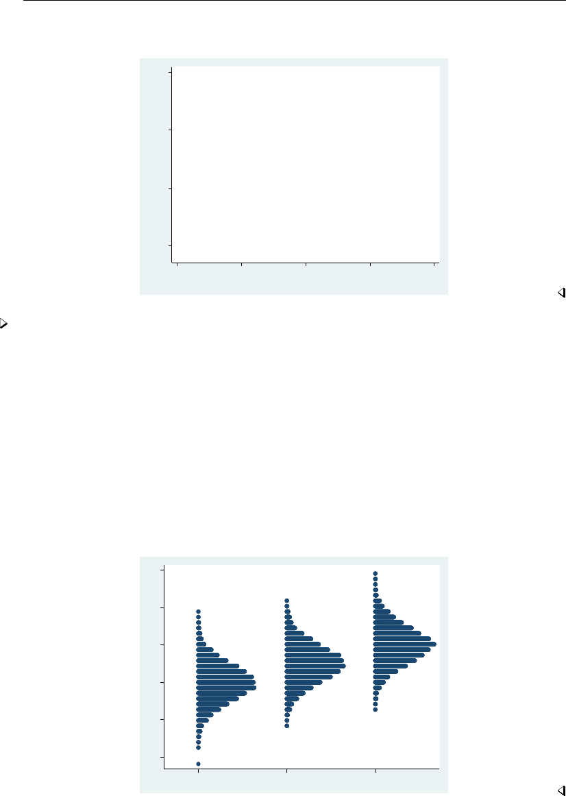
442 dotplot — Comparative scatterplots
. dotplot weight, over(gear_ratio) m(none) mlabel(hi_price) mlabp(0) center
> xlabel(#5)
o
o
|
o
o||
|
||
o
o
o
||
|
|
||
|
|
|
|||
|
|
|
|
||||
||
o
|
|
o
|
|
|
|
||
|
|
||
|
|
|
|
|
|
|| |
|
|
|
|
o
|
|
|
|
|
|
|
|
| |
|
2,000 3,000 4,000 5,000
Weight (lbs.)
2 2.5 3 3.5 4
Gear Ratio
Example 6
The following figure is included mostly for aesthetic reasons. It also demonstrates dotplot’s
ability to cope with even very large datasets. The sample size for each variable is 10,000, so it may
take a long time to print.
. clear all
. set seed 123456789
. set obs 10000
. gen norm0 = rnormal()
. gen norm1 = rnormal() + 1
. gen norm2 = rnormal() + 2
. label variable norm0 "N(0,1)"
. label variable norm1 "N(1,1)"
. label variable norm2 "N(2,1)"
. dotplot norm0 norm1 norm2
−4 −2 0 2 4 6
N(0,1) N(1,1) N(2,1)

dotplot — Comparative scatterplots 443
Stored results
dotplot stores the following in r():
Scalars
r(nx) horizontal dot density
r(ny) vertical dot density
Acknowledgments
dotplot was written by Peter Sasieni of the Wolfson Institute of Preventive Medicine, London,
and Patrick Royston of the MRC Clinical Trials Unit, London, and coauthor of the Stata Press book
Flexible Parametric Survival Analysis Using Stata: Beyond the Cox Model.
References
Sasieni, P. D., and P. Royston. 1994. gr14: dotplot: Comparative scatterplots.Stata Technical Bulletin 19: 8–10.
Reprinted in Stata Technical Bulletin Reprints, vol. 4, pp. 50–54. College Station, TX: Stata Press.
. 1996. Dotplots. Applied Statistics 45: 219–234.

Title
dstdize — Direct and indirect standardization
Syntax Menu Description Options for dstdize
Options for istdize Remarks and examples Stored results Methods and formulas
Acknowledgments References Also see
Syntax
Direct standardization
dstdize charvar popvar stratavars if in , by(groupvars)dstdize options
Indirect standardization
istdize casevarspopvarsstratavars if in using filename,
popvars(casevarppopvarp)|rate(ratevarp#|crudevarp)
istdize options
dstdize options Description
Main
∗by(groupvars)study populations
using( filename)use standard population from Stata dataset
base(#|string)use standard population from a value of grouping variable
level(#)set confidence level; default is level(95)
Options
saving( filename)save computed standard population distribution as a Stata dataset
format(%fmt)final summary table display format; default is %10.0g
print include table summary of standard population in output
nores suppress storing results in r()
∗by(groupvars)is required.
istdize options Description
Main
∗popvars(casevarppopvarp)for standard population, casevarpis number of cases and
popvarpis number of individuals
∗rate(ratevarp#|crudevarp)ratevarpis stratum-specific rates and #or crudevarpis the
crude case rate value or variable
level(#)set confidence level; default is level(95)
Options
by(groupvars)variables identifying study populations
format(%fmt)final summary table display format; default is %10.0g
print include table summary of standard population in output
∗Either popvars(casevarppopvarp)or rate(ratevarp{#|crudevarp})must be specified.
444

dstdize — Direct and indirect standardization 445
Menu
dstdize
Statistics >Epidemiology and related >Other >Direct standardization
istdize
Statistics >Epidemiology and related >Other >Indirect standardization
Description
dstdize produces standardized rates for charvar, which are defined as a weighted average of the
stratum-specific rates. These rates can be used to compare the characteristic charvar across different
populations identified by groupvars. Weights used in the standardization are given by popvar; the
strata across which the weights are to be averaged are defined by stratavars.
istdize produces indirectly standardized rates for a study population based on a standard popu-
lation. This standardization method is appropriate when the stratum-specific rates for the population
being studied are either unavailable or based on small samples and thus are unreliable. The standard-
ization uses the stratum-specific rates of a standard population to calculate the expected number of
cases in the study population(s), sums them, and then compares them with the actual number of cases
observed. The standard population is in another Stata data file specified by using filename, and it
must contain popvar and stratavars.
In addition to calculating rates, the indirect standardization command produces point estimates and
exact confidence intervals of the study population’s standardized mortality ratio (SMR), if death is the
event of interest, or the standardized incidence ratio (SIR) for studies of incidence. Here we refer to
both ratios as SMR.
casevarsis the variable name for the study population’s number of cases (usually deaths). It must
contain integers, and for each group, defined by groupvar, each subpopulation identified by stratavars
must have the same values or missing.
popvarsidentifies the number of subjects represented by each observation in the study population.
stratavars define the strata.
Options for dstdize
Main
by(groupvars)is required for the dstdize command; it specifies the variables identifying the study
populations. If base() is also specified, there must be only one variable in the by() group. If
you do not have a variable for this option, you can generate one by using something like gen
newvar=1 and then use newvar as the argument to this option.
using(filename)or base(#|string)may be used to specify the standard population. You may not
specify both options. using( filename)supplies the name of a .dta file containing the standard
population. The standard population must contain the popvar and the stratavars. If using() is
not specified, the standard population distribution will be obtained from the data. base(#|string)
lets you specify one of the values of groupvar—either a numeric value or a string—to be used
as the standard population. If neither base() nor using() is specified, the entire dataset is used
to determine an estimate of the standard population.

446 dstdize — Direct and indirect standardization
level(#)specifies the confidence level, as a percentage, for a confidence interval of the adjusted
rate. The default is level(95) or as set by set level; see [U] 20.7 Specifying the width of
confidence intervals.
Options
saving( filename)saves the computed standard population distribution as a Stata dataset that can be
used in further analyses.
format(%fmt)specifies the format in which to display the final summary table. The default is
%10.0g.
print includes a table summary of the standard population before displaying the study population
results.
nores suppresses storing results in r(). This option is seldom specified. Some results are stored
in matrices. If there are more groups than matsize,dstdize will report “matsize too small”.
Then you can either increase matsize or specify nores. The nores option does not change how
results are calculated but specifies that results need not be left behind for use by other programs.
Options for istdize
Main
popvars(casevarppopvarp)or rate(ratevarp#|ratevarpcrudevarp)must be specified with ist-
dize. Only one of these two options is allowed. These options are used to describe the standard
population’s data.
With popvars(casevarppopvarp),casevarprecords the number of cases (deaths) for each stratum
in the standard population, and popvarprecords the total number of individuals in each stratum
(individuals at risk).
With rate(ratevarp#|crudevarp),ratevarpcontains the stratum-specific rates. #|crudevarp
specifies the crude case rate either by a variable name or by the crude case rate value. If a crude
rate variable is used, it must be the same for all observations, although it could be missing for
some.
level(#)specifies the confidence level, as a percentage, for a confidence interval of the adjusted
rate. The default is level(95) or as set by set level; see [U] 20.7 Specifying the width of
confidence intervals.
Options
by(groupvars)specifies variables identifying study populations when more than one exists in the
data. If this option is not specified, the entire study population is treated as one group.
format(%fmt)specifies the format in which to display the final summary table. The default is
%10.0g.
print outputs a table summary of the standard population before displaying the study population
results.

dstdize — Direct and indirect standardization 447
Remarks and examples
Remarks are presented under the following headings:
Direct standardization
Indirect standardization
In epidemiology and other fields, you will often need to compare rates for some characteristic
across different populations. These populations often differ on factors associated with the characteristic
under study; thus directly comparing overall rates may be misleading.
See van Belle et al. (2004, 642–684), Fleiss, Levin, and Paik (2003, chap. 19), or Kirkwood and
Sterne (2003, chap. 25) for a discussion of direct and indirect standardization.
Direct standardization
The direct method of adjusting for differences among populations involves computing the overall
rates that would result if, instead of having different distributions, all populations had the same
standard distribution. The standardized rate is defined as a weighted average of the stratum-specific
rates, with the weights taken from the standard distribution. Direct standardization may be applied
only when the specific rates for a given population are available.
dstdize generates adjusted summary measures of occurrence, which can be used to compare
prevalence, incidence, or mortality rates between populations that may differ on certain characteristics
(for example, age, gender, race). These underlying differences may affect the crude prevalence,
mortality, or incidence rates.
Example 1
We have data (Rothman 1986, 42) on mortality rates for Sweden and Panama for 1962, and we
wish to compare mortality in these two countries:
. use http://www.stata-press.com/data/r13/mortality
(1962 Mortality, Sweden & Panama)
. describe
Contains data from http://www.stata-press.com/data/r13/mortality.dta
obs: 6 1962 Mortality, Sweden & Panama
vars: 4 14 Apr 2013 16:18
size: 90
storage display value
variable name type format label variable label
nation str6 %9s Nation
age_category byte %9.0g age_lbl Age Category
population float %10.0gc Population in Age Category
deaths float %9.0gc Deaths in Age Category
Sorted by:

448 dstdize — Direct and indirect standardization
. list, sepby(nation) abbrev(12) divider
nation age_category population deaths
1. Sweden 0 - 29 3145000 3,523
2. Sweden 30 - 59 3057000 10,928
3. Sweden 60+ 1294000 59,104
4. Panama 0 - 29 741,000 3,904
5. Panama 30 - 59 275,000 1,421
6. Panama 60+ 59,000 2,456
We divide the total number of cases in the population by the population to obtain the crude rate:
. collapse (sum) pop deaths, by(nation)
. list, abbrev(10) divider
nation population deaths
1. Panama 1075000 7,781
2. Sweden 7496000 73,555
. generate crude = deaths/pop
. list, abbrev(10) divider
nation population deaths crude
1. Panama 1075000 7,781 .0072381
2. Sweden 7496000 73,555 .0098126
If we examine the total number of deaths in the two nations, the total crude mortality rate in
Sweden is higher than that in Panama. From the original data, we see one possible explanation:
Swedes are older than Panamanians, making direct comparison of the mortality rates difficult.
Direct standardization lets us remove the distortion caused by the different age distributions. The
adjusted rate is defined as the weighted sum of the crude rates, where the weights are given by the
standard distribution. Suppose that we wish to standardize these mortality rates to the following age
distribution:
. use http://www.stata-press.com/data/r13/1962, clear
(Standard Population Distribution)
. list, abbrev(12) divider
age_category population
1. 0 - 29 .35
2. 30 - 59 .35
3. 60+ .3
. save 1962
file 1962.dta saved
If we multiply the above weights for the age strata by the crude rate for the corresponding age
category, the sum gives us the standardized rate.

dstdize — Direct and indirect standardization 449
. use http://www.stata-press.com/data/r13/mortality
(1962 Mortality, Sweden & Panama)
. generate crude=deaths/pop
. drop pop
. merge m:1 age_cat using 1962
age_category was byte now float
Result # of obs.
not matched 0
matched 6 (_merge==3)
. list, sepby(age_category) abbrev(12)
nation age_category deaths crude population _merge
1. Sweden 0 - 29 3,523 .0011202 .35 matched (3)
2. Panama 0 - 29 3,904 .0052686 .35 matched (3)
3. Panama 30 - 59 1,421 .0051673 .35 matched (3)
4. Sweden 30 - 59 10,928 .0035747 .35 matched (3)
5. Panama 60+ 2,456 .0416271 .3 matched (3)
6. Sweden 60+ 59,104 .0456754 .3 matched (3)
. generate product = crude*pop
. by nation, sort: egen adj_rate = sum(product)
. drop _merge
. list, sepby(nation)
nation age_ca~y deaths crude popula~n product adj_rate
1. Panama 0 - 29 3,904 .0052686 .35 .001844 .0161407
2. Panama 30 - 59 1,421 .0051673 .35 .0018085 .0161407
3. Panama 60+ 2,456 .0416271 .3 .0124881 .0161407
4. Sweden 60+ 59,104 .0456754 .3 .0137026 .0153459
5. Sweden 30 - 59 10,928 .0035747 .35 .0012512 .0153459
6. Sweden 0 - 29 3,523 .0011202 .35 .0003921 .0153459
Comparing the standardized rates indicates that the Swedes have a slightly lower mortality rate.

450 dstdize — Direct and indirect standardization
To perform the above analysis with dstdize, type
. use http://www.stata-press.com/data/r13/mortality, clear
(1962 Mortality, Sweden & Panama)
. dstdize deaths pop age_cat, by(nation) using(1962)
-> nation= Panama
Unadjusted Std.
Pop. Stratum Pop.
Stratum Pop. Cases Dist. Rate[s] Dst[P] s*P
0 - 29 741000 3904 0.689 0.0053 0.350 0.0018
30 - 59 275000 1421 0.256 0.0052 0.350 0.0018
60+ 59000 2456 0.055 0.0416 0.300 0.0125
Totals: 1075000 7781 Adjusted Cases: 17351.2
Crude Rate: 0.0072
Adjusted Rate: 0.0161
95% Conf. Interval: [0.0156, 0.0166]
-> nation= Sweden
Unadjusted Std.
Pop. Stratum Pop.
Stratum Pop. Cases Dist. Rate[s] Dst[P] s*P
0 - 29 3145000 3523 0.420 0.0011 0.350 0.0004
30 - 59 3057000 10928 0.408 0.0036 0.350 0.0013
60+ 1294000 59104 0.173 0.0457 0.300 0.0137
Totals: 7496000 73555 Adjusted Cases: 115032.5
Crude Rate: 0.0098
Adjusted Rate: 0.0153
95% Conf. Interval: [0.0152, 0.0155]
Summary of Study Populations:
nation N Crude Adj_Rate Confidence Interval
Panama 1075000 0.007238 0.016141 [ 0.015645, 0.016637]
Sweden 7496000 0.009813 0.015346 [ 0.015235, 0.015457]
The summary table above lets us make a quick inspection of the results within the study populations,
and the detail tables give the behavior among the strata within the study populations.
Example 2
We have individual-level data on persons in four cities over several years. Included in the data is
a variable indicating whether the person has high blood pressure, together with information on the
person’s age, sex, and race. We wish to obtain standardized high blood pressure rates for each city
for 1990 and 1992, using, as the standard, the age, sex, and race distribution of the four cities and
two years combined.

dstdize — Direct and indirect standardization 451
Our dataset contains
. use http://www.stata-press.com/data/r13/hbp
. describe
Contains data from http://www.stata-press.com/data/r13/hbp.dta
obs: 1,130
vars: 7 21 Feb 2013 06:42
size: 19,210
storage display value
variable name type format label variable label
id str10 %10s Record identification number
city byte %8.0g
year int %8.0g
sex byte %8.0g sexfmt
age_group byte %8.0g agefmt
race byte %8.0g racefmt
hbp byte %8.0g yn high blood pressure
Sorted by:
The dstdize command is designed to work with aggregate data but will work with individual-
level data only if we create a variable recording the population represented by each observation. For
individual-level data, this is one:
. generate pop = 1
On the next page, we specify print to obtain a listing of the standard population and level(90)
to request 90% rather than 95% confidence intervals. Typing if year==1990 | year==1992 restricts
the data to the two years for both summary tables and the standard population.

452 dstdize — Direct and indirect standardization
. dstdize hbp pop age race sex if year==1990 | year==1992, by(city year) print
> level(90)
Standard Population
Stratum Pop. Dist.
15 - 19 Black Female 35 0.077
15 - 19 Black Male 44 0.097
15 - 19 Hispanic Female 5 0.011
15 - 19 Hispanic Male 10 0.022
15 - 19 White Female 7 0.015
15 - 19 White Male 5 0.011
20 - 24 Black Female 43 0.095
20 - 24 Black Male 67 0.147
20 - 24 Hispanic Female 14 0.031
20 - 24 Hispanic Male 13 0.029
20 - 24 White Female 4 0.009
20 - 24 White Male 21 0.046
25 - 29 Black Female 17 0.037
25 - 29 Black Male 44 0.097
25 - 29 Hispanic Female 7 0.015
25 - 29 Hispanic Male 13 0.029
25 - 29 White Female 9 0.020
25 - 29 White Male 16 0.035
30 - 34 Black Female 16 0.035
30 - 34 Black Male 32 0.070
30 - 34 Hispanic Female 2 0.004
30 - 34 Hispanic Male 3 0.007
30 - 34 White Female 5 0.011
30 - 34 White Male 23 0.051
Total: 455
(6 observations excluded because of missing values)
-> city year= 1 1990
Unadjusted Std.
Pop. Stratum Pop.
Stratum Pop. Cases Dist. Rate[s] Dst[P] s*P
15 - 19 Black Female 6 2 0.128 0.3333 0.077 0.0256
15 - 19 Black Male 6 0 0.128 0.0000 0.097 0.0000
15 - 19 Hispanic Male 1 0 0.021 0.0000 0.022 0.0000
20 - 24 Black Female 3 0 0.064 0.0000 0.095 0.0000
20 - 24 Black Male 11 0 0.234 0.0000 0.147 0.0000
25 - 29 Black Female 4 0 0.085 0.0000 0.037 0.0000
25 - 29 Black Male 6 1 0.128 0.1667 0.097 0.0161
25 - 29 Hispanic Female 2 0 0.043 0.0000 0.015 0.0000
25 - 29 White Female 1 0 0.021 0.0000 0.020 0.0000
30 - 34 Black Female 1 0 0.021 0.0000 0.035 0.0000
30 - 34 Black Male 6 0 0.128 0.0000 0.070 0.0000
Totals: 47 3 Adjusted Cases: 2.0
Crude Rate: 0.0638
Adjusted Rate: 0.0418
90% Conf. Interval: [0.0074, 0.0761]

dstdize — Direct and indirect standardization 453
-> city year= 1 1992
Unadjusted Std.
Pop. Stratum Pop.
Stratum Pop. Cases Dist. Rate[s] Dst[P] s*P
15 - 19 Black Female 3 0 0.054 0.0000 0.077 0.0000
15 - 19 Black Male 9 0 0.161 0.0000 0.097 0.0000
15 - 19 Hispanic Male 1 0 0.018 0.0000 0.022 0.0000
20 - 24 Black Female 7 0 0.125 0.0000 0.095 0.0000
20 - 24 Black Male 9 0 0.161 0.0000 0.147 0.0000
20 - 24 Hispanic Female 1 0 0.018 0.0000 0.031 0.0000
25 - 29 Black Female 2 0 0.036 0.0000 0.037 0.0000
25 - 29 Black Male 11 1 0.196 0.0909 0.097 0.0088
25 - 29 Hispanic Male 1 0 0.018 0.0000 0.029 0.0000
30 - 34 Black Female 7 0 0.125 0.0000 0.035 0.0000
30 - 34 Black Male 4 0 0.071 0.0000 0.070 0.0000
30 - 34 White Female 1 0 0.018 0.0000 0.011 0.0000
Totals: 56 1 Adjusted Cases: 0.5
Crude Rate: 0.0179
Adjusted Rate: 0.0088
90% Conf. Interval: [0.0000, 0.0226]
-> city year= 2 1990
Unadjusted Std.
Pop. Stratum Pop.
Stratum Pop. Cases Dist. Rate[s] Dst[P] s*P
15 - 19 Black Female 5 0 0.078 0.0000 0.077 0.0000
15 - 19 Black Male 7 1 0.109 0.1429 0.097 0.0138
15 - 19 Hispanic Male 1 0 0.016 0.0000 0.022 0.0000
20 - 24 Black Female 7 1 0.109 0.1429 0.095 0.0135
20 - 24 Black Male 8 0 0.125 0.0000 0.147 0.0000
20 - 24 Hispanic Female 5 0 0.078 0.0000 0.031 0.0000
20 - 24 Hispanic Male 2 0 0.031 0.0000 0.029 0.0000
20 - 24 White Male 2 0 0.031 0.0000 0.046 0.0000
25 - 29 Black Female 3 0 0.047 0.0000 0.037 0.0000
25 - 29 Black Male 9 0 0.141 0.0000 0.097 0.0000
25 - 29 Hispanic Female 2 0 0.031 0.0000 0.015 0.0000
25 - 29 White Female 1 0 0.016 0.0000 0.020 0.0000
25 - 29 White Male 2 1 0.031 0.5000 0.035 0.0176
30 - 34 Black Female 1 0 0.016 0.0000 0.035 0.0000
30 - 34 Black Male 5 0 0.078 0.0000 0.070 0.0000
30 - 34 Hispanic Female 2 0 0.031 0.0000 0.004 0.0000
30 - 34 White Female 1 0 0.016 0.0000 0.011 0.0000
30 - 34 White Male 1 0 0.016 0.0000 0.051 0.0000
Totals: 64 3 Adjusted Cases: 2.9
Crude Rate: 0.0469
Adjusted Rate: 0.0449
90% Conf. Interval: [0.0091, 0.0807]

454 dstdize — Direct and indirect standardization
-> city year= 2 1992
Unadjusted Std.
Pop. Stratum Pop.
Stratum Pop. Cases Dist. Rate[s] Dst[P] s*P
15 - 19 Black Female 1 0 0.015 0.0000 0.077 0.0000
15 - 19 Black Male 5 0 0.075 0.0000 0.097 0.0000
15 - 19 Hispanic Female 3 0 0.045 0.0000 0.011 0.0000
15 - 19 Hispanic Male 1 0 0.015 0.0000 0.022 0.0000
15 - 19 White Male 1 0 0.015 0.0000 0.011 0.0000
20 - 24 Black Female 8 0 0.119 0.0000 0.095 0.0000
20 - 24 Black Male 11 0 0.164 0.0000 0.147 0.0000
20 - 24 Hispanic Female 6 0 0.090 0.0000 0.031 0.0000
20 - 24 Hispanic Male 4 2 0.060 0.5000 0.029 0.0143
20 - 24 White Female 1 0 0.015 0.0000 0.009 0.0000
20 - 24 White Male 2 0 0.030 0.0000 0.046 0.0000
25 - 29 Black Female 2 0 0.030 0.0000 0.037 0.0000
25 - 29 Black Male 3 0 0.045 0.0000 0.097 0.0000
25 - 29 Hispanic Female 2 0 0.030 0.0000 0.015 0.0000
25 - 29 Hispanic Male 4 0 0.060 0.0000 0.029 0.0000
25 - 29 White Female 4 0 0.060 0.0000 0.020 0.0000
25 - 29 White Male 2 0 0.030 0.0000 0.035 0.0000
30 - 34 Black Female 1 0 0.015 0.0000 0.035 0.0000
30 - 34 Black Male 2 0 0.030 0.0000 0.070 0.0000
30 - 34 Hispanic Male 1 0 0.015 0.0000 0.007 0.0000
30 - 34 White Female 2 0 0.030 0.0000 0.011 0.0000
30 - 34 White Male 1 0 0.015 0.0000 0.051 0.0000
Totals: 67 2 Adjusted Cases: 1.0
Crude Rate: 0.0299
Adjusted Rate: 0.0143
90% Conf. Interval: [0.0025, 0.0260]
-> city year= 3 1990
Unadjusted Std.
Pop. Stratum Pop.
Stratum Pop. Cases Dist. Rate[s] Dst[P] s*P
15 - 19 Black Female 3 0 0.043 0.0000 0.077 0.0000
15 - 19 Black Male 1 0 0.014 0.0000 0.097 0.0000
15 - 19 Hispanic Female 1 0 0.014 0.0000 0.011 0.0000
15 - 19 White Female 3 0 0.043 0.0000 0.015 0.0000
15 - 19 White Male 1 0 0.014 0.0000 0.011 0.0000
20 - 24 Black Female 1 0 0.014 0.0000 0.095 0.0000
20 - 24 Black Male 9 0 0.130 0.0000 0.147 0.0000
20 - 24 Hispanic Male 3 0 0.043 0.0000 0.029 0.0000
20 - 24 White Female 2 0 0.029 0.0000 0.009 0.0000
20 - 24 White Male 8 1 0.116 0.1250 0.046 0.0058
25 - 29 Black Female 1 0 0.014 0.0000 0.037 0.0000
25 - 29 Black Male 8 3 0.116 0.3750 0.097 0.0363
25 - 29 Hispanic Male 4 0 0.058 0.0000 0.029 0.0000
25 - 29 White Female 1 0 0.014 0.0000 0.020 0.0000
25 - 29 White Male 6 0 0.087 0.0000 0.035 0.0000
30 - 34 Black Male 6 2 0.087 0.3333 0.070 0.0234
30 - 34 White Male 11 5 0.159 0.4545 0.051 0.0230
Totals: 69 11 Adjusted Cases: 6.1
Crude Rate: 0.1594
Adjusted Rate: 0.0885
90% Conf. Interval: [0.0501, 0.1268]

dstdize — Direct and indirect standardization 455
-> city year= 3 1992
Unadjusted Std.
Pop. Stratum Pop.
Stratum Pop. Cases Dist. Rate[s] Dst[P] s*P
15 - 19 Black Female 2 0 0.054 0.0000 0.077 0.0000
15 - 19 Hispanic Male 3 0 0.081 0.0000 0.022 0.0000
15 - 19 White Female 2 0 0.054 0.0000 0.015 0.0000
15 - 19 White Male 1 0 0.027 0.0000 0.011 0.0000
20 - 24 Black Male 3 0 0.081 0.0000 0.147 0.0000
20 - 24 Hispanic Female 1 0 0.027 0.0000 0.031 0.0000
20 - 24 Hispanic Male 3 0 0.081 0.0000 0.029 0.0000
20 - 24 White Female 1 0 0.027 0.0000 0.009 0.0000
20 - 24 White Male 6 1 0.162 0.1667 0.046 0.0077
25 - 29 Hispanic Male 1 0 0.027 0.0000 0.029 0.0000
25 - 29 White Male 5 1 0.135 0.2000 0.035 0.0070
30 - 34 Black Male 1 0 0.027 0.0000 0.070 0.0000
30 - 34 White Male 8 5 0.216 0.6250 0.051 0.0316
Totals: 37 7 Adjusted Cases: 1.7
Crude Rate: 0.1892
Adjusted Rate: 0.0463
90% Conf. Interval: [0.0253, 0.0674]
-> city year= 5 1990
Unadjusted Std.
Pop. Stratum Pop.
Stratum Pop. Cases Dist. Rate[s] Dst[P] s*P
15 - 19 Black Female 9 0 0.196 0.0000 0.077 0.0000
15 - 19 Black Male 7 0 0.152 0.0000 0.097 0.0000
15 - 19 Hispanic Male 1 0 0.022 0.0000 0.022 0.0000
15 - 19 White Male 1 0 0.022 0.0000 0.011 0.0000
20 - 24 Black Female 4 0 0.087 0.0000 0.095 0.0000
20 - 24 Black Male 6 0 0.130 0.0000 0.147 0.0000
20 - 24 Hispanic Female 1 0 0.022 0.0000 0.031 0.0000
25 - 29 Black Female 3 1 0.065 0.3333 0.037 0.0125
25 - 29 Black Male 5 0 0.109 0.0000 0.097 0.0000
25 - 29 Hispanic Female 1 0 0.022 0.0000 0.015 0.0000
25 - 29 White Female 2 1 0.043 0.5000 0.020 0.0099
30 - 34 Black Female 2 0 0.043 0.0000 0.035 0.0000
30 - 34 Black Male 3 0 0.065 0.0000 0.070 0.0000
30 - 34 White Male 1 0 0.022 0.0000 0.051 0.0000
Totals: 46 2 Adjusted Cases: 1.0
Crude Rate: 0.0435
Adjusted Rate: 0.0223
90% Conf. Interval: [0.0020, 0.0426]

456 dstdize — Direct and indirect standardization
-> city year= 5 1992
Unadjusted Std.
Pop. Stratum Pop.
Stratum Pop. Cases Dist. Rate[s] Dst[P] s*P
15 - 19 Black Female 6 0 0.087 0.0000 0.077 0.0000
15 - 19 Black Male 9 0 0.130 0.0000 0.097 0.0000
15 - 19 Hispanic Female 1 0 0.014 0.0000 0.011 0.0000
15 - 19 Hispanic Male 2 0 0.029 0.0000 0.022 0.0000
15 - 19 White Female 2 0 0.029 0.0000 0.015 0.0000
15 - 19 White Male 1 0 0.014 0.0000 0.011 0.0000
20 - 24 Black Female 13 0 0.188 0.0000 0.095 0.0000
20 - 24 Black Male 10 0 0.145 0.0000 0.147 0.0000
20 - 24 Hispanic Male 1 0 0.014 0.0000 0.029 0.0000
20 - 24 White Male 3 0 0.043 0.0000 0.046 0.0000
25 - 29 Black Female 2 0 0.029 0.0000 0.037 0.0000
25 - 29 Black Male 2 0 0.029 0.0000 0.097 0.0000
25 - 29 Hispanic Male 3 0 0.043 0.0000 0.029 0.0000
25 - 29 White Male 1 0 0.014 0.0000 0.035 0.0000
30 - 34 Black Female 4 0 0.058 0.0000 0.035 0.0000
30 - 34 Black Male 5 0 0.072 0.0000 0.070 0.0000
30 - 34 Hispanic Male 2 0 0.029 0.0000 0.007 0.0000
30 - 34 White Female 1 0 0.014 0.0000 0.011 0.0000
30 - 34 White Male 1 1 0.014 1.0000 0.051 0.0505
Totals: 69 1 Adjusted Cases: 3.5
Crude Rate: 0.0145
Adjusted Rate: 0.0505
90% Conf. Interval: [0.0505, 0.0505]
Summary of Study Populations:
city
year N Crude Adj_Rate Confidence Interval
1
1990 47 0.063830 0.041758 [ 0.007427, 0.076089]
1
1992 56 0.017857 0.008791 [ 0.000000, 0.022579]
2
1990 64 0.046875 0.044898 [ 0.009072, 0.080724]
2
1992 67 0.029851 0.014286 [ 0.002537, 0.026035]
3
1990 69 0.159420 0.088453 [ 0.050093, 0.126813]
3
1992 37 0.189189 0.046319 [ 0.025271, 0.067366]
5
1990 46 0.043478 0.022344 [ 0.002044, 0.042644]
5
1992 69 0.014493 0.050549 [ 0.050549, 0.050549]

dstdize — Direct and indirect standardization 457
Indirect standardization
Standardization of rates can be performed via the indirect method whenever the stratum-specific
rates are either unknown or unreliable. If the stratum-specific rates are known, the direct standardization
method is preferred.
To apply the indirect method, you must have the following information:
•The observed number of cases in each population to be standardized, O. For example, if death
rates in two states are being standardized using the U.S. death rate for the same period, you must
know the total number of deaths in each state.
•The distribution across the various strata for the population being studied, n1, . . . , nk. If you are
standardizing the death rate in the two states, adjusting for age, you must know the number of
individuals in each of the kage groups.
•The stratum-specific rates for the standard population, p1, . . . , pk. For example, you must have
the U.S. death rate for each stratum (age group).
•The crude rate of the standard population, C. For example, you must have the U.S. mortality rate
for the year.
The indirect adjusted rate is then
Rindirect =CO
E
where Eis the expected number of cases (deaths) in each population. See Methods and formulas for
a more detailed description of calculations.
Example 3
This example is borrowed from Kahn and Sempos (1989, 95–105). We want to compare 1970
mortality rates in California and Maine, adjusting for age. Although we have age-specific population
counts for the two states, we lack age-specific death rates. Direct standardization is not feasible here.
We can use the U.S. population census data for the same year to produce indirectly standardized rates
for these two states.
From the U.S. census, the standard population for this example was entered into Stata and saved
in popkahn.dta.
. use http://www.stata-press.com/data/r13/popkahn, clear
. list age pop deaths rate, sep(4)
age population deaths rate
1. <15 57,900,000 103,062 .00178
2. 15-24 35,441,000 45,261 .00128
3. 25-34 24,907,000 39,193 .00157
4. 35-44 23,088,000 72,617 .00315
5. 45-54 23,220,000 169,517 .0073
6. 55-64 18,590,000 308,373 .01659
7. 65-74 12,436,000 445,531 .03583
8. 75+ 7,630,000 736,758 .09656

458 dstdize — Direct and indirect standardization
The standard population contains for each age stratum the total number of individuals (pop) and
both the age-specific mortality rate (rate) and the number of deaths. The standard population need
not contain all three. If we have only the age-specific mortality rate, we can use the rate(ratevarp
crudevarp)or rate(ratevarp#)option, where crudevarprefers to the variable containing the total
population’s crude death rate or #is the total population’s crude death rate.
Now let’s look at the states’ data (study population):
. use http://www.stata-press.com/data/r13/kahn
. list, sep(4)
state age populat~n death st death_~e
1. California <15 5,524,000 166,285 1 .0016
2. California 15-24 3,558,000 166,285 1 .0013
3. California 25-34 2,677,000 166,285 1 .0015
4. California 35-44 2,359,000 166,285 1 .0028
5. California 45-54 2,330,000 166,285 1 .0067
6. California 55-64 1,704,000 166,285 1 .0154
7. California 65-74 1,105,000 166,285 1 .0328
8. California 75+ 696,000 166,285 1 .0917
9. Maine <15 286,000 11,051 2 .0019
10. Maine 15-24 168,000 . 2 .0011
11. Maine 25-34 110,000 . 2 .0014
12. Maine 35-44 109,000 . 2 .0029
13. Maine 45-54 110,000 . 2 .0069
14. Maine 55-64 94,000 . 2 .0173
15. Maine 65-74 69,000 . 2 .039
16. Maine 75+ 46,000 . 2 .1041
For each state, the number of individuals in each stratum (age group) is contained in the pop variable.
The death variable is the total number of deaths observed in the state during the year. It must have
the same value for all observations in the group, as for California, or it could be missing in all but
one observation per group, as for Maine.
To match these two datasets, the strata variables must have the same name in both datasets and
ideally the same levels. If a level is missing from either dataset, that level will not be included in the
standardization.
With kahn.dta in memory, we now execute the command. We will use the print option to
obtain the standard population’s summary table, and because we have both the standard population’s
age-specific count and deaths, we will specify the popvars(casevarppopvarp)option. Or, we could
specify the rate(rate 0.00945) option because we know that 0.00945 is the U.S. crude death rate
for 1970.

dstdize — Direct and indirect standardization 459
. istdize death pop age using http://www.stata-press.com/data/r13/popkahn,
> by(state) pop(deaths pop) print
Standard Population
Stratum Rate
<15 0.00178
15-24 0.00128
25-34 0.00157
35-44 0.00315
45-54 0.00730
55-64 0.01659
65-74 0.03583
75+ 0.09656
Standard population’s crude rate: 0.00945
-> state= California
Indirect Standardization
Standard
Population Observed Cases
Stratum Rate Population Expected
<15 0.0018 5524000 9832.72
15-24 0.0013 3558000 4543.85
25-34 0.0016 2677000 4212.46
35-44 0.0031 2359000 7419.59
45-54 0.0073 2330000 17010.10
55-64 0.0166 1704000 28266.14
65-74 0.0358 1105000 39587.63
75+ 0.0966 696000 67206.23
Totals: 19953000 178078.73
Observed Cases: 166285
SMR (Obs/Exp): 0.93
SMR exact 95% Conf. Interval: [0.9293, 0.9383]
Crude Rate: 0.0083
Adjusted Rate: 0.0088
95% Conf. Interval: [0.0088, 0.0089]
-> state= Maine
Indirect Standardization
Standard
Population Observed Cases
Stratum Rate Population Expected
<15 0.0018 286000 509.08
15-24 0.0013 168000 214.55
25-34 0.0016 110000 173.09
35-44 0.0031 109000 342.83
45-54 0.0073 110000 803.05
55-64 0.0166 94000 1559.28
65-74 0.0358 69000 2471.99
75+ 0.0966 46000 4441.79
Totals: 992000 10515.67
Observed Cases: 11051
SMR (Obs/Exp): 1.05
SMR exact 95% Conf. Interval: [1.0314, 1.0707]
Crude Rate: 0.0111
Adjusted Rate: 0.0099
95% Conf. Interval: [0.0097, 0.0101]

460 dstdize — Direct and indirect standardization
Summary of Study Populations (Rates):
Cases
state Observed Crude Adj_Rate Confidence Interval
California 166285 0.008334 0.008824 [0.008782, 0.008866]
Maine 11051 0.011140 0.009931 [0.009747, 0.010118]
Summary of Study Populations (SMR):
Cases Cases Exact
state Observed Expected SMR Confidence Interval
California 166285 178078.73 0.934 [0.929290, 0.938271]
Maine 11051 10515.67 1.051 [1.031405, 1.070688]
Stored results
dstdize stores the following in r():
Scalars
r(k) number of populations
Macros
r(by) variable names specified in by()
r(c#)values of r(by) for #th group
Matrices
r(se) 1×kvector of standard errors of adjusted rates
r(ub) 1×kvector of upper bounds of confidence intervals for adjusted rates
r(lb) 1×kvector of lower bounds of confidence intervals for adjusted rates
r(Nobs) 1×kvector of number of observations
r(crude) 1×kvector of crude rates (*)
r(adj) 1×kvector of adjusted rates (*)
(*) If, in a group, the number of observations is 0, then 9 is stored for the corresponding crude and adjusted rates.
istdize stores the following in r():
Scalars
r(k) number of populations
Macros
r(by) variable names specified in by()
r(c#)values of r(by) for #th group
Matrices
r(cases obs) 1×kvector of number of observed cases
r(cases exp) 1×kvector of number of expected cases
r(ub adj) 1×kvector of upper bounds of confidence intervals for adjusted rates
r(lb adj) 1×kvector of lower bounds of confidence intervals for adjusted rates
r(crude) 1×kvector of crude rates
r(adj) 1×kvector of adjusted rates
r(smr) 1×kvector of SMRs
r(ub smr) 1×kvector of upper bounds of confidence intervals for SMRs
r(lb smr) 1×kvector of lower bounds of confidence intervals for SMRs

dstdize — Direct and indirect standardization 461
Methods and formulas
The directly standardized rate, SR, is defined by
SR=
k
X
i=1
wiRi
k
X
i=1
wi
(Rothman 1986, 44), where Riis the stratum-specific rate in stratum iand wiis the weight for
stratum iderived from the standard population.
If niis the population of stratum i, the standard error, se(SR), in stratified sampling for proportions
(ignoring the finite population correction) is
se(SR) = 1
Pwiv
u
u
tk
X
i=1
wi2Ri(1 −Ri)
ni
(Cochran 1977, 108), from which the confidence intervals are calculated.
For indirect standardization, define Oas the observed number of cases in each population to be
standardized; n1, . . . , nkas the distribution across the various strata for the population being studied;
R1, . . . , Rkas the stratum-specific rates for the standard population; and Cas the crude rate of the
standard population. The expected number of cases (deaths), E, in each population is obtained by
applying the standard population stratum-specific rates, R1, . . . , Rk, to the study populations:
E=
k
X
i=1
niRi
The indirectly adjusted rate is then
Rindirect =CO
E
and O/E is the study population’s SMR if death is the event of interest or the SIR for studies of
disease (or other) incidence.
The exact confidence interval is calculated for each estimated SMR by assuming a Poisson process
as described in Breslow and Day (1987, 69–71). These intervals are obtained by first calculating
the upper and lower bounds for the confidence interval of the Poisson-distributed observed events,
O—say, Land U, respectively—and then computing SMRL=L/E and SMRU=U/E.
Acknowledgments
We gratefully acknowledge the collaboration of Dr. Joel A. Harrison, consultant; Dr. Jos´
e Maria
Pacheco of the Departamento de Epidemiologia, Faculdade de Sa´
ude P´
ublica/USP, Sao Paulo, Brazil;
and Dr John L. Moran of the Queen Elizabeth Hospital, Woodville, Australia.

462 dstdize — Direct and indirect standardization
References
Breslow, N. E., and N. E. Day. 1987. Statistical Methods in Cancer Research: Vol. 2—The Design and Analysis of
Cohort Studies. Lyon: IARC.
Cleves, M. A. 1998. sg80: Indirect standardization.Stata Technical Bulletin 42: 43–47. Reprinted in Stata Technical
Bulletin Reprints, vol. 7, pp. 224–228. College Station, TX: Stata Press.
Cochran, W. G. 1977. Sampling Techniques. 3rd ed. New York: Wiley.
Consonni, D. 2012. A command to calculate age-standardized rates with efficient interval estimation.Stata Journal
12: 688–701.
Fleiss, J. L., B. Levin, and M. C. Paik. 2003. Statistical Methods for Rates and Proportions. 3rd ed. New York:
Wiley.
Forthofer, R. N., and E. S. Lee. 1995. Introduction to Biostatistics: A Guide to Design, Analysis, and Discovery.
New York: Academic Press.
Juul, S., and M. Frydenberg. 2014. An Introduction to Stata for Health Researchers. 4th ed. College Station, TX:
Stata Press.
Kahn, H. A., and C. T. Sempos. 1989. Statistical Methods in Epidemiology. New York: Oxford University Press.
Kirkwood, B. R., and J. A. C. Sterne. 2003. Essential Medical Statistics. 2nd ed. Malden, MA: Blackwell.
McGuire, T. J., and J. A. Harrison. 1994. sbe11: Direct standardization.Stata Technical Bulletin 21: 5–9. Reprinted
in Stata Technical Bulletin Reprints, vol. 4, pp. 88–94. College Station, TX: Stata Press.
Pagano, M., and K. Gauvreau. 2000. Principles of Biostatistics. 2nd ed. Belmont, CA: Duxbury.
Rothman, K. J. 1986. Modern Epidemiology. Boston: Little, Brown.
van Belle, G., L. D. Fisher, P. J. Heagerty, and T. S. Lumley. 2004. Biostatistics: A Methodology for the Health
Sciences. 2nd ed. New York: Wiley.
Wang, D. 2000. sbe40: Modeling mortality data using the Lee–Carter model.Stata Technical Bulletin 57: 15–17.
Reprinted in Stata Technical Bulletin Reprints, vol. 10, pp. 118–121. College Station, TX: Stata Press.
Also see
[ST]epitab — Tables for epidemiologists
[SVY]direct standardization — Direct standardization of means, proportions, and ratios

Title
dydx — Calculate numeric derivatives and integrals
Syntax Menu Description Options
Remarks and examples Stored results Methods and formulas Acknowledgment
References Also see
Syntax
Derivatives of numeric functions
dydx yvar xvar if in , generate(newvar)dydx options
Integrals of numeric functions
integ yvar xvar if in ,integ options
dydx options Description
Main
∗generate(newvar)create variable named newvar
replace overwrite the existing variable
∗generate(newvar)is required.
integ options Description
Main
generate(newvar)create variable named newvar
trapezoid use trapezoidal rule to compute integrals; default is cubic splines
initial(#)initial value of integral; default is initial(0)
replace overwrite the existing variable
by is allowed with dydx and integ; see [D] by.
Menu
dydx
Data >Create or change data >Other variable-creation commands >Calculate numerical derivatives
integ
Data >Create or change data >Other variable-creation commands >Calculate numeric integrals
463
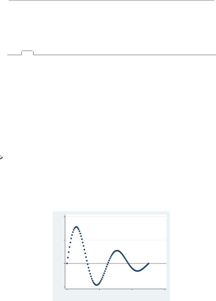
464 dydx — Calculate numeric derivatives and integrals
Description
dydx and integ calculate derivatives and integrals of numeric “functions”.
Options
Main
generate(newvar)specifies the name of the new variable to be created. It must be specified with
dydx.
trapezoid requests that the trapezoidal rule [the sum of (xi−xi−1)(yi+yi−1)/2be used to
compute integrals. The default is cubic splines, which give superior results for most smooth
functions; for irregular functions, trapezoid may give better results.
initial(#)specifies the initial condition for calculating definite integrals; see Methods and formulas
below. The default is initial(0).
replace specifies that if an existing variable is specified for generate(), it should be overwritten.
Remarks and examples
dydx and integ lets you extend Stata’s graphics capabilities beyond data analysis and into
mathematics. (See Gould [1993] for another command that draws functions.)
Example 1
We graph y=e−x/6sin(x)over the interval [0,12.56 ]:
. range x 0 12.56 100
obs was 0, now 100
. generate y = exp(-x/6)*sin(x)
. label variable y "exp(-x/6)*sin(x)"
. twoway connected y x, connect(i) yline(0)
−.5 0 .5 1
exp(−x/6)*sin(x)
0 5 10 15
x
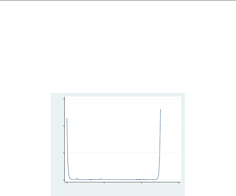
dydx — Calculate numeric derivatives and integrals 465
We estimate the derivative by using dydx and compute the relative difference between this estimate
and the true derivative.
. dydx y x, gen(dy)
. generate dytrue = exp(-x/6)*(cos(x) - sin(x)/6)
. generate error = abs(dy - dytrue)/dytrue
The error is greatest at the endpoints, as we would expect. The error is approximately 0.5% at each
endpoint, but the error quickly falls to less than 0.01%.
. label variable error "Error in derivative estimate"
. twoway line error x, ylabel(0(.002).006)
0 .002 .004 .006
Error in derivative estimate
0 5 10 15
x
We now estimate the integral by using integ:
. integ y x, gen(iy)
number of points = 100
integral = .85316396
. generate iytrue = (36/37)*(1 - exp(-x/6)*(cos(x) + sin(x)/6))
. display iytrue[_N]
.85315901
. display abs(r(integral) - iytrue[_N])/iytrue[_N]
5.799e-06
. generate diff = iy - iytrue
The relative difference between the estimate [stored in r(integral)] and the true value of the
integral is about 6 ×10⁻⁶. A graph of the absolute difference (diff) is shown below. Here error is
cumulative. Again most of the error is due to a relatively poorer fit near the endpoints.
. label variable diff "Error in integral estimate"
. twoway line diff x, ylabel(0(5.00e-06).00001)
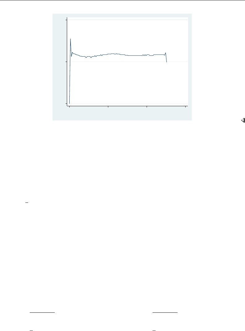
466 dydx — Calculate numeric derivatives and integrals
0 5.00e−06 .00001
Error in integral estimate
0 5 10 15
x
Stored results
dydx stores the following in r():
Macros
r(y) name of yvar
integ stores the following in r():
Scalars
r(N points) number of unique xpoints
r(integral) estimate of the integral
Methods and formulas
Consider a set of data points, (x1, y1),. . . ,(xn, yn), generated by a function y=f(x).dydx and
integ first fit these points with a cubic spline, which is then analytically differentiated (integrated)
to give an approximation for the derivative (integral) of f.
The cubic spline (see, for example, Press et al. [2007]) consists of n−1 cubic polynomials Pi(x),
with the ith one defined on the interval [xi, xi+1],
Pi(x) = yiai(x) + yi+1bi(x) + y00
ici(x) + y00
i+1di(x)
where
ai(x) = xi+1 −x
xi+1 −xi
ci(x) = 1
6(xi+1 −xi)2ai(x)[{ai(x)}2−1]
bi(x) = x−xi
xi+1 −xi
di(x) = 1
6(xi+1 −xi)2bi(x)[{bi(x)}2−1]
and y00
iand y00
i+1 are constants whose values will be determined as described below. The notation for
these constants is justified because P00
i(xi) = y00
iand P00
i(xi+1) = y00
i+1.

dydx — Calculate numeric derivatives and integrals 467
Because ai(xi) = 1, ai(xi+1) = 0, bi(xi) = 0, and bi(xi+1) = 1. Therefore, Pi(xi) = yi, and
Pi(xi+1) = yi+1. Thus the Pijointly define a function that is continuous at the interval boundaries.
The first derivative should be continuous at the interval boundaries; that is,
P0
i(xi+1) = P0
i+1(xi+1)
The above n−2 equations (one equation for each point except the two endpoints) and the values of
the first derivative at the endpoints, P0
1(x1)and P0
n−1(xn), determine the nconstants y00
i.
The value of the first derivative at an endpoint is set to the value of the derivative obtained by
fitting a quadratic to the endpoint and the two adjacent points; namely, we use
P0
1(x1) = y1−y2
x1−x2
+y1−y3
x1−x3−y2−y3
x2−x3
and a similar formula for the upper endpoint.
dydx approximates f0(xi)by using P0
i(xi).
integ approximates F(xi) = F(x1) + Rxi
x1f(x)dx by using
I0+
i−1
X
k=1 Zxk+1
xk
Pk(x)dx
where I0(an estimate of F(x1)) is the value specified by the initial(#)option. If the trapezoid
option is specified, integ approximates the integral by using the trapezoidal rule:
I0+
i−1
X
k=1
1
2(xk+1 −xk)(yk+1 +yk)
If there are ties among the xi, the mean of yiis computed at each set of ties and the cubic spline
is fit to these values.
Acknowledgment
The present versions of dydx and integ were inspired by the dydx2 command written by Patrick
Royston of the MRC Clinical Trials Unit, London, and coauthor of the Stata Press book Flexible
Parametric Survival Analysis Using Stata: Beyond the Cox Model.
References
Gould, W. W. 1993. ssi5.1: Graphing functions.Stata Technical Bulletin 16: 23–26. Reprinted in Stata Technical
Bulletin Reprints, vol. 3, pp. 188–193. College Station, TX: Stata Press.
. 1997. crc46: Better numerical derivatives and integrals.Stata Technical Bulletin 35: 3–5. Reprinted in Stata
Technical Bulletin Reprints, vol. 6, pp. 8–12. College Station, TX: Stata Press.
Press, W. H., S. A. Teukolsky, W. T. Vetterling, and B. P. Flannery. 2007. Numerical Recipes: The Art of Scientific
Computing. 3rd ed. New York: Cambridge University Press.


Title
eform option — Displaying exponentiated coefficients
Description Remarks and examples Reference Also see
Description
An eform option causes the coefficient table to be displayed in exponentiated form: for each
coefficient, ebrather than bis displayed. Standard errors and confidence intervals (CIs) are also
transformed.
An eform option is one of the following:
eform option Description
eform(string)use string for the column title
eform exponentiated coefficient, string is exp(b)
hr hazard ratio, string is Haz. Ratio
shr subhazard ratio, string is SHR
irr incidence-rate ratio, string is IRR
or odds ratio, string is Odds Ratio
rrr relative-risk ratio, string is RRR
Remarks and examples
Example 1
Here is a simple example of the or option with svy: logit. The CI for the odds ratio is computed
by transforming (by exponentiating) the endpoints of the CI for the corresponding coefficient.
. use http://www.stata-press.com/data/r13/nhanes2d
. svy, or: logit highbp female black
(running logit on estimation sample)
(output omitted )
Linearized
highbp Odds Ratio Std. Err. t P>|t| [95% Conf. Interval]
female .6107011 .0326159 -9.23 0.000 .5476753 .6809798
black 1.384865 .1336054 3.37 0.002 1.137507 1.686011
_cons .7249332 .0551062 -4.23 0.000 .6208222 .8465035
We also could have specified the following command and received the same results as above:
. svy: logit highbp female black, or
469


Title
eivreg — Errors-in-variables regression
Syntax Menu Description Options
Remarks and examples Stored results Methods and formulas References
Also see
Syntax
eivreg depvar indepvars if in weight ,options
options Description
Model
reliab(indepvar #indepvar # . . . )
specify measurement reliability for each indepvar measured with error
Reporting
level(#)set confidence level; default is level(95)
display options control column formats, row spacing, line width, display of omitted
variables and base and empty cells, and factor-variable labeling
coeflegend display legend instead of statistics
indepvars may contain factor variables; see [U] 11.4.3 Factor variables.
bootstrap,by,jackknife,rolling, and statsby are allowed; see [U] 11.1.10 Prefix commands.
Weights are not allowed with the bootstrap prefix; see [R] bootstrap.
aweights are not allowed with the jackknife prefix; see [R] jackknife.
aweights and fweights are allowed; see [U] 11.1.6 weight.
coeflegend does not appear in the dialog box.
See [U] 20 Estimation and postestimation commands for more capabilities of estimation commands.
Menu
Statistics >Linear models and related >Errors-in-variables regression
Description
eivreg fits errors-in-variables regression models.
Options
Model
reliab(indepvar #indepvar # . . . )specifies the measurement reliability for each independent
variable measured with error. Reliabilities are specified as pairs consisting of an independent
variable name (a name that appears in indepvars) and the corresponding reliability r, 0 < r ≤1.
Independent variables for which no reliability is specified are assumed to have reliability 1. If the
option is not specified, all variables are assumed to have reliability 1, and the result is thus the
same as that produced by regress (the ordinary least-squares results).
471

472 eivreg — Errors-in-variables regression
Reporting
level(#); see [R]estimation options.
display options:noomitted,vsquish,noemptycells,baselevels,allbaselevels,nofvla-
bel,fvwrap(#),fvwrapon(style),cformat(%fmt),pformat(% fmt),sformat(% fmt), and
nolstretch; see [R]estimation options.
The following option is available with eivreg but is not shown in the dialog box:
coeflegend; see [R]estimation options.
Remarks and examples
For an introduction to errors-in-variables regression, see Draper and Smith (1998, 89–91) or
Kmenta (1997, 352–357). Treiman (2009, 258–261) compares the results of errors-in-variables re-
gression with conventional regression.
Errors-in-variables regression models are useful when one or more of the independent variables are
measured with additive noise. Standard regression (as performed by regress) would underestimate
the effect of the variable, and the other coefficients in the model can be biased to the extent that
they are correlated with the poorly measured variable. You can adjust for the biases if you know the
reliability:
r= 1 −noise variance
total variance
That is, given the model y=Xβ+u, for some variable xiin X, the xiis observed with error,
xi=x∗
i+e, and the noise variance is the variance of e. The total variance is the variance of xi.
Example 1
Say that in our automobile data, the weight of cars was measured with error, and the reliability
of our measured weight is 0.85. The result of this would be to underestimate the effect of weight
in a regression of, say, price on weight and foreign, and it would also bias the estimate of the
coefficient on foreign (because being of foreign manufacture is correlated with the weight of cars).
We would ignore all of this if we fit the model with regress:
. use http://www.stata-press.com/data/r13/auto
(1978 Automobile Data)
. regress price weight foreign
Source SS df MS Number of obs = 74
F( 2, 71) = 35.35
Model 316859273 2 158429637 Prob > F = 0.0000
Residual 318206123 71 4481776.38 R-squared = 0.4989
Adj R-squared = 0.4848
Total 635065396 73 8699525.97 Root MSE = 2117
price Coef. Std. Err. t P>|t| [95% Conf. Interval]
weight 3.320737 .3958784 8.39 0.000 2.531378 4.110096
foreign 3637.001 668.583 5.44 0.000 2303.885 4970.118
_cons -4942.844 1345.591 -3.67 0.000 -7625.876 -2259.812

eivreg — Errors-in-variables regression 473
With eivreg, we can account for our measurement error:
. eivreg price weight foreign, r(weight .85)
assumed Errors-in-variables regression
variable reliability
Number of obs = 74
weight 0.8500 F( 2, 71) = 50.37
* 1.0000 Prob > F = 0.0000
R-squared = 0.6483
Root MSE = 1773.54
price Coef. Std. Err. t P>|t| [95% Conf. Interval]
weight 4.31985 .431431 10.01 0.000 3.459601 5.180099
foreign 4637.32 624.5362 7.43 0.000 3392.03 5882.609
_cons -8257.017 1452.086 -5.69 0.000 -11152.39 -5361.639
The effect of weight is increased—as we knew it would be — and here the effect of foreign manufacture
is also increased. A priori, we knew only that the estimate of foreign might be biased; we did not
know the direction.
Technical note
Swept under the rug in our example is how we would determine the reliability, r. We can easily
see that a variable is measured with error, but we may not know the reliability because the ingredients
for calculating rdepend on the unobserved noise.
For our example, we made up a value for r, and in fact we do not believe that weight is measured
with error at all, so the reported eivreg results have no validity. The regress results were the
statistically correct results here.
But let’s say that we do suspect that weight is measured with error and that we do not know r.
We could then experiment with various values of rto describe the sensitivity of our estimates to
possible error levels. We may not know r, but rdoes have a simple interpretation, and we could
probably produce a sensible range for rby thinking about how the data were collected.
If the reliability, r, is less than the R2from a regression of the poorly measured variable on all
the other variables, including the dependent variable, the information might as well not have been
collected; no adjustment to the final results is possible. For our automobile data, running a regression
of weight on foreign and price would result in an R2of 0.6743. Thus the reliability must be at
least 0.6743 here. If we specify a reliability that is too small, eivreg will inform us and refuse to
fit the model:
. eivreg price weight foreign, r(weight .6742)
reliability r() too small
r(399);
Returning to our problem of how to estimate r, too small or not, if the measurements are summaries
of scaled items, the reliability may be estimated using the alpha command; see [MV]alpha. If the
score is computed from factor analysis and the data are scored using predict’s default options (see
[MV]factor postestimation), the square of the standard deviation of the score is an estimate of the
reliability.

474 eivreg — Errors-in-variables regression
Technical note
Consider a model with more than one variable measured with error. For instance, say that our
model is that price is a function of weight,foreign, and mpg and that both weight and mpg are
measured with error.
. eivreg price weight foreign mpg, r(weight .85 mpg .9)
assumed Errors-in-variables regression
variable reliability
Number of obs = 74
weight 0.8500 F( 3, 70) = 429.14
mpg 0.9000 Prob > F = 0.0000
* 1.0000 R-squared = 0.9728
Root MSE = 496.41
price Coef. Std. Err. t P>|t| [95% Conf. Interval]
weight 12.88302 .6820532 18.89 0.000 11.52271 14.24333
foreign 8268.951 352.8719 23.43 0.000 7565.17 8972.732
mpg 999.2043 73.60037 13.58 0.000 852.413 1145.996
_cons -56473.19 3710.015 -15.22 0.000 -63872.58 -49073.8
Stored results
eivreg stores the following in e():
Scalars
e(N) number of observations
e(df m) model degrees of freedom
e(df r) residual degrees of freedom
e(r2) R-squared
e(F) Fstatistic
e(rmse) root mean squared error
e(rank) rank of e(V)
Macros
e(cmd) eivreg
e(cmdline) command as typed
e(depvar) name of dependent variable
e(rellist) indepvars and associated reliabilities
e(wtype) weight type
e(wexp) weight expression
e(properties) b V
e(predict) program used to implement predict
e(asbalanced) factor variables fvset as asbalanced
e(asobserved) factor variables fvset as asobserved
Matrices
e(b) coefficient vector
e(Cns) constraints matrix
e(V) variance–covariance matrix of the estimators
Functions
e(sample) marks estimation sample

eivreg — Errors-in-variables regression 475
Methods and formulas
Let the model to be fit be
y=X∗β+e
X=X∗+U
where X∗are the true values and Xare the observed values. Let Wbe the user-specified weights. If
no weights are specified, W=I. If weights are specified, let vbe the specified weights. If fweight
frequency weights are specified, then W=diag(v). If aweight analytic weights are specified,
then W=diag{v/(10v)(101)}, meaning that the weights are normalized to sum to the number of
observations.
The estimates bof βare obtained as A−1X0Wy, where A=X0WX −S.Sis a diagonal
matrix with elements N(1−ri)s2
i.Nis the number of observations, riis the user-specified reliability
coefficient for the ith explanatory variable or 1 if not specified, and s2
iis the (appropriately weighted)
variance of the variable.
The variance–covariance matrix of the estimators is obtained as s2A−1X0WXA−1, where the
root mean squared error s2= (y0Wy −bAb0)/(N−p), where pis the number of estimated
parameters.
References
Draper, N., and H. Smith. 1998. Applied Regression Analysis. 3rd ed. New York: Wiley.
Kmenta, J. 1997. Elements of Econometrics. 2nd ed. Ann Arbor: University of Michigan Press.
Treiman, D. J. 2009. Quantitative Data Analysis: Doing Social Research to Test Ideas. San Francisco: Jossey-Bass.
Also see
[R]eivreg postestimation — Postestimation tools for eivreg
[R]regress — Linear regression
[SEM] example 24 — Reliability
[U] 20 Estimation and postestimation commands

Title
eivreg postestimation — Postestimation tools for eivreg
Description Syntax for predict Menu for predict Options for predict
Also see
Description
The following postestimation commands are available after eivreg:
Command Description
contrast contrasts and ANOVA-style joint tests of estimates
estat summarize summary statistics for the estimation sample
estat vce variance–covariance matrix of the estimators (VCE)
estimates cataloging estimation results
forecast dynamic forecasts and simulations
lincom point estimates, standard errors, testing, and inference for linear combinations
of coefficients
linktest link test for model specification
margins marginal means, predictive margins, marginal effects, and average marginal
effects
marginsplot graph the results from margins (profile plots, interaction plots, etc.)
nlcom point estimates, standard errors, testing, and inference for nonlinear combinations
of coefficients
predict predictions, residuals, influence statistics, and other diagnostic measures
predictnl point estimates, standard errors, testing, and inference for generalized predictions
pwcompare pairwise comparisons of estimates
test Wald tests of simple and composite linear hypotheses
testnl Wald tests of nonlinear hypotheses
Syntax for predict
predict type newvar if in ,statistic
statistic Description
Main
xb linear prediction; the default
residuals residuals
stdp standard error of the prediction
stdf standard error of the forecast
pr(a,b)Pr(a< yj<b)
e(a,b)E(yj|a< yj<b)
ystar(a,b)E(y∗
j),y∗
j=max{a, min(yj, b)}
These statistics are available both in and out of sample; type predict . . . if e(sample) . . . if wanted only for
the estimation sample.
476

eivreg postestimation — Postestimation tools for eivreg 477
where aand bmay be numbers or variables; amissing (a≥.) means −∞, and bmissing (b≥.)
means +∞; see [U] 12.2.1 Missing values.
Menu for predict
Statistics >Postestimation >Predictions, residuals, etc.
Options for predict
Main
xb, the default, calculates the linear prediction.
residuals calculates the residuals, that is, yj−xjb.
stdp calculates the standard error of the prediction, which can be thought of as the standard error of
the predicted expected value or mean for the observation’s covariate pattern. The standard error
of the prediction is also referred to as the standard error of the fitted value.
stdf calculates the standard error of the forecast, which is the standard error of the point prediction
for 1 observation and is commonly referred to as the standard error of the future or forecast value.
By construction, the standard errors produced by stdf are always larger than those produced by
stdp; see Methods and formulas in [R]regress postestimation.
pr(a,b)calculates Pr(a<xjb+uj<b), the probability that yj|xjwould be observed in the
interval (a,b).
aand bmay be specified as numbers or variable names; lb and ub are variable names;
pr(20,30) calculates Pr(20 <xjb+uj<30);
pr(lb,ub)calculates Pr(lb <xjb+uj<ub); and
pr(20,ub)calculates Pr(20 <xjb+uj<ub).
amissing (a≥.) means −∞;pr(.,30) calculates Pr(−∞ <xjb+uj<30);
pr(lb,30) calculates Pr(−∞ <xjb+uj<30)in observations for which lb ≥.
and calculates Pr(lb < xjb+uj<30)elsewhere.
bmissing (b≥.) means +∞;pr(20,.) calculates Pr(+∞>xjb+uj>20);
pr(20,ub)calculates Pr(+∞>xjb+uj>20)in observations for which ub ≥.
and calculates Pr(20 <xjb+uj<ub)elsewhere.
e(a,b)calculates E(xjb+uj|a<xjb+uj<b), the expected value of yj|xjconditional on
yj|xjbeing in the interval (a,b), meaning that yj|xjis truncated. aand bare specified as they
are for pr().
ystar(a,b)calculates E(y∗
j), where y∗
j=aif xjb+uj≤a,y∗
j=bif xjb+uj≥b, and
y∗
j=xjb+ujotherwise, meaning that y∗
jis censored. aand bare specified as they are for pr().
Also see
[R]eivreg — Errors-in-variables regression
[U] 20 Estimation and postestimation commands

Title
error messages — Error messages and return codes
Description Also see
Description
Whenever Stata detects that something is wrong — that what you typed is uninterpretable, that you
are trying to do something you should not be trying to do, or that you requested the impossible — Stata
responds by typing a message describing the problem, together with a return code. For instance,
. lsit
unrecognized command: lsit
r(199);
. list myvar
variable myvar not found
r(111);
. test a=b
last estimates not found
r(301);
In each case, the message is probably sufficient to guide you to a solution. When we typed
lsit, Stata responded with “unrecognized command”. We meant to type list. When we typed
list myvar, Stata responded with “variable myvar not found”. There is no variable named myvar
in our data. When we typed test a=b, Stata responded with “last estimates not found”. test tests
hypotheses about previously fit models, and we have not yet fit a model.
The numbers in parentheses in the r(199),r(111), and r(301) messages are called the return
codes. To find out more about these messages, type search rc #, where #is the number returned
in the parentheses.
Example 1
. search rc 301
[P] error messages . . . . . . . . . . . . . . . . . . . . Return code 301
;
You typed an estimation command such as without arguments
or attempted to perform a or typed , but there were no
previous estimation results.
Programmers should see [P]error for details on programming error messages.
Also see
[R]search — Search Stata documentation and other resources
478

Title
esize — Effect size based on mean comparison
Syntax Menu Description Options
Remarks and examples Stored results Methods and formulas References
Also see
Syntax
Effect sizes for two independent samples using groups
esize twosample varname if in , by(groupvar)options
Effect sizes for two independent samples using variables
esize unpaired varname1== varname2if in ,options
Immediate form of effect sizes for two independent samples
esizei #obs1 #mean1 #sd1 #obs2 #mean2 #sd2 ,options
Immediate form of effect sizes for F tests after an ANOVA
esizei #df1 #df2 #F, level(#)
options Description
Main
cohensd report Cohen’s d(1988)
hedgesg report Hedges’s g(1981)
glassdelta report Glass’s ∆(Smith and Glass 1977) using each group’s standard deviation
pbcorr report the point-biserial correlation coefficient (Pearson 1909)
all report all estimates of effect size
unequal use unequal variances
welch use Welch’s (1947) approximation
level(#)set confidence level; default is level(95)
by is allowed with esize; see [D] by.
Menu
esize
Statistics >Summaries, tables, and tests >Classical tests of hypotheses >Effect size based on mean comparison
esizei
Statistics >Summaries, tables, and tests >Classical tests of hypotheses >Effect-size calculator
479

480 esize — Effect size based on mean comparison
Description
esize calculates effect sizes for comparing the difference between the means of a continuous
variable for two groups. In the first form, esize calculates effect sizes for the difference between the
mean of varname for two groups defined by groupvar. In the second form, esize calculates effect
sizes for the difference between varname1and varname2, assuming unpaired data.
esizei is the immediate form of esize; see [U] 19 Immediate commands. In the first form,
esizei calculates the effect size for comparing the difference between the means of two groups. In
the second form, esizei calculates the effect size for an Ftest after an ANOVA.
Options
Main
by(groupvar)specifies the groupvar that defines the two groups that esize will use to estimate the
effect sizes. Do not confuse the by() option with the by prefix; you can specify both.
cohensd specifies that Cohen’s d(1988) be reported.
hedgesg specifies that Hedges’s g(1981) be reported.
glassdelta specifies that Glass’s ∆(Smith and Glass 1977) be reported.
pbcorr specifies that the point-biserial correlation coefficient (Pearson 1909) be reported.
all specifies that all estimates of effect size be reported. The default is Cohen’s dand Hedges’s g.
unequal specifies that the data not be assumed to have equal variances.
welch specifies that the approximate degrees of freedom for the test be obtained from Welch’s formula
(1947) rather than from Satterthwaite’s approximation formula (1946), which is the default when
unequal is specified. Specifying welch implies unequal.
level(#)specifies the confidence level, as a percentage, for confidence intervals. The default is
level(95) or as set by set level; see [U] 20.7 Specifying the width of confidence intervals.
Remarks and examples
Whereas p-values are used to assess the statistical significance of a result, measures of effect size
are used to assess the practical significance of a result. Effect sizes can be broadly categorized as
“measures of group differences” (the dfamily) and “measures of association” (the rfamily); see
Ellis (2010, table 1.1). The dfamily includes estimators such as Cohen’s d, Hedges’s g, and Glass’s ∆.
The rfamily includes estimators such as the point-biserial correlation coefficient, ω2and η2(also see
estat esize in [R]regress postestimation). For an introduction to the concepts and calculation of
effect sizes, see Kline (2013) and Thompson (2006). For a more detailed discussion, see Kirk (1996),
Ellis (2010), Cumming (2012), Grissom and Kim (2012), and Kelley and Preacher (2012).
It should be noted that there is much variation in the definitions of measures of effect size
(Kline 2013). As Ellis (2010, 27) cautions, “However, beware the inconsistent terminology. What is
labeled here as gwas labeled by Hedges and Olkin as dand vice versa. For these authors writing in
the early 1980s, gwas the mainstream effect-size index developed by Cohen and refined by Glass
(hence gfor Glass). However, since then ghas become synonymous with Hedges’s equation (not
Glass’s) and the reason it is called Hedges’s gand not Hedges’s his because it was originally named
after Glass—even though it was developed by Larry Hedges. Confused?”

esize — Effect size based on mean comparison 481
To avoid confusion, esize and esizei closely follow the notation of Hedges (1981), Smith-
son (2001), Kline (2013), and Ellis (2010).
Example 1: Effect size for two independent samples using by()
Suppose we are interested in question 1 from the fictitious depression.dta: “My statistical
software makes me feel sad”. We might have conducted a ttest to test the null hypothesis that there is
no difference in response by sex. We could then compute various measures of effect size to describe
the magnitude of the effect of sex.
. use http://www.stata-press.com/data/r13/depression
(Fictitious Depression Inventory data based on the Beck Depression Inventory)
. esize twosample qu1, by(sex) all
Effect size based on mean comparison
Obs per group:
Female = 712
Male = 288
Effect Size Estimate [95% Conf. Interval]
Cohen’s d-.0512417 -.1881184 .0856607
Hedges’s g-.0512032 -.187977 .0855963
Glass’s Delta 1 -.0517793 -.1886587 .0851364
Glass’s Delta 2 -.0499786 -.1868673 .086997
Point-Biserial r -.0232208 -.0849629 .0387995
Cohen’s d, Hedges’s g, and both estimates of Glass’s ∆indicate that the score for females is 0.05
standard deviations lower than the score for males. The point-biserial correlation coefficient indicates
that there is a small, negative correlation between the scores for females and males.
Technical note
Glass’s ∆has traditionally been estimated for experimental studies using the control group standard
deviation rather than the pooled standard deviation. Kline (2013) notes that the choice of group becomes
arbitrary for data arising from observational studies and recommends the reporting of Glass’s ∆using
each group standard deviation.
Example 2: Effect size for two independent samples by a third variable
If we are interested in the same effect sizes from example 1 stratified by race, we could use the
by prefix with the sort option to accomplish this task.

482 esize — Effect size based on mean comparison
. by race, sort: esize twosample qu1, by(sex)
-> race = Hispanic
Effect size based on mean comparison
Obs per group:
Female = 88
Male = 45
Effect Size Estimate [95% Conf. Interval]
Cohen’s d-.1042883 -.463503 .2553235
Hedges’s g-.1036899 -.4608434 .2538584
-> race = Black
Effect size based on mean comparison
Obs per group:
Female = 259
Male = 95
Effect Size Estimate [95% Conf. Interval]
Cohen’s d-.1720681 -.4073814 .063489
Hedges’s g-.1717012 -.4065128 .0633536
-> race = White
Effect size based on mean comparison
Obs per group:
Female = 365
Male = 148
Effect Size Estimate [95% Conf. Interval]
Cohen’s d.0479511 -.1430932 .2389486
Hedges’s g.0478807 -.1428831 .2385977
Example 3: Bootstrap confidence intervals for effect sizes
Simulation studies have shown that bootstrap confidence intervals may be preferable to confidence
intervals based on the noncentral tdistribution when the variable of interest does not have a normal
distribution (Kelley 2005;Algina, Keselman, and Penfield 2006). Bootstrap confidence intervals can
be easily estimated for effect sizes using the bootstrap prefix.

esize — Effect size based on mean comparison 483
. use http://www.stata-press.com/data/r13/depression
(Fictitious Depression Inventory data based on the Beck Depression Inventory)
. set seed 12345
. bootstrap r(d) r(g), reps(1000) nodots nowarn: esize twosample qu1, by(sex)
Bootstrap results Number of obs = 1000
Replications = 1000
command: esize twosample qu1, by(sex)
_bs_1: r(d)
_bs_2: r(g)
Observed Bootstrap Normal-based
Coef. Std. Err. z P>|z| [95% Conf. Interval]
_bs_1 -.0512417 .07169 -0.71 0.475 -.1917515 .0892682
_bs_2 -.0512032 .0716361 -0.71 0.475 -.1916074 .0892011
Example 4: Effect sizes for two independent samples using variables
Sometimes, the data of interest are stored in two separate variables. We can calculate effect sizes
for the two groups by using the unpaired version of esize.
. use http://www.stata-press.com/data/r13/fuel
. esize unpaired mpg1==mpg2
Effect size based on mean comparison
Number of obs = 24
Effect Size Estimate [95% Conf. Interval]
Cohen’s d-.5829654 -1.394934 .2416105
Hedges’s g-.5628243 -1.34674 .2332631
Example 5: Immediate form for effect sizes for two means
Often we do not have access to raw data, but we are given summary statistics in a report or
manuscript. To calculate the effect sizes from summary statistics, we can use the immediate command
esizei. For example, Kline (2013) in table 4.2 shows summary statistics for a hypothetical sample
where mean1=13, sd1=2.74, mean2=11, and sd2=2.24; there are 30 people in each group.
We can estimate the effect sizes from these summary data using esizei:
. esizei 30 13 2.74 30 11 2.24
Effect size based on mean comparison
Obs per group:
Group 1 = 30
Group 2 = 30
Effect Size Estimate [95% Conf. Interval]
Cohen’s d.7991948 .2695509 1.322465
Hedges’s g.7888081 .2660477 1.305277

484 esize — Effect size based on mean comparison
Example 6: Immediate form for effect sizes for F tests after an ANOVA
esizei can also be used to compute η2and ω2for Ftests after an ANOVA. The following
example from Smithson (2001, 623) illustrates the use of esizei for dfnum =4, dfden =50, and
F=4.2317.
. esizei 4 50 4.2317, level(90)
Effect sizes for linear models
Effect Size Estimate [90% Conf. Interval]
Eta-Squared .2529151 .0521585 .3603621
Omega-Squared .1931483 0 .309191
Stored results
esize and esizei for comparing two means store the following in r():
Scalars
r(d) Cohen’s d
r(lb d) lower confidence bound for Cohen’s d
r(ub d) upper confidence bound for Cohen’s d
r(g) Hedges’s g
r(lb g) lower confidence bound for Hedges’s g
r(ub g) upper confidence bound for Hedges’s g
r(delta1) Glass’s ∆for group 1
r(lb delta1) lower confidence bound for Glass’s ∆for group 1
r(ub delta1) upper confidence bound for Glass’s ∆for group 1
r(delta2) Glass’s ∆for group 2
r(lb delta2) lower confidence bound for Glass’s ∆for group 2
r(ub delta2) upper confidence bound for Glass’s ∆for group 2
r(r pb) point-biserial correlation coefficient
r(lb r pb) lower confidence bound for the point-biserial correlation coefficient
r(ub r pb) upper confidence bound for the point-biserial correlation coefficient
r(N 1) sample size n1
r(N 2) sample size n2
r(df t) degrees of freedom
r(level) confidence level
esizei for Ftests after ANOVA stores the following in r():
Scalars
r(eta2) η2
r(lb eta2) lower confidence bound for η2
r(ub eta2) upper confidence bound for η2
r(omega2) ω2
r(lb omega2) lower confidence bound for ω2
r(ub omega2) upper confidence bound for ω2
r(level) confidence level
Methods and formulas
For the dfamily, the effect-size parameter of interest is the scaled difference between the means
given by
δ=(µ1−µ2)
σ

esize — Effect size based on mean comparison 485
One of the most popular estimators of effect size is Cohen’s d, given by
Cohen’s d=(x1−x2)
s∗
where
s∗=s(n1−1)s2
1+ (n2−1)s2
2
n1+n2−2
Hedges (1981) showed that Cohen’s dis biased and proposed the unbiased estimator
Hedges’s g=Cohen’s d×c(m)
where m=n1+n2−2 and
c(m) = Γm
2
pm
2Γm−1
2
Glass (Smith and Glass 1977) proposed an estimator for δin the context of designed experiments,
Glass’s ∆ = (xtreated −xcontrol)
scontrol
where scontrol is the standard deviation for the control group.
As noted above, esize and esizei report two estimates of Glass’s ∆: one using the standard
deviation for group 1 and the other using the standard deviation for group 2:
Glass’s ∆1=(x1−x2)
s1
and
Glass’s ∆2=(x1−x2)
s2
For the rfamily, the effect-size parameter of interest is the ratio of the variance attributable to an
effect and the total variance:
η2=σ2
effect
σ2
total
A popular estimator of ηwhen there are two groups is the point-biserial correlation coefficient,
rPB =t
√t2+df
where tis the tstatistic for the difference between the means of the two groups, and df is the
corresponding degrees of freedom. Satterthwaite’s or Welch’s adjustment (see [R]ttest for details) to
the degrees of freedom can be used to calculate rPB by specifying the unequal or welch option,
respectively.

486 esize — Effect size based on mean comparison
When more than two means are being compared, as in the case of an ANOVA with pgroups, a
popular estimator of effect size is the correlation ratio denoted η2(Fisher 1925;Kerlinger 1964). η2
can be computed directly as the ratio of the SSeffect and the SStotal or as a function of the Fstatistic
with numerator degrees of freedom equal to dfnum and denominator degrees of freedom equal to
dfden.
bη2=(F×dfnum)
(F×dfnum) + dfden
Like its equivalent estimator R2,η2has an upward bias. The less biased (though not unbiased)
estimator ω2(Hays 1963) is equivalent to the adjusted R2and can be estimated directly from the
sums of squares, the Fstatistic, or as a function of η2; that is,
bω2=SSbetween −(p−1)MSwithin
SStotal +MSwithin
or
bω2=(p−1)(F−1)
(p−1)(F−1) + (p)(n)
or
bω2=η2− dfnum
dfden !×(1 −η2)
To calculate bη2and bω2directly after anova or regress, see estat esize in [R]regress
postestimation.
Cohen’s d, Hedges’s g, and Glass’s ∆have been shown to have a noncentral tdistribution
(Hedges 1981) with noncentrality parameter equal to
λ=δrn1n2
n1+n2
Confidence intervals are calculated by finding the noncentrality parameters λlower and λupper that
correspond to
Pr(df, δ, λlower) = 1 −α
2
and
Pr(df, δ, λupper) = α
2
using the function npnt(df,t,p). The noncentrality parameters are then transformed back to the
effect-size scale:
δlower =λlowerrn1+n2
n1n2
and
δupper =λupperrn1+n2
n1n2
(see Venables [1975]; Steiger and Fouladi [1997]; Cumming and Finch [2001]; Smithson [2001]).

esize — Effect size based on mean comparison 487
Confidence intervals for the point-biserial correlation coefficient are calculated similarly and
transformed back to the effect-size scale as
rlower =λlower
pλ2
lower +df
and
rupper =λupper
qλ2
upper +df
Following Smithson’s (2001) notation, the Fstatistic is written as
Fdfnum,dfden =f2(dfnum/dfden)
This equation has a noncentral Fdistribution with noncentrality parameter:
λ=f2(dfnum +dfden + 1)
where f2=R2/(1−R2).
Confidence intervals for bη2and bω2are calculated by finding the noncentrality parameters λlower
and λupper for a noncentral Fdistribution that correspond to
Pr(dfnum,dfden, F, λlower) = 1 −α
2
and
Pr(dfnum,dfden, F, λupper) = α
2
using the function npnF(df1,df2,f,p). The noncentrality parameters are transformed back to the
bη2scale as
bη2
lower =max 0,λlower
λlower +dfnum +dfden + 1!
and
bη2
upper =min 1,λupper
λupper +dfnum +dfden + 1!
The confidence limits for bω2are then calculated as a function of bη2:
bω2
lower =bη2
lower − dfnum
dfden !×(1 −bη2
lower)
and
bω2
upper =bη2
upper − dfnum
dfden !×(1 −bη2
upper)
See Smithson (2001) for further details.

488 esize — Effect size based on mean comparison
Fred Nichols Kerlinger (1910–1991) was born in New York City. He studied music at New
York University and graduated magna cum laude with a degree in education and philosophy.
After graduation, he joined the U.S. Army and served as a counterintelligence officer in Japan
in 1946. Kerlinger earned an MA and a PhD in educational psychology from the University of
Michigan and held faculty appointments at several universities, including New York University.
He was president of the American Educational Research Association and is best known for
his popular and influential book Foundations of Behavioral Research (1964), which introduced
Fisher’s (1925)η2statistic to behavioral researchers.
William Lee Hays (1926–1995) was born in Clarksville, Texas. He studied mathematics and
psychology at Paris Junior College in Paris, Texas, and at East Texas State College. He earned BS
and MS degrees from North Texas State University. Upon completion of his PhD in psychology
at the University of Michigan, he joined the faculty, where he eventually became associate vice
president for academic affairs. In 1977, Hays accepted an appointment as vice president for
academic affairs at the University of Texas at Austin, where he remained until his death in 1995.
Hays is best known for his book Statistics for Psychologists (1963), which introduced the ω2
statistic.
References
Algina, J., H. J. Keselman, and R. D. Penfield. 2006. Confidence interval coverage for Cohen’s effect size statistic.
Educational and Psychological Measurement 66: 945–960.
Cohen, J. 1988. Statistical Power Analysis for the Behavioral Sciences. 2nd ed. Hillsdale, NJ: Erlbaum.
Cumming, G. 2012. Understanding the New Statistics: Effect Sizes, Confidence Intervals, and Meta-Analysis. New
York: Taylor & Francis.
Cumming, G., and S. Finch. 2001. A primer on the understanding, use, and calculation of confidence intervals that
are based on central and noncentral distributions. Educational and Psychological Measurement 61: 532–574.
Ellis, P. D. 2010. The Essential Guide to Effect Sizes: Statistical Power, Meta-Analysis, and the Interpretation of
Research Results. Cambridge: Cambridge University Press.
Fisher, R. A. 1925. Statistical Methods for Research Workers. Edinburgh: Oliver & Boyd.
Grissom, R. J., and J. J. Kim. 2012. Effect Sizes for Research: Univariate and Multivariate Applications. 2nd ed.
New York: Taylor & Francis.
Hays, W. L. 1963. Statistics for Psychologists. New York: Holt, Rinehart & Winston.
Hedges, L. V. 1981. Distribution theory for Glass’s estimator of effect size and related estimators. Journal of Educational
Statistics 6: 107–128.
Huber, C. 2013. Measures of effect size in Stata 13. The Stata Blog: Not Elsewhere Classified.
http://blog.stata.com/2013/09/05/measures-of-effect-size-in-stata-13/.
Kelley, K. 2005. The effects of nonnormal distributions on confidence intervals around the standardized mean difference:
Bootstrap and parametric confidence intervals. Educational and Psychological Measurement 65: 51–69.
Kelley, K., and K. J. Preacher. 2012. On effect size. Psychological Methods 17: 137–152.
Kerlinger, F. N. 1964. Foundations of Behavioral Research. New York: Holt, Rinehart & Winston.
Kirk, R. E. 1996. Practical significance: A concept whose time has come. Educational and Psychological Measurement
56: 746–759.
Kline, R. B. 2013. Beyond Significance Testing: Statistics Reform in the Behavioral Sciences. 2nd ed. Washington,
DC: American Psychological Association.
Pearson, K. 1909. On a new method of determining correlation between a measured character A, and a character B,
of which only the percentage of cases wherein B exceeds (or falls short of) a given intensity is recorded for each
grade of A. Biometrika 7: 96–105.

esize — Effect size based on mean comparison 489
Satterthwaite, F. E. 1946. An approximate distribution of estimates of variance components. Biometrics Bulletin 2:
110–114.
Smith, M. L., and G. V. Glass. 1977. Meta-analysis of psychotherapy outcome studies. American Psychologist 32:
752–760.
Smithson, M. 2001. Correct confidence intervals for various regression effect sizes and parameters: The importance
of noncentral distributions in computing intervals. Educational and Psychological Measurement 61: 605–632.
Steiger, J. H., and R. T. Fouladi. 1997. Noncentrality interval estimation and the evaluation of statistical models. In
What If There Were No Significance Tests?, ed. L. L. Harlow, S. A. Mulaik, and J. H. Steiger, 221–257. Mahwah,
NJ: Erlbaum.
Thompson, B. 2006. Foundations of Behavioral Statistics: An Insight-Based Approach. New York: Guilford Press.
Venables, W. 1975. Calculation of confidence intervals for noncentrality parameters. Journal of the Royal Statistical
Society, Series B 37: 406–412.
Welch, B. L. 1947. The generalization of ‘student’s’ problem when several different population variances are involved.
Biometrika 34: 28–35.
Also see
[R]bitest — Binomial probability test
[R]ci — Confidence intervals for means, proportions, and counts
[R]mean — Estimate means
[R]oneway — One-way analysis of variance
[R]prtest — Tests of proportions
[R]sdtest — Variance-comparison tests
[R]ttest —ttests (mean-comparison tests)

Title
estat — Postestimation statistics
Syntax Description
Syntax
Command Reference
Display information criteria
estat ic , n(#)[R]estat ic
Summarize estimation sample
estat summarize eqlist,estat summ options [R]estat summarize
Display covariance matrix estimates
estat vce ,estat vce options [R]estat vce
Command-specific
estat subcommand1,options1
Description
estat displays scalar- and matrix-valued statistics after estimation; it complements predict,
which calculates variables after estimation. Exactly what statistics estat can calculate depends on
the previous estimation command.
Three sets of statistics are so commonly used that they are available after all estimation commands
that store the model log likelihood. estat ic displays Akaike’s and Schwarz’s Bayesian information
criteria. estat summarize summarizes the variables used by the command and automatically restricts
the sample to e(sample); it also summarizes the weight variable and cluster structure, if specified.
estat vce displays the covariance or correlation matrix of the parameter estimates of the previous
model.
490

Title
estat classification — Classification statistics and table
Syntax Menu for estat Description Options
Remarks and examples Stored results Methods and formulas References
Also see
Syntax
estat classification if in weight ,options
options Description
Main
all display summary statistics for all observations in the data
cutoff(#)positive outcome threshold; default is cutoff(0.5)
fweights are allowed; see [U] 11.1.6 weight.
estat classification is not appropriate after the svy prefix.
Menu for estat
Statistics >Postestimation >Reports and statistics
Description
estat classification reports various summary statistics, including the classification table.
estat classification requires that the current estimation results be from logistic,logit,
probit, or ivprobit; see [R]logistic,[R]logit,[R]probit, or [R]ivprobit.
Options
Main
all requests that the statistic be computed for all observations in the data, ignoring any if or in
restrictions specified by the estimation command.
cutoff(#)specifies the value for determining whether an observation has a predicted positive
outcome. An observation is classified as positive if its predicted probability is ≥#. The default
is 0.5.
Remarks and examples
estat classification presents the classification statistics and classification table after logistic,
logit,probit, or ivprobit.
Statistics are produced either for the estimation sample (the default) or for any set of observations.
When weights, if, or in is used with the estimation command, it is not necessary to repeat the
qualifier when you want statistics computed for the estimation sample. Specify if,in, or the all
option only when you want statistics computed for a set of observations other than the estimation
sample. Specify weights only when you want to use a different set of weights.
491

492 estat classification — Classification statistics and table
Example 1
We illustrate estat classification after logistic; see [R]logistic.
. use http://www.stata-press.com/data/r13/lbw
(Hosmer & Lemeshow data)
. logistic low age lwt i.race smoke ptl ht ui
(output omitted )
. estat classification
Logistic model for low
True
Classified D ~D Total
+ 21 12 33
- 38 118 156
Total 59 130 189
Classified + if predicted Pr(D) >= .5
True D defined as low != 0
Sensitivity Pr( +| D) 35.59%
Specificity Pr( -|~D) 90.77%
Positive predictive value Pr( D| +) 63.64%
Negative predictive value Pr(~D| -) 75.64%
False + rate for true ~D Pr( +|~D) 9.23%
False - rate for true D Pr( -| D) 64.41%
False + rate for classified + Pr(~D| +) 36.36%
False - rate for classified - Pr( D| -) 24.36%
Correctly classified 73.54%
The overall rate of correct classification is estimated to be 73.54, with 90.77% of the normal
weight group correctly classified (specificity) and only 35.59% of the low weight group correctly
classified (sensitivity). Classification is sensitive to the relative sizes of each component group, and
always favors classification into the larger group. This phenomenon is evident here.
By default, estat classification uses a cutoff of 0.5, although you can vary this with the
cutoff() option. You can use the lsens command to review the potential cutoffs; see [R]lsens.
Stored results
estat classification stores the following in r():
Scalars
r(P corr) percent correctly classified
r(P p1) sensitivity
r(P n0) specificity
r(P p0) false-positive rate given true negative
r(P n1) false-negative rate given true positive
r(P 1p) positive predictive value
r(P 0n) negative predictive value
r(P 0p) false-positive rate given classified positive
r(P 1n) false-negative rate given classified negative

estat classification — Classification statistics and table 493
Methods and formulas
Let jindex observations. Define cas the cutoff() specified by the user or, if not specified, as
0.5. Let pjbe the predicted probability of a positive outcome and yjbe the actual outcome, which
we will treat as 0 or 1, although Stata treats it as 0 and non-0, excluding missing observations.
A prediction is classified as positive if pj≥cand otherwise is classified as negative. The
classification is correct if it is positive and yj=1 or if it is negative and yj=0.
Sensitivity is the fraction of yj=1 observations that are correctly classified. Specificity is the
percentage of yj=0 observations that are correctly classified.
References
Hosmer, D. W., Jr., S. A. Lemeshow, and R. X. Sturdivant. 2013. Applied Logistic Regression. 3rd ed. Hoboken,
NJ: Wiley.
Kohler, U., and F. Kreuter. 2012. Data Analysis Using Stata. 3rd ed. College Station, TX: Stata Press.
Also see
[R]logistic — Logistic regression, reporting odds ratios
[R]logit — Logistic regression, reporting coefficients
[R]probit — Probit regression
[R]ivprobit — Probit model with continuous endogenous regressors
[R]lroc — Compute area under ROC curve and graph the curve
[R]lsens — Graph sensitivity and specificity versus probability cutoff
[R]estat gof — Pearson or Hosmer–Lemeshow goodness-of-fit test
[R]roc — Receiver operating characteristic (ROC) analysis
[U] 20 Estimation and postestimation commands

Title
estat gof — Pearson or Hosmer–Lemeshow goodness-of-fit test
Syntax Menu for estat Description Options
Remarks and examples Stored results Methods and formulas References
Also see
Syntax
estat gof if in weight ,options
options Description
Main
group(#)perform Hosmer–Lemeshow goodness-of-fit test using #quantiles
all execute test for all observations in the data
outsample adjust degrees of freedom for samples outside estimation sample
table display table of groups used for test
fweights are allowed; see [U] 11.1.6 weight.
For information on using estat gof with survey data, see [SVY] estat.
Menu for estat
Statistics >Postestimation >Reports and statistics
Description
estat gof reports the Pearson goodness-of-fit test or the Hosmer–Lemeshow goodness-of-fit test.
estat gof requires that the current estimation results be from logistic,logit, or probit; see
[R]logistic,[R]logit, or [R]probit. For estat gof after poisson, see [R]poisson postestimation.
For estat gof after sem, see [SEM]estat gof.
Options
Main
group(#)specifies the number of quantiles to be used to group the data for the Hosmer–Lemeshow
goodness-of-fit test. group(10) is typically specified. If this option is not given, the Pearson
goodness-of-fit test is computed using the covariate patterns in the data as groups.
all requests that the statistic be computed for all observations in the data, ignoring any if or in
restrictions specified by the estimation command.
outsample adjusts the degrees of freedom for the Pearson and Hosmer–Lemeshow goodness-of-fit
tests for samples outside the estimation sample. See Samples other than the estimation sample
later in this entry.
494

estat gof — Pearson or Hosmer–Lemeshow goodness-of-fit test 495
table displays a table of the groups used for the Hosmer–Lemeshow or Pearson goodness-of-fit test
with predicted probabilities, observed and expected counts for both outcomes, and totals for each
group.
Remarks and examples
Remarks are presented under the following headings:
Introduction
Samples other than the estimation sample
Introduction
estat gof computes goodness-of-fit tests: either the Pearson χ2test or the Hosmer–Lemeshow
test.
By default, estat gof computes statistics for the estimation sample by using the last model fit by
logistic,logit, or probit. However, samples other than the estimation sample can be specified;
see Samples other than the estimation sample later in this entry.
Example 1
estat gof, typed without options, presents the Pearson χ2goodness-of-fit test for the fitted model.
The Pearson χ2goodness-of-fit test is a test of the observed against expected number of responses
using cells defined by the covariate patterns; see predict with the number option in [R]logistic
postestimation for the definition of covariate patterns.
. use http://www.stata-press.com/data/r13/lbw
(Hosmer & Lemeshow data)
. logistic low age lwt i.race smoke ptl ht ui
(output omitted )
. estat gof
number of observations = 189
number of covariate patterns = 182
Pearson chi2(173) = 179.24
Prob > chi2 = 0.3567
Our model fits reasonably well. However, the number of covariate patterns is close to the number
of observations, making the applicability of the Pearson χ2test questionable but not necessarily
inappropriate. Hosmer, Lemeshow, and Sturdivant (2013, 157–160) suggest regrouping the data by
ordering on the predicted probabilities and then forming, say, 10 nearly equal-sized groups. estat
gof with the group() option does this:
. estat gof, group(10)
(Table collapsed on quantiles of estimated probabilities)
number of observations = 189
number of groups = 10
Hosmer-Lemeshow chi2(8) = 9.65
Prob > chi2 = 0.2904
Again we cannot reject our model. If we specify the table option, estat gof displays the groups
along with the expected and observed number of positive responses (low-birthweight babies):

496 estat gof — Pearson or Hosmer–Lemeshow goodness-of-fit test
. estat gof, group(10) table
(Table collapsed on quantiles of estimated probabilities)
Group Prob Obs_1 Exp_1 Obs_0 Exp_0 Total
1 0.0827 0 1.2 19 17.8 19
2 0.1276 2 2.0 17 17.0 19
3 0.2015 6 3.2 13 15.8 19
4 0.2432 1 4.3 18 14.7 19
5 0.2792 7 4.9 12 14.1 19
6 0.3138 7 5.6 12 13.4 19
7 0.3872 6 6.5 13 12.5 19
8 0.4828 7 8.2 12 10.8 19
9 0.5941 10 10.3 9 8.7 19
10 0.8391 13 12.8 5 5.2 18
number of observations = 189
number of groups = 10
Hosmer-Lemeshow chi2(8) = 9.65
Prob > chi2 = 0.2904
Technical note
estat gof with the group() option puts all observations with the same predicted probabilities
into the same group. If, as in the previous example, we request 10 groups, the groups that estat
gof makes are [p0, p10],(p10, p20],(p20, p30],. . . ,(p90, p100], where pkis the kth percentile of the
predicted probabilities, with p0the minimum and p100 the maximum.
If there are many ties at the quantile boundaries, as will often happen if all independent variables
are categorical and there are only a few of them, the sizes of the groups will be uneven. If the totals
in some of the groups are small, the χ2statistic for the Hosmer–Lemeshow test may be unreliable.
In this case, fewer groups should be specified, or the Pearson goodness-of-fit test may be a better
choice.
Example 2
The table option can be used without the group() option. We would not want to specify this
for our current model because there were 182 covariate patterns in the data, caused by including the
two continuous variables, age and lwt, in the model. As an aside, we fit a simpler model and specify
table with estat gof:

estat gof — Pearson or Hosmer–Lemeshow goodness-of-fit test 497
. logistic low i.race smoke ui
Logistic regression Number of obs = 189
LR chi2(4) = 18.80
Prob > chi2 = 0.0009
Log likelihood = -107.93404 Pseudo R2 = 0.0801
low Odds Ratio Std. Err. z P>|z| [95% Conf. Interval]
race
black 3.052746 1.498087 2.27 0.023 1.166747 7.987382
other 2.922593 1.189229 2.64 0.008 1.316457 6.488285
smoke 2.945742 1.101838 2.89 0.004 1.415167 6.131715
ui 2.419131 1.047359 2.04 0.041 1.035459 5.651788
_cons .1402209 .0512295 -5.38 0.000 .0685216 .2869447
. estat gof, table
Group Prob Obs_1 Exp_1 Obs_0 Exp_0 Total
1 0.1230 3 4.9 37 35.1 40
2 0.2533 1 1.0 3 3.0 4
3 0.2907 16 13.7 31 33.3 47
4 0.2923 15 12.6 28 30.4 43
5 0.2997 3 3.9 10 9.1 13
6 0.4978 4 4.0 4 4.0 8
7 0.4998 4 4.5 5 4.5 9
8 0.5087 2 1.5 1 1.5 3
9 0.5469 2 4.4 6 3.6 8
10 0.5577 6 5.6 4 4.4 10
11 0.7449 3 3.0 1 1.0 4
Group Prob race smoke ui
1 0.1230 white nonsmoker 0
2 0.2533 white nonsmoker 1
3 0.2907 other nonsmoker 0
4 0.2923 white smoker 0
5 0.2997 black nonsmoker 0
6 0.4978 other nonsmoker 1
7 0.4998 white smoker 1
8 0.5087 black nonsmoker 1
9 0.5469 other smoker 0
10 0.5577 black smoker 0
11 0.7449 other smoker 1
number of observations = 189
number of covariate patterns = 11
Pearson chi2(6) = 5.71
Prob > chi2 = 0.4569

498 estat gof — Pearson or Hosmer–Lemeshow goodness-of-fit test
Technical note
logistic,logit, or probit and estat gof keep track of the estimation sample. If you type,
for instance, logistic . . . if x==1, then when you type estat gof, the statistics will be calculated
on the x==1 subsample of the data automatically.
You should specify if or in with estat gof only when you wish to calculate statistics for a set
of observations other than the estimation sample. See Samples other than the estimation sample later
in this entry.
If the logistic model was fit with fweights, estat gof properly accounts for the weights in its
calculations. (estat gof only allows fweights.) You do not have to specify the weights when you
run estat gof. Weights should be specified with estat gof only when you wish to use a different
set of weights.
Samples other than the estimation sample
estat gof can be used with samples other than the estimation sample. By default, estat gof
remembers the estimation sample used with the last logistic,logit, or probit command. To
override this, simply use an if or in restriction to select another set of observations, or specify the
all option to force the command to use all the observations in the dataset.
If you use estat gof with a sample that is completely different from the estimation sample (that
is, no overlap), you should also specify the outsample option so that the χ2statistic properly adjusts
the degrees of freedom upward. For an overlapping sample, the conservative thing to do is to leave
the degrees of freedom the same as they are for the estimation sample.
Example 3
We want to develop a model for predicting low-birthweight babies. One approach would be to
divide our data into two groups, a developmental sample and a validation sample. See Lemeshow and
Gall (1994) and Tilford, Roberson, and Fiser (1995) for more information on developing prediction
models and severity-scoring systems.
We will do this with the low-birthweight data that we considered previously. First, we randomly
divide the data into two samples.
. use http://www.stata-press.com/data/r13/lbw, clear
(Hosmer & Lemeshow data)
. set seed 1
. generate r = runiform()
. sort r
. generate group = 1 if _n <= _N/2
(95 missing values generated)
. replace group = 2 if group==.
(95 real changes made)
Then we fit a model using the first sample (group =1), which is our developmental sample.

estat gof — Pearson or Hosmer–Lemeshow goodness-of-fit test 499
. logistic low age lwt i.race smoke ptl ht ui if group==1
Logistic regression Number of obs = 94
LR chi2(8) = 29.14
Prob > chi2 = 0.0003
Log likelihood = -44.293342 Pseudo R2 = 0.2475
low Odds Ratio Std. Err. z P>|z| [95% Conf. Interval]
age .91542 .0553937 -1.46 0.144 .8130414 1.03069
lwt .9744276 .0112295 -2.25 0.025 .9526649 .9966874
race
black 5.063678 3.78442 2.17 0.030 1.170327 21.90913
other 2.606209 1.657608 1.51 0.132 .7492483 9.065522
smoke .909912 .5252898 -0.16 0.870 .2934966 2.820953
ptl 3.033543 1.507048 2.23 0.025 1.145718 8.03198
ht 21.07656 22.64788 2.84 0.005 2.565304 173.1652
ui .988479 .6699458 -0.02 0.986 .2618557 3.731409
_cons 30.73641 56.82168 1.85 0.064 .8204589 1151.462
To test calibration in the developmental sample, we calculate the Hosmer–Lemeshow goodness-of-fit
test by using estat gof.
. estat gof, group(10)
(Table collapsed on quantiles of estimated probabilities)
number of observations = 94
number of groups = 10
Hosmer-Lemeshow chi2(8) = 6.67
Prob > chi2 = 0.5721
We did not specify an if statement with estat gof because we wanted to use the estimation sample.
Because the test is not significant, we are satisfied with the fit of our model.
Running lroc (see [R]lroc) gives a measure of the discrimination:
. lroc, nograph
Logistic model for low
number of observations = 94
area under ROC curve = 0.8156
Now we test the calibration of our model by performing a goodness-of-fit test on the validation
sample. We specify the outsample option so that the number of degrees of freedom is 10 rather
than 8.

500 estat gof — Pearson or Hosmer–Lemeshow goodness-of-fit test
. estat gof if group==2, group(10) table outsample
(Table collapsed on quantiles of estimated probabilities)
Group Prob Obs_1 Exp_1 Obs_0 Exp_0 Total
1 0.0725 1 0.4 9 9.6 10
2 0.1202 4 0.8 5 8.2 9
3 0.1549 3 1.3 7 8.7 10
4 0.1888 1 1.5 8 7.5 9
5 0.2609 3 2.2 7 7.8 10
6 0.3258 4 2.7 5 6.3 9
7 0.4217 2 3.7 8 6.3 10
8 0.4915 3 4.1 6 4.9 9
9 0.6265 4 5.5 6 4.5 10
10 0.9737 4 7.1 5 1.9 9
number of observations = 95
number of groups = 10
Hosmer-Lemeshow chi2(10) = 28.03
Prob > chi2 = 0.0018
We must acknowledge that our model does not fit well on the validation sample. The model’s
discrimination in the validation sample is appreciably lower, as well.
. lroc if group==2, nograph
Logistic model for low
number of observations = 95
area under ROC curve = 0.5839
Stored results
estat gof stores the following in r():
Scalars
r(N) number of observations
r(m) number of covariate patterns or groups
r(df) degrees of freedom
r(chi2) χ2
Methods and formulas
Let Mbe the total number of covariate patterns among the Nobservations. View the data as
collapsed on covariate patterns j=1, 2, . . . ,M, and define mjas the total number of observations
having covariate pattern jand yjas the total number of positive responses among observations with
covariate pattern j. Define pjas the predicted probability of a positive outcome in covariate pattern
j.
The Pearson χ2goodness-of-fit statistic is
χ2=
M
X
j=1
(yj−mjpj)2
mjpj(1 −pj)

estat gof — Pearson or Hosmer–Lemeshow goodness-of-fit test 501
This χ2statistic has approximately M−kdegrees of freedom for the estimation sample, where k
is the number of independent variables, including the constant. For a sample outside the estimation
sample, the statistic has Mdegrees of freedom.
The Hosmer–Lemeshow goodness-of-fit χ2(Hosmer and Lemeshow 1980;Lemeshow and Hos-
mer 1982;Hosmer, Lemeshow, and Klar 1988) is calculated similarly, except that rather than using
the Mcovariate patterns as the group definition, the quantiles of the predicted probabilities are used
to form groups. Let G=#be the number of quantiles requested with group(#). The smallest index
1≤q(i)≤M, such that
Wq(i)=
q(i)
X
j=1
mj≥N
G
gives pq(i)as the upper boundary of the ith quantile for i=1,2, . . . , G. Let q(0) = 1 denote the
first index.
The groups are then
[pq(0), pq(1)],(pq(1), pq(2)],...,(pq(G−1), pq(G)]
If the table option is given, the upper boundaries pq(1), . . . , pq(G)of the groups appear next to the
group number on the output.
The resulting χ2statistic has approximately G−2 degrees of freedom for the estimation sample.
For a sample outside the estimation sample, the statistic has Gdegrees of freedom.
References
Archer, K. J., and S. A. Lemeshow. 2006. Goodness-of-fit test for a logistic regression model fitted using survey
sample data.Stata Journal 6: 97–105.
Fagerland, M. W., and D. W. Hosmer, Jr. 2012. A generalized HosmerLemeshow goodness-of-fit test for multinomial
logistic regression models.Stata Journal 12: 447–453.
Hosmer, D. W., Jr., and S. A. Lemeshow. 1980. Goodness of fit tests for the multiple logistic regression model.
Communications in Statistics—Theory and Methods 9: 1043–1069.
Hosmer, D. W., Jr., S. A. Lemeshow, and J. Klar. 1988. Goodness-of-fit testing for the logistic regression model
when the estimated probabilities are small. Biometrical Journal 30: 911–924.
Hosmer, D. W., Jr., S. A. Lemeshow, and R. X. Sturdivant. 2013. Applied Logistic Regression. 3rd ed. Hoboken,
NJ: Wiley.
Lemeshow, S. A., and J.-R. L. Gall. 1994. Modeling the severity of illness of ICU patients: A systems update. Journal
of the American Medical Association 272: 1049–1055.
Lemeshow, S. A., and D. W. Hosmer, Jr. 1982. A review of goodness of fit statistics for the use in the development
of logistic regression models. American Journal of Epidemiology 115: 92–106.
Tilford, J. M., P. K. Roberson, and D. H. Fiser. 1995. sbe12: Using lfit and lroc to evaluate mortality prediction
models.Stata Technical Bulletin 28: 14–18. Reprinted in Stata Technical Bulletin Reprints, vol. 5, pp. 77–81.
College Station, TX: Stata Press.

502 estat gof — Pearson or Hosmer–Lemeshow goodness-of-fit test
Also see
[R]logistic — Logistic regression, reporting odds ratios
[R]logit — Logistic regression, reporting coefficients
[R]probit — Probit regression
[R]estat classification — Classification statistics and table
[R]lroc — Compute area under ROC curve and graph the curve
[R]lsens — Graph sensitivity and specificity versus probability cutoff
[U] 20 Estimation and postestimation commands

Title
estat ic — Display information criteria
Syntax Menu for estat Description Option
Remarks and examples Stored results Methods and formulas References
Also see
Syntax
estat ic , n(#)
Menu for estat
Statistics >Postestimation >Reports and statistics
Description
estat ic displays Akaike’s and Schwarz’s Bayesian information criteria.
Option
n(#)specifies the Nto be used in calculating BIC; see [R]BIC note.
Remarks and examples
estat ic calculates two information criteria used to compare models. Unlike likelihood-ratio,
Wald, and similar testing procedures, the models need not be nested to compare the information
criteria. Because they are based on the log-likelihood function, information criteria are available only
after commands that report the log likelihood.
In general, “smaller is better”: given two models, the one with the smaller AIC fits the data better
than the one with the larger AIC. As with the AIC, a smaller BIC indicates a better-fitting model. For
AIC and BIC formulas, see Methods and formulas.
Example 1
In [R]mlogit, we fit a model explaining the type of insurance a person has on the basis of age,
gender, race, and site of study. Here we refit the model with and without the site dummies and
compare the models.
503

504 estat ic — Display information criteria
. use http://www.stata-press.com/data/r13/sysdsn1
(Health insurance data)
. mlogit insure age male nonwhite
(output omitted )
. estat ic
Akaike’s information criterion and Bayesian information criterion
Model Obs ll(null) ll(model) df AIC BIC
. 615 -555.8545 -545.5833 8 1107.167 1142.54
Note: N=Obs used in calculating BIC; see
. mlogit insure age male nonwhite i.site
(output omitted )
. estat ic
Akaike’s information criterion and Bayesian information criterion
Model Obs ll(null) ll(model) df AIC BIC
. 615 -555.8545 -534.3616 12 1092.723 1145.783
Note: N=Obs used in calculating BIC; see
The AIC indicates that the model including the site dummies fits the data better, whereas the BIC
indicates the opposite. As is often the case, different model-selection criteria have led to conflicting
conclusions.
Technical note
glm and binreg, ml report a slightly different version of AIC and BIC; see [R]glm for the
formulas used. That version is commonly used within the GLM literature; see, for example, Hardin
and Hilbe (2012). The literature on information criteria is vast; see, among others, Akaike (1973),
Sawa (1978), and Raftery (1995). Judge et al. (1985) contains a discussion of using information criteria
in econometrics. Royston and Sauerbrei (2008, chap. 2) examine the use of information criteria as
an alternative to stepwise procedures for selecting model variables.
Stored results
estat ic stores the following in r():
Matrices
r(S) 1×6 matrix of results:
1. sample size
2. log likelihood of null model
3. log likelihood of full model
4. degrees of freedom
5. AIC
6. BIC

estat ic — Display information criteria 505
Methods and formulas
Akaike’s (1974) information criterion is defined as
AIC = −2lnL+ 2k
where lnLis the maximized log-likelihood of the model and kis the number of parameters estimated.
Some authors define the AIC as the expression above divided by the sample size.
Schwarz’s (1978) Bayesian information criterion is another measure of fit defined as
BIC = −2lnL+klnN
where Nis the sample size. See [R]BIC note for additional information on calculating and interpreting
BIC.
Hirotugu Akaike (1927–2009) was born in Fujinomiya City, Shizuoka Prefecture, Japan. He was
the son of a silkworm farmer. He gained BA and DSc degrees from the University of Tokyo.
Akaike’s career from 1952 at the Institute of Statistical Mathematics in Japan culminated in
service as Director General; after 1994, he was Professor Emeritus. His best known work in a
prolific career is on what is now known as the Akaike information criterion (AIC), which was
formulated to help selection of the most appropriate model from a number of candidates.
Gideon E. Schwarz (1933–2007) was a professor of Statistics at the Hebrew University, Jerusalem.
He was born in Salzburg, Austria, and obtained an MSc in 1956 from the Hebrew University and
a PhD in 1961 from Columbia University. His interests included stochastic processes, sequential
analysis, probability, and geometry. He is best known for the Bayesian information criterion
(BIC).
References
Akaike, H. 1973. Information theory and an extension of the maximum likelihood principle. In Second International
Symposium on Information Theory, ed. B. N. Petrov and F. Csaki, 267–281. Budapest: Akailseoniai–Kiudo.
. 1974. A new look at the statistical model identification. IEEE Transactions on Automatic Control 19: 716–723.
Findley, D. F., and E. Parzen. 1995. A conversation with Hirotugu Akaike. Statistical Science 10: 104–117.
Hardin, J. W., and J. M. Hilbe. 2012. Generalized Linear Models and Extensions. 3rd ed. College Station, TX: Stata
Press.
Judge, G. G., W. E. Griffiths, R. C. Hill, H. L¨
utkepohl, and T.-C. Lee. 1985. The Theory and Practice of Econometrics.
2nd ed. New York: Wiley.
Raftery, A. E. 1995. Bayesian model selection in social research. In Vol. 25 of Sociological Methodology, ed. P. V.
Marsden, 111–163. Oxford: Blackwell.
Royston, P., and W. Sauerbrei. 2008. Multivariable Model-building: A Pragmatic Approach to Regression Analysis
Based on Fractional Polynomials for Modelling Continuous Variables. Chichester, UK: Wiley.
Sawa, T. 1978. Information criteria for discriminating among alternative regression models. Econometrica 46: 1273–
1291.
Schwarz, G. 1978. Estimating the dimension of a model. Annals of Statistics 6: 461–464.
Tong, H. 2010. Professor Hirotugu Akaike, 1927–2009. Journal of the Royal Statistical Society, Series A 173:
451–454.


Title
estat summarize — Summarize estimation sample
Syntax Menu for estat Description Options
Remarks and examples Stored results Also see
Syntax
estat summarize eqlist ,estat summ options
estat summ options Description
equation display summary by equation
group display summary by group; only after sem
labels display variable labels
noheader suppress the header
noweights ignore weights
display options control row spacing, line width, display of omitted variables
and base and empty cells, and factor-variable labeling
eqlist is rarely used and specifies the variables, with optional equation name, to be summarized. eqlist may be
varlist or (eqname1:varlist) (eqname2:varlist). . . .varlist may contain time-series operators; see
[U] 11.4.4 Time-series varlists.
Menu for estat
Statistics >Postestimation >Reports and statistics
Description
estat summarize summarizes the variables used by the command and automatically restricts the
sample to e(sample); it also summarizes the weight variable and cluster structure, if specified.
Options
equation requests that the dependent variables and the independent variables in the equations be
displayed in the equation-style format of estimation commands, repeating the summary information
about variables entered in more than one equation.
group displays summary information separately for each group. group is only allowed after sem
with a group() variable specified.
labels displays variable labels.
noheader suppresses the header.
noweights ignores the weights, if any, from the previous estimation command. The default when
weights are present is to perform a weighted summarize on all variables except the weight variable
itself. An unweighted summarize is performed on the weight variable.
507

508 estat summarize — Summarize estimation sample
display options:noomitted,vsquish,noemptycells,baselevels,allbaselevels,nofvla-
bel,fvwrap(#), and fvwrapon(style); see [R]estimation options.
Remarks and examples
Often when fitting a model, you will also be interested in obtaining summary statistics, such as
the sample means and standard deviations of the variables in the model. estat summarize makes
this process simple. The output displayed is similar to that obtained by typing
. summarize varlist if e(sample)
without the need to type the varlist containing the dependent and independent variables.
Example 1
Continuing with the example in [R]estat ic, here we summarize the variables by using estat
summarize.
. use http://www.stata-press.com/data/r13/sysdsn1
(Health insurance data)
. mlogit insure age male nonwhite i.site
(output omitted )
. estat summarize, noomitted
Estimation sample mlogit Number of obs = 615
Variable Mean Std. Dev. Min Max
insure 1.596748 .6225846 1 3
age 44.46832 14.18523 18.1109 86.0725
male .2504065 .4335998 0 1
nonwhite .196748 .3978638 0 1
site
2 .3707317 .4833939 0 1
3 .3138211 .4644224 0 1
The output in the previous example contains all the variables in one table, though mlogit presents
its results in a multiple-equation format. For models in which the same variables appear in all
equations, that is fine; but for other multiple-equation models, we may prefer to have the variables
separated by the equation in which they appear. The equation option makes this possible.
Example 2
Systems of simultaneous equations typically have different variables in each equation, and the
equation option of estat summarize is helpful in such situations. In example 2 of [R]reg3, we
have a model of supply and demand. We first refit the model and then call estat summarize.

estat summarize — Summarize estimation sample 509
. use http://www.stata-press.com/data/r13/supDem
. reg3 (Demand:quantity price pcompete income) (Supply:quantity price praw),
> endog(price)
(output omitted )
. estat summarize, equation
Estimation sample reg3 Number of obs = 49
Variable Mean Std. Dev. Min Max
depvar
quantity 12.61818 2.774952 7.71069 20.0477
quantity 12.61818 2.774952 7.71069 20.0477
demale
price 32.70944 2.882684 26.3819 38.4769
pcompete 5.929975 3.508264 .207647 11.5549
income 7.811735 4.18859 .570417 14.0077
Supply
price 32.70944 2.882684 26.3819 38.4769
praw 4.740891 2.962565 .151028 9.79881
The first block of the table contains statistics on the dependent (or, more accurately, left-hand-side)
variables, and because we specified quantity as the left-hand-side variable in both equations, it is
listed twice. The second block refers to the variables in the first equation we specified, which we
labeled “Demand” in our call to reg3; and the final block refers to the supply equation.
Stored results
estat summarize stores the following in r():
Scalars
r(N groups) number of groups (group only)
Matrices
r(stats) k×4 matrix of means, standard deviations, minimums, and maximums
r(stats#)k×4 matrix of means, standard deviations, minimums, and maximums for group #(group
only)
Also see
[R]estat — Postestimation statistics
[R]estat ic — Display information criteria
[R]estat vce — Display covariance matrix estimates

Title
estat vce — Display covariance matrix estimates
Syntax Menu for estat Description Options
Remarks and examples Stored results Reference Also see
Syntax
estat vce ,estat vce options
estat vce options Description
covariance display as covariance matrix; the default
correlation display as correlation matrix
equation(spec)display only specified equations
block display submatrices by equation
diag display submatrices by equation; diagonal blocks only
format(%fmt)display format for covariances and correlations
nolines suppress lines between equations
display options control display of omitted variables and base and empty cells
Menu for estat
Statistics >Postestimation >Reports and statistics
Description
estat vce displays the covariance or correlation matrix of the parameter estimates of the previous
model.
Options
covariance displays the matrix as a variance–covariance matrix; this is the default.
correlation displays the matrix as a correlation matrix rather than a variance–covariance matrix.
rho is a synonym.
equation(spec)selects part of the VCE to be displayed. If spec is eqlist, the VCE for the listed
equations is displayed. If spec is eqlist1 \eqlist2, the part of the VCE associated with the equations
in eqlist1 (rowwise) and eqlist2 (columnwise) is displayed. If spec is *, all equations are displayed.
equation() implies block if diag is not specified.
block displays the submatrices pertaining to distinct equations separately.
diag displays the diagonal submatrices pertaining to distinct equations separately.
format(%fmt)specifies the number format for displaying the elements of the matrix. The default is
format(%10.0g) for covariances and format(%8.4f) for correlations. See [U] 12.5 Formats:
Controlling how data are displayed for more information.
510

estat vce — Display covariance matrix estimates 511
nolines suppresses lines between equations.
display options:noomitted,noemptycells,baselevels,allbaselevels; see [R]estimation
options.
Remarks and examples
estat vce allows you to display the VCE of the parameters of the previously fit model, as either
a covariance matrix or a correlation matrix.
Example 1
Returning to the example in [R]estat ic, here we display the covariance matrix of the parameters
of the mlogit model by using estat vce.
. use http://www.stata-press.com/data/r13/sysdsn1
(Health insurance data)
. mlogit insure age male nonwhite
(output omitted )
. estat vce, block
Covariance matrix of coefficients of mlogit model
covariances of equation Indemnity
o. o. o. o.
age male nonwhite _cons
o.age 0
o.male 0 0
o.nonwhite 0 0 0
o._cons 0 0 0 0
covariances of equation Prepaid (row) by equation Indemnity (column)
o. o. o. o.
age male nonwhite _cons
age 0
male 0 0
nonwhite 0 0 0
_cons 0 0 0 0
covariances of equation Prepaid
age male nonwhite _cons
age .00003711
male -.00015303 .0402091
nonwhite -.00008948 .00470608 .04795135
_cons -.00159095 -.00398961 -.00628886 .08000462
covariances of equation Uninsure (row) by equation Indemnity (column)
o. o. o. o.
age male nonwhite _cons
age 0
male 0 0
nonwhite 0 0 0
_cons 0 0 0 0

512 estat vce — Display covariance matrix estimates
covariances of equation Uninsure (row) by equation Prepaid (column)
age male nonwhite _cons
age .00001753 -.00007926 -.00004564 -.00076886
male -.00007544 .02188398 .0023186 -.00145923
nonwhite -.00004577 .00250588 .02813553 -.00263872
_cons -.00077045 -.00130535 -.00257593 .03888032
covariances of equation Uninsure
age male nonwhite _cons
age .00013022
male -.00050406 .13248095
nonwhite -.00026145 .01505449 .16861327
_cons -.00562159 -.01686629 -.02474852 .28607591
The block option is particularly useful for multiple-equation estimators. The first block of output
here corresponds to the VCE of the estimated parameters for the first equation—the square roots of
the diagonal elements of this matrix are equal to the standard errors of the first equation’s parameters.
Similarly, the final block corresponds to the VCE of the parameters for the second equation. The middle
block shows the covariances between the estimated parameters of the first and second equations.
Stored results
estat vce stores the following in r():
Matrices
r(V) VCE or correlation matrix
Reference
Hamilton, L. C. 2013. Statistics with Stata: Updated for Version 12. 8th ed. Boston: Brooks/Cole.
Also see
[R]estat — Postestimation statistics
[R]estat ic — Display information criteria
[R]estat summarize — Summarize estimation sample

Title
estimates — Save and manipulate estimation results
Syntax Description Remarks and examples Also see
Syntax
Command Reference
Save and use results from disk
estimates save filename [R]estimates save
estimates use filename [R]estimates save
estimates describe using filename [R]estimates describe
estimates esample: . . . [R]estimates save
Store and restore estimates in memory
estimates store name [R]estimates store
estimates restore name [R]estimates store
estimates query [R]estimates store
estimates dir [R]estimates store
estimates drop namelist [R]estimates store
estimates clear [R]estimates store
Set titles and notes
estimates title: text [R]estimates title
estimates title [R]estimates title
estimates notes: text [R]estimates notes
estimates notes [R]estimates notes
estimates notes list . . . [R]estimates notes
estimates notes drop . . . [R]estimates notes
Report
estimates describe name [R]estimates describe
estimates replay namelist [R]estimates replay
Tables and statistics
estimates table namelist [R]estimates table
estimates stats namelist [R]estimates stats
estimates for namelist:. . . [R]estimates for
513

514 estimates — Save and manipulate estimation results
Description
estimates allows you to store and manipulate estimation results:
•You can save estimation results in a file for use in later sessions.
•You can store estimation results in memory so that you can
a. switch among separate estimation results and
b. form tables combining separate estimation results.
Remarks and examples
estimates is for use after you have fit a model, be it with regress,logistic, etc. You can
use estimates after any estimation command, whether it be an official estimation command of Stata
or a user-written one.
estimates has three separate but related capabilities:
1. You can save estimation results in a file on disk so that you can use them later, even in a
different Stata session.
2. You can store up to 300 estimation results in memory so that they are at your fingertips.
3. You can make tables comparing any results you have stored in memory.
Remarks are presented under the following headings:
Saving and using estimation results
Storing and restoring estimation results
Comparing estimation results
Jargon
Saving and using estimation results
After you have fit a model, say, with regress, type
. use http://www.stata-press.com/data/r13/auto
(1978 Automobile Data)
. regress mpg weight displ foreign
(output omitted )
You can save the results in a file:
. estimates save basemodel
(file basemodel.ster saved)
Later, say, in a different session, you can reload those results:
. estimates use basemodel
The situation is now nearly identical to what it was immediately after you fit the model. You can
replay estimation results:
. regress
(output omitted )
You can perform tests:
. test foreign==0
(output omitted )

estimates — Save and manipulate estimation results 515
And you can use any postestimation command or postestimation capability of Stata. The only difference
is that Stata no longer knows what the estimation sample, e(sample) in Stata jargon, was. When
you reload the estimation results, you might not even have the original data in memory. That is okay.
Stata will know to refuse to calculate anything that can be calculated only on the original estimation
sample.
If it is important that you use a postestimation command that can be used only on the original
estimation sample, there is a way you can do that. You use the original data and then use estimates
esample: to tell Stata what the original sample was.
See [R]estimates save for details.
Storing and restoring estimation results
Storing and restoring estimation results in memory is much like saving them to disk. You type
. estimates store base
to save the current estimation results under the name base, and you type
. estimates restore base
to get them back later. You can find out what you have stored by typing
. estimates dir
Saving estimation results to disk is more permanent than storing them in memory, so why would
you want merely to store them? The answer is that, once they are stored, you can use other estimates
commands to produce tables and reports from them.
See [R]estimates store for details about the estimates store and restore commands.
Comparing estimation results
Let’s say that you have done the following:
. use http://www.stata-press.com/data/r13/auto
(1978 Automobile Data)
. regress mpg weight displ
(output omitted )
. estimates store base
. regress mpg weight displ foreign
(output omitted )
. estimates store alt
You can now get a table comparing the coefficients:
. estimates table base alt
Variable base alt
weight -.00656711 -.00677449
displacement .00528078 .00192865
foreign -1.6006312
_cons 40.084522 41.847949
estimates table can do much more; see [R]estimates table. Also see [R]estimates stats.
estimates stats works similarly to estimates table but produces model comparisons in terms
of BIC and AIC.

516 estimates — Save and manipulate estimation results
Jargon
You know that if you fit a model, say, by typing
. regress mpg weight displacement
then you can later replay the results by typing
. regress
and you can do tests and calculate other postestimation statistics by typing
. test displacement==0
. estat vif
. predict mpghat
As a result, we often refer to the estimation results or the current estimation results or the most
recent estimation results or the last estimation results or the estimation results in memory.
With estimates store and estimates restore, you can have many estimation results in
memory. One set of those, the set most recently estimated, or the set most recently restored, are the
current or active estimation results, which you can replay, which you can test, or from which you
can calculate postestimation statistics.
Current and active are the two words we will use interchangeably from now on.
Also see
[P]estimates — Manage estimation results

Title
estimates describe — Describe estimation results
Syntax Menu Description Option
Remarks and examples Stored results Also see
Syntax
estimates describe
estimates describe name
estimates describe using filename , number(#)
Menu
Statistics >Postestimation >Manage estimation results >Describe results
Description
estimates describe describes the current (active) estimates. Reported are the command line
that produced the estimates, any title that was set by estimates title (see [R]estimates title), and
any notes that were added by estimates notes (see [R]estimates notes).
estimates describe name does the same but reports results for estimates stored by estimates
store (see [R]estimates store).
estimates describe using filename does the same but reports results for estimates saved by
estimates save (see [R]estimates save). If filename contains multiple sets of estimates (saved in
it by estimates save, append), the number of sets of estimates is also reported. If filename is
specified without an extension, .ster is assumed.
Option
number(#)specifies that the #th set of estimation results from filename be described. This assumes
that multiple sets of estimation results have been saved in filename by estimates save, append.
The default is number(1).
Remarks and examples
estimates describe can be used to describe the estimation results currently in memory,
. estimates describe
Estimation results produced by
. regress mpg weight displ if foreign
517

518 estimates describe — Describe estimation results
or to describe results saved by estimates save in a .ster file:
. estimates describe using final
Estimation results "Final results" saved on 12apr2013 14:20, produced by
. logistic myopic age sex drug1 drug2 if complete==1
Notes:
1. Used file patient.dta
2. "datasignature myopic age sex drug1 drug2 if complete==1"
reports 148:5(58763):2252897466:3722318443
3. must be reviewed by rgg
Example 1
. use http://www.stata-press.com/data/r13/auto
(1978 Automobile Data)
. regress mpg weight displ if foreign
(output omitted )
. estimates notes: file ‘c(filename)’
. datasignature
74:12(71728):3831085005:1395876116
. estimates notes: datasignature report ‘r(datasignature)’
. estimates save foreign
file foreign.ster saved
. regress mpg weight displ if !foreign
(output omitted )
. estimates describe using foreign
Estimation results saved on 02may2013 10:33, produced by
. regress mpg weight displ if foreign
Notes:
1. file http://www.stata-press.com/data/r13/auto.dta
2. datasignature report 74:12(71728):3831085005:1395876116
Stored results
estimates describe and estimates describe name store the following in r():
Macros
r(title) title
r(cmdline) original command line
estimates describe using filename stores the above and the following in r():
Scalars
r(datetime) %tc value of date/time file saved
r(nestresults) number of sets of estimation results in file
Also see
[R]estimates — Save and manipulate estimation results

Title
estimates for — Repeat postestimation command across models
Syntax Description Options Remarks and examples Also see
Syntax
estimates for namelist ,options :postestimation command
where namelist is a name, a list of names, all, or *. A name may be ., meaning the current (active)
estimates. all and *mean the same thing.
options Description
noheader do not display title
nostop do not stop if command fails
Description
estimates for performs postestimation command on each estimation result specified.
Options
noheader suppresses the display of the header as postestimation command is executed each time.
nostop specifies that execution of postestimation command is to be performed on the remaining
models even if it fails on some.
Remarks and examples
In the example that follows, we fit a model two different ways, store the results, and then use
estimates for to perform the same test on both of them:
Example 1
. use http://www.stata-press.com/data/r13/auto
(1978 Automobile Data)
. generate gpm = 1/mpg
. regress gpm i.foreign i.foreign#c.weight displ
(output omitted )
. estimates store reg
. qreg gpm i.foreign i.foreign#c.weight displ
(output omitted )
. estimates store qreg
519

520 estimates for — Repeat postestimation command across models
. estimates for reg qreg: test 0.foreign#c.weight==1.foreign#c.weight
Model
( 1) 0b.foreign#c.weight - 1.foreign#c.weight = 0
F( 1, 69) = 4.87
Prob > F = 0.0307
Model
( 1) 0b.foreign#c.weight - 1.foreign#c.weight = 0
F( 1, 69) = 0.03
Prob > F = 0.8554
Also see
[R]estimates — Save and manipulate estimation results

Title
estimates notes — Add notes to estimation results
Syntax Description Remarks and examples Also see
Syntax
estimates notes: text
estimates notes
estimates notes list in noterange
estimates notes drop in noterange
where noterange is #or #/#and where #may be a number, the letter f(meaning first), or the letter
l(meaning last).
Description
estimates notes: text adds a note to the current (active) estimation results.
estimates notes and estimates notes list list the current notes.
estimates notes drop in noterange eliminates the specified notes.
Remarks and examples
After adding or removing notes, if estimates have been stored, do not forget to store them again.
If estimates have been saved, do not forget to save them again.
Notes are most useful when you intend to save estimation results in a file; see [R]estimates save.
For instance, after fitting a model, you might type
. estimates note: I think these are final
. estimates save lock2
and then, later when going through your files, you could type
. estimates use lock2
. estimates notes
1. I think these are final
Up to 9,999 notes can be attached to estimation results. If estimation results are important, we
recommend that you add a note identifying the .dta dataset you used. The best way to do that is to
type
. estimates notes: file ‘c(filename)’
521

522 estimates notes — Add notes to estimation results
because ‘c(filename)’ will expand to include not just the name of the file but also its full path;
see [P]creturn.
If estimation results took a long time to estimate—say, they were produced by asmprobit or
gllamm (see [R]asmprobit and http://www.gllamm.org)—it is also a good idea to add a data signature.
A data signature takes less time to compute than reestimation when you need proof that you really
have the right dataset. The easy way to do that is to type
. datasignature
74:12(71728):3831085005:1395876116
. estimates notes: datasignature reports ‘r(datasignature)’
Now when you ask to see the notes, you will see
. estimates notes
1. I think these are final
2. file C:\project\one\pat4.dta
3. datasignature reports 74:12(71728):3831085005:1395876116
See [D]datasignature.
Notes need not be positive. You might set a note to be, “I need to check that age is defined
correctly.”
Example 1
. use http://www.stata-press.com/data/r13/auto
(1978 Automobile Data)
. regress mpg weight displ if foreign
(output omitted )
. estimates notes: file ‘c(filename)’
. datasignature
74:12(71728):3831085005:1395876116
. estimates notes: datasignature report ‘r(datasignature)’
. estimates save foreign
file foreign.ster saved
. estimates notes list in 1/2
1. file http://www.stata-press.com/data/r13/auto.dta
2. datasignature report 74:12(71728):3831085005:1395876116
. estimates notes drop in 2
(1 note dropped)
. estimates notes
1. file http://www.stata-press.com/data/r13/auto.dta
Also see
[R]estimates — Save and manipulate estimation results

Title
estimates replay — Redisplay estimation results
Syntax Menu Description Remarks and examples Also see
Syntax
estimates replay
estimates replay namelist
where namelist is a name, a list of names, all, or *. A name may be ., meaning the current (active)
estimates. all and *mean the same thing.
Menu
Statistics >Postestimation >Manage estimation results >Redisplay estimation output
Description
estimates replay redisplays the current (active) estimation results, just as typing the name of
the estimation command would do.
estimates replay namelist redisplays each specified estimation result. The active estimation
results are left unchanged.
Remarks and examples
In the example that follows, we fit a model two different ways, store the results, use estimates
for to perform the same test on both of them, and then replay the results:
Example 1
. use http://www.stata-press.com/data/r13/auto
(1978 Automobile Data)
. generate gpm = 1/mpg
. regress gpm i.foreign i.foreign#c.weight displ
(output omitted )
. estimates store reg
. qreg gpm i.foreign i.foreign#c.weight displ
(output omitted )
. estimates store qreg
523

524 estimates replay — Redisplay estimation results
. estimates for reg qreg: test 0.foreign#c.weight==1.foreign#c.weight
Model
( 1) 0b.foreign#c.weight - 1.foreign#c.weight = 0
F( 1, 69) = 4.87
Prob > F = 0.0307
Model
( 1) 0b.foreign#c.weight - 1.foreign#c.weight = 0
F( 1, 69) = 0.03
Prob > F = 0.8554
. estimates replay
Model
Median regression Number of obs = 74
Raw sum of deviations .7555689 (about .05)
Min sum of deviations .3201479 Pseudo R2 = 0.5763
gpm Coef. Std. Err. t P>|t| [95% Conf. Interval]
foreign
Foreign .0065352 .0109777 0.60 0.554 -.0153647 .0284351
foreign#
c.weight
Domestic .0000147 2.93e-06 5.00 0.000 8.81e-06 .0000205
Foreign .0000155 4.17e-06 3.71 0.000 7.16e-06 .0000238
displacement .0000179 .0000239 0.75 0.457 -.0000298 .0000656
_cons .0003134 .0059612 0.05 0.958 -.0115789 .0122056

estimates replay — Redisplay estimation results 525
. estimates replay reg
Model
Source SS df MS Number of obs = 74
F( 4, 69) = 61.62
Model .009342436 4 .002335609 Prob > F = 0.0000
Residual .002615192 69 .000037901 R-squared = 0.7813
Adj R-squared = 0.7686
Total .011957628 73 .000163803 Root MSE = .00616
gpm Coef. Std. Err. t P>|t| [95% Conf. Interval]
foreign
Foreign -.0117756 .0086088 -1.37 0.176 -.0289497 .0053986
foreign#
c.weight
Domestic .0000123 2.30e-06 5.36 0.000 7.75e-06 .0000169
Foreign .00002 3.27e-06 6.12 0.000 .0000135 .0000265
displacement .0000296 .0000187 1.58 0.119 -7.81e-06 .000067
_cons .0053352 .0046748 1.14 0.258 -.0039909 .0146612
Also see
[R]estimates — Save and manipulate estimation results

Title
estimates save — Save and use estimation results
Syntax Menu Description Options
Remarks and examples Stored results Also see
Syntax
estimates save filename , append replace
estimates use filename , number(#)
estimates esample: varlist if in weight
, replace stringvars(varlist) zeroweight
estimates esample
Menu
estimates save
Statistics >Postestimation >Manage estimation results >Save to disk
estimates use
Statistics >Postestimation >Manage estimation results >Load from disk
Description
estimates save filename saves the current (active) estimation results in filename.
estimates use filename loads the results saved in filename into the current (active) estimation
results.
In both cases, if filename is specified without an extension, .ster is assumed.
estimates esample: (note the colon) resets e(sample). After estimates use filename,
e(sample) is set to contain 0, meaning that none of the observations currently in memory was used
in obtaining the estimates.
estimates esample (without a colon) displays how e(sample) is currently set.
Options
append, used with estimates save, specifies that results be appended to an existing file. If the file
does not already exist, a new file is created.
replace, used with estimates save, specifies that filename can be replaced if it already exists.
526

estimates save — Save and use estimation results 527
number(#), used with estimates use, specifies that the #th set of estimation results from filename
be loaded. This assumes that multiple sets of estimation results have been saved in filename by
estimates save, append. The default is number(1).
replace, used with estimates esample:, specifies that e(sample) can be replaced even if it is
already set.
stringvars(varlist), used with estimates esample:, specifies string variables. Observations
containing variables that contain "" will be omitted from e(sample).
zeroweight, used with estimates esample:, specifies that observations with zero weights are to
be included in e(sample).
Remarks and examples
See [R]estimates for an overview of the estimates commands.
For a description of estimates save and estimates use, see Saving and using estimation
results in [R]estimates.
The rest of this entry concerns e(sample).
Remarks are presented under the following headings:
Setting e(sample)
Resetting e(sample)
Determining who set e(sample)
Setting e(sample)
After estimates use filename, the situation is nearly identical to what it was immediately after
you fit the model. The one difference is that e(sample) is set to 0.
e(sample) is Stata’s function to mark which observations among those currently in memory were
used in producing the estimates. For instance, you might type
. use http://www.stata-press.com/data/r13/auto
(1978 Automobile Data)
. regress mpg weight displ if foreign
(output omitted )
. summarize mpg if e(sample)
(output omitted )
and summarize would report the summary statistics for the observations regress in fact used, which
would exclude not only observations for which foreign =0 but also any observations for which
mpg,weight, or displ was missing.
If you saved the above estimation results and then reloaded them, however, summarize mpg if
e(sample) would produce
. summarize mpg if e(sample)
Variable Obs Mean Std. Dev. Min Max
mpg 0
Stata thinks that none of these observations was used in producing the estimates currently loaded.

528 estimates save — Save and use estimation results
What else could Stata think? When you estimates use filename, you do not have to have the
original data in memory. Even if you do have data in memory that look like the original data, they
might not be. Setting e(sample) to 0 is the safe thing to do. There are some postestimation statistics,
for instance, that are appropriate only when calculated on the estimation sample. Setting e(sample)
to 0 ensures that if you ask for one of them, you will get back a null result.
We recommend that you leave e(sample) set to 0. But what if you really need to calculate
that postestimation statistic? Well, you can get it, but you are going to be responsible for setting
e(sample) correctly. Here we just happen to know that all the observations with foreign =1 were
used, so we can type
. estimates esample: if foreign
If all the observations had been used, we could simply type
. estimates esample:
The safe thing to do, however, is to look at the estimation command—estimates describe will
show it to you—and then type
. estimates esample: mpg weight displ if foreign
We include all observations with foreign =1, excluding any with missing values in the mpg,
weight, or displ variable, that are to be treated as the estimation sample.
Resetting e(sample)
estimates esample: will allow you to not only set but also reset e(sample). If e(sample)
has already been set (say that you just fit the model) and you try to set it, you will see
. estimates esample: mpg weight displ if foreign
no; e(sample) already set
r(322);
Here you can specify the replace option:
. estimates esample: mpg weight displ if foreign, replace
We do not recommend resetting e(sample), but the situation can arise where you need to. Imagine
that you estimates use filename, you set e(sample), and then you realize that you set it wrong.
Here you would want to reset it.
Determining who set e(sample)
estimates esample without a colon will report whether and how e(sample) was set. You might
see
. estimates esample
e(sample) set by estimation command
or
. estimates esample
e(sample) set by user
or
. estimates esample
e(sample) not set (0 assumed)


Title
estimates stats — Model-selection statistics
Syntax Menu Description Option
Remarks and examples Stored results Methods and formulas Also see
Syntax
estimates stats namelist , n(#)
where namelist is a name, a list of names, all, or *. A name may be ., meaning the current (active)
estimates. all and *mean the same thing.
Menu
Statistics >Postestimation >Manage estimation results >Table of fit statistics
Description
estimates stats reports model-selection statistics, including the Akaike information criterion
(AIC) and the Bayesian information criterion (BIC). These measures are appropriate for maximum
likelihood models.
If estimates stats is used for a non–likelihood-based model, such as qreg, missing values are
reported.
Option
n(#)specifies the Nto be used in calculating BIC; see [R]BIC note.
Remarks and examples
If you type estimates stats without arguments, a table for the most recent estimation results
will be shown:
. use http://www.stata-press.com/data/r13/auto
(1978 Automobile Data)
. logistic foreign mpg weight displ
(output omitted )
. estimates stats
Akaike’s information criterion and Bayesian information criterion
Model Obs ll(null) ll(model) df AIC BIC
. 74 -45.03321 -20.59083 4 49.18167 58.39793
Note: N=Obs used in calculating BIC; see
530

estimates stats — Model-selection statistics 531
Regarding the note at the bottom of the table, Nis an ingredient in the calculation of BIC; see
[R]BIC note. The note changes if you specify the n() option, which tells estimates stats what
Nto use. N=Obs is the default.
Regarding the table itself, ll(null) is the log likelihood for the constant-only model, ll(model)
is the log likelihood for the model, df is the number of degrees of freedom, and AIC and BIC are
the Akaike and Bayesian information criteria.
Models with smaller values of an information criterion are considered preferable.
estimates stats can compare estimation results:
. use http://www.stata-press.com/data/r13/auto
(1978 Automobile Data)
. logistic foreign mpg weight displ
(output omitted )
. estimates store full
. logistic foreign mpg weight
(output omitted )
. estimates store sub
. estimates stats full sub
Akaike’s information criterion and Bayesian information criterion
Model Obs ll(null) ll(model) df AIC BIC
full 74 -45.03321 -20.59083 4 49.18167 58.39793
sub 74 -45.03321 -27.17516 3 60.35031 67.26251
Note: N=Obs used in calculating BIC; see
Stored results
estimates stats stores the following in r():
Matrices
r(S) matrix with 6 columns (N, ll0, ll, df, AIC, and BIC) and rows corresponding to models in table
Methods and formulas
See [R]BIC note.
Also see
[R]estimates — Save and manipulate estimation results

Title
estimates store — Store and restore estimation results
Syntax Menu Description Option
Remarks and examples Stored results References Also see
Syntax
estimates store name , nocopy
estimates restore name
estimates query
estimates dir namelist
estimates drop namelist
estimates clear
where namelist is a name, a list of names, all, or *.all and *mean the same thing.
Menu
estimates store
Statistics >Postestimation >Manage estimation results >Store in memory
estimates restore
Statistics >Postestimation >Manage estimation results >Restore from memory
estimates dir
Statistics >Postestimation >Manage estimation results >List results stored in memory
estimates drop
Statistics >Postestimation >Manage estimation results >Drop from memory
Description
estimates store name stores the current (active) estimation results under the name name.
estimates restore name loads the results stored under name into the current (active) estimation
results.
estimates query tells you whether the current (active) estimates have been stored and, if so,
the name.
532

estimates store — Store and restore estimation results 533
estimates dir displays a list of the stored estimates.
estimates drop namelist drops the specified stored estimation results.
estimates clear drops all stored estimation results.
estimates clear,estimates drop all, and estimates drop * do the same thing. estimates
drop and estimates clear do not eliminate the current (active) estimation results.
Option
nocopy, used with estimates store, specifies that the current (active) estimation results are to be
moved into name rather than copied. Typing
. estimates store hold, nocopy
is the same as typing
. estimates store hold
. ereturn clear
except that the former is faster. The nocopy option is sometimes used by programmers.
Remarks and examples
estimates store stores estimation results in memory so that you can access them later.
. use http://www.stata-press.com/data/r13/auto
(1978 Automobile Data)
. regress mpg weight displ
(output omitted )
. estimates store myreg
. ... you do other things, including fitting other models ...
. estimates restore myreg
. regress
(same output shown again)
After estimates restore myreg, things are once again just as they were, estimationwise, just
after you typed regress mpg weight displ.
estimates store stores results in memory. When you exit Stata, those stored results vanish. If
you wish to make a permanent copy of your estimation results, see [R]estimates save.
The purpose of making copies in memory is 1) so that you can quickly switch between them and
2) so that you can make tables comparing estimation results. Concerning the latter, see [R]estimates
table and [R]estimates stats.
Stored results
estimates dir stores the following in r():
Macros
r(names) names of stored results


Title
estimates table — Compare estimation results
Syntax Menu Description Options
Remarks and examples Stored results References Also see
Syntax
estimates table namelist ,options
where namelist is a name, a list of names, all, or *. A name may be ., meaning the current (active)
estimates. all and *mean the same thing.
options Description
Main
stats(scalarlist)report scalarlist in table
star(#1 #2 #3)use stars to denote significance levels
Options
keep(coeflist)report coefficients in order specified
drop(coeflist)omit specified coefficients from table
equations(matchlist)match equations of models as specified
Numerical formats
b(%fmt)how to format coefficients, which are always reported
se(%fmt)report standard errors and use optional format
t(%fmt)report tor zand use optional format
p(%fmt)report p-values and use optional format
stfmt(%fmt)how to format scalar statistics
General format
varwidth(#)use #characters to display variable names and statistics
modelwidth(#)use #characters to display model names
eform display coefficients in exponentiated form
varlabel display variable labels rather than variable names
newpanel display statistics in separate table from coefficients
style(oneline) put vertical line after variable names; the default
style(columns) put vertical line separating every column
style(noline) suppress all vertical lines
coded display compact table
535

536 estimates table — Compare estimation results
Reporting
display options control row spacing, line width, and display of omitted variables and
base and empty cells
title(string)title for table
title() does not appear in the dialog box.
where
•Ascalarlist is a list of any or all of the names of scalars stored in e(), plus aic,bic, and
rank.
•#1 #2 #3 are three numbers such as .05 .01 .001.
•Acoeflist is a list of coefficient names, each name of which may be simple (for example,
price), an equation name followed by a colon (for example, mean:), or a full name (for
example, mean:price). Names are separated by blanks.
•Amatchlist specifies how equations from different estimation results are to be matched. If
you need to specify a matchlist, the solution is usually 1, as in equations(1). The full
syntax is
matchlist := term ,term . . .
term := eqname =#:#. . . :#
eqname =#
See equations() under Options below.
Menu
Statistics >Postestimation >Manage estimation results >Table of estimation results
Description
estimates table displays a table of coefficients and statistics for one or more sets of estimation
results.
Options
Main
stats(scalarlist)specifies one or more scalar statistics to be displayed in the table. scalarlist may
contain
aic Akaike’s information criterion
bic Schwarz’s Bayesian information criterion
rank rank of e(V) (#of free parameters in model)
along with the names of any scalars stored in e(). The specified statistics do not have to be
available for all estimation results being displayed.

estimates table — Compare estimation results 537
For example, stats(N ll chi2 aic) specifies that e(N),e(ll),e(chi2), and AIC be included.
In Stata, e(N) records the number of observations; e(ll), the log likelihood; and e(chi2), the
chi-squared test that all coefficients in the first equation of the model are equal to zero.
star and star(#1 #2 #3)specify that stars (asterisks) are to be used to mark significance. The
second syntax specifies the significance levels for one, two, and three stars. If you specify simply
star, that is equivalent to specifying star(.05 .01 .001), which means one star (*) if p < 0.05,
two stars (**) if p < 0.01, and three stars (***) if p < 0.001.
The star and star() options may not be combined with se,t, or poption.
Options
keep(coeflist)and drop(coeflist)are alternatives; they specify coefficients to be included or omitted
from the table. The default is to display all coefficients.
If keep() is specified, it specifies not only the coefficients to be included but also the order in
which they appear.
Acoeflist is a list of coefficient names, each name of which may be simple (for example, price),
an equation name followed by a colon (for example, mean:), or a full name (for example,
mean:price). Names are separated from each other by blanks.
When full names are not specified, all coefficients that match the partial specification are included.
For instance, drop( cons) would omit cons for all equations.
equations(matchlist)specifies how the equations of the models in namelist are to be matched. The
default is to match equations by name. Matching by name usually works well when all results were
fit by the same estimation command. When you are comparing results from different estimation
commands, however, specifying equations() may be necessary.
The most common usage is equations(1), which indicates that all first equations are to be
matched into one equation named #1.
matchlist has the syntax
term ,term . . .
where term is
eqname =#:#. . .:#(syntax 1)
eqname =#(syntax 2)
In syntax 1, each #is a number or a period (.). If a number, it specifies the position of the equation
in the corresponding model; 1:3:1 would indicate that equation 1 in the first model matches
equation 3 in the second, which matches equation 1 in the third. A period indicates that there
is no corresponding equation in the model; 1:.:1 indicates that equation 1 in the first matches
equation 1 in the third.
In syntax 2, you specify just one number, say, 1or 2, and that is shorthand for 1:1. . . :1 or
2:2. . . :2, meaning that equation 1 matches across all models specified or that equation 2 matches
across all models specified.
Now that you can specify a term, you can put that together into a matchlist by separating one term
from the other by commas. In what follows, we will assume that three names were specified,
. estimates table alpha beta gamma, ...
equations(1) is equivalent to equations(1:1:1); we would be saying that the first equations
match across the board.

538 estimates table — Compare estimation results
equations(1:.:1) would specify that equation 1 matches in models alpha and gamma but that
there is nothing corresponding in model beta.
equations(1,2) is equivalent to equations(1:1:1, 2:2:2). We would be saying that the first
equations match across the board and so do the second equations.
equations(1, 2:.:2) would specify that the first equations match across the board, that the
second equations match for models alpha and gamma, and that there is nothing equivalent to
equation 2 in model beta.
If equations() is specified, equations not matched by position are matched by name.
Numerical formats
b(%fmt)specifies how the coefficients are to be displayed. You might specify b(%9.2f) to make
decimal points line up. There is also a boption, which specifies that coefficients are to be displayed,
but that is just included for consistency with the se,t, and poptions. Coefficients are always
displayed.
se,t, and pspecify that standard errors, tor zstatistics, and significance levels are to be displayed.
The default is not to display them. se(%fmt),t(% fmt), and p(% fmt)specify that each is to be
displayed and specifies the display format to be used to format them.
stfmt(%fmt)specifies the format for displaying the scalar statistics included by the stats() option.
General format
varwidth(#)specifies the number of character positions used to display the names of the variables
and statistics. The default is 12.
modelwidth(#)specifies the number of character positions used to display the names of the models.
The default is 12.
eform displays coefficients in exponentiated form. For each coefficient, exp(β) rather than βis
displayed, and standard errors are transformed appropriately. Display of the intercept, if any, is
suppressed.
varlabel specifies that variable labels be displayed instead of variable names.
newpanel specifies that the statistics be displayed in a table separated by a blank line from the table
with coefficients rather than in the style of another equation in the table of coefficients.
style(stylespec)specifies the style of the coefficient table.
style(oneline) specifies that a vertical line be displayed after the variables but not between
the models. This is the default.
style(columns) specifies that vertical lines be displayed after each column.
style(noline) specifies that no vertical lines be displayed.
coded specifies that a compact table be displayed. This format is especially useful for comparing
variables that are included in a large collection of models.
Reporting
display options:noomitted,vsquish,noemptycells,baselevels,allbaselevels,nofvla-
bel,fvwrap(#), and fvwrapon(style); see [R]estimation options.
The following option is available with estimates table but is not shown in the dialog box:
title(string)specifies the title to appear above the table.

estimates table — Compare estimation results 539
Remarks and examples
If you type estimates table without arguments, a table of the most recent estimation results
will be shown:
. use http://www.stata-press.com/data/r13/auto
(1978 Automobile Data)
. regress mpg weight displ
(output omitted )
. estimates table
Variable active
weight -.00656711
displacement .00528078
_cons 40.084522
The real use of estimates table, however, is for comparing estimation results, and that requires
using it after estimates store:
. regress mpg weight displ
(output omitted )
. estimates store base
. regress mpg weight displ foreign
(output omitted )
. estimates store alt
. qreg mpg weight displ foreign
(output omitted )
. estimates store qreg
. estimates table base alt qreg, stats(r2)
Variable base alt qreg
weight -.00656711 -.00677449 -.00595056
displacement .00528078 .00192865 .00018552
foreign -1.6006312 -2.1326004
_cons 40.084522 41.847949 39.213348
r2 .6529307 .66287957
Stored results
estimates table stores the following in r():
Macros
r(names) names of results used
Matrices
r(coef) matrix M:n×2∗m
M[i, 2j−1] = ith parameter estimate for model j;
M[i, 2j] = variance of M[i, 2j−1];i=1,...,n;j=1,...,m
r(stats) matrix S:k×m(if option stats() specified)
S[i, j] = ith statistic for model j;i=1,...,k;j=1,...,m


Title
estimates title — Set title for estimation results
Syntax Menu Description Remarks and examples Also see
Syntax
estimates title: text
estimates title
Menu
Statistics >Postestimation >Manage estimation results >Title/retitle results
Description
estimates title: (note the colon) sets or clears the title for the current estimation results. The
title is used by estimates table and estimates stats (see [R]estimates table and [R]estimates
stats).
estimates title without the colon displays the current title.
Remarks and examples
After setting the title, if estimates have been stored, do not forget to store them again:
. use http://www.stata-press.com/data/r13/auto
(1978 Automobile Data)
. regress mpg gear turn
(output omitted )
. estimates store reg
Now let’s add a title:
. estimates title: "My regression"
. estimates store reg
Also see
[R]estimates — Save and manipulate estimation results
541

Title
estimation options — Estimation options
Syntax Description Options Also see
Syntax
estimation cmd . . . ,options
options Description
Model
noconstant suppress constant term
offset(varnameo)include varnameoin model with coefficient constrained to 1
exposure(varnamee)include ln(varnamee) in model with coefficient constrained to 1
constraints(constraints)apply specified linear constraints
collinear keep collinear variables
Reporting
level(#)set confidence level; default is level(95)
noskip perform overall model test as a likelihood-ratio test
nocnsreport do not display constraints
noomitted do not display omitted collinear variables
vsquish suppress blank space separating factor variables or time-series variables
noemptycells do not display empty interaction cells of factor variables
baselevels report base levels whose bases cannot be inferred
allbaselevels display all base levels for factor variables and interactions
nofvlabel display factor-variable level values rather than value labels
fvwrap(#)allow #lines when wrapping long value labels
fvwrapon(style)apply style for wrapping long value labels;
style may be word or width
cformat(%fmt)format for coefficients, standard errors, and confidence limits
pformat(%fmt)format for p-values
sformat(%fmt)format for test statistics
nolstretch do not automatically widen coefficient table for long variable names
Integration
intmethod(intmethod)integration method for random-effects models
intpoints(#)use #integration (quadrature) points
coeflegend display legend instead of statistics
Description
This entry describes the options common to many estimation commands. Not all the options
documented here work with all estimation commands. See the documentation for the particular
estimation command; if an option is listed there, it is applicable.
542

estimation options — Estimation options 543
Options
Model
noconstant suppresses the constant term (intercept) in the model.
offset(varnameo)specifies that varnameobe included in the model with the coefficient constrained
to be 1.
exposure(varnamee)specifies a variable that reflects the amount of exposure over which the depvar
events were observed for each observation; ln(varnamee) with coefficient constrained to be 1 is
entered into the log-link function.
constraints(numlist |matname)specifies the linear constraints to be applied during estimation.
The default is to perform unconstrained estimation. See [R]reg3 for the use of constraints in
multiple-equation contexts.
constraints(numlist)specifies the constraints by number after they have been defined by using
the constraint command; see [R]constraint. Some commands (for example, slogit) allow
only constraints(numlist).
constraints(matname)specifies a matrix containing the constraints; see [P]makecns.
constraints(clist)is used by some estimation commands, such as mlogit, where clist has the
form #-#,#-#. . . .
collinear specifies that the estimation command not omit collinear variables. Usually, there is no
reason to leave collinear variables in place, and, in fact, doing so usually causes the estimation
to fail because of the matrix singularity caused by the collinearity. However, with certain models,
the variables may be collinear, yet the model is fully identified because of constraints or other
features of the model. In such cases, using the collinear option allows the estimation to take
place, leaving the equations with collinear variables intact. This option is seldom used.
Reporting
level(#)specifies the confidence level, as a percentage, for confidence intervals. The default is
level(95) or as set by set level; see [U] 20.7 Specifying the width of confidence intervals.
noskip specifies that a full maximum-likelihood model with only a constant for the regression equation
be fit. This model is not displayed but is used as the base model to compute a likelihood-ratio test
for the model test statistic displayed in the estimation header. By default, the overall model test
statistic is an asymptotically equivalent Wald test of all the parameters in the regression equation
being zero (except the constant). For many models, this option can substantially increase estimation
time.
nocnsreport specifies that no constraints be reported. The default is to display user-specified
constraints above the coefficient table.
noomitted specifies that variables that were omitted because of collinearity not be displayed. The
default is to include in the table any variables omitted because of collinearity and to label them
as “(omitted)”.
vsquish specifies that the blank space separating factor-variable terms or time-series–operated variables
from other variables in the model be suppressed.
noemptycells specifies that empty cells for interactions of factor variables not be displayed. The
default is to include in the table interaction cells that do not occur in the estimation sample and
to label them as “(empty)”.

544 estimation options — Estimation options
baselevels and allbaselevels control whether the base levels of factor variables and interactions
are displayed. The default is to exclude from the table all base categories.
baselevels specifies that base levels be reported for factor variables and for interactions whose
bases cannot be inferred from their component factor variables.
allbaselevels specifies that all base levels of factor variables and interactions be reported.
nofvlabel displays factor-variable level values rather than attached value labels. This option overrides
the fvlabel setting; see [R]set showbaselevels.
fvwrap(#)specifies how many lines to allow when long value labels must be wrapped. Labels
requiring more than #lines are truncated. This option overrides the fvwrap setting; see [R]set
showbaselevels.
fvwrapon(style)specifies whether value labels that wrap will break at word boundaries or break
based on available space.
fvwrapon(word), the default, specifies that value labels break at word boundaries.
fvwrapon(width) specifies that value labels break based on available space.
This option overrides the fvwrapon setting; see [R]set showbaselevels.
cformat(%fmt)specifies how to format coefficients, standard errors, and confidence limits in the
coefficient table. The maximum format width is 9.
pformat(%fmt)specifies how to format p-values in the coefficient table. The maximum format width
is 5.
sformat(%fmt)specifies how to format test statistics in the coefficient table. The maximum format
width is 8.
nolstretch specifies that the width of the coefficient table not be automatically widened to accom-
modate longer variable names. The default, lstretch, is to automatically widen the coefficient
table up to the width of the Results window. To change the default, use set lstretch off.
nolstretch is not shown in the dialog box.
Integration
intmethod(intmethod)specifies the integration method to be used for the random-effects model.
It accepts one of four arguments: mvaghermite, the default for all but a crossed random-effects
model, performs mean and variance adaptive Gauss–Hermite quadrature; mcaghermite performs
mode and curvature adaptive Gauss–Hermite quadrature; ghermite performs nonadaptive Gauss–
Hermite quadrature; and laplace, the default for crossed random-effects models, performs the
Laplacian approximation.
intpoints(#)specifies the number of integration points to use for integration by quadrature. The
default is intpoints(12); the maximum is intpoints(195). Increasing this value improves
the accuracy but also increases computation time. Computation time is roughly proportional to its
value.
The following option is not shown in the dialog box:
coeflegend specifies that the legend of the coefficients and how to specify them in an expression
be displayed rather than displaying the statistics for the coefficients.
Also see
[U] 20 Estimation and postestimation commands

Title
exit — Exit Stata
Syntax Description Option Remarks and examples Also see
Syntax
exit , clear
Description
Typing exit causes Stata to stop processing and return control to the operating system. If the
dataset in memory has changed since the last save command, you must specify the clear option
before Stata will let you exit.
exit may also be used for exiting do-files or programs; see [P]exit.
Stata for Windows users may also exit Stata by clicking on the Close button or by pressing Alt+F4.
Stata for Mac users may also exit Stata by pressing Command+Q.
Stata(GUI) users may also exit Stata by clicking on the Close button.
Option
clear permits you to exit, even if the current dataset has not been saved.
Remarks and examples
Type exit to leave Stata and return to the operating system. If the dataset in memory has changed
since the last time it was saved, however, Stata will refuse. At that point, you can either save the
dataset and then type exit, or type exit, clear:
. exit
no; data in memory would be lost
r(4);
. exit, clear
Also see
[P]exit — Exit from a program or do-file
545

Title
exlogistic — Exact logistic regression
Syntax Menu Description Options
Remarks and examples Stored results Methods and formulas References
Also see
Syntax
exlogistic depvar indepvars if in weight ,options
options Description
Model
condvars(varlist)condition on variables in varlist
group(varname)groups/strata are stratified by unique values of varname
binomial(varname |#)data are in binomial form and the number of trials is contained in
varname or in #
estconstant estimate constant term; do not condition on the number of successes
noconstant suppress constant term
Terms
terms(termsdef )terms definition
Options
memory(#b|k|m|g)set limit on memory usage; default is memory(10m)
saving(filename)save the joint conditional distribution to filename
Reporting
level(#)set confidence level; default is level(95)
coef report estimated coefficients
test(testopt)report significance of observed sufficient statistic, conditional scores test,
or conditional probabilities test
mue(varlist)compute the median unbiased estimates for varlist
midp use the mid-p-value rule
nolog do not display the enumeration log
by,statsby, and xi are allowed; see [U] 11.1.10 Prefix commands.
fweights are allowed; see [U] 11.1.6 weight.
See [U] 20 Estimation and postestimation commands for more capabilities of estimation commands.
Menu
Statistics >Exact statistics >Exact logistic regression
546

exlogistic — Exact logistic regression 547
Description
exlogistic fits an exact logistic regression model of depvar on indepvars.
exlogistic is an alternative to logistic, the standard maximum-likelihood–based logistic
regression estimator; see [R]logistic.exlogistic produces more-accurate inference in small samples
because it does not depend on asymptotic results and exlogistic can better deal with one-way
causation, such as the case where all females are observed to have a positive outcome.
exlogistic with the group(varname)option is an alternative to clogit, the conditional logistic
regression estimator; see [R]clogit. Like clogit,exlogistic conditions on the number of positive
outcomes within stratum.
depvar can be specified in two ways. It can be zero/nonzero, with zero indicating failure and
nonzero representing positive outcomes (successes), or if you specify the binomial(varname |#)
option, depvar may contain the number of positive outcomes within each trial.
exlogistic is computationally intensive. Unlike most estimators, rather than calculating coef-
ficients for all independent variables at once, results for each independent variable are calculated
separately with the other independent variables temporarily conditioned out. You can save considerable
computer time by skipping the parameter calculations for variables that are not of direct interest.
Specify such variables in the condvars() option rather than among the indepvars; see condvars()
below.
Unlike Stata’s other estimation commands, you may not use test,lincom, or other postestimation
commands after exlogistic. Given the method used to calculate estimates, hypothesis tests must
be performed during estimation by using exlogistic’s terms() option; see terms() below.
Options
Model
condvars(varlist)specifies variables whose parameter estimates are not of interest to you. You can
save substantial computer time and memory moving such variables from indepvars to condvars().
Understand that you will get the same results for x1 and x3 whether you type
. exlogistic y x1 x2 x3 x4
or
. exlogistic y x1 x3, condvars(x2 x4)
group(varname)specifies the variable defining the strata, if any. A constant term is assumed for
each stratum identified in varname, and the sufficient statistics for indepvars are conditioned on
the observed number of successes within each group. This makes the model estimated equivalent
to that estimated by clogit, Stata’s conditional logistic regression command (see [R]clogit).
group() may not be specified with noconstant or estconstant.
binomial(varname |#)indicates that the data are in binomial form and depvar contains the number
of successes. varname contains the number of trials for each observation. If all observations have
the same number of trials, you can instead specify the number as an integer. The number of trials
must be a positive integer at least as great as the number of successes. If binomial() is not
specified, the data are assumed to be Bernoulli, meaning that depvar equaling zero or nonzero
records one failure or success.
estconstant estimates the constant term. By default, the models are assumed to have an intercept
(constant), but the value of the intercept is not calculated. That is, the conditional distribution of

548 exlogistic — Exact logistic regression
the sufficient statistics for the indepvars is computed given the number of successes in depvar,
thus conditioning out the constant term of the model. Use estconstant if you want the estimate
of the intercept reported. estconstant may not be specified with group().
noconstant; see [R]estimation options.noconstant may not be specified with group().
Terms
terms(termname =variable . . . variable ,termname =variable . . . variable . . . )defines additional
terms of the model on which you want exlogistic to perform joint-significance hypothesis tests.
By default, exlogistic reports tests individually on each variable in indepvars. For instance,
if variables x1 and x3 are in indepvars, and you want to jointly test their significance, specify
terms(t1=x1 x3). To also test the joint significance of x2 and x4, specify terms(t1=x1 x3,
t2=x2 x4). Each variable can be assigned to only one term.
Joint tests are computed only for the conditional scores tests and the conditional probabilities tests.
See the test() option below.
Options
memory(#b|k|m|g)sets a limit on the amount of memory exlogistic can use when computing
the conditional distribution of the parameter sufficient statistics. The default is memory(10m),
where mstands for megabyte, or 1,048,576 bytes. The following are also available: bstands for
byte; kstands for kilobyte, which is equal to 1,024 bytes; and gstands for gigabyte, which is
equal to 1,024 megabytes. The minimum setting allowed is 1m and the maximum is 2048m or
2g, but do not attempt to use more memory than is available on your computer. Also see the first
technical note under example 4 on counting the conditional distribution.
saving(filename , replace )saves the joint conditional distribution to filename. This distribution
is conditioned on those variables specified in condvars(). Use replace to replace an existing
file with filename. A Stata data file is created containing all the feasible values of the parameter
sufficient statistics. The variable names are the same as those in indepvars, in addition to a variable
named fcontaining the feasible value frequencies (sometimes referred to as the condition
numbers).
Reporting
level(#); see [R]estimation options. The level(#)option will not work on replay because
confidence intervals are based on estimator-specific enumerations. To change the confidence level,
you must refit the model.
coef reports the estimated coefficients rather than odds ratios (exponentiated coefficients). coef may
be specified when the model is fit or upon replay. coef affects only how results are displayed and
not how they are estimated.
test(sufficient |score |probability) reports the significance level of the observed sufficient
statistics, the conditional scores tests, or the conditional probabilities tests, respectively. The default
is test(sufficient). If terms() is included in the specification, the conditional scores test
and the conditional probabilities test are applied to each term providing conditional inference for
several parameters simultaneously. All the statistics are computed at estimation time regardless of
which is specified. Each statistic may thus also be displayed postestimation without having to refit
the model; see [R]exlogistic postestimation.
mue(varlist)specifies that median unbiased estimates (MUEs) be reported for the variables in varlist.
By default, the conditional maximum likelihood estimates (CMLEs) are reported, except for those
parameters for which the CMLEs are infinite. Specify mue( all) if you want MUEs for all the
indepvars.

exlogistic — Exact logistic regression 549
midp instructs exlogistic to use the mid-p-value rule when computing the MUEs, significance
levels, and confidence intervals. This adjustment is for the discreteness of the distribution and
halves the value of the discrete probability of the observed statistic before adding it to the p-value.
The mid-p-value rule cannot be applied to MUEs whose corresponding parameter CMLE is infinite.
nolog prevents the display of the enumeration log. By default, the enumeration log is displayed,
showing the progress of computing the conditional distribution of the sufficient statistics.
Remarks and examples
Exact logistic regression is the estimation of the logistic model parameters by using the conditional
distribution of the parameter sufficient statistics. The estimates are referred to as the conditional
maximum likelihood estimates (CMLEs). This technique was first introduced by Cox and Snell (1989)
as an alternative to using maximum likelihood estimation, which can perform poorly for small sample
sizes. For stratified data, exact logistic regression is a small-sample alternative to conditional logistic
regression. See [R]logit,[R]logistic, and [R]clogit to obtain maximum likelihood estimates (MLEs)
for the logistic model and the conditional logistic model. For a comprehensive overview of exact
logistic regression, see Mehta and Patel (1995).
Let Yidenote a Bernoulli random variable where we observe the outcome Yi=yi,i=1, . . . , n.
Associated with each independent observation is a 1 ×pvector of covariates, xi. We will denote
πi=Pr (Yi|xi)and let the logit function model the relationship between Yiand xi,
log πi
1−πi=θ+xiβ
where the constant term θand the 1 ×pvector of regression parameters βare unknown. The
probability of observing Yi=yi,i=1, . . . , n, is
Pr(Y=y) =
n
Y
i=1
πyi
i(1−πi)1−yi
where Y= (Y1, . . . , Yn)and y= (y1, . . . , yn). The MLEs for θand βmaximize the log of this
function.
The sufficient statistics for θand βj,j=1, . . . , p, are M=Pn
i=1 Yiand Tj=Pn
i=1 Yixij ,
respectively, and we observe M=mand Tj=tj. By default, exlogistic tallies the conditional
distribution of T= (T1, . . . , Tp)given M=m. This distribution will have a size of n
m. (It
would have a size of 2nwithout conditioning on M=m.) Denote one of these vectors T(k)=
(t(k)
1, . . . , t(k)
p),k=1, . . . , N, with combinatorial coefficient (frequency) ck,PN
k=1 ck=n
m.
For each independent variable xj,j=1, . . . , p, we reduce the conditional distribution further by
conditioning on all other observed sufficient statistics Tl=tl,l6=j. The conditional probability of
observing Tj=tjhas the form
Pr(Tj=tj|Tl=tl, l 6=j, M =m) = c etjβj
Pkcket(k)
jβj

550 exlogistic — Exact logistic regression
where the sum is over the subset of Tvectors such that (T(k)
1=t1, . . . , T (k)
j=t(k)
j, . . . , T (k)
p=tp)
and cis the combinatorial coefficient associated with the observed t. The CMLE for βjmaximizes
the log of this function.
Specifying nuisance variables in condvars() will reduce the size of the conditional distribution by
conditioning on their observed sufficient statistics as well as conditioning on M=m. This reduces
the amount of memory consumed at the cost of not obtaining regression estimates for those variables
specified in condvars().
Inferences from MLEs rely on asymptotics, and if your sample size is small, these inferences may
not be valid. On the other hand, inferences from the CMLEs are exact in the sense that they use the
conditional distribution of the sufficient statistics outlined above.
For small datasets, it is common for the dependent variable to be completely determined by the
data. Here the MLEs and the CMLEs are unbounded. exlogistic will instead compute the MUE,
the regression estimate that places the observed sufficient statistic at the median of the conditional
distribution.
Example 1
One example presented by Mehta and Patel (1995) is data from a prospective study of perinatal
infection and human immunodeficiency virus type 1 (HIV-1). We use a variation of this dataset. There
was an investigation Hutto et al. (1991) into whether the blood serum levels of glycoproteins CD4
and CD8 measured in infants at 6 months of age might predict their development of HIV infection.
The blood serum levels are coded as ordinal values 0, 1, and 2.
. use http://www.stata-press.com/data/r13/hiv1
(prospective study of perinatal infection of HIV-1)
. list in 1/5
hiv cd4 cd8
1. 1 0 0
2. 0 0 0
3. 1 0 2
4. 1 1 0
5. 0 1 0
We first obtain the MLEs from logistic so that we can compare the estimates and associated statistics
with the CMLEs from exlogistic.
. logistic hiv cd4 cd8, coef
Logistic regression Number of obs = 47
LR chi2(2) = 15.75
Prob > chi2 = 0.0004
Log likelihood = -20.751687 Pseudo R2 = 0.2751
hiv Coef. Std. Err. z P>|z| [95% Conf. Interval]
cd4 -2.541669 .8392231 -3.03 0.002 -4.186517 -.8968223
cd8 1.658586 .821113 2.02 0.043 .0492344 3.267938
_cons .5132389 .6809007 0.75 0.451 -.8213019 1.84778

exlogistic — Exact logistic regression 551
. exlogistic hiv cd4 cd8, coef
Enumerating sample-space combinations:
observation 1: enumerations = 2
observation 2: enumerations = 3
(output omitted )
observation 46: enumerations = 601
observation 47: enumerations = 326
Exact logistic regression Number of obs = 47
Model score = 13.34655
Pr >= score = 0.0006
hiv Coef. Suff. 2*Pr(Suff.) [95% Conf. Interval]
cd4 -2.387632 10 0.0004 -4.699633 -.8221807
cd8 1.592366 12 0.0528 -.0137905 3.907876
exlogistic produced a log showing how many records are generated as it processes each observation.
The primary purpose of the log is to provide feedback because generating the distribution can be time
consuming, but we also see from the last entry that the joint distribution for the sufficient statistics
for cd4 and cd8 conditioned on the total number of successes has 326 unique values (but a size of
47
14= 341,643,774,795).
The statistics for logistic are based on asymptotics: for a large sample size, each Zstatistic
will be approximately normally distributed (with a mean of zero and a standard deviation of one)
if the associated regression parameter is zero. The question is whether a sample size of 47 is large
enough.
On the other hand, the p-values computed by exlogistic are from the conditional distributions
of the sufficient statistics for each parameter given the sufficient statistics for all other parameters.
In this sense, these p-values are exact. By default, exlogistic reports the sufficient statistics for
the regression parameters and the probability of observing a more extreme value. These are single-
parameter tests for H0:βcd4 =0 and H0:βcd8 =0 versus the two-sided alternatives. The conditional
scores test, located in the coefficient table header, is testing that both H0:βcd4 =0 and H0:βcd8 =0.
We find these p-values to be in fair agreement with the Wald and likelihood-ratio tests from logistic.
The confidence intervals for exlogistic are computed from the exact conditional distributions.
The exact confidence intervals are asymmetrical about the estimate and are wider than the normal-based
confidence intervals from logistic.
Both estimation techniques indicate that the incidence of HIV infection decreases with increasing
CD4 blood serum levels and increases with increasing CD8 blood serum levels. The constant term is
missing from the exact logistic coefficient table because we conditioned out its observed sufficient
statistic when tallying the joint distribution of the sufficient statistics for the cd4 and cd8 parameters.
The test() option provides two other test statistics used in exact logistic: the conditional scores
test, test(score), and the conditional probabilities test, test(probability). For comparison, we
display the individual parameter conditional scores tests.

552 exlogistic — Exact logistic regression
. exlogistic, test(score) coef
Exact logistic regression Number of obs = 47
Model score = 13.34655
Pr >= score = 0.0006
hiv Coef. Score Pr>=Score [95% Conf. Interval]
cd4 -2.387632 12.88022 0.0003 -4.699633 -.8221807
cd8 1.592366 4.604816 0.0410 -.0137905 3.907876
For the probabilities test, the probability statistic is computed from (1) in Methods and formulas
with β=0. For this example, the significance of the probabilities tests matches the scores tests so
they are not displayed here.
Technical note
Typically, the value of θ, the constant term, is of little interest, as well as perhaps some of the
parameters in β, but we need to include all parameters in the model to correctly specify it. By
conditioning out the nuisance parameters, we can reduce the size of the joint conditional distribution
that is used to estimate the regression parameters of interest. The condvars() option allows you to
specify a varlist of nuisance variables. By default, exlogistic conditions on the sufficient statistic
of θ, which is the number of successes. You can save computation time and computer memory by
using the condvars() option because infeasible values of the sufficient statistics associated with the
variables in condvars() can be dropped from consideration before all nobservations are processed.
Specifying some of your independent variables in condvars() will not change the estimated
regression coefficients of the remaining independent variables. For instance, in example 1, if we
instead type
. exlogistic hiv cd4, condvars(cd8) coef
the regression coefficient for cd4 (as well as all associated inference) will be identical.
One reason to have multiple variables in indepvars is to make conditional inference of several
parameters simultaneously by using the terms() option. If you do not wish to test several parameters
simultaneously, it may be more efficient to obtain estimates for individual variables by calling
exlogistic multiple times with one variable in indepvars and all other variables listed in condvars().
The estimates will be the same as those with all variables in indepvars.
Technical note
If you fit a clogit (see [R]clogit) model to the HIV data from example 1, you will find that
the estimates differ from those with exlogistic. (To fit the clogit model, you will have to create
a group variable that includes all observations.) The regression estimates will be different because
clogit conditions on the constant term only, whereas the estimates from exlogistic condition on
the sufficient statistic of the other regression parameter as well as the constant term.
Example 2
The HIV data presented in table IV of Mehta and Patel (1995) are in a binomial form, where the
variable hiv contains the HIV cases that tested positive and the variable ncontains the number of
individuals with the same CD4 and CD8 levels, the binomial number-of-trials parameter. Here depvar
is hiv, and we use the binomial(n) option to identify the number-of-trials variable.

exlogistic — Exact logistic regression 553
. use http://www.stata-press.com/data/r13/hiv_n
(prospective study of perinatal infection of HIV-1; binomial form)
. list
cd4 cd8 hiv n
1. 0 2 1 1
2. 1 2 2 2
3. 0 0 4 7
4. 1 1 4 12
5. 2 2 1 3
6. 1 0 2 7
7. 2 0 0 2
8. 2 1 0 13
Further, the cd4 and cd8 variables of the hiv dataset are actually factor variables, where each has
the ordered levels of (0,1,2). Another approach to the analysis is to use indicator variables, and
following Mehta and Patel (1995), we used a 0–1 coding scheme that will give us the odds ratio of
level 0 versus 2 and level 1 versus 2.
. generate byte cd4_0 = (cd4==0)
. generate byte cd4_1 = (cd4==1)
. generate byte cd8_0 = (cd8==0)
. generate byte cd8_1 = (cd8==1)
. exlogistic hiv cd4_0 cd4_1 cd8_0 cd8_1, terms(cd4=cd4_0 cd4_1,
> cd8=cd8_0 cd8_1) binomial(n) test(probability) saving(dist, replace) nolog
note: saving distribution to file dist.dta
note: CMLE estimate for cd4_0 is +inf; computing MUE
note: CMLE estimate for cd4_1 is +inf; computing MUE
note: CMLE estimate for cd8_0 is -inf; computing MUE
note: CMLE estimate for cd8_1 is -inf; computing MUE
Exact logistic regression Number of obs = 47
Binomial variable: n Model prob. = 3.19e-06
Pr <= prob. = 0.0011
hiv Odds Ratio Prob. Pr<=Prob. [95% Conf. Interval]
cd4 .0007183 0.0055
cd4_0 18.82831* .007238 0.0072 1.714079 +Inf
cd4_1 11.53732* .0063701 0.0105 1.575285 +Inf
cd8 .0053212 0.0323
cd8_0 .1056887* .0289948 0.0290 0 1.072531
cd8_1 .0983388* .0241503 0.0242 0 .9837203
(*) median unbiased estimates (MUE)
. matrix list e(sufficient)
e(sufficient)[1,4]
cd4_0 cd4_1 cd8_0 cd8_1
r1 5 8 6 4
. display e(n_possible)
1091475
Here we used terms() to specify two terms in the model, cd4 and cd8, that make up the cd4 and cd8
indicator variables. By doing so, we obtained a conditional probabilities test for cd4, simultaneously
testing both cd4 0 and cd4 1, and for cd8, simultaneously testing both cd8 0 and cd8 1. The
significance levels for the two terms are 0.0055 and 0.0323, respectively.

554 exlogistic — Exact logistic regression
This example also illustrates instances where the dependent variable is completely determined by
the independent variables and CMLEs are infinite. If we try to obtain MLEs, logistic will drop each
variable and then terminate with a no-data error, error number 2000.
. use http://www.stata-press.com/data/r13/hiv_n, clear
(prospective study of perinatal infection of HIV-1; binomial form)
. generate byte cd4_0 = (cd4==0)
. generate byte cd4_1 = (cd4==1)
. generate byte cd8_0 = (cd8==0)
. generate byte cd8_1 = (cd8==1)
. expand n
(39 observations created)
. logistic hiv cd4_0 cd4_1 cd8_0 cd8_1
note: cd4_0 != 0 predicts success perfectly
cd4_0 dropped and 8 obs not used
note: cd4_1 != 0 predicts success perfectly
cd4_1 dropped and 21 obs not used
note: cd8_0 != 0 predicts failure perfectly
cd8_0 dropped and 2 obs not used
outcome = cd8_1 <= 0 predicts data perfectly
r(2000);
In example 2,exlogistic generated the joint conditional distribution of Tcd4 0,Tcd4 1,Tcd8 0,
and Tcd8 1 given M=14 (the number of individuals that tested positive), and for reference, we
listed the observed sufficient statistics that are stored in the matrix e(sufficient). Below we take
that distribution and further condition on Tcd4 1 =8, Tcd8 0 =6, and Tcd8 1 =4, giving the
conditional distribution of Tcd4 0. Here we see that the observed sufficient statistic Tcd4 0 =5 is last
in the sorted listing or, equivalently, Tcd4 0 is at the domain boundary of the conditional probability
distribution. When this occurs, the conditional probability distribution is monotonically increasing in
βcd4 0 and a maximum does not exist.
. use dist, clear
. keep if cd4_1==8 & cd8_0==6 & cd8_1==4
(4139 observations deleted)
. list, sep(0)
_f_ cd4_0 cd4_1 cd8_0 cd8_1
1. 1668667 0 8 6 4
2. 18945542 1 8 6 4
3. 55801053 2 8 6 4
4. 55867350 3 8 6 4
5. 17423175 4 8 6 4
6. 1091475 5 8 6 4
When the CMLEs are infinite, the MUEs are computed (Hirji, Tsiatis, and Mehta 1989). For the cd4 0
estimate, we compute the value βcd4 0 such that
Pr(Tcd4 0 ≥5|βcd4 0 =βcd4 0, Tcd4 1 = 8, Tcd8 0 = 6, Tcd8 1 = 4, M = 14) = 1/2
using (1) in Methods and formulas.

exlogistic — Exact logistic regression 555
The output is in agreement with example 1: there is an increase in risk of HIV infection for a CD4
blood serum level of 0 relative to a level of 2 and for a level of 1 relative to a level of 2; there is a
decrease in risk of HIV infection for a CD8 blood serum level of 0 relative to a level of 2 and for a
level of 1 relative to a level of 2.
We also displayed e(n possible). This is the combinatorial coefficient associated with the
observed sufficient statistics. The same value is found in the fvariable of the conditional distribution
dataset listed above. The size of the distribution is 47
14=341,643,774,795. This can be verified
by summing the fvariable of the generated conditional distribution dataset.
. use dist, clear
. summarize _f_, meanonly
. di %15.1f r(sum)
341643774795.0
Example 3
One can think of exact logistic regression as a covariate-adjusted exact binomial. To demonstrate
this point, we will use exlogistic to compute a binomial confidence interval for msuccesses of
ntrials, by fitting the constant-only model, and we will compare it with the confidence interval
computed by ci (see [R]ci). We will use the saving() option to retain the dataset containing the
feasible values for the constant term sufficient statistic, namely, the number of successes, m, given
ntrials and their associated combinatorial coefficients n
m,m=0,1, . . . , n.
. input y
y
1. 1
2. 0
3. 1
4. 0
5. 1
6. 1
7. end
. ci y, binomial
Binomial Exact
Variable Obs Mean Std. Err. [95% Conf. Interval]
y 6 .6666667 .1924501 .2227781 .9567281
. exlogistic y, estconstant nolog coef saving(binom)
note: saving distribution to file binom.dta
Exact logistic regression
Number of obs = 6
y Coef. Suff. 2*Pr(Suff.) [95% Conf. Interval]
_cons .6931472 4 0.6875 -1.24955 3.096017
We use the postestimation program estat predict to transform the estimated constant term and its
confidence bounds by using the inverse logit function, invlogit() (see [D]functions). The standard
error for the estimated probability is computed using the delta method.

556 exlogistic — Exact logistic regression
. estat predict
y Predicted Std. Err. [95% Conf. Interval]
Probability 0.6667 0.1925 0.2228 0.9567
. use binom, replace
. list, sep(0)
_f_ _cons_
1. 1 0
2. 6 1
3. 15 2
4. 20 3
5. 15 4
6. 6 5
7. 1 6
Examining the listing of the generated data, the values contained in the variable cons are the
feasible values of M, and the values contained in the variable fare the binomial coefficients 6
m
with total
6
X
m=0 6
m=26=64. In the coefficient table, the sufficient statistic for the constant term,
labeled Suff., is m= 4. This value is located at record 5 of the dataset. Therefore, the two-tailed
probability of the sufficient statistic is computed as 0.6875 =2(15 +6+1)/64.
The constant term is the value of θthat maximizes the probability of observing M=4; see (1)
of Methods and formulas:
Pr(M= 4|θ) = 15e4α
1+6eα+ 15e2α+ 20e3α+ 15e4α+ 6e5α+e6α
The maximum is at the value θ= log 2, which is demonstrated in the figure below.
(log(2),0.33)
0 .1 .2 .3 .4
prob
−2 0 2 4
constant term
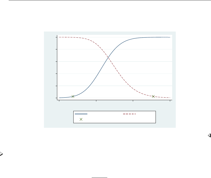
exlogistic — Exact logistic regression 557
The lower and upper confidence bounds are the values of θsuch that Pr(M≥4|θ) = 0.025
and Pr(M≤4|θ) = 0.025, respectively. These probabilities are plotted in the figure below for
θ∈[−2,4].
(3.1, .025)(−1.25, .025)
0 .2 .4 .6 .8 1
cummlative probability
−2 0 2 4
constant term
Pr(M >= 4) Pr(M <= 4)
confidence bounds
Example 4
This example demonstrates the group() option, which allows the analysis of stratified data. Here
the logistic model is
log πik
1−πik =θk+xkiβ
where kindexes the sstrata, k=1, . . . , s, and θkis the strata-specific constant term whose sufficient
statistic is Mk=Pnk
i=1 Yki.
Mehta and Patel (1995) use a case–control study to demonstrate this model, which is useful in
comparing the estimates from exlogistic and clogit. This study was intended to determine the role
of birth complications in people with schizophrenia (Garsd 1988). Siblings from seven families took
part in the study, and each individual was classified as normal or schizophrenic. A birth complication
index is recorded for each individual that ranges from 0, an uncomplicated birth, to 15, a very
complicated birth. Some of the frequencies contained in variable fare greater than 1, and these count
different births at different times where the individual has the same birth complications index, found
in variable BCindex.

558 exlogistic — Exact logistic regression
. use http://www.stata-press.com/data/r13/schizophrenia, clear
(case-control study on birth complications for people with schizophrenia)
. list, sepby(family)
family BCindex schizo f
1. 1 6 0 1
2. 1 7 0 1
3. 1 3 0 2
4. 1 2 0 3
5. 1 5 0 1
6. 1 0 0 1
7. 1 15 1 1
8. 2 2 1 1
9. 2 0 0 1
10. 3 2 0 1
11. 3 9 1 1
12. 3 1 0 1
13. 4 2 1 1
14. 4 0 0 4
15. 5 3 1 1
16. 5 6 0 1
17. 5 0 1 1
18. 6 3 0 1
19. 6 0 1 1
20. 6 0 0 2
21. 7 2 0 1
22. 7 6 1 1
. exlogistic schizo BCindex [fw=f], group(family) test(score) coef
Enumerating sample-space combinations:
observation 1: enumerations = 2
observation 2: enumerations = 3
observation 3: enumerations = 4
observation 4: enumerations = 5
observation 5: enumerations = 6
observation 6: enumerations = 7
(output omitted )
observation 21: enumerations = 72
observation 22: enumerations = 40
Exact logistic regression Number of obs = 29
Group variable: family Number of groups = 7
Obs per group: min = 2
avg = 4.1
max = 10
Model score = 6.32803
Pr >= score = 0.0167
schizo Coef. Score Pr>=Score [95% Conf. Interval]
BCindex .3251178 6.328033 0.0167 .0223423 .7408832

exlogistic — Exact logistic regression 559
The asymptotic alternative for this model can be estimated using clogit (equivalently, xtlogit,
fe) and is listed below for comparison. We must expand the data because clogit will not accept
frequency weights if they are not constant within the groups.
. expand f
(7 observations created)
. clogit schizo BCindex, group(family) nolog
note: multiple positive outcomes within groups encountered.
Conditional (fixed-effects) logistic regression Number of obs = 29
LR chi2(1) = 5.20
Prob > chi2 = 0.0226
Log likelihood = -6.2819819 Pseudo R2 = 0.2927
schizo Coef. Std. Err. z P>|z| [95% Conf. Interval]
BCindex .3251178 .1678981 1.94 0.053 -.0039565 .654192
Both techniques compute the same regression estimate for the BCindex, which might not be too
surprising because both estimation techniques condition on the total number of successes in each group.
The difference lies in the p-values and confidence intervals. The p-value testing H0:βBCindex =0
is approximately 0.0167 for the exact conditional scores test and 0.053 for the asymptotic Wald test.
Moreover, the exact confidence interval is asymmetric about the estimate and does not contain zero.
Technical note
The memory(#)option limits the amount of memory that exlogistic will consume when
computing the conditional distribution of the parameter sufficient statistics. memory() is independent
of the data maximum memory setting (see set max memory in [D]memory), and it is possible
for exlogistic to exceed the memory limit specified in set max memory without terminating.
By default, a log is provided that displays the number of enumerations (the size of the conditional
distribution) after processing each observation. Typically, you will see the number of enumerations
increase, and then at some point they will decrease as the multivariate shift algorithm (Hirji, Mehta,
and Patel 1987) determines that some of the enumerations cannot achieve the observed sufficient
statistics of the conditioning variables. When the algorithm is complete, however, it is necessary
to store the conditional distribution of the parameter sufficient statistics as a dataset. It is possible,
therefore, to get a memory error when the algorithm has completed if there is not enough memory
to store the conditional distribution.
Technical note
Computing the conditional distributions and reported statistics requires data sorting and numerical
comparisons. If there is at least one single-precision variable specified in the model, exlogistic
will make comparisons with a relative precision of 2−5. Otherwise, a relative precision of 2−11 is
used. Be careful if you use recast to promote a single-precision variable to double precision (see
[D]recast). You might try listing the data in full precision (maybe %20.15g; see [D]format) to make
sure that this is really what you want. See [D]data types for information on precision of numeric
storage types.

560 exlogistic — Exact logistic regression
Stored results
exlogistic stores the following in e():
Scalars
e(N) number of observations
e(k groups) number of groups
e(n possible) number of distinct possible outcomes where sum(sufficient) equals observed
e(sufficient)
e(n trials) binomial number-of-trials parameter
e(sum y) sum of depvar
e(k indvars) number of independent variables
e(k terms) number of model terms
e(k condvars) number of conditioning variables
e(condcons) conditioned on the constant(s) indicator
e(midp) mid-p-value rule indicator
e(eps) relative difference tolerance
Macros
e(cmd) exlogistic
e(cmdline) command as typed
e(title) title in estimation output
e(depvar) name of dependent variable
e(indvars) independent variables
e(condvars) conditional variables
e(groupvar) group variable
e(binomial) binomial number-of-trials variable
e(level) confidence level
e(wtype) weight type
e(wexp) weight expression
e(datasignature) the checksum
e(datasignaturevars) variables used in calculation of checksum
e(properties) b
e(estat cmd) program used to implement estat
e(marginsnotok) predictions disallowed by margins
Matrices
e(b) coefficient vector
e(mue indicators) indicator for elements of e(b) estimated using MUE instead of CMLE
e(se) e(b) standard errors (CMLEs only)
e(ci) matrix of e(level) confidence intervals for e(b)
e(sum y groups) sum of e(depvar) for each group
e(N g) number of observations in each group
e(sufficient) sufficient statistics for e(b)
e(p sufficient) p-value for e(sufficient)
e(scoretest) conditional scores tests for indepvars
e(p scoretest) p-values for e(scoretest)
e(probtest) conditional probabilities tests for indepvars
e(p probtest) p-value for e(probtest)
e(scoretest m) conditional scores tests for model terms
e(p scoretest m) p-value for e(scoretest m)
e(probtest m) conditional probabilities tests for model terms
e(p probtest m) p-value for e(probtest m)
Functions
e(sample) marks estimation sample

exlogistic — Exact logistic regression 561
Methods and formulas
Methods and formulas are presented under the following headings:
Sufficient statistics
Conditional distribution and CMLE
Median unbiased estimates and exact CI
Conditional hypothesis tests
Sufficient-statistic p-value
Sufficient statistics
Let {Y1, Y2, . . . , Yn}be a set of nindependent Bernoulli random variables, each of which can
realize two outcomes, {0,1}. For each i=1, . . . , n, we observe Yi=yi, and associated with each
observation is the covariate row vector of length p,xi= (xi1, . . . , xip). Denote β= (β1, . . . , βp)Tto
be the column vector of regression parameters and θto be the constant. The sufficient statistic for βjis
Tj=Pn
i=1 Yixij ,j=1, . . . , p, and for θis M=Pn
i=1 Yi. We observe Tj=tj,tj=Pn
i=1 yixij ,
and M=m,m=Pn
i=1 yi. The probability of observing (Y1=y1, Y2=y2, . . . , Yn=yn)is
Pr(Y1=y1, . . . , Yn=yn|β,X) = exp(mθ +tβ)
Qn
i=1{1 + exp(θ+xiβ)}
where t= (t1, . . . , tp)and X= (xT
1,...,xT
n)T.
The joint distribution of the sufficient statistics Tis obtained by summing over all possible binary
sequences Y1, . . . , Ynsuch that T=tand M=m. This probability function is
Pr(T1=t1, . . . , Tp=tp, M =m|β,X) = c(t, m) exp(mθ +tβ)
Qn
i=1{1 + exp(θ+xiβ)}
where c(t, m)is the combinatorial coefficient of (t, m)or the number of distinct binary sequences
Y1, . . . , Ynsuch that T=tand M=m(Cox and Snell 1989).
Conditional distribution and CMLE
Without loss of generality, we will restrict our discussion to computing the CMLE of β1. If we
condition on observing M=mand T2=t2, . . . , Tp=tp, the probability function of (T1|β1, T2=
t2, . . . , Tp=tp, M =m)is
Pr(T1=t1|β1, T2=t2, . . . , Tp=tp, M =m) = c(t, m)et1β1
Puc(u, t2, . . . , tp, m)euβ1(1)
where the sum in the denominator is over all possible values of T1such that M=mand
T2=t2, . . . , Tp=tpand c(u, t2, . . . , tp, m)is the combinatorial coefficient of (u, t2, . . . , tp, m)
(Cox and Snell 1989). The CMLE for β1is the value b
β1that maximizes the log of (1). This optimization
task is carried out by ml, using the conditional frequency distribution of (T1|T2=t2, . . . , Tp=
tp, M =m)as a dataset. Generating the joint conditional distribution is efficiently computed using
the multivariate shift algorithm described by Hirji, Mehta, and Patel (1987).
Difficulties in computing b
β1arise if the observed (T1=t1, . . . , Tp=tp, M =m)lies on
the boundaries of the distribution of (T1|T2=t2, . . . , Tp=tp, M =m), where the conditional
probability function is monotonically increasing (or decreasing) in β1. Here the CMLE is plus infinity if
it is on the upper boundary, Pr(T1≤t1|T2=t2, . . . , Tp=tp, M =m) = 1, and is minus infinity
if it is on the lower boundary of the distribution, Pr(T1≥t1|T2=t2, . . . , Tp=tp, M =m) = 1.
This concept is demonstrated in example 2. When infinite CMLEs occur, the MUE is computed.

562 exlogistic — Exact logistic regression
Median unbiased estimates and exact CI
The MUE is computed using the technique outlined by Hirji, Tsiatis, and Mehta (1989). First, we
find the values of β(u)
1and β(l)
1such that
Pr(T1≤t1|β1=β(u)
1, T2=t2, . . . , Tp=tp, M =m) =
Pr(T1≥t1|β1=β(l)
1, T2=t2, . . . , Tp=tp, M =m)=1/2(2)
The MUE is then β1=β(l)
1+β(u)
1/2. However, if T1is equal to the minimum of the domain of
the conditional distribution, β(l)does not exist and β1=β(u). If T1is equal to the maximum of the
domain of the conditional distribution, β(u)does not exist and β1=β(l).
Confidence bounds for βare computed similarly, except that we substitute α/2 for 1/2 in (2),
where 1 −αis the confidence level. Here β(l)
1would then be the lower confidence bound and β(u)
1
would be the upper confidence bound (see example 3).
Conditional hypothesis tests
To test H0:β1=0 versus H1:β16=0, we obtain the exact p-value from Pu∈Ef1(u)−f1(t1)/2
if the mid-p-value rule is used and Pu∈Ef1(u)otherwise. Here Eis a critical region, and we define
f1(u) = Pr(T1=u|β1=0, T2=t2, . . . , Tp=tp, M =m)for ease of notation. There are two
popular ways to define the critical region: the conditional probabilities test and the conditional scores
test (Mehta and Patel 1995). The critical region when using the conditional probabilities test is all
values of the sufficient statistic for β1that have a probability less than or equal to that of the observed
t1,Ep={u:f1(u)≤f1(t1)}. The critical region of the conditional scores test is defined as all
values of the sufficient statistic for β1such that its score is greater than or equal to that of t1,
Es=u: (u−µ1)2/σ2
1≥(t1−µ1)2/σ2
1)
Here µ1and σ2
1are the mean and variance of (T1|β1= 0, T2=t2, . . . , Tp=tp, M =m).
The score statistic is defined as
∂`(β)
∂β 2−E∂2`(β)
∂β2−1
evaluated at H0:β=0, where `is the log of (1). The score test simplifies to (t−E[T|β])2/var(T|β)
(Hirji 2006), where the mean and variance are computed from the conditional distribution of the
sufficient statistic with β=0 and tis the observed sufficient statistic.
Sufficient-statistic p-value
The p-value for testing H0:β1=0 versus the two-sided alternative when (T1=t1|T2=
t2, . . . , Tp=tp)is computed as 2×min(pl, pu), where
pl=Pu≤t1c(u, t2, . . . , tp, m)
Puc(u, t2, . . . , tp, m)
pu=Pu≥t1c(u, t2, . . . , tp, m)
Puc(u, t2, . . . , tp, m)
It is the probability of observing a more extreme T1.

exlogistic — Exact logistic regression 563
References
Cox, D. R., and E. J. Snell. 1989. Analysis of Binary Data. 2nd ed. London: Chapman & Hall.
Garsd, A. 1988. Schizophrenia and birth complications. Unpublished manuscript.
Hirji, K. F. 2006. Exact Analysis of Discrete Data. Boca Raton: Chapman & Hall/CRC.
Hirji, K. F., C. R. Mehta, and N. R. Patel. 1987. Computing distributions for exact logistic regression. Journal of the
American Statistical Association 82: 1110–1117.
Hirji, K. F., A. A. Tsiatis, and C. R. Mehta. 1989. Median unbiased estimation for binary data. American Statistician
43: 7–11.
Hutto, C., W. P. Parks, S. Lai, M. T. Mastrucci, C. Mitchell, J. Mu˜
noz, E. Trapido, I. M. Master, and G. B. Scott.
1991. A hospital-based prospective study of perinatal infection with human immunodeficiency virus type 1. Journal
of Pediatrics 118: 347–353.
Mehta, C. R., and N. R. Patel. 1995. Exact logistic regression: Theory and examples. Statistics in Medicine 14:
2143–2160.
Also see
[R]exlogistic postestimation — Postestimation tools for exlogistic
[R]binreg — Generalized linear models: Extensions to the binomial family
[R]clogit — Conditional (fixed-effects) logistic regression
[R]expoisson — Exact Poisson regression
[R]logistic — Logistic regression, reporting odds ratios
[R]logit — Logistic regression, reporting coefficients
[U] 20 Estimation and postestimation commands

Title
exlogistic postestimation — Postestimation tools for exlogistic
Description Syntax for estat Menu for estat Options for estat predict
Option for estat se Remarks and examples Stored results Reference
Also see
Description
The following postestimation commands are of special interest after exlogistic:
Command Description
estat predict single-observation prediction
estat se report ORs or coefficients and their asymptotic standard errors
The following standard postestimation command is also available:
Command Description
estat summarize summary statistics for the estimation sample
estat summarize is not allowed if the binomial() option was specified in exlogistic.
See [R]estat summarize for details.
Special-interest postestimation commands
estat predict computes a predicted probability (or linear predictor), its asymptotic standard
error, and its exact confidence interval for 1 observation. Predictions are carried out by estimating the
constant coefficient after shifting the independent variables and conditioned variables by the values
specified in the at() option or by their medians. Therefore, predictions must be done with the
estimation sample in memory. If a different dataset is used or if the dataset is modified, then an error
will result.
estat se reports odds ratio or coefficients and their asymptotic standard errors. The estimates are
stored in the matrix r(estimates).
564

exlogistic postestimation — Postestimation tools for exlogistic 565
Syntax for estat
Single-observation prediction
estat predict ,options
Report ORs or coefficients and their asymptotic standard errors
estat se , coef
options Description
pr probability; the default
xb linear effect
at(atspec)use the specified values for the indepvars and condvars()
level(#)set confidence level for the predicted value; default is level(95)
memory(#b|k|m|g)set limit on memory usage; default is memory(10m)
nolog do not display the enumeration log
These statistics are available only for the estimation sample.
Menu for estat
Statistics >Postestimation >Reports and statistics
Options for estat predict
pr, the default, calculates the probability.
xb calculates the linear effect.
at(varname =#varname =# . . . )specifies values to use in computing the predicted
value. Here varname is one of the independent variables, indepvars, or the conditioned variables,
condvars(). The default is to use the median of each independent and conditioned variable.
level(#)specifies the confidence level, as a percentage, for confidence intervals. The default is
level(95) or as set by set level; see [U] 20.7 Specifying the width of confidence intervals.
memory(#b|k|m|g)sets a limit on the amount of memory estat predict can use when
generating the conditional distribution of the constant parameter sufficient statistic. The default is
memory(10m), where mstands for megabyte, or 1,048,576 bytes. The following are also available:
bstands for byte; kstands for kilobyte, which is equal to 1,024 bytes; and gstands for gigabyte,
which is equal to 1,024 megabytes. The minimum setting allowed is 1m and the maximum is 512m
or 0.5g, but do not attempt to use more memory than is available on your computer. Also see
Remarks and examples in [R]exlogistic for details on enumerating the conditional distribution.
nolog prevents the display of the enumeration log. By default, the enumeration log is displayed
showing the progress of enumerating the distribution of the observed successes conditioned on the
independent variables shifted by the values specified in at() (or by their medians). See Methods
and formulas in [R]exlogistic for details of the computations.

566 exlogistic postestimation — Postestimation tools for exlogistic
Option for estat se
coef requests that the estimated coefficients and their asymptotic standard errors be reported. The
default is to report the odds ratios and their asymptotic standard errors.
Remarks and examples
Predictions must be done using the estimation sample. This is because the prediction is really an
estimated constant coefficient (the intercept) after shifting the independent variables and conditioned
variables by the values specified in at() or by their medians. The justification for this approach can
be seen by rewriting the model as
log πi
1−πi= (α+x0β)+(xi−x0)β
where x0are the specified values for the indepvars (Mehta and Patel 1995). Because the estimation
of the constant term is required, this technique is not appropriate for stratified models that used the
group() option.
Example 1
To demonstrate, we return to the example 2 in [R]exlogistic using data from a prospective study
of perinatal infection and HIV-1. Here there was an investigation into whether the blood serum levels
of CD4 and CD8 measured in infants at 6 months of age might predict their development of HIV
infection. The blood serum levels are coded as ordinal values 0, 1, and 2. These data are used by
Mehta and Patel (1995) as an exposition of exact logistic.
. use http://www.stata-press.com/data/r13/hiv_n
(prospective study of perinatal infection of HIV-1; binomial form)
. generate byte cd4_0 = (cd4==0)
. generate byte cd4_1 = (cd4==1)
. generate byte cd8_0 = (cd8==0)
. generate byte cd8_1 = (cd8==1)
. exlogistic hiv cd4_0 cd4_1 cd8_0 cd8_1, terms(cd4=cd4_0 cd4_1,
> cd8=cd8_0 cd8_1) binomial(n) test(probability) saving(dist)
(output omitted )

exlogistic postestimation — Postestimation tools for exlogistic 567
. estat predict
Enumerating sample-space combinations:
observation 1: enumerations = 3
observation 2: enumerations = 12
observation 3: enumerations = 5
observation 4: enumerations = 5
observation 5: enumerations = 5
observation 6: enumerations = 35
observation 7: enumerations = 15
observation 8: enumerations = 15
observation 9: enumerations = 9
observation 10: enumerations = 9
observation 11: enumerations = 5
observation 12: enumerations = 18
note: CMLE estimate for _cons is -inf; computing MUE
Predicted value at cd4_0 = 0, cd4_1 = 0, cd8_0 = 0, cd8_1 = 1
hiv Predicted Std. Err. [95% Conf. Interval]
Probability 0.0390* N/A 0.0000 0.1962
(*) identifies median unbiased estimates (MUE); because an MUE
is computed, there is no SE estimate
Because we did not specify values by using the at() option, the median values of the indepvars
are used for the prediction. By default, medians are used instead of means because we want to use
values that are observed in the dataset. If the means of the binary variables cd4 0–cd8 1 were
used, we would have created floating point variables in (0,1) that not only do not properly represent
the indicator variables but also would be a source of computational inefficiency in generating the
conditional distribution. Because the MUE is computed for the predicted value, there is no standard-error
estimate.
From the example discussions in [R]exlogistic, the infants at highest risk are those with a CD4
level of 0 and a CD8 level of 2. Below we use the at() option to make a prediction at these blood
serum levels.
. estat predict, at(cd4_0=1 cd4_1=0 cd8_0=0 cd8_1=0) nolog
note: CMLE estimate for _cons is +inf; computing MUE
Predicted value at cd4_0 = 1, cd4_1 = 0, cd8_0 = 0, cd8_1 = 0
hiv Predicted Std. Err. [95% Conf. Interval]
Probability 0.9063* N/A 0.4637 1.0000
(*) identifies median unbiased estimates (MUE); because an MUE
is computed, there is no SE estimate

568 exlogistic postestimation — Postestimation tools for exlogistic
Stored results
estat predict stores the following in r():
Scalars
r(imue) 1 if r(pred) is an MUE and 0if a CMLE
r(pred) estimated probability or the linear effect
r(se) asymptotic standard error of r(pred)
Macros
r(estimate) prediction type: pr or xb
r(level) confidence level
Matrices
r(ci) confidence interval
r(x) indepvars and condvars() values
Reference
Mehta, C. R., and N. R. Patel. 1995. Exact logistic regression: Theory and examples. Statistics in Medicine 14:
2143–2160.
Also see
[R]exlogistic — Exact logistic regression
[U] 20 Estimation and postestimation commands

Title
expoisson — Exact Poisson regression
Syntax Menu Description Options
Remarks and examples Stored results Methods and formulas References
Also see
Syntax
expoisson depvar indepvars if in weight ,options
options Description
Model
condvars(varlist)condition on variables in varlist
group(varname)groups/strata are stratified by unique values of varname
exposure(varnamee)include ln(varnamee) in model with coefficient constrained to 1
offset(varnameo)include varnameoin model with coefficient constrained to 1
Options
memory(#b|k|m|g)set limit on memory usage; default is memory(25m)
saving(filename)save the joint conditional distribution to filename
Reporting
level(#)set confidence level; default is level(95)
irr report incidence-rate ratios
test(testopt)report significance of observed sufficient statistic, conditional scores test,
or conditional probabilities test
mue(varlist)compute the median unbiased estimates for varlist
midp use the mid-p-value rule
nolog do not display the enumeration log
by,statsby, and xi are allowed; see [U] 11.1.10 Prefix commands.
fweights are allowed; see [U] 11.1.6 weight.
See [U] 20 Estimation and postestimation commands for more capabilities of estimation commands.
Menu
Statistics >Exact statistics >Exact Poisson regression
Description
expoisson fits an exact Poisson regression model of depvar on indepvars. Exact Poisson regression
is an alternative to standard maximum-likelihood–based Poisson regression (see [R]poisson) that
offers more accurate inference in small samples because it does not depend on asymptotic results.
For stratified data, expoisson is an alternative to fixed-effects Poisson regression (see xtpoisson,
fe in [XT]xtpoisson); like fixed-effects Poisson regression, exact Poisson regression conditions on
the number of events in each stratum.
569

570 expoisson — Exact Poisson regression
Exact Poisson regression is computationally intensive, so if you have regressors whose parameter
estimates are not of interest (that is, nuisance parameters), you should specify those variables in the
condvars() option instead of in indepvars.
Options
Model
condvars(varlist)specifies variables whose parameter estimates are not of interest to you. You
can save substantial computer time and memory by moving such variables from indepvars to
condvars(). Understand that you will get the same results for x1 and x3 whether you type
. expoisson y x1 x2 x3 x4
or
. expoisson y x1 x3, condvars(x2 x4)
group(varname)specifies the variable defining the strata, if any. A constant term is assumed for
each stratum identified in varname, and the sufficient statistics for indepvars are conditioned on
the observed number of successes within each group (as well as other variables in the model).
The group variable must be integer valued.
exposure(varnamee),offset(varnameo); see [R]estimation options.
Options
memory(#b|k|m|g)sets a limit on the amount of memory expoisson can use when computing
the conditional distribution of the parameter sufficient statistics. The default is memory(25m),
where mstands for megabyte, or 1,048,576 bytes. The following are also available: bstands for
byte; kstands for kilobyte, which is equal to 1,024 bytes; and gstands for gigabyte, which is
equal to 1,024 megabytes. The minimum setting allowed is 1m and the maximum is 2048m or
2g, but do not attempt to use more memory than is available on your computer. Also see the first
technical note under example 3 on counting the conditional distribution.
saving(filename , replace )saves the joint conditional distribution for each independent variable
specified in indepvars. There is one file for each variable, and it is named using the prefix filename
with the variable name appended. For example, saving(mydata) with an independent variable
named Xwould generate a data file named mydata X.dta. Use replace to replace an existing
file. Each file contains the conditional distribution for one of the independent variables specified in
indepvars conditioned on all other indepvars and those variables specified in condvars(). There
are two variables in each data file: the feasible sufficient statistics for the variable’s parameter and
their associated weights. The weights variable is named w.
Reporting
level(#); see [R]estimation options. The level(#)option will not work on replay because
confidence intervals are based on estimator-specific enumerations. To change the confidence level,
you must refit the model.
irr reports estimated coefficients transformed to incidence-rate ratios, that is, exp(β)rather than β.
Standard errors and confidence intervals are similarly transformed. This option affects how results
are displayed, not how they are estimated or stored. irr may be specified at estimation or when
replaying previously estimated results.
test(sufficient |score |probability) reports the significance level of the observed suffi-
cient statistic, the conditional scores test, or the conditional probabilities test. The default is
test(sufficient). All the statistics are computed at estimation time, and each statistic may be
displayed postestimation; see [R]expoisson postestimation.

expoisson — Exact Poisson regression 571
mue(varlist)specifies that median unbiased estimates (MUEs) be reported for the variables in varlist.
By default, the conditional maximum likelihood estimates (CMLEs) are reported, except for those
parameters for which the CMLEs are infinite. Specify mue( all) if you want MUEs for all the
indepvars.
midp instructs expoisson to use the mid-p-value rule when computing the MUEs, significance levels,
and confidence intervals. This adjustment is for the discreteness of the distribution by halving
the value of the discrete probability of the observed statistic before adding it to the p-value. The
mid-p-value rule cannot be MUEs whose corresponding parameter CMLE is infinite.
nolog prevents the display of the enumeration log. By default, the enumeration log is displayed,
showing the progress of computing the conditional distribution of the sufficient statistics.
Remarks and examples
Exact Poisson regression estimates the model parameters by using the conditional distributions
of the parameters’ sufficient statistics, and the resulting parameter estimates are known as CMLEs.
Exact Poisson regression is a small-sample alternative to the maximum-likelihood ML Poisson model.
See [R]poisson and [XT]xtpoisson to obtain maximum likelihood estimates (MLEs) for the Poisson
model and the fixed-effects Poisson model.
Let Yidenote a Poisson random variable where we observe the outcome Yi=yi,i=1, . . . , n.
Associated with each independent observation is a 1 ×pvector of covariates, xi. We will denote
µi=E[Yi|xi]and use the log linear model to model the relationship between Yiand xi,
log (µi) = θ+xiβ
where the constant term, θ, and the p×1 vector of regression parameters, β, are unknown. The
probability of observing Yi=yi,i= 1, . . . , n, is
Pr(Y=y) =
n
Y
i=1
µyi
ie−µi
yi!
where Y= (Y1, . . . , Yn)and y= (y1, . . . , yn). The MLEs for θand βmaximize the log of this
function.
The sufficient statistics for θand βj,j=1, . . . , p, are M=Pn
i=1 Yiand Tj=Pn
i=1 Yixij ,
respectively, and we observe M=mand Tj=tj.expoisson tallies the conditional distribution
for each Tj, given the other sufficient statistics Tl=tl,l6=jand M=m. Denote one of these
values to be t(k)
j,k= 1, . . . , N, with weight wkthat accounts for all the generated Yvectors that
give rise to t(k)
j. The conditional probability of observing Tj=tjhas the form
Pr(Tj=tj|Tl=tl, l 6=j, M =m) = w etjβj
Pkwket(k)
jβj
(1)
where the sum is over the subset of Tvectors such that (T(k)
1=t1, . . . , T (k)
j=t(k)
j, . . . , T (k)
p=tp)
and wis the weight associated with the observed t. The CMLE for βjmaximizes the log of this
function.
Specifying nuisance variables in condvars() prevents expoisson from estimating their associated
regression coefficients. These variables are still conditional variables when tallying the conditional
distribution for the variables in indepvars.

572 expoisson — Exact Poisson regression
Inferences from MLEs rely on asymptotics, and if your sample size is small, these inferences may
not be valid. On the other hand, inferences from the CMLEs are exact in that they use the conditional
distribution of the sufficient statistics outlined above.
For small datasets, the dependent variable can be completely determined by the data. Here the MLEs
and the CMLEs are unbounded. When this occurs, expoisson will compute the MUE, the regression
estimate that places the observed sufficient statistic at the median of the conditional distribution.
See [R]exlogistic for a more thorough discussion of exact estimation and related statistics.
Example 1
Armitage, Berry, and Matthews (2002, 499–501) fit a log-linear model to data containing the
number of cerebrovascular accidents experienced by 41 men during a fixed period, each of whom
had recovered from a previous cerebrovascular accident and was hypertensive. Sixteen men received
treatment, and in the original data, there are three age groups (40–49, 50–59, ≥60), but we pool the
first two age groups to simplify the example. Armitage, Berry, and Matthews point out that this was
not a controlled trial, but the data are useful to inquire whether there is evidence of fewer accidents
for the treatment group and if age may be an important factor. The dependent variable count contains
the number of accidents, variable treat is an indicator for the treatment group (1 =treatment, 0 =
control), and variable age is an indicator for the age group (0 =40−59; 1 =≥60).
First, we load the data, list it, and tabulate the cerebrovascular accident counts by treatment and
age group.
. use http://www.stata-press.com/data/r13/cerebacc
(cerebrovascular accidents in hypotensive-treated and control groups)
. list
treat count age
1. control 0 40/59
2. control 0 >=60
3. control 1 40/59
4. control 1 >=60
5. control 2 40/59
6. control 2 >=60
7. control 3 40/59
(output omitted )
35. treatment 0 40/59
36. treatment 0 40/59
37. treatment 0 40/59
38. treatment 0 40/59
39. treatment 1 40/59
40. treatment 1 40/59
41. treatment 1 40/59
. tabulate treat age [fw=count]
hypotensiv
e drug age group
treatment 40/59 >=60 Total
control 15 10 25
treatment 4 0 4
Total 19 10 29

expoisson — Exact Poisson regression 573
Next we estimate the CMLE with expoisson and, for comparison, the MLE with poisson.
. expoisson count treat age
Estimating: treat
Enumerating sample-space combinations:
observation 1: enumerations = 11
observation 2: enumerations = 11
observation 3: enumerations = 11
(output omitted )
observation 39: enumerations = 410
observation 40: enumerations = 410
observation 41: enumerations = 30
Estimating: age
Enumerating sample-space combinations:
observation 1: enumerations = 5
observation 2: enumerations = 15
observation 3: enumerations = 15
(output omitted )
observation 39: enumerations = 455
observation 40: enumerations = 455
observation 41: enumerations = 30
Exact Poisson regression
Number of obs = 41
count Coef. Suff. 2*Pr(Suff.) [95% Conf. Interval]
treat -1.594306 4 0.0026 -3.005089 -.4701708
age -.5112067 10 0.2794 -1.416179 .3429232
. poisson count treat age, nolog
Poisson regression Number of obs = 41
LR chi2(2) = 10.64
Prob > chi2 = 0.0049
Log likelihood = -38.97981 Pseudo R2 = 0.1201
count Coef. Std. Err. z P>|z| [95% Conf. Interval]
treat -1.594306 .5573614 -2.86 0.004 -2.686714 -.5018975
age -.5112067 .4043525 -1.26 0.206 -1.303723 .2813096
_cons .233344 .2556594 0.91 0.361 -.2677391 .7344271
expoisson generates an enumeration log for each independent variable in indepvars. The con-
ditional distribution of the parameter sufficient statistic is tallied for each independent variable. The
conditional distribution for treat, for example, has 30 records containing the weights, wk, and
feasible sufficient statistics, t(k)
treat. In essence, the set of points (wk, t(k)
treat),k=1,...,30, tallied by
expoisson now become the data to estimate the regression coefficient for treat, using (1) as the
likelihood. Remember that one of the 30 (wk, t(k)
treat)must contain the observed sufficient statistic,
ttreat =P41
i=1 treati×counti=4, and its relative position in the sorted set of points (sorted by
t(k)
treat) is how the sufficient-statistic significance is computed. This algorithm is repeated for the age
variable.
The regression coefficients for treat and age are numerically identical for both Poisson models.
Both models indicate that the treatment is significant at reducing the rate of cerebrovascular accidents,
≈e−1.59 ≈0.204, or a reduction of about 80%. There is no significant age effect.

574 expoisson — Exact Poisson regression
The p-value for the treatment regression-coefficient sufficient statistic indicates that the treatment
effect is a bit more significant than for the corresponding asymptotic Zstatistic from poisson.
However, the exact confidence intervals are wider than their asymptotic counterparts.
Example 2
Agresti (2013, 129) used the data from Laird and Olivier (1981) to demonstrate the Poisson model
for modeling rates. The data consist of patient survival after heart valve replacement operations. The
sample consists of 109 patients that are classified by type of heart valve (aortic, mitral) and by age
(<55, ≥55). Follow-up observations cover lengths from 3 to 97 months, and the time at risk, or
exposure, is stored in the variable TAR. The response is whether the subject died. First, we take a
look at the data and then estimate the incidence rates (IRs) with expoisson and poisson.
. use http://www.stata-press.com/data/r13/heartvalve
(heart valve replacement data)
. list
age valve deaths TAR
1. < 55 aortic 4 1259
2. < 55 mitral 1 2082
3. >= 55 aortic 7 1417
4. >= 55 mitral 9 1647
The age variable is coded 0 for age <55 and 1 for age ≥55, and the valve variable is coded 0 for
the aortic valve and 1 for the mitral valve. The total number of deaths, M=21, is small enough that
enumerating the conditional distributions for age and valve type is feasible and asymptotic inferences
associated with standard ML Poisson regression may be questionable.
. expoisson deaths age valve, exposure(TAR) irr
Estimating: age
Enumerating sample-space combinations:
observation 1: enumerations = 11
observation 2: enumerations = 11
observation 3: enumerations = 132
observation 4: enumerations = 22
Estimating: valve
Enumerating sample-space combinations:
observation 1: enumerations = 17
observation 2: enumerations = 17
observation 3: enumerations = 102
observation 4: enumerations = 22
Exact Poisson regression
Number of obs = 4
deaths IRR Suff. 2*Pr(Suff.) [95% Conf. Interval]
age 3.390401 16 0.0194 1.182297 11.86935
valve .7190197 10 0.5889 .2729881 1.870068
ln(TAR) 1 (exposure)

expoisson — Exact Poisson regression 575
. poisson deaths age valve, exposure(TAR) irr nolog
Poisson regression Number of obs = 4
LR chi2(2) = 7.62
Prob > chi2 = 0.0222
Log likelihood = -8.1747285 Pseudo R2 = 0.3178
deaths IRR Std. Err. z P>|z| [95% Conf. Interval]
age 3.390401 1.741967 2.38 0.017 1.238537 9.280965
valve .7190197 .3150492 -0.75 0.452 .3046311 1.6971
_cons .0018142 .0009191 -12.46 0.000 .0006722 .0048968
ln(TAR) 1 (exposure)
The CMLE and the MLE are numerically identical. The death rate for the older age group is about
3.4 times higher than the younger age group, and this difference is significant at the 5% level. This
means that for every death in the younger group each month, we would expect about three deaths
in the older group. The IR estimate for valve type is approximately 0.72, but it is not significantly
different from one. The exact Poisson confidence intervals are a bit wider than the asymptotic CIs.
You can use ir (see [ST]epitab) to estimate IRs and exact CIs for one covariate, and we compare
these CIs with those from expoisson, where we estimate the incidence rate by using age only.
. ir deaths age TAR
age of patient
Exposed Unexposed Total
number of deaths 16 5 21
time at risk 3064 3341 6405
Incidence rate .0052219 .0014966 .0032787
Point estimate [95% Conf. Interval]
Inc. rate diff. .0037254 .00085 .0066007
Inc. rate ratio 3.489295 1.221441 12.17875 (exact)
Attr. frac. ex. .7134092 .1812948 .9178898 (exact)
Attr. frac. pop .5435498
(midp) Pr(k>=16) = 0.0049 (exact)
(midp) 2*Pr(k>=16) = 0.0099 (exact)
. expoisson deaths age, exposure(TAR) irr midp nolog
Exact Poisson regression
Number of obs = 4
deaths IRR Suff. 2*Pr(Suff.) [95% Conf. Interval]
age 3.489295 16 0.0099 1.324926 10.64922
ln(TAR) 1 (exposure)
mid-p-value computed for the probabilities and CIs
Both ir and expoisson give identical IRs and p-values. Both report the two-sided exact significance
by using the mid-p-value rule that accounts for the discreteness in the distribution by subtracting p1/2=
Pr(T=t)/2 from pl= Pr(T≤t)and pg= Pr(T≥t), computing 2 ×min(pl−p1/2, pg−p1/2).
By default, expoisson will not use the mid-p-value rule (when you exclude the midp option), and
here the two-sided exact significance would be 2 ×min(pl, pg) = 0.0158. The confidence intervals
differ because expoisson uses the mid-p-value rule when computing the confidence intervals, yet

576 expoisson — Exact Poisson regression
ir does not. You can verify this by executing expoisson without the midp option for this example;
you will get the same CIs as ir.
You can replay expoisson to view the conditional scores test or the conditional probabilities test
by using the test() option.
. expoisson, test(score) irr
Exact Poisson regression
Number of obs = 4
deaths IRR Score Pr>=Score [95% Conf. Interval]
age 3.489295 6.76528 0.0113 1.324926 10.64922
ln(TAR) 1 (exposure)
mid-p-value computed for the probabilities and CIs
All the statistics for expoisson are defined in Methods and formulas of [R]exlogistic. Apart
from enumerating the conditional distributions for the logistic and Poisson sufficient statistics, com-
putationally, the primary difference between exlogistic and expoisson is the weighting values in
the likelihood for the parameter sufficient statistics.
Example 3
In this example, we fabricate data that will demonstrate the difference between the CMLE and
the MUE when the CMLE is not infinite. A difference in these estimates will be more pronounced
when the probability of the coefficient sufficient statistic is skewed when plotted as a function of the
regression coefficient.
. clear
. input y x
y x
1. 0 2
2. 1 1
3. 1 0
4. 0 0
5. 0 .5
6. 1 .5
7. 2 .01
8. 3 .001
9. 4 .0001
10. end
. expoisson y x, test(score)
Enumerating sample-space combinations:
observation 1: enumerations = 13
observation 2: enumerations = 91
observation 3: enumerations = 169
observation 4: enumerations = 169
observation 5: enumerations = 313
observation 6: enumerations = 313
observation 7: enumerations = 1469
observation 8: enumerations = 5525
observation 9: enumerations = 5479
Exact Poisson regression
Number of obs = 9
y Coef. Score Pr>=Score [95% Conf. Interval]
x -1.534468 2.955316 0.0810 -3.761718 .0485548
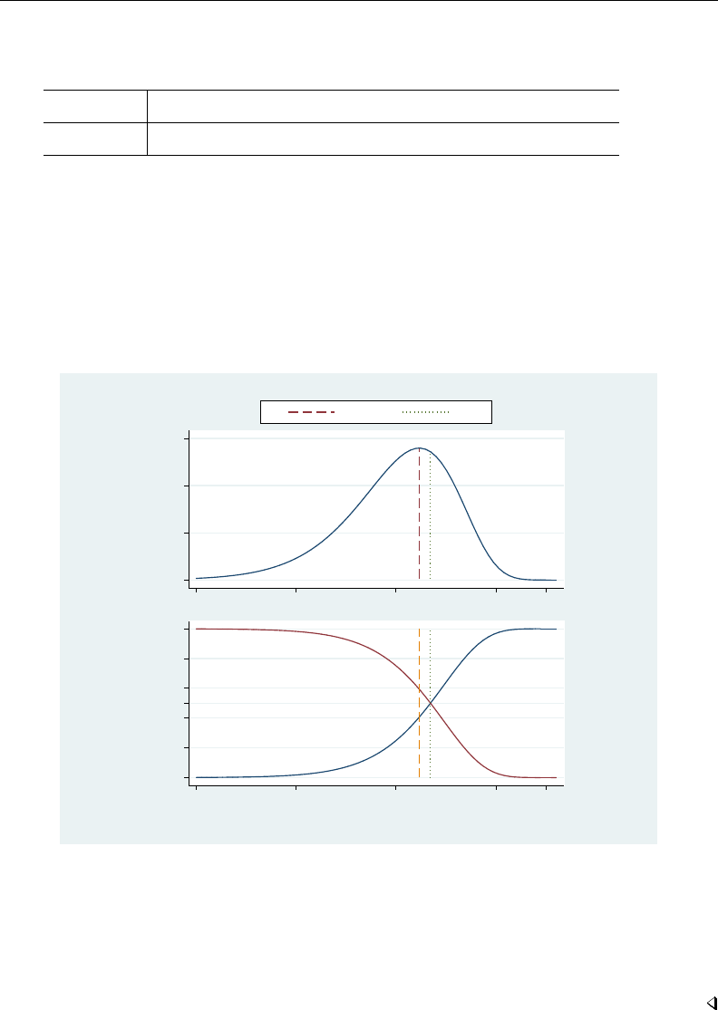
expoisson — Exact Poisson regression 577
. expoisson y x, test(score) mue(x) nolog
Exact Poisson regression
Number of obs = 9
y Coef. Score Pr>=Score [95% Conf. Interval]
x -1.309268* 2.955316 0.0810 -3.761718 .0485548
(*) median unbiased estimates (MUE)
We observe (xi, yi),i=1,...,9. If we condition on m=P9
i=1 yi=12, the conditional
distribution of Tx=PiYixihas a size of 5,479 elements. For each entry in this enumeration,
a realization of Yi=y(k)
i,k=1,...,5,479, is generated such that Piy(k)
i=12. One of these
realizations produces the observed tx=Piyixi≈1.5234.
Below is a graphical display comparing the CMLE with the MUE. We plot Pr(Tx=tx|M=12, βx)
versus βx,−6≤βx≤1, in the upper panel and the cumulative probabilities, Pr(Tx≤tx|M=
12, βx)and Pr(Tx≥tx|M=12, βx), in the lower panel.
0 .0001 .0002 .0003
probability
CMLE MUE
0 .2 .4 .5 .6 .8 1
cumulative probability
−6 −4 −2 0 1
x coefficient
The location of the CMLE, indicated by the dashed line, is at the mode of the probability profile, and
the MUE, indicated by the dotted line, is to the right of the mode. If we solve for the β(u)
xand β(l)
x
such that Pr(Tx≤tx|M=12, β(u)
x) = 1/2 and Pr(Tx≥tx|M=12, β(l)
x) = 1/2, the MUE is
(β(u)
x+β(l)
x)/2. As you can see in the lower panel, the MUE cuts through the intersection of these
cumulative probability profiles.

578 expoisson — Exact Poisson regression
Technical note
The memory(#)option limits the amount of memory that expoisson will consume when computing
the conditional distribution of the parameter sufficient statistics. memory() is independent of the data
maximum memory setting (see set max memory in [D]memory), and it is possible for expoisson
to exceed the memory limit specified in set max memory without terminating. By default, a log
is provided that displays the number of enumerations (the size of the conditional distribution)
after processing each observation. Typically, you will see the number of enumerations increase,
and then at some point they will decrease as the multivariate shift algorithm (Hirji, Mehta, and
Patel 1987) determines that some of the enumerations cannot achieve the observed sufficient statistics
of the conditioning variables. When the algorithm is complete, however, it is necessary to store the
conditional distribution of the parameter sufficient statistics as a dataset. It is possible, therefore, to
get a memory error when the algorithm has completed if there is not enough memory to store the
conditional distribution.
Technical note
Computing the conditional distributions and reported statistics requires data sorting and numerical
comparisons. If there is at least one single-precision variable specified in the model, expoisson
will make comparisons with a relative precision of 2−5. Otherwise, a relative precision of 2−11 is
used. Be careful if you use recast to promote a single-precision variable to double precision (see
[D]recast). You might try listing the data in full precision (maybe %20.15g; see [D]format) to make
sure that this is really what you want. See [D]data types for information on precision of numeric
storage types.
Stored results
expoisson stores the following in e():
Scalars
e(N) number of observations
e(k groups) number of groups
e(relative weight) relative weight for the observed e(sufficient) and e(condvars)
e(sum y) sum of depvar
e(k indvars) number of independent variables
e(k condvars) number of conditioning variables
e(midp) mid-p-value rule indicator
e(eps) relative difference tolerance
Macros
e(cmd) expoisson
e(cmdline) command as typed
e(title) title in estimation output
e(depvar) name of dependent variable
e(indvars) independent variables
e(condvars) conditional variables
e(groupvar) group variable
e(exposure) exposure variable
e(offset) linear offset variable
e(level) confidence level
e(wtype) weight type
e(wexp) weight expression
e(datasignature) the checksum
e(datasignaturevars) variables used in calculation of checksum
e(properties) b V
e(estat cmd) program used to implement estat
e(marginsnotok) predictions disallowed by margins

expoisson — Exact Poisson regression 579
Matrices
e(b) coefficient vector
e(mue indicators) indicator for elements of e(b) estimated using MUE instead of CMLE
e(se) e(b) standard errors (CMLEs only)
e(ci) matrix of e(level) confidence intervals for e(b)
e(sum y groups) sum of e(depvar) for each group
e(N g) number of observations in each group
e(sufficient) sufficient statistics for e(b)
e(p sufficient) p-value for e(sufficient)
e(scoretest) conditional scores tests for indepvars
e(p scoretest) p-values for e(scoretest)
e(probtest) conditional probability tests for indepvars
e(p probtest) p-value for e(probtest)
Functions
e(sample) marks estimation sample
Methods and formulas
Let {Y1, Y2, . . . , Yn}be a set of nindependent Poisson random variables. For each i=1, . . . , n,
we observe Yi=yi≥0, and associated with each observation is the covariate row vector of length
p,xi= (xi1, . . . , xip). Denote β= (β1, . . . , βp)Tto be the column vector of regression parameters
and θto be the constant. The sufficient statistic for βjis Tj=Pn
i=1 Yixij ,j=1, . . . , p, and for θis
M=Pn
i=1 Yi. We observe Tj=tj,tj=Pn
i=1 yixij , and M=m,m=Pn
i=1 yi. Let κibe the
exposure for the ith observation. Then the probability of observing (Y1=y1, Y2=y2, . . . , Yn=yn)
is
Pr(Y1=y1, . . . , Yn=yn|β,X,κ) = exp(mθ +tβ)
exp{Pn
i=1 κiexp(θ+xiβ)}
n
Y
i=1
κyi
i
yi!
where t= (t1, . . . , tp),X= (xT
1,...,xT
n)T, and κ= (κ1, . . . , κn)T.
The joint distribution of the sufficient statistics (T, M )is obtained by summing over all possible
sequences Y1≥0, . . . , Yn≥0such that T=tand M=m. This probability function is
Pr(T1=t1, . . . , Tp=tp, M =m|β,X,κ) = exp(mθ +tβ)
exp {Pn
i=1 κiexp(θ+xiβ)} X
u
n
Y
i=1
κui
i
ui!!
where the sum Puis over all nonnegative vectors uof length nsuch that Pn
i=1 ui=mand
Pn
i=1 uixi=t.
Conditional distribution
Without loss of generality, we will restrict our discussion to the conditional distribution of the
sufficient statistic for β1,T1. If we condition on observing M=mand T2=t2, . . . , Tp=tp, the
probability function of (T1|β1, T2=t2, . . . , Tp=tp, M =m)is
Pr(T1=t1|β1, T2=t2, . . . , Tp=tp, M =m) = PuQn
i=1
κui
i
ui!et1β1
PvQn
i=1
κvi
i
vi!eβ1Pivixi1
(2)

580 expoisson — Exact Poisson regression
where the sum Puis over all nonnegative vectors uof length nsuch that Pn
i=1 ui=mand
Pn
i=1 uixi=t, and the sum Pvis over all nonnegative vectors vof length nsuch that Pn
i=1 vi=m,
Pn
i=1 vixi2=t2,. . . ,Pn
i=1 vixip =tp. The CMLE for β1is the value that maximizes the log of
(1). This optimization task is carried out by ml (see [R]ml), using the conditional distribution of
(T1|T2=t2, . . . , Tp=tp, M =m)as a dataset. This dataset consists of the feasible values and
weights for T1,
( s1,
n
Y
i=1
κvi
i
vi!!:
n
X
i=1
vi=m,
n
X
i=1
vixi1=s1,
n
X
i=1
vixi2=t2,...,
n
X
i=1
vixip =tp)
Computing the CMLE,MUE, confidence intervals, conditional hypothesis tests, and sufficient statistic
p-values is discussed in Methods and formulas of [R]exlogistic. The only difference between the
two techniques is the use of the weights; that is, the weights for exact logistic are the combinatorial
coefficients, c(t, m), in (1) of Methods and formulas in [R]exlogistic.expoisson and exlogistic
use the same ml likelihood evaluator to compute the CMLEs as well as the same ado-programs and
Mata functions to compute the MUEs and estimate statistics.
References
Agresti, A. 2013. Categorical Data Analysis. 3rd ed. Hoboken, NJ: Wiley.
Armitage, P., G. Berry, and J. N. S. Matthews. 2002. Statistical Methods in Medical Research. 4th ed. Oxford:
Blackwell.
Cox, D. R., and E. J. Snell. 1989. Analysis of Binary Data. 2nd ed. London: Chapman & Hall.
Hirji, K. F., C. R. Mehta, and N. R. Patel. 1987. Computing distributions for exact logistic regression. Journal of the
American Statistical Association 82: 1110–1117.
Laird, N. M., and D. Olivier. 1981. Covariance analysis of censored survival data using log-linear analysis techniques.
Journal of the American Statistical Association 76: 231–240.
Also see
[R]expoisson postestimation — Postestimation tools for expoisson
[R]poisson — Poisson regression
[XT]xtpoisson — Fixed-effects, random-effects, and population-averaged Poisson models
[U] 20 Estimation and postestimation commands

Title
expoisson postestimation — Postestimation tools for expoisson
Description Syntax for estat se Menu for estat Option for estat se
Remarks and examples Also see
Description
The following postestimation command is of special interest after expoisson:
Command Description
estat se report coefficients or IRRs and their asymptotic standard errors
The following standard postestimation command is also available:
Command Description
estat summarize summary statistics for the estimation sample
See [R]estat summarize for details.
Special-interest postestimation command
estat se reports regression coefficients or incidence-rate asymptotic standard errors. The estimates
are stored in the matrix r(estimates).
Syntax for estat se
estat se , irr
Menu for estat
Statistics >Postestimation >Reports and statistics
Option for estat se
irr requests that the incidence-rate ratios and their asymptotic standard errors be reported. The default
is to report the coefficients and their asymptotic standard errors.
581

582 expoisson postestimation — Postestimation tools for expoisson
Remarks and examples
Example 1
To demonstrate estat se after expoisson, we use the British physicians smoking data.
. use http://www.stata-press.com/data/r13/smokes
(cigarette smoking and lung cancer among British physicians (45-49 years))
. expoisson cases smokes, exposure(peryrs) irr nolog
Exact Poisson regression
Number of obs = 7
cases IRR Suff. 2*Pr(Suff.) [95% Conf. Interval]
smokes 1.077718 797.4 0.0000 1.04552 1.111866
ln(peryrs) 1 (exposure)
. estat se, irr
cases IRR Std. Err.
smokes 1.077718 .0168547
Also see
[R]expoisson — Exact Poisson regression
[U] 20 Estimation and postestimation commands

Title
fp — Fractional polynomial regression
Syntax Menu Description
Options for fp Options for fp generate Remarks and examples
Stored results Methods and formulas Acknowledgment
References Also see
Syntax
Estimation
fp <term>,est options :est cmd
est cmd may be almost any estimation command that stores the e(ll) result. To confirm
whether fp works with a specific est cmd, see the documentation for that est cmd.
Instances of <term>(with the angle brackets) that occur within est cmd are replaced in
est cmd by a varlist containing the fractional powers of the variable term. These variables
will be named term 1,term 2,. . . .
fp performs est cmd with this substitution, fitting a fractional polynomial regression in term.
est cmd in either this or the following syntax may not contain other prefix commands; see
[U] 11.1.10 Prefix commands.
Estimation (alternate syntax)
fp <term>(varname),est options :est cmd
Use this syntax to specify that fractional powers of varname are to be calculated. The
fractional polynomial power variables will still be named term 1,term 2,. . . .
Replay estimation results
fp ,replay options
Create specified fractional polynomial power variables
fp generate type newvar =varname^(numlist)if in ,gen options
583

584 fp — Fractional polynomial regression
est options Description
Main
Search
powers(# # . . . #)powers to be searched; default is powers(-2 -1 -.5 0 .5 1 2 3)
dimension(#)maximum degree of fractional polynomial; default is dimension(2)
Or specify
fp(# # . . . #)use specified fractional polynomial
And then specify any of these options
Options
classic perform automatic scaling and centering and omit comparison table
replace replace existing fractional polynomial power variables named
term 1,term 2,. . .
all generate term 1,term 2,. . . in all observations; default is in
observations if esample()
scale(# a # b)use (term+a)/b; default is to use variable term as is
scale specify aand bautomatically
center(# c)report centered-on-cresults; default is uncentered results
center specify cto be the mean of (scaled) term
zero set term 1,term 2,. . . to zero if scaled term ≤0; default is to issue
an error message
catzero same as zero and include term 0= (term ≤0) among
fractional polynomial power variables
Reporting
replay options specify how results are displayed
replay options Description
Reporting
nocompare do not display model-comparison test results
reporting options any options allowed by est cmd for replaying estimation results
gen options Description
Main
replace replace existing fractional polynomial power variables named
term 1,term 2,. . .
scale(# a # b)use (term+a)/b; default is to use variable term as is
scale specify aand bautomatically
center(# c)report centered-on-cresults; default is uncentered results
center specify cto be the mean of (scaled) term
zero set term 1,term 2,. . . to zero if scaled term ≤0; default is to issue
an error message
catzero same as zero and include term 0= (term ≤0) among
fractional polynomial power variables

fp — Fractional polynomial regression 585
Menu
fp
Statistics >Linear models and related >Fractional polynomials >Fractional polynomial regression
fp generate
Statistics >Linear models and related >Fractional polynomials >Create fractional polynomial variables
Description
fp <term>: est cmd fits models with the “best”-fitting fractional polynomial substituted for
<term>wherever it appears in est cmd.fp <weight>: regress mpg <weight> foreign would fit
a regression model of mpg on a fractional polynomial in weight and (linear) foreign.
By specifying option fp(), you may set the exact powers to be used. Otherwise, a search through
all possible fractional polynomials up to the degree set by dimension() with the powers set by
powers() is performed.
fp without arguments redisplays the previous estimation results, just as typing est cmd would.
You can type either one. fp will include a fractional polynomial comparison table.
fp generate creates fractional polynomial power variables for a given set of powers. For
instance, fp <weight>: regress mpg <weight> foreign might produce the fractional polynomial
weight(−2,−1) and store weight−2in weight 1and weight−1in weight 2. Typing fp generate
weight^(-2 -1) would allow you to create the same variables in another dataset.
See [R]mfp for multivariable fractional polynomial models.
Options for fp
Main
powers(# # . . . #)specifies that a search be performed and details about the search provided.
powers() works with the dimension() option; see below. The default is powers(-2 -1 -.5 0
.5 1 2 3).
dimension(#)specifies the maximum degree of the fractional polynomial to be searched. The default
is dimension(2).
If the defaults for both powers() and dimension() are used, then the fractional polynomial
could be any of the following 44 possibilities:

586 fp — Fractional polynomial regression
term(−2)
term(−1)
.
.
.
term(3)
term(−2),term(−2)
term(−2),term(−1)
.
.
.
term(−2),term(3)
term(−1),term(−2)
.
.
.
term(3),term(3)
fp(# # . . . #)specifies that no search be performed and that the fractional polynomial specified be
used. fp() is an alternative to powers() and dimension().
Options
classic performs automatic scaling and centering and omits the comparison table. Specifying
classic is equivalent to specifying scale,center, and nocompare.
replace replaces existing fractional polynomial power variables named term 1,term 2,. . . .
all specifies that term 1,term 2,. . . be filled in for all observations in the dataset rather than just
for those in e(sample).
scale(# a # b)specifies that term be scaled in the way specified, namely, that (term+a)/bbe
calculated. All values of scaled term are required to be greater than zero unless you specify options
zero or catzero. Values should not be too large or too close to zero, because by default, cubic
powers and squared reciprocal powers will be considered. When scale(a b)is specified, values
in the variable term are not modified; fp merely remembers to scale the values whenever powers
are calculated.
You will probably not use scale(a b)for values of aand bthat you create yourself, although
you could. It is usually easier just to generate a scaled variable. For instance, if term is age,
and age in your data is required to be greater than or equal to 20, you might generate an age5
variable, for use as term:
. generate age5 = (age-19)/5
scale(a b)is useful when you previously fit a model using automatic scaling (option scale) in
one dataset and now want to create the fractional polynomials in another. In the first dataset, fp
with scale added notes to the dataset concerning the values of aand b. You can see them by
typing
. notes
You can then use fp generate, scale(a b)in the second dataset.
The default is to use term as it is used in calculating fractional powers; thus term’s values are
required to be greater than zero unless you specify options zero or catzero. Values should not
be too large, because by default, cubic powers will be considered.
scale specifies that term be scaled to be greater than zero and not too large in calculating fractional
powers. See Scaling for more details. When scale is specified, values in the variable term are
not modified; fp merely remembers to scale the values whenever powers are calculated.

fp — Fractional polynomial regression 587
center(# c)reports results for the fractional polynomial in (scaled) term, centered on c. The default
is to perform no centering.
term(p1,p2,...,pm)-c(p1,p2,...,pm)is reported. This makes the constant coefficient (intercept) easier
to interpret. See Centering for more details.
center performs center(c), where cis the mean of (scaled) term.
zero and catzero specify how nonpositive values of term are to be handled. By default, nonpositive
values of term are not allowed, because we will be calculating natural logarithms and fractional
powers of term. Thus an error message is issued.
zero sets the fractional polynomial value to zero for nonpositive values of (scaled) term.
catzero sets the fractional polynomial value to zero for nonpositive values of (scaled) term and
includes a dummy variable indicating where nonpositive values of (scaled) term appear in the
model.
Reporting
nocompare suppresses display of the comparison tests.
reporting options are any options allowed by est cmd for replaying estimation results.
Options for fp generate
Main
replace replaces existing fractional polynomial power variables named term 1,term 2,. . . .
scale(# a # b)specifies that term be scaled in the way specified, namely, that (term+a)/bbe
calculated. All values of scaled term are required to be greater than zero unless you specify options
zero or catzero. Values should not be too large or too close to zero, because by default, cubic
powers and squared reciprocal powers will be considered. When scale(a b)is specified, values
in the variable term are not modified; fp merely remembers to scale the values whenever powers
are calculated.
You will probably not use scale(a b)for values of aand bthat you create yourself, although
you could. It is usually easier just to generate a scaled variable. For instance, if term is age,
and age in your data is required to be greater than or equal to 20, you might generate an age5
variable, for use as term:
. generate age5 = (age-19)/5
scale(a b)is useful when you previously fit a model using automatic scaling (option scale) in
one dataset and now want to create the fractional polynomials in another. In the first dataset, fp
with scale added notes to the dataset concerning the values of aand b. You can see them by
typing
. notes
You can then use fp generate, scale(a b)in the second dataset.
The default is to use term as it is used in calculating fractional powers; thus term’s values are
required to be greater than zero unless you specify options zero or catzero. Values should not
be too large, because by default, cubic powers will be considered.
scale specifies that term be scaled to be greater than zero and not too large in calculating fractional
powers. See Scaling for more details. When scale is specified, values in the variable term are
not modified; fp merely remembers to scale the values whenever powers are calculated.

588 fp — Fractional polynomial regression
center(# c)reports results for the fractional polynomial in (scaled) term, centered on c. The default
is to perform no centering.
term(p1,p2,...,pm)-c(p1,p2,...,pm)is reported. This makes the constant coefficient (intercept) easier
to interpret. See Centering for more details.
center performs center(c), where cis the mean of (scaled) term.
zero and catzero specify how nonpositive values of term are to be handled. By default, nonpositive
values of term are not allowed, because we will be calculating natural logarithms and fractional
powers of term. Thus an error message is issued.
zero sets the fractional polynomial value to zero for nonpositive values of (scaled) term.
catzero sets the fractional polynomial value to zero for nonpositive values of (scaled) term and
includes a dummy variable indicating where nonpositive values of (scaled) term appear in the
model.
Remarks and examples
Remarks are presented under the following headings:
Fractional polynomial regression
Scaling
Centering
Examples
Fractional polynomial regression
Regression models based on fractional polynomial functions of a continuous covariate are described
by Royston and Altman (1994).
Fractional polynomials increase the flexibility afforded by the family of conventional polynomial
models. Although polynomials are popular in data analysis, linear and quadratic functions are limited
in their range of curve shapes, whereas cubic and higher-order curves often produce undesirable
artifacts such as edge effects and waves.
Fractional polynomials differ from regular polynomials in that 1) they allow logarithms, 2) they
allow noninteger powers, and 3) they allow powers to be repeated.
We will write a fractional polynomial in xas
x(p1,p2,...,pm)0β
We will write x(p)to mean a regular power except that x(0) is to be interpreted as meaning ln(x)
rather than x(0) =1.
Then if there are no repeated powers in (p1, p2, . . . , pm),
x(p1,p2,...,pm)0β=β0+β1x(p1)+β2x(p2)+··· +βmx(pm)
Powers are allowed to repeat in fractional polynomials. Each time a power repeats, it is multiplied
by another ln(x). As an extreme case, consider the fractional polynomial with all-repeated powers,
say, mof them,
x(p,p,...,p)0β=β0+β1x(p)+β2x(p)ln(x) + ··· +βmx(p){ln(x)}m−1

fp — Fractional polynomial regression 589
Thus the fractional polynomial x(0,0,2)0βwould be
x(0,0,2)0β=β0+β1x(0) +β2x(0) ln(x) + β3x(2)
=β0+β1ln(x) + β2{ln(x)}2+β3x2
With this definition, we can obtain a much wider range of shapes than can be obtained with regular
polynomials. The following graphs appeared in Royston and Sauerbrei (2008, sec. 4.5). The first
graph shows the shapes of differing fractional polynomials.
−2
−1
−0.5
0
0.5
1
2
3
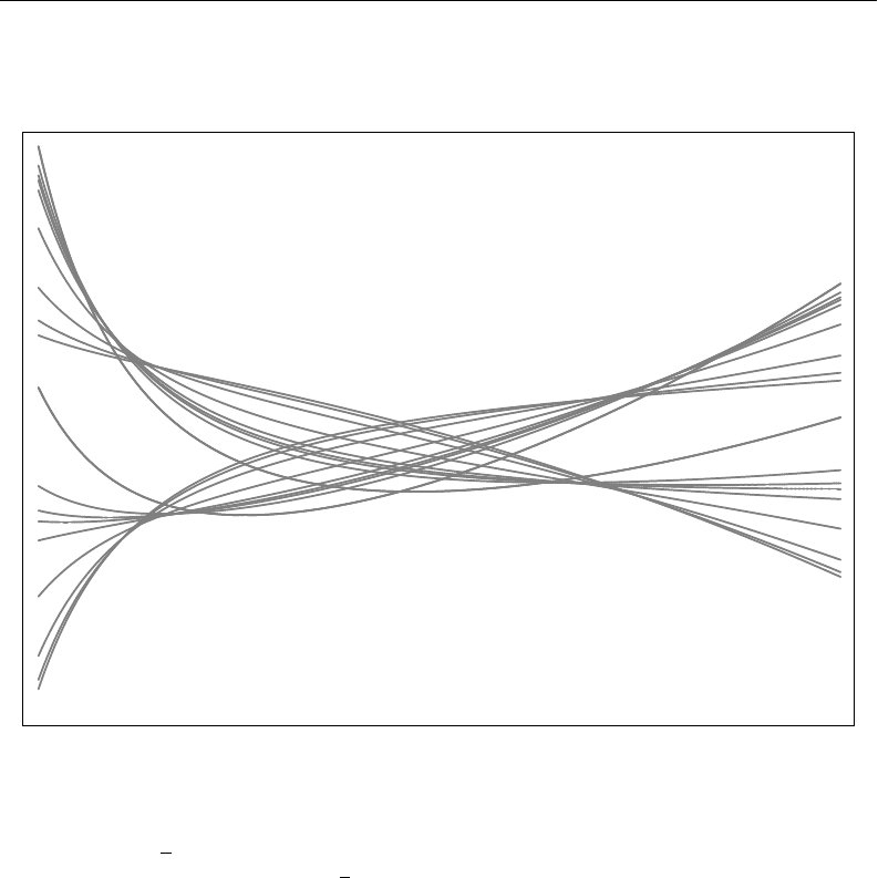
590 fp — Fractional polynomial regression
The second graph shows some of the curve shapes available with different βs for the degree-2
fractional polynomial, x(−2,2).
In modeling a fractional polynomial, Royston and Sauerbrei (2008) recommend choosing powers
from among {−2,−1,−0.5,0,0.5,1,2,3}. By default, fp chooses powers from this set, but other
powers can be explicitly specified in the powers() option.
fp <term>: est cmd fits models with the terms of the best-fitting fractional polynomial substituted
for <term>wherever it appears in est cmd. We will demonstrate with auto.dta, which contains
repair records and other information about a variety of vehicles in 1978.
We use fp to find the best fractional polynomial in automobile weight (lbs.) (weight) for the
linear regression of miles per gallon (mpg) on weight and an indicator of whether the vehicle is
foreign (foreign).
By default, fp will fit degree-2 fractional polynomial (FP2) models and choose the fractional powers
from the set {−2,−1,−0.5,0,0.5,1,2,3}. Because car weight is measured in pounds and will have
a cubic transformation applied to it, we shrink it to a smaller scale before estimation by dividing by
1,000.
We modify the existing weight variable for conciseness and to facilitate the comparison of tables.
When applying a data transformation in practice, rather than modifying the existing variables, you
should create new variables that hold the transformed values.

fp — Fractional polynomial regression 591
. use http://www.stata-press.com/data/r13/auto
(1978 Automobile Data)
. replace weight = weight/1000
weight was int now float
(74 real changes made)
. fp <weight>: regress mpg <weight> foreign
(fitting 44 models)
(....10%....20%....30%....40%....50%....60%....70%....80%....90%....100%)
Fractional polynomial comparisons:
weight df Deviance Res. s.d. Dev. dif. P(*) Powers
omitted 0 456.347 5.356 75.216 0.000
linear 1 388.366 3.407 7.236 0.082 1
m = 1 2 381.806 3.259 0.675 0.733 -.5
m = 2 4 381.131 3.268 0.000 -- -2 -2
(*) P = sig. level of model with m = 2 based on F with 68 denominator
dof.
Source SS df MS Number of obs = 74
F( 3, 70) = 52.95
Model 1696.05949 3 565.353163 Prob > F = 0.0000
Residual 747.399969 70 10.6771424 R-squared = 0.6941
Adj R-squared = 0.6810
Total 2443.45946 73 33.4720474 Root MSE = 3.2676
mpg Coef. Std. Err. t P>|t| [95% Conf. Interval]
weight_1 15.88527 20.60329 0.77 0.443 -25.20669 56.97724
weight_2 127.9349 47.53106 2.69 0.009 33.13723 222.7326
foreign -2.222515 1.053782 -2.11 0.039 -4.324218 -.1208131
_cons 3.705981 3.367949 1.10 0.275 -3.011182 10.42314
fp begins by showing the model-comparison table. This table shows the best models of each
examined degree, obtained by searching through all possible power combinations. The fractional
powers of the models are shown in the Powers column. A separate row is provided for the linear
fractional polynomial because it is often the default used when including a predictor in the model.
The null model does not include any fractional polynomial terms for weight. The df column shows
the count of the additional parameters used in each model beyond the quantity of parameters used in
the null model. The model deviance, which we define as twice the negative log likelihood, is given
in the Deviance column. The difference of the model deviance from the deviance of the model with
the lowest deviance is given in the Dev. dif. column.
The p-value for the partial Ftest comparing the models and the lowest deviance model is given
in the P(*) column. An estimate of the residual standard error is given in the Res. Sd. column.
Under linear regression, a partial Ftest is used in the model-comparison table. In other settings, a
likelihood-ratio test is performed. Then a χ2statistic is reported.
Under robust variance estimation and some other cases (see [R]lrtest), the likelihood-ratio test
cannot be performed. When the likelihood-ratio test cannot be performed on the model specified in
est cmd,fp still reports the model-comparison table, but the comparison tests are not performed.
fp reports the “best” model as the model with the lowest deviance; however, users may choose a
more efficient model based on the comparison table. They may choose the lowest degree model that
the partial Ftest (or likelihood-ratio test) fails to reject in favor of the lowest deviance model.
After the comparison table, the results of the estimation command for the lowest deviance model
are shown. Here the best model has terms weight(−2,−2). However, based on the model-comparison

592 fp — Fractional polynomial regression
table, we can reject the model without weight and the linear model at the 0.1 significance level. We
fail to reject the m=1model at any reasonable level. We will choose the FP1 model, which includes
weight(−.5).
We use fp again to estimate the parameters for this model. We use the fp() option to specify
what powers we want to use; this option specifies that we do not want to perform a search for
the best powers. We also specify the replace option to overwrite the previously created fractional
polynomial power variables.
. fp <weight>, fp(-.5) replace: regress mpg <weight> foreign
->
Source SS df MS Number of obs = 74
F( 2, 71) = 79.51
Model 1689.20865 2 844.604325 Prob > F = 0.0000
Residual 754.25081 71 10.6232508 R-squared = 0.6913
Adj R-squared = 0.6826
Total 2443.45946 73 33.4720474 Root MSE = 3.2593
mpg Coef. Std. Err. t P>|t| [95% Conf. Interval]
weight_1 66.89665 6.021749 11.11 0.000 54.88963 78.90368
foreign -2.095622 1.043513 -2.01 0.048 -4.176329 -.0149157
_cons -17.58651 3.397992 -5.18 0.000 -24.36192 -10.81111
Alternatively, we can use fp generate to create the fractional polynomial variable corresponding
to weight(−.5) and then use regress. We store weight(−.5) in the new variable wgt nsqrt.
. fp generate wgt_nsqrt=weight^(-.5)
. regress mpg wgt_nsqrt foreign
Source SS df MS Number of obs = 74
F( 2, 71) = 79.51
Model 1689.20874 2 844.604371 Prob > F = 0.0000
Residual 754.250718 71 10.6232495 R-squared = 0.6913
Adj R-squared = 0.6826
Total 2443.45946 73 33.4720474 Root MSE = 3.2593
mpg Coef. Std. Err. t P>|t| [95% Conf. Interval]
wgt_nsqrt_1 66.89665 6.021748 11.11 0.000 54.88963 78.90368
foreign -2.095622 1.043513 -2.01 0.048 -4.176328 -.0149155
_cons -17.58651 3.397991 -5.18 0.000 -24.36191 -10.81111
Scaling
Fractional polynomials are only defined for positive term variables. By default, fp will assume
that the variable xis positive and attempt to compute fractional powers of x. If the positive value
assumption is incorrect, an error will be reported and estimation will not be performed.
If the values of the variable are too large or too small, the reported results of fp may be difficult
to interpret. By default, cubic powers and squared reciprocal powers will be considered in the search
for the best fractional polynomial in term.
We can scale the variable xto 1) make it positive and 2) ensure its magnitude is not too large or
too small.
Suppose you have data on hospital patients with age as a fractional polynomial variable of interest.
age is required to be greater than or equal to 20, so you might generate an age5 variable by typing

fp — Fractional polynomial regression 593
. generate age5 = (age-19)/5
A unit change in age5 is equivalent to a five-year change in age, and the minimum value of age5
is 1/5 instead of 20.
In the automobile example of Fractional polynomial regression, our term variable was automobile
weight (lbs.). Cars weigh in the thousands of pounds, so cubing their weight figures results in large
numbers. We prevented this from being a problem by shrinking the weight by 1,000; that is, we typed
. replace weight = weight/1000
Calendar year is another type of variable that can have a problematically large magnitude. We can
shrink this by dividing by 10, making a unit change correspond to a decade.
. generate decade = calendar_year/10
You may also have a variable that measures deviation from zero. Perhaps xhas already been
demeaned and is symmetrically about zero. The fractional polynomial in xwill be undefined for half
of its domain. We can shift the location of x, making it positive by subtracting its minimum and
adding a small number to it. Suppose xranges from −4 to 4; we could use
. generate newx = x+5
Rescaling ourselves provides easily communicated results. We can tell exactly how the scaling
was performed and how it should be performed in similar applications.
Alternatively, fp can scale the fractional polynomial variable so that its values are positive and the
magnitude of the values are not too large. This can be done automatically or by directly specifying
the scaling values.
Scaling can be automatically performed with fp by specifying the scale option. If term has
nonpositive values, the minimum value of term is subtracted from each observation of term. In this
case, the counting interval, the minimum distance between the sorted values of term, is also added
to each observation of term.
After adjusting the location of term so that its minimum value is positive, creating term∗, automatic
scaling will divide each observation of term by a power of ten. The exponent of this scaling factor
is given by
p= log10 {max(term∗)−min(term∗)}
p∗=sign(p)floor (|p|)
Rather than letting fp automatically choose the scaling of term, you may specify adjustment and
scale factors aand bby using the scale(a b)option. Fractional powers are then calculated using
the (term+a)/bvalues.
When scale or scale(a b)is specified, values in the variable term are not modified; fp merely
remembers to scale the values whenever powers are calculated.
In addition to fp, both scale and scale(a b)may be used with fp generate.
You will probably not use scale(a b)with fp for values of aand bthat you create yourself,
although you could. As we demonstrated earlier, it is usually easier just to generate a scaled variable.
scale(a b)is useful when you previously fit a model using scale in one dataset and now want
to create the fractional polynomials in another. In the first dataset, fp with scale added notes to
the dataset concerning the values of aand b. You can see them by typing
. notes

594 fp — Fractional polynomial regression
You can then use fp generate, scale(a b)in the second dataset.
When you apply the scaling rules of a previously fit model to new data with the scale(a b)
option, it is possible that the scaled term may have nonpositive values. fp will be unable to calculate
the fractional powers of the term in this case and will issue an error.
The options zero and catzero cause fp and fp generate to output zero values for each fractional
polynomial variable when the input (scaled) fractional polynomial variable is nonpositive. Specifying
catzero causes a dummy variable indicating nonpositive values of the (scaled) fractional polynomial
variable to be included in the model. A detailed example of the use of catzero and zero is shown
in example 3 below.
Using the scaling options, we can fit our previous model again using the auto.dta. We specify
scale(0 1000) so that fp will shrink the magnitude of weight in estimating the regression. This is
done for demonstration purposes because our scaling rule is simple. As mentioned before, in practice,
you would probably only use scale(a b)when applying the scaling rules from a previous analysis.
Allowing fp to scale does have the advantage of not altering the original variable, weight.
. use http://www.stata-press.com/data/r13/auto, clear
(1978 Automobile Data)
. fp <weight>, fp(-.5) scale(0 1000): regress mpg <weight> foreign
->
Source SS df MS Number of obs = 74
F( 2, 71) = 79.51
Model 1689.20861 2 844.604307 Prob > F = 0.0000
Residual 754.250846 71 10.6232514 R-squared = 0.6913
Adj R-squared = 0.6826
Total 2443.45946 73 33.4720474 Root MSE = 3.2593
mpg Coef. Std. Err. t P>|t| [95% Conf. Interval]
weight_1 66.89665 6.021749 11.11 0.000 54.88963 78.90368
foreign -2.095622 1.043513 -2.01 0.048 -4.176329 -.0149159
_cons -17.58651 3.397992 -5.18 0.000 -24.36192 -10.81111
The scaling is clearly indicated in the variable notes for the generated variable weight 1.
. notes weight_1
weight_1:
1. fp term 1 of x^(-.5), where x is weight scaled.
2. Scaling was user specified: x = (weight+a)/b where a=0 and b=1000
3. Fractional polynomial variables created by
4. To re-create the fractional polynomial variables, for instance, in another
dataset, type
Centering
The fractional polynomial of term, centered on cis
term(p1,...,pm)−c(p1,...,pm)0β
The intercept of a centered fractional polynomial can be interpreted as the effect at zero for all the
covariates. When we center the fractional polynomial terms using c, the intercept is now interpreted
as the effect at term =cand zero values for the other covariates.

fp — Fractional polynomial regression 595
Suppose we wanted to center the fractional polynomial of xwith powers (0, 0, 2) at x=c.
x(0,0,2) −c(0,0,2)0β
=β0+β1x(0) −c(0)+β2nx(0) ln(x)−c(0) ln(c)o+β3x(2) −c(2)
=β0+β1{ln(x)−ln(c)}+β2{ln(x)}2− {ln(c)}2+β3x2−c2
When center is specified, fp centers based on the sample mean of (scaled) term. A previously
chosen value for centering, c, may also be specified in center(c). This would be done when applying
the results of a previous model fitting to a new dataset.
The center and center(c)options may be used in fp or fp generate.
Returning to the model of mileage per gallon based on automobile weight and foreign origin, we
refit the model with the fractional polynomial of weight centered at its scaled mean.
. use http://www.stata-press.com/data/r13/auto, clear
(1978 Automobile Data)
. fp <weight>, fp(-.5) scale(0 1000) center: regress mpg <weight> foreign
->
Source SS df MS Number of obs = 74
F( 2, 71) = 79.51
Model 1689.20861 2 844.604307 Prob > F = 0.0000
Residual 754.250846 71 10.6232514 R-squared = 0.6913
Adj R-squared = 0.6826
Total 2443.45946 73 33.4720474 Root MSE = 3.2593
mpg Coef. Std. Err. t P>|t| [95% Conf. Interval]
weight_1 66.89665 6.021749 11.11 0.000 54.88963 78.90368
foreign -2.095622 1.043513 -2.01 0.048 -4.176329 -.0149159
_cons 20.91163 .4624143 45.22 0.000 19.9896 21.83366
Note that the coefficients for weight 1 and foreign do not change. Only the intercept cons
changes. It can be interpreted as the estimated average miles per gallon of an American-made car of
average weight.

596 fp — Fractional polynomial regression
Examples
Example 1: Linear regression
Consider the serum immunoglobulin G (IgG) dataset from Isaacs et al. (1983), which consists of
298 independent observations in young children. The dependent variable sqrtigg is the square root
of the IgG concentration, and the independent variable age is the age of each child. (Preliminary
Box–Cox analysis shows that a square root transformation removes the skewness in IgG.)
The aim is to find a model that accurately predicts the mean of sqrtigg given age. We use fp
to find the best FP2 model (the default option). We specify center for automatic centering. The age
of each child is small in magnitude and positive, so we do not use the scaling options of fp or scale
ourselves.
. use http://www.stata-press.com/data/r13/igg, clear
(Immunoglobulin in children)
. fp <age>, scale center: regress sqrtigg <age>
(fitting 44 models)
(....10%....20%....30%....40%....50%....60%....70%....80%....90%....100%)
Fractional polynomial comparisons:
age df Deviance Res. s.d. Dev. dif. P(*) Powers
omitted 0 427.539 0.497 108.090 0.000
linear 1 337.561 0.428 18.113 0.000 1
m = 1 2 327.436 0.421 7.987 0.020 0
m = 2 4 319.448 0.416 0.000 -- -2 2
(*) P = sig. level of model with m = 2 based on F with 293
denominator dof.
Source SS df MS Number of obs = 298
F( 2, 295) = 64.49
Model 22.2846976 2 11.1423488 Prob > F = 0.0000
Residual 50.9676492 295 .172771692 R-squared = 0.3042
Adj R-squared = 0.2995
Total 73.2523469 297 .246640898 Root MSE = .41566
sqrtigg Coef. Std. Err. t P>|t| [95% Conf. Interval]
age_1 -.1562156 .027416 -5.70 0.000 -.2101713 -.10226
age_2 .0148405 .0027767 5.34 0.000 .0093757 .0203052
_cons 2.283145 .0305739 74.68 0.000 2.222974 2.343315
The new variables created by fp contain the best-fitting fractional polynomial powers of age, as
centered by fp. For example, age 1 is centered by subtracting the mean of age raised to the power
−2.
The variables created by fp and fp generate are centered or scaled as specified by the user, which
is reflected in the estimated regression coefficients and intercept. Centering does have its advantages
(see Centering earlier in this entry). By default, fp will not perform scaling or centering. For a more
detailed discussion, see Royston and Sauerbrei (2008, sec. 4.11).
The fitted curve has an asymmetric S shape. The best model has powers (−2,2)and deviance
319.448. We reject lesser degree models: the null, linear, and natural log power models at the 0.05
level. As many as 44 models have been fit in the search for the best powers. Now let’s look at
models of degree ≤4. The highest allowed degree is specified in dimension(). We overwrite the
previously generated fractional polynomial power variables by including replace.

fp — Fractional polynomial regression 597
. fp <age>, dimension(4) center replace: regress sqrtigg <age>
(fitting 494 models)
(....10%....20%....30%....40%....50%....60%....70%....80%....90%....100%)
Fractional polynomial comparisons:
age df Deviance Res. s.d. Dev. dif. P(*) Powers
omitted 0 427.539 0.497 109.795 0.000
linear 1 337.561 0.428 19.818 0.007 1
m = 1 2 327.436 0.421 9.692 0.149 0
m = 2 4 319.448 0.416 1.705 0.798 -2 2
m = 3 6 319.275 0.416 1.532 0.476 -2 1 1
m = 4 8 317.744 0.416 0.000 -- 0 3 3 3
(*) P = sig. level of model with m = 4 based on F with 289
denominator dof.
Source SS df MS Number of obs = 298
F( 4, 293) = 32.63
Model 22.5754541 4 5.64386353 Prob > F = 0.0000
Residual 50.6768927 293 .172958678 R-squared = 0.3082
Adj R-squared = 0.2987
Total 73.2523469 297 .246640898 Root MSE = .41588
sqrtigg Coef. Std. Err. t P>|t| [95% Conf. Interval]
age_1 .8761824 .1898721 4.61 0.000 .5024962 1.249869
age_2 -.1922029 .0684934 -2.81 0.005 -.3270044 -.0574015
age_3 .2043794 .074947 2.73 0.007 .0568767 .3518821
age_4 -.0560067 .0212969 -2.63 0.009 -.097921 -.0140924
_cons 2.238735 .0482705 46.38 0.000 2.143734 2.333736
It appears that the FP4 model is not significantly different from the other fractional polynomial models
(at the 0.05 level).
Let’s compare the curve shape from the m=2 model with that from a conventional quartic
polynomial whose fit turns out to be significantly better than a cubic (not shown). We use the ability
of fp both to generate the required powers of age, namely, (1,2,3,4)for the quartic and (−2,2)
for the second-degree fractional polynomial, and to fit the model. The fp() option is used to specify
the powers. We use predict to obtain the fitted values of each regression. We fit both models with
fp and graph the resulting curves with twoway scatter.

598 fp — Fractional polynomial regression
. fp <age>, center fp(1 2 3 4) replace: regress sqrtigg <age>
->
Source SS df MS Number of obs = 298
F( 4, 293) = 32.65
Model 22.5835458 4 5.64588646 Prob > F = 0.0000
Residual 50.668801 293 .172931061 R-squared = 0.3083
Adj R-squared = 0.2989
Total 73.2523469 297 .246640898 Root MSE = .41585
sqrtigg Coef. Std. Err. t P>|t| [95% Conf. Interval]
age_1 2.047831 .4595962 4.46 0.000 1.143302 2.952359
age_2 -1.058902 .2822803 -3.75 0.000 -1.614456 -.5033479
age_3 .2284917 .0667591 3.42 0.001 .0971037 .3598798
age_4 -.0168534 .0053321 -3.16 0.002 -.0273475 -.0063594
_cons 2.240012 .0480157 46.65 0.000 2.145512 2.334511
. predict fit1
(option xb assumed; fitted values)
. label variable fit1 "Quartic"
. fp <age>, center fp(-2 2) replace: regress sqrtigg <age>
->
Source SS df MS Number of obs = 298
F( 2, 295) = 64.49
Model 22.2846976 2 11.1423488 Prob > F = 0.0000
Residual 50.9676492 295 .172771692 R-squared = 0.3042
Adj R-squared = 0.2995
Total 73.2523469 297 .246640898 Root MSE = .41566
sqrtigg Coef. Std. Err. t P>|t| [95% Conf. Interval]
age_1 -.1562156 .027416 -5.70 0.000 -.2101713 -.10226
age_2 .0148405 .0027767 5.34 0.000 .0093757 .0203052
_cons 2.283145 .0305739 74.68 0.000 2.222974 2.343315
. predict fit2
(option xb assumed; fitted values)
. label variable fit2 "FP 2"
. scatter sqrtigg fit1 fit2 age, c(. l l) m(o i i) msize(small)
> lpattern(. -_.) ytitle("Square root of IgG") xtitle("Age, years")

fp — Fractional polynomial regression 599
1 2 3 4
Square root of IgG
0 2 4 6
Age, years
Square root of IgG Quartic
FP 2
The quartic curve has an unsatisfactory wavy appearance that is implausible for the known behavior
of IgG, the serum level of which increases throughout early life. The fractional polynomial curve
(FP2) increases monotonically and is therefore biologically the more plausible curve. The two models
have approximately the same deviance.
Example 2: Cox regression
Data from Smith et al. (1992) contain times to complete healing of leg ulcers in a randomized,
controlled clinical trial of two treatments in 192 elderly patients. Several covariates were available,
of which an important one is mthson, the number of months since the recorded onset of the ulcer.
This time is recorded in whole months, not fractions of a month; therefore, some zero values are
recorded.
Because the response variable is time to an event of interest and some (in fact, about one-half) of
the times are censored, using Cox regression to analyze the data is appropriate. We consider fractional
polynomials in mthson, adjusting for four other covariates: age;ulcarea, the area of tissue initially
affected by the ulcer; deepppg, a binary variable indicating the presence or absence of deep vein
involvement; and treat, a binary variable indicating treatment type.
We fit fractional polynomials of degrees 1 and 2 with fp. We specify scale to perform automatic
scaling on mthson. This makes it positive and ensures that its magnitude is not too large. (See Scaling
for more details.) The display option nohr is specified before the colon so that the coefficients and
not the hazard ratios are displayed.
The center option is specified to obtain automatic centering. age and ulcarea are also demeaned
by using summarize and then subtracting the returned result r(mean).
In Cox regression, there is no constant term, so we cannot see the effects of centering in the
table of regression estimates. The effects would be present if we were to graph the baseline hazard
or survival function because these functions are defined with all predictors set equal to 0.
In these graphs, we will see the estimated baseline hazard or survival function under no deep vein
involvement or treatment and under mean age, ulcer area, and number of months since the recorded
onset of the ulcer.

600 fp — Fractional polynomial regression
. use http://www.stata-press.com/data/r13/legulcer1, clear
(Leg ulcer clinical trial)
. stset ttevent, fail(cens)
failure event: censored != 0 & censored < .
obs. time interval: (0, ttevent]
exit on or before: failure
192 total observations
0 exclusions
192 observations remaining, representing
92 failures in single-record/single-failure data
13825 total analysis time at risk and under observation
at risk from t = 0
earliest observed entry t = 0
last observed exit t = 206
. qui sum age
. replace age = age - r(mean)
age was byte now float
(192 real changes made)
. qui sum ulcarea
. replace ulcarea = ulcarea - r(mean)
ulcarea was int now float
(192 real changes made)
. fp <mthson>, center scale nohr: stcox <mthson> age ulcarea deepppg treat
(fitting 44 models)
(....10%....20%....30%....40%....50%....60%....70%....80%....90%....100%)
Fractional polynomial comparisons:
mthson df Deviance Dev. dif. P(*) Powers
omitted 0 754.345 17.636 0.001
linear 1 751.680 14.971 0.002 1
m = 1 2 738.969 2.260 0.323 -.5
m = 2 4 736.709 0.000 -- .5 .5
(*) P = sig. level of model with m = 2 based on chi^2 of dev. dif.
Cox regression -- Breslow method for ties
No. of subjects = 192 Number of obs = 192
No. of failures = 92
Time at risk = 13825
LR chi2(6) = 108.59
Log likelihood = -368.35446 Prob > chi2 = 0.0000
_t Coef. Std. Err. z P>|z| [95% Conf. Interval]
mthson_1 -2.81425 .6996385 -4.02 0.000 -4.185516 -1.442984
mthson_2 1.541451 .4703143 3.28 0.001 .6196521 2.46325
age -.0261111 .0087983 -2.97 0.003 -.0433556 -.0088667
ulcarea -.0017491 .000359 -4.87 0.000 -.0024527 -.0010455
deepppg -.5850499 .2163173 -2.70 0.007 -1.009024 -.1610758
treat -.1624663 .2171048 -0.75 0.454 -.5879838 .2630513
The best-fitting fractional polynomial of degree 2 has powers (0.5,0.5)and deviance 736.709. However,
this model does not fit significantly better than the fractional polynomial of degree 1 (at the 0.05
level), which has power −0.5 and deviance 738.969. We prefer the model with m=1.

fp — Fractional polynomial regression 601
. fp <mthson>, replace center scale nohr fp(-.5): stcox <mthson> age ulcarea
> deepppg treat
->
Cox regression -- Breslow method for ties
No. of subjects = 192 Number of obs = 192
No. of failures = 92
Time at risk = 13825
LR chi2(5) = 106.33
Log likelihood = -369.48426 Prob > chi2 = 0.0000
_t Coef. Std. Err. z P>|z| [95% Conf. Interval]
mthson_1 .1985592 .0493922 4.02 0.000 .1017523 .2953662
age -.02691 .0087875 -3.06 0.002 -.0441331 -.0096868
ulcarea -.0017416 .0003482 -5.00 0.000 -.0024241 -.0010591
deepppg -.5740759 .2185134 -2.63 0.009 -1.002354 -.1457975
treat -.1798575 .2175726 -0.83 0.408 -.6062921 .246577
The hazard for healing is much higher for patients whose ulcer is of recent onset than for those who
have had an ulcer for many months.
A more appropriate analysis of this dataset, if one wanted to model all the predictors, possibly
with fractional polynomial functions, would be to use mfp; see [R]mfp.
Example 3: Logistic regression
The zero option permits fitting a fractional polynomial model to the positive values of a covariate,
taking nonpositive values as zero. An application is the assessment of the effect of cigarette smoking
as a risk factor. Whitehall 1 is an epidemiological study, which was examined in Royston and
Sauerbrei (2008), of 18,403 male British Civil Servants employed in London. We examine the data
collected in Whitehall 1 and use logistic regression to model the odds of death based on a fractional
polynomial in the number of cigarettes smoked.
Nonsmokers may be qualitatively different from smokers, so the effect of smoking (regarded as a
continuous variable) may not be continuous between zero cigarettes and one cigarette. To allow for
this possibility, we model the risk as a constant for the nonsmokers and as a fractional polynomial
function of the number of cigarettes for the smokers, adjusted for age.
The dependent variable all10 is an indicator of whether the individual passed away in the 10 years
under study. cigs is the number of cigarettes consumed per day. After loading the data, we demean
age and create a dummy variable, nonsmoker. We then use fp to fit the model.

602 fp — Fractional polynomial regression
. use http://www.stata-press.com/data/r13/smoking, clear
(Smoking and mortality data)
. qui sum age
. replace age = age - r(mean)
age was byte now float
(17260 real changes made)
. generate byte nonsmoker = cond(cigs==0, 1, 0) if cigs < .
. fp <cigs>, zero: logit all10 <cigs> nonsmoker age
(fitting 44 models)
(....10%....20%....30%....40%....50%....60%....70%....80%....90%....100%)
Fractional polynomial comparisons:
cigs df Deviance Dev. dif. P(*) Powers
omitted 0 9990.804 46.096 0.000
linear 1 9958.801 14.093 0.003 1
m = 1 2 9946.603 1.895 0.388 0
m = 2 4 9944.708 0.000 -- -1 -1
(*) P = sig. level of model with m = 2 based on chi^2 of dev. dif.
Logistic regression Number of obs = 17260
LR chi2(4) = 1029.03
Prob > chi2 = 0.0000
Log likelihood = -4972.3539 Pseudo R2 = 0.0938
all10 Coef. Std. Err. z P>|z| [95% Conf. Interval]
cigs_1 -1.285867 .3358483 -3.83 0.000 -1.944117 -.6276162
cigs_2 -1.982424 .572109 -3.47 0.001 -3.103736 -.8611106
nonsmoker -1.223749 .1119583 -10.93 0.000 -1.443183 -1.004315
age .1194541 .0045818 26.07 0.000 .1104739 .1284343
_cons -1.591489 .1052078 -15.13 0.000 -1.797693 -1.385286
Omission of the zero option would cause fp to halt with an error message because nonpositive
covariate values (for example, values of cigs) are invalid unless the scale option is specified.
A closely related approach involves the catzero option. Here we no longer need to have nonsmoker
in the model, because fp creates its own dummy variable cigs 0 to indicate whether the individual
does not smoke on that day.

fp — Fractional polynomial regression 603
. fp <cigs>, catzero replace: logit all10 <cigs> age
(fitting 44 models)
(....10%....20%....30%....40%....50%....60%....70%....80%....90%....100%)
Fractional polynomial comparisons:
cigs df Deviance Dev. dif. P(*) Powers
omitted 0 10175.75 231.047 0.000
linear 2 9958.80 14.093 0.003 1
m = 1 3 9946.60 1.895 0.388 0
m = 2 5 9944.71 0.000 -- -1 -1
(*) P = sig. level of model with m = 2 based on chi^2 of dev. dif.
Logistic regression Number of obs = 17260
LR chi2(4) = 1029.03
Prob > chi2 = 0.0000
Log likelihood = -4972.3539 Pseudo R2 = 0.0938
all10 Coef. Std. Err. z P>|z| [95% Conf. Interval]
cigs_0 -1.223749 .1119583 -10.93 0.000 -1.443183 -1.004315
cigs_1 -1.285867 .3358483 -3.83 0.000 -1.944117 -.6276162
cigs_2 -1.982424 .572109 -3.47 0.001 -3.103736 -.8611106
age .1194541 .0045818 26.07 0.000 .1104739 .1284343
_cons -1.591489 .1052078 -15.13 0.000 -1.797693 -1.385286
Under both approaches, the comparison table suggests that we can accept the FP1 model instead
of the FP2 model. We estimate the parameters of the accepted model—that is, the one that uses the
natural logarithm of cigs—with fp.
. fp <cigs>, catzero replace fp(0): logit all10 <cigs> age
->
Logistic regression Number of obs = 17260
LR chi2(3) = 1027.13
Prob > chi2 = 0.0000
Log likelihood = -4973.3016 Pseudo R2 = 0.0936
all10 Coef. Std. Err. z P>|z| [95% Conf. Interval]
cigs_0 .1883732 .1553093 1.21 0.225 -.1160274 .4927738
cigs_1 .3469842 .0543552 6.38 0.000 .2404499 .4535185
age .1194976 .0045818 26.08 0.000 .1105174 .1284778
_cons -3.003767 .1514909 -19.83 0.000 -3.300683 -2.70685
The high p-value for cigs 0 in the output indicates that we cannot reject that there is no extra
effect at zero for nonsmokers.

604 fp — Fractional polynomial regression
Stored results
In addition to the results that est cmd stores, fp stores the following in e():
Scalars
e(fp dimension) degree of fractional polynomial
e(fp center mean) value used for centering or .
e(fp scale a) value used for scaling or .
e(fp scale b) value used for scaling or .
e(fp compare df2) denominator degree of freedom in Ftest
Macros
e(fp cmd) fp, search(): or fp, powers():
e(fp cmdline) full fp command as typed
e(fp variable) fractional polynomial variable
e(fp terms) generated fp variables
e(fp gen cmdline) fp generate command to re-create e(fp terms) variables
e(fp catzero) catzero, if specified
e(fp zero) zero, if specified
e(fp compare type) F or chi2
Matrices
e(fp fp) powers used in fractional polynomial
e(fp compare) results of model comparisons
e(fp compare stat) Ftest statistics
e(fp compare df1) numerator degree of Ftest
e(fp compare fp) powers of comparison models
e(fp compare length) encoded string for display of row titles
e(fp powers) powers that are searched
fp generate stores the following in r():
Scalars
r(fp center mean) value used for centering or .
r(fp scale a) value used for scaling or .
r(fp scale b) value used for scaling or .
Macros
r(fp cmdline) full fp generate command as typed
r(fp variable) fractional polynomial variable
r(fp terms) generated fp variables
r(fp catzero) catzero, if specified
r(fp zero) zero, if specified
Matrices
r(fp fp) powers used in fractional polynomial
Methods and formulas
The general definition of a fractional polynomial, accommodating possible repeated powers, may
be written for functions H1(x), . . . , Hm(x)of x > 0 as
β0+
m
X
j=1
βjHj(x)
where H1(x) = x(p1)and for j=2, . . . , m,
Hj(x) = x(pj)if pj6=pj−1
Hj−1(x)ln(x)if pj=pj−1

fp — Fractional polynomial regression 605
For example, a fractional polynomial of degree 3 with powers (1,3,3)has H1(x) = x,H2(x) = x3,
and H3(x) = x3ln(x)and equals β0+β1x+β2x3+β3x3ln(x).
We can express a fractional polynomial in vector notation by using H(x) = [H1(x), . . . , Hd(x)]0.
We define x(p1,p2,...,pm)= [H(x)0,1]0. Under this notation, we can write
x(1,3,3)0β=β0+β1x+β2x3+β3x3ln(x)
The fractional polynomial may be centered so that the intercept can be more easily interpreted.
When centering the fractional polynomial of xat c, we subtract c(p1,p2,...,pm)from x(p1,p2,...,pm),
where c(p1,p2,...,pd)= [H(x)0,0]0. The centered fractional polynomial is
x(p1,...,pd)−c(p1,...,pd)0β
The definition may be extended to allow x≤0 values. For these values, the fractional polynomial
is equal to the intercept β0or equal to a zero-offset term α0plus the intercept β0.
A fractional polynomial model of degree mis taken to have 2m+1 degrees of freedom (df ): one
for β0and one for each βjand its associated power. Because the powers in a fractional polynomial
are chosen from a finite set rather than from the entire real line, the df defined in this way are
approximate.
The deviance Dof a model is defined as −2 times its maximized log likelihood. For normal-errors
models, we use the formula
D=n1−l+ln 2πRSS
n
where nis the sample size, lis the mean of the lognormalized weights (l=0 if the weights are all
equal), and RSS is the residual sum of squares as fit by regress.
fp reports a table comparing fractional polynomial models of degree k < m with the degree m
fractional polynomial model, which will have the lowest deviance.
The p-values reported by fp are calculated differently for normal and nonnormal regressions. Let
Dkand Dmbe the deviances of the models with degrees kand m, respectively. For normal-errors
models, a variance ratio Fis calculated as
F=n2
n1exp Dk−Dm
n−1
where n1is the numerator df, the quantity of the additional parameters that the degree mmodel has
over the degree kmodel. n2is the denominator df and equals the residual degrees of freedom of the
degree mmodel, minus the number of powers estimated, m. The p-value is obtained by referring F
to an Fdistribution on (n1, n2)df.
For nonnormal models, the p-value is obtained by referring Dk−Dmto a χ2distribution on
2m−2kdf. These p-values for comparing models are approximate and are typically somewhat
conservative (Royston and Altman 1994).

606 fp — Fractional polynomial regression
Acknowledgment
We thank Patrick Royston of the MRC Clinical Trials Unit, London, and coauthor of the Stata
Press book Flexible Parametric Survival Analysis Using Stata: Beyond the Cox Model for writing
fracpoly and fracgen, the commands on which fp and fp generate are based. We also thank
Professor Royston for his advice on and review of the new fp commands.
References
Becketti, S. 1995. sg26.2: Calculating and graphing fractional polynomials.Stata Technical Bulletin 24: 14–16.
Reprinted in Stata Technical Bulletin Reprints, vol. 4, pp. 129–132. College Station, TX: Stata Press.
Isaacs, D., D. G. Altman, C. E. Tidmarsh, H. B. Valman, and A. D. Webster. 1983. Serum immunoglobulin
concentrations in preschool children measured by laser nephelometry: Reference ranges for IgG, IgA, IgM. Journal
of Clinical Pathology 36: 1193–1196.
Libois, F., and V. Verardi. 2013. Semiparametric fixed-effects estimator.Stata Journal 13: 329–336.
Royston, P. 1995. sg26.3: Fractional polynomial utilities.Stata Technical Bulletin 25: 9–13. Reprinted in Stata Technical
Bulletin Reprints, vol. 5, pp. 82–87. College Station, TX: Stata Press.
Royston, P., and D. G. Altman. 1994. Regression using fractional polynomials of continuous covariates: Parsimonious
parametric modelling. Applied Statistics 43: 429–467.
Royston, P., and G. Ambler. 1999a. sg112: Nonlinear regression models involving power or exponential functions of
covariates.Stata Technical Bulletin 49: 25–30. Reprinted in Stata Technical Bulletin Reprints, vol. 9, pp. 173–179.
College Station, TX: Stata Press.
. 1999b. sg81.1: Multivariable fractional polynomials: Update.Stata Technical Bulletin 49: 17–23. Reprinted in
Stata Technical Bulletin Reprints, vol. 9, pp. 161–168. College Station, TX: Stata Press.
. 1999c. sg112.1: Nonlinear regression models involving power or exponential functions of covariates: Update.
Stata Technical Bulletin 50: 26. Reprinted in Stata Technical Bulletin Reprints, vol. 9, p. 180. College Station,
TX: Stata Press.
. 1999d. sg81.2: Multivariable fractional polynomials: Update.Stata Technical Bulletin 50: 25. Reprinted in Stata
Technical Bulletin Reprints, vol. 9, p. 168. College Station, TX: Stata Press.
Royston, P., and W. Sauerbrei. 2008. Multivariable Model-building: A Pragmatic Approach to Regression Analysis
Based on Fractional Polynomials for Modelling Continuous Variables. Chichester, UK: Wiley.
Smith, J. M., C. J. Dore, A. Charlett, and J. D. Lewis. 1992. A randomized trial of Biofilm dressing for venous leg
ulcers. Phlebology 7: 108–113.
Also see
[R]fp postestimation — Postestimation tools for fp
[R]mfp — Multivariable fractional polynomial models
[U] 20 Estimation and postestimation commands

Title
fp postestimation — Postestimation tools for fp
Description Syntax for predict Syntax for fp plot and fp predict
Menu for fp plot and fp predict Options for fp plot Options for fp predict
Remarks and examples Methods and formulas Acknowledgment
References Also see
Description
The following postestimation commands are of special interest after fp:
Command Description
fp plot component-plus-residual plot from most recently fit fractional polynomial model
fp predict create variable containing prediction or SEs of fractional polynomials
The following standard postestimation commands are also available if available after est cmd:
Command Description
contrast contrasts and ANOVA-style joint tests of estimates
estat ic Akaike’s and Schwarz’s Bayesian information criteria (AIC and BIC)
estat summarize summary statistics for the estimation sample
estat vce variance–covariance matrix of the estimators (VCE)
estimates cataloging estimation results
hausman Hausman’s specification test
lincom point estimates, standard errors, testing, and inference for linear combinations
of coefficients
linktest link test for model specification
lrtest likelihood-ratio test
margins marginal means, predictive margins, marginal effects, and average marginal
effects
marginsplot graph the results from margins (profile plots, interaction plots, etc.)
nlcom point estimates, standard errors, testing, and inference for nonlinear combinations
of coefficients
predict predictions, residuals, influence statistics, and other diagnostic measures
predictnl point estimates, standard errors, testing, and inference for generalized predictions
pwcompare pairwise comparisons of estimates
suest seemingly unrelated estimation
test Wald tests of simple and composite linear hypotheses
testnl Wald tests of nonlinear hypotheses
607

608 fp postestimation — Postestimation tools for fp
Special-interest postestimation commands
fp plot produces a component-plus-residual plot. The fractional polynomial comprises the com-
ponent, and the residual is specified by the user in residuals(). The component-plus-residuals are
plotted against the fractional polynomial variable. If you only want to plot the component fit, without
residuals, you would specify residuals(none).
fp predict generates the fractional polynomial or the standard error of the fractional polynomial.
The fractional polynomial prediction is equivalent to the fitted values prediction given by predict,
xb, with the covariates other than the fractional polynomial variable set to zero. The standard error
may be quite large if the range of the other covariates is far from zero. In this situation, the covariates
would be centered and their range would include, or come close to including, zero.
These postestimation commands can be used only when the fractional polynomial variables do
not interact with other variables in the specification of est cmd. See [U] 11.4.3 Factor variables for
more information about interactions.
Syntax for predict
The behavior of predict following fp is determined by est cmd. See the corresponding est cmd
postestimation entry for available predict options.
Also see information on fp predict below.
Syntax for fp plot and fp predict
Component-plus-residual plot for most recently fit fractional polynomial model
fp plot if in , residuals(res option)graph options
Create variable containing the prediction or SEs of fractional polynomials
fp predict type newvar if in ,predict options

fp postestimation — Postestimation tools for fp 609
graph options Description
Main
∗residuals(res option)residual option name to use in predict after est cmd, or
residuals(none) if residuals are not to be graphed
equation(eqno)specify equation
level(#)set confidence level; default is level(95)
Plot
plotopts(scatter options)affect rendition of the component-plus-residual scatter points
Fitted line
lineopts(cline options)affect rendition of the fitted line
CI plot
ciopts(area options)affect rendition of the confidence bands
Add plots
addplot(plot)add other plots to the generated graph
Y axis, X axis, Titles, Legend, Overall
twoway options any options other than by() documented in [G-3]twoway options
∗residuals(res option)is required.
predict options Description
Main
fp calculate the fractional polynomial; the default
stdp calculate the standard error of the fractional polynomial
equation(eqno)specify equation
Menu for fp plot and fp predict
fp plot
Statistics >Linear models and related >Fractional polynomials >Component-plus-residual plot
fp predict
Statistics >Linear models and related >Fractional polynomials >Fractional polynomial prediction
Options for fp plot
Main
residuals(res option)specifies what type of residuals to plot in the component-plus-residual plot.
res option is the same option that would be specified to predict after est cmd. Residuals can
be omitted from the plot by specifying residuals(none).residuals() is required.
equation(eqno)is relevant only when you have previously fit a multiple-equation model in est cmd.
It specifies the equation to which you are referring.
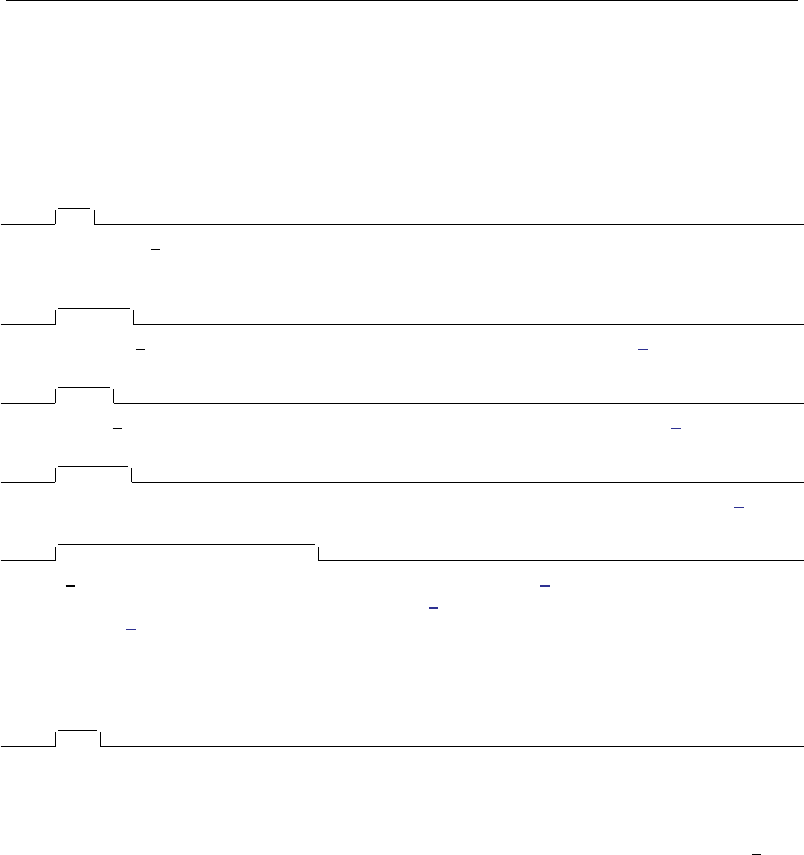
610 fp postestimation — Postestimation tools for fp
equation(#1) would mean that the calculation is to be made for the first equation, equation(#2)
would mean the second, and so on. You could also refer to the equations by their names:
equation(income) would refer to the equation name income, and equation(hours) would
refer to the equation named hours.
If you do not specify equation(), the results are the same as if you specified equation(#1).
level(#); see [R]estimation options.
Plot
plotopts(scatter options)affects the rendition of the component-plus-residual scatter points; see
[G-2]graph twoway scatter.
Fitted line
lineopts(cline options)affects the rendition of the fitted line; see [G-3]cline options.
CI plot
ciopts(area options)affects the rendition of the confidence bands; see [G-3]area options.
Add plots
addplot(plot)provides a way to add other plots to the generated graph. See [G-3]addplot option.
Y axis, X axis, Titles, Legend, Overall
twoway options are any of the options documented in [G-3]twoway options, excluding by(). These
include options for titling the graph (see [G-3]title options) and for saving the graph to disk (see
[G-3]saving option).
Options for fp predict
Main
fp calculates the fractional polynomial, the linear prediction with other variables set to zero. This is
the default.
stdp calculates the standard error of the fractional polynomial.
equation(eqno)is relevant only when you have previously fit a multiple-equation model in est cmd.
It specifies the equation to which you are referring.
equation(#1) would mean that the calculation is to be made for the first equation, equation(#2)
would mean the second, and so on. You could also refer to the equations by their names:
equation(income) would refer to the equation name income, and equation(hours) would
refer to the equation named hours.
If you do not specify equation(), the results are the same as if you specified equation(#1).

fp postestimation — Postestimation tools for fp 611
Remarks and examples
After a model is fit using fp, the estimated fractional polynomial may be of interest. This is the
linear combination of the fractional polynomial terms and the constant intercept using the model
coefficients estimated by fp. It is equivalent to the fitted values prediction given by predict,xb,
with the covariates and the fractional polynomial variable set to zero. When these other covariates
have been centered, the prediction is made at the centering values of the covariates.
A component-plus-residual plot is generated by fp plot. The fractional polynomial comprises
the component, and the residual is specified by the user in residuals(). The residuals() option
takes the same argument that would be supplied to predict after est cmd to obtain the desired
type of residuals. If you only want to plot the component fit, without residuals, you would specify
residuals(none).
fp predict generates the fractional polynomial. If the stdp option is specified, the standard error
of the fractional polynomial is generated instead. This standard error may be quite large if the range
of the other covariates is far from zero. In this situation, the covariates would be centered and their
range would include, or come close to including, zero.
These postestimation commands can be used only when the fractional polynomial terms do not
interact with other variables in the specification of est cmd. See [U] 11.4.3 Factor variables for more
information about interactions.
Examples
Example 1: fp plot after linear regression
In example 1 of [R]fp, we modeled the mean of the square root of a child’s serum immunoglobulin
G (IgG) level as a fractional polynomial function of the child’s age. An FP2 model with powers
(−2,2)is chosen.
We load the data and then fit the model with fp. Then we use fp plot to draw the component-
plus-residual plot. A 95% confidence interval is produced for the fractional polynomial in age (the
component). The residuals prediction option for regress is specified in the residuals() option
in fp plot so that the residuals are rendered.
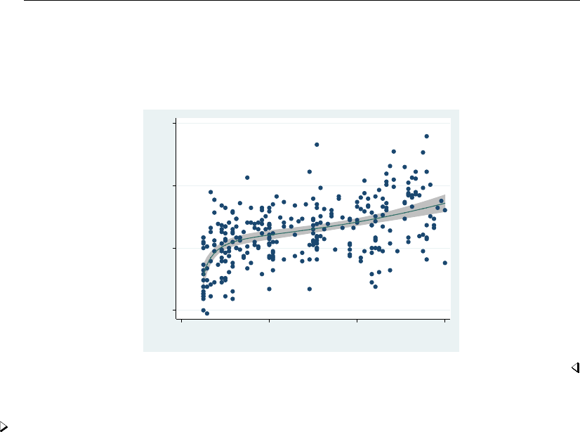
612 fp postestimation — Postestimation tools for fp
. use http://www.stata-press.com/data/r13/igg
(Immunoglobulin in children)
. fp <age>, scale center: regress sqrtigg <age>
(output omitted )
. fp plot, residuals(residuals)
1 2 3 4
Component+residual of sqrtigg
0 2 4 6
Age (years)
Example 2: fp plot after Cox regression
In example 2 of [R]fp, we modeled the time to complete healing of leg ulcers for 192 elderly
patients using a Cox regression. A one-degree fractional polynomial in mthson, the number of months
since the onset of the ulcer, is used as a predictor in the regression. The power −0.5 is used for
mthson. Other covariates are age (age), ulcer area (ulcarea), treatment type, and a binary indicator
of deep vein involvement (deepppg).
We load the data and then demean ulcer area and age. Then we fit the model with fp and draw
the component-plus-residual plot with fp plot.mgale is specified in the residuals() option to
obtain martingale residuals. See [ST]stcox postestimation for more details.
. use http://www.stata-press.com/data/r13/legulcer1, clear
(Leg ulcer clinical trial)
. quietly stset ttevent, failure(cens)
. quietly summarize age
. replace age = age - r(mean)
age was byte now float
(192 real changes made)
. quietly summarize ulcarea
. replace ulcarea = ulcarea - r(mean)
ulcarea was int now float
(192 real changes made)
. fp <mthson>, replace center scale nohr fp(-.5): stcox <mthson> age ulcarea
> deepppg treat
(output omitted )
. fp plot, residuals(mgale)
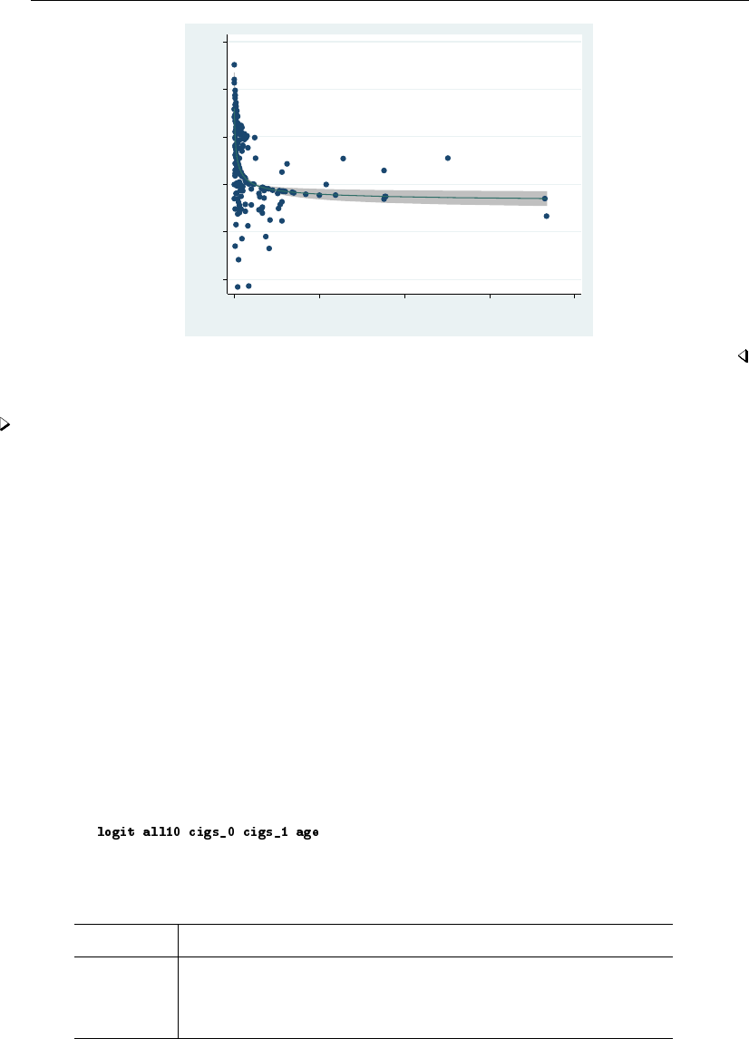
fp postestimation — Postestimation tools for fp 613
−2 −1 0 1 2 3
Component+residual of _t
0 100 200 300 400
Months since onset
Example 3: fp plot and fp predict after logistic regression
In example 3 of [R]fp, we used logistic regression to model the odds of death for male civil
servants in Britain conditional on cigarette consumption. The dependent variable all10 is an indicator
of whether the individual passed away in the 10 years under study.
Nonsmokers may be qualitatively different from smokers, so the effect of smoking (regarded as
a continuous variable) may not be continuous between zero cigarettes and one cigarette. To allow
for this possibility, we model the risk as constant intercept for the nonsmokers and as a fractional
polynomial function of the number of cigarettes for the smokers, cigs, adjusted for age. An FP1
model with power 0 is chosen.
We load the data and demean age. Then we fit the model using fp and graph the fit of the
model and 95% confidence interval using fp plot. Only the component fit is graphed by specifying
residuals(none).
. use http://www.stata-press.com/data/r13/smoking, clear
(Smoking and mortality data)
. quietly summarize age
. replace age = age - r(mean)
age was byte now float
(17260 real changes made)
. fp <cigs>, catzero replace fp(0): logit all10 <cigs> age
->
Logistic regression Number of obs = 17260
LR chi2(3) = 1027.13
Prob > chi2 = 0.0000
Log likelihood = -4973.3016 Pseudo R2 = 0.0936
all10 Coef. Std. Err. z P>|z| [95% Conf. Interval]
cigs_0 .1883732 .1553093 1.21 0.225 -.1160274 .4927738
cigs_1 .3469842 .0543552 6.38 0.000 .2404499 .4535185
age .1194976 .0045818 26.08 0.000 .1105174 .1284778
_cons -3.003767 .1514909 -19.83 0.000 -3.300683 -2.70685

614 fp postestimation — Postestimation tools for fp
. fp plot, residuals(none)
−3.5 −3 −2.5 −2 −1.5
Component
0 20 40 60
Daily cigarette consumption
We see a small spike at zero for cigs because of the effect of cigs 0 on the fractional polynomial;
however, the high p-value for cigs 0 in the model output indicates that we cannot reject that there
is no extra effect at zero for nonsmokers.
We can also use fp predict to predict the fractional polynomial for nonsmokers and the mean
of age. This is the value at the spike. We store the result in fp0. We see it is equivalent to the sum
of the constant intercept estimate and the estimate of the cigs 0 coefficient.
. fp predict fp0 if cigs == 0
(7157 missing values generated)
. summarize fp0
Variable Obs Mean Std. Dev. Min Max
fp0 10103 -2.815393 0 -2.815393 -2.815393
. display _b[cigs_0]+_b[_cons]
-2.8153935
Methods and formulas
Let the data consist of triplets (yi, xi,zi),i=1, . . . , n, where ziis the vector of covariates for
the ith observation and xiis the fractional polynomial variable.
fp predict calculates the fractional polynomial at the centering value x0,bηi= (xi(p1,...,pd)−
x0(p1,...,pm))0b
β. This is equivalent to the linear predictor of the model at zi=0. The standard error
is calculated from the variance–covariance matrix of b
β, ignoring estimation of the powers. When
xi≤0,H(xi), and thus xi(p1,...,pm), is either undefined or zero. A zero offset term, α0, may be
added to bηifor these nonpositive xivalues.
The values bηirepresent the behavior of the fractional polynomial model for xat fixed values
z=0of the (centered) covariates. The ith component-plus-residual is defined as bηi+di, where
diis the residual for the ith observation. The definition of diwill change according to the type of
model used and the preference of the user. fp plot plots bηi+diversus xi, overlaying bηiand its
confidence interval.

fp postestimation — Postestimation tools for fp 615
Acknowledgment
We thank Patrick Royston of the MRC Clinical Trials Unit, London, and coauthor of the Stata
Press book Flexible Parametric Survival Analysis Using Stata: Beyond the Cox Model for writing
fracplot and fracpred, the commands on which fp plot and fp predict are based. We also
thank Professor Royston for his advice on and review of fp plot and fp predict.
References
Becketti, S. 1995. sg26.2: Calculating and graphing fractional polynomials.Stata Technical Bulletin 24: 14–16.
Reprinted in Stata Technical Bulletin Reprints, vol. 4, pp. 129–132. College Station, TX: Stata Press.
Royston, P. 1995. sg26.3: Fractional polynomial utilities.Stata Technical Bulletin 25: 9–13. Reprinted in Stata Technical
Bulletin Reprints, vol. 5, pp. 82–87. College Station, TX: Stata Press.
Royston, P., and G. Ambler. 1999a. sg112: Nonlinear regression models involving power or exponential functions of
covariates.Stata Technical Bulletin 49: 25–30. Reprinted in Stata Technical Bulletin Reprints, vol. 9, pp. 173–179.
College Station, TX: Stata Press.
. 1999b. sg81.1: Multivariable fractional polynomials: Update.Stata Technical Bulletin 49: 17–23. Reprinted in
Stata Technical Bulletin Reprints, vol. 9, pp. 161–168. College Station, TX: Stata Press.
. 1999c. sg112.1: Nonlinear regression models involving power or exponential functions of covariates: Update.
Stata Technical Bulletin 50: 26. Reprinted in Stata Technical Bulletin Reprints, vol. 9, p. 180. College Station,
TX: Stata Press.
. 1999d. sg81.2: Multivariable fractional polynomials: Update.Stata Technical Bulletin 50: 25. Reprinted in Stata
Technical Bulletin Reprints, vol. 9, p. 168. College Station, TX: Stata Press.
Also see
[R]fp — Fractional polynomial regression
[U] 20 Estimation and postestimation commands

Title
frontier — Stochastic frontier models
Syntax Menu Description Options
Remarks and examples Stored results Methods and formulas References
Also see
Syntax
frontier depvar indepvars if in weight ,options
options Description
Model
noconstant suppress constant term
distribution(hnormal) half-normal distribution for the inefficiency term
distribution(exponential) exponential distribution for the inefficiency term
distribution(tnormal) truncated-normal distribution for the inefficiency term
ufrom(matrix)specify untransformed log likelihood; only with d(tnormal)
cm(varlist , noconstant )fit conditional mean model; only with d(tnormal); use
noconstant to suppress constant term
Model 2
constraints(constraints)apply specified linear constraints
collinear keep collinear variables
uhet(varlist , noconstant )explanatory variables for technical inefficiency variance
function; use noconstant to suppress constant term
vhet(varlist , noconstant )explanatory variables for idiosyncratic error variance
function; use noconstant to suppress constant term
cost fit cost frontier model; default is production frontier model
SE
vce(vcetype)vcetype may be oim,opg,bootstrap, or jackknife
Reporting
level(#)set confidence level; default is level(95)
nocnsreport do not display constraints
display options control column formats, row spacing, line width, display of omitted
variables and base and empty cells, and factor-variable labeling
Maximization
maximize options control the maximization process; seldom used
coeflegend display legend instead of statistics
indepvars and varlist may contain factor variables; see [U] 11.4.3 Factor variables.
bootstrap,by,fp,jackknife,rolling, and statsby are allowed; see [U] 11.1.10 Prefix commands.
Weights are not allowed with the bootstrap prefix; see [R] bootstrap.
fweights, iweights, and pweights are allowed; see [U] 11.1.6 weight.
coeflegend does not appear in the dialog box.
See [U] 20 Estimation and postestimation commands for more capabilities of estimation commands.
616

frontier — Stochastic frontier models 617
Menu
Statistics >Linear models and related >Frontier models
Description
frontier fits stochastic production or cost frontier models; the default is a production frontier
model. It provides estimators for the parameters of a linear model with a disturbance that is assumed
to be a mixture of two components, which have a strictly nonnegative and symmetric distribution,
respectively. frontier can fit models in which the nonnegative distribution component (a measurement
of inefficiency) is assumed to be from a half-normal, exponential, or truncated-normal distribution.
See Kumbhakar and Lovell (2000) for a detailed introduction to frontier analysis.
Options
Model
noconstant; see [R]estimation options.
distribution(distname)specifies the distribution for the inefficiency term as half-normal (hnormal),
exponential, or truncated-normal (tnormal). The default is hnormal.
ufrom(matrix)specifies a 1 ×Kmatrix of untransformed starting values when the distribution is
truncated-normal (tnormal). frontier can estimate the parameters of the model by maximizing
either the log likelihood or a transformed log likelihood (see Methods and formulas). frontier
automatically transforms the starting values before passing them on to the transformed log likelihood.
The matrix must have the same number of columns as there are parameters to estimate.
cm(varlist , noconstant )may be used only with distribution(tnormal). Here frontier
will fit a conditional mean model in which the mean of the truncated-normal distribution is modeled
as a linear function of the set of covariates specified in varlist. Specifying noconstant suppresses
the constant in the mean function.
Model 2
constraints(constraints),collinear; see [R]estimation options.
By default, when fitting the truncated-normal model or the conditional mean model, frontier
maximizes a transformed log likelihood. When constraints are applied, frontier will maximize
the untransformed log likelihood with constraints defined in the untransformed metric.
uhet(varlist, noconstant )specifies that the technical inefficiency component is heteroskedastic,
with the variance function depending on a linear combination of varlistu. Specifying noconstant
suppresses the constant term from the variance function. This option may not be specified with
distribution(tnormal).
vhet(varlist, noconstant )specifies that the idiosyncratic error component is heteroskedastic,
with the variance function depending on a linear combination of varlistv. Specifying noconstant
suppresses the constant term from the variance function. This option may not be specified with
distribution(tnormal).
cost specifies that frontier fit a cost frontier model.

618 frontier — Stochastic frontier models
SE
vce(vcetype)specifies the type of standard error reported, which includes types that are derived
from asymptotic theory (oim,opg) and that use bootstrap or jackknife methods (bootstrap,
jackknife); see [R]vce option.
Reporting
level(#); see [R]estimation options.
nocnsreport; see [R]estimation options.
display options:noomitted,vsquish,noemptycells,baselevels,allbaselevels,nofvla-
bel,fvwrap(#),fvwrapon(style),cformat(%fmt),pformat(% fmt),sformat(% fmt), and
nolstretch; see [R]estimation options.
Maximization
maximize options:difficult,technique(algorithm spec),iterate(#),nolog,trace,
gradient,showstep,hessian,showtolerance,tolerance(#),ltolerance(#),
nrtolerance(#),nonrtolerance, and from(init specs); see [R]maximize. These options are
seldom used.
Setting the optimization type to technique(bhhh) resets the default vcetype to vce(opg).
The following option is available with frontier but is not shown in the dialog box:
coeflegend; see [R]estimation options.
Remarks and examples
Stochastic production frontier models were introduced by Aigner, Lovell, and Schmidt (1977) and
Meeusen and van den Broeck (1977). Since then, stochastic frontier models have become a popular
subfield in econometrics. Kumbhakar and Lovell (2000) provide a good introduction.
frontier fits three stochastic frontier models with distinct parameterizations of the inefficiency
term and can fit stochastic production or cost frontier models.
Let’s review the nature of the stochastic frontier problem. Suppose that a producer has a production
function f(zi,β). In a world without error or inefficiency, the ith firm would produce
qi=f(zi,β)
Stochastic frontier analysis assumes that each firm potentially produces less than it might due to
a degree of inefficiency. Specifically,
qi=f(zi,β)ξi
where ξiis the level of efficiency for firm i;ξimust be in the interval (0,1]. If ξi=1, the firm
is achieving the optimal output with the technology embodied in the production function f(zi,β).
When ξi<1, the firm is not making the most of the inputs zigiven the technology embodied in the
production function f(zi,β). Because the output is assumed to be strictly positive (that is, qi>0),
the degree of technical efficiency is assumed to be strictly positive (that is, ξi>0).
Output is also assumed to be subject to random shocks, implying that
qi=f(zi,β)ξiexp(vi)

frontier — Stochastic frontier models 619
Taking the natural log of both sides yields
ln(qi) = lnf(zi,β)+ln(ξi) + vi
Assuming that there are kinputs and that the production function is linear in logs, defining
ui=−ln(ξi)yields
ln(qi) = β0+
k
X
j=1
βjln(zji) + vi−ui(1)
Because uiis subtracted from ln(qi), restricting ui≥0 implies that 0 < ξi≤1, as specified above.
Kumbhakar and Lovell (2000) provide a detailed version of the above derivation, and they show
that performing an analogous derivation in the dual cost function problem allows us to specify the
problem as
ln(ci) = β0+βqln(qi) +
k
X
j=1
βjln(pji) + vi+ui(2)
where qiis output, zji are input quantities, ciis cost, and the pji are input prices.
Intuitively, the inefficiency effect is required to lower output or raise expenditure, depending on the
specification.
Technical note
The model that frontier actually fits is of the form
yi=β0+
k
X
j=1
βjxji +vi−sui
where
s=1,for production functions
−1,for cost functions
so, in the context of the discussion above, yi=ln(qi), and xji =ln(zji)for a production function;
and for a cost function, yi=ln(ci), and the xji are the ln(pji)and ln(qi). You must take the
natural logarithm of the data before fitting a stochastic frontier production or cost model. frontier
performs no transformations on the data.
Different specifications of the uiand the viterms give rise to distinct models. frontier provides
estimators for the parameters of three basic models in which the idiosyncratic component, vi, is
assumed to be independently N(0, σv)distributed over the observations. The basic models differ in
their specification of the inefficiency term, ui, as follows:
exponential: the uiare independently exponentially distributed with variance σ2
u
hnormal: the uiare independently half-normally N+(0, σ2
u)distributed
tnormal: the uiare independently N+(µ, σ2
u)distributed with truncation point at 0
For half-normal or exponential distributions, frontier can fit models with heteroskedastic error
components, conditional on a set of covariates. For a truncated-normal distribution, frontier can
also fit a conditional mean model in which the mean is modeled as a linear function of a set of
covariates.

620 frontier — Stochastic frontier models
Example 1: The half-normal and the exponential models
For our first example, we demonstrate the half-normal and exponential models by reproducing a
study found in Greene (2003, 505), which uses data originally published in Zellner and Revankar (1969).
In this study of the transportation-equipment manufacturing industry, observations on value added,
capital, and labor are used to estimate a Cobb–Douglas production function. The variable lnv is the
log-transformed value added, lnk is the log-transformed capital, and lnl is the log-transformed labor.
OLS estimates are compared with those from stochastic frontier models using both the half-normal
and exponential distribution for the inefficiency term.
. use http://www.stata-press.com/data/r13/greene9
. regress lnv lnk lnl
Source SS df MS Number of obs = 25
F( 2, 22) = 397.54
Model 44.1727741 2 22.086387 Prob > F = 0.0000
Residual 1.22225984 22 .055557265 R-squared = 0.9731
Adj R-squared = 0.9706
Total 45.3950339 24 1.89145975 Root MSE = .23571
lnv Coef. Std. Err. t P>|t| [95% Conf. Interval]
lnk .2454281 .1068574 2.30 0.032 .0238193 .4670368
lnl .805183 .1263336 6.37 0.000 .5431831 1.067183
_cons 1.844416 .2335928 7.90 0.000 1.359974 2.328858
. frontier lnv lnk lnl
Iteration 0: log likelihood = 2.3357572
Iteration 1: log likelihood = 2.4673009
Iteration 2: log likelihood = 2.4695125
Iteration 3: log likelihood = 2.4695222
Iteration 4: log likelihood = 2.4695222
Stoc. frontier normal/half-normal model Number of obs = 25
Wald chi2(2) = 743.71
Log likelihood = 2.4695222 Prob > chi2 = 0.0000
lnv Coef. Std. Err. z P>|z| [95% Conf. Interval]
lnk .2585478 .098764 2.62 0.009 .0649738 .4521218
lnl .7802451 .1199399 6.51 0.000 .5451672 1.015323
_cons 2.081135 .281641 7.39 0.000 1.529128 2.633141
/lnsig2v -3.48401 .6195353 -5.62 0.000 -4.698277 -2.269743
/lnsig2u -3.014599 1.11694 -2.70 0.007 -5.203761 -.8254368
sigma_v .1751688 .0542616 .0954514 .3214633
sigma_u .2215073 .1237052 .074134 .6618486
sigma2 .0797496 .0426989 -.0039388 .163438
lambda 1.264536 .1678684 .9355204 1.593552
Likelihood-ratio test of sigma_u=0: chibar2(01) = 0.43 Prob>=chibar2 = 0.256
. predict double u_h, u

frontier — Stochastic frontier models 621
. frontier lnv lnk lnl, distribution(exponential)
Iteration 0: log likelihood = 2.7270659
Iteration 1: log likelihood = 2.8551532
Iteration 2: log likelihood = 2.8604815
Iteration 3: log likelihood = 2.8604897
Iteration 4: log likelihood = 2.8604897
Stoc. frontier normal/exponential model Number of obs = 25
Wald chi2(2) = 845.68
Log likelihood = 2.8604897 Prob > chi2 = 0.0000
lnv Coef. Std. Err. z P>|z| [95% Conf. Interval]
lnk .2624859 .0919988 2.85 0.004 .0821717 .4428002
lnl .7703795 .1109569 6.94 0.000 .5529079 .9878511
_cons 2.069242 .2356159 8.78 0.000 1.607444 2.531041
/lnsig2v -3.527598 .4486176 -7.86 0.000 -4.406873 -2.648324
/lnsig2u -4.002457 .9274575 -4.32 0.000 -5.820241 -2.184674
sigma_v .1713925 .0384448 .1104231 .2660258
sigma_u .1351691 .0626818 .0544692 .3354317
sigma2 .0476461 .0157921 .016694 .0785981
lambda .7886525 .087684 .616795 .9605101
Likelihood-ratio test of sigma_u=0: chibar2(01) = 1.21 Prob>=chibar2 = 0.135
. predict double u_e, u
. list state u_h u_e
state u_h u_e
1. Alabama .2011338 .14592865
2. California .14480966 .0972165
3. Connecticut .1903485 .13478797
4. Florida .51753139 .5903303
5. Georgia .10397912 .07140994
6. Illinois .12126696 .0830415
7. Indiana .21128212 .15450664
8. Iowa .24933153 .20073081
9. Kansas .10099517 .06857629
10. Kentucky .05626919 .04152443
11. Louisiana .20332731 .15066405
12. Maine .22263164 .17245793
13. Maryland .13534062 .09245501
14. Massachusetts .15636999 .10932923
15. Michigan .15809566 .10756915
16. Missouri .10288047 .0704146
17. NewJersey .09584337 .06587986
18. NewYork .27787793 .22249416
19. Ohio .22914231 .16981857
20. Pennsylvania .1500667 .10302905
21. Texas .20297875 .14552218
22. Virginia .14000132 .09676078
23. Washington .11047581 .07533251
24. WestVirginia .15561392 .11236153
25. Wisconsin .14067066 .0970861

622 frontier — Stochastic frontier models
The parameter estimates and the estimates of the inefficiency terms closely match those published in
Greene (2003, 505), but the standard errors of the parameter estimates are estimated differently (see
the technical note below).
The output from frontier includes estimates of the standard deviations of the two error components,
σvand σu, which are labeled sigma v and sigma u, respectively. In the log likelihood, they are
parameterized as lnσ2
vand lnσ2
u, and these estimates are labeled /lnsig2v and /lnsig2u in the
output. frontier also reports two other useful parameterizations. The estimate of the total error
variance, σ2
S=σ2
v+σ2
u, is labeled sigma2, and the estimate of the ratio of the standard deviation
of the inefficiency component to the standard deviation of the idiosyncratic component, λ=σu/σv,
is labeled lambda.
At the bottom of the output, frontier reports the results of a test that there is no technical
inefficiency component in the model. This is a test of the null hypothesis H0:σ2
u=0 against
the alternative hypotheses H1:σ2
u>0. If the null hypothesis is true, the stochastic frontier model
reduces to an OLS model with normal errors. However, because the test lies on the boundary of the
parameter space of σ2
u, the standard likelihood-ratio test is not valid, and a one-sided generalized
likelihood-ratio test must be constructed; see Gutierrez, Carter, and Drukker (2001). For this example,
the output shows LR = 0.43 with a p-value of 0.256 for the half-normal model and LR = 1.21 with
ap-value of 0.135 for the exponential model. There are several possible reasons for the failure to
reject the null hypothesis, but the fact that the test is based on an asymptotic distribution and the
sample size was 25 is certainly a leading candidate among those possibilities.
Technical note
frontier maximizes the log-likelihood function of a stochastic frontier model by using the
Newton–Raphson method, and the estimated variance–covariance matrix is calculated as the inverse
of the negative Hessian (matrix of second partial derivatives); see [R]ml. When comparing the results
with those published using other software, be aware of the difference in the optimization methods,
which may result in different, yet asymptotically equivalent, variance estimates.
Example 2: Models with heteroskedasticity
Often the error terms may not have constant variance. frontier allows you to model heteroskedas-
ticity in either error term as a linear function of a set of covariates. The variance of either the technical
inefficiency or the idiosyncratic component may be modeled as
σ2
i= exp(wiδ)
The default constant included in wimay be suppressed by appending a noconstant option to the
list of covariates. Also, you can simultaneously specify covariates for both σuiand σvi.
In this example, we use a sample of 756 observations of fictional firms producing a manufactured
good by using capital and labor. The firms are hypothesized to use a constant returns-to-scale technology,
but the sizes of the firms differ. Believing that this size variation will introduce heteroskedasticity
into the idiosyncratic error term, we estimate the parameters of a Cobb–Douglas production function.
To do this, we use a conditional heteroskedastic half-normal model, with the size of the firm as an
explanatory variable in the variance function for the idiosyncratic error. We also perform a test of the
hypothesis that the firms use a constant returns-to-scale technology.

frontier — Stochastic frontier models 623
. use http://www.stata-press.com/data/r13/frontier1, clear
. frontier lnoutput lnlabor lncapital, vhet(size)
Iteration 0: log likelihood = -1508.3692
Iteration 1: log likelihood = -1501.583
Iteration 2: log likelihood = -1500.3942
Iteration 3: log likelihood = -1500.3794
Iteration 4: log likelihood = -1500.3794
Stoc. frontier normal/half-normal model Number of obs = 756
Wald chi2(2) = 9.68
Log likelihood = -1500.3794 Prob > chi2 = 0.0079
lnoutput Coef. Std. Err. z P>|z| [95% Conf. Interval]
lnoutput
lnlabor .7090933 .2349374 3.02 0.003 .2486244 1.169562
lncapital .3931345 .5422173 0.73 0.468 -.6695919 1.455861
_cons 1.252199 3.14656 0.40 0.691 -4.914946 7.419344
lnsig2v
size -.0016951 .0004748 -3.57 0.000 -.0026256 -.0007645
_cons 3.156091 .9265826 3.41 0.001 1.340023 4.97216
lnsig2u
_cons 1.947487 .1017653 19.14 0.000 1.748031 2.146943
sigma_u 2.647838 .134729 2.396514 2.925518
. test _b[lnlabor] + _b[lncapital] = 1
( 1) [lnoutput]lnlabor + [lnoutput]lncapital = 1
chi2( 1) = 0.03
Prob > chi2 = 0.8622
The output above indicates that the variance of the idiosyncratic error term is a function of firm size.
Also, we failed to reject the hypothesis that the firms use a constant returns-to-scale technology.
Technical note
In small samples, the conditional heteroskedastic estimators will lack precision for the variance
parameters and may fail to converge altogether.
Example 3: The truncated-normal model
Let’s turn our attention to the truncated-normal model. Once again, we will use fictional data. For
this example, we have 1,231 observations on the quantity of output, the total cost of production for
each firm, the prices that each firm paid for labor and capital services, and a categorical variable
measuring the quality of each firm’s management. After taking the natural logarithm of the costs
(lncost), prices (lnp k and lnp l), and output (lnout), we fit a stochastic cost frontier model
and specify the distribution for the inefficiency term to be truncated normal.

624 frontier — Stochastic frontier models
. use http://www.stata-press.com/data/r13/frontier2
. frontier lncost lnp_k lnp_l lnout, distribution(tnormal) cost
Iteration 0: log likelihood = -2386.9523
Iteration 1: log likelihood = -2386.5146
Iteration 2: log likelihood = -2386.2704
Iteration 3: log likelihood = -2386.2504
Iteration 4: log likelihood = -2386.2493
Iteration 5: log likelihood = -2386.2493
Stoc. frontier normal/truncated-normal model Number of obs = 1231
Wald chi2(3) = 8.82
Log likelihood = -2386.2493 Prob > chi2 = 0.0318
lncost Coef. Std. Err. z P>|z| [95% Conf. Interval]
lnp_k .3410717 .2363861 1.44 0.149 -.1222366 .80438
lnp_l .6608628 .4951499 1.33 0.182 -.3096131 1.631339
lnout .7528653 .3468968 2.17 0.030 .0729601 1.432771
_cons 2.602609 1.083004 2.40 0.016 .4799595 4.725259
/mu 1.095705 .881517 1.24 0.214 -.632037 2.823446
/lnsigma2 1.5534 .1873464 8.29 0.000 1.186208 1.920592
/ilgtgamma 1.257862 .2589522 4.86 0.000 .7503255 1.765399
sigma2 4.727518 .8856833 3.274641 6.825001
gamma .7786579 .0446303 .6792496 .8538846
sigma_u2 3.681119 .7503408 2.210478 5.15176
sigma_v2 1.046399 .2660035 .5250413 1.567756
H0: No inefficiency component: z = 5.595 Prob>=z = 0.000
In addition to the coefficients, the output reports estimates for several parameters. sigma v2 is the
estimate of σ2
v.sigma u2 is the estimate of σ2
u.gamma is the estimate of γ=σ2
u/σ2
S.sigma2 is the
estimate of σ2
S=σ2
v+σ2
u. Because γmust be between 0 and 1, the optimization is parameterized
in terms of the inverse logit of γ, and this estimate is reported as ilgtgamma. Because σ2
Smust
be positive, the optimization is parameterized in terms of ln(σ2
S), whose estimate is reported as
lnsigma2. Finally, mu is the estimate of µ, the mean of the truncated-normal distribution.
In the output above, the generalized log-likelihood test for the presence of the inefficiency term
has been replaced with a test based on the third moment of the OLS residuals. When µ=0 and
σu=0, the truncated-normal model reduces to a linear regression model with normally distributed
errors. However, the distribution of the test statistic under the null hypothesis is not well established,
because it becomes impossible to evaluate the log likelihood as σuapproaches zero, prohibiting the
use of the likelihood-ratio test.
However, Coelli (1995) noted that the presence of an inefficiency term would negatively skew the
residuals from an OLS regression. By identifying negative skewness in the residuals with the presence
of an inefficiency term, Coelli derived a one-sided test for the presence of the inefficiency term. The
results of this test are given at the bottom of the output. For this example, the null hypothesis of no
inefficiency component is rejected.
In the example below, we fit a truncated model and detect a statistically significant inefficiency
term in the model. We might question whether the inefficiency term is identically distributed over
all firms or whether there might be heterogeneity across firms. frontier provides an extension
to the truncated normal model by allowing the mean of the inefficiency term to be modeled as a
linear function of a set of covariates. In our dataset, we have a categorical variable that measures the
quality of a firm’s management. We refit the model, including the cm() option, specifying a set of

frontier — Stochastic frontier models 625
binary indicator variables representing the different categories of the quality-measurement variable as
covariates.
. frontier lncost lnp_k lnp_l lnout, distribution(tnormal) cm(i.quality) cost
Iteration 0: log likelihood = -2386.9523
Iteration 1: log likelihood = -2384.936
Iteration 2: log likelihood = -2382.3942
Iteration 3: log likelihood = -2382.324
Iteration 4: log likelihood = -2382.3233
Iteration 5: log likelihood = -2382.3233
Stoc. frontier normal/truncated-normal model Number of obs = 1231
Wald chi2(3) = 9.31
Log likelihood = -2382.3233 Prob > chi2 = 0.0254
lncost Coef. Std. Err. z P>|z| [95% Conf. Interval]
lncost
lnp_k .3611204 .2359749 1.53 0.126 -.1013819 .8236227
lnp_l .680446 .4934935 1.38 0.168 -.2867835 1.647675
lnout .7605533 .3466102 2.19 0.028 .0812098 1.439897
_cons 2.550769 1.078911 2.36 0.018 .4361417 4.665396
mu
quality
2 .5056067 .3382907 1.49 0.135 -.1574309 1.168644
3 .783223 .376807 2.08 0.038 .0446947 1.521751
4 .5577511 .3355061 1.66 0.096 -.0998288 1.215331
5 .6792882 .3428073 1.98 0.048 .0073981 1.351178
_cons .6014025 .990167 0.61 0.544 -1.339289 2.542094
/lnsigma2 1.541784 .1790926 8.61 0.000 1.190769 1.892799
/ilgtgamma 1.242302 .2588968 4.80 0.000 .734874 1.749731
sigma2 4.67292 .8368852 3.289611 6.637923
gamma .7759645 .0450075 .6758739 .8519189
sigma_u2 3.62602 .7139576 2.226689 5.025351
sigma_v2 1.0469 .2583469 .5405491 1.553251
The conditional mean model was developed in the context of panel-data estimators, and we can
apply frontier’s conditional mean model to panel data.

626 frontier — Stochastic frontier models
Stored results
frontier stores the following in e():
Scalars
e(N) number of observations
e(df m) model degrees of freedom
e(k) number of parameters
e(k eq) number of equations in e(b)
e(k eq model) number of equations in overall model test
e(k dv) number of dependent variables
e(chi2) χ2
e(ll) log likelihood
e(ll c) log likelihood for H0:σu=0
e(z) test for negative skewness of OLS residuals
e(sigma u) standard deviation of technical inefficiency
e(sigma v) standard deviation of vi
e(p) significance
e(chi2 c) LR test statistic
e(p z) p-value for z
e(rank) rank of e(V)
e(ic) number of iterations
e(rc) return code
e(converged) 1 if converged, 0otherwise
Macros
e(cmd) frontier
e(cmdline) command as typed
e(depvar) name of dependent variable
e(function) production or cost
e(wtype) weight type
e(wexp) weight expression
e(title) title in estimation output
e(chi2type) Wald; type of model χ2test
e(dist) distribution assumption for ui
e(het) heteroskedastic components
e(u hetvar) varlist in uhet()
e(v hetvar) varlist in vhet()
e(vce) vcetype specified in vce()
e(vcetype) title used to label Std. Err.
e(opt) type of optimization
e(which) max or min; whether optimizer is to perform maximization or minimization
e(ml method) type of ml method
e(user) name of likelihood-evaluator program
e(technique) maximization technique
e(properties) b V
e(predict) program used to implement predict
e(asbalanced) factor variables fvset as asbalanced
e(asobserved) factor variables fvset as asobserved

frontier — Stochastic frontier models 627
Matrices
e(b) coefficient vector
e(Cns) constraints matrix
e(ilog) iteration log (up to 20 iterations)
e(gradient) gradient vector
e(V) variance–covariance matrix of the estimators
e(V modelbased) model-based variance
Functions
e(sample) marks estimation sample
Methods and formulas
Consider an equation of the form
yi=xiβ+vi−sui
where yiis the dependent variable, xiis a 1×kvector of observations on the independent variables
included as indent covariates, βis a k×1vector of coefficients, and
s=1,for production functions
−1,for cost functions
The log-likelihood functions are as follows.
Normal/half-normal model:
lnL=
N
X
i=1 1
2ln 2
π−lnσS+lnΦ−siλ
σS−2
i
2σ2
S
Normal/exponential model:
lnL=
N
X
i=1
−lnσu+σ2
v
2σ2
u
+lnΦ
−si−σ2
v
σu
σv
+si
σu
Normal/truncated-normal model:
lnL=
N
X
i=1 −1
2ln (2π)−lnσS−lnΦµ
σS√γ
+lnΦ"(1 −γ)µ−sγi
{σ2
Sγ(1 −γ)}1/2#−1
2i+sµ
σS2)

628 frontier — Stochastic frontier models
where σS= (σ2
u+σ2
v)1/2,λ=σu/σv,γ=σ2
u/σ2
S,i=yi−xiβ, and Φ() is the cumulative
distribution function of the standard normal distribution.
To obtain estimation for ui, you can use either the mean or the mode of the conditional distribution
f(u|).
E(ui|i) = µ∗i+σ∗φ(−µ∗i/σ∗)
Φ(µ∗i/σ∗)
M(ui|i) = nµ∗iif µ∗i≥0
0otherwise
Then the technical efficiency (s=1) or cost efficiency (s=−1) will be estimated by
Ei=E{exp(−sui)|i}
=1−Φ (sσ∗−µ∗i/σ∗)
1−Φ (−µ∗i/σ∗)exp −sµ∗i+1
2σ2
∗
where µ∗iand σ∗are defined for the normal/half-normal model as
µ∗i=−siσ2
u/σ2
S
σ∗=σuσv/σS
for the normal/exponential model as
µ∗i=−si−σ2
v/σu
σ∗=σv
and for the normal/truncated-normal model as
µ∗i=−siσ2
u+µσ2
v
σ2
S
σ∗=σuσv/σS
In the half-normal and exponential models, when heteroskedasticity is assumed, the standard
deviations, σuor σv, will be replaced in the above equations by
σ2
i= exp(wiδ)
where wis the vector of explanatory variables in the variance function.
In the conditional mean model, the mean parameter of the truncated normal distribution, µ, is
modeled as a linear combination of the set of covariates, w.
µ=wiδ

frontier — Stochastic frontier models 629
Therefore, the log-likelihood function can be rewritten as
lnL=
N
X
i=1 "−1
2ln (2π)−lnσS−lnΦ wiδ
pσ2
Sγ!
+lnΦ((1 −γ)wiδ−sγi
pσ2
Sγ(1 −γ))−1
2i+swiδ
σS2#
The ztest reported in the output of the truncated-normal model is a third-moment test developed by
Coelli (1995) as an extension of a test previously developed by Pagan and Hall (1983). Coelli shows
that under the null of normally distributed errors, the statistic
z=m3
6m3
2
N1/2
has a standard normal distribution, where m3is the third moment from the OLS regression. Because
the residuals are either negatively skewed (production function) or positively skewed (cost function),
a one-sided p-value is used.
References
Aigner, D. J., C. A. K. Lovell, and P. Schmidt. 1977. Formulation and estimation of stochastic frontier production
function models. Journal of Econometrics 6: 21–37.
Belotti, F., S. Daidone, G. Ilardi, and V. Atella. 2013. Stochastic frontier analysis using Stata.Stata Journal 13:
719–758.
Caudill, S. B., J. M. Ford, and D. M. Gropper. 1995. Frontier estimation and firm-specific inefficiency measures in
the presence of heteroscedasticity. Journal of Business and Economic Statistics 13: 105–111.
Coelli, T. J. 1995. Estimators and hypothesis tests for a stochastic frontier function: A Monte Carlo analysis. Journal
of Productivity Analysis 6: 247–268.
Gould, W. W., J. S. Pitblado, and B. P. Poi. 2010. Maximum Likelihood Estimation with Stata. 4th ed. College
Station, TX: Stata Press.
Greene, W. H. 2003. Econometric Analysis. 5th ed. Upper Saddle River, NJ: Prentice Hall.
Gutierrez, R. G., S. L. Carter, and D. M. Drukker. 2001. sg160: On boundary-value likelihood-ratio tests.Stata
Technical Bulletin 60: 15–18. Reprinted in Stata Technical Bulletin Reprints, vol. 10, pp. 269–273. College Station,
TX: Stata Press.
Kumbhakar, S. C., and C. A. K. Lovell. 2000. Stochastic Frontier Analysis. Cambridge: Cambridge University Press.
Meeusen, W., and J. van den Broeck. 1977. Efficiency estimation from Cobb–Douglas production functions with
composed error. International Economic Review 18: 435–444.
Pagan, A. R., and A. D. Hall. 1983. Diagnostic tests as residual analysis. Econometric Reviews 2: 159–218.
Petrin, A. K., B. P. Poi, and J. A. Levinsohn. 2004. Production function estimation in Stata using inputs to control
for unobservables.Stata Journal 4: 113–123.
Stevenson, R. E. 1980. Likelihood functions for generalized stochastic frontier estimation. Journal of Econometrics
13: 57–66.
Tauchmann, H. 2012. Partial frontier efficiency analysis.Stata Journal 12: 461–478.
Zellner, A., and N. S. Revankar. 1969. Generalized production functions. Review of Economic Studies 36: 241–250.


Title
frontier postestimation — Postestimation tools for frontier
Description Syntax for predict Menu for predict Options for predict
Remarks and examples Reference Also see
Description
The following postestimation commands are available after frontier:
Command Description
contrast contrasts and ANOVA-style joint tests of estimates
estat ic Akaike’s and Schwarz’s Bayesian information criteria (AIC and BIC)
estat summarize summary statistics for the estimation sample
estat vce variance–covariance matrix of the estimators (VCE)
estimates cataloging estimation results
lincom point estimates, standard errors, testing, and inference for linear combinations
of coefficients
linktest link test for model specification
lrtest likelihood-ratio test
margins marginal means, predictive margins, marginal effects, and average marginal
effects
marginsplot graph the results from margins (profile plots, interaction plots, etc.)
nlcom point estimates, standard errors, testing, and inference for nonlinear combinations
of coefficients
predict predictions, residuals, influence statistics, and other diagnostic measures
predictnl point estimates, standard errors, testing, and inference for generalized predictions
pwcompare pairwise comparisons of estimates
test Wald tests of simple and composite linear hypotheses
testnl Wald tests of nonlinear hypotheses
Syntax for predict
predict type newvar if in ,statistic
predict type stub*|newvarxb newvarvnewvaru if in , scores
631

632 frontier postestimation — Postestimation tools for frontier
statistic Description
Main
xb linear prediction; the default
stdp standard error of the prediction
uestimates of minus the natural log of the technical efficiency via E(ui|i)
mestimates of minus the natural log of the technical efficiency via M(ui|i)
te estimates of the technical efficiency via E{exp(−sui)|i}
s=1,for production functions
−1,for cost functions
These statistics are available both in and out of sample; type predict . . . if e(sample) . . . if wanted only for
the estimation sample.
Menu for predict
Statistics >Postestimation >Predictions, residuals, etc.
Options for predict
Main
xb, the default, calculates the linear prediction.
stdp calculates the standard error of the linear prediction.
uproduces estimates of minus the natural log of the technical efficiency via E(ui|i).
mproduces estimates of minus the natural log of the technical efficiency via M(ui|i).
te produces estimates of the technical efficiency via E{exp(−sui)|i}.
scores calculates equation-level score variables.
The first new variable will contain ∂ln L/∂(xiβ).
The second new variable will contain ∂ln L/∂(lnsig2v).
The third new variable will contain ∂ln L/∂(lnsig2u).
Remarks and examples
Example 1
In example 2 of [R]frontier, we modeled heteroskedasticity by specifying the vhet() option. We
would like to compare the predicted efficiency in that case with respect to a model specification without
accounting for the presence of heteroskedasticity in the error term. Kumbhakar and Lovell (2000,
117) show that failing to account for heteroskedasticity associated with firm size may lead to bias in
the estimation of the technical efficiency. By incorrectly assuming homoskedasticity, the estimates for
relatively small firms would be biased upward, while the estimates for relatively large firms would
be biased downward. Let’s refit the model and use the te option of predict:
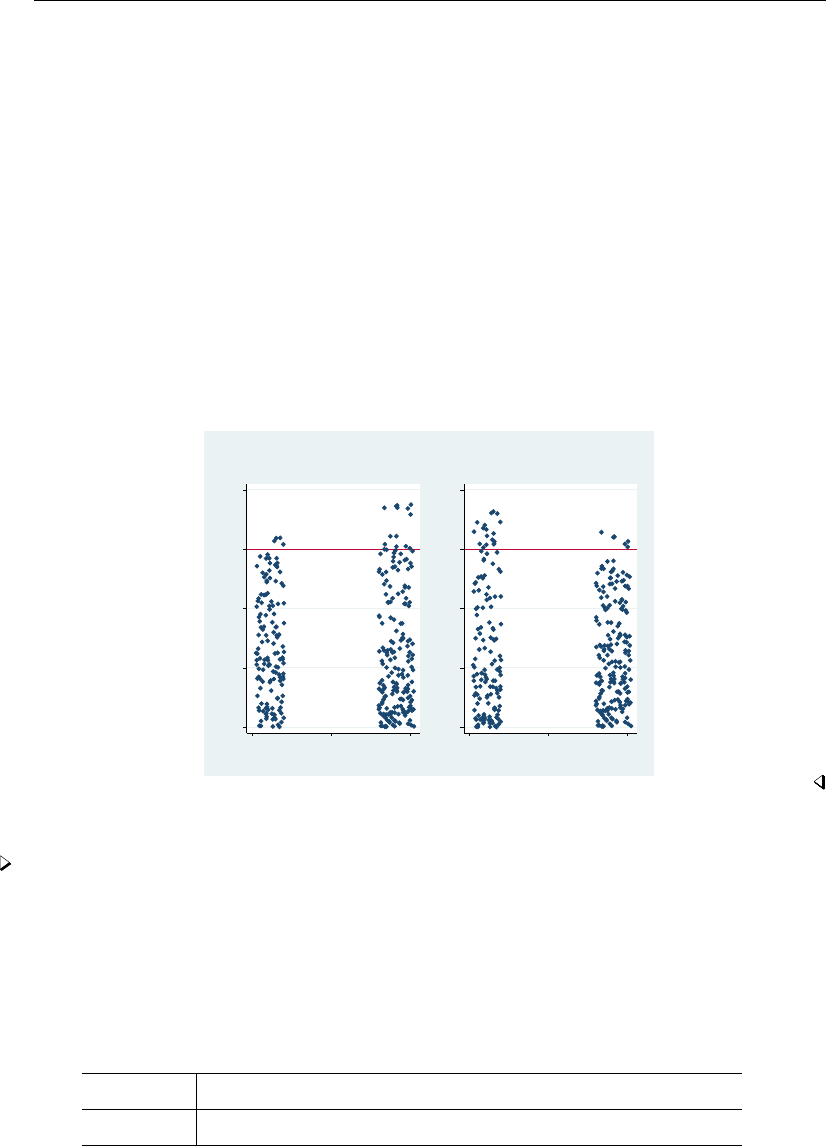
frontier postestimation — Postestimation tools for frontier 633
. use http://www.stata-press.com/data/r13/frontier1
. frontier lnoutput lnlabor lncapital, vhet(size)
(output omitted )
. predict te_vhet, te
Next we fit the model assuming homoskedasticity and then again predict the technical efficiency
with the te option of predict:
. frontier lnoutput lnlabor lncapital
(output omitted )
. predict te, te
The graph below shows the estimates for technical efficiency for the smaller and larger firms. The
technical efficiency tends to be smaller for smaller firms when the model specification accounts for the
presence of heteroskedasticity, whereas the predictions for the technical efficiency tends to be smaller
for larger firms assuming homoskedasticity. These results agree with the theoretical statement in
Kumbhakar and Lovell (2000) because the firm size was actually relevant to model heteroskedasticity
in the idiosyncratic component of the error term.
0 .2 .4 .6 .8
te_vhet
1500 2000 2500
firm size
Modeling heteroskedasticity
0 .2 .4 .6 .8
te
1500 2000 2500
firm size
Assuming homoskedasticity
Predicted technical efficiency for smaller and larger firms
Example 2
We also test in example 2 of [R]frontier whether the firms use constant returns to scale. We can
use lincom as an alternative to perform an equivalent test based on the normal distribution.
. use http://www.stata-press.com/data/r13/frontier1, clear
. frontier lnoutput lnlabor lncapital, vhet(size)
(output omitted )
. lincom _b[lnlabor] + _b[lncapital]-1
( 1) [lnoutput]lnlabor + [lnoutput]lncapital = 1
lnoutput Coef. Std. Err. z P>|z| [95% Conf. Interval]
(1) .1022278 .5888511 0.17 0.862 -1.051899 1.256355

634 frontier postestimation — Postestimation tools for frontier
The p-value is exactly the same as the one we obtained with the test command in example 2 of
[R]frontier. However, notice that by using lincom, we obtained an estimate of the deviation from
the constant returns-to-scale assumption, which is not significantly different from zero in this case.
Reference
Kumbhakar, S. C., and C. A. K. Lovell. 2000. Stochastic Frontier Analysis. Cambridge: Cambridge University Press.
Also see
[R]frontier — Stochastic frontier models
[U] 20 Estimation and postestimation commands

Title
fvrevar — Factor-variables operator programming command
Syntax Description Options Remarks and examples
Stored results Also see
Syntax
fvrevar varlist if in , substitute tsonly list stub(stub)
You must tsset your data before using fvrevar if varlist contains time-series operators; see [TS] tsset.
Description
fvrevar creates an equivalent, temporary variable list for a varlist that might contain factor
variables, interactions, or time-series–operated variables so that the resulting variable list can be used
by commands that do not otherwise support factor variables or time-series–operated variables. The
resulting list also could be used in a program to speed execution at the cost of using more memory.
Options
substitute specifies that equivalent, temporary variables be substituted for any factor variables,
interactions, or time-series–operated variables in varlist.substitute is the default action taken
by fvrevar; you do not need to specify the option.
tsonly specifies that equivalent, temporary variables be substituted for only the time-series–operated
variables in varlist.
list specifies that all factor-variable operators and time-series operators be removed from varlist
and the resulting list of base variables be returned in r(varlist). No new variables are created
with this option.
stub(stub)specifies that fvrevar generate named variables instead of temporary variables. The
new variables will be named stub#.
Remarks and examples
fvrevar might create no new variables, one new variable, or many new variables, depending on
the number of factor variables, interactions, and time-series operators appearing in varlist. Any new
variables created are temporary. The new, equivalent varlist is returned in r(varlist). The new
varlist corresponds one to one with the original varlist.
Example 1
Typing
. use http://www.stata-press.com/data/r13/auto2
. fvrevar i.rep78 mpg turn
635

636 fvrevar — Factor-variables operator programming command
creates five temporary variables corresponding to the levels of rep78. No new variables are created
for variables mpg and turn because they do not contain factor-variable or time-series operators.
The resulting variable list is
. display "‘r(varlist)’"
000000 000001 000002 000003 000004 mpg turn
(Your temporary variable names may be different, but that is of no consequence.)
Temporary variables automatically vanish when the program concludes.
Example 2
Suppose we want to create temporary variables for specific levels of a factor variable. To do this,
we can use the parenthesis notation of factor-variable syntax.
. fvrevar i(2,3)bn.rep78 mpg
creates two temporary variables corresponding to levels 2 and 3 of rep78. Notice that we specified
that neither level 2 nor 3 be set as the base level by using the bn notation. If we did not specify bn,
level 2 would have been treated as the base level.
The resulting variable list is
. display "‘r(varlist)’"
000005 000002 mpg
We can see the results by listing the new variables alongside the original value of rep78.
. list rep78 ‘r(varlist)’ in 1/5
rep78 __000005 __000002 mpg
1. Average 0 1 22
2. Average 0 1 17
3. . . . 22
4. Average 0 1 20
5. Good 0 0 15
If we had needed only the base-variable names, we could have specified
. fvrevar i(2,3)bn.rep78 mpg, list
. display "‘r(varlist)’"
mpg rep78
The order of the list will probably differ from that of the original list; base variables are listed only
once.
Example 3
Now let’s assume we have a varlist containing both an interaction and time-series–operated variables.
If we want to create temporary variables for the entire equivalent varlist, we can specify fvrevar
with no options.

fvrevar — Factor-variables operator programming command 637
. generate t = _n
. tsset t
time variable: t, 1 to 74
delta: 1 unit
. fvrevar c.turn#i(2,3).rep78 L.mpg
The resulting variable list is
. display "‘r(varlist)’"
000006 000007 000008
If we want to create temporary variables only for the time-series–operated variables, we can specify
the tsonly option.
. fvrevar c.turn#i(2,3).rep78 L.mpg, tsonly
The resulting variable list is
. display "‘r(varlist)’"
c.turn#2b.rep78 c.turn#3.rep78 000008
Notice that fvrevar returned the expanded factor-variable list with the tsonly option.
Technical note
fvrevar, substitute avoids creating duplicate variables. Consider
. fvrevar i.rep78 turn mpg i.rep78
i.rep78 appears twice in the varlist. fvrevar will create only one set of new variables for the
five levels of rep78 and will use these new variables once in the resulting r(varlist). Moreover,
fvrevar will do this even across multiple calls:
. fvrevar i.rep78 turn mpg
. fvrevar i.rep78
i.rep78 appears in two separate calls. At the first call, fvrevar creates five temporary variables
corresponding to the five levels of rep78. At the second call, fvrevar remembers what it has done
and uses the same temporary variables for i.rep78.
Stored results
fvrevar stores the following in r():
Macros
r(varlist) the modified variable list or list of base-variable names
Also see
[TS]tsrevar — Time-series operator programming command
[P]syntax — Parse Stata syntax
[P]unab — Unabbreviate variable list
[U] 11 Language syntax
[U] 11.4.4 Time-series varlists
[U] 18 Programming Stata

Title
fvset — Declare factor-variable settings
Syntax Description Options Remarks and examples Stored results
Syntax
Declare base settings
fvset base base spec varlist
Declare design settings
fvset design design spec varlist
Clear the current settings
fvset clear varlist
Report the current settings
fvset report varlist , base(base spec) design(design spec)
base spec Description
default default base
first lowest level value; the default
last highest level value
frequent most frequent level value
none no base
#nonnegative integer value
design spec Description
default default base
asbalanced accumulate using 1/k,k=number of levels
asobserved accumulate using observed relative frequencies; the default
Description
fvset declares factor-variable settings. Factor-variable settings identify the base level and how to
accumulate statistics over levels.
fvset base specifies the base level for each variable in varlist. The default for factor variables
without a declared base level is first.
638

fvset — Declare factor-variable settings 639
fvset design specifies how to accumulate over the levels of a factor variable. The margins
command is the only command aware of this setting; see [R]margins. By default, margins assumes
that factor variables are asobserved, meaning that they are accumulated by weighting by the number
of observations or the sum of the weights if weights have been specified.
fvset clear removes factor-variable settings for each variable in varlist.fvset clear all
removes all factor-variable settings from all variables.
fvset report reports the current factor-variable settings for each variable in varlist.fvset
without arguments is a synonym for fvset report.
Options
base(base spec)restricts fvset report to report only the factor-variable settings for variables with
the specified base spec.
design(design spec)restricts fvset report to report only the factor-variable settings for variables
with the specified design spec.
Remarks and examples
Example 1
Using auto2.dta, we include factor variable i.rep78 in a regression:
. use http://www.stata-press.com/data/r13/auto2
(1978 Automobile Data)
. regress mpg i.rep78, baselevels
Source SS df MS Number of obs = 69
F( 4, 64) = 4.91
Model 549.415777 4 137.353944 Prob > F = 0.0016
Residual 1790.78712 64 27.9810488 R-squared = 0.2348
Adj R-squared = 0.1869
Total 2340.2029 68 34.4147485 Root MSE = 5.2897
mpg Coef. Std. Err. t P>|t| [95% Conf. Interval]
rep78
Poor 0 (base)
Fair -1.875 4.181884 -0.45 0.655 -10.22927 6.479274
Average -1.566667 3.863059 -0.41 0.686 -9.284014 6.150681
Good .6666667 3.942718 0.17 0.866 -7.209818 8.543152
Excellent 6.363636 4.066234 1.56 0.123 -1.759599 14.48687
_cons 21 3.740391 5.61 0.000 13.52771 28.47229
We specified the baselevels option so that the base level would be included in the output. By
default, the first level is the base level. We can change the base level to 2:

640 fvset — Declare factor-variable settings
. fvset base 2 rep78
. regress mpg i.rep78, baselevels
Source SS df MS Number of obs = 69
F( 4, 64) = 4.91
Model 549.415777 4 137.353944 Prob > F = 0.0016
Residual 1790.78712 64 27.9810488 R-squared = 0.2348
Adj R-squared = 0.1869
Total 2340.2029 68 34.4147485 Root MSE = 5.2897
mpg Coef. Std. Err. t P>|t| [95% Conf. Interval]
rep78
Poor 1.875 4.181884 0.45 0.655 -6.479274 10.22927
Fair 0 (base)
Average .3083333 2.104836 0.15 0.884 -3.896559 4.513226
Good 2.541667 2.247695 1.13 0.262 -1.948621 7.031954
Excellent 8.238636 2.457918 3.35 0.001 3.32838 13.14889
_cons 19.125 1.870195 10.23 0.000 15.38886 22.86114
Let’s set rep78 to have no base level and fit a cell-means regression:
. fvset base none rep78
. regress mpg i.rep78, noconstant
Source SS df MS Number of obs = 69
F( 5, 64) = 227.47
Model 31824.2129 5 6364.84258 Prob > F = 0.0000
Residual 1790.78712 64 27.9810488 R-squared = 0.9467
Adj R-squared = 0.9426
Total 33615 69 487.173913 Root MSE = 5.2897
mpg Coef. Std. Err. t P>|t| [95% Conf. Interval]
rep78
Poor 21 3.740391 5.61 0.000 13.52771 28.47229
Fair 19.125 1.870195 10.23 0.000 15.38886 22.86114
Average 19.43333 .9657648 20.12 0.000 17.504 21.36267
Good 21.66667 1.246797 17.38 0.000 19.1759 24.15743
Excellent 27.36364 1.594908 17.16 0.000 24.17744 30.54983
Example 2
By default, margins accumulates a margin by using the observed relative frequencies of the factor
levels.
. regress mpg i.foreign
Source SS df MS Number of obs = 74
F( 1, 72) = 13.18
Model 378.153515 1 378.153515 Prob > F = 0.0005
Residual 2065.30594 72 28.6848048 R-squared = 0.1548
Adj R-squared = 0.1430
Total 2443.45946 73 33.4720474 Root MSE = 5.3558
mpg Coef. Std. Err. t P>|t| [95% Conf. Interval]
foreign
Foreign 4.945804 1.362162 3.63 0.001 2.230384 7.661225
_cons 19.82692 .7427186 26.70 0.000 18.34634 21.30751

fvset — Declare factor-variable settings 641
. margins
Predictive margins Number of obs = 74
Model VCE : OLS
Expression : Linear prediction, predict()
Delta-method
Margin Std. Err. t P>|t| [95% Conf. Interval]
_cons 21.2973 .6226014 34.21 0.000 20.05616 22.53843
Let’s set foreign to always accumulate using equal relative frequencies:
. fvset design asbalanced foreign
. regress mpg i.foreign
Source SS df MS Number of obs = 74
F( 1, 72) = 13.18
Model 378.153515 1 378.153515 Prob > F = 0.0005
Residual 2065.30594 72 28.6848048 R-squared = 0.1548
Adj R-squared = 0.1430
Total 2443.45946 73 33.4720474 Root MSE = 5.3558
mpg Coef. Std. Err. t P>|t| [95% Conf. Interval]
foreign
Foreign 4.945804 1.362162 3.63 0.001 2.230384 7.661225
_cons 19.82692 .7427186 26.70 0.000 18.34634 21.30751
. margins
Adjusted predictions Number of obs = 74
Model VCE : OLS
Expression : Linear prediction, predict()
at : foreign (asbalanced)
Delta-method
Margin Std. Err. t P>|t| [95% Conf. Interval]
_cons 22.29983 .6810811 32.74 0.000 20.94211 23.65754
Suppose that we issued the fvset design command earlier in our session and that we cannot
remember which variables we set as asbalanced. We can retrieve this information by using the
fvset report command:
. fvset report, design(asbalanced)
Variable Base Design
foreign asbalanced
Technical note
margins is aware of a factor variable’s design setting only through the estimation results it is
working with. The design setting is stored by the estimation command; thus changing the design
setting between the estimation command and margins will have no effect. For example, the output
from the following two calls to margins yields the same results:

642 fvset — Declare factor-variable settings
. fvset clear foreign
. regress mpg i.foreign
Source SS df MS Number of obs = 74
F( 1, 72) = 13.18
Model 378.153515 1 378.153515 Prob > F = 0.0005
Residual 2065.30594 72 28.6848048 R-squared = 0.1548
Adj R-squared = 0.1430
Total 2443.45946 73 33.4720474 Root MSE = 5.3558
mpg Coef. Std. Err. t P>|t| [95% Conf. Interval]
foreign
Foreign 4.945804 1.362162 3.63 0.001 2.230384 7.661225
_cons 19.82692 .7427186 26.70 0.000 18.34634 21.30751
. margins
Predictive margins Number of obs = 74
Model VCE : OLS
Expression : Linear prediction, predict()
Delta-method
Margin Std. Err. t P>|t| [95% Conf. Interval]
_cons 21.2973 .6226014 34.21 0.000 20.05616 22.53843
. fvset design asbalanced foreign
. margins
Predictive margins Number of obs = 74
Model VCE : OLS
Expression : Linear prediction, predict()
Delta-method
Margin Std. Err. t P>|t| [95% Conf. Interval]
_cons 21.2973 .6226014 34.21 0.000 20.05616 22.53843
Stored results
fvset stores the following in r():
Macros
r(varlist) varlist
r(baselist) base setting for each variable in varlist
r(designlist) design setting for each variable in varlist

Title
gllamm — Generalized linear and latent mixed models
Description Remarks and examples References Also see
Description
GLLAMM stands for generalized linear latent and mixed models, and gllamm is a Stata command
for fitting such models written by Sophia Rabe-Hesketh (University of California–Berkeley) as part of
joint work with Anders Skrondal (Norwegian Institute of Public Health) and Andrew Pickles (King’s
College London).
Remarks and examples
Generalized linear latent and mixed models are a class of multilevel latent variable models, where
a latent variable is a factor or a random effect (intercept or coefficient), or a disturbance (residual).
The gllamm command for fitting such models is not an official command of Stata; it has been
independently developed by highly regarded authors and is itself highly regarded. You can learn more
about gllamm by visiting http://www.gllamm.org.
gllamm is available from the Statistical Software Components (SSC) archive. To install, type
. ssc describe gllamm
. ssc install gllamm
If you later wish to uninstall gllamm, type ado uninstall gllamm.
References
Miranda, A., and S. Rabe-Hesketh. 2006. Maximum likelihood estimation of endogenous switching and sample
selection models for binary, ordinal, and count variables.Stata Journal 6: 285–308.
Rabe-Hesketh, S., and B. S. Everitt. 2007. A Handbook of Statistical Analyses Using Stata. 4th ed. Boca Raton, FL:
Chapman & Hall/CRC.
Rabe-Hesketh, S., A. Pickles, and C. Taylor. 2000. sg129: Generalized linear latent and mixed models.Stata Technical
Bulletin 53: 47–57. Reprinted in Stata Technical Bulletin Reprints, vol. 9, pp. 293–307. College Station, TX: Stata
Press.
Rabe-Hesketh, S., and A. Skrondal. 2012. Multilevel and Longitudinal Modeling Using Stata. 3rd ed. College Station,
TX: Stata Press.
Rabe-Hesketh, S., A. Skrondal, and A. Pickles. 2002. Reliable estimation of generalized linear mixed models using
adaptive quadrature.Stata Journal 2: 1–21.
. 2003. Maximum likelihood estimation of generalized linear models with covariate measurement error.Stata
Journal 3: 386–411.
Skrondal, A., and S. Rabe-Hesketh. 2004. Generalized Latent Variable Modeling: Multilevel, Longitudinal, and
Structural Equation Models. Boca Raton, FL: Chapman & Hall/CRC.
Zheng, X., and S. Rabe-Hesketh. 2007. Estimating parameters of dichotomous and ordinal item response models with
gllamm.Stata Journal 7: 313–333.
The references above are restricted to works by the primary authors of gllamm. There are many other
books and articles that use or discuss gllamm; see http://www.gllamm.org/pub.html for a list.
643


Title
glm — Generalized linear models
Syntax Menu Description Options
Remarks and examples Stored results Methods and formulas Acknowledgments
References Also see
Syntax
glm depvar indepvars if in weight ,options
options Description
Model
family(familyname)distribution of depvar; default is family(gaussian)
link(linkname)link function; default is canonical link for family() specified
Model 2
noconstant suppress constant term
exposure(varname)include ln(varname) in model with coefficient constrained to 1
offset(varname)include varname in model with coefficient constrained to 1
constraints(constraints)apply specified linear constraints
collinear keep collinear variables
asis retain perfect predictor variables
mu(varname)use varname as the initial estimate for the mean of depvar
init(varname)synonym for mu(varname)
SE/Robust
vce(vcetype)vcetype may be oim,robust,cluster clustvar,eim,opg,
bootstrap,jackknife,hac kernel,jackknife1, or unbiased
vfactor(#)multiply variance matrix by scalar #
disp(#)quasilikelihood multiplier
scale(x2 |dev |#)set the scale parameter
Reporting
level(#)set confidence level; default is level(95)
eform report exponentiated coefficients
nocnsreport do not display constraints
display options control column formats, row spacing, line width, display of omitted
variables and base and empty cells, and factor-variable labeling
Maximization
ml use maximum likelihood optimization; the default
irls use iterated, reweighted least-squares optimization of the deviance
maximize options control the maximization process; seldom used
fisher(#)use the Fisher scoring Hessian or expected information matrix (EIM)
search search for good starting values
645

646 glm — Generalized linear models
noheader suppress header table from above coefficient table
notable suppress coefficient table
nodisplay suppress the output; iteration log is still displayed
coeflegend display legend instead of statistics
familyname Description
gaussian Gaussian (normal)
igaussian inverse Gaussian
binomial varnameN|#NBernoulli/binomial
poisson Poisson
nbinomial #k|ml negative binomial
gamma gamma
linkname Description
identity identity
log log
logit logit
probit probit
cloglog cloglog
power #power
opower #odds power
nbinomial negative binomial
loglog log-log
logc log-complement
indepvars may contain factor variables; see [U] 11.4.3 Factor variables.
depvar and indepvars may contain time-series operators; see [U] 11.4.4 Time-series varlists.
bootstrap,by,fp,jackknife,mfp,mi estimate,nestreg,rolling,statsby,stepwise, and svy are allowed;
see [U] 11.1.10 Prefix commands.
vce(bootstrap),vce(jackknife), and vce(jackknife1) are not allowed with the mi estimate prefix; see
[MI] mi estimate.
Weights are not allowed with the bootstrap prefix; see [R] bootstrap.
aweights are not allowed with the jackknife prefix; see [R] jackknife.
vce(),vfactor(),disp(),scale(),irls,fisher(),noheader,notable,nodisplay, and weights are not
allowed with the svy prefix; see [SVY] svy.
fweights, aweights, iweights, and pweights are allowed; see [U] 11.1.6 weight.
noheader,notable,nodisplay, and coeflegend do not appear in the dialog box.
See [U] 20 Estimation and postestimation commands for more capabilities of estimation commands.
Menu
Statistics >Generalized linear models >Generalized linear models (GLM)
Description
glm fits generalized linear models. It can fit models by using either IRLS (maximum quasilikelihood)
or Newton–Raphson (maximum likelihood) optimization, which is the default.

glm — Generalized linear models 647
See [U] 26 Overview of Stata estimation commands for a description of all of Stata’s estimation
commands, several of which fit models that can also be fit using glm.
Options
Model
family( familyname)specifies the distribution of depvar;family(gaussian) is the default.
link(linkname)specifies the link function; the default is the canonical link for the family()
specified (except for family(nbinomial)).
Model 2
noconstant,exposure(varname),offset(varname),constraints(constraints),collinear;
see [R]estimation options.constraints(constraints)and collinear are not allowed with
irls.
asis forces retention of perfect predictor variables and their associated, perfectly predicted observations
and may produce instabilities in maximization; see [R]probit. This option is only allowed with
option family(binomial) with a denominator of 1.
mu(varname)specifies varname as the initial estimate for the mean of depvar. This option can be
useful with models that experience convergence difficulties, such as family(binomial) models
with power or odds-power links. init(varname)is a synonym.
SE/Robust
vce(vcetype)specifies the type of standard error reported, which includes types that are derived from
asymptotic theory (oim,opg), that are robust to some kinds of misspecification (robust), that
allow for intragroup correlation (cluster clustvar), and that use bootstrap or jackknife methods
(bootstrap,jackknife); see [R]vce option.
In addition to the standard vcetypes, glm allows the following alternatives:
vce(eim) specifies that the EIM estimate of variance be used.
vce(jackknife1) specifies that the one-step jackknife estimate of variance be used.
vce(hac kernel #)specifies that a heteroskedasticity- and autocorrelation-consistent (HAC)
variance estimate be used. HAC refers to the general form for combining weighted matrices
to form the variance estimate. There are three kernels built into glm.kernel is a user-written
program or one of
nwest |gallant |anderson
#specifies the number of lags. If #is not specified, N−2 is assumed. If you wish to specify
vce(hac . . . ), you must tsset your data before calling glm.
vce(unbiased) specifies that the unbiased sandwich estimate of variance be used.
vfactor(#)specifies a scalar by which to multiply the resulting variance matrix. This option allows
you to match output with other packages, which may apply degrees of freedom or other small-sample
corrections to estimates of variance.
disp(#)multiplies the variance of depvar by #and divides the deviance by #. The resulting
distributions are members of the quasilikelihood family.
scale(x2 |dev |#)overrides the default scale parameter. This option is allowed only with Hessian
(information matrix) variance estimates.

648 glm — Generalized linear models
By default, scale(1) is assumed for the discrete distributions (binomial, Poisson, and negative
binomial), and scale(x2) is assumed for the continuous distributions (Gaussian, gamma, and
inverse Gaussian).
scale(x2) specifies that the scale parameter be set to the Pearson chi-squared (or generalized chi-
squared) statistic divided by the residual degrees of freedom, which is recommended by McCullagh
and Nelder (1989) as a good general choice for continuous distributions.
scale(dev) sets the scale parameter to the deviance divided by the residual degrees of freedom.
This option provides an alternative to scale(x2) for continuous distributions and overdispersed
or underdispersed discrete distributions.
scale(#)sets the scale parameter to #. For example, using scale(1) in family(gamma)
models results in exponential-errors regression. Additional use of link(log) rather than the
default link(power -1) for family(gamma) essentially reproduces Stata’s streg, dist(exp)
nohr command (see [ST]streg) if all the observations are uncensored.
Reporting
level(#); see [R]estimation options.
eform displays the exponentiated coefficients and corresponding standard errors and confidence
intervals. For family(binomial) link(logit) (that is, logistic regression), exponentiation
results are odds ratios; for family(nbinomial) link(log) (that is, negative binomial regression)
and for family(poisson) link(log) (that is, Poisson regression), exponentiated coefficients
are incidence-rate ratios.
nocnsreport; see [R]estimation options.
display options:noomitted,vsquish,noemptycells,baselevels,allbaselevels,nofvla-
bel,fvwrap(#),fvwrapon(style),cformat(%fmt),pformat(% fmt),sformat(% fmt), and
nolstretch; see [R]estimation options.
Maximization
ml requests that optimization be carried out using Stata’s ml commands and is the default.
irls requests iterated, reweighted least-squares (IRLS) optimization of the deviance instead of Newton–
Raphson optimization of the log likelihood. If the irls option is not specified, the optimization
is carried out using Stata’s ml commands, in which case all options of ml maximize are also
available.
maximize options:difficult,technique(algorithm spec),iterate(#),nolog,trace,
gradient,showstep,hessian,showtolerance,tolerance(#),ltolerance(#),
nrtolerance(#),nonrtolerance, and from(init specs); see [R]maximize. These options are
seldom used.
Setting the optimization type to technique(bhhh) resets the default vcetype to vce(opg).
fisher(#)specifies the number of Newton–Raphson steps that should use the Fisher scoring Hessian
or EIM before switching to the observed information matrix (OIM). This option is useful only for
Newton–Raphson optimization (and not when using irls).
search specifies that the command search for good starting values. This option is useful only for
Newton–Raphson optimization (and not when using irls).
The following options are available with glm but are not shown in the dialog box:
noheader suppresses the header information from the output. The coefficient table is still displayed.

glm — Generalized linear models 649
notable suppresses the table of coefficients from the output. The header information is still displayed.
nodisplay suppresses the output. The iteration log is still displayed.
coeflegend; see [R]estimation options.
Remarks and examples
Remarks are presented under the following headings:
General use
Variance estimators
User-defined functions
General use
glm fits generalized linear models of ywith covariates x:
gE(y)=xβ,y∼F
g( ) is called the link function, and Fis the distributional family. Substituting various definitions
for g( ) and Fresults in a surprising array of models. For instance, if yis distributed as Gaussian
(normal) and g( ) is the identity function, we have
E(y) = xβ,y∼Normal
or linear regression. If g( ) is the logit function and yis distributed as Bernoulli, we have
logitE(y)=xβ,y∼Bernoulli
or logistic regression. If g( ) is the natural log function and yis distributed as Poisson, we have
lnE(y)=xβ,y∼Poisson
or Poisson regression, also known as the log-linear model. Other combinations are possible.
Although glm can be used to perform linear regression (and, in fact, does so by default), this
regression should be viewed as an instructional feature; regress produces such estimates more
quickly, and many postestimation commands are available to explore the adequacy of the fit; see
[R]regress and [R]regress postestimation.
In any case, you specify the link function by using the link() option and specify the distributional
family by using family(). The available link functions are
Link function glm option
identity link(identity)
log link(log)
logit link(logit)
probit link(probit)
complementary log-log link(cloglog)
odds power link(opower #)
power link(power #)
negative binomial link(nbinomial)
log-log link(loglog)
log-complement link(logc)
Define µ=E(y)and η=g(µ), meaning that g(·)maps E(y)to η=xβ+offset.

650 glm — Generalized linear models
Link functions are defined as follows:
identity is defined as η=g(µ) = µ.
log is defined as η=ln(µ).
logit is defined as η=lnµ/(1−µ), the natural log of the odds.
probit is defined as η= Φ−1(µ), where Φ−1( ) is the inverse Gaussian cumulative.
cloglog is defined as η=ln−ln(1−µ).
opower is defined as η=µ/(1−µ)n−1/n, the power of the odds. The function is
generalized so that link(opower 0) is equivalent to link(logit), the natural log of the odds.
power is defined as η=µn. Specifying link(power 1) is equivalent to specifying
link(identity). The power function is generalized so that µ0≡ln(µ). Thus link(power
0) is equivalent to link(log). Negative powers are, of course, allowed.
nbinomial is defined as η=lnµ/(µ+k), where k=1 if family(nbinomial) is specified,
k=#kif family(nbinomial #k)is specified, and kis estimated via maximum likelihood if
family(nbinomial ml) is specified.
loglog is defined as η=−ln{−ln(µ)}.
logc is defined as η=ln(1−µ).
The available distributional families are
Family glm option
Gaussian (normal) family(gaussian)
inverse Gaussian family(igaussian)
Bernoulli/binomial family(binomial)
Poisson family(poisson)
negative binomial family(nbinomial)
gamma family(gamma)
family(normal) is a synonym for family(gaussian).
The binomial distribution can be specified as 1) family(binomial), 2) family(binomial #N),
or 3) family(binomial varnameN). In case 2, #Nis the value of the binomial denominator N, the
number of trials. Specifying family(binomial 1) is the same as specifying family(binomial).
In case 3, varnameNis the variable containing the binomial denominator, allowing the number of
trials to vary across observations.
The negative binomial distribution can be specified as 1) family(nbinomial), 2) fam-
ily(nbinomial #k), or 3) family(nbinomial ml). Omitting #kis equivalent to specifying
family(nbinomial 1). In case 3, the value of #kis estimated via maximum likelihood. The value
#kenters the variance and deviance functions. Typical values range between 0.01 and 2; see the
technical note below.
You do not have to specify both family() and link(); the default link() is the canonical link
for the specified family() (except for nbinomial):

glm — Generalized linear models 651
Family Default link
family(gaussian) link(identity)
family(igaussian) link(power -2)
family(binomial) link(logit)
family(poisson) link(log)
family(nbinomial) link(log)
family(gamma) link(power -1)
If you specify both family() and link(), not all combinations make sense. You may choose from
the following combinations:
identity log logit probit cloglog power opower nbinomial loglog logc
Gaussian x x x
inverse Gaussian x x x
binomial x x x x x x x x x
Poisson x x x
negative binomial x x x x
gamma x x x
Technical note
Some family() and link() combinations result in models already fit by Stata. These are
family() link() Options Equivalent Stata command
gaussian identity nothing |irls |irls vce(oim) regress
gaussian identity t(var) vce(hac nwest #) newey, t(var) lag(#)(see note 1)
vfactor(#v)
binomial cloglog nothing |irls vce(oim) cloglog (see note 2)
binomial probit nothing |irls vce(oim) probit (see note 2)
binomial logit nothing |irls |irls vce(oim) logit or logistic (see note 3)
poisson log nothing |irls |irls vce(oim) poisson (see note 3)
nbinomial log nothing |irls vce(oim) nbreg (see note 4)
gamma log scale(1) streg, dist(exp) nohr (see note 5)
Notes:
1. The variance factor #vshould be set to n/(n−k), where nis the number of observations and
kthe number of regressors. If the number of regressors is not specified, the estimated standard
errors will, as a result, differ by this factor.
2. Because the link is not the canonical link for the binomial family, you must specify the vce(oim)
option if using irls to get equivalent standard errors. If irls is used without vce(oim),
the regression coefficients will be the same but the standard errors will be only asymptotically
equivalent. If no options are specified (nothing), glm will optimize using Newton–Raphson, making
it equivalent to the other Stata command.
See [R]cloglog and [R]probit for more details about these commands.
3. Because the canonical link is being used, the standard errors will be equivalent whether the EIM
or the OIM estimator of variance is used.

652 glm — Generalized linear models
4. Family negative binomial, log-link models—also known as negative binomial regression
models—are used for data with an overdispersed Poisson distribution. Although glm can be
used to fit such models, using Stata’s maximum likelihood nbreg command is probably better. In
the GLM approach, you specify family(nbinomial #k)and then search for a #kthat results in
the deviance-based dispersion being 1. You can also specify family(nbinomial ml) to estimate
#kvia maximum likelihood, which will report the same value returned from nbreg. However,
nbreg also reports a confidence interval for it; see [R]nbreg and Rogers (1993). Of course, glm
allows links other than log, and for those links, including the canonical nbinomial link, you will
need to use glm.
5. glm can be used to estimate parameters from exponential regressions, but this method requires
specifying scale(1). However, censoring is not available. Censored exponential regression may
be modeled using glm with family(poisson). The log of the original response is entered into
a Poisson model as an offset, whereas the new response is the censor variable. The result of such
modeling is identical to the log relative hazard parameterization of streg, dist(exp) nohr. See
[ST]streg for details about the streg command.
In general, where there is overlap between a capability of glm and that of some other Stata
command, we recommend using the other Stata command. Our recommendation is not because of
some inferiority of the GLM approach. Rather, those other commands, by being specialized, provide
options and ancillary commands that are missing in the broader glm framework. Nevertheless, glm
does produce the same answers where it should.
Special note. When equivalence is expected, for some datasets, you may still see very slight differences
in the results, most often only in the later digits of the standard errors. When you compare glm
output to an equivalent Stata command, these tiny discrepancies arise for many reasons:
a. glm uses a general methodology for starting values, whereas the equivalent Stata command may
be more specialized in its treatment of starting values.
b. When using a canonical link, glm, irls should be equivalent to the maximum likelihood method
of the equivalent Stata command, yet the convergence criterion is different (one is for deviance,
the other for log likelihood). These discrepancies are easily resolved by adjusting one convergence
criterion to correspond to the other.
c. When both glm and the equivalent Stata command use Newton–Raphson, small differences may
still occur if the Stata command has a different default convergence criterion from that of glm.
Adjusting the convergence criterion will resolve the difference. See [R]ml and [R]maximize for
more details.
Example 1
In example 1 of [R]logistic, we fit a model based on data from a study of risk factors associated
with low birthweight (Hosmer, Lemeshow, and Sturdivant 2013, 24). We can replicate the estimation
by using glm:

glm — Generalized linear models 653
. use http://www.stata-press.com/data/r13/lbw
(Hosmer & Lemeshow data)
. glm low age lwt i.race smoke ptl ht ui, family(binomial) link(logit)
Iteration 0: log likelihood = -101.0213
Iteration 1: log likelihood = -100.72519
Iteration 2: log likelihood = -100.724
Iteration 3: log likelihood = -100.724
Generalized linear models No. of obs = 189
Optimization : ML Residual df = 180
Scale parameter = 1
Deviance = 201.4479911 (1/df) Deviance = 1.119156
Pearson = 182.0233425 (1/df) Pearson = 1.011241
Variance function: V(u) = u*(1-u) [Bernoulli]
Link function : g(u) = ln(u/(1-u)) [Logit]
AIC = 1.1611
Log likelihood = -100.7239956 BIC = -742.0665
OIM
low Coef. Std. Err. z P>|z| [95% Conf. Interval]
age -.0271003 .0364504 -0.74 0.457 -.0985418 .0443412
lwt -.0151508 .0069259 -2.19 0.029 -.0287253 -.0015763
race
black 1.262647 .5264101 2.40 0.016 .2309024 2.294392
other .8620792 .4391532 1.96 0.050 .0013548 1.722804
smoke .9233448 .4008266 2.30 0.021 .137739 1.708951
ptl .5418366 .346249 1.56 0.118 -.136799 1.220472
ht 1.832518 .6916292 2.65 0.008 .4769494 3.188086
ui .7585135 .4593768 1.65 0.099 -.1418484 1.658875
_cons .4612239 1.20459 0.38 0.702 -1.899729 2.822176
glm, by default, presents coefficient estimates, whereas logistic presents the exponentiated
coefficients—the odds ratios. glm’s eform option reports exponentiated coefficients, and glm, like
Stata’s other estimation commands, replays results.

654 glm — Generalized linear models
. glm, eform
Generalized linear models No. of obs = 189
Optimization : ML Residual df = 180
Scale parameter = 1
Deviance = 201.4479911 (1/df) Deviance = 1.119156
Pearson = 182.0233425 (1/df) Pearson = 1.011241
Variance function: V(u) = u*(1-u) [Bernoulli]
Link function : g(u) = ln(u/(1-u)) [Logit]
AIC = 1.1611
Log likelihood = -100.7239956 BIC = -742.0665
OIM
low Odds Ratio Std. Err. z P>|z| [95% Conf. Interval]
age .9732636 .0354759 -0.74 0.457 .9061578 1.045339
lwt .9849634 .0068217 -2.19 0.029 .9716834 .9984249
race
black 3.534767 1.860737 2.40 0.016 1.259736 9.918406
other 2.368079 1.039949 1.96 0.050 1.001356 5.600207
smoke 2.517698 1.00916 2.30 0.021 1.147676 5.523162
ptl 1.719161 .5952579 1.56 0.118 .8721455 3.388787
ht 6.249602 4.322408 2.65 0.008 1.611152 24.24199
ui 2.1351 .9808153 1.65 0.099 .8677528 5.2534
_cons 1.586014 1.910496 0.38 0.702 .1496092 16.8134
These results are the same as those reported in example 1 of [R]logistic.
Included in the output header are values for the Akaike (1973) information criterion (AIC) and the
Bayesian information criterion (BIC) (Raftery 1995). Both are measures of model fit adjusted for the
number of parameters that can be compared across models. In both cases, a smaller value generally
indicates a better model fit. AIC is based on the log likelihood and thus is available only when
Newton–Raphson optimization is used. BIC is based on the deviance and thus is always available.
Technical note
The values for AIC and BIC reported in the output after glm are different from those reported by
estat ic:
. estat ic
Akaike’s information criterion and Bayesian information criterion
Model Obs ll(null) ll(model) df AIC BIC
. 189 . -100.724 9 219.448 248.6237
Note: N=Obs used in calculating BIC; see
There are various definitions of these information criteria (IC) in the literature; glm and estat ic
use different definitions. glm bases its computation of the BIC on deviance, whereas estat ic uses
the likelihood. Both glm and estat ic use the likelihood to compute the AIC; however, the AIC from
estat ic is equal to N, the number of observations, times the AIC from glm. Refer to Methods and
formulas in this entry and [R]estat ic for the references and formulas used by glm and estat ic,
respectively, to compute AIC and BIC. Inferences based on comparison of IC values reported by glm

glm — Generalized linear models 655
for different GLM models will be equivalent to those based on comparison of IC values reported by
estat ic after glm.
Example 2
We use data from an early insecticide experiment, given in Pregibon (1980). The variables are
ldose, the log dose of insecticide; n, the number of flour beetles subjected to each dose; and r, the
number killed.
. use http://www.stata-press.com/data/r13/ldose
. list, sep(4)
ldose n r
1. 1.6907 59 6
2. 1.7242 60 13
3. 1.7552 62 18
4. 1.7842 56 28
5. 1.8113 63 52
6. 1.8369 59 53
7. 1.861 62 61
8. 1.8839 60 60
The aim of the analysis is to estimate a dose–response relationship between p, the proportion
killed, and X, the log dose.
As a first attempt, we will formulate the model as a linear logistic regression of pon ldose; that
is, we will take the logit of pand represent the dose–response curve as a straight line in X:
lnp/(1 −p)=β0+β1X
Because the data are grouped, we cannot use Stata’s logistic command to fit the model. Stata does,
however, already have a command for performing logistic regression on data organized in this way,
so we could type
. blogit r n ldose

656 glm — Generalized linear models
Instead, we will fit the model by using glm:
. glm r ldose, family(binomial n) link(logit)
Iteration 0: log likelihood = -18.824848
Iteration 1: log likelihood = -18.715271
Iteration 2: log likelihood = -18.715123
Iteration 3: log likelihood = -18.715123
Generalized linear models No. of obs = 8
Optimization : ML Residual df = 6
Scale parameter = 1
Deviance = 11.23220702 (1/df) Deviance = 1.872035
Pearson = 10.0267936 (1/df) Pearson = 1.671132
Variance function: V(u) = u*(1-u/n) [Binomial]
Link function : g(u) = ln(u/(n-u)) [Logit]
AIC = 5.178781
Log likelihood = -18.71512262 BIC = -1.244442
OIM
r Coef. Std. Err. z P>|z| [95% Conf. Interval]
ldose 34.27034 2.912141 11.77 0.000 28.56265 39.97803
_cons -60.71747 5.180713 -11.72 0.000 -70.87149 -50.56346
The only difference between blogit and glm here is how they obtain the answer. blogit expands
the data to contain 481 observations (the sum of n) so that it can run Stata’s standard, individual-level
logistic command. glm, on the other hand, uses the information on the binomial denominator directly.
We specified family(binomial n), meaning that variable ncontains the denominator. Parameter
estimates and standard errors from the two approaches do not differ.
An alternative model, which gives asymmetric sigmoid curves for p, involves the complementary
log-log, or cloglog, function:
ln−ln(1 −p)=β0+β1X
We fit this model by using glm:
. glm r ldose, family(binomial n) link(cloglog)
Iteration 0: log likelihood = -14.883594
Iteration 1: log likelihood = -14.822264
Iteration 2: log likelihood = -14.822228
Iteration 3: log likelihood = -14.822228
Generalized linear models No. of obs = 8
Optimization : ML Residual df = 6
Scale parameter = 1
Deviance = 3.446418004 (1/df) Deviance = .574403
Pearson = 3.294675153 (1/df) Pearson = .5491125
Variance function: V(u) = u*(1-u/n) [Binomial]
Link function : g(u) = ln(-ln(1-u/n)) [Complementary log-log]
AIC = 4.205557
Log likelihood = -14.82222811 BIC = -9.030231
OIM
r Coef. Std. Err. z P>|z| [95% Conf. Interval]
ldose 22.04118 1.793089 12.29 0.000 18.52679 25.55557
_cons -39.57232 3.229047 -12.26 0.000 -45.90114 -33.24351

glm — Generalized linear models 657
The complementary log-log model is preferred; the deviance for the logistic model, 11.23, is much
higher than the deviance for the cloglog model, 3.45. This change also is evident by comparing log
likelihoods, or equivalently, AIC values.
This example also shows the advantage of the glm command—we can vary assumptions easily.
Note the minor difference in what we typed to obtain the logistic and cloglog models:
. glm r ldose, family(binomial n) link(logit)
. glm r ldose, family(binomial n) link(cloglog)
If we were performing this work for ourselves, we would have typed the commands in a more
abbreviated form:
. glm r ldose, f(b n) l(l)
. glm r ldose, f(b n) l(cl)
Technical note
Factor variables may be used with glm. Say that, in the example above, we had ldose, the
log dose of insecticide; n, the number of flour beetles subjected to each dose; and r, the number
killed—all as before—except that now we have results for three different kinds of beetles. Our
hypothetical data include beetle, which contains the values 1 (“Destructive flour”), 2 (“Red flour”),
and 3 (“Mealworm”).
. use http://www.stata-press.com/data/r13/beetle
. list, sep(0)
beetle ldose n r
1. 1 1.6907 59 6
2. 1 1.7242 60 13
3. 1 1.7552 62 18
4. 1 1.7842 56 28
5. 1 1.8113 63 52
(output omitted )
23. 3 1.861 64 23
24. 3 1.8839 58 22
Let’s assume that, at first, we wish merely to add a shift factor for the type of beetle. We could type
. glm r i.beetle ldose, family(bin n) link(cloglog)
Iteration 0: log likelihood = -79.012269
Iteration 1: log likelihood = -76.94951
Iteration 2: log likelihood = -76.945645
Iteration 3: log likelihood = -76.945645
Generalized linear models No. of obs = 24
Optimization : ML Residual df = 20
Scale parameter = 1
Deviance = 73.76505595 (1/df) Deviance = 3.688253
Pearson = 71.8901173 (1/df) Pearson = 3.594506
Variance function: V(u) = u*(1-u/n) [Binomial]
Link function : g(u) = ln(-ln(1-u/n)) [Complementary log-log]
AIC = 6.74547
Log likelihood = -76.94564525 BIC = 10.20398

658 glm — Generalized linear models
OIM
r Coef. Std. Err. z P>|z| [95% Conf. Interval]
beetle
Red flour -.0910396 .1076132 -0.85 0.398 -.3019576 .1198783
Mealworm -1.836058 .1307125 -14.05 0.000 -2.09225 -1.579867
ldose 19.41558 .9954265 19.50 0.000 17.46458 21.36658
_cons -34.84602 1.79333 -19.43 0.000 -38.36089 -31.33116
We find strong evidence that the insecticide works differently on the mealworm. We now check
whether the curve is merely shifted or also differently sloped:
. glm r beetle##c.ldose, family(bin n) link(cloglog)
Iteration 0: log likelihood = -67.270188
Iteration 1: log likelihood = -65.149316
Iteration 2: log likelihood = -65.147978
Iteration 3: log likelihood = -65.147978
Generalized linear models No. of obs = 24
Optimization : ML Residual df = 18
Scale parameter = 1
Deviance = 50.16972096 (1/df) Deviance = 2.787207
Pearson = 49.28422567 (1/df) Pearson = 2.738013
Variance function: V(u) = u*(1-u/n) [Binomial]
Link function : g(u) = ln(-ln(1-u/n)) [Complementary log-log]
AIC = 5.928998
Log likelihood = -65.14797776 BIC = -7.035248
OIM
r Coef. Std. Err. z P>|z| [95% Conf. Interval]
beetle
Red flour -.79933 4.470882 -0.18 0.858 -9.562098 7.963438
Mealworm 17.78741 4.586429 3.88 0.000 8.798172 26.77664
ldose 22.04118 1.793089 12.29 0.000 18.52679 25.55557
beetle#
c.ldose
Red flour .3838708 2.478477 0.15 0.877 -4.473855 5.241596
Mealworm -10.726 2.526412 -4.25 0.000 -15.67768 -5.774321
_cons -39.57232 3.229047 -12.26 0.000 -45.90114 -33.24351
We find that the (complementary log-log) dose–response curve for the mealworm has roughly half
the slope of that for the destructive flour beetle.
See [U] 25 Working with categorical data and factor variables; what is said there concerning
linear regression is applicable to any GLM model.

glm — Generalized linear models 659
Variance estimators
glm offers many variance options and gives different types of standard errors when used in various
combinations. We highlight some of them here, but for a full explanation, see Hardin and Hilbe (2012).
Example 3
Continuing with our flour beetle data, we rerun the most recently displayed model, this time
requesting estimation via IRLS.
. use http://www.stata-press.com/data/r13/beetle
. glm r beetle##c.ldose, f(bin n) l(cloglog) ltol(1e-13) irls
Iteration 1: deviance = 54.41414
Iteration 2: deviance = 50.19424
Iteration 3: deviance = 50.16973
(output omitted )
Generalized linear models No. of obs = 24
Optimization : MQL Fisher scoring Residual df = 18
(IRLS EIM) Scale parameter = 1
Deviance = 50.16972096 (1/df) Deviance = 2.787207
Pearson = 49.28422567 (1/df) Pearson = 2.738013
Variance function: V(u) = u*(1-u/n) [Binomial]
Link function : g(u) = ln(-ln(1-u/n)) [Complementary log-log]
BIC = -7.035248
EIM
r Coef. Std. Err. z P>|z| [95% Conf. Interval]
beetle
Red flour -.79933 4.586649 -0.17 0.862 -9.788997 8.190337
Mealworm 17.78741 4.624834 3.85 0.000 8.7229 26.85192
ldose 22.04118 1.799356 12.25 0.000 18.5145 25.56785
beetle#
c.ldose
Red flour .3838708 2.544068 0.15 0.880 -4.602411 5.370152
Mealworm -10.726 2.548176 -4.21 0.000 -15.72033 -5.731665
_cons -39.57232 3.240274 -12.21 0.000 -45.92314 -33.2215
Note our use of the ltol() option, which, although unrelated to our discussion on variance estimation,
was used so that the regression coefficients would match those of the previous Newton–Raphson (NR)
fit.
Because IRLS uses the EIM for optimization, the variance estimate is also based on EIM. If we want
optimization via IRLS but the variance estimate based on OIM, we specify glm, irls vce(oim):

660 glm — Generalized linear models
. glm r beetle##c.ldose, f(b n) l(cl) ltol(1e-15) irls vce(oim) noheader nolog
OIM
r Coef. Std. Err. z P>|z| [95% Conf. Interval]
beetle
Red flour -.79933 4.470882 -0.18 0.858 -9.562098 7.963438
Mealworm 17.78741 4.586429 3.88 0.000 8.798172 26.77664
ldose 22.04118 1.793089 12.29 0.000 18.52679 25.55557
beetle#
c.ldose
Red flour .3838708 2.478477 0.15 0.877 -4.473855 5.241596
Mealworm -10.726 2.526412 -4.25 0.000 -15.67768 -5.774321
_cons -39.57232 3.229047 -12.26 0.000 -45.90114 -33.24351
This approach is identical to NR except for the convergence path. Because the cloglog link is not
the canonical link for the binomial family, EIM and OIM produce different results. Both estimators,
however, are asymptotically equivalent.
Going back to NR, we can also specify vce(robust) to get the Huber/White/sandwich estimator
of variance:
. glm r beetle##c.ldose, f(b n) l(cl) vce(robust) noheader nolog
Robust
r Coef. Std. Err. z P>|z| [95% Conf. Interval]
beetle
Red flour -.79933 5.733049 -0.14 0.889 -12.0359 10.43724
Mealworm 17.78741 5.158477 3.45 0.001 7.676977 27.89784
ldose 22.04118 .8998551 24.49 0.000 20.27749 23.80486
beetle#
c.ldose
Red flour .3838708 3.174427 0.12 0.904 -5.837892 6.605633
Mealworm -10.726 2.800606 -3.83 0.000 -16.21508 -5.236912
_cons -39.57232 1.621306 -24.41 0.000 -42.75003 -36.39462
The sandwich estimator gets its name from the form of the calculation—it is the multiplication
of three matrices, with the outer two matrices (the “bread”) set to the OIM variance matrix. When
irls is used along with vce(robust), the EIM variance matrix is instead used as the bread. Using
a result from McCullagh and Nelder (1989), Newson (1999) points out that the EIM and OIM variance
matrices are equivalent under the canonical link. Thus if irls is specified with the canonical link,
the resulting variance is labeled “Robust”. When the noncanonical link for the family is used, which
is the case in the example below, the EIM and OIM variance matrices differ, so the resulting variance
is labeled “Semirobust”.

glm — Generalized linear models 661
. glm r beetle##c.ldose, f(b n) l(cl) irls ltol(1e-15) vce(robust) noheader
> nolog
Semirobust
r Coef. Std. Err. z P>|z| [95% Conf. Interval]
beetle
Red flour -.79933 6.288963 -0.13 0.899 -13.12547 11.52681
Mealworm 17.78741 5.255307 3.38 0.001 7.487194 28.08762
ldose 22.04118 .9061566 24.32 0.000 20.26514 23.81721
beetle#
c.ldose
Red flour .3838708 3.489723 0.11 0.912 -6.455861 7.223603
Mealworm -10.726 2.855897 -3.76 0.000 -16.32345 -5.128542
_cons -39.57232 1.632544 -24.24 0.000 -42.77205 -36.3726
The outer product of the gradient (OPG) estimate of variance is one that avoids the calculation of
second derivatives. It is equivalent to the “middle” part of the sandwich estimate of variance and can
be specified by using glm, vce(opg), regardless of whether NR or IRLS optimization is used.
. glm r beetle##c.ldose, f(b n) l(cl) vce(opg) noheader nolog
OPG
r Coef. Std. Err. z P>|z| [95% Conf. Interval]
beetle
Red flour -.79933 6.664045 -0.12 0.905 -13.86062 12.26196
Mealworm 17.78741 6.838505 2.60 0.009 4.384183 31.19063
ldose 22.04118 3.572983 6.17 0.000 15.03826 29.0441
beetle#
c.ldose
Red flour .3838708 3.700192 0.10 0.917 -6.868372 7.636114
Mealworm -10.726 3.796448 -2.83 0.005 -18.1669 -3.285097
_cons -39.57232 6.433101 -6.15 0.000 -52.18097 -26.96368
The OPG estimate of variance is a component of the BHHH (Berndt et al. 1974) optimization
technique. This method of optimization is also available with glm with the technique() option;
however, the technique() option is not allowed with the irls option.
Example 4
The Newey–West (1987) estimator of variance is a sandwich estimator with the “middle” of
the sandwich modified to take into account possible autocorrelation between the observations. These
estimators are a generalization of those given by the Stata command newey for linear regression. See
[TS]newey for more details.
For example, consider the dataset given in [TS]newey, which has time-series measurements on
usr and idle. We want to perform a linear regression with Newey–West standard errors.

662 glm — Generalized linear models
. use http://www.stata-press.com/data/r13/idle2
. list usr idle time
usr idle time
1. 0 100 1
2. 0 100 2
3. 0 97 3
4. 1 98 4
5. 2 94 5
(output omitted )
29. 1 98 29
30. 1 98 30
Examining Methods and formulas of [TS]newey, we see that the variance estimate is multiplied
by a correction factor of n/(n−k), where kis the number of regressors. glm, vce(hac . . . )does
not make this correction, so to get the same standard errors, we must use the vfactor() option
within glm to make the correction manually.
. display 30/28
1.0714286
. tsset time
time variable: time, 1 to 30
delta: 1 unit
. glm usr idle, vce(hac nwest 3) vfactor(1.0714286)
Iteration 0: log likelihood = -71.743396
Generalized linear models No. of obs = 30
Optimization : ML Residual df = 28
Scale parameter = 7.493297
Deviance = 209.8123165 (1/df) Deviance = 7.493297
Pearson = 209.8123165 (1/df) Pearson = 7.493297
Variance function: V(u) = 1 [Gaussian]
Link function : g(u) = u [Identity]
HAC kernel (lags): Newey-West (3)
AIC = 4.916226
Log likelihood = -71.74339627 BIC = 114.5788
HAC
usr Coef. Std. Err. z P>|z| [95% Conf. Interval]
idle -.2281501 .0690928 -3.30 0.001 -.3635694 -.0927307
_cons 23.13483 6.327033 3.66 0.000 10.73407 35.53558
The glm command above reproduces the results given in [TS]newey. We may now generalize this
output to models other than simple linear regression and to different kernel weights.

glm — Generalized linear models 663
. glm usr idle, fam(gamma) link(log) vce(hac gallant 3)
Iteration 0: log likelihood = -61.76593
Iteration 1: log likelihood = -60.963233
Iteration 2: log likelihood = -60.95097
Iteration 3: log likelihood = -60.950965
Generalized linear models No. of obs = 30
Optimization : ML Residual df = 28
Scale parameter = .431296
Deviance = 9.908506707 (1/df) Deviance = .3538752
Pearson = 12.07628677 (1/df) Pearson = .431296
Variance function: V(u) = u^2 [Gamma]
Link function : g(u) = ln(u) [Log]
HAC kernel (lags): Gallant (3)
AIC = 4.196731
Log likelihood = -60.95096484 BIC = -85.32502
HAC
usr Coef. Std. Err. z P>|z| [95% Conf. Interval]
idle -.0796609 .0184647 -4.31 0.000 -.115851 -.0434708
_cons 7.771011 1.510198 5.15 0.000 4.811078 10.73094
glm also offers variance estimators based on the bootstrap (resampling your data with replacement)
and the jackknife (refitting the model with each observation left out in succession). Also included is
the one-step jackknife estimate, which, instead of performing full reestimation when each observation
is omitted, calculates a one-step NR estimate, with the full data regression coefficients as starting
values.
. set seed 1
. glm usr idle, fam(gamma) link(log) vce(bootstrap, reps(100) nodots)
Generalized linear models No. of obs = 30
Optimization : ML Residual df = 28
Scale parameter = .431296
Deviance = 9.908506707 (1/df) Deviance = .3538752
Pearson = 12.07628677 (1/df) Pearson = .431296
Variance function: V(u) = u^2 [Gamma]
Link function : g(u) = ln(u) [Log]
AIC = 4.196731
Log likelihood = -60.95096484 BIC = -85.32502
Observed Bootstrap Normal-based
usr Coef. Std. Err. z P>|z| [95% Conf. Interval]
idle -.0796609 .0216591 -3.68 0.000 -.1221119 -.0372099
_cons 7.771011 1.80278 4.31 0.000 4.237627 11.3044
See Hardin and Hilbe (2012) for a full discussion of the variance options that go with glm and,
in particular, of how the different variance estimators are modified when vce(cluster clustvar)is
specified. Finally, not all variance options are supported with all types of weights. See help glm for
a current table of the variance options that are supported with the different weights.

664 glm — Generalized linear models
User-defined functions
glm may be called with a user-written link function, variance (family) function, Newey–West
kernel-weight function, or any combination of the three.
Syntax of link functions
program progname
version 13
args todo eta mu return
if ‘todo’ == -1 {
/* Set global macros for output */
global SGLM_lt "title for link function"
global SGLM_lf "subtitle showing link definition"
exit
}
if ‘todo’ == 0 {
/* set η=g(µ)*/
/* Intermediate calculations go here */
generate double ‘eta’ = . . .
exit
}
if ‘todo’ == 1 {
/* set µ=g−1(η)*/
/* Intermediate calculations go here */
generate double ‘mu’ = . . .
exit
}
if ‘todo’ == 2 {
/* set return =∂µ/∂η */
/* Intermediate calculations go here */
generate double ‘return’ = . . .
exit
}
if ‘todo’ == 3 {
/* set return =∂2µ/∂η2*/
/* Intermediate calculations go here */
generate double ‘return’ = . . .
exit
}
display as error "Unknown call to glm link function"
exit 198
end

glm — Generalized linear models 665
Syntax of variance functions
program progname
version 13
args todo eta mu return
if ‘todo’ == -1 {
/* Set global macros for output */
/* Also check that depvar is in proper range */
/* Note: For this call, eta contains indicator for whether each obs. is in est. sample */
global SGLM_vt "title for variance function"
global SGLM_vf "subtitle showing function definition"
global SGLM_mu "program to call to enforce boundary conditions on µ"
exit
}
if ‘todo’ == 0 {
/* set ηto initial value. */
/* Intermediate calculations go here */
generate double ‘eta’ = . . .
exit
}
if ‘todo’ == 1 {
/* set return =V(µ)*/
/* Intermediate calculations go here */
generate double ‘return’ = . . .
exit
}
if ‘todo’ == 2 {
/* set return =∂V (µ)/∂µ */
/* Intermediate calculations go here */
generate double ‘return’ = . . .
exit
}
if ‘todo’ == 3 {
/* set return =squared deviance (per observation) */
/* Intermediate calculations go here */
generate double ‘return’ = . . .
exit
}
if ‘todo’ == 4 {
/* set return =Anscombe residual */
/* Intermediate calculations go here */
generate double ‘return’ = . . .
exit
}
if ‘todo’ == 5 {
/* set return =log likelihood */
/* Intermediate calculations go here */
generate double ‘return’ = . . .
exit
}
if ‘todo’ == 6 {
/* set return =adjustment for deviance residuals */
/* Intermediate calculations go here */
generate double ‘return’ = . . .
exit
}
display as error "Unknown call to glm variance function"
exit 198
end

666 glm — Generalized linear models
Syntax of Newey–West kernel-weight functions
program progname, rclass
version 13
args G j
/* G is the maximum lag */
/* j is the current lag */
/* Intermediate calculations go here */
return scalar wt = computed weight
return local setype "Newey-West"
return local sewtype "name of kernel"
end
Global macros available for user-written programs
Global macro Description
SGLM V program name of variance (family) evaluator
SGLM L program name of link evaluator
SGLM y dependent variable name
SGLM m binomial denominator
SGLM a negative binomial k
SGLM p power if power() or opower() is used, or
an argument from a user-specified link function
SGLM s1 indicator; set to one if scale is equal to one
SGLM ph value of scale parameter
Example 5
Suppose that we wish to perform Poisson regression with a log-link function. Although this
regression is already possible with standard glm, we will write our own version for illustrative
purposes.
Because we want a log link, η=g(µ) = ln(µ), and for a Poisson family the variance function
is V(µ) = µ.
The Poisson density is given by
f(yi) = e−exp(µi)eµiyi
yi!
resulting in a log likelihood of
L=
n
X
i=1{−eµi+µiyi−ln(yi!)}
The squared deviance of the ith observation for the Poisson family is given by
d2
i=2bµiif yi=0
2yiln(yi/bµi)−(yi−bµi)otherwise

glm — Generalized linear models 667
We now have enough information to write our own Poisson-log glm module. We create the file
mylog.ado, which contains
program mylog
version 13
args todo eta mu return
if ‘todo’ == -1 {
global SGLM_lt "My Log" // Titles for output
global SGLM_lf "ln(u)"
exit
}
if ‘todo’ == 0 {
gen double ‘eta’ = ln(‘mu’) // η=ln(µ)
exit
}
if ‘todo’ == 1 {
gen double ‘mu’ = exp(‘eta’) // µ= exp(η)
exit
}
if ‘todo’ == 2 {
gen double ‘return’ = ‘mu’ // ∂µ/∂η = exp(η) = µ
exit
}
if ‘todo’ == 3 {
gen double ‘return’ = ‘mu’ // ∂2µ/∂η2= exp(η) = µ
exit
}
di as error "Unknown call to glm link function"
exit 198
end
and we create the file mypois.ado, which contains
program mypois
version 13
args todo eta mu return
if ‘todo’ == -1 {
local y "$SGLM y"
local touse "‘eta’" // ‘eta’ marks estimation sample here
capture assert ‘y’>=0 if ‘touse’ // check range of y
if _rc {
di as error ‘"dependent variable ‘y’ has negative values"’
exit 499
}
global SGLM vt "My Poisson" // Titles for output
global SGLM vf "u"
global SGLM mu "glim_mu 0 ." // see note 1
exit
}
if ‘todo’ == 0 { // Initialization of η; see note 2
gen double ‘eta’ = ln(‘mu’)
exit
}

668 glm — Generalized linear models
if ‘todo’ == 1 {
gen double ‘return’ = ‘mu’ // V(µ) = µ
exit
}
if ‘todo’ == 2 { // ∂ V (µ)/∂µ
gen byte ‘return’ = 1
exit
}
if ‘todo’ == 3 { // squared deviance, defined above
local y "$SGLM y"
if "‘y’" == "" {
local y "‘e(depvar)’"
}
gen double ‘return’ = cond(‘y’==0, 2*‘mu’, /*
*/ 2*(‘y’*ln(‘y’/‘mu’)-(‘y’-‘mu’)))
exit
}
if ‘todo’ == 4 { // Anscombe residual; see note 3
local y "$SGLM y"
if "‘y’" == "" {
local y "‘e(depvar)’"
}
gen double ‘return’ = 1.5*(‘y’^(2/3)-‘mu’^(2/3)) / ‘mu’^(1/6)
exit
}
if ‘todo’ == 5 { // log likelihood; see note 4
local y "$SGLM y"
if "‘y’" == "" {
local y "‘e(depvar)’"
}
gen double ‘return’ = -‘mu’+‘y’*ln(‘mu’)-lngamma(‘y’+1)
exit
}
if ‘todo’ == 6 { // adjustment to residual; see note 5
gen double ‘return’ = 1/(6*sqrt(‘mu’))
exit
}
di as error "Unknown call to glm variance function"
error 198
end
Notes:
1. glim mu is a Stata program that will, at each iteration, bring bµback into its plausible range,
should it stray out of it. Here glim mu is called with the arguments zero and missing, meaning
that zero is the lower bound of bµand there exists no upper bound—such is the case for Poisson
models.
2. Here the initial value of ηis easy because we intend to fit this model with our user-defined
log link. In general, however, the initialization may need to vary according to the link to obtain
convergence. If so, the global macro SGLM L is used to determine which link is being utilized.
3. The Anscombe formula is given here because we know it. If we were not interested in Anscombe
residuals, we could merely set ‘return’ to missing. Also, the local macro yis set either to
SGLM y if it is in current estimation or to e(depvar) if this function is being accessed by predict.
4. If we were not interested in ML estimation, we could omit this code entirely and just leave an
exit statement in its place. Similarly, if we were not interested in deviance or IRLS optimization,
we could set ‘return’ in the deviance portion of the code (‘todo’==3) to missing.

glm — Generalized linear models 669
5. This code defines the term to be added to the predicted residuals if the adjusted option is
specified. Again, if we were not interested, we could set ‘return’ to missing.
We can now test our Poisson-log module by running it on the airline data presented in [R]poisson.
. use http://www.stata-press.com/data/r13/airline
. list airline injuries n XYZowned
airline injuries n XYZowned
1. 1 11 0.0950 1
2. 2 7 0.1920 0
3. 3 7 0.0750 0
4. 4 19 0.2078 0
5. 5 9 0.1382 0
6. 6 4 0.0540 1
7. 7 3 0.1292 0
8. 8 1 0.0503 0
9. 9 3 0.0629 1
. generate lnN=ln(n)
. glm injuries XYZowned lnN, f(mypois) l(mylog) scale(1)
Iteration 0: log likelihood = -22.557572
Iteration 1: log likelihood = -22.332861
Iteration 2: log likelihood = -22.332276
Iteration 3: log likelihood = -22.332276
Generalized linear models No. of obs = 9
Optimization : ML Residual df = 6
Scale parameter = 1
Deviance = 12.70432823 (1/df) Deviance = 2.117388
Pearson = 12.7695081 (1/df) Pearson = 2.128251
Variance function: V(u) = u [My Poisson]
Link function : g(u) = ln(u) [My Log]
AIC = 5.629395
Log likelihood = -22.33227605 BIC = -.4790192
OIM
injuries Coef. Std. Err. z P>|z| [95% Conf. Interval]
XYZowned .6840668 .3895877 1.76 0.079 -.0795111 1.447645
lnN 1.424169 .3725155 3.82 0.000 .6940517 2.154286
_cons 4.863891 .7090501 6.86 0.000 3.474178 6.253603
(Standard errors scaled using dispersion equal to square root of 1.)
These are precisely the results given in [R]poisson and are those that would have been given had
we run glm, family(poisson) link(log). The only minor adjustment we needed to make was
to specify the scale(1) option. If scale() is left unspecified, glm assumes scale(1) for discrete
distributions and scale(x2) for continuous ones. By default, glm assumes that any user-defined
family is continuous because it has no way of checking. Thus we needed to specify scale(1) because
our model is discrete.
Because we were careful in defining the squared deviance, we could have fit this model with IRLS.
Because log is the canonical link for the Poisson family, we would not only get the same regression
coefficients but also the same standard errors.

670 glm — Generalized linear models
Example 6
Suppose now that we wish to use our log link (mylog.ado) with glm’s binomial family. This task
requires some modification because our current function is not equipped to deal with the binomial
denominator, which we are allowed to specify. This denominator is accessible to our link function
through the global macro SGLM m. We now make the modifications and store them in mylog2.ado.
program mylog2 // <-- changed
version 13
args todo eta mu return
if ‘todo’ == -1 {
global SGLM_lt "My Log, Version 2" // <-- changed
if "$SGLM m" == "1" { // <-- changed
global SGLM lf "ln(u)" // <-- changed
} // <-- changed
else global SGLM lf "ln(u/$SGLM m)" // <-- changed
exit
}
if ‘todo’ == 0 {
gen double ‘eta’ = ln(‘mu’/$SGLM m) // <-- changed
exit
}
if ‘todo’ == 1 {
gen double ‘mu’ = $SGLM m*exp(‘eta’) // <-- changed
exit
}
if ‘todo’ == 2 {
gen double ‘return’ = ‘mu’
exit
}
if ‘todo’ == 3 {
gen double ‘return’ = ‘mu’
exit
}
di as error "Unknown call to glm link function"
exit 198
end
We can now run our new log link with glm’s binomial family. Using the flour beetle data from
earlier, we have

glm — Generalized linear models 671
. use http://www.stata-press.com/data/r13/beetle, clear
. glm r ldose, f(bin n) l(mylog2) irls
Iteration 1: deviance = 2212.108
Iteration 2: deviance = 452.9352
Iteration 3: deviance = 429.95
Iteration 4: deviance = 429.2745
Iteration 5: deviance = 429.2192
Iteration 6: deviance = 429.2082
Iteration 7: deviance = 429.2061
Iteration 8: deviance = 429.2057
Iteration 9: deviance = 429.2056
Iteration 10: deviance = 429.2056
Iteration 11: deviance = 429.2056
Iteration 12: deviance = 429.2056
Generalized linear models No. of obs = 24
Optimization : MQL Fisher scoring Residual df = 22
(IRLS EIM) Scale parameter = 1
Deviance = 429.205599 (1/df) Deviance = 19.50935
Pearson = 413.088142 (1/df) Pearson = 18.77673
Variance function: V(u) = u*(1-u/n) [Binomial]
Link function : g(u) = ln(u/n) [My Log, Version 2]
BIC = 359.2884
EIM
r Coef. Std. Err. z P>|z| [95% Conf. Interval]
ldose 8.478908 .4702808 18.03 0.000 7.557175 9.400642
_cons -16.11006 .8723167 -18.47 0.000 -17.81977 -14.40035
For a more detailed discussion on user-defined functions, and for an example of a user-defined
Newey–West kernel weight, see Hardin and Hilbe (2012).
John Ashworth Nelder (1924–2010) was born in Somerset, England. He studied mathematics
and statistics at Cambridge and worked as a statistician at the National Vegetable Research
Station and then Rothamsted Experimental Station. In retirement, he was actively affiliated with
Imperial College London. Nelder was especially well known for his contributions to the theory
of linear models and to statistical computing. He was the principal architect of generalized and
hierarchical generalized linear models and of the programs GenStat and GLIM.
Robert William Maclagan Wedderburn (1947–1975) was born in Edinburgh and studied mathe-
matics and statistics at Cambridge. At Rothamsted Experimental Station, he developed the theory
of generalized linear models with Nelder and originated the concept of quasilikelihood. He died
of anaphylactic shock from an insect bite on a canal holiday.

672 glm — Generalized linear models
Stored results
glm, ml stores the following in e():
Scalars
e(N) number of observations
e(k) number of parameters
e(k eq) number of equations in e(b)
e(k eq model) number of equations in overall model test
e(k dv) number of dependent variables
e(df m) model degrees of freedom
e(df) residual degrees of freedom
e(phi) scale parameter
e(aic) model AIC
e(bic) model BIC
e(ll) log likelihood, if NR
e(N clust) number of clusters
e(chi2) χ2
e(p) significance
e(deviance) deviance
e(deviance s) scaled deviance
e(deviance p) Pearson deviance
e(deviance ps) scaled Pearson deviance
e(dispers) dispersion
e(dispers s) scaled dispersion
e(dispers p) Pearson dispersion
e(dispers ps) scaled Pearson dispersion
e(nbml) 1 if negative binomial parameter estimated via ML, 0otherwise
e(vf) factor set by vfactor(), 1 if not set
e(power) power set by power(),opower()
e(rank) rank of e(V)
e(ic) number of iterations
e(rc) return code
e(converged) 1 if converged, 0otherwise

glm — Generalized linear models 673
Macros
e(cmd) glm
e(cmdline) command as typed
e(depvar) name of dependent variable
e(varfunc) program to calculate variance function
e(varfunct) variance title
e(varfuncf) variance function
e(link) program to calculate link function
e(linkt) link title
e(linkf) link function
e(m) number of binomial trials
e(wtype) weight type
e(wexp) weight expression
e(title) title in estimation output
e(clustvar) name of cluster variable
e(offset) linear offset variable
e(chi2type) Wald; type of model χ2test
e(cons) set if noconstant specified
e(hac kernel) HAC kernel
e(hac lag) HAC lag
e(vce) vcetype specified in vce()
e(vcetype) title used to label Std. Err.
e(opt) ml or irls
e(opt1) optimization title, line 1
e(which) max or min; whether optimizer is to perform maximization or minimization
e(ml method) type of ml method
e(user) name of likelihood-evaluator program
e(technique) maximization technique
e(properties) b V
e(predict) program used to implement predict
e(marginsok) predictions allowed by margins
e(marginsnotok) predictions disallowed by margins
e(asbalanced) factor variables fvset as asbalanced
e(asobserved) factor variables fvset as asobserved
Matrices
e(b) coefficient vector
e(Cns) constraints matrix
e(ilog) iteration log (up to 20 iterations)
e(gradient) gradient vector
e(V) variance–covariance matrix of the estimators
e(V modelbased) model-based variance
Functions
e(sample) marks estimation sample

674 glm — Generalized linear models
glm, irls stores the following in e():
Scalars
e(N) number of observations
e(k) number of parameters
e(k eq model) number of equations in overall model test
e(df m) model degrees of freedom
e(df) residual degrees of freedom
e(phi) scale parameter
e(disp) dispersion parameter
e(bic) model BIC
e(N clust) number of clusters
e(deviance) deviance
e(deviance s) scaled deviance
e(deviance p) Pearson deviance
e(deviance ps) scaled Pearson deviance
e(dispers) dispersion
e(dispers s) scaled dispersion
e(dispers p) Pearson dispersion
e(dispers ps) scaled Pearson dispersion
e(nbml) 1 if negative binomial parameter estimated via ML, 0otherwise
e(vf) factor set by vfactor(), 1 if not set
e(power) power set by power(),opower()
e(rank) rank of e(V)
e(rc) return code
Macros
e(cmd) glm
e(cmdline) command as typed
e(depvar) name of dependent variable
e(varfunc) program to calculate variance function
e(varfunct) variance title
e(varfuncf) variance function
e(link) program to calculate link function
e(linkt) link title
e(linkf) link function
e(m) number of binomial trials
e(wtype) weight type
e(wexp) weight expression
e(clustvar) name of cluster variable
e(offset) linear offset variable
e(cons) set if noconstant specified
e(hac kernel) HAC kernel
e(hac lag) HAC lag
e(vce) vcetype specified in vce()
e(vcetype) title used to label Std. Err.
e(opt) ml or irls
e(opt1) optimization title, line 1
e(opt2) optimization title, line 2
e(properties) b V
e(predict) program used to implement predict
e(marginsok) predictions allowed by margins
e(marginsnotok) predictions disallowed by margins
e(asbalanced) factor variables fvset as asbalanced
e(asobserved) factor variables fvset as asobserved
Matrices
e(b) coefficient vector
e(Cns) constraints matrix
e(V) variance–covariance matrix of the estimators
e(V modelbased) model-based variance
Functions
e(sample) marks estimation sample

glm — Generalized linear models 675
Methods and formulas
The canonical reference on GLM is McCullagh and Nelder (1989). The term “generalized linear
model” is from Nelder and Wedderburn (1972). Many people use the acronym GLIM for GLM models
because of the classic GLM software tool GLIM, by Baker and Nelder (1985). See Dobson and
Barnett (2008) for a concise introduction and overview. See Rabe-Hesketh and Everitt (2007) for
more examples of GLM using Stata. Hoffmann (2004) focuses on applying generalized linear models,
using real-world datasets, along with interpreting computer output, which for the most part is obtained
using Stata.
This discussion highlights the details of parameter estimation and predicted statistics. For a more
detailed treatment, and for information on variance estimation, see Hardin and Hilbe (2012). glm
supports estimation with survey data. For details on VCEs with survey data, see [SVY]variance
estimation.
glm obtains results by IRLS, as described in McCullagh and Nelder (1989), or by maximum
likelihood using Newton–Raphson. The implementation here, however, allows user-specified weights,
which we denote as vjfor the jth observation. Let Mbe the number of “observations” ignoring
weights. Define
wj=
1 if no weights are specified
vjif fweights or iweights are specified
Mvj/(Pkvk)if aweights or pweights are specified
The number of observations is then N=Pjwjif fweights are specified and N=Motherwise.
Each IRLS step is performed by regress using wjas the weights.
Let d2
jdenote the squared deviance residual for the jth observation:
For the Gaussian family, d2
j= (yj−bµj)2.
For the Bernoulli family (binomial with denominator 1),
d2
j=−2ln(1−bµj)if yj=0
−2ln(bµj)otherwise
For the binomial family with denominator mj,
d2
j=
2yjln(yj/bµj) + 2(mj−yj)ln(mj−yj)/(mj−bµj)if 0 < yj< mj
2mjlnmj/(mj−bµj)if yj=0
2yjln(yj/bµj)if yj=mj
For the Poisson family,
d2
j=2bµjif yj=0
2yjln(yj/bµj)−(yj−bµj)otherwise
For the gamma family, d2
j=−2ln(yj/bµj)−(yj−bµj)/bµj.
For the inverse Gaussian, d2
j= (yj−bµj)2/(bµ2
jyj).

676 glm — Generalized linear models
For the negative binomial,
d2
j=2ln(1+kbµj)/k if yj=0
2yjln(yj/bµj)−2{(1+kyj)/k}ln{(1+kyj)/(1+kbµj)}otherwise
Let φ= 1 if the scale parameter is set to one; otherwise, define φ=b
φ0(n−k)/n, where b
φ0is the
estimated scale parameter and kis the number of covariates in the model (including intercept).
Let lnLjdenote the log likelihood for the jth observation:
For the Gaussian family,
lnLj=−1
2(yj−bµj)2
φ+ln(2πφ)
For the binomial family with denominator mj(Bernoulli if all mj= 1),
lnLj=φ×
ln{Γ(mj+ 1)} − ln{Γ(yj+ 1)}+ln{Γ(mj−yj+ 1)}if 0 < yj< mj
+(mj−yj)ln(1 −bµj/mj) + yjln(bµj/mj)
mjln(1 −bµj/mj)if yj=0
mjln(bµj/mj)if yj=mj
For the Poisson family,
lnLj=φ[yjln(bµj)−bµj−ln{Γ(yj+ 1)}]
For the gamma family, lnLj=−yj/bµj+ln(1/bµj).
For the inverse Gaussian,
lnLj=−1
2((yj−bµj)2
yjbµ2
j
+ 3 ln(yj) + ln(2π))
For the negative binomial (let m= 1/k),
lnLj=φ[ln{Γ(m+yj)} − ln{Γ(yj+ 1)} − ln{Γ(m)}
−mln(1 + bµj/m) + yjln{bµj/(bµj+m)}]
The overall deviance reported by glm is D2=Pjwjd2
j. The dispersion of the deviance is D2
divided by the residual degrees of freedom.
The Akaike information criterion (AIC) and Bayesian information criterion (BIC) are given by
AIC =−2lnL+ 2k
N
BIC =D2−(N−k)ln(N)
where lnL=PjwjlnLjis the overall log likelihood.

glm — Generalized linear models 677
The Pearson deviance reported by glm is Pjwjr2
j. The corresponding Pearson dispersion is the
Pearson deviance divided by the residual degrees of freedom. glm also calculates the scaled versions
of all these quantities by dividing by the estimated scale parameter.
Acknowledgments
glm was written by James Hardin of the Arnold School of Public Health at the University of
South Carolina and Joseph Hilbe of Arizona State University, the coauthors of the Stata Press book
Generalized Linear Models and Extensions. The previous version of this routine was written by Patrick
Royston of the MRC Clinical Trials Unit, London, and coauthor of the Stata Press book Flexible
Parametric Survival Analysis Using Stata: Beyond the Cox Model. The original version of this routine
was published in Royston (1994). Royston’s work, in turn, was based on a prior implementation
by Joseph Hilbe, first published in Hilbe (1993). Roger Newson wrote an early implementation
(Newson 1999) of robust variance estimates for GLM. Parts of this entry are excerpts from Hardin
and Hilbe (2012).
References
Akaike, H. 1973. Information theory and an extension of the maximum likelihood principle. In Second International
Symposium on Information Theory, ed. B. N. Petrov and F. Csaki, 267–281. Budapest: Akailseoniai–Kiudo.
Anscombe, F. J. 1953. Contribution of discussion paper by H. Hotelling “New light on the correlation coefficient and
its transforms”. Journal of the Royal Statistical Society, Series B 15: 229–230.
Baker, R. J., and J. A. Nelder. 1985. The Generalized Linear Interactive Modelling System, Release 3.77. Oxford:
Numerical Algorithms Group.
Basu, A. 2005. Extended generalized linear models: Simultaneous estimation of flexible link and variance functions.
Stata Journal 5: 501–516.
Berndt, E. K., B. H. Hall, R. E. Hall, and J. A. Hausman. 1974. Estimation and inference in nonlinear structural
models. Annals of Economic and Social Measurement 3/4: 653–665.
Cummings, P. 2009. Methods for estimating adjusted risk ratios.Stata Journal 9: 175–196.
Dobson, A. J., and A. G. Barnett. 2008. An Introduction to Generalized Linear Models. 3rd ed. Boca Raton, FL:
Chapman & Hall/CRC.
Hardin, J. W., and J. M. Hilbe. 2012. Generalized Linear Models and Extensions. 3rd ed. College Station, TX: Stata
Press.
Hilbe, J. M. 1993. sg16: Generalized linear models.Stata Technical Bulletin 11: 20–28. Reprinted in Stata Technical
Bulletin Reprints, vol. 2, pp. 149–159. College Station, TX: Stata Press.
. 2000. sg126: Two-parameter log-gamma and log-inverse Gaussian models.Stata Technical Bulletin 53: 31–32.
Reprinted in Stata Technical Bulletin Reprints, vol. 9, pp. 273–275. College Station, TX: Stata Press.
. 2009. Logistic Regression Models. Boca Raton, FL: Chapman & Hill/CRC.
Hoffmann, J. P. 2004. Generalized Linear Models: An Applied Approach. Boston: Pearson.
Hosmer, D. W., Jr., S. A. Lemeshow, and R. X. Sturdivant. 2013. Applied Logistic Regression. 3rd ed. Hoboken,
NJ: Wiley.
McCullagh, P., and J. A. Nelder. 1989. Generalized Linear Models. 2nd ed. London: Chapman & Hall/CRC.
Nelder, J. A. 1975. Robert William MacLagan Wedderburn, 1947–1975. Journal of the Royal Statistical Society, Series
A138: 587.
Nelder, J. A., and R. W. M. Wedderburn. 1972. Generalized linear models. Journal of the Royal Statistical Society,
Series A 135: 370–384.
Newey, W. K., and K. D. West. 1987. A simple, positive semi-definite, heteroskedasticity and autocorrelation consistent
covariance matrix. Econometrica 55: 703–708.
Newson, R. B. 1999. sg114: rglm—Robust variance estimates for generalized linear models.Stata Technical Bulletin
50: 27–33. Reprinted in Stata Technical Bulletin Reprints, vol. 9, pp. 181–190. College Station, TX: Stata Press.

678 glm — Generalized linear models
. 2004. Generalized power calculations for generalized linear models and more.Stata Journal 4: 379–401.
Orsini, N., R. Bellocco, and P. C. Sj¨
olander. 2013. Doubly robust estimation in generalized linear models.Stata
Journal 13: 185–205.
Parner, E. T., and P. K. Andersen. 2010. Regression analysis of censored data using pseudo-observations.Stata Journal
10: 408–422.
Pregibon, D. 1980. Goodness of link tests for generalized linear models. Applied Statistics 29: 15–24.
Rabe-Hesketh, S., and B. S. Everitt. 2007. A Handbook of Statistical Analyses Using Stata. 4th ed. Boca Raton, FL:
Chapman & Hall/CRC.
Rabe-Hesketh, S., A. Pickles, and C. Taylor. 2000. sg129: Generalized linear latent and mixed models.Stata Technical
Bulletin 53: 47–57. Reprinted in Stata Technical Bulletin Reprints, vol. 9, pp. 293–307. College Station, TX: Stata
Press.
Rabe-Hesketh, S., A. Skrondal, and A. Pickles. 2002. Reliable estimation of generalized linear mixed models using
adaptive quadrature.Stata Journal 2: 1–21.
Raftery, A. E. 1995. Bayesian model selection in social research. In Vol. 25 of Sociological Methodology, ed. P. V.
Marsden, 111–163. Oxford: Blackwell.
Rogers, W. H. 1993. sg16.4: Comparison of nbreg and glm for negative binomial.Stata Technical Bulletin 16: 7.
Reprinted in Stata Technical Bulletin Reprints, vol. 3, pp. 82–84. College Station, TX: Stata Press.
Royston, P. 1994. sg22: Generalized linear models: Revision of glm.Stata Technical Bulletin 18: 6–11. Reprinted in
Stata Technical Bulletin Reprints, vol. 3, pp. 112–121. College Station, TX: Stata Press.
Sasieni, P. D. 2012. Age–period–cohort models in Stata.Stata Journal 12: 45–60.
Schonlau, M. 2005. Boosted regression (boosting): An introductory tutorial and a Stata plugin.Stata Journal 5:
330–354.
Senn, S. J. 2003. A conversation with John Nelder. Statistical Science 18: 118–131.
Williams, R. 2010. Fitting heterogeneous choice models with oglm.Stata Journal 10: 540–567.
Also see
[R]glm postestimation — Postestimation tools for glm
[R]cloglog — Complementary log-log regression
[R]logistic — Logistic regression, reporting odds ratios
[R]nbreg — Negative binomial regression
[R]poisson — Poisson regression
[R]regress — Linear regression
[ME]meglm — Multilevel mixed-effects generalized linear model
[MI]estimation — Estimation commands for use with mi estimate
[SVY]svy estimation — Estimation commands for survey data
[XT]xtgee — Fit population-averaged panel-data models by using GEE
[U] 20 Estimation and postestimation commands

Title
glm postestimation — Postestimation tools for glm
Description Syntax for predict Menu for predict Options for predict
Remarks and examples Methods and formulas References Also see
Description
The following postestimation commands are available after glm:
Command Description
contrast contrasts and ANOVA-style joint tests of estimates
estat ic Akaike’s and Schwarz’s Bayesian information criteria (AIC and BIC)
estat summarize summary statistics for the estimation sample
estat vce variance–covariance matrix of the estimators (VCE)
estat (svy) postestimation statistics for survey data
estimates cataloging estimation results
forecast1dynamic forecasts and simulations
lincom point estimates, standard errors, testing, and inference for linear combinations
of coefficients
linktest link test for model specification
lrtest2likelihood-ratio test
margins marginal means, predictive margins, marginal effects, and average marginal
effects
marginsplot graph the results from margins (profile plots, interaction plots, etc.)
nlcom point estimates, standard errors, testing, and inference for nonlinear combinations
of coefficients
predict predictions, residuals, influence statistics, and other diagnostic measures
predictnl point estimates, standard errors, testing, and inference for generalized predictions
pwcompare pairwise comparisons of estimates
suest seemingly unrelated estimation
test Wald tests of simple and composite linear hypotheses
testnl Wald tests of nonlinear hypotheses
1forecast is not appropriate with mi or svy estimation results.
2lrtest is not appropriate with svy estimation results.
679

680 glm postestimation — Postestimation tools for glm
Syntax for predict
predict type newvar if in ,statistic options
statistic Description
Main
mu expected value of y; the default
xb linear prediction η=xb
β
eta synonym of xb
stdp standard error of the linear prediction
anscombe Anscombe (1953) residuals
cooksd Cook’s distance
deviance deviance residuals
hat diagonals of the “hat” matrix
likelihood a weighted average of standardized deviance and standardized Pearson residuals
pearson Pearson residuals
response differences between the observed and fitted outcomes
score first derivative of the log likelihood with respect to xjβ
working working residuals
options Description
Options
nooffset modify calculations to ignore offset variable
adjusted adjust deviance residual to speed up convergence
standardized multiply residual by the factor (1−h)−1/2
studentized multiply residual by one over the square root of the estimated scale parameter
modified modify denominator of residual to be a reasonable estimate of the variance of
depvar
These statistics are available both in and out of sample; type predict . . . if e(sample) . . . if wanted only for
the estimation sample.
mu,xb,stdp, and score are the only statistics allowed with svy estimation results.
Menu for predict
Statistics >Postestimation >Predictions, residuals, etc.
Options for predict
Main
mu, the default, specifies that predict calculate the expected value of y, equal to g−1(xb
β)[ng−1(xb
β)
for the binomial family].
xb calculates the linear prediction η=xb
β.
eta is a synonym for xb.
stdp calculates the standard error of the linear prediction.
anscombe calculates the Anscombe (1953) residuals to produce residuals that closely follow a normal
distribution.

glm postestimation — Postestimation tools for glm 681
cooksd calculates Cook’s distance, which measures the aggregate change in the estimated coefficients
when each observation is left out of the estimation.
deviance calculates the deviance residuals. Deviance residuals are recommended by McCullagh and
Nelder (1989) and by others as having the best properties for examining the goodness of fit of a
GLM. They are approximately normally distributed if the model is correct. They may be plotted
against the fitted values or against a covariate to inspect the model’s fit. Also see the pearson
option below.
hat calculates the diagonals of the “hat” matrix, analogous to linear regression.
likelihood calculates a weighted average of standardized deviance and standardized Pearson residuals.
pearson calculates the Pearson residuals. Pearson residuals often have markedly skewed distributions
for nonnormal family distributions. Also see the deviance option above.
response calculates the differences between the observed and fitted outcomes.
score calculates the equation-level score, ∂ln L/∂(xjβ).
working calculates the working residuals, which are response residuals weighted according to the
derivative of the link function.
Options
nooffset is relevant only if you specified offset(varname)for glm. It modifies the calculations
made by predict so that they ignore the offset variable; the linear prediction is treated as xjb
rather than as xjb+offsetj.
adjusted adjusts the deviance residual to speed up the convergence to the limiting normal distribution.
The adjustment deals with adding to the deviance residual a higher-order term that depends on the
variance function family. This option is allowed only when deviance is specified.
standardized requests that the residual be multiplied by the factor (1−h)−1/2, where his the
diagonal of the hat matrix. This operation is done to account for the correlation between depvar
and its predicted value.
studentized requests that the residual be multiplied by one over the square root of the estimated
scale parameter.
modified requests that the denominator of the residual be modified to be a reasonable estimate
of the variance of depvar. The base residual is multiplied by the factor (k/w)−1/2, where kis
either one or the user-specified dispersion parameter and wis the specified weight (or one if left
unspecified).
Remarks and examples
Remarks are presented under the following headings:
Predictions
Other postestimation commands

682 glm postestimation — Postestimation tools for glm
Predictions
Example 1
After glm estimation, predict may be used to obtain various predictions based on the model.
In example 2 of [R]glm, we mentioned that the complementary log-log link seemed to fit the data
better than the logit link. Now we go back and obtain the fitted values and deviance residuals:
. use http://www.stata-press.com/data/r13/ldose
. glm r ldose, family(binomial n) link(logit)
(output omitted )
. predict mu_logit
(option mu assumed; predicted mean r)
. predict dr_logit, deviance
. quietly glm r ldose, f(binomial n) l(cloglog)
. predict mu_cl
(option mu assumed; predicted mean r)
. predict dr_cl, d
. format mu_logit dr_logit mu_cl dr_cl %9.5f
. list r mu_logit dr_logit mu_cl dr_cl, sep(4)
r mu_logit dr_logit mu_cl dr_cl
1. 6 3.45746 1.28368 5.58945 0.18057
2. 13 9.84167 1.05969 11.28067 0.55773
3. 18 22.45139 -1.19611 20.95422 -0.80330
4. 28 33.89761 -1.59412 30.36942 -0.63439
5. 52 50.09584 0.60614 47.77644 1.28883
6. 53 53.29092 -0.12716 54.14273 -0.52366
7. 61 59.22216 1.25107 61.11331 -0.11878
8. 60 58.74297 1.59398 59.94723 0.32495
In six of the eight cases, |dr logit|>|dr cl|. The above represents only one of the many available
options for predict. See Hardin and Hilbe (2012) for a more in-depth examination.
Other postestimation commands
Technical note
After glm estimation, you may perform any of the postestimation commands that you would
perform after any other kind of estimation in Stata; see [U] 20 Estimation and postestimation
commands. Below we test the joint significance of all the interaction terms.

glm postestimation — Postestimation tools for glm 683
. use http://www.stata-press.com/data/r13/beetle, clear
. glm r beetle##c.ldose, family(binomial n) link(cloglog)
(output omitted )
. testparm i.beetle beetle#c.ldose
( 1) [r]2.beetle = 0
( 2) [r]3.beetle = 0
( 3) [r]2.beetle#c.ldose = 0
( 4) [r]3.beetle#c.ldose = 0
chi2( 4) = 249.69
Prob > chi2 = 0.0000
If you wanted to print the variance–covariance matrix of the estimators, you would type estat
vce.
If you use the linktest postestimation command, you must also specify the family() and
link() options; see [R]linktest.
Methods and formulas
We follow the terminology used in Methods and formulas of [R]glm.
The deviance residual calculated by predict following glm is rD
j=sign(yj−bµj)qd2
j.
The Pearson residual calculated by predict following glm is
rP
j=yj−bµj
pV(bµj)
where V(bµj)is the family-specific variance function.
V(bµj) =
bµj(1−bµj/mj)if binomial or Bernoulli (mj=1)
bµ2
jif gamma
1 if Gaussian
bµ3
jif inverse Gaussian
bµj+kbµ2
jif negative binomial
bµjif Poisson
The response residuals are given by rR
i=yi−µi. The working residuals are
rW
i= (yi−bµi)∂η
∂µ i
and the score residuals are
rS
i=yi−bµi
V(bµi)∂η
∂µ −1
i
Define c
W=V(bµ)and Xto be the covariate matrix. hi, then, is the ith diagonal of the hat matrix
given by
b
H=c
W1/2X(XTc
W X)−1XTc
W1/2

684 glm postestimation — Postestimation tools for glm
As a result, the likelihood residuals are given by
rL
i=sign(yi−bµi)hi(rP
i0)2+ (1 −hi)(rD
i0)21/2
where rP
i0and rD
i0are the standardized Pearson and standardized deviance residuals, respectively.
By standardized, we mean that the residual is divided by {1−hi}1/2.
Cook’s distance is an overall measure of the change in the regression coefficients caused by
omitting the ith observation from the analysis. Computationally, Cook’s distance is obtained as
Ci=(rP
i0)2hi
k(1 −hi)
where kis the number of regressors, including the constant.
Anscombe residuals are given by
rA
i=A(yi)−A(bµi)
A0(bµi){V(bµi)}1/2
where
A(·) = Zdµ
V1/3(µ)
Deviance residuals may be adjusted (predict, adjusted) to make the following correction:
rD
ia=rD
i+1
6ρ3(θ)
where ρ3(θ)is a family-specific correction. See Hardin and Hilbe (2012) for the exact forms of ρ3(θ)
for each family.
References
Anscombe, F. J. 1953. Contribution of discussion paper by H. Hotelling “New light on the correlation coefficient and
its transforms”. Journal of the Royal Statistical Society, Series B 15: 229–230.
Hardin, J. W., and J. M. Hilbe. 2012. Generalized Linear Models and Extensions. 3rd ed. College Station, TX: Stata
Press.
McCullagh, P., and J. A. Nelder. 1989. Generalized Linear Models. 2nd ed. London: Chapman & Hall/CRC.
Newson, R. B. 2013. Attributable and unattributable risks and fractions and other scenario comparisons.Stata Journal
13: 672–698.
Also see
[R]glm — Generalized linear models
[R]regress postestimation — Postestimation tools for regress
[U] 20 Estimation and postestimation commands

Title
glogit — Logit and probit regression for grouped data
Syntax Menu Description
Options for blogit and bprobit Options for glogit and gprobit Remarks and examples
Stored results Methods and formulas References
Also see
Syntax
Logistic regression for grouped data
blogit pos var pop var indepvars if in ,blogit options
Probit regression for grouped data
bprobit pos var pop var indepvars if in ,bprobit options
Weighted least-squares logistic regression for grouped data
glogit pos var pop var indepvars if in ,glogit options
Weighted least-squares probit regression for grouped data
gprobit pos var pop var indepvars if in ,gprobit options
blogit options Description
Model
noconstant suppress constant term
asis retain perfect predictor variables
offset(varname)include varname in model with coefficient constrained to 1
constraints(constraints)apply specified linear constraints
collinear keep collinear variables
SE/Robust
vce(vcetype)vcetype may be oim,robust,cluster clustvar,bootstrap, or
jackknife
Reporting
level(#)set confidence level; default is level(95)
or report odds ratios
nocnsreport do not display constraints
display options control column formats, row spacing, line width, display of omitted
variables and base and empty cells, and factor-variable labeling
Maximization
maximize options control the maximization process; seldom used
nocoef do not display coefficient table; seldom used
coeflegend display legend instead of statistics
685

686 glogit — Logit and probit regression for grouped data
bprobit options Description
Model
noconstant suppress constant term
asis retain perfect predictor variables
offset(varname)include varname in model with coefficient constrained to 1
constraints(constraints)apply specified linear constraints
collinear keep collinear variables
SE/Robust
vce(vcetype)vcetype may be oim,robust,cluster clustvar,bootstrap, or
jackknife
Reporting
level(#)set confidence level; default is level(95)
nocnsreport do not display constraints
display options control column formats, row spacing, line width, display of omitted
variables and base and empty cells, and factor-variable labeling
Maximization
maximize options control the maximization process; seldom used
nocoef do not display coefficient table; seldom used
coeflegend display legend instead of statistics
glogit options Description
SE
vce(vcetype)vcetype may be ols,bootstrap, or jackknife
Reporting
level(#)set confidence level; default is level(95)
or report odds ratios
display options control column formats, row spacing, line width, display of omitted
variables and base and empty cells, and factor-variable labeling
coeflegend display legend instead of statistics
gprobit options Description
SE
vce(vcetype)vcetype may be ols,bootstrap, or jackknife
Reporting
level(#)set confidence level; default is level(95)
display options control column formats, row spacing, line width, display of omitted
variables and base and empty cells, and factor-variable labeling
coeflegend display legend instead of statistics

glogit — Logit and probit regression for grouped data 687
indepvars may contain factor variables; see [U] 11.4.3 Factor variables.
bootstrap,by,jackknife,rolling, and statsby are allowed; see [U] 11.1.10 Prefix commands.fp is allowed
with blogit and bprobit.
nocoef and coeflegend do not appear in the dialog box.
See [U] 20 Estimation and postestimation commands for more capabilities of estimation commands.
Menu
blogit
Statistics >Binary outcomes >Grouped data >Logit regression for grouped data
bprobit
Statistics >Binary outcomes >Grouped data >Probit regression for grouped data
glogit
Statistics >Binary outcomes >Grouped data >Weighted least-squares logit regression
gprobit
Statistics >Binary outcomes >Grouped data >Weighted least-squares probit regression
Description
blogit and bprobit produce maximum-likelihood logit and probit estimates on grouped
(“blocked”) data; glogit and gprobit produce weighted least-squares estimates. In the syntax
diagrams above, pos var and pop var refer to variables containing the total number of positive
responses and the total population.
See [R]logistic for a list of related estimation commands.
Options for blogit and bprobit
Model
noconstant; see [R]estimation options.
asis forces retention of perfect predictor variables and their associated perfectly predicted observations
and may produce instabilities in maximization; see [R]probit.
offset(varname),constraints(constraints),collinear; see [R]estimation options.
SE/Robust
vce(vcetype)specifies the type of standard error reported, which includes types that are derived
from asymptotic theory (oim), that are robust to some kinds of misspecification (robust), that
allow for intragroup correlation (cluster clustvar), and that use bootstrap or jackknife methods
(bootstrap,jackknife); see [R]vce option.
Reporting
level(#); see [R]estimation options.

688 glogit — Logit and probit regression for grouped data
or (blogit only) reports the estimated coefficients transformed to odds ratios, that is, ebrather than b.
Standard errors and confidence intervals are similarly transformed. This option affects how results
are displayed, not how they are estimated. or may be specified at estimation or when replaying
previously estimated results.
nocnsreport; see [R]estimation options.
display options:noomitted,vsquish,noemptycells,baselevels,allbaselevels,nofvla-
bel,fvwrap(#),fvwrapon(style),cformat(%fmt),pformat(% fmt),sformat(% fmt), and
nolstretch; see [R]estimation options.
Maximization
maximize options:difficult,technique(algorithm spec),iterate(#),nolog,trace,
gradient,showstep,hessian,showtolerance,tolerance(#),ltolerance(#),
nrtolerance(#),nonrtolerance, and from(init specs); see [R]maximize. These options are
seldom used.
The following options are available with blogit and bprobit but are not shown in the dialog box:
nocoef specifies that the coefficient table not be displayed. This option is sometimes used by program
writers but is useless interactively.
coeflegend; see [R]estimation options.
Options for glogit and gprobit
SE
vce(vcetype)specifies the type of standard error reported, which includes types that are derived from
asymptotic theory (ols) and that use bootstrap or jackknife methods (bootstrap,jackknife);
see [R]vce option.
vce(ols), the default, uses the standard variance estimator for ordinary least-squares regression.
Reporting
level(#); see [R]estimation options.
or (glogit only) reports the estimated coefficients transformed to odds ratios, that is, ebrather than b.
Standard errors and confidence intervals are similarly transformed. This option affects how results
are displayed, not how they are estimated. or may be specified at estimation or when replaying
previously estimated results.
display options:noomitted,vsquish,noemptycells,baselevels,allbaselevels,nofvla-
bel,fvwrap(#),fvwrapon(style),cformat(%fmt),pformat(% fmt),sformat(% fmt), and
nolstretch; see [R]estimation options.
The following option is available with glogit and gprobit but is not shown in the dialog box:
coeflegend; see [R]estimation options.
Remarks and examples
Remarks are presented under the following headings:
Maximum likelihood estimates
Weighted least-squares estimates

glogit — Logit and probit regression for grouped data 689
Maximum likelihood estimates
blogit produces the same results as logit and logistic, and bprobit produces the same
results as probit, but the “blocked” commands accept data in a slightly different “shape”. Consider
the following two datasets:
. use http://www.stata-press.com/data/r13/xmpl1
. list, sepby(agecat)
agecat exposed died pop
1. 0 0 0 115
2. 0 0 1 5
3. 0 1 0 98
4. 0 1 1 8
5. 1 0 0 69
6. 1 0 1 16
7. 1 1 0 76
8. 1 1 1 22
. use http://www.stata-press.com/data/r13/xmpl2
. list
agecat exposed deaths pop
1. 0 0 5 120
2. 0 1 8 106
3. 1 0 16 85
4. 1 1 22 98
These two datasets contain the same information; observations 1 and 2 of xmpl1 correspond to
observation 1 of xmpl2, observations 3 and 4 of xmpl1 correspond to observation 2 of xmpl2, and
so on.
The first observation of xmpl1 says that for agecat==0 and exposed==0, 115 subjects did not
die (died==0). The second observation says that for the same agecat and exposed groups, five
subjects did die (died==1). In xmpl2, the first observation says that there were five deaths of a
population of 120 in agecat==0 and exposed==0. These are two different ways of saying the same
thing. Both datasets are transcriptions from the following table, reprinted in Rothman, Greenland,
and Lash (2008, 260), for age-specific deaths from all causes for tolbutamide and placebo treatment
groups (University Group Diabetes Program 1970):
Age through 54 Age 55 and above
Tolbutamide Placebo Tolbutamide Placebo
Dead 8 5 22 16
Surviving 98 115 76 79
The data in xmpl1 are said to be “fully relational”, which is computer jargon meaning that each
observation corresponds to one cell of the table. Stata typically prefers data in this format. The second
form of storing these data in xmpl2 is said to be “folded”, which is computer jargon for something
less than fully relational.
blogit and bprobit deal with “folded” data and produce the same results that logit and probit
would have if the data had been stored in the “fully relational” representation.

690 glogit — Logit and probit regression for grouped data
Example 1
For the tolbutamide data, the fully relational representation is preferred. We could then use
logistic,logit, and any of the epidemiological table commands; see [R]logistic,[R]logit, and
[ST]epitab. Nevertheless, there are occasions when the folded representation seems more natural.
With blogit and bprobit, we avoid the tedium of having to unfold the data:
. use http://www.stata-press.com/data/r13/xmpl2
. blogit deaths pop agecat exposed, or
Logistic regression for grouped data Number of obs = 409
LR chi2(2) = 22.47
Prob > chi2 = 0.0000
Log likelihood = -142.6212 Pseudo R2 = 0.0730
_outcome Odds Ratio Std. Err. z P>|z| [95% Conf. Interval]
agecat 4.216299 1.431519 4.24 0.000 2.167361 8.202223
exposed 1.404674 .4374454 1.09 0.275 .7629451 2.586175
_cons .0513818 .0170762 -8.93 0.000 .0267868 .0985593
If we had not specified the or option, results would have been presented as coefficients instead of as
odds ratios. The estimated odds ratio of death for tolbutamide exposure is 1.40, although the 95%
confidence interval includes 1. (By comparison, these data, in fully relational form and analyzed using
the cs command [see [ST]epitab], produce a Mantel–Haenszel weighted odds ratio of 1.40 with a
95% confidence interval of 0.76 to 2.59.)
We can see the underlying coefficients by replaying the estimation results and not specifying the
or option:
. blogit
Logistic regression for grouped data Number of obs = 409
LR chi2(2) = 22.47
Prob > chi2 = 0.0000
Log likelihood = -142.6212 Pseudo R2 = 0.0730
_outcome Coef. Std. Err. z P>|z| [95% Conf. Interval]
agecat 1.438958 .3395203 4.24 0.000 .7735101 2.104405
exposed .3398053 .3114213 1.09 0.275 -.2705692 .9501798
_cons -2.968471 .33234 -8.93 0.000 -3.619846 -2.317097

glogit — Logit and probit regression for grouped data 691
Example 2
bprobit works like blogit, substituting the probit for the logit-likelihood function.
. bprobit deaths pop agecat exposed
Probit regression for grouped data Number of obs = 409
LR chi2(2) = 22.58
Prob > chi2 = 0.0000
Log likelihood = -142.56478 Pseudo R2 = 0.0734
_outcome Coef. Std. Err. z P>|z| [95% Conf. Interval]
agecat .7542049 .1709692 4.41 0.000 .4191114 1.089298
exposed .1906236 .1666059 1.14 0.253 -.1359179 .5171651
_cons -1.673973 .1619594 -10.34 0.000 -1.991408 -1.356539
Weighted least-squares estimates
Example 3
We have state data for the United States on the number of marriages (marriage), the total
population aged 18 years or more (pop18p), and the median age (medage). The dataset excludes
Nevada, so it has 49 observations. We now wish to estimate a logit equation for the marriage rate.
We will include age squared by specifying the term c.medage#c.medage:
. use http://www.stata-press.com/data/r13/census7
(1980 Census data by state)
. glogit marriage pop18p medage c.medage#c.medage
Weighted LS logistic regression for grouped data
Source SS df MS Number of obs = 49
F( 2, 46) = 12.89
Model .71598314 2 .35799157 Prob > F = 0.0000
Residual 1.27772858 46 .027776708 R-squared = 0.3591
Adj R-squared = 0.3313
Total 1.99371172 48 .041535661 Root MSE = .16666
Coef. Std. Err. t P>|t| [95% Conf. Interval]
medage -.6459349 .2828381 -2.28 0.027 -1.215258 -.0766114
c.medage#
c.medage .0095414 .0046608 2.05 0.046 .0001598 .0189231
_cons 6.503833 4.288977 1.52 0.136 -2.129431 15.1371

692 glogit — Logit and probit regression for grouped data
Example 4
We could just as easily have fit a grouped-probit model by typing gprobit rather than glogit:
. gprobit marriage pop18p medage c.medage#c.medage
Weighted LS probit regression for grouped data
Source SS df MS Number of obs = 49
F( 2, 46) = 12.94
Model .108222962 2 .054111481 Prob > F = 0.0000
Residual .192322476 46 .004180923 R-squared = 0.3601
Adj R-squared = 0.3323
Total .300545438 48 .006261363 Root MSE = .06466
Coef. Std. Err. t P>|t| [95% Conf. Interval]
medage -.2755007 .1121042 -2.46 0.018 -.5011548 -.0498466
c.medage#
c.medage .0041082 .0018422 2.23 0.031 .0004001 .0078163
_cons 2.357708 1.704446 1.38 0.173 -1.073164 5.788579
Stored results
blogit and bprobit store the following in e():
Scalars
e(N) number of observations
e(N cds) number of completely determined successes
e(N cdf) number of completely determined failures
e(k) number of parameters
e(k eq) number of equations in e(b)
e(k eq model) number of equations in overall model test
e(k dv) number of dependent variables
e(df m) model degrees of freedom
e(r2 p) pseudo-R-squared
e(ll) log likelihood
e(ll 0) log likelihood, constant-only model
e(N clust) number of clusters
e(chi2) χ2
e(p) significance of model test
e(rank) rank of e(V)
e(ic) number of iterations
e(rc) return code
e(converged) 1 if converged, 0otherwise

glogit — Logit and probit regression for grouped data 693
Macros
e(cmd) blogit or bprobit
e(cmdline) command as typed
e(depvar) variable containing number of positive responses and variable containing population size
e(wtype) weight type
e(wexp) weight expression
e(title) title in estimation output
e(clustvar) name of cluster variable
e(offset) linear offset variable
e(chi2type) Wald or LR; type of model χ2test
e(vce) vcetype specified in vce()
e(vcetype) title used to label Std. Err.
e(opt) type of optimization
e(which) max or min; whether optimizer is to perform maximization or minimization
e(ml method) type of ml method
e(user) name of likelihood-evaluator program
e(technique) maximization technique
e(properties) b V
e(predict) program used to implement predict
e(marginsok) predictions allowed by margins
e(asbalanced) factor variables fvset as asbalanced
e(asobserved) factor variables fvset as asobserved
Matrices
e(b) coefficient vector
e(Cns) constraints matrix
e(ilog) iteration log (up to 20 iterations)
e(gradient) gradient vector
e(mns) vector of means of the independent variables
e(rules) information about perfect predictors
e(V) variance–covariance matrix of the estimators
e(V modelbased) model-based variance
Functions
e(sample) marks estimation sample
glogit and gprobit store the following in e():
Scalars
e(N) number of observations
e(mss) model sum of squares
e(df m) model degrees of freedom
e(rss) residual sum of squares
e(df r) residual degrees of freedom
e(r2) R-squared
e(r2 a) adjusted R-squared
e(F) Fstatistic
e(rmse) root mean squared error
e(rank) rank of e(V)
Macros
e(cmd) glogit or gprobit
e(cmdline) command as typed
e(depvar) variable containing number of positive responses and variable containing population size
e(model) ols
e(title) title in estimation output
e(vce) vcetype specified in vce()
e(vcetype) title used to label Std. Err.
e(properties) b V
e(predict) program used to implement predict
e(marginsok) predictions allowed by margins
e(asbalanced) factor variables fvset as asbalanced
e(asobserved) factor variables fvset as asobserved

694 glogit — Logit and probit regression for grouped data
Matrices
e(b) coefficient vector
e(V) variance–covariance matrix of the estimators
Functions
e(sample) marks estimation sample
Methods and formulas
Methods and formulas are presented under the following headings:
Maximum likelihood estimates
Weighted least-squares estimates
Maximum likelihood estimates
The results reported by blogit and bprobit are obtained by maximizing a weighted logit- or
probit-likelihood function. Let F( ) denote the normal- or logistic-likelihood function. The likelihood
of observing each observation in the data is then
F(βx)s1−F(βx)t−s
where sis the number of successes and tis the population. The term above is counted as contributing
s+ (t−s) = tdegrees of freedom. All of this follows directly from the definitions of logit and
probit.
blogit and bprobit support the Huber/White/sandwich estimator of the variance and its clustered
version using vce(robust) and vce(cluster clustvar), respectively. See [P]robust, particularly
Maximum likelihood estimators and Methods and formulas.
Weighted least-squares estimates
The logit function is defined as the log of the odds ratio. If there is one explanatory variable, the
model can be written as
logpj
1−pj=β0+β1xj+j(1)
where pjrepresents successes divided by population for the jth observation. (If there is more than
one explanatory variable, we simply interpret β1as a row vector and xjas a column vector.) The
large-sample expectation of jis zero, and its variance is
σ2
j=1
njpj(1 −pj)
where njrepresents the population for observation j. We can thus apply weighted least squares to
the observations, with weights proportional to njpj(1−pj).
As in any feasible generalized least-squares problem, estimation proceeds in two steps. First, we
fit (1) by OLS and compute the predicted probabilities as
bpj=exp(c
β0+c
β1xj)
1 + exp(c
β0+c
β1xj)
In the second step, we fit (1) by using analytic weights equal to njbpj(1 −bpj).

glogit — Logit and probit regression for grouped data 695
For gprobit, write Φ(·)for the cumulative normal distribution, and define zjimplicitly by
Φ(zj) = pj, where pjis the fraction of successes for observation j. The probit model for one
explanatory variable can be written as
Φ−1(pj) = β0+β1xj+j
(If there is more than one explanatory variable, we simply interpret β1as a row vector and xjas a
column vector.)
The expectation of jis zero, and its variance is given by
σ2
j=pj(1 −pj)
njφ2Φ−1(pj)
where φ(·)represents the normal density (Amemiya 1981, 1498). We can thus apply weighted least
squares to the observations with weights proportional to 1/σ2
j. As for grouped logit, we use a two-step
estimator to obtain the weighted least-squares estimates.
References
Amemiya, T. 1981. Qualitative response models: A survey. Journal of Economic Literature 19: 1483–1536.
Hosmer, D. W., Jr., S. A. Lemeshow, and R. X. Sturdivant. 2013. Applied Logistic Regression. 3rd ed. Hoboken,
NJ: Wiley.
Judge, G. G., W. E. Griffiths, R. C. Hill, H. L¨
utkepohl, and T.-C. Lee. 1985. The Theory and Practice of Econometrics.
2nd ed. New York: Wiley.
Rothman, K. J., S. Greenland, and T. L. Lash. 2008. Modern Epidemiology. 3rd ed. Philadelphia: Lippincott Williams
& Wilkins.
University Group Diabetes Program. 1970. A study of the effects of hypoglycemic agents on vascular complications
in patients with adult-onset diabetes, II: Mortality results. Diabetes 19, supplement 2: 789–830.
Also see
[R]glogit postestimation — Postestimation tools for glogit, gprobit, blogit, and bprobit
[R]logistic — Logistic regression, reporting odds ratios
[R]logit — Logistic regression, reporting coefficients
[R]probit — Probit regression
[R]scobit — Skewed logistic regression
[U] 20 Estimation and postestimation commands

Title
glogit postestimation — Postestimation tools for glogit, gprobit, blogit, and bprobit
Description Syntax for predict Menu for predict Options for predict
Also see
Description
The following postestimation commands are available after glogit,gprobit,blogit, and bpro-
bit:
Command Description
contrast contrasts and ANOVA-style joint tests of estimates
∗estat ic Akaike’s and Schwarz’s Bayesian information criteria (AIC and BIC)
estat summarize summary statistics for the estimation sample
estat vce variance–covariance matrix of the estimators (VCE)
estimates cataloging estimation results
lincom point estimates, standard errors, testing, and inference for linear combinations
of coefficients
∗lrtest likelihood-ratio test
margins marginal means, predictive margins, marginal effects, and average marginal
effects
marginsplot graph the results from margins (profile plots, interaction plots, etc.)
nlcom point estimates, standard errors, testing, and inference for nonlinear combinations
of coefficients
predict predictions, residuals, influence statistics, and other diagnostic measures
predictnl point estimates, standard errors, testing, and inference for generalized predictions
pwcompare pairwise comparisons of estimates
test Wald tests of simple and composite linear hypotheses
testnl Wald tests of nonlinear hypotheses
∗estat ic and lrtest are not appropriate after glogit and gprobit.
Syntax for predict
predict type newvar if in ,statistic
statistic Description
Main
npredicted count; the default
pr probability of a positive outcome
xb linear prediction
stdp standard error of the linear prediction
These statistics are available both in and out of sample; type predict . . . if e(sample) . . . if wanted only for
the estimation sample.
696

glogit postestimation — Postestimation tools for glogit, gprobit, blogit, and bprobit 697
Menu for predict
Statistics >Postestimation >Predictions, residuals, etc.
Options for predict
Main
n, the default, calculates the expected count, that is, the estimated probability times pop var, which
is the total population.
pr calculates the predicted probability of a positive outcome.
xb calculates the linear prediction.
stdp calculates the standard error of the linear prediction.
Also see
[R]glogit — Logit and probit regression for grouped data
[U] 20 Estimation and postestimation commands

Title
gmm — Generalized method of moments estimation
Syntax Menu Description Options
Remarks and examples Stored results Methods and formulas References
Also see
Syntax
Interactive version
gmm (eqname1:<mexp1>) (eqname2:<mexp2>). . .if in weight ,options
Moment-evaluator program version
gmm moment prog if in weight ,equations(namelist)|nequations(#)
parameters(namelist)|nparameters(#) options program options
where
mexpjis the substitutable expression for the jth moment equation and
moment prog is a moment-evaluator program.
options Description
Model
derivative(<dexpmn>)specify derivative of mexpmwith respect to parameter n; can be
specified more than once (interactive version only)
∗twostep use two-step GMM estimator; the default
∗onestep use one-step GMM estimator
∗igmm use iterative GMM estimator
Instruments
instruments(<eqlist>:varlist, noconstant)
specify instruments; can be specified more than once
xtinstruments(<eqlist>:varlist, lags(#1/#2))
specify panel-style instruments; can be specified more than once
Weight matrix
wmatrix(wmtype, independent)
specify weight matrix; wmtype may be robust,cluster clustvar,
hac kernel lags , or unadjusted
center center moments in weight-matrix computation
winitial(iwtype, independent)
specify initial weight matrix; iwtype may be identity,
unadjusted,xt xtspec, or the name of a Stata matrix
698

gmm — Generalized method of moments estimation 699
Options
variables(varlist)specify variables in model
nocommonesample do not restrict estimation sample to be the same for all equations
SE/Robust
vce(vcetype, independent)
vcetype may be robust,cluster clustvar,bootstrap,
jackknife,hac kernel lags, or unadjusted
quickderivatives use alternative method of computing numerical derivatives
for VCE
Reporting
level(#)set confidence level; default is level(95)
title(string)display string as title above the table of parameter estimates
title2(string)display string as subtitle
display options control column formats and line width
Optimization
from(initial values)specify initial values for parameters
‡igmmiterate(#)specify maximum number of iterations for iterated GMM estimator
‡igmmeps(#)specify #for iterated GMM parameter convergence criterion;
default is igmmeps(1e-6)
‡igmmweps(#)specify #for iterated GMM weight-matrix convergence criterion;
default is igmmweps(1e-6)
optimization options control the optimization process; seldom used
coeflegend display legend instead of statistics
∗You can specify at most one of these options.
‡These options may be specified only when igmm is specified.
program options Description
Model
evaluator options additional options to be passed to the moment-evaluator program
∗hasderivatives moment-evaluator program can calculate parameter-level derivatives
∗haslfderivatives moment-evaluator program can calculate linear-form derivatives
†equations(namelist)specify moment-equation names
†nequations(#)specify number of moment equations
‡parameters(namelist)specify parameter names
‡nparameters(#)specify number of parameters
∗You may not specify both hasderivatives and haslfderivatives.
†You must specify equations(namelist)or nequations(#); you may specify both.
‡You must specify parameters(namelist)or nparameters(#); you may specify both.

700 gmm — Generalized method of moments estimation
bootstrap,by,jackknife,rolling,statsby, and xi are allowed; see [U] 11.1.10 Prefix commands.
Weights are not allowed with the bootstrap prefix; see [R] bootstrap.
aweights are not allowed with the jackknife prefix; see [R] jackknife.
aweights, fweights, iweights, and pweights are allowed; see [U] 11.1.6 weight.
coeflegend does not appear in the dialog box.
See [U] 20 Estimation and postestimation commands for more capabilities of estimation commands.
<mexpj>and <dexpmn>are extensions of valid Stata expressions that also contain parameters
to be estimated. The parameters are enclosed in curly braces and must otherwise satisfy the naming
requirements for variables; {beta} is an example of a parameter. Also allowed is a notation of the
form {<eqname>:varlist}for linear combinations of multiple covariates and their parameters. For
example, {xb: mpg price turn} defines a linear combination of the variables mpg,price, and
turn. See Substitutable expressions under Remarks and examples below.
Menu
Statistics >Endogenous covariates >Generalized method of moments estimation
Description
gmm performs generalized method of moments (GMM) estimation. With the interactive version of
the command, you enter the moment equations directly into the dialog box or on the command line
using substitutable expressions. The moment-evaluator program version gives you greater flexibility
in exchange for increased complexity; with this version, you write a program in an ado-file that
calculates the moments based on a vector of parameters passed to it.
gmm can fit both single- and multiple-equation models, and it allows moment conditions of the
form E{ziui(β)}=0, where ziis a vector of instruments and ui(β)is often an additive regression
error term, as well as more general moment conditions of the form E{hi(zi;β)}=0.gmm works
with cross-sectional, time-series, and longitudinal (panel) data.
Options
Model
derivative(eqname |#/name =<dexpmn>)specifies the derivative of moment equation eqname
or #with respect to parameter name. If eqname or #is not specified, gmm assumes that the derivative
applies to the first moment equation.
For a moment equation of the form E{zmiumi(β)}=0,derivative(m/βj=<dexpmn>)is
to contain a substitutable expression for ∂umi/∂βj.
For a moment equation of the form E{hmi(zi;β)}=0,derivative(m/βj=<dexpmn>)is
to contain a substitutable expression for ∂hmi/∂βj.
<dexpmn>uses the same substitutable expression syntax as is used to specify moment equations.
If you declare a linear combination in a moment equation, you provide the derivative for the linear
combination; gmm then applies the chain rule for you. See Specifying derivatives under Remarks
and examples below for examples.
If you do not specify the derivative() option, gmm calculates derivatives numerically. You must
either specify no derivatives or specify all the derivatives that are not identically zero; you cannot
specify some analytic derivatives and have gmm compute the rest numerically.

gmm — Generalized method of moments estimation 701
twostep,onestep, and igmm specify which estimator is to be used. You can specify at most one
of these options. twostep is the default.
twostep requests the two-step GMM estimator. gmm obtains parameter estimates based on the initial
weight matrix, computes a new weight matrix based on those estimates, and then reestimates the
parameters based on that weight matrix.
onestep requests the one-step GMM estimator. The parameters are estimated based on an initial
weight matrix, and no updating of the weight matrix is performed except when calculating the
appropriate variance–covariance (VCE) matrix.
igmm requests the iterative GMM estimator. gmm obtains parameter estimates based on the initial
weight matrix, computes a new weight matrix based on those estimates, reestimates the parameters
based on that weight matrix, computes a new weight matrix, and so on, to convergence. Convergence
is declared when the relative change in the parameter vector is less than igmmeps(), the relative
change in the weight matrix is less than igmmweps(), or igmmiterate() iterations have been
completed. Hall (2005, sec. 2.4 and 3.6) mentions that there may be gains to finite-sample efficiency
from using the iterative estimator.
Instruments
instruments(<eqlist>:varlist, noconstant)specifies a list of instrumental variables to be
used. If you specify a single moment equation, then you do not need to specify the equations to
which the instruments apply; you can omit the eqlist and simply specify instruments(varlist).
By default, a constant term is included in varlist; to omit the constant term, use the noconstant
suboption: instruments(varlist, noconstant).
If you specify a model with multiple moment conditions of the form
E
z1iu1i(β)
···
zqiuqi(β)
=0
then you can specify the equations to indicate the moment equations for which the list of variables
is to be used as instruments if you do not want that list applied to all the moment equations. For
example, you might type
gmm (main:<mexp1>) (<mexp2>) (<mexp3>), instruments(z1 z2) ///
instruments(2: z3) instruments(main 3: z4)
Variables z1 and z2 will be used as instruments for all three equations, z3 will be used as an
instrument for the second equation, and z4 will be used as an instrument for the first and third
equations. Notice that we chose to supply a name for the first moment equation but not the second
two.
varlist may contain factor variables and time-series operators; see [U] 11.4.3 Factor variables and
[U] 11.4.4 Time-series varlists, respectively.
xtinstruments(<eqlist>:varlist, lags(#1/#2)) is for use with panel-data models in which the
set of available instruments depends on the time period. As with instruments(), you can prefix
the list of variables with equation names or numbers to target instruments to specific equations.
Unlike with instruments(), a constant term is not included in varlist. You must xtset your
data before using this option; see [XT]xtset.
If you specify
gmm . . ., xtinstruments(x, lags(1/.)) . . .

702 gmm — Generalized method of moments estimation
then for panel iand period t,gmm uses as instruments xi,t−1, xi,t−2, . . . , xi1. More generally,
specifying xtinstruments(x, lags(#1,#2)) uses as instruments xi,t−#1, . . . , xi,t−#2; setting
#2=.requests all available lags. #1and #2must be zero or positive integers.
gmm automatically excludes observations for which no valid instruments are available. It does,
however, include observations for which only a subset of the lags is available. For example, if you
request that lags one through three be used, then gmm will include the observations for the second
and third time periods even though fewer than three lags are available as instruments.
Weight matrix
wmatrix(wmtype, independent )specifies the type of weight matrix to be used in conjunction
with the two-step and iterated GMM estimators.
Specifying wmatrix(robust) requests a weight matrix that is appropriate when the errors are
independent but not necessarily identically distributed. wmatrix(robust) is the default.
Specifying wmatrix(cluster clustvar)requests a weight matrix that accounts for arbitrary
correlation among observations within clusters identified by clustvar.
Specifying wmatrix(hac kernel #)requests a heteroskedasticity- and autocorrelation-consistent
(HAC) weight matrix using the specified kernel (see below) with #lags. The bandwidth of a kernel
is equal to the number of lags plus one.
Specifying wmatrix(hac kernel opt) requests an HAC weight matrix using the specified kernel,
and the lag order is selected using Newey and West’s (1994) optimal lag-selection algorithm.
Specifying wmatrix(hac kernel)requests an HAC weight matrix using the specified kernel and
N−2 lags, where Nis the sample size.
There are three kernels available for HAC weight matrices, and you may request each one by using
the name used by statisticians or the name perhaps more familiar to economists:
bartlett or nwest requests the Bartlett (Newey–West) kernel;
parzen or gallant requests the Parzen (Gallant) kernel; and
quadraticspectral or andrews requests the quadratic spectral (Andrews) kernel.
Specifying wmatrix(unadjusted) requests a weight matrix that is suitable when the errors are
homoskedastic. In some applications, the GMM estimator so constructed is known as the (nonlinear)
two-stage least-squares (2SLS) estimator.
Including the independent suboption creates a weight matrix that assumes moment equations are
independent. This suboption is often used to replicate other models that can be motivated outside
the GMM framework, such as the estimation of a system of equations by system-wide 2SLS. This
suboption has no effect if only one moment equation is specified.
wmatrix() has no effect if onestep is also specified.
center requests that the sample moments be centered (demeaned) when computing GMM weight
matrices. By default, centering is not done.
winitial(wmtype, independent )specifies the weight matrix to use to obtain the first-step
parameter estimates.
Specifying winitial(unadjusted) requests a weight matrix that assumes the moment equations
are independent and identically distributed. This matrix is of the form (Z0Z)−1, where Zrepresents
all the instruments specified in the instruments() option. To avoid a singular weight matrix,
you should specify at least q−1moment equations of the form E{zhiuhi(β)}=0, where qis
the number of moment equations, or you should specify the independent suboption.

gmm — Generalized method of moments estimation 703
Including the independent suboption creates a weight matrix that assumes moment equations are
independent. Elements of the weight matrix corresponding to covariances between two moment
equations are set equal to zero. This suboption has no effect if only one moment equation is
specified.
winitial(unadjusted) is the default.
winitial(xt xtspec)is for use with dynamic panel-data models in which one of the moment
equations is specified in first-differences form. xtspec is a string consisting of the letters “L” and
“D”, the length of which is equal to the number of moment equations in the model. You specify
“L” for a moment equation if that moment equation is written in levels, and you specify “D” for a
moment equation if it is written in first-differences; xtspec is not case sensitive. When you specify
this option, you can specify at most one moment equation in levels and one moment equation
in first-differences. See the examples listed in Dynamic panel-data models under Remarks and
examples below.
winitial(identity) requests that the identity matrix be used.
winitial(matname)requests that Stata matrix matname be used. You cannot specify the inde-
pendent suboption if you specify winitial(matname).
Options
variables(varlist)specifies the variables in the model. gmm ignores observations for which any of
these variables has a missing value. If you do not specify variables(), then gmm assumes all the
observations are valid and issues an error message with return code 480 if any moment equations
evaluate to missing for any observations at the initial value of the parameter vector.
nocommonesample requests that gmm not restrict the estimation sample to be the same for all
equations. By default, gmm will restrict the estimation sample to observations that are available
for all equations in the model, mirroring the behavior of other multiple-equation estimators such
as nlsur,sureg, or reg3. For certain models, however, different equations can have different
numbers of observations. For these models, you should specify nocommonesample. See Dynamic
panel-data models below for one application of this option. You cannot specify weights if you
specify nocommonesample.
SE/Robust
vce(vcetype, independent )specifies the type of standard error reported, which includes types
that are robust to some kinds of misspecification (robust), that allow for intragroup correlation
(cluster clustvar), and that use bootstrap or jackknife methods (bootstrap,jackknife); see
[R]vce option.
vce(unadjusted) specifies that an unadjusted (nonrobust) VCE matrix be used; this, along with
the twostep option, results in the “optimal two-step GMM” estimates often discussed in textbooks.
The default vcetype is based on the wmtype specified in the wmatrix() option. If wmatrix()
is specified but vce() is not, then vcetype is set equal to wmtype. To override this behavior and
obtain an unadjusted (nonrobust) VCE matrix, specify vce(unadjusted).
Specifying vce(bootstrap) or vce(jackknife) results in standard errors based on the bootstrap
or jackknife, respectively. See [R]vce option,[R]bootstrap, and [R]jackknife for more information
on these VCEs.
The syntax for vcetypes other than bootstrap and jackknife is identical to those for wmatrix().

704 gmm — Generalized method of moments estimation
quickderivatives requests that an alternative method be used to compute the numerical derivatives
for the VCE. This option has no effect if you specify the derivatives(),hasderivatives, or
haslfderivatives option.
The VCE depends on a matrix of partial derivatives that gmm must compute numerically unless you
supply analytic derivatives. This Jacobian matrix will be especially large if your model has many
instruments, moment equations, or parameters.
By default, gmm computes each element of the Jacobian matrix individually, searching for an optimal
step size each time. Although this procedure results in accurate derivatives, it is computationally
taxing: gmm may have to evaluate the moments of your model five or more times for each element
of the Jacobian matrix.
When you specify the quickderivatives option, gmm computes all derivatives corresponding to
a parameter at once, using a fixed step size proportional to the parameter’s value. This method
requires just two evaluations of the model’s moments to compute an entire column of the Jacobian
matrix and therefore has the most impact when you specify many instruments or moment equations.
Most of the time, the two methods produce virtually identical results, but the quickderivatives
method may fail if a moment equation is highly nonlinear or if instruments differ by orders of
magnitude. In the rare case where you specify quickderivatives and obtain suspiciously large
or small standard errors, try refitting your model without this option.
Reporting
level(#); see [R]estimation options.
title(string)specifies an optional title that will be displayed just above the table of parameter
estimates.
title2(string)specifies an optional subtitle that will be displayed between the title specified in
title() and the table of parameter estimates. If title2() is specified but title() is not,
title2() has the same effect as title().
display options:cformat(%fmt),pformat(% fmt),sformat(% fmt), and nolstretch; see [R]es-
timation options.
Optimization
from(initial values)specifies the initial values to begin the estimation. You can specify a 1 ×k
matrix, where kis the number of parameters in the model, or you can specify a parameter name,
its initial value, another parameter name, its initial value, and so on. For example, to initialize
alpha to 1.23 and delta to 4.57, you would type
gmm ..., from(alpha 1.23 delta 4.57) ...
Initial values declared using this option override any that are declared within substitutable expres-
sions. If you specify a parameter that does not appear in your model, gmm exits with error code
480. If you specify a matrix, the values must be in the same order in which the parameters are
declared in your model. gmm ignores the row and column names of the matrix.
igmmiterate(#),igmmeps(#), and igmmweps(#)control the iterative process for the iterative
GMM estimator. These options can be specified only if you also specify igmm.
igmmiterate(#)specifies the maximum number of iterations to perform with the iterative GMM
estimator. The default is the number set using set maxiter (set [R]maximize), which is
16,000 by default.

gmm — Generalized method of moments estimation 705
igmmeps(#)specifies the convergence criterion used for successive parameter estimates when the
iterative GMM estimator is used. The default is igmmeps(1e-6). Convergence is declared when
the relative difference between successive parameter estimates is less than igmmeps() and the
relative difference between successive estimates of the weight matrix is less than igmmweps().
igmmweps(#)specifies the convergence criterion used for successive estimates of the weight matrix
when the iterative GMM estimator is used. The default is igmmweps(1e-6). Convergence is
declared when the relative difference between successive parameter estimates is less than
igmmeps() and the relative difference between successive estimates of the weight matrix is
less than igmmweps().
optimization options:technique(),conv maxiter(),conv ptol(),conv vtol(),
conv nrtol(),tracelevel().technique() specifies the optimization technique to use; gn
(the default), nr,dfp, and bfgs are allowed. conv maxiter() specifies the maximum number
of iterations; conv ptol(),conv vtol(), and conv nrtol() specify the convergence criteria
for the parameters, gradient, and scaled Hessian, respectively. tracelevel() allows you to obtain
additional details during the iterative process. See [M-5]optimize( ).
The following options pertain only to the moment-evaluator program version of gmm.
Model
evaluator options refer to any options allowed by your moment prog.
hasderivatives and haslfderivatives indicate that you have written your moment-evaluator
program to compute derivatives. You may specify one or the other but not both. If you do not
specify either of these options, gmm computes the derivatives numerically.
hasderivatives indicates that your moment-evaluator program computes parameter-level deriva-
tives.
haslfderivatives indicates that your moment-evaluator program computes equation-level
derivatives and is useful only when you specify the parameters of your model using the
<eqname>:<varname>syntax of the parameters() option.
See Details of moment-evaluator programs below for more information.
equations(namelist)specifies the names of the moment equations in the model. If you specify both
equations() and nequations(), the number of names in the former must match the number
specified in the latter.
nequations(#)specifies the number of moment equations in the model. If you do not specify
names with the equations() option, gmm numbers the moment equations 1, 2, 3, . . . . If you
specify both equations() and nequations(), the number of names in the former must match
the number specified in the latter.
parameters(namelist)specifies the names of the parameters in the model. The names of the
parameters must adhere to the naming conventions of Stata’s variables;
see [U] 11.3 Naming conventions.
Alternatively, you may specify a list of names in which each item in the list is of the form
<eqname>:<varname>, where eqname is an equation name used to group parameters, and
varname is the name of an existing variable or cons to indicate a constant term. When you
use this syntax, gmm adorns the parameter vector passed to your evaluator program with these
names so that you can use matrix score (see [P]matrix score) to compute linear combinations
of parameters. These equation names are not related to the names you may give to the moment
equations.

706 gmm — Generalized method of moments estimation
If you specify both parameters() and nparameters(), the number of names in the former
must match the number specified in the latter.
nparameters(#)specifies the number of parameters in the model. If you do not specify names with
the parameters() option, gmm names them b1,b2,. . . ,b#. If you specify both parameters()
and nparameters(), the number of names in the former must match the number specified in the
latter.
The following option is available with gmm but is not shown in the dialog box:
coeflegend; see [R]estimation options.
Remarks and examples
Remarks are presented under the following headings:
Introduction
Substitutable expressions
The weight matrix and two-step estimation
Obtaining standard errors
Exponential (Poisson) regression models
Specifying derivatives
Exponential regression models with panel data
Rational-expectations models
System estimators
Dynamic panel-data models
Details of moment-evaluator programs
Introduction
The generalized method of moments (GMM) estimator is a workhorse of modern econometrics and
is discussed in all the leading textbooks, including Cameron and Trivedi (2005,2010), Davidson and
MacKinnon (1993,2004), Greene (2012, 468–506), Ruud (2000), Hayashi (2000), Wooldridge (2010),
Hamilton (1994), and Baum (2006). An excellent treatise on GMM with a focus on time-series
applications is Hall (2005). The collection of papers by M´
aty´
as (1999) provides both theoretical and
applied aspects of GMM. Here we give a brief introduction to the methodology and emphasize how
the various options of gmm are used.
The starting point for the generalized method of moments (GMM) estimator is the analogy principle,
which says we can estimate a parameter by replacing a population moment condition with its sample
analogue. For example, the mean of an independent and identically distributed (i.i.d.) population is
defined as the value µsuch that the first (central) population moment is zero; that is, µsolves
E(y−µ)=0where yis a random draw from the population. The analogy principle tells us that to
obtain an estimate, bµ, of µ, we replace the population-expectations operator with its sample analogue
(Manski 1988;Wooldridge 2010):
E(y−µ)=0 −→ 1
N
N
X
i=1
(yi−bµ)=0 −→ bµ=1
N
N
X
i=1
yi
where Ndenotes sample size and yirepresents the ith observation of yin our dataset. The estimator
bµis known as the method of moments (MM) estimator, because we started with a population moment
condition and then applied the analogy principle to obtain an estimator that depends on the observed
data.

gmm — Generalized method of moments estimation 707
Ordinary least-squares (OLS) regression can also be viewed as an MM estimator. In the model
y=x0β+u
we assume that uhas mean zero conditional on x:E(u|x) = 0. This conditional expectation implies
the unconditional expectation E(xu) = 0because, using the law of iterated expectations,
E(xu) = Ex{E(xu|x)}=Ex{xE(u|x)}=0
(Using the law of iterated expectations to derive unconditional expectations based on conditional
expectations, perhaps motivated by subject theory, is extremely common in GMM estimation.) Con-
tinuing,
E(xu) = E{x(y−x0β)}=0
Applying the analogy principle,
E{x(y−x0β)} −→ 1
N
N
X
i=1
xi(yi−x0
iβ) = 0
so that
b
β=Xixix0
i−1Xixiyi
which is just the more familiar formula b
β= (X0X)−1X0ywritten using summation notation.
In both the previous examples, the number of parameters we were estimating equaled the number
of moment conditions. In the first example, we estimated one parameter, µ, and had one moment
condition E(y−µ) = 0. In the second example, the parameter vector βhad kelements, as did
the vector of regressors x, yielding kmoment conditions. Ignoring peculiar cases, a model of m
equations in munknowns has a unique solution, and because the moment equations in these examples
were linear, we were able to solve for the parameters analytically. Had the moment conditions been
nonlinear, we would have had to use numerical techniques to solve for the parameters, but that is not
a significant limitation with modern computers.
What if we have more moment conditions than parameters? Say we have lmoment conditions
and kparameters. A model of l > k equations in kunknowns does not have a unique solution.
Any size-ksubset of the moment conditions would yield a consistent parameter estimate, though the
parameter estimate so obtained would in general be different based on which kmoment conditions
we used.
For concreteness, let’s return to our regression model,
y=x0β+u
but we no longer wish to assume that E(xu) = 0; we suspect that the error term uaffects one
or more elements of x. As a result, we can no longer use the OLS estimator. Suppose we have a
vector zwith the properties that E(zu) = 0, that the rank of E(z0z)equals l, and that the rank
of E(z0x) = k. The first assumption simply states that zis not correlated with the error term. The
second assumption rules out perfect collinearity among the elements of z. The third assumption,
known as the rank condition in econometrics, ensures that zis sufficiently correlated with xand
that the estimator is feasible. If some elements of xare not correlated with u, then they should also
appear in z.
If l < k, then the rank of E(z0x)< k, violating the rank condition.

708 gmm — Generalized method of moments estimation
If l=k, then we can use the simpler MM estimator we already discussed; we would obtain what
is sometimes called the simple instrumental-variables estimator b
β= (Pizix0
i)−1Piziyi. The rank
condition ensures that Pizix0
iis invertible, at least in the population.
If l > k, the GMM estimator chooses the value, b
β, that minimizes a quadratic function of the
moment conditions. We could define
b
β≡arg minβ1
NXiziui(β)01
NXiziui(β)(1)
where for our linear regression example ui(β) = yi−x0
iβ. This estimator tries to make the moment
conditions as close to zero as possible. This simple estimator, however, applies equal weight to each
of the moment conditions; and as we shall see later, we can obtain more efficient estimators by
choosing to weight some moment conditions more highly than others.
Consider the quadratic function
Q(β) = 1
NXiziui(β)0W1
NXiziui(β)
where Wis a symmetric positive-definite matrix known as a weight matrix. Then we define the GMM
estimator as b
β≡arg minβQ(β) (2)
Continuing with our regression model example, if we choose
W=1
NXiziz0
i−1
(3)
then we obtain
b
β=(1
NXixiz0
i1
NXiziz0
i−11
NXizix0
i)−1
×
1
NXixiz0
i1
NXiziz0
i−11
NXiziyi
which is the well-known two-stage least-squares (2SLS) estimator. Our choice of weight matrix here
was based on the assumption that uwas homoskedastic. A feature of GMM estimation is that by
selecting different weight matrices, we can obtain estimators that can tolerate heteroskedasticity,
clustering, autocorrelation, and other features of u. See [R]ivregress for more information about the
2SLS and linear GMM estimators.
Returning to the case where the model is “just identified”, meaning that l=k, if we apply the
GMM estimator, we will obtain the same estimate, b
β, regardless of our choice of W. Because l=k,
if a unique solution exists, it will set all the sample moment conditions to zero jointly, so Whas no
impact on the value of βthat minimizes the objective function.
We will highlight other features of the GMM estimator and the gmm command as we proceed
through examples. First, though, we discuss how to specify moment equations by using substitutable
expressions.

gmm — Generalized method of moments estimation 709
Substitutable expressions
To use the interactive version of gmm, you define the moment equations by using substitutable
expressions. In most applications, your moment conditions are of the form E{ziui(β)}, where ui(β)
is a residual term that depends on the parameter vector βas well as variables in your dataset, though
we suppress expressing the variables for notational simplicity; we refer to ui(β)as the moment
equation to differentiate it from the moment conditions E{z0
iui(β)}=0.
Substitutable expressions in gmm work much like those used in nl and nlsur, though with one
important difference. For the latter two commands, you type the name of the dependent variable,
an equal sign, and then the regression function. For example, in nl, if you want to fit the function
y=f(x;β) + u, you would type
nl (y = <expression for f(x;β)>), ...
On the other hand, gmm requires you to write a substitutable expression for u; in this example,
u=y−f(x;β), so you would type
gmm (y - <expression for f(x;β)>), ...
The advantage of writing the substitutable expression directly in terms of uis that you are not
restricted to fitting models with additive error terms as you are with nl and nlsur.
You specify substitutable expressions just like any other mathematical expression involving scalars
and variables, such as those you would use with Stata’s generate command, except that the
parameters to be estimated are bound in braces. See [U] 13.2 Operators and [U] 13.3 Functions
for more information on expressions. Parameter names must follow the same conventions as variable
names. See [U] 11.3 Naming conventions.
For example, say that the tth observation on a sample moment is
ut= 1 −β(1 + rt+1)(ct+1/ct)−γ
where tdenotes time period, βand γare the parameters to be estimated, and rand care variables
in your dataset. Then you would type
gmm (1 - {beta}*((1 + F.r)*(F.c/c)^(-1*{gamma}))), ...
Because βand γare parameters, we enclose them in braces. Also notice our use of the forward
operator to refer to the values of rand cone period ahead; time-series operators are allowed
in substitutable expressions as long as you have previously tsset (see [TS]tsset) your data. See
[U] 13.9 Time-series operators for more information on time-series operators.
To specify initial values for some parameters, you can include an equal sign and the initial value
after a parameter:
gmm (1 - {beta}*((1 + F.r)*(F.c/c)^(-1*{gamma=1}))), ...
would initialize γto be one. If you do not specify an initial value for a parameter, it is initialized to
zero.
Frequently, even nonlinear functions contain linear combinations of variables. As an example,
suppose you have this moment equation:
u={y−exp(β1x1+β2x2+β3x3)}/exp(β1x1+β2x2+β3x3)
Instead of typing
gmm ((y - exp({beta1}*x1 + {beta2}*x2 + {beta3}*x3)) / ///
exp({beta1}*x1 + {beta2}*x2 + {beta3}*x3)) ...

710 gmm — Generalized method of moments estimation
you can type
gmm ((y - exp({xb:x1 x2 x3})) / exp({xb:})) .....
The notation {xb:x1 x2 x3} tells gmm that you want a linear combination of the variables x1,x2,
and x3. We named this linear combination xb, so gmm will name the three parameters corresponding
to the three variables xb x1,xb x2, and xb x3. You can name the linear combination anything
you wish (subject to Stata’s naming conventions for variable names); gmm then names the parameter
corresponding to variable xlc x, where lc is the name of your linear combination. You cannot use
the same name for both an individual parameter and a linear combination. You can, however, refer to
one parameter in a linear combination after it has been declared as you would any other parameter
by using the notation {lc x}. Linear combinations do not include a constant term.
Once we have declared the variables in the linear combination xb, we can subsequently refer
to the linear combination in our substitutable expression by using the notation xb:. The colon is
not optional; it tells gmm that you are referring to a previously declared linear combination, not an
individual parameter. This shorthand notation is also handy when specifying derivatives, as we will
show later.
In general, there are three rules to follow when defining substitutable expressions:
1. Parameters of the model are bound in braces: {b0},{param}, etc.
2. Initial values for parameters are given by including an equal sign and the initial value inside
the braces: {b0=1},{param=3.571}, etc.
3. Linear combinations of variables can be included using the notation {eqname:varlist}:{xb:
mpg price weight},{score: w x z}, etc. Parameters of linear combinations are initialized
to zero.
If you specify initial values by using the from() option, they override whatever initial values
are given within the substitutable expression. Substitutable expressions are so named because, once
values are assigned to the parameters, the resulting expressions can be handled by generate and
replace.
Example 1: OLS regression
In Introduction, we stated that OLS is an MM estimator. Say that we want to fit the model
mpg =β0+β1weight +β2length +u
where uis an i.i.d. error term. We type

gmm — Generalized method of moments estimation 711
. use http://www.stata-press.com/data/r13/auto
(1978 Automobile Data)
. gmm (mpg - {b1}*weight - {b2}*length - {b0}), instruments(weight length)
Step 1
Iteration 0: GMM criterion Q(b) = 475.4138
Iteration 1: GMM criterion Q(b) = 3.305e-20
Iteration 2: GMM criterion Q(b) = 3.795e-27
Step 2
Iteration 0: GMM criterion Q(b) = 7.401e-28
Iteration 1: GMM criterion Q(b) = 3.771e-31
GMM estimation
Number of parameters = 3
Number of moments = 3
Initial weight matrix: Unadjusted Number of obs = 74
GMM weight matrix: Robust
Robust
Coef. Std. Err. z P>|z| [95% Conf. Interval]
/b1 -.0038515 .0019472 -1.98 0.048 -.0076678 -.0000351
/b2 -.0795935 .0677528 -1.17 0.240 -.2123864 .0531995
/b0 47.88487 7.505985 6.38 0.000 33.17341 62.59633
Instruments for equation 1: weight length _cons
Recall that the moment condition for OLS regression is E(xu) = 0, where x, the list of instruments, is
the same as the list of regressors in the model. In our command, we defined the residual term, u, inside
parentheses by using a substitutable expression; because linear combinations declared in substitutable
expressions do not include a constant term, we included our own (b0). Inside the instruments()
option, we listed our instruments; by default, gmm includes a constant term among the instrument list.
Because the number of moments equals the number of parameters we are estimating, the model
is said to be “just identified” or “exactly identified.” Therefore, the choice of weight matrix has no
impact on the solution to (2), and the criterion function Q(β)achieves its minimum value at zero.
The OLS estimator is a one-step GMM estimator, but we did not bother to specify the onestep
option because the model is just identified. Doing a second step of GMM estimation affects neither
the point estimates nor the standard errors, so to keep the syntax as simple as possible, we did not
include the onestep option. The first step of estimation resulted in Q(β) = 0 as expected, and the
second step of estimation did not change the minimized value of Q(β). (4 ×10⁻²⁷ and 3 ×10⁻³¹
are both zero for all practical purposes.)
When you do not specify either the wmatrix() or the vce() option, gmm reports heteroskedasticity-
robust standard errors. The parameter estimates reported here match those that we would obtain from
the command
. regress mpg weight length, vce(robust)
The standard errors reported by that regress command would be larger than those reported by gmm by
a factor of sqrt(74/71)because regress makes a small-sample adjustment to the estimated variance
matrix while gmm does not. Likewise, had we specified the vce(unadjusted) option with our gmm
command, then our standard errors would differ by a factor of sqrt(74/71)from those reported by
regress without the vce(robust) option.
Using the notation for linear combinations of parameters, we could have typed
. gmm (mpg - {xb: weight length} - {b0}), instruments(weight length)

712 gmm — Generalized method of moments estimation
and obtained identical results. Instead of having parameters b1 and b2, with this syntax we would
have parameters xb weight and xb length.
Example 2: Instrumental-variables regression
In Introduction, we mentioned that 2SLS can be viewed as a GMM estimator. In example 1 of
[R]ivregress, we fit by 2SLS a model of rental rates (rent) as a function of the value of owner-occupied
housing (hsngval) and the percentage of the population living in urban areas (pcturban):
rent =β0+β1hsngval +β2pcturban +u
by 2SLS. We argued that random shocks that affect rental rates likely also affect housing values, so
we treated hsngval as an endogenous variable. As additional instruments, we used family income,
faminc, and three regional dummies (reg2–reg4).
To replicate the results of ivregress 2sls by using gmm, we type
. use http://www.stata-press.com/data/r13/hsng2
(1980 Census housing data)
. gmm (rent - {xb:hsngval pcturban} - {b0}),
> instruments(pcturban faminc reg2-reg4) vce(unadjusted) onestep
Step 1
Iteration 0: GMM criterion Q(b) = 56115.03
Iteration 1: GMM criterion Q(b) = 110.91583
Iteration 2: GMM criterion Q(b) = 110.91583
GMM estimation
Number of parameters = 3
Number of moments = 6
Initial weight matrix: Unadjusted Number of obs = 50
Coef. Std. Err. z P>|z| [95% Conf. Interval]
/xb_hsngval .0022398 .0003284 6.82 0.000 .0015961 .0028836
/xb_pcturban .081516 .2987652 0.27 0.785 -.504053 .667085
/b0 120.7065 15.22839 7.93 0.000 90.85942 150.5536
Instruments for equation 1: pcturban faminc reg2 reg3 reg4 _cons
We specified vce(unadjusted) so that we would obtain an unadjusted VCE matrix and our
standard errors would match those reported in [R]ivregress.
Pay attention to how we specified the instruments() option. In Introduction, we mentioned
that the moment conditions for the 2SLS estimator are E(zu) = 0, and we mentioned that if some
elements of x(the regressors) are not endogenous, then they should also appear in z. In this model,
we assume the regressor pcturban is exogenous, so we included it in the list of instrumental
variables. Commands like ivregress,ivprobit, and ivtobit accept standard varlists, so they can
deduce the exogenous regressors in the model. Because gmm accepts arbitrary functions in the form
of substitutable expressions, it has no way of discerning the exogenous variables of the model on its
own.
Also notice that we specified the onestep option. The 2SLS estimator is a one-step GMM estimator
that is based on a weight matrix that assumes the error terms are i.i.d. Unlike the previous example,
here we had more instruments than parameters, so the minimized value of Q(β)is nonzero. We
discuss the weight matrix and its relationship to two-step estimation next.

gmm — Generalized method of moments estimation 713
The weight matrix and two-step estimation
Recall our definition of the GMM estimator given in (2). The estimator, b
β, depends on the choice
of the weight matrix, W. Under relatively mild assumptions, our estimator, b
β, is consistent regardless
of the choice of W, so how are we to decide what Wto use? The most common solution is to use
the two-step estimator, which we now describe.
A key result in Hansen’s (1982) seminal paper is that if we denote by Sthe covariance matrix of
the moment conditions, then the optimal (in a way we make precise later) GMM estimator is the one
that uses a weight matrix equal to the inverse of the moment covariance matrix. That is, if we let
S=Cov(zu), then we want to use W=S−1. But how do we obtain Sin the first place?
If we assume that the errors are i.i.d., then
Cov(zu) = E(u2zz0) = σ2E(zz0)
where σ2is the variance of u. Because σ2is a positive scalar, we can ignore it when solving (2).
Thus we compute
c
W1=1
NXiziz0
i−1
(4)
which does not depend on any unknown model parameters. (Notice that c
W1is the same weight
matrix used in 2SLS.) Given c
W1, we can solve (2) to obtain an initial estimate, say, b
β1.
Our estimate, b
β1, is consistent, so by Slutsky’s theorem, the sample residuals bucomputed at
this value of βwill also be consistent. Using virtually the same arguments used to justify the
Huber/Eicker/White heteroskedasticity-robust VCE, if we assume that the residuals are independent
though not identically distributed, we can estimate Sas
b
S=1
NX
ibu2
iziz0
i
Then, in the second step, we re-solve (2), using c
W2=b
S−1, yielding the two-step GMM estimate
b
β2. If the residuals exhibit clustering, you can specify wmatrix(cluster varname)so that gmm
computes a weight matrix that does not assume the ui’s are independent within clusters identified by
varname. You can specify wmatrix(hac . . .)to obtain weight matrices that are suitable for when
the ui’s exhibit autocorrelation as well as heteroskedasticity.
We could take the point estimates from the second round of estimation and use them to compute
yet another weight matrix, c
W3, say, re-solve (2) yet again, and so on, stopping when the parameters
or weight matrix do not change much from one iteration to the next. This procedure is known as
the iterative GMM estimator and is obtained with the igmm option. Asymptotically, the two-step and
iterative GMM estimators have the same distribution. However, Hall (2005, 90) suggests that the
iterative estimator may have better finite-sample properties.
Instead of computing c
W1as in (4), we could simply choose c
W1=I, the identity matrix.
The initial estimate, b
β1, would still be consistent. You can request this behavior by specifying
the winitial(identity) option. However, if you specify all your moment equations of the form
E(zu) = 0, we recommend using the default winitial(unadjusted) instead; the rescaling of
the moment conditions implied by using a homoskedastic initial weight matrix makes the numerical
routines used to solve (2) more stable.

714 gmm — Generalized method of moments estimation
If you fit a model with more than one of the moment equations of the form E{h(z;β)}=0, then
you must use winitial(identity) or winitial(unadjusted, independent). With moment
equations of that form, you do not specify a list of instruments, and gmm cannot evaluate (4)—the
matrix expression in parentheses would necessarily be singular, so it cannot be inverted.
Example 3: Two-step linear GMM estimator
From the previous discussion and the comments in Introduction, we see that the linear 2SLS
estimator is a one-step GMM estimator where we use the weight matrix defined in (4) that assumes
the errors are i.i.d. If we use the 2SLS estimate of βto obtain the sample residuals, compute a new
weight matrix based on those residuals, and then do a second step of GMM estimation, we obtain the
linear two-step GMM estimator as implemented by ivregress gmm.
In example 3 of [R]ivregress, we fit the model of rental rates as discussed in example 2 above.
We now allow the residuals to be heteroskedastic, though we will maintain our assumption that they
are independent. We type
. gmm (rent - {xb:hsngval pcturban} - {b0}), inst(pcturban faminc reg2-reg4)
Step 1
Iteration 0: GMM criterion Q(b) = 56115.03
Iteration 1: GMM criterion Q(b) = 110.91583
Iteration 2: GMM criterion Q(b) = 110.91583
Step 2
Iteration 0: GMM criterion Q(b) = .2406087
Iteration 1: GMM criterion Q(b) = .13672801
Iteration 2: GMM criterion Q(b) = .13672801 (backed up)
GMM estimation
Number of parameters = 3
Number of moments = 6
Initial weight matrix: Unadjusted Number of obs = 50
GMM weight matrix: Robust
Robust
Coef. Std. Err. z P>|z| [95% Conf. Interval]
/xb_hsngval .0014643 .0004473 3.27 0.001 .0005877 .002341
/xb_pcturban .7615482 .2895105 2.63 0.009 .1941181 1.328978
/b0 112.1227 10.80234 10.38 0.000 90.95052 133.2949
Instruments for equation 1: pcturban faminc reg2 reg3 reg4 _cons
By default, gmm computes a heteroskedasticity-robust weight matrix before the second step of
estimation, though we could have specified wmatrix(robust) if we wanted to be explicit. Because
we did not specify the vce() option, gmm used a heteroskedasticity-robust one. Our results match
those in example 3 of [R]ivregress. Moreover, the only substantive difference between this example
and example 2 is that here we did not specify the onestep option, so we obtain the two-step
estimates.

gmm — Generalized method of moments estimation 715
Obtaining standard errors
This section is a bit more theoretical and can be skipped on first reading. However, the information
is sufficiently important that you should return to this section at some point.
So far in our discussion, we have focused on point estimation without much mention of how we
obtain the standard errors of the estimates. We also mentioned that if we choose Wto be the inverse
of the covariance matrix of the moment conditions, then we obtain the “optimal” GMM estimator. We
elaborate those points now.
Using mostly standard statistical arguments, we can show that for the GMM estimator defined in
(2), the variance of b
βis given by
Var(b
β) = 1
NnG(b
β)0WG(b
β)o−1
G(b
β)0WSWG(b
β)nG(b
β)0WG(b
β)o−1(5)
where
G(b
β) = 1
NXizi
∂ui
∂ββ=b
β
or G(b
β) = 1
NXi
∂hi
∂ββ=b
β
as the case may be and S=E(zuu0z0).
Assuming the vce(unadjusted) option is not specified, gmm reports standard errors based on the
robust variance matrix defined in (5). For the two-step estimator, Wis the weight matrix requested
using the wmatrix() option, and it is calculated based on the residuals obtained after the first
estimation step. The second-step point estimates and residuals are obtained, and Sis calculated based
on the specification of the vce() option. For the iterated estimator, Wis calculated based on the
second-to-last round of estimation, while Sis based on the residuals obtained after the last round of
estimation. Computation of the covariance matrix for the one-step estimator is, perhaps surprisingly,
more involved; we discuss the covariance matrix with the one-step estimator in the technical note at
the end of this section.
If we choose the weight matrix to be the inverse of the covariance matrix of the moment conditions
so that W=S−1, then (5) simplifies substantially:
Var(b
β) = 1
NnG(b
β)0WG(b
β)o−1(6)
The GMM estimator constructed using this choice of weight matrix along with the covariance matrix
in (6) is known as the “optimal” GMM estimator. One can show that if in fact W=S−1, then the
variance in (6) is smaller than the variance in (5) of any other GMM estimator based on the same
moment conditions but with a different choice of weight matrix. Thus the optimal GMM estimator
is also known as the efficient GMM estimator, because it has the smallest variance of any estimator
based on the given moment conditions.
To obtain standard errors from gmm based on the optimal GMM estimator, you specify the
vce(unadjusted) option. We call that VCE unadjusted because we do not recompute the residuals
after estimation to obtain the matrix Srequired in (5) or allow for the fact that those residuals may
not be i.i.d. Some statistical packages by default report standard errors based on (6) and offer standard
errors based on (5) only as an option or not at all. While the optimal GMM estimator is theoretically
appealing, Cameron and Trivedi (2005, 177) suggest that in finite samples it need not perform better
than the GMM estimator that uses (5) to obtain standard errors.

716 gmm — Generalized method of moments estimation
Technical note
Computing the covariance matrix of the parameters after using the one-step estimator is actually a
bit more complex than after using the two-step or iterative estimators. We can illustrate most of the
intricacies by using linear regression with moment conditions of the form E{x(y−x0β)}=0.
If you specify winitial(unadjusted) and vce(unadjusted), then the initial weight matrix
will be computed as
c
W1= 1
NX
i
xix0
i!−1
(7)
Moreover, for linear regression, we can show that
G(b
β) = 1
NX
i
xix0
i
so that (6) becomes
Var(b
β) = 1
N
1
NX
i
xix0
i! 1
NX
i
xix0
i!−1 1
NX
i
xix0
i!
−1
= X
i
xix0
i!−1
= (X0X)−1(8)
However, we know that the nonrobust covariance matrix for the OLS estimator is actually bσ2(X0X)−1.
What is missing from (8) is the scalar bσ2, the estimated variance of the residuals. When you use the
one-step estimator and specify winitial(unadjusted), the weight matrix (7) does not include the
bσ2term because gmm does not have a consistent estimate of βfrom which it can then estimate σ2.
The point estimates are still correct, because multiplying the weight matrix by a scalar factor does
not affect the solution to the minimization problem.
To circumvent this issue, if you specify winitial(unadjusted) and vce(unadjusted),gmm
uses the estimated b
β(which is consistent) to obtain a new unadjusted weight matrix that does include
the term bσ2so that evaluating (6) will yield correct standard errors.
If you use the two-step or iterated GMM estimators, this extra effort is not needed to obtain standard
errors because the first-step (and subsequent steps’) estimate of βis consistent and can be used to
estimate σ2or some other weight matrix based on the wmatrix() option. Straightforward algebra
shows that this extra effort is also not needed if you request any type of adjusted (robust) covariance
matrix with the one-step estimator.
A similar issue arises when you specify winitial(identity) and vce(unadjusted) with the
one-step estimator. Again the solution is to compute an unadjusted weight matrix after obtaining b
β
so that (6) provides the correct standard errors.
We have illustrated the problem and solution using a single-equation linear model. However, the
problem arises whenever you use the one-step estimator with an unadjusted VCE, regardless of the
number of equations; and gmm handles all the details automatically. Computation of Hansen’s J
statistic presents an identical issue, and gmm takes care of that as well.

gmm — Generalized method of moments estimation 717
If you supply your own initial weight matrix by using winitial(matname), then the standard
errors (as well as the Jstatistic reported by estat overid) are based on that weight matrix. You
should verify that the weight matrix you provide will yield appropriate statistics.
Exponential (Poisson) regression models
Exponential regression models are frequently encountered in applied work. For example, they can
be used as alternatives to linear regression models on log-transformed dependent variables, obviating
the need for post-hoc transformations to obtain predicted values in the original metric of the dependent
variable. When the dependent variable represents a discrete count variable, they are also known as
Poisson regression models; see Cameron and Trivedi (2013).
For now, we consider models of the form
y=exp(x0β) + u(9)
where uis a zero-mean additive error term so that E(y) = exp(x0β). Because the error term is
additive, if xrepresents strictly exogenous regressors, then we have the population moment condition
E[x{y−exp(x0β)}] = 0(10)
Moreover, because the number of parameters in the model is equal to the number of instruments,
there is no point to using the two-step GMM estimator.
Example 4: Exponential regression
Cameron and Trivedi (2010, 323) fit a model of the number of doctor visits based on whether the
patient has private insurance, whether the patient has a chronic disease, gender, and income. Here
we fit that model by using gmm. To allow for potential excess dispersion, we will obtain a robust VCE
matrix, which is the default for gmm anyway. We type
. use http://www.stata-press.com/data/r13/docvisits
. gmm (docvis - exp({xb:private chronic female income}+{b0})),
> instruments(private chronic female income) onestep
Step 1
Iteration 0: GMM criterion Q(b) = 16.853973
Iteration 1: GMM criterion Q(b) = 2.2706472
Iteration 2: GMM criterion Q(b) = .19088097
Iteration 3: GMM criterion Q(b) = .00041101
Iteration 4: GMM criterion Q(b) = 3.939e-09
Iteration 5: GMM criterion Q(b) = 6.572e-19
GMM estimation
Number of parameters = 5
Number of moments = 5
Initial weight matrix: Unadjusted Number of obs = 4412
Robust
Coef. Std. Err. z P>|z| [95% Conf. Interval]
/xb_private .7986654 .1089891 7.33 0.000 .5850507 1.01228
/xb_chronic 1.091865 .0559888 19.50 0.000 .9821291 1.201601
/xb_female .4925481 .0585298 8.42 0.000 .3778317 .6072644
/xb_income .003557 .0010824 3.29 0.001 .0014356 .0056784
/b0 -.2297263 .1108607 -2.07 0.038 -.4470093 -.0124434
Instruments for equation 1: private chronic female income _cons

718 gmm — Generalized method of moments estimation
Our point estimates agree with those reported by Cameron and Trivedi to at least six significant digits;
the small discrepancies are attributable to different optimization techniques and convergence criteria
being used by gmm and poisson. The standard errors differ by a factor of sqrt(4412/4411)because
gmm uses Nin the denominator of the formula for the robust covariance matrix, while the robust
covariance matrix estimator used by poisson uses N−1.
Technical note
That the GMM and maximum likelihood estimators of the exponential regression model coincide is
not a general property of these two classes of estimators. The maximum likelihood estimator solves
the score equations
1
N
N
X
i=1
∂ln `i
∂β=0
where liis the likelihood for the ith observation. These score equations can be viewed as the sample
analogues of the population moment conditions
E∂ln `i
∂β=0
establishing that maximum likelihood estimators represent a subset of the class of GMM estimators.
For the Poisson model,
ln `i=−exp(x0
iβ) + yix0
iβ−ln yi!
so the score equations are
1
N
N
X
i=1
xi{yi−exp(x0
iβ)}=0
which are just the sample moment conditions implied by (10) that we used in the previous example.
That is why our results using gmm match Cameron and Trivedi’s results using poisson.
On the other hand, an intuitive set of moment conditions to consider for GMM estimation of a
probit model is
E[x{y−Φ(x0β)}] = 0
where Φ() is the standard normal cumulative distribution function. Differentiating the likelihood
function for the maximum likelihood probit estimator, we can show that the corresponding score
equations are
1
N
N
X
i=1 xiyi
φ(x0
iβ)
Φ(x0
iβ)−(1 −yi)φ(x0
iβ)
1−Φ(x0
iβ)=0
where φ() is the standard normal density function. These two moment conditions are not equivalent,
so the maximum likelihood and GMM probit estimators are distinct.

gmm — Generalized method of moments estimation 719
Example 5: Comparison of GMM and maximum likelihood
Using the automobile dataset, here we fit a probit model of foreign on gear ratio,length,
and headroom using first the score equations and then the intuitive set of GMM equations. We type
. use http://www.stata-press.com/data/r13/auto
(1978 Automobile Data)
. global xb "{b1}*gear_ratio + {b2}*length + {b3}*headroom + {b0}"
. global phi "normalden($xb)"
. global Phi "normal($xb)"
. gmm (foreign*$phi/$Phi - (1-foreign)*$phi/(1-$Phi)),
> instruments(gear_ratio length headroom) onestep
(output omitted )
. estimates store ml
. gmm (foreign - $Phi), instruments(gear_ratio length headroom) onestep
(output omitted )
. estimates store gmm
. estimates table ml gmm, b se
Variable ml gmm
b1
_cons 2.9586277 2.8489213
.64042341 .63570247
b2
_cons -.02148933 -.02056033
.01382043 .01396954
b3
_cons .01136927 .02240761
.27278528 .2849891
b0
_cons -6.0222289 -5.8595615
3.5594588 3.5188028
legend: b/se
The coefficients on gear ratio and length are close for the two estimators. The GMM estimate of
the coefficient on headroom is twice that of the maximum likelihood estimate, though the relatively
large standard errors imply that this difference is not significant. You can verify that the coefficients
in the column marked “ml” match those you would obtain using probit. We have not discussed the
differences among standard errors based on the various GMM and maximum-likelihood covariance
matrix estimators to avoid tedious algebra, though you can verify that the robust covariance matrix
after one-step GMM estimation differs by only a finite-sample adjustment factor of (N/N −1)from
the robust covariance matrix reported by probit. Both the maximum likelihood and GMM probit
estimators require the normality assumption, and the maximum likelihood estimator is efficient if that
normality assumption is correct; therefore, in this particular example, there is no reason to prefer the
GMM estimator.
We can modify (10) easily to allow for endogenous regressors. Suppose that xjis endogenous in
the sense that E(u|xj)6= 0. Then (10) is no longer a valid moment condition. However, suppose we
have some variables other than xsuch that E(u|z) = 0. We can instead use the moment conditions

720 gmm — Generalized method of moments estimation
E(zu) = E[z{y−exp(x0β)}] = 0(11)
As usual, if some elements of xare exogenous, then they should appear in zas well.
Example 6: Exponential regression with endogenous regressors
Returning to the model discussed in example 4, here we treat income as endogenous; unobservable
factors that determine a person’s income may also affect the number of times a person visits a doctor.
We use a person’s age and race as instruments. These are valid instruments if we believe that age
and race influence a person’s income but do not have a direct impact on the number of doctor visits.
(Whether this belief is justified is another matter; we test that belief in [R]gmm postestimation.)
Because we have more instruments (seven) than parameters (five), we have an overidentified model.
Therefore, the choice of weight matrix does matter. We will utilize the default two-step GMM estimator.
In the first step, we will use a weight matrix that assumes the errors are i.i.d. In the second step, we
will use a weight matrix that assumes heteroskedasticity. When you specify twostep, these are the
defaults for the first- and second-step weight matrices, so we do not have to use the winitial() or
wmatrix() options. We will again obtain a robust VCE, which is also the default. We type
. use http://www.stata-press.com/data/r13/docvisits
. gmm (docvis - exp({xb:private chronic female income}+{b0})),
> instruments(private chronic female age black hispanic) twostep
Step 1
Iteration 0: GMM criterion Q(b) = 16.910173
Iteration 1: GMM criterion Q(b) = .82276104
Iteration 2: GMM criterion Q(b) = .21832032
Iteration 3: GMM criterion Q(b) = .12685935
Iteration 4: GMM criterion Q(b) = .12672369
Iteration 5: GMM criterion Q(b) = .12672365
Step 2
Iteration 0: GMM criterion Q(b) = .00234641
Iteration 1: GMM criterion Q(b) = .00215957
Iteration 2: GMM criterion Q(b) = .00215911
Iteration 3: GMM criterion Q(b) = .00215911
GMM estimation
Number of parameters = 5
Number of moments = 7
Initial weight matrix: Unadjusted Number of obs = 4412
GMM weight matrix: Robust
Robust
Coef. Std. Err. z P>|z| [95% Conf. Interval]
/xb_private .535335 .1599039 3.35 0.001 .2219291 .8487409
/xb_chronic 1.090126 .0617659 17.65 0.000 .9690668 1.211185
/xb_female .6636579 .0959884 6.91 0.000 .4755241 .8517918
/xb_income .0142855 .0027162 5.26 0.000 .0089618 .0196092
/b0 -.5983477 .138433 -4.32 0.000 -.8696713 -.327024
Instruments for equation 1: private chronic female age black hispanic _cons
Once we control for the endogeneity of income, we find that its coefficient has quadrupled in size.
Additionally, access to private insurance has less of an impact on the number of doctor visits and
gender has more of an impact.

gmm — Generalized method of moments estimation 721
Technical note
Although perhaps at first tempting, unlike the Poisson model, you cannot simply replace xin
the moment conditions for the probit (or logit) model with a vector of instruments, z, if you have
endogenous regressors. See Wilde (2008).
Mullahy (1997) considers a slightly more complicated version of the exponential regression model
that incorporates nonadditive unobserved heterogeneity. His model can be written as
yi=exp(x0
iβ)ηi+i
where ηi>0is an unobserved heterogeneity term that may be correlated with xi. One result from
his paper is that instead of using the additive moment condition (10), we can use the multiplicative
moment condition
Ezy−exp(x0β)
exp(x0β)=E[z{yexp(−x0β)−1}] = 0(12)
Windmeijer and Santos Silva (1997) discuss the use of additive versus multiplicative moment conditions
with endogenous regressors and note that a set of instruments that satisfies the additive moment
conditions will not also satisfy the multiplicative moment conditions. They remark that which to
use is an empirical issue that can at least partially be settled by using the test of overidentifying
restrictions that is implemented by estat overid after gmm to ascertain whether the instruments for
a given model are valid. See [R]gmm postestimation for information on the test of overidentifying
restrictions.
Specifying derivatives
By default, gmm calculates derivatives numerically, and the method used produces accurate results
for the vast majority of applications. However, if you refit the same model repeatedly or else have
the derivatives available, then gmm will run more quickly if you supply it with analytic derivatives.
When you use the interactive version of gmm, you specify derivatives using substitutable expressions
in much the same way you specify the moment equations. There are three rules you must follow:
1. As with the substitutable expressions that define residual equations, you bind parameters of
the model in braces: {b0},{param}, etc.
2. You must specify a derivative for each parameter that appears in each moment equation. If
a parameter does not appear in a moment equation, then you do not specify a derivative for
that parameter in that moment equation.
3. If you declare a linear combination in an equation, then you specify a derivative with respect
to that linear combination. gmm applies the chain rule to obtain the derivatives with respect
to the individual parameters encompassed by that linear combination.
We illustrate with several examples.
Example 7: Derivatives for a single-equation model
Consider a simple exponential regression model with one exogenous regressor and a constant term.
We have
ui=yi−exp(β0+β1xi)
Now ∂ui
∂β0
=−exp(β0+β1xi)and ∂ui
∂β1
=−xiexp(β0+β1xi)

722 gmm — Generalized method of moments estimation
In Stata, we type
. gmm (docvis - exp({b0} + {b1}*income)), instruments(income)
> deriv(/b0 = -1*exp({b0} + {b1}*income))
> deriv(/b1 = -1*income*exp({b0}+{b1}*income)) onestep
Step 1
Iteration 0: GMM criterion Q(b) = 9.1548611
Iteration 1: GMM criterion Q(b) = 3.5146131
Iteration 2: GMM criterion Q(b) = .01344695
Iteration 3: GMM criterion Q(b) = 3.690e-06
Iteration 4: GMM criterion Q(b) = 4.606e-13
Iteration 5: GMM criterion Q(b) = 1.501e-26
GMM estimation
Number of parameters = 2
Number of moments = 2
Initial weight matrix: Unadjusted Number of obs = 4412
Robust
Coef. Std. Err. z P>|z| [95% Conf. Interval]
/b0 1.204888 .0462355 26.06 0.000 1.114268 1.295507
/b1 .0046702 .0009715 4.81 0.000 .0027662 .0065743
Instruments for equation 1: income _cons
Notice how we specified the derivative() option for each parameter. We simply specified a slash,
the name of the parameter, an equal sign, then a substitutable expression that represents the derivative.
Because our model has only one residual equation, we do not need to specify equation numbers in
the derivative() options.
When you specify a linear combination of variables, your derivative should be with respect to the
entire linear combination. For example, say we have the residual equation
ui=y−exp(x0
iβ+β0)
for which we would type
. gmm (y - exp({xb: x1 x2 x3} + {b0}) ...
Then in addition to the derivative ∂ui/∂β0, we are to compute and specify
∂ui
∂x0
iβ=−exp(x0
iβ+β0)
Using the chain rule, ∂ui/∂βj=∂ui/∂(x0
iβ)×∂(x0
iβ)/∂βj=−xij exp(x0
iβ+β0). Stata does this
last calculation automatically. It knows the variables in the linear combination, so all it needs is the
derivative of the residual function with respect to the linear combination. This allows you to change
the variables in your linear combination without having to change the derivatives.
Example 8: Derivatives with a linear combination
We refit the model described in the example illustrating exponential regression with endogenous
regressors, now providing analytic derivatives. We type

gmm — Generalized method of moments estimation 723
. gmm (docvis - exp({xb:private chronic female income}+{b0})),
> instruments(private chronic female age black hispanic)
> derivative(/xb = -1*exp({xb:} + {b0}))
> derivative(/b0 = -1*exp({xb:} + {b0}))
Step 1
Iteration 0: GMM criterion Q(b) = 16.910173
Iteration 1: GMM criterion Q(b) = .82270871
Iteration 2: GMM criterion Q(b) = .21831995
Iteration 3: GMM criterion Q(b) = .12685934
Iteration 4: GMM criterion Q(b) = .12672369
Iteration 5: GMM criterion Q(b) = .12672365
Step 2
Iteration 0: GMM criterion Q(b) = .00234641
Iteration 1: GMM criterion Q(b) = .00215957
Iteration 2: GMM criterion Q(b) = .00215911
Iteration 3: GMM criterion Q(b) = .00215911
GMM estimation
Number of parameters = 5
Number of moments = 7
Initial weight matrix: Unadjusted Number of obs = 4412
GMM weight matrix: Robust
Robust
Coef. Std. Err. z P>|z| [95% Conf. Interval]
/xb_private .535335 .159904 3.35 0.001 .221929 .848741
/xb_chronic 1.090126 .0617659 17.65 0.000 .9690668 1.211185
/xb_female .6636579 .0959885 6.91 0.000 .475524 .8517918
/xb_income .0142855 .0027162 5.26 0.000 .0089618 .0196092
/b0 -.5983477 .138433 -4.32 0.000 -.8696714 -.327024
Instruments for equation 1: private chronic female age black hispanic _cons
In the first derivative() option, we specified the name of the linear combination, xb, instead of
an individual parameter’s name. We already declared the variables of our linear combination in the
substitutable expression for the residual equation, so in our substitutable expressions for the derivatives,
we can use the shorthand notation {xb:} to refer to it.
Our point estimates are identical to those we obtained earlier. The standard errors and confidence
intervals differ by only trivial amounts.
Exponential regression models with panel data
In addition to supporting cross-sectional and time-series data, gmm also works with panel-data
models. Here we illustrate gmm’s panel-data capabilities by expanding our discussion of exponential
regression models to allow for panel data. This also provides us the opportunity to demonstrate
the moment-evaluator program version of gmm. Our discussion is based on Blundell, Griffith, and
Windmeijer (2002). Also see Wooldridge (1999) for further discussion of nonlinear panel-data models.
First, we expand (9) for panel data. With individual heterogeneity term ηi, we have
E(yit|xit, ηi) = exp(x0
itβ+ηi) = µitνi
where µit =exp(x0
itβ)and νi=exp(ηi). Note that there is no constant term in this model because
its effect cannot be disentangled from νi. With an additive idiosyncratic error term, we have the
regression model
yit =µitνi+it

724 gmm — Generalized method of moments estimation
We do not impose the assumption E(xitηi) = 0, so ηican be considered a fixed effect in the sense
that it may be correlated with the regressors.
As discussed by Blundell, Griffith, and Windmeijer (2002), if xit is strictly exogenous, meaning
E(xitis) = 0for all tand s, then we can estimate the parameters of the model by using the sample
moment conditions X
iX
t
xit yit −µit
yi
µi=0(13)
where yiand µiare the means of yit and µit for panel i, respectively. Because µidepends on
the parameters of the model, it must be recomputed each time gmm needs to evaluate the residual
equation. Therefore, we cannot use the substitutable expression version of gmm. Instead, we must use
the moment-evaluator program version.
The moment-evaluator program version of gmm functions much like the function-evaluator program
versions of nl and nlsur. The program you write is passed one or more variables to be filled in with
the residuals evaluated at the parameter values specified in an option passed to your program. For the
fixed-effects Poisson model with strictly exogenous regressors, our first crack at a function-evaluator
program is
program gmm_poi
version 13
syntax varlist if, at(name)
quietly {
tempvar mu mubar ybar
gen double ‘mu’ = exp(x1*‘at’[1,1] + x2*‘at’[1,2] ///
+ x3*‘at’[1,3]) ‘if’
egen double ‘mubar’ = mean(‘mu’) ‘if’, by(id)
egen double ‘ybar’ = mean(y) ‘if’, by(id)
replace ‘varlist’ = y - ‘mu’*‘ybar’/‘mubar’ ‘if’
}
end
You can save your program in an ado-file named name.ado, where name is the name you use for
your program; here we would save the program in the ado-file gmm poi.ado. Alternatively, if you
are working from within a do-file, you can simply define the program before calling gmm. The syntax
statement declares that we are expecting to receive a varlist, containing the names of variables whose
values we are to replace with the values of the residual equations, and an if expression that will
mark the estimation sample; because our model has one residual equation, varlist will consist of one
variable. at() is a required option to our program, and it will contain the name of a matrix containing
the parameter values at which we are to evaluate the residual equation. All moment-evaluator programs
must accept the varlist,if condition, and at() option.
The first part of our program computes µit. In the model we will fit shortly, we have three
regressors, named x1,x2, and x3. The ‘at’ vector will have three elements, one for each of those
variables. Notice that we included ‘if’ at the end of each statement that affects variables to restrict
the computations to the relevant estimation sample. The two egen statements compute µiand yi;
in the example dataset we will use shortly, the panel variable is named id, and for simplicity we
hardcoded that variable into our program as well. Finally, we compute the residual equation, which
is the portion of (13) bound in parentheses.

gmm — Generalized method of moments estimation 725
Example 9: Panel Poisson with strictly exogenous regressors
To fit our model, we type
. use http://www.stata-press.com/data/r13/poisson1
. gmm gmm_poi, nequations(1) parameters(b1 b2 b3)
> instruments(x1 x2 x3, noconstant) vce(cluster id) onestep
Step 1
Iteration 0: GMM criterion Q(b) = 51.99142
Iteration 1: GMM criterion Q(b) = .04345191
Iteration 2: GMM criterion Q(b) = 8.720e-06
Iteration 3: GMM criterion Q(b) = 7.115e-13
Iteration 4: GMM criterion Q(b) = 5.130e-27
GMM estimation
Number of parameters = 3
Number of moments = 3
Initial weight matrix: Unadjusted Number of obs = 409
(Std. Err. adjusted for 45 clusters in id)
Robust
Coef. Std. Err. z P>|z| [95% Conf. Interval]
/b1 1.94866 .1000265 19.48 0.000 1.752612 2.144709
/b2 -2.966119 .0923592 -32.12 0.000 -3.14714 -2.785099
/b3 1.008634 .1156561 8.72 0.000 .781952 1.235315
Instruments for equation 1: x1 x2 x3
All three of our regressors are strictly exogenous, so they can serve as their own regressors.
There is no constant term in the model (it would be unidentified), so we exclude a constant term
from our list of instruments. We have one residual equation as indicated by nequations(1), and
we have three parameters, named b1,b2, and b3. The order in which you declare parameters in
the parameters() option determines the order in which they appear in the ‘at’ vector in the
moment-evaluator program. We specified vce(cluster id) to obtain standard errors that allow for
correlation among observations within each panel.
The program we just wrote is sufficient to fit the model to the poisson1 dataset, but if we want
to fit that model to other datasets, we would need to change the variable names and perhaps account
for having a different number of parameters as well. Despite those limitations, if you just want to fit
a single model, that program is adequate.
Next we take advantage of the ability to specify full equation names in the parameters() option
and rewrite our evaluator program so that we can more easily change the variables in our model.
This approach is particularly useful if some of the moment equations are linear in the parameters,
because then we can use matrix score (see [P]matrix score) to evaluate those moments.

726 gmm — Generalized method of moments estimation
Our new evaluator program is
program gmm_poieq
version 13
syntax varlist if, at(name)
quietly {
tempvar mu mubar ybar
matrix score double ‘mu’ = ‘at’ ‘if’, eq(#1)
replace ‘mu’ = exp(‘mu’)
egen double ‘mubar’ = mean(‘mu’) ‘if’, by(id)
egen double ‘ybar’ = mean(y) ‘if’, by(id)
replace ‘varlist’ = y - ‘mu’*‘ybar’/‘mubar’ ‘if’
}
end
Rather than using generate to compute the temporary variable ‘mu’, we used matrix score to
obtain the linear combination x0
itβand then called replace to compute exp(x0
itβ).
Example 10: Panel Poisson using matrix score
To fit our model, we type
. use http://www.stata-press.com/data/r13/poisson1
. gmm gmm_poieq, nequations(1) parameters(y:x1 y:x2 y:x3)
> instruments(x1 x2 x3, noconstant) vce(cluster id) onestep
Step 1
Iteration 0: GMM criterion Q(b) = 51.99142
Iteration 1: GMM criterion Q(b) = .04345191
Iteration 2: GMM criterion Q(b) = 8.720e-06
Iteration 3: GMM criterion Q(b) = 7.115e-13
Iteration 4: GMM criterion Q(b) = 5.106e-27
GMM estimation
Number of parameters = 3
Number of moments = 3
Initial weight matrix: Unadjusted Number of obs = 409
(Std. Err. adjusted for 45 clusters in id)
Robust
Coef. Std. Err. z P>|z| [95% Conf. Interval]
x1 1.94866 .1000265 19.48 0.000 1.752612 2.144709
x2 -2.966119 .0923592 -32.12 0.000 -3.14714 -2.785099
x3 1.008634 .1156561 8.72 0.000 .781952 1.235315
Instruments for equation 1: x1 x2 x3
Instead of specifying simple parameter names in the parameters() option, we specified an
equation name and the variables associated with that equation. We named our equation y, but you
could use any valid Stata name. When we use this syntax, the rows of the coefficient table are grouped
by the equation names.
Say we wanted to refit our model using just x1 and x3 as regressors. We do not need to make
any changes to gmm poieq. We just change the specification of the parameters() option:
. gmm gmm_poieq, nequations(1) parameters(y:x1 y:x3) ///
> instruments(x1 x3, noconstant) vce(cluster id) onestep

gmm — Generalized method of moments estimation 727
In this evaluator program, we have still hard-coded the name of the dependent variable. The next two
examples include methods to tackle that shortcoming.
Technical note
Say we specify the parameters() option like this:
. gmm . . ., parameters(y1:x1 y1:x2 y1:_cons y2:_cons y3:x1 y3:_cons)
Then the ‘at’ vector passed to our program will have the following column names attached to it:
‘at’[1,6]
y1: y1: y1: y2: y3: y3:
x1 x2 _cons _cons x1 _cons
Typing
. matrix score double eq1 = ‘at’, eq(#1)
is equivalent to typing
. generate double eq1 = x1*‘at’[1,1] + x2*‘at’[1,2] + ‘at’[1,3]
with one important difference. If we change some of the variables in the parameters() option when
we call gmm,matrix score will compute the correct linear combination. If we were to use the
generate statement instead, then every time we wanted to change the variables in our model, we
would have to modify that statement as well.
The command
. matrix score double alpha = ‘at’, eq(#2) scalar
is equivalent to
. scalar alpha = ‘at’[1,4]
Thus even if you specify equation and variable names in the parameters() option, you can still
have scalar parameters in your model.
When past values of the idiosyncratic error term affect the value of a regressor, we say that regressor
is predetermined. When one or more regressors are predetermined, sample moment condition (10) is
no longer valid. However, Chamberlain (1992) shows that a simple alternative is to consider moment
conditions of the form
X
i
T
X
t=2
xi,t−1yi,t−1−µi,t−1
yit
µit =0(14)
Also see Wooldridge (1997) and Windmeijer (2000) for other moment conditions that can be used
with predetermined regressors.

728 gmm — Generalized method of moments estimation
Example 11: Panel Poisson with predetermined regressors
Here we refit the previous model, treating all the regressors as predetermined and using the moment
conditions in (14). Our moment-evaluator program is
program gmm_poipre
version 13
syntax varlist if, at(name) mylhs(varlist)
quietly {
tempvar mu
matrix score double ‘mu’ = ‘at’ ‘if’, eq(#1)
replace ‘mu’ = exp(‘mu’)
replace ‘varlist’ = L.‘mylhs’ - L.‘mu’*‘mylhs’/‘mu’ ‘if’
}
end
To compute the moment equation, we used lag-operator notation so that Stata properly handles gaps
in our panel dataset. We also made our program accept an additional option that we will use to pass
in the dependent variable. When we specify this option in our gmm statement, it will get passed to
our evaluator program because gmm will not recognize the option as one of its own. Equation (14)
shows that we are to use the first lags of the regressors as instruments, so we type
. gmm gmm_poipre, mylhs(y) nequations(1) vce(cluster id) onestep
> parameters(y:x1 y:x2 y:x3) instruments(L.(x1 x2 x3), noconstant)
warning: 45 missing values returned for equation 1 at initial values
Step 1
Iteration 0: GMM criterion Q(b) = 52.288048
Iteration 1: GMM criterion Q(b) = 2.3599714
Iteration 2: GMM criterion Q(b) = .16951739
Iteration 3: GMM criterion Q(b) = .00020399
Iteration 4: GMM criterion Q(b) = 3.392e-10
Iteration 5: GMM criterion Q(b) = 9.230e-22
GMM estimation
Number of parameters = 3
Number of moments = 3
Initial weight matrix: Unadjusted Number of obs = 319
(Std. Err. adjusted for 45 clusters in id)
Robust
Coef. Std. Err. z P>|z| [95% Conf. Interval]
x1 2.025956 .2777156 7.30 0.000 1.481644 2.570269
x2 -2.909646 .2577577 -11.29 0.000 -3.414842 -2.404451
x3 1.202926 .1873571 6.42 0.000 .8357131 1.570139
Instruments for equation 1: L.x1 L.x2 L.x3
Here, like earlier with strictly exogenous regressors, the number of instruments equals the number of
parameters, so there is no gain to using the two-step or iterated estimators. However, if you do have
more instruments than parameters, you will most likely want to use one of those other estimators
instead.
Instead of making our program accept the mylhs() option, we could have used Stata’s coleq
extended macro function to determine the dependent variable based on the column names attached to
the ‘at’ vector; see [P]macro. Then we could refit our model with a different dependent variable by
changing the eqname used in the parameters() option. In the next example, we take this approach.

gmm — Generalized method of moments estimation 729
In the previous example, we used xi,t−1as instruments. A more efficient GMM estimator would
also use xi,t−2,xi,t−3,...,xi,1as instruments in period tas well. gmm’s xtinstruments() option
allows you to specify instrument lists that grow as tincreases. Later we discuss the xtinstruments()
option in detail in the context of linear dynamic panel-data models.
When a regressor is contemporaneously correlated with the idiosyncratic error term, we say that
regressor is endogenous. Windmeijer (2000) shows that here we can use the moment condition
X
i
T
X
t=3
xi,t−2yit
µit −yi,t−1
µi,t−1
Here we use the second lag of the endogenous regressor as an instrument. If a variable is strictly
exogenous, it can of course serve as its own instrument.
Example 12: Panel Poisson with endogenous regressors
Here we refit the model, treating x3 as endogenous and x1 and x2 as strictly exogenous. Our
moment-evaluator program is
program gmm_poiend
version 13
syntax varlist if, at(name)
quietly {
tempvar mu
matrix score double ‘mu’ = ‘at’ ‘if’, eq(#1)
replace ‘mu’ = exp(‘mu’)
local mylhs : coleq ‘at’
local mylhs : word 1 of ‘mylhs’
replace ‘varlist’ = ‘mylhs’/‘mu’ - L.‘mylhs’/L.‘mu’ ‘if’
}
end
Now we call gmm using x1,x2, and L2.x3 as instruments:

730 gmm — Generalized method of moments estimation
. use http://www.stata-press.com/data/r13/poisson2
. gmm gmm_poiend, nequations(1) vce(cluster id) onestep
> parameters(y:x1 y:x2 y:x3) instruments(x1 x2 L2.x3, noconstant)
warning: 500 missing values returned for equation 1 at initial values
Step 1
Iteration 0: GMM criterion Q(b) = 43.799922
Iteration 1: GMM criterion Q(b) = .06998898
Iteration 2: GMM criterion Q(b) = .04165161
Iteration 3: GMM criterion Q(b) = .03573502
Iteration 4: GMM criterion Q(b) = .00001981
Iteration 5: GMM criterion Q(b) = 3.168e-12
Iteration 6: GMM criterion Q(b) = 1.529e-23
GMM estimation
Number of parameters = 3
Number of moments = 3
Initial weight matrix: Unadjusted Number of obs = 3266
(Std. Err. adjusted for 500 clusters in id)
Robust
Coef. Std. Err. z P>|z| [95% Conf. Interval]
x1 1.857766 .2631454 7.06 0.000 1.34201 2.373521
x2 -2.865858 .2151529 -13.32 0.000 -3.28755 -2.444167
x3 4.961867 14.91462 0.33 0.739 -24.27025 34.19399
Instruments for equation 1: x1 x2 L2.x3
The warning at the top of the output indicates that we have 500 panels in our dataset. Our moment
equation includes lagged terms and therefore cannot be evaluated for the first time period within each
panel. Warning messages like that can be ignored once you know why they occurred. If you receive
a warning message that you were not expecting, you should first investigate the cause of the warning
before trusting the results. As in the previous example, instead of using just xi,t−2as an instrument,
we could use all further lags of xit as instruments as well.
Rational-expectations models
Macroeconomic models typically assume that agents’ expectations about the future are formed
rationally. By rational expectations, we mean that agents use all information available when forming
their forecasts, so the forecast error is uncorrelated with the information available when the forecast was
made. Say that at time t, people make a forecast, byt+1, of variable yin the next period. If Ωtdenotes
all available information at time t, then rational expectations implies that E{(byt+1 −yt+1)|Ωt}= 0.
If Ωtdenotes observable variables such as interest rates or prices, then this conditional expectation
can serve as the basis of a moment condition for GMM estimation.
Example 13: Fitting a Euler equation
In a well-known article, Hansen and Singleton (1982) consider a model of portfolio decision
making and discuss parameter estimation using GMM. We will consider a simple example with one
asset in which the agent can invest. A consumer wants to maximize the present value of his lifetime
utility derived from consuming the good. On the one hand, the consumer is impatient, so he would
rather consume today than wait until tomorrow. On the other hand, if he consumes less today, he can
invest more of his money, earning more interest that he can then use to consume more of the good
tomorrow. Thus there is a tradeoff between having his cake today or sacrificing a bit today to have
more cake tomorrow.

gmm — Generalized method of moments estimation 731
If we assume a specific form for the agent’s utility function, known as the constant relative-risk
aversion utility function, we can show that the Euler equation is
Ezt1−β(1 + rt+1)(ct+1/ct)−γ=0
where βand γare the parameters to estimate, rtis the return to the financial asset, and ctis
consumption in period t.βmeasures the agent’s discount factor. If βis near one, the agent is patient
and is more willing to forgo consumption this period. If βis close to zero, the agent is less patient
and prefers to consume more now. The parameter γcharacterizes the agent’s utility function. If γ
equals zero, the utility function is linear. As γtends toward one, the utility function tends toward
u=log(c).
We have data on 3-month Treasury bills (rt) and consumption expenditures (ct). As instruments,
we will use lagged rates of return and past growth rates of consumption. We will use the two-step
estimator and a weight matrix that allows for heteroskedasticity and autocorrelation up to four lags
with the Bartlett kernel. In Stata, we type
. use http://www.stata-press.com/data/r13/cr
. generate cgrowth = c / L.c
(1 missing value generated)
. gmm (1 - {b=1}*(1+F.r)*(F.c/c)^(-1*{gamma=1})),
> inst(L.r L2.r cgrowth L.cgrowth) wmat(hac nw 4) twostep
warning: 1 missing value returned for equation 1 at initial values
Step 1
Iteration 0: GMM criterion Q(b) = .00226482
Iteration 1: GMM criterion Q(b) = .00054369
Iteration 2: GMM criterion Q(b) = .00053904
Iteration 3: GMM criterion Q(b) = .00053904
Step 2
Iteration 0: GMM criterion Q(b) = .0600729
Iteration 1: GMM criterion Q(b) = .0596369
Iteration 2: GMM criterion Q(b) = .0596369
GMM estimation
Number of parameters = 2
Number of moments = 5
Initial weight matrix: Unadjusted Number of obs = 239
GMM weight matrix: HAC Bartlett 4
HAC
Coef. Std. Err. z P>|z| [95% Conf. Interval]
/b .9204617 .0134646 68.36 0.000 .8940716 .9468518
/gamma -4.222361 1.473895 -2.86 0.004 -7.111143 -1.333579
HAC standard errors based on Bartlett kernel with 4 lags.
Instruments for equation 1: L.r L2.r cgrowth L.cgrowth _cons
The warning message at the top of the output appears because the forward operator in our substitutable
expression says that residuals can be computed only for 239 observations; our dataset contains 240
observations. Our estimate of βis near one, in line with expectations and published results. However,
our estimate of γimplies risk-loving behavior and therefore a poorly specified model.

732 gmm — Generalized method of moments estimation
System estimators
In many economic models, two or more variables are determined jointly through a system of
simultaneous equations. Indeed, some of the earliest work in econometrics, including that of the
Cowles Commission, was centered around estimation of the parameters of simultaneous equations.
The 2SLS and IV estimators we have already discussed are used in some circumstances to estimate
such parameters. Here we focus on the joint estimation of all the parameters of systems of equations,
and we begin with the well-known three-stage least-squares (3SLS) estimator.
Recall that the 2SLS estimator is based on the moment conditions E(zu) = 0. The 2SLS estimator
can be used to estimate the parameters of one equation of a system of structural equations. Moreover,
with the 2SLS estimator, we do not even need to specify the structural relationship among all the
endogenous variables; we need to specify only the equation on which interest focuses and simply
assume reduced-form relationships among the endogenous regressors of the equation of interest and
the exogenous variables of the model. If we are willing to specify the complete system of structural
equations, then assuming our model is correctly specified, by estimating all the equations jointly, we
can obtain estimates that are more efficient than equation-by-equation 2SLS.
In [R]reg3, we fit a simple two-equation macroeconomic model:
consump =β0+β1wagepriv +β2wagegovt +1(15)
wagepriv =β3+β4consump +β5govt +β6capital1 +2(16)
where consump represents aggregate consumption; wagepriv and wagegovt are total wages paid
by the private and government sectors, respectively; govt is government spending; and capital1 is
the previous period’s capital stock. We are not willing to assume that 1and 2are independent, so
we must treat both consump and wagepriv as endogenous. Suppose that a random shock makes 2
positive. Then by (16), wagepriv will be higher than it otherwise would. Moreover, 1will either
be higher or lower, depending on the correlation between it and 2. The shock to 2has made both
wagepriv and 1move, implying that in (15) wagepriv is an endogenous regressor. A similar
argument shows that consump is an endogenous regressor in the second equation. In our model,
wagegovt,govt, and capital1 are all exogenous variables.
Let z1and z2denote the instruments for the first and second equations, respectively; we will
discuss what comprises them shortly. We have two sets of moment conditions:
Ez1(consump −β0−β1wagepriv −β2wagegovt)
z2(wagepriv −β3−β4consump −β5govt −β6capital1)=0(17)
One of the defining characteristics of 3SLS is that the errors are homoskedastic conditional on the
instrumental variables. Using this assumption, we have
Ez11
z22{z0
11z0
22}=σ11E(z1z0
1)σ12E(z1z0
2)
σ21E(z2z0
1)σ22E(z2z0
2)(18)
where σij =cov(i, j). Let Σdenote the 2 ×2 matrix with typical element σij .
The second defining characteristic of the 3SLS estimator is that it uses all the exogenous variables
as instruments for all equations; here z1=z2= (wagegovt,govt,capital1,1), where the 1
indicates a constant term. From our discussion on the weight matrix and two-step estimation, we
want to use the sample analogue of the matrix inverse of the right-hand side of (18) as our weight
matrix.
To implement the 3SLS estimator, we apparently need to know Σor at least have a consistent
estimator of it. The solution is to fit (15) and (16) by 2SLS, use the sample residuals b1and b2to
estimate Σ, then estimate the parameters of (17) via GMM by using the weight matrix just discussed.

gmm — Generalized method of moments estimation 733
Example 14: 3SLS estimation
3SLS is easier to do using gmm than it sounds. The 3SLS estimator is a two-step GMM estimator. In
the first step, we do the equivalent of 2SLS on each equation, and then we compute a weight matrix
based on (18). Finally, we perform a second step of GMM with this weight matrix.
In Stata, we type
. use http://www.stata-press.com/data/r13/klein, clear
. gmm (eq1: consump - {b0} - {xb: wagepriv wagegovt})
> (eq2: wagepriv - {c0} - {xc: consump govt capital1}),
> instruments(eq1: wagegovt govt capital1)
> instruments(eq2: wagegovt govt capital1)
> winitial(unadjusted, independent) wmatrix(unadjusted) twostep
Step 1
Iteration 0: GMM criterion Q(b) = 4195.4487
Iteration 1: GMM criterion Q(b) = .22175631
Iteration 2: GMM criterion Q(b) = .22175631 (backed up)
Step 2
Iteration 0: GMM criterion Q(b) = .09716589
Iteration 1: GMM criterion Q(b) = .07028208
Iteration 2: GMM criterion Q(b) = .07028208
GMM estimation
Number of parameters = 7
Number of moments = 8
Initial weight matrix: Unadjusted Number of obs = 22
GMM weight matrix: Unadjusted
Coef. Std. Err. z P>|z| [95% Conf. Interval]
/b0 19.3559 3.583772 5.40 0.000 12.33184 26.37996
/xb_wagepriv .8012754 .1279329 6.26 0.000 .5505314 1.052019
/xb_wagegovt 1.029531 .3048424 3.38 0.001 .432051 1.627011
/c0 14.63026 10.26693 1.42 0.154 -5.492552 34.75306
/xc_consump .4026076 .2567312 1.57 0.117 -.1005764 .9057916
/xc_govt 1.177792 .5421253 2.17 0.030 .1152461 2.240338
/xc_capital1 -.0281145 .0572111 -0.49 0.623 -.1402462 .0840173
Instruments for equation 1: wagegovt govt capital1 _cons
Instruments for equation 2: wagegovt govt capital1 _cons
The independent suboption of the winitial() option tells gmm to assume that the residuals
are independent across equations; this suboption sets σ21 =σ12 = 0 in (18). Assuming both
homoskedasticity and cross-equation independence is equivalent to fitting the two equations of our
model independently by 2SLS. The wmatrix() option controls how the weight matrix is computed
based on the first-step parameter estimates before the second step of estimation; here we request a
weight matrix that assumes conditional homoskedasticity but that does not impose the cross-equation
independence like the initial weight matrix we used. In this example, we also illustrated how to
name equations and how equation names can be used in the instruments() option. Our results are
identical to those in [R]reg3.
We could have specified our instruments with the syntax
instruments(wagegovt govt capital1)
because gmm uses the variables listed in the instruments() option for all equations unless you
specify which equations the list of instruments is to be used with. However, we wanted to emphasize
that the same instruments are being used for both equations; in a moment, we will discuss an estimator
that does not use the same instruments in all equations.

734 gmm — Generalized method of moments estimation
In the previous example, if we omit the twostep option, the resulting coefficients will be
equivalent to equation-by-equation 2SLS, which Wooldridge (2010, 216) calls the “system 2SLS
estimator”. Eliminating the twostep option makes the wmatrix() option irrelevant, so that option
can be eliminated as well.
So far, we have developed the traditional 3SLS estimator. Wooldridge (2010, chap. 8) discusses the
“GMM 3SLS” estimator that extends the traditional 3SLS estimator by allowing for heteroskedasticity
and different instruments for different equations.
Generalizing (18) to an arbitrary number of equations, we have
E(Z00Z) = E(Z0ΣZ) (19)
where
Z=
z10··· 0
0 z2··· 0
.
.
..
.
.....
.
.
0 0 ··· zm
and Σis now m×m. Equation (19) is the multivariate analogue of a homoskedasticity assumption;
for each equation, the error variance is constant for all observations, as is the covariance between
any two equations’ errors.
We can relax this homoskedasticity assumption by considering different weight matrices. For
example, if we continue to assume that observations are independent but not necessarily identically
distributed, then by specifying wmatrix(robust), we would obtain a weight matrix that allows for
heteroskedasticity:
c
W=1
NX
i
Z0
ibib0
iZi
This is the weight matrix in Wooldridge’s (2010, 218) Procedure 8.1, “GMM with Optimal Weighting
Matrix”. By default, gmm would report standard errors based on his covariance matrix (8.27); specifying
vce(unadjusted) would provide the optimal GMM standard errors. If you have multiple observations
for each individual or firm in your dataset, you could specify wmatrix(cluster id), where id
identifies individuals or firms. This would allow arbitrary within-individual correlation, though it does
not account for an individual-specific fixed or random effect. In both cases, we would continue to
use winitial(unadjusted, independent) so that the first-step estimates are the system 2SLS
estimates.
Wooldridge (2010, sec. 9.6) discusses instances where it is necessary to use different instruments
in different equations. The GMM 3SLS estimator with different instruments in different equations but
with conditional homoskedasticity is what Hayashi (2000, 275) calls the “full-information instrumental
variables efficient” (FIVE) estimator. Implementing the FIVE estimator is easy with gmm. For example,
say we have a two-equation system, where kids,age,income, and education are all valid
instruments for the first equation; but education is not a valid instrument for the second equation.
Then our syntax would take the form
gmm (<mexp 1>) (<mexp 2>), instruments(1:kids age income education)
instruments(2:kids age income)
The following syntax is equivalent:
gmm (<mexp 1>) (<mexp 2>), instruments(kids age income)
instruments(1:education)

gmm — Generalized method of moments estimation 735
Because we did not specify a list of equations in the second example’s first instruments() option,
those variables are used as instruments in both equations. You can use whichever syntax you prefer.
The first requires a bit more typing but is arguably more transparent.
If all the regressors in the model are exogenous, then the traditional 3SLS estimator is the seemingly
unrelated regression (SUR) estimator. Here you would specify all the regressors as instruments.
Dynamic panel-data models
Commands in Stata that work with panel data expect the data to be in the “long” format, meaning
that each row of the dataset consists of one subobservation that is a member of a logical observation
(represented by the panel identifier variable). See [D]reshape for a discussion of the long versus
“wide” data forms. gmm is no exception in this respect when used with panel data. From a theoretical
perspective, however, it is sometimes easier to view GMM estimators for panel data as system estimators
in which we have Nobservations on a system of Tequations, where Nand Tare the number of
observations and panels, respectively, rather than a single-equation estimator with NT observations.
Usually, each of the Tequations will in fact be the same, though we will want to specify different
instruments for each of these equations.
In a dynamic panel-data model, lagged values of the dependent variable are included as regressors.
Here we consider a simple model with one lag of the dependent variable yas a regressor and a vector
of strictly exogenous regressors, xit:
yit =ρyi,t−1+x0
itβ+ui+it (20)
uican be either a fixed- or a random-effect term, in the sense that we do not require xit to be
independent of it. Even with the assumption that it is i.i.d., the presence of both yi,t−1and uiin
(20) renders both the standard fixed- and random-effects estimators to be inconsistent because of the
well-known Nickell (1981) bias. OLS regression of yit on yi,t−1and xit also produces inconsistent
estimates, because yi,t−1will be correlated with the error term.
Technical note
Stata has the xtabond,xtdpd, and xtdpdsys commands (see [XT]xtabond,[XT]xtdpd, and
[XT]xtdpdsys) to fit equations like (20), and for everyday use those commands are preferred because
they offer features such as Windmeijer (2005) bias-corrected standard errors to account for the bias
of traditional two-step GMM standard errors seen in dynamic panel-data models and, being linear
estimators, only require you to specify variable names instead of complete equations. However, using
gmm has several pedagogical advantages, including the ability to tie those model-specific commands
into a more general framework, a clear illustration of how certain types of instrument matrices for
panel-data models are formed, and demonstrations of several advanced features of gmm.
First-differencing (20) removes the panel-specific uiterm:
yit −yi,t−1=ρ(yi,t−1−yi,t−2)+(xit −xi,t−1)0β+ (it −i,t−1) (21)
However, now (yi,t−1−yi,t−2)is correlated with (it −i,t−1). Thus we need an instrument that is
correlated with the former but not the latter. The lagged variables in (21) mean that equation is not
estimable for t < 3, so consider when t=3. We have
yi3−yi2=ρ(yi2−yi1)+(xi3−xi2)0β+ (i3−i2) (22)

736 gmm — Generalized method of moments estimation
In the Arellano–Bond (1991) estimator, lagged levels of the dependent variable are used as instruments.
With our assumption that the it are i.i.d., (20) intimates that yi1can serve as an instrumental variable
when we fit (22).
Next consider (21) when t=4. We have
yi4−yi3=ρ(yi3−yi2)+(xi4−xi3)0β+ (i4−i3)
Now (20) shows that both yi1and yi2are uncorrelated with the error term (i4−i3), so we have
two instruments available. For t=5, you can show that yi1,yi2, and yi3can serve as instruments.
As may now be apparent, one of the key features of these dynamic panel-data models is that the
available instruments depend on the time period, t, as was the case for some of the panel Poisson
models we considered earlier. Because the xit are strictly exogenous by assumption, they can serve
as their own instruments.
The initial weight matrix that is appropriate for the GMM dynamic panel-data estimator is slightly
more involved than the unadjusted matrix we have used in most of our previous examples that assumes
the errors are i.i.d. First, rewrite (21) for panel ias
yi−yL
i=ρ(yL
i−yLL
i)+(Xi−XL
i)β+ (i−L
i)
where yi= (yi3, . . . , yiT )and yL
i= (yi2, . . . , yi,T −1),yLL
i= (yi1, . . . , yi,T −2), and Xi,XL
i,i,
and L
iare defined analogously. Let Zdenote the full matrix of instruments for panel i, including the
variables specified in both the instruments() and xtinstruments() options; the exact structure
is detailed in Methods and formulas.
By assumption, it is i.i.d., so the first-difference (it −i,t−1)is necessarily autocorrelated
with correlation −0.5. Therefore, we should not use a weight matrix that assumes the errors are
independent. For dynamic panel-data models, we can show that the appropriate initial weight matrix
is
c
W=1
NXiZ0
iHDZi−1
where
HD=
1−0.5 0 . . . 0 0
−0.5 1 −0.5. . . 0 0
.
.
..
.
..
.
.....
.
..
.
.
0 0 0 . . . 1−0.5
0 0 0 . . . −0.5 1
We can obtain this initial weight matrix by specifying winitial(xt D). The letter Dindicates that
the equation we are estimating is specified in first-differences.
Example 15: Arellano–Bond estimator
Say we want to fit the model
nit =ρni,t−1+β1wit +β2wi,t−1+β3kit +β4ki,t−1+ui+it (23)
where we assume that wit and kit are strictly exogenous. First-differencing, our residual equation is
∗
it = (it −i,t−1) =nit −ni,t−1−ρ(ni,t−1−ni,t−2)−β1(wit −wi,t−1)
−β2(wi,t−1−wi,t−2)−β3(kit −ki,t−1)−β4(ki,t−1−ki,t−2) (24)

gmm — Generalized method of moments estimation 737
In Stata, we type
. use http://www.stata-press.com/data/r13/abdata
. gmm (D.n - {rho}*LD.n - {xb:D.w LD.w D.k LD.k}),
> xtinstruments(n, lags(2/.)) instruments(D.w LD.w D.k LD.k, noconstant)
> deriv(/rho = -1*LD.n) deriv(/xb = -1) winitial(xt D) onestep
Step 1
Iteration 0: GMM criterion Q(b) = .0011455
Iteration 1: GMM criterion Q(b) = .00009103
Iteration 2: GMM criterion Q(b) = .00009103 (backed up)
GMM estimation
Number of parameters = 5
Number of moments = 32
Initial weight matrix: XT D Number of obs = 751
Robust
Coef. Std. Err. z P>|z| [95% Conf. Interval]
/rho .8041712 .1199819 6.70 0.000 .5690111 1.039331
/xb_D_w -.5600476 .1619472 -3.46 0.001 -.8774583 -.242637
/xb_LD_w .3946699 .1092229 3.61 0.000 .1805969 .6087429
/xb_D_k .3520286 .0536546 6.56 0.000 .2468676 .4571897
/xb_LD_k -.2160435 .0679689 -3.18 0.001 -.3492601 -.0828269
Instruments for equation 1:
XT-style: L(2/.).n
Standard: D.w LD.w D.k LD.k
Because wand kare strictly exogenous, we specified the variants of them that appear in (24) in the
instruments() option; because there is no constant term in the model, we specified noconstant
to omit the constant from the instrument list.
We specified xtinstruments(n, lags(2/.)) to tell gmm what instruments to use for the lagged
dependent variable included as a regressor in (23). Based on our previous discussion, lags two and
higher of nit can serve as instruments. The lags(2/.) suboption tells gmm that the first available
instrument for nit is the lag-two value ni,t−2. The “.” tells gmm to use all further lags of nit as
instruments as well. The instrument matrices in dynamic panel-data models can become large if the
dataset has many time periods per panel. In those cases, you could specify, for example, lags(2/4)
to use just lags two through four instead of using all available lags.
Our results are identical to those we would obtain using xtabond with the syntax
xtabond n L(0/1).w L(0/1).k, lags(1) noconstant vce(robust)
Had we left off the vce(robust) option in our call to xtabond, we would have had to specify
vce(unadjusted) in our call to gmm to obtain the same standard errors.
Technical note
gmm automatically excludes observations for which there are no valid observations for the panel-
style instruments. However, it keeps in the estimation sample those observations for which fewer than
the maximum number of instruments you requested are available. For example, if you specify the
lags(2/4) suboption, you have requested three instruments, but gmm will keep observations even if
only one or two instruments are available.

738 gmm — Generalized method of moments estimation
Example 16: Two-step Arellano–Bond estimator
Here we refit the model from example 15, using the two-step GMM estimator.
. gmm (D.n - {rho}*LD.n - {xb:D.w LD.w D.k LD.k}),
> xtinstruments(n, lags(2/.)) instruments(D.w LD.w D.k LD.k, noconstant)
> deriv(/rho = -1*LD.n) deriv(/xb = -1) winitial(xt D) wmatrix(robust)
> vce(unadjusted)
Step 1
Iteration 0: GMM criterion Q(b) = .0011455
Iteration 1: GMM criterion Q(b) = .00009103
Iteration 2: GMM criterion Q(b) = .00009103 (backed up)
Step 2
Iteration 0: GMM criterion Q(b) = .44107941
Iteration 1: GMM criterion Q(b) = .4236729
Iteration 2: GMM criterion Q(b) = .4236729
GMM estimation
Number of parameters = 5
Number of moments = 32
Initial weight matrix: XT D Number of obs = 751
GMM weight matrix: Robust
Coef. Std. Err. z P>|z| [95% Conf. Interval]
/rho .8044783 .0534763 15.04 0.000 .6996667 .90929
/xb_D_w -.5154978 .0335506 -15.36 0.000 -.5812557 -.4497399
/xb_LD_w .4059309 .0637294 6.37 0.000 .2810235 .5308384
/xb_D_k .3556204 .0390892 9.10 0.000 .2790071 .4322337
/xb_LD_k -.2204521 .046439 -4.75 0.000 -.3114709 -.1294332
Instruments for equation 1:
XT-style: L(2/.).n
Standard: D.w LD.w D.k LD.k
Our results match those you would obtain with the command
xtabond n L(0/1).(w k), lags(1) noconstant twostep
Technical note
Had we specified vce(robust) in our call to gmm, we would have obtained the traditional
sandwich-based robust covariance matrix, but our standard errors would not match those we would
obtain by specifying vce(robust) with the xtabond command. The xtabond,xtdpd, and xtdpdsys
commands implement a bias-corrected robust VCE for the two-step GMM dynamic panel-data estimator.
Traditional VCEs computed after the two-step dynamic panel-data estimator have been shown to exhibit
often-severe bias; see Windmeijer (2005).
Neither of the two dynamic panel-data examples (15 and 16) we have fit so far include a constant
term. When a constant term is included, the dynamic panel-data estimator is in fact a two-equation
system estimator. For notational simplicity, consider a simple model containing just a constant term
and one lag of the dependent variable:
yit =α+ρyi,t−1+ui+it

gmm — Generalized method of moments estimation 739
First-differencing to remove the uiterm, we have
yit −yi,t−1=ρ(yi,t−1−yi,t−2)+(it −i,t−1) (25)
This has also eliminated the constant term. If we assume E(ui) = 0, which is reasonable if a constant
term is included in the model, then we can recover αby including the moment condition
yit =α+ρyi,t−1+0
it (26)
where 0
it =ui+it. The parameter ρcontinues to be identified by (25), so the only instrument we
use with (26) is a constant term. As before, the error term (i,t −i,t−1)is necessarily autocorrelated
with correlation coefficient −0.5, though the error term 0
it is white noise. Therefore, our initial weight
matrix should be
c
W=1
NXiZ0
iHZi−1
where
H=HD0
0 I
and Iis a conformable identity matrix.
One complication arises concerning the relevant estimation sample. Looking at (25), we apparently
lose the first two observations from each panel because of the presence of yi,t−2, but in (26) we need
only to sacrifice one observation, for yi,t−1. For most multiple-equation models, we need to use the
same estimation sample for all equations. However, in dynamic panel-data models, we can use more
observations to fit the equation in level form [(26) here] than the equation in first-differences [equation
(25)]. To request this behavior, we specify the nocommonesample option to gmm. That option tells
gmm to use as many observations as possible for each equation, ignoring the loss of observations due
to lagging or differencing.
Example 17: Arellano–Bond estimator with constant term
Here we fit the model
nit =α+ρni,t−1+ui+it
Without specifying derivatives, our command would be
. gmm (D.n - {rho}*LD.n) (n - {alpha} - {rho}*L.n),
> xtinstruments(1: n, lags(2/.)) instruments(1:, noconstant) onestep
> winitial(xt DL) vce(unadj) nocommonesample
We would specify winitial(xt DL) to obtain the required initial weight matrix. The notation DL
indicates that our first moment equation is in first-differences and the second moment equation is
in levels (not first-differenced). We exclude a constant in the instrument list for the first equation,
because first-differencing removed the constant term. Because we do not specify the instruments()
option for the second moment equation, a constant is used by default.
This example also provides us the opportunity to illustrate how to specify derivatives for multiple-
equation GMM models. Within the derivative() option, instead of specifying just the parameter
name, now you must specify the equation name or number, a slash, and the parameter name to which
the derivative applies. In Stata, we type

740 gmm — Generalized method of moments estimation
. gmm (D.n - {rho}*LD.n) (n - {alpha} - {rho}*L.n),
> xtinstruments(1: n, lags(2/.)) instruments(1:, noconstant)
> derivative(1/rho = -1*LD.n) derivative(2/alpha = -1)
> derivative(2/rho = -1*L.n) winitial(xt DL) vce(unadj)
> nocommonesample onestep
Step 1
Iteration 0: GMM criterion Q(b) = .09894466
Iteration 1: GMM criterion Q(b) = .00023508
Iteration 2: GMM criterion Q(b) = .00023508
GMM estimation
Number of parameters = 2
Number of moments = 29
Initial weight matrix: XT DL Number of obs = *
Coef. Std. Err. z P>|z| [95% Conf. Interval]
/rho 1.023349 .0608293 16.82 0.000 .9041259 1.142572
/alpha -.0690864 .0660343 -1.05 0.295 -.1985112 .0603384
* Number of observations for equation 1: 751
Number of observations for equation 2: 891
Instruments for equation 1:
XT-style: L(2/.).n
Instruments for equation 2:
Standard: _cons
These results are identical to those we would obtain by typing
xtabond n, lags(1)
Because we specified nocommonesample,gmm did not report the number of observations used in
the header of the output. In this dataset, there are in fact 1,031 observations on 140 panels. In the
second equation, the presence of the lagged value of nreduces the sample size for that equation to
1031 −140 =891. In the first equation, we lose the first two observations per panel due to lagging
and differencing, leading to 751 usable observations. These tallies are listed after the coefficient table
in the output.
Technical note
Specifying
xtinstruments(x1 x2 x3, lags(1/3))
differs from
instruments(L(1/3).(x1 x2 x3))
in how observations are excluded from the estimation sample. When you use the latter syntax, gmm
must exclude the first three observations from each panel when computing the moment equation: you
requested three lags of each regressor be used as instruments, so the first residual that could be interacted
with those instruments is the one for t=4. On the other hand, when you use xtinstruments(), you
are telling gmm that you would like to use up to the first three lags of x1,x2, and x3 as instruments
but that using just one lag is acceptable. Because most panel datasets have a relatively modest number
of observations per panel, dynamic instrument lists are typically used so that the number of usable
observations is maximized. Dynamic instrument lists also accommodate the fact that there are more
valid instruments for later time periods than earlier time periods.

gmm — Generalized method of moments estimation 741
Specifying panel-style instruments using the xtinstruments() option also affects how the standard
instruments specified in the instruments() option are treated. To illustrate, suppose we have a
balanced panel dataset with T=5 observations per panel and we specify
. gmm . . ., xtinstruments(w, lags(1/2)) instruments(x)
We will lose the first observation because we need at least one lag of wto serve as an instrument.
Our instrument matrix for panel iwill therefore be
Zi=
wi10 0 0
0wi10 0
0wi20 0
0 0 wi20
0 0 wi30
0 0 0 wi3
0 0 0 wi4
xi2xi3xi4xi5
1 1 1 1
(27)
The vector of ones in the final row represents the constant term implied by the instruments()
option. Because we lost the first observation, the residual vector uiwill be 4 ×1. Thus our moment
conditions for the ith panel can be written in matrix notation as
E{Ziui(β)}=E
Zi
ui2(β)
ui3(β)
ui4(β)
ui5(β)
=0
The moment conditions corresponding to the final two rows of (27) say that
E(T=4
X
t=2
xituit(β))= 0 and E(T=4
X
t=2
uit(β))= 0
Because we specified panel-style instruments with the xtinstruments() option, gmm no longer
uses moment conditions for strictly exogenous variables of the form E{xituit(β)}= 0 for each t.
Instead, the moment conditions now stipulate that the average (over t) of xituit(β)has expectation
zero. This corresponds to the approach proposed by Arellano and Bond (1991, 280) and others.
When you request panel-style instruments with the xtinstruments() option, the number of
instruments in the Zimatrix increases quadratically in the number of periods. The dynamic panel-
data estimators we have discussed in this section are designed for datasets that contain a large number
of panels and a modest number of time periods. When the number of time periods is large, estimators
that use standard (non–panel-style) instruments are more appropriate.
We have focused on the Arellano–Bond dynamic panel-data estimator because of its relative
simplicity. gmm can additionally fit any models that can be formulated using the xtdpd and xtdpdsys
commands; see [XT]xtdpd and [XT]xtdpdsys. The key is to determine the appropriate instruments
to use for the level and difference equations. You may find it useful to fit a version of your model
with those commands to determine what instruments and XT-style instruments to use. We conclude
this section with an example using the Arellano–Bover/Blundell–Bond estimator.

742 gmm — Generalized method of moments estimation
Example 18: Arellano–Bover/Blundell–Bond estimator
We fit a small model that includes one lag of the dependent variable nas a regressor as well as
the contemporaneous and first lag of w, which we assume are strictly exogenous. We could fit our
model using xtdpdsys using the syntax
xtdpdsys n L(0/1).w, lags(1) twostep
Applying virtually all the syntax issues we have discussed so far, the equivalent gmm command is
. gmm (n - {rho}*L.n - {w}*w - {lagw}*L.w - {c})
> (D.n - {rho}*LD.n - {w}*D.w - {lagw}*LD.w),
> xtinst(1: D.n, lags(1/1)) xtinst(2: n, lags(2/.))
> inst(2: D.w LD.w, noconstant)
> deriv(1/rho = -1*L.n) deriv(1/w = -1*w)
> deriv(1/lagw = -1*L.w) deriv(1/c = -1)
> deriv(2/rho = -1*LD.n) deriv(2/w = -1*D.w)
> deriv(2/lagw = -1*LD.w)
> winit(xt LD) wmatrix(robust) vce(unadjusted)
> nocommonesample
Step 1
Iteration 0: GMM criterion Q(b) = .10170339
Iteration 1: GMM criterion Q(b) = .00022772
Iteration 2: GMM criterion Q(b) = .00022772
Step 2
Iteration 0: GMM criterion Q(b) = .59965014
Iteration 1: GMM criterion Q(b) = .56578186
Iteration 2: GMM criterion Q(b) = .56578186
GMM estimation
Number of parameters = 4
Number of moments = 39
Initial weight matrix: XT LD Number of obs = *
GMM weight matrix: Robust
Coef. Std. Err. z P>|z| [95% Conf. Interval]
/rho 1.122738 .0206512 54.37 0.000 1.082263 1.163214
/w -.6719909 .0246148 -27.30 0.000 -.7202351 -.6237468
/lagw .571274 .0403243 14.17 0.000 .4922398 .6503083
/c .154309 .17241 0.90 0.371 -.1836084 .4922263
* Number of observations for equation 1: 891
Number of observations for equation 2: 751
Instruments for equation 1:
XT-style: LD.n
Standard: _cons
Instruments for equation 2:
XT-style: L(2/.).n
Standard: D.w LD.w
Details of moment-evaluator programs
In examples 9,10,11, and 12, we used moment-evaluator programs to evaluate moment conditions
that could not be specified using the interactive version of gmm. In example 11, we also showed how to
pass additional information to an evaluator program. Here we discuss how to make moment-evaluator
programs provide derivatives and accept weights.

gmm — Generalized method of moments estimation 743
The complete specification for a moment-evaluator program’s syntax statement is
syntax varlist if [weight], at(name) options [derivatives(varlist)]
The macro ‘varlist’ contains the list of variables that we are to fill in with the values of our
residual equations. The macro ‘if’ represents an if condition that restricts the estimation sample.
The macro ‘at’ represents a vector containing the parameter values at which we are to evaluate our
residual equations. options represent other options that you specify in your call to gmm and want to
have passed to your moment-evaluator programs. In example 11, we included the mylhs() option
so that we could pass the name of the dependent variable to our evaluator program.
Two new elements of the syntax statement allow for weights and derivatives. weight specifies
the types of weights your program allows. The interactive version of gmm allows for fweights,
aweights, and pweights. However, unless you explicitly allow your moment evaluator program to
accept weights, you cannot specify weights in your call to gmm with the moment-evaluator program
version.
The derivatives() option is used to pass to your program a set of variables that you are to fill
in with the derivatives of your residual equations with respect to the parameters.
To indicate that your program can calculate derivatives, you specify either the hasderivatives
or the haslfderivatives option to gmm. The hasderivatives option indicates that your program
calculates parameter-level derivatives; that method requires more work but can be applied to any GMM
problem. The haslfderivatives option requires less work but can be used only when the model’s
residual equations satisfy certain restrictions and you use the <eqname>:<varname>syntax with
the parameters() option.
We first consider how to write the derivative computation logic to work with the hasderivatives
option and provide an example; then we do the same for the haslfderivatives option.
Say you specify kparameters in the nparameters() or parameters() option and qequations in the
nequations() or equations() option and you specify hasderivatives. Then ‘derivatives’
will contain k×qvariables. The first kvariables are for the derivatives of the first residual equation
with respect to the kparameters, the second kvariables are for the derivatives of the second residual
equation, and so on.
Example 19: Specifying derivatives with simple parameter names
To focus on how to specify derivatives, we return to the simple moment-evaluator program we
used in example 9, in which we had three regressors, and extend it to supply derivatives. The residual
equation corresponding to moment condition (13) is
uit(β) = yit −µit
yi
µi
where µit,µi, and yiwere defined previously. Now
∂
∂βj
uit(β) = −µit
yi
µ2
i x(j)
it µi−1
T
l=T
X
l=1
x(j)
il µil!(28)
where x(j)
it represents the jth element of xit.

744 gmm — Generalized method of moments estimation
Our moment-evaluator program is
program gmm_poideriv
version 13
syntax varlist if, at(name) [derivatives(varlist)]
quietly {
// Calculate residuals as before
tempvar mu mubar ybar
gen double ‘mu’ = exp(x1*‘at’[1,1] + x2*‘at’[1,2] ///
+ x3*‘at’[1,3]) ‘if’
egen double ‘mubar’ = mean(‘mu’) ‘if’, by(id)
egen double ‘ybar’ = mean(y) ‘if’, by(id)
replace ‘varlist’ = y - ‘mu’*‘ybar’/‘mubar’ ‘if’
// Did -gmm- request derivatives?
if "‘derivatives’" == "" {
exit // no, so we are done
}
// Calculate derivatives
// We need the panel means of x1*mu, x2*mu, and x3*mu
tempvar work x1mubar x2mubar x3mubar
generate double ‘work’ = x1*‘mu’ ‘if’
egen double ‘x1mubar’ = mean(‘work’) ‘if’, by(id)
replace ‘work’ = x2*‘mu’ ‘if’
egen double ‘x2mubar’ = mean(‘work’) ‘if’, by(id)
replace ‘work’ = x3*‘mu’ ‘if’
egen double ‘x3mubar’ = mean(‘work’) ‘if’, by(id)
local d1: word 1 of ‘derivatives’
local d2: word 2 of ‘derivatives’
local d3: word 3 of ‘derivatives’
replace ‘d1’ = -1*‘mu’*‘ybar’/‘mubar’^2*(x1*‘mubar’ - ‘x1mubar’)
replace ‘d2’ = -1*‘mu’*‘ybar’/‘mubar’^2*(x2*‘mubar’ - ‘x2mubar’)
replace ‘d3’ = -1*‘mu’*‘ybar’/‘mubar’^2*(x3*‘mubar’ - ‘x3mubar’)
}
end
The derivatives() option is made optional in the syntax statement by placing it in square brackets.
If gmm needs to evaluate your moment equations but does not need derivatives at that time, then the
derivatives() option will be empty. In our program, we check to see if that is the case, and, if
so, exit without calculating derivatives. As is often the case with [R]ml as well, the portion of our
program devoted to derivatives is longer than the code to compute the objective function.
The first part of our derivative code computes the term
1
T
l=T
X
l=1
x(j)
il µil (29)
for x(j)
it =x1,x2, and, x3. The ‘derivatives’ macro contains three variable names, corresponding
to the three parameters of the ‘at’ matrix. We extract those names into local macros ‘d1’,‘d2’,
and ‘d3’, and then fill in the variables those macros represent with the derivatives shown in (28).

gmm — Generalized method of moments estimation 745
With our program written, we fit our model by typing
. use http://www.stata-press.com/data/r13/poisson1
. gmm gmm_poideriv, nequations(1) parameters(b1 b2 b3)
> instruments(x1 x2 x3, noconstant) vce(cluster id) onestep hasderivatives
Step 1
Iteration 0: GMM criterion Q(b) = 51.99142
Iteration 1: GMM criterion Q(b) = .04345191
Iteration 2: GMM criterion Q(b) = 8.720e-06
Iteration 3: GMM criterion Q(b) = 7.115e-13
Iteration 4: GMM criterion Q(b) = 5.129e-27
GMM estimation
Number of parameters = 3
Number of moments = 3
Initial weight matrix: Unadjusted Number of obs = 409
(Std. Err. adjusted for 45 clusters in id)
Robust
Coef. Std. Err. z P>|z| [95% Conf. Interval]
/b1 1.94866 .1000265 19.48 0.000 1.752612 2.144709
/b2 -2.966119 .0923592 -32.12 0.000 -3.14714 -2.785099
/b3 1.008634 .1156561 8.72 0.000 .781952 1.235315
Instruments for equation 1: x1 x2 x3
Our results are identical to those in example 9. Another way to verify that our program calculates
derivatives correctly would be to type
. gmm gmm_poideriv, nequations(1) parameters(b1 b2 b3)
> instruments(x1 x2 x3, noconstant) vce(cluster id) onestep
Without the hasderivatives or haslfderivatives option, gmm will not request derivatives from
your program, even if it contains code to compute them. If you have trouble obtaining convergence
with the hasderivatives or haslfderivatives option but do not have trouble without specifying
one of them, then you need to recheck your derivatives.
After example 9, we remarked that the evaluator program would have to be changed to ac-
commodate different regressors. We then showed how you can specify parameters using the syntax
<eqname>:<varname>and then use matrix score to compute linear combinations of variables.
To specify derivatives when you specify parameters using this equation-name syntax, ensure that your
residual equations satisfy the “linear-form restriction” analogous to the restrictions of linear-form
evaluators used by ml. See [R]ml and Gould, Pitblado, and Poi (2010) for more information about
linear-form evaluators.
AGMM residual equation satisfies the linear-form restriction if the equation can be written in
terms of a single observation in the dataset and if the equation for observation idoes not depend on
any observations j6=i. Cross-sectional models satisfy the linear-form restriction. Time-series models
satisfy the linear-form restriction only when no lags or leads are used.
Panel-data models often do not satisfy the linear-form restriction. For example, recall moment
condition (13) for a panel Poisson model. That residual equation included panel-level mean terms ¯yi
and ¯µi, so the residual equation for an individual observation depends on all the observations in the
same panel.
When a residual equation does not satisfy the linear-form restriction, neither will its derivatives. To
apply the chain rule, we need a way to multiply the eqname-level derivative by each of the variables

746 gmm — Generalized method of moments estimation
in the equation to obtain parameter-level derivatives. In (28), for example, there is no way to factor
out each x(j)
it variable and obtain an eqname-level derivative that we then multiply by each of the
x(j)
it s.
Suppose we do have a model with q=2 moment equations, both of which do satisfy the linear-form
restriction, and we specify the parameters() option like this:
. gmm . . ., parameters(eq1:x1 eq1:x2 eq1:_cons eq2:_cons eq3:x1 eq3:x2 eq3:_cons)
We have specified n=3eqnames in the parameters() option: eq1,eq2, and eq3. When we specify
the haslfderivatives option, gmm will pass n×q=3×2=6 variables in the derivatives()
option. The first three variables are to be filled with
∂
∂eq1 u1i(β)∂
∂eq2 u1i(β)and ∂
∂eq3 u1i(β)
where u1i(β)is the ith observation for the first moment equation. Then the second three variables
are to be filled with
∂
∂eq1 u2i(β)∂
∂eq2 u2i(β)and ∂
∂eq3 u2i(β)
where u2i(β)is the second moment equation. In this example, we filled in a total of six variables with
derivatives. If we instead used the hasderivatives option, we would have filled k×q=7×2=14
variables; moreover, if we wanted to change the number of variables in our model, we would have
modified our evaluator program.
Example 20: Specifying derivatives with linear-form residual equations
In examples 7and 8, we showed how to specify derivatives with an exponential regression model
when using the interactive version of gmm. Here we show how to write a moment-evaluator program
for the exponential regression model, including derivatives.
The residual equation for observation iis
ui=yi−exp(x0
iβ)
where ximay include a constant term. The derivative with respect to the linear combination x0
iβis
∂ui
∂x0
iβ=−exp(x0
iβ)
To verify this residual equation satisfies the linear-form restriction, we see that for the jth element
of β, we have
∂ui
∂βj
=−xij exp(x0
iβ) = ∂ui
∂x0
iβ×xij
so that given ∂ui/∂x0
iβ,gmm can apply the chain rule to obtain the derivatives with respect to the
individual parameters.

gmm — Generalized method of moments estimation 747
Our moment-evaluator program is
program gmm_poideriv2
version 13
syntax varlist if, at(name) [derivatives(varlist)]
quietly {
tempvar mu
matrix score double ‘mu’ = ‘at’ ‘if’, eq(#1)
replace ‘mu’ = exp(‘mu’)
local depvar : coleq ‘at’
local depvar : word 1 of ‘depvar’
replace ‘varlist’ = ‘depvar’ - ‘mu’ ‘if’
// Did -gmm- request derivatives?
if "‘derivatives’" == "" {
exit // no, so we are done
}
// Calculate derivatives
// The derivatives macro only has one variable
// for this model.
replace ‘derivatives’ = -1*‘mu’ ‘if’
}
end
To fit our model of doctor visits treating income as an endogenous regressor, we type
. use http://www.stata-press.com/data/r13/docvisits
. gmm gmm_poideriv2, nequations(1)
> instruments(private chronic female age black hispanic)
> parameters(docvis:private docvis:chronic
> docvis:female docvis:income docvis:_cons) haslfderivatives
Step 1
Iteration 0: GMM criterion Q(b) = 16.910173
Iteration 1: GMM criterion Q(b) = .82270871
Iteration 2: GMM criterion Q(b) = .21831995
Iteration 3: GMM criterion Q(b) = .12685934
Iteration 4: GMM criterion Q(b) = .12672369
Iteration 5: GMM criterion Q(b) = .12672365
Step 2
Iteration 0: GMM criterion Q(b) = .00234641
Iteration 1: GMM criterion Q(b) = .00215957
Iteration 2: GMM criterion Q(b) = .00215911
Iteration 3: GMM criterion Q(b) = .00215911
GMM estimation
Number of parameters = 5
Number of moments = 7
Initial weight matrix: Unadjusted Number of obs = 4412
GMM weight matrix: Robust
Robust
Coef. Std. Err. z P>|z| [95% Conf. Interval]
private .535335 .159904 3.35 0.001 .221929 .848741
chronic 1.090126 .0617659 17.65 0.000 .9690668 1.211185
female .6636579 .0959885 6.91 0.000 .475524 .8517918
income .0142855 .0027162 5.26 0.000 .0089618 .0196092
_cons -.5983477 .138433 -4.32 0.000 -.8696714 -.327024
Instruments for equation 1: private chronic female age black hispanic _cons
Our results match those shown in example 8.

748 gmm — Generalized method of moments estimation
We can change the variables in our model just by changing the parameters() and instruments()
options; we do not need to make any changes to the moment-evaluator program, because we used
linear-form derivatives.
Depending on your model, allowing your moment-evaluator program to accept weights may be as
easy as modifying the syntax command to allow them, or it may require significantly more work.
If your program uses only commands like generate and replace, then just modifying the syntax
command is all you need to do; gmm takes care of applying the weights to the observation-level residuals
when computing the sample moments, derivatives, and weight matrices. On the other hand, if your
moment-evaluator program computes residuals using statistics that depend on multiple observations,
then you must apply the weights passed to your program when computing those statistics.
In our examples of panel Poisson with strictly exogenous regressors (9and 18), we used the
statistics µiand yiwhen computing the residuals. If we are to allow weights with our moment-
evaluator program, then we must incorporate those weights when computing µiand yi. Moreover,
looking at the derivative in (28), the term highlighted in (29) is in fact a sample mean, so we must
incorporate weights when computing it.
Example 21: Panel Poisson with derivatives and weights
Here we modify the program in example 19. to accept frequency weights. One complication
immediately arises: we had been using egen to compute µiand yi.egen does not accept weights, so
we must compute µiand yiourselves, incorporating any weights the user may specify. Our program
is

gmm — Generalized method of moments estimation 749
program gmm_poiderivfw
version 13
syntax varlist if [fweight/], at(name) [derivatives(varlist)]
quietly {
if "‘exp’" == "" { // no weights
local exp 1 // weight each observation equally
}
// Calculate residuals as before
tempvar mu mubar ybar sumwt
gen double ‘mu’ = exp(x1*‘at’[1,1] + x2*‘at’[1,2] ///
+ x3*‘at’[1,3]) ‘if’
bysort id: gen double ‘sumwt’ = sum(‘exp’)
by id: gen double ‘mubar’ = sum(‘mu’*‘exp’)
by id: gen double ‘ybar’ = sum(y*‘exp’)
by id: replace ‘mubar’ = ‘mubar’[_N] / ‘sumwt’[_N]
by id: replace ‘ybar’ = ‘ybar’[_N] / ‘sumwt’[_N]
replace ‘varlist’ = y - ‘mu’*‘ybar’/‘mubar’ ‘if’
// Did -gmm- request derivatives?
if "‘derivatives’" == "" {
exit // no, so we are done
}
// Calculate derivatives
// We need the panel means of x1*mu, x2*mu, and x3*mu
tempvar work x1mubar x2mubar x3mubar
generate double ‘work’ = x1*‘mu’ ‘if’
by id: generate double ‘x1mubar’ = sum(‘work’*‘exp’)
by id: replace ‘x1mubar’ = ‘x1mubar’[_N] / ‘sumwt’[_N]
replace ‘work’ = x2*‘mu’ ‘if’
by id: generate double ‘x2mubar’ = sum(‘work’*‘exp’)
by id: replace ‘x2mubar’ = ‘x2mubar’[_N] / ‘sumwt’[_N]
replace ‘work’ = x3*‘mu’ ‘if’
by id: generate double ‘x3mubar’ = sum(‘work’*‘exp’)
by id: replace ‘x3mubar’ = ‘x3mubar’[_N] / ‘sumwt’[_N]
local d1: word 1 of ‘derivatives’
local d2: word 2 of ‘derivatives’
local d3: word 3 of ‘derivatives’
replace ‘d1’ = -1*‘mu’*‘ybar’/‘mubar’^2*(x1*‘mubar’ - ‘x1mubar’)
replace ‘d2’ = -1*‘mu’*‘ybar’/‘mubar’^2*(x2*‘mubar’ - ‘x2mubar’)
replace ‘d3’ = -1*‘mu’*‘ybar’/‘mubar’^2*(x3*‘mubar’ - ‘x3mubar’)
}
end
Our syntax command now indicates that fweights are allowed. The first part of our code looks
at the macro ‘exp’. If it is empty, then the user did not specify weights in their call to gmm; and
we set the macro equal to 1, so that we weight each observation equally. After we compute µit, we
calculate µiand yi, taking into account weights. To compute frequency-weighted means for each
panel, we just multiply each observation by its respective weight, sum over all observations in the
panel, then divide by the sum of the weights for the panel. (See [U] 20.23 Weighted estimation for
information on how to handle aweights and pweights.) We use the same procedure to compute the
frequency-weighted variant of expression (29) in the derivative calculations.

750 gmm — Generalized method of moments estimation
To use our program, we type
. use http://www.stata-press.com/data/r13/poissonwts
. gmm gmm_poiderivfw [fw=fwt], nequations(1) parameters(b1 b2 b3)
> instruments(x1 x2 x3, noconstant) vce(cluster id) onestep hasderivatives
(sum of wgt is 819)
Step 1
Iteration 0: GMM criterion Q(b) = 49.8292
Iteration 1: GMM criterion Q(b) = .11136736
Iteration 2: GMM criterion Q(b) = .00008519
Iteration 3: GMM criterion Q(b) = 7.110e-11
Iteration 4: GMM criterion Q(b) = 5.596e-23
GMM estimation
Number of parameters = 3
Number of moments = 3
Initial weight matrix: Unadjusted Number of obs = 819
(Std. Err. adjusted for 45 clusters in id)
Robust
Coef. Std. Err. z P>|z| [95% Conf. Interval]
/b1 1.967766 .111795 17.60 0.000 1.748652 2.186881
/b2 -3.060838 .0935561 -32.72 0.000 -3.244205 -2.877472
/b3 1.037594 .1184227 8.76 0.000 .80549 1.269698
Instruments for equation 1: x1 x2 x3
Testing whether our program works correctly with frequency weights is easy. A frequency-weighted
dataset is just a compact form of a larger dataset in which identical observations are omitted and a
frequency-weight variable is included to tell us how many times each observation in the smaller dataset
appears in the larger dataset. Therefore, we can expand our smaller dataset by the frequency-weight
variable and then refit our model without specifying frequency weights. If we obtain the same results,
our program works correctly. When we type
. expand fw
. gmm gmm_poiderivfw, nequations(1) parameters(b1 b2 b3)
> instruments(x1 x2 x3, noconstant) vce(cluster id) onestep
we obtain the same results as before.

gmm — Generalized method of moments estimation 751
Stored results
gmm stores the following in e():
Scalars
e(N) number of observations
e(k) number of parameters
e(k eq) number of equations in e(b)
e(k eq model) number of equations in overall model test
e(k aux) number of auxiliary parameters
e(n moments) number of moments
e(n eq) number of equations in moment-evaluator program
e(Q) criterion function
e(J) Hansen J χ2statistic
e(J df) Jstatistic degrees of freedom
e(k i)number of parameters in equation i
e(has xtinst) 1 if panel-style instruments specified, 0otherwise
e(N clust) number of clusters
e(type) 1 if interactive version, 2if moment-evaluator program version
e(rank) rank of e(V)
e(ic) number of iterations used by iterative GMM estimator
e(converged) 1 if converged, 0otherwise
Macros
e(cmd) gmm
e(cmdline) command as typed
e(title) title specified in title()
e(title 2) title specified in title2()
e(clustvar) name of cluster variable
e(inst i)equation iinstruments
e(eqnames) equation names
e(winit) initial weight matrix used
e(winitname) name of user-supplied initial weight matrix
e(estimator) onestep,twostep, or igmm
e(rhs) variables specified in variables()
e(params i)equation iparameters
e(wmatrix) wmtype specified in wmatrix()
e(vce) vcetype specified in vce()
e(vcetype) title used to label Std. Err.
e(params) parameter names
e(sexp i)substitutable expression for equation i
e(evalprog) moment-evaluator program
e(evalopts) options passed to moment-evaluator program
e(nocommonesample) nocommonesample, if specified
e(technique) optimization technique
e(properties) b V
e(estat cmd) program used to implement estat
e(predict) program used to implement predict
e(marginsnotok) predictions disallowed by margins
Matrices
e(b) coefficient vector
e(init) initial values of the estimators
e(Wuser) user-supplied initial weight matrix
e(W) weight matrix used for final round of estimation
e(S) moment covariance matrix used in robust VCE computations
e(N byequation) number of observations per equation, if nocommonesample specified
e(V) variance–covariance matrix
e(V modelbased) model-based variance
Functions
e(sample) marks estimation sample

752 gmm — Generalized method of moments estimation
Methods and formulas
Let qdenote the number of moment equations. For observation i,i=1, . . . , N, write the jth
moment equation as zij uij (βj)for j=1, . . . , q.zij is a 1 ×mjvector, where mjis the number
of instruments specified for equation j. Let m=m1+··· +mq.
Our notation can incorporate moment conditions of the form hij (wij ;βj)with instruments wij
by defining zij =1 and uij (βj) = hij (wij ;βj), so except when necessary we do not distinguish
between the two types of moment conditions. We could instead use notation so that all our moment
conditions are of the form hij (wij ;βj), or we could adopt notation that explicitly combines both
forms of moment equations. However, because moment conditions of the form z0
ij uij (βj)are arguably
more common, we use that notation.
Let βdenote a k×1vector of parameters, consisting of all the unique parameters of β1,...,βq.
Then we can stack the moment conditions and write them more compactly as Z0
iui(β), where
Zi=
zi10··· 0
0 zi2··· 0
.
.
..
.
.....
.
.
0 0 ··· ziq
and ui(β) =
ui1(β1)
ui2(β2)
.
.
.
uiq(βj)
The GMM estimator b
βis the value of βthat minimizes
Q(β) = (N−1
N
X
i=1
Z0
iui(β))0
W(N−1
N
X
i=1
Z0
iui(β))(A1)
for q×qweight matrix W.
By default, gmm minimizes (A1) using the Gauss–Newton method. See Hayashi (2000, 498) for
a derivation. This technique is typically faster than quasi-Newton methods and does not require
second-order derivatives.
Methods and formulas are presented under the following headings:
Initial weight matrix
Weight matrix
Variance–covariance matrix
Hansen’s J statistic
Panel-style instruments
Initial weight matrix
If you specify winitial(identity), then we set W=Iq.
If you specify winitial(unadjusted), then we create matrix Λwith typical submatrix
Λrs =N−1
N
X
i=1
z0
irzis
for r=1, . . . , q and s=1, . . . , q. If you include the independent suboption, then we set Λrs =0
for r6=s. The weight matrix Wequals Λ−1.
If you specify winitial(matname), then we set Wequal to Stata matrix matname.

gmm — Generalized method of moments estimation 753
If you specify winitial(xt xtspec), then you must specify one or two items in xtspec, one
for each equation. gmm allows you to specify at most two moment equations when you specify
winitial(xt xtspec), one in first-differences and one in levels. We create the block-diagonal matrix
Hwith typical block Hj. If the jth element of xtspec is “L”, then Hjis the identity matrix of
suitable dimension. If the jth element of xtspec is “D”, then
Hj=
1−0.5 0 . . . 0 0
−0.5 1 −0.5. . . 0 0
.
.
..
.
..
.
.....
.
..
.
.
0 0 0 . . . 1−0.5
0 0 0 . . . −0.5 1
Then
ΛH=N−1
g
g=NG
X
g=1
Z0
gHZg
where gindexes panels in the dataset, NGis the number of panels, Zgis the full instrument matrix
for panel g, and W=Λ−1
H. See Panel-style instruments below for a discussion of how Zgis formed.
Weight matrix
Specification of the weight matrix applies only to the two-step and iterative estimators. When you
use the onestep option, the wmatrix() option is ignored.
We first evaluate (A1) using the initial weight matrix described above and then compute ui(b
β).
In all cases, W=Λ−1. If you specify wmatrix(unadjusted), then we create Λto have typical
submatrix
Λrs =σrs N−1
N
X
i=1
z0
irzis
where
σrs =N−1
N
X
i=1
uir(b
β)uis(b
β)
and rand sindex moment equations. For all types of weight matrices, if the independent suboption
is specified, then Λrs =0for r6=s, where Λrs measures the covariance between moment conditions
for equations rand s.
If you specify wmatrix(robust), then
Λ=N−1
N
X
i=1
Ziui(b
β)u0
i(b
β)Z0
i
If you specify wmatrix(cluster clustvar), then
Λ=N−1
c=NC
X
c=1
qcq0
c

754 gmm — Generalized method of moments estimation
where cindexes clusters, NCis the number of clusters, and
qc=X
i∈cj
Ziui(b
β)
If you specify wmatrix(hac kernel #), then
Λ=N−1
N
X
i=1
Ziui(b
β)ui(b
β)0Z0
i+
N−1
l=n−1
X
l=1
N
X
i=l+1
K(l, m)nZiui(b
β)u0
i−l(b
β)Z0
i−l+Zi−lui−l(b
β)u0
i(b
β)Z0
io
where m= # if #is specified and m=N−2 otherwise. Define z=l/(m+1). If kernel is
bartlett or nwest, then
K(l, m) = n1−z0≤z≤1
0otherwise
If kernel is parzen or gallant, then
K(l, m) = (1−6z2+ 6z30≤z≤0.5
2(1 −z)30.5< z ≤1
0otherwise
If kernel is quadraticspectral or andrews, then
K(l, m) = 1z= 0
3{sin(θ)/θ −cos(θ)}/θ2otherwise
where θ=6πz/5.
If wmatrix(hac kernel opt) is specified, then gmm uses Newey and West’s (1994) automatic
lag-selection algorithm, which proceeds as follows. Define hto be an m×1 vector of ones. Note
that this definition of his slightly different than the one used by ivregress. There, the element of
hcorresponding to the constant term equals zero, effectively ignoring the effect of the constant in
determining the optimal lag length. Here we include the effect of the constant term. Now define
fi={Z0
iui(β)}0h
bσj=N−1
N
X
i=j+1
fifi−jj= 0, . . . , m∗
bs(q)= 2
j=m∗
X
j=1 bσjjq
bs(0) =bσ0+ 2
j=m∗
X
j=1 bσj
bγ=cγ(bs(q)
bs(0) 2)1/(2q+1)
m=bγN1/(2q+1)

gmm — Generalized method of moments estimation 755
where q,m∗, and cγdepend on the kernel specified:
Kernel q m∗cγ
Bartlett/Newey–West 1 int 20(T/100)2/91.1447
Parzen/Gallant 2 int 20(T/100)4/252.6614
Quadratic spectral/Andres 2 int 20(T/100)2/251.3221
where int(x)denotes the integer obtained by truncating xtoward zero. For the Bartlett and Parzen
kernels, the optimal lag is min{int(m), m∗}. For the quadratic spectral kernel, the optimal lag is
min{m, m∗}.
Variance–covariance matrix
If you specify vce(unadjusted), then the VCE matrix is computed as
Var(b
β) = N−1nG(b
β)0WG(b
β)o−1(A2)
where
G(b
β) = N−1
N
X
i=1
Z0
i
∂ui(β)
∂β0β=b
β
(A3)
For the two-step and iterated estimators, we use the weight matrix Wthat was used to compute the
final-round estimate b
β.
When you do not specify analytic derivatives, gmm must compute the Jacobian matrix (A3)
numerically. By default, gmm computes each element of the matrix individually by using the Mata
deriv() function; see [M-5]deriv( ). This procedure results in accurate derivatives but can be slow
if your model has many instruments or parameters.
When you specify the quickderivatives option, gmm computes all derivatives corresponding
to parameter βj,j=1, . . . , q, at once, using two-sided derivatives with a step size of |βj|1/3,
where is the machine precision of a double precision number (approximately 2.22045 ×10⁻¹⁶).
This method requires just two evaluations of the model’s moments to compute an entire column of
(A3) and therefore has the most impact when you specify many instruments or moment equations so
that (A3) has many rows.
For the one-step estimator, how the unadjusted VCE is computed depends on the type of initial weight
matrix requested and the form of the moment equations. If you specify two or more moment equations
of the form hij (wij ;βj), then gmm issues a warning message and computes a heteroskedasticity-
robust VCE because here the matrix Z0Zis necessarily singular; moreover, here you must use the
identity matrix as the initial weight matrix. Otherwise, if you specify winitial(identity) or
winitial(unadjusted), then gmm first computes an unadjusted weight matrix based on b
βbefore
evaluating (A2). If you specify winitial(matname), then (A2) is evaluated based on matname; the
user is responsible for verifying that the VCE and other statistics so produced are appropriate.
All types of robust VCEs computed by gmm take the form
Var(b
β) = N−1nG(b
β)0WG(b
β)o−1
G(b
β)0WSWG(b
β)nG(b
β)0WG(b
β)o−1

756 gmm — Generalized method of moments estimation
For the one-step estimator, Wrepresents the initial weight matrix requested using the winitial()
option, and Sis computed based on the specification of the vce() option. The formulas for the S
matrix are identical to the ones that define the Λmatrix in Weight matrix above, except that Sis
computed after the moment equations are reevaluated using the final estimate of b
β. For the two-step
and iterated GMM estimators, computation of Wis controlled by the wmatrix() option based on
the penultimate estimate of b
β.
For details on computation of the VCE matrix with dynamic panel-data models, see Panel-style
instruments below.
Hansen’s J statistic
Hansen’s (1982)Jtest of overidentifying restrictions is J=N×Q(b
β).J∼χ2(m−k). If
m < k,gmm issues an error message without estimating the parameters. If m=k, the model is
just-identified and Jis saved as missing (“.”). For the two-step and iterated GMM estimators, the
Jstatistic is based on the last-computed weight matrix as determined by the wmatrix() option.
For the one-step estimator, gmm recomputes a weight matrix as described in the second paragraph
of Variance–covariance matrix above. To obtain Hansen’s Jstatistic, you use estat overid; see
[R]gmm postestimation.
Panel-style instruments
Here we discuss several issues that arise only when you specify panel-style instruments by using
the xtinstruments() option. When you specify the xtinstruments() option, we can no longer
consider the instruments for one observation in isolation; instead, we must consider the instrument
matrix for an entire panel at once. In the following discussion, we let Tdenote the number of
time periods in a panel. To accommodate unbalanced datasets, conceptually we simply use zeros as
instruments and residuals for time periods that are missing in a panel.
We consider the case where you specify both an equation in levels and an equation in differences,
yielding two residual equations. Let uL
pt(β)denote the residual for the level equation for panel pin
period t, and let uD
pt(β)denote the residual for the corresponding difference equation. Now define
the 2T×1 vector up(β)as
up(β)=[uL
p1(β), uL
p2(β), . . . , uL
pT (β), uD
p2(β), uD
p3(β), . . . , uD
pT (β)]
The T+1 element of upis uD
p2(β)since we lose the first observation of the difference equation
because of differencing.
We write the moment conditions for the pth panel as Zpup(β). To see how Zpis defined, let
wL
pt and wD
pt denote the vectors of panel-style instruments for the level and difference equations,
respectively, and let time be denoted by t; we discuss their dimensions momentarily. Also let xL
pt
and xD
pt denote the vectors of instruments specified in instruments() for the level and difference
equations at time t. Without loss of generality, for our discussion we assume that you specify the
level equation first. Then Zphas the form

gmm — Generalized method of moments estimation 757
Zp=
wL
10··· 0 0 0 ··· 0
0 wL
2··· 0 0 0 ··· 0
.
.
..
.
.....
.
..
.
..
.
.....
.
.
0 0 ··· wL
T0 0 ··· 0
xL
1xL
2··· xL
T0 0 ··· 0
0 0 ··· 0 wD
10··· 0
0 0 ··· 0 0 wD
2··· 0
.
.
..
.
.....
.
..
.
..
.
.....
.
.
0 0 ··· 0 0 0 ··· wD
T
0 0 ··· 0 xD
1xD
2··· xD
T
(A4)
To see how the wvectors are formed, suppose you specify
xtinstruments(eq(1): d, lags( a/b))
Then wL
twill be a (b−a+1)×1 vector consisting of dt−a, . . . , dt−b. If (t−a)≤0, then instead
we set wL
t=0. If (t−a)>0 but (t−b)≤0, then we create wL
tto consist of dt−a, . . . , d1. With
this definition, (b−a+1)defines the maximum number of lags of dused, but gmm will proceed
with fewer lags if all (b−a+1)lags are not available. If you specify two panel-style instruments,
dand e, say, then wL
twill consist of dt−a, . . . , dt−b, et−a, . . . , et−b.wD
tis handled analogously.
The xL
tvectors are simply j×1 vectors, where jis the number of regular instruments specified
with the instruments() option; these vectors include a “1” unless you specify the noconstant
suboption.
Looking carefully at (A4), you will notice that for dynamic panel-data models, moment conditions
corresponding to the instruments xL
pt take the form
E"t=T
X
t=1
xL
ptuL
pt(β)#=0
and likewise for xD
pt. Instead of having separate moment conditions for each time period, there is one
moment condition equal to the average of individual periods’ moments. See Arellano and Bond (1991,
280). To include separate moment conditions for each time period, instead of specifying, say,
instruments(1: x)
you could instead first generate a variable called one equal to unity for all observations and specify
xtinstruments(1: x one)
(Creating the variable one is necessary because a constant is not automatically included in variable
lists specified in xtinstruments().)
Unbalanced panels are essentially handled by including zeros rows and columns of Zpand up(β)
corresponding to missing time periods. However, the numbers of instruments and moment conditions
reported by gmm do not reflect this trickery and instead reflect the numbers of instruments and moment
conditions that are not manipulated in this way. Moreover, gmm includes code to work through these
situations efficiently without actually having to fill in zeros.
When you specify winitial(xt . . .), the one-step unadjusted VCE is computed as
Var(b
β) = bσ2
1ΛH

758 gmm — Generalized method of moments estimation
where ΛHwas defined previously,
bσ2
1= (N−k)−1
p=P
X
p=1
uD
p(b
β)
and uD
p(b
β) = [uD
p2(b
β), . . . , uD
pT (b
β)]. Here we use (N−k)−1instead of N−1to match xtdpd.
References
Arellano, M., and S. Bond. 1991. Some tests of specification for panel data: Monte Carlo evidence and an application
to employment equations. Review of Economic Studies 58: 277–297.
Baum, C. F. 2006. An Introduction to Modern Econometrics Using Stata. College Station, TX: Stata Press.
Blundell, R., R. Griffith, and F. Windmeijer. 2002. Individual effects and dynamics in count data models. Journal of
Econometrics 108: 113–131.
Cameron, A. C., and P. K. Trivedi. 2005. Microeconometrics: Methods and Applications. New York: Cambridge
University Press.
. 2010. Microeconometrics Using Stata. Rev. ed. College Station, TX: Stata Press.
. 2013. Regression Analysis of Count Data. 2nd ed. New York: Cambridge University Press.
Chamberlain, G. 1992. Comment: Sequential moment restrictions in panel data. Journal of Business and Economic
Statistics 10: 20–26.
Davidson, R., and J. G. MacKinnon. 1993. Estimation and Inference in Econometrics. New York: Oxford University
Press.
. 2004. Econometric Theory and Methods. New York: Oxford University Press.
Doris, A., D. O’Neill, and O. Sweetman. 2011. GMM estimation of the covariance structure of longitudinal data on
earnings.Stata Journal 11: 439–459.
Flynn, Z. L., and L. M. Magnusson. 2013. Parametric inference using structural break tests.Stata Journal 13: 836–861.
Gould, W. W., J. S. Pitblado, and B. P. Poi. 2010. Maximum Likelihood Estimation with Stata. 4th ed. College
Station, TX: Stata Press.
Greene, W. H. 2012. Econometric Analysis. 7th ed. Upper Saddle River, NJ: Prentice Hall.
Hall, A. R. 2005. Generalized Method of Moments. Oxford: Oxford University Press.
Hamilton, J. D. 1994. Time Series Analysis. Princeton: Princeton University Press.
Hansen, L. P. 1982. Large sample properties of generalized method of moments estimators. Econometrica 50:
1029–1054.
Hansen, L. P., and K. J. Singleton. 1982. Generalized instrumental variables estimation of nonlinear rational expectations
models. Econometrica 50: 1269–1286.
Hayashi, F. 2000. Econometrics. Princeton, NJ: Princeton University Press.
Manski, C. F. 1988. Analog Estimation Methods in Econometrics. New York: Chapman & Hall/CRC.
M´
aty´
as, L. 1999. Generalized Method of Moments Estimation. Cambridge: Cambridge University Press.
Mullahy, J. 1997. Instrumental-variable estimation of count data models: Applications to models of cigarette smoking
behavior. Review of Economics and Statistics 79: 586–593.
Newey, W. K., and K. D. West. 1994. Automatic lag selection in covariance matrix estimation. Review of Economic
Studies 61: 631–653.
Nickell, S. J. 1981. Biases in dynamic models with fixed effects. Econometrica 49: 1417–1426.
Ruud, P. A. 2000. An Introduction to Classical Econometric Theory. New York: Oxford University Press.
Wilde, J. 2008. A note on GMM estimation of probit models with endogenous regressors. Statistical Papers 49:
471–484.

gmm — Generalized method of moments estimation 759
Windmeijer, F. 2000. Moment conditions for fixed effects count data models with endogenous regressors. Economics
Letters 68: 21–24.
. 2005. A finite sample correction for the variance of linear efficient two-step GMM estimators. Journal of
Econometrics 126: 25–51.
Windmeijer, F., and J. M. C. Santos Silva. 1997. Endogeneity in count data models: An application to demand for
health care. Journal of Applied Econometrics 12: 281–294.
Wooldridge, J. M. 1997. Multiplicative panel data models without the strict exogeneity assumption. Econometric
Theory 13: 667–678.
. 1999. Distribution-free estimation of some nonlinear panel data models. Journal of Econometrics 90: 77–97.
. 2010. Econometric Analysis of Cross Section and Panel Data. 2nd ed. Cambridge, MA: MIT Press.
Also see
[R]gmm postestimation — Postestimation tools for gmm
[R]ivregress — Single-equation instrumental-variables regression
[R]ml — Maximum likelihood estimation
[R]mlexp — Maximum likelihood estimation of user-specified expressions
[R]nl — Nonlinear least-squares estimation
[R]nlsur — Estimation of nonlinear systems of equations
[XT]xtabond — Arellano–Bond linear dynamic panel-data estimation
[XT]xtdpd — Linear dynamic panel-data estimation
[XT]xtdpdsys — Arellano–Bover/Blundell–Bond linear dynamic panel-data estimation
[U] 20 Estimation and postestimation commands

Title
gmm postestimation — Postestimation tools for gmm
Description Syntax for predict Menu for predict Option for predict
Syntax for estat overid Menu for estat Remarks and examples Stored results
Reference Also see
Description
The following postestimation command is of special interest after gmm:
Command Description
estat overid perform test of overidentifying restrictions
The following standard postestimation commands are also available:
Command Description
estat vce variance–covariance matrix of the estimators (VCE)
estimates cataloging estimation results
lincom point estimates, standard errors, testing, and inference for linear combinations
of coefficients
nlcom point estimates, standard errors, testing, and inference for nonlinear combinations
of coefficients
predict residuals
predictnl point estimates, standard errors, testing, and inference for generalized predictions
test Wald tests of simple and composite linear hypotheses
testnl Wald tests of nonlinear hypotheses
Special-interest postestimation command
estat overid reports Hansen’s Jstatistic, which is used to determine the validity of the
overidentifying restrictions in a GMM model. If the model is correctly specified in the sense that
E{ziui(β)}=0, then the sample analog to that condition should hold at the estimated value of β.
Hansen’s Jstatistic is valid only if the weight matrix is optimal, meaning that it equals the inverse of
the covariance matrix of the moment conditions. Therefore, estat overid only reports Hansen’s J
statistic after two-step or iterated estimation, or if you specified winitial(matname)when calling
gmm. In the latter case, it is your responsibility to determine the validity of the Jstatistic.
Syntax for predict
predict type newvar if in , equation(#eqno |eqname)
predict type {stub*|newvar1. . . newvarq}if in
760

gmm postestimation — Postestimation tools for gmm 761
Residuals are available both in and out of sample; type predict . . . if e(sample) . . . if wanted only for the
estimation sample.
You specify one new variable and (optionally) equation(), or you specify stub*or qnew variables, where qis the
number of moment equations.
Menu for predict
Statistics >Postestimation >Predictions, residuals, etc.
Option for predict
Main
equation(#eqno |eqname)specifies the equation for which residuals are desired. Specifying equa-
tion(#1) indicates that the calculation is to be made for the first moment equation. Specifying
equation(demand) would indicate that the calculation is to be made for the moment equation
named demand, assuming there is an equation named demand in the model.
If you specify one new variable name and omit equation(), results are the same as if you had
specified equation(#1).
For more information on using predict after multiple-equation estimation commands, see [R]pre-
dict.
Syntax for estat overid
estat overid
Menu for estat
Statistics >Postestimation >Reports and statistics
Remarks and examples
As we noted in Introduction of [R]gmm, underlying generalized method of moments (GMM)
estimators is a set of lmoment conditions, E{ziui(β)}=0. When lis greater than the number
of parameters, k, any size-ksubset of the moment conditions would yield a consistent parameter
estimate. We remarked that the parameter estimates we would obtain would in general depend on
which kmoment conditions we used. However, if all our moment conditions are indeed valid, then
the parameter estimates should not differ too much regardless of which kmoment conditions we
used to estimate the parameters. The test of overidentifying restrictions is a model specification test
based on this observation. The test of overidentifying restrictions requires that the number of moment
conditions be greater than the number of parameters in the model.
Recall that the GMM criterion function is
Q=(1
NX
i
ziui(β))0
W(1
NX
i
ziui(β))

762 gmm postestimation — Postestimation tools for gmm
The test of overidentifying restrictions is remarkably simple. If Wis an optimal weight matrix, under
the null hypothesis H0:E{ziui(β)}=0, the test statistic J=N×Q∼χ2(l−k). A large test
statistic casts doubt on the null hypothesis.
For the test to be valid, Wmust be optimal, meaning that Wmust be the inverse of the covariance
matrix of the moment conditions:
W−1=E{ziui(β)u0
i(β)z0
i}
Therefore, estat overid works only after the two-step and iterated estimators, or if you supplied
your own initial weight matrix by using the winitial(matname)option to gmm and used the one-step
estimator.
Often the overidentifying restrictions test is interpreted as a test of the validity of the instruments
z. However, other forms of model misspecification can sometimes lead to a significant test statistic.
See Hall (2005, sec. 5.1) for a discussion of the overidentifying restrictions test and its behavior in
correctly and misspecified models.
Example 1
In example 6 of [R]gmm, we fit an exponential regression model of the number of doctor visits
based on the person’s gender, income, possession of private health insurance, and presence of a
chronic disease. We argued that the variable income may be endogenous; we used the person’s age
and race as additional instrumental variables. Here we refit the model and test the specification of
the model. We type
. use http://www.stata-press.com/data/r13/docvisits
. gmm (docvis - exp({xb:private chronic female income} + {b0})),
> instruments(private chronic female age black hispanic)
(output omitted )
. estat overid
Test of overidentifying restriction:
Hansen’s J chi2(2) = 9.52598 (p = 0.0085)
The Jstatistic is significant even at the 1% significance level, so we conclude that our model is
misspecified. One possibility is that age and race directly affect the number of doctor visits, so we
are not justified in excluding them from the model.
A simple technique to explore whether any of the instruments is invalid is to examine the statistics
rj=W1/2
jj (1
N
N
X
i=1
zij ui(b
β))
for j= 1, . . . , k, where Wjj denotes the jth diagonal element of W,ui(b
β)denotes the sample
residuals, and kis the number of instruments. If all the instruments are valid, then the scaled sample
moments should at least be on the same order of magnitude. If one (or more) instrument’s rjis large
in absolute value relative to the others, then that could be an indication that instrument is not valid.
In Stata, we type
. predict double r if e(sample) // obtain residual from the model
. matrix W = e(W) // retrieve weight matrix
. local i 1
. // loop over each instrument and compute r_j
. foreach var of varlist private chronic female age black hispanic {
2. generate double r‘var’ = r*‘var’*sqrt(W[‘i’, ‘i’])
3. local ‘++i’
4. }

gmm postestimation — Postestimation tools for gmm 763
. summarize r*
Variable Obs Mean Std. Dev. Min Max
r 4412 .0344373 8.26176 -151.1847 113.059
rprivate 4412 .007988 3.824118 -72.66254 54.33852
rchronic 4412 .0026947 2.0707 -43.7311 32.703
rfemale 4412 .0028168 1.566397 -12.7388 24.43621
rage 4412 .0360978 4.752986 -89.74112 55.58143
rblack 4412 -.0379317 1.062027 -24.39747 27.34512
rhispanic 4412 -.017435 1.08567 -5.509386 31.53512
We notice that the rjstatistics for age,black, and hispanic are larger than those for the other
instruments in our model, supporting our suspicion that age and race may have a direct impact on
the number of doctor visits.
Stored results
estat overid stores the following in r():
Scalars
r(J) Hansen’s Jstatistic
r(J df) Jstatistic degrees of freedom
r(J p) Jstatistic p-value
Reference
Hall, A. R. 2005. Generalized Method of Moments. Oxford: Oxford University Press.
Also see
[R]gmm — Generalized method of moments estimation
[U] 20 Estimation and postestimation commands

Title
grmeanby — Graph means and medians by categorical variables
Syntax Menu Description Options
Remarks and examples References
Syntax
grmeanby varlist if in weight , summarize(varname),options
options Description
Main
∗summarize(varname)graph mean (or median) of varname
median graph medians; default is to graph means
Plot
cline options change the look of the lines
marker options change look of markers (color, size, etc.)
marker label options add marker labels; change look or position
Y axis, X axis, Titles, Legend, Overall
twoway options any options other than by() documented in
[G-3]twoway options
∗summarize(varname)is required.
aweights and fweights are allowed; see [U] 11.1.6 weight.
Menu
Statistics >Summaries, tables, and tests >Summary and descriptive statistics >Graph means/medians by groups
Description
grmeanby graphs the (optionally weighted) means or medians of varname according to the values
of the variables in varlist. The variables in varlist may be string or numeric and, if numeric, may be
labeled.
Options
Main
summarize(varname)is required; it specifies the name of the variable whose mean or median is to
be graphed.
median specifies that the graph is to be of medians, not means.
764
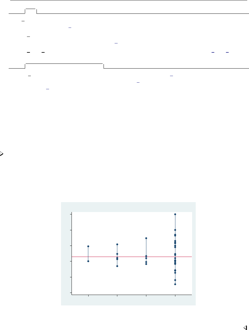
grmeanby — Graph means and medians by categorical variables 765
Plot
cline options affect the rendition of the lines through the markers, including their color, pattern, and
width; see [G-3]cline options.
marker options affect the rendition of markers drawn at the plotted points, including their shape,
size, color, and outline; see [G-3]marker options.
marker label options specify if and how the markers are to be labeled; see [G-3]marker label options.
Y axis, X axis, Titles, Legend, Overall
twoway options are any of the options documented in [G-3]twoway options, excluding by(). These
include options for titling the graph (see [G-3]title options) and for saving the graph to disk (see
[G-3]saving option).
Remarks and examples
The idea of graphing means of categorical variables was shown in Chambers and Hastie (1992,
3). Because this was shown in the context of an S function for making such graphs, it doubtless has
roots going back further than that. grmeanby is, in any case, another implementation of what we
will assume is their idea.
Example 1
Using a variation of our auto dataset, we graph the mean of mpg by foreign,rep77,rep78, and
make:
. use http://www.stata-press.com/data/r13/auto1
(Automobile Models)
. grmeanby foreign rep77 rep78 make, sum(mpg)
Fiat
Honda
BMW
AMC
Toyota
Subaru
Buick
Chev.
VW
Audi
Datsun
Merc.
Pont.
Peugeot
Renault
Dodge
Volvo
Mazda
Linc.
Plym.
Ford
Cad.
Olds
Average
Good
Fair
Poor
Exc
Average
Exc
Good
Poor
Fair
Domestic
Foreign
10 15 20 25 30 35
foreign rep77 rep78 make
Means of mpg, Mileage (mpg)
If we had wanted a graph of medians rather than means, we could have typed
. grmeanby foreign rep77 rep78 make, sum(mpg) median

766 grmeanby — Graph means and medians by categorical variables
References
Chambers, J. M., and T. J. Hastie, ed. 1992. Statistical Models in S. Pacific Grove, CA: Wadsworth and Brooks/Cole.
Gould, W. W. 1993. gr12: Graphs of means and medians by categorical variables.Stata Technical Bulletin 12: 13.
Reprinted in Stata Technical Bulletin Reprints, vol. 2, pp. 44–45. College Station, TX: Stata Press.

Title
hausman — Hausman specification test
Syntax Menu Description Options
Remarks and examples Stored results Methods and formulas Acknowledgment
References Also see
Syntax
hausman name-consistent name-efficient ,options
options Description
Main
constant include estimated intercepts in comparison; default is to exclude
alleqs use all equations to perform test; default is first equation only
skipeqs(eqlist)skip specified equations when performing test
equations(matchlist)associate/compare the specified (by number) pairs of equations
force force performance of test, even though assumptions are not met
df(#)use #degrees of freedom
sigmamore base both (co)variance matrices on disturbance variance
estimate from efficient estimator
sigmaless base both (co)variance matrices on disturbance variance
estimate from consistent estimator
Advanced
tconsistent(string)consistent estimator column header
tefficient(string)efficient estimator column header
where name-consistent and name-efficient are names under which estimation results were stored via
estimates store; see [R]estimates store.
A period (.) may be used to refer to the last estimation results, even if these were not already stored.
Not specifying name-efficient is equivalent to specifying the last estimation results as “.”.
Menu
Statistics >Postestimation >Tests >Hausman specification test
Description
hausman performs Hausman’s (1978) specification test.
Options
Main
constant specifies that the estimated intercept(s) be included in the model comparison; by default,
they are excluded. The default behavior is appropriate for models in which the constant does not
have a common interpretation across the two models.
767

768 hausman — Hausman specification test
alleqs specifies that all the equations in the models be used to perform the Hausman test; by default,
only the first equation is used.
skipeqs(eqlist)specifies in eqlist the names of equations to be excluded from the test. Equation
numbers are not allowed in this context, because the equation names, along with the variable
names, are used to identify common coefficients.
equations(matchlist)specifies, by number, the pairs of equations that are to be compared.
The matchlist in equations() should follow the syntax
#c:#e,#c:#e,. . .
where #c(#e) is an equation number of the always-consistent (efficient under H0) estimator. For
instance, equations(1:1),equations(1:1, 2:2), or equations(1:2).
If equations() is not specified, then equations are matched on equation names.
equations() handles the situation in which one estimator uses equation names and the other
does not. For instance, equations(1:2) means that equation 1 of the always-consistent estimator
is to be tested against equation 2 of the efficient estimator. equations(1:1, 2:2) means that
equation 1 is to be tested against equation 1 and that equation 2 is to be tested against equation 2.
If equations() is specified, the alleqs and skipeqs options are ignored.
force specifies that the Hausman test be performed, even though the assumptions of the Hausman
test seem not to be met, for example, because the estimators were pweighted or the data were
clustered.
df(#)specifies the degrees of freedom for the Hausman test. The default is the matrix rank of the
variance of the difference between the coefficients of the two estimators.
sigmamore and sigmaless specify that the two covariance matrices used in the test be based on a
common estimate of disturbance variance (σ2).
sigmamore specifies that the covariance matrices be based on the estimated disturbance variance
from the efficient estimator. This option provides a proper estimate of the contrast variance for
so-called tests of exogeneity and overidentification in instrumental-variables regression.
sigmaless specifies that the covariance matrices be based on the estimated disturbance variance
from the consistent estimator.
These options can be specified only when both estimators store e(sigma) or e(rmse), or with
the xtreg command. e(sigma e) is stored after the xtreg command with the fe or mle option.
e(rmse) is stored after the xtreg command with the re option.
sigmamore or sigmaless are recommended when comparing fixed-effects and random-effects
linear regression because they are much less likely to produce a non–positive-definite-differenced
covariance matrix (although the tests are asymptotically equivalent whether or not one of the
options is specified).
Advanced
tconsistent(string)and tefficient(string)are formatting options. They allow you to specify
the headers of the columns of coefficients that default to the names of the models. These options
will be of interest primarily to programmers.

hausman — Hausman specification test 769
Remarks and examples
hausman is a general implementation of Hausman’s (1978) specification test, which compares an
estimator b
θ1that is known to be consistent with an estimator b
θ2that is efficient under the assumption
being tested. The null hypothesis is that the estimator b
θ2is indeed an efficient (and consistent)
estimator of the true parameters. If this is the case, there should be no systematic difference between
the two estimators. If there exists a systematic difference in the estimates, you have reason to doubt
the assumptions on which the efficient estimator is based.
The assumption of efficiency is violated if the estimator is pweighted or the data are clustered,
so hausman cannot be used. The test can be forced by specifying the force option with hausman.
For an alternative to using hausman in these cases, see [R]suest.
To use hausman, you
. (compute the always-consistent estimator)
. estimates store name-consistent
. (compute the estimator that is efficient under H 0)
. hausman name-consistent .
Alternatively, you can turn this around:
. (compute the estimator that is efficient under H 0)
. estimates store name-efficient
. (fit the less-efficient model)
. (compute the always-consistent estimator)
. hausman . name-efficient
You can, of course, also compute and store both the always-consistent and efficient-under-H0
estimators and perform the Hausman test with
. hausman name-consistent name-efficient
Example 1
We are studying the factors that affect the wages of young women in the United States between
1970 and 1988, and we have a panel-data sample of individual women over that time span.
. use http://www.stata-press.com/data/r13/nlswork4
(National Longitudinal Survey. Young Women 14-26 years of age in 1968)
. describe
Contains data from http://www.stata-press.com/data/r13/nlswork4.dta
obs: 28,534 National Longitudinal Survey.
Young Women 14-26 years of age
in 1968
vars: 6 29 Jan 2013 16:35
size: 370,942
storage display value
variable name type format label variable label
idcode int %8.0g NLS ID
year byte %8.0g interview year
age byte %8.0g age in current year
msp byte %8.0g 1 if married, spouse present
ttl_exp float %9.0g total work experience
ln_wage float %9.0g ln(wage/GNP deflator)
Sorted by: idcode year

770 hausman — Hausman specification test
We believe that a random-effects specification is appropriate for individual-level effects in our model.
We fit a fixed-effects model that will capture all temporally constant individual-level effects.
. xtreg ln_wage age msp ttl_exp, fe
Fixed-effects (within) regression Number of obs = 28494
Group variable: idcode Number of groups = 4710
R-sq: within = 0.1373 Obs per group: min = 1
between = 0.2571 avg = 6.0
overall = 0.1800 max = 15
F(3,23781) = 1262.01
corr(u_i, Xb) = 0.1476 Prob > F = 0.0000
ln_wage Coef. Std. Err. t P>|t| [95% Conf. Interval]
age -.005485 .000837 -6.55 0.000 -.0071256 -.0038443
msp .0033427 .0054868 0.61 0.542 -.0074118 .0140971
ttl_exp .0383604 .0012416 30.90 0.000 .0359268 .0407941
_cons 1.593953 .0177538 89.78 0.000 1.559154 1.628752
sigma_u .37674223
sigma_e .29751014
rho .61591044 (fraction of variance due to u_i)
F test that all u_i=0: F(4709, 23781) = 7.76 Prob > F = 0.0000
We assume that this model is consistent for the true parameters and store the results by using
estimates store under a name, fixed:
. estimates store fixed
Now we fit a random-effects model as a fully efficient specification of the individual effects
under the assumption that they are random and follow a normal distribution. We then compare these
estimates with the previously stored results by using the hausman command.
. xtreg ln_wage age msp ttl_exp, re
Random-effects GLS regression Number of obs = 28494
Group variable: idcode Number of groups = 4710
R-sq: within = 0.1373 Obs per group: min = 1
between = 0.2552 avg = 6.0
overall = 0.1797 max = 15
Wald chi2(3) = 5100.33
corr(u_i, X) = 0 (assumed) Prob > chi2 = 0.0000
ln_wage Coef. Std. Err. z P>|z| [95% Conf. Interval]
age -.0069749 .0006882 -10.13 0.000 -.0083238 -.0056259
msp .0046594 .0051012 0.91 0.361 -.0053387 .0146575
ttl_exp .0429635 .0010169 42.25 0.000 .0409704 .0449567
_cons 1.609916 .0159176 101.14 0.000 1.578718 1.641114
sigma_u .32648519
sigma_e .29751014
rho .54633481 (fraction of variance due to u_i)

hausman — Hausman specification test 771
. hausman fixed ., sigmamore
Coefficients
(b) (B) (b-B) sqrt(diag(V_b-V_B))
fixed . Difference S.E.
age -.005485 -.0069749 .0014899 .0004803
msp .0033427 .0046594 -.0013167 .0020596
ttl_exp .0383604 .0429635 -.0046031 .0007181
b = consistent under Ho and Ha; obtained from xtreg
B = inconsistent under Ha, efficient under Ho; obtained from xtreg
Test: Ho: difference in coefficients not systematic
chi2(3) = (b-B)’[(V_b-V_B)^(-1)](b-B)
= 260.40
Prob>chi2 = 0.0000
Under the current specification, our initial hypothesis that the individual-level effects are adequately
modeled by a random-effects model is resoundingly rejected. This result is based on the rest of our
model specification, and random effects might be appropriate for some alternate model of wages.
Jerry Allen Hausman was born in West Virginia in 1946. He studied economics at Brown and
Oxford, has been at MIT since 1972, and has made many outstanding contributions to econometrics
and applied microeconomics.
Example 2
A stringent assumption of multinomial and conditional logit models is that outcome categories
for the model have the property of independence of irrelevant alternatives (IIA). Stated simply, this
assumption requires that the inclusion or exclusion of categories does not affect the relative risks
associated with the regressors in the remaining categories.
One classic example of a situation in which this assumption would be violated involves the choice
of transportation mode; see McFadden (1974). For simplicity, postulate a transportation model with
the four possible outcomes: rides a train to work, takes a bus to work, drives the Ford to work, and
drives the Chevrolet to work. Clearly, “drives the Ford” is a closer substitute to “drives the Chevrolet”
than it is to “rides a train” (at least for most people). This means that excluding “drives the Ford”
from the model could be expected to affect the relative risks of the remaining options and that the
model would not obey the IIA assumption.
Using the data presented in [R]mlogit, we will use a simplified model to test for IIA. The choice
of insurance type among indemnity, prepaid, and uninsured is modeled as a function of age and
gender. The indemnity category is allowed to be the base category, and the model including all three
outcomes is fit. The results are then stored under the name allcats.

772 hausman — Hausman specification test
. use http://www.stata-press.com/data/r13/sysdsn3
(Health insurance data)
. mlogit insure age male
Iteration 0: log likelihood = -555.85446
Iteration 1: log likelihood = -551.32973
Iteration 2: log likelihood = -551.32802
Iteration 3: log likelihood = -551.32802
Multinomial logistic regression Number of obs = 615
LR chi2(4) = 9.05
Prob > chi2 = 0.0598
Log likelihood = -551.32802 Pseudo R2 = 0.0081
insure Coef. Std. Err. z P>|z| [95% Conf. Interval]
Indemnity (base outcome)
Prepaid
age -.0100251 .0060181 -1.67 0.096 -.0218204 .0017702
male .5095747 .1977893 2.58 0.010 .1219147 .8972346
_cons .2633838 .2787575 0.94 0.345 -.2829708 .8097383
Uninsure
age -.0051925 .0113821 -0.46 0.648 -.0275011 .0171161
male .4748547 .3618462 1.31 0.189 -.2343508 1.18406
_cons -1.756843 .5309602 -3.31 0.001 -2.797506 -.7161803
. estimates store allcats
Under the IIA assumption, we would expect no systematic change in the coefficients if we excluded
one of the outcomes from the model. (For an extensive discussion, see Hausman and McFadden
[1984].) We reestimate the parameters, excluding the uninsured outcome, and perform a Hausman
test against the fully efficient full model.
. mlogit insure age male if insure != "Uninsure":insure
Iteration 0: log likelihood = -394.8693
Iteration 1: log likelihood = -390.4871
Iteration 2: log likelihood = -390.48643
Iteration 3: log likelihood = -390.48643
Multinomial logistic regression Number of obs = 570
LR chi2(2) = 8.77
Prob > chi2 = 0.0125
Log likelihood = -390.48643 Pseudo R2 = 0.0111
insure Coef. Std. Err. z P>|z| [95% Conf. Interval]
Indemnity (base outcome)
Prepaid
age -.0101521 .0060049 -1.69 0.091 -.0219214 .0016173
male .5144003 .1981735 2.60 0.009 .1259874 .9028133
_cons .2678043 .2775563 0.96 0.335 -.276196 .8118046

hausman — Hausman specification test 773
. hausman . allcats, alleqs constant
Coefficients
(b) (B) (b-B) sqrt(diag(V_b-V_B))
. allcats Difference S.E.
age -.0101521 -.0100251 -.0001269 .
male .5144003 .5095747 .0048256 .0123338
_cons .2678043 .2633838 .0044205 .
b = consistent under Ho and Ha; obtained from mlogit
B = inconsistent under Ha, efficient under Ho; obtained from mlogit
Test: Ho: difference in coefficients not systematic
chi2(3) = (b-B)’[(V_b-V_B)^(-1)](b-B)
= 0.08
Prob>chi2 = 0.9944
(V_b-V_B is not positive definite)
The syntax of the if condition on the mlogit command simply identified the "Uninsured"
category with the insure value label; see [U] 12.6.3 Value labels. On examining the output from
hausman, we see that there is no evidence that the IIA assumption has been violated.
Because the Hausman test is a standardized comparison of model coefficients, using it with
mlogit requires that the base outcome be the same in both competing models. In particular, if the
most-frequent category (the default base outcome) is being removed to test for IIA, you must use the
baseoutcome() option in mlogit to manually set the base outcome to something else. Or you can
use the equation() option of the hausman command to align the equations of the two models.
Having the missing values for the square root of the diagonal of the covariance matrix of the
differences is not comforting, but it is also not surprising. This covariance matrix is guaranteed to be
positive definite only asymptotically (it is a consequence of the assumption that one of the estimators
is efficient), and assurances are not made about the diagonal elements. Negative values along the
diagonal are possible, and the fourth column of the table is provided mainly for descriptive use.
We can also perform the Hausman IIA test against the remaining alternative in the model:
. mlogit insure age male if insure != "Prepaid":insure
Iteration 0: log likelihood = -132.59913
Iteration 1: log likelihood = -131.78009
Iteration 2: log likelihood = -131.76808
Iteration 3: log likelihood = -131.76807
Multinomial logistic regression Number of obs = 338
LR chi2(2) = 1.66
Prob > chi2 = 0.4356
Log likelihood = -131.76807 Pseudo R2 = 0.0063
insure Coef. Std. Err. z P>|z| [95% Conf. Interval]
Indemnity (base outcome)
Uninsure
age -.0041055 .0115807 -0.35 0.723 -.0268033 .0185923
male .4591074 .3595663 1.28 0.202 -.2456296 1.163844
_cons -1.801774 .5474476 -3.29 0.001 -2.874752 -.7287968

774 hausman — Hausman specification test
. hausman . allcats, alleqs constant
Coefficients
(b) (B) (b-B) sqrt(diag(V_b-V_B))
. allcats Difference S.E.
age -.0041055 -.0051925 .001087 .0021355
male .4591074 .4748547 -.0157473 .
_cons -1.801774 -1.756843 -.0449311 .1333421
b = consistent under Ho and Ha; obtained from mlogit
B = inconsistent under Ha, efficient under Ho; obtained from mlogit
Test: Ho: difference in coefficients not systematic
chi2(3) = (b-B)’[(V_b-V_B)^(-1)](b-B)
= -0.18 chi2<0 ==> model fitted on these
data fails to meet the asymptotic
assumptions of the Hausman test;
see suest for a generalized test
Here the χ2statistic is actually negative. We might interpret this result as strong evidence that
we cannot reject the null hypothesis. Such a result is not an unusual outcome for the Hausman test,
particularly when the sample is relatively small—there are only 45 uninsured individuals in this
dataset.
Are we surprised by the results of the Hausman test in this example? Not really. Judging from
the zstatistics on the original multinomial logit model, we were struggling to identify any structure
in the data with the current specification. Even when we were willing to assume IIA and computed
the efficient estimator under this assumption, few of the effects could be identified as statistically
different from those on the base category. Trying to base a Hausman test on a contrast (difference)
between two poor estimates is just asking too much of the existing data.
In example 2, we encountered a case in which the Hausman was not well defined. Unfortunately,
in our experience this happens fairly often. Stata provides an alternative to the Hausman test that
overcomes this problem through an alternative estimator of the variance of the difference between
the two estimators. This other estimator is guaranteed to be positive semidefinite. This alternative
estimator also allows a widening of the scope of problems to which Hausman-type tests can be applied
by relaxing the assumption that one of the estimators is efficient. For instance, you can perform
Hausman-type tests to clustered observations and survey estimators. See [R]suest for details.
Stored results
hausman stores the following in r():
Scalars
r(chi2) χ2
r(df) degrees of freedom for the statistic
r(p) p-value for the χ2
r(rank) rank of (V b-V B)^(-1)

hausman — Hausman specification test 775
Methods and formulas
The Hausman statistic is distributed as χ2and is computed as
H= (βc−βe)0(Vc−Ve)−1(βc−βe)
where βcis the coefficient vector from the consistent estimator
βeis the coefficient vector from the efficient estimator
Vcis the covariance matrix of the consistent estimator
Veis the covariance matrix of the efficient estimator
When the difference in the variance matrices is not positive definite, a Moore–Penrose generalized
inverse is used. As noted in Gourieroux and Monfort (1995, 125–128), the choice of generalized
inverse is not important asymptotically.
The number of degrees of freedom for the statistic is the rank of the difference in the variance
matrices. When the difference is positive definite, this is the number of common coefficients in the
models being compared.
Acknowledgment
Portions of hausman are based on an early implementation by Jeroen Weesie of the Department
of Sociology at Utrecht University, The Netherlands.
References
Baltagi, B. H. 2011. Econometrics. 5th ed. Berlin: Springer.
Gourieroux, C. S., and A. Monfort. 1995. Statistics and Econometric Models, Vol 2: Testing, Confidence Regions,
Model Selection, and Asymptotic Theory. Trans. Q. Vuong. Cambridge: Cambridge University Press.
Hausman, J. A. 1978. Specification tests in econometrics. Econometrica 46: 1251–1271.
Hausman, J. A., and D. L. McFadden. 1984. Specification tests for the multinomial logit model. Econometrica 52:
1219–1240.
McFadden, D. L. 1974. Measurement of urban travel demand. Journal of Public Economics 3: 303–328.
Also see
[R]lrtest — Likelihood-ratio test after estimation
[R]suest — Seemingly unrelated estimation
[R]test — Test linear hypotheses after estimation
[XT]xtreg — Fixed-, between-, and random-effects and population-averaged linear models

Title
heckman — Heckman selection model
Syntax Menu
Description Options for Heckman selection model (ML)
Options for Heckman selection model (two-step) Remarks and examples
Stored results Methods and formulas
References Also see
Syntax
Basic syntax
heckman depvar indepvars , select(varlists)twostep
or
heckman depvar indepvars , select(depvars=varlists)twostep
Full syntax for maximum likelihood estimates only
heckman depvar indepvars if in weight ,
select( depvars=varlists, noconstant offset(varnameo))
heckman ml options
Full syntax for Heckman’s two-step consistent estimates only
heckman depvar indepvars if in , twostep
select( depvars=varlists, noconstant )heckman ts options
776

heckman — Heckman selection model 777
heckman ml options Description
Model
∗select() specify selection equation: dependent and independent
variables; whether to have constant term and offset variable
noconstant suppress constant term
offset(varname)include varname in model with coefficient constrained to 1
constraints(constraints)apply specified linear constraints
collinear keep collinear variables
SE/Robust
vce(vcetype)vcetype may be oim,robust,cluster clustvar,opg,bootstrap,
or jackknife
Reporting
level(#)set confidence level; default is level(95)
first report first-step probit estimates
noskip perform likelihood-ratio test
nshazard(newvar)generate nonselection hazard variable
mills(newvar)synonym for nshazard()
nocnsreport do not display constraints
display options control column formats, row spacing, line width, display of omitted
variables and base and empty cells, and factor-variable labeling
Maximization
maximize options control the maximization process; seldom used
coeflegend display legend instead of statistics
∗select( ) is required.
The full specification is select( depvars=varlists, noconstant offset(varnameo)).

778 heckman — Heckman selection model
heckman ts options Description
Model
∗select() specify selection equation: dependent and independent
variables; whether to have constant term
∗twostep produce two-step consistent estimate
noconstant suppress constant term
rhosigma truncate ρto [−1,1]with consistent σ
rhotrunc truncate ρto [−1,1]
rholimited truncate ρin limited cases
rhoforce do not truncate ρ
SE
vce(vcetype)vcetype may be conventional,bootstrap, or jackknife
Reporting
level(#)set confidence level; default is level(95)
first report first-step probit estimates
nshazard(newvar)generate nonselection hazard variable
mills(newvar)synonym for nshazard()
display options control column formats, row spacing, line width, display of omitted
variables and base and empty cells, and factor-variable labeling
coeflegend display legend instead of statistics
∗select( ) and twostep are required.
The full specification is select( depvars=varlists, noconstant ).
indepvars and varlistsmay contain factor variables; see [U] 11.4.3 Factor variables.
depvar,indepvars,varlists, and depvarsmay contain time-series operators; see [U] 11.4.4 Time-series varlists.
bootstrap,by,fp,jackknife,rolling,statsby, and svy are allowed; see [U] 11.1.10 Prefix commands.
Weights are not allowed with the bootstrap prefix; see [R] bootstrap.
aweights are not allowed with the jackknife prefix; see [R] jackknife.
twostep,vce(),first,noskip, and weights are not allowed with the svy prefix; see [SVY] svy.
pweights, aweights, fweights, and iweights are allowed with maximum likelihood estimation; see [U] 11.1.6 weight.
No weights are allowed if twostep is specified.
coeflegend does not appear in the dialog box.
See [U] 20 Estimation and postestimation commands for more capabilities of estimation commands.
Menu
heckman for maximum likelihood estimates
Statistics >Sample-selection models >Heckman selection model (ML)
heckman for two-step consistent estimates
Statistics >Sample-selection models >Heckman selection model (two-step)

heckman — Heckman selection model 779
Description
heckman fits regression models with selection by using either Heckman’s two-step consistent
estimator or full maximum likelihood.
Options for Heckman selection model (ML)
Model
select( depvars=varlists, noconstant offset(varnameo))specifies the variables and
options for the selection equation. It is an integral part of specifying a Heckman model and is
required. The selection equation should contain at least one variable that is not in the outcome
equation.
If depvarsis specified, it should be coded as 0 or 1, with 0 indicating an observation not selected
and 1 indicating a selected observation. If depvarsis not specified, observations for which depvar
is not missing are assumed selected, and those for which depvar is missing are assumed not
selected.
noconstant suppresses the selection constant term (intercept).
offset(varnameo)specifies that selection offset varnameobe included in the model with the
coefficient constrained to be 1.
noconstant,offset(varname),constraints(constraints),collinear; see [R]estimation op-
tions.
SE/Robust
vce(vcetype)specifies the type of standard error reported, which includes types that are derived from
asymptotic theory (oim,opg), that are robust to some kinds of misspecification (robust), that
allow for intragroup correlation (cluster clustvar), and that use bootstrap or jackknife methods
(bootstrap,jackknife); see [R]vce option.
Reporting
level(#); see [R]estimation options.
first specifies that the first-step probit estimates of the selection equation be displayed before
estimation.
noskip specifies that a full maximum-likelihood model with only a constant for the regression equation
be fit. This model is not displayed but is used as the base model to compute a likelihood-ratio test
for the model test statistic displayed in the estimation header. By default, the overall model test
statistic is an asymptotically equivalent Wald test that all the parameters in the regression equation
are zero (except the constant). For many models, this option can substantially increase estimation
time.
nshazard(newvar)and mills(newvar)are synonyms; either will create a new variable containing
the nonselection hazard—what Heckman (1979) referred to as the inverse of the Mills’ ratio—from
the selection equation. The nonselection hazard is computed from the estimated parameters of the
selection equation.
nocnsreport; see [R]estimation options.
display options:noomitted,vsquish,noemptycells,baselevels,allbaselevels,nofvla-
bel,fvwrap(#),fvwrapon(style),cformat(%fmt),pformat(% fmt),sformat(% fmt), and
nolstretch; see [R]estimation options.

780 heckman — Heckman selection model
Maximization
maximize options:difficult,technique(algorithm spec),iterate(#),nolog,trace,
gradient,showstep,hessian,showtolerance,tolerance(#),ltolerance(#),
nrtolerance(#),nonrtolerance, and from(init specs); see [R]maximize. These options are
seldom used.
Setting the optimization type to technique(bhhh) resets the default vcetype to vce(opg).
The following option is available with heckman but is not shown in the dialog box:
coeflegend; see [R]estimation options.
Options for Heckman selection model (two-step)
Model
select( depvars=varlists, noconstant )specifies the variables and options for the selection
equation. It is an integral part of specifying a Heckman model and is required. The selection equation
should contain at least one variable that is not in the outcome equation.
If depvarsis specified, it should be coded as 0 or 1, with 0 indicating an observation not selected
and 1 indicating a selected observation. If depvarsis not specified, observations for which depvar
is not missing are assumed selected, and those for which depvar is missing are assumed not
selected.
noconstant suppresses the selection constant term (intercept).
twostep specifies that Heckman’s (1979) two-step efficient estimates of the parameters, standard
errors, and covariance matrix be produced.
noconstant; see [R]estimation options.
rhosigma,rhotrunc,rholimited, and rhoforce are rarely used options to specify how the
two-step estimator (option twostep) handles unusual cases in which the two-step estimate of ρis
outside the admissible range for a correlation, [−1,1]. When abs(ρ)>1, the two-step estimate of
the coefficient variance–covariance matrix may not be positive definite and thus may be unusable
for testing. The default is rhosigma.
rhosigma specifies that ρbe truncated, as with the rhotrunc option, and that the estimate of σbe
made consistent with bρ, the truncated estimate of ρ. So, bσ=βmbρ; see Methods and formulas for
the definition of βm. Both the truncated ρand the new estimate of bσare used in all computations
to estimate the two-step covariance matrix.
rhotrunc specifies that ρbe truncated to lie in the range [−1,1]. If the two-step estimate is less
than −1, ρis set to −1; if the two-step estimate is greater than 1, ρis set to 1. This truncated
value of ρis used in all computations to estimate the two-step covariance matrix.
rholimited specifies that ρbe truncated only in computing the diagonal matrix Das it enters
Vtwostep and Q; see Methods and formulas. In all other computations, the untruncated estimate
of ρis used.
rhoforce specifies that the two-step estimate of ρbe retained, even if it is outside the admissible
range for a correlation. This option may, in rare cases, lead to a non–positive-definite covariance
matrix.
These options have no effect when estimation is by maximum likelihood, the default. They also
have no effect when the two-step estimate of ρis in the range [−1,1 ].

heckman — Heckman selection model 781
SE
vce(vcetype)specifies the type of standard error reported, which includes types that are derived from
asymptotic theory (conventional) and that use bootstrap or jackknife methods (bootstrap,
jackknife); see [R]vce option.
vce(conventional), the default, uses the two-step variance estimator derived by Heckman.
Reporting
level(#); see [R]estimation options.
first specifies that the first-step probit estimates of the selection equation be displayed before
estimation.
nshazard(newvar)and mills(newvar)are synonyms; either will create a new variable containing
the nonselection hazard—what Heckman (1979) referred to as the inverse of the Mills’ ratio—from
the selection equation. The nonselection hazard is computed from the estimated parameters of the
selection equation.
display options:noomitted,vsquish,noemptycells,baselevels,allbaselevels,nofvla-
bel,fvwrap(#),fvwrapon(style),cformat(%fmt),pformat(% fmt),sformat(% fmt), and
nolstretch; see [R]estimation options.
The following option is available with heckman but is not shown in the dialog box:
coeflegend; see [R]estimation options.
Remarks and examples
The Heckman selection model (Gronau 1974;Lewis 1974;Heckman 1976) assumes that there
exists an underlying regression relationship,
yj=xjβ+u1jregression equation
The dependent variable, however, is not always observed. Rather, the dependent variable for
observation jis observed if
zjγ+u2j>0selection equation
where
u1∼N(0, σ)
u2∼N(0,1)
corr(u1, u2) = ρ
When ρ6=0, standard regression techniques applied to the first equation yield biased results. heckman
provides consistent, asymptotically efficient estimates for all the parameters in such models.
In one classic example, the first equation describes the wages of women. Women choose whether
to work, and thus, from our point of view as researchers, whether we observe their wages in our
data. If women made this decision randomly, we could ignore that not all wages are observed and
use ordinary regression to fit a wage model. Such an assumption of random participation, however,
is unlikely to be true; women who would have low wages may be unlikely to choose to work, and
thus the sample of observed wages is biased upward. In the jargon of economics, women choose not
to work when their personal reservation wage is greater than the wage offered by employers. Thus
women who choose not to work might have even higher offer wages than those who do work—they
may have high offer wages, but they have even higher reservation wages. We could tell a story that
competency is related to wages, but competency is rewarded more at home than in the labor force.

782 heckman — Heckman selection model
In any case, in this problem—which is the paradigm for most such problems—a solution can
be found if there are some variables that strongly affect the chances for observation (the reservation
wage) but not the outcome under study (the offer wage). Such a variable might be the number of
children in the home. (Theoretically, we do not need such identifying variables, but without them,
we depend on functional form to identify the model. It would be difficult for anyone to take such
results seriously because the functional form assumptions have no firm basis in theory.)
Example 1
In the syntax for heckman,depvar and indepvars are the dependent variable and regressors for the
underlying regression model to be fit (y=Xβ), and varlistsare the variables (Z) thought to determine
whether depvar is observed or unobserved (selected or not selected). In our female wage example,
the number of children at home would be included in the second list. By default, heckman assumes
that missing values (see [U] 12.2.1 Missing values) of depvar imply that the dependent variable is
unobserved (not selected). With some datasets, it is more convenient to specify a binary variable
(depvars) that identifies the observations for which the dependent is observed/selected (depvars6=0)
or not observed (depvars=0); heckman will accommodate either type of data.
We have a (fictional) dataset on 2,000 women, 1,343 of whom work:
. use http://www.stata-press.com/data/r13/womenwk
. summarize age educ married children wage
Variable Obs Mean Std. Dev. Min Max
age 2000 36.208 8.28656 20 59
education 2000 13.084 3.045912 10 20
married 2000 .6705 .4701492 0 1
children 2000 1.6445 1.398963 0 5
wage 1343 23.69217 6.305374 5.88497 45.80979
We will assume that the hourly wage is a function of education and age, whereas the likelihood
of working (the likelihood of the wage being observed) is a function of marital status, the number of
children at home, and (implicitly) the wage (via the inclusion of age and education, which we think
determine the wage):

heckman — Heckman selection model 783
. heckman wage educ age, select(married children educ age)
Iteration 0: log likelihood = -5178.7009
Iteration 1: log likelihood = -5178.3049
Iteration 2: log likelihood = -5178.3045
Heckman selection model Number of obs = 2000
(regression model with sample selection) Censored obs = 657
Uncensored obs = 1343
Wald chi2(2) = 508.44
Log likelihood = -5178.304 Prob > chi2 = 0.0000
wage Coef. Std. Err. z P>|z| [95% Conf. Interval]
wage
education .9899537 .0532565 18.59 0.000 .8855729 1.094334
age .2131294 .0206031 10.34 0.000 .1727481 .2535108
_cons .4857752 1.077037 0.45 0.652 -1.625179 2.59673
select
married .4451721 .0673954 6.61 0.000 .3130794 .5772647
children .4387068 .0277828 15.79 0.000 .3842534 .4931601
education .0557318 .0107349 5.19 0.000 .0346917 .0767718
age .0365098 .0041533 8.79 0.000 .0283694 .0446502
_cons -2.491015 .1893402 -13.16 0.000 -2.862115 -2.119915
/athrho .8742086 .1014225 8.62 0.000 .6754241 1.072993
/lnsigma 1.792559 .027598 64.95 0.000 1.738468 1.84665
rho .7035061 .0512264 .5885365 .7905862
sigma 6.004797 .1657202 5.68862 6.338548
lambda 4.224412 .3992265 3.441942 5.006881
LR test of indep. eqns. (rho = 0): chi2(1) = 61.20 Prob > chi2 = 0.0000
heckman assumes that wage is the dependent variable and that the first variable list (educ and age)
are the determinants of wage. The variables specified in the select() option (married,children,
educ, and age) are assumed to determine whether the dependent variable is observed (the selection
equation). Thus we fit the model
wage =β0+β1educ +β2age +u1
and we assumed that wage is observed if
γ0+γ1married +γ2children +γ3educ +γ4age +u2>0
where u1and u2have correlation ρ.
The reported results for the wage equation are interpreted exactly as though we observed wage
data for all women in the sample; the coefficients on age and education level represent the estimated
marginal effects of the regressors in the underlying regression equation. The results for the two
ancillary parameters require some explanation. heckman does not directly estimate ρ; to constrain
ρwithin its valid limits, and for numerical stability during optimization, it estimates the inverse
hyperbolic tangent of ρ:
atanh ρ=1
2ln1 + ρ
1−ρ

784 heckman — Heckman selection model
This estimate is reported as /athrho. In the bottom panel of the output, heckman undoes this
transformation for you: the estimated value of ρis 0.7035061. The standard error for ρis computed
using the delta method, and its confidence intervals are the transformed intervals of /athrho.
Similarly, σ, the standard error of the residual in the wage equation, is not directly estimated; for
numerical stability, heckman instead estimates ln σ. The untransformed sigma is reported at the end
of the output: 6.004797.
Finally, some researchers—especially economists—are used to the selectivity effect summarized
not by ρbut by λ=ρσ.heckman reports this, too, along with an estimate of the standard error and
confidence interval.
Technical note
If each of the equations in the model had contained many regressors, the heckman command could
have become long. An alternate way of specifying our wage model would be to use Stata’s global
macros. The following lines are an equivalent way of specifying our model:
. global wageeq "wage educ age"
. global seleq "married children educ age"
. heckman $wageeq, select($seleq)
(output omitted )
Technical note
The reported model χ2test is a Wald test that all coefficients in the regression model (except
the constant) are 0. heckman is an estimation command, so you can use test,testnl, or lrtest
to perform tests against whatever nested alternate model you choose; see [R]test,[R]testnl, and
[R]lrtest.
The estimation of ρand σin the forms atanh ρand ln σextends the range of these parameters to
infinity in both directions, thus avoiding boundary problems during the maximization. Tests of ρmust
be made in the transformed units. However, because atanh(0) = 0, the reported test for atanh ρ=0
is equivalent to the test for ρ=0.
The likelihood-ratio test reported at the bottom of the output is an equivalent test for ρ=0 and is
computationally the comparison of the joint likelihood of an independent probit model for the selection
equation and a regression model on the observed wage data against the Heckman model likelihood.
Because χ2=61.20, this clearly justifies the Heckman selection equation with these data.
Example 2
heckman supports the Huber/White/sandwich estimator of variance under the vce(robust) and
vce(cluster clustvar)options or when pweights are used for population-weighted data; see
[U] 20.21 Obtaining robust variance estimates. We can obtain robust standard errors for our wage
model by specifying clustering on county of residence (the county variable).

heckman — Heckman selection model 785
. heckman wage educ age, select(married children educ age) vce(cluster county)
Iteration 0: log pseudolikelihood = -5178.7009
Iteration 1: log pseudolikelihood = -5178.3049
Iteration 2: log pseudolikelihood = -5178.3045
Heckman selection model Number of obs = 2000
(regression model with sample selection) Censored obs = 657
Uncensored obs = 1343
Wald chi2(1) = .
Log pseudolikelihood = -5178.304 Prob > chi2 = .
(Std. Err. adjusted for 10 clusters in county)
Robust
wage Coef. Std. Err. z P>|z| [95% Conf. Interval]
wage
education .9899537 .0600061 16.50 0.000 .8723438 1.107564
age .2131294 .020995 10.15 0.000 .17198 .2542789
_cons .4857752 1.302103 0.37 0.709 -2.066299 3.03785
select
married .4451721 .0731472 6.09 0.000 .3018062 .5885379
children .4387068 .0312386 14.04 0.000 .3774802 .4999333
education .0557318 .0110039 5.06 0.000 .0341645 .0772991
age .0365098 .004038 9.04 0.000 .0285954 .0444242
_cons -2.491015 .1153305 -21.60 0.000 -2.717059 -2.264972
/athrho .8742086 .1403337 6.23 0.000 .5991596 1.149258
/lnsigma 1.792559 .0258458 69.36 0.000 1.741902 1.843216
rho .7035061 .0708796 .5364513 .817508
sigma 6.004797 .155199 5.708189 6.316818
lambda 4.224412 .5186709 3.207835 5.240988
Wald test of indep. eqns. (rho = 0): chi2(1) = 38.81 Prob > chi2 = 0.0000
The robust standard errors tend to be a bit larger, but we notice no systematic differences. This finding
is not surprising because the data were not constructed to have any county-specific correlations or
any other characteristics that would deviate from the assumptions of the Heckman model.
Example 3
Stata also produces Heckman’s (1979) two-step efficient estimator of the model with the twostep
option. Maximum likelihood estimation of the parameters can be time consuming with large datasets,
and the two-step estimates may provide a good alternative in such cases. Continuing with the women’s
wage model, we can obtain the two-step estimates with Heckman’s consistent covariance estimates
by typing

786 heckman — Heckman selection model
. heckman wage educ age, select(married children educ age) twostep
Heckman selection model -- two-step estimates Number of obs = 2000
(regression model with sample selection) Censored obs = 657
Uncensored obs = 1343
Wald chi2(2) = 442.54
Prob > chi2 = 0.0000
wage Coef. Std. Err. z P>|z| [95% Conf. Interval]
wage
education .9825259 .0538821 18.23 0.000 .8769189 1.088133
age .2118695 .0220511 9.61 0.000 .1686502 .2550888
_cons .7340391 1.248331 0.59 0.557 -1.712645 3.180723
select
married .4308575 .074208 5.81 0.000 .2854125 .5763025
children .4473249 .0287417 15.56 0.000 .3909922 .5036576
education .0583645 .0109742 5.32 0.000 .0368555 .0798735
age .0347211 .0042293 8.21 0.000 .0264318 .0430105
_cons -2.467365 .1925635 -12.81 0.000 -2.844782 -2.089948
mills
lambda 4.001615 .6065388 6.60 0.000 2.812821 5.19041
rho 0.67284
sigma 5.9473529
Technical note
The Heckman selection model depends strongly on the model being correct, much more so than
ordinary regression. Running a separate probit or logit for sample inclusion followed by a regression,
referred to in the literature as the two-part model (Manning, Duan, and Rogers 1987)—not to be
confused with Heckman’s two-step procedure—is an especially attractive alternative if the regression
part of the model arose because of taking a logarithm of zero values. When the goal is to analyze an
underlying regression model or to predict the value of the dependent variable that would be observed
in the absence of selection, however, the Heckman model is more appropriate. When the goal is to
predict an actual response, the two-part model is usually the better choice.
The Heckman selection model can be unstable when the model is not properly specified or if a
specific dataset simply does not support the model’s assumptions. For example, let’s examine the
solution to another simulated problem.

heckman — Heckman selection model 787
. use http://www.stata-press.com/data/r13/twopart
. heckman yt x1 x2 x3, select(z1 z2) nonrtol
Iteration 0: log likelihood = -111.94996
Iteration 1: log likelihood = -110.82258
Iteration 2: log likelihood = -110.17707
Iteration 3: log likelihood = -107.70663 (not concave)
Iteration 4: log likelihood = -107.07729 (not concave)
(output omitted )
Iteration 33: log likelihood = -104.0825 (not concave)
Iteration 34: log likelihood = -104.0825
Heckman selection model Number of obs = 150
(regression model with sample selection) Censored obs = 87
Uncensored obs = 63
Wald chi2(3) = 8.64e+08
Log likelihood = -104.0825 Prob > chi2 = 0.0000
yt Coef. Std. Err. z P>|z| [95% Conf. Interval]
yt
x1 .8974192 .0002247 3994.69 0.000 .8969789 .8978595
x2 -2.525303 .0001472 -1.7e+04 0.000 -2.525591 -2.525014
x3 2.855786 .0004181 6829.86 0.000 2.854966 2.856605
_cons .6975442 .0920515 7.58 0.000 .5171265 .8779619
select
z1 -.6825988 .0900159 -7.58 0.000 -.8590267 -.5061709
z2 1.003605 .132347 7.58 0.000 .7442097 1.263
_cons -.3604652 .1232778 -2.92 0.003 -.6020852 -.1188452
/athrho 16.19193 280.9822 0.06 0.954 -534.523 566.9069
/lnsigma -.5396153 .1318714 -4.09 0.000 -.7980786 -.2811521
rho 1 9.73e-12 -1 1
sigma .5829725 .0768774 .4501931 .7549135
lambda .5829725 .0768774 .4322955 .7336494
LR test of indep. eqns. (rho = 0): chi2(1) = 25.67 Prob > chi2 = 0.0000
The model has converged to a value of ρthat is 1.0—within machine-rounding tolerances. Given
the form of the likelihood for the Heckman selection model, this implies a division by zero, and it
is surprising that the model solution turns out as well as it does. Reparameterizing ρhas allowed
the estimation to converge, but we clearly have problems with the estimates. Moreover, if this had
occurred in a large dataset, waiting for convergence might take considerable time.
This dataset was not intentionally developed to cause problems. It is actually generated by a
“Heckman process” and when generated starting from different random values can be easily estimated.
The luck of the draw here merely led to data that, despite the source, did not support the assumptions
of the Heckman model.
The two-step model is generally more stable when the data are problematic. It even tolerates
estimates of ρless than −1 and greater than 1. For these reasons, the two-step model may be
preferred when exploring a large dataset. Still, if the maximum likelihood estimates cannot converge,
or converge to a value of ρthat is at the boundary of acceptable values, there is scant support for
fitting a Heckman selection model on the data. Heckman (1979) discusses the implications of ρbeing
exactly 1 or 0, together with the implications of other possible covariance relationships among the
model’s determinants.

788 heckman — Heckman selection model
James Joseph Heckman was born in Chicago in 1944 and studied mathematics at Colorado
College and economics at Princeton. He has taught economics at Columbia and (since 1973) at
the University of Chicago. He has worked on developing a scientific basis for economic policy
evaluation, with emphasis on models of individuals or disaggregated groups and the problems and
possibilities created by heterogeneity, diversity, and unobserved counterfactual states. In 2000,
he shared the Nobel Prize in Economics with Daniel L. McFadden.
Stored results
heckman (maximum likelihood) stores the following in e():
Scalars
e(N) number of observations
e(N cens) number of censored observations
e(k) number of parameters
e(k eq) number of equations in e(b)
e(k eq model) number of equations in overall model test
e(k aux) number of auxiliary parameters
e(k dv) number of dependent variables
e(df m) model degrees of freedom
e(ll) log likelihood
e(ll 0) log likelihood, constant-only model
e(N clust) number of clusters
e(lambda) λ
e(selambda) standard error of λ
e(sigma) sigma
e(chi2) χ2
e(chi2 c) χ2for comparison test
e(p c) p-value for comparison test
e(p) significance of comparison test
e(rho) ρ
e(rank) rank of e(V)
e(rank0) rank of e(V) for constant-only model
e(ic) number of iterations
e(rc) return code
e(converged) 1 if converged, 0otherwise

heckman — Heckman selection model 789
Macros
e(cmd) heckman
e(cmdline) command as typed
e(depvar) names of dependent variables
e(wtype) weight type
e(wexp) weight expression
e(title) title in estimation output
e(title2) secondary title in estimation output
e(clustvar) name of cluster variable
e(offset1) offset for regression equation
e(offset2) offset for selection equation
e(mills) variable containing nonselection hazard (inverse of Mills’)
e(chi2type) Wald or LR; type of model χ2test
e(chi2 ct) Wald or LR; type of model χ2test corresponding to e(chi2 c)
e(vce) vcetype specified in vce()
e(vcetype) title used to label Std. Err.
e(opt) type of optimization
e(which) max or min; whether optimizer is to perform maximization or minimization
e(method) ml
e(ml method) type of ml method
e(user) name of likelihood-evaluator program
e(technique) maximization technique
e(properties) b V
e(predict) program used to implement predict
e(marginsok) predictions allowed by margins
e(asbalanced) factor variables fvset as asbalanced
e(asobserved) factor variables fvset as asobserved
Matrices
e(b) coefficient vector
e(Cns) constraints matrix
e(ilog) iteration log (up to 20 iterations)
e(gradient) gradient vector
e(V) variance–covariance matrix of the estimators
e(V modelbased) model-based variance
Functions
e(sample) marks estimation sample

790 heckman — Heckman selection model
heckman (two-step) stores the following in e():
Scalars
e(N) number of observations
e(N cens) number of censored observations
e(df m) model degrees of freedom
e(lambda) λ
e(selambda) standard error of λ
e(sigma) sigma
e(chi2) χ2
e(p) significance of comparison test
e(rho) ρ
e(rank) rank of e(V)
Macros
e(cmd) heckman
e(cmdline) command as typed
e(depvar) names of dependent variables
e(title) title in estimation output
e(title2) secondary title in estimation output
e(mills) variable containing nonselection hazard (inverse of Mills’)
e(chi2type) Wald or LR; type of model χ2test
e(vce) vcetype specified in vce()
e(vcetype) title used to label Std. Err.
e(rhometh) rhosigma,rhotrunc,rholimited, or rhoforce
e(method) twostep
e(properties) b V
e(predict) program used to implement predict
e(marginsok) predictions allowed by margins
e(marginsnotok) predictions disallowed by margins
e(asbalanced) factor variables fvset as asbalanced
e(asobserved) factor variables fvset as asobserved
Matrices
e(b) coefficient vector
e(Cns) constraints matrix
e(V) variance–covariance matrix of the estimators
Functions
e(sample) marks estimation sample
Methods and formulas
Cameron and Trivedi (2010, 556–562) and Greene (2012, 873–880) provide good introductions to
the Heckman selection model. Adkins and Hill (2011, sec. 16.8) describe the two-step estimator with
an application using Stata. Jones (2007, 35–40) illustrates Heckman estimation with an application
to health economics.
Regression estimates using the nonselection hazard (Heckman 1979) provide starting values for
maximum likelihood estimation.
The regression equation is
yj=xjβ+u1j
The selection equation is
zjγ+u2j>0

heckman — Heckman selection model 791
where
u1∼N(0, σ)
u2∼N(0,1)
corr(u1, u2) = ρ
The log likelihood for observation j, lnLj=lj, is
lj=
wjlnΦ(zjγ+ (yj−xjβ)ρ/σ
p1−ρ2)−wj
2yj−xjβ
σ2
−wjln(√2πσ)yjobserved
wjln Φ(−zjγ)yjnot observed
where Φ(·)is the standard cumulative normal and wjis an optional weight for observation j.
In the maximum likelihood estimation, σand ρare not directly estimated. Directly estimated are
ln σand atanh ρ:
atanh ρ=1
2ln1 + ρ
1−ρ
The standard error of λ=ρσ is approximated through the propagation of error (delta) method; that
is,
Var(λ)≈DVar(atanh ρlnσ)D0
where Dis the Jacobian of λwith respect to atanh ρand ln σ.
With maximum likelihood estimation, this command supports the Huber/White/sandwich estimator
of the variance and its clustered version using vce(robust) and vce(cluster clustvar), respectively.
See [P]robust, particularly Maximum likelihood estimators and Methods and formulas.
The maximum likelihood version of heckman also supports estimation with survey data. For details
on VCEs with survey data, see [SVY]variance estimation.
The two-step estimates are computed using Heckman’s (1979) procedure.
Probit estimates of the selection equation
Pr(yjobserved |zj) = Φ(zjγ)
are obtained. From these estimates, the nonselection hazard—what Heckman (1979) referred to as
the inverse of the Mills’ ratio, mj—for each observation jis computed as
mj=φ(zjbγ)
Φ(zjbγ)
where φis the normal density. We also define
δj=mj(mj+bγzj)
Following Heckman, the two-step parameter estimates of βare obtained by augmenting the
regression equation with the nonselection hazard m. Thus the regressors become [X m ], and we
obtain the additional parameter estimate βmon the variable containing the nonselection hazard.

792 heckman — Heckman selection model
A consistent estimate of the regression disturbance variance is obtained using the residuals from
the augmented regression and the parameter estimate on the nonselection hazard,
bσ2=e0e+β2
mPN
j=1 δj
N
The two-step estimate of ρis then
bρ=βm
bσ
Heckman derived consistent estimates of the coefficient covariance matrix on the basis of the
augmented regression.
Let W= [ X m ]and Rbe a square, diagonal matrix of dimension N, with (1 −bρ2δj)as the
diagonal elements. The conventional VCE is
Vtwostep =bσ2(W0W)−1(W0RW +Q)(W0W)−1
where
Q=bρ2(W0DZ)Vp(Z0DW)
where Dis the square, diagonal matrix of dimension Nwith δjas the diagonal elements; Zis the
data matrix of selection equation covariates; and Vpis the variance–covariance estimate from the
probit estimation of the selection equation.
References
Adkins, L. C., and R. C. Hill. 2011. Using Stata for Principles of Econometrics. 4th ed. Hoboken, NJ: Wiley.
Baum, C. F. 2006. An Introduction to Modern Econometrics Using Stata. College Station, TX: Stata Press.
Cameron, A. C., and P. K. Trivedi. 2010. Microeconometrics Using Stata. Rev. ed. College Station, TX: Stata Press.
Chiburis, R., and M. Lokshin. 2007. Maximum likelihood and two-step estimation of an ordered-probit selection
model.Stata Journal 7: 167–182.
Greene, W. H. 2012. Econometric Analysis. 7th ed. Upper Saddle River, NJ: Prentice Hall.
Gronau, R. 1974. Wage comparisons: A selectivity bias. Journal of Political Economy 82: 1119–1143.
Heckman, J. 1976. The common structure of statistical models of truncation, sample selection and limited dependent
variables and a simple estimator for such models. Annals of Economic and Social Measurement 5: 475–492.
. 1979. Sample selection bias as a specification error. Econometrica 47: 153–161.
Jones, A. 2007. Applied Econometrics for Health Economists: A Practical Guide. 2nd ed. Abingdon, UK: Radcliffe.
Lewis, H. G. 1974. Comments on selectivity biases in wage comparisons. Journal of Political Economy 82: 1145–1155.
Manning, W. G., N. Duan, and W. H. Rogers. 1987. Monte Carlo evidence on the choice between sample selection
and two-part models. Journal of Econometrics 35: 59–82.

heckman — Heckman selection model 793
Also see
[R]heckman postestimation — Postestimation tools for heckman
[R]heckoprobit — Ordered probit model with sample selection
[R]heckprobit — Probit model with sample selection
[R]regress — Linear regression
[R]tobit — Tobit regression
[SVY]svy estimation — Estimation commands for survey data
[TE]etregress — Linear regression with endogenous treatment effects
[U] 20 Estimation and postestimation commands

Title
heckman postestimation — Postestimation tools for heckman
Description Syntax for predict Menu for predict Options for predict
Remarks and examples Reference Also see
Description
The following postestimation commands are available after heckman:
Command Description
contrast contrasts and ANOVA-style joint tests of estimates
estat ic1Akaike’s and Schwarz’s Bayesian information criteria (AIC and BIC)
estat summarize summary statistics for the estimation sample
estat vce variance–covariance matrix of the estimators (VCE)
estat (svy) postestimation statistics for survey data
estimates cataloging estimation results
lincom point estimates, standard errors, testing, and inference for linear combinations
of coefficients
lrtest2likelihood-ratio test; not available with two-step estimator
margins marginal means, predictive margins, marginal effects, and average marginal
effects
marginsplot graph the results from margins (profile plots, interaction plots, etc.)
nlcom point estimates, standard errors, testing, and inference for nonlinear combinations
of coefficients
predict predictions, residuals, influence statistics, and other diagnostic measures
predictnl point estimates, standard errors, testing, and inference for generalized predictions
pwcompare pairwise comparisons of estimates
suest1seemingly unrelated estimation
test Wald tests of simple and composite linear hypotheses
testnl Wald tests of nonlinear hypotheses
1estat ic and suest are not appropriate after heckman, twostep.
2lrtest is not appropriate with svy estimation results.
794

heckman postestimation — Postestimation tools for heckman 795
Syntax for predict
After ML or twostep
predict type newvar if in ,statistic nooffset
After ML
predict type stub*|newvarreg newvarsel newvarathrho newvarlnsigma
if in , scores
statistic Description
Main
xb linear prediction; the default
stdp standard error of the prediction
stdf standard error of the forecast
xbsel linear prediction for selection equation
stdpsel standard error of the linear prediction for selection equation
pr(a,b)Pr(yj|a < yj< b)
e(a,b)E(yj|a<yj< b)
ystar(a,b)E(y∗
j),y∗
j=max{a, min(yj, b)}
ycond E(yj|yjobserved)
yexpected E(y∗
j),yjtaken to be 0 where unobserved
nshazard or mills nonselection hazard (also called the inverse of Mills’ ratio)
psel Pr(yjobserved)
These statistics are available both in and out of sample; type predict . . . if e(sample) . . . if wanted only for
the estimation sample.
stdf is not allowed with svy estimation results.
where aand bmay be numbers or variables; amissing (a≥.) means −∞, and bmissing (b≥.)
means +∞; see [U] 12.2.1 Missing values.
Menu for predict
Statistics >Postestimation >Predictions, residuals, etc.
Options for predict
Main
xb, the default, calculates the linear prediction xjb.
stdp calculates the standard error of the prediction, which can be thought of as the standard error of
the predicted expected value or mean for the observation’s covariate pattern. The standard error
of the prediction is also referred to as the standard error of the fitted value.
stdf calculates the standard error of the forecast, which is the standard error of the point prediction
for 1 observation. It is commonly referred to as the standard error of the future or forecast value.
By construction, the standard errors produced by stdf are always larger than those produced by
stdp; see Methods and formulas in [R]regress postestimation.

796 heckman postestimation — Postestimation tools for heckman
xbsel calculates the linear prediction for the selection equation.
stdpsel calculates the standard error of the linear prediction for the selection equation.
pr(a,b)calculates Pr(a<xjb+u1<b), the probability that yj|xjwould be observed in the
interval (a,b).
aand bmay be specified as numbers or variable names; lb and ub are variable names;
pr(20,30) calculates Pr(20 <xjb+u1<30);pr(lb,ub)calculates Pr(lb <xjb+u1<ub);
and pr(20,ub)calculates Pr(20 <xjb+u1<ub).
amissing (a≥.) means −∞;pr(.,30) calculates Pr(−∞ <xjb+uj<30);
pr(lb,30) calculates Pr(−∞ <xjb+uj<30)in observations for which lb ≥.
and calculates Pr(lb < xjb+uj<30)elsewhere.
bmissing (b≥.) means +∞;pr(20,.) calculates Pr(+∞>xjb+uj>20);
pr(20,ub)calculates Pr(+∞>xjb+uj>20)in observations for which ub ≥.
and calculates Pr(20 <xjb+uj<ub)elsewhere.
e(a,b)calculates E(xjb+u1|a<xjb+u1<b), the expected value of yj|xjconditional on
yj|xjbeing in the interval (a,b), meaning that yj|xjis truncated.
aand bare specified as they are for pr().
ystar(a,b)calculates E(y∗
j), where y∗
j=aif xjb+uj≤a,y∗
j=bif xjb+uj≥b, and
y∗
j=xjb+ujotherwise, meaning that y∗
jis censored. aand bare specified as they are for pr().
ycond calculates the expected value of the dependent variable conditional on the dependent variable
being observed, that is, selected; E(yj|yjobserved).
yexpected calculates the expected value of the dependent variable (y∗
j), where that value is taken
to be 0 when it is expected to be unobserved; y∗
j= Pr(yjobserved)E(yj|yjobserved).
The assumption of 0 is valid for many cases where nonselection implies nonparticipation (for
example, unobserved wage levels, insurance claims from those who are uninsured) but may be
inappropriate for some problems (for example, unobserved disease incidence).
nshazard and mills are synonyms; both calculate the nonselection hazard—what Heckman (1979)
referred to as the inverse of the Mills’ ratio—from the selection equation.
psel calculates the probability of selection (or being observed):
Pr(yjobserved) = Pr(zjγ+u2j>0).
nooffset is relevant when you specify offset(varname)for heckman. It modifies the calculations
made by predict so that they ignore the offset variable; the linear prediction is treated as xjb
rather than as xjb+offsetj.
scores, not available with twostep, calculates equation-level score variables.
The first new variable will contain ∂ln L/∂(xjβ).
The second new variable will contain ∂ln L/∂(zjγ).
The third new variable will contain ∂ln L/∂(atanh ρ).
The fourth new variable will contain ∂ln L/∂(ln σ).

heckman postestimation — Postestimation tools for heckman 797
Remarks and examples
Example 1
The default statistic produced by predict after heckman is the expected value of the dependent
variable from the underlying distribution of the regression model. In the wage model of [R]heckman,
this is the expected wage rate among all women, regardless of whether they were observed to
participate in the labor force:
. use http://www.stata-press.com/data/r13/womenwk
. heckman wage educ age, select(married children educ age) vce(cluster county)
(output omitted )
. predict heckwage
(option xb assumed; fitted values)
It is instructive to compare these predicted wage values from the Heckman model with an ordinary
regression model—a model without the selection adjustment:
. regress wage educ age
Source SS df MS Number of obs = 1343
F( 2, 1340) = 227.49
Model 13524.0337 2 6762.01687 Prob > F = 0.0000
Residual 39830.8609 1340 29.7245231 R-squared = 0.2535
Adj R-squared = 0.2524
Total 53354.8946 1342 39.7577456 Root MSE = 5.452
wage Coef. Std. Err. t P>|t| [95% Conf. Interval]
education .8965829 .0498061 18.00 0.000 .7988765 .9942893
age .1465739 .0187135 7.83 0.000 .109863 .1832848
_cons 6.084875 .8896182 6.84 0.000 4.339679 7.830071
. predict regwage
(option xb assumed; fitted values)
. summarize heckwage regwage
Variable Obs Mean Std. Dev. Min Max
heckwage 2000 21.15532 3.83965 14.6479 32.85949
regwage 2000 23.12291 3.241911 17.98218 32.66439
Since this dataset was concocted, we know the true coefficients of the wage regression equation to
be 1, 0.2, and 1, respectively. We can compute the true mean wage for our sample.
. generate truewage = 1 + .2*age + 1*educ
. summarize truewage
Variable Obs Mean Std. Dev. Min Max
truewage 2000 21.3256 3.797904 15 32.8
Whereas the mean of the predictions from heckman is within 18 cents of the true mean wage,
ordinary regression yields predictions that are on average about $1.80 per hour too high because of
the selection effect. The regression predictions also show somewhat less variation than the true wages.
The coefficients from heckman are so close to the true values that they are not worth testing.
Conversely, the regression equation is significantly off but seems to give the right sense. Would we
be led far astray if we relied on the OLS coefficients? The effect of age is off by more than 5 cents
per year of age, and the coefficient on education level is off by about 10%. We can test the OLS
coefficient on education level against the true value by using test.

798 heckman postestimation — Postestimation tools for heckman
. test educ = 1
( 1) education = 1
F( 1, 1340) = 4.31
Prob > F = 0.0380
Not only is the OLS coefficient on education substantially lower than the true parameter, but the
difference from the true parameter is also statistically significant beyond the 5% level. We can perform
a similar test for the OLS age coefficient:
. test age = .2
( 1) age = .2
F( 1, 1340) = 8.15
Prob > F = 0.0044
We find even stronger evidence that the OLS regression results are biased away from the true
parameters.
Example 2
Several other interesting aspects of the Heckman model can be explored with predict. Continuing
with our wage model, we can obtain the expected wages for women conditional on participating in
the labor force with the ycond option. Let’s get these predictions and compare them with actual
wages for women participating in the labor force.
. use http://www.stata-press.com/data/r13/womenwk, clear
. heckman wage educ age, select(married children educ age)
(output omitted )
. predict hcndwage, ycond
. summarize wage hcndwage if wage != .
Variable Obs Mean Std. Dev. Min Max
wage 1343 23.69217 6.305374 5.88497 45.80979
hcndwage 1343 23.68239 3.335087 16.18337 33.7567
We see that the average predictions from heckman are close to the observed levels but do not have
the same mean. These conditional wage predictions are available for all observations in the dataset
but can be directly compared only with observed wages, where individuals are participating in the
labor force.
What if we were interested in making predictions about mean wages for all women? Here the
expected wage is 0 for those who are not expected to participate in the labor force, with expected
participation determined by the selection equation. These values can be obtained with the yexpected
option of predict. For comparison, a variable can be generated where the wage is set to 0 for
nonparticipants.
. predict hexpwage, yexpected
. generate wage0 = wage
(657 missing values generated)
. replace wage0 = 0 if wage == .
(657 real changes made)

heckman postestimation — Postestimation tools for heckman 799
. summarize hexpwage wage0
Variable Obs Mean Std. Dev. Min Max
hexpwage 2000 15.92511 5.979336 2.492469 32.45858
wage0 2000 15.90929 12.27081 0 45.80979
Again we note that the predictions from heckman are close to the observed mean hourly wage
rate for all women. Why aren’t the predictions using ycond and yexpected equal to their observed
sample equivalents? For the Heckman model, unlike linear regression, the sample moments implied
by the optimal solution to the model likelihood do not require that these predictions match observed
data. Properly accounting for the additional variation from the selection equation requires that the
model use more information than just the sample moments of the observed wages.
Reference
Heckman, J. 1979. Sample selection bias as a specification error. Econometrica 47: 153–161.
Also see
[R]heckman — Heckman selection model
[U] 20 Estimation and postestimation commands

Title
heckoprobit — Ordered probit model with sample selection
Syntax Menu Description Options
Remarks and examples Stored results Methods and formulas References
Also see
Syntax
heckoprobit depvar indepvars if in weight ,
select( depvars=varlists, noconstant offset(varnameo))options
options Description
Model
∗select() specify selection equation: dependent and independent
variables; whether to have constant term and offset variable
offset(varname)include varname in model with coefficient constrained to 1
constraints(constraints)apply specified linear constraints
collinear keep collinear variables
SE/Robust
vce(vcetype)vcetype may be oim,robust,cluster clustvar,opg,bootstrap,
or jackknife
Reporting
level(#)set confidence level; default is level(95)
first report first-step probit estimates
noheader do not display header above parameter table
nofootnote do not display footnotes below parameter table
nocnsreport do not display constraints
display options control column formats, row spacing, line width, display of omitted
variables and base and empty cells, and factor-variable labeling
Maximization
maximize options control the maximization process; seldom used
coeflegend display legend instead of statistics
∗select() is required.
The full specification is select( depvars=varlists, noconstant offset(varnameo)).
indepvars and varlistsmay contain factor variables; see [U] 11.4.3 Factor variables.
depvar,indepvars,depvars, and varlistsmay contain time-series operators; see [U] 11.4.4 Time-series varlists.
bootstrap,by,jackknife,rolling,statsby, and svy are allowed; see [U] 11.1.10 Prefix commands.
Weights are not allowed with the bootstrap prefix; see [R] bootstrap.
vce(),first, and weights are not allowed with the svy prefix; see [SVY] svy.
pweights, fweights, and iweights are allowed; see [U] 11.1.6 weight.
coeflegend does not appear in the dialog box.
See [U] 20 Estimation and postestimation commands for more capabilities of estimation commands.
800

heckoprobit — Ordered probit model with sample selection 801
Menu
Statistics >Sample-selection models >Ordered probit model with selection
Description
heckoprobit fits maximum-likelihood ordered probit models with sample selection.
Options
Model
select( depvars=varlists, noconstant offset(varnameo)). specifies the variables and
options for the selection equation. It is an integral part of specifying a selection model and is
required. The selection equation should contain at least one variable that is not in the outcome
equation.
If depvarsis specified, it should be coded as 0 or 1, 0 indicating an observation not selected and 1
indicating a selected observation. If depvarsis not specified, observations for which depvar is not
missing are assumed selected, and those for which depvar is missing are assumed not selected.
noconstant suppresses the selection constant term (intercept).
offset(varnameo)specifies that selection offset varnameobe included in the model with the
coefficient constrained to be 1.
offset(varname),constraints(constraints),collinear; see [R]estimation options.
SE/Robust
vce(vcetype)specifies the type of standard error reported, which includes types that are derived from
asymptotic theory (oim,opg), that are robust to some kinds of misspecification (robust), that
allow for intragroup correlation (cluster clustvar), and that use bootstrap or jackknife methods
(bootstrap,jackknife); see [R]vce option.
Reporting
level(#); see [R]estimation options.
first specifies that the first-step probit estimates of the selection equation be displayed before
estimation.
noheader suppresses the header above the parameter table, the display that reports the final log-
likelihood value, number of observations, etc.
nofootnote suppresses the footnotes displayed below the parameter table.
nocnsreport; see [R]estimation options.
display options:noomitted,vsquish,noemptycells,baselevels,allbaselevels,nofvla-
bel,fvwrap(#),fvwrapon(style),cformat(%fmt),pformat(% fmt),sformat(% fmt), and
nolstretch; see [R]estimation options.

802 heckoprobit — Ordered probit model with sample selection
Maximization
maximize options:difficult,technique(algorithm spec),iterate(#),nolog,trace,
gradient,showstep,hessian,showtolerance,tolerance(#),ltolerance(#),
nrtolerance(#),nonrtolerance, and from(init specs); see [R]maximize. These options are
seldom used.
Setting the optimization type to technique(bhhh) resets the default vcetype to vce(opg).
The following option is available with heckoprobit but is not shown in the dialog box:
coeflegend; see [R]estimation options.
Remarks and examples
heckoprobit estimates the parameters of a regression model for an ordered categorical outcome
from a nonrandom sample known as a selected sample. Selected samples suffer from “selection on
unobservables” because the errors that determine whether a case is missing are correlated with the
errors that determine the outcome.
For ordered categorical regression from samples that do not suffer from selection on unobservables,
see [R]oprobit or [R]ologit. For regression of a continuous outcome variable from a selected sample,
see [R]heckman.
Even though we are interested in modeling a single ordinal outcome, there are two dependent
variables in the ordered probit sample-selection model because we must also model the sample-
selection process. First, there is the ordinal outcome yj. Second, there is a binary variable that
indicates whether each case in the sample is observed or unobserved. To handle the sample-selection
problem, we model both dependent variables jointly. Both variables are categorical. Their categorical
values are determined by the values of linear combinations of covariates and normally distributed error
terms relative to certain cutpoints that partition the real line. The error terms used in the determination
of selection and the ordinal outcome value may be correlated.
The probability that the ordinal outcome yjis equal to the value vhis given by the probability
that xjβ+u1jfalls within the cutpoints κh−1and κh,
Pr(yj=vh) = Pr(κh−1<xjβ+u1j≤κh)
where xjis the outcome covariates, βis the coefficients, and u1jis a random-error term. The
observed outcome values v1, . . . , vHare integers such that vi< vmfor i < m.κ0is taken as −∞
and κHis taken as +∞.
We model the selection process for the outcome by
sj=1(zjγ+u2j>0)
where sj=1 if we observed yjand 0 otherwise, zjis the covariates used to model the selection
process, γis the coefficients for the selection process, 1(·)denotes the indicator function, and u2j
is a random-error term.
(u1j, u2j)have bivariate normal distribution with mean zero and variance matrix
1ρ
ρ1

heckoprobit — Ordered probit model with sample selection 803
When ρ6=0, standard ordered probit techniques applied to the outcome equation yield inconsistent
results. heckoprobit provides consistent, asymptotically efficient estimates for all the parameters in
such models.
De Luca and Perotti (2011) describe the maximum likelihood estimator used in heckoprobit.
Example 1
We have a simulated dataset containing a sample of 5,000 women, 3,480 of whom work. The
outcome of interest is a woman’s job satisfaction, and we suspect that unobservables that determine job
satisfaction and the unobservables that increase the likelihood of employment are correlated. Women
may make a decision to work based on how satisfying their job would be. We estimate the parameters
of an ordered probit sample-selection model for the outcome of job satisfaction (satisfaction)
with selection on employment (work). Age (age) and years of education (education) are used as
outcome covariates, and we also expect that they affect selection. Additional covariates for selection
are marital status (married) and the number of children at home (children).
Here we estimate the parameters of the model with heckoprobit. We use the factorial interaction
of married and children in select(). This specifies that the number of children and marital
status affect selection, and it allows the effect of the number of children to differ among married
and nonmarried women. The factorial interaction is specified using factor-variable notation, which is
described in [U] 11.4.3 Factor variables.

804 heckoprobit — Ordered probit model with sample selection
. use http://www.stata-press.com/data/r13/womensat
(Job satisfaction, female)
. heckoprobit satisfaction education age,
> select(work=education age i.married##c.children)
Fitting oprobit model:
Iteration 0: log likelihood = -3934.1474
Iteration 1: log likelihood = -3571.886
Iteration 2: log likelihood = -3570.2616
Iteration 3: log likelihood = -3570.2616
Fitting selection model:
Iteration 0: log likelihood = -3071.0775
Iteration 1: log likelihood = -2565.5092
Iteration 2: log likelihood = -2556.8369
Iteration 3: log likelihood = -2556.8237
Iteration 4: log likelihood = -2556.8237
Comparison: log likelihood = -6127.0853
Fitting full model:
Iteration 0: log likelihood = -6127.0853
Iteration 1: log likelihood = -6093.8868
Iteration 2: log likelihood = -6083.215
Iteration 3: log likelihood = -6083.0376
Iteration 4: log likelihood = -6083.0372
Ordered probit model with sample selection Number of obs = 5000
Censored obs = 1520
Uncensored obs = 3480
Wald chi2(2) = 842.42
Log likelihood = -6083.037 Prob > chi2 = 0.0000
Coef. Std. Err. z P>|z| [95% Conf. Interval]
satisfaction
education .1536381 .0068266 22.51 0.000 .1402583 .1670179
age .0334463 .0024049 13.91 0.000 .0287329 .0381598
work
education .0512494 .0068095 7.53 0.000 .037903 .0645958
age .0288084 .0026528 10.86 0.000 .023609 .0340078
1.married .6120876 .0700055 8.74 0.000 .4748794 .7492958
children .5140995 .0288529 17.82 0.000 .4575489 .5706501
married#
c.children
1 -.1337573 .035126 -3.81 0.000 -.202603 -.0649117
_cons -2.203036 .125772 -17.52 0.000 -2.449545 -1.956528
/cut1 1.728757 .1232063 14.03 0.000 1.487277 1.970237
/cut2 2.64357 .116586 22.67 0.000 2.415066 2.872075
/cut3 3.642911 .1178174 30.92 0.000 3.411993 3.873829
/athrho .7430919 .0780998 9.51 0.000 .5900191 .8961646
rho .6310096 .0470026 .5299093 .7144252
LR test of indep. eqns. (rho = 0): chi2(1) = 88.10 Prob > chi2 = 0.0000
The output shows several iteration logs. The first iteration log corresponds to running the ordered
probit model for those observations in the sample where we have observed the outcome. The second
iteration log corresponds to running the selection probit model, which models whether we observe

heckoprobit — Ordered probit model with sample selection 805
our outcome of interest. If ρ=0, the sum of the log likelihoods from these two models will equal
the log likelihood of the ordered probit sample-selection model; this sum is printed in the iteration
log as the comparison log likelihood. The final iteration log is for fitting the full ordered probit
sample-selection model.
The Wald test in the header is highly significant, indicating a good model fit. All the covariates
are statistically significant. The likelihood-ratio test in the footer indicates that we can reject the null
hypothesis that the errors for outcome and selection are uncorrelated. This means that we should use
the ordered probit sample-selection model instead of the simple ordered probit model.
The positive estimate of 0.63 for ρindicates that unobservables that increase job satisfaction tend
to occur with unobservables that increase the chance of having a job.
Stored results
heckoprobit stores the following in e():
Scalars
e(N) number of observations
e(N cens) number of censored observations
e(N cd) number of completely determined observations
e(k cat) number of categories
e(k) number of parameters
e(k eq) number of equations in e(b)
e(k eq model) number of equations in overall model test
e(k aux) number of auxiliary parameters
e(k dv) number of dependent variables
e(df m) model degrees of freedom
e(ll) log likelihood
e(ll c) log likelihood, comparison model
e(N clust) number of clusters
e(chi2) χ2
e(chi2 c) χ2for comparison test
e(p c) p-value for comparison test
e(p) significance of comparison test
e(rho) ρ
e(rank) rank of e(V)
e(ic) number of iterations
e(rc) return code
e(converged) 1 if converged, 0otherwise

806 heckoprobit — Ordered probit model with sample selection
Macros
e(cmd) heckoprobit
e(cmdline) command as typed
e(depvar) names of dependent variables
e(wtype) weight type
e(wexp) weight expression
e(title) title in estimation output
e(title2) secondary title in estimation output
e(clustvar) name of cluster variable
e(offset1) offset for regression equation
e(offset2) offset for selection equation
e(chi2type) Wald or LR; type of model χ2test
e(chi2 ct) type of comparison χ2test
e(vce) vcetype specified in vce()
e(vcetype) title used to label Std. Err.
e(opt) type of optimization
e(which) max or min; whether optimizer is to perform maximization or minimization
e(method) ml
e(ml method) type of ml method
e(user) name of likelihood-evaluator program
e(technique) maximization technique
e(properties) b V
e(predict) program used to implement predict
e(marginsok) predictions allowed by margins
e(asbalanced) factor variables fvset as asbalanced
e(asobserved) factor variables fvset as asobserved
Matrices
e(b) coefficient vector
e(Cns) constraints matrix
e(ilog) iteration log (up to 20 iterations)
e(gradient) gradient vector
e(cat) category values
e(V) variance–covariance matrix of the estimators
e(V modelbased) model-based variance
Functions
e(sample) marks estimation sample
Methods and formulas
De Luca and Perotti (2011) provide an introduction to this model.
The ordinal outcome equation is
yj=
H
X
h=1
vh1 (κh−1<xjβ+u1j≤κh)
where xjis the outcome covariates, βis the coefficients, and u1jis a random-error term. The
observed outcome values v1, . . . , vHare integers such that vi< vmfor i<m.κ1, . . . , κH−1are
real numbers such that κi< κmfor i<m.κ0is taken as −∞ and κHis taken as +∞.
The selection equation is
sj=1(zjγ+u2j>0)
where sj=1 if we observed yjand 0 otherwise, zjis the covariates used to model the selection
process, γis the coefficients for the selection process, and u2jis a random-error term.
(u1j, u2j)have bivariate normal distribution with mean zero and variance matrix
1ρ
ρ1

heckoprobit — Ordered probit model with sample selection 807
Let aj=zjγ+ offsetγ
jand bj=xjβ+ offsetβ
j. This yields the log likelihood
lnL=X
j6∈S
wjln {Φ (−aj)}+
H
X
h=1 X
j∈S
yj=vh
wjln {Φ2(aj, κh−bj,−ρ)−Φ2(aj, κh−1−bj,−ρ)}
where Sis the set of observations for which yjis observed, Φ2(·)is the cumulative bivariate normal
distribution function (with mean [ 0 0 ]0), Φ(·)is the standard cumulative normal, and wjis an
optional weight for observation j.
In the maximum likelihood estimation, ρis not directly estimated. Directly estimated is atanh ρ:
atanh ρ=1
2ln1 + ρ
1−ρ
From the form of the likelihood, it is clear that if ρ=0, the log likelihood for the ordered probit
sample-selection model is equal to the sum of the ordered probit model for the outcome yand the
selection model. We can perform a likelihood-ratio test by comparing the log likelihood of the full
model with the sum of the log likelihoods for the ordered probit and selection models.
References
Baum, C. F. 2006. An Introduction to Modern Econometrics Using Stata. College Station, TX: Stata Press.
Cameron, A. C., and P. K. Trivedi. 2005. Microeconometrics: Methods and Applications. New York: Cambridge
University Press.
Chiburis, R., and M. Lokshin. 2007. Maximum likelihood and two-step estimation of an ordered-probit selection
model.Stata Journal 7: 167–182.
De Luca, G., and V. Perotti. 2011. Estimation of ordered response models with sample selection.Stata Journal 11:
213–239.
Greene, W. H. 2012. Econometric Analysis. 7th ed. Upper Saddle River, NJ: Prentice Hall.
Heckman, J. 1979. Sample selection bias as a specification error. Econometrica 47: 153–161.
Miranda, A., and S. Rabe-Hesketh. 2006. Maximum likelihood estimation of endogenous switching and sample
selection models for binary, ordinal, and count variables.Stata Journal 6: 285–308.
Muro, J., C. Su´
arez, and M. Zamora. 2010. Computing Murphy–Topel-corrected variances in a heckprobit model with
endogeneity.Stata Journal 10: 252–258.
Van de Ven, W. P. M. M., and B. M. S. Van Pragg. 1981. The demand for deductibles in private health insurance:
A probit model with sample selection. Journal of Econometrics 17: 229–252.
Wooldridge, J. M. 2010. Econometric Analysis of Cross Section and Panel Data. 2nd ed. Cambridge, MA: MIT Press.

808 heckoprobit — Ordered probit model with sample selection
Also see
[R]heckoprobit postestimation — Postestimation tools for heckoprobit
[R]heckman — Heckman selection model
[R]heckprobit — Probit model with sample selection
[R]oprobit — Ordered probit regression
[R]probit — Probit regression
[R]regress — Linear regression
[R]tobit — Tobit regression
[SVY]svy estimation — Estimation commands for survey data
[U] 20 Estimation and postestimation commands

Title
heckoprobit postestimation — Postestimation tools for heckoprobit
Description Syntax for predict Menu for predict Options for predict
Remarks and examples Methods and formulas Also see
Description
The following postestimation commands are available after heckoprobit:
Command Description
contrast contrasts and ANOVA-style joint tests of estimates
estat ic Akaike’s and Schwarz’s Bayesian information criteria (AIC and BIC)
estat summarize summary statistics for the estimation sample
estat vce variance–covariance matrix of the estimators (VCE)
estat (svy) postestimation statistics for survey data
estimates cataloging estimation results
lincom point estimates, standard errors, testing, and inference for linear combinations
of coefficients
lrtest1likelihood-ratio test
margins marginal means, predictive margins, marginal effects, and average marginal
effects
marginsplot graph the results from margins (profile plots, interaction plots, etc.)
nlcom point estimates, standard errors, testing, and inference for nonlinear combinations
of coefficients
predict predictions, standard errors, and other diagnostic measures
predictnl point estimates, standard errors, testing, and inference for generalized predictions
pwcompare pairwise comparisons of estimates
suest seemingly unrelated estimation
test Wald tests of simple and composite linear hypotheses
testnl Wald tests of nonlinear hypotheses
1lrtest is not appropriate with svy estimation results.
809

810 heckoprobit postestimation — Postestimation tools for heckoprobit
Syntax for predict
predict type stub*|newvar |newvarlist if in ,statistic
outcome(outcome) nooffset
predict type stub*|newvarreg newvarsel newvar1. . . newvarhnewvarathrho
if in , scores
statistic Description
Main
pmargin marginal probabilities; the default
p1 bivariate probabilities of levels with selection
p0 bivariate probabilities of levels with no selection
pcond1 probabilities of levels conditional on selection
pcond0 probabilities of levels conditional on no selection
psel selection probability
xb linear prediction
stdp standard error of the linear prediction
xbsel linear prediction for selection equation
stdpsel standard error of the linear prediction for selection equation
If you do not specify outcome(),pmargin (with one new variable specified) assumes outcome(#1).
You specify one or knew variables with pmargin, where kis the number of outcomes.
You specify one new variable with psel,xb,stdp,xbsel, and stdpsel.
These statistics are available both in and out of sample; type predict . . . if e(sample) . . . if wanted only for
the estimation sample.
Menu for predict
Statistics >Postestimation >Predictions, residuals, etc.
Options for predict
Main
pmargin, the default, calculates the predicted marginal probabilities.
You specify one or knew variables, where kis the number of categories of the outcome variable
yj. If you specify the outcome() option, you must specify one new variable. If you specify one
new variable and do not specify outcome(),outcome(#1) is assumed.
When outcome() is specified, the marginal probability that yjis equal to the level outcome() is
calculated. When outcome() is not specified, the marginal probabilities for each outcome level
are calculated.
p1 calculates the predicted bivariate probabilities of outcome levels with selection.
You specify one or knew variables, where kis the number of categories of the outcome variable
yj. If you specify the outcome() option, you must specify one new variable. If you specify one
new variable and do not specify outcome(),outcome(#1) is assumed.

heckoprobit postestimation — Postestimation tools for heckoprobit 811
When outcome() is specified, the bivariate probability that yjis equal to the level outcome()
and that yjis observed is calculated. When outcome() is not specified, the bivariate probabilities
for each outcome level and selection are calculated.
p0 calculates the predicted bivariate probabilities of outcome levels with no selection.
You specify one or knew variables, where kis the number of categories of the outcome variable
yj. If you specify the outcome() option, you must specify one new variable. If you specify one
new variable and do not specify outcome(),outcome(#1) is assumed.
When outcome() is specified, the bivariate probability that yjis equal to the level outcome() and
that yjis not observed is calculated. When outcome() is not specified, the bivariate probabilities
for each outcome level and no selection are calculated.
pcond1 calculates the predicted probabilities of outcome levels conditional on selection.
You specify one or knew variables, where kis the number of categories of the outcome variable
yj. If you specify the outcome() option, you must specify one new variable. If you specify one
new variable and do not specify outcome(),outcome(#1) is assumed.
When outcome() is specified, the probability that yjis equal to the level outcome() given that
yjis observed is calculated. When outcome() is not specified, the probabilities for each outcome
level conditional on selection are calculated.
pcond0 calculates the predicted probabilities of outcome levels conditional on no selection.
You specify one or knew variables, where kis the number of categories of the outcome variable
yj. If you specify the outcome() option, you must specify one new variable. If you specify one
new variable and do not specify outcome(),outcome(#1) is assumed.
When outcome() is specified, the probability that yjis equal to the level outcome() given that
yjis not observed is calculated. When outcome() is not specified, the probabilities for each
outcome level conditional on no selection are calculated.
psel calculates the predicted univariate (marginal) probability of selection.
xb calculates the linear prediction for outcome variable, which is xjβif offset() was not specified
and xjβ+offsetβ
jif offset() was specified.
stdp calculates the standard error of the prediction, which can be thought of as the standard error of
the predicted expected value or mean for the observation’s covariate pattern. The standard error
of the prediction is also referred to as the standard error of the fitted value.
xbsel calculates the linear prediction for the selection equation, which is zjγif offset() was not
specified in select() and zjγ+offsetγ
jif offset() was specified in select().
stdpsel calculates the standard error of the linear prediction for the selection equation.
outcome(outcome)specifies for which outcome the predicted probabilities are to be calculated.
outcome() should contain either one value of the dependent variable or one of #1,#2,. . . , with
#1 meaning the first category of the dependent variable, #2 meaning the second category, etc.
nooffset is relevant only if you specified offset(varname)for heckoprobit. It modifies the
calculations made by predict so that they ignore the offset variable; the linear prediction is
treated as xjbrather than as xjb+offsetj.

812 heckoprobit postestimation — Postestimation tools for heckoprobit
scores calculates equation-level score variables.
The first new variable will contain ∂ln L/∂(xjβ).
The second new variable will contain ∂ln L/∂(zjγ).
When the dependent variable takes kdifferent values, new variables three through k+1 will
contain ∂ln L/∂(κj−2).
The last new variable will contain ∂ln L/∂(atanh ρ).
Remarks and examples
Example 1
In example 1 of [R]heckoprobit, we examined a simulated dataset of 5,000 women, 3,480 of whom
work and can thus report job satisfaction. Using job satisfaction (satisfaction) as the outcome
variable and employment (work) as the selection variable, we estimated the parameters of an ordered
probit sample-selection model. Covariates age (age), years of education (education), number of
children (children), and marital status (married) are expected to affect selection. The outcome,
job satisfaction, is affected by age (age) and education (education).
We first reestimate the parameters of the regression, but this time we request a robust variance
estimator:
. use http://www.stata-press.com/data/r13/womensat
(Job satisfaction, female)
. heckoprobit satisfaction education age,
> select(work=education age i.married##c.children) vce(robust)
(output omitted )
We then use margins (see [R]margins) to estimate the average marginal effect of education on
the probability of having low job satisfaction.
. margins, dydx(education) vce(unconditional)
Average marginal effects Number of obs = 5000
Expression : Pr(satisfaction=1), predict()
dy/dx w.r.t. : education
Unconditional
dy/dx Std. Err. z P>|z| [95% Conf. Interval]
education -.0234776 .0019176 -12.24 0.000 -.027236 -.0197192
The estimated average marginal effect of education on the probability of having low job satisfaction
is approximately −0.023.
Methods and formulas
The ordinal outcome equation is
yj=
H
X
h=1
vh1 (κh−1<xjβ+u1j≤κh)

heckoprobit postestimation — Postestimation tools for heckoprobit 813
where xjis the outcome covariates, βis the coefficients, and u1jis a random-error term. The
observed outcome values v1, . . . , vHare integers such that vi< vmfor i<m.κ1, . . . , κH−1are
real numbers such that κi< κmfor i<m.κ0is taken as −∞ and κHis taken as +∞.
The selection equation is
sj= 1(zjγ+u2j>0)
where sj=1 if we observed yjand 0 otherwise, zjis the covariates used to model the selection
process, γis the coefficients for the selection process, and u2jis a random-error term.
(u1j, u2j)have bivariate normal distribution with mean zero and variance matrix
1ρ
ρ1
The probability of selection is
Pr(sj= 1) = Φ(zjγ+ offsetγ
j)
Φ(·)is the standard cumulative normal distribution function.
The probability of selection and the outcome yj=vhis
Pr(yj=vh, sj= 1) = Φ2zjγ+ offsetγ
j, κh−xjβ−offsetβ
j,−ρ
−Φ2zjγ+ offsetγ
j, κh−1−xjβ−offsetβ
j,−ρ
Φ2(·)is the cumulative bivariate normal distribution function (with mean [ 0 0 ]0).
The probability of yjnot being selected and the outcome yj=vhis
Pr(yj=vh, sj= 0) = Φ2−zjγ−offsetγ
j, κh−xjβ−offsetβ
j, ρ
−Φ2−zjγ−offsetγ
j, κh−1−xjβ−offsetβ
j, ρ
The probability of outcome yj=vhgiven selection is
Pr(yj=vh|sj= 1) = Pr(yj=vh, sj= 1)
Pr(sj= 1)
The probability of outcome yj=vhgiven yjis not selected is
Pr(yj=vh|sj= 0) = Pr(yj=vh, sj= 0)
Pr(sj= 0)
The marginal probabilities of the outcome yjare
Pr(yj=v1) = Φ(κ1−xjβ−offsetβ
j)
Pr(yj=vH) = 1 −Φ(κH−1−xjβ−offsetβ
j)
Pr(yj=vh) = Φ(κh−xjβ−offsetβ
j)−Φ(κh−1−xjβ−offsetβ
j)
Also see
[R]heckoprobit — Ordered probit model with sample selection
[U] 20 Estimation and postestimation commands

Title
heckprobit — Probit model with sample selection
Syntax Menu Description Options
Remarks and examples Stored results Methods and formulas References
Also see
Syntax
heckprobit depvar indepvars if in weight ,
select( depvars=varlists, noconstant offset(varnameo))options
options Description
Model
∗select() specify selection equation: dependent and independent
variables; whether to have constant term and offset variable
noconstant suppress constant term
offset(varname)include varname in model with coefficient constrained to 1
constraints(constraints)apply specified linear constraints
collinear keep collinear variables
SE/Robust
vce(vcetype)vcetype may be oim,robust,cluster clustvar,opg,bootstrap,
or jackknife
Reporting
level(#)set confidence level; default is level(95)
first report first-step probit estimates
noskip perform likelihood-ratio test
nocnsreport do not display constraints
display options control column formats, row spacing, line width, display of omitted
variables and base and empty cells, and factor-variable labeling
Maximization
maximize options control the maximization process; seldom used
coeflegend display legend instead of statistics
∗select( ) is required.
The full specification is select( depvars=varlists, noconstant offset(varnameo)).
indepvars and varlistsmay contain factor variables; see [U] 11.4.3 Factor variables.
depvar,indepvars,depvars, and varlistsmay contain time-series operators; see [U] 11.4.4 Time-series varlists.
bootstrap,by,fp,jackknife,rolling,statsby, and svy are allowed; see [U] 11.1.10 Prefix commands.
Weights are not allowed with the bootstrap prefix; see [R] bootstrap.
vce(),first,noskip, and weights are not allowed with the svy prefix; see [SVY] svy.
pweights, fweights, and iweights are allowed; see [U] 11.1.6 weight.
coeflegend does not appear in the dialog box.
See [U] 20 Estimation and postestimation commands for more capabilities of estimation commands.
814

heckprobit — Probit model with sample selection 815
Menu
Statistics >Sample-selection models >Probit model with selection
Description
heckprobit fits maximum-likelihood probit models with sample selection.
heckprob is a synonym for heckprobit.
Options
Model
select( depvars=varlists, noconstant offset(varnameo))specifies the variables and
options for the selection equation. It is an integral part of specifying a selection model and is
required. The selection equation should contain at least one variable that is not in the outcome
equation.
If depvarsis specified, it should be coded as 0 or 1, 0 indicating an observation not selected and 1
indicating a selected observation. If depvarsis not specified, observations for which depvar is not
missing are assumed selected, and those for which depvar is missing are assumed not selected.
noconstant suppresses the selection constant term (intercept).
offset(varnameo)specifies that selection offset varnameobe included in the model with the
coefficient constrained to be 1.
noconstant,offset(varname),constraints(constraints),collinear; see [R]estimation op-
tions.
SE/Robust
vce(vcetype)specifies the type of standard error reported, which includes types that are derived from
asymptotic theory (oim,opg), that are robust to some kinds of misspecification (robust), that
allow for intragroup correlation (cluster clustvar), and that use bootstrap or jackknife methods
(bootstrap,jackknife); see [R]vce option.
Reporting
level(#); see [R]estimation options.
first specifies that the first-step probit estimates of the selection equation be displayed before
estimation.
noskip specifies that a full maximum-likelihood model with only a constant for the regression equation
be fit. This model is not displayed but is used as the base model to compute a likelihood-ratio test
for the model test statistic displayed in the estimation header. By default, the overall model test
statistic is an asymptotically equivalent Wald test that all the parameters in the regression equation
are zero (except the constant). For many models, this option can substantially increase estimation
time.
nocnsreport; see [R]estimation options.
display options:noomitted,vsquish,noemptycells,baselevels,allbaselevels,nofvla-
bel,fvwrap(#),fvwrapon(style),cformat(%fmt),pformat(% fmt),sformat(% fmt), and
nolstretch; see [R]estimation options.

816 heckprobit — Probit model with sample selection
Maximization
maximize options:difficult,technique(algorithm spec),iterate(#),nolog,trace,
gradient,showstep,hessian,showtolerance,tolerance(#),ltolerance(#),
nrtolerance(#),nonrtolerance, and from(init specs); see [R]maximize. These options are
seldom used.
Setting the optimization type to technique(bhhh) resets the default vcetype to vce(opg).
The following option is available with heckprobit but is not shown in the dialog box:
coeflegend; see [R]estimation options.
Remarks and examples
The probit model with sample selection (Van de Ven and Van Pragg 1981) assumes that there
exists an underlying relationship
y∗
j=xjβ+u1jlatent equation
such that we observe only the binary outcome
yprobit
j= (y∗
j>0) probit equation
The dependent variable, however, is not always observed. Rather, the dependent variable for observation
jis observed if
yselect
j= (zjγ+u2j>0)selection equation
where
u1∼N(0,1)
u2∼N(0,1)
corr(u1, u2) = ρ
When ρ6=0, standard probit techniques applied to the first equation yield biased results. heckprobit
provides consistent, asymptotically efficient estimates for all the parameters in such models.
For the model to be well identified, the selection equation should have at least one variable that
is not in the probit equation. Otherwise, the model is identified only by functional form, and the
coefficients have no structural interpretation.
Example 1
We use the data from Pindyck and Rubinfeld (1998). In this dataset, the variables are whether
children attend private school (private), number of years the family has been at the present residence
(years), log of property tax (logptax), log of income (loginc), and whether one voted for an
increase in property taxes (vote).
In this example, we alter the meaning of the data. Here we assume that we observe whether children
attend private school only if the family votes for increasing the property taxes. This assumption is
not true in the dataset, and we make it only to illustrate the use of this command.
We observe whether children attend private school only if the head of household voted for an
increase in property taxes. We assume that the vote is affected by the number of years in residence,
the current property taxes paid, and the household income. We wish to model whether children are
sent to private school on the basis of the number of years spent in the current residence and the
current property taxes paid.

heckprobit — Probit model with sample selection 817
. use http://www.stata-press.com/data/r13/school
. heckprob private years logptax, select(vote=years loginc logptax)
Fitting probit model:
Iteration 0: log likelihood = -17.122381
Iteration 1: log likelihood = -16.243974
(output omitted )
Iteration 5: log likelihood = -15.883655
Fitting selection model:
Iteration 0: log likelihood = -63.036914
Iteration 1: log likelihood = -58.534843
Iteration 2: log likelihood = -58.497292
Iteration 3: log likelihood = -58.497288
Comparison: log likelihood = -74.380943
Fitting starting values:
Iteration 0: log likelihood = -40.895684
Iteration 1: log likelihood = -16.654497
(output omitted )
Iteration 6: log likelihood = -15.753765
Fitting full model:
Iteration 0: log likelihood = -75.010619 (not concave)
Iteration 1: log likelihood = -74.287786
Iteration 2: log likelihood = -74.250137
Iteration 3: log likelihood = -74.245088
Iteration 4: log likelihood = -74.244973
Iteration 5: log likelihood = -74.244973
Probit model with sample selection Number of obs = 95
Censored obs = 36
Uncensored obs = 59
Wald chi2(2) = 1.04
Log likelihood = -74.24497 Prob > chi2 = 0.5935
Coef. Std. Err. z P>|z| [95% Conf. Interval]
private
years -.1142597 .1461717 -0.78 0.434 -.400751 .1722317
logptax .3516098 1.016485 0.35 0.729 -1.640665 2.343884
_cons -2.780665 6.905838 -0.40 0.687 -16.31586 10.75453
vote
years -.0167511 .0147735 -1.13 0.257 -.0457067 .0122045
loginc .9923024 .4430009 2.24 0.025 .1240366 1.860568
logptax -1.278783 .5717545 -2.24 0.025 -2.399401 -.1581647
_cons -.545821 4.070418 -0.13 0.893 -8.523694 7.432052
/athrho -.8663156 1.450028 -0.60 0.550 -3.708318 1.975687
rho -.6994973 .7405343 -.9987984 .962269
LR test of indep. eqns. (rho = 0): chi2(1) = 0.27 Prob > chi2 = 0.6020
The output shows several iteration logs. The first iteration log corresponds to running the probit model
for those observations in the sample where we have observed the outcome. The second iteration log
corresponds to running the selection probit model, which models whether we observe our outcome of
interest. If ρ=0, the sum of the log likelihoods from these two models will equal the log likelihood
of the probit model with sample selection; this sum is printed in the iteration log as the comparison
log likelihood. The third iteration log shows starting values for the iterations.

818 heckprobit — Probit model with sample selection
The final iteration log is for fitting the full probit model with sample selection. A likelihood-ratio
test of the log likelihood for this model and the comparison log likelihood is presented at the end of
the output. If we had specified the vce(robust) option, this test would be presented as a Wald test
instead of as a likelihood-ratio test.
Example 2
In example 1, we could have obtained robust standard errors by specifying the vce(robust)
option. We do this here and also eliminate the iteration logs by using the nolog option:
. heckprob private years logptax, sel(vote=years loginc logptax) vce(robust) nolog
Probit model with sample selection Number of obs = 95
Censored obs = 36
Uncensored obs = 59
Wald chi2(2) = 2.55
Log pseudolikelihood = -74.24497 Prob > chi2 = 0.2798
Robust
Coef. Std. Err. z P>|z| [95% Conf. Interval]
private
years -.1142597 .1113977 -1.03 0.305 -.3325951 .1040758
logptax .3516098 .7358265 0.48 0.633 -1.090584 1.793803
_cons -2.780665 4.786678 -0.58 0.561 -12.16238 6.601051
vote
years -.0167511 .0173344 -0.97 0.334 -.0507259 .0172237
loginc .9923024 .4228044 2.35 0.019 .1636209 1.820984
logptax -1.278783 .5095156 -2.51 0.012 -2.277415 -.2801508
_cons -.545821 4.543892 -0.12 0.904 -9.451686 8.360044
/athrho -.8663156 1.630643 -0.53 0.595 -4.062318 2.329687
rho -.6994973 .8327753 -.9994079 .981233
Wald test of indep. eqns. (rho = 0): chi2(1) = 0.28 Prob > chi2 = 0.5952
Regardless of whether we specify the vce(robust) option, the outcome is not significantly different
from the outcome obtained by fitting the probit and selection models separately. This result is not
surprising because the selection mechanism estimated was invented for the example rather than borne
from any economic theory.

heckprobit — Probit model with sample selection 819
Stored results
heckprobit stores the following in e():
Scalars
e(N) number of observations
e(N cens) number of censored observations
e(k) number of parameters
e(k eq) number of equations in e(b)
e(k eq model) number of equations in overall model test
e(k aux) number of auxiliary parameters
e(k dv) number of dependent variables
e(df m) model degrees of freedom
e(ll) log likelihood
e(ll 0) log likelihood, constant-only model
e(ll c) log likelihood, comparison model
e(N clust) number of clusters
e(chi2) χ2
e(chi2 c) χ2for comparison test
e(p c) p-value for comparison test
e(p) significance of comparison test
e(rho) ρ
e(rank) rank of e(V)
e(rank0) rank of e(V) for constant-only model
e(ic) number of iterations
e(rc) return code
e(converged) 1 if converged, 0otherwise
Macros
e(cmd) heckprobit
e(cmdline) command as typed
e(depvar) names of dependent variables
e(wtype) weight type
e(wexp) weight expression
e(title) title in estimation output
e(clustvar) name of cluster variable
e(offset1) offset for regression equation
e(offset2) offset for selection equation
e(chi2type) Wald or LR; type of model χ2test
e(chi2 ct) type of comparison χ2test
e(vce) vcetype specified in vce()
e(vcetype) title used to label Std. Err.
e(opt) type of optimization
e(which) max or min; whether optimizer is to perform maximization or minimization
e(ml method) type of ml method
e(user) name of likelihood-evaluator program
e(technique) maximization technique
e(properties) b V
e(predict) program used to implement predict
e(asbalanced) factor variables fvset as asbalanced
e(asobserved) factor variables fvset as asobserved
Matrices
e(b) coefficient vector
e(Cns) constraints matrix
e(ilog) iteration log (up to 20 iterations)
e(gradient) gradient vector
e(V) variance–covariance matrix of the estimators
e(V modelbased) model-based variance
Functions
e(sample) marks estimation sample

820 heckprobit — Probit model with sample selection
Methods and formulas
Van de Ven and Van Pragg (1981) provide an introduction and an explanation of this model.
The probit equation is
yj= (xjβ+u1j>0)
The selection equation is
zjγ+u2j>0
where
u1∼N(0,1)
u2∼N(0,1)
corr(u1, u2) = ρ
The log likelihood is
lnL=X
j∈S
yj6=0
wjln nΦ2xjβ+ offsetβ
j, zjγ+ offsetγ
j, ρo
+X
j∈S
yj=0
wjln nΦ2−xjβ+ offsetβ
j, zjγ+ offsetγ
j,−ρo
+X
j6∈S
wjln 1−Φzjγ+ offsetγ
j
where Sis the set of observations for which yjis observed, Φ2(·)is the cumulative bivariate normal
distribution function (with mean [ 0 0 ]0), Φ(·)is the standard cumulative normal, and wjis an
optional weight for observation j.
In the maximum likelihood estimation, ρis not directly estimated. Directly estimated is atanh ρ:
atanh ρ=1
2ln1 + ρ
1−ρ
From the form of the likelihood, it is clear that if ρ= 0, the log likelihood for the probit model
with sample selection is equal to the sum of the probit model for the outcome yand the selection
model. We can perform a likelihood-ratio test by comparing the likelihood of the full model with the
sum of the log likelihoods for the probit and selection models.
This command supports the Huber/White/sandwich estimator of the variance and its clustered
version using vce(robust) and vce(cluster clustvar), respectively. See [P]robust, particularly
Maximum likelihood estimators and Methods and formulas.
heckprobit also supports estimation with survey data. For details on VCEs with survey data, see
[SVY]variance estimation.
References
Baum, C. F. 2006. An Introduction to Modern Econometrics Using Stata. College Station, TX: Stata Press.
Chiburis, R., and M. Lokshin. 2007. Maximum likelihood and two-step estimation of an ordered-probit selection
model.Stata Journal 7: 167–182.

heckprobit — Probit model with sample selection 821
De Luca, G. 2008. SNP and SML estimation of univariate and bivariate binary-choice models.Stata Journal 8:
190–220.
De Luca, G., and V. Perotti. 2011. Estimation of ordered response models with sample selection.Stata Journal 11:
213–239.
Greene, W. H. 2012. Econometric Analysis. 7th ed. Upper Saddle River, NJ: Prentice Hall.
Heckman, J. 1979. Sample selection bias as a specification error. Econometrica 47: 153–161.
Lokshin, M., and Z. Sajaia. 2011. Impact of interventions on discrete outcomes: Maximum likelihood estimation of
the binary choice models with binary endogenous regressors.Stata Journal 11: 368–385.
Miranda, A., and S. Rabe-Hesketh. 2006. Maximum likelihood estimation of endogenous switching and sample
selection models for binary, ordinal, and count variables.Stata Journal 6: 285–308.
Muro, J., C. Su´
arez, and M. Zamora. 2010. Computing Murphy–Topel-corrected variances in a heckprobit model with
endogeneity.Stata Journal 10: 252–258.
Pindyck, R. S., and D. L. Rubinfeld. 1998. Econometric Models and Economic Forecasts. 4th ed. New York:
McGraw–Hill.
Van de Ven, W. P. M. M., and B. M. S. Van Pragg. 1981. The demand for deductibles in private health insurance:
A probit model with sample selection. Journal of Econometrics 17: 229–252.
Also see
[R]heckprobit postestimation — Postestimation tools for heckprobit
[R]heckman — Heckman selection model
[R]heckoprobit — Ordered probit model with sample selection
[R]probit — Probit regression
[SVY]svy estimation — Estimation commands for survey data
[TE]etregress — Linear regression with endogenous treatment effects
[U] 20 Estimation and postestimation commands

Title
heckprobit postestimation — Postestimation tools for heckprobit
Description Syntax for predict Menu for predict Options for predict
Remarks and examples Also see
Description
The following postestimation commands are available after heckprobit:
Command Description
contrast contrasts and ANOVA-style joint tests of estimates
estat ic Akaike’s and Schwarz’s Bayesian information criteria (AIC and BIC)
estat summarize summary statistics for the estimation sample
estat vce variance–covariance matrix of the estimators (VCE)
estat (svy) postestimation statistics for survey data
estimates cataloging estimation results
lincom point estimates, standard errors, testing, and inference for linear combinations
of coefficients
lrtest1likelihood-ratio test
margins marginal means, predictive margins, marginal effects, and average marginal
effects
marginsplot graph the results from margins (profile plots, interaction plots, etc.)
nlcom point estimates, standard errors, testing, and inference for nonlinear combinations
of coefficients
predict predictions, residuals, influence statistics, and other diagnostic measures
predictnl point estimates, standard errors, testing, and inference for generalized predictions
pwcompare pairwise comparisons of estimates
suest seemingly unrelated estimation
test Wald tests of simple and composite linear hypotheses
testnl Wald tests of nonlinear hypotheses
1lrtest is not appropriate with svy estimation results.
822

heckprobit postestimation — Postestimation tools for heckprobit 823
Syntax for predict
predict type newvar if in ,statistic nooffset
predict type stub*|newvarreg newvarsel newvarathrho if in , scores
statistic Description
Main
pmargin Φ(xjb), success probability; the default
p11 Φ2(xjb,zjg, ρ), predicted probability Pr(yprobit
j= 1, yselect
j= 1)
p10 Φ2(xjb,−zjg,−ρ), predicted probability Pr(yprobit
j= 1, yselect
j= 0)
p01 Φ2(−xjb,zjg,−ρ), predicted probability Pr(yprobit
j= 0, yselect
j= 1)
p00 Φ2(−xjb,−zjg, ρ), predicted probability Pr(yprobit
j= 0, yselect
j= 0)
psel Φ(zjg), selection probability
pcond Φ2(xjb,zjg, ρ)/Φ(zjg), probability of success conditional on selection
xb linear prediction
stdp standard error of the linear prediction
xbsel linear prediction for selection equation
stdpsel standard error of the linear prediction for selection equation
where Φ(·)is the standard normal distribution function and Φ2(·)is the bivariate normal distribution
function.
These statistics are available both in and out of sample; type predict . . . if e(sample) . . . if wanted only for
the estimation sample.
Menu for predict
Statistics >Postestimation >Predictions, residuals, etc.
Options for predict
Main
pmargin, the default, calculates the univariate (marginal) predicted probability of success
Pr(yprobit
j=1).
p11 calculates the bivariate predicted probability Pr(yprobit
j= 1, yselect
j=1).
p10 calculates the bivariate predicted probability Pr(yprobit
j= 1, yselect
j=0).
p01 calculates the bivariate predicted probability Pr(yprobit
j= 0, yselect
j=1).
p00 calculates the bivariate predicted probability Pr(yprobit
j= 0, yselect
j=0).
psel calculates the univariate (marginal) predicted probability of selection Pr(yselect
j=1).
pcond calculates the conditional (on selection) predicted probability of success
Pr(yprobit
j=1, yselect
j=1)/Pr(yselect
j=1).
xb calculates the probit linear prediction xjb.

824 heckprobit postestimation — Postestimation tools for heckprobit
stdp calculates the standard error of the prediction, which can be thought of as the standard error of
the predicted expected value or mean for the observation’s covariate pattern. The standard error
of the prediction is also referred to as the standard error of the fitted value.
xbsel calculates the linear prediction for the selection equation.
stdpsel calculates the standard error of the linear prediction for the selection equation.
nooffset is relevant only if you specified offset(varname)for heckprobit. It modifies the
calculations made by predict so that they ignore the offset variable; the linear prediction is
treated as xjbrather than as xjb+offsetj.
scores calculates equation-level score variables.
The first new variable will contain ∂ln L/∂(xjβ).
The second new variable will contain ∂ln L/∂(zjγ).
The third new variable will contain ∂ln L/∂(atanh ρ).
Remarks and examples
Example 1
It is instructive to compare the marginal predicted probabilities with the predicted probabilities
that we would obtain by ignoring the selection mechanism. To compare the two approaches, we will
synthesize data so that we know the “true” predicted probabilities.
First, we need to generate correlated error terms, which we can do using a standard Cholesky
decomposition approach. For our example, we will clear any data from memory and then generate
errors that have a correlation of 0.5 by using the following commands. We set the seed so that
interested readers can type in these same commands and obtain the same results.
. set seed 12309
. set obs 5000
obs was 0, now 5000
. gen c1 = rnormal()
. gen c2 = rnormal()
. matrix P = (1,.5\.5,1)
. matrix A = cholesky(P)
. local fac1 = A[2,1]
. local fac2 = A[2,2]
. gen u1 = c1
. gen u2 = ‘fac1’*c1 + ‘fac2’*c2
We can check that the errors have the correct correlation by using the correlate command. We
will also normalize the errors so that they have a standard deviation of one, so we can generate a
bivariate probit model with known coefficients. We do that with the following commands:

heckprobit postestimation — Postestimation tools for heckprobit 825
. correlate u1 u2
(obs=5000)
u1 u2
u1 1.0000
u2 0.5020 1.0000
. summarize u1
(output omitted )
. replace u1 = u1/r(sd)
(5000 real changes made)
. summarize u2
(output omitted )
. replace u2 = u2/r(sd)
(5000 real changes made)
. drop c1 c2
. gen x1 = runiform()-.5
. gen x2 = runiform()+1/3
. gen y1s = 0.5 + 4*x1 + u1
. gen y2s = 3 - 3*x2 + .5*x1 + u2
. gen y1 = (y1s>0)
. gen y2 = (y2s>0)
We have now created two dependent variables, y1 and y2, which are defined by our specified
coefficients. We also included error terms for each equation, and the error terms are correlated. We
run heckprobit to verify that the data have been correctly generated according to the model
y1=.5+4x1+u1
y2= 3 + .5x1−3x2+u2
where we assume that y1is observed only if y2=1.
. heckprobit y1 x1, sel(y2 = x1 x2) nolog
Probit model with sample selection Number of obs = 5000
Censored obs = 1762
Uncensored obs = 3238
Wald chi2(1) = 953.71
Log likelihood = -3679.5 Prob > chi2 = 0.0000
Coef. Std. Err. z P>|z| [95% Conf. Interval]
y1
x1 3.784705 .1225532 30.88 0.000 3.544505 4.024905
_cons .4630922 .0453952 10.20 0.000 .3741192 .5520653
y2
x1 .3693052 .0721694 5.12 0.000 .2278558 .5107547
x2 -3.05069 .0832424 -36.65 0.000 -3.213842 -2.887538
_cons 3.037696 .0777733 39.06 0.000 2.885263 3.190128
/athrho .5186232 .083546 6.21 0.000 .354876 .6823705
rho .4766367 .0645658 .3406927 .5930583
LR test of indep. eqns. (rho = 0): chi2(1) = 40.43 Prob > chi2 = 0.0000

826 heckprobit postestimation — Postestimation tools for heckprobit
Now that we have verified that we have generated data according to a known model, we can obtain
and then compare predicted probabilities from the probit model with sample selection and a (usual)
probit model.
. predict pmarg
(option pmargin assumed; Pr(y1=1))
. probit y1 x1 if y2==1
(output omitted )
. predict phat
(option pr assumed; Pr(y1))
Using the (marginal) predicted probabilities from the probit model with sample selection (pmarg)
and the predicted probabilities from the (usual) probit model (phat), we can also generate the “true”
predicted probabilities from the synthesized y1s variable and then compare the predicted probabilities:
. gen ptrue = normal(y1s)
. summarize pmarg ptrue phat
Variable Obs Mean Std. Dev. Min Max
pmarg 5000 .6071226 .3147861 .0766334 .9907113
ptrue 5000 .5974195 .348396 5.53e-06 .9999999
phat 5000 .6568175 .3025085 .1059824 .9954919
Here we see that ignoring the selection mechanism (comparing the phat variable with the true
ptrue variable) results in predicted probabilities that are much higher than the true values. Looking
at the marginal predicted probabilities from the model with sample selection, however, results in more
accurate predictions.
Also see
[R]heckprobit — Probit model with sample selection
[U] 20 Estimation and postestimation commands

Title
help — Display help in Stata
Syntax Menu Description Options
Remarks and examples Also see
Syntax
help command or topic name, nonew name(viewername) marker(markername)
Menu
Help >Stata Command...
Description
The help command displays help information about the specified command or topic.
Stata for Mac, Stata for Unix(GUI), and Stata for Windows:
help launches a new Viewer to display help for the specified command or topic. If help is
not followed by a command or a topic name, Stata launches the Viewer and displays help
help advice, advice for using the help system and documentation.
Help may be accessed either by selecting Help > Stata Command... and filling in the desired
command name or by typing help followed by a command or topic name.
Stata for Unix(console):
Typing help followed by a command name or a topic name will display help on the console.
If help is not followed by a command or a topic name, a description of how to use the help
system is displayed.
Options
nonew specifies that a new Viewer window not be opened for the help topic if a Viewer window is
already open. The default is for a new Viewer window to be opened each time help is typed so
that multiple help files may be viewed at once. nonew causes the help file to be displayed in the
topmost open Viewer.
name(viewername)specifies that help be displayed in a Viewer window named viewername. If the
named window already exists, its contents will be replaced. If the named window does not exist,
it will be created.
marker(markername)specifies that the help file be opened to the position of markername within
the help file.
Remarks and examples
To obtain help for any Stata command, type help command or select Help > Stata Command...
and fill in command.
827

828 help — Display help in Stata
help is best explained by examples.
To obtain help for . . . type
regress help regress
postestimation tools for regress help regress postestimation or
help regress post
graph option xlabel() help graph xlabel()
Stata function strpos() help strpos()
Mata function optimize() help mata optimize()
Tips:
•help displays advice for using the help system and documentation.
•help guide displays a table of contents for basic Stata concepts.
•help estimation commands displays an alphabetical listing of all Stata estimation com-
mands.
•help functions displays help on Stata functions by category.
•help mata functions displays a subject table of contents for Mata’s functions.
•help ts glossary displays the glossary for the time-series manual, and similarly for the
other Stata specialty manuals.
If you type help topic and help for topic is not found, Stata will automatically perform a search
for topic.
For instance, try typing help forecasting. A forecasting help file is not found, so Stata executes
search forecasting and displays the results in the Viewer.
See [U] 4 Stata’s help and search facilities for a complete description of how to use help.
Technical note
When you type help topic, Stata first looks along the adopath for topic.sthlp; see [U] 17.5 Where
does Stata look for ado-files?.
Video examples
Quick help in Stata
Also see
[R]net search — Search the Internet for installable packages
[R]search — Search Stata documentation and other resources
[GSM] 4 Getting help
[GSW] 4 Getting help
[GSU] 4 Getting help
[U] 4 Stata’s help and search facilities

Title
hetprobit — Heteroskedastic probit model
Syntax Menu Description Options
Remarks and examples Stored results Methods and formulas References
Also see
Syntax
hetprobit depvar indepvars if in weight ,
het(varlist, offset(varnameo))options
options Description
Model
∗het(varlist. . .)independent variables to model the variance and possible
offset variable
noconstant suppress constant term
offset(varname)include varname in model with coefficient constrained to 1
asis retain perfect predictor variables
constraints(constraints)apply specified linear constraints
collinear keep collinear variables
SE/Robust
vce(vcetype)vcetype may be oim,robust,cluster clustvar,opg,bootstrap,
or jackknife
Reporting
level(#)set confidence level; default is level(95)
noskip perform likelihood-ratio test
nolrtest perform Wald test on variance
nocnsreport do not display constraints
display options control column formats, row spacing, line width, display of omitted
variables and base and empty cells, and factor-variable labeling
Maximization
maximize options control the maximization process; seldom used
coeflegend display legend instead of statistics
∗het() is required. The full specification is het(varlist , offset(varnameo)).
indepvars and varlist may contain factor variables; see [U] 11.4.3 Factor variables.
depvar,indepvars, and varlist may contain time-series operators; see [U] 11.4.4 Time-series varlists.
bootstrap,by,fp,jackknife,rolling,statsby, and svy are allowed; see [U] 11.1.10 Prefix commands.
Weights are not allowed with the bootstrap prefix; see [R] bootstrap.
vce(),noskip, and weights are not allowed with the svy prefix; see [SVY] svy.
fweights, iweights, and pweights are allowed; see [U] 11.1.6 weight.
coeflegend does not appear in the dialog box.
See [U] 20 Estimation and postestimation commands for more capabilities of estimation commands.
829

830 hetprobit — Heteroskedastic probit model
Menu
Statistics >Binary outcomes >Heteroskedastic probit regression
Description
hetprobit fits a maximum-likelihood heteroskedastic probit model.
hetprob is a synonym for hetprobit.
See [R]logistic for a list of related estimation commands.
Options
Model
het(varlist , offset(varnameo))specifies the independent variables and the offset variable, if
there is one, in the variance function. het() is required.
offset(varnameo)specifies that selection offset varnameobe included in the model with the
coefficient constrained to be 1.
noconstant,offset(varname); see [R]estimation options.
asis forces the retention of perfect predictor variables and their associated perfectly predicted
observations and may produce instabilities in maximization; see [R]probit.
constraints(constraints),collinear; see [R]estimation options.
SE/Robust
vce(vcetype)specifies the type of standard error reported, which includes types that are derived from
asymptotic theory (oim,opg), that are robust to some kinds of misspecification (robust), that
allow for intragroup correlation (cluster clustvar), and that use bootstrap or jackknife methods
(bootstrap,jackknife); see [R]vce option.
Reporting
level(#); see [R]estimation options.
noskip requests fitting of the constant-only model and calculation of the corresponding likelihood-ratio
χ2statistic for testing significance of the full model. By default, a Wald χ2statistic is computed
for testing the significance of the full model.
nolrtest specifies that a Wald test of whether lnsigma2 =0 be performed instead of the LR test.
nocnsreport; see [R]estimation options.
display options:noomitted,vsquish,noemptycells,baselevels,allbaselevels,nofvla-
bel,fvwrap(#),fvwrapon(style),cformat(%fmt),pformat(% fmt),sformat(% fmt), and
nolstretch; see [R]estimation options.
Maximization
maximize options:difficult,technique(algorithm spec),iterate(#),nolog,trace,
gradient,showstep,hessian,showtolerance,tolerance(#),ltolerance(#),
nrtolerance(#),nonrtolerance, and from(init specs); see [R]maximize. These options are
seldom used.
Setting the optimization type to technique(bhhh) resets the default vcetype to vce(opg).

hetprobit — Heteroskedastic probit model 831
The following option is available with hetprobit but is not shown in the dialog box:
coeflegend; see [R]estimation options.
Remarks and examples
Remarks are presented under the following headings:
Introduction
Robust standard errors
Introduction
hetprobit fits a maximum-likelihood heteroskedastic probit model, which is a generalization of
the probit model. Let yj, j =1, . . . , N , be a binary outcome variable taking on the value 0 (failure)
or 1 (success). In the probit model, the probability that yjtakes on the value 1 is modeled as a
nonlinear function of a linear combination of the kindependent variables xj= (x1j, x2j, . . . , xkj ),
Pr(yj= 1) = Φ(xjb)
in which Φ() is the cumulative distribution function (CDF) of a standard normal random variable, that is,
a normally distributed (Gaussian) random variable with mean 0 and variance 1. The linear combination
of the independent variables, xjb, is commonly called the index function, or index. Heteroskedastic
probit generalizes the probit model by generalizing Φ() to a normal CDF with a variance that is
no longer fixed at 1 but can vary as a function of the independent variables. hetprobit models
the variance as a multiplicative function of these mvariables zj= (z1j, z2j, . . . , zmj ), following
Harvey (1976):
σ2
j={exp(zjγ)}2
Thus the probability of success as a function of all the independent variables is
Pr(yj= 1) = Φnxjb/exp(zjγ)o
From this expression, it is clear that, unlike the index xjb, no constant term can be present in zjγ
if the model is to be identifiable.
Suppose that the binary outcomes yjare generated by thresholding an unobserved random variable,
w, which is normally distributed with mean xjband variance 1 such that
yj=1if wj>0
0if wj≤0
This process gives the probit model:
Pr(yj= 1) = Pr(wj>0) = Φ(xjb)
Now suppose that the unobserved wjare heteroskedastic with variance
σ2
j={exp(zjγ)}2
Relaxing the homoskedastic assumption of the probit model in this manner yields our multiplicative
heteroskedastic probit model:
Pr(yj= 1) = Φnxjb/exp(zjγ)o

832 hetprobit — Heteroskedastic probit model
Example 1
For this example, we generate simulated data for a simple heteroskedastic probit model and then
estimate the coefficients with hetprobit:
. set obs 1000
obs was 0, now 1000
. set seed 1234567
. gen x = 1-2*runiform()
. gen xhet = runiform()
. gen sigma = exp(1.5*xhet)
. gen p = normal((0.3+2*x)/sigma)
. gen y = cond(runiform()<=p,1,0)
. hetprob y x, het(xhet)
Fitting probit model:
Iteration 0: log likelihood = -688.53208
Iteration 1: log likelihood = -591.59895
Iteration 2: log likelihood = -591.50674
Iteration 3: log likelihood = -591.50674
Fitting full model:
Iteration 0: log likelihood = -591.50674
Iteration 1: log likelihood = -572.12219
Iteration 2: log likelihood = -570.7742
Iteration 3: log likelihood = -569.48921
Iteration 4: log likelihood = -569.47828
Iteration 5: log likelihood = -569.47827
Heteroskedastic probit model Number of obs = 1000
Zero outcomes = 452
Nonzero outcomes = 548
Wald chi2(1) = 78.66
Log likelihood = -569.4783 Prob > chi2 = 0.0000
y Coef. Std. Err. z P>|z| [95% Conf. Interval]
y
x 2.228031 .2512073 8.87 0.000 1.735673 2.720388
_cons .2493822 .0862833 2.89 0.004 .08027 .4184943
lnsigma2
xhet 1.602537 .2640131 6.07 0.000 1.085081 2.119993
Likelihood-ratio test of lnsigma2=0: chi2(1) = 44.06 Prob > chi2 = 0.0000
Above we created two variables, xand xhet, and then simulated the model
Pr(y= 1) = Fn(β0+β1x)/exp(γ1xhet)o
for β0=0.3, β1=2, and γ1=1.5. According to hetprobit’s output, all coefficients are significant,
and, as we would expect, the Wald test of the full model versus the constant-only model—for example,
the index consisting of β0+β1xversus that of just β0—is significant with χ2(1) = 79. Likewise, the
likelihood-ratio test of heteroskedasticity, which tests the full model with heteroskedasticity against
the full model without, is significant with χ2(1) = 44. See [R]maximize for more explanation of
the output. For this simple model, hetprobit took five iterations to converge. As stated elsewhere
(Greene 2012, 714), this is a difficult model to fit, and it is not uncommon for it to require many
iterations or for the optimizer to print out warnings and informative messages during the optimization.
Slow convergence is especially common for models in which one or more of the independent variables
appear in both the index and variance functions.

hetprobit — Heteroskedastic probit model 833
Technical note
Stata interprets a value of 0 as a negative outcome (failure) and treats all other values (except
missing) as positive outcomes (successes). Thus if your dependent variable takes on the values 0 and
1, then 0 is interpreted as failure and 1 as success. If your dependent variable takes on the values 0,
1, and 2, then 0 is still interpreted as failure, but both 1 and 2 are treated as successes.
Robust standard errors
If you specify the vce(robust) option, hetprobit reports robust standard errors as described
in [U] 20.21 Obtaining robust variance estimates. To illustrate the effect of this option, we will
reestimate our coefficients by using the same model and data in our example, this time adding
vce(robust) to our hetprobit command.
Example 2
. hetprob y x, het(xhet) vce(robust) nolog
Heteroskedastic probit model Number of obs = 1000
Zero outcomes = 452
Nonzero outcomes = 548
Wald chi2(1) = 65.23
Log pseudolikelihood = -569.4783 Prob > chi2 = 0.0000
Robust
y Coef. Std. Err. z P>|z| [95% Conf. Interval]
y
x 2.22803 .2758597 8.08 0.000 1.687355 2.768705
_cons .2493821 .0843367 2.96 0.003 .0840853 .4146789
lnsigma2
xhet 1.602537 .2671326 6.00 0.000 1.078967 2.126107
Wald test of lnsigma2=0: chi2(1) = 35.99 Prob > chi2 = 0.0000
The vce(robust) standard errors for two of the three parameters are larger than the previously
reported conventional standard errors. This is to be expected, even though (by construction) we
have perfect model specification because this option trades off efficient estimation of the coefficient
variance–covariance matrix for robustness against misspecification.
Specifying the vce(cluster clustvar)option relaxes the usual assumption of independence
between observations to the weaker assumption of independence just between clusters; that is,
hetprobit, vce(cluster clustvar)is robust with respect to within-cluster correlation. This option
is less efficient than the xtgee population-averaged models because hetprobit inefficiently sums
within cluster for the standard-error calculation rather than attempting to exploit what might be
assumed about the within-cluster correlation.

834 hetprobit — Heteroskedastic probit model
Stored results
hetprobit stores the following in e():
Scalars
e(N) number of observations
e(N f) number of zero outcomes
e(N s) number of nonzero outcomes
e(k) number of parameters
e(k eq) number of equations in e(b)
e(k eq model) number of equations in overall model test
e(k dv) number of dependent variables
e(df m) model degrees of freedom
e(ll) log likelihood
e(ll 0) log likelihood, constant-only model
e(ll c) log likelihood, comparison model
e(N clust) number of clusters
e(chi2) χ2
e(chi2 c) χ2for heteroskedasticity LR test
e(p c) p-value for heteroskedasticity LR test
e(df m c) degrees of freedom for heteroskedasticity LR test
e(p) significance
e(rank) rank of e(V)
e(rank0) rank of e(V) for constant-only model
e(ic) number of iterations
e(rc) return code
e(converged) 1 if converged, 0otherwise
Macros
e(cmd) hetprobit
e(cmdline) command as typed
e(depvar) name of dependent variable
e(wtype) weight type
e(wexp) weight expression
e(title) title in estimation output
e(clustvar) name of cluster variable
e(offset1) offset for probit equation
e(offset2) offset for variance equation
e(chi2type) Wald or LR; type of model χ2test
e(chi2 ct) Wald or LR; type of model χ2test corresponding to e(chi2 c)
e(vce) vcetype specified in vce()
e(vcetype) title used to label Std. Err.
e(opt) type of optimization
e(which) max or min; whether optimizer is to perform maximization or minimization
e(method) requested estimation method
e(ml method) type of ml method
e(user) name of likelihood-evaluator
e(technique) maximization technique
e(properties) b V
e(predict) program used to implement predict
e(asbalanced) factor variables fvset as asbalanced
e(asobserved) factor variables fvset as asobserved
Matrices
e(b) coefficient vector
e(Cns) constraints matrix
e(ilog) iteration log (up to 20 iterations)
e(gradient) gradient vector
e(V) variance–covariance matrix of the estimators
e(V modelbased) model-based variance
Functions
e(sample) marks estimation sample

hetprobit — Heteroskedastic probit model 835
Methods and formulas
The heteroskedastic probit model is a generalization of the probit model because it allows the scale
of the inverse link function to vary from observation to observation as a function of the independent
variables.
The log-likelihood function for the heteroskedastic probit model is
lnL=X
j∈S
wjlnΦ{xjβ/exp(zγ)}+X
j6∈S
wjln1−Φ{xjβ/exp(zγ)}
where Sis the set of all observations jsuch that yj6=0 and wjdenotes the optional weights. lnL
is maximized as described in [R]maximize.
This command supports the Huber/White/sandwich estimator of the variance and its clustered
version using vce(robust) and vce(cluster clustvar), respectively. See [P]robust, particularly
Maximum likelihood estimators and Methods and formulas.
hetprobit also supports estimation with survey data. For details on VCEs with survey data, see
[SVY]variance estimation.
References
Blevins, J. R., and S. Khan. 2013. Distribution-free estimation of heteroskedastic binary response models in Stata.
Stata Journal 13: 588–602.
Greene, W. H. 2012. Econometric Analysis. 7th ed. Upper Saddle River, NJ: Prentice Hall.
Harvey, A. C. 1976. Estimating regression models with multiplicative heteroscedasticity. Econometrica 44: 461–465.
Also see
[R]hetprobit postestimation — Postestimation tools for hetprobit
[R]logistic — Logistic regression, reporting odds ratios
[R]probit — Probit regression
[SVY]svy estimation — Estimation commands for survey data
[XT]xtprobit — Random-effects and population-averaged probit models
[U] 20 Estimation and postestimation commands

Title
hetprobit postestimation — Postestimation tools for hetprobit
Description Syntax for predict Menu for predict Options for predict
Remarks and examples Also see
Description
The following postestimation commands are available after hetprobit:
Command Description
contrast contrasts and ANOVA-style joint tests of estimates
estat ic Akaike’s and Schwarz’s Bayesian information criteria (AIC and BIC)
estat summarize summary statistics for the estimation sample
estat vce variance–covariance matrix of the estimators (VCE)
estat (svy) postestimation statistics for survey data
estimates cataloging estimation results
forecast1dynamic forecasts and simulations
lincom point estimates, standard errors, testing, and inference for linear combinations
of coefficients
linktest link test for model specification
lrtest2likelihood-ratio test
margins marginal means, predictive margins, marginal effects, and average marginal
effects
marginsplot graph the results from margins (profile plots, interaction plots, etc.)
nlcom point estimates, standard errors, testing, and inference for nonlinear combinations
of coefficients
predict predictions, residuals, influence statistics, and other diagnostic measures
predictnl point estimates, standard errors, testing, and inference for generalized predictions
pwcompare pairwise comparisons of estimates
suest seemingly unrelated estimation
test Wald tests of simple and composite linear hypotheses
testnl Wald tests of nonlinear hypotheses
1forecast is not appropriate with svy estimation results.
2lrtest is not appropriate with svy estimation results.
836

hetprobit postestimation — Postestimation tools for hetprobit 837
Syntax for predict
predict type newvar if in ,statistic nooffset
predict type stub*|newvarreg newvarlnsigma2 if in , scores
statistic Description
Main
pr probability of a positive outcome; the default
xb linear prediction
sigma standard deviation of the error term
These statistics are available both in and out of sample; type predict . . . if e(sample) . . . if wanted only for the
estimation sample.
Menu for predict
Statistics >Postestimation >Predictions, residuals, etc.
Options for predict
Main
pr, the default, calculates the probability of a positive outcome.
xb calculates the linear prediction.
sigma calculates the standard deviation of the error term.
nooffset is relevant only if you specified offset(varname)for hetprobit. It modifies the
calculations made by predict so that they ignore the offset variable; the linear prediction is
treated as xjbrather than as xjb+offsetj.
scores calculates equation-level score variables.
The first new variable will contain ∂ln L/∂(xjβ).
The second new variable will contain ∂ln L/∂(zjγ).
Remarks and examples
Once you have fit a model, you can use the predict command to obtain the predicted probabilities
for both the estimation sample and other samples; see [U] 20 Estimation and postestimation
commands and [R]predict.predict without arguments calculates the predicted probability of a
positive outcome. With the xb option, predict calculates the index function combination, xjb,
where xjare the independent variables in the jth observation and bis the estimated parameter vector.
With the sigma option, predict calculates the predicted standard deviation, σj= exp(zjγ).
Example 1
We use predict to compute the predicted probabilities and standard deviations based on the
model in example 2 in [R]hetprobit to compare these with the actual values:

838 hetprobit postestimation — Postestimation tools for hetprobit
. predict phat
(option pr assumed; Pr(y))
. gen diff_p = phat - p
. summarize diff_p
Variable Obs Mean Std. Dev. Min Max
diff_p 1000 -.0107081 .0131869 -.0466331 .010482
. predict sigmahat, sigma
. gen diff_s = sigmahat - sigma
. summarize diff_s
Variable Obs Mean Std. Dev. Min Max
diff_s 1000 .1558882 .1363698 .0000417 .4819107
Also see
[R]hetprobit — Heteroskedastic probit model
[U] 20 Estimation and postestimation commands

Title
histogram — Histograms for continuous and categorical variables
Syntax Menu
Description Options for use in the continuous case
Options for use in the discrete case Options for use in the continuous and discrete cases
Remarks and examples References
Also see
Syntax
histogram varname if in weight ,continuous opts |discrete opts options
continuous opts Description
Main
bin(#)set number of bins to #
width(#)set width of bins to #
start(#)set lower limit of first bin to #
discrete opts Description
Main
discrete specify that data are discrete
width(#)set width of bins to #
start(#)set theoretical minimum value to #
839

840 histogram — Histograms for continuous and categorical variables
options Description
Main
density draw as density; the default
fraction draw as fractions
frequency draw as frequencies
percent draw as percentages
bar options rendition of bars
addlabels add height labels to bars
addlabopts(marker label options)affect rendition of labels
Density plots
normal add a normal density to the graph
normopts(line options)affect rendition of normal density
kdensity add a kernel density estimate to the graph
kdenopts(kdensity options)affect rendition of kernel density
Add plots
addplot(plot)add other plots to the histogram
Y axis, X axis, Titles, Legend, Overall, By
twoway options any options documented in [G-3]twoway options
fweights are allowed; see [U] 11.1.6 weight.
Menu
Graphics >Histogram
Description
histogram draws histograms of varname, which is assumed to be the name of a continuous
variable unless the discrete option is specified.
Options for use in the continuous case
Main
bin(#)and width(#)are alternatives. They specify how the data are to be aggregated into bins:
bin() by specifying the number of bins (from which the width can be derived) and width() by
specifying the bin width (from which the number of bins can be derived).
If neither option is specified, results are the same as if bin(k)had been specified, where
k= minnsqrt(N),10 ln(N)/ln(10)o
and where Nis the (weighted) number of observations.
start(#)specifies the theoretical minimum of varname. The default is start(m), where mis the
observed minimum value of varname.

histogram — Histograms for continuous and categorical variables 841
Specify start() when you are concerned about sparse data, for instance, if you know that varname
can have a value of 0, but you are concerned that 0 may not be observed.
start(#), if specified, must be less than or equal to m, or else an error will be issued.
Options for use in the discrete case
Main
discrete specifies that varname is discrete and that you want each unique value of varname to have
its own bin (bar of histogram).
width(#)is rarely specified in the discrete case; it specifies the width of the bins. The default is
width(d), where dis the observed minimum difference between the unique values of varname.
Specify width() if you are concerned that your data are sparse. For example, in theory varname
could take on the values, say, 1, 2, 3, . . . , 9, but because of the sparseness, perhaps only the
values 2, 4, 7, and 8 are observed. Here the default width calculation would produce width(2),
and you would want to specify width(1).
start(#)is also rarely specified in the discrete case; it specifies the theoretical minimum value of
varname. The default is start(m), where mis the observed minimum value.
As with width(), specify start(#)if you are concerned that your data are sparse. In the previous
example, you might also want to specify start(1).start() does nothing more than add white
space to the left side of the graph.
The value of #in start() must be less than or equal to m, or an error will be issued.
Options for use in the continuous and discrete cases
Main
density,fraction,frequency, and percent specify whether you want the histogram scaled to
density units, fractional units, frequencies, or percentages. density is the default.
density scales the height of the bars so that the sum of their areas equals 1.
fraction scales the height of the bars so that the sum of their heights equals 1.
frequency scales the height of the bars so that each bar’s height is equal to the number
of observations in the category. Thus the sum of the heights is equal to the total number of
observations.
percent scales the height of the bars so that the sum of their heights equals 100.
bar options are any of the options allowed by graph twoway bar; see [G-2]graph twoway bar.
One of the most useful bar options is barwidth(#), which specifies the width of the bars in
varname units. By default, histogram draws the bars so that adjacent bars just touch. If you want
gaps between the bars, do not specify histogram’s width() option—which would change how
the histogram is calculated—but specify the bar option barwidth() or the histogram option
gap, both of which affect only how the bar is rendered.
The bar option horizontal cannot be used with the addlabels option.
addlabels specifies that the top of each bar be labeled with the density, fraction, or frequency, as
determined by the density,fraction, and frequency options.

842 histogram — Histograms for continuous and categorical variables
addlabopts(marker label options)specifies how to render the labels atop the bars. See
[G-3]marker label options. Do not specify the marker label option mlabel(varname), which
specifies the variable to be used; this is specified for you by histogram.
addlabopts() will accept more options than those documented in [G-3]marker label options.
All options allowed by twoway scatter are also allowed by addlabopts(); see [G-2]graph
twoway scatter. One particularly useful option is yvarformat(); see [G-3]advanced options.
Density plots
normal specifies that the histogram be overlaid with an appropriately scaled normal density. The
normal will have the same mean and standard deviation as the data.
normopts(line options)specifies details about the rendition of the normal curve, such as the color
and style of line used. See [G-2]graph twoway line.
kdensity specifies that the histogram be overlaid with an appropriately scaled kernel density estimate
of the density. By default, the estimate will be produced using the Epanechnikov kernel with an
“optimal” half-width. This default corresponds to the default of kdensity; see [R]kdensity. How
the estimate is produced can be controlled using the kdenopts() option described below.
kdenopts(kdensity options)specifies details about how the kernel density estimate is to be produced
along with details about the rendition of the resulting curve, such as the color and style of line
used. The kernel density estimate is described in [G-2]graph twoway kdensity. As an example,
if you wanted to produce kernel density estimates by using the Gaussian kernel with optimal
half-width, you would specify kdenopts(gauss) and if you also wanted a half-width of 5, you
would specify kdenopts(gauss width(5)).
Add plots
addplot(plot)allows adding more graph twoway plots to the graph; see [G-3]addplot option.
Y axis, X axis, Titles, Legend, Overall, By
twoway options are any of the options documented in [G-3]twoway options. This includes, most
importantly, options for titling the graph (see [G-3]title options), options for saving the graph to
disk (see [G-3]saving option), and the by() option, which will allow you to simultaneously graph
histograms for different subsets of the data (see [G-3]by option).
Remarks and examples
Remarks are presented under the following headings:
Histograms of continuous variables
Overlaying normal and kernel density estimates
Histograms of discrete variables
Use with by()
Video example
For an example of editing a histogram with the Graph Editor, see Pollock (2011, 29–31).
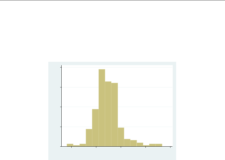
histogram — Histograms for continuous and categorical variables 843
Histograms of continuous variables
histogram assumes that the variable is continuous, so you need type only histogram followed
by the variable name:
. use http://www.stata-press.com/data/r13/sp500
(S&P 500)
. histogram volume
(bin=15, start=4103, width=1280.3533)
0 5.0e−05 1.0e−04 1.5e−04 2.0e−04
Density
5,000 10,000 15,000 20,000 25,000
Volume (thousands)
The small values reported for density on the yaxis are correct; if you added up the area of the bars,
you would get 1. Nevertheless, many people are used to seeing histograms scaled so that the bar
heights sum to 1,
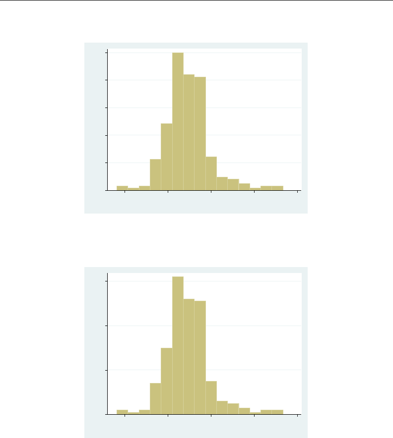
844 histogram — Histograms for continuous and categorical variables
. histogram volume, fraction
(bin=15, start=4103, width=1280.3533)
0 .05 .1 .15 .2 .25
Fraction
5,000 10,000 15,000 20,000 25,000
Volume (thousands)
and others are used to seeing histograms so that the bar height reflects the number of observations,
. histogram volume, frequency
(bin=15, start=4103, width=1280.3533)
0 20 40 60
Frequency
5,000 10,000 15,000 20,000 25,000
Volume (thousands)
Regardless of the scale you prefer, you can specify other options to make the graph look more
impressive:
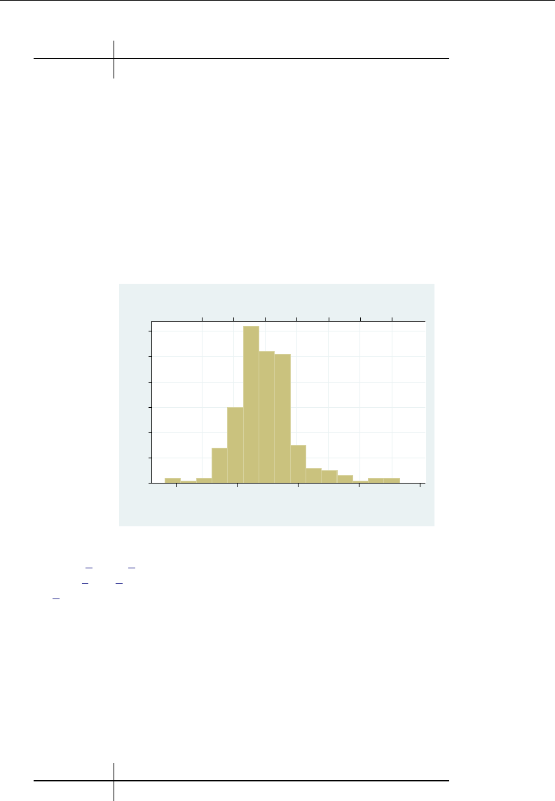
histogram — Histograms for continuous and categorical variables 845
. summarize volume
Variable Obs Mean Std. Dev. Min Max
volume 248 12320.68 2585.929 4103 23308.3
. histogram volume, freq
> xaxis(1 2)
> ylabel(0(10)60, grid)
> xlabel(12321 "mean"
> 9735 "-1 s.d."
> 14907 "+1 s.d."
> 7149 "-2 s.d."
> 17493 "+2 s.d."
> 20078 "+3 s.d."
> 22664 "+4 s.d."
> , axis(2) grid gmax)
> xtitle("", axis(2))
> subtitle("S&P 500, January 2001 - December 2001")
> note("Source: Yahoo! Finance and Commodity Systems, Inc.")
(bin=15, start=4103, width=1280.3533)
0 10 20 30 40 50 60
Frequency
mean−1 s.d. +1 s.d.−2 s.d. +2 s.d. +3 s.d. +4 s.d.
5,000 10,000 15,000 20,000 25,000
Volume (thousands)
Source: Yahoo! Finance and Commodity Systems, Inc.
S&P 500, January 2001 − December 2001
For an explanation of the xaxis() option—it created the upper and lower xaxis—
see [G-3]axis choice options. For an explanation of the ylabel() and xlabel() options,
see [G-3]axis label options. For an explanation of the subtitle() and note() options, see
[G-3]title options.
Overlaying normal and kernel density estimates
Specifying normal will overlay a normal density over the histogram. It would be enough to type
. histogram volume, normal
but we will add the option to our more impressive rendition:
. summarize volume
Variable Obs Mean Std. Dev. Min Max
volume 248 12320.68 2585.929 4103 23308.3
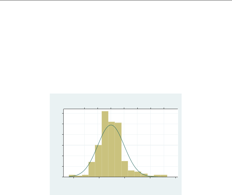
846 histogram — Histograms for continuous and categorical variables
. histogram volume, freq normal
> xaxis(1 2)
> ylabel(0(10)60, grid)
> xlabel(12321 "mean"
> 9735 "-1 s.d."
> 14907 "+1 s.d."
> 7149 "-2 s.d."
> 17493 "+2 s.d."
> 20078 "+3 s.d."
> 22664 "+4 s.d."
> , axis(2) grid gmax)
> xtitle("", axis(2))
> subtitle("S&P 500, January 2001 - December 2001")
> note("Source: Yahoo! Finance and Commodity Systems, Inc.")
(bin=15, start=4103, width=1280.3533)
0 10 20 30 40 50 60
Frequency
mean−1 s.d. +1 s.d.−2 s.d. +2 s.d. +3 s.d. +4 s.d.
5,000 10,000 15,000 20,000 25,000
Volume (thousands)
Source: Yahoo! Finance and Commodity Systems, Inc.
S&P 500, January 2001 − December 2001
If we instead wanted to overlay a kernel density estimate, we could specify kdensity in place of
normal.
Histograms of discrete variables
Specify histogram’s discrete option when you wish to treat the data as discrete—when you wish
each unique value of the variable to be assigned its own bin. For instance, in the automobile data,
mpg is a continuous variable, but the mileage ratings have been measured to integer precision. If we
were to type
. use http://www.stata-press.com/data/r13/auto
(1978 Automobile Data)
. histogram mpg
(bin=8, start=12, width=3.625)
mpg would be treated as continuous and categorized into eight bins by the default number-of-bins
calculation, which is based on the number of observations, 74.
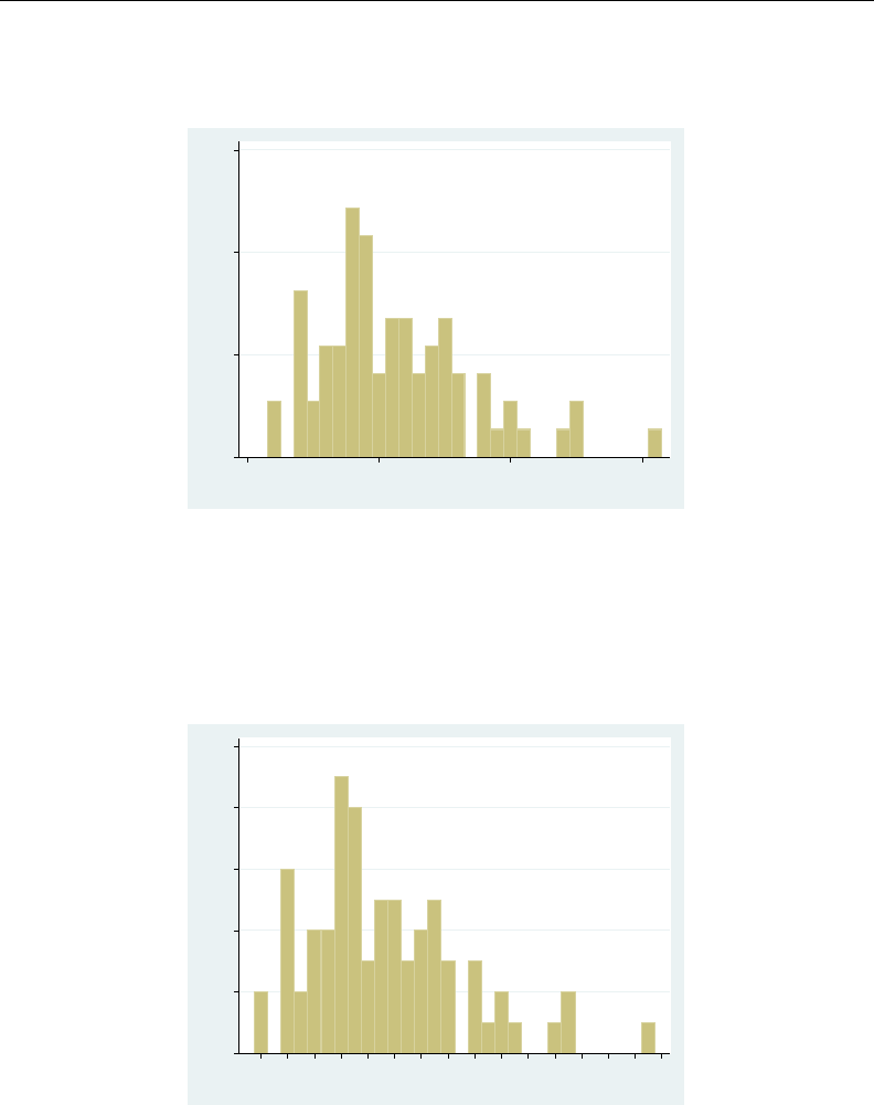
histogram — Histograms for continuous and categorical variables 847
Adding the discrete option makes a histogram with a bin for each of the 21 unique values.
. histogram mpg, discrete
(start=12, width=1)
0 .05 .1 .15
Density
10 20 30 40
Mileage (mpg)
Just as in the continuous case, the yaxis was reported in density, and we could specify the fraction
or frequency options if we wanted it to be reported differently. Below we specify frequency, we
specify addlabels to add a report of frequencies printed above the bars, we specify ylabel(,grid)
to add horizontal grid lines, and we specify xlabel(12(2)42) to label the values 12, 14, . . . , 42
on the xaxis:
. histogram mpg, discrete freq addlabels ylabel(,grid) xlabel(12(2)42)
(start=12, width=1)
2
6
2
4 4
9
8
3
5 5
3
4
5
3 3
1
2
1 1
2
1
0 2 4 6 8 10
Frequency
12 14 16 18 20 22 24 26 28 30 32 34 36 38 40 42
Mileage (mpg)
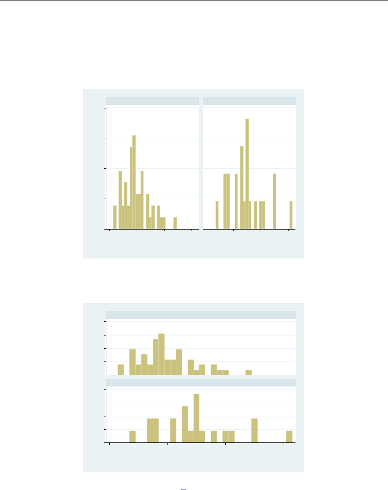
848 histogram — Histograms for continuous and categorical variables
Use with by()
histogram may be used with graph twoway’s by(); for example,
. use http://www.stata-press.com/data/r13/auto
(1978 Automobile Data)
. histogram mpg, discrete by(foreign)
0 .05 .1 .15 .2
10 20 30 40 10 20 30 40
Domestic Foreign
Density
Mileage (mpg)
Graphs by Car type
Here results would be easier to compare if the graphs were presented in one column:
. histogram mpg, discrete by(foreign, col(1))
0 .05 .1 .15 .20 .05 .1 .15 .2
10 20 30 40
Domestic
Foreign
Density
Mileage (mpg)
Graphs by Car type
col(1) is a by() suboption—see [G-3]by option—and there are other useful suboptions, such
as total, which will add an overall total histogram. total is a suboption of by(), not an option
of histogram, so you would type
. histogram mpg, discrete by(foreign, total)
and not histogram mpg, discrete by(foreign) total.

histogram — Histograms for continuous and categorical variables 849
As another example, Lipset (1993) reprinted data from the New York Times (November 5, 1992)
collected by the Voter Research and Surveys based on questionnaires completed by 15,490 U.S.
presidential voters from 300 polling places on election day in 1992.
. use http://www.stata-press.com/data/r13/voter
. histogram candi [freq=pop], discrete fraction by(inc, total)
> gap(40) xlabel(2 3 4, valuelabel)
0 .2 .4 .60 .2 .4 .6
Clinton Bush Perot Clinton Bush Perot Clinton Bush Perot
<$15k $15−30k $30−50k
$50−75k $75k+ Total
Fraction
Candidate voted for, 1992
Graphs by Family Income
We specified gap(40) to reduce the width of the bars by 40%. We also used xlabel()’s
valuelabel suboption, which caused our bars to be labeled “Clinton”, “Bush”, and “Perot”, rather
than 2, 3, and 4; see [G-3]axis label options.
Video example
Histograms in Stata
References
Cox, N. J. 2004. Speaking Stata: Graphing distributions.Stata Journal 4: 66–88.
. 2005. Speaking Stata: Density probability plots.Stata Journal 5: 259–273.
Harrison, D. A. 2005. Stata tip 20: Generating histogram bin variables.Stata Journal 5: 280–281.
Lipset, S. M. 1993. The significance of the 1992 election. PS: Political Science and Politics 26: 7–16.
Pollock, P. H., III. 2011. A Stata Companion to Political Analysis. 2nd ed. Washington, DC: CQ Press.
Also see
[R]kdensity — Univariate kernel density estimation
[R]spikeplot — Spike plots and rootograms
[G-2]graph twoway histogram — Histogram plots

Title
icc — Intraclass correlation coefficients
Syntax Menu
Description Options for one-way RE model
Options for two-way RE and ME models Remarks and examples
Stored results Methods and formulas
References Also see
Syntax
Calculate intraclass correlations for one-way random-effects model
icc depvar target if in ,oneway options
Calculate intraclass correlations for two-way random-effects model
icc depvar target rater if in ,twoway re options
Calculate intraclass correlations for two-way mixed-effects model
icc depvar target rater if in , mixed twoway me options
oneway options Description
Main
absolute estimate absolute agreement; the default
testvalue(#)test whether intraclass correlations equal #;
default is testvalue(0)
Reporting
level(#)set confidence level; default is level(95)
format(%fmt)display format for statistics and confidence intervals;
default is format(%9.0g)
twoway re options Description
Main
absolute estimate absolute agreement; the default
consistency estimate consistency of agreement
testvalue(#)test whether intraclass correlations equal #;
default is testvalue(0)
Reporting
level(#)set confidence level; default is level(95)
format(%fmt)display format for statistics and confidence intervals;
default is format(%9.0g)
850

icc — Intraclass correlation coefficients 851
twoway me options Description
Main
∗mixed estimate intraclass correlations for a mixed-effects model
consistency estimate consistency of agreement; the default
absolute estimate absolute agreement
testvalue(#)test whether intraclass correlations equal #;
default is testvalue(0)
Reporting
level(#)set confidence level; default is level(95)
format(%fmt)display format for statistics and confidence intervals;
default is format(%9.0g)
∗mixed is required.
bootstrap,by,jackknife, and statsby are allowed; see [U] 11.1.10 Prefix commands.
Menu
Statistics >Summaries, tables, and tests >Summary and descriptive statistics >Intraclass correlations
Description
icc estimates intraclass correlations for one-way random-effects models, two-way random-effects
models, or two-way mixed-effects models for both individual and average measurements. Intraclass
correlations measuring consistency of agreement or absolute agreement of the measurements may be
estimated.
Options for one-way RE model
Main
absolute specifies that intraclass correlations measuring absolute agreement of the measurements
be estimated. This is the default for random-effects models.
testvalue(#)tests whether intraclass correlations equal #. The default is testvalue(0).
Reporting
level(#)specifies the confidence level, as a percentage, for confidence intervals. The default is
level(95) or as set by set level; see [R]level.
format(%fmt)specifies how the intraclass correlation estimates and confidence intervals are to be
formatted. The default is format(%9.0g).

852 icc — Intraclass correlation coefficients
Options for two-way RE and ME models
Main
mixed is required to calculate two-way mixed-effects models. mixed specifies that intraclass corre-
lations for a mixed-effects model be estimated.
absolute specifies that intraclass correlations measuring absolute agreement of the measurements be
estimated. This is the default for random-effects models. Only one of absolute or consistency
may be specified.
consistency specifies that intraclass correlations measuring consistency of agreement of the mea-
surements be estimated. This is the default for mixed-effects models. Only one of absolute or
consistency may be specified.
testvalue(#)tests whether intraclass correlations equal #. The default is testvalue(0).
Reporting
level(#)specifies the confidence level, as a percentage, for confidence intervals. The default is
level(95) or as set by set level; see [R]level.
format(%fmt)specifies how the intraclass correlation estimates and confidence intervals are to be
formatted. The default is format(%9.0g).
Remarks and examples
Remarks are presented under the following headings:
Introduction
One-way random effects
Two-way random effects
Two-way mixed effects
Adoption study
Relationship between ICCs
Tests against nonzero values
Introduction
In some disciplines, such as psychology and sociology, data are often measured with error that
can seriously affect statistical interpretation of the results. Thus it is important to assess the amount
of measurement error by evaluating the consistency or reliability of measurements. The intraclass
correlation coefficient (ICC) is often used to measure the consistency or homogeneity of measurements.
Several versions of ICCs are introduced in the literature depending on the experimental design and
goals of the study (see, for example, Shrout and Fleiss [1979] and McGraw and Wong [1996a]).
Following Shrout and Fleiss (1979), we describe various forms of ICCs in the context of a reliability
study of ratings of different targets (or objects of measurements) by several raters.
Consider ntargets (for example, students, patients, athletes) that are randomly sampled from a
population of interest. Each target is rated independently by a set of kraters (for example, teachers,
doctors, judges). One rating per target and rater is obtained. It is of interest to determine the extent
of the agreement of the ratings.
As noted by Shrout and Fleiss (1979) and McGraw and Wong (1996a), you need to answer several
questions to decide what version of ICC is appropriate to measure the agreement in your study:

icc — Intraclass correlation coefficients 853
1. Is a one-way or two-way analysis-of-variance model appropriate for your study?
2. Are differences between raters’ mean ratings relevant to the reliability of interest?
3. Is the unit of analysis an individual rating or the mean rating over several raters?
4. Is the consistency of agreement or the absolute agreement of ratings of interest?
Three types of analysis-of-variance models are considered for the reliability study: one-way random
effects, two-way random effects, and two-way mixed effects. Mixed models contain both fixed effects
and random effects. In the one-way random-effects model, each target is rated by a different set of
kindependent raters, who are randomly drawn from the population of raters. The target is the only
random effect in this model; the effects due to raters and possibly due to rater-and-target interaction
cannot be separated from random error. In the two-way random-effects model, each target is rated
by the same set of kindependent raters, who are randomly drawn from the population of raters.
The random effects in this model are target and rater and possibly their interaction, although in the
absence of repeated measurements for each rater on each target, the effect of an interaction cannot
be separated from random error. In the two-way mixed-effects model, each target is rated by the
same set of kindependent raters. Because they are the only raters of interest, rater is a fixed effect.
The random effects are target and possibly target-and-rater interaction, but again the interaction effect
cannot be separated from random error without repeated measurements for each rater and target. The
definition of ICC depends on the chosen random-effects model; see Methods and formulas for details.
In summary, use a one-way model if there are no systematic differences in measurements due to
raters and use a two-way model otherwise. If you want to generalize your results to a population
of raters from which the observed raters are sampled, use a two-way random-effects model, treating
raters as random. If you are only interested in the effects of the observed kraters, use a two-way
mixed-effects model, treating raters as fixed. For example, suppose you compare judges’ ratings of
targets from different groups. If you use the combined data from kjudges to compare the groups,
the random-effects model is appropriate. If you compare groups separately for each judge and then
pool the differences, the mixed-effects model is appropriate.
The definition of ICC also depends on the unit of analysis in a study—whether the agreement is
measured between individual ratings (individual ICC) or between the averages of ratings over several
raters (average ICC). The data on individual ratings are more common. The data on average ratings
are typically used when individual ratings are deemed unreliable. The average ICC can also be used
when teams of raters are used to rate a target. For example, the ratings of teams of physicians may
be evaluated in this manner. When the unit of analysis is an average rating, you should remember
that the interpretation of ICC pertains to average ratings and not individual ratings.
Finally, depending on whether consistency of agreement or absolute agreement is of interest, two
types of ICC are used: consistency-of-agreement ICC (CA-ICC) and absolute-agreement ICC (AA-ICC).
Under consistency of agreement, the scores are considered consistent if the scores from any two raters
differ by the same constant value for all targets. This implies that raters give the same ranking to
all targets. Under absolute agreement, the scores are considered in absolute agreement if the scores
from all raters match exactly.
For example, suppose we observe three targets and two raters. The ratings are (2,4), (4,6), and
(6,8), with rater 1 giving the scores (2,4,6) and rater 2 giving the scores (4,6,8), two points higher
than rater 1. The CA-ICC between individual ratings is 1 because the scores from rater 1 and rater 2
differ by a constant value (two points) for all targets. That rater 1 gives lower scores than rater 2 is
deemed irrelevant under the consistency measure of agreement. The raters have the same difference
of opinion on every target, and the variation between raters that is caused by this difference is not
relevant. On the other hand, the AA-ICC between individual ratings is 8/12 =0.67, where 8 is the
estimated between-target variance and 12 is the estimated total variance of ratings.

854 icc — Intraclass correlation coefficients
Either CA-ICC or AA-ICC can serve as a useful measure of agreement depending on whether rater
variability is relevant for determining the degree of agreement. As McGraw and Wong (1996a) point
out, CA-ICC is useful when comparative judgments are made about objects of measurement. The
CA-ICC represents correlation when the rater is fixed; the AA-ICC represents correlation when the rater
is random.
See Shrout and Fleiss (1979) and McGraw and Wong (1996a) for more detailed guidelines about
the choice of appropriate ICC.
Shrout and Fleiss (1979) and McGraw and Wong (1996a) describe 10 versions of ICCs based on
the concepts above: individual and average AA-ICCs for a one-way model (consistency of agreement is
not defined for this model); individual and average AA-ICCs and CA-ICCs for a two-way random-effects
model; and individual and average AA-ICCs and CA-ICCs for a two-way mixed-effects model. Although
each of these ICCs has its own definition and interpretation, the estimators for some are identical,
leading to the same estimates of those ICCs; see Relationship between ICCs and Methods and formulas
for details.
The icc command calculates ICCs for each of the three analysis-of-variance models. You can use
option absolute to compute AA-ICCs or option consistency to compute CA-ICCs. By default, icc
computes ICCs corresponding to the correlation between ratings and between average ratings made
on the same target: AA-ICC for a random-effects model and CA-ICC for a mixed-effects model. As
pointed out by Shrout and Fleiss (1979), although the data on average ratings might be needed for
reliability, the generalization of interest might be individuals. For this reason, icc reports ICCs for
both units, individual and average, for each model.
In addition to estimates of ICCs, icc provides confidence intervals and one-sided Ftests. The F
test of Ho:ρ=0 versus Ha:ρ > 0 is the same for the individual and average ICCs, so icc reports
one test. This is not true, however, for nonzero null hypotheses (see Tests against nonzero values for
details), so icc reports a separate test in this case.
The icc command requires data in long form; see [D]reshape for how to convert data in wide form
to long form. The data must also be balanced and contain one observation per target and rater. For
unbalanced data, icc omits all targets with fewer than kratings from computation. Under one-way
models, kis determined as the largest number of observed ratings for a target. Under two-way models,
kis the number of unique raters. If multiple observations per target and rater are detected, icc issues
an error.
We demonstrate the use of icc using datasets from Shrout and Fleiss (1979) and McGraw and
Wong (1996a). In the next three sections, we use an example from table 2 of Shrout and Fleiss (1979)
with six targets and four judges. For instructional purposes, we analyze these data under each of the
three different models: one-way random effects, two-way random effects, and two-way mixed effects.
One-way random effects
In the one-way random-effects model, we assume that the ntargets being rated are randomly
selected from the population of potential targets. Each is rated by a different set of kraters randomly
drawn from the population of potential raters. McGraw and Wong (1996a) describe an example of
this setting, where behavioral genetics data are used to assess familial resemblance. Family units can
be viewed as “targets”, and children can be viewed as “raters”. By taking a measurement on a child
of the family unit, we obtain the “rating” of the family unit by the “child-rater”. In this case, we can
use ICC to assess similarity between children within a family or, in other words, assess if there is a
family effect in these data.

icc — Intraclass correlation coefficients 855
As we mentioned in the introduction, only AA-ICC is defined for a one-way model. The consistency
of agreement is not defined in this case, as each target is evaluated by a different set of raters. Thus
there is no between-rater variability in this model.
In a one-way model, the AA-ICC corresponds to the correlation coefficient between ratings within
a target. It is also a ratio of the between-target variance of ratings to the total variance of ratings, the
sum of the between-target and error variances.
Example 1: One-way random-effects ICCs
Consider data from table 2 of Shrout and Fleiss (1979) stored in judges.dta. The data contain
24 ratings of n=6 targets by k=4 judges. We list the first eight observations:
. use http://www.stata-press.com/data/r13/judges
(Ratings of targets by judges)
. list in 1/8, sepby(target)
rating target judge
1. 9 1 1
2. 2 1 2
3. 5 1 3
4. 8 1 4
5. 6 2 1
6. 1 2 2
7. 3 2 3
8. 2 2 4
For a moment, let’s ignore that targets are rated by the same set of judges. Instead, we assume that
a different set of four judges is used to rate each target. In this case, the only systematic variation in
the data is due to targets, so the one-way random-effects model is appropriate.
We use icc to estimate the intraclass correlations for these data. To compute ICCs for a one-way
model, we specify the dependent variable rating followed by the target variable target:
. icc rating target
Intraclass correlations
One-way random-effects model
Absolute agreement
Random effects: target Number of targets = 6
Number of raters = 4
rating ICC [95% Conf. Interval]
Individual .1657418 -.1329323 .7225601
Average .4427971 -.8844422 .9124154
F test that
ICC=0.00: F(5.0, 18.0) = 1.79 Prob > F = 0.165
Note: ICCs estimate correlations between individual measurements
and between average measurements made on the same target.
icc reports the AA-ICCs for both individual and average ratings. The individual AA-ICC corresponds
to ICC(1) in McGraw and Wong (1996a) or ICC(1,1) in Shrout and Fleiss (1979). The average AA-ICC
corresponds to ICC(k)in McGraw and Wong (1996a) or ICC(1,k)in Shrout and Fleiss (1979).

856 icc — Intraclass correlation coefficients
The estimated correlation between individual ratings is 0.17, indicating little similarity between
ratings within a target, low reliability of individual target ratings, or no target effect. The estimated
intraclass correlation between ratings averaged over k=4 judges is higher, 0.44. (The average ICC
will typically be higher than the individual ICC.) The estimated intraclass correlation measures the
similarity or reliability of mean ratings from groups of four judges. We do not have statistical evidence
that either ICC is different from zero based on reported confidence intervals and the one-sided Ftest.
Note that although the estimates of ICCs cannot be negative in this setting, the lower bound of the
computed confidence interval may be negative. A common ad-hoc way of handling this is to truncate
the lower bound at zero.
The estimates of both the individual and the average AA-ICC are also computed by the loneway
command (see [R]loneway), which performs a one-way analysis of variance.
Technical note
Mean rating is commonly used when individual rating is unreliable because the reliability of a
mean rating is always higher than the reliability of the individual rating when the individual reliability
is positive.
In the previous example, we estimated low reliability of the individual ratings of a target, 0.17.
The reliability increased to 0.44 for the ratings averaged over four judges. What if we had more
judges?
We can use the Spearman–Brown formula (Spearman 1910;Brown 1910) to compute the m-average
ICC based on the individual ICC:
ICC(m) = mICC(1)
1+(m−1)ICC(1)
Using this formula for the previous example, we find that the mean reliability over, say, 10 judges
is 10 ×0.17/(1+9×0.17) = 0.67.
Alternatively, we can invert the Spearman–Brown formula to determine the number of judges (or
the number of ratings of a target) we need to achieve the desired reliability. Suppose we would like
an average reliability of 0.9, then
m=ICC(m){(1 −ICC(1))}
ICC(1){1−ICC(m)}=0.9(1 −0.17)
0.17(1 −0.9) = 44
See, for example, Bliese (2000) for other examples.
Two-way random effects
As before, we assume that the targets being rated are randomly selected from the population of
potential targets. We now also assume that each target is evaluated by the same set of kraters, who
have been randomly sampled from the population of raters. In this scenario, we want to generalize
our findings to the population of raters from which the observed kraters were sampled. For example,
suppose we want to estimate the reliability of doctors’ evaluations of patients with a certain condition.
Unless the reliability at a specific hospital is of interest, the doctors may be interchanged with others
in the relevant population of doctors.

icc — Intraclass correlation coefficients 857
As for a one-way model, the AA-ICC corresponds to the correlation between measurements on the
same target and is also a ratio of the between-target variance to the total variance of measurements in a
two-way random-effects model. The total variance is now the sum of the between-target, between-rater,
and error variances. Unlike a one-way model, the CA-ICC can be computed for a two-way random-
effects model when the consistency of agreement is of interest rather than the absolute agreement.
The CA-ICC is also the ratio of the between-target variance to the total variance, but the total variance
does not include the between-rater variance because the between-rater variability is irrelevant for the
consistency of agreement.
Again, the two versions, individual and average, are available for each ICC.
Example 2: Two-way random-effects ICCs
Continuing with example 1, recall that we previously ignored that each target is rated by the same
set of four judges and instead assumed different sets of judges. We return to the original data setting.
We want to evaluate the agreement between judges’ ratings of targets in a population represented by
the observed set of four judges.
In a two-way model, we must specify both the target and the rater variables. In icc, we now
additionally specify the rater variable judge following the target variable target; the random-effects
model is assumed by default.
. icc rating target judge
Intraclass correlations
Two-way random-effects model
Absolute agreement
Random effects: target Number of targets = 6
Random effects: judge Number of raters = 4
rating ICC [95% Conf. Interval]
Individual .2897638 .0187865 .7610844
Average .6200505 .0711368 .927232
F test that
ICC=0.00: F(5.0, 15.0) = 11.03 Prob > F = 0.000
Note: ICCs estimate correlations between individual measurements
and between average measurements made on the same target.
As for a one-way random-effects model, icc by default reports AA-ICCs that correspond to the
correlation between ratings on a target. Notice that both individual and average ICCs are larger in
the two-way random-effects model than in the previous one-way model—0.29 versus 0.17 and 0.62
versus 0.44, respectively. We also have statistical evidence to reject the null hypothesis that neither
ICC is zero based on confidence intervals and the Ftest. If a one-way model is used when a two-way
model is appropriate, the true ICC will generally be underestimated.
The individual AA-ICC corresponds to ICC(A,1) in McGraw and Wong (1996a) or ICC(2,1) in Shrout
and Fleiss (1979). The average AA-ICC corresponds to ICC(A,k)in McGraw and Wong (1996a) or
ICC(2,k)in Shrout and Fleiss (1979).
Instead of the absolute agreement, we can also assess the consistency of agreement. The individual
and average CA-ICCs are considered in McGraw and Wong (1996a) and denoted as ICC(C,1) and
ICC(C,k), respectively. These ICCs are not considered in Shrout and Fleiss (1979) because they are not
correlations in the strict sense. Although CA-ICCs do not estimate correlation, they can provide useful
information about the reliability of the raters. McGraw and Wong (1996a) note that the practical
value of the individual and average CA-ICCs in the two-way random-effects model setting is well
documented in measurement theory, citing Hartmann (1982) and Suen (1988).

858 icc — Intraclass correlation coefficients
To estimate the individual and average CA-ICCs, we specify the consistency option:
. icc rating target judge, consistency
Intraclass correlations
Two-way random-effects model
Consistency of agreement
Random effects: target Number of targets = 6
Random effects: judge Number of raters = 4
rating ICC [95% Conf. Interval]
Individual .7148407 .3424648 .9458583
Average .9093155 .6756747 .9858917
F test that
ICC=0.00: F(5.0, 15.0) = 11.03 Prob > F = 0.000
We estimate that the consistency of agreement of ratings in the considered population of raters is
high, 0.71, based on the individual CA-ICC. On the other hand, the absolute agreement of ratings is
low, 0.29, based on the individual AA-ICC from the previous output.
The measure of consistency of agreement among means, the average CA-ICC, is equivalent to
Cronbach’s alpha (Cronbach 1951); see [MV]alpha. The individual CA-ICC can also be equivalent to
the Pearson’s correlation coefficient between raters when k=2; see McGraw and Wong (1996a) for
details.
In the next example, we will see that the actual estimates of the individual and average AA-ICCs
and CA-ICCs are the same whether we examine a random-effects model or a mixed-effects model.
The differences between these ICCs are in their definitions and interpretations.
Two-way mixed effects
As in a two-way random-effects model, we assume that the targets are randomly selected from the
population of potential targets and that each is evaluated by the same set of kraters. In a mixed-effects
model, however, we assume that these raters are the only raters of interest. So as before, the targets
are random, but now the raters are fixed.
In the two-way mixed-effects model, the fixed effect of the rater does not contribute to the between-
rater random variance component to the total variance. As such, the definitions and interpretations of
ICCs are different in a mixed-effects model than in a random-effects model. However, the estimates
of ICCs as well as test statistics and confidence intervals are the same. The only exceptions are
average AA-ICCs and CA-ICCs. These are not estimable in a two-way mixed-effects model including an
interaction term between target and rater; see Relationship between ICCs and Methods and formulas
for details.
In a two-way mixed-effects model, the CA-ICC corresponds to the correlation between measurements
on the same target. As pointed out by Shrout and Fleiss (1979), when the rater variance is ignored, the
correlation coefficient is interpreted in terms of rater consistency rather than rater absolute agreement.
Formally, the CA-ICC is the ratio of the covariance between measurements on the target to the total
variance of the measurements. The AA-ICC corresponds to the same ratio, but includes a variance of
the fixed factor, rater, in its denominator.

icc — Intraclass correlation coefficients 859
Example 3: Two-way mixed-effects ICCs
Continuing with example 2, suppose that we are now interested in assessing the agreement of
ratings from only the observed four judges. The judges are now fixed effects, and the appropriate
model is a two-way mixed-effects model.
To estimate ICCs for a two-way mixed-effects model, we specify the mixed option with icc:
. icc rating target judge, mixed
Intraclass correlations
Two-way mixed-effects model
Consistency of agreement
Random effects: target Number of targets = 6
Fixed effects: judge Number of raters = 4
rating ICC [95% Conf. Interval]
Individual .7148407 .3424648 .9458583
Average .9093155 .6756747 .9858917
F test that
ICC=0.00: F(5.0, 15.0) = 11.03 Prob > F = 0.000
Note: ICCs estimate correlations between individual measurements
and between average measurements made on the same target.
As we described in the introduction, icc by default reports ICCs corresponding to the correlations.
So, for a mixed-effects model, icc reports CA-ICCs by default. The individual and average CA-ICCs
are denoted as ICC(3,1) and ICC(3,k)in Shrout and Fleiss (1979) and ICC(C,1) and ICC(C,k)in McGraw
and Wong (1996a).
Our estimates of the individual and average CA-ICCs are identical to the CA-ICC estimates obtained
under the two-way random-effects model in example 2, but our interpretation of the results is different.
Under a mixed-effects model, 0.71 and 0.91 are the estimates, respectively, of the correlation between
individual measurements and the correlation between average measurements made on the same target.
We can also estimate the AA-ICCs in this setting by specifying the absolute option:
. icc rating target judge, mixed absolute
Intraclass correlations
Two-way mixed-effects model
Absolute agreement
Random effects: target Number of targets = 6
Fixed effects: judge Number of raters = 4
rating ICC [95% Conf. Interval]
Individual .2897638 .0187865 .7610844
Average .6200505 .0711368 .927232
F test that
ICC=0.00: F(5.0, 15.0) = 11.03 Prob > F = 0.000
The intraclass correlation estimates match the individual and average AA-ICCs obtained under the
two-way random-effects model in example 2; but in a mixed-effects model, they do not represent
correlations. We demonstrate the use of an individual AA-ICC in a mixed-effects setting in the next
example.
The AA-ICCs under a mixed-effects model are not considered by Shrout and Fleiss (1979). They
are denoted as ICC(A,1) and ICC(A,k)in McGraw and Wong (1996a).

860 icc — Intraclass correlation coefficients
Adoption study
In this section, we consider the adoption study described in McGraw and Wong (1996a). Adoption
studies commonly include two effects of interest. One is the mean difference between the adopted
child and its biological parents. It is used to determine if characteristics of adopted children differ on
average from those of their biological parents. Another effect of interest is the correlation between
genetically paired individuals and genetically unrelated individuals who live together. This effect is
used to evaluate the impact of genetic differences on individual differences.
As discussed in McGraw and Wong (1996a), a consistent finding from adoption research using IQ
as a trait characteristic is that while adopted children typically have higher IQs than their biological
parents, their IQs correlate better with those of their biological parents than with those of their adoptive
parents. Both effects are important, and there is additional need to reconcile the two findings. McGraw
and Wong (1996a) propose to use the individual AA-ICC for this purpose.
Example 4: Absolute-agreement ICC in a mixed-effects model
The adoption.dta dataset contains the data from table 6 of McGraw and Wong (1996a) on IQ
scores:
. use http://www.stata-press.com/data/r13/adoption
(Biological mother and adopted child IQ scores)
. describe
Contains data from http://www.stata-press.com/data/r13/adoption.dta
obs: 20 Biological mother and adopted
child IQ scores
vars: 5 15 May 2013 13:50
size: 160 (_dta has notes)
storage display value
variable name type format label variable label
family byte %9.0g Adoptive family ID
mc byte %9.0g mcvalues 1=Mother, 2=Child
iq3 int %9.0g IQ scores, mother-child
difference of 3 pts
iq9 int %9.0g IQ scores, mother-child
difference of 9 pts
iq15 int %9.0g IQ scores, mother-child
difference of 15 pts
Sorted by:
The family variable contains adoptive family identifiers, the mc variable records a mother or a child,
and the iq3,iq9, and iq15 variables record IQ scores with differences between mother and child
mean IQ scores of 3, 9, and 15 points, respectively.

icc — Intraclass correlation coefficients 861
. by mc, sort: summarize iq*
-> mc = Mother
Variable Obs Mean Std. Dev. Min Max
iq3 10 97 15.0037 62 116
iq9 10 91 15.0037 56 110
iq15 10 85 15.0037 50 104
-> mc = Child
Variable Obs Mean Std. Dev. Min Max
iq3 10 100 15.0037 65 119
iq9 10 100 15.0037 65 119
iq15 10 100 15.0037 65 119
The variances of the mother and child IQ scores are the same.
Children are fixed effects, so the mixed-effects model is appropriate for these data. We want to
compare individual CA-ICC with individual AA-ICC for each of the three IQ variables. We could issue a
separate icc command for each of the three IQ variables to obtain the intraclass correlations. Instead,
we use reshape to convert our data to long form with one iq variable and the new diff variable
recording mean differences:
. reshape long iq, i(family mc) j(diff)
(note: j = 3 9 15)
Data wide -> long
Number of obs. 20 -> 60
Number of variables 5 -> 4
j variable (3 values) -> diff
xij variables:
iq3 iq9 iq15 -> iq
We can now use the by prefix with icc to estimate intraclass correlations for the three groups of
interest:

862 icc — Intraclass correlation coefficients
. by diff, sort: icc iq family mc, mixed
-> diff = 3
Intraclass correlations
Two-way mixed-effects model
Consistency of agreement
Random effects: family Number of targets = 10
Fixed effects: mc Number of raters = 2
iq ICC [95% Conf. Interval]
Individual .7142152 .1967504 .920474
Average .8332853 .3288078 .9585904
F test that
ICC=0.00: F(9.0, 9.0) = 6.00 Prob > F = 0.007
Note: ICCs estimate correlations between individual measurements
and between average measurements made on the same target.
-> diff = 9
Intraclass correlations
Two-way mixed-effects model
Consistency of agreement
Random effects: family Number of targets = 10
Fixed effects: mc Number of raters = 2
iq ICC [95% Conf. Interval]
Individual .7142152 .1967504 .920474
Average .8332853 .3288078 .9585904
F test that
ICC=0.00: F(9.0, 9.0) = 6.00 Prob > F = 0.007
Note: ICCs estimate correlations between individual measurements
and between average measurements made on the same target.
-> diff = 15
(output omitted )
The estimated CA-ICCs are the same in all three groups and are equal to the corresponding estimates
of the Pearson’s correlation coefficients because mothers’ and childrens’ IQ scores have the same
variability. The scores differ only in means, and mean differences are irrelevant when measuring the
consistency of agreement.

icc — Intraclass correlation coefficients 863
The AA-ICCs, however, differ across the three groups:
. by diff, sort: icc iq family mc, mixed absolute
-> diff = 3
Intraclass correlations
Two-way mixed-effects model
Absolute agreement
Random effects: family Number of targets = 10
Fixed effects: mc Number of raters = 2
iq ICC [95% Conf. Interval]
Individual .7204023 .2275148 .9217029
Average .8374812 .3706917 .9592564
F test that
ICC=0.00: F(9.0, 9.0) = 6.00 Prob > F = 0.007
-> diff = 9
Intraclass correlations
Two-way mixed-effects model
Absolute agreement
Random effects: family Number of targets = 10
Fixed effects: mc Number of raters = 2
iq ICC [95% Conf. Interval]
Individual .6203378 .0293932 .8905025
Average .7656895 .0571077 .9420802
F test that
ICC=0.00: F(9.0, 9.0) = 6.00 Prob > F = 0.007
-> diff = 15
Intraclass correlations
Two-way mixed-effects model
Absolute agreement
Random effects: family Number of targets = 10
Fixed effects: mc Number of raters = 2
iq ICC [95% Conf. Interval]
Individual .4854727 -.1194157 .8466905
Average .6536272 -.2712191 .9169815
F test that
ICC=0.00: F(9.0, 9.0) = 6.00 Prob > F = 0.007
As the mean differences increase, the AA-ICCs decrease. Their attenuation reflects the difference in
means between biological mother and child IQs while still measuring their agreement. Notice that for
small mean differences, the estimates of AA-ICCs and CA-ICCs are very similar.
Note that our estimates match those given in McGraw and Wong (1996b), who correct the original
table 6 of McGraw and Wong (1996a).

864 icc — Intraclass correlation coefficients
Relationship between ICCs
In examples 2and 3, we saw that the estimates of AA-ICCs and CA-ICCs are the same for two-
way random-effects and two-way mixed-effects models. In this section, we consider the relationship
between various forms of ICCs in more detail; also see Methods and formulas.
There are 10 different versions of ICCs, but only six different estimators are needed to compute
them. These estimators include the two estimators for the individual and average AA-ICCs in a one-way
model, the two estimators for the individual and average AA-ICCs in two-way models, and the two
estimators for the individual and average CA-ICCs in two-way models.
Only individual and average AA-ICCs are defined for the one-way model. The estimates of AA-ICCs
based on the one-way model will typically be smaller than individual and average estimates of AA-ICCs
and CA-ICCs based on two-way models. The estimates of individual and average CA-ICCs will typically
be larger than the estimates of individual and average AA-ICCs.
Although AA-ICCs and CA-ICCs have the same respective estimators in two-way random-effects
and mixed-effects models, their definitions and interpretations are different. The AA-ICCs based on
a random-effects model contain the between-rater variance component in the denominator of the
variance ratio. The AA-ICCs based on a mixed-effects model contain the variance of the fixed-factor
rater instead of the random between-rater variability. The AA-ICCs in a random-effects model represent
correlations between any two measurements made on a target. The AA-ICCs in a mixed-effects model
measure absolute agreement of measurements treating raters as fixed. The CA-ICCs for random-effects
and mixed-effects models have the same definition but different interpretations. The CA-ICCs represent
correlations between any two measurements made on a target in a mixed-effects model but estimate the
degree of consistency among measurements treating raters as random in a random-effects model. The
difference in the definitions of AA-ICCs and CA-ICCs is that CA-ICCs do not contain the between-rater
variance in the denominator of the variance ratio.
For two-way models, the definitions and interpretations (but not the estimators) of ICCs also
depend on whether the model contains an interaction between target and rater. For two-way models
with interaction, ICCs include an additional variance component for the target-rater interaction in the
denominator of the variance ratio. This component cannot be separated from random error because
there is only one observation per target and rater.
Also, under a two-way mixed-effects model including interaction, the interaction components are
not mutually independent, as they are in a two-way random-effects model. The considered version
of the mixed-effects model places a constraint on the interaction effects—the sum of the interaction
effects over levels of the fixed factor is zero; see, for example, chapter 7 in Kuehl (2000) for an
introductory discussion of mixed models. In this version of the model, there is a correlation between
the interaction effects. Specifically, the two interaction effects for the same target and two different
raters are negatively correlated. As a result, the estimated intraclass correlation can be negative under
a two-way mixed-effects model with interaction. Also, average AA-ICC and average CA-ICC cannot
be estimated in a two-way mixed-effects model including interaction; see Methods and formulas and
McGraw and Wong (1996a) for details.
Tests against nonzero values
It may be of interest to test whether the intraclass correlation is equal to a value other than zero.
icc supports testing against positive values through the use of the testvalue() option. Specifying
testvalue(#)provides a one-sided hypothesis test of Ho:ρ=#versus Ha:ρ > #. The test is
provided separately for both individual and average ICCs.

icc — Intraclass correlation coefficients 865
Example 5: Testing ICC against a nonzero value
We return to the two-way random-effects model for the judge and target data from Shrout and
Fleiss (1979). Suppose we want to test whether the individual and average AA-ICCs are each equal
to 0.2. We specify the testvalue(0.2) option with icc:
. use http://www.stata-press.com/data/r13/judges, clear
(Ratings of targets by judges)
. icc rating target judge, testvalue(0.2)
Intraclass correlations
Two-way random-effects model
Absolute agreement
Random effects: target Number of targets = 6
Random effects: judge Number of raters = 4
rating ICC [95% Conf. Interval]
Individual .2897638 .0187865 .7610844
Average .6200505 .0711368 .927232
F test that
ICC(1)=0.20: F(5.0, 5.3) = 1.54 Prob > F = 0.317
ICC(k)=0.20: F(5.0, 9.4) = 4.35 Prob > F = 0.026
Note: ICCs estimate correlations between individual measurements
and between average measurements made on the same target.
We reject the null hypothesis that the average AA-ICC, labeled as ICC(k)in the output, is equal to
0.2, but we do not have statistical evidence to reject the null hypothesis that the individual AA-ICC,
labeled as ICC(1), is equal to 0.2.
Stored results
icc stores the following in r():
Scalars
r(N target) number of targets
r(N rater) number of raters
r(icc i) intraclass correlation for individual measurements
r(icc i F) Ftest statistic for individual ICC
r(icc i df1) numerator degrees of freedom for r(icc i F)
r(icc i df2) denominator degrees of freedom for r(icc i F)
r(icc i p) p-value for F test of individual ICC
r(icc i lb) lower endpoint for confidence intervals of individual ICC
r(icc i ub) upper endpoint for confidence intervals of individual ICC
r(icc avg) intraclass correlation for average measurements
r(icc avg F) Ftest statistic for average ICC
r(icc avg df1) numerator degrees of freedom for r(icc avg F)
r(icc avg df2) denominator degrees of freedom for r(icc avg F)
r(icc avg p) p-value for Ftest of average ICC
r(icc avg lb) lower endpoint for confidence intervals of average ICC
r(icc avg ub) upper endpoint for confidence intervals of average ICC
r(testvalue) null hypothesis value
r(level) confidence level
Macros
r(model) analysis-of-variance model
r(depvar) name of dependent variable
r(target) target variable
r(rater) rater variable
r(type) type of ICC estimated (absolute or consistency)

866 icc — Intraclass correlation coefficients
Methods and formulas
We observe yij , where i=1, . . . , n and j=1, . . . , k.yij is the jth rating on the ith target. Let
α=1−l/100, where lis the significance level specified by the user.
Methods and formulas are presented under the following headings:
Mean squares
One-way random effects
Two-way random effects
Two-way mixed effects
Mean squares
The mean squares within targets are
WMS =X
iX
j
(yij −yi·)2
n(k−1)
where yi·=Pjyij /k.
The mean squares between targets are
BMS =X
i
(yi·−y··)2
n−1
where y·· =Piyi·/n.
These are the only mean squares needed to estimate ICC in the one-way random-effects model.
For the two-way models, we need two additional mean squares.
The mean squares between raters are
JMS =X
j
(y·j−y··)2
k−1
where y·j=Piyij /n and y·· =Pjy·j/k.
The residual or error mean square is
EMS =PiPj(yij −y)2−(k−1)JMS −(n−1)BMS
(n−1)(k−1)

icc — Intraclass correlation coefficients 867
One-way random effects
Under the one-way random-effects model, we observe
yij =µ+ri+ij (M1)
where µis the mean rating, riis the target random effect, and ij is random error. The ris are
i.i.d. N(0, σ2
r);ij s are i.i.d. N(0, σ2
)and are independent of ris. There is no rater effect separate
from the residual error because each target is evaluated by a different set of raters.
The individual AA-ICC is the correlation between individual measurements on the same target:
ρ1=ICC(1) = Corr(yij , yij0) = σ2
r
σ2
r+σ2
The average AA-ICC is the correlation between average measurements of size kmade on the same
target:
ρk=ICC(k) = Corr(yi., y0
i.) = σ2
r
σ2
r+σ2
/k
They are estimated by
bρ1=d
ICC(1) = BMS −WMS
BMS + (k−1)WMS
bρk=d
ICC(k) = BMS −WMS
BMS
Confidence intervals. Let Fobs =BMS/WMS, let Flbe the (1−α/2)×100th percentile of the
Fn−1,n(k−1) distribution, and let Fube the (1−α/2)×100th percentile of the Fn(k−1),n−1
distribution. Let FL=Fobs/Fland FU=FobsFu.
A(1−α)×100% confidence interval for ρ1is
FL−1
Fl+k−1,FU−1
FU+k−1(1)
A(1−α)×100% confidence interval for ρkis
1−1
FL
,1−1
FU(2)
Hypothesis tests. Consider a one-sided hypothesis test of Ho:ICC =ρ0versus Ha:ICC > ρ0.
The test statistic for ρ1is
Fρ1=BMS
WMS
1−ρ0
1+(k−1)ρ0
(3)
The test statistic for ρkis
Fρk=BMS
WMS (1 −ρ0) (4)
Under the null hypothesis, both Fρ1and Fρkhave the Fn−1,n(k−1) distribution. When ρ0=0,
the two test statistics coincide.

868 icc — Intraclass correlation coefficients
Two-way random effects
In this setting, the target is evaluated by the same set of raters, who are randomly drawn from the
population of raters. The underlying models with and without interaction are
yij =µ+ri+cj+ (rc)ij +ij (M2)
yij =µ+ri+cj+ij (M2A)
where yij is the rating of the ith target by the jth rater, µis the mean rating, riis the target
random effect, cjis the rater random effect, (rc)ij is the target-rater random effect, and ij is random
error. The ris are i.i.d. N(0, σ2
r),cjs are i.i.d. N(0, σ2
c),(rc)ij s are i.i.d. N(0, σ2
rc), and ij s are
i.i.d. N(0, σ2
). Each effect is mutually independent of the others.
Below we provide formulas for ICCs for model (M2). The corresponding ICCs for model (M2A)
can be obtained by setting σ2
rc =0.
The individual AA-ICC is the correlation between individual measurements on the same target:
ρA,1=ICC(A,1) =Corr(yij , yij0) = σ2
r
σ2
r+σ2
c+ (σ2
rc +σ2
)
The average AA-ICC is the correlation between average measurements of size kmade on the same
target:
ρA,k =ICC(A,k)=Corr(yi., y0
i.) = σ2
r
σ2
r+ (σ2
c+σ2
rc +σ2
)/k
The consistency-of-agreement intraclass correlation for individual measurements, individual CA-ICC,
is
ρC,1=ICC(C,1) =σ2
r
σ2
r+ (σ2
rc +σ2
)
The consistency-of-agreement intraclass correlation for average measurements of size k, average
CA-ICC, is
ρC,k =ICC(C,k)=σ2
r
σ2
r+ (σ2
rc +σ2
)/k
With one observation per target and rater, σ2
rc and σ2
cannot be estimated separately.
The estimators of intraclass correlations, confidence intervals, and test statistics are the same for
models (M2) and (M2A). The estimators of ICCs are

icc — Intraclass correlation coefficients 869
bρA,1=d
ICC(A,1) =BMS −EMS
BMS + (k−1)EMS +k
n(JMS −EMS)
bρA,k =d
ICC(A,k)=BMS −EMS
BMS +1
n(JMS −EMS)
bρC,1=d
ICC(C,1) =BMS −EMS
BMS + (k−1)EMS
bρC,k =d
ICC(C,k) =BMS −EMS
BMS
Confidence intervals. Let a=kbρA,1/{n(1 −bρA,1)},b=1+kbρA,1(n−1)/{n(1−bρA,1)}, and
v=(aJMS +bEMS)2
a2JMS2
k−1+b2EMS2
(n−1)(k−1)
(5)
Let Flbe the (1−α/2)×100th percentile of the Fn−1,v distribution and Fube the (1−α/2)×100th
percentile of the Fv,n−1distribution.
A(1−α)×100% confidence interval for ρA,1is given by (L, U ), where
L=n(BMS −FlEMS)
Fl{kJMS + (kn −k−n)EMS}+nBMS
U=n(FuBMS −EMS)
kJMS + (kn −k−n)EMS +nFuBMS
(6)
A(1−α)×100% confidence intervals for ρA,k is a special case of (6) with k=1, where
a=bρA,k/{n(1−bρA,k)},b=1+bρA,k(n−1)/{n(1−bρA,k)}, and vis defined in (5).
To define confidence intervals for ρC,1and ρC,k, let Fobs =BMS/EMS,Flbe the (1−α/2)×100th
percentile of the Fn−1,(n−1)(k−1) distribution, and Fube the (1−α/2)×100th percentile of the
F(n−1)(k−1),n−1distribution. Let FL=Fobs/Fland FL=FobsFu.
A(1−α)×100% confidence intervals for ρC,1and ρC,k are then as given by (1) and (2) for
model (M1).
Hypothesis tests. Consider a one-sided hypothesis test of Ho:ICC =ρ0versus Ha:ICC > ρ0. Let
a=kρ0/{n(1−ρ0)}and b=1+kρ0(n−1)/{n(1−ρ0)}.
The test statistic for ρA,1is
FρA,1=BMS
aJMS +bEMS
Under the null hypothesis, FρA,1has the Fn−1,v distribution, where vis defined in (5).
The test statistic for ρA,k is defined similarly, except a=ρ0/{n(1−ρ0)}and b=1+
ρ0(n−1)/{n(1−ρ0)}. Under the null hypothesis, FρA,k has the Fn−1,v distribution, where vis
defined in (5). When ρ0=0, then a=0, b=1, and the two test statistics coincide.
The test statistics for ρC,1and ρC,k are defined by (3) and (4), respectively, with WMS replaced by
EMS. Under the null hypothesis, both FρC,1and FρC,k have the Fn−1,(n−1)(k−1) distribution. They
also both have the same value when ρ0=0.

870 icc — Intraclass correlation coefficients
Two-way mixed effects
In this setting, every target is evaluated by the same set of judges, who are the only judges of
interest. The underlying models with and without interaction are
yij =µ+ri+cj+ (rc)ij +ij (M3)
yij =µ+ri+cj+ij (M3A)
where yij is the rating of the ith target by the jth rater, µis the mean rating, riis the target random
effect, cjis the rater random effect, (rc)ij is an interaction effect between target and rater, and ij is
random error. The ris are i.i.d. N(0, σ2
r),(rc)ij s are N(0, σ2
rc), and ij s are i.i.d. N(0, σ2
). Each
random effect is mutually independent of the others. The cjs are fixed such that Pjcj=0. The
variance of cjs is θ2
c=Pc2
j/(k−1).
In the presence of an interaction, two versions of a mixed-effects model may be considered.
One assumes that (rc)ij s are i.i.d. N(0, σ2
rc). Another assumes that (rc)ij s are N(0, σ2
rc)with an
additional constraint that Pj(rc)ij =0 (for example, Kuehl [2000]), so only interaction terms
involving different targets are independent. The latter model is considered here.
We now define the intraclass correlations for individual measurements for model (M3).
The individual CA-ICC, the correlation between individual measurements on the same target, is
ρC,1=ICC(C,1) =Corr(yij , yij0) = σ2
r−σ2
rc/(k−1)
σ2
r+ (σ2
rc +σ2
)
The absolute-agreement intraclass correlation for individual measurements, individual AA-ICC, is
ρA,1=ICC(A,1) =σ2
r−σ2
rc/(k−1)
σ2
r+θ2
c+ (σ2
rc +σ2
)
Shrout and Fleiss (1979) show that the individual ICC could be negative in this case—a phenomenon
first pointed out by Sitgreaves (1960). This can happen when the interaction term has a high variance
relative to the targets and there are not many raters.
The individual intraclass correlations for model (M3A) have similar definitions with σ2
rc = 0. The
individual CA-ICC is the correlation between individual measurements on the same target, Corr(yij , yij0).
We now discuss the intraclass correlations that correspond to average measurements. Neither
average AA-ICC,ρA,k, nor average CA-ICC,ρC,k, can be estimated under model (M3) (Shrout and
Fleiss 1979;McGraw and Wong 1996a). The problem is that in this model, σ2
r, which is the covariance
between two means based on kraters, cannot be estimated.
Specifically, the parameter σ2
rappears only in the expectation of the between-target mean squares
BMS. Under the restriction Pj(rc)ij =0,
E(BMS) = kσ2
r+σ2
Note that σ2
rc does not appear in the expectation of between-target mean squares. With one
observation per target and rater, σ2
rc and σ2
cannot be estimated separately (only their sum σ2
rc +σ2
can be estimated), so BMS alone cannot be used to estimate σ2
r.

icc — Intraclass correlation coefficients 871
Under model (M3A), however, there is no interaction (and thus no interaction variance component
σ2
rc), so ρA,k or ρC,k can be estimated.
The average AA-ICC, the absolute-agreement intraclass correlation for average measurements of
size k, is
ρA,k =ICC(A,k)=σ2
r
σ2
r+ (θ2
c+σ2
)/k
The average CA-ICC, the correlation between average measurements of size kmade on the same
target, is
ρC,k =ICC(C,k)=Corr(yi., y0
i.) = σ2
r
σ2
r+σ2
/k
The estimators of ICCs, their confidence intervals, and hypothesis tests are as described for two-way
random-effects models, except ρA,k and ρC,k are not defined under model (M3).
References
Bliese, P. D. 2000. Within-group agreement, non-independence, and reliability: Implications for data aggregation
and analysis. In Multilevel Theory, Research, and Methods in Organizations: Foundations, Extensions, and New
Directions, ed. K. J. Klein and S. W. J. Kozlowski, 349–381. San Francisco: Jossey-Bass.
Brown, W. 1910. Some experimental results in the correlation of mental abilities. British Journal of Psychology 3:
296–322.
Cronbach, L. J. 1951. Coefficient alpha and the internal structure of tests. Psychometrika 16: 297–334.
Hartmann, D. P. 1982. Assessing the dependability of observational data. In Using Observers to Study Behavior,
51–65. San Francisco: Jossey-Bass.
Kuehl, R. O. 2000. Design of Experiments: Statistical Principles of Research Design and Analysis. 2nd ed. Belmont,
CA: Duxbury.
McGraw, K. O., and S. P. Wong. 1996a. Forming inferences about some intraclass correlation coefficients. Psychological
Methods 1: 30–46.
. 1996b. Forming inferences about some intraclass correlation coefficients: Correction. Psychological Methods 1:
390.
Shrout, P. E., and J. L. Fleiss. 1979. Intraclass correlations: Uses in assessing rater reliability. Psychological Bulletin
86: 420–428.
Sitgreaves, R. 1960. Book reviews: Intraclass Correlation and the Analysis of Variance, Ernest A. Haggard. Journal
of the American Statistical Association 55: 384–385.
Spearman, C. E. 1910. Correlation calculated from faulty data. British Journal of Psychology 3: 271–295.
Suen, H. K. 1988. Agreement, reliability, accuracy, and validity: Toward a clarification. Behavioral Assessment 10:
343–366.
Also see
[R]anova — Analysis of variance and covariance
[R]correlate — Correlations (covariances) of variables or coefficients
[R]loneway — Large one-way ANOVA, random effects, and reliability
[MV]alpha — Compute interitem correlations (covariances) and Cronbach’s alpha

Title
inequality — Inequality measures
Remarks and examples References
Remarks and examples
Stata does not have commands for inequality measures, except roctab has an option to report
Gini and Pietra indices; see [R]roctab. Stata users, however, have developed an excellent suite of
commands, many of which have been published in the Stata Journal (SJ) and in the Stata Technical
Bulletin (STB).
Issue Insert Author(s) Command Description
SJ-12-3 st0266 I. Alm˚
as, adgini Adjusting for age effects in cross-sectional
T. Havnes, distributions
M. Mogstad
STB-48 gr35 N. J. Cox psm,qsm, Diagnostic plots for assessing Singh–Maddala
pdagum, and Dagum distributions fit by MLE
qdagum
SJ-11-3 st0237 A. Doris, gmmcovearn GMM estimation of the covariance structure
D. O’Neill, of longitudinal data
O. Sweetman
STB-23 sg31 R. Goldstein rspread Measures of diversity: Absolute and relative
STB-48 sg104 S. P. Jenkins sumdist, Analysis of income distributions
xfrac,
ineqdeco,
geivars,
ineqfac,
povdeco
STB-48 sg106 S. P. Jenkins smfit, Fitting Singh–Maddala and Dagum
dagumfit distributions by maximum likelihood
STB-51 sg115 D. Jolliffe, ineqerr Bootstrap standard errors for indices of
B. Krushelnytskyy inequality
STB-51 sg117 D. Jolliffe, sepov Robust standard errors for the Foster–Greer–
A. Semykina Thorbecke class of poverty indices
SJ-8-4 st0100 1 A. L´
opez-Feldman descogini Decomposing inequality and obtaining
marginal effects
SJ-6-4 snp15 7 R. Newson somersd Gini coefficient is a special case of Somers’ D
SJ-7-2 gr0001 3S. P. Van Kerm, glcurve Generalized Lorenz curves and related graphs
P. Jenkins
STB-48 sg108 P. Van Kerm poverty Computing poverty indices
STB-23 sg30 E. Whitehouse lorenz, Measures of inequality in Stata
inequal,
atkinson,
relsgini
More commands may be available; enter Stata and type search inequality measure, historical.
872

inequality — Inequality measures 873
Max Otto Lorenz (1876–1959) was born in Iowa and studied at the Universities of Iowa and
Wisconsin. He proposed what is now known as the Lorenz curve in 1905. Lorenz worked for
the Interstate Commerce Commission between 1911 and 1944, mainly with transportation data.
His hobbies included calendar reform and Interlingua, a proposed international language.
To download and install the Jenkins and Van Kerm glcurve command from the Internet, for
instance, you could
1. Select Help > SJ and User-written Programs.
2. Click on Stata Journal.
3. Click on sj7-2.
4. Click on gr0001 3.
5. Click on click here to install.
or you could instead do the following:
1. Navigate to the appropriate SJ issue:
a. Type net from http://www.stata-journal.com/software
Type net cd sj7-2
or
b. Type net from http://www.stata-journal.com/software/sj7-2
2. Type net describe gr0001 3
3. Type net install gr0001 3
To download and install the Jenkins sumdist command from the Internet, for instance, you could
1. Select Help > SJ and User-written Programs.
2. Click on STB.
3. Click on stb48.
4. Click on sg104.
5. Click on click here to install.
or you could instead do the following:
1. Navigate to the appropriate STB issue:
a. Type net from http://www.stata.com
Type net cd stb
Type net cd stb48
or
b. Type net from http://www.stata.com/stb/stb48
2. Type net describe sg104
3. Type net install sg104

874 inequality — Inequality measures
References
Alm˚
as, I., T. Havnes, and M. Mogstad. 2012. Adjusting for age effects in cross-sectional distributions.Stata Journal
12: 393–405.
Cox, N. J. 1999. gr35: Diagnostic plots for assessing Singh–Maddala and Dagum distributions fitted by MLE.Stata
Technical Bulletin 48: 2–4. Reprinted in Stata Technical Bulletin Reprints, vol. 8, pp. 72–74. College Station, TX:
Stata Press.
Doris, A., D. O’Neill, and O. Sweetman. 2011. GMM estimation of the covariance structure of longitudinal data on
earnings.Stata Journal 11: 439–459.
Goldstein, R. 1995. sg31: Measures of diversity: Absolute and relative.Stata Technical Bulletin 23: 23–26. Reprinted
in Stata Technical Bulletin Reprints, vol. 4, pp. 150–154. College Station, TX: Stata Press.
Haughton, J. H., and S. R. Khandker. 2009. Handbook on Poverty + Inequality. Washington, DC: World Bank.
Jenkins, S. P. 1999a. sg104: Analysis of income distributions.Stata Technical Bulletin 48: 4–18. Reprinted in Stata
Technical Bulletin Reprints, vol. 8, pp. 243–260. College Station, TX: Stata Press.
. 1999b. sg106: Fitting Singh–Maddala and Dagum distributions by maximum likelihood.Stata Technical Bulletin
48: 19–25. Reprinted in Stata Technical Bulletin Reprints, vol. 8, pp. 261–268. College Station, TX: Stata Press.
Jenkins, S. P., and P. Van Kerm. 1999a. sg107: Generalized Lorenz curves and related graphs.Stata Technical Bulletin
48: 25–29. Reprinted in Stata Technical Bulletin Reprints, vol. 8, pp. 269–274. College Station, TX: Stata Press.
. 1999b. sg107.1: Generalized Lorenz curves and related graphs.Stata Technical Bulletin 49: 23. Reprinted in
Stata Technical Bulletin Reprints, vol. 9, p. 171. College Station, TX: Stata Press.
. 2001. Generalized Lorenz curves and related graphs: An update for Stata 7.Stata Journal 1: 107–112.
. 2004. gr0001 1: Software Updates: Generalized Lorenz curves and related graphs.Stata Journal 4: 490.
. 2006. gr0001 2: Software Updates: Generalized Lorenz curves and related graphs.Stata Journal 6: 597.
. 2007. gr0001 3: Software Updates: Generalized Lorenz curves and related graphs.Stata Journal 7: 280.
Jolliffe, D., and B. Krushelnytskyy. 1999. sg115: Bootstrap standard errors for indices of inequality.Stata Technical
Bulletin 51: 28–32. Reprinted in Stata Technical Bulletin Reprints, vol. 9, pp. 191–196. College Station, TX: Stata
Press.
Jolliffe, D., and A. Semykina. 1999. sg117: Robust standard errors for the Foster–Greer–Thorbecke class of poverty
indices.Stata Technical Bulletin 51: 34–36. Reprinted in Stata Technical Bulletin Reprints, vol. 9, pp. 200–203.
College Station, TX: Stata Press.
Kleiber, C., and S. Kotz. 2003. Statistical Size Distributions in Economics and Actuarial Sciences. Hoboken, NJ:
Wiley.
L´
opez-Feldman, A. 2006. Decomposing inequality and obtaining marginal effects.Stata Journal 6: 106–111.
. 2008. Software Updates: Decomposing inequality and obtaining marginal effects.Stata Journal 8: 594.
Lorenz, M. O. 1905. Methods of measuring the concentration of wealth. American Statistical Association 9: 209–219.
Newson, R. B. 2006. Confidence intervals for rank statistics: Percentile slopes, differences, and ratios.Stata Journal
6: 497–520.
Van Kerm, P. 1999. sg108: Computing poverty indices.Stata Technical Bulletin 48: 29–33. Reprinted in Stata Technical
Bulletin Reprints, vol. 8, pp. 274–278. College Station, TX: Stata Press.
Whitehouse, E. 1995. sg30: Measures of inequality in Stata.Stata Technical Bulletin 23: 20–23. Reprinted in Stata
Technical Bulletin Reprints, vol. 4, pp. 146–150. College Station, TX: Stata Press.

Title
intreg — Interval regression
Syntax Menu Description Options
Remarks and examples Stored results Methods and formulas References
Also see
Syntax
intreg depvar1depvar2indepvars if in weight ,options
options Description
Model
noconstant suppress constant term
het(varlist, noconstant)independent variables to model the variance; use noconstant
to suppress constant term
offset(varname)include varname in model with coefficient constrained to 1
constraints(constraints)apply specified linear constraints
collinear keep collinear variables
SE/Robust
vce(vcetype)vcetype may be oim,robust,cluster clustvar,opg,
bootstrap, or jackknife
Reporting
level(#)set confidence level; default is level(95)
nocnsreport do not display constraints
display options control column formats, row spacing, line width, display of omitted
variables and base and empty cells, and factor-variable labeling
Maximization
maximize options control the maximization process; seldom used
coeflegend display legend instead of statistics
indepvars and varlist may contain factor variables; see [U] 11.4.3 Factor variables.
depvar1,depvar2,indepvars, and varlist may contain time-series operators; see [U] 11.4.4 Time-series varlists.
bootstrap,by,fp,jackknife,mfp,nestreg,rolling,statsby,stepwise, and svy are allowed; see
[U] 11.1.10 Prefix commands.
Weights are not allowed with the bootstrap prefix; see [R] bootstrap.
aweights are not allowed with the jackknife prefix; see [R] jackknife.
vce() and weights are not allowed with the svy prefix; see [SVY] svy.
aweights, fweights, iweights, and pweights are allowed; see [U] 11.1.6 weight.
coeflegend does not appear in the dialog box.
See [U] 20 Estimation and postestimation commands for more capabilities of estimation commands.
875

876 intreg — Interval regression
Menu
Statistics >Linear models and related >Censored regression >Interval regression
Description
intreg fits a model of y= [ depvar1,depvar2]on indepvars, where yfor each observation is
point data, interval data, left-censored data, or right-censored data.
depvar1and depvar2should have the following form:
Type of data depvar1depvar2
point data a= [ a, a ]a a
interval data [a, b ]a b
left-censored data (−∞, b ].b
right-censored data [a, +∞)a.
Options
Model
noconstant; see [R]estimation options.
het(varlist , noconstant)specifies that varlist be included in the specification of the conditional
variance. This varlist enters the variance specification collectively as multiplicative heteroskedas-
ticity.
offset(varname),constraints(constraints),collinear; see [R]estimation options.
SE/Robust
vce(vcetype)specifies the type of standard error reported, which includes types that are derived from
asymptotic theory (oim,opg), that are robust to some kinds of misspecification (robust), that
allow for intragroup correlation (cluster clustvar), and that use bootstrap or jackknife methods
(bootstrap,jackknife); see [R]vce option.
Reporting
level(#); see [R]estimation options.
nocnsreport; see [R]estimation options.
display options:noomitted,vsquish,noemptycells,baselevels,allbaselevels,nofvla-
bel,fvwrap(#),fvwrapon(style),cformat(%fmt),pformat(% fmt),sformat(% fmt), and
nolstretch; see [R]estimation options.
Maximization
maximize options:difficult,technique(algorithm spec),iterate(#),nolog,trace,
gradient,showstep,hessian,showtolerance,tolerance(#),ltolerance(#),
nrtolerance(#),nonrtolerance, and from(init specs); see [R]maximize. These options are
seldom used.
Setting the optimization type to technique(bhhh) resets the default vcetype to vce(opg).

intreg — Interval regression 877
The following option is available with intreg but is not shown in the dialog box:
coeflegend; see [R]estimation options.
Remarks and examples
intreg is a generalization of the models fit by tobit.Cameron and Trivedi (2010, 548–550)
discuss the differences among censored, truncated, and interval data. If you know that the value for
the jth individual is somewhere in the interval [y1j, y2j], then the likelihood contribution from this
individual is simply Pr(y1j≤Yj≤y2j). For censored data, their likelihoods contain terms of the
form Pr(Yj≤yj)for left-censored data and Pr(Yj≥yj)for right-censored data, where yjis the
observed censoring value and Yjdenotes the random variable representing the dependent variable in
the model.
Hence, intreg can fit models for data where each observation represents interval data, left-censored
data, right-censored data, or point data. Regardless of the type of observation, the data should be
stored in the dataset as interval data; that is, two dependent variables, depvar1and depvar2, are used
to hold the endpoints of the interval. If the data are left-censored, the lower endpoint is −∞ and is
represented by a missing value, ‘.’, or an extended missing value, ‘.a,.b,. . . ,.z’, in depvar1. If
the data are right-censored, the upper endpoint is +∞and is represented by a missing value, ‘.’ (or
an extended missing value), in depvar2. Point data are represented by the two endpoints being equal.
Type of data depvar1depvar2
point data a= [ a, a ]a a
interval data [a, b ]a b
left-censored data (−∞, b ].b
right-censored data [a, +∞)a.
Truly missing values of the dependent variable must be represented by missing values in both depvar1
and depvar2.
Interval data arise naturally in many contexts, such as wage data. Often you know only that, for
example, a person’s salary is between $30,000 and $40,000. Below we give an example for wage
data and show how to set up depvar1and depvar2.
Example 1
We have a dataset that contains the yearly wages of working women. Women were asked via a
questionnaire to indicate a category for their yearly income from employment. The categories were
less than 5,000, 5,001–10,000, . . . , 25,001–30,000, 30,001– 40,000, 40,001 – 50,000, and more than
50,000. The wage categories are stored in the wagecat variable.

878 intreg — Interval regression
. use http://www.stata-press.com/data/r13/womenwage
(Wages of women)
. tabulate wagecat
Wage
category
($1000s) Freq. Percent Cum.
5 14 2.87 2.87
10 83 17.01 19.88
15 158 32.38 52.25
20 107 21.93 74.18
25 57 11.68 85.86
30 30 6.15 92.01
40 19 3.89 95.90
50 14 2.87 98.77
51 6 1.23 100.00
Total 488 100.00
A value of 5 for wagecat represents the category less than 5,000, a value of 10 represents 5,001–10,000,
. . . , and a value of 51 represents greater than 50,000.
To use intreg, we must create two variables, wage1 and wage2, containing the lower and upper
endpoints of the wage categories. Here is one way to do it. We first create a dataset containing the
nine wage categories, lag the wage categories into wage1, and match-merge this dataset with nine
observations back into the main one.
. by wagecat: keep if _n==1
(479 observations deleted)
. generate wage1 = wagecat[_n-1]
(1 missing value generated)
. keep wagecat wage1
. save lagwage
file lagwage.dta saved
. use http://www.stata-press.com/data/r13/womenwage
(Wages of women)
. merge m:1 wagecat using lagwage
Result # of obs.
not matched 0
matched 488 (_merge==3)
Now we create the upper endpoint and list the new variables:
. generate wage2 = wagecat
. replace wage2 = . if wagecat == 51
(6 real changes made, 6 to missing)
. sort age, stable

intreg — Interval regression 879
. list wage1 wage2 in 1/10
wage1 wage2
1. . 5
2. 5 10
3. 5 10
4. 10 15
5. . 5
6. . 5
7. . 5
8. 5 10
9. 5 10
10. 5 10
We can now run intreg:
. intreg wage1 wage2 age c.age#c.age nev_mar rural school tenure
Fitting constant-only model:
Iteration 0: log likelihood = -967.24956
Iteration 1: log likelihood = -967.1368
Iteration 2: log likelihood = -967.1368
Fitting full model:
Iteration 0: log likelihood = -856.65324
Iteration 1: log likelihood = -856.33294
Iteration 2: log likelihood = -856.33293
Interval regression Number of obs = 488
LR chi2(6) = 221.61
Log likelihood = -856.33293 Prob > chi2 = 0.0000
Coef. Std. Err. z P>|z| [95% Conf. Interval]
age .7914438 .4433604 1.79 0.074 -.0775265 1.660414
c.age#c.age -.0132624 .0073028 -1.82 0.069 -.0275757 .0010509
nev_mar -.2075022 .8119581 -0.26 0.798 -1.798911 1.383906
rural -3.043044 .7757324 -3.92 0.000 -4.563452 -1.522637
school 1.334721 .1357873 9.83 0.000 1.068583 1.600859
tenure .8000664 .1045077 7.66 0.000 .5952351 1.004898
_cons -12.70238 6.367117 -1.99 0.046 -25.1817 -.2230583
/lnsigma 1.987823 .0346543 57.36 0.000 1.919902 2.055744
sigma 7.299626 .2529634 6.82029 7.81265
Observation summary: 14 left-censored observations
0 uncensored observations
6 right-censored observations
468 interval observations

880 intreg — Interval regression
We could also model these data by using an ordered probit model with oprobit (see [R]oprobit):
. oprobit wagecat age c.age#c.age nev_mar rural school tenure
Iteration 0: log likelihood = -881.1491
Iteration 1: log likelihood = -764.31729
Iteration 2: log likelihood = -763.31191
Iteration 3: log likelihood = -763.31049
Iteration 4: log likelihood = -763.31049
Ordered probit regression Number of obs = 488
LR chi2(6) = 235.68
Prob > chi2 = 0.0000
Log likelihood = -763.31049 Pseudo R2 = 0.1337
wagecat Coef. Std. Err. z P>|z| [95% Conf. Interval]
age .1674519 .0620333 2.70 0.007 .0458689 .289035
c.age#c.age -.0027983 .0010214 -2.74 0.006 -.0048001 -.0007964
nev_mar -.0046417 .1126737 -0.04 0.967 -.225478 .2161946
rural -.5270036 .1100449 -4.79 0.000 -.7426875 -.3113196
school .2010587 .0201189 9.99 0.000 .1616263 .2404911
tenure .0989916 .0147887 6.69 0.000 .0700063 .127977
/cut1 2.650637 .8957245 .8950495 4.406225
/cut2 3.941018 .8979167 2.181134 5.700903
/cut3 5.085205 .9056582 3.310148 6.860263
/cut4 5.875534 .9120933 4.087864 7.663204
/cut5 6.468723 .918117 4.669247 8.268199
/cut6 6.922726 .9215455 5.11653 8.728922
/cut7 7.34471 .9237628 5.534168 9.155252
/cut8 7.963441 .9338881 6.133054 9.793828
We can directly compare the log likelihoods for the intreg and oprobit models because both
likelihoods are discrete. If we had point data in our intreg estimation, the likelihood would be a
mixture of discrete and continuous terms, and we could not compare it directly with the oprobit
likelihood.
Here the oprobit log likelihood is significantly larger (that is, less negative), so it fits better than
the intreg model. The intreg model assumes normality, but the distribution of wages is skewed
and definitely nonnormal. Normality is more closely approximated if we model the log of wages.

intreg — Interval regression 881
. generate logwage1 = log(wage1)
(14 missing values generated)
. generate logwage2 = log(wage2)
(6 missing values generated)
. intreg logwage1 logwage2 age c.age#c.age nev_mar rural school tenure
Fitting constant-only model:
Iteration 0: log likelihood = -889.23647
Iteration 1: log likelihood = -889.06346
Iteration 2: log likelihood = -889.06346
Fitting full model:
Iteration 0: log likelihood = -773.81968
Iteration 1: log likelihood = -773.36566
Iteration 2: log likelihood = -773.36563
Interval regression Number of obs = 488
LR chi2(6) = 231.40
Log likelihood = -773.36563 Prob > chi2 = 0.0000
Coef. Std. Err. z P>|z| [95% Conf. Interval]
age .0645589 .0249954 2.58 0.010 .0155689 .1135489
c.age#c.age -.0010812 .0004115 -2.63 0.009 -.0018878 -.0002746
nev_mar -.0058151 .0454867 -0.13 0.898 -.0949674 .0833371
rural -.2098361 .0439454 -4.77 0.000 -.2959675 -.1237047
school .0804832 .0076783 10.48 0.000 .0654341 .0955323
tenure .0397144 .0058001 6.85 0.000 .0283464 .0510825
_cons .7084023 .3593193 1.97 0.049 .0041495 1.412655
/lnsigma -.906989 .0356265 -25.46 0.000 -.9768157 -.8371623
sigma .4037381 .0143838 .3765081 .4329373
Observation summary: 14 left-censored observations
0 uncensored observations
6 right-censored observations
468 interval observations
The log likelihood of this intreg model is close to the oprobit log likelihood, and the zstatistics
for both models are similar.
Technical note
intreg has two parameterizations for the log-likelihood function: the transformed parameterization
(β/σ,1/σ) and the untransformed parameterization (β, ln(σ)). By default, the log likelihood for
intreg is parameterized in the transformed parameter space. This parameterization tends to be more
convergent, but it requires that any starting values and constraints have the same parameterization, and
it prevents the estimation with multiplicative heteroskedasticity. Therefore, when the het() option is
specified, intreg switches to the untransformed log likelihood for the fit of the conditional-variance
model. Similarly, specifying from() or constraints() causes the optimization in the untransformed
parameter space to allow constraints on (and starting values for) the coefficients on the covariates
without reference to σ.
The estimation results are all stored in the (β, ln(σ)) metric.

882 intreg — Interval regression
Stored results
intreg stores the following in e():
Scalars
e(N) number of observations
e(N unc) number of uncensored observations
e(N lc) number of left-censored observations
e(N rc) number of right-censored observations
e(N int) number of interval observations
e(k) number of parameters
e(k aux) number of auxiliary parameters
e(k eq) number of equations in e(b)
e(k eq model) number of equations in overall model test
e(k dv) number of dependent variables
e(df m) model degrees of freedom
e(ll) log likelihood
e(ll 0) log likelihood, constant-only model
e(ll c) log likelihood, comparison model
e(N clust) number of clusters
e(chi2) χ2
e(p) p-value for model χ2test
e(sigma) sigma
e(se sigma) standard error of sigma
e(rank) rank of e(V)
e(rank0) rank of e(V) for constant-only model
e(ic) number of iterations
e(rc) return code
e(converged) 1 if converged, 0otherwise
Macros
e(cmd) intreg
e(cmdline) command as typed
e(depvar) names of dependent variables
e(wtype) weight type
e(wexp) weight expression
e(title) title in estimation output
e(clustvar) name of cluster variable
e(offset) linear offset variable
e(chi2type) Wald or LR; type of model χ2test
e(vce) vcetype specified in vce()
e(vcetype) title used to label Std. Err.
e(het) heteroskedasticity, if het() specified
e(ml score) program used to implement scores
e(opt) type of optimization
e(which) max or min; whether optimizer is to perform maximization or minimization
e(ml method) type of ml method
e(user) name of likelihood-evaluator program
e(technique) maximization technique
e(properties) b V
e(predict) program used to implement predict
e(footnote) program and arguments to display footnote
e(asbalanced) factor variables fvset as asbalanced
e(asobserved) factor variables fvset as asobserved
Matrices
e(b) coefficient vector
e(Cns) constraints matrix
e(ilog) iteration log (up to 20 iterations)
e(gradient) gradient vector
e(V) variance–covariance matrix of the estimators
e(V modelbased) model-based variance
Functions
e(sample) marks estimation sample

intreg — Interval regression 883
Methods and formulas
See Wooldridge (2013, sec. 17.4) or Davidson and MacKinnon (2004, sec. 11.6) for an introduction
to censored and truncated regression models.
The likelihood for intreg subsumes that of the tobit models.
Let y=Xβ+be the model. yrepresents continuous outcomes— either observed or not observed.
Our model assumes ∼N(0, σ2I).
For observations j∈ C, we observe yj, that is, point data. Observations j∈ L are left-censored;
we know only that the unobserved yjis less than or equal to yLj, a censoring value that we do know.
Similarly, observations j∈ R are right-censored; we know only that the unobserved yjis greater
than or equal to yRj. Observations j∈ I are intervals; we know only that the unobserved yjis in
the interval [y1j, y2j].
The log likelihood is
lnL=−1
2X
j∈C
wj(yj−xβ
σ2
+ log 2πσ2)
+X
j∈L
wjlog ΦyLj−xβ
σ
+X
j∈R
wjlog 1−ΦyRj−xβ
σ
+X
j∈I
wjlog Φy2j−xβ
σ−Φy1j−xβ
σ
where Φ() is the standard cumulative normal and wjis the weight for the jth observation. If no
weights are specified, wj=1. If aweights are specified, wj=1, and σis replaced by σ/√ajin
the above, where ajare the aweights normalized to sum to N.
Maximization is as described in [R]maximize; the estimate reported as sigma is bσ.
See Amemiya (1973) for a generalization of the tobit model to variable, but known, cutoffs.
This command supports the Huber/White/sandwich estimator of the variance and its clustered
version using vce(robust) and vce(cluster clustvar), respectively. See [P]robust, particularly
Maximum likelihood estimators and Methods and formulas.
intreg also supports estimation with survey data. For details on VCEs with survey data, see
[SVY]variance estimation.
References
Amemiya, T. 1973. Regression analysis when the dependent variable is truncated normal. Econometrica 41: 997–1016.
Cameron, A. C., and P. K. Trivedi. 2010. Microeconometrics Using Stata. Rev. ed. College Station, TX: Stata Press.
Conroy, R. M. 2005. Stings in the tails: Detecting and dealing with censored data.Stata Journal 5: 395–404.
Davidson, R., and J. G. MacKinnon. 1993. Estimation and Inference in Econometrics. New York: Oxford University
Press.
. 2004. Econometric Theory and Methods. New York: Oxford University Press.
Goldberger, A. S. 1983. Abnormal selection bias. In Studies in Econometrics, Time Series, and Multivariate Statistics,
ed. S. Karlin, T. Amemiya, and L. A. Goodman, 67–84. New York: Academic Press.

884 intreg — Interval regression
Hurd, M. 1979. Estimation in truncated samples when there is heteroscedasticity. Journal of Econometrics 11: 247–258.
Long, J. S. 1997. Regression Models for Categorical and Limited Dependent Variables. Thousand Oaks, CA: Sage.
Stewart, M. B. 1983. On least squares estimation when the dependent variable is grouped. Review of Economic
Studies 50: 737–753.
Wooldridge, J. M. 2013. Introductory Econometrics: A Modern Approach. 5th ed. Mason, OH: South-Western.
Also see
[R]intreg postestimation — Postestimation tools for intreg
[R]regress — Linear regression
[R]tobit — Tobit regression
[SVY]svy estimation — Estimation commands for survey data
[XT]xtintreg — Random-effects interval-data regression models
[XT]xttobit — Random-effects tobit models
[U] 20 Estimation and postestimation commands

Title
intreg postestimation — Postestimation tools for intreg
Description Syntax for predict Menu for predict Options for predict
Remarks and examples Also see
Description
The following postestimation commands are available after intreg:
Command Description
contrast contrasts and ANOVA-style joint tests of estimates
estat ic Akaike’s and Schwarz’s Bayesian information criteria (AIC and BIC)
estat summarize summary statistics for the estimation sample
estat vce variance–covariance matrix of the estimators (VCE)
estat (svy) postestimation statistics for survey data
estimates cataloging estimation results
lincom point estimates, standard errors, testing, and inference for linear combinations
of coefficients
lrtest1likelihood-ratio test
margins marginal means, predictive margins, marginal effects, and average marginal
effects
marginsplot graph the results from margins (profile plots, interaction plots, etc.)
nlcom point estimates, standard errors, testing, and inference for nonlinear combinations
of coefficients
predict predictions, residuals, influence statistics, and other diagnostic measures
predictnl point estimates, standard errors, testing, and inference for generalized predictions
pwcompare pairwise comparisons of estimates
suest seemingly unrelated estimation
test Wald tests of simple and composite linear hypotheses
testnl Wald tests of nonlinear hypotheses
1lrtest is not appropriate with svy estimation results.
885

886 intreg postestimation — Postestimation tools for intreg
Syntax for predict
predict type newvar if in ,statistic nooffset
predict type stub*|newvarreg newvarlnsigma if in , scores
statistic Description
Main
xb linear prediction; the default
stdp standard error of the prediction
stdf standard error of the forecast
pr(a,b)Pr(a< yj<b)
e(a,b)E(yj|a< yj<b)
ystar(a,b)E(y∗
j),y∗
j=max{a, min(yj, b)}
These statistics are available both in and out of sample; type predict . . . if e(sample) . . . if wanted only for
the estimation sample.
stdf is not allowed with svy postestimation results.
where aand bmay be numbers or variables; amissing (a≥.) means −∞, and bmissing (b≥.)
means +∞; see [U] 12.2.1 Missing values.
Menu for predict
Statistics >Postestimation >Predictions, residuals, etc.
Options for predict
Main
xb, the default, calculates the linear prediction.
stdp calculates the standard error of the prediction, which can be thought of as the standard error of
the predicted expected value or mean for the observation’s covariate pattern. The standard error
of the prediction is also referred to as the standard error of the fitted value.
stdf calculates the standard error of the forecast, which is the standard error of the point prediction
for 1 observation. It is commonly referred to as the standard error of the future or forecast value.
By construction, the standard errors produced by stdf are always larger than those produced by
stdp; see Methods and formulas in [R]regress postestimation.
pr(a,b)calculates Pr(a<xjb+uj<b), the probability that yj|xjwould be observed in the
interval (a,b).
aand bmay be specified as numbers or variable names; lb and ub are variable names;
pr(20,30) calculates Pr(20 <xjb+uj<30);
pr(lb,ub)calculates Pr(lb <xjb+uj<ub); and
pr(20,ub)calculates Pr(20 <xjb+uj<ub).
amissing (a≥.) means −∞;pr(.,30) calculates Pr(−∞ <xjb+uj<30);
pr(lb,30) calculates Pr(−∞ <xjb+uj<30)in observations for which lb ≥.
and calculates Pr(lb < xjb+uj<30)elsewhere.

intreg postestimation — Postestimation tools for intreg 887
bmissing (b≥.) means +∞;pr(20,.) calculates Pr(+∞>xjb+uj>20);
pr(20,ub)calculates Pr(+∞>xjb+uj>20)in observations for which ub ≥.
and calculates Pr(20 <xjb+uj<ub)elsewhere.
e(a,b)calculates E(xjb+uj|a<xjb+uj<b), the expected value of yj|xjconditional on
yj|xjbeing in the interval (a,b), meaning that yj|xjis truncated.
aand bare specified as they are for pr().
ystar(a,b)calculates E(y∗
j), where y∗
j=aif xjb+uj≤a,y∗
j=bif xjb+uj≥b, and
y∗
j=xjb+ujotherwise, meaning that y∗
jis censored. aand bare specified as they are for pr().
nooffset is relevant only if you specified offset(varname). It modifies the calculations made by
predict so that they ignore the offset variable; the linear prediction is treated as xjbrather than
as xjb+offsetj.
scores calculates equation-level score variables.
The first new variable will contain ∂ln L/∂(xjβ).
The second new variable will contain ∂ln L/∂ lnσ.
Remarks and examples
Example 1
We continue with example 1 of [R]intreg.
. use http://www.stata-press.com/data/r13/intregxmpl
. intreg wage1 wage2 age c.age#c.age nev_mar rural school tenure
(output omitted )
By default, the predict command produces the linear prediction, which in this case is the expected
wage for each individual.
. predict w1
(option xb assumed; fitted values)
We can use the e(a,b)option to compute the expected wage, conditional on it being larger than
$5,000:
. predict w2, e(5,.)
The probability of earning more than $5,000 might vary with age. We can use margins to compute
the marginal means for those probabilities for different ages.
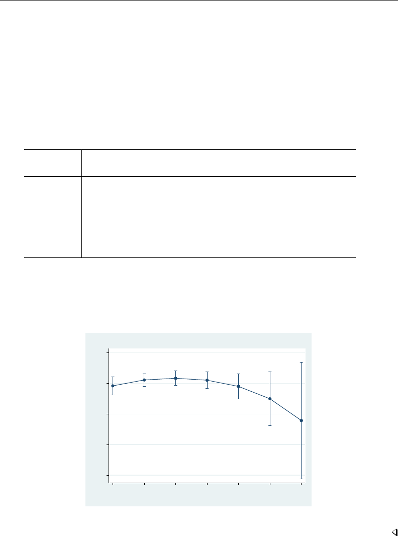
888 intreg postestimation — Postestimation tools for intreg
. margins, predict(pr(5,.)) at(age=(20(5)50))
Predictive margins Number of obs = 488
Model VCE : OIM
Expression : Pr(y>5), predict(pr(5,.))
1._at : age = 20
2._at : age = 25
3._at : age = 30
4._at : age = 35
5._at : age = 40
6._at : age = 45
7._at : age = 50
Delta-method
Margin Std. Err. z P>|z| [95% Conf. Interval]
_at
1 .8912598 .0151773 58.72 0.000 .8615127 .9210068
2 .9104568 .0103467 87.99 0.000 .8901775 .930736
3 .9160005 .0120025 76.32 0.000 .892476 .9395251
4 .9096667 .0136693 66.55 0.000 .8828753 .9364581
5 .8894289 .0206992 42.97 0.000 .8488593 .9299985
6.8491103 .0447429 18.98 0.000 .7614159 .9368048
7 .7781644 .0970557 8.02 0.000 .5879387 .9683902
We can visualize these results by using marginsplot:
. qui margins, predict(pr(5,.)) at(age=(20(5)50))
. marginsplot
Variables that uniquely identify margins: age
.6 .7 .8 .9 1
Pr(Y>5)
20 25 30 35 40 45 50
age in current year
Predictive Margins with 95% CIs
The probability increases until age 30, and it decreases after that age.


Title
ivpoisson — Poisson regression with endogenous regressors
Syntax Menu Description Options
Remarks and examples Stored results Methods and formulas References
Also see
Syntax
Generalized method of moments estimator
ivpoisson gmm depvar varlist1 (varlist2=varlistiv) if in weight
,reg err opt options
Control-function estimator
ivpoisson cfunction depvar varlist1(varlist2=varlistiv)if in weight
,options
reg err opt Description
Model
additive add regression errors to the conditional mean term; the default
multiplicative multiply regression errors by the conditional mean term
890

ivpoisson — Poisson regression with endogenous regressors 891
options Description
Model
noconstant suppress constant term
exposure(varnamee)include ln(varnamee) in model with coefficient constrained to 1
offset(varnameo)include varnameoin model with coefficient constrained to 1
∗twostep use two-step GMM estimator; the default for ivpoisson gmm
∗onestep use one-step GMM estimator; the default for ivpoisson cfunction
∗igmm use iterative GMM estimator
Weight matrix
wmatrix(wmtype)specify weight matrix; wmtype may be robust,cluster clustvar,
or unadjusted
center center moments in weight-matrix computation
winitial(iwtype, independent)
specify initial weight matrix; iwtype may be unadjusted,
identity, or the name of a Stata matrix
(independent may not be specified with ivpoisson gmm)
SE/Robust
vce(vcetype)vcetype may be robust,cluster clustvar,bootstrap,
jackknife, or unadjusted
Reporting
level(#)set confidence level; default is level(95)
irr report incidence-rate ratios
display options control column formats, row spacing, line width, display of omitted
variables and base and empty cells, and factor-variable labeling
Optimization
from(initial values)specify initial values for parameters
‡igmmiterate(#)specify maximum number of iterations for iterated GMM estimator
‡igmmeps(#)specify #for iterated GMM parameter convergence criterion;
default is igmmeps(1e-6)
‡igmmweps(#)specify #for iterated GMM weight-matrix convergence criterion;
default is igmmweps(1e-6)
optimization options control the optimization process; seldom used
∗You can specify at most one of these options.
‡These options may be specified only when igmm is specified.
varlist1and varlistiv may contain factor variables; see [U] 11.4.3 Factor variables.
depvar,varlist1,varlist2, and varlistiv may contain time-series operators; see [U] 11.4.4 Time-series varlists.
bootstrap,by,jackknife,rolling, and statsby are allowed; see [U] 11.1.10 Prefix commands.
Weights are not allowed with the bootstrap prefix; see [R] bootstrap.
aweights are not allowed with the jackknife prefix; see [R] jackknife.
aweights, fweights, iweights, and pweights are allowed; see [U] 11.1.6 weight.
See [U] 20 Estimation and postestimation commands for more capabilities of estimation commands.

892 ivpoisson — Poisson regression with endogenous regressors
Menu
Statistics >Endogenous covariates >Poisson regression with endogenous regressors
Description
ivpoisson estimates the parameters of a Poisson regression model in which some of the regressors
are endogenous. The model is also known as an exponential conditional mean model in which some of
the regressors are endogenous. The model may be specified using either additive or multiplicative error
terms. The model is frequently used to model count outcomes and is also used to model nonnegative
outcome variables.
Options
Model
noconstant,exposure(varnamee),offset(varnameo); see [R]estimation options.
additive, the default, specifies that the regression errors be added to the conditional mean term and
have mean 0.
multiplicative specifies that the regression errors be multiplied by the conditional mean term and
have mean 1.
twostep,onestep, and igmm specify which estimator is to be used.
twostep requests the two-step GMM estimator. gmm obtains parameter estimates based on the initial
weight matrix, computes a new weight matrix based on those estimates, and then reestimates the
parameters based on that weight matrix. twostep is the default for ivpoisson gmm.
onestep requests the one-step GMM estimator. The parameters are estimated based on an initial
weight matrix, and no updating of the weight matrix is performed except when calculating the
appropriate variance–covariance (VCE) matrix. onestep is the default for ivpoisson cfunction.
igmm requests the iterative GMM estimator. gmm obtains parameter estimates based on the initial
weight matrix, computes a new weight matrix based on those estimates, reestimates the parameters
based on that weight matrix, computes a new weight matrix, and so on, to convergence. Convergence
is declared when the relative change in the parameter vector is less than igmmeps(), the relative
change in the weight matrix is less than igmmweps(), or igmmiterate() iterations have been
completed. Hall (2005, sec. 2.4 and 3.6) mentions that there may be gains to finite-sample efficiency
from using the iterative estimator.
Weight matrix
wmatrix(wmtype)specifies the type of weight matrix to be used in conjunction with the two-step
and iterated GMM estimators.
Specifying wmatrix(robust) requests a weight matrix that is appropriate when the errors are
independent but not necessarily identically distributed. wmatrix(robust) is the default.
Specifying wmatrix(cluster clustvar)requests a weight matrix that accounts for arbitrary
correlation among observations within clusters identified by clustvar.
Specifying wmatrix(unadjusted) requests a weight matrix that is suitable when the errors are
homoskedastic.
wmatrix() cannot be specified if onestep is also specified.

ivpoisson — Poisson regression with endogenous regressors 893
center requests that the sample moments be centered (demeaned) when computing GMM weight
matrices. By default, centering is not done.
winitial(wmtype, independent )specifies the weight matrix to use to obtain the first-step
parameter estimates.
Specifying winitial(unadjusted) requests a weighting matrix that assumes the error functions
are independent and identically distributed. This matrix is of the form (Z0Z)−1, where Zrepresents
all the exogenous and instrumental variables.
winitial(identity) requests that the identity matrix be used.
winitial(matname)requests that Stata matrix matname be used.
Including the independent suboption creates a weight matrix that assumes error functions are
independent. Elements of the weight matrix corresponding to covariances between any two error
functions are set equal to zero. This suboption only applies to ivpoisson cfunction.
winitial(unadjusted) is the default for ivpoisson gmm.
winitial(unadjusted, independent) is the default for ivpoisson cfunction.
SE/Robust
vce(vcetype)specifies the type of standard error reported, which includes types that are robust to
some kinds of misspecification (robust), that allow for intragroup correlation (cluster clustvar),
and that use bootstrap or jackknife methods (bootstrap,jackknife); see [R]vce option.
vce(unadjusted) specifies that an unadjusted (nonrobust) VCE matrix be used; this, along with
the twostep option, results in the “optimal two-step GMM” estimates often discussed in textbooks.
vce(unadjusted) may not be set in ivpoisson cfunction.
The default vcetype is based on the wmtype specified in the wmatrix() option. If wmatrix()
is specified but vce() is not, then vcetype is set equal to wmtype. To override this behavior in
ivpoisson gmm and obtain an unadjusted (nonrobust) VCE matrix, specify vce(unadjusted).
The default vcetype for ivpoisson cfunction is robust.
Specifying vce(bootstrap) or vce(jackknife) results in standard errors based on the bootstrap
or jackknife, respectively. See [R]vce option,[R]bootstrap, and [R]jackknife for more information
on these VCEs.
The syntax for vcetypes is identical to those for wmatrix().
Reporting
level(#); see [R]estimation options.
irr reports estimated coefficients transformed to incidence-rate ratios, that is, eβirather than βi.
Standard errors and confidence intervals are similarly transformed. This option affects how results
are displayed, not how they are estimated or stored. irr may be specified at estimation or when
replaying previously estimated results. irr is not allowed with additive.
display options:noomitted,vsquish,noemptycells,baselevels,allbaselevels,nofvla-
bel,fvwrap(#),fvwrapon(style),cformat(%fmt),pformat(% fmt),sformat(% fmt), and
nolstretch; see [R]estimation options.
Optimization
from(initial values)specifies the initial values to begin the estimation. You can specify a 1 ×k
matrix, where kis the number of parameters in the model, or you can specify a parameter name,

894 ivpoisson — Poisson regression with endogenous regressors
its initial value, another parameter name, its initial value, and so on. For example, to initialize the
coefficient for male to 1.23 and the constant cons to 4.57, you would type
ivpoisson ..., from(male 1.23 _cons 4.57) ...
Initial values declared using this option override any that are declared within substitutable expres-
sions. If you specify a parameter that does not appear in your model, ivpoisson exits with error
code 480. If you specify a matrix, the values must be in the same order in which the parameters
are declared in your model. ivpoisson ignores the row and column names of the matrix.
igmmiterate(#),igmmeps(#), and igmmweps(#)control the iterative process for the iterative
GMM estimator for ivpoisson. These options can be specified only if you also specify igmm.
igmmiterate(#)specifies the maximum number of iterations to perform with the iterative GMM
estimator. The default is the number set using set maxiter (set [R]maximize), which is
16,000 by default.
igmmeps(#)specifies the convergence criterion used for successive parameter estimates when the
iterative GMM estimator is used. The default is igmmeps(1e-6). Convergence is declared when
the relative difference between successive parameter estimates is less than igmmeps() and the
relative difference between successive estimates of the weight matrix is less than igmmweps().
igmmweps(#)specifies the convergence criterion used for successive estimates of the weight matrix
when the iterative GMM estimator is used. The default is igmmweps(1e-6). Convergence is
declared when the relative difference between successive parameter estimates is less than
igmmeps() and the relative difference between successive estimates of the weight matrix is
less than igmmweps().
optimization options:technique(),conv maxiter(),conv ptol(),conv vtol(),
conv nrtol(), and tracelevel().technique() specifies the optimization technique to use;
gn (the default), nr,dfp, and bfgs are allowed. conv maxiter() specifies the maximum number
of iterations; conv ptol(),conv vtol(), and conv nrtol() specify the convergence criteria
for the parameters, gradient, and scaled Hessian, respectively. tracelevel() allows you to obtain
additional details during the iterative process. See [M-5]optimize( ).
Remarks and examples
ivpoisson estimates the parameters of a Poisson regression model in which some of the regressors
are endogenous. A regressor is endogenous if it is related to the unobserved error term. The model is
also known as an exponential conditional mean model in which some of the regressors are endogenous.
The model may be specified using either additive or multiplicative error terms.
The model is frequently used to model count outcomes and is also used to model nonnegative
outcome variables. Poisson regression is a special exponential conditional mean model. See [R]poisson
for more information on Poisson regression.
The exponential conditional mean model has an error form representation in which the dependent
variable yis a function of the exogenous regressors x, endogenous regressors y2, and an error .
The regressors xare independent of , while y2are not.
ivpoisson allows to enter either additively,
yi= exp(x0
iβ1+y0
2,iβ2) + i
or multiplicatively,
yi= exp(x0
iβ1+y0
2,iβ2)i

ivpoisson — Poisson regression with endogenous regressors 895
Mullahy (1997), Cameron and Trivedi (2013), Windmeijer and Santos Silva (1997), and
Wooldridge (2010) discuss the generalized method of moments (GMM) estimators implemented
in ivpoisson.GMM is frequently used in modern econometrics. Many econometric and statistical
models can be expressed as conditions on the population moments. The parameter estimates produced
by GMM estimators make the sample-moment conditions as true as possible given the data. See
[R]gmm for further information on GMM estimation and how Stata performs it.
The rest of the discussion is presented under the following headings:
GMM estimator for additive model
GMM estimator for multiplicative model
CF estimator for multiplicative model
GMM estimator for additive model
The GMM estimator uses additional variables, known as instruments and denoted by zi, to specify
moment conditions that hold in the population. The GMM parameter estimates make the sample versions
of these population-moment conditions as close to true as possible. The instrumental variables are
assumed to be correlated with the endogenous regressors y2,i but independent of the errors i.
Under additive errors, the dependent variable yiis determined by exogenous regressors xi,
endogenous regressors y2,i, and zero-mean error ias
yi= exp(x0
iβ1+y0
2,iβ2) + i
This leads to the following error function
u(yi,xi,y2,i,β1,β2) = yi−exp(x0
iβ1+y0
2,iβ2)
The population-moment conditions for GMM estimation are E{e
ziu(yi,xi,y2,i,β1,β2)}=0,
where the vector e
ziis partitioned as (x0
i,z0
i). The sample-moment conditions are formed by replacing
the expectation with the corresponding sample mean. The GMM estimator solves a minimization problem
to make the sample-moment conditions as close to zero as possible. Details on how estimation is
performed are given in Methods and formulas.
Now we will demonstrate how ivpoisson gmm works in the additive error setting with an example.
Example 1: ivpoisson gmm with additive errors
This example uses simulated data based on the following story. A news website randomly samples
500 young adults in a major city. The website wants to model the number of times the sampled
individuals visit its website (visits) based on their overall time spent on the Internet (time) and
the number of times they receive an ad for the website through email or viewing another website
(ad). The website also suspects the gender of the individual may matter, so an exogenous dummy
variable, female, is included in the model.
We suspect time spent on the Internet is correlated with unobserved factors that additively affect the
number of times an individual visits the website. So we treat time as an endogenous regressor. Two
instruments are used for this variable. The time spent on the phone (phone) is one instrument. The
other instrument is the time spent interacting with friends and family that live out of town (frfam).
We model the number of visits the website receives using an exponential conditional mean model
with additive errors and use ivpoisson gmm to estimate the parameters of the regression in the
output below. To allow for heteroskedasticity of the errors, we use robust standard errors, which is
the default; see Obtaining standard errors in [R]gmm for a discussion of why robust standard errors
is the default.

896 ivpoisson — Poisson regression with endogenous regressors
.use http://www.stata-press.com/data/r13/website
(Visits to website)
. ivpoisson gmm visits ad female (time = phone frfam)
Step 1
Iteration 0: GMM criterion Q(b) = .33829416
Iteration 1: GMM criterion Q(b) = .00362656
Iteration 2: GMM criterion Q(b) = .00131886
Iteration 3: GMM criterion Q(b) = .00131876
Step 2
Iteration 0: GMM criterion Q(b) = .00027102
Iteration 1: GMM criterion Q(b) = .00025811
Iteration 2: GMM criterion Q(b) = .00025811
Exponential mean model with endogenous regressors
Number of parameters = 4 Number of obs = 500
Number of moments = 5
Initial weight matrix: Unadjusted
GMM weight matrix: Robust
Robust
visits Coef. Std. Err. z P>|z| [95% Conf. Interval]
time .0589294 .0107942 5.46 0.000 .0377732 .0800857
ad .137344 .010157 13.52 0.000 .1174366 .1572515
female -.0247707 .0376218 -0.66 0.510 -.098508 .0489666
_cons 1.041505 .0385848 26.99 0.000 .9658807 1.11713
Instrumented: time
Instruments: ad female phone frfam
We find significant coefficients for all regressors but female. At fixed values of the other regressors,
increased time spent on the Internet will raise the expected number of website visits. Receiving
additional advertisements will also cause an increase in the expected number of website visits.
GMM estimator for multiplicative model
Under multiplicative errors, the dependent variable yiis determined by exogenous regressors xi,
endogenous regressors y2,i, and unit-mean errors ias
yi= exp(x0
iβ1+y0
2,iβ2)i
This setting yields a different error function than the additive error case. This ratio formulation is
u(yi,xi,y2,i,β1,β2) = yi/exp(x0
iβ1+y0
2,iβ2)−1
Given the instrumental variables z, the population-moment conditions for GMM estimation are
E{e
ziu(yi,xi,y2,i,β1,β2)}=0. The vector e
ziis partitioned as (x0
i,z0
i). As above, the sample-
moment conditions are the sample analogs of the population-moment conditions, and the GMM
estimator solves a minimization problem to make the sample-moment conditions as close to zero as
possible. Details on how estimation is performed are given in Methods and formulas.

ivpoisson — Poisson regression with endogenous regressors 897
Example 2: ivpoisson gmm with multiplicative errors
In this example, we observe a simulated random sample of 5,000 households. We model the
number of trips taken by members of the household in the 24-hour period immediately prior to the
interview time by using an exponential conditional mean model with multiplicative errors. Exogenous
regressors include the distance to the central business district from the household (cbd), the distance
from the household to a public transit node (ptn), whether there is a full-time worker in the
household (worker), and whether the examined period is on a weekend (weekend). We suspect
that the endogenous regressor, the transportation cost of the household in the prior week (tcost),
is correlated with unobserved factors that affect the number of trips taken. This transportation cost
includes gasoline and bus, train tickets, etc.
The ratio of the cost of a public transit day pass in the sampled area to the national average cost
of such a pass (pt) is also observed. This is used as an instrument for transportation cost.
In the output below, we estimate the parameters of the regression with ivpoisson gmm. To allow
for heteroskedasticity of the errors, we use robust standard errors, which is the default.
. use http://www.stata-press.com/data/r13/trip
(Household trips)
. ivpoisson gmm trips cbd ptn worker weekend (tcost = pt), multiplicative
Step 1
Iteration 0: GMM criterion Q(b) = .04949852
Iteration 1: GMM criterion Q(b) = .00011194
Iteration 2: GMM criterion Q(b) = 1.563e-08
Iteration 3: GMM criterion Q(b) = 3.685e-16
Step 2
Iteration 0: GMM criterion Q(b) = 2.287e-16
Iteration 1: GMM criterion Q(b) = 1.413e-31
Exponential mean model with endogenous regressors
Number of parameters = 6 Number of obs = 5000
Number of moments = 6
Initial weight matrix: Unadjusted
GMM weight matrix: Robust
Robust
trips Coef. Std. Err. z P>|z| [95% Conf. Interval]
tcost .0352185 .0098182 3.59 0.000 .0159752 .0544617
cbd -.008398 .0020172 -4.16 0.000 -.0123517 -.0044444
ptn -.0113146 .0021819 -5.19 0.000 -.015591 -.0070383
worker .6623018 .0519909 12.74 0.000 .5604015 .764202
weekend .3009323 .0362682 8.30 0.000 .2298479 .3720167
_cons .2654423 .1550127 1.71 0.087 -.0383769 .5692616
Instrumented: tcost
Instruments: cbd ptn worker weekend pt
We find that all coefficients are significant. At fixed values of the other regressors, we see that
additional mileage from the central business district and public transit nodes reduces the expected
number of trips taken. Individuals who live farther away from the central business district may still
be out of the house the same amount of time, but they will take fewer trips because the transit time
has increased. The situation is similar for those who live farther from public transit.
To interpret the other parameters, we will look at the partial effects of their respective independent
variables. The partial effects of a change in an independent variable on the modeled conditional expec-
tation function vary over the data because the model is nonlinear. However, under the multiplicative

898 ivpoisson — Poisson regression with endogenous regressors
error model, the ratio of the new value to the old value after a discrete change in an independent
variable is constant over the data.
Let w= (x0,y0
2)0. If we add 1 to the jth independent variable in w, the functional form of the
model implies that
E(y|w, wj+ 1, )
E(y|w, wj, )=E(y|w1, . . . , wj+ 1, . . . , wk, )
E(y|w1, . . . , wj, . . . , wk, )=eβj
When yis a count variable, this normalized effect is called the incidence-rate ratio (IRR) for a
one-unit change in wj.
More generally, the IRR for a ∆wjchange in wjis eβj∆wjunder a multiplicative-error exponential
conditional mean model. We can calculate incidence-rate ratios for different changes in the regressors
by using lincom; see [R]lincom.
Here we replay the ivpoisson results by typing the command name and we specify the irr
option to get the incidence-rate ratios. Each significance test for a coefficient equaling zero becomes
a test for the incidence-rate ratio equaling one.
. ivpoisson, irr
Exponential mean model with endogenous regressors
Number of parameters = 6 Number of obs = 5000
Number of moments = 6
Initial weight matrix: Unadjusted
GMM weight matrix: Robust
Robust
trips IRR Std. Err. z P>|z| [95% Conf. Interval]
tcost 1.035846 .0101701 3.59 0.000 1.016103 1.055972
cbd .9916371 .0020003 -4.16 0.000 .9877243 .9955655
ptn .9887491 .0021573 -5.19 0.000 .9845299 .9929864
worker 1.939251 .1008234 12.74 0.000 1.751376 2.14728
weekend 1.351118 .0490026 8.30 0.000 1.258409 1.450657
_cons 1.304008 .2021377 1.71 0.087 .9623501 1.766962
Instrumented: tcost
Instruments: cbd ptn worker weekend pt
Holding other regressors and the error constant, the expected number of trips made from houses
with a full-time worker is nearly twice that of those houses without a full-time worker. Similarly,
the expected number of trips made during a weekend day is close to 35% higher than the expected
number of trips made on other days. For each additional dollar of weekly transportation cost, the
expected number of household trips is increased by approximately 3.6%.
CF estimator for multiplicative model
Control-function (CF) estimators can be used to account for endogenous regressors. As
Wooldridge (2010, sec. 18.5) describes, CF estimators assume a certain structural relationship between
the endogenous regressors and the exogenous regressors and use functions of first-stage parameter
estimates to control for the endogeneity in the second stage.

ivpoisson — Poisson regression with endogenous regressors 899
Wooldridge (2010, sec. 18.5) notes that the VCE of the second-stage estimator must be adjusted to
account for estimates from the first stage. ivpoisson cfunction solves this problem by stacking the
moment conditions that define each stage and applying a single GMM estimator. See Newey (1984)
and Wooldridge (2010, sec. 14.2) for a description of this technique. No adjustment to the VCE is
necessary because there is only one stage.
The CF estimator augments the original multiplicative model with an estimated term that controls
for the endogeneity of y2,i. When y2,i is exogenous, the coefficient on this control term is zero. Let
zbe instrumental variables, and the vector e
zibe (x0
i,z0
i).
The augmented model is
yi= exp(x0
iβ1+y0
2,iβ2+v0
iρ+ci)
where
y2,i =Be
z0
i+vi
The term v0
iρcontrols for the endogeneity of y2,i, and we normalize E{exp(ci)}=1. The coefficient
vector ρmeasures the strength of the endogeneity of y2,i;y2,i is exogenous when ρ=0.
ivpoisson cfunction estimates β1and β2and the auxiliary parameters ρand Bby GMM; see
Methods and formulas for details.
Example 3: Control-function estimator
We return to the previous example, where we estimated the parameters of an exponential conditional
mean model for the number of trips taken by a household in a 24-hour period. We will estimate
the parameters of the regression with the CF estimator method and compare our results with those
obtained with the GMM estimator in example 2.
In the output below, we estimate the parameters of the regression with the ivpoisson cfunction
command.

900 ivpoisson — Poisson regression with endogenous regressors
. ivpoisson cfunction trips cbd ptn worker weekend (tcost = pt)
Step 1
Iteration 0: GMM criterion Q(b) = .00056156
Iteration 1: GMM criterion Q(b) = 2.366e-07
Iteration 2: GMM criterion Q(b) = 5.552e-14
Iteration 3: GMM criterion Q(b) = 9.772e-27
Exponential mean model with endogenous regressors
Number of parameters = 13 Number of obs = 5000
Number of moments = 13
Initial weight matrix: Unadjusted
GMM weight matrix: Robust
Robust
trips Coef. Std. Err. z P>|z| [95% Conf. Interval]
trips
cbd -.0082567 .0020005 -4.13 0.000 -.0121777 -.0043357
ptn -.0113719 .0021625 -5.26 0.000 -.0156102 -.0071335
worker .6903044 .0521642 13.23 0.000 .5880645 .7925444
weekend .2978149 .0356474 8.35 0.000 .2279472 .3676825
tcost .0320718 .0092738 3.46 0.001 .0138955 .0502481
_cons .2145986 .1359327 1.58 0.114 -.0518246 .4810218
tcost
cbd .0165466 .0043693 3.79 0.000 .0079829 .0251102
ptn -.040652 .0045946 -8.85 0.000 -.0496573 -.0316467
worker 1.550985 .0996496 15.56 0.000 1.355675 1.746294
weekend .0423009 .0779101 0.54 0.587 -.1104002 .1950019
pt .7739176 .0150072 51.57 0.000 .7445041 .8033312
_cons 12.13934 .1123471 108.05 0.000 11.91915 12.35954
/c_tcost .1599984 .0111752 14.32 0.000 .1380954 .1819014
Instrumented: tcost
Instruments: cbd ptn worker weekend pt
The output table presents results for the estimated coefficients in each of three equations. First, in
the trips equation, we see the results for the estimated coefficients in the equation for the dependent
variable trips. Second, in the tcost equation, we see the estimated coefficients in the regression
of tcost on the instrumental and exogenous variables. Third, the /c tcost ancillary parameter
corresponds to the estimate of ρ, the coefficient on the residual variable included to control for the
endogeneity of tcost.
We find that all coefficients are significant in the exponential conditional mean equation, trips.
The coefficient estimates in the trips equation are similar to the estimates obtained by the GMM
estimator in example 2. That the estimated coefficient on the tcost control variable is significantly
different from zero suggests that tcost is endogenous.

ivpoisson — Poisson regression with endogenous regressors 901
Stored results
ivpoisson stores the following in e():
Scalars
e(N) number of observations
e(k) number of parameters
e(k eq) number of equations
e(k aux) number of auxiliary parameters
e(k dv) number of dependent variables
e(Q) criterion function
e(J) Hansen J χ2statistic
e(J df) Jstatistic degrees of freedom
e(N clust) number of clusters
e(rank) rank of e(V)
e(ic) number of iterations used by iterative GMM estimator
e(converged) 1 if converged, 0otherwise
Macros
e(cmd) ivpoisson
e(cmdline) command as typed
e(depvar) dependent variable of regression
e(instd) instrumented variable
e(insts) instruments
e(wtype) weight type
e(wexp) weight expression
e(title) title in estimation output
e(clustvar) name of cluster variable
e(offset1) offset variable for first equation
e(winit) initial weight matrix used
e(winitname) name of user-supplied initial weight matrix
e(estimator) gmm or cfunction
e(additive) additive if additive errors specified
e(multiplicative) multiplicative if multiplicative errors specified
e(gmmestimator) onestep,twostep, or igmm
e(wmatrix) wmtype specified in wmatrix()
e(vce) vcetype specified in vce()
e(vcetype) title used to label Std. Err.
e(technique) optimization technique
e(properties) b V
e(estat cmd) program used to implement estat
e(predict) program used to implement predict
e(footnote) program used to implement footnote display
e(marginsok) predictions allowed by margins
e(asbalanced) factor variables fvset as asbalanced
e(asobserved) factor variables fvset as asobserved
Matrices
e(b) coefficient vector
e(V) variance–covariance matrix
e(init) initial values of the estimators
e(Wuser) user-supplied initial weight matrix
e(W) weight matrix used for final round of estimation
e(S) moment covariance matrix used in robust VCE computations
e(V modelbased) model-based variance
Functions
e(sample) marks estimation sample

902 ivpoisson — Poisson regression with endogenous regressors
Methods and formulas
The estimators in ivpoisson are GMM estimators that can be expressed in terms of error functions
and the instruments that are used to form the moment conditions. When offsets oβ
jare used in the
outcome variable equation, the following formulas apply with x0
jβ1changed to x0
jβ1+oβ
j.
The error functions for the GMM estimators are given in the text.
Here we provide some details about the form of the error function used by the CF estimator.
Recall that the multiplicative model is
yi= exp(x0
iβ1+y0
2,iβ2)i
We parameterize the endogenous variables in the form
y2,i =Be
z0
i+vi
This allows us to decompose ias
i= exp(v0
iρ+ci)
Given this setup, we obtain the following conditional mean:
E(y|xi,zi,y2,i,vi) = exp(x0
iβ1+y0
2,iβ2+v0
iρ)
We estimate vias the residuals of the linear regression of y2,i on e
zi. The estimates of viare
used as additional regressors in the exponential conditional mean model for yto estimate β1,β2,
and ρ. In essence, the estimates of vicontrol for the endogeneity.
The error functions for the endogenous regressors are defined as
uen,i(y2,i,e
zi,B) = y2,i −Be
z0
i
Now we define the error function for the dependent variable as
uy(yi,xi,y2,i,uen,i,β1,β2,ρ) = yi/exp(x0
iβ1+y0
2,iβ2+u0
en,iρ)−1
uen,i will be vector valued if we have multiple endogenous regressors y2,i. Call the dimension of
y2,i g.uen,i and uy,i define g+1 separate error functions. We will use variables e
zito instrument
each error function in uen,i. So for error function j=1, . . . , g, we have the error function uen,i,j
and the population-moment conditions E(e
ziuen,i,j ) = 0.
We calculate b
voi previous to estimation as the residuals of the linear regression of y2,i on e
zi. We
use variables xi,y2,i, and b
voi to instrument the error function uy. This leads to the population-moment
conditions E(x0
i,y0
2,i,b
v0
oi)uy,i=0
Details of GMM estimation can be found in Methods and formulas of [R]gmm. Determination of
the weight matrix WNis discussed there.
Under the GMM estimation, the GMM estimators b
β1and b
β2are the values of β1and β2that
minimize
Q(β1,β2) = 1
NXie
ziui(yi,xi,y2,i,β1,β2)0WN1
NXie
ziui(yi,xi,y2,i,β1,β2)(1)

ivpoisson — Poisson regression with endogenous regressors 903
for q×qweight matrix WN, where qis the dimension of e
zi. The error functions uiwere defined
in the text.
In the CF method, we have multiple error functions as defined above. We can stack the moment
conditions and write them more compactly as Z0
iui(B,β1,β2,ρ), where
Zi=
x0
i0 0 ··· 0
0 y0
2,i 0··· 0
0 0 e
zi··· 0
.
.
..
.
..
.
.....
.
.
0 0 0 ··· e
zi
and
ui(B,β1,β2,ρ) = uy(yi,xi,y2,i,uen,i,β1,β2,ρ)
uen(y2,i,e
zi,B)
The matrix Zihas g+1 rows and k+gz columns, where kis the number of regressors for yi
and zis the number of exogenous regressors in e
zi.
The GMM estimators b
B,b
β1,b
β2, and bρare the values of B,β1,β2, and ρthat minimize
Q(B,β1,β2,ρ) =
(N−1
N
X
i=1
Z0
iui(B,β1,β2,ρ))0
WN(N−1
N
X
i=1
Z0
iui(B,β1,β2,ρ))(2)
for (k+gz)×(k+gz)weight matrix WN.
By default, ivpoisson minimizes (1) and (2) using the Gauss–Newton method. See Hayashi (2000,
498) for a derivation. This technique is typically faster than quasi-Newton methods and does not
require second-order derivatives.
References
Cameron, A. C., and P. K. Trivedi. 2013. Regression Analysis of Count Data. 2nd ed. New York: Cambridge
University Press.
Hall, A. R. 2005. Generalized Method of Moments. Oxford: Oxford University Press.
Hayashi, F. 2000. Econometrics. Princeton, NJ: Princeton University Press.
Mullahy, J. 1997. Instrumental-variable estimation of count data models: Applications to models of cigarette smoking
behavior. Review of Economics and Statistics 79: 586–593.
Newey, W. K. 1984. A method of moments interpretation of sequential estimators. Economics Letters 14: 201–206.
Windmeijer, F., and J. M. C. Santos Silva. 1997. Endogeneity in count data models: An application to demand for
health care. Journal of Applied Econometrics 12: 281–294.
Wooldridge, J. M. 2010. Econometric Analysis of Cross Section and Panel Data. 2nd ed. Cambridge, MA: MIT Press.

904 ivpoisson — Poisson regression with endogenous regressors
Also see
[R]ivpoisson postestimation — Postestimation tools for ivpoisson
[R]gmm — Generalized method of moments estimation
[R]ivprobit — Probit model with continuous endogenous regressors
[R]ivregress — Single-equation instrumental-variables regression
[R]ivtobit — Tobit model with continuous endogenous regressors
[R]nl — Nonlinear least-squares estimation
[R]nlsur — Estimation of nonlinear systems of equations
[R]poisson — Poisson regression
[R]regress — Linear regression
[U] 20 Estimation and postestimation commands

Title
ivpoisson postestimation — Postestimation tools for ivpoisson
Description Syntax for predict Menu for predict
Options for predict Syntax for estat overid Menu for estat
Remarks and examples Stored results Methods and formulas
Reference Also see
Description
The following postestimation command is of special interest after ivpoisson:
Command Description
estat overid perform test of overidentifying restrictions
The following standard postestimation commands are also available:
Command Description
contrast contrasts and ANOVA-style joint tests of estimates
estat summarize summary statistics for the estimation sample
estat vce variance–covariance matrix of the estimators (VCE)
estimates cataloging estimation results
lincom point estimates, standard errors, testing, and inference for linear combinations
of coefficients
margins marginal means, predictive margins, marginal effects, and average marginal
effects
marginsplot graph the results from margins (profile plots, interaction plots, etc.)
nlcom point estimates, standard errors, testing, and inference for nonlinear combinations
of coefficients
predict predictions and probabilities
predictnl point estimates, standard errors, testing, and inference for generalized predictions
pwcompare pairwise comparisons of estimates
test Wald tests of simple and composite linear hypotheses
testnl Wald tests of nonlinear hypotheses
Special-interest postestimation command
estat overid reports Hansen’s Jstatistic, which is used to determine the validity of the
overidentifying restrictions in a GMM model. ivpoisson gmm uses GMM estimation to obtain parameter
estimates. Under additive and multiplicative errors, Hansen’s Jstatistic can be accurately reported
when more instruments than endogenous regressors are specified. It is not appropriate to report the
Jstatistic after ivpoisson cfunction, because a just-identified model is fit.
905

906 ivpoisson postestimation — Postestimation tools for ivpoisson
If the model is correctly specified in the sense that E{e
ziu(yi,xi,y2,i,β)}=0, then the sample
analog to that condition should hold at the estimated value of β1and β2. The e
zivariables are the
exogenous regressors xiand instrumental variables ziused in ivpoisson gmm. The y2,i are the
endogenous regressors. The ufunction is the error function, which will have a different form for
multiplicative and additive errors in the regression.
Hansen’s Jstatistic is valid only if the weight matrix is optimal, meaning that it equals the inverse
of the covariance matrix of the moment conditions. Therefore, estat overid only reports Hansen’s
Jstatistic after two-step or iterated estimation or if you specified winitial(matname)when calling
ivpoisson gmm. In the latter case, it is your responsibility to determine the validity of the Jstatistic.
Syntax for predict
predict type newvar if in ,statistic nooffset
statistic Description
Main
nnumber of events; the default
xbtotal linear prediction, using residual estimates for ivpoisson cfunction
xb linear prediction
residuals residuals
These statistics are available both in and out of sample; type predict . . . if e(sample) . . . if wanted
only for the estimation sample.
Menu for predict
Statistics >Postestimation >Predictions, residuals, etc.
Options for predict
Main
n, the default, calculates the predicted number of events via the exponential-form estimate. This is
exp(x0
jβ1+y0
2,j β2)if neither offset() nor exposure() was specified, exp(x0
jβ1+y0
2,j β2+
offsetj)if offset() was specified, or exp(x0
jβ1+y0
2,j β2)×exposurejif exposure() was
specified.
After generalized method of moments estimation, the exponential-form estimate is not a consistent
estimate of the conditional mean of yj, because it is not corrected for E(j|y2,j ). More details
are found in Methods and formulas.
After control-function estimation, we correct the exponential-form estimate for E(j|y2,j )by using
the estimated residuals of y2,j and the c * auxiliary parameters. This supplements the direct effect
of y2,j and xjthrough β1and β2with the indirect effects of y2,j ,xj, and the instruments zj
through the endogenous error j. Thus the exponential-form estimate consistently estimates the
conditional mean of yj.
xbtotal calculates the linear prediction, which is x0
jβ1+y0
2,j β2if neither offset() nor exposure()
was specified, x0
jβ1+y0
2,j β2+offsetjif offset() was specified, or x0
jβ1+y0
2,j β2+ln(exposurej)
if exposure() was specified.

ivpoisson postestimation — Postestimation tools for ivpoisson 907
After control-function estimation, the estimate of the linear form x0
jβ1includes the estimated
residuals of the endogenous regressors with coefficients from the c * auxiliary parameters.
xb calculates the linear prediction, which is x0
jβ1+y0
2,j β2if neither offset() nor exposure() was
specified, x0
jβ1+y0
2,j β2+offsetjif offset() was specified, or x0
jβ1+y0
2,j β2+ln(exposurej)
if exposure() was specified.
residuals calculates the residuals. Under additive errors, these are calculated as yj−exp(x0
jβ1+
y0
2,j β2). Under multiplicative errors, they are calculated as yj/exp(x0
jβ1+y0
2,j β2)−1.
When offset() or exposure() is specified, x0
jβ1is not used directly in the residuals. x0
jβ1+
offsetjis used if offset() was specified. x0
jβ1+ln(exposurej)is used if exposure() was
specified. See nooffset below.
After control-function estimation, the estimate of the linear form x0
jβ1includes the estimated
residuals of the endogenous regressors with coefficients from the c * auxiliary parameters.
nooffset is relevant only if you specified offset() or exposure() when you fit the model. It
modifies the calculations made by predict so that they ignore the offset or exposure variable.
nooffset removes the offset from calculations involving both the treat() equation and the
dependent count variable.
Syntax for estat overid
estat overid
Menu for estat
Statistics >Postestimation >Reports and statistics
Remarks and examples
estat overid reports Hansen’s Jstatistic, which is used to determine the validity of the
overidentifying restrictions in a GMM model. It is not appropriate to use it after ivpoisson cfunction,
because a just-identified model is fit.
Recall that the GMM criterion function is
Q(β) = 1
NXie
ziu(yi,xi,y2,i,β1,β2)0WN1
NXie
ziu(yi,xi,y2,i,β1,β2)(A1)
Our ufunction within this formula will change depending on whether we use additive or multiplicative
errors. The e
zvector contains the exogenous regressors and instrumental variables used. ivpoisson
gmm estimates regression coefficients to minimize Q.
Let lbe the dimension of e
zand kthe number of regressors. If WNis an optimal weight matrix, under
the null hypothesis H0:E{e
ziu(yi,xi,y2,i,β1,β2)}=0, the test statistic J=N×Q∼χ2(l−k).
A large test statistic casts doubt on the null hypothesis.
Because the weight matrix WNmust be optimal, estat overid works only after the two-step and
iterated estimation or if you supplied your own initial weight matrix by using the winitial(matname)
option of ivpoisson gmm and used the one-step estimator.

908 ivpoisson postestimation — Postestimation tools for ivpoisson
Often the overidentifying restrictions test is interpreted as a test of the validity of the instruments
z. However, other forms of model misspecification can sometimes lead to a significant test statistic.
See Hall (2005, sec. 5.1) for a discussion of the overidentifying restrictions test and its behavior in
correctly specified and misspecified models.
Note that ivpoisson gmm defaults to the two-step estimator when other options are not specified
to override the default. Thus it is appropriate to perform the Jtest after the regression of example 1
in [R]ivpoisson.
Example 1: Specification test
Recall example 1 of [R]ivpoisson. We estimated the parameters of an exponential conditional
mean model for the number of visits to a website. Additive errors were used. Exogenous regressors
included the gender of an individual and the number of ads received from the website.
An endogenous regressor, time spent on the Internet, was also included in the model. Two
instruments were used. One of the instruments measured the time spent interacting with friends and
out-of-town family. The other measured the time spent on the phone.
We will reestimate the parameters of the regression here and then test the specification.
. use http://www.stata-press.com/data/r13/website
(Visits to website)
. ivpoisson gmm visits ad female (time = phone frfam)
(output omitted )
. estat overid
Test of overidentifying restriction:
Hansen’s J chi2(1) = .129055 (p = 0.7194)
We have two instruments for one endogenous variable, so the Jstatistic has one degree of freedom.
The Jstatistic is not significant. We fail to reject the null hypothesis that the model is correctly
specified.
Stored results
estat overid stores the following in r():
Scalars
r(J) Hansen’s Jstatistic
r(J df) Jstatistic degrees of freedom
r(J p) Jstatistic p-value
Methods and formulas
The vector xicontains the exogenous regressors, and zithe instruments. The vector e
ziis partitioned
as (xi,zi). The vector y2,i contains the endogenous regressors.
Under multiplicative errors, the conditional mean of yiis
E(yi|y2,i,e
zi) = E{E(yi|xi,y2,i, i)|y2,i,e
zi}
=Eexp x0
iβ1+y0
2,iβ2i|y2,i,e
zi
= exp x0
iβ1+y0
2,iβ2E(i|y2,i,e
zi)

ivpoisson postestimation — Postestimation tools for ivpoisson 909
Under the CF estimator,
E(i|y2,i,e
zi) = E{E(i|vi, ci)|y2,i,e
zi}
=E{exp(v0
iρ+ci)|y2,i,e
zi}
= exp {(y2,i −Be
z0
i)0ρ}E(ci|y2,i,e
zi)
= exp {(y2,i −Be
z0
i)0ρ}
Thus under the CF estimator, we estimate the conditional mean of yias
E(yi|y2,i,e
zi) = exp x0
iβ1+y0
2,iβ2+ (y2,i −Be
z0
i)0ρ
The CF estimator explicitly models the functional form of the endogeneity of y2,i and iwith the
instruments and exogenous regressors e
zi. This allows it to correct the exponential-form estimator for
the E(i|y2,i,e
zi)term.
In contrast, the GMM estimator does not model the functional form of the endogeneity of y2,i and i.
Therefore, E(i|y2,i,e
zi)is not estimated, and the exponential-form estimator under GMM estimation
simply ignores this term. Noting that because e
ziand iare independent, E(i|y2,i,e
zi) = E(i|y2,i),
we can obviously see that ignoring the term will lead to inconsistent estimation of the conditional
mean of yi.y2,i and iare not independent, so E(i|y2,i)may vary based on y2,i.
In the additive errors setting, a similar derivation will show that the exponential-form estimator
obtained from GMM estimation is inconsistent for the conditional mean of yi.
Reference
Hall, A. R. 2005. Generalized Method of Moments. Oxford: Oxford University Press.
Also see
[R]ivpoisson — Poisson regression with endogenous regressors
[U] 20 Estimation and postestimation commands

Title
ivprobit — Probit model with continuous endogenous regressors
Syntax Menu Description
Options for ML estimator Options for two-step estimator Remarks and examples
Stored results Methods and formulas Acknowledgments
References Also see
Syntax
Maximum likelihood estimator
ivprobit depvar varlist1(varlist2=varlistiv)if in weight ,mle options
Two-step estimator
ivprobit depvar varlist1(varlist2=varlistiv)if in weight , twostep
tse options
mle options Description
Model
mle use conditional maximum-likelihood estimator; the default
asis retain perfect predictor variables
constraints(constraints)apply specified linear constraints
SE/Robust
vce(vcetype)vcetype may be oim,robust,cluster clustvar,opg,bootstrap,
or jackknife
Reporting
level(#)set confidence level; default is level(95)
first report first-stage regression
nocnsreport do not display constraints
display options control column formats, row spacing, line width, display of omitted
variables and base and empty cells, and factor-variable labeling
Maximization
maximize options control the maximization process
coeflegend display legend instead of statistics
910

ivprobit — Probit model with continuous endogenous regressors 911
tse options Description
Model
∗twostep use Newey’s two-step estimator; the default is mle
asis retain perfect predictor variables
SE
vce(vcetype)vcetype may be twostep,bootstrap, or jackknife
Reporting
level(#)set confidence level; default is level(95)
first report first-stage regression
display options control column formats, row spacing, line width, display of omitted
variables and base and empty cells, and factor-variable labeling
coeflegend display legend instead of statistics
∗twostep is required.
varlist1and varlistiv may contain factor variables; see [U] 11.4.3 Factor variables.
depvar,varlist1,varlist2, and varlistiv may contain time-series operators; see [U] 11.4.4 Time-series varlists.
bootstrap,by,jackknife,rolling,statsby, and svy are allowed; see [U] 11.1.10 Prefix commands.fp is
allowed with the maximum likelihood estimator.
Weights are not allowed with the bootstrap prefix; see [R] bootstrap.
vce(),first,twostep, and weights are not allowed with the svy prefix; see [SVY] svy.
fweights, iweights, and pweights are allowed with the maximum likelihood estimator. fweights are allowed with
Newey’s two-step estimator. See [U] 11.1.6 weight.
coeflegend does not appear in the dialog box.
See [U] 20 Estimation and postestimation commands for more capabilities of estimation commands.
Menu
Statistics >Endogenous covariates >Probit model with endogenous covariates
Description
ivprobit fits probit models where one or more of the regressors are endogenously determined.
By default, ivprobit uses maximum likelihood estimation. Alternatively, Newey’s (1987) minimum
chi-squared estimator can be invoked with the twostep option. Both estimators assume that the
endogenous regressors are continuous and are not appropriate for use with discrete endogenous
regressors. See [R]ivtobit for tobit estimation with endogenous regressors and [R]probit for probit
estimation when the model contains no endogenous regressors.
Options for ML estimator
Model
mle requests that the conditional maximum-likelihood estimator be used. This is the default.

912 ivprobit — Probit model with continuous endogenous regressors
asis requests that all specified variables and observations be retained in the maximization process.
This option is typically not used and may introduce numerical instability. Normally, ivprobit
drops any endogenous or exogenous variables that perfectly predict success or failure in the
dependent variable. The associated observations are also dropped. For more information, see
Model identification in [R]probit.
constraints(constraints); see [R]estimation options.
SE/Robust
vce(vcetype)specifies the type of standard error reported, which includes types that are derived from
asymptotic theory (oim,opg), that are robust to some kinds of misspecification (robust), that
allow for intragroup correlation (cluster clustvar), and that use bootstrap or jackknife methods
(bootstrap,jackknife); see [R]vce option.
Reporting
level(#); see [R]estimation options.
first requests that the parameters for the reduced-form equations showing the relationships between
the endogenous variables and instruments be displayed. For the two-step estimator, first shows
the first-stage regressions. For the maximum likelihood estimator, these parameters are estimated
jointly with the parameters of the probit equation. The default is not to show these parameter
estimates.
nocnsreport; see [R]estimation options.
display options:noomitted,vsquish,noemptycells,baselevels,allbaselevels,nofvla-
bel,fvwrap(#),fvwrapon(style),cformat(%fmt),pformat(% fmt),sformat(% fmt), and
nolstretch; see [R]estimation options.
Maximization
maximize options:difficult,technique(algorithm spec),iterate(#),nolog,trace,
gradient,showstep,hessian,showtolerance,tolerance(#),ltolerance(#),
nrtolerance(#),nonrtolerance, and from(init specs); see [R]maximize. This model’s
likelihood function can be difficult to maximize, especially with multiple endogenous variables.
The difficult and technique(bfgs) options may be helpful in achieving convergence.
Setting the optimization type to technique(bhhh) resets the default vcetype to vce(opg).
The following option is available with ivprobit but is not shown in the dialog box:
coeflegend; see [R]estimation options.
Options for two-step estimator
Model
twostep is required and requests that Newey’s (1987) efficient two-step estimator be used to obtain
the coefficient estimates.
asis requests that all specified variables and observations be retained in the maximization process.
This option is typically not used and may introduce numerical instability. Normally, ivprobit
drops any endogenous or exogenous variables that perfectly predict success or failure in the
dependent variable. The associated observations are also dropped. For more information, see
Model identification in [R]probit.

ivprobit — Probit model with continuous endogenous regressors 913
SE
vce(vcetype)specifies the type of standard error reported, which includes types that are derived
from asymptotic theory (twostep) and that use bootstrap or jackknife methods (bootstrap,
jackknife); see [R]vce option.
Reporting
level(#); see [R]estimation options.
first requests that the parameters for the reduced-form equations showing the relationships between
the endogenous variables and instruments be displayed. For the two-step estimator, first shows
the first-stage regressions. For the maximum likelihood estimator, these parameters are estimated
jointly with the parameters of the probit equation. The default is not to show these parameter
estimates.
display options:noomitted,vsquish,noemptycells,baselevels,allbaselevels,nofvla-
bel,fvwrap(#),fvwrapon(style),cformat(%fmt),pformat(% fmt),sformat(% fmt), and
nolstretch; see [R]estimation options.
The following option is available with ivprobit but is not shown in the dialog box:
coeflegend; see [R]estimation options.
Remarks and examples
Remarks are presented under the following headings:
Model setup
Model identification
Model setup
ivprobit fits models with dichotomous dependent variables and endogenous regressors. You can
use it to fit a probit model when you suspect that one or more of the regressors are correlated with
the error term. ivprobit is to probit modeling what ivregress is to linear regression analysis; see
[R]ivregress for more information.
Formally, the model is
y∗
1i=y2iβ+x1iγ+ui
y2i=x1iΠ1+x2iΠ2+vi
where i=1, . . . , N,y2iis a 1×pvector of endogenous variables, x1iis a 1×k1vector of exogenous
variables, x2iis a 1 ×k2vector of additional instruments, and the equation for y2iis written in
reduced form. By assumption, (ui,vi)∼N(0,Σ), where σ11 is normalized to one to identify the
model. βand γare vectors of structural parameters, and Π1and Π2are matrices of reduced-form
parameters. This is a recursive model: y2iappears in the equation for y∗
1i, but y∗
1idoes not appear
in the equation for y2i. We do not observe y∗
1i; instead, we observe
y1i=0y∗
1i<0
1y∗
1i≥0
The order condition for identification of the structural parameters requires that k2≥p. Presumably,
Σis not block diagonal between uiand vi; otherwise, y2iwould not be endogenous.

914 ivprobit — Probit model with continuous endogenous regressors
Technical note
This model is derived under the assumption that (ui,vi)is independent and identically distributed
multivariate normal for all i. The vce(cluster clustvar)option can be used to control for a lack of
independence. As with most probit models, if uiis heteroskedastic, point estimates will be inconsistent.
Example 1
We have hypothetical data on 500 two-parent households, and we wish to model whether the
woman is employed. We have a variable, fem work, that is equal to one if she has a job and zero
otherwise. Her decision to work is a function of the number of children at home (kids), number of
years of schooling completed (fem educ), and other household income measured in thousands of
dollars (other inc). We suspect that unobservable shocks affecting the woman’s decision to hold a
job also affect the household’s other income. Therefore, we treat other inc as endogenous. As an
instrument, we use the number of years of schooling completed by the man (male educ).
The syntax for specifying the exogenous, endogenous, and instrumental variables is identical to
that used in ivregress; see [R]ivregress for details.
. use http://www.stata-press.com/data/r13/laborsup
. ivprobit fem_work fem_educ kids (other_inc = male_educ)
Fitting exogenous probit model
Iteration 0: log likelihood = -344.63508
Iteration 1: log likelihood = -255.36855
Iteration 2: log likelihood = -255.31444
Iteration 3: log likelihood = -255.31444
Fitting full model
Iteration 0: log likelihood = -2371.4753
Iteration 1: log likelihood = -2369.3178
Iteration 2: log likelihood = -2368.2198
Iteration 3: log likelihood = -2368.2062
Iteration 4: log likelihood = -2368.2062
Probit model with endogenous regressors Number of obs = 500
Wald chi2(3) = 163.88
Log likelihood = -2368.2062 Prob > chi2 = 0.0000
Coef. Std. Err. z P>|z| [95% Conf. Interval]
other_inc -.0542756 .0060854 -8.92 0.000 -.0662027 -.0423485
fem_educ .211111 .0268648 7.86 0.000 .1584569 .2637651
kids -.1820929 .0478267 -3.81 0.000 -.2758316 -.0883543
_cons .3672083 .4480724 0.82 0.412 -.5109975 1.245414
/athrho .3907858 .1509443 2.59 0.010 .0949403 .6866313
/lnsigma 2.813383 .0316228 88.97 0.000 2.751404 2.875363
rho .3720374 .1300519 .0946561 .5958135
sigma 16.66621 .5270318 15.66461 17.73186
Instrumented: other_inc
Instruments: fem_educ kids male_educ
Wald test of exogeneity (/athrho = 0): chi2(1) = 6.70 Prob > chi2 = 0.0096
Because we did not specify mle or twostep,ivprobit used the maximum likelihood estimator
by default. At the top of the output, we see the iteration log. ivprobit fits a probit model ignoring

ivprobit — Probit model with continuous endogenous regressors 915
endogeneity to obtain starting values for the endogenous model. The header of the output contains
the sample size as well as a Wald statistic and p-value for the test of the hypothesis that all the slope
coefficients are jointly zero. Below the table of coefficients, Stata reminds us that the endogenous
variable is other inc and that fem educ,kids, and male educ were used as instruments.
At the bottom of the output is a Wald test of the exogeneity of the instrumented variables. We
reject the null hypothesis of no endogeneity. However, if the test statistic is not significant, there
is not sufficient information in the sample to reject the null, so a regular probit regression may be
appropriate. The point estimates from ivprobit are still consistent, though those from probit (see
[R]probit) are likely to have smaller standard errors.
Various two-step estimators have also been proposed for the endogenous probit model, and Newey’s
(1987) minimum chi-squared estimator is available with the twostep option.
Example 2
Refitting our labor-supply model with the two-step estimator yields
. ivprobit fem_work fem_educ kids (other_inc = male_educ), twostep
Checking reduced-form model...
Two-step probit with endogenous regressors Number of obs = 500
Wald chi2(3) = 93.97
Prob > chi2 = 0.0000
Coef. Std. Err. z P>|z| [95% Conf. Interval]
other_inc -.058473 .0093364 -6.26 0.000 -.0767719 -.040174
fem_educ .227437 .0281628 8.08 0.000 .1722389 .282635
kids -.1961748 .0496323 -3.95 0.000 -.2934522 -.0988973
_cons .3956061 .4982649 0.79 0.427 -.5809752 1.372187
Instrumented: other_inc
Instruments: fem_educ kids male_educ
Wald test of exogeneity: chi2(1) = 6.50 Prob > chi2 = 0.0108
All the coefficients have the same signs as their counterparts in the maximum likelihood model. The
Wald test at the bottom of the output confirms our earlier finding of endogeneity.
Technical note
In a standard probit model, the error term is assumed to have a variance of one. In the probit
model with endogenous regressors, we assume that (ui,vi)is multivariate normal with covariance
matrix
Var(ui,vi) = Σ=1Σ0
21
Σ21 Σ22
With the properties of the multivariate normal distribution, Var(ui|vi)=1−Σ0
21Σ−1
22 Σ21. As a
result, Newey’s estimator and other two-step probit estimators do not yield estimates of βand γbut
rather β/σ and γ/σ, where σis the square root of Var(ui|vi). Hence, we cannot directly compare
the estimates obtained from Newey’s estimator with those obtained via maximum likelihood or with
those obtained from probit. See Wooldridge (2010, 585–594) for a discussion of Rivers and Vuong’s
(1988) two-step estimator. The issues raised pertaining to the interpretation of the coefficients of that

916 ivprobit — Probit model with continuous endogenous regressors
estimator are identical to those that arise with Newey’s estimator. Wooldridge also discusses ways to
obtain marginal effects from two-step estimators.
Despite the coefficients not being directly comparable to their maximum likelihood counterparts,
the two-step estimator is nevertheless useful. The maximum likelihood estimator may have difficulty
converging, especially with multiple endogenous variables. The two-step estimator, consisting of
nothing more complicated than a probit regression, will almost certainly converge. Moreover, although
the coefficients from the two models are not directly comparable, the two-step estimates can still be
used to test for statistically significant relationships.
Model identification
As in the linear simultaneous-equation model, the order condition for identification requires that
the number of excluded exogenous variables (that is, the additional instruments) be at least as great
as the number of included endogenous variables. ivprobit checks this for you and issues an error
message if the order condition is not met.
Like probit,logit, and logistic,ivprobit checks the exogenous and endogenous variables
to see if any of them predict the outcome variable perfectly. It will then drop offending variables
and observations and fit the model on the remaining data. Instruments that are perfect predictors
do not affect estimation, so they are not checked. See Model identification in [R]probit for more
information.
ivprobit will also occasionally display messages such as
Note: 4 failures and 0 successes completely determined.
For an explanation of this message, see [R]logit.
Stored results
ivprobit, mle stores the following in e():
Scalars
e(N) number of observations
e(N cds) number of completely determined successes
e(N cdf) number of completely determined failures
e(k) number of parameters
e(k eq) number of equations in e(b)
e(k eq model) number of equations in overall model test
e(k aux) number of auxiliary parameters
e(k dv) number of dependent variables
e(df m) model degrees of freedom
e(ll) log likelihood
e(N clust) number of clusters
e(endog ct) number of endogenous regressors
e(p) model Wald p-value
e(p exog) exogeneity test Wald p-value
e(chi2) model Wald χ2
e(chi2 exog) Wald χ2test of exogeneity
e(rank) rank of e(V)
e(ic) number of iterations
e(rc) return code
e(converged) 1 if converged, 0otherwise

ivprobit — Probit model with continuous endogenous regressors 917
Macros
e(cmd) ivprobit
e(cmdline) command as typed
e(depvar) name of dependent variable
e(instd) instrumented variables
e(insts) instruments
e(wtype) weight type
e(wexp) weight expression
e(title) title in estimation output
e(clustvar) name of cluster variable
e(chi2type) Wald; type of model χ2test
e(vce) vcetype specified in vce()
e(vcetype) title used to label Std. Err.
e(asis) asis, if specified
e(method) ml
e(opt) type of optimization
e(which) max or min; whether optimizer is to perform maximization or minimization
e(ml method) type of ml method
e(user) name of likelihood-evaluator program
e(technique) maximization technique
e(properties) b V
e(estat cmd) program used to implement estat
e(predict) program used to implement predict
e(footnote) program used to implement the footnote display
e(marginsok) predictions allowed by margins
e(asbalanced) factor variables fvset as asbalanced
e(asobserved) factor variables fvset as asobserved
Matrices
e(b) coefficient vector
e(Cns) constraints matrix
e(rules) information about perfect predictors
e(ilog) iteration log (up to 20 iterations)
e(gradient) gradient vector
e(Sigma) b
Σ
e(V) variance–covariance matrix of the estimators
e(V modelbased) model-based variance
Functions
e(sample) marks estimation sample

918 ivprobit — Probit model with continuous endogenous regressors
ivprobit, twostep stores the following in e():
Scalars
e(N) number of observations
e(N cds) number of completely determined successes
e(N cdf) number of completely determined failures
e(df m) model degrees of freedom
e(df exog) degrees of freedom for χ2test of exogeneity
e(p) model Wald p-value
e(p exog) exogeneity test Wald p-value
e(chi2) model Wald χ2
e(chi2 exog) Wald χ2test of exogeneity
e(rank) rank of e(V)
Macros
e(cmd) ivprobit
e(cmdline) command as typed
e(depvar) name of dependent variable
e(instd) instrumented variables
e(insts) instruments
e(wtype) weight type
e(wexp) weight expression
e(chi2type) Wald; type of model χ2test
e(vce) vcetype specified in vce()
e(vcetype) title used to label Std. Err.
e(asis) asis, if specified
e(method) twostep
e(properties) b V
e(estat cmd) program used to implement estat
e(predict) program used to implement predict
e(footnote) program used to implement the footnote display
e(marginsok) predictions allowed by margins
e(asbalanced) factor variables fvset as asbalanced
e(asobserved) factor variables fvset as asobserved
Matrices
e(b) coefficient vector
e(Cns) constraints matrix
e(rules) information about perfect predictors
e(V) variance–covariance matrix of the estimators
Functions
e(sample) marks estimation sample
Methods and formulas
Fitting limited-dependent variable models with endogenous regressors has received considerable
attention in the econometrics literature. Building on the results of Amemiya (1978,1979), Newey (1987)
developed an efficient method of estimation that encompasses both Rivers and Vuong’s (1988)
simultaneous-equations probit model and Smith and Blundell’s (1986) simultaneous-equations tobit
model. With modern computers, maximum likelihood estimation is feasible as well. For compactness,
we write the model as
y∗
1i=ziδ+ui(1a)
y2i=xiΠ+vi(1b)
where zi= (y2i,x1i),xi= (x1i,x2i),δ= (β0,γ0)0, and Π= (Π0
1,Π0
2)0.
Deriving the likelihood function is straightforward because we can write the joint density
f(y1i,y2i|xi)as f(y1i|y2i,xi)f(y2i|xi). When there is an endogenous regressor, the log likelihood
for observation iis

ivprobit — Probit model with continuous endogenous regressors 919
lnLi=wiy1ilnΦ (mi) + (1 −y1i)ln {1−Φ (mi)}+lnφy2i−xiΠ
σ−lnσ
where
mi=ziδ+ρ(y2i−xiΠ)/σ
(1 −ρ2)1
2
Φ(·)and φ(·)are the standard normal distribution and density functions, respectively; σis the standard
deviation of vi;ρis the correlation coefficient between uiand vi; and wiis the weight for observation
ior one if no weights were specified. Instead of estimating σand ρ, we estimate lnσand atanh ρ,
where
atanh ρ=1
2ln 1 + ρ
1−ρ
For multiple endogenous regressors, let
Var(ui,vi) = Σ=1Σ0
21
Σ21 Σ22
As in any probit model, we have imposed the normalization Var(ui) = 1 to identify the model. The
log likelihood for observation iis
lnLi=wiy1ilnΦ (mi) + (1 −y1i)ln {1−Φ (mi)}+lnf(y2i|xi)
where
lnf(y2i|xi) = −p
2ln2π−1
2ln |Σ22| − 1
2(y2i−xiΠ)Σ−1
22 (y2i−xiΠ)0
and
mi=1−Σ0
21Σ−1
22 Σ21−1
2ziδ+ (y2i−xiΠ)Σ−1
22 Σ21
Instead of maximizing the log-likelihood function with respect to Σ, we maximize with respect
to the Cholesky decomposition Sof Σ; that is, there exists a lower triangular matrix, S, such that
SS0=Σ. This maximization ensures that Σis positive definite, as a covariance matrix must be. Let
S=
1 0 0 . . . 0
s21 s22 0. . . 0
s31 s32 s33 . . . 0
.
.
..
.
..
.
.....
.
.
sp+1,1sp+1,2sp+1,3. . . sp+1,p+1

920 ivprobit — Probit model with continuous endogenous regressors
With maximum likelihood estimation, this command supports the Huber/White/sandwich estimator
of the variance and its clustered version using vce(robust) and vce(cluster clustvar), respectively.
See [P]robust, particularly Maximum likelihood estimators and Methods and formulas.
The maximum likelihood version of ivprobit also supports estimation with survey data. For
details on VCEs with survey data, see [SVY]variance estimation.
The two-step estimates are obtained using Newey’s (1987) minimum chi-squared estimator. The
reduced-form equation for y∗
1iis
y∗
1i= (xiΠ+vi)β+x1iγ+ui
=xiα+viβ+ui
=xiα+νi
where νi=viβ+ui. Because uiand viare jointly normal, νiis also normal. Note that
α=Π1
Π2β+I
0γ=D(Π)δ
where D(Π)=(Π,I1)and I1is defined such that xiI1=x1i. Letting bzi= (xib
Π,x1i),bziδ=
xiD(b
Π)δ, where D(b
Π) = (b
Π,I1). Thus one estimator of αis D(b
Π)δ; denote this estimator by b
Dδ.
αcould also be estimated directly as the solution to
max
α,λ
N
X
i=1
l(y1i,xiα+bviλ) (2)
where l(·)is the log likelihood for probit. Denote this estimator by eα. The inclusion of the bviλterm
follows because the multivariate normality of (ui,vi)implies that, conditional on y2i, the expected
value of uiis nonzero. Because viis unobservable, the least-squares residuals from fitting (1b)are
used.
Amemiya (1978) shows that the estimator of δdefined by
max
δ(eα−b
Dδ)0b
Ω−1(eα−b
Dδ)
where b
Ωis a consistent estimator of the covariance of √N(eα−b
Dδ), is asymptotically efficient
relative to all other estimators that minimize the distance between eαand D(b
Π)δ. Thus an efficient
estimator of δis
b
δ= ( b
D0b
Ω−1b
D)−1b
D0b
Ω−1eα(3)
and
Var(b
δ)=(b
D0b
Ω−1b
D)−1(4)
To implement this estimator, we need b
Ω−1.
Consider the two-step maximum likelihood estimator that results from first fitting (1b)by OLS and
computing the residuals bvi=y2i−xib
Π. The estimator is then obtained by solving
max
δ,λ
N
X
i=1
l(y1i,ziδ+bviλ)

ivprobit — Probit model with continuous endogenous regressors 921
This is the two-step instrumental variables (2SIV) estimator proposed by Rivers and Vuong (1988),
and its role will become apparent shortly.
From Proposition 5 of Newey (1987), √N(eα−b
Dδ)d
−→N(0,Ω), where
Ω=J−1
αα + (λ−β)0Σ22(λ−β)Q−1
and Σ22 =E{v0
ivi}.J−1
αα is simply the covariance matrix of eα, ignoring that b
Πis an estimated
parameter matrix. Moreover, Newey shows that the covariance matrix from an OLS regression of
y2i(b
λ−b
β)on xiis a consistent estimator of the second term. b
λcan be obtained from solving (2),
and the 2SIV estimator yields a consistent estimate, b
β.
Mechanically, estimation proceeds in several steps.
1. Each of the endogenous right-hand-side variables is regressed on all the exogenous variables,
and the fitted values and residuals are calculated. The matrix b
D=D(b
Π)is assembled from the
estimated coefficients.
2. probit is used to solve (2) and obtain eαand b
λ. The portion of the covariance matrix corresponding
to α,J−1
αα, is also saved.
3. The 2SIV estimator is evaluated, and the parameters b
βcorresponding to y2iare collected.
4. y2i(b
λ−b
β)is regressed on xi. The covariance matrix of the parameters from this regression is
added to J−1
αα, yielding b
Ω.
5. Evaluating (3) and (4) yields the estimates b
δand Var(b
δ).
6. A Wald test of the null hypothesis H0:λ=0, using the 2SIV estimates, serves as our test of
exogeneity.
The two-step estimates are not directly comparable to those obtained from the maximum likelihood
estimator or from probit. The argument is the same for Newey’s efficient estimator as for Rivers
and Vuong’s (1988)2SIV estimator, so we consider the simpler 2SIV estimator. From the properties
of the normal distribution,
E(ui|vi) = viΣ−1
22 Σ21 and Var(ui|vi)=1−Σ0
21Σ−1
22 Σ21
We write uias ui=viΣ−1
22 Σ21 +ei=viλ+ei, where ei∼N(0,1−ρ2),ρ2=Σ0
21Σ−1
22 Σ21,
and eiis independent of vi. In the second stage of 2SIV, we use a probit regression to estimate the
parameters of
y1i=ziδ+viλ+ei
Because viis unobservable, we use the sample residuals from the first-stage regressions.
Pr(y1i= 1|zi,vi) = Pr(ziδ+viλ+ei>0|zi,vi) = Φ n(1 −ρ2)−1
2(ziδ+viλ)o
Hence, as mentioned previously, 2SIV and Newey’s estimator do not estimate δand λbut rather
δρ=1
(1 −ρ2)1
2
δand λρ=1
(1 −ρ2)1
2
λ

922 ivprobit — Probit model with continuous endogenous regressors
Acknowledgments
The two-step estimator is based on the probitiv command written by Jonah Gelbach of the
Department of Economics at Yale University and the ivprob command written by Joe Harkness of
the Institute of Policy Studies at Johns Hopkins University.
References
Amemiya, T. 1978. The estimation of a simultaneous equation generalized probit model. Econometrica 46: 1193–1205.
. 1979. The estimation of a simultaneous-equation tobit model. International Economic Review 20: 169–181.
Finlay, K., and L. M. Magnusson. 2009. Implementing weak-instrument robust tests for a general class of instrumental-
variables models.Stata Journal 9: 398–421.
Miranda, A., and S. Rabe-Hesketh. 2006. Maximum likelihood estimation of endogenous switching and sample
selection models for binary, ordinal, and count variables.Stata Journal 6: 285–308.
Newey, W. K. 1987. Efficient estimation of limited dependent variable models with endogenous explanatory variables.
Journal of Econometrics 36: 231–250.
Rivers, D., and Q. H. Vuong. 1988. Limited information estimators and exogeneity tests for simultaneous probit
models. Journal of Econometrics 39: 347–366.
Smith, R. J., and R. Blundell. 1986. An exogeneity test for the simultaneous equation tobit model with an application
to labor supply. Econometrica 54: 679–685.
Wooldridge, J. M. 2010. Econometric Analysis of Cross Section and Panel Data. 2nd ed. Cambridge, MA: MIT Press.
Also see
[R]ivprobit postestimation — Postestimation tools for ivprobit
[R]gmm — Generalized method of moments estimation
[R]ivregress — Single-equation instrumental-variables regression
[R]ivtobit — Tobit model with continuous endogenous regressors
[R]probit — Probit regression
[SVY]svy estimation — Estimation commands for survey data
[XT]xtprobit — Random-effects and population-averaged probit models
[U] 20 Estimation and postestimation commands

Title
ivprobit postestimation — Postestimation tools for ivprobit
Description Syntax for predict Menu for predict Options for predict
Remarks and examples Methods and formulas Also see
Description
The following postestimation commands are of special interest after ivprobit:
Command Description
estat classification report various summary statistics, including the classification table
lroc compute area under ROC curve and graph the curve
lsens graph sensitivity and specificity versus probability cutoff
These commands are not appropriate after the two-step estimator or the svy prefix.
The following standard postestimation commands are also available:
Command Description
contrast contrasts and ANOVA-style joint tests of estimates
estat ic1Akaike’s and Schwarz’s Bayesian information criteria (AIC and BIC)
estat summarize summary statistics for the estimation sample
estat vce variance–covariance matrix of the estimators (VCE)
estat (svy) postestimation statistics for survey data
estimates cataloging estimation results
forecast2dynamic forecasts and simulations
hausman Hausman’s specification test
lincom point estimates, standard errors, testing, and inference for linear combinations
of coefficients
lrtest3likelihood-ratio test; not available with two-step estimator
margins marginal means, predictive margins, marginal effects, and average marginal
effects
marginsplot graph the results from margins (profile plots, interaction plots, etc.)
nlcom point estimates, standard errors, testing, and inference for nonlinear combinations
of coefficients
predict predictions, residuals, influence statistics, and other diagnostic measures
predictnl point estimates, standard errors, testing, and inference for generalized predictions
pwcompare pairwise comparisons of estimates
suest1seemingly unrelated estimation
test Wald tests of simple and composite linear hypotheses
testnl Wald tests of nonlinear hypotheses
1estat ic and suest are not appropriate after ivprobit, twostep.
2forecast is not appropriate with svy estimation results or after ivprobit, twostep.
3lrtest is not appropriate with svy estimation results.
923

924 ivprobit postestimation — Postestimation tools for ivprobit
Syntax for predict
After ML or twostep
predict type newvar if in ,statistic rules asif
After ML
predict type stub*|newvarlist if in , scores
statistic Description
Main
xb linear prediction; the default
stdp standard error of the linear prediction
pr probability of a positive outcome; not available with two-step estimator
These statistics are available both in and out of sample; type predict . . . if e(sample) . . . if wanted only for
the estimation sample.
Menu for predict
Statistics >Postestimation >Predictions, residuals, etc.
Options for predict
Main
xb, the default, calculates the linear prediction.
stdp calculates the standard error of the linear prediction.
pr calculates the probability of a positive outcome. pr is not available with the two-step estimator.
rules requests that Stata use any rules that were used to identify the model when making the
prediction. By default, Stata calculates missing for excluded observations. rules is not available
with the two-step estimator.
asif requests that Stata ignore the rules and the exclusion criteria and calculate predictions for all
observations possible using the estimated parameters from the model. asif is not available with
the two-step estimator.
scores, not available with twostep, calculates equation-level score variables.
For models with one endogenous regressor, four new variables are created.
The first new variable will contain ∂lnL/∂(ziδ).
The second new variable will contain ∂lnL/∂(xiΠ).
The third new variable will contain ∂lnL/∂ atanh ρ.
The fourth new variable will contain ∂lnL/∂ lnσ.
For models with pendogenous regressors, p+{(p+1)(p+2)}/2 new variables are created.
The first new variable will contain ∂lnL/∂(ziδ).

ivprobit postestimation — Postestimation tools for ivprobit 925
The second through (p+ 1)th new variables will contain ∂lnL/∂(xiΠk),k= 1, . . . , p, where
Πkis the kth column of Π.
The remaining score variables will contain the partial derivatives of lnLwith respect to s21,
s31,. . . ,sp+1,1,s22,. . . ,sp+1,2,. . . ,sp+1,p+1, where sm,n denotes the (m, n)element of
the Cholesky decomposition of the error covariance matrix.
Remarks and examples
Remarks are presented under the following headings:
Marginal effects
Obtaining predicted values
Marginal effects
Example 1
We can obtain marginal effects by using the margins command after ivprobit. We will calculate
average marginal effects by using the labor-supply model of example 1 in [R]ivprobit.
. use http://www.stata-press.com/data/r13/laborsup
. ivprobit fem_work fem_educ kids (other_inc = male_educ)
(output omitted )
. margins, dydx(*) predict(pr)
Average marginal effects Number of obs = 500
Model VCE : OIM
Expression : Probability of positive outcome, predict(pr)
dy/dx w.r.t. : other_inc fem_educ kids male_educ
Delta-method
dy/dx Std. Err. z P>|z| [95% Conf. Interval]
other_inc -.014015 .0009836 -14.25 0.000 -.0159428 -.0120872
fem_educ .0545129 .0066007 8.26 0.000 .0415758 .06745
kids -.0470199 .0123397 -3.81 0.000 -.0712052 -.0228346
male_educ 0 (omitted)
Here we see that a $1,000 increase in other inc leads to an average decrease of 0.014 in the
probability that the woman has a job. male edu has no effect because it appears only as an instrument.
Obtaining predicted values
After fitting your model with ivprobit, you can obtain the linear prediction and its standard
error for both the estimation sample and other samples by using the predict command; see
[U] 20 Estimation and postestimation commands and [R]predict. If you had used the maximum
likelihood estimator, you could also obtain the probability of a positive outcome.

926 ivprobit postestimation — Postestimation tools for ivprobit
predict’s pr option calculates the probability of a positive outcome, remembering any rules used
to identify the model, and calculates missing for excluded observations. predict’s rules option
uses the rules in predicting probabilities, whereas predict’s asif option ignores both the rules and
the exclusion criteria and calculates probabilities for all possible observations by using the estimated
parameters from the model. See Obtaining predicted values in [R]probit postestimation for an
example.
Methods and formulas
The linear prediction is calculated as zib
δ, where b
δis the estimated value of δ, and ziand δare
defined in (1a)of [R]ivprobit. The probability of a positive outcome is Φ(zib
δ), where Φ(·)is the
standard normal distribution function.
Also see
[R]ivprobit — Probit model with continuous endogenous regressors
[R]estat classification — Classification statistics and table
[R]lroc — Compute area under ROC curve and graph the curve
[R]lsens — Graph sensitivity and specificity versus probability cutoff
[U] 20 Estimation and postestimation commands

Title
ivregress — Single-equation instrumental-variables regression
Syntax Menu Description Options
Remarks and examples Stored results Methods and formulas References
Also see
Syntax
ivregress estimator depvar varlist1(varlist2=varlistiv)if in weight
,options
estimator Description
2sls two-stage least squares (2SLS)
liml limited-information maximum likelihood (LIML)
gmm generalized method of moments (GMM)
options Description
Model
noconstant suppress constant term
hascons has user-supplied constant
GMM1
wmatrix(wmtype)wmtype may be robust,cluster clustvar,hac kernel, or unadjusted
center center moments in weight matrix computation
igmm use iterative instead of two-step GMM estimator
eps(#)2specify #for parameter convergence criterion; default is eps(1e-6)
weps(#)2specify #for weight matrix convergence criterion; default is
weps(1e-6)
optimization options2control the optimization process; seldom used
SE/Robust
vce(vcetype)vcetype may be unadjusted,robust,cluster clustvar,bootstrap,
jackknife, or hac kernel
Reporting
level(#)set confidence level; default is level(95)
first report first-stage regression
small make degrees-of-freedom adjustments and report small-sample
statistics
noheader display only the coefficient table
depname(depname)substitute dependent variable name
eform(string)report exponentiated coefficients and use string to label them
display options control column formats, row spacing, line width, display of omitted
variables and base and empty cells, and factor-variable labeling
927

928 ivregress — Single-equation instrumental-variables regression
perfect do not check for collinearity between endogenous regressors and
excluded instruments
coeflegend display legend instead of statistics
1These options may be specified only when gmm is specified.
2These options may be specified only when igmm is specified.
varlist1,varlist2, and varlistiv may contain factor variables; see [U] 11.4.3 Factor variables.
depvar,varlist1,varlist2, and varlistiv may contain time-series operators; see [U] 11.4.4 Time-series varlists.
bootstrap,by,jackknife,rolling,statsby, and svy are allowed; see [U] 11.1.10 Prefix commands.
Weights are not allowed with the bootstrap prefix; see [R] bootstrap.
aweights are not allowed with the jackknife prefix; see [R] jackknife.
hascons,vce(),noheader,depname(), and weights are not allowed with the svy prefix; see [SVY] svy.
aweights, fweights, iweights, and pweights are allowed; see [U] 11.1.6 weight.
perfect and coeflegend do not appear in the dialog box.
See [U] 20 Estimation and postestimation commands for more capabilities of estimation commands.
Menu
Statistics >Endogenous covariates >Single-equation instrumental-variables regression
Description
ivregress fits a linear regression of depvar on varlist1and varlist2, using varlistiv (along with
varlist1) as instruments for varlist2.ivregress supports estimation via two-stage least squares (2SLS),
limited-information maximum likelihood (LIML), and generalized method of moments (GMM).
In the language of instrumental variables, varlist1and varlistiv are the exogenous variables, and
varlist2are the endogenous variables.
Options
Model
noconstant; see [R]estimation options.
hascons indicates that a user-defined constant or its equivalent is specified among the independent
variables.
GMM
wmatrix(wmtype)specifies the type of weighting matrix to be used in conjunction with the GMM
estimator.
Specifying wmatrix(robust) requests a weighting matrix that is optimal when the error term is
heteroskedastic. wmatrix(robust) is the default.
Specifying wmatrix(cluster clustvar)requests a weighting matrix that accounts for arbitrary
correlation among observations within clusters identified by clustvar.
Specifying wmatrix(hac kernel #)requests a heteroskedasticity- and autocorrelation-consistent
(HAC) weighting matrix using the specified kernel (see below) with #lags. The bandwidth of a
kernel is equal to #+1.

ivregress — Single-equation instrumental-variables regression 929
Specifying wmatrix(hac kernel opt) requests an HAC weighting matrix using the specified kernel,
and the lag order is selected using Newey and West’s (1994) optimal lag-selection algorithm.
Specifying wmatrix(hac kernel)requests an HAC weighting matrix using the specified kernel and
N−2 lags, where Nis the sample size.
There are three kernels available for HAC weighting matrices, and you may request each one by
using the name used by statisticians or the name perhaps more familiar to economists:
bartlett or nwest requests the Bartlett (Newey–West) kernel;
parzen or gallant requests the Parzen (Gallant 1987) kernel; and
quadraticspectral or andrews requests the quadratic spectral (Andrews 1991) kernel.
Specifying wmatrix(unadjusted) requests a weighting matrix that is suitable when the errors are
homoskedastic. The GMM estimator with this weighting matrix is equivalent to the 2SLS estimator.
center requests that the sample moments be centered (demeaned) when computing GMM weight
matrices. By default, centering is not done.
igmm requests that the iterative GMM estimator be used instead of the default two-step GMM estimator.
Convergence is declared when the relative change in the parameter vector from one iteration to
the next is less than eps() or the relative change in the weight matrix is less than weps().
eps(#)specifies the convergence criterion for successive parameter estimates when the iterative GMM
estimator is used. The default is eps(1e-6). Convergence is declared when the relative difference
between successive parameter estimates is less than eps() and the relative difference between
successive estimates of the weighting matrix is less than weps().
weps(#)specifies the convergence criterion for successive estimates of the weighting matrix when
the iterative GMM estimator is used. The default is weps(1e-6). Convergence is declared when
the relative difference between successive parameter estimates is less than eps() and the relative
difference between successive estimates of the weighting matrix is less than weps().
optimization options:iterate(#),nolog.iterate() specifies the maximum number of iterations
to perform in conjunction with the iterative GMM estimator. The default is 16,000 or the number
set using set maxiter (see [R]maximize). log/nolog specifies whether to show the iteration
log. These options are seldom used.
SE/Robust
vce(vcetype)specifies the type of standard error reported, which includes types that are robust to
some kinds of misspecification (robust), that allow for intragroup correlation (cluster clustvar),
and that use bootstrap or jackknife methods (bootstrap,jackknife); see [R]vce option.
vce(unadjusted), the default for 2sls and liml, specifies that an unadjusted (nonrobust) VCE
matrix be used. The default for gmm is based on the wmtype specified in the wmatrix() option;
see wmatrix(wmtype)above. If wmatrix() is specified with gmm but vce() is not, then vcetype
is set equal to wmtype. To override this behavior and obtain an unadjusted (nonrobust) VCE matrix,
specify vce(unadjusted).
ivregress also allows the following:
vce(hac kernel #|opt )specifies that an HAC covariance matrix be used. The syntax used
with vce(hac kernel . . .)is identical to that used with wmatrix(hac kernel . . .); see
wmatrix(wmtype)above.
Reporting
level(#); see [R]estimation options.

930 ivregress — Single-equation instrumental-variables regression
first requests that the first-stage regression results be displayed.
small requests that the degrees-of-freedom adjustment N/(N−k)be made to the variance–covariance
matrix of parameters and that small-sample Fand tstatistics be reported, where Nis the sample
size and kis the number of parameters estimated. By default, no degrees-of-freedom adjustment
is made, and Wald and zstatistics are reported. Even with this option, no degrees-of-freedom
adjustment is made to the weighting matrix when the GMM estimator is used.
noheader suppresses the display of the summary statistics at the top of the output, displaying only
the coefficient table.
depname(depname)is used only in programs and ado-files that use ivregress to fit models other than
instrumental-variables regression. depname() may be specified only at estimation time. depname
is recorded as the identity of the dependent variable, even though the estimates are calculated using
depvar. This method affects the labeling of the output—not the results calculated—but could
affect later calculations made by predict, where the residual would be calculated as deviations
from depname rather than depvar.depname() is most typically used when depvar is a temporary
variable (see [P]macro) used as a proxy for depname.
eform(string)is used only in programs and ado-files that use ivregress to fit models other
than instrumental-variables regression. eform() specifies that the coefficient table be displayed in
“exponentiated form”, as defined in [R]maximize, and that string be used to label the exponentiated
coefficients in the table.
display options:noomitted,vsquish,noemptycells,baselevels,allbaselevels,nofvla-
bel,fvwrap(#),fvwrapon(style),cformat(%fmt),pformat(% fmt),sformat(% fmt), and
nolstretch; see [R]estimation options.
The following options are available with ivregress but are not shown in the dialog box:
perfect requests that ivregress not check for collinearity between the endogenous regressors and
excluded instruments, allowing one to specify “perfect” instruments. This option cannot be used
with the LIML estimator. This option may be required when using ivregress to implement other
estimators.
coeflegend; see [R]estimation options.
Remarks and examples
ivregress performs instrumental-variables regression and weighted instrumental-variables regres-
sion. For a general discussion of instrumental variables, see Baum (2006), Cameron and Trivedi (2005;
2010, chap. 6) Davidson and MacKinnon (1993,2004), Greene (2012, chap. 8), and Wooldridge
(2010,2013). See Hall (2005) for a lucid presentation of GMM estimation. Angrist and Pischke (2009,
chap. 4) offer a casual yet thorough introduction to instrumental-variables estimators, including their
use in estimating treatment effects. Some of the earliest work on simultaneous systems can be
found in Cowles Commission monographs—Koopmans and Marschak (1950) and Koopmans and
Hood (1953)—with the first developments of 2SLS appearing in Theil (1953) and Basmann (1957).
However, Stock and Watson (2011, 422–424) present an example of the method of instrumental
variables that was first published in 1928 by Philip Wright.
The syntax for ivregress assumes that you want to fit one equation from a system of equations
or an equation for which you do not want to specify the functional form for the remaining equations
of the system. To fit a full system of equations, using either 2SLS equation-by-equation or three-stage
least squares, see [R]reg3. An advantage of ivregress is that you can fit one equation of a
multiple-equation system without specifying the functional form of the remaining equations.

ivregress — Single-equation instrumental-variables regression 931
Formally, the model fit by ivregress is
yi=yiβ1+x1iβ2+ui(1)
yi=x1iΠ1+x2iΠ2+vi(2)
Here yiis the dependent variable for the ith observation, yirepresents the endogenous regressors
(varlist2in the syntax diagram), x1irepresents the included exogenous regressors (varlist1in the syntax
diagram), and x2irepresents the excluded exogenous regressors (varlistiv in the syntax diagram).
x1iand x2iare collectively called the instruments. uiand viare zero-mean error terms, and the
correlations between uiand the elements of viare presumably nonzero.
The rest of the discussion is presented under the following headings:
2SLS and LIML estimators
GMM estimator
2SLS and LIML estimators
The most common instrumental-variables estimator is 2SLS.
Example 1: 2SLS estimator
We have state data from the 1980 census on the median dollar value of owner-occupied housing
(hsngval) and the median monthly gross rent (rent). We want to model rent as a function of
hsngval and the percentage of the population living in urban areas (pcturban):
renti=β0+β1hsngvali+β2pcturbani+ui
where iindexes states and uiis an error term.
Because random shocks that affect rental rates in a state probably also affect housing values, we
treat hsngval as endogenous. We believe that the correlation between hsngval and uis not equal
to zero. On the other hand, we have no reason to believe that the correlation between pcturban and
uis nonzero, so we assume that pcturban is exogenous.
Because we are treating hsngval as an endogenous regressor, we must have one or more additional
variables available that are correlated with hsngval but uncorrelated with u. Moreover, these excluded
exogenous variables must not affect rent directly, because if they do then they should be included
in the regression equation we specified above. In our dataset, we have a variable for family income
(faminc) and for region of the country (region) that we believe are correlated with hsngval but
not the error term. Together, pcturban,faminc, and factor variables 2.region,3.region, and
4.region constitute our set of instruments.
To fit the equation in Stata, we specify the dependent variable and the list of included exogenous
variables. In parentheses, we specify the endogenous regressors, an equal sign, and the excluded
exogenous variables. Only the additional exogenous variables must be specified to the right of the
equal sign; the exogenous variables that appear in the regression equation are automatically included
as instruments.

932 ivregress — Single-equation instrumental-variables regression
Here we fit our model with the 2SLS estimator:
. use http://www.stata-press.com/data/r13/hsng
(1980 Census housing data)
. ivregress 2sls rent pcturban (hsngval = faminc i.region)
Instrumental variables (2SLS) regression Number of obs = 50
Wald chi2(2) = 90.76
Prob > chi2 = 0.0000
R-squared = 0.5989
Root MSE = 22.166
rent Coef. Std. Err. z P>|z| [95% Conf. Interval]
hsngval .0022398 .0003284 6.82 0.000 .0015961 .0028836
pcturban .081516 .2987652 0.27 0.785 -.504053 .667085
_cons 120.7065 15.22839 7.93 0.000 90.85942 150.5536
Instrumented: hsngval
Instruments: pcturban faminc 2.region 3.region 4.region
As we would expect, states with higher housing values have higher rental rates. The proportion
of a state’s population that is urban does not have a significant effect on rents.
Technical note
In a simultaneous-equations framework, we could write the model we just fit as
hsngvali=π0+π1faminci+π22.regioni+π33.regioni+π44.regioni+vi
renti=β0+β1hsngvali+β2pcturbani+ui
which here happens to be recursive (triangular), because hsngval appears in the equation for rent
but rent does not appear in the equation for hsngval. In general, however, systems of simultaneous
equations are not recursive. Because this system is recursive, we could fit the two equations individually
via OLS if we were willing to assume that uand vwere independent. For a more detailed discussion
of triangular systems, see Kmenta (1997, 719–720).
Historically, instrumental-variables estimation and systems of simultaneous equations were taught
concurrently, and older textbooks describe instrumental-variables estimation solely in the context of
simultaneous equations. However, in recent decades, the treatment of endogeneity and instrumental-
variables estimation has taken on a much broader scope, while interest in the specification of
complete systems of simultaneous equations has waned. Most recent textbooks, such as Cameron
and Trivedi (2005), Davidson and MacKinnon (1993,2004), and Wooldridge (2010,2013), treat
instrumental-variables estimation as an integral part of the modern economists’ toolkit and introduce
it long before shorter discussions on simultaneous equations.
In addition to the 2SLS member of the κ-class estimators, ivregress implements the LIML
estimator. Both theoretical and Monte Carlo exercises indicate that the LIML estimator may yield less
bias and confidence intervals with better coverage rates than the 2SLS estimator. See Poi (2006) and
Stock, Wright, and Yogo (2002) (and the papers cited therein) for Monte Carlo evidence.

ivregress — Single-equation instrumental-variables regression 933
Example 2: LIML estimator
Here we refit our model with the LIML estimator:
. ivregress liml rent pcturban (hsngval = faminc i.region)
Instrumental variables (LIML) regression Number of obs = 50
Wald chi2(2) = 75.71
Prob > chi2 = 0.0000
R-squared = 0.4901
Root MSE = 24.992
rent Coef. Std. Err. z P>|z| [95% Conf. Interval]
hsngval .0026686 .0004173 6.39 0.000 .0018507 .0034865
pcturban -.1827391 .3571132 -0.51 0.609 -.8826681 .5171899
_cons 117.6087 17.22625 6.83 0.000 83.84587 151.3715
Instrumented: hsngval
Instruments: pcturban faminc 2.region 3.region 4.region
These results are qualitatively similar to the 2SLS results, although the coefficient on hsngval is
about 19% higher.
GMM estimator
Since the celebrated paper of Hansen (1982), the GMM has been a popular method of estimation
in economics and finance, and it lends itself well to instrumental-variables estimation. The basic
principle is that we have some moment or orthogonality conditions of the form
E(ziui) = 0(3)
From (1), we have ui=yi−yiβ1−x1iβ2. What are the elements of the instrument vector zi? By
assumption, x1iis uncorrelated with ui, as are the excluded exogenous variables x2i, and so we use
zi= [x1ix2i]. The moment conditions are simply the mathematical representation of the assumption
that the instruments are exogenous—that is, the instruments are orthogonal to (uncorrelated with) ui.
If the number of elements in ziis just equal to the number of unknown parameters, then we can
apply the analogy principle to (3) and solve
1
NX
i
ziui=1
NX
i
zi(yi−yiβ1−x1iβ2) = 0(4)
This equation is known as the method of moments estimator. Here where the number of instruments
equals the number of parameters, the method of moments estimator coincides with the 2SLS estimator,
which also coincides with what has historically been called the indirect least-squares estimator (Judge
et al. 1985, 595).
The “generalized” in GMM addresses the case in which the number of instruments (columns of zi)
exceeds the number of parameters to be estimated. Here there is no unique solution to the population
moment conditions defined in (3), so we cannot use (4). Instead, we define the objective function
Q(β1,β2) = 1
NX
i
ziui!0
W 1
NX
i
ziui!(5)

934 ivregress — Single-equation instrumental-variables regression
where Wis a positive-definite matrix with the same number of rows and columns as the number of
columns of zi.Wis known as the weighting matrix, and we specify its structure with the wmatrix()
option. The GMM estimator of (β1,β2)minimizes Q(β1,β2); that is, the GMM estimator chooses
β1and β2to make the moment conditions as close to zero as possible for a given W. For a more
general GMM estimator, see [R]gmm.gmm does not restrict you to fitting a single linear equation,
though the syntax is more complex.
A well-known result is that if we define the matrix S0to be the covariance of ziuiand set
W=S−1
0, then we obtain the optimal two-step GMM estimator, where by optimal estimator we mean
the one that results in the smallest variance given the moment conditions defined in (3).
Suppose that the errors uiare heteroskedastic but independent among observations. Then
S0=E(ziuiuiz0
i) = E(u2
iziz0
i)
and the sample analogue is
b
S=1
NX
ibu2
iziz0
i(6)
To implement this estimator, we need estimates of the sample residuals bui.ivregress gmm obtains
the residuals by estimating β1and β2by 2SLS and then evaluates (6) and sets W=b
S−1. Equation (6)
is the same as the center term of the “sandwich” robust covariance matrix available from most Stata
estimation commands through the vce(robust) option.
Example 3: GMM estimator
Here we refit our model of rents by using the GMM estimator, allowing for heteroskedasticity in
ui:
. ivregress gmm rent pcturban (hsngval = faminc i.region), wmatrix(robust)
Instrumental variables (GMM) regression Number of obs = 50
Wald chi2(2) = 112.09
Prob > chi2 = 0.0000
R-squared = 0.6616
GMM weight matrix: Robust Root MSE = 20.358
Robust
rent Coef. Std. Err. z P>|z| [95% Conf. Interval]
hsngval .0014643 .0004473 3.27 0.001 .0005877 .002341
pcturban .7615482 .2895105 2.63 0.009 .1941181 1.328978
_cons 112.1227 10.80234 10.38 0.000 90.95052 133.2949
Instrumented: hsngval
Instruments: pcturban faminc 2.region 3.region 4.region
Because we requested that a heteroskedasticity-consistent weighting matrix be used during estimation
but did not specify the vce() option, ivregress reported standard errors that are robust to
heteroskedasticity. Had we specified vce(unadjusted), we would have obtained standard errors that
would be correct only if the weighting matrix Wdoes in fact converge to S−1
0.

ivregress — Single-equation instrumental-variables regression 935
Technical note
Many software packages that implement GMM estimation use the same heteroskedasticity-consistent
weighting matrix we used in the previous example to obtain the optimal two-step estimates but do not use
a heteroskedasticity-consistent VCE, even though they may label the standard errors as being “robust”.
To replicate results obtained from other packages, you may have to use the vce(unadjusted) option.
See Methods and formulas below for a discussion of robust covariance matrix estimation in the GMM
framework.
By changing our definition of S0, we can obtain GMM estimators suitable for use with other types
of data that violate the assumption that the errors are independent and identically distributed. For
example, you may have a dataset that consists of multiple observations for each person in a sample.
The observations that correspond to the same person are likely to be correlated, and the estimation
technique should account for that lack of independence. Say that in your dataset, people are identified
by the variable personid and you type
. ivregress gmm ..., wmatrix(cluster personid)
Here ivregress estimates S0as
b
S=1
NX
c∈C
qcq0
c
where Cdenotes the set of clusters and
qc=X
i∈cjbuizi
where cjdenotes the jth cluster. This weighting matrix accounts for the within-person correlation
among observations, so the GMM estimator that uses this version of S0will be more efficient than
the estimator that ignores this correlation.
Example 4: GMM estimator with clustering
We have data from the National Longitudinal Survey on young women’s wages as reported in a
series of interviews from 1968 through 1988, and we want to fit a model of wages as a function of
each woman’s age and age squared, job tenure, birth year, and level of education. We believe that
random shocks that affect a woman’s wage also affect her job tenure, so we treat tenure as endogenous.
As additional instruments, we use her union status, number of weeks worked in the past year, and a
dummy indicating whether she lives in a metropolitan area. Because we have several observations for
each woman (corresponding to interviews done over several years), we want to control for clustering
on each person.

936 ivregress — Single-equation instrumental-variables regression
. use http://www.stata-press.com/data/r13/nlswork
(National Longitudinal Survey. Young Women 14-26 years of age in 1968)
. ivregress gmm ln_wage age c.age#c.age birth_yr grade
> (tenure = union wks_work msp), wmatrix(cluster idcode)
Instrumental variables (GMM) regression Number of obs = 18625
Wald chi2(5) = 1807.17
Prob > chi2 = 0.0000
R-squared = .
GMM weight matrix: Cluster (idcode) Root MSE = .46951
(Std. Err. adjusted for 4110 clusters in idcode)
Robust
ln_wage Coef. Std. Err. z P>|z| [95% Conf. Interval]
tenure .099221 .0037764 26.27 0.000 .0918194 .1066227
age .0171146 .0066895 2.56 0.011 .0040034 .0302259
c.age#c.age -.0005191 .000111 -4.68 0.000 -.0007366 -.0003016
birth_yr -.0085994 .0021932 -3.92 0.000 -.012898 -.0043008
grade .071574 .0029938 23.91 0.000 .0657062 .0774417
_cons .8575071 .1616274 5.31 0.000 .5407231 1.174291
Instrumented: tenure
Instruments: age c.age#c.age birth_yr grade union wks_work msp
Both job tenure and years of schooling have significant positive effects on wages.
Time-series data are often plagued by serial correlation. In these cases, we can construct a weighting
matrix to account for the fact that the error in period tis probably correlated with the errors in periods
t−1, t−2, etc. An HAC weighting matrix can be used to account for both serial correlation and
potential heteroskedasticity.
To request an HAC weighting matrix, you specify the wmatrix(hac kernel #|opt )option.
kernel specifies which of three kernels to use: bartlett,parzen, or quadraticspectral.kernel
determines the amount of weight given to lagged values when computing the HAC matrix, and #
denotes the maximum number of lags to use. Many texts refer to the bandwidth of the kernel instead
of the number of lags; the bandwidth is equal to the number of lags plus one. If neither opt nor #
is specified, then N−2 lags are used, where Nis the sample size.
If you specify wmatrix(hac kernel opt), then ivregress uses Newey and West’s (1994)
algorithm for automatically selecting the number of lags to use. Although the authors’ Monte Carlo
simulations do show that the procedure may result in size distortions of hypothesis tests, the procedure
is still useful when little other information is available to help choose the number of lags.
For more on GMM estimation, see Baum (2006); Baum, Schaffer, and Stillman (2003,2007);
Cameron and Trivedi (2005); Davidson and MacKinnon (1993,2004); Hayashi (2000); or
Wooldridge (2010). See Newey and West (1987) and Wang and Wu (2012) for an introduction
to HAC covariance matrix estimation.

ivregress — Single-equation instrumental-variables regression 937
Stored results
ivregress stores the following in e():
Scalars
e(N) number of observations
e(mss) model sum of squares
e(df m) model degrees of freedom
e(rss) residual sum of squares
e(df r) residual degrees of freedom
e(r2) R2
e(r2 a) adjusted R2
e(F) Fstatistic
e(rmse) root mean squared error
e(N clust) number of clusters
e(chi2) χ2
e(kappa) κused in LIML estimator
e(J) value of GMM objective function
e(wlagopt) lags used in HAC weight matrix (if Newey–West algorithm used)
e(vcelagopt) lags used in HAC VCE matrix (if Newey–West algorithm used)
e(rank) rank of e(V)
e(iterations) number of GMM iterations (0if not applicable)
Macros
e(cmd) ivregress
e(cmdline) command as typed
e(depvar) name of dependent variable
e(instd) instrumented variable
e(insts) instruments
e(constant) noconstant or hasconstant if specified
e(wtype) weight type
e(wexp) weight expression
e(title) title in estimation output
e(clustvar) name of cluster variable
e(hac kernel) HAC kernel
e(hac lag) HAC lag
e(vce) vcetype specified in vce()
e(vcetype) title used to label Std. Err.
e(estimator) 2sls,liml, or gmm
e(exogr) exogenous regressors
e(wmatrix) wmtype specified in wmatrix()
e(moments) centered if center specified
e(small) small if small-sample statistics
e(depname) depname if depname(depname)specified; otherwise same as e(depvar)
e(properties) b V
e(estat cmd) program used to implement estat
e(predict) program used to implement predict
e(footnote) program used to implement footnote display
e(marginsok) predictions allowed by margins
e(marginsnotok) predictions disallowed by margins
e(asbalanced) factor variables fvset as asbalanced
e(asobserved) factor variables fvset as asobserved
Matrices
e(b) coefficient vector
e(Cns) constraints matrix
e(W) weight matrix used to compute GMM estimates
e(S) moment covariance matrix used to compute GMM variance–covariance matrix
e(V) variance–covariance matrix of the estimators
e(V modelbased) model-based variance
Functions
e(sample) marks estimation sample

938 ivregress — Single-equation instrumental-variables regression
Methods and formulas
Methods and formulas are presented under the following headings:
Notation
2SLS and LIML estimators
GMM estimator
Notation
Items printed in lowercase and italicized (for example, x) are scalars. Items printed in lowercase
and boldfaced (for example, x) are vectors. Items printed in uppercase and boldfaced (for example,
X) are matrices.
The model is
y=Yβ1+X1β2+u=Xβ+u
Y=X1Π1+X2Π2+v=ZΠ+V
where yis an N×1 vector of the left-hand-side variable; Nis the sample size; Yis an N×p
matrix of pendogenous regressors; X1is an N×k1matrix of k1included exogenous regressors;
X2is an N×k2matrix of k2excluded exogenous variables, X= [Y X1],Z= [X1X2];uis an
N×1 vector of errors; Vis an N×pmatrix of errors; β= [β1β2]is a k= (p+k1)×1vector
of parameters; and Πis a (k1+k2)×pvector of parameters. If a constant term is included in the
model, then one column of X1contains all ones.
Let vbe a column vector of weights specified by the user. If no weights are specified, v=1.
Let wbe a column vector of normalized weights. If no weights are specified or if the user specified
fweights or iweights, w=v; otherwise, w=v/(10v)(101). Let Ddenote the N×Nmatrix
with won the main diagonal and zeros elsewhere. If no weights are specified, Dis the identity
matrix.
The weighted number of observations nis defined as 10w. For iweights, this is truncated to an
integer. The sum of the weights is 10v. Define c=1 if there is a constant in the regression and zero
otherwise.
The order condition for identification requires that k2≥p: the number of excluded exogenous
variables must be at least as great as the number of endogenous regressors.
In the following formulas, if weights are specified, X0
1X1,X0X,X0y,y0y,Z0Z,Z0X, and Z0y
are replaced with X0
1DX1,X0DX,X0Dy,y0Dy,Z0DZ,Z0DX, and Z0Dy, respectively. We
suppress the Dbelow to simplify the notation.
2SLS and LIML estimators
Define the κ-class estimator of βas
b=X0(I−κMZ)X−1X0(I−κMZ)y
where MZ=I−Z(Z0Z)−1Z0. The 2SLS estimator results from setting κ= 1. The LIML estimator
results from selecting κto be the minimum eigenvalue of (Y0MZY)−1/2Y0MX1Y(Y0MZY)−1/2,
where MX1=I−X1(X0
1X1)−1X0
1.
The total sum of squares (TSS) equals y0yif there is no intercept and y0y−(10y)2/notherwise.
The degrees of freedom is n−c. The error sum of squares (ESS) is defined as y0y−2bX0y+b0X0Xb.
The model sum of squares (MSS) equals TSS −ESS. The degrees of freedom is k−c.

ivregress — Single-equation instrumental-variables regression 939
The mean squared error, s2, is defined as ESS/(n−k)if small is specified and ESS/n otherwise.
The root mean squared error is s, its square root.
If c=1 and small is not specified, a Wald statistic, W, of the joint significance of the k−1
parameters of βexcept the constant term is calculated; W∼χ2(k−1). If c=1 and small is
specified, then an Fstatistic is calculated as F=W/(k−1);F∼F(k−1, n −k).
The R-squared is defined as R2=1−ESS/TSS.
The adjusted R-squared is R2
a=1−(1−R2)(n−c)/(n−k).
If robust is not specified, then Var(b) = s2X0(I−κMZ)X−1. For a discussion of robust
variance estimates in regression and regression with instrumental variables, see Methods and formulas
in [R]regress. If small is not specified, then k=0 in the formulas given there.
This command also supports estimation with survey data. For details on VCEs with survey data,
see [SVY]variance estimation.
GMM estimator
We obtain an initial consistent estimate of βby using the 2SLS estimator; see above. Using this
estimate of β, we compute the weighting matrix Wand calculate the GMM estimator
bGMM =X0ZWZ0X−1X0ZWZ0y
The variance of bGMM is
Var(bGMM) = nX0ZWZ0X−1X0ZWb
SWZ0XX0ZWZ0X−1
Var(bGMM)is of the sandwich form DMD; see [P]robust. If the user specifies the small option,
ivregress implements a small-sample adjustment by multiplying the VCE by N/(N−k).
If vce(unadjusted) is specified, then we set b
S=W−1and the VCE reduces to the “optimal”
GMM variance estimator
Var(βGMM) = nX0ZWZ0X−1
However, if W−1is not a good estimator of E(ziuiuiz0
i), then the optimal GMM estimator is
inefficient, and inference based on the optimal variance estimator could be misleading.
Wis calculated using the residuals from the initial 2SLS estimates, whereas Sis estimated using
the residuals based on bGMM. The wmatrix() option affects the form of W, whereas the vce()
option affects the form of S. Except for different residuals being used, the formulas for W−1and
Sare identical, so we focus on estimating W−1.
If wmatrix(unadjusted) is specified, then
W−1=s2
nX
i
ziz0
i
where s2=Piu2
i/n. This weight matrix is appropriate if the errors are homoskedastic.
If wmatrix(robust) is specified, then
W−1=1
nX
i
u2
iziz0
i
which is appropriate if the errors are heteroskedastic.

940 ivregress — Single-equation instrumental-variables regression
If wmatrix(cluster clustvar)is specified, then
W−1=1
nX
c
qcq0
c
where cindexes clusters,
qc=X
i∈cj
uizi
and cjdenotes the jth cluster.
If wmatrix(hac kernel #)is specified, then
W−1=1
nX
i
u2
iziz0
i+1
n
l=n−1
X
l=1
i=n
X
i=l+1
K(l, m)uiui−lziz0
i−l+zi−lz0
i
where m=#if #is specified and m=n−2 otherwise. Define z=l/(m+1). If kernel is nwest,
then
K(l, m) = n1−z0≤z≤1
0otherwise
If kernel is gallant, then
K(l, m) = (1−6z2+ 6z30≤z≤0.5
2(1 −z)30.5< z ≤1
0otherwise
If kernel is quadraticspectral, then
K(l, m) = 1z= 0
3{sin(θ)/θ −cos(θ)}/θ2otherwise
where θ= 6πz/5.
If wmatrix(hac kernel opt) is specified, then ivregress uses Newey and West’s (1994) automatic
lag-selection algorithm, which proceeds as follows. Define hto be a (k1+k2)×1vector containing
ones in all rows except for the row corresponding to the constant term (if present); that row contains
a zero. Define
fi= (uizi)h
bσj=1
n
n
X
i=j+1
fifi−jj= 0, . . . , m∗
bs(q)= 2
m∗
X
j=1 bσjjq
bs(0) =bσ0+ 2
m∗
X
j=1 bσj
bγ=cγ(bs(q)
bs(0) 2)1/2q+1
m=bγn1/(2q+1)

ivregress — Single-equation instrumental-variables regression 941
where q,m∗, and cγdepend on the kernel specified:
Kernel q m∗cγ
Bartlett 1 int 20(T/100)2/91.1447
Parzen 2 int 20(T /100)4/252.6614
Quadratic spectral 2 int 20(T/100)2/251.3221
where int(x)denotes the integer obtained by truncating xtoward zero. For the Bartlett and Parzen
kernels, the optimal lag is min{int(m), m∗}. For the quadratic spectral, the optimal lag is min{m, m∗}.
If center is specified, when computing weighting matrices ivregress replaces the term uiziin
the formulas above with uizi−uz, where uz=Piuizi/N.
References
Andrews, D. W. K. 1991. Heteroskedasticity and autocorrelation consistent covariance matrix estimation. Econometrica
59: 817–858.
Angrist, J. D., and J.-S. Pischke. 2009. Mostly Harmless Econometrics: An Empiricist’s Companion. Princeton, NJ:
Princeton University Press.
Basmann, R. L. 1957. A generalized classical method of linear estimation of coefficients in a structural equation.
Econometrica 25: 77–83.
Bauldry, S. 2014. miivfind: A command for identifying model-implied instrumental variables for structural equation
models in Stata.Stata Journal 14: 60–75.
Baum, C. F. 2006. An Introduction to Modern Econometrics Using Stata. College Station, TX: Stata Press.
Baum, C. F., M. E. Schaffer, and S. Stillman. 2003. Instrumental variables and GMM: Estimation and testing.Stata
Journal 3: 1–31.
. 2007. Enhanced routines for instrumental variables/generalized method of moments estimation and testing.Stata
Journal 7: 465–506.
Cameron, A. C., and P. K. Trivedi. 2005. Microeconometrics: Methods and Applications. New York: Cambridge
University Press.
. 2010. Microeconometrics Using Stata. Rev. ed. College Station, TX: Stata Press.
Davidson, R., and J. G. MacKinnon. 1993. Estimation and Inference in Econometrics. New York: Oxford University
Press.
. 2004. Econometric Theory and Methods. New York: Oxford University Press.
Desbordes, R., and V. Verardi. 2012. A robust instrumental-variables estimator.Stata Journal 12: 169–181.
Finlay, K., and L. M. Magnusson. 2009. Implementing weak-instrument robust tests for a general class of instrumental-
variables models.Stata Journal 9: 398–421.
Gallant, A. R. 1987. Nonlinear Statistical Models. New York: Wiley.
Greene, W. H. 2012. Econometric Analysis. 7th ed. Upper Saddle River, NJ: Prentice Hall.
Hall, A. R. 2005. Generalized Method of Moments. Oxford: Oxford University Press.
Hansen, L. P. 1982. Large sample properties of generalized method of moments estimators. Econometrica 50:
1029–1054.
Hayashi, F. 2000. Econometrics. Princeton, NJ: Princeton University Press.
Judge, G. G., W. E. Griffiths, R. C. Hill, H. L¨
utkepohl, and T.-C. Lee. 1985. The Theory and Practice of Econometrics.
2nd ed. New York: Wiley.
Kmenta, J. 1997. Elements of Econometrics. 2nd ed. Ann Arbor: University of Michigan Press.
Koopmans, T. C., and W. C. Hood. 1953. Studies in Econometric Method. New York: Wiley.

942 ivregress — Single-equation instrumental-variables regression
Koopmans, T. C., and J. Marschak. 1950. Statistical Inference in Dynamic Economic Models. New York: Wiley.
Newey, W. K., and K. D. West. 1987. A simple, positive semi-definite, heteroskedasticity and autocorrelation consistent
covariance matrix. Econometrica 55: 703–708.
. 1994. Automatic lag selection in covariance matrix estimation. Review of Economic Studies 61: 631–653.
Nichols, A. 2007. Causal inference with observational data.Stata Journal 7: 507–541.
Palmer, T. M., V. Didelez, R. R. Ramsahai, and N. A. Sheehan. 2011. Nonparametric bounds for the causal effect
in a binary instrumental-variable model.Stata Journal 11: 345–367.
Poi, B. P. 2006. Jackknife instrumental variables estimation in Stata.Stata Journal 6: 364–376.
Stock, J. H., and M. W. Watson. 2011. Introduction to Econometrics. 3rd ed. Boston: Addison–Wesley.
Stock, J. H., J. H. Wright, and M. Yogo. 2002. A survey of weak instruments and weak identification in generalized
method of moments. Journal of Business and Economic Statistics 20: 518–529.
Theil, H. 1953. Repeated Least Squares Applied to Complete Equation Systems. Mimeograph from the Central
Planning Bureau, The Hague.
Wang, Q., and N. Wu. 2012. Long-run covariance and its applications in cointegration regression.Stata Journal 12:
515–542.
Wooldridge, J. M. 2010. Econometric Analysis of Cross Section and Panel Data. 2nd ed. Cambridge, MA: MIT Press.
. 2013. Introductory Econometrics: A Modern Approach. 5th ed. Mason, OH: South-Western.
Wright, P. G. 1928. The Tariff on Animal and Vegetable Oils. New York: Macmillan.
Also see
[R]ivregress postestimation — Postestimation tools for ivregress
[R]gmm — Generalized method of moments estimation
[R]ivprobit — Probit model with continuous endogenous regressors
[R]ivtobit — Tobit model with continuous endogenous regressors
[R]reg3 — Three-stage estimation for systems of simultaneous equations
[R]regress — Linear regression
[SEM]intro 5 — Tour of models
[SVY]svy estimation — Estimation commands for survey data
[TS]forecast — Econometric model forecasting
[XT]xtivreg — Instrumental variables and two-stage least squares for panel-data models
[U] 20 Estimation and postestimation commands

Title
ivregress postestimation — Postestimation tools for ivregress
Description Syntax for predict Menu for predict Options for predict
Syntax for estat Menu for estat Options for estat Remarks and examples
Stored results Methods and formulas References Also see
Description
The following postestimation commands are of special interest after ivregress:
Command Description
estat endogenous perform tests of endogeneity
estat firststage report “first-stage” regression statistics
estat overid perform tests of overidentifying restrictions
These commands are not appropriate after the svy prefix.
The following postestimation commands are also available:
Command Description
contrast contrasts and ANOVA-style joint tests of estimates
estat summarize summary statistics for the estimation sample
estat vce variance–covariance matrix of the estimators (VCE)
estat (svy) postestimation statistics for survey data
estimates cataloging estimation results
forecast1dynamic forecasts and simulations
hausman Hausman’s specification test
lincom point estimates, standard errors, testing, and inference for linear combinations
of coefficients
margins marginal means, predictive margins, marginal effects, and average marginal
effects
marginsplot graph the results from margins (profile plots, interaction plots, etc.)
nlcom point estimates, standard errors, testing, and inference for nonlinear combinations
of coefficients
predict predictions, residuals, influence statistics, and other diagnostic measures
predictnl point estimates, standard errors, testing, and inference for generalized predictions
pwcompare pairwise comparisons of estimates
test Wald tests of simple and composite linear hypotheses
testnl Wald tests of nonlinear hypotheses
1forecast is not appropriate with svy estimation results.
943

944 ivregress postestimation — Postestimation tools for ivregress
Special-interest postestimation commands
estat endogenous performs tests to determine whether endogenous regressors in the model are
in fact exogenous. After GMM estimation, the C(difference-in-Sargan) statistic is reported. After 2SLS
estimation with an unadjusted VCE, the Durbin (1954) and Wu–Hausman (Wu 1974;Hausman 1978)
statistics are reported. After 2SLS estimation with a robust VCE, Wooldridge’s (1995) robust score test
and a robust regression-based test are reported. In all cases, if the test statistic is significant, then the
variables being tested must be treated as endogenous. estat endogenous is not available after LIML
estimation.
estat firststage reports various statistics that measure the relevance of the excluded exogenous
variables. By default, whether the equation has one or more than one endogenous regressor determines
what statistics are reported.
estat overid performs tests of overidentifying restrictions. If the 2SLS estimator was used,
Sargan’s (1958) and Basmann’s (1960)χ2tests are reported, as is Wooldridge’s (1995) robust score
test; if the LIML estimator was used, Anderson and Rubin’s (1950)χ2test and Basmann’s Ftest
are reported; and if the GMM estimator was used, Hansen’s (1982)Jstatistic χ2test is reported. A
statistically significant test statistic always indicates that the instruments may not be valid.
Syntax for predict
predict type newvar if in ,statistic
predict type stub*|newvarlist if in , scores
statistic Description
Main
xb linear prediction; the default
residuals residuals
stdp standard error of the prediction
stdf standard error of the forecast
pr(a,b)Pr(a< yj<b)
e(a,b)E(yj|a< yj<b)
ystar(a,b)E(y∗
j),y∗
j=max{a, min(yj, b)}
These statistics are available both in and out of sample; type predict . . . if e(sample) . . . if wanted only for
the estimation sample.
stdf is not allowed with svy estimation results.
where aand bmay be numbers or variables; amissing (a≥.) means −∞, and bmissing (b≥.)
means +∞; see [U] 12.2.1 Missing values.
Menu for predict
Statistics >Postestimation >Predictions, residuals, etc.

ivregress postestimation — Postestimation tools for ivregress 945
Options for predict
Main
xb, the default, calculates the linear prediction.
residuals calculates the residuals, that is, yj−xjb. These are based on the estimated equation when
the observed values of the endogenous variables are used—not the projections of the instruments
onto the endogenous variables.
stdp calculates the standard error of the prediction, which can be thought of as the standard error of
the predicted expected value or mean for the observation’s covariate pattern. This is also referred
to as the standard error of the fitted value.
stdf calculates the standard error of the forecast, which is the standard error of the point prediction
for 1 observation. It is commonly referred to as the standard error of the future or forecast value.
By construction, the standard errors produced by stdf are always larger than those produced by
stdp; see Methods and formulas in [R]regress postestimation.
pr(a,b)calculates Pr(a<xjb+uj<b), the probability that yj|xjwould be observed in the
interval (a,b).
aand bmay be specified as numbers or variable names; lb and ub are variable names;
pr(20,30) calculates Pr(20 <xjb+uj<30);
pr(lb,ub)calculates Pr(lb <xjb+uj<ub); and
pr(20,ub)calculates Pr(20 <xjb+uj<ub).
amissing (a≥.) means −∞;pr(.,30) calculates Pr(−∞ <xjb+uj<30);
pr(lb,30) calculates Pr(−∞ <xjb+uj<30)in observations for which lb ≥.
and calculates Pr(lb < xjb+uj<30)elsewhere.
bmissing (b≥.) means +∞;pr(20,.) calculates Pr(+∞>xjb+uj>20);
pr(20,ub)calculates Pr(+∞>xjb+uj>20)in observations for which ub ≥.
and calculates Pr(20 <xjb+uj<ub)elsewhere.
e(a,b)calculates E(xjb+uj|a<xjb+uj<b), the expected value of yj|xjconditional on
yj|xjbeing in the interval (a,b), meaning that yj|xjis truncated.
aand bare specified as they are for pr().
ystar(a,b)calculates E(y∗
j), where y∗
j=aif xjb+uj≤a,y∗
j=bif xjb+uj≥b, and
y∗
j=xjb+ujotherwise, meaning that y∗
jis censored. aand bare specified as they are for pr().
scores calculates the scores for the model. A new score variable is created for each endogenous
regressor, as well as an equation-level score that applies to all exogenous variables and constant
term (if present).
Syntax for estat
Perform tests of endogeneity
estat endogenous varlist , lags(#) forceweights forcenonrobust
Report “first-stage” regression statistics
estat firststage , all forcenonrobust

946 ivregress postestimation — Postestimation tools for ivregress
Perform tests of overidentifying restrictions
estat overid , lags(#) forceweights forcenonrobust
Menu for estat
Statistics >Postestimation >Reports and statistics
Options for estat
Options for estat are presented under the following headings:
Options for estat endogenous
Options for estat firststage
Options for estat overid
Options for estat endogenous
lags(#)specifies the number of lags to use for prewhitening when computing the heteroskedasticity-
and autocorrelation-consistent (HAC) version of the score test of endogeneity. Specifying lags(0)
requests no prewhitening. This option is valid only when the model was fit via 2SLS and an HAC
covariance matrix was requested when the model was fit. The default is lags(1).
forceweights requests that the tests of endogeneity be computed even though aweights, pweights,
or iweights were used in the previous estimation. By default, these tests are conducted only after
unweighted or frequency-weighted estimation. The reported critical values may be inappropriate
for weighted data, so the user must determine whether the critical values are appropriate for a
given application.
forcenonrobust requests that the Durbin and Wu–Hausman tests be performed after 2SLS estimation
even though a robust VCE was used at estimation time. This option is available only if the model
was fit by 2SLS.
Options for estat firststage
all requests that all first-stage goodness-of-fit statistics be reported regardless of whether the model
contains one or more endogenous regressors. By default, if the model contains one endogenous
regressor, then the first-stage R2, adjusted R2, partial R2, and Fstatistics are reported, whereas
if the model contains multiple endogenous regressors, then Shea’s partial R2and adjusted partial
R2are reported instead.
forcenonrobust requests that the minimum eigenvalue statistic and its critical values be reported
even though a robust VCE was used at estimation time. The reported critical values assume that
the errors are independent and identically distributed (i.i.d.) normal, so the user must determine
whether the critical values are appropriate for a given application.

ivregress postestimation — Postestimation tools for ivregress 947
Options for estat overid
lags(#)specifies the number of lags to use for prewhitening when computing the heteroskedasticity-
and autocorrelation-consistent (HAC) version of the score test of overidentifying restrictions.
Specifying lags(0) requests no prewhitening. This option is valid only when the model was fit
via 2SLS and an HAC covariance matrix was requested when the model was fit. The default is
lags(1).
forceweights requests that the tests of overidentifying restrictions be computed even though
aweights, pweights, or iweights were used in the previous estimation. By default, these tests
are conducted only after unweighted or frequency-weighted estimation. The reported critical values
may be inappropriate for weighted data, so the user must determine whether the critical values are
appropriate for a given application.
forcenonrobust requests that the Sargan and Basmann tests of overidentifying restrictions be
performed after 2SLS or LIML estimation even though a robust VCE was used at estimation time.
These tests assume that the errors are i.i.d. normal, so the user must determine whether the critical
values are appropriate for a given application.
Remarks and examples
Remarks are presented under the following headings:
estat endogenous
estat firststage
estat overid
estat endogenous
A natural question to ask is whether a variable presumed to be endogenous in the previously fit
model could instead be treated as exogenous. If the endogenous regressors are in fact exogenous,
then the OLS estimator is more efficient; and depending on the strength of the instruments and other
factors, the sacrifice in efficiency by using an instrumental-variables estimator can be significant.
Thus, unless an instrumental-variables estimator is really needed, OLS should be used instead. estat
endogenous provides several tests of endogeneity after 2SLS and GMM estimation.
Example 1
In example 1 of [R]ivregress, we fit a model of the average rental rate for housing in a state as
a function of the percentage of the population living in urban areas and the average value of houses.
We treated hsngval as endogenous because unanticipated shocks that affect rental rates probably
affect house prices as well. We used family income and region dummies as additional instruments
for hsngval. Here we test whether we could treat hsngval as exogenous.
. use http://www.stata-press.com/data/r13/hsng
(1980 Census housing data)
. ivregress 2sls rent pcturban (hsngval = faminc i.region)
(output omitted )
. estat endogenous
Tests of endogeneity
Ho: variables are exogenous
Durbin (score) chi2(1) = 12.8473 (p = 0.0003)
Wu-Hausman F(1,46) = 15.9067 (p = 0.0002)

948 ivregress postestimation — Postestimation tools for ivregress
Because we did not specify any variable names after the estat endogenous command, Stata by
default tested all the endogenous regressors (namely, hsngval) in our model. The null hypothesis
of the Durbin and Wu–Hausman tests is that the variable under consideration can be treated as
exogenous. Here both test statistics are highly significant, so we reject the null of exogeneity; we
must continue to treat hsngval as endogenous.
The difference between the Durbin and Wu–Hausman tests of endogeneity is that the former uses
an estimate of the error term’s variance based on the model assuming the variables being tested
are exogenous, while the latter uses an estimate of the error variance based on the model assuming
the variables being tested are endogenous. Under the null hypothesis that the variables being tested
are exogenous, both estimates of the error variance are consistent. What we label the Wu–Hausman
statistic is Wu’s (1974) “T2” statistic, which Hausman (1978) showed can be calculated very easily
via linear regression. Baum, Schaffer, and Stillman (2003,2007) provide a lucid discussion of these
tests.
When you fit a model with multiple endogenous regressors, you can test the exogeneity of a subset
of the regressors while continuing to treat the others as endogenous. For example, say you have three
endogenous regressors, y1,y2, and y3, and you fit your model by typing
. ivregress depvar . . . (y1 y2 y3 = . . .)
Suppose you are confident that y1 must be treated as endogenous, but you are undecided about y2
and y3. To test whether y2 and y3 can be treated as exogenous, you would type
. estat endogenous y2 y3
The Durbin and Wu–Hausman tests assume that the error term is i.i.d. Therefore, if you requested
a robust VCE at estimation time, estat endogenous will instead report Wooldridge’s (1995) score
test and a regression-based test of exogeneity. Both these tests can tolerate heteroskedastic and
autocorrelated errors, while only the regression-based test is amenable to clustering.
Example 2
We refit our housing model, requesting robust standard errors, and then test the exogeneity of
hsngval:
. use http://www.stata-press.com/data/r13/hsng
(1980 Census housing data)
. ivregress 2sls rent pcturban (hsngval = faminc i.region), vce(robust)
(output omitted )
. estat endogenous
Tests of endogeneity
Ho: variables are exogenous
Robust score chi2(1) = 2.10428 (p = 0.1469)
Robust regression F(1,46) = 4.31101 (p = 0.0435)
Wooldridge’s score test does not reject the null hypothesis that hsngval is exogenous at conventional
significance levels (p=0.1469). However, the regression-based test does reject the null hypothesis at
the 5% significance level (p=0.0435). Typically, these two tests yield the same conclusion; the fact
that our dataset has only 50 observations could be contributing to the discrepancy. Here we would
be inclined to continue to treat hsngval as endogenous. Even if hsngval is exogenous, the 2SLS
estimates are still consistent. On the other hand, if hsngval is in fact endogenous, the OLS estimates
would not be consistent. Moreover, as we will see in our discussion of the estat overid command,
our additional instruments may be invalid. To test whether an endogenous variable can be treated as
exogenous, we must have a valid set of instruments to use to fit the model in the first place!

ivregress postestimation — Postestimation tools for ivregress 949
Unlike the Durbin and Wu–Hausman tests, Wooldridge’s score and the regression-based tests do
not allow you to test a subset of the endogenous regressors in the model; you can test only whether
all the endogenous regressors are in fact exogenous.
After GMM estimation, estat endogenous calculates what Hayashi (2000, 220) calls the C
statistic, also known as the difference-in-Sargan statistic. The Cstatistic can be made robust to
heteroskedasticity, autocorrelation, and clustering; and the version reported by estat endogenous
is determined by the weight matrix requested via the wmatrix() option used when fitting the model
with ivregress. Additionally, the test can be used to determine the exogeneity of a subset of the
endogenous regressors, regardless of the type of weight matrix used.
If you fit your model using the LIML estimator, you can use the hausman command to carry out
a traditional Hausman (1978) test between the OLS and LIML estimates.
estat firststage
For an excluded exogenous variable to be a valid instrument, it must be sufficiently correlated with
the included endogenous regressors but uncorrelated with the error term. In recent decades, researchers
have paid considerable attention to the issue of instruments that are only weakly correlated with the
endogenous regressors. In such cases, the usual 2SLS,GMM, and LIML estimators are biased toward the
OLS estimator, and inference based on the standard errors reported by, for example, ivregress can be
severely misleading. For more information on the theory behind instrumental-variables estimation with
weak instruments, see Nelson and Startz (1990); Staiger and Stock (1997); Hahn and Hausman (2003);
the survey article by Stock, Wright, and Yogo (2002); and Angrist and Pischke (2009, chap. 4).
When the instruments are only weakly correlated with the endogenous regressors, some Monte
Carlo evidence suggests that the LIML estimator performs better than the 2SLS and GMM estimators;
see, for example, Poi (2006) and Stock, Wright, and Yogo (2002) (and the papers cited therein). On
the other hand, the LIML estimator often results in confidence intervals that are somewhat larger than
those from the 2SLS estimator.
Moreover, using more instruments is not a solution, because the biases of instrumental-variables
estimators increase with the number of instruments. See Hahn and Hausman (2003).
estat firststage produces several statistics for judging the explanatory power of the instruments
and is most easily explained with examples.
Example 3
Again building on the model fit in example 1 of [R]ivregress, we now explore the degree of
correlation between the additional instruments faminc,2.region,3.region, and 4.region and
the endogenous regressor hsngval:
. use http://www.stata-press.com/data/r13/hsng
(1980 Census housing data)
. ivregress 2sls rent pcturban (hsngval = faminc i.region)
(output omitted )
. estat firststage
First-stage regression summary statistics
Adjusted Partial
Variable R-sq. R-sq. R-sq. F(4,44) Prob > F
hsngval 0.6908 0.6557 0.5473 13.2978 0.0000

950 ivregress postestimation — Postestimation tools for ivregress
Minimum eigenvalue statistic = 13.2978
Critical Values # of endogenous regressors: 1
Ho: Instruments are weak # of excluded instruments: 4
5% 10% 20% 30%
2SLS relative bias 16.85 10.27 6.71 5.34
10% 15% 20% 25%
2SLS Size of nominal 5% Wald test 24.58 13.96 10.26 8.31
LIML Size of nominal 5% Wald test 5.44 3.87 3.30 2.98
To understand these results, recall that the first-stage regression is
hsngvali=π0+π1pcturbani+π2faminc +π32.region +π43.region +π54.region +vi
where viis an error term. The column marked “R-sq.” is the simple R2from fitting the first-stage
regression by OLS, and the column marked “Adjusted R-sq.” is the adjusted R2from that regression.
Higher values purportedly indicate stronger instruments, and instrumental-variables estimators exhibit
less bias when the instruments are strongly correlated with the endogenous variable.
Looking at just the R2and adjusted R2can be misleading, however. If hsngval were strongly
correlated with the included exogenous variable pcturban but only weakly correlated with the
additional instruments, then these statistics could be large even though a weak-instrument problem is
present.
The partial R2statistic measures the correlation between hsngval and the additional instruments
after partialling out the effect of pcturban. Unlike the R2and adjusted R2statistics, the partial R2
statistic will not be inflated because of strong correlation between hsngval and pcturban.Bound,
Jaeger, and Baker (1995) and others have promoted using this statistic.
The column marked “F(4, 44)” is an Fstatistic for the joint significance of π2,π3,π4, and π5,
the coefficients on the additional instruments. Its p-value is listed in the column marked “Prob >F”.
If the Fstatistic is not significant, then the additional instruments have no significant explanatory
power for hsngval after controlling for the effect of pcturban. However, Hall, Rudebusch, and
Wilcox (1996) used Monte Carlo simulation to show that simply having an Fstatistic that is significant
at the typical 5% or 10% level is not sufficient. Stock, Wright, and Yogo (2002) suggest that the F
statistic should exceed 10 for inference based on the 2SLS estimator to be reliable when there is one
endogenous regressor.
estat firststage also presents the Cragg and Donald (1993) minimum eigenvalue statistic as
a further test of weak instruments. Stock and Yogo (2005) discuss two characterizations of weak
instruments: first, weak instruments cause instrumental-variables estimators to be biased; second,
hypothesis tests of parameters estimated by instrumental-variables estimators may suffer from severe
size distortions. The test statistic in our example is 13.30, which is identical to the Fstatistic just
discussed because our model contains one endogenous regressor.
The null hypothesis of each of Stock and Yogo’s tests is that the set of instruments is weak. To
perform these tests, we must first choose either the largest relative bias of the 2SLS estimator we are
willing to tolerate or the largest rejection rate of a nominal 5% Wald test we are willing to tolerate.
If the test statistic exceeds the critical value, we can conclude that our instruments are not weak.
The row marked “2SLS relative bias” contains critical values for the test that the instruments are
weak based on the bias of the 2SLS estimator relative to the bias of the OLS estimator. For example,
from past experience we might know that the OLS estimate of a parameter βmay be 50% too high.
Saying that we are willing to tolerate a 10% relative bias means that we are willing to tolerate a
bias of the 2SLS estimator no greater than 5% (that is, 10% of 50%). In our rental rate model, if we

ivregress postestimation — Postestimation tools for ivregress 951
are willing to tolerate a 10% relative bias, then we can conclude that our instruments are not weak
because the test statistic of 13.30 exceeds the critical value of 10.22. However, if we were willing
to tolerate only a relative bias of 5%, we would conclude that our instruments are weak because
13.30 <16.85.
The rows marked “2SLS Size of nominal 5% Wald test” and “LIML Size of nominal 5% Wald
test” contain critical values pertaining to Stock and Yogo’s (2005) second characterization of weak
instruments. This characterization defines a set of instruments to be weak if a Wald test at the 5% level
can have an actual rejection rate of no more than 10%, 15%, 20%, or 25%. Using the current example,
suppose that we are willing to accept a rejection rate of at most 10%. Because 13.30 <24.58, we
cannot reject the null hypothesis of weak instruments. On the other hand, if we use the LIML estimator
instead, then we can reject the null hypothesis because 13.30 >5.44.
Technical note
Stock and Yogo (2005) tabulated critical values for 2SLS relative biases of 5%, 10%, 20%, and
30% for models with 1, 2, or 3 endogenous regressors and between 3 and 30 excluded exogenous
variables (instruments). They also provide critical values for worst-case rejection rates of 5%, 10%,
20%, and 25% for nominal 5% Wald tests of the endogenous regressors with 1 or 2 endogenous
regressors and between 1 and 30 instruments. If the model previously fit by ivregress has more
instruments or endogenous regressors than these limits, the critical values are not shown. Stock and
Yogo did not consider GMM estimators.
When the model being fit contains more than one endogenous regressor, the R2and Fstatistics
described above can overstate the relevance of the excluded instruments. Suppose that there are two
endogenous regressors, Y1and Y2, and that there are two additional instruments, z1and z2. Say that
z1is highly correlated with both Y1and Y2but z2is not correlated with either Y1or Y2. Then the
first-stage regression of Y1on z1and z2(along with the included exogenous variables) will produce
large R2and Fstatistics, as will the regression of Y2on z1,z2, and the included exogenous variables.
Nevertheless, the lack of correlation between z2and Y1and Y2is problematic. Here, although the
order condition indicates that the model is just identified (the number of excluded instruments equals
the number of endogenous regressors), the irrelevance of z2implies that the model is in fact not
identified. Even if the model is overidentified, including irrelevant instruments can adversely affect
the properties of instrumental-variables estimators, because their biases increase as the number of
instruments increases.
Example 4
estat firststage presents different statistics when the model contains multiple endogenous
regressors. For illustration, we refit our model of rental rates, assuming that both hsngval and faminc
are endogenously determined. We use i.region along with popden, a measure of population density,
as additional instruments.

952 ivregress postestimation — Postestimation tools for ivregress
. ivregress 2sls rent pcturban (hsngval faminc = i.region popden)
(output omitted )
. estat firststage
Shea’s partial R-squared
Shea’s Shea’s
Variable Partial R-sq. Adj. Partial R-sq.
hsngval 0.3477 0.2735
faminc 0.1893 0.0972
Minimum eigenvalue statistic = 2.51666
Critical Values # of endogenous regressors: 2
Ho: Instruments are weak # of excluded instruments: 4
5% 10% 20% 30%
2SLS relative bias 11.04 7.56 5.57 4.73
10% 15% 20% 25%
2SLS Size of nominal 5% Wald test 16.87 9.93 7.54 6.28
LIML Size of nominal 5% Wald test 4.72 3.39 2.99 2.79
Consider the endogenous regressor hsngval. Part of its variation is attributable to its correlation
with the other regressors pcturban and faminc. The other component of hsngval’s variation is
peculiar to it and orthogonal to the variation in the other regressors. Similarly, we can think of the
instruments as predicting the variation in hsngval in two ways, one stemming from the fact that
the predicted values of hsngval are correlated with the predicted values of the other regressors and
one from the variation in the predicted values of hsngval that is orthogonal to the variation in the
predicted values of the other regressors.
What really matters for instrumental-variables estimation is whether the component of hsngval
that is orthogonal to the other regressors can be explained by the component of the predicted value of
hsngval that is orthogonal to the predicted values of the other regressors in the model. Shea’s (1997)
partial R2statistic measures this correlation. Because the bias of instrumental-variables estimators
increases as more instruments are used, Shea’s adjusted partial R2statistic is often used instead, as
it makes a degrees-of-freedom adjustment for the number of instruments, analogous to the adjusted
R2measure used in OLS regression. Although what constitutes a “low” value for Shea’s partial R2
depends on the specifics of the model being fit and the data used, these results, taken in isolation, do
not strike us as being a particular cause for concern.
However, with this specification the minimum eigenvalue statistic is low. We cannot reject the null
hypothesis of weak instruments for either of the characterizations we have discussed.
By default, estat firststage determines which statistics to present based on the number of
endogenous regressors in the model previously fit. However, you can specify the all option to obtain
all the statistics.
Technical note
If the previous estimation was conducted using aweights, pweights, or iweights, then the
first-stage regression summary statistics are computed using those weights. However, in these cases
the minimum eigenvalue statistic and its critical values are not available.

ivregress postestimation — Postestimation tools for ivregress 953
If the previous estimation included a robust VCE, then the first-stage Fstatistic is based on a
robust VCE as well; for example, if you fit your model with an HAC VCE using the Bartlett kernel
and four lags, then the Fstatistic reported is based on regression results using an HAC VCE using the
Bartlett kernel and four lags. By default, the minimum eigenvalue statistic and its critical values are
not displayed. You can use the forcenonrobust option to obtain them in these cases; the minimum
eigenvalue statistic is computed using the weights, though the critical values reported may not be
appropriate.
estat overid
In addition to the requirement that instrumental variables be correlated with the endogenous
regressors, the instruments must also be uncorrelated with the structural error term. If the model is
overidentified, meaning that the number of additional instruments exceeds the number of endogenous
regressors, then we can test whether the instruments are uncorrelated with the error term. If the model
is just identified, then we cannot perform a test of overidentifying restrictions.
The estimator you used to fit the model determines which tests of overidentifying restrictions
estat overid reports. If you used the 2SLS estimator without a robust VCE,estat overid reports
Sargan’s (1958) and Basmann’s (1960)χ2tests. If you used the 2SLS estimator and requested a robust
VCE, Wooldridge’s robust score test of overidentifying restrictions is performed instead; without a
robust VCE, Wooldridge’s test statistic is identical to Sargan’s test statistic. If you used the LIML
estimator, estat overid reports the Anderson–Rubin (1950) likelihood-ratio test and Basmann’s
(1960)Ftest. estat overid reports Hansen’s (1982)Jstatistic if you used the GMM estimator.
Davidson and MacKinnon (1993, 235–236) give a particularly clear explanation of the intuition behind
tests of overidentifying restrictions. Also see Judge et al. (1985, 614–616) for a summary of tests of
overidentifying restrictions for the 2SLS and LIML estimators.
Tests of overidentifying restrictions actually test two different things simultaneously. One, as we
have discussed, is whether the instruments are uncorrelated with the error term. The other is that the
equation is misspecified and that one or more of the excluded exogenous variables should in fact be
included in the structural equation. Thus a significant test statistic could represent either an invalid
instrument or an incorrectly specified structural equation.
Example 5
Here we refit the model that treated just hsngval as endogenous using 2SLS, and then we perform
tests of overidentifying restrictions:
. ivregress 2sls rent pcturban (hsngval = faminc i.region)
(output omitted )
. estat overid
Tests of overidentifying restrictions:
Sargan (score) chi2(3) = 11.2877 (p = 0.0103)
Basmann chi2(3) = 12.8294 (p = 0.0050)
Both test statistics are significant at the 5% test level, which means that either one or more of our
instruments are invalid or that our structural model is specified incorrectly.
One possibility is that the error term in our structural model is heteroskedastic. Both Sargan’s and
Basmann’s tests assume that the errors are i.i.d.; if the errors are not i.i.d., then these tests are not
valid. Here we refit the model by requesting heteroskedasticity-robust standard errors, and then we
use estat overid to obtain Wooldridge’s score test of overidentifying restrictions, which is robust
to heteroskedasticity.

954 ivregress postestimation — Postestimation tools for ivregress
. ivregress 2sls rent pcturban (hsngval = faminc i.region), vce(robust)
(output omitted )
. estat overid
Test of overidentifying restrictions:
Score chi2(3) = 6.8364 (p = 0.0773)
Here we no longer reject the null hypothesis that our instruments are valid at the 5% significance
level, though we do reject the null at the 10% level. You can verify that the robust standard error
on the coefficient for hsngval is more than twice as large as its nonrobust counterpart and that the
robust standard error for pcturban is nearly 50% larger.
Technical note
The test statistic for the test of overidentifying restrictions performed after GMM estimation is simply
the sample size times the value of the objective function Q(β1,β2)defined in (5) of [R]ivregress,
evaluated at the GMM parameter estimates. If the weighting matrix Wis optimal, meaning that
W= Var (ziui), then Q(β1,β2)A
∼χ2(q), where qis the number of overidentifying restrictions.
However, if the estimated Wis not optimal, then the test statistic will not have an asymptotic χ2
distribution.
Like the Sargan and Basmann tests of overidentifying restrictions for the 2SLS estimator, the
Anderson–Rubin and Basmann tests after LIML estimation are predicated on the errors’ being i.i.d. If
the previous LIML results were reported with robust standard errors, then estat overid by default
issues an error message and refuses to report the Anderson–Rubin and Basmann test statistics. You
can use the forcenonrobust option to override this behavior. You can also use forcenonrobust
to obtain the Sargan and Basmann test statistics after 2SLS estimation with robust standard errors.
By default, estat overid issues an error message if the previous estimation was conducted using
aweights, pweights, or iweights. You can use the forceweights option to override this behavior,
though the test statistics may no longer have the expected χ2distributions.
Stored results
After 2SLS estimation, estat endogenous stores the following in r():
Scalars
r(durbin) Durbin χ2statistic
r(p durbin) p-value for Durbin χ2statistic
r(wu) Wu–Hausman Fstatistic
r(p wu) p-value for Wu–Hausman Fstatistic
r(df) degrees of freedom
r(wudf r) denominator degrees of freedom for Wu–Hausman F
r(r score) robust score statistic
r(p r score) p-value for robust score statistic
r(hac score) HAC score statistic
r(p hac score) p-value for HAC score statistic
r(lags) lags used in prewhitening
r(regF) regression-based Fstatistic
r(p regF) p-value for regression-based Fstatistic
r(regFdf n) regression-based Fnumerator degrees of freedom
r(regFdf r) regression-based Fdenominator degrees of freedom

ivregress postestimation — Postestimation tools for ivregress 955
After GMM estimation, estat endogenous stores the following in r():
Scalars
r(C) C χ2statistic
r(p C) p-value for C χ2statistic
r(df) degrees of freedom
estat firststage stores the following in r():
Scalars
r(mineig) minimum eigenvalue statistic
Matrices
r(mineigcv) critical values for minimum eigenvalue statistic
r(multiresults) Shea’s partial R2statistics
r(singleresults) first-stage R2and Fstatistics
After 2SLS estimation, estat overid stores the following in r():
Scalars
r(lags) lags used in prewhitening
r(df) χ2degrees of freedom
r(score) score χ2statistic
r(p score) p-value for score χ2statistic
r(basmann) Basmann χ2statistic
r(p basmann) p-value for Basmann χ2statistic
r(sargan) Sargan χ2statistic
r(p sargan) p-value for Sargan χ2statistic
After LIML estimation, estat overid stores the following in r():
Scalars
r(ar) Anderson–Rubin χ2statistic
r(p ar) p-value for Anderson–Rubin χ2statistic
r(ar df) χ2degrees of freedom
r(basmann) Basmann Fstatistic
r(p basmann) p-value for Basmann Fstatistic
r(basmann df n) Fnumerator degrees of freedom
r(basmann df d) Fdenominator degrees of freedom
After GMM estimation, estat overid stores the following in r():
Scalars
r(HansenJ) Hansen’s J χ2statistic
r(p HansenJ) p-value for Hansen’s J χ2statistic
r(J df) χ2degrees of freedom
Methods and formulas
Methods and formulas are presented under the following headings:
Notation
estat endogenous
estat firststage
estat overid

956 ivregress postestimation — Postestimation tools for ivregress
Notation
Recall from [R]ivregress that the model is
y=Yβ1+X1β2+u=Xβ+u
Y=X1Π1+X2Π2+V=ZΠ+V
where yis an N×1vector of the left-hand-side variable, Nis the sample size, Yis an N×p
matrix of pendogenous regressors, X1is an N×k1matrix of k1included exogenous regressors,
X2is an N×k2matrix of k2excluded exogenous variables, X= [Y X1],Z= [X1X2],uis an
N×1vector of errors, Vis an N×pmatrix of errors, β= [β1β2]is a k= (p+k1)×1vector
of parameters, and Πis a (k1+k2)×pvector of parameters. If a constant term is included in the
model, then one column of X1contains all ones.
estat endogenous
Partition Yas Y= [Y1Y2], where Y1represents the p1endogenous regressors whose endogeneity
is being tested and Y2represents the p2endogenous regressors whose endogeneity is not being tested.
If the endogeneity of all endogenous regressors is being tested, Y=Y1and p2= 0. After GMM
estimation, estat endogenous refits the model treating Y1as exogenous using the same type of
weight matrix as requested at estimation time with the wmatrix() option; denote the Sargan statistic
from this model by Jeand the estimated weight matrix by We. Let Se=W−1
e.estat endogenous
removes from Sethe rows and columns corresponding to the variables represented by Y1; denote
the inverse of the resulting matrix by W0
e. Next estat endogenous fits the model treating both Y1
and Y2as endogenous, using the weight matrix W0
e; denote the Sargan statistic from this model by
Jc. Then C= (Je−Jc)∼χ2(p1). If one simply used the Jstatistic from the original model fit by
ivregress in place of Jc, then in finite samples Je−Jmight be negative. The procedure used by
estat endogenous is guaranteed to yield C≥0; see Hayashi (2000, 220).
Let b
ucdenote the residuals from the model treating both Y1and Y2as endogenous, and let b
ue
denote the residuals from the model treating only Y2as endogenous. Then Durbin’s (1954) statistic
is
D=b
u0
ePZY1b
ue−b
u0
cPZb
uc
b
u0
eb
ue/N
where PZ=Z(Z0Z)−1Z0and PZY1= [Z Y1]([Z Y1]0[Z Y1])−1[Z Y1]0D∼χ2(p1). The
Wu–Hausman (Wu 1974;Hausman 1978) statistic is
W H =(b
u0
ePZY1b
ue−b
u0
cPZb
uc)/p1
{b
u0
eb
ue−(b
u0
ePZY1b
ue−b
u0
cPZb
uc)}/(N−k1−p−p1)
W H ∼F(p1, N −k1−p−p1).Baum, Schaffer, and Stillman (2003,2007) discuss these tests in
more detail.
Next we describe Wooldridge’s (1995) score test. The nonrobust version of Wooldridge’s test is
identical to Durbin’s test. Suppose a robust covariance matrix was used at estimation time. Let b
e
denote the sample residuals obtained by fitting the model via OLS, treating Yas exogenous. We then
regress each variable represented in Yon Z; call the residuals for the jth regression b
rj,j= 1, . . . , p.
Define b
kij =beibrij ,i= 1, . . . , N. We then run the regression
1=θ1b
k1+··· +θpb
kp+

ivregress postestimation — Postestimation tools for ivregress 957
where 1is an N×1vector of ones and is a regression error term. N−RSS ∼χ2(p), where RSS
is the residual sum of squares from the regression just described. If instead an HAC VCE was used
at estimation time, then before running the final regression we prewhiten the b
kjseries by using a
VAR(q) model, where qis the number of lags specified with the lags() option.
The regression-based test proceeds as follows. Following Hausman (1978, 1259), we regress Y
on Zand obtain the residuals b
V. Next we fit the augmented regression
y=Yβ1+X1β2+b
Vγ+
by OLS regression, where is a regression error term. A test of the exogeneity of Yis equivalent
to a test of γ=0. As Cameron and Trivedi (2005, 276) suggest, this test can be made robust to
heteroskedasticity, autocorrelation, or clustering by using the appropriate robust VCE when testing
γ=0. When a nonrobust VCE is used, this test is equivalent to the Wu–Hausman test described
earlier. One cannot simply fit this augmented regression via 2SLS to test the endogeneity of a subset
of the endogenous regressors; Davidson and MacKinnon (1993, 229–231) discuss a test of γ=0for
the homoskedastic version of the augmented regression fit by 2SLS, but an appropriate robust test is
not apparent.
estat firststage
When the structural equation includes one endogenous regressor, estat firststage fits the
regression
Y=X1π1+X2π2+v
via OLS. The R2and adjusted R2from that regression are reported in the output, as well as the F
statistic from the Wald test of H0:π2=0. To obtain the partial R2statistic, estat firststage
fits the regression
MX1y=MX1X2ξ+
by OLS, where is a regression error term, ξis a k2×1parameter vector, and MX1=I−
X1(X0
1X1)−1X0
1; that is, the partial R2is the R2between yand X2after eliminating the effects
of X1. If the model contains multiple endogenous regressors and the all option is specified, these
statistics are calculated for each endogenous regressor in turn.
To calculate Shea’s partial R2, let y1denote the endogenous regressor whose statistic is being
calculated and Y0denote the other endogenous regressors. Define e
y1as the residuals obtained from
regressing y1on Y0and X1. Let b
y1denote the fitted values obtained from regressing y1on X1
and X2; that is, b
y1are the fitted values from the first-stage regression for y1, and define the
columns of b
Y0analogously. Finally, let e
b
y1denote the residuals from regressing b
y1on b
Y0and X1.
Shea’s partial R2is the simple R2from the regression of e
y1on e
b
y1; denote this as R2
S. Shea’s
adjusted partial R2is equal to 1−(1 −R2
S)(N−1)/(N−kZ+ 1) if a constant term is included
and 1−(1 −R2
S)(N−1)/(N−kZ)if there is no constant term included in the model, where
kZ=k1+k2. For one endogenous regressor, one instrument, no exogenous regressors, and a constant
term, R2
Sequals the adjusted R2
S.
The Stock and Yogo minimum eigenvalue statistic, first proposed by Cragg and Donald (1993) as
a test for underidentification, is the minimum eigenvalue of the matrix
G=1
kZb
Σ−1/2
VV Y0M0
X1X2(X0
2MX1X2)−1X0
2MX1Yb
Σ−1/2
VV

958 ivregress postestimation — Postestimation tools for ivregress
where
b
ΣVV =1
N−kZ
Y0MZY
MZ=I−Z(Z0Z)−1Z0, and Z= [X1X2]. Critical values are obtained from the tables in Stock
and Yogo (2005).
estat overid
The Sargan (1958) and Basmann (1960)χ2statistics are calculated by running the auxiliary
regression
b
u=Zδ+e
where b
uare the sample residuals from the model and eis an error term. Then Sargan’s statistic is
S=N1−b
e0b
e
b
u0b
u
where b
eare the residuals from that auxiliary regression. Basmann’s statistic is calculated as
B=SN−kZ
N−S
Both Sand Bare distributed χ2(m), where m, the number of overidentifying restrictions, is equal
to kZ−k, where kis the number of endogenous regressors.
Wooldridge’s (1995) score test of overidentifying restrictions is identical to Sargan’s (1958) statistic
under the assumption of i.i.d. and therefore is not recomputed unless a robust VCE was used at estimation
time. If a heteroskedasticity-robust VCE was used, Wooldridge’s test proceeds as follows. Let b
Ydenote
the N×kmatrix of fitted values obtained by regressing the endogenous regressors on X1and X2.
Let Qdenote an N×mmatrix of excluded exogenous variables; the test statistic to be calculated is
invariant to whichever mof the k2excluded exogenous variables is chosen. Define the ith element
of b
kj,i=1, . . . , N,j=1, . . . , m, as
kij =bqij ui
where bqij is the ith element of b
qj, the fitted values from regressing the jth column of Qon b
Yand
X1. Finally, fit the regression
1=θ1b
k1+··· +θmb
km+
where 1is an N×1 vector of ones and is a regression error term, and calculate the residual sum
of squares, RSS. Then the test statistic is W=N−RSS.W∼χ2(m). If an HAC VCE was used at
estimation, then the b
kjare prewhitened using a VAR(p) model, where pis specified using the lags()
option.
The Anderson–Rubin (1950), AR, test of overidentifying restrictions for use after the LIML estimator
is calculated as AR =N(κ−1), where κis the minimal eigenvalue of a certain matrix defined in
Methods and formulas of [R]ivregress.AR ∼χ2(m). (Some texts define this statistic as Nln(κ)
because ln(x)≈(x−1)for xnear one.) Basmann’s Fstatistic for use after the LIML estimator is
calculated as BF= (κ−1)(N−kZ)/m.BF∼F(m, N −kZ).
Hansen’s Jstatistic is simply the sample size times the value of the GMM objective function
defined in (5) of [R]ivregress, evaluated at the estimated parameter values. Under the null hypothesis
that the overidentifying restrictions are valid, J∼χ2(m).

ivregress postestimation — Postestimation tools for ivregress 959
References
Anderson, T. W., and H. Rubin. 1950. The asymptotic properties of estimates of the parameters of a single equation
in a complete system of stochastic equations. Annals of Mathematical Statistics 21: 570–582.
Angrist, J. D., and J.-S. Pischke. 2009. Mostly Harmless Econometrics: An Empiricist’s Companion. Princeton, NJ:
Princeton University Press.
Basmann, R. L. 1960. On finite sample distributions of generalized classical linear identifiability test statistics. Journal
of the American Statistical Association 55: 650–659.
Baum, C. F., M. E. Schaffer, and S. Stillman. 2003. Instrumental variables and GMM: Estimation and testing.Stata
Journal 3: 1–31.
. 2007. Enhanced routines for instrumental variables/generalized method of moments estimation and testing.Stata
Journal 7: 465–506.
Bound, J., D. A. Jaeger, and R. M. Baker. 1995. Problems with instrumental variables estimation when the correlation
between the instruments and the endogenous explanatory variable is weak. Journal of the American Statistical
Association 90: 443–450.
Cameron, A. C., and P. K. Trivedi. 2005. Microeconometrics: Methods and Applications. New York: Cambridge
University Press.
Cragg, J. G., and S. G. Donald. 1993. Testing identifiability and specification in instrumental variable models.
Econometric Theory 9: 222–240.
Davidson, R., and J. G. MacKinnon. 1993. Estimation and Inference in Econometrics. New York: Oxford University
Press.
Durbin, J. 1954. Errors in variables. Review of the International Statistical Institute 22: 23–32.
Hahn, J., and J. A. Hausman. 2003. Weak instruments: Diagnosis and cures in empirical econometrics. American
Economic Review Papers and Proceedings 93: 118–125.
Hall, A. R., G. D. Rudebusch, and D. W. Wilcox. 1996. Judging instrument relevance in instrumental variables
estimation. International Economic Review 37: 283–298.
Hansen, L. P. 1982. Large sample properties of generalized method of moments estimators. Econometrica 50:
1029–1054.
Hausman, J. A. 1978. Specification tests in econometrics. Econometrica 46: 1251–1271.
Hayashi, F. 2000. Econometrics. Princeton, NJ: Princeton University Press.
Judge, G. G., W. E. Griffiths, R. C. Hill, H. L¨
utkepohl, and T.-C. Lee. 1985. The Theory and Practice of Econometrics.
2nd ed. New York: Wiley.
Nelson, C. R., and R. Startz. 1990. The distribution of the instrumental variable estimator and its t ratio when the
instrument is a poor one. Journal of Business 63: S125–S140.
Poi, B. P. 2006. Jackknife instrumental variables estimation in Stata.Stata Journal 6: 364–376.
Sargan, J. D. 1958. The estimation of economic relationships using instrumental variables. Econometrica 26: 393–415.
Shea, J. S. 1997. Instrument relevance in multivariate linear models: A simple measure. Review of Economics and
Statistics 79: 348–352.
Staiger, D. O., and J. H. Stock. 1997. Instrumental variables regression with weak instruments. Econometrica 65:
557–586.
Stock, J. H., J. H. Wright, and M. Yogo. 2002. A survey of weak instruments and weak identification in generalized
method of moments. Journal of Business and Economic Statistics 20: 518–529.
Stock, J. H., and M. Yogo. 2005. Testing for weak instruments in linear IV regression. In Identification and Inference
for Econometric Models: Essays in Honor of Thomas Rothenberg, ed. D. W. K. Andrews and J. H. Stock, 80–108.
New York: Cambridge University Press.
Wooldridge, J. M. 1995. Score diagnostics for linear models estimated by two stage least squares. In Advances in
Econometrics and Quantitative Economics: Essays in Honor of Professor C. R. Rao, ed. G. S. Maddala, P. C. B.
Phillips, and T. N. Srinivasan, 66–87. Oxford: Blackwell.
Wu, D.-M. 1974. Alternative tests of independence between stochastic regressors and disturbances: Finite sample
results. Econometrica 42: 529–546.


Title
ivtobit — Tobit model with continuous endogenous regressors
Syntax Menu Description
Options for ML estimator Options for two-step estimator Remarks and examples
Stored results Methods and formulas Acknowledgments
References Also see
Syntax
Maximum likelihood estimator
ivtobit depvar varlist1(varlist2=varlistiv)if in weight ,
ll(#)ul(#) mle options
Two-step estimator
ivtobit depvar varlist1(varlist2=varlistiv)if in weight , twostep
ll(#)ul(#)tse options
mle options Description
Model
∗ll(#)lower limit for left censoring
∗ul(#)upper limit for right censoring
mle use conditional maximum-likelihood estimator; the default
constraints(constraints)apply specified linear constraints
SE/Robust
vce(vcetype)vcetype may be oim,robust,cluster clustvar,opg,bootstrap,
or jackknife
Reporting
level(#)set confidence level; default is level(95)
first report first-stage regression
nocnsreport do not display constraints
display options control column formats, row spacing, line width, display of omitted
variables and base and empty cells, and factor-variable labeling
Maximization
maximize options control the maximization process
coeflegend display legend instead of statistics
∗You must specify at least one of ll(#)and ul(#).
961

962 ivtobit — Tobit model with continuous endogenous regressors
tse options Description
Model
∗twostep use Newey’s two-step estimator; the default is mle
∗ll(#)lower limit for left censoring
∗ul(#)upper limit for right censoring
SE
vce(vcetype)vcetype may be twostep,bootstrap, or jackknife
Reporting
level(#)set confidence level; default is level(95)
first report first-stage regression
display options control column formats, row spacing, line width, display of omitted
variables and base and empty cells, and factor-variable labeling
coeflegend display legend instead of statistics
∗twostep is required. You must specify at least one of ll(#)and ul(#).
varlist1and varlistiv may contain factor variables; see [U] 11.4.3 Factor variables.
depvar,varlist1,varlist2, and varlistiv may contain time-series operators; see [U] 11.4.4 Time-series varlists.
bootstrap,by,jackknife,rolling,statsby, and svy are allowed; see [U] 11.1.10 Prefix commands.fp is
allowed with the maximum likelihood estimator.
Weights are not allowed with the bootstrap prefix; see [R] bootstrap.
vce(),first,twostep, and weights are not allowed with the svy prefix; see [SVY] svy.
fweights, iweights, and pweights are allowed with the maximum likelihood estimator. fweights are allowed with
Newey’s two-step estimator. See [U] 11.1.6 weight.
coeflegend does not appear in the dialog box.
See [U] 20 Estimation and postestimation commands for more capabilities of estimation commands.
Menu
Statistics >Endogenous covariates >Tobit model with endogenous covariates
Description
ivtobit fits tobit models where one or more of the regressors is endogenously determined.
By default, ivtobit uses maximum likelihood estimation. Alternatively, Newey’s (1987) minimum
chi-squared estimator can be invoked with the twostep option. Both estimators assume that the
endogenous regressors are continuous and so are not appropriate for use with discrete endogenous
regressors. See [R]ivprobit for probit estimation with endogenous regressors and [R]tobit for tobit
estimation when the model contains no endogenous regressors.

ivtobit — Tobit model with continuous endogenous regressors 963
Options for ML estimator
Model
ll(#)and ul(#)indicate the lower and upper limits for censoring, respectively. You may specify
one or both. Observations with depvar ≤ll() are left-censored; observations with depvar ≥
ul() are right-censored; and remaining observations are not censored. You do not have to specify
the censoring values at all. It is enough to type ll,ul, or both. When you do not specify a
censoring value, ivtobit assumes that the lower limit is the minimum observed in the data (if
ll is specified) and that the upper limit is the maximum (if ul is specified).
mle requests that the conditional maximum-likelihood estimator be used. This is the default.
constraints(constraints); see [R]estimation options.
SE/Robust
vce(vcetype)specifies the type of standard error reported, which includes types that are derived from
asymptotic theory (oim,opg), that are robust to some kinds of misspecification (robust), that
allow for intragroup correlation (cluster clustvar), and that use bootstrap or jackknife methods
(bootstrap,jackknife); see [R]vce option.
Reporting
level(#); see [R]estimation options.
first requests that the parameters for the reduced-form equations showing the relationships between
the endogenous variables and instruments be displayed. For the two-step estimator, first shows
the first-stage regressions. For the maximum likelihood estimator, these parameters are estimated
jointly with the parameters of the tobit equation. The default is not to show these parameter
estimates.
nocnsreport; see [R]estimation options.
display options:noomitted,vsquish,noemptycells,baselevels,allbaselevels,nofvla-
bel,fvwrap(#),fvwrapon(style),cformat(%fmt),pformat(% fmt),sformat(% fmt), and
nolstretch; see [R]estimation options.
Maximization
maximize options:difficult,technique(algorithm spec),iterate(#),nolog,trace,
gradient,showstep,hessian,showtolerance,tolerance(#),ltolerance(#),
nrtolerance(#),nonrtolerance, and from(init specs); see [R]maximize. This model’s
likelihood function can be difficult to maximize, especially with multiple endogenous variables.
The difficult and technique(bfgs) options may be helpful in achieving convergence.
Setting the optimization type to technique(bhhh) resets the default vcetype to vce(opg).
The following option is available with ivtobit but is not shown in the dialog box:
coeflegend; see [R]estimation options.
Options for two-step estimator
Model
twostep is required and requests that Newey’s (1987) efficient two-step estimator be used to obtain
the coefficient estimates.

964 ivtobit — Tobit model with continuous endogenous regressors
ll(#)and ul(#)indicate the lower and upper limits for censoring, respectively. You may specify
one or both. Observations with depvar ≤ll() are left-censored; observations with depvar ≥
ul() are right-censored; and remaining observations are not censored. You do not have to specify
the censoring values at all. It is enough to type ll,ul, or both. When you do not specify a
censoring value, ivtobit assumes that the lower limit is the minimum observed in the data (if
ll is specified) and that the upper limit is the maximum (if ul is specified).
SE
vce(vcetype)specifies the type of standard error reported, which includes types that are derived
from asymptotic theory (twostep) and that use bootstrap or jackknife methods (bootstrap,
jackknife); see [R]vce option.
Reporting
level(#); see [R]estimation options.
first requests that the parameters for the reduced-form equations showing the relationships between
the endogenous variables and instruments be displayed. For the two-step estimator, first shows
the first-stage regressions. For the maximum likelihood estimator, these parameters are estimated
jointly with the parameters of the tobit equation. The default is not to show these parameter
estimates.
display options:noomitted,vsquish,noemptycells,baselevels,allbaselevels,nofvla-
bel,fvwrap(#),fvwrapon(style),cformat(%fmt),pformat(% fmt),sformat(% fmt), and
nolstretch; see [R]estimation options.
The following option is available with ivtobit but is not shown in the dialog box:
coeflegend; see [R]estimation options.
Remarks and examples
ivtobit fits models with censored dependent variables and endogenous regressors. You can use
it to fit a tobit model when you suspect that one or more of the regressors is correlated with the
error term. ivtobit is to tobit what ivregress is to linear regression analysis; see [R]ivregress
for more information.
Formally, the model is
y∗
1i=y2iβ+x1iγ+ui
y2i=x1iΠ1+x2iΠ2+vi
where i=1, . . . , N;y2iis a 1×pvector of endogenous variables; x1iis a 1×k1vector of exogenous
variables; x2iis a 1×k2vector of additional instruments; and the equation for y2iis written in
reduced form. By assumption (ui,vi)∼N(0).βand γare vectors of structural parameters, and Π1
and Π2are matrices of reduced-form parameters. We do not observe y∗
1i; instead, we observe
y1i=
a y∗
1i< a
y∗
1ia≤y∗
1i≤b
b y∗
1i> b
The order condition for identification of the structural parameters is that k2≥p. Presumably, Σis
not block diagonal between uiand vi; otherwise, y2iwould not be endogenous.

ivtobit — Tobit model with continuous endogenous regressors 965
Technical note
This model is derived under the assumption that (ui,vi)is independent and identically distributed
multivariate normal for all i. The vce(cluster clustvar)option can be used to control for a lack of
independence. As with the standard tobit model without endogeneity, if uiis heteroskedastic, point
estimates will be inconsistent.
Example 1
Using the same dataset as in [R]ivprobit, we now want to estimate women’s incomes. In our
hypothetical world, all women who choose not to work receive $10,000 in welfare and child-support
payments. Therefore, we never observe incomes under $10,000: a woman offered a job with an
annual wage less than that would not accept and instead would collect the welfare payment. We
model income as a function of the number of years of schooling completed, the number of children
at home, and other household income. We again believe that other inc is endogenous, so we use
male educ as an instrument.
. use http://www.stata-press.com/data/r13/laborsup
. ivtobit fem_inc fem_educ kids (other_inc = male_educ), ll
Fitting exogenous tobit model
Fitting full model
Iteration 0: log likelihood = -3228.4224
Iteration 1: log likelihood = -3226.2882
Iteration 2: log likelihood = -3226.085
Iteration 3: log likelihood = -3226.0845
Iteration 4: log likelihood = -3226.0845
Tobit model with endogenous regressors Number of obs = 500
Wald chi2(3) = 117.42
Log likelihood = -3226.0845 Prob > chi2 = 0.0000
Coef. Std. Err. z P>|z| [95% Conf. Interval]
other_inc -.9045399 .1329762 -6.80 0.000 -1.165168 -.6439114
fem_educ 3.272391 .3968708 8.25 0.000 2.494538 4.050243
kids -3.312357 .7218628 -4.59 0.000 -4.727182 -1.897532
_cons 19.24735 7.372391 2.61 0.009 4.797725 33.69697
/alpha .2907654 .1379965 2.11 0.035 .0202972 .5612336
/lns 2.874031 .0506672 56.72 0.000 2.774725 2.973337
/lnv 2.813383 .0316228 88.97 0.000 2.751404 2.875363
s 17.70826 .897228 16.03422 19.55707
v 16.66621 .5270318 15.66461 17.73186
Instrumented: other_inc
Instruments: fem_educ kids male_educ
Wald test of exogeneity (/alpha = 0): chi2(1) = 4.44 Prob > chi2 = 0.0351
Obs. summary: 272 left-censored observations at fem_inc<=10
228 uncensored observations
0 right-censored observations
Because we did not specify mle or twostep,ivtobit used the maximum likelihood estimator by
default. ivtobit fits a tobit model, ignoring endogeneity, to get starting values for the full model.
The header of the output contains the maximized log likelihood, the number of observations, and a

966 ivtobit — Tobit model with continuous endogenous regressors
Wald statistic and p-value for the test of the hypothesis that all the slope coefficients are jointly zero.
At the end of the output, we see a count of the censored and uncensored observations.
Near the bottom of the output is a Wald test of the exogeneity of the instrumented variables. If
the test statistic is not significant, there is not sufficient information in the sample to reject the null
hypothesis of no endogeneity. Then the point estimates from ivtobit are consistent, although those
from tobit are likely to have smaller standard errors.
Various two-step estimators have also been proposed for the endogenous tobit model, and Newey’s
(1987) minimum chi-squared estimator is available with the twostep option.
Example 2
Refitting our labor-supply model with the two-step estimator yields
. ivtobit fem_inc fem_educ kids (other_inc = male_educ), ll twostep
Two-step tobit with endogenous regressors Number of obs = 500
Wald chi2(3) = 117.38
Prob > chi2 = 0.0000
Coef. Std. Err. z P>|z| [95% Conf. Interval]
other_inc -.9045397 .1330015 -6.80 0.000 -1.165218 -.6438616
fem_educ 3.27239 .3969399 8.24 0.000 2.494402 4.050378
kids -3.312356 .7220066 -4.59 0.000 -4.727463 -1.897249
_cons 19.24735 7.37392 2.61 0.009 4.794728 33.69997
Instrumented: other_inc
Instruments: fem_educ kids male_educ
Wald test of exogeneity: chi2(1) = 4.64 Prob > chi2 = 0.0312
Obs. summary: 272 left-censored observations at fem_inc<=10
228 uncensored observations
0 right-censored observations
All the coefficients have the same signs as their counterparts in the maximum likelihood model. The
Wald test at the bottom of the output confirms our earlier finding of endogeneity.
Technical note
In the tobit model with endogenous regressors, we assume that (ui,vi)is multivariate normal with
covariance matrix
Var(ui,vi) = Σ=σ2
uΣ0
21
Σ21 Σ22
Using the properties of the multivariate normal distribution, Var(ui|vi)≡σ2
u|v=σ2
u−Σ0
21Σ−1
22 Σ21.
Calculating the marginal effects on the conditional expected values of the observed and latent
dependent variables and on the probability of censoring requires an estimate of σ2
u. The two-step
estimator identifies only σ2
u|v, not σ2
u, so only the linear prediction and its standard error are available
after you have used the twostep option. However, unlike the two-step probit estimator described in
[R]ivprobit, the two-step tobit estimator does identify βand γ. See Wooldridge (2010, 683–684)
for more information.

ivtobit — Tobit model with continuous endogenous regressors 967
Stored results
ivtobit, mle stores the following in e():
Scalars
e(N) number of observations
e(N unc) number of uncensored observations
e(N lc) number of left-censored observations
e(N rc) number of right-censored observations
e(llopt) contents of ll()
e(ulopt) contents of ul()
e(k) number of parameters
e(k eq) number of equations in e(b)
e(k eq model) number of equations in overall model test
e(k aux) number of auxiliary parameters
e(k dv) number of dependent variables
e(df m) model degrees of freedom
e(ll) log likelihood
e(N clust) number of clusters
e(endog ct) number of endogenous regressors
e(p) model Wald p-value
e(p exog) exogeneity test Wald p-value
e(chi2) model Wald χ2
e(chi2 exog) Wald χ2test of exogeneity
e(rank) rank of e(V)
e(ic) number of iterations
e(rc) return code
e(converged) 1 if converged, 0otherwise
Macros
e(cmd) ivtobit
e(cmdline) command as typed
e(depvar) name of dependent variable
e(instd) instrumented variables
e(insts) instruments
e(wtype) weight type
e(wexp) weight expression
e(title) title in estimation output
e(clustvar) name of cluster variable
e(chi2type) Wald; type of model χ2test
e(vce) vcetype specified in vce()
e(vcetype) title used to label Std. Err.
e(method) ml
e(opt) type of optimization
e(which) max or min; whether optimizer is to perform maximization or minimization
e(ml method) type of ml method
e(user) name of likelihood-evaluator program
e(technique) maximization technique
e(properties) b V
e(predict) program used to implement predict
e(footnote) program used to implement the footnote display
e(marginsok) predictions allowed by margins
e(asbalanced) factor variables fvset as asbalanced
e(asobserved) factor variables fvset as asobserved

968 ivtobit — Tobit model with continuous endogenous regressors
Matrices
e(b) coefficient vector
e(Cns) constraints matrix
e(ilog) iteration log (up to 20 iterations)
e(gradient) gradient vector
e(Sigma) b
Σ
e(V) variance–covariance matrix of the estimators
e(V modelbased) model-based variance
Functions
e(sample) marks estimation sample
ivtobit, twostep stores the following in e():
Scalars
e(N) number of observations
e(N unc) number of uncensored observations
e(N lc) number of left-censored observations
e(N rc) number of right-censored observations
e(llopt) contents of ll()
e(ulopt) contents of ul()
e(df m) model degrees of freedom
e(df exog) degrees of freedom for χ2test of exogeneity
e(p) model Wald p-value
e(p exog) exogeneity test Wald p-value
e(chi2) model Wald χ2
e(chi2 exog) Wald χ2test of exogeneity
e(rank) rank of e(V)
Macros
e(cmd) ivtobit
e(cmdline) command as typed
e(depvar) name of dependent variable
e(instd) instrumented variables
e(insts) instruments
e(wtype) weight type
e(wexp) weight expression
e(chi2type) Wald; type of model χ2test
e(vce) vcetype specified in vce()
e(vcetype) title used to label Std. Err.
e(method) twostep
e(properties) b V
e(predict) program used to implement predict
e(footnote) program used to implement the footnote display
e(marginsok) predictions allowed by margins
e(asbalanced) factor variables fvset as asbalanced
e(asobserved) factor variables fvset as asobserved
Matrices
e(b) coefficient vector
e(Cns) constraints matrix
e(V) variance–covariance matrix of the estimators
e(V modelbased) model-based variance
Functions
e(sample) marks estimation sample
Methods and formulas
The estimation procedure used by ivtobit is similar to that used by ivprobit. For compactness,
we write the model as

ivtobit — Tobit model with continuous endogenous regressors 969
y∗
1i=ziδ+ui(1a)
y2i=xiΠ+vi(1b)
where zi= (y2i,x1i),xi= (x1i,x2i),δ= (β0,γ0)0, and Π= (Π0
1,Π0
2)0. We do not observe y∗
1i;
instead, we observe
y1i=
a y∗
1i< a
y∗
1ia≤y∗
1i≤b
b y∗
1i> b
(ui,vi)is distributed multivariate normal with mean zero and covariance matrix
Σ=σ2
uΣ0
21
Σ21 Σ22
Using the properties of the multivariate normal distribution, we can write ui=v0
iα+i, where
α=Σ−1
22 Σ21;i∼N(0; σ2
u|v), where σ2
u|v=σ2
u−Σ0
21Σ−1
22 Σ21; and iis independent of vi,zi,
and xi.
The likelihood function is straightforward to derive because we can write the joint density
f(y1i,y2i|xi)as f(y1i|y2i,xi)f(y2i|xi). With one endogenous regressor,
lnf(y2i|xi) = −1
2ln2π+lnσ2
v+(y2i−xiΠ)2
σ2
v
and
lnf(y1i|y2i,xi) =
ln n1−Φmi−a
σu|vo y1i=a
−1
2ln2π+lnσ2
u|v+(y1i−mi)2
σ2
u|va < y1i< b
lnΦmi−b
σu|vy1i=b
where
mi=ziδ+α(y2i−xiΠ)
and Φ(·)is the normal distribution function so that the log likelihood for observation iis
lnLi=wi{lnf(y1i|y2i,xi) + lnf(y2i|xi)}
where wiis the weight for observation ior one if no weights were specified. Instead of estimating
σu|vand σvdirectly, we estimate lnσu|vand lnσv.
For multiple endogenous regressors, we have
lnf(y2i|xi) = −1
2ln2π+ln |Σ22|+v0
iΣ−1
22 vi
and lnf(y1i|y2i,xi)is the same as before, except that now
mi=ziδ+ (y2i−xiΠ)Σ−1
22 Σ21
Instead of maximizing the log-likelihood function with respect to Σ, we maximize with respect
to the Cholesky decomposition Sof Σ; that is, there exists a lower triangular matrix Ssuch that
SS0=Σ. This maximization ensures that Σis positive definite, as a covariance matrix must be. Let

970 ivtobit — Tobit model with continuous endogenous regressors
S=
s11 0 0 . . . 0
s21 s22 0. . . 0
s31 s32 s33 . . . 0
.
.
..
.
..
.
.....
.
.
sp+1,1sp+1,2sp+1,3. . . sp+1,p+1
With maximum likelihood estimation, this command supports the Huber/White/sandwich estimator
of the variance and its clustered version using vce(robust) and vce(cluster clustvar), respectively.
See [P]robust, particularly Maximum likelihood estimators and Methods and formulas.
The maximum likelihood version of ivtobit also supports estimation with survey data. For details
on VCEs with survey data, see [SVY]variance estimation.
The two-step estimates are obtained using Newey’s (1987) minimum chi-squared estimator. The
procedure is identical to the one described in [R]ivprobit, except that tobit is used instead of
probit.
Acknowledgments
The two-step estimator is based on the tobitiv command written by Jonah Gelbach of the
Department of Economics at Yale University and the ivtobit command written by Joe Harkness of
the Institute of Policy Studies at Johns Hopkins University.
References
Finlay, K., and L. M. Magnusson. 2009. Implementing weak-instrument robust tests for a general class of instrumental-
variables models.Stata Journal 9: 398–421.
Miranda, A., and S. Rabe-Hesketh. 2006. Maximum likelihood estimation of endogenous switching and sample
selection models for binary, ordinal, and count variables.Stata Journal 6: 285–308.
Newey, W. K. 1987. Efficient estimation of limited dependent variable models with endogenous explanatory variables.
Journal of Econometrics 36: 231–250.
Wooldridge, J. M. 2010. Econometric Analysis of Cross Section and Panel Data. 2nd ed. Cambridge, MA: MIT Press.
Also see
[R]ivtobit postestimation — Postestimation tools for ivtobit
[R]gmm — Generalized method of moments estimation
[R]ivprobit — Probit model with continuous endogenous regressors
[R]ivregress — Single-equation instrumental-variables regression
[R]regress — Linear regression
[R]tobit — Tobit regression
[SVY]svy estimation — Estimation commands for survey data
[XT]xtintreg — Random-effects interval-data regression models
[XT]xttobit — Random-effects tobit models
[U] 20 Estimation and postestimation commands

Title
ivtobit postestimation — Postestimation tools for ivtobit
Description Syntax for predict Menu for predict Options for predict
Remarks and examples Methods and formulas Also see
Description
The following postestimation commands are available after ivtobit:
Command Description
contrast contrasts and ANOVA-style joint tests of estimates
estat ic1Akaike’s and Schwarz’s Bayesian information criteria (AIC and BIC)
estat summarize summary statistics for the estimation sample
estat vce variance–covariance matrix of the estimators (VCE)
estat (svy) postestimation statistics for survey data
estimates cataloging estimation results
forecast2dynamic forecasts and simulations
hausman Hausman’s specification test
lincom point estimates, standard errors, testing, and inference for linear combinations
of coefficients
lrtest3likelihood-ratio test; not available with two-step estimator
margins marginal means, predictive margins, marginal effects, and average marginal
effects
marginsplot graph the results from margins (profile plots, interaction plots, etc.)
nlcom point estimates, standard errors, testing, and inference for nonlinear combinations
of coefficients
predict predictions, residuals, influence statistics, and other diagnostic measures
predictnl point estimates, standard errors, testing, and inference for generalized predictions
pwcompare pairwise comparisons of estimates
suest1seemingly unrelated estimation
test Wald tests of simple and composite linear hypotheses
testnl Wald tests of nonlinear hypotheses
1estat ic and suest are not appropriate after ivtobit, twostep.
2forecast is not appropriate with svy estimation results or after ivtobit, twostep.
3lrtest is not appropriate with svy estimation results.
971

972 ivtobit postestimation — Postestimation tools for ivtobit
Syntax for predict
After ML or twostep
predict type newvar if in ,statistic
After ML
predict type stub*|newvarlist if in , scores
statistic Description
Main
xb linear prediction; the default
stdp standard error of the linear prediction
stdf standard error of the forecast; not available with two-step estimator
pr(a,b)Pr(a<yj< b); not available with two-step estimator
e(a,b)E(yj|a<yj< b); not available with two-step estimator
ystar(a,b)E(y∗
j),yj= max{a, min(yj, b)}; not available with two-step estimator
These statistics are available both in and out of sample; type predict . . . if e(sample) . . . if wanted only for
the estimation sample.
stdf is not allowed with svy estimation results.
where aand bmay be numbers or variables; amissing (a≥.) means −∞, and bmissing (b≥.)
means +∞; see [U] 12.2.1 Missing values.
Menu for predict
Statistics >Postestimation >Predictions, residuals, etc.
Options for predict
Main
xb, the default, calculates the linear prediction.
stdp calculates the standard error of the linear prediction. It can be thought of as the standard error
of the predicted expected value or mean for the observation’s covariate pattern. The standard error
of the prediction is also referred to as the standard error of the fitted value.
stdf calculates the standard error of the forecast, which is the standard error of the point prediction
for 1 observation. It is commonly referred to as the standard error of the future or forecast value.
By construction, the standard errors produced by stdf are always larger than those produced by
stdp; see Methods and formulas in [R]regress postestimation.stdf is not available with the
two-step estimator.
pr(a,b)calculates Pr(a<xjb+uj<b), the probability that yj|xjwould be observed in the
interval (a,b).
aand bmay be specified as numbers or variable names; lb and ub are variable names;
pr(20,30) calculates Pr(20 <xjb+uj<30);
pr(lb,ub)calculates Pr(lb <xjb+uj<ub); and
pr(20,ub)calculates Pr(20 <xjb+uj<ub).

ivtobit postestimation — Postestimation tools for ivtobit 973
amissing (a≥.) means −∞;pr(.,30) calculates Pr(−∞ <xjb+uj<30);
pr(lb,30) calculates Pr(−∞ <xjb+uj<30)in observations for which lb ≥.
and calculates Pr(lb < xjb+uj<30)elsewhere.
bmissing (b≥.) means +∞;pr(20,.) calculates Pr(+∞>xjb+uj>20);
pr(20,ub)calculates Pr(+∞>xjb+uj>20)in observations for which ub ≥.
and calculates Pr(20 <xjb+uj<ub)elsewhere.
pr(a,b)is not available with the two-step estimator.
e(a,b)calculates E(xjb+uja < xjb+uj< b), the expected value of yj|xjconditional on
yj|xjbeing in the interval (a, b), meaning that yj|xjis truncated. aand bare specified as they
are for pr().e(a,b)is not available with the two-step estimator.
ystar(a,b)calculates E(y∗
j), where y∗
j=aif xjb+uj≤a,y∗
j=bif xjb+uj≥b, and
y∗
j=xjb+ujotherwise, meaning that y∗
jis censored. aand bare specified as they are for pr().
ystar(a,b)is not available with the two-step estimator.
scores, not available with twostep, calculates equation-level score variables.
For models with one endogenous regressor, five new variables are created.
The first new variable will contain ∂lnL/∂(ziδ).
The second new variable will contain ∂lnL/∂(xiΠ).
The third new variable will contain ∂lnL/∂α.
The fourth new variable will contain ∂lnL/∂ lnσu|v.
The fifth new variable will contain ∂lnL/∂ lnσv.
For models with pendogenous regressors, p+{(p+1)(p+2)}/2+1 new variables are created.
The first new variable will contain ∂lnL/∂(ziδ).
The second through (p+ 1)th new score variables will contain ∂lnL/∂(xiΠk),k=1, . . . , p,
where Πkis the kth column of Π.
The remaining score variables will contain the partial derivatives of lnLwith respect to s11,
s21,. . . ,sp+1,1,s22,. . . ,sp+1,2,. . . ,sp+1,p+1, where sm,n denotes the (m, n)element of
the Cholesky decomposition of the error covariance matrix.
Remarks and examples
Remarks are presented under the following headings:
Marginal effects
Obtaining predicted values
Marginal effects
Example 1
We can obtain average marginal effects by using the margins command after ivtobit. For the
labor-supply model of example 1 in [R]ivtobit, suppose that we wanted to know the average marginal
effects on the woman’s expected income, conditional on her income being greater than $10,000.

974 ivtobit postestimation — Postestimation tools for ivtobit
. use http://www.stata-press.com/data/r13/laborsup
. ivtobit fem_inc fem_educ kids (other_inc = male_educ), ll
(output omitted )
. margins, dydx(*) predict(e(10, .))
Average marginal effects Number of obs = 500
Model VCE : OIM
Expression : E(fem_inc|fem_inc>10), predict(e(10, .))
dy/dx w.r.t. : other_inc fem_educ kids male_educ
Delta-method
dy/dx Std. Err. z P>|z| [95% Conf. Interval]
other_inc -.3420189 .0553591 -6.18 0.000 -.4505208 -.233517
fem_educ 1.237336 .1534025 8.07 0.000 .9366723 1.537999
kids -1.252447 .2725166 -4.60 0.000 -1.78657 -.7183246
male_educ 0 (omitted)
In our sample, increasing the number of children in the family by one decreases the expected wage
by $1,252 on average (wages in our dataset are measured in thousands of dollars). male edu has no
effect because it appears only as an instrument.
Obtaining predicted values
After fitting your model using ivtobit, you can obtain the linear prediction and its standard
error for both the estimation sample and other samples using the predict command. If you used
the maximum likelihood estimator, you can also obtain conditional expected values of the observed
and latent dependent variables, the standard error of the forecast, and the probability of observing
the dependent variable in a specified interval. See [U] 20 Estimation and postestimation commands
and [R]predict.
Methods and formulas
The linear prediction is calculated as zib
δ, where b
δis the estimated value of δ, and ziand δ
are defined in (1a) of [R]ivtobit. Expected values and probabilities are calculated using the same
formulas as those used by the standard exogenous tobit model.
Also see
[R]ivtobit — Tobit model with continuous endogenous regressors
[U] 20 Estimation and postestimation commands

Title
jackknife — Jackknife estimation
Syntax Menu Description Options
Remarks and examples Stored results Methods and formulas References
Also see
Syntax
jackknife exp list ,options eform option :command
options Description
Main
eclass number of observations used is stored in e(N)
rclass number of observations used is stored in r(N)
n(exp)specify exp that evaluates to the number of observations used
Options
cluster(varlist)variables identifying sample clusters
idcluster(newvar)create new cluster ID variable
saving( filename,. . .)save results to filename; save statistics in double precision;
save results to filename every #replications
keep keep pseudovalues
mse use MSE formula for variance estimation
Reporting
level(#)set confidence level; default is level(95)
notable suppress table of results
noheader suppress table header
nolegend suppress table legend
verbose display the full table legend
nodots suppress replication dots
noisily display any output from command
trace trace command
title(text)use text as title for jackknife results
display options control column formats, row spacing, line width, display of omitted
variables and base and empty cells, and factor-variable labeling
eform option display coefficient table in exponentiated form
Advanced
nodrop do not drop observations
reject(exp)identify invalid results
coeflegend display legend instead of statistics
svy is allowed; see [SVY] svy jackknife.
All weight types supported by command are allowed except aweights; see [U] 11.1.6 weight.
coeflegend does not appear in the dialog box.
See [U] 20 Estimation and postestimation commands for more capabilities of estimation commands.
975

976 jackknife — Jackknife estimation
exp list contains (name:elist)
elist
eexp
elist contains newvar = (exp)
(exp)
eexp is specname
[eqno]specname
specname is b
b[]
se
se[]
eqno is ##
name
exp is a standard Stata expression; see [U] 13 Functions and expressions.
Distinguish between [ ], which are to be typed, and , which indicate optional arguments.
Menu
Statistics >Resampling >Jackknife estimation
Description
jackknife performs jackknife estimation. Typing
. jackknife exp list:command
executes command once for each observation in the dataset, leaving the associated observation out of
the calculations that make up exp list.
command defines the statistical command to be executed. Most Stata commands and user-written
programs can be used with jackknife, as long as they follow standard Stata syntax and allow the
if qualifier; see [U] 11 Language syntax. The by prefix may not be part of command.
exp list specifies the statistics to be collected from the execution of command. If command changes
the contents in e(b),exp list is optional and defaults to b.
Many estimation commands allow the vce(jackknife) option. For those commands, we rec-
ommend using vce(jackknife) over jackknife because the estimation command already handles
clustering and other model-specific details for you. The jackknife prefix command is intended
for use with nonestimation commands, such as summarize, user-written commands, or functions of
coefficients.
jknife is a synonym for jackknife.
Options
Main
eclass,rclass, and n(exp)specify where command stores the number of observations on which
it based the calculated results. We strongly advise you to specify one of these options.

jackknife — Jackknife estimation 977
eclass specifies that command store the number of observations in e(N).
rclass specifies that command store the number of observations in r(N).
n(exp)specifies an expression that evaluates to the number of observations used. Specifying
n(r(N)) is equivalent to specifying the rclass option. Specifying n(e(N)) is equivalent to
specifying the eclass option. If command stores the number of observations in r(N1), specify
n(r(N1)).
If you specify no options, jackknife will assume eclass or rclass, depending on which of
e(N) and r(N) is not missing (in that order). If both e(N) and r(N) are missing, jackknife
assumes that all observations in the dataset contribute to the calculated result. If that assumption
is incorrect, the reported standard errors will be incorrect. For instance, say that you specify
. jackknife coef=_b[x2]: myreg y x1 x2 x3
where myreg uses e(n) instead of e(N) to identify the number of observations used in calculations.
Further assume that observation 42 in the dataset has x3 equal to missing. The 42nd observation
plays no role in obtaining the estimates, but jackknife has no way of knowing that and will use
the wrong N. If, on the other hand, you specify
. jackknife coef=_b[x2], n(e(n)): myreg y x1 x2 x3
jackknife will notice that observation 42 plays no role. The n(e(n)) option is specified because
myreg is an estimation command but it stores the number of observations used in e(n) (instead
of the standard e(N)). When jackknife runs the regression omitting the 42nd observation,
jackknife will observe that e(n) has the same value as when jackknife previously ran the
regression using all the observations. Thus jackknife will know that myreg did not use the
observation.
Options
cluster(varlist)specifies the variables identifying sample clusters. If cluster() is specified, one
cluster is left out of each call to command, instead of 1 observation.
idcluster(newvar)creates a new variable containing a unique integer identifier for each resampled
cluster, starting at 1and leading up to the number of clusters. This option may be specified only
when the cluster() option is specified. idcluster() helps identify the cluster to which a
pseudovalue belongs.
saving( filename,suboptions )creates a Stata data file (.dta file) consisting of (for each statistic
in exp list) a variable containing the replicates.
double specifies that the results for each replication be saved as doubles, meaning 8-byte reals.
By default, they are saved as floats, meaning 4-byte reals. This option may be used without
the saving() option to compute the variance estimates by using double precision.
every(#)specifies that results be written to disk every #th replication. every() should be specified
only in conjunction with saving() when command takes a long time for each replication. This
option will allow recovery of partial results should some other software crash your computer.
See [P]postfile.
replace specifies that filename be overwritten if it exists. This option does not appear in the
dialog box.
keep specifies that new variables be added to the dataset containing the pseudovalues of the requested
statistics. For instance, if you typed
. jackknife coef=_b[x2], eclass keep: regress y x1 x2 x3

978 jackknife — Jackknife estimation
new variable coef would be added to the dataset containing the pseudovalues for b[x2]. Let b
be the value of b[x2] when all observations are used to fit the model, and let b(j)be the value
when the jth observation is omitted. The pseudovalues are defined as
pseudovaluej=N{b−b(j)}+b(j)
where Nis the number of observations used to produce b.
When the cluster() option is specified, each cluster is given at most one nonmissing pseudovalue.
The keep option implies the nodrop option.
mse specifies that jackknife compute the variance by using deviations of the replicates from the
observed value of the statistics based on the entire dataset. By default, jackknife computes the
variance by using deviations of the pseudovalues from their mean.
Reporting
level(#); see [R]estimation options.
notable suppresses the display of the table of results.
noheader suppresses the display of the table header. This option implies nolegend.
nolegend suppresses the display of the table legend. The table legend identifies the rows of the table
with the expressions they represent.
verbose specifies that the full table legend be displayed. By default, coefficients and standard errors
are not displayed.
nodots suppresses display of the replication dots. By default, one dot character is displayed for each
successful replication. A red ‘x’ is displayed if command returns an error or if one of the values
in exp list is missing.
noisily specifies that any output from command be displayed. This option implies the nodots
option.
trace causes a trace of the execution of command to be displayed. This option implies the noisily
option.
title(text)specifies a title to be displayed above the table of jackknife results; the default title is
Jackknife results or what is produced in e(title) by an estimation command.
display options:noomitted,vsquish,noemptycells,baselevels,allbaselevels,nofvla-
bel,fvwrap(#),fvwrapon(style),cformat(%fmt),pformat(% fmt),sformat(% fmt), and
nolstretch; see [R]estimation options.
eform option causes the coefficient table to be displayed in exponentiated form; see [R]eform option.
command determines which eform option is allowed (eform(string)and eform are always
allowed).

jackknife — Jackknife estimation 979
command determines which of the following are allowed (eform(string)and eform are always
allowed):
eform option Description
eform(string)use string for the column title
eform exponentiated coefficient, string is exp(b)
hr hazard ratio, string is Haz. Ratio
shr subhazard ratio, string is SHR
irr incidence-rate ratio, string is IRR
or odds ratio, string is Odds Ratio
rrr relative-risk ratio, string is RRR
Advanced
nodrop prevents observations outside e(sample) and the if and in qualifiers from being dropped
before the data are resampled.
reject(exp)identifies an expression that indicates when results should be rejected. When exp is
true, the resulting values are reset to missing values.
The following option is available with jackknife but is not shown in the dialog box:
coeflegend; see [R]estimation options.
Remarks and examples
Remarks are presented under the following headings:
Introduction
Jackknifed standard deviation
Collecting multiple statistics
Collecting coefficients
Introduction
Although the jackknife—developed in the late 1940s and early 1950s—is of largely historical
interest today, it is still useful in searching for overly influential observations. This feature is often
forgotten. In any case, the jackknife is
•an alternative, first-order unbiased estimator for a statistic;
•a data-dependent way to calculate the standard error of the statistic and to obtain significance
levels and confidence intervals; and
•a way of producing measures called pseudovalues for each observation, reflecting the observation’s
influence on the overall statistic.
The idea behind the simplest form of the jackknife—the one implemented here—is to repeatedly
calculate the statistic in question, each time omitting just one of the dataset’s observations. Assume
that our statistic of interest is the sample mean. Let yjbe the jth observation of our data on some
measurement y, where j=1, . . . , N and Nis the sample size. If yis the sample mean of yusing
the entire dataset and y(j)is the mean when the jth observation is omitted, then
y=(N−1) y(j)+yj
N

980 jackknife — Jackknife estimation
Solving for yj, we obtain
yj=N y −(N−1)y(j)
These are the pseudovalues that jackknife calculates. To move this discussion beyond the sample
mean, let b
θbe the value of our statistic (not necessarily the sample mean) using the entire dataset,
and let b
θ(j)be the computed value of our statistic with the jth observation omitted. The pseudovalue
for the jth observation is
b
θ∗
j=Nb
θ−(N−1)b
θ(j)
The mean of the pseudovalues is the alternative, first-order unbiased estimator mentioned above,
and the standard error of the mean of the pseudovalues is an estimator for the standard error of b
θ
(Tukey 1958).
When the cluster() option is given, clusters are omitted instead of observations, and Nis the
number of clusters instead of the sample size.
The jackknife estimate of variance has been largely replaced by the bootstrap estimate (see
[R]bootstrap), which is widely viewed as more efficient and robust. The use of jackknife pseudovalues
to detect outliers is too often forgotten and is something the bootstrap does not provide. See Mosteller
and Tukey (1977, 133–163) and Mooney and Duval (1993, 22–27) for more information.
Example 1
As our first example, we will show that the jackknife standard error of the sample mean is
equivalent to the standard error of the sample mean computed using the classical formula in the ci
command. We use the double option to compute the standard errors with the same precision as the
ci command.
. use http://www.stata-press.com/data/r13/auto
(1978 Automobile Data)
. jackknife r(mean), double: summarize mpg
(running summarize on estimation sample)
Jackknife replications (74)
12345
.................................................. 50
........................
Jackknife results Number of obs = 74
Replications = 74
command: summarize mpg
_jk_1: r(mean)
n(): r(N)
Jackknife
Coef. Std. Err. t P>|t| [95% Conf. Interval]
_jk_1 21.2973 .6725511 31.67 0.000 19.9569 22.63769
. ci mpg
Variable Obs Mean Std. Err. [95% Conf. Interval]
mpg 74 21.2973 .6725511 19.9569 22.63769

jackknife — Jackknife estimation 981
Jackknifed standard deviation
Example 2
Mosteller and Tukey (1977, 139–140) request a 95% confidence interval for the standard deviation
of the 11 values:
0.1, 0.1, 0.1, 0.4, 0.5, 1.0, 1.1, 1.3, 1.9, 1.9, 4.7
Stata’s summarize command calculates the mean and standard deviation and stores them as r(mean)
and r(sd). To obtain the jackknifed standard deviation of the 11 values and save the pseudovalues
as a new variable, sd, we would type
. clear
. input x
x
1. 0.1
2. 0.1
3. 0.1
4. 0.4
5. 0.5
6. 1.0
7. 1.1
8. 1.3
9. 1.9
10. 1.9
11. 4.7
12. end
. jackknife sd=r(sd), rclass keep: summarize x
(running summarize on estimation sample)
Jackknife replications (11)
12345
...........
Jackknife results Number of obs = 11
Replications = 11
command: summarize x
sd: r(sd)
n(): r(N)
Jackknife
Coef. Std. Err. t P>|t| [95% Conf. Interval]
sd 1.343469 .624405 2.15 0.057 -.047792 2.73473
Interpreting the output, the standard deviation reported by summarize mpg is 1.34. The jackknife
standard error is 0.62. The 95% confidence interval for the standard deviation is −0.048 to 2.73.

982 jackknife — Jackknife estimation
By specifying keep,jackknife creates in our dataset a new variable, sd, for the pseudovalues.
. list, sep(4)
x sd
1. .1 1.139977
2. .1 1.139977
3. .1 1.139977
4. .4 .8893147
5. .5 .824267
6. 1 .632489
7. 1.1 .6203189
8. 1.3 .6218889
9. 1.9 .835419
10. 1.9 .835419
11. 4.7 7.703949
The jackknife estimate is the average of the sd variable, so sd contains the individual values of our
statistic. We can see that the last observation is substantially larger than the others. The last observation
is certainly an outlier, but whether that reflects the considerable information it contains or indicates
that it should be excluded from analysis depends on the context of the problem. Here Mosteller
and Tukey created the dataset by sampling from an exponential distribution, so the observation is
informative.
Example 3
Let’s repeat the example above using the automobile dataset, obtaining the standard error of the
standard deviation of mpg.
. use http://www.stata-press.com/data/r13/auto, clear
(1978 Automobile Data)
. jackknife sd=r(sd), rclass keep: summarize mpg
(running summarize on estimation sample)
Jackknife replications (74)
12345
.................................................. 50
........................
Jackknife results Number of obs = 74
Replications = 74
command: summarize mpg
sd: r(sd)
n(): r(N)
Jackknife
Coef. Std. Err. t P>|t| [95% Conf. Interval]
sd 5.785503 .6072509 9.53 0.000 4.575254 6.995753

jackknife — Jackknife estimation 983
Let’s look at sd more carefully:
. summarize sd, detail
pseudovalues: r(sd)
Percentiles Smallest
1% 2.870471 2.870471
5% 2.870471 2.870471
10% 2.906255 2.870471 Obs 74
25% 3.328489 2.870471 Sum of Wgt. 74
50% 3.948335 Mean 5.817374
Largest Std. Dev. 5.22377
75% 6.844418 17.34316
90% 9.597018 19.7617 Variance 27.28777
95% 17.34316 19.7617 Skewness 4.07202
99% 38.60905 38.60905 Kurtosis 23.37823
. list make mpg sd if sd > 30
make mpg sd
71. VW Diesel 41 38.60905
Here the VW Diesel is the only diesel car in our dataset.
Collecting multiple statistics
Example 4
jackknife is not limited to collecting just one statistic. For instance, we can use summarize,
detail and then obtain the jackknife estimate of the standard deviation and skewness. summarize,
detail stores the standard deviation in r(sd) and the skewness in r(skewness), so we might type
. use http://www.stata-press.com/data/r13/auto, clear
(1978 Automobile Data)
. jackknife sd=r(sd) skew=r(skewness), rclass: summarize mpg, detail
(running summarize on estimation sample)
Jackknife replications (74)
12345
.................................................. 50
........................
Jackknife results Number of obs = 74
Replications = 74
command: summarize mpg, detail
sd: r(sd)
skew: r(skewness)
n(): r(N)
Jackknife
Coef. Std. Err. t P>|t| [95% Conf. Interval]
sd 5.785503 .6072509 9.53 0.000 4.575254 6.995753
skew .9487176 .3367242 2.82 0.006 .2776272 1.619808

984 jackknife — Jackknife estimation
Collecting coefficients
Example 5
jackknife can also collect coefficients from estimation commands. For instance, using auto.dta,
we might wish to obtain the jackknife standard errors of the coefficients from a regression in which
we model the mileage of a car by its weight and trunk space. To do this, we could refer to the
coefficients as b[weight],b[trunk],se[weight], and se[trunk] in the exp list, or we
could simply use the extended expressions b. In fact, jackknife assumes bby default when used
with estimation commands.
. use http://www.stata-press.com/data/r13/auto
(1978 Automobile Data)
. jackknife: regress mpg weight trunk
(running regress on estimation sample)
Jackknife replications (74)
12345
.................................................. 50
........................
Linear regression Number of obs = 74
Replications = 74
F( 2, 73) = 78.10
Prob > F = 0.0000
R-squared = 0.6543
Adj R-squared = 0.6446
Root MSE = 3.4492
Jackknife
mpg Coef. Std. Err. t P>|t| [95% Conf. Interval]
weight -.0056527 .0010216 -5.53 0.000 -.0076887 -.0036167
trunk -.096229 .1486236 -0.65 0.519 -.3924354 .1999773
_cons 39.68913 1.873324 21.19 0.000 35.9556 43.42266
If you are going to use jackknife to estimate standard errors of model coefficients, we recommend
using the vce(jackknife) option when it is allowed with the estimation command; see [R]vce option.
. regress mpg weight trunk, vce(jackknife, nodots)
Linear regression Number of obs = 74
Replications = 74
F( 2, 73) = 78.10
Prob > F = 0.0000
R-squared = 0.6543
Adj R-squared = 0.6446
Root MSE = 3.4492
Jackknife
mpg Coef. Std. Err. t P>|t| [95% Conf. Interval]
weight -.0056527 .0010216 -5.53 0.000 -.0076887 -.0036167
trunk -.096229 .1486236 -0.65 0.519 -.3924354 .1999773
_cons 39.68913 1.873324 21.19 0.000 35.9556 43.42266

jackknife — Jackknife estimation 985
John Wilder Tukey (1915–2000) was born in Massachusetts. He studied chemistry at Brown
and mathematics at Princeton and afterward worked at both Princeton and Bell Labs, as well as
being involved in a great many government projects, consultancies, and committees. He made
outstanding contributions to several areas of statistics, including time series, multiple comparisons,
robust statistics, and exploratory data analysis. Tukey was extraordinarily energetic and inventive,
not least in his use of terminology: he is credited with inventing the terms bit and software, in
addition to ANOVA, boxplot, data analysis, hat matrix, jackknife, stem-and-leaf plot, trimming,
and winsorizing, among many others. Tukey’s direct and indirect impacts mark him as one of
the greatest statisticians of all time.
Stored results
jknife stores the following in e():
Scalars
e(N) sample size
e(N reps) number of complete replications
e(N misreps) number of incomplete replications
e(N clust) number of clusters
e(k eq) number of equations in e(b)
e(k extra) number of extra equations
e(k exp) number of expressions
e(k eexp) number of extended expressions ( bor se)
e(df r) degrees of freedom
Macros
e(cmdname) command name from command
e(cmd) same as e(cmdname) or jackknife
e(command) command
e(cmdline) command as typed
e(prefix) jackknife
e(wtype) weight type
e(wexp) weight expression
e(title) title in estimation output
e(cluster) cluster variables
e(pseudo) new variables containing pseudovalues
e(nfunction) e(N),r(N),n() option, or empty
e(exp#)expression for the #th statistic
e(mse) from mse option
e(vce) jackknife
e(vcetype) title used to label Std. Err.
e(properties) b V
Matrices
e(b) observed statistics
e(b jk) jackknife estimates
e(V) jackknife variance–covariance matrix
e(V modelbased) model-based variance
When exp list is b,jackknife will also carry forward most of the results already in e() from
command.

986 jackknife — Jackknife estimation
Methods and formulas
Let b
θbe the observed value of the statistic, that is, the value of the statistic calculated using the
original dataset. Let b
θ(j)be the value of the statistic computed by leaving out the jth observation
(or cluster); thus j=1,2, . . . , N identifies an individual observation (or cluster), and Nis the total
number of observations (or clusters). The jth pseudovalue is given by
b
θ∗
j=b
θ(j)+N{b
θ−b
θ(j)}
When the mse option is specified, the standard error is estimated as
bse = N−1
N
N
X
j=1
(b
θ(j)−b
θ)21/2
and the jackknife estimate is
¯
θ(.)=1
N
N
X
j=1 b
θ(j)
Otherwise, the standard error is estimated as
bse = 1
N(N−1)
N
X
j=1
(b
θ∗
j−¯
θ∗)21/2
¯
θ∗=1
N
N
X
j=1 b
θ∗
j
where ¯
θ∗is the jackknife estimate. The variance–covariance matrix is similarly computed.
References
Brillinger, D. R. 2002. John W. Tukey: His life and professional contributions. Annals of Statistics 30: 1535–1575.
Gould, W. W. 1995. sg34: Jackknife estimation.Stata Technical Bulletin 24: 25–29. Reprinted in Stata Technical
Bulletin Reprints, vol. 4, pp. 165–170. College Station, TX: Stata Press.
Mooney, C. Z., and R. D. Duval. 1993. Bootstrapping: A Nonparametric Approach to Statistical Inference. Newbury
Park, CA: Sage.
Mosteller, C. F., and J. W. Tukey. 1977. Data Analysis and Regression: A Second Course in Statistics. Reading, MA:
Addison–Wesley.
Tukey, J. W. 1958. Bias and confidence in not-quite large samples. Abstract in Annals of Mathematical Statistics 29:
614.
Also see
[R]jackknife postestimation — Postestimation tools for jackknife
[R]bootstrap — Bootstrap sampling and estimation
[R]permute — Monte Carlo permutation tests
[R]simulate — Monte Carlo simulations
[SVY]svy jackknife — Jackknife estimation for survey data
[U] 13.5 Accessing coefficients and standard errors
[U] 13.6 Accessing results from Stata commands
[U] 20 Estimation and postestimation commands

Title
jackknife postestimation — Postestimation tools for jackknife
Description Syntax for predict Also see
Description
The following postestimation commands are available after jackknife:
Command Description
∗contrast contrasts and ANOVA-style joint tests of estimates
estat ic Akaike’s and Schwarz’s Bayesian information criteria (AIC and BIC)
estat summarize summary statistics for the estimation sample
estat vce variance–covariance matrix of the estimators (VCE)
estimates cataloging estimation results
lincom point estimates, standard errors, testing, and inference for linear combinations
of coefficients
∗margins marginal means, predictive margins, marginal effects, and average marginal
effects
∗marginsplot graph the results from margins (profile plots, interaction plots, etc.)
nlcom point estimates, standard errors, testing, and inference for nonlinear combinations
of coefficients
∗predict predictions, residuals, influence statistics, and other diagnostic measures
∗predictnl point estimates, standard errors, testing, and inference for nonlinear combinations
of coefficients
∗pwcompare pairwise comparisons of estimates
test Wald tests of simple and composite linear hypotheses
testnl Wald tests of nonlinear hypotheses
∗This postestimation command is allowed only if it may be used after command.
Syntax for predict
The syntax of predict (and whether predict is even allowed) following jackknife depends
on the command used with jackknife.
Also see
[R]jackknife — Jackknife estimation
[U] 20 Estimation and postestimation commands
987

Title
kappa — Interrater agreement
Syntax Menu Description Options
Remarks and examples Stored results Methods and formulas References
Syntax
Interrater agreement, two unique raters
kap varname1varname2if in weight ,options
Weights for weighting disagreements
kapwgt wgtid 1 \ #1\# # 1. . .
Interrater agreement, nonunique raters, variables record ratings for each rater
kap varname1varname2varname3. . .if in weight
Interrater agreement, nonunique raters, variables record frequency of ratings
kappa varlist if in
options Description
Main
tab display table of assessments
wgt(wgtid)specify how to weight disagreements; see Options for alternatives
absolute treat rating categories as absolute
fweights are allowed; see [U] 11.1.6 weight.
Menu
kap: two unique raters
Statistics >Epidemiology and related >Other >Interrater agreement, two unique raters
kapwgt
Statistics >Epidemiology and related >Other >Define weights for the above (kap)
kap: nonunique raters
Statistics >Epidemiology and related >Other >Interrater agreement, nonunique raters
kappa
Statistics >Epidemiology and related >Other >Interrater agreement, nonunique raters with frequencies
988

kappa — Interrater agreement 989
Description
kap (first syntax) calculates the kappa-statistic measure of interrater agreement when there are two
unique raters and two or more ratings.
kapwgt defines weights for use by kap in measuring the importance of disagreements.
kap (second syntax) and kappa calculate the kappa-statistic measure when there are two or more
(nonunique) raters and two outcomes, more than two outcomes when the number of raters is fixed,
and more than two outcomes when the number of raters varies. kap (second syntax) and kappa
produce the same results; they merely differ in how they expect the data to be organized.
kap assumes that each observation is a subject. varname1contains the ratings by the first rater,
varname2by the second rater, and so on.
kappa also assumes that each observation is a subject. The variables, however, record the frequencies
with which ratings were assigned. The first variable records the number of times the first rating was
assigned, the second variable records the number of times the second rating was assigned, and so on.
Options
Main
tab displays a tabulation of the assessments by the two raters.
wgt(wgtid)specifies that wgtid be used to weight disagreements. You can define your own weights
by using kapwgt;wgt() then specifies the name of the user-defined matrix. For instance, you
might define
. kapwgt mine 1 \ .8 1 \ 0 .8 1 \ 0 0 .8 1
and then
. kap rata ratb, wgt(mine)
Also, two prerecorded weights are available.
wgt(w) specifies weights 1 − |i−j|/(k−1), where iand jindex the rows and columns of the
ratings by the two raters and kis the maximum number of possible ratings.
wgt(w2) specifies weights 1 − {(i−j)/(k−1)}2.
absolute is relevant only if wgt() is also specified. The absolute option modifies how i,j, and
kare defined and how corresponding entries are found in a user-defined weighting matrix. When
absolute is not specified, iand jrefer to the row and column index, not to the ratings themselves.
Say that the ratings are recorded as {0,1,1.5,2}. There are four ratings; k=4, and iand jare
still 1, 2, 3, and 4 in the formulas above. Index 3, for instance, corresponds to rating =1.5. This
system is convenient but can, with some data, lead to difficulties.
When absolute is specified, all ratings must be integers, and they must be coded from the set
{1,2,3, . . .}. Not all values need be used; integer values that do not occur are simply assumed to
be unobserved.

990 kappa — Interrater agreement
Remarks and examples
Remarks are presented under the following headings:
Two raters
More than two raters
The kappa-statistic measure of agreement is scaled to be 0 when the amount of agreement is what
would be expected to be observed by chance and 1 when there is perfect agreement. For intermediate
values, Landis and Koch (1977a, 165) suggest the following interpretations:
below 0.0 Poor
0.00 – 0.20 Slight
0.21 – 0.40 Fair
0.41 – 0.60 Moderate
0.61 – 0.80 Substantial
0.81 – 1.00 Almost perfect
Two raters
Example 1
Consider the classification by two radiologists of 85 xeromammograms as normal, benign disease,
suspicion of cancer, or cancer (a subset of the data from Boyd et al. [1982] and discussed in the
context of kappa in Altman [1991, 403–405]).
. use http://www.stata-press.com/data/r13/rate2
(Altman p. 403)
. tabulate rada radb
Radiologist
A’s Radiologist B’s assessment
assessment normal benign suspect cancer Total
normal 21 12 0 0 33
benign 4 17 1 0 22
suspect 3 9 15 2 29
cancer 0 0 0 1 1
Total 28 38 16 3 85
Our dataset contains two variables: rada, radiologist A’s assessment, and radb, radiologist B’s
assessment. Each observation is a patient.
We can obtain the kappa measure of interrater agreement by typing
. kap rada radb
Expected
Agreement Agreement Kappa Std. Err. Z Prob>Z
63.53% 30.82% 0.4728 0.0694 6.81 0.0000
If each radiologist had made his determination randomly (but with probabilities equal to the overall
proportions), we would expect the two radiologists to agree on 30.8% of the patients. In fact, they
agreed on 63.5% of the patients, or 47.3% of the way between random agreement and perfect
agreement. The amount of agreement indicates that we can reject the hypothesis that they are making
their determinations randomly.

kappa — Interrater agreement 991
Example 2: Weighted kappa, prerecorded weight w
There is a difference between two radiologists disagreeing about whether a xeromammogram
indicates cancer or the suspicion of cancer and disagreeing about whether it indicates cancer or is
normal. The weighted kappa attempts to deal with this. kap provides two “prerecorded” weights, w
and w2:
. kap rada radb, wgt(w)
Ratings weighted by:
1.0000 0.6667 0.3333 0.0000
0.6667 1.0000 0.6667 0.3333
0.3333 0.6667 1.0000 0.6667
0.0000 0.3333 0.6667 1.0000
Expected
Agreement Agreement Kappa Std. Err. Z Prob>Z
86.67% 69.11% 0.5684 0.0788 7.22 0.0000
The wweights are given by 1 − |i−j|/(k−1), where iand jindex the rows of columns of the
ratings by the two raters and kis the maximum number of possible ratings. The weighting matrix
is printed above the table. Here the rows and columns of the 4 ×4 matrix correspond to the ratings
normal, benign, suspicious, and cancerous.
A weight of 1 indicates that an observation should count as perfect agreement. The matrix has
1s down the diagonals—when both radiologists make the same assessment, they are in agreement.
A weight of, say, 0.6667 means that they are in two-thirds agreement. In our matrix, they get that
score if they are “one apart”—one radiologist assesses cancer and the other is merely suspicious, or
one is suspicious and the other says benign, and so on. An entry of 0.3333 means that they are in
one-third agreement, or, if you prefer, two-thirds disagreement. That is the score attached when they
are “two apart”. Finally, they are in complete disagreement when the weight is zero, which happens
only when they are three apart—one says cancer and the other says normal.
Example 3: Weighted kappa, prerecorded weight w2
The other prerecorded weight is w2, where the weights are given by 1 − {(i−j)/(k−1)}2:
. kap rada radb, wgt(w2)
Ratings weighted by:
1.0000 0.8889 0.5556 0.0000
0.8889 1.0000 0.8889 0.5556
0.5556 0.8889 1.0000 0.8889
0.0000 0.5556 0.8889 1.0000
Expected
Agreement Agreement Kappa Std. Err. Z Prob>Z
94.77% 84.09% 0.6714 0.1079 6.22 0.0000
The w2 weight makes the categories even more alike and is probably inappropriate here.

992 kappa — Interrater agreement
Example 4: Weighted kappa, user-defined weights
In addition to using prerecorded weights, we can define our own weights with the kapwgt
command. For instance, we might feel that suspicious and cancerous are reasonably similar, that
benign and normal are reasonably similar, but that the suspicious/cancerous group is nothing like the
benign/normal group:
. kapwgt xm 1 \ .8 1 \ 0 0 1 \ 0 0 .8 1
. kapwgt xm
1.0000
0.8000 1.0000
0.0000 0.0000 1.0000
0.0000 0.0000 0.8000 1.0000
We name the weights xm, and after the weight name, we enter the lower triangle of the weighting
matrix, using \to separate rows. We have four outcomes, so we continued entering numbers until
we had defined the fourth row of the weighting matrix. If we type kapwgt followed by a name and
nothing else, it shows us the weights recorded under that name. Satisfied that we have entered them
correctly, we now use the weights to recalculate kappa:
. kap rada radb, wgt(xm)
Ratings weighted by:
1.0000 0.8000 0.0000 0.0000
0.8000 1.0000 0.0000 0.0000
0.0000 0.0000 1.0000 0.8000
0.0000 0.0000 0.8000 1.0000
Expected
Agreement Agreement Kappa Std. Err. Z Prob>Z
80.47% 52.67% 0.5874 0.0865 6.79 0.0000
Technical note
In addition to using weights for weighting the differences in categories, you can specify Stata’s
traditional weights for weighting the data. In the examples above, we have 85 observations in our
dataset—one for each patient. If we only knew the table of outcomes—that there were 21 patients
rated normal by both radiologists, etc. — it would be easier to enter the table into Stata and work
from it. The easiest way to enter the data is with tabi; see [R]tabulate twoway.
. tabi 21 12 0 0 \ 4 17 1 0 \ 3 9 15 2 \ 0 0 0 1, replace
col
row 1 2 3 4 Total
1 21 12 0 0 33
2 4 17 1 0 22
3 3 9 15 2 29
4 0 0 0 1 1
Total 28 38 16 3 85
Pearson chi2(9) = 77.8111 Pr = 0.000
tabi reported the Pearson χ2for this table, but we do not care about it. The important thing is that,
with the replace option, tabi left the table in memory:

kappa — Interrater agreement 993
. list in 1/5
row col pop
1. 1 1 21
2. 1 2 12
3. 1 3 0
4. 1 4 0
5. 2 1 4
The variable row is radiologist A’s assessment, col is radiologist B’s assessment, and pop is the
number so assessed by both. Thus
. kap row col [freq=pop]
Expected
Agreement Agreement Kappa Std. Err. Z Prob>Z
63.53% 30.82% 0.4728 0.0694 6.81 0.0000
If we are going to keep these data, the names row and col are not indicative of what the data reflect.
We could type (see [U] 12.6 Dataset, variable, and value labels)
. rename row rada
. rename col radb
. label var rada "Radiologist A’s assessment"
. label var radb "Radiologist B’s assessment"
. label define assess 1 normal 2 benign 3 suspect 4 cancer
. label values rada assess
. label values radb assess
. label data "Altman p. 403"
kap’s tab option, which can be used with or without weighted data, shows the table of assessments:
. kap rada radb [freq=pop], tab
Radiologist
A’s Radiologist B’s assessment
assessment normal benign suspect cancer Total
normal 21 12 0 0 33
benign 4 17 1 0 22
suspect 3 9 15 2 29
cancer 0 0 0 1 1
Total 28 38 16 3 85
Expected
Agreement Agreement Kappa Std. Err. Z Prob>Z
63.53% 30.82% 0.4728 0.0694 6.81 0.0000

994 kappa — Interrater agreement
Technical note
You have data on individual patients. There are two raters, and the possible ratings are 1, 2, 3,
and 4, but neither rater ever used rating 3:
. use http://www.stata-press.com/data/r13/rate2no3, clear
. tabulate ratera raterb
raterb
ratera 1 2 4 Total
1 6 4 3 13
2 5 3 3 11
4 1 1 26 28
Total 12 8 32 52
Here kap would determine that the ratings are from the set {1,2,4}because those were the only
values observed. kap would expect a user-defined weighting matrix to be 3 ×3, and if it were not,
kap would issue an error message. In the formula-based weights, the calculation would be based on
i, j =1,2,3 corresponding to the three observed ratings {1,2,4}.
Specifying the absolute option would clarify that the ratings are 1, 2, 3, and 4; it just so happens
that rating 3 was never assigned. If a user-defined weighting matrix were also specified, kap would
expect it to be 4 ×4 or larger (larger because we can think of the ratings being 1, 2, 3, 4, 5, . . . and
it just so happens that ratings 5, 6, . . . were never observed, just as rating 3 was not observed). In
the formula-based weights, the calculation would be based on i, j =1,2,4.
. kap ratera raterb, wgt(w)
Ratings weighted by:
1.0000 0.5000 0.0000
0.5000 1.0000 0.5000
0.0000 0.5000 1.0000
Expected
Agreement Agreement Kappa Std. Err. Z Prob>Z
79.81% 57.17% 0.5285 0.1169 4.52 0.0000
. kap ratera raterb, wgt(w) absolute
Ratings weighted by:
1.0000 0.6667 0.0000
0.6667 1.0000 0.3333
0.0000 0.3333 1.0000
Expected
Agreement Agreement Kappa Std. Err. Z Prob>Z
81.41% 55.08% 0.5862 0.1209 4.85 0.0000
If all conceivable ratings are observed in the data, specifying absolute makes no difference.
For instance, if rater A assigns ratings {1,2,4}and rater B assigns {1,2,3,4}, the complete set of
assigned ratings is {1,2,3,4}, the same that absolute would specify. Without absolute, it makes
no difference whether the ratings are coded {1,2,3,4},{0,1,2,3},{1,7,9,100},{0,1,1.5,2.0}, or
otherwise.

kappa — Interrater agreement 995
More than two raters
For more than two raters, the mathematics are such that the two raters are not considered unique.
For instance, if there are three raters, there is no assumption that the three raters who rate the first
subject are the same as the three raters who rate the second. Although we call this the “more than
two raters” case, it can be used with two raters when the raters’ identities vary.
The nonunique rater case can be usefully broken down into three subcases: 1) there are two possible
ratings, which we will call positive and negative; 2) there are more than two possible ratings, but the
number of raters per subject is the same for all subjects; and 3) there are more than two possible
ratings, and the number of raters per subject varies. kappa handles all these cases. To emphasize that
there is no assumption of constant identity of raters across subjects, the variables specified contain
counts of the number of raters rating the subject into a particular category.
Jacob Cohen (1923–1998) was born in New York City. After studying psychology at City College
of New York and New York University, he worked as a medical psychologist until 1959 when he
became a full professor in the Department of Psychology at New York University. He made many
contributions to research methods, including the kappa measure. He persistently emphasized the
value of multiple regression and the importance of power and of measuring effects rather than
testing significance.
Example 5: Two ratings
Fleiss, Levin, and Paik (2003, 612) offers the following hypothetical ratings by different sets of
raters on 25 subjects:
No. of No. of No. of No. of
Subject raters pos. ratings Subject raters pos. ratings
1 2 2 14 4 3
2 2 0 15 2 0
3 3 2 16 2 2
4 4 3 17 3 1
5 3 3 18 2 1
6 4 1 19 4 1
7 3 0 20 5 4
8 5 0 21 3 2
9 2 0 22 4 0
10 4 4 23 3 0
11 5 5 24 3 3
12 3 3 25 2 2
13 4 4
We have entered these data into Stata, and the variables are called subject,raters, and pos.
kappa, however, requires that we specify variables containing the number of positive ratings and
negative ratings, that is, pos and raters-pos:
. use http://www.stata-press.com/data/r13/p612
. gen neg = raters-pos
. kappa pos neg
Two-outcomes, multiple raters:
Kappa Z Prob>Z
0.5415 5.28 0.0000

996 kappa — Interrater agreement
We would have obtained the same results if we had typed kappa neg pos.
Example 6: More than two ratings, constant number of raters, kappa
Each of 10 subjects is rated into one of three categories by five raters (Fleiss, Levin, and Paik 2003,
615):
. use http://www.stata-press.com/data/r13/p615, clear
. list
subject cat1 cat2 cat3
1. 1 1 4 0
2. 2 2 0 3
3. 3 0 0 5
4. 4 4 0 1
5. 5 3 0 2
6. 6 1 4 0
7. 7 5 0 0
8. 8 0 4 1
9. 9 1 0 4
10. 10 3 0 2
We obtain the kappa statistic:
. kappa cat1-cat3
Outcome Kappa Z Prob>Z
cat1 0.2917 2.92 0.0018
cat2 0.6711 6.71 0.0000
cat3 0.3490 3.49 0.0002
combined 0.4179 5.83 0.0000
The first part of the output shows the results of calculating kappa for each of the categories separately
against an amalgam of the remaining categories. For instance, the cat1 line is the two-rating kappa,
where positive is cat1 and negative is cat2 or cat3. The test statistic, however, is calculated
differently (see Methods and formulas). The combined kappa is the appropriately weighted average
of the individual kappas. There is considerably less agreement about the rating of subjects into the
first category than there is for the second.
Example 7: More than two ratings, constant number of raters, kap
Now suppose that we have the same data as in the previous example but that the data are organized
differently:

kappa — Interrater agreement 997
. use http://www.stata-press.com/data/r13/p615b
. list
subject rater1 rater2 rater3 rater4 rater5
1. 112222
2. 211333
3. 333333
4. 411113
5. 511133
6. 612222
7. 711111
8. 822223
9. 913333
10. 10 1 1 1 3 3
Here we would use kap rather than kappa because the variables record ratings for each rater.
. kap rater1 rater2 rater3 rater4 rater5
There are 5 raters per subject:
Outcome Kappa Z Prob>Z
1 0.2917 2.92 0.0018
2 0.6711 6.71 0.0000
3 0.3490 3.49 0.0002
combined 0.4179 5.83 0.0000
It does not matter which rater is which when there are more than two raters.
Example 8: More than two ratings, varying number of raters, kappa
In this unfortunate case, kappa can be calculated, but there is no test statistic for testing against
κ > 0. We do nothing differently—kappa calculates the total number of raters for each subject, and,
if it is not a constant, kappa suppresses the calculation of test statistics.
. use http://www.stata-press.com/data/r13/rvary
. list
subject cat1 cat2 cat3
1. 1 1 3 0
2. 2 2 0 3
3. 3 0 0 5
4. 4 4 0 1
5. 5 3 0 2
6. 6 1 4 0
7. 7 5 0 0
8. 8 0 4 1
9. 9 1 0 2
10. 10 3 0 2

998 kappa — Interrater agreement
. kappa cat1-cat3
Outcome Kappa Z Prob>Z
cat1 0.2685 . .
cat2 0.6457 . .
cat3 0.2938 . .
combined 0.3816 . .
Note: number of ratings per subject vary; cannot calculate test
statistics.
Example 9: More than two ratings, varying number of raters, kap
This case is similar to the previous example, but the data are organized differently:
. use http://www.stata-press.com/data/r13/rvary2
. list
subject rater1 rater2 rater3 rater4 rater5
1. 1122.2
2. 211333
3. 333333
4. 411113
5. 511133
6. 612222
7. 711111
8. 822223
9. 913..3
10. 10 1 1 1 3 3
Here we specify kap instead of kappa because the variables record ratings for each rater.
. kap rater1-rater5
There are between 3 and 5 (median = 5.00) raters per subject:
Outcome Kappa Z Prob>Z
1 0.2685 . .
2 0.6457 . .
3 0.2938 . .
combined 0.3816 . .
Note: number of ratings per subject vary; cannot calculate test
statistics.

kappa — Interrater agreement 999
Stored results
kap and kappa store the following in r():
Scalars
r(N) number of subjects (kap only) r(kappa) kappa
r(prop o) observed proportion of agreement (kap
only)
r(z) zstatistic
r(prop e) expected proportion of agreement (kap
only)
r(se) standard error for kappa statistic
Methods and formulas
The kappa statistic was first proposed by Cohen (1960). The generalization for weights reflecting
the relative seriousness of each possible disagreement is due to Cohen (1968). The analysis-of-variance
approach for k=2 and m≥2 is due to Landis and Koch (1977b). See Altman (1991, 403–409)
or Dunn (2000, chap. 2) for an introductory treatment and Fleiss, Levin, and Paik (2003, chap. 18)
for a more detailed treatment. All formulas below are as presented in Fleiss, Levin, and Paik (2003).
Let mbe the number of raters, and let kbe the number of rating outcomes.
Methods and formulas are presented under the following headings:
kap: m =2
kappa: m >2, k =2
kappa: m >2, k >2
kap: m = 2
Define wij (i=1, . . . , k and j=1, . . . , k) as the weights for agreement and disagreement
(wgt()), or, if the data are not weighted, define wii =1 and wij =0 for i6=j. If wgt(w) is
specified, wij =1− |i−j|/(k−1). If wgt(w2) is specified, wij =1−(i−j)/(k−1)2.
The observed proportion of agreement is
po=
k
X
i=1
k
X
j=1
wij pij
where pij is the fraction of ratings iby the first rater and jby the second. The expected proportion
of agreement is
pe=
k
X
i=1
k
X
j=1
wij pi·p·j
where pi·=Pjpij and p·j=Pipij .
Kappa is given by bκ= (po−pe)/(1−pe).
The standard error of bκfor testing against 0 is
bs0=1
(1 −pe)√nhX
iX
j
pi·p·j{wij −(wi·+w·j)}2i−p2
e1/2
where nis the number of subjects being rated, wi·=Pjp·jwij , and w·j=Pipi·wij . The test
statistic Z=bκ/bs0is assumed to be distributed N(0,1).

1000 kappa — Interrater agreement
kappa: m > 2, k = 2
Each subject i,i=1, . . . , n, is found by xiof miraters to be positive (the choice as to what is
labeled positive is arbitrary).
The overall proportion of positive ratings is p=Pixi/(nm), where m=Pimi/n. The
between-subjects mean square is (approximately)
B=1
nX
i
(xi−mip)2
mi
and the within-subject mean square is
W=1
n(m−1) X
i
xi(mi−xi)
mi
Kappa is then defined as
bκ=B−W
B+ (m−1)W
The standard error for testing against 0 (Fleiss and Cuzick 1979) is approximately equal to and is
calculated as
bs0=1
(m−1)√nmH2(mH−1) + (m−mH)(1 −4pq)
mpq 1/2
where mHis the harmonic mean of miand q=1−p.
The test statistic Z=bκ/bs0is assumed to be distributed N(0,1).
kappa: m > 2, k > 2
Let xij be the number of ratings on subject i,i=1, . . . , n, into category j,j=1, . . . , k. Define
pjas the overall proportion of ratings in category j,qj=1−pj, and let bκjbe the kappa statistic
given above for k=2 when category jis compared with the amalgam of all other categories. Kappa
is
κ=P
j
pjqjbκj
P
j
pjqj
(Landis and Koch 1977b). In the case where the number of raters per subject, Pjxij , is a constant m
for all i,Fleiss, Nee, and Landis (1979) derived the following formulas for the approximate standard
errors. The standard error for testing bκjagainst 0 is
bsj=2
nm(m−1)1/2

kappa — Interrater agreement 1001
and the standard error for testing κis
s=√2
P
j
pjqjpnm(m−1)X
j
pjqj2−X
j
pjqj(qj−pj)1/2
References
Abramson, J. H., and Z. H. Abramson. 2001. Making Sense of Data: A Self-Instruction Manual on the Interpretation
of Epidemiological Data. 3rd ed. New York: Oxford University Press.
Altman, D. G. 1991. Practical Statistics for Medical Research. London: Chapman & Hall/CRC.
Boyd, N. F., C. Wolfson, M. Moskowitz, T. Carlile, M. Petitclerc, H. A. Ferri, E. Fishell, A. Gregoire, M. Kiernan,
J. D. Longley, I. S. Simor, and A. B. Miller. 1982. Observer variation in the interpretation of xeromammograms.
Journal of the National Cancer Institute 68: 357–363.
Campbell, M. J., D. Machin, and S. J. Walters. 2007. Medical Statistics: A Textbook for the Health Sciences. 4th
ed. Chichester, UK: Wiley.
Cohen, J. 1960. A coefficient of agreement for nominal scales. Educational and Psychological Measurement 20:
37–46.
. 1968. Weighted kappa: Nominal scale agreement with provision for scaled disagreement or partial credit.
Psychological Bulletin 70: 213–220.
Cox, N. J. 2006. Assessing agreement of measurements and predictions in geomorphology. Geomorphology 76:
332–346.
Dunn, G. 2000. Statistics in Psychiatry. London: Arnold.
Fleiss, J. L., and J. Cuzick. 1979. The reliability of dichotomous judgments: Unequal numbers of judges per subject.
Applied Psychological Measurement 3: 537–542.
Fleiss, J. L., B. Levin, and M. C. Paik. 2003. Statistical Methods for Rates and Proportions. 3rd ed. New York:
Wiley.
Fleiss, J. L., J. C. M. Nee, and J. R. Landis. 1979. Large sample variance of kappa in the case of different sets of
raters. Psychological Bulletin 86: 974–977.
Gould, W. W. 1997. stata49: Interrater agreement.Stata Technical Bulletin 40: 2–8. Reprinted in Stata Technical
Bulletin Reprints, vol. 7, pp. 20–28. College Station, TX: Stata Press.
Landis, J. R., and G. G. Koch. 1977a. The measurement of observer agreement for categorical data. Biometrics 33:
159–174.
. 1977b. A one-way components of variance model for categorical data. Biometrics 33: 671–679.
Reichenheim, M. E. 2000. sxd3: Sample size for the kappa-statistic of interrater agreement.Stata Technical Bulletin
58: 41–45. Reprinted in Stata Technical Bulletin Reprints, vol. 10, pp. 382–387. College Station, TX: Stata Press.
. 2004. Confidence intervals for the kappa statistic.Stata Journal 4: 421–428.
Shrout, P. E. 2001. Jacob Cohen (1923–1998). American Psychologist 56: 166.
Steichen, T. J., and N. J. Cox. 1998a. sg84: Concordance correlation coefficient.Stata Technical Bulletin 43: 35–39.
Reprinted in Stata Technical Bulletin Reprints, vol. 8, pp. 137–143. College Station, TX: Stata Press.
. 1998b. sg84.1: Concordance correlation coefficient, revisited.Stata Technical Bulletin 45: 21–23. Reprinted in
Stata Technical Bulletin Reprints, vol. 8, pp. 143–145. College Station, TX: Stata Press.
. 2000a. sg84.3: Concordance correlation coefficient: Minor corrections.Stata Technical Bulletin 58: 9. Reprinted
in Stata Technical Bulletin Reprints, vol. 10, p. 137. College Station, TX: Stata Press.
. 2000b. sg84.2: Concordance correlation coefficient: Update for Stata 6.Stata Technical Bulletin 54: 25–26.
Reprinted in Stata Technical Bulletin Reprints, vol. 9, pp. 169–170. College Station, TX: Stata Press.
. 2002. A note on the concordance correlation coefficient.Stata Journal 2: 183–189.

Title
kdensity — Univariate kernel density estimation
Syntax Menu Description Options
Remarks and examples Stored results Methods and formulas Acknowledgments
References Also see
Syntax
kdensity varname if in weight ,options
options Description
Main
kernel(kernel)specify kernel function; default is kernel(epanechnikov)
bwidth(#)half-width of kernel
generate(newvarxnewvard)store the estimation points in newvarxand the density
estimate in newvard
n(#)estimate density using #points; default is min(N, 50)
at(varx)estimate density using the values specified by varx
nograph suppress graph
Kernel plot
cline options affect rendition of the plotted kernel density estimate
Density plots
normal add normal density to the graph
normopts(cline options)affect rendition of normal density
student(#)add Student’s tdensity with #degrees of freedom to the graph
stopts(cline options)affect rendition of the Student’s tdensity
Add plots
addplot(plot)add other plots to the generated graph
Y axis, X axis, Titles, Legend, Overall
twoway options any options other than by() documented in [G-3]twoway options
kernel Description
epanechnikov Epanechnikov kernel function; the default
epan2 alternative Epanechnikov kernel function
biweight biweight kernel function
cosine cosine trace kernel function
gaussian Gaussian kernel function
parzen Parzen kernel function
rectangle rectangle kernel function
triangle triangle kernel function
fweights, aweights, and iweights are allowed; see [U] 11.1.6 weight.
1002

kdensity — Univariate kernel density estimation 1003
Menu
Statistics >Nonparametric analysis >Kernel density estimation
Description
kdensity produces kernel density estimates and graphs the result.
Options
Main
kernel(kernel)specifies the kernel function for use in calculating the kernel density estimate. The
default kernel is the Epanechnikov kernel (epanechnikov).
bwidth(#)specifies the half-width of the kernel, the width of the density window around each point.
If bwidth() is not specified, the “optimal” width is calculated and used. The optimal width is
the width that would minimize the mean integrated squared error if the data were Gaussian and a
Gaussian kernel were used, so it is not optimal in any global sense. In fact, for multimodal and highly
skewed densities, this width is usually too wide and oversmooths the density (Silverman 1992).
generate(newvarxnewvard)stores the results of the estimation. newvarxwill contain the points
at which the density is estimated. newvardwill contain the density estimate.
n(#)specifies the number of points at which the density estimate is to be evaluated. The default is
min(N, 50), where Nis the number of observations in memory.
at(varx)specifies a variable that contains the values at which the density should be estimated.
This option allows you to more easily obtain density estimates for different variables or different
subsamples of a variable and then overlay the estimated densities for comparison.
nograph suppresses the graph. This option is often used with the generate() option.
Kernel plot
cline options affect the rendition of the plotted kernel density estimate. See [G-3]cline options.
Density plots
normal requests that a normal density be overlaid on the density estimate for comparison.
normopts(cline options)specifies details about the rendition of the normal curve, such as the color
and style of line used. See [G-3]cline options.
student(#)specifies that a Student’s tdensity with #degrees of freedom be overlaid on the density
estimate for comparison.
stopts(cline options)affects the rendition of the Student’s tdensity. See [G-3]cline options.
Add plots
addplot(plot)provides a way to add other plots to the generated graph. See [G-3]addplot option.

1004 kdensity — Univariate kernel density estimation
Y axis, X axis, Titles, Legend, Overall
twoway options are any of the options documented in [G-3]twoway options, excluding by(). These
include options for titling the graph (see [G-3]title options) and for saving the graph to disk (see
[G-3]saving option).
Remarks and examples
Kernel density estimators approximate the density f(x)from observations on x. Histograms do
this, too, and the histogram itself is a kind of kernel density estimate. The data are divided into
nonoverlapping intervals, and counts are made of the number of data points within each interval.
Histograms are bar graphs that depict these frequency counts—the bar is centered at the midpoint of
each interval—and its height reflects the average number of data points in the interval.
In more general kernel density estimates, the range is still divided into intervals, and estimates of
the density at the center of intervals are produced. One difference is that the intervals are allowed
to overlap. We can think of sliding the interval — called a window—along the range of the data
and collecting the center-point density estimates. The second difference is that, rather than merely
counting the number of observations in a window, a kernel density estimator assigns a weight between
0 and 1—based on the distance from the center of the window—and sums the weighted values. The
function that determines these weights is called the kernel.
Kernel density estimates have the advantages of being smooth and of being independent of the
choice of origin (corresponding to the location of the bins in a histogram).
See Salgado-Ugarte, Shimizu, and Taniuchi (1993) and Fox (1990) for discussions of kernel density
estimators that stress their use as exploratory data-analysis tools.
Cox (2007) gives a lucid introductory tutorial on kernel density estimation with several Stata
produced examples. He provides tips and tricks for working with skewed or bounded distributions
and applying the same techniques to estimate the intensity function of a point process.
Example 1: Histogram and kernel density estimate
Goeden (1978) reports data consisting of 316 length observations of coral trout. We wish to
investigate the underlying density of the lengths. To begin on familiar ground, we might draw a
histogram. In [R]histogram, we suggest setting the bins to min(√n, 10 ·log10n), which for n=316
is roughly 18:
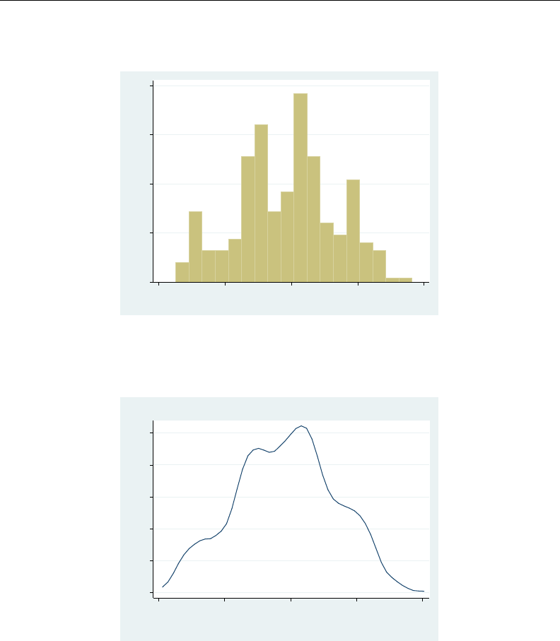
kdensity — Univariate kernel density estimation 1005
. use http://www.stata-press.com/data/r13/trocolen
. histogram length, bin(18)
(bin=18, start=226, width=19.777778)
0 .002 .004 .006 .008
Density
200 300 400 500 600
length
The kernel density estimate, on the other hand, is smooth.
. kdensity length
0 .001 .002 .003 .004 .005
Density
200 300 400 500 600
length
kernel = epanechnikov, bandwidth = 20.1510
Kernel density estimate
Kernel density estimators are, however, sensitive to an assumption, just as are histograms. In histograms,
we specify a number of bins. For kernel density estimators, we specify a width. In the graph above,
we used the default width. kdensity is smarter than twoway histogram in that its default width
is not a fixed constant. Even so, the default width is not necessarily best.
kdensity stores the width in the returned scalar bwidth, so typing display r(bwidth) reveals
it. Doing this, we discover that the width is approximately 20.
Widths are similar to the inverse of the number of bins in a histogram in that smaller widths
provide more detail. The units of the width are the units of x, the variable being analyzed. The width
is specified as a half-width, meaning that the kernel density estimator with half-width 20 corresponds
to sliding a window of size 40 across the data.

1006 kdensity — Univariate kernel density estimation
We can specify half-widths for ourselves by using the bwidth() option. Smaller widths do not
smooth the density as much:
. kdensity length, bwidth(10)
0 .002 .004 .006 .008
Density
200 300 400 500 600
length
kernel = epanechnikov, bandwidth = 10.0000
Kernel density estimate
. kdensity length, bwidth(15)
0 .002 .004 .006
Density
200 300 400 500 600
length
kernel = epanechnikov, bandwidth = 15.0000
Kernel density estimate
Example 2: Different kernels can produce different results
When widths are held constant, different kernels can produce surprisingly different results. This
is really an attribute of the kernel and width combination; for a given width, some kernels are more
sensitive than others at identifying peaks in the density estimate.
We can see this when using a dataset with lots of peaks. In the automobile dataset, we characterize
the density of weight, the weight of the vehicles. Below we compare the Epanechnikov and Parzen
kernels.
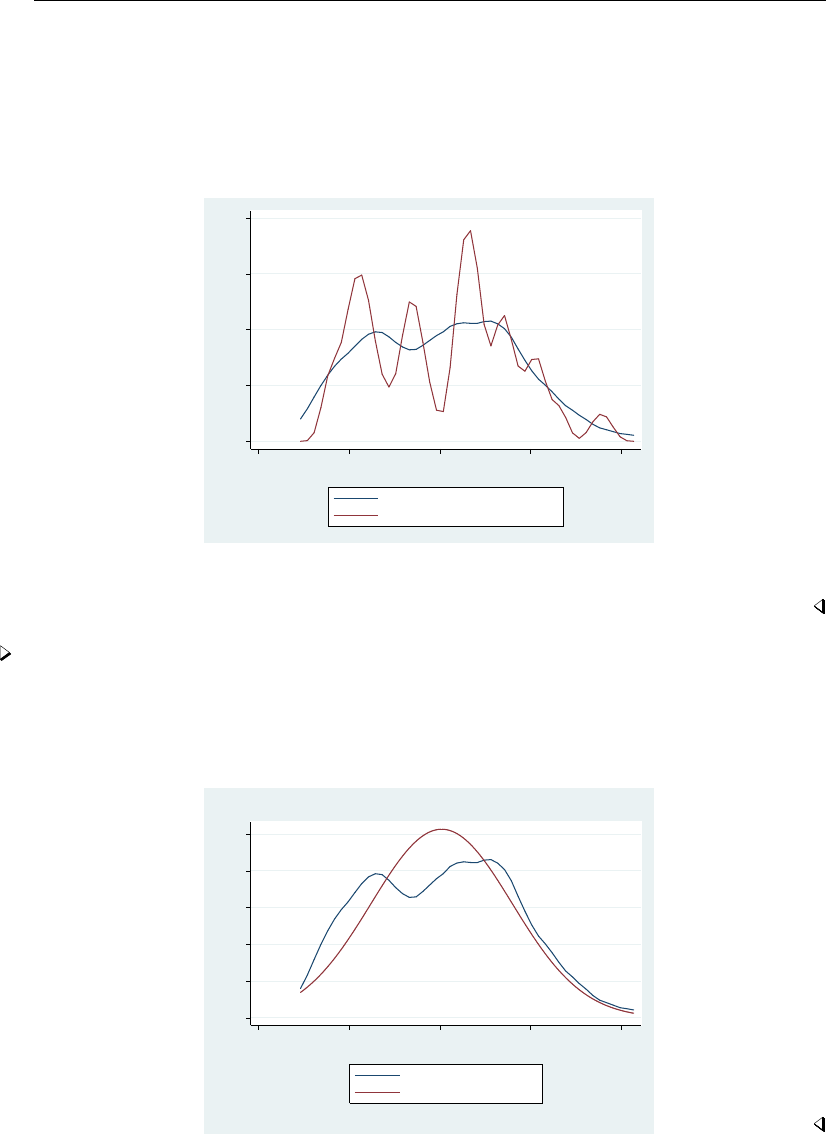
kdensity — Univariate kernel density estimation 1007
. use http://www.stata-press.com/data/r13/auto
(1978 Automobile Data)
. kdensity weight, kernel(epanechnikov) nograph generate(x epan)
. kdensity weight, kernel(parzen) nograph generate(x2 parzen)
. label var epan "Epanechnikov density estimate"
. label var parzen "Parzen density estimate"
. line epan parzen x, sort ytitle(Density) legend(cols(1))
0 .0002 .0004 .0006 .0008
Density
1000 2000 3000 4000 5000
Weight (lbs.)
Epanechnikov density estimate
Parzen density estimate
We did not specify a width, so we obtained the default width. That width is not a function of the
selected kernel, but of the data. See Methods and formulas for the calculation of the optimal width.
Example 3: Density with overlaid normal density
In examining the density estimates, we may wish to overlay a normal density or a Student’s t
density for comparison. Using automobile weights, we can get an idea of the distance from normality
by using the normal option.
. kdensity weight, kernel(epanechnikov) normal
0 .0001 .0002 .0003 .0004 .0005
Density
1000 2000 3000 4000 5000
Weight (lbs.)
Kernel density estimate
Normal density
kernel = epanechnikov, bandwidth = 295.7504
Kernel density estimate
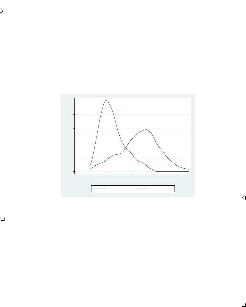
1008 kdensity — Univariate kernel density estimation
Example 4: Compare two densities
We also may want to compare two or more densities. In this example, we will compare the density
estimates of the weights for the foreign and domestic cars.
. use http://www.stata-press.com/data/r13/auto, clear
(1978 Automobile Data)
. kdensity weight, nograph generate(x fx)
. kdensity weight if foreign==0, nograph generate(fx0) at(x)
. kdensity weight if foreign==1, nograph generate(fx1) at(x)
. label var fx0 "Domestic cars"
. label var fx1 "Foreign cars"
. line fx0 fx1 x, sort ytitle(Density)
0 .0002 .0004 .0006 .0008 .001
Density
1000 2000 3000 4000 5000
Weight (lbs.)
Domestic cars Foreign cars
Technical note
Although all the examples we included had densities of less than 1, the density may exceed 1.
The probability density f(x)of a continuous variable, x, has the units and dimensions of the
reciprocal of x. If xis measured in meters, f(x)has units 1/meter. Thus the density is not measured
on a probability scale, so it is possible for f(x)to exceed 1.
To see this, think of a uniform density on the interval 0 to 1. The area under the density curve is
1: this is the product of the density, which is constant at 1, and the range, which is 1. If the variable
is then transformed by doubling, the area under the curve remains 1 and is the product of the density,
constant at 0.5, and the range, which is 2. Conversely, if the variable is transformed by halving, the
area under the curve also remains at 1 and is the product of the density, constant at 2, and the range,
which is 0.5. (Strictly, the range is measured in certain units, and the density is measured in the
reciprocal of those units, so the units cancel on multiplication.)

kdensity — Univariate kernel density estimation 1009
Stored results
kdensity stores the following in r():
Scalars
r(bwidth) kernel bandwidth
r(n) number of points at which the estimate was evaluated
r(scale) density bin width
Macros
r(kernel) name of kernel
Methods and formulas
A kernel density estimate is formed by summing the weighted values calculated with the kernel
function K, as in
b
fK=1
qh
n
X
i=1
wiKx−Xi
h
where q=Piwiif weights are frequency weights (fweight) or analytic weights (aweight), and
q=1 if weights are importance weights (iweights). Analytic weights are rescaled so that Piwi=n
(see [U] 11 Language syntax). If weights are not used, then wi=1, for i=1, . . . , n.kdensity
includes seven different kernel functions. The Epanechnikov is the default function if no other kernel
is specified and is the most efficient in minimizing the mean integrated squared error.
Kernel Formula
Biweight K[z] = 15
16 (1 −z2)2if |z|<1
0otherwise
Cosine K[z] = n1 + cos(2πz)if |z|<1/2
0otherwise
Epanechnikov K[z] = 3
4(1 −1
5z2)/√5if |z|<√5
0otherwise
Epan2 K[z] = 3
4(1 −z2)if |z|<1
0otherwise
Gaussian K[z] = 1
√2πe−z2/2
Parzen K[z] =
4
3−8z2+ 8|z|3if |z| ≤ 1/2
8(1 − |z|)3/3if 1/2<|z| ≤ 1
0otherwise
Rectangular K[z] = n1/2if |z|<1
0otherwise
Triangular K[z] = n1− |z|if |z|<1
0otherwise
From the definitions given in the table, we can see that the choice of hwill drive how many
values are included in estimating the density at each point. This value is called the window width or
bandwidth. If the window width is not specified, it is determined as

1010 kdensity — Univariate kernel density estimation
m=min √variancex,interquartile rangex
1.349
h=0.9m
n1/5
where xis the variable for which we wish to estimate the kernel and nis the number of observations.
Most researchers agree that the choice of kernel is not as important as the choice of bandwidth.
There is a great deal of literature on choosing bandwidths under various conditions; see, for example,
Parzen (1962)orTapia and Thompson (1978). Also see Newton (1988) for a comparison with sample
spectral density estimation in time-series applications.
Acknowledgments
We gratefully acknowledge the previous work by Isa´
ıas H. Salgado-Ugarte of Universidad Nacional
Aut´
onoma de M´
exico, and Makoto Shimizu and Toru Taniuchi of the University of Tokyo; see
Salgado-Ugarte, Shimizu, and Taniuchi (1993). Their article provides a good overview of the subject
of univariate kernel density estimation and presents arguments for its use in exploratory data analysis.
References
Cox, N. J. 2005. Speaking Stata: Density probability plots.Stata Journal 5: 259–273.
. 2007. Kernel estimation as a basic tool for geomorphological data analysis. Earth Surface Processes and
Landforms 32: 1902–1912.
Fiorio, C. V. 2004. Confidence intervals for kernel density estimation.Stata Journal 4: 168–179.
Fox, J. 1990. Describing univariate distributions. In Modern Methods of Data Analysis, ed. J. Fox and J. S. Long,
58–125. Newbury Park, CA: Sage.
Goeden, G. B. 1978. A monograph of the coral trout, Plectropomus leopardus (Lac´
ep`
ede). Queensland Fisheries
Services Research Bulletin 1: 1–42.
Kohler, U., and F. Kreuter. 2012. Data Analysis Using Stata. 3rd ed. College Station, TX: Stata Press.
Newton, H. J. 1988. TIMESLAB: A Time Series Analysis Laboratory. Belmont, CA: Wadsworth.
Parzen, E. 1962. On estimation of a probability density function and mode. Annals of Mathematical Statistics 33:
1065–1076.
Royston, P., and N. J. Cox. 2005. A multivariable scatterplot smoother.Stata Journal 5: 405–412.
Salgado-Ugarte, I. H., and M. A. P´
erez-Hern´
andez. 2003. Exploring the use of variable bandwidth kernel density
estimators.Stata Journal 3: 133–147.
Salgado-Ugarte, I. H., M. Shimizu, and T. Taniuchi. 1993. snp6: Exploring the shape of univariate data using kernel
density estimators.Stata Technical Bulletin 16: 8–19. Reprinted in Stata Technical Bulletin Reprints, vol. 3, pp.
155–173. College Station, TX: Stata Press.
. 1995a. snp6.1: ASH, WARPing, and kernel density estimation for univariate data.Stata Technical Bulletin 26:
23–31. Reprinted in Stata Technical Bulletin Reprints, vol. 5, pp. 161–172. College Station, TX: Stata Press.
. 1995b. snp6.2: Practical rules for bandwidth selection in univariate density estimation.Stata Technical Bulletin
27: 5–19. Reprinted in Stata Technical Bulletin Reprints, vol. 5, pp. 172–190. College Station, TX: Stata Press.
. 1997. snp13: Nonparametric assessment of multimodality for univariate data.Stata Technical Bulletin 38: 27–35.
Reprinted in Stata Technical Bulletin Reprints, vol. 7, pp. 232–243. College Station, TX: Stata Press.
Scott, D. W. 1992. Multivariate Density Estimation: Theory, Practice, and Visualization. New York: Wiley.
Silverman, B. W. 1992. Density Estimation for Statistics and Data Analysis. London: Chapman & Hall.
Simonoff, J. S. 1996. Smoothing Methods in Statistics. New York: Springer.

kdensity — Univariate kernel density estimation 1011
Steichen, T. J. 1998. gr33: Violin plots.Stata Technical Bulletin 46: 13–18. Reprinted in Stata Technical Bulletin
Reprints, vol. 8, pp. 57–65. College Station, TX: Stata Press.
Tapia, R. A., and J. R. Thompson. 1978. Nonparametric Probability Density Estimation. Baltimore: Johns Hopkins
University Press.
Van Kerm, P. 2003. Adaptive kernel density estimation.Stata Journal 3: 148–156.
. 2012. Kernel-smoothed cumulative distribution function estimation with akdensity.Stata Journal 12: 543–548.
Wand, M. P., and M. C. Jones. 1995. Kernel Smoothing. London: Chapman & Hall.
Also see
[R]histogram — Histograms for continuous and categorical variables

Title
ksmirnov — Kolmogorov–Smirnov equality-of-distributions test
Syntax Menu Description
Options for two-sample test Remarks and examples Stored results
Methods and formulas References Also see
Syntax
One-sample Kolmogorov–Smirnov test
ksmirnov varname =exp if in
Two-sample Kolmogorov–Smirnov test
ksmirnov varname if in , by(groupvar)exact
Menu
Statistics >Nonparametric analysis >Tests of hypotheses >Kolmogorov-Smirnov test
Description
ksmirnov performs one- and two-sample Kolmogorov–Smirnov tests of the equality of distributions.
In the first syntax, varname is the variable whose distribution is being tested, and exp must evaluate to
the corresponding (theoretical) cumulative. In the second syntax, groupvar must take on two distinct
values. The distribution of varname for the first value of groupvar is compared with that of the second
value.
When testing for normality, please see [R]sktest and [R]swilk.
Options for two-sample test
Main
by(groupvar)is required. It specifies a binary variable that identifies the two groups.
exact specifies that the exact p-value be computed. This may take a long time if n > 50.
Remarks and examples
Example 1: Two-sample test
Say that we have data on xthat resulted from two different experiments, labeled as group==1
and group==2. Our data contain
1012

ksmirnov — Kolmogorov–Smirnov equality-of-distributions test 1013
. use http://www.stata-press.com/data/r13/ksxmpl
. list
group x
1. 2 2
2. 1 0
3. 2 3
4. 1 4
5. 1 5
6. 2 8
7. 2 10
We wish to use the two-sample Kolmogorov –Smirnov test to determine if there are any differences
in the distribution of xfor these two groups:
. ksmirnov x, by(group)
Two-sample Kolmogorov-Smirnov test for equality of distribution functions
Smaller group D P-value Corrected
1: 0.5000 0.424
2: -0.1667 0.909
Combined K-S: 0.5000 0.785 0.735
The first line tests the hypothesis that xfor group 1 contains smaller values than for group 2. The
largest difference between the distribution functions is 0.5. The approximate p-value for this is 0.424,
which is not significant.
The second line tests the hypothesis that xfor group 1 contains larger values than for group 2.
The largest difference between the distribution functions in this direction is 0.1667. The approximate
p-value for this small difference is 0.909.
Finally, the approximate p-value for the combined test is 0.785, corrected to 0.735. The p-values
ksmirnov calculates are based on the asymptotic distributions derived by Smirnov (1933). These
approximations are not good for small samples (n < 50). They are too conservative—real p-values
tend to be substantially smaller. We have also included a less conservative approximation for the
nondirectional hypothesis based on an empirical continuity correction—the 0.735 reported in the third
column.
That number, too, is only an approximation. An exact value can be calculated using the exact
option:
. ksmirnov x, by(group) exact
Two-sample Kolmogorov-Smirnov test for equality of distribution functions
Smaller group D P-value Exact
1: 0.5000 0.424
2: -0.1667 0.909
Combined K-S: 0.5000 0.785 0.657
Example 2: One-sample test
Let’s now test whether xin the example above is distributed normally. Kolmogorov–Smirnov is
not a particularly powerful test in testing for normality, and we do not endorse such use of it; see
[R]sktest and [R]swilk for better tests.

1014 ksmirnov — Kolmogorov–Smirnov equality-of-distributions test
In any case, we will test against a normal distribution with the same mean and standard deviation:
. summarize x
Variable Obs Mean Std. Dev. Min Max
x 7 4.571429 3.457222 0 10
. ksmirnov x = normal((x-4.571429)/3.457222)
One-sample Kolmogorov-Smirnov test against theoretical distribution
normal((x-4.571429)/3.457222)
Smaller group D P-value Corrected
x: 0.1650 0.683
Cumulative: -0.1250 0.803
Combined K-S: 0.1650 0.991 0.978
Because Stata has no way of knowing that we based this calculation on the calculated mean and standard
deviation of x, the test statistics will be slightly conservative in addition to being approximations.
Nevertheless, they clearly indicate that the data cannot be distinguished from normally distributed
data.
Stored results
ksmirnov stores the following in r():
Scalars
r(D 1) Dfrom line 1 r(D) combined D
r(p 1) p-value from line 1 r(p) combined p-value
r(D 2) Dfrom line 2 r(p cor) corrected combined p-value
r(p 2) p-value from line 2 r(p exact) exact combined p-value
Macros
r(group1) name of group from line 1 r(group2) name of group from line 2
Methods and formulas
In general, the Kolmogorov – Smirnov test (Kolmogorov 1933;Smirnov 1933; also see Conover
[1999], 428–465) is not very powerful against differences in the tails of distributions. In return for
this, it is fairly powerful for alternative hypotheses that involve lumpiness or clustering in the data.
The directional hypotheses are evaluated with the statistics
D+= max
xnF(x)−G(x)o
D−= min
xnF(x)−G(x)o
where F(x)and G(x)are the empirical distribution functions for the sample being compared. The
combined statistic is
D= max|D+|,|D−|
The p-value for this statistic may be obtained by evaluating the asymptotic limiting distribution. Let
mbe the sample size for the first sample, and let nbe the sample size for the second sample.
Smirnov (1933) shows that

ksmirnov — Kolmogorov–Smirnov equality-of-distributions test 1015
lim
m,n→∞ Prnpmn/(m+n)Dm,n ≤zo= 1 −2∞
X
i=1 −1i−1exp −2i2z2
The first five terms form the approximation Paused by Stata. The exact p-value is calculated by a
counting algorithm; see Gibbons and Chakraborti (2011, 236–238). A corrected p-value was obtained
by modifying the asymptotic p-value by using a numerical approximation technique:
Z= Φ−1(Pa)+1.04/min(m, n)+2.09/max(m, n)−1.35/pmn/(m+n)
p-value = Φ(Z)
where Φ(·)is the cumulative normal distribution.
Andrei Nikolayevich Kolmogorov (1903–1987), of Russia, was one of the great mathematicians
of the twentieth century, making outstanding contributions in many different branches, including
set theory, measure theory, probability and statistics, approximation theory, functional analysis,
classical dynamics, and theory of turbulence. He was a faculty member at Moscow State University
for more than 60 years.
Nikolai Vasilyevich Smirnov (1900–1966) was a Russian statistician whose work included
contributions in nonparametric statistics, order statistics, and goodness of fit. After army service
and the study of philosophy and philology, he turned to mathematics and eventually rose to be
head of mathematical statistics at the Steklov Mathematical Institute in Moscow.
References
Aivazian, S. A. 1997. Smirnov, Nikolai Vasil’yevich. In Leading Personalities in Statistical Sciences: From the
Seventeenth Century to the Present, ed. N. L. Johnson and S. Kotz, 208–210. New York: Wiley.
Conover, W. J. 1999. Practical Nonparametric Statistics. 3rd ed. New York: Wiley.
Gibbons, J. D., and S. Chakraborti. 2011. Nonparametric Statistical Inference. 5th ed. Boca Raton, FL: Chapman &
Hall/CRC.
Goerg, S. J., and J. Kaiser. 2009. Nonparametric testing of distributions—the Epss–Singleton two-sample test using
the empirical characteristic function.Stata Journal 9: 454–465.
Jann, B. 2008. Multinomial goodness-of-fit: Large-sample tests with survey design correction and exact tests for small
samples.Stata Journal 8: 147–169.
Johnson, N. L., and S. Kotz. 1997. Kolmogorov, Andrei Nikolayevich. In Leading Personalities in Statistical Sciences:
From the Seventeenth Century to the Present, ed. N. L. Johnson and S. Kotz, 255–256. New York: Wiley.
Kolmogorov, A. N. 1933. Sulla determinazione empirica di una legge di distribuzione. Giornale dell’ Istituto Italiano
degli Attuari 4: 83–91.
Riffenburgh, R. H. 2012. Statistics in Medicine. 3rd ed. San Diego, CA: Academic Press.
Smirnov, N. V. 1933. Estimate of deviation between empirical distribution functions in two independent samples.
Bulletin Moscow University 2: 3–16.
Also see
[R]runtest — Test for random order
[R]sktest — Skewness and kurtosis test for normality
[R]swilk — Shapiro –Wilk and Shapiro – Francia tests for normality

Title
kwallis — Kruskal–Wallis equality-of-populations rank test
Syntax Menu Description Option
Remarks and examples Stored results Methods and formulas References
Also see
Syntax
kwallis varname if in , by(groupvar)
Menu
Statistics >Nonparametric analysis >Tests of hypotheses >Kruskal-Wallis rank test
Description
kwallis tests the hypothesis that several samples are from the same population. In the syntax
diagram above, varname refers to the variable recording the outcome, and groupvar refers to the
variable denoting the population. by() is required.
Option
by(groupvar)is required. It specifies a variable that identifies the groups.
Remarks and examples
Example 1
We have data on the 50 states. The data contain the median age of the population, medage, and
the region of the country, region, for each state. We wish to test for the equality of the median age
distribution across all four regions simultaneously:
. use http://www.stata-press.com/data/r13/census
(1980 Census data by state)
. kwallis medage, by(region)
Kruskal-Wallis equality-of-populations rank test
region Obs Rank Sum
NE 9 376.50
N Cntrl 12 294.00
South 16 398.00
West 13 206.50
chi-squared = 17.041 with 3 d.f.
probability = 0.0007
chi-squared with ties = 17.062 with 3 d.f.
probability = 0.0007
1016

kwallis — Kruskal–Wallis equality-of-populations rank test 1017
From the output, we see that we can reject the hypothesis that the populations are the same at any
level below 0.07%.
Stored results
kwallis stores the following in r():
Scalars
r(df) degrees of freedom
r(chi2) χ2
r(chi2 adj) χ2adjusted for ties
Methods and formulas
The Kruskal–Wallis test (Kruskal and Wallis 1952,1953; also see Altman [1991, 213–215];
Conover [1999, 288–297]; and Riffenburgh [2012, sec. 11.6]) is a multiple-sample generalization of
the two-sample Wilcoxon (also called Mann–Whitney) rank sum test (Wilcoxon 1945;Mann and
Whitney 1947). Samples of sizes nj,j=1, . . . , m, are combined and ranked in ascending order of
magnitude. Tied values are assigned the average ranks. Let ndenote the overall sample size, and let
Rj=Pnj
i=1 R(Xji)denote the sum of the ranks for the jth sample. The Kruskal – Wallis one-way
analysis-of-variance test, H, is defined as
H=1
S2
m
X
j=1
R2
j
nj−n(n+ 1)2
4
where
S2=1
n−1
X
all ranks
R(Xji)2−n(n+ 1)2
4
If there are no ties, this equation simplifies to
H=12
n(n+ 1)
m
X
j=1
R2
j
nj−3(n+ 1)
The sampling distribution of His approximately χ2with m−1 degrees of freedom.
William Henry Kruskal (1919–2005) was born in New York City. He studied mathematics and
statistics at Antioch College, Harvard, and Columbia, and joined the University of Chicago
in 1951. He made many outstanding contributions to linear models, nonparametric statistics,
government statistics, and the history and methodology of statistics.
Wilson Allen Wallis (1912–1998) was born in Philadelphia. He studied psychology and economics
at the Universities of Minnesota and Chicago and at Columbia. He taught at Yale, Stanford, and
Chicago, before moving as president (later chancellor) to the University of Rochester in 1962. He
also served in several Republican administrations. Wallis served as editor of the Journal of the
American Statistical Association, coauthored a popular introduction to statistics, and contributed
to nonparametric statistics.

1018 kwallis — Kruskal–Wallis equality-of-populations rank test
References
Altman, D. G. 1991. Practical Statistics for Medical Research. London: Chapman & Hall/CRC.
Conover, W. J. 1999. Practical Nonparametric Statistics. 3rd ed. New York: Wiley.
Fienberg, S. E., S. M. Stigler, and J. M. Tanur. 2007. The William Kruskal Legacy: 1919–2005. Statistical Science
22: 255–261.
Kruskal, W. H., and W. A. Wallis. 1952. Use of ranks in one-criterion variance analysis. Journal of the American
Statistical Association 47: 583–621.
. 1953. Errata: Use of ranks in one-criterion variance analysis. Journal of the American Statistical Association
48: 907–911.
Mann, H. B., and D. R. Whitney. 1947. On a test of whether one of two random variables is stochastically larger
than the other. Annals of Mathematical Statistics 18: 50–60.
Newson, R. B. 2006. Confidence intervals for rank statistics: Somers’ D and extensions.Stata Journal 6: 309–334.
Olkin, I. 1991. A conversation with W. Allen Wallis. Statistical Science 6: 121–140.
Riffenburgh, R. H. 2012. Statistics in Medicine. 3rd ed. San Diego, CA: Academic Press.
Wilcoxon, F. 1945. Individual comparisons by ranking methods. Biometrics 1: 80–83.
Zabell, S. L. 1994. A conversation with William Kruskal. Statistical Science 9: 285–303.
Also see
[R]nptrend — Test for trend across ordered groups
[R]oneway — One-way analysis of variance
[R]sdtest — Variance-comparison tests
[R]signrank — Equality tests on matched data

Title
ladder — Ladder of powers
Syntax Menu Description
Options for ladder Options for gladder Options for qladder
Remarks and examples Stored results Methods and formulas
Acknowledgment References Also see
Syntax
Ladder of powers
ladder varname if in , generate(newvar) noadjust
Ladder-of-powers histograms
gladder varname if in ,histogram options combine options
Ladder-of-powers quantile–normal plots
qladder varname if in ,qnorm options combine options
by is allowed with ladder; see [D] by.
Menu
ladder
Statistics >Summaries, tables, and tests >Distributional plots and tests >Ladder of powers
gladder
Statistics >Summaries, tables, and tests >Distributional plots and tests >Ladder-of-powers histograms
qladder
Statistics >Summaries, tables, and tests >Distributional plots and tests >Ladder-of-powers quantile-normal plots
Description
ladder searches a subset of the ladder of powers (Tukey 1977) for a transform that converts
varname into a normally distributed variable. sktest tests for normality; see [R]sktest. Also see
[R]boxcox.
gladder displays nine histograms of transforms of varname according to the ladder of powers.
gladder is useful pedagogically, but we do not advise looking at histograms for research work;
ladder or qnorm (see [R]diagnostic plots) is preferred.
qladder displays the quantiles of transforms of varname according to the ladder of powers against
the quantiles of a normal distribution.
1019

1020 ladder — Ladder of powers
Options for ladder
Main
generate(newvar)saves the transformed values corresponding to the minimum chi-squared value
from the table. We do not recommend using generate() because it is literal in interpreting the
minimum, thus ignoring nearly equal but perhaps more interpretable transforms.
noadjust is the noadjust option to sktest; see [R]sktest.
Options for gladder
histogram options affect the rendition of the histograms across all relevant transformations; see
[R]histogram. Here the normal option is assumed, so you must supply the nonormal option
to suppress the overlaid normal density. Also, gladder does not allow the width(#)option of
histogram.
combine options are any of the options documented in [G-2]graph combine. These include options for
titling the graph (see [G-3]title options) and for saving the graph to disk (see [G-3]saving option).
Options for qladder
qnorm options affect the rendition of the quantile–normal plots across all relevant transformations.
See [R]diagnostic plots.
combine options are any of the options documented in [G-2]graph combine. These include options for
titling the graph (see [G-3]title options) and for saving the graph to disk (see [G-3]saving option).
Remarks and examples
Example 1: ladder
We have data on the mileage rating of 74 automobiles and wish to find a transform that makes
the variable normally distributed:
. use http://www.stata-press.com/data/r13/auto
(1978 Automobile Data)
. ladder mpg
Transformation formula chi2(2) P(chi2)
cubic mpg^3 43.59 0.000
square mpg^2 27.03 0.000
identity mpg 10.95 0.004
square root sqrt(mpg) 4.94 0.084
log log(mpg) 0.87 0.647
1/(square root) 1/sqrt(mpg) 0.20 0.905
inverse 1/mpg 2.36 0.307
1/square 1/(mpg^2) 11.99 0.002
1/cubic 1/(mpg^3) 24.30 0.000
If we had typed ladder mpg, gen(mpgx), the variable mpgx containing 1/√mpg would have been
automatically generated for us. This is the perfect example of why you should not, in general, specify
the generate() option. We also cannot reject the hypothesis that the inverse of mpg is normally
distributed and that 1/mpg—gallons per mile—has a better interpretation. It is a measure of energy
consumption.
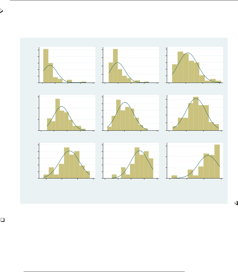
ladder — Ladder of powers 1021
Example 2: gladder
gladder explores the same transforms as ladder but presents results graphically:
. gladder mpg, fraction
0 .1 .2 .3 .4 .5
0 20000 40000 60000 80000
cubic
0 .1 .2 .3 .4
0 500 1000 1500 2000
square
0 .05 .1 .15 .2 .25
10 20 30 40
identity
0 .1 .2 .3
3 4 5 6 7
sqrt
0 .05 .1 .15 .2 .25
2.5 3 3.5 4
log
0 .05 .1 .15 .2
−.3 −.25 −.2 −.15
1/sqrt
0 .05 .1 .15 .2 .25
−.08 −.06 −.04 −.02
inverse
0 .05 .1 .15 .2 .25
−.008 −.006 −.004 −.002 0
1/square
0 .1 .2 .3
−.0006 −.0004 −.0002 0
1/cubic
Fraction
Mileage (mpg)
Histograms by transformation
Technical note
gladder is useful pedagogically, but be careful when using it for research work, especially with
many observations. For instance, consider the following data on the average July temperature in
degrees Fahrenheit for 954 U.S. cities:
. use http://www.stata-press.com/data/r13/citytemp
(City Temperature Data)
. ladder tempjuly
Transformation formula chi2(2) P(chi2)
cubic tempjuly^3 47.49 0.000
square tempjuly^2 19.70 0.000
identity tempjuly 3.83 0.147
square root sqrt(tempjuly) 1.83 0.400
log log(tempjuly) 5.40 0.067
1/(square root) 1/sqrt(tempjuly) 13.72 0.001
inverse 1/tempjuly 26.36 0.000
1/square 1/(tempjuly^2) 64.43 0.000
1/cubic 1/(tempjuly^3) . 0.000
The period in the last line indicates that the χ2is very large; see [R]sktest.
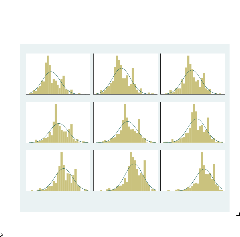
1022 ladder — Ladder of powers
From the table, we see that there is certainly a difference in normality between the square and
square-root transform. If, however, you can see the difference between the transforms in the diagram
below, you have better eyes than we do:
. gladder tempjuly, l1title("") ylabel(none) xlabel(none)
cubic square identity
sqrt log 1/sqrt
inverse 1/square 1/cubic
Average July temperature
Histograms by transformation
Example 3: qladder
A better graph for seeing normality is the quantile–normal graph, which can be produced by qladder.
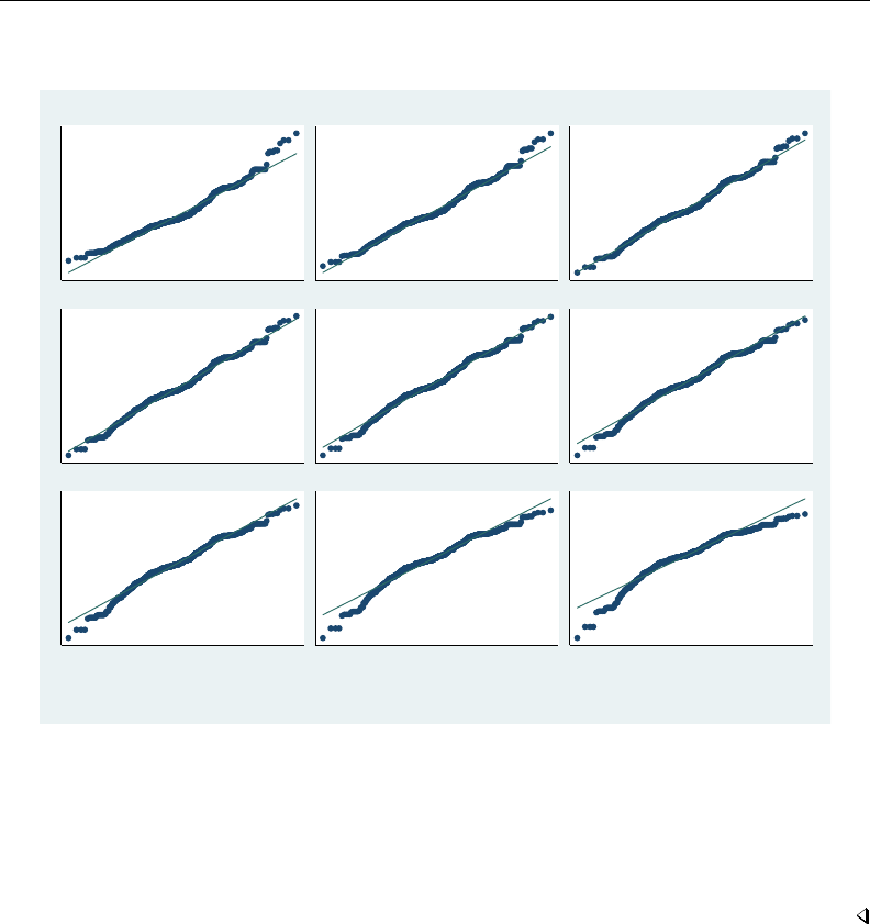
ladder — Ladder of powers 1023
. qladder tempjuly, ylabel(none) xlabel(none)
cubic square identity
sqrt log 1/sqrt
inverse 1/square 1/cubic
Average July temperature
Quantile−Normal plots by transformation
This graph shows that for the square transform, the upper tail—and only the upper tail—diverges
from what would be expected. This divergence is detected by sktest (see [R]sktest) as a problem
with skewness, as we would learn from using sktest to examine tempjuly squared and square
rooted.

1024 ladder — Ladder of powers
Stored results
ladder stores the following in r():
Scalars
r(N) number of observations
r(invcube) χ2for inverse-cubic transformation
r(P invcube) significance level for inverse-cubic transformation
r(invsq) χ2for inverse-square transformation
r(P invsq) significance level for inverse-square transformation
r(inv) χ2for inverse transformation
r(P inv) significance level for inverse transformation
r(invsqrt) χ2for inverse-root transformation
r(P invsqrt) significance level for inverse-root transformation
r(log) χ2for log transformation
r(P log) significance level for log transformation
r(sqrt) χ2for square-root transformation
r(P sqrt) significance level for square-root transformation
r(ident) χ2for untransformed data
r(P ident) significance level for untransformed data
r(square) χ2for square transformation
r(P square) significance level for square transformation
r(cube) χ2for cubic transformation
r(P cube) significance level for cubic transformation
Methods and formulas
For ladder, results are as reported by sktest; see [R]sktest. If generate() is specified, the
transform with the minimum χ2value is chosen.
gladder sets the number of bins to min(√n, 10 log10 n), rounded to the closest integer, where
nis the number of unique values of varname. See [R]histogram for a discussion of the optimal
number of bins.
Also see Findley (1990) for a ladder-of-powers variable transformation program that produces
one-way graphs with overlaid box plots, in addition to histograms with overlaid normals. Buchner and
Findley (1990) discuss ladder-of-powers transformations as one aspect of preliminary data analysis.
Also see Hamilton (1992, 18–23) and Hamilton (2013, 129–132).
Acknowledgment
qladder was written by Jeroen Weesie of the Department of Sociology at Utrecht University, The
Netherlands.
References
Buchner, D. M., and T. W. Findley. 1990. Research in physical medicine and rehabilitation: VIII. Preliminary data
analysis. American Journal of Physical Medicine and Rehabilitation 69: 154–169.
Cox, N. J. 2005. Speaking Stata: Density probability plots.Stata Journal 5: 259–273.
Findley, T. W. 1990. sed3: Variable transformation and evaluation.Stata Technical Bulletin 2: 15. Reprinted in Stata
Technical Bulletin Reprints, vol. 1, pp. 85–86. College Station, TX: Stata Press.
Hamilton, L. C. 1992. Regression with Graphics: A Second Course in Applied Statistics. Belmont, CA: Duxbury.
. 2013. Statistics with Stata: Updated for Version 12. 8th ed. Boston: Brooks/Cole.
Tukey, J. W. 1977. Exploratory Data Analysis. Reading, MA: Addison–Wesley.


Title
level — Set default confidence level
Syntax Description Option Remarks and examples Also see
Syntax
set level #, permanently
Description
set level specifies the default confidence level for confidence intervals for all commands that
report confidence intervals. The initial value is 95, meaning 95% confidence intervals. #may be
between 10.00 and 99.99, and #can have at most two digits after the decimal point.
Option
permanently specifies that, in addition to making the change right now, the level setting be
remembered and become the default setting when you invoke Stata.
Remarks and examples
To change the level of confidence intervals reported by a particular command, you need not reset
the default confidence level. All commands that report confidence intervals have a level(#)option.
When you do not specify the option, the confidence intervals are calculated for the default level set
by set level, or for 95% if you have not reset set level.
Example 1
We use the ci command to obtain the confidence interval for the mean of mpg:
. use http://www.stata-press.com/data/r13/auto
(1978 Automobile Data)
. ci mpg
Variable Obs Mean Std. Err. [95% Conf. Interval]
mpg 74 21.2973 .6725511 19.9569 22.63769
To obtain 90% confidence intervals, we would type
. ci mpg, level(90)
Variable Obs Mean Std. Err. [90% Conf. Interval]
mpg 74 21.2973 .6725511 20.17683 22.41776
or
. set level 90
. ci mpg
Variable Obs Mean Std. Err. [90% Conf. Interval]
mpg 74 21.2973 .6725511 20.17683 22.41776
1026

level — Set default confidence level 1027
If we opt for the second alternative, the next time that we fit a model (say, with regress), 90%
confidence intervals will be reported. If we wanted 95% confidence intervals, we could specify
level(95) on the estimation command, or we could reset the default by typing set level 95.
The current setting of level() is stored as the c-class value c(level); see [P]creturn.
Also see
[R]query — Display system parameters
[P]creturn — Return c-class values
[U] 20 Estimation and postestimation commands
[U] 20.7 Specifying the width of confidence intervals

Title
limits — Quick reference for limits
Description Remarks and examples Also see
Description
This entry provides a quick reference for the size limits in Stata. Note that most of these limits
are so high that you will never encounter them.
Remarks and examples
Remarks are presented under the following headings:
Maximum size limits
Matrix size
Determining which flavor of Stata you are running
Maximum size limits
Stata/MP and
Small Stata/IC Stata/SE
#of observations (1) 1,200 2,147,483,647 2,147,483,647
#of variables 99 2,047 32,767
width of a dataset in bytes 800 24,564 393,192
value of matsize 100 800 11,000
#of RHS variables 98 798 10,998
#characters in a command 13,416 165,216 1,081,527
#options for a command 70 70 70
#of elements in a numlist 2,500 2,500 2,500
#of interacted continuous variables 8 8 8
#of interacted factor variables 8 8 8
#of unique time-series operators in
a command 100 100 100
#seasonal suboperators per time-series
operator 8 8 8
#of dyadic operators in an expression 66 800 800
#of numeric literals in an expression 50 300 300
#of string literals in an expression 256 512 512
length of string in string expression 2,000,000,000 2,000,000,000 2,000,000,000
#of sum functions in an expression 5 5 5
#of pairs of nested parentheses 249 249 249
#of characters in a macro (2) 13,400 165,200 1,081,511
#of nested do-files 64 64 64
1028

limits — Quick reference for limits 1029
Stata/MP and
continued Small Stata/IC Stata/SE
#of lines in a program 3,500 3,500 3,500
#of characters in a program 135,600 135,600 135,600
length of a variable name 32 32 32
length of ado-command name 32 32 32
length of a global macro name 32 32 32
length of a local macro name 31 31 31
length of a str# variable 2,045 2,045 2,045
length of a strL variable 2,000,000,000 2,000,000,000 2,000,000,000
anova
#of variables in one anova term 8 8 8
#of terms in the repeated() option 4 4 4
char
length of one characteristic 13,400 67,784 67,784
constraint
#of constraints 1,999 1,999 1,999
encode and decode
#of unique values 1,000 65,536 65,536
estimates hold
#of stored estimation results 300 300 300
estimates store
#of stored estimation results 300 300 300
exlogistic and expoisson
maximum memory specification in memory(#)2gb 2gb 2gb
grmeanby
#of unique values in varlist N/2N/2N/2
graph twoway
#of variables in a plot 100 100 100
#of styles in an option’s stylelist 20 20 20
infile (free format)
record length without dictionary none none none
infile (fixed format)
record length with a dictionary 524,275 524,275 524,275
infix (fixed format)
record length with a dictionary 524,275 524,275 524,275

1030 limits — Quick reference for limits
Stata/MP and
continued Small Stata/IC Stata/SE
label
length of dataset label 80 80 80
length of variable label 80 80 80
length of value label string 32,000 32,000 32,000
length of name of value label 32 32 32
#of codings within one value label 1,000 65,536 65,536
label language
#of different languages 100 100 100
macro
#of nested macros 20 20 20
manova
#of variables in single manova term 8 8 8
matrix (3)
dimension of single matrix 40 ×40 800 ×800 11,000 ×11,000
maximize options
iterate() maximum 16,000 16,000 16,000
mprobit
#of categories in a depvar 30 30 30
net
#of description lines in .pkg file 100 100 100
nlogit and nlogittree
#of levels in model 8 8 8
notes
length of one note 13,400 67,784 67,784
#of notes attached to dta 9,999 9,999 9,999
#of notes attached to each variable 9,999 9,999 9,999
numlist
#of elements in the numeric list 2,500 2,500 2,500
reg3,sureg, and other system estimators
#of equations 40 800 11,000
set adosize
memory ado-files may consume 1000K 1000K 1000K
set scrollbufsize
memory for Results window buffer 2000K 2000K 2000k

limits — Quick reference for limits 1031
Stata/MP and
continued Small Stata/IC Stata/SE
slogit
#of categories in a depvar 30 30 30
snapspan
length of label 80 80 80
#of saved snapshots 1,000 1,000 1,000
stcox
#of variables in strata() option 5 5 5
stcurve
#of curves plotted on the same graph 10 10 10
table and tabdisp
#of by variables 4 4 4
#of margins, i.e., sum of rows,
columns, supercolumns, and by groups 3,000 3,000 3,000
tabulate oneway
#of rows in one-way table 500 3,000 12,000
tabulate twoway
#of rows & cols in two-way table 160 ×20 300 ×20 1,200 ×80
tabulate, summarize()
#of cells (rows X cols) 375 375 375
teffects
#of treatments 20 20 20
xt estimation commands (e.g., xtgee,
xtgls,xtpoisson,xtprobit,xtreg
with mle option, and xtpcse when
neither option hetonly nor option
independent is specified)
#of time periods within panel 40 800 11,000
#of integration points accepted 195 195 195
by intpoints(#)
(1) 2,147,483,647 is a theoretical maximum; memory availability will certainly impose a smaller
maximum.
(2) The maximum length of the contents of a macro are fixed in Stata/IC and settable in Stata/SE
and Stata/MP. The currently set maximum length is recorded in c(macrolen); type display
c(macrolen). The maximum length can be changed with set maxvar. If you set maxvar to a
larger value, the maximum length increases; if you set maxvar to a smaller value, the maximum
length decreases. The relationship between them is maximum length =33 ×maxvar +200.
(3) In Mata, matrices are limited only by the amount of memory on your computer.

1032 limits — Quick reference for limits
Matrix size
See [R]matsize.
Determining which flavor of Stata you are running
Type
. about
The response will be Stata/MP, Stata/SE, Stata/IC, or Small Stata. Other information is also shown,
including your serial number. See [R]about.
Also see
[R]about — Display information about your Stata
[R]matsize — Set the maximum number of variables in a model
[D]compress — Compress data in memory
[D]data types — Quick reference for data types
[D]import — Overview of importing data into Stata
[D]infile (fixed format) — Read text data in fixed format with a dictionary
[D]infile (free format) — Read unformatted text data
[D]memory — Memory management
[D]obs — Increase the number of observations in a dataset

Title
lincom — Linear combinations of estimators
Syntax Menu Description Options
Remarks and examples Stored results References Also see
Syntax
lincom exp ,options
options Description
eform generic label; exp(b)
or odds ratio
hr hazard ratio
shr subhazard ratio
irr incidence-rate ratio
rrr relative-risk ratio
level(#)set confidence level; default is level(95)
display options control column formats
df(#)use tdistribution with #degrees of freedom for computing p-values
and confidence intervals
exp is any linear combination of coefficients that is a valid syntax for test; see [R] test.exp must not
contain an equal sign.
df(#)does not appear in the dialog box.
Menu
Statistics >Postestimation >Linear combinations of estimates
Description
lincom computes point estimates, standard errors, tor zstatistics, p-values, and confidence
intervals for linear combinations of coefficients after any estimation command. Results can optionally
be displayed as odds ratios, hazard ratios, incidence-rate ratios, or relative-risk ratios.
lincom can be used with svy estimation results; see [SVY]svy postestimation.
Options
eform,or,hr,shr,irr, and rrr all report coefficient estimates as exp(b
β)rather than b
β. Standard
errors and confidence intervals are similarly transformed. or is the default after logistic. The
only difference in these options is how the output is labeled.
1033

1034 lincom — Linear combinations of estimators
Option Label Explanation Example commands
eform exp(b) Generic label cloglog
or Odds Ratio Odds ratio logistic,logit
hr Haz. Ratio Hazard ratio stcox,streg
shr SHR Subhazard ratio stcrreg
irr IRR Incidence-rate ratio poisson
rrr RRR Relative-risk ratio mlogit
exp may not contain any additive constants when you use the eform,or,hr,irr, or rrr option.
level(#)specifies the confidence level, as a percentage, for confidence intervals. The default is
level(95) or as set by set level; see [U] 20.7 Specifying the width of confidence intervals.
display options:cformat(%fmt),pformat(% fmt), and sformat(% fmt); see [R]estimation options.
The following option is available with lincom but is not shown in the dialog box:
df(#)specifies that the tdistribution with #degrees of freedom be used for computing p-values and
confidence intervals. The default is to use e(df r) degrees of freedom or the standard normal
distribution if e(df r) is missing.
Remarks and examples
Remarks are presented under the following headings:
Using lincom
Odds ratios and incidence-rate ratios
Multiple-equation models
Using lincom
After fitting a model and obtaining estimates for coefficients β1, β2, . . . , βk, you may want to
view estimates for linear combinations of the βi, such as β1−β2.lincom can display estimates for
any linear combination of the form c0+c1β1+c2β2+··· +ckβk.
lincom works after any estimation command for which test works. Any valid expression for
test syntax 1 (see [R]test) is a valid expression for lincom.
lincom is useful for viewing odds ratios, hazard ratios, etc., for one group (that is, one set of
covariates) relative to another group (that is, another set of covariates). See the examples below.

lincom — Linear combinations of estimators 1035
Example 1
We perform a linear regression:
. use http://www.stata-press.com/data/r13/regress
. regress y x1 x2 x3
Source SS df MS Number of obs = 148
F( 3, 144) = 96.12
Model 3259.3561 3 1086.45203 Prob > F = 0.0000
Residual 1627.56282 144 11.3025196 R-squared = 0.6670
Adj R-squared = 0.6600
Total 4886.91892 147 33.2443464 Root MSE = 3.3619
y Coef. Std. Err. t P>|t| [95% Conf. Interval]
x1 1.457113 1.07461 1.36 0.177 -.666934 3.581161
x2 2.221682 .8610358 2.58 0.011 .5197797 3.923583
x3 -.006139 .0005543 -11.08 0.000 -.0072345 -.0050435
_cons 36.10135 4.382693 8.24 0.000 27.43863 44.76407
To see the difference of the coefficients of x2 and x1, we type
. lincom x2 - x1
( 1) - x1 + x2 = 0
y Coef. Std. Err. t P>|t| [95% Conf. Interval]
(1) .7645682 .9950282 0.77 0.444 -1.20218 2.731316
The expression can be any linear combination.
. lincom 3*x1 + 500*x3
( 1) 3*x1 + 500*x3 = 0
y Coef. Std. Err. t P>|t| [95% Conf. Interval]
(1) 1.301825 3.396624 0.38 0.702 -5.411858 8.015507
Nonlinear expressions are not allowed.
. lincom x2/x1
not possible with test
r(131);
For information about estimating nonlinear expressions, see [R]nlcom.
Technical note
lincom uses the same shorthands for coefficients as does test (see [R]test). When you type x1,
for instance, lincom knows that you mean the coefficient of x1. The formal syntax for referencing this
coefficient is actually b[x1], or alternatively, coef[x1]. So, more formally, in the last example
we could have typed
. lincom 3*_b[x1] + 500*_b[x3]
(output omitted )

1036 lincom — Linear combinations of estimators
Odds ratios and incidence-rate ratios
After logistic regression, the or option can be specified with lincom to display odds ratios for any
effect. Incidence-rate ratios after commands such as poisson can be similarly obtained by specifying
the irr option.
Example 2
Consider the low birthweight dataset from Hosmer, Lemeshow, and Sturdivant (2013, 24). We fit
a logistic regression model of low birthweight (variable low) on the following variables:
Variable Description Coding
age age in years
race race 1 if white, 2 if black, 3 if other
smoke smoking status 1 if smoker, 0 if nonsmoker
ht history of hypertension 1 if yes, 0 if no
ui uterine irritability 1 if yes, 0 if no
lwd maternal weight before pregnancy 1 if weight <110 lb., 0 otherwise
ptd history of premature labor 1 if yes, 0 if no
c.age##lwd age main effects, lwd main effects,
and their interaction
smoke##lwd smoke main effects, lwd main effects,
and their interaction
We first fit a model without the interaction terms by using logit.
. use http://www.stata-press.com/data/r13/lbw3
(Hosmer & Lemeshow data)
. logit low age lwd i.race smoke ptd ht ui
Iteration 0: log likelihood = -117.336
Iteration 1: log likelihood = -99.3982
Iteration 2: log likelihood = -98.780418
Iteration 3: log likelihood = -98.777998
Iteration 4: log likelihood = -98.777998
Logistic regression Number of obs = 189
LR chi2(8) = 37.12
Prob > chi2 = 0.0000
Log likelihood = -98.777998 Pseudo R2 = 0.1582
low Coef. Std. Err. z P>|z| [95% Conf. Interval]
age -.0464796 .0373888 -1.24 0.214 -.1197603 .0268011
lwd .8420615 .4055338 2.08 0.038 .0472299 1.636893
race
black 1.073456 .5150753 2.08 0.037 .0639273 2.082985
other .815367 .4452979 1.83 0.067 -.0574008 1.688135
smoke .8071996 .404446 2.00 0.046 .0145001 1.599899
ptd 1.281678 .4621157 2.77 0.006 .3759478 2.187408
ht 1.435227 .6482699 2.21 0.027 .1646414 2.705813
ui .6576256 .4666192 1.41 0.159 -.2569313 1.572182
_cons -1.216781 .9556797 -1.27 0.203 -3.089878 .656317

lincom — Linear combinations of estimators 1037
To get the odds ratio for black smokers relative to white nonsmokers (the reference group), we type
. lincom 2.race + smoke, or
( 1) [low]2.race + [low]smoke = 0
low Odds Ratio Std. Err. z P>|z| [95% Conf. Interval]
(1) 6.557805 4.744692 2.60 0.009 1.588176 27.07811
lincom computed exp(β2.race +βsmoke) = 6.56. To see the odds ratio for white smokers relative
to black nonsmokers, we type
. lincom smoke - 2.race, or
( 1) - [low]2.race + [low]smoke = 0
low Odds Ratio Std. Err. z P>|z| [95% Conf. Interval]
(1) .7662425 .4430176 -0.46 0.645 .2467334 2.379603
Now let’s add the interaction terms to the model (Hosmer and Lemeshow 1989, table 4.10). This
time, we will use logistic rather than logit. By default, logistic displays odds ratios.
. logistic low i.race ht ui ptd c.age##lwd smoke##lwd
Logistic regression Number of obs = 189
LR chi2(10) = 42.66
Prob > chi2 = 0.0000
Log likelihood = -96.00616 Pseudo R2 = 0.1818
low Odds Ratio Std. Err. z P>|z| [95% Conf. Interval]
race
black 2.95383 1.532789 2.09 0.037 1.068277 8.167465
other 2.137589 .9919138 1.64 0.102 .8608708 5.307752
ht 3.893141 2.575201 2.05 0.040 1.064768 14.2346
ui 2.071284 .9931388 1.52 0.129 .8092926 5.301192
ptd 3.426633 1.615282 2.61 0.009 1.360252 8.632089
age .9194513 .041896 -1.84 0.065 .8408967 1.005344
1.lwd .1772934 .3312384 -0.93 0.354 .0045539 6.902367
lwd#c.age
1 1.15883 .09602 1.78 0.075 .9851215 1.36317
smoke
smoker 3.168096 1.452378 2.52 0.012 1.289956 7.78076
smoke#lwd
smoker 1 .2447849 .2003996 -1.72 0.086 .0491956 1.217988
_cons .599443 .6519163 -0.47 0.638 .0711271 5.051971
Hosmer and Lemeshow (1989, table 4.13) consider the effects of smoking (smoke =1) and low
maternal weight before pregnancy (lwd =1). The effect of smoking among non–low-weight mothers
(lwd =0) is given by the odds ratio 3.17 for smoke in the logistic output. The effect of smoking
among low-weight mothers is given by

1038 lincom — Linear combinations of estimators
. lincom 1.smoke + 1.smoke#1.lwd
( 1) [low]1.smoke + [low]1.smoke#1.lwd = 0
low Odds Ratio Std. Err. z P>|z| [95% Conf. Interval]
(1) .7755022 .574951 -0.34 0.732 .1813465 3.316323
We did not have to specify the or option. After logistic,lincom assumes or by default.
The effect of low weight (lwd =1) is more complicated because we fit an age ×lwd interaction.
We must specify the age of mothers for the effect. The effect among 30-year-old nonsmokers is given
by
. lincom 1.lwd + 30*1.lwd#c.age
( 1) [low]1.lwd + 30*[low]1.lwd#c.age = 0
low Odds Ratio Std. Err. z P>|z| [95% Conf. Interval]
(1) 14.7669 13.5669 2.93 0.003 2.439264 89.39633
lincom computed exp(βlwd +30βagelwd) = 14.8. It may seem odd that we entered it as 1.lwd
+ 30*1.lwd#c.age, but remember that these terms are just lincom’s (and test’s) shorthands for
b[1.lwd] and b[1.lwd#c.age]. We could have typed
. lincom _b[1.lwd] + 30*_b[1.lwd#c.age]
( 1) [low]1.lwd + 30*[low]1.lwd#c.age = 0
low Odds Ratio Std. Err. z P>|z| [95% Conf. Interval]
(1) 14.7669 13.5669 2.93 0.003 2.439264 89.39633
Multiple-equation models
lincom also works with multiple-equation models. The only difference is how you refer to the
coefficients. Recall that for multiple-equation models, coefficients are referenced using the syntax
[eqno]varname
where eqno is the equation number or equation name and varname is the corresponding variable name
for the coefficient; see [U] 13.5 Accessing coefficients and standard errors and [R]test for details.

lincom — Linear combinations of estimators 1039
Example 3
Let’s consider example 4 from [R]mlogit (Tarlov et al. 1989; Wells et al. 1989).
. use http://www.stata-press.com/data/r13/sysdsn1
(Health insurance data)
. mlogit insure age male nonwhite i.site, nolog
Multinomial logistic regression Number of obs = 615
LR chi2(10) = 42.99
Prob > chi2 = 0.0000
Log likelihood = -534.36165 Pseudo R2 = 0.0387
insure Coef. Std. Err. z P>|z| [95% Conf. Interval]
Indemnity (base outcome)
Prepaid
age -.011745 .0061946 -1.90 0.058 -.0238862 .0003962
male .5616934 .2027465 2.77 0.006 .1643175 .9590693
nonwhite .9747768 .2363213 4.12 0.000 .5115955 1.437958
site
2 .1130359 .2101903 0.54 0.591 -.2989296 .5250013
3 -.5879879 .2279351 -2.58 0.010 -1.034733 -.1412433
_cons .2697127 .3284422 0.82 0.412 -.3740222 .9134476
Uninsure
age -.0077961 .0114418 -0.68 0.496 -.0302217 .0146294
male .4518496 .3674867 1.23 0.219 -.268411 1.17211
nonwhite .2170589 .4256361 0.51 0.610 -.6171725 1.05129
site
2 -1.211563 .4705127 -2.57 0.010 -2.133751 -.2893747
3 -.2078123 .3662926 -0.57 0.570 -.9257327 .510108
_cons -1.286943 .5923219 -2.17 0.030 -2.447872 -.1260134
To see the estimate of the sum of the coefficient of male and the coefficient of nonwhite for the
Prepaid outcome, we type

1040 lincom — Linear combinations of estimators
. lincom [Prepaid]male + [Prepaid]nonwhite
( 1) [Prepaid]male + [Prepaid]nonwhite = 0
insure Coef. Std. Err. z P>|z| [95% Conf. Interval]
(1) 1.53647 .3272489 4.70 0.000 .8950741 2.177866
To view the estimate as a ratio of relative risks (see [R]mlogit for the definition and interpretation),
we specify the rrr option.
. lincom [Prepaid]male + [Prepaid]nonwhite, rrr
( 1) [Prepaid]male + [Prepaid]nonwhite = 0
insure RRR Std. Err. z P>|z| [95% Conf. Interval]
(1) 4.648154 1.521103 4.70 0.000 2.447517 8.827451
Stored results
lincom stores the following in r():
Scalars
r(estimate) point estimate
r(se) estimate of standard error
r(df) degrees of freedom
References
Hosmer, D. W., Jr., and S. A. Lemeshow. 1989. Applied Logistic Regression. New York: Wiley.
Hosmer, D. W., Jr., S. A. Lemeshow, and R. X. Sturdivant. 2013. Applied Logistic Regression. 3rd ed. Hoboken,
NJ: Wiley.
Tarlov, A. R., J. E. Ware, Jr., S. Greenfield, E. C. Nelson, E. Perrin, and M. Zubkoff. 1989. The medical outcomes
study. An application of methods for monitoring the results of medical care. Journal of the American Medical
Association 262: 925–930.
Wells, K. B., R. D. Hays, M. A. Burnam, W. H. Rogers, S. Greenfield, and J. E. Ware, Jr. 1989. Detection of
depressive disorder for patients receiving prepaid or fee-for-service care. Results from the Medical Outcomes Survey.
Journal of the American Medical Association 262: 3298–3302.
Also see
[R]nlcom — Nonlinear combinations of estimators
[R]test — Test linear hypotheses after estimation
[R]testnl — Test nonlinear hypotheses after estimation
[U] 13.5 Accessing coefficients and standard errors
[U] 20 Estimation and postestimation commands

Title
linktest — Specification link test for single-equation models
Syntax Menu Description Option
Remarks and examples Stored results Methods and formulas References
Also see
Syntax
linktest if in ,cmd options
When if and in are not specified, the link test is performed on the same sample as the previous estimation.
Menu
Statistics >Postestimation >Tests >Specification link test for single-equation models
Description
linktest performs a link test for model specification after any single-equation estimation command,
such as logistic,regress,stcox, etc.
Option
Main
cmd options must be the same options specified with the underlying estimation command, except
the display options may differ.
Remarks and examples
The form of the link test implemented here is based on an idea of Tukey (1949), which was further
described by Pregibon (1980), elaborating on work in his unpublished thesis (Pregibon 1979). See
Methods and formulas below for more details.
Example 1
We want to explain the mileage ratings of cars in our automobile dataset by using the weight,
engine displacement, and whether the car is manufactured outside the United States:
1041

1042 linktest — Specification link test for single-equation models
. use http://www.stata-press.com/data/r13/auto
(1978 Automobile Data)
. regress mpg weight displ foreign
Source SS df MS Number of obs = 74
F( 3, 70) = 45.88
Model 1619.71935 3 539.906448 Prob > F = 0.0000
Residual 823.740114 70 11.7677159 R-squared = 0.6629
Adj R-squared = 0.6484
Total 2443.45946 73 33.4720474 Root MSE = 3.4304
mpg Coef. Std. Err. t P>|t| [95% Conf. Interval]
weight -.0067745 .0011665 -5.81 0.000 -.0091011 -.0044479
displacement .0019286 .0100701 0.19 0.849 -.0181556 .0220129
foreign -1.600631 1.113648 -1.44 0.155 -3.821732 .6204699
_cons 41.84795 2.350704 17.80 0.000 37.15962 46.53628
On the basis of the R2, we are reasonably pleased with this model.
If our model really is specified correctly, then if we were to regress mpg on the prediction and the
prediction squared, the prediction squared would have no explanatory power. This is what linktest
does:
. linktest
Source SS df MS Number of obs = 74
F( 2, 71) = 76.75
Model 1670.71514 2 835.357572 Prob > F = 0.0000
Residual 772.744316 71 10.8837228 R-squared = 0.6837
Adj R-squared = 0.6748
Total 2443.45946 73 33.4720474 Root MSE = 3.299
mpg Coef. Std. Err. t P>|t| [95% Conf. Interval]
_hat -.4127198 .6577736 -0.63 0.532 -1.724283 .8988434
_hatsq .0338198 .015624 2.16 0.034 .0026664 .0649732
_cons 14.00705 6.713276 2.09 0.041 .6211539 27.39294
We find that the prediction squared does have explanatory power, so our specification is not as
good as we thought.
Although linktest is formally a test of the specification of the dependent variable, it is often
interpreted as a test that, conditional on the specification, the independent variables are specified
incorrectly. We will follow that interpretation and now include weight squared in our model:

linktest — Specification link test for single-equation models 1043
. regress mpg weight c.weight#c.weight displ foreign
Source SS df MS Number of obs = 74
F( 4, 69) = 39.37
Model 1699.02634 4 424.756584 Prob > F = 0.0000
Residual 744.433124 69 10.7888859 R-squared = 0.6953
Adj R-squared = 0.6777
Total 2443.45946 73 33.4720474 Root MSE = 3.2846
mpg Coef. Std. Err. t P>|t| [95% Conf. Interval]
weight -.0173257 .0040488 -4.28 0.000 -.0254028 -.0092486
c.weight#
c.weight 1.87e-06 6.89e-07 2.71 0.008 4.93e-07 3.24e-06
displacement -.0101625 .0106236 -0.96 0.342 -.031356 .011031
foreign -2.560016 1.123506 -2.28 0.026 -4.801349 -.3186832
_cons 58.23575 6.449882 9.03 0.000 45.36859 71.10291
Now we perform the link test on our new model:
. linktest
Source SS df MS Number of obs = 74
F( 2, 71) = 81.08
Model 1699.39489 2 849.697445 Prob > F = 0.0000
Residual 744.06457 71 10.4797827 R-squared = 0.6955
Adj R-squared = 0.6869
Total 2443.45946 73 33.4720474 Root MSE = 3.2372
mpg Coef. Std. Err. t P>|t| [95% Conf. Interval]
_hat 1.141987 .7612218 1.50 0.138 -.3758456 2.659821
_hatsq -.0031916 .0170194 -0.19 0.852 -.0371272 .0307441
_cons -1.50305 8.196444 -0.18 0.855 -17.84629 14.84019
We now pass the link test.
Example 2
Above we followed a standard misinterpretation of the link test—when we discovered a problem,
we focused on the explanatory variables of our model. We might consider varying exactly what the
link test tests. The link test told us that our dependent variable was misspecified. For those with an
engineering background, mpg is indeed a strange measure. It would make more sense to model energy
consumption—gallons per mile—in terms of weight and displacement:

1044 linktest — Specification link test for single-equation models
. gen gpm = 1/mpg
. regress gpm weight displ foreign
Source SS df MS Number of obs = 74
F( 3, 70) = 76.33
Model .009157962 3 .003052654 Prob > F = 0.0000
Residual .002799666 70 .000039995 R-squared = 0.7659
Adj R-squared = 0.7558
Total .011957628 73 .000163803 Root MSE = .00632
gpm Coef. Std. Err. t P>|t| [95% Conf. Interval]
weight .0000144 2.15e-06 6.72 0.000 .0000102 .0000187
displacement .0000186 .0000186 1.00 0.319 -.0000184 .0000557
foreign .0066981 .0020531 3.26 0.002 .0026034 .0107928
_cons .0008917 .0043337 0.21 0.838 -.0077515 .009535
This model looks every bit as reasonable as our original model:
. linktest
Source SS df MS Number of obs = 74
F( 2, 71) = 117.06
Model .009175219 2 .004587609 Prob > F = 0.0000
Residual .002782409 71 .000039189 R-squared = 0.7673
Adj R-squared = 0.7608
Total .011957628 73 .000163803 Root MSE = .00626
gpm Coef. Std. Err. t P>|t| [95% Conf. Interval]
_hat .6608413 .515275 1.28 0.204 -.3665877 1.68827
_hatsq 3.275857 4.936655 0.66 0.509 -6.567553 13.11927
_cons .008365 .0130468 0.64 0.523 -.0176496 .0343795
Specifying the model in terms of gallons per mile also solves the specification problem and results
in a more parsimonious specification.
Example 3
The link test can be used with any single-equation estimation procedure, not solely regression.
Let’s turn our problem around and attempt to explain whether a car is manufactured outside the
United States by its mileage rating and weight. To save paper, we will specify logit’s nolog option,
which suppresses the iteration log:
. logit foreign mpg weight, nolog
Logistic regression Number of obs = 74
LR chi2(2) = 35.72
Prob > chi2 = 0.0000
Log likelihood = -27.175156 Pseudo R2 = 0.3966
foreign Coef. Std. Err. z P>|z| [95% Conf. Interval]
mpg -.1685869 .0919175 -1.83 0.067 -.3487418 .011568
weight -.0039067 .0010116 -3.86 0.000 -.0058894 -.001924
_cons 13.70837 4.518709 3.03 0.002 4.851859 22.56487

linktest — Specification link test for single-equation models 1045
When we run linktest after logit, the result is another logit specification:
. linktest, nolog
Logistic regression Number of obs = 74
LR chi2(2) = 36.83
Prob > chi2 = 0.0000
Log likelihood = -26.615714 Pseudo R2 = 0.4090
foreign Coef. Std. Err. z P>|z| [95% Conf. Interval]
_hat .8438531 .2738759 3.08 0.002 .3070661 1.38064
_hatsq -.1559115 .1568642 -0.99 0.320 -.4633596 .1515366
_cons .2630557 .4299598 0.61 0.541 -.57965 1.105761
The link test reveals no problems with our specification.
If there had been a problem, we would have been virtually forced to accept the misinterpretation
of the link test—we would have reconsidered our specification of the independent variables. When
using logit, we have no control over the specification of the dependent variable other than to change
likelihood functions.
We admit to having seen a dataset once for which the link test rejected the logit specification.
We did change the likelihood function, refitting the model using probit, and satisfied the link test.
Probit has thinner tails than logit. In general, however, you will not be so lucky.
Technical note
You should specify the same options with linktest that you do with the estimation command,
although you do not have to follow this advice as literally as we did in the preceding example.
logit’s nolog option merely suppresses a part of the output, not what is estimated. We specified
nolog both times to save space.
If you are testing a tobit model, you must specify the censoring points just as you do with the
tobit command.
If you are not sure which options are important, duplicate exactly what you specified on the
estimation command.
If you do not specify if exp or in range with linktest, Stata will by default perform the
link test on the same sample as the previous estimation. Suppose that you omitted some data when
performing your estimation, but want to calculate the link test on all the data, which you might do
if you believe the model is appropriate for all the data. You would type linktest if e(sample) <
.to do this.
Stored results
linktest stores the following in r():
Scalars
r(t) tstatistic on hatsq
r(df) degrees of freedom
linktest is not an estimation command in the sense that it leaves previous estimation results
unchanged. For instance, after running a regression and performing the link test, typing regress
without arguments after the link test still replays the original regression.

1046 linktest — Specification link test for single-equation models
For integrating an estimation command with linktest,linktest assumes that the name of the
estimation command is stored in e(cmd) and that the name of the dependent variable is stored in
e(depvar). After estimation, it assumes that the number of degrees of freedom for the ttest is given
by e(df m) if the macro is defined.
If the estimation command reports zstatistics instead of tstatistics, linktest will also report
zstatistics. The zstatistic, however, is still returned in r(t), and r(df) is set to a missing value.
Methods and formulas
The link test is based on the idea that if a regression or regression-like equation is properly
specified, you should be able to find no additional independent variables that are significant except
by chance. One kind of specification error is called a link error. In regression, this means that the
dependent variable needs a transformation or “link” function to properly relate to the independent
variables. The idea of a link test is to add an independent variable to the equation that is especially
likely to be significant if there is a link error.
Let
y=f(Xβ)
be the model and b
βbe the parameter estimates. linktest calculates
hat =Xb
β
and
hatsq =hat2
The model is then refit with these two variables, and the test is based on the significance of hatsq.
This is the form suggested by Pregibon (1979) based on an idea of Tukey (1949). Pregibon (1980)
suggests a slightly different method that has come to be known as “Pregibon’s goodness-of-link
test”. We prefer the older version because it is universally applicable, straightforward, and a good
second-order approximation. It can be applied to any single-equation estimation technique, whereas
Pregibon’s more recent tests are estimation-technique specific.
References
Pregibon, D. 1979. Data analytic methods for generalized linear models. PhD diss., University of Toronto.
. 1980. Goodness of link tests for generalized linear models. Applied Statistics 29: 15–24.
Tukey, J. W. 1949. One degree of freedom for non-additivity. Biometrics 5: 232–242.
Also see
[R]regress postestimation — Postestimation tools for regress

Title
lnskew0 — Find zero-skewness log or Box – Cox transform
Syntax Menu Description Options
Remarks and examples Stored results Methods and formulas Acknowledgment
Reference Also see
Syntax
Zero-skewness log transform
lnskew0 newvar =exp if in ,options
Zero-skewness Box–Cox transform
bcskew0 newvar =exp if in ,options
options Description
Main
delta(#)increment for derivative of skewness function; default is
delta(0.02) for lnskew0 and delta(0.01) for bcskew0
zero(#)value for determining convergence; default is zero(0.001)
level(#)set confidence level; default is level(95)
Menu
lnskew0
Data >Create or change data >Other variable-creation commands >Zero-skewness log transform
bcskew0
Data >Create or change data >Other variable-creation commands >Box-Cox transform
Description
lnskew0 creates newvar =ln(±exp −k), choosing kand the sign of exp so that the skewness
of newvar is zero.
bcskew0 creates newvar = (expλ−1)/λ, the Box – Cox power transformation (Box and Cox 1964),
choosing λso that the skewness of newvar is zero. exp must be strictly positive. Also see [R]boxcox
for maximum likelihood estimation of λ.
Options
Main
delta(#)specifies the increment used for calculating the derivative of the skewness function with
respect to k(lnskew0) or λ(bcskew0). The default values are 0.02 for lnskew0 and 0.01 for
bcskew0.
1047

1048 lnskew0 — Find zero-skewness log or Box–Cox transform
zero(#)specifies a value for skewness to determine convergence that is small enough to be considered
zero and is, by default, 0.001.
level(#)specifies the confidence level for the confidence interval for k(lnskew0) or λ(bcskew0).
The confidence interval is calculated only if level() is specified. #is specified as an integer; 95
means 95% confidence intervals. The level() option is honored only if the number of observations
exceeds 7.
Remarks and examples
Example 1: lnskew0
Using our automobile dataset (see [U] 1.2.2 Example datasets), we want to generate a new variable
equal to ln(mpg −k)to be approximately normally distributed. mpg records the miles per gallon for
each of our cars. One feature of the normal distribution is that it has skewness 0.
. use http://www.stata-press.com/data/r13/auto
(1978 Automobile Data)
. lnskew0 lnmpg = mpg
Transform k [95% Conf. Interval] Skewness
ln(mpg-k) 5.383659 (not calculated) -7.05e-06
This created the new variable lnmpg =ln(mpg −5.384):
. describe lnmpg
storage display value
variable name type format label variable label
lnmpg float %9.0g ln(mpg-5.383659)
Because we did not specify the level() option, no confidence interval was calculated. At the outset,
we could have typed
. use http://www.stata-press.com/data/r13/auto, clear
(Automobile Data)
. lnskew0 lnmpg = mpg, level(95)
Transform k [95% Conf. Interval] Skewness
ln(mpg-k) 5.383659 -17.12339 9.892416 -7.05e-06
The confidence interval is calculated under the assumption that ln(mpg −k)really does have a normal
distribution. It would be perfectly reasonable to use lnskew0, even if we did not believe that the
transformed variable would have a normal distribution—if we literally wanted the zero-skewness
transform—although, then the confidence interval would be an approximation of unknown quality to
the true confidence interval. If we now wanted to test the believability of the confidence interval, we
could also test our new variable lnmpg by using swilk (see [R]swilk) with the lnnormal option.
Technical note
lnskew0 and bcskew0 report the resulting skewness of the variable merely to reassure you of the
accuracy of its results. In our example above, lnskew0 found ksuch that the resulting skewness was
−7×10⁻⁶, a number close enough to zero for all practical purposes. If we wanted to make it even
smaller, we could specify the zero() option. Typing lnskew0 new=mpg, zero(1e-8) changes the
estimated kto 5.383552 from 5.383659 and reduces the calculated skewness to −2×10⁻¹¹.

lnskew0 — Find zero-skewness log or Box–Cox transform 1049
When you request a confidence interval, lnskew0 may report the lower confidence interval as ‘.’,
which should be taken as indicating the lower confidence limit kL=−∞. (This cannot happen with
bcskew0.)
As an example, consider a sample of size non xand assume that the skewness of xis positive,
but not significantly so, at the desired significance level—say, 5%. Then no matter how large and
negative you make kL, there is no value extreme enough to make the skewness of ln(x−kL)equal
the corresponding percentile (97.5 for a 95% confidence interval) of the distribution of skewness in a
normal distribution of the same sample size. You cannot do this because the distribution of ln(x−kL)
tends to that of x—apart from location and scale shift—as x→ ∞. This “problem” never applies
to the upper confidence limit, kU, because the skewness of ln(x−kU)tends to −∞ as ktends
upward to the minimum value of x.
Example 2: bcskew0
In example 1, using lnskew0 with a variable such as mpg is probably undesirable. mpg has a
natural zero, and we are shifting that zero arbitrarily. On the other hand, use of lnskew0 with a
variable such as temperature measured in Fahrenheit or Celsius would be more appropriate, as the
zero is indeed arbitrary.
For a variable like mpg, it makes more sense to use the Box–Cox power transform (Box and
Cox 1964):
y(λ)=yλ−1
λ
λis free to take on any value, but y(1) =y−1, y(0) =ln(y), and y(−1) =1−1/y.
bcskew0 works like lnskew0:
. bcskew0 bcmpg = mpg, level(95)
Transform L [95% Conf. Interval] Skewness
(mpg^L-1)/L -.3673283 -1.212752 .4339645 .0001898
The 95% confidence interval includes λ=−1 (λis labeled Lin the output), which has a rather
more pleasing interpretation—gallons per mile—than (mpg−0.3673 −1)/(−0.3673). The confidence
interval, however, is calculated assuming that the power transformed variable is normally distributed.
It makes perfect sense to use bcskew0, even when you do not believe that the transformed variable
will be normally distributed, but then the confidence interval is an approximation of unknown quality.
If you believe that the transformed data are normally distributed, you can alternatively use boxcox
to estimate λ; see [R]boxcox.
Stored results
lnskew0 and bcskew0 store the following in r():
Scalars
r(gamma) k(lnskew0)
r(lambda) λ(bcskew0)
r(lb) lower bound of confidence interval
r(ub) upper bound of confidence interval
r(skewness) resulting skewness of transformed variable

1050 lnskew0 — Find zero-skewness log or Box–Cox transform
Methods and formulas
Skewness is as calculated by summarize; see [R]summarize. Newton’s method with numeric,
uncentered derivatives is used to estimate k(lnskew0) and λ(bcskew0). For lnskew0, the initial
value is chosen so that the minimum of x−kis 1, and thus ln(x−k)is 0. bcskew0 starts with
λ=1.
Acknowledgment
lnskew0 and bcskew0 were written by Patrick Royston of the MRC Clinical Trials Unit, London,
and coauthor of the Stata Press book Flexible Parametric Survival Analysis Using Stata: Beyond the
Cox Model.
Reference
Box, G. E. P., and D. R. Cox. 1964. An analysis of transformations. Journal of the Royal Statistical Society, Series
B26: 211–252.
Also see
[R]boxcox — Box–Cox regression models
[R]ladder — Ladder of powers
[R]swilk — Shapiro –Wilk and Shapiro – Francia tests for normality

Title
log — Echo copy of session to file
Syntax Menu
Description Options for use with both log and cmdlog
Options for use with log Option for use with set logtype
Remarks and examples Stored results
Also see
Syntax
Report status of log file
log
log query logname |all
Open log file
log using filename , append replace text |smcl name(logname)
Close log
log close logname |all
Temporarily suspend logging or resume logging
log off |on logname
Report status of command log file
cmdlog
Open command log file
cmdlog using filename , append replace
Close command log, temporarily suspend logging, or resume logging
cmdlog close |on |off
Set default format for logs
set logtype text |smcl , permanently
Specify screen width
set linesize #
In addition to using the log command, you may access the capabilities of log by selecting File > Log
from the menu and choosing one of the options in the list.
1051

1052 log — Echo copy of session to file
Menu
File >Log
Description
log allows you to make a full record of your Stata session. A log is a file containing what you
type and Stata’s output. You may start multiple log files at the same time, and you may refer to them
with a logname. If you do not specify a logname, Stata will use the name <unnamed>.
cmdlog allows you to make a record of what you type during your Stata session. A command log
contains only what you type, so it is a subset of a full log.
You can make full logs, command logs, or both simultaneously. Neither is produced until you tell
Stata to start logging.
Command logs are always text files, making them easy to convert into do-files. (In this respect, it
would make more sense if the default extension of a command log file was .do because command
logs are do-files. The default is .txt, not .do, however, to keep you from accidentally overwriting
your important do-files.)
Full logs are recorded in one of two formats: Stata Markup and Control Language (SMCL) or plain
text. The default is SMCL, but you can use set logtype to change that, or you can specify an option
to state the format you wish. We recommend SMCL because it preserves fonts and colors. SMCL logs
can be converted to text or to other formats by using the translate command; see [R]translate.
You can also use translate to produce printable versions of SMCL logs. SMCL logs can be viewed
and printed from the Viewer, as can any text file; see [R]view.
When using multiple log files, you may have up to five SMCL logs and five text logs open at the
same time.
log or cmdlog, typed without arguments, reports the status of logging. log query, when passed
an optional logname, reports the status of that log.
log using and cmdlog using open a log file. log close and cmdlog close close the file.
Between times, log off and cmdlog off, and log on and cmdlog on, can temporarily suspend and
resume logging.
If filename is specified without an extension, one of the suffixes .smcl,.log, or .txt is added.
The extension .smcl or .log is added by log, depending on whether the file format is SMCL or
text. The extension .txt is added by cmdlog. If filename contains embedded spaces, remember to
enclose it in double quotes.
set logtype specifies the default format in which full logs are to be recorded. Initially, full logs
are recorded in SMCL format.
set linesize specifies the maximum width, in characters, of Stata output. Most commands in
Stata do not respect linesize, because it is not important for most commands. Most users never
need to set linesize, because it will automatically be reset if you resize your Results window.
This is also why there is no permanently option allowed with set linesize.set linesize is
for use with commands such as list and display and is typically used by programmers who wish
the output of those commands to be wider or narrower than the current width of the Results window.

log — Echo copy of session to file 1053
Options for use with both log and cmdlog
append specifies that results be appended to an existing file. If the file does not already exist, a new
file is created.
replace specifies that filename, if it already exists, be overwritten. When you do not specify either
replace or append, the file is assumed to be new. If the specified file already exists, an error
message is issued and logging is not started.
Options for use with log
text and smcl specify the format in which the log is to be recorded. The default is complicated to
describe but is what you would expect:
If you specify the file as filename.smcl, the default is to write the log in SMCL format (regardless
of the value of set logtype).
If you specify the file as filename.log, the default is to write the log in text format (regardless
of the value of set logtype).
If you type filename without an extension and specify neither the smcl option nor the text
option, the default is to write the file according to the value of set logtype. If you have not
set logtype, then the default is SMCL. Also, the filename you specified will be fixed to read
filename.smcl if a SMCL log is being created or filename.log if a text log is being created.
If you specify either the text or smcl option, then what you specify determines how the log is
written. If filename was specified without an extension, the appropriate extension is added for you.
If you open multiple log files, you may choose a different format for each file.
name(logname)specifies an optional name you may use to refer to the log while it is open. You
can start multiple log files, give each a different logname, and then close, temporarily suspend, or
resume them each individually.
Option for use with set logtype
permanently specifies that, in addition to making the change right now, the logtype setting be
remembered and become the default setting when you invoke Stata.
Remarks and examples
For a detailed explanation of logs, see [U] 15 Saving and printing output—log files.
When you open a full log, the default is to show the name of the file and a time and date stamp:
. log using myfile
name: <unnamed>
log: C:\data\proj1\myfile.smcl
log type: smcl
opened on: 12 Jan 2013, 12:28:23
.
The above information will appear in the log. If you do not want this information to appear, precede
the command by quietly:
. quietly log using myfile
quietly will not suppress any error messages or anything else you need to know.

1054 log — Echo copy of session to file
Similarly, when you close a full log, the default is to show the full information,
. log close
name: <unnamed>
log: C:\data\proj1\myfile.smcl
log type: smcl
closed on: 12 Jan 2013, 12:32:41
and that information will also appear in the log. If you want to suppress that, type quietly log
close.
Stored results
log and cmdlog store the following in r():
Macros
r(name) logname
r(filename) name of file
r(status) on or off
r(type) smcl or text
log query all stores the following in r():
Scalars
r(numlogs) number of open log files
For each open log file, log query all also stores
r(name#)logname
r(filename#)name of file
r(status#) on or off
r(type#) smcl or text
where #varies between 1and the value of r(numlogs). Be aware that #will not necessarily represent the order
in which the log files were first opened, nor will it necessarily remain constant for a given log file upon multiple
calls to log query.
Also see
[R]query — Display system parameters
[R]translate — Print and translate logs
[GSM] 16 Saving and printing results by using logs
[GSW] 16 Saving and printing results by using logs
[GSU] 16 Saving and printing results by using logs
[U] 15 Saving and printing output—log files

Title
logistic — Logistic regression, reporting odds ratios
Syntax Menu Description Options
Remarks and examples Stored results Methods and formulas References
Also see
Syntax
logistic depvar indepvars if in weight ,options
options Description
Model
noconstant suppress constant term
offset(varname)include varname in model with coefficient constrained to 1
asis retain perfect predictor variables
constraints(constraints)apply specified linear constraints
collinear keep collinear variables
SE/Robust
vce(vcetype)vcetype may be oim,robust,cluster clustvar,bootstrap, or
jackknife
Reporting
level(#)set confidence level; default is level(95)
coef report estimated coefficients
nocnsreport do not display constraints
display options control column formats, row spacing, line width, display of omitted
variables and base and empty cells, and factor-variable labeling
Maximization
maximize options control the maximization process; seldom used
coeflegend display legend instead of statistics
indepvars may contain factor variables; see [U] 11.4.3 Factor variables.
depvar and indepvars may contain time-series operators; see [U] 11.4.4 Time-series varlists.
bootstrap,by,fp,jackknife,mfp,mi estimate,nestreg,rolling,statsby,stepwise, and svy are allowed;
see [U] 11.1.10 Prefix commands.
vce(bootstrap) and vce(jackknife) are not allowed with the mi estimate prefix; see [MI] mi estimate.
Weights are not allowed with the bootstrap prefix; see [R] bootstrap.
vce() and weights are not allowed with the svy prefix; see [SVY] svy.
fweights, iweights, and pweights are allowed; see [U] 11.1.6 weight.
coeflegend does not appear in the dialog box.
See [U] 20 Estimation and postestimation commands for more capabilities of estimation commands.
1055

1056 logistic — Logistic regression, reporting odds ratios
Menu
Statistics >Binary outcomes >Logistic regression (reporting odds ratios)
Description
logistic fits a logistic regression model of depvar on indepvars, where depvar is a 0/1 variable
(or, more precisely, a 0/non-0 variable). Without arguments, logistic redisplays the last logistic
estimates. logistic displays estimates as odds ratios; to view coefficients, type logit after running
logistic. To obtain odds ratios for any covariate pattern relative to another, see [R]lincom.
Options
Model
noconstant,offset(varname),constraints(constraints),collinear; see [R]estimation op-
tions.
asis forces retention of perfect predictor variables and their associated perfectly predicted observations
and may produce instabilities in maximization; see [R]probit.
SE/Robust
vce(vcetype)specifies the type of standard error reported, which includes types that are derived
from asymptotic theory (oim), that are robust to some kinds of misspecification (robust), that
allow for intragroup correlation (cluster clustvar), and that use bootstrap or jackknife methods
(bootstrap,jackknife); see [R]vce option.
Reporting
level(#); see [R]estimation options.
coef causes logistic to report the estimated coefficients rather than the odds ratios (exponentiated
coefficients). coef may be specified when the model is fit or may be used later to redisplay results.
coef affects only how results are displayed and not how they are estimated.
nocnsreport; see [R]estimation options.
display options:noomitted,vsquish,noemptycells,baselevels,allbaselevels,nofvla-
bel,fvwrap(#),fvwrapon(style),cformat(%fmt),pformat(% fmt),sformat(% fmt), and
nolstretch; see [R]estimation options.
Maximization
maximize options:difficult,technique(algorithm spec),iterate(#),nolog,trace,
gradient,showstep,hessian,showtolerance,tolerance(#),ltolerance(#),
nrtolerance(#),nonrtolerance, and from(init specs); see [R]maximize. These options are
seldom used.
The following option is available with logistic but is not shown in the dialog box:
coeflegend; see [R]estimation options.

logistic — Logistic regression, reporting odds ratios 1057
Remarks and examples
Remarks are presented under the following headings:
logistic and logit
Robust estimate of variance
Video examples
logistic and logit
logistic provides an alternative and preferred way to fit maximum-likelihood logit models, the
other choice being logit ([R]logit).
First, let’s dispose of some confusing terminology. We use the words logit and logistic to mean
the same thing: maximum likelihood estimation. To some, one or the other of these words connotes
transforming the dependent variable and using weighted least squares to fit the model, but that is not
how we use either word here. Thus the logit and logistic commands produce the same results.
The logistic command is generally preferred to the logit command because logistic
presents the estimates in terms of odds ratios rather than coefficients. To some people, this may seem
disadvantageous, but you can type logit without arguments after logistic to see the underlying
coefficients. You should be cautious when interpreting the odds ratio of the constant term. Usually,
this odds ratio represents the baseline odds of the model when all predictor variables are set to zero.
However, you must verify that a zero value for all predictor variables in the model actually makes
sense before continuing with this interpretation.
Nevertheless, [R]logit is still worth reading because logistic shares the same features as logit,
including omitting variables due to collinearity or one-way causation.
For an introduction to logistic regression, see Lemeshow and Hosmer (2005), Pagano and Gau-
vreau (2000, 470–487), or Pampel (2000); for a complete but nonmathematical treatment, see Kleinbaum
and Klein (2010); and for a thorough discussion, see Hosmer, Lemeshow, and Sturdivant (2013).
See Gould (2000) for a discussion of the interpretation of logistic regression. See Dupont (2009) or
Hilbe (2009) for a discussion of logistic regression with examples using Stata. For a discussion using
Stata with an emphasis on model specification, see Vittinghoff et al. (2012).
Stata has a variety of commands for performing estimation when the dependent variable is dichoto-
mous or polytomous. See Long and Freese (2014) for a book devoted to fitting these models with Stata.
Here is a list of some estimation commands that may be of interest. See help estimation commands
for a complete list of all of Stata’s estimation commands.

1058 logistic — Logistic regression, reporting odds ratios
asclogit [R] asclogit Alternative-specific conditional logit (McFadden’s choice) model
asmprobit [R] asmprobit Alternative-specific multinomial probit regression
asroprobit [R] asroprobit Alternative-specific rank-ordered probit regression
binreg [R] binreg Generalized linear models for the binomial family
biprobit [R] biprobit Bivariate probit regression
blogit [R] glogit Logit regression for grouped data
bprobit [R] glogit Probit regression for grouped data
clogit [R] clogit Conditional (fixed-effects) logistic regression
cloglog [R] cloglog Complementary log-log regression
exlogistic [R] exlogistic Exact logistic regression
glm [R] glm Generalized linear models
glogit [R] glogit Weighted least-squares logistic regression for grouped data
gprobit [R] glogit Weighted least-squares probit regression for grouped data
heckoprobit [R] heckoprobit Ordered probit model with sample selection
heckprobit [R] heckprobit Probit model with sample selection
hetprobit [R] hetprobit Heteroskedastic probit model
ivprobit [R] ivprobit Probit model with endogenous regressors
logit [R] logit Logistic regression, reporting coefficients
mecloglog [ME] mecloglog Multilevel mixed-effects complementary log-log regression
meglm [ME] meglm Multilevel mixed-effects generalized linear model
melogit [ME] melogit Multilevel mixed-effects logistic regression
meprobit [ME] meprobit Multilevel mixed-effects probit regression
mlogit [R] mlogit Multinomial (polytomous) logistic regression
mprobit [R] mprobit Multinomial probit regression
nlogit [R] nlogit Nested logit regression (RUM-consistent and nonnormalized)
ologit [R] ologit Ordered logistic regression
oprobit [R] oprobit Ordered probit regression
probit [R] probit Probit regression
rologit [R] rologit Rank-ordered logistic regression
scobit [R] scobit Skewed logistic regression
slogit [R] slogit Stereotype logistic regression
svy: cmd [SVY] svy estimation Survey versions of many of these commands are available;
see [SVY] svy estimation
xtcloglog [XT] xtcloglog Random-effects and population-averaged cloglog models
xtgee [XT] xtgee GEE population-averaged generalized linear models
xtlogit [XT] xtlogit Fixed-effects, random-effects, and population-averaged logit models
xtologit [XT] xtologit Random-effects ordered logistic models
xtoprobit [XT] xtoprobit Random-effects ordered probit models
xtprobit [XT] xtprobit Random-effects and population-averaged probit models

logistic — Logistic regression, reporting odds ratios 1059
Example 1
Consider the following dataset from a study of risk factors associated with low birthweight described
in Hosmer, Lemeshow, and Sturdivant (2013, 24).
. use http://www.stata-press.com/data/r13/lbw
(Hosmer & Lemeshow data)
. describe
Contains data from http://www.stata-press.com/data/r13/lbw.dta
obs: 189 Hosmer & Lemeshow data
vars: 11 15 Jan 2013 05:01
size: 2,646
storage display value
variable name type format label variable label
id int %8.0g identification code
low byte %8.0g birthweight<2500g
age byte %8.0g age of mother
lwt int %8.0g weight at last menstrual period
race byte %8.0g race race
smoke byte %9.0g smoke smoked during pregnancy
ptl byte %8.0g premature labor history (count)
ht byte %8.0g has history of hypertension
ui byte %8.0g presence, uterine irritability
ftv byte %8.0g number of visits to physician
during 1st trimester
bwt int %8.0g birthweight (grams)
Sorted by:
We want to investigate the causes of low birthweight. Here race is a categorical variable indicating
whether a person is white (race =1), black (race =2), or some other race (race =3). We want
indicator (dummy) variables for race included in the regression, so we will use factor variables.
. logistic low age lwt i.race smoke ptl ht ui
Logistic regression Number of obs = 189
LR chi2(8) = 33.22
Prob > chi2 = 0.0001
Log likelihood = -100.724 Pseudo R2 = 0.1416
low Odds Ratio Std. Err. z P>|z| [95% Conf. Interval]
age .9732636 .0354759 -0.74 0.457 .9061578 1.045339
lwt .9849634 .0068217 -2.19 0.029 .9716834 .9984249
race
black 3.534767 1.860737 2.40 0.016 1.259736 9.918406
other 2.368079 1.039949 1.96 0.050 1.001356 5.600207
smoke 2.517698 1.00916 2.30 0.021 1.147676 5.523162
ptl 1.719161 .5952579 1.56 0.118 .8721455 3.388787
ht 6.249602 4.322408 2.65 0.008 1.611152 24.24199
ui 2.1351 .9808153 1.65 0.099 .8677528 5.2534
_cons 1.586014 1.910496 0.38 0.702 .1496092 16.8134
The odds ratios are for a one-unit change in the variable. If we wanted the odds ratio for age to be
in terms of 4-year intervals, we would type

1060 logistic — Logistic regression, reporting odds ratios
. gen age4 = age/4
. logistic low age4 lwt i.race smoke ptl ht ui
(output omitted )
After logistic, we can type logit to see the model in terms of coefficients and standard errors:
. logit
Logistic regression Number of obs = 189
LR chi2(8) = 33.22
Prob > chi2 = 0.0001
Log likelihood = -100.724 Pseudo R2 = 0.1416
low Coef. Std. Err. z P>|z| [95% Conf. Interval]
age4 -.1084012 .1458017 -0.74 0.457 -.3941673 .1773649
lwt -.0151508 .0069259 -2.19 0.029 -.0287253 -.0015763
race
black 1.262647 .5264101 2.40 0.016 .2309024 2.294392
other .8620792 .4391532 1.96 0.050 .0013548 1.722804
smoke .9233448 .4008266 2.30 0.021 .137739 1.708951
ptl .5418366 .346249 1.56 0.118 -.136799 1.220472
ht 1.832518 .6916292 2.65 0.008 .4769494 3.188086
ui .7585135 .4593768 1.65 0.099 -.1418484 1.658875
_cons .4612239 1.20459 0.38 0.702 -1.899729 2.822176
If we wanted to see the logistic output again, we would type logistic without arguments.
Example 2
We can specify the confidence interval for the odds ratios with the level() option, and we can
do this either at estimation time or when replaying the model. For instance, to see our first model in
example 1 with narrower, 90% confidence intervals, we might type
. logistic, level(90)
Logistic regression Number of obs = 189
LR chi2(8) = 33.22
Prob > chi2 = 0.0001
Log likelihood = -100.724 Pseudo R2 = 0.1416
low Odds Ratio Std. Err. z P>|z| [90% Conf. Interval]
age4 .8972675 .1308231 -0.74 0.457 .7059409 1.140448
lwt .9849634 .0068217 -2.19 0.029 .9738063 .9962483
race
black 3.534767 1.860737 2.40 0.016 1.487028 8.402379
other 2.368079 1.039949 1.96 0.050 1.149971 4.876471
smoke 2.517698 1.00916 2.30 0.021 1.302185 4.867819
ptl 1.719161 .5952579 1.56 0.118 .9726876 3.038505
ht 6.249602 4.322408 2.65 0.008 2.003487 19.49478
ui 2.1351 .9808153 1.65 0.099 1.00291 4.545424
_cons 1.586014 1.910496 0.38 0.702 .2186791 11.50288

logistic — Logistic regression, reporting odds ratios 1061
Robust estimate of variance
If you specify vce(robust), Stata reports the robust estimate of variance described in [U] 20.21 Ob-
taining robust variance estimates. Here is the model previously fit with the robust estimate of variance:
. logistic low age lwt i.race smoke ptl ht ui, vce(robust)
Logistic regression Number of obs = 189
Wald chi2(8) = 29.02
Prob > chi2 = 0.0003
Log pseudolikelihood = -100.724 Pseudo R2 = 0.1416
Robust
low Odds Ratio Std. Err. z P>|z| [95% Conf. Interval]
age .9732636 .0329376 -0.80 0.423 .9108015 1.040009
lwt .9849634 .0070209 -2.13 0.034 .9712984 .9988206
race
black 3.534767 1.793616 2.49 0.013 1.307504 9.556051
other 2.368079 1.026563 1.99 0.047 1.012512 5.538501
smoke 2.517698 .9736417 2.39 0.017 1.179852 5.372537
ptl 1.719161 .7072902 1.32 0.188 .7675715 3.850476
ht 6.249602 4.102026 2.79 0.005 1.726445 22.6231
ui 2.1351 1.042775 1.55 0.120 .8197749 5.560858
_cons 1.586014 1.939482 0.38 0.706 .144345 17.42658
Also you can specify vce(cluster clustvar)and then, within cluster, relax the assumption of
independence. To illustrate this, we have made some fictional additions to the low-birthweight data.
Say that these data are not a random sample of mothers but instead are a random sample of
mothers from a random sample of hospitals. In fact, that may be true—we do not know the history
of these data.
Hospitals specialize, and it would not be too incorrect to say that some hospitals specialize in
more difficult cases. We are going to show two extremes. In one, all hospitals are alike, but we are
going to estimate under the possibility that they might differ. In the other, hospitals are strikingly
different. In both cases, we assume that patients are drawn from 20 hospitals.
In both examples, we will fit the same model, and we will type the same command to fit it. Below
are the same data we have been using but with a new variable, hospid, that identifies from which
of the 20 hospitals each patient was drawn (and which we have made up):

1062 logistic — Logistic regression, reporting odds ratios
. use http://www.stata-press.com/data/r13/hospid1, clear
. logistic low age lwt i.race smoke ptl ht ui, vce(cluster hospid)
Logistic regression Number of obs = 189
Wald chi2(8) = 49.67
Prob > chi2 = 0.0000
Log pseudolikelihood = -100.724 Pseudo R2 = 0.1416
(Std. Err. adjusted for 20 clusters in hospid)
Robust
low Odds Ratio Std. Err. z P>|z| [95% Conf. Interval]
age .9732636 .0397476 -0.66 0.507 .898396 1.05437
lwt .9849634 .0057101 -2.61 0.009 .9738352 .9962187
race
black 3.534767 2.013285 2.22 0.027 1.157563 10.79386
other 2.368079 .8451325 2.42 0.016 1.176562 4.766257
smoke 2.517698 .8284259 2.81 0.005 1.321062 4.79826
ptl 1.719161 .6676221 1.40 0.163 .8030814 3.680219
ht 6.249602 4.066275 2.82 0.005 1.74591 22.37086
ui 2.1351 1.093144 1.48 0.138 .7827337 5.824014
_cons 1.586014 1.661913 0.44 0.660 .2034094 12.36639
The standard errors are similar to the standard errors we have previously obtained, whether we used
the robust or conventional estimators. In this example, we invented the hospital IDs randomly.
Here are the results of the estimation with the same data but with a different set of hospital IDs:
. use http://www.stata-press.com/data/r13/hospid2
. logistic low age lwt i.race smoke ptl ht ui, vce(cluster hospid)
Logistic regression Number of obs = 189
Wald chi2(8) = 7.19
Prob > chi2 = 0.5167
Log pseudolikelihood = -100.724 Pseudo R2 = 0.1416
(Std. Err. adjusted for 20 clusters in hospid)
Robust
low Odds Ratio Std. Err. z P>|z| [95% Conf. Interval]
age .9732636 .0293064 -0.90 0.368 .9174862 1.032432
lwt .9849634 .0106123 -1.41 0.160 .9643817 1.005984
race
black 3.534767 3.120338 1.43 0.153 .6265521 19.9418
other 2.368079 1.297738 1.57 0.116 .8089594 6.932114
smoke 2.517698 1.570287 1.48 0.139 .7414969 8.548655
ptl 1.719161 .6799153 1.37 0.171 .7919045 3.732161
ht 6.249602 7.165454 1.60 0.110 .660558 59.12808
ui 2.1351 1.411977 1.15 0.251 .5841231 7.804266
_cons 1.586014 1.946253 0.38 0.707 .1431423 17.573
Note the strikingly larger standard errors. What happened? In these data, women most likely to have
low-birthweight babies are sent to certain hospitals, and the decision on likeliness is based not just
on age, smoking history, etc., but on other things that doctors can see but that are not recorded in
our data. Thus merely because a woman is at one of the centers identifies her to be more likely to
have a low-birthweight baby.

logistic — Logistic regression, reporting odds ratios 1063
Video examples
Logistic regression, part 1: Binary predictors
Logistic regression, part 2: Continuous predictors
Logistic regression, part 3: Factor variables
Stored results
logistic stores the following in e():
Scalars
e(N) number of observations
e(N cds) number of completely determined successes
e(N cdf) number of completely determined failures
e(k) number of parameters
e(k eq) number of equations in e(b)
e(k eq model) number of equations in overall model test
e(k dv) number of dependent variables
e(df m) model degrees of freedom
e(r2 p) pseudo-R-squared
e(ll) log likelihood
e(ll 0) log likelihood, constant-only model
e(N clust) number of clusters
e(chi2) χ2
e(p) significance of model test
e(rank) rank of e(V)
e(ic) number of iterations
e(rc) return code
e(converged) 1 if converged, 0otherwise
Macros
e(cmd) logistic
e(cmdline) command as typed
e(depvar) name of dependent variable
e(wtype) weight type
e(wexp) weight expression
e(title) title in estimation output
e(clustvar) name of cluster variable
e(offset) linear offset variable
e(chi2type) Wald or LR; type of model χ2test
e(vce) vcetype specified in vce()
e(vcetype) title used to label Std. Err.
e(opt) type of optimization
e(which) max or min; whether optimizer is to perform maximization or minimization
e(ml method) type of ml method
e(user) name of likelihood-evaluator program
e(technique) maximization technique
e(properties) b V
e(estat cmd) program used to implement estat
e(predict) program used to implement predict
e(marginsnotok) predictions disallowed by margins
e(asbalanced) factor variables fvset as asbalanced
e(asobserved) factor variables fvset as asobserved

1064 logistic — Logistic regression, reporting odds ratios
Matrices
e(b) coefficient vector
e(Cns) constraints matrix
e(ilog) iteration log (up to 20 iterations)
e(gradient) gradient vector
e(mns) vector of means of the independent variables
e(rules) information about perfect predictors
e(V) variance–covariance matrix of the estimators
e(V modelbased) model-based variance
Functions
e(sample) marks estimation sample
Methods and formulas
Define xjas the (row) vector of independent variables, augmented by 1, and bas the corresponding
estimated parameter (column) vector. The logistic regression model is fit by logit; see [R]logit for
details of estimation.
The odds ratio corresponding to the ith coefficient is ψi=exp(bi). The standard error of the odds
ratio is sψ
i=ψisi, where siis the standard error of biestimated by logit.
Define Ij=xjbas the predicted index of the jth observation. The predicted probability of a
positive outcome is
pj=exp(Ij)
1 + exp(Ij)
This command supports the Huber/White/sandwich estimator of the variance and its clustered
version using vce(robust) and vce(cluster clustvar), respectively. See [P]robust, particularly
Maximum likelihood estimators and Methods and formulas.
logistic also supports estimation with survey data. For details on VCEs with survey data, see
[SVY]variance estimation.
References
Archer, K. J., and S. A. Lemeshow. 2006. Goodness-of-fit test for a logistic regression model fitted using survey
sample data.Stata Journal 6: 97–105.
Brady, A. R. 1998. sbe21: Adjusted population attributable fractions from logistic regression.Stata Technical Bulletin
42: 8–12. Reprinted in Stata Technical Bulletin Reprints, vol. 7, pp. 137–143. College Station, TX: Stata Press.
Buis, M. L. 2010a. Direct and indirect effects in a logit model.Stata Journal 10: 11–29.
. 2010b. Stata tip 87: Interpretation of interactions in nonlinear models.Stata Journal 10: 305–308.
Cleves, M. A., and A. Tosetto. 2000. sg139: Logistic regression when binary outcome is measured with uncertainty.
Stata Technical Bulletin 55: 20–23. Reprinted in Stata Technical Bulletin Reprints, vol. 10, pp. 152–156. College
Station, TX: Stata Press.
Collett, D. 2003. Modelling Survival Data in Medical Research. 2nd ed. London: Chapman & Hall/CRC.
de Irala-Est´
evez, J., and M. A. Mart´
ınez. 2000. sg125: Automatic estimation of interaction effects and their confidence
intervals.Stata Technical Bulletin 53: 29–31. Reprinted in Stata Technical Bulletin Reprints, vol. 9, pp. 270–273.
College Station, TX: Stata Press.
Dupont, W. D. 2009. Statistical Modeling for Biomedical Researchers: A Simple Introduction to the Analysis of
Complex Data. 2nd ed. Cambridge: Cambridge University Press.
Freese, J. 2002. Least likely observations in regression models for categorical outcomes.Stata Journal 2: 296–300.

logistic — Logistic regression, reporting odds ratios 1065
Garrett, J. M. 1997. sbe14: Odds ratios and confidence intervals for logistic regression models with effect modification.
Stata Technical Bulletin 36: 15–22. Reprinted in Stata Technical Bulletin Reprints, vol. 6, pp. 104–114. College
Station, TX: Stata Press.
Gould, W. W. 2000. sg124: Interpreting logistic regression in all its forms.Stata Technical Bulletin 53: 19–29.
Reprinted in Stata Technical Bulletin Reprints, vol. 9, pp. 257–270. College Station, TX: Stata Press.
Hilbe, J. M. 1997. sg63: Logistic regression: Standardized coefficients and partial correlations.Stata Technical Bulletin
35: 21–22. Reprinted in Stata Technical Bulletin Reprints, vol. 6, pp. 162–163. College Station, TX: Stata Press.
. 2009. Logistic Regression Models. Boca Raton, FL: Chapman & Hill/CRC.
Hosmer, D. W., Jr., S. A. Lemeshow, and R. X. Sturdivant. 2013. Applied Logistic Regression. 3rd ed. Hoboken,
NJ: Wiley.
Kleinbaum, D. G., and M. Klein. 2010. Logistic Regression: A Self-Learning Text. 3rd ed. New York: Springer.
Lemeshow, S. A., and J.-R. L. Gall. 1994. Modeling the severity of illness of ICU patients: A systems update. Journal
of the American Medical Association 272: 1049–1055.
Lemeshow, S. A., and D. W. Hosmer, Jr. 2005. Logistic regression. In Vol. 2 of Encyclopedia of Biostatistics, ed.
P. Armitage and T. Colton, 2870–2880. Chichester, UK: Wiley.
Long, J. S., and J. Freese. 2014. Regression Models for Categorical Dependent Variables Using Stata. 3rd ed. College
Station, TX: Stata Press.
Miranda, A., and S. Rabe-Hesketh. 2006. Maximum likelihood estimation of endogenous switching and sample
selection models for binary, ordinal, and count variables.Stata Journal 6: 285–308.
Mitchell, M. N., and X. Chen. 2005. Visualizing main effects and interactions for binary logit models.Stata Journal
5: 64–82.
Pagano, M., and K. Gauvreau. 2000. Principles of Biostatistics. 2nd ed. Belmont, CA: Duxbury.
Pampel, F. C. 2000. Logistic Regression: A Primer. Thousand Oaks, CA: Sage.
Paul, C. 1998. sg92: Logistic regression for data including multiple imputations.Stata Technical Bulletin 45: 28–30.
Reprinted in Stata Technical Bulletin Reprints, vol. 8, pp. 180–183. College Station, TX: Stata Press.
Pearce, M. S. 2000. sg148: Profile likelihood confidence intervals for explanatory variables in logistic regression.
Stata Technical Bulletin 56: 45–47. Reprinted in Stata Technical Bulletin Reprints, vol. 10, pp. 211–214. College
Station, TX: Stata Press.
Pregibon, D. 1981. Logistic regression diagnostics. Annals of Statistics 9: 705–724.
Reilly, M., and A. Salim. 2000. sg156: Mean score method for missing covariate data in logistic regression models.
Stata Technical Bulletin 58: 25–27. Reprinted in Stata Technical Bulletin Reprints, vol. 10, pp. 256–258. College
Station, TX: Stata Press.
Schonlau, M. 2005. Boosted regression (boosting): An introductory tutorial and a Stata plugin.Stata Journal 5:
330–354.
Vittinghoff, E., D. V. Glidden, S. C. Shiboski, and C. E. McCulloch. 2012. Regression Methods in Biostatistics:
Linear, Logistic, Survival, and Repeated Measures Models. 2nd ed. New York: Springer.
Xu, J., and J. S. Long. 2005. Confidence intervals for predicted outcomes in regression models for categorical
outcomes.Stata Journal 5: 537–559.

1066 logistic — Logistic regression, reporting odds ratios
Also see
[R]logistic postestimation — Postestimation tools for logistic
[R]brier — Brier score decomposition
[R]cloglog — Complementary log-log regression
[R]exlogistic — Exact logistic regression
[R]logit — Logistic regression, reporting coefficients
[R]roc — Receiver operating characteristic (ROC) analysis
[MI]estimation — Estimation commands for use with mi estimate
[SVY]svy estimation — Estimation commands for survey data
[XT]xtlogit — Fixed-effects, random-effects, and population-averaged logit models
[U] 20 Estimation and postestimation commands

Title
logistic postestimation — Postestimation tools for logistic
Description Syntax for predict Menu for predict Options for predict
Remarks and examples Methods and formulas References Also see
Description
The following postestimation commands are of special interest after logistic:
Command Description
estat classification report various summary statistics, including the classification table
estat gof Pearson or Hosmer–Lemeshow goodness-of-fit test
lroc compute area under ROC curve and graph the curve
lsens graph sensitivity and specificity versus probability cutoff
These commands are not appropriate after the svy prefix.
The following standard postestimation commands are also available:
Command Description
contrast contrasts and ANOVA-style joint tests of estimates
estat ic Akaike’s and Schwarz’s Bayesian information criteria (AIC and BIC)
estat summarize summary statistics for the estimation sample
estat vce variance–covariance matrix of the estimators (VCE)
estat (svy) postestimation statistics for survey data
estimates cataloging estimation results
forecast1dynamic forecasts and simulations
lincom point estimates, standard errors, testing, and inference for linear combinations
of coefficients
linktest link test for model specification
lrtest2likelihood-ratio test
margins marginal means, predictive margins, marginal effects, and average marginal
effects
marginsplot graph the results from margins (profile plots, interaction plots, etc.)
nlcom point estimates, standard errors, testing, and inference for nonlinear combinations
of coefficients
predict predictions, residuals, influence statistics, and other diagnostic measures
predictnl point estimates, standard errors, testing, and inference for generalized predictions
pwcompare pairwise comparisons of estimates
suest seemingly unrelated estimation
test Wald tests of simple and composite linear hypotheses
testnl Wald tests of nonlinear hypotheses
1forecast is not appropriate with mi or svy estimation results.
2lrtest is not appropriate with svy estimation results.
1067

1068 logistic postestimation — Postestimation tools for logistic
Syntax for predict
predict type newvar if in ,statistic nooffset rules asif
statistic Description
Main
pr probability of a positive outcome; the default
xb linear prediction
stdp standard error of the prediction
∗dbeta Pregibon (1981)∆b
βinfluence statistic
∗deviance deviance residual
∗dx2 Hosmer, Lemeshow, and Sturdivant (2013)∆χ2influence statistic
∗ddeviance Hosmer, Lemeshow, and Sturdivant (2013)∆Dinfluence statistic
∗hat Pregibon (1981) leverage
∗number sequential number of the covariate pattern
∗residuals Pearson residuals; adjusted for number sharing covariate pattern
∗rstandard standardized Pearson residuals; adjusted for number sharing covariate pattern
score first derivative of the log likelihood with respect to xjβ
Unstarred statistics are available both in and out of sample; type predict . . . if e(sample) . . . if wanted only for
the estimation sample. Starred statistics are calculated only for the estimation sample, even when if e(sample)
is not specified.
pr,xb,stdp, and score are the only options allowed with svy estimation results.
Menu for predict
Statistics >Postestimation >Predictions, residuals, etc.
Options for predict
Main
pr, the default, calculates the probability of a positive outcome.
xb calculates the linear prediction.
stdp calculates the standard error of the linear prediction.
dbeta calculates the Pregibon (1981)∆b
βinfluence statistic, a standardized measure of the difference
in the coefficient vector that is due to deletion of the observation along with all others that share
the same covariate pattern. In Hosmer, Lemeshow, and Sturdivant (2013, 154–155) jargon, this
statistic is M-asymptotic; that is, it is adjusted for the number of observations that share the same
covariate pattern.
deviance calculates the deviance residual.
dx2 calculates the Hosmer, Lemeshow, and Sturdivant (2013, 191) ∆χ2influence statistic, reflecting
the decrease in the Pearson χ2that is due to the deletion of the observation and all others that
share the same covariate pattern.
ddeviance calculates the Hosmer, Lemeshow, and Sturdivant (2013, 191) ∆Dinfluence statistic,
which is the change in the deviance residual that is due to deletion of the observation and all
others that share the same covariate pattern.

logistic postestimation — Postestimation tools for logistic 1069
hat calculates the Pregibon (1981) leverage or the diagonal elements of the hat matrix adjusted for
the number of observations that share the same covariate pattern.
number numbers the covariate patterns — observations with the same covariate pattern have the same
number. Observations not used in estimation have number set to missing. The first covariate
pattern is numbered 1, the second 2, and so on.
residuals calculates the Pearson residual as given by Hosmer, Lemeshow, and Sturdivant (2013,
155) and adjusted for the number of observations that share the same covariate pattern.
rstandard calculates the standardized Pearson residual as given by Hosmer, Lemeshow, and Stur-
divant (2013, 191) and adjusted for the number of observations that share the same covariate
pattern.
score calculates the equation-level score, ∂ln L/∂(xjβ).
Options
nooffset is relevant only if you specified offset(varname)for logistic. It modifies the calcu-
lations made by predict so that they ignore the offset variable; the linear prediction is treated as
xjbrather than as xjb+offsetj.
rules requests that Stata use any rules that were used to identify the model when making the
prediction. By default, Stata calculates missing for excluded observations. See example 1 in
[R]logit postestimation.
asif requests that Stata ignore the rules and the exclusion criteria and calculate predictions for all
observations possible by using the estimated parameter from the model. See example 1 in [R]logit
postestimation.
Remarks and examples
predict is used after logistic to obtain predicted probabilities, residuals, and influence statistics
for the estimation sample. The suggested diagnostic graphs below are from Hosmer, Lemeshow, and
Sturdivant (2013), where they are more elaborately explained. Also see Collett (2003, 129–168) for
a thorough discussion of model checking.
Remarks are presented under the following headings:
predict without options
predict with the xb and stdp options
predict with the residuals option
predict with the number option
predict with the deviance option
predict with the rstandard option
predict with the hat option
predict with the dx2 option
predict with the ddeviance option
predict with the dbeta option
predict without options
Typing predict newvar after estimation calculates the predicted probability of a positive outcome.
In example 1 of [R]logistic, we ran the model logistic low age lwt i.race smoke ptl ht
ui. We obtain the predicted probabilities of a positive outcome by typing
. use http://www.stata-press.com/data/r13/lbw

1070 logistic postestimation — Postestimation tools for logistic
(Hosmer & Lemeshow data)
. logistic low age lwt i.race smoke ptl ht ui
(output omitted )
. predict p
(option pr assumed; Pr(low))
. summarize p low
Variable Obs Mean Std. Dev. Min Max
p 189 .3121693 .1913915 .0272559 .8391283
low 189 .3121693 .4646093 0 1
predict with the xb and stdp options
predict with the xb option calculates the linear combination xjb, where xjare the independent
variables in the jth observation and bis the estimated parameter vector. This is sometimes known as
the index function because the cumulative distribution function indexed at this value is the probability
of a positive outcome.
With the stdp option, predict calculates the standard error of the prediction, which is not adjusted
for replicated covariate patterns in the data. The influence statistics described below are adjusted for
replicated covariate patterns in the data.
predict with the residuals option
predict can calculate more than predicted probabilities. The Pearson residual is defined as the
square root of the contribution of the covariate pattern to the Pearson χ2goodness-of-fit statistic,
signed according to whether the observed number of positive responses within the covariate pattern
is less than or greater than expected. For instance,
. predict r, residuals
. summarize r, detail
Pearson residual
Percentiles Smallest
1% -1.750923 -2.283885
5% -1.129907 -1.750923
10% -.9581174 -1.636279 Obs 189
25% -.6545911 -1.636279 Sum of Wgt. 189
50% -.3806923 Mean -.0242299
Largest Std. Dev. .9970949
75% .8162894 2.23879
90% 1.510355 2.317558 Variance .9941981
95% 1.747948 3.002206 Skewness .8618271
99% 3.002206 3.126763 Kurtosis 3.038448
We notice the prevalence of a few large positive residuals:
. sort r
. list id r low p age race in -5/l
id r low p age race
185. 33 2.224501 1 .1681123 19 white
186. 57 2.23879 1 .166329 15 white
187. 16 2.317558 1 .1569594 27 other
188. 77 3.002206 1 .0998678 26 white
189. 36 3.126763 1 .0927932 24 white

logistic postestimation — Postestimation tools for logistic 1071
predict with the number option
Covariate patterns play an important role in logistic regression. Two observations are said to share
the same covariate pattern if the independent variables for the two observations are identical. Although
we might think of having individual observations, the statistical information in the sample can be
summarized by the covariate patterns, the number of observations with that covariate pattern, and the
number of positive outcomes within the pattern. Depending on the model, the number of covariate
patterns can approach or be equal to the number of observations, or it can be considerably less.
Stata calculates all the residual and diagnostic statistics in terms of covariate patterns, not ob-
servations. That is, all observations with the same covariate pattern are given the same residual
and diagnostic statistics. Hosmer, Lemeshow, and Sturdivant (2013, 154–155) argue that such “M-
asymptotic” statistics are more useful than “N-asymptotic” statistics.
To understand the difference, think of an observed positive outcome with predicted probability
of 0.8. Taking the observation in isolation, the residual must be positive—we expected 0.8 positive
responses and observed 1. This may indeed be the correct residual, but not necessarily. Under the
M-asymptotic definition, we ask how many successes we observed across all observations with this
covariate pattern. If that number were, say, six, and there were a total of 10 observations with this
covariate pattern, then the residual is negative for the covariate pattern—we expected eight positive
outcomes but observed six. predict makes this kind of calculation and then attaches the same
residual to all observations in the covariate pattern.
Occasionally, you might want to find all observations sharing a covariate pattern. number allows
you to do this:
. predict pattern, number
. summarize pattern
Variable Obs Mean Std. Dev. Min Max
pattern 189 89.2328 53.16573 1 182
We previously fit the model logistic low age lwt i.race smoke ptl ht ui over 189 observations.
There are 182 covariate patterns in our data.
predict with the deviance option
The deviance residual is defined as the square root of the contribution to the likelihood-ratio test
statistic of a saturated model versus the fitted model. It has slightly different properties from the
Pearson residual (see Hosmer, Lemeshow, and Sturdivant [2013, 155–157]):
. predict d, deviance
. summarize d, detail
deviance residual
Percentiles Smallest
1% -1.843472 -1.911621
5% -1.33477 -1.843472
10% -1.148316 -1.843472 Obs 189
25% -.8445325 -1.674869 Sum of Wgt. 189
50% -.5202702 Mean -.1228811
Largest Std. Dev. 1.049237
75% .9129041 1.894089
90% 1.541558 1.924457 Variance 1.100898
95% 1.673338 2.146583 Skewness .6598857
99% 2.146583 2.180542 Kurtosis 2.036938
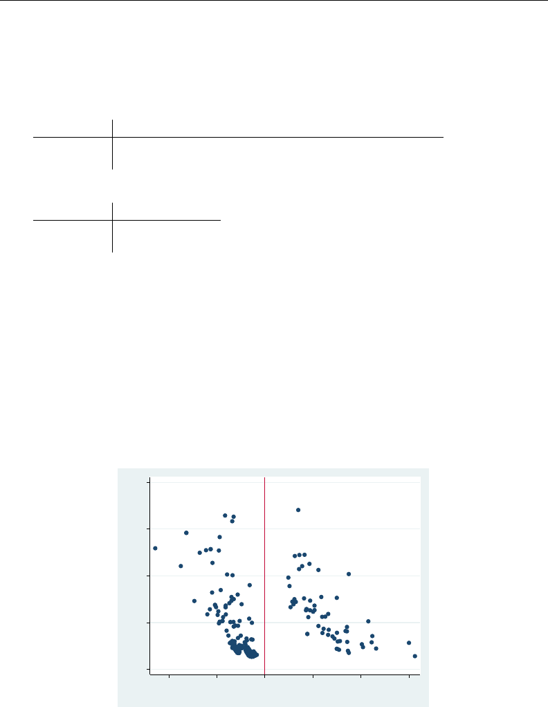
1072 logistic postestimation — Postestimation tools for logistic
predict with the rstandard option
Pearson residuals do not have a standard deviation equal to 1. rstandard generates Pearson
residuals normalized to have an expected standard deviation equal to 1.
. predict rs, rstandard
. summarize r rs
Variable Obs Mean Std. Dev. Min Max
r 189 -.0242299 .9970949 -2.283885 3.126763
rs 189 -.0279135 1.026406 -2.4478 3.149081
. correlate r rs
(obs=189)
r rs
r 1.0000
rs 0.9998 1.0000
Remember that we previously created rcontaining the (unstandardized) Pearson residuals. In these
data, whether we use standardized or unstandardized residuals does not matter much.
predict with the hat option
hat calculates the leverage of a covariate pattern—a scaled measure of distance in terms of the
independent variables. Large values indicate covariate patterns far from the average covariate pattern
that can have a large effect on the fitted model even if the corresponding residual is small. Consider
the following graph:
. predict h, hat
. scatter h r, xline(0)
0 .05 .1 .15 .2
leverage
−2 −1 0 1 2 3
Pearson residual
The points to the left of the vertical line are observed negative outcomes; here our data contain
almost as many covariate patterns as observations, so most covariate patterns are unique. In such
unique patterns, we observe either 0 or 1 success and expect p, thus forcing the sign of the residual.
If we had fewer covariate patterns—if we did not have continuous variables in our model—there
would be no such interpretation, and we would not have drawn the vertical line at 0.
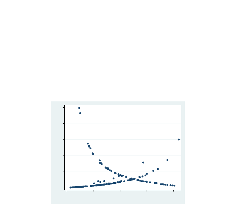
logistic postestimation — Postestimation tools for logistic 1073
Points on the left and right edges of the graph represent large residuals—covariate patterns that
are not fit well by our model. Points at the top of our graph represent high leverage patterns. When
analyzing the influence of observations on the model, we are most interested in patterns with high
leverage and small residuals — patterns that might otherwise escape our attention.
predict with the dx2 option
There are many ways to measure influence, and hat is one example. dx2 measures the decrease
in the Pearson χ2goodness-of-fit statistic that would be caused by deleting an observation (and all
others sharing the covariate pattern):
. predict dx2, dx2
. scatter dx2 p
0 2 4 6 8 10
H−L dX^2
0 .2 .4 .6 .8
Pr(low)
Paraphrasing Hosmer, Lemeshow, and Sturdivant (2013, 195–197), the points going from the top
left to the bottom right correspond to covariate patterns with the number of positive outcomes equal
to the number in the group; the points on the other curve correspond to 0 positive outcomes. In our
data, most of the covariate patterns are unique, so the points tend to lie along one or the other curves;
the points that are off the curves correspond to the few repeated covariate patterns in our data in
which all the outcomes are not the same.
We examine this graph for large values of dx2 —there are two at the top left.
predict with the ddeviance option
Another measure of influence is the change in the deviance residuals due to deletion of a covariate
pattern:
. predict dd, ddeviance
As with dx2, we typically graph ddeviance against the probability of a positive outcome. We direct
you to Hosmer, Lemeshow, and Sturdivant (2013, 195) for an example and for the interpretation of
this graph.
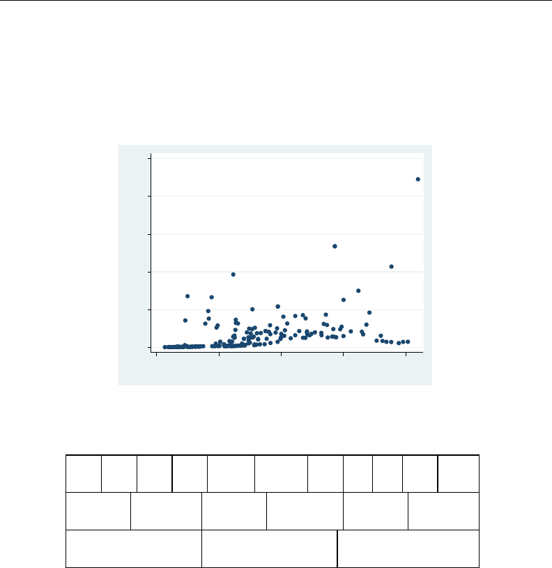
1074 logistic postestimation — Postestimation tools for logistic
predict with the dbeta option
One of the more direct measures of influence of interest to model fitters is the Pregibon (1981)
dbeta measure, a measure of the change in the coefficient vector that would be caused by deleting
an observation (and all others sharing the covariate pattern):
. predict db, dbeta
. scatter db p
0 .2 .4 .6 .8 1
Pregibon’s dbeta
0 .2 .4 .6 .8
Pr(low)
One observation has a large effect on the estimated coefficients. We can easily find this point:
. sort db
. list in l
189. id low age lwt race smoke ptl ht ui ftv bwt
188 0 25 95 white smoker 3 0 1 0 3637
p r pattern d rs h
.8391283 -2.283885 117 -1.911621 -2.4478 .1294439
dx2 dd db
5.991726 4.197658 .8909163
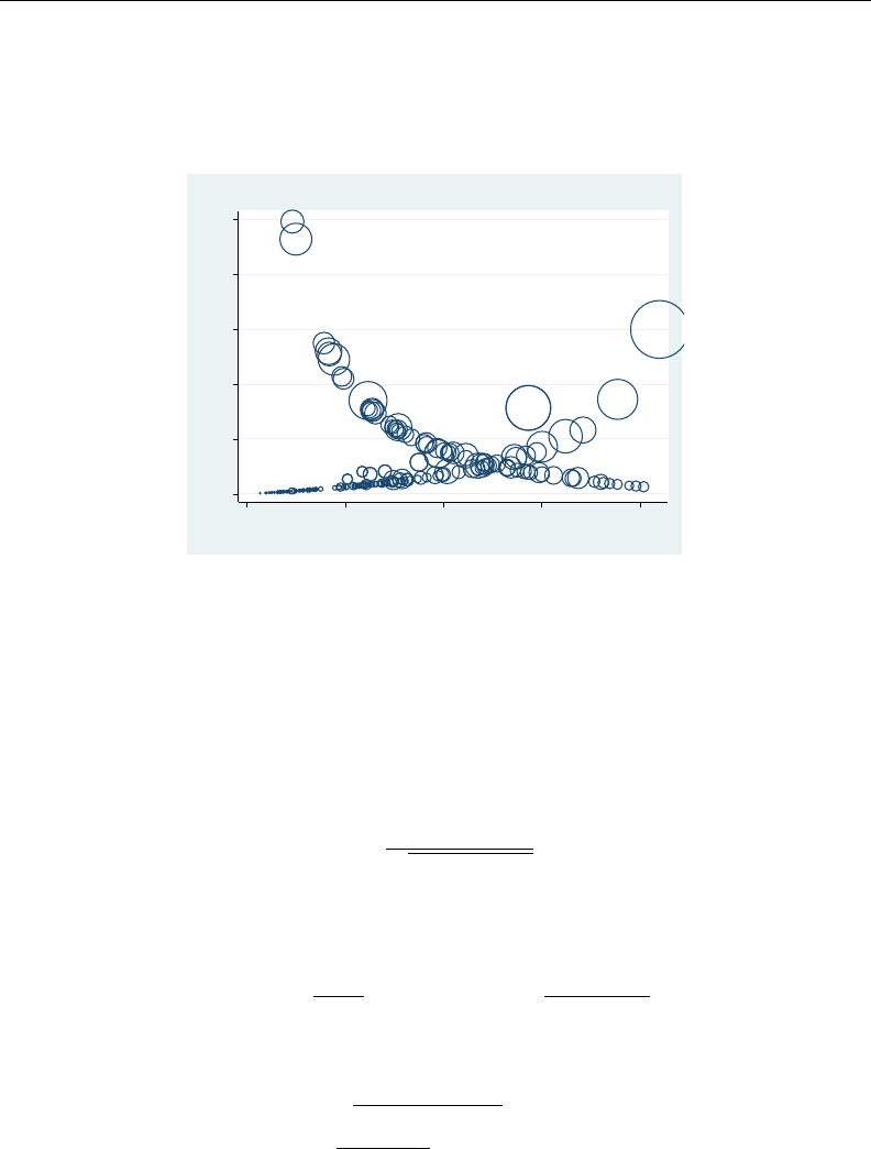
logistic postestimation — Postestimation tools for logistic 1075
Hosmer, Lemeshow, and Sturdivant (2013, 196) suggest a graph that combines two of the influence
measures:
. scatter dx2 p [w=db], title("Symbol size proportional to dBeta") mfcolor(none)
(analytic weights assumed)
(analytic weights assumed)
0 2 4 6 8 10
H−L dX^2
0 .2 .4 .6 .8
Pr(low)
Symbol size proportional to dBeta
We can easily spot the most influential points by the dbeta and dx2 measures.
Methods and formulas
Let jindex observations. Define Mjfor each observation as the total number of observations
sharing j’s covariate pattern. Define Yjas the total number of positive responses among observations
sharing j’s covariate pattern.
The Pearson residual for the jth observation is defined as
rj=Yj−Mjpj
pMjpj(1 −pj)
For Mj>1, the deviance residual djis defined as
dj=± 2"YjlnYj
Mjpj+ (Mj−Yj)lnMj−Yj
Mj(1 −pj)#!1/2
where the sign is the same as the sign of (Yj−Mjpj). In the limiting cases, the deviance residual
is given by
dj=(−p2Mj|ln(1 −pj)|if Yj= 0
p2Mj|lnpj|if Yj=Mj
The unadjusted diagonal elements of the hat matrix hUjare given by hUj= (XVX0)jj , where
Vis the estimated covariance matrix of parameters. The adjusted diagonal elements hjcreated by
hat are then hj=Mjpj(1−pj)hUj.

1076 logistic postestimation — Postestimation tools for logistic
The standardized Pearson residual rSjis rj/p1−hj.
The Pregibon (1981)∆b
βjinfluence statistic is
∆b
βj=r2
jhj
(1 −hj)2
The corresponding change in the Pearson χ2is r2
Sj. The corresponding change in the deviance residual
is ∆Dj=d2
j/(1−hj).
References
Collett, D. 2003. Modelling Survival Data in Medical Research. 2nd ed. London: Chapman & Hall/CRC.
Garrett, J. M. 2000. sg157: Predicted values calculated from linear or logistic regression models.Stata Technical
Bulletin 58: 27–30. Reprinted in Stata Technical Bulletin Reprints, vol. 10, pp. 258–261. College Station, TX:
Stata Press.
Hosmer, D. W., Jr., S. A. Lemeshow, and R. X. Sturdivant. 2013. Applied Logistic Regression. 3rd ed. Hoboken,
NJ: Wiley.
Mitchell, M. N., and X. Chen. 2005. Visualizing main effects and interactions for binary logit models.Stata Journal
5: 64–82.
Newson, R. B. 2013. Attributable and unattributable risks and fractions and other scenario comparisons.Stata Journal
13: 672–698.
Powers, D. A., H. Yoshioka, and M.-S. Yun. 2011. mvdcmp: Multivariate decomposition for nonlinear response
models.Stata Journal 11: 556–576.
Pregibon, D. 1981. Logistic regression diagnostics. Annals of Statistics 9: 705–724.
Wang, Z. 2007. Two postestimation commands for assessing confounding effects in epidemiological studies.Stata
Journal 7: 183–196.
Also see
[R]logistic — Logistic regression, reporting odds ratios
[R]estat classification — Classification statistics and table
[R]estat gof — Pearson or Hosmer–Lemeshow goodness-of-fit test
[R]lroc — Compute area under ROC curve and graph the curve
[R]lsens — Graph sensitivity and specificity versus probability cutoff
[U] 20 Estimation and postestimation commands

Title
logit — Logistic regression, reporting coefficients
Syntax Menu Description Options
Remarks and examples Stored results Methods and formulas References
Also see
Syntax
logit depvar indepvars if in weight ,options
options Description
Model
noconstant suppress constant term
offset(varname)include varname in model with coefficient constrained to 1
asis retain perfect predictor variables
constraints(constraints)apply specified linear constraints
collinear keep collinear variables
SE/Robust
vce(vcetype)vcetype may be oim,robust,cluster clustvar,bootstrap, or
jackknife
Reporting
level(#)set confidence level; default is level(95)
or report odds ratios
nocnsreport do not display constraints
display options control column formats, row spacing, line width, display of omitted
variables and base and empty cells, and factor-variable labeling
Maximization
maximize options control the maximization process; seldom used
nocoef do not display coefficient table; seldom used
coeflegend display legend instead of statistics
indepvars may contain factor variables; see [U] 11.4.3 Factor variables.
depvar and indepvars may contain time-series operators; see [U] 11.4.4 Time-series varlists.
bootstrap,by,fp,jackknife,mfp,mi estimate,nestreg,rolling,statsby,stepwise, and svy are allowed;
see [U] 11.1.10 Prefix commands.
vce(bootstrap) and vce(jackknife) are not allowed with the mi estimate prefix; see [MI] mi estimate.
Weights are not allowed with the bootstrap prefix; see [R] bootstrap.
vce(),nocoef, and weights are not allowed with the svy prefix; see [SVY] svy.
fweights, iweights, and pweights are allowed; see [U] 11.1.6 weight.
nocoef and coeflegend do not appear in the dialog box.
See [U] 20 Estimation and postestimation commands for more capabilities of estimation commands.
1077

1078 logit — Logistic regression, reporting coefficients
Menu
Statistics >Binary outcomes >Logistic regression
Description
logit fits a logit model for a binary response by maximum likelihood; it models the probability
of a positive outcome given a set of regressors. depvar equal to nonzero and nonmissing (typically
depvar equal to one) indicates a positive outcome, whereas depvar equal to zero indicates a negative
outcome.
Also see [R]logistic;logistic displays estimates as odds ratios. Many users prefer the logistic
command to logit. Results are the same regardless of which you use—both are the maximum-
likelihood estimator. Several auxiliary commands that can be run after logit,probit, or logistic
estimation are described in [R]logistic postestimation. A list of related estimation commands is given
in [R]logistic.
If estimating on grouped data, see [R]glogit.
Options
Model
noconstant,offset(varname),constraints(constraints),collinear; see [R]estimation op-
tions.
asis forces retention of perfect predictor variables and their associated perfectly predicted observations
and may produce instabilities in maximization; see [R]probit.
SE/Robust
vce(vcetype)specifies the type of standard error reported, which includes types that are derived
from asymptotic theory (oim), that are robust to some kinds of misspecification (robust), that
allow for intragroup correlation (cluster clustvar), and that use bootstrap or jackknife methods
(bootstrap,jackknife); see [R]vce option.
Reporting
level(#); see [R]estimation options.
or reports the estimated coefficients transformed to odds ratios, that is, ebrather than b. Standard errors
and confidence intervals are similarly transformed. This option affects how results are displayed,
not how they are estimated. or may be specified at estimation or when replaying previously
estimated results.
nocnsreport; see [R]estimation options.
display options:noomitted,vsquish,noemptycells,baselevels,allbaselevels,nofvla-
bel,fvwrap(#),fvwrapon(style),cformat(%fmt),pformat(% fmt),sformat(% fmt), and
nolstretch; see [R]estimation options.
Maximization
maximize options:difficult,technique(algorithm spec),iterate(#),nolog,trace,
gradient,showstep,hessian,showtolerance,tolerance(#),ltolerance(#),
nrtolerance(#),nonrtolerance, and from(init specs); see [R]maximize. These options are
seldom used.

logit — Logistic regression, reporting coefficients 1079
The following options are available with logit but are not shown in the dialog box:
nocoef specifies that the coefficient table not be displayed. This option is sometimes used by program
writers but is of no use interactively.
coeflegend; see [R]estimation options.
Remarks and examples
Remarks are presented under the following headings:
Basic usage
Model identification
Basic usage
logit fits maximum likelihood models with dichotomous dependent (left-hand-side) variables
coded as 0/1 (or, more precisely, coded as 0 and not-0).
Example 1
We have data on the make, weight, and mileage rating of 22 foreign and 52 domestic automobiles.
We wish to fit a logit model explaining whether a car is foreign on the basis of its weight and mileage.
Here is an overview of our data:
. use http://www.stata-press.com/data/r13/auto
(1978 Automobile Data)
. keep make mpg weight foreign
. describe
Contains data from http://www.stata-press.com/data/r13/auto.dta
obs: 74 1978 Automobile Data
vars: 4 13 Apr 2013 17:45
size: 1,702 (_dta has notes)
storage display value
variable name type format label variable label
make str18 %-18s Make and Model
mpg int %8.0g Mileage (mpg)
weight int %8.0gc Weight (lbs.)
foreign byte %8.0g origin Car type
Sorted by: foreign
Note: dataset has changed since last saved
. inspect foreign
foreign: Car type Number of Observations
Total Integers Nonintegers
# Negative - - -
# Zero 52 52 -
# Positive 22 22 -
#
# # Total 74 74 -
# # Missing -
0 1 74
(2 unique values)
foreign is labeled and all values are documented in the label.

1080 logit — Logistic regression, reporting coefficients
The variable foreign takes on two unique values, 0 and 1. The value 0 denotes a domestic car,
and 1 denotes a foreign car.
The model that we wish to fit is
Pr(foreign = 1) = F(β0+β1weight +β2mpg)
where F(z) = ez/(1 + ez)is the cumulative logistic distribution.
To fit this model, we type
. logit foreign weight mpg
Iteration 0: log likelihood = -45.03321
Iteration 1: log likelihood = -29.238536
Iteration 2: log likelihood = -27.244139
Iteration 3: log likelihood = -27.175277
Iteration 4: log likelihood = -27.175156
Iteration 5: log likelihood = -27.175156
Logistic regression Number of obs = 74
LR chi2(2) = 35.72
Prob > chi2 = 0.0000
Log likelihood = -27.175156 Pseudo R2 = 0.3966
foreign Coef. Std. Err. z P>|z| [95% Conf. Interval]
weight -.0039067 .0010116 -3.86 0.000 -.0058894 -.001924
mpg -.1685869 .0919175 -1.83 0.067 -.3487418 .011568
_cons 13.70837 4.518709 3.03 0.002 4.851859 22.56487
We find that heavier cars are less likely to be foreign and that cars yielding better gas mileage are
also less likely to be foreign, at least holding the weight of the car constant.
Technical note
Stata interprets a value of 0 as a negative outcome (failure) and treats all other values (except
missing) as positive outcomes (successes). Thus if your dependent variable takes on the values 0 and
1, then 0 is interpreted as failure and 1 as success. If your dependent variable takes on the values 0,
1, and 2, then 0 is still interpreted as failure, but both 1 and 2 are treated as successes.
If you prefer a more formal mathematical statement, when you type logit y x, Stata fits the
model
Pr(yj6= 0 |xj) = exp(xjβ)
1 + exp(xjβ)
Model identification
The logit command has one more feature, and it is probably the most useful. logit automatically
checks the model for identification and, if it is underidentified, drops whatever variables and observations
are necessary for estimation to proceed. (logistic,probit, and ivprobit do this as well.)

logit — Logistic regression, reporting coefficients 1081
Example 2
Have you ever fit a logit model where one or more of your independent variables perfectly predicted
one or the other outcome?
For instance, consider the following data:
Outcome yIndependent variable x
0 1
0 1
0 0
1 0
Say that we wish to predict the outcome on the basis of the independent variable. The outcome is
always zero whenever the independent variable is one. In our data, Pr(y=0|x=1) = 1, which
means that the logit coefficient on xmust be minus infinity with a corresponding infinite standard
error. At this point, you may suspect that we have a problem.
Unfortunately, not all such problems are so easily detected, especially if you have a lot of
independent variables in your model. If you have ever had such difficulties, you have experienced one
of the more unpleasant aspects of computer optimization. The computer has no idea that it is trying
to solve for an infinite coefficient as it begins its iterative process. All it knows is that at each step,
making the coefficient a little bigger, or a little smaller, works wonders. It continues on its merry
way until either 1) the whole thing comes crashing to the ground when a numerical overflow error
occurs or 2) it reaches some predetermined cutoff that stops the process. In the meantime, you have
been waiting. The estimates that you finally receive, if you receive any at all, may be nothing more
than numerical roundoff.
Stata watches for these sorts of problems, alerts us, fixes them, and properly fits the model.
Let’s return to our automobile data. Among the variables we have in the data is one called repair,
which takes on three values. A value of 1 indicates that the car has a poor repair record, 2 indicates
an average record, and 3 indicates a better-than-average record. Here is a tabulation of our data:
. use http://www.stata-press.com/data/r13/repair, clear
(1978 Automobile Data)
. tabulate foreign repair
repair
Car type 1 2 3 Total
Domestic 10 27 9 46
Foreign 0 3 9 12
Total 10 30 18 58
All the cars with poor repair records (repair =1) are domestic. If we were to attempt to predict
foreign on the basis of the repair records, the predicted probability for the repair =1 category
would have to be zero. This in turn means that the logit coefficient must be minus infinity, and that
would set most computer programs buzzing.

1082 logit — Logistic regression, reporting coefficients
Let’s try Stata on this problem.
. logit foreign b3.repair
note: 1.repair != 0 predicts failure perfectly
1.repair dropped and 10 obs not used
Iteration 0: log likelihood = -26.992087
Iteration 1: log likelihood = -22.483187
Iteration 2: log likelihood = -22.230498
Iteration 3: log likelihood = -22.229139
Iteration 4: log likelihood = -22.229138
Logistic regression Number of obs = 48
LR chi2(1) = 9.53
Prob > chi2 = 0.0020
Log likelihood = -22.229138 Pseudo R2 = 0.1765
foreign Coef. Std. Err. z P>|z| [95% Conf. Interval]
repair
1 0 (empty)
2 -2.197225 .7698003 -2.85 0.004 -3.706005 -.6884436
_cons -1.98e-16 .4714045 -0.00 1.000 -.9239359 .9239359
Remember that all the cars with poor repair records (repair =1) are domestic, so the model
cannot be fit, or at least it cannot be fit if we restrict ourselves to finite coefficients. Stata noted
that fact “note: 1.repair !=0 predicts failure perfectly”. This is Stata’s mathematically precise way of
saying what we said in English. When repair is 1, the car is domestic.
Stata then went on to say “1.repair dropped and 10 obs not used”. This is Stata eliminating
the problem. First 1.repair had to be removed from the model because it would have an infinite
coefficient. Then the 10 observations that led to the problem had to be eliminated, as well, so as
not to bias the remaining coefficients in the model. The 10 observations that are not used are the 10
domestic cars that have poor repair records.
Stata then fit what was left of the model, using the remaining observations. Because no observations
remained for cars with poor repair records, Stata reports “(empty)” in the row for repair =1.
Technical note
Stata is pretty smart about catching problems like this. It will catch “one-way causation by a
dummy variable”, as we demonstrated above.
Stata also watches for “two-way causation”, that is, a variable that perfectly determines the
outcome, both successes and failures. Here Stata says, “so-and-so predicts outcome perfectly” and
stops. Statistics dictates that no model can be fit.
Stata also checks your data for collinear variables; it will say, “so-and-so omitted because of
collinearity”. No observations need to be eliminated in this case, and model fitting will proceed
without the offending variable.
It will also catch a subtle problem that can arise with continuous data. For instance, if we were
estimating the chances of surviving the first year after an operation, and if we included in our model
age, and if all the persons over 65 died within the year, Stata would say, “age >65 predicts failure
perfectly”. It would then inform us about the fix-up it takes and fit what can be fit of our model.

logit — Logistic regression, reporting coefficients 1083
logit (and logistic,probit, and ivprobit) will also occasionally display messages such as
Note: 4 failures and 0 successes completely determined.
There are two causes for a message like this. The first—and most unlikely—case occurs when
a continuous variable (or a combination of a continuous variable with other continuous or dummy
variables) is simply a great predictor of the dependent variable. Consider Stata’s auto.dta dataset
with 6 observations removed.
. use http://www.stata-press.com/data/r13/auto
(1978 Automobile Data)
. drop if foreign==0 & gear_ratio > 3.1
(6 observations deleted)
. logit foreign mpg weight gear_ratio, nolog
Logistic regression Number of obs = 68
LR chi2(3) = 72.64
Prob > chi2 = 0.0000
Log likelihood = -6.4874814 Pseudo R2 = 0.8484
foreign Coef. Std. Err. z P>|z| [95% Conf. Interval]
mpg -.4944907 .2655508 -1.86 0.063 -1.014961 .0259792
weight -.0060919 .003101 -1.96 0.049 -.0121698 -.000014
gear_ratio 15.70509 8.166234 1.92 0.054 -.300436 31.71061
_cons -21.39527 25.41486 -0.84 0.400 -71.20747 28.41694
Note: 4 failures and 0 successes completely determined.
There are no missing standard errors in the output. If you receive the “completely determined” message
and have one or more missing standard errors in your output, see the second case discussed below.
Note gear ratio’s large coefficient. logit thought that the 4 observations with the smallest
predicted probabilities were essentially predicted perfectly.
. predict p
(option pr assumed; Pr(foreign))
. sort p
. list p in 1/4
p
1. 1.34e-10
2. 6.26e-09
3. 7.84e-09
4. 1.49e-08
If this happens to you, you do not have to do anything. Computationally, the model is sound. The
second case discussed below requires careful examination.
The second case occurs when the independent terms are all dummy variables or continuous ones
with repeated values (for example, age). Here one or more of the estimated coefficients will have
missing standard errors. For example, consider this dataset consisting of 5 observations.

1084 logit — Logistic regression, reporting coefficients
. use http://www.stata-press.com/data/r13/logitxmpl, clear
. list, separator(0)
y x1 x2
1. 0 0 0
2. 0 0 0
3. 0 1 0
4. 1 1 0
5. 0 0 1
6. 1 0 1
. logit y x1 x2
Iteration 0: log likelihood = -3.819085
Iteration 1: log likelihood = -2.9527336
Iteration 2: log likelihood = -2.8110282
Iteration 3: log likelihood = -2.7811973
Iteration 4: log likelihood = -2.7746107
Iteration 5: log likelihood = -2.7730128
(output omitted )
Iteration 15996: log likelihood = -2.7725887 (not concave)
Iteration 15997: log likelihood = -2.7725887 (not concave)
Iteration 15998: log likelihood = -2.7725887 (not concave)
Iteration 15999: log likelihood = -2.7725887 (not concave)
Iteration 16000: log likelihood = -2.7725887 (not concave)
convergence not achieved
Logistic regression Number of obs = 6
LR chi2(1) = 2.09
Prob > chi2 = 0.1480
Log likelihood = -2.7725887 Pseudo R2 = 0.2740
y Coef. Std. Err. z P>|z| [95% Conf. Interval]
x1 18.3704 2 9.19 0.000 14.45047 22.29033
x2 18.3704 . . . . .
_cons -18.3704 1.414214 -12.99 0.000 -21.14221 -15.5986
Note: 2 failures and 0 successes completely determined.
convergence not achieved
r(430);
Three things are happening here. First, logit iterates almost forever and then declares nonconver-
gence. Second, logit can fit the outcome (y= 0) for the covariate pattern x1 =0 and x2 =0 (that
is, the first two observations) perfectly. This observation is the “2 failures and 0 successes completely
determined”. Third, if this observation is dropped, then x1,x2, and the constant are collinear.
This is the cause of the nonconvergence, the message “completely determined”, and the missing
standard errors. It happens when you have a covariate pattern (or patterns) with only one outcome
and there is collinearity when the observations corresponding to this covariate pattern are dropped.
If this happens to you, confirm the causes. First, identify the covariate pattern with only one
outcome. (For your data, replace x1 and x2 with the independent variables of your model.)

logit — Logistic regression, reporting coefficients 1085
. egen pattern = group(x1 x2)
. quietly logit y x1 x2, iterate(100)
. predict p
(option pr assumed; Pr(y))
. summarize p
Variable Obs Mean Std. Dev. Min Max
p 6 .3333333 .2581989 1.05e-08 .5
If successes were completely determined, that means that there are predicted probabilities that are
almost 1. If failures were completely determined, that means that there are predicted probabilities
that are almost 0. The latter is the case here, so we locate the corresponding value of pattern:
. tabulate pattern if p < 1e-7
group(x1
x2) Freq. Percent Cum.
1 2 100.00 100.00
Total 2 100.00
Once we omit this covariate pattern from the estimation sample, logit can deal with the collinearity:
. logit y x1 x2 if pattern != 1, nolog
note: x2 omitted because of collinearity
Logistic regression Number of obs = 4
LR chi2(1) = 0.00
Prob > chi2 = 1.0000
Log likelihood = -2.7725887 Pseudo R2 = 0.0000
y Coef. Std. Err. z P>|z| [95% Conf. Interval]
x1 0 2 0.00 1.000 -3.919928 3.919928
x2 0 (omitted)
_cons 0 1.414214 0.00 1.000 -2.771808 2.771808
We omit the collinear variable. Then we must decide whether to include or omit the observations
with pattern =1. We could include them,
. logit y x1, nolog
Logistic regression Number of obs = 6
LR chi2(1) = 0.37
Prob > chi2 = 0.5447
Log likelihood = -3.6356349 Pseudo R2 = 0.0480
y Coef. Std. Err. z P>|z| [95% Conf. Interval]
x1 1.098612 1.825742 0.60 0.547 -2.479776 4.677001
_cons -1.098612 1.154701 -0.95 0.341 -3.361784 1.164559

1086 logit — Logistic regression, reporting coefficients
or exclude them,
. logit y x1 if pattern != 1, nolog
Logistic regression Number of obs = 4
LR chi2(1) = 0.00
Prob > chi2 = 1.0000
Log likelihood = -2.7725887 Pseudo R2 = 0.0000
y Coef. Std. Err. z P>|z| [95% Conf. Interval]
x1 0 2 0.00 1.000 -3.919928 3.919928
_cons 0 1.414214 0.00 1.000 -2.771808 2.771808
If the covariate pattern that predicts outcome perfectly is meaningful, you may want to exclude these
observations from the model. Here you would report that covariate pattern such and such predicted
outcome perfectly and that the best model for the rest of the data is . . . . But, more likely, the perfect
prediction was simply the result of having too many predictors in the model. Then you would omit
the extraneous variables from further consideration and report the best model for all the data.
Stored results
logit stores the following in e():
Scalars
e(N) number of observations
e(N cds) number of completely determined successes
e(N cdf) number of completely determined failures
e(k) number of parameters
e(k eq) number of equations in e(b)
e(k eq model) number of equations in overall model test
e(k dv) number of dependent variables
e(df m) model degrees of freedom
e(r2 p) pseudo-R-squared
e(ll) log likelihood
e(ll 0) log likelihood, constant-only model
e(N clust) number of clusters
e(chi2) χ2
e(p) significance of model test
e(rank) rank of e(V)
e(ic) number of iterations
e(rc) return code
e(converged) 1 if converged, 0otherwise

logit — Logistic regression, reporting coefficients 1087
Macros
e(cmd) logit
e(cmdline) command as typed
e(depvar) name of dependent variable
e(wtype) weight type
e(wexp) weight expression
e(title) title in estimation output
e(clustvar) name of cluster variable
e(offset) linear offset variable
e(chi2type) Wald or LR; type of model χ2test
e(vce) vcetype specified in vce()
e(vcetype) title used to label Std. Err.
e(opt) type of optimization
e(which) max or min; whether optimizer is to perform maximization or minimization
e(ml method) type of ml method
e(user) name of likelihood-evaluator program
e(technique) maximization technique
e(properties) b V
e(estat cmd) program used to implement estat
e(predict) program used to implement predict
e(marginsnotok) predictions disallowed by margins
e(asbalanced) factor variables fvset as asbalanced
e(asobserved) factor variables fvset as asobserved
Matrices
e(b) coefficient vector
e(Cns) constraints matrix
e(ilog) iteration log (up to 20 iterations)
e(gradient) gradient vector
e(mns) vector of means of the independent variables
e(rules) information about perfect predictors
e(V) variance–covariance matrix of the estimators
e(V modelbased) model-based variance
Functions
e(sample) marks estimation sample
Methods and formulas
Cramer (2003, chap. 9) surveys the prehistory and history of the logit model. The word “logit”
was coined by Berkson (1944) and is analogous to the word “probit”. For an introduction to probit
and logit, see, for example, Aldrich and Nelson (1984), Cameron and Trivedi (2010), Greene (2012),
Jones (2007), Long (1997), Long and Freese (2014), Pampel (2000), or Powers and Xie (2008).
The likelihood function for logit is
lnL=X
j∈S
wjlnF(xjb) + X
j6∈S
wjln1−F(xjb)

1088 logit — Logistic regression, reporting coefficients
where Sis the set of all observations j, such that yj6= 0,F(z) = ez/(1+ez), and wjdenotes the
optional weights. lnLis maximized as described in [R]maximize.
This command supports the Huber/White/sandwich estimator of the variance and its clustered version
using vce(robust) and vce(cluster clustvar), respectively. See [P]robust, particularly Maximum
likelihood estimators and Methods and formulas. The scores are calculated as uj={1−F(xjb)}xj
for the positive outcomes and −F(xjb)xjfor the negative outcomes.
logit also supports estimation with survey data. For details on VCEs with survey data, see
[SVY]variance estimation.
Joseph Berkson (1899–1982) was born in New York City and studied at the College of the City
of New York, Columbia, and Johns Hopkins, earning both an MD and a doctorate in statistics.
He then worked at Johns Hopkins before moving to the Mayo Clinic in 1931 as a biostatistician.
Among many other contributions, his most influential one drew upon a long-sustained interest
in the logistic function, especially his 1944 paper on bioassay, in which he introduced the term
“logit”. Berkson was a frequent participant in controversy—sometimes humorous, sometimes
bitter—on subjects such as the evidence for links between smoking and various diseases and the
relative merits of probit and logit methods and of different calculation methods.
References
Aldrich, J. H., and F. D. Nelson. 1984. Linear Probability, Logit, and Probit Models. Newbury Park, CA: Sage.
Archer, K. J., and S. A. Lemeshow. 2006. Goodness-of-fit test for a logistic regression model fitted using survey
sample data.Stata Journal 6: 97–105.
Berkson, J. 1944. Application of the logistic function to bio-assay. Journal of the American Statistical Association
39: 357–365.
Buis, M. L. 2010a. Direct and indirect effects in a logit model.Stata Journal 10: 11–29.
. 2010b. Stata tip 87: Interpretation of interactions in nonlinear models.Stata Journal 10: 305–308.
Cameron, A. C., and P. K. Trivedi. 2010. Microeconometrics Using Stata. Rev. ed. College Station, TX: Stata Press.
Cleves, M. A., and A. Tosetto. 2000. sg139: Logistic regression when binary outcome is measured with uncertainty.
Stata Technical Bulletin 55: 20–23. Reprinted in Stata Technical Bulletin Reprints, vol. 10, pp. 152–156. College
Station, TX: Stata Press.
Cramer, J. S. 2003. Logit Models from Economics and Other Fields. Cambridge: Cambridge University Press.
Greene, W. H. 2012. Econometric Analysis. 7th ed. Upper Saddle River, NJ: Prentice Hall.
Hilbe, J. M. 2009. Logistic Regression Models. Boca Raton, FL: Chapman & Hill/CRC.
Hosmer, D. W., Jr., S. A. Lemeshow, and R. X. Sturdivant. 2013. Applied Logistic Regression. 3rd ed. Hoboken,
NJ: Wiley.
Jones, A. 2007. Applied Econometrics for Health Economists: A Practical Guide. 2nd ed. Abingdon, UK: Radcliffe.
Judge, G. G., W. E. Griffiths, R. C. Hill, H. L¨
utkepohl, and T.-C. Lee. 1985. The Theory and Practice of Econometrics.
2nd ed. New York: Wiley.
Long, J. S. 1997. Regression Models for Categorical and Limited Dependent Variables. Thousand Oaks, CA: Sage.
Long, J. S., and J. Freese. 2014. Regression Models for Categorical Dependent Variables Using Stata. 3rd ed. College
Station, TX: Stata Press.
Miranda, A., and S. Rabe-Hesketh. 2006. Maximum likelihood estimation of endogenous switching and sample
selection models for binary, ordinal, and count variables.Stata Journal 6: 285–308.
Mitchell, M. N., and X. Chen. 2005. Visualizing main effects and interactions for binary logit models.Stata Journal
5: 64–82.

logit — Logistic regression, reporting coefficients 1089
O’Fallon, W. M. 1998. Berkson, Joseph. In Vol. 1 of Encyclopedia of Biostatistics, ed. P. Armitage and T. Colton,
290–295. Chichester, UK: Wiley.
Orsini, N., R. Bellocco, and P. C. Sj¨
olander. 2013. Doubly robust estimation in generalized linear models.Stata
Journal 13: 185–205.
Pampel, F. C. 2000. Logistic Regression: A Primer. Thousand Oaks, CA: Sage.
Powers, D. A., and Y. Xie. 2008. Statistical Methods for Categorical Data Analysis. 2nd ed. Bingley, UK: Emerald.
Pregibon, D. 1981. Logistic regression diagnostics. Annals of Statistics 9: 705–724.
Schonlau, M. 2005. Boosted regression (boosting): An introductory tutorial and a Stata plugin.Stata Journal 5:
330–354.
Xu, J., and J. S. Long. 2005. Confidence intervals for predicted outcomes in regression models for categorical
outcomes.Stata Journal 5: 537–559.
Also see
[R]logit postestimation — Postestimation tools for logit
[R]brier — Brier score decomposition
[R]cloglog — Complementary log-log regression
[R]exlogistic — Exact logistic regression
[R]glogit — Logit and probit regression for grouped data
[R]logistic — Logistic regression, reporting odds ratios
[R]probit — Probit regression
[R]roc — Receiver operating characteristic (ROC) analysis
[ME]melogit — Multilevel mixed-effects logistic regression
[MI]estimation — Estimation commands for use with mi estimate
[SVY]svy estimation — Estimation commands for survey data
[XT]xtlogit — Fixed-effects, random-effects, and population-averaged logit models
[U] 20 Estimation and postestimation commands

Title
logit postestimation — Postestimation tools for logit
Description Syntax for predict Menu for predict Options for predict
Remarks and examples Methods and formulas References Also see
Description
The following postestimation commands are of special interest after logit:
Command Description
estat classification report various summary statistics, including the classification table
estat gof Pearson or Hosmer–Lemeshow goodness-of-fit test
lroc compute area under ROC curve and graph the curve
lsens graph sensitivity and specificity versus probability cutoff
These commands are not appropriate after the svy prefix.
The following standard postestimation commands are also available:
Command Description
contrast contrasts and ANOVA-style joint tests of estimates
estat ic Akaike’s and Schwarz’s Bayesian information criteria (AIC and BIC)
estat summarize summary statistics for the estimation sample
estat vce variance–covariance matrix of the estimators (VCE)
estat (svy) postestimation statistics for survey data
estimates cataloging estimation results
forecast1dynamic forecasts and simulations
lincom point estimates, standard errors, testing, and inference for linear combinations
of coefficients
linktest link test for model specification
lrtest2likelihood-ratio test
margins marginal means, predictive margins, marginal effects, and average marginal
effects
marginsplot graph the results from margins (profile plots, interaction plots, etc.)
nlcom point estimates, standard errors, testing, and inference for nonlinear combinations
of coefficients
predict predictions, residuals, influence statistics, and other diagnostic measures
predictnl point estimates, standard errors, testing, and inference for generalized predictions
pwcompare pairwise comparisons of estimates
suest seemingly unrelated estimation
test Wald tests of simple and composite linear hypotheses
testnl Wald tests of nonlinear hypotheses
1forecast is not appropriate with mi or svy estimation results.
2lrtest is not appropriate with svy estimation results.
1090

logit postestimation — Postestimation tools for logit 1091
Syntax for predict
predict type newvar if in ,statistic nooffset rules asif
statistic Description
Main
pr probability of a positive outcome; the default
xb linear prediction
stdp standard error of the prediction
∗dbeta Pregibon (1981)∆b
βinfluence statistic
∗deviance deviance residual
∗dx2 Hosmer, Lemeshow, and Sturdivant (2013)∆χ2influence statistic
∗ddeviance Hosmer, Lemeshow, and Sturdivant (2013)∆Dinfluence statistic
∗hat Pregibon (1981) leverage
∗number sequential number of the covariate pattern
∗residuals Pearson residuals; adjusted for number sharing covariate pattern
∗rstandard standardized Pearson residuals; adjusted for number sharing covariate pattern
score first derivative of the log likelihood with respect to xjβ
Unstarred statistics are available both in and out of sample; type predict . . . if e(sample) . . . if wanted only for
the estimation sample. Starred statistics are calculated only for the estimation sample, even when if e(sample)
is not specified.
pr,xb,stdp, and score are the only options allowed with svy estimation results.
Menu for predict
Statistics >Postestimation >Predictions, residuals, etc.
Options for predict
Main
pr, the default, calculates the probability of a positive outcome.
xb calculates the linear prediction.
stdp calculates the standard error of the linear prediction.
dbeta calculates the Pregibon (1981)∆b
βinfluence statistic, a standardized measure of the difference
in the coefficient vector that is due to deletion of the observation along with all others that share
the same covariate pattern. In Hosmer, Lemeshow, and Sturdivant (2013, 154–155) jargon, this
statistic is M-asymptotic; that is, it is adjusted for the number of observations that share the same
covariate pattern.
deviance calculates the deviance residual.
dx2 calculates the Hosmer, Lemeshow, and Sturdivant (2013, 191) ∆χ2influence statistic, reflecting
the decrease in the Pearson χ2that is due to deletion of the observation and all others that share
the same covariate pattern.
ddeviance calculates the Hosmer, Lemeshow, and Sturdivant (2013, 191) ∆Dinfluence statistic,
which is the change in the deviance residual that is due to deletion of the observation and all
others that share the same covariate pattern.

1092 logit postestimation — Postestimation tools for logit
hat calculates the Pregibon (1981) leverage or the diagonal elements of the hat matrix adjusted for
the number of observations that share the same covariate pattern.
number numbers the covariate patterns — observations with the same covariate pattern have the same
number. Observations not used in estimation have number set to missing. The first covariate
pattern is numbered 1, the second 2, and so on.
residuals calculates the Pearson residual as given by Hosmer, Lemeshow, and Sturdivant (2013,
155) and adjusted for the number of observations that share the same covariate pattern.
rstandard calculates the standardized Pearson residual as given by Hosmer, Lemeshow, and Stur-
divant (2013, 191) and adjusted for the number of observations that share the same covariate
pattern.
score calculates the equation-level score, ∂ln L/∂(xjβ).
Options
nooffset is relevant only if you specified offset(varname)for logit. It modifies the calculations
made by predict so that they ignore the offset variable; the linear prediction is treated as xjb
rather than as xjb+offsetj.
rules requests that Stata use any rules that were used to identify the model when making the
prediction. By default, Stata calculates missing for excluded observations.
asif requests that Stata ignore the rules and exclusion criteria and calculate predictions for all
observations possible by using the estimated parameter from the model.
Remarks and examples
Once you have fit a logit model, you can obtain the predicted probabilities by using the predict
command for both the estimation sample and other samples; see [U] 20 Estimation and postestimation
commands and [R]predict. Here we will make only a few more comments.
predict without arguments calculates the predicted probability of a positive outcome, that is,
Pr(yj= 1) = F(xjb). With the xb option, predict calculates the linear combination xjb, where
xjare the independent variables in the jth observation and bis the estimated parameter vector. This
is sometimes known as the index function because the cumulative distribution function indexed at
this value is the probability of a positive outcome.
In both cases, Stata remembers any rules used to identify the model and calculates missing for
excluded observations, unless rules or asif is specified. For information about the other statistics
available after predict, see [R]logistic postestimation.
Example 1: Predicted probabilities
In example 2 of [R]logit, we fit the logit model logit foreign b3.repair. To obtain predicted
probabilities, type
. use http://www.stata-press.com/data/r13/repair
(1978 Automobile Data)
. logit foreign b3.repair
note: 1.repair != 0 predicts failure perfectly
1.repair dropped and 10 obs not used
(output omitted )
. predict p
(option pr assumed; Pr(foreign))
(10 missing values generated)

logit postestimation — Postestimation tools for logit 1093
. summarize foreign p
Variable Obs Mean Std. Dev. Min Max
foreign 58 .2068966 .4086186 0 1
p 48 .25 .1956984 .1 .5
Stata remembers any rules used to identify the model and sets predictions to missing for any excluded
observations. logit dropped the variable 1.repair from our model and excluded 10 observations.
Thus when we typed predict p, those same 10 observations were again excluded, and their predictions
were set to missing.
predict’s rules option uses the rules in the prediction. During estimation, we were told “1.repair
!= 0 predicts failure perfectly”, so the rule is that when 1.repair is not zero, we should predict 0
probability of success or a positive outcome:
. predict p2, rules
(option pr assumed; Pr(foreign))
. summarize foreign p p2
Variable Obs Mean Std. Dev. Min Max
foreign 58 .2068966 .4086186 0 1
p 48 .25 .1956984 .1 .5
p2 58 .2068966 .2016268 0 .5
predict’s asif option ignores the rules and exclusion criteria and calculates predictions for all
observations possible by using the estimated parameters from the model:
. predict p3, asif
(option pr assumed; Pr(foreign))
. summarize foreign p p2 p3
Variable Obs Mean Std. Dev. Min Max
foreign 58 .2068966 .4086186 0 1
p 48 .25 .1956984 .1 .5
p2 58 .2068966 .2016268 0 .5
p3 58 .2931035 .2016268 .1 .5
Which is right? What predict does by default is the most conservative approach. If many
observations had been excluded because of a simple rule, we could be reasonably certain that the
rules prediction is correct. The asif prediction is correct only if the exclusion is a fluke, and we
would be willing to exclude the variable from the analysis anyway. Then, however, we would refit
the model to include the excluded observations.
Example 2: Predictive margins
We can use the command margins, contrast after logit to make comparisons on the probability
scale. Let’s fit a model predicting low birthweight from characteristics of the mother:
. use http://www.stata-press.com/data/r13/lbw, clear
(Hosmer & Lemeshow data)

1094 logit postestimation — Postestimation tools for logit
. logit low age i.race i.smoke ptl i.ht i.ui
Iteration 0: log likelihood = -117.336
Iteration 1: log likelihood = -103.81846
Iteration 2: log likelihood = -103.40486
Iteration 3: log likelihood = -103.40384
Iteration 4: log likelihood = -103.40384
Logistic regression Number of obs = 189
LR chi2(7) = 27.86
Prob > chi2 = 0.0002
Log likelihood = -103.40384 Pseudo R2 = 0.1187
low Coef. Std. Err. z P>|z| [95% Conf. Interval]
age -.0403293 .0357127 -1.13 0.259 -.1103249 .0296663
race
black 1.009436 .5025122 2.01 0.045 .0245302 1.994342
other 1.001908 .4248342 2.36 0.018 .1692485 1.834568
smoke
smoker .9631876 .3904357 2.47 0.014 .1979477 1.728427
ptl .6288678 .3399067 1.85 0.064 -.0373371 1.295073
1.ht 1.358142 .6289555 2.16 0.031 .125412 2.590872
1.ui .8001832 .4572306 1.75 0.080 -.0959724 1.696339
_cons -1.184127 .9187461 -1.29 0.197 -2.984837 .6165818
The coefficients are log odds-ratios: conditional on the other predictors, smoking during pregnancy
is associated with an increase of 0.96 in the log odds-ratios of low birthweight. The model is linear
in the log odds-scale, so the estimate of 0.96 has the same interpretation, whatever the values of
the other predictors might be. We could convert 0.96 to an odds ratio by replaying the results with
logit, or.
But what if we want to talk about the probability of low birthweight, and not the odds? Then
we will need the command margins, contrast. We will use the r. contrast operator to compare
each level of smoke with a reference level. (smoke has only two levels, so there will be only one
comparison: a comparison of smokers with nonsmokers.)
. margins r.smoke, contrast
Contrasts of predictive margins
Model VCE : OIM
Expression : Pr(low), predict()
df chi2 P>chi2
smoke 1 6.32 0.0119
Delta-method
Contrast Std. Err. [95% Conf. Interval]
smoke
(smoker vs nonsmoker) .1832779 .0728814 .0404329 .3261229
We see that maternal smoking is associated with an 18.3% increase in the probability of low
birthweight. (We received a contrast in the probability scale because predicted probabilities are the
default when margins is used after logit.)

logit postestimation — Postestimation tools for logit 1095
The contrast of 18.3% is a difference of margins that are computed by averaging over the predictions
for observations in the estimation sample. If the values of the other predictors were different, the
contrast for smoke would be different, too. Let’s estimate the contrast for 25-year-old mothers:
. margins r.smoke, contrast at(age=25)
Contrasts of predictive margins
Model VCE : OIM
Expression : Pr(low), predict()
at : age = 25
df chi2 P>chi2
smoke 1 6.19 0.0129
Delta-method
Contrast Std. Err. [95% Conf. Interval]
smoke
(smoker vs nonsmoker) .1808089 .0726777 .0383632 .3232547
Specifying a maternal age of 25 changed the contrast to 18.1%. Our contrast of probabilities
changed because the logit model is nonlinear in the probability scale. A contrast of log odds-ratios
would not have changed.
Methods and formulas
See Methods and formulas of the individual postestimation commands for details.
References
Hosmer, D. W., Jr., S. A. Lemeshow, and R. X. Sturdivant. 2013. Applied Logistic Regression. 3rd ed. Hoboken,
NJ: Wiley.
Newson, R. B. 2013. Attributable and unattributable risks and fractions and other scenario comparisons.Stata Journal
13: 672–698.
Powers, D. A., H. Yoshioka, and M.-S. Yun. 2011. mvdcmp: Multivariate decomposition for nonlinear response
models.Stata Journal 11: 556–576.
Pregibon, D. 1981. Logistic regression diagnostics. Annals of Statistics 9: 705–724.
Also see
[R]logit — Logistic regression, reporting coefficients
[R]estat classification — Classification statistics and table
[R]estat gof — Pearson or Hosmer–Lemeshow goodness-of-fit test
[R]lroc — Compute area under ROC curve and graph the curve
[R]lsens — Graph sensitivity and specificity versus probability cutoff
[U] 20 Estimation and postestimation commands

Title
loneway — Large one-way ANOVA, random effects, and reliability
Syntax Menu Description Options
Remarks and examples Stored results Methods and formulas Acknowledgment
References Also see
Syntax
loneway response var group var if in weight ,options
options Description
Main
mean expected value of Fdistribution; default is 1
median median of Fdistribution; default is 1
exact exact confidence intervals (groups must be equal with no weights)
level(#)set confidence level; default is level(95)
by is allowed; see [D] by.
aweights are allowed; see [U] 11.1.6 weight.
Menu
Statistics >Linear models and related >ANOVA/MANOVA >Large one-way ANOVA
Description
loneway fits one-way analysis-of-variance (ANOVA) models on datasets with many levels of
group var and presents different ancillary statistics from oneway (see [R]oneway):
Feature oneway loneway
Fit one-way model x x
on fewer than 376 levels x x
on more than 376 levels x
Bartlett’s test for equal variance x
Multiple-comparison tests x
Intragroup correlation and SE x
Intragroup correlation confidence interval x
Est. reliability of group-averaged score x
Est. SD of group effect x
Est. SD within group x
Options
Main
mean specifies that the expected value of the Fk−1,N −kdistribution be used as the reference point
Fmin the estimation of ρinstead of the default value of 1.
1096

loneway — Large one-way ANOVA, random effects, and reliability 1097
median specifies that the median of the Fk−1,N−kdistribution be used as the reference point Fmin
the estimation of ρinstead of the default value of 1.
exact requests that exact confidence intervals be computed, as opposed to the default asymptotic
confidence intervals. This option is allowed only if the groups are equal in size and weights are
not used.
level(#)specifies the confidence level, as a percentage, for confidence intervals of the coefficients.
The default is level(95) or as set by set level; see [U] 20.7 Specifying the width of confidence
intervals.
Remarks and examples
Remarks are presented under the following headings:
The one-way ANOVA model
R-squared
The random-effects ANOVA model
Intraclass correlation
Estimated reliability of the group-averaged score
The one-way ANOVA model
Example 1
loneway’s output looks like that of oneway, except that loneway presents more information at the
end. Using our automobile dataset, we have created a (numeric) variable called manufacturer grp
identifying the manufacturer of each car, and within each manufacturer we have retained a maximum
of four models, selecting those with the lowest mpg. We can compute the intraclass correlation of
mpg for all manufacturers with at least four models as follows:
. use http://www.stata-press.com/data/r13/auto7
(1978 Automobile Data)
. loneway mpg manufacturer_grp if nummake == 4
One-way Analysis of Variance for mpg: Mileage (mpg)
Number of obs = 36
R-squared = 0.5228
Source SS df MS F Prob > F
Between manufactur~p 621.88889 8 77.736111 3.70 0.0049
Within manufactur~p 567.75 27 21.027778
Total 1189.6389 35 33.989683
Intraclass Asy.
correlation S.E. [95% Conf. Interval]
0.40270 0.18770 0.03481 0.77060
Estimated SD of manufactur~p effect 3.765247
Estimated SD within manufactur~p 4.585605
Est. reliability of a manufactur~p mean 0.72950
(evaluated at n=4.00)
In addition to the standard one-way ANOVA output, loneway produces the R-squared, the estimated
standard deviation of the group effect, the estimated standard deviation within group, the intragroup
correlation, the estimated reliability of the group-averaged mean, and, for unweighted data, the
asymptotic standard error and confidence interval for the intragroup correlation.

1098 loneway — Large one-way ANOVA, random effects, and reliability
R-squared
The R-squared is, of course, simply the underlying R2for a regression of response var on the
levels of group var, or mpg on the various manufacturers here.
The random-effects ANOVA model
loneway assumes that we observe a variable, yij , measured for nielements within kgroups or
classes such that
yij =µ+αi+ij , i = 1,2, . . . , k, j = 1,2, . . . , ni
and αiand ij are independent zero-mean random variables with variance σ2
αand σ2
, respectively.
This is the random-effects ANOVA model, also known as the components-of-variance model, in which
it is typically assumed that the yij are normally distributed.
The interpretation with respect to our example is that the observed value of our response variable,
mpg, is created in two steps. First, the ith manufacturer is chosen, and a value, αi, is determined —the
typical mpg for that manufacturer less the overall mpg µ. Then a deviation, ij , is chosen for the jth
model within this manufacturer. This is how much that particular automobile differs from the typical
mpg value for models from this manufacturer.
For our sample of 36 car models, the estimated standard deviations are σα=3.8 and σ=4.6.
Thus a little more than half of the variation in mpg between cars is attributable to the car model,
with the rest attributable to differences between manufacturers. These standard deviations differ from
those that would be produced by a (standard) fixed-effects regression in that the regression would
require the sum within each manufacturer of the ij ,i. for the ith manufacturer, to be zero, whereas
these estimates merely impose the constraint that the sum is expected to be zero.
Intraclass correlation
There are various estimators of the intraclass correlation, such as the pairwise estimator, which is
defined as the Pearson product-moment correlation computed over all possible pairs of observations
that can be constructed within groups. For a discussion of various estimators, see Donner (1986).
loneway computes what is termed the analysis of variance, or ANOVA, estimator. This intraclass
correlation is the theoretical upper bound on the variation in response var that is explainable by
group var, of which R-squared is an overestimate because of the serendipity of fitting. This correlation
is comparable to an R-squared—you do not have to square it.
In our example, the intra-manu correlation, the correlation of mpg within manufacturer, is 0.40.
Because aweights were not used and the default correlation was computed (that is, the mean and
median options were not specified), loneway also provided the asymptotic confidence interval and
standard error of the intraclass correlation estimate.
Estimated reliability of the group-averaged score
The estimated reliability of the group-averaged score or mean has an interpretation similar to that
of the intragroup correlation; it is a comparable number if we average response var by group var,
or mpg by manu in our example. It is the theoretical upper bound of a regression of manufacturer-
averaged mpg on characteristics of manufacturers. Why would we want to collapse our 36-observation
dataset into a 9-observation dataset of manufacturer averages? Because the 36 observations might be
a mirage. When General Motors builds cars, do they sometimes put a Pontiac label and sometimes
a Chevrolet label on them, so that it appears in our data as if we have two cars when we really have

loneway — Large one-way ANOVA, random effects, and reliability 1099
only one, replicated? If that were the case, and if it were the case for many other manufacturers,
then we would be forced to admit that we do not have data on 36 cars; we instead have data on nine
manufacturer-averaged characteristics.
Stored results
loneway stores the following in r():
Scalars
r(N) number of observations r(rho t) estimated reliability
r(rho) intraclass correlation r(se) asymp. SE of intraclass correlation
r(lb) lower bound of 95% CI for rho r(sd w) estimated SD within group
r(ub) upper bound of 95% CI for rho r(sd b) estimated SD of group effect
Methods and formulas
The mean squares in the loneway’s ANOVA table are computed as
MSα=X
i
wi·(yi·−y··)2/(k−1)
and
MS=X
iX
j
wij (yij −yi·)2/(N−k)
in which
wi·=X
j
wij w·· =X
i
wi·yi·=X
j
wij yij /wi·and y.. =X
i
wi·yi·/w··
The corresponding expected values of these mean squares are
E(MSα) = σ2
+gσ2
αand E(MS) = σ2
in which
g=w·· −Piw2
i·/w··
k−1
In the unweighted case, we get
g=N−Pin2
i/N
k−1
As expected, g=mfor the case of no weights and equal group sizes in the data, that is, ni=mfor
all i. Replacing the expected values with the observed values and solving yields the ANOVA estimates
of σ2
αand σ2
. Substituting these into the definition of the intraclass correlation
ρ=σ2
α
σ2
α+σ2
yields the ANOVA estimator of the intraclass correlation:
ρA=Fobs −1
Fobs −1 + g

1100 loneway — Large one-way ANOVA, random effects, and reliability
Fobs is the observed value of the Fstatistic from the ANOVA table. For no weights and equal ni,ρA
=roh, which is the intragroup correlation defined by Kish (1965). Two slightly different estimators
are available through the mean and median options (Gleason 1997). If either of these options is
specified, the estimate of ρbecomes
ρ=Fobs −Fm
Fobs + (g−1)Fm
For the mean option, Fm=E(Fk−1,N−K) = (N−k)/(N−k−2), that is, the expected value of the
ANOVA table’s Fstatistic. For the median option, Fmis simply the median of the Fstatistic. Setting
Fmto 1 gives ρA, so for large samples, these different point estimators are essentially the same.
Also, because the intraclass correlation of the random-effects model is by definition nonnegative, for
any of the three possible point estimators, ρis truncated to zero if Fobs is less than Fm.
For no weighting, interval estimators for ρAare computed. If the groups are equal sized (all ni
equal) and the exact option is specified, the following exact (assuming that the yij are normally
distributed) 100(1−α)% confidence interval is computed:
Fobs −FmFu
Fobs + (g−1)FmFu
,Fobs −FmFl
Fobs + (g−1)FmFl
with Fm=1, Fl=Fα/2,k−1,N −k, and Fu=F1−α/2,k−1,N −k,F·,k−1,N−kbeing the cumulative
distribution function for the Fdistribution with k−1 and N−kdegrees of freedom. If mean or
median is specified, Fmis defined as above. If the groups are equal sized and exact is not specified,
the following asymptotic 100(1−α)% confidence interval for ρAis computed,
ρA−zα/2pV(ρA), ρA+zα/2pV(ρA)
where zα/2is the 100(1−α/2)percentile of the standard normal distribution and pV(ρA)is the
asymptotic standard error of ρdefined below. This confidence interval is also available for unequal
groups. It is not applicable and, therefore, not computed for the estimates of ρprovided by the mean
and median options. Again, because the intraclass coefficient is nonnegative, if the lower bound is
negative for either confidence interval, it is truncated to zero. As might be expected, the coverage
probability of a truncated interval is higher than its nominal value.
The asymptotic standard error of ρA, assuming that the yij are normally distributed, is also
computed when appropriate, namely, for unweighted data and when ρAis computed (neither the mean
option nor the median option is specified):
V(ρA) = 2(1 −ρ)2
g2(A+B+C)
with
A={1 + ρ(g−1)}2
N−k
B=(1 −ρ){1 + ρ(2g−1)}
k−1
C=ρ2{Pn2
i−2N−1Pn3
i+N−2(Pn2
i)2}
(k−1)2
and ρAis substituted for ρ(Donner 1986).

loneway — Large one-way ANOVA, random effects, and reliability 1101
The estimated reliability of the group-averaged score, known as the Spearman–Brown prediction
formula in the psychometric literature (Winer, Brown, and Michels 1991, 1014), is
ρt=tρ
1+(t−1)ρ
for group size t.loneway computes ρtfor t=g.
The estimated standard deviation of the group effect is σα=p(MSα−MS)/g. This deviation
comes from the assumption that an observation is derived by adding a group effect to a within-group
effect.
The estimated standard deviation within group is the square root of the mean square due to error,
or √MS.
Acknowledgment
We thank John Gleason of Syracuse University (retired) for his contributions to improving loneway.
References
Donner, A. 1986. A review of inference procedures for the intraclass correlation coefficient in the one-way random
effects model. International Statistical Review 54: 67–82.
Gleason, J. R. 1997. sg65: Computing intraclass correlations and large ANOVAs.Stata Technical Bulletin 35: 25–31.
Reprinted in Stata Technical Bulletin Reprints, vol. 6, pp. 167–176. College Station, TX: Stata Press.
Kish, L. 1965. Survey Sampling. New York: Wiley.
Marchenko, Y. V. 2006. Estimating variance components in Stata.Stata Journal 6: 1–21.
Winer, B. J., D. R. Brown, and K. M. Michels. 1991. Statistical Principles in Experimental Design. 3rd ed. New
York: McGraw–Hill.
Also see
[R]anova — Analysis of variance and covariance
[R]icc — Intraclass correlation coefficients
[R]oneway — One-way analysis of variance

Title
lowess — Lowess smoothing
Syntax Menu Description Options
Remarks and examples Methods and formulas Acknowledgment References
Also see
Syntax
lowess yvar xvar if in ,options
options Description
Main
mean running-mean smooth; default is running-line least squares
noweight suppress weighted regressions; default is tricube weighting function
bwidth(#)use #for the bandwidth; default is bwidth(0.8)
logit transform dependent variable to logits
adjust adjust smoothed mean to equal mean of dependent variable
nograph suppress graph
generate(newvar)create newvar containing smoothed values of yvar
Plot
marker options change look of markers (color, size, etc.)
marker label options add marker labels; change look or position
Smoothed line
lineopts(cline options)affect rendition of the smoothed line
Add plots
addplot(plot)add other plots to generated graph
Y axis, X axis, Titles, Legend, Overall, By
twoway options any of the options documented in [G-3]twoway options
yvar and xvar may contain time-series operators; see [U] 11.4.4 Time-series varlists.
Menu
Statistics >Nonparametric analysis >Lowess smoothing
Description
lowess carries out a locally weighted regression of yvar on xvar, displays the graph, and optionally
saves the smoothed variable.
Warning: lowess is computationally intensive and may therefore take a long time to run on a
slow computer. Lowess calculations on 1,000 observations, for instance, require performing 1,000
regressions.
1102

lowess — Lowess smoothing 1103
Options
Main
mean specifies running-mean smoothing; the default is running-line least-squares smoothing.
noweight prevents the use of Cleveland’s (1979) tricube weighting function; the default is to use the
weighting function.
bwidth(#)specifies the bandwidth. Centered subsets of bwidth() ×Nobservations are used for
calculating smoothed values for each point in the data except for the end points, where smaller,
uncentered subsets are used. The greater the bwidth(), the greater the smoothing. The default is
0.8.
logit transforms the smoothed yvar into logits. Predicted values less than 0.0001 or greater than
0.9999 are set to 1/N and 1 −1/N, respectively, before taking logits.
adjust adjusts the mean of the smoothed yvar to equal the mean of yvar by multiplying by an
appropriate factor. This option is useful when smoothing binary (0/1) data.
nograph suppresses displaying the graph.
generate(newvar)creates newvar containing the smoothed values of yvar.
Plot
marker options affect the rendition of markers drawn at the plotted points, including their shape,
size, color, and outline; see [G-3]marker options.
marker label options specify if and how the markers are to be labeled; see [G-3]marker label options.
Smoothed line
lineopts(cline options)affects the rendition of the lowess-smoothed line; see [G-3]cline options.
Add plots
addplot(plot)provides a way to add other plots to the generated graph; see [G-3]addplot option.
Y axis, X axis, Titles, Legend, Overall, By
twoway options are any of the options documented in [G-3]twoway options. These include op-
tions for titling the graph (see [G-3]title options), options for saving the graph to disk (see
[G-3]saving option), and the by() option (see [G-3]by option).
Remarks and examples
By default, lowess provides locally weighted scatterplot smoothing. The basic idea is to create
a new variable (newvar) that, for each yvar yi, contains the corresponding smoothed value. The
smoothed values are obtained by running a regression of yvar on xvar by using only the data (xi, yi)
and a few of the data near this point. In lowess, the regression is weighted so that the central point
(xi, yi)gets the highest weight and points that are farther away (based on the distance |xj−xi|)
receive less weight. The estimated regression line is then used to predict the smoothed value byifor
yionly. The procedure is repeated to obtain the remaining smoothed values, which means that a
separate weighted regression is performed for every point in the data.
Lowess is a desirable smoother because of its locality—it tends to follow the data. Polynomial
smoothing methods, for instance, are global in that what happens on the extreme left of a scatterplot
can affect the fitted values on the extreme right.
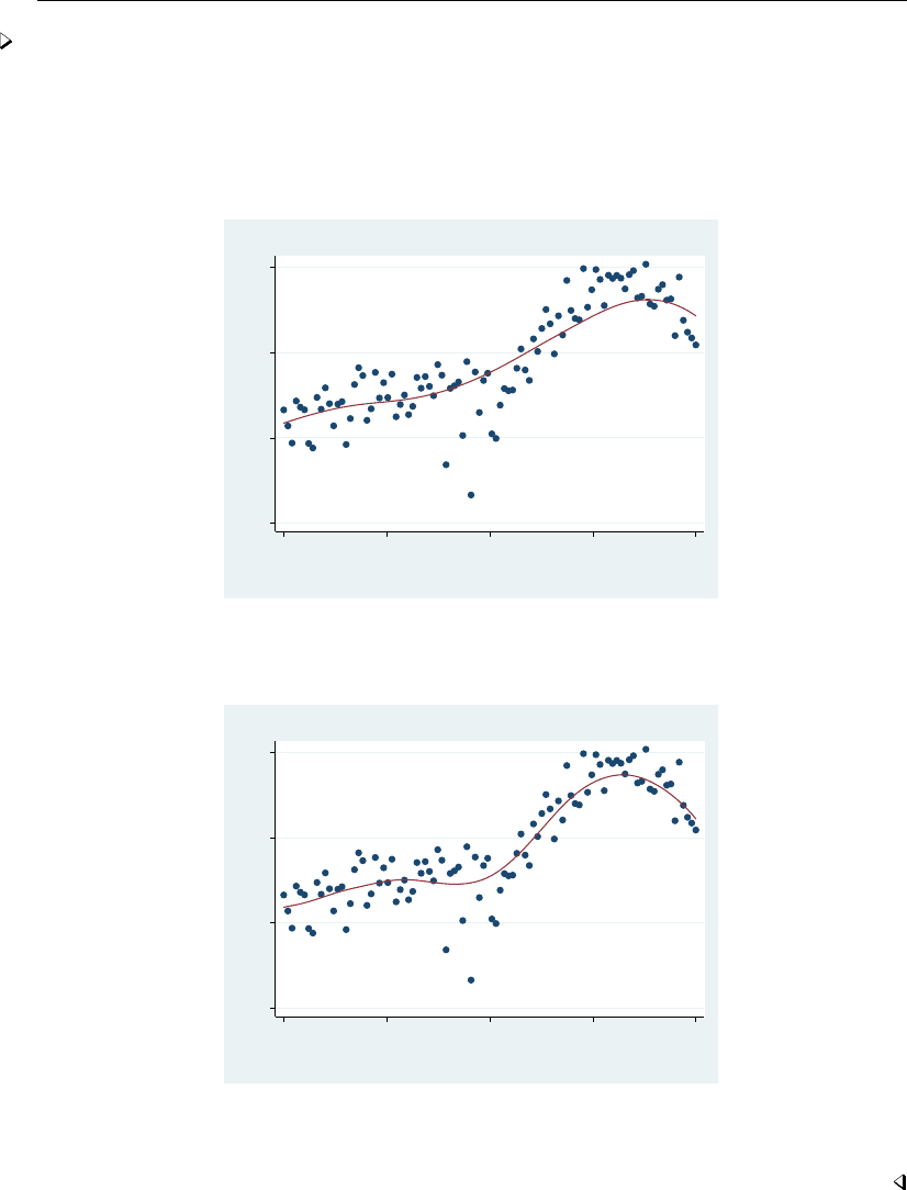
1104 lowess — Lowess smoothing
Example 1
The amount of smoothing is affected by bwidth(#). You are warned to experiment with different
values. For instance,
. use http://www.stata-press.com/data/r13/lowess1
(example data for lowess)
. lowess h1 depth
0 5 10 15
Wet hole 1
0 100 200 300 400
depth
bandwidth = .8
Lowess smoother
Now compare that with
. lowess h1 depth, bwidth(.4)
0 5 10 15
Wet hole 1
0 100 200 300 400
depth
bandwidth = .4
Lowess smoother
In the first case, the default bandwidth of 0.8 is used, meaning that 80% of the data are used
in smoothing each point. In the second case, we explicitly specified a bandwidth of 0.4. Smaller
bandwidths follow the original data more closely.
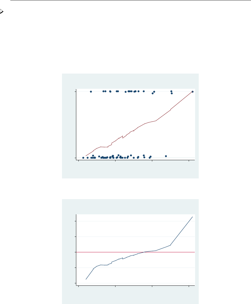
lowess — Lowess smoothing 1105
Example 2
Two lowess options are especially useful with binary (0/1) data: adjust and logit.adjust
adjusts the resulting curve (by multiplication) so that the mean of the smoothed values is equal to
the mean of the unsmoothed values. logit specifies that the smoothed curve be in terms of the log
of the odds ratio:
. use http://www.stata-press.com/data/r13/auto
(1978 Automobile Data)
. lowess foreign mpg, ylabel(0 "Domestic" 1 "Foreign") jitter(5) adjust
Domestic Foreign
Car type
10 20 30 40
Mileage (mpg)
bandwidth = .8
Mean adjusted smooth
Lowess smoother
. lowess foreign mpg, logit yline(0)
−4 −2 0 2 4
Car type
10 20 30 40
Mileage (mpg)
bandwidth = .8
Logit transformed smooth
Lowess smoother
With binary data, if you do not use the logit option, it is a good idea to specify graph’s
jitter() option; see [G-2]graph twoway scatter. Because the underlying data (whether the car
was manufactured outside the United States here) take on only two values, raw data points are more
likely to be on top of each other, thus making it impossible to tell how many points there are. graph’s
jitter() option adds some noise to the data to shift the points around. This noise affects only the
location of points on the graph, not the lowess curve.

1106 lowess — Lowess smoothing
When you specify the logit option, the display of the raw data is suppressed.
Technical note
lowess can be used for more than just lowess smoothing. Lowess can be usefully thought of as
a combination of two smoothing concepts: the use of predicted values from regression (rather than
means) for imputing a smoothed value and the use of the tricube weighting function (rather than a
constant weighting function). lowess allows you to combine these concepts freely. You can use line
smoothing without weighting (specify noweight), mean smoothing with tricube weighting (specify
mean), or mean smoothing without weighting (specify mean and noweight).
Methods and formulas
Let yiand xibe the two variables, and assume that the data are ordered so that xi≤xi+1 for
i=1, . . . , N −1. For each yi, a smoothed value ys
iis calculated.
The subset used in calculating ys
iis indices i−= max(1, i−k)through i+= min(i+k, N), where
k=b(N×bwidth −0.5)/2c. The weights for each of the observations between j=i−, . . . , i+
are either 1 (noweight) or the tricube (default),
wj=1−|xj−xi|
∆33
where ∆ = 1.0001 max(xi+−xi, xi−xi−). The smoothed value ys
iis then the (weighted) mean
or the (weighted) regression prediction at xi.
William Swain Cleveland (1943– ) studied mathematics and statistics at Princeton and Yale. He
worked for several years at Bell Labs in New Jersey and now teaches statistics and computer
science at Purdue. He has made key contributions in many areas of statistics, including graphics
and data visualization, time series, environmental applications, and analysis of Internet traffic
data.
Acknowledgment
lowess is a modified version of a command originally written by Patrick Royston of the MRC
Clinical Trials Unit, London, and coauthor of the Stata Press book Flexible Parametric Survival
Analysis Using Stata: Beyond the Cox Model.
References
Chambers, J. M., W. S. Cleveland, B. Kleiner, and P. A. Tukey. 1983. Graphical Methods for Data Analysis. Belmont,
CA: Wadsworth.
Cleveland, W. S. 1979. Robust locally weighted regression and smoothing scatterplots. Journal of the American
Statistical Association 74: 829–836.

lowess — Lowess smoothing 1107
. 1993. Visualizing Data. Summit, NJ: Hobart.
. 1994. The Elements of Graphing Data. Rev. ed. Summit, NJ: Hobart.
Cox, N. J. 2005. Speaking Stata: Smoothing in various directions.Stata Journal 5: 574–593.
Goodall, C. 1990. A survey of smoothing techniques. In Modern Methods of Data Analysis, ed. J. Fox and J. S.
Long, 126–176. Newbury Park, CA: Sage.
Lindsey, C., and S. J. Sheather. 2010. Model fit assessment via marginal model plots.Stata Journal 10: 215–225.
Royston, P. 1991. gr6: Lowess smoothing.Stata Technical Bulletin 3: 7–9. Reprinted in Stata Technical Bulletin
Reprints, vol. 1, pp. 41–44. College Station, TX: Stata Press.
Royston, P., and N. J. Cox. 2005. A multivariable scatterplot smoother.Stata Journal 5: 405–412.
Salgado-Ugarte, I. H., and M. Shimizu. 1995. snp8: Robust scatterplot smoothing: Enhancements to Stata’s ksm.Stata
Technical Bulletin 25: 23–26. Reprinted in Stata Technical Bulletin Reprints, vol. 5, pp. 190–194. College Station,
TX: Stata Press.
Sasieni, P. D. 1994. snp7: Natural cubic splines.Stata Technical Bulletin 22: 19–22. Reprinted in Stata Technical
Bulletin Reprints, vol. 4, pp. 171–174. College Station, TX: Stata Press.
Also see
[R]lpoly — Kernel-weighted local polynomial smoothing
[R]smooth — Robust nonlinear smoother
[D]ipolate — Linearly interpolate (extrapolate) values

Title
lpoly — Kernel-weighted local polynomial smoothing
Syntax Menu Description Options
Remarks and examples Stored results Methods and formulas References
Also see
Syntax
lpoly yvar xvar if in weight ,options
options Description
Main
kernel(kernel)specify kernel function; default is kernel(epanechnikov)
bwidth(#|varname)specify kernel bandwidth
degree(#)specify degree of the polynomial smooth; default is degree(0)
generate(newvarxnewvars)store smoothing grid in newvarxand smoothed points in
newvars
n(#)obtain the smooth at #points; default is min(N, 50)
at(varname)obtain the smooth at the values specified by varname
nograph suppress graph
noscatter suppress scatterplot only
SE/CI
ci plot confidence bands
level(#)set confidence level; default is level(95)
se(newvar)store standard errors in newvar
pwidth(#)specify pilot bandwidth for standard error calculation
var(#|varname)specify estimates of residual variance
Scatterplot
marker options change look of markers (color, size, etc.)
marker label options add marker labels; change look or position
Smoothed line
lineopts(cline options)affect rendition of the smoothed line
CI plot
ciopts(cline options)affect rendition of the confidence bands
Add plots
addplot(plot)add other plots to the generated graph
Y axis, X axis, Titles, Legend, Overall
twoway options any options other than by() documented in [G-3]twoway options
1108

lpoly — Kernel-weighted local polynomial smoothing 1109
kernel Description
epanechnikov Epanechnikov kernel function; the default
epan2 alternative Epanechnikov kernel function
biweight biweight kernel function
cosine cosine trace kernel function
gaussian Gaussian kernel function
parzen Parzen kernel function
rectangle rectangle kernel function
triangle triangle kernel function
fweights and aweights are allowed; see [U] 11.1.6 weight.
Menu
Statistics >Nonparametric analysis >Local polynomial smoothing
Description
lpoly performs a kernel-weighted local polynomial regression of yvar on xvar and displays a
graph of the smoothed values with (optional) confidence bands.
Options
Main
kernel(kernel)specifies the kernel function for use in calculating the weighted local polynomial
estimate. The default is kernel(epanechnikov).
bwidth(#|varname)specifies the half-width of the kernel—the width of the smoothing window
around each point. If bwidth() is not specified, a rule-of-thumb (ROT) bandwidth estimator is
calculated and used. A local variable bandwidth may be specified in varname, in conjunction with
an explicit smoothing grid using the at() option.
degree(#)specifies the degree of the polynomial to be used in the smoothing. The default is
degree(0), meaning local-mean smoothing.
generate( [newvarx]newvars)stores the smoothing grid in newvarxand the smoothed values in
newvars. If at() is not specified, then both newvarxand newvarsmust be specified. Otherwise,
only newvarsis to be specified.
n(#)specifies the number of points at which the smooth is to be calculated. The default is min(N, 50),
where Nis the number of observations.
at(varname)specifies a variable that contains the values at which the smooth should be calculated.
By default, the smoothing is done on an equally spaced grid, but you can use at() to instead
perform the smoothing at the observed x’s, for example. This option also allows you to more easily
obtain smooths for different variables or different subsamples of a variable and then overlay the
estimates for comparison.
nograph suppresses drawing the graph of the estimated smooth. This option is often used with the
generate() option.
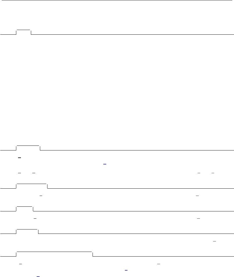
1110 lpoly — Kernel-weighted local polynomial smoothing
noscatter suppresses superimposing a scatterplot of the observed data over the smooth. This option
is useful when the number of resulting points would be so large as to clutter the graph.
SE/CI
ci plots confidence bands, using the confidence level specified in level().
level(#)specifies the confidence level, as a percentage, for confidence intervals. The default is
level(95) or as set by set level; see [U] 20.7 Specifying the width of confidence intervals.
se(newvar)stores the estimates of the standard errors in newvar. This option requires specifying
generate() or at().
pwidth(#)specifies the pilot bandwidth to be used for standard-error computations. The default is
chosen to be 1.5 times the value of the ROT bandwidth selector. If you specify pwidth() without
specifying se() or ci, then the ci option is assumed.
var(#|varname)specifies an estimate of a constant residual variance or a variable containing estimates
of the residual variances at each grid point required for standard-error computation. By default,
the residual variance at each smoothing point is estimated by the normalized weighted residual
sum of squares obtained from locally fitting a polynomial of order p+2, where pis the degree
specified in degree().var(varname)is allowed only if at() is specified. If you specify var()
without specifying se() or ci, then the ci option is assumed.
Scatterplot
marker options affect the rendition of markers drawn at the plotted points, including their shape,
size, color, and outline; see [G-3]marker options.
marker label options specify if and how the markers are to be labeled; see [G-3]marker label options.
Smoothed line
lineopts(cline options)affects the rendition of the smoothed line; see [G-3]cline options.
CI plot
ciopts(cline options)affects the rendition of the confidence bands; see [G-3]cline options.
Add plots
addplot(plot)provides a way to add other plots to the generated graph; see [G-3]addplot option.
Y axis, X axis, Titles, Legend, Overall
twoway options are any of the options documented in [G-3]twoway options, excluding by(). These
include options for titling the graph (see [G-3]title options) and for saving the graph to disk (see
[G-3]saving option).
Remarks and examples
Remarks are presented under the following headings:
Introduction
Local polynomial smoothing
Choice of a bandwidth
Confidence bands

lpoly — Kernel-weighted local polynomial smoothing 1111
Introduction
The last 25 years or so has seen a significant outgrowth in the literature on scatterplot smoothing,
otherwise known as univariate nonparametric regression. Of most appeal is the idea of making no
assumptions about the functional form for the expected value of a response given a regressor, but
instead allowing the data to “speak for themselves”. Various methods and estimators fall into the
category of nonparametric regression, including local mean smoothing as described independently
by Nadaraya (1964) and Watson (1964), the Gasser and M¨
uller (1979) estimator, locally weighted
scatterplot smoothing (LOWESS) as described by Cleveland (1979), wavelets (for example, Donoho
[1995]), and splines (Eubank 1999), to name a few. Much of the vast literature focuses on automating
the amount of smoothing to be performed and dealing with the bias/variance tradeoff inherent to
this type of estimation. For example, for Nadaraya–Watson the amount of smoothing is controlled by
choosing a bandwidth.
Smoothing via local polynomials is by no means a new idea but instead one that has been rediscovered
in recent years in articles such as Fan (1992). A natural extension of the local mean smoothing of
Nadaraya–Watson, local polynomial regression involves fitting the response to a polynomial form of
the regressor via locally weighted least squares. Higher-order polynomials have better bias properties
than the zero-degree local polynomials of the Nadaraya–Watson estimator; in general, higher-order
polynomials do not require bias adjustment at the boundary of the regression space. For a definitive
reference on local polynomial smoothing, see Fan and Gijbels (1996).
Local polynomial smoothing
Consider a set of scatterplot data {(x1, y1),...,(xn, yn)}from the model
yi=m(xi) + σ(xi)i(1)
for some unknown mean and variance functions m(·)and σ2(·), and symmetric errors iwith
E(i)=0and Var(i)=1. The goal is to estimate m(x0) = E[Y|X=x0], making no assumption
about the functional form of m(·).
lpoly estimates m(x0)as the constant term (intercept) of a regression, weighted by the kernel
function specified in kernel(), of yvar on the polynomial terms (xvar−x0),(xvar−x0)2,...,(xvar−
x0)pfor each smoothing point x0. The degree of the polynomial, p, is specified in degree(), the
amount of smoothing is controlled by the bandwidth specified in bwidth(), and the chosen kernel
function is specified in kernel().
Example 1
Consider the motorcycle data as examined (among other places) in Fan and Gijbels (1996). The
data consist of 133 observations and measure the acceleration (accel measured in grams [g]) of
a dummy’s head during impact over time (time measured in milliseconds). For these data, we use
lpoly to fit a local cubic polynomial with the default bandwidth (obtained using the ROT method)
and the default Epanechnikov kernel.
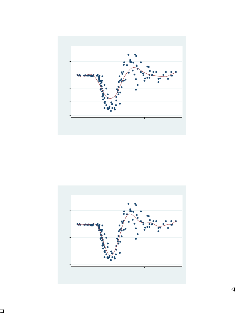
1112 lpoly — Kernel-weighted local polynomial smoothing
. use http://www.stata-press.com/data/r13/motorcycle
(Motorcycle data from Fan & Gijbels (1996))
. lpoly accel time, degree(3)
−150 −100 −50 0 50 100
acceleration (g)
0 20 40 60
time (msec)
kernel = epanechnikov, degree = 3, bandwidth = 6.04
Local polynomial smooth
The default bandwidth and kernel settings do not provide a satisfactory fit in this example. To
improve the fit, we can either supply a different bandwidth by using the bwidth() option or specify
a different kernel by using the kernel() option. For example, using the alternative Epanechnikov
kernel, kernel(epan2), below provides a better fit for these data.
. lpoly accel time, degree(3) kernel(epan2)
−150 −100 −50 0 50 100
acceleration (g)
0 20 40 60
time (msec)
kernel = epan2, degree = 3, bandwidth = 6.88
Local polynomial smooth
Technical note
lpoly allows specifying in degree() both odd and even orders of the polynomial to be used for
the smoothing. However, the odd-order, 2k+1, polynomial approximations are preferable. They have
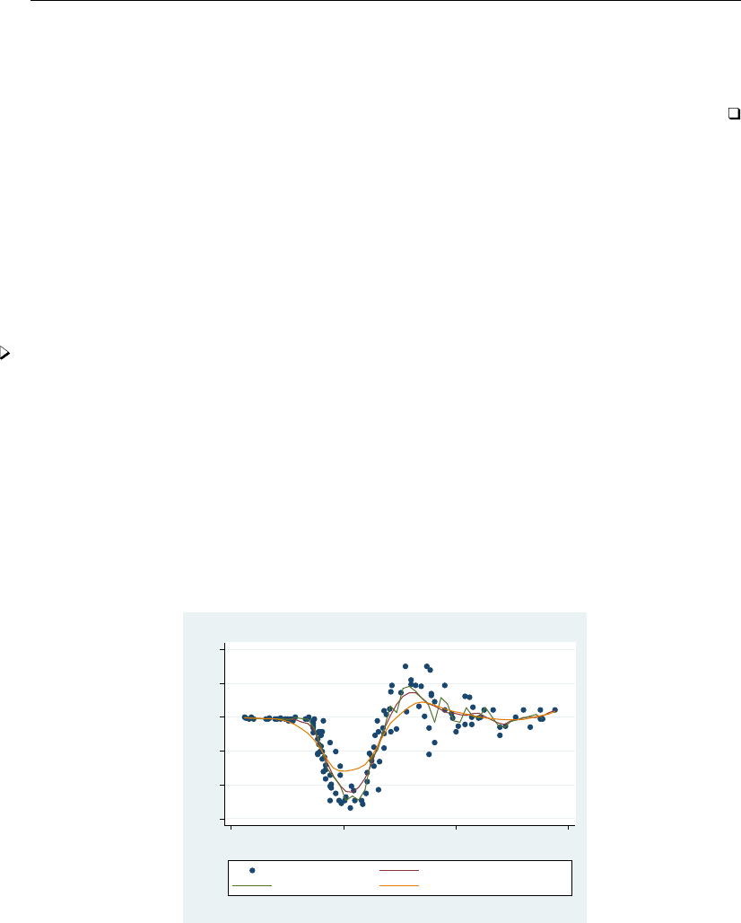
lpoly — Kernel-weighted local polynomial smoothing 1113
an extra parameter compared with the even-order, 2k, approximations, which leads to a significant
bias reduction and there is no increase of variability associated with adding this extra parameter.
Using an odd order when estimating the regression function is therefore usually sufficient. For a more
thorough discussion, see Fan and Gijbels (1996).
Choice of a bandwidth
The choice of a bandwidth is crucial for many smoothing techniques, including local polynomial
smoothing. In general, using a large bandwidth gives smooths with a large bias, whereas a small
bandwidth may result in highly variable smoothed values. Various techniques exist for optimal
bandwidth selection. By default, lpoly uses the ROT method to estimate the bandwidth used for the
smoothing; see Methods and formulas for details.
Example 2
Using the motorcycle data, we demonstrate how a local linear polynomial fit changes using
different bandwidths.
. lpoly accel time, degree(1) kernel(epan2) bwidth(1) generate(at smooth1)
> nograph
. lpoly accel time, degree(1) kernel(epan2) bwidth(7) at(at) generate(smooth2)
> nograph
. label variable smooth1 "smooth: width = 1"
. label variable smooth2 "smooth: width = 7"
. lpoly accel time, degree(1) kernel(epan2) at(at) addplot(line smooth* at)
> legend(label(2 "smooth: width = 3.42 (ROT)")) note("kernel = epan2, degree = 1")
−150 −100 −50 0 50 100
acceleration (g)
0 20 40 60
time (msec)
acceleration (g) smooth: width = 3.42 (ROT)
smooth: width = 1 smooth: width = 7
kernel = epan2, degree = 1
Local polynomial smooth
From this graph, we can see that the local linear polynomial fit with larger bandwidth (width =
7) corresponds to a smoother line but fails to fit the curvature of the scatterplot data. The smooth
obtained using the width equal to one seems to fit most data points, but the corresponding line has
several spikes indicating larger variability. The smooth obtained using the ROT bandwidth estimator
seems to have a good tradeoff between the fit and variability in this example.
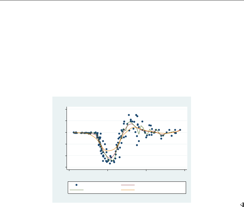
1114 lpoly — Kernel-weighted local polynomial smoothing
In the above, we also demonstrated how the generate() and addplot() options may be used to
produce overlaid plots obtained from lpoly with different options. The nograph option saves time
when you need to save only results with generate().
However, to avoid generating variables manually, one can use twoway lpoly instead; see [G-2]graph
twoway lpoly for more details.
. twoway scatter accel time ||
> lpoly accel time, degree(1) kernel(epan2) lpattern(solid) ||
> lpoly accel time, degree(1) kernel(epan2) bwidth(1) ||
> lpoly accel time, degree(1) kernel(epan2) bwidth(7) ||
> , legend(label(2 "smooth: width = 3.42 (ROT)") label(3 "smooth: width = 1")
> label(4 "smooth: width = 7"))
> title("Local polynomial smooth") note("kernel = epan2, degree = 1")
> xtitle("time (msec)") ytitle("acceleration (g)")
−150 −100 −50 0 50 100
acceleration (g)
0 20 40 60
time (msec)
acceleration (g) smooth: width = 3.42 (ROT)
smooth: width = 1 smooth: width = 7
kernel = epan2, degree = 1
Local polynomial smooth
The ROT estimate is commonly used as an initial guess for the amount of smoothing; this approach
may be sufficient when the choice of a bandwidth is less important. In other cases, you can pick
your own bandwidth.
When the shape of the regression function has a combination of peaked and flat regions, a variable
bandwidth may be preferable over the constant bandwidth to allow for different degrees of smoothness
in different regions. The bwidth() option allows you to specify the values of the local variable
bandwidths as those stored in a variable in your data.
Similar issues with bias and variability arise when choosing a pilot bandwidth (the pwidth()
option) used to compute standard errors of the local polynomial smoother. The default value is chosen
to be 1.5 ×ROT. For a review of methods for pilot bandwidth selection, see Fan and Gijbels (1996).
Confidence bands
The established asymptotic normality of the local polynomial estimators under certain conditions
allows the construction of approximate confidence bands. lpoly offers the ci option to plot these
bands.
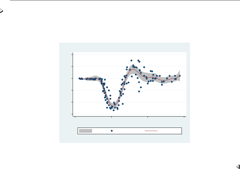
lpoly — Kernel-weighted local polynomial smoothing 1115
Example 3
Let us plot the confidence bands for the local polynomial fit from example 1.
. lpoly accel time, degree(3) kernel(epan2) ci
−150 −100 −50 0 50 100
acceleration (g)
0 20 40 60
time (msec)
95% CI acceleration (g) lpoly smooth
kernel = epan2, degree = 3, bandwidth = 6.88, pwidth = 10.33
Local polynomial smooth
You can obtain graphs with overlaid confidence bands by using twoway lpolyci; see [G-2]graph
twoway lpolyci for examples.
Constructing the confidence intervals involves computing standard errors obtained by taking a
square root of the estimate of the conditional variance of the local polynomial estimator at each
grid point x0. Estimating the conditional variance requires fitting a polynomial of a higher order
locally by using a different bandwidth, the pilot bandwidth. The value of the pilot bandwidth may
be supplied by using pwidth(). By default, the value of 1.5 ×ROT is used. Also, estimates of the
residual variance σ2(x0)at each grid point, x0, are required to obtain the estimates of the conditional
variances. These estimates may be supplied by using the var() option. By default, they are computed
using the normalized weighted residual sum of squares from a local polynomial fit of a higher order.
See Methods and formulas for details. The standard errors may be saved by using se().
Stored results
lpoly stores the following in r():
Scalars
r(degree) smoothing polynomial degree r(bwidth) bandwidth of the smooth
r(ngrid) number of successful regressions r(pwidth) pilot bandwidth
r(N) sample size
Macros
r(kernel) name of kernel

1116 lpoly — Kernel-weighted local polynomial smoothing
Methods and formulas
Consider model (1), written in matrix notation,
y=m(x) +
where yand xare the n×1vectors of scatterplot values, is the n×1vector of errors with zero
mean and covariance matrix Σ=diag{σ(xi)}In, and m() and σ() are some unknown functions.
Define m(x0) = E[Y|X=x0]and σ2(x0) = Var[Y|X=x0]to be the conditional mean and
conditional variance of random variable Y(residual variance), respectively, for some realization x0
of random variable X.
The method of local polynomial smoothing is based on the approximation of m(x)locally by a
pth order polynomial in (x−x0)for some xin the neighborhood of x0. For the scatterplot data
{(x1, y1),...,(xn, yn)}, the pth-order local polynomial smooth bm(x0)is equal to b
β0, an estimate
of the intercept of the weighted linear regression,
b
β= (XTWX)−1XTWy (2)
where b
β= (b
β0,b
β1,...,b
βp)Tis the vector of estimated regression coefficients (with {b
βj=
(j!)−1bm(j)(x)|x=x0, j = 0, . . . , p}also representing estimated coefficients from a corresponding
Taylor expansion); X={(xi−x0)j}n,p
i,j=1,0is a design matrix; and W=diag{Kh(xi−x0)}n×n
is a weighting matrix with weights Kh(·)defined as Kh(x) = h−1K(x/h), with K(·)being a
kernel function and hdefining a bandwidth. The kernels are defined in Methods and formulas of
[R]kdensity.
The default bandwidth is obtained using the ROT method of bandwidth selection. The ROT bandwidth
is the plugin estimator of the asymptotically optimal constant bandwidth. This is the bandwidth that
minimizes the conditional weighted mean integrated squared error. The ROT plugin bandwidth selector
for the smoothing bandwidth his defined as follows; assuming constant residual variance σ2(x0) = σ2
and odd degree p:
b
h=C0,p(K)"bσ2Rw0(x)dx
nR{bm(p+1)(x)}2w0(x)f(x)dx #1/(2p+3)
(3)
where C0,p(K)is a constant, as defined in Fan and Gijbels (1996), that depends on the kernel function
K(·), and the degree of a polynomial pand w0is chosen to be an indicator function on the interval
[minx+0.05 ×rangex,maxx−0.05 ×rangex]with minx, maxx, and rangexbeing, respectively, the
minimum, maximum, and the range of x. To obtain the estimates of a constant residual variance, bσ2,
and (p+1)th order derivative of m(x), denoted as bm(p+1)(x), a polynomial in xof order (p+3)
is fit globally to y.bσ2is estimated as a standardized residual sum of squares from this fit.
The expression for the asymptotically optimal constant bandwidth used in constructing the ROT
bandwidth estimator is derived for the odd-order polynomial approximations. For even-order polynomial
fits the expression would depend not only on m(p+1)(x)but also on m(p+2)(x)and the design density
and its derivative, f(x)and f0(x). Therefore, the ROT bandwidth selector would require estimation
of these additional quantities. Instead, for an even-degree pof the local polynomial, lpoly uses the
value of the ROT estimator (3) computed using degree p+1. As such, for even degrees this is not a
plugin estimator of the asymptotically optimal constant bandwidth.
The estimates of the conditional variance of local polynomial estimators are obtained using
d
Var{bm(x0)|X=x0}=bσ2
m(x0)=(XTWX)−1(XTW2X)(XTWX)−1bσ2(x0) (4)

lpoly — Kernel-weighted local polynomial smoothing 1117
where bσ2(x0)is estimated by the normalized weighted residual sum of squares from the (p+ 2)th
order polynomial fit using pilot bandwidth h?.
When the bias is negligible the normal-approximation method yields a (1−α)×100% confidence
interval for m(x0),
bm(x0)−z(1−α/2) bσm(x0),bm(x0) + z(1−α/2)bσm(x0)
where z(1−α/2) is the (1−α/2)th quantile of the standard Gaussian distribution, and bm(x0)and
bσm(x0)are as defined in (2) and (4), respectively.
References
Cleveland, W. S. 1979. Robust locally weighted regression and smoothing scatterplots. Journal of the American
Statistical Association 74: 829–836.
Cox, N. J. 2005. Speaking Stata: Smoothing in various directions.Stata Journal 5: 574–593.
Donoho, D. L. 1995. Nonlinear solution of linear inverse problems by wavelet-vaguelette decomposition. Applied and
Computational Harmonic Analysis 2: 101–126.
Eubank, R. L. 1999. Nonparametric Regression and Spline Smoothing. 2nd ed. New York: Dekker.
Fan, J. 1992. Design-adaptive nonparametric regression. Journal of the American Statistical Association 87: 998–1004.
Fan, J., and I. Gijbels. 1996. Local Polynomial Modelling and Its Applications. London: Chapman & Hall.
Gasser, T., and H.-G. M¨
uller. 1979. Kernel estimation of regression functions. In Smoothing Techniques for Curve
Estimation, Lecture Notes in Mathematics, ed. T. Gasser and M. Rosenblatt, 23–68. New York: Springer.
Gutierrez, R. G., J. M. Linhart, and J. S. Pitblado. 2003. From the help desk: Local polynomial regression and Stata
plugins.Stata Journal 3: 412–419.
Nadaraya, E. A. 1964. On estimating regression. Theory of Probability and Its Application 9: 141–142.
Sheather, S. J., and M. C. Jones. 1991. A reliable data-based bandwidth selection method for kernel density estimation.
Journal of the Royal Statistical Society, Series B 53: 683–690.
Verardi, V., and N. Debarsy. 2012. Robinson’s square root of Nconsistent semiparametric regression estimator in
Stata.Stata Journal 12: 726–735.
Watson, G. S. 1964. Smooth regression analysis. Sankhy¯
a Series A 26: 359–372.
Also see
[R]kdensity — Univariate kernel density estimation
[R]lowess — Lowess smoothing
[R]smooth — Robust nonlinear smoother
[G-2]graph twoway lpoly — Local polynomial smooth plots
[G-2]graph twoway lpolyci — Local polynomial smooth plots with CIs

Title
lroc — Compute area under ROC curve and graph the curve
Syntax Menu Description Options
Remarks and examples Stored results Methods and formulas References
Also see
Syntax
lroc depvar if in weight ,options
options Description
Main
all compute area under ROC curve and graph curve for all observations
nograph suppress graph
Advanced
beta(matname)row vector containing model coefficients
Plot
cline options change the look of the line
marker options change look of markers (color, size, etc.)
marker label options add marker labels; change look or position
Reference line
rlopts(cline options)affect rendition of the reference line
Add plots
addplot(plot)add other plots to the generated graph
Y axis, X axis, Titles, Legend, Overall
twoway options any options other than by() documented in [G-3]twoway options
fweights are allowed; see [U] 11.1.6 weight.
lroc is not appropriate after the svy prefix.
Menu
Statistics >Binary outcomes >Postestimation >ROC curve after logistic/logit/probit/ivprobit
Description
lroc graphs the ROC curve and calculates the area under the curve.
lroc requires that the current estimation results be from logistic,logit,probit, or ivprobit;
see [R]logistic,[R]logit,[R]probit, or [R]ivprobit.
1118

lroc — Compute area under ROC curve and graph the curve 1119
Options
Main
all requests that the statistic be computed for all observations in the data, ignoring any if or in
restrictions specified by the estimation command.
nograph suppresses graphical output.
Advanced
beta(matname)specifies a row vector containing model coefficients. The columns of the row vector
must be labeled with the corresponding names of the independent variables in the data. The
dependent variable depvar must be specified immediately after the command name. See Models
other than the last fitted model later in this entry.
Plot
cline options,marker options, and marker label options affect the rendition of the ROC curve—the
plotted points connected by lines. These options affect the size and color of markers, whether and
how the markers are labeled, and whether and how the points are connected; see [G-3]cline options,
[G-3]marker options, and [G-3]marker label options.
Reference line
rlopts(cline options)affects the rendition of the reference line; see [G-3]cline options.
Add plots
addplot(plot)provides a way to add other plots to the generated graph; see [G-3]addplot option.
Y axis, X axis, Titles, Legend, Overall
twoway options are any of the options documented in [G-3]twoway options, excluding by(). These
include options for titling the graph (see [G-3]title options) and for saving the graph to disk (see
[G-3]saving option).
Remarks and examples
Remarks are presented under the following headings:
Introduction
Samples other than the estimation sample
Models other than the last fitted model
Introduction
Stata also has a suite of commands for performing both parametric and nonparametric receiver
operating characteristic (ROC) analysis. See [R]roc for an overview of these commands.
lroc graphs the ROC curve—a graph of sensitivity versus one minus specificity as the cutoff c
is varied—and calculates the area under it. Sensitivity is the fraction of observed positive-outcome
cases that are correctly classified; specificity is the fraction of observed negative-outcome cases that
are correctly classified. When the purpose of the analysis is classification, you must choose a cutoff.

1120 lroc — Compute area under ROC curve and graph the curve
The curve starts at (0,0), corresponding to c=1, and continues to (1,1), corresponding to c=0.
A model with no predictive power would be a 45◦line. The greater the predictive power, the more
bowed the curve, and hence the area beneath the curve is often used as a measure of the predictive
power. A model with no predictive power has area 0.5; a perfect model has area 1.
The ROC curve was first discussed in signal detection theory (Peterson, Birdsall, and Fox 1954)
and then was quickly introduced into psychology (Tanner and Swets 1954). It has since been applied
in other fields, particularly medicine (for instance, Metz [1978]). For a classic text on ROC techniques,
see Green and Swets (1966).
lsens also plots sensitivity and specificity; see [R]lsens.
Example 1
Hardin and Hilbe (2012) examine data from the National Canadian Registry of Cardiovascular
Disease (FASTRAK), sponsored by Hoffman-La Roche Canada. They model death within 48 hours
based on whether a patient suffers an anterior infarct (heart attack) rather than an inferior infarct using
a logistic regression and evaluate the model using an ROC curve. We replicate their analysis here.
Both anterior and inferior refer to sites on the heart where damage occurs. The model is also
adjusted for hcabg, whether the subject has had a cardiac bypass surgery (CABG); age, a four-category
age-group indicator; and killip, a four-level risk indicator.
We load the data and then estimate the parameters of the logistic regression with logistic.
Factor-variable notation is used for each predictor, because they are categorical; see [U] 11.4.3 Factor
variables.
. use http://www.stata-press.com/data/r13/heart
(Heart attacks)
. logistic death i.site i.hcabg i.killip i.age
Logistic regression Number of obs = 4483
LR chi2(8) = 211.37
Prob > chi2 = 0.0000
Log likelihood = -636.62553 Pseudo R2 = 0.1424
death Odds Ratio Std. Err. z P>|z| [95% Conf. Interval]
site
Anterior 1.901333 .3185757 3.83 0.000 1.369103 2.640464
1.hcabg 2.105275 .7430694 2.11 0.035 1.054076 4.204801
killip
2 2.251732 .4064423 4.50 0.000 1.580786 3.207453
3 2.172105 .584427 2.88 0.004 1.281907 3.680487
4 14.29137 5.087654 7.47 0.000 7.112964 28.71423
age
60-69 1.63726 .5078582 1.59 0.112 .8914261 3.007115
70-79 4.532029 1.206534 5.68 0.000 2.689568 7.636647
>=80 8.893222 2.41752 8.04 0.000 5.219991 15.15125
_cons .0063961 .0016541 -19.54 0.000 .0038529 .010618
The odds ratios for a unit change in each covariate are reported by logistic. At fixed values of
the other covariates, patients who enter Canadian hospitals with an anterior infarct have nearly twice
the odds of death within 48 hours than those with an inferior infarct. Those who have had a previous
CABG have approximately twice the risk of death of those who have not. Those with higher Killip
risks and those who are older are also at greater risk of death.
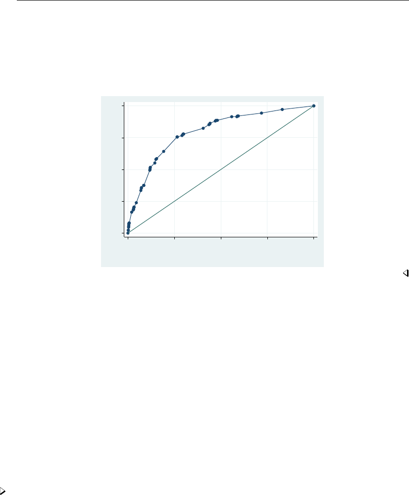
lroc — Compute area under ROC curve and graph the curve 1121
We use lroc to draw the ROC curve for the model. The area under the curve of approximately
0.8 indicates acceptable discrimination for the model.
. lroc
Logistic model for death
number of observations = 4483
area under ROC curve = 0.7965
0.00 0.25 0.50 0.75 1.00
Sensitivity
0.00 0.25 0.50 0.75 1.00
1 − Specificity
Area under ROC curve = 0.7965
Samples other than the estimation sample
lroc can be used with samples other than the estimation sample. By default, lroc remembers
the estimation sample used with the last logistic,logit,probit, or ivprobit command. To
override this, simply use an if or in restriction to select another set of observations, or specify the
all option to force the command to use all the observations in the dataset.
See example 3 in [R]estat gof for an example of using lroc with a sample other than the
estimation sample.
Models other than the last fitted model
By default, lroc uses the last model fit by logistic,logit,probit, or ivprobit. You may
also directly specify the model to lroc by inputting a vector of coefficients with the beta() option
and passing the name of the dependent variable depvar to lroc.
Example 2
Suppose that someone publishes the following logistic model of low birthweight:
Pr(low =1) = F(−0.02 age −0.01 lwt +1.3 black +1.1 smoke +0.5 ptl +1.8 ht +0.8 ui +0.5)
where Fis the cumulative logistic distribution. These coefficients are not odds ratios; they are the
equivalent of what logit produces.

1122 lroc — Compute area under ROC curve and graph the curve
We can see whether this model fits our data. First we enter the coefficients as a row vector and
label its columns with the names of the independent variables plus cons for the constant (see
[P]matrix define and [P]matrix rownames).
. use http://www.stata-press.com/data/r13/lbw3, clear
(Hosmer & Lemeshow data)
. matrix input b = (-.02, -.01, 1.3, 1.1, .5, 1.8, .8, .5)
. matrix colnames b = age lwt black smoke ptl ht ui _cons
Here we use lroc to examine the predictive ability of the model:
. lroc low, beta(b) nograph
Logistic model for low
number of observations = 189
area under ROC curve = 0.7275
The area under the curve indicates that this model does have some predictive power. We can obtain
a graph of sensitivity and specificity as a function of the cutoff probability by typing
. lsens low, beta(b)
0.00 0.25 0.50 0.75 1.00
Sensitivity/Specificity
0.00 0.25 0.50 0.75 1.00
Probability cutoff
Sensitivity Specificity
See [R]lsens.
Stored results
lroc stores the following in r():
Scalars
r(N) number of observations
r(area) area under the ROC curve
Methods and formulas
The ROC curve is a graph of specificity against (1 −sensitivity). This is guaranteed to be a
monotone nondecreasing function because the number of correctly predicted successes increases and
the number of correctly predicted failures decreases as the classification cutoff cdecreases.

lroc — Compute area under ROC curve and graph the curve 1123
The area under the ROC curve is the area on the bottom of this graph and is determined by
integrating the curve. The vertices of the curve are determined by sorting the data according to the
predicted index, and the integral is computed using the trapezoidal rule.
References
Green, D. M., and J. A. Swets. 1966. Signal Detection Theory and Psychophysics. New York: Wiley.
Hardin, J. W., and J. M. Hilbe. 2012. Generalized Linear Models and Extensions. 3rd ed. College Station, TX: Stata
Press.
Hosmer, D. W., Jr., S. A. Lemeshow, and R. X. Sturdivant. 2013. Applied Logistic Regression. 3rd ed. Hoboken,
NJ: Wiley.
Metz, C. E. 1978. Basic principles of ROC analysis. Seminars in Nuclear Medicine 8: 283–298.
Peterson, W. W., T. G. Birdsall, and W. C. Fox. 1954. The theory of signal detectability. Transactions IRE Professional
Group on Information Theory PGIT-4: 171–212.
Tanner, W. P., Jr., and J. A. Swets. 1954. A decision-making theory of visual detection. Psychological Review 61:
401–409.
Tilford, J. M., P. K. Roberson, and D. H. Fiser. 1995. sbe12: Using lfit and lroc to evaluate mortality prediction
models.Stata Technical Bulletin 28: 14–18. Reprinted in Stata Technical Bulletin Reprints, vol. 5, pp. 77–81.
College Station, TX: Stata Press.
Also see
[R]logistic — Logistic regression, reporting odds ratios
[R]logit — Logistic regression, reporting coefficients
[R]probit — Probit regression
[R]ivprobit — Probit model with continuous endogenous regressors
[R]lsens — Graph sensitivity and specificity versus probability cutoff
[R]estat classification — Classification statistics and table
[R]estat gof — Pearson or Hosmer–Lemeshow goodness-of-fit test
[R]roc — Receiver operating characteristic (ROC) analysis
[U] 20 Estimation and postestimation commands

Title
lrtest — Likelihood-ratio test after estimation
Syntax Menu Description Options
Remarks and examples Stored results Methods and formulas References
Also see
Syntax
lrtest modelspec1modelspec2,options
where modelspec is name |.|(namelist)
where name is the name under which estimation results were stored using estimates store (see
[R]estimates store), and “.” refers to the last estimation results, whether or not these were already
stored.
options Description
stats display statistical information about the two models
dir display descriptive information about the two models
df(#)override the automatic degrees-of-freedom calculation; seldom used
force force testing even when apparently invalid
Menu
Statistics >Postestimation >Tests >Likelihood-ratio test
Description
lrtest performs a likelihood-ratio test of the null hypothesis that the parameter vector of a
statistical model satisfies some smooth constraint. To conduct the test, both the unrestricted and the
restricted models must be fit using the maximum likelihood method (or some equivalent method),
and the results of at least one must be stored using estimates store; see [R]estimates store.
modelspec1and modelspec2specify the restricted and unrestricted model in any order. modelspec1
and modelspec2cannot have names in common; for example, lrtest (A B C) (C D E) is not allowed
because both model specifications include C. If modelspec2is not specified, the last estimation result
is used; this is equivalent to specifying modelspec2as a period (.).
lrtest supports composite models specified by a parenthesized list of model names. In a composite
model, we assume that the log likelihood and dimension (number of free parameters) of the full model
are obtained as the sum of the log-likelihood values and dimensions of the constituting models.
lrtest provides an important alternative to test (see [R]test) for models fit via maximum
likelihood or equivalent methods.
1124

lrtest — Likelihood-ratio test after estimation 1125
Options
stats displays statistical information about the unrestricted and restricted models, including the
information indices of Akaike and Schwarz.
dir displays descriptive information about the unrestricted and restricted models; see estimates
dir in [R]estimates store.
df(#)is seldom specified; it overrides the automatic degrees-of-freedom calculation.
force forces the likelihood-ratio test calculations to take place in situations where lrtest would
normally refuse to do so and issue an error. Such situations arise when one or more assumptions
of the test are violated, for example, if the models were fit with vce(robust),vce(cluster
clustvar), or pweights; when the dependent variables in the two models differ; when the null log
likelihoods differ; when the samples differ; or when the estimation commands differ. If you use
the force option, there is no guarantee as to the validity or interpretability of the resulting test.
Remarks and examples
The standard way to use lrtest is to do the following:
1. Fit either the restricted model or the unrestricted model by using one of Stata’s estimation commands
and then store the results using estimates store name.
2. Fit the alternative model (the unrestricted or restricted model) and then type ‘lrtest name .’.
lrtest determines for itself which of the two models is the restricted model by comparing the
degrees of freedom.
Often you may want to store the alternative model with estimates store name2, for instance,
if you plan additional tests against models yet to be fit. The likelihood-ratio test is then obtained as
lrtest name name2.
Remarks are presented under the following headings:
Nested models
Composite models
Nested models
lrtest may be used with any estimation command that reports a log likelihood, including
heckman,logit,poisson,stcox, and streg. You must check that one of the model specifications
implies a statistical model that is nested within the model implied by the other specification. Usually,
this means that both models are fit with the same estimation command (for example, both are fit
by logit, with the same dependent variables) and that the set of covariates of one model is a
subset of the covariates of the other model. Second, lrtest is valid only for models that are fit by
maximum likelihood or by some equivalent method, so it does not apply to models that were fit with
probability weights or clusters. Specifying the vce(robust) option similarly would indicate that you
are worried about the valid specification of the model, so you would not use lrtest. Third, lrtest
assumes that under the null hypothesis, the test statistic is (approximately) distributed as chi-squared.
This assumption is not true for likelihood-ratio tests of “boundary conditions”, such as tests for the
presence of overdispersion or random effects (Gutierrez, Carter, and Drukker 2001).
Example 1
We have data on infants born with low birthweights along with the characteristics of the mother
(Hosmer, Lemeshow, and Sturdivant 2013; see also [R]logistic). We fit the following model:

1126 lrtest — Likelihood-ratio test after estimation
. use http://www.stata-press.com/data/r13/lbw
(Hosmer & Lemeshow data)
. logistic low age lwt i.race smoke ptl ht ui
Logistic regression Number of obs = 189
LR chi2(8) = 33.22
Prob > chi2 = 0.0001
Log likelihood = -100.724 Pseudo R2 = 0.1416
low Odds Ratio Std. Err. z P>|z| [95% Conf. Interval]
age .9732636 .0354759 -0.74 0.457 .9061578 1.045339
lwt .9849634 .0068217 -2.19 0.029 .9716834 .9984249
race
black 3.534767 1.860737 2.40 0.016 1.259736 9.918406
other 2.368079 1.039949 1.96 0.050 1.001356 5.600207
smoke 2.517698 1.00916 2.30 0.021 1.147676 5.523162
ptl 1.719161 .5952579 1.56 0.118 .8721455 3.388787
ht 6.249602 4.322408 2.65 0.008 1.611152 24.24199
ui 2.1351 .9808153 1.65 0.099 .8677528 5.2534
_cons 1.586014 1.910496 0.38 0.702 .1496092 16.8134
We now wish to test the constraint that the coefficients on age,lwt,ptl, and ht are all zero or,
equivalently here, that the odds ratios are all 1. One solution is to type
. test age lwt ptl ht
( 1) [low]age = 0
( 2) [low]lwt = 0
( 3) [low]ptl = 0
( 4) [low]ht = 0
chi2( 4) = 12.38
Prob > chi2 = 0.0147
This test is based on the inverse of the information matrix and is therefore based on a quadratic
approximation to the likelihood function; see [R]test. A more precise test would be to refit the model,
applying the proposed constraints, and then calculate the likelihood-ratio test.
We first save the current model:
. estimates store full
We then fit the constrained model, which here is the model omitting age,lwt,ptl, and ht:
. logistic low i.race smoke ui
Logistic regression Number of obs = 189
LR chi2(4) = 18.80
Prob > chi2 = 0.0009
Log likelihood = -107.93404 Pseudo R2 = 0.0801
low Odds Ratio Std. Err. z P>|z| [95% Conf. Interval]
race
black 3.052746 1.498087 2.27 0.023 1.166747 7.987382
other 2.922593 1.189229 2.64 0.008 1.316457 6.488285
smoke 2.945742 1.101838 2.89 0.004 1.415167 6.131715
ui 2.419131 1.047359 2.04 0.041 1.035459 5.651788
_cons .1402209 .0512295 -5.38 0.000 .0685216 .2869447

lrtest — Likelihood-ratio test after estimation 1127
That done, lrtest compares this model with the model we previously stored:
. lrtest full .
Likelihood-ratio test LR chi2(4) = 14.42
(Assumption: . nested in full) Prob > chi2 = 0.0061
Let’s compare results. test reported that age,lwt,ptl, and ht were jointly significant at the 1.5%
level; lrtest reports that they are significant at the 0.6% level. Given the quadratic approximation
made by test, we could argue that lrtest’s results are more accurate.
lrtest explicates the assumption that, from a comparison of the degrees of freedom, it has assessed
that the last fit model (.) is nested within the model stored as full. In other words, full is the
unconstrained model and .is the constrained model.
The names in “(Assumption: . nested in full)” are actually links. Click on a name, and the
results for that model are replayed.
Aside: The nestreg command provides a simple syntax for performing likelihood-ratio tests for
nested model specifications; see [R]nestreg. In the previous example, we fit a full logistic model,
used estimates store to store the full model, fit a constrained logistic model, and used lrtest
to report a likelihood-ratio test between two models. To do this with one call to nestreg, use the
lrtable option.
Technical note
lrtest determines the degrees of freedom of a model as the rank of the (co)variance matrix
e(V). There are two issues here. First, the numerical determination of the rank of a matrix is a subtle
problem that can, for instance, be affected by the scaling of the variables in the model. The rank of a
matrix depends on the number of (independent) linear combinations of coefficients that sum exactly
to zero. In the world of numerical mathematics, it is hard to tell whether a very small number is
really nonzero or is a real zero that happens to be slightly off because of roundoff error from the finite
precision with which computers make floating-point calculations. Whether a small number is being
classified as one or the other, typically on the basis of a threshold, affects the determined degrees of
freedom. Although Stata generally makes sensible choices, it is bound to make mistakes occasionally.
The moral of this story is to make sure that the calculated degrees of freedom is as you expect before
interpreting the results.
Technical note
A second issue involves regress and related commands such as anova. Mainly for historical
reasons, regress does not treat the residual variance, σ2, the same way that it treats the regression
coefficients. Type estat vce after regress, and you will see the regression coefficients, not bσ2.
Most estimation commands for models with ancillary parameters (for example, streg and heckman)
treat all parameters as equals. There is nothing technically wrong with regress here; we are usually
focused on the regression coefficients, and their estimators are uncorrelated with bσ2. But, formally,
σ2adds a degree of freedom to the model, which does not matter if you are comparing two regression
models by a likelihood-ratio test. This test depends on the difference in the degrees of freedom,
and hence being “off by 1” in each does not matter. But, if you are comparing a regression model
with a larger model—for example, a heteroskedastic regression model fit by arch—the automatic
determination of the degrees of freedom is incorrect, and you must specify the df(#)option.

1128 lrtest — Likelihood-ratio test after estimation
Example 2
Returning to the low-birthweight data in the example 1, we now wish to test that the coefficient
on 2.race (black) is equal to that on 3.race (other). The base model is still stored under the name
full, so we need only fit the constrained model and perform the test. With zas the index of the
logit model, the base model is
z=β0+β1age +β2lwt +β32.race +β43.race +···
If β3=β4, this can be written as
z=β0+β1age +β2lwt +β3(2.race +3.race) + ···
We can fit the constrained model as follows:
. constraint 1 2.race = 3.race
. logistic low age lwt i.race smoke ptl ht ui, constraints(1)
Logistic regression Number of obs = 189
Wald chi2(7) = 25.17
Log likelihood = -100.9997 Prob > chi2 = 0.0007
( 1) [low]2.race - [low]3.race = 0
low Odds Ratio Std. Err. z P>|z| [95% Conf. Interval]
age .9716799 .0352638 -0.79 0.429 .9049649 1.043313
lwt .9864971 .0064627 -2.08 0.038 .9739114 .9992453
race
black 2.728186 1.080207 2.53 0.011 1.255586 5.927907
other 2.728186 1.080207 2.53 0.011 1.255586 5.927907
smoke 2.664498 1.052379 2.48 0.013 1.228633 5.778414
ptl 1.709129 .5924776 1.55 0.122 .8663666 3.371691
ht 6.116391 4.215585 2.63 0.009 1.58425 23.61385
ui 2.09936 .9699702 1.61 0.108 .8487997 5.192407
_cons 1.309371 1.527398 0.23 0.817 .1330839 12.8825
Comparing this model with our original model, we obtain
. lrtest full .
Likelihood-ratio test LR chi2(1) = 0.55
(Assumption: . nested in full) Prob > chi2 = 0.4577
By comparison, typing test 2.race=3.race after fitting our base model results in a significance
level of 0.4572. Alternatively, we can first store the restricted model, here using the name equal.
Next lrtest is invoked specifying the names of the restricted and unrestricted models (we do not
care about the order). This time, we also add the option stats requesting a table of model statistics,
including the model selection indices AIC and BIC.
. estimates store equal
. lrtest equal full, stats
Likelihood-ratio test LR chi2(1) = 0.55
(Assumption: equal nested in full) Prob > chi2 = 0.4577
Model Obs ll(null) ll(model) df AIC BIC
equal 189 . -100.9997 8 217.9994 243.9334
full 189 -117.336 -100.724 9 219.448 248.6237
Note: N=Obs used in calculating BIC; see

lrtest — Likelihood-ratio test after estimation 1129
Composite models
lrtest supports composite models; that is, models that can be fit by fitting a series of simpler
models or by fitting models on subsets of the data. Theoretically, a composite model is one in which
the likelihood function, L(θ), of the parameter vector, θ, can be written as the product
L(θ) = L1(θ1)×L2(θ2)× ··· × Lk(θk)
of likelihood terms with θ= (θ1, . . . , θk)a partitioning of the full parameter vector. In such a
case, the full-model likelihood L(θ)is maximized by maximizing the likelihood terms Lj(θj)in
turn. Obviously, log L(b
θ) = Pk
j=1 log Lj(b
θj). The degrees of freedom for the composite model is
obtained as the sum of the degrees of freedom of the constituting models.
Example 3
As an example of the application of composite models, we consider a test of the hypothesis that the
coefficients of a statistical model do not differ between different portions (“regimes”) of the covariate
space. Economists call a test for such a hypothesis a Chow test.
We continue the analysis of the data on children of low birthweight by using logistic regression
modeling and study whether the regression coefficients are the same among the three races: white,
black, and other. A likelihood-ratio Chow test can be obtained by fitting the logistic regression model
for each of the races and then comparing the combined results with those of the model previously
stored as full. Because the full model included dummies for the three races, this version of the
Chow test allows the intercept of the logistic regression model to vary between the regimes (races).
. logistic low age lwt smoke ptl ht ui if 1.race, nolog
Logistic regression Number of obs = 96
LR chi2(6) = 13.86
Prob > chi2 = 0.0312
Log likelihood = -45.927061 Pseudo R2 = 0.1311
low Odds Ratio Std. Err. z P>|z| [95% Conf. Interval]
age .9869674 .0527757 -0.25 0.806 .8887649 1.096021
lwt .9900874 .0106101 -0.93 0.353 .9695089 1.011103
smoke 4.208697 2.680133 2.26 0.024 1.20808 14.66222
ptl 1.592145 .7474264 0.99 0.322 .6344379 3.995544
ht 2.900166 3.193537 0.97 0.334 .3350554 25.1032
ui 1.229523 .9474768 0.27 0.789 .2715165 5.567715
_cons .4891008 .993785 -0.35 0.725 .0091175 26.23746
. estimates store white

1130 lrtest — Likelihood-ratio test after estimation
. logistic low age lwt smoke ptl ht ui if 2.race, nolog
Logistic regression Number of obs = 26
LR chi2(6) = 10.12
Prob > chi2 = 0.1198
Log likelihood = -12.654157 Pseudo R2 = 0.2856
low Odds Ratio Std. Err. z P>|z| [95% Conf. Interval]
age .8735313 .1377846 -0.86 0.391 .6412332 1.189983
lwt .9747736 .016689 -1.49 0.136 .9426065 1.008038
smoke 16.50373 24.37044 1.90 0.058 .9133647 298.2083
ptl 4.866916 9.33151 0.83 0.409 .1135573 208.5895
ht 85.05605 214.6382 1.76 0.078 .6049308 11959.27
ui 67.61338 133.3313 2.14 0.033 1.417399 3225.322
_cons 48.7249 169.9216 1.11 0.265 .0523961 45310.94
. estimates store black
. logistic low age lwt smoke ptl ht ui if 3.race, nolog
Logistic regression Number of obs = 67
LR chi2(6) = 14.06
Prob > chi2 = 0.0289
Log likelihood = -37.228444 Pseudo R2 = 0.1589
low Odds Ratio Std. Err. z P>|z| [95% Conf. Interval]
age .9263905 .0665386 -1.06 0.287 .8047407 1.06643
lwt .9724499 .015762 -1.72 0.085 .9420424 1.003839
smoke .7979034 .6340585 -0.28 0.776 .1680885 3.787586
ptl 2.845675 1.777944 1.67 0.094 .8363053 9.682908
ht 7.767503 10.00537 1.59 0.112 .6220764 96.98826
ui 2.925006 2.046473 1.53 0.125 .7423107 11.52571
_cons 49.09444 113.9165 1.68 0.093 .5199275 4635.769
. estimates store other
We are now ready to perform the likelihood-ratio Chow test:
. lrtest (full) (white black other), stats
Likelihood-ratio test LR chi2(12) = 9.83
Prob > chi2 = 0.6310
Assumption: (full) nested in (white, black, other)
Model Obs ll(null) ll(model) df AIC BIC
full 189 -117.336 -100.724 9 219.448 248.6237
white 96 -52.85752 -45.92706 7 105.8541 123.8046
black 26 -17.71291 -12.65416 7 39.30831 48.11499
other 67 -44.26039 -37.22844 7 88.45689 103.8897
Note: N=Obs used in calculating BIC; see
We cannot reject the hypothesis that the logistic regression model applies to each of the races at any
reasonable significance level. By specifying the stats option, we can verify the degrees of freedom
of the test: 12 =7+7+7−9. We can obtain the same test by fitting an expanded model with
interactions between all covariates and race.

lrtest — Likelihood-ratio test after estimation 1131
. logistic low race##c.(age lwt smoke ptl ht ui)
Logistic regression Number of obs = 189
LR chi2(20) = 43.05
Prob > chi2 = 0.0020
Log likelihood = -95.809661 Pseudo R2 = 0.1835
low Odds Ratio Std. Err. z P>|z| [95% Conf. Interval]
race
black 99.62137 402.0829 1.14 0.254 .0365434 271578.9
other 100.3769 309.586 1.49 0.135 .2378638 42358.38
age .9869674 .0527757 -0.25 0.806 .8887649 1.096021
lwt .9900874 .0106101 -0.93 0.353 .9695089 1.011103
smoke 4.208697 2.680133 2.26 0.024 1.20808 14.66222
ptl 1.592145 .7474264 0.99 0.322 .6344379 3.995544
ht 2.900166 3.193537 0.97 0.334 .3350554 25.1032
ui 1.229523 .9474768 0.27 0.789 .2715165 5.567715
race#c.age
black .885066 .1474079 -0.73 0.464 .638569 1.226714
other .9386232 .0840486 -0.71 0.479 .7875366 1.118695
race#c.lwt
black .9845329 .0198857 -0.77 0.440 .9463191 1.02429
other .9821859 .0190847 -0.93 0.355 .9454839 1.020313
race#c.smoke
black 3.921338 6.305992 0.85 0.395 .167725 91.67917
other .1895844 .1930601 -1.63 0.102 .025763 1.395113
race#c.ptl
black 3.05683 6.034089 0.57 0.571 .0638301 146.3918
other 1.787322 1.396789 0.74 0.457 .3863582 8.268285
race#c.ht
black 29.328 80.7482 1.23 0.220 .1329492 6469.623
other 2.678295 4.538712 0.58 0.561 .0966916 74.18702
race#c.ui
black 54.99155 116.4274 1.89 0.058 .8672471 3486.977
other 2.378976 2.476124 0.83 0.405 .309335 18.29579
_cons .4891008 .993785 -0.35 0.725 .0091175 26.23746
. lrtest full .
Likelihood-ratio test LR chi2(12) = 9.83
(Assumption: full nested in .) Prob > chi2 = 0.6310
Applying lrtest for the full model against the model with all interactions yields the same test
statistic and p-value as for the full model against the composite model for the three regimes. Here
the specification of the model with interactions was convenient, and logistic had no problem
computing the estimates for the expanded model. In models with more complicated likelihoods, such
as Heckman’s selection model (see [R]heckman) or complicated survival-time models (see [ST]streg),
fitting the models with all interactions may be numerically demanding and may be much more time
consuming than fitting a series of models separately for each regime.
Given the model with all interactions, we could also test the hypothesis of no differences among
the regions (races) by a Wald version of the Chow test by using the testparm command; see [R]test.

1132 lrtest — Likelihood-ratio test after estimation
. testparm race#c.(age lwt smoke ptl ht ui)
( 1) [low]2.race#c.age = 0
( 2) [low]3.race#c.age = 0
( 3) [low]2.race#c.lwt = 0
( 4) [low]3.race#c.lwt = 0
( 5) [low]2.race#c.smoke = 0
( 6) [low]3.race#c.smoke = 0
( 7) [low]2.race#c.ptl = 0
( 8) [low]3.race#c.ptl = 0
( 9) [low]2.race#c.ht = 0
(10) [low]3.race#c.ht = 0
(11) [low]2.race#c.ui = 0
(12) [low]3.race#c.ui = 0
chi2( 12) = 8.24
Prob > chi2 = 0.7663
We conclude that, here, the Wald version of the Chow test is similar to the likelihood-ratio version
of the Chow test.
Stored results
lrtest stores the following in r():
Scalars
r(p) level of significance
r(df) degrees of freedom
r(chi2) LR test statistic
Programmers wishing their estimation commands to be compatible with lrtest should note that
lrtest requires that the following results be returned:
e(cmd) name of estimation command
e(ll) log likelihood
e(V) variance–covariance matrix of the estimators
e(N) number of observations
lrtest also verifies that e(N),e(ll 0), and e(depvar) are consistent between two noncomposite
models.
Methods and formulas
Let L0and L1be the log-likelihood values associated with the full and constrained models,
respectively. The test statistic of the likelihood-ratio test is LR =−2(L1−L0). If the constrained
model is true, LR is approximately χ2distributed with d0−d1degrees of freedom, where d0and
d1are the model degrees of freedom associated with the full and constrained models, respectively
(Greene 2012, 526–527).
lrtest determines the degrees of freedom of a model as the rank of e(V), computed as the
number of nonzero diagonal elements of invsym(e(V)).

lrtest — Likelihood-ratio test after estimation 1133
References
Greene, W. H. 2012. Econometric Analysis. 7th ed. Upper Saddle River, NJ: Prentice Hall.
Gutierrez, R. G., S. L. Carter, and D. M. Drukker. 2001. sg160: On boundary-value likelihood-ratio tests.Stata
Technical Bulletin 60: 15–18. Reprinted in Stata Technical Bulletin Reprints, vol. 10, pp. 269–273. College Station,
TX: Stata Press.
Hosmer, D. W., Jr., S. A. Lemeshow, and R. X. Sturdivant. 2013. Applied Logistic Regression. 3rd ed. Hoboken,
NJ: Wiley.
Kleinbaum, D. G., and M. Klein. 2010. Logistic Regression: A Self-Learning Text. 3rd ed. New York: Springer.
P´
erez-Hoyos, S., and A. Tob´
ıas. 1999. sg111: A modified likelihood-ratio test command.Stata Technical Bulletin 49:
24–25. Reprinted in Stata Technical Bulletin Reprints, vol. 9, pp. 171–173. College Station, TX: Stata Press.
Wang, Z. 2000. sg133: Sequential and drop one term likelihood-ratio tests.Stata Technical Bulletin 54: 46–47.
Reprinted in Stata Technical Bulletin Reprints, vol. 9, pp. 332–334. College Station, TX: Stata Press.
Also see
[R]test — Test linear hypotheses after estimation
[R]testnl — Test nonlinear hypotheses after estimation
[R]nestreg — Nested model statistics

Title
lsens — Graph sensitivity and specificity versus probability cutoff
Syntax Menu Description Options
Remarks and examples Stored results Methods and formulas Reference
Also see
Syntax
lsens depvar if in weight ,options
options Description
Main
all graph all observations in the data
genprob(varname)create variable containing probability cutoffs
gensens(varname)create variable containing sensitivity
genspec(varname)create variable containing specificity
replace overwrite existing variables
nograph suppress the graph
Advanced
beta(matname)row vector containing model coefficients
Plot
connect options affect rendition of the plotted points connected by lines
Add plots
addplot(plot)add other plots to the generated graph
Y axis, X axis, Titles, Legend, Overall
twoway options any options other than by() documented in [G-3]twoway options
fweights are allowed; see [U] 11.1.6 weight.
lsens is not appropriate after the svy prefix.
Menu
Statistics >Binary outcomes >Postestimation >Sensitivity/specificity plot
Description
lsens graphs sensitivity and specificity versus probability cutoff and optionally creates new
variables containing these data.
lsens requires that the current estimation results be from logistic,logit,probit, or ivprobit;
see [R]logistic,[R]logit,[R]probit, or [R]ivprobit.
1134

lsens — Graph sensitivity and specificity versus probability cutoff 1135
Options
Main
all requests that the statistic be computed for all observations in the data, ignoring any if or in
restrictions specified by the estimation command.
genprob(varname),gensens(varname), and genspec(varname)specify the names of new variables
created to contain, respectively, the probability cutoffs and the corresponding sensitivity and
specificity.
replace requests that existing variables specified for genprob(),gensens(), or genspec() be
overwritten.
nograph suppresses graphical output.
Advanced
beta(matname)specifies a row vector containing model coefficients. The columns of the row vector
must be labeled with the corresponding names of the independent variables in the data. The
dependent variable depvar must be specified immediately after the command name. See Models
other than the last fitted model later in this entry.
Plot
connect options affect the rendition of the plotted points connected by lines; see connect options in
[G-2]graph twoway scatter.
Add plots
addplot(plot)provides a way to add other plots to the generated graph. See [G-3]addplot option.
Y axis, X axis, Titles, Legend, Overall
twoway options are any of the options documented in [G-3]twoway options, excluding by(). These
include options for titling the graph (see [G-3]title options) and for saving the graph to disk (see
[G-3]saving option).
Remarks and examples
Remarks are presented under the following headings:
Introduction
Models other than the last fitted model
Introduction
lsens plots sensitivity and specificity; it plots both sensitivity and specificity versus probability
cutoff c. The graph is equivalent to what you would get from estat classification (see [R]estat
classification) if you varied the cutoff probability cfrom 0 to 1.
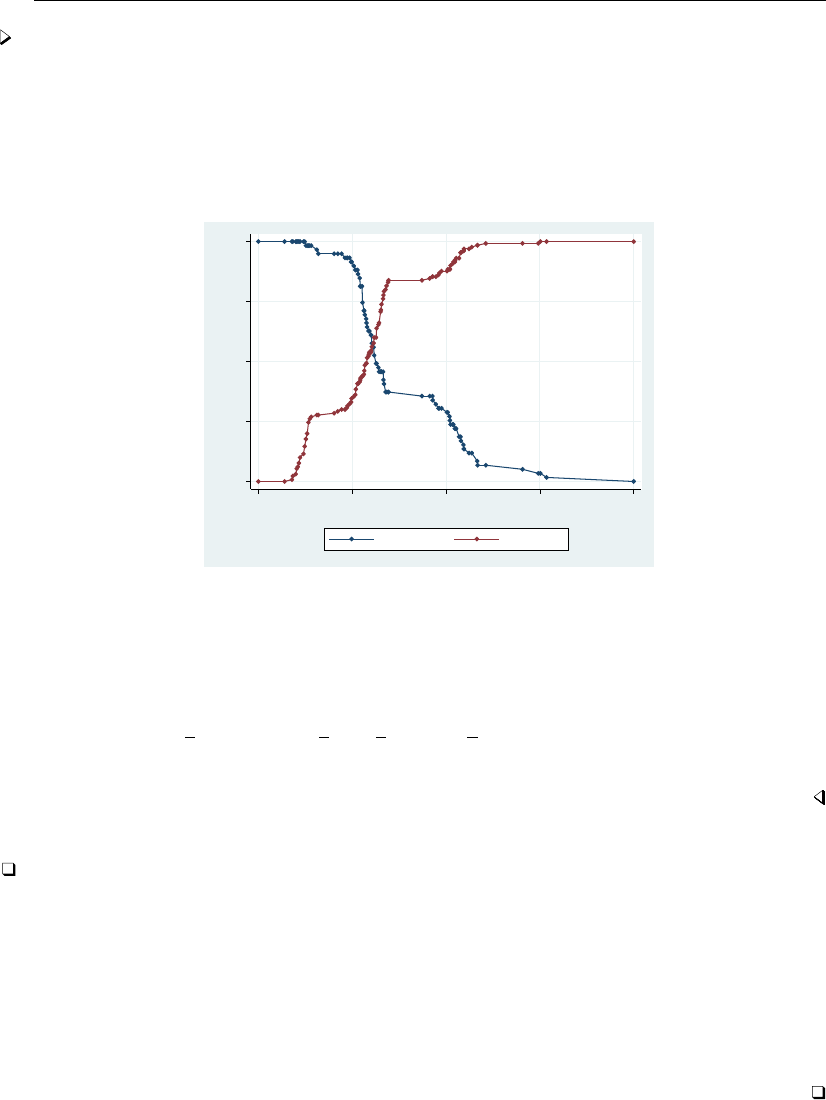
1136 lsens — Graph sensitivity and specificity versus probability cutoff
Example 1
We illustrate lsens after logistic; see [R]logistic.
. use http://www.stata-press.com/data/r13/lbw
(Hosmer & Lemeshow data)
. logistic low age i.race smoke ui
(output omitted )
. lsens
0.00 0.25 0.50 0.75 1.00
Sensitivity/Specificity
0.00 0.25 0.50 0.75 1.00
Probability cutoff
Sensitivity Specificity
lsens optionally creates new variables containing the probability cutoff, sensitivity, and specificity.
. lsens, genprob(p) gensens(sens) genspec(spec) nograph
The variables created will have M+2 distinct nonmissing values: one for each of the Mcovariate
patterns, one for c=0, and another for c=1. Values are recorded for p=0, for each of the
observed predicted probabilities, and for p=1. The total number of observations required to do this
can be fewer than N, the same as N, or N+1, or N+2. If more observations are added, they
are added at the end of the dataset and the values of the original variables are set to missing in the
added observations. How the values added align with existing observations is irrelevant.
Technical note
logistic,logit,probit, or ivprobit and lsens keep track of the estimation sample. If you
type, for instance, logistic . . . if x==1, then when you type lsens, the statistics will be calculated
on the x==1 subsample of the data automatically.
You should specify if or in with lsens only when you wish to produce graphs and calculate
statistics for a set of observations other than the estimation sample.
If the logistic model was fit with fweights, lsens properly accounts for the weights in its
calculations. You do not have to specify the weights when you run lsens. Weights should be specified
with lsens only when you wish to use a different set of weights.
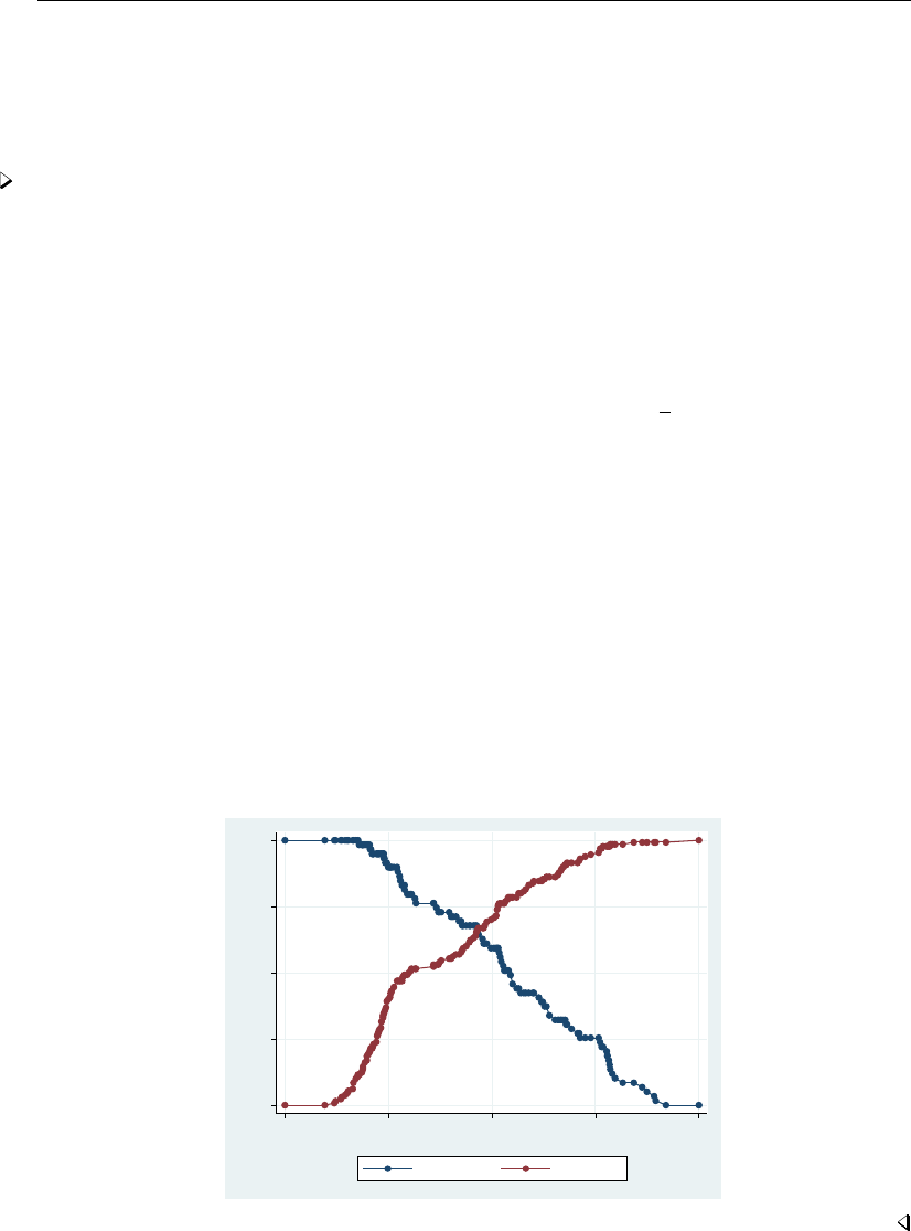
lsens — Graph sensitivity and specificity versus probability cutoff 1137
Models other than the last fitted model
By default, lsens uses the last model fit. You may also directly specify the model to lsens by
inputting a vector of coefficients with the beta() option and passing the name of the dependent
variable depvar to lsens.
Example 2
Suppose that someone publishes the following logistic model of low birthweight:
Pr(low =1) = F(−0.02 age −0.01 lwt +1.3 black +1.1 smoke +0.5 ptl +1.8 ht +0.8 ui +0.5)
where Fis the cumulative logistic distribution. These coefficients are not odds ratios; they are the
equivalent of what logit produces.
We can see whether this model fits our data. First we enter the coefficients as a row vector and
label its columns with the names of the independent variables plus cons for the constant (see
[P]matrix define and [P]matrix rownames).
. use http://www.stata-press.com/data/r13/lbw3, clear
(Hosmer & Lemeshow data)
. matrix input b = (-0.02, -.01, 1.3, 1.1, .5, 1.8, .8, .5)
. matrix colnames b = age lwt black smoke ptl ht ui _cons
We can use lroc (see [R]lroc) to examine the predictive ability of the model:
. lroc low, beta(b) nograph
Logistic model for low
number of observations = 189
area under ROC curve = 0.7275
The area under the curve indicates that this model does have some predictive power. We can obtain
a graph of sensitivity and specificity as a function of the cutoff probability by typing
. lsens low, beta(b)
0.00 0.25 0.50 0.75 1.00
Sensitivity/Specificity
0.00 0.25 0.50 0.75 1.00
Probability cutoff
Sensitivity Specificity

1138 lsens — Graph sensitivity and specificity versus probability cutoff
Stored results
lsens stores the following in r():
Scalars
r(N) number of observations
Methods and formulas
Let jindex observations and cbe the cutoff probability. Let pjbe the predicted probability of a
positive outcome and yjbe the actual outcome, which we will treat as 0 or 1, although Stata treats
it as 0 and non-0, excluding missing observations.
A prediction is classified as positive if pj≥cand otherwise is classified as negative. The
classification is correct if it is positive and yj=1 or if it is negative and yj=0.
Sensitivity is the fraction of yj=1 observations that are correctly classified. Specificity is the
percentage of yj=0 observations that are correctly classified.
Reference
Hosmer, D. W., Jr., S. A. Lemeshow, and R. X. Sturdivant. 2013. Applied Logistic Regression. 3rd ed. Hoboken,
NJ: Wiley.
Also see
[R]logistic — Logistic regression, reporting odds ratios
[R]logit — Logistic regression, reporting coefficients
[R]probit — Probit regression
[R]ivprobit — Probit model with continuous endogenous regressors
[R]lroc — Compute area under ROC curve and graph the curve
[R]estat classification — Classification statistics and table
[R]estat gof — Pearson or Hosmer–Lemeshow goodness-of-fit test
[R]roc — Receiver operating characteristic (ROC) analysis
[U] 20 Estimation and postestimation commands

Title
lv — Letter-value displays
Syntax Menu Description Options
Remarks and examples Stored results Methods and formulas References
Also see
Syntax
lv varlist if in , generate tail(#)
by is allowed; see [D] by.
Menu
Statistics >Summaries, tables, and tests >Distributional plots and tests >Letter-value display
Description
lv shows a letter-value display (Tukey 1977, 44–49; Hoaglin 1983) for each variable in varlist.
If no variables are specified, letter-value displays are shown for each numeric variable in the data.
Options
Main
generate adds four new variables to the data: mid, containing the midsummaries; spread,
containing the spreads; psigma, containing the pseudosigmas; and z2, containing the squared
values from a standard normal distribution corresponding to the particular letter value. If the
variables mid,spread,psigma, and z2 already exist, their contents are replaced. At most,
only the first 11 observations of each variable are used; the remaining observations contain missing.
If varlist specifies more than one variable, the newly created variables contain results for the last
variable specified. The generate option may not be used with the by prefix.
tail(#)indicates the inverse of the tail density through which letter values are to be displayed: 2
corresponds to the median (meaning half in each tail), 4 to the fourths (roughly the 25th and 75th
percentiles), 8 to the eighths, and so on. #may be specified as 4, 8, 16, 32, 64, 128, 256, 512, or
1,024 and defaults to a value of #that has corresponding depth just greater than 1. The default
is taken as 1,024 if the calculation results in a number larger than 1,024. Given the intelligent
default, this option is rarely specified.
Remarks and examples
Letter-value displays are a collection of observations drawn systematically from the data, focusing
especially on the tails rather than the middle of the distribution. The displays are called letter-value
displays because letters have been (almost arbitrarily) assigned to tail densities:
Letter Tail area Letter Tail area
M 1/2 B 1/64
F 1/4 A 1/128
E 1/8 Z 1/256
D 1/16 Y 1/512
C 1/32 X 1/1024
1139

1140 lv — Letter-value displays
Example 1
We have data on the mileage ratings of 74 automobiles. To obtain a letter-value display, we type
. use http://www.stata-press.com/data/r13/auto
(1978 Automobile Data)
. lv mpg
# 74 Mileage (mpg)
M 37.5 20 spread pseudosigma
F 19 18 21.5 25 7 5.216359
E 10 15 21.5 28 13 5.771728
D 5.5 14 22.25 30.5 16.5 5.576303
C 3 14 24.5 35 21 5.831039
B 2 12 23.5 35 23 5.732448
A 1.5 12 25 38 26 6.040635
1 12 26.5 41 29 6.16562
# below # above
inner fence 7.5 35.5 0 1
outer fence -3 46 0 0
The decimal points can be made to line up and thus the output made more readable by specifying
a display format for the variable; see [U] 12.5 Formats: Controlling how data are displayed.
. format mpg %9.2f
. lv mpg
# 74 Mileage (mpg)
M 37.5 20.00 spread pseudosigma
F 19 18.00 21.50 25.00 7.00 5.22
E 10 15.00 21.50 28.00 13.00 5.77
D 5.5 14.00 22.25 30.50 16.50 5.58
C 3 14.00 24.50 35.00 21.00 5.83
B 2 12.00 23.50 35.00 23.00 5.73
A 1.5 12.00 25.00 38.00 26.00 6.04
1 12.00 26.50 41.00 29.00 6.17
# below # above
inner fence 7.50 35.50 0 1
outer fence -3.00 46.00 0 0
At the top, the number of observations is indicated as 74. The first line shows the statistics associated
with M, the letter value that puts half the density in each tail, or the median. The median has depth
37.5 (that is, in the ordered data, M is 37.5 observations in from the extremes) and has value 20. The
next line shows the statistics associated with F or the fourths. The fourths have depth 19 (that is, in
the ordered data, the lower fourth is observation 19, and the upper fourth is observation 74 −19 +1),
and the values of the lower and upper fourths are 18 and 25. The number in the middle is the point
halfway between the fourths—called a midsummary. If the distribution were perfectly symmetric,
the midsummary would equal the median. The spread is the difference between the lower and upper
summaries (25 −18 =7). For fourths, half the data lie within a 7-mpg band. The pseudosigma is a
calculation of the standard deviation using only the lower and upper summaries and assuming that
the variable is normally distributed. If the data really were normally distributed, all the pseudosigmas
would be roughly equal.
After the letter values, the line labeled with depth 1 reports the minimum and maximum values.
Here the halfway point between the extremes is 26.5, which is greater than the median, indicating
that 41 is more extreme than 12, at least relative to the median. And with each letter value, the
midsummaries are increasing—our data are skewed. The pseudosigmas are also increasing, indicating

lv — Letter-value displays 1141
that the data are spreading out relative to a normal distribution, although, given the evident skewness,
this elongation may be an artifact of the skewness.
At the end is an attempt to identify outliers, although the points so identified are merely outside
some predetermined cutoff. Points outside the inner fence are called outside values or mild outliers.
Points outside the outer fence are called severe outliers. The inner fence is defined as (3/2)IQR and
the outer fence as 3IQR above and below the F summaries, where the interquartile range (IQR) is the
spread of the fourths.
Technical note
The form of the letter-value display has varied slightly with different authors. lv displays appear
as described by Hoaglin (1983) but as modified by Emerson and Stoto (1983), where they included the
midpoint of each of the spreads. This format was later adopted by Hoaglin (1985). If the distribution
is symmetric, the midpoints will all be roughly equal. On the other hand, if the midpoints vary
systematically, the distribution is skewed.
The pseudosigmas are obtained from the lower and upper summaries for each letter value. For
each letter value, they are the standard deviation a normal distribution would have if its spread for
the given letter value were to equal the observed spread. If the pseudosigmas are all roughly equal,
the data are said to have neutral elongation. If the pseudosigmas increase systematically, the data are
said to be more elongated than a normal, that is, have thicker tails. If the pseudosigmas decrease
systematically, the data are said to be less elongated than a normal, that is, have thinner tails.
Interpretation of the number of mild and severe outliers is more problematic. The following
discussion is drawn from Hamilton (1991):
Obviously, the presence of any such outliers does not rule out that the data have been drawn from
a normal distribution; in large datasets, there will most certainly be observations outside (3/2)IQR and
3IQR. Severe outliers, however, make up about two per million (0.0002%) of a normal population. In
samples, they lie far enough out to have substantial effects on means, standard deviations, and other
classical statistics. The 0.0002%, however, should be interpreted carefully; outliers appear more often
in small samples than one might expect from population proportions because of sampling variation in
estimated quartiles. Monte Carlo simulation by Hoaglin, Iglewicz, and Tukey (1986) obtained these
results on the percentages and numbers of outliers in random samples from a normal population:
percentage number
n any outliers severe any outliers severe
10 2.83 .362 .283 .0362
20 1.66 .074 .332 .0148
50 1.15 .011 .575 .0055
100 .95 .002 .95 .002
200 .79 .001 1.58 .002
300 .75 .001 2.25 .003
∞.70 .0002 ∞ ∞
Thus the presence of any severe outliers in samples of less than 300 is sufficient to reject normality.
Hoaglin, Iglewicz, and Tukey (1981) suggested the approximation 0.00698 +0.4/n for the fraction
of mild outliers in a sample of size nor, equivalently, 0.00698n+0.4 for the number of outliers.

1142 lv — Letter-value displays
Example 2
The generate option adds the mid,spread,psigma, and z2 variables to our data, making
possible many of the diagnostic graphs suggested by Hoaglin (1985).
. lv mpg, generate
(output omitted )
. list _mid _spread _psigma _z2 in 1/12
_mid _spread _psigma _z2
1. 20 . . .
2. 21.5 7 5.216359 .4501955
3. 21.5 13 5.771728 1.26828
4. 22.25 16.5 5.576303 2.188846
5. 24.5 21 5.831039 3.24255
6. 23.5 23 5.732448 4.024532
7. 25 26 6.040635 4.631499
8. . . . .
9. . . . .
10. . . . .
11. 26.5 29 6.16562 5.53073
12. . . . .
Observations 12 through the end are missing for these new variables. The definition of the observations
is always the same. The first observation contains the M summary; the second, the F; the third, the E; and
so on. Observation 11 always contains the summary for depth 1. Observations 8–10—corresponding
to letter values Z, Y, and X—contain missing because these statistics were not calculated. We have
only 74 observations, and their depth would be 1.
Hoaglin (1985) suggests graphing the midsummary against z2. If the distribution is not skewed,
the points in the resulting graph will be along a horizontal line:
. scatter _mid _z2
20 22 24 26
mpg midsummary
0 2 4 6
Z squared
The graph clearly indicates the skewness of the distribution. We might also graph psigma against
z2 to examine elongation.

lv — Letter-value displays 1143
Stored results
lv stores the following in r():
Scalars
r(N) number of observations r(u C) upper 32nd
r(min) minimum r(l B) lower 64th
r(max) maximum r(u B) upper 64th
r(median) median r(l A) lower 128th
r(l F) lower 4th r(u A) upper 128th
r(u F) upper 4th r(l Z) lower 256th
r(l E) lower 8th r(u Z) upper 256th
r(u E) upper 8th r(l Y) lower 512th
r(l D) lower 16th r(u Y) upper 512th
r(u D) upper 16th r(l X) lower 1024th
r(l C) lower 32nd r(u X) upper 1024th
The lower/upper 8ths, 16ths, . . . , 1024ths will be defined only if there are sufficient data.
Methods and formulas
Let Nbe the number of (nonmissing) observations on x, and let x(i)refer to the ordered data
when iis an integer. Define x(i+0.5) = (x(i)+x(i+1))/2; the median is defined as x{(N+1)/2}.
Define x[d]as the pair of numbers x(d)and x(N+1−d), where dis called the depth. Thus x[1]
refers to the minimum and maximum of the data. Define m= (N+1)/2 as the depth of the median,
f= (bmc+1)/2 as the depth of the fourths, e= (bfc+1)/2 as the depth of the eighths, and so
on. Depths are reported on the far left of the letter-value display. The corresponding fourths of the
data are x[f], the eighths are x[e], and so on. These values are reported inside the display. The middle
value is defined as the corresponding midpoint of x[·]. The spreads are defined as the difference in
x[·].
The corresponding point zion a standard normal distribution is obtained as (Hoaglin 1985,
456–457)
zi=(F−1(di−1/3)/(N+ 1/3)if di>1
F−10.695/(N+ 0.390)otherwise
where diis the depth of the letter value. The corresponding pseudosigma is obtained as the ratio of
the spread to −2zi(Hoaglin 1985, 431).
Define (Fl, Fu) = x[f]. The inner fence has cutoffs Fl−3
2(Fu−Fl)and Fu+3
2(Fu−Fl). The
outer fence has cutoffs Fl−3(Fu−Fl)and Fu+3(Fu−Fl).
The inner-fence values reported by lv are almost equal to those used by graph, box to identify
outside points. The only difference is that graph uses a slightly different definition of fourths, namely,
the 25th and 75th percentiles as defined by summarize; see [R]summarize.

1144 lv — Letter-value displays
References
Emerson, J. D., and M. A. Stoto. 1983. Transforming data. In Understanding Robust and Exploratory Data Analysis,
ed. D. C. Hoaglin, C. F. Mosteller, and J. W. Tukey, 97–128. New York: Wiley.
Fox, J. 1990. Describing univariate distributions. In Modern Methods of Data Analysis, ed. J. Fox and J. S. Long,
58–125. Newbury Park, CA: Sage.
Hamilton, L. C. 1991. sed4: Resistant normality check and outlier identification.Stata Technical Bulletin 3: 15–18.
Reprinted in Stata Technical Bulletin Reprints, vol. 1, pp. 86–90. College Station, TX: Stata Press.
Hoaglin, D. C. 1983. Letter values: A set of selected order statistics. In Understanding Robust and Exploratory Data
Analysis, ed. D. C. Hoaglin, C. F. Mosteller, and J. W. Tukey, 33–57. New York: Wiley.
. 1985. Using quantiles to study shape. In Exploring Data Tables, Trends, and Shapes, ed. D. C. Hoaglin, C. F.
Mosteller, and J. W. Tukey, 417–460. New York: Wiley.
Hoaglin, D. C., B. Iglewicz, and J. W. Tukey. 1981. Small-sample performance of a resistant rule for outlier detection.
In 1980 Proceedings of the Statistical Computing Section. Washington, DC: American Statistical Association.
. 1986. Performance of some resistant rules for outlier labeling. Journal of the American Statistical Association
81: 991–999.
Tukey, J. W. 1977. Exploratory Data Analysis. Reading, MA: Addison–Wesley.
Also see
[R]diagnostic plots — Distributional diagnostic plots
[R]stem — Stem-and-leaf displays
[R]summarize — Summary statistics

Title
margins — Marginal means, predictive margins, and marginal effects
Syntax Menu Description Options
Remarks and examples Stored results Methods and formulas References
Also see
Syntax
margins marginlist if in weight ,response options options
where marginlist is a list of factor variables or interactions that appear in the current estimation results.
The variables may be typed with or without the i. prefix, and you may use any factor-variable syntax:
. margins i.sex i.group i.sex#i.group
. margins sex group sex#i.group
. margins sex##group
response options Description
Main
predict(pred opt)estimate margins for predict, pred opt
expression(pnl exp)estimate margins for pnl exp
dydx(varlist)estimate marginal effect of variables in varlist
eyex(varlist)estimate elasticities of variables in varlist
dyex(varlist)estimate semielasticity—d(y)/d(lnx)
eydx(varlist)estimate semielasticity—d(lny)/d(x)
continuous treat factor-level indicators as continuous
options Description
Main
grand add the overall margin; default if no marginlist
At
at(atspec)estimate margins at specified values of covariates
atmeans estimate margins at the means of covariates
asbalanced treat all factor variables as balanced
if/in/over
over(varlist)estimate margins at unique values of varlist
subpop(subspec)estimate margins for subpopulation
Within
within(varlist)estimate margins at unique values of the nesting factors in varlist
Contrast
contrast options any options documented in [R]margins, contrast
Pairwise comparisons
pwcompare options any options documented in [R]margins, pwcompare
1145

1146 margins — Marginal means, predictive margins, and marginal effects
SE
vce(delta) estimate SEs using delta method; the default
vce(unconditional) estimate SEs allowing for sampling of covariates
nose do not estimate SEs
Advanced
noweights ignore weights specified in estimation
noesample do not restrict margins to the estimation sample
emptycells(empspec)treatment of empty cells for balanced factors
estimtolerance(tol)specify numerical tolerance used to determine estimable functions;
default is estimtolerance(1e-5)
noestimcheck suppress estimability checks
force estimate margins despite potential problems
chainrule use the chain rule when computing derivatives
nochainrule do not use the chain rule
Reporting
level(#)set confidence level; default is level(95)
mcompare(method)adjust for multiple comparisons; default is mcompare(noadjust)
noatlegend suppress legend of fixed covariate values
post post margins and their VCE as estimation results
display options control columns and column formats, row spacing, line width and
factor-variable labeling
df(#)use tdistribution with #degrees of freedom for computing p-values
and confidence intervals
method Description
noadjust do not adjust for multiple comparisons; the default
bonferroni adjustall Bonferroni’s method; adjust across all terms
sidak adjustall ˇ
Sid´
ak’s method; adjust across all terms
scheffe Scheff´
e’s method
Time-series operators are allowed if they were used in the estimation.
See at() under Options for a description of atspec.
fweights, aweights, iweights, and pweights are allowed; see [U] 11.1.6 weight.
df(#)does not appear in the dialog box.
Menu
Statistics >Postestimation >Marginal means and predictive margins
Statistics >Postestimation >Marginal effects
Description
Margins are statistics calculated from predictions of a previously fit model at fixed values of some
covariates and averaging or otherwise integrating over the remaining covariates.

margins — Marginal means, predictive margins, and marginal effects 1147
The margins command estimates margins of responses for specified values of covariates and
presents the results as a table.
Capabilities include estimated marginal means, least-squares means, average and conditional
marginal and partial effects (which may be reported as derivatives or as elasticities), average and
conditional adjusted predictions, and predictive margins.
Options
Warning: The option descriptions are brief and use jargon. Skip to Remarks and examples if you are
reading about margins for the first time.
Main
predict(pred opt)and expression(pnl exp)are mutually exclusive; they specify the response. If
neither is specified, the response will be the default prediction that would be produced by predict
after the underlying estimation command.
predict(pred opt)specifies the option(s) to be specified with the predict command to produce
the variable that will be used as the response. After estimation by logistic, you could specify
predict(xb) to obtain linear predictions rather than the predict command’s default, the
probabilities.
expression(pnl exp)specifies the response as an expression. See [R]predictnl for a
full description of pnl exp. After estimation by logistic, you might specify expres-
sion(exp(predict(xb))) to use relative odds rather than probabilities as the response.
For examples, see Example 12: Margins of a specified expression.
dydx(varlist),eyex(varlist),dyex(varlist), and eydx(varlist)request that margins report deriva-
tives of the response with respect to varlist rather than on the response itself. eyex(),dyex(),
and eydx() report derivatives as elasticities; see Expressing derivatives as elasticities.
continuous is relevant only when one of dydx() or eydx() is also specified. It specifies that the
levels of factor variables be treated as continuous; see Derivatives versus discrete differences. This
option is implied if there is a single-level factor variable specified in dydx() or eydx().
grand specifies that the overall margin be reported. grand is assumed when marginlist is empty.
At
at(atspec)specifies values for covariates to be treated as fixed.
at(age=20) fixes covariate age to the value specified. at() may be used to fix continuous or
factor covariates.
at(age=20 sex=1) simultaneously fixes covariates age and sex at the values specified.
at(age=(20 30 40 50)) fixes age first at 20, then at 30, . . . .margins produces separate results
for each specified value.
at(age=(20(10)50)) does the same as at(age=(20 30 40 50)); that is, you may specify a
numlist.
at((mean) age (median) distance) fixes the covariates at the summary statistics specified.
at((p25) all) fixes all covariates at their 25th percentile values. See Syntax of at() for the
full list of summary-statistic modifiers.
at((mean) all (median) x x2=1.2 z=(1 2 3)) is read from left to right, with latter specifiers
overriding former ones. Thus all covariates are fixed at their means except for x(fixed at its
median), x2 (fixed at 1.2), and z(fixed first at 1, then at 2, and finally at 3).

1148 margins — Marginal means, predictive margins, and marginal effects
at((means) all (asobserved) x2) is a convenient way to set all covariates except x2 to the
mean.
Multiple at() options can be specified, and each will produce a different set of margins.
See Syntax of at() for more information.
atmeans specifies that covariates be fixed at their means and is shorthand for at((mean) all).
atmeans differs from at((mean) all) in that atmeans will affect subsequent at() options.
For instance,
. margins . . . , atmeans at((p25) x) at((p75) x)
produces two sets of margins with both sets evaluated at the means of all covariates except x.
asbalanced is shorthand for at((asbalanced) factor) and specifies that factor covariates be
evaluated as though there were an equal number of observations in each level; see Obtaining margins
as though the data were balanced.asbalanced differs from at((asbalanced) factor) in
that asbalanced will affect subsequent at() options in the same way as atmeans does.
if/in/over
over(varlist)specifies that separate sets of margins be estimated for the groups defined by varlist. The
variables in varlist must contain nonnegative integer values. The variables need not be covariates
in your model. When over() is combined with the vce(unconditional) option, each group is
treated as a subpopulation; see [SVY]subpopulation estimation.
subpop(varname if )is intended for use with the vce(unconditional) option. It specifies
that margins be estimated for the single subpopulation identified by the indicator variable or by
the if expression or by both. Zero indicates that the observation be excluded; nonzero, that it be
included; and missing value, that it be treated as outside of the population (and so ignored). See
[SVY]subpopulation estimation for why subpop() is preferred to if expressions and in ranges
when also using vce(unconditional). If subpop() is used without vce(unconditional), it
is treated merely as an additional if qualifier.
Within
within(varlist)allows for nested designs. varlist contains the nesting variable(s) over which margins
are to be estimated. See Obtaining margins with nested designs. As with over(varlist), when
within(varlist)is combined with vce(unconditional), each level of the variables in varlist
is treated as a subpopulation.
Contrast
contrast options are any of the options documented in [R]margins, contrast.
Pairwise comparisons
pwcompare options are any of the options documented in [R]margins, pwcompare.
SE
vce(delta) and vce(unconditional) specify how the VCE and, correspondingly, standard errors
are calculated.
vce(delta) is the default. The delta method is applied to the formula for the response and the
VCE of the estimation command. This method assumes that values of the covariates used to
calculate the response are given or, if all covariates are not fixed using at(), that the data are
given.

margins — Marginal means, predictive margins, and marginal effects 1149
vce(unconditional) specifies that the covariates that are not fixed be treated in a way that
accounts for their having been sampled. The VCE is estimated using the linearization method.
This method allows for heteroskedasticity or other violations of distributional assumptions
and allows for correlation among the observations in the same manner as vce(robust) and
vce(cluster . . . ), which may have been specified with the estimation command. This method
also accounts for complex survey designs if the data are svyset. See Obtaining margins with
survey data and representative samples. When you use complex survey data, this method
requires that the linearized variance estimation method be used for the model. See [SVY]svy
postestimation for an example of margins with replication-based methods.
nose suppresses calculation of the VCE and standard errors. See Requirements for model specification
for an example of the use of this option.
Advanced
noweights specifies that any weights specified on the previous estimation command be ignored by
margins. By default, margins uses the weights specified on the estimator to average responses and
to compute summary statistics. If weights are specified on the margins command, they override
previously specified weights, making it unnecessary to specify noweights. The noweights option
is not allowed after svy: estimation when the vce(unconditional) option is specified.
noesample specifies that margins not restrict its computations to the estimation sample used by the
previous estimation command. See Example 15: Margins evaluated out of sample.
With the default delta-method VCE,noesample margins may be estimated on samples other than
the estimation sample; such results are valid under the assumption that the data used are treated
as being given.
You can specify noesample and vce(unconditional) together, but if you do, you should be
sure that the data in memory correspond to the original e(sample). To show that you understand
that, you must also specify the force option. Be aware that making the vce(unconditional)
calculation on a sample different from the estimation sample would be equivalent to estimating
the coefficients on one set of data and computing the scores used by the linearization on another
set; see [P]robust.
emptycells(strict) and emptycells(reweight) are relevant only when the asbalanced option
is also specified. emptycells() specifies how empty cells are handled in interactions involving
factor variables that are being treated as balanced; see Obtaining margins as though the data were
balanced.
emptycells(strict) is the default; it specifies that margins involving empty cells be treated as
not estimable.
emptycells(reweight) specifies that the effects of the observed cells be increased to accom-
modate any missing cells. This makes the margin estimable but changes its interpretation.
emptycells(reweight) is implied when the within() option is specified.
estimtolerance(tol)specifies the numerical tolerance used to determine estimable functions. The
default is estimtolerance(1e-5).
A linear combination of the model coefficients zis found to be not estimable if
mreldif(z,z×H)>tol
where His defined in Methods and formulas.

1150 margins — Marginal means, predictive margins, and marginal effects
noestimcheck specifies that margins not check for estimability. By default, the requested margins
are checked and those found not estimable are reported as such. Nonestimability is usually caused
by empty cells. If noestimcheck is specified, estimates are computed in the usual way and
reported even though the resulting estimates are manipulable, which is to say they can differ across
equivalent models having different parameterizations. See Estimability of margins.
force instructs margins to proceed in some situations where it would otherwise issue an error
message because of apparent violations of assumptions. Do not be casual about specifying force.
You need to understand and fully evaluate the statistical issues. For an example of the use of
force, see Using margins after the estimates use command.
chainrule and nochainrule specify whether margins uses the chain rule when numerically
computing derivatives. You need not specify these options when using margins after any official
Stata estimator; margins will choose the appropriate method automatically.
Specify nochainrule after estimation by a user-written command. We recommend using nochain-
rule, even though chainrule is usually safe and is always faster. nochainrule is safer because
it makes no assumptions about how the parameters and covariates join to form the response.
nochainrule is implied when the expression() option is specified.
Reporting
level(#)specifies the confidence level, as a percentage, for confidence intervals. The default is
level(95) or as set by set level; see [U] 20.7 Specifying the width of confidence intervals.
mcompare(method)specifies the method for computing p-values and confidence intervals that account
for multiple comparisons within a factor-variable term.
Most methods adjust the comparisonwise error rate, αc, to achieve a prespecified experimentwise
error rate, αe.
mcompare(noadjust) is the default; it specifies no adjustment.
αc=αe
mcompare(bonferroni) adjusts the comparisonwise error rate based on the upper limit of the
Bonferroni inequality
αe≤mαc
where mis the number of comparisons within the term.
The adjusted comparisonwise error rate is
αc=αe/m
mcompare(sidak) adjusts the comparisonwise error rate based on the upper limit of the probability
inequality
αe≤1−(1 −αc)m
where mis the number of comparisons within the term.
The adjusted comparisonwise error rate is
αc= 1 −(1 −αe)1/m
This adjustment is exact when the mcomparisons are independent.
mcompare(scheffe) controls the experimentwise error rate using the For χ2distribution with
degrees of freedom equal to the rank of the term.

margins — Marginal means, predictive margins, and marginal effects 1151
mcompare(method adjustall) specifies that the multiple-comparison adjustments count all
comparisons across all terms rather than performing multiple comparisons term by term. This
leads to more conservative adjustments when multiple variables or terms are specified in
marginslist. This option is compatible only with the bonferroni and sidak methods.
noatlegend specifies that the legend showing the fixed values of covariates be suppressed.
post causes margins to behave like a Stata estimation (e-class) command. margins posts the vector
of estimated margins along with the estimated variance–covariance matrix to e(), so you can treat
the estimated margins just as you would results from any other estimation command. For example,
you could use test to perform simultaneous tests of hypotheses on the margins, or you could use
lincom to create linear combinations. See Example 10: Testing margins—contrasts of margins.
display options:noci,nopvalues,vsquish,nofvlabel,fvwrap(#),fvwrapon(style),
cformat(%fmt),pformat(% fmt),sformat(% fmt), and nolstretch.
noci suppresses confidence intervals from being reported in the coefficient table.
nopvalues suppresses p-values and their test statistics from being reported in the coefficient table.
vsquish specifies that the blank space separating factor-variable terms or time-series–operated
variables from other variables in the model be suppressed.
nofvlabel displays factor-variable level values rather than attached value labels. This option
overrides the fvlabel setting; see [R]set showbaselevels.
fvwrap(#)allows long value labels to wrap the first #lines in the coefficient table. This option
overrides the fvwrap setting; see [R]set showbaselevels.
fvwrapon(style)specifies whether value labels that wrap will break at word boundaries or break
based on available space.
fvwrapon(word), the default, specifies that value labels break at word boundaries.
fvwrapon(width) specifies that value labels break based on available space.
This option overrides the fvwrapon setting; see [R]set showbaselevels.
cformat(% fmt)specifies how to format margins, standard errors, and confidence limits in the
table of estimated margins.
pformat(% fmt)specifies how to format p-values in the table of estimated margins.
sformat(% fmt)specifies how to format test statistics in the table of estimated margins.
nolstretch specifies that the width of the table of estimated margins not be automatically widened
to accommodate longer variable names. The default, lstretch, is to automatically widen the
table of estimated margins up to the width of the Results window. To change the default, use
set lstretch off.nolstretch is not shown in the dialog box.
The following option is available with margins but is not shown in the dialog box:
df(#)specifies that the tdistribution with #degrees of freedom be used for computing p-values and
confidence intervals. The default typically is to use the standard normal distribution. However, if
the estimation command computes the residual degrees of freedom (e(df r)) and predict(xb)
is specified with margins, the default is to use the tdistribution with e(df r) degrees of freedom.

1152 margins — Marginal means, predictive margins, and marginal effects
Remarks and examples
Remarks are presented under the following headings:
Introduction
Obtaining margins of responses
Example 1: A simple case after regress
Example 2: A simple case after logistic
Example 3: Average response versus response at average
Example 4: Multiple margins from one command
Example 5: Margins with interaction terms
Example 6: Margins with continuous variables
Example 7: Margins of continuous variables
Example 8: Margins of interactions
Example 9: Decomposing margins
Example 10: Testing margins—contrasts of margins
Example 11: Margins of a specified prediction
Example 12: Margins of a specified expression
Example 13: Margins with multiple outcomes (responses)
Example 14: Margins with multiple equations
Example 15: Margins evaluated out of sample
Obtaining margins of derivatives of responses (a.k.a. marginal effects)
Do not specify marginlist when you mean over()
Use at() freely, especially with continuous variables
Expressing derivatives as elasticities
Derivatives versus discrete differences
Example 16: Average marginal effect (partial effects)
Example 17: Average marginal effect of all covariates
Example 18: Evaluating marginal effects over the response surface
Obtaining margins with survey data and representative samples
Example 19: Inferences for populations, margins of response
Example 20: Inferences for populations, marginal effects
Example 21: Inferences for populations with svyset data
Standardizing margins
Obtaining margins as though the data were balanced
Balancing using asbalanced
Balancing by standardization
Balancing nonlinear responses
Treating a subset of covariates as balanced
Using fvset design
Balancing in the presence of empty cells
Obtaining margins with nested designs
Introduction
Margins with nested designs as though the data were balanced
Coding of nested designs
Special topics
Requirements for model specification
Estimability of margins
Manipulability of tests
Using margins after the estimates use command
Syntax of at()
Estimation commands that may be used with margins
Video examples
Glossary
Introduction
margins is a postestimation command, a command for use after you have fit a model using an
estimation command such as regress or logistic, or using almost any other estimation command.
margins estimates and reports margins of responses and margins of derivatives of responses, also
known as marginal effects. A margin is a statistic based on a fitted model in which some of or all the

margins — Marginal means, predictive margins, and marginal effects 1153
covariates are fixed. Marginal effects are changes in the response for change in a covariate, which
can be reported as a derivative, elasticity, or semielasticity.
For a brief overview of margins, see Williams (2012).
Obtaining margins of responses
What we call margins of responses are also known as predictive margins, adjusted predictions, and
recycled predictions. When applied to balanced data, margins of responses are also called estimated
marginal means and least-squares means.
A margin is a statistic based on a fitted model calculated over a dataset in which some of or
all the covariates are fixed at values different from what they really are. For instance, after a linear
regression fit on males and females, the marginal mean (margin of mean) for males is the predicted
mean of the dependent variable, where every observation is treated as if it represents a male; thus those
observations that in fact do represent males are included, as well as those observations that represent
females. The marginal mean for female would be similarly obtained by treating all observations as
if they represented females.
In making the calculation, sex is treated as male or female everywhere it appears in the model.
The model might be
. regress y age bp i.sex sex#c.age sex#c.bp
and then, in making the marginal calculation of the mean for males and females, margins not only
accounts for the direct effect of i.sex but also for the indirect effects of sex#c.age and sex#c.bp.
The response being margined can be any statistic produced by [R]predict, or any expression of
those statistics.
Standard errors are obtained by the delta method, at least by default. The delta method assumes
that the values at which the covariates are evaluated to obtain the marginal responses are fixed.
When your sample represents a population, whether you are using svy or not (see [SVY]svy), you
can specify margins’vce(unconditional) option and margins will produce standard errors that
account for the sampling variability of the covariates. Some researchers reserve the term predictive
margins to describe this.
The best way to understand margins is to see some examples. You can run the following examples
yourself if you type
. use http://www.stata-press.com/data/r13/margex
(Artificial data for margins)

1154 margins — Marginal means, predictive margins, and marginal effects
Example 1: A simple case after regress
. regress y i.sex i.group
(output omitted )
. margins sex
Predictive margins Number of obs = 3000
Model VCE : OLS
Expression : Linear prediction, predict()
Delta-method
Margin Std. Err. t P>|t| [95% Conf. Interval]
sex
male 60.56034 .5781782 104.74 0.000 59.42668 61.69401
female 78.88236 .5772578 136.65 0.000 77.7505 80.01422
The numbers reported in the “Margin” column are average values of y. Based on a linear regression
of yon sex and group, 60.6 would be the average value of yif everyone in the data were treated
as if they were male, and 78.9 would be the average value if everyone were treated as if they were
female.
Example 2: A simple case after logistic
margins may be used after almost any estimation command.
. logistic outcome i.sex i.group
(output omitted )
. margins sex
Predictive margins Number of obs = 3000
Model VCE : OIM
Expression : Pr(outcome), predict()
Delta-method
Margin Std. Err. z P>|z| [95% Conf. Interval]
sex
male .1286796 .0111424 11.55 0.000 .106841 .1505182
female .1905087 .0089719 21.23 0.000 .1729241 .2080933
The numbers reported in the “Margin” column are average predicted probabilities. Based on a
logistic regression of outcome on sex and group, 0.13 would be the average probability of outcome
if everyone in the data were treated as if they were male, and 0.19 would be the average probability
if everyone were treated as if they were female.
margins reports average values after regress and average probabilities after logistic. By
default, margins makes tables of whatever it is that predict (see [R]predict) predicts by default.
Alternatively, margins can make tables of anything that predict can produce if you use margins’
predict() option; see Example 11: Margins of a specified prediction.

margins — Marginal means, predictive margins, and marginal effects 1155
Example 3: Average response versus response at average
In example 2,margins reported average probabilities of outcome for sex =0 and sex =1.
If we instead wanted the predicted probabilities evaluated at the mean of the covariates, we would
specify margins’atmeans option. We previously typed
. logistic outcome i.sex i.group
(output omitted )
. margins sex
(output omitted )
and now we type
. margins sex, atmeans
Adjusted predictions Number of obs = 3000
Model VCE : OIM
Expression : Pr(outcome), predict()
at : 0.sex = .4993333 (mean)
1.sex = .5006667 (mean)
1.group = .3996667 (mean)
2.group = .3726667 (mean)
3.group = .2276667 (mean)
Delta-method
Margin Std. Err. z P>|z| [95% Conf. Interval]
sex
male .0966105 .0089561 10.79 0.000 .0790569 .1141641
female .1508362 .0118064 12.78 0.000 .127696 .1739764
The prediction at the average of the covariates is different from the average of the predictions.
The first is the expected probability of a person with average characteristics, a person who, in another
problem, might be 3/4 married and have 1.2 children. The second is the average of the probability
among actual persons in the data.
When you specify atmeans or any other at option, margins reports the values used for the
covariates in the legend above the table. margins lists the values for all the covariates, including
values it may not use, in the results that follow. In this example, margins reported means for sex
even though those means were not used. They were not used because we asked for the margins of
sex, so sex was fixed first at 0 and then at 1.
If you wish to suppress this legend, specify the nolegend option.
Example 4: Multiple margins from one command
More than one margin can be reported by just one margins command. You can type
. margins sex group
and doing that is equivalent in terms of the output to typing
. margins sex
. margins group
When multiple margins are requested on the same command, each is estimated separately. There
is, however, a difference when you also specify margins’post option. Then the variance–covariance
matrix for all margins requested is posted, and that is what allows you to test equality of margins,
etc. Testing equality of margins is covered in Example 10: Testing margins—contrasts of margins.

1156 margins — Marginal means, predictive margins, and marginal effects
In any case, below we request margins for sex and for group.
. margins sex group
Predictive margins Number of obs = 3000
Model VCE : OIM
Expression : Pr(outcome), predict()
Delta-method
Margin Std. Err. z P>|z| [95% Conf. Interval]
sex
male .1286796 .0111424 11.55 0.000 .106841 .1505182
female .1905087 .0089719 21.23 0.000 .1729241 .2080933
group
1 .2826207 .0146234 19.33 0.000 .2539593 .311282
2 .1074814 .0094901 11.33 0.000 .0888812 .1260817
3 .0291065 .0073417 3.96 0.000 .0147169 .043496
Example 5: Margins with interaction terms
The estimation command on which margins bases its calculations may contain interaction terms,
such as an interaction of sex and group:
. logistic outcome i.sex i.group sex#group
(output omitted )
. margins sex group
Predictive margins Number of obs = 3000
Model VCE : OIM
Expression : Pr(outcome), predict()
Delta-method
Margin Std. Err. z P>|z| [95% Conf. Interval]
sex
male .1561738 .0132774 11.76 0.000 .1301506 .182197
female .1983749 .0101546 19.54 0.000 .1784723 .2182776
group
1 .3211001 .0176403 18.20 0.000 .2865257 .3556744
2 .1152127 .0099854 11.54 0.000 .0956417 .1347838
3 .0265018 .0109802 2.41 0.016 .0049811 .0480226
We fit the model by typing logistic outcome i.sex i.group sex#group, but the meaning
would have been the same had we typed logistic outcome sex##group.
As mentioned in example 4, the results for sex and the results for group are calculated independently,
and we would have obtained the same results had we typed margins sex followed by margins
group.
The margin for male (sex =0) is 0.16. The probability 0.16 is the average probability if everyone
in the data were treated as if sex =0, including sex =0 in the main effect and sex =0 in the
interaction of sex with group.
Had we specified margins sex, atmeans, we would have obtained not average probabilities but
the probabilities evaluated at the average. Rather than obtaining 0.16, we would have obtained 0.10

margins — Marginal means, predictive margins, and marginal effects 1157
for sex =0. The 0.10 is calculated by taking the fitted model, plugging in sex =0 everywhere, and
plugging in the average value of the group indicator variables everywhere they are used. That is, rather
than treating the group indicators as being (1,0,0), (0,1,0), or (0,0,1) depending on observation, the
group indicators are treated as being (0.40,0.37,0.23), which are the average values of group =1,
group =2, and group =3.
Example 6: Margins with continuous variables
To the above example, we will add the continuous covariate age to the model and then rerun
margins sex group.
. logistic outcome i.sex i.group sex#group age
(output omitted )
. margins sex group
Predictive margins Number of obs = 3000
Model VCE : OIM
Expression : Pr(outcome), predict()
Delta-method
Margin Std. Err. z P>|z| [95% Conf. Interval]
sex
male .1600644 .0125653 12.74 0.000 .1354368 .184692
female .1966902 .0100043 19.66 0.000 .1770821 .2162983
group
1 .2251302 .0123233 18.27 0.000 .200977 .2492834
2 .150603 .0116505 12.93 0.000 .1277685 .1734376
3 .0736157 .0337256 2.18 0.029 .0075147 .1397167
Compared with the results presented in example 5, results for sex change little, but results for
groups 1 and 3 change markedly. The tables differ because now we are adjusting for the continuous
covariate age, as well as for sex and group.
We will continue examining interactions in example 8. Because we have added a continuous
variable, let’s take a detour to explain how to obtain margins for continuous variables and to explain
their interpretation.
Example 7: Margins of continuous variables
Continuing with our example of
. logistic outcome i.sex i.group sex#group age
let’s examine the continuous covariate age.

1158 margins — Marginal means, predictive margins, and marginal effects
You are not allowed to type margins age; doing that will produce an error:
. margins age
‘age’ not found in list of covariates
r(322);
The message “‘age’ not found in list of covariates” is margins’ way of saying, “Yes, age might
be in the model, but if it is, it is not included as a factor variable; it is in as a continuous variable.”
Sometimes, Stata is overly terse. margins might also say that because age is continuous there are
an infinite number of values at which it could evaluate the margins. At what value(s) should age be
fixed? margins requires more guidance with continuous covariates. We can provide that guidance
by using the at() option and typing
. margins, at(age=40)
To understand why that yields the desired result, let us tell you that if you were to type
. margins
margins would report the overall margin—the margin that holds nothing constant. Because our model
is logistic, the average value of the predicted probabilities would be reported. The at() option fixes
one or more covariates to the value(s) specified and can be used with both factor and continuous
variables. Thus, if you typed margins, at(age=40), then margins would average over the data
the responses for everybody, setting age=40. Here is what happens when you type that:
. margins, at(age=40)
Predictive margins Number of obs = 3000
Model VCE : OIM
Expression : Pr(outcome), predict()
at : age = 40
Delta-method
Margin Std. Err. z P>|z| [95% Conf. Interval]
_cons .1133603 .0070731 16.03 0.000 .0994972 .1272234
Reported is the margin for age =40, adjusted for the other covariates in our model.
If we wanted to obtain the margins for age 30, 35, 40, 45, and 50, we could type
. margins, at(age=(30 35 40 45 50))
or, equivalently,
. margins, at(age=(30(5)50))
Example 8: Margins of interactions
Our model is
. logistic outcome i.sex i.group sex#group age

margins — Marginal means, predictive margins, and marginal effects 1159
We can obtain the margins of all possible combinations of the levels of sex and the levels of
group by typing
. margins sex#group
Predictive margins Number of obs = 3000
Model VCE : OIM
Expression : Pr(outcome), predict()
Delta-method
Margin Std. Err. z P>|z| [95% Conf. Interval]
sex#group
male#1 .2379605 .0237178 10.03 0.000 .1914745 .2844465
male#2 .0658294 .0105278 6.25 0.000 .0451953 .0864636
male#3 .0538001 .0136561 3.94 0.000 .0270347 .0805656
female#1 .2158632 .0112968 19.11 0.000 .1937218 .2380045
female#2 .2054406 .0183486 11.20 0.000 .1694781 .2414032
female#3 .085448 .0533914 1.60 0.110 -.0191973 .1900932
The first line in the table reports the marginal probability for sex =0 (male) and group =1. That
is, it reports the estimated probability if everyone in the data were treated as if they were sex =0
and group =1.
Also reported are all the other combinations of sex and group.
By the way, we could have typed margins sex#group even if our fitted model did not include
sex#group. Estimation is one thing, and asking questions about the nature of the estimates is another.
margins does, however, require that i.sex and i.group appear somewhere in the model, because
fixing a value outside the model would just produce the grand margin, and you can separately ask
for that if you want it by typing margins without arguments.
Example 9: Decomposing margins
We have the model
. logistic outcome i.sex i.group sex#group age
In example 6, we typed margins sex and obtained 0.160 for males and 0.197 for females. We
are going to decompose each of those numbers. Let us explain:
1. The margin for males, 0.160, treats everyone as if they were male, and that amounts to
simultaneously
1a. treating males as males and
1b. treating females as males.
2. The margin for females, 0.197, treats everyone as if they were female, and that amounts to
simultaneously
2a. treating males as females and
2b. treating females as females.
The margins 1a and 1b are the decomposition of 1, and the margins 2a and 2b are the decomposition
of 2.
We could obtain 1a and 2a by typing
. margins if sex==0, at(sex=(0 1))

1160 margins — Marginal means, predictive margins, and marginal effects
because the qualifier if sex==0 would restrict margins to running on only the males. Similarly, we
could obtain 1b and 2b by typing
. margins if sex==1, at(sex=(0 1))
We run these examples below:
. margins if sex==0, at(sex=(0 1))
Predictive margins Number of obs = 1498
Model VCE : OIM
Expression : Pr(outcome), predict()
1._at : sex = 0
2._at : sex = 1
Delta-method
Margin Std. Err. z P>|z| [95% Conf. Interval]
_at
1 .0794393 .0062147 12.78 0.000 .0672586 .0916199
2 .1335584 .0127351 10.49 0.000 .1085981 .1585187
. margins if sex==1, at(sex=(0 1))
Predictive margins Number of obs = 1502
Model VCE : OIM
Expression : Pr(outcome), predict()
1._at : sex = 0
2._at : sex = 1
Delta-method
Margin Std. Err. z P>|z| [95% Conf. Interval]
_at
1 .2404749 .0199709 12.04 0.000 .2013326 .2796171
2 .2596538 .0104756 24.79 0.000 .2391219 .2801857
Putting together the results from example 6 and the results above, we have
Margin treating everybody as themself 0.170
Margin treating everybody as male 0.160
Margin treating male as male 0.079
Margin treating female as male 0.240
Margin treating everybody as female 0.197
Margin treating male as female 0.134
Margin treating female as female 0.260
Example 10: Testing margins—contrasts of margins
Continuing with the previous example, it would be interesting to test the equality of 2b and 1b,
to test whether the average probability of a positive outcome for females treated as females is equal
to that for females treated as males. That test would be different from testing the overall significance
of sex in our model. The test performed on our model would be a test of whether the probability
of a positive outcome differs between males and females when they have equal values of the other
covariates. The test of equality of margins is a test of whether the average probabilities differ given
the different pattern of values of the other covariates that the two sexes have in our data.

margins — Marginal means, predictive margins, and marginal effects 1161
We can also perform such tests by treating the results from margins as estimation results. There
are three steps required to perform tests on margins. First, you must arrange it so that all the margins
of interest are reported by just one margins command. Second, you must specify margins’post
option. Third, you perform the test with the test command.
Such tests and comparisons can be readily performed by contrasting margins; see [R]margins,
contrast. Also see Contrasts of margins—effects (discrete marginal effects) in [R]marginsplot.
In the previous example, we used two commands to obtain our results, namely,
. margins if sex==0, at(sex=(0 1))
. margins if sex==1, at(sex=(0 1))
We could, however, have obtained the same results by typing just one command:
. margins, over(sex) at(sex=(0 1))
Performing margins, over(sex) first restricts the sample to sex==0 and then restricts it to
sex==1, and that is equivalent to the two different if conditions that we specified before.
To test whether females treated as females is equal to females treated as males, we will need to
type
. margins, over(sex) at(sex=(0 1)) post
. test _b[2._at#1.sex] = _b[1._at#1.sex]
We admit that the second command may seem to have come out of nowhere. When we specify
post on the margins command, margins behaves as if it were an estimation command, which
means that 1) it posts its estimates and full VCE to e(), 2) it gains the ability to replay results just
as any estimation command can, and 3) it gains access to the standard postestimation commands.
Item 3 explains why we could use test. We learned that we wanted to test b[2. at#1.sex] and
b[1. at#1.sex] by replaying the estimation results, but this time with the standard estimation
command coeflegend option. So what we typed was
. margins, over(sex) at(sex=(0 1)) post
. margins, coeflegend
. test _b[2._at#1.sex] = _b[1._at#1.sex]

1162 margins — Marginal means, predictive margins, and marginal effects
We will let you try margins, coeflegend for yourself. The results of running the other two
commands are
. margins, over(sex) at(sex=(0 1)) post
Predictive margins Number of obs = 3000
Model VCE : OIM
Expression : Pr(outcome), predict()
over : sex
1._at : 0.sex
sex = 0
1.sex
sex = 0
2._at : 0.sex
sex = 1
1.sex
sex = 1
Delta-method
Margin Std. Err. z P>|z| [95% Conf. Interval]
_at#sex
1#male .0794393 .0062147 12.78 0.000 .0672586 .0916199
1#female .2404749 .0199709 12.04 0.000 .2013326 .2796171
2#male .1335584 .0127351 10.49 0.000 .1085981 .1585187
2#female .2596538 .0104756 24.79 0.000 .2391219 .2801857
. test _b[2._at#1.sex] = _b[1._at#1.sex]
( 1) - 1bn._at#1.sex + 2._at#1.sex = 0
chi2( 1) = 0.72
Prob > chi2 = 0.3951
We can perform the same test in one command using contrasts of margins:
. logistic outcome i.sex i.group sex#group age
(output omitted )
. margins, over(sex) at(sex=(0 1)) contrast(atcontrast(r._at) wald)
Contrasts of predictive margins
Model VCE : OIM
Expression : Pr(outcome), predict()
over : sex
1._at : 0.sex
sex = 0
1.sex
sex = 0
2._at : 0.sex
sex = 1
1.sex
sex = 1
df chi2 P>chi2
_at@sex
(2 vs 1) male 1 14.59 0.0001
(2 vs 1) female 1 0.72 0.3951
Joint 2 16.13 0.0003

margins — Marginal means, predictive margins, and marginal effects 1163
Delta-method
Contrast Std. Err. [95% Conf. Interval]
_at@sex
(2 vs 1) male .0541192 .0141706 .0263453 .081893
(2 vs 1) female .0191789 .0225516 -.0250215 .0633793
We refitted our logistic model because its estimation results were replaced when we posted our
margins. The syntax to perform the contrast we want is admittedly not obvious. Contrasting (testing)
across at() groups is more difficult than contrasting across the margins themselves or across over()
groups, because we have no natural place for the contrast operators (r., in our case). We also
explicitly requested Wald tests of the contrasts, which are not provided by default. Nevertheless, the
chi-squared statistic and its p-value for (2 vs 1) for male matches the results of our test command.
We also obtain the test of whether the response of males treated as males is equal to the response of
males treated as females.
For a gentler introduction to contrasts of margins, see [R]margins, contrast.
Example 11: Margins of a specified prediction
We will fit the model
. use http://www.stata-press.com/data/r13/margex
. tobit ycn i.sex i.group sex#group age, ul(90)
and we will tell the following story about the variables: We run a peach orchard where we allow
people to pick their own peaches. A person receives one empty basket in exchange for $20, along
with the right to enter the orchard. There is no official limit on how many peaches a person can pick,
but only 90 peaches will fit into a basket. The dependent variable in the above tobit model, ycn, is
the number of peaches picked. We use tobit, a special case of censored-normal regression, because
ycn is censored at 90.
After fitting this model, if we typed
. margins sex
we would obtain the margins for males and for females of the uncensored number of peaches picked.
We would obtain that because predict after tobit produces the uncensored number by default. To
obtain the censored prediction, we would have to specify predict’s ystar(.,90) option. If we
want the margins based on that response, we type
. margins sex, predict(ystar(.,90))

1164 margins — Marginal means, predictive margins, and marginal effects
The results of typing that are
. tobit ycn i.sex i.group sex#group age, ul(90)
(output omitted )
. margins sex, predict(ystar(.,90))
Predictive margins Number of obs = 3000
Model VCE : OIM
Expression : E(ycn*|ycn<90), predict(ystar(.,90))
Delta-method
Margin Std. Err. z P>|z| [95% Conf. Interval]
sex
male 62.21804 .5996928 103.75 0.000 61.04266 63.39342
female 78.34272 .455526 171.98 0.000 77.4499 79.23553
In our previous examples, sex =1 has designated females, so evidently the females visiting our
orchard are better at filling baskets than the men.
Example 12: Margins of a specified expression
Continuing with our peach orchard example and the previously fit model
. use http://www.stata-press.com/data/r13/margex
. tobit ycn i.sex i.group sex#group age, ul(90)
let’s examine how well our baskets are working for us. What is the proportion of the number of
peaches actually picked to the number that would have been picked were the baskets larger? As
mentioned in example 11,predict, ystar(.,90) produces the expected number picked given the
limit of basket size. predict, xb would predict the expected number without a limit. We want the
ratio of those two predictions. That ratio will measure as a proportion how well the baskets work.
Thus we could type
. margins sex, expression(predict(ystar(.,90))/predict(xb))
That would give us the proportion for everyone treated as male and everyone treated as female, but
what we want to know is how well baskets work for true males and true females, so we will type
. margins, over(sex) expression(predict(ystar(.,90))/predict(xb))
. margins, over(sex) expression(predict(ystar(0,90))/predict(xb))
Predictive margins Number of obs = 3000
Model VCE : OIM
Expression : predict(ystar(0,90))/predict(xb)
over : sex
Delta-method
Margin Std. Err. z P>|z| [95% Conf. Interval]
sex
male .9811785 .0013037 752.60 0.000 .9786233 .9837337
female .9419962 .0026175 359.88 0.000 .936866 .9471265
By the way, we could count the number of peaches saved by the limited basket size during the
period of data collection by typing

margins — Marginal means, predictive margins, and marginal effects 1165
. count
3000
. margins, expression(3000*(predict(xb)-predict(ystar(.,90))))
(output omitted )
The number of peaches saved turns outs to be 9,183.
Example 13: Margins with multiple outcomes (responses)
Estimation commands such as mlogit and mprobit (see [R]mlogit and [R]mprobit) calculate
multiple responses, and those multiple responses are reflected in the options available with predict
after estimation. Obtaining margins for such estimators is thus the same as obtaining margins of a
specified prediction, which was demonstrated in example 11. The solution is to include the predict opt
that selects the desired response in margins’predict(predict opt)option.
If we fit the multinomial logistic model
. mlogit group i.sex age
then to obtain the margins for the probability that group =1, we would type
. margins sex, predict(outcome(1))
and to obtain the margins for the probability that group =3, we would type
. margins sex, predict(outcome(3))
We learned about the outcome(1) and outcome(3) options by looking in [R]mlogit postestima-
tion. For an example using margins with a multiple-outcome estimator, see example 4 in [R]mlogit
postestimation.
Example 14: Margins with multiple equations
Estimation commands such as mvreg,manova,sureg, and reg3 (see [MV]mvreg,[MV]manova,
[R]sureg, and [R]reg3) fit multiple equations. Obtaining margins for such estimators is the same as
obtaining margins with multiple outcomes (see example 13), which in turn is the same as obtaining
margins of a specified prediction (see example 11). You place the relevant option from the estimator’s
predict command into margins’predict(predict opt)option.
If we fit the seemingly unrelated regression model
. sureg (y = i.sex age) (distance = i.sex i.group)
we can obtain the marginal means of yfor males and females by typing
. margins sex, predict(equation(y))
and we can obtain the marginal means of distance by typing
. margins sex, predict(equation(distance))
We could obtain the difference between the margins of yand distance by typing
. margins sex, expression(predict(equation(y)) -
> predict(equation(distance)))
More examples can be found in [MV]manova and [MV]manova postestimation.

1166 margins — Marginal means, predictive margins, and marginal effects
Example 15: Margins evaluated out of sample
You can fit your model on one dataset and use margins on another if you specify margins’
noesample option. Remember that margins reports estimated average responses, and, unless you
lock all the covariates at fixed values by using the at() option, the remaining variables are allowed
to vary as they are observed to vary in the data. That is indeed the point of using margins. The
fitted model provides the basis for adjusting for the remaining variables, and the data provide their
values. The predictions produced by margins are of interest assuming the data used by margins
are in some sense interesting or representative. In some cases, you might need to fit your model on
one set of data and perform margins on another.
In example 11, we fit the model
. tobit ycn i.sex i.group sex#group age, ul(90)
and we told a story about our peach orchard in which we charged people $20 to collect a basket of
peaches, where baskets could hold at most 90 peaches. Let us now tell you that we believe the data on
which we estimated those margins were unrepresentative, or at least, we have a more representative
sample stored in another .dta file. That dataset includes the demographics of our customers but does
not include counts of peaches picked. It is a lot of work counting those peaches.
Thus we will fit our model just as we did previously using the detailed data, but we will bring the other,
more representative dataset into memory before issuing the margins sex, predict(ystar(.,90))
command, and we will add noesample to it.
. use http://www.stata-press.com/data/r13/margex
(Artificial data for margins)
. tobit ycn i.sex i.group sex#group age, ul(90)
(output omitted )
. use http://www.stata-press.com/data/r13/peach
. margins sex, predict(ystar(.,90)) noesample
Predictive margins Number of obs = 2727
Model VCE : OIM
Expression : E(ycn*|ycn<90), predict(ystar(.,90))
Delta-method
Margin Std. Err. z P>|z| [95% Conf. Interval]
sex
0 56.79774 1.003727 56.59 0.000 54.83047 58.76501
1 75.02146 .643742 116.54 0.000 73.75975 76.28317
In example 12, we produced an estimate of the number of peaches saved by the limited-size
baskets. We can update that estimate using the new demographic data by typing
. count
2727
. margins, exp(2727*(predict(xb)-predict(ystar(.,90)))) noesample
(output omitted )
By running the above, we find that the updated number of peaches saved is 6,408.

margins — Marginal means, predictive margins, and marginal effects 1167
Obtaining margins of derivatives of responses (a.k.a. marginal effects)
Derivatives of responses are themselves responses, so everything said above in Obtaining margins
of responses is equally true of derivatives of responses, and every example above could be repeated
here substituting the derivative of the response for the response.
Derivatives are of interest because they are an informative way of summarizing fitted results. The
change in a response for a change in the covariate is easy to understand and to explain. In simple
models, one hardly needs margins to assist in obtaining such margins. Consider the simple linear
regression
y=β0+β1×sex +β2×age +
The derivatives of the responses are
dy/d(sex) = β1
dy/d(age) = β2
The derivatives are the fitted coefficients. How does ychange between males and females? It changes
by β1. How does ychange with age? It changes by β2per year.
If you make the model a little more complicated, however, the need for margins arises. Consider
the model
y=β0+β1×sex +β2×age +β3×age2+
Now the derivative with respect to age is
dy/d(age) = β2+ 2 ×β3×age
The change in yfor a change in age itself changes with age, and so to better understand the fitted
results, you might want to make a table of the change in yfor a change in age for age =30, age =40,
and age =50. margins can do that.
Consider an even more complicated model, such as
y=β0+β1×sex +β2×age +β3×age2+β4×bp +β5×sex ×bp +β6×tmt
+β7×tmt ×age +β8×tmt ×age2+(1)
The derivatives are
dy/d(sex) = β1+β5×bp
dy/d(age) = β2+ 2 ×β3×age +β7×tmt + 2 ×β8×tmt ×age
dy/d(bp) = β4+β5×sex
dy/d(tmt) = β6+β7×age +β8×age2
At this point, margins becomes indispensable.

1168 margins — Marginal means, predictive margins, and marginal effects
Do not specify marginlist when you mean over()
margins has the same syntax when used with derivatives of responses as when used with responses.
To obtain derivatives, one specifies the dydx() option. If we wanted to examine the response variable
dy/d(tmt), we would specify margins’dydx(tmt) option. The rest of the margins command
has the same syntax as ordinarily, although one tends to specify different syntactical elements. For
instance, one usually does not specify a marginlist. If we typed
. margins sex, dydx(tmt)
we would obtain dy/d(tmt)calculated first as if everyone were male and then as if everyone were
female. At the least, we would probably want to specify
. margins sex, dydx(tmt) grand
so as also to obtain dy/d(tmt), the overall margin, the margin with everyone having their own value
of sex. Usually, however, all we want is the overall margin, and because grand is the default when
the marginlist is not specified, we would just type
. margins, dydx(tmt)
Alternatively, if we were interested in the decomposition by sex, then rather than type margins
sex, dydx(tmt), we probably want to type
. margins, over(sex) dydx(tmt)
This command gives us the average effect of tmt for males and again for females rather than the
average effect with everyone treated as male and then again with everyone treated as female.
Use at() freely, especially with continuous variables
Another option one tends to use more often with derivatives of responses than one does with
responses is at(). Such use is often to better understand or to communicate how the response varies,
or, in technical jargon, to explore the nature of the response surface.
For instance, the effect dy/d(tmt)in (1) is equal to β6+β7×age +β8×age2, and so simply to
understand how treatment varies with age, we may want to fix age at various values. We might type
. margins, dydx(tmt) over(sex) at(age=(30 40 50))
Expressing derivatives as elasticities
You specify the dydx(varname)option on the margins command to use dy/d(varname)as the re-
sponse variable. If you want that derivative expressed as an elasticity, you can specify eyex(varname),
eydx(varname), or dyex(varname). You substitute efor dwhere you want an elasticity. The formulas
are
dydx() =dy/dx
eyex() =dy/dx ×(x/y)
eydx() =dy/dx ×(1/y)
dyex() =dy/dx ×(x)

margins — Marginal means, predictive margins, and marginal effects 1169
and the interpretations are
dydx(): change in yfor a change in x
eyex(): proportional change in yfor a proportional change in x
eydx(): proportional change in yfor a change in x
dyex(): change in yfor a proportional change in x
As margins always does with response functions, calculations are made at the observational level
and are then averaged. Let’s assume that in observation 5, dy/dx =0.5, y=15, and x=30; then
dydx() = 0.5
eyex() = 1.0
eydx() = 0.03
dyex() = 15.0
Many social scientists would informally explain the meaning of eyex() =1 as “yincreases 100%
when xincreases 100%” or as “ydoubles when xdoubles”, although neither statement is literally
true. eyex(),eydx(), and dyex() are rates evaluated at a point, just as dydx() is a rate, and all
such interpretations are valid only for small (infinitesimal) changes in x. It is true that eyex() =1
means yincreases with xat a rate such that, if the rate were constant, ywould double if xdoubled.
This issue of casual interpretation is no different from casually interpreting dydx() as if it represents
the response to a unit change. It is not necessarily true that dydx() =0.5 means that “yincreases
by 0.5 if xincreases by 1”. It is true that “yincreases with xat a rate such that, if the rate were
constant, ywould increase by 0.5 if xincreased by 1”.
dydx(),eyex(),eydx(), and dyex() may be used with continuous xvariables. dydx() and
eydx() may also be used with factor variables.
Derivatives versus discrete differences
In (1),
y=β0+β1×sex +β2×age +β3×age2+β4×bp +β5×sex ×bp +β6×tmt
+β7×tmt ×age +β8×tmt ×age2+
Let us call your attention to the derivatives of ywith respect to age and sex:
dy/d(age) = β2+ 2 ×β3×age +β7×tmt + 2 ×β8×tmt ×age (2)
dy/d(sex) = β1+β5×bp (3)
age is presumably a continuous variable and (2) is precisely how margins calculates its derivatives
when you type margins, dydx(age).sex, however, is presumably a factor variable, and margins
does not necessarily make the calculation using (3) were you to type margins, dydx(sex). We will
explain, but let us first clarify what we mean by a continuous and a factor variable. Say that you fit
(1) by typing
. regress y i.sex age c.age#c.age i.bp bp#sex
> i.tmt tmt#c.age tmt#c.age#c.age

1170 margins — Marginal means, predictive margins, and marginal effects
It is important that sex entered the model as a factor variable. It would not do to type regress y
sex . . . because then sex would be a continuous variable, or at least it would be a continuous variable
from Stata’s point of view. The model estimates would be the same, but margins’ understanding
of those estimates would be a little different. With the model estimated using i.sex,margins
understands that either sex is 0 or sex is 1. With the model estimated using sex,margins thinks
sex is continuous and, for instance, sex =1.5 is a possibility.
margins calculates dydx() differently for continuous and for factor variables. For continuous
variables, margins calculates dy/dx. For factor variables, margins calculates the discrete first-
difference from the base category. To obtain that for sex, write down the model and then subtract
from it the model evaluated at the base category for sex, which is sex =0. If you do that, you will
get the same formula as we obtained for the derivative, namely,
discrete difference{(sex = 1) −(sex = 0)}=β1+β5×bp
We obtain the same formula because our model is linear regression. Outside of linear regression,
and outside of linear response functions generally, the discrete difference is not equal to the derivative.
The discrete difference is not equal to the derivative for logistic regression, probit, etc. The discrete
difference calculation is generally viewed as better for factor variables than the derivative calculation
because the discrete difference is what would actually be observed.
If you want the derivative calculation for your factor variables, specify the continuous option
on the margins command.
Example 16: Average marginal effect (partial effects)
Concerning the title of this example, the way we use the term marginal effect, the effects of factor
variables are calculated using discrete first-differences. If you wanted the continuous calculation, you
would specify margins’continuous option in what follows.
. use http://www.stata-press.com/data/r13/margex
(Artificial data for margins)
. logistic outcome treatment##group age c.age#c.age treatment#c.age
(output omitted )
. margins, dydx(treatment)
Average marginal effects Number of obs = 3000
Model VCE : OIM
Expression : Pr(outcome), predict()
dy/dx w.r.t. : 1.treatment
Delta-method
dy/dx Std. Err. z P>|z| [95% Conf. Interval]
1.treatment .0385625 .0162848 2.37 0.018 .0066449 .0704801
Note: dy/dx for factor levels is the discrete change from the base level.
The average marginal effect of treatment on the probability of a positive outcome is 0.039.

margins — Marginal means, predictive margins, and marginal effects 1171
Example 17: Average marginal effect of all covariates
We will continue with the model
. logistic outcome treatment##group age c.age#c.age treatment#c.age
if we wanted the average marginal effects for all covariates, we would type margins, dydx(*)
or margins, dydx( all); they mean the same thing. This is probably the most common way
margins, dydx() is used.
. margins, dydx(*)
Average marginal effects Number of obs = 3000
Model VCE : OIM
Expression : Pr(outcome), predict()
dy/dx w.r.t. : 1.treatment 2.group 3.group age
Delta-method
dy/dx Std. Err. z P>|z| [95% Conf. Interval]
1.treatment .0385625 .0162848 2.37 0.018 .0066449 .0704801
group
2 -.0776906 .0181584 -4.28 0.000 -.1132805 -.0421007
3 -.1505652 .0400882 -3.76 0.000 -.2291366 -.0719937
age .0095868 .0007796 12.30 0.000 .0080589 .0111148
Note: dy/dx for factor levels is the discrete change from the base level.
Example 18: Evaluating marginal effects over the response surface
Continuing with the model
. logistic outcome treatment##group age c.age#c.age treatment#c.age
What follows maps out the entire response surface of our fitted model. We report the marginal
effect of treatment evaluated at age =20,30,...,60, by each level of group.

1172 margins — Marginal means, predictive margins, and marginal effects
. margins group, dydx(treatment) at(age=(20(10)60))
Conditional marginal effects Number of obs = 3000
Model VCE : OIM
Expression : Pr(outcome), predict()
dy/dx w.r.t. : 1.treatment
1._at : age = 20
2._at : age = 30
3._at : age = 40
4._at : age = 50
5._at : age = 60
Delta-method
dy/dx Std. Err. z P>|z| [95% Conf. Interval]
1.treatment
_at#group
1 1 -.0208409 .0152862 -1.36 0.173 -.0508013 .0091196
1 2 .009324 .0059896 1.56 0.120 -.0024155 .0210635
1 3 .0006558 .0048682 0.13 0.893 -.0088856 .0101972
2 1 -.0436964 .0279271 -1.56 0.118 -.0984325 .0110397
2 2 .0382959 .0120405 3.18 0.001 .014697 .0618949
2 3 .0064564 .0166581 0.39 0.698 -.0261929 .0391057
3 1 -.055676 .0363191 -1.53 0.125 -.1268601 .015508
3 2 .1152235 .0209858 5.49 0.000 .074092 .156355
3 3 .0284808 .0471293 0.60 0.546 -.0638908 .1208524
4 1 -.027101 .0395501 -0.69 0.493 -.1046177 .0504158
4 2 .2447682 .0362623 6.75 0.000 .1736954 .315841
4 3 .0824401 .1025028 0.80 0.421 -.1184616 .2833418
5 1 .0292732 .0587751 0.50 0.618 -.0859239 .1444703
5 2 .3757777 .0578106 6.50 0.000 .2624709 .4890844
5 3 .1688268 .1642191 1.03 0.304 -.1530368 .4906904
Note: dy/dx for factor levels is the discrete change from the base level.
Obtaining margins with survey data and representative samples
The standard errors and confidence intervals produced by margins are based by default on the
delta method applied to the VCE of the current estimates. Delta-method standard errors treat the
covariates at which the response is evaluated as given or fixed. Such standard errors are appropriate
if you specify at() to fix the covariates, and they are appropriate when you are making inferences
about groups exactly like your sample whether you specify at() or not.
On the other hand, if you have a representative sample of the population or if you have complex survey
data and if you want to make inferences about the underlying population, you need to account for the vari-
ation in the covariates that would arise in repeated sampling. You do that using vce(unconditional),
which invokes a different standard-error calculation based on Korn and Graubard (1999). Syntactically,
there are three cases. They all involve specifying the vce(unconditional) option on the margins
command:
1. You have a representative random sample, and you have not svyset your data.
When you fit the model, you need to specify the vce(robust) or vce(cluster clustvar)op-
tion. When you issue the margins command, you need to specify the vce(unconditional)
option.

margins — Marginal means, predictive margins, and marginal effects 1173
2. You have a weighted sample, and you have not svyset your data.
You need to specify [pw=weight] when you fit the model and, of course, specify the
vce(unconditional) option on the margins command. You do not need to specify the
weights on the margins command because margins will obtain them from the estimation
results.
3. You have svyset your data, whether it be a simple random sample or something more
complex including weights, strata, sampling units, or poststratification, and you are using
the linearized variance estimator.
You need to use the svy prefix when you fit the model. You need to specify
vce(unconditional) when you issue the margins command. You do not need to respecify
the weights.
Even though the data are svyset, and even though the estimation was svy esti-
mation, margins does not default to vce(unconditional). It does not default to
vce(unconditional) because there are valid reasons to want the data-specific, vce(delta)
standard-error estimates. Whether you specify vce(unconditional) or not, margins uses
the weights, so you do not need to respecify them even if you are using vce(unconditional).
vce(unconditional) is allowed only after estimation with vce(robust),vce(cluster . . .),
or the svy prefix with the linearized variance estimator. If the VCE of the current estimates was
specified as clustered, so will be the VCE estimates of margins. If the estimates were from a survey
estimation, the survey settings in the dataset will be used by margins.
When you use vce(unconditional), never specify if exp or in range on the margins
command; instead, specify the subpop(if exp)option. You do that for the usual reasons; see
[SVY]subpopulation estimation. If you specify over(varlist)to examine subgroups, the subgroups
will automatically be treated as subpopulations.
If you are using a replication-based variance estimator, you may want to use this method to estimate
the variance of your margins; see [SVY]svy postestimation.
Example 19: Inferences for populations, margins of response
In example 6, we fit the model
. logistic outcome i.sex i.group sex#group age
and we obtained margins by sex and margins by group,
. margins sex group
If our data were randomly drawn from the population of interest and we wanted to account for
this, we would have typed
. logistic outcome i.sex i.group sex#group age, vce(robust)
. margins sex group, vce(unconditional)
We do that below:

1174 margins — Marginal means, predictive margins, and marginal effects
. logistic outcome i.sex i.group sex#group age, vce(robust)
(output omitted )
. margins sex group, vce(unconditional)
Predictive margins Number of obs = 3000
Expression : Pr(outcome), predict()
Unconditional
Margin Std. Err. z P>|z| [95% Conf. Interval]
sex
male .1600644 .0131685 12.16 0.000 .1342546 .1858743
female .1966902 .0104563 18.81 0.000 .1761963 .2171841
group
1 .2251302 .0127069 17.72 0.000 .200225 .2500354
2 .150603 .0118399 12.72 0.000 .1273972 .1738088
3 .0736157 .0343188 2.15 0.032 .0063522 .1408793
The estimated margins are the same as they were in example 6, but the standard errors and
confidence intervals differ, although not by much. Given that we have 3,000 observations in our
randomly drawn sample, we should expect this.
Example 20: Inferences for populations, marginal effects
In example 17, we fit a logistic model and then obtained the average marginal effects for all
covariates by typing
. logistic outcome treatment##group age c.age#c.age treatment#c.age
. margins, dydx(*)
To repeat that and also obtain standard errors for our population, we would type
. logistic outcome treatment##group age c.age#c.age treatment#c.age,
> vce(robust)
. margins, dydx(*) vce(unconditional)
The results are
. logistic outcome treatment##group age c.age#c.age treatment#c.age, vce(robust)
(output omitted )
. margins, dydx(*) vce(unconditional)
Average marginal effects Number of obs = 3000
Expression : Pr(outcome), predict()
dy/dx w.r.t. : 1.treatment 2.group 3.group age
Unconditional
dy/dx Std. Err. z P>|z| [95% Conf. Interval]
1.treatment .0385625 .0163872 2.35 0.019 .0064442 .0706808
group
2 -.0776906 .0179573 -4.33 0.000 -.1128863 -.0424949
3 -.1505652 .0411842 -3.66 0.000 -.2312848 -.0698456
age .0095868 .0007814 12.27 0.000 .0080553 .0111183
Note: dy/dx for factor levels is the discrete change from the base level.

margins — Marginal means, predictive margins, and marginal effects 1175
Example 21: Inferences for populations with svyset data
See example 3 in [SVY]svy postestimation.
Standardizing margins
A standardized margin is the margin calculated on data different from the data used to fit the
model. Typically, the word standardized is reserved for situations in which the alternate population
is a reference population, which may be real or artificial, and which is treated as fixed.
Say that you work for a hospital and have fit a model of mortality on the demographic characteristics
of the hospital’s patients. At this stage, were you to type
. margins
you would obtain the mortality rate for your hospital. You have another dataset, hstandard.dta,
that contains demographic characteristics of patients across all hospitals along with the population
of each hospital recorded in the pop variable. You could obtain the expected mortality rate at your
hospital if your patients matched the characteristics of the standard population by typing
. use http://www.stata-press.com/data/r13/hstandard, clear
. margins [fw=pop], noesample
You specified noesample because the margin is being calculated on data other than the data used
to estimate the model. You specified [fw=pop] because the reference dataset you are using included
population counts, as many reference datasets do.
Obtaining margins as though the data were balanced
Here we discuss what are commonly called estimated marginal means or least-squares means.
These are margins assuming that all levels of factor variables are equally likely or, equivalently, that
the design is balanced. The seminal reference on these margins is Searle, Speed, and Milliken (1980).
In designed experiments, observations are often allocated in a balanced way so that the variances can
be easily compared and decomposed. At the Acme Portable Widget Company, they are experimenting
with a new machine. The machine has three temperature settings and two pressure settings; a
combination of settings will be optimal on any particular day, determined by the weather. At start-up,
one runs a quick test and chooses the optimal setting for the day. Across different days, each setting
will be used about equally, says the manufacturer.
In experiments with the machine, 10 widgets were collected for stress testing at each of the settings
over a six-week period. We wish to know the average stress-test value that can be expected from
these machines over a long period.
Balancing using asbalanced
The data were intended to be balanced, but unfortunately, the stress test sometimes destroys samples
before the stress can be measured. Thus even though the experiment was designed to be balanced,
the data are not balanced. You specify the asbalanced option to estimate the margins as if the data
were balanced. We will type
. use http://www.stata-press.com/data/r13/acmemanuf
. regress y pressure##temp
. margins, asbalanced

1176 margins — Marginal means, predictive margins, and marginal effects
So that you can compare the asbalanced results with the observed results, we will also include
margins without the asbalanced option in what follows:
. use http://www.stata-press.com/data/r13/acmemanuf
. regress y pressure##temp
(output omitted )
. margins
Predictive margins Number of obs = 49
Model VCE : OLS
Expression : Linear prediction, predict()
Delta-method
Margin Std. Err. t P>|t| [95% Conf. Interval]
_cons 109.9214 1.422629 77.27 0.000 107.0524 112.7904
. margins, asbalanced
Adjusted predictions Number of obs = 49
Model VCE : OLS
Expression : Linear prediction, predict()
at : pressure (asbalanced)
temp (asbalanced)
Delta-method
Margin Std. Err. t P>|t| [95% Conf. Interval]
_cons 115.3758 1.530199 75.40 0.000 112.2899 118.4618
Technical note
Concerning how asbalanced calculations are performed, if a factor variable has llevels, then
each level’s coefficient contributes to the response weighted by 1/l. If two factors, aand b, interact,
then each coefficient associated with their interaction is weighted by 1/(la×lb).
If a balanced factor interacts with a continuous variable, then each coefficient in the interaction is
applied to the value of the continuous variable, and the results are weighted equally. So, if the factor
being interacted has lalevels, the effect of each coefficient on the value of the continuous covariate
is weighted by 1/la.
Balancing by standardization
To better understand the balanced results, we can perform the balancing ourselves by using the
standardizing method shown in Standardizing margins. To do that, we will input a balanced dataset
and then type margins, noesample.

margins — Marginal means, predictive margins, and marginal effects 1177
. use http://www.stata-press.com/data/r13/acmemanuf
. regress y pressure##temp
(output omitted )
. drop _all
. input pressure temp
pressure temp
1. 1 1
2. 1 2
3. 1 3
4. 2 1
5. 2 2
6. 2 3
7. end
. margins, noesample
Predictive margins Number of obs = 6
Model VCE : OLS
Expression : Linear prediction, predict()
Delta-method
Margin Std. Err. t P>|t| [95% Conf. Interval]
_cons 115.3758 1.530199 75.40 0.000 112.2899 118.4618
We obtain the same results as previously.
Balancing nonlinear responses
If our testing had produced a binary outcome, say, acceptable/unacceptable, rather than a continuous
variable, we would type
. use http://www.stata-press.com/data/r13/acmemanuf, clear
. logistic acceptable pressure##temp
. margins, asbalanced
The result of doing that would be 0.680. If we omitted the asbalanced option, the result would
have been 0.667. The two results are so similar because acmemanuf.dta is nearly balanced.
Even though the asbalanced option can be used on both linear and nonlinear responses, such
as probabilities, there is an issue of which you should be aware. The most widely used formulas for
balancing responses apply the balancing to the linear prediction, average that as if it were balanced,
and then apply the nonlinear transform. That is the calculation that produced 0.680.
An alternative would be to apply the standardization method. That amounts to making the linear
predictions observation by observation, applying the nonlinear transform to each, and then averaging
the nonlinear result as if it were balanced. You could do that by typing
. use http://www.stata-press.com/data/r13/acmemanuf, clear
. logistic acceptable pressure##temp
. clear
. input pressure temp
(see above for entered data)
. margins, noesample

1178 margins — Marginal means, predictive margins, and marginal effects
The result from the standardization procedure would be 0.672. These two ways of averaging
nonlinear responses are discussed in detail in Lane and Nelder (1982) within the context of general
linear models.
Concerning the method used by the asbalanced option, if your data start balanced and you have
a nonlinear response, you will get different results with and without the asbalanced option!
Treating a subset of covariates as balanced
So far, we have treated all the covariates as if they were balanced. margins will allow you to treat
a subset of the covariates as balanced, too. For instance, you might be performing an experiment in
which you are randomly allocating patients to a treatment arm and so want to balance on arm, but you
do not want to balance the other characteristics because you want mean effects for the experiment’s
population.
In this example, we will imagine that the outcome of the experiment is continuous. We type
. use http://www.stata-press.com/data/r13/margex, clear
. regress y arm##sex sex##agegroup
. margins, at((asbalanced) arm)
If we wanted results balanced on agegroup as well, we could type
. margins, at((asbalanced) arm agegroup)
If we wanted results balanced on all three covariates, we could type
. margins, at((asbalanced) arm agegroup sex)
or we could type
. margins, at((asbalanced) _factor)
or we could type
. margins, asbalanced
Using fvset design
As a convenience feature, equivalent to
. regress y arm##sex sex##agegroup
. margins, at((asbalanced) arm sex)
is
. fvset design asbalanced arm sex
. regress y arm##sex sex##agegroup
. margins
The advantage of the latter is that you have to set the variables as balanced only once. This is
useful when balancing is a design characteristic of certain variables and you wish to avoid accidentally
treating them as unbalanced.
If you save your data after fvsetting, the settings will be remembered in future sessions. If you
want to clear the setting(s), type
. fvset clear varlist
See [R]fvset.

margins — Marginal means, predictive margins, and marginal effects 1179
Balancing in the presence of empty cells
The issue of empty cells is not exclusively an issue of balancing, but there are special considerations
when balancing. Empty cells are discussed generally in Estimability of margins.
An empty cell is an interaction of levels of two or more factor variables for which you have
no data. Usually, margins involving empty cells cannot be estimated. When balancing, there is an
alternate definition of the margin that allows the margin to be estimated. margins makes the alternate
calculation when you specify the emptycells(reweight) option. By default, margins uses the
emptycells(strict) option.
If you have empty cells in your data and you request margins involving the empty cells, those
margins will be marked as not estimable even if you specify the asbalanced option.
. use http://www.stata-press.com/data/r13/estimability, clear
(margins estimability)
. regress y sex##group
(output omitted )
. margins sex, asbalanced
Adjusted predictions Number of obs = 69
Model VCE : OLS
Expression : Linear prediction, predict()
at : sex (asbalanced)
group (asbalanced)
Delta-method
Margin Std. Err. t P>|t| [95% Conf. Interval]
sex
male 21.91389 1.119295 19.58 0.000 19.67572 24.15206
female . (not estimable)
This example is discussed in Estimability of margins, although without the asbalanced option.
What is said there is equally relevant to the asbalanced case. For reasons explained there, the
margin for sex =1 (female) cannot be estimated.
The margin for sex =1 can be estimated in the asbalanced case if you are willing to
make an assumption. Remember that margins makes the balanced calculation by summing the
responses associated with the levels and then dividing by the number of levels. If you specify
emptycells(reweight),margins sums what is available and divides by the number available.
Thus you are assuming that, whatever the responses in the empty cells, those responses are such that
they would not change the overall mean of what is observed.

1180 margins — Marginal means, predictive margins, and marginal effects
The results of specifying emptycells(reweight) are
. margins sex, asbalanced emptycells(reweight)
Adjusted predictions Number of obs = 69
Model VCE : OLS
Expression : Linear prediction, predict()
Empty cells : reweight
at : sex (asbalanced)
group (asbalanced)
Delta-method
Margin Std. Err. t P>|t| [95% Conf. Interval]
sex
male 21.91389 1.119295 19.58 0.000 19.67572 24.15206
female 24.85185 1.232304 20.17 0.000 22.38771 27.316
Obtaining margins with nested designs
Introduction
Factors whose meaning depends on other factors are called nested factors, and the factors on which
their meaning depends are called the nesting factors. For instance, assume that we have a sample
of patients and each patient is assigned to one doctor. Then patient is nested within doctor. Let the
identifiers of the first 5 observations of our data be
Doctor Patient Name
1 1 Fred
1 2 Mary
1 3 Bob
2 1 Karen
2 2 Hank
The first patient on one doctor’s list has nothing whatsoever to do with the first patient on another
doctor’s list. The meaning of patient =1 is defined only when the value of doctor is supplied.
Nested factors enter into models as interactions of nesting and nested; the nested factor does not
appear by itself. We might estimate a model such as
. regress y . . . i.doctor doctor#patient . . .
You do not include i.patient because the coding for patient has no meaning except within
doctor. Patient 1 is Fred for doctor 1 and Karen for doctor 2, etc.
margins provides an option to help account for the structure of nested models. The within(varlist)
option specifies that margins estimate and report a set of margins for the value combinations of
varlist. We might type
. margins, within(doctor)
Margin calculations are performed first for doctor =1, then for doctor =2, and so on.
Sometimes you need to specify within(), and other times you do not. Let’s consider the particular
model
. regress y i.doctor doctor#patient i.sex sex#doctor#patient

margins — Marginal means, predictive margins, and marginal effects 1181
The guidelines are the following:
1. You may compute overall margins by typing
margins.
2. You may compute overall margins within levels of a nesting factor by typing
margins, within(doctor).
3. You may compute margins of a nested factor within levels of its nesting factor by typing
margins patient, within(doctor).
4. You may compute margins of factors in your model, as long as the factor does not nest
other factors and is not nested within other factors, by typing
margins sex.
5. You may not compute margins of a nesting factor, such as margins doctor, because they
are not estimable.
For examples using within(), see [R]anova.
Margins with nested designs as though the data were balanced
To obtain margins with nested designs as though the data were balanced, the guidelines are the
same as above except that 1) you add the asbalanced option and 2) whenever you do not specify
within(), you specify emptycells(reweight). The updated guidelines are
1. You may compute overall margins by typing
margins, asbalanced emptycells(reweight).
2. You may compute overall margins within levels of a nesting factor by typing
margins, asbalanced within(doctor).
3. You may compute margins of a nested factor within levels of its nesting factor by typing
margins patient, asbalanced within(doctor).
4. You may compute margins of factors in your model, as long as the factor does not nest
other factors and is not nested within other factors, by typing
margins sex, asbalanced emptycells(reweight).
5. You may not compute margins of a nesting factor, such as margins doctor, because they
are not estimable.
Just as explained in Using fvset design, rather than specifying the asbalanced option, you may
set the balancing characteristic on the factor variables once and for all by using the command fvset
design asbalanced varlist.
Technical note
Specifying either emptycells(reweight) or within(varlist)causes margins to rebalance over
all empty cells in your model. If you have interactions in your model that are not involved in the
nesting, margins will lose its ability to detect estimability.
Technical note
Careful readers will note that the description of within(varlist)matches closely the description of
over(varlist). The concept of nesting is similar to the concept of subpopulations. within() differs
from over() in that it gracefully handles the missing cells when margins are computed as balanced.

1182 margins — Marginal means, predictive margins, and marginal effects
Coding of nested designs
In the Introduction to this section, we showed a coding of the nested variable patient, where
the coding started over with each doctor:
Doctor Patient Name
1 1 Fred
1 2 Mary
1 3 Bob
2 1 Karen
2 2 Hank
That coding style is not required. The data could just as well have been coded
Doctor Patient Name
1 1 Fred
1 2 Mary
1 3 Bob
2 4 Karen
2 5 Hank
or even
Doctor Patient Name
1 1037239 Fred
1 2223942 Mary
1 0611393 Bob
2 4433329 Karen
2 6110271 Hank
Actually, either of the above two alternatives are better than the first one because margins will
be better able to give you feedback about estimability should you make a mistake following the
guidelines. On the other hand, both of these two alternatives require more memory at the estimation
step. If you run short of memory, you will need to recode your patient ID to the first coding style,
which you could do by typing
. sort doctor patient
. by doctor: gen newpatient = _n
Alternatively, you can set emptycells drop and continue to use your patient ID variable just as
it is coded. If you do this, we recommend that you remember to type set emptycells keep when
you are finished; margins is better able to determine estimability that way. If you regularly work
with large nested models, you can set emptycells keep, permanently so that the setting persists
across sessions. See [R]set emptycells.

margins — Marginal means, predictive margins, and marginal effects 1183
Special topics
Requirements for model specification
The results that margins reports are based on the most recently fit model or, in Stata jargon, the
most recently issued estimation command. Here we discuss 1) mechanical requirements for how you
specify that estimation command, 2) work-arounds to use when those restrictions prove impossible,
and 3) requirements for margins’predict(pred opt)option to work.
Concerning 1, when you specify the estimation command, covariates that are logically factor
variables must be Stata factor variables, and that includes indicator variables, binary variables, and
dummies. It will not do to type
. regress y . . . female . . .
even if female is a 0/1 variable. You must type
. regress y . . . i.female . . .
If you violate this rule, you will not get incorrect results, but you will discover that you will be
unable to obtain margins on female:
. margins female
factor female not found in e(b)
r(111);
It is also important that if the same continuous variable appears in your model more than once,
differently transformed, those transforms be performed via Stata’s factor-variable notation. It will not
do to type
. generate age2 = age^2
. regress y . . . age age2 . . .
You must type
. regress y . . . age c.age#c.age . . .
You must do that because margins needs to know everywhere that variable appears in the model
if it is to be able to set covariates to fixed values.
Concerning 2, sometimes the transformations you desire may not be achievable using the factor-
variable notation; in those situations, there is a work-around. Let’s assume you wish to estimate
. generate age1_5 = age^1.5
. regress y . . . age age1_5 . . .
There is no factor-variable notation for including age and age1.5in a model, so obviously you
are going to obtain the estimates by typing just what we have shown. In what follows, it would be
okay if there are interactions of age and age1 5 with other variables specified by the factor-variable
notation, so the model could just as well be
. regress y . . . age age1_5 sex#c.age sex#c.age1_5 . . .
Let’s assume you have fit one of these two models. On any subsequent margins command where
you leave age free to vary, there will be no issue. You can type
. margins female

1184 margins — Marginal means, predictive margins, and marginal effects
and results will be correct. Issues arise when you attempt to fix age at predetermined values. The
following would produce incorrect results:
. margins female, at(age=20)
The results would be incorrect because they leave age1 5 free to vary, and, logically, fixing age
implies that age1 5 should also be fixed. Because we were unable to state the relationship between
age and age1 5 using the factor-variable notation, margins does not know to fix age1 5 at 201.5
when it fixes age at 20. To get the correct results, you must fix the value of age1 5 yourself:
. margins female, at(age=20 age1_5=89.442719)
That command produces correct results. In the command, 89.442719 is 201.5.
In summary, when there is a functional relationship between covariates of your model and that
functional relationship is not communicated to margins via the factor-variable notation, then it
becomes your responsibility to ensure that all variables that are functionally related are set to the
appropriate fixed values when any one of them is set to a fixed value.
Concerning 3, we wish to amend our claim that you can calculate margins for anything that
predict will produce. We need to add a qualifier. Let us show you an example where the statement
is not true. After regress,predict will predict something it calls pr(a,b), which is the probability
a≤y≤b. Yet if we attempted to use pr() with margins after estimation by regress, we would
obtain
. margins sex, predict(pr(10,20))
prediction is a function of possibly stochastic quantities other than e(b)
r(498);
What we should have stated was that you can calculate margins for anything that predict will
produce for which all the estimated quantities used in its calculation appear in e(V), the estimated
VCE.pr() is a function of β, the estimated coefficients, and of s2, the estimated variance of the
residual. regress does not post the variance of the residual variance (sic) in e(V), or even estimate it,
and therefore, predict(pr(10,20)) cannot be specified with margins after estimation by regress.
It is unlikely that you will ever encounter these kinds of problems because there are so few
predictions where the components are not posted to e(V). If you do encounter the problem, the
solution may be to specify nose to suppress the standard-error calculation. If the problem is not with
computing the margin, but with computing its standard error, margins will report the result:
. margins sex, predict(pr(10,20)) nose
(output appears with SEs, tests, and CIs left blank)
Technical note
Programmers: If you run into this after running an estimation command that you have written, be
aware that as of Stata 11, you are supposed to set in e(marginsok) the list of options allowed with
predict that are okay to use with margins. When that list is not set, margins looks for violations
of its assumptions and, if it finds any, refuses to proceed.

margins — Marginal means, predictive margins, and marginal effects 1185
Estimability of margins
Sometimes margins will report that a margin cannot be estimated:
. use http://www.stata-press.com/data/r13/estimability, clear
(margins estimability)
. regress y sex##group
(output omitted )
. margins sex
Predictive margins Number of obs = 69
Model VCE : OLS
Expression : Linear prediction, predict()
Delta-method
Margin Std. Err. t P>|t| [95% Conf. Interval]
sex
male 21 .8500245 24.71 0.000 19.30027 22.69973
female . (not estimable)
In the above output, the margin for sex =0 (male) is estimated, but the margin for sex =1
(female) is not estimable. This occurs because of empty cells. An empty cell is an interaction of levels
of two or more factor variables for which you have no data. In the example, the lack of estimability
arises because we have two empty cells:
. table sex group
group
sex 1 2 3 4 5
male 2 9 27 8 2
female 9 9 3
To calculate the marginal mean response for sex =1, we have no responses to average over for
group =4 and group =5. We obviously could calculate that mean for the observations that really
are sex =1, but remember, the marginal calculation for sex =1 treats everyone as if female, and
we will thus have 8 and 2 observations for which we have no basis for estimating the response.
There is no solution for this problem unless you are willing to treat the data as if it were balanced
and adjust your definition of a margin; see Balancing in the presence of empty cells.
Manipulability of tests
Manipulability is a problem that arises with some tests, and in particular, arises with Wald tests.
Tests of margins are based on Wald tests, hence our interest. This is a generic issue and not specific
to the margins command.
Let’s understand the problem. Consider performing a test of whether some statistic φis 0. Whatever
the outcome of that test, it would be desirable if the outcome were the same were we to test whether
the sqrt(φ)were 0, or whether φ2were 0, or whether any other monotonic transform of φwere 0
(for φ2, we were considering only the positive half of the number line). If a test does not have that
property, it is manipulable.
Wald tests are manipulable, and that means the tests produced by margins are manipulable. You
can see this for yourself by typing

1186 margins — Marginal means, predictive margins, and marginal effects
. use http://www.stata-press.com/data/r13/margex, clear
. replace y = y - 65
. regress y sex##group
. margins, df(.)
. margins, expression(predict(xb)^2)
To compare the results from the two margins commands, we added the df(.) option to the
first one, forcing it to report a zstatistic even though a tstatistic would have been appropriate in
this case. We would prefer if the test against zero produced by margins, df(.) was equal to the
test produced by margins, expression(predict(xb)^2). But alas, they produce different results.
The first produces z=12.93, and the second produces z=12.57.
The difference is not much in our example, but behind the scenes, we worked to make it small.
We subtracted 65 from yso that the experiment would be for a case where it might be reasonable that
you would be testing against 0. One does not typically test whether the mean income in the United
States is zero or whether the mean blood pressure of live patients is zero. Had we left yas it was
originally, we would have obtained z=190 and z=96. We did not want to show that comparison
to you first because the mean of yis so far from 0 that you probably would never be testing it. The
corresponding difference in φis tiny.
Regardless of the example, it is important that you base your tests in the metric where the
likelihood surface is most quadratic. For further discussion on manipulability, see Manipulability in
[R]predictnl.
This manipulability is not limited to Wald tests after estimation; you can also see the manipulability
of results produced by linear regression just by applying nonlinear transforms to a covariate (Phillips
and Park 1988;Gould 1996).
Using margins after the estimates use command
Assume you fit and used estimates save (see [R]estimates save) to save the estimation results:
. regress y sex##group age c.age*c.age if site==1
.. . .
. estimates save mymodel
(file mymodel.ster saved)
Later, perhaps in a different Stata session, you reload the estimation results by typing
. estimates use mymodel
You plan to use margins with the reloaded results. You must remember that margins bases its
results not only on the current estimation results but also on the current data in memory. Before you
can use margins, you must reload the dataset on which you fit the model or, if you wish to produce
standardized margins, some other dataset.
. use mydata, clear
(data for fitting models)
If the dataset you loaded contained the data for standardization, you can stop reading; you know
that to produce standardized margins, you need to specify the noesample option.
We reloaded the original data and want to produce margins for the estimation sample. In addition
to the data, margins requires that e(sample) be set, as margins will remind us:
. margins sex
e(sample) does not identify the estimation sample
r(322);

margins — Marginal means, predictive margins, and marginal effects 1187
The best solution is to use estimates esample to rebuild e(sample):
. estimates esample: y sex group age if site==1
If we knew we had no missing values in yand the covariates, we could type
. estimates esample: if site==1
Either way, margins would now work:
. margins sex
(usual output appears)
There is an alternative. We do not recommend it, but we admit that we have used it. Rather
than rebuilding e(sample), you can use margins’noesample option to tell margins to skip
using e(sample). You could then specify the appropriate if statement (if necessary) to identify the
estimation sample:
. estimates use mymodel
. use mydata, clear
(data for fitting models)
. margins sex if !missing(y, sex, group age) & site==1, noesample
(usual output appears)
In the above, we are not really running on a sample different from the estimation sample; we are
merely using noesample to fool margins, and then we are specifying on the margins command
the conditions equivalent to re-create e(sample).
If we wish to obtain vce(unconditional) results, however, noesample will be insufficient. We
must also specify the force option,
. margins sex if !missing(y, sex, group age) & site==1,
> vce(unconditional) noesample force
(usual output appears)
Regardless of the approach you choose—resetting e(sample) or specifying noesample and
possibly force—make sure you are right. In the vce(delta) case, you want to be right to ensure
that you obtain the results you want. In the vce(unconditional) case, you need to be right because
otherwise results will be statistically invalid.
Syntax of at()
In at(atspec),atspec may contain one or more of the following specifications:
varlist
(stat)varlist
varname =#
varname = (numlist)
varname = generate(exp)
where
1. varnames must be covariates in the previously fit model (estimation command).
2. Variable names (whether in varname or varlist) may be continuous variables, factor variables,
or specific level variables, such as age,group, or 3.group.

1188 margins — Marginal means, predictive margins, and marginal effects
3. varlist may also be one of three standard lists:
a. all (all covariates),
b. factor (all factor-variable covariates), or
c. continuous (all continuous covariates).
4. Specifications are processed from left to right with latter specifications overriding previous
ones.
5. stat can be any of the following:
Variables
stat Description allowed
asobserved at observed values in the sample (default) all
mean means (default for varlist) all
median medians continuous
p1 1st percentile continuous
p2 2nd percentile continuous
. . . 3rd–49th percentiles continuous
p50 50th percentile (same as median) continuous
. . . 51st–97th percentiles continuous
p98 98th percentile continuous
p99 99th percentile continuous
min minimums continuous
max maximums continuous
zero fixed at zero continuous
base base level factors
asbalanced all levels equally probable and sum to 1 factors
Any stat except zero,base, and asbalanced may be prefixed with an oto get the overall
statistic—the sample over all over() groups. For example, omean,omedian, and op25. Overall
statistics differ from their correspondingly named statistics only when the over() or within() option
is specified. When no stat is specified, mean is assumed.
Estimation commands that may be used with margins
margins may be used after most estimation commands.
margins cannot be used after estimation commands that do not produce full variance matrices,
such as exlogistic and expoisson (see [R]exlogistic and [R]expoisson).
margins is all about covariates and cannot be used after estimation commands that do not post
the covariates, which eliminates gmm (see [R]gmm).
margins cannot be used after estimation commands that have an odd data organization, and
that excludes asclogit,asmprobit,asroprobit, and nlogit (see [R]asclogit,[R]asmprobit,
[R]asroprobit, and [R]nlogit).

margins — Marginal means, predictive margins, and marginal effects 1189
Video examples
Introduction to margins, part 1: Categorical variables
Introduction to margins, part 2: Continuous variables
Introduction to margins, part 3: Interactions
Glossary
adjusted mean. A margin when the response is the linear predictor from linear regression, ANOVA,
etc. For some authors, adjusting also implies adjusting for unbalanced data. See Obtaining margins
of responses and see Obtaining margins as though the data were balanced.
average marginal effect. See marginal effect and average marginal effect.
average partial effect. See partial effect and average partial effect.
conditional margin. A margin when the response is evaluated at fixed values of all the covariates.
If any covariates are left to vary, the margin is called a predictive margin.
effect. The effect of xis the derivative of the response with respect to covariate x, or it is the
difference in responses caused by a discrete change in x. Also see marginal effect.
The effect of xmeasures the change in the response for a change in x. Derivatives or differences
might be reported as elasticities. If xis continuous, the effect is measured continuously. If xis a
factor, the effect is measured with respect to each level of the factor and may be calculated as a
discrete difference or as a continuous change, as measured by the derivative. margins calculates
the discrete difference by default and calculates the derivative if the continuous option is specified.
elasticity and semielasticity. The elasticity of ywith respect to xis d(lny)/d(lnx) = (x/y)×(dy/dx),
which is approximately equal to the proportional change in yfor a proportional change in x.
The semielasticity of ywith respect to xis either 1) dy/d(lnx) = x×(dy/dx)or 2) d(lny)/dx =
(1/y)×(dy/dx), which is approximately 1) the change in yfor a proportional change in xor
2) the proportional change in yfor a change in x.
empty cell. An interaction of levels of two or more factor variables for which you have no data. For
instance, you have sex interacted with group in your model, and in your data there are no females
in group 1. Empty cells affect which margins can be estimated; see Estimability of margins.
estimability. Estimability concerns whether a margin can be uniquely estimated (identified); see
Estimability of margins.
estimated marginal mean. This is one of the few terms that has the same meaning across authors.
An estimated marginal mean is a margin assuming the levels of each factor covariate are equally
likely (balanced), including interaction terms. This is obtained using margins’asbalanced
option. In addition, there is an alternate definition of estimated marginal mean in which margins
involving empty cells are redefined so that they become estimable. This is invoked by margins’
emptycells(reweight) option. See Balancing in the presence of empty cells.
least-squares mean. Synonym for estimated marginal mean.
margin. A statistic calculated from predictions or other statistics of a previously fit model at fixed
values of some covariates and averaging or otherwise integrating over the remaining covariates.
The prediction or other statistic on which the margin is based is called the response.
If all the covariates are fixed, then the margin is called a conditional margin. If any covariates are
left to vary, the margin is called a predictive margin.

1190 margins — Marginal means, predictive margins, and marginal effects
In this documentation, we divide margins on the basis of whether the statistic is a response or a
derivative of a response; see Obtaining margins of responses and Obtaining margins of derivatives
of responses.
marginal effect and average marginal effect. The marginal effect of xis the margin of the effect
of x. The term is popular with social scientists, and because of that, you might think the word
marginal in marginal effect means derivative because of terms like marginal cost and marginal
revenue. Marginal used in that way, however, refers to the derivative of revenue and the derivative
of cost; it refers to the numerator, whereas marginal effect refers to the denominator. Moreover,
effect is already a derivative or difference.
Some researchers interpret marginal in marginal effect to mean instantaneous, and thus a marginal
effect is the instantaneous derivative rather than the discrete first-difference, corresponding to
margins’continuous option. Researchers who use marginal in this way refer to the discrete
difference calculation of an effect as a partial effect.
Other researchers define marginal effect to be the margin when all covariates are held fixed and
the average marginal effect when some covariates are not fixed.
out-of-sample prediction. Predictions made in one dataset using the results from a model fit on
another. Sample here refers to the sample on which the model was fit, and out-of-sample refers
to the dataset on which the predictions are made.
partial effect and average partial effect. Some authors restrict the term marginal effect to mean
derivatives and use the term partial effect to denote discrete differences; see marginal effect and
average marginal effect.
population marginal mean. The theoretical (true) value that is estimated by estimated marginal mean.
We avoid this term because it can be confused with the concept of a population in survey statistics,
with which the population marginal mean has no connection.
posting results,posting margins. A Stata concept having to do with storing the results from the
margins command in e() so that those results can be used as if they were estimation results,
thus allowing the subsequent use of postestimation commands, such as test,testnl,lincom,
and nlcom (see [R]test,[R]testnl,[R]lincom, and [R]nlcom). This is achieved by specifying
margins’post option. See Example 10: Testing margins—contrasts of margins.
predictive margin. A margin in which all the covariates are not fixed. When all covariates are fixed,
it is called a conditional margin.
recycled prediction. A synonym for predictive margin.
response. A prediction or other statistic derived from combining the parameter estimates of a fitted
model with data or specified values on covariates. Derivatives of responses are themselves responses.
Responses are what we take margins of.
standardized margin. The margin calculated on data different from the data used to fit the model.
The term standardized is usually reserved for situations in which the alternate population is a
reference population, which may be real or artificial, and which is treated as fixed.
subpopulation. A subset of your sample that represents a subset of the population, such as the
males in a sample of people. In survey contexts when it is desired to account for sampling of the
covariates, standard errors for marginal statistics and effects need to account for both the population
and the subpopulation. This is accomplished by specifying the vce(unconditional) option and
one of the subpop() or over() options. In fact, the above is allowed even when your data are
not svyset because vce(unconditional) implies that the sample represents a population.

margins — Marginal means, predictive margins, and marginal effects 1191
Stored results
margins stores the following in r():
Scalars
r(N) number of observations
r(N sub) subpopulation observations
r(N clust) number of clusters
r(N psu) number of sampled PSUs, survey data only
r(N strata) number of strata, survey data only
r(df r) variance degrees of freedom, survey data only
r(N poststrata) number of post strata, survey data only
r(k margins) number of terms in marginlist
r(k by) number of subpopulations
r(k at) number of at() options
r(level) confidence level of confidence intervals
Macros
r(cmd) margins
r(cmdline) command as typed
r(est cmd) e(cmd) from original estimation results
r(est cmdline) e(cmdline) from original estimation results
r(title) title in output
r(subpop) subspec from subpop()
r(model vce) vcetype from estimation command
r(model vcetype) Std. Err. title from estimation command
r(vce) vcetype specified in vce()
r(vcetype) title used to label Std. Err.
r(clustvar) name of cluster variable
r(margins) marginlist
r(predict label) label from predict()
r(expression) response expression
r(xvars) varlist from dydx(),dyex(),eydx(), or eyex()
r(derivatives) “ ”, “dy/dx”, “dy/ex”, “ey/dx”, “ey/ex”
r(over) varlist from over()
r(within) varlist from within()
r(by) union of r(over) and r(within) lists
r(by#)interaction notation identifying the #th subpopulation
r(atstats#)the #th at() specification
r(emptycells) empspec from emptycells()
r(mcmethod) method from mcompare()
r(mcadjustall) adjustall or empty
Matrices
r(b) estimates
r(V) variance–covariance matrix of the estimates
r(Jacobian) Jacobian matrix
r( N) sample size corresponding to each margin estimate
r(at) matrix of values from the at() options
r(chainrule) chainrule information from the fitted model
r(error) margin estimability codes;
0means estimable,
8means not estimable
r(table) matrix containing the margins with their standard errors, test statistics, p-values,
and confidence intervals

1192 margins — Marginal means, predictive margins, and marginal effects
margins with the post option also stores the following in e():
Scalars
e(N) number of observations
e(N sub) subpopulation observations
e(N clust) number of clusters
e(N psu) number of sampled PSUs, survey data only
e(N strata) number of strata, survey data only
e(df r) variance degrees of freedom, survey data only
e(N poststrata) number of post strata, survey data only
e(k margins) number of terms in marginlist
e(k by) number of subpopulations
e(k at) number of at() options
Macros
e(cmd) margins
e(cmdline) command as typed
e(est cmd) e(cmd) from original estimation results
e(est cmdline) e(cmdline) from original estimation results
e(title) title in estimation output
e(subpop) subspec from subpop()
e(model vce) vcetype from estimation command
e(model vcetype) Std. Err. title from estimation command
e(vce) vcetype specified in vce()
e(vcetype) title used to label Std. Err.
e(clustvar) name of cluster variable
e(margins) marginlist
e(predict label) label from predict()
e(expression) prediction expression
e(xvars) varlist from dydx(),dyex(),eydx(), or eyex()
e(derivatives) “ ”, “dy/dx”, “dy/ex”, “ey/dx”, “ey/ex”
e(over) varlist from over()
e(within) varlist from within()
e(by) union of r(over) and r(within) lists
e(by#)interaction notation identifying the #th subpopulation
e(atstats#)the #th at() specification
e(emptycells) empspec from emptycells()
e(mcmethod) method from mcompare()
e(mcadjustall) adjustall or empty
Matrices
e(b) estimates
e(V) variance–covariance matrix of the estimates
e(Jacobian) Jacobian matrix
e( N) sample size corresponding to each margin estimate
e(at) matrix of values from the at() options
e(chainrule) chainrule information from the fitted model
Functions
e(sample) marks estimation sample
Methods and formulas
Margins are statistics calculated from predictions of a previously fit model at fixed values of
some covariates and averaging or otherwise integrating over the remaining covariates. There are many
names for the different statistics that margins can compute: estimates marginal means (see Searle,
Speed, and Milliken [1980]), predictive margins (see Graubard and Korn [2004]), marginal effects
(see Greene [2012]), and average marginal/partial effects (see Wooldridge [2010] and Bartus [2005]).

margins — Marginal means, predictive margins, and marginal effects 1193
Methods and formulas are presented under the following headings:
Notation
Marginal effects
Fixing covariates and balancing factors
Estimable functions
Standard errors conditional on the covariates
Unconditional standard errors
Notation
Let θbe the vector of parameters in the current model fit, let zbe a vector of covariate values, and
let f(z,θ)be a scalar-valued function returning the value of the predictions of interest. The following
table illustrates the parameters and default prediction for several of Stata’s estimation commands.
Command θzf(z,θ)
regress βxxβ
cloglog βx1−e−exβ
logit βx1/(1 + e−xβ)
poisson βxexβ
probit βxΦ(xβ)
biprobit β1,β2, ρ x1,x2Φ2(x1β1,x2β2, ρ)
mlogit β1,β2,...,βkxe−xβ1/(Pie−xβi)
nbreg β,lnαxexβ
Φ() and Φ2() are cumulative distribution functions: Φ() for the standard normal distribution and
Φ2() for the standard bivariate normal distribution.
margins computes estimates of
p(θ) = 1
MSp
M
X
j=1
δj(Sp)f(zj,θ)
where δj(Sp)identifies elements within the subpopulation Sp(for the prediction of interest),
δj(Sp) = 1, j ∈Sp
0, j 6∈ Sp
MSpis the subpopulation size,
MSp=
M
X
j=1
δj(Sp)
and Mis the population size.
Let b
θbe the vector of parameter estimates. Then margins estimates p(θ)via
bp=1
w·
N
X
j=1
δj(Sp)wjf(zj,b
θ)

1194 margins — Marginal means, predictive margins, and marginal effects
where
w·=
N
X
j=1
δj(Sp)wj
δj(Sp)indicates whether observation jis in subpopulation Sp,wjis the weight for the jth observation,
and Nis the sample size.
Marginal effects
margins also computes marginal/partial effects. For the marginal effect of continuous covariate
x,margins computes
bp=1
w·
N
X
j=1
δj(Sp)wjh(zj,b
θ)
where
h(z,θ) = ∂f(z,θ)
∂x
The marginal effect for level kof factor variable Ais the simple contrast (a.k.a. difference) comparing
its margin with the margin at the base level.
h(z,θ) = f(z,θ|A=k)−f(z,θ|A= base)
Fixing covariates and balancing factors
margins controls the values in each zvector through the marginlist, the at() option, the atmeans
option, and the asbalanced and emptycells() options. Suppose zis composed of the elements
from the equation specification
A##B x
where Ais a factor variable with alevels, Bis a factor variable with blevels, and xis a continuous
covariate. To simplify the notation for this discussion, assume the levels of Aand Bstart with 1 and
are contiguous. Then
z= (A1, . . . , Aa, B1, . . . , Bb, A1B1, A1B2, . . . , AaBb, x, 1)
where Ai,Bj, and AiBjrepresent the indicator values for the factor variables Aand Band the
interaction A#B.
When factor Ais in the marginlist,margins replaces Awith iand then computes the mean of the
subsequent prediction, for i=1, . . . , a. When the interaction term A#B is in the marginlist,margins
replaces Awith iand Bwith j, and then computes the mean of the subsequent prediction, for all
combinations of i=1, . . . , a and j=1, . . . , b.

margins — Marginal means, predictive margins, and marginal effects 1195
The at() option sets model covariates to fixed values. For example, at(x=15) causes margins
to temporarily set xto 15 for each observation in the dataset before computing any predictions.
Similarly, at((median) x) causes margins to temporarily set xto the median of xusing the current
dataset.
When factor variable Ais specified as asbalanced,margins sets each Aito 1/a. Thus each z
vector will look like
z= (1/a, . . . , 1/a, B1, . . . , Bb, B1/a, B2/a, . . . , Bb/a, x, 1)
If Bis also specified as asbalanced, then each Bjis set to 1/b, and each zvector will look like
z= (1/a, . . . , 1/a, 1/b, . . . , 1/b, 1/ab, 1/ab, . . . , 1/ab, x, 1)
If emptycells(reweight) is also specified, then margins uses a different balancing weight for each
element of z, depending on how many empty cells the element is associated with. Let δij indicate
that the ijth cell of A#B was observed in the estimation sample.
δij =0,A=iand B=jwas an empty cell
1,otherwise
For the grand margin, the affected elements of zand their corresponding balancing weights are
Ai=Pjδij
PkPjδkj
Bj=Piδij
PiPkδik
AiBj=δij
PkPlδkl
For the jth margin of B, the affected elements of zand their corresponding balancing weights are
Ai=δij
Pkδkj
Bl=1,if l=jand not all δij are zero
0,otherwise
AiBl=δil
Pkδkl
Bl

1196 margins — Marginal means, predictive margins, and marginal effects
Estimable functions
The fundamental idea behind estimable functions is clearly defined in the statistical literature for
linear models; see Searle (1971). Assume that we are working with the following linear model:
y=Xb +e
where yis an N×1 vector of responses, Xis an N×pmatrix of covariate values, bis a p×1 vector
of coefficients, and eis a vector of random errors. Assuming a constant variance for the random
errors, the normal equations for the least-squares estimator, b
b, are
X0Xb
b=X0y
When Xis not of full column rank, we will need a generalized inverse (g-inverse) of X0Xto solve
for b
b. Let Gbe a g-inverse of X0X.
Searle (1971) defines a linear function of the parameters as estimable if it is identically equal to
some linear function of the expected values of the yvector. Let H=GX0X. Then this definition
simplifies to the following rule:
zb is estimable if z=zH
margins generalizes this to nonlinear functions by assuming the prediction function f(z,θ)is a
function of one or more of the linear predictions from the equations in the model that θrepresents.
f(z,θ) = h(z1β1,z2β2,...,zkβk)
ziβiis considered estimable if zi=ziHi, where Hi=GiX0
iXi,Giis a g-inverse for X0
iXi, and
Xiis the matrix of covariates from the ith equation of the fitted model. margins considers p(θ)to
be estimable if every ziβiis estimable.
Standard errors conditional on the covariates
By default, margins uses the delta method to estimate the variance of bp.
c
Var(bp|z) = v0Vv
where Vis a variance estimate for b
θand
v=∂bp
∂θθ=b
θ
This variance estimate is conditional on the zvectors used to compute the marginalized predictions.

margins — Marginal means, predictive margins, and marginal effects 1197
Unconditional standard errors
margins with the vce(unconditional) option uses linearization to estimate the unconditional
variance of b
θ. Linearization uses the variance estimator for the total of a score variable for bpas an
approximate estimator for Var(bp); see [SVY]variance estimation.margins requires that the model
was fit using some form of linearized variance estimator and that predict, scores computes the
appropriate score values for the linearized variance estimator.
The score for bpfrom the jth observation is given by
sj=∂bp
∂wj
=−δj(Sp)
w·bp+δj(Sp)
w·
f(zj,b
θ) + 1
w·
N
X
i=1
δi(Sp)wi
∂f(zi,b
θ)
∂wj
The remaining partial derivative can be decomposed using the chain rule.
∂f(zi,b
θ)
∂wj
=∂f(zi,θ)
∂θθ=b
θ ∂b
θ
∂wj!0
This is the inner product of two vectors, the second of which is not a function of the iindex. Thus
the score is
sj=−δj(Sp)
w·bp+δj(Sp)
w·
f(zj,b
θ) + ∂bp
∂θθ=b
θ ∂b
θ
∂wj!0
If b
θwas derived from a system of equations (such as in linear regression or maximum likelihood
estimation), then b
θis the solution to
G(θ) =
N
X
j=1
δj(Sm)wjg(θ,yj,xj) = 0
where Smidentifies the subpopulation used to fit the model, g() is the model’s gradient function,
and yjand xjare the values of the dependent and independent variables for the jth observation. We
can use linearization to derive a first-order approximation for ∂b
θ/∂wj.
G(b
θ)≈G(θ0) + ∂G(θ)
∂θθ=θ0
(b
θ−θ0)
Let Hbe the Hessian matrix
H=∂G(θ)
∂θθ=θ0
Then
b
θ≈θ0+ (−H)−1G(θ0)

1198 margins — Marginal means, predictive margins, and marginal effects
and
∂b
θ
∂wj≈(−H)−1∂G(θ)
∂wjθ=b
θ
= (−H)−1δj(Sm)g(b
θ,yj,xj)
The computed value of the score for bpfor the jth observation is
sj=v0uj
where
v=
−bp
w·
1
w·
∂bp
∂b
θ(−H)−1
and
uj=
δj(Sp)
δj(Sp)f(zj,b
θ)
δj(Sm)g(b
θ,yj,xj)
Thus the variance estimate for bpis
c
Var(bp) = v0c
Var(b
U)v
where
b
U=
N
X
j=1
wjuj
margins uses the model-based variance estimates for (−H)−1and the scores from predict for
g(b
θ,yj,xj).
References
Bartus, T. 2005. Estimation of marginal effects using margeff.Stata Journal 5: 309–329.
Baum, C. F. 2010. Stata tip 88: Efficiently evaluating elasticities with the margins command.Stata Journal 10:
309–312.
Buis, M. L. 2010. Stata tip 87: Interpretation of interactions in nonlinear models.Stata Journal 10: 305–308.
Chang, I. M., R. Gelman, and M. Pagano. 1982. Corrected group prognostic curves and summary statistics. Journal
of Chronic Diseases 35: 669–674.
Cummings, P. 2011. Estimating adjusted risk ratios for matched and unmatched data: An update.Stata Journal 11:
290–298.
Gould, W. W. 1996. crc43: Wald test of nonlinear hypotheses after model estimation.Stata Technical Bulletin 29:
2–4. Reprinted in Stata Technical Bulletin Reprints, vol. 5, pp. 15–18. College Station, TX: Stata Press.

margins — Marginal means, predictive margins, and marginal effects 1199
Graubard, B. I., and E. L. Korn. 2004. Predictive margins with survey data. Biometrics 55: 652–659.
Greene, W. H. 2012. Econometric Analysis. 7th ed. Upper Saddle River, NJ: Prentice Hall.
Korn, E. L., and B. I. Graubard. 1999. Analysis of Health Surveys. New York: Wiley.
Lane, P. W., and J. A. Nelder. 1982. Analysis of covariance and standardization as instances of prediction. Biometrics
38: 613–621.
Mitchell, M. N. 2012. Interpreting and Visualizing Regression Models Using Stata. College Station, TX: Stata Press.
Newson, R. B. 2013. Attributable and unattributable risks and fractions and other scenario comparisons.Stata Journal
13: 672–698.
Phillips, P. C. B., and J. Y. Park. 1988. On the formulation of Wald tests of nonlinear restrictions. Econometrica 56:
1065–1083.
Searle, S. R. 1971. Linear Models. New York: Wiley.
. 1997. Linear Models for Unbalanced Data. New York: Wiley.
Searle, S. R., F. M. Speed, and G. A. Milliken. 1980. Population marginal means in the linear model: An alternative
to least squares means. American Statistician 34: 216–221.
Williams, R. 2012. Using the margins command to estimate and interpret adjusted predictions and marginal effects.
Stata Journal 12: 308–331.
Wooldridge, J. M. 2010. Econometric Analysis of Cross Section and Panel Data. 2nd ed. Cambridge, MA: MIT Press.
Also see
[R]contrast — Contrasts and linear hypothesis tests after estimation
[R]margins, contrast — Contrasts of margins
[R]margins, pwcompare — Pairwise comparisons of margins
[R]margins postestimation — Postestimation tools for margins
[R]marginsplot — Graph results from margins (profile plots, etc.)
[R]lincom — Linear combinations of estimators
[R]nlcom — Nonlinear combinations of estimators
[R]predict — Obtain predictions, residuals, etc., after estimation
[R]predictnl — Obtain nonlinear predictions, standard errors, etc., after estimation
[U] 20 Estimation and postestimation commands

Title
margins postestimation — Postestimation tools for margins
Description Remarks and examples Also see
Description
The following standard postestimation command is available after margins:
Command Description
marginsplot graph the results from margins—profile plots, interaction plots, etc.
For information on marginsplot, see [R]marginsplot.
The following standard postestimation commands are available after margins, post:
Command Description
contrast contrasts and ANOVA-style joint tests of estimates
estat summarize summary statistics for the estimation sample
estimates cataloging estimation results
lincom point estimates, standard errors, testing, and inference for linear combinations
of coefficients
nlcom point estimates, standard errors, testing, and inference for nonlinear combinations
of coefficients
pwcompare pairwise comparisons of estimates
test Wald tests of simple and composite linear hypotheses
testnl Wald tests of nonlinear hypotheses
Remarks and examples
Continuing with the example from Example 8: Margins of interactions in [R]margins, we use
the dataset and reestimate the logistic model of outcome:
. use http://www.stata-press.com/data/r13/margex
(Artificial data for margins)
. logistic outcome sex##group age
(output omitted )
1200

margins postestimation — Postestimation tools for margins 1201
We then estimate the margins for males and females and post the margins as estimation results
with a full VCE.
. margins sex, post
Predictive margins Number of obs = 3000
Model VCE : OIM
Expression : Pr(outcome), predict()
Delta-method
Margin Std. Err. z P>|z| [95% Conf. Interval]
sex
male .1600644 .0125653 12.74 0.000 .1354368 .184692
female .1966902 .0100043 19.66 0.000 .1770821 .2162983
We can now use nlcom (see [R]nlcom) to estimate a risk ratio of females to males using the
average probabilities for females and males posted by margins:
. nlcom (risk_ratio: _b[1.sex] / _b[0.sex])
risk_ratio: _b[1.sex] / _b[0.sex]
Coef. Std. Err. z P>|z| [95% Conf. Interval]
risk_ratio 1.228819 .1149538 10.69 0.000 1.003514 1.454124
We could similarly estimate the average risk difference between females and males:
. nlcom (risk_diff: _b[1.sex] - _b[0.sex])
risk_diff: _b[1.sex] - _b[0.sex]
Coef. Std. Err. z P>|z| [95% Conf. Interval]
risk_diff .0366258 .0160632 2.28 0.023 .0051425 .068109
Also see
[R]margins — Marginal means, predictive margins, and marginal effects
[R]marginsplot — Graph results from margins (profile plots, etc.)
[U] 20 Estimation and postestimation commands

Title
margins, contrast — Contrasts of margins
Syntax Menu Description Suboptions
Remarks and examples Stored results Methods and formulas Reference
Also see
Syntax
margins marginlist if in weight , contrast margins options
margins marginlist if in weight , contrast(suboptions)margins options
where marginlist is a list of factor variables or interactions that appear in the current estimation results.
The variables may be typed with or without contrast operators, and you may use any factor-variable
syntax:
. margins sex##group, contrast
. margins sex##g.group, contrast
. margins sex@group, contrast
See the operators (op.)table in [R]contrast for the list of contrast operators. Contrast operators may
also be specified on the variables in margins’over() and within() options to perform contrasts
across the levels of those variables.
See [R]margins for the available margins options.
suboptions Description
Contrast
overall add a joint hypothesis test for all specified contrasts
lincom treat user-defined contrasts as linear combinations
atcontrast(op. at )apply the op.contrast operator to the groups defined by at()
atjoint test jointly across all groups defined by at()
overjoint test jointly across all levels of the unoperated over() variables
withinjoint test jointly across all levels of the unoperated within() variables
marginswithin perform contrasts within the levels of the unoperated terms in marginlist
cieffects show effects table with confidence intervals
pveffects show effects table with p-values
effects show effects table with confidence intervals and p-values
nowald suppress table of Wald tests
noatlevels report only the overall Wald test for terms that use the within @
or nested |operator
nosvyadjust compute unadjusted Wald tests for survey results
fweights, aweights, iweights, and pweights are allowed; see [U] 11.1.6 weight.
1202

margins, contrast — Contrasts of margins 1203
Menu
Statistics >Postestimation >Contrasts of margins
Description
margins with the contrast option or with contrast operators performs contrasts of margins. This
extends the capabilities of contrast to any of the nonlinear responses, predictive margins, or other
margins that can be estimated by margins.
Suboptions
Contrast
overall specifies that a joint hypothesis test over all terms be performed.
lincom specifies that user-defined contrasts be treated as linear combinations. The default is to require
that all user-defined contrasts sum to zero. (Summing to zero is part of the definition of a contrast.)
atcontrast(op. at )specifies that the op.contrast operator be applied to the groups defined by
the at() option(s). The default behavior, by comparison, is to perform tests and contrasts within
the groups defined by the at() option(s).
See example 6 in Remarks and examples.
atjoint specifies that joint tests be performed across all groups defined by the at() option. The
default behavior, by comparison, is to perform contrasts and tests within each group.
See example 5 in Remarks and examples.
overjoint specifies how unoperated variables in the over() option are treated.
Each variable in the over() option may be specified either with or without a contrast operator.
For contrast-operated variables, the specified contrast comparisons are always performed.
overjoint specifies that joint tests be performed across all levels of the unoperated variables.
The default behavior, by comparison, is to perform contrasts and tests within each combination of
levels of the unoperated variables.
See example 3 in Remarks and examples.
withinjoint specifies how unoperated variables in the within() option are treated.
Each variable in the within() option may be specified either with or without a contrast operator.
For contrast-operated variables, the specified contrast comparisons are always performed.
withinjoint specifies that joint tests be performed across all levels of the unoperated variables.
The default behavior, by comparison, is to perform contrasts and tests within each combination of
levels of the unoperated variables.
marginswithin specifies how unoperated variables in marginlist are treated.
Each variable in marginlist may be specified either with or without a contrast operator. For
contrast-operated variables, the specified contrast comparisons are always performed.
marginswithin specifies that contrasts and tests be performed within each combination of levels
of the unoperated variables. The default behavior, by comparison, is to perform joint tests across
all levels of the unoperated variables.
See example 4 in Remarks and examples.

1204 margins, contrast — Contrasts of margins
cieffects specifies that a table containing a confidence interval for each individual contrast be
reported.
pveffects specifies that a table containing a p-value for each individual contrast be reported.
effects specifies that a single table containing a confidence interval and p-value for each individual
contrast be reported.
nowald suppresses the table of Wald tests.
noatlevels indicates that only the overall Wald test be reported for each term containing within or
nested (@or |) operators.
nosvyadjust is for use with svy estimation commands. It specifies that the Wald test be carried out
without the default adjustment for the design degrees of freedom. That is to say the test is carried
out as W/k ∼F(k, d)rather than as (d−k+1)W/(kd)∼F(k, d −k+1), where kis the
dimension of the test and dis the total number of sampled PSUs minus the total number of strata.
Remarks and examples
Remarks are presented under the following headings:
Contrasts of margins
Contrasts and the over() option
The overjoint suboption
The marginswithin suboption
Contrasts and the at() option
Estimating treatment effects with margins
Conclusion
Contrasts of margins
Example 1
Estimating contrasts of margins is as easy as adding a contrast operator to the variable name. Let’s
review Example 2: A simple case after logistic of [R]margins. Variable sex is coded 0for males
and 1for females.
. use http://www.stata-press.com/data/r13/margex
. logistic outcome i.sex i.group
(output omitted )
. margins sex
Predictive margins Number of obs = 3000
Model VCE : OIM
Expression : Pr(outcome), predict()
Delta-method
Margin Std. Err. z P>|z| [95% Conf. Interval]
sex
male .1286796 .0111424 11.55 0.000 .106841 .1505182
female .1905087 .0089719 21.23 0.000 .1729241 .2080933
The first margin, 0.13, is the average probability of a positive outcome, treating everyone as if
they were male. The second margin, 0.19, is the average probability of a positive outcome, treating
everyone as if they were female. We can compare females with males by rerunning margins and
adding a contrast operator:

margins, contrast — Contrasts of margins 1205
. margins r.sex
Contrasts of predictive margins
Model VCE : OIM
Expression : Pr(outcome), predict()
df chi2 P>chi2
sex 1 16.61 0.0000
Delta-method
Contrast Std. Err. [95% Conf. Interval]
sex
(female vs male) .0618291 .0151719 .0320927 .0915656
The r. prefix for sex is the reference-category contrast operator—see [R]contrast. (The default
reference category is zero, the lowest value of sex.) Contrast operators in a marginlist work just as
they do in the termlist of a contrast command.
The contrast estimate of 0.06 says that unconditional on group, females on average are about 6%
more likely than males to have a positive outcome. The chi-squared statistic of 16.61 shows that the
contrast is significantly different from zero.
You may be surprised that we did not need to include the contrast option to estimate our contrast.
If we had included the option, our output would not have changed:
. margins r.sex, contrast
Contrasts of predictive margins
Model VCE : OIM
Expression : Pr(outcome), predict()
df chi2 P>chi2
sex 1 16.61 0.0000
Delta-method
Contrast Std. Err. [95% Conf. Interval]
sex
(female vs male) .0618291 .0151719 .0320927 .0915656
The contrast option is useful mostly for its suboptions, which control the output and how
contrasts are estimated in more complicated situations. But contrast may be specified on its own
(without contrast operators or suboptions) if we do not need estimates or confidence intervals:
. margins sex group, contrast
Contrasts of predictive margins
Model VCE : OIM
Expression : Pr(outcome), predict()
df chi2 P>chi2
sex 1 16.61 0.0000
group 2 225.76 0.0000

1206 margins, contrast — Contrasts of margins
Each chi-squared statistic is a joint test of constituent contrasts. The test for group has two degrees
of freedom because group has three levels.
Contrasts and the over() option
Example 2
It is common to estimate margins at combinations of factor levels, and margins, contrast
includes several suboptions for contrasting such margins. Let’s fit a model with two categorical
predictors and their interaction:
. logistic outcome agegroup##group
Logistic regression Number of obs = 3000
LR chi2(8) = 520.64
Prob > chi2 = 0.0000
Log likelihood = -1105.7504 Pseudo R2 = 0.1906
outcome Odds Ratio Std. Err. z P>|z| [95% Conf. Interval]
agegroup
30-39 3.54191 2.226951 2.01 0.044 1.032882 12.14576
40+ 16.23351 9.61188 4.71 0.000 5.086452 51.80955
group
2 .834507 .5663738 -0.27 0.790 .2206611 3.15598
3 .2146729 .1772897 -1.86 0.062 .0425407 1.083303
agegroup#
group
30-39#2 .4426927 .3358505 -1.07 0.283 .1000772 1.958257
30-39#3 1.160885 1.103527 0.16 0.875 .1801543 7.480553
40+#2 .440672 .3049393 -1.18 0.236 .1135259 1.71055
40+#3 .4407912 .4034688 -0.89 0.371 .0733 2.650709
_cons .0379747 .0223371 -5.56 0.000 .0119897 .1202762
Each of agegroup and group has three levels. To compare each age group with the reference
category on the probability scale, we can again use margins with the r. contrast operator.

margins, contrast — Contrasts of margins 1207
. margins r.agegroup
Contrasts of predictive margins
Model VCE : OIM
Expression : Pr(outcome), predict()
df chi2 P>chi2
agegroup
(30-39 vs 20-29) 1 10.04 0.0015
(40+ vs 20-29) 1 224.44 0.0000
Joint 2 238.21 0.0000
Delta-method
Contrast Std. Err. [95% Conf. Interval]
agegroup
(30-39 vs 20-29) .044498 .0140448 .0169706 .0720253
(40+ vs 20-29) .2059281 .0137455 .1789874 .2328688
Our model includes an interaction, though, so it would be nice to estimate the contrasts separately
for each value of group. We need the over() option:
. margins r.agegroup, over(group)
Contrasts of predictive margins
Model VCE : OIM
Expression : Pr(outcome), predict()
over : group
df chi2 P>chi2
agegroup@group
(30-39 vs 20-29) 1 1 6.94 0.0084
(30-39 vs 20-29) 2 1 1.18 0.2783
(30-39 vs 20-29) 3 1 3.10 0.0783
(40+ vs 20-29) 1 1 173.42 0.0000
(40+ vs 20-29) 2 1 57.77 0.0000
(40+ vs 20-29) 3 1 5.12 0.0236
Joint 6 266.84 0.0000
Delta-method
Contrast Std. Err. [95% Conf. Interval]
agegroup@group
(30-39 vs 20-29) 1 .0819713 .0311208 .0209757 .142967
(30-39 vs 20-29) 2 .0166206 .0153309 -.0134275 .0466686
(30-39 vs 20-29) 3 .0243462 .0138291 -.0027583 .0514508
(40+ vs 20-29) 1 .3447797 .0261811 .2934658 .3960937
(40+ vs 20-29) 2 .1540882 .0202722 .1143554 .193821
(40+ vs 20-29) 3 .0470319 .0207774 .006309 .0877548
The effect of agegroup appears to be greatest for the first level of group.
Including a variable in the over() option is not equivalent to including the variable in the main
marginlist. The variables in the marginlist are manipulated in the analysis, so that we can measure, for
example, the effect of being in age group 3 and not age group 1. (The manipulation could be mimicked
by running replace and then predict, but the manipulations actually performed by margins do not

1208 margins, contrast — Contrasts of margins
change the data in memory.) The variables in the over() option are not so manipulated—the values
of the over() variables are left as they were observed, and the marginlist variables are manipulated
separately for each observed over() group. For more information, see Do not specify marginlist
when you mean over() in [R]margins.
The overjoint suboption
Example 3
Each variable in an over() option may be specified with or without contrast operators. Our option
over(group) did not include a contrast operator, so margins estimated the contrasts separately for
each level of group. If we had instead specified over(r.group), we would have received differences
of the contrasts:
. margins r.agegroup, over(r.group)
Contrasts of predictive margins
Model VCE : OIM
Expression : Pr(outcome), predict()
over : group
df chi2 P>chi2
group#agegroup
(2 vs 1) (30-39 vs 20-29) 1 3.55 0.0596
(2 vs 1) (40+ vs 20-29) 1 33.17 0.0000
(3 vs 1) (30-39 vs 20-29) 1 2.86 0.0906
(3 vs 1) (40+ vs 20-29) 1 79.36 0.0000
Joint 4 83.88 0.0000
Delta-method
Contrast Std. Err. [95% Conf. Interval]
group#agegroup
(2 vs 1) (30-39 vs 20-29) -.0653508 .0346921 -.133346 .0026445
(2 vs 1) (40+ vs 20-29) -.1906915 .0331121 -.25559 -.1257931
(3 vs 1) (30-39 vs 20-29) -.0576251 .0340551 -.1243719 .0091216
(3 vs 1) (40+ vs 20-29) -.2977479 .0334237 -.3632572 -.2322385
The contrasts are double differences: the estimate of −0.19, for example, says that the difference
in the probability of success between age group 3 and age group 1 is smaller in group 2 than in
group 1. We can jointly test pairs of the double differences with the overjoint suboption:
. margins r.agegroup, over(group) contrast(overjoint)
Contrasts of predictive margins
Model VCE : OIM
Expression : Pr(outcome), predict()
over : group
df chi2 P>chi2
group#agegroup
(joint) (30-39 vs 20-29) 2 3.62 0.1641
(joint) (40+ vs 20-29) 2 79.45 0.0000
Joint 4 83.88 0.0000

margins, contrast — Contrasts of margins 1209
The contrast(overjoint) option overrides the default behavior of over() and requests joint
tests over the levels of the unoperated variable group. The chi-squared statistic of 3.62 tests that the
first and third contrasts from the previous table are jointly zero. The chi-squared statistic of 79.45
jointly tests the other pair of contrasts.
The marginswithin suboption
Example 4
Another suboption that may usefully be combined with over() is marginswithin.margins-
within requests that contrasts be performed within the levels of unoperated variables in the main
marginlist, instead of performing them jointly across the levels. marginswithin affects only unop-
erated variables because contrast operators take precedence over suboptions.
Let’s first look at the default behavior, which occurs when marginswithin is not specified:
. margins agegroup, over(r.group) contrast(effects)
Contrasts of predictive margins
Model VCE : OIM
Expression : Pr(outcome), predict()
over : group
df chi2 P>chi2
group#agegroup
(2 vs 1) (joint) 2 33.94 0.0000
(3 vs 1) (joint) 2 83.38 0.0000
Joint 4 83.88 0.0000
Delta-method
Contrast Std. Err. z P>|z| [95% Conf. Interval]
group#
agegroup
(2 vs 1)
(30-39
vs
base) -.0653508 .0346921 -1.88 0.060 -.133346 .0026445
(2 vs 1)
(40+
vs
base) -.1906915 .0331121 -5.76 0.000 -.25559 -.1257931
(3 vs 1)
(30-39
vs
base) -.0576251 .0340551 -1.69 0.091 -.1243719 .0091216
(3 vs 1)
(40+
vs
base) -.2977479 .0334237 -8.91 0.000 -.3632572 -.2322385
Here agegroup in the main marginlist is an unoperated variable, so margins by default performs
joint tests across the levels of agegroup: the chi-squared statistic of 33.94, for example, jointly tests
whether the first two contrast estimates in the lower table differ significantly from zero.

1210 margins, contrast — Contrasts of margins
When we specify marginswithin, the contrasts will instead be performed within the levels of
agegroup:
. margins agegroup, over(r.group) contrast(marginswithin effects)
Contrasts of predictive margins
Model VCE : OIM
Expression : Pr(outcome), predict()
over : group
df chi2 P>chi2
group@agegroup
(2 vs 1) 20-29 1 0.06 0.7991
(2 vs 1) 30-39 1 7.55 0.0060
(2 vs 1) 40+ 1 68.39 0.0000
(3 vs 1) 20-29 1 1.80 0.1798
(3 vs 1) 30-39 1 10.47 0.0012
(3 vs 1) 40+ 1 159.89 0.0000
Joint 6 186.87 0.0000
Delta-method
Contrast Std. Err. z P>|z| [95% Conf. Interval]
group@
agegroup
(2 vs 1)
20-29 -.0058686 .0230533 -0.25 0.799 -.0510523 .039315
(2 vs 1)
30-39 -.0712194 .0259246 -2.75 0.006 -.1220308 -.0204081
(2 vs 1)
40+ -.1965602 .0237688 -8.27 0.000 -.2431461 -.1499742
(3 vs 1)
20-29 -.0284991 .0212476 -1.34 0.180 -.0701436 .0131453
(3 vs 1)
30-39 -.0861243 .0266137 -3.24 0.001 -.1382862 -.0339624
(3 vs 1)
40+ -.326247 .0258009 -12.64 0.000 -.3768159 -.2756781
The joint tests in the top table have been replaced by one-degree-of-freedom tests, one for each
combination of the two reference comparisons and three levels of agegroup. The reference-category
contrasts for group have been performed within levels of agegroup.
Contrasts and the at() option
Example 5
The at() option of margins is used to set predictors to particular values. When at() is used,
contrasts are by default performed within each at() level:

margins, contrast — Contrasts of margins 1211
. margins r.agegroup, at(group=(1/3))
Contrasts of adjusted predictions
Model VCE : OIM
Expression : Pr(outcome), predict()
1._at : group = 1
2._at : group = 2
3._at : group = 3
df chi2 P>chi2
agegroup@_at
(30-39 vs 20-29) 1 1 6.94 0.0084
(30-39 vs 20-29) 2 1 1.18 0.2783
(30-39 vs 20-29) 3 1 3.10 0.0783
(40+ vs 20-29) 1 1 173.42 0.0000
(40+ vs 20-29) 2 1 57.77 0.0000
(40+ vs 20-29) 3 1 5.12 0.0236
Joint 6 266.84 0.0000
Delta-method
Contrast Std. Err. [95% Conf. Interval]
agegroup@_at
(30-39 vs 20-29) 1 .0819713 .0311208 .0209757 .142967
(30-39 vs 20-29) 2 .0166206 .0153309 -.0134275 .0466686
(30-39 vs 20-29) 3 .0243462 .0138291 -.0027583 .0514508
(40+ vs 20-29) 1 .3447797 .0261811 .2934658 .3960937
(40+ vs 20-29) 2 .1540882 .0202722 .1143554 .193821
(40+ vs 20-29) 3 .0470319 .0207774 .006309 .0877548
Our option at(group=(1/3)) manipulates the values of group and is therefore not equivalent
to over(group). We see that the reference-category contrasts for agegroup have been performed
within each at() level. For a similar example that uses the . at operator instead of the at() option,
see Contrasts of at() groups—discrete effects in [R]marginsplot.
The default within behavior of at() may be changed to joint behavior with the atjoint suboption:
. margins r.agegroup, at(group=(1/3)) contrast(atjoint)
Contrasts of adjusted predictions
Model VCE : OIM
Expression : Pr(outcome), predict()
1._at : group = 1
2._at : group = 2
3._at : group = 3
df chi2 P>chi2
_at#agegroup
(joint) (30-39 vs 20-29) 2 3.62 0.1641
(joint) (40+ vs 20-29) 2 79.45 0.0000
Joint 4 83.88 0.0000
Now the tests are performed jointly over the levels of group, the at() variable. The atjoint
suboption is the analogue for at() of the overjoint suboption from example 3.

1212 margins, contrast — Contrasts of margins
Example 6
What if we would like to apply a contrast operator, like r., to the at() levels? It is not possible
to specify the operator inside the at() option. Instead, we need a new suboption, atcontrast():
. margins r.agegroup, at(group=(1/3)) contrast(atcontrast(r))
Contrasts of adjusted predictions
Model VCE : OIM
Expression : Pr(outcome), predict()
1._at : group = 1
2._at : group = 2
3._at : group = 3
df chi2 P>chi2
_at#agegroup
(2 vs 1) (30-39 vs 20-29) 1 3.55 0.0596
(2 vs 1) (40+ vs 20-29) 1 33.17 0.0000
(3 vs 1) (30-39 vs 20-29) 1 2.86 0.0906
(3 vs 1) (40+ vs 20-29) 1 79.36 0.0000
Joint 4 83.88 0.0000
Delta-method
Contrast Std. Err. [95% Conf. Interval]
_at#agegroup
(2 vs 1) (30-39 vs 20-29) -.0653508 .0346921 -.133346 .0026445
(2 vs 1) (40+ vs 20-29) -.1906915 .0331121 -.25559 -.1257931
(3 vs 1) (30-39 vs 20-29) -.0576251 .0340551 -.1243719 .0091216
(3 vs 1) (40+ vs 20-29) -.2977479 .0334237 -.3632572 -.2322385
When we specify contrast(atcontrast(r)),margins will apply the r. reference-category
operator to the levels of group, the variable specified inside at(). The default reference category is
1, the lowest level of group.
Estimating treatment effects with margins
margins with the contrast option can also be used to estimate treatment effects in certain cases.
A treatment effect represents the change in an outcome variable that is attributable to a particular
event, controlling for all other factors that could affect the outcome. For example, we might want
to know how a person’s wage changes as a result of being in a union. Here the outcome variable
is the person’s wage, and the “event” is membership in a union. The treatment effect measures the
difference in a person’s wage as a result of being or not being in a union once we control for the
person’s educational background, level of experience, industry, and other factors.
In fact, Stata has an entire manual dedicated to estimators designed specifically for estimating
treatment effects; see the Stata Treatment-Effects Reference Manual. Here we show how margins can
be used to estimate treatment effects using the regression-adjustment estimator when the conditional
independence assumption is met; see [TE]teffects intro. Regression adjustment simply means that
we are going to use a regression model to predict the outcome variable, controlling for treatment
status and other characteristics. The conditional independence assumption implies that we have enough
variables in our dataset so that once we control for them in our regression model, the outcomes one
would obtain with and without treatment are independent of how treatment status is determined.

margins, contrast — Contrasts of margins 1213
Example 7: Regression adjustment with a binary treatment variable
nlsw88.dta contains women’s wages (wage) in dollars per hour, a binary variable indicating their
union status (union), years of experience (ttl exp), and a variable, grade, indicating the number
of years of schooling completed. We want to know how being in a union (the treatment) affects
women’s wages. Traditionally, a wage equation of the form
ln wagei=β0+β1unioni+β2gradei+β3ttl exp +β4ttl exp2+i
would be fit. However, there are two shortcomings that we will improve upon. First, to avoid the
problem of predicting the level of a log-transformed dependent variable, we will use poisson with
the vce(robust) option to fit an exponential regression model; see Wooldridge (2010, sec. 18.2)
for background on this approach. Second, the previous equation implies that factors other than union
status have the same impact on wages for both union and nonunion workers. Regression-adjustment
estimators allow all the variables to have different impacts depending on the level of the treatment
variable, and we can accomplish that here using factor-variable notation. In Stata, we fit our model
by typing
. use http://www.stata-press.com/data/r13/nlsw88
(NLSW, 1988 extract)
. poisson wage i.union##(c.grade c.ttl_exp##c.ttl_exp), vce(robust)
note: you are responsible for interpretation of noncount dep. variable
Iteration 0: log pseudolikelihood = -4770.7957
Iteration 1: log pseudolikelihood = -4770.7693
Iteration 2: log pseudolikelihood = -4770.7693
Poisson regression Number of obs = 1876
Wald chi2(7) = 1047.11
Prob > chi2 = 0.0000
Log pseudolikelihood = -4770.7693 Pseudo R2 = 0.1195
Robust
wage Coef. Std. Err. z P>|z| [95% Conf. Interval]
union
union .8638376 .168233 5.13 0.000 .534107 1.193568
grade .0895252 .0056874 15.74 0.000 .0783782 .1006722
ttl_exp .0805737 .0114534 7.03 0.000 .0581255 .103022
c.ttl_exp#
c.ttl_exp -.0015502 .0004612 -3.36 0.001 -.0024541 -.0006463
union#
c.grade
union -.0310298 .0088259 -3.52 0.000 -.0483282 -.0137314
union#
c.ttl_exp
union -.0404226 .0230113 -1.76 0.079 -.085524 .0046788
union#
c.ttl_exp#
c.ttl_exp
union .0011808 .0008428 1.40 0.161 -.0004711 .0028327
_cons .017488 .0893602 0.20 0.845 -.1576547 .1926308

1214 margins, contrast — Contrasts of margins
To see how union status affects wages, we can use margins:
. margins r.union, vce(unconditional)
Contrasts of predictive margins
Expression : Predicted number of events, predict()
df chi2 P>chi2
union 1 26.22 0.0000
Unconditional
Contrast Std. Err. [95% Conf. Interval]
union
(union vs nonunion) 1.004119 .1960944 .6197815 1.388457
The estimated contrast 1.004 indicates that on average, belonging to a union causes a woman’s wage
to be slightly more than a dollar higher than if she were not in the union. This estimated contrast is
called the average treatment effect (ATE). Conceptually, we predicted the wage of each woman in the
estimation sample assuming she was in a union and obtained the sample mean. We then predicted
each woman’s wage assuming she was not in a union and obtained that sample mean. The difference
between these two sample means represents the ATE.
We obtain essentially the same results by using teffects ra:
. teffects ra (wage c.grade c.ttl_exp##c.ttl_exp, poisson) (union)
Iteration 0: EE criterion = 2.611e-13
Iteration 1: EE criterion = 1.098e-26
Treatment-effects estimation Number of obs = 1876
Estimator : regression adjustment
Outcome model : Poisson
Treatment model: none
Robust
wage Coef. Std. Err. z P>|z| [95% Conf. Interval]
ATE
union
(union
vs
nonunion) 1.004119 .1960421 5.12 0.000 .619884 1.388355
POmean
union
nonunion 7.346493 .1096182 67.02 0.000 7.131645 7.561341
The point estimates of the ATE are identical to those we obtained using margins, though the standard
errors differ slightly from those reported by margins. The standard errors from the two estimators
are, however, asymptotically equivalent, meaning they would coincide with a sufficiently large dataset.
The last statistic in this output table indicates the untreated potential-outcome mean (untreated POM),
which is the mean predicted wage assuming each woman did not belong to a union.
If we specify the pomeans option with teffects ra, we can obtain both the treated and the
untreated POMs, which represent the predicted mean wages assuming all women were or were not in
the union:

margins, contrast — Contrasts of margins 1215
. teffects ra (wage c.grade c.ttl_exp##c.ttl_exp, poisson) (union), pomeans
Iteration 0: EE criterion = 2.611e-13
Iteration 1: EE criterion = 1.098e-26
Treatment-effects estimation Number of obs = 1876
Estimator : regression adjustment
Outcome model : Poisson
Treatment model: none
Robust
wage Coef. Std. Err. z P>|z| [95% Conf. Interval]
POmeans
union
nonunion 7.346493 .1096182 67.02 0.000 7.131645 7.561341
union 8.350612 .1757346 47.52 0.000 8.006179 8.695046
Notice that the difference between these two POMs equals 1.004119, which is the ATE we obtained
earlier.
In some applications, the average treatment effect of the treated (ATET) is more germane than
the ATE. For example, if the untreated subjects in the sample could not possibly receive treatment
(perhaps because a medical condition precludes their taking an experimental drug), then considering
the counterfactual outcome had those subjects taken the drug may not be relevant. In these cases,
the ATET is a better statistic because it measures the effect of the treatment only for those subjects
who actually did receive treatment. Like the ATE, the ATET involves computing predicted outcomes
for each treatment level, obtaining the sample means, and computing the difference between those
two means. Unlike the ATE, however, we only use observations corresponding to treated subjects.
Example 8: Regression adjustment with a binary treatment variable (continued)
Here we calculate the ATET of union membership, first using margins. Because teffects ra
overwrote our estimation results, we first quietly refit our poisson model. We then call margins to
obtain the ATET:
. quietly poisson wage i.union##(c.grade c.ttl_exp##c.ttl_exp), vce(robust)
. margins r.union, subpop(union) vce(unconditional)
Contrasts of predictive margins
Expression : Predicted number of events, predict()
df chi2 P>chi2
union 1 18.86 0.0000
Unconditional
Contrast Std. Err. [95% Conf. Interval]
union
(union vs nonunion) .901419 .2075863 .4945574 1.308281
The key here was specifying the subpop(union) option to restrict margin’s computations to those
women who are union members. The results indicate that being in the union causes the union members’
wages to be about 90 cents higher than they would otherwise be.

1216 margins, contrast — Contrasts of margins
To replicate these results using teffects ra, we include the atet option to obtain ATETs:
. teffects ra (wage c.grade c.ttl_exp##c.ttl_exp, poisson) (union), atet
Iteration 0: EE criterion = 2.611e-13
Iteration 1: EE criterion = 9.324e-27
Treatment-effects estimation Number of obs = 1876
Estimator : regression adjustment
Outcome model : Poisson
Treatment model: none
Robust
wage Coef. Std. Err. z P>|z| [95% Conf. Interval]
ATET
union
(union
vs
nonunion) .901419 .2075309 4.34 0.000 .4946658 1.308172
POmean
union
nonunion 7.776417 .162121 47.97 0.000 7.458665 8.094168
We obtain the same point estimate of the effect of union status as with margins. As before, the
standard errors differ slightly between the two estimators, but they are asymptotically equivalent. The
output also indicates that among the women who are in a union, their average wage would be $7.78
if they were not in a union.
Technical note
One advantage of the ATET over the ATE is that the ATET can be consistently estimated with slightly
weaker assumptions than are required to consistently estimate the ATE. See Comparing the ATE and
ATET in Remarks and examples of [TE]teffects intro advanced.
Both margins and teffects can estimate treatment effects using regression adjustment, so which
should you use? In addition to regression adjustment, the teffects command implements other
estimators of treatment effects; some of these estimators possess desirable robustness properties that
we cannot replicate using margins. Moreover, all the teffects estimators use a common syntax
and automatically present the estimated treatment effects, whereas we must first fit our own regression
model and then call margins to obtain the treatment effects.
On the other hand, particularly with the at() option, margins gives us more flexibility in
specifying our scenarios. The teffects commands allow us to measure the effect of a single binary
or multinomial treatment, but we can have margins compute the effects of arbitrary interventions,
as we illustrate in the next example.
Example 9: Interventions involving multiple variables
Suppose we want to see how women’s wages would be affected if we could increase each woman’s
education level by one year. That is, we want to measure the treatment effect of an additional year of
schooling. We assume that if a woman attains another year of schooling, she cannot simultaneously
work. Thus an additional year of education implies her total work experience must decrease by a
year. The flexible at() option of margins allows us to manipulate both variables at once:

margins, contrast — Contrasts of margins 1217
. quietly poisson wage i.union##(c.grade c.ttl_exp##c.ttl_exp), vce(robust)
. margins, at((asobserved) _all)
> at(grade=generate(grade+1) ttl_exp=generate(ttl_exp-1))
> contrast(atcontrast(r._at))
Contrasts of predictive margins
Model VCE : Robust
Expression : Predicted number of events, predict()
1._at : (asobserved)
2._at : grade = grade+1
ttl_exp = ttl_exp-1
df chi2 P>chi2
_at 1 58.53 0.0000
Delta-method
Contrast Std. Err. [95% Conf. Interval]
_at
(2 vs 1) .3390392 .0443161 .2521813 .4258971
The first at() option instructs margins to obtain predicted wages for all women in the sample
using their existing values for grade and ttl exp and to record the mean of those predictions. The
second at() option instructs margins to obtain the mean predicted wage under the counterfactual
scenario where each woman’s education level is increased by one year and total work experience
is simultaneously decreased by one year. The contrast() option instructs margins to compute
the difference between the two means. The output indicates that increasing education by one year,
which will necessarily decrease work experience by the same amount, will cause the average wage
to increase by about 34 cents per hour, a statistically significant amount.
Conclusion
margins, contrast is a powerful command, and its abundance of suboptions may seem daunting.
The suboptions are in the service of only three goals, however. There are three things that margins,
contrast can do with a factor variable or a set of at() definitions:
1. Perform contrasts across the levels of the factor or set (as in example 1).
2. Perform a joint test across the levels of the factor or set (as in example 5).
3. Perform other tests and contrasts within each level of the factor or set (as in example 4).
The default behavior for variables specified inside at(),over(), and within() is to perform
contrasts within groups; the default behavior for variables in the marginlist is to perform joint tests
across groups.

1218 margins, contrast — Contrasts of margins
Stored results
margins, contrast stores the following additional results in r():
Scalars
r(k terms) number of terms participating in contrasts
Macros
r(cmd) contrast
r(cmd2) margins
r(overall) overall or empty
Matrices
r(L) matrix of contrasts applied to the margins
r(chi2) vector of χ2statistics
r(p) vector of p-values corresponding to r(chi2)
r(df) vector of degrees of freedom corresponding to r(p)
margins, contrast with the post option also stores the following additional results in e():
Scalars
e(k terms) number of terms participating in contrasts
Macros
e(cmd) contrast
e(cmd2) margins
e(overall) overall or empty
Matrices
e(L) matrix of contrasts applied to the margins
e(chi2) vector of χ2statistics
e(p) vector of p-values corresponding to e(chi2)
e(df) vector of degrees of freedom corresponding to e(p)
Methods and formulas
See Methods and formulas in [R]margins and Methods and formulas in [R]contrast.
Reference
Wooldridge, J. M. 2010. Econometric Analysis of Cross Section and Panel Data. 2nd ed. Cambridge, MA: MIT Press.
Also see
[R]contrast — Contrasts and linear hypothesis tests after estimation
[R]lincom — Linear combinations of estimators
[R]margins — Marginal means, predictive margins, and marginal effects
[R]margins postestimation — Postestimation tools for margins
[R]margins, pwcompare — Pairwise comparisons of margins
[R]pwcompare — Pairwise comparisons

Title
margins, pwcompare — Pairwise comparisons of margins
Syntax Menu Description Suboptions
Remarks and examples Stored results Methods and formulas Also see
Syntax
margins marginlist if in weight , pwcompare margins options
margins marginlist if in weight , pwcompare(suboptions)margins options
where marginlist is a list of factor variables or interactions that appear in the current estimation results.
The variables may be typed with or without the i. prefix, and you may use any factor-variable syntax:
. margins i.sex i.group i.sex#i.group, pwcompare
. margins sex group sex#i.group, pwcompare
. margins sex##group, pwcompare
See [R]margins for the available margins options.
suboptions Description
Pairwise comparisons
cieffects show effects table with confidence intervals; the default
pveffects show effects table with p-values
effects show effects table with confidence intervals and p-values
cimargins show table of margins and confidence intervals
groups show table of margins and group codes
sort sort the margins or contrasts in each term
fweights, aweights, iweights, and pweights are allowed; see [U] 11.1.6 weight.
Menu
Statistics >Postestimation >Pairwise comparisons of margins
Description
margins with the pwcompare option performs pairwise comparisons of margins. margins,
pwcompare extends the capabilities of pwcompare to any of the nonlinear responses, predictive
margins, or other margins that can be estimated by margins.
1219

1220 margins, pwcompare — Pairwise comparisons of margins
Suboptions
Pairwise comparisons
cieffects specifies that a table of the pairwise comparisons with their standard errors and confidence
intervals be reported. This is the default.
pveffects specifies that a table of the pairwise comparisons with their standard errors, test statistics,
and p-values be reported.
effects specifies that a table of the pairwise comparisons with their standard errors, test statistics,
p-values, and confidence intervals be reported.
cimargins specifies that a table of the margins with their standard errors and confidence intervals
be reported.
groups specifies that a table of the margins with their standard errors and group codes be reported.
Margins with the same letter in the group code are not significantly different at the specified
significance level.
sort specifies that the reported tables be sorted on the margins or contrasts in each term.
Remarks and examples
You should be familiar with the concepts and syntax of both margins and pwcompare before using
the pwcompare option of margins. These remarks build on those in [R]margins and [R]pwcompare.
margins can perform pairwise comparisons of any of the margins that it estimates.
We begin by fitting a logistic regression model using the NHANES II dataset, ignoring the complex
survey nature of the data. Our dependent variable is highbp, an indicator for whether a person has
high blood pressure. We fit an interacted model including two factor variables representing the region
of the country as well as the continuous covariate bmi.
. use http://www.stata-press.com/data/r13/nhanes2
. logistic highbp region##c.bmi
(output omitted )
By default, margins will compute the predictive margins of the probability of a positive outcome
for each of the terms in marginlist after logistic regression. We will margin on region so that
margins will estimate the average predicted probabilities of having high blood pressure conditional
on being in each of the four regions and unconditional on BMI. We can specify the pwcompare option
to obtain all possible pairwise comparisons of these predictive margins:

margins, pwcompare — Pairwise comparisons of margins 1221
. margins region, pwcompare
Pairwise comparisons of predictive margins
Model VCE : OIM
Expression : Pr(highbp), predict()
Delta-method Unadjusted
Contrast Std. Err. [95% Conf. Interval]
region
MW vs NE -.0377194 .0133571 -.0638987 -.01154
S vs NE -.0156843 .0133986 -.041945 .0105764
W vs NE -.006873 .0136595 -.0336451 .019899
S vs MW .0220351 .0124564 -.0023789 .0464492
W vs MW .0308463 .0127366 .0058831 .0558096
W vs S .0088112 .0127801 -.0162373 .0338598
This table gives each of the pairwise differences with confidence intervals. We can see that the
confidence interval in the row labeled MW vs NE does not include 0. At the 5% level, the predictive
margins for the first and second regions, the Northeast and the Midwest, are significantly different.
The same is true of the second and fourth regions, the Midwest and the West. With many pairwise
comparisons, output in this format can be difficult to sort through. We can organize it by adding the
group suboption:
. margins region, pwcompare(group)
Pairwise comparisons of predictive margins
Model VCE : OIM
Expression : Pr(highbp), predict()
Delta-method Unadjusted
Margin Std. Err. Groups
region
NE .4388358 .010069 B
MW .4011164 .0087764 A
S .4231516 .0088395 AB
W .4319628 .0092301 B
Note: Margins sharing a letter in the group label
are not significantly different at the 5%
level.
The group output includes the predictive margins for each region and letters denoting margins
that are not significantly different from one another. In this case, the Northeast (NE), South (S), and
West (W) regions have the letter Bin the “Unadjusted Groups” column. The letter Bindicates that the
average predicted probability for the Northeast region is not significantly different from the average
predicted probabilities for the South and West regions at the 5% significance level. The Midwest (MW)
region does not share a letter with the Northeast region nor the West region, which indicates that the
average predicted probability for the Midwest region is significantly different for each of the other
two regions at our 5% level.
We can also include the mcompare(bonferroni) option to perform tests using Bonferroni’s
method to account for making multiple comparisons.

1222 margins, pwcompare — Pairwise comparisons of margins
. margins region, pwcompare(group) mcompare(bonferroni)
Pairwise comparisons of predictive margins
Model VCE : OIM
Expression : Pr(highbp), predict()
Number of
Comparisons
region 6
Delta-method Bonferroni
Margin Std. Err. Groups
region
NE .4388358 .010069 B
MW .4011164 .0087764 A
S .4231516 .0088395 AB
W .4319628 .0092301 AB
Note: Margins sharing a letter in the group label
are not significantly different at the 5%
level.
We now see the letter Aon the row corresponding to the West region. At the 5% level and with
Bonferroni’s adjustment, the predictive margins for the probability in the Midwest and West regions
are not significantly different.
Stored results
margins, pwcompare stores the following additional results in r():
Scalars
r(k terms) number of terms participating in pairwise comparisons
Macros
r(cmd) pwcompare
r(cmd2) margins
r(group#)group code for the #th margin in r(b)
r(mcmethod vs) method from mcompare()
r(mctitle vs) title for method from mcompare()
r(mcadjustall vs) adjustall or empty
Matrices
r(b) margin estimates
r(V) variance–covariance matrix of the margin estimates
r(b vs) margin difference estimates
r(V vs) variance–covariance margin difference of the margin estimates
r(error vs) margin difference estimability codes;
0means estimable,
8means not estimable
r(table vs) matrix containing the margin differences with their standard errors, test statistics,
p-values, and confidence intervals
r(L) matrix that produces the margin differences

margins, pwcompare — Pairwise comparisons of margins 1223
margins, pwcompare with the post option also stores the following additional results in e():
Scalars
e(k terms) number of terms participating in pairwise comparisons
Macros
e(cmd) pwcompare
e(cmd2) margins
Matrices
e(b) margin estimates
e(V) variance–covariance matrix of the margin estimates
e(b vs) margin difference estimates
e(V vs) variance–covariance margin difference of the margin estimates
e(error vs) margin difference estimability codes;
0means estimable,
8means not estimable
e(L) matrix that produces the margin differences
Methods and formulas
See Methods and formulas in [R]margins and Methods and formulas in [R]pwcompare.
Also see
[R]contrast — Contrasts and linear hypothesis tests after estimation
[R]margins — Marginal means, predictive margins, and marginal effects
[R]margins, contrast — Contrasts of margins
[R]margins postestimation — Postestimation tools for margins
[R]pwcompare — Pairwise comparisons

Title
marginsplot — Graph results from margins (profile plots, etc.)
Syntax Menu Description
Options Remarks and examples Addendum: Advanced uses of dimlist
Acknowledgments References Also see
Syntax
marginsplot ,options
options Description
Main
xdimension(dimlist ,dimopts )use dimlist to define xaxis
plotdimension(dimlist ,dimopts )create plots for groups in dimlist
bydimension(dimlist ,dimopts )create subgraphs for groups in dimlist
graphdimension(dimlist ,dimopts )create graphs for groups in dimlist
horizontal swap xand yaxes
noci do not plot confidence intervals
name(name |stub , replace )name of graph, or stub if multiple graphs
Labels
allxlabels place ticks and labels on the xaxis for each value
nolabels label groups with their values, not their labels
allsimplelabels forgo variable name and equal signs in all labels
nosimplelabels include variable name and equal signs in all labels
separator(string)separator for labels when multiple variables are specified
in a dimension
noseparator do not use a separator
Plot
plotopts(plot options)affect rendition of all margin plots
plot#opts(plot options)affect rendition of #th margin plot
recast(plottype)plot margins using plottype
CI plot
ciopts(rcap options)affect rendition of all confidence interval plots
ci#opts(rcap options)affect rendition of #th confidence interval plot
recastci(plottype)plot confidence intervals using plottype
mcompare(method)adjust for multiple comparisons
level(#)set confidence level
Pairwise
unique plot only unique pairwise comparisons
csort sort comparison categories first
Add plots
addplot(plot)add other plots to the graph
1224

marginsplot — Graph results from margins (profile plots, etc.) 1225
Y axis, X axis, Titles, Legend, Overall, By
twoway options any options documented in [G-3]twoway options
byopts(byopts)how subgraphs are combined, labeled, etc.
where dimlist may be any of the dimensions across which margins were computed in the immediately preceding
margins command; see [R] margins. That is to say, dimlist may be any variable used in the margins command,
including variables specified in the at(),over(), and within() options. More advanced specifications of dimlist
are covered in Addendum: Advanced uses of dimlist.
dimopts Description
labels(lablist)list of quoted strings to label each level of the dimension
elabels(elablist)list of enumerated labels
nolabels label groups with their values, not their labels
allsimplelabels forgo variable name and equal signs in all labels
nosimplelabels include variable name and equal signs in all labels
separator(string)separator for labels when multiple variables are specified
in the dimension
noseparator do not use a separator
where lablist is defined as
"label""label". . .
elablist is defined as
#"label"#"label". . .
and the #s are the indices of the levels of the dimension—1 is the first level, 2 is the second level,
and so on.
plot options Description
marker options change look of markers (color, size, etc.)
marker label options add marker labels; change look or position
cline options change look of the line
method Description
noadjust do not adjust for multiple comparisons
bonferroni adjustall Bonferroni’s method; adjust across all terms
sidak adjustall ˇ
Sid´
ak’s method; adjust across all terms
scheffe Scheff´
e’s method
Menu
Statistics >Postestimation >Margins plots and profile plots

1226 marginsplot — Graph results from margins (profile plots, etc.)
Description
marginsplot graphs the results of the immediately preceding margins command; see [R]margins.
Common names for some of the graphs that marginsplot can produce are profile plots and interaction
plots.
Options
Main
xdimension(),plotdimension(),bydimension(), and graphdimension() specify the variables
from the preceding margins command whose group levels will be used for the graph’s xaxis,
plots, by() subgraphs, and graphs.
marginsplot chooses default dimensions based on the margins command. In most cases, the
first variable appearing in an at() option and evaluated over more than one value is used for
the xaxis. If no at() variable meets this condition, the first variable in the marginlist is usually
used for the xaxis and the remaining variables determine the plotted lines or markers. Pairwise
comparisons and graphs of marginal effects (derivatives) have different defaults. In all cases, you
may override the defaults and explicitly control which variables are used on each dimension of
the graph by using these dimension options.
Each of these options supports suboptions that control the labeling of the dimension—axis labels
for xdimension(), plot labels for plotdimension(), subgraph titles for bydimension(), and
graph titles for graphdimension() titles.
For examples using the dimension options, see Controlling the graph’s dimensions.
xdimension(dimlist ,dimopts )specifies the variables for the xaxis in dimlist and controls
the content of those labels with dimopts.
plotdimension(dimlist ,dimopts )specifies in dimlist the variables whose group levels
determine the plots and optionally specifies in dimopts the content of the plots’ labels.
bydimension(dimlist ,dimopts )specifies in dimlist the variables whose group levels
determine the by() subgraphs and optionally specifies in dimopts the content of the subgraphs’
titles. For an example using by(), see Three-way interactions.
graphdimension(dimlist ,dimopts )specifies in dimlist the variables whose group levels
determine the graphs and optionally specifies in dimopts the content of the graphs’ titles.
horizontal reverses the default xand yaxes. By default, the yaxis represents the estimates of
the margins and the xaxis represents one or more factors or continuous covariates. Specifying
horizontal swaps the axes so that the xaxis represents the estimates of the margins. This option
can be useful if the labels on the factor or continuous covariates are long.
The horizontal option is discussed in Horizontal is sometimes better.
noci removes plots of the pointwise confidence intervals. The default is to plot the confidence
intervals.
name(name |stub , replace )specifies the name of the graph or graphs. If the graphdimension()
option is specified, or if the default action is to produce multiple graphs, then the argument of
name() is taken to be stub and graphs named stub1,stub2,. . . are created.
The replace suboption causes existing graphs with the specified name or names to be replaced.
If name() is not specified, default names are used and the graphs may be replaced by subsequent
marginsplot or other graphing commands.

marginsplot — Graph results from margins (profile plots, etc.) 1227
Labels
With the exception of allxlabels, all of these options may be specified either directly as
options or as dimopts within options xdimension(),plotdimension(),bydimension(), and
graphdimension(). When specified in one of the dimension options, only the labels for that
dimension are affected. When specified outside the dimension options, all labels on all dimensions
are affected. Specifications within the dimension options take precedence.
allxlabels specifies that tick marks and labels be placed on the xaxis for each value of the
x-dimension variables. By default, if there are more than 25 ticks, default graph axis labeling rules
are applied. Labeling may also be specified using the standard graph twoway x-axis label rules
and options—xlabel(); see [G-3]axis label options.
nolabels specifies that value labels not be used to construct graph labels and titles for the group
levels in the dimension. By default, if a variable in a dimension has value labels, those labels are
used to construct labels and titles for axis ticks, plots, subgraphs, and graphs.
Graphs of contrasts and pairwise comparisons are an exception to this rule and are always labeled
with values rather than value labels.
allsimplelabels and nosimplelabels control whether graphs’ labels and titles include just the
values of the variables or include variable names and equal signs. The default is to use just the
value label for variables that have value labels and to use variable names and equal signs for
variables that do not have value labels. An example of the former is “Female” and the latter is
“country=2”.
Sometimes value labels are universally descriptive, and sometimes they have meaning only when
considered in relation to their variable. For example, “Male” and “Female” are typically universal,
regardless of the variable from which they are taken. “High” and “Low” may not have mean-
ing unless you know they are in relation to a specific measure, say, blood-pressure level. The
allsimplelabels and nosimplelabels options let you override the default labeling.
allsimplelabels specifies that all titles and labels use just the value or value label of the
variable.
nosimplelabels specifies that all titles and labels include varname=before the value or value
label of the variable.
separator(string)and noseparator control the separator between label sections when more than
one variable is used to specify a dimension. The default separator is a comma followed by a space,
but no separator may be requested with noseparator or the default may be changed to any string
with separator().
For example, if plotdimension(a b) is specified, the plot labels in our graph legend might
be “a=1, b=1”, “a=1, b=2”, . . . . Specifying separator(:) would create labels “a=1:b=1”,
“a=1:b=2”, . . . .
Plot
plotopts(plot options)affects the rendition of all margin plots. The plot options can affect the size
and color of markers, whether and how the markers are labeled, and whether and how the points
are connected; see [G-3]marker options,[G-3]marker label options, and [G-3]cline options.
These settings may be overridden for specific plots by using the plot#opts() option.
plot#opts(plot options)affects the rendition of the #th margin plot. The plot options can affect the
size and color of markers, whether and how the markers are labeled, and whether and how the points
are connected; see [G-3]marker options,[G-3]marker label options, and [G-3]cline options.

1228 marginsplot — Graph results from margins (profile plots, etc.)
recast(plottype)specifies that margins be plotted using plottype.plottype may be scatter,line,
connected,bar,area,spike,dropline, or dot; see [G-2]graph twoway. When recast()
is specified, the plot-rendition options appropriate to the specified plottype may be used in lieu of
plot options. For details on those options, follow the appropriate link from [G-2]graph twoway.
For an example using recast(), see Continuous covariates.
You may specify recast() within a plotopts() or plot#opts() option. It is better, however,
to specify it as documented here, outside those options. When specified outside those options, you
have greater access to the plot-specific rendition options of your specified plottype.
CI plot
ciopts(rcap options)affects the rendition of all confidence interval plots; see [G-3]rcap options.
These settings may be overridden for specific confidence interval plots with the ci#opts() option.
ci#opts(rcap options)affects the rendition of the #th confidence interval; see [G-3]rcap options.
recastci(plottype)specifies that confidence intervals be plotted using plottype.plottype may be
rarea,rbar,rspike,rcap,rcapsym,rline,rconnected, or rscatter; see [G-2]graph
twoway. When recastci() is specified, the plot-rendition options appropriate to the specified
plottype may be used in lieu of rcap options. For details on those options, follow the appropriate
link from [G-2]graph twoway.
For an example using recastci(), see Continuous covariates.
You may specify recastci() within a ciopts() or ci#opts() option. It is better, however, to
specify it as documented here, outside those options. When specified outside those options, you
have greater access to the plot-specific rendition options of your specified plottype.
mcompare(method)specifies the method for confidence intervals that account for multiple comparisons
within a factor-variable term. The default is determined by the margins results stored in r(). If
marginsplot is working from margins results stored in e(), the default is mcompare(noadjust).
level(#)specifies the confidence level, as a percentage, for confidence intervals. The default is
determined by the margins results stored in r(). If marginsplot is working from margins
results stored in e(), the default is level(95) or as set by set level; see [U] 20.7 Specifying
the width of confidence intervals.
Pairwise
These options have an effect only when the pwcompare option was specified on the preceding
margins command.
unique specifies that only unique pairwise comparisons be plotted. The default is to plot all pairwise
comparisons, including those that are mirror images of each other—“male” versus “female”
and “female” versus “male”. margins reports only the unique pairwise comparisons. unique
also changes the default xdimension() for graphs of pairwise comparisons from the reference
categories ( pw0) to the comparisons of each pairwise category ( pw).
Unique comparisons are often preferred with horizontal graphs that put all pairwise comparisons
on the xaxis, whereas including the full matrix of comparisons is preferred for charts showing
the reference groups on an axis and the comparison groups as plots; see Pairwise comparisons
and Horizontal is sometimes better.
csort specifies that comparison categories are sorted first, and then reference categories are sorted
within comparison category. The default is to sort reference categories first, and then sort comparison
categories within reference categories. This option has an observable effect only when pw is also

marginsplot — Graph results from margins (profile plots, etc.) 1229
specified in one of the dimension options. It then determines the order of the labeling in the
dimension where pw is specified.
Add plots
addplot(plot)provides a way to add other plots to the generated graph; see [G-3]addplot option.
For an example using addplot(), see Adding scatterplots of the data.
If multiple graphs are drawn by a single marginsplot command or if plot specifies plots with
multiple yvariables, for example, scatter y1 y2 x, then the graph’s legend will not clearly identify
all the plots and will require customization using the legend() option; see [G-3]legend options.
Y axis, X axis, Titles, Legend, Overall, By
twoway options are any of the options documented in [G-3]twoway options. These include options
for titling the graph (see [G-3]title options); for saving the graph to disk (see [G-3]saving option);
for controlling the labeling and look of the axes (see [G-3]axis options); for controlling the look,
contents, position, and organization of the legend (see [G-3]legend options); for adding lines
(see [G-3]added line options) and text (see [G-3]added text options); and for controlling other
aspects of the graph’s appearance (see [G-3]twoway options).
The label() suboption of the legend() option has no effect on marginsplot. Use the order()
suboption instead.
byopts(byopts)affects the appearance of the combined graph when bydimension() is specified or
when the default graph has subgraphs, including the overall graph title, the position of the legend,
and the organization of subgraphs. See [G-3]by option.
Remarks and examples
Remarks are presented under the following headings:
Introduction
Dataset
Profile plots
Interaction plots
Contrasts of margins—effects (discrete marginal effects)
Three-way interactions
Continuous covariates
Plots at every value of a continuous covariate
Contrasts of at() groups—discrete effects
Controlling the graph’s dimensions
Pairwise comparisons
Horizontal is sometimes better
Marginal effects
Plotting a subset of the results from margins
Advanced usage
Plots with multiple terms
Plots with multiple at() options
Adding scatterplots of the data
Video examples

1230 marginsplot — Graph results from margins (profile plots, etc.)
Introduction
marginsplot is a post-margins command. It graphs the results of the margins command,
whether those results are marginal means, predictive margins, marginal effects, contrasts, pairwise
comparisons, or other statistics; see [R]margins.
By default, the margins are plotted on the yaxis, and all continuous and factor covariates specified
in the margins command will usually be placed on the xaxis or used to identify plots. Exceptions
are discussed in the following sections and in Addendum: Advanced uses of dimlist below.
marginsplot produces classic plots, such as profile plots and interaction plots. Beyond that,
anything that margins can compute, marginsplot can graph.
We will be using some relatively complicated margins commands with little explanation of the
syntax. We will also avoid lengthy interpretations of the results of margins. See [R]margins for the
complete syntax of margins and discussions of its results.
All graphs in this entry were drawn using the s2gcolor scheme; see [G-4]scheme s2.
Mitchell (2012) shows in many examples how to use marginsplot to understand a fitted model.
Dataset
For continuity, we will use one dataset for most examples—the Second National Health and
Nutrition Examination Survey (NHANES II) (McDowell et al. 1981). NHANES II is part of a study to
assess the health and nutritional status of adults and children in the United States. It is designed to
be a nationally representative sample of the U.S. population. This particular sample is from 1976 to
1980.
The survey nature of the dataset—weights, strata, and sampling units—will be ignored in our
analyses. We are discussing graphing, not survey statistics. If you would like to see the results with
the appropriate adjustments for the survey design, just add svy: before each estimation command, and
if you wish, add vce(unconditional) as an option to each margins command. See [R]margins,
particularly the discussion and examples under Obtaining margins with survey data and representative
samples, for reasons why you probably would want to add vce(unconditional) when analyzing
survey data. For the most part, adjusting for survey design produces moderately larger confidence
intervals and relatively small changes in point estimates.
Profile plots
What does my estimation say about how my response varies as one (or more) of my covariates
changes? That is the question that is answered by profile plots. Profile plots are also referred to as
plots of estimated (or expected, or least-squares) means, though that is unnecessarily restrictive when
considering models of binary, count, and ordered outcomes. In the latter cases, we might prefer to
say they plot conditional expectations of responses, where a response might be a probability.
What we do with the other covariates depends on the questions we wish to answer. Sometimes we
wish to hold other covariates at fixed values, and sometimes we wish to average the response over
their values. margins can do either, so you can graph either.
We can fit a fully factorial two-way ANOVA of systolic blood pressure on age group and sex using
the NHANES II data.

marginsplot — Graph results from margins (profile plots, etc.) 1231
. use http://www.stata-press.com/data/r13/nhanes2
. anova bpsystol agegrp##sex
Number of obs = 10351 R-squared = 0.2497
Root MSE = 20.2209 Adj R-squared = 0.2489
Source Partial SS df MS F Prob > F
Model 1407229.28 11 127929.935 312.88 0.0000
agegrp 1243037.82 5 248607.565 608.02 0.0000
sex 27728.3794 1 27728.3794 67.81 0.0000
agegrp#sex 88675.043 5 17735.0086 43.37 0.0000
Residual 4227440.75 10339 408.882943
Total 5634670.03 10350 544.412563
If you are more comfortable with regression than ANOVA, then type
. regress bpsystol agegrp##sex
The anova and regress commands fit identical models. The output from anova displays all
the terms in the model and thus tends to be more conducive to exploration with margins and
marginsplot.
We estimate the predictive margins of systolic blood pressure for each age group using margins.
. margins agegrp
Predictive margins Number of obs = 10351
Expression : Linear prediction, predict()
Delta-method
Margin Std. Err. t P>|t| [95% Conf. Interval]
agegrp
20-29 117.2684 .419845 279.31 0.000 116.4454 118.0914
30-39 120.2383 .5020813 239.48 0.000 119.2541 121.2225
40-49 126.9255 .56699 223.86 0.000 125.8141 128.0369
50-59 135.682 .5628593 241.06 0.000 134.5787 136.7853
60-69 141.5285 .3781197 374.30 0.000 140.7873 142.2696
70+ 148.1096 .6445073 229.80 0.000 146.8463 149.373
The six predictive margins are just the averages of the predictions over the estimation sample,
holding agegrp to each of its six levels. If this were a designed experiment rather than survey data, we
might wish to assume the cells are balanced—that they have the same number of observations—and
thus estimate what are often called expected means or least-squares means. To do that, we would
simply add the asbalanced option to the margins command. The NHANES II data are decidedly
unbalanced over sex#agegrp cells. So much so that it is unreasonable to assume the cells are
balanced.
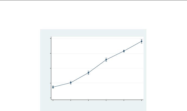
1232 marginsplot — Graph results from margins (profile plots, etc.)
We graph the results:
. marginsplot
Variables that uniquely identify margins: agegrp
110 120 130 140 150
Linear Prediction
20−29 30−39 40−49 50−59 60−69 70+
Age Group
Predictive Margins of agegrp with 95% CIs
Profile plots are often drawn without confidence intervals (CIs). The CIs may be removed by adding
the noci option. We prefer to see the CIs.
Disciplines vary widely in their use of the term profile plot. Some disciplines consider any connected
plot of a response over values of other variables to be a profile plot. By that definition, most graphs
in this entry are profile plots.
Interaction plots
Interaction plots are often used to explore the form of an interaction. The interaction term in our
ANOVA results is highly significant. Are the interaction effects also large enough to matter? What form
do they take? We can answer these questions by fixing agegrp and sex to each possible combination
of the two covariates and estimating the margins for those cells.
. margins agegrp#sex
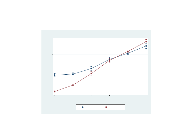
marginsplot — Graph results from margins (profile plots, etc.) 1233
Then we can graph the results:
. marginsplot
Variables that uniquely identify margins: agegrp sex
110 120 130 140 150
Linear Prediction
20−29 30−39 40−49 50−59 60−69 70+
Age Group
Male Female
Adjusted Predictions of agegrp#sex with 95% CIs
It is clear that the effect of age differs by sex—there is an interaction. If there were no interaction,
then the two lines would be parallel.
While males start out with higher systolic blood pressure, females catch up to the males as age
increases and may even surpass males in the upper age groups. We say “may” because we cannot
tell if the differences are statistically significant. The CIs overlap for the top three age groups. It is
tempting to conclude from this overlap that the differences are not statistically significant. Do not fall
into this trap. Likewise, do not fall into the trap that the first three age groups are different because
their CIs do not overlap. The CIs are for the point estimates, not the differences. There is a covariance
between the differences that we must consider if we are to make statements about those differences.
Contrasts of margins—effects (discrete marginal effects)
To assess the differences, all we need do is ask margins to contrast the sets of effects that we
just estimated; see [R]margins, contrast. With only two groups in sex, it does not matter much
which contrast operator we choose. We will use the reference contrast. It will compare the difference
between males and females, with males (the first category) as the reference category.
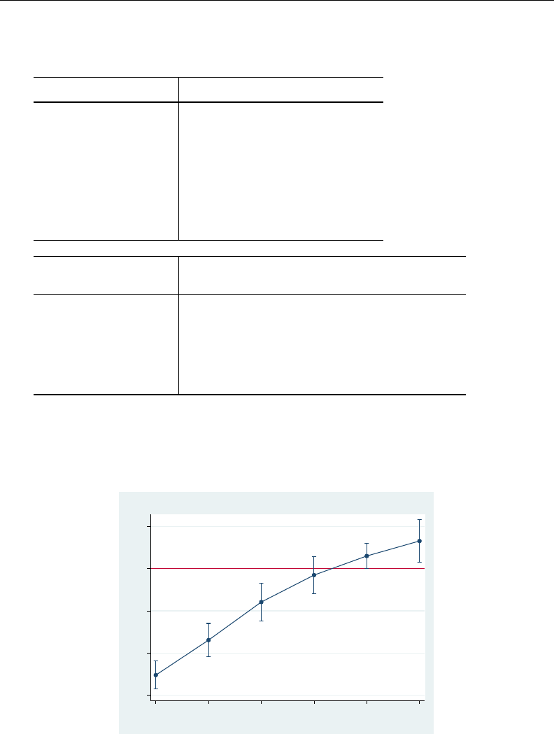
1234 marginsplot — Graph results from margins (profile plots, etc.)
. margins r.sex@agegrp
Contrasts of adjusted predictions
Expression : Linear prediction, predict()
df F P>F
sex@agegrp
(Female vs Male) 20-29 1 224.92 0.0000
(Female vs Male) 30-39 1 70.82 0.0000
(Female vs Male) 40-49 1 12.15 0.0005
(Female vs Male) 50-59 1 0.47 0.4949
(Female vs Male) 60-69 1 3.88 0.0488
(Female vs Male) 70+ 1 6.37 0.0116
Joint 6 53.10 0.0000
Denominator 10339
Delta-method
Contrast Std. Err. [95% Conf. Interval]
sex@agegrp
(Female vs Male) 20-29 -12.60132 .8402299 -14.24833 -10.9543
(Female vs Male) 30-39 -8.461161 1.005448 -10.43203 -6.490288
(Female vs Male) 40-49 -3.956451 1.134878 -6.181031 -1.731871
(Female vs Male) 50-59 -.7699782 1.128119 -2.981309 1.441353
(Female vs Male) 60-69 1.491684 .756906 .0080022 2.975367
(Female vs Male) 70+ 3.264762 1.293325 .729594 5.79993
Because we are looking for effects that are different from 0, we will add a reference line at 0 to
our graph.
. marginsplot, yline(0)
Variables that uniquely identify margins: agegrp
−15 −10 −5 0 5
Contrasts of Linear Prediction
20−29 30−39 40−49 50−59 60−69 70+
Age Group
Contrasts of Adjusted Predictions of sex@agegrp with 95% CIs
We can now say that females’ systolic blood pressure is substantially and significantly lower than
males’ in the first three age groups but is significantly higher in the last two age groups. Despite the
overlapping CIs for the last two age groups in the interaction graph, the effect of sex is significant in
these age groups.

marginsplot — Graph results from margins (profile plots, etc.) 1235
The terminology for what we just estimated and graphed varies widely across disciplines. Those
versed in design of experiments refer to these values as contrasts or effects. Economists and some other
social scientists call them marginal or partial effects. The latter groups might be more comfortable if
we avoided the whole concept of contrasts and instead estimated the effects by typing
. margins agegrp, dydx(sex)
This will produce estimates that are identical to those shown above, and we can graph them by typing
marginsplot.
The advantage of using the contrast notation and thinking in contrasts is most evident when we
take marginal effects with respect to a categorical covariate with more than two levels. Marginal
effects for each level of the covariate will be taken with respect to a specified base level. Contrasts are
much more flexible. Using the r. operator, we can reproduce the marginal-effects results by taking
derivatives with respect to a reference level (as we saw above.) We can also estimate the marginal
effect of first moving from level 1 to level 2, then from level 2 to level 3, then from level 3 to
level 4, . . . using the ar. or “reverse adjacent” operator. Adjacent effects (marginal effects) can be
valuable when evaluating an ordinal covariate, such as agegrp in our current model. For a discussion
of contrasts, see [R]contrast and [R]margins, contrast.
Three-way interactions
marginsplot can handle any number of covariates in your margins command. Consider the
three-way ANOVA model that results from adding an indicator for whether an individual has been
diagnosed with diabetes. We will fully interact the new covariate with the others in the model.
. anova bpsystol agegrp##sex##diabetes
Number of obs = 10349 R-squared = 0.2572
Root MSE = 20.131 Adj R-squared = 0.2556
Source Partial SS df MS F Prob > F
Model 1448983.17 23 62999.2681 155.45 0.0000
agegrp 107963.582 5 21592.7164 53.28 0.0000
sex 1232.79267 1 1232.79267 3.04 0.0812
agegrp#sex 11679.5925 5 2335.91849 5.76 0.0000
diabetes 7324.98924 1 7324.98924 18.07 0.0000
agegrp#diabetes 5484.54623 5 1096.90925 2.71 0.0189
sex#diabetes 102.988239 1 102.988239 0.25 0.6142
agegrp#sex#diabetes 4863.14971 5 972.629943 2.40 0.0349
Residual 4184296.88 10325 405.258778
Total 5633280.05 10348 544.38346
The three-way interaction is significant, as is the main effect of diabetes and its interaction with
agegrp.
Again, if you are more comfortable with regression than ANOVA, you may type
. regress bpsystol agegrp##sex##diabetes
The margins and marginsplot results will be the same.
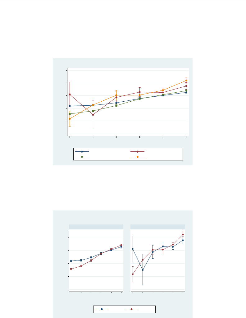
1236 marginsplot — Graph results from margins (profile plots, etc.)
We estimate the expected cell means for each combination of agegrp,sex, and diabetes, and
then graph the results by typing
. margins agegrp#sex#diabetes
(output omitted )
. marginsplot
Variables that uniquely identify margins: agegrp sex diabetes
80 100 120 140 160 180
Linear Prediction
20−29 30−39 40−49 50−59 60−69 70+
Age Group
Male, diabetes=0 Male, diabetes=1
Female, diabetes=0 Female, diabetes=1
Adjusted Predictions of agegrp#sex#diabetes with 95% CIs
The graph is busy and difficult to interpret.
We can make it better by putting those with diabetes on one subgraph and those without on another:
. marginsplot, by(diabetes)
Variables that uniquely identify margins: agegrp sex diabetes
80 100 120 140 160
20−29 30−39 40−49 50−59 60−69 70+ 20−29 30−39 40−49 50−59 60−69 70+
diabetes=0 diabetes=1
Male Female
Linear Prediction
Age Group
Adjusted Predictions of agegrp#sex#diabetes with 95% CIs
We notice much larger CIs for diabetics. That is not surprising because our sample contains only 499
diabetics compared with 9,850 nondiabetics.
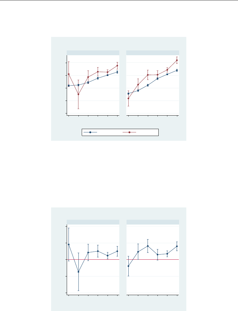
marginsplot — Graph results from margins (profile plots, etc.) 1237
A more interesting way to arrange the plots is by grouping the subgraphs on sex:
. marginsplot, by(sex)
Variables that uniquely identify margins: agegrp sex diabetes
80 100 120 140 160
20−29 30−39 40−49 50−59 60−69 70+ 20−29 30−39 40−49 50−59 60−69 70+
Male Female
diabetes=0 diabetes=1
Linear Prediction
Age Group
Adjusted Predictions of agegrp#sex#diabetes with 95% CIs
Aside from increased systolic blood pressure in the upper-age groups, which we saw earlier,
it appears that those with diabetes are at greater risk of higher systolic blood pressure for many
upper-age groups. We can check that by having margins estimate the differences between diabetics
and nondiabetics, and graphing the results.
. margins r.diabetes@agegrp#sex
(output omitted )
. marginsplot, by(sex) yline(0)
Variables that uniquely identify margins: agegrp sex
−40 −20 0 20 40
20−29 30−39 40−49 50−59 60−69 70+ 20−29 30−39 40−49 50−59 60−69 70+
sex: Male sex: Female
Contrasts of Linear Prediction
Age Group
Contrasts of Adjusted Predictions of diabetes@agegrp#sex with 95% CIs
With CIs above 0 for six of eight age groups over 40, this graph provides evidence that diabetes is
related to higher blood pressure in those over 40.
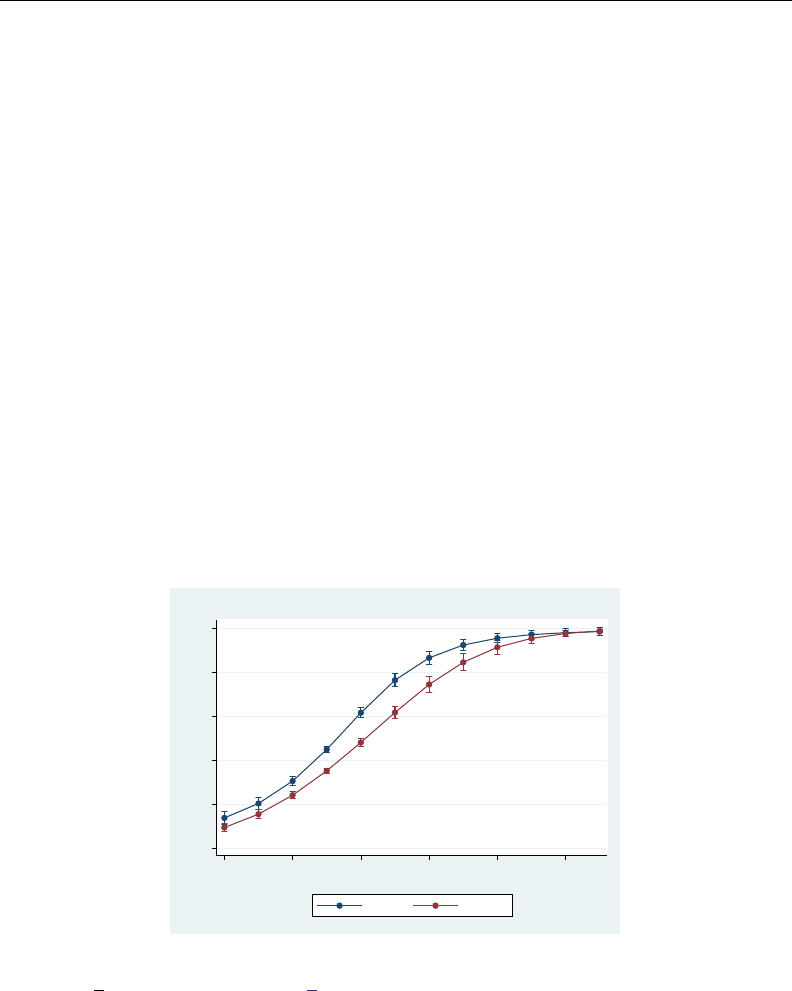
1238 marginsplot — Graph results from margins (profile plots, etc.)
Continuous covariates
margins and marginsplot are just as useful with continuous covariates as they are with factor
variables. As a variation on our ANOVA/regression models, let’s move to a logistic regression, using
as our dependent variable an indicator for whether a person has high blood pressure. We introduce a
continuous covariate—body mass index (BMI), a measure of weight relative to height. High BMI is
often associated with high blood pressure. We will allow the effect of BMI to vary across sexes, age
groups, and sex/age combinations by fully interacting the covariates.
. logistic highbp sex##agegrp##c.bmi
If we wished, we could perform all the analyses above on this model. Instead of estimating margins,
contrasts, and marginal effects on the level of systolic blood pressure, we would be estimating margins,
contrasts, and marginal effects on the probability of having high blood pressure. You can see those
results by repeating any of the prior commands that involve sex and agegrp. In this section, we will
focus on the continuous covariate bmi.
With continuous covariates, rather than specify them in the marginlist of margins, we specify the
specific values at which we want the covariate evaluated in an at() option. at() options are very
flexible, and there are many ways to specify values; see Syntax of at() in [R]margins.
BMI in our sample ranges from 12.4 to 61.1. Let’s estimate the predictive margins for males and
females at levels of BMI from 10 through 65 at intervals of 5 and graph the results:
. margins sex, at(bmi=(10(5)65))
(output omitted )
. marginsplot, xlabel(10(10)60)
Variables that uniquely identify margins: bmi sex
0 .2 .4 .6 .8 1
Pr(Highbp)
10 20 30 40 50 60
Body Mass Index (BMI)
Male Female
Predictive Margins of sex with 95% CIs
We added the xlabel(10(10)60) option to improve the labeling of the xaxis. You may add
any twoway options (see [G-3]twoway options) to the marginsplot command.
For a given BMI, males are generally more susceptible to high blood pressure, though the effect
is attenuated by the logistic response when the probabilities approach 0 or 1.
Because bmi is continuous, we might prefer to see the response graphed using a line. We might
also prefer that the CIs be plotted as areas. We change the plottype of the response by using the
recast() option and the plottype of the CI by using the recastci() option:
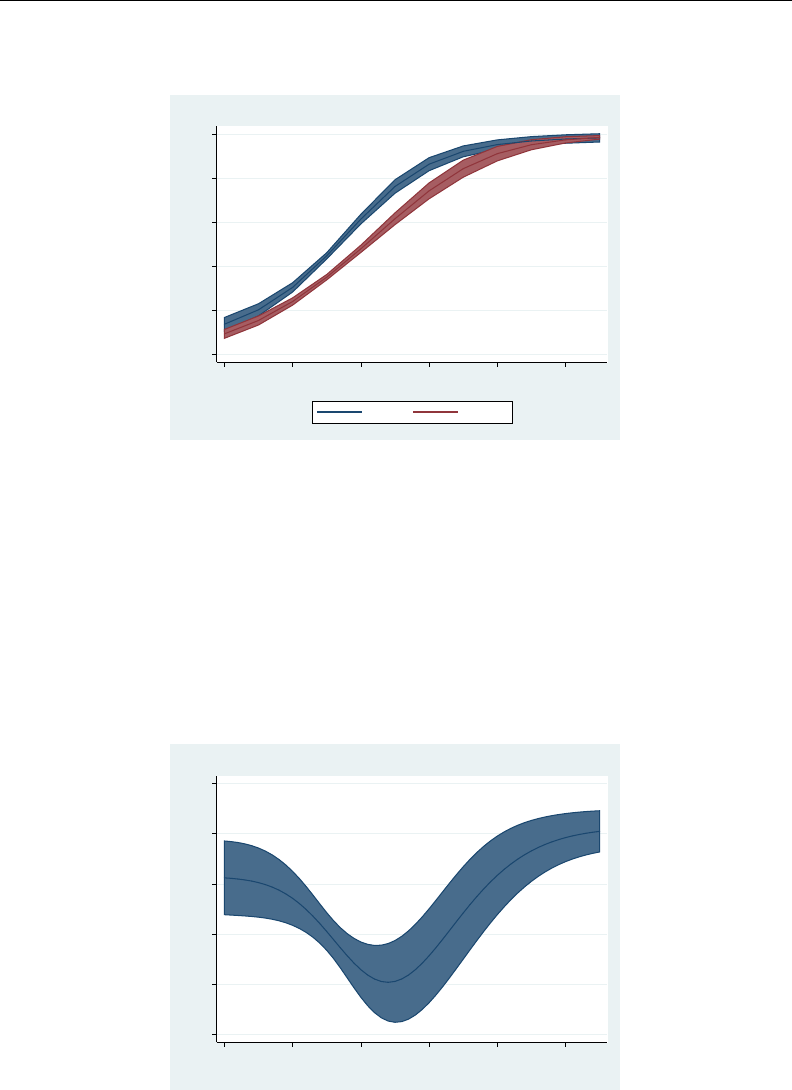
marginsplot — Graph results from margins (profile plots, etc.) 1239
. marginsplot, xlabel(10(10)60) recast(line) recastci(rarea)
Variables that uniquely identify margins: bmi sex
0 .2 .4 .6 .8 1
Pr(Highbp)
10 20 30 40 50 60
Body Mass Index (BMI)
Male Female
Predictive Margins of sex with 95% CIs
The CIs are a little dark for our tastes. You can dim them a bit by reducing the intensity of their
color. Adding ciopts(color(*.8)) to our marginsplot command will do that. Any plot option
accepted by twoway rarea (see [G-2]graph twoway rarea) may be specified in a ciopts() option.
Given their confidence regions, the male and female profiles appear to be statistically different over
most of the range of BMI. As with the profiles of categorical covariates, we can check that assertion
by contrasting the two profiles on sex and graphing the results. Let’s improve the smoothness of the
response by specifying intervals of 1 instead of 5.
. margins r.sex, at(bmi=(10(1)65))
(output omitted )
. marginsplot, xlabel(10(10)60) recast(line) recastci(rarea)
Variables that uniquely identify margins: bmi
−.2 −.15 −.1 −.05 0 .05
Contrasts of Pr(Highbp)
10 20 30 40 50 60
Body Mass Index (BMI)
Contrasts of Predictive Margins of sex with 95% CIs
We see that the difference between the sexes is largest at a BMI of about 35 and that the sexes
respond more similarly with very high and very low BMI. This shape is largely determined by the
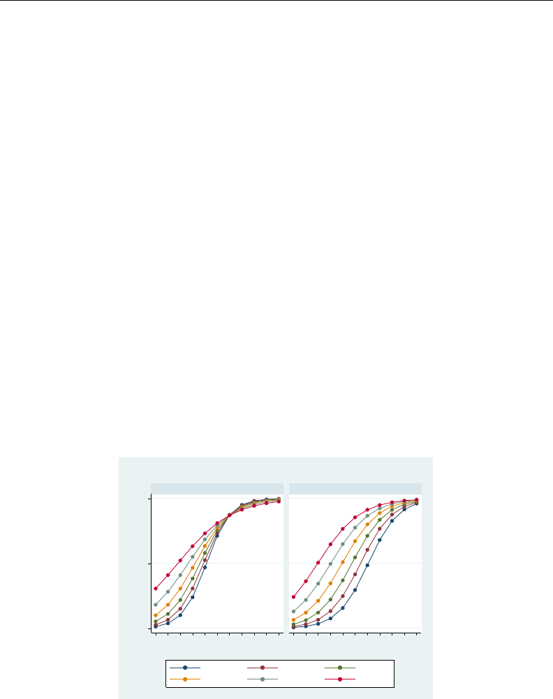
1240 marginsplot — Graph results from margins (profile plots, etc.)
response of the logistic function, which is attenuated near probabilities 0 and 1, combined with the
fact that the lowest measured BMIs are associated with low probabilities of high blood pressure and
the highest measured BMIs are associated with high probabilities of high blood pressure.
As when we contrasted profiles of categorical variables, different disciplines will think of this
graph differently. Those familiar with designed experiments will be comfortable with the terms used
above—this is a contrast of profiles, or a profile of effects, or a profile of a contrast. Many social
scientists will prefer to think of this as a graph of marginal or partial effects. For them, this is a plot
of the discrete marginal effect of being female for various levels of BMI. They can obtain an identical
graph, with labeling more appropriate for the marginal effect’s interpretation, by typing
. margins, at(bmi=(10(1)65)) dydx(sex)
. marginsplot, xlabel(10(10)60) recast(line) recastci(rarea)
We can also plot profiles of the response of BMI by levels of another continuous covariate (rather
than by the categorical variable sex). To do so, we will need another continuous variable in our
model. We have been using age groups as a covariate to emphasize the treatment of categorical
variables and to allow the effect of age to be flexible. Our dataset also has age recorded in integer
years. We replace agegrp with continuous age in our logistic regression.
. logistic highbp sex##c.age##c.bmi
We can now obtain profiles of BMI for different ages by specifying ranges for both bmi and age
in a single at() option on the margins command:
. margins sex, at(bmi=(10(5)60) age=(20(10)70))
With six ages specified, we have many profiles, so we will dispense with the CIs by adding the
noci option and also tidy up the graph by asking for three columns in the legend:
. marginsplot, noci by(sex) legend(cols(3))
Variables that uniquely identify margins: bmi age sex
0 .5 1
10 15 20 25 30 35 40 45 50 55 60 10 15 20 25 30 35 40 45 50 55 60
Male Female
age=20 age=30 age=40
age=50 age=60 age=70
Pr(Highbp)
Body Mass Index (BMI)
Adjusted Predictions of sex
Our model seems to indicate that males have a sharper reaction to body mass indices than do
females. Likewise, younger subjects display a sharper response, while older subjects have a more
gradual response with earlier onset. That interpretation might be a result of our parametric treatment
of age. As it turns out, the interpretation holds if we allow age to take more flexible forms or return
to our use of age groups, which allows each of seven age groups to have unique BMI profiles. Here
are the commands to perform that analysis:
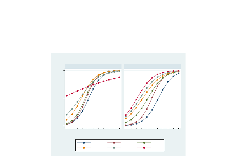
marginsplot — Graph results from margins (profile plots, etc.) 1241
. logistic highbp sex##agegrp##c.bmi
(output omitted )
. margins sex#agegrp, at(bmi=(10(5)60))
(output omitted )
. marginsplot, noci by(sex) legend(cols(3))
Variables that uniquely identify margins: bmi sex agegrp
0 .5 1
10 15 20 25 30 35 40 45 50 55 60 10 15 20 25 30 35 40 45 50 55 60
Male Female
20−29 30−39 40−49
50−59 60−69 70+
Pr(Highbp)
Body Mass Index (BMI)
Adjusted Predictions of sex#agegrp
Plots at every value of a continuous covariate
In some cases, the specific values of a continuous covariate are important, and we want to plot
the response at those specific values. Return to our logistic example with age treated as a continuous
covariate.
. logistic highbp sex##c.age##c.bmi
We can use a programming trick to extract all the values of age and then supply them in an at()
option, just as we would any list of values.
. levelsof age
. margins sex, at(age=(‘r(levels)’))
See [P]levelsof for a discussion of the levelsof command. levelsof returns in r(levels) the
sorted list of unique values of the specified varlist, in our case, age.
We can then plot the results using marginsplot.
This is not a very interesting trick when using our age variable, which is recorded as integers
from 20 to 74, but the approach will work with almost any continuous variable. In our model, bmi
might seem more interesting, but there are 9,941 unique values of bmi in our dataset. A graph cannot
resolve so many different values. For that reason, we usually recommend against plotting at every
value of a covariate. Instead, graph at reasonable values over the range of the covariate by using the
at() option, as we did earlier. This trick is best reserved for variables with a few, or at most a few
dozen, unique values.
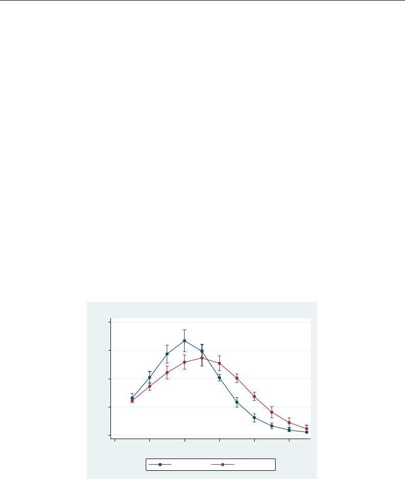
1242 marginsplot — Graph results from margins (profile plots, etc.)
Contrasts of at() groups—discrete effects
We have previously contrasted across the values of factor variables in our model. Put another way,
we have estimated the discrete marginal effects of factor variables. We can do the same for the levels
of variables in at() specifications and across separate at() specifications.
Returning to one of our logistic models and its margins, we earlier estimated the predictive margins
of BMI at 5-unit intervals for both sexes. These are the commands we typed:
. logistic highbp sex##agegrp##c.bmi
. margins sex, at(bmi=(10(5)65))
. marginsplot, xlabel(10(10)60)
We can estimate the discrete effects by sex of bmi moving from 10 to 15, then from 15 to 20, . . . ,
and then from 60 to 65 by contrasting the levels of the at() groups using the reverse-adjacent contrast
operator (ar.). We specify the operator within the atcontrast() suboption of the contrast()
option. We need to specify one other option. By default, margins, contrast will apply a contrast
to all variables in its marginlist when a contrast has been requested. In this case, we do not want
to contrast across sexes but rather to contrast across the levels of BMI within each sex. To prevent
margins from contrasting across the sexes, we specify the marginswithin option. Our margins
command is
. margins sex, at(bmi=(10(5)65)) contrast(atcontrast(ar._at) marginswithin)
And we graph the results using marginsplot:
. marginsplot
Variables that uniquely identify margins: bmi sex
0 .05 .1 .15 .2
Contrasts of Pr(Highbp)
10 20 30 40 50 60
Body Mass Index (BMI)
sex: Male sex: Female
Contrasts of Predictive Margins of sex with 95% CIs
The graph shows the contrasts (or if you prefer, discrete changes) in the probability of high blood
pressure by sex as one increases BMI in 5-unit increments.
We can even estimate contrasts (discrete effects) across at() options. To start, let’s compare the
age-group profiles of the probability of high blood pressure for those in the 25th and 75th percentile
of BMI.
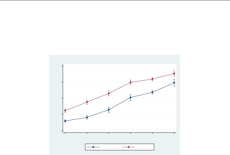
marginsplot — Graph results from margins (profile plots, etc.) 1243
. margins agegrp, at((p25) bmi) at((p75) bmi)
(output omitted )
. marginsplot
Variables that uniquely identify margins: agegrp _atopt
Multiple at() options specified:
_atoption=1: (p25) bmi
_atoption=2: (p75) bmi
0 .2 .4 .6 .8
Pr(Highbp)
20−29 30−39 40−49 50−59 60−69 70+
Age Group
(p25) bmi (p75) bmi
Predictive Margins of agegrp with 95% CIs
For each age group, people whose BMI is at the 75th percentile have a much higher probability of
high blood pressure than those at the 25th percentile. What is that difference in probability and its
CI? To contrast across the percentiles of BMI within age groups, we again specify a contrast operator
on the at() groups using atcontrast(), and we also tell margins to perform that contrast within
the levels of the marginlist by using the marginswithin option.
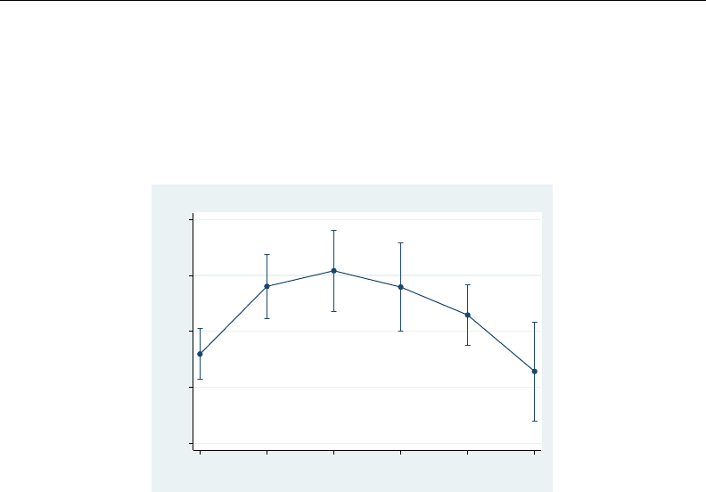
1244 marginsplot — Graph results from margins (profile plots, etc.)
. margins agegrp, at((p25) bmi) at((p75) bmi)
> contrast(atcontrast(r._at) marginswithin)
(output omitted )
. marginsplot
Variables that uniquely identify margins: agegrp _atopt
Multiple at() options specified:
_atoption=1: (p25) bmi
_atoption=2: (p75) bmi
.05 .1 .15 .2 .25
Contrasts of Pr(Highbp)
20−29 30−39 40−49 50−59 60−69 70+
Age Group
Contrasts of Predictive Margins of agegrp with 95% CIs
The differences in probability between 25th and 75th BMI percentiles are clearly significantly
greater than 0. The differences appear to be smallest for those in the youngest and oldest age groups.
Controlling the graph’s dimensions
Thus far, marginsplot has miraculously done almost exactly what we want in most cases. The
things we want on the xaxis have been there, the choice of plots has made sense, etc. Some of
that luck sprang from the relatively simple analyses we were performing, and some was from careful
specification of our margins command. Sometimes, we will not be so lucky.
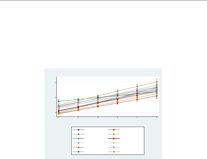
marginsplot — Graph results from margins (profile plots, etc.) 1245
Consider the following regress,margins, and marginsplot commands:
. regress bpsystol agegrp##sex##c.bmi
(output omitted )
. margins agegrp, over(sex) at(bmi=(10(10)60))
(output omitted )
. marginsplot
Variables that uniquely identify margins: agegrp _atopt
Multiple at() options specified:
_atoption=1: (p25) bmi
_atoption=2: (p75) bmi
100 150 200
Linear Prediction
10 20 30 40 50 60
Body Mass Index (BMI)
20−29, Male 20−29, Female
30−39, Male 30−39, Female
40−49, Male 40−49, Female
50−59, Male 50−59, Female
60−69, Male 60−69, Female
70+, Male 70+, Female
Predictive Margins of agegrp with 95% CIs
By default, marginsplot places the levels of the first multilevel at() specification on the xaxis,
and then usually plots the levels of all remaining variables as connected lines. That is what we see
in the graph above—bmi, the at() variable, is on the xaxis, and each combination of agegrp and
sex is plotted as a separate connected line. If there is no multilevel at() specification, then the first
variable in marginlist becomes the xaxis. There are many more rules, but it is usually best to simply
type marginsplot and see what happens. If you do not like marginsplot’s choices, change them.
What if we wanted agegrp on the xaxis instead of BMI? We tell marginsplot to make that
change by specifying agegrp in the xdimension() option:
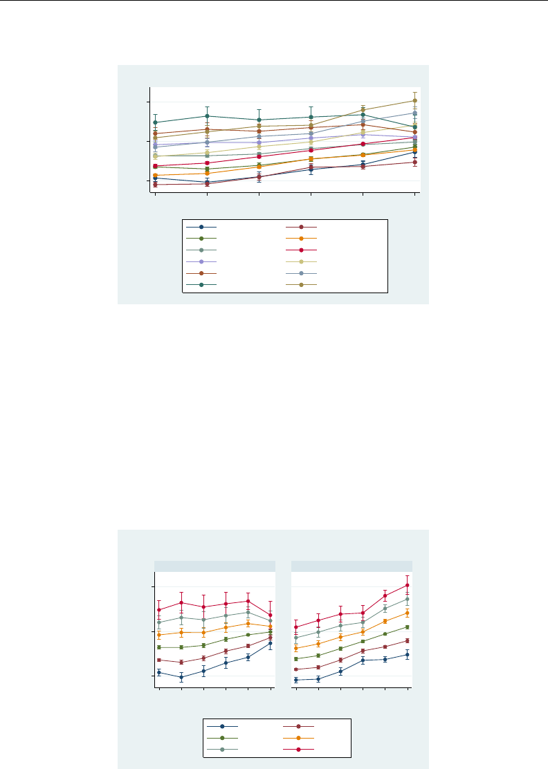
1246 marginsplot — Graph results from margins (profile plots, etc.)
. marginsplot, xdimension(agegrp)
Variables that uniquely identify margins: bmi agegrp sex
100 150 200
Linear Prediction
20−29 30−39 40−49 50−59 60−69 70+
Age Group
bmi=10, Male bmi=10, Female
bmi=20, Male bmi=20, Female
bmi=30, Male bmi=30, Female
bmi=40, Male bmi=40, Female
bmi=50, Male bmi=50, Female
bmi=60, Male bmi=60, Female
Predictive Margins of agegrp with 95% CIs
We have been suppressing the Results window output for marginsplot, but that output is helpful
if we want to change how things are plotted. You may specify any variable used in your margins
command in any of the dimension options—xdimension(),plotdimension(),bydimension(),
and graphdimension(). (In fact, there are some pseudovariables that you may also specify in some
cases; see Addendum: Advanced uses of dimlist for details.) marginsplot tries to help you narrow
your choices by listing a set of variables that uniquely identify all your margins. You are not restricted
to this list.
We have a different xaxis and a different set of plots, but our graph is still busy and difficult to
read. We can make it better by creating separate graph panels for each sex. We do that by adding a
bydimension() option with sex as the argument.
. marginsplot, xdimension(agegrp) bydimension(sex)
Variables that uniquely identify margins: bmi agegrp sex
100 150 200
20−29 30−39 40−49 50−59 60−69 70+ 20−29 30−39 40−49 50−59 60−69 70+
Male Female
bmi=10 bmi=20
bmi=30 bmi=40
bmi=50 bmi=60
Linear Prediction
Age Group
Predictive Margins of agegrp with 95% CIs
The patterns and the differences between males and females are now easier to see.
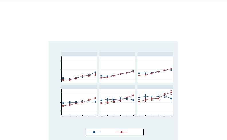
marginsplot — Graph results from margins (profile plots, etc.) 1247
If our interest is in comparing males and females, we might even choose to create a separate panel
for each level of BMI:
. marginsplot, xdimension(agegrp) bydimension(bmi) xlabel(, angle(45))
Variables that uniquely identify margins: bmi agegrp sex
100 150 200100 150 200
20−29
30−39
40−49
50−59
60−69
70+
20−29
30−39
40−49
50−59
60−69
70+
20−29
30−39
40−49
50−59
60−69
70+
bmi=10 bmi=20 bmi=30
bmi=40 bmi=50 bmi=60
Male Female
Linear Prediction
Age Group
Predictive Margins of agegrp with 95% CIs
The x-axis labels did not fit, so we angled them.
We leave you to explore the use of the graphdimension() option. It is much like bydimension()
but creates separate graphs rather than separate panels. Operationally, the plotdimension() option
is rarely used. All variables not in the xdimension and not specified elsewhere become the plotted
connected lines.
You will likely use the dimension options frequently. This is one of the rare cases where we
recommend using the minimal abbreviations of the options—x() for xdimension(),plot() for
plotdimension(),by() for bydimension(), and graph() for graphdimension(). The abbre-
viations are easy to read and just as meaningful as the full option names. The full names exist to
reinforce the relationship between the dimension options.
Pairwise comparisons
marginsplot can graph the results of margins, pwcompare; see [R]margins, pwcompare. We
return to one of our ANOVA examples. Here we request pairwise comparisons with the pwcompare
option of margins, and we request Bonferroni-adjusted CIs with the mcompare() option:
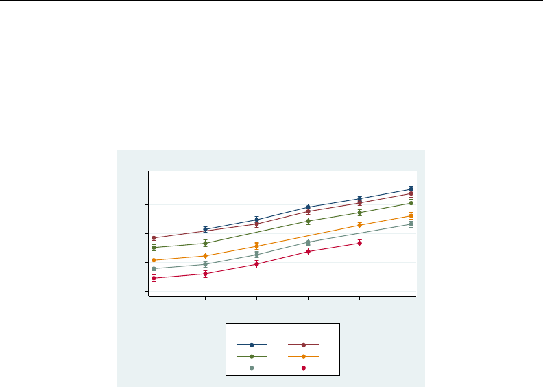
1248 marginsplot — Graph results from margins (profile plots, etc.)
. anova bpsystol agegrp##sex
(output omitted )
. margins agegrp, pwcompare mcompare(bonferroni)
(output omitted )
. marginsplot
Variables that uniquely identify margins: _pw1 _pw0
_pw enumerates all pairwise comparisons; _pw0 enumerates the reference
categories; _pw1 enumerates the comparison categories.
−40 −20 0 20 40
Comparisons of Linear Prediction
1 2 3 4 5 6
Comparison category
1 2
3 4
5 6
Reference category
Pairwise Comparisons of Predictive Margins of agegrp with 95% CIs
Each connected line plot in the graph represents a reference age-group category for the pairwise
comparison. The ticks on the xaxis represent comparison age-group categories. So, each plot is a
profile for a reference category showing its comparison to each other category.
Horizontal is sometimes better
Another interesting way to graph pairwise comparisons is to simply plot each comparison and
label the two categories being compared. This type of graph works better if it is oriented horizontally
rather than vertically.
Continuing with the example above, we will switch the graph to horizontal. We will also make
several changes to display the graph better. We specify that only unique comparisons be plotted. The
graph above plotted both 1 versus 2 and 2 versus 1, which are the same comparison with opposite
signs. We add a reference line at 0 because we are interested in comparisons that differ from 0. This
graph looks better without the connecting lines, so we add the option recast(scatter). We also
reverse the yscale so that the smallest levels of age group appear at the top of the axis.
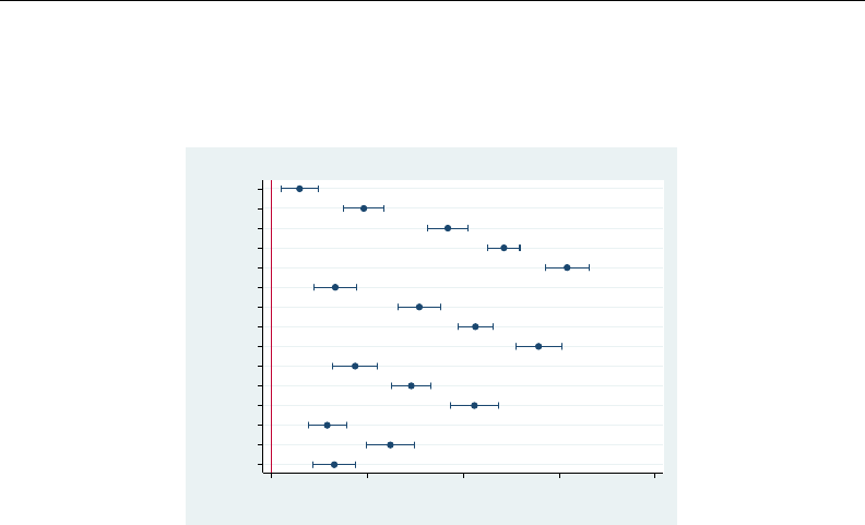
marginsplot — Graph results from margins (profile plots, etc.) 1249
. marginsplot, horizontal unique xline(0) recast(scatter) yscale(reverse)
Variables that uniquely identify margins: _pw1 _pw0
_pw enumerates all pairwise comparisons; _pw0 enumerates the reference
categories; _pw1 enumerates the comparison categories.
2 vs 1
3 vs 1
4 vs 1
5 vs 1
6 vs 1
3 vs 2
4 vs 2
5 vs 2
6 vs 2
4 vs 3
5 vs 3
6 vs 3
5 vs 4
6 vs 4
6 vs 5
Comparisons
0 10 20 30 40
Comparisons of Linear Prediction
Pairwise Comparisons of Predictive Margins of agegrp with 95% CIs
All the comparisons differ from 0, so all our age groups are statistically different from each other.
The horizontal option can be useful outside of pairwise comparisons. Profile plots are usually
oriented vertically. However, when your covariates have long labels or there are many levels at which
the margins are being evaluated, the graph may be easier to read when rendered horizontally.
Marginal effects
We have seen how to graph discrete effects for factor variables and continuous variables by using
contrasts, and optionally by using the dydx() option of margins:Contrasts of margins—effects
(discrete marginal effects) and Continuous covariates. Let’s now consider graphing instantaneous
marginal effects for continuous covariates. Begin by refitting our logistic model of high blood
pressure as a function of sex, age, and BMI:
. logistic highbp sex##agegrp##c.bmi
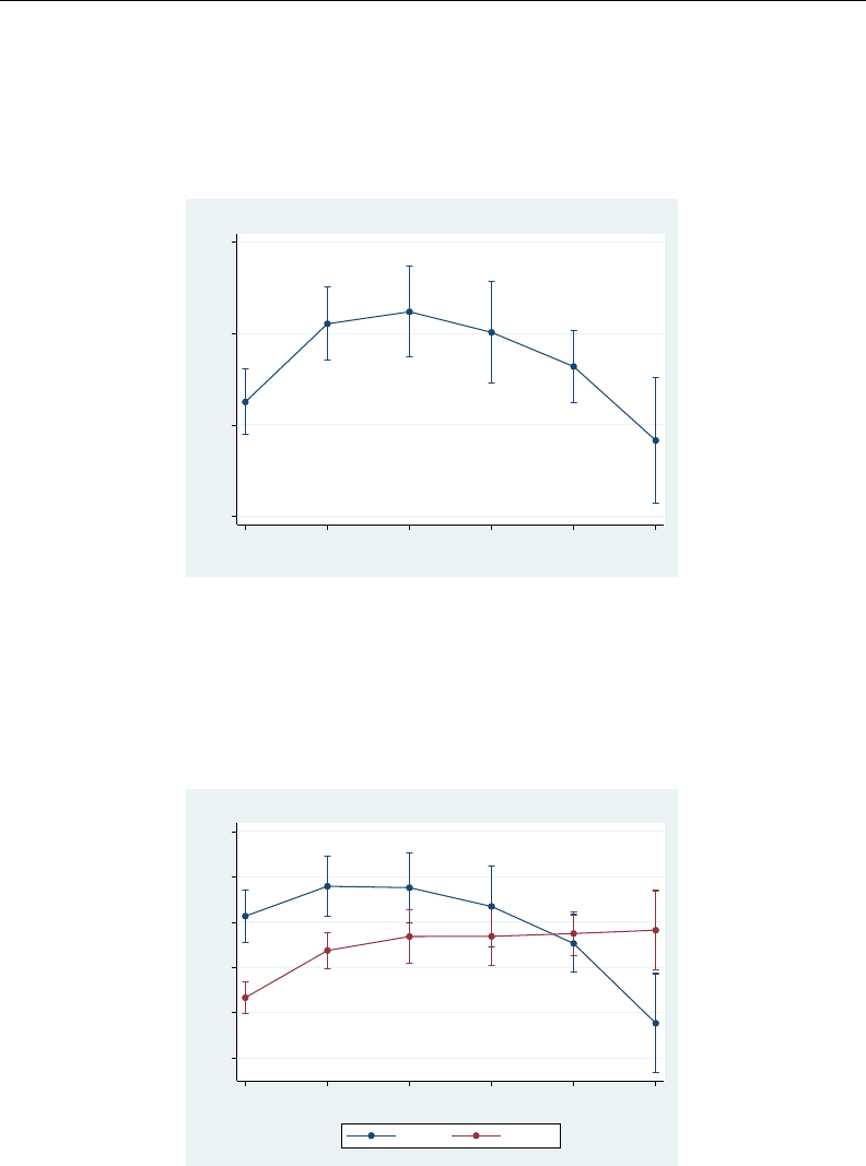
1250 marginsplot — Graph results from margins (profile plots, etc.)
We estimate the average marginal effect of BMI on the probability of high blood pressure for each
age group and then graph the results by typing
. margins agegrp, dydx(bmi)
(output omitted )
. marginsplot
Variables that uniquely identify margins: agegrp
.01 .02 .03 .04
Effects on Pr(Highbp)
20−29 30−39 40−49 50−59 60−69 70+
Age Group
Average Marginal Effects of bmi with 95% CIs
These are the conditional expectations of the marginal effects treating everyone in the sample as
though they were in each age group. We can estimate fully conditional marginal effects that do not
depend on averaging over the sample by also margining on our one remaining covariate—sex.
. margins agegrp#sex, dydx(bmi)
(output omitted )
. marginsplot
Variables that uniquely identify margins: agegrp sex
0 .01 .02 .03 .04 .05
Effects on Pr(Highbp)
20−29 30−39 40−49 50−59 60−69 70+
Age Group
Male Female
Average Marginal Effects of bmi with 95% CIs
The effect of BMI on the probability of high blood pressure looks to increase with age for females.
The marginal effect is higher for males than females in the younger age groups but then decreases
with age for males after the 40–49 age group.

marginsplot — Graph results from margins (profile plots, etc.) 1251
You may want to test for differences in the marginal effect of BMI for males and females by
contrasting across sexes within agegrp:
. margins r.sex@agegrp, dydx(bmi)
Plotting a subset of the results from margins
marginsplot plots all the margins produced by the preceding margins command. If you want a
graph that does not include all the margins, then enter a margins command that produces a reduced
set of margins. Obvious ways to reduce the number of margins include not specifying some factors or
interactions in the marginlist of margins, not specifying some at() or over() options, or reducing
the values specified in an at() option. A less obvious technique uses selection lists in factor operators
to select specific sets of levels from factor variables specified in the marginlist.
Instead of typing
. margins agegrp
which will give you margins for all six age groups in our sample, type
. margins i(2/4).agegrp
which will give you only three margins—those for groups 2, 3, and 4. See [U] 11.4.3.4 Selecting
levels.
Advanced usage
margins is incredibly flexible in the statistics it can estimate and in the grouping of those estimates.
Many of the estimates that margins can produce do not make convincing graphs. marginsplot plots
the results of any margins command, regardless of whether the resulting graph is easily interpreted.
Here we demonstrate some options that can make complicated margins into graphs that are somewhat
more useful than those produced by marginsplot’s defaults. Others may find truly useful applications
for these approaches.
Plots with multiple terms
Margins plots are rarely interesting when you specify multiple terms on your margins command,
for example, margins a b. Such plots often compare things that are not comparable. The defaults
for marginsplot rarely produce useful plots with multiple terms. Perhaps the most interesting graph
in such cases puts all the levels of all the terms together on the vertical axis and plots their margins
on the horizontal axis. We do that by including the marginlist from margins in an xdimension()
option on marginsplot. The long labels on such graphs look better with a horizontal orientation,
and there is no need to connect the margin estimates, so we specify the recast(scatter) option.
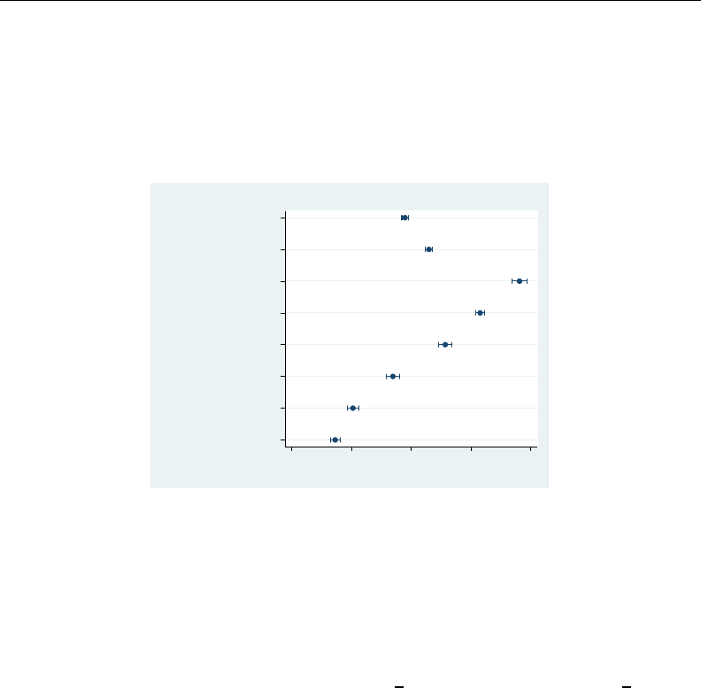
1252 marginsplot — Graph results from margins (profile plots, etc.)
Using one of our ANOVA examples from earlier,
. anova bpsystol agegrp##sex
(output omitted )
. margins agegrp sex
(output omitted )
. marginsplot, xdimension(agegrp sex) horizontal recast(scatter)
Variables that uniquely identify margins: agegrp sex
20−29, asobserved
30−39, asobserved
40−49, asobserved
50−59, asobserved
60−69, asobserved
70+, asobserved
asobserved, Male
asobserved, Female
agegrp, sex
110 120 130 140 150
Linear Prediction
Predictive Margins with 95% CIs
The “asobserved” notations in the y-axis labels are informing us that, for example, when the margin
for females is evaluated, the values of age group are taken as they are observed in the dataset. The
margin is computed as an average over those values.
Plots with multiple at() options
Some disciplines like to compute margins at the means of other covariates in their model and
others like to compute the response for each observation and then take the means of the response.
These correspond to the margins options at((mean) all) and at((asobserved) all). For
responses that are linear functions of the coefficients, such as predict after regress, the two
computations yield identical results. For responses that are nonlinear functions of the coefficients, the
two computations estimate different things.
Using one of our logistic models of high blood pressure,
. logistic highbp sex##agegrp##c.bmi
and computing both sets of margins for each age group,
. margins agegrp, at((mean) _all) at((asobserved) _all)

marginsplot — Graph results from margins (profile plots, etc.) 1253
we can use marginsplot to compare the approaches:
. marginsplot
Variables that uniquely identify margins: agegrp _atopt
Multiple at() options specified:
_atoption=1: (mean)_all
_atoption=2: (asobserved) _all
0 .2 .4 .6 .8
Pr(Highbp)
20−29 30−39 40−49 50−59 60−69 70+
Age Group
(mean) _all (asobserved) _all
Predictive Margins of agegrp with 95% CIs
For the first three age groups, the probabilities of high blood pressure are lower at the means of sex
and bpi than are the mean probabilities of high blood pressure averaged over the observed values of
sex and bpi. The reverse is true for the last three age groups, although the values are very similar
in these older age groups.
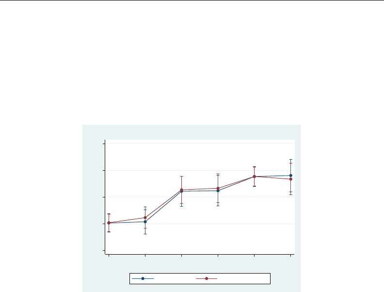
1254 marginsplot — Graph results from margins (profile plots, etc.)
Such comparisons come up even more frequently when evaluating marginal effects. We can estimate
the marginal effects of sex at each age group and graph the results by adding dydx(sex) to our
margins command:
. margins agegrp, at((mean) _all) at((asobserved) _all) dydx(sex)
(output omitted )
. marginsplot
Variables that uniquely identify margins: agegrp _atopt
Multiple at() options specified:
_atoption=1: (mean)_all
_atoption=2: (asobserved) _all
−.3 −.2 −.1 0 .1
Effects on Pr(Highbp)
20−29 30−39 40−49 50−59 60−69 70+
Age Group
(mean) _all (asobserved) _all
Average Marginal Effects of 2.sex with 95% CIs
The average marginal effect is smaller for most age groups, but the CIs for both sets of estimates are
wide. Can we tell the difference between the estimates? To answer that, we use the now-familiar tactic of
taking the contrast of our estimated marginal-effects profiles. That means adding contrast(atjoint
marginswithin) to our margins command. We will also add mcompare(bonferroni) to account
for the fact that we will be comparing six contrasts.
. margins agegrp, at((mean) _all) at((asobserved) _all) dydx(sex)
> contrast(atjoint marginswithin) mcompare(bonferroni)
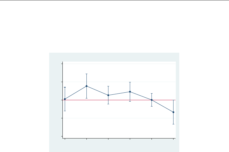
marginsplot — Graph results from margins (profile plots, etc.) 1255
We will also add the familiar reference line at 0 to our graph of the contrasts.
. marginsplot, yline(0)
Variables that uniquely identify margins: agegrp _atopt
Multiple at() options specified:
_atoption=1: (mean)_all
_atoption=2: (asobserved) _all
−.04 −.02 0 .02 .04
Contrasts of Pr(Highbp)
20−29 30−39 40−49 50−59 60−69 70+
Age Group
Contrasts of Average Marginal Effects of 2.sex with 95% CIs
While the difference in the estimates of marginal effects is not large, we can distinguish the estimates
for the 30–39 and 70+ age groups.
The at() option of margins provides far more flexibility than demonstrated above. It can be
used to evaluate a response or marginal effect at almost any point of interest or combinations of such
points. See Syntax of at() in [R]margins.
Adding scatterplots of the data
We can add scatterplots of the observed data to our plots of the margins. The NHANES II dataset
is too large for this to be interesting, so for this example, we will use auto.dta. We fit mileage
on whether the care is foreign and on a quadratic in the weight of the car. We convert the weight
into tons (U.S. definition) to improve the scaling, and we format the new tons variable to improve
its labels on the graph. For our graph, we create separate variables for mileage of domestic and of
foreign cars. We fit a fully interacted model so that the effect of weight on mileage can be different
for foreign and for domestic cars.
. use http://www.stata-press.com/data/r13/auto
. generate tons = weight/2000
. format tons %6.2f
. separate mpg, by(foreign)
. regress mpg foreign##c.tons##c.tons
We then estimate the margins over the range of tons, using the option over(foreign) to obtain
separate estimates for foreign and domestic cars.
. margins, at(tons=(.8(.05)2.4)) over(foreign)
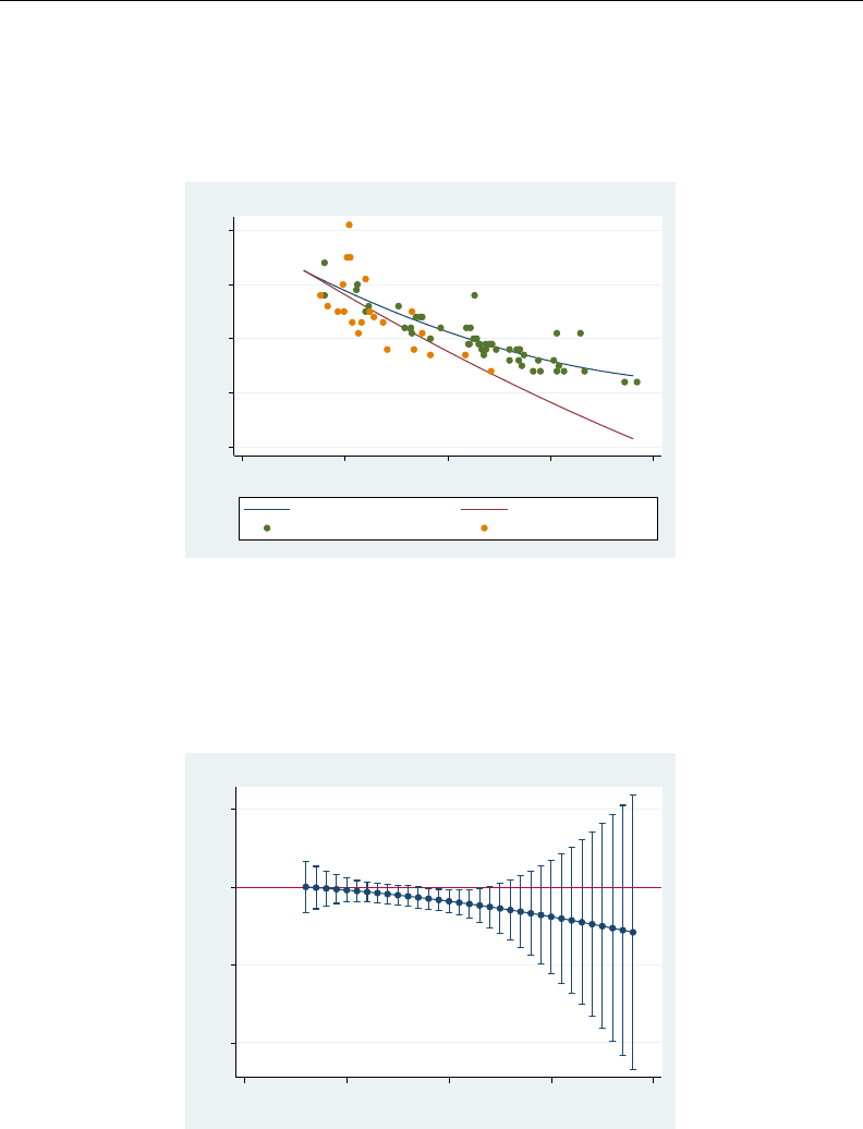
1256 marginsplot — Graph results from margins (profile plots, etc.)
Adding scatterplots of mileage for domestic and foreign cars is easy. We insert into an addplot()
option of marginsplot the same scatterplot syntax for twoway that we would type to produce a
scatterplot of the data:
. marginsplot, addplot(scatter mpg0 tons || scatter mpg1 tons) recast(line) noci
Variables that uniquely identify margins: tons foreign
0 10 20 30 40
Linear Prediction
0.50 1.00 1.50 2.00 2.50
tons
Domestic Foreign
mpg, foreign == Domestic mpg, foreign == Foreign
Predictive Margins
Many will be surprised that the mileage profile is higher in 1978 for domestic (U.S. built) cars.
Is the difference significant?
. margins, at(tons=(.8(.05)2.4)) over(r.for)
(output omitted )
. marginsplot, yline(0)
Variables that uniquely identify margins: tons
−40 −20 0 20
Contrasts of Linear Prediction
0.50 1.00 1.50 2.00 2.50
tons
Contrasts of Predictive Margins with 95% CIs
As we did earlier, we contrast the two profiles. We can discern some difference between the two
profiles for midweight vehicles, but otherwise there is insufficient information to believe mileage
differs across domestic and foreign cars.

marginsplot — Graph results from margins (profile plots, etc.) 1257
Video examples
Profile plots and interaction plots, part 1: A single categorical variable
Profile plots and interaction plots, part 2: A single continuous variable
Profile plots and interaction plots, part 3: Interactions between categorical variables
Profile plots and interaction plots, part 4: Interactions of continuous and categorical variables
Profile plots and interaction plots, part 5: Interactions of two continuous variables
Addendum: Advanced uses of dimlist
dimlist specifies the dimensions from the immediately preceding margins command that are to
be used for the marginsplot’s xaxis, plots, subgraphs, and graphs. dimlist may contain:
dim Description
varname Any variable referenced in the preceding margins command.
at(varname)If a variable is specified in both the marginlist or the over() option and in the
at() option of margins, then the two uses can be distinguished in marginsplot
by typing the at() variables as at(varname)in dimlist.
deriv If the preceding margins command included a dydx(),eyex(),dyex(), or
eydx() option, dimlist may also contain deriv to specify all the variables over
which derivatives were taken.
term If the preceding margins command included multiple terms (for example, margins
a b), then dimlist may contain term to enumerate those terms.
atopt If the preceding margins command included multiple at() options, then dimlist
may contain atopt to enumerate those at() options.
When the pairwise option is specified on margins, you may specify dimensions that enumerate
the pairwise comparisons.
pw enumerates all the pairwise comparisons
pw0 enumerates the reference categories of the comparisons
pw1 enumerates the comparison categories of the comparisons
Acknowledgments
We thank Philip B. Ender of UCLA Academic Technology Services for his programs that demonstrated
what could be done in this area. We also thank Michael N. Mitchell, author of the Stata Press books
Data Management Using Stata: A Practical Handbook and A Visual Guide to Stata Graphics, for his
generous advice and comprehensive insight into the application of margins and their plots.
References
McDowell, A., A. Engel, J. T. Massey, and K. Maurer. 1981. Plan and operation of the Second National Health and
Nutrition Examination Survey, 1976–1980. Vital and Health Statistics 1(15): 1–144.
Mitchell, M. N. 2012. Interpreting and Visualizing Regression Models Using Stata. College Station, TX: Stata Press.
Royston, P. 2013. marginscontplot: Plotting the marginal effects of continuous predictors.Stata Journal 13: 510–527.
Williams, R. 2012. Using the margins command to estimate and interpret adjusted predictions and marginal effects.
Stata Journal 12: 308–331.

1258 marginsplot — Graph results from margins (profile plots, etc.)
Also see
[R]margins — Marginal means, predictive margins, and marginal effects
[R]margins, contrast — Contrasts of margins
[R]margins, pwcompare — Pairwise comparisons of margins
[R]margins postestimation — Postestimation tools for margins

Title
matsize — Set the maximum number of variables in a model
Syntax Description Option Remarks and examples Also see
Syntax
set matsize #, permanently
where 10 ≤#≤11000 for Stata/MP and Stata/SE and where 10 ≤#≤800 for Stata/IC.
Description
set matsize sets the maximum number of variables that can be included in any of Stata’s
estimation commands.
For Stata/MP and Stata/SE, the default value is 400, but it may be changed upward or downward.
The upper limit is 11,000.
For Stata/IC, the initial value is 400, but it may be changed upward or downward. The upper limit
is 800.
This command may not be used with Small Stata; matsize is permanently frozen at 100.
Changing matsize has no effect on Mata.
Option
permanently specifies that, in addition to making the change right now, the matsize setting be
remembered and become the default setting when you invoke Stata.
Remarks and examples
set matsize controls the internal size of matrices that Stata uses. The default of 400 for Stata/IC,
for instance, means that linear regression models are limited to 198 independent variables—198
because the constant uses one position and the dependent variable another, making a total of 200.
You may change matsize with data in memory, but increasing matsize increases the amount of
memory consumed by Stata, increasing the probability of page faults and thus of making Stata run
more slowly.
Example 1
We wish to fit a model of yon the variables x1 through x400. Without thinking, we type
. regress y x1-x400
matsize too small
You have attempted to create a matrix with more than 400 rows or columns
or to fit a model with more than 400 variables plus ancillary parameters.
You need to increase matsize by using the set matsize command; see help
matsize.
r(908);
1259

1260 matsize — Set the maximum number of variables in a model
We realize that we need to increase matsize, so we type
. set matsize 450
. regress y x1-x400
(output omitted )
Programmers should note that the current setting of matsize is stored as the c-class value
c(matsize); see [P]creturn.
Also see
[R]query — Display system parameters
[D]memory — Memory management
[U] 6 Managing memory

Title
maximize — Details of iterative maximization
Syntax Description Maximization options
Option for set maxiter Remarks and examples Stored results
Methods and formulas References Also see
Syntax
Maximum likelihood optimization
mle cmd . . . ,options
Set default maximum iterations
set maxiter #, permanently
options Description
difficult use a different stepping algorithm in nonconcave regions
technique(algorithm spec)maximization technique
iterate(#)perform maximum of #iterations; default is iterate(16000)
no log display an iteration log of the log likelihood; typically, the default
trace display current parameter vector in iteration log
gradient display current gradient vector in iteration log
showstep report steps within an iteration in iteration log
hessian display current negative Hessian matrix in iteration log
showtolerance report the calculated result that is compared to the effective
convergence criterion
tolerance(#)tolerance for the coefficient vector; see Options for the defaults
ltolerance(#)tolerance for the log likelihood; see Options for the defaults
nrtolerance(#)tolerance for the scaled gradient; see Options for the defaults
qtolerance(#)when specified with algorithms bhhh,dfp, or bfgs, the q−H
matrix is used as the final check for convergence rather than
nrtolerance() and the Hmatrix; seldom used
nonrtolerance ignore the nrtolerance() option
from(init specs)initial values for the coefficients
where algorithm spec is
algorithm #algorithm # . . .
algorithm is nr |bhhh |dfp |bfgs
1261

1262 maximize — Details of iterative maximization
and init specs is one of
matname , skip copy
eqname:name =#|/eqname =# . . .
##. . . , copy
Description
All Stata commands maximize likelihood functions using moptimize() and optimize(); see
Methods and formulas below. Commands use the Newton–Raphson method with step halving
and special fixups when they encounter nonconcave regions of the likelihood. For details, see
[M-5]moptimize( ) and [M-5]optimize( ). For more information about programming maximum like-
lihood estimators in ado-files and Mata, see [R]ml and the fourth edition of Maximum Likelihood
Estimation with Stata (Gould, Pitblado, and Poi 2010).
set maxiter specifies the default maximum number of iterations for estimation commands that
iterate. The initial value is 16000, and #can be 0to 16000. To change the maximum number of
iterations performed by a particular estimation command, you need not reset maxiter; you can
specify the iterate(#)option. When iterate(#)is not specified, the maxiter value is used.
Maximization options
difficult specifies that the likelihood function is likely to be difficult to maximize because of
nonconcave regions. When the message “not concave” appears repeatedly, ml’s standard stepping
algorithm may not be working well. difficult specifies that a different stepping algorithm be
used in nonconcave regions. There is no guarantee that difficult will work better than the
default; sometimes it is better and sometimes it is worse. You should use the difficult option
only when the default stepper declares convergence and the last iteration is “not concave” or
when the default stepper is repeatedly issuing “not concave” messages and producing only tiny
improvements in the log likelihood.
technique(algorithm spec)specifies how the likelihood function is to be maximized. The following
algorithms are allowed. For details, see Gould, Pitblado, and Poi (2010).
technique(nr) specifies Stata’s modified Newton–Raphson (NR) algorithm.
technique(bhhh) specifies the Berndt–Hall–Hall–Hausman (BHHH) algorithm.
technique(dfp) specifies the Davidon–Fletcher–Powell (DFP) algorithm.
technique(bfgs) specifies the Broyden–Fletcher–Goldfarb–Shanno (BFGS) algorithm.
The default is technique(nr).
You can switch between algorithms by specifying more than one in the technique() option. By
default, an algorithm is used for five iterations before switching to the next algorithm. To specify a
different number of iterations, include the number after the technique in the option. For example,
specifying technique(bhhh 10 nr 1000) requests that ml perform 10 iterations with the BHHH
algorithm followed by 1000 iterations with the NR algorithm, and then switch back to BHHH for
10 iterations, and so on. The process continues until convergence or until the maximum number
of iterations is reached.

maximize — Details of iterative maximization 1263
iterate(#)specifies the maximum number of iterations. When the number of iterations equals
iterate(), the optimizer stops and presents the current results. If convergence is declared before
this threshold is reached, it will stop when convergence is declared. Specifying iterate(0)
is useful for viewing results evaluated at the initial value of the coefficient vector. Specifying
iterate(0) and from() together allows you to view results evaluated at a specified coefficient
vector; however, not all commands allow the from() option. The default value of iterate(#)
for both estimators programmed internally and estimators programmed with ml is the current value
of set maxiter, which is iterate(16000) by default.
log and nolog specify whether an iteration log showing the progress of the log likelihood is to be
displayed. For most commands, the log is displayed by default, and nolog suppresses it. For a
few commands (such as the svy maximum likelihood estimators), you must specify log to see
the log.
trace adds to the iteration log a display of the current parameter vector.
gradient adds to the iteration log a display of the current gradient vector.
showstep adds to the iteration log a report on the steps within an iteration. This option was added so
that developers at StataCorp could view the stepping when they were improving the ml optimizer
code. At this point, it mainly provides entertainment.
hessian adds to the iteration log a display of the current negative Hessian matrix.
showtolerance adds to the iteration log the calculated value that is compared with the effective
convergence criterion at the end of each iteration. Until convergence is achieved, the smallest
calculated value is reported.
shownrtolerance is a synonym of showtolerance.
Below we describe the three convergence tolerances. Convergence is declared when the nrtol-
erance() criterion is met and either the tolerance() or the ltolerance() criterion is also
met.
tolerance(#)specifies the tolerance for the coefficient vector. When the relative change in the
coefficient vector from one iteration to the next is less than or equal to tolerance(), the
tolerance() convergence criterion is satisfied.
tolerance(1e-4) is the default for estimators programmed with ml.
tolerance(1e-6) is the default.
ltolerance(#)specifies the tolerance for the log likelihood. When the relative change in the log
likelihood from one iteration to the next is less than or equal to ltolerance(), the ltolerance()
convergence is satisfied.
ltolerance(0) is the default for estimators programmed with ml.
ltolerance(1e-7) is the default.
nrtolerance(#)specifies the tolerance for the scaled gradient. Convergence is declared when
gH−1g0<nrtolerance(). The default is nrtolerance(1e-5).
qtolerance(#)when specified with algorithms bhhh,dfp, or bfgs uses the q−Hmatrix as the
final check for convergence rather than nrtolerance() and the Hmatrix.
Beginning with Stata 12, by default, Stata now computes the Hmatrix when the q−Hmatrix passes
the convergence tolerance, and Stata requires that Hbe concave and pass the nrtolerance()
criterion before concluding convergence has occurred.
qtolerance() provides a way for the user to obtain Stata’s earlier behavior.

1264 maximize — Details of iterative maximization
nonrtolerance specifies that the default nrtolerance() criterion be turned off.
from() specifies initial values for the coefficients. Not all estimators in Stata support this option. You
can specify the initial values in one of three ways: by specifying the name of a vector containing
the initial values (for example, from(b0), where b0 is a properly labeled vector); by specifying
coefficient names with the values (for example, from(age=2.1 /sigma=7.4)); or by specifying
a list of values (for example, from(2.1 7.4, copy)). from() is intended for use when doing
bootstraps (see [R]bootstrap) and in other special situations (for example, with iterate(0)).
Even when the values specified in from() are close to the values that maximize the likelihood,
only a few iterations may be saved. Poor values in from() may lead to convergence problems.
skip specifies that any parameters found in the specified initialization vector that are not also
found in the model be ignored. The default action is to issue an error message.
copy specifies that the list of values or the initialization vector be copied into the initial-value
vector by position rather than by name.
Option for set maxiter
permanently specifies that, in addition to making the change right now, the maxiter setting be
remembered and become the default setting when you invoke Stata.
Remarks and examples
Only in rare circumstances would you ever need to specify any of these options, except nolog.
The nolog option is useful for reducing the amount of output appearing in log files.
The following is an example of an iteration log:
Iteration 0: log likelihood = -3791.0251
Iteration 1: log likelihood = -3761.738
Iteration 2: log likelihood = -3758.0632 (not concave)
Iteration 3: log likelihood = -3758.0447
Iteration 4: log likelihood = -3757.5861
Iteration 5: log likelihood = -3757.474
Iteration 6: log likelihood = -3757.4613
Iteration 7: log likelihood = -3757.4606
Iteration 8: log likelihood = -3757.4606
(table of results omitted )
At iteration 8, the model converged. The message “not concave” at the second iteration is notable.
This example was produced using the heckman command; its likelihood is not globally concave, so
it is not surprising that this message sometimes appears. The other message that is occasionally seen
is “backed up”. Neither of these messages should be of any concern unless they appear at the final
iteration.
If a “not concave” message appears at the last step, there are two possibilities. One is that the
result is valid, but there is collinearity in the model that the command did not otherwise catch. Stata
checks for obvious collinearity among the independent variables before performing the maximization,
but strange collinearities or near collinearities can sometimes arise between coefficients and ancillary
parameters. The second, more likely cause for a “not concave” message at the final step is that the
optimizer entered a flat region of the likelihood and prematurely declared convergence.
If a “backed up” message appears at the last step, there are also two possibilities. One is that Stata
found a perfect maximum and could not step to a better point; if this is the case, all is fine, but this
is a highly unlikely occurrence. The second is that the optimizer worked itself into a bad concave
spot where the computed gradient and Hessian gave a bad direction for stepping.

maximize — Details of iterative maximization 1265
If either of these messages appears at the last step, perform the maximization again with the
gradient option. If the gradient goes to zero, the optimizer has found a maximum that may not
be unique but is a maximum. From the standpoint of maximum likelihood estimation, this is a valid
result. If the gradient is not zero, it is not a valid result, and you should try tightening up the
convergence criterion, or try ltol(0) tol(1e-7) to see if the optimizer can work its way out of
the bad region.
If you get repeated “not concave” steps with little progress being made at each step, try specifying
the difficult option. Sometimes difficult works wonderfully, reducing the number of iterations
and producing convergence at a good (that is, concave) point. Other times, difficult works poorly,
taking much longer to converge than the default stepper.
Stored results
Maximum likelihood estimators store the following in e():
Scalars
e(N) number of observations always stored
e(k) number of parameters always stored
e(k eq) number of equations in e(b) usually stored
e(k eq model) number of equations in overall usually stored
model test
e(k dv) number of dependent variables usually stored
e(df m) model degrees of freedom always stored
e(r2 p) pseudo-R-squared sometimes stored
e(ll) log likelihood always stored
e(ll 0) log likelihood, constant-only model stored when constant-only model is fit
e(N clust) number of clusters stored when vce(cluster clustvar)is specified;
see [U] 20.21 Obtaining robust variance estimates
e(chi2) χ2usually stored
e(p) significance of model of test usually stored
e(rank) rank of e(V) always stored
e(rank0) rank of e(V) for constant-only model stored when constant-only model is fit
e(ic) number of iterations usually stored
e(rc) return code usually stored
e(converged) 1 if converged, 0otherwise usually stored

1266 maximize — Details of iterative maximization
Macros
e(cmd) name of command always stored
e(cmdline) command as typed always stored
e(depvar) names of dependent variables always stored
e(wtype) weight type stored when weights are specified or implied
e(wexp) weight expression stored when weights are specified or implied
e(title) title in estimation output usually stored by commands using ml
e(clustvar) name of cluster variable stored when vce(cluster clustvar)is specified;
see [U] 20.21 Obtaining robust variance estimates
e(chi2type) Wald or LR; type of model χ2test usually stored
e(vce) vcetype specified in vce() stored when command allows (vce())
e(vcetype) title used to label Std. Err. sometimes stored
e(opt) type of optimization always stored
e(which) max or min; whether optimizer is to always stored
perform maximization or
minimization
e(ml method) type of ml method always stored by commands using ml
e(user) name of likelihood-evaluator program always stored
e(technique) from technique() option sometimes stored
e(singularHmethod) m-marquardt or hybrid; method sometimes stored1
used when Hessian is singular
e(crittype) optimization criterion always stored1
e(properties) estimator properties always stored
e(predict) program used to implement predict usually stored
Matrices
e(b) coefficient vector always stored
e(Cns) constraints matrix sometimes stored
e(ilog) iteration log (up to 20 iterations) usually stored
e(gradient) gradient vector usually stored
e(V) variance–covariance matrix of always stored
the estimators
e(V modelbased) model-based variance only stored when e(V) is neither the OIM nor
OPG variance
Functions
e(sample) marks estimation sample always stored
1. Type ereturn list, all to view these results; see [P] return.
See Stored results in the manual entry for any maximum likelihood estimator for a list of returned
results.
Methods and formulas
Optimization is currently performed by moptimize() and optimize(), with the former imple-
mented in terms of the latter; see [M-5]moptimize( ) and [M-5]optimize( ). Some estimators use
moptimize() and optimize() directly, and others use the ml ado-file interface to moptimize().
Prior to Stata 11, Stata had three separate optimization engines: an internal one used by estimation
commands implemented in C code; ml implemented in ado-code separately from moptimize()
and used by most estimators; and moptimize() and optimize() used by a few recently written

maximize — Details of iterative maximization 1267
estimators. These days, the internal optimizer and the old version of ml are used only under version
control. In addition, arch and arima (see [TS]arch and [TS]arima) are currently implemented using
the old ml.
Let L1be the log likelihood of the full model (that is, the log-likelihood value shown on the
output), and let L0be the log likelihood of the “constant-only” model. The likelihood-ratio χ2model
test is defined as 2(L1−L0). The pseudo-R2(McFadden 1974) is defined as 1 −L1/L0. This
is simply the log likelihood on a scale where 0 corresponds to the “constant-only” model and 1
corresponds to perfect prediction for a discrete model (in which case the overall log likelihood is 0).
Some maximum likelihood routines can report coefficients in an exponentiated form, for example,
odds ratios in logistic. Let bbe the unexponentiated coefficient, sits standard error, and b0and b1
the reported confidence interval for b. In exponentiated form, the point estimate is eb, the standard
error ebs, and the confidence interval eb0and eb1. The displayed Z(or t) statistics and p-values are
the same as those for the unexponentiated results. This is justified because eb=1 and b=0 are
equivalent hypotheses, and normality is more likely to hold in the bmetric.
References
Gould, W. W., J. S. Pitblado, and B. P. Poi. 2010. Maximum Likelihood Estimation with Stata. 4th ed. College
Station, TX: Stata Press.
McFadden, D. L. 1974. Conditional logit analysis of qualitative choice behavior. In Frontiers in Econometrics, ed.
P. Zarembka, 105–142. New York: Academic Press.
Also see
[R]ml — Maximum likelihood estimation
[SVY]ml for svy — Maximum pseudolikelihood estimation for survey data
[M-5]moptimize( ) — Model optimization
[M-5]optimize( ) — Function optimization

Title
mean — Estimate means
Syntax Menu Description Options
Remarks and examples Stored results Methods and formulas References
Also see
Syntax
mean varlist if in weight ,options
options Description
Model
stdize(varname)variable identifying strata for standardization
stdweight(varname)weight variable for standardization
nostdrescale do not rescale the standard weight variable
if/in/over
over(varlist, nolabel )group over subpopulations defined by varlist; optionally,
suppress group labels
SE/Cluster
vce(vcetype)vcetype may be analytic,cluster clustvar,bootstrap, or
jackknife
Reporting
level(#)set confidence level; default is level(95)
noheader suppress table header
nolegend suppress table legend
display options control column formats and line width
coeflegend display legend instead of statistics
bootstrap,jackknife,mi estimate,rolling,statsby, and svy are allowed; see [U] 11.1.10 Prefix commands.
vce(bootstrap) and vce(jackknife) are not allowed with the mi estimate prefix; see [MI] mi estimate.
Weights are not allowed with the bootstrap prefix; see [R] bootstrap.
aweights are not allowed with the jackknife prefix; see [R] jackknife.
vce() and weights are not allowed with the svy prefix; see [SVY] svy.
fweights, aweights, iweights, and pweights are allowed; see [U] 11.1.6 weight.
coeflegend does not appear in the dialog box.
See [U] 20 Estimation and postestimation commands for more capabilities of estimation commands.
Menu
Statistics >Summaries, tables, and tests >Summary and descriptive statistics >Means
1268

mean — Estimate means 1269
Description
mean produces estimates of means, along with standard errors.
Options
Model
stdize(varname)specifies that the point estimates be adjusted by direct standardization across the
strata identified by varname. This option requires the stdweight() option.
stdweight(varname)specifies the weight variable associated with the standard strata identified in
the stdize() option. The standardization weights must be constant within the standard strata.
nostdrescale prevents the standardization weights from being rescaled within the over() groups.
This option requires stdize() but is ignored if the over() option is not specified.
if/in/over
over(varlist , nolabel )specifies that estimates be computed for multiple subpopulations, which
are identified by the different values of the variables in varlist.
When this option is supplied with one variable name, such as over(varname), the value labels of
varname are used to identify the subpopulations. If varname does not have labeled values (or there
are unlabeled values), the values themselves are used, provided that they are nonnegative integers.
Noninteger values, negative values, and labels that are not valid Stata names are substituted with
a default identifier.
When over() is supplied with multiple variable names, each subpopulation is assigned a unique
default identifier.
nolabel requests that value labels attached to the variables identifying the subpopulations be
ignored.
SE/Cluster
vce(vcetype)specifies the type of standard error reported, which includes types that are derived from
asymptotic theory (analytic), that allow for intragroup correlation (cluster clustvar), and that
use bootstrap or jackknife methods (bootstrap,jackknife); see [R]vce option.
vce(analytic), the default, uses the analytically derived variance estimator associated with the
sample mean.
Reporting
level(#); see [R]estimation options.
noheader prevents the table header from being displayed. This option implies nolegend.
nolegend prevents the table legend identifying the subpopulations from being displayed.
display options:cformat(%fmt)and nolstretch; see [R]estimation options.
The following option is available with mean but is not shown in the dialog box:
coeflegend; see [R]estimation options.

1270 mean — Estimate means
Remarks and examples
Example 1
Using the fuel data from example 3 of [R]ttest, we estimate the average mileage of the cars
without the fuel treatment (mpg1) and those with the fuel treatment (mpg2).
. use http://www.stata-press.com/data/r13/fuel
. mean mpg1 mpg2
Mean estimation Number of obs = 12
Mean Std. Err. [95% Conf. Interval]
mpg1 21 .7881701 19.26525 22.73475
mpg2 22.75 .9384465 20.68449 24.81551
Using these results, we can test the equality of the mileage between the two groups of cars.
. test mpg1 = mpg2
( 1) mpg1 - mpg2 = 0
F( 1, 11) = 5.04
Prob > F = 0.0463
Example 2
In example 1, the joint observations of mpg1 and mpg2 were used to estimate a covariance between
their means.
. matrix list e(V)
symmetric e(V)[2,2]
mpg1 mpg2
mpg1 .62121212
mpg2 .4469697 .88068182
If the data were organized this way out of convenience but the two variables represent independent
samples of cars (coincidentally of the same sample size), we should reshape the data and use the
over() option to ensure that the covariance between the means is zero.
. use http://www.stata-press.com/data/r13/fuel
. stack mpg1 mpg2, into(mpg) clear
. mean mpg, over(_stack)
Mean estimation Number of obs = 24
1: _stack = 1
2: _stack = 2
Over Mean Std. Err. [95% Conf. Interval]
mpg
1 21 .7881701 19.36955 22.63045
2 22.75 .9384465 20.80868 24.69132

mean — Estimate means 1271
. matrix list e(V)
symmetric e(V)[2,2]
mpg: mpg:
1 2
mpg:1 .62121212
mpg:2 0 .88068182
Now we can test the equality of the mileage between the two independent groups of cars.
. test [mpg]1 = [mpg]2
( 1) [mpg]1 - [mpg]2 = 0
F( 1, 23) = 2.04
Prob > F = 0.1667
Example 3: standardized means
Suppose that we collected the blood pressure data from example 2 of [R]dstdize, and we wish to
obtain standardized high blood pressure rates for each city in 1990 and 1992, using, as the standard,
the age, sex, and race distribution of the four cities and two years combined. Our rate is really the
mean of a variable that indicates whether a sampled individual has high blood pressure. First, we
generate the strata and weight variables from our standard distribution, and then use mean to compute
the rates.
. use http://www.stata-press.com/data/r13/hbp, clear
. egen strata = group(age race sex) if inlist(year, 1990, 1992)
(675 missing values generated)
. by strata, sort: gen stdw = _N
. mean hbp, over(city year) stdize(strata) stdweight(stdw)
Mean estimation
N. of std strata = 24 Number of obs = 455
Over: city year
_subpop_1: 1 1990
_subpop_2: 1 1992
_subpop_3: 2 1990
_subpop_4: 2 1992
_subpop_5: 3 1990
_subpop_6: 3 1992
_subpop_7: 5 1990
_subpop_8: 5 1992
Over Mean Std. Err. [95% Conf. Interval]
hbp
_subpop_1 .058642 .0296273 .0004182 .1168657
_subpop_2 .0117647 .0113187 -.0104789 .0340083
_subpop_3 .0488722 .0238958 .0019121 .0958322
_subpop_4 .014574 .007342 .0001455 .0290025
_subpop_5 .1011211 .0268566 .0483425 .1538998
_subpop_6 .0810577 .0227021 .0364435 .1256719
_subpop_7 .0277778 .0155121 -.0027066 .0582622
_subpop_8 .0548926 0 . .
The standard error of the high blood pressure rate estimate is missing for city 5 in 1992 because
there was only one individual with high blood pressure; that individual was the only person observed
in the stratum of white males 30–35 years old.

1272 mean — Estimate means
By default, mean rescales the standard weights within the over() groups. In the following, we
use the nostdrescale option to prevent this, thus reproducing the results in [R]dstdize.
. mean hbp, over(city year) nolegend stdize(strata) stdweight(stdw)
> nostdrescale
Mean estimation
N. of std strata = 24 Number of obs = 455
Over Mean Std. Err. [95% Conf. Interval]
hbp
_subpop_1 .0073302 .0037034 .0000523 .0146082
_subpop_2 .0015432 .0014847 -.0013745 .004461
_subpop_3 .0078814 .0038536 .0003084 .0154544
_subpop_4 .0025077 .0012633 .000025 .0049904
_subpop_5 .0155271 .0041238 .007423 .0236312
_subpop_6 .0081308 .0022772 .0036556 .012606
_subpop_7 .0039223 .0021904 -.0003822 .0082268
_subpop_8 .0088735 0 . .
Video example
Descriptive statistics in Stata
Stored results
mean stores the following in e():
Scalars
e(N) number of observations
e(N over) number of subpopulations
e(N stdize) number of standard strata
e(N clust) number of clusters
e(k eq) number of equations in e(b)
e(df r) sample degrees of freedom
e(rank) rank of e(V)
Macros
e(cmd) mean
e(cmdline) command as typed
e(varlist) varlist
e(stdize) varname from stdize()
e(stdweight) varname from stdweight()
e(wtype) weight type
e(wexp) weight expression
e(title) title in estimation output
e(cluster) name of cluster variable
e(over) varlist from over()
e(over labels) labels from over() variables
e(over namelist) names from e(over labels)
e(vce) vcetype specified in vce()
e(vcetype) title used to label Std. Err.
e(properties) b V
e(estat cmd) program used to implement estat
e(marginsnotok) predictions disallowed by margins

mean — Estimate means 1273
Matrices
e(b) vector of mean estimates
e(V) (co)variance estimates
e( N) vector of numbers of nonmissing observations
e( N stdsum) number of nonmissing observations within the standard strata
e( p stdize) standardizing proportions
e(error) error code corresponding to e(b)
Functions
e(sample) marks estimation sample
Methods and formulas
Methods and formulas are presented under the following headings:
The mean estimator
Survey data
The survey mean estimator
The standardized mean estimator
The poststratified mean estimator
The standardized poststratified mean estimator
Subpopulation estimation
The mean estimator
Let ybe the variable on which we want to calculate the mean and yjan individual observation on
y, where j=1, . . . , n and nis the sample size. Let wjbe the weight, and if no weight is specified,
define wj=1 for all j. For aweights, the wjare normalized to sum to n. See The survey mean
estimator for pweighted data.
Let Wbe the sum of the weights
W=
n
X
j=1
wj
The mean is defined as
y=1
W
n
X
j=1
wjyj
The default variance estimator for the mean is
b
V(y) = 1
W(W−1)
n
X
j=1
wj(yj−y)2
The standard error of the mean is the square root of the variance.
If x,xj, and xare similarly defined for another variable (observed jointly with y), the covariance
estimator between xand yis
d
Cov(x, y) = 1
W(W−1)
n
X
j=1
wj(xj−x)(yj−y)

1274 mean — Estimate means
Survey data
See [SVY]variance estimation,[SVY]direct standardization, and [SVY]poststratification for
discussions that provide background information for the following formulas. The following formulas
are derived from the fact that the mean is a special case of the ratio estimator where the denominator
variable is one, xj= 1; see [R]ratio.
The survey mean estimator
Let Yjbe a survey item for the jth individual in the population, where j=1, . . . , M and M
is the size of the population. The associated population mean for the item of interest is Y=Y /M
where
Y=
M
X
j=1
Yj
Let yjbe the survey item for the jth sampled individual from the population, where j=1, . . . , m
and mis the number of observations in the sample.
The estimator for the mean is y=b
Y /c
M, where
b
Y=
m
X
j=1
wjyjand c
M=
m
X
j=1
wj
and wjis a sampling weight. The score variable for the mean estimator is
zj(y) = yj−y
c
M=c
Myj−b
Y
c
M2
The standardized mean estimator
Let Dgdenote the set of sampled observations that belong to the gth standard stratum and define
IDg(j)to indicate if the jth observation is a member of the gth standard stratum; where g=1, . . . ,
LDand LDis the number of standard strata. Also, let πgdenote the fraction of the population that
belongs to the gth standard stratum, thus π1+···+πLD=1. πgis derived from the stdweight()
option.
The estimator for the standardized mean is
yD=
LD
X
g=1
πgb
Yg
c
Mg
where
b
Yg=
m
X
j=1
IDg(j)wjyjand c
Mg=
m
X
j=1
IDg(j)wj
The score variable for the standardized mean is
zj(yD) =
LD
X
g=1
πgIDg(j)c
Mgyj−b
Yg
c
M2
g

mean — Estimate means 1275
The poststratified mean estimator
Let Pkdenote the set of sampled observations that belong to poststratum kand define IPk(j)
to indicate if the jth observation is a member of poststratum k; where k=1, . . . , LPand LPis
the number of poststrata. Also let Mkdenote the population size for poststratum k.Pkand Mkare
identified by specifying the poststrata() and postweight() options on svyset; see [SVY]svyset.
The estimator for the poststratified mean is
yP=b
YP
c
MP=b
YP
M
where
b
YP=
LP
X
k=1
Mk
c
Mkb
Yk=
LP
X
k=1
Mk
c
Mk
m
X
j=1
IPk(j)wjyj
and
c
MP=
LP
X
k=1
Mk
c
Mkc
Mk=
LP
X
k=1
Mk=M
The score variable for the poststratified mean is
zj(yP) = zj(b
YP)
M=1
M
LP
X
k=1
IPk(j)Mk
c
Mk yj−b
Yk
c
Mk!
The standardized poststratified mean estimator
The estimator for the standardized poststratified mean is
yDP =
LD
X
g=1
πgb
YP
g
c
MP
g
where
b
YP
g=
Lp
X
k=1
Mk
c
Mkb
Yg,k =
Lp
X
k=1
Mk
c
Mk
m
X
j=1
IDg(j)IPk(j)wjyj
and
c
MP
g=
Lp
X
k=1
Mk
c
Mkc
Mg,k =
Lp
X
k=1
Mk
c
Mk
m
X
j=1
IDg(j)IPk(j)wj
The score variable for the standardized poststratified mean is
zj(yDP ) =
LD
X
g=1
πgc
MP
gzj(b
YP
g)−b
YP
gzj(c
MP
g)
(c
MP
g)2
where
zj(b
YP
g) =
LP
X
k=1
IPk(j)Mk
c
Mk(IDg(j)yj−b
Yg,k
c
Mk)
and
zj(c
MP
g) =
LP
X
k=1
IPk(j)Mk
c
Mk(IDg(j)−c
Mg,k
c
Mk)

1276 mean — Estimate means
Subpopulation estimation
Let Sdenote the set of sampled observations that belong to the subpopulation of interest, and
define IS(j)to indicate if the jth observation falls within the subpopulation.
The estimator for the subpopulation mean is yS=b
YS/c
MS, where
b
YS=
m
X
j=1
IS(j)wjyjand c
MS=
m
X
j=1
IS(j)wj
Its score variable is
zj(yS) = IS(j)yj−yS
c
MS=IS(j)c
MSyj−b
YS
(c
MS)2
The estimator for the standardized subpopulation mean is
yDS =
LD
X
g=1
πgb
YS
g
c
MS
g
where
b
YS
g=
m
X
j=1
IDg(j)IS(j)wjyjand c
MS
g=
m
X
j=1
IDg(j)IS(j)wj
Its score variable is
zj(yDS ) =
LD
X
g=1
πgIDg(j)IS(j)c
MS
gyj−b
YS
g
(c
MS
g)2
The estimator for the poststratified subpopulation mean is
yP S =b
YP S
c
MP S
where
b
YP S =
LP
X
k=1
Mk
c
Mkb
YS
k=
LP
X
k=1
Mk
c
Mk
m
X
j=1
IPk(j)IS(j)wjyj
and
c
MP S =
LP
X
k=1
Mk
c
Mkc
MS
k=
LP
X
k=1
Mk
c
Mk
m
X
j=1
IPk(j)IS(j)wj
Its score variable is
zj(yP S ) = c
MP S zj(b
YP S )−b
YP S zj(c
MP S )
(c
MP S )2
where
zj(b
YP S ) =
LP
X
k=1
IPk(j)Mk
c
Mk(IS(j)yj−b
YS
k
c
Mk)

mean — Estimate means 1277
and
zj(c
MP S ) =
LP
X
k=1
IPk(j)Mk
c
Mk(IS(j)−c
MS
k
c
Mk)
The estimator for the standardized poststratified subpopulation mean is
yDP S =
LD
X
g=1
πgb
YP S
g
c
MP S
g
where
b
YP S
g=
Lp
X
k=1
Mk
c
Mkb
YS
g,k =
Lp
X
k=1
Mk
c
Mk
m
X
j=1
IDg(j)IPk(j)IS(j)wjyj
and
c
MP S
g=
Lp
X
k=1
Mk
c
Mkc
MS
g,k =
Lp
X
k=1
Mk
c
Mk
m
X
j=1
IDg(j)IPk(j)IS(j)wj
Its score variable is
zj(yDP S ) =
LD
X
g=1
πgc
MP S
gzj(b
YP S
g)−b
YP S
gzj(c
MP S
g)
(c
MP S
g)2
where
zj(b
YP S
g) =
LP
X
k=1
IPk(j)Mk
c
Mk(IDg(j)IS(j)yj−b
YS
g,k
c
Mk)
and
zj(c
MP S
g) =
LP
X
k=1
IPk(j)Mk
c
Mk(IDg(j)IS(j)−c
MS
g,k
c
Mk)
References
Bakker, A. 2003. The early history of average values and implications for education. Journal of Statistics Education
11(1). http://www.amstat.org/publications/jse/v11n1/bakker.html.
Cochran, W. G. 1977. Sampling Techniques. 3rd ed. New York: Wiley.
Stuart, A., and J. K. Ord. 1994. Kendall’s Advanced Theory of Statistics: Distribution Theory, Vol I. 6th ed. London:
Arnold.

1278 mean — Estimate means
Also see
[R]mean postestimation — Postestimation tools for mean
[R]ameans — Arithmetic, geometric, and harmonic means
[R]proportion — Estimate proportions
[R]ratio — Estimate ratios
[R]summarize — Summary statistics
[R]total — Estimate totals
[MI]estimation — Estimation commands for use with mi estimate
[SVY]direct standardization — Direct standardization of means, proportions, and ratios
[SVY]poststratification — Poststratification for survey data
[SVY]subpopulation estimation — Subpopulation estimation for survey data
[SVY]svy estimation — Estimation commands for survey data
[SVY]variance estimation — Variance estimation for survey data
[U] 20 Estimation and postestimation commands

Title
mean postestimation — Postestimation tools for mean
Description Remarks and examples Also see
Description
The following postestimation commands are available after mean:
Command Description
estat vce variance–covariance matrix of the estimators (VCE)
estat (svy) postestimation statistics for survey data
estimates cataloging estimation results
lincom point estimates, standard errors, testing, and inference for linear combinations
of coefficients
nlcom point estimates, standard errors, testing, and inference for nonlinear combinations
of coefficients
test Wald tests of simple and composite linear hypotheses
testnl Wald tests of nonlinear hypotheses
Remarks and examples
Example 1
We have a dataset with monthly rates of returns on the Dow and NASDAQ stock indices. We can
use mean to compute the average quarterly rates of return for the two indices separately;
. use http://www.stata-press.com/data/r13/rates
. mean dow nasdaq
Mean estimation Number of obs = 357
Mean Std. Err. [95% Conf. Interval]
dow .2489137 6.524386 -12.58227 13.0801
nasdaq 10.78477 4.160821 2.601887 18.96765
If you chose just one of the indices for your portfolio, you either did rather well or rather poorly,
depending on which one you picked. However, as we now show with the postestimation command
lincom, if you diversified your portfolio, you would have earned a respectable 5.5% rate of return
without having to guess which index would be the better performer.
1279


Title
meta — Meta-analysis
Remarks and examples References
Remarks and examples
Stata does not have a meta-analysis command. Stata users, however, have developed an excellent
suite of commands for performing meta-analysis, including commands for performing standard and
cumulative meta-analysis, commands for producing forest plots and contour-enhanced funnel plots,
and commands for nonparametric analysis of publication bias.
Many articles describing these commands have been published in the Stata Technical Bulletin and
the Stata Journal. These articles were updated and published in a cohesive collection: Meta-Analysis
in Stata: An Updated Collection from the Stata Journal.
In this collection, editor Jonathan Sterne discusses how these articles relate to each other and how
they fit in the overall literature of meta-analysis. Sterne has organized the collection into four areas:
classic meta-analysis; meta-regression; graphical and analytic tools for detecting bias; and recent
advances such as meta-analysis for dose–response curves, diagnostic accuracy, multivariate analysis,
and studies containing missing values.
All meta-analysis commands discussed in this collection may be downloaded by visiting
http://www.stata-press.com/books/mais.html.
We highly recommend that Stata users interested in meta-analysis read this book. Since the
publication of the meta-analysis collection, Kontopantelis and Reeves (2010) published an article
in the Stata Journal describing a new command metaan that performs fixed- or random-effects
meta-analysis.
Please also see the following FAQ on the Stata website:
What meta-analysis features are available in Stata?
http://www.stata.com/support/faqs/stat/meta.html
References
Borenstein, M., L. V. Hedges, J. P. T. Higgins, and H. R. Rothstein. 2009. Introduction to Meta-Analysis. Chichester,
UK: Wiley.
Crowther, M. J., S. R. Hinchliffe, A. Donald, and A. J. Sutton. 2013. Simulation-based sample-size calculation for
designing new clinical trials and diagnostic test accuracy studies to update an existing meta-analysis.Stata Journal
13: 451–473.
Crowther, M. J., D. Langan, and A. J. Sutton. 2012. Graphical augmentations to the funnel plot to assess the impact
of a new study on an existing meta-analysis.Stata Journal 12: 605–622.
Egger, M., G. Davey Smith, and D. G. Altman, ed. 2001. Systematic Reviews in Health Care: Meta-analysis in
Context. 2nd ed. London: BMJ Books.
Kontopantelis, E., and D. Reeves. 2010. metaan: Random-effects meta-analysis.Stata Journal 10: 395–407.
. 2013. A short guide and a forest plot command (ipdforest) for one-stage meta-analysis.Stata Journal 13:
574–587.
Miladinovic, B., I. Hozo, A. Chaimani, and B. Djulbegovic. 2014. Indirect treatment comparison.Stata Journal 14:
76–86.
1281

1282 meta — Meta-analysis
Miladinovic, B., I. Hozo, and B. Djulbegovic. 2013. Trial sequential boundaries for cumulative meta-analyses.Stata
Journal 13: 77–91.
Ringquist, E. J. 2013. Meta-Analysis for Public Management and Policy. San Francisco: Jossey-Bass.
Sterne, J. A. C., ed. 2009. Meta-Analysis in Stata: An Updated Collection from the Stata Journal. College Station,
TX: Stata Press.
Sutton, A. J., K. R. Abrams, D. R. Jones, T. A. Sheldon, and F. Song. 2000. Methods for Meta-Analysis in Medical
Research. New York: Wiley.
White, I. R. 2011. Multivariate random-effects meta-regression: Updates to mvmeta.Stata Journal 11: 240–254.

Title
mfp — Multivariable fractional polynomial models
Syntax Menu Description Options
Remarks and examples Stored results Acknowledgments References
Also see
Syntax
mfp ,options :regression cmd yvar1yvar2 xvarlist if in weight
,regression cmd options
options Description
Model 2
sequential use the Royston and Altman model-selection algorithm; default uses
closed-test procedure
cycles(#)maximum number of iteration cycles; default is cycles(5)
dfdefault(#)default maximum degrees of freedom; default is dfdefault(4)
center(cent list)specification of centering for the independent variables
alpha(alpha list)p-values for testing between FP models; default is alpha(0.05)
df(df list)degrees of freedom for each predictor
powers(numlist)list of FP powers to use; default is
powers(-2 -1(.5)1 2 3)
Adv. model
xorder(+ |-|n) order of entry into model-selection algorithm; default is xorder(+)
select(select list)nominal p-values for selection on each predictor
xpowers(xp list)FP powers for each predictor
zero(varlist)treat nonpositive values of specified predictors as zero when FP
transformed
catzero(varlist)add indicator variable for specified predictors
all include out-of-sample observations in generated variables
Reporting
level(#)set confidence level; default is level(95)
display options control column formats and line width
regression cmd options Description
Adv. model
regression cmd options options appropriate to the regression command in use
All weight types supported by regression cmd are allowed; see [U] 11.1.6 weight.
See [U] 20 Estimation and postestimation commands for more capabilities of estimation commands.
fp generate may be used to create new variables containing fractional polynomial powers. See [R] fp.
1283

1284 mfp — Multivariable fractional polynomial models
where
regression cmd may be clogit,glm,intreg,logistic,logit,mlogit,nbreg,ologit,
oprobit,poisson,probit,qreg,regress,rreg,stcox,stcrreg,streg, or xtgee.
yvar1is not allowed for streg,stcrreg, and stcox. For these commands, you must first stset
your data.
yvar1and yvar2must both be specified when regression cmd is intreg.
xvarlist has elements of type varlist and/or (varlist), for example, x1 x2 (x3 x4 x5)
Elements enclosed in parentheses are tested jointly for inclusion in the model and are not eligible
for fractional polynomial transformation.
Menu
Statistics >Linear models and related >Fractional polynomials >Multivariable fractional polynomial models
Description
mfp selects the multivariable fractional polynomial (MFP) model that best predicts the outcome
variable from the right-hand-side variables in xvarlist.
For univariate fractional polynomials, fp can be used to fit a wider range of models than mfp.
See [R]fp for more details.
Options
Model 2
sequential chooses the sequential fractional polynomial (FP) selection algorithm (see Methods of
FP model selection).
cycles(#)sets the maximum number of iteration cycles permitted. cycles(5) is the default.
dfdefault(#)determines the default maximum degrees of freedom (df) for a predictor. The default
is dfdefault(4) (second-degree FP).
center(cent list)defines the centering of the covariates xvar1,xvar2,. . . of xvarlist. The default
is center(mean), except for binary covariates, where it is center(#), with #being the lower
of the two distinct values of the covariate. A typical item in cent list is varlist:{mean |#|no}.
Items are separated by commas. The first item is special in that varlist is optional, and if it is
omitted, the default is reset to the specified value (mean,#, or no). For example, center(no,
age:mean) sets the default to no (that is, no centering) and the centering of age to mean.
alpha(alpha list)sets the significance levels for testing between FP models of different degrees.
The rules for alpha list are the same as those for df list in the df() option (see below). The
default nominal p-value (significance level, selection level) is 0.05 for all variables.
Example: alpha(0.01) specifies that all variables have an FP selection level of 1%.
Example: alpha(0.05, weight:0.1) specifies that all variables except weight have an FP
selection level of 5%; weight has a level of 10%.

mfp — Multivariable fractional polynomial models 1285
df(df list)sets the df for each predictor. The df (not counting the regression constant, cons) is
twice the degree of the FP, so, for example, an xvar fit as a second-degree FP (FP2) has 4 df. The
first item in df list may be either #or varlist:#. Subsequent items must be varlist:#. Items are
separated by commas, and varlist is specified in the usual way for variables. With the first type
of item, the df for all predictors is taken to be #. With the second type of item, all members of
varlist (which must be a subset of xvarlist) have #df.
The default number of degrees of freedom for a predictor of type varlist specified in xvarlist but
not in df list is assigned according to the number of distinct (unique) values of the predictor, as
follows:
#of distinct values Default df
1 (invalid predictor)
2–3 1
4–5 min(2, dfdefault())
≥6dfdefault()
Example: df(4)
All variables have 4 df.
Example: df(2, weight displ:4)
weight and displ have 4 df; all other variables have 2 df.
Example: df(weight displ:4, mpg:2)
weight and displ have 4 df, mpg has 2 df; all other variables have default df.
powers(numlist)is the set of FP powers to be used. The default set is −2, −1, −0.5, 0, 0.5, 1, 2,
3 (0 means log).
Adv. model
xorder(+ |-|n) determines the order of entry of the covariates into the model-selection algorithm.
The default is xorder(+), which enters them in decreasing order of significance in a multiple
linear regression (most significant first). xorder(-) places them in reverse significance order,
whereas xorder(n) respects the original order in xvarlist.
select(select list)sets the nominal p-values (significance levels) for variable selection by backward
elimination. A variable is dropped if its removal causes a nonsignificant increase in deviance. The
rules for select list are the same as those for df list in the df() option (see above). Using the
default selection level of 1 for all variables forces them all into the model. Setting the nominal
p-value to be 1 for a given variable forces it into the model, leaving others to be selected or
not. The nominal p-value for elements of xvarlist bound by parentheses is specified by including
(varlist)in select list.
Example: select(0.05)
All variables have a nominal p-value of 5%.
Example: select(0.05, weight:1)
All variables except weight have a nominal p-value of 5%; weight is forced into the model.
Example: select(a (b c):0.05)
All variables except a,b, and care forced into the model. band care tested jointly with 2 df at
the 5% level, and ais tested singly at the 5% level.

1286 mfp — Multivariable fractional polynomial models
xpowers(xp list)sets the permitted FP powers for covariates individually. The rules for xp list are
the same as for df list in the df() option. The default selection is the same as that for the
powers() option.
Example: xpowers(-1 0 1)
All variables have powers −1, 0, 1.
Example: xpowers(x5:-1 0 1)
All variables except x5 have default powers; x5 has powers −1, 0, 1.
zero(varlist)treats negative and zero values of members of varlist as zero when FP transformations
are applied. By default, such variables are subjected to a preliminary linear transformation to avoid
negative and zero values, as described in the scale option of [R]fp.varlist must be part of
xvarlist.
catzero(varlist)is a variation on zero(); see Zeros and zero categories below. varlist must be
part of xvarlist.
regression cmd options may be any of the options appropriate to regression cmd.
all includes out-of-sample observations when generating the FP variables. By default, the generated
FP variables contain missing values outside the estimation sample.
Reporting
level(#)specifies the confidence level, as a percentage, for confidence intervals. The default is
level(95) or as set by set level; see [U] 20.7 Specifying the width of confidence intervals.
display options:cformat(%fmt),pformat(% fmt),sformat(% fmt), and nolstretch; see [R]es-
timation options.
Remarks and examples
Remarks are presented under the following headings:
Iteration report
Estimation algorithm
Methods of FP model selection
Zeros and zero categories
For elements in xvarlist not enclosed in parentheses, mfp leaves variables in the data named
Ixvar 1,Ixvar 2,. . . , where xvar represents the first four letters of the name of xvar1, and so
on, for xvar2,xvar3, etc. The new variables contain the best-fitting FP powers of xvar1,xvar2,. . . .
Iteration report
By default, for each continuous predictor, x,mfp compares null, linear, and FP1 models for x
with an FP2 model. The deviance for each of these nested submodels is given in the column labeled
“Deviance”. The line labeled “Final” gives the deviance for the selected model and its powers. All
the other predictors currently selected are included, with their transformations (if any). For models
specified as having 1 df, the only choice is whether the variable enters the model.

mfp — Multivariable fractional polynomial models 1287
Estimation algorithm
The estimation algorithm in mfp processes the xvars in turn. Initially, mfp silently arranges xvarlist
in order of increasing p-value (that is, of decreasing statistical significance) for omitting each predictor
from the model comprising xvarlist, with each term linear. The aim is to model relatively important
variables before unimportant ones. This approach may help to reduce potential model-fitting difficulties
caused by collinearity or, more generally, “concurvity” among the predictors. See the xorder() option
above for details on how to change the ordering.
At the initial cycle, the best-fitting FP function for xvar1(the first of xvarlist) is determined, with
all the other variables assumed to be linear. Either the default or the alternative procedure is used
(see Methods of FP model selection below). The functional form (but not the estimated regression
coefficients) for xvar1is kept, and the process is repeated for xvar2,xvar3, etc. The first iteration
concludes when all the variables have been processed in this way. The next cycle is similar, except
that the functional forms from the initial cycle are retained for all variables except the one currently
being processed.
A variable whose functional form is prespecified to be linear (that is, to have 1 df) is tested
for exclusion within the above procedure when its nominal p-value (selection level) according to
select() is less than 1; otherwise, it is included.
Updating of FP functions and candidate variables continues until the functions and variables included
in the overall model do not change (convergence). Convergence is usually achieved within 1–4 cycles.
Methods of FP model selection
mfp includes two algorithms for FP model selection, both of which combine backward elimination
with the selection of an FP function. For each continuous variable in turn, they start from a most-
complex permitted FP model and attempt to simplify the model by reducing the degree. The default
algorithm resembles a closed-test procedure, a sequence of tests maintaining the overall type I error
rate at a prespecified nominal level, such as 5%. All significance tests are approximate; therefore, the
algorithm is not precisely a closed-test procedure (Royston and Sauerbrei 2008, chap. 6).
The closed-test algorithm for choosing an FP model with maximum permitted degree m=2 (that
is, an FP2 model with 4 df) for one continuous predictor, x, is as follows:
1. Inclusion: Test FP2 against the null model for xon 4 df at the significance level determined
by select(). If xis significant, continue; otherwise, drop xfrom the model.
2. Nonlinearity: Test FP2 against a straight line in xon 3 df at the significance level determined
by alpha(). If significant, continue; otherwise, stop, with the chosen model for xbeing a
straight line.
3. Simplification: Test FP2 against FP1 on 2 df at the significance level determined by alpha().
If significant, the final model is FP2; otherwise, it is FP1.
The first step is omitted if xis to be retained in the model, that is, if its nominal p-value, according
to the select() option, is 1.
An alternative algorithm is available with the sequential option, as originally suggested by
Royston and Altman (1994):
1. Test FP2 against FP1 on 2 df at the alpha() significance level. If significant, the final model
is FP2; otherwise, continue.
2. Test FP1 against a straight line on 1 df at the alpha() level. If significant, the final model
is FP1; otherwise, continue.

1288 mfp — Multivariable fractional polynomial models
3. Test a straight line against omitting xon 1 df at the select() level. If significant, the final
model is a straight line; otherwise, drop x.
The final step is omitted if xis to be retained in the model, that is, if its nominal p-value, according
to the select() option, is 1.
If xis uninfluential, the overall type I error rate of this procedure is about double that of the
closed-test procedure, for which the rate is close to the nominal value. This inflated type I error rate
confers increased apparent power to detect nonlinear relationships.
Zeros and zero categories
The zero() option permits fitting an FP model to the positive values of a covariate, taking
nonpositive values as zero. An application is the assessment of the effect of cigarette smoking as a
risk factor in an epidemiological study. Nonsmokers may be qualitatively different from smokers, so
the effect of smoking (regarded as a continuous variable) may not be continuous between one and
zero cigarettes. To allow for this, the risk may be modeled as constant for the nonsmokers and as an
FP function of the number of cigarettes for the smokers:
. generate byte nonsmokr = cond(n_cigs==0, 1, 0) if n_cigs != .
. mfp, zero(n_cigs) df(4, nonsmokr:1): logit case n_cigs nonsmokr age
Omission of zero(n cigs) would cause n cigs to be transformed before analysis by the addition
of a suitable constant, probably 1.
A closely related approach involves the catzero() option. The command
. mfp, catzero(n_cigs): logit case n_cigs age
would achieve a similar result to the previous command but with important differences. First, mfp
would create the equivalent of the binary variable nonsmokr automatically and include it in the
model. Second, the two smoking variables would be treated as one predictor in the model. With the
select() option active, the two variables would be tested jointly for inclusion in the model. A
modified version is described in Royston and Sauerbrei (2008, sec. 4.15).
Example 1
We illustrate two of the analyses performed by Sauerbrei and Royston (1999). We use
brcancer.dta, which contains prognostic factors data from the German Breast Cancer Study
Group of patients with node-positive breast cancer. The response variable is recurrence-free survival
time (rectime), and the censoring variable is censrec. There are 686 patients with 299 events. We
use Cox regression to predict the log hazard of recurrence from prognostic factors of which five are
continuous (x1,x3,x5,x6,x7) and three are binary (x2,x4a,x4b). Hormonal therapy (hormon) is
known to reduce recurrence rates and is forced into the model. We use mfp to build a model from the
initial set of eight predictors by using the backfitting model-selection algorithm. We set the nominal
p-value for variable and FP selection to 0.05 for all variables except hormon, which it is set to 1:
. use http://www.stata-press.com/data/r13/brcancer
(German breast cancer data)
. stset rectime, fail(censrec)
(output omitted )

mfp — Multivariable fractional polynomial models 1289
. mfp, alpha(.05) select(.05, hormon:1): stcox x1 x2 x3 x4a x4b x5 x6 x7 hormon,
> nohr
Deviance for model with all terms untransformed = 3471.637, 686 observations
Variable Model (vs.) Deviance Dev diff. P Powers (vs.)
x5 null FP2 3503.610 61.366 0.000* . .5 3
lin. 3471.637 29.393 0.000+ 1
FP1 3449.203 6.959 0.031+ 0
Final 3442.244 .5 3
x6 null FP2 3464.113 29.917 0.000* . -2 .5
lin. 3442.244 8.048 0.045+ 1
FP1 3435.550 1.354 0.508 .5
Final 3435.550 .5
[hormon included with 1 df in model]
x4a null lin. 3440.749 5.199 0.023* . 1
Final 3435.550 1
x3 null FP2 3436.832 3.560 0.469 . -2 3
Final 3436.832 .
x2 null lin. 3437.589 0.756 0.384 . 1
Final 3437.589 .
x4b null lin. 3437.848 0.259 0.611 . 1
Final 3437.848 .
x1 null FP2 3437.893 18.085 0.001* . -2 -.5
lin. 3437.848 18.040 0.000+ 1
FP1 3433.628 13.820 0.001+ -2
Final 3419.808 -2 -.5
x7 null FP2 3420.805 3.715 0.446 . -.5 3
Final 3420.805 .
End of Cycle 1: deviance = 3420.805
x5 null FP2 3494.867 74.143 0.000* . -2 -1
lin. 3451.795 31.071 0.000+ 1
FP1 3428.023 7.299 0.026+ 0
Final 3420.724 -2 -1
x6 null FP2 3452.093 32.704 0.000* . 0 0
lin. 3427.703 8.313 0.040+ 1
FP1 3420.724 1.334 0.513 .5
Final 3420.724 .5
[hormon included with 1 df in model]
x4a null lin. 3425.310 4.586 0.032* . 1
Final 3420.724 1
x3 null FP2 3420.724 5.305 0.257 . -.5 0
Final 3420.724 .
x2 null lin. 3420.724 0.214 0.644 . 1
Final 3420.724 .
x4b null lin. 3420.724 0.145 0.703 . 1
Final 3420.724 .
x1 null FP2 3440.057 19.333 0.001* . -2 -.5
lin. 3440.038 19.314 0.000+ 1
FP1 3436.949 16.225 0.000+ -2
Final 3420.724 -2 -.5
x7 null FP2 3420.724 2.152 0.708 . -1 3
Final 3420.724 .
Fractional polynomial fitting algorithm converged after 2 cycles.

1290 mfp — Multivariable fractional polynomial models
Transformations of covariates:
-> gen double Ix1__1 = X^-2-.0355294635 if e(sample)
-> gen double Ix1__2 = X^-.5-.4341573547 if e(sample)
(where: X = x1/10)
-> gen double Ix5__1 = X^-2-3.983723313 if e(sample)
-> gen double Ix5__2 = X^-1-1.99592668 if e(sample)
(where: X = x5/10)
-> gen double Ix6__1 = X^.5-.3331600619 if e(sample)
(where: X = (x6+1)/1000)
Final multivariable fractional polynomial model for _t
Variable Initial Final
df Select Alpha Status df Powers
x1 4 0.0500 0.0500 in 4 -2 -.5
x2 1 0.0500 0.0500 out 0
x3 4 0.0500 0.0500 out 0
x4a 1 0.0500 0.0500 in 1 1
x4b 1 0.0500 0.0500 out 0
x5 4 0.0500 0.0500 in 4 -2 -1
x6 4 0.0500 0.0500 in 2 .5
x7 4 0.0500 0.0500 out 0
hormon 1 1.0000 0.0500 in 1 1
Cox regression -- Breslow method for ties
Entry time _t0 Number of obs = 686
LR chi2(7) = 155.62
Prob > chi2 = 0.0000
Log likelihood = -1710.3619 Pseudo R2 = 0.0435
_t Coef. Std. Err. z P>|z| [95% Conf. Interval]
Ix1__1 44.73377 8.256682 5.42 0.000 28.55097 60.91657
Ix1__2 -17.92302 3.909611 -4.58 0.000 -25.58571 -10.26032
x4a .5006982 .2496324 2.01 0.045 .0114276 .9899687
Ix5__1 .0387904 .0076972 5.04 0.000 .0237041 .0538767
Ix5__2 -.5490645 .0864255 -6.35 0.000 -.7184554 -.3796736
Ix6__1 -1.806966 .3506314 -5.15 0.000 -2.494191 -1.119741
hormon -.4024169 .1280843 -3.14 0.002 -.6534575 -.1513763
Deviance: 3420.724.
Some explanation of the output from the model-selection algorithm is desirable. Consider the first
few lines of output in the iteration log:
1. Deviance for model with all terms untransformed = 3471.637, 686 observations
Variable Model (vs.) Deviance Dev diff. P Powers (vs.)
2. x5 null FP2 3503.610 61.366 0.000* . .5 3
3. lin. 3471.637 29.393 0.000+ 1
4. FP1 3449.203 6.959 0.031+ 0
5. Final 3442.244 .5 3
Line 1 gives the deviance (−2×log partial likelihood) for the Cox model with all terms linear, the
place where the algorithm starts. The model is modified variable by variable in subsequent steps. The
most significant linear term turns out to be x5, which is therefore processed first. Line 2 compares
the best-fitting FP2 for x5 with a model omitting x5. The FP has powers (0.5, 3), and the test for
inclusion of x5 is highly significant. The reported deviance of 3,503.610 is of the null model, not
for the FP2 model. The deviance for the FP2 model may be calculated by subtracting the deviance

mfp — Multivariable fractional polynomial models 1291
difference (Dev diff.) from the reported deviance, giving 3,503.610 −61.366 =3,442.244. Line 3
shows that the FP2 model is also a significantly better fit than a straight line (lin.) and line 4 that
FP2 is also somewhat better than FP1 (p=0.031). Thus at this stage in the model-selection procedure,
the final model for x5 (line 5) is FP2 with powers (0.5, 3). The overall model with an FP2 for x5 and
all other terms linear has a deviance of 3,442.244.
After all the variables have been processed (cycle 1) and reprocessed (cycle 2) in this way,
convergence is achieved because the functional forms (FP powers and variables included) after cycle
2 are the same as they were after cycle 1. The model finally chosen is Model II as given in tables 3
and 4 of Sauerbrei and Royston (1999). Because of scaling of variables, the regression coefficients
reported there are different, but the model and its deviance are identical. The model includes x1 with
powers (−2,−0.5),x4a,x5 with powers (−2,−1), and x6 with power 0.5. There is strong evidence
of nonlinearity for x1 and for x5, the deviance differences for comparison with a straight-line model
(FP2 vs lin.) being, respectively, 19.3 and 31.1 at convergence (cycle 2). Predictors x2,x3,x4b,
and x7 are dropped, as may be seen from their status out in the table Final multivariable
fractional polynomial model for t (the assumed depvar when using stcox).
All predictors except x4a and hormon, which are binary, have been centered on the mean of
the original variable. For example, the mean of x1 (age) is 53.05 years. The first FP-transformed
variable for x1 is x1^-2 and is created by the expression gen double Ix1 1 = X^-2-.0355
if e(sample). The value 0.0355 is obtained from (53.05/10)−2. The division by 10 is applied
automatically to improve the scaling of the regression coefficient for Ix1 1.
According to Sauerbrei and Royston (1999), medical knowledge dictates that the estimated risk
function for x5 (number of positive nodes), which was based on the above FP with powers (−2,−1),
should be monotonic, but it was not. They improved Model II by estimating a preliminary exponential
transformation, x5e = exp(−0.12 ·x5), for x5 and fitting a degree 1 FP for x5e, thus obtaining
a monotonic risk function. The value of −0.12 was estimated univariately using nonlinear Cox
regression with the ado-file boxtid (Royston and Ambler 1999b,1999d). To ensure a negative
exponent, Sauerbrei and Royston (1999) restricted the powers for x5e to be positive. Their Model III
may be fit by using the following command:
. mfp, alpha(.05) select(.05, hormon:1) df(x5e:2) xpowers(x5e:0.5 1 2 3):
> stcox x1 x2 x3 x4a x4b x5e x6 x7 hormon
Other than the customization for x5e, the command is the same as it was before. The resulting
model is as reported in table 4 of Sauerbrei and Royston (1999):

1292 mfp — Multivariable fractional polynomial models
. use http://www.stata-press.com/data/r13/brcancer, clear
(German breast cancer data)
. stset rectime, fail(censrec)
(output omitted )
. mfp, alpha(.05) select(.05, hormon:1) df(x5e:2) xpowers(x5e:0.5 1 2 3):
> stcox x1 x2 x3 x4a x4b x5e x6 x7 hormon, nohr
(output omitted )
Final multivariable fractional polynomial model for _t
Variable Initial Final
df Select Alpha Status df Powers
x1 4 0.0500 0.0500 in 4 -2 -.5
x2 1 0.0500 0.0500 out 0
x3 4 0.0500 0.0500 out 0
x4a 1 0.0500 0.0500 in 1 1
x4b 1 0.0500 0.0500 out 0
x5e 2 0.0500 0.0500 in 1 1
x6 4 0.0500 0.0500 in 2 .5
x7 4 0.0500 0.0500 out 0
hormon 1 1.0000 0.0500 in 1 1
Cox regression -- Breslow method for ties
Entry time _t0 Number of obs = 686
LR chi2(6) = 153.11
Prob > chi2 = 0.0000
Log likelihood = -1711.6186 Pseudo R2 = 0.0428
_t Coef. Std. Err. z P>|z| [95% Conf. Interval]
Ix1__1 43.55382 8.253433 5.28 0.000 27.37738 59.73025
Ix1__2 -17.48136 3.911882 -4.47 0.000 -25.14851 -9.814212
x4a .5174351 .2493739 2.07 0.038 .0286713 1.006199
Ix5e__1 -1.981213 .2268903 -8.73 0.000 -2.425909 -1.536516
Ix6__1 -1.84008 .3508432 -5.24 0.000 -2.52772 -1.15244
hormon -.3944998 .128097 -3.08 0.002 -.6455654 -.1434342
Deviance: 3423.237.

mfp — Multivariable fractional polynomial models 1293
Stored results
In addition to what regression cmd stores, mfp stores the following in e():
Scalars
e(fp nx) number of predictors in xvarlist
e(fp dev) deviance of final model fit
e(Fp id#)initial degrees of freedom for the #th element of xvarlist
e(Fp fd#)final degrees of freedom for the #th element of xvarlist
e(Fp al#)FP selection level for the #th element of xvarlist
e(Fp se#)backward elimination selection level for the #th element of xvarlist
Macros
e(fp cmd) fracpoly
e(fp cmd2) mfp
e(cmdline) command as typed
e(fracpoly) command used to fit the selected model using fracpoly
e(fp fvl) variables in final model
e(fp depv) yvar1(yvar2)
e(fp opts) estimation command options
e(fp x1) first variable in xvarlist
e(fp x2) second variable in xvarlist
. . .
e(fp xN)last variable in xvarlist,N=e(fp nx)
e(fp k1) power for first variable in xvarlist (*)
e(fp k2) power for second variable in xvarlist (*)
. . .
e(fp kN)power for last var. in xvarlist (*), N=e(fp nx)
Note: (*) contains ‘.’ if the variable is not selected in the final model.
Acknowledgments
mfp is an update of mfracpol by Royston and Ambler (1998).
References
Ambler, G., and P. Royston. 2001. Fractional polynomial model selection procedures: Investigation of Type I error
rate. Journal of Statistical Computation and Simulation 69: 89–108.
Royston, P., and D. G. Altman. 1994. Regression using fractional polynomials of continuous covariates: Parsimonious
parametric modelling. Applied Statistics 43: 429–467.
Royston, P., and G. Ambler. 1998. sg81: Multivariable fractional polynomials.Stata Technical Bulletin 43: 24–32.
Reprinted in Stata Technical Bulletin Reprints, vol. 8, pp. 123–132. College Station, TX: Stata Press.
. 1999a. sg112: Nonlinear regression models involving power or exponential functions of covariates.Stata
Technical Bulletin 49: 25–30. Reprinted in Stata Technical Bulletin Reprints, vol. 9, pp. 173–179. College Station,
TX: Stata Press.
. 1999b. sg81.1: Multivariable fractional polynomials: Update.Stata Technical Bulletin 49: 17–23. Reprinted in
Stata Technical Bulletin Reprints, vol. 9, pp. 161–168. College Station, TX: Stata Press.
. 1999c. sg112.1: Nonlinear regression models involving power or exponential functions of covariates: Update.
Stata Technical Bulletin 50: 26. Reprinted in Stata Technical Bulletin Reprints, vol. 9, p. 180. College Station,
TX: Stata Press.
. 1999d. sg81.2: Multivariable fractional polynomials: Update.Stata Technical Bulletin 50: 25. Reprinted in Stata
Technical Bulletin Reprints, vol. 9, p. 168. College Station, TX: Stata Press.
Royston, P., and W. Sauerbrei. 2007. Multivariable modeling with cubic regression splines: A principled approach.
Stata Journal 7: 45–70.

1294 mfp — Multivariable fractional polynomial models
. 2008. Multivariable Model-building: A Pragmatic Approach to Regression Analysis Based on Fractional
Polynomials for Modelling Continuous Variables. Chichester, UK: Wiley.
. 2009a. Two techniques for investigating interactions between treatment and continuous covariates in clinical
trials.Stata Journal 9: 230–251.
. 2009b. Bootstrap assessment of the stability of multivariable models.Stata Journal 9: 547–570.
Sauerbrei, W., and P. Royston. 1999. Building multivariable prognostic and diagnostic models: Transformation of the
predictors by using fractional polynomials. Journal of the Royal Statistical Society, Series A 162: 71–94.
. 2002. Corrigendum: Building multivariable prognostic and diagnostic models: Transformation of the predictors
by using fractional polynomials. Journal of the Royal Statistical Society, Series A 165: 399–400.
Also see
[R]mfp postestimation — Postestimation tools for mfp
[R]fp — Fractional polynomial regression
[U] 20 Estimation and postestimation commands

Title
mfp postestimation — Postestimation tools for mfp
Description Syntax for fracplot and fracpred Menu for fracplot and fracpred
Options for fracplot Options for fracpred Remarks and examples
Methods and formulas Also see
Description
The following postestimation commands are of special interest after mfp:
Command Description
fracplot plot data and fit from most recently fit fractional polynomial model
fracpred create variable containing prediction, deviance residuals, or SEs of fitted values
The following standard postestimation commands are also available if available after regression cmd:
Command Description
estat ic Akaike’s and Schwarz’s Bayesian information criteria (AIC and BIC)
estat summarize summary statistics for the estimation sample
estat vce variance–covariance matrix of the estimators (VCE)
estimates cataloging estimation results
lincom point estimates, standard errors, testing, and inference for linear combinations
of coefficients
linktest link test for model specification
lrtest likelihood-ratio test
nlcom point estimates, standard errors, testing, and inference for nonlinear combinations
of coefficients
test Wald tests of simple and composite linear hypotheses
testnl Wald tests of nonlinear hypotheses
Special-interest postestimation commands
fracplot plots the data and fit, with 95% confidence limits, from the most recently fit fractional
polynomial (FP) model. The data and fit are plotted against varname, which may be xvar1or another
of the covariates (xvar2,. . . , or a variable from xvarlist). If varname is not specified, xvar1is
assumed.
fracpred creates newvar containing the fitted index or deviance residuals for the whole model,
or the fitted index or its standard error for varname, which may be xvar1or another covariate.
1295

1296 mfp postestimation — Postestimation tools for mfp
Syntax for fracplot and fracpred
Plot data and fit from most recently fit fractional polynomial model
fracplot varname if in ,fracplot options
Create variable containing the prediction, deviance residuals, or SEs of fitted values
fracpred newvar ,fracpred options
fracplot options Description
Plot
marker options change look of markers (color, size, etc.)
marker label options add marker labels; change look or position
Fitted line
lineopts(cline options)affect rendition of the fitted line
CI plot
ciopts(area options)affect rendition of the confidence bands
Add plots
addplot(plot)add other plots to the generated graph
Y axis, X axis, Titles, Legend, Overall
twoway options any options other than by() documented in [G-3]twoway options
fracpred options Description
for(varname)compute prediction for varname
dresid compute deviance residuals
stdp compute standard errors of the fitted values varname
fracplot is not allowed after mfp with clogit,mlogit, or stcrreg.fracpred, dresid is not
allowed after mfp with clogit,mlogit, or stcrreg.

mfp postestimation — Postestimation tools for mfp 1297
Menu for fracplot and fracpred
fracplot
Statistics >Linear models and related >Fractional polynomials >Multivariable fractional polynomial plot
fracpred
Statistics >Linear models and related >Fractional polynomials >Multivariable fractional polynomial prediction
Options for fracplot
Plot
marker options affect the rendition of markers drawn at the plotted points, including their shape,
size, color, and outline; see [G-3]marker options.
marker label options specify if and how the markers are to be labeled; see [G-3]marker label options.
Fitted line
lineopts(cline options)affect the rendition of the fitted line; see [G-3]cline options.
CI plot
ciopts(area options)affect the rendition of the confidence bands; see [G-3]area options.
Add plots
addplot(plot)provides a way to add other plots to the generated graph. See [G-3]addplot option.
Y axis, X axis, Titles, Legend, Overall
twoway options are any of the options documented in [G-3]twoway options, excluding by(). These
include options for titling the graph (see [G-3]title options) and for saving the graph to disk (see
[G-3]saving option).
Options for fracpred
for(varname)specifies (partial) prediction for variable varname. The fitted values are adjusted to
the value specified by the center() option in mfp.
dresid specifies that deviance residuals be calculated.
stdp specifies calculation of the standard errors of the fitted values varname, adjusted for all the
other predictors at the values specified by center().
Remarks and examples
fracplot actually produces a component-plus-residual plot. For normal-error models with constant
weights and one covariate, this amounts to a plot of the observations with the fitted line inscribed.
For other normal-error models, weighted residuals are calculated and added to the fitted values.
For models with additional covariates, the line is the partial linear predictor for the variable in
question (xvar1or a covariate) and includes the intercept β0.
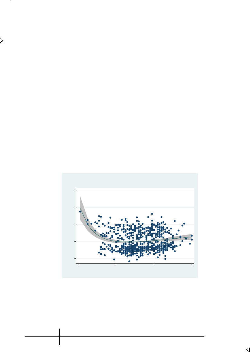
1298 mfp postestimation — Postestimation tools for mfp
For generalized linear and Cox models, the fitted values are plotted on the scale of the “index” (linear
predictor). Deviance residuals are added to the (partial) linear predictor to give component-plus-residual
values. These values are plotted as small circles.
Example 1
In example 1 of [R]mfp, we used Cox regression to predict the log hazard of breast cancer
recurrence from prognostic factors of which five are continuous (x1,x3,x5,x6,x7) and three are
binary (x2,x4a,x4b). We also controlled for hormonal therapy (hormon). We used mfp to build a
model from the initial set of eight predictors by using the backfitting model-selection algorithm. The
nominal p-value for variable and FP selection was set to 0.05 for all variables except hormon, which
is set to 1.
. use http://www.stata-press.com/data/r13/brcancer
(German breast cancer data)
. stset rectime, fail(censrec)
(output omitted )
. mfp, alpha(.05) select(.05, hormon:1): stcox x1 x2 x3 x4a x4b x5 x6 x7 hormon,
> nohr
(output omitted )
We can use fracplot to produce component-plus-residual plots of the continuous variables. We
produce the component-plus-residual plot for x1 with fracplot by specifying x1 after the command
name.
. fracplot x1
−2 0 2 4 6
Partial predictor+residual of _t
20 40 60 80
age, years
Fractional Polynomial (−2 −.5),
adjusted for covariates
We use fracpred with the stdp option to predict the standard error of the fractional polynomial
prediction for x1. The standard error prediction will be stored in variable sepx1. We specify that
prediction is made for x1 with the for() option. After prediction, we use summarize to show how
the standard error estimate varies over different values of x1.
. fracpred sepx1, stdp for(x1)
. summarize sepx1
Variable Obs Mean Std. Dev. Min Max
sepx1 686 .0542654 .0471993 .0003304 .6862065

mfp postestimation — Postestimation tools for mfp 1299
Methods and formulas
The general definition of an FP, accommodating possible repeated powers, may be written for
functions H1(x), . . . , Hm(x)as
β0+
m
X
j=1
βjHj(x)
where H1(x) = x(p1)and for j=2, . . . , m,
Hj(x) = x(pj)if pj6=pj−1
Hj−1(x) log xif pj=pj−1
For example, an FP of degree 3 with powers (1,3,3)has H1(x) = x,H2(x) = x3, and H3(x) =
x3log xand equals β0+β1x+β2x3+β3x3log x.
The component-plus-residual values graphed by fracplot are calculated as follows: Let the
data consist of triplets (yi, xi,zi),i=1, . . . , n, where ziis the vector of covariates for the ith
observation, after applying possible fractional polynomial transformation and adjustment as described
earlier. Let bηi=b
β0+{H(xi)−H(x0)}0b
β+z0
ibγbe the linear predictor from the FP model, as
given by the fracpred command or, equivalently, by the predict command with the xb option,
following mfp. Here H(xi) = {H1(xi), . . . , Hm(xi)}0is the vector of FP functions described above,
H(x0) = {H1(x0), . . . , Hm(x0)}0is the vector of adjustments to x0(often, x0is chosen to be the
mean of the xi), b
βis the estimated parameter vector, and bγis the estimated parameter vector for
the covariates. The values bη∗
i=b
β0+{H(xi)−H(x0)}0b
βrepresent the behavior of the FP model
for xat fixed values z=0of the (adjusted) covariates. The ith component-plus-residual is defined
as bη∗
i+di, where diis the deviance residual for the ith observation. For normal-errors models,
di=√wi(yi−bηi), where wiis the case weight (or 1, if weight is not specified). For logistic, Cox,
and generalized linear regression models, see [R]logistic,[R]probit,[ST]stcox, and [R]glm for the
formula for di. The formula for poisson models is the same as that for glm with family(poisson).
For stcox,diis the partial martingale residual (see [ST]stcox postestimation).
fracplot plots the values of diand the curve represented by bη∗
iagainst xi. The confidence
interval for bη∗
iis obtained from the variance–covariance matrix of the entire model and takes into
account the uncertainty in estimating β0,β, and γ(but not in estimating the FP powers for x).
fracpred with the for(varname)option calculates the predicted index at xi=x0and zi=0;
that is, bηi=b
β0+{H(xi)−H(x0)}0b
β. The standard error is calculated from the variance–covariance
matrix of (b
β0,b
β), again ignoring estimation of the powers.
Also see
[R]mfp — Multivariable fractional polynomial models
[U] 20 Estimation and postestimation commands

Title
misstable — Tabulate missing values
Syntax Menu Description Options
Remarks and examples Stored results Also see
Syntax
Report counts of missing values
misstable summarize varlist if in ,summarize options
Report pattern of missing values
misstable patterns varlist if in ,patterns options
Present a tree view of the pattern of missing values
misstable tree varlist if in ,tree options
List the nesting rules that describe the missing-value pattern
misstable nested varlist if in ,nested options
summarize options Description
all show all variables
showzeros show zeros in table
generate(stub , exok )generate missing-value indicators
patterns options Description
asis use variables in order given
frequency report frequencies instead of percentages
exok treat .a,.b,. . . ,.z as nonmissing
replace replace data in memory with dataset of patterns
clear okay to replace even if original unsaved
bypatterns list by patterns rather than by frequency
tree options Description
asis use variables in order given
frequency report frequencies instead of percentages
exok treat .a,.b,. . . ,.z as nonmissing
1300

misstable — Tabulate missing values 1301
nested options Description
exok treat .a,.b,. . . ,.z as nonmissing
In addition, programmer’s option nopreserve is allowed with all syntaxes; see [P]nopreserve option.
Menu
Statistics >Summaries, tables, and tests >Other tables >Tabulate missing values
Description
misstable makes tables that help you understand the pattern of missing values in your data.
Options
Options are presented under the following headings:
Options for misstable summarize
Options for misstable patterns
Options for misstable tree
Option for misstable nested
Common options
Options for misstable summarize
all specifies that the table should include all the variables specified or all the variables in the dataset.
The default is to include only numeric variables that contain missing values.
showzeros specifies that zeros in the table should display as 0 rather than being omitted.
generate(stub , exok )requests that a missing-value indicator newvar, a new binary variable
containing 0for complete observations and 1for incomplete observations, be generated for every
numeric variable in varlist containing missing values. If the all option is specified, missing-value
indicators are created for all the numeric variables specified or for all the numeric variables in the
dataset. If exok is specified within generate(), the extended missing values .a,.b,. . . ,.z are
treated as if they do not designate missing.
For each variable in varlist,newvar is the corresponding variable name varname prefixed with
stub. If the total length of stub and varname exceeds 32 characters, newvar is abbreviated so that
its name does not exceed 32 characters.
Options for misstable patterns
asis,frequency, and exok – see Common options below.
replace specifies that the data in memory be replaced with a dataset corresponding to the table just
displayed; see misstable patterns under Remarks and examples below.
clear is for use with replace; it specifies that it is okay to change the data in memory even if they
have not been saved to disk.

1302 misstable — Tabulate missing values
bypatterns specifies the table be ordered by pattern rather than by frequency. That is, bypatterns
specifies that patterns containing one incomplete variable be listed first, followed by those for two
incomplete variables, and so on. The default is to list the most frequent pattern first, followed by
the next most frequent pattern, etc.
Options for misstable tree
asis,frequency, and exok – see Common options below.
Option for misstable nested
exok – see Common options below.
Common options
asis specifies that the order of the variables in the table be the same as the order in which they
are specified on the misstable command. The default is to order the variables by the number of
missing values, and within that, by the amount of overlap of missing values.
frequency specifies that the table should report frequencies instead of percentages.
exok specifies that the extended missing values .a,.b,. . . ,.z should be treated as if they do not
designate missing. Some users use extended missing values to designate values that are missing
for a known and valid reason.
nopreserve is a programmer’s option allowed with all misstable commands; see [P]nopreserve
option.
Remarks and examples
Remarks are presented under the following headings:
misstable summarize
misstable patterns
misstable tree
misstable nested
Execution time of misstable nested
In what follows, we will use data from a 125-observation, fictional, student-satisfaction survey:
. use http://www.stata-press.com/data/r13/studentsurvey
(Student Survey)
. summarize
Variable Obs Mean Std. Dev. Min Max
m1 125 2.456 .8376619 1 4
m2 125 2.472 .8089818 1 4
age 122 18.97541 .8763477 17 21
female 122 .5245902 .5014543 0 1
dept 116 2.491379 1.226488 1 4
offcampus 125 .36 .4819316 0 1
comment 0
The m1 and m2 variables record the student’s satisfaction with teaching and with academics.
comment is a string variable recording any comments the student might have had.

misstable — Tabulate missing values 1303
misstable summarize
Example 1
misstable summarize reports counts of missing values:
. misstable summarize
Obs<.
Unique
Variable Obs=. Obs>. Obs<. values Min Max
age 3 122 5 17 21
female 3 122 2 0 1
dept 9 116 4 1 4
Stata provides 27 different missing values, namely, .,.a,.b,. . . ,.z. The first of those, ., is often
called system missing. The remaining missing values are called extended missings. The nonmissing
and missing values are ordered nonmissing <.<.a <.b <··· <.z. Thus reported in the column
“Obs=.” are counts of system missing values; in the column “Obs>.”, extended missing values; and
in the column “Obs<.”, nonmissing values.
The rightmost portion of the table is included to remind you how the variables are encoded.
Our data contain seven variables and yet misstable reported only three of them. The omitted
variables contain no missing values or are string variables. Even if we specified the varlist explicitly,
those variables would not appear in the table unless we specified the all option.
We can also create missing-value indicators for each of the variables above using the generate()
option:
. quietly misstable summarize, generate(miss_)
. describe miss_*
storage display value
variable name type format label variable label
miss_age byte %8.0g (age>=.)
miss_female byte %8.0g (female>=.)
miss_dept byte %8.0g (dept>=.)
For each variable containing missing values, the generate() option creates a new binary variable
containing 0for complete observations and 1for incomplete observations. In our example, three new
missing-value indicators are generated, one for each of the incomplete variables age,female, and
dept. The naming convention of generate() is to prefix the corresponding variable names with the
specified stub, which is miss in this example.
Missing-value indicators are useful, for example, for checking whether data are missing completely
at random. They are also often used within the multiple-imputation context to identify the observed
and imputed data; see [MI]intro substantive for a general introduction to multiple imputation. Within
Stata’s multiple-imputation commands, an incomplete value is identified by the system missing value,
a dot. By default, misstable summarize, generate() marks the extended missing values as
incomplete values, as well. You can use exok within generate() to treat extended missing values
as complete when creating missing-value identifiers.

1304 misstable — Tabulate missing values
misstable patterns
Example 2
misstable patterns reports the pattern of missing values:
. misstable patterns
Missing-value patterns
(1 means complete)
Pattern
Percent 1 2 3
93% 1 1 1
5 1 1 0
2 0 0 0
100%
Variables are (1) age (2) female (3) dept
There are three patterns in these data: (1,1,1), (1,1,0), and (0,0,0). By default, the rows of the table
are ordered by frequency. In larger tables that have more patterns, it is sometimes useful to order the
rows by pattern. We could have obtained that by typing mi misstable patterns, bypatterns.
In a pattern, 1 indicates that all values of the variable are nonmissing and 0 indicates that all values
are missing. Thus pattern (1,1,1) means no missing values, and 93% of our data have that pattern.
There are two patterns in which variables are missing, (1,1,0) and (0,0,0). Pattern (1,1,0) means that
age is nonmissing, female is nonmissing, and dept is missing. The order of the variables in the
patterns appears in the key at the bottom of the table. Five percent of the observations have pattern
(1,1,0). The remaining 2% have pattern (0,0,0), meaning that all three variables contain missing.
As with misstable summarize, only numeric variables that contain missing are listed, so had
we typed misstable patterns comments age female offcampus dept, we still would have
obtained the same table. Variables that are automatically omitted contain no missing values or are
string variables.
The variables in the table are ordered from lowest to highest frequency of missing values, although
you cannot see that from the information presented in the table. The variables are ordered this way
even if you explicitly specify the varlist with a different ordering. Typing misstable patterns
dept female age would produce the same table as above. Specify the asis option if you want the
variables in the order in which you specify them.
You can obtain a dataset of the patterns by specifying the replace option:
. misstable patterns, replace clear
Missing-value patterns
(1 means complete)
Pattern
Percent 1 2 3
93% 1 1 1
5 1 1 0
2 0 0 0
100%
Variables are (1) age (2) female (3) dept
(summary data now in memory)

misstable — Tabulate missing values 1305
. list
_freq age female dept
1. 3 0 0 0
2. 6 1 1 0
3. 116 1 1 1
The differences between the dataset and the printed table are that 1) the dataset always records
frequency and 2) the rows are reversed.
misstable tree
Example 3
misstable tree presents a tree view of the pattern of missing values:
. use http://www.stata-press.com/data/r13/studentsurvey, clear
(Student Survey)
. misstable tree, frequency
Nested pattern of missing values
dept age female
9 3 3
0
6 0
6
116 0 0
0
116 0
116
(number missing listed first)
In this example, we specified the frequency option to see the table in frequency rather than
percentage terms. In the table, each column sums to the total number of observations in the data,
125. Variables are ordered from those with the most missing values to those with the least. Start with
the first column. The dept variable is missing in 9 observations and, farther down, the table reports
that it is not missing in 116 observations.
Go back to the first row and read across, but only to the second column. The dept variable is
missing in 9 observations. Within those 9, age is missing in 3 of them and is not missing in the
remaining 6. Reading down the second column, within the 116 observations that dept is not missing,
age is missing in 0 and not missing in 116.
Reading straight across the first row again, dept is missing in 9 observations, and within the 9,
age is missing in 3, and within the 3, female is also missing in 3. Skipping down just a little, within
the 6 observations for which dept is missing and age is not missing, female is not missing, too.

1306 misstable — Tabulate missing values
misstable nested
Example 4
misstable nested lists the nesting rules that describe the missing-value pattern,
. misstable nested
1. female(3) <-> age(3) -> dept(9)
This line says that in observations in which female is missing, so is age missing, and vice versa,
and in observations in which age (or female) is missing, so is dept. The numbers in parentheses
are counts of the missing values. The female variable happens to be missing in 3 observations, and
the same is true for age; the dept variable is missing in 9 observations. Thus dept is missing in
the 3 observations for which age and female are missing, and in 6 more observations, too.
In these data, it turns out that the missing-value pattern can be summarized in one statement. In
a larger dataset, you might see something like this:
. misstable nested
1. female(50) <-> age(50) -> dept(120)
2. female(50) -> m1(58)
3. offcampus(11)
misstable nested accounts for every missing value. In the above, in addition to female <->
age -> dept, we have that female -> m1, and we have offcampus, the last all by itself. The last
line says that the 11 missing values in offcampus are not themselves nested in the missing value of
any other variable, nor do they imply the missing values in another variable. In some datasets, all
the statements will be of this last form.
In our data, however, we have one statement:
. misstable nested
1. female(3) <-> age(3) -> dept(9)
When the missing-value pattern can be summarized in one misstable nested statement, the
pattern of missing values in the data is said to be monotone.
Execution time of misstable nested
The execution time of misstable nested is affected little by the number of observations but can
grow quickly with the number of variables, depending on the fraction of missing values within variable.
The execution time of the example above, which has 3 variables containing missing, is instant. In
worst-case scenarios, with 500 variables, the time might be 25 seconds; with 1,000 variables, the
execution time might be closer to an hour.
In situations where misstable nested takes a long time to complete, it will produce thousands
of rules that will defy interpretation. A 523-variable dataset we have seen ran in 20 seconds and
produced 8,040 rules. Although we spotted a few rules in the output that did not surprise us, such
as the year of the date being missing implied that the month and the day were also missing, mostly
the output was not helpful.
If you have such a dataset, we recommend you run misstable on groups of variables that you
have reason to believe the pattern of missing values might be related.

misstable — Tabulate missing values 1307
Stored results
misstable summarize stores the following values of the last variable summarized in r():
Scalars
r(N eq dot) number of observations containing .
r(N gt dot) number of observations containing .a,.b,. . . ,.z
r(N lt dot) number of observations containing nonmissing
r(K uniq) number of unique, nonmissing values
r(min) variable’s minimum value
r(max) variable’s maximum value
Macros
r(vartype) numeric,string, or none
r(K uniq) contains .if the number of unique, nonmissing values is greater than 500. r(vartype)
contains none if no variables are summarized, and in that case, the value of the scalars are all set to
missing (.). Programmers intending to access results after misstable summarize should specify the
all option.
misstable patterns stores the following in r():
Scalars
r(N complete) number of complete observations
r(N incomplete) number of incomplete observations
r(K) number of patterns
Macros
r(vars) variables used in order presented
r(N complete) and r(N incomplete) are defined with respect to the variables specified if variables
were specified and otherwise, defined with respect to all the numeric variables in the dataset. r(N complete)
is the number of observations that contain no missing values.
misstable tree stores the following in r():
Macros
r(vars) variables used in order presented
misstable nested stores the following in r():
Scalars
r(K) number of statements
Macros
r(stmt1) first statement
r(stmt2) second statement
. .
. .
r(stmt‘r(K)’) last statement
r(stmt1wc) r(stmt1) with missing-value counts
r(vars) variables considered
A statement is encoded “varname”, “varname op varname”, or “varname op varname op varname”, and so on;
op is either “->” or “<->”.
Also see
[MI]mi misstable — Tabulate pattern of missing values
[R]summarize — Summary statistics
[R]tabulate oneway — One-way table of frequencies
[R]tabulate twoway — Two-way table of frequencies

Title
mkspline — Linear and restricted cubic spline construction
Syntax Menu Description Options
Remarks and examples Methods and formulas Acknowledgment References
Also see
Syntax
Linear spline with knots at specified points
mkspline newvar1#1[newvar2#2[. . .] ] newvark=oldvar if in , marginal
displayknots
Linear spline with knots equally spaced or at percentiles of data
mkspline stubname # =oldvar if in weight , marginal pctile
displayknots
Restricted cubic spline
mkspline stubname =oldvar if in weight , cubic nknots(#) knots(numlist)
displayknots
fweights are allowed with the second and third syntax; see [U] 11.1.6 weight.
Menu
Data >Create or change data >Other variable-creation commands >Linear and cubic spline construction
Description
mkspline creates variables containing a linear spline or a restricted cubic spline of oldvar.
In the first syntax, mkspline creates newvar1,. . . ,newvarkcontaining a linear spline of oldvar
with knots at the specified #1,. . . ,#k−1.
In the second syntax, mkspline creates #variables named stubname1,. . . ,stubname# containing
a linear spline of oldvar. The knots are equally spaced over the range of oldvar or are placed at the
percentiles of oldvar.
In the third syntax, mkspline creates variables containing a restricted cubic spline of oldvar.
This is also known as a natural spline. The location and spacing of the knots is determined by the
specification of the nknots() and knots() options.
1308

mkspline — Linear and restricted cubic spline construction 1309
Options
Options
marginal is allowed with the first or second syntax. It specifies that the new variables be constructed
so that, when used in estimation, the coefficients represent the change in the slope from the
preceding interval. The default is to construct the variables so that, when used in estimation, the
coefficients measure the slopes for the interval.
displayknots displays the values of the knots that were used in creating the linear or restricted
cubic spline.
pctile is allowed only with the second syntax. It specifies that the knots be placed at percentiles of
the data rather than being equally spaced over the range.
nknots(#)is allowed only with the third syntax. It specifies the number of knots that are to be used
for a restricted cubic spline. This number must be between 3 and 7 unless the knot locations are
specified using knots(). The default number of knots is 5.
knots(numlist)is allowed only with the third syntax. It specifies the exact location of the knots to
be used for a restricted cubic spline. The values of these knots must be given in increasing order.
When this option is omitted, the default knot values are based on Harrell’s recommended percentiles
with the additional restriction that the smallest knot may not be less than the fifth-smallest value
of oldvar and the largest knot may not be greater than the fifth-largest value of oldvar. If both
nknots() and knots() are given, they must specify the same number of knots.
Remarks and examples
Remarks are presented under the following headings:
Linear splines
Restricted cubic splines
Linear splines
Linear splines allow estimating the relationship between yand xas a piecewise linear function,
which is a function composed of linear segments—straight lines. One linear segment represents the
function for values of xbelow x0, another linear segment handles values between x0and x1, and
so on. The linear segments are arranged so that they join at x0,x1,. . . , which are called the knots.
An example of a piecewise linear function is shown below.
knot 1
knot 2
2 3 4 5
z
0 1 2 3
x
A piecewise linear function

1310 mkspline — Linear and restricted cubic spline construction
Example 1
We wish to fit a model of log income on education and age by using a piecewise linear function
for age:
lninc =b0+b1educ +f(age) + u
The knots are to be placed at 10-year intervals: 20, 30, 40, 50, and 60.
. use http://www.stata-press.com/data/r13/mksp1
. mkspline age1 20 age2 30 age3 40 age4 50 age5 60 age6 = age, marginal
. regress lninc educ age1-age6
(output omitted )
Because we specified the marginal option, we could test whether the age effect is the same in
the 30–40 and 40–50 intervals by asking whether the age4 coefficient is zero. With the marginal
option, coefficients measure the change in slope from the preceding group. Specifying marginal
changes only the interpretation of the coefficients; the same model is fit in either case. Without the
marginal option, the interpretation of the coefficients would have been
dy
dage =
a1if age <20
a2if 20 ≤age <30
a3if 30 ≤age <40
a4if 40 ≤age <50
a5if 50 ≤age <60
a6otherwise
With the marginal option, the interpretation is
dy
dage =
a1if age <20
a1+a2if 20 ≤age <30
a1+a2+a3if 30 ≤age <40
a1+a2+a3+a4if 40 ≤age <50
a1+a2+a3+a4+a5if 50 ≤age <60
a1+a2+a3+a4+a5+a6otherwise
Example 2
Say that we have a binary outcome variable called outcome. We are beginning an analysis and
wish to parameterize the effect of dosage on outcome. We wish to divide the data into five equal-width
groups of dosage for the piecewise linear function.
. use http://www.stata-press.com/data/r13/mksp2, clear
. mkspline dose 5 = dosage, displayknots
knot1 knot2 knot3 knot4
dosage 20 40 60 80
. logistic outcome dose1-dose5
(output omitted )

mkspline — Linear and restricted cubic spline construction 1311
mkspline dose 5 = dosage creates five variables—dose1,dose2,. . . ,dose5—equally spacing the
knots over the range of dosage. Because dosage varied between 0 and 100, the mkspline command
above has the same effect as typing
. mkspline dose1 20 dose2 40 dose3 60 dose4 80 dose5 = dosage
The pctile option sets the knots to divide the data into five equal sample-size groups rather than
five equal-width ranges. Typing
. mkspline pctdose 5 = dosage, pctile displayknots
knot1 knot2 knot3 knot4
dosage 16 36.4 55.6 82
places the knots at the 20th, 40th, 60th, and 80th percentiles of the data.
Restricted cubic splines
A linear spline can be used to fit many functions well. However, a restricted cubic spline may
be a better choice than a linear spline when working with a very curved function. When using a
restricted cubic spline, one obtains a continuous smooth function that is linear before the first knot,
a piecewise cubic polynomial between adjacent knots, and linear again after the last knot.
Example 3
Returning to the data from example 1, we may feel that a curved function is a better fit. First, we
will use the knots() option to specify the five knots that we used previously.
. use http://www.stata-press.com/data/r13/mksp1, clear
. mkspline agesp = age, cubic knots(20 30 40 50 60)
. regress lninc educ agesp*
(output omitted )
Harrell (2001, 23) recommends placing knots at equally spaced percentiles of the original variable’s
marginal distribution. If we do not specify the knots() option, variables will be created containing
a restricted cubic spline with five knots determined by Harrell’s default percentiles.
. use http://www.stata-press.com/data/r13/mksp1, clear
. mkspline agesp = age, cubic displayknots
. regress lninc educ agesp*
(output omitted )
Methods and formulas
Methods and formulas are presented under the following headings:
Linear splines
Restricted cubic splines

1312 mkspline — Linear and restricted cubic spline construction
Linear splines
Let Vi,i=1, . . . , n, be the variables to be created; ki,i=1, . . . , n −1, be the corresponding
knots; and Vbe the original variable (the command is mkspline V1k1V2k2. . . Vn=V). Then
V1= min(V, k1)
Vi= maxnmin(V, ki), ki−1o−ki−1i= 2, . . . , n −1
Vn= max(V, kn−1)−kn−1
If the marginal option is specified, the definitions are
V1=V
Vi= max(0,V − ki−1)i= 2, . . . , n
In the second syntax, mkspline stubname # =V, so let mand Mbe the minimum and maximum
of V. Without the pctile option, knots are set at m+ (M−m)(i/n)for i=1, . . . , n −1. If
pctile is specified, knots are set at the 100(i/n)percentiles, for i=1, . . . , n −1. Percentiles are
calculated by centile; see [R]centile.
Restricted cubic splines
Let ki,i=1, . . . , n, be the knot values; Vi,i=1, . . . , n −1, be the variables to be created; and
Vbe the original variable. Then
V1=V
Vi+1 =(V − ki)3
+−(kn−kn−1)−1{(V − kn−1)3
+(kn−ki)−(V − kn)3
+(kn−1−ki)}
(kn−k1)2
i= 1, . . . , n −2
where
(u)+=(u, if u > 0
0, if u≤0
Without the knots() option, the locations of the knots are determined by the percentiles rec-
ommended in Harrell (2001, 23). These percentiles are based on the chosen number of knots as
follows:
No.
of knots Percentiles
3 10 50 90
4 5 35 65 95
5 5 27.5 50 72.5 95
6 5 23 41 59 77 95
7 2.5 18.33 34.17 50 65.83 81.67 97.5

mkspline — Linear and restricted cubic spline construction 1313
Harrell provides default percentiles when the number of knots is between 3 and 7. When using a
number of knots outside this range, the location of the knots must be specified in knots().
Acknowledgment
The restricted cubic spline portion of mkspline is based on the rc spline command by William
Dupont of the Department of Biostatistics at Vanderbilt University.
References
Gould, W. W. 1993. sg19: Linear splines and piecewise linear functions.Stata Technical Bulletin 15: 13–17. Reprinted
in Stata Technical Bulletin Reprints, vol. 3, pp. 98–104. College Station, TX: Stata Press.
Greene, W. H. 2012. Econometric Analysis. 7th ed. Upper Saddle River, NJ: Prentice Hall.
Harrell, F. E., Jr. 2001. Regression Modeling Strategies: With Applications to Linear Models, Logistic Regression,
and Survival Analysis. New York: Springer.
Newson, R. B. 2000. sg151: B-splines and splines parameterized by their values at reference points on the x-axis.
Stata Technical Bulletin 57: 20–27. Reprinted in Stata Technical Bulletin Reprints, vol. 10, pp. 221–230. College
Station, TX: Stata Press.
. 2012. Sensible parameters for univariate and multivariate splines.Stata Journal 12: 479–504.
Orsini, N., and S. Greenland. 2011. A procedure to tabulate and plot results after flexible modeling of a quantitative
covariate.Stata Journal 11: 1–29.
Panis, C. 1994. sg24: The piecewise linear spline transformation.Stata Technical Bulletin 18: 27–29. Reprinted in
Stata Technical Bulletin Reprints, vol. 3, pp. 146–149. College Station, TX: Stata Press.
Also see
[R]fp — Fractional polynomial regression

Title
ml — Maximum likelihood estimation
Syntax Description Options Remarks and examples
Stored results Methods and formulas References Also see
Syntax
ml model in interactive mode
ml model method progname eq eq . . . if in weight
,model options svy diparm options
ml model method funcname() eq eq . . . if in weight
,model options svy diparm options
ml model in noninteractive mode
ml model method progname eq eq . . . if in weight , maximize
model options svy diparm options noninteractive options
ml model method funcname() eq eq . . . if in weight , maximize
model options svy diparm options noninteractive options
Noninteractive mode is invoked by specifying the maximize option. Use maximize when ml will
be used as a subroutine of another ado-file or program and you want to carry forth the problem,
from definition to posting of results, in one command.
ml clear
ml query
ml check
ml search /eqname:#lb #ub . . . ,search options
ml plot eqname:name ### , saving(filename, replace )
ml init eqname:name=#|/eqname=# . . .
ml init ##. . . , copy
ml init matname , copy skip
ml report
ml trace on |off 1314

ml — Maximum likelihood estimation 1315
ml count clear |on |off
ml maximize ,ml maximize options display options eform option
ml graph # , saving(filename, replace )
ml display ,display options eform option
ml footnote
ml score newvar if in , equation(eqname) missing
ml score newvarlist if in , missing
ml score type stub*if in , missing
where method is one of
lf d0 lf0 gf0
d1 lf1
d1debug lf1debug
d2 lf2
d2debug lf2debug
or method can be specified using one of the longer, more descriptive names
method Longer name
lf linearform
d0 derivative0
d1 derivative1
d1debug derivative1debug
d2 derivative2
d2debug derivative2debug
lf0 linearform0
lf1 linearform1
lf1debug linearform1debug
lf2 linearform2
lf2debug linearform2debug
gf0 generalform0
eq is the equation to be estimated, enclosed in parentheses, and optionally with a name to be given
to the equation, preceded by a colon,
(eqname:varlisty=varlistx,eq options )
or eq is the name of a parameter, such as sigma, with a slash in front
/eqname which is equivalent to (eqname:)
and diparm options is one or more diparm(diparm args)options where diparm args is either
sep or anything accepted by the “undocumented” diparm command; see help diparm.

1316 ml — Maximum likelihood estimation
eq options Description
noconstant do not include an intercept in the equation
offset(varnameo)include varnameoin model with coefficient constrained to 1
exposure(varnamee)include ln(varnamee)in model with coefficient constrained to 1
model options Description
group(varname)use varname to identify groups
vce(vcetype)vcetype may be robust,cluster clustvar,oim, or opg
constraints(numlist)constraints by number to be applied
constraints(matname)matrix that contains the constraints to be applied
nocnsnotes do not display notes when constraints are dropped
title(string)place a title on the estimation output
nopreserve do not preserve the estimation subsample in memory
collinear keep collinear variables within equations
missing keep observations containing variables with missing values
lf0(#k#ll)number of parameters and log-likelihood value of the
constant-only model
continue specifies that a model has been fit and sets the initial values
b0for the model to be fit based on those results
waldtest(#)perform a Wald test; see Options for use with ml model in
interactive or noninteractive mode below
obs(#)number of observations
crittype(string)describe the criterion optimized by ml
subpop(varname)compute estimates for the single subpopulation
nosvyadjust carry out Wald test as W/k ∼F(k, d)
technique(nr) Stata’s modified Newton–Raphson (NR) algorithm
technique(bhhh) Berndt–Hall–Hall–Hausman (BHHH) algorithm
technique(dfp) Davidon–Fletcher–Powell (DFP) algorithm
technique(bfgs) Broyden–Fletcher–Goldfarb–Shanno (BFGS) algorithm
noninteractive options Description
init(ml init args)set the initial values b0
search(on) equivalent to ml search, repeat(0); the default
search(norescale) equivalent to ml search, repeat(0) norescale
search(quietly) same as search(on), except that output is suppressed
search(off) prevents calling ml search
repeat(#) ml search’s repeat() option; see below
bounds(ml search bounds)specify bounds for ml search
nowarning suppress “convergence not achieved” message of iterate(0)
novce substitute the zero matrix for the variance matrix
negh indicates that the evaluator returns the negative Hessian matrix
score(newvars)new variables containing the contribution to the score
maximize options control the maximization process; seldom used

ml — Maximum likelihood estimation 1317
search options Description
repeat(#)number of random attempts to find better initial-value
vector; default is repeat(10) in interactive mode and
repeat(0) in noninteractive mode
restart use random actions to find starting values; not recommended
norescale do not rescale to improve parameter vector; not recommended
maximize options control the maximization process; seldom used
ml maximize options Description
nowarning suppress “convergence not achieved” message of iterate(0)
novce substitute the zero matrix for the variance matrix
negh indicates that the evaluator returns the negative Hessian matrix
score(newvars|stub*) new variables containing the contribution to the score
nooutput suppress display of final results
noclear do not clear ml problem definition after model has converged
maximize options control the maximization process; seldom used
display options Description
noheader suppress header display above the coefficient table
nofootnote suppress footnote display below the coefficient table
level(#)set confidence level; default is level(95)
first display coefficient table reporting results for first equation only
neq(#)display coefficient table reporting first #equations
showeqns display equation names in the coefficient table
plus display coefficient table ending in dashes–plus-sign–dashes
nocnsreport suppress constraints display above the coefficient table
noomitted suppress display of omitted variables
vsquish suppress blank space separating factor-variable terms or
time-series–operated variables from other variables
noemptycells suppress empty cells for interactions of factor variables
baselevels report base levels of factor variables and interactions
allbaselevels display all base levels of factor variables and interactions
cformat(%fmt)format the coefficients, standard errors, and confidence limits in
the coefficient table
pformat(%fmt)format the p-values in the coefficient table
sformat(%fmt)format the test statistics in the coefficient table
nolstretch do not automatically widen the coefficient table to accommodate
longer variable names
coeflegend display legend instead of statistics

1318 ml — Maximum likelihood estimation
eform option Description
eform(string)display exponentiated coefficients; column title is “string”
eform display exponentiated coefficients; column title is “exp(b)”
hr report hazard ratios
shr report subhazard ratios
irr report incidence-rate ratios
or report odds ratios
rrr report relative-risk ratios
fweights, aweights, iweights, and pweights are allowed; see [U] 11.1.6 weight. With all but method lf, you must
write your likelihood-evaluation program carefully if pweights are to be specified, and pweights may not be
specified with method d0, d1, d1debug, d2, or d2debug. See Gould, Pitblado, and Poi (2010, chap. 6) for details.
See [U] 20 Estimation and postestimation commands for more capabilities of estimation commands.
To redisplay results, type ml display.
Syntax of subroutines for use by evaluator programs
mleval newvar =vecname , eq(#)
mleval scalarname =vecname , scalar eq(#)
mlsum scalarnamelnf =exp if , noweight
mlvecsum scalarnamelnf rowvecname =exp if , eq(#)
mlmatsum scalarnamelnf matrixname =exp if , eq(#,#)
mlmatbysum scalarnamelnf matrixname varnameavarnamebvarnamec if ,
by(varname)eq(#,#)
Syntax of user-written evaluator
Summary of notation
The log-likelihood function is ln L(θ1j, θ2j, . . . , θEj ), where θij =xij bi,j=1, . . . , N indexes
observations, and i=1, . . . , E indexes the linear equations defined by ml model. If the likelihood
satisfies the linear-form restrictions, it can be decomposed as ln L=PN
j=1 ln `(θ1j, θ2j, . . . , θEj ).
Method-lf evaluators
program progname
version 13
args lnfj theta1 theta2 . . .
// if you need to create any intermediate results:
tempvar tmp1 tmp2 . . .
quietly gen double ‘tmp1’ = . . .
. . .
quietly replace ‘lnfj’ = . . .
end

ml — Maximum likelihood estimation 1319
where
‘lnfj’ variable to be filled in with observation-by-observation values of ln`j
‘theta1’ variable containing evaluation of first equation θ1j=x1jb1
‘theta2’ variable containing evaluation of second equation θ2j=x2jb2
. . .
Method-d0 evaluators
program progname
version 13
args todo b lnf
tempvar theta1 theta2 . . .
mleval ‘theta1’ = ‘b’, eq(1)
mleval ‘theta2’ = ‘b’, eq(2) // if there is a θ2
. . .
// if you need to create any intermediate results:
tempvar tmp1 tmp2 . . .
gen double ‘tmp1’ = . . .
. . .
mlsum ‘lnf’ = . . .
end
where
‘todo’ always contains 0(may be ignored)
‘b’ full parameter row vector b=(b1,b2,...,bE)
‘lnf’ scalar to be filled in with overall lnL
Method-d1 evaluators
program progname
version 13
args todo b lnf g
tempvar theta1 theta2 . . .
mleval ‘theta1’ = ‘b’, eq(1)
mleval ‘theta2’ = ‘b’, eq(2) // if there is a θ2
. . .
// if you need to create any intermediate results:
tempvar tmp1 tmp2 . . .
gen double ‘tmp1’ = . . .
. . .
mlsum ‘lnf’ = . . .
if (‘todo’==0 | ‘lnf’>=.) exit
tempname d1 d2 . . .
mlvecsum ‘lnf’ ‘d1’ = formula for ∂ln`j/∂θ1j, eq(1)
mlvecsum ‘lnf’ ‘d2’ = formula for ∂ln`j/∂θ2j, eq(2)
. . .
matrix ‘g’ = (‘d1’,‘d2’, . . . )
end
where
‘todo’ contains 0or 1
0⇒‘lnf’to be filled in;
1⇒‘lnf’ and ‘g’ to be filled in
‘b’ full parameter row vector b=(b1,b2,...,bE)
‘lnf’ scalar to be filled in with overall lnL
‘g’ row vector to be filled in with overall g=∂lnL/∂b

1320 ml — Maximum likelihood estimation
Method-d2 evaluators
program progname
version 13
args todo b lnf g H
tempvar theta1 theta2 . . .
mleval ‘theta1’ = ‘b’, eq(1)
mleval ‘theta2’ = ‘b’, eq(2) // if there is a θ2
. . .
// if you need to create any intermediate results:
tempvar tmp1 tmp2 . . .
gen double ‘tmp1’ = . . .
. . .
mlsum ‘lnf’ = . . .
if (‘todo’==0 | ‘lnf’>=.) exit
tempname d1 d2 . . .
mlvecsum ‘lnf’ ‘d1’ = formula for ∂ln`j/∂θ1j, eq(1)
mlvecsum ‘lnf’ ‘d2’ = formula for ∂ln`j/∂θ2j, eq(2)
. . .
matrix ‘g’ = (‘d1’,‘d2’, . . . )
if (‘todo’==1 | ‘lnf’>=.) exit
tempname d11 d12 d22 . . .
mlmatsum ‘lnf’ ‘d11’ = formula for ∂2ln`j/∂θ2
1j, eq(1)
mlmatsum ‘lnf’ ‘d12’ = formula for ∂2ln`j/∂θ1j∂θ2j, eq(1,2)
mlmatsum ‘lnf’ ‘d22’ = formula for ∂2ln`j/∂θ2
2j, eq(2)
. . .
matrix ‘H’ = (‘d11’,‘d12’, . . . \ ‘d12’’,‘d22’, . . . )
end
where
‘todo’ contains 0,1, or 2
0⇒‘lnf’ to be filled in;
1⇒‘lnf’ and ‘g’ to be filled in;
2⇒‘lnf’,‘g’, and ‘H’ to be filled in
‘b’ full parameter row vector b=(b1,b2,...,bE)
‘lnf’ scalar to be filled in with overall lnL
‘g’ row vector to be filled in with overall g=∂ln L/∂b
‘H’ matrix to be filled in with overall Hessian H=∂2ln L/∂b∂b0
Method-lf0 evaluators
program progname
version 13
args todo b lnfj
tempvar theta1 theta2 . . .
mleval ‘theta1’ = ‘b’, eq(1)
mleval ‘theta2’ = ‘b’, eq(2) // if there is a θ2
. . .
// if you need to create any intermediate results:
tempvar tmp1 tmp2 . . .
gen double ‘tmp1’ = . . .
. . .
quietly replace ‘lnfj’ = . . .
end
where
‘todo’ always contains 0 (may be ignored)
‘b’ full parameter row vector b=(b1,b2,...,bE)
‘lnfj’ variable to be filled in with observation-by-observation values of ln`j

ml — Maximum likelihood estimation 1321
Method-lf1 evaluators
program progname
version 13
args todo b lnfj g1 g2 . . .
tempvar theta1 theta2 . . .
mleval ‘theta1’ = ‘b’, eq(1)
mleval ‘theta2’ = ‘b’, eq(2) // if there is a θ2
. . .
// if you need to create any intermediate results:
tempvar tmp1 tmp2 . . .
gen double ‘tmp1’ = . . .
. . .
quietly replace ‘lnfj’ = . . .
if (‘todo’==0) exit
quietly replace ‘g1’ = formula for ∂ln`j/∂θ1j
quietly replace ‘g2’ = formula for ∂ln`j/∂θ2j
. . .
end
where
‘todo’ contains 0or 1
0⇒‘lnfj’to be filled in;
1⇒‘lnfj’,‘g1’,‘g2’,. . ., to be filled in
‘b’ full parameter row vector b=(b1,b2,...,bE)
‘lnfj’ variable to be filled in with observation-by-observation values of ln`j
‘g1’ variable to be filled in with ∂ln`j/∂θ1j
‘g2’ variable to be filled in with ∂ln`j/∂θ2j
. . .
Method-lf2 evaluators
program progname
version 13
args todo b lnfj g1 g2 . . . H
tempvar theta1 theta2 . . .
mleval ‘theta1’ = ‘b’, eq(1)
mleval ‘theta2’ = ‘b’, eq(2) // if there is a θ2
. . .
// if you need to create any intermediate results:
tempvar tmp1 tmp2 . . .
gen double ‘tmp1’ = . . .
. . .
quietly replace ‘lnfj’ = . . .
if (‘todo’==0) exit
quietly replace ‘g1’ = formula for ∂ln`j/∂θ1j
quietly replace ‘g2’ = formula for ∂ln`j/∂θ2j
. . .
if (‘todo’==1) exit
tempname d11 d12 d22 lnf . . .
mlmatsum ‘lnf’ ‘d11’ = formula for ∂2ln`j/∂θ2
1j, eq(1)
mlmatsum ‘lnf’ ‘d12’ = formula for ∂2ln`j/∂θ1j∂θ2j, eq(1,2)
mlmatsum ‘lnf’ ‘d22’ = formula for ∂2ln`j/∂θ2
2j, eq(2)
. . .
matrix ‘H’ = (‘d11’,‘d12’, . . . \ ‘d12’’,‘d22’, . . . )
end

1322 ml — Maximum likelihood estimation
where
‘todo’ contains 0or 1
0⇒‘lnfj’to be filled in;
1⇒‘lnfj’,‘g1’,‘g2’,. . ., to be filled in
2⇒‘lnfj’,‘g1’,‘g2’,. . ., and ‘H’ to be filled in
‘b’ full parameter row vector b=(b1,b2,...,bE)
‘lnfj’ scalar to be filled in with observation-by-observation lnL
‘g1’ variable to be filled in with ∂ln`j/∂θ1j
‘g2’ variable to be filled in with ∂ln`j/∂θ2j
. . .
‘H’ matrix to be filled in with overall Hessian H=∂2ln L/∂b∂b0
Method-gf0 evaluators
program progname
version 13
args todo b lnfj
tempvar theta1 theta2 . . .
mleval ‘theta1’ = ‘b’, eq(1)
mleval ‘theta2’ = ‘b’, eq(2) // if there is a θ2
. . .
// if you need to create any intermediate results:
tempvar tmp1 tmp2 . . .
gen double ‘tmp1’ = . . .
. . .
quietly replace ‘lnfj’ = . . .
end
where
‘todo’ always contains 0(may be ignored)
‘b’ full parameter row vector b=(b1,b2,...,bE)
‘lnfj’ variable to be filled in with the values of the log-likelihood ln`j
Global macros for use by all evaluators
$ML y1 name of first dependent variable
$ML y2 name of second dependent variable, if any
. . .
$ML samp variable containing 1 if observation to be used; 0 otherwise
$ML w variable containing weight associated with observation or 1 if no weights specified
Method-lf evaluators can ignore $ML samp, but restricting calculations to the $ML samp==1
subsample will speed execution. Method-lf evaluators must ignore $ML w; application of weights
is handled by the method itself.
Methods d0, d1, d2, lf0, lf1, lf2, and gf0 can ignore $ML samp as long as ml model’s nopreserve
option is not specified. These methods will run more quickly if nopreserve is specified. These
evaluators can ignore $ML w only if they use mlsum,mlvecsum,mlmatsum, and mlmatbysum to
produce all final results.
Description
ml model defines the current problem.
ml clear clears the current problem definition. This command is rarely used because when you type
ml model, any previous problem is automatically cleared.
ml query displays a description of the current problem.
ml check verifies that the log-likelihood evaluator you have written works. We strongly recommend
using this command.

ml — Maximum likelihood estimation 1323
ml search searches for (better) initial values. We recommend using this command.
ml plot provides a graphical way of searching for (better) initial values.
ml init provides a way to specify initial values.
ml report reports ln L’s values, gradient, and Hessian at the initial values or current parameter
estimates, b0.
ml trace traces the execution of the user-defined log-likelihood evaluation program.
ml count counts the number of times the user-defined log-likelihood evaluation program is called;
this command is seldom used. ml count clear clears the counter. ml count on turns on the
counter. ml count without arguments reports the current values of the counter. ml count off
stops counting calls.
ml maximize maximizes the likelihood function and reports results. Once ml maximize has success-
fully completed, the previously mentioned ml commands may no longer be used unless noclear
is specified. ml graph and ml display may be used whether or not noclear is specified.
ml graph graphs the log-likelihood values against the iteration number.
ml display redisplays results.
ml footnote displays a warning message when the model did not converge within the specified
number of iterations.
ml score creates new variables containing the equation-level scores. The variables generated by ml
score are equivalent to those generated by specifying the score() option of ml maximize (and
ml model . . . ,. . . maximize).
progname is the name of a Stata program you write to evaluate the log-likelihood function.
funcname() is the name of a Mata function you write to evaluate the log-likelihood function.
In this documentation, progname and funcname() are referred to as the user-written evaluator, the
likelihood evaluator, or sometimes simply as the evaluator. The program you write is written in
the style required by the method you choose. The methods are lf, d0, d1, d2, lf0, lf1, lf2, and
gf0. Thus, if you choose to use method lf, your program is called a method-lf evaluator.
Method-lf evaluators are required to evaluate the observation-by-observation log likelihood ln `j,
j=1, . . . , N.
Method-d0 evaluators are required to evaluate the overall log likelihood ln L. Method-d1 evaluators
are required to evaluate the overall log likelihood and its gradient vector g=∂ln L/∂b. Method-d2
evaluators are required to evaluate the overall log likelihood, its gradient, and its Hessian matrix
H=∂2ln L/∂b∂b0.
Method-lf0 evaluators are required to evaluate the observation-by-observation log likelihood ln `j,
j=1, . . . , N. Method-lf1 evaluators are required to evaluate the observation-by-observation log
likelihood and its equation-level scores gji =∂ln `/∂xjibi. Method-lf2 evaluators are required to
evaluate the observation-by-observation log likelihood, its equation-level scores, and its Hessian
matrix H=∂2ln `/∂b∂b0.
Method-gf0 evaluators are required to evaluate the summable pieces of the log likelihood ln `k,
k=1, . . . , K.
mleval is a subroutine used by evaluators of methods d0, d1, d2, lf0, lf1, lf2, and gf0 to evaluate
the coefficient vector, b, that they are passed.
mlsum is a subroutine used by evaluators of methods d0, d1, and d2 to define the value, ln L, that is
to be returned.

1324 ml — Maximum likelihood estimation
mlvecsum is a subroutine used by evaluators of methods d1 and d2 to define the gradient vector, g,
that is to be returned. It is suitable for use only when the likelihood function meets the linear-form
restrictions.
mlmatsum is a subroutine used by evaluators of methods d2 and lf2 to define the Hessian matrix, H,
that is to be returned. It is suitable for use only when the likelihood function meets the linear-form
restrictions.
mlmatbysum is a subroutine used by evaluator of method d2 to help define the Hessian matrix, H,
that is to be returned. It is suitable for use when the likelihood function contains terms made
up of grouped sums, such as in panel-data models. For such models, use mlmatsum to compute
the observation-level outer products and mlmatbysum to compute the group-level outer products.
mlmatbysum requires that the data be sorted by the variable identified in the by() option.
Options
Options are presented under the following headings:
Options for use with ml model in interactive or noninteractive mode
Options for use with ml model in noninteractive mode
Options for use when specifying equations
Options for use with ml search
Option for use with ml plot
Options for use with ml init
Options for use with ml maximize
Option for use with ml graph
Options for use with ml display
Options for use with mleval
Option for use with mlsum
Option for use with mlvecsum
Option for use with mlmatsum
Options for use with mlmatbysum
Options for use with ml score
Options for use with ml model in interactive or noninteractive mode
group(varname)specifies the numeric variable that identifies groups. This option is typically used
to identify panels for panel-data models.
vce(vcetype)specifies the type of standard error reported, which includes types that are robust to
some kinds of misspecification (robust), that allow for intragroup correlation (cluster clustvar),
and that are derived from asymptotic theory (oim,opg); see [R]vce option.
vce(robust),vce(cluster clustvar),pweight, and svy will work with evaluators of methods
lf, lf0, lf1, lf2, and gf0; all you need do is specify them.
These options will not work with evaluators of methods d0, d1, or d2, and specifying these options
will produce an error message.
constraints(numlist |matname)specifies the linear constraints to be applied during estimation.
constraints(numlist)specifies the constraints by number. Constraints are defined by using
the constraint command; see [R]constraint.constraint(matname)specifies a matrix that
contains the constraints.
nocnsnotes prevents notes from being displayed when constraints are dropped. A constraint will
be dropped if it is inconsistent, contradicts other constraints, or causes some other error when the
constraint matrix is being built. Constraints are checked in the order in which they are specified.

ml — Maximum likelihood estimation 1325
title(string)specifies the title for the estimation output when results are complete.
nopreserve specifies that ml need not ensure that only the estimation subsample is in memory when
the user-written likelihood evaluator is called. nopreserve is irrelevant when you use method lf.
For the other methods, if nopreserve is not specified, ml saves the data in a file (preserves the
original dataset) and drops the irrelevant observations before calling the user-written evaluator.
This way, even if the evaluator does not restrict its attentions to the $ML samp==1 subsample,
results will still be correct. Later, ml automatically restores the original dataset.
ml need not go through these machinations for method lf because the user-written evaluator
calculates observation-by-observation values, and ml itself sums the components.
ml goes through these machinations if and only if the estimation sample is a subsample of the data
in memory. If the estimation sample includes every observation in memory, ml does not preserve
the original dataset. Thus programmers must not alter the original dataset unless they preserve
the data themselves.
We recommend that interactive users of ml not specify nopreserve; the speed gain is not worth
the possibility of getting incorrect results.
We recommend that programmers specify nopreserve, but only after verifying that their evaluator
really does restrict its attentions solely to the $ML samp==1 subsample.
collinear specifies that ml not remove the collinear variables within equations. There is no reason
to leave collinear variables in place, but this option is of interest to programmers who, in their code,
have already removed collinear variables and do not want ml to waste computer time checking
again.
missing specifies that observations containing variables with missing values not be eliminated from
the estimation sample. There are two reasons you might want to specify missing:
Programmers may wish to specify missing because, in other parts of their code, they have already
eliminated observations with missing values and do not want ml to waste computer time looking
again.
You may wish to specify missing if your model explicitly deals with missing values. Stata’s
heckman command is a good example of this. In such cases, there will be observations where
missing values are allowed and other observations where they are not—where their presence should
cause the observation to be eliminated. If you specify missing, it is your responsibility to specify
an if exp that eliminates the irrelevant observations.
lf0(#k#ll)is typically used by programmers. It specifies the number of parameters and log-likelihood
value of the constant-only model so that ml can report a likelihood-ratio test rather than a Wald
test. These values may have been analytically determined, or they may have been determined by
a previous fitting of the constant-only model on the estimation sample.
Also see the continue option directly below.
If you specify lf0(), it must be safe for you to specify the missing option, too, else how did
you calculate the log likelihood for the constant-only model on the same sample? You must have
identified the estimation sample, and done so correctly, so there is no reason for ml to waste time
rechecking your results. All of which is to say, do not specify lf0() unless you are certain your
code identifies the estimation sample correctly.
lf0(), even if specified, is ignored if vce(robust),vce(cluster clustvar),pweight, or svy
is specified because, in that case, a likelihood-ratio test would be inappropriate.

1326 ml — Maximum likelihood estimation
continue is typically specified by programmers and does two things:
First, it specifies that a model has just been fit by either ml or some other estimation command,
such as logit, and that the likelihood value stored in e(ll) and the number of parameters stored
in e(b) as of that instant are the relevant values of the constant-only model. The current value of
the log likelihood is used to present a likelihood-ratio test unless vce(robust),vce(cluster
clustvar),pweight,svy, or constraints() is specified. A likelihood-ratio test is inappropriate
when vce(robust),vce(cluster clustvar),pweight, or svy is specified. We suggest using
lrtest when constraints() is specified; see [R]lrtest.
Second, continue sets the initial values, b0, for the model about to be fit according to the e(b)
currently stored.
The comments made about specifying missing with lf0() apply equally well here.
waldtest(#)is typically specified by programmers. By default, ml presents a Wald test, but that is
overridden if the lf0() or continue option is specified. A Wald test is performed if vce(robust),
vce(cluster clustvar), or pweight is specified.
waldtest(0) prevents even the Wald test from being reported.
waldtest(-1) is the default. It specifies that a Wald test be performed by constraining all coeffi-
cients except the intercept to 0 in the first equation. Remaining equations are to be unconstrained.
A Wald test is performed if neither lf0() nor continue was specified, and a Wald test is forced
if vce(robust),vce(cluster clustvar), or pweight was specified.
waldtest(k)for k≤ −1 specifies that a Wald test be performed by constraining all coefficients
except intercepts to 0 in the first |k|equations; remaining equations are to be unconstrained. A
Wald test is performed if neither lf0() nor continue was specified, and a Wald test is forced if
vce(robust),vce(cluster clustvar), or pweight was specified.
waldtest(k)for k≥1 works like the options above, except that it forces a Wald test to be
reported even if the information to perform the likelihood-ratio test is available and even if none of
vce(robust),vce(cluster clustvar), or pweight was specified. waldtest(k),k≥1, may
not be specified with lf0().
obs(#)is used mostly by programmers. It specifies that the number of observations reported and
ultimately stored in e(N) be #. Ordinarily, ml works that out for itself. Programmers may want
to specify this option when, for the likelihood evaluator to work for Nobservations, they first had
to modify the dataset so that it contained a different number of observations.
crittype(string)is used mostly by programmers. It allows programmers to supply a string (up to
32 characters long) that describes the criterion that is being optimized by ml. The default is "log
likelihood" for nonrobust and "log pseudolikelihood" for robust estimation.
svy indicates that ml is to pick up the svy settings set by svyset and use the robust variance
estimator. This option requires the data to be svyset; see [SVY]svyset.svy may not be specified
with vce() or weights.
subpop(varname)specifies that estimates be computed for the single subpopulation defined by the
observations for which varname 6=0. Typically, varname =1 defines the subpopulation, and
varname =0 indicates observations not belonging to the subpopulation. For observations whose
subpopulation status is uncertain, varname should be set to missing (‘.’). This option requires the
svy option.
nosvyadjust specifies that the model Wald test be carried out as W/k ∼F(k, d), where Wis the
Wald test statistic, kis the number of terms in the model excluding the constant term, dis the total
number of sampled PSUs minus the total number of strata, and F(k, d)is an Fdistribution with
knumerator degrees of freedom and ddenominator degrees of freedom. By default, an adjusted

ml — Maximum likelihood estimation 1327
Wald test is conducted: (d−k+1)W/(kd)∼F(k, d −k+1). See Korn and Graubard (1990)
for a discussion of the Wald test and the adjustments thereof. This option requires the svy option.
technique(algorithm spec)specifies how the likelihood function is to be maximized. The following
algorithms are currently implemented in ml. For details, see Gould, Pitblado, and Poi (2010).
technique(nr) specifies Stata’s modified Newton–Raphson (NR) algorithm.
technique(bhhh) specifies the Berndt–Hall–Hall–Hausman (BHHH) algorithm.
technique(dfp) specifies the Davidon–Fletcher–Powell (DFP) algorithm.
technique(bfgs) specifies the Broyden–Fletcher–Goldfarb–Shanno (BFGS) algorithm.
The default is technique(nr).
You can switch between algorithms by specifying more than one in the technique() option. By
default, ml will use an algorithm for five iterations before switching to the next algorithm. To
specify a different number of iterations, include the number after the technique in the option. For
example, technique(bhhh 10 nr 1000) requests that ml perform 10 iterations using the BHHH
algorithm, followed by 1,000 iterations using the NR algorithm, and then switch back to BHHH for
10 iterations, and so on. The process continues until convergence or until reaching the maximum
number of iterations.
Options for use with ml model in noninteractive mode
The following extra options are for use with ml model in noninteractive mode. Noninteractive
mode is for programmers who use ml as a subroutine and want to issue one command that will carry
forth the estimation from start to finish.
maximize is required. It specifies noninteractive mode.
init(ml init args)sets the initial values, b0.ml init args are whatever you would type after the
ml init command.
search(on |norescale |quietly |off) specifies whether ml search is to be used to improve the
initial values. search(on) is the default and is equivalent to separately running ml search, re-
peat(0).search(norescale) is equivalent to separately running ml search, repeat(0)
norescale.search(quietly) is equivalent to search(on), except that it suppresses ml
search’s output. search(off) prevents calling ml search.
repeat(#)is ml search’s repeat() option. repeat(0) is the default.
bounds(ml search bounds)specifies the search bounds. ml search bounds is specified as
eqn name lower bound upper bound . . . eqn name lower bound upper bound
for instance, bounds(100 100 lnsigma 0 10). The ml model command issues ml search
ml search bounds, repeat(#). Specifying search bounds is optional.
nowarning,novce,negh, and score() are ml maximize’s equivalent options.
maximize options:difficult,technique(algorithm spec),iterate(#),nolog,trace,
gradient,showstep,hessian,showtolerance,tolerance(#),ltolerance(#),
nrtolerance(#),nonrtolerance, and from(init specs); see [R]maximize. These options are
seldom used.

1328 ml — Maximum likelihood estimation
Options for use when specifying equations
noconstant specifies that the equation not include an intercept.
offset(varnameo)specifies that the equation be xb +varnameo—that it include varnameowith
coefficient constrained to be 1.
exposure(varnamee)is an alternative to offset(varnameo); it specifies that the equation be
xb +ln(varnamee). The equation is to include ln(varnamee)with coefficient constrained to be 1.
Options for use with ml search
repeat(#)specifies the number of random attempts that are to be made to find a better initial-value
vector. The default is repeat(10).
repeat(0) specifies that no random attempts be made. More precisely, repeat(0) specifies that
no random attempts be made if the first initial-value vector is a feasible starting point. If it is
not, ml search will make random attempts, even if you specify repeat(0), because it has no
alternative. The repeat() option refers to the number of random attempts to be made to improve
the initial values. When the initial starting value vector is not feasible, ml search will make up to
1,000 random attempts to find starting values. It stops when it finds one set of values that works
and then moves into its improve-initial-values logic.
repeat(k),k > 0, specifies the number of random attempts to be made to improve the initial
values.
restart specifies that random actions be taken to obtain starting values and that the resulting starting
values not be a deterministic function of the current values. Generally, you should not specify this
option because, with restart,ml search intentionally does not produce as good a set of starting
values as it could. restart is included for use by the optimizer when it gets into serious trouble.
The random actions ensure that the optimizer and ml search, working together, do not cause an
endless loop.
restart implies norescale, which is why we recommend that you do not specify restart.
In testing, sometimes rescale worked so well that, even after randomization, the rescaler would
bring the starting values right back to where they had been the first time and thus defeat the
intended randomization.
norescale specifies that ml search not engage in its rescaling actions to improve the parameter
vector. We do not recommend specifying this option because rescaling tends to work so well.
maximize options:nolog and trace; see [R]maximize. These options are seldom used.
Option for use with ml plot
saving( filename[, replace])specifies that the graph be saved in filename.gph.
See [G-3]saving option.
Options for use with ml init
copy specifies that the list of numbers or the initialization vector be copied into the initial-value
vector by position rather than by name.
skip specifies that any parameters found in the specified initialization vector that are not also found
in the model be ignored. The default action is to issue an error message.

ml — Maximum likelihood estimation 1329
Options for use with ml maximize
nowarning is allowed only with iterate(0).nowarning suppresses the “convergence not achieved”
message. Programmers might specify iterate(0) nowarning when they have a vector balready
containing the final estimates and want ml to calculate the variance matrix and postestimation
results. Then specify init(b) search(off) iterate(0) nowarning nolog.
novce is allowed only with iterate(0).novce substitutes the zero matrix for the variance matrix,
which in effect posts estimation results as fixed constants.
negh indicates that the evaluator returns the negative Hessian matrix. By default, ml assumes d2 and
lf2 evaluators return the Hessian matrix.
score(newvars|stub*) creates new variables containing the contributions to the score for each
equation and ancillary parameter in the model; see [U] 20.22 Obtaining scores.
If score(newvars)is specified, the newvars must contain knew variables. For evaluators of
methods lf, lf0, lf1, and lf2, kis the number of equations. For evaluators of method gf0, kis the
number of parameters. If score(stub*) is specified, variables named stub1,stub2,. . . ,stubkare
created.
For evaluators of methods lf, lf0, lf1, and lf2, the first variable contains ∂ln `j/∂(x1jb1), the
second variable contains ∂ln `j/∂(x2jb2), and so on.
For evaluators of method gf0, the first variable contains ∂ln `j/∂b1, the second variable contains
∂ln `j/∂b2, and so on.
nooutput suppresses display of results. This option is different from prefixing ml maximize with
quietly in that the iteration log is still displayed (assuming that nolog is not specified).
noclear specifies that the ml problem definition not be cleared after the model has converged.
Perhaps you are having convergence problems and intend to run the model to convergence. If so,
use ml search to see if those values can be improved, and then restart the estimation.
maximize options:difficult,iterate(#),nolog,trace,gradient,showstep,hessian,
showtolerance,tolerance(#),ltolerance(#),nrtolerance(#),nonrtolerance; see
[R]maximize. These options are seldom used.
display options; see Options for use with ml display below.
eform option; see Options for use with ml display below.
Option for use with ml graph
saving( filename[, replace])specifies that the graph be saved in filename.gph.
See [G-3]saving option.
Options for use with ml display
noheader suppresses the header display above the coefficient table that displays the final log-likelihood
value, the number of observations, and the model significance test.
nofootnote suppresses the footnote display below the coefficient table, which displays a warning
if the model fit did not converge within the specified number of iterations. Use ml footnote to
display the warning if 1) you add to the coefficient table using the plus option or 2) you have
your own footnotes and want the warning to be last.

1330 ml — Maximum likelihood estimation
level(#)is the standard confidence-level option. It specifies the confidence level, as a percentage,
for confidence intervals of the coefficients. The default is level(95) or as set by set level;
see [U] 20.7 Specifying the width of confidence intervals.
first displays a coefficient table reporting results for the first equation only, and the report makes
it appear that the first equation is the only equation. This option is used by programmers who
estimate ancillary parameters in the second and subsequent equations and who wish to report the
values of such parameters themselves.
neq(#)is an alternative to first.neq(#)displays a coefficient table reporting results for the first
#equations. This option is used by programmers who estimate ancillary parameters in the #+1
and subsequent equations and who wish to report the values of such parameters themselves.
showeqns is a seldom-used option that displays the equation names in the coefficient table. ml
display uses the numbers stored in e(k eq) and e(k aux) to determine how to display the
coefficient table. e(k eq) identifies the number of equations, and e(k aux) identifies how many
of these are for ancillary parameters. The first option is implied when showeqns is not specified
and all but the first equation are for ancillary parameters.
plus displays the coefficient table, but rather than ending the table in a line of dashes, ends it in
dashes–plus-sign–dashes. This is so that programmers can write additional display code to add
more results to the table and make it appear as if the combined result is one table. Programmers
typically specify plus with the first or neq() options. This option implies nofootnote.
nocnsreport suppresses the display of constraints above the coefficient table. This option is ignored
if constraints were not used to fit the model.
noomitted specifies that variables that were omitted because of collinearity not be displayed. The
default is to include in the table any variables omitted because of collinearity and to label them
as “(omitted)”.
vsquish specifies that the blank space separating factor-variable terms or time-series–operated variables
from other variables in the model be suppressed.
noemptycells specifies that empty cells for interactions of factor variables not be displayed. The
default is to include in the table interaction cells that do not occur in the estimation sample and
to label them as “(empty)”.
baselevels and allbaselevels control whether the base levels of factor variables and interactions
are displayed. The default is to exclude from the table all base categories.
baselevels specifies that base levels be reported for factor variables and for interactions whose
bases cannot be inferred from their component factor variables.
allbaselevels specifies that all base levels of factor variables and interactions be reported.
cformat(%fmt)specifies how to format coefficients, standard errors, and confidence limits in the
coefficient table.
pformat(%fmt)specifies how to format p-values in the coefficient table.
sformat(%fmt)specifies how to format test statistics in the coefficient table.
nolstretch specifies that the width of the coefficient table not be automatically widened to accom-
modate longer variable names. The default, lstretch, is to automatically widen the coefficient
table up to the width of the Results window. To change the default, use set lstretch off.
nolstretch is not shown in the dialog box.
coeflegend specifies that the legend of the coefficients and how to specify them in an expression
be displayed rather than displaying the statistics for the coefficients.

ml — Maximum likelihood estimation 1331
eform option:eform(string),eform,hr,shr,irr,or, and rrr display the coefficient table in
exponentiated form: for each coefficient, exp(b)rather than bis displayed, and standard errors and
confidence intervals are transformed. string is the table header that will be displayed above the
transformed coefficients and must be 11 characters or shorter in length—for example, eform("Odds
ratio"). The options eform,hr,shr,irr,or, and rrr provide a default string equivalent to
“exp(b)”, “Haz. Ratio”, “SHR”, “IRR”, “Odds Ratio”, and “RRR”, respectively. These options
may not be combined.
ml display looks at e(k eform) to determine how many equations are affected by an
eform option; by default, only the first equation is affected. Type ereturn list, all to view
e(k eform); see [P]ereturn.
Options for use with mleval
eq(#)specifies the equation number, i, for which θij =xij biis to be evaluated. eq(1) is assumed
if eq() is not specified.
scalar asserts that the ith equation is known to evaluate to a constant, meaning that the equation
was specified as (),(name:), or /name on the ml model statement. If you specify this option,
the new variable created is created as a scalar. If the ith equation does not evaluate to a scalar,
an error message is issued.
Option for use with mlsum
noweight specifies that weights ($ML w) be ignored when summing the likelihood function.
Option for use with mlvecsum
eq(#)specifies the equation for which a gradient vector ∂ln L/∂biis to be constructed. The default
is eq(1).
Option for use with mlmatsum
eq(#,#)specifies the equations for which the Hessian matrix is to be constructed. The default is
eq(1), which is the same as eq(1,1), which means ∂2ln L/∂b1∂b0
1. Specifying eq(i,j)results
in ∂2ln L/∂bi∂b0
j.
Options for use with mlmatbysum
by(varname)is required and specifies the group variable.
eq(#,#)specifies the equations for which the Hessian matrix is to be constructed. The default is
eq(1), which is the same as eq(1,1), which means ∂2ln L/∂b1∂b0
1. Specifying eq(i,j)results
in ∂2ln L/∂bi∂b0
j.
Options for use with ml score
equation(eqname)identifies from which equation the observation scores are to come. This option
may be used only when generating one variable.
missing specifies that observations containing variables with missing values not be eliminated from
the estimation sample.

1332 ml — Maximum likelihood estimation
Remarks and examples
For a thorough discussion of ml, see the fourth edition of Maximum Likelihood Estimation with Stata
(Gould, Pitblado, and Poi 2010). The book provides a tutorial introduction to ml, notes on advanced
programming issues, and a discourse on maximum likelihood estimation from both theoretical and
practical standpoints. See Survey options and ml at the end of Remarks and examples for examples
of the new svy options. For more information about survey estimation, see [SVY]survey,[SVY]svy
estimation, and [SVY]variance estimation.
ml requires that you write a program that evaluates the log-likelihood function and, possibly, its
first and second derivatives. The style of the program you write depends upon the method you choose.
Methods lf, lf0, d0, and gf0 require that your program evaluate the log likelihood only. Methods d1
and lf1 require that your program evaluate the log likelihood and its first derivatives. Methods d2
and lf2 requires that your program evaluate the log likelihood and its first and second derivatives.
Methods lf, lf0, d0, and gf0 differ from each other in that, with methods lf and lf0, your program
is required to produce observation-by-observation log-likelihood values ln `jand it is assumed that
ln L=Pjln `j; with method d0, your program is required to produce only the overall value ln L;
and with method gf0, your program is required to produce the summable pieces of the log likelihood,
such as those in panel-data models.
Once you have written the program—called an evaluator—you define a model to be fit using ml
model and obtain estimates using ml maximize. You might type
. ml model . . .
. ml maximize
but we recommend that you type
. ml model . . .
. ml check
. ml search
. ml maximize
ml check verifies your evaluator has no obvious errors, and ml search finds better initial values.
You fill in the ml model statement with 1) the method you are using, 2) the name of your
program, and 3) the “equations”. You write your evaluator in terms of θ1,θ2,. . . , each of which
has a linear equation associated with it. That linear equation might be as simple as θi=b0, it might
be θi=b1mpg +b2weight +b3, or it might omit the intercept b3. The equations are specified in
parentheses on the ml model line.
Suppose that you are using method lf and the name of your evaluator program is myprog. The
statement
. ml model lf myprog (mpg weight)
would specify one equation with θi=b1mpg +b2weight +b3. If you wanted to omit b3, you would
type
. ml model lf myprog (mpg weight, nocons)
and if all you wanted was θi=b0, you would type
. ml model lf myprog ()
With multiple equations, you list the equations one after the other; so, if you typed
. ml model lf myprog (mpg weight) ()

ml — Maximum likelihood estimation 1333
you would be specifying θ1=b1mpg +b2weight +b3and θ2=b4. You would write your likelihood
in terms of θ1and θ2. If the model was linear regression, θ1might be the xb part and θ2the variance
of the residuals.
When you specify the equations, you also specify any dependent variables. If you typed
. ml model lf myprog (price = mpg weight) ()
price would be the one and only dependent variable, and that would be passed to your program in
$ML y1. If your model had two dependent variables, you could type
. ml model lf myprog (price displ = mpg weight) ()
Then $ML y1 would be price and $ML y2 would be displ. You can specify however many dependent
variables are necessary and specify them on any equation. It does not matter on which equation you
specify them; the first one specified is placed in $ML y1, the second in $ML y2, and so on.
Example 1: Method lf
Using method lf, we want to produce observation-by-observation values of the log likelihood. The
probit log-likelihood function is
ln `j=ln Φ(θ1j)if yj=1
ln Φ(−θ1j)if yj=0
θ1j=xjb1
The following is the method-lf evaluator for this likelihood function:
program myprobit
version 13
args lnf theta1
quietly replace ‘lnf’ = ln(normal(‘theta1’)) if $ML_y1==1
quietly replace ‘lnf’ = ln(normal(-‘theta1’)) if $ML_y1==0
end
If we wanted to fit a model of foreign on mpg and weight, we would type the following
commands. The ‘foreign =’ part specifies that yis foreign. The ‘mpg weight’ part specifies that
θ1j=b1mpgj+b2weightj+b3.

1334 ml — Maximum likelihood estimation
. use http://www.stata-press.com/data/r13/auto
(1978 Automobile Data)
. ml model lf myprobit (foreign = mpg weight)
. ml maximize
initial: log likelihood = -51.292891
alternative: log likelihood = -45.055272
rescale: log likelihood = -45.055272
Iteration 0: log likelihood = -45.055272
Iteration 1: log likelihood = -27.905385
Iteration 2: log likelihood = -26.858058
Iteration 3: log likelihood = -26.844198
Iteration 4: log likelihood = -26.844189
Iteration 5: log likelihood = -26.844189
Number of obs = 74
Wald chi2(2) = 20.75
Log likelihood = -26.844189 Prob > chi2 = 0.0000
foreign Coef. Std. Err. z P>|z| [95% Conf. Interval]
mpg -.1039503 .0515689 -2.02 0.044 -.2050235 -.0028772
weight -.0023355 .0005661 -4.13 0.000 -.003445 -.0012261
_cons 8.275464 2.554142 3.24 0.001 3.269438 13.28149
Example 2: Method lf for two-equation, two-dependent-variable model
A two-equation, two-dependent-variable model is a little different. Rather than receiving one θ,
our program will receive two. Rather than there being one dependent variable in $ML y1, there will
be dependent variables in $ML y1 and $ML y2. For instance, the Weibull regression log-likelihood
function is
ln `j=−(tje−θ1j)exp(θ2j)+dj{θ2j−θ1j+ (eθ2j−1)(ln tj−θ1j)}
θ1j=xjb1
θ2j=s
where tjis the time of failure or censoring and dj=1 if failure and 0 if censored. We can make
the log likelihood a little easier to program by introducing some extra variables:
pj=exp(θ2j)
Mj={tjexp(−θ1j)}pj
Rj=ln tj−θ1j
ln `j=−Mj+dj{θ2j−θ1j+ (pj−1)Rj}
The method-lf evaluator for this is
program myweib
version 13
args lnf theta1 theta2
tempvar p M R
quietly gen double ‘p’ = exp(‘theta2’)
quietly gen double ‘M’ = ($ML_y1*exp(-‘theta1’))^‘p’
quietly gen double ‘R’ = ln($ML_y1)-‘theta1’
quietly replace ‘lnf’ = -‘M’ + $ML_y2*(‘theta2’-‘theta1’ + (‘p’-1)*‘R’)
end

ml — Maximum likelihood estimation 1335
We can fit a model by typing
. ml model lf myweib (studytime died = i.drug age) ()
. ml maximize
Note that we specified ‘()’ for the second equation. The second equation corresponds to the Weibull
shape parameter s, and the linear combination we want for scontains just an intercept. Alternatively,
we could type
. ml model lf myweib (studytime died = i.drug age) /s
Typing /s means the same thing as typing (s:), and both really mean the same thing as (). The
s, either after a slash or in parentheses before a colon, labels the equation. It makes the output look
prettier, and that is all:
. use http://www.stata-press.com/data/r13/cancer, clear
(Patient Survival in Drug Trial)
. ml model lf myweib (studytime died = i.drug age) /s
. ml maximize
initial: log likelihood = -744
alternative: log likelihood = -356.14276
rescale: log likelihood = -200.80201
rescale eq: log likelihood = -136.69232
Iteration 0: log likelihood = -136.69232 (not concave)
Iteration 1: log likelihood = -124.11726
Iteration 2: log likelihood = -113.91566
Iteration 3: log likelihood = -110.30559
Iteration 4: log likelihood = -110.26747
Iteration 5: log likelihood = -110.26736
Iteration 6: log likelihood = -110.26736
Number of obs = 48
Wald chi2(3) = 35.25
Log likelihood = -110.26736 Prob > chi2 = 0.0000
Coef. Std. Err. z P>|z| [95% Conf. Interval]
eq1
drug
2 1.012966 .2903917 3.49 0.000 .4438086 1.582123
3 1.45917 .2821195 5.17 0.000 .9062261 2.012114
age -.0671728 .0205688 -3.27 0.001 -.1074868 -.0268587
_cons 6.060723 1.152845 5.26 0.000 3.801188 8.320259
s
_cons .5573333 .1402154 3.97 0.000 .2825162 .8321504
Example 3: Method d0
Method-d0 evaluators receive b= (b1,b2,...,bE), the coefficient vector, rather than the already
evaluated θ1, θ2, . . . , θE, and they are required to evaluate the overall log-likelihood ln Lrather than
ln `j,j=1, . . . , N.
Use mleval to produce the thetas from the coefficient vector.
Use mlsum to sum the components that enter into ln L.

1336 ml — Maximum likelihood estimation
In the case of Weibull, ln L=Pln `j, and our method-d0 evaluator is
program weib0
version 13
args todo b lnf
tempvar theta1 theta2
mleval ‘theta1’ = ‘b’, eq(1)
mleval ‘theta2’ = ‘b’, eq(2)
local t "$ML_y1" // this is just for readability
local d "$ML_y2"
tempvar p M R
quietly gen double ‘p’ = exp(‘theta2’)
quietly gen double ‘M’ = (‘t’*exp(-‘theta1’))^‘p’
quietly gen double ‘R’ = ln(‘t’)-‘theta1’
mlsum ‘lnf’ = -‘M’ + ‘d’*(‘theta2’-‘theta1’ + (‘p’-1)*‘R’)
end
To fit our model using this evaluator, we would type
. ml model d0 weib0 (studytime died = i.drug age) /s
. ml maximize
Technical note
Method d0 does not require ln L=Pjln `j,j=1, . . . , N, as method lf does. Your likelihood
function might have independent components only for groups of observations. Panel-data estimators
have a log-likelihood value ln L=Piln Li, where iindexes the panels, each of which contains
multiple observations. Conditional logistic regression has ln L=Pkln Lk, where kindexes the risk
pools. Cox regression has ln L=P(t)ln L(t), where (t)denotes the ordered failure times.
To evaluate such likelihood functions, first calculate the within-group log-likelihood contributions.
This usually involves generate and replace statements prefixed with by, as in
tempvar sumd
by group: gen double ‘sumd’ = sum($ML_y1)
Structure your code so that the log-likelihood contributions are recorded in the last observation of
each group. Say that a variable is named ‘cont’. To sum the contributions, code
tempvar last
quietly by group: gen byte ‘last’ = (_n==_N)
mlsum ‘lnf’ = ‘cont’ if ‘last’
You must inform mlsum which observations contain log-likelihood values to be summed. First, you
do not want to include intermediate results in the sum. Second, mlsum does not skip missing values.
Rather, if mlsum sees a missing value among the contributions, it sets the overall result, ‘lnf’, to
missing. That is how ml maximize is informed that the likelihood function could not be evaluated
at the particular value of b.ml maximize will then take action to escape from what it thinks is an
infeasible area of the likelihood function.
When the likelihood function violates the linear-form restriction ln L=Pjln `j,j=1, . . . , N,
with ln `jbeing a function solely of values within the jth observation, use method d0. In the following
examples, we will demonstrate methods d1 and d2 with likelihood functions that meet this linear-form
restriction. The d1 and d2 methods themselves do not require the linear-form restriction, but the
utility routines mlvecsum and mlmatsum do. Using method d1 or d2 when the restriction is violated
is difficult; however, mlmatbysum may be of some help for method-d2 evaluators.

ml — Maximum likelihood estimation 1337
Example 4: Method d1
Method-d1 evaluators are required to produce the gradient vector g=∂ln L/∂b, as well as
the overall log-likelihood value. Using mlvecsum, we can obtain ∂ln L/∂bfrom ∂lnL/∂θi,i=
1, . . . , E. The derivatives of the Weibull log-likelihood function are
∂ln `j
∂θ1j
=pj(Mj−dj)
∂ln `j
∂θ2j
=dj−Rjpj(Mj−dj)
The method-d1 evaluator for this is
program weib1
version 13
args todo b lnf g // g is new
tempvar t1 t2
mleval ‘t1’ = ‘b’, eq(1)
mleval ‘t2’ = ‘b’, eq(2)
local t "$ML_y1"
local d "$ML_y2"
tempvar p M R
quietly gen double ‘p’ = exp(‘t2’)
quietly gen double ‘M’ = (‘t’*exp(-‘t1’))^‘p’
quietly gen double ‘R’ = ln(‘t’)-‘t1’
mlsum ‘lnf’ = -‘M’ + ‘d’*(‘t2’-‘t1’ + (‘p’-1)*‘R’)
if (‘todo’==0 | ‘lnf’>=.) exit /* <-- new */
tempname d1 d2 /* <-- new */
mlvecsum ‘lnf’ ‘d1’ = ‘p’*(‘M’-‘d’), eq(1) /* <-- new */
mlvecsum ‘lnf’ ‘d2’ = ‘d’ - ‘R’*‘p’*(‘M’-‘d’), eq(2) /* <-- new */
matrix ‘g’ = (‘d1’,‘d2’) /* <-- new */
end
We obtained this code by starting with our method-d0 evaluator and then adding the extra lines that
method d1 requires. To fit our model using this evaluator, we could type
. ml model d1 weib1 (studytime died = drug2 drug3 age) /s
. ml maximize
but we recommend substituting method d1debug for method d1 and typing
. ml model d1debug weib1 (studytime died = drug2 drug3 age) /s
. ml maximize
Method d1debug will compare the derivatives we calculate with numerical derivatives and thus verify
that our program is correct. Once we are certain the program is correct, then we would switch from
method d1debug to method d1.
Example 5: Method d2
Method-d2 evaluators are required to produce H=∂2ln L/∂b∂b0, the Hessian matrix, as well as
the gradient and log-likelihood value. mlmatsum will help calculate ∂2ln L/∂b∂b0from the second
derivatives with respect to θ. For the Weibull model, these second derivatives are

1338 ml — Maximum likelihood estimation
∂2ln `j
∂θ2
1j
=−p2
jMj
∂2ln `j
∂θ1j∂θ2j
=pj(Mj−dj+RjpjMj)
∂2ln `j
∂θ2
2j
=−pjRj(RjpjMj+Mj−dj)
The method-d2 evaluator is
program weib2
version 13
args todo b lnf g H // H added
tempvar t1 t2
mleval ‘t1’ = ‘b’, eq(1)
mleval ‘t2’ = ‘b’, eq(2)
local t "$ML_y1"
local d "$ML_y2"
tempvar p M R
quietly gen double ‘p’ = exp(‘t2’)
quietly gen double ‘M’ = (‘t’*exp(-‘t1’))^‘p’
quietly gen double ‘R’ = ln(‘t’)-‘t1’
mlsum ‘lnf’ = -‘M’ + ‘d’*(‘t2’-‘t1’ + (‘p’-1)*‘R’)
if (‘todo’==0 | ‘lnf’>=.) exit
tempname d1 d2
mlvecsum ‘lnf’ ‘d1’ = ‘p’*(‘M’-‘d’), eq(1)
mlvecsum ‘lnf’ ‘d2’ = ‘d’ - ‘R’*‘p’*(‘M’-‘d’), eq(2)
matrix ‘g’ = (‘d1’,‘d2’)
if (‘todo’==1 | ‘lnf’>=.) exit // new from here down
tempname d11 d12 d22
mlmatsum ‘lnf’ ‘d11’ = -‘p’^2 * ‘M’, eq(1)
mlmatsum ‘lnf’ ‘d12’ = ‘p’*(‘M’-‘d’ + ‘R’*‘p’*‘M’), eq(1,2)
mlmatsum ‘lnf’ ‘d22’ = -‘p’*‘R’*(‘R’*‘p’*‘M’ + ‘M’ - ‘d’) , eq(2)
matrix ‘H’ = (‘d11’,‘d12’ \ ‘d12’’,‘d22’)
end
We started with our previous method-d1 evaluator and added the lines that method d2 requires. We
could now fit a model by typing
. ml model d2 weib2 (studytime died = drug2 drug3 age) /s
. ml maximize
but we would recommend substituting method d2debug for method d2 and typing
. ml model d2debug weib2 (studytime died = drug2 drug3 age) /s
. ml maximize
Method d2debug will compare the first and second derivatives we calculate with numerical derivatives
and thus verify that our program is correct. Once we are certain the program is correct, then we
would switch from method d2debug to method d2.
As we stated earlier, to produce the robust variance estimator with method lf, there is nothing to
do except specify vce(robust),vce(cluster clustvar), or pweight. For methods d0, d1, and d2,
these options do not work. If your likelihood function meets the linear-form restrictions, you can use
methods lf0, lf1, and lf2, then these options will work. The equation scores are defined as
∂ln `j
∂θ1j
,∂ln `j
∂θ2j
, . . .

ml — Maximum likelihood estimation 1339
Your evaluator will be passed variables, one for each equation, which you fill in with the equation
scores. For both method lf1 and lf2, these variables are passed in the fourth and subsequent positions
of the argument list. That is, you must process the arguments as
args todo b lnf g1 g2 ... H
Note that for method lf1, the ‘H’ argument is not used and can be ignored.
Example 6: Robust variance estimates
If you have used mlvecsum in your evaluator of method d1 or d2, it is easy to turn it into evaluator
of method lf1 or lf2 that allows the computation of the robust variance estimator. The expression that
you specified on the right-hand side of mlvecsum is the equation score.
Here we turn the program that we gave earlier in the method-d1 example into a method-lf1 evaluator
that allows vce(robust),vce(cluster clustvar), or pweight.
program weib1
version 13
args todo b lnfj g1 g2 // g1 and g2 are new
tempvar t1 t2
mleval ‘t1’ = ‘b’, eq(1)
mleval ‘t2’ = ‘b’, eq(2)
local t "$ML_y1"
local d "$ML_y2"
tempvar p M R
quietly gen double ‘p’ = exp(‘t2’)
quietly gen double ‘M’ = (‘t’*exp(-‘t1’))^‘p’
quietly gen double ‘R’ = ln(‘t’)-‘t1’
quietly replace ‘lnfj’ = -‘M’ + ‘d’*(‘t2’-‘t1’ + (‘p’-1)*‘R’)
if (‘todo’==0) exit
quietly replace ‘g1’ = ‘p’*(‘M’-‘d’) /* <-- new */
quietly replace ‘g2’ = ‘d’ - ‘R’*‘p’*(‘M’-‘d’) /* <-- new */
end
To fit our model and get the robust variance estimates, we type
. ml model lf1 weib1 (studytime died = drug2 drug3 age) /s, vce(robust)
. ml maximize
Survey options and ml
ml can handle stratification, poststratification, multiple stages of clustering, and finite population
corrections. Specifying the svy option implies that the data come from a survey design and also
implies that the survey linearized variance estimator is to be used; see [SVY]variance estimation.
Example 7
Suppose that we are interested in a probit analysis of data from a survey in which q1 is the answer
to a yes/no question and x1,x2,x3 are demographic responses. The following is a lf2 evaluator
for the probit model that meets the requirements for vce(robust) (linear form and computes the
scores).

1340 ml — Maximum likelihood estimation
program mylf2probit
version 13
args todo b lnfj g1 H
tempvar z Fz lnf
mleval ‘z’ = ‘b’
quietly gen double ‘Fz’ = normal( ‘z’) if $ML_y1 == 1
quietly replace ‘Fz’ = normal(-‘z’) if $ML_y1 == 0
quietly replace ‘lnfj’ = log(‘Fz’)
if (‘todo’==0) exit
quietly replace ‘g1’ = normalden(‘z’)/‘Fz’ if $ML_y1 == 1
quietly replace ‘g1’ = -normalden(‘z’)/‘Fz’ if $ML_y1 == 0
if (‘todo’==1) exit
mlmatsum ‘lnf’ ‘H’ = -‘g1’*(‘g1’+‘z’), eq(1,1)
end
To fit a model, we svyset the data, then use svy with ml.
. svyset psuid [pw=w], strata(strid)
. ml model lf2 mylf2probit (q1 = x1 x2 x3), svy
. ml maximize
We could also use the subpop() option to make inferences about the subpopulation identified by the
variable sub:
. svyset psuid [pw=w], strata(strid)
. ml model lf2 mylf2probit (q1 = x1 x2 x3), svy subpop(sub)
. ml maximize
Stored results
For results stored by ml without the svy option, see [R]maximize.
For results stored by ml with the svy option, see [SVY]svy.
Methods and formulas
ml is implemented using moptimize(); see [M-5]moptimize( ).
References
Gould, W. W., J. S. Pitblado, and B. P. Poi. 2010. Maximum Likelihood Estimation with Stata. 4th ed. College
Station, TX: Stata Press.
Korn, E. L., and B. I. Graubard. 1990. Simultaneous testing of regression coefficients with complex survey data: Use
of Bonferroni tstatistics. American Statistician 44: 270–276.
Royston, P. 2007. Profile likelihood for estimation and confidence intervals.Stata Journal 7: 376–387.
Also see
[R]maximize — Details of iterative maximization
[R]mlexp — Maximum likelihood estimation of user-specified expressions
[R]nl — Nonlinear least-squares estimation
[M-5]moptimize( ) — Model optimization
[M-5]optimize( ) — Function optimization

Title
mlexp — Maximum likelihood estimation of user-specified expressions
Syntax Menu Description Options
Remarks and examples Stored results Methods and formulas References
Also see
Syntax
mlexp (<lexp>). . . if in weight ,options
where
<lexp>is a substitutable expression representing the log-likelihood function.
options Description
Model
variables(varlist)specify variables in model
from(initial values)specify initial values for parameters
Derivatives
derivative(/name =<dexp>)specify derivative of <lexp>with respect to parameter name;
can be specified more than once
SE/Robust
vce(vcetype)vcetype may be oim,opg,robust,cluster clustvar,
bootstrap, or jackknife
Reporting
level(#)set confidence level; default is level(95)
title(string)display string as title above the table of parameter estimates
title2(string)display string as subtitle
display options control column formats
Maximization
maximize options control the maximization process; seldom used
coeflegend display legend instead of statistics
<lexp>may contain time-series operators; see [U] 13.9 Time-series operators.
bootstrap,by,jackknife,rolling,statsby, and svy are allowed; see [U] 11.1.10 Prefix commands.
Weights are not allowed with the bootstrap prefix; see [R] bootstrap.
aweights are not allowed with the jackknife prefix; see [R] jackknife.
aweights, fweights, iweights, and pweights are allowed; see [U] 11.1.6 weight.
coeflegend does not appear in the dialog box.
See [U] 20 Estimation and postestimation commands for more capabilities of estimation commands.
<lexp>and <dexp>are extensions of valid Stata expressions that also contain parameters to
be estimated. The parameters are enclosed in curly braces and must otherwise satisfy the naming
requirements for variables; {beta} is an example of a parameter. Also allowed is a notation of the
1341

1342 mlexp — Maximum likelihood estimation of user-specified expressions
form {<eqname>:varlist}for linear combinations of multiple covariates and their parameters. For
example, {xb: mpg price turn} defines a linear combination of the variables mpg,price, and
turn. See Substitutable expressions under Remarks and examples below.
Menu
Statistics >Other >Maximum likelihood estimation of expression
Description
mlexp performs maximum likelihood estimation of models that satisfy the linear-form restrictions,
which is to say models for which you can write down the log likelihood for an individual observation
and for which the overall log likelihood is simply the sum of the individual observations’ log
likelihoods.
You express the observation-level log-likelihood function by using a substitutable expression.
Unlike models fit using ml, you do not need to do any programming. However, ml can fit classes of
models that cannot be fit by mlexp.
Options
Model
variables(varlist)specifies the variables in the model. mlexp ignores observations for which any
of these variables has missing values. If you do not specify variables(), then mlexp assumes
all the observations are valid. If the log likelihood cannot be calculated at the initial values for
any observation, mlexp will exit with an error message.
from(initial values)specifies the initial values to begin the estimation. You can specify a 1 ×k
matrix, where kis the number of parameters in the model, or you can specify parameter names
and values. For example, to initialize alpha to 1.23 and delta to 4.57, you would type
mlexp ..., from(alpha=1.23 delta=4.57) ...
Initial values declared using this option override any that are declared within substitutable expres-
sions. If you specify a parameter that does not appear in your model, mlexp exits with an error.
If you specify a matrix, the values must be in the same order in which the parameters are declared
in your model. mlexp ignores the row and column names of the matrix.
Derivatives
derivative(/name =<dexp>)specifies the derivative of the observation-level log-likelihood
function with respect to parameter name.
<dexp>uses the same substitutable expression syntax as is used to specify the log-likelihood
function. If you declare a linear combination in the log-likelihood function, you provide the
derivative for the linear combination; mlexp then applies the chain rule for you. See Specifying
derivatives under Remarks and examples below for examples.
If you do not specify the derivative() option, mlexp calculates derivatives numerically. You
must either specify no derivatives or specify all the derivatives; you cannot specify some analytic
derivatives and have mlexp compute the rest numerically.
If you are estimating multiple parameters, you supply derivatives using multiple derivative()
specifications.

mlexp — Maximum likelihood estimation of user-specified expressions 1343
SE/Robust
vce(vcetype)specifies the type of standard error reported, which includes types that are derived from
asymptotic theory (oim,opg), that are robust to some kinds of misspecification (robust), that
allow for intragroup correlation (cluster clustvar), and that use bootstrap or jackknife methods
(bootstrap,jackknife); see [R]vce option.
Reporting
level(#); see [R]estimation options.
title(string)specifies an optional title that will be displayed just above the table of parameter
estimates.
title2(string)specifies an optional subtitle that will be displayed between the title specified in
title() and the table of parameter estimates. If title2() is specified but title() is not, then
title2() has the same effect as title().
display options:cformat(%fmt),pformat(% fmt), and sformat(% fmt); see [R]estimation options.
Maximization
maximize options:difficult,technique(algorithm spec),iterate(#),nolog,trace,
gradient,showstep,hessian,showtolerance,tolerance(#),ltolerance(#),
nrtolerance(#), and nonrtolerance; see [R]maximize. These options are seldom used.
The following option is available with mlexp but is not shown in the dialog box:
coeflegend; see [R]estimation options.
Remarks and examples
Remarks are presented under the following headings:
Introduction
Substitutable expressions
Parameter constraints
Specifying derivatives
Introduction
mlexp performs maximum likelihood estimation of models that satisfy the linear-form restrictions,
which is to say models for which you can write down the log likelihood for a single observation and
for which the overall log likelihood is simply the sum of the individual observations’ log likelihoods.
Models designed for use with cross-sectional data usually meet the linear-form restrictions, including
linear regression, many discrete-choice models, limited-dependent-variable models, and selection
models. Examples of models that do not satisfy the linear-form restrictions are random-effects panel-
data models (because the likelihood function is defined at the panel level) and Cox proportional
hazards models (because the likelihood function is defined for risk sets).
Because of its straightforward syntax and accessibility from the menu system, mlexp is particularly
suited to users who are new to Stata and to those using Stata for pedagogical purposes. You express
the observation-level log-likelihood function by using a substitutable expression, which we explain
below. Unlike models fit using ml, you do not need to do any programming. However, ml can fit
classes of models that cannot be fit by mlexp, including those that do not meet the linear-form
restrictions.

1344 mlexp — Maximum likelihood estimation of user-specified expressions
Substitutable expressions
You specify the log-likelihood function that mlexp is to maximize by using substitutable expressions
that are similar to those used by nl,nlsur, and gmm. You specify substitutable expressions just
as you would specify any other mathematical expression involving scalars and variables, such as
those expressions you would use with Stata’s generate command, except that the parameters
to be estimated are bound in braces. See [U] 13.2 Operators and [U] 13.3 Functions for more
information on expressions. Parameter names must follow the same conventions as variable names.
See [U] 11.3 Naming conventions.
For example, say that you have observations on variable x, and the log likelihood for the ith
observation is
ln`i=lnλ−λxi
where λis a parameter to be estimated. Then you would type
. mlexp (ln({lambda}) - {lambda}*x)
Because λis a parameter, we enclosed it in braces. To specify initial values for a parameter, you can
include an equal sign and the initial value after the parameter; for example,
. mlexp (ln({lambda = 0.75}) - {lambda}*x)
would initialize λto be 0.75. If you do not initialize a parameter, mlexp initializes it to zero.
Frequently, even nonlinear functions contain linear combinations of variables. Continuing the
previous example, say that we want to parameterize λas
λi=α1ui+α2vi
where uand vare variables in the dataset. Instead of typing
. mlexp (ln({alpha1}*u + {alpha2}*v) - ({alpha1}*u + {alpha2}*v)*x)
you can instead type
. mlexp (ln({lambda: u v}) - {lambda:}*x)
The notation {lambda: u v} indicates to mlexp that you want a linear combination of the variables
uand v. We named the linear combination lambda, so mlexp will name the parameters for the two
variables lambda u and lambda v, respectively. Once you have declared a linear combination, you
can subsequently refer to the linear combination by specifying its name and a colon inside braces, as
we did with this example. You cannot use the same name for both an individual parameter and a linear
combination. However, after a linear combination has been declared, you can refer to the parameter
of an individual variable within that linear combination by using the notation {lc z}, where lc is the
name of the linear combination and zis the variable whose parameter you want to reference. Linear
combinations do not include a constant term.
There are three rules to follow when defining substitutable expressions:
1. Parameters of the model are bound in braces: {b0},{param}, etc.
2. Initial values for parameters are given by including an equal sign and the initial value inside
the braces: {b0=1},{param=3.571}, etc.
3. Linear combinations of variables can be included using the notation {eqname:varlist}:
{xb: mpg price weight},{score: w x z}, etc. Parameters of linear combinations are
initialized to zero.

mlexp — Maximum likelihood estimation of user-specified expressions 1345
If you specify initial values by using the from() option, they override whatever initial values are
given within the substitutable expression. Substitutable expressions are so named because once values
are assigned to the parameters, the resulting expressions can be handled by generate and replace.
Regardless of whether you specify initial values, mlexp performs a search procedure for better
starting values before commencing the first iteration of the maximization routine. If you specify initial
values, the search procedure tries to improve upon those values. Otherwise, the search procedure
begins with all parameters set to zero.
Example 1: The gamma density function
The two-parameter gamma density function for y≥0 is
f(y) = λP
Γ(P)exp(−λy)yP−1λ > 0, P > 0
so that the log likelihood for the ith observation is
ln`i=Plnλ−lnΓ(P)−λyi+ (P−1) lnyi
The dataset greenegamma.dta, based on Greene (2012, 460–461), contains 20 observations drawn
randomly from the two-parameter gamma distribution. We want to estimate the parameters of that
distribution. We type
. use http://www.stata-press.com/data/r13/greenegamma
. mlexp ({P}*ln({lambda}) - lngamma({P}) - {lambda}*y + ({P}-1)*ln(y))
initial: log likelihood = -<inf> (could not be evaluated)
feasible: log likelihood = -363.37264
rescale: log likelihood = -153.09898
rescale eq: log likelihood = -88.863468
Iteration 0: log likelihood = -88.863468
Iteration 1: log likelihood = -85.405011
Iteration 2: log likelihood = -85.375857
Iteration 3: log likelihood = -85.375669
Iteration 4: log likelihood = -85.375669
Maximum likelihood estimation
Log likelihood = -85.375669 Number of obs = 20
Coef. Std. Err. z P>|z| [95% Conf. Interval]
/P 2.410602 .7158452 3.37 0.001 1.007571 3.813633
/lambda .0770702 .0254361 3.03 0.002 .0272164 .1269241
In our substitutable expression for the log-likelihood function, we enclosed the two parameters of
our model, Pand λ, in curly braces. We used the lngamma() function to compute lnΓ(P)because
Stata (unlike Mata) does not have a built-in function to compute Γ(P), and numerical algorithms for
computing lnΓ(P)directly are more accurate than taking the natural logarithm of Γ(P), anyway.
Because we did not specify initial values, mlexp initialized Pand λto be zero. When both
parameters are zero, the log-likelihood function cannot be evaluated because ln(0)is undefined.
Therefore, in the iteration log above the coefficient table, we see that mlexp reported the initial log
likelihood to be -<inf> (could not be evaluated).mlexp uses a search routine to find alternative
initial values that do allow the log-likelihood function to be calculated.

1346 mlexp — Maximum likelihood estimation of user-specified expressions
Example 2: Obtaining alternative VCEs
In example 1, by default mlexp reported standard errors based on the observed information matrix
of the log-likelihood function. See [R]vce option for an overview or Gould, Pitblado, and Poi (2010)
for an in-depth discussion of different ways of obtaining the VCE in maximum likelihood estimation.
With mlexp, we can use the vce() option to obtain standard errors based on alternative VCEs. For
example, to obtain the outer product of gradients (OPG) standard errors, we type
. mlexp ({P}*ln({lambda}) - lngamma({P}) - {lambda}*y + ({P}-1)*ln(y)), vce(opg)
initial: log likelihood = -<inf> (could not be evaluated)
feasible: log likelihood = -363.37264
rescale: log likelihood = -153.09898
rescale eq: log likelihood = -88.863468
Iteration 0: log likelihood = -88.863468
Iteration 1: log likelihood = -85.405011
Iteration 2: log likelihood = -85.375857
Iteration 3: log likelihood = -85.375669
Iteration 4: log likelihood = -85.375669
Maximum likelihood estimation
Log likelihood = -85.375669 Number of obs = 20
OPG
Coef. Std. Err. z P>|z| [95% Conf. Interval]
/P 2.410602 .8768255 2.75 0.006 .6920557 4.129149
/lambda .0770702 .0270771 2.85 0.004 .0240001 .1301404
Parameter constraints
In examples 1and 2, we were lucky. The two-parameter gamma density function is defined
only when both λand Pare positive. However, mlexp does not know this; when maximizing the
log-likelihood function, it will consider all real values for the parameters. Rather than relying on luck,
we should instead reparameterize our model so that we avoid having to directly estimate parameters
that are restricted.
For example, consider the parameter λ > 0, and suppose we define the new parameter θ=ln(λ)
so that λ= exp(θ). With this parameterization, for any real value of θthat mlexp might try to use
when evaluating the log-likelihood function, λis guaranteed to be positive.
Example 3: Classical normal regression
In the classical normal variant of linear regression (Goldberger 1991, chap. 19), we assume not
only that yi=x0
iβ+ibut also that xiis nonstochastic and that iis distributed independently and
identically normal with mean zero and variance σ2. This is equivalent to assuming that
yi|xi∼N(x0
iβ, σ2)
Using the properties of the normal distribution, we could write the log likelihood for the ith
observation as
ln`i=ln 1
σφyi−x0
iβ
σ

mlexp — Maximum likelihood estimation of user-specified expressions 1347
where φ(·)is the standard normal density function. In Stata, we use the three-argument version of
the normalden() function and directly specify the conditional mean (x0
iβ) and standard deviation
(σ) as the additional arguments.
The normal density function is defined only for σ > 0, so instead of estimating σdirectly, we
will instead estimate the unconstrained parameter θand let σ= exp(θ). For any real value of θ, this
transformation ensures that σ > 0.
Using auto.dta, say that we want to fit the classical normal regression
mpgi=β0+β1weighti+i
We type
. use http://www.stata-press.com/data/r13/auto
(1978 Automobile Data)
. mlexp (ln(normalden(mpg, {b0} + {b1}*weight, exp({theta}))))
initial: log likelihood = -<inf> (could not be evaluated)
feasible: log likelihood = -882.02886
rescale: log likelihood = -882.02886
rescale eq: log likelihood = -274.09391
Iteration 0: log likelihood = -274.09391 (not concave)
(output omitted )
Iteration 13: log likelihood = -195.38869
Maximum likelihood estimation
Log likelihood = -195.38869 Number of obs = 74
Coef. Std. Err. z P>|z| [95% Conf. Interval]
/b0 39.44028 1.592043 24.77 0.000 36.31993 42.56063
/b1 -.0060087 .0005108 -11.76 0.000 -.0070099 -.0050075
/theta 1.221449 .0821995 14.86 0.000 1.060341 1.382557
To recover our estimate of σ, we can use nlcom:
. nlcom (sigma: exp(_b[/theta]))
sigma: exp(_b[/theta])
Coef. Std. Err. z P>|z| [95% Conf. Interval]
sigma 3.392099 .2788288 12.17 0.000 2.845605 3.938594
In the previous example, we named the unconstrained parameter θtheta. In actual practice,
however, we would generally name that parameter lnsigma to indicate that it is ln(σ).
Two other parameter restrictions often appear in maximum likelihood estimation. Consider the
correlation coefficient ρ. In general, it must be true that −1< ρ < 1. Define the parameter
η= tanh−1(ρ), where tanh−1(·)is the hyperbolic arctangent function. Then ρ= tanh(η), and by
the properties of the hyperbolic tangent function, for any real value of η, we will have −1<ρ<1.
Stata has the built-in function tanh(), so recovering ρfrom ηis easy. In practice, instead of naming
the unconstrained parameter eta in our likelihood expression, we would name it atanhrho to remind
us that it is the hyperbolic arctangent of ρ.

1348 mlexp — Maximum likelihood estimation of user-specified expressions
Other parameters, such as those that represent probabilities or ratios of variances, are often
restricted to be between 0 and 1. Say that we have the restriction 0 <κ<1. Consider the parameter
ψ=ln {κ/(1−κ)}. Then κ=eψ/(1+eψ)and for any real value of ψ, we have 0 <κ<1.
The formula for κin terms of ψis known as the inverse logit transformation and is available as
invlogit() in Stata. Thus in our likelihood expression, we would code invlogit({logitk}) to
map the unconstrained parameter logitk into the (0,1)interval.
Specifying derivatives
By default, mlexp calculates derivatives of the log-likelihood function numerically using a sophis-
ticated algorithm that produces accurate results. However, mlexp will fit your model more quickly
(and even more accurately) if you specify analytic derivatives.
You specify derivatives by using substitutable expressions in much the same way as you specify
the log-likelihood function. If you specify a linear combination in your log-likelihood function, then
you supply a derivative with respect to that linear combination; mlexp then uses the chain rule to
obtain the derivatives with respect to the individual parameters.
We will illustrate how to specify derivatives using the probit model for dichotomous outcomes.
The log likelihood for the probit model is often written as
ln`i=lnΦ(x0
iβ)yi= 1
lnΦ(−x0
iβ)yi= 0
using the fact that 1−Φ(x0
iβ) = Φ(−x0
iβ), where Φ(·)is the cumulative standard normal distribution
function. If we use the trick suggested by Greene (2012, 691, fn. 7), we can simplify the log-likelihood
function, making the derivative calculation easier. Let qi=2yi−1. Then we can write the log-
likelihood function as
ln`i=lnΦ(qix0
iβ) (1)
and the first derivative as ∂ln`i
∂β=qiφ(qix0
iβ)
Φ(qix0
iβ)xi(2)
Example 4: Probit with one regressor
Say that we want to fit a probit model of foreign on mpg and a constant term. We have two
parameters, so we will need to specify two derivatives; xiconsists of the ith observation on mpg
and a 1as the constant term. Because the term qix0
iβwill appear several times in our command, we
create a macro to store it. We type

mlexp — Maximum likelihood estimation of user-specified expressions 1349
. use http://www.stata-press.com/data/r13/auto
(1978 Automobile Data)
. generate q = 2*foreign - 1
. global qxb "q*({b1}*mpg + {b0})"
. mlexp (ln(normal($qxb))), derivative(/b1 = q*normalden($qxb)/normal($qxb)*mpg)
> deriv(/b0 = q*normalden($qxb)/normal($qxb))
initial: log likelihood = -51.292891
alternative: log likelihood = -2017.3105
rescale: log likelihood = -47.888213
rescale eq: log likelihood = -46.343247
Iteration 0: log likelihood = -46.343247
Iteration 1: log likelihood = -39.268764
Iteration 2: log likelihood = -39.258972
Iteration 3: log likelihood = -39.258972
Maximum likelihood estimation
Log likelihood = -39.258972 Number of obs = 74
Coef. Std. Err. z P>|z| [95% Conf. Interval]
/b1 .0960601 .0301523 3.19 0.001 .0369627 .1551575
/b0 -2.635268 .6841462 -3.85 0.000 -3.97617 -1.294366
When you specify a linear combination of variables, you specify the derivative with respect to the
linear combination. That way, if you change the variables that comprise the linear combination, you
do not need to change the derivative at all. To see why this is the case, consider the function f(x0
iβ),
where x0
iβis a linear combination. Then, using the chain rule,
∂f(x0
iβ)
∂βj
=∂f(x0
iβ)
∂x0
iβ×∂x0
iβ
∂βj
=∂f(x0
iβ)
∂x0
iβ×xij
Once the derivative with respect to the linear combination is known, mlexp can then multiply it
by each of the variables in the linear combination to get the full set of derivatives with respect to
the parameters needed to maximize the likelihood function. Moreover, the derivative with respect to
the linear combination does not depend on the variables within the linear combination, so even if
you change the variables in it, you will not need to modify the specification of the corresponding
derivative() option.
Example 5: Probit with a linear combination
Now let’s fit a probit model of foreign on mpg and gear ratio. We could specify the parameters
and independent variables individually, but we will use a linear combination instead. First, note that
∂ln`i
∂x0
iβ=qiφ(qix0
iβ)
Φ(qix0
iβ)

1350 mlexp — Maximum likelihood estimation of user-specified expressions
We type
. use http://www.stata-press.com/data/r13/auto, clear
(1978 Automobile Data)
. generate q = 2*foreign - 1
. global qxb "q*({xb:} + {b0})"
. mlexp (ln(normal(q*({xb:mpg gear_ratio}+{b0})))),
> deriv(/xb = q*normalden($qxb)/normal($qxb))
> deriv(/b0 = q*normalden($qxb)/normal($qxb))
initial: log likelihood = -51.292891
alternative: log likelihood = -2556.2172
rescale: log likelihood = -47.865271
rescale eq: log likelihood = -46.658776
Iteration 0: log likelihood = -46.658776
Iteration 1: log likelihood = -22.541058
Iteration 2: log likelihood = -21.467371
Iteration 3: log likelihood = -21.454446
Iteration 4: log likelihood = -21.454436
Iteration 5: log likelihood = -21.454436
Maximum likelihood estimation
Log likelihood = -21.454436 Number of obs = 74
Coef. Std. Err. z P>|z| [95% Conf. Interval]
/xb_mpg -.0282433 .0464514 -0.61 0.543 -.1192864 .0627998
/xb_gear_r~o 3.699635 .8368276 4.42 0.000 2.059483 5.339787
/b0 -11.57588 2.337239 -4.95 0.000 -16.15678 -6.994972
We first redefined our global macro $qxb to contain the linear combination xb and a constant term
b0. More importantly, we did not specify the variables in the linear combination just yet. Instead, we
will use $qxb after we explicitly declare the variables in xb when we specify our model. To avoid
making mistakes, you can declare the variables in a linear combination only once when you set up
your model. If we had declared the variables when we defined $qxb, we would have received an
error because, upon substituting for $qxb, we would have declared the variables multiple times in
our call to mlexp.

mlexp — Maximum likelihood estimation of user-specified expressions 1351
Stored results
mlexp stores the following in e():
Scalars
e(N) number of observations
e(k) number of parameters
e(k aux) number of ancillary parameters
e(k eq) number of equations in e(b)
e(k eq model) number of equations in overall model test
e(df m) model degrees of freedom
e(ll) log likelihood
e(N clust) number of clusters
e(rank) rank of e(V)
e(ic) number of iterations
e(rc) return code
e(converged) 1 if converged, 0otherwise
Macros
e(cmd) mlexp
e(cmdline) command as typed
e(lexp) likelihood expression
e(wtype) weight type
e(wexp) weight expression
e(usrtitle) user-specified title
e(usrtitle2) user-specified secondary title
e(vce) vcetype specified in vce()
e(vcetype) title used to label Std. Err.
e(params) names of parameters
e(hasderiv) yes, if derivative() is specified
e(d j)derivative expression for parameter j
e(rhs) contents of variables()
e(opt) type of optimization
e(ml method) type of ml method
e(technique) maximization technique
e(singularHmethod) m-marquardt or hybrid; method used when Hessian is singular1
e(crittype) optimization criterion1
e(properties) b V
e(estat cmd) program used to implement estat
e(predict) program used to implement predict
e(marginsnotok) predictions disallowed by margins
e(marginsprop) signals to the margins command
Matrices
e(b) coefficient vector
e(ilog) iteration log (up to 20 iterations)
e(init) initial values
e(gradient) gradient vector
e(V) variance–covariance matrix of the estimators
e(V modelbased) model-based variance
Functions
e(sample) marks estimation sample
1. Type ereturn list, all to view these results; see [P] return.

1352 mlexp — Maximum likelihood estimation of user-specified expressions
Methods and formulas
Optimization is carried out using moptimize(); see [M-5]moptimize( ).
References
Goldberger, A. S. 1991. A Course in Econometrics. Cambridge, MA: Harvard University Press.
Gould, W. W., J. S. Pitblado, and B. P. Poi. 2010. Maximum Likelihood Estimation with Stata. 4th ed. College
Station, TX: Stata Press.
Greene, W. H. 2012. Econometric Analysis. 7th ed. Upper Saddle River, NJ: Prentice Hall.
Also see
[R]mlexp postestimation — Postestimation tools for mlexp
[R]gmm — Generalized method of moments estimation
[R]maximize — Details of iterative maximization
[R]ml — Maximum likelihood estimation
[R]nl — Nonlinear least-squares estimation
[R]nlsur — Estimation of nonlinear systems of equations

Title
mlexp postestimation — Postestimation tools for mlexp
Description Syntax for predict Menu for predict Option for predict Also see
Description
The following postestimation commands are available after mlexp:
Command Description
estat ic Akaike’s and Schwarz’s Bayesian information criteria (AIC and BIC)
estat summarize summary statistics for the estimation sample
estat vce variance–covariance matrix of the estimators (VCE)
estimates cataloging estimation results
lincom point estimates, standard errors, testing, and inference for linear combinations
of coefficients
lrtest1likelihood-ratio test
nlcom point estimates, standard errors, testing, and inference for nonlinear combinations
of coefficients
predict scores
predictnl point estimates, standard errors, testing, and inference for generalized predictions
suest seemingly unrelated estimation
test Wald tests of simple and composite linear hypotheses
testnl Wald tests of nonlinear hypotheses
1lrtest is not appropriate with svy estimation results.
Syntax for predict
predict type stub*|newvar1. . . newvark if in , scores
This statistic is only available for observations within the estimation sample. krepresents the number of parameters
in the model.
Menu for predict
Statistics >Postestimation >Predictions, residuals, etc.
Option for predict
scores, the default, calculates the equation-level score variables. The jth new variable will contain
the scores for the jth parameter of the model. Linear combinations are expanded prior to computing
scores, so each variable’s parameter will have its own score variable.
1353


Title
mlogit — Multinomial (polytomous) logistic regression
Syntax Menu Description Options
Remarks and examples Stored results Methods and formulas References
Also see
Syntax
mlogit depvar indepvars if in weight ,options
options Description
Model
noconstant suppress constant term
baseoutcome(#)value of depvar that will be the base outcome
constraints(clist)apply specified linear constraints; clist has the form #-#,#-#. . .
collinear keep collinear variables
SE/Robust
vce(vcetype)vcetype may be oim,robust,cluster clustvar,bootstrap,
or jackknife
Reporting
level(#)set confidence level; default is level(95)
rrr report relative-risk ratios
nocnsreport do not display constraints
display options control column formats, row spacing, line width, display of omitted
variables and base and empty cells, and factor-variable labeling
Maximization
maximize options control the maximization process; seldom used
coeflegend display legend instead of statistics
indepvars may contain factor variables; see [U] 11.4.3 Factor variables.
indepvars may contain time-series operators; see [U] 11.4.4 Time-series varlists.
bootstrap,by,fp,jackknife,mfp,mi estimate,rolling,statsby, and svy are allowed; see [U] 11.1.10 Prefix
commands.
vce(bootstrap) and vce(jackknife) are not allowed with the mi estimate prefix; see [MI] mi estimate.
Weights are not allowed with the bootstrap prefix; see [R] bootstrap.
vce() and weights are not allowed with the svy prefix; see [SVY] svy.
fweights, iweights, and pweights are allowed; see [U] 11.1.6 weight.
coeflegend does not appear in the dialog box.
See [U] 20 Estimation and postestimation commands for more capabilities of estimation commands.
1355

1356 mlogit — Multinomial (polytomous) logistic regression
Menu
Statistics >Categorical outcomes >Multinomial logistic regression
Description
mlogit fits maximum-likelihood multinomial logit models, also known as polytomous logis-
tic regression. You can define constraints to perform constrained estimation. Some people refer to
conditional logistic regression as multinomial logit. If you are one of them, see [R]clogit.
See [R]logistic for a list of related estimation commands.
Options
Model
noconstant; see [R]estimation options.
baseoutcome(#)specifies the value of depvar to be treated as the base outcome. The default is to
choose the most frequent outcome.
constraints(clist),collinear; see [R]estimation options.
SE/Robust
vce(vcetype)specifies the type of standard error reported, which includes types that are derived
from asymptotic theory (oim), that are robust to some kinds of misspecification (robust), that
allow for intragroup correlation (cluster clustvar), and that use bootstrap or jackknife methods
(bootstrap,jackknife); see [R]vce option.
If specifying vce(bootstrap) or vce(jackknife), you must also specify baseoutcome().
Reporting
level(#); see [R]estimation options.
rrr reports the estimated coefficients transformed to relative-risk ratios, that is, ebrather than b; see
Description of the model below for an explanation of this concept. Standard errors and confidence
intervals are similarly transformed. This option affects how results are displayed, not how they are
estimated. rrr may be specified at estimation or when replaying previously estimated results.
nocnsreport; see [R]estimation options.
display options:noomitted,vsquish,noemptycells,baselevels,allbaselevels,nofvla-
bel,fvwrap(#),fvwrapon(style),cformat(%fmt),pformat(% fmt),sformat(% fmt), and
nolstretch; see [R]estimation options.
Maximization
maximize options:difficult,technique(algorithm spec),iterate(#),nolog,trace,
gradient,showstep,hessian,showtolerance,tolerance(#),ltolerance(#),
nrtolerance(#),nonrtolerance, and from(init specs); see [R]maximize. These options are
seldom used.
The following option is available with mlogit but is not shown in the dialog box:
coeflegend; see [R]estimation options.

mlogit — Multinomial (polytomous) logistic regression 1357
Remarks and examples
Remarks are presented under the following headings:
Description of the model
Fitting unconstrained models
Fitting constrained models
mlogit fits maximum likelihood models with discrete dependent (left-hand-side) variables when
the dependent variable takes on more than two outcomes and the outcomes have no natural ordering.
If the dependent variable takes on only two outcomes, estimates are identical to those produced by
logistic or logit; see [R]logistic or [R]logit. If the outcomes are ordered, see [R]ologit.
Description of the model
For an introduction to multinomial logit models, see Greene (2012, 763–766), Hosmer, Lemeshow,
and Sturdivant (2013, 269–289), Long (1997, chap. 6), Long and Freese (2014, chap. 8), and
Treiman (2009, 336–341). For a description emphasizing the difference in assumptions and data
requirements for conditional and multinomial logit, see Davidson and MacKinnon (1993).
Consider the outcomes 1, 2, 3, . . . ,mrecorded in y, and the explanatory variables X. Assume that
there are m=3 outcomes: “buy an American car”, “buy a Japanese car”, and “buy a European car”.
The values of yare then said to be “unordered”. Even though the outcomes are coded 1, 2, and 3, the
numerical values are arbitrary because 1 <2<3 does not imply that outcome 1 (buy American) is
less than outcome 2 (buy Japanese) is less than outcome 3 (buy European). This unordered categorical
property of ydistinguishes the use of mlogit from regress (which is appropriate for a continuous
dependent variable), from ologit (which is appropriate for ordered categorical data), and from logit
(which is appropriate for two outcomes, which can be thought of as ordered).
In the multinomial logit model, you estimate a set of coefficients, β(1),β(2), and β(3), corresponding
to each outcome:
Pr(y= 1) = eXβ(1)
eXβ(1) +eXβ(2) +eXβ(3)
Pr(y= 2) = eXβ(2)
eXβ(1) +eXβ(2) +eXβ(3)
Pr(y= 3) = eXβ(3)
eXβ(1) +eXβ(2) +eXβ(3)
The model, however, is unidentified in the sense that there is more than one solution to β(1),β(2),
and β(3) that leads to the same probabilities for y=1, y=2, and y=3. To identify the model, you
arbitrarily set one of β(1),β(2), or β(3) to 0—it does not matter which. That is, if you arbitrarily
set β(1) =0, the remaining coefficients β(2) and β(3) will measure the change relative to the y=1
group. If you instead set β(2) =0, the remaining coefficients β(1) and β(3) will measure the change
relative to the y=2 group. The coefficients will differ because they have different interpretations,
but the predicted probabilities for y=1, 2, and 3 will still be the same. Thus either parameterization
will be a solution to the same underlying model.

1358 mlogit — Multinomial (polytomous) logistic regression
Setting β(1) =0, the equations become
Pr(y= 1) = 1
1 + eXβ(2) +eXβ(3)
Pr(y= 2) = eXβ(2)
1 + eXβ(2) +eXβ(3)
Pr(y= 3) = eXβ(3)
1 + eXβ(2) +eXβ(3)
The relative probability of y=2 to the base outcome is
Pr(y= 2)
Pr(y= 1) =eXβ(2)
Let’s call this ratio the relative risk, and let’s further assume that Xand β(2)
kare vectors equal to
(x1, x2, . . . , xk)and (β(2)
1, β(2)
2, . . . , β(2)
k)0, respectively. The ratio of the relative risk for a one-unit
change in xiis then
eβ(2)
1x1+···+β(2)
i(xi+1)+···+β(2)
kxk
eβ(2)
1x1+···+β(2)
ixi+···+β(2)
kxk
=eβ(2)
i
Thus the exponentiated value of a coefficient is the relative-risk ratio for a one-unit change in the
corresponding variable (risk is measured as the risk of the outcome relative to the base outcome).
Fitting unconstrained models
Example 1: A first example
We have data on the type of health insurance available to 616 psychologically depressed subjects
in the United States (Tarlov et al. 1989; Wells et al. 1989). The insurance is categorized as either an
indemnity plan (that is, regular fee-for-service insurance, which may have a deductible or coinsurance
rate) or a prepaid plan (a fixed up-front payment allowing subsequent unlimited use as provided,
for instance, by an HMO). The third possibility is that the subject has no insurance whatsoever. We
wish to explore the demographic factors associated with each subject’s insurance choice. One of the
demographic factors in our data is the race of the participant, coded as white or nonwhite:

mlogit — Multinomial (polytomous) logistic regression 1359
. use http://www.stata-press.com/data/r13/sysdsn1
(Health insurance data)
. tabulate insure nonwhite, chi2 col
Key
frequency
column percentage
nonwhite
insure 0 1 Total
Indemnity 251 43 294
50.71 35.54 47.73
Prepaid 208 69 277
42.02 57.02 44.97
Uninsure 36 9 45
7.27 7.44 7.31
Total 495 121 616
100.00 100.00 100.00
Pearson chi2(2) = 9.5599 Pr = 0.008
Although insure appears to take on the values Indemnity,Prepaid, and Uninsure, it actually
takes on the values 1, 2, and 3. The words appear because we have associated a value label with the
numeric variable insure; see [U] 12.6.3 Value labels.
When we fit a multinomial logit model, we can tell mlogit which outcome to use as the base
outcome, or we can let mlogit choose. To fit a model of insure on nonwhite, letting mlogit
choose the base outcome, we type
. mlogit insure nonwhite
Iteration 0: log likelihood = -556.59502
Iteration 1: log likelihood = -551.78935
Iteration 2: log likelihood = -551.78348
Iteration 3: log likelihood = -551.78348
Multinomial logistic regression Number of obs = 616
LR chi2(2) = 9.62
Prob > chi2 = 0.0081
Log likelihood = -551.78348 Pseudo R2 = 0.0086
insure Coef. Std. Err. z P>|z| [95% Conf. Interval]
Indemnity (base outcome)
Prepaid
nonwhite .6608212 .2157321 3.06 0.002 .2379942 1.083648
_cons -.1879149 .0937644 -2.00 0.045 -.3716896 -.0041401
Uninsure
nonwhite .3779586 .407589 0.93 0.354 -.4209011 1.176818
_cons -1.941934 .1782185 -10.90 0.000 -2.291236 -1.592632
mlogit chose the indemnity outcome as the base outcome and presented coefficients for the
outcomes prepaid and uninsured. According to the model, the probability of prepaid for whites
(nonwhite =0) is

1360 mlogit — Multinomial (polytomous) logistic regression
Pr(insure =Prepaid) = e−.188
1 + e−.188 +e−1.942 =0.420
Similarly, for nonwhites, the probability of prepaid is
Pr(insure =Prepaid) = e−.188+.661
1 + e−.188+.661 +e−1.942+.378 =0.570
These results agree with the column percentages presented by tabulate because the mlogit model
is fully saturated. That is, there are enough terms in the model to fully explain the column percentage
in each cell. The model chi-squared and the tabulate chi-squared are in almost perfect agreement;
both test that the column percentages of insure are the same for both values of nonwhite.
Example 2: Specifying the base outcome
By specifying the baseoutcome() option, we can control which outcome of the dependent variable
is treated as the base. Left to its own, mlogit chose to make outcome 1, indemnity, the base outcome.
To make outcome 2, prepaid, the base, we would type
. mlogit insure nonwhite, base(2)
Iteration 0: log likelihood = -556.59502
Iteration 1: log likelihood = -551.78935
Iteration 2: log likelihood = -551.78348
Iteration 3: log likelihood = -551.78348
Multinomial logistic regression Number of obs = 616
LR chi2(2) = 9.62
Prob > chi2 = 0.0081
Log likelihood = -551.78348 Pseudo R2 = 0.0086
insure Coef. Std. Err. z P>|z| [95% Conf. Interval]
Indemnity
nonwhite -.6608212 .2157321 -3.06 0.002 -1.083648 -.2379942
_cons .1879149 .0937644 2.00 0.045 .0041401 .3716896
Prepaid (base outcome)
Uninsure
nonwhite -.2828627 .3977302 -0.71 0.477 -1.0624 .4966742
_cons -1.754019 .1805145 -9.72 0.000 -2.107821 -1.400217
The baseoutcome() option requires that we specify the numeric value of the outcome, so we could
not type base(Prepaid).
Although the coefficients now appear to be different, the summary statistics reported at the top
are identical. With this parameterization, the probability of prepaid insurance for whites is
Pr(insure =Prepaid) = 1
1+e.188 +e−1.754 =0.420
This is the same answer we obtained previously.

mlogit — Multinomial (polytomous) logistic regression 1361
Example 3: Displaying relative-risk ratios
By specifying rrr, which we can do at estimation time or when we redisplay results, we see the
model in terms of relative-risk ratios:
. mlogit, rrr
Multinomial logistic regression Number of obs = 616
LR chi2(2) = 9.62
Prob > chi2 = 0.0081
Log likelihood = -551.78348 Pseudo R2 = 0.0086
insure RRR Std. Err. z P>|z| [95% Conf. Interval]
Indemnity
nonwhite .516427 .1114099 -3.06 0.002 .3383588 .7882073
_cons 1.206731 .1131483 2.00 0.045 1.004149 1.450183
Prepaid (base outcome)
Uninsure
nonwhite .7536233 .2997387 -0.71 0.477 .3456255 1.643247
_cons .1730769 .0312429 -9.72 0.000 .1215024 .2465434
Looked at this way, the relative risk of choosing an indemnity over a prepaid plan is 0.516 for
nonwhites relative to whites.
To illustrate, from the output and discussions of examples 1and 2we find that
Pr (insure =Indemnity |white) = 1
1+e−.188 +e−1.942 =0.507
and thus the relative risk of choosing indemnity over prepaid (for whites) is
Pr (insure =Indemnity |white)
Pr (insure =Prepaid |white)=0.507
0.420 =1.207
For nonwhites,
Pr (insure =Indemnity |not white) = 1
1+e−.188+.661 +e−1.942+.378 =0.355
and thus the relative risk of choosing indemnity over prepaid (for nonwhites) is
Pr (insure =Indemnity |not white)
Pr (insure =Prepaid |not white)=0.355
0.570 =0.623
The ratio of these two relative risks, hence the name “relative-risk ratio”, is 0.623/1.207 =0.516, as
given in the output under the heading “RRR”.

1362 mlogit — Multinomial (polytomous) logistic regression
Technical note
In models where only two categories are considered, the mlogit model reduces to standard logit.
Consequently the exponentiated regression coefficients, labeled as RRR within mlogit, are equal to
the odds ratios as given when the or option is specified under logit; see [R]logit.
As such, always referring to mlogit’s exponentiated coefficients as odds ratios may be tempting.
However, the discussion in example 3 demonstrates that doing so would be incorrect. In general
mlogit models, the exponentiated coefficients are ratios of relative risks, not ratios of odds.
Example 4: Model with continuous and multiple categorical variables
One of the advantages of mlogit over tabulate is that we can include continuous variables and
multiple categorical variables in the model. In examining the data on insurance choice, we decide
that we want to control for age, gender, and site of study (the study was conducted in three sites):
. mlogit insure age male nonwhite i.site
Iteration 0: log likelihood = -555.85446
Iteration 1: log likelihood = -534.67443
Iteration 2: log likelihood = -534.36284
Iteration 3: log likelihood = -534.36165
Iteration 4: log likelihood = -534.36165
Multinomial logistic regression Number of obs = 615
LR chi2(10) = 42.99
Prob > chi2 = 0.0000
Log likelihood = -534.36165 Pseudo R2 = 0.0387
insure Coef. Std. Err. z P>|z| [95% Conf. Interval]
Indemnity (base outcome)
Prepaid
age -.011745 .0061946 -1.90 0.058 -.0238862 .0003962
male .5616934 .2027465 2.77 0.006 .1643175 .9590693
nonwhite .9747768 .2363213 4.12 0.000 .5115955 1.437958
site
2 .1130359 .2101903 0.54 0.591 -.2989296 .5250013
3 -.5879879 .2279351 -2.58 0.010 -1.034733 -.1412433
_cons .2697127 .3284422 0.82 0.412 -.3740222 .9134476
Uninsure
age -.0077961 .0114418 -0.68 0.496 -.0302217 .0146294
male .4518496 .3674867 1.23 0.219 -.268411 1.17211
nonwhite .2170589 .4256361 0.51 0.610 -.6171725 1.05129
site
2 -1.211563 .4705127 -2.57 0.010 -2.133751 -.2893747
3 -.2078123 .3662926 -0.57 0.570 -.9257327 .510108
_cons -1.286943 .5923219 -2.17 0.030 -2.447872 -.1260134
These results suggest that the inclination of nonwhites to choose prepaid care is even stronger than
it was without controlling. We also see that subjects in site 2 are less likely to be uninsured.

mlogit — Multinomial (polytomous) logistic regression 1363
Fitting constrained models
mlogit can fit models with subsets of coefficients constrained to be zero, with subsets of coefficients
constrained to be equal both within and across equations, and with subsets of coefficients arbitrarily
constrained to equal linear combinations of other estimated coefficients.
Before fitting a constrained model, you define the constraints with the constraint command;
see [R]constraint. Once the constraints are defined, you estimate using mlogit, specifying the
constraint() option. Typing constraint(4) would use the constraint you previously saved as
4. Typing constraint(1,4,6) would use the previously stored constraints 1, 4, and 6. Typing
constraint(1-4,6) would use the previously stored constraints 1, 2, 3, 4, and 6.
Sometimes you will not be able to specify the constraints without knowing the omitted outcome.
In such cases, assume that the omitted outcome is whatever outcome is convenient for you, and
include the baseoutcome() option when you specify the mlogit command.
Example 5: Specifying constraints to test hypotheses
We can use constraints to test hypotheses, among other things. In our insurance-choice model,
let’s test the hypothesis that there is no distinction between having indemnity insurance and being
uninsured. Indemnity-style insurance was the omitted outcome, so we type
. test [Uninsure]
( 1) [Uninsure]age = 0
( 2) [Uninsure]male = 0
( 3) [Uninsure]nonwhite = 0
( 4) [Uninsure]1b.site = 0
( 5) [Uninsure]2.site = 0
( 6) [Uninsure]3.site = 0
Constraint 4 dropped
chi2( 5) = 9.31
Prob > chi2 = 0.0973
If indemnity had not been the omitted outcome, we would have typed test [Uninsure=Indemnity].
The results produced by test are an approximation based on the estimated covariance matrix of
the coefficients. Because the probability of being uninsured is low, the log likelihood may be nonlinear
for the uninsured. Conventional statistical wisdom is not to trust the asymptotic answer under these
circumstances but to perform a likelihood-ratio test instead.
To use Stata’s lrtest (likelihood-ratio test) command, we must fit both the unconstrained and
constrained models. The unconstrained model is the one we have previously fit. Following the
instruction in [R]lrtest, we first store the unconstrained model results:
. estimates store unconstrained
To fit the constrained model, we must refit our model with all the coefficients except the constant set
to 0 in the Uninsure equation. We define the constraint and then refit:

1364 mlogit — Multinomial (polytomous) logistic regression
. constraint 1 [Uninsure]
. mlogit insure age male nonwhite i.site, constraints(1)
Iteration 0: log likelihood = -555.85446
Iteration 1: log likelihood = -539.80523
Iteration 2: log likelihood = -539.75644
Iteration 3: log likelihood = -539.75643
Multinomial logistic regression Number of obs = 615
Wald chi2(5) = 29.70
Log likelihood = -539.75643 Prob > chi2 = 0.0000
( 1) [Uninsure]o.age = 0
( 2) [Uninsure]o.male = 0
( 3) [Uninsure]o.nonwhite = 0
( 4) [Uninsure]2o.site = 0
( 5) [Uninsure]3o.site = 0
insure Coef. Std. Err. z P>|z| [95% Conf. Interval]
Indemnity (base outcome)
Prepaid
age -.0107025 .0060039 -1.78 0.075 -.0224699 .0010649
male .4963616 .1939683 2.56 0.010 .1161907 .8765324
nonwhite .9421369 .2252094 4.18 0.000 .5007346 1.383539
site
2 .2530912 .2029465 1.25 0.212 -.1446767 .6508591
3 -.5521773 .2187237 -2.52 0.012 -.9808678 -.1234869
_cons .1792752 .3171372 0.57 0.572 -.4423023 .8008527
Uninsure
age 0 (omitted)
male 0 (omitted)
nonwhite 0 (omitted)
site
2 0 (omitted)
3 0 (omitted)
_cons -1.87351 .1601099 -11.70 0.000 -2.18732 -1.5597
We can now perform the likelihood-ratio test:
. lrtest unconstrained .
Likelihood-ratio test LR chi2(5) = 10.79
(Assumption: . nested in unconstrained) Prob > chi2 = 0.0557
The likelihood-ratio chi-squared is 10.79 with 5 degrees of freedom—just slightly greater than the
magic p=0.05 level—so we should not call this difference significant.
Technical note
In certain circumstances, you should fit a multinomial logit model with conditional logit; see
[R]clogit. With substantial data manipulation, clogit can handle the same class of models with
some interesting additions. For example, if we had available the price and deductible of the most
competitive insurance plan of each type, mlogit could not use this information, but clogit could.

mlogit — Multinomial (polytomous) logistic regression 1365
Stored results
mlogit stores the following in e():
Scalars
e(N) number of observations
e(N cd) number of completely determined observations
e(k out) number of outcomes
e(k) number of parameters
e(k eq) number of equations in e(b)
e(k eq model) number of equations in overall model test
e(k dv) number of dependent variables
e(df m) model degrees of freedom
e(r2 p) pseudo-R-squared
e(ll) log likelihood
e(ll 0) log likelihood, constant-only model
e(N clust) number of clusters
e(chi2) χ2
e(p) significance
e(k eq base) equation number of the base outcome
e(baseout) the value of depvar to be treated as the base outcome
e(ibaseout) index of the base outcome
e(rank) rank of e(V)
e(ic) number of iterations
e(rc) return code
e(converged) 1 if converged, 0otherwise
Macros
e(cmd) mlogit
e(cmdline) command as typed
e(depvar) name of dependent variable
e(wtype) weight type
e(wexp) weight expression
e(title) title in estimation output
e(clustvar) name of cluster variable
e(chi2type) Wald or LR; type of model χ2test
e(vce) vcetype specified in vce()
e(vcetype) title used to label Std. Err.
e(eqnames) names of equations
e(baselab) value label corresponding to base outcome
e(opt) type of optimization
e(which) max or min; whether optimizer is to perform maximization or minimization
e(ml method) type of ml method
e(user) name of likelihood-evaluator program
e(technique) maximization technique
e(properties) b V
e(predict) program used to implement predict
e(marginsnotok) predictions disallowed by margins
e(asbalanced) factor variables fvset as asbalanced
e(asobserved) factor variables fvset as asobserved

1366 mlogit — Multinomial (polytomous) logistic regression
Matrices
e(b) coefficient vector
e(out) outcome values
e(Cns) constraints matrix
e(ilog) iteration log (up to 20 iterations)
e(gradient) gradient vector
e(V) variance–covariance matrix of the estimators
e(V modelbased) model-based variance
Functions
e(sample) marks estimation sample
Methods and formulas
The multinomial logit model is described in Greene (2012, 763–766).
Suppose that there are kcategorical outcomes and—without loss of generality—let the base
outcome be 1. The probability that the response for the jth observation is equal to the ith outcome is
pij = Pr(yj=i) =
1
1 +
k
P
m=2
exp(xjβm)
, if i= 1
exp(xjβi)
1 +
k
P
m=2
exp(xjβm)
, if i > 1
where xjis the row vector of observed values of the independent variables for the jth observation
and βmis the coefficient vector for outcome m. The log pseudolikelihood is
lnL=X
j
wj
k
X
i=1
Ii(yj)lnpik
where wjis an optional weight and
Ii(yj) = (1, if yj=i
0, otherwise
Newton–Raphson maximum likelihood is used; see [R]maximize.
For constrained equations, the set of constraints is orthogonalized, and a subset of maximizable
parameters is selected. For example, a parameter that is constrained to zero is not a maximizable
parameter. If two parameters are constrained to be equal to each other, only one is a maximizable
parameter.
Let rbe the vector of maximizable parameters. ris physically a subset of the solution parameters,
b. A matrix, T, and a vector, m, are defined as
b=Tr +m

mlogit — Multinomial (polytomous) logistic regression 1367
so that ∂f
∂b=∂f
∂rT0
∂2f
∂b2=T∂2f
∂r2T0
Tconsists of a block form in which one part is a permutation of the identity matrix and the other
part describes how to calculate the constrained parameters from the maximizable parameters.
This command supports the Huber/White/sandwich estimator of the variance and its clustered
version using vce(robust) and vce(cluster clustvar), respectively. See [P]robust, particularly
Maximum likelihood estimators and Methods and formulas.
mlogit also supports estimation with survey data. For details on VCEs with survey data, see
[SVY]variance estimation.
References
Davidson, R., and J. G. MacKinnon. 1993. Estimation and Inference in Econometrics. New York: Oxford University
Press.
Freese, J., and J. S. Long. 2000. sg155: Tests for the multinomial logit model.Stata Technical Bulletin 58: 19–25.
Reprinted in Stata Technical Bulletin Reprints, vol. 10, pp. 247–255. College Station, TX: Stata Press.
Greene, W. H. 2012. Econometric Analysis. 7th ed. Upper Saddle River, NJ: Prentice Hall.
Haan, P., and A. Uhlendorff. 2006. Estimation of multinomial logit models with unobserved heterogeneity using
maximum simulated likelihood.Stata Journal 6: 229–245.
Hamilton, L. C. 1993. sqv8: Interpreting multinomial logistic regression.Stata Technical Bulletin 13: 24–28. Reprinted
in Stata Technical Bulletin Reprints, vol. 3, pp. 176–181. College Station, TX: Stata Press.
. 2013. Statistics with Stata: Updated for Version 12. 8th ed. Boston: Brooks/Cole.
Hendrickx, J. 2000. sbe37: Special restrictions in multinomial logistic regression.Stata Technical Bulletin 56: 18–26.
Reprinted in Stata Technical Bulletin Reprints, vol. 10, pp. 93–103. College Station, TX: Stata Press.
Hole, A. R. 2007. Fitting mixed logit models by using maximum simulated likelihood.Stata Journal 7: 388–401.
Hosmer, D. W., Jr., S. A. Lemeshow, and R. X. Sturdivant. 2013. Applied Logistic Regression. 3rd ed. Hoboken,
NJ: Wiley.
Kleinbaum, D. G., and M. Klein. 2010. Logistic Regression: A Self-Learning Text. 3rd ed. New York: Springer.
Long, J. S. 1997. Regression Models for Categorical and Limited Dependent Variables. Thousand Oaks, CA: Sage.
Long, J. S., and J. Freese. 2014. Regression Models for Categorical Dependent Variables Using Stata. 3rd ed. College
Station, TX: Stata Press.
Tarlov, A. R., J. E. Ware, Jr., S. Greenfield, E. C. Nelson, E. Perrin, and M. Zubkoff. 1989. The medical outcomes
study. An application of methods for monitoring the results of medical care. Journal of the American Medical
Association 262: 925–930.
Treiman, D. J. 2009. Quantitative Data Analysis: Doing Social Research to Test Ideas. San Francisco: Jossey-Bass.
Wells, K. B., R. D. Hays, M. A. Burnam, W. H. Rogers, S. Greenfield, and J. E. Ware, Jr. 1989. Detection of
depressive disorder for patients receiving prepaid or fee-for-service care. Results from the Medical Outcomes Survey.
Journal of the American Medical Association 262: 3298–3302.
Xu, J., and J. S. Long. 2005. Confidence intervals for predicted outcomes in regression models for categorical
outcomes.Stata Journal 5: 537–559.

1368 mlogit — Multinomial (polytomous) logistic regression
Also see
[R]mlogit postestimation — Postestimation tools for mlogit
[R]clogit — Conditional (fixed-effects) logistic regression
[R]logistic — Logistic regression, reporting odds ratios
[R]logit — Logistic regression, reporting coefficients
[R]mprobit — Multinomial probit regression
[R]nlogit — Nested logit regression
[R]ologit — Ordered logistic regression
[R]rologit — Rank-ordered logistic regression
[R]slogit — Stereotype logistic regression
[MI]estimation — Estimation commands for use with mi estimate
[SVY]svy estimation — Estimation commands for survey data
[U] 20 Estimation and postestimation commands

Title
mlogit postestimation — Postestimation tools for mlogit
Description Syntax for predict Menu for predict Options for predict
Remarks and examples Reference Also see
Description
The following postestimation commands are available after mlogit:
Command Description
contrast contrasts and ANOVA-style joint tests of estimates
estat ic Akaike’s and Schwarz’s Bayesian information criteria (AIC and BIC)
estat summarize summary statistics for the estimation sample
estat vce variance–covariance matrix of the estimators (VCE)
estat (svy) postestimation statistics for survey data
estimates cataloging estimation results
forecast1dynamic forecasts and simulations
hausman Hausman’s specification test
lincom point estimates, standard errors, testing, and inference for linear combinations
of coefficients
lrtest2likelihood-ratio test
margins marginal means, predictive margins, marginal effects, and average marginal
effects
marginsplot graph the results from margins (profile plots, interaction plots, etc.)
nlcom point estimates, standard errors, testing, and inference for nonlinear combinations
of coefficients
predict predictions, residuals, influence statistics, and other diagnostic measures
predictnl point estimates, standard errors, testing, and inference for generalized predictions
pwcompare pairwise comparisons of estimates
suest seemingly unrelated estimation
test Wald tests of simple and composite linear hypotheses
testnl Wald tests of nonlinear hypotheses
1forecast is not appropriate with mi or svy estimation results.
2lrtest is not appropriate with svy estimation results.
1369

1370 mlogit postestimation — Postestimation tools for mlogit
Syntax for predict
predict type stub*|newvar |newvarlist if in ,statistic outcome(outcome)
predict type stub*|newvarlist if in , scores
statistic Description
Main
pr probability of a positive outcome; the default
xb linear prediction
stdp standard error of the linear prediction
stddp standard error of the difference in two linear predictions
If you do not specify outcome(),pr (with one new variable specified), xb, and stdp assume outcome(#1). You
must specify outcome() with the stddp option.
You specify one or knew variables with pr, where kis the number of outcomes.
You specify one new variable with xb,stdp, and stddp.
These statistics are available both in and out of sample; type predict . . . if e(sample) . . . if wanted only for
the estimation sample.
Menu for predict
Statistics >Postestimation >Predictions, residuals, etc.
Options for predict
Main
pr, the default, calculates the probability of each of the categories of the dependent variable or the
probability of the level specified in outcome(outcome). If you specify the outcome(outcome)
option, you need to specify only one new variable; otherwise, you must specify a new variable
for each category of the dependent variable.
xb calculates the linear prediction. You must also specify the outcome(outcome)option.
stdp calculates the standard error of the linear prediction. You must also specify the out-
come(outcome)option.
stddp calculates the standard error of the difference in two linear predictions. You must specify the
outcome(outcome)option, and here you specify the two particular outcomes of interest inside
the parentheses, for example, predict sed, stddp outcome(1,3).
outcome(outcome)specifies the outcome for which the statistic is to be calculated. equation() is
a synonym for outcome(): it does not matter which you use. outcome() or equation() can
be specified using
#1,#2,. . . , where #1 means the first category of the dependent variable, #2 means the
second category, etc.;
the values of the dependent variable; or
the value labels of the dependent variable if they exist.

mlogit postestimation — Postestimation tools for mlogit 1371
scores calculates equation-level score variables. The number of score variables created will be one
less than the number of outcomes in the model. If the number of outcomes in the model were k,
then
the first new variable will contain ∂ln L/∂(xjβ1);
the second new variable will contain ∂ln L/∂(xjβ2);
. . .
the (k−1)th new variable will contain ∂ln L/∂(xjβk−1).
Remarks and examples
Remarks are presented under the following headings:
Obtaining predicted values
Calculating marginal effects
Testing hypotheses about coefficients
Obtaining predicted values
Example 1: Obtaining predicted probabilities
After estimation, we can use predict to obtain predicted probabilities, index values, and standard
errors of the index, or differences in the index. For instance, in example 4 of [R]mlogit, we fit a
model of insurance choice on various characteristics. We can obtain the predicted probabilities for
outcome 1 by typing
. use http://www.stata-press.com/data/r13/sysdsn1
(Health insurance data)
. mlogit insure age i.male i.nonwhite i.site
(output omitted )
. predict p1 if e(sample), outcome(1)
(option pr assumed; predicted probability)
(29 missing values generated)
. summarize p1
Variable Obs Mean Std. Dev. Min Max
p1 615 .4764228 .1032279 .1698142 .71939
We added the i. prefix to the male,nonwhite, and site variables to explicitly identify them as
factor variables. That makes no difference in the estimated results, but we will take advantage of it in
later examples. We also included if e(sample) to restrict the calculation to the estimation sample.
In example 4 of [R]mlogit, the multinomial logit model was fit on 615 observations, so there must
be missing values in our dataset.
Although we typed outcome(1), specifying 1for the indemnity outcome, we could have typed
outcome(Indemnity). For instance, to obtain the probabilities for prepaid, we could type
. predict p2 if e(sample), outcome(Prepaid)
(option pr assumed; predicted probability)
(29 missing values generated)
. summarize p2
Variable Obs Mean Std. Dev. Min Max
p2 615 .4504065 .1125962 .1964103 .7885724

1372 mlogit postestimation — Postestimation tools for mlogit
We must specify the label exactly as it appears in the underlying value label (or how it appears in
the mlogit output), including capitalization.
Here we have used predict to obtain probabilities for the same sample on which we estimated.
That is not necessary. We could use another dataset that had the independent variables defined (in
our example, age,male,nonwhite, and site) and use predict to obtain predicted probabilities;
here, we would not specify if e(sample).
Example 2: Obtaining index values
predict can also be used to obtain the index values — the Pxib
β(k)
i—as well as the probabilities:
. predict idx1, outcome(Indemnity) xb
(1 missing value generated)
. summarize idx1
Variable Obs Mean Std. Dev. Min Max
idx1 643 0 0 0 0
The indemnity outcome was our base outcome—the outcome for which all the coefficients were set
to 0—so the index is always 0. For the prepaid and uninsured outcomes, we type
. predict idx2, outcome(Prepaid) xb
(1 missing value generated)
. predict idx3, outcome(Uninsure) xb
(1 missing value generated)
. summarize idx2 idx3
Variable Obs Mean Std. Dev. Min Max
idx2 643 -.0566113 .4962973 -1.298198 1.700719
idx3 643 -1.980747 .6018139 -3.112741 -.8258458
We can obtain the standard error of the index by specifying the stdp option:
. predict se2, outcome(Prepaid) stdp
(1 missing value generated)
. list p2 idx2 se2 in 1/5
p2 idx2 se2
1. .3709022 -.4831167 .2437772
2. .4977667 .055111 .1694686
3. .4113073 -.1712106 .1793498
4. .5424927 .3788345 .2513701
5. . -.0925817 .1452616
We obtained the probability, p2, in the previous example.

mlogit postestimation — Postestimation tools for mlogit 1373
Finally, predict can calculate the standard error of the difference in the index values between
two outcomes with the stddp option:
. predict se_2_3, outcome(Prepaid,Uninsure) stddp
(1 missing value generated)
. list idx2 idx3 se_2_3 in 1/5
idx2 idx3 se_2_3
1. -.4831167 -3.073253 .5469354
2. .055111 -2.715986 .4331918
3. -.1712106 -1.579621 .3053815
4. .3788345 -1.462007 .4492552
5. -.0925817 -2.814022 .4024784
In the first observation, the difference in the indexes is −0.483 −(−3.073) = 2.59. The standard
error of that difference is 0.547.
Example 3: Interpreting results using predictive margins
It is more difficult to interpret the results from mlogit than those from clogit or logit because
there are multiple equations. For example, suppose that one of the independent variables in our model
takes on the values 0 and 1, and we are attempting to understand the effect of this variable. Assume
that the coefficient on this variable for the second outcome, β(2), is positive. We might then be
tempted to reason that the probability of the second outcome is higher if the variable is 1 rather than
0. Most of the time, that will be true, but occasionally we will be surprised. The probability of some
other outcome could increase even more (say, β(3) > β(2)), and thus the probability of outcome 2
would actually fall relative to that outcome. We can use predict to help interpret such results.
Continuing with our previously fit insurance-choice model, we wish to describe the model’s
predictions by race. For this purpose, we can use the method of predictive margins (also known
as recycled predictions), in which we vary characteristics of interest across the whole dataset and
average the predictions. That is, we have data on both whites and nonwhites, and our individuals
have other characteristics as well. We will first pretend that all the people in our data are white but
hold their other characteristics constant. We then calculate the probabilities of each outcome. Next
we will pretend that all the people in our data are nonwhite, still holding their other characteristics
constant. Again we calculate the probabilities of each outcome. The difference in those two sets of
calculated probabilities, then, is the difference due to race, holding other characteristics constant.
. gen byte nonwhold=nonwhite // save real race
. replace nonwhite=0 // make everyone white
(126 real changes made)
. predict wpind, outcome(Indemnity) // predict probabilities
(option pr assumed; predicted probability)
(1 missing value generated)
. predict wpp, outcome(Prepaid)
(option pr assumed; predicted probability)
(1 missing value generated)
. predict wpnoi, outcome(Uninsure)
(option pr assumed; predicted probability)
(1 missing value generated)
. replace nonwhite=1 // make everyone nonwhite
(644 real changes made)

1374 mlogit postestimation — Postestimation tools for mlogit
. predict nwpind, outcome(Indemnity)
(option pr assumed; predicted probability)
(1 missing value generated)
. predict nwpp, outcome(Prepaid)
(option pr assumed; predicted probability)
(1 missing value generated)
. predict nwpnoi, outcome(Uninsure)
(option pr assumed; predicted probability)
(1 missing value generated)
. replace nonwhite=nonwhold // restore real race
(518 real changes made)
. summarize wp* nwp*, sep(3)
Variable Obs Mean Std. Dev. Min Max
wpind 643 .5141673 .0872679 .3092903 .71939
wpp 643 .4082052 .0993286 .1964103 .6502247
wpnoi 643 .0776275 .0360283 .0273596 .1302816
nwpind 643 .3112809 .0817693 .1511329 .535021
nwpp 643 .630078 .0979976 .3871782 .8278881
nwpnoi 643 .0586411 .0287185 .0209648 .0933874
In example 1 of [R]mlogit, we presented a cross-tabulation of insurance type and race. Those
values were unadjusted. The means reported above are the values adjusted for age, sex, and site.
Combining the results gives
Unadjusted Adjusted
white nonwhite white nonwhite
Indemnity 0.51 0.36 0.51 0.31
Prepaid 0.42 0.57 0.41 0.63
Uninsured 0.07 0.07 0.08 0.06
We find, for instance, after adjusting for age, sex, and site, that although 57% of nonwhites in our
data had prepaid plans, 63% of nonwhites chose prepaid plans.
Computing predictive margins by hand was instructive, but we can compute these values more
easily using the margins command (see [R]margins). The two margins for the indemnity outcome
can be estimated by typing
. margins nonwhite, predict(outcome(Indemnity)) noesample
Predictive margins Number of obs = 643
Model VCE : OIM
Expression : Pr(insure==Indemnity), predict(outcome(Indemnity))
Delta-method
Margin Std. Err. z P>|z| [95% Conf. Interval]
nonwhite
0 .5141673 .0223485 23.01 0.000 .470365 .5579695
1 .3112809 .0418049 7.45 0.000 .2293448 .393217
margins also estimates the standard errors and confidence intervals of the margins. By default,
margins uses only the estimation sample. We added the noesample option so that margins would
use the entire sample and produce results comparable to our earlier analysis.
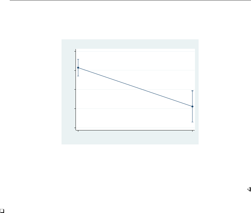
mlogit postestimation — Postestimation tools for mlogit 1375
We can use marginsplot to graph the results from margins:
. marginsplot
Variables that uniquely identify margins: nonwhite
.2 .3 .4 .5 .6
Pr(Insure==Indemnity)
0 1
nonwhite
Predictive Margins of nonwhite with 95% CIs
The margins for the other two outcomes can be computed by typing
. margins nonwhite, predict(outcome(Prepaid)) noesample
(output omitted )
. margins nonwhite, predict(outcome(Uninsure)) noesample
(output omitted )
Technical note
You can use predict to classify predicted values and compare them with the observed outcomes
to interpret a multinomial logit model. This is a variation on the notions of sensitivity and specificity
for logistic regression. Here we will classify indemnity and prepaid as definitely predicting indemnity,
definitely predicting prepaid, and ambiguous.
. predict indem, outcome(Indemnity) index // obtain indexes
(1 missing value generated)
. predict prepaid, outcome(Prepaid) index
(1 missing value generated)
. gen diff = prepaid-indem // obtain difference
(1 missing value generated)
. predict sediff, outcome(Indemnity,Prepaid) stddp // & its standard error
(1 missing value generated)
. gen type = 1 if diff/sediff < -1.96 // definitely indemnity
(504 missing values generated)
. replace type = 3 if diff/sediff > 1.96 // definitely prepaid
(100 real changes made)
. replace type = 2 if type>=. & diff/sediff < . // ambiguous
(404 real changes made)
. label def type 1 "Def Ind" 2 "Ambiguous" 3 "Def Prep"
. label values type type // label results

1376 mlogit postestimation — Postestimation tools for mlogit
. tabulate insure type
type
insure Def Ind Ambiguous Def Prep Total
Indemnity 78 183 33 294
Prepaid 44 177 56 277
Uninsure 12 28 5 45
Total 134 388 94 616
We can see that the predictive power of this model is modest. There are many misclassifications in
both directions, though there are more correctly classified observations than misclassified observations.
Also the uninsured look overwhelmingly as though they might have come from the indemnity
system rather than from the prepaid system.
Calculating marginal effects
Example 4
We have already noted that the coefficients from multinomial logit can be difficult to interpret
because they are relative to the base outcome. Another way to evaluate the effect of covariates is to
examine the marginal effect of changing their values on the probability of observing an outcome.
The margins command can be used for this too. We can estimate the marginal effect of each
covariate on the probability of observing the first outcome—indemnity insurance—by typing
. margins, dydx(*) predict(outcome(Indemnity))
Average marginal effects Number of obs = 615
Model VCE : OIM
Expression : Pr(insure==Indemnity), predict(outcome(Indemnity))
dy/dx w.r.t. : age 1.male 1.nonwhite 2.site 3.site
Delta-method
dy/dx Std. Err. z P>|z| [95% Conf. Interval]
age .0026655 .001399 1.91 0.057 -.0000765 .0054074
1.male -.1295734 .0450945 -2.87 0.004 -.2179571 -.0411898
1.nonwhite -.2032404 .0482554 -4.21 0.000 -.2978192 -.1086616
site
2 .0070995 .0479993 0.15 0.882 -.0869775 .1011765
3 .1216165 .0505833 2.40 0.016 .022475 .220758
Note: dy/dx for factor levels is the discrete change from the base level.
By default, margins estimates the average marginal effect over the estimation sample, and that is
what we see above. Being male decreases the average probability of having indemnity insurance by
0.130. We also see, from the note at the bottom of the table, that the marginal effect was computed
as a discrete change in the probability of being male rather than female. That is why we made male
a factor variable when fitting the model.
The dydx(*) option requested that margins estimate the marginal effect for each regressor,
dydx(age) would have produced estimates only for the effect of age.margins has many options
for controlling how the marginal effect is computed, including the ability to average over subgroups
or to compute estimates for specified values of the regressors; see [R]margins.

mlogit postestimation — Postestimation tools for mlogit 1377
We could evaluate the marginal effects on the other two outcomes by typing
. margins, dydx(*) predict(outcome(Prepaid))
(output omitted )
. margins, dydx(*) predict(outcome(Uninsure))
(output omitted )
Testing hypotheses about coefficients
Example 5
test tests hypotheses about the coefficients just as after any estimation command; see [R]test.
Note, however, test’s syntax for dealing with multiple-equation models. Because test bases its
results on the estimated covariance matrix, we might prefer a likelihood-ratio test; see example 5 in
[R]mlogit for an example of lrtest.
If we simply list variables after the test command, we are testing that the corresponding coefficients
are zero across all equations:
. test 2.site 3.site
( 1) [Indemnity]2o.site = 0
( 2) [Prepaid]2.site = 0
( 3) [Uninsure]2.site = 0
( 4) [Indemnity]3o.site = 0
( 5) [Prepaid]3.site = 0
( 6) [Uninsure]3.site = 0
Constraint 1 dropped
Constraint 4 dropped
chi2( 4) = 19.74
Prob > chi2 = 0.0006
We can test that all the coefficients (except the constant) in an equation are zero by simply typing
the outcome in square brackets:
. test [Uninsure]
( 1) [Uninsure]age = 0
( 2) [Uninsure]0b.male = 0
( 3) [Uninsure]1.male = 0
( 4) [Uninsure]0b.nonwhite = 0
( 5) [Uninsure]1.nonwhite = 0
( 6) [Uninsure]1b.site = 0
( 7) [Uninsure]2.site = 0
( 8) [Uninsure]3.site = 0
Constraint 2 dropped
Constraint 4 dropped
Constraint 6 dropped
chi2( 5) = 9.31
Prob > chi2 = 0.0973
We specify the outcome just as we do with predict; we can specify the label if the outcome variable
is labeled, or we can specify the numeric value of the outcome. We would have obtained the same
test as above if we had typed test [3] because 3 is the value of insure for the outcome uninsured.
We can combine the two syntaxes. To test that the coefficients on the site variables are 0 in the
equation corresponding to the outcome prepaid, we can type

1378 mlogit postestimation — Postestimation tools for mlogit
. test [Prepaid]: 2.site 3.site
( 1) [Prepaid]2.site = 0
( 2) [Prepaid]3.site = 0
chi2( 2) = 10.78
Prob > chi2 = 0.0046
We specified the outcome and then followed that with a colon and the variables we wanted to test.
We can also test that coefficients are equal across equations. To test that all coefficients except the
constant are equal for the prepaid and uninsured outcomes, we can type
. test [Prepaid=Uninsure]
( 1) [Prepaid]age - [Uninsure]age = 0
( 2) [Prepaid]0b.male - [Uninsure]0b.male = 0
( 3) [Prepaid]1.male - [Uninsure]1.male = 0
( 4) [Prepaid]0b.nonwhite - [Uninsure]0b.nonwhite = 0
( 5) [Prepaid]1.nonwhite - [Uninsure]1.nonwhite = 0
( 6) [Prepaid]1b.site - [Uninsure]1b.site = 0
( 7) [Prepaid]2.site - [Uninsure]2.site = 0
( 8) [Prepaid]3.site - [Uninsure]3.site = 0
Constraint 2 dropped
Constraint 4 dropped
Constraint 6 dropped
chi2( 5) = 13.80
Prob > chi2 = 0.0169
To test that only the site variables are equal, we can type
. test [Prepaid=Uninsure]: 2.site 3.site
( 1) [Prepaid]2.site - [Uninsure]2.site = 0
( 2) [Prepaid]3.site - [Uninsure]3.site = 0
chi2( 2) = 12.68
Prob > chi2 = 0.0018
Finally, we can test any arbitrary constraint by simply entering the equation and specifying the
coefficients as described in [U] 13.5 Accessing coefficients and standard errors. The following
hypothesis is senseless but illustrates the point:
. test ([Prepaid]age+[Uninsure]2.site)/2 = 2-[Uninsure]1.nonwhite
( 1) .5*[Prepaid]age + [Uninsure]1.nonwhite + .5*[Uninsure]2.site = 2
chi2( 1) = 22.45
Prob > chi2 = 0.0000
See [R]test for more information about test. The information there about combining hypotheses
across test commands (the accumulate option) also applies after mlogit.
Reference
Fagerland, M. W., and D. W. Hosmer, Jr. 2012. A generalized HosmerLemeshow goodness-of-fit test for multinomial
logistic regression models.Stata Journal 12: 447–453.
Also see
[R]mlogit — Multinomial (polytomous) logistic regression
[U] 20 Estimation and postestimation commands

Title
more — The —more— message
Syntax Description Option Remarks and examples Also see
Syntax
Tell Stata to pause or not pause for —more— messages
set more on |off , permanently
Set number of lines between —more— messages
set pagesize #
Description
set more on, which is the default, tells Stata to wait until you press a key before continuing
when a more message is displayed.
set more off tells Stata not to pause or display the more message.
set pagesize #sets the number of lines between more messages. The permanently option
is not allowed with set pagesize.
Option
permanently specifies that, in addition to making the change right now, the more setting be
remembered and become the default setting when you invoke Stata.
Remarks and examples
When you see more at the bottom of the screen,
Press . . . and Stata . . .
letter lor Enter displays the next line
letter qacts as if you pressed Break
Spacebar or any other key displays the next screen
You can also click on the More button or click on more to display the next screen.
more is Stata’s way of telling you that it has something more to show you but that showing
it to you will cause the information on the screen to scroll off.
If you type set more off,more conditions will never arise, and Stata’s output will scroll by
at full speed.
If you type set more on,more conditions will be restored at the appropriate places.
Programmers should see [P]more for information on the more programming command.
1379


Title
mprobit — Multinomial probit regression
Syntax Menu Description Options
Remarks and examples Stored results Methods and formulas References
Also see
Syntax
mprobit depvar indepvars if in weight ,options
options Description
Model
noconstant suppress constant terms
baseoutcome(#|lbl)outcome used to normalize location
probitparam use the probit variance parameterization
constraints(constraints)apply specified linear constraints
collinear keep collinear variables
SE/Robust
vce(vcetype)vcetype may be oim,robust,cluster clustvar,opg,bootstrap,
or jackknife
Reporting
level(#)set confidence level; default is level(95)
nocnsreport do not display constraints
display options control column formats, row spacing, line width, display of omitted
variables and base and empty cells, and factor-variable labeling
Integration
intpoints(#)number of quadrature points
Maximization
maximize options control the maximization process; seldom used
coeflegend display legend instead of statistics
indepvars may contain factor variables; see [U] 11.4.3 Factor variables.
bootstrap,by,fp,jackknife,mi estimate,rolling,statsby, and svy are allowed; see [U] 11.1.10 Prefix
commands.
vce(bootstrap) and vce(jackknife) are not allowed with the mi estimate prefix; see [MI] mi estimate.
Weights are not allowed with the bootstrap prefix; see [R] bootstrap.
vce() and weights are not allowed with the svy prefix; see [SVY] svy.
fweights, iweights, and pweights are allowed; see [U] 11.1.6 weight.
coeflegend does not appear in the dialog box.
See [U] 20 Estimation and postestimation commands for more capabilities of estimation commands.
1381

1382 mprobit — Multinomial probit regression
Menu
Statistics >Categorical outcomes >Independent multinomial probit
Description
mprobit fits multinomial probit (MNP) models via maximum likelihood. depvar contains the
outcome for each observation, and indepvars are the associated covariates. The error terms are
assumed to be independent, standard normal, random variables. See [R]asmprobit for the case where
the latent-variable errors are correlated or heteroskedastic and you have alternative-specific variables.
Options
Model
noconstant suppresses the J−1 constant terms.
baseoutcome(#|lbl)specifies the outcome used to normalize the location of the latent variable. The
base outcome may be specified as a number or a label. The default is to use the most frequent
outcome. The coefficients associated with the base outcome are zero.
probitparam specifies to use the probit variance parameterization by fixing the variance of the
differenced latent errors between the scale and the base alternatives to be one. The default is to
make the variance of the base and scale latent errors one, thereby making the variance of the
difference to be two.
constraints(constraints),collinear; see [R]estimation options.
SE/Robust
vce(vcetype)specifies the type of standard error reported, which includes types that are derived from
asymptotic theory (oim,opg), that are robust to some kinds of misspecification (robust), that
allow for intragroup correlation (cluster clustvar), and that use bootstrap or jackknife methods
(bootstrap,jackknife); see [R]vce option.
If specifying vce(bootstrap) or vce(jackknife), you must also specify baseoutcome().
Reporting
level(#); see [R]estimation options.
nocnsreport; see [R]estimation options.
display options:noomitted,vsquish,noemptycells,baselevels,allbaselevels,nofvla-
bel,fvwrap(#),fvwrapon(style),cformat(%fmt),pformat(% fmt),sformat(% fmt), and
nolstretch; see [R]estimation options.
Integration
intpoints(#)specifies the number of Gaussian quadrature points to use in approximating the
likelihood. The default is 15.

mprobit — Multinomial probit regression 1383
Maximization
maximize options:difficult,technique(algorithm spec),iterate(#),nolog,trace,
gradient,showstep,hessian,showtolerance,tolerance(#),ltolerance(#),
nrtolerance(#),nonrtolerance, and from(init specs); see [R]maximize. These options are
seldom used.
Setting the optimization type to technique(bhhh) resets the default vcetype to vce(opg).
The following option is available with mprobit but is not shown in the dialog box:
coeflegend; see [R]estimation options.
Remarks and examples
The MNP model is used with discrete dependent variables that take on more than two outcomes
that do not have a natural ordering. The stochastic error terms for this implementation of the model
are assumed to have independent, standard normal distributions. To use mprobit, you must have one
observation for each decision maker in the sample. See [R]asmprobit for another implementation of
the MNP model that permits correlated and heteroskedastic errors and is suitable when you have data
for each alternative that a decision maker faced.
The MNP model is frequently motivated using a latent-variable framework. The latent variable for
the jth alternative, j=1, . . . , J, is
ηij =ziαj+ξij
where the 1×qrow vector zicontains the observed independent variables for the ith decision maker.
Associated with ziare the Jvectors of regression coefficients αj. The ξi,1, . . . , ξi,J are distributed
independently and identically standard normal. The decision maker chooses the alternative ksuch
that ηik ≥ηim for m6=k.
Suppose that case ichooses alternative k, and take the difference between latent variable ηik and
the J−1 others:
vijk =ηij −ηik
=zi(αj−αk) + ξij −ξik
=ziγj0+ij0
(1)
where j0=jif j < k and j0=j−1 if j > k so that j0=1, . . . , J−1. Var(ij0) = Var(ξij −ξik) = 2
and Cov(ij0, il0) = 1 for j06=l0. The probability that alternative kis chosen is
Pr(ichooses k) = Pr(vi1k≤0, . . . , vi,J−1,k ≤0)
= Pr(i1≤ −ziγ1, . . . , i,J−1≤ −ziγJ−1)
Hence, evaluating the likelihood function involves computing probabilities from the multivariate
normal distribution. That all the covariances are equal simplifies the problem somewhat; see Methods
and formulas for details.
In (1), not all Jof the αjare identifiable. To remove the indeterminacy, αlis set to the zero vector,
where lis the base outcome as specified in the baseoutcome() option. That fixes the lth latent
variable to zero so that the remaining variables measure the attractiveness of the other alternatives
relative to the base.

1384 mprobit — Multinomial probit regression
Example 1
As discussed in example 1 of [R]mlogit, we have data on the type of health insurance available
to 616 psychologically depressed subjects in the United States (Tarlov et al. 1989; Wells et al. 1989).
Patients may have either an indemnity (fee-for-service) plan or a prepaid plan such as an HMO, or
the patient may be uninsured. Demographic variables include age, gender, race, and site. Indemnity
insurance is the most popular alternative, so mprobit will choose it as the base outcome by default.
. use http://www.stata-press.com/data/r13/sysdsn1
(Health insurance data)
. mprobit insure age male nonwhite i.site
Iteration 0: log likelihood = -535.89424
Iteration 1: log likelihood = -534.56173
Iteration 2: log likelihood = -534.52835
Iteration 3: log likelihood = -534.52833
Multinomial probit regression Number of obs = 615
Wald chi2(10) = 40.18
Log likelihood = -534.52833 Prob > chi2 = 0.0000
insure Coef. Std. Err. z P>|z| [95% Conf. Interval]
Indemnity (base outcome)
Prepaid
age -.0098536 .0052688 -1.87 0.061 -.0201802 .000473
male .4774678 .1718316 2.78 0.005 .1406841 .8142515
nonwhite .8245003 .1977582 4.17 0.000 .4369013 1.212099
site
2 .0973956 .1794546 0.54 0.587 -.2543289 .4491201
3 -.495892 .1904984 -2.60 0.009 -.869262 -.1225221
_cons .22315 .2792424 0.80 0.424 -.324155 .7704549
Uninsure
age -.0050814 .0075327 -0.67 0.500 -.0198452 .0096823
male .3332637 .2432986 1.37 0.171 -.1435929 .8101203
nonwhite .2485859 .2767734 0.90 0.369 -.29388 .7910518
site
2 -.6899485 .2804497 -2.46 0.014 -1.23962 -.1402771
3 -.1788447 .2479898 -0.72 0.471 -.6648957 .3072063
_cons -.9855917 .3891873 -2.53 0.011 -1.748385 -.2227986
The likelihood function for mprobit is derived under the assumption that all decision-making
units face the same choice set, which is the union of all outcomes observed in the dataset. If that
is not true for your model, then an alternative is to use the asmprobit command, which does not
require this assumption. To do that, you will need to expand the dataset so that each decision maker
has kiobservations, where kiis the number of alternatives in the choice set faced by decision maker
i. You will also need to create a binary variable to indicate the choice made by each decision maker.
Moreover, you will need to use the correlation(independent) and stddev(homoskedastic)
options with asmprobit unless you have alternative-specific variables.

mprobit — Multinomial probit regression 1385
Stored results
mprobit stores the following in e():
Scalars
e(N) number of observations
e(k out) number of outcomes
e(k points) number of quadrature points
e(k) number of parameters
e(k eq) number of equations in e(b)
e(k eq model) number of equations in overall model test
e(k indvars) number of independent variables
e(k dv) number of dependent variables
e(df m) model degrees of freedom
e(ll) log simulated-likelihood
e(N clust) number of clusters
e(chi2) χ2
e(p) significance
e(i base) base outcome index
e(const) 0 if noconstant is specified, 1otherwise
e(probitparam) 1 if probitparam is specified, 0otherwise
e(rank) rank of e(V)
e(ic) number of iterations
e(rc) return code
e(converged) 1 if converged, 0otherwise
Macros
e(cmd) mprobit
e(cmdline) command as typed
e(depvar) name of dependent variable
e(indvars) independent variables
e(wtype) weight type
e(wexp) weight expression
e(title) title in estimation output
e(clustvar) name of cluster variable
e(chi2type) Wald, type of model χ2test
e(vce) vcetype specified in vce()
e(vcetype) title used to label Std. Err.
e(outeqs) outcome equations
e(out#)outcome labels, #=1,...,e(k out)
e(opt) type of optimization
e(which) max or min; whether optimizer is to perform maximization or minimization
e(ml method) type of ml method
e(user) name of likelihood-evaluator program
e(technique) maximization technique
e(properties) b V
e(predict) program used to implement predict
e(marginsnotok) predictions disallowed by margins
e(asbalanced) factor variables fvset as asbalanced
e(asobserved) factor variables fvset as asobserved

1386 mprobit — Multinomial probit regression
Matrices
e(b) coefficient vector
e(outcomes) outcome values
e(Cns) constraints matrix
e(ilog) iteration log (up to 20 iterations)
e(gradient) gradient vector
e(V) variance–covariance matrix of the estimators
e(V modelbased) model-based variance
Functions
e(sample) marks estimation sample
Methods and formulas
See Cameron and Trivedi (2005, chap. 15) for a discussion of multinomial models, including
multinomial probit. Long and Freese (2014, chap. 8) discuss the multinomial logistic, multinomial
probit, and stereotype logistic regression models, with examples using Stata.
As discussed in Remarks and examples, the latent variables for a J-alternative model are ηij =
ziαj+ξij , for j= 1, . . . , J,i= 1, . . . , n, and {ξi,1, . . . , ξi,J} ∼ i.i.d.N(0,1). The experimenter
observes alternative kfor the ith observation if ηik > ηil for l6=k. For j6=k, let
vij0=ηij −ηik
=zi(αj−αk) + ξij −ξik
=ziγj0+ij0
where j0=jif j < k and j0=j−1if j > k so that j0= 1, . . . , J −1.i= (i1, . . . , i,J−1)∼
MV N(0,Σ), where
Σ=
211. . . 1
121. . . 1
112. . . 1
.
.
..
.
..
.
.....
.
.
111. . . 2
Denote the deterministic part of the model as λij0=ziγj0; the probability that subject ichooses
outcome kis
Pr(yi=k) = Pr(vi1≤0, . . . , vi,J−1≤0)
= Pr(i1≤ −λi1, . . . , i,J−1≤ −λi,J−1)
=1
(2π)(J−1)/2|Σ|1/2Z−λi1
−∞ ···Z−λi,J−1
−∞
exp −1
2z0Σ−1zdz
Because of the exchangeable correlation structure of Σ(ρij =1/2 for all i6=j), we can use
Dunnett’s (1989) result to reduce the multidimensional integral to one dimension:
Pr(yi=k) = 1
√πZ∞
0
J−1
Y
j=1
Φ−z√2−λij +
J−1
Y
j=1
Φz√2−λij
e−z2dz

mprobit — Multinomial probit regression 1387
Gaussian quadrature is used to approximate this integral, resulting in the K-point quadrature formula
Pr(yi=k)≈1
2
K
X
k=1
wk
J−1
Y
j=1
Φ−√2xk−λij +
J−1
Y
j=1
Φ√2xk−λij
where wkand xkare the weights and roots of the Laguerre polynomial of order K. In mprobit,K
is specified by the intpoints() option.
This command supports the Huber/White/sandwich estimator of the variance and its clustered
version using vce(robust) and vce(cluster clustvar), respectively. See [P]robust, particularly
Maximum likelihood estimators and Methods and formulas.
mprobit also supports estimation with survey data. For details on VCEs with survey data, see
[SVY]variance estimation.
References
Cameron, A. C., and P. K. Trivedi. 2005. Microeconometrics: Methods and Applications. New York: Cambridge
University Press.
Dunnett, C. W. 1989. Algorithm AS 251: Multivariate normal probability integrals with product correlation structure.
Journal of the Royal Statistical Society, Series C 38: 564–579.
Haan, P., and A. Uhlendorff. 2006. Estimation of multinomial logit models with unobserved heterogeneity using
maximum simulated likelihood.Stata Journal 6: 229–245.
Hole, A. R. 2007. Fitting mixed logit models by using maximum simulated likelihood.Stata Journal 7: 388–401.
Long, J. S., and J. Freese. 2014. Regression Models for Categorical Dependent Variables Using Stata. 3rd ed. College
Station, TX: Stata Press.
Tarlov, A. R., J. E. Ware, Jr., S. Greenfield, E. C. Nelson, E. Perrin, and M. Zubkoff. 1989. The medical outcomes
study. An application of methods for monitoring the results of medical care. Journal of the American Medical
Association 262: 925–930.
Wells, K. B., R. D. Hays, M. A. Burnam, W. H. Rogers, S. Greenfield, and J. E. Ware, Jr. 1989. Detection of
depressive disorder for patients receiving prepaid or fee-for-service care. Results from the Medical Outcomes Survey.
Journal of the American Medical Association 262: 3298–3302.
Also see
[R]mprobit postestimation — Postestimation tools for mprobit
[R]asmprobit — Alternative-specific multinomial probit regression
[R]clogit — Conditional (fixed-effects) logistic regression
[R]mlogit — Multinomial (polytomous) logistic regression
[R]nlogit — Nested logit regression
[R]ologit — Ordered logistic regression
[R]oprobit — Ordered probit regression
[MI]estimation — Estimation commands for use with mi estimate
[SVY]svy estimation — Estimation commands for survey data
[U] 20 Estimation and postestimation commands

Title
mprobit postestimation — Postestimation tools for mprobit
Description Syntax for predict Menu for predict Options for predict
Remarks and examples References Also see
Description
The following postestimation commands are available after mprobit:
Command Description
contrast contrasts and ANOVA-style joint tests of estimates
estat ic Akaike’s and Schwarz’s Bayesian information criteria (AIC and BIC)
estat summarize summary statistics for the estimation sample
estat vce variance–covariance matrix of the estimators (VCE)
estat (svy) postestimation statistics for survey data
estimates cataloging estimation results
forecast1dynamic forecasts and simulations
hausman Hausman’s specification test
lincom point estimates, standard errors, testing, and inference for linear combinations
of coefficients
lrtest2likelihood-ratio test
margins marginal means, predictive margins, marginal effects, and average marginal
effects
marginsplot graph the results from margins (profile plots, interaction plots, etc.)
nlcom point estimates, standard errors, testing, and inference for nonlinear combinations
of coefficients
predict predicted probabilities, linear predictions, and standard errors
predictnl point estimates, standard errors, testing, and inference for generalized predictions
pwcompare pairwise comparisons of estimates
suest seemingly unrelated estimation
test Wald tests of simple and composite linear hypotheses
testnl Wald tests of nonlinear hypotheses
1forecast is not appropriate with mi or svy estimation results.
2lrtest is not appropriate with svy estimation results.
1388

mprobit postestimation — Postestimation tools for mprobit 1389
Syntax for predict
predict type stub*|newvar |newvarlist if in ,statistic outcome(outcome)
predict type stub*|newvarlist if in , scores
statistic Description
Main
pr probability of a positive outcome; the default
xb linear prediction
stdp standard error of the linear prediction
If you do not specify outcome(),pr (with one new variable specified), xb, and stdp assume outcome(#1).
You specify one or knew variables with pr, where kis the number of outcomes.
You specify one new variable with xb and stdp.
These statistics are available both in and out of sample; type predict . . . if e(sample) . . . if wanted only for
the estimation sample.
Menu for predict
Statistics >Postestimation >Predictions, residuals, etc.
Options for predict
Main
pr, the default, calculates the probability of each of the categories of the dependent variable or the
probability of the level specified in outcome(outcome). If you specify the outcome(outcome)
option, you need to specify only one new variable; otherwise, you must specify a new variable
for each category of the dependent variable.
xb calculates the linear prediction, xiαj, for alternative jand individual i. The index, j, corresponds
to the outcome specified in outcome().
stdp calculates the standard error of the linear prediction.
outcome(outcome)specifies the outcome for which the statistic is to be calculated. equation() is
a synonym for outcome(): it does not matter which you use. outcome() or equation() can
be specified using
#1,#2,. . . , where #1 means the first category of the dependent variable, #2 means the
second category, etc.;
the values of the dependent variable; or
the value labels of the dependent variable if they exist.
scores calculates the equation-level score variables. The jth new variable will contain the scores for
the jth fitted equation.

1390 mprobit postestimation — Postestimation tools for mprobit
Remarks and examples
Once you have fit a multinomial probit model, you can use predict to obtain probabilities that
an individual will choose each of the alternatives for the estimation sample, as well as other samples;
see [U] 20 Estimation and postestimation commands and [R]predict.
Example 1
In example 1 of [R]mprobit, we fit the multinomial probit model to a dataset containing the type
of health insurance available to 616 psychologically depressed subjects in the United States (Tarlov
et al. 1989; Wells et al. 1989). We can obtain the predicted probabilities by typing
. use http://www.stata-press.com/data/r13/sysdsn1
(Health insurance data)
. mprobit insure age male nonwhite i.site
(output omitted )
. predict p1-p3
(option pr assumed; predicted probabilities)
. list p1-p3 insure in 1/10
p1 p2 p3 insure
1. .5961306 .3741824 .029687 Indemnity
2. .4719296 .4972289 .0308415 Prepaid
3. .4896086 .4121961 .0981953 Indemnity
4. .3730529 .5416623 .0852848 Prepaid
5. .5063069 .4629773 .0307158 .
6. .4768125 .4923548 .0308327 Prepaid
7. .5035672 .4657016 .0307312 Prepaid
8. .3326361 .5580404 .1093235 .
9. .4758165 .4384811 .0857024 Uninsure
10. .5734057 .3316601 .0949342 Prepaid
insure contains a missing value for observations 5 and 8. Because of that, those two observations
were not used in the estimation. However, because none of the independent variables is missing,
predict can still calculate the probabilities. Had we typed
. predict p1-p3 if e(sample)
predict would have filled in missing values for p1,p2, and p3 for those observations because they
were not used in the estimation.
References
Tarlov, A. R., J. E. Ware, Jr., S. Greenfield, E. C. Nelson, E. Perrin, and M. Zubkoff. 1989. The medical outcomes
study. An application of methods for monitoring the results of medical care. Journal of the American Medical
Association 262: 925–930.
Wells, K. B., R. D. Hays, M. A. Burnam, W. H. Rogers, S. Greenfield, and J. E. Ware, Jr. 1989. Detection of
depressive disorder for patients receiving prepaid or fee-for-service care. Results from the Medical Outcomes Survey.
Journal of the American Medical Association 262: 3298–3302.
Also see
[R]mprobit — Multinomial probit regression
[U] 20 Estimation and postestimation commands

Title
nbreg — Negative binomial regression
Syntax Menu Description Options for nbreg
Options for gnbreg Remarks and examples Stored results Methods and formulas
References Also see
Syntax
Negative binomial regression model
nbreg depvar indepvars if in weight ,nbreg options
Generalized negative binomial model
gnbreg depvar indepvars if in weight ,gnbreg options
nbreg options Description
Model
noconstant suppress constant term
dispersion(mean) parameterization of dispersion; the default
dispersion(constant) constant dispersion for all observations
exposure(varnamee)include ln(varnamee) in model with coefficient constrained to 1
offset(varnameo)include varnameoin model with coefficient constrained to 1
constraints(constraints)apply specified linear constraints
collinear keep collinear variables
SE/Robust
vce(vcetype)vcetype may be oim,robust,cluster clustvar,opg,bootstrap,
or jackknife
Reporting
level(#)set confidence level; default is level(95)
nolrtest suppress likelihood-ratio test
irr report incidence-rate ratios
nocnsreport do not display constraints
display options control column formats, row spacing, line width, display of omitted
variables and base and empty cells, and factor-variable labeling
Maximization
maximize options control the maximization process; seldom used
coeflegend display legend instead of statistics
1391

1392 nbreg — Negative binomial regression
gnbreg options Description
Model
noconstant suppress constant term
lnalpha(varlist)dispersion model variables
exposure(varnamee)include ln(varnamee) in model with coefficient constrained to 1
offset(varnameo)include varnameoin model with coefficient constrained to 1
constraints(constraints)apply specified linear constraints
collinear keep collinear variables
SE/Robust
vce(vcetype)vcetype may be oim,robust,cluster clustvar,opg,bootstrap,
or jackknife
Reporting
level(#)set confidence level; default is level(95)
irr report incidence-rate ratios
nocnsreport do not display constraints
display options control column formats, row spacing, line width, display of omitted
variables and base and empty cells, and factor-variable labeling
Maximization
maximize options control the maximization process; seldom used
coeflegend display legend instead of statistics
indepvars and varlist may contain factor variables; see [U] 11.4.3 Factor variables.
depvar,indepvars,varnamee, and varnameomay contain time-series operators (nbreg only); see [U] 11.4.4 Time-series
varlists.
bootstrap,by (nbreg only), fp (nbreg only), jackknife,mfp (nbreg only), mi estimate,nestreg (nbreg
only), rolling,statsby,stepwise, and svy are allowed; see [U] 11.1.10 Prefix commands.
vce(bootstrap) and vce(jackknife) are not allowed with the mi estimate prefix; see [MI] mi estimate.
Weights are not allowed with the bootstrap prefix; see [R] bootstrap.
vce() and weights are not allowed with the svy prefix; see [SVY] svy.
fweights, iweights, and pweights are allowed; see [U] 11.1.6 weight.
coeflegend does not appear in the dialog box.
See [U] 20 Estimation and postestimation commands for more capabilities of estimation commands.
Menu
nbreg
Statistics >Count outcomes >Negative binomial regression
gnbreg
Statistics >Count outcomes >Generalized negative binomial regression
Description
nbreg fits a negative binomial regression model of depvar on indepvars, where depvar is a
nonnegative count variable. In this model, the count variable is believed to be generated by a Poisson-
like process, except that the variation is greater than that of a true Poisson. This extra variation is
referred to as overdispersion. See [R]poisson before reading this entry.

nbreg — Negative binomial regression 1393
gnbreg fits a generalization of the negative binomial mean-dispersion model; the shape parameter
αmay also be parameterized.
If you have panel data, see [XT]xtnbreg and [ME]menbreg.
Options for nbreg
Model
noconstant; see [R]estimation options.
dispersion(mean |constant) specifies the parameterization of the model. dispersion(mean),
the default, yields a model with dispersion equal to 1+αexp(xjβ+offsetj); that is, the dispersion
is a function of the expected mean: exp(xjβ+offsetj).dispersion(constant) has dispersion
equal to 1 +δ; that is, it is a constant for all observations.
exposure(varnamee),offset(varnameo),constraints(constraints),collinear; see [R]esti-
mation options.
SE/Robust
vce(vcetype)specifies the type of standard error reported, which includes types that are derived from
asymptotic theory (oim,opg), that are robust to some kinds of misspecification (robust), that
allow for intragroup correlation (cluster clustvar), and that use bootstrap or jackknife methods
(bootstrap,jackknife); see [R]vce option.
Reporting
level(#); see [R]estimation options.
nolrtest suppresses fitting the Poisson model. Without this option, a comparison Poisson model is
fit, and the likelihood is used in a likelihood-ratio test of the null hypothesis that the dispersion
parameter is zero.
irr reports estimated coefficients transformed to incidence-rate ratios, that is, eβirather than βi.
Standard errors and confidence intervals are similarly transformed. This option affects how results
are displayed, not how they are estimated or stored. irr may be specified at estimation or when
replaying previously estimated results.
nocnsreport; see [R]estimation options.
display options:noomitted,vsquish,noemptycells,baselevels,allbaselevels,nofvla-
bel,fvwrap(#),fvwrapon(style),cformat(%fmt),pformat(% fmt),sformat(% fmt), and
nolstretch; see [R]estimation options.
Maximization
maximize options:difficult,technique(algorithm spec),iterate(#),nolog,trace,
gradient,showstep,hessian,showtolerance,tolerance(#),ltolerance(#),
nrtolerance(#),nonrtolerance, and from(init specs); see [R]maximize. These options are
seldom used.
Setting the optimization type to technique(bhhh) resets the default vcetype to vce(opg).
The following option is available with nbreg but is not shown in the dialog box:
coeflegend; see [R]estimation options.

1394 nbreg — Negative binomial regression
Options for gnbreg
Model
noconstant; see [R]estimation options.
lnalpha(varlist)allows you to specify a linear equation for lnα. Specifying lnalpha(male old)
means that lnα=γ0+γ1male +γ2old, where γ0,γ1, and γ2are parameters to be estimated
along with the other model coefficients. If this option is not specified, gnbreg and nbreg will
produce the same results because the shape parameter will be parameterized as a constant.
exposure(varnamee),offset(varnameo),constraints(constraints),collinear; see [R]esti-
mation options.
SE/Robust
vce(vcetype)specifies the type of standard error reported, which includes types that are derived from
asymptotic theory (oim,opg), that are robust to some kinds of misspecification (robust), that
allow for intragroup correlation (cluster clustvar), and that use bootstrap or jackknife methods
(bootstrap,jackknife); see [R]vce option.
Reporting
level(#); see [R]estimation options.
irr reports estimated coefficients transformed to incidence-rate ratios, that is, eβirather than βi.
Standard errors and confidence intervals are similarly transformed. This option affects how results
are displayed, not how they are estimated or stored. irr may be specified at estimation or when
replaying previously estimated results.
nocnsreport; see [R]estimation options.
display options:noomitted,vsquish,noemptycells,baselevels,allbaselevels,nofvla-
bel,fvwrap(#),fvwrapon(style),cformat(%fmt),pformat(% fmt),sformat(% fmt), and
nolstretch; see [R]estimation options.
Maximization
maximize options:difficult,technique(algorithm spec),iterate(#),nolog,trace,
gradient,showstep,hessian,showtolerance,tolerance(#),ltolerance(#),
nrtolerance(#),nonrtolerance, and from(init specs); see [R]maximize. These options are
seldom used.
Setting the optimization type to technique(bhhh) resets the default vcetype to vce(opg).
The following option is available with gnbreg but is not shown in the dialog box:
coeflegend; see [R]estimation options.
Remarks and examples
Remarks are presented under the following headings:
Introduction to negative binomial regression
nbreg
gnbreg

nbreg — Negative binomial regression 1395
Introduction to negative binomial regression
Negative binomial regression models the number of occurrences (counts) of an event when the
event has extra-Poisson variation, that is, when it has overdispersion. The Poisson regression model
is
yj∼Poisson(µj)
where
µj= exp(xjβ+offsetj)
for observed counts yjwith covariates xjfor the jth observation. One derivation of the negative
binomial mean-dispersion model is that individual units follow a Poisson regression model, but there
is an omitted variable νj, such that eνjfollows a gamma distribution with mean 1 and variance α:
yj∼Poisson(µ∗
j)
where
µ∗
j= exp(xjβ+offsetj+νj)
and
eνj∼Gamma(1/α, α)
With this parameterization, a Gamma(a, b)distribution will have expectation ab and variance ab2.
We refer to αas the overdispersion parameter. The larger αis, the greater the overdispersion.
The Poisson model corresponds to α=0. nbreg parameterizes αas lnα.gnbreg allows lnαto be
modeled as lnαj=zjγ, a linear combination of covariates zj.
nbreg will fit two different parameterizations of the negative binomial model. The default, described
above and also given by the dispersion(mean) option, has dispersion for the jth observation equal
to 1 + αexp(xjβ+offsetj). This is seen by noting that the above implies that
µ∗
j∼Gamma(1/α, αµj)
and thus
Var(yj) = EVar(yj|µ∗
j)+Var E(yj|µ∗
j)
=E(µ∗
j) + Var(µ∗
j)
=µj(1 + αµj)
The alternative parameterization, given by the dispersion(constant) option, has dispersion equal
to 1 +δ; that is, it is constant for all observations. This is so because the constant-dispersion model
assumes instead that
µ∗
j∼Gamma(µj/δ, δ)
and thus Var(yj) = µj(1 + δ). The Poisson model corresponds to δ=0.
For detailed derivations of both models, see Cameron and Trivedi (2013, 80–89). In particular,
note that the mean-dispersion model is known as the NB2 model in their terminology, whereas the
constant-dispersion model is referred to as the NB1 model.
See Long and Freese (2014) and Cameron and Trivedi (2010, chap. 17) for a discussion of the
negative binomial regression model with Stata examples and for a discussion of other regression
models for count data.
Hilbe (2011) provides an extensive review of the negative binomial model and its variations, using
Stata examples.

1396 nbreg — Negative binomial regression
nbreg
It is not uncommon to posit a Poisson regression model and observe a lack of model fit. The
following data appeared in Rodr´
ıguez (1993):
. use http://www.stata-press.com/data/r13/rod93
. list, sepby(cohort)
cohort age_mos deaths exposure
1. 1941-1949 0.5 168 278.4
2. 1941-1949 2.0 48 538.8
3. 1941-1949 4.5 63 794.4
4. 1941-1949 9.0 89 1,550.8
5. 1941-1949 18.0 102 3,006.0
6. 1941-1949 42.0 81 8,743.5
7. 1941-1949 90.0 40 14,270.0
8. 1960-1967 0.5 197 403.2
9. 1960-1967 2.0 48 786.0
10. 1960-1967 4.5 62 1,165.3
11. 1960-1967 9.0 81 2,294.8
12. 1960-1967 18.0 97 4,500.5
13. 1960-1967 42.0 103 13,201.5
14. 1960-1967 90.0 39 19,525.0
15. 1968-1976 0.5 195 495.3
16. 1968-1976 2.0 55 956.7
17. 1968-1976 4.5 58 1,381.4
18. 1968-1976 9.0 85 2,604.5
19. 1968-1976 18.0 87 4,618.5
20. 1968-1976 42.0 70 9,814.5
21. 1968-1976 90.0 10 5,802.5
. generate logexp = ln(exposure)
. poisson deaths i.cohort, offset(logexp)
Iteration 0: log likelihood = -2160.0544
Iteration 1: log likelihood = -2159.5162
Iteration 2: log likelihood = -2159.5159
Iteration 3: log likelihood = -2159.5159
Poisson regression Number of obs = 21
LR chi2(2) = 49.16
Prob > chi2 = 0.0000
Log likelihood = -2159.5159 Pseudo R2 = 0.0113
deaths Coef. Std. Err. z P>|z| [95% Conf. Interval]
cohort
1960-1967 -.3020405 .0573319 -5.27 0.000 -.4144089 -.1896721
1968-1976 .0742143 .0589726 1.26 0.208 -.0413698 .1897983
_cons -3.899488 .0411345 -94.80 0.000 -3.98011 -3.818866
logexp 1 (offset)

nbreg — Negative binomial regression 1397
. estat gof
Deviance goodness-of-fit = 4190.689
Prob > chi2(18) = 0.0000
Pearson goodness-of-fit = 15387.67
Prob > chi2(18) = 0.0000
The extreme significance of the goodness-of-fit χ2indicates that the Poisson regression model is
inappropriate, suggesting to us that we should try a negative binomial model:
. nbreg deaths i.cohort, offset(logexp) nolog
Negative binomial regression Number of obs = 21
LR chi2(2) = 0.40
Dispersion = mean Prob > chi2 = 0.8171
Log likelihood = -131.3799 Pseudo R2 = 0.0015
deaths Coef. Std. Err. z P>|z| [95% Conf. Interval]
cohort
1960-1967 -.2676187 .7237203 -0.37 0.712 -1.686084 1.150847
1968-1976 -.4573957 .7236651 -0.63 0.527 -1.875753 .9609618
_cons -2.086731 .511856 -4.08 0.000 -3.08995 -1.083511
logexp 1 (offset)
/lnalpha .5939963 .2583615 .0876171 1.100376
alpha 1.811212 .4679475 1.09157 3.005295
Likelihood-ratio test of alpha=0: chibar2(01) = 4056.27 Prob>=chibar2 = 0.000
Our original Poisson model is a special case of the negative binomial—it corresponds to α=0.
nbreg, however, estimates αindirectly, estimating instead lnα. In our model, lnα=0.594, meaning
that α=1.81 (nbreg undoes the transformation for us at the bottom of the output).
To test α=0 (equivalent to lnα=−∞), nbreg performs a likelihood-ratio test. The staggering
χ2value of 4,056 asserts that the probability that we would observe these data conditional on α=0
is virtually zero, that is, conditional on the process being Poisson. The data are not Poisson. It is not
accidental that this χ2value is close to the goodness-of-fit statistic from the Poisson regression itself.
Technical note
The usual Gaussian test of α=0 is omitted because this test occurs on the boundary, invalidating
the usual theory associated with such tests. However, the likelihood-ratio test of α= 0 has been
modified to be valid on the boundary. In particular, the null distribution of the likelihood-ratio test
statistic is not the usual χ2
1, but rather a 50 : 50 mixture of a χ2
0(point mass at zero) and a χ2
1,
denoted as χ2
01.See Gutierrez, Carter, and Drukker (2001) for more details.
Technical note
The negative binomial model deals with cases in which there is more variation than would
be expected if the process were Poisson. The negative binomial model is not helpful if there is
less than Poisson variation—if the variance of the count variable is less than its mean. However,
underdispersion is uncommon. Poisson models arise because of independently generated events.
Overdispersion comes about if some of the parameters (causes) of the Poisson processes are unknown.
To obtain underdispersion, the sequence of events somehow would have to be regulated; that is, events
would not be independent but controlled based on past occurrences.

1398 nbreg — Negative binomial regression
gnbreg
gnbreg is a generalization of nbreg,dispersion(mean). Whereas in nbreg, one lnαis
estimated, gnbreg allows lnαto vary, observation by observation, as a linear combination of another
set of covariates: lnαj=zjγ.
We will assume that the number of deaths is a function of age, whereas the lnαparameter is a
function of cohort. To fit the model, we type
. gnbreg deaths age_mos, lnalpha(i.cohort) offset(logexp)
Fitting constant-only model:
Iteration 0: log likelihood = -187.067 (not concave)
Iteration 1: log likelihood = -137.4064
Iteration 2: log likelihood = -134.07766
Iteration 3: log likelihood = -131.60668
Iteration 4: log likelihood = -131.57951
Iteration 5: log likelihood = -131.57948
Iteration 6: log likelihood = -131.57948
Fitting full model:
Iteration 0: log likelihood = -124.34327
Iteration 1: log likelihood = -117.70256
Iteration 2: log likelihood = -117.56373
Iteration 3: log likelihood = -117.56164
Iteration 4: log likelihood = -117.56164
Generalized negative binomial regression Number of obs = 21
LR chi2(1) = 28.04
Prob > chi2 = 0.0000
Log likelihood = -117.56164 Pseudo R2 = 0.1065
deaths Coef. Std. Err. z P>|z| [95% Conf. Interval]
deaths
age_mos -.0516657 .0051747 -9.98 0.000 -.061808 -.0415233
_cons -1.867225 .2227944 -8.38 0.000 -2.303894 -1.430556
logexp 1 (offset)
lnalpha
cohort
1960-1967 .0939546 .7187747 0.13 0.896 -1.314818 1.502727
1968-1976 .0815279 .7365476 0.11 0.912 -1.362079 1.525135
_cons -.4759581 .5156502 -0.92 0.356 -1.486614 .5346978
We find that age is a significant determinant of the number of deaths. The standard errors for the
variables in the lnαequation suggest that the overdispersion parameter does not vary across cohorts.
We can test this assertion by typing
. test 2.cohort 3.cohort
( 1) [lnalpha]2.cohort = 0
( 2) [lnalpha]3.cohort = 0
chi2( 2) = 0.02
Prob > chi2 = 0.9904
There is no evidence of variation by cohort in these data.

nbreg — Negative binomial regression 1399
Technical note
Note the intentional absence of a likelihood-ratio test for α= 0 in gnbreg. The test is affected
by the same boundary condition that affects the comparison test in nbreg; however, when αis
parameterized by more than a constant term, the null distribution becomes intractable. For this reason,
we recommend using nbreg to test for overdispersion and, if you have reason to believe that
overdispersion exists, only then modeling the overdispersion using gnbreg.
Stored results
nbreg and gnbreg store the following in e():
Scalars
e(N) number of observations
e(k) number of parameters
e(k aux) number of auxiliary parameters
e(k eq) number of equations in e(b)
e(k eq model) number of equations in overall model test
e(k dv) number of dependent variables
e(df m) model degrees of freedom
e(r2 p) pseudo-R-squared
e(ll) log likelihood
e(ll 0) log likelihood, constant-only mode
e(ll c) log likelihood, comparison model
e(alpha) value of alpha
e(delta) value of delta
e(N clust) number of clusters
e(chi2) χ2
e(chi2 c) χ2for comparison test
e(p) significance
e(rank) rank of e(V)
e(rank0) rank of e(V) for constant-only model
e(ic) number of iterations
e(rc) return code
e(converged) 1 if converged, 0otherwise
Macros
e(cmd) nbreg or gnbreg
e(cmdline) command as typed
e(depvar) name of dependent variable
e(wtype) weight type
e(wexp) weight expression
e(title) title in estimation output
e(clustvar) name of cluster variable
e(offset) linear offset variable (nbreg)
e(offset1) linear offset variable (gnbreg)
e(chi2type) Wald or LR; type of model χ2test
e(chi2 ct) Wald or LR; type of model χ2test corresponding to e(chi2 c)
e(dispers) mean or constant
e(vce) vcetype specified in vce()
e(vcetype) title used to label Std. Err.
e(opt) type of optimization
e(which) max or min; whether optimizer is to perform maximization or minimization
e(ml method) type of ml method
e(user) name of likelihood-evaluator program
e(technique) maximization technique
e(properties) b V
e(predict) program used to implement predict
e(asbalanced) factor variables fvset as asbalanced
e(asobserved) factor variables fvset as asobserved

1400 nbreg — Negative binomial regression
Matrices
e(b) coefficient vector
e(Cns) constraints matrix
e(ilog) iteration log (up to 20 iterations)
e(gradient) gradient vector
e(V) variance–covariance matrix of the estimators
e(V modelbased) model-based variance
Functions
e(sample) marks estimation sample
Methods and formulas
See [R]poisson and Johnson, Kemp, and Kotz (2005, chap. 4) for an introduction to the Poisson
distribution.
Methods and formulas are presented under the following headings:
Mean-dispersion model
Constant-dispersion model
Mean-dispersion model
A negative binomial distribution can be regarded as a gamma mixture of Poisson random variables.
The number of times something occurs, yj, is distributed as Poisson(νjµj). That is, its conditional
likelihood is
f(yj|νj) = (νjµj)yje−νjµj
Γ(yj+ 1)
where µj= exp(xjβ+offsetj)and νjis an unobserved parameter with a Gamma(1/α, α)density:
g(ν) = ν(1−α)/αe−ν/α
α1/αΓ(1/α)
This gamma distribution has mean 1 and variance α, where αis our ancillary parameter.
The unconditional likelihood for the jth observation is therefore
f(yj) = Z∞
0
f(yj|ν)g(ν)dν =Γ(m+yj)
Γ(yj+ 1)Γ(m)pm
j(1 −pj)yj
where pj=1/(1+αµj)and m=1/α. Solutions for αare handled by searching for lnαbecause
αmust be greater than zero.
The log likelihood (with weights wjand offsets) is given by
m= 1/α pj= 1/(1 + αµj)µj= exp(xjβ+ offsetj)
lnL=
n
X
j=1
wjln{Γ(m+yj)} − ln{Γ(yj+ 1)}
−ln{Γ(m)}+mln(pj) + yjln(1 −pj)
For gnbreg,αcan vary across the observations according to the parameterization lnαj=zjγ.

nbreg — Negative binomial regression 1401
Constant-dispersion model
The constant-dispersion model assumes that yjis conditionally distributed as Poisson(µ∗
j), where
µ∗
j∼Gamma(µj/δ, δ)for some dispersion parameter δ(by contrast, the mean-dispersion model
assumes that µ∗
j∼Gamma(1/α, αµj)). The log likelihood is given by
mj=µj/δ p = 1/(1 + δ)
lnL=
n
X
j=1
wjln{Γ(mj+yj)} − ln{Γ(yj+ 1)}
−ln{Γ(mj)}+mjln(p) + yjln(1 −p)
with everything else defined as before in the calculations for the mean-dispersion model.
nbreg and gnbreg support the Huber/White/sandwich estimator of the variance and its clustered
version using vce(robust) and vce(cluster clustvar), respectively. See [P]robust, particularly
Maximum likelihood estimators and Methods and formulas.
These commands also support estimation with survey data. For details on VCEs with survey data,
see [SVY]variance estimation.
References
Cameron, A. C., and P. K. Trivedi. 2010. Microeconometrics Using Stata. Rev. ed. College Station, TX: Stata Press.
. 2013. Regression Analysis of Count Data. 2nd ed. New York: Cambridge University Press.
Deb, P., and P. K. Trivedi. 2006. Maximum simulated likelihood estimation of a negative binomial regression model
with multinomial endogenous treatment.Stata Journal 6: 246–255.
Gutierrez, R. G., S. L. Carter, and D. M. Drukker. 2001. sg160: On boundary-value likelihood-ratio tests.Stata
Technical Bulletin 60: 15–18. Reprinted in Stata Technical Bulletin Reprints, vol. 10, pp. 269–273. College Station,
TX: Stata Press.
Hilbe, J. M. 1998. sg91: Robust variance estimators for MLE Poisson and negative binomial regression.Stata Technical
Bulletin 45: 26–28. Reprinted in Stata Technical Bulletin Reprints, vol. 8, pp. 177–180. College Station, TX: Stata
Press.
. 1999. sg102: Zero-truncated Poisson and negative binomial regression.Stata Technical Bulletin 47: 37–40.
Reprinted in Stata Technical Bulletin Reprints, vol. 8, pp. 233–236. College Station, TX: Stata Press.
. 2011. Negative Binomial Regression. 2nd ed. Cambridge: Cambridge University Press.
Johnson, N. L., A. W. Kemp, and S. Kotz. 2005. Univariate Discrete Distributions. 3rd ed. New York: Wiley.
Long, J. S. 1997. Regression Models for Categorical and Limited Dependent Variables. Thousand Oaks, CA: Sage.
Long, J. S., and J. Freese. 2001. Predicted probabilities for count models.Stata Journal 1: 51–57.
. 2014. Regression Models for Categorical Dependent Variables Using Stata. 3rd ed. College Station, TX: Stata
Press.
Miranda, A., and S. Rabe-Hesketh. 2006. Maximum likelihood estimation of endogenous switching and sample
selection models for binary, ordinal, and count variables.Stata Journal 6: 285–308.
Rodr´
ıguez, G. 1993. sbe10: An improvement to poisson.Stata Technical Bulletin 11: 11–14. Reprinted in Stata
Technical Bulletin Reprints, vol. 2, pp. 94–98. College Station, TX: Stata Press.
Rogers, W. H. 1991. sbe1: Poisson regression with rates.Stata Technical Bulletin 1: 11–12. Reprinted in Stata
Technical Bulletin Reprints, vol. 1, pp. 62–64. College Station, TX: Stata Press.
. 1993. sg16.4: Comparison of nbreg and glm for negative binomial.Stata Technical Bulletin 16: 7. Reprinted
in Stata Technical Bulletin Reprints, vol. 3, pp. 82–84. College Station, TX: Stata Press.

1402 nbreg — Negative binomial regression
Also see
[R]nbreg postestimation — Postestimation tools for nbreg and gnbreg
[R]glm — Generalized linear models
[R]poisson — Poisson regression
[R]tnbreg — Truncated negative binomial regression
[R]zinb — Zero-inflated negative binomial regression
[ME]menbreg — Multilevel mixed-effects negative binomial regression
[MI]estimation — Estimation commands for use with mi estimate
[SVY]svy estimation — Estimation commands for survey data
[XT]xtnbreg — Fixed-effects, random-effects, & population-averaged negative binomial models
[U] 20 Estimation and postestimation commands

Title
nbreg postestimation — Postestimation tools for nbreg and gnbreg
Description Syntax for predict Menu for predict Options for predict
Remarks and examples Methods and formulas Also see
Description
The following postestimation commands are available after nbreg and gnbreg:
Command Description
contrast contrasts and ANOVA-style joint tests of estimates
estat ic Akaike’s and Schwarz’s Bayesian information criteria (AIC and BIC)
estat summarize summary statistics for the estimation sample
estat vce variance–covariance matrix of the estimators (VCE)
estat (svy) postestimation statistics for survey data
estimates cataloging estimation results
forecast1dynamic forecasts and simulations
lincom point estimates, standard errors, testing, and inference for linear combinations
of coefficients
linktest link test for model specification
lrtest2likelihood-ratio test
margins marginal means, predictive margins, marginal effects, and average marginal
effects
marginsplot graph the results from margins (profile plots, interaction plots, etc.)
nlcom point estimates, standard errors, testing, and inference for nonlinear combinations
of coefficients
predict predictions, residuals, influence statistics, and other diagnostic measures
predictnl point estimates, standard errors, testing, and inference for generalized predictions
pwcompare pairwise comparisons of estimates
suest seemingly unrelated estimation
test Wald tests of simple and composite linear hypotheses
testnl Wald tests of nonlinear hypotheses
1forecast is not appropriate with mi or svy estimation results.
2lrtest is not appropriate with svy estimation results.
1403

1404 nbreg postestimation — Postestimation tools for nbreg and gnbreg
Syntax for predict
predict type newvar if in ,statistic nooffset
predict type stub*|newvarreg newvardisp if in , scores
statistic Description
Main
nnumber of events; the default
ir incidence rate (equivalent to predict . . . , n nooffset)
pr(n)probability Pr(yj=n)
pr(a,b)probability Pr(a≤yj≤b)
xb linear prediction
stdp standard error of the linear prediction
In addition, relevant only after gnbreg are the following:
statistic Description
Main
alpha predicted values of αj
lnalpha predicted values of lnαj
stdplna standard error of predicted lnαj
These statistics are available both in and out of sample; type predict . . . if e(sample) . . . if wanted
only for the estimation sample.
Menu for predict
Statistics >Postestimation >Predictions, residuals, etc.
Options for predict
Main
n, the default, calculates the predicted number of events, which is exp(xjβ)if neither off-
set(varnameo)nor exposure(varnamee)was specified when the model was fit; exp(xjβ+
offsetj)if offset() was specified; or exp(xjβ)×exposurejif exposure() was specified.
ir calculates the incidence rate exp(xjβ), which is the predicted number of events when exposure
is 1. This is equivalent to specifying both the nand the nooffset options.
pr(n)calculates the probability Pr(yj=n), where nis a nonnegative integer that may be specified
as a number or a variable.
pr(a,b)calculates the probability Pr(a≤yj≤b), where aand bare nonnegative integers that may
be specified as numbers or variables;
bmissing (b≥.) means +∞;
pr(20,.) calculates Pr(yj≥20);
pr(20,b)calculates Pr(yj≥20)in observations for which b≥.and calculates
Pr(20 ≤yj≤b)elsewhere.

nbreg postestimation — Postestimation tools for nbreg and gnbreg 1405
pr(.,b)produces a syntax error. A missing value in an observation of the variable acauses a
missing value in that observation for pr(a,b).
xb calculates the linear prediction, which is xjβif neither offset() nor exposure() was specified;
xjβ+offsetjif offset() was specified; or xjβ+ln(exposurej)if exposure() was specified;
see nooffset below.
stdp calculates the standard error of the linear prediction.
alpha,lnalpha, and stdplna are relevant after gnbreg estimation only; they produce the predicted
values of αj, lnαj, and the standard error of the predicted lnαj, respectively.
nooffset is relevant only if you specified offset() or exposure() when you fit the model. It
modifies the calculations made by predict so that they ignore the offset or exposure variable; the
linear prediction is treated as xjβrather than as xjβ+offsetjor xjβ+ln(exposurej). Specifying
predict . . . , nooffset is equivalent to specifying predict . . . , ir.
scores calculates equation-level score variables.
The first new variable will contain ∂ln L/∂(xjβ).
The second new variable will contain ∂ln L/∂(lnαj)for dispersion(mean) and gnbreg.
The second new variable will contain ∂ln L/∂(lnδ)for dispersion(constant).
Remarks and examples
After nbreg and gnbreg,predict returns the expected number of deaths per cohort and the
probability of observing the number of deaths recorded or fewer.
. use http://www.stata-press.com/data/r13/rod93
. nbreg deaths i.cohort, nolog
Negative binomial regression Number of obs = 21
LR chi2(2) = 0.14
Dispersion = mean Prob > chi2 = 0.9307
Log likelihood = -108.48841 Pseudo R2 = 0.0007
deaths Coef. Std. Err. z P>|z| [95% Conf. Interval]
cohort
1960-1967 .0591305 .2978419 0.20 0.843 -.5246289 .64289
1968-1976 -.0538792 .2981621 -0.18 0.857 -.6382662 .5305077
_cons 4.435906 .2107213 21.05 0.000 4.0229 4.848912
/lnalpha -1.207379 .3108622 -1.816657 -.5980999
alpha .29898 .0929416 .1625683 .5498555
Likelihood-ratio test of alpha=0: chibar2(01) = 434.62 Prob>=chibar2 = 0.000
. predict count
(option n assumed; predicted number of events)
. predict p, pr(0, deaths)
. summarize deaths count p
Variable Obs Mean Std. Dev. Min Max
deaths 21 84.66667 48.84192 10 197
count 21 84.66667 4.00773 80 89.57143
p 21 .4991542 .2743702 .0070255 .9801285

1406 nbreg postestimation — Postestimation tools for nbreg and gnbreg
The expected number of deaths ranges from 80 to 90. The probability Pr(yi≤deaths)ranges
from 0.007 to 0.98.
Methods and formulas
In the following, we use the same notation as in [R]nbreg.
Methods and formulas are presented under the following headings:
Mean-dispersion model
Constant-dispersion model
Mean-dispersion model
The equation-level scores are given by
score(xβ)j=pj(yj−µj)
score(τ)j=−mαj(µj−yj)
1 + αjµj−ln(1 + αjµj) + ψ(yj+m)−ψ(m)
where τj=lnαjand ψ(z)is the digamma function.
Constant-dispersion model
The equation-level scores are given by
score(xβ)j=mj{ψ(yj+mj)−ψ(mj) + ln(p)}
score(τ)j=yj−(yj+mj)(1 −p)−score(xβ)j
where τj=lnδj.
Also see
[R]nbreg — Negative binomial regression
[U] 20 Estimation and postestimation commands

Title
nestreg — Nested model statistics
Syntax Menu Description Options
Remarks and examples Stored results Acknowledgment Reference
Also see
Syntax
Standard estimation command syntax
nestreg ,options :command name depvar (varlist)(varlist). . .
if in weight command options
Survey estimation command syntax
nestreg ,options : svy vcetype ,svy options :command name depvar
(varlist)(varlist). . . if in ,command options
options Description
Reporting
waldtable report Wald test results; the default
lrtable report likelihood-ratio test results
quietly suppress any output from command name
store(stub)store nested estimation results in est stub#
by is allowed; see [U] 11.1.10 Prefix commands.
Weights are allowed if command name allows them; see [U] 11.1.6 weight.
Avarlist in parentheses indicates that this list of variables is to be considered as a block. Each variable in a varlist
not bound in parentheses will be treated as its own block.
All postestimation commands behave as they would after command name without the nestreg prefix; see the
postestimation manual entry for command name.
Menu
Statistics >Other >Nested model statistics
Description
nestreg fits nested models by sequentially adding blocks of variables and then reports comparison
tests between the nested models.
1407

1408 nestreg — Nested model statistics
Options
Reporting
waldtable specifies that the table of Wald test results be reported. waldtable is the default.
lrtable specifies that the table of likelihood-ratio tests be reported. This option is not allowed if
pweights, the vce(robust) option, or the vce(cluster clustvar)option is specified. lrtable
is also not allowed with the svy prefix.
quietly suppresses the display of any output from command name.
store(stub)specifies that each model fit by nestreg be stored under the name est stub#, where
#is the nesting order from first to last.
Remarks and examples
Remarks are presented under the following headings:
Estimation commands
Wald tests
Likelihood-ratio tests
Programming for nestreg
Estimation commands
nestreg removes collinear predictors and observations with missing values from the estimation
sample before calling command name.
The following Stata commands are supported by nestreg:
clogit nbreg regress
cloglog ologit scobit
glm oprobit stcox
intreg poisson stcrreg
logistic probit streg
logit qreg tobit
You do not supply a depvar for stcox,stcrreg, or streg; otherwise, depvar is required. You
must supply two depvars for intreg.
Wald tests
Use nestreg to test the significance of blocks of predictors, building the regression model one
block at a time. Using the data from example 1 of [R]test, we wish to test the significance of the
following predictors of birth rate: medage,medagesq, and region (already partitioned into four
indicator variables: reg1,reg2,reg3, and reg4).

nestreg — Nested model statistics 1409
. use http://www.stata-press.com/data/r13/census4
(birth rate, median age)
. nestreg: regress brate (medage) (medagesq) (reg2-reg4)
Block 1: medage
Source SS df MS Number of obs = 50
F( 1, 48) = 164.72
Model 32675.1044 1 32675.1044 Prob > F = 0.0000
Residual 9521.71561 48 198.369075 R-squared = 0.7743
Adj R-squared = 0.7696
Total 42196.82 49 861.159592 Root MSE = 14.084
brate Coef. Std. Err. t P>|t| [95% Conf. Interval]
medage -15.24893 1.188141 -12.83 0.000 -17.63785 -12.86002
_cons 618.3935 35.15416 17.59 0.000 547.7113 689.0756
Block 2: medagesq
Source SS df MS Number of obs = 50
F( 2, 47) = 158.75
Model 36755.8524 2 18377.9262 Prob > F = 0.0000
Residual 5440.96755 47 115.765267 R-squared = 0.8711
Adj R-squared = 0.8656
Total 42196.82 49 861.159592 Root MSE = 10.759
brate Coef. Std. Err. t P>|t| [95% Conf. Interval]
medage -109.8925 15.96663 -6.88 0.000 -142.0132 -77.7718
medagesq 1.607332 .2707228 5.94 0.000 1.062708 2.151956
_cons 2007.071 235.4316 8.53 0.000 1533.444 2480.698
Block 3: reg2 reg3 reg4
Source SS df MS Number of obs = 50
F( 5, 44) = 100.63
Model 38803.419 5 7760.68381 Prob > F = 0.0000
Residual 3393.40095 44 77.1227489 R-squared = 0.9196
Adj R-squared = 0.9104
Total 42196.82 49 861.159592 Root MSE = 8.782
brate Coef. Std. Err. t P>|t| [95% Conf. Interval]
medage -109.0957 13.52452 -8.07 0.000 -136.3526 -81.83886
medagesq 1.635208 .2290536 7.14 0.000 1.173581 2.096835
reg2 15.00284 4.252068 3.53 0.001 6.433365 23.57233
reg3 7.366435 3.953336 1.86 0.069 -.6009898 15.33386
reg4 21.39679 4.650602 4.60 0.000 12.02412 30.76946
_cons 1947.61 199.8405 9.75 0.000 1544.858 2350.362
Block Residual Change
Block F df df Pr > F R2 in R2
1 164.72 1 48 0.0000 0.7743
2 35.25 1 47 0.0000 0.8711 0.0967
3 8.85 3 44 0.0001 0.9196 0.0485

1410 nestreg — Nested model statistics
This single call to nestreg ran regress three times, adding a block of predictors to the model
for each run as in
. regress brate medage
Source SS df MS Number of obs = 50
F( 1, 48) = 164.72
Model 32675.1044 1 32675.1044 Prob > F = 0.0000
Residual 9521.71561 48 198.369075 R-squared = 0.7743
Adj R-squared = 0.7696
Total 42196.82 49 861.159592 Root MSE = 14.084
brate Coef. Std. Err. t P>|t| [95% Conf. Interval]
medage -15.24893 1.188141 -12.83 0.000 -17.63785 -12.86002
_cons 618.3935 35.15416 17.59 0.000 547.7113 689.0756
. regress brate medage medagesq
Source SS df MS Number of obs = 50
F( 2, 47) = 158.75
Model 36755.8524 2 18377.9262 Prob > F = 0.0000
Residual 5440.96755 47 115.765267 R-squared = 0.8711
Adj R-squared = 0.8656
Total 42196.82 49 861.159592 Root MSE = 10.759
brate Coef. Std. Err. t P>|t| [95% Conf. Interval]
medage -109.8925 15.96663 -6.88 0.000 -142.0132 -77.7718
medagesq 1.607332 .2707228 5.94 0.000 1.062708 2.151956
_cons 2007.071 235.4316 8.53 0.000 1533.444 2480.698
. regress brate medage medagesq reg2-reg4
Source SS df MS Number of obs = 50
F( 5, 44) = 100.63
Model 38803.419 5 7760.68381 Prob > F = 0.0000
Residual 3393.40095 44 77.1227489 R-squared = 0.9196
Adj R-squared = 0.9104
Total 42196.82 49 861.159592 Root MSE = 8.782
brate Coef. Std. Err. t P>|t| [95% Conf. Interval]
medage -109.0957 13.52452 -8.07 0.000 -136.3526 -81.83886
medagesq 1.635208 .2290536 7.14 0.000 1.173581 2.096835
reg2 15.00284 4.252068 3.53 0.001 6.433365 23.57233
reg3 7.366435 3.953336 1.86 0.069 -.6009898 15.33386
reg4 21.39679 4.650602 4.60 0.000 12.02412 30.76946
_cons 1947.61 199.8405 9.75 0.000 1544.858 2350.362
nestreg collected the Fstatistic for the corresponding block of predictors and the model R2
statistic from each model fit.
The Fstatistic for the first block, 164.72, is for a test of the joint significance of the first block
of variables; it is simply the Fstatistic from the regression of brate on medage. The Fstatistic
for the second block, 35.25, is for a test of the joint significance of the second block of variables
in a regression of both the first and second blocks of variables. In our example, it is an Ftest
of medagesq in the regression of brate on medage and medagesq. Similarly, the third block’s F
statistic of 8.85 corresponds to a joint test of reg2,reg3, and reg4 in the final regression.

nestreg — Nested model statistics 1411
Likelihood-ratio tests
The nestreg command provides a simple syntax for performing likelihood-ratio tests for nested
model specifications; also see lrtest. Using the data from example 1 of [R]lrtest, we wish to
jointly test the significance of the following predictors of low birthweight: age,lwt,ptl, and ht.
. use http://www.stata-press.com/data/r13/lbw
(Hosmer & Lemeshow data)
. xi: nestreg, lr: logistic low (i.race smoke ui) (age lwt ptl ht)
i.race _Irace_1-3 (naturally coded; _Irace_1 omitted)
Block 1: _Irace_2 _Irace_3 smoke ui
Logistic regression Number of obs = 189
LR chi2(4) = 18.80
Prob > chi2 = 0.0009
Log likelihood = -107.93404 Pseudo R2 = 0.0801
low Odds Ratio Std. Err. z P>|z| [95% Conf. Interval]
_Irace_2 3.052746 1.498087 2.27 0.023 1.166747 7.987382
_Irace_3 2.922593 1.189229 2.64 0.008 1.316457 6.488285
smoke 2.945742 1.101838 2.89 0.004 1.415167 6.131715
ui 2.419131 1.047359 2.04 0.041 1.035459 5.651788
_cons .1402209 .0512295 -5.38 0.000 .0685216 .2869447
Block 2: age lwt ptl ht
Logistic regression Number of obs = 189
LR chi2(8) = 33.22
Prob > chi2 = 0.0001
Log likelihood = -100.724 Pseudo R2 = 0.1416
low Odds Ratio Std. Err. z P>|z| [95% Conf. Interval]
_Irace_2 3.534767 1.860737 2.40 0.016 1.259736 9.918406
_Irace_3 2.368079 1.039949 1.96 0.050 1.001356 5.600207
smoke 2.517698 1.00916 2.30 0.021 1.147676 5.523162
ui 2.1351 .9808153 1.65 0.099 .8677528 5.2534
age .9732636 .0354759 -0.74 0.457 .9061578 1.045339
lwt .9849634 .0068217 -2.19 0.029 .9716834 .9984249
ptl 1.719161 .5952579 1.56 0.118 .8721455 3.388787
ht 6.249602 4.322408 2.65 0.008 1.611152 24.24199
_cons 1.586014 1.910496 0.38 0.702 .1496092 16.8134
Block LL LR df Pr > LR AIC BIC
1 -107.934 18.80 4 0.0009 225.8681 242.0768
2 -100.724 14.42 4 0.0061 219.448 248.6237
The estimation results from the full model are left in e(), so we can later use estat and other
postestimation commands.
. estat gof
number of observations = 189
number of covariate patterns = 182
Pearson chi2(173) = 179.24
Prob > chi2 = 0.3567

1412 nestreg — Nested model statistics
Programming for nestreg
If you want your user-written command (command name) to work with nestreg, it must follow
standard Stata syntax and allow the if qualifier. Furthermore, command name must have sw or swml
as a program property; see [P]program properties. If command name has swml as a property,
command name must store the log-likelihood value in e(ll) and the model degrees of freedom in
e(df m).
Stored results
nestreg stores the following in r():
Matrices
r(wald) matrix corresponding to the Wald table
r(lr) matrix corresponding to the likelihood-ratio table
Acknowledgment
We thank Paul H. Bern of Syracuse University for developing the hierarchical regression command
that inspired nestreg.
Reference
Acock, A. C. 2014. A Gentle Introduction to Stata. 4th ed. College Station, TX: Stata Press.
Also see
[P]program properties — Properties of user-defined programs

Title
net — Install and manage user-written additions from the Internet
Syntax Description Options Remarks and examples
References Also see
Syntax
Set current location for net
net from directory or url
Change to a different net directory
net cd path or url
Change to a different net site
net link linkname
Search for installed packages
net search (see [R]net search)
Report current net location
net
Describe a package
net describe pkgname , from(directory or url)
Set location where packages will be installed
net set ado dirname
Set location where ancillary files will be installed
net set other dirname
Report net ‘from’, ‘ado’, and ‘other’ settings
net query
Install ado-files and help files from a package
net install pkgname , all replace force from(directory or url)
1413

1414 net — Install and manage user-written additions from the Internet
Install ancillary files from a package
net get pkgname , all replace force from(directory or url)
Shortcut to access Stata Journal (SJ) net site
net sj vol-issue insert
Shortcut to access Stata Technical Bulletin (STB) net site
net stb issue insert
List installed packages
ado , find(string) from(dirname)
ado dir pkgid , find(string) from(dirname)
Describe installed packages
ado describe pkgid , find(string) from(dirname)
Uninstall an installed package
ado uninstall pkgid , from(dirname)
where
pkgname is name of a package
pkgid is name of a package
or a number in square brackets: [#]
dirname is a directory name
or PLUS (default)
or PERSONAL
or SITE
Description
net downloads and installs additions to Stata. The additions can be obtained from the Internet or
from physical media. The additions can be ado-files (new commands), help files, or even datasets.
Collections of files are bound together into packages. For instance, the package named zz49 might
add the xyz command to Stata. At a minimum, such a package would contain xyz.ado, the code
to implement the new command, and xyz.sthlp, the system help to describe it. That the package
contains two files is a detail: you use net to download the package zz49, regardless of the number
of files.
ado manages the packages you have installed by using net. The ado command lets you list and
uninstall previously installed packages.
You can also access the net and ado features by selecting Help > SJ and User-written Programs;
this is the recommended method to find and install additions to Stata.

net — Install and manage user-written additions from the Internet 1415
Options
all is used with net install and net get. Typing it with either one makes the command equivalent
to typing net install followed by net get.
replace is for use with net install and net get. It specifies that the downloaded files replace
existing files if any of the files already exists.
force specifies that the downloaded files replace existing files if any of the files already exists, even
if Stata thinks all the files are the same. force implies replace.
find(string)is for use with ado,ado dir, and ado describe. It specifies that the descriptions of
the packages installed on your computer be searched, and that the package descriptions containing
string be listed.
from(dirname), when used with ado, specifies where the packages are installed. The default is
from(PLUS).PLUS is a code word that Stata understands to correspond to a particular directory
on your computer that was set at installation time. On Windows computers, PLUS probably means
the directory c:\ado\plus, but it might mean something else. You can find out what it means
by typing sysdir, but doing so is irrelevant if you use the defaults.
from(directory or url), when used with net, specifies the directory or URL where installable packages
may be found. The directory or URL is the same as the one that would have been specified with
net from.
Remarks and examples
For an introduction to using net and ado, see [U] 28 Using the Internet to keep up to date. The
purpose of this documentation is
•to briefly, but accurately, describe net and ado and all their features and
•to provide documentation to those who wish to set up their own sites to distribute additions to
Stata.
Remarks are presented under the following headings:
Definition of a package
The purpose of the net and ado commands
Content pages
Package-description pages
Where packages are installed
A summary of the net command
A summary of the ado command
Relationship of net and ado to the point-and-click interface
Creating your own site
Format of content and package-description files
Example 1
Example 2
Additional package directives
SMCL in content and package-description files
Error-free file delivery

1416 net — Install and manage user-written additions from the Internet
Definition of a package
Apackage is a collection of files—typically, .ado and .sthlp files—that together provide a new
feature in Stata. Packages contain additions that you wish had been part of Stata at the outset. We
write such additions, and so do other users.
One source of these additions is the Stata Journal, a printed and electronic journal with corresponding
software. If you want the journal, you must subscribe, but the software is available for free from our
website.
The purpose of the net and ado commands
The net command makes it easy to distribute and install packages. The goal is to get you quickly
to a package-description page that summarizes the addition, for example,
. net describe rte_stat, from(http://www.wemakeitupaswego.edu/faculty/sgazer/)
package from http://www.wemakeitupaswego.edu/faculty/sgazer/
rte_stat. The robust-to-everything statistic; update.
S. Gazer, Dept. of Applied Theoretical Mathematics, WMIUAWG Univ.
Aleph-0 100% confidence intervals proved too conservative for some
applications; Aleph-1 confidence intervals have been substituted.
The new robust-to-everything supplants the previous robust-to-
everything-conceivable statistic. See "Inference in the absence
of data" (forthcoming). After installation, see help .
(type )
rte.ado
rte.sthlp
nullset.ado
random.ado
If you decide that the addition might prove useful, net makes the installation easy:
. net install rte_stat
checking consistency and verifying not already installed...
installing into c:\ado\plus\ ...
installation complete.
The ado command helps you manage packages installed with net. Perhaps you remember that
you installed a package that calculates the robust-to-everything statistic, but you cannot remember
the command’s name. You could use ado to search what you have previously installed for the rte
command,
. ado
[1] package from http://www.stata.com/stb/stb56
(output omitted )
[15] package from http://www.wemakeitupaswego.edu/faculty/sgazer
(output omitted )
[21] package from http://www.stata-journal.com/software/sj7-1

net — Install and manage user-written additions from the Internet 1417
or you might type
. ado, find("robust-to-everything")
[15] package from http://www.wemakeitupaswego.edu/faculty/sgazer
Perhaps you decide that rte, despite the author’s claims, is not worth the disk space it occupies. You
can use ado to erase it:
. ado uninstall rte_stat
package from http://www.wemakeitupaswego.edu/faculty/sgazer
ado uninstall is easier than erasing the files by hand because ado uninstall erases every file
associated with the package, and, moreover, ado knows where on your computer rte stat is
installed; you would have to hunt for these files.
Content pages
There are two types of pages displayed by net: content pages and package-description pages.
When you type net from,net cd,net link, or net without arguments, Stata goes to the specified
place and displays the content page:
. net from http://www.stata.com
http://www.stata.com/
Welcome to StataCorp.
Below we provide links to sites providing additions to Stata, including
the Stata Journal, STB, and Statalist. These are NOT THE OFFICIAL UPDATES;
you fetch and install the official updates by typing - -.
PLACES you could - - to:
sj The Stata Journal
DIRECTORIES you could - - to:
stb materials published in the Stata Technical Bulletin
users materials written by various people, including StataCorp
employees
meetings software packages from Stata Users Group meetings
links links to other locations providing additions to Stata
A content page tells you about other content pages and package-description pages. The example above
lists other content pages only. Below we follow one of the links for the Stata Journal:

1418 net — Install and manage user-written additions from the Internet
. net link sj
http://www.stata-journal.com/
The Stata Journal is a refereed, quarterly journal containing articles
of interest to Stata users. For more details and subscription information,
visit the Stata Journal website at http://www.stata-journal.com.
PLACES you could - - to:
stata StataCorp website
DIRECTORIES you could - - to:
production Files for authors of the Stata Journal
software Software associated with Stata Journal articles
. net cd software
http://www.stata-journal.com/software/
PLACES you could - - to:
stata StataCorp website
stb Stata Technical Bulletin (STB) software archive
DIRECTORIES you could - - to:
(output omitted )
sj7-1 volume 7, issue 1
(output omitted )
sj1-1 volume 1, issue 1
. net cd sj7-1
http://www.stata-journal.com/software/sj7-1/
DIRECTORIES you could - - to:
.. Other Stata Journals
PACKAGES you could - -:
dm0027 File filtering in Stata: handling complex data
formats and navigating log files efficiently
st0119 Rasch analysis
st0120 Multivariable regression spline models
st0121 mhbounds - Sensitivity Analysis for Average
Treatment Effects
dm0027,st0119,. . . ,st0121 are links to package-description pages.
1. When you type net from, you follow that with a location to display the location’s content
page.
a. The location could be a URL, such as http://www.stata.com. The content page at that
location would then be listed.
b. The location could be e: on a Windows computer or a mounted volume on a Mac
computer. The content page on that source would be listed. That would work if you had
special media obtained from StataCorp or special media prepared by another user.
c. The location could even be a directory on your computer, but that would work only if
that directory contained the right kind of files.

net — Install and manage user-written additions from the Internet 1419
2. Once you have specified a location, typing net cd will take you into subdirectories of that
location, if there are any. Typing
. net from http://www.stata-journal.com
. net cd software
is equivalent to typing
. net from http://www.stata-journal.com/software
Typing net cd displays the content page from that location.
3. Typing net without arguments redisplays the current content page, which is the content page
last displayed.
4. net link is similar to net cd in that the result is to change the location, but rather than
changing to subdirectories of the current location, net link jumps to another location:
. net from http://www.stata-journal.com
http://www.stata-journal.com/
The Stata Journal is a refereed, quarterly journal containing articles
of interest to Stata users. For more details and subscription information,
visit the Stata Journal website at
http://www.stata-journal.com.
PLACES you could - - to:
stata StataCorp website
DIRECTORIES you could - - to:
production Files for authors of the Stata Journal
software Software associated with Stata Journal articles
Typing net link stata would jump to http://www.stata.com:
. net link stata
http://www.stata.com/
Welcome to StataCorp.
(output omitted )
Package-description pages
Package-description pages describe what could be installed:

1420 net — Install and manage user-written additions from the Internet
. net from http://www.stata-journal.com/software/sj7-1
http://www.stata-journal.com/software/sj7-1/
(output omitted )
. net describe st0119
package from http://www.stata-journal.com/software/sj7-1
SJ7-1 st0119. Rasch analysis
Rasch analysis
by Jean-Benoit Hardouin, University of Nantes, France
Support: jean-benoit.hardouin@univ-nantes.fr
After installation, type help , ,
, , and
(type )
st0119/raschtest.ado
st0119/raschtest.hlp
st0119/raschtestv7.ado
st0119/raschtestv7.hlp
st0119/gammasym.ado
st0119/gammasym.hlp
st0119/gausshermite.ado
st0119/gausshermite.hlp
st0119/geekel2d.ado
st0119/geekel2d.hlp
(type )
st0119/data.dta
st0119/outrasch.do
A package-description page describes the package and tells you how to install the component files.
Package-description pages potentially describe two types of files:
1. Installation files: files that you type net install to install and that are required to make the
addition work.
2. Ancillary files: additional files that you might want to install—you type net get to install them—
but that you can ignore. Ancillary files are typically datasets that are useful for demonstration
purposes. Ancillary files are not really installed in the sense of being copied to an official place
for use by Stata itself. They are merely copied into the current directory so that you may use
them if you wish.
You install the official files by typing net install followed by the package name. For example, to
install st0119, you would type
. net install st0119
checking consistency and verifying not already installed...
installing into c:\ado\plus\ ...
installation complete.
You get the ancillary files—if there are any and if you want them—by typing net get followed by
the package name:

net — Install and manage user-written additions from the Internet 1421
. net get st0119
checking consistency and verifying not already installed...
copying into ...
copying
copying
ancillary files successfully copied.
Most users ignore the ancillary files.
Once you have installed a package—by typing net install—use ado to redisplay the package-
description page whenever you wish:
. ado describe st0119
[1] package from http://www.stata-journal.com/software/sj7-1
SJ7-1 st0119. Rasch analysis
Rasch analysis
by Jean-Benoit Hardouin, University of Nantes, France
Support: jean-benoit.hardouin@univ-nantes.fr
After installation, type help , ,
, , and
r/raschtest.ado
r/raschtest.hlp
r/raschtestv7.ado
r/raschtestv7.hlp
g/gammasym.ado
g/gammasym.hlp
g/gausshermite.ado
g/gausshermite.hlp
g/geekel2d.ado
g/geekel2d.hlp
24 Apr 2013
The package-description page shown by ado includes the location from which we got the package and
when we installed it. It does not mention the ancillary files that were originally part of this package
because they are not tracked by ado.
Where packages are installed
Packages should be installed in PLUS or SITE, which are code words that Stata understands and
that correspond to some real directories on your computer. Typing sysdir will tell you where these
are, if you care.
. sysdir
STATA: C:\Program Files\Stata13\
BASE: C:\Program Files\Stata13\ado\base\
SITE: C:\Program Files\Stata13\ado\site\
PLUS: c:\ado\plus\
PERSONAL: c:\ado\personal\
OLDPLACE: c:\ado\
If you type sysdir, you may obtain different results.

1422 net — Install and manage user-written additions from the Internet
By default, net installs in the PLUS directory, and ado tells you about what is installed there. If
you are on a multiple-user system, you may wish to install some packages in the SITE directory.
This way, they will be available to other Stata users. To do that, before using net install, type
. net set ado SITE
and when reviewing what is installed or removing packages, redirect ado to that directory:
. ado . . ., from(SITE)
In both cases, you type SITE because Stata will understand that SITE means the site ado-directory
as defined by sysdir. To install into SITE, you must have write access to that directory.
If you reset where net installs and then, in the same session, wish to install into your private
ado-directory, type
. net set ado PLUS
That is how things were originally. If you are confused as to where you are, type net query.
A summary of the net command
The net command displays content pages and package-description pages. Such pages are provided
over the Internet, and most users get them there. We recommend that you start at http://www.stata.com
and work out from there. We also recommend using net search to find packages of interest to you;
see [R]net search.
net from moves you to a location and displays the content page.
net cd and net link change from your current location to other locations. net cd enters
subdirectories of the original location. net link jumps from one location to another, depending on
the code on the content page.
net describe lists a package-description page. Packages are named, and you type net describe
pkgname.
net install installs a package into your copy of Stata. net get copies any additional files
(ancillary files) to your current directory.
net sj and net stb simplify loading files from the Stata Journal and its predecessor, the Stata
Technical Bulletin.
net sj vol-issue
is a synonym for typing
net from http://www.stata-journal.com/software/sjvol-issue
whereas
net sj vol-issue insert
is a synonym for typing
net from http://www.stata-journal.com/software/sjvol-issue
net describe insert
net set controls where net installs files. By default, net installs in the PLUS directory; see
[P]sysdir.net set ado SITE would cause subsequent net commands to install in the SITE directory.
net set other sets where ancillary files, such as .dta files, are installed. The default is the current
directory.
net query displays the current net from,net set ado, and net set other settings.

net — Install and manage user-written additions from the Internet 1423
A summary of the ado command
The ado command lists the package descriptions of previously installed packages.
Typing ado without arguments is the same as typing ado dir. Both list the names and titles of
the packages you have installed.
ado describe lists full package-description pages.
ado uninstall removes packages from your computer.
Because you can install packages from a variety of sources, the package names may not always be
unique. Thus the packages installed on your computer are numbered sequentially, and you may refer
to them by name or by number. For instance, say that you wanted to get rid of the robust-to-everything
statistic command you installed. Type
. ado, find("robust-to-everything")
[15] package from http://www.wemakeitupaswego.edu/faculty/sgazer
You could then type
. ado uninstall rte_stat
or
. ado uninstall [15]
Typing ado uninstall rte stat would work only if the name rte stat were unique; otherwise,
ado would refuse, and you would have to type the number.
The find() option is allowed with ado dir and ado describe. It searches the package description
for the word or phrase you specify, ignoring case (alpha matches Alpha). The complete package
description is searched, including the author’s name and the name of the files. Thus if rte was the
name of a command that you wanted to eliminate, but you could not remember the name of the
package, you could type
. ado, find(rte)
[15] package from http://www.wemakeitupaswego.edu/faculty/sgazer
Relationship of net and ado to the point-and-click interface
Users may instead select Help > SJ and User-written Programs. There are advantages and
disadvantages:
1. Flipping through content and package-description pages is easier; it is much like a browser.
See [GS]19 Updating and extending Stata—Internet functionality (GSM,GSU, or GSW).
2. When browsing a product-description page, note that the .sthlp files are highlighted. You
may click on .sthlp files to review them before installing the package.
3. You may not redirect from where ado searches for files.

1424 net — Install and manage user-written additions from the Internet
Creating your own site
The rest of this entry concerns how to create your own site to distribute additions to Stata. The
idea is that you have written additions for use with Stata—say, xyz.ado and xyz.sthlp—and you
wish to put them out so that coworkers or researchers at other institutions can easily install them.
Or, perhaps you just have a dataset that you and others want to share.
In any case, all you need is a webpage. You place the files that you want to distribute on your
webpage (or in a subdirectory), and you add two more files—a content file and a package-description
file—and you are done.
Format of content and package-description files
The content file describes the content page. It must be named stata.toc:
begin stata.toc
OFF (to make site unavailable temporarily)
*lines starting with *are comments; they are ignored
*blank lines are ignored, too
* v indicates version—specify v 3, which is the current version of .toc files
v 3
* d lines display description text
*the first dline is the title, and the remaining ones are text
*blank dlines display a blank line
dtitle
dtext
dtext
d
. . .
* l lines display links
lword-to-show path-or-url [description]
lword-to-show path-or-url [description]
. . .
* t lines display other directories within the site
tpath [description]
tpath [description]
. . .
* p lines display packages
ppkgname [description]
ppkgname [description]
. . .
end stata.toc
Package files describe packages and are named pkgname.pkg:

net — Install and manage user-written additions from the Internet 1425
begin pkgname.pkg
*lines starting with *are comments; they are ignored
*blank lines are ignored, too
* v indicates version—specify v 3, which is the current version of .toc files
v 3
* d lines display package description text
*the first dline is the title, and the remaining ones are text
*blank dlines display a blank line
dtitle
dtext
d Distribution-Date: date
dtext
d
. . .
* f identifies the component files
f[path/]filename [description]
f[path/]filename [description]
. . .
* e line is optional; it means stop reading
e
end pkgname.pkg
Note the Distribution-Date description line. This line is optional but recommended. Stata can look
for updates to user-written programs with the adoupdate command if the package files from which
those programs were installed contain a Distribution-Date description line.
Example 1
Say that we want the user to see the following:
. net from http://www.university.edu/~me
http://www.university.edu/~me
PACKAGES you could - -:
xyz interval-truncated survival
. net describe xyz
package from http://www.university.edu/~me
xyz. interval-truncated survival.
C. Farrar, Uni University.
(type )
xyz.ado
xyz.sthlp
(type )
sample.dta
The files needed to do this would be
begin stata.toc
v 3
d Chris Farrar, Uni University
p xyz interval-truncated survival
end stata.toc

1426 net — Install and manage user-written additions from the Internet
begin xyz.pkg
v 3
d xyz. interval-truncated survival.
d C. Farrar, Uni University.
f xyz.ado
f xyz.sthlp
f sample.dta
end xyz.pkg
On his homepage, Chris would place the following files:
stata.toc (shown above)
xyz.pkg (shown above)
xyz.ado file to be delivered (for use by net install)
xyz.sthlp file to be delivered (for use by net install)
sample.dta file to be delivered (for use by net get)
Chris does nothing to distinguish ancillary files from installation files.
Example 2
S. Gazer wants to create a more complex site:
. net from http://www.wemakeitupaswego.edu/faculty/sgazer
http://www.wemakeitupaswego.edu/faculty/sgazer
S. Gazer, Department of Applied Theoretical Mathematics
Also see my homepage for the preprint of "Irrefutable inference".
PLACES you could - - to:
stata StataCorp website
DIRECTORIES you could - - to:
ir irrefutable inference programs (work in progress)
PACKAGES you could - -:
rtec Robust-to-everything-conceivable statistic
rte Robust-to-everything statistic

net — Install and manage user-written additions from the Internet 1427
. net describe rte
package from http://www.wemakeitupaswego.edu/faculty/sgazer/
rte. The robust-to-everything statistic; update.
Aleph-0 100% confidence intervals proved too conservative for some
applications; Aleph-1 confidence intervals have been substituted.
The new robust-to-everything supplants the previous robust-to-
everything-conceivable statistic. See "Inference in the absence
of data" (forthcoming). After installation, see help .
Distribution-Date: 20130420
Support: email sgazer@wemakeitupaswego.edu
(type )
rte.ado
rte.sthlp
nullset.ado
random.ado
(type )
empty.dta
The files needed to do this would be
begin stata.toc
v 3
d Data-free inference materials
d S. Gazer, Department of Applied Theoretical Mathematics
d
d Also see my homepage for the preprint of "Irrefutable inference".
l stata http://www.stata.com
t ir irrefutable inference programs (work in progress)
p rtec Robust-to-everything-conceivable statistic
p rte Robust-to-everything statistic
end stata.toc
begin rte.pkg
v 3
d rte. The robust-to-everything statistic; update.
d {bf:S. Gazer, Dept. of Applied Theoretical Mathematics, WMIUAWG Univ.}
d Aleph-0 100% confidence intervals proved too conservative for some
d applications; Aleph-1 confidence intervals have been substituted.
d The new robust-to-everything supplants the previous robust-to-
d everything-conceivable statistic. See "Inference in the absence
d of data" (forthcoming). After installation, see help {bf:rte}.
d
d Distribution-Date: 20130420
d
d Support: email sgazer@wemakeitupaswego.edu
f rte.ado
f rte.sthlp
f nullset.ado
f random.ado
f empty.dta
end rte.pkg

1428 net — Install and manage user-written additions from the Internet
On his homepage, Mr. Gazer would place the following files:
stata.toc (shown above)
rte.pkg (shown above)
rte.ado (file to be delivered)
rte.sthlp (file to be delivered)
nullset.ado (file to be delivered)
random.ado (file to be delivered)
empty.dta (file to be delivered)
rtec.pkg the other package referred to in stata.toc
rtec.ado the corresponding files to be delivered
rtec.sthlp
ir/stata.toc the contents file for when the user types net cd ir
ir/. . . whatever other .pkg files are referred to
ir/. . . whatever other files are to be delivered
If Mr. Gazer later updated the rte package, he could change the Distribution-Date description line
in his package. Then, if someone who had previously installed the rte packaged wanted to obtain
the latest version, that person could use the adoupdate command; see [R]adoupdate.
For complex sites, a different structure may prove more convenient:
stata.toc (shown above)
rte.pkg (shown above)
rtec.pkg the other package referred to in stata.toc
rte/ directory containing rte files to be delivered:
rte/rte.ado (file to be delivered)
rte/rte.sthlp (file to be delivered)
rte/nullset.ado (file to be delivered)
rte/random.ado (file to be delivered)
rte/empty.dta (file to be delivered)
rtec/ directory containing rtec files to be delivered:
rtec/. . . (files to be delivered)
ir/stata.toc the contents file for when the user types net cd ir
ir/*.pkg whatever other package files are referred to
ir/*/. . . whatever other files are to be delivered
If you prefer this structure, it is simply a matter of changing the bottom of the rte.pkg from
f rte.ado
f rte.sthlp
f nullset.ado
f random.ado
f empty.dta
to
f rte/rte.ado
f rte/rte.sthlp
f rte/nullset.ado
f rte/random.ado
f rte/empty.dta
In writing paths and files, the directory separator forward slash (/) is used, regardless of operating
system, because this is what the Internet uses.
It does not matter whether the files you put out are in Windows, Mac, or Unix format (how lines
end is recorded differently). When Stata reads the files over the Internet, it will figure out the file
format on its own and will automatically translate the files to what is appropriate for the receiver.

net — Install and manage user-written additions from the Internet 1429
Additional package directives
Ffilename is similar to ffilename, except that, when the file is installed, it will always be copied to
the system directories (and not the current directory).
With ffilename, the file is installed into a directory according to the file’s suffix. For instance,
xyz.ado would be installed in the system directories, whereas xyz.dta would be installed in the
current directory.
Coding F xyz.ado would have the same result as coding f xyz.ado.
Coding F xyz.dta, however, would state that xyz.dta is to be installed in the system directories.
gplatformname filename is also a variation on ffilename. It specifies that the file be installed only
if the user’s operating system is of type platformname; otherwise, the file is ignored. The platform
names are WIN64A (64-bit x86-64) and WIN (32-bit x86) for Windows; MACINTEL64 (64-bit Intel,
GUI), OSX.X8664 (64-bit Intel, console), MACINTEL (32-bit Intel, GUI), and OSX.X86 (32-bit Intel,
console) for Mac; and LINUX64 (64-bit x86-64), LINUX (32-bit x86), SOLX8664 (64-bit x86-64),
and SOL64 for Unix.
Gplatformname filename is a variation on Ffilename. The file, if not ignored, is to be installed in
the system directories.
gplatformname filename1 filename2 is a more detailed version of gplatformname filename. In this
case, filename1 is the name of the file on the server (the file to be copied), and filename2 is to
be the name of the file on the user’s system; for example, you might code
g WIN mydll.forwin mydll.plugin
g LINUX mydll.forlinux mydll.plugin
When you specify one filename, the result is the same as specifying two identical filenames.
Gplatformname filename1 filename2 is the install-in-system-directories version of gplatformname
filename1 filename2.
hfilename asserts that filename must be loaded, or this package is not to be installed; for example,
you might code
g WIN mydll.forwin mydll.plugin
g LINUX mydll.forlinux mydll.plugin
h mydll.plugin
if you were offering the plugin mydll.plugin for Windows and Linux only.
SMCL in content and package-description files
The text listed on the second and subsequent dlines in both stata.toc and pkgname.pkg may
contain SMCL as long as you include v 3; see [P]smcl.
Thus, in rte.pkg, S. Gazer coded the third line as
d {bf:S. Gazer, Dept. of Applied Theoretical Mathematics, WMIUAWG Univ.}

1430 net — Install and manage user-written additions from the Internet
Error-free file delivery
Most people transport files over the Internet and never worry about the file being corrupted in the
process because corruption rarely occurs. If, however, the files must be delivered perfectly or not at
all, you can include checksum files in the directory.
For instance, say that big.dta is included in your package and that it must be sent perfectly.
First, use Stata to make the checksum file for big.dta
. checksum big.dta, save
That command creates a small file called big.sum; see [D]checksum. Then copy both big.dta
and big.sum to your homepage. If set checksum is on (the default is off), whenever Stata reads
filename.whatever over the net, it also looks for filename.sum. If it finds such a file, it uses the
information recorded in it to verify that what was copied was error free.
If you do this, be cautious. If you put big.dta and big.sum on your homepage and then later
change big.dta without changing big.sum, people will think that there are transmission errors when
they try to download big.dta.
References
Baum, C. F., and N. J. Cox. 1999. ip29: Metadata for user-written contributions to the Stata programming language.
Stata Technical Bulletin 52: 10–12. Reprinted in Stata Technical Bulletin Reprints, vol. 9, pp. 121–124. College
Station, TX: Stata Press.
Cox, N. J., and C. F. Baum. 2000. ip29.1: Metadata for user-written contributions to the Stata programming language.
Stata Technical Bulletin 54: 21–22. Reprinted in Stata Technical Bulletin Reprints, vol. 9, pp. 124–126. College
Station, TX: Stata Press.
Also see
[R]adoupdate — Update user-written ado-files
[R]net search — Search the Internet for installable packages
[R]netio — Control Internet connections
[R]search — Search Stata documentation and other resources
[R]sj — Stata Journal and STB installation instructions
[R]ssc — Install and uninstall packages from SSC
[R]update — Check for official updates
[D]checksum — Calculate checksum of file
[P]smcl — Stata Markup and Control Language
[GSM] 19 Updating and extending Stata—Internet functionality
[GSU] 19 Updating and extending Stata—Internet functionality
[GSW] 19 Updating and extending Stata—Internet functionality
[U] 28 Using the Internet to keep up to date

Title
net search — Search the Internet for installable packages
Syntax Description Options Remarks and examples
References Also see
Syntax
net search word word . . . ,options
options Description
or list packages that contain any of the keywords; default is all
nosj search non-SJ and non-STB sources
tocpkg search both tables of contents and packages; the default
toc search tables of contents only
pkg search packages only
everywhere search packages for match
filenames search filenames associated with package for match
errnone make return code 111 instead of 0 when no matches found
Description
net search searches the Internet for user-written additions to Stata, including, but not limited to,
user-written additions published in the Stata Journal (SJ) and in the Stata Technical Bulletin (STB).
net search lists the available additions that contain the specified keywords.
The user-written materials found are available for immediate download by using the net command
or by clicking on the link.
In addition to typing net search, you may select Help > Search... and choose Search net
resources. This is the recommended way to search for user-written additions to Stata.
Options
or is relevant only when multiple keywords are specified. By default, net search lists only packages
that include all the keywords. or changes the command to list packages that contain any of the
keywords.
nosj specifies that net search not list matches that were published in the SJ or in the STB.
tocpkg,toc, and pkg determine what is searched. tocpkg is the default, meaning that both tables
of contents (tocs) and packages (pkgs) are searched. toc restricts the search to tables of contents.
pkg restricts the search to packages.
everywhere and filenames determine where in packages net search looks for keywords. The
default is everywhere.filenames restricts net search to search for matches only in the
filenames associated with a package. Specifying everywhere implies pkg.
errnone is a programmer’s option that causes the return code to be 111 instead of 0 when no matches
are found.
1431

1432 net search — Search the Internet for installable packages
Remarks and examples
net search searches the Internet for user-written additions to Stata. If you want to search the
Stata documentation for a particular topic, command, or author, see [R]search.net search word
word . . .(without options) is equivalent to typing search word word . . ., net.
Remarks are presented under the following headings:
Topic searches
Author searches
Command searches
Where does net search look?
How does net search work?
Topic searches
Example: Find what is available about random effects
. net search random effect
Comments:
•It is best to search using the singular form of a word. net search random effect will find
both “random effect” and “random effects”.
•net search random effect will also find “random-effect” because net search performs a
string search and not a word search.
•net search random effect lists all packages containing the words “random” and “effect”,
not necessarily used together.
•If you wanted all packages containing the word “random” or the word “effect”, you would type
net search random effect, or.
Author searches
Example: Find what is available by author Jeroen Weesie
. net search weesie
Comments:
•You could type net search jeroen weesie, but that might list fewer results because sometimes
the last name is used without the first.
•You could type net search Weesie, but it would not matter. Capitalization is ignored in the
search.
Example: Find what is available by Jeroen Weesie, excluding SJ and STB materials
. net search weesie, nosj
•The SJ and the STB tend to dominate search results because so much has been published in
them. If you know that what you are looking for is not in the SJ or in the STB, specifying the
nosj option will narrow the search.
•net search weesie lists everything that net search weesie, nosj lists, and more. If you
just type net search weesie, look down the list. SJ and STB materials are listed first, and
non-SJ and non-STB materials are listed last.

net search — Search the Internet for installable packages 1433
Command searches
Example: Find the user-written command kursus
. net search kursus, file
•You could just type net search kursus, and that will list everything net search kursus,
file lists, and more. Because you know kursus is a command, however, there must be a
kursus.ado file associated with the package. Typing net search kursus, file narrows the
search.
•You could also type net search kursus.ado, file to narrow the search even more.
Where does net search look?
net search looks everywhere, not just at http://www.stata.com.
net search begins by looking at http://www.stata.com, but then follows every link, which takes
it to other places, and then follows every link again, which takes it to even more places, and so on.
Authors: Please let us know if you have a site that we should include in our search by sending
an email to webmaster@stata.com. We will then link to your site from ours to ensure that net
search finds your materials. That is not strictly necessary, however, as long as your site is directly
or indirectly linked from some site that is linked to ours.
How does net search work?
www.stata.com
The Internet
crawler
net search database
Your computer
talks to www.stata.com

1434 net search — Search the Internet for installable packages
Our website maintains a database of Stata resources. When you use net search, it contacts
http://www.stata.com with your request, http://www.stata.com searches its database, and Stata returns
the results to you.
Another part of the system is called the crawler, which searches the web for new Stata resources
to add to the net search database and verifies that the resources already found are still available.
When a new resource becomes available, the crawler takes about 2 days to add it to the database, and,
similarly, if a resource disappears, the crawler takes roughly 2 days to remove it from the database.
References
Baum, C. F., and N. J. Cox. 1999. ip29: Metadata for user-written contributions to the Stata programming language.
Stata Technical Bulletin 52: 10–12. Reprinted in Stata Technical Bulletin Reprints, vol. 9, pp. 121–124. College
Station, TX: Stata Press.
Cox, N. J., and C. F. Baum. 2000. ip29.1: Metadata for user-written contributions to the Stata programming language.
Stata Technical Bulletin 54: 21–22. Reprinted in Stata Technical Bulletin Reprints, vol. 9, pp. 124–126. College
Station, TX: Stata Press.
Gould, W. W., and A. R. Riley. 2000. stata55: Search web for installable packages.Stata Technical Bulletin 54: 4–6.
Reprinted in Stata Technical Bulletin Reprints, vol. 9, pp. 10–13. College Station, TX: Stata Press.
Also see
[R]adoupdate — Update user-written ado-files
[R]net — Install and manage user-written additions from the Internet
[R]search — Search Stata documentation and other resources
[R]sj — Stata Journal and STB installation instructions
[R]ssc — Install and uninstall packages from SSC
[R]update — Check for official updates

Title
netio — Control Internet connections
Syntax Description Options Remarks and examples Also see
Syntax
Turn on or off the use of a proxy server
set httpproxy on |off, init
Set proxy host name
set httpproxyhost "name"
Set the proxy port number
set httpproxyport #
Turn on or off proxy authorization
set httpproxyauth on |off
Set proxy authorization user ID
set httpproxyuser "name"
Set proxy authorization password
set httpproxypw "password"
Set time limit for establishing initial connection
set timeout1 #seconds , permanently
Set time limit for data transfer
set timeout2 #seconds , permanently
Description
Several commands (for example, net,news, and update) are designed specifically for use over
the Internet. Many other Stata commands that read a file (for example, copy,type, and use) can
also read directly from a URL. All of these commands will usually work without your ever needing
to concern yourself with the set commands discussed here. These set commands provide control
over network system parameters.
If you experience problems when using Stata’s network features, ask your system administrator if
your site uses a proxy. A proxy is a server between your computer and the rest of the Internet, and
your computer may need to communicate with other computers on the Internet through this proxy.
If your site uses a proxy, your system administrator can provide you with its host name and the port
your computer can use to communicate with it. If your site’s proxy requires you to log in to it before
it will respond, your system administrator will provide you with a user ID and password.
1435

1436 netio — Control Internet connections
set httpproxyhost sets the name of the host to be used as a proxy server. set httpproxyport
sets the port number. set httpproxy turns on or off the use of a proxy server, leaving the proxy
host name and port intact, even when not in use.
Under the Mac and Windows operating systems, when you set httpproxy on, Stata will attempt
to obtain the values of httpproxyhost and httpproxyport from the operating system if they have
not been previously set. set httpproxy on, init attempts to obtain these values from the operating
system, even if they have been previously set.
If the proxy requires authorization (user ID and password), set authorization on via set http-
proxyauth on. The proxy user and proxy password must also be set to the appropriate user ID and
password by using set httpproxyuser and set httpproxypw.
Stata remembers the various proxy settings between sessions and does not need a permanently
option.
set timeout1 changes the time limit in seconds that Stata imposes for establishing the initial
connection with a remote host. The default value is 30. set timeout2 changes the time limit in
seconds that Stata imposes for subsequent data transfer with the host. The default value is 180. If
these time limits are exceeded, a “connection timed out” message and error code 2 are produced.
You should seldom need to change these settings.
Options
init specifies that set httpproxy on attempts to initialize httpproxyhost and httpproxyport
from the operating system (Mac and Windows only).
permanently specifies that, in addition to making the change right now, the timeout1 and timeout2
settings be remembered and become the default setting when you invoke Stata.
The various httpproxy settings do not have a permanently option because permanently is
implied.
Remarks and examples
If you receive an error message, see http://www.stata.com/support/faqs/web/ for the latest infor-
mation.
1. remote connection failed r(677);
If you see
remote connection failed
r(677);
then you asked for something to be done over the web, and Stata tried but could not contact the
specified host. Stata was able to talk over the network and look up the host but was not able to
establish a connection to that host. Perhaps the host is down; try again later.
If all your web accesses result in this message, then perhaps your network connection is through
a proxy server. If it is, then you must tell Stata.

netio — Control Internet connections 1437
Contact your system administrator. Ask for the name and port of the “HTTP proxy server”. Say
that you are told
HTTP proxy server: jupiter.myuni.edu
port number: 8080
In Stata, type
. set httpproxyhost jupiter.myuni.edu
. set httpproxyport 8080
. set httpproxy on
Your web accesses should then work.
2. connection timed out r(2);
If you see
connection timed out
r(2);
then an Internet connection has timed out. This can happen when
a. the connection between you and the host is slow, or
b. the connection between you and the host has disappeared, and so it eventually “timed out”.
For (b), wait a while (say, 5 minutes) and try again (sometimes pieces of the Internet can break
for up to a day, but that is rare). For (a), you can reset the limits for what constitutes “timed out”.
There are two numbers to set.
The time to establish the initial connection is timeout1. By default, Stata waits 30 seconds before
declaring a timeout. You can change the limit:
. set timeout1 #seconds
You might try doubling the usual limit and specify 60; #seconds must be between 1 and 32,000.
The time to retrieve data from an open connection is timeout2. By default, Stata waits 180 seconds
(3 minutes) before declaring a timeout. To change the limit, type
. set timeout2 #seconds
You might try doubling the usual limit and specify 360; #seconds must be between 1 and 32,000.
Also see
[R]query — Display system parameters
[P]creturn — Return c-class values
[U] 28 Using the Internet to keep up to date

Title
news — Report Stata news
Syntax Menu Description Remarks and examples Also see
Syntax
news
Menu
Help >News
Description
news displays a brief listing of recent Stata news and information, which it obtains from Stata’s
website. news requires that your computer be connected to the Internet.
You may also execute news by selecting Help > News.
Remarks and examples
news provides an easy way of displaying a brief list of the latest Stata news:
. news
___ ____ ____ ____ ____
/__ / ____/ / ____/
___/ / /___/ / /___/ News The latest from http://www.stata.com
Stata 13 is now available. Visit http://www.stata.com/stata13/
for more information.
Quick summary: 1) 2-billion character long string variables.
2) Treatment-effects estimators. 3) More multilevel
mixed-effects models. 4) Multivariate mixed-effects and
generalized linear SEM. 5) Forecasts. 6) Power and sample
size. 7) New and extended random-effects panel-data estimators.
8) Effect sizes. 9) Project Manager. 10) Java plugins.
11) ...
Visit http://www.stata.com/public-training/ for course
offerings and dates.
Click here (equivalent to pulling down and selecting
) or type update from http://www.stata.com.
See http://www.stata.com/netcourse/ for more information.
(output omitted )
1438


Title
nl — Nonlinear least-squares estimation
Syntax Menu Description Options
Remarks and examples Stored results Methods and formulas Acknowledgments
References Also see
Syntax
Interactive version
nl (depvar =<sexp>)if in weight ,options
Programmed substitutable expression version
nl sexp prog :depvar varlist if in weight ,options
Function evaluator program version
nl func prog @depvar varlist if in weight ,
parameters(namelist)|nparameters(#)options
where
depvar is the dependent variable;
<sexp>is a substitutable expression;
sexp prog is a substitutable expression program; and
func prog is a function evaluator program.
1440

nl — Nonlinear least-squares estimation 1441
options Description
Model
variables(varlist)variables in model
initial(initial values)initial values for parameters
∗parameters(namelist)parameters in model (function evaluator program version only)
∗nparameters(#)number of parameters in model
(function evaluator program version only)
sexp options options for substitutable expression program
func options options for function evaluator program
Model 2
lnlsq(#)use log least-squares where ln(depvar −#)is assumed to be
normally distributed
noconstant the model has no constant term; seldom used
hasconstant(name)use name as constant term; seldom used
SE/Robust
vce(vcetype)vcetype may be gnr,robust,cluster clustvar,bootstrap,
jacknife,hac kernel,hc2, or hc3
Reporting
level(#)set confidence level; default is level(95)
leave create variables containing derivative of E(y)
title(string)display string as title above the table of parameter estimates
title2(string)display string as subtitle
display options control column formats and line width
Optimization
optimization options control the optimization process; seldom used
eps(#)specify #for convergence criterion; default is eps(1e-5)
delta(#)specify #for computing derivatives; default is delta(4e-7)
coeflegend display legend instead of statistics
∗For function evaluator program version, you must specify parameters(namelist)or nparameters(#), or both.
bootstrap,by,jackknife,rolling,statsby, and svy are allowed; see [U] 11.1.10 Prefix commands.
Weights are not allowed with the bootstrap prefix; see [R] bootstrap.
aweights are not allowed with the jackknife prefix; see [R] jackknife.
vce(),leave, and weights are not allowed with the svy prefix; see [SVY] svy.
aweights, fweights, and iweights are allowed; see [U] 11.1.6 weight.
coeflegend does not appear in the dialog box.
See [U] 20 Estimation and postestimation commands for more capabilities of estimation commands.
Menu
Statistics >Linear models and related >Nonlinear least squares

1442 nl — Nonlinear least-squares estimation
Description
nl fits an arbitrary nonlinear regression function by least squares. With the interactive version of
the command, you enter the function directly on the command line or in the dialog box by using a
substitutable expression. If you have a function that you use regularly, you can write a substitutable
expression program and use the second syntax to avoid having to reenter the function every time.
The function evaluator program version gives you the most flexibility in exchange for increased
complexity; with this version, your program is given a vector of parameters and a variable list, and
your program computes the regression function.
When you write a substitutable expression program or function evaluator program, the first two
letters of the name must be nl.sexp prog and func prog refer to the name of the program without
the first two letters. For example, if you wrote a function evaluator program named nlregss, you
would type nl regss @ . . . to estimate the parameters.
Options
Model
variables(varlist)specifies the variables in the model. nl ignores observations for which any of
these variables have missing values. If you do not specify variables(), then nl issues an error
message with return code 480 if the estimation sample contains any missing values.
initial(initial values)specifies the initial values to begin the estimation. You can specify a 1 ×k
matrix, where kis the number of parameters in the model, or you can specify a parameter name,
its initial value, another parameter name, its initial value, and so on. For example, to initialize
alpha to 1.23 and delta to 4.57, you would type
nl . . . , initial(alpha 1.23 delta 4.57) . . .
Initial values declared using this option override any that are declared within substitutable expres-
sions. If you specify a parameter that does not appear in your model, nl exits with error code
480. If you specify a matrix, the values must be in the same order that the parameters are declared
in your model. nl ignores the row and column names of the matrix.
parameters(namelist)specifies the names of the parameters in the model. The names of the
parameters must adhere to the naming conventions of Stata’s variables; see [U] 11.3 Naming
conventions. If you specify both parameters() and nparameters(), the number of names in
the former must match the number specified in the latter; if not, nl issues an error message with
return code 198.
nparameters(#)specifies the number of parameters in the model. If you do not specify names with
the parameters() option, nl names them b1,b2,. . . ,b#. If you specify both parameters()
and nparameters(), the number of names in the former must match the number specified in the
latter; if not, nl issues an error message with return code 198.
sexp options refer to any options allowed by your sexp prog.
func options refer to any options allowed by your func prog.
Model 2
lnlsq(#)fits the model by using log least-squares, which we define as least squares with shifted
lognormal errors. In other words, ln(depvar −#)is assumed to be normally distributed. Sums of
squares and deviance are adjusted to the same scale as depvar.

nl — Nonlinear least-squares estimation 1443
noconstant indicates that the function does not include a constant term. This option is generally
not needed, even if there is no constant term in the model, unless the coefficient of variation (over
observations) of the partial derivative of the function with respect to a parameter is less than eps()
and that parameter is not a constant term.
hasconstant(name)indicates that parameter name be treated as the constant term in the model and
that nl should not use its default algorithm to find a constant term. As with noconstant, this
option is seldom used.
SE/Robust
vce(vcetype)specifies the type of standard error reported, which includes types that are derived
from asymptotic theory (gnr), that are robust to some kinds of misspecification (robust), that
allow for intragroup correlation (cluster clustvar), and that use bootstrap or jackknife methods
(bootstrap,jackknife); see [R]vce option.
vce(gnr), the default, uses the conventionally derived variance estimator for nonlinear models fit
using Gauss–Newton regression.
nl also allows the following:
vce(hac kernel #)specifies that a heteroskedasticity- and autocorrelation-consistent (HAC)
variance estimate be used. HAC refers to the general form for combining weighted matrices to
form the variance estimate. There are three kernels available for nl:
nwest |gallant |anderson
#specifies the number of lags. If #is not specified, N−2 is assumed.
vce(hac kernel #)is not allowed if weights are specified.
vce(hc2) and vce(hc3) specify alternative bias corrections for the robust variance calculation.
vce(hc2) and vce(hc3) may not be specified with the svy prefix. By default, vce(robust)
uses bσ2
j={n/(n−k)}u2
jas an estimate of the variance of the jth observation, where ujis the
calculated residual and n/(n−k)is included to improve the overall estimate’s small-sample
properties.
vce(hc2) instead uses u2
j/(1 −hjj )as the observation’s variance estimate, where hjj is the
jth diagonal element of the hat (projection) matrix. This produces an unbiased estimate of the
covariance matrix if the model is homoskedastic. vce(hc2) tends to produce slightly more
conservative confidence intervals than vce(robust).
vce(hc3) uses u2
j/(1 −hjj )2as suggested by Davidson and MacKinnon (1993 and 2004),
who report that this often produces better results when the model is heteroskedastic. vce(hc3)
produces confidence intervals that tend to be even more conservative.
See, in particular, Davidson and MacKinnon (2004, 239), who advocate the use of vce(hc2)
or vce(hc3) instead of the plain robust estimator for nonlinear least squares.
Reporting
level(#); see [R]estimation options.
leave leaves behind after estimation a set of new variables with the same names as the estimated
parameters containing the derivatives of E(y)with respect to the parameters. If the dataset contains
an existing variable with the same name as a parameter, then using leave causes nl to issue an
error message with return code 110.
leave may not be specified with vce(cluster clustvar)or the svy prefix.

1444 nl — Nonlinear least-squares estimation
title(string)specifies an optional title that will be displayed just above the table of parameter
estimates.
title2(string)specifies an optional subtitle that will be displayed between the title specified in
title() and the table of parameter estimates. If title2() is specified but title() is not,
title2() has the same effect as title().
display options:cformat(%fmt),pformat(% fmt),sformat(% fmt), and nolstretch; see [R]es-
timation options.
Optimization
optimization options:iterate(#),nolog,trace.iterate() specifies the maximum number of
iterations, log/nolog specifies whether to show the iteration log, and trace specifies that the
iteration log should include the current parameter vector. These options are seldom used.
eps(#)specifies the convergence criterion for successive parameter estimates and for the residual
sum of squares. The default is eps(1e-5).
delta(#)specifies the relative change in a parameter to be used in computing the numeric deriva-
tives. The derivative for parameter βiis computed as {f(X, β1, β2, . . . , βi+d, βi+1, . . .)−
f(X, β1, β2, . . . , βi, βi+1, . . .)}/d, where dis δ(βi+δ). The default is delta(4e-7).
The following options are available with nl but are not shown in the dialog box:
coeflegend; see [R]estimation options.
Remarks and examples
Remarks are presented under the following headings:
Substitutable expressions
Substitutable expression programs
Built-in functions
Lognormal errors
Other uses
Weights
Potential errors
General comments on fitting nonlinear models
Function evaluator programs
nl fits an arbitrary nonlinear function by least squares. The interactive version allows you to enter
the function directly on the command line or dialog box using substitutable expressions. You can
write a substitutable expression program for functions that you fit frequently to save yourself time.
Finally, function evaluator programs give you the most flexibility in defining your nonlinear function,
though they are more complicated to use.
The next section explains the substitutable expressions that are used to define the regression
function, and the section thereafter explains how to write substitutable expression program files so
that you do not need to type in commonly used functions over and over. Later sections highlight
other features of nl.
The final section discusses function evaluator programs. If you find substitutable expressions
adequate to define your nonlinear function, then you can skip that section entirely. Function evaluator
programs are generally needed only for complicated problems, such as multistep estimators. The
program receives a vector of parameters at which it is to compute the function and a variable into
which the results are to be placed.

nl — Nonlinear least-squares estimation 1445
Substitutable expressions
You define the nonlinear function to be fit by nl by using a substitutable expression. Substitutable
expressions are just like any other mathematical expressions involving scalars and variables, such as
those you would use with Stata’s generate command, except that the parameters to be estimated are
bound in braces. See [U] 13.2 Operators and [U] 13.3 Functions for more information on expressions.
For example, suppose that you wish to fit the function
yi=β0(1 −e−β1xi) + i
where β0and β1are the parameters to be estimated and iis an error term. You would simply type
. nl (y = {b0}*(1 - exp(-1*{b1}*x)))
You must enclose the entire equation in parentheses. Because b0 and b1 are enclosed in braces, nl
knows that they are parameters in the model. nl will initialize b0 and b1 to zero by default. To
request that nl initialize b0 to 1 and b1 to 0.25, you would type
. nl (y = {b0=1}*(1 - exp(-1*{b1=0.25}*x)))
That is, inside the braces denoting a parameter, you put the parameter name followed by an equal sign
and the initial value. If a parameter appears in your function multiple times, you need only specify
an initial value only once (or never, if you wish to set the initial value to zero). If you do specify
more than one initial value for the same parameter, nl will use the last value given. Parameter names
must follow the same conventions as variable names. See [U] 11.3 Naming conventions.
Frequently, even nonlinear functions contain linear combinations of variables. As an example,
suppose that you wish to fit the function
yi=β0n1−e−(β1x1i+β2x2i+β3x3i)o+i
nl allows you to declare a linear combination of variables by using the shorthand notation
. nl (y = {b0=1}*(1 - exp(-1*{xb: x1 x2 x3})))
In the syntax {xb: x1 x2 x3}, you are telling nl that you are declaring a linear combination named
xb that is a function of three variables, x1,x2, and x3.nl will create three parameters, named
xb x1,xb x2, and xb x3, and initialize them to zero. Instead of typing the previous command, you
could have typed
. nl (y = {b0=1}*(1 - exp(-1*({xb x1}*x1 + {xb x2}*x2 + {xb x3}*x3))))
and yielded the same result. You can refer to the parameters created by nl in the linear combination
later in the function, though you must declare the linear combination first if you intend to do that.
When creating linear combinations, nl ensures that the parameter names it chooses are unique and
have not yet been used in the function.
In general, there are three rules to follow when defining substitutable expressions:
1. Parameters of the model are bound in braces: {b0},{param}, etc.
2. Initial values for parameters are given by including an equal sign and
the initial value inside the braces: {b0=1},{param=3.571}, etc.
3. Linear combinations of variables can be included using the notation
{eqname:varlist}, for example, {xb: mpg price weight},{score: w x z}, etc.
Parameters of linear combinations are initialized to zero.

1446 nl — Nonlinear least-squares estimation
If you specify initial values by using the initial() option, they override whatever initial values
are given within the substitutable expression. Substitutable expressions are so named because, once
values are assigned to the parameters, the resulting expression can be handled by generate and
replace.
Example 1
We wish to fit the CES production function
lnQi=β0−1
ρln δK−ρ
i+ (1 −δ)L−ρ
i+i(1)
where lnQiis the log of output for firm i;Kiand Liare firm i’s capital and labor usage, respectively;
and iis a regression error term. Because ρappears in the denominator of a fraction, zero is not a
feasible initial value; for a CES production function, ρ= 1 is a reasonable choice. Setting δ=0.5
implies that labor and capital have equal impacts on output, which is also a reasonable choice for an
initial value. We type
. use http://www.stata-press.com/data/r13/production
. nl (lnoutput = {b0} - 1/{rho=1}*ln({delta=0.5}*capital^(-1*{rho}) +
> (1 - {delta})*labor^(-1*{rho})))
(obs = 100)
Iteration 0: residual SS = 29.38631
Iteration 1: residual SS = 29.36637
Iteration 2: residual SS = 29.36583
Iteration 3: residual SS = 29.36581
Iteration 4: residual SS = 29.36581
Iteration 5: residual SS = 29.36581
Iteration 6: residual SS = 29.36581
Iteration 7: residual SS = 29.36581
Source SS df MS
Number of obs = 100
Model 91.1449924 2 45.5724962 R-squared = 0.7563
Residual 29.3658055 97 .302740263 Adj R-squared = 0.7513
Root MSE = .5502184
Total 120.510798 99 1.21728079 Res. dev. = 161.2538
lnoutput Coef. Std. Err. t P>|t| [95% Conf. Interval]
/b0 3.792158 .099682 38.04 0.000 3.594316 3.989999
/rho 1.386993 .472584 2.93 0.004 .4490443 2.324941
/delta .4823616 .0519791 9.28 0.000 .3791975 .5855258
Parameter b0 taken as constant term in model & ANOVA table
nl will attempt to find a constant term in the model and, if one is found, mention it at the bottom of
the output. nl found b0 to be a constant because the partial derivative ∂lnQi/∂b0 has a coefficient
of variation less than eps() in the estimation sample.
The elasticity of substitution for the CES production function is σ= 1/(1 + ρ); and, having fit
the model, we can use nlcom to estimate it:
. nlcom (1/(1 + _b[/rho]))
_nl_1: 1/(1 + _b[/rho])
lnoutput Coef. Std. Err. z P>|z| [95% Conf. Interval]
_nl_1 .4189372 .0829424 5.05 0.000 .256373 .5815014

nl — Nonlinear least-squares estimation 1447
See [R]nlcom and [U] 13.5 Accessing coefficients and standard errors for more information.
nl’s output closely mimics that of regress; see [R]regress for more information. The R2, sums
of squares, and similar statistics are calculated in the same way that regress calculates them. If
no “constant” term is specified, the usual caveats apply to the interpretation of the R2statistic; see
the comments and references in Goldstein (1992). Unlike regress,nl does not report a model F
statistic, because a test of the joint significance of all the parameters except the constant term may
not be relevant in a nonlinear model.
Substitutable expression programs
If you fit the same model often or if you want to write an estimator that will operate on whatever
variables you specify, then you will want to write a substitutable expression program. That program
will return a macro containing a substitutable expression that nl can then evaluate, and it may
optionally calculate initial values as well. The name of the program must begin with the letters nl.
To illustrate, suppose that you use the CES production function often in your work. Instead of
typing in the formula each time, you can write a program like this:
program nlces, rclass
version 13
syntax varlist(min=3 max=3) [if]
local logout : word 1 of ‘varlist’
local capital : word 2 of ‘varlist’
local labor : word 3 of ‘varlist’
// Initial value for b0 given delta=0.5 and rho=1
tempvar y
generate double ‘y’ = ‘logout’ + ln(0.5*‘capital’^-1 + 0.5*‘labor’^-1)
summarize ‘y’ ‘if’, meanonly
local b0val = r(mean)
// Terms for substitutable expression
local capterm "{delta=0.5}*‘capital’^(-1*{rho})"
local labterm "(1-{delta})*‘labor’^(-1*{rho})"
local term2 "1/{rho=1}*ln(‘capterm’ + ‘labterm’)"
// Return substitutable expression and title
return local eq "‘logout’ = {b0=‘b0val’} - ‘term2’"
return local title "CES ftn., ln Q=‘logout’, K=‘capital’, L=‘labor’"
end
The program accepts three variables for log output, capital, and labor, and it accepts an if exp
qualifier to restrict the estimation sample. All programs that you write to use with nl must accept
an if exp qualifier because, when nl calls the program, it passes a binary variable that marks the
estimation sample (the variable equals one if the observation is in the sample and zero otherwise).
When calculating initial values, you will want to restrict your computations to the estimation sample,
and you can do so by using if with any commands that accept if exp qualifiers. Even if your
program does not calculate initial values or otherwise use the if qualifier, the syntax statement must
still allow it. See [P]syntax for more information on the syntax command and the use of if.
As in the previous example, reasonable initial values for δand ρare 0.5 and 1, respectively.
Conditional on those values, (1) can be rewritten as
β0=lnQi+ln(0.5K−1
i+ 0.5L−1
i)−i(2)
so a good initial value for β0is the mean of the right-hand side of (2) ignoring i. Lines 7–10 of
the function evaluator program calculate that mean and store it in a local macro. Notice the use of
if in the summarize statement so that the mean is calculated only for the estimation sample.

1448 nl — Nonlinear least-squares estimation
The final part of the program returns two macros. The macro title is optional and defines a
short description of the model that will be displayed in the output immediately above the table of
parameter estimates. The macro eq is required and defines the substitutable expression that nl will
use. If the expression is short, you can define it all at once. However, because the expression used
here is somewhat lengthy, defining local macros and then building up the final expression from them
is easier.
To verify that there are no errors in your program, you can call it directly and then use return
list:
. use http://www.stata-press.com/data/r13/production
. nlces lnoutput capital labor
(output omitted )
. return list
macros:
r(title) : "CES ftn., ln Q=lnoutput, K=capital, L=labor"
r(eq) : "lnoutput = {b0=3.711606264663641} - 1/{rho=1}*ln({delt
> a=0.5}*capital^(-1*{rho}) + (1-{delta})*labor^(-1*{rho}))"
The macro r(eq) contains the same substitutable expression that we specified at the command line
in the preceding example, except for the initial value for b0. In short, an nl substitutable expression
program should return in r(eq) the same substitutable expression you would type at the command
line. The only difference is that when writing a substitutable expression program, you do not bind
the entire expression inside parentheses.
Having written the program, you can use it by typing
. nl ces: lnoutput capital labor
(There is a space between nl and ces.) The output is identical to that shown in example 1, save
for the title defined in the function evaluator program that appears immediately above the table of
parameter estimates.
Technical note
You will want to store nlces as an ado-file called nlces.ado. The alternative is to type the code
into Stata interactively or to place the code in a do-file. While those alternatives are adequate for
occasional use, if you save the program as an ado-file, you can use the function anytime you use
Stata without having to redefine the program. When nl attempts to execute nlces, if the program is
not in Stata’s memory, Stata will search the disk(s) for an ado-file of the same name and, if found,
automatically load it. All you have to do is name the file with the .ado suffix and then place it
in a directory where Stata will find it. You should put the file in the directory Stata reserves for
user-written ado-files, which, depending on your operating system, is c:\ado\personal (Windows),
~/ado/personal (Unix), or ~:ado:personal (Mac). See [U] 17 Ado-files.
Sometimes you may want to pass additional options to the substitutable expression program. You
can modify the syntax statement of your program to accept whatever options you wish. Then when
you call nl with the syntax
. nl func prog:varlist,options
any options that are not recognized by nl (see the table of options at the beginning of this entry) are
passed on to your function evaluator program. The only other restriction is that your program cannot
accept an option named at because nl uses that option with function evaluator programs.

nl — Nonlinear least-squares estimation 1449
Built-in functions
Some functions are used so often that nl has them built in so that you do not need to write
them yourself. nl automatically chooses initial values for the parameters, though you can use the
initial(. . .)option to override them.
Three alternatives are provided for exponential regression with one asymptote:
exp3 yi=β0+β1βxi
2+i
exp2 yi=β1βxi
2+i
exp2a yi=β11−βxi
2+i
For instance, typing nl exp3: ras dvl fits the three-parameter exponential model (parameters β0,
β1, and β2) using yi=ras and xi=dvl.
Two alternatives are provided for the logistic function (symmetric sigmoid shape; not to be confused
with logistic regression):
log4 yi=β0+β1.h1+ exp−β2(xi−β3)i+i
log3 yi=β1.h1+ exp−β2(xi−β3)i+i
Finally, two alternatives are provided for the Gompertz function (asymmetric sigmoid shape):
gom4 yi=β0+β1exph−exp−β2(xi−β3)i+i
gom3 yi=β1exph−exp−β2(xi−β3)i+i
Lognormal errors
A nonlinear model with errors that are independent and identically distributed normal may be
written as
yi=f(xi,β) + ui, ui∼N(0, σ2) (3)
for i=1, . . . , n. If the yiare thought to have a k-shifted lognormal instead of a normal distribution—
that is, ln(yi−k)∼N(ζi, τ 2), and the systematic part f(xi,β)of the original model is still thought
appropriate for yi—the model becomes
ln(yi−k) = ζi+vi=lnf(xi,β)−k+vi, vi∼N(0, τ2) (4)
This model is fit if lnlsq(k)is specified.
If model (4) is correct, the variance of (yi−k)is proportional to f(xi,β)−k2. Probably the
most common case is k=0, sometimes called “proportional errors” because the standard error of yi
is proportional to its expectation, f(xi,β). Assuming that the value of kis known, (4) is just another
nonlinear model in β, and it may be fit as usual. However, we may wish to compare the fit of (3) with
that of (4) using the residual sum of squares (RSS) or the deviance D,D=−2×log-likelihood, from
each model. To do so, we must allow for the change in scale introduced by the log transformation.
Assuming, then, the yito be normally distributed, Atkinson (1985, 85–87, 184), by considering
the Jacobian Q|∂ln(yi−k)/∂yi|, showed that multiplying both sides of (4) by the geometric mean
of yi−k,˙y, gives residuals on the same scale as those of yi. The geometric mean is given by
˙y=en−1Pln(yi−k)
which is a constant for a given dataset. The residual deviance for (3) and for (4) may be expressed
as
D(b
β) = n1 + ln(2πbσ2)on(5)

1450 nl — Nonlinear least-squares estimation
where b
βis the maximum likelihood estimate (MLE) of βfor each model and nbσ2is the RSS from
(3), or that from (4) multiplied by ˙y2.
Because (3) and (4) are models with different error structures but the same functional form, the
arithmetic difference in their RSS or deviances is not easily tested for statistical significance. However,
if the deviance difference is large (>4, say), we would naturally prefer the model with the smaller
deviance. Of course, the residuals for each model should be examined for departures from assumptions
(nonconstant variance, nonnormality, serial correlations, etc.) in the usual way.
Alternatively, consider modeling
E(yi)=1/(C+AeBxi) (6)
E(1/yi) = E(y0
i) = C+AeBxi(7)
where C,A, and Bare parameters to be estimated. Using the data (y, x)=(0.04,5),(0.06,12),
(0.08,25),(0.1,35),(0.15,42),(0.2,48),(0.25,60),(0.3,75), and (0.5,120)(Danuso 1991), fitting
the models yields
Model C A B RSS Deviance
(6) 1.781 25.74 −0.03926 −0.001640 −51.95
(6) with lnlsq(0) 1.799 25.45 −0.04051 −0.001431 −53.18
(7) 1.781 25.74 −0.03926 8.197 24.70
(7) with lnlsq(0) 1.799 27.45 −0.04051 3.651 17.42
There is little to choose between the two versions of the logistic model (6), whereas for the exponential
model (7), the fit using lnlsq(0) is much better (a deviance difference of 7.28). The reciprocal
transformation has introduced heteroskedasticity into y0
i, which is countered by the proportional
errors property of the lognormal distribution implicit in lnlsq(0). The deviances are not comparable
between the logistic and exponential models because the change of scale has not been allowed for,
although in principle it could be.
Other uses
Even if you are fitting linear regression models, you may find that nl can save you some typing.
Because you specify the parameters of your model explicitly, you can impose constraints on them
directly.
Example 2
In example 2 of [R]cnsreg, we showed how to fit the model
mpg =β0+β1price +β2weight +β3displ +β4gear ratio +β5foreign +
β6length +u
subject to the constraints
β1=β2=β3=β6
β4=−β5=β0/20

nl — Nonlinear least-squares estimation 1451
An alternative way is to use nl:
. use http://www.stata-press.com/data/r13/auto, clear
(1978 Automobile Data)
. nl (mpg = {b0} + {b1}*price + {b1}*weight + {b1}*displ +
> {b0}/20*gear_ratio - {b0}/20*foreign + {b1}*length)
(obs = 74)
Iteration 0: residual SS = 1578.522
Iteration 1: residual SS = 1578.522
Source SS df MS
Number of obs = 74
Model 34429.4777 2 17214.7389 R-squared = 0.9562
Residual 1578.52226 72 21.9239203 Adj R-squared = 0.9549
Root MSE = 4.682299
Total 36008 74 486.594595 Res. dev. = 436.4562
mpg Coef. Std. Err. t P>|t| [95% Conf. Interval]
/b0 26.52229 1.375178 19.29 0.000 23.78092 29.26365
/b1 -.000923 .0001534 -6.02 0.000 -.0012288 -.0006172
The point estimates and standard errors for β0and β1are identical to those reported in example 2
of [R]cnsreg. To get the estimate for β4, we can use nlcom:
. nlcom _b[/b0]/20
_nl_1: _b[/b0]/20
mpg Coef. Std. Err. z P>|z| [95% Conf. Interval]
_nl_1 1.326114 .0687589 19.29 0.000 1.191349 1.460879
The advantage to using nl is that we do not need to use the constraint command six times.
nl is also a useful tool when doing exploratory data analysis. For example, you may want to run
a regression of yon a function of x, though you have not decided whether to use sqrt(x)or ln(x).
You can use nl to run both regressions without having first to generate two new variables:
. nl (y = {b0} + {b1}*ln(x))
. nl (y = {b0} + {b1}*sqrt(x))
Poi (2008) shows the advantages of using nl when marginal effects of transformed variables are
desired as well.
Weights
Weights are specified in the usual way— analytic and frequency weights as well as iweights
are supported; see [U] 20.23 Weighted estimation. Use of analytic weights implies that the yihave
different variances. Therefore, model (3) may be rewritten as
yi=f(xi,β) + ui, ui∼N(0, σ2/wi) (3a)
where wiare (positive) weights, assumed to be known and normalized such that their sum equals the
number of observations. The residual deviance for (3a)is
D(b
β) = 1 + ln(2πbσ2)n−Xln(wi) (5a)

1452 nl — Nonlinear least-squares estimation
[compare with (5)], where
nbσ2=RSS =Xwiyi−f(xi,b
β)2
Defining and fitting a model equivalent to (4) when weights have been specified as in (3a)is not
straightforward and has not been attempted. Thus deviances using and not using the lnlsq() option
may not be strictly comparable when analytic weights (other than 0 and 1) are used.
You do not need to modify your substitutable expression in any way to use weights. If, however,
you write a substitutable expression program, then you should account for weights when obtaining
initial values. When nl calls your program, it passes whatever weight expression (if any) was specified
by the user. Here is an outline of a substitutable expression program that accepts weights:
program nl name, rclass
version 13
syntax varlist [aw fw iw] if
...
// Obtain initial values allowing weights
// Use the syntax [‘weight’‘exp’]. For example,
summarize varname [‘weight’‘exp’] ‘if’
regress depvar varlist [‘weight’‘exp’] ‘if’
...
// Return substitutable expression
return local eq "substitutable expression"
return local title "description of estimator"
end
For details on how the syntax command processes weight expressions, see [P]syntax.
Potential errors
nl is reasonably robust to the inability of your nonlinear function to be evaluated at some parameter
values. nl does assume that your function can be evaluated at the initial values of the parameters. If
your function cannot be evaluated at the initial values, an error message is issued with return code
480. Recall that if you do not specify an initial value for a parameter, then nl initializes it to zero.
Many nonlinear functions cannot be evaluated when some parameters are zero, so in those cases
specifying alternative initial values is crucial.
Thereafter, as nl changes the parameter values, it monitors your function for unexpected missing
values. If these are detected, nl backs up. That is, nl finds a point between the previous, known-to-
be-good parameter vector and the new, known-to-be-bad vector at which the function can be evaluated
and continues its iterations from that point.
nl requires that once a parameter vector is found where the predictions can be calculated, small
changes to the parameter vector be made to calculate numeric derivatives. If a boundary is encountered
at this point, an error message is issued with return code 481.
When specifying lnlsq(), an attempt to take logarithms of yi−kwhen yi≤kresults in an
error message with return code 482.
If iterate() iterations are performed and estimates still have not converged, results are presented
with a warning, and the return code is set to 430.
If you use the programmed substitutable expression version of nl with a function evaluator program,
or vice versa, Stata issues an error message. Verify that you are using the syntax appropriate for the
program you have.

nl — Nonlinear least-squares estimation 1453
General comments on fitting nonlinear models
Achieving convergence is often problematic. For example, a unique minimum of the sum-of-
squares function may not exist. Much literature exists on different algorithms that have been used,
on strategies for obtaining good initial parameter values, and on tricks for parameterizing the model
to make its behavior as linear-like as possible. Selected references are Kennedy and Gentle (1980,
chap. 10) for computational matters and Ross (1990) and Ratkowsky (1983) for all three aspects.
Ratkowsky’s book is particularly clear and approachable, with useful discussion on the meaning and
practical implications of intrinsic and parameter-effects nonlinearity. An excellent text on nonlinear
estimation is Gallant (1987). Also see Davidson and MacKinnon (1993 and 2004).
To enhance the success of nl, pay attention to the form of the model fit, along the lines of
Ratkowsky and Ross. For example, Ratkowsky (1983, 49–59) analyzes three possible three-parameter
yield-density models for plant growth:
E(yi) =
(α+βxi)−1/θ
(α+βxi+γx2
i)−1
(α+βxφ
i)−1
All three models give similar fits. However, he shows that the second formulation is dramatically
more linear-like than the other two and therefore has better convergence properties. In addition, the
parameter estimates are virtually unbiased and normally distributed, and the asymptotic approximation
to the standard errors, correlations, and confidence intervals is much more accurate than for the other
models. Even within a given model, the way the parameters are expressed (for example, φxior eθxi)
affects the degree of linearity and convergence behavior.
Function evaluator programs
Occasionally, a nonlinear function may be so complex that writing a substitutable expression for it
is impractical. For example, there could be many parameters in the model. Alternatively, if you are
implementing a two-step estimator, writing a substitutable expression may be altogether impossible.
Function evaluator programs can be used in these situations.
nl will pass to your function evaluator program a list of variables, a weight expression, a variable
marking the estimation sample, and a vector of parameters. Your program is to replace the dependent
variable, which is the first variable in the variables list, with the values of the nonlinear function
evaluated at those parameters. As with substitutable expression programs, the first two letters of the
name must be nl.
To focus on the mechanics of the function evaluator program, again let’s compare the CES production
function to the previous examples. The function evaluator program is

1454 nl — Nonlinear least-squares estimation
program nlces2
version 13
syntax varlist(min=3 max=3) if, at(name)
local logout : word 1 of ‘varlist’
local capital : word 2 of ‘varlist’
local labor : word 3 of ‘varlist’
// Retrieve parameters out of at matrix
tempname b0 rho delta
scalar ‘b0’ = ‘at’[1, 1]
scalar ‘rho’ = ‘at’[1, 2]
scalar ‘delta’ = ‘at’[1, 3]
tempvar kterm lterm
generate double ‘kterm’ = ‘delta’*‘capital’^(-1*‘rho’) ‘if’
generate double ‘lterm’ = (1-‘delta’)*‘labor’^(-1*‘rho’) ‘if’
// Fill in dependent variable
replace ‘logout’ = ‘b0’ - 1/‘rho’*ln(‘kterm’ + ‘lterm’) ‘if’
end
Unlike the previous nlces program, this one is not declared to be r-class. The syntax statement
again accepts three variables: one for log output, one for capital, and one for labor. An if exp is
again required because nl will pass a binary variable marking the estimation sample. All function
evaluator programs must accept an option named at() that takes a name as an argument—that is
how nl passes the parameter vector to your program.
The next part of the program retrieves the output, labor, and capital variables from the variables
list. It then breaks up the temporary matrix at and retrieves the parameters b0,rho, and delta. Pay
careful attention to the order in which the parameters refer to the columns of the at matrix because
that will affect the syntax you use with nl. The temporary names you use inside this program are
immaterial, however.
The rest of the program computes the nonlinear function, using some temporary variables to hold
intermediate results. The final line of the program then replaces the dependent variable with the values
of the function. Notice the use of ‘if’ to restrict attention to the estimation sample. nl makes a
copy of your dependent variable so that when the command is finished your data are left unchanged.
To use the program and fit your model, you type
. use http://www.stata-press.com/data/r13/production, clear
. nl ces2 @ lnoutput capital labor, parameters(b0 rho delta)
> initial(b0 0 rho 1 delta 0.5)
The output is again identical to that shown in example 1. The order in which the parameters were
specified in the parameters() option is the same in which they are retrieved from the at matrix in
the program. To initialize them, you simply list the parameter name, a space, the initial value, and
so on.
If you use the nparameters() option instead of the parameters() option, the parameters are
named b1,b2,. . . ,bk, where kis the number of parameters. Thus you could have typed
. nl ces2 @ lnoutput capital labor, nparameters(3) initial(b1 0 b2 1 b3 0.5)
With that syntax, the parameters called b0,rho, and delta in the program will be labeled b1,b2,
and b3, respectively. In programming situations or if there are many parameters, instead of listing
the parameter names and initial values in the initial() option, you may find it more convenient
to pass a column vector. In those cases, you could type
. matrix myvals = (0, 1, 0.5)
. nl ces2 @ lnoutput capital labor, nparameters(3) initial(myvals)

nl — Nonlinear least-squares estimation 1455
In summary, a function evaluator program receives a list of variables, the first of which is the
dependent variable that you are to replace with the values of your nonlinear function. Additionally,
it must accept an if exp, as well as an option named at that will contain the vector of parameters
at which nl wants the function evaluated. You are then free to do whatever is necessary to evaluate
your function and replace the dependent variable.
If you wish to use weights, your function evaluator program’s syntax statement must accept
them. If your program consists only of, for example, generate statements, you need not do anything
with the weights passed to your program. However, if in calculating the nonlinear function you
use commands such as summarize or regress, then you will want to use the weights with those
commands.
As with substitutable expression programs, nl will pass to it any options specified that nl does
not accept, providing you with a way to pass more information to your function.
Technical note
Before version 9 of Stata, the nl command used a different syntax, which required you to write
an nlfcn program, and it did not have a syntax for interactive use other than the seven functions that
were built-in. The old syntax of nl still works, and you can still use those nlfcn programs. If nl
does not see a colon, an at sign, or a set of parentheses surrounding the equation in your command,
it assumes that the old syntax is being used.
The current version of nl uses scalars and matrices to store intermediate calculations instead of
local and global macros as the old version did, so the current version produces more accurate results.
In practice, however, any discrepancies are likely to be small.

1456 nl — Nonlinear least-squares estimation
Stored results
nl stores the following in e():
Scalars
e(N) number of observations
e(k) number of parameters
e(k eq model) number of equations in overall model test; always 0
e(df m) model degrees of freedom
e(df r) residual degrees of freedom
e(df t) total degrees of freedom
e(mss) model sum of squares
e(rss) residual sum of squares
e(tss) total sum of squares
e(mms) model mean square
e(msr) residual mean square
e(ll) log likelihood assuming i.i.d. normal errors
e(r2) R-squared
e(r2 a) adjusted R-squared
e(rmse) root mean squared error
e(dev) residual deviance
e(N clust) number of clusters
e(lnlsq) value of lnlsq if specified
e(log t) 1 if lnlsq specified, 0otherwise
e(gm 2) square of geometric mean of (y−k)if lnlsq;1otherwise
e(cj) position of constant in e(b) or 0if no constant
e(delta) relative change used to compute derivatives
e(rank) rank of e(V)
e(ic) number of iterations
e(converge) 1 if converged, 0otherwise
Macros
e(cmd) nl
e(cmdline) command as typed
e(depvar) name of dependent variable
e(wtype) weight type
e(wexp) weight expression
e(title) title in estimation output
e(title 2) secondary title in estimation output
e(clustvar) name of cluster variable
e(hac kernel) HAC kernel
e(hac lag) HAC lag
e(vce) vcetype specified in vce()
e(vcetype) title used to label Std. Err.
e(type) 1 = interactively entered expression
2= substitutable expression program
3= function evaluator program
e(sexp) substitutable expression
e(params) names of parameters
e(funcprog) function evaluator program
e(rhs) contents of variables()
e(properties) b V
e(predict) program used to implement predict
e(marginsnotok) predictions disallowed by margins
Matrices
e(b) coefficient vector
e(init) initial values vector
e(V) variance–covariance matrix of the estimators
Functions
e(sample) marks estimation sample

nl — Nonlinear least-squares estimation 1457
Methods and formulas
The derivation here is based on Davidson and MacKinnon (2004, chap. 6). Let βdenote the k×1
vector of parameters, and write the regression function using matrix notation as y=f(x,β) + uso
that the objective function can be written as
SSR(β) = {y−f(x,β)}0D{y−f(x,β)}
The Dmatrix contains the weights and is defined in [R]regress; if no weights are specified, then D
is the N×Nidentity matrix. Taking a second-order Taylor series expansion centered at β0yields
SSR(β)≈SSR(β0) + g0(β0)(β−β0) + 1
2(β−β0)0H(β0)(β−β0) (8)
where g(β0)denotes the k×1 gradient of SSR(β)evaluated at β0and H(β0)denotes the k×k
Hessian of SSR(β)evaluated at β0. Letting Xdenote the N×kmatrix of derivatives of f(x,β)
with respect to β, the gradient g(β)is
g(β) = −2X0Du (9)
Xand uare obviously functions of β, though for notational simplicity that dependence is not shown
explicitly. The (m, n)element of the Hessian can be written as
Hmn(β) = −2
i=N
X
i=1
dii ∂2fi
∂βm∂βn
ui−XimXin(10)
where dii is the ith diagonal element of D. As discussed in Davidson and MacKinnon (2004, chap. 6),
the first term inside the brackets of (10) has expectation zero, so the Hessian can be approximated as
H(β) = 2X0DX (11)
Differentiating the Taylor series expansion of SSR(β)shown in (8) yields the first-order condition
for a minimum
g(β0) + H(β0)(β−β0) = 0
which suggests the iterative procedure
βj+1 =βj−αH−1(βj)g(βj) (12)
where αis a “step size” parameter chosen at each iteration to improve convergence. Using (9) and
(11), we can write (12) as
βj+1 =βj+α(X0DX)−1X0Du (13)
where Xand uare evaluated at βj. Apart from the scalar α, the second term on the right-hand
side of (13) can be computed via a (weighted) regression of the columns of Xon the errors. nl
computes the derivatives numerically and then calls regress. At each iteration, αis set to one, and
a candidate value β∗
j+1 is computed by (13). If SSR(β∗
j+1)<SSR(βj), then βj+1 =β∗
j+1 and the
iteration is complete. Otherwise, αis halved, a new β∗
j+1 is calculated, and the process is repeated.
Convergence is declared when α|βj+1,m| ≤ (|βjm|+τ)for all m=1, . . . , k.nl uses τ=10−3
and, by default, =10−5, though you can specify an alternative value of with the eps() option.

1458 nl — Nonlinear least-squares estimation
As derived, for example, in Davidson and MacKinnon (2004, chap. 6), an expedient way to
obtain the covariance matrix is to compute uand the columns of Xat the final estimate b
βand then
regress that uon X. The covariance matrix of the estimated parameters of that regression serves
as an estimate of Var(b
β). If that regression employs a robust covariance matrix estimator, then the
covariance matrix for the parameters of the nonlinear regression will also be robust.
All other statistics are calculated analogously to those in linear regression, except that the nonlinear
function f(xi,β)plays the role of the linear function x0
iβ. See [R]regress.
This command supports estimation with survey data. For details on VCEs with survey data, see
[SVY]variance estimation.
Acknowledgments
The original version of nl was written by Patrick Royston (1992) of the MRC Clinical Trials
Unit, London, and coauthor of the Stata Press book Flexible Parametric Survival Analysis Using
Stata: Beyond the Cox Model. Francesco Danuso’s menu-driven nonlinear regression program (1991)
provided the inspiration.
References
Atkinson, A. C. 1985. Plots, Transformations, and Regression: An Introduction to Graphical Methods of Diagnostic
Regression Analysis. Oxford: Oxford University Press.
Canette, I. 2011. A tip to debug your nl/nlsur function evaluator program. The Stata Blog: Not Elsewhere Classified.
http://blog.stata.com/2011/12/05/a-tip-to-debug-your-nlnlsur-function-evaluator-program/.
Danuso, F. 1991. sg1: Nonlinear regression command.Stata Technical Bulletin 1: 17–19. Reprinted in Stata Technical
Bulletin Reprints, vol. 1, pp. 96–98. College Station, TX: Stata Press.
Davidson, R., and J. G. MacKinnon. 1993. Estimation and Inference in Econometrics. New York: Oxford University
Press.
. 2004. Econometric Theory and Methods. New York: Oxford University Press.
Gallant, A. R. 1987. Nonlinear Statistical Models. New York: Wiley.
Goldstein, R. 1992. srd7: Adjusted summary statistics for logarithmic regressions.Stata Technical Bulletin 5: 17–21.
Reprinted in Stata Technical Bulletin Reprints, vol. 1, pp. 178–183. College Station, TX: Stata Press.
Kennedy, W. J., Jr., and J. E. Gentle. 1980. Statistical Computing. New York: Dekker.
Poi, B. P. 2008. Stata tip 58: nl is not just for nonlinear models.Stata Journal 8: 139–141.
Ratkowsky, D. A. 1983. Nonlinear Regression Modeling: A Unified Practical Approach. New York: Dekker.
Ross, G. J. S. 1987. MLP User Manual, Release 3.08. Oxford: Numerical Algorithms Group.
. 1990. Nonlinear Estimation. New York: Springer.
Royston, P. 1992. sg7: Centile estimation command.Stata Technical Bulletin 8: 12–15. Reprinted in Stata Technical
Bulletin Reprints, vol. 2, pp. 122–125. College Station, TX: Stata Press.
. 1993. sg1.4: Standard nonlinear curve fits.Stata Technical Bulletin 11: 17. Reprinted in Stata Technical Bulletin
Reprints, vol. 2, p. 121. College Station, TX: Stata Press.

nl — Nonlinear least-squares estimation 1459
Also see
[R]nl postestimation — Postestimation tools for nl
[R]gmm — Generalized method of moments estimation
[R]ml — Maximum likelihood estimation
[R]mlexp — Maximum likelihood estimation of user-specified expressions
[R]nlcom — Nonlinear combinations of estimators
[R]nlsur — Estimation of nonlinear systems of equations
[R]regress — Linear regression
[SVY]svy estimation — Estimation commands for survey data
[U] 20 Estimation and postestimation commands

Title
nl postestimation — Postestimation tools for nl
Description Syntax for predict Menu for predict Options for predict
Remarks and examples Also see
Description
The following postestimation commands are available after nl:
Command Description
estat ic Akaike’s and Schwarz’s Bayesian information criteria (AIC and BIC)
estat summarize summary statistics for the estimation sample
estat vce variance–covariance matrix of the estimators (VCE)
estat (svy) postestimation statistics for survey data
estimates cataloging estimation results
forecast1dynamic forecasts and simulations
lincom point estimates, standard errors, testing, and inference for linear
combinations of coefficients
lrtest2likelihood-ratio test
margins3marginal means, predictive margins, marginal effects, and average marginal
effects
marginsplot graph the results from margins (profile plots, interaction plots, etc.)
nlcom point estimates, standard errors, testing, and inference for nonlinear combinations
of coefficients
predict predictions and residuals
predictnl point estimates, standard errors, testing, and inference for generalized predictions
test Wald tests of simple and composite linear hypotheses
testnl Wald tests of nonlinear hypotheses
1forecast is not appropriate with svy estimation results.
2lrtest is not appropriate with svy estimation results.
3You must specify the variables() option with nl.
1460

nl postestimation — Postestimation tools for nl 1461
Syntax for predict
predict type newvar if in ,statistic
predict type stub*|newvar1. . . newvark if in , scores
where kis the number of parameters in the model.
statistic Description
Main
yhat fitted values; the default
residuals residuals
pr(a,b)Pr(yj|a < yj< b)
e(a,b)E(yj|a<yj< b)
ystar(a,b)E(y∗
j),y∗
j=max{a, min(yj, b)}
These statistics are available both in and out of sample; type predict . . . if e(sample) . . . if wanted
only for the estimation sample.
Menu for predict
Statistics >Postestimation >Predictions, residuals, etc.
Options for predict
Main
yhat, the default, calculates the fitted values.
residuals calculates the residuals.
pr(a,b)calculates Pr(a<xjb+uj<b), the probability that yj|xjwould be observed in the
interval (a,b).
aand bmay be specified as numbers or variable names; lb and ub are variable names;
pr(20,30) calculates Pr(20 <xjb+uj<30);
pr(lb,ub)calculates Pr(lb <xjb+uj<ub); and
pr(20,ub)calculates Pr(20 <xjb+uj<ub).
amissing (a≥.) means −∞;pr(.,30) calculates Pr(−∞ <xjb+uj<30);
pr(lb,30) calculates Pr(−∞ <xjb+uj<30)in observations for which lb ≥.
and calculates Pr(lb < xjb+uj<30)elsewhere.
bmissing (b≥.) means +∞;pr(20,.) calculates Pr(+∞>xjb+uj>20);
pr(20,ub)calculates Pr(+∞>xjb+uj>20)in observations for which ub ≥.
and calculates Pr(20 <xjb+uj<ub)elsewhere.
e(a,b)calculates E(xjb+uj|a<xjb+uj<b), the expected value of yj|xjconditional on
yj|xjbeing in the interval (a,b), meaning that yj|xjis truncated. aand bare specified as they
are for pr().
ystar(a,b)calculates E(y∗
j), where y∗
j=aif xjb+uj≤a,y∗
j=bif xjb+uj≥b, and
y∗
j=xjb+ujotherwise, meaning that y∗
jis censored. aand bare specified as they are for pr().
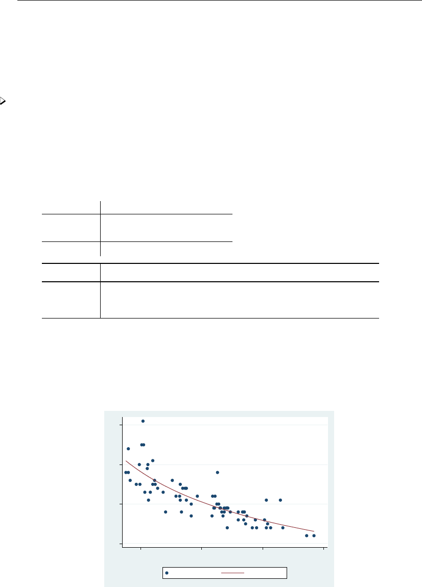
1462 nl postestimation — Postestimation tools for nl
scores calculates the scores. The jth new variable created will contain the score for the jth parameter
in e(b).
Remarks and examples
Example 1
Obtaining predictions after fitting a nonlinear regression model with nl is no more difficult than
obtaining predictions after fitting a linear regression model with regress. Here we fit a model of
mpg on weight, allowing for a nonlinear relationship:
. use http://www.stata-press.com/data/r13/auto
(1978 Automobile Data)
. nl (mpg = {b0} + {b1}*weight^{gamma=-.5}), variables(weight) nolog
(obs = 74)
Source SS df MS
Number of obs = 74
Model 1646.43761 2 823.218806 R-squared = 0.6738
Residual 797.021847 71 11.2256598 Adj R-squared = 0.6646
Root MSE = 3.350472
Total 2443.45946 73 33.4720474 Res. dev. = 385.8874
mpg Coef. Std. Err. t P>|t| [95% Conf. Interval]
/b0 -18.17583 60.61713 -0.30 0.765 -139.0429 102.6913
/b1 1377.267 5292.443 0.26 0.795 -9175.564 11930.1
/gamma -.4460916 .6763643 -0.66 0.512 -1.794724 .9025405
Parameter b0 taken as constant term in model & ANOVA table
Now we obtain the predicted values of mpg and plot them in a graph along with the observed
values:
. predict mpghat
(option yhat assumed; fitted values)
. scatter mpg weight || line mpghat weight, sort
10 20 30 40
2,000 3,000 4,000 5,000
Weight (lbs.)
Mileage (mpg) Fitted values

nl postestimation — Postestimation tools for nl 1463
Suppose we wanted to know how sensitive mpg is to changes in weight for cars that weigh 3,000
pounds. We can use margins to find out:
. margins, eyex(weight) at(weight = 3000)
Warning: cannot perform check for estimable functions.
Conditional marginal effects Number of obs = 74
Model VCE : GNR
Expression : Fitted values, predict()
ey/ex w.r.t. : weight
at : weight = 3000
Delta-method
ey/ex Std. Err. z P>|z| [95% Conf. Interval]
weight -.8408119 .0804379 -10.45 0.000 -.9984673 -.6831565
With the eyex() option, margins reports elasticities. These results show that if we increase weight
by 1%, then mpg decreases by about 0.84%.
Technical note
Observant readers will notice that margins issued a warning message stating that it could not
perform its usual check for estimable functions. In the case of nl, as long as you do not specify the
predict() option of margins or specify the default predict(yhat), you can safely ignore that
message. The predicted values that nl produces are suitable for use with margins. However, if you
specify any predict() options other than yhat, then the output from margins after using nl will
not be correct.
Also see
[R]nl — Nonlinear least-squares estimation
[U] 20 Estimation and postestimation commands

Title
nlcom — Nonlinear combinations of estimators
Syntax Menu Description Options
Remarks and examples Stored results Methods and formulas References
Also see
Syntax
Nonlinear combination of estimators—one expression
nlcom name:exp ,options
Nonlinear combinations of estimators—more than one expression
nlcom (name:exp)(name:exp ,options
options Description
level(#)set confidence level; default is level(95)
iterate(#)maximum number of iterations
post post estimation results
display options control column formats and line width
noheader suppress output header
df(#)use tdistribution with #degrees of freedom for computing p-values
and confidence intervals
noheader and df(#)do not appear in the dialog box.
The second syntax means that if more than one expression is specified, each must be surrounded by
parentheses. The optional name is any valid Stata name and labels the transformations.
exp is a possibly nonlinear expression containing
b[coef ]
b[eqno:coef ]
[eqno]coef
[eqno] b[coef ]
eqno is
##
name
coef identifies a coefficient in the model. coef is typically a variable name, a level indicator, an
interaction indicator, or an interaction involving continuous variables. Level indicators identify one
level of a factor variable and interaction indicators identify one combination of levels of an interaction;
see [U] 11.4.3 Factor variables.coef may contain time-series operators; see [U] 11.4.4 Time-series
varlists.
Distinguish between [ ], which are to be typed, and , which indicate optional arguments.
1464

nlcom — Nonlinear combinations of estimators 1465
Menu
Statistics >Postestimation >Nonlinear combinations of estimates
Description
nlcom computes point estimates, standard errors, test statistics, significance levels, and confidence
intervals for (possibly) nonlinear combinations of parameter estimates after any Stata estimation
command. Results are displayed in the usual table format used for displaying estimation results.
Calculations are based on the “delta method”, an approximation appropriate in large samples.
nlcom can be used with svy estimation results; see [SVY]svy postestimation.
Options
level(#)specifies the confidence level, as a percentage, for confidence intervals. The default is
level(95) or as set by set level; see [U] 20.7 Specifying the width of confidence intervals.
iterate(#)specifies the maximum number of iterations used to find the optimal step size in
calculating numerical derivatives of the transformation(s) with respect to the original parameters.
By default, the maximum number of iterations is 100, but convergence is usually achieved after
only a few iterations. You should rarely have to use this option.
post causes nlcom to behave like a Stata estimation (eclass) command. When post is specified,
nlcom will post the vector of transformed estimators and its estimated variance–covariance matrix to
e(). This option, in essence, makes the transformation permanent. Thus you could, after posting,
treat the transformed estimation results in the same way as you would treat results from other
Stata estimation commands. For example, after posting, you could redisplay the results by typing
nlcom without any arguments, or use test to perform simultaneous tests of hypotheses on linear
combinations of the transformed estimators; see [R]test.
Specifying post clears out the previous estimation results, which can be recovered only by refitting
the original model or by storing the estimation results before running nlcom and then restoring
them; see [R]estimates store.
display options:cformat(%fmt),pformat(% fmt),sformat(% fmt), and nolstretch; see [R]es-
timation options.
The following options are available with nlcom but are not shown in the dialog box:
noheader suppresses the output header.
df(#)specifies that the tdistribution with #degrees of freedom be used for computing p-values and
confidence intervals.
Remarks and examples
Remarks are presented under the following headings:
Introduction
Basics
Using the post option
Reparameterizing ML estimators for univariate data
nlcom versus eform

1466 nlcom — Nonlinear combinations of estimators
Introduction
nlcom and predictnl both use the delta method. They take nonlinear transformations of the
estimated parameter vector from some fitted model and apply the delta method to calculate the variance,
standard error, Wald test statistic, etc., of the transformations. nlcom is designed for functions of the
parameters, and predictnl is designed for functions of the parameters and of the data, that is, for
predictions.
nlcom generalizes lincom (see [R]lincom) in two ways. First, nlcom allows the transformations
to be nonlinear. Second, nlcom can be used to simultaneously estimate many transformations (whether
linear or nonlinear) and to obtain the estimated variance–covariance matrix of these transformations.
Basics
In [R]lincom, the following regression was performed:
. use http://www.stata-press.com/data/r13/regress
. regress y x1 x2 x3
Source SS df MS Number of obs = 148
F( 3, 144) = 96.12
Model 3259.3561 3 1086.45203 Prob > F = 0.0000
Residual 1627.56282 144 11.3025196 R-squared = 0.6670
Adj R-squared = 0.6600
Total 4886.91892 147 33.2443464 Root MSE = 3.3619
y Coef. Std. Err. t P>|t| [95% Conf. Interval]
x1 1.457113 1.07461 1.36 0.177 -.666934 3.581161
x2 2.221682 .8610358 2.58 0.011 .5197797 3.923583
x3 -.006139 .0005543 -11.08 0.000 -.0072345 -.0050435
_cons 36.10135 4.382693 8.24 0.000 27.43863 44.76407
Then lincom was used to estimate the difference between the coefficients of x1 and x2:
. lincom _b[x2] - _b[x1]
( 1) - x1 + x2 = 0
y Coef. Std. Err. t P>|t| [95% Conf. Interval]
(1) .7645682 .9950282 0.77 0.444 -1.20218 2.731316
It was noted, however, that nonlinear expressions are not allowed with lincom:
. lincom _b[x2]/_b[x1]
not possible with test
r(131);
Nonlinear transformations are instead estimated using nlcom:
. nlcom _b[x2]/_b[x1]
_nl_1: _b[x2]/_b[x1]
y Coef. Std. Err. z P>|z| [95% Conf. Interval]
_nl_1 1.524714 .9812848 1.55 0.120 -.3985686 3.447997

nlcom — Nonlinear combinations of estimators 1467
Technical note
The notation b[name]is the standard way in Stata to refer to regression coefficients; see
[U] 13.5 Accessing coefficients and standard errors. Some commands, such as lincom and test,
allow you to drop the b[] and just refer to the coefficients by name.nlcom, however, requires the
full specification b[name].
Returning to our linear regression example, nlcom also allows simultaneous estimation of more
than one combination:
. nlcom (_b[x2]/_b[x1]) (_b[x3]/_b[x1]) (_b[x3]/_b[x2])
_nl_1: _b[x2]/_b[x1]
_nl_2: _b[x3]/_b[x1]
_nl_3: _b[x3]/_b[x2]
y Coef. Std. Err. z P>|z| [95% Conf. Interval]
_nl_1 1.524714 .9812848 1.55 0.120 -.3985686 3.447997
_nl_2 -.0042131 .0033483 -1.26 0.208 -.0107756 .0023494
_nl_3 -.0027632 .0010695 -2.58 0.010 -.0048594 -.000667
We can also label the transformations to produce more informative names in the estimation table:
. nlcom (ratio21:_b[x2]/_b[x1]) (ratio31:_b[x3]/_b[x1]) (ratio32:_b[x3]/_b[x2])
ratio21: _b[x2]/_b[x1]
ratio31: _b[x3]/_b[x1]
ratio32: _b[x3]/_b[x2]
y Coef. Std. Err. z P>|z| [95% Conf. Interval]
ratio21 1.524714 .9812848 1.55 0.120 -.3985686 3.447997
ratio31 -.0042131 .0033483 -1.26 0.208 -.0107756 .0023494
ratio32 -.0027632 .0010695 -2.58 0.010 -.0048594 -.000667
nlcom stores the vector of estimated combinations and its estimated variance–covariance matrix
in r().
. matrix list r(b)
r(b)[1,3]
ratio21 ratio31 ratio32
c1 1.5247143 -.00421315 -.00276324
. matrix list r(V)
symmetric r(V)[3,3]
ratio21 ratio31 ratio32
ratio21 .96291982
ratio31 -.00287781 .00001121
ratio32 -.00014234 2.137e-06 1.144e-06

1468 nlcom — Nonlinear combinations of estimators
Using the post option
When used with the post option, nlcom stores the estimation vector and variance–covariance
matrix in e(), making the transformation permanent:
. quietly nlcom (ratio21:_b[x2]/_b[x1]) (ratio31:_b[x3]/_b[x1])
> (ratio32:_b[x3]/_b[x2]), post
. matrix list e(b)
e(b)[1,3]
ratio21 ratio31 ratio32
y1 1.5247143 -.00421315 -.00276324
. matrix list e(V)
symmetric e(V)[3,3]
ratio21 ratio31 ratio32
ratio21 .96291982
ratio31 -.00287781 .00001121
ratio32 -.00014234 2.137e-06 1.144e-06
After posting, we can proceed as if we had just run a Stata estimation (eclass) command. For
instance, we can replay the results,
. nlcom
y Coef. Std. Err. z P>|z| [95% Conf. Interval]
ratio21 1.524714 .9812848 1.55 0.120 -.3985686 3.447997
ratio31 -.0042131 .0033483 -1.26 0.208 -.0107756 .0023494
ratio32 -.0027632 .0010695 -2.58 0.010 -.0048594 -.000667
or perform other postestimation tasks in the transformed metric, this time making reference to the
new “coefficients”:
. display _b[ratio31]
-.00421315
. estat vce, correlation
Correlation matrix of coefficients of nlcom model
e(V) ratio21 ratio31 ratio32
ratio21 1.0000
ratio31 -0.8759 1.0000
ratio32 -0.1356 0.5969 1.0000
. test _b[ratio21] = 1
( 1) ratio21 = 1
chi2( 1) = 0.29
Prob > chi2 = 0.5928
We see that testing b[ratio21]=1 in the transformed metric is equivalent to testing using testnl
b[x2]/ b[x1]=1 in the original metric:
. quietly regress y x1 x2 x3
. testnl _b[x2]/_b[x1] = 1
(1) _b[x2]/_b[x1] = 1
chi2(1) = 0.29
Prob > chi2 = 0.5928
We needed to refit the regression model to recover the original parameter estimates.
nlcom — Nonlinear combinations of estimators 1469
Technical note
In a previous technical note, we mentioned that commands such as lincom and test permit
reference to name instead of b[name]. This is not the case when lincom and test are used after
nlcom, post. In the above, we used
. test _b[ratio21] = 1
rather than
. test ratio21 = 1
which would have returned an error. Consider this a limitation of Stata. For the shorthand notation
to work, you need a variable named name in the data. In nlcom, however, name is just a coefficient
label that does not necessarily correspond to any variable in the data.
Reparameterizing ML estimators for univariate data
When run using only a response and no covariates, Stata’s maximum likelihood (ML) estimation
commands will produce ML estimates of the parameters of some assumed univariate distribution for
the response. The parameterization, however, is usually not one we are used to dealing with in a
nonregression setting. In such cases, nlcom can be used to transform the estimation results from a
regression model to those from a maximum likelihood estimation of the parameters of a univariate
probability distribution in a more familiar metric.
Example 1
Consider the following univariate data on Y=# of traffic accidents at a certain intersection in a
given year:
. use http://www.stata-press.com/data/r13/trafint
. summarize accidents
Variable Obs Mean Std. Dev. Min Max
accidents 12 13.83333 14.47778 0 41
A quick glance of the output from summarize leads us to quickly reject the assumption that Yis
distributed as Poisson because the estimated variance of Yis much greater than the estimated mean
of Y.
Instead, we choose to model the data as univariate negative binomial, of which a common
parameterization is
Pr(Y=y) = Γ(r+y)
Γ(r)Γ(y+ 1)pr(1 −p)y0≤p≤1, r > 0, y = 0,1, . . .
with
E(Y) = r(1 −p)
pVar(Y) = r(1 −p)
p2
There exist no closed-form solutions for the maximum likelihood estimates of pand r, yet they
may be estimated by the iterative method of Newton–Raphson. One way to get these estimates would
be to write our own Newton–Raphson program for the negative binomial. Another way would be to
write our own ML evaluator; see [R]ml.

1470 nlcom — Nonlinear combinations of estimators
The easiest solution, however, would be to use Stata’s existing negative binomial ML regres-
sion command, nbreg. The only problem with this solution is that nbreg estimates a different
parameterization of the negative binomial, but we can worry about that later.
. nbreg accidents
Fitting Poisson model:
Iteration 0: log likelihood = -105.05361
Iteration 1: log likelihood = -105.05361
Fitting constant-only model:
Iteration 0: log likelihood = -43.948619
Iteration 1: log likelihood = -43.891483
Iteration 2: log likelihood = -43.89144
Iteration 3: log likelihood = -43.89144
Fitting full model:
Iteration 0: log likelihood = -43.89144
Iteration 1: log likelihood = -43.89144
Negative binomial regression Number of obs = 12
LR chi2(0) = 0.00
Dispersion = mean Prob > chi2 = .
Log likelihood = -43.89144 Pseudo R2 = 0.0000
accidents Coef. Std. Err. z P>|z| [95% Conf. Interval]
_cons 2.627081 .3192233 8.23 0.000 2.001415 3.252747
/lnalpha .1402425 .4187147 -.6804233 .9609083
alpha 1.150553 .4817534 .5064026 2.61407
Likelihood-ratio test of alpha=0: chibar2(01) = 122.32 Prob>=chibar2 = 0.000
. nbreg, coeflegend
Negative binomial regression Number of obs = 12
LR chi2(0) = 0.00
Dispersion = mean Prob > chi2 = .
Log likelihood = -43.89144 Pseudo R2 = 0.0000
accidents Coef. Legend
_cons 2.627081 _b[accidents:_cons]
/lnalpha .1402425 _b[lnalpha:_cons]
alpha 1.150553
Likelihood-ratio test of alpha=0: chibar2(01) = 122.32 Prob>=chibar2 = 0.000
From this output, we see that, when used with univariate data, nbreg estimates a regression
intercept, β0, and the logarithm of some parameter α. This parameterization is useful in regression
models: β0is the intercept meant to be augmented with other terms of the linear predictor, and αis
an overdispersion parameter used for comparison with the Poisson regression model.
However, we need to transform (β0,lnα)to (p, r). Examining Methods and formulas of [R]nbreg
reveals the transformation as
p={1 + αexp(β0)}−1r=α−1
which we apply using nlcom:

nlcom — Nonlinear combinations of estimators 1471
. nlcom (p:1/(1 + exp([lnalpha]_b[_cons] + _b[_cons])))
> (r:exp(-[lnalpha]_b[_cons]))
p: 1/(1 + exp([lnalpha]_b[_cons] + _b[_cons]))
r: exp(-[lnalpha]_b[_cons])
accidents Coef. Std. Err. z P>|z| [95% Conf. Interval]
p .0591157 .0292857 2.02 0.044 .0017168 .1165146
r .8691474 .3639248 2.39 0.017 .1558679 1.582427
Given the invariance of maximum likelihood estimators and the properties of the delta method, the
above parameter estimates, standard errors, etc., are precisely those we would have obtained had we
instead performed the Newton–Raphson optimization in the (p, r)metric.
Technical note
Note how we referred to the estimate of lnαabove as [lnalpha] b[ cons]. This is not entirely
evident from the output of nbreg, which is why we redisplayed the results using the coeflegend
option so that we would know how to refer to the coefficients; [U] 13.5 Accessing coefficients and
standard errors.
nlcom versus eform
Many Stata estimation commands allow you to display exponentiated regression coefficients, some
by default, some optionally. Known as “eform” in Stata terminology, this reparameterization serves
many uses: it gives odds ratios for logistic models, hazard ratios in survival models, incidence-rate
ratios in Poisson models, and relative-risk ratios in multinomial logit models, to name a few.
For example, consider the following estimation taken directly from the technical note in [R]poisson:
. use http://www.stata-press.com/data/r13/airline
. generate lnN = ln(n)
. poisson injuries XYZowned lnN
Iteration 0: log likelihood = -22.333875
Iteration 1: log likelihood = -22.332276
Iteration 2: log likelihood = -22.332276
Poisson regression Number of obs = 9
LR chi2(2) = 19.15
Prob > chi2 = 0.0001
Log likelihood = -22.332276 Pseudo R2 = 0.3001
injuries Coef. Std. Err. z P>|z| [95% Conf. Interval]
XYZowned .6840667 .3895877 1.76 0.079 -.0795111 1.447645
lnN 1.424169 .3725155 3.82 0.000 .6940517 2.154285
_cons 4.863891 .7090501 6.86 0.000 3.474178 6.253603

1472 nlcom — Nonlinear combinations of estimators
When we replay results and specify the irr (incidence-rate ratios) option,
. poisson, irr
Poisson regression Number of obs = 9
LR chi2(2) = 19.15
Prob > chi2 = 0.0001
Log likelihood = -22.332276 Pseudo R2 = 0.3001
injuries IRR Std. Err. z P>|z| [95% Conf. Interval]
XYZowned 1.981921 .7721322 1.76 0.079 .9235678 4.253085
lnN 4.154402 1.547579 3.82 0.000 2.00181 8.621728
_cons 129.5272 91.84126 6.86 0.000 32.2713 519.8828
we obtain the exponentiated regression coefficients and their estimated standard errors.
Contrast this with what we obtain if we exponentiate the coefficients manually by using nlcom:
. nlcom (E_XYZowned:exp(_b[XYZowned])) (E_lnN:exp(_b[lnN]))
E_XYZowned: exp(_b[XYZowned])
E_lnN: exp(_b[lnN])
injuries Coef. Std. Err. z P>|z| [95% Conf. Interval]
E_XYZowned 1.981921 .7721322 2.57 0.010 .4685701 3.495273
E_lnN 4.154402 1.547579 2.68 0.007 1.121203 7.187602
There are three things to note when comparing poisson, irr (and eform in general) with nlcom:
1. The exponentiated coefficients and standard errors are identical. This is certainly good news.
2. The Wald test statistic (z) and level of significance are different. When using poisson, irr and
other related eform options, the Wald test does not change from what you would have obtained
without the eform option, and you can see this by comparing both versions of the poisson output
given previously.
When you use eform, Stata knows that what is usually desired is a test of
H0: exp(β)=1
and not the uninformative-by-comparison
H0: exp(β)=0
The test of H0: exp(β)=1is asymptotically equivalent to a test of H0:β= 0, the Wald test in
the original metric, but the latter has better small-sample properties. Thus if you specify eform,
you get a test of H0:β= 0.
nlcom, however, is general. It does not attempt to infer the test of greatest interest for a given
transformation, and so a test of
H0:transformed coefficient = 0
is always given, regardless of the transformation.
3. You may be surprised to see that, even though the coefficients and standard errors are identical,
the confidence intervals (both 95%) are different.

nlcom — Nonlinear combinations of estimators 1473
eform confidence intervals are standard confidence intervals with the endpoints transformed. For
example, the confidence interval for the coefficient on lnN is [0.694,2.154], whereas the confidence
interval for the incidence-rate ratio due to lnN is [exp(0.694),exp(2.154)] = [2.002,8.619], which,
except for some roundoff error, is what we see from the output of poisson, irr. For exponentiated
coefficients, confidence intervals based on transform-the-endpoints methodology generally have
better small-sample properties than their asymptotically equivalent counterparts.
The transform-the-endpoints method, however, gives valid coverage only when the transformation
is monotonic. nlcom uses a more general and asymptotically equivalent method for calculating
confidence intervals, as described in Methods and formulas.
Stored results
nlcom stores the following in r():
Scalars
r(N) number of observations
r(df r) residual degrees of freedom
Matrices
r(b) vector of transformed coefficients
r(V) estimated variance–covariance matrix of the transformed coefficients
If post is specified, nlcom also stores the following in e():
Scalars
e(N) number of observations
e(df r) residual degrees of freedom
e(N strata) number of strata L, if used after svy
e(N psu) number of sampled PSUs n, if used after svy
e(rank) rank of e(V)
Macros
e(cmd) nlcom
e(predict) program used to implement predict
e(properties) b V
Matrices
e(b) vector of transformed coefficients
e(V) estimated variance–covariance matrix of the transformed coefficients
e(V srs) simple-random-sampling-without-replacement (co)variance b
Vsrswor, if svy
e(V srswr) simple-random-sampling-with-replacement (co)variance b
Vsrswr, if svy and fpc()
e(V msp) misspecification (co)variance b
Vmsp, if svy and available
Functions
e(sample) marks estimation sample
Methods and formulas
Given a 1×kvector of parameter estimates, b
θ= (b
θ1,...,b
θk), consider the estimated p-dimensional
transformation
g(b
θ) = [g1(b
θ), g2(b
θ), . . . , gp(b
θ)]
The estimated variance–covariance of g(b
θ)is given by
c
Var ng(b
θ)o=GVG0

1474 nlcom — Nonlinear combinations of estimators
where Gis the p×kmatrix of derivatives for which
Gij =∂gi(θ)
∂θjθ=b
θ
i= 1, . . . , p j = 1, . . . , k
and Vis the estimated variance–covariance matrix of b
θ. Standard errors are obtained as the square
roots of the variances.
The Wald test statistic for testing
H0:gi(θ)=0
versus the two-sided alternative is given by
Zi=gi(b
θ)
hc
Varii ng(b
θ)oi1/2
When the variance–covariance matrix of b
θis an asymptotic covariance matrix, Ziis approximately
distributed as Gaussian. For linear regression, Ziis taken to be approximately distributed as t1,r
where ris the residual degrees of freedom from the original fitted model.
A(1−α)×100% confidence interval for gi(θ)is given by
gi(b
θ)±zα/2hc
Varii ng(b
θ)oi1/2
for those cases where Ziis Gaussian and
gi(b
θ)±tα/2,rhc
Varii ng(b
θ)oi1/2
for those cases where Ziis tdistributed. zpis the 1 −pquantile of the standard normal distribution,
and tp,r is the 1 −pquantile of the tdistribution with rdegrees of freedom.
References
Feiveson, A. H. 1999. FAQ: What is the delta method and how is it used to estimate the standard error of a
transformed parameter? http://www.stata.com/support/faqs/stat/deltam.html.
Gould, W. W. 1996. crc43: Wald test of nonlinear hypotheses after model estimation.Stata Technical Bulletin 29:
2–4. Reprinted in Stata Technical Bulletin Reprints, vol. 5, pp. 15–18. College Station, TX: Stata Press.
Oehlert, G. W. 1992. A note on the delta method. American Statistician 46: 27–29.
Phillips, P. C. B., and J. Y. Park. 1988. On the formulation of Wald tests of nonlinear restrictions. Econometrica 56:
1065–1083.
Also see
[R]lincom — Linear combinations of estimators
[R]predictnl — Obtain nonlinear predictions, standard errors, etc., after estimation
[R]test — Test linear hypotheses after estimation
[R]testnl — Test nonlinear hypotheses after estimation
[U] 20 Estimation and postestimation commands

Title
nlogit — Nested logit regression
Syntax Menu Description Options
Remarks and examples Stored results Methods and formulas References
Also see
Syntax
Nested logit regression
nlogit depvar indepvars if in weight || lev1 equation
|| lev2 equation . . . || altvar:byaltvarlist , case(varname)options
where the syntax of lev# equation is
altvar:byaltvarlist , base(#|lbl) estconst
Create variable based on specification of branches
nlogitgen newaltvar =altvar (branchlist), nolog
where branchlist is
branch,branch ,branch . . .
and branch is
label:alternative |alternative |alternative . . .
Display tree structure
nlogittree altvarlist if in weight , choice(depvar) nolabel nobranches
1475

1476 nlogit — Nested logit regression
options Description
Model
∗case(varname)use varname to identify cases
base(#|lbl)use the specified level or label of altvar as the base alternative for
the bottom level
noconstant suppress the constant terms for the bottom-level alternatives
nonnormalized use the nonnormalized parameterization
altwise use alternativewise deletion instead of casewise deletion
constraints(constraints)apply specified linear constraints
collinear keep collinear variables
SE/Robust
vce(vcetype)vcetype may be oim,robust,cluster clustvar,
bootstrap, or jackknife
Reporting
level(#)set confidence level; default is level(95)
notree suppress display of tree-structure output; see also
nolabel and nobranches
nocnsreport do not display constraints
display options control column formats and line width
Maximization
maximize options control the maximization process; seldom used
∗case(varname)is required.
bootstrap,by,fp,jackknife,statsby, and xi are allowed; see [U] 11.1.10 Prefix commands.
Weights are not allowed with the bootstrap prefix; see [R] bootstrap.
fweights, iweights, and pweights are allowed with nlogit, and fweights are allowed with nlogittree; see
[U] 11.1.6 weight. Weights for nlogit must be constant within case.
See [U] 20 Estimation and postestimation commands for more capabilities of estimation commands.
Menu
nlogit
Statistics >Categorical outcomes >Nested logit regression
nlogitgen
Statistics >Categorical outcomes >Setup for nested logit regression
nlogittree
Statistics >Categorical outcomes >Display nested logit tree structure
Description
nlogit performs full information maximum-likelihood estimation for nested logit models. These
models relax the assumption of independently distributed errors and the independence of irrelevant
alternatives inherent in conditional and multinomial logit models by clustering similar alternatives
into nests.

nlogit — Nested logit regression 1477
By default, nlogit uses a parameterization that is consistent with random utility maximization
(RUM). Before version 10 of Stata, a nonnormalized version of the nested logit model was fit, which
you can request by specifying the nonnormalized option.
You must use nlogitgen to generate a new categorical variable to specify the branches of the
decision tree before calling nlogit.
Options
Specification and options for lev# equation
altvar is a variable identifying alternatives at this level of the hierarchy.
byaltvarlist specifies the variables to be used to compute the by-alternative regression coefficients for
that level. For each variable specified in the variable list, there will be one regression coefficient
for each alternative of that level of the hierarchy. If the variable is constant across each alternative
(a case-specific variable), the regression coefficient associated with the base alternative is not
identifiable. These regression coefficients are labeled as (base) in the regression table. If the
variable varies among the alternatives, a regression coefficient is estimated for each alternative.
base(#|lbl)can be specified in each level equation where it identifies the base alternative to be
used at that level. The default is the alternative that has the highest frequency.
If vce(bootstrap) or vce(jackknife) is specified, you must specify the base alternative for
each level that has a byaltvarlist or if the constants will be estimated. Doing so ensures that the
same model is fit with each call to nlogit.
estconst applies to all the level equations except the bottom-level equation. Specifying estconst
requests that constants for each alternative (except the base alternative) be estimated. By default,
no constant is estimated at these levels. Constants can be estimated in only one level of the tree
hierarchy. If you specify estconst for one of the level equations, you must specify noconstant
for the bottom-level equation.
Options for nlogit
Model
case(varname)specifies the variable that identifies each case. case() is required.
base(#|lbl)can be specified in each level equation where it identifies the base alternative to be
used at that level. The default is the alternative that has the highest frequency.
If vce(bootstrap) or vce(jackknife) is specified, you must specify the base alternative for
each level that has a byaltvarlist or if the constants will be estimated. Doing so ensures that the
same model is fit with each call to nlogit.
noconstant applies only to the equation defining the bottom level of the hierarchy. By default,
constants are estimated for each alternative of altvar, less the base alternative. To suppress the
constant terms for this level, specify noconstant. If you do not specify noconstant, you cannot
specify estconst for the higher-level equations.
nonnormalized requests a nonnormalized parameterization of the model that does not scale the
inclusive values by the degree of dissimilarity of the alternatives within each nest. Use this
option to replicate results from older versions of Stata. The default is to use the RUM–consistent
parameterization.

1478 nlogit — Nested logit regression
altwise specifies that alternativewise deletion be used when marking out observations because of
missing values in your variables. The default is to use casewise deletion. This option does not
apply to observations that are marked out by the if or in qualifier or the by prefix.
constraints(constraints); see [R]estimation options.
The inclusive-valued/dissimilarity parameters are parameterized as ml ancillary parameters. They
are labeled as alternative tauconst, where alternative is one of the alternatives defining a
branch in the tree. To constrain the inclusive-valued/dissimilarity parameter for alternative a1 to
be, say, equal to alternative a2, you would use the following syntax:
. constraint 1 [a1_tau]_cons = [a2_tau]_cons
. nlogit ..., constraints(1)
collinear prevents collinear variables from being dropped. Use this option when you know that
you have collinear variables and you are applying constraints() to handle the rank reduction.
See [R]estimation options for details on using collinear with constraints().
nlogit will not allow you to specify an independent variable in more than one level equation.
Specifying the collinear option will allow execution to proceed in this case, but it is your
responsibility to ensure that the parameters are identified.
SE/Robust
vce(vcetype)specifies the type of standard error reported, which includes types that are derived
from asymptotic theory (oim), that are robust to some kinds of misspecification (robust), that
allow for intragroup correlation (cluster clustvar), and that use bootstrap or jackknife methods
(bootstrap,jackknife); see [R]vce option.
If vce(robust) or vce(cluster clustvar)is specified, the likelihood-ratio test for the indepen-
dence of irrelevant alternatives (IIA) is not computed.
Reporting
level(#); see [R]estimation options.
notree specifies that the tree structure of the nested logit model not be displayed. See also nolabel
and nobranches below for when notree is not specified.
nocnsreport; see [R]estimation options.
display options:cformat(%fmt),pformat(% fmt),sformat(% fmt), and nolstretch; see [R]es-
timation options.
Maximization
maximize options:difficult,technique(algorithm spec),iterate(#),nolog,trace,
gradient,showstep,hessian,showtolerance,tolerance(#),ltolerance(#),
nrtolerance(#),nonrtolerance, and from(init specs); see [R]maximize. These options are
seldom used.
The technique(bhhh) option is not allowed.
Specification and options for nlogitgen
newaltvar and altvar are variables identifying alternatives at each level of the hierarchy.
label defines a label to associate with the branch. If no label is given, a numeric value is used.

nlogit — Nested logit regression 1479
alternative specifies an alternative, of altvar specified in the syntax, to be included in the branch. It
is either a numeric value or the label associated with that value. An example of nlogitgen is
. nlogitgen type = restaurant(fast: 1 | 2,
> family: CafeEccell | LosNortenos | WingsNmore, fancy: 6 | 7)
nolog suppresses the display of the iteration log.
Specification and options for nlogittree
Main
altvarlist is a list of alternative variables that define the tree hierarchy. The first variable must define
bottom-level alternatives, and the order continues to the variable defining the top-level alternatives.
choice(depvar)defines the choice indicator variable and forces nlogittree to compute and display
choice frequencies for each bottom-level alternative.
nolabel forces nlogittree to suppress value labels in tree-structure output.
nobranches forces nlogittree to suppress drawing branches in the tree-structure output.
Remarks and examples
Remarks are presented under the following headings:
Introduction
Data setup and the tree structure
Estimation
Testing for the IIA
Nonnormalized model
Introduction
nlogit performs full information maximum-likelihood estimation for nested logit models. These
models relax the assumption of independently distributed errors and the IIA inherent in conditional
and multinomial logit models by clustering similar alternatives into nests. Because the nested logit
model is a direct generalization of the alternative-specific conditional logit model (also known as
McFadden’s choice model), you may want to read [R]asclogit before continuing.
By default, nlogit uses a parameterization that is consistent with RUM. Before version 10 of
Stata, a nonnormalized version of the nested logit model was fit, which you can request by specifying
the nonnormalized option. We recommend using the RUM-consistent version of the model for new
projects because it is based on a sound model of consumer behavior.
McFadden (1977,1981) showed how this model can be derived from a rational choice framework.
Amemiya (1985, chap. 9) contains a nice discussion of how this model can be derived under the
assumption of utility maximization. Hensher, Rose, and Greene (2005) provide a lucid introduction
to choice models including nested logit.
Throughout this entry, we consider a model of restaurant choice. We begin by introducing the
data.

1480 nlogit — Nested logit regression
Example 1
We have fictional data on 300 families and their choice of seven local restaurants. Freebirds and
Mama’s Pizza are fast food restaurants; Caf´
e Eccell, Los Norte˜
nos, and Wings ’N More are family
restaurants; and Christopher’s and Mad Cows are fancy restaurants. We want to model the decision
of where to eat as a function of household income (income, in thousands of dollars), the number
of children in the household (kids), the rating of the restaurant according to a local restaurant
guide (rating, coded 0–5), the average meal cost per person (cost), and the distance between the
household and the restaurant (distance, in miles). income and kids are attributes of the family,
rating is an attribute of the alternative (the restaurant), and cost and distance are attributes of
the alternative as perceived by the families—that is, each family has its own cost and distance for
each restaurant.
We begin by loading the data and listing some of the variables for the first three families:
. use http://www.stata-press.com/data/r13/restaurant
. describe
Contains data from http://www.stata-press.com/data/r13/restaurant.dta
obs: 2,100
vars: 8 10 Mar 2013 01:17
size: 67,200
storage display value
variable name type format label variable label
family_id float %9.0g family ID
restaurant float %12.0g names choices of restaurants
income float %9.0g household income
cost float %9.0g average meal cost per person
kids float %9.0g number of kids in the household
rating float %9.0g ratings in local restaurant guide
distance float %9.0g distance between home and
restaurant
chosen float %9.0g 0 no 1 yes
Sorted by: family_id

nlogit — Nested logit regression 1481
. list family_id restaurant chosen kids rating distance in 1/21, sepby(fam)
> abbrev(10)
family_id restaurant chosen kids rating distance
1. 1 Freebirds 1 1 0 1.245553
2. 1 MamasPizza 0 1 1 2.82493
3. 1 CafeEccell 0 1 2 4.21293
4. 1 LosNortenos 0 1 3 4.167634
5. 1 WingsNmore 0 1 2 6.330531
6. 1 Christophers 0 1 4 10.19829
7. 1 MadCows 0 1 5 5.601388
8. 2 Freebirds 0 3 0 4.162657
9. 2 MamasPizza 0 3 1 2.865081
10. 2 CafeEccell 0 3 2 5.337799
11. 2 LosNortenos 1 3 3 4.282864
12. 2 WingsNmore 0 3 2 8.133914
13. 2 Christophers 0 3 4 8.664631
14. 2 MadCows 0 3 5 9.119597
15. 3 Freebirds 1 3 0 2.112586
16. 3 MamasPizza 0 3 1 2.215329
17. 3 CafeEccell 0 3 2 6.978715
18. 3 LosNortenos 0 3 3 5.117877
19. 3 WingsNmore 0 3 2 5.312941
20. 3 Christophers 0 3 4 9.551273
21. 3 MadCows 0 3 5 5.539806
Because each family chose among seven restaurants, there are 7 observations in the dataset for each
family. The variable chosen is coded 0/1, with 1 indicating the chosen restaurant and 0 otherwise.
We could fit a conditional logit model to our data. Because income and kids are constant within
each family, we would use the asclogit command instead of clogit. However, the conditional
logit may be inappropriate. That model assumes that the random errors are independent, and as a
result it forces the odds ratio of any two alternatives to be independent of the other alternatives, a
property known as the IIA. We will discuss the IIA assumption in more detail later.
Assuming that unobserved shocks influencing a decision maker’s attitude toward one alternative
have no effect on his attitudes toward the other alternatives may seem innocuous, but often this
assumption is too restrictive. Suppose that when a family was deciding which restaurant to visit, they
were pressed for time because of plans to attend a movie later. The unobserved shock (being in a
hurry) would raise the likelihood that the family goes to either fast food restaurant (Freebirds or
Mama’s Pizza). Similarly, another family might be choosing a restaurant to celebrate a birthday and
therefore be inclined to attend a fancy restaurant (Christopher’s or Mad Cows).
Nested logit models relax the independence assumption and allow us to group alternatives for
which unobserved shocks may have concomitant effects. Here we suspect that restaurants should be
grouped by type (fast, family, or fancy). The tree structure of a family’s decision about where to eat
might look like this:
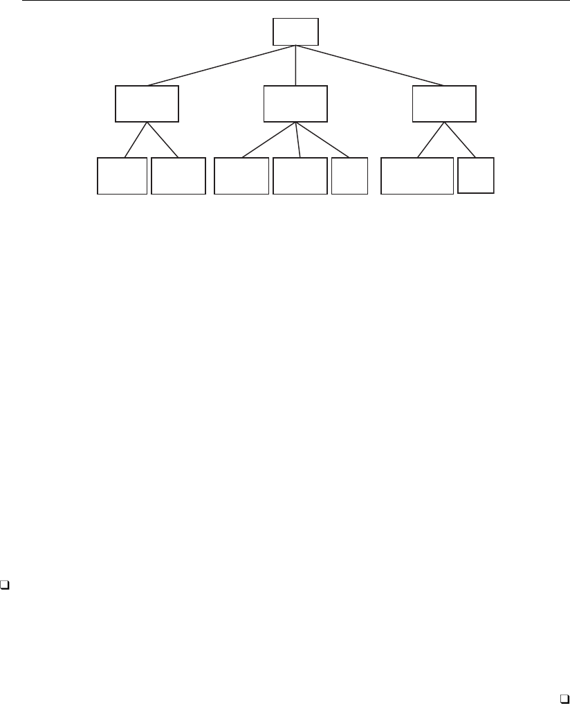
1482 nlogit — Nested logit regression
Dining
Fast food
restaurants
Family
restaurants
Fancy
restaurants
Mama's
Pizza
Freebirds Los
Norteños
Mad
Cows
Café
Eccell
Wings 'N
More
Christopher's
At the bottom of the tree are the individual restaurants, indicating that there are some random
shocks that affect a family’s decision to eat at each restaurant independently. Above the restaurants
are the three types of restaurants, indicating that other random shocks affect the type of restaurant
chosen. As is customary when drawing decision trees, at the top level is one box, representing the
family making the decision.
We use the following terms to describe nested logit models.
level, or decision level, is the level or stage at which a decision is made. The example above has
only two levels. In the first level, a type of restaurant is chosen—fast food, family, or fancy—and
in the second level, a specific restaurant is chosen.
bottom level is the level where the final decision is made. In our example, this is when we choose a
specific restaurant.
alternative set is the set of all possible alternatives at any given decision level.
bottom alternative set is the set of all possible alternatives at the bottom level. This concept is
often referred to as the choice set in the economics-choice literature. In our example, the bottom
alternative set is all seven of the specific restaurants.
alternative is a specific alternative within an alternative set. In the first level of our example, “fast
food” is an alternative. In the second or bottom level, “Mad Cows” is an alternative. Not all
alternatives within an alternative set are available to someone making a choice at a specific stage,
only those that are nested within all higher-level decisions.
chosen alternative is the alternative from an alternative set that we observe someone having chosen.
Technical note
Although decision trees in nested logit analysis are often interpreted as implying that the highest-
level decisions are made first, followed by decisions at lower levels, and finally the decision among
alternatives at the bottom level, no such temporal ordering is implied. See Hensher, Rose, and
Greene (2005, chap. 13). In our example, we are not assuming that families first choose whether to
attend a fast, family, or fancy restaurant and then choose the particular restaurant; we assume merely
that they choose one of the seven restaurants.

nlogit — Nested logit regression 1483
Data setup and the tree structure
To fit a nested logit model, you must first create a variable that defines the structure of your
decision tree.
Example 2
To run nlogit, we need to generate a categorical variable that identifies the first-level set
of alternatives: fast food, family restaurants, or fancy restaurants. We can do so easily by using
nlogitgen.
. nlogitgen type = restaurant(fast: Freebirds | MamasPizza,
> family: CafeEccell | LosNortenos| WingsNmore, fancy: Christophers | MadCows)
new variable type is generated with 3 groups
label list lb_type
lb_type:
1 fast
2 family
3 fancy
. nlogittree restaurant type, choice(chosen)
tree structure specified for the nested logit model
type N restaurant N k
fast 600 Freebirds 300 12
MamasPizza 300 15
family 900 CafeEccell 300 78
LosNortenos 300 75
WingsNmore 300 69
fancy 600 Christophers 300 27
MadCows 300 24
total 2100 300
k = number of times alternative is chosen
N = number of observations at each level
The new categorical variable is type, which takes on value 1 (fast) if restaurant is Freebirds
or Mama’s Pizza; value 2 (family) if restaurant is Caf´
e Eccell, Los Norte˜
nos, or Wings ’N More;
and value 3 (fancy) otherwise. nlogittree displays the tree structure.
Technical note
We could also use values instead of value labels of restaurant in nlogitgen. Value labels are
optional, and the default value labels for type are type1,type2, and type3. The vertical bar is
also optional.
. use http://www.stata-press.com/data/r13/restaurant, clear
. nlogitgen type = restaurant(1 2, 3 4 5, 6 7)
new variable type is generated with 3 groups
label list lb_type
lb_type:
1 type1
2 type2
3 type3
1484 nlogit — Nested logit regression
. nlogittree restaurant type
tree structure specified for the nested logit model
type N restaurant N
type1 600 Freebirds 300
MamasPizza 300
type2 900 CafeEccell 300
LosNortenos 300
WingsNmore 300
type3 600 Christophers 300
MadCows 300
total 2100
N = number of observations at each level
In our dataset, every family was able to choose among all seven restaurants. However, in other
applications some decision makers may not have been able to choose among all possible alternatives.
For example, two cases may have choice hierarchies of
case 1 case 2
type restaurant type restaurant
fast Freebirds fast Freebirds
MamasPizza MamasPizza
family CafeEccell family LosNortenos
LosNortenos WingsNmore
WingsNmore
fancy Christophers fancy Christophers
MadCows
where the second case does not have the restaurant alternatives Caf´
e Eccell or Mad Cows available
to them. The only restriction is that the relationships between higher- and lower-level alternative sets
be the same for all decision makers. In this two-level example, Freebirds and Mama’s Pizza are
classified as fast food restaurants for both cases; Caf´
e Eccell, Los Norte˜
nos, and Wings ’N More are
family restaurants; and Christopher’s and Mad Cows are fancy restaurants. nlogit requires only that
hierarchy be maintained for all cases.
Estimation
Example 3
With our type variable created that defines the three types of restaurants, we can now examine how
the alternative-specific attributes (cost,rating, and distance) apply to the bottom alternative set
(the seven restaurants) and how family-specific attributes (income and kid) apply to the alternative
set at the first decision level (the three types of restaurants).

nlogit — Nested logit regression 1485
. use http://www.stata-press.com/data/r13/restaurant, clear
. qui nlogitgen type = restaurant(fast: Freebirds | MamasPizza,
> family: CafeEccell | LosNortenos| WingsNmore, fancy: Christophers | MadCows)
. nlogit chosen cost rating distance || type: income kids, base(family) ||
> restaurant:, noconstant case(family_id)
tree structure specified for the nested logit model
type N restaurant N k
fast 600 Freebirds 300 12
MamasPizza 300 15
family 900 CafeEccell 300 78
LosNortenos 300 75
WingsNmore 300 69
fancy 600 Christophers 300 27
MadCows 300 24
total 2100 300
k = number of times alternative is chosen
N = number of observations at each level
Iteration 0: log likelihood = -541.93581
(output omitted )
Iteration 17: log likelihood = -485.47331
RUM-consistent nested logit regression Number of obs = 2100
Case variable: family_id Number of cases = 300
Alternative variable: restaurant Alts per case: min = 7
avg = 7.0
max = 7
Wald chi2(7) = 46.71
Log likelihood = -485.47331 Prob > chi2 = 0.0000
chosen Coef. Std. Err. z P>|z| [95% Conf. Interval]
restaurant
cost -.1843847 .0933975 -1.97 0.048 -.3674404 -.0013289
rating .463694 .3264935 1.42 0.156 -.1762215 1.10361
distance -.3797474 .1003828 -3.78 0.000 -.5764941 -.1830007
type equations
fast
income -.0266038 .0117306 -2.27 0.023 -.0495952 -.0036123
kids -.0872584 .1385026 -0.63 0.529 -.3587184 .1842016
family
income 0 (base)
kids 0 (base)
fancy
income .0461827 .0090936 5.08 0.000 .0283595 .0640059
kids -.3959413 .1220356 -3.24 0.001 -.6351267 -.1567559
dissimilarity parameters
type
/fast_tau 1.712878 1.48685 -1.201295 4.627051
/family_tau 2.505113 .9646351 .614463 4.395763
/fancy_tau 4.099844 2.810123 -1.407896 9.607583
LR test for IIA (tau = 1): chi2(3) = 6.87 Prob > chi2 = 0.0762

1486 nlogit — Nested logit regression
First, let’s examine how we called nlogit. The delimiters (||) separate equations. The first
equation specifies the dependent variable, chosen, and three alternative-specific variables, cost,
rating, and distance. We refer to these variables as alternative-specific because they vary among
the bottom-level alternatives, the restaurants. We obtain one parameter estimate for each variable.
These estimates are listed in the equation subtable labeled restaurant.
For the second equation, we specify the type variable. It identifies the first-level alternatives, the
restaurant types. Following the colon after type, we specify two case-specific variables, income and
kids. Here we obtain a parameter estimate for each variable for each alternative at this level. That is
why we call these variable lists by-alternative variables. Because income and kids do not vary within
each case, to identify the model one alternative’s set of parameters must be set to zero. We specified
the base(family) option with this equation to restrict the parameters for the family alternative.
The variable identifying the bottom-level alternatives, restaurant, is specified after the second
equation delimiter. We do not specify any variables after the colon delimiter at this level. Had we
specified variables here, we would have obtained an estimate for each variable in each equation. As
we will see below, these variables parameterize the constant term in the utility equation for each
bottom-level alternative. The noconstant option suppresses bottom-level alternative-specific constant
terms.
Near the bottom of the output are the dissimilarity parameters, which measure the degree of
correlation of random shocks within each of the three types of restaurants. Dissimilarity parameters
greater than one imply that the model is inconsistent with RUM;Hensher, Rose, and Greene (2005,
sec. 13.6) discuss this in detail. We will ignore the fact that all our dissimilarity parameters exceed
one.
The conditional logit model is a special case of nested logit in which all the dissimilarity parameters
are equal to one. At the bottom of the output, we find a likelihood-ratio test of this hypothesis. Here
we have mixed evidence of the null hypothesis that all the parameters are one. Equivalently, the
property known as the IIA imposed by the conditional logit model holds if and only if all dissimilarity
parameters are equal to one. We discuss the IIA in more detail now.
Testing for the IIA
The IIA is a property of the multinomial and conditional logit models that forces the odds of
choosing one alternative over another to be independent of the other alternatives. For simplicity,
suppose that a family was choosing only between Freebirds and Mama’s Pizza, and the family was
equally likely to choose either of the restaurants. The probability of going to each restaurant is 50%.
Now suppose that Bill’s Burritos opens up next door to Freebirds, which is also a burrito restaurant.
If the IIA holds, then the probability of going to each restaurant must now be 33.33% so that the
family remains equally likely to go to Mama’s Pizza or Freebirds.
The IIA may sometimes be a plausible assumption. However, a more likely scenario would be for
the probability of going to Mama’s Pizza to remain at 50% and the probabilities of going to Freebirds
and Bill’s Burritos to be 25% each, because the two restaurants are next door to each other and serve
the same food. Nested logit analysis would allow us to relax the IIA assumption of conditional logit.
We could group Bill’s Burritos and Freebirds into one nest that encompasses all burrito restaurants
and create a second nest for pizzerias.
The IIA is a consequence of assuming that the errors are independent and identically distributed (i.i.d.).
Because the errors are i.i.d., they cannot contain any alternative-specific unobserved information, and
therefore adding a new alternative cannot affect the relationship between a pair of existing alternatives.

nlogit — Nested logit regression 1487
In the previous example, we saw that a joint test that the dissimilarity parameters were equal
to one is one way to test for IIA. However, that test required us to specify a decision tree for the
nested logit model, and different specifications could lead to conflicting results of the test. Hausman
and McFadden (1984) suggest that if part of the choice set truly is irrelevant with respect to the
other alternatives, omitting that subset from the conditional logit model will not lead to inconsistent
estimates. Therefore, Hausman’s (1978) specification test can be used to test for IIA, and this test
will not be sensitive to the tree structure we specify for a nested logit model.
Example 4
We want to test the IIA for the subset of family restaurants against the alternatives of fast food
and fancy restaurants. To do so, we need to use Stata’s hausman command; see [R]hausman.
We first run the estimation on the full bottom alternative set, store the results by using estimates
store, and then run the estimation on the bottom alternative set, excluding the alternatives of family
restaurants. We then run the hausman test.
. generate incFast = (type == 1) * income
. generate incFancy = (type == 3) * income
. generate kidFast = (type == 1) * kids
. generate kidFancy = (type == 3) * kids
. clogit chosen cost rating distance incFast incFancy kidFast kidFancy,
> group(family_id) nolog
Conditional (fixed-effects) logistic regression Number of obs = 2100
LR chi2(7) = 189.73
Prob > chi2 = 0.0000
Log likelihood = -488.90834 Pseudo R2 = 0.1625
chosen Coef. Std. Err. z P>|z| [95% Conf. Interval]
cost -.1367799 .0358479 -3.82 0.000 -.2070404 -.0665193
rating .3066622 .1418291 2.16 0.031 .0286823 .584642
distance -.1977505 .0471653 -4.19 0.000 -.2901927 -.1053082
incFast -.0390183 .0094018 -4.15 0.000 -.0574455 -.0205911
incFancy .0407053 .0080405 5.06 0.000 .0249462 .0564644
kidFast -.2398757 .1063674 -2.26 0.024 -.448352 -.0313994
kidFancy -.3893862 .1143797 -3.40 0.001 -.6135662 -.1652061
. estimates store fullset
. clogit chosen cost rating distance incFast kidFast if type != 2,
> group(family_id) nolog
note: 222 groups (888 obs) dropped because of all positive or
all negative outcomes.
Conditional (fixed-effects) logistic regression Number of obs = 312
LR chi2(5) = 44.35
Prob > chi2 = 0.0000
Log likelihood = -85.955324 Pseudo R2 = 0.2051
chosen Coef. Std. Err. z P>|z| [95% Conf. Interval]
cost -.0616621 .067852 -0.91 0.363 -.1946496 .0713254
rating .1659001 .2832041 0.59 0.558 -.3891698 .72097
distance -.244396 .0995056 -2.46 0.014 -.4394234 -.0493687
incFast -.0737506 .0177444 -4.16 0.000 -.108529 -.0389721
kidFast .4105386 .2137051 1.92 0.055 -.0083157 .8293928

1488 nlogit — Nested logit regression
. hausman . fullset
Coefficients
(b) (B) (b-B) sqrt(diag(V_b-V_B))
. fullset Difference S.E.
cost -.0616621 -.1367799 .0751178 .0576092
rating .1659001 .3066622 -.1407621 .2451308
distance -.244396 -.1977505 -.0466456 .0876173
incFast -.0737506 -.0390183 -.0347323 .015049
kidFast .4105386 -.2398757 .6504143 .1853533
b = consistent under Ho and Ha; obtained from clogit
B = inconsistent under Ha, efficient under Ho; obtained from clogit
Test: Ho: difference in coefficients not systematic
chi2(5) = (b-B)’[(V_b-V_B)^(-1)](b-B)
= 10.70
Prob>chi2 = 0.0577
(V_b-V_B is not positive definite)
Similar to our findings in example 3, the results of the test of the IIA are mixed. We cannot reject
the IIA at the commonly used 5% significance level, but we could at the 10% level. Substantively, a
significant test result suggests that the odds of going to one of the fancy restaurants versus going to
one of the fast food restaurants changes if we include the family restaurants in the alternative set and
that a nested logit specification may be warranted.
Nonnormalized model
Previous versions of Stata fit a nonnormalized nested logit model that is available via the nonnor-
malized option. The nonnormalized version is presented in, for example, Greene (2012, 768–770).
Here we outline the differences between the RUM-consistent and nonnormalized models. Our discus-
sion follows Heiss (2002) and assumes the decision tree has two levels, with Malternatives at the
upper level and a total of Jalternatives at the bottom level.
In a RUM framework, by consuming alternative j, decision maker iobtains utility
Uij =Vij +ij =αj+xij βj+ziγj+ij
where Vij is the deterministic part of utility and ij is the random part. xij are alternative-specific
variables and ziare case-specific variables. The set of errors i1, . . . , iJ are assumed to follow the
generalized extreme-value (GEV) distribution, which is a generalization of the type 1 extreme-value
distribution that allows for alternatives within nests of the tree structure to be correlated. Let ρm
denote the correlation in nest m, and define the dissimilarity parameter τm=√1−ρm.τm=0
implies that the alternatives in nest mare perfectly correlated, whereas τm=1 implies independence.
The inclusive value for the mth nest corresponds to the expected value of the utility that decision
maker iobtains by consuming an alternative in nest m. Denote this value by IVm:
IVm=ln X
j∈Bm
exp (Vk/τm) (1)
where Bmdenotes the set of alternatives in nest m. Given the inclusive values, we can show that
the probability that random-utility–maximizing decision maker ichooses alternative jis
Prj=exp {Vj/τ(j)}
exp {IV(j)}
exp {τ(j)IV(j)}
Pmexp (τmIVm)

nlogit — Nested logit regression 1489
where τ(j)and IV(j)are the dissimilarity parameter and inclusive value for the nest in which
alternative jlies.
In contrast, for the nonnormalized model, we have a latent variable
e
Vi,j =eαj+xi,j e
βj+zieγj
and corresponding inclusive values
e
IVm=ln X
j∈Bm
exp (e
Vk) (2)
The probability of choosing alternative jis
Prj=exp (e
Vj)
exp e
IV(j)exp τ(j)e
IV(j)
Pmexp (τme
IVm)
Equations (1) and (2) represent the key difference between the RUM-consistent and nonnormalized
models. By scaling the Vij within each nest, the RUM-consistent model allows utilities to be compared
across nests. Without the rescaling, utilities can be compared only for goods within the same nest.
Moreover, adding a constant to each Vij for consumer iwill not affect the probabilities of the RUM-
consistent model, but adding a constant to each e
Vij will affect the probabilities from the nonnormalized
model. Decisions based on utility maximization can depend only on utility differences and not the
scale or zero point of the utility function because utility is an ordinal concept, so the nonnormalized
model cannot be consistent with utility maximization.
Heiss (2002) showed that the nonnormalized model can be RUM consistent in the special case
where all the variables are specified in the bottom-level equation. Then multiplying the nonnormalized
coefficients by the respective dissimilarity parameters results in the RUM-consistent coefficients.
Technical note
Degenerate nests occur when there is only one alternative in a branch of the tree hierarchy. The
associated dissimilarity parameter of the RUM model is not defined. The inclusive-valued parameter
of the nonnormalized model will be identifiable if there are alternative-specific variables specified
in (1) of the model specification (the indepvars in the model syntax). Numerically, you can skirt
the issue of nonidentifiable/undefined parameters by setting constraints on them. For the RUM model
constraint, set the dissimilarity parameter to 1. See the description of constraints() in Options
for details on setting constraints on the dissimilarity parameters.

1490 nlogit — Nested logit regression
Stored results
nlogit stores the following in e():
Scalars
e(N) number of observations
e(N case) number of cases
e(k eq) number of equations in e(b)
e(k eq model) number of equations in overall model test
e(k alt) number of alternatives for bottom level
e(k altj)number of alternatives for jth level
e(k indvars) number of independent variables
e(k ind2vars) number of by-alternative variables for bottom level
e(k ind2varsj)number of by-alternative variables for jth level
e(df m) model degrees of freedom
e(df c) clogit model degrees of freedom
e(ll) log likelihood
e(ll c) clogit model log likelihood
e(N clust) number of clusters
e(chi2) χ2
e(chi2 c) likelihood-ratio test for IIA
e(p) p-value for model Wald test
e(p c) p-value for IIA test
e(i base) base index for bottom level
e(i basej)base index for jth level
e(levels) number of levels
e(alt min) minimum number of alternatives
e(alt avg) average number of alternatives
e(alt max) maximum number of alternatives
e(const) constant indicator for bottom level
e(constj)constant indicator for jth level
e(rum) 1 if RUM model, 0otherwise
e(rank) rank of e(V)
e(ic) number of iterations
e(rc) return code
e(converged) 1 if converged, 0otherwise

nlogit — Nested logit regression 1491
Macros
e(cmd) nlogit
e(cmdline) command as typed
e(depvar) name of dependent variable
e(indvars) name of independent variables
e(ind2vars) by-alternative variables for bottom level
e(ind2varsj)by-alternative variables for jth level
e(case) variable defining cases
e(altvar) alternative variable for bottom level
e(altvarj)alternative variable for jth level
e(alteqs) equation names for bottom level
e(alteqsj)equation names for jth level
e(alti)ith alternative for bottom level
e(altj i)ith alternative for jth level
e(wtype) weight type
e(wexp) weight expression
e(title) title in estimation output
e(clustvar) name of cluster variable
e(chi2type) Wald, type of model χ2test
e(vce) vcetype specified in vce()
e(vcetype) title used to label Std. Err.
e(opt) type of optimization
e(which) max or min; whether optimizer is to perform maximization or minimization
e(ml method) type of ml method
e(user) name of likelihood-evaluator program
e(technique) maximization technique
e(datasignature) the checksum
e(datasignaturevars) variables used in calculation of checksum
e(properties) b V
e(estat cmd) program used to implement estat
e(predict) program used to implement predict
e(marginsnotok) predictions disallowed by margins
Matrices
e(b) coefficient vector
e(Cns) constraints matrix
e(k altern) number of alternatives at each level
e(k branchj)number of branches at each alternative of jth level
e(stats) alternative statistics for bottom level
e(statsj)alternative statistics for jth level
e(altidxj)alternative indices for jth level
e(alt ind2vars) indicators for bottom level estimated by-alternative
variable—e(k alt)×e(k ind2vars)
e(alt ind2varsj)indicators for jth level estimated by-alternative variable—e(k altj)×e(k ind2varsj)
e(ilog) iteration log (up to 20 iterations)
e(gradient) gradient vector
e(V) variance–covariance matrix of the estimators
e(V modelbased) model-based variance
Functions
e(sample) marks estimation sample
Methods and formulas
Methods and formulas are presented under the following headings:
Two-level nested logit model
Three-level nested logit model

1492 nlogit — Nested logit regression
Two-level nested logit model
Consider our two-level nested logit model for restaurant choice. We define T={1,2,3}to be the
set of indices denoting the three restaurant types and R1={1,2},R2={3,4,5}, and R3={6,7}
to be the set of indices representing each restaurant within type t∈T. Let C1and C2be the
random variables that represent the choices made for the first level, restaurant type, and second level,
restaurant, of the hierarchy, where we observe the choices C1=t, t ∈T, and C2=j, j ∈Rt.
Let ztand xtj , for t∈Tand j∈Rt, refer to the row vectors of explanatory variables for the
first-level alternatives and bottom-level alternatives for one case, respectively. We write the utilities
(latent variables) as Utj =ztαt+xtj βj+tj =ηtj +tj , where αtand βjare column vectors and
the tj are random disturbances. When the xtj are alternative specific, we can drop the indices from
β, where we estimate one coefficient for each alternative in Rt,t∈T. These variables are specified
in the first equation of the nlogit syntax (see example 3).
When the random-utility framework is used to describe the choice behavior, the alternative that is
chosen is the alternative that has the highest utility. Assume for our restaurant example that we choose
restaurant type t∈T. For the RUM parameterization of nlogit, the conditional distribution of tj
given choice of restaurant type tis a multivariate version of Gumbel’s extreme-value distribution,
FR|T(|t) = exp "−(X
m∈Rt
exp(tm/τt))τt#(3)
where it has been shown that the tj ,j∈Rt, are exchangeable with correlation 1−τ2
t, for τt∈(0,1]
(Kotz and Nadarajah 2000). For example, the probability of choosing Christopher’s, j=6 given type
t=3, is
Pr(C2= 6 |C1= 3) = Pr (U36 −U37 >0)
= Pr (37 ≤36 +η36 −η37)
=Z∞
−∞ Z36+η36 −η37
−∞
fR|T(36, 37)d37d36
where f=∂F
∂36∂37
is the joint density function of given t.U37 is the utility of eating at Mad
Cows, the other fancy (t= 3) restaurant. Amemiya (1985) demonstrates that this integral evaluates
to the logistic function
Pr(C2= 6 |C1= 3) = exp(η36/τ3)
exp(η36/τ3) + exp(η37/τ3)
=exp(x36β6/τ3)
exp(x36β6/τ3) + exp(x37β7/τ3)
and in general
Pr(C2=j|C1=t) = exp(xtj βj/τt)
Pm∈Rtexp(xtmβm/τt)(4)
Letting τt= 1 in (3) reduces to the product of independent extreme-value distributions, and (4)
reduces to the multinomial logistic function.
For the logistic function in (4), we scale the linear predictors by the dissimilarity parameters.
Another formulation of the conditional probability of choosing alternative j∈Rtgiven choice t∈T
is the logistic function without this normalization:

nlogit — Nested logit regression 1493
Pr(C2=j|C1=t) = exp(xtj βj)
Pm∈Rtexp(xtmβm)
and this is what is used in nlogit’s nonnormalized parameterization.
Amemiya (1985) defines the general form for the joint distribution of the ’s as
FT,R() = exp (−X
k∈T
θk X
m∈Rk
exp(−km/τk)!τk)
from which the probability of choice t, t ∈Tcan be derived as
Pr(C1=t) = θtPm∈Rtexp(ηtm/τt)τt
Pk∈TθkPm∈Rkexp(ηkm/τk)τk(5)
nlogit sets θt= 1. Noting that
(X
m∈Rt
exp(ηtm/τt))τt
=(X
m∈Rt
exp ztαt+xtmβm
τt)τt
= exp(ztαt)(X
m∈Rt
exp (xtmβm/τt))τt
= exp(ztαt+τtIt)
we define the inclusive values Itas
It=lnX
m∈Rt
exp(xtmβm/τt)
and we can view
exp(τtIt) = (X
m∈Rt
exp(xtmβm)1/τt)τt
as a weighted average of the exp(xtmβm), for m∈Rt. For the nlogit RUM parameterization, we
can express (5) as
Pr(C1=t) = exp(ztαt+τtIt)
Pk∈Texp(zkαk+τkIk)
Next we define inclusive values for the nonnormalized model to be
e
It=lnX
m∈Rt
exp(xtmβm)
and we express Pr(C1=t)as
Pr(C1=t) = exp(ztαt+τte
It)
Pk∈Texp(zkαk+τke
Ik)(6)

1494 nlogit — Nested logit regression
Equation (5) is consistent with (6) only when ηij =xij βj, so in general the nlogit nonnormalized
model is not consistent with the RUM model.
Now assume that we have Ncases where we add a third subscript, i, to denote case i,i=1, . . . , N .
Denote yitj to be a binary variable indicating the choice made by case iso that for each ionly
one yitj is 1 and the rest are 0 for all t∈Tand j∈Rt. The log likelihood for the two-level
RUM-consistent model is
log `=
N
X
i=1 X
k∈TX
m∈Rk
yitj log {Pr(Ci1=k)Pr(Ci2=m|Ci1=k)}
=
N
X
i=1 X
k∈TX
m∈Rk
yitj "zikαk+τkIik −log (X
l∈T
exp(zilαl+τlIil))+
xitj βm/τk−log (X
l∈Rk
exp(xiklβl/τk))#
The likelihood for the nonnormalized model has a similar form, replacing Iwith e
Iand by not scaling
xikj βjby τk.
Three-level nested logit model
Here we define a three-level nested logit model that can be generalized to the four-level and higher
models. As before, let the integer set Tbe the indices for the first level of choices. Let sets St,
t∈T, be mutually exclusive sets of integers representing the choices of the second level of the
hierarchy. Finally, let Rj,j∈St, be the bottom-level choices. Let Utjk =ηtjk +tjk,k∈Rj, and
the distribution of tjk be Gumbel’s multivariate extreme value of the form
F() = exp
−X
t∈T
X
j∈St
X
k∈Rj
exp(−ηtjk/τj)
τj/υt
υj
Let C1,C2, and C3represent the choice random variables for levels 1, 2, and the bottom, respectively.
Then the set of conditional probabilities is
Pr(C3=k|C1=t, C2=j) = exp(ηtjk /τj)
Pl∈Rjexp(ηtjl/τj)
Pr(C2=j|C1=t) = nPk∈Rjexp(ηtjk/τj)oτj/υt
Pl∈StPk∈Rlexp(ηtlk/τl)τl/υt
Pr(C1=t) = Pj∈StnPk∈Rjexp(ηtjk/τj)oτj/υtυt
Pl∈TPj∈SlnPk∈Rjexp(ηljk/τj)oτj/υlυl

nlogit — Nested logit regression 1495
Assume that we can decompose the linear predictor as ηtjk =ztαt+utj γj+xtjkβk. Here zt,
utj , and xtjk are the row vectors of explanatory variables for the first, second, and bottom levels of
the hierarchy, respectively, and αt,γj, and βkare the corresponding column vectors of regression
coefficients for t∈T,j∈St, and k∈Rj. We then can define the inclusive values for the first and
second levels as
Itj = log X
k∈Rj
exp(xtjkβk/τj)
Jt= log X
j∈St
exp(utj γj/υt+τj
υt
Itj )
and rewrite the probabilities
Pr(C3=k|C1=t, C2=j) = exp(xtjkβk/τj)
Pl∈Rjexp(xtjlβl/τj)
Pr(C2=j|C1=t) = exp(utj γj/υt+τj
υtItj )
Pl∈Stexp(utlγl/υt+τl
υtItl)
Pr(C1=t) = exp(ztαt+υtJt)
Pl∈Texp(zlαl+υlJl)
We add a fourth index, i, for case and define the indicator variable yitjk,i=1, . . . , N, to
indicate the choice made by case i,t∈T,j∈St, and k∈Rj. The log likelihood for the nlogit
RUM-consistent model is
`=
N
X
i=1 X
t∈TX
j∈StX
k∈Rj
yitjk (zitαt+υtJit −log X
m∈T
zimαm+υmJim!+
uitj γj/υt+τj
υt
Iitj −log X
m∈St
uitmγm/υt+τm
υt
Iitm!+
xitjkβk/τk−X
m∈Rt
exp(xitjmβm/τk))
and for the nonnormalized nlogit model the log likelihood is
`=
N
X
i=1 X
t∈TX
j∈StX
k∈Rj
yitjk (zitαt+υtJit −log X
m∈T
zimαm+υmJim!+
uitj γj+τjIitj −log X
m∈St
uitmγm+τmIitm!+
xitjkβk−X
m∈Rt
exp(xitjmβm))
Extending the model to more than three levels is straightforward, albeit notationally cumbersome.
This command supports the Huber/White/sandwich estimator of the variance and its clustered
version using vce(robust) and vce(cluster clustvar), respectively. See [P]robust, particularly
Maximum likelihood estimators and Methods and formulas.

1496 nlogit — Nested logit regression
References
Amemiya, T. 1985. Advanced Econometrics. Cambridge, MA: Harvard University Press.
Greene, W. H. 2012. Econometric Analysis. 7th ed. Upper Saddle River, NJ: Prentice Hall.
Hausman, J. A. 1978. Specification tests in econometrics. Econometrica 46: 1251–1271.
Hausman, J. A., and D. L. McFadden. 1984. Specification tests for the multinomial logit model. Econometrica 52:
1219–1240.
Heiss, F. 2002. Structural choice analysis with nested logit models.Stata Journal 2: 227–252.
Hensher, D. A., J. M. Rose, and W. H. Greene. 2005. Applied Choice Analysis: A Primer. New York: Cambridge
University Press.
Kotz, S., and S. Nadarajah. 2000. Extreme Value Distributions: Theory and Applications. London: Imperial College
Press.
Maddala, G. S. 1983. Limited-Dependent and Qualitative Variables in Econometrics. Cambridge: Cambridge University
Press.
McFadden, D. L. 1977. Quantitative methods for analyzing travel behaviour of individuals: Some recent developments.
Working paper 474, Cowles Foundation. http://cowles.econ.yale.edu/P/cd/d04b/d0474.pdf.
. 1981. Econometric models of probabilistic choice. In Structural Analysis of Discrete Data with Econometric
Applications, ed. C. F. Manski and D. McFadden, 198–272. Cambridge, MA: MIT Press.
Also see
[R]nlogit postestimation — Postestimation tools for nlogit
[R]asclogit — Alternative-specific conditional logit (McFadden’s choice) model
[R]clogit — Conditional (fixed-effects) logistic regression
[R]mlogit — Multinomial (polytomous) logistic regression
[R]ologit — Ordered logistic regression
[R]rologit — Rank-ordered logistic regression
[R]slogit — Stereotype logistic regression
[U] 20 Estimation and postestimation commands

Title
nlogit postestimation — Postestimation tools for nlogit
Description Syntax for predict Menu for predict
Options for predict Syntax for estat alternatives Menu for estat
Remarks and examples Also see
Description
The following postestimation command is of special interest after nlogit:
Command Description
estat alternatives alternative summary statistics
The following standard postestimation commands are also available:
Command Description
estat ic Akaike’s and Schwarz’s Bayesian information criteria (AIC and BIC)
estat summarize summary statistics for the estimation sample
estat vce variance–covariance matrix of the estimators (VCE)
estimates cataloging estimation results
hausman Hausman’s specification test
lincom point estimates, standard errors, testing, and inference for linear combinations
of coefficients
lrtest likelihood-ratio test
nlcom point estimates, standard errors, testing, and inference for nonlinear combinations
of coefficients
predict predictions, residuals, influence statistics, and other diagnostic measures
predictnl point estimates, standard errors, testing, and inference for generalized predictions
test Wald tests of simple and composite linear hypotheses
testnl Wald tests of nonlinear hypotheses
Special-interest postestimation command
estat alternatives displays summary statistics about the alternatives in the estimation sample
for each level of the tree structure.
1497

1498 nlogit postestimation — Postestimation tools for nlogit
Syntax for predict
predict type newvar if in ,statistic hlevel(#) altwise
predict type stub*|newvarlist if in , scores
statistic Description
Main
pr predicted probabilities of choosing the alternatives at all levels of the hierarchy or at
level #, where #is specified by hlevel(#); the default
xb linear predictors for all levels of the hierarchy or at level #, where #is specified by
hlevel(#)
condp predicted conditional probabilities at all levels of the hierarchy or at level #, where #
is specified by hlevel(#)
iv inclusive values for levels 2, . . . ,e(levels) or for hlevel(#)
The inclusive value for the first-level alternatives is not used in estimation; therefore, it is not calculated.
These statistics are available both in and out of sample; type predict . . . if e(sample) . . . if wanted
only for the estimation sample.
Menu for predict
Statistics >Postestimation >Predictions, residuals, etc.
Options for predict
Main
pr calculates the probability of choosing each alternative at each level of the hierarchy. Use the
hlevel(#)option to compute the alternative probabilities at level #. When hlevel(#)is not
specified, jnew variables must be given, where jis the number of levels, or use the stub*option to
have predict generate jvariables with the prefix stub and numbered from 1 to j. The pr option
is the default and if one new variable is given, the probability of the bottom-level alternatives are
computed. Otherwise, probabilities for all levels are computed and the stub*option is still valid.
xb calculates the linear prediction for each alternative at each level. Use the hlevel(#)option to
compute the linear predictor at level #. When hlevel(#)is not specified, jnew variables must
be given, where jis the number of levels, or use the stub*option to have predict generate j
variables with the prefix stub and numbered from 1 to j.
condp calculates the conditional probabilities for each alternative at each level. Use the hlevel(#)
option to compute the conditional probabilities of the alternatives at level #. When hlevel(#)is
not specified, jnew variables must be given, where jis the number of levels, or use the stub*
option to have predict generate jvariables with the prefix stub and numbered from 1 to j.
iv calculates the inclusive value for each alternative at each level. Use the hlevel(#)option to
compute the inclusive value at level #. There is no inclusive value at level 1. If hlevel(#)is
not used, j−1 new variables are required, where jis the number of levels, or use stub*to have
predict generate j−1 variables with the prefix stub and numbered from 2 to j. See Methods
and formulas in [R]nlogit for a definition of the inclusive values.
hlevel(#)calculates the prediction only for hierarchy level #.

nlogit postestimation — Postestimation tools for nlogit 1499
altwise specifies that alternativewise deletion be used when marking out observations due to missing
values in your variables. The default is to use casewise deletion. The xb option always uses
alternativewise deletion.
scores calculates the scores for each coefficient in e(b). This option requires a new-variable list of
length equal to the number of columns in e(b). Otherwise, use the stub*option to have predict
generate enumerated variables with prefix stub.
Syntax for estat alternatives
estat alternatives
Menu for estat
Statistics >Postestimation >Reports and statistics
Remarks and examples
predict may be used after nlogit to obtain the predicted values of the probabilities, the conditional
probabilities, the linear predictions, and the inclusive values for each level of the nested logit model.
Predicted probabilities for nlogit must be interpreted carefully. Probabilities are estimated for each
case as a whole and not for individual observations.
Example 1
Continuing with our model in example 3 of [R]nlogit, we refit the model and then examine a
summary of the alternatives and their frequencies in the estimation sample.
. use http://www.stata-press.com/data/r13/restaurant
. nlogitgen type = restaurant(fast: Freebirds | MamasPizza,
> family: CafeEccell | LosNortenos | WingsNmore, fancy: Christophers | MadCows)
(output omitted )
. nlogit chosen cost rating distance || type: income kids, base(family) ||
> restaurant:, noconst case(family_id)
(output omitted )

1500 nlogit postestimation — Postestimation tools for nlogit
. estat alternatives
Alternatives summary for type
Alternative Cases Frequency Percent
index value label present selected selected
1 1 fast 600 27 9.00
2 2 family 900 222 74.00
3 3 fancy 600 51 17.00
Alternatives summary for restaurant
Alternative Cases Frequency Percent
index value label present selected selected
1 1 Freebirds 300 12 4.00
2 2 MamasPizza 300 15 5.00
3 3 CafeEccell 300 78 26.00
4 4 LosNortenos 300 75 25.00
5 5 WingsNmore 300 69 23.00
6 6 Christophers 300 27 9.00
7 7 MadCows 300 24 8.00
Next we predict p2 = Pr(restaurant);p1 = Pr(type);condp = Pr(restaurant |type);xb2,
the linear prediction for the bottom-level alternatives; xb1, the linear prediction for the first-level
alternatives; and iv, the inclusive values for the bottom-level alternatives.
. predict p*
(option pr assumed)
. predict condp, condp hlevel(2)
. sort family_id type restaurant
. list restaurant type chosen p2 p1 condp in 1/14, sepby(family_id) divider
restaurant type chosen p2 p1 condp
1. Freebirds fast 1 .0642332 .1189609 .5399519
2. MamasPizza fast 0 .0547278 .1189609 .4600481
3. CafeEccell family 0 .284409 .7738761 .3675124
4. LosNortenos family 0 .3045242 .7738761 .3935051
5. WingsNmore family 0 .1849429 .7738761 .2389825
6. Christophers fancy 0 .0429508 .107163 .4007991
7. MadCows fancy 0 .0642122 .107163 .5992009
8. Freebirds fast 0 .0183578 .0488948 .3754559
9. MamasPizza fast 0 .030537 .0488948 .6245441
10. CafeEccell family 0 .2832149 .756065 .3745907
11. LosNortenos family 1 .3038883 .756065 .4019341
12. WingsNmore family 0 .1689618 .756065 .2234752
13. Christophers fancy 0 .1041277 .1950402 .533878
14. MadCows fancy 0 .0909125 .1950402 .466122
. predict xb*, xb
. predict iv, iv

nlogit postestimation — Postestimation tools for nlogit 1501
. list restaurant type chosen xb* iv in 1/14, sepby(family_id) divider
restaurant type chosen xb1 xb2 iv
1. Freebirds fast 1 -1.124805 -1.476914 -.2459659
2. MamasPizza fast 0 -1.124805 -1.751229 -.2459659
3. CafeEccell family 0 0 -2.181112 .1303341
4. LosNortenos family 0 0 -2.00992 .1303341
5. WingsNmore family 0 0 -3.259229 .1303341
6. Christophers fancy 0 1.405185 -6.804211 -.745332
7. MadCows fancy 0 1.405185 -5.155514 -.745332
8. Freebirds fast 0 -1.804794 -2.552233 -.5104123
9. MamasPizza fast 0 -1.804794 -1.680583 -.5104123
10. CafeEccell family 0 0 -2.400434 .0237072
11. LosNortenos family 1 0 -2.223939 .0237072
12. WingsNmore family 0 0 -3.694409 .0237072
13. Christophers fancy 0 1.490775 -5.35932 -.6796131
14. MadCows fancy 0 1.490775 -5.915751 -.6796131
Also see
[R]nlogit — Nested logit regression
[U] 20 Estimation and postestimation commands

Title
nlsur — Estimation of nonlinear systems of equations
Syntax Menu Description Options
Remarks and examples Stored results Methods and formulas References
Also see
Syntax
Interactive version
nlsur (depvar 1 = <sexp 1>) (depvar 2 = <sexp 2>). . . if in weight ,options
Programmed substitutable expression version
nlsur sexp prog :depvar 1depvar 2. . . varlist if in weight ,options
Function evaluator program version
nlsur func prog @depvar 1depvar 2. . . varlist if in weight ,
nequations(#)parameters(namelist)|nparameters(#)options
where
depvar j is the dependent variable for equation j;
<sexp>jis the substitutable expression for equation j;
sexp prog is a substitutable expression program; and
func prog is a function evaluator program.
1502

nlsur — Estimation of nonlinear systems of equations 1503
options Description
Model
fgnls use two-step FGNLS estimator; the default
ifgnls use iterative FGNLS estimator
nls use NLS estimator
variables(varlist)variables in model
initial(initial values)initial values for parameters
nequations(#)number of equations in model (function evaluator program version only)
∗parameters(namelist)parameters in model (function evaluator program version only)
∗nparameters(#)number of parameters in model
(function evaluator program version only)
sexp options options for substitutable expression program
func options options for function evaluator program
SE/Robust
vce(vcetype)vcetype may be gnr,robust,cluster clustvar,bootstrap,
or jackknife
Reporting
level(#)set confidence level; default is level(95)
title(string)display string as title above the table of parameter estimates
title2(string)display string as subtitle
display options control column formats and line width
Optimization
optimization options control the optimization process; seldom used
eps(#)specify #for convergence criteria; default is eps(1e-5)
ifgnlsiterate(#)set maximum number of FGNLS iterations
ifgnlseps(#)specify #for FGNLS convergence criterion; default is ifgnlseps(1e-10)
delta(#)specify stepsize #for computing derivatives; default is delta(4e-7)
noconstants no equations have constant terms
hasconstants(namelist)use namelist as constant terms
coeflegend display legend instead of statistics
∗You must specify parameters(namelist),nparameters(#), or both.
bootstrap,by,jackknife,rolling, and statsby are allowed; see [U] 11.1.10 Prefix commands.
Weights are not allowed with the bootstrap prefix; see [R] bootstrap.
aweights are not allowed with the jackknife prefix; see [R] jackknife.
aweights, fweights, iweights, and pweights are allowed; see [U] 11.1.6 weight.
coeflegend does not appear in the dialog box.
See [U] 20 Estimation and postestimation commands for more capabilities of estimation commands.
Menu
Statistics >Linear models and related >Multiple-equation models >Nonlinear seemingly unrelated regression

1504 nlsur — Estimation of nonlinear systems of equations
Description
nlsur fits a system of nonlinear equations by feasible generalized nonlinear least squares (FGNLS).
With the interactive version of the command, you enter the system of equations on the command line
or in the dialog box by using substitutable expressions. If you have a system that you use regularly,
you can write a substitutable expression program and use the second syntax to avoid having to
reenter the system every time. The function evaluator program version gives you the most flexibility
in exchange for increased complexity; with this version, your program is given a vector of parameters
and a variable list, and your program computes the system of equations.
When you write a substitutable expression program or a function evaluator program, the first five
letters of the name must be nlsur.sexp prog and func prog refer to the name of the program without
the first five letters. For example, if you wrote a function evaluator program named nlsurregss,
you would type nlsur regss @ . . . to estimate the parameters.
Options
Model
fgnls requests the two-step FGNLS estimator; this is the default.
ifgnls requests the iterative FGNLS estimator. For the nonlinear systems estimator, this is equivalent
to maximum likelihood estimation.
nls requests the nonlinear least-squares (NLS) estimator.
variables(varlist)specifies the variables in the system. nlsur ignores observations for which any
of these variables has missing values. If you do not specify variables(),nlsur issues an error
message if the estimation sample contains any missing values.
initial(initial values)specifies the initial values to begin the estimation. You can specify a 1×k
matrix, where kis the total number of parameters in the system, or you can specify a parameter
name, its initial value, another parameter name, its initial value, and so on. For example, to
initialize alpha to 1.23 and delta to 4.57, you would type
. nlsur . . . , initial(alpha 1.23 delta 4.57) . . .
Initial values declared using this option override any that are declared within substitutable expres-
sions. If you specify a matrix, the values must be in the same order in which the parameters are
declared in your model. nlsur ignores the row and column names of the matrix.
nequations(#)specifies the number of equations in the system.
parameters(namelist)specifies the names of the parameters in the system. The names of the
parameters must adhere to the naming conventions of Stata’s variables; see [U] 11.3 Naming
conventions. If you specify both parameters() and nparameters(), the number of names in
the former must match the number specified in the latter.
nparameters(#)specifies the number of parameters in the system. If you do not specify names with
the parameters() options, nlsur names them b1,b2,. . . ,b#. If you specify both parameters()
and nparameters(), the number of names in the former must match the number specified in the
latter.
sexp options refer to any options allowed by your sexp prog.
func options refer to any options allowed by your func prog.

nlsur — Estimation of nonlinear systems of equations 1505
SE/Robust
vce(vcetype)specifies the type of standard error reported, which includes types that are derived
from asymptotic theory (gnr), that are robust to some kinds of misspecification (robust), that
allow for intragroup correlation (cluster clustvar), and that use bootstrap or jackknife methods
(bootstrap,jackknife); see [R]vce option.
vce(gnr), the default, uses the conventionally derived variance estimator for nonlinear models fit
using Gauss–Newton regression.
Reporting
level(#); see [R]estimation options.
title(string)specifies an optional title that will be displayed just above the table of parameter
estimates.
title2(string)specifies an optional subtitle that will be displayed between the title specified in
title() and the table of parameter estimates. If title2() is specified but title() is not,
title2() has the same effect as title().
display options:cformat(%fmt),pformat(% fmt),sformat(% fmt), and nolstretch; see [R]es-
timation options.
Optimization
optimization options:iterate(#),nolog,trace.iterate() specifies the maximum number
of iterations to use for NLS at each round of FGNLS estimation. This option is different from
ifgnlsiterate(), which controls the maximum rounds of FGNLS estimation to use when the
ifgnls option is specified. log/nolog specifies whether to show the iteration log, and trace
specifies that the iteration log should include the current parameter vector.
eps(#)specifies the convergence criterion for successive parameter estimates and for the residual
sum of squares (RSS). The default is eps(1e-5) (0.00001). eps() also specifies the convergence
criterion for successive parameter estimates between rounds of iterative FGNLS estimation when
ifgnls is specified.
ifgnlsiterate(#)specifies the maximum number of FGNLS iterations to perform. The default is
the number set using set maxiter (see [R]maximize), which is 16,000 by default. To use this
option, you must also specify the ifgnls option.
ifgnlseps(#)specifies the convergence criterion for successive estimates of the error covariance
matrix during iterative FGNLS estimation. The default is ifgnlseps(1e-10). To use this option,
you must also specify the ifgnls option.
delta(#)specifies the relative change in a parameter, δ, to be used in computing the numeric
derivatives. The derivative for parameter βiis computed as
{fi(xi, β1, β2, . . . , βi+d, βi+1, . . .)−fi(xi, β1, β2, . . . , βi, βi+1, . . .)}/d
where d=δ(|βi|+δ). The default is delta(4e-7).
noconstants indicates that none of the equations in the system includes constant terms. This option
is generally not needed, even if there are no constant terms in the system; though in rare cases
without this option, nlsur may claim that there is one or more constant terms even if there are
none.

1506 nlsur — Estimation of nonlinear systems of equations
hasconstants(namelist)indicates the parameters that are to be treated as constant terms in the
system of equations. The number of elements of namelist must equal the number of equations in
the system. The ith entry of namelist specifies the constant term in the ith equation. If an equation
does not include a constant term, specify a period (.) instead of a parameter name. This option is
seldom needed with the interactive and programmed substitutable expression versions, because in
those cases nlsur can almost always find the constant terms automatically.
The following options are available with nlsur but are not shown in the dialog box:
coeflegend; see [R]estimation options.
Remarks and examples
Remarks are presented under the following headings:
Introduction
Substitutable expression programs
Function evaluator programs
Introduction
nlsur fits a system of nonlinear equations by FGNLS. It can be viewed as a nonlinear variant of
Zellner’s seemingly unrelated regression model (Zellner 1962;Zellner and Huang 1962;Zellner 1963)
and is therefore commonly called nonlinear SUR or nonlinear SURE. The model is also discussed in
textbooks such as Davidson and MacKinnon (1993,2004) and Greene (2012, 305–306). Formally,
the model fit by nlsur is
yi1=f1(xi,β) + ui1
yi2=f2(xi,β) + ui2
.
.
.=.
.
.
yiM =fM(xi,β) + uiM
for i= 1, . . . , N observations and m= 1, . . . , M equations. The errors for the ith observation,
ui1, ui2, . . . , uiM , may be correlated, so fitting the mequations jointly may lead to more efficient
estimates. Moreover, fitting the equations jointly allows us to impose cross-equation restrictions on
the parameters. Not all elements of the parameter vector βand data vector ximust appear in all the
equations, though each element of βmust appear in at least one equation for βto be identified. For this
model, iterative FGNLS estimation is equivalent to maximum likelihood estimation with multivariate
normal disturbances.
The syntax you use with nlsur closely mirrors that used with nl. In particular, you use substitutable
expressions with the interactive and programmed substitutable expression versions to define the functions
in your system. See [R]nl for more information on substitutable expressions. Here we reiterate the
three rules that you must follow:
1. Parameters of the model are bound in braces: {b0},{param}, etc.
2. Initial values for parameters are given by including an equal sign and the initial value
inside the braces: {b0=1},{param=3.571}, etc. If you do not specify an initial value, that
parameter is initialized to zero. The initial() option overrides initial values in substitutable
expressions.

nlsur — Estimation of nonlinear systems of equations 1507
3. Linear combinations of variables can be included using the notation {eqname:varlist}, for
example, {xb: mpg price weight},{score: w x z}, etc. Parameters of linear combinations
are initialized to zero.
Example 1: Interactive version using two-step FGNLS estimator
We have data from an experiment in which two closely related types of bacteria were placed
in a Petri dish, and the number of each type of bacteria were recorded every hour. We suspect a
two-parameter exponential growth model can be used to model each type of bacteria, but because
they shared the same dish, we want to allow for correlation in the error terms. We want to fit the
system of equations
p1=β1β2t+u1
p2=γ1γ2t+u2
where p1and p2are the two populations and tis time, and we want to allow for nonzero correlation
between u1and u2. We type
. use http://www.stata-press.com/data/r13/petridish
. nlsur (p1 = {b1}*{b2}^t) (p2 = {g1}*{g2}^t)
(obs = 25)
Calculating NLS estimates...
Iteration 0: Residual SS = 335.5286
Iteration 1: Residual SS = 333.8583
Iteration 2: Residual SS = 219.9233
Iteration 3: Residual SS = 127.9355
Iteration 4: Residual SS = 14.86765
Iteration 5: Residual SS = 8.628459
Iteration 6: Residual SS = 8.281268
Iteration 7: Residual SS = 8.28098
Iteration 8: Residual SS = 8.280979
Iteration 9: Residual SS = 8.280979
Calculating FGNLS estimates...
Iteration 0: Scaled RSS = 49.99892
Iteration 1: Scaled RSS = 49.99892
Iteration 2: Scaled RSS = 49.99892
FGNLS regression
Equation Obs Parms RMSE R-sq Constant
1 p1 25 2 .4337019 0.9734* (none)
2 p2 25 2 .3783479 0.9776* (none)
* Uncentered R-sq
Coef. Std. Err. z P>|z| [95% Conf. Interval]
/b1 .3926631 .064203 6.12 0.000 .2668275 .5184987
/b2 1.119593 .0088999 125.80 0.000 1.102149 1.137036
/g1 .5090441 .0669495 7.60 0.000 .3778256 .6402626
/g2 1.102315 .0072183 152.71 0.000 1.088167 1.116463
The header of the output contains a summary of each equation, including the number of observations
and parameters and the root mean squared error of the residuals. nlsur checks to see whether each
equation contains a constant term, and if an equation does contain a constant term, an R2statistic is

1508 nlsur — Estimation of nonlinear systems of equations
presented. If an equation does not have a constant term, an uncentered R2is instead reported. The
R2statistic for each equation measures the percentage of variance explained by the nonlinear function
and may be useful for descriptive purposes, though it does not have the same formal interpretation
in the context of FGNLS as it does with NLS estimation. As we would expect, β2and γ2are both
greater than one, indicating the two bacterial populations increased in size over time.
The model we fit in the next three examples is in fact linear in the parameters, so it could be fit
using the sureg command. However, we will fit the model using nlsur so that we can focus on the
mechanics of using the command. Moreover, using nlsur will obviate the need to generate several
variables as well as the need to use the constraint command to impose parameter restrictions.
Example 2: Interactive version using iterative FGNLS estimator—the translog production
function
Greene (1997, sec. 15.6) discusses the transcendental logarithmic (translog) cost function and
provides cost and input price data for capital, labor, energy, and materials for the U.S. economy. One
way to fit the translog production function to these data is to fit the system of three equations
sk=βk+δkk ln pk
pm+δkl ln pl
pm+δke ln pe
pm+u1
sl=βl+δkl ln pk
pm+δll ln pl
pm+δle ln pe
pm+u2
se=βe+δke ln pk
pm+δle ln pl
pm+δee ln pe
pm+u3
where skis capital’s cost share, slis labor’s cost share, and seis energy’s cost share; pk,pl,pe, and
pmare the prices of capital, labor, energy, and materials, respectively; the u’s are regression error
terms; and the βs and δs are parameters to be estimated. There are three cross-equation restrictions
on the parameters: δkl,δke, and δle each appear in two equations. To fit this model by using the
iterative FGNLS estimator, we type

nlsur — Estimation of nonlinear systems of equations 1509
. use http://www.stata-press.com/data/r13/mfgcost
. nlsur (s_k = {bk} + {dkk}*ln(pk/pm) + {dkl}*ln(pl/pm) + {dke}*ln(pe/pm))
> (s_l = {bl} + {dkl}*ln(pk/pm) + {dll}*ln(pl/pm) + {dle}*ln(pe/pm))
> (s_e = {be} + {dke}*ln(pk/pm) + {dle}*ln(pl/pm) + {dee}*ln(pe/pm)),
> ifgnls
(obs = 25)
Calculating NLS estimates...
Iteration 0: Residual SS = .0009989
Iteration 1: Residual SS = .0009989
Calculating FGNLS estimates...
Iteration 0: Scaled RSS = 65.45197
Iteration 1: Scaled RSS = 65.45197
(output omitted )
FGNLS iteration 10...
Iteration 0: Scaled RSS = 75
Iteration 1: Scaled RSS = 75
Parameter change = 4.074e-06
Covariance matrix change = 6.265e-10
FGNLS regression
Equation Obs Parms RMSE R-sq Constant
1 s_k 25 4 .0031722 0.4776 bk
2 s_l 25 4 .0053963 0.8171 bl
3 s_e 25 4 .00177 0.6615 be
Coef. Std. Err. z P>|z| [95% Conf. Interval]
/bk .0568925 .0013454 42.29 0.000 .0542556 .0595294
/dkk .0294833 .0057956 5.09 0.000 .0181241 .0408425
/dkl -.0000471 .0038478 -0.01 0.990 -.0075887 .0074945
/dke -.0106749 .0033882 -3.15 0.002 -.0173157 -.0040341
/bl .253438 .0020945 121.00 0.000 .2493329 .2575432
/dll .0754327 .0067572 11.16 0.000 .0621889 .0886766
/dle -.004756 .002344 -2.03 0.042 -.0093501 -.0001619
/be .0444099 .0008533 52.04 0.000 .0427374 .0460823
/dee .0183415 .0049858 3.68 0.000 .0085694 .0281135
We draw your attention to the iteration log at the top of the output. When iterative FGNLS estimation
is used, the final scaled RSS will equal the product of the number of observations in the estimation
sample and the number of equations; see Methods and formulas for details. Because the RSS is
scaled by the error covariance matrix during each round of FGNLS estimation, the scaled RSS is not
comparable from one FGNLS iteration to the next.
Technical note
You may have noticed that we mentioned having data for four factors of production, yet we fit only
three share equations. Because the four shares sum to one, we must drop one of the equations to avoid
having a singular error covariance matrix. The iterative FGNLS estimator is equivalent to maximum
likelihood estimation, and thus it is invariant to which one of the four equations we choose to drop.
The (linearly restricted) parameters of the fourth equation can be obtained using the lincom command.
Nonlinear functions of the parameters, such as the elasticities of substitution, can be computed using
nlcom.

1510 nlsur — Estimation of nonlinear systems of equations
Substitutable expression programs
If you fit the same model repeatedly or you want to share code with colleagues, you can write
asubstitutable expression program to define your system of equations and avoid having to retype
the system every time. The first five letters of the program’s name must be nlsur, and the program
must set the r-class macro r(n eq) to the number of equations in your system. The first equation’s
substitutable expression must be returned in r(eq 1), the second equation’s in r(eq 2), and so on.
You may optionally set r(title) to label your output; that has the same effect as specifying the
title() option.
Example 3: Programmed substitutable expression version
We return to our translog cost function, for which a substitutable expression program is
program nlsurtranslog, rclass
version 13
syntax varlist(min=7 max=7) [if]
tokenize ‘varlist’
args sk sl se pk pl pe pm
local pkpm ln(‘pk’/‘pm’)
local plpm ln(‘pl’/‘pm’)
local pepm ln(‘pe’/‘pm’)
return scalar n_eq = 3
return local eq_1 "‘sk’= {bk} + {dkk}*‘pkpm’ + {dkl}*‘plpm’ + {dke}*‘pepm’"
return local eq_2 "‘sl’= {bl} + {dkl}*‘pkpm’ + {dll}*‘plpm’ + {dle}*‘pepm’"
return local eq_3 "‘se’= {be} + {dke}*‘pkpm’ + {dle}*‘plpm’ + {dee}*‘pepm’"
return local title "4-factor translog cost function"
end
We made our program accept seven variables, for the three dependent variables sk,sl, and se,
and the four factor prices pk,pl,pm, and pe. The tokenize command assigns to macros ‘1’,‘2’,
. . . ,‘7’ the seven variables stored in ‘varlist’, and the args command transfers those numbered
macros to macros ‘sk’,‘sl’,. . . ,‘pm’. Because we knew our substitutable expressions were
going to be somewhat long, we created local macros to hold the log price ratios. These are simply
macros that hold strings such as ln(pk/pm), not variables, and they will save us some repetitious
typing when we define our substitutable expressions. Our program returns the number of equations
in r(n eq), and we defined our substitutable expressions in eq 1,eq 2, and eq 3. We do not bind
the expressions in parentheses as we do with the interactive version of nlsur. Finally, we put a title
in r(title) to label our output.
Our syntax command also accepts an if clause, and that is how nlsur indicates the estimation
sample to our program. In this application, we can safely ignore it, because our program does not
compute initial values. However, had we used commands such as summarize or regress to obtain
initial values, then we would need to restrict those commands to analyze only the estimation sample.
In those cases, typically, you simply need to include ‘if’ with the commands you are using. For
example, instead of the command
summarize ‘depvar’, meanonly
you would use
summarize ‘depvar’ ‘if’, meanonly

nlsur — Estimation of nonlinear systems of equations 1511
We can check our program by typing
. nlsurtranslog s_k s_l s_e pk pl pe pm
. return list
scalars:
r(n_eq) = 3
macros:
r(title) : "4-factor translog cost function"
r(eq_3) : "s_e= {be} + {dke}*ln(pk/pm) + {dle}*ln(pl/pm) + {.."
r(eq_2) : "s_l= {bl} + {dkl}*ln(pk/pm) + {dll}*ln(pl/pm) + {.."
r(eq_1) : "s_k= {bk} + {dkk}*ln(pk/pm) + {dkl}*ln(pl/pm) + {.."
Now that we know that our program works, we fit our model by typing
. nlsur translog: s_k s_l s_e pk pl pe pm, ifgnls
(obs = 25)
Calculating NLS estimates...
Iteration 0: Residual SS = .0009989
Iteration 1: Residual SS = .0009989
Calculating FGNLS estimates...
Iteration 0: Scaled RSS = 65.45197
Iteration 1: Scaled RSS = 65.45197
FGNLS iteration 2...
Iteration 0: Scaled RSS = 73.28311
Iteration 1: Scaled RSS = 73.28311
Iteration 2: Scaled RSS = 73.28311
Parameter change = 6.537e-03
Covariance matrix change = 1.002e-06
(output omitted )
FGNLS iteration 10...
Iteration 0: Scaled RSS = 75
Iteration 1: Scaled RSS = 75
Parameter change = 4.074e-06
Covariance matrix change = 6.265e-10
FGNLS regression
Equation Obs Parms RMSE R-sq Constant
1 s_k 25 4 .0031722 0.4776 bk
2 s_l 25 4 .0053963 0.8171 bl
3 s_e 25 4 .00177 0.6615 be
4-factor translog cost function
Coef. Std. Err. z P>|z| [95% Conf. Interval]
/bk .0568925 .0013454 42.29 0.000 .0542556 .0595294
/dkk .0294833 .0057956 5.09 0.000 .0181241 .0408425
/dkl -.0000471 .0038478 -0.01 0.990 -.0075887 .0074945
/dke -.0106749 .0033882 -3.15 0.002 -.0173157 -.0040341
/bl .253438 .0020945 121.00 0.000 .2493329 .2575432
/dll .0754327 .0067572 11.16 0.000 .0621889 .0886766
/dle -.004756 .002344 -2.03 0.042 -.0093501 -.0001619
/be .0444099 .0008533 52.04 0.000 .0427374 .0460823
/dee .0183415 .0049858 3.68 0.000 .0085694 .0281135
Because we set r(title) in our substitutable expression program, the coefficient table has a title
attached to it. The estimates are identical to those we obtained in example 2.

1512 nlsur — Estimation of nonlinear systems of equations
Technical note
nlsur accepts frequency and analytic weights as well as pweights (sampling weights) and
iweights (importance weights). You do not need to modify your substitutable expressions in any
way to perform weighted estimation, though you must make two changes to your substitutable
expression program. The general outline of a sexp prog program is
program nlsur name, rclass
version 13
syntax varlist [fw aw pw iw] [if]
// Obtain initial values incorporating weights. For example,
summarize varname [‘weight’‘exp’] ‘if’
. . .
// Return n_eqn and substitutable expressions
return scalar n_eq = #
return local eq_1 = . . .
. . .
end
First, we wrote the syntax statement to accept a weight expression. Here we allow all four types
of weights, but if you know that your estimator is valid, say, for only frequency weights, then you
should modify the syntax line to accept only fweights. Second, if your program computes starting
values, then any commands you use must incorporate the weights passed to the program; you do that
by including [‘weight’‘exp’] when calling those commands.
Function evaluator programs
Although substitutable expressions are extremely flexible, there are some problems for which the
nonlinear system cannot be defined using them. You can use the function evaluator program version of
nlsur in these cases. We present two examples, a simple one to illustrate the mechanics of function
evaluator programs and a more complicated one to illustrate the power of nlsur.

nlsur — Estimation of nonlinear systems of equations 1513
Example 4: Function evaluator program version
Here we write a function evaluator program to fit the translog cost function used in examples 2
and 3. The function evaluator program is
program nlsurtranslog2
version 13
syntax varlist(min=7 max=7) [if], at(name)
tokenize ‘varlist’
args sk sl se pk pl pe pm
tempname bk dkk dkl dke bl dll dle be dee
scalar ‘bk’ = ‘at’[1,1]
scalar ‘dkk’ = ‘at’[1,2]
scalar ‘dkl’ = ‘at’[1,3]
scalar ‘dke’ = ‘at’[1,4]
scalar ‘bl’ = ‘at’[1,5]
scalar ‘dll’ = ‘at’[1,6]
scalar ‘dle’ = ‘at’[1,7]
scalar ‘be’ = ‘at’[1,8]
scalar ‘dee’ = ‘at’[1,9]
local pkpm ln(‘pk’/‘pm’)
local plpm ln(‘pl’/‘pm’)
local pepm ln(‘pe’/‘pm’)
quietly {
replace ‘sk’ = ‘bk’ + ‘dkk’*‘pkpm’ + ‘dkl’*‘plpm’ + ///
‘dke’*‘pepm’ ‘if’
replace ‘sl’ = ‘bl’ + ‘dkl’*‘pkpm’ + ‘dll’*‘plpm’ + ///
‘dle’*‘pepm’ ‘if’
replace ‘se’ = ‘be’ + ‘dke’*‘pkpm’ + ‘dle’*‘plpm’ + ///
‘dee’*‘pepm’ ‘if’
}
end
Unlike the substitutable expression program we wrote in example 3,nlsurtranslog2 is not
declared as r-class because we will not be returning any stored results. We are again expecting seven
variables: three shares and four factor prices, and nlsur will again mark the estimation sample with
an if expression.
Our function evaluator program also accepts an option named at(), which will receive a parameter
vector at which we are to evaluate the system of equations. All function evaluator programs must
accept this option. Our model has nine parameters to estimate, and we created nine temporary scalars
to hold the elements of the ‘at’ matrix.
Because our model has three equations, the first three variables passed to our program are the
dependent variables that we are to fill in with the function values. We replaced only the observations
in our estimation sample by including the ‘if’ qualifier in the replace statements. Here we could
have ignored the ‘if’ qualifier because nlsur will skip over observations not in the estimation
sample and we did not perform any computations requiring knowledge of the estimation sample.
However, including the ‘if’ is good practice and may result in a slight speed improvement if the
functions of your model are complicated and the estimation sample is much smaller than the dataset
in memory.
We could have avoided creating temporary scalars to hold our individual parameters by writing
the replace statements as, for example,
replace ‘sk’ = ‘at’[1,1] + ‘at’[1,2]*‘pkpm’ + ‘at’[1,3]*‘plpm’ + ‘at’[1,4]*‘pepm’ ‘if’
You can use whichever method you find more appealing, though giving the parameters descriptive
names reduces the chance for mistakes and makes debugging easier.

1514 nlsur — Estimation of nonlinear systems of equations
To fit our model by using the function evaluator program version of nlsur, we type
. nlsur translog2 @ s_k s_l s_e pk pl pe pm, ifgnls nequations(3)
> parameters(bk dkk dkl dke bl dll dle be dee)
> hasconstants(bk bl be)
(obs = 25)
Calculating NLS estimates...
Iteration 0: Residual SS = .0009989
Iteration 1: Residual SS = .0009989
Calculating FGNLS estimates...
Iteration 0: Scaled RSS = 65.45197
Iteration 1: Scaled RSS = 65.45197
FGNLS iteration 2...
Iteration 0: Scaled RSS = 73.28311
Iteration 1: Scaled RSS = 73.28311
Iteration 2: Scaled RSS = 73.28311
Parameter change = 6.537e-03
Covariance matrix change = 1.002e-06
FGNLS iteration 3...
Iteration 0: Scaled RSS = 74.7113
Iteration 1: Scaled RSS = 74.7113
Parameter change = 2.577e-03
Covariance matrix change = 3.956e-07
FGNLS iteration 4...
Iteration 0: Scaled RSS = 74.95356
Iteration 1: Scaled RSS = 74.95356
Iteration 2: Scaled RSS = 74.95356
Parameter change = 1.023e-03
Covariance matrix change = 1.571e-07
FGNLS iteration 5...
Iteration 0: Scaled RSS = 74.99261
Iteration 1: Scaled RSS = 74.99261
Parameter change = 4.067e-04
Covariance matrix change = 6.250e-08
FGNLS iteration 6...
Iteration 0: Scaled RSS = 74.99883
Iteration 1: Scaled RSS = 74.99883
Iteration 2: Scaled RSS = 74.99883
Parameter change = 1.619e-04
Covariance matrix change = 2.489e-08
FGNLS iteration 7...
Iteration 0: Scaled RSS = 74.99981
Iteration 1: Scaled RSS = 74.99981
Iteration 2: Scaled RSS = 74.99981
Parameter change = 6.449e-05
Covariance matrix change = 9.912e-09
FGNLS iteration 8...
Iteration 0: Scaled RSS = 74.99997
Iteration 1: Scaled RSS = 74.99997
Iteration 2: Scaled RSS = 74.99997
Parameter change = 2.569e-05
Covariance matrix change = 3.948e-09
FGNLS iteration 9...
Iteration 0: Scaled RSS = 75
Iteration 1: Scaled RSS = 75
Parameter change = 1.023e-05
Covariance matrix change = 1.573e-09
FGNLS iteration 10...
Iteration 0: Scaled RSS = 75
Iteration 1: Scaled RSS = 75
Parameter change = 4.074e-06
Covariance matrix change = 6.265e-10

nlsur — Estimation of nonlinear systems of equations 1515
FGNLS regression
Equation Obs Parms RMSE R-sq Constant
1 s_k 25 . .0031722 0.4776 bk
2 s_l 25 . .0053963 0.8171 bl
3 s_e 25 . .00177 0.6615 be
Coef. Std. Err. z P>|z| [95% Conf. Interval]
/bk .0568925 .0013454 42.29 0.000 .0542556 .0595294
/dkk .0294833 .0057956 5.09 0.000 .0181241 .0408425
/dkl -.0000471 .0038478 -0.01 0.990 -.0075887 .0074945
/dke -.0106749 .0033882 -3.15 0.002 -.0173157 -.0040341
/bl .253438 .0020945 121.00 0.000 .2493329 .2575432
/dll .0754327 .0067572 11.16 0.000 .0621889 .0886766
/dle -.004756 .002344 -2.03 0.042 -.0093501 -.0001619
/be .0444099 .0008533 52.04 0.000 .0427374 .0460823
/dee .0183415 .0049858 3.68 0.000 .0085694 .0281135
When we use the function evaluator program version, nlsur requires us to specify the number of
equations in nequations(), and it requires us to either specify names for each of our parameters
or the number of parameters in the model. Here we used the parameters() option to name our
parameters; the order in which we specified them in this option is the same as the order in which we
extracted them from the ‘at’ matrix in our program. Had we instead specified nparameters(9),
our parameters would have been labeled /b1,/b2,. . . ,/b9 in the output.
nlsur has no way of telling how many parameters appear in each equation, so the Parms column
in the header contains missing values. Moreover, the function evaluator program version of nlsur
does not attempt to identify constant terms, so we used the hasconstant option to tell nlsur which
parameter in each equation is a constant term.
The estimates are identical to those we obtained in examples 2and 3.
Technical note
As with substitutable expression programs, if you intend to do weighted estimation with a function
evaluator program, you must modify your func prog program’s syntax statement to accept weights.
Moreover, if you use any statistical commands when computing your nonlinear functions, then you
must include the weight expression with those commands.
Example 5: Fitting the basic AIDS model using nlsur
Deaton and Muellbauer (1980) introduce the almost ideal demand system (AIDS), and Poi (2012)
presents a set of commands and several extensions for fitting the AIDS automatically. Here we show
how to fit the basic AIDS model, which is a common example of a nonlinear system of equations, by
manually using nlsur. The dataset food.dta contains household expenditures, expenditure shares,
and log prices for four broad food groups. For a four-good demand system, we need to fit the following
system of three equations:

1516 nlsur — Estimation of nonlinear systems of equations
w1=α1+γ11 lnp1+γ12 lnp2+γ13 lnp3+β1ln m
P(p)+u1
w2=α2+γ12 lnp1+γ22 lnp2+γ23 lnp3+β2ln m
P(p)+u2
w3=α3+γ13 lnp1+γ23 lnp2+γ33 lnp3+β3ln m
P(p)+u3
where wkdenotes a household’s fraction of expenditures on good k, lnpkdenotes the logarithm of
the price paid for good k,mdenotes a household’s total expenditure on all four goods, the u’s are
regression error terms, and
lnP(p) = α0+
4
X
i=1
αilnpi+1
2
4
X
i=1
4
X
j=1
γij lnpilnpj
The parameters for the fourth good’s share equation can be recovered from the following constraints
that are imposed by economic theory:
4
X
i=1
αi= 1
4
X
i=1
βi= 0 γij =γji and
4
X
i=1
γij = 0 for all j
Our model has a total of 12 unrestricted parameters. We will not estimate α0directly. Instead, we
will set it equal to 5; see Deaton and Muellbauer (1980) for a discussion of why treating α0as fixed
is acceptable.

nlsur — Estimation of nonlinear systems of equations 1517
Our function evaluator program is
program nlsuraids
version 13
syntax varlist(min=8 max=8) if, at(name)
tokenize ‘varlist’
args w1 w2 w3 lnp1 lnp2 lnp3 lnp4 lnm
tempname a1 a2 a3 a4
scalar ‘a1’ = ‘at’[1,1]
scalar ‘a2’ = ‘at’[1,2]
scalar ‘a3’ = ‘at’[1,3]
scalar ‘a4’ = 1 - ‘a1’ - ‘a2’ - ‘a3’
tempname b1 b2 b3
scalar ‘b1’ = ‘at’[1,4]
scalar ‘b2’ = ‘at’[1,5]
scalar ‘b3’ = ‘at’[1,6]
tempname g11 g12 g13 g14
tempname g21 g22 g23 g24
tempname g31 g32 g33 g34
tempname g41 g42 g43 g44
scalar ‘g11’ = ‘at’[1,7]
scalar ‘g12’ = ‘at’[1,8]
scalar ‘g13’ = ‘at’[1,9]
scalar ‘g14’ = -‘g11’-‘g12’-‘g13’
scalar ‘g21’ = ‘g12’
scalar ‘g22’ = ‘at’[1,10]
scalar ‘g23’ = ‘at’[1,11]
scalar ‘g24’ = -‘g21’-‘g22’-‘g23’
scalar ‘g31’ = ‘g13’
scalar ‘g32’ = ‘g23’
scalar ‘g33’ = ‘at’[1,12]
scalar ‘g34’ = -‘g31’-‘g32’-‘g33’
scalar ‘g41’ = ‘g14’
scalar ‘g42’ = ‘g24’
scalar ‘g43’ = ‘g34’
scalar ‘g44’ = -‘g41’-‘g42’-‘g43’
quietly {
tempvar lnpindex
gen double ‘lnpindex’ = 5 + ‘a1’*‘lnp1’ + ‘a2’*‘lnp2’ + ///
‘a3’*‘lnp3’ + ‘a4’*‘lnp4’
forvalues i = 1/4 {
forvalues j = 1/4 {
replace ‘lnpindex’ = ‘lnpindex’ + ///
0.5*‘g‘i’‘j’’*‘lnp‘i’’*‘lnp‘j’’
}
}
replace ‘w1’ = ‘a1’ + ‘g11’*‘lnp1’ + ‘g12’*‘lnp2’ + ///
‘g13’*‘lnp3’ + ‘g14’*‘lnp4’ + ///
‘b1’*(‘lnm’ - ‘lnpindex’)
replace ‘w2’ = ‘a2’ + ‘g21’*‘lnp1’ + ‘g22’*‘lnp2’ + ///
‘g23’*‘lnp3’ + ‘g24’*‘lnp4’ + ///
‘b2’*(‘lnm’ - ‘lnpindex’)
replace ‘w3’ = ‘a3’ + ‘g31’*‘lnp1’ + ‘g32’*‘lnp2’ + ///
‘g33’*‘lnp3’ + ‘g34’*‘lnp4’ + ///
‘b3’*(‘lnm’ - ‘lnpindex’)
}
end
The syntax statement accepts eight variables: three expenditure share variables, all four log-price
variables, and a variable for log expenditures ( lnm). Most of the code simply extracts the parameters

1518 nlsur — Estimation of nonlinear systems of equations
from the ‘at’ matrix. Although we are estimating only 12 parameters, to calculate the price index
term and the expenditure share equations, we need the restricted parameters as well. Notice how we
impose the constraints on the parameters. We then created a temporary variable to hold lnP(p), and
we filled the three dependent variables with the predicted expenditure shares.
To fit our model, we type
. use http://www.stata-press.com/data/r13/food
. nlsur aids @ w1 w2 w3 lnp1 lnp2 lnp3 lnp4 lnexp,
> parameters(a1 a2 a3 b1 b2 b3
> g11 g12 g13 g22 g32 g33)
> neq(3) ifgnls
(obs = 4048)
Calculating NLS estimates...
Iteration 0: Residual SS = 126.9713
Iteration 1: Residual SS = 125.669
Iteration 2: Residual SS = 125.669
Iteration 3: Residual SS = 125.669
Iteration 4: Residual SS = 125.669
Calculating FGNLS estimates...
Iteration 0: Scaled RSS = 12080.14
Iteration 1: Scaled RSS = 12080.14
Iteration 2: Scaled RSS = 12080.14
Iteration 3: Scaled RSS = 12080.14
FGNLS iteration 2...
Iteration 0: Scaled RSS = 12143.99
Iteration 1: Scaled RSS = 12143.99
Iteration 2: Scaled RSS = 12143.99
Parameter change = 1.972e-04
Covariance matrix change = 2.936e-06
FGNLS iteration 3...
Iteration 0: Scaled RSS = 12144
Iteration 1: Scaled RSS = 12144
Parameter change = 2.178e-06
Covariance matrix change = 3.469e-08
FGNLS regression
Equation Obs Parms RMSE R-sq Constant
1 w1 4048 . .1333175 0.9017* (none)
2 w2 4048 . .1024166 0.8480* (none)
3 w3 4048 . .053777 0.7906* (none)
* Uncentered R-sq
Coef. Std. Err. z P>|z| [95% Conf. Interval]
/a1 .3163959 .0073871 42.83 0.000 .3019175 .3308742
/a2 .2712501 .0056938 47.64 0.000 .2600904 .2824097
/a3 .1039898 .0029004 35.85 0.000 .0983051 .1096746
/b1 .0161044 .0034153 4.72 0.000 .0094105 .0227983
/b2 -.0260771 .002623 -9.94 0.000 -.0312181 -.0209361
/b3 .0014538 .0013776 1.06 0.291 -.0012463 .0041539
/g11 .1215838 .0057186 21.26 0.000 .1103756 .1327921
/g12 -.0522943 .0039305 -13.30 0.000 -.0599979 -.0445908
/g13 -.0351292 .0021788 -16.12 0.000 -.0393996 -.0308588
/g22 .0644298 .0044587 14.45 0.000 .0556909 .0731687
/g32 -.0011786 .0019767 -0.60 0.551 -.0050528 .0026957
/g33 .0424381 .0017589 24.13 0.000 .0389909 .0458854

nlsur — Estimation of nonlinear systems of equations 1519
To get the restricted parameters for the fourth share equation, we can use lincom. For example,
to obtain α4, we type
. lincom 1 - [a1]_cons - [a2]_cons - [a3]_cons
( 1) - [a1]_cons - [a2]_cons - [a3]_cons = -1
Coef. Std. Err. z P>|z| [95% Conf. Interval]
(1) .3083643 .0052611 58.61 0.000 .2980528 .3186758
For more information on lincom, see [R]lincom.
Stored results
nlsur stores the following in e():
Scalars
e(N) number of observations
e(k) number of parameters
e(k #)number of parameters for equation #
e(k eq) number of equation names in e(b)
e(k eq model) number of equations in overall model test
e(n eq) number of equations
e(mss #)model sum of squares for equation #
e(rss #)RSS for equation #
e(rmse #)root mean squared error for equation #
e(r2 #)R2for equation #
e(ll) Gaussian log likelihood (iflgs version only)
e(N clust) number of clusters
e(rank) rank of e(V)
e(converge) 1 if converged, 0otherwise
Macros
e(cmd) nlsur
e(cmdline) command as typed
e(method) fgnls,ifgnls, or nls
e(depvar) names of dependent variables
e(depvar #)dependent variable for equation #
e(wtype) weight type
e(wexp) weight expression
e(title) title in estimation output
e(title 2) secondary title in estimation output
e(clustvar) name of cluster variable
e(vce) vcetype specified in vce()
e(vcetype) title used in label Std. Err.
e(type) 1 = interactively entered expression
2= substitutable expression program
3= function evaluator program
e(sexpprog) substitutable expression program
e(sexp #)substitutable expression for equation #
e(params) names of all parameters
e(params #)parameters in equation #
e(funcprog) function evaluator program
e(rhs) contents of variables()
e(constants) identifies constant terms
e(properties) b V
e(predict) program used to implement predict

1520 nlsur — Estimation of nonlinear systems of equations
Matrices
e(b) coefficient vector
e(init) initial values vector
e(Sigma) error covariance matrix (b
Σ)
e(V) variance–covariance matrix of the estimators
Functions
e(sample) marks estimation sample
Methods and formulas
Write the system of equations for the ith observation as
yi=f(xi,β) + ui(1)
where yiand uiare 1 ×Mvectors, for i=1, . . . , N;fis a function that returns a 1 ×Mvector;
xirepresents all the exogenous variables in the system; and βis a 1 ×kvector of parameters. The
generalized nonlinear least-squares system estimator is defined as
b
β≡argminβ
N
X
i=1 {yi−f(xi,β)}Σ−1{yi−f(xi,β)}0
where Σ=E(u0
iui)is an M×Mpositive-definite weight matrix. Let Tbe the Cholesky decom-
position of Σ−1; that is, TT0=Σ−1. Postmultiply (1) by T:
yiT=f(xi,β)T+uiT(2)
Because E(T0u0
iuiT) = I, we can “stack” the columns of (2) and write
y1T1=f(x1,β)T1+eu11
y1T2=f(x1,β)T2+eu12
.
.
.=.
.
.
y1TM=f(x1,β)TM+eu1M
.
.
.=.
.
.
yNT1=f(xN,β)T1+euN1
yNT2=f(xN,β)T2+euN2
.
.
.=.
.
.
yNTM=f(xN,β)TM+euN M
(3)
where Tjdenotes the jth column of T. By construction, all euij are independently distributed with
unit variance. As a result, by transforming the model in (1) to that shown in (3), we have reduced the
multivariate generalized nonlinear least-squares system estimator to a univariate nonlinear least-squares
problem; and the same parameter estimation technique used by nl can be used here. See [R]nl for
the details. Moreover, because the euij all have variance 1, the final scaled RSS reported by nlsur is
equal to NM.

nlsur — Estimation of nonlinear systems of equations 1521
To make the estimator feasible, we require an estimate b
Σof Σ.nlsur first sets b
Σ=I. Although
not efficient, the resulting estimate, b
βNLS, is consistent. If the nls option is specified, estimation is
complete. Otherwise, the residuals
b
ui=yi−f(xi,b
βNLS)
are calculated and used to compute
b
Σ=1
N
N
X
i=1 b
u0
ib
ui
With b
Σin hand, a new estimate b
βis then obtained.
If the ifgnls option is specified, the new b
βis used to recompute the residuals and obtain a new
estimate of b
Σ, from which b
βcan then be reestimated. Iterations stop when the relative change in
b
βis less than eps(), the relative change in b
Σis less than ifgnlseps(), or if ifgnlsiterate()
iterations have been performed.
If the vce(robust) and vce(cluster clustvar)options were not specified, then
V(b
β) = N
X
i=1
X0
ib
Σ−1Xi!−1
where the M×kmatrix Xihas typical element Xist, the derivative of the sth element of fwith
respect to the tth element of β, evaluated at xiand b
β. As a practical matter, once the model is
written in the form of (3), the variance–covariance matrix can be calculated via a Gauss–Newton
regression; see Davidson and MacKinnon (1993, chap. 6).
If robust is specified, then
VR(b
β) = N
X
i=1
X0
ib
Σ−1Xi!−1N
X
i=1
X0
ib
Σ−1b
u0
ib
uib
Σ−1Xi N
X
i=1
X0
ib
Σ−1Xi!−1
The cluster–robust variance matrix is
VC(b
β) = N
X
i=1
X0
ib
Σ−1Xi!−1NC
X
c=1
w0
cwc N
X
i=1
X0
ib
Σ−1Xi!−1
where NCis the number of clusters and
wc=X
j∈Ck
X0
jb
Σ−1b
u0
j
with Ckdenoting the set of observations in the kth cluster. In evaluating these formulas, we use the
value of b
Σused in calculating the final estimate of b
β. That is, we do not recalculate b
Σafter we
obtain the final value of b
β.

1522 nlsur — Estimation of nonlinear systems of equations
The RSS for the jth equation, RSSj, is
RSSj=
N
X
i=1
(byij −yij )2
where byij is the predicted value of the ith observation on the jth dependent variable; the total sum
of squares (TSS) for the jth equation, TSSj, is
TSSj=
N
X
i=1
(yij −¯yj)2
if there is a constant term in the jth equation, where ¯yjis the sample mean of the jth dependent
variable, and
TSSj=
N
X
i=1
y2
ij
if there is no constant term in the jth equation; and the model sum of squares (MSS) for the jth
equation, MSSj, is TSSj−RSSj.
The R2for the jth equation is MSSj/TSSj. If an equation does not have a constant term, then the
reported R2for that equation is “uncentered” and based on the latter definition of TSSj.
Under the assumption that the uiare independent and identically distributed N(0,b
Σ), the log
likelihood for the model is
lnL=−MN
2{1 + ln(2π)} − N
2ln b
Σ
The log likelihood is reported only when the ifgnls option is specified.
References
Canette, I. 2011. A tip to debug your nl/nlsur function evaluator program. The Stata Blog: Not Elsewhere Classified.
http://blog.stata.com/2011/12/05/a-tip-to-debug-your-nlnlsur-function-evaluator-program/.
Davidson, R., and J. G. MacKinnon. 1993. Estimation and Inference in Econometrics. New York: Oxford University
Press.
. 2004. Econometric Theory and Methods. New York: Oxford University Press.
Deaton, A. S., and J. Muellbauer. 1980. An almost ideal demand system. American Economic Review 70: 312–326.
Greene, W. H. 1997. Econometric Analysis. 3rd ed. Upper Saddle River, NJ: Prentice Hall.
. 2012. Econometric Analysis. 7th ed. Upper Saddle River, NJ: Prentice Hall.
Poi, B. P. 2012. Easy demand-system estimation with quaids.Stata Journal 12: 433–446.
Zellner, A. 1962. An efficient method of estimating seemingly unrelated regressions and tests for aggregation bias.
Journal of the American Statistical Association 57: 348–368.
. 1963. Estimators for seemingly unrelated regression equations: Some exact finite sample results. Journal of the
American Statistical Association 58: 977–992.
Zellner, A., and D. S. Huang. 1962. Further properties of efficient estimators for seemingly unrelated regression
equations. International Economic Review 3: 300–313.

nlsur — Estimation of nonlinear systems of equations 1523
Also see
[R]nlsur postestimation — Postestimation tools for nlsur
[R]nl — Nonlinear least-squares estimation
[R]gmm — Generalized method of moments estimation
[R]ml — Maximum likelihood estimation
[R]mlexp — Maximum likelihood estimation of user-specified expressions
[R]reg3 — Three-stage estimation for systems of simultaneous equations
[R]sureg — Zellner’s seemingly unrelated regression
[U] 20 Estimation and postestimation commands

Title
nlsur postestimation — Postestimation tools for nlsur
Description Syntax for predict Menu for predict Options for predict
Remarks and examples Also see
Description
The following postestimation commands are available after nlsur:
Command Description
estat ic Akaike’s and Schwarz’s Bayesian information criteria (AIC and BIC)
estat summarize summary statistics for the estimation sample
estat vce variance–covariance matrix of the estimators (VCE)
estimates cataloging estimation results
forecast dynamic forecasts and simulations
lincom point estimates, standard errors, testing, and inference for linear combinations
of coefficients
lrtest likelihood-ratio test
margins1marginal means, predictive margins, marginal effects, and average marginal
effects
marginsplot graph the results from margins (profile plots, interaction plots, etc.)
nlcom point estimates, standard errors, testing, and inference for nonlinear combinations
of coefficients
predict predictions, residuals, influence statistics, and other diagnostic measures
predictnl point estimates, standard errors, testing, and inference for generalized predictions
test Wald tests of simple and composite linear hypotheses
testnl Wald tests of nonlinear hypotheses
1You must specify the variables() option with nlsur.
Syntax for predict
predict type newvar if in , equation(#eqno) yhat residuals
These statistics are available both in and out of sample; type predict . . . if e(sample) . . . if wanted only
for the estimation sample.
Menu for predict
Statistics >Postestimation >Predictions, residuals, etc.
1524

nlsur postestimation — Postestimation tools for nlsur 1525
Options for predict
Main
equation(#eqno)specifies to which equation you are referring. equation(#1) would mean that the
calculation is to be made for the first equation, equation(#2) would mean the second, and so on.
If you do not specify equation(), results are the same as if you had specified equation(#1).
yhat, the default, calculates the fitted values for the specified equation.
residuals calculates the residuals for the specified equation.
Remarks and examples
Example 1
In example 2 of [R]nlsur, we fit a four-factor translog cost function to data for the U.S. economy.
The own-price elasticity for a factor measures the percentage change in its usage as a result of a
1% increase in the factor’s price, assuming that output is held constant. For the translog production
function, the own-price factor elasticities are
ηi=δii +si(si−1)
si
Here we compute the elasticity for capital at the sample mean of capital’s factor share. First, we
use summarize to get the mean of s k and store that value in a scalar:
. summarize s_k
Variable Obs Mean Std. Dev. Min Max
s_k 25 .053488 .0044795 .04602 .06185
. scalar kmean = r(mean)
Now we can use nlcom to calculate the elasticity:
. nlcom (([dkk]_cons + kmean*(kmean-1)) / kmean)
_nl_1: ([dkk]_cons + kmean*(kmean-1)) / kmean
Coef. Std. Err. z P>|z| [95% Conf. Interval]
_nl_1 -.3952986 .1083535 -3.65 0.000 -.6076676 -.1829295
If the price of capital increases by 1%, its usage will decrease by about 0.4%. To maintain its current
level of output, a firm would increase its usage of other inputs to compensate for the lower capital
usage. The standard error reported by nlcom reflects the sampling variance of the estimated parameter
c
δkk, but nlcom treats the sample mean of s k as a fixed parameter that does not contribute to the
sampling variance of the estimated elasticity.


Title
nptrend — Test for trend across ordered groups
Syntax Menu Description Options
Remarks and examples Stored results Methods and formulas Acknowledgments
References Also see
Syntax
nptrend varname if in , by(groupvar)nodetail score(scorevar)
Menu
Statistics >Nonparametric analysis >Tests of hypotheses >Trend test across ordered groups
Description
nptrend performs a nonparametric test for trend across ordered groups.
Options
Main
by(groupvar)is required; it specifies the group on which the data are to be ordered.
nodetail suppresses the listing of group rank sums.
score(scorevar)defines scores for groups. When it is not specified, the values of groupvar are used
for the scores.
Remarks and examples
nptrend performs the nonparametric test for trend across ordered groups developed by Cuz-
ick (1985), which is an extension of the Wilcoxon rank-sum test (see [R]ranksum). A correction
for ties is incorporated into the test. nptrend is a useful adjunct to the Kruskal–Wallis test; see
[R]kwallis.
If your data are not grouped, you can test for trend with the signtest and spearman commands;
see [R]signrank and [R]spearman. With signtest, you can perform the Cox and Stuart test, a
sign test applied to differences between equally spaced observations of varname. With spearman,
you can perform the Daniels test, a test of zero Spearman correlation between varname and a time
index. See Conover (1999, 169–175, 323) for a discussion of these tests and their asymptotic relative
efficiency.
1527

1528 nptrend — Test for trend across ordered groups
Example 1
The following data (Altman 1991, 217) show ocular exposure to ultraviolet radiation for 32 pairs
of sunglasses classified into three groups according to the amount of visible light transmitted.
Transmission of
Group visible light Ocular exposure to ultraviolet radiation
1<25% 1.4 1.4 1.4 1.6 2.3 2.3
2 25 to 35% 0.9 1.0 1.1 1.1 1.2 1.2 1.5 1.9 2.2 2.6 2.6
2.6 2.8 2.8 3.2 3.5 4.3 5.1
3>35% 0.8 1.7 1.7 1.7 3.4 7.1 8.9 13.5
Entering these data into Stata, we have
. use http://www.stata-press.com/data/r13/sg
. list, sep(6)
group exposure
1. 1 1.4
2. 1 1.4
3. 1 1.4
4. 1 1.6
5. 1 2.3
6. 1 2.3
7. 2 .9
(output omitted )
31. 3 8.9
32. 3 13.5
We use nptrend to test for a trend of (increasing) exposure across the three groups by typing
. nptrend exposure, by(group)
group score obs sum of ranks
1 1 6 76
2 2 18 290
3 3 8 162
z = 1.52
Prob > |z| = 0.129
When the groups are given any equally spaced scores (such as −1, 0, 1), we will obtain the same
answer as above. To illustrate the effect of changing scores, an analysis of these data with scores 1,
2, and 5 (admittedly not sensible here) produces
. gen mysc = cond(group==3,5,group)
. nptrend exposure, by(group) score(mysc)
group score obs sum of ranks
1 1 6 76
2 2 18 290
3 5 8 162
z = 1.46
Prob > |z| = 0.143
This example suggests that the analysis is not all that sensitive to the scores chosen.

nptrend — Test for trend across ordered groups 1529
Technical note
The grouping variable may be either a string variable or a numeric variable. If it is a string variable
and no score variable is specified, the natural numbers 1, 2, 3, . . . are assigned to the groups in
the sort order of the string variable. This may not always be what you expect. For example, the sort
order of the strings “one”, “two”, “three” is “one”, “three”, “two”.
Stored results
nptrend stores the following in r():
Scalars
r(N) number of observations r(z) zstatistic
r(p) two-sided p-value r(T) test statistic
Methods and formulas
nptrend is based on a method in Cuzick (1985). The following description of the statistic is from
Altman (1991, 215–217). We have kgroups of sample sizes ni(i=1, . . . , k). The groups are given
scores, li, which reflect their ordering, such as 1, 2, and 3. The scores do not have to be equally
spaced, but they usually are. N=Pniobservations are ranked from 1 to N, and the sums of the
ranks in each group, Ri, are obtained. L, the weighted sum of all the group scores, is
L=
k
X
i=1
lini
The statistic Tis calculated as
T=
k
X
i=1
liRi
Under the null hypothesis, the expected value of Tis E(T) = 0.5(N+1)L, and its standard error is
se(T) = v
u
u
tN+ 1
12 N
k
X
i=1
l2
ini−L2
so that the test statistic, z, is given by z={T−E(T)}/se(T), which has an approximately standard
normal distribution when the null hypothesis of no trend is true.
The correction for ties affects the standard error of T. Let e
Nbe the number of unique values of
the variable being tested ( e
N≤N), and let tjbe the number of times the jth unique value of the
variable appears in the data. Define
a=Pe
N
j=1 tj(t2
j−1)
N(N2−1)
The corrected standard error of Tis ese(T) = √1−ase(T).

1530 nptrend — Test for trend across ordered groups
Acknowledgments
nptrend was written by K. A. Stepniewska and D. G. Altman (1992) of the Cancer Research UK.
References
Altman, D. G. 1991. Practical Statistics for Medical Research. London: Chapman & Hall/CRC.
Conover, W. J. 1999. Practical Nonparametric Statistics. 3rd ed. New York: Wiley.
Cuzick, J. 1985. A Wilcoxon-type test for trend. Statistics in Medicine 4: 87–90.
Sasieni, P. D. 1996. snp12: Stratified test for trend across ordered groups.Stata Technical Bulletin 33: 24–27. Reprinted
in Stata Technical Bulletin Reprints, vol. 6, pp. 196–200. College Station, TX: Stata Press.
Sasieni, P. D., K. A. Stepniewska, and D. G. Altman. 1996. snp11: Test for trend across ordered groups revisited.
Stata Technical Bulletin 32: 27–29. Reprinted in Stata Technical Bulletin Reprints, vol. 6, pp. 193–196. College
Station, TX: Stata Press.
Stepniewska, K. A., and D. G. Altman. 1992. snp4: Non-parametric test for trend across ordered groups.Stata
Technical Bulletin 9: 21–22. Reprinted in Stata Technical Bulletin Reprints, vol. 2, p. 169. College Station, TX:
Stata Press.
Also see
[R]kwallis — Kruskal –Wallis equality-of-populations rank test
[R]signrank — Equality tests on matched data
[R]spearman — Spearman’s and Kendall’s correlations
[R]symmetry — Symmetry and marginal homogeneity tests
[ST]epitab — Tables for epidemiologists
[ST]strate — Tabulate failure rates and rate ratios

Title
ologit — Ordered logistic regression
Syntax Menu Description Options
Remarks and examples Stored results Methods and formulas References
Also see
Syntax
ologit depvar indepvars if in weight ,options
options Description
Model
offset(varname)include varname in model with coefficient constrained to 1
constraints(constraints)apply specified linear constraints
collinear keep collinear variables
SE/Robust
vce(vcetype)vcetype may be oim,robust,cluster clustvar,bootstrap, or
jackknife
Reporting
level(#)set confidence level; default is level(95)
or report odds ratios
nocnsreport do not display constraints
display options control column formats, row spacing, line width, display of omitted
variables and base and empty cells, and factor-variable labeling
Maximization
maximize options control the maximization process; seldom used
coeflegend display legend instead of statistics
indepvars may contain factor variables; see [U] 11.4.3 Factor variables.
depvar and indepvars may contain time-series operators; see [U] 11.4.4 Time-series varlists.
bootstrap,by,fp,jackknife,mfp,mi estimate,nestreg,rolling,statsby,stepwise, and svy are allowed;
see [U] 11.1.10 Prefix commands.
vce(bootstrap) and vce(jackknife) are not allowed with the mi estimate prefix; see [MI] mi estimate.
Weights are not allowed with the bootstrap prefix; see [R] bootstrap.
vce() and weights are not allowed with the svy prefix; see [SVY] svy.
fweights, iweights, and pweights are allowed; see [U] 11.1.6 weight.
coeflegend does not appear in the dialog box.
See [U] 20 Estimation and postestimation commands for more capabilities of estimation commands.
Menu
Statistics >Ordinal outcomes >Ordered logistic regression
1531

1532 ologit — Ordered logistic regression
Description
ologit fits ordered logit models of ordinal variable depvar on the independent variables indepvars.
The actual values taken on by the dependent variable are irrelevant, except that larger values are
assumed to correspond to “higher” outcomes.
See [R]logistic for a list of related estimation commands.
Options
Model
offset(varname),constraints(constraints),collinear; see [R]estimation options.
SE/Robust
vce(vcetype)specifies the type of standard error reported, which includes types that are derived
from asymptotic theory (oim), that are robust to some kinds of misspecification (robust), that
allow for intragroup correlation (cluster clustvar), and that use bootstrap or jackknife methods
(bootstrap,jackknife); see [R]vce option.
Reporting
level(#); see [R]estimation options.
or reports the estimated coefficients transformed to odds ratios, that is, ebrather than b. Standard errors
and confidence intervals are similarly transformed. This option affects how results are displayed,
not how they are estimated. or may be specified at estimation or when replaying previously
estimated results.
nocnsreport; see [R]estimation options.
display options:noomitted,vsquish,noemptycells,baselevels,allbaselevels,nofvla-
bel,fvwrap(#),fvwrapon(style),cformat(%fmt),pformat(% fmt),sformat(% fmt), and
nolstretch; see [R]estimation options.
Maximization
maximize options:difficult,technique(algorithm spec),iterate(#),nolog,trace,
gradient,showstep,hessian,showtolerance,tolerance(#),ltolerance(#),
nrtolerance(#),nonrtolerance, and from(init specs); see [R]maximize. These options are
seldom used.
The following option is available with ologit but is not shown in the dialog box:
coeflegend; see [R]estimation options.
Remarks and examples
Ordered logit models are used to estimate relationships between an ordinal dependent variable and
a set of independent variables. An ordinal variable is a variable that is categorical and ordered, for
instance, “poor”, “good”, and “excellent”, which might indicate a person’s current health status or
the repair record of a car. If there are only two outcomes, see [R]logistic,[R]logit, and [R]probit.
This entry is concerned only with more than two outcomes. If the outcomes cannot be ordered (for
example, residency in the north, east, south, or west), see [R]mlogit. This entry is concerned only
with models in which the outcomes can be ordered.

ologit — Ordered logistic regression 1533
In ordered logit, an underlying score is estimated as a linear function of the independent variables
and a set of cutpoints. The probability of observing outcome icorresponds to the probability that the
estimated linear function, plus random error, is within the range of the cutpoints estimated for the
outcome:
Pr(outcomej=i) = Pr(κi−1< β1x1j+β2x2j+··· +βkxkj +uj≤κi)
ujis assumed to be logistically distributed in ordered logit. In either case, we estimate the coefficients
β1,β2,. . . ,βktogether with the cutpoints κ1,κ2,. . . ,κk−1, where kis the number of possible
outcomes. κ0is taken as −∞, and κkis taken as +∞. All of this is a direct generalization of the
ordinary two-outcome logit model.
Example 1
We wish to analyze the 1977 repair records of 66 foreign and domestic cars. The data are a
variation of the automobile dataset described in [U] 1.2.2 Example datasets. The 1977 repair records,
like those in 1978, take on values “Poor”, “Fair”, “Average”, “Good”, and “Excellent”. Here is a
cross-tabulation of the data:
. use http://www.stata-press.com/data/r13/fullauto
(Automobile Models)
. tabulate rep77 foreign, chi2
Repair
Record Foreign
1977 Domestic Foreign Total
Poor 2 1 3
Fair 10 1 11
Average 20 7 27
Good 13 7 20
Excellent 0 5 5
Total 45 21 66
Pearson chi2(4) = 13.8619 Pr = 0.008
Although it appears that foreign takes on the values Domestic and Foreign, it is actually a
numeric variable taking on the values 0 and 1. Similarly, rep77 takes on the values 1, 2, 3, 4, and
5, corresponding to Poor,Fair, and so on. The more meaningful words appear because we have
attached value labels to the data; see [U] 12.6.3 Value labels.
Because the chi-squared value is significant, we could claim that there is a relationship between
foreign and rep77. Literally, however, we can only claim that the distributions are different; the
chi-squared test is not directional. One way to model these data is to model the categorization that
took place when the data were created. Cars have a true frequency of repair, which we will assume
is given by Sj=βforeignj+uj, and a car is categorized as “poor” if Sj≤κ0, as “fair” if
κ0< Sj≤κ1, and so on:

1534 ologit — Ordered logistic regression
. ologit rep77 foreign
Iteration 0: log likelihood = -89.895098
Iteration 1: log likelihood = -85.951765
Iteration 2: log likelihood = -85.908227
Iteration 3: log likelihood = -85.908161
Iteration 4: log likelihood = -85.908161
Ordered logistic regression Number of obs = 66
LR chi2(1) = 7.97
Prob > chi2 = 0.0047
Log likelihood = -85.908161 Pseudo R2 = 0.0444
rep77 Coef. Std. Err. z P>|z| [95% Conf. Interval]
foreign 1.455878 .5308951 2.74 0.006 .4153425 2.496413
/cut1 -2.765562 .5988208 -3.939229 -1.591895
/cut2 -.9963603 .3217706 -1.627019 -.3657016
/cut3 .9426153 .3136398 .3278925 1.557338
/cut4 3.123351 .5423257 2.060412 4.18629
Our model is Sj=1.46 foreignj+uj; the expected value for foreign cars is 1.46 and, for domestic
cars, 0; foreign cars have better repair records.
The estimated cutpoints tell us how to interpret the score. For a foreign car, the probability of
a poor record is the probability that 1.46 +uj≤ −2.77, or equivalently, uj≤ −4.23. Making this
calculation requires familiarity with the logistic distribution: the probability is 1/(1+e4.23) = 0.014.
On the other hand, for domestic cars, the probability of a poor record is the probability uj≤ −2.77,
which is 0.059.
This, it seems to us, is a far more reasonable prediction than we would have made based on
the table alone. The table showed that 2 of 45 domestic cars had poor records, whereas 1 of 21
foreign cars had poor records—corresponding to probabilities 2/45 =0.044 and 1/21 =0.048. The
predictions from our model imposed a smoothness assumption—foreign cars should not, overall,
have better repair records without the difference revealing itself in each category. In our data, the
fractions of foreign and domestic cars in the poor category are virtually identical only because of the
randomness associated with small samples.
Thus if we were asked to predict the true fractions of foreign and domestic cars that would be
classified in the various categories, we would choose the numbers implied by the ordered logit model:
tabulate logit
Domestic Foreign Domestic Foreign
Poor 0.044 0.048 0.059 0.014
Fair 0.222 0.048 0.210 0.065
Average 0.444 0.333 0.450 0.295
Good 0.289 0.333 0.238 0.467
Excellent 0.000 0.238 0.043 0.159
See [R]ologit postestimation for a more complete explanation of how to generate predictions
from an ordered logit model.

ologit — Ordered logistic regression 1535
Technical note
Here ordered logit provides an alternative to ordinary two-outcome logistic models with an arbitrary
dichotomization, which might otherwise have been tempting. We could, for instance, have summarized
these data by converting the five-outcome rep77 variable to a two-outcome variable, combining cars
in the average, fair, and poor categories to make one outcome and combining cars in the good and
excellent categories to make the second.
Another even less appealing alternative would have been to use ordinary regression, arbitrarily
labeling “excellent” as 5, “good” as 4, and so on. The problem is that with different but equally valid
labelings (say, 10 for “excellent”), we would obtain different estimates. We would have no way of
choosing one metric over another. That assertion is not, however, true of ologit. The actual values
used to label the categories make no difference other than through the order they imply.
In fact, our labeling was 5 for “excellent”, 4 for “good”, and so on. The words “excellent” and
“good” appear in our output because we attached a value label to the variables; see [U] 12.6.3 Value
labels. If we were to now go back and type replace rep77=10 if rep77==5, changing all the 5s
to 10s, we would still obtain the same results when we refit our model.
Example 2
In the example above, we used ordered logit as a way to model a table. We are not, however,
limited to including only one explanatory variable or to including only categorical variables. We can
explore the relationship of rep77 with any of the variables in our data. We might, for instance, model
rep77 not only in terms of the origin of manufacture, but also including length (a proxy for size)
and mpg:
. ologit rep77 foreign length mpg
Iteration 0: log likelihood = -89.895098
Iteration 1: log likelihood = -78.775147
Iteration 2: log likelihood = -78.254294
Iteration 3: log likelihood = -78.250719
Iteration 4: log likelihood = -78.250719
Ordered logistic regression Number of obs = 66
LR chi2(3) = 23.29
Prob > chi2 = 0.0000
Log likelihood = -78.250719 Pseudo R2 = 0.1295
rep77 Coef. Std. Err. z P>|z| [95% Conf. Interval]
foreign 2.896807 .7906411 3.66 0.000 1.347179 4.446435
length .0828275 .02272 3.65 0.000 .0382972 .1273579
mpg .2307677 .0704548 3.28 0.001 .0926788 .3688566
/cut1 17.92748 5.551191 7.047344 28.80761
/cut2 19.86506 5.59648 8.896161 30.83396
/cut3 22.10331 5.708936 10.914 33.29262
/cut4 24.69213 5.890754 13.14647 36.2378
foreign still plays a role—and an even larger role than previously. We find that larger cars tend to
have better repair records, as do cars with better mileage ratings.

1536 ologit — Ordered logistic regression
Stored results
ologit stores the following in e():
Scalars
e(N) number of observations
e(N cd) number of completely determined observations
e(k cat) number of categories
e(k) number of parameters
e(k aux) number of auxiliary parameters
e(k eq) number of equations in e(b)
e(k eq model) number of equations in overall model test
e(k dv) number of dependent variables
e(df m) model degrees of freedom
e(r2 p) pseudo-R-squared
e(ll) log likelihood
e(ll 0) log likelihood, constant-only model
e(N clust) number of clusters
e(chi2) χ2
e(p) significance of model test
e(rank) rank of e(V)
e(ic) number of iterations
e(rc) return code
e(converged) 1 if converged, 0otherwise
Macros
e(cmd) ologit
e(cmdline) command as typed
e(depvar) name of dependent variable
e(wtype) weight type
e(wexp) weight expression
e(title) title in estimation output
e(clustvar) name of cluster variable
e(offset) linear offset variable
e(chi2type) Wald or LR; type of model χ2test
e(vce) vcetype specified in vce()
e(vcetype) title used to label Std. Err.
e(opt) type of optimization
e(which) max or min; whether optimizer is to perform maximization or minimization
e(ml method) type of ml method
e(user) name of likelihood-evaluator program
e(technique) maximization technique
e(properties) b V
e(predict) program used to implement predict
e(asbalanced) factor variables fvset as asbalanced
e(asobserved) factor variables fvset as asobserved
Matrices
e(b) coefficient vector
e(Cns) constraints matrix
e(ilog) iteration log (up to 20 iterations)
e(gradient) gradient vector
e(cat) category values
e(V) variance–covariance matrix of the estimators
e(V modelbased) model-based variance
Functions
e(sample) marks estimation sample

ologit — Ordered logistic regression 1537
Methods and formulas
See Long and Freese (2014, chap. 7) for a discussion of models for ordinal outcomes and examples
that use Stata. Cameron and Trivedi (2005, chap. 15) describe multinomial models, including the
model fit by ologit. When you have a qualitative dependent variable, several estimation procedures
are available. A popular choice is multinomial logistic regression (see [R]mlogit), but if you use this
procedure when the response variable is ordinal, you are discarding information because multinomial
logit ignores the ordered aspect of the outcome. Ordered logit and probit models provide a means to
exploit the ordering information.
There is more than one “ordered logit” model. The model fit by ologit, which we will call the
ordered logit model, is also known as the proportional odds model. Another popular choice, not fit
by ologit, is known as the stereotype model; see [R]slogit. All ordered logit models have been
derived by starting with a binary logit/probit model and generalizing it to allow for more than two
outcomes.
The proportional-odds ordered logit model is so called because, if we consider the odds odds(k) =
P(Y≤k)/P (Y > k), then odds(k1)and odds(k2)have the same ratio for all independent variable
combinations. The model is based on the principle that the only effect of combining adjoining categories
in ordered categorical regression problems should be a loss of efficiency in estimating the regression
parameters (McCullagh 1980). This model was also described by McKelvey and Zavoina (1975) and,
previously, by Aitchison and Silvey (1957) in a different algebraic form. Brant (1990) offers a set of
diagnostics for the model.
Peterson and Harrell (1990) suggest a model that allows nonproportional odds for a subset of the
explanatory variables. ologit does not allow this, but a model similar to this was implemented by
Fu (1998).
The stereotype model rejects the principle on which the ordered logit model is based. An-
derson (1984) argues that there are two distinct types of ordered categorical variables: “grouped
continuous”, such as income, where the “type a” model applies; and “assessed”, such as extent
of pain relief, where the stereotype model applies. Greenland (1985) independently developed the
same model. The stereotype model starts with a multinomial logistic regression model and imposes
constraints on this model.
Goodness of fit for ologit can be evaluated by comparing the likelihood value with that obtained by
fitting the model with mlogit. Let lnL1be the log-likelihood value reported by ologit, and let lnL0
be the log-likelihood value reported by mlogit. If there are pindependent variables (excluding the
constant) and kcategories, mlogit will estimate p(k−1)additional parameters. We can then perform
a “likelihood-ratio test”, that is, calculate −2(lnL1−lnL0), and compare it with χ2p(k−2).
This test is suggestive only because the ordered logit model is not nested within the multinomial logit
model. A large value of −2(lnL1−lnL0)should, however, be taken as evidence of poorness of fit.
Marginally large values, on the other hand, should not be taken too seriously.
The coefficients and cutpoints are estimated using maximum likelihood as described in [R]maximize.
In our parameterization, no constant appears, because the effect is absorbed into the cutpoints.
ologit and oprobit begin by tabulating the dependent variable. Category i=1 is defined as
the minimum value of the variable, i=2 as the next ordered value, and so on, for the empirically
determined kcategories.

1538 ologit — Ordered logistic regression
The probability of a given observation for ordered logit is
pij = Pr(yj=i) = Prκi−1<xjβ+u≤κi
=1
1 + exp(−κi+xjβ)−1
1 + exp(−κi−1+xjβ)
κ0is defined as −∞ and κkas +∞.
For ordered probit, the probability of a given observation is
pij = Pr(yj=i) = Prκi−1<xjβ+u≤κi
= Φκi−xjβ−Φκi−1−xjβ
where Φ(·)is the standard normal cumulative distribution function.
The log likelihood is
lnL=
N
X
j=1
wj
k
X
i=1
Ii(yj)lnpij
where wjis an optional weight and
Ii(yj) = (1, if yj=i
0, otherwise
ologit and oprobit support the Huber/White/sandwich estimator of the variance and its clustered
version using vce(robust) and vce(cluster clustvar), respectively. See [P]robust, particularly
Maximum likelihood estimators and Methods and formulas.
These commands also support estimation with survey data. For details on VCEs with survey data,
see [SVY]variance estimation.
References
Aitchison, J., and S. D. Silvey. 1957. The generalization of probit analysis to the case of multiple responses. Biometrika
44: 131–140.
Anderson, J. A. 1984. Regression and ordered categorical variables (with discussion). Journal of the Royal Statistical
Society, Series B 46: 1–30.
Brant, R. 1990. Assessing proportionality in the proportional odds model for ordinal logistic regression. Biometrics
46: 1171–1178.
Cameron, A. C., and P. K. Trivedi. 2005. Microeconometrics: Methods and Applications. New York: Cambridge
University Press.
Fu, V. K. 1998. sg88: Estimating generalized ordered logit models.Stata Technical Bulletin 44: 27–30. Reprinted in
Stata Technical Bulletin Reprints, vol. 8, pp. 160–164. College Station, TX: Stata Press.
Goldstein, R. 1997. sg59: Index of ordinal variation and Neyman–Barton GOF.Stata Technical Bulletin 33: 10–12.
Reprinted in Stata Technical Bulletin Reprints, vol. 6, pp. 145–147. College Station, TX: Stata Press.
Greenland, S. 1985. An application of logistic models to the analysis of ordinal responses. Biometrical Journal 27:
189–197.

ologit — Ordered logistic regression 1539
Kleinbaum, D. G., and M. Klein. 2010. Logistic Regression: A Self-Learning Text. 3rd ed. New York: Springer.
Long, J. S. 1997. Regression Models for Categorical and Limited Dependent Variables. Thousand Oaks, CA: Sage.
Long, J. S., and J. Freese. 2014. Regression Models for Categorical Dependent Variables Using Stata. 3rd ed. College
Station, TX: Stata Press.
Lunt, M. 2001. sg163: Stereotype ordinal regression.Stata Technical Bulletin 61: 12–18. Reprinted in Stata Technical
Bulletin Reprints, vol. 10, pp. 298–307. College Station, TX: Stata Press.
McCullagh, P. 1977. A logistic model for paired comparisons with ordered categorical data. Biometrika 64: 449–453.
. 1980. Regression models for ordinal data (with discussion). Journal of the Royal Statistical Society, Series B
42: 109–142.
McCullagh, P., and J. A. Nelder. 1989. Generalized Linear Models. 2nd ed. London: Chapman & Hall/CRC.
McKelvey, R. D., and W. Zavoina. 1975. A statistical model for the analysis of ordinal level dependent variables.
Journal of Mathematical Sociology 4: 103–120.
Miranda, A., and S. Rabe-Hesketh. 2006. Maximum likelihood estimation of endogenous switching and sample
selection models for binary, ordinal, and count variables.Stata Journal 6: 285–308.
Peterson, B., and F. E. Harrell, Jr. 1990. Partial proportional odds models for ordinal response variables. Applied
Statistics 39: 205–217.
Williams, R. 2006. Generalized ordered logit/partial proportional odds models for ordinal dependent variables.Stata
Journal 6: 58–82.
. 2010. Fitting heterogeneous choice models with oglm.Stata Journal 10: 540–567.
Wolfe, R. 1998. sg86: Continuation-ratio models for ordinal response data.Stata Technical Bulletin 44: 18–21.
Reprinted in Stata Technical Bulletin Reprints, vol. 8, pp. 149–153. College Station, TX: Stata Press.
Wolfe, R., and W. W. Gould. 1998. sg76: An approximate likelihood-ratio test for ordinal response models.Stata
Technical Bulletin 42: 24–27. Reprinted in Stata Technical Bulletin Reprints, vol. 7, pp. 199–204. College Station,
TX: Stata Press.
Xu, J., and J. S. Long. 2005. Confidence intervals for predicted outcomes in regression models for categorical
outcomes.Stata Journal 5: 537–559.
Also see
[R]ologit postestimation — Postestimation tools for ologit
[R]clogit — Conditional (fixed-effects) logistic regression
[R]logistic — Logistic regression, reporting odds ratios
[R]logit — Logistic regression, reporting coefficients
[R]mlogit — Multinomial (polytomous) logistic regression
[R]oprobit — Ordered probit regression
[R]rologit — Rank-ordered logistic regression
[R]slogit — Stereotype logistic regression
[ME]meologit — Multilevel mixed-effects ordered logistic regression
[MI]estimation — Estimation commands for use with mi estimate
[SVY]svy estimation — Estimation commands for survey data
[XT]xtologit — Random-effects ordered logistic models
[U] 20 Estimation and postestimation commands

Title
ologit postestimation — Postestimation tools for ologit
Description Syntax for predict Menu for predict Options for predict
Remarks and examples Also see
Description
The following postestimation commands are available after ologit:
Command Description
contrast contrasts and ANOVA-style joint tests of estimates
estat ic Akaike’s and Schwarz’s Bayesian information criteria (AIC and BIC)
estat summarize summary statistics for the estimation sample
estat vce variance–covariance matrix of the estimators (VCE)
estat (svy) postestimation statistics for survey data
estimates cataloging estimation results
forecast1dynamic forecasts and simulations
lincom point estimates, standard errors, testing, and inference for linear combinations
of coefficients
linktest link test for model specification
lrtest2likelihood-ratio test
margins marginal means, predictive margins, marginal effects, and average marginal
effects
marginsplot graph the results from margins (profile plots, interaction plots, etc.)
nlcom point estimates, standard errors, testing, and inference for nonlinear combinations
of coefficients
predict predictions, residuals, influence statistics, and other diagnostic measures
predictnl point estimates, standard errors, testing, and inference for generalized predictions
pwcompare pairwise comparisons of estimates
suest seemingly unrelated estimation
test Wald tests of simple and composite linear hypotheses
testnl Wald tests of nonlinear hypotheses
1forecast is not appropriate with mi or svy estimation results.
2lrtest is not appropriate with svy estimation results.
1540

ologit postestimation — Postestimation tools for ologit 1541
Syntax for predict
predict type stub*|newvar |newvarlist if in ,statistic
outcome(outcome) nooffset
predict type stub*|newvarlist if in , scores
statistic Description
Main
pr predicted probabilities; the default
xb linear prediction
stdp standard error of the linear prediction
If you do not specify outcome(),pr (with one new variable specified) assumes outcome(#1).
You specify one or knew variables with pr, where kis the number of outcomes.
You specify one new variable with xb and stdp.
These statistics are available both in and out of sample; type predict . . . if e(sample) . . . if wanted only for
the estimation sample.
Menu for predict
Statistics >Postestimation >Predictions, residuals, etc.
Options for predict
Main
pr, the default, calculates the predicted probabilities. If you do not also specify the outcome()
option, you specify knew variables, where kis the number of categories of the dependent variable.
Say that you fit a model by typing ologit result x1 x2, and result takes on three values.
Then you could type predict p1 p2 p3 to obtain all three predicted probabilities. If you specify
the outcome() option, you must specify one new variable. Say that result takes on the values
1, 2, and 3. Typing predict p1, outcome(1) would produce the same p1.
xb calculates the linear prediction. You specify one new variable, for example, predict linear,
xb. The linear prediction is defined, ignoring the contribution of the estimated cutpoints.
stdp calculates the standard error of the linear prediction. You specify one new variable, for example,
predict se, stdp.
outcome(outcome)specifies for which outcome the predicted probabilities are to be calculated.
outcome() should contain either one value of the dependent variable or one of #1,#2,. . . , with
#1 meaning the first category of the dependent variable, #2 meaning the second category, etc.
nooffset is relevant only if you specified offset(varname)for ologit. It modifies the calculations
made by predict so that they ignore the offset variable; the linear prediction is treated as xjb
rather than as xjb+offsetj.

1542 ologit postestimation — Postestimation tools for ologit
scores calculates equation-level score variables. The number of score variables created will equal
the number of outcomes in the model. If the number of outcomes in the model was k, then
the first new variable will contain ∂ln L/∂(xjb);
the second new variable will contain ∂ln L/∂κ1;
the third new variable will contain ∂ln L/∂κ2;
. . .
and the kth new variable will contain ∂ln L/∂κk−1, where κirefers to the ith cutpoint.
Remarks and examples
See [U] 20 Estimation and postestimation commands for instructions on obtaining the variance–
covariance matrix of the estimators, predicted values, and hypothesis tests. Also see [R]lrtest for
performing likelihood-ratio tests.
Example 1
In example 2 of [R]ologit, we fit the model ologit rep77 foreign length mpg. The predict
command can be used to obtain the predicted probabilities.
We type predict followed by the names of the new variables to hold the predicted probabilities,
ordering the names from low to high. In our data, the lowest outcome is “poor”, and the highest is
“excellent”. We have five categories, so we must type five names following predict; the choice of
names is up to us:
. use http://www.stata-press.com/data/r13/fullauto
(Automobile Models)
. ologit rep77 foreign length mpg
(output omitted )
. predict poor fair avg good exc
(option pr assumed; predicted probabilities)
. list exc good make model rep78 if rep77>=., sep(4) divider
exc good make model rep78
3. .0033341 .0393056 AMC Spirit .
10. .0098392 .1070041 Buick Opel .
32. .0023406 .0279497 Ford Fiesta Good
44. .015697 .1594413 Merc. Monarch Average
53. .065272 .4165188 Peugeot 604 .
56. .005187 .059727 Plym. Horizon Average
57. .0261461 .2371826 Plym. Sapporo .
63. .0294961 .2585825 Pont. Phoenix .
The eight cars listed were introduced after 1977, so they do not have 1977 repair records in our data.
We predicted what their 1977 repair records might have been using the fitted model. We see that,
based on its characteristics, the Peugeot 604 had about a 41.65 +6.53 ≈48.2% chance of a good or
excellent repair record. The Ford Fiesta, which had only a 3% chance of a good or excellent repair
record, in fact, had a good record when it was introduced in the following year.

ologit postestimation — Postestimation tools for ologit 1543
Technical note
For ordered logit, predict, xb produces Sj=x1jβ1+x2jβ2+···+xkj βk. The ordered-logit
predictions are then the probability that Sj+ujlies between a pair of cutpoints, κi−1and κi. Some
handy formulas are
Pr(Sj+uj< κ)=1/(1 + eSj−κ)
Pr(Sj+uj> κ)=1−1/(1 + eSj−κ)
Pr(κ1< Sj+uj< κ2)=1/(1 + eSj−κ2)−1/(1 + eSj−κ1)
Rather than using predict directly, we could calculate the predicted probabilities by hand. If we
wished to obtain the predicted probability that the repair record is excellent and the probability that it
is good, we look back at ologit’s output to obtain the cutpoints. We find that “good” corresponds
to the interval /cut3 < Sj+u < /cut4 and “excellent” to the interval Sj+u > /cut4:
. predict score, xb
. generate probgood = 1/(1+exp(score-_b[/cut4])) - 1/(1+exp(score-_b[/cut3]))
. generate probexc = 1 - 1/(1+exp(score-_b[/cut4]))
The results of our calculation will be the same as those produced in the previous example. We refer
to the estimated cutpoints just as we would any coefficient, so b[/cut3] refers to the value of the
/cut3 coefficient; see [U] 13.5 Accessing coefficients and standard errors.
Also see
[R]ologit — Ordered logistic regression
[U] 20 Estimation and postestimation commands

Title
oneway — One-way analysis of variance
Syntax Menu Description Options
Remarks and examples Stored results Methods and formulas References
Also see
Syntax
oneway response var factor var if in weight ,options
options Description
Main
bonferroni Bonferroni multiple-comparison test
scheffe Scheff´
e multiple-comparison test
sidak ˇ
Sid´
ak multiple-comparison test
tabulate produce summary table
nomeans include or suppress means; default is means
nostandard include or suppress standard deviations; default is standard
nofreq include or suppress frequencies; default is freq
noobs include or suppress number of obs; default is obs if data are weighted
noanova suppress the ANOVA table
nolabel show numeric codes, not labels
wrap do not break wide tables
missing treat missing values as categories
by is allowed; see [D] by.
aweights and fweights are allowed; see [U] 11.1.6 weight.
Menu
Statistics >Linear models and related >ANOVA/MANOVA >One-way ANOVA
Description
The oneway command reports one-way analysis-of-variance (ANOVA) models and performs multiple-
comparison tests.
If you wish to fit more complicated ANOVA layouts or wish to fit analysis-of-covariance (ANCOVA)
models, see [R]anova.
See [D]encode for examples of fitting ANOVA models on string variables.
See [R]loneway for an alternative oneway command with slightly different features.
1544

oneway — One-way analysis of variance 1545
Options
Main
bonferroni reports the results of a Bonferroni multiple-comparison test.
scheffe reports the results of a Scheff´
e multiple-comparison test.
sidak reports the results of a ˇ
Sid´
ak multiple-comparison test.
tabulate produces a table of summary statistics of the response var by levels of the factor var.
The table includes the mean, standard deviation, frequency, and, if the data are weighted, the
number of observations. Individual elements of the table may be included or suppressed by using
the [no]means,[no]standard,[no]freq, and [no]obs options. For example, typing
oneway response factor, tabulate means standard
produces a summary table that contains only the means and standard deviations. You could achieve
the same result by typing
oneway response factor, tabulate nofreq
[no]means includes or suppresses only the means from the table produced by the tabulate option.
See tabulate above.
[no]standard includes or suppresses only the standard deviations from the table produced by the
tabulate option. See tabulate above.
[no]freq includes or suppresses only the frequencies from the table produced by the tabulate
option. See tabulate above.
[no]obs includes or suppresses only the reported number of observations from the table produced by
the tabulate option. If the data are not weighted, only the frequency is reported. If the data are
weighted, the frequency refers to the sum of the weights. See tabulate above.
noanova suppresses the display of the ANOVA table.
nolabel causes the numeric codes to be displayed rather than the value labels in the ANOVA and
multiple-comparison test tables.
wrap requests that Stata not break up wide tables to make them more readable.
missing requests that missing values of factor var be treated as a category rather than as observations
to be omitted from the analysis.
Remarks and examples
Remarks are presented under the following headings:
Introduction
Obtaining observed means
Multiple-comparison tests
Weighted data
Video example
Introduction
The oneway command reports one-way ANOVA models. To perform a one-way layout of a variable
called endog on exog, type oneway endog exog.

1546 oneway — One-way analysis of variance
Example 1
We run an experiment varying the amount of fertilizer used in growing apple trees. We test four
concentrations, using each concentration in three groves of 12 trees each. Later in the year, we
measure the average weight of the fruit.
If all had gone well, we would have had 3 observations on the average weight for each of the
four concentrations. Instead, two of the groves were mistakenly leveled by a confused man on a large
bulldozer. We are left with the following dataset:
. use http://www.stata-press.com/data/r13/apple
(Apple trees)
. describe
Contains data from http://www.stata-press.com/data/r13/apple.dta
obs: 10 Apple trees
vars: 2 16 Jan 2013 11:23
size: 100
storage display value
variable name type format label variable label
treatment int %8.0g Fertilizer
weight double %10.0g Average weight in grams
Sorted by:
. list, abbreviate(10)
treatment weight
1. 1 117.5
2. 1 113.8
3. 1 104.4
4. 2 48.9
5. 2 50.4
6. 2 58.9
7. 3 70.4
8. 3 86.9
9. 4 87.7
10. 4 67.3
To obtain the one-way ANOVA results, we type
. oneway weight treatment
Analysis of Variance
Source SS df MS F Prob > F
Between groups 5295.54433 3 1765.18144 21.46 0.0013
Within groups 493.591667 6 82.2652778
Total 5789.136 9 643.237333
Bartlett’s test for equal variances: chi2(3) = 1.3900 Prob>chi2 = 0.708
We find significant (at better than the 1% level) differences among the four concentrations.

oneway — One-way analysis of variance 1547
Technical note
Rather than using the oneway command, we could have performed this analysis by using anova.
Example 1 in [R]anova repeats this same analysis. You may wish to compare the output.
You will find the oneway command quicker than the anova command, and, as you will learn,
oneway allows you to perform multiple-comparison tests. On the other hand, anova will let you
generate predictions, examine the covariance matrix of the estimators, and perform more general
hypothesis tests.
Technical note
Although the output is a usual ANOVA table, let’s run through it anyway. The between-group
sum of squares for the model is 5295.5 with 3 degrees of freedom, resulting in a mean square of
5295.5/3≈1765.2. The corresponding Fstatistic is 21.46 and has a significance level of 0.0013.
Thus the model appears to be significant at the 0.13% level.
The second line summarizes the within-group (residual) variation. The within-group sum of squares
is 493.59 with 6 degrees of freedom, resulting in a mean squared error of 82.27.
The between- and residual-group variations sum to the total sum of squares (TSS), which is reported
as 5789.1 in the last line of the table. This is the TSS of weight after removal of the mean. Similarly,
the between plus residual degrees of freedom sum to the total degrees of freedom, 9. Remember that
there are 10 observations. Subtracting 1 for the mean, we are left with 9 total degrees of freedom.
At the bottom of the table, Bartlett’s test for equal variances is reported. The value of the statistic
is 1.39. The corresponding significance level (χ2with 3 degrees of freedom) is 0.708, so we cannot
reject the assumption that the variances are homogeneous.
Obtaining observed means
Example 2
We typed oneway weight treatment to obtain an ANOVA table of weight of fruit by fertilizer
concentration. Although we obtained the table, we obtained no information on which fertilizer seems
to work the best. If we add the tabulate option, we obtain that additional information:
. oneway weight treatment, tabulate
Summary of Average weight in grams
Fertilizer Mean Std. Dev. Freq.
1 111.9 6.7535176 3
2 52.733333 5.3928966 3
3 78.65 11.667262 2
4 77.5 14.424978 2
Total 80.62 25.362124 10
Analysis of Variance
Source SS df MS F Prob > F
Between groups 5295.54433 3 1765.18144 21.46 0.0013
Within groups 493.591667 6 82.2652778
Total 5789.136 9 643.237333
Bartlett’s test for equal variances: chi2(3) = 1.3900 Prob>chi2 = 0.708

1548 oneway — One-way analysis of variance
We find that the average weight was largest when we used fertilizer concentration 1.
Multiple-comparison tests
Example 3: Bonferroni multiple-comparison test
oneway can also perform multiple-comparison tests using either Bonferroni, Scheff´
e, or ˇ
Sid´
ak
normalizations. For instance, to obtain the Bonferroni multiple-comparison test, we specify the
bonferroni option:
. oneway weight treatment, bonferroni
Analysis of Variance
Source SS df MS F Prob > F
Between groups 5295.54433 3 1765.18144 21.46 0.0013
Within groups 493.591667 6 82.2652778
Total 5789.136 9 643.237333
Bartlett’s test for equal variances: chi2(3) = 1.3900 Prob>chi2 = 0.708
Comparison of Average weight in grams by Fertilizer
(Bonferroni)
Row Mean-
Col Mean 1 2 3
2 -59.1667
0.001
3 -33.25 25.9167
0.042 0.122
4 -34.4 24.7667 -1.15
0.036 0.146 1.000
The results of the Bonferroni test are presented as a matrix. The first entry, −59.17, represents the
difference between fertilizer concentrations 2 and 1 (labeled “Row Mean - Col Mean” in the upper stub
of the table). Remember that in the previous example we requested the tabulate option. Looking
back, we find that the means of concentrations 1 and 2 are 111.90 and 52.73, respectively. Thus
52.73 −111.90 =−59.17.
Underneath that number is reported “0.001”. This is the Bonferroni-adjusted significance of the
difference. The difference is significant at the 0.1% level. Looking down the column, we see that
concentration 3 is also worse than concentration 1 (4.2% level), as is concentration 4 (3.6% level).
On the basis of this evidence, we would use concentration 1 if we grew apple trees.
Example 4: Scheff´
e multiple-comparison test
We can just as easily obtain the Scheff´
e-adjusted significance levels. Rather than specifying the
bonferroni option, we specify the scheffe option.

oneway — One-way analysis of variance 1549
We will also add the noanova option to prevent Stata from redisplaying the ANOVA table:
. oneway weight treatment, noanova scheffe
Comparison of Average weight in grams by Fertilizer
(Scheffe)
Row Mean-
Col Mean 1 2 3
2 -59.1667
0.001
3 -33.25 25.9167
0.039 0.101
4 -34.4 24.7667 -1.15
0.034 0.118 0.999
The differences are the same as those we obtained in the Bonferroni output, but the significance levels
are not. According to the Bonferroni-adjusted numbers, the significance of the difference between
fertilizer concentrations 1 and 3 is 4.2%. The Scheff´
e-adjusted significance level is 3.9%.
We will leave it to you to decide which results are more accurate.
Example 5: ˇ
Sid´
ak multiple-comparison test
Let’s conclude this example by obtaining the ˇ
Sid´
ak-adjusted multiple-comparison tests. We do this
to illustrate Stata’s capabilities to calculate these results, because searching across adjustment methods
until you find the results you want is not a valid technique for obtaining significance levels.
. oneway weight treatment, noanova sidak
Comparison of Average weight in grams by Fertilizer
(Sidak)
Row Mean-
Col Mean 1 2 3
2 -59.1667
0.001
3 -33.25 25.9167
0.041 0.116
4 -34.4 24.7667 -1.15
0.035 0.137 1.000
We find results that are similar to the Bonferroni-adjusted numbers.
Henry Scheff´
e (1907–1977) was born in New York. He studied mathematics at the University of
Wisconsin, gaining a doctorate with a dissertation on differential equations. He taught mathematics
at Wisconsin, Oregon State University, and Reed College, but his interests changed to statistics and
he joined Wilks at Princeton. After periods at Syracuse, UCLA, and Columbia, Scheff´
e settled in
Berkeley from 1953. His research increasingly focused on linear models and particularly ANOVA,
on which he produced a celebrated monograph. His death was the result of a bicycle accident.

1550 oneway — One-way analysis of variance
Weighted data
Example 6
oneway can work with both weighted and unweighted data. Let’s assume that we wish to perform
a one-way layout of the death rate on the four census regions of the United States using state data.
Our data contain three variables, drate (the death rate), region (the region), and pop (the population
of the state).
To fit the model, we type oneway drate region [weight=pop], although we typically abbreviate
weight as w. We will also add the tabulate option to demonstrate how the table of summary statistics
differs for weighted data:
. use http://www.stata-press.com/data/r13/census8
(1980 Census data by state)
. oneway drate region [w=pop], tabulate
(analytic weights assumed)
Census Summary of Death Rate
region Mean Std. Dev. Freq. Obs.
NE 97.15 5.82 49135283 9
N Cntrl 88.10 5.58 58865670 12
South 87.05 10.40 74734029 16
West 75.65 8.23 43172490 13
Total 87.34 10.43 2.259e+08 50
Analysis of Variance
Source SS df MS F Prob > F
Between groups 2360.92281 3 786.974272 12.17 0.0000
Within groups 2974.09635 46 64.6542685
Total 5335.01916 49 108.877942
Bartlett’s test for equal variances: chi2(3) = 5.4971 Prob>chi2 = 0.139
When the data are weighted, the summary table has four columns rather than three. The column
labeled “Freq.” reports the sum of the weights. The overall frequency is 2.259 ×10⁸, meaning that
there are approximately 226 million people in the United States.
The ANOVA table is appropriately weighted. Also see [U] 11.1.6 weight.
Video example
One-way ANOVA in Stata

oneway — One-way analysis of variance 1551
Stored results
oneway stores the following in r():
Scalars
r(N) number of observations r(df m) between-group degrees of freedom
r(F) Fstatistic r(rss) within-group sum of squares
r(df r) within-group degrees of freedom r(chi2bart) Bartlett’s χ2
r(mss) between-group sum of squares r(df bart) Bartlett’s degrees of freedom
Methods and formulas
Methods and formulas are presented under the following headings:
One-way analysis of variance
Bartlett’s test
Multiple-comparison tests
One-way analysis of variance
The model of one-way ANOVA is
yij =µ+αi+ij
for levels i=1, . . . , k and observations j=1, . . . , ni. Define yias the (weighted) mean of yij over
jand yas the overall (weighted) mean of yij . Define wij as the weight associated with yij , which
is 1 if the data are unweighted. wij is normalized to sum to n=Piniif aweights are used and
is otherwise not normalized. wirefers to Pjwij , and wrefers to Piwi.
The between-group sum of squares is then
S1=X
i
wi(yi−y)2
The TSS is
S=X
iX
j
wij (yij −y)2
The within-group sum of squares is given by Se=S−S1.
The between-group mean square is s2
1=S1/(k−1), and the within-group mean square is
s2
e=Se/(w−k). The test statistic is F=s2
1/s2
e. See, for instance, Snedecor and Cochran (1989).
Bartlett’s test
Bartlett’s test assumes that you have mindependent, normal, random samples and tests the
hypothesis σ2
1=σ2
2=··· =σ2
m. The test statistic, M, is defined as
M=(T−m)lnbσ2−P(Ti−1) lnbσ2
i
1 + 1
3(m−1) nP1
Ti−1−1
T−mo

1552 oneway — One-way analysis of variance
where there are Toverall observations, Tiobservations in the ith group, and
(Ti−1)bσ2
i=
Ti
X
j=1
(yij −yi)2
(T−m)bσ2=
m
X
i=1
(Ti−1)bσ2
i
An approximate test of the homogeneity of variance is based on the statistic Mwith critical values
obtained from the χ2distribution of m−1 degrees of freedom. See Bartlett (1937)orDraper and
Smith (1998, 56–57).
Multiple-comparison tests
Let’s begin by reviewing the logic behind these adjustments. The “standard” tstatistic for the
comparison of two means is
t=yi−yj
sq1
ni+1
nj
where sis the overall standard deviation, yiis the measured average of yin group i, and niis the
number of observations in the group. We perform hypothesis tests by calculating this tstatistic. We
simultaneously choose a critical level, α, and look up the tstatistic corresponding to that level in
a table. We reject the hypothesis if our calculated texceeds the value we looked up. Alternatively,
because we have a computer at our disposal, we calculate the significance level ecorresponding to
our calculated tstatistic, and if e<α, we reject the hypothesis.
This logic works well when we are performing one test. Now consider what happens when we
perform several separate tests, say, nof them. Let’s assume, just for discussion, that we set αequal to
0.05 and that we will perform six tests. For each test, we have a 0.05 probability of falsely rejecting
the equality-of-means hypothesis. Overall, then, our chances of falsely rejecting at least one of the
hypotheses is 1 −(1−0.05)6≈0.26 if the tests are independent.
The idea behind multiple-comparison tests is to control for the fact that we will perform multiple
tests and to reduce our overall chances of falsely rejecting each hypothesis to αrather than letting
our chances increase with each additional test. (See Miller [1981] and Hochberg and Tamhane [1987]
for rather advanced texts on multiple-comparison procedures.)
The Bonferroni adjustment (see Miller [1981]; also see van Belle et al. [2004, 534–537]) does
this by (falsely but approximately) asserting that the critical level we should use, a, is the true critical
level, α, divided by the number of tests, n; that is, a=α/n. For instance, if we are going to perform
six tests, each at the 0.05 significance level, we want to adopt a critical level of 0.05/6≈0.00833.
We can just as easily apply this logic to e, the significance level associated with our tstatistic, as
to our critical level α. If a comparison has a calculated significance of e, then its “real” significance,
adjusted for the fact of ncomparisons, is n×e. If a comparison has a significance level of, say,
0.012, and we perform six tests, then its “real” significance is 0.072. If we adopt a critical level of
0.05, we cannot reject the hypothesis. If we adopt a critical level of 0.10, we can reject it.
Of course, this calculation can go above 1, but that just means that there is no α < 1 for which
we could reject the hypothesis. (This situation arises because of the crude nature of the Bonferroni
adjustment.) Stata handles this case by simply calling the significance level 1. Thus the formula for
the Bonferroni significance level is
eb=min(1, en)
where n=k(k−1)/2 is the number of comparisons.

oneway — One-way analysis of variance 1553
The ˇ
Sid´
ak adjustment (ˇ
Sid´
ak [1967]; also see Winer, Brown, and Michels [1991, 165 – 166]) is
slightly different and provides a tighter bound. It starts with the assertion that
a= 1 −(1 −α)1/n
Turning this formula around and substituting calculated significance levels, we obtain
es=minn1,1−(1 −e)no
For example, if the calculated significance is 0.012 and we perform six tests, the “real” significance
is approximately 0.07.
The Scheff´
e test (Scheff´
e [1953,1959]; also see Kuehl [2000, 97–98]) differs in derivation, but
it attacks the same problem. Let there be kmeans for which we want to make all the pairwise tests.
Two means are declared significantly different if
t≥p(k−1)F(α;k−1, ν)
where F(α;k−1, ν)is the α-critical value of the Fdistribution with k−1 numerator and ν
denominator degrees of freedom. Scheff´
e’s test has the nicety that it never declares a contrast
significant if the overall Ftest is not significant.
Turning the test around, Stata calculates a significance level
be=Ft2
k−1, k −1, ν
For instance, you have a calculated tstatistic of 4.0 with 50 degrees of freedom. The simple ttest says
that the significance level is 0.00021. The Ftest equivalent, 16 with 1 and 50 degrees of freedom,
says the same. If you are comparing three means, however, you calculate an Ftest of 8.0 with 2 and
50 degrees of freedom, which says that the significance level is 0.0010.
References
Acock, A. C. 2014. A Gentle Introduction to Stata. 4th ed. College Station, TX: Stata Press.
Altman, D. G. 1991. Practical Statistics for Medical Research. London: Chapman & Hall/CRC.
Bartlett, M. S. 1937. Properties of sufficiency and statistical tests. Proceedings of the Royal Society, Series A 160:
268–282.
Daniel, C., and E. L. Lehmann. 1979. Henry Scheff´
e 1907–1977. Annals of Statistics 7: 1149–1161.
Draper, N., and H. Smith. 1998. Applied Regression Analysis. 3rd ed. New York: Wiley.
Hochberg, Y., and A. C. Tamhane. 1987. Multiple Comparison Procedures. New York: Wiley.
Kuehl, R. O. 2000. Design of Experiments: Statistical Principles of Research Design and Analysis. 2nd ed. Belmont,
CA: Duxbury.
Marchenko, Y. V. 2006. Estimating variance components in Stata.Stata Journal 6: 1–21.
Miller, R. G., Jr. 1981. Simultaneous Statistical Inference. 2nd ed. New York: Springer.
Scheff´
e, H. 1953. A method for judging all contrasts in the analysis of variance. Biometrika 40: 87–104.
. 1959. The Analysis of Variance. New York: Wiley.
ˇ
Sid´
ak, Z. 1967. Rectangular confidence regions for the means of multivariate normal distributions. Journal of the
American Statistical Association 62: 626–633.

1554 oneway — One-way analysis of variance
Snedecor, G. W., and W. G. Cochran. 1989. Statistical Methods. 8th ed. Ames, IA: Iowa State University Press.
van Belle, G., L. D. Fisher, P. J. Heagerty, and T. S. Lumley. 2004. Biostatistics: A Methodology for the Health
Sciences. 2nd ed. New York: Wiley.
Winer, B. J., D. R. Brown, and K. M. Michels. 1991. Statistical Principles in Experimental Design. 3rd ed. New
York: McGraw–Hill.
Also see
[R]anova — Analysis of variance and covariance
[R]loneway — Large one-way ANOVA, random effects, and reliability
[PSS]power oneway — Power analysis for one-way analysis of variance

Title
oprobit — Ordered probit regression
Syntax Menu Description Options
Remarks and examples Stored results Methods and formulas References
Also see
Syntax
oprobit depvar indepvars if in weight ,options
options Description
Model
offset(varname)include varname in model with coefficient constrained to 1
constraints(constraints)apply specified linear constraints
collinear keep collinear variables
SE/Robust
vce(vcetype)vcetype may be oim,robust,cluster clustvar,bootstrap, or
jackknife
Reporting
level(#)set confidence level; default is level(95)
nocnsreport do not display constraints
display options control column formats, row spacing, line width, display of omitted
variables and base and empty cells, and factor-variable labeling
Maximization
maximize options control the maximization process; seldom used
coeflegend display legend instead of statistics
indepvars may contain factor variables; see [U] 11.4.3 Factor variables.
depvar and indepvars may contain time-series operators; see [U] 11.4.4 Time-series varlists.
bootstrap,by,fp,jackknife,mfp,mi estimate,nestreg,rolling,statsby,stepwise, and svy are allowed;
see [U] 11.1.10 Prefix commands.
vce(bootstrap) and vce(jackknife) are not allowed with the mi estimate prefix; see [MI] mi estimate.
Weights are not allowed with the bootstrap prefix; see [R] bootstrap.
vce() and weights are not allowed with the svy prefix; see [SVY] svy.
fweights, iweights, and pweights are allowed; see [U] 11.1.6 weight.
coeflegend does not appear in the dialog box.
See [U] 20 Estimation and postestimation commands for more capabilities of estimation commands.
Menu
Statistics >Ordinal outcomes >Ordered probit regression
1555

1556 oprobit — Ordered probit regression
Description
oprobit fits ordered probit models of ordinal variable depvar on the independent variables
indepvars. The actual values taken on by the dependent variable are irrelevant, except that larger
values are assumed to correspond to “higher” outcomes.
See [R]logistic for a list of related estimation commands.
Options
Model
offset(varname),constraints(constraints),collinear; see [R]estimation options.
SE/Robust
vce(vcetype)specifies the type of standard error reported, which includes types that are derived
from asymptotic theory (oim), that are robust to some kinds of misspecification (robust), that
allow for intragroup correlation (cluster clustvar), and that use bootstrap or jackknife methods
(bootstrap,jackknife); see [R]vce option.
Reporting
level(#); see [R]estimation options.
nocnsreport; see [R]estimation options.
display options:noomitted,vsquish,noemptycells,baselevels,allbaselevels,nofvla-
bel,fvwrap(#),fvwrapon(style),cformat(%fmt),pformat(% fmt),sformat(% fmt), and
nolstretch; see [R]estimation options.
Maximization
maximize options:difficult,technique(algorithm spec),iterate(#),nolog,trace,
gradient,showstep,hessian,showtolerance,tolerance(#),ltolerance(#),
nrtolerance(#),nonrtolerance, and from(init specs); see [R]maximize. These options are
seldom used.
The following option is available with oprobit but is not shown in the dialog box:
coeflegend; see [R]estimation options.
Remarks and examples
An ordered probit model is used to estimate relationships between an ordinal dependent variable
and a set of independent variables. An ordinal variable is a variable that is categorical and ordered,
for instance, “poor”, “good”, and “excellent”, which might indicate a person’s current health status or
the repair record of a car. If there are only two outcomes, see [R]logistic,[R]logit, and [R]probit.
This entry is concerned only with more than two outcomes. If the outcomes cannot be ordered (for
example, residency in the north, east, south, or west), see [R]mlogit. This entry is concerned only
with models in which the outcomes can be ordered.

oprobit — Ordered probit regression 1557
In ordered probit, an underlying score is estimated as a linear function of the independent variables
and a set of cutpoints. The probability of observing outcome icorresponds to the probability that the
estimated linear function, plus random error, is within the range of the cutpoints estimated for the
outcome:
Pr(outcomej=i) = Pr(κi−1< β1x1j+β2x2j+··· +βkxkj +uj≤κi)
ujis assumed to be normally distributed. In either case, we estimate the coefficients β1,β2,. . . ,
βktogether with the cutpoints κ1,κ2,. . . ,κI−1, where Iis the number of possible outcomes.
κ0is taken as −∞, and κIis taken as +∞. All of this is a direct generalization of the ordinary
two-outcome probit model.
Example 1
In example 2 of [R]ologit, we use a variation of the automobile dataset (see [U] 1.2.2 Example
datasets) to analyze the 1977 repair records of 66 foreign and domestic cars. We use ordered logit
to explore the relationship of rep77 in terms of foreign (origin of manufacture), length (a proxy
for size), and mpg. Here we fit the same model using ordered probit rather than ordered logit:
. use http://www.stata-press.com/data/r13/fullauto
(Automobile Models)
. oprobit rep77 foreign length mpg
Iteration 0: log likelihood = -89.895098
Iteration 1: log likelihood = -78.106316
Iteration 2: log likelihood = -78.020086
Iteration 3: log likelihood = -78.020025
Iteration 4: log likelihood = -78.020025
Ordered probit regression Number of obs = 66
LR chi2(3) = 23.75
Prob > chi2 = 0.0000
Log likelihood = -78.020025 Pseudo R2 = 0.1321
rep77 Coef. Std. Err. z P>|z| [95% Conf. Interval]
foreign 1.704861 .4246796 4.01 0.000 .8725037 2.537217
length .0468675 .012648 3.71 0.000 .022078 .0716571
mpg .1304559 .0378628 3.45 0.001 .0562463 .2046656
/cut1 10.1589 3.076754 4.128577 16.18923
/cut2 11.21003 3.107527 5.119389 17.30067
/cut3 12.54561 3.155233 6.361467 18.72975
/cut4 13.98059 3.218793 7.671874 20.28931
We find that foreign cars have better repair records, as do larger cars and cars with better mileage
ratings.

1558 oprobit — Ordered probit regression
Stored results
oprobit stores the following in e():
Scalars
e(N) number of observations
e(N cd) number of completely determined observations
e(k cat) number of categories
e(k) number of parameters
e(k aux) number of auxiliary parameters
e(k eq) number of equations in e(b)
e(k eq model) number of equations in overall model test
e(k dv) number of dependent variables
e(df m) model degrees of freedom
e(r2 p) pseudo-R-squared
e(ll) log likelihood
e(ll 0) log likelihood, constant-only model
e(N clust) number of clusters
e(chi2) χ2
e(p) significance of model test
e(rank) rank of e(V)
e(ic) number of iterations
e(rc) return code
e(converged) 1 if converged, 0otherwise
Macros
e(cmd) oprobit
e(cmdline) command as typed
e(depvar) name of dependent variable
e(wtype) weight type
e(wexp) weight expression
e(title) title in estimation output
e(clustvar) name of cluster variable
e(offset) linear offset variable
e(chi2type) Wald or LR; type of model χ2test
e(vce) vcetype specified in vce()
e(vcetype) title used to label Std. Err.
e(opt) type of optimization
e(which) max or min; whether optimizer is to perform maximization or minimization
e(ml method) type of ml method
e(user) name of likelihood-evaluator program
e(technique) maximization technique
e(properties) b V
e(predict) program used to implement predict
e(asbalanced) factor variables fvset as asbalanced
e(asobserved) factor variables fvset as asobserved
Matrices
e(b) coefficient vector
e(Cns) constraints matrix
e(ilog) iteration log (up to 20 iterations)
e(gradient) gradient vector
e(cat) category values
e(V) variance–covariance matrix of the estimators
e(V modelbased) model-based variance
Functions
e(sample) marks estimation sample

oprobit — Ordered probit regression 1559
Methods and formulas
See Methods and formulas of [R]ologit.
References
Aitchison, J., and S. D. Silvey. 1957. The generalization of probit analysis to the case of multiple responses. Biometrika
44: 131–140.
Cameron, A. C., and P. K. Trivedi. 2005. Microeconometrics: Methods and Applications. New York: Cambridge
University Press.
Chiburis, R., and M. Lokshin. 2007. Maximum likelihood and two-step estimation of an ordered-probit selection
model.Stata Journal 7: 167–182.
De Luca, G., and V. Perotti. 2011. Estimation of ordered response models with sample selection.Stata Journal 11:
213–239.
Goldstein, R. 1997. sg59: Index of ordinal variation and Neyman–Barton GOF.Stata Technical Bulletin 33: 10–12.
Reprinted in Stata Technical Bulletin Reprints, vol. 6, pp. 145–147. College Station, TX: Stata Press.
Long, J. S. 1997. Regression Models for Categorical and Limited Dependent Variables. Thousand Oaks, CA: Sage.
Long, J. S., and J. Freese. 2014. Regression Models for Categorical Dependent Variables Using Stata. 3rd ed. College
Station, TX: Stata Press.
Miranda, A., and S. Rabe-Hesketh. 2006. Maximum likelihood estimation of endogenous switching and sample
selection models for binary, ordinal, and count variables.Stata Journal 6: 285–308.
Stewart, M. B. 2004. Semi-nonparametric estimation of extended ordered probit models.Stata Journal 4: 27–39.
Williams, R. 2010. Fitting heterogeneous choice models with oglm.Stata Journal 10: 540–567.
Wolfe, R. 1998. sg86: Continuation-ratio models for ordinal response data.Stata Technical Bulletin 44: 18–21.
Reprinted in Stata Technical Bulletin Reprints, vol. 8, pp. 149–153. College Station, TX: Stata Press.
Wolfe, R., and W. W. Gould. 1998. sg76: An approximate likelihood-ratio test for ordinal response models.Stata
Technical Bulletin 42: 24–27. Reprinted in Stata Technical Bulletin Reprints, vol. 7, pp. 199–204. College Station,
TX: Stata Press.
Xu, J., and J. S. Long. 2005. Confidence intervals for predicted outcomes in regression models for categorical
outcomes.Stata Journal 5: 537–559.
Also see
[R]oprobit postestimation — Postestimation tools for oprobit
[R]heckoprobit — Ordered probit model with sample selection
[R]logistic — Logistic regression, reporting odds ratios
[R]mlogit — Multinomial (polytomous) logistic regression
[R]mprobit — Multinomial probit regression
[R]ologit — Ordered logistic regression
[R]probit — Probit regression
[ME]meoprobit — Multilevel mixed-effects ordered probit regression
[MI]estimation — Estimation commands for use with mi estimate
[SVY]svy estimation — Estimation commands for survey data
[XT]xtoprobit — Random-effects ordered probit models
[U] 20 Estimation and postestimation commands

Title
oprobit postestimation — Postestimation tools for oprobit
Description Syntax for predict Menu for predict Options for predict
Remarks and examples Also see
Description
The following postestimation commands are available after oprobit:
Command Description
contrast contrasts and ANOVA-style joint tests of estimates
estat ic Akaike’s and Schwarz’s Bayesian information criteria (AIC and BIC)
estat summarize summary statistics for the estimation sample
estat vce variance–covariance matrix of the estimators (VCE)
estat (svy) postestimation statistics for survey data
estimates cataloging estimation results
forecast1dynamic forecasts and simulations
lincom point estimates, standard errors, testing, and inference for linear combinations
of coefficients
linktest link test for model specification
lrtest2likelihood-ratio test
margins marginal means, predictive margins, marginal effects, and average marginal
effects
marginsplot graph the results from margins (profile plots, interaction plots, etc.)
nlcom point estimates, standard errors, testing, and inference for nonlinear combinations
of coefficients
predict predictions, residuals, influence statistics, and other diagnostic measures
predictnl point estimates, standard errors, testing, and inference for generalized predictions
pwcompare pairwise comparisons of estimates
suest seemingly unrelated estimation
test Wald tests of simple and composite linear hypotheses
testnl Wald tests of nonlinear hypotheses
1forecast is not appropriate with mi or svy estimation results.
2lrtest is not appropriate with svy estimation results.
1560

oprobit postestimation — Postestimation tools for oprobit 1561
Syntax for predict
predict type stub*|newvar |newvarlist if in ,statistic
outcome(outcome) nooffset
predict type stub*|newvarlist if in , scores
statistic Description
Main
pr predicted probabilities; the default
xb linear prediction
stdp standard error of the linear prediction
If you do not specify outcome(),pr (with one new variable specified) assumes outcome(#1).
You specify one or knew variables with pr, where kis the number of outcomes.
You specify one new variable with xb and stdp.
These statistics are available both in and out of sample; type predict . . . if e(sample) . . . if wanted only for
the estimation sample.
Menu for predict
Statistics >Postestimation >Predictions, residuals, etc.
Options for predict
Main
pr, the default, calculates the predicted probabilities. If you do not also specify the outcome()
option, you specify knew variables, where kis the number of categories of the dependent variable.
Say that you fit a model by typing oprobit result x1 x2, and result takes on three values.
Then you could type predict p1 p2 p3 to obtain all three predicted probabilities. If you specify
the outcome() option, you must specify one new variable. Say that result takes on values 1,
2, and 3. Typing predict p1, outcome(1) would produce the same p1.
xb calculates the linear prediction. You specify one new variable, for example, predict linear,
xb. The linear prediction is defined, ignoring the contribution of the estimated cutpoints.
stdp calculates the standard error of the linear prediction. You specify one new variable, for example,
predict se, stdp.
outcome(outcome)specifies for which outcome the predicted probabilities are to be calculated.
outcome() should contain either one value of the dependent variable or one of #1,#2,. . . , with
#1 meaning the first category of the dependent variable, #2 meaning the second category, etc.
nooffset is relevant only if you specified offset(varname)for oprobit. It modifies the calculations
made by predict so that they ignore the offset variable; the linear prediction is treated as xjb
rather than as xjb+offsetj.

1562 oprobit postestimation — Postestimation tools for oprobit
scores calculates equation-level score variables. The number of score variables created will equal
the number of outcomes in the model. If the number of outcomes in the model was k, then
the first new variable will contain ∂ln L/∂(xjb);
the second new variable will contain ∂ln L/∂κ1;
the third new variable will contain ∂ln L/∂κ2;
. . .
and the kth new variable will contain ∂ln L/∂κk−1, where κirefers to the ith cutpoint.
Remarks and examples
See [U] 20 Estimation and postestimation commands for instructions on obtaining the variance–
covariance matrix of the estimators, predicted values, and hypothesis tests. Also see [R]lrtest for
performing likelihood-ratio tests.
Example 1
In example 1 of [R]oprobit, we fit the model oprobit rep77 foreign length mpg. The
predict command can be used to obtain the predicted probabilities. We type predict followed by
the names of the new variables to hold the predicted probabilities, ordering the names from low to
high. In our data, the lowest outcome is “poor” and the highest is “excellent”. We have five categories,
so we must type five names following predict; the choice of names is up to us:
. use http://www.stata-press.com/data/r13/fullauto
(Automobile Models)
. oprobit rep77 foreign length mpg
(output omitted )
. predict poor fair avg good exc
(option pr assumed; predicted probabilities)
. list make model exc good if rep77>=., sep(4) divider
make model exc good
3. AMC Spirit .0006044 .0351813
10. Buick Opel .0043803 .1133763
32. Ford Fiesta .0002927 .0222789
44. Merc. Monarch .0093209 .1700846
53. Peugeot 604 .0734199 .4202766
56. Plym. Horizon .001413 .0590294
57. Plym. Sapporo .0197543 .2466034
63. Pont. Phoenix .0234156 .266771

oprobit postestimation — Postestimation tools for oprobit 1563
Technical note
For ordered probit, predict, xb produces Sj=x1jβ1+x2jβ2+···+xkj βk. Ordered probit is
identical to ordered logit, except that we use different distribution functions for calculating probabilities.
The ordered-probit predictions are then the probability that Sj+ujlies between a pair of cutpoints
κi−1and κi. The formulas for ordered probit are
Pr(Sj+u < κ) = Φ(κ−Sj)
Pr(Sj+u > κ)=1−Φ(κ−Sj) = Φ(Sj−κ)
Pr(κ1< Sj+u<κ2) = Φ(κ2−Sj)−Φ(κ1−Sj)
Rather than using predict directly, we could calculate the predicted probabilities by hand.
. predict pscore, xb
. generate probexc = normal(pscore-_b[/cut4])
. generate probgood = normal(_b[/cut4]-pscore) - normal(_b[/cut3]-pscore)
Also see
[R]oprobit — Ordered probit regression
[U] 20 Estimation and postestimation commands

Title
orthog — Orthogonalize variables and compute orthogonal polynomials
Syntax Menu Description
Options for orthog Options for orthpoly Remarks and examples
Methods and formulas References Also see
Syntax
Orthogonalize variables
orthog varlist if in weight , generate(newvarlist)matrix(matname)
Compute orthogonal polynomial
orthpoly varname if in weight ,
generate(newvarlist)|poly(matname) degree(#)
orthpoly requires that generate(newvarlist)or poly(matname), or both, be specified.
varlist may contain time-series operators; see [U] 11.4.4 Time-series varlists.
iweights, aweights, fweights, and pweights are allowed, see [U] 11.1.6 weight.
Menu
orthog
Data >Create or change data >Other variable-creation commands >Orthogonalize variables
orthpoly
Data >Create or change data >Other variable-creation commands >Orthogonal polynomials
Description
orthog orthogonalizes a set of variables, creating a new set of orthogonal variables (all of type
double), using a modified Gram–Schmidt procedure (Golub and Van Loan 1996). The order of the
variables determines the orthogonalization; hence, the “most important” variables should be listed
first.
Execution time is proportional to the square of the number of variables. With many ( >10) variables,
orthog will be fairly slow.
orthpoly computes orthogonal polynomials for one variable.
Options for orthog
Main
generate(newvarlist)is required. generate() creates new orthogonal variables of type double.
For orthog,newvarlist will contain the orthogonalized varlist. If varlist contains dvariables, then
so will newvarlist.newvarlist can be specified by giving a list of exactly dnew variable names,
or it can be abbreviated using the styles newvar1-newvardor newvar*. For these two styles of
abbreviation, new variables newvar1,newvar2,. . . ,newvardare generated.
1564

orthog — Orthogonalize variables and compute orthogonal polynomials 1565
matrix(matname)creates a (d+1)×(d+1)matrix containing the matrix Rdefined by X=QR,
where Xis the N×(d+1)matrix representation of varlist plus a column of ones and Qis the
N×(d+1)matrix representation of newvarlist plus a column of ones (d=number of variables
in varlist, and N=number of observations).
Options for orthpoly
Main
generate(newvarlist)or poly(), or both, must be specified. generate() creates new orthogonal
variables of type double.newvarlist will contain orthogonal polynomials of degree 1, 2, . . . ,
devaluated at varname, where dis as specified by degree(d).newvarlist can be specified by
giving a list of exactly dnew variable names, or it can be abbreviated using the styles newvar1-
newvardor newvar*. For these two styles of abbreviation, new variables newvar1,newvar2,. . . ,
newvardare generated.
poly(matname)creates a (d+1)×(d+1)matrix called matname containing the coefficients of
the orthogonal polynomials. The orthogonal polynomial of degree i≤dis
matname[i,d+1] + matname[i, 1 ]*varname +matname[i, 2 ]*varname2
+··· +matname[i,i]*varnamei
The coefficients corresponding to the constant term are placed in the last column of the matrix.
The last row of the matrix is all zeros, except for the last column, which corresponds to the
constant term.
degree(#)specifies the highest-degree polynomial to include. Orthogonal polynomials of degree 1,
2, . . . ,d=#are computed. The default is d=1.
Remarks and examples
Orthogonal variables are useful for two reasons. The first is numerical accuracy for highly collinear
variables. Stata’s regress and other estimation commands can face much collinearity and still produce
accurate results. But, at some point, these commands will drop variables because of collinearity. If
you know with certainty that the variables are not perfectly collinear, you may want to retain all their
effects in the model. If you use orthog or orthpoly to produce a set of orthogonal variables, all
variables will be present in the estimation results.
Users are more likely to find orthogonal variables useful for the second reason: ease of interpreting
results. orthog and orthpoly create a set of variables such that the “effects” of all the preceding
variables have been removed from each variable. For example, if we issue the command
. orthog x1 x2 x3, generate(q1 q2 q3)
the effect of the constant is removed from x1 to produce q1; the constant and x1 are removed from
x2 to produce q2; and finally the constant, x1, and x2 are removed from x3 to produce q3. Hence,
q1 =r01 +r11 x1
q2 =r02 +r12 x1 +r22 x2
q3 =r03 +r13 x1 +r23 x2 +r33 x3
This effect can be generalized and written in matrix notation as
X=QR
1566 orthog — Orthogonalize variables and compute orthogonal polynomials
where Xis the N×(d+1)matrix representation of varlist plus a column of ones, and Qis the
N×(d+1)matrix representation of newvarlist plus a column of ones (d=number of variables
in varlist and N=number of observations). The (d+1)×(d+1)matrix Ris a permuted upper-
triangular matrix, that is, Rwould be upper triangular if the constant were first, but the constant is
last, so the first row/column has been permuted with the last row/column. Because Stata’s estimation
commands list the constant term last, this allows R, obtained via the matrix() option, to be used
to transform estimation results.
Example 1: orthog
Consider Stata’s auto.dta dataset. Suppose that we postulate a model in which price depends
on the car’s length,weight,headroom, and trunk size (trunk). These predictors are collinear, but
not extremely so—the correlations are not that close to 1:
. use http://www.stata-press.com/data/r13/auto
(1978 Automobile Data)
. correlate length weight headroom trunk
(obs=74)
length weight headroom trunk
length 1.0000
weight 0.9460 1.0000
headroom 0.5163 0.4835 1.0000
trunk 0.7266 0.6722 0.6620 1.0000
regress certainly has no trouble fitting this model:
. regress price length weight headroom trunk
Source SS df MS Number of obs = 74
F( 4, 69) = 10.20
Model 236016580 4 59004145 Prob > F = 0.0000
Residual 399048816 69 5783316.17 R-squared = 0.3716
Adj R-squared = 0.3352
Total 635065396 73 8699525.97 Root MSE = 2404.9
price Coef. Std. Err. t P>|t| [95% Conf. Interval]
length -101.7092 42.12534 -2.41 0.018 -185.747 -17.67147
weight 4.753066 1.120054 4.24 0.000 2.518619 6.987512
headroom -711.5679 445.0204 -1.60 0.114 -1599.359 176.2236
trunk 114.0859 109.9488 1.04 0.303 -105.2559 333.4277
_cons 11488.47 4543.902 2.53 0.014 2423.638 20553.31
However, we may believe a priori that length is the most important predictor, followed by weight,
headroom, and trunk. We would like to remove the “effect” of length from all the other predictors,
remove weight from headroom and trunk, and remove headroom from trunk. We can do this by
running orthog, and then we fit the model again using the orthogonal variables:

orthog — Orthogonalize variables and compute orthogonal polynomials 1567
. orthog length weight headroom trunk, gen(olength oweight oheadroom otrunk)
> matrix(R)
. regress price olength oweight oheadroom otrunk
Source SS df MS Number of obs = 74
F( 4, 69) = 10.20
Model 236016580 4 59004145 Prob > F = 0.0000
Residual 399048816 69 5783316.17 R-squared = 0.3716
Adj R-squared = 0.3352
Total 635065396 73 8699525.97 Root MSE = 2404.9
price Coef. Std. Err. t P>|t| [95% Conf. Interval]
olength 1265.049 279.5584 4.53 0.000 707.3454 1822.753
oweight 1175.765 279.5584 4.21 0.000 618.0617 1733.469
oheadroom -349.9916 279.5584 -1.25 0.215 -907.6955 207.7122
otrunk 290.0776 279.5584 1.04 0.303 -267.6262 847.7815
_cons 6165.257 279.5584 22.05 0.000 5607.553 6722.961
Using the matrix R, we can transform the results obtained using the orthogonal predictors back to
the metric of original predictors:
. matrix b = e(b)*inv(R)’
. matrix list b
b[1,5]
length weight headroom trunk _cons
y1 -101.70924 4.7530659 -711.56789 114.08591 11488.475
Technical note
The matrix Robtained using the matrix() option with orthog can also be used to recover X
(the original varlist) from Q(the orthogonalized newvarlist), one variable at a time. Continuing with
the previous example, we illustrate how to recover the trunk variable:
. matrix C = R[1...,"trunk"]’
. matrix score double rtrunk = C
. compare rtrunk trunk
difference
count minimum average maximum
rtrunk>trunk 74 1.42e-14 2.27e-14 3.55e-14
jointly defined 74 1.42e-14 2.27e-14 3.55e-14
total 74
Here the recovered variable rtrunk is almost exactly the same as the original trunk variable.
When you are orthogonalizing many variables, this procedure can be performed to check the numerical
soundness of the orthogonalization. Because of the ordering of the orthogonalization procedure, the
last variable and the variables near the end of the varlist are the most important ones to check.
The orthpoly command effectively does for polynomial terms what the orthog command does
for an arbitrary set of variables.

1568 orthog — Orthogonalize variables and compute orthogonal polynomials
Example 2: orthpoly
Again consider the auto.dta dataset. Suppose that we wish to fit the model
mpg =β0+β1weight +β2weight2+β3weight3+β4weight4+
We will first compute the regression with natural polynomials:
. gen double w1 = weight
. gen double w2 = w1*w1
. gen double w3 = w2*w1
. gen double w4 = w3*w1
. correlate w1-w4
(obs=74)
w1 w2 w3 w4
w1 1.0000
w2 0.9915 1.0000
w3 0.9665 0.9916 1.0000
w4 0.9279 0.9679 0.9922 1.0000
. regress mpg w1-w4
Source SS df MS Number of obs = 74
F( 4, 69) = 36.06
Model 1652.73666 4 413.184164 Prob > F = 0.0000
Residual 790.722803 69 11.4597508 R-squared = 0.6764
Adj R-squared = 0.6576
Total 2443.45946 73 33.4720474 Root MSE = 3.3852
mpg Coef. Std. Err. t P>|t| [95% Conf. Interval]
w1 .0289302 .1161939 0.25 0.804 -.2028704 .2607307
w2 -.0000229 .0000566 -0.40 0.687 -.0001359 .0000901
w3 5.74e-09 1.19e-08 0.48 0.631 -1.80e-08 2.95e-08
w4 -4.86e-13 9.14e-13 -0.53 0.596 -2.31e-12 1.34e-12
_cons 23.94421 86.60667 0.28 0.783 -148.8314 196.7198
Some of the correlations among the powers of weight are very large, but this does not create any
problems for regress. However, we may wish to look at the quadratic trend with the constant
removed, the cubic trend with the quadratic and constant removed, etc. orthpoly will generate
polynomial terms with this property:
. orthpoly weight, generate(pw*) deg(4) poly(P)
. regress mpg pw1-pw4
Source SS df MS Number of obs = 74
F( 4, 69) = 36.06
Model 1652.73666 4 413.184164 Prob > F = 0.0000
Residual 790.722803 69 11.4597508 R-squared = 0.6764
Adj R-squared = 0.6576
Total 2443.45946 73 33.4720474 Root MSE = 3.3852
mpg Coef. Std. Err. t P>|t| [95% Conf. Interval]
pw1 -4.638252 .3935245 -11.79 0.000 -5.423312 -3.853192
pw2 .8263545 .3935245 2.10 0.039 .0412947 1.611414
pw3 -.3068616 .3935245 -0.78 0.438 -1.091921 .4781982
pw4 -.209457 .3935245 -0.53 0.596 -.9945168 .5756028
_cons 21.2973 .3935245 54.12 0.000 20.51224 22.08236

orthog — Orthogonalize variables and compute orthogonal polynomials 1569
Compare the p-values of the terms in the natural polynomial regression with those in the orthogonal
polynomial regression. With orthogonal polynomials, it is easy to see that the pure cubic and quartic
trends are not significant and that the constant, linear, and quadratic terms each have p < 0.05.
The matrix Pobtained with the poly() option can be used to transform coefficients for orthogonal
polynomials to coefficients for natural polynomials:
. orthpoly weight, poly(P) deg(4)
. matrix b = e(b)*P
. matrix list b
b[1,5]
deg1 deg2 deg3 deg4 _cons
y1 .02893016 -.00002291 5.745e-09 -4.862e-13 23.944212
Methods and formulas
orthog’s orthogonalization can be written in matrix notation as
X=QR
where Xis the N×(d+1)matrix representation of varlist plus a column of ones and Qis the
N×(d+1)matrix representation of newvarlist plus a column of ones (d=number of variables in
varlist, and N=number of observations). The (d+1)×(d+1)matrix Ris a permuted upper-
triangular matrix; that is, Rwould be upper triangular if the constant were first, but the constant is
last, so the first row/column has been permuted with the last row/column.
Qand Rare obtained using a modified Gram–Schmidt procedure; see Golub and Van Loan (1996,
218–219) for details. The traditional Gram–Schmidt procedure is notoriously unsound, but the modified
procedure is good. orthog performs two passes of this procedure.
orthpoly uses the Christoffel–Darboux recurrence formula (Abramowitz and Stegun 1972).
Both orthog and orthpoly normalize the orthogonal variables such that
Q0W Q =M I
where W=diag(w1, w2, . . . , wN)with weights w1, w2, . . . , wN(all 1 if weights are not specified),
and Mis the sum of the weights (the number of observations if weights are not specified).
References
Abramowitz, M., and I. A. Stegun, ed. 1972. Handbook of Mathematical Functions with Formulas, Graphs, and
Mathematical Tables. 10th ed. Washington, DC: National Bureau of Standards.
Golub, G. H., and C. F. Van Loan. 1996. Matrix Computations. 3rd ed. Baltimore: Johns Hopkins University Press.
Sribney, W. M. 1995. sg37: Orthogonal polynomials.Stata Technical Bulletin 25: 17–18. Reprinted in Stata Technical
Bulletin Reprints, vol. 5, pp. 96–98. College Station, TX: Stata Press.
Also see
[R]regress — Linear regression

Title
pcorr — Partial and semipartial correlation coefficients
Syntax Menu Description Remarks and examples
Stored results Methods and formulas Acknowledgment References
Also see
Syntax
pcorr varname1varlist if in weight
varname1and varlist may contain time-series operators; see [U] 11.4.4 Time-series varlists.
by is allowed; see [D] by.
aweights and fweights are allowed; see [U] 11.1.6 weight.
Menu
Statistics >Summaries, tables, and tests >Summary and descriptive statistics >Partial correlations
Description
pcorr displays the partial and semipartial correlation coefficients of varname1with each variable
in varlist after removing the effects of all other variables in varlist. The squared correlations and
corresponding significance are also reported.
Remarks and examples
Assume that yis determined by x1,x2,. . . ,xk. The partial correlation between yand x1is an
attempt to estimate the correlation that would be observed between yand x1if the other x’s did
not vary. The semipartial correlation, also called part correlation, between yand x1is an attempt to
estimate the correlation that would be observed between yand x1after the effects of all other x’s
are removed from x1but not from y.
Both squared correlations estimate the proportion of the variance of ythat is explained by each
predictor. The squared semipartial correlation between yand x1represents the proportion of variance
in ythat is explained by x1only. This squared correlation can also be interpreted as the decrease
in the model’s R2value that results from removing x1from the full model. Thus one could use
the squared semipartial correlations as criteria for model selection. The squared partial correlation
between yand x1represents the proportion of variance in ynot associated with any other x’s that is
explained by x1. Thus the squared partial correlation gives an estimate of how much of the variance
of ynot explained by the other x’s is explained by x1.
Example 1
Using our automobile dataset (described in [U] 1.2.2 Example datasets), we can obtain the simple
correlations between price,mpg,weight, and foreign from correlate (see [R]correlate):
1570

pcorr — Partial and semipartial correlation coefficients 1571
. use http://www.stata-press.com/data/r13/auto
(1978 Automobile Data)
. correlate price mpg weight foreign
(obs=74)
price mpg weight foreign
price 1.0000
mpg -0.4686 1.0000
weight 0.5386 -0.8072 1.0000
foreign 0.0487 0.3934 -0.5928 1.0000
Although correlate gave us the full correlation matrix, our interest is in just the first column. We
find, for instance, that the higher the mpg, the lower the price. We obtain the partial and semipartial
correlation coefficients by using pcorr:
. pcorr price mpg weight foreign
(obs=74)
Partial and semipartial correlations of price with
Partial Semipartial Partial Semipartial Significance
Variable Corr. Corr. Corr.^2 Corr.^2 Value
mpg 0.0352 0.0249 0.0012 0.0006 0.7693
weight 0.5488 0.4644 0.3012 0.2157 0.0000
foreign 0.5402 0.4541 0.2918 0.2062 0.0000
We now find that the partial and semipartial correlations of price with mpg are near 0. In the
simple correlations, we found that price and foreign were virtually uncorrelated. In the partial and
semipartial correlations, we find that price and foreign are positively correlated. The nonsignificance
of mpg tells us that the amount in which R2decreases by removing mpg from the model is not
significant. We find that removing either weight or foreign results in a significant drop in the R2
of the model.
Technical note
Use caution when interpreting the above results. As we said at the outset, the partial and semipartial
correlation coefficients are an attempt to estimate the correlation that would be observed if the effects
of all other variables were taken out of both yand xor only x.pcorr makes it too easy to ignore
the fact that we are fitting a model. In the example above, the model is
price =β0+β1mpg +β2weight +β3foreign +
which is, in all honesty, a rather silly model. Even if we accept the implied economic assumptions of
the model—that consumers value mpg,weight, and foreign—do we really believe that consumers
place equal value on every extra 1,000 pounds of weight? That is, have we correctly parameterized
the model? If we have not, then the estimated partial and semipartial correlation coefficients may not
represent what they claim to represent. Partial and semipartial correlation coefficients are a reasonable
way to summarize data if we are convinced that the underlying model is reasonable. We should
not, however, pretend that there is no underlying model and that these correlation coefficients are
unaffected by the assumptions and parameterization.

1572 pcorr — Partial and semipartial correlation coefficients
Stored results
pcorr stores the following in r():
Scalars
r(N) number of observations
r(df) degrees of freedom
Matrices
r(p corr) partial correlation coefficient vector
r(sp corr) semipartial correlation coefficient vector
Methods and formulas
Results are obtained by fitting a linear regression of varname1on varlist; see [R]regress. The
partial correlation coefficient between varname1and each variable in varlist is then calculated as
t
√t2+n−k
(Greene 2012, 37), where tis the tstatistic, nis the number of observations, and kis the number
of independent variables, including the constant but excluding any dropped variables.
The semipartial correlation coefficient between varname1and each variable in varlist is calculated
as
sign(t)rt2(1 −R2)
n−k
(Cohen et al. 2003, 89), where R2is the model R2value, and t,n, and kare as described above.
The significance is given by 2Pr(tn−k>|t|), where tn−kfollows a Student’s tdistribution with
n−kdegrees of freedom.
Acknowledgment
The addition of semipartial correlation coefficients to pcorr is based on the pcorr2 command
by Richard Williams of the Department of Sociology at the University of Notre Dame.
References
Cohen, J., P. Cohen, S. G. West, and L. S. Aiken. 2003. Applied Multiple Regression/Correlation Analysis for the
Behavioral Sciences. 3rd ed. Hillsdale, NJ: Erlbaum.
Greene, W. H. 2012. Econometric Analysis. 7th ed. Upper Saddle River, NJ: Prentice Hall.
Also see
[R]correlate — Correlations (covariances) of variables or coefficients
[R]spearman — Spearman’s and Kendall’s correlations

Title
permute — Monte Carlo permutation tests
Syntax Menu Description Options
Remarks and examples Stored results References Also see
Syntax
Compute permutation test
permute permvar exp list ,options :command
Report saved results
permute varlist using filename ,display options
options Description
Main
reps(#)perform #random permutations; default is reps(100)
left |right compute one-sided p-values; default is two-sided
Options
strata(varlist)permute within strata
saving( filename,. . .)save results to filename; save statistics in double precision;
save results to filename every #replications
Reporting
level(#)set confidence level; default is level(95)
noheader suppress table header
nolegend suppress table legend
verbose display full table legend
nodrop do not drop observations
nodots suppress replication dots
noisily display any output from command
trace trace command
title(text)use text as title for permutation results
Advanced
eps(#)numerical tolerance; seldom used
nowarn do not warn when e(sample) is not set
force do not check for weights or svy commands; seldom used
reject(exp)identify invalid results
seed(#)set random-number seed to #
weights are not allowed in command.
1573

1574 permute — Monte Carlo permutation tests
display options Description
left |right compute one-sided p-values; default is two-sided
level(#)set confidence level; default is level(95)
noheader suppress table header
nolegend suppress table legend
verbose display full table legend
title(text)use text as title for results
eps(#)numerical tolerance; seldom used
exp list contains (name:elist)
elist
eexp
elist contains newvar = (exp)
(exp)
eexp is specname
[eqno]specname
specname is b
b[]
se
se[]
eqno is ##
name
exp is a standard Stata expression; see [U] 13 Functions and expressions.
Distinguish between [ ], which are to be typed, and , which indicate optional arguments.
Menu
Statistics >Resampling >Permutation tests
Description
permute estimates p-values for permutation tests on the basis of Monte Carlo simulations. Typing
. permute permvar exp list, reps(#): command
randomly permutes the values in permvar # times, each time executing command and collecting the
associated values from the expression in exp list.
These p-value estimates can be one-sided: Pr(T∗≤T)or Pr(T∗≥T). The default is two-sided:
Pr(|T∗| ≥ |T|). Here T∗denotes the value of the statistic from a randomly permuted dataset, and
Tdenotes the statistic as computed on the original data.
permvar identifies the variable whose observed values will be randomly permuted.

permute — Monte Carlo permutation tests 1575
command defines the statistical command to be executed. Most Stata commands and user-written
programs can be used with permute, as long as they follow standard Stata syntax; see [U] 11 Language
syntax. The by prefix may not be part of command.
exp list specifies the statistics to be collected from the execution of command.
permute may be used for replaying results, but this feature is appropriate only when a dataset
generated by permute is currently in memory or is identified by the using option. The variables
specified in varlist in this context must be present in the respective dataset.
Options
Main
reps(#)specifies the number of random permutations to perform. The default is 100.
left or right requests that one-sided p-values be computed. If left is specified, an estimate of
Pr(T∗≤T)is produced, where T∗is the test statistic and Tis its observed value. If right is
specified, an estimate of Pr(T∗≥T)is produced. By default, two-sided p-values are computed;
that is, Pr(|T∗|≥|T|)is estimated.
Options
strata(varlist)specifies that the permutations be performed within each stratum defined by the
values of varlist.
saving( filename,suboptions )creates a Stata data file (.dta file) consisting of (for each statistic
in exp list) a variable containing the replicates.
double specifies that the results for each replication be saved as doubles, meaning 8-byte reals.
By default, they are saved as floats, meaning 4-byte reals.
every(#)specifies that results are to be written to disk every #th replication. every() should
be specified only in conjunction with saving() when command takes a long time for each
replication. This will allow recovery of partial results should some other software crash your
computer. See [P]postfile.
replace specifies that filename be overwritten if it exists. This option does not appear in the
dialog box.
Reporting
level(#)specifies the confidence level, as a percentage, for confidence intervals. The default is
level(95) or as set by set level; see [R]level.
noheader suppresses display of the table header. This option implies the nolegend option.
nolegend suppresses display of the table legend. The table legend identifies the rows of the table
with the expressions they represent.
verbose requests that the full table legend be displayed. By default, coefficients and standard errors
are not displayed.
nodrop prevents permute from dropping observations outside the if and in qualifiers. nodrop
will also cause permute to ignore the contents of e(sample) if it exists as a result of running
command. By default, permute temporarily drops out-of-sample observations.

1576 permute — Monte Carlo permutation tests
nodots suppresses display of the replication dots. By default, one dot character is displayed for each
successful replication. A red ‘x’ is displayed if command returns an error or if one of the values
in exp list is missing.
noisily requests that any output from command be displayed. This option implies the nodots
option.
trace causes a trace of the execution of command to be displayed. This option implies the noisily
option.
title(text)specifies a title to be displayed above the table of permutation results; the default title
is Monte Carlo permutation results.
Advanced
eps(#)specifies the numerical tolerance for testing |T∗| ≥ |T|,T∗≤T, or T∗≥T. These are
considered true if, respectively, |T∗| ≥ |T|−#,T∗≤T+#, or T∗≥T−#. The default is 1e-7.
You will not have to specify eps() under normal circumstances.
nowarn suppresses the printing of a warning message when command does not set e(sample).
force suppresses the restriction that command may not specify weights or be a svy command.
permute is not suited for weighted estimation, thus permute should not be used with weights
or svy.permute reports an error when it encounters weights or svy in command if the force
option is not specified. This is a seldom used option, so use it only if you know what you are
doing!
reject(exp)identifies an expression that indicates when results should be rejected. When exp is
true, the resulting values are reset to missing values.
seed(#)sets the random-number seed. Specifying this option is equivalent to typing the following
command prior to calling permute:
. set seed #
Remarks and examples
Permutation tests determine the significance of the observed value of a test statistic in light of
rearranging the order (permuting) of the observed values of a variable.
Example 1: A simple two-sample test
Suppose that we conducted an experiment to determine the effect of a treatment on the development
of cells. Further suppose that we are restricted to six experimental units because of the extreme cost
of the experiment. Thus three units are to be given a placebo, and three units are given the treatment.
The measurement is the number of newly developed healthy cells. The following listing gives the
hypothetical data, along with some summary statistics.
. input y treatment
y treatment
1. 7 0
2. 9 0
3. 11 0
4. 10 1
5. 12 1
6. 14 1
7. end
. sort treatment

permute — Monte Carlo permutation tests 1577
. summarize y
Variable Obs Mean Std. Dev. Min Max
y 6 10.5 2.428992 7 14
. by treatment: summarize y
-> treatment = 0
Variable Obs Mean Std. Dev. Min Max
y 3 9 2 7 11
-> treatment = 1
Variable Obs Mean Std. Dev. Min Max
y 3 12 2 10 14
Clearly, there are more cells in the treatment group than in the placebo group, but a statistical
test is needed to conclude that the treatment does affect the development of cells. If the sum of the
treatment measures is our test statistic, we can use permute to determine the probability of observing
36 or more cells, given the observed data and assuming that there is no effect due to the treatment.
. set seed 1234
. permute y sum=r(sum), saving(permdish) right nodrop nowarn: sum y if treatment
(running summarize on estimation sample)
Permutation replications (100)
12345
.................................................. 50
.................................................. 100
Monte Carlo permutation results Number of obs = 6
command: summarize y if treatment
sum: r(sum)
permute var: y
T T(obs) c n p=c/n SE(p) [95% Conf. Interval]
sum 36 10 100 0.1000 0.0300 .0490047 .1762226
Note: confidence interval is with respect to p=c/n.
Note: c = #{T >= T(obs)}
We see that 10 of the 100 randomly permuted datasets yielded sums from the treatment group
larger than or equal to the observed sum of 36. Thus the evidence is not strong enough, at the 5%
level, to reject the null hypothesis that there is no effect of the treatment.
Because of the small size of this experiment, we could have calculated the exact permutation
p-value from all possible permutations. There are six units, but we want the sum of the treatment
units. Thus there are 6
3=20 permutation sums from the possible unique permutations.

1578 permute — Monte Carlo permutation tests
7 + 9 + 10 = 26
7 + 9 + 11 = 27
7 + 9 + 12 = 28
7 + 9 + 14 = 30
7 + 10 + 11 = 28
7 + 10 + 12 = 29
7 + 10 + 14 = 31
7 + 11 + 12 = 30
7 + 11 + 14 = 32
7 + 12 + 14 = 33
9 + 10 + 11 = 30
9 + 10 + 12 = 31
9 + 10 + 14 = 33
9 + 11 + 12 = 32
9 + 11 + 14 = 34
9 + 12 + 14 = 35
10 + 11 + 12 = 33
10 + 11 + 14 = 35
10 + 12 + 14 = 36
11 + 12 + 14 = 37
Two of the 20 permutation sums are greater than or equal to 36. Thus the exact p-value for this
permutation test is 0.1. Tied values will decrease the number of unique permutations.
When the saving() option is supplied, permute saves the values of the permutation statistic to
the indicated file, in our case, permdish.dta. This file can be used to replay the result of permute.
The level() option controls the confidence level of the confidence interval for the permutation
p-value. This confidence interval is calculated using cii with the reported n(number of nonmissing
replications) and c(the counter for events of significance).
. permute using permdish, level(80)
Monte Carlo permutation results Number of obs = 6
command: summarize y if treatment
sum: r(sum)
permute var: y
T T(obs) c n p=c/n SE(p) [80% Conf. Interval]
sum 36 10 100 0.1000 0.0300 .0631113 .1498826
Note: confidence interval is with respect to p=c/n.
Note: c = #{|T| >= |T(obs)|}
Example 2: Permutation tests with ANOVA
Consider some fictional data from a randomized complete-block design in which we wish to
determine the significance of five treatments.
. use http://www.stata-press.com/data/r13/permute1, clear
. list y treatment in 1/10, abbrev(10)
y treatment
1. 4.407557 1
2. 5.693386 1
3. 7.099699 1
4. 3.12132 1
5. 5.242648 1
6. 4.280349 2
7. 4.508785 2
8. 4.079967 2
9. 5.904368 2
10. 3.010556 2

permute — Monte Carlo permutation tests 1579
These data may be analyzed using anova.
. anova y treatment subject
Number of obs = 50 R-squared = 0.3544
Root MSE = .914159 Adj R-squared = 0.1213
Source Partial SS df MS F Prob > F
Model 16.5182188 13 1.27063221 1.52 0.1574
treatment 13.0226706 9 1.44696341 1.73 0.1174
subject 3.49554813 4 .873887032 1.05 0.3973
Residual 30.0847503 36 .835687509
Total 46.6029691 49 .951081002
Suppose that we want to compute the significance of the Fstatistic for treatment by using
permute. All we need to do is write a short program that will save the result of this statistic for
permute to use. For example,
program panova, rclass
version 13
args response fac_intrst fac_other
anova ‘response’ ‘fac_intrst’ ‘fac_other’
return scalar Fmodel = e(F)
test ‘fac_intrst’
return scalar F = r(F)
end
Now in panova,test saves the Fstatistic for the factor of interest in r(F). This is different
from e(F), which is the overall model Fstatistic for the model fit by anova that panova saves
in r(Fmodel). In the following example, we use the strata() option so that the treatments are
randomly rearranged within each subject. It should not be too surprising that the estimated p-values
are equal for this example, because the two Fstatistics are equivalent when controlling for differences
between subjects. However, we would not expect to always get the same p-values every time we
reran permute.
. set seed 1234
. permute treatment treatmentF=r(F) modelF=e(F), reps(1000) strata(subject)
> saving(permanova) nodots: panova y treatment subject
Monte Carlo permutation results
Number of strata = 5 Number of obs = 50
command: panova y treatment subject
treatmentF: r(F)
modelF: e(F)
permute var: treatment
T T(obs) c n p=c/n SE(p) [95% Conf. Interval]
treatmentF 1.731465 118 1000 0.1180 0.0102 .0986525 .1396277
modelF 1.520463 118 1000 0.1180 0.0102 .0986525 .1396277
Note: confidence intervals are with respect to p=c/n.
Note: c = #{|T| >= |T(obs)|}

1580 permute — Monte Carlo permutation tests
Example 3: Wilcoxon rank-sum test
As a final example, let’s consider estimating the p-value of the Zstatistic returned by ranksum.
Suppose that we collected data from some experiment: yis some measure we took on 17 individuals,
and group identifies the group that an individual belongs to.
. use http://www.stata-press.com/data/r13/permute2
. list
group y
1. 1 6
2. 1 11
3. 1 20
4. 1 2
5. 1 9
6. 1 5
7. 0 2
8. 0 1
9. 0 6
10. 0 0
11. 0 2
12. 0 3
13. 0 3
14. 0 12
15. 0 4
16. 0 1
17. 0 5
Next we analyze the data using ranksum and notice that the observed value of the test statistic
(stored as r(z)) is −2.02 with an approximate p-value of 0.0434.
. ranksum y, by(group)
Two-sample Wilcoxon rank-sum (Mann-Whitney) test
group obs rank sum expected
0 11 79 99
1 6 74 54
combined 17 153 153
unadjusted variance 99.00
adjustment for ties -0.97
adjusted variance 98.03
Ho: y(group==0) = y(group==1)
z = -2.020
Prob > |z| = 0.0434
The observed value of the rank-sum statistic is 79, with an expected value (under the null
hypothesis of no group effect) of 99. There are 17 observations, so the permutation distribution
contains 17
6=12,376 possible values of the rank-sum statistic if we ignore ties. With ties, we have
fewer possible values but still too many to want to count them. Thus we use permute with 10,000
replications and see that the Monte Carlo permutation test agrees with the result of the test based on
the normal approximation.

permute — Monte Carlo permutation tests 1581
. set seed 18385766
. permute y z=r(z), reps(10000) nowarn nodots: ranksum y, by(group)
Monte Carlo permutation results Number of obs = 17
command: ranksum y, by(group)
z: r(z)
permute var: y
T T(obs) c n p=c/n SE(p) [95% Conf. Interval]
z -2.020002 468 10000 0.0468 0.0021 .0427429 .0511236
Note: confidence interval is with respect to p=c/n.
Note: c = #{|T| >= |T(obs)|}
For an application of a permutation test to a problem in epidemiology, see Hayes and Moulton (2009,
190–193).
Technical note
permute reports confidence intervals for pto emphasize that it is based on the binomial estimator
for proportions. When the variability implied by the confidence interval makes conclusions difficult,
you may increase the number of replications to determine more precisely the significance of the test
statistic of interest. In other words, the value of pfrom permute will converge to the true permutation
p-value as the number of replications gets arbitrarily large.
Stored results
permute stores the following in r():
Scalars
r(N) sample size r(k exp) number of standard expressions
r(N reps) number of requested replications r(k eexp) number of b/se expressions
r(level) confidence level
Macros
r(cmd) permute r(left) left or empty
r(command) command following colon r(right) right or empty
r(permvar) permutation variable r(seed) initial random-number seed
r(title) title in output r(event) T <= T(obs),T >= T(obs),
r(exp#)#th expression or |T| <= |T(obs)|
Matrices
r(b) observed statistics r(p) observed proportions
r(c) count when r(event) is true r(se) standard errors of observed proportions
r(reps) number of nonmissing results r(ci) confidence intervals of observed pro-
portions
References
¨
Angquist, L. 2010. Stata tip 92: Manual implementation of permutations and bootstraps.Stata Journal 10: 686–688.
Good, P. I. 2006. Resampling Methods: A Practical Guide to Data Analysis. 3rd ed. Boston: Birkh¨
auser.
Hayes, R. J., and L. H. Moulton. 2009. Cluster Randomised Trials. Boca Raton, FL: Chapman & Hall/CRC.
Kaiser, J. 2007. An exact and a Monte Carlo proposal to the Fisher–Pitman permutation tests for paired replicates
and for independent samples.Stata Journal 7: 402–412.


Title
pk — Pharmacokinetic (biopharmaceutical) data
Description Remarks and examples References
Description
The term pk refers to pharmacokinetic data and the Stata commands, all of which begin with the
letters pk, designed to do some of the analyses commonly performed in the pharmaceutical industry.
The system is intended for the analysis of pharmacokinetic data, although some of the commands are
for general use.
The pk commands are
pkexamine [R]pkexamine Calculate pharmacokinetic measures
pksumm [R]pksumm Summarize pharmacokinetic data
pkshape [R]pkshape Reshape (pharmacokinetic) Latin-square data
pkcross [R]pkcross Analyze crossover experiments
pkequiv [R]pkequiv Perform bioequivalence tests
pkcollapse [R]pkcollapse Generate pharmacokinetic measurement dataset
Remarks and examples
Several types of clinical trials are commonly performed in the pharmaceutical industry. Examples
include combination trials, multicenter trials, equivalence trials, and active control trials. For each
type of trial, there is an optimal study design for estimating the effects of interest. Currently, the
pk system can be used to analyze equivalence trials, which are usually conducted using a crossover
design; however, it is possible to use a parallel design and still draw conclusions about equivalence.
Equivalence trials assess bioequivalence between two drugs. Although proving that two drugs
behave the same is impossible, the United States Food and Drug Administration believes that if the
absorption properties of two drugs are similar, the two drugs will produce similar effects and have
similar safety profiles. Generally, the goal of an equivalence trial is to assess the equivalence of a generic
drug to an existing drug. This goal is commonly accomplished by comparing a confidence interval
about the difference between a pharmacokinetic measurement of two drugs with a confidence limit
constructed from U.S. federal regulations. If the confidence interval is entirely within the confidence
limit, the drugs are declared bioequivalent. Another approach to assessing bioequivalence is to use
the method of interval hypotheses testing. pkequiv is used to conduct these tests of bioequivalence.
Several pharmacokinetic measures can be used to ascertain how available a drug is for cellular
absorption. The most common measure is the area under the time-versus-concentration curve (AUC).
Another common measure of drug availability is the maximum concentration (Cmax) achieved by
the drug during the follow-up period. Stata reports these and other less common measures of drug
availability, including the time at which the maximum drug concentration was observed and the
duration of the period during which the subject was being measured. Stata also reports the elimination
rate, that is, the rate at which the drug is metabolized, and the drug’s half-life, that is, the time it
takes for the drug concentration to fall to one-half of its maximum concentration.
1583

1584 pk — Pharmacokinetic (biopharmaceutical) data
pkexamine computes and reports all the pharmacokinetic measures that Stata produces, including
four calculations of the area under the time-versus-concentration curve. The standard area under the
curve from 0 to the maximum observed time (AUC0,tmax ) is computed using cubic splines or the
trapezoidal rule. Additionally, pkexamine also computes the area under the curve from 0 to infinity
by extending the standard time-versus-concentration curve from the maximum observed time by using
three different methods. The first method simply extends the standard curve by using a least-squares
linear fit through the last few data points. The second method extends the standard curve by fitting
a decreasing exponential curve through the last few data points. Finally, the third method extends
the curve by fitting a least-squares linear regression line on the log concentration. The mathematical
details of these extensions are described in Methods and formulas of [R]pkexamine.
Data from an equivalence trial may also be analyzed using methods appropriate to the particular
study design. When you have a crossover design, pkcross can be used to fit an appropriate ANOVA
model. As an aside, a crossover design is simply a restricted Latin square; therefore, pkcross can
also be used to analyze any Latin-square design.
There are some practical concerns when dealing with data from equivalence trials. Primarily, the
data must be organized in a manner that Stata can use. The pk commands include pkcollapse and
pkshape, which are designed to help transform data from a common format to one that is suitable
for analysis with Stata.
In the following example, we illustrate several different data formats that are often encountered in
pharmaceutical research and describe how these formats can be transformed to formats that can be
analyzed with Stata.
Example 1
Assume that we have one subject and are interested in determining the drug profile for that subject.
A reasonable experiment would be to give the subject the drug and then measure the concentration
of the drug in the subject’s blood over a given period. For example, here is a part of a dataset from
Chow and Liu (2009, 13):
. use http://www.stata-press.com/data/r13/auc
. list, abbrev(14)
id time concentration
1. 1 0 0
2. 1 .5 0
3. 1 1 2.8
4. 1 1.5 4.4
5. 1 2 4.4
6. 1 3 4.7
7. 1 4 4.1
8. 1 6 4
9. 1 8 3.6
10. 1 12 3
11. 1 16 2.5
12. 1 24 2
13. 1 32 1.6
Examining these data, we notice that the concentration quickly increases, plateaus for a short
period, and then slowly decreases over time. pkexamine is used to calculate the pharmacokinetic
measures of interest. pkexamine is explained in detail in [R]pkexamine. The output is

pk — Pharmacokinetic (biopharmaceutical) data 1585
. pkexamine time conc
Maximum concentration = 4.7
Time of maximum concentration = 3
Time of last observation (Tmax) = 32
Elimination rate = 0.0279
Half life = 24.8503
Area under the curve
AUC [0, inf.) AUC [0, inf.) AUC [0, inf.)
AUC [0, Tmax] Linear of log conc. Linear fit Exponential fit
85.24 142.603 107.759 142.603
Fit based on last 3 points.
Clinical trials, however, require that data be collected on more than one subject. There are several
ways to enter raw measured data collected on several subjects. It would be reasonable to enter for
each subject the drug concentration value at specific points in time. Such data could be
id conc1 conc2 conc3 conc4 conc5 conc6 conc7
10147 531
20265 432
30123 541
where conc1 is the concentration at the first measured time, conc2 is the concentration at the second
measured time, etc. This format requires that each drug concentration measurement be made at the
same time on each subject. Another more flexible way to enter the data is to have an observation
with three variables for each time measurement on a subject. Each observation would have a subject
ID, the time at which the measurement was made, and the corresponding drug concentration at that
time. The data would be

1586 pk — Pharmacokinetic (biopharmaceutical) data
. use http://www.stata-press.com/data/r13/pkdata
. list id concA time, sepby(id)
id concA time
1. 1 0 0
2. 1 3.073403 .5
3. 1 5.188444 1
4. 1 5.898577 1.5
5. 1 5.096378 2
6. 1 6.094085 3
7. 1 5.158772 4
8. 1 5.7065 6
9. 1 5.272467 8
10. 1 4.4576 12
11. 1 5.146423 16
12. 1 4.947427 24
13. 1 1.920421 32
14. 2 0 0
15. 2 2.48462 .5
16. 2 4.883569 1
17. 2 7.253442 1.5
18. 2 5.849345 2
19. 2 6.761085 3
20. 2 4.33839 4
21. 2 5.04199 6
22. 2 4.25128 8
23. 2 6.205004 12
24. 2 5.566165 16
25. 2 3.689007 24
26. 2 3.644063 32
27. 3 0 0
(output omitted )
207. 20 4.673281 24
208. 20 3.487347 32
Stata expects the data to be organized in the second form. If your data are organized as described in
the first dataset, you will need to use reshape to change the data to the second form; see [D]reshape.
Because the data in the second (or long) format contain information for one drug on several subjects,
pksumm can be used to produce summary statistics of the pharmacokinetic measurements. The output
is
. pksumm id time concA
................
Summary statistics for the pharmacokinetic measures
Number of observations = 16
Measure Mean Median Variance Skewness Kurtosis p-value
auc 151.63 152.18 127.58 -0.34 2.07 0.55
aucline 397.09 219.83 178276.59 2.69 9.61 0.00
aucexp 668.60 302.96 720356.98 2.67 9.54 0.00
auclog 665.95 298.03 752573.34 2.71 9.70 0.00
half 90.68 29.12 17750.70 2.36 7.92 0.00
ke 0.02 0.02 0.00 0.88 3.87 0.08
cmax 7.37 7.42 0.40 -0.64 2.75 0.36
tomc 3.38 3.00 7.25 2.27 7.70 0.00
tmax 32.00 32.00 0.00 . . .

pk — Pharmacokinetic (biopharmaceutical) data 1587
Until now, we have been concerned with the profile of only one drug. We have characterized the
profile of that drug by individual subjects by using pkexamine and by a group of subjects by using
pksumm. The goal of an equivalence trial, however, is to compare two drugs, which we will do in
the rest of this example.
For equivalence trials, the study design most often used is the crossover design. For a complete
discussion of crossover designs, see Ratkowsky, Evans, and Alldredge (1993).
In brief, crossover designs require that each subject be given both treatments at two different times.
The order in which the treatments are applied changes between groups. For example, if we had 20
subjects numbered 1–20, the first 10 would receive treatment A during the first period of the study,
and then they would be given treatment B. The second 10 subjects would be given treatment B during
the first period of the study, and then they would be given treatment A. Each subject in the study
will have four variables that describe the observation: a subject identifier, a sequence identifier that
indicates the order of treatment, and two outcome variables, one for each treatment. The outcome
variables for each subject are the pharmacokinetic measures. The data must be transformed from a
series of measurements on individual subjects to data containing the pharmacokinetic measures for
each subject. In Stata parlance, this is referred to as a collapse, which can be done with pkcollapse;
see [R]pkcollapse.
Here is a part of our data:
. list, sepby(id)
id seq time concA concB
1. 1 1 0 0 0
2. 1 1 .5 3.073403 3.712592
3. 1 1 1 5.188444 6.230602
4. 1 1 1.5 5.898577 7.885944
5. 1 1 2 5.096378 9.241735
6. 1 1 3 6.094085 13.10507
7. 1 1 4 5.158772 .169429
8. 1 1 6 5.7065 8.759894
9. 1 1 8 5.272467 7.985409
10. 1 1 12 4.4576 7.740126
11. 1 1 16 5.146423 7.607208
12. 1 1 24 4.947427 7.588428
13. 1 1 32 1.920421 2.791115
14. 2 1 0 0 0
15. 2 1 .5 2.48462 .9209593
16. 2 1 1 4.883569 5.925818
17. 2 1 1.5 7.253442 8.710549
18. 2 1 2 5.849345 10.90552
19. 2 1 3 6.761085 8.429898
20. 2 1 4 4.33839 5.573152
21. 2 1 6 5.04199 6.32341
22. 2 1 8 4.25128 .5251224
23. 2 1 12 6.205004 7.415988
24. 2 1 16 5.566165 6.323938
25. 2 1 24 3.689007 1.133553
26. 2 1 32 3.644063 5.759489
27. 3 1 0 0 0
(output omitted )
207. 20 2 24 4.673281 6.059818
208. 20 2 32 3.487347 5.213639

1588 pk — Pharmacokinetic (biopharmaceutical) data
This format is similar to the second format described above, except that now we have measurements
for two drugs at each time for each subject. We transform these data with pkcollapse:
. pkcollapse time concA concB, id(id) keep(seq) stat(auc)
................................
. list, sep(8) abbrev(10)
id seq auc_concA auc_concB
1. 1 1 150.9643 218.5551
2. 2 1 146.7606 133.3201
3. 3 1 160.6548 126.0635
4. 4 1 157.8622 96.17461
5. 5 1 133.6957 188.9038
6. 7 1 160.639 223.6922
7. 8 1 131.2604 104.0139
8. 9 1 168.5186 237.8962
9. 10 2 137.0627 139.7382
10. 12 2 153.4038 202.3942
11. 13 2 163.4593 136.7848
12. 14 2 146.0462 104.5191
13. 15 2 158.1457 165.8654
14. 18 2 147.1977 139.235
15. 19 2 164.9988 166.2391
16. 20 2 145.3823 158.5146
For this example, we chose to use the AUC for two drugs as our pharmacokinetic measure. We
could have used any of the measures computed by pkexamine. In addition to the AUCs, the dataset
also contains a sequence variable for each subject indicating when each treatment was administered.
The data produced by pkcollapse are in what Stata calls wide format; that is, there is one
observation per subject containing two or more outcomes. To use pkcross and pkequiv, we need to
transform these data to long format. This goal can be accomplished using pkshape; see [R]pkshape.
Consider the first subject in the dataset. This subject is in sequence one, which means that
treatment A was applied during the first period of the study and treatment B was applied in the second
period of the study. We need to split the first observation into two observations so that the outcome
measure is only in one variable. Also we need two new variables, one indicating the treatment the
subject received and another recording the period of the study when the subject received that treatment.
We might expect the expansion of the first subject to be
id sequence auc treat period
1 1 150.9643 A 1
1 1 218.5551 B 2
We see that subject number 1 was in sequence 1, had an AUC of 150.9643 when treatment A was
applied in the first period of the study, and had an AUC of 218.5551 when treatment B was applied.
Similarly, the expansion of subject 10 (the first subject in sequence 2) would be
id sequence auc treat period
10 2 137.0627 B 1
10 2 139.7382 A 2
Here treatment B was applied to the subject during the first period of the study, and treatment A
was applied to the subject during the second period of the study.
An additional complication is common in crossover study designs. The treatment applied in the first
period of the study might still have some effect on the outcome in the second period. In this example,

pk — Pharmacokinetic (biopharmaceutical) data 1589
each subject was given one treatment followed by another treatment. To get accurate estimates of
treatment effects, it is necessary to account for the effect that the first treatment has in the second
period of the study. This is called the carryover effect. We must, therefore, have a variable that
indicates which treatment was applied in the first treatment period. pkshape creates a variable that
indicates the carryover effect. For treatments applied during the first treatment period, there will never
be a carryover effect. Thus the expanded data created by pkshape for subject 1 will be
id sequence outcome treat period carry
1 1 150.9643 A 1 0
1 1 218.5551 B 2 A
and the data for subject 10 will be
id sequence outcome treat period carry
10 2 137.0627 B 1 0
10 2 139.7382 A 2 B
We pkshape the data:
. pkshape id seq auc*, order(ab ba)
. sort id sequence period
. list, sep(16)
id sequence outcome treat carry period
1. 1 1 150.9643 1 0 1
2. 1 1 218.5551 2 1 2
3. 2 1 146.7606 1 0 1
4. 2 1 133.3201 2 1 2
5. 3 1 160.6548 1 0 1
6. 3 1 126.0635 2 1 2
7. 4 1 157.8622 1 0 1
8. 4 1 96.17461 2 1 2
9. 5 1 133.6957 1 0 1
10. 5 1 188.9038 2 1 2
11. 7 1 160.639 1 0 1
12. 7 1 223.6922 2 1 2
13. 8 1 131.2604 1 0 1
14. 8 1 104.0139 2 1 2
15. 9 1 168.5186 1 0 1
16. 9 1 237.8962 2 1 2
17. 10 2 137.0627 2 0 1
18. 10 2 139.7382 1 2 2
19. 12 2 153.4038 2 0 1
20. 12 2 202.3942 1 2 2
21. 13 2 163.4593 2 0 1
22. 13 2 136.7848 1 2 2
23. 14 2 146.0462 2 0 1
24. 14 2 104.5191 1 2 2
25. 15 2 158.1457 2 0 1
26. 15 2 165.8654 1 2 2
27. 18 2 147.1977 2 0 1
28. 18 2 139.235 1 2 2
29. 19 2 164.9988 2 0 1
30. 19 2 166.2391 1 2 2
31. 20 2 145.3823 2 0 1
32. 20 2 158.5146 1 2 2
As an aside, crossover designs do not require that each subject receive each treatment, but if they
do, the crossover design is referred to as a complete crossover design.

1590 pk — Pharmacokinetic (biopharmaceutical) data
The last dataset is organized in a manner that can be analyzed with Stata. To fit an ANOVA model
to these data, we can use anova or pkcross. To conduct equivalence tests, we can use pkequiv.
This example is further analyzed in [R]pkcross and [R]pkequiv.
References
Chow, S.-C., and J.-P. Liu. 2009. Design and Analysis of Bioavailability and Bioequivalence Studies. 3rd ed. Boca
Raton, FL: Chapman & Hall/CRC.
Ratkowsky, D. A., M. A. Evans, and J. R. Alldredge. 1993. Cross-over Experiments: Design, Analysis, and Application.
New York: Dekker.

Title
pkcollapse — Generate pharmacokinetic measurement dataset
Syntax Menu Description Options
Remarks and examples Methods and formulas Also see
Syntax
pkcollapse time concentration if , id(id var)options
options Description
Main
∗id(id var)subject ID variable
stat(measures)create specified measures; default is all
trapezoid use trapezoidal rule; default is cubic splines
fit(#)use #points to estimate AUC0,∞; default is fit(3)
keep(varlist)keep variables in varlist
force force collapse
nodots suppress dots during calculation
∗id(id var)is required.
measures Description
auc area under the concentration-time curve (AUC0,∞)
aucline area under the concentration-time curve from 0to ∞using a linear extension
aucexp area under the concentration-time curve from 0to ∞using an exponential
extension
auclog area under the log-concentration-time curve extended with a linear fit
half half-life of the drug
ke elimination rate
cmax maximum concentration
tmax time at last concentration
tomc time of maximum concentration
Menu
Statistics >Epidemiology and related >Other >Generate pharmacokinetic measurement dataset
Description
pkcollapse generates new variables with the pharmacokinetic summary measures of interest.
pkcollapse is one of the pk commands. Please read [R]pk before reading this entry.
1591

1592 pkcollapse — Generate pharmacokinetic measurement dataset
Options
Main
id(id var)is required and specifies the variable that contains the subject ID over which pkcollapse
is to operate.
stat(measures)specifies the measures to be generated. The default is to generate all the measures.
trapezoid tells Stata to use the trapezoidal rule when calculating the AUC. The default is to use
cubic splines, which give better results for most functions. When the curve is irregular, trapezoid
may give better results.
fit(#)specifies the number of points to use in estimating the AUC0,∞. The default is fit(3), the
last three points. This number should be viewed as a minimum; the appropriate number of points
will depend on your data.
keep(varlist)specifies the variables to be kept during the collapse. Variables not specified with the
keep() option will be dropped. When keep() is specified, the keep variables are checked to
ensure that all values of the variables are the same within id var.
force forces the collapse, even when the values of the keep() variables are different within the
id var.
nodots suppresses the display of dots during calculation.
Remarks and examples
pkcollapse generates all the summary pharmacokinetic measures.
Example 1
We demonstrate the use of pkcollapse with the data described in [R]pk. We have drug
concentration data on 15 subjects. Each subject is measured at 13 time points over a 32-hour period.
Some of the records are
. use http://www.stata-press.com/data/r13/pkdata
. list, sep(0)
id seq time concA concB
1. 1 1 0 0 0
2. 1 1 .5 3.073403 3.712592
3. 1 1 1 5.188444 6.230602
4. 1 1 1.5 5.898577 7.885944
5. 1 1 2 5.096378 9.241735
6. 1 1 3 6.094085 13.10507
(output omitted )
14. 2 1 0 0 0
15. 2 1 .5 2.48462 .9209593
16. 2 1 1 4.883569 5.925818
17. 2 1 1.5 7.253442 8.710549
18. 2 1 2 5.849345 10.90552
19. 2 1 3 6.761085 8.429898
(output omitted )
207. 20 2 24 4.673281 6.059818
208. 20 2 32 3.487347 5.213639

pkcollapse — Generate pharmacokinetic measurement dataset 1593
Although pksumm allows us to view all the pharmacokinetic measures, we can create a dataset with
the measures by using pkcollapse.
. pkcollapse time concA concB, id(id) stat(auc) keep(seq)
................................
. list, sep(8) abbrev(10)
id seq auc_concA auc_concB
1. 1 1 150.9643 218.5551
2. 2 1 146.7606 133.3201
3. 3 1 160.6548 126.0635
4. 4 1 157.8622 96.17461
5. 5 1 133.6957 188.9038
6. 7 1 160.639 223.6922
7. 8 1 131.2604 104.0139
8. 9 1 168.5186 237.8962
9. 10 2 137.0627 139.7382
10. 12 2 153.4038 202.3942
11. 13 2 163.4593 136.7848
12. 14 2 146.0462 104.5191
13. 15 2 158.1457 165.8654
14. 18 2 147.1977 139.235
15. 19 2 164.9988 166.2391
16. 20 2 145.3823 158.5146
The resulting dataset, which we will call pkdata2, contains 1 observation per subject. This dataset
is in wide format. If we want to use pkcross or pkequiv, we must transform these data to long
format, which we do in the last example of [R]pkshape.
Methods and formulas
The statistics generated by pkcollapse are described in [R]pkexamine.
Also see
[R]pk — Pharmacokinetic (biopharmaceutical) data

Title
pkcross — Analyze crossover experiments
Syntax Menu Description Options
Remarks and examples Methods and formulas References Also see
Syntax
pkcross outcome if in ,options
options Description
Model
sequence(varname)sequence variable; default is sequence(sequence)
treatment(varname)treatment variable; default is treatment(treat)
period(varname)period variable; default is period(period)
id(varname)ID variable
carryover(varname)name of carryover variable; default is carryover(carry)
carryover(none) omit carryover effects from model; default is carryover(carry)
model(string)specify the model to fit
sequential estimate sequential instead of partial sums of squares
Parameterization
param(3) estimate mean and the period, treatment, and sequence effects;
assume no carryover effects exist; the default
param(1) estimate mean and the period, treatment, and carryover effects;
assume no sequence effects exist
param(2) estimate mean, period and treatment effects, and period-by-treatment
interaction; assume no sequence or carryover effects exist
param(4) estimate mean, period and treatment effects, and period-by-treatment
interaction; assume no period or crossover effects exist
Menu
Statistics >Epidemiology and related >Other >Analyze crossover experiments
Description
pkcross analyzes data from a crossover design experiment. When analyzing pharmaceutical trial
data, if the treatment, carryover, and sequence variables are known, the omnibus test for separability
of the treatment and carryover effects is calculated.
pkcross is one of the pk commands. Please read [R]pk before reading this entry.
1594

pkcross — Analyze crossover experiments 1595
Options
Model
sequence(varname)specifies the variable that contains the sequence in which the treatment was
administered. If this option is not specified, sequence(sequence) is assumed.
treatment(varname)specifies the variable that contains the treatment information. If this option is
not specified, treatment(treat) is assumed.
period(varname)specifies the variable that contains the period information. If this option is not
specified, period(period) is assumed.
id(varname)specifies the variable that contains the subject identifiers. If this option is not specified,
id(id) is assumed.
carryover(varname |none) specifies the variable that contains the carryover information. If
carry(none) is specified, the carryover effects are omitted from the model. If this option is
not specified, carryover(carry) is assumed.
model(string)specifies the model to be fit. For higher-order crossover designs, this option can be
useful if you want to fit a model other than the default. However, anova (see [R]anova) can also
be used to fit a crossover model. The default model for higher-order crossover designs is outcome
predicted by sequence, period, treatment, and carryover effects. By default, the model statement
is model(sequence period treat carry).
sequential specifies that sequential sums of squares be estimated.
Parameterization
param(#)specifies which of the four parameterizations to use for the analysis of a 2 ×2 crossover
experiment. This option is ignored with higher-order crossover designs. The default is param(3).
See the technical note for 2 ×2 crossover designs for more details.
param(3) estimates the overall mean, the period effects, the treatment effects, and the sequence
effects, assuming that no carryover effects exist. This is the default parameterization.
param(1) estimates the overall mean, the period effects, the treatment effects, and the carryover
effects, assuming that no sequence effects exist.
param(2) estimates the overall mean, the period effects, the treatment effects, and the period-by-
treatment interaction, assuming that no sequence or carryover effects exist.
param(4) estimates the overall mean, the sequence effects, the treatment effects, and the sequence-
by-treatment interaction, assuming that no period or crossover effects exist. When the sequence
by treatment is equivalent to the period effect, this reduces to the third parameterization.
Remarks and examples
pkcross is designed to analyze crossover experiments. Use pkshape first to reshape your data;
see [R]pkshape.pkcross assumes that the data were reshaped by pkshape or are organized in the
same manner as produced with pkshape. Washout periods are indicated by the number 0. See the
technical note in this entry for more information on analyzing 2 ×2 crossover experiments.

1596 pkcross — Analyze crossover experiments
Technical note
The 2 ×2 crossover design cannot be used to estimate more than four parameters because there
are only four pieces of information (the four cell means) collected. pkcross uses ANOVA models to
analyze the data, so one of the four parameters must be the overall mean of the model, leaving just
3 degrees of freedom to estimate the remaining effects (period, sequence, treatment, and carryover).
Thus the model is overparameterized. Estimation of treatment and carryover effects requires the
assumption of either no period effects or no sequence effects. Some researchers maintain that it
estimating carryover effects at the expense of other effects is a bad idea. This is a limitation of this
design. pkcross implements four parameterizations for this model. They are numbered sequentially
from one to four and are described in Options.
Example 1
Consider the example data published in Chow and Liu (2009, 71) and described in [R]pkshape.
We have entered and reshaped the data with pkshape and have variables that identify the subjects,
periods, treatments, sequence, and carryover treatment. To compute the ANOVA table, use pkcross:
. use http://www.stata-press.com/data/r13/chowliu
. pkshape id seq period1 period2, order(ab ba)
. pkcross outcome
sequence variable = sequence
period variable = period
treatment variable = treat
carryover variable = carry
id variable = id
Analysis of variance (ANOVA) for a 2x2 crossover study
Source of Variation Partial SS df MS F Prob > F
Intersubjects
Sequence effect 276.00 1 276.00 0.37 0.5468
Residuals 16211.49 22 736.89 4.41 0.0005
Intrasubjects
Treatment effect 62.79 1 62.79 0.38 0.5463
Period effect 35.97 1 35.97 0.22 0.6474
Residuals 3679.43 22 167.25
Total 20265.68 47
Omnibus measure of separability of treatment and carryover = 29.2893%
There is evidence of intersubject variability, but there are no other significant effects. The omnibus
test for separability is a measure reflecting the degree to which the study design allows the treatment
effects to be estimated independently of the carryover effects. The measure of separability of the
treatment and carryover effects indicates approximately 29% separability, which can be interpreted
as the degree to which the treatment and carryover effects are orthogonal. This is a characteristic
of the design of the study. For a complete discussion, see Ratkowsky, Evans, and Alldredge (1993).
Compared to the output in Chow and Liu (2009), the sequence effect is mislabeled as a carryover effect.
See Ratkowsky, Evans, and Alldredge (1993, sec. 3.2) for a complete discussion of the mislabeling.
pkcross — Analyze crossover experiments 1597
By specifying param(1), we obtain parameterization 1 for this model.
. pkcross outcome, param(1)
sequence variable = sequence
period variable = period
treatment variable = treat
carryover variable = carry
id variable = id
Analysis of variance (ANOVA) for a 2x2 crossover study
Source of Variation Partial SS df MS F Prob > F
Treatment effect 301.04 1 301.04 0.67 0.4189
Period effect 255.62 1 255.62 0.57 0.4561
Carryover effect 276.00 1 276.00 0.61 0.4388
Residuals 19890.92 44 452.07
Total 20265.68 47
Omnibus measure of separability of treatment and carryover = 29.2893%
Example 2
Consider the case of a two-treatment, four-sequence, two-period crossover design. This design is
commonly referred to as Balaam’s design (Balaam 1968). Ratkowsky, Evans, and Alldredge (1993,
140) published the following data from an amantadine trial, originally published by Taka and
Armitage (1983):
. use http://www.stata-press.com/data/r13/balaam, clear
. list, sep(0)
id seq period1 period2 period3
1. 1 -ab 9 8.75 8.75
2. 2 -ab 12 10.5 9.75
3. 3 -ab 17 15 18.5
4. 4 -ab 21 21 21.5
5. 1 -ba 23 22 18
6. 2 -ba 15 15 13
7. 3 -ba 13 14 13.75
8. 4 -ba 24 22.75 21.5
9. 5 -ba 18 17.75 16.75
10. 1 -aa 14 12.5 14
11. 2 -aa 27 24.25 22.5
12. 3 -aa 19 17.25 16.25
13. 4 -aa 30 28.25 29.75
14. 1 -bb 21 20 19.51
15. 2 -bb 11 10.5 10
16. 3 -bb 20 19.5 20.75
17. 4 -bb 25 22.5 23.5
The sequence identifier must be a string with zeros to indicate washout or baseline periods, or
a number. If the sequence identifier is numeric, the order option must be specified with pkshape.
If the sequence identifier is a string, pkshape will create sequence, period, and treatment identifiers
without the order option. In this example, the dash is used to indicate a baseline period, which is
an invalid code for this purpose. As a result, the data must be encoded; see [D]encode.

1598 pkcross — Analyze crossover experiments
. encode seq, gen(num_seq)
. pkshape id num_seq period1 period2 period3, order(0aa 0ab 0ba 0bb)
. pkcross outcome, se
sequence variable = sequence
period variable = period
treatment variable = treat
carryover variable = carry
id variable = id
Analysis of variance (ANOVA) for a crossover study
Source of Variation SS df MS F Prob > F
Intersubjects
Sequence effect 285.82 3 95.27 1.01 0.4180
Residuals 1221.49 13 93.96 59.96 0.0000
Intrasubjects
Period effect 15.13 2 7.56 6.34 0.0048
Treatment effect 8.48 1 8.48 8.86 0.0056
Carryover effect 0.11 1 0.11 0.12 0.7366
Residuals 29.56 30 0.99
Total 1560.59 50
Omnibus measure of separability of treatment and carryover = 64.6447%
In this example, the sequence specifier used dashes instead of zeros to indicate a baseline period
during which no treatment was given. For pkcross to work, we need to encode the string sequence
variable and then use the order option with pkshape. A word of caution: encode does not necessarily
choose the first sequence to be sequence 1, as in this example. Always double-check the sequence
numbering when using encode.

pkcross — Analyze crossover experiments 1599
Example 3
Continuing with the example from [R]pkshape, we fit an ANOVA model.
. use http://www.stata-press.com/data/r13/pkdata3, clear
. list, sep(8)
id sequence outcome treat carry period
1. 1 1 150.9643 A 0 1
2. 2 1 146.7606 A 0 1
3. 3 1 160.6548 A 0 1
4. 4 1 157.8622 A 0 1
5. 5 1 133.6957 A 0 1
6. 7 1 160.639 A 0 1
7. 8 1 131.2604 A 0 1
8. 9 1 168.5186 A 0 1
9. 10 2 137.0627 B 0 1
10. 12 2 153.4038 B 0 1
11. 13 2 163.4593 B 0 1
12. 14 2 146.0462 B 0 1
13. 15 2 158.1457 B 0 1
14. 18 2 147.1977 B 0 1
15. 19 2 164.9988 B 0 1
16. 20 2 145.3823 B 0 1
17. 1 1 218.5551 B A 2
18. 2 1 133.3201 B A 2
19. 3 1 126.0635 B A 2
20. 4 1 96.17461 B A 2
21. 5 1 188.9038 B A 2
22. 7 1 223.6922 B A 2
23. 8 1 104.0139 B A 2
24. 9 1 237.8962 B A 2
25. 10 2 139.7382 A B 2
26. 12 2 202.3942 A B 2
27. 13 2 136.7848 A B 2
28. 14 2 104.5191 A B 2
29. 15 2 165.8654 A B 2
30. 18 2 139.235 A B 2
31. 19 2 166.2391 A B 2
32. 20 2 158.5146 A B 2

1600 pkcross — Analyze crossover experiments
The ANOVA model is fit using pkcross:
. pkcross outcome
sequence variable = sequence
period variable = period
treatment variable = treat
carryover variable = carry
id variable = id
Analysis of variance (ANOVA) for a 2x2 crossover study
Source of Variation Partial SS df MS F Prob > F
Intersubjects
Sequence effect 378.04 1 378.04 0.29 0.5961
Residuals 17991.26 14 1285.09 1.40 0.2691
Intrasubjects
Treatment effect 455.04 1 455.04 0.50 0.4931
Period effect 419.47 1 419.47 0.46 0.5102
Residuals 12860.78 14 918.63
Total 32104.59 31
Omnibus measure of separability of treatment and carryover = 29.2893%
Example 4
Consider the case of a six-treatment crossover trial in which the squares are not variance balanced.
The following dataset is from a partially balanced crossover trial published by Patterson and Lucas (1962)
and reproduced in Ratkowsky, Evans, and Alldredge (1993, 231):
. use http://www.stata-press.com/data/r13/nobalance
. list, sep(4)
cow seq period1 period2 period3 period4 block
1. 1 adbe 38.7 37.4 34.3 31.3 1
2. 2 baed 48.9 46.9 42 39.6 1
3. 3 ebda 34.6 32.3 28.5 27.1 1
4. 4 deab 35.2 33.5 28.4 25.1 1
5. 1 dafc 32.9 33.1 27.5 25.1 2
6. 2 fdca 30.4 29.5 26.7 23.1 2
7. 3 cfad 30.8 29.3 26.4 23.2 2
8. 4 acdf 25.7 26.1 23.4 18.7 2
9. 1 efbc 25.4 26 23.9 19.9 3
10. 2 becf 21.8 23.9 21.7 17.6 3
11. 3 fceb 21.4 22 19.4 16.6 3
12. 4 cbfe 22.8 21 18.6 16.1 3

pkcross — Analyze crossover experiments 1601
When there is no variance balance in the design, a square or blocking variable is needed to indicate
in which treatment cell a sequence was observed, but the mechanical steps are the same.
. pkshape cow seq period1 period2 period3 period4
. pkcross outcome, model(block cow|block period|block treat carry) se
Number of obs = 48 R-squared = 0.9965
Root MSE = .740408 Adj R-squared = 0.9903
Source Seq. SS df MS F Prob > F
Model 2650.1331 30 88.3377701 161.14 0.0000
block 1607.01128 2 803.505642 1465.71 0.0000
cow|block 628.706274 9 69.8562527 127.43 0.0000
period|block 408.031253 9 45.3368059 82.70 0.0000
treat 2.50000057 5 .500000114 0.91 0.4964
carry 3.88428906 5 .776857812 1.42 0.2680
Residual 9.31945887 17 .548203463
Total 2659.45256 47 56.584097
When the model statement is used and the omnibus measure of separability is desired, specify the
variables in the treatment(),carryover(), and sequence() options to pkcross.
Methods and formulas
pkcross uses ANOVA to fit models for crossover experiments; see [R]anova.
The omnibus measure of separability is
S= 100(1 −V)%
where Vis Cram´
er’s Vand is defined as
V=(χ2
N
min(r−1, c −1) )1
2
The χ2is calculated as
χ2=X
iX
j((Oij −Eij )2
Eij )
where Oand Eare the observed and expected counts in a table of the number of times each treatment
is followed by the other treatments.
References
Balaam, L. N. 1968. A two-period design with t2experimental units. Biometrics 24: 61–73.
Chow, S.-C., and J.-P. Liu. 2009. Design and Analysis of Bioavailability and Bioequivalence Studies. 3rd ed. Boca
Raton, FL: Chapman & Hall/CRC.
Kutner, M. H., C. J. Nachtsheim, J. Neter, and W. Li. 2005. Applied Linear Statistical Models. 5th ed. New York:
McGraw–Hill/Irwin.

1602 pkcross — Analyze crossover experiments
Patterson, H. D., and H. L. Lucas. 1962. Change-over designs. Technical Bulletin 147, North Carolina Agricultural
Experiment Station and the USDA.
Ratkowsky, D. A., M. A. Evans, and J. R. Alldredge. 1993. Cross-over Experiments: Design, Analysis, and Application.
New York: Dekker.
Taka, M. T., and P. Armitage. 1983. Autoregressive models in clinical trials. Communications in Statistics—Theory
and Methods 12: 865–876.
Also see
[R]pk — Pharmacokinetic (biopharmaceutical) data

Title
pkequiv — Perform bioequivalence tests
Syntax Menu Description Options
Remarks and examples Stored results Methods and formulas References
Also see
Syntax
pkequiv outcome treatment period sequence id if in ,options
options Description
Options
compare(string)compare the two specified values of the treatment variable
limit(#)equivalence limit (between 0.10 and 0.99); default is 0.2
level(#)set confidence level; default is level(90)
fieller calculate confidence interval by Fieller’s theorem
symmetric calculate symmetric equivalence interval
anderson Anderson and Hauck hypothesis test for bioequivalence
tost two one-sided hypothesis tests for bioequivalence
noboot do not estimate probability that CI lies within confidence limits
Menu
Statistics >Epidemiology and related >Other >Bioequivalence tests
Description
pkequiv performs bioequivalence testing for two treatments. By default, pkequiv calculates
a standard confidence interval symmetric about the difference between the two treatment means.
pkequiv also calculates confidence intervals symmetric about zero and intervals based on Fieller’s
theorem. Also, pkequiv can perform interval hypothesis tests for bioequivalence.
pkequiv is one of the pk commands. Please read [R]pk before reading this entry.
Options
Options
compare(string)specifies the two treatments to be tested for equivalence. Sometimes there may be
more than two treatments, but the equivalence can be determined only between any two treatments.
limit(#)specifies the equivalence limit. The default is 0.2. The equivalence limit can be changed
only symmetrically; that is, it is not possible to have a 0.15 lower limit and a 0.2 upper limit in
the same test.
level(#)specifies the confidence level, as a percentage, for confidence intervals. The default is
level(90). This setting is not controlled by the set level command.
1603

1604 pkequiv — Perform bioequivalence tests
fieller specifies that an equivalence interval based on Fieller’s theorem be calculated.
symmetric specifies that a symmetric equivalence interval be calculated.
anderson specifies that the Anderson and Hauck (1983) hypothesis test for bioequivalence be computed.
This option is ignored when calculating equivalence intervals based on Fieller’s theorem or when
calculating a confidence interval that is symmetric about zero.
tost specifies that the two one-sided hypothesis tests for bioequivalence be computed. This option
is ignored when calculating equivalence intervals based on Fieller’s theorem or when calculating
a confidence interval that is symmetric about zero.
noboot prevents the estimation of the probability that the confidence interval lies within the confidence
limits. If this option is not specified, this probability is estimated by resampling the data.
Remarks and examples
pkequiv is designed to conduct tests for bioequivalence based on data from a crossover experiment.
pkequiv requires that the user specify the outcome,treatment,period,sequence, and id variables.
The data must be in the same format as that produced by pkshape; see [R]pkshape.

pkequiv — Perform bioequivalence tests 1605
Example 1
We have the following data on which we want to conduct a bioequivalence test between treat =A
and treat =B.
. use http://www.stata-press.com/data/r13/pkdata3
. list, sep(4)
id sequence outcome treat carry period
1. 1 1 150.9643 A 0 1
2. 2 1 146.7606 A 0 1
3. 3 1 160.6548 A 0 1
4. 4 1 157.8622 A 0 1
5. 5 1 133.6957 A 0 1
6. 7 1 160.639 A 0 1
7. 8 1 131.2604 A 0 1
8. 9 1 168.5186 A 0 1
9. 10 2 137.0627 B 0 1
10. 12 2 153.4038 B 0 1
11. 13 2 163.4593 B 0 1
12. 14 2 146.0462 B 0 1
13. 15 2 158.1457 B 0 1
14. 18 2 147.1977 B 0 1
15. 19 2 164.9988 B 0 1
16. 20 2 145.3823 B 0 1
17. 1 1 218.5551 B A 2
18. 2 1 133.3201 B A 2
19. 3 1 126.0635 B A 2
20. 4 1 96.17461 B A 2
21. 5 1 188.9038 B A 2
22. 7 1 223.6922 B A 2
23. 8 1 104.0139 B A 2
24. 9 1 237.8962 B A 2
25. 10 2 139.7382 A B 2
26. 12 2 202.3942 A B 2
27. 13 2 136.7848 A B 2
28. 14 2 104.5191 A B 2
29. 15 2 165.8654 A B 2
30. 18 2 139.235 A B 2
31. 19 2 166.2391 A B 2
32. 20 2 158.5146 A B 2
. set seed 1
. pkequiv outcome treat period seq id
Classic confidence interval for bioequivalence
[equivalence limits] [ test limits ]
difference: -30.296 30.296 -11.332 26.416
ratio: 80% 120% 92.519% 117.439%
probability test limits are within equivalence limits = 0.6410
note: reference treatment = 1

1606 pkequiv — Perform bioequivalence tests
The default output for pkequiv shows a confidence interval for the difference of the means (test
limits), the ratio of the means, and the federal equivalence limits. The classic confidence interval can
be constructed around the difference between the average measure of effect for the two drugs or around
the ratio of the average measure of effect for the two drugs. pkequiv reports both the difference
measure and the ratio measure. For these data, U.S. federal government regulations state that the
confidence interval for the difference must be entirely contained within the range [−30.296,30.296 ]
and between 80% and 120% for the ratio. Here the test limits are within the equivalence limits.
Although the test limits are inside the equivalence limits, there is only a 64% assurance that the
observed confidence interval will be within the equivalence limits in the long run. This is an interesting
case because, although this sample shows bioequivalence, the evaluation of the long-run performance
indicates possible problems. These fictitious data were generated with high intersubject variability,
which causes poor long-run performance.
If we conduct a bioequivalence test with the data published in Chow and Liu (2009, 71), which
we introduced in [R]pk and fully described in [R]pkshape, we observe that the probability that the
test limits are within the equivalence limits is high.
. use http://www.stata-press.com/data/r13/chowliu2
. set seed 1
. pkequiv outcome treat period seq id
Classic confidence interval for bioequivalence
[equivalence limits] [ test limits ]
difference: -16.512 16.512 -8.698 4.123
ratio: 80% 120% 89.464% 104.994%
probability test limits are within equivalence limits = 0.9980
note: reference treatment = 1
For these data, the test limits are well within the equivalence limits, and the probability that the
test limits are within the equivalence limits is 99.8%.
Example 2
We compute a confidence interval that is symmetric about zero:
. pkequiv outcome treat period seq id, symmetric
Westlake’s symmetric confidence interval for bioequivalence
[Equivalence limits] [ Test mean ]
Test formulation: 75.145 89.974 80.272
note: reference treatment = 1
The reported equivalence limit is constructed symmetrically about the reference mean, which is
equivalent to constructing a confidence interval symmetric about zero for the difference in the two
drugs. In the output above, we see that the test formulation mean of 80.272 is within the equivalence
limits, indicating that the test drug is bioequivalent to the reference drug.

pkequiv — Perform bioequivalence tests 1607
pkequiv displays interval hypothesis tests of bioequivalence if you specify the tost or the
anderson option, or both. For example,
. pkequiv outcome treat period seq id, tost anderson
Classic confidence interval for bioequivalence
[equivalence limits] [ test limits ]
difference: -16.512 16.512 -8.698 4.123
ratio: 80% 120% 89.464% 104.994%
probability test limits are within equivalence limits = 0.9990
Schuirmann’s two one-sided tests
upper test statistic = -5.036 p-value = 0.000
lower test statistic = 3.810 p-value = 0.001
Anderson and Hauck’s test
noncentrality parameter = 4.423
test statistic = -0.613 empirical p-value = 0.0005
note: reference treatment = 1
Both of Schuirmann’s one-sided tests are highly significant, suggesting that the two drugs are
bioequivalent. A similar conclusion is drawn from the Anderson and Hauck test of bioequivalence.
Stored results
pkequiv stores the following in r():
Scalars
r(stddev) pooled-sample standard deviation of period differences from both sequences
r(uci) upper confidence interval for a classic interval
r(lci) lower confidence interval for a classic interval
r(delta) delta value used in calculating a symmetric confidence interval
r(u3) upper confidence interval for Fieller’s confidence interval
r(l3) lower confidence interval for Fieller’s confidence interval
Methods and formulas
The lower confidence interval for the difference in the two treatments for the classic shortest
confidence interval is
L1=YT−YR−t(α,n1+n2−2)bσdr1
n1
+1
n2
The upper limit is
U1=YT−YR+t(α,n1+n2−2)bσdr1
n1
+1
n2

1608 pkequiv — Perform bioequivalence tests
The limits for the ratio measure are
L2=L1
YR
+ 1100%
and
U2=U1
YR
+ 1100%
where YTis the mean of the test formulation of the drug, YRis the mean of the reference formulation
of the drug, and t(α,n1+n2−2) is the tdistribution with n1+n2−2degrees of freedom. bσdis the
pooled sample variance of the period differences from both sequences, defined as
bσd=1
n1+n2−2
2
X
k=1
nk
X
i=1 dik −d.k2
The upper and lower limits for the symmetric confidence interval are YR+ ∆ and YR−∆, where
∆ = k1bσdr1
n1
+1
n2−YT−YR
and (simultaneously)
∆ = −k2bσdr1
n1
+1
n2
+ 2 YT−YR
and k1and k2are computed iteratively to satisfy the above equalities and the condition
Zk2
k1
f(t)dt = 1 −2α
where f(t)is the probability density function of the tdistribution with n1+n2−2 degrees of
freedom.
See Chow and Liu (2009, 88–92) for details about calculating the confidence interval based on
Fieller’s theorem.
The two test statistics for the two one-sided tests of equivalence are
TL=YT−YR−θL
bσdq1
n1+1
n2
and
TU=YT−YR−θU
bσdq1
n1+1
n2
where −θL=θUand are the regulated confidence limits.

pkequiv — Perform bioequivalence tests 1609
The logic of the Anderson and Hauck test is tricky; see Chow and Liu (2009) for a complete
explanation. However, the test statistic is
TAH =YT−YR−θL+θU
2
bσdq1
n1+1
n2
and the noncentrality parameter is estimated by
b
δ=θU−θL
2bσdq1
n1+1
n2
The empirical p-value is calculated as
p=Ft|TAH | − b
δ−Ft−|TAH | − b
δ
where Ftis the cumulative distribution function of the tdistribution with n1+n2−2 degrees of
freedom.
References
Anderson, S., and W. W. Hauck. 1983. A new procedure for testing equivalence in comparative bioavailability and
other clinical trials. Communications in Statistics—Theory and Methods 12: 2663–2692.
Chow, S.-C., and J.-P. Liu. 2009. Design and Analysis of Bioavailability and Bioequivalence Studies. 3rd ed. Boca
Raton, FL: Chapman & Hall/CRC.
Fieller, E. C. 1954. Some problems in interval estimation. Journal of the Royal Statistical Society, Series B 16:
175–185.
Kutner, M. H., C. J. Nachtsheim, J. Neter, and W. Li. 2005. Applied Linear Statistical Models. 5th ed. New York:
McGraw–Hill/Irwin.
Locke, C. S. 1984. An exact confidence interval from untransformed data for the ratio of two formulation means.
Journal of Pharmacokinetics and Biopharmaceutics 12: 649–655.
Schuirmann, D. J. 1989. Confidence intervals for the ratio of two means from a cross-over study. In Proceedings of
the Biopharmaceutical Section, 121–126. Washington, DC: American Statistical Association.
Westlake, W. J. 1976. Symmetrical confidence intervals for bioequivalence trials. Biometrics 32: 741–744.
Also see
[R]pk — Pharmacokinetic (biopharmaceutical) data

Title
pkexamine — Calculate pharmacokinetic measures
Syntax Menu Description Options
Remarks and examples Stored results Methods and formulas Reference
Also see
Syntax
pkexamine time concentration if in ,options
options Description
Main
fit(#)use #points to estimate AUC0,∞; default is fit(3)
trapezoid use trapezoidal rule; default is cubic splines
graph graph the AUC
line graph the linear extension
log graph the log extension
exp(#)plot the exponential fit for the AUC0,∞
AUC plot
cline options affect rendition of plotted points connected by lines
marker options change look of markers (color, size, etc.)
marker label options add marker labels; change look or position
Add plots
addplot(plot)add other plots to the generated graph
Y axis, X axis, Titles, Legend, Overall
twoway options any options other than by() documented in [G-3]twoway options
by is allowed; see [D] by.
Menu
Statistics >Epidemiology and related >Other >Pharmacokinetic measures
Description
pkexamine calculates pharmacokinetic measures from time-and-concentration subject-level data.
pkexamine computes and displays the maximum measured concentration, the time at the maximum
measured concentration, the time of the last measurement, the elimination time, the half-life, and the
area under the concentration-time curve (AUC). Three estimates of the area under the concentration-time
curve from 0 to infinity (AUC0,∞) are also calculated.
pkexamine is one of the pk commands. Please read [R]pk before reading this entry.
1610

pkexamine — Calculate pharmacokinetic measures 1611
Options
Main
fit(#)specifies the number of points, counting back from the last measurement, to use in fitting
the extension to estimate the AUC0,∞. The default is fit(3), or the last three points. This value
should be viewed as a minimum; the appropriate number of points will depend on your data.
trapezoid specifies that the trapezoidal rule be used to calculate the AUC. The default is cubic
splines, which give better results for most functions. When the curve is irregular, trapezoid may
give better results.
graph tells pkexamine to graph the concentration-time curve.
line and log specify the estimates of the AUC0,∞to display when graphing the AUC0,∞. These
options are ignored, unless they are specified with the graph option.
exp(#)specifies that the exponential fit for the AUC0,∞be plotted. You must specify the maximum
time value to which you want to plot the curve, and this time value must be greater than the
maximum time measurement in the data. If you specify 0, the curve will be plotted to the point
at which the linear extension would cross the xaxis. This option is not valid with the line or
log option and is ignored, unless the graph option is also specified.
AUC plot
cline options affect the rendition of the plotted points connected by lines; see [G-3]cline options.
marker options specify the look of markers. This look includes the marker symbol, the marker size,
and its color and outline; see [G-3]marker options.
marker label options specify if and how the markers are to be labeled; see
[G-3]marker label options.
Add plots
addplot(plot)provides a way to add other plots to the generated graph. See [G-3]addplot option.
Y axis, X axis, Titles, Legend, Overall
twoway options are any of the options documented in [G-3]twoway options, excluding by(). These
include options for titling the graph (see [G-3]title options) and for saving the graph to disk (see
[G-3]saving option).
Remarks and examples
pkexamine computes summary statistics for a given patient in a pharmacokinetic trial. If by idvar:
is specified, statistics will be displayed for each subject in the data.
Example 1
Chow and Liu (2009, 13) present data on a study examining primidone concentrations versus time
for a subject over a 32-hour period after dosing.

1612 pkexamine — Calculate pharmacokinetic measures
. use http://www.stata-press.com/data/r13/auc
. list, abbrev(14)
id time concentration
1. 1 0 0
2. 1 .5 0
3. 1 1 2.8
4. 1 1.5 4.4
5. 1 2 4.4
6. 1 3 4.7
7. 1 4 4.1
8. 1 6 4
9. 1 8 3.6
10. 1 12 3
11. 1 16 2.5
12. 1 24 2
13. 1 32 1.6
We use pkexamine to produce the summary statistics:
. pkexamine time conc, graph
Maximum concentration = 4.7
Time of maximum concentration = 3
Time of last observation (Tmax) = 32
Elimination rate = 0.0279
Half life = 24.8503
Area under the curve
AUC [0, inf.) AUC [0, inf.) AUC [0, inf.)
AUC [0, Tmax] Linear of log conc. Linear fit Exponential fit
85.24 142.603 107.759 142.603
Fit based on last 3 points.
0 1 2 3 4 5
Concentration
0 10 20 30
Analysis Time

pkexamine — Calculate pharmacokinetic measures 1613
The maximum concentration of 4.7 occurs at time 3, and the time of the last observation (Tmax) is
32. In addition to the AUC, which is calculated from 0 to the maximum value of time,pkexamine
also reports the area under the curve, computed by extending the curve with each of three methods:
a linear fit to the log of the concentration, a linear regression line, and a decreasing exponential
regression line. See Methods and formulas for details on these three methods.
By default, all extensions to the AUC are based on the last three points. Looking at the graph for
these data, it seems more appropriate to use the last seven points to estimate the AUC0,∞:
. pkexamine time conc, fit(7)
Maximum concentration = 4.7
Time of maximum concentration = 3
Time of last observation (Tmax) = 32
Elimination rate = 0.0349
Half life = 19.8354
Area under the curve
AUC [0, inf.) AUC [0, inf.) AUC [0, inf.)
AUC [0, Tmax] Linear of log conc. Linear fit Exponential fit
85.24 131.027 96.805 129.181
Fit based on last 7 points.
This approach decreased the estimate of the AUC0,∞for all extensions. To see a graph of the AUC0,∞
using a linear extension, specify the graph and line options.
. pkexamine time conc, fit(7) graph line
Maximum concentration = 4.7
Time of maximum concentration = 3
Time of last observation (Tmax) = 32
Elimination rate = 0.0349
Half life = 19.8354
Area under the curve
AUC [0, inf.) AUC [0, inf.) AUC [0, inf.)
AUC [0, Tmax] Linear of log conc. Linear fit Exponential fit
85.24 131.027 96.805 129.181
Fit based on last 7 points.
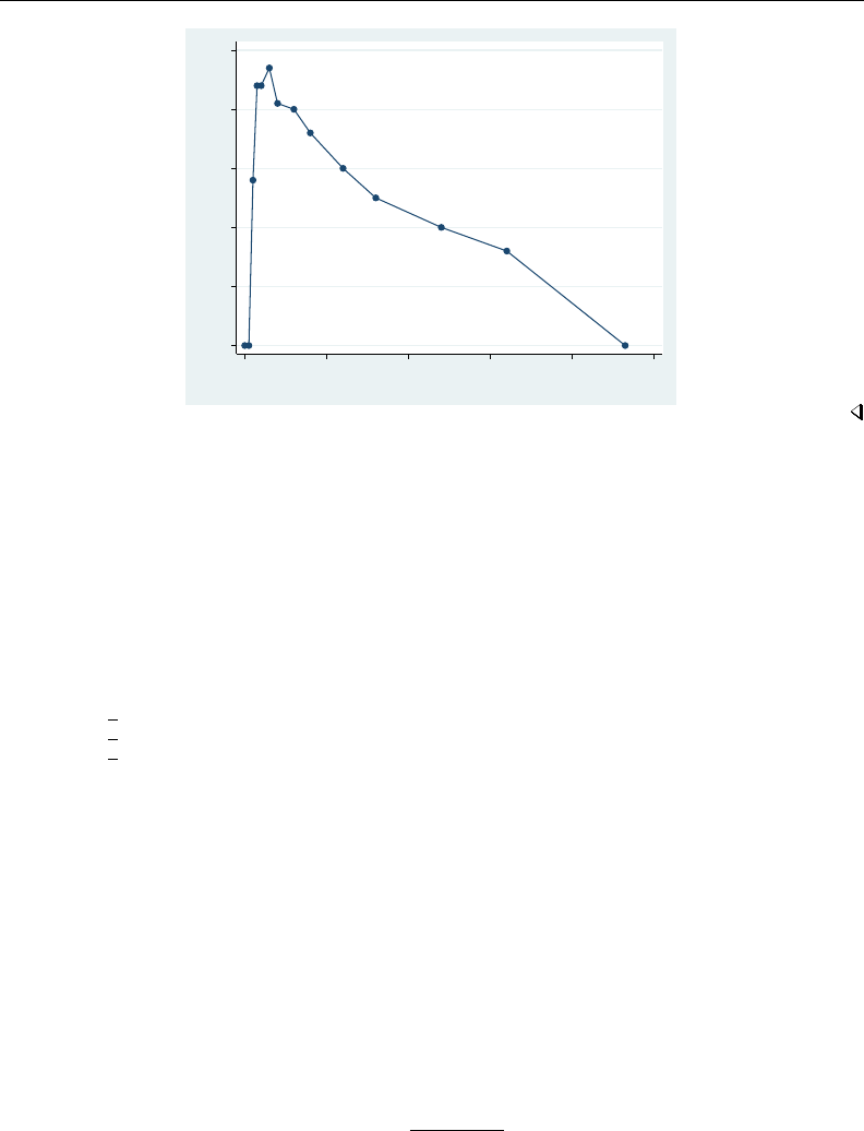
1614 pkexamine — Calculate pharmacokinetic measures
0 1 2 3 4 5
Concentration
0 10 20 30 40 50
Analysis Time
Stored results
pkexamine stores the following in r():
Scalars
r(auc) area under the concentration curve
r(half) half-life of the drug
r(ke) elimination rate
r(tmax) time at last concentration measurement
r(cmax) maximum concentration
r(tomc) time of maximum concentration
r(auc line) AUC0,∞estimated with a linear fit
r(auc exp) AUC0,∞estimated with an exponential fit
r(auc ln) AUC0,∞estimated with a linear fit of the natural log
Methods and formulas
Let iindex the observations sorted by time, let kbe the number of observations, and let fbe the
number of points specified in the fit(#)option.
The AUC0,tmax is defined as
AUC0,tmax =Ztmax
0
Ctdt
where Ctis the concentration at time t. By default, the integral is calculated numerically using cubic
splines. However, if the trapezoidal rule is used, the AUC0,tmax is given as
AUC0,tmax =
k
X
i=2
Ci−1+Ci
2(ti−ti−1)

pkexamine — Calculate pharmacokinetic measures 1615
The AUC0,∞is the AUC0,tmax +AUCtmax ,∞, or
AUC0,∞=Ztmax
0
Ctdt +Z∞
tmax
Ctdt
When using the linear extension to the AUC0,tmax , the integration is cut off when the line crosses
the xaxis. The log extension is a linear extension on the log concentration scale. The area for the
exponential extension is
AUC0,∞=Z∞
tmax
e−(β0+tβ1)dt =−e−(β0+tmaxβ1)
β1
The elimination rate Keq is the negative of the slope from a linear regression of log concentration
on time fit to the number of points specified in the fit(#)option:
Keq =−Pk
i=k−f+1 ti−tlnCi−lnC
Pk
i=k−f+1 ti−t2
The half-life is
thalf =ln2
Keq
Reference
Chow, S.-C., and J.-P. Liu. 2009. Design and Analysis of Bioavailability and Bioequivalence Studies. 3rd ed. Boca
Raton, FL: Chapman & Hall/CRC.
Also see
[R]pk — Pharmacokinetic (biopharmaceutical) data

Title
pkshape — Reshape (pharmacokinetic) Latin-square data
Syntax Menu Description Options
Remarks and examples References Also see
Syntax
pkshape id sequence period1 period2 period list ,options
options Description
order(string)apply treatments in specified order
outcome(newvar)name for outcome variable; default is outcome(outcome)
treatment(newvar)name for treatment variable; default is treatment(treat)
carryover(newvar)name for carryover variable; default is carryover(carry)
sequence(newvar)name for sequence variable; default is sequence(sequence)
period(newvar)name for period variable; default is period(period)
Menu
Statistics >Epidemiology and related >Other >Reshape pharmacokinetic latin-square data
Description
pkshape reshapes the data for use with anova,pkcross, and pkequiv; see [R]anova,[R]pkcross,
and [R]pkequiv. Latin-square and crossover data are often organized in a manner that cannot be
analyzed easily with Stata. pkshape reorganizes the data in memory for use in Stata.
pkshape is one of the pk commands. Please read [R]pk before reading this entry.
Options
order(string)specifies the order in which treatments were applied. If the sequence() specifier is a
string variable that specifies the order, this option is not necessary. Otherwise, order() specifies
how to generate the treatment and carryover variables. Any string variable can be used to specify
the order. For crossover designs, any washout periods can be indicated with the number 0.
outcome(newvar)specifies the name for the outcome variable in the reorganized data. By default,
outcome(outcome) is used.
treatment(newvar)specifies the name for the treatment variable in the reorganized data. By default,
treatment(treat) is used.
carryover(newvar)specifies the name for the carryover variable in the reorganized data. By default,
carryover(carry) is used.
sequence(newvar)specifies the name for the sequence variable in the reorganized data. By default,
sequence(sequence) is used.
period(newvar)specifies the name for the period variable in the reorganized data. By default,
period(period) is used.
1616

pkshape — Reshape (pharmacokinetic) Latin-square data 1617
Remarks and examples
Often data from a Latin-square experiment are naturally organized in a manner that Stata cannot
manage easily. pkshape reorganizes Latin-square data so that they can be used with anova (see
[R]anova) or any pk command. This includes the classic 2 ×2 crossover design commonly used in
pharmaceutical research, as well as many other Latin-square designs.
Example 1
Consider the example data published in Chow and Liu (2009, 71). There are 24 patients, 12 in
each sequence. Sequence 1 consists of the reference formulation followed by the test formulation;
sequence 2 is the test formulation followed by the reference formulation. The measurements reported
are the AUC0−tmax for each patient and for each period.
. use http://www.stata-press.com/data/r13/chowliu
. list, sep(4)
id seq period1 period2
1. 1 1 74.675 73.675
2. 4 1 96.4 93.25
3. 5 1 101.95 102.125
4. 6 1 79.05 69.45
5. 11 1 79.05 69.025
6. 12 1 85.95 68.7
7. 15 1 69.725 59.425
8. 16 1 86.275 76.125
9. 19 1 112.675 114.875
10. 20 1 99.525 116.25
11. 23 1 89.425 64.175
12. 24 1 55.175 74.575
13. 2 2 74.825 37.35
14. 3 2 86.875 51.925
15. 7 2 81.675 72.175
16. 8 2 92.7 77.5
17. 9 2 50.45 71.875
18. 10 2 66.125 94.025
19. 13 2 122.45 124.975
20. 14 2 99.075 85.225
21. 17 2 86.35 95.925
22. 18 2 49.925 67.1
23. 21 2 42.7 59.425
24. 22 2 91.725 114.05
Because the outcome for one person is in two different variables, the treatment that was applied to
an individual is a function of the period and the sequence. To analyze this treatment using anova, all
the outcomes must be in one variable, and each covariate must be in its own variable. To reorganize
these data, use pkshape:
. pkshape id seq period1 period2, order(ab ba)
. sort seq id treat

1618 pkshape — Reshape (pharmacokinetic) Latin-square data
. list, sep(8)
id sequence outcome treat carry period
1. 1 1 74.675 1 0 1
2. 1 1 73.675 2 1 2
3. 4 1 96.4 1 0 1
4. 4 1 93.25 2 1 2
5. 5 1 101.95 1 0 1
6. 5 1 102.125 2 1 2
7. 6 1 79.05 1 0 1
8. 6 1 69.45 2 1 2
9. 11 1 79.05 1 0 1
10. 11 1 69.025 2 1 2
11. 12 1 85.95 1 0 1
12. 12 1 68.7 2 1 2
13. 15 1 69.725 1 0 1
14. 15 1 59.425 2 1 2
15. 16 1 86.275 1 0 1
16. 16 1 76.125 2 1 2
17. 19 1 112.675 1 0 1
18. 19 1 114.875 2 1 2
19. 20 1 99.525 1 0 1
20. 20 1 116.25 2 1 2
21. 23 1 89.425 1 0 1
22. 23 1 64.175 2 1 2
23. 24 1 55.175 1 0 1
24. 24 1 74.575 2 1 2
25. 2 2 37.35 1 2 2
26. 2 2 74.825 2 0 1
27. 3 2 51.925 1 2 2
28. 3 2 86.875 2 0 1
29. 7 2 72.175 1 2 2
30. 7 2 81.675 2 0 1
31. 8 2 77.5 1 2 2
32. 8 2 92.7 2 0 1
33. 9 2 71.875 1 2 2
34. 9 2 50.45 2 0 1
35. 10 2 94.025 1 2 2
36. 10 2 66.125 2 0 1
37. 13 2 124.975 1 2 2
38. 13 2 122.45 2 0 1
39. 14 2 85.225 1 2 2
40. 14 2 99.075 2 0 1
41. 17 2 95.925 1 2 2
42. 17 2 86.35 2 0 1
43. 18 2 67.1 1 2 2
44. 18 2 49.925 2 0 1
45. 21 2 59.425 1 2 2
46. 21 2 42.7 2 0 1
47. 22 2 114.05 1 2 2
48. 22 2 91.725 2 0 1
Now the data are organized into separate variables that indicate each factor level for each of the
covariates, so the data may be used with anova or pkcross; see [R]anova and [R]pkcross.

pkshape — Reshape (pharmacokinetic) Latin-square data 1619
Example 2
Consider the study of background music on bank teller productivity published in Kutner et al. (2005).
The data are
Week Monday Tuesday Wednesday Thursday Friday
1 18(D) 17(C) 14(A) 21(B) 17(E)
2 13(C) 34(B) 21(E) 16(A) 15(D)
3 7(A) 29(D) 32(B) 27(E) 13(C)
4 17(E) 13(A) 24(C) 31(D) 25(B)
5 21(B) 26(E) 26(D) 31(C) 7(A)
The numbers are the productivity scores, and the letters represent the treatment. We entered the
data into Stata:
. use http://www.stata-press.com/data/r13/music, clear
. list
id seq day1 day2 day3 day4 day5
1. 1 dcabe 18 17 14 21 17
2. 2 cbead 13 34 21 16 15
3. 3 adbec 7 29 32 27 13
4. 4 eacdb 17 13 24 31 25
5. 5 bedca 21 26 26 31 7
We reshape these data with pkshape:
. pkshape id seq day1 day2 day3 day4 day5
. list, sep(0)
id sequence outcome treat carry period
1. 3 1 7 1 0 1
2. 5 2 21 3 0 1
3. 2 3 13 5 0 1
4. 1 4 18 2 0 1
5. 4 5 17 4 0 1
6. 3 1 29 2 1 2
7. 5 2 26 4 3 2
8. 2 3 34 3 5 2
9. 1 4 17 5 2 2
10. 4 5 13 1 4 2
11. 3 1 32 3 2 3
12. 5 2 26 2 4 3
13. 2 3 21 4 3 3
14. 1 4 14 1 5 3
15. 4 5 24 5 1 3
16. 3 1 27 4 3 4
17. 5 2 31 5 2 4
18. 2 3 16 1 4 4
19. 1 4 21 3 1 4
20. 4 5 31 2 5 4
21. 3 1 13 5 4 5
22. 5 2 7 1 5 5
23. 2 3 15 2 1 5
24. 1 4 17 4 3 5
25. 4 5 25 3 2 5

1620 pkshape — Reshape (pharmacokinetic) Latin-square data
Here the sequence variable is a string variable that specifies how the treatments were applied, so
the order option is not used. When the sequence variable is a string and the order is specified, the
arguments from the order option are used. We could now produce an ANOVA table:
. anova outcome seq period treat
Number of obs = 25 R-squared = 0.8666
Root MSE = 3.96232 Adj R-squared = 0.7331
Source Partial SS df MS F Prob > F
Model 1223.6 12 101.966667 6.49 0.0014
sequence 82 4 20.5 1.31 0.3226
period 477.2 4 119.3 7.60 0.0027
treat 664.4 4 166.1 10.58 0.0007
Residual 188.4 12 15.7
Total 1412 24 58.8333333
Example 3
Consider the Latin-square crossover example published in Kutner et al. (2005). The example is
about apple sales given different methods for displaying apples.
Pattern Store Week 1 Week 2 Week 3
1 1 9(B) 12(C) 15(A)
2 4(B) 12(C) 9(A)
2 1 12(A) 14(B) 3(C)
2 13(A) 14(B) 3(C)
3 1 7(C) 18(A) 6(B)
2 5(C) 20(A) 4(B)
We entered the data into Stata:
. use http://www.stata-press.com/data/r13/applesales, clear
. list, sep(2)
id seq p1 p2 p3 square
1. 1 1 9 12 15 1
2. 2 1 4 12 9 2
3. 3 2 12 14 3 1
4. 4 2 13 14 3 2
5. 5 3 7 18 6 1
6. 6 3 5 20 4 2

pkshape — Reshape (pharmacokinetic) Latin-square data 1621
Now the data can be reorganized using descriptive names for the outcome variables.
. pkshape id seq p1 p2 p3, order(bca abc cab) seq(pattern) period(order)
> treat(displays)
. anova outcome pattern order display id|pattern
Number of obs = 18 R-squared = 0.9562
Root MSE = 1.59426 Adj R-squared = 0.9069
Source Partial SS df MS F Prob > F
Model 443.666667 9 49.2962963 19.40 0.0002
pattern .333333333 2 .166666667 0.07 0.9370
order 233.333333 2 116.666667 45.90 0.0000
displays 189 2 94.5 37.18 0.0001
id|pattern 21 3 7 2.75 0.1120
Residual 20.3333333 8 2.54166667
Total 464 17 27.2941176
These are the same results reported by Kutner et al. (2005).
Example 4
We continue with example 1 from [R]pkcollapse; the data are
. use http://www.stata-press.com/data/r13/pkdata2, clear
. list, sep(4) abbrev(10)
id seq auc_concA auc_concB
1. 1 1 150.9643 218.5551
2. 2 1 146.7606 133.3201
3. 3 1 160.6548 126.0635
4. 4 1 157.8622 96.17461
5. 5 1 133.6957 188.9038
6. 7 1 160.639 223.6922
7. 8 1 131.2604 104.0139
8. 9 1 168.5186 237.8962
9. 10 2 137.0627 139.7382
10. 12 2 153.4038 202.3942
11. 13 2 163.4593 136.7848
12. 14 2 146.0462 104.5191
13. 15 2 158.1457 165.8654
14. 18 2 147.1977 139.235
15. 19 2 164.9988 166.2391
16. 20 2 145.3823 158.5146
. pkshape id seq auc_concA auc_concB, order(ab ba)
. sort period id

1622 pkshape — Reshape (pharmacokinetic) Latin-square data
. list, sep(4)
id sequence outcome treat carry period
1. 1 1 150.9643 1 0 1
2. 2 1 146.7606 1 0 1
3. 3 1 160.6548 1 0 1
4. 4 1 157.8622 1 0 1
5. 5 1 133.6957 1 0 1
6. 7 1 160.639 1 0 1
7. 8 1 131.2604 1 0 1
8. 9 1 168.5186 1 0 1
9. 10 2 137.0627 2 0 1
10. 12 2 153.4038 2 0 1
11. 13 2 163.4593 2 0 1
12. 14 2 146.0462 2 0 1
13. 15 2 158.1457 2 0 1
14. 18 2 147.1977 2 0 1
15. 19 2 164.9988 2 0 1
16. 20 2 145.3823 2 0 1
17. 1 1 218.5551 2 1 2
18. 2 1 133.3201 2 1 2
19. 3 1 126.0635 2 1 2
20. 4 1 96.17461 2 1 2
21. 5 1 188.9038 2 1 2
22. 7 1 223.6922 2 1 2
23. 8 1 104.0139 2 1 2
24. 9 1 237.8962 2 1 2
25. 10 2 139.7382 1 2 2
26. 12 2 202.3942 1 2 2
27. 13 2 136.7848 1 2 2
28. 14 2 104.5191 1 2 2
29. 15 2 165.8654 1 2 2
30. 18 2 139.235 1 2 2
31. 19 2 166.2391 1 2 2
32. 20 2 158.5146 1 2 2
We call the resulting dataset pkdata3. We conduct equivalence testing on the data in [R]pkequiv,
and we fit an ANOVA model to these data in the third example of [R]pkcross.
References
Chow, S.-C., and J.-P. Liu. 2009. Design and Analysis of Bioavailability and Bioequivalence Studies. 3rd ed. Boca
Raton, FL: Chapman & Hall/CRC.
Kutner, M. H., C. J. Nachtsheim, J. Neter, and W. Li. 2005. Applied Linear Statistical Models. 5th ed. New York:
McGraw–Hill/Irwin.


Title
pksumm — Summarize pharmacokinetic data
Syntax Menu Description Options
Remarks and examples Methods and formulas Also see
Syntax
pksumm id time concentration if in ,options
options Description
Main
trapezoid use trapezoidal rule to calculate AUC; default is cubic splines
fit(#)use #points to estimate AUC; default is fit(3)
notimechk do not check whether follow-up time for all subjects is the same
nodots suppress the dots during calculation
graph graph the distribution of statistic
stat(statistic)graph the specified statistic; default is stat(auc)
Histogram, Density plots, Y axis, X axis, Titles, Legend, Overall
histogram options any option other than by() documented in [R]histogram
statistic Description
auc area under the concentration-time curve (AUC0,∞); the default
aucline area under the concentration-time curve from 0to ∞using a linear extension
aucexp area under the concentration-time curve from 0to ∞using an exponential extension
auclog area under the log-concentration-time curve extended with a linear fit
half half-life of the drug
ke elimination rate
cmax maximum concentration
tmax time at last concentration
tomc time of maximum concentration
Menu
Statistics >Epidemiology and related >Other >Summarize pharmacokinetic data
Description
pksumm obtains summary measures based on the first four moments from the empirical distribution
of each pharmacokinetic measurement and tests the null hypothesis that the distribution of that
measurement is normally distributed.
pksumm is one of the pk commands. Please read [R]pk before reading this entry.
1624

pksumm — Summarize pharmacokinetic data 1625
Options
Main
trapezoid specifies that the trapezoidal rule be used to calculate the AUC. The default is cubic
splines, which give better results for most situations. When the curve is irregular, the trapezoidal
rule may give better results.
fit(#)specifies the number of points, counting back from the last time measurement, to use in
fitting the extension to estimate the AUC0,∞. The default is fit(3), the last three points. This
default should be viewed as a minimum; the appropriate number of points will depend on the data.
notimechk suppresses the check that the follow-up time for all subjects is the same. By default,
pksumm expects the maximum follow-up time to be equal for all subjects.
nodots suppresses the progress dots during calculation. By default, a period is displayed for every
call to calculate the pharmacokinetic measures.
graph requests a graph of the distribution of the statistic specified with stat().
stat(statistic)specifies the statistic that pksumm should graph. The default is stat(auc). If the
graph option is not specified, this option is ignored.
Histogram, Density plots, Y axis, X axis, Titles, Legend, Overall
histogram options are any of the options documented in [R]histogram, excluding by(). For pksumm,
fraction is the default, not density.
Remarks and examples
pksumm produces summary statistics for the distribution of nine common pharmacokinetic mea-
surements. If there are more than eight subjects, pksumm also computes a test for normality on each
measurement. The nine measurements summarized by pksumm are listed above and are described in
Methods and formulas of [R]pkexamine.
Example 1
We demonstrate the use of pksumm on a variation of the data described in [R]pk. We have drug
concentration data on 15 subjects, each measured at 13 time points over a 32-hour period. A few of
the records are

1626 pksumm — Summarize pharmacokinetic data
. use http://www.stata-press.com/data/r13/pksumm
. list, sep(0)
id time conc
1. 1 0 0
2. 1 .5 3.073403
3. 1 1 5.188444
4. 1 1.5 5.898577
5. 1 2 5.096378
6. 1 3 6.094085
(output omitted )
183. 15 0 0
184. 15 .5 3.86493
185. 15 1 6.432444
186. 15 1.5 6.969195
187. 15 2 6.307024
188. 15 3 6.509584
189. 15 4 6.555091
190. 15 6 7.318319
191. 15 8 5.329813
192. 15 12 5.411624
193. 15 16 3.891397
194. 15 24 5.167516
195. 15 32 2.649686
We can use pksumm to view the summary statistics for all the pharmacokinetic parameters.
. pksumm id time conc
...............
Summary statistics for the pharmacokinetic measures
Number of observations = 15
Measure Mean Median Variance Skewness Kurtosis p-value
auc 150.74 150.96 123.07 -0.26 2.10 0.69
aucline 408.30 214.17 188856.87 2.57 8.93 0.00
aucexp 691.68 297.08 762679.94 2.56 8.87 0.00
auclog 688.98 297.67 797237.24 2.59 9.02 0.00
half 94.84 29.39 18722.13 2.26 7.37 0.00
ke 0.02 0.02 0.00 0.89 3.70 0.09
cmax 7.36 7.42 0.42 -0.60 2.56 0.44
tomc 3.47 3.00 7.62 2.17 7.18 0.00
tmax 32.00 32.00 0.00 . . .
For the 15 subjects, the mean AUC0,tmax is 150.74, and σ2=123.07. The skewness of −0.26 indicates
that the distribution is slightly skewed left. The p-value of 0.69 for the χ2test of normality indicates
that we cannot reject the null hypothesis that the distribution is normal.
If we were to consider any of the three variants of the AUC0,∞, we would see that there is huge
variability and that the distribution is heavily skewed. A skewness different from 0 and a kurtosis
different from 3 are expected because the distribution of the AUC0,∞is not normal.
We now graph the distribution of AUC0,tmax by specifying the graph option.
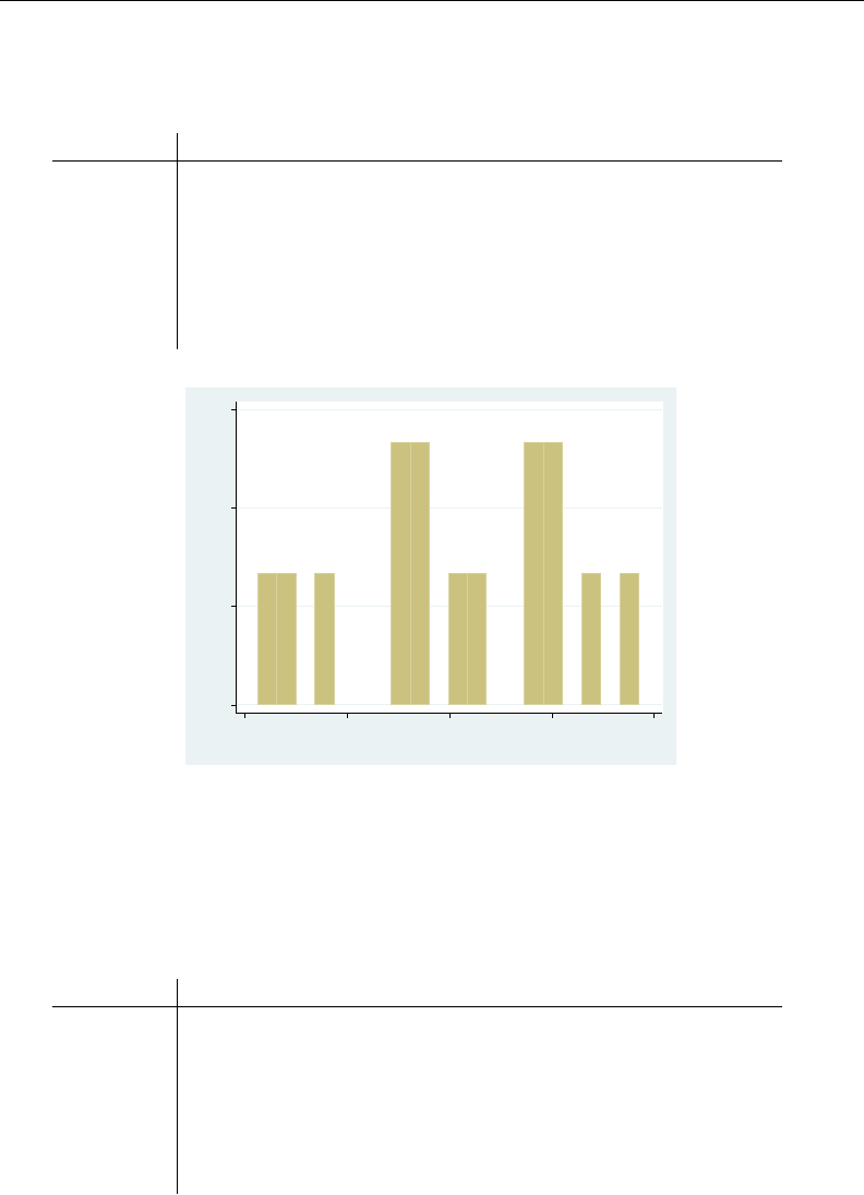
pksumm — Summarize pharmacokinetic data 1627
. pksumm id time conc, graph bin(20)
...............
Summary statistics for the pharmacokinetic measures
Number of observations = 15
Measure Mean Median Variance Skewness Kurtosis p-value
auc 150.74 150.96 123.07 -0.26 2.10 0.69
aucline 408.30 214.17 188856.87 2.57 8.93 0.00
aucexp 691.68 297.08 762679.94 2.56 8.87 0.00
auclog 688.98 297.67 797237.24 2.59 9.02 0.00
half 94.84 29.39 18722.13 2.26 7.37 0.00
ke 0.02 0.02 0.00 0.89 3.70 0.09
cmax 7.36 7.42 0.42 -0.60 2.56 0.44
tomc 3.47 3.00 7.62 2.17 7.18 0.00
tmax 32.00 32.00 0.00 . . .
0 .05 .1 .15
Fraction
130 140 150 160 170
Area Under Curve (AUC)
graph, by default, plots AUC0,tmax . To plot a graph of one of the other pharmacokinetic measurements,
we need to specify the stat() option. For example, we can ask Stata to produce a plot of the AUC0,∞
using the log extension:
. pksumm id time conc, stat(auclog) graph bin(20)
...............
Summary statistics for the pharmacokinetic measures
Number of observations = 15
Measure Mean Median Variance Skewness Kurtosis p-value
auc 150.74 150.96 123.07 -0.26 2.10 0.69
aucline 408.30 214.17 188856.87 2.57 8.93 0.00
aucexp 691.68 297.08 762679.94 2.56 8.87 0.00
auclog 688.98 297.67 797237.24 2.59 9.02 0.00
half 94.84 29.39 18722.13 2.26 7.37 0.00
ke 0.02 0.02 0.00 0.89 3.70 0.09
cmax 7.36 7.42 0.42 -0.60 2.56 0.44
tomc 3.47 3.00 7.62 2.17 7.18 0.00
tmax 32.00 32.00 0.00 . . .
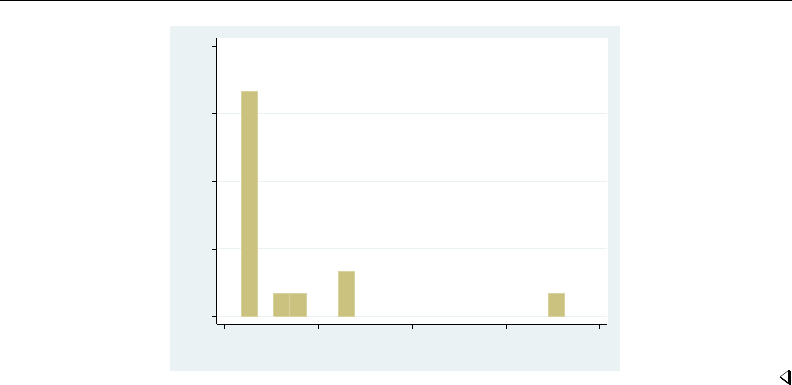
1628 pksumm — Summarize pharmacokinetic data
0 .2 .4 .6 .8
Fraction
0 1000 2000 3000 4000
Linear fit to log concentration AUC for AUC 0−inf.
Methods and formulas
The χ2test for normality is conducted with sktest; see [R]sktest for more information on the
test of normality.
The statistics reported by pksumm are identical to those reported by summarize and sktest; see
[R]summarize and [R]sktest.
Also see
[R]pk — Pharmacokinetic (biopharmaceutical) data

Title
poisson — Poisson regression
Syntax Menu Description Options
Remarks and examples Stored results Methods and formulas References
Also see
Syntax
poisson depvar indepvars if in weight ,options
options Description
Model
noconstant suppress constant term
exposure(varnamee)include ln(varnamee) in model with coefficient constrained to 1
offset(varnameo)include varnameoin model with coefficient constrained to 1
constraints(constraints)apply specified linear constraints
collinear keep collinear variables
SE/Robust
vce(vcetype)vcetype may be oim,robust,cluster clustvar,opg,bootstrap,
or jackknife
Reporting
level(#)set confidence level; default is level(95)
irr report incidence-rate ratios
nocnsreport do not display constraints
display options control column formats, row spacing, line width, display of omitted
variables and base and empty cells, and factor-variable labeling
Maximization
maximize options control the maximization process; seldom used
coeflegend display legend instead of statistics
indepvars may contain factor variables; see [U] 11.4.3 Factor variables.
depvar,indepvars,varnamee, and varnameomay contain time-series operators; see [U] 11.4.4 Time-series varlists.
bootstrap,by,fp,jackknife,mfp,mi estimate,nestreg,rolling,statsby,stepwise, and svy are allowed;
see [U] 11.1.10 Prefix commands.
vce(bootstrap) and vce(jackknife) are not allowed with the mi estimate prefix; see [MI] mi estimate.
Weights are not allowed with the bootstrap prefix; see [R] bootstrap.
vce() and weights are not allowed with the svy prefix; see [SVY] svy.
fweights, iweights, and pweights are allowed; see [U] 11.1.6 weight.
coeflegend does not appear in the dialog box.
See [U] 20 Estimation and postestimation commands for more capabilities of estimation commands.
1629

1630 poisson — Poisson regression
Menu
Statistics >Count outcomes >Poisson regression
Description
poisson fits a Poisson regression of depvar on indepvars, where depvar is a nonnegative count
variable.
If you have panel data, see [XT]xtpoisson.
Options
Model
noconstant,exposure(varnamee),offset(varnameo),constraints(constraints),collinear;
see [R]estimation options.
SE/Robust
vce(vcetype)specifies the type of standard error reported, which includes types that are derived from
asymptotic theory (oim,opg), that are robust to some kinds of misspecification (robust), that
allow for intragroup correlation (cluster clustvar), and that use bootstrap or jackknife methods
(bootstrap,jackknife); see [R]vce option.
Reporting
level(#); see [R]estimation options.
irr reports estimated coefficients transformed to incidence-rate ratios, that is, eβirather than βi.
Standard errors and confidence intervals are similarly transformed. This option affects how results
are displayed, not how they are estimated or stored. irr may be specified at estimation or when
replaying previously estimated results.
nocnsreport; see [R]estimation options.
display options:noomitted,vsquish,noemptycells,baselevels,allbaselevels,nofvla-
bel,fvwrap(#),fvwrapon(style),cformat(%fmt),pformat(% fmt),sformat(% fmt), and
nolstretch; see [R]estimation options.
Maximization
maximize options:difficult,technique(algorithm spec),iterate(#),nolog,trace,
gradient,showstep,hessian,showtolerance,tolerance(#),ltolerance(#),
nrtolerance(#),nonrtolerance, and from(init specs); see [R]maximize. These options are
seldom used.
Setting the optimization type to technique(bhhh) resets the default vcetype to vce(opg).
The following option is available with poisson but is not shown in the dialog box:
coeflegend; see [R]estimation options.

poisson — Poisson regression 1631
Remarks and examples
The basic idea of Poisson regression was outlined by Coleman (1964, 378–379). See Cameron
and Trivedi (2013;2010, chap. 17) and Johnson, Kemp, and Kotz (2005, chap. 4) for information
about the Poisson distribution. See Cameron and Trivedi (2013), Long (1997, chap. 8), Long and
Freese (2014, chap. 9), McNeil (1996, chap. 6), and Selvin (2011, chap. 6) for an introduction
to Poisson regression. Also see Selvin (2004, chap. 5) for a discussion of the analysis of spatial
distributions, which includes a discussion of the Poisson distribution. An early example of Poisson
regression was Cochran (1940).
Poisson regression fits models of the number of occurrences (counts) of an event. The Poisson
distribution has been applied to diverse events, such as the number of soldiers kicked to death by
horses in the Prussian army (von Bortkiewicz 1898); the pattern of hits by buzz bombs launched
against London during World War II (Clarke 1946); telephone connections to a wrong number
(Thorndike 1926); and disease incidence, typically with respect to time, but occasionally with respect
to space. The basic assumptions are as follows:
1. There is a quantity called the incidence rate that is the rate at which events occur. Examples
are 5 per second, 20 per 1,000 person-years, 17 per square meter, and 38 per cubic centimeter.
2. The incidence rate can be multiplied by exposure to obtain the expected number of observed
events. For example, a rate of 5 per second multiplied by 30 seconds means that 150 events
are expected; a rate of 20 per 1,000 person-years multiplied by 2,000 person-years means that
40 events are expected; and so on.
3. Over very small exposures , the probability of finding more than one event is small compared
with .
4. Nonoverlapping exposures are mutually independent.
With these assumptions, to find the probability of kevents in an exposure of size E, you divide
Einto nsubintervals E1,E2,. . . ,En, and approximate the answer as the binomial probability of
observing ksuccesses in ntrials. If you let n→ ∞, you obtain the Poisson distribution.
In the Poisson regression model, the incidence rate for the jth observation is assumed to be given
by
rj=eβ0+β1x1,j +···+βkxk,j
If Ejis the exposure, the expected number of events, Cj, will be
Cj=Ejeβ0+β1x1,j +···+βkxk,j
=eln(Ej)+β0+β1x1,j +···+βkxk,j
This model is fit by poisson. Without the exposure() or offset() options, Ejis assumed to be
1 (equivalent to assuming that exposure is unknown), and controlling for exposure, if necessary, is
your responsibility.
Comparing rates is most easily done by calculating incidence-rate ratios (IRRs). For instance,
what is the relative incidence rate of chromosome interchanges in cells as the intensity of radiation
increases; the relative incidence rate of telephone connections to a wrong number as load increases;
or the relative incidence rate of deaths due to cancer for females relative to males? That is, you want
to hold all the x’s in the model constant except one, say, the ith. The IRR for a one-unit change in
xiis
eln(E)+β1x1+···+βi(xi+1)+···+βkxk
eln(E)+β1x1+···+βixi+···+βkxk
=eβi

1632 poisson — Poisson regression
More generally, the IRR for a ∆xichange in xiis eβi∆xi. The lincom command can be used after
poisson to display incidence-rate ratios for any group relative to another; see [R]lincom.
Example 1
Chatterjee and Hadi (2012, 174) give the number of injury incidents and the proportion of flights
for each airline out of the total number of flights from New York for nine major U.S. airlines in one
year:
. use http://www.stata-press.com/data/r13/airline
. list
airline injuries n XYZowned
1. 1 11 0.0950 1
2. 2 7 0.1920 0
3. 3 7 0.0750 0
4. 4 19 0.2078 0
5. 5 9 0.1382 0
6. 6 4 0.0540 1
7. 7 3 0.1292 0
8. 8 1 0.0503 0
9. 9 3 0.0629 1
To their data, we have added a fictional variable, XYZowned. We will imagine that an accusation is
made that the airlines owned by XYZ Company have a higher injury rate.
. poisson injuries XYZowned, exposure(n) irr
Iteration 0: log likelihood = -23.027197
Iteration 1: log likelihood = -23.027177
Iteration 2: log likelihood = -23.027177
Poisson regression Number of obs = 9
LR chi2(1) = 1.77
Prob > chi2 = 0.1836
Log likelihood = -23.027177 Pseudo R2 = 0.0370
injuries IRR Std. Err. z P>|z| [95% Conf. Interval]
XYZowned 1.463467 .406872 1.37 0.171 .8486578 2.523675
_cons 58.04416 8.558145 27.54 0.000 43.47662 77.49281
ln(n) 1 (exposure)
We specified irr to see the IRRs rather than the underlying coefficients. We estimate that XYZ Airlines’
injury rate is 1.46 times larger than that for other airlines, but the 95% confidence interval is 0.85 to
2.52; we cannot even reject the hypothesis that XYZ Airlines has a lower injury rate.
Technical note
In example 1, we assumed that each airline’s exposure was proportional to its fraction of flights
out of New York. What if “large” airlines, however, also used larger planes, and so had even more
passengers than would be expected, given this measure of exposure? A better measure would be each
airline’s fraction of passengers on flights out of New York, a number that we do not have. Even so,
we suppose that nrepresents this number to some extent, so a better estimate of the effect might be

poisson — Poisson regression 1633
. gen lnN=ln(n)
. poisson injuries XYZowned lnN
Iteration 0: log likelihood = -22.333875
Iteration 1: log likelihood = -22.332276
Iteration 2: log likelihood = -22.332276
Poisson regression Number of obs = 9
LR chi2(2) = 19.15
Prob > chi2 = 0.0001
Log likelihood = -22.332276 Pseudo R2 = 0.3001
injuries Coef. Std. Err. z P>|z| [95% Conf. Interval]
XYZowned .6840667 .3895877 1.76 0.079 -.0795111 1.447645
lnN 1.424169 .3725155 3.82 0.000 .6940517 2.154285
_cons 4.863891 .7090501 6.86 0.000 3.474178 6.253603
Here rather than specifying the exposure() option, we explicitly included the variable that would
normalize for exposure in the model. We did not specify the irr option, so we see coefficients rather
than IRRs. We started with the model
rate =eβ0+β1XYZowned
The observed counts are therefore
count =neβ0+β1XYZowned =eln(n)+β0+β1XYZowned
which amounts to constraining the coefficient on ln(n)to 1. This is what was estimated when
we specified the exposure(n) option. In the above model, we included the normalizing exposure
ourselves and, rather than constraining the coefficient to be 1, estimated the coefficient.
The estimated coefficient is 1.42, a respectable distance away from 1, and is consistent with our
speculation that larger airlines also use larger airplanes. With this small amount of data, however, we
also have a wide confidence interval that includes 1.
Our estimated coefficient on XYZowned is now 0.684, and the implied IRR is e0.684 ≈1.98 (which
we could also see by typing poisson, irr). The 95% confidence interval for the coefficient still
includes 0 (the interval for the IRR includes 1), so although the point estimate is now larger, we still
cannot be certain of our results.
Our expert opinion would be that, although there is not enough evidence to support the charge,
there is enough evidence to justify collecting more data.
Example 2
In a famous age-specific study of coronary disease deaths among male British doctors, Doll and
Hill (1966) reported the following data (reprinted in Rothman, Greenland, and Lash [2008, 264]):
Smokers Nonsmokers
Age Deaths Person-years Deaths Person-years
35 – 44 32 52,407 2 18,790
45 – 54 104 43,248 12 10,673
55 – 64 206 28,612 28 5,710
65 – 74 186 12,663 28 2,585
75 – 84 102 5,317 31 1,462

1634 poisson — Poisson regression
The first step is to enter these data into Stata, which we have done:
. use http://www.stata-press.com/data/r13/dollhill3, clear
. list
agecat smokes deaths pyears
1. 35-44 1 32 52,407
2. 45-54 1 104 43,248
3. 55-64 1 206 28,612
4. 65-74 1 186 12,663
5. 75-84 1 102 5,317
6. 35-44 0 2 18,790
7. 45-54 0 12 10,673
8. 55-64 0 28 5,710
9. 65-74 0 28 2,585
10. 75-84 0 31 1,462
The most “natural” analysis of these data would begin by introducing indicator variables for each age
category and one indicator for smoking:
. poisson deaths smokes i.agecat, exposure(pyears) irr
Iteration 0: log likelihood = -33.823284
Iteration 1: log likelihood = -33.600471
Iteration 2: log likelihood = -33.600153
Iteration 3: log likelihood = -33.600153
Poisson regression Number of obs = 10
LR chi2(5) = 922.93
Prob > chi2 = 0.0000
Log likelihood = -33.600153 Pseudo R2 = 0.9321
deaths IRR Std. Err. z P>|z| [95% Conf. Interval]
smokes 1.425519 .1530638 3.30 0.001 1.154984 1.759421
agecat
45-54 4.410584 .8605197 7.61 0.000 3.009011 6.464997
55-64 13.8392 2.542638 14.30 0.000 9.654328 19.83809
65-74 28.51678 5.269878 18.13 0.000 19.85177 40.96395
75-84 40.45121 7.775511 19.25 0.000 27.75326 58.95885
_cons .0003636 .0000697 -41.30 0.000 .0002497 .0005296
ln(pyears) 1 (exposure)
In the above, we specified irr to obtain IRRs. We estimate that smokers have 1.43 times the mortality
rate of nonsmokers. See, however, example 1 in [R]poisson postestimation.

poisson — Poisson regression 1635
Stored results
poisson stores the following in e():
Scalars
e(N) number of observations
e(k) number of parameters
e(k eq) number of equations in e(b)
e(k eq model) number of equations in overall model test
e(k dv) number of dependent variables
e(df m) model degrees of freedom
e(r2 p) pseudo-R-squared
e(ll) log likelihood
e(ll 0) log likelihood, constant-only model
e(N clust) number of clusters
e(chi2) χ2
e(p) significance
e(rank) rank of e(V)
e(ic) number of iterations
e(rc) return code
e(converged) 1 if converged, 0otherwise
Macros
e(cmd) poisson
e(cmdline) command as typed
e(depvar) name of dependent variable
e(wtype) weight type
e(wexp) weight expression
e(title) title in estimation output
e(clustvar) name of cluster variable
e(offset) linear offset variable
e(chi2type) Wald or LR; type of model χ2test
e(vce) vcetype specified in vce()
e(vcetype) title used to label Std. Err.
e(opt) type of optimization
e(which) max or min; whether optimizer is to perform maximization or minimization
e(ml method) type of ml method
e(user) name of likelihood-evaluator program
e(technique) maximization technique
e(properties) b V
e(estat cmd) program used to implement estat
e(predict) program used to implement predict
e(asbalanced) factor variables fvset as asbalanced
e(asobserved) factor variables fvset as asobserved
Matrices
e(b) coefficient vector
e(Cns) constraints matrix
e(ilog) iteration log (up to 20 iterations)
e(gradient) gradient vector
e(V) variance–covariance matrix of the estimators
e(V modelbased) model-based variance
Functions
e(sample) marks estimation sample

1636 poisson — Poisson regression
Methods and formulas
The log likelihood (with weights wjand offsets) is given by
Pr(Y=y) = e−λλy
y!
ξj=xjβ+offsetj
f(yj) = e−exp(ξj)eξjyj
yj!
lnL=
n
X
j=1
wj−eξj+ξjyj−ln(yj!)
This command supports the Huber/White/sandwich estimator of the variance and its clustered
version using vce(robust) and vce(cluster clustvar), respectively. See [P]robust, particularly
Maximum likelihood estimators and Methods and formulas.
poisson also supports estimation with survey data. For details on VCEs with survey data, see
[SVY]variance estimation.
Sim´
eon-Denis Poisson (1781–1840) was a French mathematician and physicist who contributed
to several fields: his name is perpetuated in Poisson brackets, Poisson’s constant, Poisson’s
differential equation, Poisson’s integral, and Poisson’s ratio. Among many other results, he
produced a version of the law of large numbers. His rather misleadingly titled Recherches sur la
probabilit´
e des jugements embraces a complete treatise on probability, as the subtitle indicates,
including what is now known as the Poisson distribution. That, however, was discovered earlier
by the Huguenot–British mathematician Abraham de Moivre (1667–1754).
References
Bru, B. 2001. Sim´
eon-Denis Poisson. In Statisticians of the Centuries, ed. C. C. Heyde and E. Seneta, 123–126.
New York: Springer.
Cameron, A. C., and P. K. Trivedi. 2010. Microeconometrics Using Stata. Rev. ed. College Station, TX: Stata Press.
. 2013. Regression Analysis of Count Data. 2nd ed. New York: Cambridge University Press.
Chatterjee, S., and A. S. Hadi. 2012. Regression Analysis by Example. 5th ed. New York: Hoboken, NJ.
Clarke, R. D. 1946. An application of the Poisson distribution. Journal of the Institute of Actuaries 72: 481.
Cochran, W. G. 1940. The analysis of variance when experimental errors follow the Poisson or binomial laws. Annals
of Mathematical Statistics 11: 335–347.
. 1982. Contributions to Statistics. New York: Wiley.
Coleman, J. S. 1964. Introduction to Mathematical Sociology. New York: Free Press.
Doll, R., and A. B. Hill. 1966. Mortality of British doctors in relation to smoking: Observations on coronary
thrombosis. Journal of the National Cancer Institute, Monographs 19: 205–268.
Gould, W. W. 2011. Use poisson rather than regress; tell a friend. The Stata Blog: Not Elsewhere Classified.
http://blog.stata.com/2011/08/22/use-poisson-rather-than-regress-tell-a-friend/.
Harris, T., Z. Yang, and J. W. Hardin. 2012. Modeling underdispersed count data with generalized Poisson regression.
Stata Journal 12: 736–747.

poisson — Poisson regression 1637
Hilbe, J. M. 1998. sg91: Robust variance estimators for MLE Poisson and negative binomial regression.Stata Technical
Bulletin 45: 26–28. Reprinted in Stata Technical Bulletin Reprints, vol. 8, pp. 177–180. College Station, TX: Stata
Press.
. 1999. sg102: Zero-truncated Poisson and negative binomial regression.Stata Technical Bulletin 47: 37–40.
Reprinted in Stata Technical Bulletin Reprints, vol. 8, pp. 233–236. College Station, TX: Stata Press.
Hilbe, J. M., and D. H. Judson. 1998. sg94: Right, left, and uncensored Poisson regression.Stata Technical Bulletin
46: 18–20. Reprinted in Stata Technical Bulletin Reprints, vol. 8, pp. 186–189. College Station, TX: Stata Press.
Johnson, N. L., A. W. Kemp, and S. Kotz. 2005. Univariate Discrete Distributions. 3rd ed. New York: Wiley.
Long, J. S. 1997. Regression Models for Categorical and Limited Dependent Variables. Thousand Oaks, CA: Sage.
Long, J. S., and J. Freese. 2001. Predicted probabilities for count models.Stata Journal 1: 51–57.
. 2014. Regression Models for Categorical Dependent Variables Using Stata. 3rd ed. College Station, TX: Stata
Press.
McNeil, D. 1996. Epidemiological Research Methods. Chichester, UK: Wiley.
Miranda, A., and S. Rabe-Hesketh. 2006. Maximum likelihood estimation of endogenous switching and sample
selection models for binary, ordinal, and count variables.Stata Journal 6: 285–308.
Newman, S. C. 2001. Biostatistical Methods in Epidemiology. New York: Wiley.
Poisson, S. D. 1837. Recherches sur la probabilit´
e des jugements en mati`
ere criminelle et en mati`
ere civile: pr´
ec´
ed´
ees
des r`
egles g´
en´
erales du calcul des probabilit´
es. Paris: Bachelier.
Raciborski, R. 2011. Right-censored Poisson regression model.Stata Journal 11: 95–105.
Rodr´
ıguez, G. 1993. sbe10: An improvement to poisson.Stata Technical Bulletin 11: 11–14. Reprinted in Stata
Technical Bulletin Reprints, vol. 2, pp. 94–98. College Station, TX: Stata Press.
Rogers, W. H. 1991. sbe1: Poisson regression with rates.Stata Technical Bulletin 1: 11–12. Reprinted in Stata
Technical Bulletin Reprints, vol. 1, pp. 62–64. College Station, TX: Stata Press.
Rothman, K. J., S. Greenland, and T. L. Lash. 2008. Modern Epidemiology. 3rd ed. Philadelphia: Lippincott Williams
& Wilkins.
Rutherford, E., J. Chadwick, and C. D. Ellis. 1930. Radiations from Radioactive Substances. Cambridge: Cambridge
University Press.
Rutherford, M. J., P. C. Lambert, and J. R. Thompson. 2010. Age–period–cohort modeling.Stata Journal 10: 606–627.
Sasieni, P. D. 2012. Age–period–cohort models in Stata.Stata Journal 12: 45–60.
Schonlau, M. 2005. Boosted regression (boosting): An introductory tutorial and a Stata plugin.Stata Journal 5:
330–354.
Selvin, S. 2004. Statistical Analysis of Epidemiologic Data. 3rd ed. New York: Oxford University Press.
. 2011. Statistical Tools for Epidemiologic Research. New York: Oxford University Press.
Thorndike, F. 1926. Applications of Poisson’s probability summation. Bell System Technical Journal 5: 604–624.
Tob´
ıas, A., and M. J. Campbell. 1998. sg90: Akaike’s information criterion and Schwarz’s criterion.Stata Technical
Bulletin 45: 23–25. Reprinted in Stata Technical Bulletin Reprints, vol. 8, pp. 174–177. College Station, TX: Stata
Press.
von Bortkiewicz, L. 1898. Das Gesetz der Kleinen Zahlen. Leipzig: Teubner.

1638 poisson — Poisson regression
Also see
[R]poisson postestimation — Postestimation tools for poisson
[R]glm — Generalized linear models
[R]nbreg — Negative binomial regression
[R]tpoisson — Truncated Poisson regression
[R]zip — Zero-inflated Poisson regression
[ME]mepoisson — Multilevel mixed-effects Poisson regression
[MI]estimation — Estimation commands for use with mi estimate
[SVY]svy estimation — Estimation commands for survey data
[XT]xtpoisson — Fixed-effects, random-effects, and population-averaged Poisson models
[U] 20 Estimation and postestimation commands

Title
poisson postestimation — Postestimation tools for poisson
Description Syntax for predict Menu for predict
Options for predict Syntax for estat gof Menu for estat
Remarks and examples Methods and formulas Also see
Description
The following postestimation command is of special interest after poisson:
Command Description
estat gof goodness-of-fit test
estat gof is not appropriate after the svy prefix.
The following standard postestimation commands are also available:
Command Description
contrast contrasts and ANOVA-style joint tests of estimates
estat ic Akaike’s and Schwarz’s Bayesian information criteria (AIC and BIC)
estat summarize summary statistics for the estimation sample
estat vce variance–covariance matrix of the estimators (VCE)
estat (svy) postestimation statistics for survey data
estimates cataloging estimation results
forecast1dynamic forecasts and simulations
lincom point estimates, standard errors, testing, and inference for linear combinations
of coefficients
linktest link test for model specification
lrtest2likelihood-ratio test
margins marginal means, predictive margins, marginal effects, and average marginal
effects
marginsplot graph the results from margins (profile plots, interaction plots, etc.)
nlcom point estimates, standard errors, testing, and inference for nonlinear combinations
of coefficients
predict predictions, residuals, influence statistics, and other diagnostic measures
predictnl point estimates, standard errors, testing, and inference for generalized predictions
pwcompare pairwise comparisons of estimates
suest seemingly unrelated estimation
test Wald tests of simple and composite linear hypotheses
testnl Wald tests of nonlinear hypotheses
1forecast is not appropriate with mi or svy estimation results.
2lrtest is not appropriate with svy estimation results.
1639

1640 poisson postestimation — Postestimation tools for poisson
Special-interest postestimation command
estat gof performs a goodness-of-fit test of the model. Both the deviance statistic and the Pearson
statistic are reported. If the tests are significant, the Poisson regression model is inappropriate. Then
you could try a negative binomial model; see [R]nbreg.
Syntax for predict
predict type newvar if in ,statistic nooffset
statistic Description
Main
nnumber of events; the default
ir incidence rate
pr(n)probability Pr(yj=n)
pr(a,b)probability Pr(a≤yj≤b)
xb linear prediction
stdp standard error of the linear prediction
score first derivative of the log likelihood with respect to xjβ
These statistics are available both in and out of sample; type predict . . . if e(sample) . . . if wanted
only for the estimation sample.
Menu for predict
Statistics >Postestimation >Predictions, residuals, etc.
Options for predict
Main
n, the default, calculates the predicted number of events, which is exp(xjβ)if neither offset()
nor exposure() was specified when the model was fit; exp(xjβ+offsetj)if offset() was
specified; or exp(xjβ)×exposurejif exposure() was specified.
ir calculates the incidence rate exp(xjβ), which is the predicted number of events when exposure
is 1. Specifying ir is equivalent to specifying nwhen neither offset() nor exposure() was
specified when the model was fit.
pr(n)calculates the probability Pr(yj=n), where nis a nonnegative integer that may be specified
as a number or a variable.
pr(a,b)calculates the probability Pr(a≤yj≤b), where aand bare nonnegative integers that may
be specified as numbers or variables;
bmissing (b≥.) means +∞;
pr(20,.) calculates Pr(yj≥20);
pr(20,b)calculates Pr(yj≥20)in observations for which b≥.and calculates
Pr(20 ≤yj≤b)elsewhere.
pr(.,b)produces a syntax error. A missing value in an observation of the variable acauses a
missing value in that observation for pr(a,b).

poisson postestimation — Postestimation tools for poisson 1641
xb calculates the linear prediction, which is xjβif neither offset() nor exposure() was specified;
xjβ+offsetjif offset() was specified; or xjβ+ln(exposurej)if exposure() was specified;
see nooffset below.
stdp calculates the standard error of the linear prediction.
score calculates the equation-level score, ∂ln L/∂(xjβ).
nooffset is relevant only if you specified offset() or exposure() when you fit the model. It
modifies the calculations made by predict so that they ignore the offset or exposure variable; the
linear prediction is treated as xjβrather than as xjβ+offsetjor xjβ+ln(exposurej). Specifying
predict . . . , nooffset is equivalent to specifying predict . . . , ir.
Syntax for estat gof
estat gof
Menu for estat
Statistics >Postestimation >Reports and statistics
Remarks and examples
Example 1
Continuing with example 2 of [R]poisson, we use estat gof to determine whether the model
fits the data well.
. use http://www.stata-press.com/data/r13/dollhill3
. poisson deaths smokes i.agecat, exp(pyears) irr
(output omitted )
. estat gof
Deviance goodness-of-fit = 12.13244
Prob > chi2(4) = 0.0164
Pearson goodness-of-fit = 11.15533
Prob > chi2(4) = 0.0249
The deviance goodness-of-fit test tells us that, given the model, we can reject the hypothesis that
these data are Poisson distributed at the 1.64% significance level. The Pearson goodness-of-fit test
tells us that we can reject the hypothesis at the 2.49% significance level.
So let us now back up and be more careful. We can most easily obtain the incidence-rate ratios
within age categories by using ir; see [ST]epitab:
. ir deaths smokes pyears, by(agecat) nohet
age category IRR [95% Conf. Interval] M-H Weight
35-44 5.736638 1.463557 49.40468 1.472169 (exact)
45-54 2.138812 1.173714 4.272545 9.624747 (exact)
55-64 1.46824 .9863624 2.264107 23.34176 (exact)
65-74 1.35606 .9081925 2.096412 23.25315 (exact)
75-84 .9047304 .6000757 1.399687 24.31435 (exact)
Crude 1.719823 1.391992 2.14353 (exact)
M-H combined 1.424682 1.154703 1.757784

1642 poisson postestimation — Postestimation tools for poisson
We find that the mortality incidence ratios are greatly different within age category, being highest
for the youngest categories and actually dropping below 1 for the oldest. (In the last case, we might
argue that those who smoke and who have not died by age 75 are self-selected to be particularly
robust.)
Seeing this, we will now parameterize the smoking effects separately for each category, although
we will begin by constraining the smoking effects on third and fourth age categories to be equivalent:
. constraint 1 smokes#3.agecat = smokes#4.agecat
. poisson deaths c.smokes#agecat i.agecat, exposure(pyears) irr constraints(1)
Iteration 0: log likelihood = -31.95424
Iteration 1: log likelihood = -27.796801
Iteration 2: log likelihood = -27.574177
Iteration 3: log likelihood = -27.572645
Iteration 4: log likelihood = -27.572645
Poisson regression Number of obs = 10
Wald chi2(8) = 632.14
Log likelihood = -27.572645 Prob > chi2 = 0.0000
( 1) [deaths]3.agecat#c.smokes - [deaths]4.agecat#c.smokes = 0
deaths IRR Std. Err. z P>|z| [95% Conf. Interval]
agecat#
c.smokes
35-44 5.736637 4.181256 2.40 0.017 1.374811 23.93711
45-54 2.138812 .6520701 2.49 0.013 1.176691 3.887609
55-64 1.412229 .2017485 2.42 0.016 1.067343 1.868557
65-74 1.412229 .2017485 2.42 0.016 1.067343 1.868557
75-84 .9047304 .1855513 -0.49 0.625 .6052658 1.35236
agecat
45-54 10.5631 8.067701 3.09 0.002 2.364153 47.19623
55-64 47.671 34.37409 5.36 0.000 11.60056 195.8978
65-74 98.22765 70.85012 6.36 0.000 23.89324 403.8244
75-84 199.2099 145.3356 7.26 0.000 47.67693 832.3648
_cons .0001064 .0000753 -12.94 0.000 .0000266 .0004256
ln(pyears) 1 (exposure)
. estat gof
Deviance goodness-of-fit = .0774185
Prob > chi2(1) = 0.7808
Pearson goodness-of-fit = .0773882
Prob > chi2(1) = 0.7809
The goodness-of-fit is now small; we are no longer running roughshod over the data. Let us now
consider simplifying the model. The point estimate of the incidence-rate ratio for smoking in age
category 1 is much larger than that for smoking in age category 2, but the confidence interval for
smokes#1.agecat is similarly wide. Is the difference real?
. test smokes#1.agecat = smokes#2.agecat
( 1) [deaths]1b.agecat#c.smokes - [deaths]2.agecat#c.smokes = 0
chi2( 1) = 1.56
Prob > chi2 = 0.2117
The point estimates of the incidence-rate ratio for smoking in the 35–44 age category is much larger
than that for smoking in the 45–54 age category, but there is insufficient data, and we may be
observing random differences. With that success, might we also combine the smokers in the third
and fourth categories with those in the first and second categories?

poisson postestimation — Postestimation tools for poisson 1643
. test smokes#2.agecat = smokes#3.agecat, accum
( 1) [deaths]1b.agecat#c.smokes - [deaths]2.agecat#c.smokes = 0
( 2) [deaths]2.agecat#c.smokes - [deaths]3.agecat#c.smokes = 0
chi2( 2) = 4.73
Prob > chi2 = 0.0938
Combining the first four categories may be overdoing it—the 9.38% significance level is enough to
stop us, although others may disagree.
Thus we now fit our final model:
. constraint 2 smokes#1.agecat = smokes#2.agecat
. poisson deaths c.smokes#agecat i.agecat, exposure(pyears) irr constraints(1/2)
Iteration 0: log likelihood = -31.550722
Iteration 1: log likelihood = -28.525057
Iteration 2: log likelihood = -28.514535
Iteration 3: log likelihood = -28.514535
Poisson regression Number of obs = 10
Wald chi2(7) = 642.25
Log likelihood = -28.514535 Prob > chi2 = 0.0000
( 1) [deaths]3.agecat#c.smokes - [deaths]4.agecat#c.smokes = 0
( 2) [deaths]1b.agecat#c.smokes - [deaths]2.agecat#c.smokes = 0
deaths IRR Std. Err. z P>|z| [95% Conf. Interval]
agecat#
c.smokes
35-44 2.636259 .7408403 3.45 0.001 1.519791 4.572907
45-54 2.636259 .7408403 3.45 0.001 1.519791 4.572907
55-64 1.412229 .2017485 2.42 0.016 1.067343 1.868557
65-74 1.412229 .2017485 2.42 0.016 1.067343 1.868557
75-84 .9047304 .1855513 -0.49 0.625 .6052658 1.35236
agecat
45-54 4.294559 .8385329 7.46 0.000 2.928987 6.296797
55-64 23.42263 7.787716 9.49 0.000 12.20738 44.94164
65-74 48.26309 16.06939 11.64 0.000 25.13068 92.68856
75-84 97.87965 34.30881 13.08 0.000 49.24123 194.561
_cons .0002166 .0000652 -28.03 0.000 .0001201 .0003908
ln(pyears) 1 (exposure)

1644 poisson postestimation — Postestimation tools for poisson
The above strikes us as a fair representation of the data. The probabilities of observing the deaths
seen in these data are estimated using the following predict command:
. predict p, pr(0, deaths)
. list deaths p
deaths p
1. 32 .6891766
2. 104 .4456625
3. 206 .5455328
4. 186 .4910622
5. 102 .5263011
6. 2 .227953
7. 12 .7981917
8. 28 .4772961
9. 28 .6227565
10. 31 .5475718
The probability Pr(y≤deaths)ranges from 0.23 to 0.80.
Methods and formulas
In the following, we use the same notation as in [R]poisson.
The equation-level scores are given by
score(xβ)j=yj−eξj
The deviance (D) and Pearson (P) goodness-of-fit statistics are given by
lnLmax =
n
X
j=1
wj[−yj{ln(yj)−1} − ln(yj!)]
χ2
D=−2{lnL−lnLmax}
χ2
P=
n
X
j=1
wj(yj−eξj)2
eξj
Also see
[R]poisson — Poisson regression
[U] 20 Estimation and postestimation commands

Title
predict — Obtain predictions, residuals, etc., after estimation
Syntax Menu for predict Description Options
Remarks and examples Methods and formulas Also see
Syntax
After single-equation (SE)models
predict type newvar if in ,single options
After multiple-equation (ME)models
predict type newvar if in ,multiple options
predict type stub*|newvar1. . . newvarq if in , scores
single options Description
Main
xb calculate linear prediction
stdp calculate standard error of the prediction
score calculate first derivative of the log likelihood with respect to xjβ
Options
nooffset ignore any offset() or exposure() variable
other options command-specific options
multiple options Description
Main
equation(eqno,eqno )specify equations
xb calculate linear prediction
stdp calculate standard error of the prediction
stddp calculate the difference in linear predictions
Options
nooffset ignore any offset() or exposure() variable
other options command-specific options
Menu for predict
Statistics >Postestimation >Predictions, residuals, etc.
1645

1646 predict — Obtain predictions, residuals, etc., after estimation
Description
predict calculates predictions, residuals, influence statistics, and the like after estimation. Exactly
what predict can do is determined by the previous estimation command; command-specific options
are documented with each estimation command. Regardless of command-specific options, the actions
of predict share certain similarities across estimation commands:
1. predict newvar creates newvar containing “predicted values”—numbers related to the
E(yj|xj). For instance, after linear regression, predict newvar creates xjband, after probit,
creates the probability Φ(xjb).
2. predict newvar, xb creates newvar containing xjb. This may be the same result as option
1 (for example, linear regression) or different (for example, probit), but regardless, option xb
is allowed.
3. predict newvar, stdp creates newvar containing the standard error of the linear prediction
xjb.
4. predict newvar,other options may create newvar containing other useful quantities; see
help or the reference manual entry for the particular estimation command to find out about
other available options.
5. nooffset added to any of the above commands requests that the calculation ignore any offset
or exposure variable specified by including the offset(varnameo)or exposure(varnamee)
option when you fit the model.
predict can be used to make in-sample or out-of-sample predictions:
6. predict calculates the requested statistic for all possible observations, whether they were used
in fitting the model or not. predict does this for standard options 1–3 and generally does this
for estimator-specific options 4.
7. predict newvar if e(sample), . . . restricts the prediction to the estimation subsample.
8. Some statistics make sense only with respect to the estimation subsample. In such cases, the
calculation is automatically restricted to the estimation subsample, and the documentation for
the specific option states this. Even so, you can still specify if e(sample) if you are uncertain.
9. predict can make out-of-sample predictions even using other datasets. In particular, you can
. use ds1
.(fit a model)
. use two /* another dataset */
. predict yhat, ... /* fill in the predictions */
Options
Main
xb calculates the linear prediction from the fitted model. That is, all models can be thought of as
estimating a set of parameters b1,b2,. . . ,bk, and the linear prediction is byj=b1x1j+b2x2j+
··· +bkxkj , often written in matrix notation as b
yj=xjb. For linear regression, the values byj
are called the predicted values or, for out-of-sample predictions, the forecast. For logit and probit,
for example, byjis called the logit or probit index.
x1j,x2j,. . . ,xkj are obtained from the data currently in memory and do not necessarily correspond
to the data on the independent variables used to fit the model (obtaining b1,b2,. . . ,bk).

predict — Obtain predictions, residuals, etc., after estimation 1647
stdp calculates the standard error of the linear prediction. Here the prediction means the same thing
as the “index”, namely, xjb. The statistic produced by stdp can be thought of as the standard
error of the predicted expected value, or mean index, for the observation’s covariate pattern. The
standard error of the prediction is also commonly referred to as the standard error of the fitted
value. The calculation can be made in or out of sample.
stddp is allowed only after you have previously fit a multiple-equation model. The standard error of
the difference in linear predictions (x1jb−x2jb)between equations 1 and 2 is calculated. This
option requires that equation(eqno1,eqno2)be specified.
score calculates the equation-level score, ∂ln L/∂(xjβ). Here lnLrefers to the log-likelihood
function.
scores is the ME model equivalent of the score option, resulting in multiple equation-level score
variables. An equation-level score variable is created for each equation in the model; ancillary
parameters—such as lnσand atanhρ—make up separate equations.
equation(eqno,eqno )—synonym outcome()—is relevant only when you have previously fit a
multiple-equation model. It specifies the equation to which you are referring.
equation() is typically filled in with one eqno—it would be filled in that way with options
xb and stdp, for instance. equation(#1) would mean the calculation is to be made for the
first equation, equation(#2) would mean the second, and so on. You could also refer to the
equations by their names. equation(income) would refer to the equation named income and
equation(hours) to the equation named hours.
If you do not specify equation(), results are the same as if you specified equation(#1).
Other statistics, such as stddp, refer to between-equation concepts. In those cases, you might
specify equation(#1,#2) or equation(income,hours). When two equations must be specified,
equation() is required.
Options
nooffset may be combined with most statistics and specifies that the calculation should be made,
ignoring any offset or exposure variable specified when the model was fit.
This option is available, even if it is not documented for predict after a specific command. If
neither the offset(varnameo)option nor the exposure(varnamee)option was specified when
the model was fit, specifying nooffset does nothing.
other options refers to command-specific options that are documented with each command.
Remarks and examples
Remarks are presented under the following headings:
Estimation-sample predictions
Out-of-sample predictions
Residuals
Single-equation (SE) models
SE model scores
Multiple-equation (ME) models
ME model scores
Most of the examples are presented using linear regression, but the general syntax is applicable
to all estimators.

1648 predict — Obtain predictions, residuals, etc., after estimation
You can think of any estimation command as estimating a set of coefficients b1,b2,. . . ,bk
corresponding to the variables x1,x2,. . . ,xk, along with a (possibly empty) set of ancillary statistics
γ1,γ2,. . . ,γm. All estimation commands store the bis and γis. predict accesses that stored
information and combines it with the data currently in memory to make various calculations. For
instance, predict can calculate the linear prediction, byj=b1x1j+b2x2j+··· +bkxkj . The data
on which predict makes the calculation can be the same data used to fit the model or a different
dataset—it does not matter. predict uses the stored parameter estimates from the model, obtains
the corresponding values of xfor each observation in the data, and then combines them to produce
the desired result.
Estimation-sample predictions
Example 1
We have a 74-observation dataset on automobiles, including the mileage rating (mpg), the car’s
weight (weight), and whether the car is foreign (foreign). We fit the model
. use http://www.stata-press.com/data/r13/auto
(1978 Automobile Data)
. regress mpg weight if foreign
Source SS df MS Number of obs = 22
F( 1, 20) = 17.47
Model 427.990298 1 427.990298 Prob > F = 0.0005
Residual 489.873338 20 24.4936669 R-squared = 0.4663
Adj R-squared = 0.4396
Total 917.863636 21 43.7077922 Root MSE = 4.9491
mpg Coef. Std. Err. t P>|t| [95% Conf. Interval]
weight -.010426 .0024942 -4.18 0.000 -.0156287 -.0052232
_cons 48.9183 5.871851 8.33 0.000 36.66983 61.16676
If we were to type predict pmpg now, we would obtain the linear predictions for all 74 observations.
To obtain the predictions just for the sample on which we fit the model, we could type
. predict pmpg if e(sample)
(option xb assumed; fitted values)
(52 missing values generated)
Here e(sample) is true only for foreign cars because we typed if foreign when we fit the model
and because there are no missing values among the relevant variables. If there had been missing
values, e(sample) would also account for those.
By the way, the if e(sample) restriction can be used with any Stata command, so we could
obtain summary statistics on the estimation sample by typing
. summarize if e(sample)
(output omitted )

predict — Obtain predictions, residuals, etc., after estimation 1649
Out-of-sample predictions
By out-of-sample predictions, we mean predictions extending beyond the estimation sample. In
the example above, typing predict pmpg would generate linear predictions using all 74 observations.
predict will work on other datasets, too. You can use a new dataset and type predict to obtain
results for that sample.
Example 2
Using the same auto dataset, assume that we wish to fit the model
mpg =β1weight +β2ln(weight) + β3foreign +β4
We first create the ln(weight)variable, and then type the regress command:
. use http://www.stata-press.com/data/r13/auto, clear
(1978 Automobile Data)
. generate lnweight = ln(weight)
. regress mpg weight lnweight foreign
Source SS df MS Number of obs = 74
F( 3, 70) = 52.36
Model 1690.27997 3 563.426657 Prob > F = 0.0000
Residual 753.179489 70 10.759707 R-squared = 0.6918
Adj R-squared = 0.6785
Total 2443.45946 73 33.4720474 Root MSE = 3.2802
mpg Coef. Std. Err. t P>|t| [95% Conf. Interval]
weight .003304 .0038995 0.85 0.400 -.0044734 .0110813
lnweight -29.59133 11.52018 -2.57 0.012 -52.5676 -6.615061
foreign -2.125299 1.052324 -2.02 0.047 -4.224093 -.0265044
_cons 248.0548 80.37079 3.09 0.003 87.76035 408.3493
If we typed predict pmpg now, we would obtain predictions for all 74 cars in the current data.
Instead, we are going to use a new dataset.
The dataset newautos.dta contains the make, weight, and place of manufacture of two cars, the
Pontiac Sunbird and the Volvo 260. Let’s use the dataset and create the predictions:
. use http://www.stata-press.com/data/r13/newautos, clear
(New Automobile Models)
. list
make weight foreign
1. Pont. Sunbird 2690 Domestic
2. Volvo 260 3170 Foreign
. predict mpg
(option xb assumed; fitted values)
variable lnweight not found
r(111);
Things did not work. We typed predict mpg, and Stata responded with the message “variable
lnweight not found”. predict can calculate predicted values on a different dataset only if that dataset
contains the variables that went into the model. Here our dataset does not contain a variable called
lnweight.lnweight is just the log of weight, so we can create it and try again:

1650 predict — Obtain predictions, residuals, etc., after estimation
. generate lnweight = ln(weight)
. predict mpg
(option xb assumed; fitted values)
. list
make weight foreign lnweight mpg
1. Pont. Sunbird 2690 Domestic 7.897296 23.25097
2. Volvo 260 3170 Foreign 8.061487 17.85295
We obtained our predicted values. The Pontiac Sunbird has a predicted mileage rating of 23.3 mpg,
whereas the Volvo 260 has a predicted rating of 17.9 mpg.
Residuals
Example 3
With many estimators, predict can calculate more than predicted values. With most regression-
type estimators, we can, for instance, obtain residuals. Using our regression example, we return to
our original data and obtain residuals by typing
. use http://www.stata-press.com/data/r13/auto, clear
(1978 Automobile Data)
. generate lnweight = ln(weight)
. regress mpg weight lnweight foreign
(output omitted )
. predict double resid, residuals
. summarize resid
Variable Obs Mean Std. Dev. Min Max
resid 74 -1.51e-15 3.212091 -5.453078 13.83719
We could do this without refitting the model. Stata always remembers the last set of estimates, even
as we use new datasets.
It was not necessary to type the double in predict double resid, residuals, but we wanted
to remind you that you can specify the type of a variable in front of the variable’s name; see
[U] 11.4.2 Lists of new variables. We made the new variable resid adouble rather than the default
float.
If you want your residuals to have a mean as close to zero as possible, remember to request the
extra precision of double. If we had not specified double, the mean of resid would have been
roughly 10−9rather than 10−14. Although 10−14 sounds more precise than 10−9, the difference
really does not matter.
For linear regression, predict can also calculate standardized residuals and Studentized residuals
with the options rstandard and rstudent; for examples, see [R]regress postestimation.

predict — Obtain predictions, residuals, etc., after estimation 1651
Single-equation (SE) models
If you have not read the discussion above on using predict after linear regression, please do
so. And predict’s default calculation almost always produces a statistic in the same metric as the
dependent variable of the fitted model—for example, predicted counts for Poisson regression. In any
case, xb can always be specified to obtain the linear prediction.
predict can calculate the standard error of the prediction, which is obtained by using the covariance
matrix of the estimators.
Example 4
After most binary outcome models (for example, logistic,logit,probit,cloglog,scobit),
predict calculates the probability of a positive outcome if we do not tell it otherwise. We can
specify the xb option if we want the linear prediction (also known as the logit or probit index). The
odd abbreviation xb is meant to suggest xβ. In logit and probit models, for example, the predicted
probability is p=F(xβ), where F() is the logistic or normal cumulative distribution function,
respectively.
. logistic foreign mpg weight
(output omitted )
. predict phat
(option pr assumed; Pr(foreign))
. predict idxhat, xb
. summarize foreign phat idxhat
Variable Obs Mean Std. Dev. Min Max
foreign 74 .2972973 .4601885 0 1
phat 74 .2972973 .3052979 .000729 .8980594
idxhat 74 -1.678202 2.321509 -7.223107 2.175845
Because this is a logit model, we could obtain the predicted probabilities ourselves from the predicted
index
. generate phat2 = exp(idxhat)/(1+exp(idxhat))
but using predict without options is easier.
Example 5
For all models, predict attempts to produce a predicted value in the same metric as the dependent
variable of the model. We have seen that for dichotomous outcome models, the default statistic
produced by predict is the probability of a success. Similarly, for Poisson regression, the default
statistic produced by predict is the predicted count for the dependent variable. You can always
specify the xb option to obtain the linear combination of the coefficients with an observation’s xvalues
(the inner product of the coefficients and xvalues). For poisson (without an explicit exposure), this
is the natural log of the count.
. use http://www.stata-press.com/data/r13/airline, clear
. poisson injuries XYZowned
(output omitted )

1652 predict — Obtain predictions, residuals, etc., after estimation
. predict injhat
(option n assumed; predicted number of events)
. predict idx, xb
. generate exp_idx = exp(idx)
. summarize injuries injhat exp_idx idx
Variable Obs Mean Std. Dev. Min Max
injuries 9 7.111111 5.487359 1 19
injhat 9 7.111111 .8333333 6 7.666667
exp_idx 9 7.111111 .8333333 6 7.666667
idx 9 1.955174 .1225612 1.791759 2.036882
We note that our “hand-computed” prediction of the count (exp idx) matches what was produced
by the default operation of predict.
If our model has an exposure-time variable, we can use predict to obtain the linear prediction
with or without the exposure. Let’s verify what we are getting by obtaining the linear prediction with
and without exposure, transforming these predictions to count predictions and comparing them with
the default count prediction from predict. We must remember to multiply by the exposure time
when using predict . . . , nooffset.
. use http://www.stata-press.com/data/r13/airline, clear
. poisson injuries XYZowned, exposure(n)
(output omitted )
. predict double injhat
(option n assumed; predicted number of events)
. predict double idx, xb
. gen double exp_idx = exp(idx)
. predict double idxn, xb nooffset
. gen double exp_idxn = exp(idxn)*n
. summarize injuries injhat exp_idx exp_idxn idx idxn
Variable Obs Mean Std. Dev. Min Max
injuries 9 7.111111 5.487359 1 19
injhat 9 7.111111 3.10936 2.919621 12.06158
exp_idx 9 7.111111 3.10936 2.919621 12.06158
exp_idxn 9 7.111111 3.10936 2.919621 12.06158
idx 9 1.869722 .4671044 1.071454 2.490025
idxn 9 4.18814 .1904042 4.061204 4.442013
Looking at the identical means and standard deviations for injhat,exp idx, and exp idxn, we
see that we can reproduce the default computations of predict for poisson estimations. We have
also demonstrated the relationship between the count predictions and the linear predictions with and
without exposure.
SE model scores
Example 6
With most maximum likelihood estimators, predict can calculate equation-level scores. The first
derivative of the log likelihood with respect to xjβis the equation-level score.

predict — Obtain predictions, residuals, etc., after estimation 1653
. use http://www.stata-press.com/data/r13/auto, clear
(1978 Automobile Data)
. logistic foreign mpg weight
(output omitted )
. predict double sc, score
. summarize sc
Variable Obs Mean Std. Dev. Min Max
sc 74 -1.37e-12 .3533133 -.8760856 .8821309
See [P]robust and [SVY]variance estimation for details regarding the role equation-level scores
play in linearization-based variance estimators.
Technical note
predict after some estimation commands, such as regress and cnsreg, allows the score option
as a synonym for the residuals option.
Multiple-equation (ME) models
If you have not read the above discussion on using predict after SE models, please do so. With
the exception of the ability to select specific equations to predict from, the use of predict after ME
models follows almost the same form that it does for SE models.
Example 7
The details of prediction statistics that are specific to particular ME models are documented with
the estimation command. If you are using ME commands that do not have separate discussions on
obtaining predictions, read Obtaining predicted values in [R]mlogit postestimation, even if your
interest is not in multinomial logistic regression. As a general introduction to the ME models, we will
demonstrate predict after sureg:
. use http://www.stata-press.com/data/r13/auto, clear
(1978 Automobile Data)
. sureg (price foreign displ) (weight foreign length)
Seemingly unrelated regression
Equation Obs Parms RMSE "R-sq" chi2 P
price 74 2 2202.447 0.4348 45.21 0.0000
weight 74 2 245.5238 0.8988 658.85 0.0000
Coef. Std. Err. z P>|z| [95% Conf. Interval]
price
foreign 3137.894 697.3805 4.50 0.000 1771.054 4504.735
displacement 23.06938 3.443212 6.70 0.000 16.32081 29.81795
_cons 680.8438 859.8142 0.79 0.428 -1004.361 2366.049
weight
foreign -154.883 75.3204 -2.06 0.040 -302.5082 -7.257674
length 30.67594 1.531981 20.02 0.000 27.67331 33.67856
_cons -2699.498 302.3912 -8.93 0.000 -3292.173 -2106.822

1654 predict — Obtain predictions, residuals, etc., after estimation
sureg estimated two equations, one called price and the other weight; see [R]sureg.
. predict pred_p, equation(price)
(option xb assumed; fitted values)
. predict pred_w, equation(weight)
(option xb assumed; fitted values)
. summarize price pred_p weight pred_w
Variable Obs Mean Std. Dev. Min Max
price 74 6165.257 2949.496 3291 15906
pred_p 74 6165.257 1678.805 2664.81 10485.33
weight 74 3019.459 777.1936 1760 4840
pred_w 74 3019.459 726.0468 1501.602 4447.996
You may specify the equation by name, as we did above, or by number: equation(#1) means the
same thing as equation(price) in this case.
ME model scores
Example 8
For ME models, predict allows you to specify a stub when generating equation-level score variables.
predict generates new variables using this stub by appending an equation index. Depending upon
the command, the index will start with 0 or 1. Here is an example where predict starts indexing
the score variables with 0.
. ologit rep78 mpg weight
(output omitted )
. predict double sc*, scores
. summarize sc*
Variable Obs Mean Std. Dev. Min Max
sc0 69 -1.33e-11 .5337363 -.9854088 .921433
sc1 69 -7.69e-13 .186919 -.2738537 .9854088
sc2 69 -2.87e-11 .4061637 -.5188487 1.130178
sc3 69 -1.04e-10 .5315368 -1.067351 .8194842
sc4 69 1.47e-10 .360525 -.921433 .6140182
Although it involves much more typing, we could also specify the new variable names individually.
. predict double (sc_xb sc_1 sc_2 sc_3 sc_4), scores
. summarize sc_*
Variable Obs Mean Std. Dev. Min Max
sc_xb 69 -1.33e-11 .5337363 -.9854088 .921433
sc_1 69 -7.69e-13 .186919 -.2738537 .9854088
sc_2 69 -2.87e-11 .4061637 -.5188487 1.130178
sc_3 69 -1.04e-10 .5315368 -1.067351 .8194842
sc_4 69 1.47e-10 .360525 -.921433 .6140182

predict — Obtain predictions, residuals, etc., after estimation 1655
Methods and formulas
Denote the previously estimated coefficient vector as band its estimated variance matrix as V.
predict works by recalling various aspects of the model, such as b, and combining that information
with the data currently in memory. Let’s write xjfor the jth observation currently in memory.
The predicted value (xb option) is defined as byj=xjb+offsetj
The standard error of the prediction (the stdp option) is defined as spj=qxjVx0
j
The standard error of the difference in linear predictions between equations 1 and 2 is defined as
sdpj={(x1j,−x2j,0,...,0)V(x1j,−x2j,0,...,0)0}1
2
See the individual estimation commands for information about calculating command-specific
predict statistics.
Also see
[R]predictnl — Obtain nonlinear predictions, standard errors, etc., after estimation
[P]predict — Obtain predictions, residuals, etc., after estimation programming command
[U] 20 Estimation and postestimation commands

Title
predictnl — Obtain nonlinear predictions, standard errors, etc., after estimation
Syntax Menu Description Options
Remarks and examples Methods and formulas References Also see
Syntax
predictnl type newvar =pnl exp if in ,options
options Description
Main
se(newvar)create newvar containing standard errors
variance(newvar)create newvar containing variances
wald(newvar)create newvar containing the Wald test statistic
p(newvar)create newvar containing the significance level (p-value) of the
Wald test
ci(newvars)create newvars containing lower and upper confidence intervals
level(#)set confidence level; default is level(95)
g(stub)create stub1,stub2,. . . ,stubkvariables containing observation-
specific derivatives
Advanced
iterate(#)maximum iterations for finding optimal step size; default is 100
force calculate standard errors, etc., even when possibly inappropriate
df(#)use Fdistribution with #denominator degrees of freedom for the
reference distribution of the test statistic
df(#)does not appear in the dialog box.
Menu
Statistics >Postestimation >Nonlinear predictions
Description
predictnl calculates (possibly) nonlinear predictions after any Stata estimation command and
optionally calculates the variances, standard errors, Wald test statistics, significance levels, and
confidence limits for these predictions. Unlike its companion nonlinear postestimation commands
testnl and nlcom,predictnl generates functions of the data (that is, predictions), not scalars. The
quantities generated by predictnl are thus vectorized over the observations in the data.
Consider some general prediction, g(θ,xi), for i= 1, . . . , n, where θare the model parameters
and xiare some data for the ith observation; xiis assumed fixed. Typically, g(θ,xi)is estimated
by g(b
θ,xi), where b
θare the estimated model parameters, which are stored in e(b) following any
Stata estimation command.
1656

predictnl — Obtain nonlinear predictions, standard errors, etc., after estimation 1657
In its most common use, predictnl generates two variables: one containing the estimated
prediction, g(b
θ,xi), the other containing the estimated standard error of g(b
θ,xi). The calculation of
standard errors (and other obtainable quantities that are based on the standard errors, such as test
statistics) is based on the delta method, an approximation appropriate in large samples; see Methods
and formulas.
predictnl can be used with svy estimation results (assuming that predict is also allowed), see
[SVY]svy postestimation.
The specification of g(b
θ,xi)is handled by specifying pnl exp, and the values of g(b
θ,xi)are
stored in the new variable newvar of storage type type.pnl exp is any valid Stata expression and
may also contain calls to two special functions unique to predictnl:
1. predict([predict options]): When you are evaluating pnl exp,predict() is a convenience
function that replicates the calculation performed by the command
predict . . .,predict options
As such, the predict() function may be used either as a shorthand for the formula used to
make this prediction or when the formula is not readily available. When used without arguments,
predict() replicates the default prediction for that particular estimation command.
2. xb([eqno]): The xb() function replicates the calculation of the linear predictor xibfor equation
eqno. If xb() is specified without eqno, the linear predictor for the first equation (or the only
equation in single-equation estimation) is obtained.
For example, xb(#1) (or equivalently, xb() with no arguments) translates to the linear predictor
for the first equation, xb(#2) for the second, and so on. You could also refer to the equations by
their names, such as xb(income).
When specifying pnl exp, both of these functions may be used repeatedly, in combination, and in
combination with other Stata functions and expressions. See Remarks and examples for examples
that use both of these functions.
Options
Main
se(newvar)adds newvar of storage type type, where for each iin the prediction sample, newvar[i]
contains the estimated standard error of g(b
θ,xi).
variance(newvar)adds newvar of storage type type, where for each iin the prediction sample,
newvar[i] contains the estimated variance of g(b
θ,xi).
wald(newvar)adds newvar of storage type type, where for each iin the prediction sample, newvar[i]
contains the Wald test statistic for the test of the hypothesis H0:g(θ,xi)=0.
p(newvar)adds newvar of storage type type, where newvar[i] contains the significance level (p-value)
of the Wald test of H0:g(θ,xi)=0versus the two-sided alternative.
ci(newvars)requires the specification of two newvars, such that the ith observation of each will
contain the left and right endpoints (respectively) of a confidence interval for g(θ,xi). The level
of the confidence intervals is determined by level(#).
level(#)specifies the confidence level, as a percentage, for confidence intervals. The default is
level(95) or as set by set level; see [U] 20.7 Specifying the width of confidence intervals.

1658 predictnl — Obtain nonlinear predictions, standard errors, etc., after estimation
g(stub)specifies that new variables, stub1,stub2,. . . ,stubkbe created, where kis the dimension
of θ.stub1will contain the observation-specific derivatives of g(θ,xi)with respect to the first
element, θ1, of θ;stub2will contain the derivatives of g(θ,xi)with respect to θ2, etc.; If the
derivative of g(θ,xi)with respect to a particular coefficient in θequals zero for all observations
in the prediction sample, the stub variable for that coefficient is not created. The ordering of the
parameters in θis precisely that of the stored vector of parameter estimates e(b).
Advanced
iterate(#)specifies the maximum number of iterations used to find the optimal step size in the
calculation of numerical derivatives of g(θ,xi)with respect to θ. By default, the maximum number
of iterations is 100, but convergence is usually achieved after only a few iterations. You should
rarely have to use this option.
force forces the calculation of standard errors and other inference-related quantities in situations
where predictnl would otherwise refuse to do so. The calculation of standard errors takes place
by evaluating (at b
θ) the numerical derivative of g(θ,xi)with respect to θ. If predictnl detects
that g() is possibly a function of random quantities other than b
θ, it will refuse to calculate standard
errors or any other quantity derived from them. The force option forces the calculation to take
place anyway. If you use the force option, there is no guarantee that any inference quantities (for
example, standard errors) will be correct or that the values obtained can be interpreted.
The following option is available with predictnl but is not shown in the dialog box:
df(#)specifies that the Fdistribution with #denominator degrees of freedom be used for the
reference distribution of the test statistic.
Remarks and examples
Remarks are presented under the following headings:
Introduction
Nonlinear transformations and standard errors
Using xb() and predict()
Multiple-equation (ME) estimators
Test statistics and significance levels
Manipulability
Confidence intervals
Introduction
predictnl and nlcom both use the delta method. They take a nonlinear transformation of the
estimated parameter vector from some fitted model and apply the delta method to calculate the
variance, standard error, Wald test statistic, etc., of this transformation. nlcom is designed for scalar
functions of the parameters, and predictnl is designed for functions of the parameters and of the
data, that is, for predictions.
Nonlinear transformations and standard errors
We begin by fitting a probit model to the low-birthweight data of Hosmer, Lemeshow, and
Sturdivant (2013, 24). The data are described in detail in example 1 of [R]logistic.
. use http://www.stata-press.com/data/r13/lbw

predictnl — Obtain nonlinear predictions, standard errors, etc., after estimation 1659
(Hosmer & Lemeshow data)
. probit low lwt smoke ptl ht
Iteration 0: log likelihood = -117.336
Iteration 1: log likelihood = -106.75886
Iteration 2: log likelihood = -106.67852
Iteration 3: log likelihood = -106.67851
Probit regression Number of obs = 189
LR chi2(4) = 21.31
Prob > chi2 = 0.0003
Log likelihood = -106.67851 Pseudo R2 = 0.0908
low Coef. Std. Err. z P>|z| [95% Conf. Interval]
lwt -.0095164 .0036875 -2.58 0.010 -.0167438 -.0022891
smoke .3487004 .2041772 1.71 0.088 -.0514794 .7488803
ptl .365667 .1921201 1.90 0.057 -.0108815 .7422154
ht 1.082355 .410673 2.64 0.008 .2774503 1.887259
_cons .4238985 .4823224 0.88 0.379 -.5214361 1.369233
After we fit such a model, we first would want to generate the predicted probabilities of a low
birthweight, given the covariate values in the estimation sample. This is easily done using predict
after probit, but it doesn’t answer the question, “What are the standard errors of those predictions?”
For the time being, we will consider ourselves ignorant of any automated way to obtain the
predicted probabilities after probit. The formula for the prediction is
Pr(y6= 0|xi) = Φ(xiβ)
where Φis the standard cumulative normal. Thus for this example, g(θ,xi) = Φ(xiβ). Armed with
the formula, we can use predictnl to generate the predictions and their standard errors:
. predictnl phat = normal(_b[_cons] + _b[ht]*ht + _b[ptl]*ptl +
> _b[smoke]*smoke + _b[lwt]*lwt), se(phat_se)
. list phat phat_se lwt smoke ptl ht in -10/l
phat phat_se lwt smoke ptl ht
180. .2363556 .042707 120 0 0 0
181. .6577712 .1580714 154 0 1 1
182. .2793261 .0519958 106 0 0 0
183. .1502118 .0676339 190 1 0 0
184. .5702871 .0819911 101 1 1 0
185. .4477045 .079889 95 1 0 0
186. .2988379 .0576306 100 0 0 0
187. .4514706 .080815 94 1 0 0
188. .5615571 .1551051 142 0 0 1
189. .7316517 .1361469 130 1 0 1
Thus subject 180 in our data has an estimated probability of low birthweight of 23.6% with standard
error 4.3%.
Used without options, predictnl is not much different from generate. By specifying the
se(phat se) option, we were able to obtain a variable containing the standard errors of the
predictions; therein lies the utility of predictnl.

1660 predictnl — Obtain nonlinear predictions, standard errors, etc., after estimation
Using xb() and predict()
As was the case above, a prediction is often not a function of a few isolated parameters and
their corresponding variables but instead is some (possibly elaborate) function of the entire linear
predictor. For models with many predictors, the brute-force expression for the linear predictor can be
cumbersome to type. An alternative is to use the inline function xb().xb() is a shortcut for having
to type b[ cons] + b[ht]*ht + b[ptl]*ptl + . . . ,
. drop phat phat_se
. predictnl phat = norm(xb()), se(phat_se)
. list phat phat_se lwt smoke ptl ht in -10/l
phat phat_se lwt smoke ptl ht
180. .2363556 .042707 120 0 0 0
181. .6577712 .1580714 154 0 1 1
182. .2793261 .0519958 106 0 0 0
183. .1502118 .0676339 190 1 0 0
184. .5702871 .0819911 101 1 1 0
185. .4477045 .079889 95 1 0 0
186. .2988379 .0576306 100 0 0 0
187. .4514706 .080815 94 1 0 0
188. .5615571 .1551051 142 0 0 1
189. .7316517 .1361469 130 1 0 1
which yields the same results. This approach is easier, produces more readable code, and is less prone
to error, such as forgetting to include a term in the sum.
Here we used xb() without arguments because we have only one equation in our model. In
multiple-equation (ME) settings, xb() (or equivalently xb(#1)) yields the linear predictor from the
first equation, xb(#2) from the second, etc. You can also refer to equations by their names, for
example, xb(income).
Technical note
Most estimation commands in Stata allow the postestimation calculation of linear predictors and
their standard errors via predict. For example, to obtain these for the first (or only) equation in the
model, you could type
predict xbvar, xb
predict stdpvar, stdp
Equivalently, you could type
predictnl xbvar = xb(), se(stdpvar)
but we recommend the first method, as it is faster. As we demonstrated above, however, predictnl
is more general.
Returning to our probit example, we can further simplify the calculation by using the inline function
predict().predict(pred options)works by substituting, within our predictnl expression, the
calculation performed by
predict . . .,pred options

predictnl — Obtain nonlinear predictions, standard errors, etc., after estimation 1661
In our example, we are interested in the predicted probabilities after a probit regression, normally
obtained via
predict . . ., p
We can obtain these predictions (and standard errors) by using
. drop phat phat_se
. predictnl phat = predict(p), se(phat_se)
. list phat phat_se lwt smoke ptl ht in -10/l
phat phat_se lwt smoke ptl ht
180. .2363556 .042707 120 0 0 0
181. .6577712 .1580714 154 0 1 1
182. .2793261 .0519958 106 0 0 0
183. .1502118 .0676339 190 1 0 0
184. .5702871 .0819911 101 1 1 0
185. .4477045 .079889 95 1 0 0
186. .2988379 .0576306 100 0 0 0
187. .4514706 .080815 94 1 0 0
188. .5615571 .1551051 142 0 0 1
189. .7316517 .1361469 130 1 0 1
which again replicates what we have already done by other means. However, this version did not
require knowledge of the formula for the predicted probabilities after a probit regression—predict(p)
took care of that for us.
Because the predicted probability is the default prediction after probit, we could have just used
predict() without arguments, namely,
. predictnl phat = predict(), se(phat_se)
Also, the expression pnl exp can be inordinately complicated, with multiple calls to predict() and
xb(). For example,
. predictnl phat = normal(invnormal(predict()) + predict(xb)/xb() - 1),
> se(phat_se)
is perfectly valid and will give the same result as before, albeit a bit inefficiently.
Technical note
When using predict() and xb(), the formula for the calculation is substituted within pnl exp,
not the values that result from the application of that formula. To see this, note the subtle difference
between
. predict xbeta, xb
. predictnl phat = normal(xbeta), se(phat_se)
and
. predictnl phat = normal(xb()), se(phat_se)

1662 predictnl — Obtain nonlinear predictions, standard errors, etc., after estimation
Both sequences will yield the same phat, yet for the first sequence, phat se will equal zero
for all observations. The reason is that, once evaluated, xbeta will contain the values of the linear
predictor, yet these values are treated as fixed and nonstochastic as far as predictnl is concerned. By
contrast, because xb() is shorthand for the formula used to calculate the linear predictor, it contains
not values, but references to the estimated regression coefficients and corresponding variables. Thus
the second method produces the desired result.
Multiple-equation (ME) estimators
In [R]mlogit, data on insurance choice (Tarlov et al. 1989; Wells et al. 1989) were examined,
and a multinomial logit was used to assess the effects of age, gender, race, and site of study (one of
three sites) on the type of insurance:
. use http://www.stata-press.com/data/r13/sysdsn1, clear
(Health insurance data)
. mlogit insure age male nonwhite i.site, nolog
Multinomial logistic regression Number of obs = 615
LR chi2(10) = 42.99
Prob > chi2 = 0.0000
Log likelihood = -534.36165 Pseudo R2 = 0.0387
insure Coef. Std. Err. z P>|z| [95% Conf. Interval]
Indemnity (base outcome)
Prepaid
age -.011745 .0061946 -1.90 0.058 -.0238862 .0003962
male .5616934 .2027465 2.77 0.006 .1643175 .9590693
nonwhite .9747768 .2363213 4.12 0.000 .5115955 1.437958
site
2 .1130359 .2101903 0.54 0.591 -.2989296 .5250013
3 -.5879879 .2279351 -2.58 0.010 -1.034733 -.1412433
_cons .2697127 .3284422 0.82 0.412 -.3740222 .9134476
Uninsure
age -.0077961 .0114418 -0.68 0.496 -.0302217 .0146294
male .4518496 .3674867 1.23 0.219 -.268411 1.17211
nonwhite .2170589 .4256361 0.51 0.610 -.6171725 1.05129
site
2 -1.211563 .4705127 -2.57 0.010 -2.133751 -.2893747
3 -.2078123 .3662926 -0.57 0.570 -.9257327 .510108
_cons -1.286943 .5923219 -2.17 0.030 -2.447872 -.1260134
Of particular interest is the estimation of the relative risk, which, for a given selection, is the ratio of
the probability of making that selection to the probability of selecting the base category (Indemnity
here), given a set of covariate values. In a multinomial logit model, the relative risk (when comparing
to the base category) simplifies to the exponentiated linear predictor for that selection.
Using this example, we can estimate the observation-specific relative risks of selecting a prepaid
plan over the base category (with standard errors) by either referring to the Prepaid equation by
name or number,
. predictnl RRppaid = exp(xb(Prepaid)), se(SERRppaid)

predictnl — Obtain nonlinear predictions, standard errors, etc., after estimation 1663
or
. predictnl RRppaid = exp(xb(#1)), se(SERRppaid)
because Prepaid is the first equation in the model.
Those of us for whom the simplified formula for the relative risk does not immediately come to
mind may prefer to calculate the relative risk directly from its definition, that is, as a ratio of two
predicted probabilities. After mlogit, the predicted probability for a category may be obtained using
predict, but we must specify the category as the outcome:
. predictnl RRppaid = predict(outcome(Prepaid))/predict(outcome(Indemnity)),
> se(SERRppaid)
(1 missing value generated)
. list RRppaid SERRppaid age male nonwhite site in 1/10
RRppaid SERRpp~d age male nonwhite site
1. .6168578 .1503759 73.722107 0 0 2
2. 1.056658 .1790703 27.89595 0 0 2
3. .8426442 .1511281 37.541397 0 0 1
4. 1.460581 .3671465 23.641327 0 1 3
5. .9115747 .1324168 40.470901 0 0 2
6. 1.034701 .1696923 29.683777 0 0 2
7. .9223664 .1344981 39.468857 0 0 2
8. 1.678312 .4216626 26.702255 1 0 1
9. .9188519 .2256017 63.101974 0 1 3
10. .5766296 .1334877 69.839828 0 0 1
The “(1 missing value generated)” message is not an error; further examination of the data would
reveal that age is missing in one observation and that the offending observation (among others) is
not in the estimation sample. Just as with predict,predictnl can generate predictions in or out
of the estimation sample.
Thus we estimate (among other things) that a white, female, 73-year-old from site 2 is less likely
to choose a prepaid plan over an indemnity plan—her relative risk is about 62% with standard error
15%.
Test statistics and significance levels
Often a standard error calculation is just a means to an end, and what is really desired is a test
of the hypothesis,
H0:g(θ,xi) = 0
versus the two-sided alternative.
We can use predictnl to obtain the Wald test statistics or significance levels (or both) for the
above tests, whether or not we want standard errors. To obtain the Wald test statistics, we use the
wald() option; for significance levels, we use p().
Returning to our mlogit example, suppose that we wanted for each observation a test of whether
the relative risk of choosing a prepaid plan over an indemnity plan is different from one. One way to
do this would be to define g() to be the relative risk minus one and then test whether g() is different
from zero.
. predictnl RRm1 = exp(xb(Prepaid)) - 1, wald(W_RRm1) p(sig_RRm1)
(1 missing value generated)

1664 predictnl — Obtain nonlinear predictions, standard errors, etc., after estimation
note: significance levels are with respect to the chi-squared(1) distribution
. list RRm1 W_RRm1 sig_RRm1 age male nonwhite in 1/10
RRm1 W_RRm1 sig_RRm1 age male nonwhite
1. -.3831422 6.491778 .0108375 73.722107 0 0
2. .0566578 .100109 .7516989 27.89595 0 0
3. -.1573559 1.084116 .2977787 37.541397 0 0
4. .4605812 1.573743 .2096643 23.641327 0 1
5. -.0884253 .4459299 .5042742 40.470901 0 0
6. .0347015 .0418188 .8379655 29.683777 0 0
7. -.0776336 .3331707 .563798 39.468857 0 0
8. .6783119 2.587788 .1076906 26.702255 1 0
9. -.0811482 .1293816 .719074 63.101974 0 1
10. -.4233705 10.05909 .001516 69.839828 0 0
The newly created variable W RRm1 contains the Wald test statistic for each observation, and
sig RRm1 contains the level of significance. Thus our 73-year-old white female represented by the
first observation would have a relative risk of choosing prepaid over indemnity that is significantly
different from 1, at least at the 5% level. For this test, it was not necessary to generate a variable
containing the standard error of the relative risk minus 1, but we could have done so had we wanted.
We could have also omitted specifying wald(W RRm1) if all we cared about were, say, the significance
levels of the tests.
In this regard, predictnl acts as an observation-specific version of testnl, with the test results
vectorized over the observations in the data. The significance levels are pointwise—they are not
adjusted to reflect any simultaneous testing over the observations in the data.
Manipulability
There are many ways to specify g(θ,xi)to yield tests such that, for multiple specifications of
g(), the theoretical conditions for which
H0:g(θ,xi)=0
is true will be equivalent. However, this does not mean that the tests themselves will be equivalent.
This is known as the manipulability of the Wald test for nonlinear hypotheses; also see [R]boxcox.
As an example, consider the previous section where we defined g() to be the relative risk between
choosing a prepaid plan over an indemnity plan, minus 1. We could also have defined g() to be
the risk difference—the probability of choosing a prepaid plan minus the probability of choosing
an indemnity plan. Either specification of g() yields a mathematically equivalent specification of
H0:g() = 0; that is, the risk difference will equal zero when the relative risk equals one. However,
the tests themselves do not give the same results:

predictnl — Obtain nonlinear predictions, standard errors, etc., after estimation 1665
. predictnl RD = predict(outcome(Prepaid)) - predict(outcome(Indemnity)),
> wald(W_RD) p(sig_RD)
(1 missing value generated)
note: significance levels are with respect to the chi-squared(1) distribution
. list RD W_RD sig_RD RRm1 W_RRm1 sig_RRm1 in 1/10
RD W_RD sig_RD RRm1 W_RRm1 sig_RRm1
1. -.2303744 4.230243 .0397097 -.3831422 6.491778 .0108375
2. .0266902 .1058542 .7449144 .0566578 .100109 .7516989
3. -.0768078 .9187646 .3377995 -.1573559 1.084116 .2977787
4. .1710702 2.366535 .1239619 .4605812 1.573743 .2096643
5. -.0448509 .4072922 .5233471 -.0884253 .4459299 .5042742
6. .0165251 .0432816 .835196 .0347015 .0418188 .8379655
7. -.0391535 .3077611 .5790573 -.0776336 .3331707 .563798
8. .22382 4.539085 .0331293 .6783119 2.587788 .1076906
9. -.0388409 .1190183 .7301016 -.0811482 .1293816 .719074
10. -.2437626 6.151558 .0131296 -.4233705 10.05909 .001516
In certain cases (such as subject 8), the difference can be severe enough to potentially change the
conclusion. The reason for this inconsistency is that the nonlinear Wald test is actually a standard
Wald test of a first-order Taylor approximation of g(), and this approximation can differ according
to how g() is specified.
As such, keep in mind the manipulability of nonlinear Wald tests when drawing scientific conclusions.
Confidence intervals
We can also use predictnl to obtain confidence intervals for the observation-specific g(θ,xi)
by using the ci() option to specify two new variables to contain the left and right endpoints of the
confidence interval, respectively. For example, we could generate confidence intervals for the risk
differences calculated previously:
. drop RD
. predictnl RD = predict(outcome(Prepaid)) - predict(outcome(Indemnity)),
> ci(RD_lcl RD_rcl)
(1 missing value generated)
note: Confidence intervals calculated using Z critical values
. list RD RD_lcl RD_rcl age male nonwhite in 1/10
RD RD_lcl RD_rcl age male nonwhite
1. -.2303744 -.4499073 -.0108415 73.722107 0 0
2. .0266902 -.1340948 .1874752 27.89595 0 0
3. -.0768078 -.2338625 .080247 37.541397 0 0
4. .1710702 -.0468844 .3890248 23.641327 0 1
5. -.0448509 -.1825929 .092891 40.470901 0 0
6. .0165251 -.1391577 .1722078 29.683777 0 0
7. -.0391535 -.177482 .099175 39.468857 0 0
8. .22382 .0179169 .4297231 26.702255 1 0
9. -.0388409 -.2595044 .1818226 63.101974 0 1
10. -.2437626 -.4363919 -.0511332 69.839828 0 0
The confidence level, here, 95%, is either set using the level() option or obtained from the current
default level, c(level); see [U] 20.7 Specifying the width of confidence intervals.

1666 predictnl — Obtain nonlinear predictions, standard errors, etc., after estimation
From the above output, we can see that, for subjects 1, 8, and 10, a 95% confidence interval for
the risk difference does not contain zero, meaning that, for these subjects, there is some evidence of
a significant difference in risks.
The confidence intervals calculated by predictnl are pointwise; there is no adjustment (such
as a Bonferroni correction) made so that these confidence intervals may be considered jointly at the
specified level.
Methods and formulas
For the ith observation, consider the transformation g(θ,xi), estimated by g(b
θ,xi), for the 1×k
parameter vector θand data xi(xiis assumed fixed). The variance of g(b
θ,xi)is estimated by
c
Var ng(b
θ,xi)o=GVG0
where Gis the vector of derivatives
G=∂g(θ,xi)
∂θθ=b
θ(1×k)
and Vis the estimated variance–covariance matrix of b
θ. Standard errors, b
se{g(b
θ,xi)}, are obtained
as the square roots of the variances.
The Wald test statistic for testing
H0:g(θ,xi)=0
versus the two-sided alternative is given by
Wi=ng(b
θ,xi)o2
c
Var ng(b
θ,xi)o
When the variance–covariance matrix of b
θis an asymptotic covariance matrix, Wiis approximately
distributed as χ2with 1 degree of freedom. For linear regression, Wiis taken to be approximately
distributed as F1,r, where ris the residual degrees of freedom from the original model fit. The levels
of significance of the observation-by-observation tests of H0versus the two-sided alternative are given
by
pi=Pr(T > Wi)
where Tis either a χ2- or F-distributed random variable, as described above.
A(1−α)×100% confidence interval for g(θ,xi)is given by
g(b
θ,xi)±zα/2hb
se ng(b
θ,xi)oi
when Wiis χ2-distributed, and
g(b
θ,xi)±tα/2,r hb
se ng(b
θ,xi)oi

predictnl — Obtain nonlinear predictions, standard errors, etc., after estimation 1667
when Wiis F-distributed. zpis the 1 −pquantile of the standard normal distribution, and tp,r is
the 1 −pquantile of the tdistribution with rdegrees of freedom.
References
Gould, W. W. 1996. crc43: Wald test of nonlinear hypotheses after model estimation.Stata Technical Bulletin 29:
2–4. Reprinted in Stata Technical Bulletin Reprints, vol. 5, pp. 15–18. College Station, TX: Stata Press.
Hosmer, D. W., Jr., S. A. Lemeshow, and R. X. Sturdivant. 2013. Applied Logistic Regression. 3rd ed. Hoboken,
NJ: Wiley.
Phillips, P. C. B., and J. Y. Park. 1988. On the formulation of Wald tests of nonlinear restrictions. Econometrica 56:
1065–1083.
Tarlov, A. R., J. E. Ware, Jr., S. Greenfield, E. C. Nelson, E. Perrin, and M. Zubkoff. 1989. The medical outcomes
study. An application of methods for monitoring the results of medical care. Journal of the American Medical
Association 262: 925–930.
Wells, K. B., R. D. Hays, M. A. Burnam, W. H. Rogers, S. Greenfield, and J. E. Ware, Jr. 1989. Detection of
depressive disorder for patients receiving prepaid or fee-for-service care. Results from the Medical Outcomes Survey.
Journal of the American Medical Association 262: 3298–3302.
Also see
[R]lincom — Linear combinations of estimators
[R]nlcom — Nonlinear combinations of estimators
[R]predict — Obtain predictions, residuals, etc., after estimation
[R]test — Test linear hypotheses after estimation
[R]testnl — Test nonlinear hypotheses after estimation
[U] 20 Estimation and postestimation commands

Title
probit — Probit regression
Syntax Menu Description Options
Remarks and examples Stored results Methods and formulas References
Also see
Syntax
probit depvar indepvars if in weight ,options
options Description
Model
noconstant suppress constant term
offset(varname)include varname in model with coefficient constrained to 1
asis retain perfect predictor variables
constraints(constraints)apply specified linear constraints
collinear keep collinear variables
SE/Robust
vce(vcetype)vcetype may be oim,robust,cluster clustvar,bootstrap, or
jackknife
Reporting
level(#)set confidence level; default is level(95)
nocnsreport do not display constraints
display options control column formats, row spacing, line width, display of omitted
variables and base and empty cells, and factor-variable labeling
Maximization
maximize options control the maximization process; seldom used
nocoef do not display the coefficient table; seldom used
coeflegend display legend instead of statistics
indepvars may contain factor variables; see [U] 11.4.3 Factor variables.
depvar and indepvars may contain time-series operators; see [U] 11.4.4 Time-series varlists.
bootstrap,by,fp,jackknife,mfp,mi estimate,nestreg,rolling,statsby,stepwise, and svy are allowed;
see [U] 11.1.10 Prefix commands.
vce(bootstrap) and vce(jackknife) are not allowed with the mi estimate prefix; see [MI] mi estimate.
Weights are not allowed with the bootstrap prefix; see [R] bootstrap.
vce(),nocoef, and weights are not allowed with the svy prefix; see [SVY] svy.
fweights, iweights, and pweights are allowed; see [U] 11.1.6 weight.
nocoef and coeflegend do not appear in the dialog box.
See [U] 20 Estimation and postestimation commands for more capabilities of estimation commands.
1668

probit — Probit regression 1669
Menu
Statistics >Binary outcomes >Probit regression
Description
probit fits a maximum-likelihood probit model.
If estimating on grouped data, see the bprobit command described in [R]glogit.
Several auxiliary commands may be run after probit,logit, or logistic; see [R]logistic
postestimation for a description of these commands.
See [R]logistic for a list of related estimation commands.
Options
Model
noconstant,offset(varname),constraints(constraints),collinear; see [R]estimation op-
tions.
asis specifies that all specified variables and observations be retained in the maximization process.
This option is typically not specified and may introduce numerical instability. Normally probit
drops variables that perfectly predict success or failure in the dependent variable along with their
associated observations. In those cases, the effective coefficient on the dropped variables is infinity
(negative infinity) for variables that completely determine a success (failure). Dropping the variable
and perfectly predicted observations has no effect on the likelihood or estimates of the remaining
coefficients and increases the numerical stability of the optimization process. Specifying this option
forces retention of perfect predictor variables and their associated observations.
SE/Robust
vce(vcetype)specifies the type of standard error reported, which includes types that are derived
from asymptotic theory (oim), that are robust to some kinds of misspecification (robust), that
allow for intragroup correlation (cluster clustvar), and that use bootstrap or jackknife methods
(bootstrap,jackknife); see [R]vce option.
Reporting
level(#); see [R]estimation options.
nocnsreport; see [R]estimation options.
display options:noomitted,vsquish,noemptycells,baselevels,allbaselevels,nofvla-
bel,fvwrap(#),fvwrapon(style),cformat(%fmt),pformat(% fmt),sformat(% fmt), and
nolstretch; see [R]estimation options.
Maximization
maximize options:difficult,technique(algorithm spec),iterate(#),nolog,trace,
gradient,showstep,hessian,showtolerance,tolerance(#),ltolerance(#),
nrtolerance(#),nonrtolerance, and from(init specs); see [R]maximize. These options are
seldom used.

1670 probit — Probit regression
The following options are available with probit but are not shown in the dialog box:
nocoef specifies that the coefficient table not be displayed. This option is sometimes used by
programmers but is of no use interactively.
coeflegend; see [R]estimation options.
Remarks and examples
Remarks are presented under the following headings:
Robust standard errors
Model identification
probit fits maximum likelihood models with dichotomous dependent (left-hand-side) variables
coded as 0/1 (more precisely, coded as 0 and not 0).
Example 1
We have data on the make, weight, and mileage rating of 22 foreign and 52 domestic automobiles.
We wish to fit a probit model explaining whether a car is foreign based on its weight and mileage.
Here is an overview of our data:
. use http://www.stata-press.com/data/r13/auto
(1978 Automobile Data)
. keep make mpg weight foreign
. describe
Contains data from http://www.stata-press.com/data/r13/auto.dta
obs: 74 1978 Automobile Data
vars: 4 13 Apr 2013 17:45
size: 1,702 (_dta has notes)
storage display value
variable name type format label variable label
make str18 %-18s Make and Model
mpg int %8.0g Mileage (mpg)
weight int %8.0gc Weight (lbs.)
foreign byte %8.0g origin Car type
Sorted by: foreign
Note: dataset has changed since last saved
. inspect foreign
foreign: Car type Number of Observations
Total Integers Nonintegers
# Negative - - -
# Zero 52 52 -
# Positive 22 22 -
#
# # Total 74 74 -
# # Missing -
0 1 74
(2 unique values)
foreign is labeled and all values are documented in the label.

probit — Probit regression 1671
The foreign variable takes on two unique values, 0 and 1. The value 0 denotes a domestic car,
and 1 denotes a foreign car.
The model that we wish to fit is
Pr(foreign = 1) = Φ(β0+β1weight +β2mpg)
where Φis the cumulative normal distribution.
To fit this model, we type
. probit foreign weight mpg
Iteration 0: log likelihood = -45.03321
Iteration 1: log likelihood = -27.914626
(output omitted )
Iteration 5: log likelihood = -26.844189
Probit regression Number of obs = 74
LR chi2(2) = 36.38
Prob > chi2 = 0.0000
Log likelihood = -26.844189 Pseudo R2 = 0.4039
foreign Coef. Std. Err. z P>|z| [95% Conf. Interval]
weight -.0023355 .0005661 -4.13 0.000 -.003445 -.0012261
mpg -.1039503 .0515689 -2.02 0.044 -.2050235 -.0028772
_cons 8.275464 2.554142 3.24 0.001 3.269437 13.28149
We find that heavier cars are less likely to be foreign and that cars yielding better gas mileage are
also less likely to be foreign, at least holding the weight of the car constant.
See [R]maximize for an explanation of the output.
Technical note
Stata interprets a value of 0 as a negative outcome (failure) and treats all other values (except
missing) as positive outcomes (successes). Thus if your dependent variable takes on the values 0 and
1, then 0 is interpreted as failure and 1 as success. If your dependent variable takes on the values 0,
1, and 2, then 0 is still interpreted as failure, but both 1 and 2 are treated as successes.
If you prefer a more formal mathematical statement, when you type probit y x, Stata fits the
model
Pr(yj6= 0 |xj) = Φ(xjβ)
where Φis the standard cumulative normal.
Robust standard errors
If you specify the vce(robust) option, probit reports robust standard errors; see [U] 20.21 Ob-
taining robust variance estimates.
Example 2
For the model from example 1, the robust calculation increases the standard error of the coefficient
on mpg by almost 15%:

1672 probit — Probit regression
. probit foreign weight mpg, vce(robust) nolog
Probit regression Number of obs = 74
Wald chi2(2) = 30.26
Prob > chi2 = 0.0000
Log pseudolikelihood = -26.844189 Pseudo R2 = 0.4039
Robust
foreign Coef. Std. Err. z P>|z| [95% Conf. Interval]
weight -.0023355 .0004934 -4.73 0.000 -.0033025 -.0013686
mpg -.1039503 .0593548 -1.75 0.080 -.2202836 .0123829
_cons 8.275464 2.539177 3.26 0.001 3.298769 13.25216
Without vce(robust), the standard error for the coefficient on mpg was reported to be 0.052 with
a resulting confidence interval of [−0.21,−0.00 ].
Example 3
The vce(cluster clustvar)option can relax the independence assumption required by the probit
estimator to independence between clusters. To demonstrate, we will switch to a different dataset.
We are studying unionization of women in the United States and have a dataset with 26,200
observations on 4,434 women between 1970 and 1988. We will use the variables age (the women
were 14–26 in 1968, and our data span the age range of 16 – 46), grade (years of schooling completed,
ranging from 0 to 18), not smsa (28% of the person-time was spent living outside an SMSA—standard
metropolitan statistical area), south (41% of the person-time was in the South), and year. Each of
these variables is included in the regression as a covariate along with the interaction between south
and year. This interaction, along with the south and year variables, is specified in the probit
command using factor-variables notation, south##c.year. We also have variable union, indicating
union membership. Overall, 22% of the person-time is marked as time under union membership, and
44% of these women have belonged to a union.

probit — Probit regression 1673
We fit the following model, ignoring that the women are observed an average of 5.9 times each
in these data:
. use http://www.stata-press.com/data/r13/union, clear
(NLS Women 14-24 in 1968)
. probit union age grade not_smsa south##c.year
Iteration 0: log likelihood = -13864.23
Iteration 1: log likelihood = -13545.541
Iteration 2: log likelihood = -13544.385
Iteration 3: log likelihood = -13544.385
Probit regression Number of obs = 26200
LR chi2(6) = 639.69
Prob > chi2 = 0.0000
Log likelihood = -13544.385 Pseudo R2 = 0.0231
union Coef. Std. Err. z P>|z| [95% Conf. Interval]
age .0118481 .0029072 4.08 0.000 .0061502 .017546
grade .0267365 .0036689 7.29 0.000 .0195457 .0339273
not_smsa -.1293525 .0202595 -6.38 0.000 -.1690604 -.0896445
1.south -.8281077 .2472219 -3.35 0.001 -1.312654 -.3435618
year -.0080931 .0033469 -2.42 0.016 -.0146529 -.0015333
south#c.year
1 .0057369 .0030917 1.86 0.064 -.0003226 .0117965
_cons -.6542487 .2007777 -3.26 0.001 -1.047766 -.2607316
The reported standard errors in this model are probably meaningless. Women are observed repeatedly,
and so the observations are not independent. Looking at the coefficients, we find a large southern
effect against unionization and a time trend for the south that is almost significantly different from
the overall downward trend. The vce(cluster clustvar)option provides a way to fit this model and
obtains correct standard errors:

1674 probit — Probit regression
. probit union age grade not_smsa south##c.year, vce(cluster id)
Iteration 0: log pseudolikelihood = -13864.23
Iteration 1: log pseudolikelihood = -13545.541
Iteration 2: log pseudolikelihood = -13544.385
Iteration 3: log pseudolikelihood = -13544.385
Probit regression Number of obs = 26200
Wald chi2(6) = 166.53
Prob > chi2 = 0.0000
Log pseudolikelihood = -13544.385 Pseudo R2 = 0.0231
(Std. Err. adjusted for 4434 clusters in idcode)
Robust
union Coef. Std. Err. z P>|z| [95% Conf. Interval]
age .0118481 .0056625 2.09 0.036 .0007499 .0229463
grade .0267365 .0078124 3.42 0.001 .0114244 .0420486
not_smsa -.1293525 .0403885 -3.20 0.001 -.2085125 -.0501925
1.south -.8281077 .3201584 -2.59 0.010 -1.455607 -.2006089
year -.0080931 .0060829 -1.33 0.183 -.0200153 .0038292
south#c.year
1 .0057369 .0040133 1.43 0.153 -.002129 .0136029
_cons -.6542487 .3485976 -1.88 0.061 -1.337487 .02899
These standard errors are larger than those reported by the inappropriate conventional calculation. By
comparison, another model we could fit is an equal-correlation population-averaged probit model:
. xtprobit union age grade not_smsa south##c.year, pa
Iteration 1: tolerance = .12544249
Iteration 2: tolerance = .0034686
Iteration 3: tolerance = .00017448
Iteration 4: tolerance = 8.382e-06
Iteration 5: tolerance = 3.997e-07
GEE population-averaged model Number of obs = 26200
Group variable: idcode Number of groups = 4434
Link: probit Obs per group: min = 1
Family: binomial avg = 5.9
Correlation: exchangeable max = 12
Wald chi2(6) = 242.57
Scale parameter: 1 Prob > chi2 = 0.0000
union Coef. Std. Err. z P>|z| [95% Conf. Interval]
age .0089699 .0053208 1.69 0.092 -.0014586 .0193985
grade .0333174 .0062352 5.34 0.000 .0210966 .0455382
not_smsa -.0715717 .027543 -2.60 0.009 -.1255551 -.0175884
1.south -1.017368 .207931 -4.89 0.000 -1.424905 -.6098308
year -.0062708 .0055314 -1.13 0.257 -.0171122 .0045706
south#c.year
1 .0086294 .00258 3.34 0.001 .0035727 .013686
_cons -.8670997 .294771 -2.94 0.003 -1.44484 -.2893592

probit — Probit regression 1675
The coefficient estimates are similar, but these standard errors are smaller than those produced by
probit, vce(cluster clustvar), as we would expect. If the equal-correlation assumption is valid,
the population-averaged probit estimator above should be more efficient.
Is the assumption valid? That is a difficult question to answer. The default population-averaged
estimates correspond to an assumption of exchangeable correlation within person. It would not be
unreasonable to assume an AR(1) correlation within person or to assume that the observations are
correlated but that we do not wish to impose any structure. See [XT]xtprobit and [XT]xtgee for full
details.
probit, vce(cluster clustvar)is robust to assumptions about within-cluster correlation. That
is, it inefficiently sums within cluster for the standard error calculation rather than attempting to
exploit what might be assumed about the within-cluster correlation.
Model identification
The probit command has one more feature that is probably the most useful. It will automatically
check the model for identification and, if the model is underidentified, drop whatever variables and
observations are necessary for estimation to proceed.
Example 4
Have you ever fit a probit model where one or more of your independent variables perfectly
predicted one or the other outcome?
For instance, consider the following data:
Outcome yIndependent variable x
0 1
0 1
0 0
1 0
Say that we wish to predict the outcome on the basis of the independent variable. The outcome is
always zero when the independent variable is one. In our data, Pr(y=0|x=1) = 1, which means
that the probit coefficient on xmust be minus infinity with a corresponding infinite standard error.
At this point, you may suspect that we have a problem.
Unfortunately, not all such problems are so easily detected, especially if you have many independent
variables in your model. If you have ever had such difficulties, then you have experienced one of the
more unpleasant aspects of computer optimization. The computer has no idea that it is trying to solve
for an infinite coefficient as it begins its iterative process. All it knows is that, at each step, making
the coefficient a little bigger, or a little smaller, works wonders. It continues on its merry way until
either 1) the whole thing comes crashing to the ground when a numerical overflow error occurs or
2) it reaches some predetermined cutoff that stops the process. Meanwhile, you have been waiting.
And the estimates that you finally receive, if any, may be nothing more than numerical roundoff.
Stata watches for these sorts of problems, alerts you, fixes them, and then properly fits the model.
Let’s return to our automobile data. Among the variables we have in the data is one called repair
that takes on three values. A value of 1 indicates that the car has a poor repair record, 2 indicates
an average record, and 3 indicates a better-than-average record. Here is a tabulation of our data:

1676 probit — Probit regression
. use http://www.stata-press.com/data/r13/repair
(1978 Automobile Data)
. tabulate foreign repair
repair
Car type 1 2 3 Total
Domestic 10 27 9 46
Foreign 0 3 9 12
Total 10 30 18 58
All the cars with poor repair records (repair =1) are domestic. If we were to attempt to predict
foreign on the basis of the repair records, the predicted probability for the repair =1 category
would have to be zero. This in turn means that the probit coefficient must be minus infinity, and that
would set most computer programs buzzing.
Let’s try using Stata on this problem.
. probit foreign b3.repair
note: 1.repair != 0 predicts failure perfectly
1.repair dropped and 10 obs not used
Iteration 0: log likelihood = -26.992087
Iteration 1: log likelihood = -22.276479
Iteration 2: log likelihood = -22.229184
Iteration 3: log likelihood = -22.229138
Iteration 4: log likelihood = -22.229138
Probit regression Number of obs = 48
LR chi2(1) = 9.53
Prob > chi2 = 0.0020
Log likelihood = -22.229138 Pseudo R2 = 0.1765
foreign Coef. Std. Err. z P>|z| [95% Conf. Interval]
repair
1 0 (empty)
2 -1.281552 .4297326 -2.98 0.003 -2.123812 -.4392911
_cons 9.89e-17 .295409 0.00 1.000 -.578991 .578991
Remember that all the cars with poor repair records (repair =1) are domestic, so the model cannot
be fit, or at least it cannot be fit if we restrict ourselves to finite coefficients. Stata noted that fact
“note: 1.repair != 0 predicts failure perfectly”. This is Stata’s mathematically precise way of saying
what we said in English. When repair is 1, the car is domestic.
Stata then went on to say, “1.repair dropped and 10 obs not used”. This is Stata eliminating
the problem. First, 1.repair had to be removed from the model because it would have an infinite
coefficient. Then the 10 observations that led to the problem had to be eliminated, as well, so as
not to bias the remaining coefficients in the model. The 10 observations that are not used are the 10
domestic cars that have poor repair records.
Stata then fit what was left of the model, using the remaining observations. Because no observations
remained for cars with poor repair records, Stata reports “(empty)” in the row for repair =1.

probit — Probit regression 1677
Technical note
Stata is pretty smart about catching these problems. It will catch “one-way causation by a dummy
variable”, as we demonstrated above.
Stata also watches for “two-way causation”, that is, a variable that perfectly determines the outcome,
both successes and failures. Here Stata says that the variable “predicts outcome perfectly” and stops.
Statistics dictate that no model can be fit.
Stata also checks your data for collinear variables; it will say “so-and-so omitted because of
collinearity”. No observations need to be eliminated here and model fitting will proceed without the
offending variable.
It will also catch a subtle problem that can arise with continuous data. For instance, if we were
estimating the chances of surviving the first year after an operation, and if we included in our model
age, and if all the persons over 65 died within the year, Stata will say, “age >65 predicts failure
perfectly”. It will then inform us about how it resolves the issue and fit what can be fit of our model.
probit (and logit,logistic, and ivprobit) will also occasionally fail to converge and then
display messages such as
Note: 4 failures and 0 successes completely determined.
The cause of this message and what to do if you see it are described in [R]logit.
Stored results
probit stores the following in e():
Scalars
e(N) number of observations
e(N cds) number of completely determined successes
e(N cdf) number of completely determined failures
e(k) number of parameters
e(k eq) number of equations in e(b)
e(k eq model) number of equations in overall model test
e(k dv) number of dependent variables
e(df m) model degrees of freedom
e(r2 p) pseudo-R-squared
e(ll) log likelihood
e(ll 0) log likelihood, constant-only model
e(N clust) number of clusters
e(chi2) χ2
e(p) significance of model test
e(rank) rank of e(V)
e(ic) number of iterations
e(rc) return code
e(converged) 1 if converged, 0otherwise

1678 probit — Probit regression
Macros
e(cmd) probit
e(cmdline) command as typed
e(depvar) name of dependent variable
e(wtype) weight type
e(wexp) weight expression
e(title) title in estimation output
e(clustvar) name of cluster variable
e(offset) linear offset variable
e(chi2type) Wald or LR; type of model χ2test
e(vce) vcetype specified in vce()
e(vcetype) title used to label Std. Err.
e(opt) type of optimization
e(which) max or min; whether optimizer is to perform maximization or minimization
e(ml method) type of ml method
e(user) name of likelihood-evaluator program
e(technique) maximization technique
e(properties) b V
e(estat cmd) program used to implement estat
e(predict) program used to implement predict
e(asbalanced) factor variables fvset as asbalanced
e(asobserved) factor variables fvset as asobserved
Matrices
e(b) coefficient vector
e(Cns) constraints matrix
e(ilog) iteration log (up to 20 iterations)
e(gradient) gradient vector
e(mns) vector of means of the independent variables
e(rules) information about perfect predictors
e(V) variance–covariance matrix of the estimators
e(V modelbased) model-based variance
Functions
e(sample) marks estimation sample
Methods and formulas
Probit analysis originated in connection with bioassay, and the word probit, a contraction of
“probability unit”, was suggested by Bliss (1934a,1934b). For an introduction to probit and logit, see,
for example, Aldrich and Nelson (1984), Cameron and Trivedi (2010), Greene (2012), Long (1997),
Pampel (2000), or Powers and Xie (2008). Long and Freese (2014, chap. 5 and 6) and Jones (2007,
chap. 3) provide introductions to probit and logit, along with Stata examples.
The log-likelihood function for probit is
lnL=X
j∈S
wjlnΦ(xjβ) + X
j6∈S
wjlnn1−Φ(xjβ)o
where Φis the cumulative normal and wjdenotes the optional weights. lnLis maximized, as
described in [R]maximize.
This command supports the Huber/White/sandwich estimator of the variance and its clustered
version using vce(robust) and vce(cluster clustvar), respectively. See [P]robust, particularly
Maximum likelihood estimators and Methods and formulas. The scores are calculated as uj=
{φ(xjb)/Φ(xjb)}xjfor the positive outcomes and −[φ(xjb)/{1−Φ(xjb)}]xjfor the negative
outcomes, where φis the normal density.
probit also supports estimation with survey data. For details on VCEs with survey data, see
[SVY]variance estimation.

probit — Probit regression 1679
Chester Ittner Bliss (1899–1979) was born in Ohio. He was educated as an entomologist, earning
degrees from Ohio State and Columbia, and was employed by the United States Department of
Agriculture until 1933. When he lost his job because of the Depression, Bliss then worked with
R. A. Fisher in London and at the Institute of Plant Protection in Leningrad before returning
to a post at the Connecticut Agricultural Experiment Station in 1938. He was also a lecturer at
Yale for 25 years. Among many contributions to biostatistics, his development and application
of probit methods to biological problems are outstanding.
References
Aldrich, J. H., and F. D. Nelson. 1984. Linear Probability, Logit, and Probit Models. Newbury Park, CA: Sage.
Berkson, J. 1944. Application of the logistic function to bio-assay. Journal of the American Statistical Association
39: 357–365.
Bliss, C. I. 1934a. The method of probits. Science 79: 38–39.
. 1934b. The method of probits—a correction. Science 79: 409–410.
Cameron, A. C., and P. K. Trivedi. 2010. Microeconometrics Using Stata. Rev. ed. College Station, TX: Stata Press.
Cochran, W. G., and D. J. Finney. 1979. Chester Ittner Bliss 1899–1979. Biometrics 35: 715–717.
De Luca, G. 2008. SNP and SML estimation of univariate and bivariate binary-choice models.Stata Journal 8:
190–220.
Greene, W. H. 2012. Econometric Analysis. 7th ed. Upper Saddle River, NJ: Prentice Hall.
Hilbe, J. M. 1996. sg54: Extended probit regression.Stata Technical Bulletin 32: 20–21. Reprinted in Stata Technical
Bulletin Reprints, vol. 6, pp. 131–132. College Station, TX: Stata Press.
Jones, A. 2007. Applied Econometrics for Health Economists: A Practical Guide. 2nd ed. Abingdon, UK: Radcliffe.
Judge, G. G., W. E. Griffiths, R. C. Hill, H. L¨
utkepohl, and T.-C. Lee. 1985. The Theory and Practice of Econometrics.
2nd ed. New York: Wiley.
Long, J. S. 1997. Regression Models for Categorical and Limited Dependent Variables. Thousand Oaks, CA: Sage.
Long, J. S., and J. Freese. 2014. Regression Models for Categorical Dependent Variables Using Stata. 3rd ed. College
Station, TX: Stata Press.
Miranda, A., and S. Rabe-Hesketh. 2006. Maximum likelihood estimation of endogenous switching and sample
selection models for binary, ordinal, and count variables.Stata Journal 6: 285–308.
Pampel, F. C. 2000. Logistic Regression: A Primer. Thousand Oaks, CA: Sage.
Powers, D. A., and Y. Xie. 2008. Statistical Methods for Categorical Data Analysis. 2nd ed. Bingley, UK: Emerald.
Xu, J., and J. S. Long. 2005. Confidence intervals for predicted outcomes in regression models for categorical
outcomes.Stata Journal 5: 537–559.

1680 probit — Probit regression
Also see
[R]probit postestimation — Postestimation tools for probit
[R]asmprobit — Alternative-specific multinomial probit regression
[R]biprobit — Bivariate probit regression
[R]brier — Brier score decomposition
[R]glm — Generalized linear models
[R]heckoprobit — Ordered probit model with sample selection
[R]hetprobit — Heteroskedastic probit model
[R]ivprobit — Probit model with continuous endogenous regressors
[R]logistic — Logistic regression, reporting odds ratios
[R]logit — Logistic regression, reporting coefficients
[R]mprobit — Multinomial probit regression
[R]roc — Receiver operating characteristic (ROC) analysis
[R]scobit — Skewed logistic regression
[ME]meprobit — Multilevel mixed-effects probit regression
[MI]estimation — Estimation commands for use with mi estimate
[SVY]svy estimation — Estimation commands for survey data
[XT]xtprobit — Random-effects and population-averaged probit models
[U] 20 Estimation and postestimation commands

Title
probit postestimation — Postestimation tools for probit
Description Syntax for predict Menu for predict Options for predict
Remarks and examples Methods and formulas Also see
Description
The following postestimation commands are of special interest after probit:
Command Description
estat classification report various summary statistics, including the classification table
estat gof Pearson or Hosmer–Lemeshow goodness-of-fit test
lroc compute area under ROC curve and graph the curve
lsens graph sensitivity and specificity versus probability cutoff
These commands are not appropriate after the svy prefix.
The following standard postestimation commands are also available:
Command Description
contrast contrasts and ANOVA-style joint tests of estimates
estat ic Akaike’s and Schwarz’s Bayesian information criteria (AIC and BIC)
estat summarize summary statistics for the estimation sample
estat vce variance–covariance matrix of the estimators (VCE)
estat (svy) postestimation statistics for survey data
estimates cataloging estimation results
forecast1dynamic forecasts and simulations
hausman Hausman’s specification test
lincom point estimates, standard errors, testing, and inference for linear
combinations of coefficients
linktest link test for model specification
lrtest2likelihood-ratio test
margins marginal means, predictive margins, marginal effects, and average marginal
effects
marginsplot graph the results from margins (profile plots, interaction plots, etc.)
nlcom point estimates, standard errors, testing, and inference for nonlinear
combinations of coefficients
predict predictions, residuals, influence statistics, and other diagnostic measures
predictnl point estimates, standard errors, testing, and inference for generalized
predictions
pwcompare pairwise comparisons of estimates
suest seemingly unrelated estimation
test Wald tests of simple and composite linear hypotheses
testnl Wald tests of nonlinear hypotheses
1forecast is not appropriate with mi or svy estimation results.
2lrtest is not appropriate with svy estimation results.
1681

1682 probit postestimation — Postestimation tools for probit
Syntax for predict
predict type newvar if in ,statistic nooffset rules asif
statistic Description
Main
pr probability of a positive outcome; the default
xb linear prediction
stdp standard error of the linear prediction
∗deviance deviance residual
score first derivative of the log likelihood with respect to xjβ
Unstarred statistics are available both in and out of sample; type predict . . . if e(sample) . . . if wanted only for
the estimation sample. Starred statistics are calculated only for the estimation sample, even when if e(sample)
is not specified.
Menu for predict
Statistics >Postestimation >Predictions, residuals, etc.
Options for predict
Main
pr, the default, calculates the probability of a positive outcome.
xb calculates the linear prediction.
stdp calculates the standard error of the linear prediction.
deviance calculates the deviance residual.
score calculates the equation-level score, ∂ln L/∂(xjβ).
nooffset is relevant only if you specified offset(varname)for probit. It modifies the calculations
made by predict so that they ignore the offset variable; the linear prediction is treated as xjb
rather than as xjb+offsetj.
rules requests that Stata use any rules that were used to identify the model when making the
prediction. By default, Stata calculates missing for excluded observations.
asif requests that Stata ignore the rules and exclusion criteria and calculate predictions for all
observations possible using the estimated parameter from the model.
Remarks and examples
Remarks are presented under the following headings:
Obtaining predicted values
Performing hypothesis tests

probit postestimation — Postestimation tools for probit 1683
Obtaining predicted values
Once you have fit a probit model, you can obtain the predicted probabilities by using the predict
command for both the estimation sample and other samples; see [U] 20 Estimation and postestimation
commands and [R]predict. Here we will make only a few additional comments.
predict without arguments calculates the predicted probability of a positive outcome. With the
xb option, predict calculates the linear combination xjb, where xjare the independent variables
in the jth observation and bis the estimated parameter vector. This is known as the index function
because the cumulative density indexed at this value is the probability of a positive outcome.
In both cases, Stata remembers any rules used to identify the model and calculates missing for
excluded observations unless rules or asif is specified. This is covered in the following example.
With the stdp option, predict calculates the standard error of the prediction, which is not
adjusted for replicated covariate patterns in the data.
You can calculate the unadjusted-for-replicated-covariate-patterns diagonal elements of the hat
matrix, or leverage, by typing
. predict pred
. predict stdp, stdp
. generate hat = stdp^2*pred*(1-pred)
Example 1
In example 4 of [R]probit, we fit the probit model probit foreign b3.repair. To obtain
predicted probabilities, we type
. predict p
(option pr assumed; Pr(foreign))
(10 missing values generated)
. summarize foreign p
Variable Obs Mean Std. Dev. Min Max
foreign 58 .2068966 .4086186 0 1
p 48 .25 .1956984 .1 .5
Stata remembers any rules used to identify the model and sets predictions to missing for any excluded
observations. In example 4 of [R]probit,probit dropped the variable 1.repair from our model
and excluded 10 observations. When we typed predict p, those same 10 observations were again
excluded and their predictions set to missing.
predict’s rules option uses the rules in the prediction. During estimation, we were told, “1.repair
!= 0 predicts failure perfectly”, so the rule is that when 1.repair is not zero, we should predict 0
probability of success or a positive outcome:
. predict p2, rules
(option pr assumed; Pr(foreign))
. summarize foreign p p2
Variable Obs Mean Std. Dev. Min Max
foreign 58 .2068966 .4086186 0 1
p 48 .25 .1956984 .1 .5
p2 58 .2068966 .2016268 0 .5
predict’s asif option ignores the rules and the exclusion criteria and calculates predictions for
all observations possible using the estimated parameters from the model:
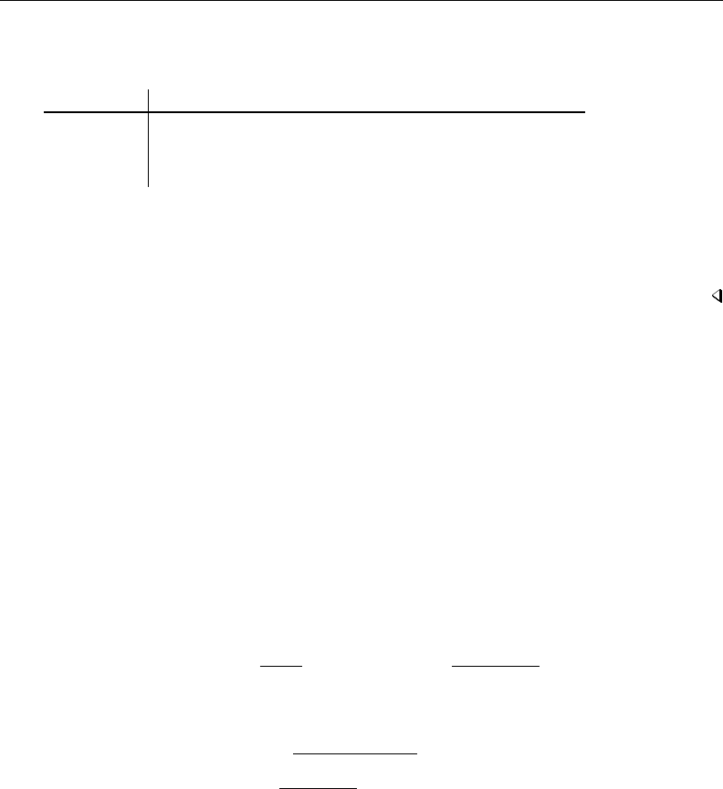
1684 probit postestimation — Postestimation tools for probit
. predict p3, asif
(option pr assumed; Pr(foreign))
. summarize for p p2 p3
Variable Obs Mean Std. Dev. Min Max
foreign 58 .2068966 .4086186 0 1
p 48 .25 .1956984 .1 .5
p2 58 .2068966 .2016268 0 .5
p3 58 .2931034 .2016268 .1 .5
Which is right? By default, predict uses the most conservative approach. If many observations
had been excluded due to a simple rule, we could be reasonably certain that the rules prediction is
correct. The asif prediction is correct only if the exclusion is a fluke and we would be willing to
exclude the variable from the analysis, anyway. Then, however, we should refit the model to include
the excluded observations.
Performing hypothesis tests
After estimation with probit, you can perform hypothesis tests by using the test or testnl
command; see [U] 20 Estimation and postestimation commands.
Methods and formulas
Let index jbe used to index observations. Define Mjfor each observation as the total number
of observations sharing j’s covariate pattern. Define Yjas the total number of positive responses
among observations sharing j’s covariate pattern. Define pjas the predicted probability of a positive
outcome for observation j.
For Mj>1, the deviance residual djis defined as
dj=± 2"YjlnYj
Mjpj+ (Mj−Yj)lnMj−Yj
Mj(1 −pj)#!1/2
where the sign is the same as the sign of (Yj−Mjpj). In the limiting cases, the deviance residual
is given by
dj=(−p2Mj|ln(1 −pj)|if Yj= 0
p2Mj|lnpj|if Yj=Mj
Also see
[R]probit — Probit regression
[R]estat classification — Classification statistics and table
[R]estat gof — Pearson or Hosmer–Lemeshow goodness-of-fit test
[R]lroc — Compute area under ROC curve and graph the curve
[R]lsens — Graph sensitivity and specificity versus probability cutoff
[U] 20 Estimation and postestimation commands

Title
proportion — Estimate proportions
Syntax Menu Description Options
Remarks and examples Stored results Methods and formulas References
Also see
Syntax
proportion varlist if in weight ,options
options Description
Model
stdize(varname)variable identifying strata for standardization
stdweight(varname)weight variable for standardization
nostdrescale do not rescale the standard weight variable
nolabel suppress value labels from varlist
missing treat missing values like other values
if/in/over
over(varlist, nolabel )group over subpopulations defined by varlist; optionally,
suppress group labels
SE/Cluster
vce(vcetype)vcetype may be analytic,cluster clustvar,bootstrap, or
jackknife
Reporting
level(#)set confidence level; default is level(95)
citype(logit |normal) method to compute limits of confidence intervals; default is
citype(logit)
noheader suppress table header
nolegend suppress table legend
display options control column formats and line width
coeflegend display legend instead of statistics
bootstrap,jackknife,mi estimate,rolling,statsby, and svy are allowed; see [U] 11.1.10 Prefix commands.
vce(bootstrap) and vce(jackknife) are not allowed with the mi estimate prefix; see [MI] mi estimate.
Weights are not allowed with the bootstrap prefix; see [R] bootstrap.
vce() and weights are not allowed with the svy prefix; see [SVY] svy.
fweights, iweights, and pweights are allowed; see [U] 11.1.6 weight.
coeflegend does not appear in the dialog box.
See [U] 20 Estimation and postestimation commands for more capabilities of estimation commands.
1685

1686 proportion — Estimate proportions
Menu
Statistics >Summaries, tables, and tests >Summary and descriptive statistics >Proportions
Description
proportion produces estimates of proportions, along with standard errors, for the categories
identified by the values in each variable of varlist.
Options
Model
stdize(varname)specifies that the point estimates be adjusted by direct standardization across the
strata identified by varname. This option requires the stdweight() option.
stdweight(varname)specifies the weight variable associated with the standard strata identified in
the stdize() option. The standardization weights must be constant within the standard strata.
nostdrescale prevents the standardization weights from being rescaled within the over() groups.
This option requires stdize() but is ignored if the over() option is not specified.
nolabel specifies that value labels attached to the variables in varlist be ignored.
missing specifies that missing values in varlist be treated as valid categories, rather than omitted
from the analysis (the default).
if/in/over
over(varlist , nolabel )specifies that estimates be computed for multiple subpopulations, which
are identified by the different values of the variables in varlist.
When this option is supplied with one variable name, such as over(varname), the value labels of
varname are used to identify the subpopulations. If varname does not have labeled values (or there
are unlabeled values), the values themselves are used, provided that they are nonnegative integers.
Noninteger values, negative values, and labels that are not valid Stata names are substituted with
a default identifier.
When over() is supplied with multiple variable names, each subpopulation is assigned a unique
default identifier.
nolabel requests that value labels attached to the variables identifying the subpopulations be
ignored.
SE/Cluster
vce(vcetype)specifies the type of standard error reported, which includes types that are derived from
asymptotic theory (analytic), that allow for intragroup correlation (cluster clustvar), and that
use bootstrap or jackknife methods (bootstrap,jackknife); see [R]vce option.
vce(analytic), the default, uses the analytically derived variance estimator associated with the
sample proportion.
Reporting
level(#); see [R]estimation options.

proportion — Estimate proportions 1687
citype(logit |normal) specifies how to compute the limits of confidence intervals.
citype(logit), the default, uses the logit transformation to compute the limits of confidence
intervals.
citype(normal) uses the normal approximation to compute the limits of confidence intervals.
noheader prevents the table header from being displayed. This option implies nolegend.
nolegend prevents the table legend identifying the subpopulations from being displayed.
display options:cformat(%fmt)and nolstretch; see [R]estimation options.
The following option is available with proportion but is not shown in the dialog box:
coeflegend; see [R]estimation options.
Remarks and examples
Example 1
We can estimate the proportion of each repair rating in auto2.dta:
. use http://www.stata-press.com/data/r13/auto2
(1978 Automobile Data)
. proportion rep78
Proportion estimation Number of obs = 69
Proportion Std. Err. [95% Conf. Interval]
rep78
Poor .0289855 .0203446 .0070061 .1121326
Fair .115942 .0388245 .0580159 .2183014
Average .4347826 .0601159 .3207109 .556206
Good .2608696 .0532498 .1690271 .3798066
Excellent .1594203 .0443922 .089188 .2686455
Here we use the missing option to include missing values as a category of rep78:
. proportion rep78, missing
Proportion estimation Number of obs = 74
_prop_6: rep78 = .
Proportion Std. Err. [95% Conf. Interval]
rep78
Poor .027027 .0189796 .0065484 .1047932
Fair .1081081 .0363433 .054094 .204402
Average .4054054 .0574637 .2977369 .523012
Good .2432432 .0502154 .1572724 .3563376
Excellent .1486486 .0416364 .0831005 .2517065
_prop_6 .0675676 .0293776 .0278144 .1550743

1688 proportion — Estimate proportions
Example 2
We can also estimate proportions over groups:
. proportion rep78, over(foreign)
Proportion estimation Number of obs = 69
Poor: rep78 = Poor
Fair: rep78 = Fair
Average: rep78 = Average
Good: rep78 = Good
Excellent: rep78 = Excellent
Domestic: foreign = Domestic
Foreign: foreign = Foreign
Over Proportion Std. Err. [95% Conf. Interval]
Poor
Domestic .0416667 .0291477 .0100299 .1572433
Foreign . (no observations)
Fair
Domestic .1666667 .0543607 .0839032 .3039797
Foreign . (no observations)
Average
Domestic .5625 .0723605 .4169211 .6980553
Foreign .1428571 .0782461 .0444941 .3736393
Good
Domestic .1875 .0569329 .0986718 .3272601
Foreign .4285714 .1106567 .2333786 .6488451
Excellent
Domestic .0416667 .0291477 .0100299 .1572433
Foreign .4285714 .1106567 .2333786 .6488451

proportion — Estimate proportions 1689
Stored results
proportion stores the following in e():
Scalars
e(N) number of observations
e(N over) number of subpopulations
e(N stdize) number of standard strata
e(N clust) number of clusters
e(k eq) number of equations in e(b)
e(df r) sample degrees of freedom
e(rank) rank of e(V)
Macros
e(cmd) proportion
e(cmdline) command as typed
e(varlist) varlist
e(stdize) varname from stdize()
e(stdweight) varname from stdweight()
e(wtype) weight type
e(wexp) weight expression
e(title) title in estimation output
e(cluster) name of cluster variable
e(over) varlist from over()
e(over labels) labels from over() variables
e(over namelist) names from e(over labels)
e(namelist) proportion identifiers
e(label#)labels from #th variable in varlist
e(vce) vcetype specified in vce()
e(vcetype) title used to label Std. Err.
e(properties) b V
e(estat cmd) program used to implement estat
e(marginsnotok) predictions disallowed by margins
Matrices
e(b) vector of proportion estimates
e(V) (co)variance estimates
e( N) vector of numbers of nonmissing observations
e( N stdsum) number of nonmissing observations within the standard strata
e( p stdize) standardizing proportions
e(error) error code corresponding to e(b)
Functions
e(sample) marks estimation sample
Methods and formulas
Proportions are means of indicator variables; see [R]mean.
Confidence intervals
Confidence intervals for proportions are calculated using a logit transform so that the endpoints
lie between 0 and 1. Let bpbe an estimated proportion and bsbe an estimate of its standard error. Let
f(bp) = ln bp
1−bp
be the logit transform of the proportion. In this metric, an estimate of the standard error is
c
SE{f(bp)}=f0(bp)bs=bs
bp(1 −bp)

1690 proportion — Estimate proportions
Thus a 100(1−α)% confidence interval in this metric is
ln bp
1−bp±t1−α/2,ν bs
bp(1 −bp)
where t1−α/2,ν is the (1−α/2)th quantile of Student’s tdistribution with νdegrees of freedom.
The endpoints of this confidence interval are transformed back to the proportion metric by using the
inverse of the logit transform
f−1(y) = ey
1 + ey
Hence, the displayed confidence intervals for proportions are
f−1ln bp
1−bp±t1−α/2,ν bs
bp(1 −bp)
References
Cochran, W. G. 1977. Sampling Techniques. 3rd ed. New York: Wiley.
Stuart, A., and J. K. Ord. 1994. Kendall’s Advanced Theory of Statistics: Distribution Theory, Vol I. 6th ed. London:
Arnold.
Also see
[R]proportion postestimation — Postestimation tools for proportion
[R]mean — Estimate means
[R]ratio — Estimate ratios
[R]total — Estimate totals
[MI]estimation — Estimation commands for use with mi estimate
[SVY]direct standardization — Direct standardization of means, proportions, and ratios
[SVY]poststratification — Poststratification for survey data
[SVY]subpopulation estimation — Subpopulation estimation for survey data
[SVY]svy estimation — Estimation commands for survey data
[SVY]variance estimation — Variance estimation for survey data
[U] 20 Estimation and postestimation commands

Title
proportion postestimation — Postestimation tools for proportion
Description Remarks and examples Also see
Description
The following postestimation commands are available after proportion:
Command Description
estat vce variance–covariance matrix of the estimators (VCE)
estat (svy) postestimation statistics for survey data
estimates cataloging estimation results
lincom point estimates, standard errors, testing, and inference for linear
combinations of coefficients
nlcom point estimates, standard errors, testing, and inference for nonlinear
combinations of coefficients
test Wald tests of simple and composite linear hypotheses
testnl Wald tests of nonlinear hypotheses
Remarks and examples
Example 1
In example 2 of [R]proportion, we computed the proportions of cars with different repair records
for each group, foreign or domestic. We use test to test whether the proportion of cars with repair
record equal to 4 is the same for domestic and foreign cars.
. use http://www.stata-press.com/data/r13/auto
(1978 Automobile Data)
. proportion rep78, over(foreign)
(output omitted )
. test [_prop_4]:Domestic=[_prop_4]:Foreign
( 1) [_prop_4]Domestic - [_prop_4]Foreign = 0
F( 1, 68) = 3.75
Prob > F = 0.0569
There is not a significant difference between those proportions at the 5% level.
Example 2
Continuing with auto.dta from example 1, we generate a new variable, highprice, that indicates
if the price is larger than $5,000 and then use proportion to see the proportion of cars with high
price among domestic and foreign cars separately.
1691

1692 proportion postestimation — Postestimation tools for proportion
. generate highprice = price>5000
. proportion highprice, over(foreign)
Proportion estimation Number of obs = 74
_prop_1: highprice = 0
_prop_2: highprice = 1
Domestic: foreign = Domestic
Foreign: foreign = Foreign
Over Proportion Std. Err. [95% Conf. Interval]
_prop_1
Domestic .5576923 .0695464 .4182157 .6886264
Foreign .3636364 .1049728 .1879015 .5852765
_prop_2
Domestic .4423077 .0695464 .3113736 .5817843
Foreign .6363636 .1049728 .4147235 .8120985
We will compute the odds ratio of having a high price in group Foreign to having a high price
in group Domestic. Usually, odds ratios are computed by using the logistic command, but here
we will perform the computation by using nlcom after proportion.
. nlcom OR: ([_prop_2]_b[Foreign]/[_prop_1]_b[Foreign])/([_prop_2]_b[Domestic]/
> [_prop_1]_b[Domestic])
OR: ([_prop_2]_b[Foreign]/[_prop_1]_b[Foreign])/([_prop_2]_b[Domesti
> c]/[_prop_1]_b[Domestic])
Proportion Coef. Std. Err. z P>|z| [95% Conf. Interval]
OR 2.206522 1.178522 1.87 0.061 -.1033393 4.516383
This is the same odds ratio that we would obtain from
. logistic highprice foreign
The odds ratio is slightly larger than 2, which means that the odds of having a high price among
foreign cars are more than twice that of having a high price among domestic cars.
Also see
[R]proportion — Estimate proportions
[SVY]svy postestimation — Postestimation tools for svy
[U] 20 Estimation and postestimation commands

Title
prtest — Tests of proportions
Syntax Menu Description Options
Remarks and examples Stored results Methods and formulas References
Also see
Syntax
One-sample test of proportion
prtest varname == #pif in , level(#)
Two-sample test of proportions using groups
prtest varname if in , by(groupvar)level(#)
Two-sample test of proportions using variables
prtest varname1== varname2if in , level(#)
Immediate form of one-sample test of proportion
prtesti #obs1 #p1#p2, level(#) count
Immediate form of two-sample test of proportions
prtesti #obs1 #p1#obs2 #p2, level(#) count
by is allowed with prtest; see [D] by.
Menu
prtest
Statistics >Summaries, tables, and tests >Classical tests of hypotheses >Proportion test
prtesti
Statistics >Summaries, tables, and tests >Classical tests of hypotheses >Proportion test calculator
Description
prtest performs tests on the equality of proportions using large-sample statistics.
In the first form, prtest tests that varname has a proportion of #p. In the second form, prtest
tests that varname has the same proportion within the two groups defined by groupvar. In the third
form, prtest tests that varname1and varname2have the same proportion.
prtesti is the immediate form of prtest; see [U] 19 Immediate commands.
1693

1694 prtest — Tests of proportions
The bitest command is a better version of the first form of prtest in that it gives exact p-values.
Researchers should use bitest when possible, especially for small samples; see [R]bitest.
Options
Main
by(groupvar)specifies a numeric variable that contains the group information for a given observation.
This variable must have only two values. Do not confuse the by() option with the by prefix; both
may be specified.
level(#)specifies the confidence level, as a percentage, for confidence intervals. The default is
level(95) or as set by set level; see [U] 20.7 Specifying the width of confidence intervals.
count specifies that integer counts instead of proportions be used in the immediate forms of prtest.
In the first syntax, prtesti expects that #obs1 and #p1are counts—#p1≤#obs1 —and #p2is a
proportion. In the second syntax, prtesti expects that all four numbers are integer counts, that
#obs1 ≥#p1, and that #obs2 ≥#p2.
Remarks and examples
The prtest output follows the output of ttest in providing a lot of information. Each proportion
is presented along with a confidence interval. The appropriate one- or two-sample test is performed,
and the two-sided and both one-sided results are included at the bottom of the output. For a two-sample
test, the calculated difference is also presented with its confidence interval. This command may be
used for both large-sample testing and large-sample interval estimation.
Example 1: One-sample test of proportion
In the first form, prtest tests whether the mean of the sample is equal to a known constant. Assume
that we have a sample of 74 automobiles. We wish to test whether the proportion of automobiles that
are foreign is different from 40%.
. use http://www.stata-press.com/data/r13/auto
(1978 Automobile Data)
. prtest foreign == .4
One-sample test of proportion foreign: Number of obs = 74
Variable Mean Std. Err. [95% Conf. Interval]
foreign .2972973 .0531331 .1931583 .4014363
p = proportion(foreign) z = -1.8034
Ho: p = 0.4
Ha: p < 0.4 Ha: p != 0.4 Ha: p > 0.4
Pr(Z < z) = 0.0357 Pr(|Z| > |z|) = 0.0713 Pr(Z > z) = 0.9643
The test indicates that we cannot reject the hypothesis that the proportion of foreign automobiles is
0.40 at the 5% significance level.

prtest — Tests of proportions 1695
Example 2: Two-sample test of proportions
We have two headache remedies that we give to patients. Each remedy’s effect is recorded as 0
for failing to relieve the headache and 1 for relieving the headache. We wish to test the equality of
the proportion of people relieved by the two treatments.
. use http://www.stata-press.com/data/r13/cure
. prtest cure1 == cure2
Two-sample test of proportions cure1: Number of obs = 50
cure2: Number of obs = 59
Variable Mean Std. Err. z P>|z| [95% Conf. Interval]
cure1 .52 .0706541 .3815205 .6584795
cure2 .7118644 .0589618 .5963013 .8274275
diff -.1918644 .0920245 -.372229 -.0114998
under Ho: .0931155 -2.06 0.039
diff = prop(cure1) - prop(cure2) z = -2.0605
Ho: diff = 0
Ha: diff < 0 Ha: diff != 0 Ha: diff > 0
Pr(Z < z) = 0.0197 Pr(|Z| < |z|) = 0.0394 Pr(Z > z) = 0.9803
We find that the proportions are statistically different from each other at any level greater than 3.9%.
Example 3: Immediate form of one-sample test of proportion
prtesti is like prtest, except that you specify summary statistics rather than variables as
arguments. For instance, we are reading an article that reports the proportion of registered voters
among 50 randomly selected eligible voters as 0.52. We wish to test whether the proportion is 0.7:
. prtesti 50 .52 .70
One-sample test of proportion x: Number of obs = 50
Variable Mean Std. Err. [95% Conf. Interval]
x .52 .0706541 .3815205 .6584795
p = proportion(x) z = -2.7775
Ho: p = 0.7
Ha: p < 0.7 Ha: p != 0.7 Ha: p > 0.7
Pr(Z < z) = 0.0027 Pr(|Z| > |z|) = 0.0055 Pr(Z > z) = 0.9973
Example 4: Immediate form of two-sample test of proportions
To judge teacher effectiveness, we wish to test whether the same proportion of people from
two classes will answer an advanced question correctly. In the first classroom of 30 students, 40%
answered the question correctly, whereas in the second classroom of 45 students, 67% answered the
question correctly.

1696 prtest — Tests of proportions
. prtesti 30 .4 45 .67
Two-sample test of proportions x: Number of obs = 30
y: Number of obs = 45
Variable Mean Std. Err. z P>|z| [95% Conf. Interval]
x .4 .0894427 .2246955 .5753045
y .67 .0700952 .532616 .807384
diff -.27 .1136368 -.4927241 -.0472759
under Ho: .1169416 -2.31 0.021
diff = prop(x) - prop(y) z = -2.3088
Ho: diff = 0
Ha: diff < 0 Ha: diff != 0 Ha: diff > 0
Pr(Z < z) = 0.0105 Pr(|Z| < |z|) = 0.0210 Pr(Z > z) = 0.9895
Stored results
prtest and prtesti store the following in r():
Scalars
r(z) zstatistic
r(P #)proportion for variable #
r(N #)number of observations for variable #
Methods and formulas
See Acock (2014, 155–161) for additional examples of tests of proportions using Stata.
A large-sample 100(1−α)% confidence interval for a proportion pis
bp±z1−α/2rbpbq
n
and a 100(1−α)% confidence interval for the difference of two proportions is given by
(bp1−bp2)±z1−α/2sbp1bq1
n1
+bp2bq2
n2
where bq= 1 −bpand zis calculated from the inverse cumulative standard normal distribution.
The one-tailed and two-tailed tests of a population proportion use a normally distributed test
statistic calculated as
z=bp−p0
pp0q0/n
where p0is the hypothesized proportion. A test of the difference of two proportions also uses a
normally distributed test statistic calculated as

prtest — Tests of proportions 1697
z=bp1−bp2
pbppbqp(1/n1+ 1/n2)
where
bpp=x1+x2
n1+n2
and x1and x2are the total number of successes in the two populations.
References
Acock, A. C. 2014. A Gentle Introduction to Stata. 4th ed. College Station, TX: Stata Press.
Wang, D. 2000. sg154: Confidence intervals for the ratio of two binomial proportions by Koopman’s method.Stata
Technical Bulletin 58: 16–19. Reprinted in Stata Technical Bulletin Reprints, vol. 10, pp. 244–247. College Station,
TX: Stata Press.
Also see
[R]bitest — Binomial probability test
[R]proportion — Estimate proportions
[R]ttest —ttests (mean-comparison tests)
[MV]hotelling — Hotelling’s T-squared generalized means test

Title
pwcompare — Pairwise comparisons
Syntax Menu Description Options
Remarks and examples Stored results Methods and formulas References
Also see
Syntax
pwcompare marginlist ,options
where marginlist is a list of factor variables or interactions that appear in the current estimation results
or eqns to reference equations. The variables may be typed with or without the i. prefix, and you
may use any factor-variable syntax:
. pwcompare i.sex i.group i.sex#i.group
. pwcompare sex group sex#group
. pwcompare sex##group
options Description
Main
mcompare(method)adjust for multiple comparisons; default is mcompare(noadjust)
asobserved treat all factor variables as observed
Equations
equation(eqspec)perform comparisons within equation eqspec
atequations perform comparisons within each equation
Advanced
emptycells(empspec)treatment of empty cells for balanced factors
noestimcheck suppress estimability checks
Reporting
level(#)confidence level; default is level(95)
cieffects show effects table with confidence intervals; the default
pveffects show effects table with p-values
effects show effects table with confidence intervals and p-values
cimargins show table of margins and confidence intervals
groups show table of margins and group codes
sort sort the margins or contrasts within each term
post post margins and their VCEs as estimation results
display options control column formats, row spacing, line width, and factor-variable labeling
eform option report exponentiated contrasts
df(#)use tdistribution with #degrees of freedom for computing p-values
and confidence intervals
df(#)does not appear in the dialog box.
1698

pwcompare — Pairwise comparisons 1699
method Description
noadjust do not adjust for multiple comparisons; the default
bonferroni adjustall Bonferroni’s method; adjust across all terms
sidak adjustall ˇ
Sid´
ak’s method; adjust across all terms
scheffe Scheff´
e’s method
∗tukey Tukey’s method
∗snk Student–Newman–Keuls’ method
∗duncan Duncan’s method
∗dunnett Dunnett’s method
∗tukey,snk,duncan, and dunnett are only allowed with results from anova,manova,regress, and mvreg.
tukey,snk,duncan, and dunnett are not allowed with results from svy.
Time-series operators are allowed if they were used in the estimation.
Menu
Statistics >Postestimation >Pairwise comparisons
Description
pwcompare performs pairwise comparisons across the levels of factor variables from the most
recently fit model. pwcompare can compare estimated cell means, marginal means, intercepts, marginal
intercepts, slopes, or marginal slopes—collectively called margins. pwcompare reports the comparisons
as contrasts (differences) of margins along with significance tests or confidence intervals for the
contrasts. The tests and confidence intervals can be adjusted for multiple comparisons.
pwcompare can be used with svy estimation results; see [SVY]svy postestimation.
See [R]margins, pwcompare for performing pairwise comparisons of margins of linear and
nonlinear predictions.
Options
Main
mcompare(method)specifies the method for computing p-values and confidence intervals that account
for multiple comparisons within a factor-variable term.
Most methods adjust the comparisonwise error rate, αc, to achieve a prespecified experimentwise
error rate, αe.
mcompare(noadjust) is the default; it specifies no adjustment.
αc=αe
mcompare(bonferroni) adjusts the comparisonwise error rate based on the upper limit of the
Bonferroni inequality:
αe≤mαc
where mis the number of comparisons within the term.
The adjusted comparisonwise error rate is
αc=αe/m

1700 pwcompare — Pairwise comparisons
mcompare(sidak) adjusts the comparisonwise error rate based on the upper limit of the probability
inequality
αe≤1−(1 −αc)m
where mis the number of comparisons within the term.
The adjusted comparisonwise error rate is
αc= 1 −(1 −αe)1/m
This adjustment is exact when the mcomparisons are independent.
mcompare(scheffe) controls the experimentwise error rate using the F(or χ2) distribution with
degrees of freedom equal to the rank of the term.
For results from anova,regress,manova, and mvreg (see [R]anova,[R]regress,[MV]manova,
and [MV]mvreg), pwcompare allows the following additional methods. These methods are not
allowed with results that used vce(robust) or vce(cluster clustvar).
mcompare(tukey) uses what is commonly referred to as Tukey’s honestly significant difference.
This method uses the Studentized range distribution instead of the tdistribution.
mcompare(snk) is a variation on mcompare(tukey) that counts only the number of margins in
the range for a given comparison instead of the full number of margins.
mcompare(duncan) is a variation on mcompare(snk) with additional adjustment to the significance
probabilities.
mcompare(dunnett) uses Dunnett’s method for making comparisons with a reference category.
mcompare(method adjustall) specifies that the multiple-comparison adjustments count all
comparisons across all terms rather than performing multiple comparisons term by term. This
leads to more conservative adjustments when multiple variables or terms are specified in
marginlist. This option is compatible only with the bonferroni and sidak methods.
asobserved specifies that factor covariates be evaluated using the cell frequencies observed when the
model was fit. The default is to treat all factor covariates as though there were an equal number
of observations at each level.
Equations
equation(eqspec)specifies the equation from which margins are to be computed. The default is to
compute margins from the first equation.
atequations specifies that the margins be computed within each equation.
Advanced
emptycells(empspec)specifies how empty cells are handled in interactions involving factor variables
that are being treated as balanced.
emptycells(strict) is the default; it specifies that margins involving empty cells be treated as
not estimable.
emptycells(reweight) specifies that the effects of the observed cells be increased to accommodate
any missing cells. This makes the margins estimable but changes their interpretation.
noestimcheck specifies that pwcompare not check for estimability. By default, the requested margins
are checked and those found not estimable are reported as such. Nonestimability is usually caused
by empty cells. If noestimcheck is specified, estimates are computed in the usual way and
reported even though the resulting estimates are manipulable, which is to say they can differ across
equivalent models having different parameterizations.

pwcompare — Pairwise comparisons 1701
Reporting
level(#)specifies the confidence level, as a percentage, for confidence intervals. The default is
level(95) or as set by set level; see [U] 20.7 Specifying the width of confidence intervals.
The significance level used by the groups option is 100 −#, expressed as a percentage.
cieffects specifies that a table of the pairwise comparisons with their standard errors and confidence
intervals be reported. This is the default.
pveffects specifies that a table of the pairwise comparisons with their standard errors, test statistics,
and p-values be reported.
effects specifies that a table of the pairwise comparisons with their standard errors, test statistics,
p-values, and confidence intervals be reported.
cimargins specifies that a table of the margins with their standard errors and confidence intervals
be reported.
groups specifies that a table of the margins with their standard errors and group codes be reported.
Margins with the same letter in the group code are not significantly different at the specified
significance level.
sort specifies that the reported tables be sorted on the margins or differences in each term.
post causes pwcompare to behave like a Stata estimation (e-class) command. pwcompare posts the
vector of estimated margins along with the estimated variance–covariance matrix to e(), so you
can treat the estimated margins just as you would results from any other estimation command. For
example, you could use test to perform simultaneous tests of hypotheses on the margins, or you
could use lincom to create linear combinations.
display options:vsquish,nofvlabel,fvwrap(#),fvwrapon(style),cformat(%fmt),
pformat(% fmt),sformat(% fmt), and nolstretch.
vsquish specifies that the blank space separating factor-variable terms or time-series–operated
variables from other variables in the model be suppressed.
nofvlabel displays factor-variable level values rather than attached value labels. This option
overrides the fvlabel setting; see [R]set showbaselevels.
fvwrap(#)specifies how many lines to allow when long value labels must be wrapped. Labels
requiring more than #lines are truncated. This option overrides the fvwrap setting; see [R]set
showbaselevels.
fvwrapon(style)specifies whether value labels that wrap will break at word boundaries or break
based on available space.
fvwrapon(word), the default, specifies that value labels break at word boundaries.
fvwrapon(width) specifies that value labels break based on available space.
This option overrides the fvwrapon setting; see [R]set showbaselevels.
cformat(% fmt)specifies how to format contrasts or margins, standard errors, and confidence
limits in the table of pairwise comparisons.
pformat(% fmt)specifies how to format p-values in the table of pairwise comparisons.
sformat(% fmt)specifies how to format test statistics in the table of pairwise comparisons.
nolstretch specifies that the width of the table of pairwise comparisons not be automatically
widened to accommodate longer variable names. The default, lstretch, is to automatically
widen the table of pairwise comparisons up to the width of the Results window. To change the
default, use set lstretch off.nolstretch is not shown in the dialog box.

1702 pwcompare — Pairwise comparisons
eform option specifies that the contrasts table be displayed in exponentiated form. econtrast is
displayed rather than contrast. Standard errors and confidence intervals are also transformed. See
[R]eform option for the list of available options.
The following option is available with pwcompare but is not shown in the dialog box:
df(#)specifies that the tdistribution with #degrees of freedom be used for computing p-values and
confidence intervals. The default is to use e(df r) degrees of freedom or the standard normal
distribution if e(df r) is missing.
Remarks and examples
pwcompare performs pairwise comparisons of margins across the levels of factor variables from
the most recently fit model. The margins can be estimated cell means, marginal means, intercepts,
marginal intercepts, slopes, or marginal slopes. With the exception of slopes, we can also consider
these margins to be marginal linear predictions.
The margins are calculated as linear combinations of the coefficients. Let kbe the number of
levels for a factor term in our model; then there are kmargins for that term, and
m=k
2=k(k−1)
2
unique pairwise comparisons of those margins.
The confidence intervals and p-values for these pairwise comparisons can be adjusted to account
for multiple comparisons. Bonferroni’s, ˇ
Sid´
ak’s, and Scheff´
e’s adjustments can be made for multiple
comparisons after fitting any type of model. In addition, Tukey’s, Student–Newman–Keuls’, Duncan’s,
and Dunnett’s adjustments are available when fitting ANOVA, linear regression, MANOVA, or multivariate
regression models.
Remarks are presented under the following headings:
Pairwise comparisons of means
Marginal means
All pairwise comparisons
Overview of multiple-comparison methods
Fisher’s protected least-significant difference (LSD)
Bonferroni’s adjustment
ˇ
Sid´
ak’s adjustment
Scheff´
e’s adjustment
Tukey’s HSD adjustment
Student–Newman–Keuls’ adjustment
Duncan’s adjustment
Dunnett’s adjustment
Example adjustments using one-way models
Fisher’s protected LSD
Tukey’s HSD
Dunnett’s method for comparisons to a control
Two-way models
Pairwise comparisons of slopes
Nonlinear models
Multiple-equation models
Unbalanced data
Empty cells

pwcompare — Pairwise comparisons 1703
Pairwise comparisons of means
Suppose we are interested in the effects of five different fertilizers on wheat yield. We could
estimate the following linear regression model to determine the effect of each type of fertilizer on
the yield.
. use http://www.stata-press.com/data/r13/yield
(Artificial wheat yield dataset)
. regress yield i.fertilizer
Source SS df MS Number of obs = 200
F( 4, 195) = 5.33
Model 1078.84207 4 269.710517 Prob > F = 0.0004
Residual 9859.55334 195 50.561812 R-squared = 0.0986
Adj R-squared = 0.0801
Total 10938.3954 199 54.9668111 Root MSE = 7.1107
yield Coef. Std. Err. t P>|t| [95% Conf. Interval]
fertilizer
10-08-22 3.62272 1.589997 2.28 0.024 .4869212 6.758518
16-04-08 .4906299 1.589997 0.31 0.758 -2.645169 3.626428
18-24-06 4.922803 1.589997 3.10 0.002 1.787005 8.058602
29-03-04 -1.238328 1.589997 -0.78 0.437 -4.374127 1.89747
_cons 41.36243 1.124298 36.79 0.000 39.14509 43.57977
In this simple case, the coefficients for fertilizers 10-08-22, 16-04-08, 18-24-06, and 29-03-04 indicate
the difference in the mean yield for that fertilizer versus the mean yield for fertilizer 10-10-10. That
the standard errors of all four coefficients are identical results from having perfectly balanced data.
Marginal means
We can use pwcompare with the cimargins option to compute the mean yield for each of the
fertilizers.
. pwcompare fertilizer, cimargins
Pairwise comparisons of marginal linear predictions
Margins : asbalanced
Unadjusted
Margin Std. Err. [95% Conf. Interval]
fertilizer
10-10-10 41.36243 1.124298 39.14509 43.57977
10-08-22 44.98515 1.124298 42.7678 47.20249
16-04-08 41.85306 1.124298 39.63571 44.0704
18-24-06 46.28523 1.124298 44.06789 48.50258
29-03-04 40.1241 1.124298 37.90676 42.34145
Looking at the confidence intervals for fertilizers 10-10-10 and 10-08-22 in the table above, we might
be tempted to conclude that these means are not significantly different because the intervals overlap.
However, as discussed in Interaction plots of [R]marginsplot, we cannot draw conclusions about the
differences in means by looking at confidence intervals for the means themselves. Instead, we would
need to look at confidence intervals for the difference in means.

1704 pwcompare — Pairwise comparisons
All pairwise comparisons
By default, pwcompare calculates all pairwise differences of the margins, in this case pairwise
differences of the mean yields.
. pwcompare fertilizer
Pairwise comparisons of marginal linear predictions
Margins : asbalanced
Unadjusted
Contrast Std. Err. [95% Conf. Interval]
fertilizer
10-08-22 vs 10-10-10 3.62272 1.589997 .4869212 6.758518
16-04-08 vs 10-10-10 .4906299 1.589997 -2.645169 3.626428
18-24-06 vs 10-10-10 4.922803 1.589997 1.787005 8.058602
29-03-04 vs 10-10-10 -1.238328 1.589997 -4.374127 1.89747
16-04-08 vs 10-08-22 -3.13209 1.589997 -6.267889 .0037086
18-24-06 vs 10-08-22 1.300083 1.589997 -1.835715 4.435882
29-03-04 vs 10-08-22 -4.861048 1.589997 -7.996847 -1.725249
18-24-06 vs 16-04-08 4.432173 1.589997 1.296375 7.567972
29-03-04 vs 16-04-08 -1.728958 1.589997 -4.864757 1.406841
29-03-04 vs 18-24-06 -6.161132 1.589997 -9.29693 -3.025333
If a confidence interval does not include zero, the means for the compared fertilizers are significantly
different. Therefore, at the 5% significance level, we would reject the hypothesis that the means
for fertilizers 10-10-10 and 10-08-22 are equivalent—as we would do for 18-24-06 vs 10-10-10,
29-03-04 vs 10-08-22,18-24-06 vs 16-04-08, and 29-03-04 vs 18-24-06.
We may prefer to see the p-values instead of looking at confidence intervals to determine whether
the pairwise differences are significantly different from zero. We could use the pveffects option
to see the differences with standard errors and p-values, or we could use the effects option to see
both p-values and confidence intervals in the same table. Here we specify effects as well as the
sort option so that the differences are sorted from smallest to largest.

pwcompare — Pairwise comparisons 1705
. pwcompare fertilizer, effects sort
Pairwise comparisons of marginal linear predictions
Margins : asbalanced
Unadjusted Unadjusted
Contrast Std. Err. t P>|t| [95% Conf. Interval]
fertilizer
29-03-04
vs
18-24-06 -6.161132 1.589997 -3.87 0.000 -9.29693 -3.025333
29-03-04
vs
10-08-22 -4.861048 1.589997 -3.06 0.003 -7.996847 -1.725249
16-04-08
vs
10-08-22 -3.13209 1.589997 -1.97 0.050 -6.267889 .0037086
29-03-04
vs
16-04-08 -1.728958 1.589997 -1.09 0.278 -4.864757 1.406841
29-03-04
vs
10-10-10 -1.238328 1.589997 -0.78 0.437 -4.374127 1.89747
16-04-08
vs
10-10-10 .4906299 1.589997 0.31 0.758 -2.645169 3.626428
18-24-06
vs
10-08-22 1.300083 1.589997 0.82 0.415 -1.835715 4.435882
10-08-22
vs
10-10-10 3.62272 1.589997 2.28 0.024 .4869212 6.758518
18-24-06
vs
16-04-08 4.432173 1.589997 2.79 0.006 1.296375 7.567972
18-24-06
vs
10-10-10 4.922803 1.589997 3.10 0.002 1.787005 8.058602
We find that 5 of the 10 pairs of means are significantly different at the 5% significance level.
We can use the groups option to obtain a table that identifies groups whose means are not
significantly different by assigning them the same letter.

1706 pwcompare — Pairwise comparisons
. pwcompare fertilizer, groups sort
Pairwise comparisons of marginal linear predictions
Margins : asbalanced
Unadjusted
Margin Std. Err. Groups
fertilizer
29-03-04 40.1241 1.124298 A
10-10-10 41.36243 1.124298 A
16-04-08 41.85306 1.124298 AB
10-08-22 44.98515 1.124298 BC
18-24-06 46.28523 1.124298 C
Note: Margins sharing a letter in the group label
are not significantly different at the 5%
level.
The letter Athat is assigned to fertilizers 29-03-04, 10-10-10, and 16-04-08 designates that the mean
yields for these fertilizers are not different at the 5% level.
Overview of multiple-comparison methods
For a single test, if we choose a 5% significance level, we would have a 5% chance of concluding
that two margins are different when the population values are actually equal. This is known as making
a type I error. When we perform m=k(k−1)/2 pairwise comparisons of the kmargins, we have
mopportunities to make a type I error.
pwcompare with the mcompare() option allows us to adjust the confidence intervals and p-values
for each comparison to account for the increased probability of making a type I error when making
multiple comparisons. Bonferroni’s adjustment, ˇ
Sid´
ak’s adjustment, and Scheff´
e’s adjustment can be
used when making pairwise comparisons of the margins after any estimation command. Tukey’s
honestly significant difference, Student–Newman–Keuls’ method, Duncan’s method, and Dunnett’s
method are only available when fitting linear models after anova,manova,regress, or mvreg.
Fisher’s protected least-significant difference (LSD)
pwcompare does not offer an mcompare() option specifically for Fisher’s protected least-significant
difference (LSD). In this methodology, no adjustment is made to the confidence intervals or p-values.
However, it is protected in the sense that no pairwise comparisons are tested unless the joint test
for the corresponding term in the model is significant. Therefore, the default mcompare(noadjust)
corresponds to Fisher’s protected LSD assuming that the corresponding joint test was performed before
using pwcompare.
Milliken and Johnson (2009) recommend using this methodology for planned comparisons, assuming
the corresponding joint test is significant.
Bonferroni’s adjustment
mcompare(bonferroni) adjusts significance levels based on the Bonferroni inequality, which,
in the case of multiple testing, tells us that the maximum error rate for all comparisons is the sum
of the error rates for the individual comparisons. Assuming that we are using the same significance
level for all tests, the experimentwise error rate is the error rate for a single test multiplied by the

pwcompare — Pairwise comparisons 1707
number of comparisons. Therefore, a p-value for each comparison can be computed by multiplying
the unadjusted p-value by the total number of comparisons. If the adjusted p-value is greater than 1,
then pwcompare will report a p-value of 1.
Bonferroni’s adjustment is popular because it is easy to compute manually and because it can be
applied to any set of tests, not only the pairwise comparisons available in pwcompare. In addition,
this method does not require equal sample sizes.
Because Bonferroni’s adjustment is so general, it is more conservative than many of the other
adjustments. It is especially conservative when a large number of tests is being performed.
ˇ
Sid´
ak’s adjustment
mcompare(sidak) performs an adjustment using ˇ
Sid´
ak’s method. This adjustment, like Bonfer-
roni’s adjustment, is derived from an inequality. However, in this case, the inequality is based on the
probability of not making a type I error. For a single test, the probability that we do not make a type
I error is 1 −α. For two independent tests, both using αas a significance level, the probability is
(1−α)(1−α). Likewise, for mindependent tests, the probability of not making a type I error is
(1−α)m. Therefore, the probability of making one or more type I errors is 1 −(1−α)m. When
tests are not independent, the probability of making at least one error is less than 1 −(1−α)m.
Therefore, we can compute an adjusted p-value as 1 −(1−up)m, where upis the unadjusted p-value
for a single comparison.
ˇ
Sid´
ak’s method is also conservative although slightly less so than Bonferroni’s method. Like
Bonferroni’s method, this method does not require equal sample sizes.
Scheff´
e’s adjustment
Scheff´
e’s adjustment is used when mcompare(scheffe) is specified. This adjustment is derived
from the joint Ftest and its correspondence to the maximum normalized comparison. To adjust for
multiple comparisons, the absolute value of the tstatistic for a particular comparison can be compared
with a critical value of p(k−1)Fk−1,ν , where νis the residual degrees of freedom. Fk−1,ν is
the distribution of the joint Ftest for the corresponding term in a one-way ANOVA model. Winer,
Brown, and Michels (1991, 191–195) discuss this in detail. For estimation commands that report z
statistics instead of tstatistics for the tests on coefficients, a χ2distribution is used instead of an F
distribution.
Scheff´
e’s method allows for making all possible comparisons of the kmargins, not just the
pairwise comparisons. Unlike the methods described above, it does not take into account the number
of comparisons that are currently being made. Therefore, this method is even more conservative
than the others. Because this method adjusts for all possible comparisons of the levels of the term,
Milliken and Johnson (2009) recommend using this procedure when making unplanned contrasts that
are suggested by the data. As Winer, Brown, and Michels (1991, 191) put it, this method is often
used to adjust for “unfettered data snooping”. When using this adjustment, a contrast will never be
significant if the joint For χ2test for the term is not also significant.
This is another method that does not require equal sample sizes.

1708 pwcompare — Pairwise comparisons
Tukey’s HSD adjustment
Tukey’s adjustment is also referred to as Tukey’s honestly significant difference (HSD) and is
used when mcompare(tukey) is specified. It is often applied to all pairwise comparisons of means.
Tukey’s HSD is commonly used as a post hoc test although this is not a requirement.
To adjust for multiple comparisons, Tukey’s method compares the absolute value of the tstatistic
from the individual comparison with a critical value based on a Studentized range distribution with
parameter equal to the number of levels in the term. When applied to pairwise comparisons of means,
q=meanmax −meanmin
s
follows a Studentized range distribution with parameter kand νdegrees of freedom. Here meanmax
and meanmin are the largest and smallest marginal means, and sis an estimate of the standard error
of the means.
Now for the comparison of the smallest and largest means, we can say that the probability of not
making a type I error is
Pr meanmax −meanmin
s≤qk,ν = 1 −α
Then the following inquality holds for all pairs of means simultaneously:
Pr |meani−meanj|
s≤qk,ν ≥1−α
Based on this procedure, Tukey’s HSD computes the p-value for each of the individual comparisons
using the Studentized range distribution. However, because the equality holds only for the difference
in the largest and smallest means, this procedure produces conservative tests for the remaining
comparisons. Winer, Brown, and Michels (1991, 172–182) discuss this in further detail.
With unequal sample sizes, mcompare(tukey) produces the Tukey–Kramer adjustment
(Tukey 1953;Kramer 1956).
Student–Newman–Keuls’ adjustment
The Student–Newman–Keuls (SNK) method is used when mcompare(snk) is specified. It is a
modification to Tukey’s method and is less conservative. In this procedure, we first order the means.
We then test the difference in the smallest and largest means using a critical value from the Studentized
range distribution with parameter k, where kis the number of levels in the term. This step uses
the same methodology as in Tukey’s procedure. However, in the next step, we will then test for
differences in the two sets of means that are the endpoints of the two ranges including k−1 means.
Specifically, we test the difference in the smallest mean and the second-largest mean using a critical
value from the Studentized range distribution with parameter k−1. We would also test the difference
in the second-smallest mean and the largest mean using this critical value. Likewise, the means that
are the endpoints of ranges including k−2 means when ordered are tested using the Studentized
range distribution with parameter k−2, and so on.
Equal sample sizes are required for this method.

pwcompare — Pairwise comparisons 1709
Duncan’s adjustment
When mcompare(duncan) is specified, tests are adjusted for multiple comparisons using Duncan’s
method, which is sometimes referred to as Duncan’s new multiple range method. This adjustment
produces tests that are less conservative than both Tukey’s HSD and SNK. This procedure is performed
in the same manner as SNK except that the p-values for the individual comparisons are adjusted as
1−(1−snkpi)1/(r+1), where snkpis the p-value computed using the SNK method and rrepresents
the number of means that, when ordered, fall between the two that are being compared.
Again equal sample sizes are required for this adjustment.
Dunnett’s adjustment
Dunnett’s adjustment is obtained by specifying mcompare(dunnett). It is used when one of the
levels of a factor can be considered a control or reference level with which each of the other levels
is being compared. When Dunnett’s adjustment is requested, k−1 instead of k(k−1)/2 pairwise
comparisons are made. Dunnett (1955,1964) developed tables of critical values for what Miller (1981,
76) refers to as the “many-one tstatistic”. The tstatistics for individual comparisons are compared
with these critical values when making many comparisons to a single reference level.
This method also requires equal sample sizes.
Example adjustments using one-way models
Fisher’s protected LSD
Fisher’s protected LSD requires that we first verify that the joint test for a term in our model is
significant before proceeding with pairwise comparisons. Using our previous example, we could have
first used the contrast command to obtain a joint test for the effects of fertilizer.
. contrast fertilizer
Contrasts of marginal linear predictions
Margins : asbalanced
df F P>F
fertilizer 4 5.33 0.0004
Denominator 195
This test for the effects of fertilizer is highly significant. Now we can say we are using Fisher’s
protected LSD when looking at the unadjusted p-values that were obtained from our previous command,
. pwcompare fertilizer, effects sort

1710 pwcompare — Pairwise comparisons
Tukey’s HSD
Because we fit a linear regression model and are interested in all pairwise comparisons of the
marginal means, we may instead choose to use Tukey’s HSD.
. pwcompare fertilizer, effects sort mcompare(tukey)
Pairwise comparisons of marginal linear predictions
Margins : asbalanced
Number of
Comparisons
fertilizer 10
Tukey Tukey
Contrast Std. Err. t P>|t| [95% Conf. Interval]
fertilizer
29-03-04
vs
18-24-06 -6.161132 1.589997 -3.87 0.001 -10.53914 -1.78312
29-03-04
vs
10-08-22 -4.861048 1.589997 -3.06 0.021 -9.239059 -.4830368
16-04-08
vs
10-08-22 -3.13209 1.589997 -1.97 0.285 -7.510101 1.245921
29-03-04
vs
16-04-08 -1.728958 1.589997 -1.09 0.813 -6.106969 2.649053
29-03-04
vs
10-10-10 -1.238328 1.589997 -0.78 0.936 -5.616339 3.139683
16-04-08
vs
10-10-10 .4906299 1.589997 0.31 0.998 -3.887381 4.868641
18-24-06
vs
10-08-22 1.300083 1.589997 0.82 0.925 -3.077928 5.678095
10-08-22
vs
10-10-10 3.62272 1.589997 2.28 0.156 -.7552913 8.000731
18-24-06
vs
16-04-08 4.432173 1.589997 2.79 0.046 .0541623 8.810185
18-24-06
vs
10-10-10 4.922803 1.589997 3.10 0.019 .5447922 9.300815
This time, our p-values have been modified, and we find that only four of the pairwise differences
are considered significantly different from zero at the 5% level.
If we only are interested in performing pairwise comparisons of a subset of our means, we can use
factor-variable operators to select the levels of the factor that we want to compare. Here we exclude
all comparisons involving fertilizer 10-10-10.

pwcompare — Pairwise comparisons 1711
. pwcompare i(2/5).fertilizer, effects sort mcompare(tukey)
Pairwise comparisons of marginal linear predictions
Margins : asbalanced
Number of
Comparisons
fertilizer 6
Tukey Tukey
Contrast Std. Err. t P>|t| [95% Conf. Interval]
fertilizer
29-03-04
vs
18-24-06 -6.161132 1.589997 -3.87 0.001 -10.28133 -2.040937
29-03-04
vs
10-08-22 -4.861048 1.589997 -3.06 0.013 -8.981242 -.7408538
16-04-08
vs
10-08-22 -3.13209 1.589997 -1.97 0.203 -7.252284 .9881042
29-03-04
vs
16-04-08 -1.728958 1.589997 -1.09 0.698 -5.849152 2.391236
18-24-06
vs
10-08-22 1.300083 1.589997 0.82 0.846 -2.820111 5.420278
18-24-06
vs
16-04-08 4.432173 1.589997 2.79 0.030 .3119792 8.552368
The adjusted p-values and confidence intervals differ from those in the previous output because
Tukey’s adjustment takes into account the total number of comparisons being made when determining
the appropriate degrees of freedom to use for the Studentized range distribution.
Dunnett’s method for comparisons to a control
If one of our five fertilizer groups represents fields where no fertilizer was applied, we may want
to use Dunnett’s method to compare each of the four fertilizers with the control group. In this case,
we make only k−1 comparisons for kgroups.

1712 pwcompare — Pairwise comparisons
. pwcompare fertilizer, effects mcompare(dunnett)
Pairwise comparisons of marginal linear predictions
Margins : asbalanced
Number of
Comparisons
fertilizer 4
Dunnett Dunnett
Contrast Std. Err. t P>|t| [95% Conf. Interval]
fertilizer
10-08-22
vs
10-10-10 3.62272 1.589997 2.28 0.079 -.2918331 7.537273
16-04-08
vs
10-10-10 .4906299 1.589997 0.31 0.994 -3.423923 4.405183
18-24-06
vs
10-10-10 4.922803 1.589997 3.10 0.008 1.00825 8.837356
29-03-04
vs
10-10-10 -1.238328 1.589997 -0.78 0.852 -5.152881 2.676225
In our previous regress command, fertilizer 10-10-10 was treated as the base. Therefore, by
default, it was treated as the control when using Dunnett’s adjustment, and the pairwise comparisons
are equivalent to the coefficients reported by regress. Based on our regress output, we would
conclude that fertilizers 10-08-22 and 18-24-06 are different from fertilizer 10-10-10 at the 5% level.
However, using Dunnett’s adjustment, we find only fertilizer 18-24-06 to be different from fertilizer
10-10-10 at this same significance level.
If the model is fit without a base level for a factor variable, then pwcompare will choose the
first level as the reference level. If we want to make comparisons with a different level than the one
mcompare(dunnett) chooses by default, we can use the b. operator to override the default. Here
we use fertilizer 5 (29-03-04) as the reference level.

pwcompare — Pairwise comparisons 1713
. pwcompare b5.fertilizer, effects sort mcompare(dunnett)
Pairwise comparisons of marginal linear predictions
Margins : asbalanced
Number of
Comparisons
fertilizer 4
Dunnett Dunnett
Contrast Std. Err. t P>|t| [95% Conf. Interval]
fertilizer
10-10-10
vs
29-03-04 1.238328 1.589997 0.78 0.852 -2.676225 5.152881
16-04-08
vs
29-03-04 1.728958 1.589997 1.09 0.649 -2.185595 5.643511
10-08-22
vs
29-03-04 4.861048 1.589997 3.06 0.009 .9464951 8.775601
18-24-06
vs
29-03-04 6.161132 1.589997 3.87 0.001 2.246579 10.07568
Two-way models
In the previous examples, we have performed pairwise comparisons after fitting a model with a
single factor. Now we include two factors and their interaction in our model.
. regress yield fertilizer##irrigation
Source SS df MS Number of obs = 200
F( 9, 190) = 27.63
Model 6200.81605 9 688.979561 Prob > F = 0.0000
Residual 4737.57936 190 24.9346282 R-squared = 0.5669
Adj R-squared = 0.5464
Total 10938.3954 199 54.9668111 Root MSE = 4.9935
yield Coef. Std. Err. t P>|t| [95% Conf. Interval]
fertilizer
10-08-22 1.882256 1.57907 1.19 0.235 -1.232505 4.997016
16-04-08 -.5687418 1.57907 -0.36 0.719 -3.683502 2.546019
18-24-06 4.904999 1.57907 3.11 0.002 1.790239 8.01976
29-03-04 -1.217496 1.57907 -0.77 0.442 -4.332257 1.897264
1.irrigation 8.899721 1.57907 5.64 0.000 5.784961 12.01448
fertilizer#
irrigation
10-08-22#1 3.480928 2.233143 1.56 0.121 -.9240084 7.885865
16-04-08#1 2.118743 2.233143 0.95 0.344 -2.286193 6.52368
18-24-06#1 .0356082 2.233143 0.02 0.987 -4.369328 4.440545
29-03-04#1 -.0416636 2.233143 -0.02 0.985 -4.4466 4.363273
_cons 36.91257 1.116571 33.06 0.000 34.7101 39.11504

1714 pwcompare — Pairwise comparisons
We can perform pairwise comparisons of the cell means defined by the fertilizer and irrigation
interaction.
. pwcompare fertilizer#irrigation, sort groups mcompare(tukey)
Pairwise comparisons of marginal linear predictions
Margins : asbalanced
Number of
Comparisons
fertilizer#irrigation 45
Tukey
Margin Std. Err. Groups
fertilizer#irrigation
29-03-04#0 35.69507 1.116571 A
16-04-08#0 36.34383 1.116571 A
10-10-10#0 36.91257 1.116571 AB
10-08-22#0 38.79482 1.116571 AB
18-24-06#0 41.81757 1.116571 BC
29-03-04#1 44.55313 1.116571 CD
10-10-10#1 45.81229 1.116571 CDE
16-04-08#1 47.36229 1.116571 DEF
18-24-06#1 50.7529 1.116571 EF
10-08-22#1 51.17547 1.116571 F
Note: Margins sharing a letter in the group label are
not significantly different at the 5% level.
Based on Tukey’s HSD and a 5% significance level, we would conclude that the mean yield for
fertilizer 29-03-04 without irrigation is not significantly different from the mean yields for fertilizers
10-10-10, 10-08-22, and 16-04-08 when used without irrigation but is significantly different from the
remaining means.
Up to this point, most of the pairwise comparisons that we have performed could have also been
obtained with pwmean (see [R]pwmean) if we had not been interested in examining the results from
the estimation command before making pairwise comparisons of the means. For instance, we could
reproduce the results from the above pwcompare command by typing
. pwmean yield, over(fertilizer irrigation) sort group mcompare(tukey)
However, pwcompare extends the capabilities of pwmean in many ways. For instance, pwmean
only allows for pairwise comparisons of the cell means determined by the highest level interaction of
the variables specified in the over() option. However, pwcompare allows us to fit a single model,
such as the two-way model that we fit above,
. regress yield fertilizer##irrigation

pwcompare — Pairwise comparisons 1715
and compute pairwise comparisons of the marginal means for only one of the variables in the model:
. pwcompare fertilizer, sort effects mcompare(tukey)
Pairwise comparisons of marginal linear predictions
Margins : asbalanced
Number of
Comparisons
fertilizer 10
Tukey Tukey
Contrast Std. Err. t P>|t| [95% Conf. Interval]
fertilizer
29-03-04
vs
18-24-06 -6.161132 1.116571 -5.52 0.000 -9.236338 -3.085925
29-03-04
vs
10-08-22 -4.861048 1.116571 -4.35 0.000 -7.936255 -1.785841
16-04-08
vs
10-08-22 -3.13209 1.116571 -2.81 0.044 -6.207297 -.0568832
29-03-04
vs
16-04-08 -1.728958 1.116571 -1.55 0.532 -4.804165 1.346249
29-03-04
vs
10-10-10 -1.238328 1.116571 -1.11 0.802 -4.313535 1.836879
16-04-08
vs
10-10-10 .4906299 1.116571 0.44 0.992 -2.584577 3.565837
18-24-06
vs
10-08-22 1.300083 1.116571 1.16 0.772 -1.775123 4.37529
10-08-22
vs
10-10-10 3.62272 1.116571 3.24 0.012 .5475131 6.697927
18-24-06
vs
16-04-08 4.432173 1.116571 3.97 0.001 1.356967 7.50738
18-24-06
vs
10-10-10 4.922803 1.116571 4.41 0.000 1.847597 7.99801
Here the standard errors for the differences in marginal means and the residual degrees of freedom
are based on the full model. Therefore, the results will differ from those obtained from pwcompare
after fitting the one-way model with only fertilizer (or equivalently using pwmean).
Pairwise comparisons of slopes
If we fit a model with a factor variable that is interacted with a continuous variable, pwcompare
will even allow us to make pairwise comparisons of the slopes of the continuous variable for the
levels of the factor variable.
In this case, we have a continuous variable, N03 N, indicating the amount of nitrate nitrogen
already existing in the soil, based on a sample taken from each field.

1716 pwcompare — Pairwise comparisons
. regress yield fertilizer##c.N03_N
Source SS df MS Number of obs = 200
F( 9, 190) = 37.61
Model 7005.69932 9 778.411035 Prob > F = 0.0000
Residual 3932.69609 190 20.6984005 R-squared = 0.6405
Adj R-squared = 0.6234
Total 10938.3954 199 54.9668111 Root MSE = 4.5495
yield Coef. Std. Err. t P>|t| [95% Conf. Interval]
fertilizer
10-08-22 18.65019 8.452061 2.21 0.029 1.97826 35.32212
16-04-08 -13.34076 10.07595 -1.32 0.187 -33.21585 6.534327
18-24-06 24.35061 9.911463 2.46 0.015 4.799973 43.90125
29-03-04 17.58529 8.446736 2.08 0.039 .9238646 34.24671
N03_N 4.915653 .7983509 6.16 0.000 3.340884 6.490423
fertilizer#
c.N03_N
10-08-22 -1.282039 .8953419 -1.43 0.154 -3.048126 .4840487
16-04-08 -1.00571 .9025862 -1.11 0.267 -2.786087 .7746662
18-24-06 -2.97627 .9136338 -3.26 0.001 -4.778438 -1.174102
29-03-04 -3.275947 .8247385 -3.97 0.000 -4.902767 -1.649127
_cons -5.459168 7.638241 -0.71 0.476 -20.52581 9.607477
These are the pairwise differences of the slopes of NO3 N for each pair of fertilizers:
. pwcompare fertilizer#c.N03_N, pveffects sort mcompare(scheffe)
Pairwise comparisons of marginal linear predictions
Margins : asbalanced
Number of
Comparisons
fertilizer#c.N03_N 10
Scheffe
Contrast Std. Err. t P>|t|
fertilizer#c.N03_N
29-03-04 vs 10-10-10 -3.275947 .8247385 -3.97 0.004
18-24-06 vs 10-10-10 -2.97627 .9136338 -3.26 0.034
29-03-04 vs 16-04-08 -2.270237 .4691771 -4.84 0.000
29-03-04 vs 10-08-22 -1.993909 .4550851 -4.38 0.001
18-24-06 vs 16-04-08 -1.97056 .612095 -3.22 0.038
18-24-06 vs 10-08-22 -1.694232 .6013615 -2.82 0.099
10-08-22 vs 10-10-10 -1.282039 .8953419 -1.43 0.727
16-04-08 vs 10-10-10 -1.00571 .9025862 -1.11 0.871
29-03-04 vs 18-24-06 -.2996772 .4900939 -0.61 0.984
16-04-08 vs 10-08-22 .276328 .5844405 0.47 0.994
Using Scheff´
e’s adjustment, we find that five of the pairs have significantly different slopes at the
5% level.

pwcompare — Pairwise comparisons 1717
Nonlinear models
pwcompare can also perform pairwise comparisons of the marginal linear predictions after fitting
a nonlinear model. For instance, we can use the dataset from Beyond linear models in [R]contrast
and fit the following logistic regression model of patient satisfaction on hospital:
. use http://www.stata-press.com/data/r13/hospital
(Artificial hospital satisfaction data)
. logit satisfied i.hospital
Iteration 0: log likelihood = -393.72216
Iteration 1: log likelihood = -387.55736
Iteration 2: log likelihood = -387.4768
Iteration 3: log likelihood = -387.47679
Logistic regression Number of obs = 802
LR chi2(2) = 12.49
Prob > chi2 = 0.0019
Log likelihood = -387.47679 Pseudo R2 = 0.0159
satisfied Coef. Std. Err. z P>|z| [95% Conf. Interval]
hospital
2 .5348129 .2136021 2.50 0.012 .1161604 .9534654
3 .7354519 .2221929 3.31 0.001 .2999618 1.170942
_cons 1.034708 .1391469 7.44 0.000 .7619855 1.307431
For this model, the marginal linear predictions are the predicted log odds for each hospital and
can be obtained with the cimargins option:
. pwcompare hospital, cimargins
Pairwise comparisons of marginal linear predictions
Margins : asbalanced
Unadjusted
Margin Std. Err. [95% Conf. Interval]
hospital
1 1.034708 .1391469 .7619855 1.307431
2 1.569521 .1620618 1.251886 1.887157
3 1.77016 .1732277 1.43064 2.10968
The pairwise comparisons are, therefore, differences in the log odds. We can specify mcom-
pare(bonferroni) and effects to request Bonferroni-adjusted p-values and confidence intervals.
. pwcompare hospital, effects mcompare(bonferroni)
Pairwise comparisons of marginal linear predictions
Margins : asbalanced
Number of
Comparisons
satisfied
hospital 3

1718 pwcompare — Pairwise comparisons
Bonferroni Bonferroni
Contrast Std. Err. z P>|z| [95% Conf. Interval]
satisfied
hospital
2 vs 1 .5348129 .2136021 2.50 0.037 .0234537 1.046172
3 vs 1 .7354519 .2221929 3.31 0.003 .2035265 1.267377
3 vs 2 .200639 .2372169 0.85 1.000 -.3672535 .7685314
For nonlinear models, only Bonferroni’s adjustment, ˇ
Sid´
ak’s adjustment, and Scheff´
e’s adjustment
are available.
If we want pairwise comparisons reported as odds ratios, we can specify the or option.
. pwcompare hospital, effects mcompare(bonferroni) or
Pairwise comparisons of marginal linear predictions
Margins : asbalanced
Number of
Comparisons
satisfied
hospital 3
Bonferroni Bonferroni
Odds Ratio Std. Err. z P>|z| [95% Conf. Interval]
satisfied
hospital
2 vs 1 1.707129 .3646464 2.50 0.037 1.023731 2.846733
3 vs 1 2.086425 .4635888 3.31 0.003 1.225718 3.551525
3 vs 2 1.222183 .2899226 0.85 1.000 .6926341 2.156597
Notice that these tests are still performed on the marginal linear predictions. The odds ratios reported
here are the exponentiated versions of the pairwise differences of log odds in the previous output.
For further discussion, see [R]contrast.
Multiple-equation models
pwcompare works with models containing multiple equations. Commands such as intreg and
gnbreg allow their ancillary parameters to be modeled as a function of independent variables,
and pwcompare can compare the margins within these equations. The equation() option can be
used to specify the equation for which pairwise comparisons of the margins should be made. The
atequations option specifies that pairwise comparisons be computed for each equation. In addition,
pwcompare allows a special pseudofactor for equation—called eqns—when working with results
from manova,mvreg,mlogit, and mprobit.
Here we use the jaw fracture dataset described in example 4 of [MV]manova. We fit a multivariate
regression model including one independent factor variable, fracture.

pwcompare — Pairwise comparisons 1719
. use http://www.stata-press.com/data/r13/jaw
(Table 4.6 Two-Way Unbalanced Data for Fractures of the Jaw -- Rencher (1998))
. mvreg y1 y2 y3 = i.fracture
Equation Obs Parms RMSE "R-sq" F P
y1 27 3 10.42366 0.2966 5.060804 0.0147
y2 27 3 6.325398 0.1341 1.858342 0.1777
y3 27 3 5.976973 0.1024 1.368879 0.2735
Coef. Std. Err. t P>|t| [95% Conf. Interval]
y1
fracture
two compo.. -8.833333 4.957441 -1.78 0.087 -19.06499 1.398322
one simpl.. 6 5.394759 1.11 0.277 -5.134235 17.13423
_cons 37 3.939775 9.39 0.000 28.8687 45.1313
y2
fracture
two compo.. -5.761905 3.008327 -1.92 0.067 -11.97079 .446977
one simpl.. -3.053571 3.273705 -0.93 0.360 -9.810166 3.703023
_cons 38.42857 2.390776 16.07 0.000 33.49425 43.36289
y3
fracture
two compo.. 4.261905 2.842618 1.50 0.147 -1.60497 10.12878
one simpl.. .9285714 3.093377 0.30 0.767 -5.455846 7.312989
_cons 58.57143 2.259083 25.93 0.000 53.90891 63.23395

1720 pwcompare — Pairwise comparisons
pwcompare performs pairwise comparisons of the margins using the coefficients from the first
equation by default:
. pwcompare fracture, mcompare(bonferroni)
Pairwise comparisons of marginal linear predictions
Margins : asbalanced
Number of
Comparisons
y1
fracture 3
Bonferroni
Contrast Std. Err. [95% Conf. Interval]
y1
fracture
two compound fractures
vs
one compound fracture -8.833333 4.957441 -21.59201 3.925341
one simple fracture
vs
one compound fracture 6 5.394759 -7.884173 19.88417
one simple fracture
vs
two compound fractures 14.83333 4.75773 2.588644 27.07802
We can use the equation() option to get pwcompare to perform comparisons in the y2 equation:
. pwcompare fracture, equation(y2) mcompare(bonferroni)
Pairwise comparisons of marginal linear predictions
Margins : asbalanced
Number of
Comparisons
y2
fracture 3
Bonferroni
Contrast Std. Err. [95% Conf. Interval]
y2
fracture
two compound fractures
vs
one compound fracture -5.761905 3.008327 -13.50426 1.980449
one simple fracture
vs
one compound fracture -3.053571 3.273705 -11.47891 5.371769
one simple fracture
vs
two compound fractures 2.708333 2.887136 -4.722119 10.13879

pwcompare — Pairwise comparisons 1721
Because we are working with mvreg results, we can use the eqns pseudofactor to compare the
margins between the three dependent variables. The levels of eqns index the equations: 1for the
first equation, 2for the second, and 3for the third.
. pwcompare _eqns, mcompare(bonferroni)
Pairwise comparisons of marginal linear predictions
Margins : asbalanced
Number of
Comparisons
_eqns 3
Bonferroni
Contrast Std. Err. [95% Conf. Interval]
_eqns
2 vs 1 -.5654762 2.545923 -7.117768 5.986815
3 vs 1 24.24603 2.320677 18.27344 30.21862
3 vs 2 24.81151 2.368188 18.71664 30.90637
For the previous command, the only methods available are mcompare(bonferroni),mcom-
pare(sidak), or mcompare(scheffe). Methods that use the Studentized range are not appropriate
for making comparisons across equations.
Unbalanced data
pwcompare treats all factors as balanced when it computes the marginal means. By “balanced”,
we mean that the number of observations in each combination of factor levels (in each cell mean)
is equal. We can alternatively specify the asobserved option when we have unbalanced data to
obtain marginal means that are based on the observed cell frequencies from the model fit. For more
details on the difference in these two types of marginal means and a discussion of when each may
be appropriate, see [R]margins and [R]contrast.
In addition, when our data are not balanced, some of the multiple-comparison adjustments are
no longer appropriate. Student–Newman–Keuls’ method, Duncan’s method, and Dunnett’s method
assume equal numbers of observations per group.
Here we use an unbalanced dataset and fit a two-way ANOVA model for cholesterol levels on race
and age group. Then we perform pairwise comparisons of the mean cholesterol levels for each race,
requesting ˇ
Sid´
ak’s adjustment as well as marginal means that are computed using the observed cell
frequencies.

1722 pwcompare — Pairwise comparisons
. use http://www.stata-press.com/data/r13/cholesterol3
(Artificial cholesterol data, unbalanced)
. anova chol race##agegrp
Number of obs = 67 R-squared = 0.8179
Root MSE = 8.37496 Adj R-squared = 0.7689
Source Partial SS df MS F Prob > F
Model 16379.9926 14 1169.99947 16.68 0.0000
race 230.754396 2 115.377198 1.64 0.2029
agegrp 13857.9877 4 3464.49693 49.39 0.0000
race#agegrp 857.815209 8 107.226901 1.53 0.1701
Residual 3647.2774 52 70.13995
Total 20027.27 66 303.443485
. pwcompare race, asobserved mcompare(sidak)
Pairwise comparisons of marginal linear predictions
Margins : asobserved
Number of
Comparisons
race 3
Sidak
Contrast Std. Err. [95% Conf. Interval]
race
white vs black -7.232433 2.686089 -13.85924 -.6056277
other vs black -5.231198 2.651203 -11.77194 1.309541
other vs white 2.001235 2.414964 -3.956682 7.959152
Empty cells
An empty cell is a combination of the levels of factor variables that is not observed in the
estimation sample. When we have empty cells in our data, the marginal means involving those empty
cells are not estimable as described in [R]margins. In addition, all pairwise comparisons involving
a marginal mean that is not estimable are themselves not estimable. Here we use a dataset where
we do not have any observations for white individuals in the 20–29 age group. We can use the
emptycells(reweight) option to reweight the nonempty cells so that we can estimate the marginal
mean for whites and compute pairwise comparisons involving that marginal mean.

pwcompare — Pairwise comparisons 1723
. use http://www.stata-press.com/data/r13/cholesterol2
(Artificial cholesterol data, empty cells)
. tabulate race agegrp
agegrp
race 10-19 20-29 30-39 40-59 60-79 Total
black 5 5 5 5 5 25
white 5 0 5 5 5 20
other 5 5 5 5 5 25
Total 15 10 15 15 15 70
. anova chol race##agegrp
Number of obs = 70 R-squared = 0.7582
Root MSE = 9.47055 Adj R-squared = 0.7021
Source Partial SS df MS F Prob > F
Model 15751.6113 13 1211.66241 13.51 0.0000
race 305.49046 2 152.74523 1.70 0.1914
agegrp 14387.8559 4 3596.96397 40.10 0.0000
race#agegrp 795.807574 7 113.686796 1.27 0.2831
Residual 5022.71559 56 89.6913498
Total 20774.3269 69 301.077201
. pwcompare race, emptycells(reweight)
Pairwise comparisons of marginal linear predictions
Margins : asbalanced
Empty cells : reweight
Unadjusted
Contrast Std. Err. [95% Conf. Interval]
race
white vs black 2.922769 2.841166 -2.768769 8.614308
other vs black -4.12621 2.678677 -9.492244 1.239824
other vs white -7.048979 2.841166 -12.74052 -1.35744
For further details on the emptycells(reweight) option, see [R]margins and [R]contrast.

1724 pwcompare — Pairwise comparisons
Stored results
pwcompare stores the following in r():
Scalars
r(df r) variance degrees of freedom
r(k terms) number of terms in marginlist
r(level) confidence level of confidence intervals
r(balanced) 1 if fully balanced data; 0otherwise
Macros
r(cmd) pwcompare
r(cmdline) command as typed
r(est cmd) e(cmd) from original estimation results
r(est cmdline) e(cmdline) from original estimation results
r(title) title in output
r(emptycells) empspec from emptycells()
r(groups#)group codes for the #th margin in r(b)
r(mcmethod vs) method from mcompare()
r(mctitle vs) title for method from mcompare()
r(mcadjustall vs) adjustall or empty
r(margin method) asbalanced or asobserved
r(vce) vcetype specified in vce() in original estimation command
Matrices
r(b) margin estimates
r(V) variance–covariance matrix of the margin estimates
r(error) margin estimability codes;
0means estimable,
8means not estimable
r(table) matrix containing the margins with their standard errors, test statistics, p-values,
and confidence intervals
r(M) matrix that produces the margins from the model coefficients
r(b vs) margin difference estimates
r(V vs) variance–covariance matrix of the margin difference estimates
r(error vs) margin difference estimability codes;
0means estimable,
8means not estimable
r(table vs) matrix containing the margin differences with their standard errors, test statistics,
p-values, and confidence intervals
r(L) matrix that produces the margin differences from the model coefficients
r(k groups) number of significance groups for each term

pwcompare — Pairwise comparisons 1725
pwcompare with the post option also stores the following in e():
Scalars
e(df r) variance degrees of freedom
e(k terms) number of terms in marginlist
e(balanced) 1 if fully balanced data; 0otherwise
Macros
e(cmd) pwcompare
e(cmdline) command as typed
e(est cmd) e(cmd) from original estimation results
e(est cmdline) e(cmdline) from original estimation results
e(title) title in output
e(emptycells) empspec from emptycells()
e(margin method) asbalanced or asobserved
e(vce) vcetype specified in vce() in original estimation command
e(properties) b V
Matrices
e(b) margin estimates
e(V) variance–covariance matrix of the margin estimates
e(error) margin estimability codes;
0means estimable,
8means not estimable
e(M) matrix that produces the margins from the model coefficients
e(b vs) margin difference estimates
e(V vs) variance–covariance matrix of the margin difference estimates
e(error vs) margin difference estimability codes;
0means estimable,
8means not estimable
e(L) matrix that produces the margin differences from the model coefficients
e(k groups) number of significance groups for each term
Methods and formulas
Methods and formulas are presented under the following headings:
Notation
Unadjusted comparisons
Bonferroni’s method
ˇ
Sid´
ak’s method
Scheff´
e’s method
Tukey’s method
Student–Newman–Keuls’ method
Duncan’s method
Dunnett’s method
Notation
pwcompare performs comparisons of margins; see Methods and formulas in [R]contrast.
If there are kmargins for a given factor term, then there are
m=k
2=k(k−1)
2
unique pairwise comparisons. Let the ith pairwise comparison be denoted by
b
δi=l0
ib

1726 pwcompare — Pairwise comparisons
where bis a column vector of coefficients from the fitted model and liis a column vector that forms
the corresponding linear combination. If b
Vdenotes the estimated variance matrix for b, then the
standard error for b
δiis given by
bse(b
δi) = ql0
ib
Vli
The corresponding test statistic is then
ti=b
δi
bse(b
δi)
and the limits for a 100(1−α)% confidence interval for the expected value of b
δiare
b
δi±ci(α)bse(b
δi)
where ci(α)is the critical value corresponding to the chosen multiple-comparison method.
Unadjusted comparisons
pwcompare computes unadjusted p-values and confidence intervals by default. pwcompare uses
the tdistribution with ν=e(df r) degrees of freedom when e(df r) is posted by the estimation
command. The unadjusted two-sided p-value is
upi= 2 Pr(tν>|ti|)
and the unadjusted critical value uci(α)satisfies the following probability statement:
α= 2 Pr {tν>uci(α)}
pwcompare uses the standard normal distribution when e(df r) is not posted.
Bonferroni’s method
For mcompare(bonferroni), the adjusted p-value is
bpi= min(1, m upi)
and the adjusted critical value is
bci(α) = uci(α/m)

pwcompare — Pairwise comparisons 1727
ˇ
Sid´
ak’s method
For mcompare(sidak), the adjusted p-value is
sipi= 1 −(1 −upi)m
and the adjusted critical value is
sici(α) = ucin1−(1 −α)1/mo
Scheff´
e’s method
For mcompare(scheffe), the adjusted p-value is
scpi= Pr Fd,ν > t2
i/d
where Fd,ν is distributed as an Fwith dnumerator and νdenominator degrees of freedom and d
is the rank of the VCE for the term. The adjusted critical value satisfies the following probability
statement:
α= Pr Fd,ν >{scci(α)}2/d
pwcompare uses the χ2distribution when e(df r) is not posted.
Tukey’s method
For mcompare(tukey), the adjusted p-value is
tpi= Pr qk,ν >|ti|√2
where qk,ν is distributed as the Studentized range statistic for kmeans and νresidual degrees of
freedom (Miller 1981). The adjusted critical value satisfies the following probability statement:
α= Pr nqk,ν >tci(α)√2o
Student–Newman–Keuls’ method
For mcompare(snk), suppose tiis comparing two margins that have rother margins between
them. Then the adjusted p-value is
snkpi= Pr qr+2,ν >|ti|√2
where rranges from 0 to k−2. The adjusted critical value snkci(α)satisfies the following probability
statement:
α= Pr nqr+2,ν >snkci(α)√2o

1728 pwcompare — Pairwise comparisons
Duncan’s method
For mcompare(duncan), the adjusted p-value is
duncpi= 1 −(1 −snkpi)1/(r+1)
and the adjusted critical value is
duncci(α) = snkci1−(1 −α)r+1
Dunnett’s method
For mcompare(dunnett), the margins are compared with a reference category, resulting in only
k−1 pairwise comparisons. The adjusted p-value is
dunnpi= Pr(dk−1,ν >|ti|)
where dk−1,ν is distributed as the many-one tstatistic (Miller 1981, 76). The adjusted critical value
dunnci(α)satisfies the following probability statement:
α= Pr {dk−1,ν >dunnci(α)}
The multiple-comparison methods for mcompare(tukey),mcompare(snk),mcompare(duncan),
and mcompare(dunnett) assume the normal distribution with equal variance; thus these methods
are allowed only with results from anova,regress,manova, and mvreg.mcompare(snk),mcom-
pare(duncan), and mcompare(dunnett) assume equal sample size for each marginal mean. These
options will cause pwcompare to report a footnote if unbalanced factors are detected.
References
Dunnett, C. W. 1955. A multiple comparison for comparing several treatments with a control. Journal of the American
Statistical Association 50: 1096–1121.
. 1964. New tables for multiple comparisons with a control. Biometrics 20: 482–491.
Kramer, C. Y. 1956. Extension of multiple range tests to group means with unequal numbers of replications. Biometrics
12: 307–310.
Miller, R. G., Jr. 1981. Simultaneous Statistical Inference. 2nd ed. New York: Springer.
Milliken, G. A., and D. E. Johnson. 2009. Analysis of Messy Data, Volume 1: Designed Experiments. 2nd ed. Boca
Raton, FL: CRC Press.
Mitchell, M. N. 2012. Interpreting and Visualizing Regression Models Using Stata. College Station, TX: Stata Press.
Searle, S. R. 1997. Linear Models for Unbalanced Data. New York: Wiley.
Tukey, J. W. 1953. The problem of multiple comparisons. Unpublished manuscript, Princeton University.
Winer, B. J., D. R. Brown, and K. M. Michels. 1991. Statistical Principles in Experimental Design. 3rd ed. New
York: McGraw–Hill.

pwcompare — Pairwise comparisons 1729
Also see
[R]pwcompare postestimation — Postestimation tools for pwcompare
[R]contrast — Contrasts and linear hypothesis tests after estimation
[R]lincom — Linear combinations of estimators
[R]margins — Marginal means, predictive margins, and marginal effects
[R]margins, pwcompare — Pairwise comparisons of margins
[R]pwmean — Pairwise comparisons of means
[R]test — Test linear hypotheses after estimation
[U] 20 Estimation and postestimation commands

Title
pwcompare postestimation — Postestimation tools for pwcompare
Description Remarks and examples Also see
Description
The following postestimation commands are available after pwcompare, post:
Command Description
estat vce variance–covariance matrix of the estimators (VCE)
estat (svy) postestimation statistics for survey data
estimates cataloging estimation results
lincom point estimates, standard errors, testing, and inference for linear combinations
of coefficients
nlcom point estimates, standard errors, testing, and inference for nonlinear combinations
of coefficients
test Wald tests of simple and composite linear hypotheses
testnl Wald tests of nonlinear hypotheses
Remarks and examples
When we use the post option with pwcompare, the marginal linear predictions are posted as
estimation results, and we can use postestimation commands to perform further analysis on them.
In Pairwise comparisons of means of [R]pwcompare, we fit a regression of wheat yield on types
of fertilizers.
. use http://www.stata-press.com/data/r13/yield
(Artificial wheat yield dataset)
. regress yield i.fertilizer
(output omitted )
We also used pwcompare with the cimargins option to obtain the marginal mean yield for each
fertilizer. We can add the post option to this command to post these marginal means and their VCEs
as estimation results.
1730

pwcompare postestimation — Postestimation tools for pwcompare 1731
. pwcompare fertilizer, cimargins post
Pairwise comparisons of marginal linear predictions
Margins : asbalanced
Unadjusted
Margin Std. Err. [95% Conf. Interval]
fertilizer
10-10-10 41.36243 1.124298 39.14509 43.57977
10-08-22 44.98515 1.124298 42.7678 47.20249
16-04-08 41.85306 1.124298 39.63571 44.0704
18-24-06 46.28523 1.124298 44.06789 48.50258
29-03-04 40.1241 1.124298 37.90676 42.34145
Now we can use nlcom to compute a percentage improvement in the mean yield for fertilizer 2
when compared with fertilizer 1.
. nlcom (pct_chg: 100*(_b[2.fertilizer] - _b[1.fertilizer])/_b[1.fertilizer])
pct_chg: 100*(_b[2.fertilizer] - _b[1.fertilizer])/_b[1.fertilizer]
Coef. Std. Err. z P>|z| [95% Conf. Interval]
pct_chg 8.758479 4.015932 2.18 0.029 .8873982 16.62956
The mean yield for fertilizer 2 is about 9% higher than that of fertilizer 1, with a standard error
of 4%.
Also see
[R]pwcompare — Pairwise comparisons
[U] 20 Estimation and postestimation commands

Title
pwmean — Pairwise comparisons of means
Syntax Menu Description Options
Remarks and examples Stored results Methods and formulas Reference
Also see
Syntax
pwmean varname, over(varlist)options
options Description
Main
∗over(varlist)compare means across each combination of the levels in varlist
mcompare(method)adjust for multiple comparisons; default is mcompare(noadjust)
Reporting
level(#)confidence level; default is level(95)
cieffects display a table of mean differences and confidence intervals; the default
pveffects display a table of mean differences and p-values
effects display a table of mean differences with p-values and confidence
intervals
cimeans display a table of means and confidence intervals
groups display a table of means with codes that group them with other means
that are not significantly different
sort sort results tables by displayed mean or difference
display options control column formats, line width, and factor-variable labeling
∗over(varlist)is required.
method Description
noadjust do not adjust for multiple comparisons; the default
bonferroni Bonferroni’s method
sidak ˇ
Sid´
ak’s method
scheffe Scheff´
e’s method
tukey Tukey’s method
snk Student–Newman–Keuls’ method
duncan Duncan’s method
dunnett Dunnett’s method
Menu
Statistics >Summaries, tables, and tests >Summary and descriptive statistics >Pairwise comparisons of means
1732

pwmean — Pairwise comparisons of means 1733
Description
pwmean performs pairwise comparisons of means. It computes all pairwise differences of the means
of varname over the combination of the levels of the variables in varlist. The tests and confidence
intervals for the pairwise comparisons assume equal variances across groups. pwmean also allows for
adjusting the confidence intervals and p-values to account for multiple comparisons using Bonferroni’s
method, Scheff´
e’s method, Tukey’s method, Dunnett’s method, and others.
See [R]pwcompare for performing pairwise comparisons of means, estimated marginal means,
and other types of marginal linear predictions after anova,regress, and most other estimation
commands.
See [R]margins, pwcompare for performing pairwise comparisons of marginal probabilities and
other linear and nonlinear predictions after estimation commands.
Options
Main
over(varlist)is required and specifies that means are computed for each combination of the levels
of the variables in varlist.
mcompare(method)specifies the method for computing p-values and confidence intervals that account
for multiple comparisons.
Most methods adjust the comparisonwise error rate, αc, to achieve a prespecified experimentwise
error rate, αe.
mcompare(noadjust) is the default; it specifies no adjustment.
αc=αe
mcompare(bonferroni) adjusts the comparisonwise error rate based on the upper limit of the
Bonferroni inequality:
αe≤mαc
where mis the number of comparisons within the term.
The adjusted comparisonwise error rate is
αc=αe/m
mcompare(sidak) adjusts the comparisonwise error rate based on the upper limit of the probability
inequality
αe≤1−(1 −αc)m
where mis the number of comparisons within the term.
The adjusted comparisonwise error rate is
αc= 1 −(1 −αe)1/m
This adjustment is exact when the mcomparisons are independent.
mcompare(scheffe) controls the experimentwise error rate using the F(or χ2) distribution with
degrees of freedom equal to k−1 where kis the number of means being compared.
mcompare(tukey) uses what is commonly referred to as Tukey’s honestly significant difference.
This method uses the Studentized range distribution instead of the tdistribution.

1734 pwmean — Pairwise comparisons of means
mcompare(snk) is a variation on mcompare(tukey) that counts only the number of means
participating in the range for a given comparison instead of the full number of means.
mcompare(duncan) is a variation on mcompare(snk) with additional adjustment to the significance
probabilities.
mcompare(dunnett) uses Dunnett’s method for making comparisons with a reference category.
Reporting
level(#)specifies the confidence level, as a percentage, for confidence intervals. The default is
level(95) or as set by set level; see [U] 20.7 Specifying the width of confidence intervals.
The significance level used by the groups option is 100 −#, expressed as a percentage.
cieffects specifies that a table of the pairwise comparisons of means with their standard errors and
confidence intervals be reported. This is the default.
pveffects specifies that a table of the pairwise comparisons of means with their standard errors,
test statistics, and p-values be reported.
effects specifies that a table of the pairwise comparisons of means with their standard errors, test
statistics, p-values, and confidence intervals be reported.
cimeans specifies that a table of the means with their standard errors and confidence intervals be
reported.
groups specifies that a table of the means with their standard errors and group codes be reported.
Means with the same letter in the group code are not significantly different at the specified
significance level.
sort specifies that the reported tables be sorted by the mean or difference that is displayed in the
table.
display options:nofvlabel,fvwrap(#),fvwrapon(style),cformat(%fmt),pformat(% fmt),
sformat(% fmt), and nolstretch.
nofvlabel displays factor-variable level values rather than attached value labels. This option
overrides the fvlabel setting; see [R]set showbaselevels.
fvwrap(#)specifies how many lines to allow when long value labels must be wrapped. Labels
requiring more than #lines are truncated. This option overrides the fvwrap setting; see [R]set
showbaselevels.
fvwrapon(style)specifies whether value labels that wrap will break at word boundaries or break
based on available space.
fvwrapon(word), the default, specifies that value labels break at word boundaries.
fvwrapon(width) specifies that value labels break based on available space.
This option overrides the fvwrapon setting; see [R]set showbaselevels.
cformat(% fmt)specifies how to format means, standard errors, and confidence limits in the table
of pairwise comparison of means.
pformat(% fmt)specifies how to format p-values in the table of pairwise comparison of means.
sformat(% fmt)specifies how to format test statistics in the table of pairwise comparison of
means.
nolstretch specifies that the width of the table of pairwise comparisons not be automatically
widened to accommodate longer variable names. The default, lstretch, is to automatically

pwmean — Pairwise comparisons of means 1735
widen the table of pairwise comparisons up to the width of the Results window. To change the
default, use set lstretch off.nolstretch is not shown in the dialog box.
Remarks and examples
pwmean performs pairwise comparisons (differences) of means, assuming a common variance
among groups. It can easily adjust the p-values and confidence intervals for the differences to account
for the elevated type I error rate due to multiple comparisons. Adjustments for multiple comparisons
can be made using Bonferroni’s method, Scheff´
e’s method, Tukey’s method, Dunnett’s method, and
others.
Remarks are presented under the following headings:
Group means
Pairwise differences of means
Group output
Adjusting for multiple comparisons
Tukey’s method
Dunnett’s method
Multiple over() variables
Equal variance assumption
Group means
Suppose we have data on the wheat yield of fields that were each randomly assigned an application
of one of five types of fertilizers. Let’s first look at the mean yield for each type of fertilizer.
. use http://www.stata-press.com/data/r13/yield
(Artificial wheat yield dataset)
. pwmean yield, over(fertilizer) cimeans
Pairwise comparisons of means with equal variances
over : fertilizer
Unadjusted
yield Mean Std. Err. [95% Conf. Interval]
fertilizer
10-10-10 41.36243 1.124298 39.14509 43.57977
10-08-22 44.98515 1.124298 42.7678 47.20249
16-04-08 41.85306 1.124298 39.63571 44.0704
18-24-06 46.28523 1.124298 44.06789 48.50258
29-03-04 40.1241 1.124298 37.90676 42.34145

1736 pwmean — Pairwise comparisons of means
Pairwise differences of means
We can compute all pairwise differences in mean wheat yields for the types of fertilizers.
. pwmean yield, over(fertilizer) effects
Pairwise comparisons of means with equal variances
over : fertilizer
Unadjusted Unadjusted
yield Contrast Std. Err. t P>|t| [95% Conf. Interval]
fertilizer
10-08-22
vs
10-10-10 3.62272 1.589997 2.28 0.024 .4869212 6.758518
16-04-08
vs
10-10-10 .4906299 1.589997 0.31 0.758 -2.645169 3.626428
18-24-06
vs
10-10-10 4.922803 1.589997 3.10 0.002 1.787005 8.058602
29-03-04
vs
10-10-10 -1.238328 1.589997 -0.78 0.437 -4.374127 1.89747
16-04-08
vs
10-08-22 -3.13209 1.589997 -1.97 0.050 -6.267889 .0037086
18-24-06
vs
10-08-22 1.300083 1.589997 0.82 0.415 -1.835715 4.435882
29-03-04
vs
10-08-22 -4.861048 1.589997 -3.06 0.003 -7.996847 -1.725249
18-24-06
vs
16-04-08 4.432173 1.589997 2.79 0.006 1.296375 7.567972
29-03-04
vs
16-04-08 -1.728958 1.589997 -1.09 0.278 -4.864757 1.406841
29-03-04
vs
18-24-06 -6.161132 1.589997 -3.87 0.000 -9.29693 -3.025333
The contrast in the row labeled (10-08-22 vs 10-10-10) is the difference in the mean wheat
yield for fertilizer 10-08-22 and fertilizer 10-10-10. At a 5% significance level, we conclude that
there is a difference in the means for these two fertilizers. Likewise, the rows labeled (18-24-06 vs
10-10-10),(29-03-04 vs 10-08-22),(18-24-06 vs 16-04-08) and (29-03-04 vs 18-24-06)
show differences in these pairs of means. In all, we find that 5 of the 10 mean differences are
significantly different from zero at a 5% significance level.

pwmean — Pairwise comparisons of means 1737
We can specify the sort option to order the differences from smallest to largest in the table.
. pwmean yield, over(fertilizer) effects sort
Pairwise comparisons of means with equal variances
over : fertilizer
Unadjusted Unadjusted
yield Contrast Std. Err. t P>|t| [95% Conf. Interval]
fertilizer
29-03-04
vs
18-24-06 -6.161132 1.589997 -3.87 0.000 -9.29693 -3.025333
29-03-04
vs
10-08-22 -4.861048 1.589997 -3.06 0.003 -7.996847 -1.725249
16-04-08
vs
10-08-22 -3.13209 1.589997 -1.97 0.050 -6.267889 .0037086
29-03-04
vs
16-04-08 -1.728958 1.589997 -1.09 0.278 -4.864757 1.406841
29-03-04
vs
10-10-10 -1.238328 1.589997 -0.78 0.437 -4.374127 1.89747
16-04-08
vs
10-10-10 .4906299 1.589997 0.31 0.758 -2.645169 3.626428
18-24-06
vs
10-08-22 1.300083 1.589997 0.82 0.415 -1.835715 4.435882
10-08-22
vs
10-10-10 3.62272 1.589997 2.28 0.024 .4869212 6.758518
18-24-06
vs
16-04-08 4.432173 1.589997 2.79 0.006 1.296375 7.567972
18-24-06
vs
10-10-10 4.922803 1.589997 3.10 0.002 1.787005 8.058602
Ordering the pairwise differences is particularly convenient when we are comparing means for a large
number of groups.
Group output
We can use the group option to see the mean of each group and a visual representation of the
tests for differences.

1738 pwmean — Pairwise comparisons of means
. pwmean yield, over(fertilizer) group sort
Pairwise comparisons of means with equal variances
over : fertilizer
Unadjusted
yield Mean Std. Err. Groups
fertilizer
29-03-04 40.1241 1.124298 A
10-10-10 41.36243 1.124298 A
16-04-08 41.85306 1.124298 AB
10-08-22 44.98515 1.124298 BC
18-24-06 46.28523 1.124298 C
Note: Means sharing a letter in the group label
are not significantly different at the 5%
level.
Fertilizers 29-03-04, 10-10-10, and 16-04-08 are all in group A. This means that at our 5% level of
significance, we have insufficient information to distinguish their means. Likewise, fertilizers 16-04-
08 and 10-08-22 are in group B and cannot be distinguished at the 5% level. The same is true for
fertilizers 10-08-22 and 18-24-06 in group C.
Fertilizer 29-03-04 and fertilizer 10-08-22 have no letters in common, indicating that the mean
yields of these two groups are significantly different at the 5% level. We can conclude that any other
fertilizers without a letter in common have significantly different means as well.
Adjusting for multiple comparisons
The statistics in the examples above take no account that we are performing 10 comparisons.
With our 5% significance level and assuming the comparisons are independent, we expect 1 in 20
tests of comparisons to be significant, even if all the population means are truly the same. If we are
performing many comparisons, then we should account for the fact that some tests will be found
significant by chance alone. More formally, the test for each pairwise comparison is made without
adjusting for the elevated type I experimentwise error rate that is introduced when performing multiple
tests. We can use the mcompare() option to adjust the confidence intervals and p-values for multiple
comparisons.
Tukey’s method
Of the available adjustments for multiple comparisons, Tukey’s honestly significant difference,
Student–Newman–Keuls’ method, and Duncan’s method are most often used when performing all
pairwise comparisons of means. Of these, Tukey’s method is the most conservative and Duncan’s
method is the least conservative. For further discussion of each of the multiple-comparison adjustments,
see [R]pwcompare.
Here we use Tukey’s adjustment to compute p-values and confidence intervals for the pairwise
differences.

pwmean — Pairwise comparisons of means 1739
. pwmean yield, over(fertilizer) effects sort mcompare(tukey)
Pairwise comparisons of means with equal variances
over : fertilizer
Number of
Comparisons
fertilizer 10
Tukey Tukey
yield Contrast Std. Err. t P>|t| [95% Conf. Interval]
fertilizer
29-03-04
vs
18-24-06 -6.161132 1.589997 -3.87 0.001 -10.53914 -1.78312
29-03-04
vs
10-08-22 -4.861048 1.589997 -3.06 0.021 -9.239059 -.4830368
16-04-08
vs
10-08-22 -3.13209 1.589997 -1.97 0.285 -7.510101 1.245921
29-03-04
vs
16-04-08 -1.728958 1.589997 -1.09 0.813 -6.106969 2.649053
29-03-04
vs
10-10-10 -1.238328 1.589997 -0.78 0.936 -5.616339 3.139683
16-04-08
vs
10-10-10 .4906299 1.589997 0.31 0.998 -3.887381 4.868641
18-24-06
vs
10-08-22 1.300083 1.589997 0.82 0.925 -3.077928 5.678095
10-08-22
vs
10-10-10 3.62272 1.589997 2.28 0.156 -.7552913 8.000731
18-24-06
vs
16-04-08 4.432173 1.589997 2.79 0.046 .0541623 8.810185
18-24-06
vs
10-10-10 4.922803 1.589997 3.10 0.019 .5447922 9.300815
When using a 5% significance level, Tukey’s adjustment indicates that four pairs of means are different.
With the adjustment, we no longer conclude that the difference in the mean yields for fertilizers
10-08-22 and 10-10-10 is significantly different from zero.

1740 pwmean — Pairwise comparisons of means
Dunnett’s method
Now let’s suppose that fertilizer 10-10-10 actually represents fields on which no fertilizer was
applied. In this case, we can use Dunnett’s method for comparing each of the fertilizers to the control.
. pwmean yield, over(fertilizer) effects mcompare(dunnett)
Pairwise comparisons of means with equal variances
over : fertilizer
Number of
Comparisons
fertilizer 4
Dunnett Dunnett
yield Contrast Std. Err. t P>|t| [95% Conf. Interval]
fertilizer
10-08-22
vs
10-10-10 3.62272 1.589997 2.28 0.079 -.2918331 7.537273
16-04-08
vs
10-10-10 .4906299 1.589997 0.31 0.994 -3.423923 4.405183
18-24-06
vs
10-10-10 4.922803 1.589997 3.10 0.008 1.00825 8.837356
29-03-04
vs
10-10-10 -1.238328 1.589997 -0.78 0.852 -5.152881 2.676225
Using Dunnett’s adjustment, we conclude that only fertilizer 4 (18-24-06) produces a mean yield that
is significantly different from the mean yield of the field with no fertilizer applied.
By default, pwmean treats the lowest level of the group variable as the control. If, for instance,
fertilizer 3 (16-04-08) was our control group, we could type
. pwmean yield, over(b3.fertilizer) effects mcompare(dunnett)
using the b3. factor-variable operator to specify this level as the reference level.

pwmean — Pairwise comparisons of means 1741
Multiple over() variables
When we specify more than one variable in the over() option, pairwise comparisons are performed
for the means defined by each combination of levels of these variables.
. pwmean yield, over(fertilizer irrigation) group
Pairwise comparisons of means with equal variances
over : fertilizer irrigation
Unadjusted
yield Mean Std. Err. Groups
fertilizer#irrigation
10-10-10#0 36.91257 1.116571 A
10-10-10#1 45.81229 1.116571 B
10-08-22#0 38.79482 1.116571 A C
10-08-22#1 51.17547 1.116571 E
16-04-08#0 36.34383 1.116571 A
16-04-08#1 47.36229 1.116571 B
18-24-06#0 41.81757 1.116571 CD
18-24-06#1 50.7529 1.116571 E
29-03-04#0 35.69507 1.116571 A
29-03-04#1 44.55313 1.116571 B D
Note: Means sharing a letter in the group label are not
significantly different at the 5% level.
Here the row labeled 10-10-10#0 is the mean for the fields treated with fertilizer 10-10-10 and
without irrigation. This mean is significantly different from the mean of all fertilizer/irrigation pairings
that do not have an A in the “Unadjusted Groups” column. These include all pairings where the fields
were irrigated as well as the fields treated with fertilizer 18-24-06 but without irrigation.
Equal variance assumption
pwmean performs multiple comparisons assuming that there is a common variance for all groups.
In the case of two groups, this is equivalent to performing the familiar two-sample ttest when equal
variances are assumed.

1742 pwmean — Pairwise comparisons of means
. ttest yield, by(irrigation)
Two-sample t test with equal variances
Group Obs Mean Std. Err. Std. Dev. [95% Conf. Interval]
0 100 37.91277 .5300607 5.300607 36.86102 38.96453
1 100 47.93122 .5630353 5.630353 46.81403 49.0484
combined 200 42.92199 .5242462 7.413961 41.8882 43.95579
diff -10.01844 .7732872 -11.54338 -8.493509
diff = mean(0) - mean(1) t = -12.9557
Ho: diff = 0 degrees of freedom = 198
Ha: diff < 0 Ha: diff != 0 Ha: diff > 0
Pr(T < t) = 0.0000 Pr(|T| > |t|) = 0.0000 Pr(T > t) = 1.0000
. pwmean yield, over(irrigation) effects
Pairwise comparisons of means with equal variances
over : irrigation
Unadjusted Unadjusted
yield Contrast Std. Err. t P>|t| [95% Conf. Interval]
irrigation
1 vs 0 10.01844 .7732872 12.96 0.000 8.493509 11.54338
The signs for the difference, the test statistic, and the confidence intervals are reversed because
the difference is taken in the opposite direction. The p-value from pwmean is equivalent to the one
for the two-sided test in the ttest output.
pwmean extends the capabilities of ttest to allow for simultaneously comparing all pairs of means
and to allow for using one common variance estimate for all the tests instead of computing a separate
pooled variance for each pair of means when using multiple ttest commands. In addition, pwmean
allows adjustments for multiple comparisons, many of which rely on an assumption of equal variances
among groups.

pwmean — Pairwise comparisons of means 1743
Stored results
pwmean stores the following in e():
Scalars
e(df r) variance degrees of freedom
e(balanced) 1 if fully balanced data; 0otherwise
Macros
e(cmd) pwmean
e(cmdline) command as typed
e(title) title in output
e(depvar) name of variable from which the means are computed
e(over) varlist from over()
e(properties) b V
Matrices
e(b) mean estimates
e(V) variance–covariance matrix of the mean estimates
e(error) mean estimability codes;
0means estimable,
8means not estimable
e(b vs) mean difference estimates
e(V vs) variance–covariance matrix of the mean difference estimates
e(error vs) mean difference estimability codes;
0means estimable,
8means not estimable
e(k groups) number of significance groups for each term
Methods and formulas
pwmean is a convenience command that uses pwcompare after fitting a fully factorial linear model.
See Methods and formulas described in [R]pwcompare.
Reference
Searle, S. R. 1997. Linear Models for Unbalanced Data. New York: Wiley.
Also see
[R]pwmean postestimation — Postestimation tools for pwmean
[R]contrast — Contrasts and linear hypothesis tests after estimation
[R]margins — Marginal means, predictive margins, and marginal effects
[R]margins, pwcompare — Pairwise comparisons of margins
[R]pwcompare — Pairwise comparisons
[R]ttest —ttests (mean-comparison tests)
[U] 20 Estimation and postestimation commands

Title
pwmean postestimation — Postestimation tools for pwmean
Description Remarks and examples Also see
Description
The following postestimation commands are available after pwmean:
Command Description
estat vce variance–covariance matrix of the estimators (VCE)
estimates cataloging estimation results
lincom point estimates, standard errors, testing, and inference for linear combinations
of coefficients
nlcom point estimates, standard errors, testing, and inference for nonlinear combinations
of coefficients
test Wald tests of simple and composite linear hypotheses
testnl Wald tests of nonlinear hypotheses
Remarks and examples
In Pairwise differences of means of [R]pwmean, we computed all pairwise differences in mean
wheat yields for five fertilizers.
. use http://www.stata-press.com/data/r13/yield
(Artificial wheat yield dataset)
. pwmean yield, over(fertilizer)
Pairwise comparisons of means with equal variances
over : fertilizer
Unadjusted
yield Contrast Std. Err. [95% Conf. Interval]
fertilizer
10-08-22 vs 10-10-10 3.62272 1.589997 .4869212 6.758518
16-04-08 vs 10-10-10 .4906299 1.589997 -2.645169 3.626428
18-24-06 vs 10-10-10 4.922803 1.589997 1.787005 8.058602
29-03-04 vs 10-10-10 -1.238328 1.589997 -4.374127 1.89747
16-04-08 vs 10-08-22 -3.13209 1.589997 -6.267889 .0037086
18-24-06 vs 10-08-22 1.300083 1.589997 -1.835715 4.435882
29-03-04 vs 10-08-22 -4.861048 1.589997 -7.996847 -1.725249
18-24-06 vs 16-04-08 4.432173 1.589997 1.296375 7.567972
29-03-04 vs 16-04-08 -1.728958 1.589997 -4.864757 1.406841
29-03-04 vs 18-24-06 -6.161132 1.589997 -9.29693 -3.025333
After pwmean, we can use testnl to test whether the improvement in mean wheat yield when
using fertilizer 18-24-06 instead of fertilizer 29-03-04 is significantly different from 10%.
1744

pwmean postestimation — Postestimation tools for pwmean 1745
. testnl (_b[4.fertilizer] - _b[5.fertilizer])/_b[5.fertilizer] = 0.1
(1) (_b[4.fertilizer] - _b[5.fertilizer])/_b[5.fertilizer] = 0.1
chi2(1) = 1.57
Prob > chi2 = 0.2106
The improvement is not significantly different from 10%.
Also see
[R]pwmean — Pairwise comparisons of means
[U] 20 Estimation and postestimation commands

Title
qc — Quality control charts
Syntax Menu Description Options
Remarks and examples Stored results Methods and formulas References
Also see
Syntax
Draw a c chart
cchart defect var unit var ,cchart options
Draw a p (fraction-defective) chart
pchart reject var unit var ssize var ,pchart options
Draw an R (range or dispersion) chart
rchart varlist if in ,rchart options
Draw an X(control line) chart
xchart varlist if in ,xchart options
Draw vertically aligned Xand R charts
shewhart varlist if in ,shewhart options
cchart options Description
Main
nograph suppress graph
Plot
connect options affect rendition of the plotted points
marker options change look of markers (color, size, etc.)
marker label options add marker labels; change look or position
Control limits
clopts(cline options)affect rendition of the control limits
Add plots
addplot(plot)add other plots to the generated graph
Y axis, X axis, Titles, Legend, Overall
twoway options any options other than by() documented in
[G-3]twoway options
1746

qc — Quality control charts 1747
pchart options Description
Main
stabilized stabilize the p chart when sample sizes are unequal
nograph suppress graph
generate(newvarfnewvarlcl newvarucl)store the fractions of defective elements and the
lower and upper control limits
Plot
connect options affect rendition of the plotted points
marker options change look of markers (color, size, etc.)
marker label options add marker labels; change look or position
Control limits
clopts(cline options)affect rendition of the control limits
Add plots
addplot(plot)add other plots to the generated graph
Y axis, X axis, Titles, Legend, Overall
twoway options any options other than by() documented in
[G-3]twoway options
rchart options Description
Main
std(#)user-specified standard deviation
nograph suppress graph
Plot
connect options affect rendition of the plotted points
marker options change look of markers (color, size, etc.)
marker label options add marker labels; change look or position
Control limits
clopts(cline options)affect rendition of the control limits
Add plots
addplot(plot)add other plots to the generated graph
Y axis, X axis, Titles, Legend, Overall
twoway options any options other than by() documented in
[G-3]twoway options

1748 qc — Quality control charts
xchart options Description
Main
std(#)user-specified standard deviation
mean(#)user-specified mean
lower(#) upper(#)lower and upper limits of the X-bar limits
nograph suppress graph
Plot
connect options affect rendition of the plotted points
marker options change look of markers (color, size, etc.)
marker label options add marker labels; change look or position
Control limits
clopts(cline options)affect rendition of the control limits
Add plots
addplot(plot)add other plots to the generated graph
Y axis, X axis, Titles, Legend, Overall
twoway options any options other than by() documented in
[G-3]twoway options
shewhart options Description
Main
std(#)user-specified standard deviation
mean(#)user-specified mean
nograph suppress graph
Plot
connect options affect rendition of the plotted points
marker options change look of markers (color, size, etc.)
marker label options add marker labels; change look or position
Control limits
clopts(cline options)affect rendition of the control limits
Y axis, X axis, Titles, Legend, Overall
combine options any options documented in [G-2]graph combine
Menu
cchart
Statistics >Other >Quality control >C chart
pchart
Statistics >Other >Quality control >P chart
rchart
Statistics >Other >Quality control >R chart

qc — Quality control charts 1749
xchart
Statistics >Other >Quality control >X-bar chart
shewhart
Statistics >Other >Quality control >Vertically aligned X-bar and R chart
Description
These commands provide standard quality-control charts. cchart draws a c chart; pchart, a p
(fraction-defective) chart; rchart, an R (range or dispersion) chart; xchart, an X (control line)
chart; and shewhart, vertically aligned X and R charts.
Options
Main
stabilized stabilizes the p chart when sample sizes are unequal.
std(#)specifies the standard deviation of the process. The R chart is calculated (based on the range)
if this option is not specified.
mean(#)specifies the grand mean, which is calculated if not specified.
lower(#)and upper(#)must be specified together or not at all. They specify the lower and upper
limits of the X chart. Calculations based on the mean and standard deviation (whether specified
by option or calculated) are used otherwise.
nograph suppresses the graph.
generate(newvarfnewvarlcl newvarucl)stores the plotted values in the p chart. newvarfwill
contain the fractions of defective elements; newvarlcl and newvarucl will contain the lower and
upper control limits, respectively.
Plot
connect options affect whether lines connect the plotted points and the rendition of those lines; see
[G-3]connect options.
marker options affect the rendition of markers drawn at the plotted points, including their shape,
size, color, and outline; see [G-3]marker options.
marker label options specify if and how the markers are to be labeled; see [G-3]marker label options.
Control limits
clopts(cline options)affects the rendition of the control limits; see [G-3]cline options.
Add plots
addplot(plot)provides a way to add other plots to the generated graph. See [G-3]addplot option.
Y axis, X axis, Titles, Legend, Overall
twoway options are any of the options documented in [G-3]twoway options, excluding by(). These
include options for titling the graph (see [G-3]title options) and for saving the graph to disk (see
[G-3]saving option).

1750 qc — Quality control charts
combine options (shewhart only) are any of the options documented in [G-2]graph combine. These
include options for titling the graph (see [G-3]title options) and for saving the graph to disk (see
[G-3]saving option).
Remarks and examples
Control charts may be used to define the goal of a repetitive process, to control that process,
and to determine if the goal has been achieved. Walter A. Shewhart of Bell Telephone Laboratories
devised the first control chart in 1924. In 1931, Shewhart published Economic Control of Quality of
Manufactured Product. According to Burr, “Few fields of knowledge have ever been so completely
explored and charted in the first exposition” (1976, 29). Shewhart states that “a phenomenon will be
said to be controlled when, through the use of past experience, we can predict, at least within limits,
how the phenomenon may be expected to vary in the future. Here it is understood that prediction within
limits means that we can state, at least approximately, the probability that the observed phenomenon
will fall within given limits” (1931, 6).
For more information on quality-control charts, see Burr (1976), Duncan (1986), Harris (1999),
or Ryan (2000).
Example 1: cchart
cchart graphs a c chart showing the number of nonconformities in a unit, where defect var
records the number of defects in each inspection unit and unit var records the unit number. The unit
numbers need not be in order. For instance, consider the following example dataset from Ryan (2000,
156):
. use http://www.stata-press.com/data/r13/ncu
. describe
Contains data from http://www.stata-press.com/data/r13/ncu.dta
obs: 30
vars: 2 31 Mar 2013 03:56
size: 240
storage display value
variable name type format label variable label
day float %9.0g Days in April
defects float %9.0g Numbers of Nonconforming Units
Sorted by:
. list in 1/5
day defects
1. 1 7
2. 2 5
3. 3 11
4. 4 13
5. 5 9
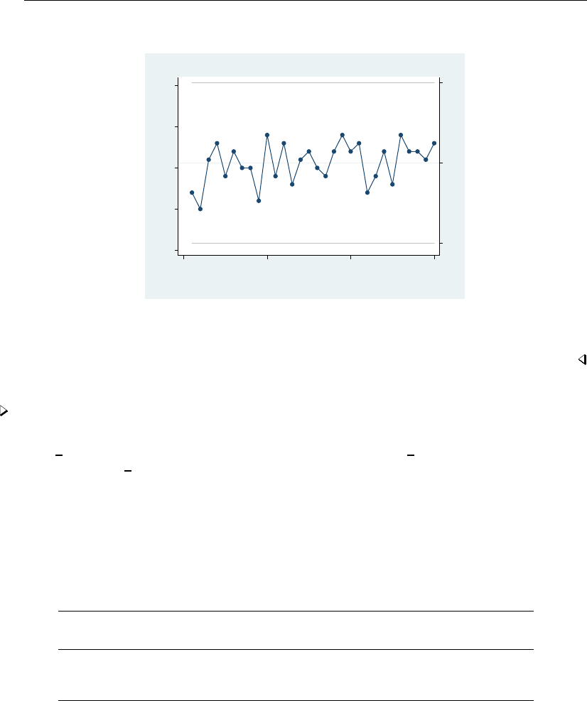
qc — Quality control charts 1751
. cchart defects day, title(c Chart for Nonconforming Transistors)
.8327076 10.6 20.36729
0 5 10 15 20
Numbers of Nonconforming Units
0 10 20 30
Days in April
0 units are out of control
c Chart for Nonconforming Transistors
The expected number of defects is 10.6, with lower and upper control limits of 0.8327 and 20.37,
respectively. No units are out of control.
Example 2: pchart
pchart graphs a p chart, which shows the fraction of nonconforming items in a subgroup, where
reject var records the number rejected in each inspection unit, unit var records the inspection unit
number, and ssize var records the number inspected in each unit.
Consider the example dataset from Ryan (2000, 156) of the number of nonconforming transistors
out of 1,000 inspected each day during the month of April:
. use http://www.stata-press.com/data/r13/ncu2
. describe
Contains data from http://www.stata-press.com/data/r13/ncu2.dta
obs: 30
vars: 3 31 Mar 2013 14:13
size: 360
storage display value
variable name type format label variable label
day float %9.0g Days in April
rejects float %9.0g Numbers of Nonconforming Units
ssize float %9.0g Sample size
Sorted by:
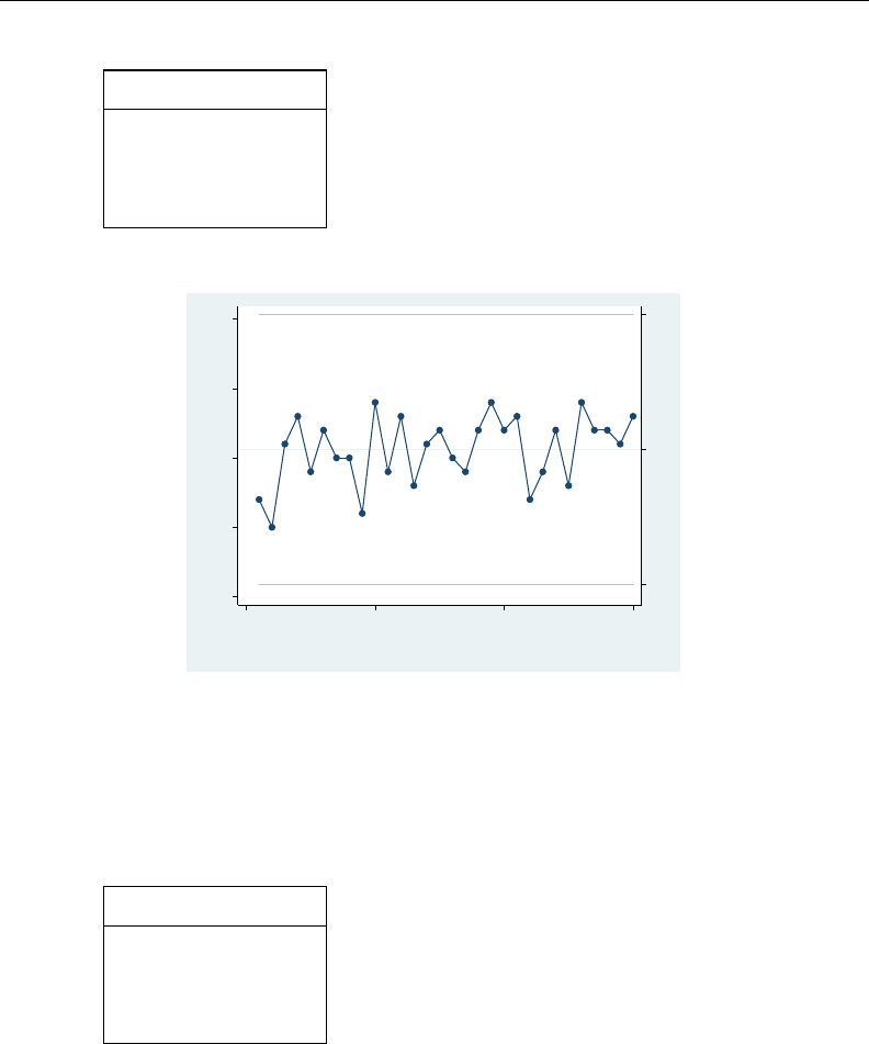
1752 qc — Quality control charts
. list in 1/5
day rejects ssize
1. 1 7 1000
2. 2 5 1000
3. 3 11 1000
4. 4 13 1000
5. 5 9 1000
. pchart rejects day ssize
.0008846 .0106 .0203154
0 .005 .01 .015 .02
Fraction defective
0 10 20 30
Days in April
0 units are out of control
All the points are within the control limits, which are 0.0009 for the lower limit and 0.0203 for the
upper limit.
Here the sample sizes are fixed at 1,000, so the ssize variable contains 1,000 for each observation.
Sample sizes need not be fixed, however. Say that our data were slightly different:
. use http://www.stata-press.com/data/r13/ncu3
. list in 1/5
day rejects ssize
1. 1 7 920
2. 2 5 920
3. 3 11 920
4. 4 13 950
5. 5 9 950
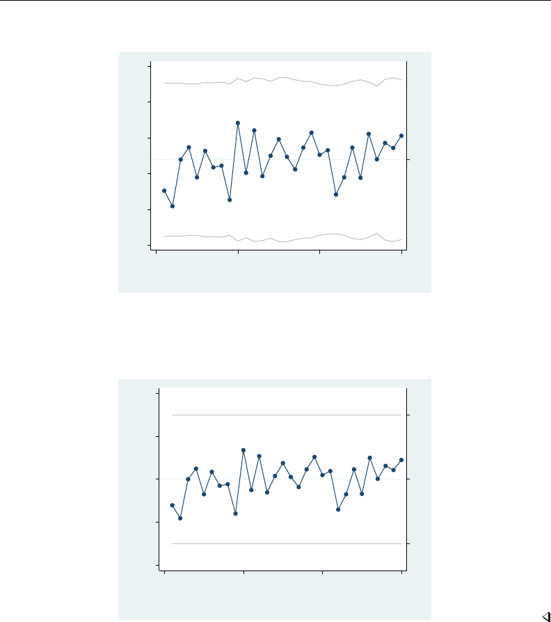
qc — Quality control charts 1753
. pchart rejects day ssize
.0119445
0 .005 .01 .015 .02 .025
Fraction defective
0 10 20 30
Days in April
0 units are out of control
Here the control limits are, like the sample size, no longer constant. The stabilize option will
stabilize the control chart:
. pchart rejects day ssize, stabilize
−3 0 3
−4 −2 0 2 4
Fraction defective
(Standard Deviation units)
0 10 20 30
Days in April
0 units are out of control
Stabilized p Chart, average number of defects = .0119
1754 qc — Quality control charts
Example 3: rchart
rchart displays an R chart showing the range for repeated measurements at various times.
Variables within observations record measurements. Observations represent different samples.
For instance, say that we take five samples of 5 observations each. In our first sample, our
measurements are 10, 11, 10, 11, and 12. The data are
. list
m1 m2 m3 m4 m5
1. 10 11 10 11 12
2. 12 10 9 10 9
3. 10 11 10 12 10
4. 9 9 9 10 11
5. 12 12 12 12 13
. rchart m1-m5, connect(l)
0 2 4.23
0 1 2 3 4
Range
1 2 3 4 5
Sample
0 units are out of control
The expected range in each sample is 2 with lower and upper control limits of 0 and 4.23, respectively.
If we know that the process standard deviation is 0.3, we could specify

qc — Quality control charts 1755
. rchart m1-m5, connect(l) std(.3)
−2.121525 .6978 2.721525
−2 −1 0 1 2 3
Range
1 2 3 4 5
Sample
1 unit is out of control
Example 4: xchart
xchart graphs an X chart for repeated measurements at various times. Variables within observations
record measurements, and observations represent different samples. Using the same data as in the
previous example, we type
. xchart m1-m5, connect(l)
9.486 10.64 11.794
9.5 10 10.5 11 11.5 12
Average
1 2 3 4 5
Sample
1 unit is out of control
The average measurement in the sample is 10.64, and the lower and upper control limits are 9.486
and 11.794, respectively. Suppose that we knew from prior information that the mean of the process
is 11. Then we would type
1756 qc — Quality control charts
. xchart m1-m5, connect(l) mean(11)
9.846 11 12.154
9.5 10 10.5 11 11.5 12
Average
1 2 3 4 5
Sample
2 units are out of control
If we also know that the standard deviation of the process is 0.3, we could type
. xchart m1-m5, connect(l) mean(11) std(.3)
10.59751 11 11.40249
9.5 10 10.5 11 11.5 12
Average
1 2 3 4 5
Sample
3 units are out of control
Finally, xchart allows us to specify our own control limits:
qc — Quality control charts 1757
. xchart m1-m5, connect(l) mean(11) lower(10) upper(12)
10 11 12
9.5 10 10.5 11 11.5 12
Average
1 2 3 4 5
Sample
2 units are out of control
Walter Andrew Shewhart (1891–1967) was born in Illinois and educated as a physicist, with
degrees from the Universities of Illinois and California. After a brief period teaching physics,
he worked for the Western Electric Company and (from 1925) the Bell Telephone Laboratories.
His name is most associated with control charts used in quality controls, but his many other
interests ranged generally from quality assurance to the philosophy of science.
Example 5: shewhart
shewhart displays a vertically aligned X and R chart in the same image. To produce the best-
looking combined image possible, you will want to use the xchart and rchart commands separately
and then combine the graphs. shewhart, however, is more convenient.
Using the same data as previously, but realizing that the standard deviation should have been 0.4,
we type

1758 qc — Quality control charts
. shewhart m1-m5, connect(l) mean(11) std(.4)
10.463341111.53666
9.5 10 10.5 11 11.5 12
Average
1 2 3 4 5
Sample
3 units are out of control
−2.8287 .9304 3.6287
−4 −2 0 2 4
Range
1 2 3 4 5
Sample
0 units are out of control
Stored results
cchart stores the following in r():
Scalars
r(cbar) expected number of nonconformities
r(lcl c) lower control limit
r(ucl c) upper control limit
r(N) number of observations
r(out c) number of units out of control
r(below c) number of units below the lower limit
r(above c) number of units above the upper limit
pchart stores the following in r():
Scalars
r(pbar) average fraction of nonconformities
r(lcl p) lower control limit
r(ucl p) upper control limit
r(N) number of observations
r(out p) number of units out of control
r(below p) number of units below the lower limit
r(above p) number of units above the upper limit
rchart stores the following in r():
Scalars
r(central line) ordinate of the central line
r(lcl r) lower control limit
r(ucl r) upper control limit
r(N) number of observations
r(out r) number of units out of control
r(below r) number of units below the lower limit
r(above r) number of units above the upper limit

qc — Quality control charts 1759
xchart stores the following in r():
Scalars
r(xbar) grand mean
r(lcl x) lower control limit
r(ucl x) upper control limit
r(N) number of observations
r(out x) number of units out of control
r(below x) number of units below the lower limit
r(above x) number of units above the upper limit
shewhart stores in r() the combination of stored results from xchart and rchart.
Methods and formulas
For the c chart, the number of defects per unit, C, is taken to be a value of a random variable
having a Poisson distribution. If kis the number of units available for estimating λ, the parameter
of the Poisson distribution, and if Ciis the number of defects in the ith unit, then λis estimated by
C=PiCi/k. Then
central line =C
UCL =C+ 3pC
LCL =C−3pC
Control limits for the p chart are based on the sampling theory for proportions, using the normal
approximation to the binomial. If ksamples are taken, the estimator of pis given by p=Pibpi/k,
where bpi=xi/ni, and xiis the number of defects in the ith sample of size ni. The central line and
the control limits are given by
central line =p
UCL =p+ 3pp(1 −p)/ni
LCL =p−3pp(1 −p)/ni
Control limits for the R chart are based on the distribution of the range of samples of size nfrom
a normal population. If the standard deviation of the process, σ, is known,
central line =d2σ
UCL =D2σ
LCL =D1σ
where d2,D1, and D2are functions of the number of observations in the sample and are obtained
from the table published in Beyer (1976).
When σis unknown,
central line =R
UCL = (D2/d2)R
LCL = (D1/d2)R
where R=PiRi/k is the range of the ksample ranges Ri.

1760 qc — Quality control charts
Control limits for the X chart are given by
central line =x
UCL =x+ (3/√n)σ
LCL =x−(3/√n)σ
if σis known. If σis unknown,
central line =x
UCL =x+A2R
LCL =x−A2R
where Ris the average range as defined above and A2is a function (op. cit.) of the number of
observations in the sample.
References
Bayart, D. 2001. Walter Andrew Shewhart. In Statisticians of the Centuries, ed. C. C. Heyde and E. Seneta, 398–401.
New York: Springer.
Beyer, W. H. 1976. Factors for computing control limits. In Vol. 2 of Handbook of Tables for Probability and
Statistics, ed. W. H. Beyer, 451–465. Cleveland, OH: The Chemical Rubber Company.
Burr, I. W. 1976. Statistical Quality Control Methods. New York: Dekker.
Caulcutt, R. 2004. Control charts in practice. Significance 1: 81–84.
Duncan, A. J. 1986. Quality Control and Industrial Statistics. 5th ed. Homewood, IL: Irwin.
Harris, R. L. 1999. Information Graphics: A Comprehensive Illustrated Reference. New York: Oxford University Press.
Ryan, T. P. 2000. Statistical Methods for Quality Improvement. 2nd ed. New York: Wiley.
Saw, S. L. C., and T. W. Soon. 1994. sqc1: Estimating process capability indices with Stata.Stata Technical Bulletin
17: 18–19. Reprinted in Stata Technical Bulletin Reprints, vol. 3, pp. 174–175. College Station, TX: Stata Press.
Shewhart, W. A. 1931. Economic Control of Quality of Manufactured Product. New York: Van Nostrand.
Also see
[R]serrbar — Graph standard error bar chart

Title
qreg — Quantile regression
Syntax Menu Description Options for qreg
Options for iqreg Options for sqreg Options for bsqreg Remarks and examples
Stored results Methods and formulas References Also see
Syntax
Quantile regression
qreg depvar indepvars if in weight ,qreg options
Interquantile range regression
iqreg depvar indepvars if in ,iqreg options
Simultaneous-quantile regression
sqreg depvar indepvars if in ,sqreg options
Bootstrapped quantile regression
bsqreg depvar indepvars if in ,bsqreg options
qreg options Description
Model
quantile(#)estimate #quantile; default is quantile(.5)
SE/Robust
vce(vcetype ,vceopts )technique used to estimate standard errors
Reporting
level(#)set confidence level; default is level(95)
display options control column formats, row spacing, line width, display of omitted
variables and base and empty cells, and factor-variable labeling
Optimization
optimization options control the optimization process; seldom used
wlsiter(#)attempt #weighted least-squares iterations before doing linear
programming iterations
vcetype Description
iid compute the VCE assuming the residuals are i.i.d.
robust compute the robust VCE
1761

1762 qreg — Quantile regression
vceopts Description
denmethod nonparametric density estimation technique
bwidth bandwidth method used by the density estimator
denmethod Description
fitted use the empirical quantile function using fitted values; the default
residual use the empirical residual quantile function
kernel(kernel)use a nonparametric kernel density estimator; default is
epanechnikov
bwidth Description
hsheather Hall–Sheather’s bandwidth; the default
bofinger Bofinger’s bandwidth
chamberlain Chamberlain’s bandwidth
kernel Description
epanechnikov Epanechnikov kernel function; the default
epan2 alternative Epanechnikov kernel function
biweight biweight kernel function
cosine cosine trace kernel function
gaussian Gaussian kernel function
parzen Parzen kernel function
rectangle rectangle kernel function
triangle triangle kernel function
iqreg options Description
Model
quantiles(# #)interquantile range; default is quantiles(.25 .75)
reps(#)perform #bootstrap replications; default is reps(20)
Reporting
level(#)set confidence level; default is level(95)
nodots suppress display of the replication dots
display options control column formats, row spacing, line width, display of omitted
variables and base and empty cells, and factor-variable labeling

qreg — Quantile regression 1763
sqreg options Description
Model
quantiles(###. . . )estimate #quantiles; default is quantiles(.5)
reps(#)perform #bootstrap replications; default is reps(20)
Reporting
level(#)set confidence level; default is level(95)
nodots suppress display of the replication dots
display options control column formats, row spacing, line width, display of omitted
variables and base and empty cells, and factor-variable labeling
bsqreg options Description
Model
quantile(#)estimate #quantile; default is quantile(.5)
reps(#)perform #bootstrap replications; default is reps(20)
Reporting
level(#)set confidence level; default is level(95)
display options control column formats, row spacing, line width, display of omitted
variables and base and empty cells, and factor-variable labeling
indepvars may contain factor variables; see [U] 11.4.3 Factor variables.
by,mi estimate,rolling, and statsby, are allowed by qreg,iqreg,sqreg, and bsqreg;mfp,nestreg, and
stepwise are allowed only with qreg; see [U] 11.1.10 Prefix commands.
qreg allows fweights, iweights, and pweights; see [U] 11.1.6 weight.
See [U] 20 Estimation and postestimation commands for more capabilities of estimation commands.
Menu
qreg
Statistics >Nonparametric analysis >Quantile regression
iqreg
Statistics >Nonparametric analysis >Interquantile regression
sqreg
Statistics >Nonparametric analysis >Simultaneous-quantile regression
bsqreg
Statistics >Nonparametric analysis >Bootstrapped quantile regression
Description
qreg fits quantile (including median) regression models, also known as least–absolute-value models
(LAV or MAD) and minimum L1-norm models. The quantile regression models fit by qreg express
the quantiles of the conditional distribution as linear functions of the independent variables.

1764 qreg — Quantile regression
iqreg estimates interquantile range regressions, regressions of the difference in quantiles. The
estimated variance–covariance matrix of the estimators (VCE) is obtained via bootstrapping.
sqreg estimates simultaneous-quantile regression. It produces the same coefficients as qreg for
each quantile. Reported standard errors will be similar, but sqreg obtains an estimate of the VCE
via bootstrapping, and the VCE includes between-quantile blocks. Thus you can test and construct
confidence intervals comparing coefficients describing different quantiles.
bsqreg is equivalent to sqreg with one quantile.
Options for qreg
Model
quantile(#)specifies the quantile to be estimated and should be a number between 0 and 1, exclusive.
Numbers larger than 1 are interpreted as percentages. The default value of 0.5 corresponds to the
median.
SE/Robust
vce(vcetype ,vceopts )specifies the type of VCE to compute and the density estimation method
to use in computing the VCE.
vcetype specifies the type of VCE to compute. Available types are iid and robust.
vce(iid), the default, computes the VCE under the assumption that the residuals are independent
and identically distributed (i.i.d.).
vce(robust) computes the robust VCE under the assumption that the residual density is contin-
uous and bounded away from 0 and infinity at the specified quantile(); see Koenker (2005,
sec. 4.2).
vceopts consists of available denmethod and bwidth options.
denmethod specifies the method to use for the nonparametric density estimator. Available
methods are fitted,residual, or kernel(kernel), where the optional kernel must be
one of the kernel choices listed below.
fitted and residual specify that the nonparametric density estimator use some of the
structure imposed by quantile regression. The default fitted uses a function of the fitted
values and residual uses a function of the residuals. vce(robust, residual) is not
allowed.
kernel() specifies that the nonparametric density estimator use a kernel method. The
available kernel functions are epanechnikov,epan2,biweight,cosine,gaussian,
parzen,rectangle, and triangle. The default is epanechnikov. See [R]kdensity
for the kernel function forms.
bwidth specifies the bandwidth method to use by the nonparametric density estimator. Available
methods are hsheather for the Hall–Sheather bandwidth, bofinger for the Bofinger
bandwidth, and chamberlain for the Chamberlain bandwidth.
See Koenker (2005, sec. 3.4 and 4.10) for a description of the sparsity estimation techniques
and the Hall–Sheather and Bofinger bandwidth formulas. See Chamberlain (1994, eq. 2.2) for the
Chamberlain bandwidth.
Reporting
level(#); see [R]estimation options.

qreg — Quantile regression 1765
display options:noomitted,vsquish,noemptycells,baselevels,allbaselevels,nofvla-
bel,fvwrap(#),fvwrapon(style),cformat(%fmt),pformat(% fmt),sformat(% fmt), and
nolstretch; see [R]estimation options.
Optimization
optimization options:iterate(#),nolog,trace.iterate() specifies the maximum number of
iterations; log/nolog specifies whether to show the iteration log; and trace specifies that the
iteration log should include the current parameter vector. These options are seldom used.
wlsiter(#)specifies the number of weighted least-squares iterations that will be attempted before
the linear programming iterations are started. The default value is 1. If there are convergence
problems, increasing this number should help.
Options for iqreg
Model
quantiles(# #)specifies the quantiles to be compared. The first number must be less than the
second, and both should be between 0 and 1, exclusive. Numbers larger than 1 are interpreted as
percentages. Not specifying this option is equivalent to specifying quantiles(.25 .75), meaning
the interquantile range.
reps(#)specifies the number of bootstrap replications to be used to obtain an estimate of the
variance–covariance matrix of the estimators (standard errors). reps(20) is the default and is
arguably too small. reps(100) would perform 100 bootstrap replications. reps(1000) would
perform 1,000 replications.
Reporting
level(#); see [R]estimation options.
nodots suppresses display of the replication dots.
display options:noomitted,vsquish,noemptycells,baselevels,allbaselevels,nofvla-
bel,fvwrap(#),fvwrapon(style),cformat(%fmt),pformat(% fmt),sformat(% fmt), and
nolstretch; see [R]estimation options.
Options for sqreg
Model
quantiles(###. . . )specifies the quantiles to be estimated and should contain numbers
between 0 and 1, exclusive. Numbers larger than 1 are interpreted as percentages. The default
value of 0.5 corresponds to the median.
reps(#)specifies the number of bootstrap replications to be used to obtain an estimate of the
variance–covariance matrix of the estimators (standard errors). reps(20) is the default and is
arguably too small. reps(100) would perform 100 bootstrap replications. reps(1000) would
perform 1,000 replications.
Reporting
level(#); see [R]estimation options.
nodots suppresses display of the replication dots.

1766 qreg — Quantile regression
display options:noomitted,vsquish,noemptycells,baselevels,allbaselevels,nofvla-
bel,fvwrap(#),fvwrapon(style),cformat(%fmt),pformat(% fmt),sformat(% fmt), and
nolstretch; see [R]estimation options.
Options for bsqreg
Model
quantile(#)specifies the quantile to be estimated and should be a number between 0 and 1, exclusive.
Numbers larger than 1 are interpreted as percentages. The default value of 0.5 corresponds to the
median.
reps(#)specifies the number of bootstrap replications to be used to obtain an estimate of the
variance–covariance matrix of the estimators (standard errors). reps(20) is the default and is
arguably too small. reps(100) would perform 100 bootstrap replications. reps(1000) would
perform 1,000 replications.
Reporting
level(#); see [R]estimation options.
display options:noomitted,vsquish,noemptycells,baselevels,allbaselevels,nofvla-
bel,fvwrap(#),fvwrapon(style),cformat(%fmt),pformat(% fmt),sformat(% fmt), and
nolstretch; see [R]estimation options.
Remarks and examples
Remarks are presented under the following headings:
Median regression
Quantile regression
Estimated standard errors
Interquantile and simultaneous-quantile regression
What are the parameters?
Median regression
qreg fits quantile regression models. The default form is median regression, where the objective is
to estimate the median of the dependent variable, conditional on the values of the independent variables.
This method is similar to ordinary regression, where the objective is to estimate the conditional mean
of the dependent variable. Simply put, median regression finds a line through the data that minimizes
the sum of the absolute residuals rather than the sum of the squares of the residuals, as in ordinary
regression. Equivalently, median regression expresses the median of the conditional distribution of
the dependent variable as a linear function of the conditioning (independent) variables. Cameron and
Trivedi (2010, chap. 7) provide a nice introduction to quantile regression using Stata.

qreg — Quantile regression 1767
Example 1: Estimating the conditional median
Consider a two-group experimental design with 5 observations per group:
. use http://www.stata-press.com/data/r13/twogrp
. list
x y
1. 0 0
2. 0 1
3. 0 3
4. 0 4
5. 0 95
6. 1 14
7. 1 19
8. 1 20
9. 1 22
10. 1 23
. qreg y x
Iteration 1: WLS sum of weighted deviations = 60.941342
Iteration 1: sum of abs. weighted deviations = 55.5
Iteration 2: sum of abs. weighted deviations = 55
Median regression Number of obs = 10
Raw sum of deviations 78.5 (about 14)
Min sum of deviations 55 Pseudo R2 = 0.2994
y Coef. Std. Err. t P>|t| [95% Conf. Interval]
x 17 18.23213 0.93 0.378 -25.04338 59.04338
_cons 3 12.89207 0.23 0.822 -26.72916 32.72916
We have estimated the equation
ymedian = 3 + 17 x
We look back at our data. xtakes on the values 0 and 1, so the median for the x=0 group is 3,
whereas for x=1 it is 3 +17 =20. The output reports that the raw sum of absolute deviations about
14 is 78.5; that is, the sum of |y−14|is 78.5. Fourteen is the unconditional median of y, although
in these data, any value between 14 and 19 could also be considered an unconditional median (we
have an even number of observations, so the median is bracketed by those two values). In any case,
the raw sum of deviations of yabout the median would be the same no matter what number we
choose between 14 and 19. (With a “median” of 14, the raw sum of deviations is 78.5. Now think
of choosing a slightly larger number for the median and recalculating the sum. Half the observations
will have larger negative residuals, but the other half will have smaller positive residuals, resulting in
no net change.)
We turn now to the actual estimated equation. The sum of the absolute deviations about the solution
ymedian =3+17xis 55. The pseudo-R2is calculated as 1 −55/78.5 ≈0.2994. This result is based
on the idea that the median regression is the maximum likelihood estimate for the double-exponential
distribution.

1768 qreg — Quantile regression
Technical note
qreg is an alternative to regular regression or robust regression—see [R]regress and [R]rreg.
Let’s compare the results:
. regress y x
Source SS df MS Number of obs = 10
F( 1, 8) = 0.00
Model 2.5 1 2.5 Prob > F = 0.9586
Residual 6978.4 8 872.3 R-squared = 0.0004
Adj R-squared = -0.1246
Total 6980.9 9 775.655556 Root MSE = 29.535
y Coef. Std. Err. t P>|t| [95% Conf. Interval]
x -1 18.6794 -0.05 0.959 -44.07477 42.07477
_cons 20.6 13.20833 1.56 0.157 -9.858465 51.05847
Unlike qreg,regress fits ordinary linear regression and is concerned with predicting the mean rather
than the median, so both results are, in a technical sense, correct. Putting aside those technicalities,
however, we tend to use either regression to describe the central tendency of the data, of which the
mean is one measure and the median another. Thus we can ask, “which method better describes the
central tendency of these data?”
Means—and therefore ordinary linear regression—are sensitive to outliers, and our data were
purposely designed to contain two such outliers: 95 for x=0 and 14 for x=1. These two outliers
dominated the ordinary regression and produced results that do not reflect the central tendency
well—you are invited to enter the data and graph yagainst x.
Robust regression attempts to correct the outlier-sensitivity deficiency in ordinary regression:
. rreg y x, genwt(wt)
Huber iteration 1: maximum difference in weights = .7311828
Huber iteration 2: maximum difference in weights = .17695779
Huber iteration 3: maximum difference in weights = .03149585
Biweight iteration 4: maximum difference in weights = .1979335
Biweight iteration 5: maximum difference in weights = .23332905
Biweight iteration 6: maximum difference in weights = .09960067
Biweight iteration 7: maximum difference in weights = .02691458
Biweight iteration 8: maximum difference in weights = .0009113
Robust regression Number of obs = 10
F( 1, 8) = 80.63
Prob > F = 0.0000
y Coef. Std. Err. t P>|t| [95% Conf. Interval]
x 18.16597 2.023114 8.98 0.000 13.50066 22.83128
_cons 2.000003 1.430558 1.40 0.200 -1.298869 5.298875
Here rreg discarded the first outlier completely. (We know this because we included the genwt()
option on rreg and, after fitting the robust regression, examined the weights.) For the other “outlier”,
rreg produced a weight of 0.47.
In any case, the answers produced by qreg and rreg to describe the central tendency are similar,
but the standard errors are different. In general, robust regression will have smaller standard errors
because it is not as sensitive to the exact placement of observations near the median. You are welcome
to try removing the first outlier in the qreg estimation to observe an improvement in the standard
errors by typing

qreg — Quantile regression 1769
. qreg y x if _n!=5
Also, some authors (Rousseeuw and Leroy 1987, 11) have noted that quantile regression, unlike the
unconditional median, may be sensitive to even one outlier if its leverage is high enough. Rousseeuw
and Leroy (1987) discuss estimators that are more robust to perturbations to the data than either mean
regression or quantile regression.
In the end, quantile regression may be more useful for the interpretation of the parameters that it
estimates than for its robustness to perturbations to the data.
Example 2: Median regression
Let’s now consider a less artificial example using the automobile data described in [U] 1.2.2 Example
datasets. Using median regression, we will regress each car’s price on its weight and length and
whether it is of foreign manufacture:
. use http://www.stata-press.com/data/r13/auto, clear
(1978 Automobile Data)
. qreg price weight length foreign
Iteration 1: WLS sum of weighted deviations = 56397.829
Iteration 1: sum of abs. weighted deviations = 55950.5
Iteration 2: sum of abs. weighted deviations = 55264.718
Iteration 3: sum of abs. weighted deviations = 54762.283
Iteration 4: sum of abs. weighted deviations = 54734.152
Iteration 5: sum of abs. weighted deviations = 54552.638
note: alternate solutions exist
Iteration 6: sum of abs. weighted deviations = 54465.511
Iteration 7: sum of abs. weighted deviations = 54443.699
Iteration 8: sum of abs. weighted deviations = 54411.294
Median regression Number of obs = 74
Raw sum of deviations 71102.5 (about 4934)
Min sum of deviations 54411.29 Pseudo R2 = 0.2347
price Coef. Std. Err. t P>|t| [95% Conf. Interval]
weight 3.933588 1.328718 2.96 0.004 1.283543 6.583632
length -41.25191 45.46469 -0.91 0.367 -131.9284 49.42456
foreign 3377.771 885.4198 3.81 0.000 1611.857 5143.685
_cons 344.6489 5182.394 0.07 0.947 -9991.31 10680.61
The estimated equation is
pricemedian =3.93 weight −41.25 length +3377.8 foreign +344.65
The output may be interpreted in the same way as linear regression output; see [R]regress. The
variables weight and foreign are significant, but length is not significant. The median price of
the cars in these data is $4,934. This value is a median (one of the two center observations), not the
median, which would typically be defined as the midpoint of the two center observations.

1770 qreg — Quantile regression
Quantile regression
Quantile regression is similar to median regression in that it estimates an equation expressing a
quantile of the conditional distribution, albeit one that generally differs from the 0.5 quantile that is
the median. For example, specifying quantile(.25) estimates the parameters that describe the 25th
percentile (first quartile) of the conditional distribution.
Quantile regression allows for effects of the independent variables to differ over the quantiles. For
example, Chamberlain (1994) finds that union membership has a larger effect on the lower quantiles
than on the higher quantiles of the conditional distribution of U.S. wages. That the effects of the
independent variables may vary over quantiles of the conditional distribution is an important advantage
of quantile regression over mean regression.
Example 3: Estimating quantiles other than the median
Returning to real data, the equation for the 25th percentile of price conditional on weight,
length, and foreign in our automobile data is
. use http://www.stata-press.com/data/r13/auto
(1978 Automobile Data)
. qreg price weight length foreign, quantile(.25)
Iteration 1: WLS sum of weighted deviations = 49469.235
Iteration 1: sum of abs. weighted deviations = 49728.883
Iteration 2: sum of abs. weighted deviations = 45669.89
Iteration 3: sum of abs. weighted deviations = 43416.646
Iteration 4: sum of abs. weighted deviations = 41947.221
Iteration 5: sum of abs. weighted deviations = 41093.025
Iteration 6: sum of abs. weighted deviations = 37623.424
Iteration 7: sum of abs. weighted deviations = 35721.453
Iteration 8: sum of abs. weighted deviations = 35226.308
Iteration 9: sum of abs. weighted deviations = 34823.319
Iteration 10: sum of abs. weighted deviations = 34801.777
.25 Quantile regression Number of obs = 74
Raw sum of deviations 41912.75 (about 4187)
Min sum of deviations 34801.78 Pseudo R2 = 0.1697
price Coef. Std. Err. t P>|t| [95% Conf. Interval]
weight 1.831789 .6328903 2.89 0.005 .5695289 3.094049
length 2.84556 21.65558 0.13 0.896 -40.34514 46.03626
foreign 2209.925 421.7401 5.24 0.000 1368.791 3051.059
_cons -1879.775 2468.46 -0.76 0.449 -6802.963 3043.413
Compared with our previous median regression, the coefficient on length now has a positive sign,
and the coefficients on foreign and weight are reduced. The actual lower quantile is $4,187,
substantially less than the median $4,934.

qreg — Quantile regression 1771
We can also estimate the upper quartile as a function of the same three variables:
. qreg price weight length foreign, quantile(.75)
Iteration 1: WLS sum of weighted deviations = 55465.741
Iteration 1: sum of abs. weighted deviations = 55652.957
Iteration 2: sum of abs. weighted deviations = 52994.785
Iteration 3: sum of abs. weighted deviations = 50189.446
Iteration 4: sum of abs. weighted deviations = 49898.245
Iteration 5: sum of abs. weighted deviations = 49398.106
Iteration 6: sum of abs. weighted deviations = 49241.835
Iteration 7: sum of abs. weighted deviations = 49197.967
.75 Quantile regression Number of obs = 74
Raw sum of deviations 79860.75 (about 6342)
Min sum of deviations 49197.97 Pseudo R2 = 0.3840
price Coef. Std. Err. t P>|t| [95% Conf. Interval]
weight 9.22291 1.785767 5.16 0.000 5.66131 12.78451
length -220.7833 61.10352 -3.61 0.001 -342.6504 -98.91616
foreign 3595.133 1189.984 3.02 0.004 1221.785 5968.482
_cons 20242.9 6965.02 2.91 0.005 6351.61 34134.2
This result tells a different story: weight is much more important, and length is now significant—with
a negative coefficient! The prices of high-priced cars seem to be determined by factors different from
those affecting the prices of low-priced cars.
Technical note
One explanation for having substantially different regression functions for different quantiles is
that the data are heteroskedastic, as we will demonstrate below. The following statements create a
sharply heteroskedastic set of data:
. drop _all
. set obs 10000
obs was 0, now 10000
. set seed 50550
. gen x = .1 + .9 * runiform()
. gen y = x * runiform()^2

1772 qreg — Quantile regression
Let’s now fit the regressions for the 5th and 95th quantiles:
. qreg y x, quantile(.05)
Iteration 1: WLS sum of weighted deviations = 540.36365
Iteration 1: sum of abs. weighted deviations = 539.15959
Iteration 2: sum of abs. weighted deviations = 141.36772
Iteration 3: sum of abs. weighted deviations = 91.234609
Iteration 4: sum of abs. weighted deviations = 91.127281
Iteration 5: sum of abs. weighted deviations = 91.126351
Iteration 6: sum of abs. weighted deviations = 91.126236
Iteration 7: sum of abs. weighted deviations = 91.126229
Iteration 8: sum of abs. weighted deviations = 91.126224
Iteration 9: sum of abs. weighted deviations = 91.126221
.05 Quantile regression Number of obs = 10000
Raw sum of deviations 91.17849 (about .0009234)
Min sum of deviations 91.12622 Pseudo R2 = 0.0006
y Coef. Std. Err. t P>|t| [95% Conf. Interval]
x .002601 .0004576 5.68 0.000 .001704 .003498
_cons -.0001393 .0002782 -0.50 0.617 -.0006846 .000406
. qreg y x, quantile(.95)
Iteration 1: WLS sum of weighted deviations = 618.77845
Iteration 1: sum of abs. weighted deviations = 619.00068
Iteration 2: sum of abs. weighted deviations = 228.32522
Iteration 3: sum of abs. weighted deviations = 169.22749
Iteration 4: sum of abs. weighted deviations = 169.21949
Iteration 5: sum of abs. weighted deviations = 169.21945
.95 Quantile regression Number of obs = 10000
Raw sum of deviations 277.3444 (about .61326343)
Min sum of deviations 169.2194 Pseudo R2 = 0.3899
y Coef. Std. Err. t P>|t| [95% Conf. Interval]
x .8898259 .0090984 97.80 0.000 .8719912 .9076605
_cons .0021514 .0055307 0.39 0.697 -.00869 .0129927
The coefficient on x, in particular, differs markedly between the two estimates. For the mathematically
inclined, it is not too difficult to show that the theoretical lines are y=0.0025 xfor the 5th percentile
and y=0.9025 xfor the 95th, numbers in close agreement with our numerical results.
The estimator for the standard errors computed by qreg assumes that the sample is independent
and identically distributed (i.i.d.); see Estimated standard errors and Methods and formulas for details.
Because the data are conditionally heteroskedastic, we should have used bsqreg to consistently
estimate the standard errors using a bootstrap method.
Estimated standard errors
The variance–covariance matrix of the estimator (VCE) depends on the reciprocal of the density
of the dependent variable evaluated at the quantile of interest. This function, known as the “sparsity
function”, is hard to estimate.

qreg — Quantile regression 1773
The default method, which uses the fitted values for the predicted quantiles, generally performs
well, but other methods may be preferred in larger samples. The vce() suboptions denmethod and
bwidth provide other estimators of the sparsity function, the details of which are described in Methods
and formulas.
For models with heteroskedastic errors, option vce(robust) computes a Huber (1967) form
of sandwich estimate (Koenker 2005). Alternatively, Gould (1992,1997b) introduced generalized
versions of qreg that obtain estimates of the standard errors by using bootstrap resampling (see Efron
and Tibshirani [1993] or Wu [1986] for an introduction to bootstrap standard errors). The iqreg,
sqreg, and bsqreg commands provide a bootstrapped estimate of the entire variance–covariance
matrix of the estimators.
Example 4: Obtaining robust standard errors
Example 2 of qreg on real data above was a median regression of price on weight,length, and
foreign using auto.dta. Suppose, after investigation, we are convinced that car price observations
are not independent. We decide that standard errors robust to non-i.i.d. errors would be appropriate
and use the option vce(robust).
. use http://www.stata-press.com/data/r13/auto, clear
(1978 Automobile Data)
. qreg price weight length foreign, vce(robust)
Iteration 1: WLS sum of weighted deviations = 56397.829
Iteration 1: sum of abs. weighted deviations = 55950.5
Iteration 2: sum of abs. weighted deviations = 55264.718
Iteration 3: sum of abs. weighted deviations = 54762.283
Iteration 4: sum of abs. weighted deviations = 54734.152
Iteration 5: sum of abs. weighted deviations = 54552.638
note: alternate solutions exist
Iteration 6: sum of abs. weighted deviations = 54465.511
Iteration 7: sum of abs. weighted deviations = 54443.699
Iteration 8: sum of abs. weighted deviations = 54411.294
Median regression Number of obs = 74
Raw sum of deviations 71102.5 (about 4934)
Min sum of deviations 54411.29 Pseudo R2 = 0.2347
Robust
price Coef. Std. Err. t P>|t| [95% Conf. Interval]
weight 3.933588 1.694477 2.32 0.023 .55406 7.313116
length -41.25191 51.73571 -0.80 0.428 -144.4355 61.93171
foreign 3377.771 728.5115 4.64 0.000 1924.801 4830.741
_cons 344.6489 5096.528 0.07 0.946 -9820.055 10509.35
We see that the robust standard error for weight increases making it less significant in modifying
the median automobile price. The standard error for length also increases, but the standard error
for the foreign indicator decreases.

1774 qreg — Quantile regression
For comparison, we repeat the estimation using bootstrap standard errors:
. use http://www.stata-press.com/data/r13/auto, clear
(1978 Automobile Data)
. set seed 1001
. bsqreg price weight length foreign
(fitting base model)
Bootstrap replications (20)
12345
....................
Median regression, bootstrap(20) SEs Number of obs = 74
Raw sum of deviations 71102.5 (about 4934)
Min sum of deviations 54411.29 Pseudo R2 = 0.2347
price Coef. Std. Err. t P>|t| [95% Conf. Interval]
weight 3.933588 3.12446 1.26 0.212 -2.297951 10.16513
length -41.25191 83.71267 -0.49 0.624 -208.2116 125.7077
foreign 3377.771 1057.281 3.19 0.002 1269.09 5486.452
_cons 344.6489 7053.301 0.05 0.961 -13722.72 14412.01
The coefficient estimates are the same—indeed, they are obtained using the same technique. Only
the standard errors differ. Therefore, the tstatistics, significance levels, and confidence intervals also
differ.
Because bsqreg (as well as sqreg and iqreg) obtains standard errors by randomly resampling
the data, the standard errors it produces will not be the same from run to run unless we first set the
random-number seed to the same number; see [R]set seed.

qreg — Quantile regression 1775
By default, bsqreg,sqreg, and iqreg use 20 replications. We can control the number of
replications by specifying the reps() option:
. bsqreg price weight length i.foreign, reps(1000)
(fitting base model)
Bootstrap replications (1000)
12345
.................................................. 50
.................................................. 100
.................................................. 150
.................................................. 200
.................................................. 250
.................................................. 300
.................................................. 350
.................................................. 400
.................................................. 450
.................................................. 500
.................................................. 550
.................................................. 600
.................................................. 650
.................................................. 700
.................................................. 750
.................................................. 800
.................................................. 850
.................................................. 900
.................................................. 950
.................................................. 1000
Median regression, bootstrap(1000) SEs Number of obs = 74
Raw sum of deviations 71102.5 (about 4934)
Min sum of deviations 54411.29 Pseudo R2 = 0.2347
price Coef. Std. Err. t P>|t| [95% Conf. Interval]
weight 3.933588 2.659381 1.48 0.144 -1.370379 9.237555
length -41.25191 69.29771 -0.60 0.554 -179.4618 96.95802
foreign
Foreign 3377.771 1094.264 3.09 0.003 1195.331 5560.211
_cons 344.6489 5916.906 0.06 0.954 -11456.25 12145.55
A comparison of the standard errors is informative.
qreg bsqreg bsqreg
Variable qreg vce(robust) reps(20) reps(1000)
weight 1.329 1.694 3.124 2.660
length 45.46 51.74 83.71 69.30
1.foreign 885.4 728.5 1057. 1094.
cons 5182. 5096. 7053. 5917.
The results shown above are typical for models with heteroskedastic errors. (Our dependent variable
is price; if our model had been in terms of ln(price), the standard errors estimated by qreg and
bsqreg would have been nearly identical.) Also, even for heteroskedastic errors, 20 replications is
generally sufficient for hypothesis tests against 0.

1776 qreg — Quantile regression
Interquantile and simultaneous-quantile regression
Consider a quantile regression model where the qth quantile is given by
Qq(y) = aq+bq,1x1+bq,2x2
For instance, the 75th and 25th quantiles are given by
Q0.75(y) = a0.75 +b0.75,1x1+b0.75,2x2
Q0.25(y) = a0.25 +b0.25,1x1+b0.25,2x2
The difference in the quantiles is then
Q0.75(y)−Q0.25(y) = (a0.75 −a0.25)+(b0.75,1−b0.25,1)x1+ (b0.75,2−b0.25,2)x2
qreg fits models such as Q0.75(y)and Q0.25(y).iqreg fits interquantile models, such as Q0.75(y)−
Q0.25(y). The relationships of the coefficients estimated by qreg and iqreg are exactly as shown:
iqreg reports coefficients that are the difference in coefficients of two qreg models, and, of course,
iqreg reports the appropriate standard errors, which it obtains by bootstrapping.
sqreg is like qreg in that it estimates the equations for the quantiles
Q0.75(y) = a0.75 +b0.75,1x1+b0.75,2x2
Q0.25(y) = a0.25 +b0.25,1x1+b0.25,2x2
The coefficients it obtains are the same that would be obtained by estimating each equation separately
using qreg.sqreg differs from qreg in that it estimates the equations simultaneously and obtains
an estimate of the entire variance–covariance matrix of the estimators by bootstrapping. Thus you
can perform hypothesis tests concerning coefficients both within and across equations.
For example, to fit the above model, you could type
. qreg y x1 x2, quantile(.25)
. qreg y x1 x2, quantile(.75)
By doing this, you would obtain estimates of the parameters, but you could not test whether
b0.25,1=b0.75,1or, equivalently, b0.75,1−b0.25,1=0. If your interest really is in the difference of
coefficients, you could type
. iqreg y x1 x2, quantiles(.25 .75)
The “coefficients” reported would be the difference in quantile coefficients. You could also estimate
both quantiles simultaneously and then test the equality of the coefficients:
. sqreg y x1 x2, quantiles(.25 .75)
. test [q25]x1 = [q75]x1
Whether you use iqreg or sqreg makes no difference for this test. sqreg, however, because it
estimates the quantiles simultaneously, allows you to test other hypotheses. iqreg, by focusing on
quantile differences, presents results in a way that is easier to read.
Finally, sqreg can estimate quantiles singly,
. sqreg y x1 x2, quantiles(.5)
and can thereby be used as a substitute for the slower bsqreg. (Gould [1997b] presents timings
demonstrating that sqreg is faster than bsqreg.) sqreg can also estimate more than two quantiles
simultaneously:
. sqreg y x1 x2, quantiles(.25 .5 .75)

qreg — Quantile regression 1777
Example 5: Simultaneous quantile estimation
In demonstrating qreg, we performed quantile regressions using auto.dta. We discovered that
the regression of price on weight,length, and foreign produced vastly different coefficients for
the 0.25, 0.5, and 0.75 quantile regressions. Here are the coefficients that we obtained:
25th 50th 75th
Variable percentile percentile percentile
weight 1.83 3.93 9.22
length 2.85 −41.25 −220.8
foreign 2209.9 3377.8 3595.1
cons −1879.8 344.6 20242.9
All we can say, having estimated these equations separately, is that price seems to depend differently
on the weight,length, and foreign variables depending on the portion of the price distribution
we examine. We cannot be more precise because the estimates have been made separately. With
sqreg, however, we can estimate all the effects simultaneously:
. use http://www.stata-press.com/data/r13/auto, clear
(1978 Automobile Data)
. set seed 1001
. sqreg price weight length foreign, q(.25 .5 .75) reps(100)
(fitting base model)
Bootstrap replications (100)
12345
.................................................. 50
.................................................. 100
Simultaneous quantile regression Number of obs = 74
bootstrap(100) SEs .25 Pseudo R2 = 0.1697
.50 Pseudo R2 = 0.2347
.75 Pseudo R2 = 0.3840
Bootstrap
price Coef. Std. Err. t P>|t| [95% Conf. Interval]
q25
weight 1.831789 1.574777 1.16 0.249 -1.309005 4.972583
length 2.84556 38.63523 0.07 0.941 -74.20998 79.9011
foreign 2209.925 1008.521 2.19 0.032 198.494 4221.357
_cons -1879.775 3665.184 -0.51 0.610 -9189.753 5430.204
q50
weight 3.933588 2.529541 1.56 0.124 -1.111423 8.978599
length -41.25191 68.62258 -0.60 0.550 -178.1153 95.61151
foreign 3377.771 1025.882 3.29 0.002 1331.715 5423.827
_cons 344.6489 6199.257 0.06 0.956 -12019.38 12708.68
q75
weight 9.22291 2.483676 3.71 0.000 4.269374 14.17645
length -220.7833 86.17422 -2.56 0.013 -392.6524 -48.91421
foreign 3595.133 1145.124 3.14 0.002 1311.255 5879.011
_cons 20242.9 9414.242 2.15 0.035 1466.79 39019.02
The coefficient estimates above are the same as those previously estimated, although the standard error
estimates are a little different. sqreg obtains estimates of variance by bootstrapping. The important
thing here, however, is that the full covariance matrix of the estimators has been estimated and stored,
and thus it is now possible to perform hypothesis tests. Are the effects of weight the same at the
25th and 75th percentiles?

1778 qreg — Quantile regression
. test [q25]weight = [q75]weight
( 1) [q25]weight - [q75]weight = 0
F( 1, 70) = 8.97
Prob > F = 0.0038
It appears that they are not. We can obtain a confidence interval for the difference by using lincom:
. lincom [q75]weight-[q25]weight
( 1) - [q25]weight + [q75]weight = 0
price Coef. Std. Err. t P>|t| [95% Conf. Interval]
(1) 7.391121 2.467548 3.00 0.004 2.469752 12.31249
Indeed, we could test whether the weight and length sets of coefficients are equal at the three
quantiles estimated:
. quietly test [q25]weight = [q50]weight
. quietly test [q25]weight = [q75]weight, accumulate
. quietly test [q25]length = [q50]length, accumulate
. test [q25]length = [q75]length, accumulate
( 1) [q25]weight - [q50]weight = 0
( 2) [q25]weight - [q75]weight = 0
( 3) [q25]length - [q50]length = 0
( 4) [q25]length - [q75]length = 0
F( 4, 70) = 2.43
Prob > F = 0.0553
iqreg focuses on one quantile comparison but presents results that are more easily interpreted:
. set seed 1001
. iqreg price weight length foreign, q(.25 .75) reps(100) nolog
.75-.25 Interquantile regression Number of obs = 74
bootstrap(100) SEs .75 Pseudo R2 = 0.3840
.25 Pseudo R2 = 0.1697
Bootstrap
price Coef. Std. Err. t P>|t| [95% Conf. Interval]
weight 7.391121 2.467548 3.00 0.004 2.469752 12.31249
length -223.6288 83.09868 -2.69 0.009 -389.3639 -57.89376
foreign 1385.208 1191.018 1.16 0.249 -990.2036 3760.619
_cons 22122.68 9009.159 2.46 0.017 4154.478 40090.88
Looking only at the 0.25 and 0.75 quantiles (the interquartile range), the iqreg command output
is easily interpreted. Increases in weight correspond significantly to increases in price dispersion.
Increases in length correspond to decreases in price dispersion. The foreign variable does not
significantly change price dispersion.
Do not make too much of these results; the purpose of this example is simply to illustrate the
sqreg and iqreg commands and to do so in a context that suggests why analyzing dispersion might
be of interest.

qreg — Quantile regression 1779
lincom after sqreg produced the same tstatistic for the interquartile range of weight, as did
the iqreg command above. In general, they will not agree exactly because of the randomness of
bootstrapping, unless the random-number seed is set to the same value before estimation (as was
done here).
Gould (1997a) presents simulation results showing that the coverage—the actual percentage of
confidence intervals containing the true value— for iqreg is appropriate.
What are the parameters?
In this section, we use a specific data-generating process (DGP) to illustrate the interpretation of the
parameters estimated by qreg. If simulation experiments are not intuitive to you, skip this section.
In general, quantile regression parameterizes the quantiles of the distribution of yconditional on
the independent variables xas xβ, where βis a vector of estimated parameters. In our example, we
include a constant term and a single independent variable, and we express quantiles of the distribution
of yconditional on xas β0+β1x.
We use simulated data to illustrate what we mean by a conditional distribution and how to interpret
the parameters βestimated by qreg. We also note how we could change our example to illustrate a
DGP for which the estimator in qreg would be misspecified.
We suppose that the distribution of yconditional on xhas a Weibull form. If yhas a Weibull
distribution, the distribution function is F(y) = 1−exp{−(y/λ)k}, where the scale parameter λ > 0
and the shape parameter k > 0. We can make yhave a Weibull distribution function conditional on
xby making the scale parameter or the shape parameter functions of x. In our example, we specify
a particular DGP by supposing that λ= (1+αx),α=1.5, x=1+√ν, and that νhas a χ2(1)
distribution. For the moment, we leave the parameter kas is so that we can discuss how this decision
relates to model specification.
Plugging in for λyields the functional form for the distribution of yconditional on x, which is
known as the conditional distribution function and is denoted F(y|x).F(y|x)is the distribution for
yfor each given value of x.
Some algebra yields that F(y|x) = 1−exp[−{y/(1+αx)}k]. Letting τ=F(y|x)implies that
0≤τ≤1, because probabilities must be between 0 and 1.
To obtain the τquantile of the distribution of yconditional on x, we solve
τ= 1 −exp[−{y/(1 + αx)}k]
for yas a function of τ,x,α, and k. The solution is
y= (1 + αx){−ln(1 −τ)}(1/k)(1)
For any value of τ∈(0,1), expression (1) gives the τquantile of the distribution of yconditional
on x. To use qreg, we must rewrite (1) as a function of x,β0, and β1. Some algebra yields that (1)
can be rewritten as
y=β0+β1∗x
where β0={−ln(1−τ)}(1/k)and β1=α{−ln(1−τ)}(1/k). We can express the conditional
quantiles as linear combinations of x, which is a property of the estimator implemented in qreg.

1780 qreg — Quantile regression
If we parameterize kas a nontrivial function of x, the conditional quantiles will not be linear
in x. If the conditional quantiles cannot be represented as linear functions of x, we cannot estimate
the true parameters of the DGP. This restriction illustrates the limits of the estimator implemented in
qreg.
We set k=2 for our example.
Conditional quantile regression allows the coefficients to change with the specified quantile. For
our DGP, the coefficients β0and β1increase as τgets larger. Substituting in for αand kyields that
β0=p−ln(1−τ)and β1=1.5p−ln(1−τ). Table 1 presents the true values for β0and β1
implied by our DGP when τ∈ {0.25,0.5,0.8}.
Table 1: True values for β0and β1
τ β0β1
0.25 0.53636 0.80454
0.5 0.8325546 1.248832
0.8 1.268636 1.902954
We can also use (1) to generate data from the specified distribution of yconditional on xby
plugging in random uniform numbers for τ. Each random uniform number substituted in for τin (1)
yields a draw from the conditional distribution of ygiven x.
Example 6
In this example, we generate 100,000 observations from our specified DGP by substituting random
uniform numbers for τin (1), with α=1.5, k=2, x=1+√ν, and νcoming from a χ2(1)
distribution.
We begin by executing the code that implements this method; below we discuss each line of the
output produced.
. clear // drop existing variables
. set seed 1234571 // set random-number seed
. set obs 100000 // set number of observations
obs was 0, now 100000
. generate double tau = runiform() // generate uniform variate
. generate double x = 1 + sqrt(rchi2(1)) // generate values for x
. generate double lambda = 1 + 1.5*x // lambda is 1 + alpha*x
. generate double k = 2 // fix value of k
. // generate random values for y
. // given x
. generate double y = lambda*((-ln(1-tau))^(1/k))
Although the comments at the end of each line briefly describe what each line is doing, we provide
a more careful description. The first line drops any variables in memory. The second sets the seed
of the random-number generator so that we will always get the same sequence of random uniform
numbers. The third line sets the sample size to 100,000 observations, and the fourth line reports the
change in sample size.
The fifth line substitutes random uniform numbers for τ. This line is the key to the algorithm.
This standard method, known as inverse-probability transforms, for computing random numbers is
discussed by Cameron and Trivedi (2010, 126–127), among others.

qreg — Quantile regression 1781
Lines 6–8 generate x,λ, and kper our specified DGP. Lines 9–11 implement (1) using the
previously generated λ,x, and k.
At the end, we have 100,000 observations on yand x, with ycoming from the conditional
distribution that we specified above.
Example 7
In the example below, we use qreg to estimate β1and β0, the parameters from the conditional
quantile function, for the 0.5 quantile from our simulated data.
. qreg y x, quantile(.5)
Iteration 1: WLS sum of weighted deviations = 68975.517
Iteration 1: sum of abs. weighted deviations = 68975.325
Iteration 2: sum of abs. weighted deviations = 68843.958
Iteration 3: sum of abs. weighted deviations = 68629.64
Iteration 4: sum of abs. weighted deviations = 68626.382
Iteration 5: sum of abs. weighted deviations = 68625.659
Iteration 6: sum of abs. weighted deviations = 68625.657
Iteration 7: sum of abs. weighted deviations = 68625.657
Median regression Number of obs = 100000
Raw sum of deviations 73840.51 (about 2.944248)
Min sum of deviations 68625.66 Pseudo R2 = 0.0706
y Coef. Std. Err. t P>|t| [95% Conf. Interval]
x 1.228536 .0118791 103.42 0.000 1.205253 1.251819
_cons .8693355 .0225288 38.59 0.000 .8251793 .9134917
In the qreg output, the results for xcorrespond to the estimate of β1, and the results for cons
correspond to the estimate of β0. The reported estimates are close to their true values of 1.248832
and 0.8325546, which are given in table 1.
The intuition in this example comes from the ability of qreg to recover the true parameters of
our specified DGP. As we increase the number of observations in our sample size, the qreg estimates
will get closer to the true values.

1782 qreg — Quantile regression
Example 8
In the example below, we estimate the parameters of the conditional quantile function for the 0.25
quantile and compare them with the true values.
. qreg y x, quantile(.25)
Iteration 1: WLS sum of weighted deviations = 65497.284
Iteration 1: sum of abs. weighted deviations = 65492.359
Iteration 2: sum of abs. weighted deviations = 60139.477
Iteration 3: sum of abs. weighted deviations = 49999.793
Iteration 4: sum of abs. weighted deviations = 49999.479
Iteration 5: sum of abs. weighted deviations = 49999.465
Iteration 6: sum of abs. weighted deviations = 49999.465
.25 Quantile regression Number of obs = 100000
Raw sum of deviations 52014.79 (about 1.857329)
Min sum of deviations 49999.47 Pseudo R2 = 0.0387
y Coef. Std. Err. t P>|t| [95% Conf. Interval]
x .7844305 .0107092 73.25 0.000 .7634405 .8054204
_cons .5633285 .0203102 27.74 0.000 .5235209 .6031362
As above, qreg reports the estimates of β1and β0in the output table for xand cons, respectively.
The reported estimates are close to their true values of 0.80454 and 0.53636, which are given in
table 1. As expected, the estimates are close to their true values. Also as expected, the estimates for
the 0.25 quantile are smaller than the estimates for the 0.5 quantile.

qreg — Quantile regression 1783
Example 9
We finish this section by estimating the parameters of the conditional quantile function for the 0.8
quantile and comparing them with the true values.
. qreg y x, quantile(.8)
Iteration 1: WLS sum of weighted deviations = 66332.299
Iteration 1: sum of abs. weighted deviations = 66332.194
Iteration 2: sum of abs. weighted deviations = 60076.645
Iteration 3: sum of abs. weighted deviations = 52589.193
Iteration 4: sum of abs. weighted deviations = 52340.961
Iteration 5: sum of abs. weighted deviations = 52262.505
Iteration 6: sum of abs. weighted deviations = 52249.305
Iteration 7: sum of abs. weighted deviations = 52245.124
Iteration 8: sum of abs. weighted deviations = 52245.103
Iteration 9: sum of abs. weighted deviations = 52245.081
Iteration 10: sum of abs. weighted deviations = 52245.075
Iteration 11: sum of abs. weighted deviations = 52245.074
Iteration 12: sum of abs. weighted deviations = 52245.073
Iteration 13: sum of abs. weighted deviations = 52245.073
Iteration 14: sum of abs. weighted deviations = 52245.073
Iteration 15: sum of abs. weighted deviations = 52245.073
.8 Quantile regression Number of obs = 100000
Raw sum of deviations 60093.34 (about 4.7121822)
Min sum of deviations 52245.07 Pseudo R2 = 0.1306
y Coef. Std. Err. t P>|t| [95% Conf. Interval]
x 1.889702 .0146895 128.64 0.000 1.860911 1.918493
_cons 1.293773 .0278587 46.44 0.000 1.23917 1.348375
As above, qreg reports the estimates of β1and β0in the output table for xand cons, respectively.
The reported estimates are close to their true values of 1.902954 and 1.268636, which are given in
table 1. As expected, the estimates are close to their true values. Also as expected, the estimates for
the 0.8 quantile are larger than the estimates for the 0.5 quantile.

1784 qreg — Quantile regression
Stored results
qreg stores the following in e():
Scalars
e(N) number of observations
e(df m) model degrees of freedom
e(df r) residual degrees of freedom
e(q) quantile requested
e(q v) value of the quantile
e(sum adev) sum of absolute deviations
e(sum rdev) sum of raw deviations
e(sum w) sum of weights
e(f r) density estimate
e(sparsity) sparsity estimate
e(bwidth) bandwidth
e(kbwidth) kernel bandwidth
e(rank) rank of e(V)
e(convcode) 0 if converged; otherwise, return code for why nonconvergence
Macros
e(cmd) qreg
e(cmdline) command as typed
e(depvar) name of dependent variable
e(bwmethod) bandwidth method; hsheather,bofinger, or chamberlain
e(denmethod) density estimation method; fitted,residual, or kernel
e(kernel) kernel function
e(wtype) weight type
e(wexp) weight expression
e(vce) vcetype specified in vce()
e(vcetype) title used to label Std. Err.
e(properties) b V
e(predict) program used to implement predict
e(marginsnotok) predictions disallowed by margins
Matrices
e(b) coefficient vector
e(V) variance–covariance matrix of the estimators
Functions
e(sample) marks estimation sample

qreg — Quantile regression 1785
iqreg stores the following in e():
Scalars
e(N) number of observations
e(df r) residual degrees of freedom
e(q0) lower quantile requested
e(q1) upper quantile requested
e(reps) number of replications
e(sumrdev0) lower quantile sum of raw deviations
e(sumrdev1) upper quantile sum of raw deviations
e(sumadev0) lower quantile sum of absolute deviations
e(sumadev1) upper quantile sum of absolute deviations
e(rank) rank of e(V)
e(convcode) 0 if converged; otherwise, return code for why nonconvergence
Macros
e(cmd) iqreg
e(cmdline) command as typed
e(depvar) name of dependent variable
e(vcetype) title used to label Std. Err.
e(properties) b V
e(predict) program used to implement predict
e(marginsnotok) predictions disallowed by margins
Matrices
e(b) coefficient vector
e(V) variance–covariance matrix of the estimators
Functions
e(sample) marks estimation sample
sqreg stores the following in e():
Scalars
e(N) number of observations
e(df r) residual degrees of freedom
e(n q) number of quantiles requested
e(q#)the quantiles requested
e(reps) number of replications
e(sumrdv#)sum of raw deviations for q#
e(sumadv#)sum of absolute deviations for q#
e(rank) rank of e(V)
e(convcode) 0 if converged; otherwise, return code for why nonconvergence
Macros
e(cmd) sqreg
e(cmdline) command as typed
e(depvar) name of dependent variable
e(eqnames) names of equations
e(vcetype) title used to label Std. Err.
e(properties) b V
e(predict) program used to implement predict
e(marginsnotok) predictions disallowed by margins
Matrices
e(b) coefficient vector
e(V) variance–covariance matrix of the estimators
Functions
e(sample) marks estimation sample

1786 qreg — Quantile regression
bsqreg stores the following in e():
Scalars
e(N) number of observations
e(df r) residual degrees of freedom
e(q) quantile requested
e(q v) value of the quantile
e(reps) number of replications
e(sum adev) sum of absolute deviations
e(sum rdev) sum of raw deviations
e(rank) rank of e(V)
e(convcode) 0 if converged; otherwise, return code for why nonconvergence
Macros
e(cmd) bsqreg
e(cmdline) command as typed
e(depvar) name of dependent variable
e(properties) b V
e(predict) program used to implement predict
e(marginsnotok) predictions disallowed by margins
Matrices
e(b) coefficient vector
e(V) variance–covariance matrix of the estimators
Functions
e(sample) marks estimation sample
Methods and formulas
Methods and formulas are presented under the following headings:
Introduction
Linear programming formulation of quantile regression
Standard errors when residuals are i.i.d.
Pseudo-R2
Introduction
According to Stuart and Ord (1991, 1084), the method of minimum absolute deviations was first
proposed by Boscovich in 1757 and was later developed by Laplace; Stigler (1986, 39–55) and
Hald (1998, 97–103, 112–116) provide historical details. According to Bloomfield and Steiger (1980),
Harris (1950) later observed that the problem of minimum absolute deviations could be turned into the
linear programming problem that was first implemented by Wagner (1959). Interest has grown in this
method because robust methods and extreme value modeling have become more popular. Statistical
and computational properties of minimum absolute deviation estimators are surveyed by Narula and
Wellington (1982). Cameron and Trivedi (2005), Hao and Naiman (2007), and Wooldridge (2010)
provide excellent introductions to quantile regression methods, while Koenker (2005) gives an in-depth
review of the topic.
Linear programming formulation of quantile regression
Define τas the quantile to be estimated; the median is τ=0.5. For each observation i, let εibe
the residual
εi=yi−x0
ib
βτ

qreg — Quantile regression 1787
The objective function to be minimized is
cτ(εi)=(τ1{εi≥0}+ (1 −τ)1{εi<0})|εi|
= (τ1{εi≥0} − (1 −τ)1{εi<0})εi
= (τ−1{εi<0})εi
(2)
where 1{·} is the indicator function. This function is sometimes referred to as the check function
because it resembles a check mark (Wooldridge 2010, 450); the slope of cτ(εi)is τwhen εi>0
and is τ−1 when εi<0, but is undefined for εi=0. Choosing the b
βτthat minimize cτ(εi)is
equivalent to finding the b
βτthat make xb
βτbest fit the quantiles of the distribution of yconditional
on x.
This minimization problem is set up as a linear programming problem and is solved with linear
programming techniques, as suggested by Armstrong, Frome, and Kung (1979) and described in detail
by Koenker (2005). Here 2nslack variables, un×1and vn×1, are introduced, where ui≥0, vi≥0,
and ui×vi=0, reformulating the problem as
min
βτ,u,v{τ10
nu+ (1 −τ)10
nv|y−Xβτ=u−v}
where 1nis a vector of 1s. This is a linear objective function on a polyhedral constraint set with n
k
vertices, and our goal is to find the vertex that minimizes (2). Each step in the search is described by
a set of kobservations through which the regression plane passes, called the basis. A step is taken
by replacing a point in the basis if the linear objective function can be improved. If this occurs, a
line is printed in the iteration log. The definition of convergence is exact in the sense that no amount
of added iterations could improve the objective function.
A series of weighted least-squares (WLS) regressions is used to identify a set of observations
as a starting basis. The WLS algorithm for τ=0.5 is taken from Schlossmacher (1973) with a
generalization for 0 < τ < 1 implied from Hunter and Lange (2000).
Standard errors when residuals are i.i.d.
The estimator for the VCE implemented in qreg assumes that the errors of the model are independent
and identically distributed (i.i.d.). When the errors are i.i.d., the large-sample VCE is
cov(βτ) = τ(1 −τ)
f2
Y(ξτ){E(xix0
i)}−1(3)
where ξτ=F−1
Y(τ)and FY(y)is the distribution function of Ywith density fY(y). See
Koenker (2005, 73) for this result. From (3), we see that the regression precision depends on
the inverse of the density function, termed the sparsity function, sτ=1/fY(ξτ).
While 1/n Pn
i=1 xix0
iestimates E(xix0
i), estimating the sparsity function is more difficult. qreg
provides several methods to estimate the sparsity function. The different estimators are specified
through the suboptions of vce(iid, denmethod bwidth). The suboption denmethod specifies the
functional form for the sparsity estimator. The default is fitted.
Here we outline the logic underlying the fitted estimator. Because FY(y)is the distribution
function for Y, we have fY(y) = {dFy(y)}/dy,τ=FY(ξτ), and ξτ=F−1
Y(τ). When differen-
tiating the identity FY{F−1
Y(τ)}=τ, the sparsity function can be written as sτ={F−1
Y(τ)}/dt.
Numerically, we can approximate the derivative using the centered difference,

1788 qreg — Quantile regression
F−1
Y(τ)
dt ≈F−1
Y(τ+h)−F−1
Y(τ−h)
2h=ξτ+h−ξτ−h
2h=bsτ(4)
where his the bandwidth.
The empirical quantile function is computed by first estimating βτ+hand βτ−h, and then computing
b
F−1
Y(τ+h) = x0b
βτ+hand b
F−1
Y(τ−h) = x0b
βτ−h, where xis the sample mean of the independent
variables x. These quantities are then substituted into (4).
Alternatively, as the option suggests, vce(iid, residual) specifies that qreg use the empirical
quantile function of the residuals to estimate the sparsity. Here we substitute F, the distribution of
the residuals, for FY, which only differ by their first moments.
The kresiduals associated with the linear programming basis will be zero, where kis the number
of regression coefficients. These zero residuals are removed before computing the τ+hand τ−h
quantiles, ε(τ+h)=b
F−1
(τ+h)and ε(τ−h)=b
F−1
(τ−h). The b
F−1
estimates are then substituted
for F−1
Yin (4).
Each of the estimators for the sparsity function depends on a bandwidth. The vce() suboption bwidth
specifies the bandwidth method to use. The three bandwidth options and their citations are hsheather
(Hall and Sheather 1988), bofinger (Bofinger 1975), and chamberlain (Chamberlain 1994).
Their formulas are
hs=n−1/3Φ−11−α
22/33
2×φ{Φ−1(τ)}4
2Φ−1(τ)2+ 11/3
hb=n−1/59
2φ{2Φ−1(τ)}4
{2Φ−1(τ)2+ 1}21/5
hc= Φ−11−α
2rτ(1 −τ)
n
where hsis the Hall–Sheather bandwidth, hbis the Bofinger bandwidth, hcis the Chamberlain
bandwidth, Φ() and φ() are the standard normal distribution and density functions, nis the sample
size, and 100(1−α)is the confidence level set by the level() option. Koenker (2005) discusses the
derivation of the Hall–Sheather and the Bofinger bandwidth formulas. You should avoid modifying
the confidence level when replaying estimates that use the Hall–Sheather or Chamberlain bandwidths
because these methods use the confidence level to estimate the coefficient standard errors.
Finally, the vce() suboption kernel(kernel)specifies that qreg use one of several kernel-density
estimators to estimate the sparsity function. kernel allows you to choose which kernel function to
use, where the default is the Epanechnikov kernel. See [R]kdensity for the functional form of the
eight kernels.
The kernel bandwidth is computed using an adaptive estimate of scale
hk= min bσ, rq
1.34×Φ−1(τ+h)−Φ−1(τ−h)
where his one of hs,hb, or hc;rqis the interquartile range; and bσis the standard deviation of y;
see Silverman (1992, 47) and Koenker (2005, 81) for discussions. Let b
f(εi)be the kernel density
estimate for the ith residual, and then the kernel estimator for the sparsity function is
bsτ=nhk
Pn
i=1 b
f(εi)

qreg — Quantile regression 1789
Finally, substituting your choice of sparsity estimate into (3) results in the i.i.d. variance–covariance
matrix
Vn=bs2
ττ(1 −τ) n
X
i=1
xix0
i!−1
Pseudo-R2
The pseudo-R2is calculated as
1−sum of weighted deviations about estimated quantile
sum of weighted deviations about raw quantile
This is based on the likelihood for a double-exponential distribution evi|εi|, where viare multipliers
vi=2τif εi>0
2(1 −τ)otherwise
Minimizing the objective function (2) with respect to βτalso minimizes Pi|εi|vi, the sum of
weighted least absolute deviations. For example, for the 50th percentile vi=1, for all i, and we
have median regression. If we want to estimate the 75th percentile, we weight the negative residuals
by 0.50 and the positive residuals by 1.50. It can be shown that the criterion is minimized when 75%
of the residuals are negative.
References
Angrist, J. D., and J.-S. Pischke. 2009. Mostly Harmless Econometrics: An Empiricist’s Companion. Princeton, NJ:
Princeton University Press.
Armstrong, R. D., E. L. Frome, and D. S. Kung. 1979. Algorithm 79-01: A revised simplex algorithm for the absolute
deviation curve fitting problem. Communications in Statistics—Simulation and Computation 8: 175–190.
Bloomfield, P., and W. Steiger. 1980. Least absolute deviations curve-fitting. SIAM Journal on Scientific Computing
1: 290–301.
Bofinger, E. 1975. Estimation of a density function using order statistics. Australian Journal of Statistics 17: 1–17.
Cameron, A. C., and P. K. Trivedi. 2005. Microeconometrics: Methods and Applications. New York: Cambridge
University Press.
. 2010. Microeconometrics Using Stata. Rev. ed. College Station, TX: Stata Press.
Chamberlain, G. 1994. Quantile regression, censoring, and the structure of wages. In Advances in Econometrics,
Vol. 1: Sixth World Congress, ed. C. A. Sims, 171–209. Cambridge: Cambridge University Press.
Efron, B., and R. J. Tibshirani. 1993. An Introduction to the Bootstrap. New York: Chapman & Hall/CRC.
Fr¨
olich, M., and B. Melly. 2010. Estimation of quantile treatment effects with Stata.Stata Journal 10: 423–457.
Gould, W. W. 1992. sg11.1: Quantile regression with bootstrapped standard errors.Stata Technical Bulletin 9: 19–21.
Reprinted in Stata Technical Bulletin Reprints, vol. 2, pp. 137–139. College Station, TX: Stata Press.
. 1997a. crc46: Better numerical derivatives and integrals.Stata Technical Bulletin 35: 3–5. Reprinted in Stata
Technical Bulletin Reprints, vol. 6, pp. 8–12. College Station, TX: Stata Press.
. 1997b. sg70: Interquantile and simultaneous-quantile regression.Stata Technical Bulletin 38: 14–22. Reprinted
in Stata Technical Bulletin Reprints, vol. 7, pp. 167–176. College Station, TX: Stata Press.
Gould, W. W., and W. H. Rogers. 1994. Quantile regression as an alternative to robust regression. In 1994 Proceedings
of the Statistical Computing Section. Alexandria, VA: American Statistical Association.

1790 qreg — Quantile regression
Hald, A. 1998. A History of Mathematical Statistics from 1750 to 1930. New York: Wiley.
Hall, P., and S. J. Sheather. 1988. On the distribution of a Studentized quantile. Journal of the Royal Statistical
Society, Series B 50: 381–391.
Hao, L., and D. Q. Naiman. 2007. Quantile Regression. Thousand Oaks, CA: Sage.
Harris, T. 1950. Regression using minimum absolute deviations. American Statistician 4: 14–15.
Huber, P. J. 1967. The behavior of maximum likelihood estimates under nonstandard conditions. In Vol. 1 of Proceedings
of the Fifth Berkeley Symposium on Mathematical Statistics and Probability, 221–233. Berkeley: University of
California Press.
. 1981. Robust Statistics. New York: Wiley.
Hunter, D. R., and K. Lange. 2000. Quantile regression via an MM algorithm. Journal of Computational and Graphical
Statistics 9: 60–77.
Jolliffe, D., B. Krushelnytskyy, and A. Semykina. 2000. sg153: Censored least absolute deviations estimator: CLAD.
Stata Technical Bulletin 58: 13–16. Reprinted in Stata Technical Bulletin Reprints, vol. 10, pp. 240–244. College
Station, TX: Stata Press.
Koenker, R. 2005. Quantile Regression. New York: Cambridge University Press.
Koenker, R., and K. Hallock. 2001. Quantile regression. Journal of Economic Perspectives 15: 143–156.
Narula, S. C., and J. F. Wellington. 1982. The minimum sum of absolute errors regression: A state of the art survey.
International Statistical Review 50: 317–326.
Orsini, N., and M. Bottai. 2011. Logistic quantile regression in Stata.Stata Journal 11: 327–344.
Rousseeuw, P. J., and A. M. Leroy. 1987. Robust Regression and Outlier Detection. New York: Wiley.
Schlossmacher, E. J. 1973. An iterative technique for absolute deviations curve fitting. Journal of the American
Statistical Association 68: 857–859.
Silverman, B. W. 1992. Density Estimation for Statistics and Data Analysis. London: Chapman & Hall.
Stigler, S. M. 1986. The History of Statistics: The Measurement of Uncertainty before 1900. Cambridge, MA: Belknap
Press.
Stuart, A., and J. K. Ord. 1991. Kendall’s Advanced Theory of Statistics: Distribution Theory, Vol I. 5th ed. New
York: Oxford University Press.
Wagner, H. M. 1959. Linear programming techniques for regression analysis. Journal of the American Statistical
Association 54: 206–212.
Wooldridge, J. M. 2010. Econometric Analysis of Cross Section and Panel Data. 2nd ed. Cambridge, MA: MIT Press.
Wu, C. F. J. 1986. Jackknife, bootstrap and other resampling methods in regression analysis. Annals of Statistics 14:
1261–1350 (including discussions and rejoinder).
Also see
[R]qreg postestimation — Postestimation tools for qreg, iqreg, sqreg, and bsqreg
[R]bootstrap — Bootstrap sampling and estimation
[R]regress — Linear regression
[R]rreg — Robust regression
[MI]estimation — Estimation commands for use with mi estimate
[U] 20 Estimation and postestimation commands

Title
qreg postestimation — Postestimation tools for qreg, iqreg, sqreg, and bsqreg
Description Syntax for predict Menu for predict Options for predict
Remarks and examples Also see
Description
The following postestimation commands are available after qreg,iqreg,bsqreg, and sqreg:
Command Description
estat summarize summary statistics for the estimation sample
estat vce variance–covariance matrix of the estimators (VCE)
estimates cataloging estimation results
forecast1dynamic forecasts and simulations
lincom point estimates, standard errors, testing, and inference for linear combinations
of coefficients
linktest link test for model specification
margins marginal means, predictive margins, marginal effects, and average marginal
effects
marginsplot graph the results from margins (profile plots, interaction plots, etc.)
nlcom point estimates, standard errors, testing, and inference for nonlinear combinations
of coefficients
predict predictions, residuals, influence statistics, and other diagnostic measures
predictnl point estimates, standard errors, testing, and inference for generalized predictions
test Wald tests of simple and composite linear hypotheses
testnl Wald tests of nonlinear hypotheses
1forecast is not appropriate with mi estimation results.
1791

1792 qreg postestimation — Postestimation tools for qreg, iqreg, sqreg, and bsqreg
Syntax for predict
For qreg, iqreg, and bsqreg
predict type newvar if in ,xb |stdp |residuals
For sqreg
predict type newvar if in , equation(eqno,eqno )statistic
statistic Description
Main
xb linear prediction; the default
stdp standard error of the linear prediction
stddp standard error of the difference in linear predictions
residuals residuals
These statistics are available both in and out of sample; type predict . . . if e(sample) . . . if wanted
only for the estimation sample.
Menu for predict
Statistics >Postestimation >Predictions, residuals, etc.
Options for predict
Main
xb, the default, calculates the linear prediction.
stdp calculates the standard error of the linear prediction.
stddp is allowed only after you have fit a model using sqreg. The standard error of the difference
in linear predictions (x1jb−x2jb)between equations 1 and 2 is calculated.
residuals calculates the residuals, that is, yj−xjb.
equation(eqno,eqno )specifies the equation to which you are making the calculation.
equation() is filled in with one eqno for the xb,stdp, and residuals options. equation(#1)
would mean that the calculation is to be made for the first equation, equation(#2) would mean
the second, and so on. You could also refer to the equations by their names. equation(income)
would refer to the equation named income and equation(hours) to the equation named hours.
If you do not specify equation(), results are the same as if you had specified equation(#1).
To use stddp, you must specify two equations. You might specify equation(#1, #2) or
equation(q80, q20) to indicate the 80th and 20th quantiles.
qreg postestimation — Postestimation tools for qreg, iqreg, sqreg, and bsqreg 1793
Remarks and examples
Example 1
In example 4 of [R]qreg, we fit regressions for the lower and the upper quartile of the price
variable. The predict command can be used to obtain the linear prediction after each regression.
. use http://www.stata-press.com/data/r13/auto
(1978 Automobile Data)
. qreg price weight length foreign, quantile(.25)
(output omitted )
. predict q25
(option xb assumed; fitted values)
. qreg price weight length foreign, quantile(.75)
(output omitted )
. predict q75
(option xb assumed; fitted values)
We can use the variables generated by predict to compute the predicted interquartile range, that
is,
. generate iqr1 = q75 - q25
If we directly perform the interquartile range regression with the iqreg command, we can predict
the interquartile range and also the standard error for the prediction.
. iqreg price weight length foreign, quantile(.25 .75)
(output omitted )
. predict iqr2
(option xb assumed; fitted values)
. predict stdp, stdp
We now plot the predicted interquartile range versus variable length:
. scatter iqr2 length
0 2000 4000 6000 8000
Linear prediction
140 160 180 200 220 240
Length (in.)
As stated in example 5 of [R]qreg, the negative coefficient for the length variable means
that increases in length imply decreases in the interquartile range and therefore in price dispersion.
Consequently, we could have expected a downward trend in the plot, but there is not. This is because
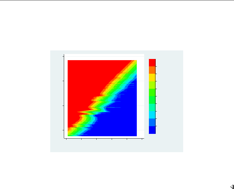
1794 qreg postestimation — Postestimation tools for qreg, iqreg, sqreg, and bsqreg
the regression output indicates that when we hold the rest of the variables constant, an increase
in length leads to a decrease in iqr2. However, there is a high correlation between weight and
length, which could be masking the effect of length on iqr2. We can achieve a better visualization
by using a contour plot.
. twoway contour iqr2 weight length, level(10)
2,000 3,000 4,000 5,000
Weight (lbs.)
140 160 180 200 220 240
Length (in.)
309.766
1,187.6
2,065.4
2,943.3
3,821.1
4,699
5,576.8
6,454.6
7,332.5
Linear prediction
We can see the effect by setting a fixed value of length on the vertical axis, say, 3,000 lbs.
When we move from left to right on the horizontal axis, we see that for small values of length,
iqr2 values are shown in red, meaning high values, and when we move toward the right, the graph
indicates transition into increasingly smaller values.
Also see
[R]qreg — Quantile regression
[U] 20 Estimation and postestimation commands

Title
query — Display system parameters
Syntax Description Remarks and examples Also see
Syntax
query memory |output |interface |graphics |efficiency |network |
update |trace |mata |other
Description
query displays the settings of various Stata parameters.
Remarks and examples
query provides more system information than you will ever want to know. You do not need to
understand every line of output that query produces if all you need is one piece of information. Here
is what happens when you type query:
. query
Memory settings
set maxvar 5000 2048-32767; max. vars allowed
set matsize 400 10-11000; max. # vars in models
set niceness 5 0-10
set min_memory 0 0-1600g
set max_memory . 32m-1600g or .
set segmentsize 32m 1m-32g
Output settings
set more on
set rmsg off
set dp period may be period or comma
set linesize 80 characters
set pagesize 28 lines
set level 95 percent confidence intervals
set showbaselevels may be empty, off, on, or all
set showemptycells may be empty, off, or on
set showomitted may be empty, off, or on
set fvlabel on
set fvwrap 1
set fvwrapon word may be word or width
set lstretch may be empty, off, or on
set cformat may be empty or a numerical format
set pformat may be empty or a numerical format
set sformat may be empty or a numerical format
1795

1796 query — Display system parameters
set coeftabresults on
set logtype smcl may be smcl or text
Interface settings
set dockable on
set dockingguides on
set floatwindows off
set locksplitters off
set pinnable on
set doublebuffer on
set linegap 1 pixels
set scrollbufsize 204800 characters
set fastscroll on
set varlabelpos (not relevant)
set reventries 5000 lines
set maxdb 50 dialog boxes
Graphics settings
set graphics on
set autotabgraphs off
set scheme s2color
set printcolor automatic may be automatic, asis, gs1, gs2, gs3
set copycolor automatic may be automatic, asis, gs1, gs2, gs3
Efficiency settings
set adosize 1000 kilobytes
Network settings
set checksum off
set timeout1 30 seconds
set timeout2 180 seconds
set httpproxy off
set httpproxyhost
set httpproxyport 80
set httpproxyauth off
set httpproxyuser
set httpproxypw
Update settings
set update_query on
set update_interval 7
set update_prompt on
Trace (programming debugging) settings
set trace off
set tracedepth 32000
set traceexpand on
set tracesep on
set traceindent on
set tracenumber off
set tracehilite

query — Display system parameters 1797
Mata settings
set matastrict off
set matalnum off
set mataoptimize on
set matafavor space may be space or speed
set matacache 400 kilobytes
set matalibs lmatabase;lmataado;lmatafc;lmatagsem;lmataopt;
> lmatapath;lmatapss;lmatasem
set matamofirst off
Other settings
set type float may be float or double
set maxiter 16000 max iterations for estimation commands
set searchdefault all may be local, net, or all
set seed X075bcd151f123bb5159a55e50022865700043e55
set varabbrev on
set emptycells keep may be keep or drop
set processors 2 1-2
set haverdir
The output is broken into several divisions: memory, output, interface, graphics, efficiency, network,
update, trace, mata, and other settings. We will discuss each one in turn.
We generated the output above using Stata/MP for Windows. Here is what happens when we type
query and we are running Stata/SE for Mac:
. query
Memory settings
set maxvar 5000 2048-32767; max. vars allowed
set matsize 400 10-11000; max. # vars in models
set niceness 5 0-10
set min_memory 0 0-1600g
set max_memory . 32m-1600g or .
set segmentsize 32m 1m-32g
Output settings
set more off
set rmsg off
set dp period may be period or comma
set linesize 80 characters
set pagesize 23 lines
set level 95 percent confidence intervals
set showbaselevels may be empty, off, on, or all
set showemptycells may be empty, off, or on
set showomitted may be empty, off, or on
set fvlabel on
set fvwrap 1
set fvwrapon word may be word or width
set lstretch may be empty, off, or on
set cformat may be empty or a numerical format
set pformat may be empty or a numerical format
set sformat may be empty or a numerical format
set coeftabresults on
set logtype smcl may be smcl or text

1798 query — Display system parameters
set charset mac may be or
set eolchar unix may be mac or unix
set notifyuser on
set playsnd off
set include_bitmap on
Interface settings
set revkeyboard on
set varkeyboard on
set smoothfonts on
set linegap 1 pixels
set scrollbufsize 204800 characters
set varlabelpos (not relevant)
set reventries 5000 lines
set maxdb 50 dialog boxes
Graphics settings
set graphics on
set scheme s2color
set printcolor automatic may be automatic, asis, gs1, gs2, gs3
set copycolor automatic may be automatic, asis, gs1, gs2, gs3
Efficiency settings
set adosize 1000 kilobytes
Network settings
set checksum off
set timeout1 30 seconds
set timeout2 180 seconds
set httpproxy off
set httpproxyhost
set httpproxyport 80
set httpproxyauth off
set httpproxyuser
set httpproxypw
Update settings
set update_query on
set update_interval 7
set update_prompt on
Trace (programming debugging) settings
set trace off
set tracedepth 32000
set traceexpand on
set tracesep on
set traceindent on
set tracenumber off
set tracehilite

query — Display system parameters 1799
Mata settings
set matastrict off
set matalnum off
set mataoptimize on
set matafavor space may be space or speed
set matacache 400 kilobytes
set matalibs lmatabase;lmataado;lmatafc;lmatagsem;lmataopt;
> lmatapath;lmatapss;lmatasem
set matamofirst off
Other settings
set type float may be float or double
set maxiter 16000 max iterations for estimation commands
set searchdefault local may be local, net, or all
set seed X075bcd151f123bb5159a55e50022865700043e55
set varabbrev on
set emptycells keep may be keep or drop
set processors 1
Memory settings
Memory settings indicate how memory is allocated, the maximum number of variables, and the
maximum size of a matrix.
For more information, see
maxvar [D]memory
matsize [R]matsize
niceness [D]memory
min memory [D]memory
max memory [D]memory
segmentsize [D]memory
Output settings
Output settings show how Stata displays output on the screen and in log files.
For more information, see
more [R]more
rmsg [P]rmsg
dp [D]format
linesize [R]log
pagesize [R]more
level [R]level
showbaselevels [R]set showbaselevels
showemptycells [R]set showbaselevels
showomitted [R]set showbaselevels
fvlabel [R]set showbaselevels
fvwrap [R]set showbaselevels
fvwrapon [R]set showbaselevels
cformat [R]set cformat
pformat [R]set cformat
sformat [R]set cformat

1800 query — Display system parameters
coeftabresults [R]set
lstretch [R]set
logtype [R]log
charset [R]set
eolchar [R]set
notifyuser [R]set
playsnd [R]set
include bitmap [R]set
Interface settings
Interface settings control how Stata’s interface works.
For more information, see
dockable [R]set
dockingguides [R]set
floatwindows [R]set
locksplitters [R]set
pinnable [R]set
doublebuffer [R]set
revkeyboard [R]set
varkeyboard [R]set
smoothfonts [R]set
linegap [R]set
scrollbufsize [R]set
fastscroll [R]set
reventries [R]set
maxdb [R]db
Graphics settings
Graphics settings indicate how Stata’s graphics are displayed.
For more information, see
graphics [G-2]set graphics
autotabgraphs [R]set
scheme [G-2]set scheme
printcolor [G-2]set printcolor
copycolor [G-2]set printcolor
Efficiency settings
The efficiency settings set the maximum amount of memory allocated to automatically loaded
do-files, the maximum number of remembered-contents dialog boxes, and the use of virtual memory.
For more information, see
adosize [P]sysdir

query — Display system parameters 1801
Network settings
Network settings determine how Stata interacts with the Internet.
For more information, see [R]netio.
Update settings
Update settings determine how Stata performs updates.
For more information, see [R]update.
Trace settings
Trace settings adjust Stata’s behavior and are particularly useful in debugging code.
For more information, see [P]trace.
Mata settings
Mata settings affect Mata’s system parameters.
For more information, see [M-3]mata set.
Other settings
The other settings are a miscellaneous collection.
For more information, see
type [D]generate
maxiter [R]maximize
searchdefault [R]search
seed [R]set seed
varabbrev [R]set
emptycells [R]set
processors [R]set
odbcmgr [D]odbc
haverdir [D]import haver
In general, the parameters displayed by query can be changed by set; see [R]set.
Also see
[R]set — Overview of system parameters
[P]creturn — Return c-class values
[M-3]mata set — Set and display Mata system parameters

Title
ranksum — Equality tests on unmatched data
Syntax Menu Description Options for ranksum
Options for median Remarks and examples Stored results Methods and formulas
References Also see
Syntax
Wilcoxon rank-sum test
ranksum varname if in , by(groupvar)porder
Nonparametric equality-of-medians test
median varname if in weight , by(groupvar)median options
ranksum options Description
Main
∗by(groupvar)grouping variable
porder probability that variable for first group is larger than variable for
second group
median options Description
Main
∗by(groupvar)grouping variable
exact perform Fisher’s exact test
medianties(below) assign values equal to the median to below group
medianties(above) assign values equal to the median to above group
medianties(drop) drop values equal to the median from the analysis
medianties(split) split values equal to the median equally between the two groups
∗by(groupvar)is required.
by is allowed with ranksum and median; see [D] by.
fweights are allowed with median; see [U] 11.1.6 weight.
Menu
ranksum
Statistics >Nonparametric analysis >Tests of hypotheses >Wilcoxon rank-sum test
median
Statistics >Nonparametric analysis >Tests of hypotheses >K-sample equality-of-medians test
1802

ranksum — Equality tests on unmatched data 1803
Description
ranksum tests the hypothesis that two independent samples (that is, unmatched data) are from
populations with the same distribution by using the Wilcoxon rank-sum test, which is also known as
the Mann–Whitney two-sample statistic (Wilcoxon 1945;Mann and Whitney 1947).
median performs a nonparametric k-sample test on the equality of medians. It tests the null
hypothesis that the ksamples were drawn from populations with the same median. For two samples,
the chi-squared test statistic is computed both with and without a continuity correction.
ranksum and median are for use with unmatched data. For equality tests on matched data, see
[R]signrank.
Options for ranksum
Main
by(groupvar)is required. It specifies the name of the grouping variable.
porder displays an estimate of the probability that a random draw from the first population is larger
than a random draw from the second population.
Options for median
Main
by(groupvar)is required. It specifies the name of the grouping variable.
exact displays the significance calculated by Fisher’s exact test. For two samples, both one- and
two-sided probabilities are displayed.
medianties(below |above |drop |split) specifies how values equal to the overall median are to
be handled. The median test computes the median for varname by using all observations and then
divides the observations into those falling above the median and those falling below the median.
When values for an observation are equal to the sample median, they can be dropped from the
analysis by specifying medianties(drop); added to the group above or below the median by
specifying medianties(above) or medianties(below), respectively; or if there is more than
1 observation with values equal to the median, they can be equally divided into the two groups by
specifying medianties(split). If this option is not specified, medianties(below) is assumed.
Remarks and examples
Example 1
We are testing the effectiveness of a new fuel additive. We run an experiment with 24 cars: 12
cars with the fuel treatment and 12 cars without. We input these data by creating a dataset with 24
observations. mpg records the mileage rating, and treat records 0 if the mileage corresponds to
untreated fuel and 1 if it corresponds to treated fuel.

1804 ranksum — Equality tests on unmatched data
. use http://www.stata-press.com/data/r13/fuel2
. ranksum mpg, by(treat)
Two-sample Wilcoxon rank-sum (Mann-Whitney) test
treat obs rank sum expected
untreated 12 128 150
treated 12 172 150
combined 24 300 300
unadjusted variance 300.00
adjustment for ties -4.04
adjusted variance 295.96
Ho: mpg(treat==untreated) = mpg(treat==treated)
z = -1.279
Prob > |z| = 0.2010
These results indicate that the medians are not statistically different at any level smaller than 20.1%.
Similarly, the median test,
. median mpg, by(treat) exact
Median test
Greater whether car received
than the fuel additive
median untreated treated Total
no 7 5 12
yes 5 7 12
Total 12 12 24
Pearson chi2(1) = 0.6667 Pr = 0.414
Fisher’s exact = 0.684
1-sided Fisher’s exact = 0.342
Continuity corrected:
Pearson chi2(1) = 0.1667 Pr = 0.683
fails to reject the null hypothesis that there is no difference between the fuel with the additive and
the fuel without the additive.
Compare these results from these two tests with those obtained from the signrank and signtest
where we found significant differences; see [R]signrank. An experiment run on 24 different cars is
not as powerful as a before-and-after comparison using the same 12 cars.
Stored results
ranksum stores the following in r():
Scalars
r(N 1) sample size n1
r(N 2) sample size n2
r(z) zstatistic
r(Var a) adjusted variance
r(group1) value of variable for first group
r(sum obs) actual sum of ranks for first group
r(sum exp) expected sum of ranks for first group
r(porder) probability that draw from first population is larger than draw from second population

ranksum — Equality tests on unmatched data 1805
median stores the following in r():
Scalars
r(N) sample size
r(chi2) Pearson’s χ2
r(p) significance of Pearson’s χ2
r(p exact) Fisher’s exact p
r(groups) number of groups compared
r(chi2 cc) continuity-corrected Pearson’s χ2
r(p cc) continuity-corrected significance
r(p1 exact) one-sided Fisher’s exact p
Methods and formulas
For a practical introduction to these techniques with an emphasis on examples rather than theory,
see Acock (2014), Bland (2000), or Sprent and Smeeton (2007). For a summary of these tests, see
Snedecor and Cochran (1989).
Methods and formulas are presented under the following headings:
ranksum
median
ranksum
For the Wilcoxon rank-sum test, there are two independent random variables, X1and X2, and we
test the null hypothesis that X1∼X2. We have a sample of size n1from X1and another of size
n2from X2.
The data are then ranked without regard to the sample to which they belong. If the data are tied,
averaged ranks are used. Wilcoxon’s test statistic (1945) is the sum of the ranks for the observations
in the first sample:
T=
n1
X
i=1
R1i
Mann and Whitney’s Ustatistic (1947) is the number of pairs (X1i, X2j)such that X1i> X2j.
These statistics differ only by a constant:
U=T−n1(n1+ 1)
2
Again Fisher’s principle of randomization provides a method for calculating the distribution of
the test statistic, ties or not. The randomization distribution consists of the n
n1ways to choose n1
ranks from the set of all n=n1+n2ranks and assign them to the first sample.
It is a straightforward exercise to verify that
E(T) = n1(n+ 1)
2and Var(T) = n1n2s2
n
where sis the standard deviation of the combined ranks, ri, for both groups:
s2=1
n−1
n
X
i=1
(ri−r)2

1806 ranksum — Equality tests on unmatched data
This formula for the variance is exact and holds both when there are no ties and when there are
ties and we use averaged ranks. (Indeed, the variance formula holds for the randomization distribution
of choosing n1numbers from any set of nnumbers.)
Using a normal approximation, we calculate
z=T−E(T)
pVar(T)
When the porder option is specified, the probability
p=U
n1n2
is computed.
Technical note
We follow the great majority of the literature in naming these tests for Wilcoxon, Mann, and
Whitney. However, they were independently developed by several other researchers in the late 1940s
and early 1950s. In addition to Wilcoxon, Mann, and Whitney, credit is due to Festinger (1946),
Whitfield (1947), Haldane and Smith (1947), and Van der Reyden (1952). Leon Festinger (1919–1989),
John Burdon Sanderson Haldane (1892–1964), and Cedric Austen Bardell Smith (1917–2002) are
well known for other work, but little seems to be known about Whitfield or van der Reyden. For a
detailed study, including information on these researchers, see Berry, Mielke, and Johnston (2012).
median
The median test examines whether it is likely that two or more samples came from populations
with the same median. The null hypothesis is that the samples were drawn from populations with
the same median. The alternative hypothesis is that at least one sample was drawn from a population
with a different median. The test should be used only with ordinal or interval data.
Assume that there are score values for kindependent samples to be compared. The median test
is performed by first computing the median score for all observations combined, regardless of the
sample group. Each score is compared with this computed grand median and is classified as being
above the grand median, below the grand median, or equal to the grand median. Observations with
scores equal to the grand median can be dropped, added to the “above” group, added to the “below”
group, or split between the two groups.
Once all observations are classified, the data are cast into a 2×kcontingency table, and a Pearson’s
chi-squared test or Fisher’s exact test is performed.

ranksum — Equality tests on unmatched data 1807
Henry Berthold Mann (1905–2000) was born in Vienna, Austria, where he completed a doctorate
in algebraic number theory. He moved to the United States in 1938 and for several years made
his livelihood by tutoring in New York. During this time, he proved a celebrated conjecture in
number theory and studied statistics at Columbia with Abraham Wald, with whom he wrote three
papers. After the war, he taught at Ohio State and the Universities of Wisconsin and Arizona.
In addition to his work in number theory and statistics, he made major contributions to algebra
and combinatorics.
Donald Ransom Whitney (1915–2007) studied at Oberlin, Princeton, and Ohio State Universities
and worked at the latter throughout his career. His PhD thesis under Henry Mann was on
nonparametric statistics. It was this work that produced the test that bears their names.
References
Acock, A. C. 2014. A Gentle Introduction to Stata. 4th ed. College Station, TX: Stata Press.
Berry, K. J., P. W. Mielke, Jr., and J. E. Johnston. 2012. The two-sample rank-sum test: Early development. Electronic
Journal for History of Probability and Statistics 8: 1–26.
http://www.jehps.net/decembre2012/BerryMielkeJohnston.pdf.
Bland, M. 2000. An Introduction to Medical Statistics. 3rd ed. Oxford: Oxford University Press.
Conroy, R. M. 2012. What hypotheses do nonparametric two-group tests actually test? Stata Journal 12: 182–190.
Feiveson, A. H. 2002. Power by simulation.Stata Journal 2: 107–124.
Festinger, L. 1946. The significance of difference between means without reference to the frequency distribution
function. Psychometrika 11: 97–105.
Fisher, R. A. 1935. The Design of Experiments. Edinburgh: Oliver & Boyd.
Goldstein, R. 1997. sg69: Immediate Mann–Whitney and binomial effect-size display.Stata Technical Bulletin 36:
29–31. Reprinted in Stata Technical Bulletin Reprints, vol. 6, pp. 187–189. College Station, TX: Stata Press.
Haldane, J. B. S., and C. A. B. Smith. 1947. A simple exact test for birth-order effect. Annals of Human Genetics
14: 117–124.
Harris, T., and J. W. Hardin. 2013. Exact Wilcoxon signed-rank and Wilcoxon Mann–Whitney ranksum tests.Stata
Journal 13: 337–343.
Kruskal, W. H. 1957. Historical notes on the Wilcoxon unpaired two-sample test. Journal of the American Statistical
Association 52: 356–360.
Mann, H. B., and D. R. Whitney. 1947. On a test of whether one of two random variables is stochastically larger
than the other. Annals of Mathematical Statistics 18: 50–60.
Newson, R. B. 2000a. snp15: somersd—Confidence intervals for nonparametric statistics and their differences.Stata
Technical Bulletin 55: 47–55. Reprinted in Stata Technical Bulletin Reprints, vol. 10, pp. 312–322. College Station,
TX: Stata Press.
. 2000b. snp15.1: Update to somersd.Stata Technical Bulletin 57: 35. Reprinted in Stata Technical Bulletin
Reprints, vol. 10, pp. 322–323. College Station, TX: Stata Press.
. 2000c. snp15.2: Update to somersd.Stata Technical Bulletin 58: 30. Reprinted in Stata Technical Bulletin
Reprints, vol. 10, p. 323. College Station, TX: Stata Press.
. 2001. snp15.3: Update to somersd.Stata Technical Bulletin 61: 22. Reprinted in Stata Technical Bulletin
Reprints, vol. 10, p. 324. College Station, TX: Stata Press.
. 2003. snp15 4: Software update for somersd.Stata Journal 3: 325.
. 2005. snp15 5: Software update for somersd.Stata Journal 5: 470.
Perkins, A. M. 1998. snp14: A two-sample multivariate nonparametric test.Stata Technical Bulletin 42: 47–49.
Reprinted in Stata Technical Bulletin Reprints, vol. 7, pp. 243–245. College Station, TX: Stata Press.
Snedecor, G. W., and W. G. Cochran. 1989. Statistical Methods. 8th ed. Ames, IA: Iowa State University Press.

1808 ranksum — Equality tests on unmatched data
Sprent, P., and N. C. Smeeton. 2007. Applied Nonparametric Statistical Methods. 4th ed. Boca Raton, FL: Chapman
& Hall/CRC.
Sribney, W. M. 1995. crc40: Correcting for ties and zeros in sign and rank tests. Stata Technical Bulletin 26: 2–4.
Reprinted in Stata Technical Bulletin Reprints, vol. 5, pp. 5–8. College Station, TX: Stata Press.
Van der Reyden, D. 1952. A simple statistical significance test. Rhodesia Agricultural Journal 49: 96–104.
Whitfield, J. W. 1947. Rank correlation between two variables, one of which is ranked, the other dichotomous.
Biometrika 34: 292–296.
Wilcoxon, F. 1945. Individual comparisons by ranking methods. Biometrics 1: 80–83.
Also see
[R]signrank — Equality tests on matched data
[R]ttest —ttests (mean-comparison tests)

Title
ratio — Estimate ratios
Syntax Menu Description Options
Remarks and examples Stored results Methods and formulas References
Also see
Syntax
Basic syntax
ratio name:varname /varname
Full syntax
ratio (name:varname /varname)
(name:varname /varname). . . if in weight ,options
options Description
Model
stdize(varname)variable identifying strata for standardization
stdweight(varname)weight variable for standardization
nostdrescale do not rescale the standard weight variable
if/in/over
over(varlist, nolabel )group over subpopulations defined by varlist; optionally,
suppress group labels
SE/Cluster
vce(vcetype)vcetype may be linearized,cluster clustvar,bootstrap, or
jackknife
Reporting
level(#)set confidence level; default is level(95)
noheader suppress table header
nolegend suppress table legend
display options control column formats and line width
coeflegend display legend instead of statistics
bootstrap,jackknife,mi estimate,rolling,statsby, and svy are allowed; see [U] 11.1.10 Prefix commands.
vce(bootstrap) and vce(jackknife) are not allowed with the mi estimate prefix; see [MI] mi estimate.
Weights are not allowed with the bootstrap prefix; see [R] bootstrap.
vce() and weights are not allowed with the svy prefix; see [SVY] svy.
fweights, iweights, and pweights are allowed; see [U] 11.1.6 weight.
coeflegend does not appear in the dialog box.
See [U] 20 Estimation and postestimation commands for more capabilities of estimation commands.
1809

1810 ratio — Estimate ratios
Menu
Statistics >Summaries, tables, and tests >Summary and descriptive statistics >Ratios
Description
ratio produces estimates of ratios, along with standard errors.
Options
Model
stdize(varname)specifies that the point estimates be adjusted by direct standardization across the
strata identified by varname. This option requires the stdweight() option.
stdweight(varname)specifies the weight variable associated with the standard strata identified in
the stdize() option. The standardization weights must be constant within the standard strata.
nostdrescale prevents the standardization weights from being rescaled within the over() groups.
This option requires stdize() but is ignored if the over() option is not specified.
if/in/over
over(varlist , nolabel )specifies that estimates be computed for multiple subpopulations, which
are identified by the different values of the variables in varlist.
When this option is supplied with one variable name, such as over(varname), the value labels of
varname are used to identify the subpopulations. If varname does not have labeled values (or there
are unlabeled values), the values themselves are used, provided that they are nonnegative integers.
Noninteger values, negative values, and labels that are not valid Stata names are substituted with
a default identifier.
When over() is supplied with multiple variable names, each subpopulation is assigned a unique
default identifier.
nolabel requests that value labels attached to the variables identifying the subpopulations be
ignored.
SE/Cluster
vce(vcetype)specifies the type of standard error reported, which includes types that are derived from
asymptotic theory (linearized), that allow for intragroup correlation (cluster clustvar), and
that use bootstrap or jackknife methods (bootstrap,jackknife); see [R]vce option.
vce(linearized), the default, uses the linearized or sandwich estimator of variance.
Reporting
level(#); see [R]estimation options.
noheader prevents the table header from being displayed. This option implies nolegend.
nolegend prevents the table legend identifying the subpopulations from being displayed.
display options:cformat(%fmt)and nolstretch; see [R]estimation options.
The following option is available with ratio but is not shown in the dialog box:
coeflegend; see [R]estimation options.

ratio — Estimate ratios 1811
Remarks and examples
Example 1
Using the fuel data from example 3 of [R]ttest, we estimate the ratio of mileage for the cars
without the fuel treatment (mpg1) to those with the fuel treatment (mpg2).
. use http://www.stata-press.com/data/r13/fuel
. ratio myratio: mpg1/mpg2
Ratio estimation Number of obs = 12
myratio: mpg1/mpg2
Linearized
Ratio Std. Err. [95% Conf. Interval]
myratio .9230769 .032493 .8515603 .9945936
Using these results, we can test to see if this ratio is significantly different from one.
. test _b[myratio] = 1
( 1) myratio = 1
F( 1, 11) = 5.60
Prob > F = 0.0373
We find that the ratio is different from one at the 5% significance level but not at the 1% significance
level.
Example 2
Using state-level census data, we want to test whether the marriage rate is equal to the death rate.
. use http://www.stata-press.com/data/r13/census2
(1980 Census data by state)
. ratio (deathrate: death/pop) (marrate: marriage/pop)
Ratio estimation Number of obs = 50
deathrate: death/pop
marrate: marriage/pop
Linearized
Ratio Std. Err. [95% Conf. Interval]
deathrate .0087368 .0002052 .0083244 .0091492
marrate .0105577 .0006184 .009315 .0118005
. test _b[deathrate] = _b[marrate]
( 1) deathrate - marrate = 0
F( 1, 49) = 6.93
Prob > F = 0.0113

1812 ratio — Estimate ratios
Stored results
ratio stores the following in e():
Scalars
e(N) number of observations
e(N over) number of subpopulations
e(N stdize) number of standard strata
e(N clust) number of clusters
e(k eq) number of equations in e(b)
e(df r) sample degrees of freedom
e(rank) rank of e(V)
Macros
e(cmd) ratio
e(cmdline) command as typed
e(varlist) varlist
e(stdize) varname from stdize()
e(stdweight) varname from stdweight()
e(wtype) weight type
e(wexp) weight expression
e(title) title in estimation output
e(cluster) name of cluster variable
e(over) varlist from over()
e(over labels) labels from over() variables
e(over namelist) names from e(over labels)
e(namelist) ratio identifiers
e(vce) vcetype specified in vce()
e(vcetype) title used to label Std. Err.
e(properties) b V
e(estat cmd) program used to implement estat
e(marginsnotok) predictions disallowed by margins
Matrices
e(b) vector of ratio estimates
e(V) (co)variance estimates
e( N) vector of numbers of nonmissing observations
e( N stdsum) number of nonmissing observations within the standard strata
e( p stdize) standardizing proportions
e(error) error code corresponding to e(b)
Functions
e(sample) marks estimation sample
Methods and formulas
Methods and formulas are presented under the following headings:
The ratio estimator
Survey data
The survey ratio estimator
The standardized ratio estimator
The poststratified ratio estimator
The standardized poststratified ratio estimator
Subpopulation estimation

ratio — Estimate ratios 1813
The ratio estimator
Let R=Y/X be the ratio to be estimated, where Yand Xare totals; see [R]total. The estimate
for Ris b
R=b
Y / b
X(the ratio of the sample totals). From the delta method (that is, a first-order
Taylor expansion), the approximate variance of the sampling distribution of the linearized b
Ris
V(b
R)≈1
X2nV(b
Y)−2RCov( b
Y , b
X) + R2V(b
X)o
Direct substitution of b
X,b
R, and the estimated variances and covariance of b
Xand b
Yleads to the
following variance estimator:
b
V(b
R) = 1
b
X2nb
V(b
Y)−2b
Rd
Cov( b
Y , b
X) + b
R2b
V(b
X)o(1)
Survey data
See [SVY]variance estimation,[SVY]direct standardization, and [SVY]poststratification for
discussions that provide background information for the following formulas.
The survey ratio estimator
Let Yjand Xjbe survey items for the jth individual in the population, where j=1, . . . , M and
Mis the size of the population. The associated population ratio for the items of interest is R=Y/X
where
Y=
M
X
j=1
Yjand X=
M
X
j=1
Xj
Let yjand xjbe the corresponding survey items for the jth sampled individual from the population,
where j=1, . . . , m and mis the number of observations in the sample.
The estimator b
Rfor the population ratio Ris b
R=b
Y / b
X, where
b
Y=
m
X
j=1
wjyjand b
X=
m
X
j=1
wjxj
and wjis a sampling weight. The score variable for the ratio estimator is
zj(b
R) = yj−b
Rxj
b
X=b
Xyj−b
Y xj
b
X2

1814 ratio — Estimate ratios
The standardized ratio estimator
Let Dgdenote the set of sampled observations that belong to the gth standard stratum and define
IDg(j)to indicate if the jth observation is a member of the gth standard stratum; where g= 1,
. . . , LDand LDis the number of standard strata. Also, let πgdenote the fraction of the population
that belongs to the gth standard stratum, thus π1+···+πLD= 1. Note that πgis derived from the
stdweight() option.
The estimator for the standardized ratio is
b
RD=
LD
X
g=1
πgb
Yg
b
Xg
where
b
Yg=
m
X
j=1
IDg(j)wjyj
and b
Xgis similarly defined. The score variable for the standardized ratio is
zj(b
RD) =
LD
X
g=1
πgIDg(j)b
Xgyj−b
Ygxj
b
X2
g
The poststratified ratio estimator
Let Pkdenote the set of sampled observations that belong to poststratum k, and define IPk(j)
to indicate if the jth observation is a member of poststratum k, where k= 1, . . . , LPand LPis
the number of poststrata. Also, let Mkdenote the population size for poststratum k.Pkand Mkare
identified by specifying the poststrata() and postweight() options on svyset; see [SVY]svyset.
The estimator for the poststratified ratio is
b
RP=b
YP
b
XP
where
b
YP=
LP
X
k=1
Mk
c
Mkb
Yk=
LP
X
k=1
Mk
c
Mk
m
X
j=1
IPk(j)wjyj
and b
XPis similarly defined. The score variable for the poststratified ratio is
zj(b
RP) = zj(b
YP)−b
RPzj(b
XP)
b
XP=b
XPzj(b
YP)−b
YPzj(b
XP)
(b
XP)2
where
zj(b
YP) =
LP
X
k=1
IPk(j)Mk
c
Mk yj−b
Yk
c
Mk!
and zj(b
XP)is similarly defined.

ratio — Estimate ratios 1815
The standardized poststratified ratio estimator
The estimator for the standardized poststratified ratio is
b
RDP =
LD
X
g=1
πgb
YP
g
b
XP
g
where
b
YP
g=
Lp
X
k=1
Mk
c
Mkb
Yg,k =
Lp
X
k=1
Mk
c
Mk
m
X
j=1
IDg(j)IPk(j)wjyj
and b
XP
gis similarly defined. The score variable for the standardized poststratified ratio is
zj(b
RDP ) =
LD
X
g=1
πgb
XP
gzj(b
YP
g)−b
YP
gzj(b
XP
g)
(b
XP
g)2
where
zj(b
YP
g) =
LP
X
k=1
IPk(j)Mk
c
Mk(IDg(j)yj−b
Yg,k
c
Mk)
and zj(b
XP
g)is similarly defined.
Subpopulation estimation
Let Sdenote the set of sampled observations that belong to the subpopulation of interest, and
define IS(j)to indicate if the jth observation falls within the subpopulation.
The estimator for the subpopulation ratio is b
RS=b
YS/b
XS, where
b
YS=
m
X
j=1
IS(j)wjyjand b
XS=
m
X
j=1
IS(j)wjxj
Its score variable is
zj(b
RS) = IS(j)yj−b
RSxj
b
XS=IS(j)b
XSyj−b
YSxj
(b
XS)2
The estimator for the standardized subpopulation ratio is
b
RDS =
LD
X
g=1
πgb
YS
g
b
XS
g
where
b
YS
g=
m
X
j=1
IDg(j)IS(j)wjyj
and b
XS
gis similarly defined. Its score variable is
zj(b
RDS ) =
LD
X
g=1
πgIDg(j)IS(j)b
XS
gyj−b
YS
gxj
(b
XS
g)2

1816 ratio — Estimate ratios
The estimator for the poststratified subpopulation ratio is
b
RP S =b
YP S
b
XP S
where
b
YP S =
LP
X
k=1
Mk
c
Mkb
YS
k=
LP
X
k=1
Mk
c
Mk
m
X
j=1
IPk(j)IS(j)wjyj
and b
XP S is similarly defined. Its score variable is
zj(b
RP S ) = b
XP S zj(b
YP S )−b
YP S zj(b
XP S )
(b
XP S )2
where
zj(b
YP S ) =
LP
X
k=1
IPk(j)Mk
c
Mk(IS(j)yj−b
YS
k
c
Mk)
and zj(b
XP S )is similarly defined.
The estimator for the standardized poststratified subpopulation ratio is
b
RDP S =
LD
X
g=1
πgb
YP S
g
b
XP S
g
where
b
YP S
g=
Lp
X
k=1
Mk
c
Mkb
YS
g,k =
Lp
X
k=1
Mk
c
Mk
m
X
j=1
IDg(j)IPk(j)IS(j)wjyj
and b
XP S
gis similarly defined. Its score variable is
zj(b
RDP S ) =
LD
X
g=1
πgb
XP S
gzj(b
YP S
g)−b
YP S
gzj(b
XP S
g)
(b
XP S
g)2
where
zj(b
YP S
g) =
LP
X
k=1
IPk(j)Mk
c
Mk(IDg(j)IS(j)yj−b
YS
g,k
c
Mk)
and zj(b
XP S
g)is similarly defined.
References
Cochran, W. G. 1977. Sampling Techniques. 3rd ed. New York: Wiley.
Stuart, A., and J. K. Ord. 1994. Kendall’s Advanced Theory of Statistics: Distribution Theory, Vol I. 6th ed. London:
Arnold.

ratio — Estimate ratios 1817
Also see
[R]ratio postestimation — Postestimation tools for ratio
[R]mean — Estimate means
[R]proportion — Estimate proportions
[R]total — Estimate totals
[MI]estimation — Estimation commands for use with mi estimate
[SVY]direct standardization — Direct standardization of means, proportions, and ratios
[SVY]poststratification — Poststratification for survey data
[SVY]subpopulation estimation — Subpopulation estimation for survey data
[SVY]svy estimation — Estimation commands for survey data
[SVY]variance estimation — Variance estimation for survey data
[U] 20 Estimation and postestimation commands

Title
ratio postestimation — Postestimation tools for ratio
Description Remarks and examples Also see
Description
The following postestimation commands are available after ratio:
Command Description
estat vce variance–covariance matrix of the estimators (VCE)
estat (svy) postestimation statistics for survey data
estimates cataloging estimation results
lincom point estimates, standard errors, testing, and inference for linear combinations
of coefficients
nlcom point estimates, standard errors, testing, and inference for nonlinear combinations
of coefficients
test Wald tests of simple and composite linear hypotheses
testnl Wald tests of nonlinear hypotheses
Remarks and examples
For examples of the use of test after ratio, see [R]ratio.
Also see
[R]ratio — Estimate ratios
[U] 20 Estimation and postestimation commands
1818

Title
reg3 — Three-stage estimation for systems of simultaneous equations
Syntax Menu Description Options
Remarks and examples Stored results Methods and formulas References
Also see
Syntax
Basic syntax
reg3 (depvar1varlist1) (depvar2varlist2). . . (depvarNvarlistN)if in weight
Full syntax
reg3 (eqname1:depvar1adepvar1b. . . =varlist1, noconstant )
(eqname2:depvar2adepvar2b. . . =varlist2, noconstant )
. . .
(eqnameN:depvarN a depvarN b . . . =varlistN, noconstant )
if in weight ,options
options Description
Model
ireg3 iterate until estimates converge
constraints(constraints)apply specified linear constraints
Model 2
exog(varlist)exogenous variables not specified in system equations
endog(varlist)additional right-hand-side endogenous variables
inst(varlist)full list of exogenous variables
allexog all right-hand-side variables are exogenous
noconstant suppress constant from instrument list
Est. method
3sls three-stage least squares; the default
2sls two-stage least squares
ols ordinary least squares (OLS)
sure seemingly unrelated regression estimation (SURE)
mvreg sure with OLS degrees-of-freedom adjustment
corr(correlation) unstructured or independent correlation structure; default is
unstructured
df adj.
small report small-sample statistics
dfk use small-sample adjustment
dfk2 use alternate adjustment
1819

1820 reg3 — Three-stage estimation for systems of simultaneous equations
Reporting
level(#)set confidence level; default is level(95)
first report first-stage regression
nocnsreport do not display constraints
display options control column formats, row spacing, line width, display of omitted
variables and base and empty cells, and factor-variable labeling
Optimization
optimization options control the optimization process; seldom used
noheader suppress display of header
notable suppress display of coefficient table
nofooter suppress display of footer
coeflegend display legend instead of statistics
varlist1,. . . ,varlistNand the exog() and the inst() varlist may contain factor variables; see [U] 11.4.3 Factor
variables. You must have the same levels of factor variables in all equations that have factor variables.
depvar and varlist may contain time-series operators; see [U] 11.4.4 Time-series varlists.
bootstrap,by,fp,jackknife,rolling, and statsby are allowed; see [U] 11.1.10 Prefix commands.
Weights are not allowed with the bootstrap prefix; see [R] bootstrap.
aweights are not allowed with the jackknife prefix; see [R] jackknife.
aweights and fweights are allowed; see [U] 11.1.6 weight.
noheader,notable,nofooter, and coeflegend do not appear in the dialog box.
See [U] 20 Estimation and postestimation commands for more capabilities of estimation commands.
Explicit equation naming (eqname:) cannot be combined with multiple dependent variables in an
equation specification.
Menu
Statistics >Endogenous covariates >Three-stage least squares
Description
reg3 estimates a system of structural equations, where some equations contain endogenous variables
among the explanatory variables. Estimation is via three-stage least squares (3SLS); see Zellner and
Theil (1962). Typically, the endogenous explanatory variables are dependent variables from other
equations in the system. reg3 supports iterated GLS estimation and linear constraints.
reg3 can also estimate systems of equations by seemingly unrelated regression estimation (SURE),
multivariate regression (MVREG), and equation-by-equation ordinary least squares (OLS) or two-stage
least squares (2SLS).
Nomenclature
Under 3SLS or 2SLS estimation, a structural equation is defined as one of the equations specified
in the system. A dependent variable will have its usual interpretation as the left-hand-side variable
in an equation with an associated disturbance term. All dependent variables are explicitly taken to
be endogenous to the system and are treated as correlated with the disturbances in the system’s
equations. Unless specified in an endog() option, all other variables in the system are treated as
exogenous to the system and uncorrelated with the disturbances. The exogenous variables are taken
to be instruments for the endogenous variables.

reg3 — Three-stage estimation for systems of simultaneous equations 1821
Options
Model
ireg3 causes reg3 to iterate over the estimated disturbance covariance matrix and parameter estimates
until the parameter estimates converge. Although the iteration is usually successful, there is no
guarantee that it will converge to a stable point. Under SURE, this iteration converges to the
maximum likelihood estimates.
constraints(constraints); see [R]estimation options.
Model 2
exog(varlist)specifies additional exogenous variables that are included in none of the system equations.
This can occur when the system contains identities that are not estimated. If implicitly exogenous
variables from the equations are listed here, reg3 will just ignore the additional information.
Specified variables will be added to the exogenous variables in the system and used in the first
stage as instruments for the endogenous variables. By specifying dependent variables from the
structural equations, you can use exog() to override their endogeneity.
endog(varlist)identifies variables in the system that are not dependent variables but are endogenous
to the system. These variables must appear in the variable list of at least one equation in the
system. Again the need for this identification often occurs when the system contains identities.
For example, a variable that is the sum of an exogenous variable and a dependent variable may
appear as an explanatory variable in some equations.
inst(varlist)specifies a full list of all exogenous variables and may not be used with the endog() or
exog() options. It must contain a full list of variables to be used as instruments for the endogenous
regressors. Like exog(), the list may contain variables not specified in the system of equations.
This option can be used to achieve the same results as the endog() and exog() options, and the
choice is a matter of convenience. Any variable not specified in the varlist of the inst() option
is assumed to be endogenous to the system. As with exog(), including the dependent variables
from the structural equations will override their endogeneity.
allexog indicates that all right-hand-side variables are to be treated as exogenous—even if they
appear as the dependent variable of another equation in the system. This option can be used to
enforce a SURE or MVREG estimation even when some dependent variables appear as regressors.
noconstant; see [R]estimation options.
Est. method
3sls specifies the full 3SLS estimation of the system and is the default for reg3.
2sls causes reg3 to perform equation-by-equation 2SLS on the full system of equations. This option
implies dfk,small, and corr(independent).
Cross-equation testing should not be performed after estimation with this option. With 2sls, no
covariance is estimated between the parameters of the equations. For cross-equation testing, use
3sls.
ols causes reg3 to perform equation-by-equation OLS on the system—even if dependent variables
appear as regressors or the regressors differ for each equation; see [MV]mvreg.ols implies
allexog,dfk,small, and corr(independent);nodfk and nosmall may be specified to
override dfk and small.
The covariance of the coefficients between equations is not estimated under this option, and
cross-equation tests should not be performed after estimation with ols. For cross-equation testing,
use sure or 3sls (the default).

1822 reg3 — Three-stage estimation for systems of simultaneous equations
sure causes reg3 to perform a SURE of the system—even if dependent variables from some equations
appear as regressors in other equations; see [R]sureg.sure is a synonym for allexog.
mvreg is identical to sure, except that the disturbance covariance matrix is estimated with an OLS
degrees-of-freedom adjustment—the dfk option. If the regressors are identical for all equations,
the parameter point estimates will be the standard MVREG results. If any of the regressors differ,
the point estimates are those for SURE with an OLS degrees-of-freedom adjustment in computing
the covariance matrix. nodfk and nosmall may be specified to override dfk and small.
corr(correlation)specifies the assumed form of the correlation structure of the equation disturbances
and is rarely requested explicitly. For the family of models fit by reg3, the only two allowable
correlation structures are unstructured and independent. The default is unstructured.
This option is used almost exclusively to estimate a system of equations by 2SLS or to perform OLS
regression with reg3 on multiple equations. In these cases, the correlation is set to independent,
forcing reg3 to treat the covariance matrix of equation disturbances as diagonal in estimating model
parameters. Thus a set of two-stage coefficient estimates can be obtained if the system contains
endogenous right-hand-side variables, or OLS regression can be imposed, even if the regressors
differ across equations. Without imposing independent disturbances, reg3 would estimate the
former by 3SLS and the latter by SURE.
Any tests performed after estimation with the independent option will treat coefficients in
different equations as having no covariance; cross-equation tests should not be used after specifying
corr(independent).
df adj.
small specifies that small-sample statistics be computed. It shifts the test statistics from χ2and
zstatistics to Fstatistics and tstatistics. This option is intended primarily to support MVREG.
Although the standard errors from each equation are computed using the degrees of freedom for
the equation, the degrees of freedom for the tstatistics are all taken to be those for the first
equation. This approach poses no problem under MVREG because the regressors are the same
across equations.
dfk specifies the use of an alternative divisor in computing the covariance matrix for the equation
residuals. As an asymptotically justified estimator, reg3 by default uses the number of sample
observations nas a divisor. When the dfk option is set, a small-sample adjustment is made, and
the divisor is taken to be p(n−ki)(n−kj), where kiand kjare the numbers of parameters in
equations iand j, respectively.
dfk2 specifies the use of an alternative divisor in computing the covariance matrix for the equation
errors. When the dfk2 option is set, the divisor is taken to be the mean of the residual degrees
of freedom from the individual equations.
Reporting
level(#); see [R]estimation options.
first requests that the first-stage regression results be displayed during estimation.
nocnsreport; see [R]estimation options.
display options:noomitted,vsquish,noemptycells,baselevels,allbaselevels,nofvla-
bel,fvwrap(#),fvwrapon(style),cformat(%fmt),pformat(% fmt),sformat(% fmt), and
nolstretch; see [R]estimation options.

reg3 — Three-stage estimation for systems of simultaneous equations 1823
Optimization
optimization options control the iterative process that minimizes the sum of squared errors when
ireg3 is specified. These options are seldom used.
iterate(#)specifies the maximum number of iterations. When the number of iterations equals #,
the optimizer stops and presents the current results, even if the convergence tolerance has not been
reached. The default value of iterate() is the current value of set maxiter (see [R]maximize),
which is iterate(16000) if maxiter has not been changed.
trace adds to the iteration log a display of the current parameter vector.
nolog suppresses the display of the iteration log.
tolerance(#)specifies the tolerance for the coefficient vector. When the relative change in the
coefficient vector from one iteration to the next is less than or equal to #, the optimization process
is stopped. tolerance(1e-6) is the default.
The following options are available with reg3 but are not shown in the dialog box:
noheader suppresses display of the header reporting the estimation method and the table of equation
summary statistics.
notable suppresses display of the coefficient table.
nofooter suppresses display of the footer reporting the list of endogenous and exogenous variables
in the model.
coeflegend; see [R]estimation options.
Remarks and examples
reg3 estimates systems of structural equations where some equations contain endogenous variables
among the explanatory variables. Generally, these endogenous variables are the dependent variables of
other equations in the system, though not always. The disturbance is correlated with the endogenous
variables—violating the assumptions of OLS. Further, because some of the explanatory variables are the
dependent variables of other equations in the system, the error terms among the equations are expected
to be correlated. reg3 uses an instrumental-variables approach to produce consistent estimates and
generalized least squares (GLS) to account for the correlation structure in the disturbances across the
equations. Good general references on three-stage estimation include Davidson and MacKinnon (1993,
651–661) and Greene (2012, 331–334).
Three-stage least squares can be thought of as producing estimates from a three-step process.
Step 1. Develop instrumented values for all endogenous variables. These instrumented values can
simply be considered as the predicted values resulting from a regression of each endogenous
variable on all exogenous variables in the system. This stage is identical to the first step in 2SLS
and is critical for the consistency of the parameter estimates.
Step 2. Obtain a consistent estimate for the covariance matrix of the equation disturbances. These
estimates are based on the residuals from a 2SLS estimation of each structural equation.
Step 3. Perform a GLS-type estimation using the covariance matrix estimated in the second stage and
with the instrumented values in place of the right-hand-side endogenous variables.

1824 reg3 — Three-stage estimation for systems of simultaneous equations
Technical note
The estimation and use of the covariance matrix of disturbances in three-stage estimation is almost
identical to the SURE method—sureg. As with SURE, using this covariance matrix improves the
efficiency of the three-stage estimator. Even without the covariance matrix, the estimates would be
consistent. (They would be 2SLS estimates.) This improvement in efficiency comes with a caveat. All
the parameter estimates now depend on the consistency of the covariance matrix estimates. If one
equation in the system is misspecified, the disturbance covariance estimates will be inconsistent, and
the resulting coefficients will be biased and inconsistent. Alternatively, if each equation is estimated
separately by 2SLS ([R]regress), only the coefficients in the misspecified equation are affected.
Technical note
If an equation is just identified, the 3SLS point estimates for that equation are identical to the 2SLS
estimates. However, as with sureg, even if all equations are just identified, fitting the model via
reg3 has at least one advantage over fitting each equation separately via ivregress; by using reg3,
tests involving coefficients in different equations can be performed easily using test or testnl.
Example 1
A simple macroeconomic model relates consumption (consump) to private and government wages
paid (wagepriv and wagegovt). Simultaneously, private wages depend on consumption, total gov-
ernment expenditures (govt), and the lagged stock of capital in the economy (capital1). Although
this is not a plausible model, it does meet the criterion of being simple. This model could be written
as
consump =β0+β1wagepriv +β2wagegovt +1
wagepriv =β3+β4consump +β5govt +β6capital1 +2
If we assume that this is the full system, consump and wagepriv will be endogenous variables,
with wagegovt,govt, and capital1 exogenous. Data for the U.S. economy on these variables are
taken from Klein (1950). This model can be fit with reg3 by typing

reg3 — Three-stage estimation for systems of simultaneous equations 1825
. use http://www.stata-press.com/data/r13/klein
. reg3 (consump wagepriv wagegovt) (wagepriv consump govt capital1)
Three-stage least-squares regression
Equation Obs Parms RMSE "R-sq" chi2 P
consump 22 2 1.776297 0.9388 208.02 0.0000
wagepriv 22 3 2.372443 0.8542 80.04 0.0000
Coef. Std. Err. z P>|z| [95% Conf. Interval]
consump
wagepriv .8012754 .1279329 6.26 0.000 .5505314 1.052019
wagegovt 1.029531 .3048424 3.38 0.001 .432051 1.627011
_cons 19.3559 3.583772 5.40 0.000 12.33184 26.37996
wagepriv
consump .4026076 .2567312 1.57 0.117 -.1005764 .9057916
govt 1.177792 .5421253 2.17 0.030 .1152461 2.240338
capital1 -.0281145 .0572111 -0.49 0.623 -.1402462 .0840173
_cons 14.63026 10.26693 1.42 0.154 -5.492552 34.75306
Endogenous variables: consump wagepriv
Exogenous variables: wagegovt govt capital1
Without showing the 2SLS results, we note that the consumption function in this system falls under
the conditions noted earlier. That is, the 2SLS and 3SLS coefficients for the equation are identical.
Example 2
Some of the most common simultaneous systems encountered are supply-and-demand models. A
simple system could be specified as
qDemand =β0+β1price +β2pcompete +β3income +1
qSupply =β4+β5price +β6praw +2
Equilibrium condition: quantity =qDemand =qSupply
where quantity is the quantity of a product produced and sold,
price is the price of the product,
pcompete is the price of a competing product,
income is the average income level of consumers, and
praw is the price of raw materials used to produce the product.
In this system, price is assumed to be determined simultaneously with demand. The important
statistical implications are that price is not a predetermined variable and that it is correlated with
the disturbances of both equations. The system is somewhat unusual: quantity is associated with
two disturbances. This fact really poses no problem because the disturbances are specified on the
behavioral demand and supply equations—two separate entities. Often one of the two equations is
rewritten to place price on the left-hand side, making this endogeneity explicit in the specification.

1826 reg3 — Three-stage estimation for systems of simultaneous equations
To provide a concrete illustration of the effects of simultaneous equations, we can simulate data
for the above system by using known coefficients and disturbance properties. Specifically, we will
simulate the data as
qDemand =40 −1.0 price +0.25 pcompete +0.5 income +1
qSupply =0.5 price −0.75 praw +2
where
1∼N(0,3.8)
2∼N(0,2.4)
For comparison, we can estimate the supply and demand equations separately by OLS. The estimates
for the demand equation are
. use http://www.stata-press.com/data/r13/supDem
. regress quantity price pcompete income
Source SS df MS Number of obs = 49
F( 3, 45) = 1.00
Model 23.1579302 3 7.71931008 Prob > F = 0.4004
Residual 346.459313 45 7.69909584 R-squared = 0.0627
Adj R-squared = 0.0002
Total 369.617243 48 7.70035923 Root MSE = 2.7747
quantity Coef. Std. Err. t P>|t| [95% Conf. Interval]
price .1186265 .1716014 0.69 0.493 -.2269965 .4642496
pcompete .0946416 .1200815 0.79 0.435 -.1472149 .3364981
income .0785339 .1159867 0.68 0.502 -.1550754 .3121432
_cons 7.563261 5.019479 1.51 0.139 -2.54649 17.67301
The OLS estimates for the supply equation are
. regress quantity price praw
Source SS df MS Number of obs = 49
F( 2, 46) = 35.71
Model 224.819549 2 112.409774 Prob > F = 0.0000
Residual 144.797694 46 3.14777596 R-squared = 0.6082
Adj R-squared = 0.5912
Total 369.617243 48 7.70035923 Root MSE = 1.7742
quantity Coef. Std. Err. t P>|t| [95% Conf. Interval]
price .724675 .1095657 6.61 0.000 .5041307 .9452192
praw -.8674796 .1066114 -8.14 0.000 -1.082077 -.652882
_cons -6.97291 3.323105 -2.10 0.041 -13.66197 -.283847
Examining the coefficients from these regressions, we note that they are not close to the known
parameters used to generate the simulated data. In particular, the positive coefficient on price in
the demand equation stands out. We constructed our simulated data to be consistent with economic
theory—people demand less of a product if its price rises and more if their personal income rises.
Although the price coefficient is statistically insignificant, the positive value contrasts starkly with
what is predicted from economic price theory and the −1.0 value that we used in the simulation.
Likewise, we are disappointed with the insignificance and level of the coefficient on average income.
The supply equation has correct signs on the two main parameters, but their levels are different
from the known values. In fact, the coefficient on price (0.724675) is different from the simulated
parameter (0.5) at the 5% level of significance.

reg3 — Three-stage estimation for systems of simultaneous equations 1827
All of these problems are to be expected. We explicitly constructed a simultaneous system of
equations that violated one of the assumptions of least squares. Specifically, the disturbances were
correlated with one of the regressors—price.
Two-stage least squares can be used to address the correlation between regressors and disturbances.
Using instruments for the endogenous variable, price,2SLS will produce consistent estimates of the
parameters in the system. Let’s use ivregress (see [R]ivregress) to see how our simulated system
behaves when fit using 2SLS.
. ivregress 2sls quantity (price = praw) pcompete income
Instrumental variables (2SLS) regression Number of obs = 49
Wald chi2(3) = 8.77
Prob > chi2 = 0.0326
R-squared = .
Root MSE = 3.7333
quantity Coef. Std. Err. z P>|z| [95% Conf. Interval]
price -1.015817 .374209 -2.71 0.007 -1.749253 -.282381
pcompete .3319504 .172912 1.92 0.055 -.0069508 .6708517
income .5090607 .1919482 2.65 0.008 .1328491 .8852723
_cons 39.89988 10.77378 3.70 0.000 18.78366 61.01611
Instrumented: price
Instruments: pcompete income praw
. ivregress 2sls quantity (price = pcompete income) praw
Instrumental variables (2SLS) regression Number of obs = 49
Wald chi2(2) = 39.25
Prob > chi2 = 0.0000
R-squared = 0.5928
Root MSE = 1.7525
quantity Coef. Std. Err. z P>|z| [95% Conf. Interval]
price .5773133 .1749974 3.30 0.001 .2343247 .9203019
praw -.7835496 .1312414 -5.97 0.000 -1.040778 -.5263213
_cons -2.550694 5.273067 -0.48 0.629 -12.88571 7.784327
Instrumented: price
Instruments: praw pcompete income
We are now much happier with the estimation results. All the coefficients from both equations are
close to the true parameter values for the system. In particular, the coefficients are all well within
95% confidence intervals for the parameters. The missing R-squared in the demand equation seems
unusual; we will discuss that more later.
Finally, this system could be estimated using 3SLS. To demonstrate how large systems might be
handled and to avoid multiline commands, we will use global macros (see [P]macro) to hold the
specifications for our equations.
. global demand "(qDemand: quantity price pcompete income)"
. global supply "(qSupply: quantity price praw)"
. reg3 $demand $supply, endog(price)
We must specify price as endogenous because it does not appear as a dependent variable in either
equation. Without this option, reg3 would assume that there are no endogenous variables in the
system and produce seemingly unrelated regression (sureg) estimates. The reg3 output from our
series of commands is

1828 reg3 — Three-stage estimation for systems of simultaneous equations
Three-stage least-squares regression
Equation Obs Parms RMSE "R-sq" chi2 P
qDemand 49 3 3.739686 -0.8540 8.68 0.0338
qSupply 49 2 1.752501 0.5928 39.25 0.0000
Coef. Std. Err. z P>|z| [95% Conf. Interval]
qDemand
price -1.014345 .3742036 -2.71 0.007 -1.74777 -.2809194
pcompete .2647206 .1464194 1.81 0.071 -.0222561 .5516973
income .5299146 .1898161 2.79 0.005 .1578819 .9019472
_cons 40.08749 10.77072 3.72 0.000 18.97726 61.19772
qSupply
price .5773133 .1749974 3.30 0.001 .2343247 .9203019
praw -.7835496 .1312414 -5.97 0.000 -1.040778 -.5263213
_cons -2.550694 5.273067 -0.48 0.629 -12.88571 7.784327
Endogenous variables: quantity price
Exogenous variables: pcompete income praw
The use of 3SLS over 2SLS is essentially an efficiency issue. The coefficients of the demand equation
from 3SLS are close to the coefficients from two-stage least squares, and those of the supply equation
are identical. The latter case was mentioned earlier for systems with some exactly identified equations.
However, even for the demand equation, we do not expect the coefficients to change systematically.
What we do expect from three-stage least squares are more precise estimates of the parameters given
the validity of our specification and reg3’s use of the covariances among the disturbances.
Let’s summarize the results. With OLS, we got obviously biased estimates of the parameters. No
amount of data would have improved the OLS estimates—they are inconsistent in the face of the
violated OLS assumptions. With 2SLS, we obtained consistent estimates of the parameters, and these
would have improved with more data. With 3SLS, we obtained consistent estimates of the parameters
that are more efficient than those obtained by 2SLS.
Technical note
We noted earlier that the R-squared was missing from the two-stage estimates of the demand
equation. Now we see that the R-squared is negative for the three-stage estimates of the same equation.
How can we have a negative R-squared?
In most estimators, other than least squares, the R-squared is no more than a summary measure of
the overall in-sample predictive power of the estimator. The computational formula for R-squared is
R-squared =1−RSS/TSS, where RSS is the residual sum of squares (sum of squared residuals) and
TSS is the total sum of squared deviations about the mean of the dependent variable. In a standard
linear model with a constant, the model from which the TSS is computed is nested within the full
model from which RSS is computed—they both have a constant term based on the same data. Thus
it must be that TSS ≥RSS and R-squared is constrained between 0 and 1.
For 2SLS and 3SLS, some of the regressors enter the model as instruments when the parameters
are estimated. However, because our goal is to fit the structural model, the actual values, not the
instruments for the endogenous right-hand-side variables, are used to determine R-squared. The model
residuals are computed over a different set of regressors from those used to fit the model. The two-

reg3 — Three-stage estimation for systems of simultaneous equations 1829
or three-stage estimates are no longer nested within a constant-only model of the dependent variable,
and the residual sum of squares is no longer constrained to be smaller than the total sum of squares.
A negative R-squared in 3SLS should be taken for exactly what it is—an indication that the
structural model predicts the dependent variable worse than a constant-only model. Is this a problem?
It depends on the application. Three-stage least squares applied to our contrived supply-and-demand
example produced good estimates of the known true parameters. Still, the demand equation produced
an R-squared of −0.854. How do we feel about our parameter estimates? This should be determined
by the estimates themselves, their associated standard errors, and the overall model significance. On
this basis, negative R-squared and all, we feel pretty good about all the parameter estimates for both
the supply and demand equations. Would we want to make predictions about equilibrium quantity by
using the demand equation alone? Probably not. Would we want to make these quantity predictions
by using the supply equation? Possibly, because based on in-sample predictions, they seem better
than those from the demand equations. However, both the supply and demand estimates are based on
limited information. If we are interested in predicting quantity, a reduced-form equation containing
all our independent variables would usually be preferred.
Technical note
As a matter of syntax, we could have specified the supply-and-demand model on one line without
using global macros.
. reg3 (quantity price pcompete income) (quantity price praw), endog(price)
Three-stage least-squares regression
Equation Obs Parms RMSE "R-sq" chi2 P
quantity 49 3 3.739686 -0.8540 8.68 0.0338
2quantity 49 2 1.752501 0.5928 39.25 0.0000
Coef. Std. Err. z P>|z| [95% Conf. Interval]
quantity
price -1.014345 .3742036 -2.71 0.007 -1.74777 -.2809194
pcompete .2647206 .1464194 1.81 0.071 -.0222561 .5516973
income .5299146 .1898161 2.79 0.005 .1578819 .9019472
_cons 40.08749 10.77072 3.72 0.000 18.97726 61.19772
2quantity
price .5773133 .1749974 3.30 0.001 .2343247 .9203019
praw -.7835496 .1312414 -5.97 0.000 -1.040778 -.5263213
_cons -2.550694 5.273067 -0.48 0.629 -12.88571 7.784327
Endogenous variables: quantity price
Exogenous variables: pcompete income praw
However, here reg3 has been forced to create a unique equation name for the supply equation—
2quantity. Both the supply and demand equations could not be designated as quantity, so a
number was prefixed to the name for the supply equation.

1830 reg3 — Three-stage estimation for systems of simultaneous equations
We could have specified
. reg3 (qDemand: quantity price pcompete income) (qSupply: quantity price praw),
> endog(price)
and obtained the same results and equation labeling as when we used global macros to hold the
equation specifications.
Without explicit equation names, reg3 always assumes that the dependent variable should be
used to name equations. When each equation has a different dependent variable, this rule causes
no problems and produces easily interpreted result tables. If the same dependent variable appears in
more than one equation, however, reg3 will create a unique equation name based on the dependent
variable name. Because equation names must be used for cross-equation tests, you have more control
in this situation if explicit names are placed on the equations.
Example 3: Using the full syntax of reg3
Klein’s (1950) model of the U.S. economy is often used to demonstrate system estimators. It
contains several common features that will serve to demonstrate the full syntax of reg3. The Klein
model is defined by the following seven relationships:
c=β0+β1p+β2L.p+β3w+1(1)
i=β4+β5p+β6L.p+β7L.k+2(2)
wp =β8+β9y+β10L.y+β11yr +3(3)
y=c+i+g(4)
p=y−t−wp (5)
k=L.k+i(6)
w=wg +wp (7)
Here we have used Stata’s lag operator L. to represent variables that appear with a one-period lag
in our model; see [U] 13.9 Time-series operators.
The variables in the model are listed below. Two sets of variable names are shown. The concise
first name uses traditional economics mnemonics, whereas the second name provides more guidance
for everyone else. The concise names serve to keep the specification of the model small (and quite
understandable to economists).
Short name Long name Variable definition Type
c consump Consumption endogenous
p profits Private industry profits endogenous
wp wagepriv Private wage bill endogenous
wg wagegovt Government wage bill exogenous
w wagetot Total wage bill endogenous
i invest Investment endogenous
k capital Capital stock endogenous
y totinc Total income/demand endogenous
g govt Government spending exogenous
t taxnetx Indirect bus. taxes + net exports exogenous
yr year Year—1931 exogenous

reg3 — Three-stage estimation for systems of simultaneous equations 1831
Equations (1)–(3) are behavioral and contain explicit disturbances (1,2, and 3). The remaining
equations are identities that specify additional variables in the system and their accounting relationships
with the variables in the behavioral equations. Some variables are explicitly endogenous by appearing
as dependent variables in (1)–(3). Others are implicitly endogenous as linear combinations that contain
other endogenous variables (for example, wand p). Still other variables are implicitly exogenous by
appearing in the identities but not in the behavioral equations (for example, wg and g).
Using the concise names, we can fit Klein’s model with the following command:
. use http://www.stata-press.com/data/r13/klein2
. reg3 (c p L.p w) (i p L.p L.k) (wp y L.y yr), endog(w p y) exog(t wg g)
Three-stage least-squares regression
Equation Obs Parms RMSE "R-sq" chi2 P
c 21 3 .9443305 0.9801 864.59 0.0000
i 21 3 1.446736 0.8258 162.98 0.0000
wp 21 3 .7211282 0.9863 1594.75 0.0000
Coef. Std. Err. z P>|z| [95% Conf. Interval]
c
p
--. .1248904 .1081291 1.16 0.248 -.0870387 .3368194
L1. .1631439 .1004382 1.62 0.104 -.0337113 .3599992
w .790081 .0379379 20.83 0.000 .715724 .8644379
_cons 16.44079 1.304549 12.60 0.000 13.88392 18.99766
i
p
--. -.0130791 .1618962 -0.08 0.936 -.3303898 .3042316
L1. .7557238 .1529331 4.94 0.000 .4559805 1.055467
k
L1. -.1948482 .0325307 -5.99 0.000 -.2586072 -.1310893
_cons 28.17785 6.793768 4.15 0.000 14.86231 41.49339
wp
y
--. .4004919 .0318134 12.59 0.000 .3381388 .462845
L1. .181291 .0341588 5.31 0.000 .1143411 .2482409
yr .149674 .0279352 5.36 0.000 .094922 .2044261
_cons 1.797216 1.115854 1.61 0.107 -.3898181 3.984251
Endogenous variables: c i wp w p y
Exogenous variables: L.p L.k L.y yr t wg g
We used the exog() option to identify t,wg, and gas exogenous variables in the system. These
variables must be identified because they are part of the system but appear directly in none of the
behavioral equations. Without this option, reg3 would not know they were part of the system and
could be used as instrumental variables. The endog() option specifying w,p, and yis also required.
Without this information, reg3 would be unaware that these variables are linear combinations that
include endogenous variables. We did not include kin the endog() option because only its lagged
value appears in the behavioral equations.

1832 reg3 — Three-stage estimation for systems of simultaneous equations
Technical note
Rather than listing additional endogenous and exogenous variables, we could specify the full list
of exogenous variables in an inst() option,
. reg3 (c p L.p w) (i p L.p L.k) (wp y L.y yr), inst(g t wg yr L.p L.k L.y)
or equivalently,
. global conseqn "(c p L.p w)"
. global inveqn "(i p L.p L.k)"
. global wageqn "(wp y L.y yr)"
. global inlist "g t wg yr L.p L.k L.y"
. reg3 $conseqn $inveqn $wageqn, inst($inlist)
Macros and explicit equations can also be mixed in the specification
. reg3 $conseqn (i p L.p L.k) $wageqn, endog(w p y) exog(t wg g)
or
. reg3 (c p L.p w) $inveqn (wp y L.y yr), endog(w p y) exog(t wg g)
Placing the equation-binding parentheses in the global macros was also arbitrary. We could have
used
. global consump "c p L.p w"
. global invest "i p L.p L.k"
. global wagepriv "wp y L.y yr"
. reg3 ($consump) ($invest) ($wagepriv), endog(w p y) exog(t wg g)
reg3 is tolerant of all combinations, and these commands will produce identical output.
Switching to the full variable names, we can fit Klein’s model with the commands below. We
will use global macros to store the lists of endogenous and exogenous variables. Again this is not
necessary: these lists could have been typed directly on the command line. However, assigning the
lists to local macros makes additional processing easier if alternative models are to be fit. We will
also use the ireg3 option to produce the iterated estimates.
. use http://www.stata-press.com/data/r13/kleinfull
. global conseqn "(consump profits L.profits wagetot)"
. global inveqn "(invest profits L.profits L.capital)"
. global wageqn "(wagepriv totinc L.totinc year)"
. global enlist "wagetot profits totinc"
. global exlist "taxnetx wagegovt govt"
. reg3 $conseqn $inveqn $wageqn, endog($enlist) exog($exlist) ireg3
Iteration 1: tolerance = .3712549
Iteration 2: tolerance = .1894712
Iteration 3: tolerance = .1076401
(output omitted )
Iteration 24: tolerance = 7.049e-07
Three-stage least-squares regression, iterated
Equation Obs Parms RMSE "R-sq" chi2 P
consump 21 3 .9565088 0.9796 970.31 0.0000
invest 21 3 2.134327 0.6209 56.78 0.0000
wagepriv 21 3 .7782334 0.9840 1312.19 0.0000

reg3 — Three-stage estimation for systems of simultaneous equations 1833
Coef. Std. Err. z P>|z| [95% Conf. Interval]
consump
profits
--. .1645096 .0961979 1.71 0.087 -.0240348 .3530539
L1. .1765639 .0901001 1.96 0.050 -.0000291 .3531569
wagetot .7658011 .0347599 22.03 0.000 .6976729 .8339294
_cons 16.55899 1.224401 13.52 0.000 14.15921 18.95877
invest
profits
--. -.3565316 .2601568 -1.37 0.171 -.8664296 .1533664
L1. 1.011299 .2487745 4.07 0.000 .5237098 1.498888
capital
L1. -.2602 .0508694 -5.12 0.000 -.3599022 -.1604978
_cons 42.89629 10.59386 4.05 0.000 22.13271 63.65987
wagepriv
totinc
--. .3747792 .0311027 12.05 0.000 .3138191 .4357394
L1. .1936506 .0324018 5.98 0.000 .1301443 .257157
year .1679262 .0289291 5.80 0.000 .1112263 .2246261
_cons 2.624766 1.195559 2.20 0.028 .2815124 4.968019
Endogenous variables: consump invest wagepriv wagetot profits totinc
Exogenous variables: L.profits L.capital L.totinc year taxnetx wagegovt
govt
Example 4: Constraints with reg3
As a simple example of constraints, (1) above may be rewritten with both wages explicitly appearing
(rather than as a variable containing the sum). Using the longer variable names, we have
consump =β0+β1profits +β2L.profits +β3wagepriv +β12 wagegovt +1
To retain the effect of the identity in (7), we need β3=β12 as a constraint on the system. We
obtain this result by defining the constraint in the usual way and then specifying its use in reg3.
Because reg3 is a system estimator, we will need to use the full equation syntax of constraint. The
assumption that the following commands are entered after the model above has been estimated. We
are simply changing the definition of the consumption equation (consump) and adding a constraint
on two of its parameters. The rest of the model definition is carried forward.
. global conseqn "(consump profits L.profits wagepriv wagegovt)"
. constraint define 1 [consump]wagepriv = [consump]wagegovt
. reg3 $conseqn $inveqn $wageqn, endog($enlist) exog($exlist) constr(1) ireg3
note: additional endogenous variables not in the system have no effect
and are ignored: wagetot
Iteration 1: tolerance = .3712547
Iteration 2: tolerance = .189471
Iteration 3: tolerance = .10764
(output omitted )
Iteration 24: tolerance = 7.049e-07

1834 reg3 — Three-stage estimation for systems of simultaneous equations
Three-stage least-squares regression, iterated
Equation Obs Parms RMSE "R-sq" chi2 P
consump 21 3 .9565086 0.9796 970.31 0.0000
invest 21 3 2.134326 0.6209 56.78 0.0000
wagepriv 21 3 .7782334 0.9840 1312.19 0.0000
( 1) [consump]wagepriv - [consump]wagegovt = 0
Coef. Std. Err. z P>|z| [95% Conf. Interval]
consump
profits
--. .1645097 .0961978 1.71 0.087 -.0240346 .353054
L1. .1765639 .0901001 1.96 0.050 -.0000291 .3531568
wagepriv .7658012 .0347599 22.03 0.000 .6976729 .8339294
wagegovt .7658012 .0347599 22.03 0.000 .6976729 .8339294
_cons 16.55899 1.224401 13.52 0.000 14.1592 18.95877
invest
profits
--. -.3565311 .2601567 -1.37 0.171 -.8664288 .1533666
L1. 1.011298 .2487744 4.07 0.000 .5237096 1.498887
capital
L1. -.2601999 .0508694 -5.12 0.000 -.359902 -.1604977
_cons 42.89626 10.59386 4.05 0.000 22.13269 63.65984
wagepriv
totinc
--. .3747792 .0311027 12.05 0.000 .313819 .4357394
L1. .1936506 .0324018 5.98 0.000 .1301443 .257157
year .1679262 .0289291 5.80 0.000 .1112263 .2246261
_cons 2.624766 1.195559 2.20 0.028 .281512 4.968019
Endogenous variables: consump invest wagepriv wagetot profits totinc
Exogenous variables: L.profits wagegovt L.capital L.totinc year taxnetx
govt
As expected, none of the parameter or standard error estimates has changed from the previous
estimates (before the seventh significant digit). We have simply decomposed the total wage variable
into its two parts and constrained the coefficients on these parts. The warning about additional
endogenous variables was just reg3’s way of letting us know that we had specified some information
that was irrelevant to the estimation of the system. We had left the wagetot variable in our endog
macro. It does not mean anything to the system to specify wagetot as endogenous because it is no
longer in the system. That’s fine with reg3 and fine for our current purposes.
We can also impose constraints across the equations. For example, the admittedly meaningless
constraint of requiring profits to have the same effect in both the consumption and investment
equations could be imposed. Retaining the constraint on the wage coefficients, we would estimate
this constrained system.

reg3 — Three-stage estimation for systems of simultaneous equations 1835
. constraint define 2 [consump]profits = [invest]profits
. reg3 $conseqn $inveqn $wageqn, endog($enlist) exog($exlist) constr(1 2) ireg3
note: additional endogenous variables not in the system have no effect
and are ignored: wagetot
Iteration 1: tolerance = .1427927
Iteration 2: tolerance = .032539
Iteration 3: tolerance = .00307811
Iteration 4: tolerance = .00016903
Iteration 5: tolerance = .00003409
Iteration 6: tolerance = 7.763e-06
Iteration 7: tolerance = 9.240e-07
Three-stage least-squares regression, iterated
Equation Obs Parms RMSE "R-sq" chi2 P
consump 21 3 .9504669 0.9798 1019.54 0.0000
invest 21 3 1.247066 0.8706 144.57 0.0000
wagepriv 21 3 .7225276 0.9862 1537.45 0.0000
( 1) [consump]wagepriv - [consump]wagegovt = 0
( 2) [consump]profits - [invest]profits = 0
Coef. Std. Err. z P>|z| [95% Conf. Interval]
consump
profits
--. .1075413 .0957767 1.12 0.262 -.0801777 .2952602
L1. .1712756 .0912613 1.88 0.061 -.0075932 .3501444
wagepriv .798484 .0340876 23.42 0.000 .7316734 .8652946
wagegovt .798484 .0340876 23.42 0.000 .7316734 .8652946
_cons 16.2521 1.212157 13.41 0.000 13.87631 18.62788
invest
profits
--. .1075413 .0957767 1.12 0.262 -.0801777 .2952602
L1. .6443378 .1058682 6.09 0.000 .43684 .8518356
capital
L1. -.1766669 .0261889 -6.75 0.000 -.2279962 -.1253375
_cons 24.31931 5.284325 4.60 0.000 13.96222 34.6764
wagepriv
totinc
--. .4014106 .0300552 13.36 0.000 .3425035 .4603177
L1. .1775359 .0321583 5.52 0.000 .1145068 .240565
year .1549211 .0282291 5.49 0.000 .099593 .2102492
_cons 1.959788 1.14467 1.71 0.087 -.2837242 4.203299
Endogenous variables: consump invest wagepriv wagetot profits totinc
Exogenous variables: L.profits wagegovt L.capital L.totinc year taxnetx
govt

1836 reg3 — Three-stage estimation for systems of simultaneous equations
Technical note
Identification in a system of simultaneous equations involves the notion that there is enough
information to estimate the parameters of the model given the specified functional form. Under-
identification usually manifests itself as one matrix in the 3SLS computations. The most commonly
violated order condition for 2SLS or 3SLS involves the number of endogenous and exogenous variables.
There must be at least as many noncollinear exogenous variables in the remaining system as there
are endogenous right-hand-side variables in an equation. This condition must hold for each structural
equation in the system.
Put as a set of rules the following:
1. Count the number of right-hand-side endogenous variables in an equation and call this mi.
2. Count the number of exogenous variables in the same equation and call this ki.
3. Count the total number of exogenous variables in all the structural equations plus any additional
variables specified in an exog() or inst() option and call this K.
4. If mi>(K−ki)for any structural equation (i), then the system is underidentified and cannot
be estimated by 3SLS.
We are also possibly in trouble if any of the exogenous variables are linearly dependent. We must
have milinearly independent variables among the exogenous variables represented by (K−ki).
The complete conditions for identification involve rank-order conditions on several matrices. For
a full treatment, see Theil (1971) or Greene (2012, 331–334).
Henri Theil (1924–2000) was born in Amsterdam and awarded a PhD in 1951 by the University of
Amsterdam. He researched and taught econometric theory, statistics, microeconomics, macroeco-
nomic modeling, and economic forecasting, and policy at (now) Erasmus University Rotterdam,
the University of Chicago, and the University of Florida. Theil’s many specific contributions
include work on 2SLS and 3SLS, inequality and concentration, and consumer demand.
Stored results
reg3 stores the following in e():
Scalars
e(N) number of observations
e(k) number of parameters
e(k eq) number of equations in e(b)
e(mss #)model sum of squares for equation #
e(df m#)model degrees of freedom for equation #
e(rss #)residual sum of squares for equation #
e(df r) residual degrees of freedom (small)
e(r2 #)R-squared for equation #
e(F #)Fstatistic for equation #(small)
e(rmse #)root mean squared error for equation #
e(dfk2 adj) divisor used with VCE when dfk2 specified
e(ll) log likelihood
e(chi2 #)χ2for equation #
e(p #)significance for equation #
e(cons #)1 when equation #has a constant, 0 otherwise
e(rank) rank of e(V)
e(ic) number of iterations

reg3 — Three-stage estimation for systems of simultaneous equations 1837
Macros
e(cmd) reg3
e(cmdline) command as typed
e(depvar) names of dependent variables
e(exog) names of exogenous variables
e(endog) names of endogenous variables
e(eqnames) names of equations
e(corr) correlation structure
e(wtype) weight type
e(wexp) weight expression
e(method) 3sls,2sls,ols,sure, or mvreg
e(small) small
e(dfk) dfk, if specified
e(properties) b V
e(predict) program used to implement predict
e(marginsok) predictions allowed by margins
e(marginsnotok) predictions disallowed by margins
e(asbalanced) factor variables fvset as asbalanced
e(asobserved) factor variables fvset as asobserved
Matrices
e(b) coefficient vector
e(Cns) constraints matrix
e(Sigma) b
Σmatrix
e(V) variance–covariance matrix of the estimators
Functions
e(sample) marks estimation sample
Methods and formulas
The most concise way to represent a system of equations for 3SLS requires thinking of the individual
equations and their associated data as being stacked. reg3 does not expect the data in this format,
but it is a convenient shorthand. The system could then be formulated as
y1
y2
.
.
.
yM
=
Z10. . . 0
0Z2. . . 0
.
.
..
.
.....
.
.
0 0 . . . ZM
β1
β2
.
.
.
βM
+
1
2
.
.
.
M
In full matrix notation, this is just
y=Z B +
The Zelements in these matrices represent both the endogenous and the exogenous right-hand-side
variables in the equations.
Also assume that there will be correlation between the disturbances of the equations so that
E(0) = Σ
where the disturbances are further assumed to have an expected value of 0; E()=0.
The first stage of 3SLS regression requires developing instrumented values for the endogenous
variables in the system. These values can be derived as the predictions from a linear regression
of each endogenous regressor on all exogenous variables in the system or, more succinctly, as
the projection of each regressor through the projection matrix of all exogenous variables onto the
regressors. Designating the set of all exogenous variables as Xresults in

1838 reg3 — Three-stage estimation for systems of simultaneous equations
b
zi=X(X0X)−1X0zifor each i
Taken collectively, these b
Zcontain the instrumented values for all the regressors. They take on
the actual values for the exogenous variables and first-stage predictions for the endogenous variables.
Given these instrumented variables, a generalized least squares (GLS) or Aitken (1935) estimator can
be formed for the parameters of the system
b
B=nb
Z0(Σ−1⊗I)b
Zo−1b
Z0(Σ−1⊗I)y
All that remains is to obtain a consistent estimator for Σ. This estimate can be formed from the
residuals of 2SLS estimates of each equation in the system. Alternately, and identically, the residuals
can be computed from the estimates formed by taking Σto be an identity matrix. This maintains the
full system of coefficients and allows constraints to be applied when the residuals are computed.
If we take Eto be the matrix of residuals from these estimates, a consistent estimate of Σis
b
Σ=E0E
n
where nis the number of observations in the sample. An alternative divisor for this estimate can be
obtained with the dfk option as outlined under options.
With the estimate of b
Σplaced into the GLS estimating equation,
b
B=nb
Z0(b
Σ−1⊗I)b
Zo−1b
Z0(b
Σ−1⊗I)y
is the 3SLS estimates of the system parameters.
The asymptotic variance–covariance matrix of the estimator is just the standard formulation for a
GLS estimator
Vb
B=nb
Z0(b
Σ−1⊗I)b
Zo−1
Iterated 3SLS estimates can be obtained by computing the residuals from the three-stage parameter
estimates, using these to formulate a new b
Σ, and recomputing the parameter estimates. This process
is repeated until the estimates b
Bconverge—if they converge. Convergence is not guaranteed. When
estimating a system by SURE, these iterated estimates will be the maximum likelihood estimates for
the system. The iterated solution can also be used to produce estimates that are invariant to choice
of system and restriction parameterization for many linear systems under full 3SLS.
The exposition above follows the parallel developments in Greene (2012) and Davidson and
MacKinnon (1993).
References
Aitken, A. C. 1935. On least squares and linear combination of observations. Proceedings of the Royal Society of
Edinburgh 55: 42–48.
Bewley, R. 2000. Mr. Henri Theil: An interview with the International Journal of Forecasting. International Journal
of Forecasting 16: 1–16.

reg3 — Three-stage estimation for systems of simultaneous equations 1839
Davidson, R., and J. G. MacKinnon. 1993. Estimation and Inference in Econometrics. New York: Oxford University
Press.
Greene, W. H. 2012. Econometric Analysis. 7th ed. Upper Saddle River, NJ: Prentice Hall.
Klein, L. R. 1950. Economic Fluctuations in the United States 1921–1941. New York: Wiley.
Nichols, A. 2007. Causal inference with observational data.Stata Journal 7: 507–541.
Poi, B. P. 2006. Jackknife instrumental variables estimation in Stata.Stata Journal 6: 364–376.
Theil, H. 1971. Principles of Econometrics. New York: Wiley.
Weesie, J. 1999. sg121: Seemingly unrelated estimation and the cluster-adjusted sandwich estimator.Stata Technical
Bulletin 52: 34–47. Reprinted in Stata Technical Bulletin Reprints, vol. 9, pp. 231–248. College Station, TX: Stata
Press.
Zellner, A., and H. Theil. 1962. Three stage least squares: Simultaneous estimate of simultaneous equations.
Econometrica 29: 54–78.
Also see
[R]reg3 postestimation — Postestimation tools for reg3
[R]ivregress — Single-equation instrumental-variables regression
[R]nlsur — Estimation of nonlinear systems of equations
[R]regress — Linear regression
[R]sureg — Zellner’s seemingly unrelated regression
[MV]mvreg — Multivariate regression
[SEM] example 7 — Nonrecursive structural model
[SEM]intro 5 — Tour of models
[TS]forecast — Econometric model forecasting
[U] 20 Estimation and postestimation commands

Title
reg3 postestimation — Postestimation tools for reg3
Description Syntax for predict Menu for predict Options for predict
Remarks and examples Methods and formulas Reference Also see
Description
The following postestimation commands are available after reg3:
Command Description
contrast contrasts and ANOVA-style joint tests of estimates
∗estat ic Akaike’s and Schwarz’s Bayesian information criteria (AIC and BIC)
estat summarize summary statistics for the estimation sample
estat vce variance–covariance matrix of the estimators (VCE)
estimates cataloging estimation results
forecast dynamic forecasts and simulations
hausman Hausman’s specification test
lincom point estimates, standard errors, testing, and inference for linear combinations
of coefficients
margins marginal means, predictive margins, marginal effects, and average marginal
effects
marginsplot graph the results from margins (profile plots, interaction plots, etc.)
nlcom point estimates, standard errors, testing, and inference for nonlinear combinations
of coefficients
predict predictions, residuals, influence statistics, and other diagnostic measures
predictnl point estimates, standard errors, testing, and inference for generalized predictions
pwcompare pairwise comparisons of estimates
test Wald tests of simple and composite linear hypotheses
testnl Wald tests of nonlinear hypotheses
∗estat ic is not appropriate after reg3, 2sls.
Syntax for predict
predict type newvar if in , equation(eqno,eqno )statistic
statistic Description
Main
xb linear prediction; the default
stdp standard error of the linear prediction
residuals residuals
difference difference between the linear predictions of two equations
stddp standard error of the difference in linear predictions
These statistics are available both in and out of sample; type predict . . . if e(sample) . . . if wanted
only for the estimation sample.
1840

reg3 postestimation — Postestimation tools for reg3 1841
Menu for predict
Statistics >Postestimation >Predictions, residuals, etc.
Options for predict
Main
equation(eqno,eqno )specifies to which equation you are referring.
equation() is filled in with one eqno for the xb,stdp, and residuals options. equation(#1)
would mean the calculation is to be made for the first equation, equation(#2) would mean the
second, and so on. You could also refer to the equations by their names. equation(income)
would refer to the equation named income and equation(hours) to the equation named hours.
If you do not specify equation(), results are the same as if you specified equation(#1).
difference and stddp refer to between-equation concepts. To use these options, you must
specify two equations, for example, equation(#1,#2) or equation(income,hours). When
two equations must be specified, equation() is required.
xb, the default, calculates the linear prediction (fitted values)—the prediction of xjbfor the specified
equation.
stdp calculates the standard error of the prediction for the specified equation. It can be thought of as
the standard error of the predicted expected value or mean for the observation’s covariate pattern.
The standard error of the prediction is also referred to as the standard error of the fitted value.
residuals calculates the residuals.
difference calculates the difference between the linear predictions of two equations in the system.
With equation(#1,#2),difference computes the prediction of equation(#1) minus the
prediction of equation(#2).
stddp is allowed only after you have previously fit a multiple-equation model. The standard error of
the difference in linear predictions (x1jb−x2jb)between equations 1 and 2 is calculated.
For more information on using predict after multiple-equation estimation commands, see [R]predict.
Remarks and examples
Example 1: Using predict
In example 2 of [R]reg3, we fit a simple supply-and-demand model. Here we obtain the fitted
supply and demand curves assuming that the exogenous regressors equal their sample means. We first
replace each of the three exogenous regressors with their sample means, then we call predict to
obtain the predictions.
. use http://www.stata-press.com/data/r13/supDem
. global demand "(qDemand: quantity price pcompete income)"
. global supply "(qSupply: quantity price praw)"
. reg3 $demand $supply, endog(price)
(output omitted )
. summarize pcompete, meanonly
. replace pcompete = r(mean)
(49 real changes made)
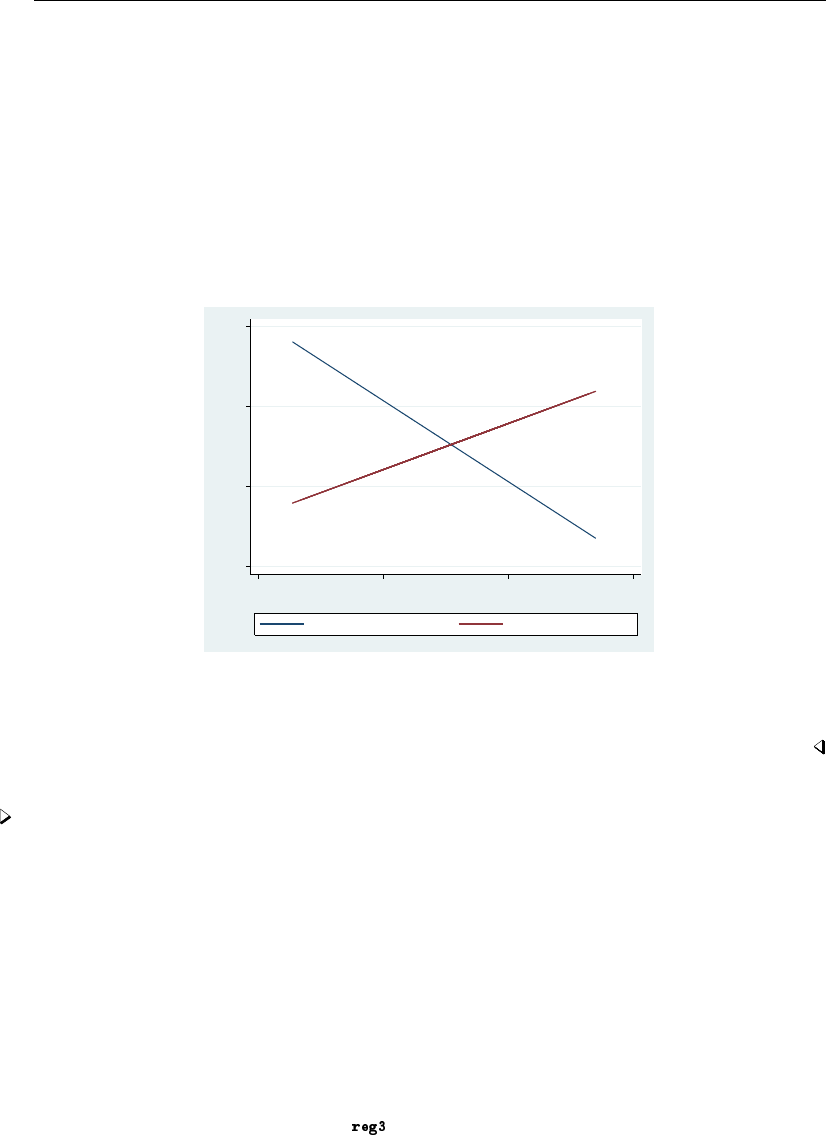
1842 reg3 postestimation — Postestimation tools for reg3
. summarize income, meanonly
. replace income = r(mean)
(49 real changes made)
. summarize praw, meanonly
. replace praw = r(mean)
(49 real changes made)
. predict demand, equation(qDemand)
(option xb assumed; fitted values)
. predict supply, equation(qSupply)
(option xb assumed; fitted values)
. graph twoway line demand price, sort || line supply price, ytitle(" ")
> legend(label(1 "Fitted values: qDemand") label(2 "Fitted values: qSupply"))
5 10 15 20
25 30 35 40
price
Fitted values: qDemand Fitted values: qSupply
As we would expect based on economic theory, the demand curve slopes downward while the
supply curve slopes upward. With the exogenous variables at their mean levels, the equilibrium price
and quantity are slightly less than 33 and 13, respectively.
Example 2: Obtaining forecasts
In example 3 of [R]reg3, we fit Klein’s (1950) model of the U.S. economy. That model includes
three stochastic equations we fit using reg3 as well as four identities. Here we briefly illustrate how
the forecast command can be used to obtain forecasts for all the endogenous variables in the model.
For a more detailed discussion of how to forecast with this model, see [TS]forecast.
In Stata, we type
. use http://www.stata-press.com/data/r13/klein2, clear
. reg3 (c p L.p w) (i p L.p L.k) (wp y L.y yr), endog(w p y) exog(t wg g)
(output omitted )
. estimates store kleineqs
. forecast create kleinmodel
Forecast model kleinmodel started.
. forecast estimates kleineqs
Added estimation results from .
Forecast model kleinmodel now contains 3 endogenous variables.
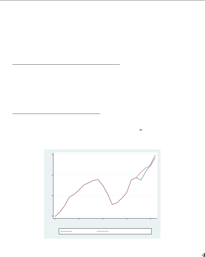
reg3 postestimation — Postestimation tools for reg3 1843
. forecast identity y = c + i + g
Forecast model kleinmodel now contains 4 endogenous variables.
. forecast identity p = y - t - wp
Forecast model kleinmodel now contains 5 endogenous variables.
. forecast identity k = L.k + i
Forecast model kleinmodel now contains 6 endogenous variables.
. forecast identity w = wg + wp
Forecast model kleinmodel now contains 7 endogenous variables.
. forecast solve, begin(1937)
Computing dynamic forecasts for model kleinmodel.
Starting period: 1937
Ending period: 1941
Forecast prefix: f_
1937: ...........................................
1938: ............................................
1939: ...........................................
1940: .........................................
1941: .............................................
Forecast 7 variables spanning 5 periods.
Here we have obtained dynamic forecasts for our 7 endogenous variables beginning in 1937. By
default, the variables containing the forecasts begin with the prefix f. Next we plot the forecast and
actual values of consumption:
. tsline c f_c
40 50 60 70
1920 1925 1930 1935 1940
year
consumption consumption (kleinmodel f_)
For more information about producing forecasts, see [TS]forecast.
Methods and formulas
The computational formulas for the statistics produced by predict can be found in [R]predict
and [R]regress postestimation.


Title
regress — Linear regression
Syntax Menu Description Options
Remarks and examples Stored results Methods and formulas Acknowledgments
References Also see
Syntax
regress depvar indepvars if in weight ,options
options Description
Model
noconstant suppress constant term
hascons has user-supplied constant
tsscons compute total sum of squares with constant; seldom used
SE/Robust
vce(vcetype)vcetype may be ols,robust,cluster clustvar,bootstrap,
jackknife,hc2, or hc3
Reporting
level(#)set confidence level; default is level(95)
beta report standardized beta coefficients
eform(string)report exponentiated coefficients and label as string
depname(varname)substitute dependent variable name; programmer’s option
display options control column formats, row spacing, line width, display of omitted
variables and base and empty cells, and factor-variable labeling
noheader suppress output header
notable suppress coefficient table
plus make table extendable
mse1 force mean squared error to 1
coeflegend display legend instead of statistics
indepvars may contain factor variables; see [U] 11.4.3 Factor variables.
depvar and indepvars may contain time-series operators; see [U] 11.4.4 Time-series varlists.
bootstrap,by,fp,jackknife,mfp,mi estimate,nestreg,rolling,statsby,stepwise, and svy are allowed;
see [U] 11.1.10 Prefix commands.
vce(bootstrap) and vce(jackknife) are not allowed with the mi estimate prefix; see [MI] mi estimate.
Weights are not allowed with the bootstrap prefix; see [R] bootstrap.
aweights are not allowed with the jackknife prefix; see [R] jackknife.
hascons,tsscons,vce(),beta,noheader,notable,plus,depname(),mse1, and weights are not allowed with
the svy prefix; see [SVY] svy.
aweights, fweights, iweights, and pweights are allowed; see [U] 11.1.6 weight.
noheader,notable,plus,mse1, and coeflegend do not appear in the dialog box.
See [U] 20 Estimation and postestimation commands for more capabilities of estimation commands.
1845

1846 regress — Linear regression
Menu
Statistics >Linear models and related >Linear regression
Description
regress fits a model of depvar on indepvars using linear regression.
Here is a short list of other regression commands that may be of interest. See help estimation
commands for a complete list.
Command Entry Description
areg [R] areg an easier way to fit regressions with many dummy variables
arch [TS] arch regression models with ARCH errors
arima [TS] arima ARIMA models
boxcox [R] boxcox Box–Cox regression models
cnsreg [R] cnsreg constrained linear regression
eivreg [R] eivreg errors-in-variables regression
etregress [TE] etregress Linear regression with endogenous treatment effects
frontier [R] frontier stochastic frontier models
gmm [R] gmm generalized method of moments estimation
heckman [R] heckman Heckman selection model
intreg [R] intreg interval regression
ivregress [R] ivregress single-equation instrumental-variables regression
ivtobit [R] ivtobit tobit regression with endogenous variables
newey [TS] newey regression with Newey – West standard errors
nl [R] nl nonlinear least-squares estimation
nlsur [R] nlsur estimation of nonlinear systems of equations
qreg [R] qreg quantile (including median) regression
reg3 [R] reg3 three-stage least-squares (3SLS) regression
rreg [R] rreg a type of robust regression
gsem [SEM] intro 5 generalized structural equation models
sem [SEM] intro 5 linear structural equation models
sureg [R] sureg seemingly unrelated regression
tobit [R] tobit tobit regression
truncreg [R] truncreg truncated regression
xtabond [XT] xtabond Arellano–Bond linear dynamic panel-data estimation
xtdpd [XT] xtdpd linear dynamic panel-data estimation
xtfrontier [XT] xtfrontier panel-data stochastic frontier models
xtgls [XT] xtgls panel-data GLS models
xthtaylor [XT] xthtaylor Hausman–Taylor estimator for error-components models
xtintreg [XT] xtintreg panel-data interval regression models
xtivreg [XT] xtivreg panel-data instrumental-variables (2SLS) regression
xtpcse [XT] xtpcse linear regression with panel-corrected standard errors
xtreg [XT] xtreg fixed- and random-effects linear models
xtregar [XT] xtregar fixed- and random-effects linear models with an AR(1) disturbance
xttobit [XT] xttobit panel-data tobit models

regress — Linear regression 1847
Options
Model
noconstant; see [R]estimation options.
hascons indicates that a user-defined constant or its equivalent is specified among the independent
variables in indepvars. Some caution is recommended when specifying this option, as resulting
estimates may not be as accurate as they otherwise would be. Use of this option requires “sweeping”
the constant last, so the moment matrix must be accumulated in absolute rather than deviation form.
This option may be safely specified when the means of the dependent and independent variables
are all reasonable and there is not much collinearity between the independent variables. The best
procedure is to view hascons as a reporting option—estimate with and without hascons and
verify that the coefficients and standard errors of the variables not affected by the identity of the
constant are unchanged.
tsscons forces the total sum of squares to be computed as though the model has a constant, that is,
as deviations from the mean of the dependent variable. This is a rarely used option that has an
effect only when specified with noconstant. It affects the total sum of squares and all results
derived from the total sum of squares.
SE/Robust
vce(vcetype)specifies the type of standard error reported, which includes types that are derived
from asymptotic theory (ols), that are robust to some kinds of misspecification (robust), that
allow for intragroup correlation (cluster clustvar), and that use bootstrap or jackknife methods
(bootstrap,jackknife); see [R]vce option.
vce(ols), the default, uses the standard variance estimator for ordinary least-squares regression.
regress also allows the following:
vce(hc2) and vce(hc3) specify an alternative bias correction for the robust variance calculation.
vce(hc2) and vce(hc3) may not be specified with svy prefix. In the unclustered case,
vce(robust) uses bσ2
j={n/(n−k)}u2
jas an estimate of the variance of the jth observation,
where ujis the calculated residual and n/(n−k)is included to improve the overall estimate’s
small-sample properties.
vce(hc2) instead uses u2
j/(1−hjj )as the observation’s variance estimate, where hjj is the
diagonal element of the hat (projection) matrix. This estimate is unbiased if the model really
is homoskedastic. vce(hc2) tends to produce slightly more conservative confidence intervals.
vce(hc3) uses u2
j/(1 −hjj )2as suggested by Davidson and MacKinnon (1993), who report
that this method tends to produce better results when the model really is heteroskedastic.
vce(hc3) produces confidence intervals that tend to be even more conservative.
See Davidson and MacKinnon (1993, 554–556) and Angrist and Pischke (2009, 294–308) for
more discussion on these two bias corrections.
Reporting
level(#); see [R]estimation options.
beta asks that standardized beta coefficients be reported instead of confidence intervals. The beta
coefficients are the regression coefficients obtained by first standardizing all variables to have a
mean of 0 and a standard deviation of 1. beta may not be specified with vce(cluster clustvar)
or the svy prefix.

1848 regress — Linear regression
eform(string)is used only in programs and ado-files that use regress to fit models other than
linear regression. eform() specifies that the coefficient table be displayed in exponentiated form
as defined in [R]maximize and that string be used to label the exponentiated coefficients in the
table.
depname(varname)is used only in programs and ado-files that use regress to fit models other than
linear regression. depname() may be specified only at estimation time. varname is recorded as
the identity of the dependent variable, even though the estimates are calculated using depvar. This
method affects the labeling of the output — not the results calculated — but could affect subsequent
calculations made by predict, where the residual would be calculated as deviations from varname
rather than depvar.depname() is most typically used when depvar is a temporary variable (see
[P]macro) used as a proxy for varname.
depname() is not allowed with the svy prefix.
display options:noomitted,vsquish,noemptycells,baselevels,allbaselevels,nofvla-
bel,fvwrap(#),fvwrapon(style),cformat(%fmt),pformat(% fmt),sformat(% fmt), and
nolstretch; see [R]estimation options.
The following options are available with regress but are not shown in the dialog box:
noheader suppresses the display of the ANOVA table and summary statistics at the top of the output;
only the coefficient table is displayed. This option is often used in programs and ado-files.
notable suppresses display of the coefficient table.
plus specifies that the output table be made extendable. This option is often used in programs and
ado-files.
mse1 is used only in programs and ado-files that use regress to fit models other than linear
regression and is not allowed with the svy prefix. mse1 sets the mean squared error to 1, forcing
the variance–covariance matrix of the estimators to be (X0DX)−1(see Methods and formulas
below) and affecting calculated standard errors. Degrees of freedom for tstatistics is calculated
as nrather than n−k.
coeflegend; see [R]estimation options.
Remarks and examples
Remarks are presented under the following headings:
Ordinary least squares
Treatment of the constant
Robust standard errors
Weighted regression
Instrumental variables and two-stage least-squares regression
Video example
regress performs linear regression, including ordinary least squares and weighted least squares.
For a general discussion of linear regression, see Draper and Smith (1998), Greene (2012), or
Kmenta (1997).
See Wooldridge (2013) for an excellent treatment of estimation, inference, interpretation, and
specification testing in linear regression models. This presentation stands out for its clarification of
the statistical issues, as opposed to the algebraic issues. See Wooldridge (2010, chap. 4) for a more
advanced discussion along the same lines.

regress — Linear regression 1849
See Hamilton (2013, chap. 7) and Cameron and Trivedi (2010, chap. 3) for an introduction to
linear regression using Stata. Dohoo, Martin, and Stryhn (2012,2010) discuss linear regression using
examples from epidemiology, and Stata datasets and do-files used in the text are available. Cameron
and Trivedi (2010) discuss linear regression using econometric examples with Stata. Mitchell (2012)
shows how to use graphics and postestimation commands to understand a fitted regression model.
Chatterjee and Hadi (2012) explain regression analysis by using examples containing typical
problems that you might encounter when performing exploratory data analysis. We also recommend
Weisberg (2005), who emphasizes the importance of the assumptions of linear regression and problems
resulting from these assumptions. Becketti (2013) discusses regression analysis with an emphasis on
time-series data. Angrist and Pischke (2009) approach regression as a tool for exploring relationships,
estimating treatment effects, and providing answers to public policy questions. For a discussion of
model-selection techniques and exploratory data analysis, see Mosteller and Tukey (1977). For a
mathematically rigorous treatment, see Peracchi (2001, chap. 6). Finally, see Plackett (1972) if you
are interested in the history of regression. Least squares, which dates back to the 1790s, was discovered
independently by Legendre and Gauss.
Ordinary least squares
Example 1: Basic linear regression
Suppose that we have data on the mileage rating and weight of 74 automobiles. The variables in
our data are mpg,weight, and foreign. The last variable assumes the value 1 for foreign and 0 for
domestic automobiles. We wish to fit the model
mpg =β0+β1weight +β2foreign +
This model can be fit with regress by typing
. use http://www.stata-press.com/data/r13/auto
(1978 Automobile Data)
. regress mpg weight foreign
Source SS df MS Number of obs = 74
F( 2, 71) = 69.75
Model 1619.2877 2 809.643849 Prob > F = 0.0000
Residual 824.171761 71 11.608053 R-squared = 0.6627
Adj R-squared = 0.6532
Total 2443.45946 73 33.4720474 Root MSE = 3.4071
mpg Coef. Std. Err. t P>|t| [95% Conf. Interval]
weight -.0065879 .0006371 -10.34 0.000 -.0078583 -.0053175
foreign -1.650029 1.075994 -1.53 0.130 -3.7955 .4954422
_cons 41.6797 2.165547 19.25 0.000 37.36172 45.99768
regress produces a variety of summary statistics along with the table of regression coefficients.
At the upper left, regress reports an analysis-of-variance (ANOVA) table. The column headings SS,
df, and MS stand for “sum of squares”, “degrees of freedom”, and “mean square”, respectively. In
this example, the total sum of squares is 2,443.5: 1,619.3 accounted for by the model and 824.2 left
unexplained. Because the regression included a constant, the total sum reflects the sum after removal
of means, as does the sum of squares due to the model. The table also reveals that there are 73
total degrees of freedom (counted as 74 observations less 1 for the mean removal), of which 2 are
consumed by the model, leaving 71 for the residual.

1850 regress — Linear regression
To the right of the ANOVA table are presented other summary statistics. The Fstatistic associated
with the ANOVA table is 69.75. The statistic has 2 numerator and 71 denominator degrees of freedom.
The Fstatistic tests the hypothesis that all coefficients excluding the constant are zero. The chance of
observing an Fstatistic that large or larger is reported as 0.0000, which is Stata’s way of indicating
a number smaller than 0.00005. The R-squared (R2) for the regression is 0.6627, and the R-squared
adjusted for degrees of freedom (R2
a) is 0.6532. The root mean squared error, labeled Root MSE, is
3.4071. It is the square root of the mean squared error reported for the residual in the ANOVA table.
Finally, Stata produces a table of the estimated coefficients. The first line of the table indicates
that the left-hand-side variable is mpg. Thereafter follow the estimated coefficients. Our fitted model
is
mpg hat =41.68 −0.0066 weight −1.65 foreign
Reported to the right of the coefficients in the output are the standard errors. For instance, the
standard error for the coefficient on weight is 0.0006371. The corresponding tstatistic is −10.34,
which has a two-sided significance level of 0.000. This number indicates that the significance is less
than 0.0005. The 95% confidence interval for the coefficient is [−0.0079,−0.0053 ].
Example 2: Transforming the dependent variable
If we had a graph comparing mpg with weight, we would notice that the relationship is distinctly
nonlinear. This is to be expected because energy usage per distance should increase linearly with
weight, but mpg is measuring distance per energy used. We could obtain a better model by generating
a new variable measuring the number of gallons used per 100 miles (gp100m) and then using this
new variable in our model:
gp100m =β0+β1weight +β2foreign +
We can now fit this model:
. generate gp100m = 100/mpg
. regress gp100m weight foreign
Source SS df MS Number of obs = 74
F( 2, 71) = 113.97
Model 91.1761694 2 45.5880847 Prob > F = 0.0000
Residual 28.4000913 71 .400001287 R-squared = 0.7625
Adj R-squared = 0.7558
Total 119.576261 73 1.63803097 Root MSE = .63246
gp100m Coef. Std. Err. t P>|t| [95% Conf. Interval]
weight .0016254 .0001183 13.74 0.000 .0013896 .0018612
foreign .6220535 .1997381 3.11 0.003 .2237871 1.02032
_cons -.0734839 .4019932 -0.18 0.855 -.8750354 .7280677
Fitting the physically reasonable model increases our R-squared to 0.7625.

regress — Linear regression 1851
Example 3: Obtaining beta coefficients
regress shares the features of all estimation commands. Among other things, this means that
after running a regression, we can use test to test hypotheses about the coefficients, estat vce to
examine the covariance matrix of the estimators, and predict to obtain predicted values, residuals,
and influence statistics. See [U] 20 Estimation and postestimation commands. Options that affect
how estimates are displayed, such as beta or level(), can be used when replaying results.
Suppose that we meant to specify the beta option to obtain beta coefficients (regression coefficients
normalized by the ratio of the standard deviation of the regressor to the standard deviation of the
dependent variable). Even though we forgot, we can specify the option now:
. regress, beta
Source SS df MS Number of obs = 74
F( 2, 71) = 113.97
Model 91.1761694 2 45.5880847 Prob > F = 0.0000
Residual 28.4000913 71 .400001287 R-squared = 0.7625
Adj R-squared = 0.7558
Total 119.576261 73 1.63803097 Root MSE = .63246
gp100m Coef. Std. Err. t P>|t| Beta
weight .0016254 .0001183 13.74 0.000 .9870255
foreign .6220535 .1997381 3.11 0.003 .2236673
_cons -.0734839 .4019932 -0.18 0.855 .
Treatment of the constant
By default, regress includes an intercept (constant) term in the model. The noconstant option
suppresses it, and the hascons option tells regress that the model already has one.
Example 4: Suppressing the constant term
We wish to fit a regression of the weight of an automobile against its length, and we wish to
impose the constraint that the weight is zero when the length is zero.
If we simply type regress weight length, we are fitting the model
weight =β0+β1length +
Here a length of zero corresponds to a weight of β0. We want to force β0to be zero or, equivalently,
estimate an equation that does not include an intercept:
weight =β1length +

1852 regress — Linear regression
We do this by specifying the noconstant option:
. regress weight length, noconstant
Source SS df MS Number of obs = 74
F( 1, 73) = 3450.13
Model 703869302 1 703869302 Prob > F = 0.0000
Residual 14892897.8 73 204012.299 R-squared = 0.9793
Adj R-squared = 0.9790
Total 718762200 74 9713002.7 Root MSE = 451.68
weight Coef. Std. Err. t P>|t| [95% Conf. Interval]
length 16.29829 .2774752 58.74 0.000 15.74528 16.8513
In our data, length is measured in inches and weight in pounds. We discover that each inch of
length adds 16 pounds to the weight.
Sometimes there is no need for Stata to include a constant term in the model. Most commonly,
this occurs when the model contains a set of mutually exclusive indicator variables. hascons is a
variation of the noconstant option— it tells Stata not to add a constant to the regression because
the regression specification already has one, either directly or indirectly.
For instance, we now refit our model of weight as a function of length and include separate
constants for foreign and domestic cars by specifying bn.foreign.bn.foreign is factor-variable
notation for “no base for foreign” or “include all levels of variable foreign in the model”; see
[U] 11.4.3 Factor variables.
. regress weight length bn.foreign, hascons
Source SS df MS Number of obs = 74
F( 2, 71) = 316.54
Model 39647744.7 2 19823872.3 Prob > F = 0.0000
Residual 4446433.7 71 62625.8268 R-squared = 0.8992
Adj R-squared = 0.8963
Total 44094178.4 73 604029.841 Root MSE = 250.25
weight Coef. Std. Err. t P>|t| [95% Conf. Interval]
length 31.44455 1.601234 19.64 0.000 28.25178 34.63732
foreign
Domestic -2850.25 315.9691 -9.02 0.000 -3480.274 -2220.225
Foreign -2983.927 275.1041 -10.85 0.000 -3532.469 -2435.385

regress — Linear regression 1853
Technical note
There is a subtle distinction between the hascons and noconstant options. We can most easily
reveal it by refitting the last regression, specifying noconstant rather than hascons:
. regress weight length bn.foreign, noconstant
Source SS df MS Number of obs = 74
F( 3, 71) = 3802.03
Model 714315766 3 238105255 Prob > F = 0.0000
Residual 4446433.7 71 62625.8268 R-squared = 0.9938
Adj R-squared = 0.9936
Total 718762200 74 9713002.7 Root MSE = 250.25
weight Coef. Std. Err. t P>|t| [95% Conf. Interval]
length 31.44455 1.601234 19.64 0.000 28.25178 34.63732
foreign
Domestic -2850.25 315.9691 -9.02 0.000 -3480.274 -2220.225
Foreign -2983.927 275.1041 -10.85 0.000 -3532.469 -2435.385
Comparing this output with that produced by the previous regress command, we see that they are
almost, but not quite, identical. The parameter estimates and their associated statistics—the second
half of the output—are identical. The overall summary statistics and the ANOVA table —the first half
of the output—are different, however.
In the first case, the R2is shown as 0.8992; here it is shown as 0.9938. In the first case, the
Fstatistic is 316.54; now it is 3,802.03. The numerator degrees of freedom is different as well. In
the first case, the numerator degrees of freedom is 2; now the degrees of freedom is 3. Which is
correct?
Both are. Specifying the hascons option causes regress to adjust the ANOVA table and its
associated statistics for the explanatory power of the constant. The regression in effect has a constant;
it is just written in such a way that a separate constant is unnecessary. No such adjustment is made
with the noconstant option.
Technical note
When the hascons option is specified, regress checks to make sure that the model does in fact
have a constant term. If regress cannot find a constant term, it automatically adds one. Fitting a
model of weight on length and specifying the hascons option, we obtain
. regress weight length, hascons
(note: hascons false)
Source SS df MS Number of obs = 74
F( 1, 72) = 613.27
Model 39461306.8 1 39461306.8 Prob > F = 0.0000
Residual 4632871.55 72 64345.4382 R-squared = 0.8949
Adj R-squared = 0.8935
Total 44094178.4 73 604029.841 Root MSE = 253.66
weight Coef. Std. Err. t P>|t| [95% Conf. Interval]
length 33.01988 1.333364 24.76 0.000 30.36187 35.67789
_cons -3186.047 252.3113 -12.63 0.000 -3689.02 -2683.073

1854 regress — Linear regression
Even though we specified hascons,regress included a constant, anyway. It also added a note to
our output: “note: hascons false”.
Technical note
Even if the model specification effectively includes a constant term, we need not specify the
hascons option. regress is always on the lookout for collinear variables and omits them from the
model. For instance,
. regress weight length bn.foreign
note: 1.foreign omitted because of collinearity
Source SS df MS Number of obs = 74
F( 2, 71) = 316.54
Model 39647744.7 2 19823872.3 Prob > F = 0.0000
Residual 4446433.7 71 62625.8268 R-squared = 0.8992
Adj R-squared = 0.8963
Total 44094178.4 73 604029.841 Root MSE = 250.25
weight Coef. Std. Err. t P>|t| [95% Conf. Interval]
length 31.44455 1.601234 19.64 0.000 28.25178 34.63732
foreign
Domestic 133.6775 77.47615 1.73 0.089 -20.80555 288.1605
Foreign 0 (omitted)
_cons -2983.927 275.1041 -10.85 0.000 -3532.469 -2435.385
Robust standard errors
regress with the vce(robust) option substitutes a robust variance matrix calculation for the
conventional calculation, or if vce(cluster clustvar)is specified, allows relaxing the assumption
of independence within groups. How this method works is explained in [U] 20.21 Obtaining robust
variance estimates. Below we show how well this approach works.
Example 5: Heteroskedasticity and robust standard errors
Specifying the vce(robust) option is equivalent to requesting White-corrected standard errors in
the presence of heteroskedasticity. We use the automobile data and, in the process of looking at the
energy efficiency of cars, analyze a variable with considerable heteroskedasticity.
We will examine the amount of energy—measured in gallons of gasoline—that the cars in the
data need to move 1,000 pounds of their weight 100 miles. We are going to examine the relative
efficiency of foreign and domestic cars.
. gen gpmw = ((1/mpg)/weight)*100*1000
. summarize gpmw
Variable Obs Mean Std. Dev. Min Max
gpmw 74 1.682184 .2426311 1.09553 2.30521
In these data, the engines consume between 1.10 and 2.31 gallons of gas to move 1,000 pounds
of the car’s weight 100 miles. If we ran a regression with conventional standard errors of gpmw on
foreign, we would obtain

regress — Linear regression 1855
. regress gpmw foreign
Source SS df MS Number of obs = 74
F( 1, 72) = 20.07
Model .936705572 1 .936705572 Prob > F = 0.0000
Residual 3.36079459 72 .046677703 R-squared = 0.2180
Adj R-squared = 0.2071
Total 4.29750017 73 .058869865 Root MSE = .21605
gpmw Coef. Std. Err. t P>|t| [95% Conf. Interval]
foreign .2461526 .0549487 4.48 0.000 .1366143 .3556909
_cons 1.609004 .0299608 53.70 0.000 1.549278 1.66873
regress with the vce(robust) option, on the other hand, reports
. regress gpmw foreign, vce(robust)
Linear regression Number of obs = 74
F( 1, 72) = 13.13
Prob > F = 0.0005
R-squared = 0.2180
Root MSE = .21605
Robust
gpmw Coef. Std. Err. t P>|t| [95% Conf. Interval]
foreign .2461526 .0679238 3.62 0.001 .1107489 .3815563
_cons 1.609004 .0234535 68.60 0.000 1.56225 1.655758
The point estimates are the same (foreign cars need one-quarter gallon more gas), but the standard errors
differ by roughly 20%. Conventional regression reports the 95% confidence interval as [0.14,0.36 ],
whereas the robust standard errors make the interval [0.11,0.38 ].
Which is right? Notice that gpmw is a variable with considerable heteroskedasticity:
. tabulate foreign, summarize(gpmw)
Summary of gpmw
Car type Mean Std. Dev. Freq.
Domestic 1.6090039 .16845182 52
Foreign 1.8551565 .30186861 22
Total 1.6821844 .24263113 74
Thus here we favor the robust standard errors. In [U] 20.21 Obtaining robust variance estimates,
we show another example using linear regression where it makes little difference whether we specify
vce(robust). The linear-regression assumptions were true, and we obtained nearly linear-regression
results. The advantage of the robust estimate is that in neither case did we have to check assumptions.
Technical note
regress purposefully suppresses displaying the ANOVA table when vce(robust) is specified, as
it is no longer appropriate in a statistical sense, even though, mechanically, the numbers would be
unchanged. That is, sums of squares remain unchanged, but the meaning of those sums is no longer
relevant. The Fstatistic, for instance, is no longer based on sums of squares; it becomes a Wald test
based on the robustly estimated variance matrix. Nevertheless, regress continues to report the R2

1856 regress — Linear regression
and the root MSE even though both numbers are based on sums of squares and are, strictly speaking,
irrelevant. In this, the root MSE is more in violation of the spirit of the robust estimator than is R2.
As a goodness-of-fit statistic, R2is still fine; just do not use it in formulas to obtain Fstatistics
because those formulas no longer apply. The root MSE is valid in a literal sense — it is the square
root of the mean squared error, but it is no longer an estimate of σbecause there is no single σ; the
variance of the residual varies observation by observation.
Example 6: Alternative robust standard errors
The vce(hc2) and vce(hc3) options modify the robust variance calculation. In the context of
linear regression without clustering, the idea behind the robust calculation is somehow to measure
σ2
j, the variance of the residual associated with the jth observation, and then to use that estimate
to improve the estimated variance of b
β. Because residuals have (theoretically and practically) mean
0, one estimate of σ2
jis the observation’s squared residual itself — u2
j. A finite-sample correction
could improve that by multiplying u2
jby n/(n−k), and, as a matter of fact, vce(robust) uses
{n/(n−k)}u2
jas its estimate of the residual’s variance.
vce(hc2) and vce(hc3) use alternative estimators of the observation-specific variances. For
instance, if the residuals are homoskedastic, we can show that the expected value of u2
jis σ2(1−hjj ),
where hjj is the jth diagonal element of the projection (hat) matrix. hjj has average value k/n, so
1−hjj has average value 1−k/n = (n−k)/n. Thus the default robust estimator bσj={n/(n−k)}u2
j
amounts to dividing u2
jby the average of the expectation.
vce(hc2) divides u2
jby 1 −hjj itself, so it should yield better estimates if the residuals really are
homoskedastic. vce(hc3) divides u2
jby (1−hjj )2and has no such clean interpretation. Davidson
and MacKinnon (1993) show that u2
j/(1−hjj )2approximates a more complicated estimator that
they obtain by jackknifing (MacKinnon and White 1985). Angrist and Pischke (2009) also illustrate
the relative merits of these adjustments.
Here are the results of refitting our efficiency model using vce(hc2) and vce(hc3):
. regress gpmw foreign, vce(hc2)
Linear regression Number of obs = 74
F( 1, 72) = 12.93
Prob > F = 0.0006
R-squared = 0.2180
Root MSE = .21605
Robust HC2
gpmw Coef. Std. Err. t P>|t| [95% Conf. Interval]
foreign .2461526 .0684669 3.60 0.001 .1096662 .3826389
_cons 1.609004 .0233601 68.88 0.000 1.562437 1.655571

regress — Linear regression 1857
. regress gpmw foreign, vce(hc3)
Linear regression Number of obs = 74
F( 1, 72) = 12.38
Prob > F = 0.0008
R-squared = 0.2180
Root MSE = .21605
Robust HC3
gpmw Coef. Std. Err. t P>|t| [95% Conf. Interval]
foreign .2461526 .069969 3.52 0.001 .1066719 .3856332
_cons 1.609004 .023588 68.21 0.000 1.561982 1.656026
Example 7: Standard errors for clustered data
The vce(cluster clustvar)option relaxes the assumption of independence. Below we have 28,534
observations on 4,711 women aged 14–46 years. Data were collected on these women between 1968
and 1988. We are going to fit a classic earnings model, and we begin by ignoring that each woman
appears an average of 6.057 times in the data.
. use http://www.stata-press.com/data/r13/regsmpl, clear
(NLS Women 14-26 in 1968)
. regress ln_wage age c.age#c.age tenure
Source SS df MS Number of obs = 28101
F( 3, 28097) = 1842.45
Model 1054.52501 3 351.508335 Prob > F = 0.0000
Residual 5360.43962 28097 .190783344 R-squared = 0.1644
Adj R-squared = 0.1643
Total 6414.96462 28100 .228290556 Root MSE = .43679
ln_wage Coef. Std. Err. t P>|t| [95% Conf. Interval]
age .0752172 .0034736 21.65 0.000 .0684088 .0820257
c.age#c.age -.0010851 .0000575 -18.86 0.000 -.0011979 -.0009724
tenure .0390877 .0007743 50.48 0.000 .0375699 .0406054
_cons .3339821 .0504413 6.62 0.000 .2351148 .4328495
The number of observations in our model is 28,101 because Stata drops observations that have a
missing value for one or more of the variables in the model. We can be reasonably certain that the
standard errors reported above are meaningless. Without a doubt, a woman with higher-than-average
wages in one year typically has higher-than-average wages in other years, and so the residuals are
not independent. One way to deal with this would be to fit a random-effects model—and we are
going to do that—but first we fit the model using regress specifying vce(cluster id), which
treats only observations with different person ids as truly independent:

1858 regress — Linear regression
. regress ln_wage age c.age#c.age tenure, vce(cluster id)
Linear regression Number of obs = 28101
F( 3, 4698) = 748.82
Prob > F = 0.0000
R-squared = 0.1644
Root MSE = .43679
(Std. Err. adjusted for 4699 clusters in idcode)
Robust
ln_wage Coef. Std. Err. t P>|t| [95% Conf. Interval]
age .0752172 .0045711 16.45 0.000 .0662557 .0841788
c.age#c.age -.0010851 .0000778 -13.94 0.000 -.0012377 -.0009325
tenure .0390877 .0014425 27.10 0.000 .0362596 .0419157
_cons .3339821 .0641918 5.20 0.000 .208136 .4598282
For comparison, we focus on the tenure coefficient, which in economics jargon can be interpreted as the
rate of return for keeping your job. The 95% confidence interval we previously estimated—an interval
we do not believe — is [0.038,0.041 ]. The robust interval is twice as wide, being [0.036,0.042 ].
As we said, one correct way to fit this model is by random-effects regression. Here is the
random-effects result:
. xtreg ln_wage age c.age#c.age tenure, re
Random-effects GLS regression Number of obs = 28101
Group variable: idcode Number of groups = 4699
R-sq: within = 0.1370 Obs per group: min = 1
between = 0.2154 avg = 6.0
overall = 0.1608 max = 15
Wald chi2(3) = 4717.05
corr(u_i, X) = 0 (assumed) Prob > chi2 = 0.0000
ln_wage Coef. Std. Err. z P>|z| [95% Conf. Interval]
age .0568296 .0026958 21.08 0.000 .0515459 .0621132
c.age#c.age -.0007566 .0000447 -16.93 0.000 -.0008441 -.000669
tenure .0260135 .0007477 34.79 0.000 .0245481 .0274789
_cons .6136792 .0394611 15.55 0.000 .5363368 .6910216
sigma_u .33542449
sigma_e .29674679
rho .56095413 (fraction of variance due to u_i)
Robust regression estimated the 95% interval [0.036,0.042 ], and xtreg (see [XT]xtreg) estimates
[0.025,0.027 ]. Which is better? The random-effects regression estimator assumes a lot. We can check
some of these assumptions by performing a Hausman test. Using estimates (see [R]estimates store),
we store the random-effects estimation results, and then we run the required fixed-effects regression
to perform the test.

regress — Linear regression 1859
. estimates store random
. xtreg ln_wage age c.age#c.age tenure, fe
Fixed-effects (within) regression Number of obs = 28101
Group variable: idcode Number of groups = 4699
R-sq: within = 0.1375 Obs per group: min = 1
between = 0.2066 avg = 6.0
overall = 0.1568 max = 15
F(3,23399) = 1243.00
corr(u_i, Xb) = 0.1380 Prob > F = 0.0000
ln_wage Coef. Std. Err. t P>|t| [95% Conf. Interval]
age .0522751 .002783 18.78 0.000 .0468202 .05773
c.age#c.age -.0006717 .0000461 -14.56 0.000 -.0007621 -.0005813
tenure .021738 .000799 27.21 0.000 .020172 .023304
_cons .687178 .0405944 16.93 0.000 .6076103 .7667456
sigma_u .38743138
sigma_e .29674679
rho .6302569 (fraction of variance due to u_i)
F test that all u_i=0: F(4698, 23399) = 7.98 Prob > F = 0.0000
. hausman . random
Coefficients
(b) (B) (b-B) sqrt(diag(V_b-V_B))
. random Difference S.E.
age .0522751 .0568296 -.0045545 .0006913
c.age#c.age -.0006717 -.0007566 .0000849 .0000115
tenure .021738 .0260135 -.0042756 .0002816
b = consistent under Ho and Ha; obtained from xtreg
B = inconsistent under Ha, efficient under Ho; obtained from xtreg
Test: Ho: difference in coefficients not systematic
chi2(3) = (b-B)’[(V_b-V_B)^(-1)](b-B)
= 336.62
Prob>chi2 = 0.0000
The Hausman test casts grave suspicions on the random-effects model we just fit, so we should be
careful in interpreting those results.
Meanwhile, our robust regression results still stand, as long as we are careful about the interpretation.
The correct interpretation is that, if the data collection were repeated (on women sampled the same
way as in the original sample), and if we were to refit the model, 95% of the time we would expect
the estimated coefficient on tenure to be in the range [0.036,0.042 ].
Even with robust regression, we must be careful about going beyond that statement. Here the
Hausman test is probably picking up something that differs within and between person, which would
cast doubt on our robust regression model in terms of interpreting [0.036,0.042 ]to contain the rate
of return for keeping a job, economywide, for all women, without exception.

1860 regress — Linear regression
Weighted regression
regress can perform weighted and unweighted regression. We indicate the weight by specifying
the [weight]qualifier. By default, regress assumes analytic weights; see the technical note below.
Example 8: Using means as regression variables
We have census data recording the death rate (drate) and median age (medage) for each state.
The data also record the region of the country in which each state is located and the overall population
of the state:
. use http://www.stata-press.com/data/r13/census9
(1980 Census data by state)
. describe
Contains data from http://www.stata-press.com/data/r13/census9.dta
obs: 50 1980 Census data by state
vars: 6 6 Apr 2013 15:43
size: 1,450
storage display value
variable name type format label variable label
state str14 %-14s State
state2 str2 %-2s Two-letter state abbreviation
drate float %9.0g Death Rate
pop long %12.0gc Population
medage float %9.2f Median age
region byte %-8.0g cenreg Census region
Sorted by:
We can use factor variables to include dummy variables for region. Because the variables in the
regression reflect means rather than individual observations, the appropriate method of estimation is
analytically weighted least squares (Davidson and MacKinnon 2004, 261–262), where the weight is
total population:
. regress drate medage i.region [w=pop]
(analytic weights assumed)
(sum of wgt is 2.2591e+08)
Source SS df MS Number of obs = 50
F( 4, 45) = 37.21
Model 4096.6093 4 1024.15232 Prob > F = 0.0000
Residual 1238.40987 45 27.5202192 R-squared = 0.7679
Adj R-squared = 0.7472
Total 5335.01916 49 108.877942 Root MSE = 5.246
drate Coef. Std. Err. t P>|t| [95% Conf. Interval]
medage 4.283183 .5393329 7.94 0.000 3.196911 5.369455
region
N Cntrl .3138738 2.456431 0.13 0.899 -4.633632 5.26138
South -1.438452 2.320244 -0.62 0.538 -6.111663 3.234758
West -10.90629 2.681349 -4.07 0.000 -16.30681 -5.505777
_cons -39.14727 17.23613 -2.27 0.028 -73.86262 -4.431915
To weight the regression by population, we added the qualifier [w=pop] to the end of the regress
command. Our qualifier was vague (we did not say [aweight=pop]), but unless told otherwise, Stata

regress — Linear regression 1861
assumes analytic weights for regress. Stata informed us that the sum of the weight is 2.2591 ×10⁸;
there were approximately 226 million people residing in the United States according to our 1980 data.
Technical note
Once we fit a weighted regression, we can obtain the appropriately weighted variance–covariance
matrix of the estimators using estat vce and perform appropriately weighted hypothesis tests using
test.
In the weighted regression in example 8, we see that 4.region is statistically significant but that
2.region and 3.region are not. We use test to test the joint significance of the region variables:
. test 2.region 3.region 4.region
( 1) 2.region = 0
( 2) 3.region = 0
( 3) 4.region = 0
F( 3, 45) = 9.84
Prob > F = 0.0000
The results indicate that the region variables are jointly significant.
regress also accepts frequency weights (fweights). Frequency weights are appropriate when the
data do not reflect cell means, but instead represent replicated observations. Specifying aweights or
fweights will not change the parameter estimates, but it will change the corresponding significance
levels.
For instance, if we specified [fweight=pop] in the weighted regression example above—which
would be statistically incorrect—Stata would treat the data as if the data represented 226 million
independent observations on death rates and median age. The data most certainly do not represent
that—they represent 50 observations on state averages.
With aweights, Stata treats the number of observations on the process as the number of observations
in the data. When we specify fweights, Stata treats the number of observations as if it were equal
to the sum of the weights; see Methods and formulas below.
Technical note
A popular request on the help line is to describe the effect of specifying [aweight=exp]with
regress in terms of transformation of the dependent and independent variables. The mechanical
answer is that typing
. regress y x1 x2 [aweight=n]
is equivalent to fitting the model
yj√nj=β0√nj+β1x1j√nj+β2x2j√nj+uj√nj
This regression will reproduce the coefficients and covariance matrix produced by the aweighted
regression. The mean squared errors (estimates of the variance of the residuals) will, however,
be different. The transformed regression reports s2
t, an estimate of Var(uj√nj). The aweighted
regression reports s2
a, an estimate of Var(uj√njpN/ Pknk), where Nis the number of observations.
Thus
s2
a=N
Pknk
s2
t=s2
t
n(1)

1862 regress — Linear regression
The logic for this adjustment is as follows: Consider the model
y=β0+β1x1+β2x2+u
Assume that, were this model fit on individuals, Var(u) = σ2
u, a constant. Assume that individual
data are not available; what is available are averages (yj, x1j, x2j)for j=1, . . . , N , and each
average is calculated over njobservations. Then it is still true that
yj=β0+β1x1j+β2x2j+uj
where ujis the average of njmean 0, variance σ2
udeviates and has variance σ2
u=σ2
u/nj. Thus
multiplying through by √njproduces
yj√nj=β0√nj+β1x1j√nj+β2x2j√nj+uj√nj
and Var(uj√nj) = σ2
u. The mean squared error, s2
t, reported by fitting this transformed regression
is an estimate of σ2
u. The coefficients and covariance matrix could also be obtained by aweighted
regress. The only difference would be in the reported mean squared error, which from (1) is
σ2
u/n. On average, each observation in the data reflects the averages calculated over n=Pknk/N
individuals, and thus this reported mean squared error is the average variance of an observation in
the dataset. We can retrieve the estimate of σ2
uby multiplying the reported mean squared error by n.
More generally, aweights are used to solve general heteroskedasticity problems. In these cases,
we have the model
yj=β0+β1x1j+β2x2j+uj
and the variance of ujis thought to be proportional to aj. If the variance is proportional to aj, it is
also proportional to αaj, where αis any positive constant. Not quite arbitrarily, but with no loss of
generality, we could choose α=Pk(1/ak)/N, the average value of the inverse of aj. We can then
write Var(uj) = kαajσ2, where kis the constant of proportionality that is no longer a function of
the scale of the weights.
Dividing this regression through by the √aj,
yj/√aj=β0/√aj+β1x1j/√aj+β2x2j/√aj+uj/√aj
produces a model with Var(uj/√aj) = kασ2, which is the constant part of Var(uj). This variance
is a function of α, the average of the reciprocal weights; if the weights are scaled arbitrarily, then so
is this variance.
We can also fit this model by typing
. regress y x1 x2 [aweight=1/a]
This input will produce the same estimates of the coefficients and covariance matrix; the reported
mean squared error is, from (1), N/ Pk(1/ak)kασ2=kσ2. This variance is independent of the
scale of aj.

regress — Linear regression 1863
Instrumental variables and two-stage least-squares regression
An alternate syntax for regress can be used to produce instrumental-variables (two-stage least
squares) estimates.
regress depvar varlist1(varlist2) if in weight ,regress options ]
This syntax is used mainly by programmers developing estimators using the instrumental-variables
estimates as intermediate results. ivregress is normally used to directly fit these models; see
[R]ivregress.
With this syntax, regress fits a structural equation of depvar on varlist1using instrumental
variables regression; (varlist2)indicates the list of instrumental variables. With the exception of
vce(hc2) and vce(hc3), all standard regress options are allowed.
Video example
Simple linear regression in Stata
Stored results
regress stores the following in e():
Scalars
e(N) number of observations
e(mss) model sum of squares
e(df m) model degrees of freedom
e(rss) residual sum of squares
e(df r) residual degrees of freedom
e(r2) R-squared
e(r2 a) adjusted R-squared
e(F) Fstatistic
e(rmse) root mean squared error
e(ll) log likelihood under additional assumption of i.i.d. normal errors
e(ll 0) log likelihood, constant-only model
e(N clust) number of clusters
e(rank) rank of e(V)
Macros
e(cmd) regress
e(cmdline) command as typed
e(depvar) name of dependent variable
e(model) ols or iv
e(wtype) weight type
e(wexp) weight expression
e(title) title in estimation output when vce() is not ols
e(clustvar) name of cluster variable
e(vce) vcetype specified in vce()
e(vcetype) title used to label Std. Err.
e(properties) b V
e(estat cmd) program used to implement estat
e(predict) program used to implement predict
e(marginsok) predictions allowed by margins
e(asbalanced) factor variables fvset as asbalanced
e(asobserved) factor variables fvset as asobserved
Matrices
e(b) coefficient vector
e(V) variance–covariance matrix of the estimators
e(V modelbased) model-based variance
Functions
e(sample) marks estimation sample

1864 regress — Linear regression
Methods and formulas
Methods and formulas are presented under the following headings:
Coefficient estimation and ANOVA table
A general notation for the robust variance calculation
Robust calculation for regress
Coefficient estimation and ANOVA table
Variables printed in lowercase and not boldfaced (for example, x) are scalars. Variables printed
in lowercase and boldfaced (for example, x) are column vectors. Variables printed in uppercase and
boldfaced (for example, X) are matrices.
Let vbe a column vector of weights specified by the user. If no weights are specified, v=1.
Let wbe a column vector of normalized weights. If no weights are specified or if the user specified
fweights or iweights, w=v. Otherwise, w=v/(10v)(101).
The number of observations, n, is defined as 10w. For iweights, this is truncated to an integer.
The sum of the weights is 10v. Define c=1 if there is a constant in the regression and zero otherwise.
Define kas the number of right-hand-side variables (including the constant).
Let Xdenote the matrix of observations on the right-hand-side variables, ythe vector of observations
on the left-hand-side variable, and Zthe matrix of observations on the instruments. If the user specifies
no instruments, then Z=X. In the following formulas, if the user specifies weights, then X0X,
X0y,y0y,Z0Z,Z0X, and Z0yare replaced by X0DX,X0Dy,y0Dy,Z0DZ,Z0DX, and Z0Dy,
respectively, where Dis a diagonal matrix whose diagonal elements are the elements of w. We
suppress the Dbelow to simplify the notation.
If no instruments are specified, define Aas X0Xand aas X0y. Otherwise, define Aas
X0Z(Z0Z)−1(X0Z)0and aas X0Z(Z0Z)−1Z0y.
The coefficient vector bis defined as A−1a. Although not shown in the notation, unless hascons
is specified, Aand aare accumulated in deviation form and the constant is calculated separately.
This comment applies to all statistics listed below.
The total sum of squares, TSS, equals y0yif there is no intercept and y0y−(10y)2/notherwise.
The degrees of freedom is n−c.
The error sum of squares, ESS, is defined as y0y−2bX0y+b0X0Xb if there are instruments
and as y0y−b0X0yotherwise. The degrees of freedom is n−k.
The model sum of squares, MSS, equals TSS −ESS. The degrees of freedom is k−c.
The mean squared error, s2, is defined as ESS/(n−k). The root mean squared error is s, its
square root.
The Fstatistic with k−cand n−kdegrees of freedom is defined as
F=MSS
(k−c)s2
if no instruments are specified. If instruments are specified and c=1, then Fis defined as
F=(b−c)0A(b−c)
(k−1)s2
where cis a vector of k−1 zeros and kth element 10y/n. Otherwise, Fis defined as “missing”.
(Here you may use the test command to construct any Ftest that you wish.)

regress — Linear regression 1865
The R-squared, R2, is defined as R2=1−ESS/TSS.
The adjusted R-squared, R2
a, is 1 −(1−R2)(n−c)/(n−k).
If vce(robust) is not specified, the conventional estimate of variance is s2A−1. The handling
of vce(robust) is described below.
A general notation for the robust variance calculation
Put aside all context of linear regression and the notation that goes with it—we will return to it.
First, we are going to establish a notation for describing robust variance calculations.
The calculation formula for the robust variance calculation is
b
V=qcb
VM
X
k=1
u(G)0
ku(G)
kb
V
where
u(G)
k=X
j∈Gk
wjuj
G1,G2,. . . ,GMare the clusters specified by vce(cluster clustvar), and wjare the user-specified
weights, normalized if aweights or pweights are specified and equal to 1 if no weights are specified.
For fweights without clusters, the variance formula is
b
V=qcb
VN
X
j=1
wju0
jujb
V
which is the same as expanding the dataset and making the calculation on the unweighted data.
If vce(cluster clustvar)is not specified, M=N, and each cluster contains 1 observation. The
inputs into this calculation are
•b
V, which is typically a conventionally calculated variance matrix;
•uj,j=1, . . . , N, a row vector of scores; and
•qc, a constant finite-sample adjustment.
Thus we can now describe how estimators apply the robust calculation formula by defining b
V,uj,
and qc.
Two definitions are popular enough for qcto deserve a name. The regression-like formula for qc
(Fuller et al. 1986) is
qc=N−1
N−k
M
M−1
where Mis the number of clusters and Nis the number of observations. For weights, Nrefers to
the sum of the weights if weights are frequency weights and the number of observations in the dataset
(ignoring weights) in all other cases. Also note that, weighted or not, M=Nwhen vce(cluster
clustvar)is not specified, and then qc=N/(N−k).
The asymptotic-like formula for qcis
qc=M
M−1
where M=Nif vce(cluster clustvar)is not specified.

1866 regress — Linear regression
See [U] 20.21 Obtaining robust variance estimates and [P]robust for a discussion of the robust
variance estimator and a development of these formulas.
Robust calculation for regress
For regress,b
V=A−1. The other terms are
No instruments, vce(robust), but not vce(hc2) or vce(hc3),
uj= (yj−xjb)xj
and qcis given by its regression-like definition.
No instruments, vce(hc2),
uj=1
p1−hjj
(yj−xjb)xj
where qc=1 and hjj =xj(X0X)−1xj0.
No instruments, vce(hc3),
uj=1
1−hjj
(yj−xjb)xj
where qc=1 and hjj =xj(X0X)−1xj0.
Instrumental variables,
uj= (yj−xjb)b
xj
where qcis given by its regression-like definition, and
b
x0
j=Pzj0
where P= (X0Z)(Z0Z)−1.
Acknowledgments
The robust estimate of variance was first implemented in Stata by Mead Over of the Center for
Global Development, Dean Jolliffe of the World Bank, and Andrew Foster of the Department of
Economics at Brown University (Over, Jolliffe, and Foster 1996).

regress — Linear regression 1867
The history of regression is long and complicated: the books by Stigler (1986) and Hald (1998) are
devoted largely to the story. Legendre published first on least squares in 1805. Gauss published
later in 1809, but he had the idea earlier. Gauss, and especially Laplace, tied least squares to a
normal errors assumption. The idea of the normal distribution can itself be traced back to De
Moivre in 1733. Laplace discussed a variety of other estimation methods and error assumptions
over his long career, while linear models long predate either innovation. Most of this work was
linked to problems in astronomy and geodesy.
A second wave of ideas started when Galton used graphical and descriptive methods on data bearing
on heredity to develop what he called regression. His term reflects the common phenomenon that
characteristics of offspring are positively correlated with those of parents but with regression slope
such that offspring “regress toward the mean”. Galton’s work was rather intuitive: contributions
from Pearson, Edgeworth, Yule, and others introduced more formal machinery, developed related
ideas on correlation, and extended application into the biological and social sciences. So most
of the elements of regression as we know it were in place by 1900.
Pierre-Simon Laplace (1749–1827) was born in Normandy and was early recognized as a
remarkable mathematician. He weathered a changing political climate well enough to rise to
Minister of the Interior under Napoleon in 1799 (although only for 6 weeks) and to be made
a Marquis by Louis XVIII in 1817. He made many contributions to mathematics and physics,
his two main interests being theoretical astronomy and probability theory (including statistics).
Laplace transforms are named for him.
Adrien-Marie Legendre (1752–1833) was born in Paris (or possibly in Toulouse) and educated in
mathematics and physics. He worked in number theory, geometry, differential equations, calculus,
function theory, applied mathematics, and geodesy. The Legendre polynomials are named for
him. His main contribution to statistics is as one of the discoverers of least squares. He died in
poverty, having refused to bow to political pressures.
Johann Carl Friedrich Gauss (1777–1855) was born in Braunschweig (Brunswick), now in
Germany. He studied there and at G¨
ottingen. His doctoral dissertation at the University of
Helmstedt was a discussion of the fundamental theorem of algebra. He made many fundamental
contributions to geometry, number theory, algebra, real analysis, differential equations, numerical
analysis, statistics, astronomy, optics, geodesy, mechanics, and magnetism. An outstanding genius,
Gauss worked mostly in isolation in G¨
ottingen.
Francis Galton (1822–1911) was born in Birmingham, England, into a well-to-do family with
many connections: he and Charles Darwin were first cousins. After an unsuccessful foray into
medicine, he became independently wealthy at the death of his father. Galton traveled widely
in Europe, the Middle East, and Africa, and became celebrated as an explorer and geographer.
His pioneering work on weather maps helped in the identification of anticyclones, which he
named. From about 1865, most of his work was centered on quantitative problems in biology,
anthropology, and psychology. In a sense, Galton (re)invented regression, and he certainly named
it. Galton also promoted the normal distribution, correlation approaches, and the use of median
and selected quantiles as descriptive statistics. He was knighted in 1909.
References
Adkins, L. C., and R. C. Hill. 2011. Using Stata for Principles of Econometrics. 4th ed. Hoboken, NJ: Wiley.
Alexandersson, A. 1998. gr32: Confidence ellipses.Stata Technical Bulletin 46: 10–13. Reprinted in Stata Technical
Bulletin Reprints, vol. 8, pp. 54–57. College Station, TX: Stata Press.

1868 regress — Linear regression
Angrist, J. D., and J.-S. Pischke. 2009. Mostly Harmless Econometrics: An Empiricist’s Companion. Princeton, NJ:
Princeton University Press.
Becketti, S. 2013. Introduction to Time Series Using Stata. College Station, TX: Stata Press.
Cameron, A. C., and P. K. Trivedi. 2010. Microeconometrics Using Stata. Rev. ed. College Station, TX: Stata Press.
Chatterjee, S., and A. S. Hadi. 2012. Regression Analysis by Example. 5th ed. New York: Hoboken, NJ.
Davidson, R., and J. G. MacKinnon. 1993. Estimation and Inference in Econometrics. New York: Oxford University
Press.
. 2004. Econometric Theory and Methods. New York: Oxford University Press.
Dohoo, I., W. Martin, and H. Stryhn. 2010. Veterinary Epidemiologic Research. 2nd ed. Charlottetown, Prince Edward
Island: VER Inc.
. 2012. Methods in Epidemiologic Research. Charlottetown, Prince Edward Island: VER Inc.
Draper, N., and H. Smith. 1998. Applied Regression Analysis. 3rd ed. New York: Wiley.
Dunnington, G. W. 1955. Gauss: Titan of Science. New York: Hafner Publishing.
Duren, P. 2009. Changing faces: The mistaken portrait of Legendre. Notices of the American Mathematical Society
56: 1440–1443.
Filoso, V. 2013. Regression anatomy, revealed.Stata Journal 13: 92–106.
Fuller, W. A., W. J. Kennedy, Jr., D. Schnell, G. Sullivan, and H. J. Park. 1986. PC CARP. Software package. Ames,
IA: Statistical Laboratory, Iowa State University.
Gillham, N. W. 2001. A Life of Sir Francis Galton: From African Exploration to the Birth of Eugenics. New York:
Oxford University Press.
Gillispie, C. C. 1997. Pierre-Simon Laplace, 1749–1827: A Life in Exact Science. Princeton: Princeton University
Press.
Gould, W. W. 2011a. Understanding matrices intuitively, part 1. The Stata Blog: Not Elsewhere Classified.
http://blog.stata.com/2011/03/03/understanding-matrices-intuitively-part-1/.
. 2011b. Use poisson rather than regress; tell a friend. The Stata Blog: Not Elsewhere Classified.
http://blog.stata.com/2011/08/22/use-poisson-rather-than-regress-tell-a-friend/.
Greene, W. H. 2012. Econometric Analysis. 7th ed. Upper Saddle River, NJ: Prentice Hall.
Hald, A. 1998. A History of Mathematical Statistics from 1750 to 1930. New York: Wiley.
Hamilton, L. C. 2013. Statistics with Stata: Updated for Version 12. 8th ed. Boston: Brooks/Cole.
Hill, R. C., W. E. Griffiths, and G. C. Lim. 2011. Principles of Econometrics. 4th ed. Hoboken, NJ: Wiley.
Kmenta, J. 1997. Elements of Econometrics. 2nd ed. Ann Arbor: University of Michigan Press.
Kohler, U., and F. Kreuter. 2012. Data Analysis Using Stata. 3rd ed. College Station, TX: Stata Press.
Long, J. S., and J. Freese. 2000. sg152: Listing and interpreting transformed coefficients from certain regression
models.Stata Technical Bulletin 57: 27–34. Reprinted in Stata Technical Bulletin Reprints, vol. 10, pp. 231–240.
College Station, TX: Stata Press.
MacKinnon, J. G., and H. L. White, Jr. 1985. Some heteroskedasticity-consistent covariance matrix estimators with
improved finite sample properties. Journal of Econometrics 29: 305–325.
Mitchell, M. N. 2012. Interpreting and Visualizing Regression Models Using Stata. College Station, TX: Stata Press.
Mosteller, C. F., and J. W. Tukey. 1977. Data Analysis and Regression: A Second Course in Statistics. Reading, MA:
Addison–Wesley.
Over, M., D. Jolliffe, and A. Foster. 1996. sg46: Huber correction for two-stage least squares estimates.Stata Technical
Bulletin 29: 24–25. Reprinted in Stata Technical Bulletin Reprints, vol. 5, pp. 140–142. College Station, TX: Stata
Press.
Peracchi, F. 2001. Econometrics. Chichester, UK: Wiley.
Plackett, R. L. 1972. Studies in the history of probability and statistics: XXIX. The discovery of the method of least
squares. Biometrika 59: 239–251.
Rogers, W. H. 1991. smv2: Analyzing repeated measurements—some practical alternatives.Stata Technical Bulletin
4: 10–16. Reprinted in Stata Technical Bulletin Reprints, vol. 1, pp. 123–131. College Station, TX: Stata Press.

regress — Linear regression 1869
Royston, P., and G. Ambler. 1998. sg79: Generalized additive models.Stata Technical Bulletin 42: 38–43. Reprinted
in Stata Technical Bulletin Reprints, vol. 7, pp. 217–224. College Station, TX: Stata Press.
Schonlau, M. 2005. Boosted regression (boosting): An introductory tutorial and a Stata plugin.Stata Journal 5:
330–354.
Stigler, S. M. 1986. The History of Statistics: The Measurement of Uncertainty before 1900. Cambridge, MA: Belknap
Press.
Tyler, J. H. 1997. sg73: Table making programs.Stata Technical Bulletin 40: 18–23. Reprinted in Stata Technical
Bulletin Reprints, vol. 7, pp. 186–192. College Station, TX: Stata Press.
Weesie, J. 1998. sg77: Regression analysis with multiplicative heteroscedasticity.Stata Technical Bulletin 42: 28–32.
Reprinted in Stata Technical Bulletin Reprints, vol. 7, pp. 204–210. College Station, TX: Stata Press.
Weisberg, S. 2005. Applied Linear Regression. 3rd ed. New York: Wiley.
Wooldridge, J. M. 2010. Econometric Analysis of Cross Section and Panel Data. 2nd ed. Cambridge, MA: MIT Press.
. 2013. Introductory Econometrics: A Modern Approach. 5th ed. Mason, OH: South-Western.
Zimmerman, F. 1998. sg93: Switching regressions. Stata Technical Bulletin 45: 30–33. Reprinted in Stata Technical
Bulletin Reprints, vol. 8, pp. 183–186. College Station, TX: Stata Press.
Also see
[R]regress postestimation — Postestimation tools for regress
[R]regress postestimation diagnostic plots — Postestimation plots for regress
[R]regress postestimation time series — Postestimation tools for regress with time series
[R]anova — Analysis of variance and covariance
[R]contrast — Contrasts and linear hypothesis tests after estimation
[MI]estimation — Estimation commands for use with mi estimate
[SEM] example 6 — Linear regression
[SEM]intro 5 — Tour of models
[SVY]svy estimation — Estimation commands for survey data
[TS]forecast — Econometric model forecasting
[U] 20 Estimation and postestimation commands

Title
regress postestimation — Postestimation tools for regress
Description Predictions DFBETA influence statistics
Tests for violation of assumptions Variance inflation factors Measures of effect size
Methods and formulas Acknowledgments References
Also see
Description
The following postestimation commands are of special interest after regress:
Command Description
dfbeta DFBETA influence statistics
estat hettest tests for heteroskedasticity
estat imtest information matrix test
estat ovtest Ramsey regression specification-error test for omitted variables
estat szroeter Szroeter’s rank test for heteroskedasticity
estat vif variance inflation factors for the independent variables
estat esize η2and ω2effect sizes
These commands are not appropriate after the svy prefix.
1870

regress postestimation — Postestimation tools for regress 1871
The following standard postestimation commands are also available:
Command Description
contrast contrasts and ANOVA-style joint tests of estimates
estat ic Akaike’s and Schwarz’s Bayesian information criteria (AIC and BIC)
estat summarize summary statistics for the estimation sample
estat vce variance–covariance matrix of the estimators (VCE)
estat (svy) postestimation statistics for survey data
estimates cataloging estimation results
forecast1dynamic forecasts and simulations
hausman Hausman’s specification test
lincom point estimates, standard errors, testing, and inference for linear combinations
of coefficients
linktest link test for model specification
lrtest2likelihood-ratio test
margins marginal means, predictive margins, marginal effects, and average marginal
effects
marginsplot graph the results from margins (profile plots, interaction plots, etc.)
nlcom point estimates, standard errors, testing, and inference for nonlinear
combinations of coefficients
predict predictions, residuals, influence statistics, and other diagnostic measures
predictnl point estimates, standard errors, testing, and inference for generalized
predictions
pwcompare pairwise comparisons of estimates
suest seemingly unrelated estimation
test Wald tests of simple and composite linear hypotheses
testnl Wald tests of nonlinear hypotheses
1forecast is not appropriate with mi or svy estimation results.
2lrtest is not appropriate with svy estimation results.

1872 regress postestimation — Postestimation tools for regress
Predictions
Syntax for predict
predict type newvar if in ,statistic
statistic Description
Main
xb linear prediction; the default
residuals residuals
score score; equivalent to residuals
rstandard standardized residuals
rstudent Studentized (jackknifed) residuals
cooksd Cook’s distance
leverage |hat leverage (diagonal elements of hat matrix)
pr(a,b)Pr(yj|a < yj< b)
e(a,b)E(yj|a<yj< b)
ystar(a,b)E(y∗
j),y∗
j=max{a, min(yj, b)}
∗dfbeta(varname)DFBETA for varname
stdp standard error of the linear prediction
stdf standard error of the forecast
stdr standard error of the residual
∗covratio COVRATIO
∗dfits DFITS
∗welsch Welsch distance
Unstarred statistics are available both in and out of sample; type predict . . . if e(sample) . . . if wanted only for
the estimation sample. Starred statistics are calculated only for the estimation sample, even when if e(sample)
is not specified.
rstandard,rstudent,cooksd,leverage,dfbeta(),stdf,stdr,covratio,dfits, and welsch are not available
if any vce() other than vce(ols) was specified with regress.
xb,residuals,score, and stdp are the only options allowed with svy estimation results.
where aand bmay be numbers or variables; amissing (a≥.) means −∞, and bmissing (b≥.) means +∞; see
[U] 12.2.1 Missing values.
Menu for predict
Statistics >Postestimation >Predictions, residuals, etc.
Options for predict
Main
xb, the default, calculates the linear prediction.
residuals calculates the residuals.
score is equivalent to residuals in linear regression.

regress postestimation — Postestimation tools for regress 1873
rstandard calculates the standardized residuals.
rstudent calculates the Studentized (jackknifed) residuals.
cooksd calculates the Cook’s Dinfluence statistic (Cook 1977).
leverage or hat calculates the diagonal elements of the projection (“hat”) matrix.
pr(a,b)calculates Pr(a<xjb+uj<b), the probability that yj|xjwould be observed in the
interval (a,b).
aand bmay be specified as numbers or variable names; lb and ub are variable names;
pr(20,30) calculates Pr(20 <xjb+uj<30);
pr(lb,ub)calculates Pr(lb <xjb+uj<ub); and
pr(20,ub)calculates Pr(20 <xjb+uj<ub).
amissing (a≥.) means −∞;pr(.,30) calculates Pr(−∞ <xjb+uj<30);
pr(lb,30) calculates Pr(−∞ <xjb+uj<30)in observations for which lb ≥.
and calculates Pr(lb < xjb+uj<30)elsewhere.
bmissing (b≥.) means +∞;pr(20,.) calculates Pr(+∞>xjb+uj>20);
pr(20,ub)calculates Pr(+∞>xjb+uj>20)in observations for which ub ≥.
and calculates Pr(20 <xjb+uj<ub)elsewhere.
e(a,b)calculates E(xjb+uj|a<xjb+uj<b), the expected value of yj|xjconditional on
yj|xjbeing in the interval (a,b), meaning that yj|xjis truncated. aand bare specified as they
are for pr().
ystar(a,b)calculates E(y∗
j), where y∗
j=aif xjb+uj≤a,y∗
j=bif xjb+uj≥b, and
y∗
j=xjb+ujotherwise, meaning that y∗
jis censored. aand bare specified as they are for pr().
dfbeta(varname)calculates the DFBETA for varname, the difference between the regression coefficient
when the jth observation is included and excluded, said difference being scaled by the estimated
standard error of the coefficient. varname must have been included among the regressors in the
previously fitted model. The calculation is automatically restricted to the estimation subsample.
stdp calculates the standard error of the prediction, which can be thought of as the standard error of
the predicted expected value or mean for the observation’s covariate pattern. The standard error
of the prediction is also referred to as the standard error of the fitted value.
stdf calculates the standard error of the forecast, which is the standard error of the point prediction
for 1 observation. It is commonly referred to as the standard error of the future or forecast value.
By construction, the standard errors produced by stdf are always larger than those produced by
stdp; see Methods and formulas.
stdr calculates the standard error of the residuals.
covratio calculates COVRATIO (Belsley, Kuh, and Welsch 1980), a measure of the influence of the
jth observation based on considering the effect on the variance–covariance matrix of the estimates.
The calculation is automatically restricted to the estimation subsample.
dfits calculates DFITS (Welsch and Kuh 1977) and attempts to summarize the information in the
leverage versus residual-squared plot into one statistic. The calculation is automatically restricted
to the estimation subsample.
welsch calculates Welsch distance (Welsch 1982) and is a variation on dfits. The calculation is
automatically restricted to the estimation subsample.

1874 regress postestimation — Postestimation tools for regress
Remarks and examples for predict
Remarks are presented under the following headings:
Terminology
Fitted values and residuals
Prediction standard errors
Prediction with weighted data
Leverage statistics
Standardized and Studentized residuals
DFITS, Cook’s Distance, and Welsch Distance
COVRATIO
Terminology
Many of these commands concern identifying influential data in linear regression. This is, un-
fortunately, a field that is dominated by jargon, codified and partially begun by Belsley, Kuh, and
Welsch (1980). In the words of Chatterjee and Hadi (1986, 416), “Belsley, Kuh, and Welsch’s book,
Regression Diagnostics, was a very valuable contribution to the statistical literature, but it unleashed
on an unsuspecting statistical community a computer speak (`
a la Orwell), the likes of which we
have never seen.” Things have only gotten worse since then. Chatterjee and Hadi’s (1986, 1988)
own attempts to clean up the jargon did not improve matters (see Hoaglin and Kempthorne [1986],
Velleman [1986], and Welsch [1986]). We apologize for the jargon, and for our contribution to the
jargon in the form of inelegant command names, we apologize most of all.
Model sensitivity refers to how estimates are affected by subsets of our data. Imagine data on y
and x, and assume that the data are to be fit by the regression yi=α+βxi+i. The regression
estimates of αand βare aand b, respectively. Now imagine that the estimated aand bwould be
different if a small portion of the dataset, perhaps even one observation, were deleted. As a data
analyst, you would like to think that you are summarizing tendencies that apply to all the data, but
you have just been told that the model you fit is unduly influenced by one point or just a few points
and that, as a matter of fact, there is another model that applies to the rest of the data — a model
that you have ignored. The search for subsets of the data that, if deleted, would change the results
markedly is a predominant theme of this entry.
There are three key issues in identifying model sensitivity to individual observations, which go by
the names residuals,leverage, and influence. In our yi=a+bxi+eiregression, the residuals are,
of course, ei—they reveal how much our fitted value byi=a+bxidiffers from the observed yi. A
point (xi, yi)with a corresponding large residual is called an outlier. Say that you are interested in
outliers because you somehow think that such points will exert undue influence on your estimates.
Your feelings are generally right, but there are exceptions. A point might have a huge residual and
yet not affect the estimated bat all. Nevertheless, studying observations with large residuals almost
always pays off.
(xi, yi)can be an outlier in another way—just as yican be far from byi,xican be far from
the center of mass of the other x’s. Such an “outlier” should interest you just as much as the more
traditional outliers. Picture a scatterplot of yagainst xwith thousands of points in some sort of mass
at the lower left of the graph and one point at the upper right of the graph. Now run a regression
line through the points—the regression line will come close to the point at the upper right of the
graph and may in fact, go through it. That is, this isolated point will not appear as an outlier as
measured by residuals because its residual will be small. Yet this point might have a dramatic effect
on our resulting estimates in the sense that, were you to delete the point, the estimates would change
markedly. Such a point is said to have high leverage. Just as with traditional outliers, a high leverage
point does not necessarily have an undue effect on regression estimates, but if it does not, it is more
the exception than the rule.

regress postestimation — Postestimation tools for regress 1875
Now all this is a most unsatisfactory state of affairs. Points with large residuals may, but need
not, have a large effect on our results, and points with small residuals may still have a large effect.
Points with high leverage may, but need not, have a large effect on our results, and points with low
leverage may still have a large effect. Can you not identify the influential points and simply have the
computer list them for you? You can, but you will have to define what you mean by “influential”.
“Influential” is defined with respect to some statistic. For instance, you might ask which points in
your data have a large effect on your estimated a, which points have a large effect on your estimated
b, which points have a large effect on your estimated standard error of b, and so on, but do not be
surprised when the answers to these questions are different. In any case, obtaining such measures
is not difficult— all you have to do is fit the regression excluding each observation one at a time
and record the statistic of interest which, in the day of the modern computer, is not too onerous.
Moreover, you can save considerable computer time by doing algebra ahead of time and working
out formulas that will calculate the same answers as if you ran each of the regressions. (Ignore the
question of pairs of observations that, together, exert undue influence, and triples, and so on, which
remains largely unsolved and for which the brute force fit-every-possible-regression procedure is not
a viable alternative.)
Fitted values and residuals
Typing predict newvar with no options creates newvar containing the fitted values. Typing
predict newvar, resid creates newvar containing the residuals.
Example 1
Continuing with example 1 from [R]regress, we wish to fit the following model:
mpg =β0+β1weight +β2foreign +
. use http://www.stata-press.com/data/r13/auto
(1978 Automobile Data)
. regress mpg weight foreign
Source SS df MS Number of obs = 74
F( 2, 71) = 69.75
Model 1619.2877 2 809.643849 Prob > F = 0.0000
Residual 824.171761 71 11.608053 R-squared = 0.6627
Adj R-squared = 0.6532
Total 2443.45946 73 33.4720474 Root MSE = 3.4071
mpg Coef. Std. Err. t P>|t| [95% Conf. Interval]
weight -.0065879 .0006371 -10.34 0.000 -.0078583 -.0053175
foreign -1.650029 1.075994 -1.53 0.130 -3.7955 .4954422
_cons 41.6797 2.165547 19.25 0.000 37.36172 45.99768
That done, we can now obtain the predicted values from the regression. We will store them in a new
variable called pmpg by typing predict pmpg. Because predict produces no output, we will follow
that by summarizing our predicted and observed values.

1876 regress postestimation — Postestimation tools for regress
. predict pmpg
(option xb assumed; fitted values)
. summarize pmpg mpg
Variable Obs Mean Std. Dev. Min Max
pmpg 74 21.2973 4.709779 9.794333 29.82151
mpg 74 21.2973 5.785503 12 41
Example 2: Out-of-sample predictions
We can just as easily obtain predicted values from the model by using a wholly different dataset
from the one on which the model was fit. The only requirement is that the data have the necessary
variables, which here are weight and foreign.
Using the data on two new cars (the Pontiac Sunbird and the Volvo 260) from the newautos.dta
dataset, we can obtain out-of-sample predictions (or forecasts) by typing
. use http://www.stata-press.com/data/r13/newautos, clear
(New Automobile Models)
. predict pmpg
(option xb assumed; fitted values)
. list, divider
make weight foreign pmpg
1. Pont. Sunbird 2690 Domestic 23.95829
2. Volvo 260 3170 Foreign 19.14607
The Pontiac Sunbird has a predicted mileage rating of 23.96 mpg, whereas the Volvo 260 has a
predicted rating of 19.15 mpg. In comparison, the actual mileage ratings are 24 for the Pontiac and
17 for the Volvo.
Prediction standard errors
predict can calculate the standard error of the forecast (stdf option), the standard error of the
prediction (stdp option), and the standard error of the residual (stdr option). It is easy to confuse
stdf and stdp because both are often called the prediction error. Consider the prediction byj=xjb,
where bis the estimated coefficient (column) vector and xjis a (row) vector of independent variables
for which you want the prediction. First, byjhas a variance due to the variance of the estimated
coefficient vector b,
Var(byj) = Var(xjb) = s2hj
where hj=xj(X0X)−1x0
jand s2is the mean squared error of the regression. Do not panic over the
algebra—just remember that Var(byj) = s2hj, whatever s2and hjare. stdp calculates this quantity.
This is the error in the prediction due to the uncertainty about b.
If you are about to hand this number out as your forecast, however, there is another error. According
to your model, the true value of yjis given by
yj=xjb+j=byj+j

regress postestimation — Postestimation tools for regress 1877
and thus the Var(yj) = Var(byj) + Var(j) = s2hj+s2, which is the square of stdf.stdf, then,
is the sum of the error in the prediction plus the residual error.
stdr has to do with an analysis-of-variance decomposition of s2, the estimated variance of y.
The standard error of the prediction is s2hj, and therefore s2hj+s2(1−hj) = s2decomposes s2
into the prediction and residual variances.
Example 3: standard error of the forecast
Returning to our model of mpg on weight and foreign, we previously predicted the mileage rating
for the Pontiac Sunbird and Volvo 260 as 23.96 and 19.15 mpg, respectively. We now want to put a
standard error around our forecast. Remember, the data for these two cars were in newautos.dta:
. use http://www.stata-press.com/data/r13/newautos, clear
(New Automobile Models)
. predict pmpg
(option xb assumed; fitted values)
. predict se_pmpg, stdf
. list, divider
make weight foreign pmpg se_pmpg
1. Pont. Sunbird 2690 Domestic 23.95829 3.462791
2. Volvo 260 3170 Foreign 19.14607 3.525875
Thus an approximate 95% confidence interval for the mileage rating of the Volvo 260 is 19.15±2·3.53 =
[12.09,26.21 ].
Prediction with weighted data
predict can be used after frequency-weighted (fweight) estimation, just as it is used after
unweighted estimation. The technical note below concerns the use of predict after analytically
weighted (aweight) estimation.
Technical note
After analytically weighted estimation, predict is willing to calculate only the prediction (no
options), residual (residual option), standard error of the prediction (stdp option), and diagonal
elements of the projection matrix (hat option). Moreover, the results produced by hat need to
be adjusted, as will be described. For analytically weighted estimation, the standard error of the
forecast and residuals, the standardized and Studentized residuals, and Cook’s Dare not statistically
well-defined concepts.

1878 regress postestimation — Postestimation tools for regress
Leverage statistics
In addition to providing fitted values and the associated standard errors, the predict command can
also be used to generate various statistics used to detect the influence of individual observations. This
section provides a brief introduction to leverage (hat) statistics, and some of the following subsections
discuss other influence statistics produced by predict.
Example 4: diagonal elements of projection matrix
The diagonal elements of the projection matrix, obtained by the hat option, are a measure of
distance in explanatory variable space. leverage is a synonym for hat.
. use http://www.stata-press.com/data/r13/auto, clear
(1978 Automobile Data)
. regress mpg weight foreign
(output omitted )
. predict xdist, hat
. summarize xdist, detail
Leverage
Percentiles Smallest
1% .0192325 .0192325
5% .0192686 .0192366
10% .0193448 .019241 Obs 74
25% .0220291 .0192686 Sum of Wgt. 74
50% .0383797 Mean .0405405
Largest Std. Dev. .0207624
75% .0494002 .0880814
90% .0693432 .099715 Variance .0004311
95% .0880814 .099715 Skewness 1.159745
99% .1003283 .1003283 Kurtosis 4.083313
Some 5% of our sample has an xdist measure in excess of 0.08. Let’s force them to reveal their
identities:
. list foreign make mpg if xdist>.08, divider
foreign make mpg
24. Domestic Ford Fiesta 28
26. Domestic Linc. Continental 12
27. Domestic Linc. Mark V 12
43. Domestic Plym. Champ 34
64. Foreign Peugeot 604 14
To understand why these cars are on this list, we must remember that the explanatory variables in our
model are weight and foreign and that xdist measures distance in this metric. The Ford Fiesta
and the Plymouth Champ are the two lightest domestic cars in our data. The Lincolns are the two
heaviest domestic cars, and the Peugeot is the heaviest foreign car.
See lvr2plot in [R]regress postestimation diagnostic plots for information on a leverage-versus-
squared-residual plot.

regress postestimation — Postestimation tools for regress 1879
Standardized and Studentized residuals
The terms standardized and Studentized residuals have meant different things to different authors.
In Stata, predict defines the standardized residual as bei=ei/(s√1−hi)and the Studentized
residual as ri=ei/(s(i)√1−hi), where s(i)is the root mean squared error of a regression with the
ith observation removed. Stata’s definition of the Studentized residual is the same as the one given
in Bollen and Jackman (1990, 264) and is what Chatterjee and Hadi (1988, 74) call the “externally
Studentized” residual. Stata’s “standardized” residual is the same as what Chatterjee and Hadi (1988,
74) call the “internally Studentized” residual.
Standardized and Studentized residuals are attempts to adjust residuals for their standard errors.
Although the itheoretical residuals are homoskedastic by assumption (that is, they all have the same
variance), the calculated eiare not. In fact,
Var(ei) = σ2(1 −hi)
where hiare the leverage measures obtained from the diagonal elements of hat matrix. Thus
observations with the greatest leverage have corresponding residuals with the smallest variance.
Standardized residuals use the root mean squared error of the regression for σ. Studentized residuals
use the root mean squared error of a regression omitting the observation in question for σ. In general,
Studentized residuals are preferable to standardized residuals for purposes of outlier identification.
Studentized residuals can be interpreted as the tstatistic for testing the significance of a dummy
variable equal to 1 in the observation in question and 0 elsewhere (Belsley, Kuh, and Welsch 1980).
Such a dummy variable would effectively absorb the observation and so remove its influence in
determining the other coefficients in the model. Caution must be exercised here, however, because
of the simultaneous testing problem. You cannot simply list the residuals that would be individually
significant at the 5% level — their joint significance would be far less (their joint significance level
would be far greater).
Example 5: standardized and Studentized residuals
In the Terminology section of Remarks and examples for predict, we distinguished residuals from
leverage and speculated on the impact of an observation with a small residual but large leverage. If
we adjust the residuals for their standard errors, however, the adjusted residual would be (relatively)
larger and perhaps large enough so that we could simply examine the adjusted residuals. Taking
our price on weight and foreign##c.mpg model from example 1 of [R]regress postestimation
diagnostic plots, we can obtain the in-sample standardized and Studentized residuals by typing
. use http://www.stata-press.com/data/r13/auto, clear
(1978 Automobile Data)
. regress price weight foreign##c.mpg
(output omitted )
. predict esta if e(sample), rstandard
. predict estu if e(sample), rstudent

1880 regress postestimation — Postestimation tools for regress
In the lvr2plot section of [R]regress postestimation diagnostic plots, we discovered that the VW
Diesel has the highest leverage in our data, but a corresponding small residual. The standardized and
Studentized residuals for the VW Diesel are
. list make price esta estu if make=="VW Diesel"
make price esta estu
71. VW Diesel 5,397 .6142691 .6114758
The Studentized residual of 0.611 can be interpreted as the tstatistic for including a dummy variable
for VW Diesel in our regression. Such a variable would not be significant.
DFITS, Cook’s Distance, and Welsch Distance
DFITS (Welsch and Kuh 1977), Cook’s Distance (Cook 1977), and Welsch Distance (Welsch 1982)
are three attempts to summarize the information in the leverage versus residual-squared plot into one
statistic. That is, the goal is to create an index that is affected by the size of the residuals—outliers—and
the size of hi—leverage. Viewed mechanically, one way to write DFITS (Bollen and Jackman 1990,
265) is
DFITSi=rirhi
1−hi
where riare the Studentized residuals. Thus large residuals increase the value of DFITS, as do large
values of hi. Viewed more traditionally, DFITS is a scaled difference between predicted values for
the ith case when the regression is fit with and without the ith observation, hence the name.
The mechanical relationship between DFITS and Cook’s Distance, Di(Bollen and Jackman 1990,
266), is
Di=1
k
s2
(i)
s2DFITS2
i
where kis the number of variables (including the constant) in the regression, sis the root mean
squared error of the regression, and s(i)is the root mean squared error when the ith observation is
omitted. Viewed more traditionally, Diis a scaled measure of the distance between the coefficient
vectors when the ith observation is omitted.
The mechanical relationship between DFITS and Welsch’s Distance, Wi(Chatterjee and Hadi 1988,
123), is
Wi=DFITSirn−1
1−hi
The interpretation of Wiis more difficult, as it is based on the empirical influence curve. Although
DFITS and Cook’s distance are similar, the Welsch distance measure includes another normalization
by leverage.
Belsley, Kuh, and Welsch (1980, 28) suggest that DFITS values greater than 2pk/n deserve more
investigation, and so values of Cook’s distance greater than 4/n should also be examined (Bollen
and Jackman 1990, 265– 266). Through similar logic, the cutoff for Welsch distance is approximately
3√k(Chatterjee and Hadi 1988, 124).

regress postestimation — Postestimation tools for regress 1881
Example 6: DFITS influence measure
Continuing with our model of price on weight and foreign##c.mpg, we can obtain the DFITS
influence measure:
. predict e if e(sample), resid
. predict dfits, dfits
We did not specify if e(sample) in computing the DFITS statistic. DFITS is available only over the
estimation sample, so specifying if e(sample) would have been redundant. It would have done no
harm, but it would not have changed the results.
Our model has k=5 independent variables (kincludes the constant) and n=74 observations;
following the 2pk/n cutoff advice, we type
. list make price e dfits if abs(dfits) > 2*sqrt(5/74), divider
make price e dfits
12. Cad. Eldorado 14,500 7271.96 .9564455
13. Cad. Seville 15,906 5036.348 1.356619
24. Ford Fiesta 4,389 3164.872 .5724172
27. Linc. Mark V 13,594 3109.193 .5200413
28. Linc. Versailles 13,466 6560.912 .8760136
42. Plym. Arrow 4,647 -3312.968 -.9384231
We calculate Cook’s distance and list the observations greater than the suggested 4/n cutoff:
. predict cooksd if e(sample), cooksd
. list make price e cooksd if cooksd > 4/74, divider
make price e cooksd
12. Cad. Eldorado 14,500 7271.96 .1492676
13. Cad. Seville 15,906 5036.348 .3328515
24. Ford Fiesta 4,389 3164.872 .0638815
28. Linc. Versailles 13,466 6560.912 .1308004
42. Plym. Arrow 4,647 -3312.968 .1700736
Here we used if e(sample) because Cook’s distance is not restricted to the estimation sample by
default. It is worth comparing this list with the preceding one.
Finally, we use Welsch distance and the suggested 3√kcutoff:
. predict wd, welsch
. list make price e wd if abs(wd) > 3*sqrt(5), divider
make price e wd
12. Cad. Eldorado 14,500 7271.96 8.394372
13. Cad. Seville 15,906 5036.348 12.81125
28. Linc. Versailles 13,466 6560.912 7.703005
42. Plym. Arrow 4,647 -3312.968 -8.981481
Here we did not need to specify if e(sample) because welsch automatically restricts the prediction
to the estimation sample.

1882 regress postestimation — Postestimation tools for regress
COVRATIO
COVRATIO (Belsley, Kuh, and Welsch 1980) measures the influence of the ith observation by
considering the effect on the variance–covariance matrix of the estimates. The measure is the ratio
of the determinants of the covariances matrix, with and without the ith observation. The resulting
formula is
COVRATIOi=1
1−hin−k−be2
i
n−k−1k
where beiis the standardized residual.
For noninfluential observations, the value of COVRATIO is approximately 1. Large values of the
residuals or large values of leverage will cause deviations from 1, although if both are large, COVRATIO
may tend back toward 1 and therefore not identify such observations (Chatterjee and Hadi 1988, 139).
Belsley, Kuh, and Welsch (1980) suggest that observations for which
|COVRATIOi−1| ≥ 3k
n
are worthy of further examination.
Example 7: COVRATIO influence measure
Using our model of price on weight and foreign##c.mpg, we can obtain the COVRATIO
measure and list the observations outside the suggested cutoff by typing
. predict covr, covratio
. list make price e covr if abs(covr-1) >= 3*5/74, divider
make price e covr
12. Cad. Eldorado 14,500 7271.96 .3814242
13. Cad. Seville 15,906 5036.348 .7386969
28. Linc. Versailles 13,466 6560.912 .4761695
43. Plym. Champ 4,425 1621.747 1.27782
53. Audi 5000 9,690 591.2883 1.206842
57. Datsun 210 4,589 19.81829 1.284801
64. Peugeot 604 12,990 1037.184 1.348219
66. Subaru 3,798 -909.5894 1.264677
71. VW Diesel 5,397 999.7209 1.630653
74. Volvo 260 11,995 1327.668 1.211888
The covratio option automatically restricts the prediction to the estimation sample.

regress postestimation — Postestimation tools for regress 1883
DFBETA influence statistics
Syntax for dfbeta
dfbeta indepvar indepvar . . . , stub(name)
Menu for dfbeta
Statistics >Linear models and related >Regression diagnostics >DFBETAs
Description for dfbeta
dfbeta will calculate one, more than one, or all the DFBETAs after regress. Although predict
will also calculate DFBETAs, predict can do this for only one variable at a time. dfbeta is a
convenience tool for those who want to calculate DFBETAs for multiple variables. The names for the
new variables created are chosen automatically and begin with the letters dfbeta .
Option for dfbeta
stub(name)specifies the leading characters dfbeta uses to name the new variables to be generated.
The default is stub( dfbeta ).
Remarks and examples for dfbeta
DFBETAs are perhaps the most direct influence measure of interest to model builders. DFBETAs
focus on one coefficient and measure the difference between the regression coefficient when the ith
observation is included and excluded, the difference being scaled by the estimated standard error of
the coefficient. Belsley, Kuh, and Welsch (1980, 28) suggest observations with |DFBETAi|>2/√n
as deserving special attention, but it is also common practice to use 1 (Bollen and Jackman 1990,
267), meaning that the observation shifted the estimate at least one standard error.
Example 8: DFBETAs influence measure; the dfbeta() option
Using our model of price on weight and foreign##c.mpg, let’s first ask which observations
have the greatest impact on the determination of the coefficient on 1.foreign. We will use the
suggested 2/√ncutoff:
. use http://www.stata-press.com/data/r13/auto, clear
(1978 Automobile Data)
. regress price weight foreign##c.mpg
(output omitted )

1884 regress postestimation — Postestimation tools for regress
. sort foreign make
. predict dfor, dfbeta(1.foreign)
. list make price foreign dfor if abs(dfor) > 2/sqrt(74), divider
make price foreign dfor
12. Cad. Eldorado 14,500 Domestic -.5290519
13. Cad. Seville 15,906 Domestic .8243419
28. Linc. Versailles 13,466 Domestic -.5283729
42. Plym. Arrow 4,647 Domestic -.6622424
43. Plym. Champ 4,425 Domestic .2371104
64. Peugeot 604 12,990 Foreign .2552032
69. Toyota Corona 5,719 Foreign -.256431
The Cadillac Seville shifted the coefficient on 1.foreign 0.82 standard deviations!
Now let us ask which observations have the greatest effect on the mpg coefficient:
. predict dmpg, dfbeta(mpg)
. list make price mpg dmpg if abs(dmpg) > 2/sqrt(74), divider
make price mpg dmpg
12. Cad. Eldorado 14,500 14 -.5970351
13. Cad. Seville 15,906 21 1.134269
28. Linc. Versailles 13,466 14 -.6069287
42. Plym. Arrow 4,647 28 -.8925859
43. Plym. Champ 4,425 34 .3186909
Once again we see the Cadillac Seville heading the list, indicating that our regression results may be
dominated by this one car.
Example 9: DFBETAs influence measure; the dfbeta command
We can use predict, dfbeta() or the dfbeta command to generate the DFBETAs. dfbeta
makes up names for the new variables automatically and, without arguments, generates the DFBETAs
for all the variables in the regression:
. dfbeta
_dfbeta_1: dfbeta(weight)
_dfbeta_2: dfbeta(1.foreign)
_dfbeta_3: dfbeta(mpg)
_dfbeta_4: dfbeta(1.foreign#c.mpg)
dfbeta created four new variables in our dataset: dfbeta 1, containing the DFBETAs for weight;
dfbeta 2, containing the DFBETAs for mpg; and so on. Had we wanted only the DFBETAs for mpg
and weight, we might have typed
. dfbeta mpg weight
_dfbeta_5: dfbeta(weight)
_dfbeta_6: dfbeta(mpg)
In the example above, we typed dfbeta mpg weight instead of dfbeta; if we had typed dfbeta
followed by dfbeta mpg weight, here is what would have happened:

regress postestimation — Postestimation tools for regress 1885
. dfbeta
_dfbeta_7: dfbeta(weight)
_dfbeta_8: dfbeta(1.foreign)
_dfbeta_9: dfbeta(mpg)
_dfbeta_10: dfbeta(1.foreign#c.mpg)
. dfbeta mpg weight
_dfbeta_11: dfbeta(weight)
_dfbeta_12: dfbeta(mpg)
dfbeta would have made up different names for the new variables. dfbeta never replaces existing
variables—it instead makes up a different name, so we need to pay attention to dfbeta’s output.
Tests for violation of assumptions
Syntax for estat hettest
estat hettest varlist , rhs normal |iid |fstat mtest(spec)
Menu for estat
Statistics >Postestimation >Reports and statistics
Description for estat hettest
estat hettest performs three versions of the Breusch–Pagan (1979) and Cook–Weisberg (1983)
test for heteroskedasticity. All three versions of this test present evidence against the null hypothesis
that t=0in Var(e) = σ2exp(zt). In the normal version, performed by default, the null hypothesis
also includes the assumption that the regression disturbances are independent-normal draws with
variance σ2. The normality assumption is dropped from the null hypothesis in the iid and fstat
versions, which respectively produce the score and Ftests discussed in Methods and formulas. If
varlist is not specified, the fitted values are used for z. If varlist or the rhs option is specified, the
variables specified are used for z.
Options for estat hettest
rhs specifies that tests for heteroskedasticity be performed for the right-hand-side (explanatory)
variables of the fitted regression model. The rhs option may be combined with a varlist.
normal, the default, causes estat hettest to compute the original Breusch–Pagan/Cook–Weisberg
test, which assumes that the regression disturbances are normally distributed.
iid causes estat hettest to compute the N∗R2version of the score test that drops the normality
assumption.
fstat causes estat hettest to compute the F-statistic version that drops the normality assumption.

1886 regress postestimation — Postestimation tools for regress
mtest(spec)specifies that multiple testing be performed. The argument specifies how p-values
are adjusted. The following specifications, spec, are supported:
bonferroni Bonferroni’s multiple testing adjustment
holm Holm’s multiple testing adjustment
sidak ˇ
Sid´
ak’s multiple testing adjustment
noadjust no adjustment is made for multiple testing
mtest may be specified without an argument. This is equivalent to specifying mtest(noadjust);
that is, tests for the individual variables should be performed with unadjusted p-values. By default,
estat hettest does not perform multiple testing. mtest may not be specified with iid or
fstat.
Syntax for estat imtest
estat imtest , preserve white
Menu for estat
Statistics >Postestimation >Reports and statistics
Description for estat imtest
estat imtest performs an information matrix test for the regression model and an orthogonal de-
composition into tests for heteroskedasticity, skewness, and kurtosis due to Cameron and Trivedi (1990);
White’s test for homoskedasticity against unrestricted forms of heteroskedasticity (1980) is available
as an option. White’s test is usually similar to the first term of the Cameron–Trivedi decomposition.
Options for estat imtest
preserve specifies that the data in memory be preserved, all variables and cases that are not needed
in the calculations be dropped, and at the conclusion the original data be restored. This option is
costly for large datasets. However, because estat imtest has to perform an auxiliary regression
on k(k+1)/2 temporary variables, where kis the number of regressors, it may not be able to
perform the test otherwise.
white specifies that White’s original heteroskedasticity test also be performed.
Syntax for estat ovtest
estat ovtest , rhs
Menu for estat
Statistics >Postestimation >Reports and statistics

regress postestimation — Postestimation tools for regress 1887
Description for estat ovtest
estat ovtest performs two versions of the Ramsey (1969) regression specification-error test
(RESET) for omitted variables. This test amounts to fitting y=xb +zt +uand then testing t=0.
If the rhs option is not specified, powers of the fitted values are used for z. If rhs is specified,
powers of the individual elements of xare used.
Option for estat ovtest
rhs specifies that powers of the right-hand-side (explanatory) variables be used in the test rather than
powers of the fitted values.
Syntax for estat szroeter
estat szroeter varlist , rhs mtest(spec)
Either varlist or rhs must be specified.
Menu for estat
Statistics >Postestimation >Reports and statistics
Description for estat szroeter
estat szroeter performs Szroeter’s rank test for heteroskedasticity for each of the variables in
varlist or for the explanatory variables of the regression if rhs is specified.
Options for estat szroeter
rhs specifies that tests for heteroskedasticity be performed for the right-hand-side (explanatory)
variables of the fitted regression model. Option rhs may be combined with a varlist.
mtest(spec)specifies that multiple testing be performed. The argument specifies how p-values are
adjusted. The following specifications, spec, are supported:
bonferroni Bonferroni’s multiple testing adjustment
holm Holm’s multiple testing adjustment
sidak ˇ
Sid´
ak’s multiple testing adjustment
noadjust no adjustment is made for multiple testing
estat szroeter always performs multiple testing. By default, it does not adjust the p-values.

1888 regress postestimation — Postestimation tools for regress
Remarks and examples for estat hettest, estat imtest, estat ovtest, and estat szroeter
We introduce some regression diagnostic commands that are designed to test for certain violations
that rvfplot (see [R]regress postestimation diagnostic plots) less formally attempts to detect. estat
ovtest provides Ramsey’s test for omitted variables—a pattern in the residuals. estat hettest
provides a test for heteroskedasticity— the increasing or decreasing variation in the residuals with
fitted values, with respect to the explanatory variables, or with respect to yet other variables. The score
test implemented in estat hettest (Breusch and Pagan 1979;Cook and Weisberg 1983) performs
a score test of the null hypothesis that b=0 against the alternative hypothesis of multiplicative
heteroskedasticity. estat szroeter provides a rank test for heteroskedasticity, which is an alternative
to the score test computed by estat hettest. Finally, estat imtest computes an information
matrix test, including an orthogonal decomposition into tests for heteroskedasticity, skewness, and
kurtosis (Cameron and Trivedi 1990). The heteroskedasticity test computed by estat imtest is
similar to the general test for heteroskedasticity that was proposed by White (1980). Cameron and
Trivedi (2010, chap. 3) discuss most of these tests and provides more examples.
Example 10: estat ovtest, estat hettest, estat szroeter, and estat imtest
We use our model of price on weight and foreign##c.mpg.
. use http://www.stata-press.com/data/r13/auto, clear
(1978 Automobile Data)
. regress price weight foreign##c.mpg
(output omitted )
. estat ovtest
Ramsey RESET test using powers of the fitted values of price
Ho: model has no omitted variables
F(3, 66) = 7.77
Prob > F = 0.0002
. estat hettest
Breusch-Pagan / Cook-Weisberg test for heteroskedasticity
Ho: Constant variance
Variables: fitted values of price
chi2(1) = 6.50
Prob > chi2 = 0.0108
Testing for heteroskedasticity in the right-hand-side variables is requested by specifying the rhs
option. By specifying the mtest(bonferroni) option, we request that tests be conducted for each
of the variables, with a Bonferroni adjustment for the p-values to accommodate our testing multiple
hypotheses.

regress postestimation — Postestimation tools for regress 1889
. estat hettest, rhs mtest(bonf)
Breusch-Pagan / Cook-Weisberg test for heteroskedasticity
Ho: Constant variance
Variable chi2 df p
weight 15.24 1 0.0004 #
foreign
Foreign 6.15 1 0.0525 #
mpg 9.04 1 0.0106 #
foreign#
c.mpg
Foreign 6.02 1 0.0566 #
simultaneous 15.60 4 0.0036
# Bonferroni-adjusted p-values
. estat szroeter, rhs mtest(holm)
Szroeter’s test for homoskedasticity
Ho: variance constant
Ha: variance monotonic in variable
Variable chi2 df p
weight 17.07 1 0.0001 #
foreign
Foreign 6.15 1 0.0131 #
mpg 11.45 1 0.0021 #
foreign#
c.mpg
Foreign 6.17 1 0.0260 #
# Holm-adjusted p-values
Finally, we request the information matrix test, which is a conditional moments test with second-,
third-, and fourth-order moment conditions.
. estat imtest
Cameron & Trivedi’s decomposition of IM-test
Source chi2 df p
Heteroskedasticity 18.86 10 0.0420
Skewness 11.69 4 0.0198
Kurtosis 2.33 1 0.1273
Total 32.87 15 0.0049
We find evidence for omitted variables, heteroskedasticity, and nonnormal skewness.
So, why bother with the various graphical commands when the tests seem so much easier to
interpret? In part, it is a matter of taste: both are designed to uncover the same problem, and both
are, in fact, going about it in similar ways. One is based on a formal calculation, whereas the other is
based on personal judgment in evaluating a graph. On the other hand, the tests are seeking evidence
of specific problems, whereas judgment is more general. The careful analyst will use both.
We performed the omitted-variable test first. Omitted variables are a more serious problem than
heteroskedasticity or the violations of higher moment conditions tested by estat imtest. If this

1890 regress postestimation — Postestimation tools for regress
were not a manual, having found evidence of omitted variables, we would never have run the
estat hettest,estat szroeter, and estat imtest commands, at least not until we solved the
omitted-variable problem.
Technical note
estat ovtest and estat hettest both perform two flavors of their respective tests. By default,
estat ovtest looks for evidence of omitted variables by fitting the original model augmented by
by2,by3, and by4, which are the fitted values from the original model. Under the assumption of no
misspecification, the coefficients on the powers of the fitted values will be zero. With the rhs option,
estat ovtest instead augments the original model with powers (second through fourth) of the
explanatory variables (except for dummy variables).
estat hettest, by default, looks for heteroskedasticity by modeling the variance as a function
of the fitted values. If, however, we specify a variable or variables, the variance will be modeled as
a function of the specified variables. In our example, if we had, a priori, some reason to suspect
heteroskedasticity and that the heteroskedasticity is a function of a car’s weight, then using a test that
focuses on weight would be more powerful than the more general tests such as White’s test or the
first term in the Cameron–Trivedi decomposition test.
estat hettest, by default, computes the original Breusch–Pagan/Cook–Weisberg test, which
includes the assumption of normally distributed errors. Koenker (1981) derived an N∗R2version
of this test that drops the normality assumption. Wooldridge (2013) gives an F-statistic version that
does not require the normality assumption.
Stored results for estat hettest, estat imtest, and estat ovtest
estat hettest stores the following results for the (multivariate) score test in r():
Scalars
r(chi2) χ2test statistic
r(df) #df for the asymptotic χ2distribution under H0
r(p) p-value
estat hettest, fstat stores results for the (multivariate) score test in r():
Scalars
r(F) test statistic
r(df m) #df of the test for the Fdistribution under H0
r(df r) #df of the residuals for the Fdistribution under H0
r(p) p-value
estat hettest (if mtest is specified) and estat szroeter store the following in r():
Matrices
r(mtest) a matrix of test results, with rows corresponding to the univariate tests
mtest[.,1] χ2test statistic
mtest[.,2] #df
mtest[.,3] unadjusted p-value
mtest[.,4] adjusted p-value (if an mtest() adjustment method is specified)
Macros
r(mtmethod) adjustment method for p-values

regress postestimation — Postestimation tools for regress 1891
estat imtest stores the following in r():
Scalars
r(chi2 t) IM-test statistic (= r(chi2 h) +r(chi2 s) +r(chi2 k))
r(df t) df for limiting χ2distribution under H0(= r(df h) +r(df s) +r(df k))
r(chi2 h) heteroskedasticity test statistic
r(df h) df for limiting χ2distribution under H0
r(chi2 s) skewness test statistic
r(df s) df for limiting χ2distribution under H0
r(chi2 k) kurtosis test statistic
r(df k) df for limiting χ2distribution under H0
r(chi2 w) White’s heteroskedasticity test (if white specified)
r(df w) df for limiting χ2distribution under H0
estat ovtest stores the following in r():
Scalars
r(p) two-sided p-value
r(F) Fstatistic
r(df) degrees of freedom
r(df r) residual degrees of freedom
Variance inflation factors
Syntax for estat vif
estat vif , uncentered
Menu for estat
Statistics >Postestimation >Reports and statistics
Description for estat vif
estat vif calculates the centered or uncentered variance inflation factors (VIFs) for the independent
variables specified in a linear regression model.
Option for estat vif
uncentered requests that the computation of the uncentered variance inflation factors. This option is
often used to detect the collinearity of the regressors with the constant. estat vif, uncentered
may be used after regression models fit without the constant term.
Remarks and examples for estat vif
Problems arise in regression when the predictors are highly correlated. In this situation, there may
be a significant change in the regression coefficients if you add or delete an independent variable.
The estimated standard errors of the fitted coefficients are inflated, or the estimated coefficients may
not be statistically significant even though a statistical relation exists between the dependent and
independent variables.

1892 regress postestimation — Postestimation tools for regress
Data analysts rely on these facts to check informally for the presence of multicollinearity. estat
vif, another command for use after regress, calculates the variance inflation factors and tolerances
for each of the independent variables.
The output shows the variance inflation factors together with their reciprocals. Some analysts
compare the reciprocals with a predetermined tolerance. In the comparison, if the reciprocal of the
VIF is smaller than the tolerance, the associated predictor variable is removed from the regression
model. However, most analysts rely on informal rules of thumb applied to the VIF; see Chatterjee
and Hadi (2012). According to these rules, there is evidence of multicollinearity if
1. The largest VIF is greater than 10 (some choose a more conservative threshold value of 30).
2. The mean of all the VIFs is considerably larger than 1.
Example 11: estat vif
We examine a regression model fit using the ubiquitous automobile dataset:
. use http://www.stata-press.com/data/r13/auto
(1978 Automobile Data)
. regress price mpg rep78 trunk headroom length turn displ gear_ratio
Source SS df MS Number of obs = 69
F( 8, 60) = 6.33
Model 264102049 8 33012756.2 Prob > F = 0.0000
Residual 312694909 60 5211581.82 R-squared = 0.4579
Adj R-squared = 0.3856
Total 576796959 68 8482308.22 Root MSE = 2282.9
price Coef. Std. Err. t P>|t| [95% Conf. Interval]
mpg -144.84 82.12751 -1.76 0.083 -309.1195 19.43948
rep78 727.5783 337.6107 2.16 0.035 52.25638 1402.9
trunk 44.02061 108.141 0.41 0.685 -172.2935 260.3347
headroom -807.0996 435.5802 -1.85 0.069 -1678.39 64.19062
length -8.688914 34.89848 -0.25 0.804 -78.49626 61.11843
turn -177.9064 137.3455 -1.30 0.200 -452.6383 96.82551
displacement 30.73146 7.576952 4.06 0.000 15.5753 45.88762
gear_ratio 1500.119 1110.959 1.35 0.182 -722.1303 3722.368
_cons 6691.976 7457.906 0.90 0.373 -8226.058 21610.01
. estat vif
Variable VIF 1/VIF
length 8.22 0.121614
displacement 6.50 0.153860
turn 4.85 0.205997
gear_ratio 3.45 0.290068
mpg 3.03 0.330171
trunk 2.88 0.347444
headroom 1.80 0.554917
rep78 1.46 0.686147
Mean VIF 4.02
The results are mixed. Although we have no VIFs greater than 10, the mean VIF is greater than 1,
though not considerably so. We could continue the investigation of collinearity, but given that other
authors advise that collinearity is a problem only when VIFs exist that are greater than 30 (contradicting
our rule above), we will not do so here.

regress postestimation — Postestimation tools for regress 1893
Example 12: estat vif, with strong evidence of multicollinearity
This example comes from a dataset described in Kutner, Nachtsheim, and Neter (2004, 257) that
examines body fat as modeled by caliper measurements on the triceps, midarm, and thigh.
. use http://www.stata-press.com/data/r13/bodyfat
(Body Fat)
. regress bodyfat tricep thigh midarm
Source SS df MS Number of obs = 20
F( 3, 16) = 21.52
Model 396.984607 3 132.328202 Prob > F = 0.0000
Residual 98.4049068 16 6.15030667 R-squared = 0.8014
Adj R-squared = 0.7641
Total 495.389513 19 26.0731323 Root MSE = 2.48
bodyfat Coef. Std. Err. t P>|t| [95% Conf. Interval]
triceps 4.334085 3.015511 1.44 0.170 -2.058512 10.72668
thigh -2.856842 2.582015 -1.11 0.285 -8.330468 2.616785
midarm -2.186056 1.595499 -1.37 0.190 -5.568362 1.19625
_cons 117.0844 99.78238 1.17 0.258 -94.44474 328.6136
. estat vif
Variable VIF 1/VIF
triceps 708.84 0.001411
thigh 564.34 0.001772
midarm 104.61 0.009560
Mean VIF 459.26
Here we see strong evidence of multicollinearity in our model. More investigation reveals that the
measurements on the thigh and the triceps are highly correlated:
. correlate triceps thigh midarm
(obs=20)
triceps thigh midarm
triceps 1.0000
thigh 0.9238 1.0000
midarm 0.4578 0.0847 1.0000
If we remove the predictor tricep from the model (because it had the highest VIF), we get
. regress bodyfat thigh midarm
Source SS df MS Number of obs = 20
F( 2, 17) = 29.40
Model 384.279748 2 192.139874 Prob > F = 0.0000
Residual 111.109765 17 6.53586854 R-squared = 0.7757
Adj R-squared = 0.7493
Total 495.389513 19 26.0731323 Root MSE = 2.5565
bodyfat Coef. Std. Err. t P>|t| [95% Conf. Interval]
thigh .8508818 .1124482 7.57 0.000 .6136367 1.088127
midarm .0960295 .1613927 0.60 0.560 -.2444792 .4365383
_cons -25.99696 6.99732 -3.72 0.002 -40.76001 -11.2339

1894 regress postestimation — Postestimation tools for regress
. estat vif
Variable VIF 1/VIF
midarm 1.01 0.992831
thigh 1.01 0.992831
Mean VIF 1.01
Note how the coefficients change and how the estimated standard errors for each of the regression
coefficients become much smaller. The calculated value of R2for the overall regression for the
subset model does not appreciably decline when we remove the correlated predictor. Removing an
independent variable from the model is one way to deal with multicollinearity. Other methods include
ridge regression, weighted least squares, and restricting the use of the fitted model to data that follow
the same pattern of multicollinearity. In economic studies, it is sometimes possible to estimate the
regression coefficients from different subsets of the data by using cross-section and time series.
All examples above demonstrated the use of centered VIFs. As pointed out by Belsley (1991), the
centered VIFs may fail to discover collinearity involving the constant term. One solution is to use the
uncentered VIFs instead. According to the definition of the uncentered VIFs, the constant is viewed
as a legitimate explanatory variable in a regression model, which allows one to obtain the VIF value
for the constant term.
Example 13: estat vif, with strong evidence of collinearity with the constant term
Consider the extreme example in which one of the regressors is highly correlated with the constant.
We simulate the data and examine both centered and uncentered VIF diagnostics after fitted regression
model as follows.
. use http://www.stata-press.com/data/r13/extreme_collin
. regress y one x z
Source SS df MS Number of obs = 100
F( 3, 96) = 2710.27
Model 223801.985 3 74600.6617 Prob > F = 0.0000
Residual 2642.42124 96 27.5252213 R-squared = 0.9883
Adj R-squared = 0.9880
Total 226444.406 99 2287.31723 Root MSE = 5.2464
y Coef. Std. Err. t P>|t| [95% Conf. Interval]
one -3.278582 10.5621 -0.31 0.757 -24.24419 17.68702
x 2.038696 .0242673 84.01 0.000 1.990526 2.086866
z 4.863137 .2681036 18.14 0.000 4.330956 5.395319
_cons 9.760075 10.50935 0.93 0.355 -11.10082 30.62097
. estat vif
Variable VIF 1/VIF
z 1.03 0.968488
x 1.03 0.971307
one 1.00 0.995425
Mean VIF 1.02

regress postestimation — Postestimation tools for regress 1895
. estat vif, uncentered
Variable VIF 1/VIF
one 402.94 0.002482
intercept 401.26 0.002492
z 2.93 0.341609
x 1.13 0.888705
Mean VIF 202.06
According to the values of the centered VIFs (1.03, 1.03, 1.00), no harmful collinearity is detected
in the model. However, by the construction of these simulated data, we know that one is highly
collinear with the constant term. As such, the large values of uncentered VIFs for one (402.94) and
intercept (401.26) reveal high collinearity of the variable one with the constant term.
Measures of effect size
Syntax for estat esize
estat esize , omega level(#)
Menu for estat
Statistics >Postestimation >Reports and statistics
Description for estat esize
estat esize calculates effect sizes for linear models after regress or anova. By default, estat
esize reports η2(eta-squared) estimates (Kerlinger 1964), which are equivalent to R2estimates. If
the option omega is specified, estat esize reports ω2estimates (Hays 1963), which are equivalent
to adjusted R2estimates. Confidence intervals for η2and ω2estimates are estimated by using
the noncentral Fdistribution (Smithson 2001). See Kline (2013) or Thompson (2006) for further
information.
Options for estat esize
omega specifies that the ω2estimates of effect size be reported. The default is η2estimates.
level(#)specifies the confidence level, as a percentage, for confidence intervals. The default is
level(95) or as set by set level; see [U] 20.7 Specifying the width of confidence intervals.

1896 regress postestimation — Postestimation tools for regress
Remarks and examples for estat esize
Whereas p-values are used to assess the statistical significance of a result, measures of effect
size are used to assess the practical significance of a result. Effect sizes can be broadly categorized
as “measures of group differences” (the dfamily) and “measures of association” (the rfamily);
see Ellis (2010, table 1.1). The dfamily includes estimators such as Cohen’s D, Hedges’s G, and
Glass’s ∆(also see [R]esize). The rfamily includes estimators such as the point-biserial correlation
coefficient, ω2, and η2. For an introduction to the concepts and calculation of effect sizes, see
Kline (2013) or Thompson (2006). For a more detailed discussion, see Kirk (1996), Ellis (2010),
Cumming (2012), Grissom and Kim (2012), and Kelley and Preacher (2012).
Example 14: Calculating effect sizes for a linear regression model
Suppose we fit a linear regression model for low-birthweight infants.
. use http://www.stata-press.com/data/r13/lbw
(Hosmer & Lemeshow data)
. regress bwt smoke i.race
Source SS df MS Number of obs = 189
F( 3, 185) = 8.69
Model 12346897.6 3 4115632.54 Prob > F = 0.0000
Residual 87568400.9 185 473342.708 R-squared = 0.1236
Adj R-squared = 0.1094
Total 99915298.6 188 531464.354 Root MSE = 688
bwt Coef. Std. Err. t P>|t| [95% Conf. Interval]
smoke -428.0254 109.0033 -3.93 0.000 -643.0746 -212.9761
race
black -450.54 153.066 -2.94 0.004 -752.5194 -148.5607
other -454.1813 116.436 -3.90 0.000 -683.8944 -224.4683
_cons 3334.858 91.74301 36.35 0.000 3153.86 3515.855
We can use the estat esize command to calculate η2for the entire model and a partial η2for
each term in the model.

regress postestimation — Postestimation tools for regress 1897
. estat esize
Effect sizes for linear models
Source Eta-Squared df [95% Conf. Interval]
Model .1235736 3 .0399862 .2041365
smoke .0769345 1 .0193577 .1579213
race .0908394 2 .0233037 .1700334
The omega option causes estat esize to report ω2and partial ω2.
. estat esize, omega
Effect sizes for linear models
Source Omega-Squared df [95% Conf. Interval]
Model .1093613 3 .0244184 .1912306
smoke .0719449 1 .0140569 .1533695
race .0810106 2 .0127448 .1610608
Example 15: Calculating effect size for an ANOVA model
We can use estat esize after ANOVA models as well.
. anova bwt smoke race
Number of obs = 189 R-squared = 0.1236
Root MSE = 687.999 Adj R-squared = 0.1094
Source Partial SS df MS F Prob > F
Model 12346897.6 3 4115632.54 8.69 0.0000
smoke 7298536.57 1 7298536.57 15.42 0.0001
race 8749453.3 2 4374726.65 9.24 0.0001
Residual 87568400.9 185 473342.708
Total 99915298.6 188 531464.354
. estat esize
Effect sizes for linear models
Source Eta-Squared df [95% Conf. Interval]
Model .1235736 3 .0399862 .2041365
smoke .0769345 1 .0193577 .1579213
race .0908394 2 .0233037 .1700334

1898 regress postestimation — Postestimation tools for regress
Technical note
η2and ω2were developed in the context of analysis of variance. Thus, the published research on
the calculation of their confidence intervals focuses on cases where the numerator degrees of freedom
are relatively small (for example, df <20).
Some combinations of the Fstatistic, numerator degrees of freedom, and denominator degrees of
freedom yield confidence limits that do not contain the corresponding estimated value for an η2or
ω2. This problem is most commonly observed for larger numerator degrees of freedom.
Nothing in the literature suggests alternative methods for constructing confidence intervals in such
cases; therefore, we recommend cautious interpretation of confidence intervals for η2and ω2when
the numerator degrees of freedom are greater than 20.
Stored results for estat esize
estat esize stores the following results in r():
Scalars
r(level) confidence level
Matrices
r(esize) a matrix of effect sizes, confidence intervals, degrees of freedom, and Fstatistics with rows
corresponding to each term in the model
esize[.,1] η2
esize[.,2] lower confidence bound for η2
esize[.,3] upper confidence bound for η2
esize[.,4] ω2
esize[.,5] lower confidence bound for ω2
esize[.,6] upper confidence bound for ω2
esize[.,7] numerator degrees of freedom
esize[.,8] denominator degrees of freedom
esize[.,9] Fstatistic
Methods and formulas
See Hamilton (2013, chap. 7), Kohler and Kreuter (2012, sec. 9.3), or Baum (2006, chap. 5) for
an overview of using Stata to perform regression diagnostics. See Peracchi (2001, chap. 8) for a
mathematically rigorous discussion of diagnostics.
Methods and formulas are presented under the following headings:
predict
Special-interest postestimation commands
predict
Assume that you have already fit the regression model
y=Xb +e
where Xis n×k.

regress postestimation — Postestimation tools for regress 1899
Denote the previously estimated coefficient vector by band its estimated variance matrix by V.
predict works by recalling various aspects of the model, such as b, and combining that information
with the data currently in memory. Let xjbe the jth observation currently in memory, and let s2be
the mean squared error of the regression.
If the user specified weights in regress, then X0Xin the following formulas is replaced by
X0DX, where Dis defined in Coefficient estimation and ANOVA table under Methods and formulas
in [R]regress.
Let V=s2(X0X)−1. Let kbe the number of independent variables including the intercept, if
any, and let yjbe the observed value of the dependent variable.
The predicted value (xb option) is defined as byj=xjb.
Let `jrepresent a lower bound for an observation jand ujrepresent an upper bound. The
probability that yj|xjwould be observed in the interval (`j, uj)—the pr(`,u)option —is
P(`j, uj) = Pr(`j<xjb+ej< uj) = Φ uj−byj
s−Φ`j−byj
s
where for the pr(`,u),e(`,u), and ystar(`,u)options, `jand ujcan be anywhere in the
range (−∞,+∞).
The option e(`,u)computes the expected value of yj|xjconditional on yj|xjbeing in the
interval (`j, uj), that is, when yj|xjis truncated. It can be expressed as
E(`j, uj) = E(xjb+ej|`j<xjb+ej< uj) = byj−s
φuj−byj
s−φ`j−byj
s
Φuj−byj
s−Φ`j−byj
s
where φis the normal density and Φis the cumulative normal.
You can also compute ystar(`, u)— the expected value of yj|xj, where yjis assumed censored
at `jand uj:
y∗
j=
`jif xjb+ej≤`j
xjb+uif `j<xjb+ej< uj
ujif xjb+ej≥uj
This computation can be expressed in several ways, but the most intuitive formulation involves a
combination of the two statistics just defined:
y∗
j=P(−∞, `j)`j+P(`j, uj)E(`j, uj) + P(uj,+∞)uj
A diagonal element of the projection matrix (hat) or (leverage) is given by
hj=xj(X0X)−1x0
j
The standard error of the prediction (the stdp option) is defined as spj=qxjVx0
j
and can also be written as spj=sphj.
The standard error of the forecast (stdf) is defined as sfj=sp1+hj.

1900 regress postestimation — Postestimation tools for regress
The standard error of the residual (stdr) is defined as srj=sp1−hj.
The residuals (residuals) are defined as bej=yj−byj.
The standardized residuals (rstandard) are defined as besj=bej/srj.
The Studentized residuals (rstudent) are defined as
rj=bej
s(j)p1−hj
where s(j)represents the root mean squared error with the jth observation removed, which is given
by
s2
(j)=s2(T−k)
T−k−1−be2
j
(T−k−1)(1 −hj)
Cook’s D(cooksd) is given by
Dj=be2
sj(spj/srj)2
k=hjbe2
j
ks2(1 −hj)2
DFITS (dfits) is given by
DFITSj=rjshj
1−hj
Welsch distance (welsch) is given by
Wj=rjphj(n−1)
1−hj
COVRATIO (covratio) is given by
COVRATIOj=1
1−hjn−k−be2
j
n−k−1k
The DFBETAs (dfbeta) for a particular regressor xiare given by
DFBETAj=rjuj
pU2(1 −hj)
where ujare the residuals obtained from a regression of xion the remaining x’s and U2=P
j
u2
j.

regress postestimation — Postestimation tools for regress 1901
Special-interest postestimation commands
The omitted-variable test (Ramsey 1969) reported by estat ovtest fits the regression yi=
xib+zit+uiand then performs a standard Ftest of t=0. The default test uses zi= (by2
i,by3
i,by4
i).
If rhs is specified, zi= (x2
1i, x3
1i, x4
1i, x2
2i, . . . , x4
mi). In either case, the variables are normalized to
have minimum 0 and maximum 1 before powers are calculated.
The test for heteroskedasticity (Breusch and Pagan 1979;Cook and Weisberg 1983) models
Var(ei) = σ2exp(zt), where zis a variable list specified by the user, the list of right-hand-side
variables, or the fitted values xb
β. The test is of t=0. Mechanically, estat hettest fits the
augmented regression be2
i/bσ2=a+zit+vi.
The original Breusch–Pagan/Cook–Weisberg version of the test assumes that the eiare normally
distributed under the null hypothesis which implies that the score test statistic Sis equal to the model
sum of squares from the augmented regression divided by 2. Under the null hypothesis, Shas the
χ2distribution with mdegrees of freedom, where mis the number of columns of z.
Koenker (1981) derived a score test of the null hypothesis that t=0under the assumption that
the eiare independent and identically distributed (i.i.d.). Koenker showed that S=N∗R2has a
large-sample χ2distribution with mdegrees of freedom, where Nis the number of observations
and R2is the R-squared in the augmented regression and mis the number of columns of z.estat
hettest, iid produces this version of the test.
Wooldridge (2013) showed that an Ftest of t=0in the augmented regression can also be used
under the assumption that the eiare i.i.d. estat hettest, fstat produces this version of the test.
Szroeter’s class of tests for homoskedasticity against the alternative that the residual variance
increases in some variable xis defined in terms of
H=Pn
i=1 h(xi)e2
i
Pn
i=1 e2
i
where h(x)is some weight function that increases in x(Szroeter 1978). His a weighted average
of the h(x), with the squared residuals serving as weights. Under homoskedasticity, Hshould be
approximately equal to the unweighted average of h(x). Large values of Hsuggest that e2
itends to be
large where h(x)is large; that is, the variance indeed increases in x, whereas small values of Hsuggest
that the variance actually decreases in x.estat szroeter uses h(xi) = rank(xiin x1. . . xn); see
Judge et al. [1985, 452] for details. estat szroeter displays a normalized version of H,
Q=r6n
n2−1H
which is approximately N(0,1)distributed under the null (homoskedasticity).
estat hettest and estat szroeter provide adjustments of p-values for multiple testing. The
supported methods are described in [R]test.
estat imtest performs the information matrix test for the regression model, as well as an
orthogonal decomposition into tests for heteroskedasticity δ1, nonnormal skewness δ2, and nonnormal
kurtosis δ3(Cameron and Trivedi 1990;Long and Trivedi 1993). The decomposition is obtained via
three auxiliary regressions. Let ebe the regression residuals, bσ2be the maximum likelihood estimate
of σ2in the regression, nbe the number of observations, Xbe the set of kvariables specified with
estat imtest, and R2
un be the uncentered R2from a regression. δ1is obtained as nR2
un from a
regression of e2−bσ2on the cross products of the variables in X.δ2is computed as nR2
un from a
regression of e3−3bσ2eon X. Finally, δ3is obtained as nR2
un from a regression of e4−6bσ2e2−3bσ4

1902 regress postestimation — Postestimation tools for regress
on X.δ1,δ2, and δ3are asymptotically χ2distributed with 1/2k(k+1),K, and 1 degree of freedom.
The information test statistic δ=δ1+δ2+δ3is asymptotically χ2distributed with 1/2k(k+ 3)
degrees of freedom. White’s test for heteroskedasticity is computed as nR2from a regression of bu2
on Xand the cross products of the variables in X. This test statistic is usually close to δ1.
estat vif calculates the centered variance inflation factor (VIFc) (Chatterjee and Hadi 2012,
248–251) for xj, given by
VIFc(xj) = 1
1−b
R2
j
where b
R2
jis the square of the centered multiple correlation coefficient that results when xjis regressed
with intercept against all the other explanatory variables.
The uncentered variance inflation factor (VIFuc) (Belsley 1991, 28–29) for xjis given by
VIFuc(xj) = 1
1−e
R2
j
where e
R2
jis the square of the uncentered multiple correlation coefficient that results when xjis
regressed without intercept against all the other explanatory variables including the constant term.
The methods and formulas for estat esize are described in Methods and formulas of [R]esize.
Acknowledgments
estat ovtest and estat hettest are based on programs originally written by Richard Goldstein
(1991,1992). estat imtest,estat szroeter, and the current version of estat hettest were
written by Jeroen Weesie of the Department of Sociology at Utrecht University, The Netherlands.
estat imtest is based in part on code written by J. Scott Long of the Department of Sociology at
Indiana University, coauthor of the Stata Press book Regression Models for Categorical and Limited
Dependent Variables, and author of the Stata Press book The Workflow of Data Analysis Using Stata.
References
Adkins, L. C., and R. C. Hill. 2011. Using Stata for Principles of Econometrics. 4th ed. Hoboken, NJ: Wiley.
Baum, C. F. 2006. An Introduction to Modern Econometrics Using Stata. College Station, TX: Stata Press.
Baum, C. F., N. J. Cox, and V. L. Wiggins. 2000. sg137: Tests for heteroskedasticity in regression error distribution.
Stata Technical Bulletin 55: 15–17. Reprinted in Stata Technical Bulletin Reprints, vol. 10, pp. 147–149. College
Station, TX: Stata Press.
Baum, C. F., and V. L. Wiggins. 2000a. sg135: Test for autoregressive conditional heteroskedasticity in regression
error distribution. Stata Technical Bulletin 55: 13–14. Reprinted in Stata Technical Bulletin Reprints, vol. 10, pp.
143–144. College Station, TX: Stata Press.
. 2000b. sg136: Tests for serial correlation in regression error distribution. Stata Technical Bulletin 55: 14–15.
Reprinted in Stata Technical Bulletin Reprints, vol. 10, pp. 145–147. College Station, TX: Stata Press.
Belsley, D. A. 1991. Conditional Diagnostics: Collinearity and Weak Data in Regression. New York: Wiley.
Belsley, D. A., E. Kuh, and R. E. Welsch. 1980. Regression Diagnostics: Identifying Influential Data and Sources of
Collinearity. New York: Wiley.
Bollen, K. A., and R. W. Jackman. 1990. Regression diagnostics: An expository treatment of outliers and influential
cases. In Modern Methods of Data Analysis, ed. J. Fox and J. S. Long, 257–291. Newbury Park, CA: Sage.
Breusch, T. S., and A. R. Pagan. 1979. A simple test for heteroscedasticity and random coefficient variation.
Econometrica 47: 1287–1294.

regress postestimation — Postestimation tools for regress 1903
Cameron, A. C., and P. K. Trivedi. 1990. The information matrix test and its applied alternative hypotheses. Working
paper 372, University of California–Davis, Institute of Governmental Affairs.
. 2010. Microeconometrics Using Stata. Rev. ed. College Station, TX: Stata Press.
Chatterjee, S., and A. S. Hadi. 1986. Influential observations, high leverage points, and outliers in linear regression.
Statistical Science 1: 379–393.
. 1988. Sensitivity Analysis in Linear Regression. New York: Wiley.
. 2012. Regression Analysis by Example. 5th ed. New York: Hoboken, NJ.
Cook, R. D. 1977. Detection of influential observation in linear regression. Technometrics 19: 15–18.
Cook, R. D., and S. Weisberg. 1982. Residuals and Influence in Regression. New York: Chapman & Hall/CRC.
. 1983. Diagnostics for heteroscedasticity in regression. Biometrika 70: 1–10.
Cox, N. J. 2004. Speaking Stata: Graphing model diagnostics.Stata Journal 4: 449–475.
Cumming, G. 2012. Understanding the New Statistics: Effect Sizes, Confidence Intervals, and Meta-Analysis. New
York: Taylor & Francis.
DeMaris, A. 2004. Regression with Social Data: Modeling Continuous and Limited Response Variables. Hoboken,
NJ: Wiley.
Ellis, P. D. 2010. The Essential Guide to Effect Sizes: Statistical Power, Meta-Analysis, and the Interpretation of
Research Results. Cambridge: Cambridge University Press.
Garrett, J. M. 2000. sg157: Predicted values calculated from linear or logistic regression models.Stata Technical
Bulletin 58: 27–30. Reprinted in Stata Technical Bulletin Reprints, vol. 10, pp. 258–261. College Station, TX:
Stata Press.
Goldstein, R. 1991. srd5: Ramsey test for heteroscedasticity and omitted variables.Stata Technical Bulletin 2: 27.
Reprinted in Stata Technical Bulletin Reprints, vol. 1, p. 177. College Station, TX: Stata Press.
. 1992. srd14: Cook–Weisberg test of heteroscedasticity.Stata Technical Bulletin 10: 27–28. Reprinted in Stata
Technical Bulletin Reprints, vol. 2, pp. 183–184. College Station, TX: Stata Press.
Grissom, R. J., and J. J. Kim. 2012. Effect Sizes for Research: Univariate and Multivariate Applications. 2nd ed.
New York: Taylor & Francis.
Hamilton, L. C. 1992. Regression with Graphics: A Second Course in Applied Statistics. Belmont, CA: Duxbury.
. 2013. Statistics with Stata: Updated for Version 12. 8th ed. Boston: Brooks/Cole.
Hardin, J. W. 1995. sg32: Variance inflation factors and variance-decomposition proportions.Stata Technical Bulletin
24: 17–22. Reprinted in Stata Technical Bulletin Reprints, vol. 4, pp. 154–160. College Station, TX: Stata Press.
Hays, W. L. 1963. Statistics for Psychologists. New York: Holt, Rinehart & Winston.
Hill, R. C., W. E. Griffiths, and G. C. Lim. 2011. Principles of Econometrics. 4th ed. Hoboken, NJ: Wiley.
Hoaglin, D. C., and P. J. Kempthorne. 1986. Comment [on Chatterjee and Hadi 1986]. Statistical Science 1: 408–412.
Hoaglin, D. C., and R. E. Welsch. 1978. The hat matrix in regression and ANOVA. American Statistician 32: 17–22.
Huber, C. 2013. Measures of effect size in Stata 13. The Stata Blog: Not Elsewhere Classified.
http://blog.stata.com/2013/09/05/measures-of-effect-size-in-stata-13/.
Judge, G. G., W. E. Griffiths, R. C. Hill, H. L¨
utkepohl, and T.-C. Lee. 1985. The Theory and Practice of Econometrics.
2nd ed. New York: Wiley.
Kelley, K., and K. J. Preacher. 2012. On effect size. Psychological Methods 17: 137–152.
Kerlinger, F. N. 1964. Foundations of Behavioral Research. New York: Holt, Rinehart & Winston.
Kirk, R. E. 1996. Practical significance: A concept whose time has come. Educational and Psychological Measurement
56: 746–759.
Kline, R. B. 2013. Beyond Significance Testing: Statistics Reform in the Behavioral Sciences. 2nd ed. Washington,
DC: American Psychological Association.
Koenker, R. 1981. A note on studentizing a test for heteroskedasticity. Journal of Econometrics 17: 107–112.
Kohler, U., and F. Kreuter. 2012. Data Analysis Using Stata. 3rd ed. College Station, TX: Stata Press.

1904 regress postestimation — Postestimation tools for regress
Kutner, M. H., C. J. Nachtsheim, and J. Neter. 2004. Applied Linear Regression Models. 4th ed. New York:
McGraw–Hill/Irwin.
Lindsey, C., and S. J. Sheather. 2010a. Optimal power transformation via inverse response plots.Stata Journal 10:
200–214.
. 2010b. Model fit assessment via marginal model plots.Stata Journal 10: 215–225.
Long, J. S., and J. Freese. 2000. sg145: Scalar measures of fit for regression models.Stata Technical Bulletin 56:
34–40. Reprinted in Stata Technical Bulletin Reprints, vol. 10, pp. 197–205. College Station, TX: Stata Press.
Long, J. S., and P. K. Trivedi. 1993. Some specification tests for the linear regression model. Sociological Methods
and Research 21: 161–204. Reprinted in Testing Structural Equation Models, ed. K. A. Bollen and J. S. Long, pp.
66–110. Newbury Park, CA: Sage.
Peracchi, F. 2001. Econometrics. Chichester, UK: Wiley.
Ramsey, J. B. 1969. Tests for specification errors in classical linear least-squares regression analysis. Journal of the
Royal Statistical Society, Series B 31: 350–371.
Ramsey, J. B., and P. Schmidt. 1976. Some further results on the use of OLS and BLUS residuals in specification
error tests. Journal of the American Statistical Association 71: 389–390.
Rousseeuw, P. J., and A. M. Leroy. 1987. Robust Regression and Outlier Detection. New York: Wiley.
Smithson, M. 2001. Correct confidence intervals for various regression effect sizes and parameters: The importance
of noncentral distributions in computing intervals. Educational and Psychological Measurement 61: 605–632.
Szroeter, J. 1978. A class of parametric tests for heteroscedasticity in linear econometric models. Econometrica 46:
1311–1327.
Thompson, B. 2006. Foundations of Behavioral Statistics: An Insight-Based Approach. New York: Guilford Press.
Velleman, P. F. 1986. Comment [on Chatterjee and Hadi 1986]. Statistical Science 1: 412–413.
Velleman, P. F., and R. E. Welsch. 1981. Efficient computing of regression diagnostics. American Statistician 35:
234–242.
Weesie, J. 2001. sg161: Analysis of the turning point of a quadratic specification.Stata Technical Bulletin 60: 18–20.
Reprinted in Stata Technical Bulletin Reprints, vol. 10, pp. 273–277. College Station, TX: Stata Press.
Weisberg, S. 2005. Applied Linear Regression. 3rd ed. New York: Wiley.
Welsch, R. E. 1982. Influence functions and regression diagnostics. In Modern Data Analysis, ed. R. L. Launer and
A. F. Siegel, 149–169. New York: Academic Press.
. 1986. Comment [on Chatterjee and Hadi 1986]. Statistical Science 1: 403–405.
Welsch, R. E., and E. Kuh. 1977. Linear Regression Diagnostics. Technical Report 923-77, Massachusetts Institute
of Technology, Cambridge, MA.
White, H. L., Jr. 1980. A heteroskedasticity-consistent covariance matrix estimator and a direct test for heteroskedasticity.
Econometrica 48: 817–838.
Wooldridge, J. M. 2013. Introductory Econometrics: A Modern Approach. 5th ed. Mason, OH: South-Western.
Also see
[R]regress — Linear regression
[R]regress postestimation diagnostic plots — Postestimation plots for regress
[R]regress postestimation time series — Postestimation tools for regress with time series
[U] 20 Estimation and postestimation commands

Title
regress postestimation diagnostic plots — Postestimation plots for regress
Description rvfplot avplot avplots cprplot acprplot
rvpplot lvr2plot Methods and formulas References Also see
Description
The following postestimation commands are of special interest after regress:
Command Description
rvfplot residual-versus-fitted plot
avplot added-variable plot
avplots all added-variables plots in one image
cprplot component-plus-residual plot
acprplot augmented component-plus-residual plot
rvpplot residual-versus-predictor plot
lvr2plot leverage-versus-squared-residual plot
These commands are not appropriate after the svy prefix.
For a discussion of the terminology used in this entry, see the Terminology section of
Remarks and examples for predict in [R]regress postestimation.
rvfplot
Syntax for rvfplot
rvfplot ,rvfplot options
rvfplot options Description
Plot
marker options change look of markers (color, size, etc.)
marker label options add marker labels; change look or position
Add plots
addplot(plot)add plots to the generated graph
Y axis, X axis, Titles, Legend, Overall
twoway options any options other than by() documented in [G-3]twoway options
1905
1906 regress postestimation diagnostic plots — Postestimation plots for regress
Menu for rvfplot
Statistics >Linear models and related >Regression diagnostics >Residual-versus-fitted plot
Description for rvfplot
rvfplot graphs a residual-versus-fitted plot, a graph of the residuals against the fitted values.
Options for rvfplot
Plot
marker options affect the rendition of markers drawn at the plotted points, including their shape,
size, color, and outline; see [G-3]marker options.
marker label options specify if and how the markers are to be labeled; see [G-3]marker label options.
Add plots
addplot(plot)provides a way to add plots to the generated graph. See [G-3]addplot option.
Y axis, X axis, Titles, Legend, Overall
twoway options are any of the options documented in [G-3]twoway options, excluding by(). These
include options for titling the graph (see [G-3]title options) and for saving the graph to disk (see
[G-3]saving option).
Remarks and examples for rvfplot
rvfplot graphs the residuals against the fitted values.
Example 1
Using auto.dta described in [U] 1.2.2 Example datasets, we will use regress to fit a
model of price on weight,mpg,foreign, and the interaction of foreign with mpg. We specify
foreign##c.mpg to obtain the interaction of foreign with mpg; see [U] 11.4.3 Factor variables.
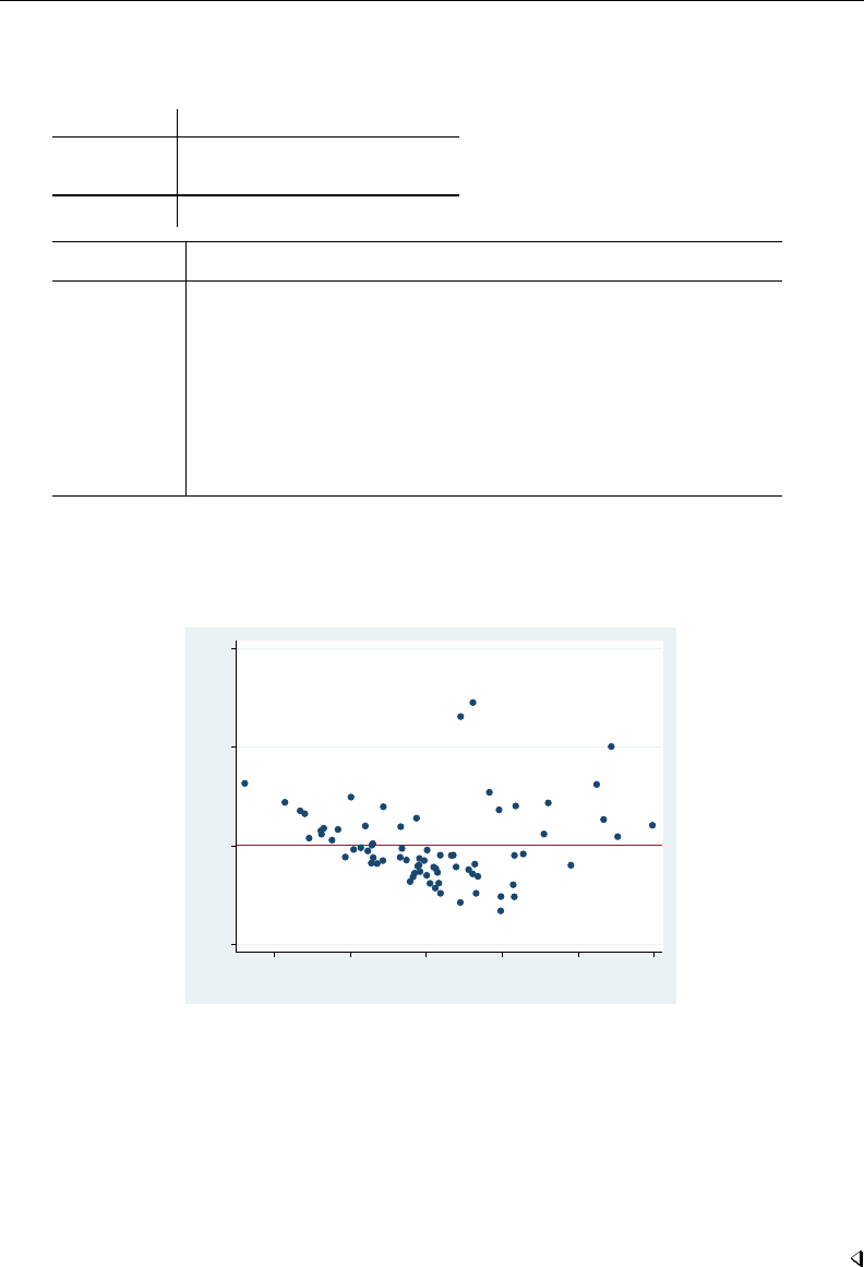
regress postestimation diagnostic plots — Postestimation plots for regress 1907
. use http://www.stata-press.com/data/r13/auto
(1978 Automobile Data)
. regress price weight foreign##c.mpg
Source SS df MS Number of obs = 74
F( 4, 69) = 21.22
Model 350319665 4 87579916.3 Prob > F = 0.0000
Residual 284745731 69 4126749.72 R-squared = 0.5516
Adj R-squared = 0.5256
Total 635065396 73 8699525.97 Root MSE = 2031.4
price Coef. Std. Err. t P>|t| [95% Conf. Interval]
weight 4.613589 .7254961 6.36 0.000 3.166263 6.060914
foreign
Foreign 11240.33 2751.681 4.08 0.000 5750.878 16729.78
mpg 263.1875 110.7961 2.38 0.020 42.15527 484.2197
foreign#c.mpg
Foreign -307.2166 108.5307 -2.83 0.006 -523.7294 -90.70368
_cons -14449.58 4425.72 -3.26 0.002 -23278.65 -5620.51
Once we have fit a model, we may use any of the regression diagnostics commands. rvfplot
(read residual-versus-fitted plot) graphs the residuals against the fitted values:
. rvfplot, yline(0)
−5000 0 5000 10000
Residuals
2000 4000 6000 8000 10000 12000
Fitted values
All the diagnostic plot commands allow the graph twoway and graph twoway scatter options;
we specified a yline(0) to draw a line across the graph at y=0; see [G-2]graph twoway scatter.
In a well-fitted model, there should be no pattern to the residuals plotted against the fitted
values—something not true of our model. Ignoring the two outliers at the top center of the graph,
we see curvature in the pattern of the residuals, suggesting a violation of the assumption that price
is linear in our independent variables. We might also have seen increasing or decreasing variation in
the residuals—heteroskedasticity. Any pattern whatsoever indicates a violation of the least-squares
assumptions.

1908 regress postestimation diagnostic plots — Postestimation plots for regress
avplot
Syntax for avplot
avplot indepvar ,avplot options
avplot options Description
Plot
marker options change look of markers (color, size, etc.)
marker label options add marker labels; change look or position
Reference line
rlopts(cline options)affect rendition of the reference line
Add plots
addplot(plot)add other plots to the generated graph
Y axis, X axis, Titles, Legend, Overall
twoway options any options other than by() documented in [G-3]twoway options
Menu for avplot
Statistics >Linear models and related >Regression diagnostics >Added-variable plot
Description for avplot
avplot graphs an added-variable plot (a.k.a. partial-regression leverage plot, partial regression
plot, or adjusted partial residual plot) after regress.indepvar may be an independent variable (a.k.a.
predictor, carrier, or covariate) that is currently in the model or not.
Options for avplot
Plot
marker options affect the rendition of markers drawn at the plotted points, including their shape,
size, color, and outline; see [G-3]marker options.
marker label options specify if and how the markers are to be labeled; see [G-3]marker label options.
Reference line
rlopts(cline options)affects the rendition of the reference line. See [G-3]cline options.
Add plots
addplot(plot)provides a way to add other plots to the generated graph. See [G-3]addplot option.
Y axis, X axis, Titles, Legend, Overall
twoway options are any of the options documented in [G-3]twoway options, excluding by(). These
include options for titling the graph (see [G-3]title options) and for saving the graph to disk (see
[G-3]saving option).

regress postestimation diagnostic plots — Postestimation plots for regress 1909
Remarks and examples for avplot
avplot graphs an added-variable plot, also known as the partial-regression leverage plot.
One of the wonderful features of one-regressor regressions (regressions of yon one x) is that we
can graph the data and the regression line. There is no easier way to understand the regression than
to examine such a graph. Unfortunately, we cannot do this when we have more than one regressor.
With two regressors, it is still theoretically possible—the graph must be drawn in three dimensions,
but with three or more regressors no graph is possible.
The added-variable plot is an attempt to project multidimensional data back to the two-dimensional
world for each of the original regressors. This is, of course, impossible without making some
concessions. Call the coordinates on an added-variable plot yand x. The added-variable plot has the
following properties:
•There is a one-to-one correspondence between (xi, yi)and the ith observation used in the original
regression.
•A regression of yon xhas the same coefficient and standard error (up to a degree-of-freedom
adjustment) as the estimated coefficient and standard error for the regressor in the original regression.
•The “outlierness” of each observation in determining the slope is in some sense preserved.
It is equally important to note the properties that are not listed. The yand xcoordinates of the
added-variable plot cannot be used to identify functional form, or, at least, not well (see Mallows
[1986]). In the construction of the added-variable plot, the relationship between yand xis forced to
be linear.
Example 2
Let’s use the same model as we used in example 1.
. use http://www.stata-press.com/data/r13/auto
(1978 Automobile Data)
. regress price weight foreign##c.mpg
(output omitted )
We can now examine the added-variable plot for mpg.
. avplot mpg
−4000 −2000 0 2000 4000 6000
e( price | X )
−5 0 5 10
e( mpg | X )
coef = 263.18749, se = 110.79612, t = 2.38

1910 regress postestimation diagnostic plots — Postestimation plots for regress
This graph suggests a problem in determining the coefficient on mpg. Were this a one-regressor
regression, the two points at the top-left corner and the one at the top right would cause us concern,
and so it does in our more complicated multiple-regressor case. To identify the problem points, we
retyped our command, modifying it to read avplot mpg, mlabel(make), and discovered that the
two cars at the top left are the Cadillac Eldorado and the Lincoln Versailles; the point at the top right
is the Cadillac Seville. These three cars account for 100% of the luxury cars in our data, suggesting
that our model is misspecified. By the way, the point at the lower right of the graph, also cause for
concern, is the Plymouth Arrow, our data entry error.
Technical note
Stata’s avplot command can be used with regressors already in the model, as we just did, or
with potential regressors not yet in the model. In either case, avplot will produce the correct graph.
The name “added-variable plot” is unfortunate in the case when the variable is already among the list
of regressors but is, we think, still preferable to the name “partial-regression leverage plot” assigned
by Belsley, Kuh, and Welsch (1980, 30) and more in the spirit of the original use of such plots by
Mosteller and Tukey (1977, 271–279). Welsch (1986, 403), however, disagrees: “I am sorry to see
that Chatterjee and Hadi [1986] endorse the term ‘added-variable plot’ when Xjis part of the original
model” and goes on to suggest the name “adjusted partial residual plot”.
avplots
Syntax for avplots
avplots ,avplots options
avplots options Description
Plot
marker options change look of markers (color, size, etc.)
marker label options add marker labels; change look or position
combine options any of the options documented in [G-2]graph combine
Reference line
rlopts(cline options)affect rendition of the reference line
Y axis, X axis, Titles, Legend, Overall
twoway options any options other than by() documented in [G-3]twoway options
Menu for avplots
Statistics >Linear models and related >Regression diagnostics >Added-variable plot

regress postestimation diagnostic plots — Postestimation plots for regress 1911
Description for avplots
avplots graphs all the added-variable plots in one image.
Options for avplots
Plot
marker options affect the rendition of markers drawn at the plotted points, including their shape,
size, color, and outline; see [G-3]marker options.
marker label options specify if and how the markers are to be labeled; see [G-3]marker label options.
combine options are any of the options documented in [G-2]graph combine. These include options for
titling the graph (see [G-3]title options) and for saving the graph to disk (see [G-3]saving option).
Reference line
rlopts(cline options)affects the rendition of the reference line. See [G-3]cline options.
Y axis, X axis, Titles, Legend, Overall
twoway options are any of the options documented in [G-3]twoway options, excluding by(). These
include options for titling the graph (see [G-3]title options) and for saving the graph to disk (see
[G-3]saving option).
Remarks and examples for avplots
Example 3
In example 2, we used avplot to examine the added-variable plot for mpg in our regression of
price on weight and foreign##c.mpg. Now let’s use avplots to graph an added-variable plot
for every regressor in the data.
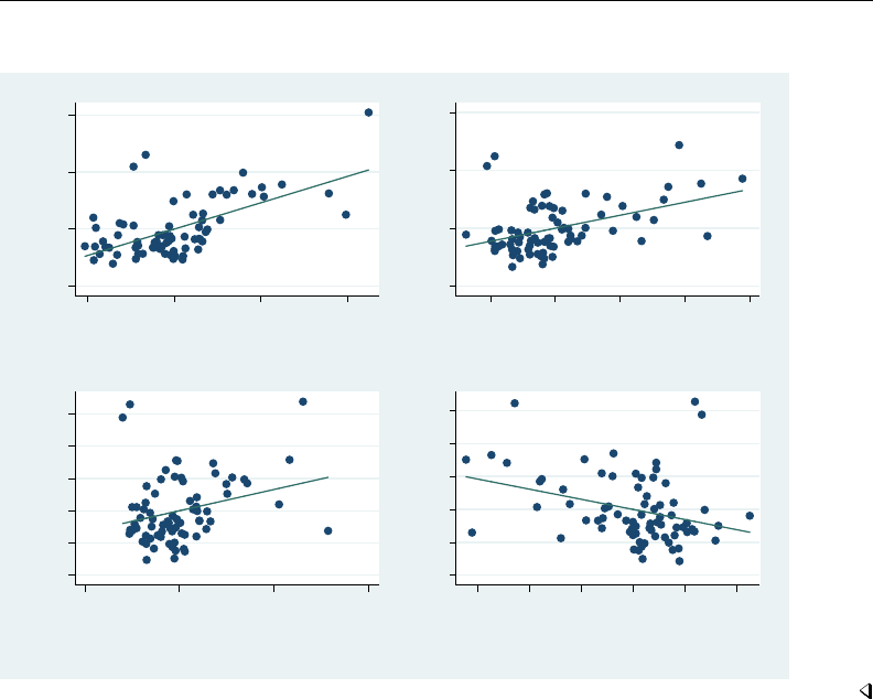
1912 regress postestimation diagnostic plots — Postestimation plots for regress
. avplots
−5000 0 5000 10000
e( price | X )
−500 0 500 1000
e( weight | X )
coef = 4.6135886, se = .7254961, t = 6.36
−5000 0 5000 10000
e( price | X )
−.1 0 .1 .2 .3
e( 1.foreign | X )
coef = 11240.331, se = 2751.6808, t = 4.08
−4000−2000 0 200040006000
e( price | X )
−5 0 5 10
e( mpg | X )
coef = 263.18749, se = 110.79612, t = 2.38
−4000−2000 0 200040006000
e( price | X )
−6 −4 −2 0 2 4
e( 1.foreign#c.mpg | X )
coef = −307.21656, se = 108.53072, t = −2.83

regress postestimation diagnostic plots — Postestimation plots for regress 1913
cprplot
Syntax for cprplot
cprplot indepvar ,cprplot options
cprplot options Description
Plot
marker options change look of markers (color, size, etc.)
marker label options add marker labels; change look or position
Reference line
rlopts(cline options)affect rendition of the reference line
Options
lowess add a lowess smooth of the plotted points
lsopts(lowess options)affect rendition of the lowess smooth
mspline add median spline of the plotted points
msopts(mspline options)affect rendition of the spline
Add plots
addplot(plot)add other plots to the generated graph
Y axis, X axis, Titles, Legend, Overall
twoway options any options other than by() documented in [G-3]twoway options
Menu for cprplot
Statistics >Linear models and related >Regression diagnostics >Component-plus-residual plot
Description for cprplot
cprplot graphs a component-plus-residual plot (a.k.a. partial residual plot) after regress.indepvar
must be an independent variable that is currently in the model.
Options for cprplot
Plot
marker options affect the rendition of markers drawn at the plotted points, including their shape,
size, color, and outline; see [G-3]marker options.
marker label options specify if and how the markers are to be labeled; see [G-3]marker label options.
Reference line
rlopts(cline options)affects the rendition of the reference line. See [G-3]cline options.

1914 regress postestimation diagnostic plots — Postestimation plots for regress
Options
lowess adds a lowess smooth of the plotted points to assist in detecting nonlinearities.
lsopts(lowess options)affects the rendition of the lowess smooth. For an explanation of these
options, especially the bwidth() option, see [R]lowess. Specifying lsopts() implies the lowess
option.
mspline adds a median spline of the plotted points to assist in detecting nonlinearities.
msopts(mspline options)affects the rendition of the spline. For an explanation of these options,
especially the bands() option, see [G-2]graph twoway mspline. Specifying msopts() implies
the mspline option.
Add plots
addplot(plot)provides a way to add other plots to the generated graph. See [G-3]addplot option.
Y axis, X axis, Titles, Legend, Overall
twoway options are any of the options documented in [G-3]twoway options, excluding by(). These
include options for titling the graph (see [G-3]title options) and for saving the graph to disk (see
[G-3]saving option).
Remarks and examples for cprplot
Added-variable plots are successful at identifying outliers, but they cannot be used to identify
functional form. The component-plus-residual plot (Ezekiel 1924;Larsen and McCleary 1972) is
another attempt at projecting multidimensional data into a two-dimensional form, but with different
properties. Although the added-variable plot can identify outliers, the component-plus-residual plot
cannot. It can, however, be used to examine the functional form assumptions of the model. Both plots
have the property that a regression line through the coordinates has a slope equal to the estimated
coefficient in the regression model.
Example 4
We illustrate component-plus-residual plots using a variation of auto.dta.
. use http://www.stata-press.com/data/r13/auto1
(Automobile Models)
. regress price mpg weight
Source SS df MS Number of obs = 74
F( 2, 71) = 14.90
Model 187716578 2 93858289 Prob > F = 0.0000
Residual 447348818 71 6300687.58 R-squared = 0.2956
Adj R-squared = 0.2757
Total 635065396 73 8699525.97 Root MSE = 2510.1
price Coef. Std. Err. t P>|t| [95% Conf. Interval]
mpg -55.9393 75.24136 -0.74 0.460 -205.9663 94.08771
weight 1.710992 .5861682 2.92 0.005 .5422063 2.879779
_cons 2197.9 3190.768 0.69 0.493 -4164.311 8560.11
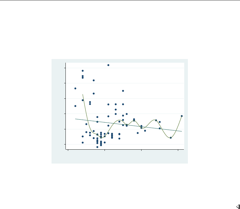
regress postestimation diagnostic plots — Postestimation plots for regress 1915
In fact, we know that the effects of mpg in this model are nonlinear—if we added mpg squared
to the model, its coefficient would have a tstatistic of 2.38, the tstatistic on mpg would become
−2.48, and weight’s effect would become about one-third of its current value and become statistically
insignificant. Pretend that we do not know this.
The component-plus-residual plot for mpg is
. cprplot mpg, mspline msopts(bands(13))
−4000 −2000 0 2000 4000 6000
Component plus residual
10 20 30 40
Mileage (mpg)
We are supposed to examine the above graph for nonlinearities or, equivalently, ask if the regression
line, which has slope equal to the estimated effect of mpg in the original model, fits the data adequately.
To assist our eyes, we added a median spline. Perhaps some people may detect nonlinearity from this
graph, but we assert that if we had not previously revealed the nonlinearity of mpg and if we had not
added the median spline, the graph would not overly bother us.

1916 regress postestimation diagnostic plots — Postestimation plots for regress
acprplot
Syntax for acprplot
acprplot indepvar ,acprplot options
acprplot options Description
Plot
marker options change look of markers (color, size, etc.)
marker label options add marker labels; change look or position
Reference line
rlopts(cline options)affect rendition of the reference line
Options
lowess add a lowess smooth of the plotted points
lsopts(lowess options)affect rendition of the lowess smooth
mspline add median spline of the plotted points
msopts(mspline options)affect rendition of the spline
Add plots
addplot(plot)add other plots to the generated graph
Y axis, X axis, Titles, Legend, Overall
twoway options any options other than by() documented in [G-3]twoway options
Menu for acprplot
Statistics >Linear models and related >Regression diagnostics >Augmented component-plus-residual plot
Description for acprplot
acprplot graphs an augmented component-plus-residual plot (a.k.a. augmented partial residual
plot) as described by Mallows (1986). This seems to work better than the component-plus-residual
plot for identifying nonlinearities in the data.
Options for acprplot
Plot
marker options affect the rendition of markers drawn at the plotted points, including their shape,
size, color, and outline; see [G-3]marker options.
marker label options specify if and how the markers are to be labeled; see [G-3]marker label options.
Reference line
rlopts(cline options)affects the rendition of the reference line. See [G-3]cline options.

regress postestimation diagnostic plots — Postestimation plots for regress 1917
Options
lowess adds a lowess smooth of the plotted points to assist in detecting nonlinearities.
lsopts(lowess options)affects the rendition of the lowess smooth. For an explanation of these
options, especially the bwidth() option, see [R]lowess. Specifying lsopts() implies the lowess
option.
mspline adds a median spline of the plotted points to assist in detecting nonlinearities.
msopts(mspline options)affects the rendition of the spline. For an explanation of these options,
especially the bands() option, see [G-2]graph twoway mspline. Specifying msopts() implies
the mspline option.
Add plots
addplot(plot)provides a way to add other plots to the generated graph. See [G-3]addplot option.
Y axis, X axis, Titles, Legend, Overall
twoway options are any of the options documented in [G-3]twoway options, excluding by(). These
include options for titling the graph (see [G-3]title options) and for saving the graph to disk (see
[G-3]saving option).
Remarks and examples for acprplot
In the cprplot section above, we discussed the component-plus-residual plot. Mallows (1986) pro-
posed an augmented component-plus-residual plot that is often more sensitive to detecting nonlinearity.
Example 5
Let’s compare the augmented component-plus-residual plot with the component-plus-residual plot
of example 4.
. use http://www.stata-press.com/data/r13/auto
(1978 Automobile Data)
. regress price weight foreign##c.mpg
(output omitted )
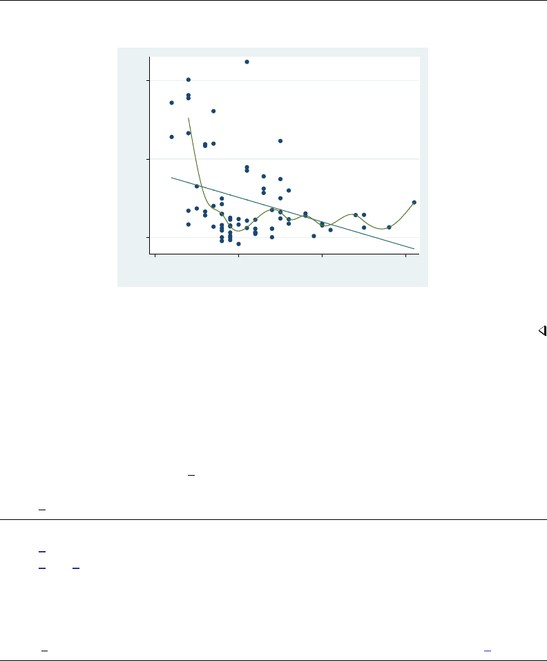
1918 regress postestimation diagnostic plots — Postestimation plots for regress
. acprplot mpg, mspline msopts(bands(13))
−15000 −10000 −5000
Augmented component plus residual
10 20 30 40
Mileage (mpg)
It does do somewhat better.
rvpplot
Syntax for rvpplot
rvpplot indepvar ,rvpplot options
rvpplot options Description
Plot
marker options change look of markers (color, size, etc.)
marker label options add marker labels; change look or position
Add plots
addplot(plot)add other plots to the generated graph
Y axis, X axis, Titles, Legend, Overall
twoway options any options other than by() documented in [G-3]twoway options
Menu for rvpplot
Statistics >Linear models and related >Regression diagnostics >Residual-versus-predictor plot
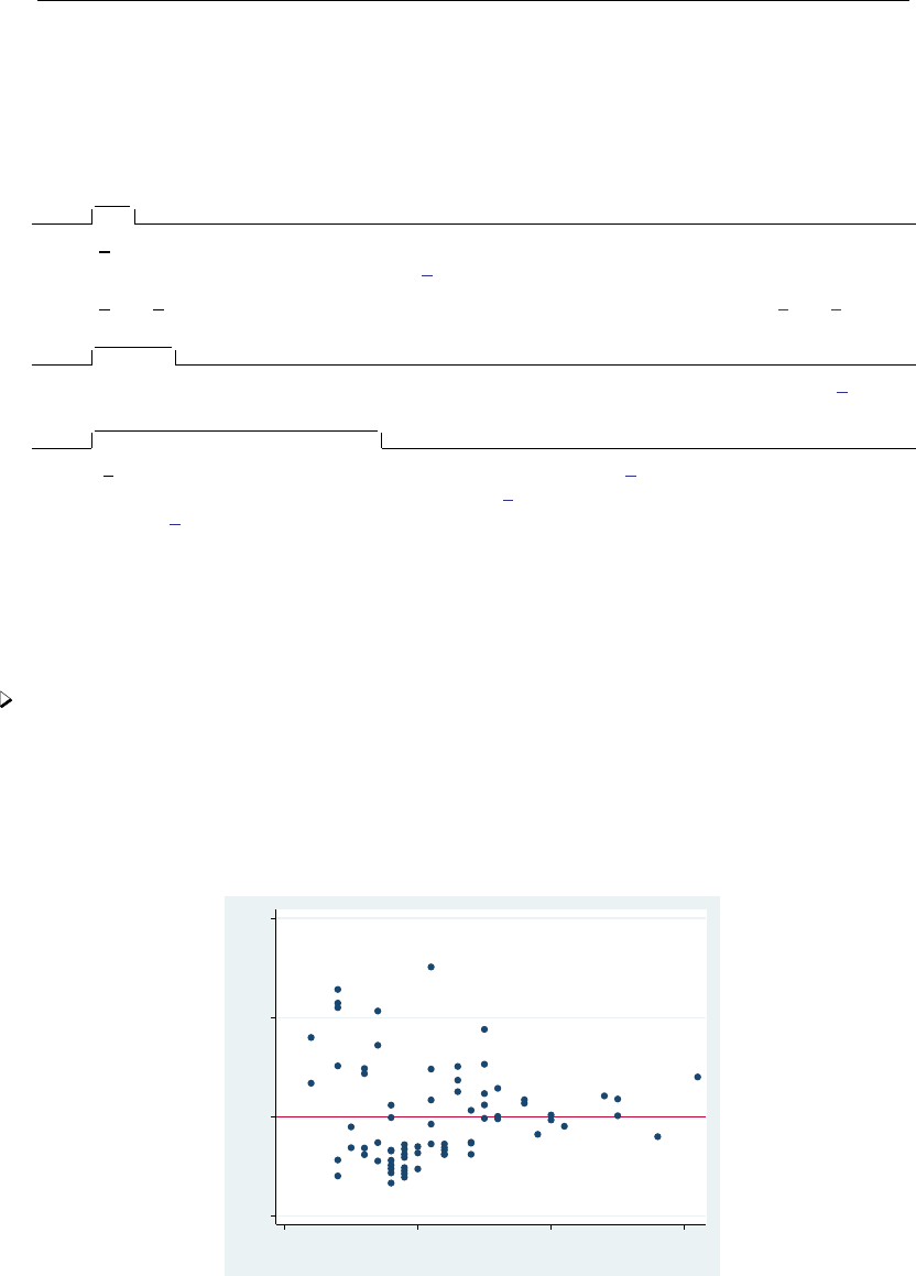
regress postestimation diagnostic plots — Postestimation plots for regress 1919
Description for rvpplot
rvpplot graphs a residual-versus-predictor plot (a.k.a. independent variable plot or carrier plot),
a graph of the residuals against the specified predictor.
Options for rvpplot
Plot
marker options affect the rendition of markers drawn at the plotted points, including their shape,
size, color, and outline; see [G-3]marker options.
marker label options specify if and how the markers are to be labeled; see [G-3]marker label options.
Add plots
addplot(plot)provides a way to add other plots to the generated graph; see [G-3]addplot option.
Y axis, X axis, Titles, Legend, Overall
twoway options are any of the options documented in [G-3]twoway options, excluding by(). These
include options for titling the graph (see [G-3]title options) and for saving the graph to disk (see
[G-3]saving option).
Remarks and examples for rvpplot
The residual-versus-predictor plot is a simple way to look for violations of the regression assumptions.
If the assumptions are correct, there should be no pattern on the graph.
Example 6
Let’s use our model of price on mpg and weight.
. use http://www.stata-press.com/data/r13/auto
(1978 Automobile Data)
. regress price weight foreign##c.mpg
(output omitted )
. rvpplot mpg, yline(0)
−5000 0 5000 10000
Residuals
10 20 30 40
Mileage (mpg)

1920 regress postestimation diagnostic plots — Postestimation plots for regress
Remember, any pattern counts as a problem, and in this graph, we see that the variation in the
residuals decreases as mpg increases.
lvr2plot
Syntax for lvr2plot
lvr2plot ,lvr2plot options
lvr2plot options Description
Plot
marker options change look of markers (color, size, etc.)
marker label options add marker labels; change look or position
Add plots
addplot(plot)add other plots to the generated graph
Y axis, X axis, Titles, Legend, Overall
twoway options any options other than by() documented in [G-3]twoway options
Menu for lvr2plot
Statistics >Linear models and related >Regression diagnostics >Leverage-versus-squared-residual plot
Description for lvr2plot
lvr2plot graphs a leverage-versus-squared-residual plot (a.k.a. L-R plot).
Options for lvr2plot
Plot
marker options affect the rendition of markers drawn at the plotted points, including their shape,
size, color, and outline; see [G-3]marker options.
marker label options specify if and how the markers are to be labeled; see [G-3]marker label options.
Add plots
addplot(plot)provides a way to add other plots to the generated graph. See [G-3]addplot option.
Y axis, X axis, Titles, Legend, Overall
twoway options are any of the options documented in [G-3]twoway options, excluding by(). These
include options for titling the graph (see [G-3]title options) and for saving the graph to disk (see
[G-3]saving option).
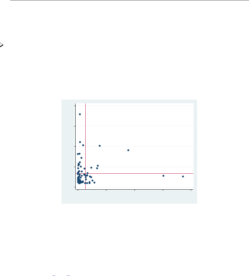
regress postestimation diagnostic plots — Postestimation plots for regress 1921
Remarks and examples for lvr2plot
One of the most useful diagnostic graphs is provided by lvr2plot (leverage-versus-residual-squared
plot), a graph of leverage against the (normalized) residuals squared.
Example 7
We illustrate lvr2plot using our model in example 1.
. use http://www.stata-press.com/data/r13/auto
(1978 Automobile Data)
. regress price weight foreign##c.mpg
(output omitted )
. lvr2plot
0 .1 .2 .3 .4
Leverage
0 .05 .1 .15 .2
Normalized residual squared
The lines on the chart show the average values of leverage and the (normalized) residuals squared.
Points above the horizontal line have higher-than-average leverage; points to the right of the vertical
line have larger-than-average residuals.
One point immediately catches our eye, and four more make us pause. The point at the top of the
graph has high leverage and a smaller-than-average residual. The other points that bother us all have
higher-than-average leverage, two with smaller-than-average residuals and two with larger-than-average
residuals.
A less pretty but more useful version of the above graph specifies that make be used as the symbol
(see [G-3]marker label options):

1922 regress postestimation diagnostic plots — Postestimation plots for regress
. lvr2plot, mlabel(make) mlabp(0) m(none) mlabsize(small)
AMC Concord
AMC Pacer
AMC Spirit
Buick Century
Buick Electra
Buick LeSabre
Buick Opel
Buick Regal
Buick Riviera
Buick Skylark
Cad. Deville Cad. Eldorado
Cad. Seville
Chev. Chevette
Chev. Impala
Chev. Malibu
Chev. Monte Carlo
Chev. Monza
Chev. Nova
Dodge Colt
Dodge Diplomat
Dodge Magnum
Dodge St. Regis
Ford Fiesta
Ford Mustang
Linc. Continental
Linc. Mark V
Linc. Versailles
Merc. Bobcat
Merc. Cougar
Merc. Marquis
Merc. Monarch
Merc. XR−7
Merc. Zephyr
Olds 98
Olds Cutl Supr
Olds Cutlass
Olds Delta 88
Olds Omega
Olds Starfire
Olds Toronado
Plym. Arrow
Plym. Champ
Plym. Horizon
Plym. Sapporo
Plym. Volare
Pont. Catalina
Pont. Firebird
Pont. Grand Prix
Pont. Le Mans
Pont. Phoenix
Pont. Sunbird
Audi 5000
Audi Fox
BMW 320i
Datsun 200
Datsun 210
Datsun 510
Datsun 810
Fiat Strada
Honda Accord
Honda Civic
Mazda GLC
Peugeot 604
Renault Le Car
Subaru
Toyota Celica
Toyota Corolla
Toyota Corona
VW Dasher
VW Diesel
VW Rabbit
VW Scirocco
Volvo 260
0 .1 .2 .3 .4
Leverage
0 .05 .1 .15 .2
Normalized residual squared
The VW Diesel, Plymouth Champ, Plymouth Arrow, and Peugeot 604 are the points that cause us the
most concern. When we further examine our data, we discover that the VW Diesel is the only diesel
in our data and that the data for the Plymouth Arrow were entered incorrectly into the computer. No
such simple explanations were found for the Plymouth Champ and Peugeot 604.
Methods and formulas
See Hamilton (2013, 209–214) and Kohler and Kreuter (2012, sec. 9.3) for a discussion of these
diagnostic graphs.
The lvr2plot command plots leverage against the squares of the normalized residuals. The
normalized residuals are defined as benj=bej/(Pibe2
i)1/2.
References
Belsley, D. A., E. Kuh, and R. E. Welsch. 1980. Regression Diagnostics: Identifying Influential Data and Sources of
Collinearity. New York: Wiley.
Chatterjee, S., and A. S. Hadi. 1986. Influential observations, high leverage points, and outliers in linear regression.
Statistical Science 1: 379–393.
Cox, N. J. 2004. Speaking Stata: Graphing model diagnostics.Stata Journal 4: 449–475.
Ezekiel, M. 1924. A method of handling curvilinear correlation for any number of variables. Journal of the American
Statistical Association 19: 431–453.
Hamilton, L. C. 1992. Regression with Graphics: A Second Course in Applied Statistics. Belmont, CA: Duxbury.
. 2013. Statistics with Stata: Updated for Version 12. 8th ed. Boston: Brooks/Cole.
Hoaglin, D. C., and R. E. Welsch. 1978. The hat matrix in regression and ANOVA. American Statistician 32: 17–22.
Kohler, U., and F. Kreuter. 2012. Data Analysis Using Stata. 3rd ed. College Station, TX: Stata Press.
Larsen, W. A., and S. J. McCleary. 1972. The use of partial residual plots in regression analysis. Technometrics 14:
781–790.
Lindsey, C., and S. J. Sheather. 2010a. Optimal power transformation via inverse response plots.Stata Journal 10:
200–214.

regress postestimation diagnostic plots — Postestimation plots for regress 1923
. 2010b. Model fit assessment via marginal model plots.Stata Journal 10: 215–225.
Mallows, C. L. 1986. Augmented partial residuals. Technometrics 28: 313–319.
Mosteller, C. F., and J. W. Tukey. 1977. Data Analysis and Regression: A Second Course in Statistics. Reading, MA:
Addison–Wesley.
Welsch, R. E. 1986. Comment [on Chatterjee and Hadi 1986]. Statistical Science 1: 403–405.
Also see
[R]regress — Linear regression
[R]regress postestimation — Postestimation tools for regress
[R]regress postestimation time series — Postestimation tools for regress with time series
[U] 20 Estimation and postestimation commands

Title
regress postestimation time series — Postestimation tools for regress with time series
Description Syntax for estat archlm Options for estat archlm
Syntax for estat bgodfrey Options for estat bgodfrey Syntax for estat durbinalt
Options for estat durbinalt Syntax for estat dwatson Menu for estat
Remarks and examples Stored results Methods and formulas
Acknowledgment References Also see
Description
The following postestimation commands for time series are available for regress:
Command Description
estat archlm test for ARCH effects in the residuals
estat bgodfrey Breusch–Godfrey test for higher-order serial correlation
estat durbinalt Durbin’s alternative test for serial correlation
estat dwatson Durbin–Watson dstatistic to test for first-order serial correlation
These commands provide regression diagnostic tools specific to time series. You must tsset your
data before using these commands; see [TS]tsset.
estat archlm tests for time-dependent volatility. estat bgodfrey,estat durbinalt, and
estat dwatson test for serial correlation in the residuals of a linear regression. For non-time-series
regression diagnostic tools, see [R]regress postestimation.
estat archlm performs Engle’s Lagrange multiplier (LM) test for the presence of autoregressive
conditional heteroskedasticity.
estat bgodfrey performs the Breusch–Godfrey test for higher-order serial correlation in the
disturbance. This test does not require that all the regressors be strictly exogenous.
estat durbinalt performs Durbin’s alternative test for serial correlation in the disturbance. This
test does not require that all the regressors be strictly exogenous.
estat dwatson computes the Durbin–Watson dstatistic (Durbin and Watson 1950) to test for
first-order serial correlation in the disturbance when all the regressors are strictly exogenous.
Syntax for estat archlm
estat archlm ,archlm options
archlm options Description
lags(numlist)test numlist lag orders
force allow test after regress, vce(robust)
1924

regress postestimation time series — Postestimation tools for regress with time series 1925
Options for estat archlm
lags(numlist)specifies a list of numbers, indicating the lag orders to be tested. The test will be
performed separately for each order. The default is order one.
force allows the test to be run after regress, vce(robust). The command will not work if the
vce(cluster clustvar)option is specified with regress; see [R]regress.
Syntax for estat bgodfrey
estat bgodfrey ,bgodfrey options
bgodfrey options Description
lags(numlist)test numlist lag orders
nomiss0 do not use Davidson and MacKinnon’s approach
small obtain p-values using the For tdistribution
Options for estat bgodfrey
lags(numlist)specifies a list of numbers, indicating the lag orders to be tested. The test will be
performed separately for each order. The default is order one.
nomiss0 specifies that Davidson and MacKinnon’s approach (1993, 358), which replaces the missing
values in the initial observations on the lagged residuals in the auxiliary regression with zeros, not
be used.
small specifies that the p-values of the test statistics be obtained using the For tdistribution instead
of the default chi-squared or normal distribution.
Syntax for estat durbinalt
estat durbinalt ,durbinalt options
durbinalt options Description
lags(numlist)test numlist lag orders
nomiss0 do not use Davidson and MacKinnon’s approach
robust compute standard errors using the robust/sandwich estimator
small obtain p-values using the For tdistribution
force allow test after regress, vce(robust) or after newey
Options for estat durbinalt
lags(numlist)specifies a list of numbers, indicating the lag orders to be tested. The test will be
performed separately for each order. The default is order one.

1926 regress postestimation time series — Postestimation tools for regress with time series
nomiss0 specifies that Davidson and MacKinnon’s approach (1993, 358), which replaces the missing
values in the initial observations on the lagged residuals in the auxiliary regression with zeros, not
be used.
robust specifies that the Huber/White/sandwich robust estimator of the variance–covariance matrix
be used in Durbin’s alternative test.
small specifies that the p-values of the test statistics be obtained using the For tdistribution instead
of the default chi-squared or normal distribution. This option may not be specified with robust,
which always uses an For tdistribution.
force allows the test to be run after regress, vce(robust) and after newey (see [R]regress and
[TS]newey). The command will not work if the vce(cluster clustvar)option is specified with
regress.
Syntax for estat dwatson
estat dwatson
Menu for estat
Statistics >Postestimation >Reports and statistics
Remarks and examples
The Durbin–Watson test is used to determine whether the error term in a linear regression model
follows an AR(1) process. For the linear model
yt=xtβ+ut
the AR(1) process can be written as
ut=ρut−1+t
In general, an AR(1) process requires only that tbe independent and identically distributed (i.i.d.).
The Durbin–Watson test, however, requires tto be distributed N(0, σ2)for the statistic to have an
exact distribution. Also, the Durbin–Watson test can be applied only when the regressors are strictly
exogenous. A regressor xis strictly exogenous if Corr(xs, ut)=0for all sand t, which precludes
the use of the Durbin–Watson statistic with models where lagged values of the dependent variable
are included as regressors.
The null hypothesis of the test is that there is no first-order autocorrelation. The Durbin–Watson
dstatistic can take on values between 0 and 4 and under the null dis equal to 2. Values of dless
than 2 suggest positive autocorrelation (ρ > 0), whereas values of dgreater than 2 suggest negative
autocorrelation (ρ < 0). Calculating the exact distribution of the dstatistic is difficult, but empirical
upper and lower bounds have been established based on the sample size and the number of regressors.
Extended tables for the dstatistic have been published by Savin and White (1977). For example,
suppose you have a model with 30 observations and three regressors (including the constant term).
For a test of the null hypothesis of no autocorrelation versus the alternative of positive autocorrelation,
the lower bound of the dstatistic is 1.284, and the upper bound is 1.567 at the 5% significance
level. You would reject the null if d < 1.284, and you would fail to reject if d > 1.567. A value
falling within the range (1.284, 1.567) leads to no conclusion about whether or not to reject the null
hypothesis.

regress postestimation time series — Postestimation tools for regress with time series 1927
When lagged dependent variables are included among the regressors, the past values of the error
term are correlated with those lagged variables at time t, implying that they are not strictly exogenous
regressors. The inclusion of covariates that are not strictly exogenous causes the dstatistic to be biased
toward the acceptance of the null hypothesis. Durbin (1970) suggested an alternative test for models
with lagged dependent variables and extended that test to the more general AR(p)serial correlation
process
ut=ρ1ut−1+··· +ρput−p+t
where tis i.i.d. with variance σ2but is not assumed or required to be normal for the test.
The null hypothesis of Durbin’s alternative test is
H0:ρ1= 0, . . . , ρp= 0
and the alternative is that at least one of the ρ’s is nonzero. Although the null hypothesis was originally
derived for an AR(p)process, this test turns out to have power against MA(p)processes as well. Hence,
the actual null of this test is that there is no serial correlation up to order pbecause the MA(p)and
the AR(p)models are locally equivalent alternatives under the null. See Godfrey (1988, 113–115) for
a discussion of this result.
Durbin’s alternative test is in fact a LM test, but it is most easily computed with a Wald test on
the coefficients of the lagged residuals in an auxiliary OLS regression of the residuals on their lags
and all the covariates in the original regression. Consider the linear regression model
yt=β1x1t+··· +βkxkt +ut(1)
in which the covariates x1through xkare not assumed to be strictly exogenous and utis assumed to
be i.i.d. and to have finite variance. The process is also assumed to be stationary. (See Wooldridge
[2013] for a discussion of stationarity.) Estimating the parameters in (1) by OLS obtains the residuals
but. Next another OLS regression is performed of buton but−1,...,but−pand the other regressors,
but=γ1but−1+··· +γpbut−p+β1x1t+··· +βkxkt +t(2)
where tstands for the random-error term in this auxiliary OLS regression. Durbin’s alternative test
is then obtained by performing a Wald test that γ1, . . . , γpare jointly zero. The test can be made
robust to an unknown form of heteroskedasticity by using a robust VCE estimator when estimating
the regression in (2). When there are only strictly exogenous regressors and p=1, this test is
asymptotically equivalent to the Durbin–Watson test.
The Breusch–Godfrey test is also an LM test of the null hypothesis of no autocorrelation versus the
alternative that utfollows an AR(p)or MA(p)process. Like Durbin’s alternative test, it is based on the
auxiliary regression (2), and it is computed as NR2, where Nis the number of observations and R2is
the simple R2from the regression. This test and Durbin’s alternative test are asymptotically equivalent.
The test statistic NR2has an asymptotic χ2distribution with pdegrees of freedom. It is valid with
or without the strict exogeneity assumption but is not robust to conditional heteroskedasticity, even
if a robust VCE is used when fitting (2).
In fitting (2), the values of the lagged residuals will be missing in the initial periods. As noted by
Davidson and MacKinnon (1993), the residuals will not be orthogonal to the other covariates in the
model in this restricted sample, which implies that the R2from the auxiliary regression will not be zero
when the lagged residuals are left out. Hence, Breusch and Godfrey’s NR2version of the test may
overreject in small samples. To correct this problem, Davidson and MacKinnon (1993) recommend
setting the missing values of the lagged residuals to zero and running the auxiliary regression in (2)
over the full sample used in (1). This small-sample correction has become conventional for both the
Breusch–Godfrey and Durbin’s alternative test, and it is the default for both commands. Specifying
the nomiss0 option overrides this default behavior and treats the initial missing values generated by
regressing on the lagged residuals as missing. Hence, nomiss0 causes these initial observations to
be dropped from the sample of the auxiliary regression.

1928 regress postestimation time series — Postestimation tools for regress with time series
Durbin’s alternative test and the Breusch–Godfrey test were originally derived for the case covered
by regress without the vce(robust) option. However, after regress, vce(robust) and newey,
Durbin’s alternative test is still valid and can be invoked if the robust and force options are
specified.
Example 1: tests for serial correlation
Using data from Klein (1950), we first fit an OLS regression of consumption on the government
wage bill:
. use http://www.stata-press.com/data/r13/klein
. tsset yr
time variable: yr, 1920 to 1941
delta: 1 unit
. regress consump wagegovt
Source SS df MS Number of obs = 22
F( 1, 20) = 17.72
Model 532.567711 1 532.567711 Prob > F = 0.0004
Residual 601.207167 20 30.0603584 R-squared = 0.4697
Adj R-squared = 0.4432
Total 1133.77488 21 53.9892799 Root MSE = 5.4827
consump Coef. Std. Err. t P>|t| [95% Conf. Interval]
wagegovt 2.50744 .5957173 4.21 0.000 1.264796 3.750085
_cons 40.84699 3.192183 12.80 0.000 34.18821 47.50577
If we assume that wagegov is a strictly exogenous variable, we can use the Durbin–Watson test
to check for first-order serial correlation in the errors.
. estat dwatson
Durbin-Watson d-statistic( 2, 22) = .3217998
The Durbin–Watson dstatistic, 0.32, is far from the center of its distribution (d=2.0). Given 22
observations and two regressors (including the constant term) in the model, the lower 5% bound is about
0.997, much greater than the computed dstatistic. Assuming that wagegov is strictly exogenous, we
can reject the null of no first-order serial correlation. Rejecting the null hypothesis does not necessarily
mean an AR process; other forms of misspecification may also lead to a significant test statistic. If we
are willing to assume that the errors follow an AR(1) process and that wagegov is strictly exogenous,
we could refit the model using arima or prais and model the error process explicitly; see [TS]arima
and [TS]prais.
If we are not willing to assume that wagegov is strictly exogenous, we could instead use Durbin’s
alternative test or the Breusch–Godfrey to test for first-order serial correlation. Because we have only
22 observations, we will use the small option.
. estat durbinalt, small
Durbin’s alternative test for autocorrelation
lags(p) F df Prob > F
1 35.035 ( 1, 19 ) 0.0000
H0: no serial correlation

regress postestimation time series — Postestimation tools for regress with time series 1929
. estat bgodfrey, small
Breusch-Godfrey LM test for autocorrelation
lags(p) F df Prob > F
1 14.264 ( 1, 19 ) 0.0013
H0: no serial correlation
Both tests strongly reject the null of no first-order serial correlation, so we decide to refit the
model with two lags of consump included as regressors and then rerun estat durbinalt and
estat bgodfrey. Because the revised model includes lagged values of the dependent variable, the
Durbin–Watson test is not applicable.
. regress consump wagegovt L.consump L2.consump
Source SS df MS Number of obs = 20
F( 3, 16) = 44.01
Model 702.660311 3 234.220104 Prob > F = 0.0000
Residual 85.1596011 16 5.32247507 R-squared = 0.8919
Adj R-squared = 0.8716
Total 787.819912 19 41.4642059 Root MSE = 2.307
consump Coef. Std. Err. t P>|t| [95% Conf. Interval]
wagegovt .6904282 .3295485 2.10 0.052 -.0081835 1.38904
consump
L1. 1.420536 .197024 7.21 0.000 1.002864 1.838208
L2. -.650888 .1933351 -3.37 0.004 -1.06074 -.241036
_cons 9.209073 5.006701 1.84 0.084 -1.404659 19.82281
. estat durbinalt, small lags(1/2)
Durbin’s alternative test for autocorrelation
lags(p) F df Prob > F
1 0.080 ( 1, 15 ) 0.7805
2 0.260 ( 2, 14 ) 0.7750
H0: no serial correlation
. estat bgodfrey, small lags(1/2)
Breusch-Godfrey LM test for autocorrelation
lags(p) F df Prob > F
1 0.107 ( 1, 15 ) 0.7484
2 0.358 ( 2, 14 ) 0.7056
H0: no serial correlation
Although wagegov and the constant term are no longer statistically different from zero at the 5%
level, the output from estat durbinalt and estat bgodfrey indicates that including the two lags
of consump has removed any serial correlation from the errors.
Engle (1982) suggests an LM test for checking for autoregressive conditional heteroskedasticity
(ARCH) in the errors. The pth-order ARCH model can be written as

1930 regress postestimation time series — Postestimation tools for regress with time series
σ2
t=E(u2
t|ut−1, . . . , ut−p)
=γ0+γ1u2
t−1+··· +γpu2
t−p
To test the null hypothesis of no autoregressive conditional heteroskedasticity (that is, γ1=··· =
γp=0), we first fit the OLS model (1), obtain the residuals but, and run another OLS regression on
the lagged residuals:
bu2
t=γ0+γ1bu2
t−1+··· +γpbu2
t−p+(3)
The test statistic is NR2, where Nis the number of observations in the sample and R2is the R2
from the regression in (3). Under the null hypothesis, the test statistic follows a χ2
pdistribution.
Example 2: estat archlm
We refit the original model that does not include the two lags of consump and then use estat
archlm to see if there is any evidence that the errors are autoregressive conditional heteroskedastic.
. regress consump wagegovt
Source SS df MS Number of obs = 22
F( 1, 20) = 17.72
Model 532.567711 1 532.567711 Prob > F = 0.0004
Residual 601.207167 20 30.0603584 R-squared = 0.4697
Adj R-squared = 0.4432
Total 1133.77488 21 53.9892799 Root MSE = 5.4827
consump Coef. Std. Err. t P>|t| [95% Conf. Interval]
wagegovt 2.50744 .5957173 4.21 0.000 1.264796 3.750085
_cons 40.84699 3.192183 12.80 0.000 34.18821 47.50577
. estat archlm, lags(1 2 3)
LM test for autoregressive conditional heteroskedasticity (ARCH)
lags(p) chi2 df Prob > chi2
1 5.543 1 0.0186
2 9.431 2 0.0090
3 9.039 3 0.0288
H0: no ARCH effects vs. H1: ARCH(p) disturbance
estat archlm shows the results for tests of ARCH(1),ARCH(2), and ARCH(3) effects, respectively. At
the 5% significance level, all three tests reject the null hypothesis that the errors are not autoregressive
conditional heteroskedastic. See [TS]arch for information on fitting ARCH models.
Stored results
estat archlm stores the following in r():
Scalars
r(N) number of observations r(N gaps) number of gaps
r(k) number of regressors
Macros
r(lags) lag order
Matrices
r(arch) test statistic for each lag order r(p) two-sided p-values
r(df) degrees of freedom

regress postestimation time series — Postestimation tools for regress with time series 1931
estat bgodfrey stores the following in r():
Scalars
r(N) number of observations r(N gaps) number of gaps
r(k) number of regressors
Macros
r(lags) lag order
Matrices
r(chi2) χ2statistic for each lag order r(p) two-sided p-values
r(F) Fstatistic for each lag order (small
only)
r(df) degrees of freedom
r(df r) residual degrees of freedom (small
only)
estat durbinalt stores the following in r():
Scalars
r(N) number of observations r(N gaps) number of gaps
r(k) number of regressors
Macros
r(lags) lag order
Matrices
r(chi2) χ2statistic for each lag order r(p) two-sided p-values
r(F) Fstatistic for each lag order (small
only)
r(df) degrees of freedom
r(df r) residual degrees of freedom (small
only)
estat dwatson stores the following in r():
Scalars
r(N) number of observations r(N gaps) number of gaps
r(k) number of regressors r(dw) Durbin–Watson statistic
Methods and formulas
Consider the regression
yt=β1x1t+··· +βkxkt +ut(4)
in which some of the covariates are not strictly exogenous. In particular, some of the xit may be
lags of the dependent variable. We are interested in whether the utare serially correlated.
The Durbin–Watson dstatistic reported by estat dwatson is
d=
n−1
P
t=1
(but+1 −but)2
n
P
t=1 bu2
t
where butrepresents the residual of the tth observation.
To compute Durbin’s alternative test and the Breusch–Godfrey test against the null hypothesis that
there is no pth order serial correlation, we fit the regression in (4), compute the residuals, and then
fit the following auxiliary regression of the residuals buton plags of butand on all the covariates in
the original regression in (4):
but=γ1but−1+··· +γpbut−p+β1x1t+··· +βkxkt +(5)

1932 regress postestimation time series — Postestimation tools for regress with time series
Durbin’s alternative test is computed by performing a Wald test to determine whether the coefficients
of but−1,...,but−pare jointly different from zero. By default, the statistic is assumed to be distributed
χ2(p). When small is specified, the statistic is assumed to follow an F(p,N−p−k) distribution.
The reported p-value is a two-sided p-value. When robust is specified, the Wald test is performed
using the Huber/White/sandwich estimator of the variance–covariance matrix, and the test is robust
to an unspecified form of heteroskedasticity.
The Breusch–Godfrey test is computed as NR2, where Nis the number of observations in the
auxiliary regression (5) and R2is the R2from the same regression (5). Like Durbin’s alternative
test, the Breusch–Godfrey test is asymptotically distributed χ2(p), but specifying small causes the
p-value to be computed using an F(p, N −p−k).
By default, the initial missing values of the lagged residuals are replaced with zeros, and the
auxiliary regression is run over the full sample used in the original regression of (4). Specifying the
nomiss0 option causes these missing values to be treated as missing values, and the observations are
dropped from the sample.
Engle’s LM test for ARCH(p)effects fits an OLS regression of bu2
ton bu2
t−1,...,bu2
t−p:
bu2
t=γ0+γ1bu2
t−1+··· +γpbu2
t−p+
The test statistic is nR2and is asymptotically distributed χ2(p).
Acknowledgment
The original versions of estat archlm,estat bgodfrey, and estat durbinalt were written
by Christopher F. Baum of the Department of Economics at Boston College and author of the Stata
Press books An Introduction to Modern Econometrics Using Stata and An Introduction to Stata
Programming.
References
Baum, C. F. 2006. An Introduction to Modern Econometrics Using Stata. College Station, TX: Stata Press.
Baum, C. F., and V. L. Wiggins. 2000a. sg135: Test for autoregressive conditional heteroskedasticity in regression
error distribution. Stata Technical Bulletin 55: 13–14. Reprinted in Stata Technical Bulletin Reprints, vol. 10, pp.
143–144. College Station, TX: Stata Press.
. 2000b. sg136: Tests for serial correlation in regression error distribution. Stata Technical Bulletin 55: 14–15.
Reprinted in Stata Technical Bulletin Reprints, vol. 10, pp. 145–147. College Station, TX: Stata Press.
Beran, R. J., and N. I. Fisher. 1998. A conversation with Geoff Watson. Statistical Science 13: 75–93.
Breusch, T. S. 1978. Testing for autocorrelation in dynamic linear models. Australian Economic Papers 17: 334–355.
Davidson, R., and J. G. MacKinnon. 1993. Estimation and Inference in Econometrics. New York: Oxford University
Press.
Durbin, J. 1970. Testing for serial correlation in least-squares regressions when some of the regressors are lagged
dependent variables. Econometrica 38: 410–421.
Durbin, J., and S. J. Koopman. 2012. Time Series Analysis by State Space Methods. 2nd ed. Oxford: Oxford
University Press.
Durbin, J., and G. S. Watson. 1950. Testing for serial correlation in least squares regression. I. Biometrika 37:
409–428.
. 1951. Testing for serial correlation in least squares regression. II. Biometrika 38: 159–177.
Engle, R. F. 1982. Autoregressive conditional heteroscedasticity with estimates of the variance of United Kingdom
inflation. Econometrica 50: 987–1007.

regress postestimation time series — Postestimation tools for regress with time series 1933
Fisher, N. I., and P. Hall. 1998. Geoffrey Stuart Watson: Tributes and obituary (3 December 1921–3 January 1998).
Australian and New Zealand Journal of Statistics 40: 257–267.
Godfrey, L. G. 1978. Testing against general autoregressive and moving average error models when the regressors
include lagged dependent variables. Econometrics 46: 1293–1301.
. 1988. Misspecification Tests in Econometrics: The Lagrange Multiplier Principle and Other Approaches.
Econometric Society Monographs, No. 16. Cambridge: Cambridge University Press.
Greene, W. H. 2012. Econometric Analysis. 7th ed. Upper Saddle River, NJ: Prentice Hall.
Klein, L. R. 1950. Economic Fluctuations in the United States 1921–1941. New York: Wiley.
Koopman, S. J. 2012. James Durbin, FBA, 1923–2012. Journal of the Royal Statistical Society, Series A 175:
1060–1064.
Phillips, P. C. B. 1988. The ET Interview: Professor James Durbin. Econometric Theory 4: 125–157.
Savin, N. E., and K. J. White. 1977. The Durbin–Watson test for serial correlation with extreme sample sizes or
many regressors. Econometrica 45: 1989–1996.
Wooldridge, J. M. 2013. Introductory Econometrics: A Modern Approach. 5th ed. Mason, OH: South-Western.
James Durbin (1923–2012) was a British statistician who was born in Wigan, near Manchester. He
studied mathematics at Cambridge and after military service and various research posts joined the
London School of Economics in 1950. Later in life, he was also affiliated with University College
London. His many contributions to statistics centered on serial correlation, time series (including
major contributions to structural or unobserved components models), sample survey methodology,
goodness-of-fit tests, and sample distribution functions, with emphasis on applications in the
social sciences. He served terms as president of the Royal Statistical Society and the International
Statistical Institute.
Geoffrey Stuart Watson (1921–1998) was born in Victoria, Australia, and earned degrees at
Melbourne University and North Carolina State University. After a visit to the University of
Cambridge, he returned to Australia, working at Melbourne and then the Australian National
University. Following periods at Toronto and Johns Hopkins, he settled at Princeton. Throughout
his wide-ranging career, he made many notable accomplishments and important contributions,
including the Durbin–Watson test for serial correlation, the Nadaraya–Watson estimator in
nonparametric regression, and methods for analyzing directional data.
Leslie G. Godfrey (1946– ) was born in London and earned degrees at the Universities of Exeter
and London. He is now a professor of econometrics at the University of York. His interests
center on implementation and interpretation of tests of econometric models, including nonnested
models.
Trevor Stanley Breusch (1949– ) was born in Queensland and earned degrees at the University
of Queensland and Australian National University (ANU). After a post at the University of
Southampton, he returned to work at ANU. His background is in econometric methods and his
recent interests include political values and social attitudes, earnings and income, and measurement
of underground economic activity.
Also see
[R]regress — Linear regression
[TS]tsset — Declare data to be time-series data
[R]regress postestimation — Postestimation tools for regress
[R]regress postestimation diagnostic plots — Postestimation plots for regress

Title
#review — Review previous commands
Syntax Description Remarks and examples
Syntax
#review #1#2
Description
The #review command displays the last few lines typed at the terminal.
Remarks and examples
#review (pronounced pound-review) is a Stata preprocessor command. #commands do not generate
a return code or generate ordinary Stata errors. The only error message associated with #commands
is “unrecognized #command”.
The #review command displays the last few lines typed at the terminal. If no arguments follow
#review, the last five lines typed at the terminal are displayed. The first argument specifies the
number of lines to be reviewed, so #review 10 displays the last 10 lines typed. The second argument
specifies the number of lines to be displayed, so #review 10 5 displays five lines, starting at the
10th previous line.
Stata reserves a buffer for #review lines and stores as many previous lines in the buffer as
will fit, rolling out the oldest line to make room for the newest. Requests to #review lines no
longer stored will be ignored. Only lines typed at the terminal are placed in the #review buffer. See
[U] 10.5 Editing previous lines in Stata.
Example 1
Typing #review by itself will show the last five lines you typed at the terminal:
. #review
5 use mydata
4 * comments go into the #review buffer, too
3 describe
2 tabulate marriage educ [freq=number]
1 tabulate marriage educ [freq=number], chi2
.
Typing #review 15 2 shows the 15th and 14th previous lines:
. #review 15 2
15 replace x=. if x<200
14 summarize x
.
1934

Title
roc — Receiver operating characteristic (ROC) analysis
Description Reference
Description
ROC analysis quantifies the accuracy of diagnostic tests or other evaluation modalities used to
discriminate between two states or conditions, which are here referred to as normal and abnormal or
control and case. The discriminatory accuracy of a diagnostic test is measured by its ability to correctly
classify known normal and abnormal subjects. For this reason, we often refer to the diagnostic test
as a classifier. The analysis uses the ROC curve, a graph of the sensitivity versus 1 −specificity of
the diagnostic test. The sensitivity is the fraction of positive cases that are correctly classified by the
diagnostic test, whereas the specificity is the fraction of negative cases that are correctly classified.
Thus the sensitivity is the true-positive rate, and the specificity is the true-negative rate.
There are six ROC commands:
Command Entry Description
roccomp [R]roccomp Tests of equality of ROC areas
rocgold [R]roccomp Tests of equality of ROC areas against a standard ROC curve
rocfit [R]rocfit Parametric ROC models
rocreg [R]rocreg Nonparametric and parametric ROC regression models
rocregplot [R]rocregplot Plot marginal and covariate-specific ROC curves
roctab [R]roctab Nonparametric ROC analysis
Postestimation commands are available after rocfit and rocreg; see [R]rocfit postestimation and
[R]rocreg postestimation.
Both nonparametric and parametric (semiparametric) methods have been suggested for generating
the ROC curve. The roctab command performs nonparametric ROC analysis for a single classifier.
roccomp extends the nonparametric ROC analysis function of roctab to situations where we have
multiple diagnostic tests of interest to be compared and tested. The rocgold command also provides
ROC analysis for multiple classifiers. rocgold compares each classifier’s ROC curve to a “gold
standard” ROC curve and makes adjustments for multiple comparisons in the analysis. Both rocgold
and roccomp also allow parametric estimation of the ROC curve through a binormal fit. In a binormal
fit, both the control and the case populations are normal.
The rocfit command also estimates the ROC curve of a classifier through a binormal fit. Unlike
roctab,roccomp, and rocgold,rocfit is an estimation command. In postestimation, graphs of
the ROC curve and confidence bands can be produced. Additional tests on the parameters can also be
conducted.
ROC analysis can be interpreted as a two-stage process. First, the control distribution of the classifier
is estimated, assuming a normal model or using a distribution-free estimation technique. The classifier
is standardized using the control distribution to 1 −percentile value, the false-positive rate. Second,
the ROC curve is estimated as the case distribution of the standardized classifier values.
Covariates may affect both stages of ROC analysis. The first stage may be affected, yielding a
covariate-adjusted ROC curve. The second stage may also be affected, producing multiple covariate-
specific ROC curves.
1935

1936 roc — Receiver operating characteristic (ROC) analysis
The rocreg command performs ROC analysis under both types of covariate effects. Both parametric
(semiparametric) and nonparametric methods may be used by rocreg. Like rocfit,rocreg is an
estimation command and provides many postestimation capabilities.
The global performance of a diagnostic test is commonly summarized by the area under the ROC
curve (AUC). This area can be interpreted as the probability that the result of a diagnostic test of a
randomly selected abnormal subject will be greater than the result of the same diagnostic test from
a randomly selected normal subject. The greater the AUC, the better the global performance of the
diagnostic test. Each of the ROC commands provides computation of the AUC.
Citing a lack of clinical relevance for the AUC, other ROC summary measures have been suggested.
These include the partial area under the ROC curve for a given false-positive rate t[pAUC(t)]. This
is the area under the ROC curve from the false-positive rate of 0 to t. The ROC value at a particular
false-positive rate and the false-positive rate for a particular ROC value are also useful summary
measures for the ROC curve. These three measures are directly estimated by rocreg during the model
fit or postestimation stages. Point estimates of ROC value are computed by the other ROC commands,
but no standard errors are reported.
See Pepe (2003) for a discussion of ROC analysis. Pepe has posted Stata datasets and programs
used to reproduce results presented in the book (http://www.stata.com/bookstore/pepe.html).
Reference
Pepe, M. S. 2003. The Statistical Evaluation of Medical Tests for Classification and Prediction. New York: Oxford
University Press.

Title
roccomp — Tests of equality of ROC areas
Syntax Menu Description Options
Remarks and examples Stored results Methods and formulas References
Also see
Syntax
Test equality of ROC areas
roccomp refvar classvar classvars if in weight ,roccomp options
Test equality of ROC area against a standard ROC curve
rocgold refvar goldvar classvar classvars if in weight ,rocgold options
roccomp options Description
Main
by(varname)split into groups by variable
test(matname)use contrast matrix for comparing ROC areas
graph graph the ROC curve
norefline suppress plotting the 45-degree reference line
separate place each ROC curve on its own graph
summary report the area under the ROC curve
binormal estimate areas by using binormal distribution assumption
line#opts(cline options)affect rendition of the #th binormal fit line
level(#)set confidence level; default is level(95)
Plot
plot#opts(plot options)affect rendition of the #th ROC curve
Reference line
rlopts(cline options)affect rendition of the reference line
Y axis, X axis, Titles, Legend, Overall
twoway options any options other than by() documented in [G-3]twoway options
1937

1938 roccomp — Tests of equality of ROC areas
rocgold options Description
Main
sidak adjust the significance probability by using ˇ
Sid´
ak’s method
test(matname)use contrast matrix for comparing ROC areas
graph graph the ROC curve
norefline suppress plotting the 45-degree reference line
separate place each ROC curve on its own graph
summary report the area under the ROC curve
binormal estimate areas by using binormal distribution assumption
line#opts(cline options)affect rendition of the #th binormal fit line
level(#)set confidence level; default is level(95)
Plot
plot#opts(plot options)affect rendition of the #th ROC curve; plot 1 is the “gold standard”
Reference line
rlopts(cline options)affect rendition of the reference line
Y axis, X axis, Titles, Legend, Overall
twoway options any options other than by() documented in [G-3]twoway options
plot options Description
marker options change look of markers (color, size, etc.)
marker label options add marker labels; change look or position
cline options change the look of the line
fweights are allowed; see [U] 11.1.6 weight.
Menu
roccomp
Statistics >Epidemiology and related >ROC analysis >Test equality of two or more ROC areas
rocgold
Statistics >Epidemiology and related >ROC analysis >Test equality of ROC area against gold standard
Description
The above commands are used to perform receiver operating characteristic (ROC) analyses with
rating and discrete classification data.
The two variables refvar and classvar must be numeric. The reference variable indicates the true
state of the observation, such as diseased and nondiseased or normal and abnormal, and must be
coded as 0 and 1. The rating or outcome of the diagnostic test or test modality is recorded in classvar,
which must be at least ordinal, with higher values indicating higher risk.

roccomp — Tests of equality of ROC areas 1939
roccomp tests the equality of two or more ROC areas obtained from applying two or more test
modalities to the same sample or to independent samples. roccomp expects the data to be in wide
form when comparing areas estimated from the same sample and in long form for areas estimated
from independent samples.
rocgold independently tests the equality of the ROC area of each of several test modalities,
specified by classvar, against a “gold standard” ROC curve, goldvar. For each comparison, rocgold
reports the raw and the Bonferroni-adjusted significance probability. Optionally, ˇ
Sid´
ak’s adjustment
for multiple comparisons can be obtained.
See [R]rocfit and [R]rocreg for commands that fit maximum-likelihood ROC models.
Options
Main
by(varname)(roccomp only) is required when comparing independent ROC areas. The by() variable
identifies the groups to be compared.
sidak (rocgold only) requests that the significance probability be adjusted for the effect of multiple
comparisons by using ˇ
Sid´
ak’s method. Bonferroni’s adjustment is reported by default.
test(matname)specifies the contrast matrix to be used when comparing ROC areas. By default, the
null hypothesis that all areas are equal is tested.
graph produces graphical output of the ROC curve.
norefline suppresses plotting the 45-degree reference line from the graphical output of the ROC
curve.
separate is meaningful only with roccomp and specifies that each ROC curve be placed on its own
graph rather than one curve on top of the other.
summary reports the area under the ROC curve, its standard error, and its confidence interval. This
option is needed only when also specifying graph.
binormal specifies that the areas under the ROC curves to be compared should be estimated using
the binormal distribution assumption. By default, areas to be compared are computed using the
trapezoidal rule.
line#opts(cline options)affects the rendition of the line representing the #th ROC curve drawn
using the binormal distribution assumption; see [G-3]cline options. These lines are drawn only if
the binormal option is specified.
level(#)specifies the confidence level, as a percentage, for the confidence intervals. The default is
level(95) or as set by set level; see [R]level.
Plot
plot#opts(plot options)affects the rendition of the #th ROC curve—the curve’s plotted points
connected by lines. The plot options can affect the size and color of markers, whether and how
the markers are labeled, and whether and how the points are connected; see [G-3]marker options,
[G-3]marker label options, and [G-3]cline options.
For rocgold,plot1opts() are applied to the ROC for the gold standard.
Reference line
rlopts(cline options)affects the rendition of the reference line; see [G-3]cline options.

1940 roccomp — Tests of equality of ROC areas
Y axis, X axis, Titles, Legend, Overall
twoway options are any of the options documented in [G-3]twoway options. These include op-
tions for titling the graph (see [G-3]title options), options for saving the graph to disk (see
[G-3]saving option), and the by() option (see [G-3]by option).
Remarks and examples
Remarks are presented under the following headings:
Introduction
Comparing areas under the ROC curve
Correlated data
Independent data
Comparing areas with a gold standard
Introduction
roccomp provides comparison of the ROC curves of multiple classifiers. rocgold compares the
ROC curves of multiple classifiers with a single “gold standard” classifier. Adjustment of inference
for multiple comparisons is also provided by rocgold.
See Pepe (2003) for a discussion of ROC analysis. Pepe has posted Stata datasets and programs
used to reproduce results presented in the book (http://www.stata.com/bookstore/pepe.html).
Comparing areas under the ROC curve
The area under multiple ROC curves can be compared by using roccomp. The command syntax
is slightly different if the ROC curves are correlated (that is, different diagnostic tests are applied to
the same sample) or independent (that is, diagnostic tests are applied to different samples).
Correlated data
Example 1
Hanley and McNeil (1983) presented data from an evaluation of two computer algorithms designed
to reconstruct CT images from phantoms. We will call these two algorithms’ modalities 1 and 2. A
sample of 112 phantoms was selected; 58 phantoms were considered normal, and the remaining 54
were abnormal. Each of the two modalities was applied to each phantom, and the resulting images
were rated by a reviewer using a six-point scale: 1 =definitely normal, 2 =probably normal, 3
=possibly normal, 4 =possibly abnormal, 5 =probably abnormal, and 6 =definitely abnormal.
Because each modality was applied to the same sample of phantoms, the two sets of outcomes are
correlated.
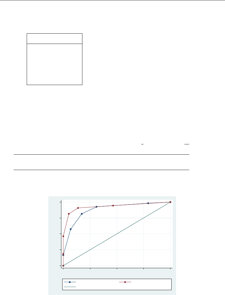
roccomp — Tests of equality of ROC areas 1941
We list the first 7 observations:
. use http://www.stata-press.com/data/r13/ct
. list in 1/7, sep(0)
mod1 mod2 status
1. 2 1 0
2. 5 5 1
3. 2 1 0
4. 2 3 0
5. 5 6 1
6. 2 2 0
7. 3 2 0
The data are in wide form, which is required when dealing with correlated data. Each observation
corresponds to one phantom. The variable mod1 identifies the rating assigned for the first modality,
and mod2 identifies the rating assigned for the second modality. The true status of the phantoms is
given by status=0 if they are normal and status=1 if they are abnormal. The observations with
at least one missing rating were dropped from the analysis.
We plot the two ROC curves and compare their areas.
. roccomp status mod1 mod2, graph summary
ROC Asymptotic Normal
Obs Area Std. Err. [95% Conf. Interval]
mod1 112 0.8828 0.0317 0.82067 0.94498
mod2 112 0.9302 0.0256 0.88005 0.98042
Ho: area(mod1) = area(mod2)
chi2(1) = 2.31 Prob>chi2 = 0.1282
0.00 0.25 0.50 0.75 1.00
Sensitivity
0.00 0.25 0.50 0.75 1.00
1−Specificity
mod1 ROC area: 0.8828 mod2 ROC area: 0.9302
Reference
By default, roccomp, with the graph option specified, plots the ROC curves on the same graph.
Optionally the curves can be plotted side by side, each on its own graph, by also specifying separate.
For each curve, roccomp reports summary statistics and provides a test for the equality of the area
under the curves, using an algorithm suggested by DeLong, DeLong, and Clarke-Pearson (1988).
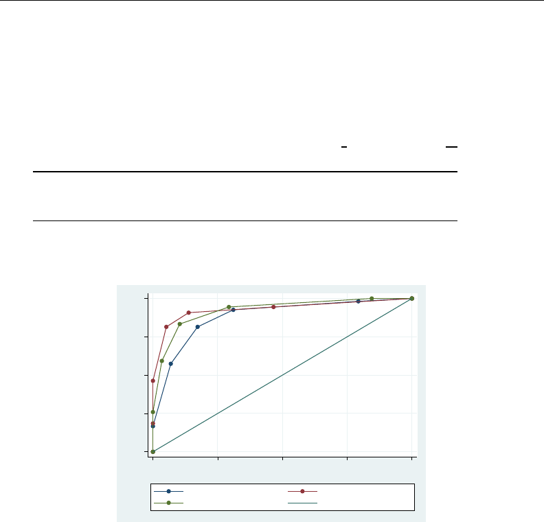
1942 roccomp — Tests of equality of ROC areas
Although the area under the ROC curve for modality 2 is larger than that of modality 1, the
chi-squared test yielded a significance probability of 0.1282, suggesting that there is no significant
difference between these two areas.
The roccomp command can also be used to compare more than two ROC areas. To illustrate this,
we modified the previous dataset by including a fictitious third modality.
. use http://www.stata-press.com/data/r13/ct2
. roccomp status mod1 mod2 mod3, graph summary
ROC Asymptotic Normal
Obs Area Std. Err. [95% Conf. Interval]
mod1 112 0.8828 0.0317 0.82067 0.94498
mod2 112 0.9302 0.0256 0.88005 0.98042
mod3 112 0.9240 0.0241 0.87670 0.97132
Ho: area(mod1) = area(mod2) = area(mod3)
chi2(2) = 6.54 Prob>chi2 = 0.0381
0.00 0.25 0.50 0.75 1.00
Sensitivity
0.00 0.25 0.50 0.75 1.00
1−Specificity
mod1 ROC area: 0.8828 mod2 ROC area: 0.9302
mod3 ROC area: 0.924 Reference
By default, roccomp tests whether the areas under the ROC curves are all equal. Other comparisons
can be tested by creating a contrast matrix and specifying test(matname), where matname is the
name of the contrast matrix.
For example, assume that we are interested in testing whether the area under the ROC for mod1 is
equal to that of mod3. To do this, we can first create an appropriate contrast matrix and then specify
its name with the test() option.
Of course, this is a trivial example because we could have just specified
. roccomp status mod1 mod3
without including mod2 to obtain the same test results. However, for illustration, we will continue
with this example.
The contrast matrix must have its number of columns equal to the number of classvars (that is,
the total number of ROC curves) and a number of rows less than or equal to the number of classvars,
and the elements of each row must add to zero.

roccomp — Tests of equality of ROC areas 1943
. matrix C=(1,0,-1)
. roccomp status mod1 mod2 mod3, test(C)
ROC Asymptotic Normal
Obs Area Std. Err. [95% Conf. Interval]
mod1 112 0.8828 0.0317 0.82067 0.94498
mod2 112 0.9302 0.0256 0.88005 0.98042
mod3 112 0.9240 0.0241 0.87670 0.97132
Ho: Comparison as defined by contrast matrix: C
chi2(1) = 5.25 Prob>chi2 = 0.0220
Although all three areas are reported, the comparison is made using the specified contrast matrix.
Perhaps more interesting would be a comparison of the area from mod1 and the average area of
mod2 and mod3.
. matrix C=(1,-.5,-.5)
. roccomp status mod1 mod2 mod3, test(C)
ROC Asymptotic Normal
Obs Area Std. Err. [95% Conf. Interval]
mod1 112 0.8828 0.0317 0.82067 0.94498
mod2 112 0.9302 0.0256 0.88005 0.98042
mod3 112 0.9240 0.0241 0.87670 0.97132
Ho: Comparison as defined by contrast matrix: C
chi2(1) = 3.43 Prob>chi2 = 0.0642
Other contrasts could be made. For example, we could test if mod3 is different from at least one
of the other two by first creating the following contrast matrix:
. matrix C=(-1,0,1 \ 0,-1,1)
. mat list C
C[2,3]
c1 c2 c3
r1 -1 0 1
r2 0 -1 1
Independent data
Example 2
In example 1, we noted that because each test modality was applied to the same sample of
phantoms, the classification outcomes were correlated. Now assume that we have collected the same
data presented by Hanley and McNeil (1983), except that we applied the first test modality to one
sample of phantoms and the second test modality to a different sample of phantoms. The resulting
measurements are now considered independent.

1944 roccomp — Tests of equality of ROC areas
Here are a few of the observations.
. use http://www.stata-press.com/data/r13/ct3
. list in 1/7, sep(0)
pop status rating mod
1. 12 0 1 1
2. 31 0 1 2
3. 1 1 1 1
4. 3 1 1 2
5. 28 0 2 1
6. 19 0 2 2
7. 3 1 2 1
The data are in long form, which is required when dealing with independent data. The data consist
of 24 observations: 6 observations corresponding to abnormal phantoms and 6 to normal phantoms
evaluated using the first modality, and similarly 6 observations corresponding to abnormal phantoms
and 6 to normal phantoms evaluated using the second modality. The number of phantoms corresponding
to each observation is given by the pop variable. Once again we have frequency-weighted data. The
variable mod identifies the modality, and rating is the assigned classification.
We can better view our data by using the table command.
. table status rating [fw=pop], by(mod) row col
mod and rating
status 1 2 3 4 5 6 Total
1
0 12 28 8 6 4 58
1 1 3 6 13 22 9 54
Total 13 31 14 19 26 9 112
2
0 31 19 5 3 58
1 3 2 5 19 15 10 54
Total 34 21 10 22 15 10 112
The status variable indicates the true status of the phantoms: status =0 if they are normal and
status =1 if they are abnormal.
We now compare the areas under the two ROC curves.
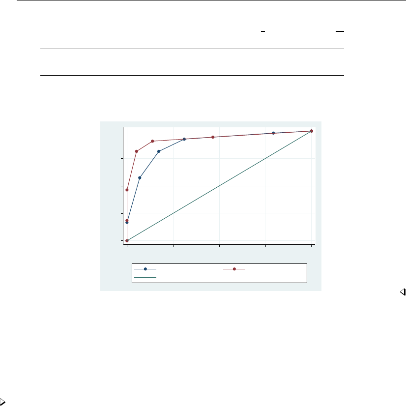
roccomp — Tests of equality of ROC areas 1945
. roccomp status rating [fw=pop], by(mod) graph summary
ROC Asymptotic Normal
mod Obs Area Std. Err. [95% Conf. Interval]
1 112 0.8828 0.0317 0.82067 0.94498
2 112 0.9302 0.0256 0.88005 0.98042
Ho: area(1) = area(2)
chi2(1) = 1.35 Prob>chi2 = 0.2447
0.00 0.25 0.50 0.75 1.00
Sensitivity
0.00 0.25 0.50 0.75 1.00
1−Specificity
1 ROC area: 0.8828 2 ROC area: 0.9302
Reference
Comparing areas with a gold standard
The area under multiple ROC curves can be compared with a gold standard using rocgold. The
command syntax is similar to that of roccomp. The tests are corrected for the effect of multiple
comparisons.
Example 3
We will use the same data (presented by Hanley and McNeil [1983]) as in the roccomp examples.
Let’s assume that the first modality is considered to be the standard against which both the second
and third modalities are compared.
We want to plot and compare both the areas of the ROC curves of mod2 and mod3 with mod1.
Because we consider mod1 to be the gold standard, it is listed first after the reference variable in the
rocgold command line.
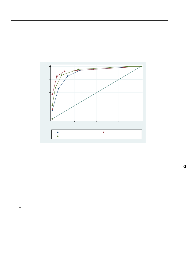
1946 roccomp — Tests of equality of ROC areas
. use http://www.stata-press.com/data/r13/ct2
. rocgold status mod1 mod2 mod3, graph summary
ROC Bonferroni
Area Std. Err. chi2 df Pr>chi2 Pr>chi2
mod1 (standard) 0.8828 0.0317
mod2 0.9302 0.0256 2.3146 1 0.1282 0.2563
mod3 0.9240 0.0241 5.2480 1 0.0220 0.0439
0.00 0.25 0.50 0.75 1.00
Sensitivity
0.00 0.25 0.50 0.75 1.00
1−Specificity
mod1 ROC area: 0.8828 mod2 ROC area: 0.9302
mod3 ROC area: 0.924 Reference
Equivalently, we could have done this in two steps by using the roccomp command.
. roccomp status mod1 mod2, graph summary
. roccomp status mod1 mod3, graph summary
Stored results
roccomp stores the following in r():
Scalars
r(N g) number of groups r(df) χ2degrees of freedom
r(p) significance probability r(chi2) χ2
Matrices
r(V) variance–covariance matrix
rocgold stores the following in r():
Scalars
r(N g) number of groups
Matrices
r(V) variance–covariance matrix r(p) significance-probability vector
r(chi2) χ2vector r(p adj) adjusted significance-probability vector
r(df) χ2degrees-of-freedom vector

roccomp — Tests of equality of ROC areas 1947
Methods and formulas
Assume that we applied a diagnostic test to each of Nnnormal and Naabnormal subjects.
Further assume that the higher the outcome value of the diagnostic test, the higher the risk of the
subject being abnormal. Let b
θbe the estimated area under the curve, and let Xi, i =1,2, . . . , Na
and Yj, j =1,2, . . . , Nnbe the values of the diagnostic test for the abnormal and normal subjects,
respectively.
Areas under ROC curves are compared using an algorithm suggested by DeLong, DeLong, and
Clarke-Pearson (1988). Let b
θ= ( b
θ1,b
θ2,..., b
θk)be a vector representing the areas under kROC
curves. See Methods and formulas in [R]roctab for the definition of these area estimates.
For the rth area, define
Vr
10(Xi) = 1
Nn
Nn
X
j=1
ψ(Xr
i, Y r
j)
and for each normal subject, j, define
Vr
01(Yj) = 1
Na
Na
X
i=1
ψ(Xr
i, Y r
j)
where
ψ(Xr, Y r) = (1Yr< Xr
1
2Yr=Xr
0Yr> Xr
Define the k×kmatrix S10 such that the (r, s)th element is
Sr,s
10 =1
Na−1
Na
X
i=1{Vr
10(Xi)−b
θr}{Vs
10(Xi)−b
θs}
and S01 such that the (r, s)th element is
Sr,s
01 =1
Nn−1
Nn
X
j=1{Vr
01(Yi)−b
θr}{Vs
01(Yi)−b
θs}
Then the covariance matrix is
S=1
Na
S10 +1
Nn
S01
Let Lbe a contrast matrix defining the comparison, so that
(b
θ−θ)0L0LSL0−1L(b
θ−θ)
has a chi-squared distribution with degrees of freedom equal to the rank of LSL0.

1948 roccomp — Tests of equality of ROC areas
References
Cleves, M. A. 1999. sg120: Receiver operating characteristic (ROC) analysis.Stata Technical Bulletin 52: 19–33.
Reprinted in Stata Technical Bulletin Reprints, vol. 9, pp. 212–229. College Station, TX: Stata Press.
. 2000. sg120.2: Correction to roccomp command.Stata Technical Bulletin 54: 26. Reprinted in Stata Technical
Bulletin Reprints, vol. 9, p. 231. College Station, TX: Stata Press.
. 2002a. Comparative assessment of three common algorithms for estimating the variance of the area under the
nonparametric receiver operating characteristic curve.Stata Journal 2: 280–289.
. 2002b. From the help desk: Comparing areas under receiver operating characteristic curves from two or more
probit or logit models.Stata Journal 2: 301–313.
DeLong, E. R., D. M. DeLong, and D. L. Clarke-Pearson. 1988. Comparing the areas under two or more correlated
receiver operating characteristic curves: A nonparametric approach. Biometrics 44: 837–845.
Erdreich, L. S., and E. T. Lee. 1981. Use of relative operating characteristic analysis in epidemiology: A method for
dealing with subjective judgment. American Journal of Epidemiology 114: 649–662.
Hanley, J. A., and B. J. McNeil. 1983. A method of comparing the areas under receiver operating characteristic
curves derived from the same cases. Radiology 148: 839–843.
Harbord, R. M., and P. Whiting. 2009. metandi: Meta-analysis of diagnostic accuracy using hierarchical logistic
regression.Stata Journal 9: 211–229.
Juul, S., and M. Frydenberg. 2014. An Introduction to Stata for Health Researchers. 4th ed. College Station, TX:
Stata Press.
Ma, G., and W. J. Hall. 1993. Confidence bands for the receiver operating characteristic curves. Medical Decision
Making 13: 191–197.
Pepe, M. S. 2003. The Statistical Evaluation of Medical Tests for Classification and Prediction. New York: Oxford
University Press.
Reichenheim, M. E., and A. Ponce de Leon. 2002. Estimation of sensitivity and specificity arising from validity
studies with incomplete design.Stata Journal 2: 267–279.
Seed, P. T., and A. Tob´
ıas. 2001. sbe36.1: Summary statistics for diagnostic tests.Stata Technical Bulletin 59: 25–27.
Reprinted in Stata Technical Bulletin Reprints, vol. 10, pp. 90–93. College Station, TX: Stata Press.
Tob´
ıas, A. 2000. sbe36: Summary statistics report for diagnostic tests.Stata Technical Bulletin 56: 16–18. Reprinted
in Stata Technical Bulletin Reprints, vol. 10, pp. 87–90. College Station, TX: Stata Press.
Working, H., and H. Hotelling. 1929. Application of the theory of error to the interpretation of trends. Journal of the
American Statistical Association 24 (Suppl.): 73–85.
Also see
[R]logistic postestimation — Postestimation tools for logistic
[R]roc — Receiver operating characteristic (ROC) analysis
[R]rocfit — Parametric ROC models
[R]rocreg — Receiver operating characteristic (ROC) regression
[R]roctab — Nonparametric ROC analysis

Title
rocfit — Parametric ROC models
Syntax Menu Description Options
Remarks and examples Stored results Methods and formulas References
Also see
Syntax
rocfit refvar classvar if in weight ,rocfit options
rocfit options Description
Model
continuous(#)divide classvar into #groups of approximately equal length
generate(newvar)create newvar containing classification groups
SE
vce(vcetype)vcetype may be oim or opg
Reporting
level(#)set confidence level; default is level(95)
Maximization
maximize options control the maximization process; seldom used
fp, is allowed; see [U] 11.1.10 Prefix commands.
fweights are allowed; see [U] 11.1.6 weight.
See [U] 20 Estimation and postestimation commands for more capabilities of estimation commands.
Menu
Statistics >Epidemiology and related >ROC analysis >Parametric ROC analysis without covariates
Description
rocfit fits maximum-likelihood ROC models assuming a binormal distribution of the latent variable.
The two variables refvar and classvar must be numeric. The reference variable indicates the true
state of the observation, such as diseased and nondiseased or normal and abnormal, and must be
coded as 0 and 1. The rating or outcome of the diagnostic test or test modality is recorded in classvar,
which must be at least ordinal, with higher values indicating higher risk.
See [R]roc for other commands designed to perform receiver operating characteristic (ROC) analyses
with rating and discrete classification data.
1949

1950 rocfit — Parametric ROC models
Options
Model
continuous(#)specifies that the continuous classvar be divided into #groups of approximately
equal length. This option is required when classvar takes on more than 20 distinct values.
continuous(.) may be specified to indicate that classvar be used as it is, even though it could
have more than 20 distinct values.
generate(newvar)specifies the new variable that is to contain the values indicating the groups
produced by continuous(#).generate() may be specified only with continuous().
SE
vce(vcetype)specifies the type of standard error reported. vcetype may be either oim or opg; see
[R]vce option.
Reporting
level(#); see [R]estimation options.
Maximization
maximize options:difficult,technique(algorithm spec),iterate(#),nolog,trace,
gradient,showstep,hessian,showtolerance,tolerance(#),ltolerance(#),
nrtolerance(#),nonrtolerance, and from(init specs); see [R]maximize. These options are
seldom used.
Setting the optimization type to technique(bhhh) resets the default vcetype to vce(opg).
Remarks and examples
Dorfman and Alf (1969) developed a generalized approach for obtaining maximum likelihood
estimates of the parameters for a smooth fitting ROC curve. The most commonly used method for
ordinal data, and the one implemented here, is based upon the binormal model; see Pepe (2003),
Pepe, Longton, and Janes (2009), and Janes, Longton, and Pepe (2009) for methods of ROC analysis
for continuous data, including methods for adjusting for covariates.
The model assumes the existence of an unobserved, continuous, latent variable that is normally
distributed (perhaps after a monotonic transformation) in both the normal and abnormal populations
with means µnand µaand variances σ2
nand σ2
a, respectively. The model further assumes that the
Kcategories of the rating variable result from partitioning the unobserved latent variable by K−1
fixed boundaries. The method fits a straight line to the empirical ROC points plotted using normal
probability scales on both axes. Maximum likelihood estimates of the line’s slope and intercept and
the K−1 boundaries are obtained simultaneously. See Methods and formulas for details.
The intercept from the fitted line is a measurement of (µa−µn)/σa,and the slope measures
σn/σa.
Thus the intercept is the standardized difference between the two latent population means, and the
slope is the ratio of the two standard deviations. The null hypothesis that there is no difference between
the two population means is evaluated by testing that the intercept =0, and the null hypothesis that
the variances in the two populations are equal is evaluated by testing that the slope =1.

rocfit — Parametric ROC models 1951
Example 1
We use Hanley and McNeil’s (1982) dataset, described in example 1 of [R]roctab, to fit a smooth
ROC curve assuming a binormal model.
. use http://www.stata-press.com/data/r13/hanley
. rocfit disease rating
Fitting binormal model:
Iteration 0: log likelihood = -123.68069
Iteration 1: log likelihood = -123.64867
Iteration 2: log likelihood = -123.64855
Iteration 3: log likelihood = -123.64855
Binormal model of disease on rating Number of obs = 109
Goodness-of-fit chi2(2) = 0.21
Prob > chi2 = 0.9006
Log likelihood = -123.64855
Coef. Std. Err. z P>|z| [95% Conf. Interval]
intercept 1.656782 0.310456 5.34 0.000 1.048300 2.265265
slope (*) 0.713002 0.215882 -1.33 0.184 0.289881 1.136123
/cut1 0.169768 0.165307 1.03 0.304 -0.154227 0.493764
/cut2 0.463215 0.167235 2.77 0.006 0.135441 0.790990
/cut3 0.766860 0.174808 4.39 0.000 0.424243 1.109477
/cut4 1.797938 0.299581 6.00 0.000 1.210770 2.385106
Indices from binormal fit
Index Estimate Std. Err. [95% Conf. Interval]
ROC area 0.911331 0.029506 0.853501 0.969161
delta(m) 2.323671 0.502370 1.339044 3.308298
d(e) 1.934361 0.257187 1.430284 2.438438
d(a) 1.907771 0.259822 1.398530 2.417012
(*) z test for slope==1
rocfit outputs the MLE for the intercept and slope of the fitted regression line along with, here, four
boundaries (because there are five ratings) labeled /cut1 through /cut4. Also rocfit computes
and reports four indices based on the fitted ROC curve: the area under the curve (labeled ROC area),
δ(m)(labeled delta(m)), de(labeled d(e)), and da(labeled d(a)). More information about these
indices can be found in Methods and formulas and in Erdreich and Lee (1981).

1952 rocfit — Parametric ROC models
Stored results
rocfit stores the following in e():
Scalars
e(N) number of observations
e(k) number of parameters
e(k eq) number of equations in e(b)
e(k eq model) number of equations in overall model test
e(k dv) number of dependent variables
e(df m) model degrees of freedom
e(ll) log likelihood
e(chi2 gf) goodness-of-fit χ2
e(df gf) goodness-of-fit degrees of freedom
e(p gf) χ2goodness-of-fit significance probability
e(area) area under the ROC curve
e(se area) standard error for the area under the ROC curve
e(deltam) delta(m)
e(se delm) standard area for delta(m)
e(de) d(e) index
e(se de) standard error for d(e) index
e(da) d(a) index
e(se da) standard error for d(a) index
e(rank) rank of e(V)
e(ic) number of iterations
e(rc) return code
e(converged) 1 if converged, 0otherwise
Macros
e(cmd) rocfit
e(cmdline) command as typed
e(depvar) refvar and classvar
e(wtype) weight type
e(wexp) weight expression
e(title) title in estimation output
e(chi2type) GOF; type of model χ2test
e(vce) vcetype specified in vce()
e(vcetype) title used to label Std. Err.
e(opt) type of optimization
e(which) max or min; whether optimizer is to perform maximization or minimization
e(ml method) type of ml method
e(user) name of likelihood-evaluator program
e(technique) maximization technique
e(properties) b V
Matrices
e(b) coefficient vector
e(ilog) iteration log (up to 20 iterations)
e(gradient) gradient vector
e(V) variance–covariance matrix of the estimators
Functions
e(sample) marks estimation sample
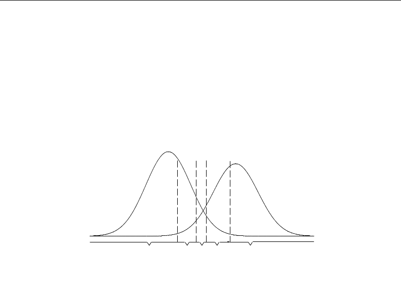
rocfit — Parametric ROC models 1953
Methods and formulas
Dorfman and Alf (1969) developed a general procedure for obtaining maximum likelihood estimates
of the parameters of a smooth-fitting ROC curve. The most common method, and the one implemented
in Stata, is based upon the binormal model.
The model assumes that there is an unobserved continuous latent variable that is normally distributed
in both the normal and abnormal populations. The idea is better explained with the following illustration:
5
4
3
2
1
4
Z
3
Z
2
Z
1
Z
Abnormal
Normal
The latent variable is assumed to be normally distributed for both the normal and abnormal subjects,
perhaps after a monotonic transformation, with means µnand µaand variances σ2
nand σ2
a, respectively.
This latent variable is assumed to be partitioned into the kcategories of the rating variable by
k−1 fixed boundaries. In the above figure, the k=5 categories of the rating variable identified on
the bottom result from the partition of the four boundaries Z1through Z4.
Let Rjfor j=1,2, . . . , k indicate the categories of the rating variable, let i=1 if the subject
belongs to the normal group, and let i=2 if the subject belongs to the abnormal group.
Then
p(Rj|i= 1) = F(Zj)−F(Zj−1)
where Zk= (xk−µn)/σn,Fis the cumulative normal distribution, F(Z0)=0, and F(Zk)=1.
Also,
p(Rj|i= 2) = F(bZj−a)−F(bZj−1−a)
where b=σn/σaand a= (µa−µn)/σa.
The parameters a,band the k−1 fixed boundaries Zjare simultaneously estimated by maximizing
the log-likelihood function
logL=
2
X
i=1
k
X
j=1
rij logp(Rj|i)
where rij is the number of Rjs in group i.

1954 rocfit — Parametric ROC models
The area under the fitted ROC curve is computed as
Φa
√1 + b2
where Φis the standard normal cumulative distribution function.
Point estimates for the ROC curve indices are as follows:
δ(m) = a
bde=2a
b+ 1 da=a√2
√1 + b2
Variances for these indices are computed using the delta method.
The δ(m)estimates (µa−µn)/σn,deestimates 2(µa−µn)/(σa−σn), and daestimates
√2(µa−µn)/(σ2
a−σ2
n)2.
Simultaneous confidence bands for the entire curve are obtained, as suggested by Ma and Hall (1993),
by first obtaining Working–Hotelling (1929) confidence bands for the fitted straight line in normal
probability coordinates and then transforming them back to ROC coordinates.
References
Bamber, D. 1975. The area above the ordinal dominance graph and the area below the receiver operating characteristic
graph. Journal of Mathematical Psychology 12: 387–415.
Choi, B. C. K. 1998. Slopes of a receiver operating characteristic curve and likelihood ratios for a diagnostic test.
American Journal of Epidemiology 148: 1127–1132.
Cleves, M. A. 1999. sg120: Receiver operating characteristic (ROC) analysis.Stata Technical Bulletin 52: 19–33.
Reprinted in Stata Technical Bulletin Reprints, vol. 9, pp. 212–229. College Station, TX: Stata Press.
. 2000. sg120.1: Two new options added to rocfit command.Stata Technical Bulletin 53: 18–19. Reprinted in
Stata Technical Bulletin Reprints, vol. 9, pp. 230–231. College Station, TX: Stata Press.
Dorfman, D. D., and E. Alf, Jr. 1969. Maximum-likelihood estimation of parameters of signal-detection theory and
determination of confidence intervals–rating-method data. Journal of Mathematical Psychology 6: 487–496.
Erdreich, L. S., and E. T. Lee. 1981. Use of relative operating characteristic analysis in epidemiology: A method for
dealing with subjective judgment. American Journal of Epidemiology 114: 649–662.
Hanley, J. A., and B. J. McNeil. 1982. The meaning and use of the area under a receiver operating characteristic
(ROC) curve. Radiology 143: 29–36.
Janes, H., G. M. Longton, and M. S. Pepe. 2009. Accommodating covariates in receiver operating characteristic
analysis.Stata Journal 9: 17–39.
Ma, G., and W. J. Hall. 1993. Confidence bands for the receiver operating characteristic curves. Medical Decision
Making 13: 191–197.
Pepe, M. S. 2003. The Statistical Evaluation of Medical Tests for Classification and Prediction. New York: Oxford
University Press.
Pepe, M. S., G. M. Longton, and H. Janes. 2009. Estimation and comparison of receiver operating characteristic
curves.Stata Journal 9: 1–16.
Working, H., and H. Hotelling. 1929. Application of the theory of error to the interpretation of trends. Journal of the
American Statistical Association 24 (Suppl.): 73–85.


Title
rocfit postestimation — Postestimation tools for rocfit
Description Syntax for rocplot Menu Options for rocplot
Remarks and examples Also see
Description
The following command is of special interest after rocfit:
Command Description
rocplot plot the fitted ROC curve and simultaneous confidence bands
The following standard postestimation commands are also available:
Command Description
estat ic Akaike’s and Schwarz’s Bayesian information criteria (AIC and BIC)
estat summarize summary statistics for the estimation sample
estat vce variance–covariance matrix of the estimators (VCE)
estimates cataloging estimation results
∗lincom point estimates, standard errors, testing, and inference for linear combinations
of coefficients
∗test Wald tests of simple and composite linear hypotheses
∗See Using lincom and test below.
Special-interest postestimation command
rocplot plots the fitted ROC curve and simultaneous confidence bands.
1956

rocfit postestimation — Postestimation tools for rocfit 1957
Syntax for rocplot
rocplot ,rocplot options
rocplot options Description
Main
confband display confidence bands
norefline suppress plotting the reference line
level(#)set confidence level; default is level(95)
Plot
plotopts(plot options)affect rendition of the ROC points
Fit line
lineopts(cline options)affect rendition of the fitted ROC line
CI plot
ciopts(area options)affect rendition of the confidence bands
Reference line
rlopts(cline options)affect rendition of the reference line
Add plots
addplot(plot)add other plots to the generated graph
Y axis, X axis, Titles, Legend, Overall
twoway options any options other than by() documented in [G-3]twoway options
plot options Description
marker options change look of markers (color, size, etc.)
marker label options add marker labels; change look or position
cline options change the look of the line
Menu
Statistics >Epidemiology and related >ROC analysis >ROC curves after rocfit
Options for rocplot
Main
confband specifies that simultaneous confidence bands be plotted around the ROC curve.
norefline suppresses plotting the 45-degree reference line from the graphical output of the ROC
curve.
level(#)specifies the confidence level, as a percentage, for the confidence bands. The default is
level(95) or as set by set level; see [R]level.
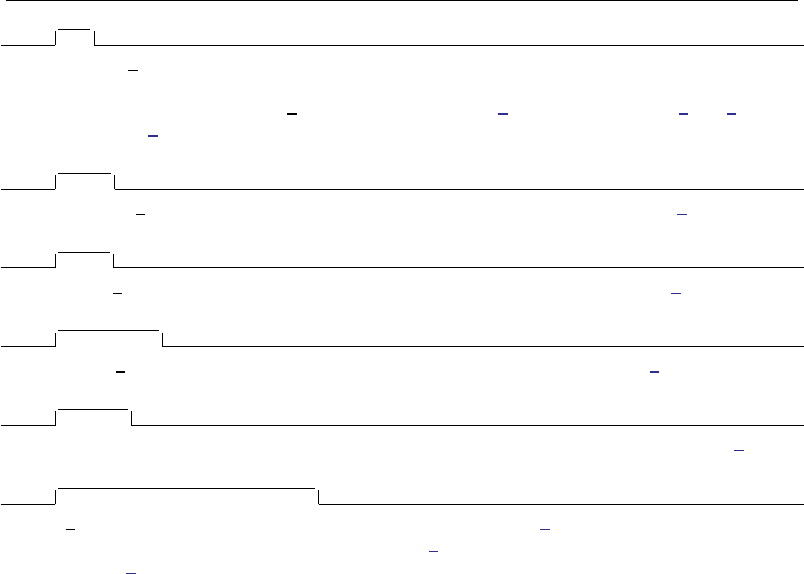
1958 rocfit postestimation — Postestimation tools for rocfit
Plot
plotopts(plot options)affects the rendition of the plotted ROC points, including the size and color of
markers, whether and how the markers are labeled, and whether and how the points are connected.
For the full list of available plot options, see [G-3]marker options,[G-3]marker label options,
and [G-3]cline options.
Fit line
lineopts(cline options)affects the rendition of the fitted ROC line; see [G-3]cline options.
CI plot
ciopts(area options)affects the rendition of the confidence bands; see [G-3]area options.
Reference line
rlopts(cline options)affects the rendition of the reference line; see [G-3]cline options.
Add plots
addplot(plot)provides a way to add other plots to the generated graph. See [G-3]addplot option.
Y axis, X axis, Titles, Legend, Overall
twoway options are any of the options documented in [G-3]twoway options, excluding by(). These
include options for titling the graph (see [G-3]title options) and for saving the graph to disk (see
[G-3]saving option).
Remarks and examples
Remarks are presented under the following headings:
Using lincom and test
Using rocplot
Using lincom and test
intercept,slope, and cut#, shown in example 1 of [R]rocfit, are equation names and not
variable names, so they need to be referenced as described in Special syntaxes after multiple-equation
estimation of [R]test. For example, instead of typing
. test intercept
intercept not found
r(111);
you should type
. test [intercept]_cons
( 1) [intercept]_cons = 0
chi2( 1) = 28.48
Prob > chi2 = 0.0000
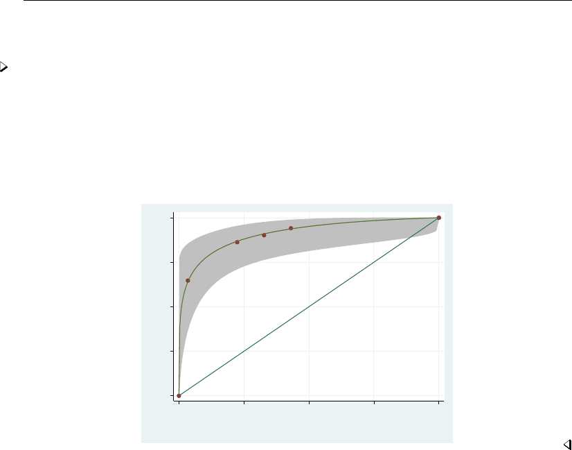
rocfit postestimation — Postestimation tools for rocfit 1959
Using rocplot
Example 1
In example 1 of [R]rocfit, we fit a ROC curve by typing rocfit disease rating.
In the output table for our model, we are testing whether the variances of the two latent populations
are equal by testing that the slope =1.
We plot the fitted ROC curve.
. rocplot, confband
0 .25 .5 .75 1
Sensitivity
0 .25 .5 .75 1
1 − Specificity
Area under curve = 0.9113 se(area) = 0.0295
Also see
[R]rocfit — Parametric ROC models
[U] 20 Estimation and postestimation commands

Title
rocreg — Receiver operating characteristic (ROC) regression
Syntax Menu Description Options
Remarks and examples Stored results Methods and formulas Acknowledgments
References Also see
Syntax
Perform nonparametric analysis of ROC curve under covariates, using bootstrap
rocreg refvar classvar classvars if in ,np options
Perform parametric analysis of ROC curve under covariates, using bootstrap
rocreg refvar classvar classvars if in , probit probit options
Perform parametric analysis of ROC curve under covariates, using maximum likelihood
rocreg refvar classvar classvars if in weight , probit ml
probit ml options
np options Description
Model
auc estimate total area under the ROC curve; the default
roc(numlist)estimate ROC for given false-positive rates
invroc(numlist)estimate false-positive rates for given ROC values
pauc(numlist)estimate partial area under the ROC curve (pAUC) up to each
false-positive rate
cluster(varname)variable identifying resampling clusters
ctrlcov(varlist)adjust control distribution for covariates in varlist
ctrlmodel(strata |linear) stratify or regress on covariates; default is ctrlmodel(strata)
pvc(empirical |normal) use empirical or normal distribution percentile value estimates;
default is pvc(empirical)
tiecorrected adjust for tied observations; not allowed with pvc(normal)
Bootstrap
nobootstrap do not perform bootstrap, just output point estimates
bseed(#)random-number seed for bootstrap
breps(#)number of bootstrap replications; default is breps(1000)
bootcc perform case–control (stratified on refvar) sampling rather than
cohort sampling in bootstrap
nobstrata ignore covariate stratification in bootstrap sampling
nodots suppress bootstrap replication dots
Reporting
level(#)set confidence level; default is level(95)
1960

rocreg — Receiver operating characteristic (ROC) regression 1961
probit options Description
Model
∗probit fit the probit model
roccov(varlist)covariates affecting ROC curve
fprpts(#)number of false-positive rate points to use in fitting ROC
curve; default is fprpts(10)
ctrlfprall fit ROC curve at each false-positive rate in control population
cluster(varname)variable identifying resampling clusters
ctrlcov(varlist)adjust control distribution for covariates in varlist
ctrlmodel(strata |linear) stratify or regress on covariates; default is ctrlmodel(strata)
pvc(empirical |normal) use empirical or normal distribution percentile value estimates;
default is pvc(empirical)
tiecorrected adjust for tied observations; not allowed with pvc(normal)
Bootstrap
nobootstrap do not perform bootstrap, just output point estimates
bseed(#)random-number seed for bootstrap
breps(#)number of bootstrap replications; default is breps(1000)
bootcc perform case–control (stratified on refvar) sampling rather than
cohort sampling in bootstrap
nobstrata ignore covariate stratification in bootstrap sampling
nodots suppress bootstrap replication dots
bsave(filename,. . . )save bootstrap replicates from parametric estimation
bfile(filename)use bootstrap replicates dataset for estimation replay
Reporting
level(#)set confidence level; default is level(95)
∗probit is required.

1962 rocreg — Receiver operating characteristic (ROC) regression
probit ml options Description
Model
∗probit fit the probit model
∗ml fit the probit model by maximum likelihood estimation
roccov(varlist)covariates affecting ROC curve
cluster(varname)variable identifying clusters
ctrlcov(varlist)adjust control distribution for covariates in varlist
Reporting
level(#)set confidence level; default is level(95)
display options control column formats, line width, and display of omitted variables
Maximization
maximize options control the maximization process; seldom used
∗probit and ml are required.
fweights, iweights, and pweights are allowed with maximum likelihood estimation; see [U] 11.1.6 weight.
See [U] 20 Estimation and postestimation commands for more capabilities of estimation commands.
Menu
Statistics >Epidemiology and related >ROC analysis >ROC regression models
Description
The rocreg command is used to perform receiver operating characteristic (ROC) analyses with
rating and discrete classification data under the presence of covariates.
The two variables refvar and classvar must be numeric. The reference variable indicates the true
state of the observation—such as diseased and nondiseased or normal and abnormal—and must be
coded as 0and 1. The refvar coded as 0can also be called the control population, while the refvar
coded as 1comprises the case population. The rating or outcome of the diagnostic test or test modality
is recorded in classvar, which must be ordinal, with higher values indicating higher risk.
rocreg can fit three models: a nonparametric model, a parametric probit model that uses the
bootstrap for inference, and a parametric probit model fit using maximum likelihood.
Options
Options are presented under the following headings:
Options for nonparametric ROC estimation, using bootstrap
Options for parametric ROC estimation, using bootstrap
Options for parametric ROC estimation, using maximum likelihood

rocreg — Receiver operating characteristic (ROC) regression 1963
Options for nonparametric ROC estimation, using bootstrap
Model
auc estimates the total area under the ROC curve. This is the default summary statistic.
roc(numlist)estimates the ROC corresponding to each of the false-positive rates in numlist. The
values of numlist must be in the range (0,1).
invroc(numlist)estimates the false-positive rates corresponding to each of the ROC values in numlist.
The values of numlist must be in the range (0,1).
pauc(numlist)estimates the partial area under the ROC curve up to each false-positive rate in numlist.
The values of numlist must in the range (0,1].
cluster(varname)specifies the variable identifying resampling clusters.
ctrlcov(varlist)specifies the covariates to be used to adjust the control population.
ctrlmodel(strata |linear) specifies how to model the control population of classifiers on
ctrlcov(). When ctrlmodel(linear) is specified, linear regression is used. The default is
ctrlmodel(strata); that is, the control population of classifiers is stratified on the control
variables.
pvc(empirical |normal) determines how the percentile values of the control population will be
calculated. When pvc(normal) is specified, the standard normal cumulative distribution function
(CDF) is used for calculation. Specifying pvc(empirical) will use the empirical CDFs of the
control population classifiers for calculation. The default is pvc(empirical).
tiecorrected adjusts the percentile values for ties. For each value of the classifier, one half the
probability that the classifier equals that value under the control population is added to the percentile
value. tiecorrected is not allowed with pvc(normal).
Bootstrap
nobootstrap specifies that bootstrap standard errors not be calculated.
bseed(#)specifies the random-number seed to be used in the bootstrap.
breps(#)sets the number of bootstrap replications. The default is breps(1000).
bootcc performs case–control (stratified on refvar) sampling rather than cohort bootstrap sampling.
nobstrata ignores covariate stratification in bootstrap sampling.
nodots suppresses bootstrap replicate dots.
Reporting
level(#); see [R]estimation options.
Options for parametric ROC estimation, using bootstrap
Model
probit fits the probit model. This option is required and implies parametric estimation.
roccov(varlist)specifies the covariates that will affect the ROC curve.
fprpts(#)sets the number of false-positive rate points to use in modeling the ROC curve. These
points form an equispaced grid on (0,1). The default is fprpts(10).

1964 rocreg — Receiver operating characteristic (ROC) regression
ctrlfprall models the ROC curve at each false-positive rate in the control population.
cluster(varname)specifies the variable identifying resampling clusters.
ctrlcov(varlist)specifies the covariates to be used to adjust the control population.
ctrlmodel(strata |linear) specifies how to model the control population of classifiers on
ctrlcov(). When ctrlmodel(linear) is specified, linear regression is used. The default is
ctrlmodel(strata); that is, the control population of classifiers is stratified on the control
variables.
pvc(empirical |normal) determines how the percentile values of the control population will be
calculated. When pvc(normal) is specified, the standard normal CDF is used for calculation.
Specifying pvc(empirical) will use the empirical CDFs of the control population classifiers for
calculation. The default is pvc(empirical).
tiecorrected adjusts the percentile values for ties. For each value of the classifier, one half the
probability that the classifier equals that value under the control population is added to the percentile
value. tiecorrected is not allowed with pvc(normal).
Bootstrap
nobootstrap specifies that bootstrap standard errors not be calculated.
bseed(#)specifies the random-number seed to be used in the bootstrap.
breps(#)sets the number of bootstrap replications. The default is breps(1000).
bootcc performs case–control (stratified on refvar) sampling rather than cohort bootstrap sampling.
nobstrata ignores covariate stratification in bootstrap sampling.
nodots suppresses bootstrap replicate dots.
bsave(filename,. . . )saves bootstrap replicates from parametric estimation in the given filename
with specified options (that is, replace). bsave() is only allowed with parametric analysis using
bootstrap.
bfile(filename)specifies to use the bootstrap replicates dataset for estimation replay. bfile() is
only allowed with parametric analysis using bootstrap.
Reporting
level(#); see [R]estimation options.
Options for parametric ROC estimation, using maximum likelihood
Model
probit fits the probit model. This option is required and implies parametric estimation.
ml fits the probit model by maximum likelihood estimation. This option is required and must be
specified with probit.
roccov(varlist)specifies the covariates that will affect the ROC curve.
cluster(varname)specifies the variable used for clustering.
ctrlcov(varlist)specifies the covariates to be used to adjust the control population.

rocreg — Receiver operating characteristic (ROC) regression 1965
Reporting
level(#); see [R]estimation options.
display options:noomitted,cformat(%fmt),pformat(% fmt),sformat(% fmt), and nolstretch;
see [R]estimation options.
Maximization
maximize options:difficult,technique(algorithm spec),iterate(#),nolog,trace,
gradient,showstep,hessian,showtolerance,tolerance(#),ltolerance(#),
nrtolerance(#),nonrtolerance, and from(init specs); see [R]maximize. These options are
seldom used. The technique(bhhh) option is not allowed.
Remarks and examples
Remarks are presented under the following headings:
Introduction
ROC statistics
Covariate-adjusted ROC curves
Parametric ROC curves: Estimating equations
Parametric ROC curves: Maximum likelihood
Introduction
Receiver operating characteristic (ROC) analysis provides a quantitative measure of the accuracy of
diagnostic tests to discriminate between two states or conditions. These conditions may be referred
to as normal and abnormal, nondiseased and diseased, or control and case. We will use these terms
interchangeably. The discriminatory accuracy of a diagnostic test is measured by its ability to correctly
classify known control and case subjects.
The analysis uses the ROC curve, a graph of the sensitivity versus 1 −specificity of the diagnostic
test. The sensitivity is the fraction of positive cases that are correctly classified by the diagnostic test,
whereas the specificity is the fraction of negative cases that are correctly classified. Thus the sensitivity
is the true-positive rate, and the specificity is the true-negative rate. We also call 1 −specificity the
false-positive rate.
These rates are functions of the possible outcomes of the diagnostic test. At each outcome, a
decision will be made by the user of the diagnostic test to classify the tested subject as either normal
or abnormal. The true-positive and false-positive rates measure the probability of correct classification
or incorrect classification of the subject as abnormal. Given the classification role of the diagnostic
test, we will refer to it as the classifier.
Using this basic definition of the ROC curve, Pepe (2000) and Pepe (2003) describe how ROC
analysis can be performed as a two-stage process. In the first stage, the control distribution of the
classifier is estimated. The specificity is then determined as the percentiles of the classifier values
calculated based on the control population. The false-positive rates are calculated as 1 −specificity.
In the second stage, the ROC curve is estimated as the cumulative distribution of the case population’s
“false-positive” rates, also known as the survival function under the case population of the previously
calculated percentiles. We use the terms ROC value and true-positive value interchangeably.
This formulation of ROC curve analysis provides simple, nonparametric estimates of several ROC
curve summary parameters: area under the ROC curve, partial area under the ROC curve, ROC value
for a given false-positive rate, and false-positive rate (also known as invROC) for a given ROC value.
In the next section, we will show how to use rocreg to compute these estimates with bootstrap
inference. There we will also show how rocreg complements the other nonparametric Stata ROC
commands roctab and roccomp.

1966 rocreg — Receiver operating characteristic (ROC) regression
Other factors beyond condition status and the diagnostic test may affect both stages of ROC analysis.
For example, a test center may affect the control distribution of the diagnostic test. Disease severity
may affect the distribution of the standardized diagnostic test under the case population. Our analysis
of the ROC curve in these situations will be more accurate if we take these covariates into account.
In a nonparametric ROC analysis, covariates may only affect the first stage of estimation; that is,
they may be used to adjust the control distribution of the classifier. In a parametric ROC analysis,
it is assumed that ROC follows a normal distribution, and thus covariates may enter the model at
both stages; they may be used to adjust the control distribution and to model ROC as a function of
these covariates and the false-positive rate. In parametric models, both sets of covariates need not be
distinct but, in fact, they are often the same.
To model covariate effects on the first stage of ROC analysis, Janes and Pepe (2009) propose a
covariate-adjusted ROC curve. We will demonstrate the covariate adjustment capabilities of rocreg
in Covariate-adjusted ROC curves.
To account for covariate effects at the second stage, we assume a parametric model. Particularly,
the ROC curve is a generalized linear model of the covariates. We will thus have a separate ROC curve
for each combination of the relevant covariates. In Parametric ROC curves: Estimating equations,
we show how to fit the model with estimating equations and bootstrap inference using rocreg.
This method, documented as the “pdf” approach in Alonzo and Pepe (2002), works well with weak
assumptions about the control distribution.
Also in Parametric ROC curves: Estimating equations, we show how to fit a constant-only parametric
model (involving no covariates) of the ROC curve with weak assumptions about the control distribution.
The constant-only model capabilities of rocreg in this context will be compared with those of rocfit.
roccomp has the binormal option, which will allow it to compute area under the ROC curve according
to a normal ROC curve, equivalent to that obtained by rocfit. We will compare this functionality
with that of rocreg.
In Parametric ROC curves: Maximum likelihood, we demonstrate maximum likelihood estimation
of the ROC curve model with rocreg. There we assume a normal linear model for the classifier
on the covariates and case–control status. This method is documented in Pepe (2003). We will also
demonstrate how to use this method with no covariates, and we will compare rocreg under the
constant-only model with rocfit and roccomp.
The rocregplot command is used repeatedly in this entry. This command provides graphical
output for rocreg and is documented in [R]rocregplot.
ROC statistics
roctab computes the ROC curve by calculating the false-positive rate and true-positive rate
empirically at every value of the input classifier. It makes no distributional assumptions about the
case or control distributions. We can get identical behavior from rocreg by using the default option
settings.
Example 1: Nonparametric ROC, AUC
Hanley and McNeil (1982) presented data from a study in which a reviewer was asked to
classify, using a five-point scale, a random sample of 109 tomographic images from patients with
neurological problems. The rating scale was as follows: 1 is definitely normal, 2 is probably normal,
3 is questionable, 4 is probably abnormal, and 5 is definitely abnormal. The true disease status was
normal for 58 of the patients and abnormal for the remaining 51 patients.
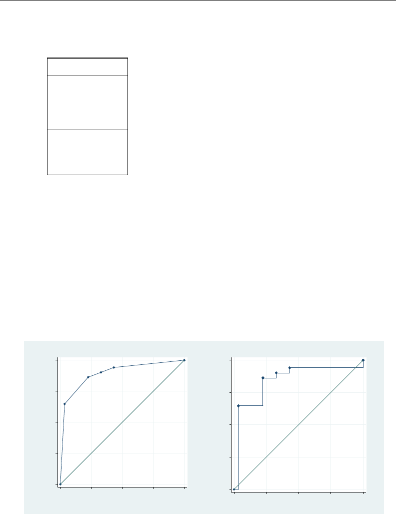
rocreg — Receiver operating characteristic (ROC) regression 1967
Here we list 9 of the 109 observations:
. use http://www.stata-press.com/data/r13/hanley
. list disease rating in 1/9
disease rating
1. 1 5
2. 0 1
3. 1 5
4. 0 4
5. 0 1
6. 0 3
7. 1 5
8. 0 5
9. 0 1
For each observation, disease identifies the true disease status of the subject (0is normal, 1is
abnormal), and rating contains the classification value assigned by the reviewer.
We run roctab on these data, specifying the graph option so that the ROC curve is rendered.
We then calculate the false-positive and true-positive rates of the ROC curve by using rocreg. We
graph the rates with rocregplot. Because we focus on rocreg output later, for now we use the
quietly prefix to omit the output of rocreg. Both graphs are combined using graph combine (see
[G-2]graph combine) for comparison. To ease the comparison, we specify the aspectratio(1)
option in roctab; this is the default aspect ratio in rocregplot.
. roctab disease rating, graph aspectratio(1) name(a) nodraw title("roctab")
. quietly rocreg disease rating
. rocregplot, name(b) nodraw legend(off) title("rocreg")
. graph combine a b
0.00 0.25 0.50 0.75 1.00
Sensitivity
0.00 0.25 0.50 0.75 1.00
1 − Specificity
Area under ROC curve = 0.8932
roctab
0 .25 .5 .75 1
True−positive rate (ROC)
0 .25 .5 .75 1
False−positive rate
rocreg
Both roctab and rocreg compute the same false-positive rate and ROC values. The stairstep
line connection style of the graph on the right emphasizes the empirical nature of its estimates. The
control distribution of the classifier is estimated using the empirical CDF estimate. Similarly, the ROC
curve, the distribution of the resulting case observation false-positive rate values, is estimated using
the empirical CDF. Note the footnote in the roctab plot. By default, roctab will estimate the area

1968 rocreg — Receiver operating characteristic (ROC) regression
under the ROC curve (AUC) using a trapezoidal approximation to the estimated false-positive rate and
true-positive rate points.
The AUC can be interpreted as the probability that a randomly selected member of the case population
will have a larger classifier value than a randomly selected member of the control population. It can
also be viewed as the average ROC value, averaged uniformly over the (0,1) false-positive rate domain
(Pepe 2003).
The nonparametric estimator of the AUC (DeLong, DeLong, and Clarke-Pearson 1988;Hanley and
Hajian-Tilaki 1997) used by rocreg is equivalent to the sample mean of the percentile values of the
case observations. Thus to calculate the nonparametric AUC estimate, we only need to calculate the
percentile values of the case observations with respect to the control distribution.
This estimate can differ from the trapezoidal approximation estimate. Under discrete classification
data, like we have here, there may be ties between classifier values from case to control. The trapezoidal
approximation uses linear interpolation between the classifier values to correct for ties. Correcting
the nonparametric estimator involves adding a correction term to each observation’s percentile value,
which measures the probability that the classifier is equal to (instead of less than) the observation’s
classifier value.
The tie-corrected nonparametric estimate (trapezoidal approximation) is used when we think the
true ROC curve is smooth. This means that the classifier we measure is a discretized approximation
of a true latent and a continuous classifier.
We now recompute the ROC curve of rating for classifying disease and calculate the AUC.
Specifying the tiecorrected option allows tie correction to be used in the rocreg calculation.
Under nonparametric estimation, rocreg bootstraps to obtain standard errors and confidence intervals
for requested statistics. We use the default 1,000 bootstrap replications to obtain confidence intervals
for our parameters. This is a reasonable lower bound to the number of replications (Mooney and
Duval 1993) required for estimating percentile confidence intervals. By specifying the summary option
in roctab, we will obtain output showing the trapezoidal approximation of the AUC estimate, along
with standard error and confidence interval estimates for the trapezoidal approximation suggested by
DeLong, DeLong, and Clarke-Pearson (1988).

rocreg — Receiver operating characteristic (ROC) regression 1969
. roctab disease rating, summary
ROC Asymptotic Normal
Obs Area Std. Err. [95% Conf. Interval]
109 0.8932 0.0307 0.83295 0.95339
. rocreg disease rating, tiecorrected bseed(29092)
(running rocregstat on estimation sample)
Bootstrap replications (1000)
12345
.................................................. 50
.................................................. 100
(output omitted )
.................................................. 950
.................................................. 1000
Bootstrap results Number of obs = 109
Replications = 1000
Nonparametric ROC estimation
Control standardization: empirical, corrected for ties
ROC method : empirical
Area under the ROC curve
Status : disease
Classifier: rating
Observed Bootstrap
AUC Coef. Bias Std. Err. [95% Conf. Interval]
.8931711 .000108 .0292028 .8359347 .9504075 (N)
.8290958 .9457951 (P)
.8280714 .9450642 (BC)
The estimates of AUC match well. The standard error from roctab is close to the bootstrap
standard error calculated by rocreg. The bootstrap standard error generalizes to the more complex
models that we consider later, whereas the roctab standard-error calculation does not.
The AUC can be used to compare different classifiers. It is the most popular summary statistic for
comparisons (Pepe, Longton, and Janes 2009). roccomp will compute the trapezoidal approximation
of the AUC and graph the ROC curves of multiple classifiers. Using the DeLong, DeLong, and Clarke-
Pearson (1988) covariance estimates for the AUC estimate, roccomp performs a Wald test of the null
hypothesis that all classifier AUC values are equal. rocreg has similar capabilities.
Example 2: Nonparametric ROC, AUC, multiple classifiers
Hanley and McNeil (1983) presented data from an evaluation of two computer algorithms designed
to reconstruct CT images from phantoms. We will call these two algorithms modalities 1 and 2. A
sample of 112 phantoms was selected; 58 phantoms were considered normal, and the remaining 54
were abnormal. Each of the two modalities was applied to each phantom, and the resulting images
were rated by a reviewer using a six-point scale: 1 is definitely normal, 2 is probably normal, 3
is possibly normal, 4 is possibly abnormal, 5 is probably abnormal, and 6 is definitely abnormal.
Because each modality was applied to the same sample of phantoms, the two sets of outcomes are
correlated.

1970 rocreg — Receiver operating characteristic (ROC) regression
We list the first seven observations:
. use http://www.stata-press.com/data/r13/ct, clear
. list in 1/7, sep(0)
mod1 mod2 status
1. 2 1 0
2. 5 5 1
3. 2 1 0
4. 2 3 0
5. 5 6 1
6. 2 2 0
7. 3 2 0
Each observation corresponds to one phantom. The mod1 variable identifies the rating assigned
for the first modality, and the mod2 variable identifies the rating assigned for the second modality.
The true status of the phantoms is given by status==0 if they are normal and status==1 if they
are abnormal. The observations with at least one missing rating were dropped from the analysis.
A fictitious dataset was created from this true dataset, adding a third test modality. We will use
roccomp to compute the AUC statistic for each modality in these data and compare the AUC of the
three modalities. We obtain the same behavior from rocreg. As before, the tiecorrected option
is specified so that the AUC is calculated with the trapezoidal approximation.
. use http://www.stata-press.com/data/r13/ct2
. roccomp status mod1 mod2 mod3, summary
ROC Asymptotic Normal
Obs Area Std. Err. [95% Conf. Interval]
mod1 112 0.8828 0.0317 0.82067 0.94498
mod2 112 0.9302 0.0256 0.88005 0.98042
mod3 112 0.9240 0.0241 0.87670 0.97132
Ho: area(mod1) = area(mod2) = area(mod3)
chi2(2) = 6.54 Prob>chi2 = 0.0381

rocreg — Receiver operating characteristic (ROC) regression 1971
. rocreg status mod1 mod2 mod3, tiecorrected bseed(38038) nodots
Bootstrap results Number of obs = 112
Replications = 1000
Nonparametric ROC estimation
Control standardization: empirical, corrected for ties
ROC method : empirical
Area under the ROC curve
Status : status
Classifier: mod1
Observed Bootstrap
AUC Coef. Bias Std. Err. [95% Conf. Interval]
.8828225 -.0006367 .0322291 .8196546 .9459903 (N)
.8147518 .9421572 (P)
.8124397 .9394085 (BC)
Status : status
Classifier: mod2
Observed Bootstrap
AUC Coef. Bias Std. Err. [95% Conf. Interval]
.9302363 -.0015402 .0259593 .8793569 .9811156 (N)
.8737522 .9737432 (P)
.8739467 .9737768 (BC)
Status : status
Classifier: mod3
Observed Bootstrap
AUC Coef. Bias Std. Err. [95% Conf. Interval]
.9240102 -.0003528 .0247037 .8755919 .9724286 (N)
.8720036 .9674485 (P)
.8693548 .965 (BC)
Ho: All classifiers have equal AUC values.
Ha: At least one classifier has a different AUC value.
P-value: .0389797 Test based on bootstrap (N) assumptions.
We see that the AUC estimates are equivalent, and the standard errors are quite close as well.
The p-value for the tests of equal AUC under rocreg leads to similar inference as the p-value from
roccomp. The Wald test performed by rocreg uses the joint bootstrap estimate variance matrix of the
three AUC estimators rather than the DeLong, DeLong, and Clarke-Pearson (1988) variance estimate
used by roccomp.
roccomp is used here on potentially correlated classifiers that are recorded in wide-format data.
It can also be used on long-format data to compare independent classifiers. Further details can be
found in [R]roccomp.
Citing the AUC’s lack of clinical relevance, there is argument against using it as a key summary
statistic of the ROC curve (Pepe 2003;Cook 2007). Pepe, Longton, and Janes (2009) suggest using
the estimate of the ROC curve itself at a particular point, or the estimate of the false-positive rate at
a given ROC value, also known as invROC.

1972 rocreg — Receiver operating characteristic (ROC) regression
Recall from example 1 how nonparametric rocreg graphs look, with the stairstep pattern in the
ROC curve. In an ideal world, the graph would be a smooth one-to-one function, and it would be
trivial to map a false-positive rate to its corresponding true-positive rate and vice versa.
However, smooth ROC curves can only be obtained by assuming a parametric model that uses
linear interpolation between observed false-positive rates and between observed true-positive rates, and
rocreg is certainly capable of that; see example 1 of [R]rocregplot. However, under nonparametric
estimation, the mapping between false-positive rates and true-positive rates is not one to one, and
estimates tend to be less reliable the further you are from an observed data point. This is somewhat
mitigated by using tie-corrected rates (the tiecorrected option).
When we examine continuous data, the difference between the tie-corrected estimates and the
standard estimates becomes negligible, and the empirical estimate of the ROC curve becomes close
to the smooth ROC curve obtained by linear interpolation. So the nonparametric ROC and invROC
estimates work well.
Fixing one rate value of interest can be difficult and subjective (Pepe 2003). A compromise measure
is the partial area under the ROC curve (pAUC) (McClish 1989;Thompson and Zucchini 1989). This
is the integral of the ROC curve from 0 and above to a given false-positive rate (perhaps the largest
clinically acceptable value). Like the AUC estimate, the nonparametric estimate of the pAUC can be
written as a sample average of the case observation percentiles, but with an adjustment based on the
prescribed maximum false-positive rate (Dodd and Pepe 2003). A tie correction may also be applied
so that it reflects the trapezoidal approximation.
We cannot compare rocreg with roctab or roccomp on the estimation of pAUC, because pAUC
is not computed by the latter two.
Example 3: Nonparametric ROC, other statistics
To see how rocreg estimates ROC, invROC, and pAUC, we will examine a new study. Wieand et al.
(1989) examined a pancreatic cancer study with two continuous classifiers, here called y1 (CA 19-9)
and y2 (CA 125). This study was also examined in Pepe, Longton, and Janes (2009). The indicator
of cancer in a subject is recorded as d. The study was a case–control study, stratifying participants
on disease status.
We list the first five observations:
. use http://labs.fhcrc.org/pepe/book/data/wiedat2b, clear
(S. Wieand - Pancreatic cancer diagnostic marker data)
. list in 1/5
y1 y2 d
1. 28 13.3 no
2. 15.5 11.1 no
3. 8.2 16.7 no
4. 3.4 12.6 no
5. 17.3 7.4 no
We will estimate the ROC curves at a large value (0.7) and a small value (0.2) of the false-positive
rate. These values are specified in roc(). The false-positive rate for ROC or sensitivity value of 0.6 will
also be estimated by specifying invroc(). Percentile confidence intervals for these parameters are
displayed in the graph obtained by rocregplot after rocreg. The pAUC statistic will be calculated
for the false-positive rate of 0.5, which is specified as an argument to the pauc() option. Following
Pepe, Longton, and Janes (2009), we use a stratified bootstrap, sampling separately from the case

rocreg — Receiver operating characteristic (ROC) regression 1973
and control populations by specifying the bootcc option. This reflects the case–control nature of the
study.
All four statistics can be estimated simultaneously by rocreg. For clarity, however, we will estimate
each statistic with a separate call to rocreg.rocregplot is used after estimation to graph the ROC
and false-positive rate estimates. The display of the individual, observation-specific false-positive rate
and ROC values will be omitted in the plot. This is accomplished by specifying msymbol(i) in our
plot1opts() and plot2opts() options to rocregplot.
. rocreg d y1 y2, roc(.7) bseed(8378923) bootcc nodots
Bootstrap results
Number of strata = 2 Number of obs = 141
Replications = 1000
Nonparametric ROC estimation
Control standardization: empirical
ROC method : empirical
ROC curve
Status : d
Classifier: y1
Observed Bootstrap
ROC Coef. Bias Std. Err. [95% Conf. Interval]
.7 .9222222 -.0021889 .0323879 .8587432 .9857013 (N)
.8444445 .9777778 (P)
.8555555 .9777778 (BC)
Status : d
Classifier: y2
Observed Bootstrap
ROC Coef. Bias Std. Err. [95% Conf. Interval]
.7 .8888889 -.0035556 .0414215 .8077043 .9700735 (N)
.8 .9611111 (P)
.7888889 .9555556 (BC)
Ho: All classifiers have equal ROC values.
Ha: At least one classifier has a different ROC value.
Test based on bootstrap (N) assumptions.
ROC P-value
.7 .5423044
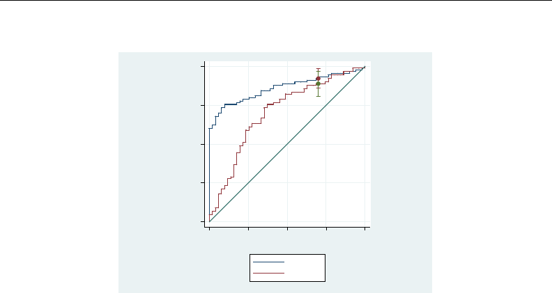
1974 rocreg — Receiver operating characteristic (ROC) regression
. rocregplot, plot1opts(msymbol(i)) plot2opts(msymbol(i))
0 .25 .5 .75 1
True−positive rate (ROC)
0 .25 .5 .75 1
False−positive rate
CA 19−9
CA 125
In this study, we see that classifier y1 (CA 19-9) is a uniformly better test than is classifier y2
(CA 125) until high levels of false-positive rate and sensitivity or ROC value are reached. At the high
level of false-positive rate, 0.7, the ROC value does not significantly differ between the two classifiers.
This can be seen in the plot by the overlapping confidence intervals.
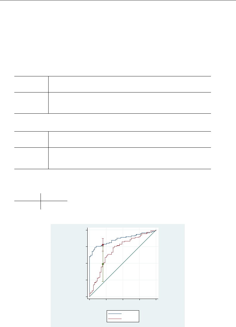
rocreg — Receiver operating characteristic (ROC) regression 1975
. rocreg d y1 y2, roc(.2) bseed(8378923) bootcc nodots
Bootstrap results
Number of strata = 2 Number of obs = 141
Replications = 1000
Nonparametric ROC estimation
Control standardization: empirical
ROC method : empirical
ROC curve
Status : d
Classifier: y1
Observed Bootstrap
ROC Coef. Bias Std. Err. [95% Conf. Interval]
.2 .7777778 .0011778 .0483655 .6829831 .8725725 (N)
.6888889 .8777778 (P)
.6777778 .8666667 (BC)
Status : d
Classifier: y2
Observed Bootstrap
ROC Coef. Bias Std. Err. [95% Conf. Interval]
.2 .4888889 -.0091667 .1339863 .2262806 .7514971 (N)
.2222222 .7 (P)
.2111111 .7 (BC)
Ho: All classifiers have equal ROC values.
Ha: At least one classifier has a different ROC value.
Test based on bootstrap (N) assumptions.
ROC P-value
.2 .043234
. rocregplot, plot1opts(msymbol(i)) plot2opts(msymbol(i))
0 .25 .5 .75 1
True−positive rate (ROC)
0 .25 .5 .75 1
False−positive rate
CA 19−9
CA 125

1976 rocreg — Receiver operating characteristic (ROC) regression
The sensitivity for the false-positive rate of 0.2 is found to be higher under y1 than under y2, and
this difference is significant at the 0.05 level. In the plot, this is shown by the vertical confidence
intervals.
. rocreg d y1 y2, invroc(.6) bseed(8378923) bootcc nodots
Bootstrap results
Number of strata = 2 Number of obs = 141
Replications = 1000
Nonparametric ROC estimation
Control standardization: empirical
ROC method : empirical
False-positive rate
Status : d
Classifier: y1
Observed Bootstrap
invROC Coef. Bias Std. Err. [95% Conf. Interval]
.6 0 .0158039 .0267288 -.0523874 .0523874 (N)
0 .0784314 (P)
0 .1372549 (BC)
Status : d
Classifier: y2
Observed Bootstrap
invROC Coef. Bias Std. Err. [95% Conf. Interval]
.6 .254902 .0101961 .0757902 .1063559 .403448 (N)
.1372549 .4313726 (P)
.1176471 .3921569 (BC)
Ho: All classifiers have equal invROC values.
Ha: At least one classifier has a different invROC value.
Test based on bootstrap (N) assumptions.
invROC P-value
.6 .0016562
. rocregplot, plot1opts(msymbol(i)) plot2opts(msymbol(i))
0 .25 .5 .75 1
True−positive rate (ROC)
0 .25 .5 .75 1
False−positive rate
CA 19−9
CA 125

rocreg — Receiver operating characteristic (ROC) regression 1977
We find significant evidence that false-positive rates corresponding to a sensitivity of 0.6 are
different from y1 to y2. This is visually indicated by the horizontal confidence intervals, which are
separated from each other.
. rocreg d y1 y2, pauc(.5) bseed(8378923) bootcc nodots
Bootstrap results
Number of strata = 2 Number of obs = 141
Replications = 1000
Nonparametric ROC estimation
Control standardization: empirical
ROC method : empirical
Partial area under the ROC curve
Status : d
Classifier: y1
Observed Bootstrap
pAUC Coef. Bias Std. Err. [95% Conf. Interval]
.5 .3932462 -.0000769 .021332 .3514362 .4350562 (N)
.3492375 .435512 (P)
.3492375 .435403 (BC)
Status : d
Classifier: y2
Observed Bootstrap
pAUC Coef. Bias Std. Err. [95% Conf. Interval]
.5 .2496732 .0019168 .0374973 .1761798 .3231666 (N)
.177451 .3253268 (P)
.1738562 .3233115 (BC)
Ho: All classifiers have equal pAUC values.
Ha: At least one classifier has a different pAUC value.
Test based on bootstrap (N) assumptions.
pAUC P-value
.5 .0011201
We also find significant evidence supporting the hypothesis that the pAUC for y1 up to a false-positive
rate of 0.5 differs from the area of the same region under the ROC curve of y2.
Covariate-adjusted ROC curves
When covariates affect the control distribution of the diagnostic test, thresholds for the test being
classified as abnormal may be chosen that vary with the covariate values. These conditional thresholds
will be more accurate than the marginal thresholds that would normally be used, because they take
into account the specific distribution of the diagnostic test under the given covariate values as opposed
to the marginal distribution over all covariate values.
By using these covariate-specific thresholds, we are essentially creating new classifiers for each
covariate-value combination, and thus we are creating multiple ROC curves. As explained in Pepe (2003),
when the case and control distributions of the covariates are the same, the marginal ROC curve will
always be bound above by these covariate-specific ROC curves. So using conditional thresholds will
never provide a less powerful test diagnostic in this case.

1978 rocreg — Receiver operating characteristic (ROC) regression
In the marginal ROC curve calculation, the classifiers are standardized to percentiles according
to the control distribution, marginalized over the covariates. Thus the ROC curve is the CDF of
the standardized case observations. The covariate-adjusted ROC curve is the CDF of one minus the
conditional control percentiles for the case observations, and the marginal ROC curve is the CDF of
one minus the marginal control percentiles for the case observations (Pepe and Cai 2004). Thus the
standardization of classifier to false-positive rate value is conditioned on the specific covariate values
under the covariate-adjusted ROC curve.
The covariate-adjusted ROC curve (Janes and Pepe 2009) at a given false-positive rate tis equivalent
to the expected value of the covariate-specific ROC at tover all covariate combinations. When the
covariates in question do not affect the case distribution of the classifier, the covariate-specific ROC will
have the same value at each covariate combination. So here the covariate-adjusted ROC is equivalent
to the covariate-specific ROC, regardless of covariate values.
When covariates do affect the case distribution of the classifier, users of the diagnostic test would
likely want to model the covariate-specific ROC curves separately. Tools to do this can be found in
the parametric modeling discussion in the following two sections. Regardless, the covariate-adjusted
ROC curve can serve as a meaningful summary of covariate-adjusted accuracy.
Also note that the ROC summary statistics defined in the previous section have covariate-adjusted
analogs. These analogs are estimated in a similar manner as under the marginal ROC curve (Janes,
Longton, and Pepe 2009). The options for their calculation in rocreg are identical to those given in
the previous section. Further details can be found in Methods and formulas.
Example 4: Nonparametric ROC, linear covariate adjustment
Norton et al. (2000) studied data from a neonatal audiology study on three tests to identify hearing
impairment in newborns. These data were also studied in Janes, Longton, and Pepe (2009). Here we
list 5 of the 5,058 observations.
. use http://www.stata-press.com/data/r13/nnhs, clear
(Norton - neonatal audiology data)
. list in 1/5
id ear male currage d y1 y2 y3
1. B0157 R M 42.42 0 -3.1 -9 -1.5
2. B0157 L M 42.42 0 -4.5 -8.7 -2.71
3. B0158 R M 40.14 1 -3.2 -13.2 -2.64
4. B0161 L F 38.14 0 -22.1 -7.8 -2.59
5. B0167 R F 37 0 -10.9 -6.6 -1.42
The classifiers y1 (DPOAE 65 at 2 kHz), y2 (TEOAE 80 at 2 kHz), and y3 (ABR) and the hearing
impairment indicator dare recorded along with some relevant covariates. The infant’s age is recorded
in months as currage, and the infant’s gender is indicated by male. Over 90% of the newborns
were tested in each ear (ear), so we will cluster on infant ID (id).
Following the strategy of Janes, Longton, and Pepe (2009), we will first perform ROC analysis for
the classifiers while adjusting for the covariate effects of the infant’s gender and age. This is done
by specifying these variables in the ctrlcov() option. We adjust using a linear regression rule,
by specifying ctrlmodel(linear). This means that when a user of the diagnostic test chooses a
threshold conditional on the age and gender covariates, they assume that the diagnostic test classifier
has some linear dependence on age and gender and equal variance as their levels vary. Our cluster
adjustment is made by specifying the cluster() option.

rocreg — Receiver operating characteristic (ROC) regression 1979
We will focus on the first classifier. The percentile, or specificity, values are calculated empirically
by default, and thus so are the false-positive rates, (1 −specificity). Also by default, the ROC curve
values are empirically defined by the false-positive rates. To draw the ROC curve, we again use
rocregplot.
The AUC is calculated by default. For brevity, we specify the nobootstrap option so that bootstrap
sampling is not performed. The AUC point estimate will be sufficient for our purposes.
. rocreg d y1, ctrlcov(male currage) ctrlmodel(linear) cluster(id) nobootstrap
Nonparametric ROC estimation
Covariate control : linear regression
Control variables : male currage
Control standardization: empirical
ROC method : empirical
Status : d
Classifier: y1
Covariate control adjustment model:
Linear regression Number of obs = 4907
F( 2, 2685) = 13.80
Prob > F = 0.0000
R-squared = 0.0081
Root MSE = 7.7515
(Std. Err. adjusted for 2686 clusters in id)
Robust
y1 Coef. Std. Err. t P>|t| [95% Conf. Interval]
male .2471744 .2603598 0.95 0.343 -.2633516 .7577005
currage -.2032456 .0389032 -5.22 0.000 -.2795288 -.1269624
_cons -1.239484 1.487855 -0.83 0.405 -4.156942 1.677973
Area under the ROC curve
Status : d
Classifier: y1
Observed Bootstrap
AUC Coef. Bias Std. Err. [95% Conf. Interval]
.6293994 . . . . (N)
. . (P)
. . (BC)
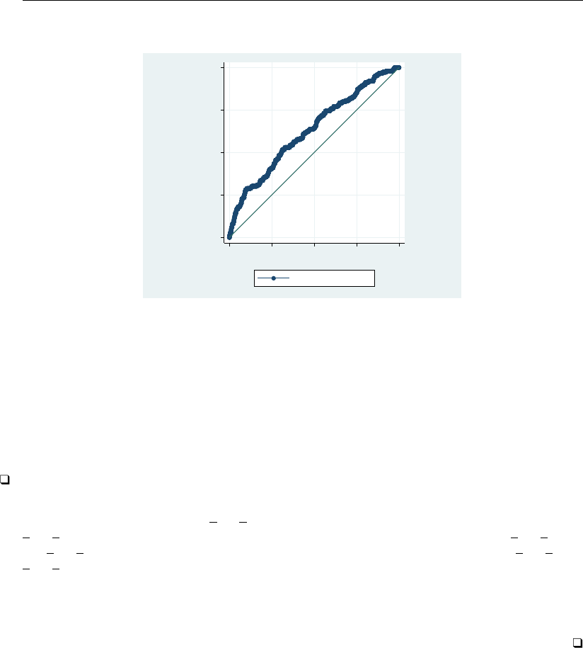
1980 rocreg — Receiver operating characteristic (ROC) regression
. rocregplot
0 .25 .5 .75 1
True−positive rate (ROC)
0 .25 .5 .75 1
False−positive rate
DPOAE 65 at 2kHz
Our covariate control adjustment model shows that currage has a negative effect on y1 (DPOAE 65
at 2 kHz) under the control population. At the 0.001 significance level, we reject that its contribution
to y1 is zero, and the point estimate has a negative sign. This result does not directly tell us about
the effect of currage on the ROC curve of y1 as a classifier of d. None of the case observations are
used in the linear regression, so information on currage for abnormal cases is not used in the model.
This result does show us how to calculate false-positive rates for tests that use thresholds conditional
on a child’s sex and current age. We will see how currage affects the ROC curve when y1 is used as
a classifier and conditional thresholds are used based on male and currage in the following section,
Parametric ROC curves: Estimating equations.
Technical note
Under this nonparametric estimation, rocreg saved the false-positive rate for each observation’s
y1 values in the utility variable fpr y1. The true-positive rates are stored in the utility variable
roc y1. For other models, say with classifier yname, these variables would be named fpr yname
and roc yname. They will also be overwritten with each call of rocreg. The variables roc * and
fpr * are usually for internal rocreg use only and are overwritten with each call of rocreg. They
are only created for nonparametric models or parametric models that do not involve ROC covariates.
In these models, covariates may only affect the first stage of estimation, the control distribution, and
not the ROC curve itself. In parametric models that allow ROC covariates, different covariate values
would lead to different ROC curves.
To see how the covariate-adjusted ROC curve estimate differs from the standard marginal estimate,
we will reestimate the ROC curve for classifier y1 without covariate adjustment. We rename these
variables before the new estimation and then draw an overlaid twoway line (see [G-2]graph twoway
line) plot to compare the two.
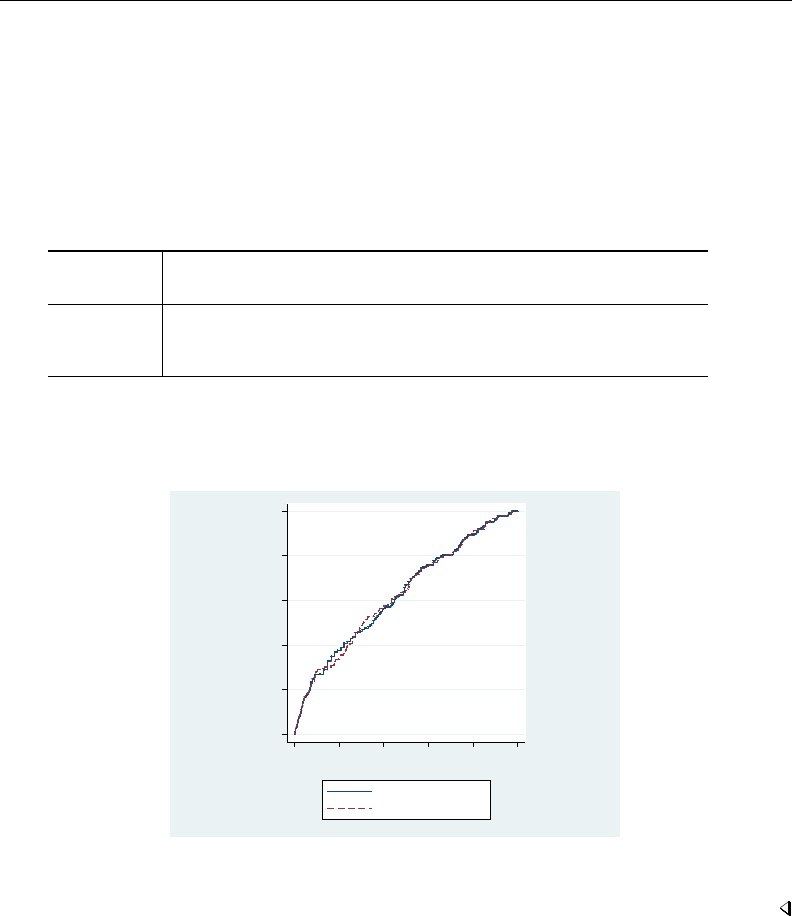
rocreg — Receiver operating characteristic (ROC) regression 1981
. rename _fpr_y1 o_fpr_y1
. rename _roc_y1 o_roc_y1
. label variable o_roc_y1 "covariate_adjusted"
. rocreg d y1, cluster(id) nobootstrap
Nonparametric ROC estimation
Control standardization: empirical
ROC method : empirical
Area under the ROC curve
Status : d
Classifier: y1
Observed Bootstrap
AUC Coef. Bias Std. Err. [95% Conf. Interval]
.6279645 . . . . (N)
. . (P)
. . (BC)
. label variable _roc_y1 "marginal"
. twoway line _roc_y1 _fpr_y1, sort(_fpr_y1 _roc_y1) connect(J) ||
> line o_roc_y1 o_fpr_y1, sort(o_fpr_y1 o_roc_y1)
> connect(J) lpattern(dash) aspectratio(1) legend(cols(1))
0 .2 .4 .6 .8 1
0 .2 .4 .6 .8 1
false−positive rate for y1
marginal
covariate_adjusted
Though they are close, particularly in AUC, there are clearly some points of difference between
the estimates. So the covariate-adjusted ROC curve may be useful here.
In our examples thus far, we have used the empirical CDF estimator to estimate the control
distribution. rocreg allows some flexibility here. The pvc(normal) option may be specified to
calculate the percentile values according to a Gaussian distribution of the control.
Covariate adjustment in rocreg may also be performed with stratification instead of linear
regression. Under the stratification method, the unique values of the stratified covariates each define
separate parameters for the control distribution of the classifier. A user of the diagnostic test chooses
a threshold based on the control distribution conditioned on the unique covariate value parameters.
We will demonstrate the use of normal percentile values and covariate stratification in our next
example.

1982 rocreg — Receiver operating characteristic (ROC) regression
Example 5: Nonparametric ROC, covariate stratification
The hearing test study of Stover et al. (1996) examined the effectiveness of negative signal-to-noise
ratio, nsnr, as a classifier of hearing loss. The test was administered under nine different settings,
corresponding to different frequency, xf, and intensity, xl, combinations. Here we list 10 of the 1,848
observations.
. use http://www.stata-press.com/data/r13/dp, clear
(Stover - DPOAE test data)
. list in 1/10
id d nsnr xf xl xd
1. 101 1 18 10.01 5.5 3.5
2. 101 1 19 20.02 5.5 3
3. 101 1 7.6 10.01 6 3.5
4. 101 1 15 20.02 6 3
5. 101 1 16 10.01 6.5 3.5
6. 101 1 5.8 20.02 6.5 3
7. 102 0 -2.6 10.01 5.5 .
8. 102 0 -3 14.16 5.5 .
9. 102 1 10 20.02 5.5 1
10. 102 0 -5.8 10.01 6 .
Hearing loss is represented by d. The covariate xd is a measure of the degree of hearing loss. We
will use this covariate in later analysis, because it only affects the case distribution of the classifier.
Multiple measurements are taken for each individual, id, so we will cluster by individual.
We evaluate the effectiveness of nsnr using xf and xl as stratification covariates with rocreg;
the default method of covariate adjustment.
As mentioned before, the default false-positive rate calculation method in rocreg estimates the
conditional control distribution of the classifiers empirically. For comparison, we will also estimate a
separate ROC curve using false-positive rates assuming the conditional control distribution is normal.
This behavior is requested by specifying the pvc(normal) option. Using the rocregplot option
name() to store the ROC plots and using the graph combine command, we are able to compare the
Gaussian and empirical ROC curves side by side. As before, for brevity we specify the nobootstrap
option to suppress bootstrap sampling.
. rocreg d nsnr, ctrlcov(xf xl) cluster(id) nobootstrap
Nonparametric ROC estimation
Covariate control : stratification
Control variables : xf xl
Control standardization: empirical
ROC method : empirical
Area under the ROC curve
Status : d
Classifier: nsnr
Observed Bootstrap
AUC Coef. Bias Std. Err. [95% Conf. Interval]
.9264192 . . . . (N)
. . (P)
. . (BC)
. rocregplot, title(Empirical FPR) name(a) nodraw

rocreg — Receiver operating characteristic (ROC) regression 1983
. rocreg d nsnr, pvc(normal) ctrlcov(xf xl) cluster(id) nobootstrap
Nonparametric ROC estimation
Covariate control : stratification
Control variables : xf xl
Control standardization: normal
ROC method : empirical
Area under the ROC curve
Status : d
Classifier: nsnr
Observed Bootstrap
AUC Coef. Bias Std. Err. [95% Conf. Interval]
.9309901 . . . . (N)
. . (P)
. . (BC)
. rocregplot, title(Normal FPR) name(b) nodraw
. graph combine a b, xsize(5)
0 .25 .5 .75 1
True−positive rate (ROC)
0 .25 .5 .75 1
False−positive rate
−SNR
Empirical FPR
0 .25 .5 .75 1
True−positive rate (ROC)
0 .25 .5 .75 1
False−positive rate
−SNR
Normal FPR
On cursory visual inspection, we see little difference between the two curves. The AUC values are close
as well. So it is sensible to assume that we have Gaussian percentile values for control standardization.
Parametric ROC curves: Estimating equations
We now assume a parametric model for covariate effects on the second stage of ROC analysis.
Particularly, the ROC curve is a probit model of the covariates. We will thus have a separate ROC
curve for each combination of the relevant covariates.
Under weak assumptions about the control distribution of the classifier, we can fit this model by
using estimating equations as described in Alonzo and Pepe (2002). This method can be also be used
without covariate effects in the second stage, assuming a parametric model for the single (constant
only) ROC curve. Covariates may still affect the first stage of estimation, so we parametrically model
the single covariate-adjusted ROC curve (from the previous section). The marginal ROC curve, involving
no covariates in either stage of estimation, can be fit parametrically as well.

1984 rocreg — Receiver operating characteristic (ROC) regression
In addition to the Alonzo and Pepe (2002) explanation, further details are given in Pepe, Longton,
and Janes (2009); Janes, Longton, and Pepe (2009); Pepe (2003); and Janes and Pepe (2009).
The parametric models that we consider assume that the ROC curve is a cumulative distribution
function ginvoked with input of a linear polynomial in the corresponding quantile function invoked
on the false-positive rate u. In this context, we assume that gcorresponds to a standard normal
cumulative distribution function, Φ. So the corresponding quantile function is Φ−1. The constant
intercept of the polynomial may depend on covariates, but the slope term α(the quantile coefficient)
may not.
ROC (u) = g{x0β+αg−1(u)}
The first step of the algorithm involves the choice of false-positive rates to use in the parametric
fit. These are typically a set of equispaced points spanning the interval (0,1). Alonzo and Pepe (2002)
examined the effect of fitting large and small sets of points, finding that relatively small sets could
be used with little loss of efficiency. Alternatively, the set can be formed by using the observed
false-positive rates in the data (Pepe 2003). Further details on the algorithm are provided in Methods
and formulas.
Under parametric estimation, all the summary measures we defined earlier, except the AUC, are not
calculated until postestimation. In models with covariates, each covariate combination would yield a
different ROC curve and thus different summary parameters, so no summary parameters are initially
estimated. In marginal parametric models (where there are no ROC covariates, but there are potentially
control covariates), we will calculate the AUC and leave the other measures for postestimation;
see [R]rocreg postestimation. As with the other parameters, we bootstrap for standard errors and
inference.
We will now demonstrate how rocreg performs the Alonzo and Pepe (2002) algorithm using the
previous section’s examples and others.
Example 6: Parametric ROC, linear covariate adjustment
We return to the neonatal audiology study with gender and age covariates (Norton et al. 2000),
which we discussed in example 4.Janes, Longton, and Pepe (2009) suspected the current age of
the infant would play a role in the case distribution of the classifier y1 (DPOAE 65 at 2 kHz). They
postulated a probit link between the ROC curve and the covariate-adjusted false-positive rates. We
follow their investigation and reach similar results.
In example 4, we saw the results of adjusting for the currage and male variables in the control
population for classifier y1. Now we see how currage affects the ROC curve when y1 is used with
thresholds conditioned on male and currage.
We specify the covariates that should affect the ROC curve in the roccov() option. By default,
rocreg will choose 10 equally spaced false-positive rates in the (0,1) interval as fitting points. The
fprpts() option allows the user to specify more or fewer points. We specify the bsave() option
with the nnhs2y1 dataset so that we can use the bootstrap resamples in postestimation.

rocreg — Receiver operating characteristic (ROC) regression 1985
. use http://www.stata-press.com/data/r13/nnhs, clear
(Norton - neonatal audiology data)
. rocreg d y1, probit ctrlcov(currage male) ctrlmodel(linear) roccov(currage)
> cluster(id) bseed(56930) bsave(nnhs2y1) nodots
Bootstrap results Number of obs = 5056
Replications = 1000
Parametric ROC estimation
Covariate control : linear regression
Control variables : currage male
Control standardization: empirical
ROC method : parametric Link: probit
Status : d
Classifier: y1
Covariate control adjustment model:
Linear regression Number of obs = 4907
F( 2, 2685) = 13.80
Prob > F = 0.0000
R-squared = 0.0081
Root MSE = 7.7515
(Std. Err. adjusted for 2686 clusters in id)
Robust
y1 Coef. Std. Err. t P>|t| [95% Conf. Interval]
currage -.2032456 .0389032 -5.22 0.000 -.2795288 -.1269624
male .2471744 .2603598 0.95 0.343 -.2633516 .7577005
_cons -1.239484 1.487855 -0.83 0.405 -4.156942 1.677973
Status : d
Classifier: y1
ROC Model :
(Replications based on 2741 clusters in id)
Observed Bootstrap
y1 Coef. Bias Std. Err. [95% Conf. Interval]
_cons -1.272505 -.0566737 1.076706 -3.38281 .8377993 (N)
-3.509356 .7178385 (P)
-3.487457 .7813575 (BC)
currage .0448228 .0015878 .0280384 -.0101316 .0997771 (N)
-.007932 .1033131 (P)
-.0102905 .101021 (BC)
probit
_cons .9372393 .0128376 .0747228 .7907853 1.083693 (N)
.8079087 1.101941 (P)
.7928988 1.083399 (BC)
Note how the number of clusters—here infants—changes from the covariate control adjustment
model fit to the ROC model. The control fit is limited to control cases and thus fewer infants. The
ROC is fit on all the data, so the variance is adjusted for all clustering on all infants.
With a 0.05 level of statistical significance, we cannot reject the null hypothesis that currage has
no effect on the ROC curve at a given false-positive rate. This is because each of our 95% bootstrap
confidence intervals contains 0. This corresponds with the finding in Janes, Longton, and Pepe (2009)
where the reported 95% intervals each contained 0. We cannot reject that the intercept parameter β0,
reported as cons in the main table, is 0 at the 0.05 level either. The slope parameter α, reported

1986 rocreg — Receiver operating characteristic (ROC) regression
as cons in the probit table, is close to 1 and cannot be rejected as being 1 at the 0.05 level.
Under the assumption that the ROC coefficients except αare 0 and that α=1, the ROC curve at
false-positive rate uis equal to u. In other words, we cannot reject that the false-positive rate is
equal to the true-positive rate, and so the test is noninformative. Further investigation of the results
requires postestimation; see [R]rocreg postestimation.
The fitting point set can be formed by using the observed false-positive rates (Pepe 2003). Our
next example will illustrate this.
Example 7: Parametric ROC, covariate stratification
We return to the hearing test study of Stover et al. (1996), which we discussed in example 5.
Pepe (2003) suspected that intensity, xd, would play a role in the case distribution of the negative
signal-to-noise ratio (nsnr) classifier. A ROC regression was fit with covariate adjustment for xf and
xl with stratification, and for ROC covariates xf,xl, and xd. There is no prohibition against the
same covariate being used in the first and second stages of ROC calculation. The false-positive rate
fitting point set was composed of all observed false-positive rates in the control data.
We fit the model with rocreg here. Using observed false-positive rates as the fitting point set can
make the dataset very large, so fitting the model is computationally intensive. We demonstrate the
fitting algorithm without precise confidence intervals, focusing instead on the coefficient estimates and
standard errors. We will thus perform only 50 bootstrap replications, a reasonable number to obtain
accurate standard error estimates (Mooney and Duval 1993). The number of replications is specified
in the breps() option.
The ROC covariates are specified in roccov(). We specify that all observed false-positive rates
in the control observations be used as fitting points with the ctrlfprall option. The nobstrata
option specifies that the bootstrap is not stratified. The covariate stratification in the first stage of
estimation does not affect the resampling. We will return to this example in postestimation, so we
save the bootstrap results in the nsnrf dataset with the bsave() option.

rocreg — Receiver operating characteristic (ROC) regression 1987
. use http://www.stata-press.com/data/r13/dp
(Stover - DPOAE test data)
. rocreg d nsnr, probit ctrlcov(xf xl) roccov(xf xl xd) ctrlfprall cluster(id)
> nobstrata bseed(156385) breps(50) bsave(nsnrf)
(running rocregstat on estimation sample)
Bootstrap replications (50)
12345
.................................................. 50
Bootstrap results Number of obs = 1848
Replications = 50
Parametric ROC estimation
Covariate control : stratification
Control variables : xf xl
Control standardization: empirical
ROC method : parametric Link: probit
Status : d
Classifier: nsnr
ROC Model :
(Replications based on 208 clusters in id)
Observed Bootstrap
nsnr Coef. Bias Std. Err. [95% Conf. Interval]
_cons 3.247872 -.0846178 .8490006 1.583862 4.911883 (N)
1.598022 4.690076 (P)
1.346904 4.690076 (BC)
xf .0502557 .014478 .0329044 -.0142357 .1147471 (N)
-.0031814 .1186107 (P)
-.0053095 .1132185 (BC)
xl -.4327223 -.0194846 .1116309 -.6515149 -.2139298 (N)
-.6570321 -.2499706 (P)
-.6570321 -.231854 (BC)
xd .4431764 .0086147 .0936319 .2596612 .6266916 (N)
.330258 .6672749 (P)
.3487118 .7674865 (BC)
probit
_cons 1.032657 -.0188887 .1224993 .7925628 1.272751 (N)
.7815666 1.236179 (P)
.7815666 1.237131 (BC)
We obtain results similar to those reported in Pepe (2003, 159). We find that the coefficients for
xl and xd differ from 0 at the 0.05 level of significance. So over certain covariate combinations, we
can have a variety of informative tests using nsnr as a classifier.
As mentioned before, when there are no covariates, rocreg can still fit a parametric model for the
ROC curve of a classifier by using the Alonzo and Pepe (2002) method. roccomp and rocfit can
fit marginal probit models as well. We will compare the behavior of rocreg with that of roccomp
and rocfit for probit models without covariates.
When the binormal option is specified, roccomp calculates the AUC for input classifiers according
to the maximum likelihood algorithm of rocfit. The rocfit algorithm expects discrete classifiers
but can slice continuous classifiers into discrete partitions. Further, the case and control distributions
are both assumed normal. Actually, the observed classification values are taken as discrete indicators

1988 rocreg — Receiver operating characteristic (ROC) regression
of the latent normally distributed classification values. This method is documented in Dorfman and
Alf (1969).
Alonzo and Pepe (2002) compared their estimating equations probability density function method
(with empirical estimation of the false-positive rates) to the maximum likelihood approach of Dorfman
and Alf (1969) and found that they had similar efficiency and mean squared error. So we should
expect rocfit and rocreg to give similar results when fitting a simple probit model.
Example 8: Parametric ROC, marginal model
We return to the Hanley and McNeil (1982) data. We will fit a probit model to the ROC curve,
assuming that the rating variable is a discrete indicator of an underlying latent normal random
variable in both the case and control populations of disease. We invoke rocfit with the default
options. rocreg is invoked with the probit option. The percentile values are calculated empirically.
Because there are fewer categories than 10, there will be fewer than 10 false-positive rates that trigger
a different true-positive rate value. So for efficiency, we invoke rocreg with the ctrlfprall option.
. use http://www.stata-press.com/data/r13/hanley
. rocfit disease rating, nolog
Binormal model of disease on rating Number of obs = 109
Goodness-of-fit chi2(2) = 0.21
Prob > chi2 = 0.9006
Log likelihood = -123.64855
Coef. Std. Err. z P>|z| [95% Conf. Interval]
intercept 1.656782 0.310456 5.34 0.000 1.048300 2.265265
slope (*) 0.713002 0.215882 -1.33 0.184 0.289881 1.136123
/cut1 0.169768 0.165307 1.03 0.304 -0.154227 0.493764
/cut2 0.463215 0.167235 2.77 0.006 0.135441 0.790990
/cut3 0.766860 0.174808 4.39 0.000 0.424243 1.109477
/cut4 1.797938 0.299581 6.00 0.000 1.210770 2.385106
Indices from binormal fit
Index Estimate Std. Err. [95% Conf. Interval]
ROC area 0.911331 0.029506 0.853501 0.969161
delta(m) 2.323671 0.502370 1.339044 3.308298
d(e) 1.934361 0.257187 1.430284 2.438438
d(a) 1.907771 0.259822 1.398530 2.417012
(*) z test for slope==1

rocreg — Receiver operating characteristic (ROC) regression 1989
. rocreg disease rating, probit ctrlfprall bseed(8574309) nodots
Bootstrap results Number of obs = 109
Replications = 1000
Parametric ROC estimation
Control standardization: empirical
ROC method : parametric Link: probit
Status : disease
Classifier: rating
ROC Model :
Observed Bootstrap
rating Coef. Bias Std. Err. [95% Conf. Interval]
_cons 1.635041 .0588548 .3609651 .9275621 2.342519 (N)
1.162363 2.556508 (P)
1.164204 2.566174 (BC)
probit
_cons .6951252 .0572146 .3241451 .0598125 1.330438 (N)
.3500569 1.430441 (P)
.3372983 1.411953 (BC)
Observed Bootstrap
AUC Coef. Bias Std. Err. [95% Conf. Interval]
.9102903 -.0051749 .0314546 .8486405 .9719402 (N)
.837113 .9605498 (P)
.8468336 .9630486 (BC)
We see that the intercept and slope parameter estimates are close. The intercept ( cons in the main
table) is clearly nonzero. Under rocreg, the slope ( cons in the probit table) and its percentile
and bias-corrected confidence intervals are close to those of rocfit. The area under the ROC curve
for each of the rocreg and rocfit estimators also matches closely.
Now we will compare the parametric fit of rocreg under the constant probit model with roccomp.
Example 9: Parametric ROC, marginal model, multiple classifiers
We now use the fictitious dataset generated from Hanley and McNeil (1983). To fit a probit model
using roccomp, we specify the binormal option. Our specification of rocreg remains the same as
before.
rocregplot is used to render the model produced by rocreg. We specify several graph options
to both roccomp and rocregplot to ease comparison. When the binormal option is specified along
with graph,roccomp will draw the binormal fitted lines in addition to connected line plots of the
empirical false-positive and true-positive rates.
In this plot, we overlay scatterplots of the empirical false-positive rates (because percentile value
calculation defaulted to pvc(empirical)) and the parametric true-positive rates.

1990 rocreg — Receiver operating characteristic (ROC) regression
. use http://www.stata-press.com/data/r13/ct2, clear
. roccomp status mod1 mod2 mod3, summary binormal graph aspectratio(1)
> plot1opts(connect(i) msymbol(o))
> plot2opts(connect(i) msymbol(s))
> plot3opts(connect(i) msymbol(t))
> legend(label(1 "mod1") label(3 "mod2") label(5 "mod3")
> label(2 "mod1 fit") label(4 "mod2 fit")
> label(6 "mod3 fit") order(1 3 5 2 4 6) cols(1))
> title(roccomp) name(a) nodraw
Fitting binormal model for: mod1
Fitting binormal model for: mod2
Fitting binormal model for: mod3
ROC
Obs Area Std. Err. [95% Conf. Interval]
mod1 112 0.8945 0.0305 0.83482 0.95422
mod2 112 0.9382 0.0264 0.88647 0.99001
mod3 112 0.9376 0.0223 0.89382 0.98139
Ho: area(mod1) = area(mod2) = area(mod3)
chi2(2) = 8.27 Prob>chi2 = 0.0160
. rocreg status mod1 mod2 mod3, probit ctrlfprall bseed(867340912) nodots
Bootstrap results Number of obs = 112
Replications = 1000
Parametric ROC estimation
Control standardization: empirical
ROC method : parametric Link: probit
Status : status
Classifier: mod1
ROC Model :
Observed Bootstrap
mod1 Coef. Bias Std. Err. [95% Conf. Interval]
_cons 1.726034 .1363112 .5636358 .6213277 2.83074 (N)
1.162477 3.277376 (P)
1.152112 3.187595 (BC)
probit
_cons .9666323 .0872018 .4469166 .0906919 1.842573 (N)
.518082 2.219548 (P)
.5568404 2.394036 (BC)
Observed Bootstrap
AUC Coef. Bias Std. Err. [95% Conf. Interval]
.8927007 -.0011794 .0313951 .8311675 .954234 (N)
.8245637 .9466904 (P)
.8210562 .9432855 (BC)

rocreg — Receiver operating characteristic (ROC) regression 1991
Status : status
Classifier: mod2
ROC Model :
Observed Bootstrap
mod2 Coef. Bias Std. Err. [95% Conf. Interval]
_cons 1.696811 .0918364 .5133386 .6906858 2.702936 (N)
1.21812 2.973929 (P)
1.22064 3.068454 (BC)
probit
_cons .4553828 .047228 .3345303 -.2002845 1.11105 (N)
.1054933 1.18013 (P)
.1267796 1.272523 (BC)
Observed Bootstrap
AUC Coef. Bias Std. Err. [95% Conf. Interval]
.938734 -.0037989 .0261066 .8875659 .9899021 (N)
.8777664 .9778214 (P)
.8823555 .9792451 (BC)
Status : status
Classifier: mod3
ROC Model :
Observed Bootstrap
mod3 Coef. Bias Std. Err. [95% Conf. Interval]
_cons 2.281359 .1062846 .6615031 .9848363 3.577881 (N)
1.637764 4.157873 (P)
1.666076 4.474779 (BC)
probit
_cons 1.107736 .0514693 .4554427 .2150843 2.000387 (N)
.58586 2.28547 (P)
.6385949 2.671192 (BC)
Observed Bootstrap
AUC Coef. Bias Std. Err. [95% Conf. Interval]
.9368321 -.0023853 .0231363 .8914859 .9821784 (N)
.8844096 .9722485 (P)
.8836259 .9718463 (BC)
Ho: All classifiers have equal AUC values.
Ha: At least one classifier has a different AUC value.
P-value: .0778556 Test based on bootstrap (N) assumptions.
. rocregplot, title(rocreg) nodraw name(b)
> plot1opts(msymbol(o)) plot2opts(msymbol(s)) plot3opts(msymbol(t))
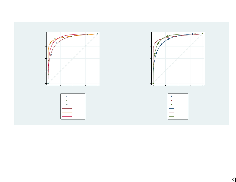
1992 rocreg — Receiver operating characteristic (ROC) regression
. graph combine a b, xsize(5)
0.00 0.25 0.50 0.75 1.00
Sensitivity
0.00 0.25 0.50 0.75 1.00
1−Specificity
mod1
mod2
mod3
mod1 fit
mod2 fit
mod3 fit
roccomp
0 .25 .5 .75 1
True−positive rate (ROC)
0 .25 .5 .75 1
False−positive rate
mod1
mod2
mod3
mod1 Fit
mod2 Fit
mod3 Fit
rocreg
We see differing true-positive rate values in the scattered points, which is expected because roccomp
gives the empirical estimate and rocreg gives the parametric estimate. However, the estimated curves
and areas under the ROC curve look similar. Using the Wald test based on the bootstrap covariance,
rocreg rejects the null hypothesis that each test has the same AUC at the 0.1 significance level.
roccomp formulates the asymptotic covariance using the rocfit estimates of AUC. Examination of
its output leads to rejection of the null hypothesis that the AUCs are equal across each test at the 0.05
significance level.
Parametric ROC curves: Maximum likelihood
The Alonzo and Pepe (2002) method of fitting a parametric model to the ROC curve is powerful
because it can be generally applied, but that can be a limitation as well. Whenever we invoke the
method and want anything other than point estimates of the parameters, we must perform bootstrap
resampling.
An alternative is to use maximum likelihood inference to fit the ROC curve. This method can save
computational time by avoiding the bootstrap.
rocreg implements maximum likelihood estimation for ROC curve analysis when both the case
and control populations are normal. Particularly, the classifier is a normal linear model on certain
covariates, and the covariate effect and variance of the classifier may change between the case and
control populations. This model is defined in Pepe (2003, 145).
y=z0β0+Dx0β1+σ(D)
Our error term, , is a standard normal random variable. The variable Dis our true status variable,
being 1 for the case population observations and 0 for the control population observations. The
variance function σis defined as
σ(D) = σ0(D= 0) + σ1(D= 1)
This provides two variance parameters in the model and does not depend on covariate values.

rocreg — Receiver operating characteristic (ROC) regression 1993
Suppose a covariate xiis present in zand x. The coefficient β1irepresents the interaction effect
of the xiand D. It is the extra effect that xihas on classifier yunder the case population, D=1,
beyond the main effect β0i. These β1coefficients are directly related to the ROC curve of y.
Under this model, the ROC curve is derived to be
ROC (u)=Φ1
σ1{x0β1+σ0Φ−1(u)}
For convenience, we reparameterize the model at this point, creating the parameters βi=σ−1
1β1i
and α=σ−1
1σ0. We refer to β0as the constant intercept, i cons. The parameter αis referred to
as the constant slope, s cons.
ROC (u) = Φ{x0β+αΦ−1(u)}
We may interpret the final coefficients as the standardized linear effect of the ROC covariate on
the classifier under the case population. The marginal effect of the covariate on the classifier in the
control population is removed, and it is rescaled by the case population standard deviation of the
classifier when all ROC covariate effects are removed. An appreciable effect on the classifier by a
ROC covariate in this measure leads to an appreciable effect on the classifier’s ROC curve by the ROC
covariate.
The advantage of estimating the control coefficients β0is similar to the gains of estimating the
covariate control models in the estimating equations ROC method and nonparametric ROC estimation.
This model would similarly apply when evaluating a test that is conditioned on control covariates.
Again we note that under parametric estimation, all the summary measures we defined earlier except
the AUC are not calculated until postestimation. In models with covariates, each covariate combination
would yield a different ROC curve and thus different summary parameters, so no summary parameters
are estimated initially. In marginal parametric models, we will calculate the AUC and leave the other
measures for postestimation. There is a simple closed-form formula for the AUC under the probit
model. Using this formula, the delta method can be invoked for inference on the AUC. Details on
AUC estimation for probit marginal models are found in Methods and formulas.
We will demonstrate the maximum likelihood method of rocreg by revisiting the models of the
previous section.
Example 10: Maximum likelihood ROC, single classifier
Returning to the hearing test study of Stover et al. (1996), we use a similar covariate grouping
as before. The frequency xf and intensity xl are control covariates (z), while all three covariates
xf,xl, and hearing loss degree xd are case covariates (x). In example 7, we fit this model using
the Alonzo and Pepe (2002) method. Earlier we stratified on the control covariates and estimated
the conditioned control distribution of nsnr empirically. Now we assume a normal linear model for
nsnr on xf and xl under the control population.
We fit the model by specifying the control covariates in the ctrlcov() option and the case
covariates in the roccov() option. The ml option tells rocreg to perform maximum likelihood
estimation.

1994 rocreg — Receiver operating characteristic (ROC) regression
. use http://www.stata-press.com/data/r13/dp, clear
(Stover - DPOAE test data)
. rocreg d nsnr, ctrlcov(xf xl) roccov(xf xl xd) probit ml cluster(id) nolog
Parametric ROC estimation
Covariate control : linear regression
Control variables : xf xl
Control standardization: normal
ROC method : parametric Link: probit
Status : d
Classifiers: nsnr
Classifier : nsnr
Covariate control adjustment model:
(Std. Err. adjusted for 208 clusters in id)
Robust
Coef. Std. Err. z P>|z| [95% Conf. Interval]
casecov
xf .4690907 .1408683 3.33 0.001 .192994 .7451874
xl -3.187785 .8976521 -3.55 0.000 -4.947151 -1.42842
xd 3.042998 .3569756 8.52 0.000 2.343339 3.742657
_cons 23.48064 5.692069 4.13 0.000 12.32439 34.63689
casesd
_cons 7.979708 .354936 22.48 0.000 7.284047 8.67537
ctrlcov
xf -.1447499 .0615286 -2.35 0.019 -.2653438 -.0241561
xl -.8631348 .2871976 -3.01 0.003 -1.426032 -.3002378
_cons 1.109477 1.964004 0.56 0.572 -2.7399 4.958854
ctrlsd
_cons 7.731203 .3406654 22.69 0.000 7.063511 8.398894
Status : d
ROC Model :
(Std. Err. adjusted for 208 clusters in id)
Robust
Coef. Std. Err. z P>|z| [95% Conf. Interval]
nsnr
i_cons 2.942543 .7569821 3.89 0.000 1.458885 4.426201
xf .0587854 .0175654 3.35 0.001 .024358 .0932129
xl -.3994865 .1171914 -3.41 0.001 -.6291775 -.1697955
xd .381342 .0449319 8.49 0.000 .2932771 .4694068
s_cons .9688578 .0623476 15.54 0.000 .8466587 1.091057
We find the results are similar to those of example 7. Frequency (xf) and intensity (xl) have a
negative effect on the classifier nsnr in the control population.
The negative control effect is mitigated for xf in the case population, but the effect for xl is even
more negative there. Hearing loss severity, xd, has a positive effect on nsnr in the case population,
and it is undefined in the control population.
The ROC coefficients are shown in the ROC Model table. Each are different from 0 at the 0.05
level. At this level, we also cannot conclude that the variances differ from case to control populations,
because 1 is in the 95% confidence interval for s cons, the ratio of the case to control standard
deviation parameters.

rocreg — Receiver operating characteristic (ROC) regression 1995
Both frequency (xf) and hearing loss severity (xd) make a positive contribution to the ROC curve
and thus make the test more powerful. Intensity (xl) has a negative effect on the ROC curve and
weakens the test. We previously saw in example 5 that the control distribution appears to be normal,
so using maximum likelihood to fit this model is a reasonable approach.
This model was also fit in Pepe (2003, 147). Pepe used separate least-squares estimates for the
case and control samples. We obtain similar results for the coefficients, but the maximum likelihood
fitting yields slightly different standard deviations by considering both case and control observations
concurrently. In addition, a misprint in Pepe (2003, 147) reports a coefficient of −4.91 for xl in the
case population instead of −3.19 as reported by Stata.
Inference on multiple classifiers using the Alonzo and Pepe (2002) estimating equation method
is performed by fitting each model separately and bootstrapping to determine the dependence of the
estimates. Using the maximum likelihood method, we also fit each model separately. We use suest
(see [R]suest) to estimate the joint variance–covariance of our parameter estimates.
For our models, we can view the score equation for each model as an estimating equation. The
estimate that solves the estimating equation (that makes the score 0) is asymptotically normal with a
variance matrix that can be estimated using the inverse of the squared scores. By stacking the score
equations of the separate models, we can estimate the variance matrix for all the parameter estimates
by using this rule. This is an informal explanation; further details can be found in [R]suest and in
the references Rogers (1993); White (1982 and 1996).
Now we will examine a case with multiple classification variables.
Example 11: Maximum likelihood ROC, multiple classifiers
We return to the neonatal audiology study with gender and age covariates (Norton et al. 2000).
In example 6, we fit a model with male and currage as control covariates, and currage as a ROC
covariate for the classifier y1 (DPOAE 65 at 2 kHz). We will refit this model, extending it to include
the classifier y2 (TEOAE 80 at 2 kHz).

1996 rocreg — Receiver operating characteristic (ROC) regression
. use http://www.stata-press.com/data/r13/nnhs
(Norton - neonatal audiology data)
. rocreg d y1 y2, probit ml ctrlcov(currage male) roccov(currage) cluster(id)
> nolog
Parametric ROC estimation
Covariate control : linear regression
Control variables : currage male
Control standardization: normal
ROC method : parametric Link: probit
Status : d
Classifiers: y1 y2
Classifier : y1
Covariate control adjustment model:
Coef. Std. Err. z P>|z| [95% Conf. Interval]
casecov
currage .494211 .2126672 2.32 0.020 .077391 .9110311
_cons -15.00403 8.238094 -1.82 0.069 -31.1504 1.142338
casesd
_cons 8.49794 .4922792 17.26 0.000 7.533091 9.46279
ctrlcov
currage -.2032048 .0323803 -6.28 0.000 -.266669 -.1397406
male .2369359 .2201391 1.08 0.282 -.1945288 .6684006
_cons -1.23534 1.252775 -0.99 0.324 -3.690734 1.220055
ctrlsd
_cons 7.749156 .0782225 99.07 0.000 7.595843 7.902469
Classifier : y2
Covariate control adjustment model:
Coef. Std. Err. z P>|z| [95% Conf. Interval]
casecov
currage .5729861 .2422662 2.37 0.018 .0981532 1.047819
_cons -18.2597 9.384968 -1.95 0.052 -36.6539 .1344949
casesd
_cons 9.723858 .5632985 17.26 0.000 8.619813 10.8279
ctrlcov
currage -.1694575 .0291922 -5.80 0.000 -.2266732 -.1122419
male .7122587 .1993805 3.57 0.000 .3214802 1.103037
_cons -5.651728 1.129452 -5.00 0.000 -7.865415 -3.438042
ctrlsd
_cons 6.986167 .0705206 99.07 0.000 6.84795 7.124385

rocreg — Receiver operating characteristic (ROC) regression 1997
Status : d
ROC Model :
(Std. Err. adjusted for 2741 clusters in id)
Robust
Coef. Std. Err. z P>|z| [95% Conf. Interval]
y1
i_cons -1.765608 1.105393 -1.60 0.110 -3.932138 .4009225
currage .0581566 .0290177 2.00 0.045 .0012828 .1150303
s_cons .9118864 .0586884 15.54 0.000 .7968593 1.026913
y2
i_cons -1.877825 .905174 -2.07 0.038 -3.651933 -.1037167
currage .0589258 .0235849 2.50 0.012 .0127002 .1051514
s_cons .7184563 .0565517 12.70 0.000 .607617 .8292957
Both classifiers have similar results. The results for y1 show the same direction as the estimating
equation results in example 6. However, we can now reject the null hypothesis that the ROC currage
coefficient is 0 at the 0.05 level.
In example 6, we could not reject that the slope parameter s cons was 1 and that the constant
intercept or ROC coefficient for current age was 0. The resulting ROC curve implied a noninformative
test using y1 as a classifier. This is not the case with our current results. As currage increases, we
expect a steeper ROC curve and thus a more powerful test, for both classifiers y1 (DPOAE 65 at 2 kHz)
and y2 (TEOAE 80 at 2 kHz).
In example 10, the clustering of observations within infant id was adjusted in the individual fit of
nsnr. In our current example, the adjustment for the clustering of observations within id is performed
during concurrent estimation, as opposed to during the individual classifier fits (as in example 10).
This adjustment, performed by suest, is still accurate.
Now we will fit constant probit models and compare rocreg with rocfit and roccomp with the
binormal option. Our first applications of rocfit and roccomp are taken directly from examples 8
and 9. The Dorfman and Alf (1969) algorithm that rocfit works with uses discrete classifiers or
uses slicing to make a classifier discrete. So we are applying the maximum likelihood method of
rocreg on discrete classification data here, where it expects continuous data. We expect to see some
discrepancies, but we do not find great divergence in the estimates. After revisiting examples 8 and
9, we will fit a probit model with a continuous classifier and no covariates using rocreg, and we
will compare the results with those from rocfit.
Example 12: Maximum likelihood ROC, marginal model
Using the Hanley and McNeil (1982) data, discussed in example 1 and in example 8, we fit a
constant probit model of the classifier rating with true status disease.rocreg is invoked with the
ml option and compared with rocfit.

1998 rocreg — Receiver operating characteristic (ROC) regression
. use http://www.stata-press.com/data/r13/hanley, clear
. rocfit disease rating, nolog
Binormal model of disease on rating Number of obs = 109
Goodness-of-fit chi2(2) = 0.21
Prob > chi2 = 0.9006
Log likelihood = -123.64855
Coef. Std. Err. z P>|z| [95% Conf. Interval]
intercept 1.656782 0.310456 5.34 0.000 1.048300 2.265265
slope (*) 0.713002 0.215882 -1.33 0.184 0.289881 1.136123
/cut1 0.169768 0.165307 1.03 0.304 -0.154227 0.493764
/cut2 0.463215 0.167235 2.77 0.006 0.135441 0.790990
/cut3 0.766860 0.174808 4.39 0.000 0.424243 1.109477
/cut4 1.797938 0.299581 6.00 0.000 1.210770 2.385106
Indices from binormal fit
Index Estimate Std. Err. [95% Conf. Interval]
ROC area 0.911331 0.029506 0.853501 0.969161
delta(m) 2.323671 0.502370 1.339044 3.308298
d(e) 1.934361 0.257187 1.430284 2.438438
d(a) 1.907771 0.259822 1.398530 2.417012
(*) z test for slope==1
. rocreg disease rating, probit ml nolog
Parametric ROC estimation
Control standardization: normal
ROC method : parametric Link: probit
Status : disease
Classifiers: rating
Classifier : rating
Covariate control adjustment model:
Coef. Std. Err. z P>|z| [95% Conf. Interval]
casecov
_cons 2.3357 .2334285 10.01 0.000 1.878188 2.793211
casesd
_cons 1.117131 .1106124 10.10 0.000 .9003344 1.333927
ctrlcov
_cons 2.017241 .1732589 11.64 0.000 1.67766 2.356823
ctrlsd
_cons 1.319501 .1225125 10.77 0.000 1.07938 1.559621
Status : disease
ROC Model :
Coef. Std. Err. z P>|z| [95% Conf. Interval]
rating
i_cons 2.090802 .2941411 7.11 0.000 1.514297 2.667308
s_cons 1.181151 .1603263 7.37 0.000 .8669177 1.495385
auc .9116494 .0261658 34.84 0.000 .8603654 .9629333

rocreg — Receiver operating characteristic (ROC) regression 1999
We compare the estimates for these models:
rocfit rocreg, ml
slope 0.7130 1.1812
SE of slope 0.2159 0.1603
intercept 1.6568 2.0908
SE of intercept 0.3105 0.2941
AUC 0.9113 0.9116
SE of AUC 0.0295 0.0262
We find that both the intercept and the slope are estimated as higher with the maximum likelihood
method under rocreg than with rocfit. The AUC (ROC area in rocfit) is close for both commands.
We find that the standard errors of each of these estimates is slightly lower under rocreg than rocfit
as well.
Both rocfit and rocreg suggest that the slope parameter of the ROC curve (slope in rocfit
and s cons in rocreg) is not significantly different from 1. Thus we cannot reject that the classifier
has the same variance in both case and control populations. There is, however, significant evidence
that the intercepts (i cons in rocreg and intercept in rocfit) differ from 0. Because of the
positive direction of the intercept estimates, the ROC curve for rating as a classifier of disease
suggests that rating provides an informative test. This is also suggested by the high AUC, which is
significantly different from 0.5, that is, a flip of a coin.
Example 13: Maximum likelihood ROC, marginal model, multiple classifiers
We use the fictitious dataset generated from Hanley and McNeil (1983), which we previously used
in example 2 and in example 9. To fit a probit model using roccomp, we specify the binormal option.
We perform parametric, maximum likelihood ROC analysis using rocreg. We use rocregplot to
plot the ROC curves created by rocreg.
. use http://www.stata-press.com/data/r13/ct2, clear
. roccomp status mod1 mod2 mod3, summary binormal graph aspectratio(1)
> plot1opts(connect(i) msymbol(o))
> plot2opts(connect(i) msymbol(s))
> plot3opts(connect(i) msymbol(t))
> legend(label(1 "mod1") label(3 "mod2") label(5 "mod3")
> label(2 "mod1 fit") label(4 "mod2 fit") label(6 "mod3 fit")
> order(1 3 5 2 4 6) cols(1)) title(roccomp) name(a) nodraw
Fitting binormal model for: mod1
Fitting binormal model for: mod2
Fitting binormal model for: mod3
ROC
Obs Area Std. Err. [95% Conf. Interval]
mod1 112 0.8945 0.0305 0.83482 0.95422
mod2 112 0.9382 0.0264 0.88647 0.99001
mod3 112 0.9376 0.0223 0.89382 0.98139
Ho: area(mod1) = area(mod2) = area(mod3)
chi2(2) = 8.27 Prob>chi2 = 0.0160

2000 rocreg — Receiver operating characteristic (ROC) regression
. rocreg status mod1 mod2 mod3, probit ml nolog
Parametric ROC estimation
Control standardization: normal
ROC method : parametric Link: probit
Status : status
Classifiers: mod1 mod2 mod3
Classifier : mod1
Covariate control adjustment model:
Coef. Std. Err. z P>|z| [95% Conf. Interval]
casecov
_cons 2.118135 .2165905 9.78 0.000 1.693626 2.542645
casesd
_cons 1.166078 .1122059 10.39 0.000 .9461589 1.385998
ctrlcov
_cons 2.344828 .1474147 15.91 0.000 2.0559 2.633755
ctrlsd
_cons 1.122677 .1042379 10.77 0.000 .9183746 1.32698
Classifier : mod2
Covariate control adjustment model:
Coef. Std. Err. z P>|z| [95% Conf. Interval]
casecov
_cons 2.659642 .2072731 12.83 0.000 2.253395 3.06589
casesd
_cons 1.288468 .1239829 10.39 0.000 1.045466 1.53147
ctrlcov
_cons 1.655172 .1105379 14.97 0.000 1.438522 1.871823
ctrlsd
_cons .8418313 .0781621 10.77 0.000 .6886365 .9950262
Classifier : mod3
Covariate control adjustment model:
Coef. Std. Err. z P>|z| [95% Conf. Interval]
casecov
_cons 2.353768 .1973549 11.93 0.000 1.966959 2.740576
casesd
_cons 1.143359 .1100198 10.39 0.000 .9277243 1.358994
ctrlcov
_cons 2.275862 .1214094 18.75 0.000 2.037904 2.51382
ctrlsd
_cons .9246267 .0858494 10.77 0.000 .7563649 1.092888
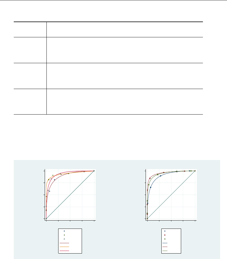
rocreg — Receiver operating characteristic (ROC) regression 2001
Status : status
ROC Model :
Robust
Coef. Std. Err. z P>|z| [95% Conf. Interval]
mod1
i_cons 1.81646 .3144804 5.78 0.000 1.20009 2.432831
s_cons .9627801 .1364084 7.06 0.000 .6954245 1.230136
auc .904657 .0343518 26.34 0.000 .8373287 .9719853
mod2
i_cons 2.064189 .3267274 6.32 0.000 1.423815 2.704563
s_cons .6533582 .1015043 6.44 0.000 .4544135 .8523029
auc .9580104 .0219713 43.60 0.000 .9149473 1.001073
mod3
i_cons 2.058643 .2890211 7.12 0.000 1.492172 2.625113
s_cons .8086932 .1163628 6.95 0.000 .5806262 1.03676
auc .9452805 .0236266 40.01 0.000 .8989732 .9915877
Ho: All classifiers have equal AUC values.
Ha: At least one classifier has a different AUC value.
P-value: .0808808
. rocregplot, title(rocreg) nodraw name(b)
> plot1opts(msymbol(o)) plot2opts(msymbol(s)) plot3opts(msymbol(t))
. graph combine a b, xsize(5)
0.00 0.25 0.50 0.75 1.00
Sensitivity
0.00 0.25 0.50 0.75 1.00
1−Specificity
mod1
mod2
mod3
mod1 fit
mod2 fit
mod3 fit
roccomp
0 .25 .5 .75 1
True−positive rate (ROC)
0 .25 .5 .75 1
False−positive rate
mod1
mod2
mod3
mod1 Fit
mod2 Fit
mod3 Fit
rocreg
We compare the AUC estimates for these models:
roccomp rocreg, ml
mod1 0.8945 0.9047
mod2 0.9382 0.9580
mod3 0.9376 0.9453
Each classifier has a higher estimated AUC under rocreg than roccomp. Each curve appears to
be raised and smoothed in the rocreg fit as compared with roccomp. They are different, but not
drastically different. The inference on whether the curve areas are the same is similar to example 9.
We reject equality at the 0.10 level under rocreg and at the 0.05 level under roccomp.

2002 rocreg — Receiver operating characteristic (ROC) regression
Each intercept is significantly different from 0 at the 0.05 level and is estimated in a positive
direction. Though all but classifier mod2 has 1 in their slope confidence intervals, the high intercepts
suggest steep ROC curves and powerful tests.
Also note that the false-positive and true-positive rate points are calculated empirically in the
roccomp graph and parametrically in rocreg. In example 9, the false-positive rates calculated by
rocreg were calculated empirically, similar to roccomp. But in this example, the rates are calculated
based on normal percentiles.
Now we will generate an example to compare rocfit and rocreg under maximum likelihood
estimation of a continuous classifier.
Example 14: Maximum likelihood ROC, graphical comparison with rocfit
We generate 500 realizations of a population under threat of disease. One quarter of the population
has the disease. A classifier xis measured, which has a control distribution of N(1,3)and a case
distribution of N(1+5,2). We will invoke rocreg with the ml option on this generated data. We
specify the continuous() option for rocfit and invoke it on the data as well. The continuous()
option tells rocfit how many discrete slices to partition the data into before fitting.
For comparison of the two curves, we will use the rocfit postestimation command, rocplot;
see [R]rocfit postestimation. This command graphs the empirical false-positive and true-positive
rates with an overlaid fit of the binormal curve estimated by rocfit.rocplot also supports an
addplot() option. We use the saved variables from rocreg in this option to overlay a line plot of
the rocreg fit.
. clear
. set seed 8675309
. set obs 500
obs was 0, now 500
. generate d = runiform() < .25
. quietly generate double epsilon = 3*invnormal(runiform()) if d == 0
. quietly replace epsilon = 2*invnormal(runiform()) if d == 1
. quietly generate double x = 1 + d*5 + epsilon

rocreg — Receiver operating characteristic (ROC) regression 2003
. rocreg d x, probit ml nolog
Parametric ROC estimation
Control standardization: normal
ROC method : parametric Link: probit
Status : d
Classifiers: x
Classifier : x
Covariate control adjustment model:
Coef. Std. Err. z P>|z| [95% Conf. Interval]
casecov
_cons 4.905612 .2411624 20.34 0.000 4.432943 5.378282
casesd
_cons 2.038278 .1299559 15.68 0.000 1.783569 2.292987
ctrlcov
_cons 1.010382 .1561482 6.47 0.000 .7043377 1.316427
ctrlsd
_cons 3.031849 .1104134 27.46 0.000 2.815443 3.248255
Status : d
ROC Model :
Coef. Std. Err. z P>|z| [95% Conf. Interval]
x
i_cons 2.406743 .193766 12.42 0.000 2.026969 2.786518
s_cons 1.487456 .1092172 13.62 0.000 1.273394 1.701518
auc .9103292 .012754 71.38 0.000 .8853318 .9353266
. rocfit d x, continuous(10) nolog
Binormal model of d on x Number of obs = 500
Goodness-of-fit chi2(7) = 1.69
Prob > chi2 = 0.9751
Log likelihood = -911.91338
Coef. Std. Err. z P>|z| [95% Conf. Interval]
intercept 2.207250 0.232983 9.47 0.000 1.750611 2.663888
slope (*) 1.281443 0.158767 1.77 0.076 0.970265 1.592620
/cut1 -1.895707 0.130255 -14.55 0.000 -2.151001 -1.640412
/cut2 -1.326900 0.089856 -14.77 0.000 -1.503015 -1.150784
/cut3 -0.723677 0.070929 -10.20 0.000 -0.862695 -0.584660
/cut4 -0.116960 0.064666 -1.81 0.070 -0.243702 0.009782
/cut5 0.442769 0.066505 6.66 0.000 0.312422 0.573116
/cut6 1.065183 0.075744 14.06 0.000 0.916728 1.213637
/cut7 1.689570 0.102495 16.48 0.000 1.488683 1.890457
/cut8 2.495841 0.185197 13.48 0.000 2.132861 2.858821
/cut9 3.417994 0.348485 9.81 0.000 2.734976 4.101012
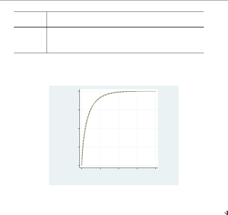
2004 rocreg — Receiver operating characteristic (ROC) regression
Indices from binormal fit
Index Estimate Std. Err. [95% Conf. Interval]
ROC area 0.912757 0.013666 0.885972 0.939542
delta(m) 1.722473 0.127716 1.472153 1.972792
d(e) 1.934960 0.125285 1.689405 2.180515
d(a) 1.920402 0.121804 1.681670 2.159135
(*) z test for slope==1
. rocplot, plotopts(msymbol(i)) lineopts(lpattern(dash))
> norefline addplot(line _roc_x _fpr_x, sort(_fpr_x _roc_x)
> lpattern(solid)) aspectratio(1) legend(off)
0 .25 .5 .75 1
Sensitivity
0 .25 .5 .75 1
1 − Specificity
Area under curve = 0.9128 se(area) = 0.0137
We find that the curves are close. As before, the rocfit estimates are lower for the slope and
intercept than under rocreg. The AUC estimates are close. Though the slope confidence interval
contains 1, a high ROC intercept suggests a steep ROC curve and thus a powerful test.

rocreg — Receiver operating characteristic (ROC) regression 2005
Stored results
Nonparametric rocreg stores the following in e():
Scalars
e(N) number of observations
e(N strata) number of covariate strata
e(N clust) number of clusters
e(rank) rank of e(V)
Macros
e(cmd) rocreg
e(cmdline) command as typed
e(classvars) classification variable list
e(refvar) status variable, reference variable
e(ctrlmodel) covariate-adjustment specification
e(ctrlcov) covariate-adjustment variables
e(pvc) percentile value calculation method
e(title) title in estimation output
e(tiecorrected) indicates whether tie correction was used
e(nobootstrap) indicates that bootstrap was performed
e(bseed) seed used in bootstrap, if bootstrap performed
e(breps) number of bootstrap resamples, if bootstrap performed
e(cc) indicates whether case–control groups were used as resampling strata
e(nobstrata) indicates whether resampling should stratify based on control covariates
e(clustvar) name of cluster variable
e(roc) false-positive rates where ROC was estimated
e(invroc) ROC values where false-positive rates were estimated
e(pauc) false-positive rates where pAUC was estimated
e(auc) indicates that AUC was calculated
e(vce) bootstrap
e(properties) b V (or bif bootstrap not performed)
Matrices
e(b) coefficient vector
e(V) variance–covariance matrix of the estimators
e(b bs) bootstrap estimates
e(bias) estimated biases
e(se) estimated standard errors
e(z0) median biases
e(ci normal) normal-approximation confidence intervals
e(ci percentile) percentile confidence intervals
e(ci bc) bias-corrected confidence intervals
Functions
e(sample) marks estimation sample

2006 rocreg — Receiver operating characteristic (ROC) regression
Parametric, bootstrap rocreg stores the following in e():
Scalars
e(N) number of observations
e(N strata) number of covariate strata
e(N clust) number of clusters
e(rank) rank of e(V)
Macros
e(cmd) rocreg
e(cmdline) command as typed
e(title) title in estimation output
e(classvars) classification variable list
e(refvar) status variable, reference variable
e(ctrlmodel) covariate-adjustment specification
e(ctrlcov) covariate-adjustment variables
e(pvc) percentile value calculation method
e(title) title in estimation output
e(tiecorrected) indicates whether tie correction was used
e(probit) probit
e(roccov) ROC covariates
e(fprpts) number of points used as false-positive rate fit points
e(ctrlfprall) indicates whether all observed false-positive rates were used as fit points
e(nobootstrap) indicates that bootstrap was performed
e(bseed) seed used in bootstrap
e(breps) number of bootstrap resamples
e(cc) indicates whether case–control groups were used as resampling strata
e(nobstrata) indicates whether resampling should stratify based on control covariates
e(clustvar) name of cluster variable
e(vce) bootstrap
e(properties) b V (or bif nobootstrap is specified)
e(predict) program used to implement predict
Matrices
e(b) coefficient vector
e(V) variance–covariance matrix of the estimators
e(b bs) bootstrap estimates
e(reps) number of nonmissing results
e(bias) estimated biases
e(se) estimated standard errors
e(z0) median biases
e(ci normal) normal-approximation confidence intervals
e(ci percentile) percentile confidence intervals
e(ci bc) bias-corrected confidence intervals
Functions
e(sample) marks estimation sample

rocreg — Receiver operating characteristic (ROC) regression 2007
Parametric, maximum likelihood rocreg stores the following in e():
Scalars
e(N) number of observations
e(N clust) number of clusters
e(rank) rank of e(V)
Macros
e(cmd) rocreg
e(cmdline) command as typed
e(classvars) classification variable list
e(refvar) status variable
e(ctrlmodel) linear
e(ctrlcov) control population covariates
e(roccov) ROC covariates
e(probit) probit
e(pvc) normal
e(wtype) weight type
e(wexp) weight expression
e(title) title in estimation output
e(clustvar) name of cluster variable
e(vce) cluster if clustering used
e(vcetype) robust if multiple classifiers or clustering used
e(ml) indicates that maximum likelihood estimation was used
e(predict) program used to implement predict
Matrices
e(b) coefficient vector
e(V) variance–covariance matrix of the estimators
Functions
e(sample) marks estimation sample
Methods and formulas
Assume that we applied a diagnostic test to each of N0control and N1case subjects. Further
assume that the higher the outcome value of the diagnostic test, the higher the risk of the subject
being abnormal. Let y1i, i =1,2, . . . , N1, and y0j, j =1,2, . . . , N0, be the values of the diagnostic
test for the case and control subjects, respectively. The true status variable Didentifies an observation
as case D=1 or control D=0. The CDF of the classifier Yis F. Conditional on D, we write the
CDF as FD.
Methods and formulas are presented under the following headings:
ROC statistics
Covariate-adjusted ROC curves
Parametric ROC curves: Estimating equations
Parametric ROC curves: Maximum likelihood

2008 rocreg — Receiver operating characteristic (ROC) regression
ROC statistics
We obtain these definitions and their estimates from Pepe (2003) and Pepe, Longton, and
Janes (2009). The false-positive and true-positive rates at cutoff care defined as
FPR (y) = PY≥yD= 0
TPR (y) = PY≥yD= 1
The true-positive rate, or ROC value at false-positive rate u, is given by
ROC (u) = P1−F0(Y)≤uD= 1
When Yis continuous, the false-positive rate can be written as
FPR (y)=1−F0(y)
The empirical CDF for the sample z1, . . . , znis given by
b
F(z) =
n
X
i=1
I(z < zi)
n
The empirical estimates c
FPR and d
ROC both use this empirical CDF estimator.
The area under the ROC curve is defined as
AUC =Z1
0
ROC (u)du
The partial area under the ROC curve for false-positive rate ais defined as
pAUC (a) = Za
0
ROC (u)du
The nonparametric estimate for the AUC is given by
d
AUC =
N1
X
i=1
1−c
FPR (y1i)
N1
The nonparametric estimate of pAUC is given by
d
pAUC (a) =
N1
X
i=1
max 1−c
FPR (y1i)−(1 −a),0
N1
For discrete classifiers, a correction term is subtracted from the false-positive rate estimate so that
the d
AUC and d
pAUC estimates correspond with a trapezoidal approximation to the area of the ROC
curve.
FPRc(y)=1−b
F0(y)−1
2
N0
X
j=1
I(y=y0j)
N0
In the nonparametric estimation of the ROC curve, all inference is performed using the bootstrap
command (see [R]bootstrap). rocreg also allows users to calculate the ROC curve and related
statistics by assuming a normal control distribution. So these formulas are updated by replacing F0
by Φ(with adjustment of the marginal mean and variance of the control distribution).

rocreg — Receiver operating characteristic (ROC) regression 2009
Covariate-adjusted ROC curves
Suppose we observe covariate vector Zin addition to the classifier Y. Let Z1i, i =1,2, . . . , N1,
and Z0j, j =1,2, . . . , N0, be the values of the covariates for the case and control subjects, respectively.
The covariate-adjusted ROC curve is defined by Janes and Pepe (2009) as
AROC (t) = EROC tZ0
It is calculated by replacing the marginal control CDF estimate, b
F0, with the conditional control CDF
estimate, b
F0Z. If we used a normal control CDF, then we would replace the marginal control mean
and variance with the conditional control mean and variance. The formulas of the previous section
can be updated for covariate-adjustment by making this substitution of the conditional CDF for the
marginal CDF in the false-positive rate calculation.
Because the calculation of the ROC value is now performed based on the conditionally calculated
false-positive rate, no further conditioning is made in its calculation under nonparametric estimation.
rocreg supports covariate adjustment with stratification and linear regression. Under stratification,
separate parameters are estimated for the control distribution at each level of the covariates. Under
linear regression, the classifier is regressed on the covariates over the control distribution, and the
resulting coefficients serve as parameters for b
F0Z.
Parametric ROC curves: Estimating equations
Under nonparametric estimation of the ROC curve with covariate adjustment, no further conditioning
occurs in the ROC curve calculation beyond the use of covariate-adjusted false-positive rates as inputs.
Under parametric estimation of the ROC curve, we can relax this restriction. We model the ROC
curve as a cumulative distribution function g(standard normal Φ) invoked with input of a linear
polynomial in the corresponding quantile function (here Φ−1) invoked on the false-positive rate u. The
constant intercept of the polynomial may depend on covariates; the slope term α(quantile coefficient)
may not.
ROC (u) = g{x0β+αg−1(u)}
Pepe (2003) notes that having a binormal ROC (g= Φ) is equivalent to specifying that some
monotone transformation of the data exists to make the case and control classifiers normally distributed.
This specification applies to the marginal case and control.
Under weak assumptions about the control distribution of the classifier, we can fit this model
by using estimating equations (Alonzo and Pepe 2002). The method can be used without covariate
effects in the second stage, assuming a parametric model for the single ROC curve. Using the Alonzo
and Pepe (2002) method, the covariate-adjusted ROC curve may be fit parametrically. The marginal
ROC curve, involving no covariates in either stage of estimation, can be fit parametrically as well. In
addition to the Alonzo and Pepe (2002) explanation, further details are given in Pepe, Longton, and
Janes (2009); Janes, Longton, and Pepe (2009); Pepe (2003); and Janes and Pepe (2009).
The algorithm can be described as follows:
1. Estimate the false-positive rates of the classifier fpr. These may be computed in any fashion
outlined so far: covariate-adjusted, empirically, etc.
2. Determine a set of npfalse-positive rates to use as fitting points f1, . . . , fnp. These may be an
equispaced grid on (0,1)or the set of observed false-positive rates from part 1.

2010 rocreg — Receiver operating characteristic (ROC) regression
3. Expand the case observation portion of the data to include a subobservation for each fitting point.
So there are now N1(np−1)additional observations in the data.
4. Generate a new dummy variable u. For subobservation j,u=I(fpr ≤fj).
5. Generate a new variable quant containing the quantiles of the false-positive rate fitting points.
For subobservation j,quant =g−1(fj).
6. Perform a binary regression (probit, g= Φ) of fpr on the covariates xand quantile variable
quant.
The coefficients of part 6 are the coefficients of the ROC model. The coefficients of the covariates
coincide naturally with estimates of β, and the αparameter is estimated by the coefficient on quant.
Because the method is so general and makes few distributional assumptions, bootstrapping must be
performed for inference. If multiple classifiers are to be fit, the algorithm is performed separately for
each in each bootstrap, and the bootstrap is used to estimate covariances.
We mentioned earlier that in parametric estimation, the AUC was the only summary parameter that
could be estimated initially. This is true when we fit the marginal probit model because there are no
covariates in part 6 of the algorithm.
To calculate the AUC statistic under a marginal probit model, we use the formula
AUC = Φ β0
√1 + α2
Alternatively, the AUC for the probit model can be calculated as pAUC(1) in postestimation. Under
both models, bootstrapping is performed for inference on the AUC.
Parametric ROC curves: Maximum likelihood
rocreg supports another form of parametric ROC estimation: maximum likelihood with a normally
distributed classifier. This method assumes that the classifier is a normal linear model on certain
covariates, and the covariate effect and variance of the classifier may change between the case and
control populations. The model is defined in Pepe (2003, 145).
y=z0β0+Dx0β1+σ(D)
Our error term, , is a standard normal random variable. The variable Dis our true status variable,
being 1 for the case population observations and 0 for the control population observations. The
variance function σis defined as
σ(D) = σ0(D= 0) + σ1(D= 1)
This provides two variance parameters in the model and does not depend on covariate values.
Under this model, the ROC curve is easily derived to be
ROC (u) = Φ 1
σ1x0β1+σ0Φ−1(u)
We reparameterize the model, creating the parameters βi=σ−1
1β1iand α=σ−1
1σ0. We refer to β0
as the constant intercept, i cons. The parameter αis referred to as the constant slope, s cons.
ROC (u) = Φ{x0β+αΦ−1(u)}

rocreg — Receiver operating characteristic (ROC) regression 2011
The original model defining the classifier yleads to the following single observation likelihoods
for D=0 and D=1:
L(β0,β1, σ1, σ0,D= 0, y, z,x) = 1
√2πσ0
exp −(y−z0β0)2
2σ2
0
L(β0,β1, σ1, σ0,D= 1, y, z,x) = 1
√2πσ1
exp −(y−z0β0−x0β1)2
2σ2
1
These can be combined to yield the observation-level log likelihood:
lnL(β0,β1, σ1, σ0,D, y, z,x) = −ln2π
2
−I(D= 0) lnσ0+(y−z0β0)2
2σ2
0
−I(D= 1) lnσ1+(y−z0β0−x0β1)2
2σ2
1
When there are multiple classifiers, each classifier is fit separately with maximum likelihood. Then
the results are combined by stacking the scores and using the sandwich variance estimator. For more
information, see [R]suest and the references White (1982); Rogers (1993); and White (1996).
Acknowledgments
We thank Margaret S. Pepe, Holly Janes, and Gary Longton of the Fred Hutchinson Cancer
Research Center for providing the inspiration for the rocreg command and for illuminating many
useful datasets for its documentation.
References
Alonzo, T. A., and M. S. Pepe. 2002. Distribution-free ROC analysis using binary regression techniques. Biostatistics
3: 421–432.
Cleves, M. A. 1999. sg120: Receiver operating characteristic (ROC) analysis.Stata Technical Bulletin 52: 19–33.
Reprinted in Stata Technical Bulletin Reprints, vol. 9, pp. 212–229. College Station, TX: Stata Press.
. 2000. sg120.2: Correction to roccomp command.Stata Technical Bulletin 54: 26. Reprinted in Stata Technical
Bulletin Reprints, vol. 9, p. 231. College Station, TX: Stata Press.
. 2002a. Comparative assessment of three common algorithms for estimating the variance of the area under the
nonparametric receiver operating characteristic curve.Stata Journal 2: 280–289.
. 2002b. From the help desk: Comparing areas under receiver operating characteristic curves from two or more
probit or logit models.Stata Journal 2: 301–313.
Cook, N. R. 2007. Use and misuse of the receiver operating characteristic curve in risk prediction. Circulation 115:
928–935.
DeLong, E. R., D. M. DeLong, and D. L. Clarke-Pearson. 1988. Comparing the areas under two or more correlated
receiver operating characteristic curves: A nonparametric approach. Biometrics 44: 837–845.
Dodd, L. E., and M. S. Pepe. 2003. Partial AUC estimation and regression. Biometrics 59: 614–623.
Dorfman, D. D., and E. Alf, Jr. 1969. Maximum-likelihood estimation of parameters of signal-detection theory and
determination of confidence intervals–rating-method data. Journal of Mathematical Psychology 6: 487–496.

2012 rocreg — Receiver operating characteristic (ROC) regression
Hanley, J. A., and K. O. Hajian-Tilaki. 1997. Sampling variability of nonparametric estimates of the areas under
receiver operating characteristic curves: An update. Academic Radiology 4: 49–58.
Hanley, J. A., and B. J. McNeil. 1982. The meaning and use of the area under a receiver operating characteristic
(ROC) curve. Radiology 143: 29–36.
. 1983. A method of comparing the areas under receiver operating characteristic curves derived from the same
cases. Radiology 148: 839–843.
Janes, H., G. M. Longton, and M. S. Pepe. 2009. Accommodating covariates in receiver operating characteristic
analysis.Stata Journal 9: 17–39.
Janes, H., and M. S. Pepe. 2009. Adjusting for covariate effects on classification accuracy using the covariate-adjusted
receiver operating characteristic curve. Biometrika 96: 371–382.
McClish, D. K. 1989. Analyzing a portion of the ROC curve. Medical Decision Making 9: 190–195.
Mooney, C. Z., and R. D. Duval. 1993. Bootstrapping: A Nonparametric Approach to Statistical Inference. Newbury
Park, CA: Sage.
Norton, S. J., M. P. Gorga, J. E. Widen, R. C. Folsom, Y. Sininger, B. Cone-Wesson, B. R. Vohr, K. Mascher,
and K. Fletcher. 2000. Identification of neonatal hearing impairment: Evaluation of transient evoked otoacoustic
emission, distortion product otoacoustic emission, and auditory brain stem response test performance. Ear and
Hearing 21: 508–528.
Pepe, M. S. 1998. Three approaches to regression analysis of receiver operating characteristic curves for continuous
test results. Biometrics 54: 124–135.
. 2000. Receiver operating characteristic methodology. Journal of the American Statistical Association 95: 308–311.
. 2003. The Statistical Evaluation of Medical Tests for Classification and Prediction. New York: Oxford University
Press.
Pepe, M. S., and T. Cai. 2004. The analysis of placement values for evaluating discriminatory measures. Biometrics
60: 528–535.
Pepe, M. S., G. M. Longton, and H. Janes. 2009. Estimation and comparison of receiver operating characteristic
curves.Stata Journal 9: 1–16.
Rogers, W. H. 1993. sg16.4: Comparison of nbreg and glm for negative binomial.Stata Technical Bulletin 16: 7.
Reprinted in Stata Technical Bulletin Reprints, vol. 3, pp. 82–84. College Station, TX: Stata Press.
Stover, L., M. P. Gorga, S. T. Neely, and D. Montoya. 1996. Toward optimizing the clinical utility of distortion
product otoacoustic emission measurements. Journal of the Acoustical Society of America 100: 956–967.
Thompson, M. L., and W. Zucchini. 1989. On the statistical analysis of ROC curves. Statistics in Medicine 8:
1277–1290.
White, H. L., Jr. 1982. Maximum likelihood estimation of misspecified models. Econometrica 50: 1–25.
. 1996. Estimation, Inference and Specification Analysis. Cambridge: Cambridge University Press.
Wieand, S., M. H. Gail, B. R. James, and K. L. James. 1989. A family of nonparametric statistics for comparing
diagnostic markers with paired or unpaired data. Biometrika 76: 585–592.
Also see
[R]rocreg postestimation — Postestimation tools for rocreg
[R]rocregplot — Plot marginal and covariate-specific ROC curves after rocreg
[R]rocfit — Parametric ROC models
[R]roc — Receiver operating characteristic (ROC) analysis

Title
rocreg postestimation — Postestimation tools for rocreg
Description Syntax for predict Menu for predict
Options for predict Syntax for estat nproc Menu for estat
Options for estat nproc Remarks and examples Stored results
Methods and formulas References Also see
Description
The following commands are of special interest after rocreg:
Command Description
estat nproc nonparametric ROC curve estimation, keeping fit information from rocreg
rocregplot plot marginal and covariate-specific ROC curves
The following standard postestimation commands are also available:
Command Description
estimates cataloging estimation results
lincom point estimates, standard errors, testing, and inference for linear combinations
nlcom point estimates, standard errors, testing, and inference for nonlinear combinations
of coefficients
predict predictions for parametric ROC curve estimation
test Wald tests of simple and composite linear hypotheses
testnl Wald tests of nonlinear hypotheses
Special-interest postestimation command
The estat nproc command allows calculation of all the ROC curve summary statistics for
covariate-specific ROC curves, as well as for a nonparametric ROC estimation. Under nonparametric
estimation, a single ROC curve is estimated by rocreg. Covariates can affect this estimation, but
there are no separate covariate-specific ROC curves. Thus the input arguments for estat nproc are
taken in the command line rather than from the data as variable values.
2013

2014 rocreg postestimation — Postestimation tools for rocreg
Syntax for predict
predict type newvar if in ,statistic options
statistic Description
Main
at(varname)input variable for statistic
auc total area under the ROC curve; the default
roc ROC values for given false-positive rates in at()
invroc false-positive rate for given ROC values in at()
pauc partial area under the ROC curve up to each false-positive
rate in at()
classvar(varname)statistic for given classifier
options Description
Options
intpts(#)points in numeric integration of pAUC calculation
se(newvar)predict standard errors
ci(stubname)produce confidence intervals, stored as variables with prefix
stubname and suffixes land u
level(#)set confidence level; default is level(95)
∗bfile(filename,. . . )load dataset containing bootstrap replicates from rocreg
∗btype(n |p|bc) produce normal-based (n), percentile (p), or bias-corrected (bc)
confidence intervals; default is btype(n)
∗bfile() and btype() are only allowed with parametric analysis using bootstrap inference.
Menu for predict
Statistics >Postestimation >Predictions, residuals, etc.
Options for predict
Main
at(varname)records the variable to be used as input for the above predictions.
auc predicts the total area under the ROC curve defined by the covariate values in the data. This is
the default statistic.
roc predicts the ROC values for false-positive rates stored in varname specified in at().
invroc predicts the false-positive rates for given ROC values stored in varname specified in at().
pauc predicts the partial area under the ROC curve up to each false-positive rate stored in varname
specified in at().
classvar(varname)performs the prediction for the specified classifier.

rocreg postestimation — Postestimation tools for rocreg 2015
Options
intpts(#)specifies that #points be used in the pAUC calculation.
se(newvar)specifies that standard errors be produced and stored in newvar.
ci(stubname)requests that confidence intervals be produced and the lower and upper bounds be
stored in stubname land stubname u, respectively.
level(#)specifies the confidence level, as a percentage, for confidence intervals. The default is
level(95) or as set by set level; see [U] 20.7 Specifying the width of confidence intervals.
bfile(filename,. . . )uses bootstrap replicates of parameters from rocreg stored in filename to
estimate standard errors and confidence intervals of predictions.
btype(n |p|bc) specifies whether to produce normal-based (n), percentile (p), or bias-corrected (bc)
confidence intervals. The default is btype(n).
Syntax for estat nproc
estat nproc ,estat nproc options
estat nproc options Description
Main
auc estimate total area under the ROC curve
roc(numlist)estimate ROC values for given false-positive rates
invroc(numlist)estimate false-positive rate for given ROC values
pauc(numlist)estimate partial area under the ROC curve up to each false-positive rate
At least one option must be specified.
Menu for estat
Statistics >Postestimation >Reports and statistics
Options for estat nproc
Main
auc estimates the total area under the ROC curve.
roc(numlist)estimates the ROC for each of the false-positive rates in numlist. The values in numlist
must be in the range (0,1).
invroc(numlist)estimates the false-positive rate for each of the ROC values in numlist. The values
in numlist must be in the range (0,1).
pauc(numlist)estimates the partial area under the ROC curve up to each false-positive rate in numlist.
The values in numlist must be in the range (0,1].

2016 rocreg postestimation — Postestimation tools for rocreg
Remarks and examples
Remarks are presented under the following headings:
Using predict after rocreg
Using estat nproc
Using predict after rocreg
predict, after parametric rocreg, predicts the AUC, the ROC value, the false-positive rate (invROC),
or the pAUC value. The default is auc.
We begin by estimating the area under the ROC curve for each of the three age-specific ROC curves
in example 1 of [R]rocregplot: 30, 40, and 50 months.
Example 1: Parametric ROC, AUC
In example 6 of [R]rocreg, a probit ROC model was fit to audiology test data from Norton et al.
(2000). The estimating equations method of Alonzo and Pepe (2002) was used to fit the model.
Gender and age were covariates that affected the control distribution of the classifier y1 (DPOAE 65
at 2 kHz). Age was a ROC covariate for the model, so we fit separate ROC curves at each age.
Following Janes, Longton, and Pepe (2009), we drew the ROC curves for ages 30, 40, and 50
months in example 1 of [R]rocregplot. Now we use predict to estimate the AUC for the ROC curve
at each of those ages.
The bootstrap dataset saved by rocreg in example 6 of [R]rocreg,nnhs2y1.dta, is used in the
bfile() option.
We will store the AUC prediction in the new variable predAUC. We specify the se() option with
the new variable name seAUC to produce an estimate of the prediction’s standard error. By specifying
the stubname cin in ci(), we tell predict to create normal-based confidence intervals (the default)
as new variables cin l and cin u.
. use http://www.stata-press.com/data/r13/nnhs
(Norton - neonatal audiology data)
. rocreg d y1, probit ctrlcov(currage male) ctrlmodel(linear) roccov(currage)
> cluster(id) bseed(56930) bsave(nnhs2y1)
(output omitted )
. set obs 5061
obs was 5058, now 5061
. quietly replace currage = 30 in 5059
. quietly replace currage = 40 in 5060
. quietly replace currage = 50 in 5061
. predict predAUC in 5059/5061, auc se(seAUC) ci(cin) bfile(nnhs2y1)
. list currage predAUC seAUC cin* in 5059/5061
currage predAUC seAUC cin_l cin_u
5059. 30 .5209999 .0712928 .3812686 .6607312
5060. 40 .6479176 .0286078 .5918474 .7039879
5061. 50 .7601378 .0746157 .6138937 .9063819

rocreg postestimation — Postestimation tools for rocreg 2017
As expected, we find the AUC to increase with age.
Essentially, we have a stored bootstrap sample of ROC covariate coefficient estimates in
nnhs2y1.dta. We calculate the AUC using each set of coefficient estimates, resulting in a sam-
ple of AUC estimates. Then the bootstrap standard error and confidence intervals are calculated based
on this AUC sample. Further details of the computation of the standard error and percentile confidence
intervals can be found in Methods and formulas and in [R]bootstrap.
We can also produce percentile or bias-corrected confidence intervals by specifying btype(p) or
btype(bc), which we now demonstrate.
. drop *AUC*
. predict predAUC in 5059/5061, auc se(seAUC) ci(cip) bfile(nnhs2y1) btype(p)
. list currage predAUC cip* in 5059/5061
currage predAUC cip_l cip_u
5059. 30 .5209999 .3760555 .6513149
5060. 40 .6479176 .5893397 .7032645
5061. 50 .7601378 .5881404 .8836223
. drop *AUC*
. predict predAUC in 5059/5061, auc se(seAUC) ci(cibc) bfile(nnhs2y1) btype(bc)
. list currage predAUC cibc* in 5059/5061
currage predAUC cibc_l cibc_u
5059. 30 .5209999 .3736968 .6500064
5060. 40 .6479176 .588947 .7010052
5061. 50 .7601378 .5812373 .8807758
predict can also estimate the ROC value and the false-positive rate (invROC).
Example 2: Parametric ROC, invROC, and ROC value
In example 7 of [R]rocreg, we fit the ROC curve for status variable hearing loss (d) and classifier
negative signal-to-noise ratio nsnr with ROC covariates frequency (xf), intensity (xl), and hearing
loss severity (xd). The data were obtained from Stover et al. (1996). The model fit was probit with
bootstrap resampling. We saved 50 bootstrap replications in the dataset nsnrf.dta.
The covariate value combinations xf = 10.01,xl = 5.5, and xd = .5, and xf = 10.01,xl =
6.5, and xd = 4 are of interest. In example 3 of [R]rocregplot, we estimated the ROC values for
false-positive rates 0.2 and 0.7 and the false-positive rate for a ROC value of 0.5 by using rocregplot.
We will use predict to replicate the estimation.
We begin by appending observations with our desired covariate combinations to the data. We also
create two new variables: rocinp, which contains the ROC values for which we wish to predict the
corresponding invROC values, and invrocinp, which contains the invROC values corresponding to
the ROC values we wish to predict.

2018 rocreg postestimation — Postestimation tools for rocreg
. clear
. input xf xl xd rocinp invrocinp
xf xl xd rocinp invrocinp
1. 10.01 5.5 .5 .2 .
2. 10.01 6.5 4 .2 .
3. 10.01 5.5 .5 .7 .5
4. 10.01 6.5 4 .7 .5
5. end
. save newdata
file newdata.dta saved
. use http://www.stata-press.com/data/r13/dp
(Stover - DPOAE test data)
. quietly rocreg d nsnr, ctrlcov(xf xl) roccov(xf xl xd) probit cluster(id)
> nobstrata ctrlfprall bseed(156385) breps(50) ctrlmodel(strata) bsave(nsnrf)
. append using newdata
. list xf xl xd invrocinp rocinp in 1849/1852
xf xl xd invroc~p rocinp
1849. 10.01 5.5 .5 . .2
1850. 10.01 6.5 4 . .2
1851. 10.01 5.5 .5 .5 .7
1852. 10.01 6.5 4 .5 .7
Now we will use predict to estimate the ROC value for the false-positive rates stored in rocinp.
We specify the roc option, and we specify rocinp in the at() option. The other options, se()
and ci(), are used to obtain standard errors and confidence intervals, respectively. The dataset of
bootstrap samples, nsnrf.dta, is specified in bfile(). After prediction, we list the point estimates
and standard errors.
. predict rocit in 1849/1852, roc at(rocinp) se(seroc) ci(cin) bfile(nsnrf)
. list xf xl xd rocinp rocit seroc if !missing(rocit)
xf xl xd rocinp rocit seroc
1849. 10.01 5.5 .5 .2 .7652956 .0735506
1850. 10.01 6.5 4 .2 .9672505 .0227977
1851. 10.01 5.5 .5 .7 .9835816 .0204353
1852. 10.01 6.5 4 .7 .999428 .0011309
These results match example 3 of [R]rocregplot. We list the confidence intervals next. These also
conform to the rocregplot results from example 3 in [R]rocregplot. We begin with the confidence
intervals for ROC under the covariate values xf=10.01,xl=5.5, and xd=.5.

rocreg postestimation — Postestimation tools for rocreg 2019
. list xf xl xd rocinp rocit cin* if inlist(_n, 1849, 1851)
xf xl xd rocinp rocit cin_l cin_u
1849. 10.01 5.5 .5 .2 .7652956 .6211391 .9094521
1851. 10.01 5.5 .5 .7 .9835816 .9435292 1.023634
Now we list the ROC confidence intervals under the covariate values xf=10.01,xl=6.5, and
xd=4.
. list xf xl xd rocinp rocit cin* if inlist(_n, 1850, 1852)
xf xl xd rocinp rocit cin_l cin_u
1850. 10.01 6.5 4 .2 .9672505 .9225678 1.011933
1852. 10.01 6.5 4 .7 .999428 .9972115 1.001644
Now we will predict the false-positive rate for a ROC value by specifying the invroc option. We
pass the invrocinp variable as an argument to the at() option. Again we list the point estimates
and standard errors first.
. drop ci*
. predict invrocit in 1849/1852, invroc at(invrocinp) se(serocinv) ci(cin)
> bfile(nsnrf)
. list xf xl xd invrocinp invrocit serocinv if !missing(invrocit)
xf xl xd invroc~p invrocit serocinv
1851. 10.01 5.5 .5 .5 .0615144 .0254042
1852. 10.01 6.5 4 .5 .0043298 .0045938
These also match those of example 3 of [R]rocregplot. Listing the confidence intervals shows
identical results as well. First we list the confidence intervals under the covariate values xf=10.01,
xl=5.5, and xd=.5.
. list xf xl xd invrocinp invrocit cin* in 1851
xf xl xd invroc~p invrocit cin_l cin_u
1851. 10.01 5.5 .5 .5 .0615144 .0117231 .1113057
Now we list the confidence intervals for false-positive rate under the covariate values xf=10.01,
xl=6.5, and xd=4.
. list xf xl xd invrocinp invrocit cin* in 1852
xf xl xd invroc~p invrocit cin_l cin_u
1852. 10.01 6.5 4 .5 .0043298 -.004674 .0133335
The predict command can also be used after a maximum-likelihood ROC model is fit.

2020 rocreg postestimation — Postestimation tools for rocreg
Example 3: Maximum likelihood ROC, invROC, and ROC value
In the previous example, we revisited the estimating equations fit of a probit model with ROC
covariates frequency (xf), intensity (xl), and hearing loss severity (xd) to the Stover et al. (1996)
audiology study data. A maximum likelihood fit of the same model was performed in example 10
of [R]rocreg. In example 2 of [R]rocregplot, we used rocregplot to estimate ROC values and
false-positive rates for this model under two covariate configurations. We will use predict to obtain
the same estimates. We will also estimate the partial area under the ROC curve.
We append the data as in the previous example. This leads to the following four final observations
in the data.
. use http://www.stata-press.com/data/r13/dp, clear
(Stover - DPOAE test data)
. rocreg d nsnr, probit ctrlcov(xf xl) roccov(xf xl xd) ml cluster(id)
(output omitted )
. append using newdata
. list xf xl xd invrocinp rocinp in 1849/1852
xf xl xd invroc~p rocinp
1849. 10.01 5.5 .5 . .2
1850. 10.01 6.5 4 . .2
1851. 10.01 5.5 .5 .5 .7
1852. 10.01 6.5 4 .5 .7
Now we predict the ROC value for false-positive rates of 0.2 and 0.7. Under maximum likelihood
prediction, only Wald-type confidence intervals are produced. We specify a new variable name for
the standard error in the se() option and a stubname for the confidence interval variables in the
ci() option.
. predict rocit in 1849/1852, roc at(rocinp) se(seroc) ci(ci)
. list xf xl xd rocinp rocit seroc ci_l ci_u if !missing(rocit), noobs
xf xl xd rocinp rocit seroc ci_l ci_u
10.01 5.5 .5 .2 .7608593 .0510501 .660803 .8609157
10.01 6.5 4 .2 .9499408 .0179824 .914696 .9851856
10.01 5.5 .5 .7 .978951 .0097382 .9598644 .9980376
10.01 6.5 4 .7 .9985001 .0009657 .9966073 1.000393
These results match our estimates in example 2 of [R]rocregplot. We also match example 2 of
[R]rocregplot when we estimate the false-positive rate for a ROC value of 0.5.
. drop ci*
. predict invrocit in 1851/1852, invroc at(invrocinp) se(serocinv) ci(ci)
. list xf xl xd invrocinp invrocit serocinv ci_l ci_u if !missing(invrocit),
> noobs
xf xl xd invroc~p invrocit serocinv ci_l ci_u
10.01 5.5 .5 .5 .0578036 .0198626 .0188736 .0967336
10.01 6.5 4 .5 .0055624 .0032645 -.0008359 .0119607

rocreg postestimation — Postestimation tools for rocreg 2021
Example 4: Maximum likelihood ROC, pAUC, and ROC value
In example 13 of [R]rocreg, we fit a maximum-likelihood marginal probit model to each classifier
of the fictitious dataset generated from Hanley and McNeil (1983). In example 5 of [R]rocregplot,
rocregplot was used to draw the ROC for the mod1 and mod3 classifiers. Estimates of the ROC
value and false-positive rate were also obtained with Wald-type confidence intervals.
We return to this example, this time using predict to estimate the ROC value and false-positive
rate. We will also estimate the pAUC for the false-positive rates of 0.3 and 0.8.
First, we add the input variables to the data. The variable paucinp will hold the 0.3 and 0.8
false-positive rates that we will input to pAUC. The variable invrocinp holds the ROC value of 0.8
for which we will estimate the false-positive rate. Finally, the variable rocinp holds the false-positive
rates of 0.15 and 0.75 for which we will estimate the ROC value.
. use http://www.stata-press.com/data/r13/ct2, clear
. rocreg status mod1 mod2 mod3, probit ml
(output omitted )
. quietly generate paucinp = .3 in 111
. quietly replace paucinp = .8 in 112
. quietly generate invrocinp = .8 in 112
. quietly generate rocinp = .15 in 111
. quietly replace rocinp = .75 in 112
Then, we estimate the ROC value for false-positive rates 0.15 and 0.75 under classifier mod1. The
point estimate is stored in roc1. Wald confidence intervals and standard errors are also estimated.
We find that these results match those of example 5 of [R]rocregplot.
. predict roc1 in 111/112, classvar(mod1) roc at(rocinp) se(sr1) ci(cir1)
. list rocinp roc1 sr1 cir1* in 111/112
rocinp roc1 sr1 cir1_l cir1_u
111. .15 .7934935 .0801363 .6364293 .9505578
112. .75 .9931655 .0069689 .9795067 1.006824
Now we perform the same estimation under the classifier mod3.
. predict roc3 in 111/112, classvar(mod3) roc at(roci) se(sr3) ci(cir3)
. list rocinp roc3 sr3 cir3* in 111/112
rocinp roc3 sr3 cir3_l cir3_u
111. .15 .8888596 .0520118 .7869184 .9908009
112. .75 .9953942 .0043435 .9868811 1.003907
Next we estimate the false-positive rate for the ROC value of 0.8. These results also match example 5
of [R]rocregplot.
. predict invroc1 in 112, classvar(mod1) invroc at(invrocinp) se(sir1) ci(ciir1)
. list invrocinp invroc1 sir1 ciir1* in 112
invroc~p invroc1 sir1 ciir1_l ciir1_u
112. .8 .1556435 .069699 .0190361 .292251

2022 rocreg postestimation — Postestimation tools for rocreg
. predict invroc3 in 112, classvar(mod3) invroc at(invrocinp) se(sir3) ci(ciir3)
. list invrocinp invroc3 sir3 ciir3* in 112
invroc~p invroc3 sir3 ciir3_l ciir3_u
112. .8 .0661719 .045316 -.0226458 .1549896
Finally, we estimate the pAUC for false-positive rates of 0.3 and 0.8. The point estimate is calculated
by numeric integration. Wald confidence intervals are obtained with the delta method. Further details
are presented in Methods and formulas.
. predict pauc1 in 111/112, classvar(mod1) pauc at(paucinp) se(sp1) ci(cip1)
. list paucinp pauc1 sp1 cip1* in 111/112
paucinp pauc1 sp1 cip1_l cip1_u
111. .3 .221409 .0240351 .174301 .268517
112. .8 .7033338 .0334766 .6377209 .7689466
. predict pauc3 in 111/112, classvar(mod3) pauc at(paucinp) se(sp3) ci(cip3)
. list paucinp pauc3 sp3 cip3* in 111/112
paucinp pauc3 sp3 cip3_l cip3_u
111. .3 .2540215 .0173474 .2200213 .2880217
112. .8 .7420408 .0225192 .6979041 .7861776
Using estat nproc
When you initially use rocreg to fit a nonparametric ROC curve, you can obtain bootstrap estimates
of a ROC value, false-positive rate, area under the ROC curve, and partial area under the ROC curve.
The estat nproc command allows the user to estimate these parameters after rocreg has originally
been used.
The seed and resampling settings used by rocreg are used by estat nproc. So the results for
these new statistics are identical to what they would be if they had been initially estimated in the
rocreg command. These new statistics, together with those previously estimated in rocreg, are
returned in r().
We demonstrate with an example.
Example 5: Nonparametric ROC, invROC, and pAUC
In example 3 of [R]rocreg, we examined data from a pancreatic cancer study (Wieand et al. 1989).
Two continuous classifiers, y1 (CA 19-9) and y2 (CA 125), were used for the true status variable d.
In that example, we estimated various quantities including the false-positive rate for a ROC value of
0.6 and the pAUC for a false-positive rate of 0.5. Here we replicate that estimation with a call to
rocreg to estimate the former and follow that with a call to estat nproc to estimate the latter. For
simplicity, we restrict estimation to classifier y1 (CA 19-9).
We start by executing rocreg, estimating the false-positive rate for a ROC value of 0.6. This value
is specified in invroc(). Case–control resampling is used by specifying the bootcc option.

rocreg postestimation — Postestimation tools for rocreg 2023
. use http://labs.fhcrc.org/pepe/book/data/wiedat2b, clear
(S. Wieand - Pancreatic cancer diagnostic marker data)
. rocreg d y1, invroc(.6) bseed(8378923) bootcc nodots
Bootstrap results
Number of strata = 2 Number of obs = 141
Replications = 1000
Nonparametric ROC estimation
Control standardization: empirical
ROC method : empirical
False-positive rate
Status : d
Classifier: y1
Observed Bootstrap
invROC Coef. Bias Std. Err. [95% Conf. Interval]
.6 0 .0158039 .0267288 -.0523874 .0523874 (N)
0 .0784314 (P)
0 .1372549 (BC)
Now we will estimate the pAUC for the false-positive rate of 0.5 using estat nproc and the
pauc() option.
. matrix list e(b)
symmetric e(b)[1,1]
y1:
invroc_1
y1 0
. estat nproc, pauc(.5)
Bootstrap results
Number of strata = 2 Number of obs = 141
Replications = 1000
Nonparametric ROC estimation
Control standardization: empirical
ROC method : empirical
False-positive rate
Status : d
Classifier: y1
Observed Bootstrap
invROC Coef. Bias Std. Err. [95% Conf. Interval]
.6 0 .0158039 .0267288 -.0523874 .0523874 (N)
0 .0784314 (P)
0 .1372549 (BC)
Partial area under the ROC curve
Status : d
Classifier: y1
Observed Bootstrap
pAUC Coef. Bias Std. Err. [95% Conf. Interval]
.5 .3932462 -.0000769 .021332 .3514362 .4350562 (N)
.3492375 .435512 (P)
.3492375 .435403 (BC)

2024 rocreg postestimation — Postestimation tools for rocreg
. matrix list r(b)
r(b)[1,2]
y1: y1:
invroc_1 pauc_1
y1 0 .39324619
. matrix list e(b)
symmetric e(b)[1,1]
y1:
invroc_1
y1 0
. matrix list r(V)
symmetric r(V)[2,2]
y1: y1:
invroc_1 pauc_1
y1:invroc_1 .00071443
y1:pauc_1 -.000326 .00045506
. matrix list e(V)
symmetric e(V)[1,1]
y1:
invroc_1
y1:invroc_1 .00071443
The advantages of using estat nproc are twofold. First, you can estimate additional parameters
of interest without having to respecify the bootstrap settings you did with rocreg; instead estat
nproc uses the bootstrap settings that were stored by rocreg. Second, parameters estimated with
estat nproc are added to those parameters estimated by rocreg and returned in the matrices r(b)
(parameter estimates) and r(V) (variance–covariance matrix). Thus you can also obtain correlations
between any quantities you wish to estimate.
Stored results
estat nproc stores the following in r():
r(b) coefficient vector
r(V) variance–covariance matrix of the estimators
r(ci normal) normal-approximation confidence intervals
r(ci percentile) percentile confidence intervals
r(ci bc) bias-corrected confidence intervals
Methods and formulas
Details on computation of the nonparametric ROC curve and the estimation of the parametric ROC
curve model coefficients can be found in [R]rocreg. Here we describe how to estimate the ROC
curve summary statistics for a parametric model. The cumulative distribution function, g, can be the
standard normal cumulative distribution function, Φ.
Methods and formulas are presented under the following headings:
Parametric model: Summary parameter definition
Maximum likelihood estimation
Estimating equations estimation

rocreg postestimation — Postestimation tools for rocreg 2025
Parametric model: Summary parameter definition
Conditioning on covariates x, we have the following ROC curve model:
ROC (u) = g{x0β+αg−1(u)}
xcan be constant, and β=β0, the constant intercept.
We can solve this equation to obtain the false-positive rate value ufor a ROC value of r:
u=g{g−1(r)−x0β}α−1
The partial area under the ROC curve for the false-positive rate uis defined by
pAUC (u) = Zu
o
g{x0β+αg−1(t)}dt
The area under the ROC curve is defined by
AUC =Z1
o
g{x0β+αg−1(t)}dt
When gis the standard normal cumulative distribution function Φ, we can express the AUC as
AUC = Φ x0β
√1 + α2
Maximum likelihood estimation
We allow maximum likelihood estimation under probit parametric models, so g= Φ. The ROC
value, false-positive rate, and AUC parameters all have closed-form expressions in terms of the covariate
values x, coefficient vector β, and slope parameter α. So to estimate these three types of summary
parameters, we use the delta method (Oehlert 1992;Phillips and Park 1988). Particularly, we use the
nlcom command (see [R]nlcom) to implement the delta method.
To estimate the partial area under the ROC curve for false-positive rate u, we use numeric integration.
A trapezoidal approximation is used in calculating the integrals. A numeric integral of the ROC(t)
function conditioned on the covariate values x, coefficient vector estimate b
β, and slope parameter
estimate bαis computed over the range t= [0, u]. This gives us the point estimate of pAUC(u).
To calculate the standard error and confidence intervals for the point estimate of pAUC(u), we
again use the delta method. Details on the delta method algorithm can be found in Methods and
formulas of [R]nlcom and the earlier mentioned references.
Under maximum likelihood estimation, the coefficient estimates b
βand slope estimate bαare
asymptotically normal with variance matrix V. For convenience, we rename the parameter vector
[β0, α]to the k-parameter vector θ= [θ1, . . . , θk]. We will also explicitly refer to the conditioning
of the ROC curve by θin its mention as ROC(t, θ).
Under the delta method, the continuous scalar function of the estimate b
θ,f(b
θ)has asymptotic
mean f(θ)and asymptotic covariance
c
Var nf(b
θ)o=fVf0

2026 rocreg postestimation — Postestimation tools for rocreg
where fis the 1 ×kmatrix of derivatives for which
f1j=∂f(θ)
∂θj
j= 1, . . . , k
The asymptotic covariance of f(b
θ)is estimated and then used in conjunction with f(b
θ)for further
inference, including Wald confidence intervals, standard errors, and hypothesis testing.
In the case of pAUC(u)estimation, our f(b
θ)is the aforementioned numeric integral of the ROC
curve. It estimates f(θ), the true integral of the ROC curve on the [0, u]range. The Vvariance matrix
is estimated using the likelihood information that rocreg calculated, and the estimation is performed
by rocreg itself.
The partial derivatives of f(θ)can be determined by using Leibnitz’s rule (Weisstein 2011):
f1j=∂
∂θjZu
0
ROC(t, θ)dt =Zu
0
∂
∂θj
ROC(t, θ)dt j = 1, . . . , k
When θjcorresponds with the slope parameter α, we obtain the following partial derivative:
∂
∂α pAUC(u) = Zu
0
φ{x0β+αΦ−1(t)}Φ−1(t)dt
The partial derivative of f(θ)[pAUC(u)] for β0is the following:
∂
∂β0
pAUC(u) = Zu
0
φ{x0β+αΦ−1(t)}dt
For a nonintercept coefficient, we obtain the following:
∂
∂βi
pAUC(u) = Zu
0
xiφ{x0β+αΦ−1(t)}dt
We can estimate each of these integrals by numeric integration, plugging in the estimates b
βand bα
for the parameters. This, together with the previously calculated estimate b
V, provides an estimate of
the asymptotic covariance of f(b
θ) = d
pAUC(u), which allows us to perform further statistical inference
on pAUC(u).
Estimating equations estimation
When we fit a model using the Alonzo and Pepe (2002) estimating equations method, we use
the bootstrap to perform inference on the ROC curve summary parameters. Each bootstrap sample
provides a sample of the coefficient estimates βand the slope estimates α. Using the formulas in
Parametric model: Summary parameter definition under Methods and formulas, we can obtain an
estimate of the ROC, false-positive rate, or AUC for each resample. Using numeric integration (with
the trapezoidal approximation), we can also estimate the pAUC of the resample.

rocreg postestimation — Postestimation tools for rocreg 2027
By making these calculations, we obtain a bootstrap sample of our summary parameter estimate. We
then obtain bootstrap standard errors, normal approximation confidence intervals, percentile confidence
intervals, and bias-corrected confidence intervals using this bootstrap sample. Further details can be
found in [R]bootstrap.
References
Alonzo, T. A., and M. S. Pepe. 2002. Distribution-free ROC analysis using binary regression techniques. Biostatistics
3: 421–432.
Choi, B. C. K. 1998. Slopes of a receiver operating characteristic curve and likelihood ratios for a diagnostic test.
American Journal of Epidemiology 148: 1127–1132.
Cleves, M. A. 1999. sg120: Receiver operating characteristic (ROC) analysis.Stata Technical Bulletin 52: 19–33.
Reprinted in Stata Technical Bulletin Reprints, vol. 9, pp. 212–229. College Station, TX: Stata Press.
. 2000. sg120.1: Two new options added to rocfit command.Stata Technical Bulletin 53: 18–19. Reprinted in
Stata Technical Bulletin Reprints, vol. 9, pp. 230–231. College Station, TX: Stata Press.
Hanley, J. A., and B. J. McNeil. 1983. A method of comparing the areas under receiver operating characteristic
curves derived from the same cases. Radiology 148: 839–843.
Janes, H., G. M. Longton, and M. S. Pepe. 2009. Accommodating covariates in receiver operating characteristic
analysis.Stata Journal 9: 17–39.
Norton, S. J., M. P. Gorga, J. E. Widen, R. C. Folsom, Y. Sininger, B. Cone-Wesson, B. R. Vohr, K. Mascher,
and K. Fletcher. 2000. Identification of neonatal hearing impairment: Evaluation of transient evoked otoacoustic
emission, distortion product otoacoustic emission, and auditory brain stem response test performance. Ear and
Hearing 21: 508–528.
Oehlert, G. W. 1992. A note on the delta method. American Statistician 46: 27–29.
Phillips, P. C. B., and J. Y. Park. 1988. On the formulation of Wald tests of nonlinear restrictions. Econometrica 56:
1065–1083.
Stover, L., M. P. Gorga, S. T. Neely, and D. Montoya. 1996. Toward optimizing the clinical utility of distortion
product otoacoustic emission measurements. Journal of the Acoustical Society of America 100: 956–967.
Weisstein, E. W. 2011. Leibniz integral rule. From Mathworld—A Wolfram Web Resource.
http://mathworld.wolfram.com/LeibnizIntegralRule.html.
Wieand, S., M. H. Gail, B. R. James, and K. L. James. 1989. A family of nonparametric statistics for comparing
diagnostic markers with paired or unpaired data. Biometrika 76: 585–592.
Also see
[R]rocreg — Receiver operating characteristic (ROC) regression
[R]rocregplot — Plot marginal and covariate-specific ROC curves after rocreg
[U] 20 Estimation and postestimation commands

Title
rocregplot — Plot marginal and covariate-specific ROC curves after rocreg
Syntax Menu Description probit options
common options boot options Remarks and examples Methods and formulas
References Also see
Syntax
Plot ROC curve after nonparametric analysis
rocregplot ,common options boot options
Plot ROC curve after parametric analysis using bootstrap
rocregplot ,probit options common options boot options
Plot ROC curve after parametric analysis using maximum likelihood
rocregplot ,probit options common options
probit options Description
Main
at(varname=#varname=#. . .)value of specified covariates/mean of unspecified covariates
at1(varname=#varname=#. . .)
at2(varname=#varname=#. . .)
. . .
∗roc(numlist)show estimated ROC values for given false-positive rates
∗invroc(numlist)show estimated false-positive rates for given ROC values
level(#)set confidence level; default is level(95)
Curve
line#opts(cline options)affect rendition of ROC curve #
∗Only one of roc() or invroc() may be specified.
2028

rocregplot — Plot marginal and covariate-specific ROC curves after rocreg 2029
common options Description
Main
classvars(varlist)restrict plotting of ROC curves to specified classifiers
norefline suppress plotting the reference line
Scatter
plot#opts(scatter options)affect rendition of classifier #s false-positive rate
and ROC scatter points; not allowed with at()
Reference line
rlopts(cline options)affect rendition of the reference line
Y axis, X axis, Titles, Legend, Overall
twoway options any options other than by() documented in
[G-3]twoway options
boot options Description
Bootstrap
†bfile(filename)load dataset containing bootstrap replicates from rocreg
btype(n |p|bc) plot normal-based (n), percentile (p), or bias-corrected (bc)
confidence intervals; default is btype(n)
†bfile() is only allowed with parametric analysis using bootstrap inference; in which case this option is
required with roc() or invroc().
Menu
Statistics >Epidemiology and related >ROC analysis >ROC curves after rocreg
Description
Under parametric estimation, rocregplot plots the fitted ROC curves for specified covariate values
and classifiers. If rocreg, probit or rocreg, probit ml were previously used, the false-positive
rates (for specified ROC values) and ROC values (for specified false-positive rates) for each curve may
also be plotted, along with confidence intervals.
Under nonparametric estimation, rocregplot will plot the fitted ROC curves using the fpr *
and roc * variables produced by rocreg. Point estimates and confidence intervals for false-positive
rates and ROC values that were computed in rocreg may be plotted as well.
probit options
Main
at(varname=#. . . )requests that the covariates specified by varname be set to #. By default, rocreg
evaluates the function by setting each covariate to its mean value. This option causes the ROC
curve to be evaluated at the value of the covariates listed in at() and at the mean of all unlisted
covariates.

2030 rocregplot — Plot marginal and covariate-specific ROC curves after rocreg
at1(varname=#. . . ),at2(varname=#. . . ),. . . ,at10(varname=#. . . )specify that ROC curves
(up to 10) be plotted on the same graph. at1(),at2(),. . . ,at10() work like the at() option.
They request that the function be evaluated at the value of the covariates specified and at the mean
of all unlisted covariates. at1() specifies the values of the covariates for the first curve, at2()
specifies the values of the covariates for the second curve, and so on.
roc(numlist)specifies that estimated ROC values for given false-positive rates be graphed.
invroc(numlist)specifies that estimated false-positive rates for given ROC values be graphed.
level(#)specifies the confidence level, as a percentage, for confidence intervals. The default is
level(95) or as set by set level; see [U] 20.7 Specifying the width of confidence intervals.
level() may be specified with either roc() or invroc().
Curve
line#opts(cline options)affects the rendition of ROC curve #. See [G-3]cline options.
common options
Main
classvars(varlist)restricts plotting ROC curves to specified classification variables.
norefline suppresses plotting the reference line.
Scatter
plot#opts(scatter options)affects the rendition of classifier #’s false-positive rate and ROC scatter
points. This option applies only to non-ROC covariate estimation graphing. See [G-2]graph twoway
scatter.
Reference line
rlopts(cline options)affects rendition of the reference line. See [G-3]cline options.
Y axis, X axis, Titles, Legend, Overall
twoway options are any of the options documented in [G-3]twoway options, excluding by(). These
include options for titling the graph (see [G-3]title options) and options for saving the graph to
disk (see [G-3]saving option).
boot options
Bootstrap
bfile(filename)uses bootstrap replicates of parameters from rocreg stored in filename to estimate
standard errors and confidence intervals of predictions. bfile() must be specified with either
roc() or invroc() if parametric estimation with bootstrapping was used.
btype(n |p|bc) indicates the desired type of confidence interval rendering. ndraws normal-based,
pdraws percentile, and bc draws bias-corrected confidence intervals for specified false-positive
rates and ROC values in roc() and invroc(). The default is btype(n).
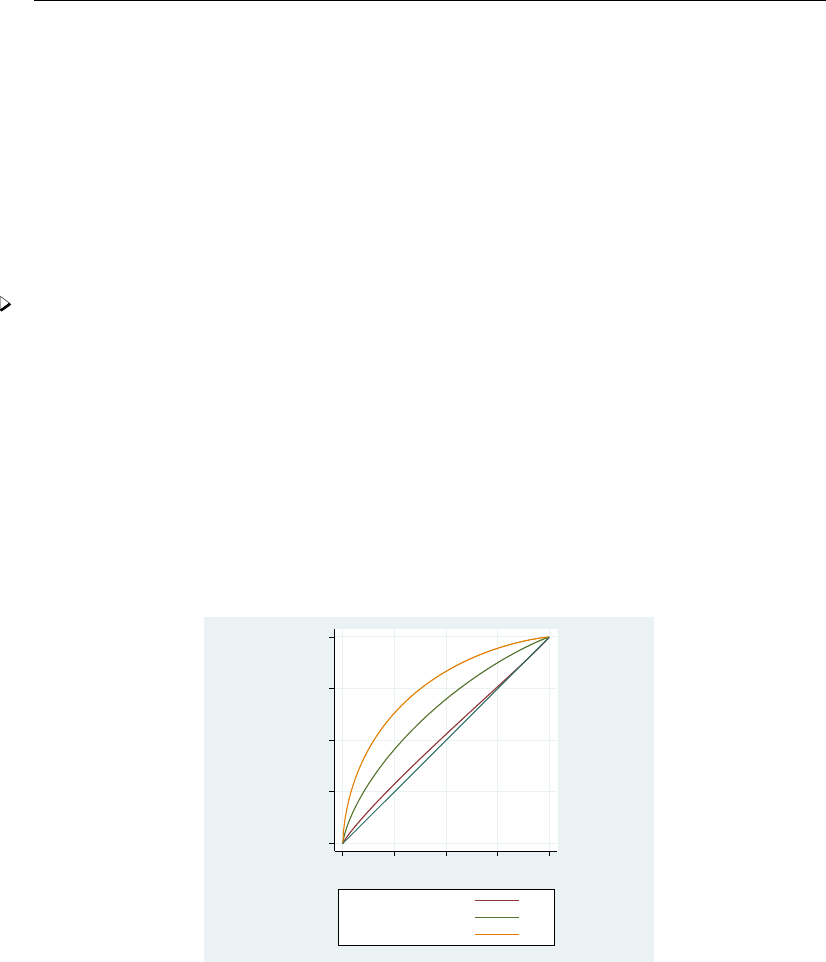
rocregplot — Plot marginal and covariate-specific ROC curves after rocreg 2031
Remarks and examples
Remarks are presented under the following headings:
Plotting covariate-specific ROC curves
Plotting marginal ROC curves
Plotting covariate-specific ROC curves
The rocregplot command is also demonstrated in [R]rocreg. We will further demonstrate its
use with several examples. Particularly, we will show how rocregplot can draw the ROC curves of
covariate models that have been fit using rocreg.
Example 1: Parametric ROC
In example 6 of [R]rocreg, we fit a probit ROC model to audiology test data from Norton et al.
(2000). The estimating equation method of Alonzo and Pepe (2002) was used to the fit the model.
Gender and age were covariates that affected the control distribution of the classifier y1 (DPOAE 65
at 2 kHz). Age was a ROC covariate for the model, so we fit separate ROC curves at each age.
Following Janes, Longton, and Pepe (2009), we draw the ROC curves for ages 30, 40, and 50
months. The at1(),at2(), and at3() options are used to specify the age covariates.
. use http://www.stata-press.com/data/r13/nnhs
(Norton - neonatal audiology data)
. rocreg d y1, probit ctrlcov(currage male) ctrlmodel(linear) roccov(currage)
> cluster(id) bseed(56930) bsave(nnhs2y1, replace)
(output omitted )
. rocregplot, at1(currage=30) at2(currage=40) at3(currage=50)
0 .25 .5 .75 1
True−positive rate (ROC)
0 .25 .5 .75 1
False−positive rate
DPOAE 65 at 2kHz At 1
At 2
At 3
Here we use the default entries of the legend, which indicate the “at #” within the specified
at* options and the classifier to which the curve corresponds. ROC curve one corresponds with
currage=30, two with currage=40, and three with currage=50. The positive effect of age on the
ROC curve is evident. At an age of 30 months (currage=30), the ROC curve of y1 (DPOAE 65 at
2 kHz) is nearly equivalent to that of a noninformative test that gives equal probability to hearing loss.
At age 50 months (currage=50), corresponding to some of the oldest children in the study, the ROC
curve shows that test y1 (DPOAE 65 at 2 kHz) is considerably more powerful than the noninformative
test.

2032 rocregplot — Plot marginal and covariate-specific ROC curves after rocreg
You may create your own legend by specifying the legend() option. The default legend is designed
for the possibility of multiple covariates. Here we could change the legend entries to currage values
and gain some extra clarity. However, this may not be feasible when there are many covariates
present.
We can also use rocregplot after maximum likelihood estimation.
Example 2: Maximum likelihood ROC
We return to the audiology study with frequency (xf), intensity (xl), and hearing loss severity
(xd) covariates from Stover et al. (1996) that we examined in example 10 of [R]rocreg. Negative
signal-to-noise ratio is again used as a classifier. Using maximum likelihood, we fit a probit model
to these data with the indicated ROC covariates.
After fitting the model, we wish to compare the ROC curves of two covariate combinations. The
first has an intensity value of 5.5 (the lowest intensity, corresponding to 55 decibels) and a frequency
of 10.01 (the lowest frequency, corresponding to 1001 hertz). We give the first combination a hearing
loss severity value of 0.5 (the lowest). The second covariate combination has the same frequency, but
the highest intensity value of 6.5 (65 decibels). We give this second covariate set a higher severity
value of 4. We will visually compare the two ROC curves resulting from these two covariate value
combinations.
We specify false-positive rates of 0.7 first followed by 0.2 in the roc() option to visually compare
the size of the ROC curve at large and small false-positive rates. Because maximum likelihood
estimation was used to fit the model, a Wald confidence interval is produced for the estimated ROC
value and false-positive rate parameters. Further details are found in Methods and formulas.
. use http://www.stata-press.com/data/r13/dp
(Stover - DPOAE test data)
. rocreg d nsnr, probit ctrlcov(xf xl) roccov(xf xl xd) ml cluster(id)
(output omitted )
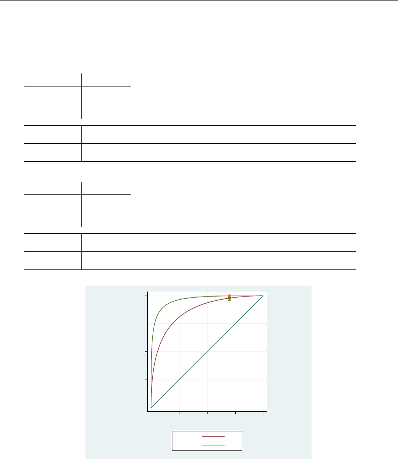
rocregplot — Plot marginal and covariate-specific ROC curves after rocreg 2033
. rocregplot, at1(xf=10.01, xl=5.5, xd=.5) at2(xf=10.01, xl=6.5, xd=4) roc(.7)
ROC curve
Status : d
Classifier: nsnr
Under covariates:
at1
xf 10.01
xl 5.5
xd .5
ROC Coef. Std. Err. [95% Conf. Interval]
.7 .978951 .0097382 .9598645 .9980376
Under covariates:
at2
xf 10.01
xl 6.5
xd 4
ROC Coef. Std. Err. [95% Conf. Interval]
.7 .9985001 .0009657 .9966073 1.000393
0 .25 .5 .75 1
True−positive rate (ROC)
0 .25 .5 .75 1
False−positive rate
−SNR At 1
At 2
At the higher false-positive rate value of 0.7, we see little difference in the ROC values and note that
the confidence intervals nearly overlap. Now we view the same curves with the lower false-positive
rate compared.
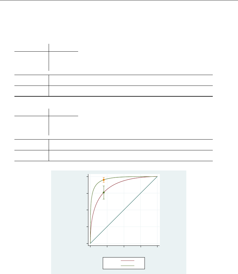
2034 rocregplot — Plot marginal and covariate-specific ROC curves after rocreg
. rocregplot, at1(xf=10.01, xl=5.5, xd=.5) at2(xf=10.01, xl=6.5, xd=4) roc(.2)
ROC curve
Status : d
Classifier: nsnr
Under covariates:
at1
xf 10.01
xl 5.5
xd .5
ROC Coef. Std. Err. [95% Conf. Interval]
.2 .7608593 .0510501 .660803 .8609157
Under covariates:
at2
xf 10.01
xl 6.5
xd 4
ROC Coef. Std. Err. [95% Conf. Interval]
.2 .9499408 .0179824 .914696 .9851856
0 .25 .5 .75 1
True−positive rate (ROC)
0 .25 .5 .75 1
False−positive rate
−SNR At 1
At 2
The lower false-positive rate of 0.2 shows clearly distinguishable ROC values. Now we specify
option invroc(.5) to view how the false-positive rates vary at a ROC value of 0.5.

rocregplot — Plot marginal and covariate-specific ROC curves after rocreg 2035
. rocregplot, at1(xf=10.01, xl=5.5, xd=.5) at2(xf=10.01, xl=6.5, xd=4) invroc(.5)
False-positive rate
Status : d
Classifier: nsnr
Under covariates:
at1
xf 10.01
xl 5.5
xd .5
invROC Coef. Std. Err. [95% Conf. Interval]
.5 .0578036 .0198626 .0188736 .0967336
Under covariates:
at2
xf 10.01
xl 6.5
xd 4
invROC Coef. Std. Err. [95% Conf. Interval]
.5 .0055624 .0032645 -.0008359 .0119607
0 .25 .5 .75 1
True−positive rate (ROC)
0 .25 .5 .75 1
False−positive rate
−SNR At 1
At 2
At a ROC value of 0.5, the false-positive rates for both curves are small and close to one another.
Technical note
We can use the testnl command to support our visual observations with statistical inference. We
use it to perform a Wald test of the null hypothesis that the two ROC curves just rendered are equal
at a false-positive rate of 0.7.

2036 rocregplot — Plot marginal and covariate-specific ROC curves after rocreg
. testnl normal(_b[i_cons]+10.01*_b[xf]+5.5*_b[xl]
> + .5*_b[xd]+_b[s_cons]*invnormal(.7)) =
> normal(_b[i_cons]+10.01*_b[xf]+6.5*_b[xl]
> + 4*_b[xd]+_b[s_cons]*invnormal(.7))
(1) normal(_b[i_cons]+10.01*_b[xf]+5.5*_b[xl] +.5*_b[xd]+_b[s_cons]*invnormal(.7))=
normal(_b[i_cons]+10.01*_b[xf]+6.5*_b[xl] + 4*_b[xd]+_b[s_cons]*invnormal(.7))
chi2(1) = 4.53
Prob > chi2 = 0.0332
The test is significant at the 0.05 level, and thus we find that the two curves are significantly
different. Now we will use testnl again to test equality of the false-positive rates for each curve
with a ROC value of 0.5. The inverse ROC formula used is derived in Methods and formulas.
. testnl normal((invnormal(.5)-(_b[i_cons]+10.01*_b[xf]+5.5*_b[xl]+.5*_b[xd]))
> /_b[s_cons]) =
> normal((invnormal(.5)-(_b[i_cons]+10.01*_b[xf]+6.5*_b[xl]+4*_b[xd]))
> /_b[s_cons])
(1) normal((invnormal(.5)-(_b[i_cons]+10.01*_b[xf]+5.5*_b[xl]+.5*_b[xd]))
/_b[s_cons]) =
normal((invnormal(.5)-(_b[i_cons]+10.01*_b[xf]+6.5*_b[xl]+4*_b[xd]))
/_b[s_cons])
chi2(1) = 8.01
Prob > chi2 = 0.0046
We again reject the null hypothesis that the two curves are equal at the 0.05 level.
The model of our last example was also fit using the estimating equations method in example 7
of [R]rocreg. We will demonstrate rocregplot after that model fit as well.
Example 3: Parametric ROC, invROC, and ROC value
In example 2, we used rocregplot after a maximum likelihood model fit of the ROC curve
for classifier nsnr and covariates frequency (xf), intensity (xl), and hearing loss severity (xd). The
data were obtained from the audiology study described in Stover et al. (1996). In example 7 of
[R]rocreg, we fit the model using the estimating equations method of Alonzo and Pepe (2002). Under
this method, bootstrap resampling is used to make inferences. We saved 50 bootstrap replications in
nsnrf.dta, which we re-create below.
We use rocregplot to draw the ROC curves for nsnr under the covariate values xf = 10.01,
xl = 5.5, and xd = .5, and xf = 10.01,xl = 6.5, and xd = 4. The at#() options are used to
specify the covariate values. The previous bootstrap results are made available to rocregplot with
the bfile() option. As before, we will specify 0.2 and 0.7 as false-positive rates in the roc() option
and 0.5 as a ROC value in the invroc() option. We do not specify btype() and thus our graph will
contain normal-based bootstrap confidence bands, the default.

rocregplot — Plot marginal and covariate-specific ROC curves after rocreg 2037
. use http://www.stata-press.com/data/r13/dp
(Stover - DPOAE test data)
. rocreg d nsnr, probit ctrlcov(xf xl) roccov(xf xl xd) cluster(id)
> nobstrata ctrlfprall bseed(156385) breps(50) bsave(nsnrf, replace)
(output omitted )
. rocregplot, at1(xf=10.01, xl=5.5, xd=.5) at2(xf=10.01, xl=6.5, xd=4)
> roc(.7) bfile(nsnrf)
ROC curve
Status : d
Classifier: nsnr
Under covariates:
at1
xf 10.01
xl 5.5
xd .5
(Replications based on 208 clusters in id)
Observed Bootstrap
ROC Coef. Bias Std. Err. [95% Conf. Interval]
.7 .9835816 .0087339 .0204353 .9435292 1.023634 (N)
.9155462 .9974037 (P)
.9392258 .9976629 (BC)
Under covariates:
at2
xf 10.01
xl 6.5
xd 4
(Replications based on 208 clusters in id)
Observed Bootstrap
ROC Coef. Bias Std. Err. [95% Conf. Interval]
.7 .999428 .0006059 .0011309 .9972115 1.001644 (N)
.9958003 .9999675 (P)
.9968304 .9999901 (BC)
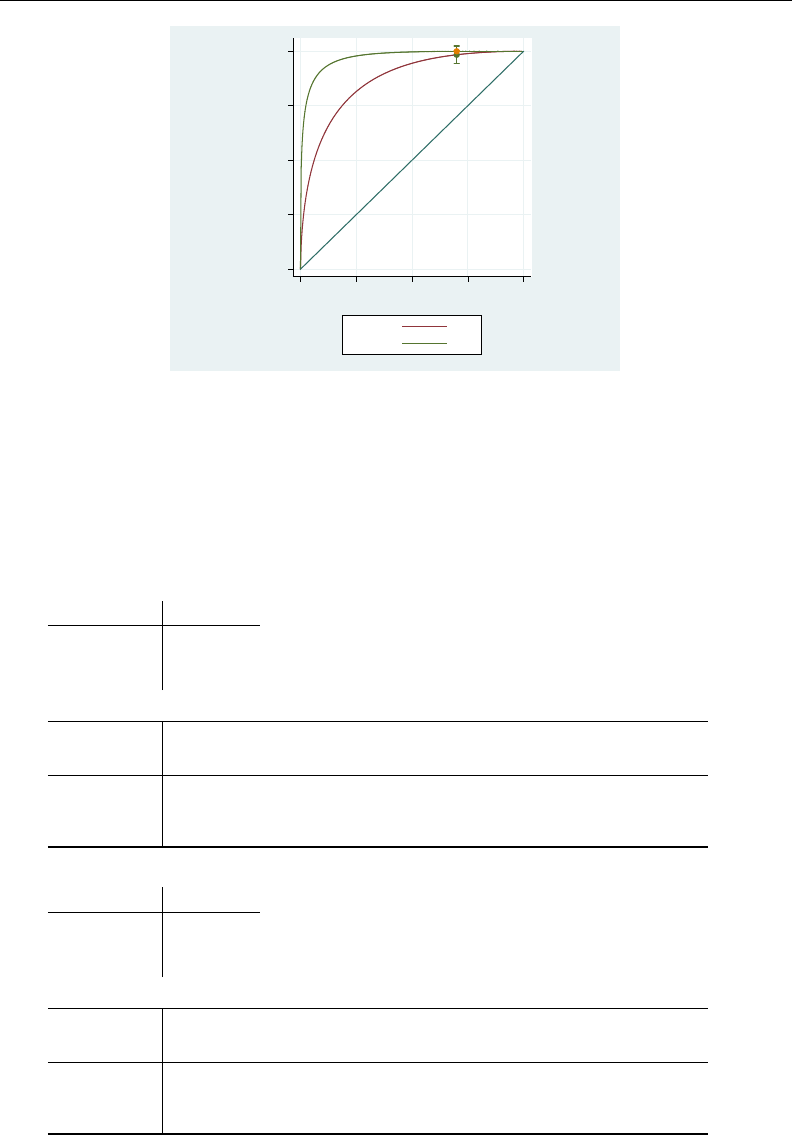
2038 rocregplot — Plot marginal and covariate-specific ROC curves after rocreg
0 .25 .5 .75 1
True−positive rate (ROC)
0 .25 .5 .75 1
False−positive rate
−SNR At 1
At 2
As shown in the graph, we find that the ROC values at a false-positive rate of 0.7 are close together,
as they were in the maximum likelihood estimation in example 2. We now repeat this process for the
lower false-positive rate of 0.2 by using the roc(.2) option.
. rocregplot, at1(xf=10.01, xl=5.5, xd=.5) at2(xf=10.01, xl=6.5, xd=4)
> roc(.2) bfile(nsnrf)
ROC curve
Status : d
Classifier: nsnr
Under covariates:
at1
xf 10.01
xl 5.5
xd .5
(Replications based on 208 clusters in id)
Observed Bootstrap
ROC Coef. Bias Std. Err. [95% Conf. Interval]
.2 .7652956 .0145111 .0735506 .6211391 .9094522 (N)
.6054495 .878052 (P)
.6394838 .9033081 (BC)
Under covariates:
at2
xf 10.01
xl 6.5
xd 4
(Replications based on 208 clusters in id)
Observed Bootstrap
ROC Coef. Bias Std. Err. [95% Conf. Interval]
.2 .9672505 .0072429 .0227977 .9225679 1.011933 (N)
.9025254 .9931714 (P)
.9235289 .9979637 (BC)

rocregplot — Plot marginal and covariate-specific ROC curves after rocreg 2039
0 .25 .5 .75 1
True−positive rate (ROC)
0 .25 .5 .75 1
False−positive rate
−SNR At 1
At 2
The ROC values are slightly higher at the false-positive rate of 0.2 than they were in the maximum
likelihood estimation in example 2. To see if the false-positive rates differ at a ROC value of 0.5, we
specify the invroc(.5) option.
. rocregplot, at1(xf=10.01, xl=5.5, xd=.5) at2(xf=10.01, xl=6.5, xd=4)
> invroc(.5) bfile(nsnrf)
False-positive rate
Status : d
Classifier: nsnr
Under covariates:
at1
xf 10.01
xl 5.5
xd .5
(Replications based on 208 clusters in id)
Observed Bootstrap
invROC Coef. Bias Std. Err. [95% Conf. Interval]
.5 .0615144 -.0063531 .0254042 .0117231 .1113057 (N)
.0225159 .1265046 (P)
.0224352 .1265046 (BC)
Under covariates:
at2
xf 10.01
xl 6.5
xd 4
(Replications based on 208 clusters in id)
Observed Bootstrap
invROC Coef. Bias Std. Err. [95% Conf. Interval]
.5 .0043298 -.0012579 .0045938 -.004674 .0133335 (N)
.0002773 .0189199 (P)
.0001292 .0134801 (BC)
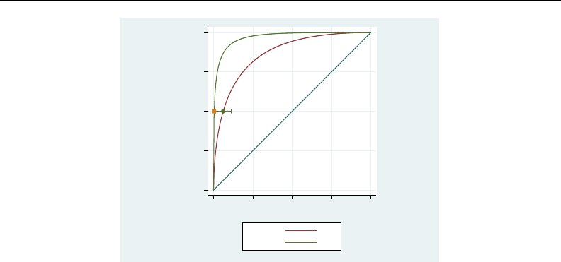
2040 rocregplot — Plot marginal and covariate-specific ROC curves after rocreg
0 .25 .5 .75 1
True−positive rate (ROC)
0 .25 .5 .75 1
False−positive rate
−SNR At 1
At 2
The point estimates of the ROC value and false-positive rate are both computed directly using the
point estimates of the ROC coefficients. Calculation of the standard errors and confidence intervals
is slightly more complicated. Essentially, we have stored a sample of our ROC covariate coefficient
estimates in nsnrf.dta. We then calculate the ROC value or false-positive rate estimates using each
set of coefficient estimates, resulting in a sample of point estimates. Then the bootstrap standard error
and confidence intervals are calculated based on these bootstrap samples. Details of the computation
of the standard error and percentile confidence intervals can be found in Methods and formulas and
in [R]bootstrap.
As mentioned in [R]rocreg, 50 resamples is a reasonable lower bound for obtaining bootstrap
standard errors (Mooney and Duval 1993). However, it may be too low for obtaining percentile and
bias-corrected confidence intervals. Normal-based confidence intervals are valid when the bootstrap
distribution exhibits normality. See [R]bootstrap postestimation for more details.
We can assess the normality of the bootstrap distribution by using a normal probability plot. Stata
provides this in the pnorm command (see [R]diagnostic plots). We will use nsnrf.dta to draw a
normal probability plot for the ROC estimate corresponding to a false-positive rate of 0.2. We use the
covariate values xf = 10.01,xl = 6.5, and xd = 4.
. use nsnrf
(bootstrap: rocregstat)
. generate double rocp2 = nsnr_b_i_cons + 10.01*nsnr_b_xf + 6.5*nsnr_b_xl +
> 4*nsnr_b_xd+nsnr_b_s_cons*invnormal(.2)
. replace rocp2 = normal(rocp2)
(50 real changes made)

rocregplot — Plot marginal and covariate-specific ROC curves after rocreg 2041
. pnorm rocp2
0.00 0.25 0.50 0.75 1.00
Normal F[(rocp2−m)/s]
0.00 0.25 0.50 0.75 1.00
Empirical P[i] = i/(N+1)
The closeness of the points to the horizontal line on the normal probability plot shows us that the
bootstrap distribution is approximately normal. So it is reasonable to use the normal-based confidence
intervals for ROC at a false-positive rate of 0.2 under covariate values xf = 10.01,xl = 6.5, and
xd = 4.
Plotting marginal ROC curves
The rocregplot command can also be used after fitting models with no covariates. We will
demonstrate this with an empirical ROC model fit in [R]rocreg.
Example 4: Nonparametric ROC
We run rocregplot after fitting the single-classifier, empirical ROC model shown in example 1 of
[R]rocreg. There we empirically predicted the ROC curve of the classifier rating for the true status
variable disease from the Hanley and McNeil (1982) data. The rocreg command saves variables
roc rating and fpr rating, which give the ROC values and false-positive rates, respectively,
for every value of rating. These variables are used by rocregplot to render the ROC curve.
. use http://www.stata-press.com/data/r13/hanley, clear
. rocreg disease rating, noboot
Nonparametric ROC estimation
Control standardization: empirical
ROC method : empirical
Area under the ROC curve
Status : disease
Classifier: rating
Observed Bootstrap
AUC Coef. Bias Std. Err. [95% Conf. Interval]
.8407708 . . . . (N)
. . (P)
. . (BC)
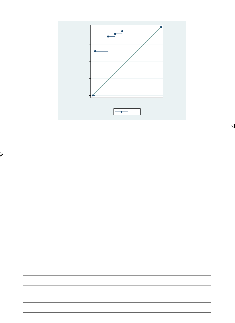
2042 rocregplot — Plot marginal and covariate-specific ROC curves after rocreg
. rocregplot
0 .25 .5 .75 1
True−positive rate (ROC)
0 .25 .5 .75 1
False−positive rate
rating
We end our discussion of rocregplot by showing its use after a marginal probit model.
Example 5: Maximum likelihood ROC, invROC, and ROC value
In example 13 of [R]rocreg, we fit a maximum-likelihood probit model to each classifier of the
fictitious dataset generated from Hanley and McNeil (1983).
We use rocregplot after the original rocreg command to draw the ROC curves for classifiers
mod1 and mod3. This is accomplished by specifying the two variables in the classvars() option.
We will use the roc() option to obtain confidence intervals for ROC values at false-positive rates of
0.15 and 0.75. We will specify the invroc() option to obtain false-positive rate confidence intervals
for a ROC value of 0.8. As mentioned previously, these are Wald confidence intervals.
First, we will view results for a false-positive rate of 0.75.
. use http://www.stata-press.com/data/r13/ct2, clear
. rocreg status mod1 mod2 mod3, probit ml
(output omitted )
. rocregplot, classvars(mod1 mod3) roc(.75)
ROC curve
Status : status
Classifier: mod1
ROC Coef. Std. Err. [95% Conf. Interval]
.75 .9931655 .0069689 .9795067 1.006824
Status : status
Classifier: mod3
ROC Coef. Std. Err. [95% Conf. Interval]
.75 .9953942 .0043435 .9868811 1.003907
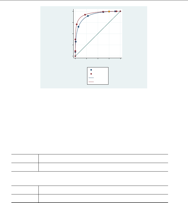
rocregplot — Plot marginal and covariate-specific ROC curves after rocreg 2043
0 .25 .5 .75 1
True−positive rate (ROC)
0 .25 .5 .75 1
False−positive rate
mod1
mod3
mod1 Fit
mod3 Fit
We see that the estimates for each of the two ROC curves are close. Because this is a marginal
model, the actual false-positive rate and the true-positive rate for each observation are plotted in
the graph. The added point estimates of the ROC value at false-positive rate 0.75 are shown as
diamond (mod3) and circle (mod1) symbols in the upper-right-hand corner of the graph at FPR =0.75.
Confidence bands are also plotted at FPR =0.75 but are so narrow that they are barely noticeable.
Under both classifiers, the ROC value at 0.75 is very high. Now we will compare these results to
those with a lower false-positive rate of 0.15.
. rocregplot, classvars(mod1 mod3) roc(.15)
ROC curve
Status : status
Classifier: mod1
ROC Coef. Std. Err. [95% Conf. Interval]
.15 .7934935 .0801363 .6364292 .9505578
Status : status
Classifier: mod3
ROC Coef. Std. Err. [95% Conf. Interval]
.15 .8888596 .0520118 .7869184 .9908008
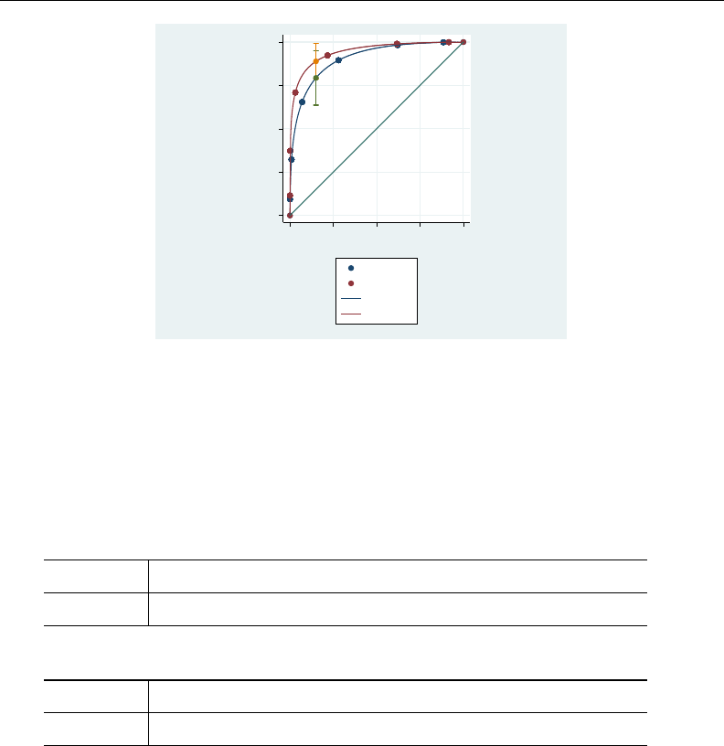
2044 rocregplot — Plot marginal and covariate-specific ROC curves after rocreg
0 .25 .5 .75 1
True−positive rate (ROC)
0 .25 .5 .75 1
False−positive rate
mod1
mod3
mod1 Fit
mod3 Fit
The ROC value for the false-positive rate of 0.15 is more separated in the two classifiers. Here
we see that mod3 has a larger ROC value than mod1 for this false-positive rate, but the confidence
intervals of the estimates overlap.
By specifying invroc(.8), we obtain invROC confidence intervals corresponding to a ROC value
of 0.8.
. rocregplot, classvars(mod1 mod3) invroc(.8)
False-positive rate
Status : status
Classifier: mod1
invROC Coef. Std. Err. [95% Conf. Interval]
.8 .1556435 .069699 .019036 .2922509
Status : status
Classifier: mod3
invROC Coef. Std. Err. [95% Conf. Interval]
.8 .0661719 .045316 -.0226458 .1549896
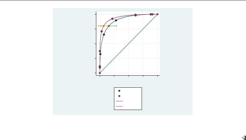
rocregplot — Plot marginal and covariate-specific ROC curves after rocreg 2045
0 .25 .5 .75 1
True−positive rate (ROC)
0 .25 .5 .75 1
False−positive rate
mod1
mod3
mod1 Fit
mod3 Fit
For estimation of the false-positive rate at a ROC value of 0.8, the confidence intervals overlap.
Both classifiers require only a small false-positive rate to achieve a ROC value of 0.8.
Methods and formulas
Details on computation of the nonparametric ROC curve and the estimation of the parametric ROC
curve model coefficients can be found in [R]rocreg. Here we describe how to estimate the ROC
values and false-positive rates of a parametric model. The cumulative distribution function gcan be
the standard normal cumulative distribution function.
Methods and formulas are presented under the following headings:
Parametric model: Summary parameter definition
Maximum likelihood estimation
Estimating equations estimation
Parametric model: Summary parameter definition
Conditioning on covariates x, we have the following ROC curve model:
ROC (u) = g{x0β+αg−1(u)}
xcan be constant, and β=β0, the constant intercept.
With simple algebra, we can solve this equation to obtain the false-positive rate value ufor a ROC
value of r:
u=g{g−1(r)−x0β}α−1

2046 rocregplot — Plot marginal and covariate-specific ROC curves after rocreg
Maximum likelihood estimation
We allow maximum likelihood estimation under probit parametric models, so g= Φ. The ROC
value and false-positive rate parameters all have closed-form expressions in terms of the covariate
values x, coefficient vector β, and slope parameter α. Thus to estimate these two types of summary
parameters, we use the delta method (Oehlert 1992;Phillips and Park 1988). Particularly, we use the
nlcom command (see [R]nlcom) to implement the delta method.
Under maximum likelihood estimation, the coefficient estimates b
βand slope estimate bαare
asymptotically normal with variance matrix V. For convenience, we rename the parameter vector
[β0, α]to the k-parameter vector θ= [θ1, . . . , θk]. We will also explicitly refer to the conditioning
of the ROC curve by θin its mention as ROC(t, θ).
Under the delta method, the continuous scalar function of the estimate b
θ,f(b
θ)has asymptotic
mean f(θ)and asymptotic covariance
c
Var nf(b
θ)o=fVf0
where fis the 1 ×kmatrix of derivatives for which
f1j=∂f(θ)
∂θj
j= 1, . . . , k
The asymptotic covariance of f(b
θ)is estimated and then used in conjunction with f(b
θ)for further
inference, including Wald confidence intervals, standard errors, and hypothesis testing.
Estimating equations estimation
When we fit a model using the Alonzo and Pepe (2002) estimating equations method, we use
the bootstrap to perform inference on the ROC curve summary parameters. Each bootstrap sample
provides a sample of the coefficient estimates βand the slope estimates α. Using the formulas above,
we can obtain an estimate of the ROC value or false-positive rate for each resample.
By making these calculations, we obtain a bootstrap sample of our summary parameter estimate. We
then obtain bootstrap standard errors, normal approximation confidence intervals, percentile confidence
intervals, and bias-corrected confidence intervals using this bootstrap sample. Further details can be
found in [R]bootstrap.
References
Alonzo, T. A., and M. S. Pepe. 2002. Distribution-free ROC analysis using binary regression techniques. Biostatistics
3: 421–432.
Bamber, D. 1975. The area above the ordinal dominance graph and the area below the receiver operating characteristic
graph. Journal of Mathematical Psychology 12: 387–415.
Choi, B. C. K. 1998. Slopes of a receiver operating characteristic curve and likelihood ratios for a diagnostic test.
American Journal of Epidemiology 148: 1127–1132.
Cleves, M. A. 1999. sg120: Receiver operating characteristic (ROC) analysis.Stata Technical Bulletin 52: 19–33.
Reprinted in Stata Technical Bulletin Reprints, vol. 9, pp. 212–229. College Station, TX: Stata Press.
. 2000. sg120.1: Two new options added to rocfit command.Stata Technical Bulletin 53: 18–19. Reprinted in
Stata Technical Bulletin Reprints, vol. 9, pp. 230–231. College Station, TX: Stata Press.

rocregplot — Plot marginal and covariate-specific ROC curves after rocreg 2047
Hanley, J. A., and B. J. McNeil. 1982. The meaning and use of the area under a receiver operating characteristic
(ROC) curve. Radiology 143: 29–36.
. 1983. A method of comparing the areas under receiver operating characteristic curves derived from the same
cases. Radiology 148: 839–843.
Janes, H., G. M. Longton, and M. S. Pepe. 2009. Accommodating covariates in receiver operating characteristic
analysis.Stata Journal 9: 17–39.
Mooney, C. Z., and R. D. Duval. 1993. Bootstrapping: A Nonparametric Approach to Statistical Inference. Newbury
Park, CA: Sage.
Norton, S. J., M. P. Gorga, J. E. Widen, R. C. Folsom, Y. Sininger, B. Cone-Wesson, B. R. Vohr, K. Mascher,
and K. Fletcher. 2000. Identification of neonatal hearing impairment: Evaluation of transient evoked otoacoustic
emission, distortion product otoacoustic emission, and auditory brain stem response test performance. Ear and
Hearing 21: 508–528.
Oehlert, G. W. 1992. A note on the delta method. American Statistician 46: 27–29.
Phillips, P. C. B., and J. Y. Park. 1988. On the formulation of Wald tests of nonlinear restrictions. Econometrica 56:
1065–1083.
Stover, L., M. P. Gorga, S. T. Neely, and D. Montoya. 1996. Toward optimizing the clinical utility of distortion
product otoacoustic emission measurements. Journal of the Acoustical Society of America 100: 956–967.
Also see
[R]rocreg — Receiver operating characteristic (ROC) regression
[R]rocreg postestimation — Postestimation tools for rocreg
[U] 20 Estimation and postestimation commands

Title
roctab — Nonparametric ROC analysis
Syntax Menu Description Options
Remarks and examples Stored results Methods and formulas References
Also see
Syntax
roctab refvar classvar if in weight ,options
roctab options Description
Main
lorenz report Gini and Pietra indices
binomial calculate exact binomial confidence intervals
nolabel display numeric codes rather than value labels
detail show details on sensitivity/specificity for each cutpoint
table display the raw data in a 2 ×kcontingency table
bamber calculate standard errors by using the Bamber method
hanley calculate standard errors by using the Hanley method
graph graph the ROC curve
norefline suppress plotting the 45-degree reference line
summary report the area under the ROC curve
specificity graph sensitivity versus specificity
level(#)set confidence level; default is level(95)
Plot
plotopts(plot options)affect rendition of the ROC curve
Reference line
rlopts(cline options)affect rendition of the reference line
Add plots
addplot(plot)add other plots to the generated graph
Y axis, X axis, Titles, Legend, Overall
twoway options any options other than by() documented in [G-3]twoway options
fweights are allowed; see [U] 11.1.6 weight.
plot options Description
marker options change look of markers (color, size, etc.)
marker label options add marker labels; change look or position
cline options change the look of the line
2048

roctab — Nonparametric ROC analysis 2049
Menu
Statistics >Epidemiology and related >ROC analysis >Nonparametric ROC analysis without covariates
Description
The above command is used to perform receiver operating characteristic (ROC) analyses with rating
and discrete classification data.
The two variables refvar and classvar must be numeric. The reference variable indicates the true
state of the observation, such as diseased and nondiseased or normal and abnormal, and must be
coded as 0 and 1. The rating or outcome of the diagnostic test or test modality is recorded in classvar,
which must be at least ordinal, with higher values indicating higher risk.
roctab performs nonparametric ROC analyses. By default, roctab calculates the area under the
ROC curve. Optionally, roctab can plot the ROC curve, display the data in tabular form, and produce
Lorenz-like plots.
See [R]rocfit for a command that fits maximum-likelihood ROC models.
Options
Main
lorenz specifies that Gini and Pietra indices be reported. Optionally, graph will plot the Lorenz-like
curve.
binomial specifies that exact binomial confidence intervals be calculated.
nolabel specifies that numeric codes be displayed rather than value labels.
detail outputs a table displaying the sensitivity, specificity, the percentage of subjects correctly
classified, and two likelihood ratios for each possible cutpoint of classvar.
table outputs a 2 ×kcontingency table displaying the raw data.
bamber specifies that the standard error for the area under the ROC curve be calculated using the
method suggested by Bamber (1975). Otherwise, standard errors are obtained as suggested by
DeLong, DeLong, and Clarke-Pearson (1988).
hanley specifies that the standard error for the area under the ROC curve be calculated using the method
suggested by Hanley and McNeil (1982). Otherwise, standard errors are obtained as suggested by
DeLong, DeLong, and Clarke-Pearson (1988).
graph produces graphical output of the ROC curve. If lorenz is specified, graphical output of a
Lorenz-like curve will be produced.
norefline suppresses plotting the 45-degree reference line from the graphical output of the ROC
curve.
summary reports the area under the ROC curve, its standard error, and its confidence interval. If
lorenz is specified, Lorenz indices are reported. This option is needed only when also specifying
graph.
specificity produces a graph of sensitivity versus specificity instead of sensitivity versus
(1 −specificity). specificity implies graph.
level(#)specifies the confidence level, as a percentage, for the confidence intervals. The default is
level(95) or as set by set level; see [R]level.

2050 roctab — Nonparametric ROC analysis
Plot
plotopts(plot options)affects the rendition of the plotted ROC curve—the curve’s plotted points
connected by lines. The plot options can affect the size and color of markers, whether and how
the markers are labeled, and whether and how the points are connected; see [G-3]marker options,
[G-3]marker label options, and [G-3]cline options.
Reference line
rlopts(cline options)affects the rendition of the reference line; see [G-3]cline options.
Add plots
addplot(plot)provides a way to add other plots to the generated graph; see [G-3]addplot option.
Y axis, X axis, Titles, Legend, Overall
twoway options are any of the options documented in [G-3]twoway options, excluding by(). These
include options for titling the graph (see [G-3]title options) and for saving the graph to disk (see
[G-3]saving option).
Remarks and examples
Remarks are presented under the following headings:
Introduction
Nonparametric ROC curves
Lorenz-like curves
Introduction
The roctab command provides nonparametric estimation of the ROC for a given classifier and
true-status reference variable. The Lorenz curve functionality of roctab, which provides an alternative
to standard ROC analysis, is discussed in Lorenz-like curves.
See Pepe (2003) for a discussion of ROC analysis. Pepe has posted Stata datasets and programs
used to reproduce results presented in the book (http://www.stata.com/bookstore/pepe.html).
Nonparametric ROC curves
The points on the nonparametric ROC curve are generated using each possible outcome of the
diagnostic test as a classification cutpoint and computing the corresponding sensitivity and 1−specificity.
These points are then connected by straight lines, and the area under the resulting ROC curve is
computed using the trapezoidal rule.
Example 1
Hanley and McNeil (1982) presented data from a study in which a reviewer was asked to classify,
using a five-point scale, a random sample of 109 tomographic images from patients with neurological
problems. The rating scale was as follows: 1 =definitely normal, 2 =probably normal, 3 =
questionable, 4 =probably abnormal, and 5 =definitely abnormal. The true disease status was
normal for 58 of the patients and abnormal for the remaining 51 patients.
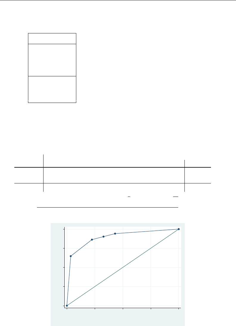
roctab — Nonparametric ROC analysis 2051
Here we list 9 of the 109 observations:
. use http://www.stata-press.com/data/r13/hanley
. list disease rating in 1/9
disease rating
1. 1 5
2. 0 1
3. 1 5
4. 0 4
5. 0 1
6. 0 3
7. 1 5
8. 0 5
9. 0 1
For each observation, disease identifies the true disease status of the subject (0 =normal, 1 =
abnormal), and rating contains the classification value assigned by the reviewer.
We can use roctab to calculate and plot the nonparametric ROC curve by specifying both the
summary and graph options. By also specifying the table option, we obtain a contingency table
summarizing our dataset.
. roctab disease rating, table graph summary
rating
disease 1 2 3 4 5 Total
0 33 6 6 11 2 58
1 3 2 2 11 33 51
Total 36 8 8 22 35 109
ROC Asymptotic Normal
Obs Area Std. Err. [95% Conf. Interval]
109 0.8932 0.0307 0.83295 0.95339
0.00 0.25 0.50 0.75 1.00
Sensitivity
0.00 0.25 0.50 0.75 1.00
1 − Specificity
Area under ROC curve = 0.8932
By default, roctab reports the area under the curve, its standard error, and its confidence interval.
The graph option can be used to plot the ROC curve.

2052 roctab — Nonparametric ROC analysis
The ROC curve is plotted by computing the sensitivity and specificity using each value of the
rating variable as a possible cutpoint. A point is plotted on the graph for each of the cutpoints. These
plotted points are joined by straight lines to form the ROC curve, and the area under the ROC curve
is computed using the trapezoidal rule.
We can tabulate the computed sensitivities and specificities for each of the possible cutpoints by
specifying detail.
. roctab disease rating, detail
Detailed report of sensitivity and specificity
Correctly
Cutpoint Sensitivity Specificity Classified LR+ LR-
( >= 1 ) 100.00% 0.00% 46.79% 1.0000
( >= 2 ) 94.12% 56.90% 74.31% 2.1835 0.1034
( >= 3 ) 90.20% 67.24% 77.98% 2.7534 0.1458
( >= 4 ) 86.27% 77.59% 81.65% 3.8492 0.1769
( >= 5 ) 64.71% 96.55% 81.65% 18.7647 0.3655
( > 5 ) 0.00% 100.00% 53.21% 1.0000
ROC Asymptotic Normal
Obs Area Std. Err. [95% Conf. Interval]
109 0.8932 0.0307 0.83295 0.95339
Each cutpoint in the table indicates the ratings used to classify tomographs as being from an abnormal
subject. For example, the first cutpoint (>= 1) indicates that all tomographs rated as 1 or greater are
classified as coming from abnormal subjects. Because all tomographs have a rating of 1 or greater, all
are considered abnormal. Consequently, all abnormal cases are correctly classified (sensitivity =100%),
but none of the normal patients is classified correctly (specificity =0%). For the second cutpoint
(>=2), tomographs with ratings of 1 are classified as normal, and those with ratings of 2 or greater are
classified as abnormal. The resulting sensitivity and specificity are 94.12% and 56.90%, respectively.
Using this cutpoint, we correctly classified 74.31% of the 109 tomographs. Similar interpretations
can be used on the remaining cutpoints. As mentioned, each cutpoint corresponds to a point on the
nonparametric ROC curve. The first cutpoint (>=1) corresponds to the point at (1,1), and the last
cutpoint (>5)corresponds to the point at (0,0).
detail also reports two likelihood ratios suggested by Choi (1998): the likelihood ratio for a
positive test result (LR+) and the likelihood ratio for a negative test result (LR–). The LR+ is the
ratio of the probability of a positive test among the truly positive subjects to the probability of a
positive test among the truly negative subjects. The LR– is the ratio of the probability of a negative
test among the truly positive subjects to the probability of a negative test among the truly negative
subjects. Choi points out that LR+ corresponds to the slope of the line from the origin to the point
on the ROC curve determined by the cutpoint. Similarly, LR– corresponds to the slope from the point
(1,1) to the point on the ROC curve determined by the cutpoint.
By default, roctab calculates the standard error for the area under the curve by using an algorithm
suggested by DeLong, DeLong, and Clarke-Pearson (1988) and asymptotic normal confidence intervals.
Optionally, standard errors based on methods suggested by Bamber (1975) or Hanley and McNeil (1982)
can be computed by specifying bamber or hanley, respectively, and an exact binomial confidence
interval can be obtained by specifying binomial.

roctab — Nonparametric ROC analysis 2053
. roctab disease rating, bamber
ROC Bamber Asymptotic Normal
Obs Area Std. Err. [95% Conf. Interval]
109 0.8932 0.0306 0.83317 0.95317
. roctab disease rating, hanley binomial
ROC Hanley Binomial Exact
Obs Area Std. Err. [95% Conf. Interval]
109 0.8932 0.0320 0.81559 0.94180
Lorenz-like curves
For applications where it is known that the risk status increases or decreases monotonically with
increasing values of the diagnostic test, the ROC curve and associated indices are useful in assessing
the overall performance of a diagnostic test. When the risk status does not vary monotonically with
increasing values of the diagnostic test, however, the resulting ROC curve can be nonconvex and its
indices can be unreliable. For these situations, Lee (1999) proposed an alternative to the ROC analysis
based on Lorenz-like curves and the associated Pietra and Gini indices.
Lee (1999) mentions at least three specific situations where results from Lorenz curves are superior
to those obtained from ROC curves: 1) a diagnostic test with similar means but very different standard
deviations in the abnormal and normal populations, 2) a diagnostic test with bimodal distributions in
either the normal or abnormal population, and 3) a diagnostic test distributed symmetrically in the
normal population and skewed in the abnormal.
When the risk status increases or decreases monotonically with increasing values of the diagnostic
test, the ROC and Lorenz curves yield interchangeable results.
Example 2
To illustrate the use of the lorenz option, we constructed a fictitious dataset that yields results
similar to those presented in Table III of Lee (1999). The data assume that a 12-point rating scale
was used to classify 442 diseased and 442 healthy subjects. We list a few of the observations.
. use http://www.stata-press.com/data/r13/lorenz, clear
. list in 1/7, noobs sep(0)
disease class pop
0 5 66
1 11 17
0 6 85
0 3 19
0 10 19
0 2 7
1 4 16
The data consist of 24 observations: 12 observations from diseased individuals and 12 from nondiseased
individuals. Each observation corresponds to one of the 12 classification values of the rating-scale
variable, class. The number of subjects represented by each observation is given by the pop variable,
making this a frequency-weighted dataset. The data were generated assuming a binormal distribution
of the latent variable with similar means for the normal and abnormal populations but with the standard
deviation for the abnormal population five times greater than that of the normal population.
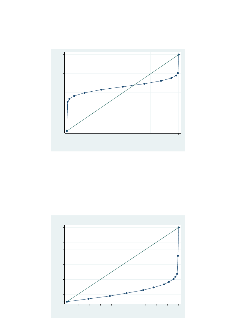
2054 roctab — Nonparametric ROC analysis
. roctab disease class [fweight=pop], graph summary
ROC Asymptotic Normal
Obs Area Std. Err. [95% Conf. Interval]
884 0.5774 0.0215 0.53517 0.61959
0.00 0.25 0.50 0.75 1.00
Sensitivity
0.00 0.25 0.50 0.75 1.00
1 − Specificity
Area under ROC curve = 0.5774
The resulting ROC curve is nonconvex or, as termed by Lee, “wiggly”. Lee argues that for this
and similar situations, the Lorenz curve and indices are preferred.
. roctab disease class [fweight=pop], lorenz summary graph
Lorenz curve
Pietra index = 0.6493
Gini index = 0.7441
0 .1 .2 .3 .4 .5 .6 .7 .8 .9 1
cumulative % of disease=1
0 .1 .2 .3 .4 .5 .6 .7 .8 .9 1
cumulative % of disease=0
Lorenz curve
Like ROC curves, a more bowed Lorenz curve suggests a better diagnostic test. This bowedness
is quantified by the Pietra index, which is geometrically equivalent to twice the largest triangle that
can be inscribed in the area between the curve and the diagonal line, and the Gini index, which is

roctab — Nonparametric ROC analysis 2055
equivalent to twice the area between the Lorenz curve and the diagonal. Lee (1999) provides several
additional interpretations for the Pietra and Gini indices.
Stored results
roctab stores the following in r():
Scalars
r(N) number of observations
r(se) standard error for the area under the ROC curve
r(lb) lower bound of CI for the area under the ROC curve
r(ub) upper bound of CI for the area under the ROC curve
r(area) area under the ROC curve
r(pietra) Pietra index
r(gini) Gini index
Methods and formulas
Assume that we applied a diagnostic test to each of Nnnormal and Naabnormal subjects.
Further assume that the higher the outcome value of the diagnostic test, the higher the risk of the
subject being abnormal. Let b
θbe the estimated area under the curve, and let Xi, i =1,2, . . . , Na
and Yj, j =1,2, . . . , Nnbe the values of the diagnostic test for the abnormal and normal subjects,
respectively.
The points on the nonparametric ROC curve are generated using each possible outcome of the
diagnostic test as a classification cutpoint and computing the corresponding sensitivity and 1−specificity.
These points are then connected by straight lines, and the area under the resulting ROC curve is
computed using the trapezoidal rule.
The default standard error for the area under the ROC curve is computed using the algorithm
described by DeLong, DeLong, and Clarke-Pearson (1988). For each abnormal subject, i, define
V10(Xi) = 1
Nn
Nn
X
j=1
ψ(Xi, Yj)
and for each normal subject, j, define
V01(Yj) = 1
Na
Na
X
i=1
ψ(Xi, Yj)
where
ψ(X, Y ) = (1Y < X
1
2Y=X
0Y > X

2056 roctab — Nonparametric ROC analysis
Define
S10 =1
Na−1
Na
X
i=1{V10(Xi)−b
θ}2
and
S01 =1
Nn−1
Nn
X
j=1{V01(Yj)−b
θ}2
The variance of the estimated area under the ROC curve is given by
var(b
θ) = 1
Na
S10 +1
Nn
S01
The hanley standard error for the area under the ROC curve is computed using the algorithm
described by Hanley and McNeil (1982). It requires the calculation of two quantities: Q1is Pr(two
randomly selected abnormal subjects will both have a higher score than a randomly selected normal
subject), and Q2is Pr(one randomly selected abnormal subject will have a higher score than any two
randomly selected normal subjects). The Hanley and McNeil variance of the estimated area under the
ROC curve is
var(b
θ) = b
θ(1 −b
θ)+(Na−1)(Q1−b
θ2)+(Nn−1)(Q2−b
θ2)
NaNn
The bamber standard error for the area under the ROC curve is computed using the algorithm
described by Bamber (1975). For any two Yvalues, Yjand Yk, and any Xivalue, define
byyx =p(Yj, Yk< Xi) + p(Xi< Yj, Yk)−2p(Yj< Xi< Yk)
and similarly, for any two Xvalues, Xiand Xl, and any Yjvalue, define
bxxy =p(Xi, Xl< Yj) + p(Yj< Xi, Xl)−2p(Xi< Yj< Xl)
Bamber’s unbiased estimate of the variance for the area under the ROC curve is
var(b
θ) = 1
4(Na−1)(Nn−1){p(X6=Y)+(Na−1)bxxy +(Nn−1)byyx−4(Na+Nn−1)(b
θ−0.5)2}
Asymptotic confidence intervals are constructed and reported by default, assuming a normal
distribution for the area under the ROC curve.
Exact binomial confidence intervals are calculated as described in [R]ci, with pequal to the area
under the ROC curve.
References
Bamber, D. 1975. The area above the ordinal dominance graph and the area below the receiver operating characteristic
graph. Journal of Mathematical Psychology 12: 387–415.
Choi, B. C. K. 1998. Slopes of a receiver operating characteristic curve and likelihood ratios for a diagnostic test.
American Journal of Epidemiology 148: 1127–1132.

roctab — Nonparametric ROC analysis 2057
Cleves, M. A. 1999. sg120: Receiver operating characteristic (ROC) analysis.Stata Technical Bulletin 52: 19–33.
Reprinted in Stata Technical Bulletin Reprints, vol. 9, pp. 212–229. College Station, TX: Stata Press.
. 2000. sg120.2: Correction to roccomp command.Stata Technical Bulletin 54: 26. Reprinted in Stata Technical
Bulletin Reprints, vol. 9, p. 231. College Station, TX: Stata Press.
. 2002a. Comparative assessment of three common algorithms for estimating the variance of the area under the
nonparametric receiver operating characteristic curve.Stata Journal 2: 280–289.
. 2002b. From the help desk: Comparing areas under receiver operating characteristic curves from two or more
probit or logit models.Stata Journal 2: 301–313.
DeLong, E. R., D. M. DeLong, and D. L. Clarke-Pearson. 1988. Comparing the areas under two or more correlated
receiver operating characteristic curves: A nonparametric approach. Biometrics 44: 837–845.
Erdreich, L. S., and E. T. Lee. 1981. Use of relative operating characteristic analysis in epidemiology: A method for
dealing with subjective judgment. American Journal of Epidemiology 114: 649–662.
Hanley, J. A., and B. J. McNeil. 1982. The meaning and use of the area under a receiver operating characteristic
(ROC) curve. Radiology 143: 29–36.
Harbord, R. M., and P. Whiting. 2009. metandi: Meta-analysis of diagnostic accuracy using hierarchical logistic
regression.Stata Journal 9: 211–229.
Juul, S., and M. Frydenberg. 2014. An Introduction to Stata for Health Researchers. 4th ed. College Station, TX:
Stata Press.
Lee, W. C. 1999. Probabilistic analysis of global performances of diagnostic tests: Interpreting the Lorenz curve-based
summary measures. Statistics in Medicine 18: 455–471.
Ma, G., and W. J. Hall. 1993. Confidence bands for the receiver operating characteristic curves. Medical Decision
Making 13: 191–197.
Pepe, M. S. 2003. The Statistical Evaluation of Medical Tests for Classification and Prediction. New York: Oxford
University Press.
Reichenheim, M. E., and A. Ponce de Leon. 2002. Estimation of sensitivity and specificity arising from validity
studies with incomplete design.Stata Journal 2: 267–279.
Seed, P. T., and A. Tob´
ıas. 2001. sbe36.1: Summary statistics for diagnostic tests.Stata Technical Bulletin 59: 25–27.
Reprinted in Stata Technical Bulletin Reprints, vol. 10, pp. 90–93. College Station, TX: Stata Press.
Tob´
ıas, A. 2000. sbe36: Summary statistics report for diagnostic tests.Stata Technical Bulletin 56: 16–18. Reprinted
in Stata Technical Bulletin Reprints, vol. 10, pp. 87–90. College Station, TX: Stata Press.
Working, H., and H. Hotelling. 1929. Application of the theory of error to the interpretation of trends. Journal of the
American Statistical Association 24 (Suppl.): 73–85.
Also see
[R]logistic postestimation — Postestimation tools for logistic
[R]roc — Receiver operating characteristic (ROC) analysis
[R]roccomp — Tests of equality of ROC areas
[R]rocfit — Parametric ROC models
[R]rocreg — Receiver operating characteristic (ROC) regression

Title
rologit — Rank-ordered logistic regression
Syntax Menu Description Options
Remarks and examples Stored results Methods and formulas Acknowledgment
References Also see
Syntax
rologit depvar indepvars if in weight , group(varname)options
options Description
Model
∗group(varname)identifier variable that links the alternatives
offset(varname)include varname in model with coefficient constrained to 1
incomplete(#)use #to code unranked alternatives; default is incomplete(0)
reverse reverse the preference order
notestrhs keep right-hand-side variables that do not vary within group
ties(spec)method to handle ties: exactm,breslow,efron, or none
SE/Robust
vce(vcetype)vcetype may be oim,robust,cluster clustvar,bootstrap,
or jackknife
Reporting
level(#)set confidence level; default is level(95)
display options control column formats, row spacing, line width, display of omitted
variables and base and empty cells, and factor-variable labeling
Maximization
maximize options control the maximization process; seldom used
coeflegend display legend instead of statistics
∗group(varname)is required.
indepvars may contain factor variables; see [U] 11.4.3 Factor variables.
bootstrap,by,fp,jackknife,rolling, and statsby are allowed; see [U] 11.1.10 Prefix commands.
Weights are not allowed with the bootstrap prefix; see [R] bootstrap.
fweights, iweights, and pweights are allowed, except with ties(efron); see [U] 11.1.6 weight.
coeflegend does not appear in the dialog box.
See [U] 20 Estimation and postestimation commands for more capabilities of estimation commands.
Menu
Statistics >Ordinal outcomes >Rank-ordered logistic regression
2058

rologit — Rank-ordered logistic regression 2059
Description
rologit fits the rank-ordered logistic regression model by maximum likelihood (Beggs, Cardell,
and Hausman 1981). This model is also known as the Plackett–Luce model (Marden 1995), as the
exploded logit model (Punj and Staelin 1978), and as the choice-based method of conjoint analysis
(Hair et al. 2010).
rologit expects the data to be in long form, similar to clogit (see [R]clogit), in which each
of the ranked alternatives forms an observation; all observations related to an individual are linked
together by the variable that you specify in the group() option. The distinction from clogit is
that depvar in rologit records the rankings of the alternatives, whereas for clogit,depvar marks
only the best alternative by a value not equal to zero. rologit interprets equal scores of depvar as
ties. The ranking information may be incomplete “at the bottom” (least preferred alternatives). That
is, unranked alternatives may be coded as 0 or as a common value that may be specified with the
incomplete() option.
If your data record only the unique best alternative, rologit fits the same model as clogit.
Options
Model
group(varname)is required, and it specifies the identifier variable (numeric or string) that links the
alternatives for an individual, which have been compared and rank ordered with respect to one
another.
offset(varname); see [R]estimation options.
incomplete(#)specifies the numeric value used to code alternatives that are not ranked. It is
assumed that unranked alternatives are less preferred than the ranked alternatives (that is, the data
record the ranking of the most preferred alternatives). It is not assumed that subjects are indifferent
between the unranked alternatives. #defaults to 0.
reverse specifies that in the preference order, a higher number means a less attractive alternative.
The default is that higher values indicate more attractive alternatives. The rank-ordered logit model
is not symmetric in the sense that reversing the ordering simply leads to a change in the signs of
the coefficients.
notestrhs suppresses the test that the independent variables vary within (at least some of) the groups.
Effects of variables that are always constant are not identified. For instance, a rater’s gender cannot
directly affect his or her rankings; it could affect the rankings only via an interaction with a
variable that does vary over alternatives.
ties(spec)specifies the method for handling ties (indifference between alternatives) (see [ST]stcox
for details):
exactm exact marginal likelihood (default)
breslow Breslow’s method (default if pweights specified)
efron Efron’s method (default if robust VCE)
none no ties allowed
SE/Robust
vce(vcetype)specifies the type of standard error reported, which includes types that are derived
from asymptotic theory (oim), that are robust to some kinds of misspecification (robust), that
allow for intragroup correlation (cluster clustvar), and that use bootstrap or jackknife methods
(bootstrap,jackknife); see [R]vce option.
If ties(exactm) is specified, vcetype may be only oim,bootstrap, or jackknife.

2060 rologit — Rank-ordered logistic regression
Reporting
level(#); see [R]estimation options.
display options:noomitted,vsquish,noemptycells,baselevels,allbaselevels,nofvla-
bel,fvwrap(#),fvwrapon(style),cformat(%fmt),pformat(% fmt),sformat(% fmt), and
nolstretch; see [R]estimation options.
Maximization
maximize options:iterate(#),trace,nolog,tolerance(#),ltolerance(#),
nrtolerance(#), and nonrtolerance; see [R]maximize. These options are seldom used.
The following option is available with rologit but is not shown in the dialog box:
coeflegend; see [R]estimation options.
Remarks and examples
The rank-ordered logit model can be applied to analyze how decision makers combine attributes of
alternatives into overall evaluations of the attractiveness of these alternatives. The model generalizes
a version of McFadden’s choice model without alternative-specific covariates, as fit by the clogit
command. It uses richer information about the comparison of alternatives, namely, how decision-makers
rank the alternatives rather than just specifying the alternative that they like best.
Remarks are presented under the following headings:
Examples
Comparing respondents
Incomplete rankings and ties
Clustered choice data
Comparison of rologit and clogit
On reversals of rankings
Examples
A popular way to study employer preferences for characteristics of employees is the quasi-
experimental “vignette method”. As an example, we consider the research by de Wolf on the labor
market position of social science graduates (de Wolf 2000). This study addresses how the educational
portfolio (for example, general skills versus specific knowledge) affects short-term and long-term
labor-market opportunities. De Wolf asked 22 human resource managers (the respondents) to rank
order the six most suitable candidates of 20 fictitious applicants and to rank order these six candidates
for three jobs, namely, 1) researcher, 2) management trainee, and 3) policy adviser. Applicants
were described by 10 attributes, including their age, gender, details of their portfolio, and work
experience. In this example, we analyze a subset of the data. Also, to simplify the output, we drop, at
random, 10 nonselected applicants per case. The resulting dataset includes 29 cases, consisting of 10
applicants each. The data are in long form: observations correspond to alternatives (the applications),
and alternatives that figured in one decision task are identified by the variable caseid. We list
the observations for caseid==7, in which the respondent considered applicants for a social-science
research position.

rologit — Rank-ordered logistic regression 2061
. use http://www.stata-press.com/data/r13/evignet
(Vignet study employer prefs (Inge de Wolf 2000))
. list pref female age grades edufit workexp boardexp if caseid==7, noobs
pref female age grades edufit workexp boardexp
0 yes 28 A/B no none no
0 no 25 C/D yes one year no
0 no 25 C/D yes none yes
0 yes 25 C/D no internship yes
1 no 25 C/D yes one year yes
2 no 25 A/B yes none no
3 yes 25 A/B yes one year no
4 yes 25 A/B yes none yes
5 no 25 A/B yes internship no
6 yes 28 A/B yes one year yes
Here six applicants were selected. The rankings are stored in the variable pref, where a value
of 6 corresponds to “best among the candidates”, a value of 5 corresponds to “second-best among
the candidates”, etc. The applicants with a ranking of 0 were not among the best six candidates for
the job. The respondent was not asked to express his preferences among these four applicants, but
by the elicitation procedure, it is known that he ranks these four applicants below the six selected
applicants. The best candidate was a female, 28 years old, with education fitting the job, with good
grades (A/B), with 1 year of work experience, and with experience being a board member of a
fraternity, a sports club, etc. The profiles of the other candidates read similarly. Here the respondent
completed the task; that is, he selected and rank ordered the six most suitable applicants. Sometimes
the respondent performed only part of the task.
. list pref female age grades edufit workexp boardexp if caseid==18, noobs
pref female age grades edufit workexp boardexp
0 no 25 C/D yes none yes
0 no 25 C/D no internship yes
0 no 28 C/D no internship yes
0 yes 25 A/B no one year no
2 yes 25 A/B no none yes
2 no 25 A/B no none yes
2 no 25 A/B no one year yes
5 no 25 A/B no none yes
5 no 25 A/B no none yes
5 yes 25 A/B no none no
The respondent selected the six best candidates and segmented these six candidates into two groups:
one group with the three best candidates, and a second group of three candidates that were “still
acceptable”. The numbers 2 and 5, indicating these two groups, are arbitrary apart from the implied
ranking of the groups. The ties between the candidates in a group indicate that the respondent was
not able to rank the candidates within the group.
The purpose of the vignette experiment was to explore and test hypotheses about which of the
employees’ attributes are valued by employers, how these attributes are weighted depending on the type
of job (described by variable job in these data), etc. In the psychometric tradition of Thurstone (1927),
value is assumed to be linear in the attributes, with the coefficients expressing the direction and weight
of the attributes. In addition, it is assumed that valuation is to some extent a random procedure,

2062 rologit — Rank-ordered logistic regression
captured by an additive random term. For instance, if value depends only on an applicant’s age and
gender, we would have
value(femalei,agei) = β1femalei+β2agei+i
where the random residual, i, captures all omitted attributes. Thus β1>0means that the em-
ployer assigns higher value to a woman than to a man. Given this conceptualization of value, it is
straightforward to model the decision (selection) among alternatives or the ranking of alternatives:
the alternative with the highest value is selected (chosen), or the alternatives are ranked according to
their value. To complete the specification of a model of choice and of ranking, we assume that the
random residual ifollows an “extreme value distribution of type I”, introduced in this context by
Luce (1959). This specific assumption is made mostly for computational convenience.
This model is known by many names. Among others, it is known as the rank-ordered logit model
in economics (Beggs, Cardell, and Hausman 1981), as the exploded logit model in marketing research
(Punj and Staelin 1978), as the choice-based conjoint analysis model (Hair et al. 2010), and as
the Plackett–Luce model (Marden 1995). The model coefficients are estimated using the method of
maximum likelihood. The implementation in rologit uses an analogy between the rank-ordered
logit model and the Cox regression model observed by Allison and Christakis (1994); see Methods
and formulas. The rologit command implements this method for rankings, whereas clogit deals
with the variant of choices, that is, only the most highly valued alternative is recorded. In the latter
case, the model is also known as the Luce–McFadden choice model. In fact, when the data record
the most preferred (unique) alternative and no additional ranking information about preferences is
available, rologit and clogit return the same information, though formatted somewhat differently.
. rologit pref female age grades edufit workexp boardexp if job==1, group(caseid)
Iteration 0: log likelihood = -95.41087
Iteration 1: log likelihood = -71.180903
Iteration 2: log likelihood = -68.47734
Iteration 3: log likelihood = -68.345918
Iteration 4: log likelihood = -68.345389
Refining estimates:
Iteration 0: log likelihood = -68.345389
Rank-ordered logistic regression Number of obs = 80
Group variable: caseid Number of groups = 8
No ties in data Obs per group: min = 10
avg = 10.00
max = 10
LR chi2(6) = 54.13
Log likelihood = -68.34539 Prob > chi2 = 0.0000
pref Coef. Std. Err. z P>|z| [95% Conf. Interval]
female -.4487287 .3671307 -1.22 0.222 -1.168292 .2708343
age -.0984926 .0820473 -1.20 0.230 -.2593024 .0623172
grades 3.064534 .6148245 4.98 0.000 1.8595 4.269568
edufit .7658064 .3602366 2.13 0.034 .0597556 1.471857
workexp 1.386427 .292553 4.74 0.000 .8130341 1.959821
boardexp .6944377 .3762596 1.85 0.065 -.0430176 1.431893
Focusing only on the variables whose coefficients are significant at the 10% level (we are analyzing
8 respondents only!), the estimated value of an applicant for a job of type 1 (research positions) can
be written as
value = 3.06*grades + 0.77*edufit + 1.39*workexp + 0.69*boardexp

rologit — Rank-ordered logistic regression 2063
Thus employers prefer applicants for a research position (job==1) whose educational portfolio fits
the job, who have better grades, who have more relevant work experience, and who have (extracurricular)
board experience. They do not seem to care much about the sex and age of applicants, which is
comforting.
Given these estimates of the valuation by employers, we consider the probabilities that each of the
applications is ranked first. Under the assumption that the iare independent and follow an extreme
value type I distribution, Luce (1959) showed that the probability, πi, that alternative iis valued
higher than alternatives 2, . . . , k can be written in the multinomial logit form
πi= Pr {value1>max(value2,...,valuem)}=exp(valuei)
Pk
j=1 exp(valuei)
The probability of observing a specific ranking can be written as the product of such terms, representing
a sequential decision interpretation in which the rater first chooses the most preferred alternative, and
then the most preferred alternative among the rest, etc.
The probabilities for alternatives to be ranked first are conveniently computed by predict.
. predict p if e(sample)
(option pr assumed; conditional probability that alternative is ranked first)
(210 missing values generated)
. sort caseid pref p
. list pref p grades edufit workexp boardexp if caseid==7, noobs
pref p grades edufit workexp boardexp
0 .0027178 C/D yes none yes
0 .0032275 C/D no internship yes
0 .0064231 A/B no none no
0 .0217202 C/D yes one year no
1 .0434964 C/D yes one year yes
2 .0290762 A/B yes none no
3 .2970933 A/B yes one year no
4 .0371747 A/B yes none yes
5 .1163203 A/B yes internship no
6 .4427504 A/B yes one year yes
There clearly is a positive relation between the stated ranking and the predicted probabilities for
alternatives to be ranked first, but the association is not perfect. In fact, we would not have expected a
perfect association, as the model specifies a (nondegenerate) probability distribution over the possible
rankings of the alternatives. These predictions for sets of 10 candidates can also be used to make
predictions for subsets of the alternatives. For instance, suppose that only the last three candidates listed
in this table would be available. According to parameter estimates of the rank-ordered logit model, the
probability that the last of these candidates is selected equals 0.443/(0.037 +0.116 +0.443) = 0.743.
Comparing respondents
The rologit model assumes that all respondents, HR managers in large public-sector organizations
in The Netherlands, use the same valuation function; that is, they apply the same decision weights. This
is the substantive interpretation of the assumption that the β’s are constant between the respondents.
To probe this assumption, we could test whether the coefficients vary between different groups of
respondents. For a metric characteristic of the HR manager, such as firmsize, we can consider a
trend-model in the valuation weights,

2064 rologit — Rank-ordered logistic regression
βij =αi0+αi1firmsizej
and we can test that the slopes αi1of firmsize are zero.
. generate firmsize = employer
. rologit pref edufit grades workexp c.firmsize#c.(edufit grades workexp boardexp)
> if job==1, group(caseid) nolog
Rank-ordered logistic regression Number of obs = 80
Group variable: caseid Number of groups = 8
No ties in data Obs per group: min = 10
avg = 10.00
max = 10
LR chi2(7) = 57.17
Log likelihood = -66.82346 Prob > chi2 = 0.0000
pref Coef. Std. Err. z P>|z| [95% Conf. Interval]
edufit 1.29122 1.13764 1.13 0.256 -.9385127 3.520953
grades 6.439776 2.288056 2.81 0.005 1.955267 10.92428
workexp 1.23342 .8065067 1.53 0.126 -.347304 2.814144
c.firmsize#
c.edufit -.0173333 .0711942 -0.24 0.808 -.1568714 .1222048
c.firmsize#
c.grades -.2099279 .1218251 -1.72 0.085 -.4487008 .028845
c.firmsize#
c.workexp .0097508 .0525081 0.19 0.853 -.0931632 .1126649
c.firmsize#
c.boardexp .0382304 .0227545 1.68 0.093 -.0063676 .0828284
. testparm c.firmsize#c.(edufit grades workexp boardexp)
( 1) c.firmsize#c.edufit = 0
( 2) c.firmsize#c.grades = 0
( 3) c.firmsize#c.workexp = 0
( 4) c.firmsize#c.boardexp = 0
chi2( 4) = 7.14
Prob > chi2 = 0.1288
The Wald test that the slopes of the interacted firmsize variables are jointly zero provides no
evidence upon which we would reject the null hypothesis; that is, we do not find evidence against the
assumption of constant valuation weights of the attributes by firms of different size. We did not enter
firmsize as a predictor variable. Characteristics of the decision-making agent do not vary between
alternatives. Thus an additive effect of these characteristics on the valuation of alternatives does not
affect the agent’s ranking of alternatives and his choice. Consequently the coefficient of firmsize is
not identified. rologit would in fact have diagnosed the problem and dropped firmsize from the
analysis. Diagnosing this problem can slow the estimation considerably; the test may be suppressed
by specifying the notestrhs option.

rologit — Rank-ordered logistic regression 2065
Incomplete rankings and ties
rologit allows incomplete rankings and ties in the rankings as proposed by Allison and Chris-
takis (1994). rologit permits rankings to be incomplete only “at the bottom”; namely, that the
ranking of the least attractive alternatives for subjects may not be known—do not confuse this with
the situation that a subject is indifferent between these alternatives. This form of incompleteness
occurred in the example discussed here, because the respondents were instructed to select and rank
only the top six alternatives. It may also be that respondents refused to rank the alternatives that are
very unattractive. rologit does not allow other forms of incompleteness, for instance, data in which
respondents indicate which of four cars they like best, and which one they like least, but not how
they rank the two intermediate cars. Another example of incompleteness that cannot be analyzed with
rologit is data in which respondents select the three alternatives they like best but are not requested
to express their preferences among the three selected alternatives.
rologit also permits ties in rankings. rologit assumes that if a subject expresses a tie between
two or more alternatives, he or she actually holds one particular strict preference ordering, but with all
possibilities of a strict ordering consistent with the expressed weak ordering being equally probable.
For instance, suppose that a respondent ranks alternative 1 highest. He prefers alternatives 2 and 3
over alternative 4, and he is indifferent between alternatives 2 and 3. We assume that this respondent
either has the strict preference ordering 1 >2>3>4 or 1 >3>2>4, with both possibilities
being equally likely. From a psychometric perspective, it may actually be more appropriate to also
assume that the alternatives 2 and 3 are close; for instance, the difference between the associated
valuations (utilities) is less than some threshold or minimally discernible difference. Computationally,
however, this is a more demanding model.
Clustered choice data
We have seen that applicants with work experience are in a relatively favorable position. To test
whether the effects of work experience vary between the jobs, we can include interactions between the
type of job and the attributes of applicants. Such interactions can be obtained using factor variables.
Because some HR managers contributed data for more than one job, we cannot assume that
their selection decisions for different jobs are independent. We can account for this by specifying
the vce(cluster clustvar)option. By treating choice data as incomplete ranking data with only
the most preferred alternative marked, rologit may be used to estimate the model parameters for
clustered choice data.

2066 rologit — Rank-ordered logistic regression
. rologit pref job##c.(female grades edufit workexp), group(caseid)
> vce(cluster employer) nolog
2.job 3.job omitted because of no within-caseid variance
Rank-ordered logistic regression Number of obs = 290
Group variable: caseid Number of groups = 29
Ties handled via the Efron method Obs per group: min = 10
avg = 10.00
max = 10
Wald chi2(12) = 79.57
Log pseudolikelihood = -296.3855 Prob > chi2 = 0.0000
(Std. Err. adjusted for 22 clusters in employer)
Robust
pref Coef. Std. Err. z P>|z| [95% Conf. Interval]
job
managemen.. 0 (omitted)
policy ad.. 0 (omitted)
female -.2286609 .2519883 -0.91 0.364 -.7225489 .2652272
grades 2.812555 .8517878 3.30 0.001 1.143081 4.482028
edufit .7027757 .2398396 2.93 0.003 .2326987 1.172853
workexp 1.224453 .3396773 3.60 0.000 .5586978 1.890208
job#c.female
managemen.. .0293815 .4829166 0.06 0.951 -.9171177 .9758808
policy ad.. .1195538 .3688844 0.32 0.746 -.6034463 .8425538
job#c.grades
managemen.. -2.364247 1.005963 -2.35 0.019 -4.335898 -.3925961
policy ad.. -1.88232 .8995277 -2.09 0.036 -3.645362 -.1192782
job#c.edufit
managemen.. -.267475 .4244964 -0.63 0.529 -1.099473 .5645226
policy ad.. -.3182995 .3689972 -0.86 0.388 -1.041521 .4049217
job#
c.workexp
managemen.. -.6870077 .3692946 -1.86 0.063 -1.410812 .0367964
policy ad.. -.4656993 .4515712 -1.03 0.302 -1.350763 .4193639
The parameter estimates for the first job type are very similar to those that would have been
obtained from an analysis isolated to these data. Differences are due only to an implied change in
the method of handling ties. With clustered observations, rologit uses Efron’s method. If we had
specified the ties(efron) option with the separate analyses, then the parameter estimates would
have been identical to the simultaneous results. Another difference is that rologit now reports robust
standard errors, adjusted for clustering within respondents. These could have been obtained for the
separate analyses, as well by specifying the vce(robust) option. In fact, this option would also
have forced rologit to switch to Efron’s method as well.
Given the combined results for the three types of jobs, we can test easily whether the weights for
the attributes of applicants vary between the jobs, in other words, whether employers are looking for
different qualifications in applicants for different jobs. A Wald test for the equality hypothesis of no
difference can be obtained with the testparm command:

rologit — Rank-ordered logistic regression 2067
. testparm job#c.(female grades edufit workexp)
( 1) 2.job#c.female = 0
( 2) 3.job#c.female = 0
( 3) 2.job#c.grades = 0
( 4) 3.job#c.grades = 0
( 5) 2.job#c.edufit = 0
( 6) 3.job#c.edufit = 0
( 7) 2.job#c.workexp = 0
( 8) 3.job#c.workexp = 0
chi2( 8) = 14.96
Prob > chi2 = 0.0599
We find only mild evidence that employers look for different qualities in candidates according to
the job for which they are being considered.
Technical note
Allison (1999) stressed that the comparison between groups of the coefficients of logistic regression
is problematic, especially in its latent-variable interpretation. In many common latent-variable models,
only the regression coefficients divided by the scale of the latent variable are identified. Thus a
comparison of logit regression coefficients between, say, men and women is meaningful only if one
is willing to argue that the standard deviation of the latent residual does not differ between the sexes.
The rank-ordered logit model is also affected by this problem. While we formulated the model with a
scale-free residual, we can actually think of the model for the value of an alternative as being scaled
by the standard deviation of the random term, representing other relevant attributes of alternatives.
Again comparing attribute weights between jobs is meaningful to the extent that we are willing to
defend the proposition that “all omitted attributes” are equally important for different kinds of jobs.
Comparison of rologit and clogit
The rank-ordered logit model also has a sequential interpretation. A subject first chooses the best
among the alternatives. Next he or she selects the best alternative among the remaining alternatives,
etc. The decisions at each of the subsequent stages are described by a conditional logit model,
and a subject is assumed to apply the same decision weights at each stage. Some authors have
expressed concern that later choices may well be made more randomly than the first few decisions.
A formalization of this idea is a heteroskedastic version of the rank-ordered logit model in which the
scale of the random term increases with the number of decisions made (for example, Hausman and
Ruud [1987]). This extended model is currently not supported by rologit. However, the hypothesis
that the same decision weights are applied at the first stage and at later stages can be tested by
applying a Hausman test.

2068 rologit — Rank-ordered logistic regression
First, we fit the rank-ordered logit model on the full ranking data for the first type of job,
. rologit pref age female edufit grades workexp boardexp if job==1,
> group(caseid) nolog
Rank-ordered logistic regression Number of obs = 80
Group variable: caseid Number of groups = 8
No ties in data Obs per group: min = 10
avg = 10.00
max = 10
LR chi2(6) = 54.13
Log likelihood = -68.34539 Prob > chi2 = 0.0000
pref Coef. Std. Err. z P>|z| [95% Conf. Interval]
age -.0984926 .0820473 -1.20 0.230 -.2593024 .0623172
female -.4487287 .3671307 -1.22 0.222 -1.168292 .2708343
edufit .7658064 .3602366 2.13 0.034 .0597556 1.471857
grades 3.064534 .6148245 4.98 0.000 1.8595 4.269568
workexp 1.386427 .292553 4.74 0.000 .8130341 1.959821
boardexp .6944377 .3762596 1.85 0.065 -.0430176 1.431893
and we save the estimates for later use with the estimates command.
. estimates store Ranking
To estimate the decision weights on the basis of the most preferred alternatives only, we create a
variable, best, that is 1 for the best alternatives, and 0 otherwise. The by prefix is useful here.
. by caseid (pref), sort: gen best = pref == pref[_N] if job==1
(210 missing values generated)
By specifying (pref) with by caseid, we ensured that the data were sorted in increasing order on
pref within caseid. Hence, the most preferred alternatives are last in the sort order. The expression
pref == pref[ N] is true (1) for the most preferred alternatives, even if the alternative is not unique,
and false (0) otherwise. If the most preferred alternatives were sometimes tied, we could still fit the
model for the based-alternatives-only data via rologit, but clogit would yield different results
because it deals with ties in a less appropriate way for continuous valuations. To ascertain whether
there are ties in the selected data regarding applicants for research positions, we can combine by with
assert:
. by caseid (pref), sort: assert pref[_N-1] != pref[_N] if job==1
There are no ties. We can now fit the model on the choice data by using either clogit or rologit.

rologit — Rank-ordered logistic regression 2069
. rologit best age edufit grades workexp boardexp if job==1, group(caseid) nolog
Rank-ordered logistic regression Number of obs = 80
Group variable: caseid Number of groups = 8
No ties in data Obs per group: min = 10
avg = 10.00
max = 10
LR chi2(5) = 17.27
Log likelihood = -9.783205 Prob > chi2 = 0.0040
best Coef. Std. Err. z P>|z| [95% Conf. Interval]
age -.1048959 .2017068 -0.52 0.603 -.5002339 .2904421
edufit .4558387 .9336775 0.49 0.625 -1.374136 2.285813
grades 3.443851 1.969002 1.75 0.080 -.4153223 7.303025
workexp 2.545648 1.099513 2.32 0.021 .3906422 4.700655
boardexp 1.765176 1.112763 1.59 0.113 -.4157988 3.946152
. estimates store Choice
The same results, though with a slightly different formatted header, would have been obtained by
using clogit on these data.
. clogit best age edufit grades workexp boardexp if job==1, group(caseid) nolog
Conditional (fixed-effects) logistic regression Number of obs = 80
LR chi2(5) = 17.27
Prob > chi2 = 0.0040
Log likelihood = -9.7832046 Pseudo R2 = 0.4689
best Coef. Std. Err. z P>|z| [95% Conf. Interval]
age -.1048959 .2017068 -0.52 0.603 -.5002339 .2904421
edufit .4558387 .9336775 0.49 0.625 -1.374136 2.285813
grades 3.443851 1.969002 1.75 0.080 -.4153223 7.303025
workexp 2.545648 1.099513 2.32 0.021 .3906422 4.700655
boardexp 1.765176 1.112763 1.59 0.113 -.4157988 3.946152
The parameters of the ranking and choice models look different, but the standard errors based
on the choice data are much larger. Are we estimating parameters with the ranking data that are
different from those with the choice data? A Hausman test compares two estimators of a parameter.
One of the estimators should be efficient under the null hypothesis, namely, that choosing the
second-best alternative is determined with the same decision weights as the best, etc. In our case, the
efficient estimator of the decision weights uses the ranking information. The other estimator should
be consistent, even if the null hypothesis is false. In our application, this is the estimator that uses
the first-choice data only.

2070 rologit — Rank-ordered logistic regression
. hausman Choice Ranking
Coefficients
(b) (B) (b-B) sqrt(diag(V_b-V_B))
Choice Ranking Difference S.E.
age -.1048959 -.0984926 -.0064033 .1842657
edufit .4558387 .7658064 -.3099676 .8613846
grades 3.443851 3.064534 .3793169 1.870551
workexp 2.545648 1.386427 1.159221 1.059878
boardexp 1.765176 .6944377 1.070739 1.04722
b = consistent under Ho and Ha; obtained from rologit
B = inconsistent under Ha, efficient under Ho; obtained from rologit
Test: Ho: difference in coefficients not systematic
chi2(5) = (b-B)’[(V_b-V_B)^(-1)](b-B)
= 3.05
Prob>chi2 = 0.6918
We do not find evidence for misspecification. We have to be cautious, though, because Hausman-
type tests are often not powerful, and the number of observations in our example is very small, which
makes the quality of the method of the null distribution by a chi-squared test rather uncertain.
On reversals of rankings
The rank-ordered logit model has a property that you may find unexpected and even unfortunate.
Compare two analyses with the rank-ordered logit model, one in which alternatives are ranked
from “most attractive” to “least attractive”, the other a reversed analysis in which these alternatives
are ranked from “most unattractive” to “least unattractive”. By unattractiveness, you probably mean
just the opposite of attractiveness, and you expect that the weights of the attributes in predicting
“attractiveness” to be minus the weights in predicting “unattractiveness”. This is, however, not true
for the rank-ordered logit model. The assumed distribution of the random residual takes the form
F() = 1 −exp{exp(−)}. This distribution is right-skewed. Therefore, slightly different models
result from adding and subtracting the random residual, corresponding with high-to-low and low-
to-high rankings. Thus the estimated coefficients will differ between the two specifications, though
usually not in an important way. You may observe the difference by specifying the reverse option
of rologit. Reversing the rank order makes rankings that are incomplete at the bottom become
incomplete at the top. Only the first kind of incompleteness is supported by rologit. Thus, for this
comparison, we exclude the alternatives that are not ranked, omitting the information that ranked
alternatives are preferred over excluded ones.
. rologit pref grades edufit workexp boardexp if job==1 & pref!=0, group(caseid)
(output omitted )
. estimates store Original
. rologit pref grades edufit workexp boardexp if job==1 & pref!=0, group(caseid)
> reverse
(output omitted )
. estimates store Reversed

rologit — Rank-ordered logistic regression 2071
. estimates table Original Reversed, stats(aic bic)
Variable Original Reversed
grades 2.0032332 -1.0955335
edufit -.13111006 -.05710681
workexp 1.2805373 -1.2096383
boardexp .46213212 -.27200317
aic 96.750452 99.665642
bic 104.23526 107.15045
Thus, although the weights of the attributes for reversed rankings are indeed mostly of opposite
signs, the magnitudes of the weights and their standard errors differ. Which one is more appropriate?
We have no advice to offer here. The specific science of the problem will determine what is appropriate,
though we would be surprised indeed if this helps here. Formal testing does not help much either, as
the models for the original and reversed rankings are not nested. The model-selection indices, such
as the AIC and BIC, however, suggest that you stick to the rank-ordered logit model applied to the
original ranking rather than to the reversed ranking.

2072 rologit — Rank-ordered logistic regression
Stored results
rologit stores the following in e():
Scalars
e(N) number of observations
e(ll 0) log likelihood of the null model (“all rankings are equiprobable”)
e(ll) log likelihood
e(df m) model degrees of freedom
e(chi2) χ2
e(p) significance
e(r2 p) pseudo-R2
e(N g) number of groups
e(g min) minimum group size
e(g avg) average group size
e(g max) maximum group size
e(code inc) value for incomplete preferences
e(N clust) number of clusters
e(rank) rank of e(V)
Macros
e(cmd) rologit
e(cmdline) command as typed
e(depvar) name of dependent variable
e(group) name of group() variable
e(wtype) weight type
e(wexp) weight expression
e(title) title in estimation output
e(clustvar) name of cluster variable
e(offset) linear offset variable
e(chi2type) Wald or LR; type of model χ2test
e(reverse) reverse, if specified
e(ties) breslow,efron,exactm
e(vce) vcetype specified in vce()
e(vcetype) title used to label Std. Err.
e(properties) b V
e(predict) program used to implement predict
e(marginsok) predictions allowed by margins
e(marginsnotok) predictions disallowed by margins
e(asbalanced) factor variables fvset as asbalanced
e(asobserved) factor variables fvset as asobserved
Matrices
e(b) coefficient vector
e(V) variance–covariance matrix of the estimators
e(V modelbased) model-based variance
Functions
e(sample) marks estimation sample
Methods and formulas
Allison and Christakis (1994) demonstrate that maximum likelihood estimates for the rank-ordered
logit model can be obtained as the maximum partial-likelihood estimates of an appropriately specified
Cox regression model for waiting time ([ST]stcox). In this analogy, a higher value for an alternative
is formally equivalent to a higher hazard rate of failure. rologit uses stcox to fit the rank-ordered
logit model based on such a specification of the data in Cox terms. A higher stated preference is
represented by a shorter waiting time until failure. Incomplete rankings are dealt with via censoring.
Moreover, decision situations (subjects) are to be treated as strata. Finally, as proposed by Allison
and Christakis, ties in rankings are handled by the marginal-likelihood method, specifying that all
strict preference orderings consistent with the stated weak preference ordering are equally likely.

rologit — Rank-ordered logistic regression 2073
The marginal-likelihood estimator is available in stcox via the exactm option. The methods of the
marginal likelihood due to Breslow and Efron are also appropriate for the analysis of rank-ordered
logit models. Because in most applications the number of ranked alternatives by one subject will be
fairly small (at most, say, 20), the number of ties is small as well, and so you rarely will need to
turn to methods to restrict computer time. Because the marginal-likelihood estimator in stcox does
not support the cluster adjustment or pweights, you should use the Efron method in such cases.
This command supports the clustered version of the Huber/White/sandwich estimator of the
variance using vce(robust) and vce(cluster clustvar). See [P]robust, particularly Maximum
likelihood estimators and Methods and formulas. Specifying vce(robust) is equivalent to specifying
vce(cluster groupvar), where groupvar is the identifier variable that links the alternatives.
Acknowledgment
The rologit command was written by Jeroen Weesie of the Department of Sociology at Utrecht
University, The Netherlands.
References
Allison, P. D. 1999. Comparing logit and probit coefficients across groups. Sociological Methods and Research 28:
186–208.
Allison, P. D., and N. Christakis. 1994. Logit models for sets of ranked items. In Vol. 24 of Sociological Methodology,
ed. P. V. Marsden, 123–126. Oxford: Blackwell.
Beggs, S., S. Cardell, and J. A. Hausman. 1981. Assessing the potential demand for electric cars. Journal of
Econometrics 17: 1–19.
de Wolf, I. 2000. Opleidingsspecialisatie en arbeidsmarktsucces van sociale wetenschappers. Amsterdam: ThelaThesis.
Hair, J. F., Jr., W. C. Black, B. J. Babin, and R. E. Anderson. 2010. Multivariate Data Analysis. 7th ed. Upper
Saddle River, NJ: Pearson.
Hausman, J. A., and P. A. Ruud. 1987. Specifying and testing econometric models for rank-ordered data. Journal of
Econometrics 34: 83–104.
Luce, R. D. 1959. Individual Choice Behavior: A Theoretical Analysis. New York: Dover.
Marden, J. I. 1995. Analyzing and Modeling Rank Data. London: Chapman & Hall.
McCullagh, P. 1993. Permutations and regression models. In Probability Models and Statistical Analysis for Ranking
Data, ed. M. A. Fligner and J. S. Verducci, 196–215. New York: Springer.
Plackett, R. L. 1975. The analysis of permutations. Applied Statistics 24: 193–202.
Punj, G. N., and R. Staelin. 1978. The choice process for graduate business schools. Journal of Marketing Research
15: 588–598.
Thurstone, L. L. 1927. A law of comparative judgment. Psychological Reviews 34: 273–286.
Yellott, J. I., Jr. 1977. The relationship between Luce’s choice axiom, Thurstone’s theory of comparative judgment,
and the double exponential distribution. Journal of Mathematical Psychology 15: 109–144.

2074 rologit — Rank-ordered logistic regression
Also see
[R]rologit postestimation — Postestimation tools for rologit
[R]clogit — Conditional (fixed-effects) logistic regression
[R]logistic — Logistic regression, reporting odds ratios
[R]mlogit — Multinomial (polytomous) logistic regression
[R]nlogit — Nested logit regression
[R]slogit — Stereotype logistic regression
[U] 20 Estimation and postestimation commands

Title
rologit postestimation — Postestimation tools for rologit
Description Syntax for predict Menu for predict Options for predict
Remarks and examples Also see
Description
The following postestimation commands are available after rologit:
Command Description
contrast contrasts and ANOVA-style joint tests of estimates
estat ic Akaike’s and Schwarz’s Bayesian information criteria (AIC and BIC)
estat summarize summary statistics for the estimation sample
estat vce variance–covariance matrix of the estimators (VCE)
estimates cataloging estimation results
hausman Hausman’s specification test
lincom point estimates, standard errors, testing, and inference for linear combinations
of coefficients
linktest link test for model specification
lrtest likelihood-ratio test
margins1marginal means, predictive margins, marginal effects, and average marginal
effects
marginsplot graph the results from margins (profile plots, interaction plots, etc.)
nlcom point estimates, standard errors, testing, and inference for nonlinear combinations
of coefficients
predict predictions, residuals, influence statistics, and other diagnostic measures
predictnl point estimates, standard errors, testing, and inference for generalized predictions
pwcompare pairwise comparisons of estimates
test Wald tests of simple and composite linear hypotheses
testnl Wald tests of nonlinear hypotheses
1The default prediction statistic pr cannot be correctly handled by margins; however, margins can be used after
rologit with the predict(xb) option.
Syntax for predict
predict type newvar if in ,statistic nooffset
statistic Description
Main
pr probability that alternatives are ranked first; the default
xb linear prediction
stdp standard error of the linear prediction
These statistics are available both in and out of sample; type predict . . . if esample() . . . if wanted
only for the estimation sample.
2075

2076 rologit postestimation — Postestimation tools for rologit
Menu for predict
Statistics >Postestimation >Predictions, residuals, etc.
Options for predict
Main
pr, the default, calculates the probability that alternatives are ranked first.
xb calculates the linear prediction.
stdp calculates the standard error of the linear prediction.
nooffset is relevant only if you specified offset(varname)for rologit. It modifies the calculations
made by predict so that they ignore the offset variable; the linear prediction is treated as xjb
rather than as xjb+offsetj.
Remarks and examples
See Comparing respondents and Clustered choice data in [R]rologit for examples of the use of
testparm, an alternative to the test command.
See Comparison of rologit and clogit and On reversals of rankings in [R]rologit for examples of
the use of estimates.
See Comparison of rologit and clogit in [R]rologit for an example of the use of hausman.
Also see
[R]rologit — Rank-ordered logistic regression
[U] 20 Estimation and postestimation commands

Title
rreg — Robust regression
Syntax Menu Description Options
Remarks and examples Stored results Methods and formulas Acknowledgment
References Also see
Syntax
rreg depvar indepvars if in ,options
options Description
Model
tune(#)use #as the biweight tuning constant; default is tune(7)
Reporting
level(#)set confidence level; default is level(95)
genwt(newvar)create newvar containing the weights assigned to each observation
display options control column formats, row spacing, line width, display of omitted
variables and base and empty cells, and factor-variable labeling
Optimization
optimization options control the optimization process; seldom used
graph graph weights during convergence
coeflegend display legend instead of statistics
indepvars may contain factor variables; see [U] 11.4.3 Factor variables.
depvar and indepvars may contain time-series operators; see [U] 11.4.4 Time-series varlists.
by,mfp,mi estimate,rolling, and statsby are allowed; see [U] 11.1.10 Prefix commands.
coeflegend does not appear in the dialog box.
See [U] 20 Estimation and postestimation commands for more capabilities of estimation commands.
Menu
Statistics >Linear models and related >Other >Robust regression
Description
rreg performs one version of robust regression of depvar on indepvars.
Also see Robust standard errors in [R]regress for standard regression with robust variance estimates
and [R]qreg for quantile (including median or least-absolute-residual) regression.
2077

2078 rreg — Robust regression
Options
Model
tune(#)is the biweight tuning constant. The default is 7, meaning seven times the median absolute
deviation (MAD) from the median residual; see Methods and formulas. Lower tuning constants
downweight outliers rapidly but may lead to unstable estimates (less than 6 is not recommended).
Higher tuning constants produce milder downweighting.
Reporting
level(#); see [R]estimation options.
genwt(newvar)creates the new variable newvar containing the weights assigned to each observation.
display options:noomitted,vsquish,noemptycells,baselevels,allbaselevels,nofvla-
bel,fvwrap(#),fvwrapon(style),cformat(%fmt),pformat(% fmt),sformat(% fmt), and
nolstretch; see [R]estimation options.
Optimization
optimization options:iterate(#),tolerance(#),nolog.iterate() specifies the maximum
number of iterations; iterations stop when the maximum change in weights drops below toler-
ance(); and log/nolog specifies whether to show the iteration log. These options are seldom
used.
graph allows you to graphically watch the convergence of the iterative technique. The weights
obtained from the most recent round of estimation are graphed against the weights obtained from
the previous round.
The following option is available with rreg but is not shown in the dialog box:
coeflegend; see [R]estimation options.
Remarks and examples
rreg first performs an initial screening based on Cook’s distance >1 to eliminate gross outliers
before calculating starting values and then performs Huber iterations followed by biweight iterations,
as suggested by Li (1985).
Example 1
We wish to examine the relationship between mileage rating, weight, and location of manufacture
for the 74 cars in our automobile data. As a point of comparison, we begin by fitting an ordinary
regression:

rreg — Robust regression 2079
. use http://www.stata-press.com/data/r13/auto
(1978 Automobile Data)
. regress mpg weight foreign
Source SS df MS Number of obs = 74
F( 2, 71) = 69.75
Model 1619.2877 2 809.643849 Prob > F = 0.0000
Residual 824.171761 71 11.608053 R-squared = 0.6627
Adj R-squared = 0.6532
Total 2443.45946 73 33.4720474 Root MSE = 3.4071
mpg Coef. Std. Err. t P>|t| [95% Conf. Interval]
weight -.0065879 .0006371 -10.34 0.000 -.0078583 -.0053175
foreign -1.650029 1.075994 -1.53 0.130 -3.7955 .4954422
_cons 41.6797 2.165547 19.25 0.000 37.36172 45.99768
We now compare this with the results from rreg:
. rreg mpg weight foreign
Huber iteration 1: maximum difference in weights = .80280176
Huber iteration 2: maximum difference in weights = .2915438
Huber iteration 3: maximum difference in weights = .08911171
Huber iteration 4: maximum difference in weights = .02697328
Biweight iteration 5: maximum difference in weights = .29186818
Biweight iteration 6: maximum difference in weights = .11988101
Biweight iteration 7: maximum difference in weights = .03315872
Biweight iteration 8: maximum difference in weights = .00721325
Robust regression Number of obs = 74
F( 2, 71) = 168.32
Prob > F = 0.0000
mpg Coef. Std. Err. t P>|t| [95% Conf. Interval]
weight -.0063976 .0003718 -17.21 0.000 -.007139 -.0056562
foreign -3.182639 .627964 -5.07 0.000 -4.434763 -1.930514
_cons 40.64022 1.263841 32.16 0.000 38.1202 43.16025
Note the large change in the foreign coefficient.
Technical note
It would have been better if we had fit the previous robust regression by typing rreg mpg weight
foreign, genwt(w). The new variable, w, would then contain the estimated weights. Let’s pretend
that we did this:

2080 rreg — Robust regression
. rreg mpg weight foreign, genwt(w)
(output omitted )
. summarize w, detail
Robust Regression Weight
Percentiles Smallest
1% 0 0
5% .0442957 0
10% .4674935 0 Obs 74
25% .8894815 .0442957 Sum of Wgt. 74
50% .9690193 Mean .8509966
Largest Std. Dev. .2746451
75% .9949395 .9996715
90% .9989245 .9996953 Variance .0754299
95% .9996715 .9997343 Skewness -2.287952
99% .9998585 .9998585 Kurtosis 6.874605
We discover that 3 observations in our data were dropped altogether (they have weight 0). We could
further explore our data:
. sort w
. list make mpg weight w if w <.467, sep(0)
make mpg weight w
1. VW Diesel 41 2,040 0
2. Subaru 35 2,050 0
3. Datsun 210 35 2,020 0
4. Plym. Arrow 28 3,260 .04429567
5. Cad. Seville 21 4,290 .08241943
6. Toyota Corolla 31 2,200 .10443129
7. Olds 98 21 4,060 .28141296
Being familiar with the automobile data, we immediately spotted two things: the VW is the only
diesel car in our data, and the weight recorded for the Plymouth Arrow is incorrect.
Example 2
If we specify no explanatory variables, rreg produces a robust estimate of the mean:
. rreg mpg
Huber iteration 1: maximum difference in weights = .64471879
Huber iteration 2: maximum difference in weights = .05098336
Huber iteration 3: maximum difference in weights = .0099887
Biweight iteration 4: maximum difference in weights = .25197391
Biweight iteration 5: maximum difference in weights = .00358606
Robust regression Number of obs = 74
F( 0, 73) = 0.00
Prob > F = .
mpg Coef. Std. Err. t P>|t| [95% Conf. Interval]
_cons 20.68825 .641813 32.23 0.000 19.40912 21.96738

rreg — Robust regression 2081
The estimate is given by the coefficient on cons. The mean is 20.69 with an estimated standard
error of 0.6418. The 95% confidence interval is [19.4,22.0 ]. By comparison, ci (see [R]ci) gives
us the standard calculation:
. ci mpg
Variable Obs Mean Std. Err. [95% Conf. Interval]
mpg 74 21.2973 .6725511 19.9569 22.63769
Stored results
rreg stores the following in e():
Scalars
e(N) number of observations
e(mss) model sum of squares
e(df m) model degrees of freedom
e(rss) residual sum of squares
e(df r) residual degrees of freedom
e(r2) R-squared
e(r2 a) adjusted R-squared
e(F) Fstatistic
e(rmse) root mean squared error
e(rank) rank of e(V)
Macros
e(cmd) rreg
e(cmdline) command as typed
e(depvar) name of dependent variable
e(genwt) variable containing the weights
e(title) title in estimation output
e(model) ols
e(vce) ols
e(properties) b V
e(predict) program used to implement predict
e(marginsok) predictions allowed by margins
e(asbalanced) factor variables fvset as asbalanced
e(asobserved) factor variables fvset as asobserved
Matrices
e(b) coefficient vector
e(V) variance–covariance matrix of the estimators
Functions
e(sample) marks estimation sample
Methods and formulas
See Berk (1990), Goodall (1983), and Rousseeuw and Leroy (1987) for a general description of
the issues and methods. Hamilton (1991a,1992) provides a more detailed description of rreg and
some Monte Carlo evaluations.
rreg begins by fitting the regression (see [R]regress), calculating Cook’s D(see [R]predict and
[R]regress postestimation), and excluding any observation for which D > 1.
Thereafter rreg works iteratively: it performs a regression, calculates case weights from absolute
residuals, and regresses again using those weights. Iterations stop when the maximum change in
weights drops below tolerance(). Weights derive from one of two weight functions, Huber weights

2082 rreg — Robust regression
and biweights. Huber weights (Huber 1964) are used until convergence, and then, from that result,
biweights are used until convergence. The biweight was proposed by Beaton and Tukey (1974, 151–
152) after the Princeton robustness study (Andrews et al. 1972) had compared various estimators.
Both weighting functions are used because Huber weights have problems dealing with severe outliers,
whereas biweights sometimes fail to converge or have multiple solutions. The initial Huber weighting
should improve the behavior of the biweight estimator.
In Huber weighting, cases with small residuals receive weights of 1; cases with larger residuals
receive gradually smaller weights. Let ei=yi−Xibrepresent the ith-case residual. The ith
scaled residual ui=ei/s is calculated, where s=M/0.6745 is the residual scale estimate and
M=med(|ei−med(ei)|)is the median absolute deviation from the median residual. Huber estimation
obtains case weights:
wi=1if |ui| ≤ ch
ch/|ui|otherwise
rreg defines ch=1.345, so downweighting begins with cases whose absolute residual exceeds
(1.345/0.6745)M≈2M.
With biweights, all cases with nonzero residuals receive some downweighting, according to the
smoothly decreasing biweight function
wi={1−(ui/cb)2}2if |ui| ≤ cb
0otherwise
where cb=4.685 ×tune()/7. Thus when tune() =7, cases with absolute residuals of
(4.685/0.6745)M≈7Mor more are assigned 0 weight and thus are effectively dropped.
Goodall (1983, 377) suggests using a value between 6 and 9, inclusive, for tune() in the bi-
weight case and states that performance is good between 6 and 12, inclusive.
The tuning constants ch=1.345 and cb=4.685 (assuming tune() is set at the default 7)
give rreg about 95% of the efficiency of OLS when applied to data with normally distributed errors
(Hamilton 1991b). Lower tuning constants downweight outliers more drastically (but give up Gaussian
efficiency); higher tuning constants make the estimator more like OLS.
Standard errors are calculated using the pseudovalues approach described in Street, Carroll, and
Ruppert (1988).
Acknowledgment
The current version of rreg is due to the work of Lawrence Hamilton of the Department of
Sociology at the University of New Hampshire.
References
Andrews, D. F., P. J. Bickel, F. R. Hampel, P. J. Huber, W. H. Rogers, and J. W. Tukey. 1972. Robust Estimates of
Location: Survey and Advances. Princeton: Princeton University Press.
Beaton, A. E., and J. W. Tukey. 1974. The fitting of power series, meaning polynomials, illustrated on band-spectroscopic
data. Technometrics 16: 147–185.
Berk, R. A. 1990. A primer on robust regression. In Modern Methods of Data Analysis, ed. J. Fox and J. S. Long,
292–324. Newbury Park, CA: Sage.
Goodall, C. 1983. M-estimators of location: An outline of the theory. In Understanding Robust and Exploratory Data
Analysis, ed. D. C. Hoaglin, C. F. Mosteller, and J. W. Tukey, 339–431. New York: Wiley.

rreg — Robust regression 2083
Gould, W. W., and W. H. Rogers. 1994. Quantile regression as an alternative to robust regression. In 1994 Proceedings
of the Statistical Computing Section. Alexandria, VA: American Statistical Association.
Hamilton, L. C. 1991a. srd1: How robust is robust regression? Stata Technical Bulletin 2: 21–26. Reprinted in Stata
Technical Bulletin Reprints, vol. 1, pp. 169–175. College Station, TX: Stata Press.
. 1991b. ssi2: Bootstrap programming.Stata Technical Bulletin 4: 18–27. Reprinted in Stata Technical Bulletin
Reprints, vol. 1, pp. 208–220. College Station, TX: Stata Press.
. 1992. Regression with Graphics: A Second Course in Applied Statistics. Belmont, CA: Duxbury.
. 2013. Statistics with Stata: Updated for Version 12. 8th ed. Boston: Brooks/Cole.
Huber, P. J. 1964. Robust estimation of a location parameter. Annals of Mathematical Statistics 35: 73–101.
Li, G. 1985. Robust regression. In Exploring Data Tables, Trends, and Shapes, ed. D. C. Hoaglin, C. F. Mosteller,
and J. W. Tukey, 281–340. New York: Wiley.
Mosteller, C. F., and J. W. Tukey. 1977. Data Analysis and Regression: A Second Course in Statistics. Reading, MA:
Addison–Wesley.
Relles, D. A., and W. H. Rogers. 1977. Statisticians are fairly robust estimators of location. Journal of the American
Statistical Association 72: 107–111.
Rousseeuw, P. J., and A. M. Leroy. 1987. Robust Regression and Outlier Detection. New York: Wiley.
Street, J. O., R. J. Carroll, and D. Ruppert. 1988. A note on computing robust regression estimates via iteratively
reweighted least squares. American Statistician 42: 152–154.
Verardi, V., and C. Croux. 2009. Robust regression in Stata.Stata Journal 9: 439–453.
Also see
[R]rreg postestimation — Postestimation tools for rreg
[R]qreg — Quantile regression
[R]regress — Linear regression
[MI]estimation — Estimation commands for use with mi estimate
[U] 20 Estimation and postestimation commands

Title
rreg postestimation — Postestimation tools for rreg
Description Syntax for predict Menu for predict Options for predict Also see
Description
The following postestimation commands are available after rreg:
Command Description
contrast contrasts and ANOVA-style joint tests of estimates
estat summarize summary statistics for the estimation sample
estat vce variance–covariance matrix of the estimators (VCE)
estimates cataloging estimation results
forecast1dynamic forecasts and simulations
lincom point estimates, standard errors, testing, and inference for linear combinations
of coefficients
margins marginal means, predictive margins, marginal effects, and average marginal
effects
marginsplot graph the results from margins (profile plots, interaction plots, etc.)
nlcom point estimates, standard errors, testing, and inference for nonlinear combinations
of coefficients
predict predictions, residuals, influence statistics, and other diagnostic measures
predictnl point estimates, standard errors, testing, and inference for generalized predictions
pwcompare pairwise comparisons of estimates
test Wald tests of simple and composite linear hypotheses
testnl Wald tests of nonlinear hypotheses
1forecast is not appropriate with mi estimation results.
Syntax for predict
predict type newvar if in ,statistic
statistic Description
Main
xb linear prediction; the default
stdp standard error of the linear prediction
residuals residuals
hat diagonal elements of the hat matrix
These statistics are available both in and out of sample; type predict . . . if e(sample) . . . if wanted
only for the estimation sample.
2084

rreg postestimation — Postestimation tools for rreg 2085
Menu for predict
Statistics >Postestimation >Predictions, residuals, etc.
Options for predict
Main
xb, the default, calculates the linear prediction.
stdp calculates the standard error of the linear prediction.
residuals calculates the residuals.
hat calculates the diagonal elements of the hat matrix. You must have run the rreg command with
the genwt() option.
Also see
[R]rreg — Robust regression
[U] 20 Estimation and postestimation commands

Title
runtest — Test for random order
Syntax Menu Description Options
Remarks and examples Stored results Methods and formulas Acknowledgment
References
Syntax
runtest varname in ,options
options Description
continuity continuity correction
drop ignore values equal to the threshold
split randomly split values equal to the threshold as above or below the
threshold; default is to count as below
mean use mean as threshold; default is median
threshold(#)assign arbitrary threshold; default is median
Menu
Statistics >Nonparametric analysis >Tests of hypotheses >Test for random order
Description
runtest tests whether the observations of varname are serially independent—that is, whether
they occur in a random order—by counting how many runs there are above and below a threshold.
By default, the median is used as the threshold. A small number of runs indicates positive serial
correlation; a large number indicates negative serial correlation.
Options
continuity specifies a continuity correction that may be helpful in small samples. If there are
fewer than 10 observations either above or below the threshold, however, the tables in Swed and
Eisenhart (1943) provide more reliable critical values. By default, no continuity correction is used.
drop directs runtest to ignore any values of varname that are equal to the threshold value when
counting runs and tabulating observations. By default, runtest counts a value as being above the
threshold when it is strictly above the threshold and as being below the threshold when it is less
than or equal to the threshold.
split directs runtest to randomly split values of varname that are equal to the threshold. In other
words, when varname is equal to threshold, a “coin” is flipped. If it comes up heads, the value is
counted as above the threshold. If it comes up tails, the value is counted as below the threshold.
mean directs runtest to tabulate runs above and below the mean rather than the median.
threshold(#)specifies an arbitrary threshold to use in counting runs. For example, if varname has
already been coded as a 0/1 variable, the median generally will not be a meaningful separating
value.
2086
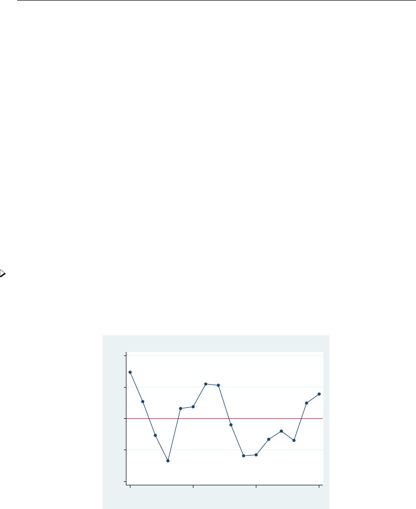
runtest — Test for random order 2087
Remarks and examples
runtest performs a nonparametric test of the hypothesis that the observations of varname occur
in a random order by counting how many runs there are above and below a threshold. If varname is
positively serially correlated, it will tend to remain above or below its median for several observations
in a row; that is, there will be relatively few runs. If, on the other hand, varname is negatively serially
correlated, observations above the median will tend to be followed by observations below the median
and vice versa; that is, there will be relatively many runs.
By default, runtest uses the median for the threshold, and this is not necessarily the best choice.
If mean is specified, the mean is used instead of the median. If threshold(#)is specified, #is used.
Because runtest divides the data into two states—above and below the threshold—it is appropriate
for data that are already binary; for example, win or lose, live or die, rich or poor, etc. Such variables
are often coded as 0 for one state and 1 for the other. Here you should specify threshold(0)
because, by default, runtest separates the observations into those that are greater than the threshold
and those that are less than or equal to the threshold.
As with most nonparametric procedures, the treatment of ties complicates the test. Observations
equal to the threshold value are ties and can be treated in one of three ways. By default, they are
treated as if they were below the threshold. If drop is specified, they are omitted from the calculation
and the total number of observations is adjusted. If split is specified, each is randomly assigned to
the above- and below-threshold groups. The random assignment is different each time the procedure
is run unless you specify the random-number seed; see [R]set seed.
Example 1
We can use runtest to check regression residuals for serial correlation.
. use http://www.stata-press.com/data/r13/run1
. scatter resid year, connect(l) yline(0) title(Regression residuals)
−4 −2 0 2 4
Residual
1975 1980 1985 1990
Year
Regression residuals
The graph gives the impression that these residuals are positively correlated. Excursions above or
below zero—the natural threshold for regression residuals—tend to last for several observations.
runtest can evaluate the statistical significance of this impression.

2088 runtest — Test for random order
. runtest resid, thresh(0)
N(resid <= 0) = 8
N(resid > 0) = 8
obs = 16
N(runs) = 5
z = -2.07
Prob>|z| = .04
There are five runs in these 16 observations. Using the normal approximation to the true distribution of
the number of runs, the five runs in this series are fewer than would be expected if the residuals were
serially independent. The p-value is 0.04, indicating a two-sided significant result at the 5% level. If the
alternative hypothesis is positive serial correlation, rather than any deviation from randomness, then the
one-sided p-value is 0.04/2=0.015. With so few observations, however, the normal approximation
may be inaccurate. (Tables compiled by Swed and Eisenhart list five runs as the 5% critical value
for a one-sided test.)
runtest is a nonparametric test. It ignores the magnitudes of the observations and notes only
whether the values are above or below the threshold. We can demonstrate this feature by reducing
the information about the regression residuals in this example to a 0/1 variable that indicates only
whether a residual is positive or negative.
. generate byte sign = resid>0
. runtest sign, thresh(0)
N(sign <= 0) = 8
N(sign > 0) = 8
obs = 16
N(runs) = 5
z = -2.07
Prob>|z| = .04
As expected, runtest produces the same answer as before.
Technical note
The run test can also be used to test the null hypothesis that two samples are drawn from the same
underlying distribution. The run test is sensitive to differences in the shapes, as well as the locations,
of the empirical distributions.
Suppose, for example, that two different additives are added to the oil in 10 different cars during
an oil change. The cars are run until a viscosity test determines that another oil change is needed,
and the number of miles traveled between oil changes is recorded. The data are

runtest — Test for random order 2089
. use http://www.stata-press.com/data/r13/additive, clear
. list
additive miles
1. 1 4024
2. 1 4756
3. 1 7993
4. 1 5025
5. 1 4188
6. 2 3007
7. 2 1988
8. 2 1051
9. 2 4478
10. 2 4232
To test whether the additives generate different distributions of miles between oil changes, we sort the
data by miles and then use runtest to see whether the marker for each additive occurs in random
order:
. sort miles
. runtest additive, thresh(1)
N(additive <= 1) = 5
N(additive > 1) = 5
obs = 10
N(runs) = 4
z = -1.34
Prob>|z| = .18
Here the additives do not produce statistically different results.
Technical note
A test that is related to the run test is the runs up-and-down test. In the latter test, the data
are classified not by whether they lie above or below a threshold but by whether they are steadily
increasing or decreasing. Thus an unbroken string of increases in the variable of interest is counted
as one run, as is an unbroken string of decreases. According to Madansky (1988), the run test is
superior to the runs up-and-down test for detecting trends in the data, but the runs up-and-down test
is superior for detecting autocorrelation.
runtest can be used to perform a runs up-and-down test. Using the regression residuals from
the example above, we can perform a runtest on their first differences:
. use http://www.stata-press.com/data/r13/run1
. generate resid_D = resid - resid[_n-1]
(1 missing value generated)
. runtest resid_D, thresh(0)
N(resid_D <= 0) = 7
N(resid_D > 0) = 8
obs = 15
N(runs) = 6
z = -1.33
Prob>|z| = .18

2090 runtest — Test for random order
Edgington (1961) has compiled a table of the small sample distribution of the runs up-and-down
statistic, and this table is reprinted in Madansky (1988). For large samples, the zstatistic reported by
runtest is incorrect for the runs up-and-down test. Let Nbe the number of observations (15 here),
and let rbe the number of runs (6). The expected number of runs in the runs up-and-down test is
µr=2N−1
3
the variance is
σ2
r=16N−29
90
and the correct zstatistic is
bz=r−µr
σr
Technical note
runtest will tolerate missing values at the beginning or end of a series, as occurred in the
technical note above (generating first differences resulted in a missing value for the first observation).
runtest, however, will issue an error message if there are any missing observations in the interior
of the series (in the portion covered by the in range modifier). To perform the test anyway, simply
drop the missing observations before using runtest.
Stored results
runtest stores the following in r():
Scalars
r(N) number of observations r(p) p-value of z
r(N below) number below the threshold r(z) zstatistic
r(N above) number above the threshold r(n runs) number of runs
r(mean) expected number of runs r(Var) variance of the number of runs
Methods and formulas
runtest begins by calculating the number of observations below the threshold, n0; the number
of observations above the threshold, n1; the total number of observations, N=n0+n1; and the
number of runs, r. These statistics are always reported, so the exact tables of critical values in Swed
and Eisenhart (1943) may be consulted if necessary.
The expected number of runs under the null is
µr=2n0n1
N+ 1

runtest — Test for random order 2091
the variance is
σ2
r=2n0n1(2n0n1−N)
N2(N−1)
and the normal approximation test statistic is
bz=r−µr
σr
Acknowledgment
runtest was written by Sean Becketti, a past editor of the Stata Technical Bulletin and author
of the Stata Press book Introduction to Time Series Using Stata.
References
Edgington, E. S. 1961. Probability table for number of runs of signs of first differences in ordered series. Journal of
the American Statistical Association 56: 156–159.
Madansky, A. 1988. Prescriptions for Working Statisticians. New York: Springer.
Swed, F. S., and C. Eisenhart. 1943. Tables for testing randomness of grouping in a sequence of alternatives. Annals
of Mathematical Statistics 14: 66–87.

Title
scobit — Skewed logistic regression
Syntax Menu Description Options
Remarks and examples Stored results Methods and formulas References
Also see
Syntax
scobit depvar indepvars if in weight ,options
options Description
Model
noconstant suppress constant term
offset(varname)include varname in model with coefficient constrained to 1
asis retain perfect predictor variables
constraints(constraints)apply specified linear constraints
collinear keep collinear variables
SE/Robust
vce(vcetype)vcetype may be oim,robust,cluster clustvar,opg,bootstrap,
or jackknife
Reporting
level(#)set confidence level; default is level(95)
or report odds ratios
nocnsreport do not display constraints
display options control column formats, row spacing, line width, display of omitted
variables and base and empty cells, and factor-variable labeling
Maximization
maximize options control the maximization process
coeflegend display legend instead of statistics
indepvars may contain factor variables; see [U] 11.4.3 Factor variables.
bootstrap,by,fp,jackknife,nestreg,rolling,statsby,stepwise, and svy are allowed; see [U] 11.1.10 Prefix
commands.
Weights are not allowed with the bootstrap prefix; see [R] bootstrap.
vce() and weights are not allowed with the svy prefix; see [SVY] svy.
fweights, iweights, and pweights are allowed; see [U] 11.1.6 weight.
coeflegend does not appear in the dialog box.
See [U] 20 Estimation and postestimation commands for more capabilities of estimation commands.
Menu
Statistics >Binary outcomes >Skewed logit regression
2092

scobit — Skewed logistic regression 2093
Description
scobit fits a maximum-likelihood skewed logit model.
See [R]logistic for a list of related estimation commands.
Options
Model
noconstant,offset(varname),constraints(constraints),collinear; see [R]estimation op-
tions.
asis forces retention of perfect predictor variables and their associated perfectly predicted observations
and may produce instabilities in maximization; see [R]probit.
SE/Robust
vce(vcetype)specifies the type of standard error reported, which includes types that are derived from
asymptotic theory (oim,opg), that are robust to some kinds of misspecification (robust), that
allow for intragroup correlation (cluster clustvar), and that use bootstrap or jackknife methods
(bootstrap,jackknife); see [R]vce option.
Reporting
level(#); see [R]estimation options.
or reports the estimated coefficients transformed to odds ratios, that is, ebrather than b. Standard errors
and confidence intervals are similarly transformed. This option affects how results are displayed,
not how they are estimated. or may be specified at estimation or when replaying previously
estimated results.
nocnsreport; see [R]estimation options.
display options:noomitted,vsquish,noemptycells,baselevels,allbaselevels,nofvla-
bel,fvwrap(#),fvwrapon(style),cformat(%fmt),pformat(% fmt),sformat(% fmt), and
nolstretch; see [R]estimation options.
Maximization
maximize options:difficult,technique(algorithm spec),iterate(#),nolog,trace,
gradient,showstep,hessian,showtolerance,tolerance(#),ltolerance(#),
nrtolerance(#),nonrtolerance, and from(init specs); see [R]maximize. These options are
seldom used.
Setting the optimization type to technique(bhhh) resets the default vcetype to vce(opg).
The following option is available with scobit but is not shown in the dialog box:
coeflegend; see [R]estimation options.
Remarks and examples
Remarks are presented under the following headings:
Skewed logistic model
Robust standard errors

2094 scobit — Skewed logistic regression
Skewed logistic model
scobit fits maximum likelihood models with dichotomous dependent variables coded as 0/1 (or,
more precisely, coded as 0 and not 0).
Example 1
We have data on the make, weight, and mileage rating of 22 foreign and 52 domestic automobiles.
We wish to fit a model explaining whether a car is foreign based on its mileage. Here is an overview
of our data:
. use http://www.stata-press.com/data/r13/auto
(1978 Automobile Data)
. keep make mpg weight foreign
. describe
Contains data from http://www.stata-press.com/data/r13/auto.dta
obs: 74 1978 Automobile Data
vars: 4 13 Apr 2013 17:45
size: 1,702 (_dta has notes)
storage display value
variable name type format label variable label
make str18 %-18s Make and Model
mpg int %8.0g Mileage (mpg)
weight int %8.0gc Weight (lbs.)
foreign byte %8.0g origin Car type
Sorted by: foreign
Note: dataset has changed since last saved
. inspect foreign
foreign: Car type Number of Observations
Total Integers Nonintegers
# Negative - - -
# Zero 52 52 -
# Positive 22 22 -
#
# # Total 74 74 -
# # Missing -
0 1 74
(2 unique values)
foreign is labeled and all values are documented in the label.
The variable foreign takes on two unique values, 0 and 1. The value 0 denotes a domestic car,
and 1 denotes a foreign car.

scobit — Skewed logistic regression 2095
The model that we wish to fit is
Pr(foreign = 1) = F(β0+β1mpg)
where F(z) = 1−1/{1 + exp(z)}α.
To fit this model, we type
. scobit foreign mpg
Fitting logistic model:
Iteration 0: log likelihood = -45.03321
Iteration 1: log likelihood = -39.380959
Iteration 2: log likelihood = -39.288802
Iteration 3: log likelihood = -39.28864
Iteration 4: log likelihood = -39.28864
Fitting full model:
Iteration 0: log likelihood = -39.28864
Iteration 1: log likelihood = -39.286393
Iteration 2: log likelihood = -39.284415
Iteration 3: log likelihood = -39.284234
Iteration 4: log likelihood = -39.284197
Iteration 5: log likelihood = -39.284196
Skewed logistic regression Number of obs = 74
Zero outcomes = 52
Log likelihood = -39.2842 Nonzero outcomes = 22
foreign Coef. Std. Err. z P>|z| [95% Conf. Interval]
mpg .1813879 .2407362 0.75 0.451 -.2904463 .6532222
_cons -4.274883 1.399305 -3.06 0.002 -7.017471 -1.532295
/lnalpha -.4450405 3.879885 -0.11 0.909 -8.049476 7.159395
alpha .6407983 2.486224 .0003193 1286.133
Likelihood-ratio test of alpha=1: chi2(1) = 0.01 Prob > chi2 = 0.9249
Note: likelihood-ratio tests are recommended for inference with scobit models.
We find that cars yielding better gas mileage are less likely to be foreign. The likelihood-ratio test
at the bottom of the output indicates that the model is not significantly different from a logit model.
Therefore, we should use the more parsimonious model.
Technical note
Stata interprets a value of 0 as a negative outcome (failure) and treats all other values (except
missing) as positive outcomes (successes). Thus if the dependent variable takes on the values 0 and
1, then 0 is interpreted as failure and 1 as success. If the dependent variable takes on the values 0,
1, and 2, then 0 is still interpreted as failure, but both 1 and 2 are treated as successes.
Formally, when we type scobit y x, Stata fits the model
Pr(yj6= 0 |xj) = 1 −1.n1 + exp(xjβ)oα

2096 scobit — Skewed logistic regression
Robust standard errors
If you specify the vce(robust) option, scobit reports robust standard errors as described in
[U] 20.21 Obtaining robust variance estimates. For the model of foreign on mpg, the robust
calculation increases the standard error of the coefficient on mpg by around 25%:
. scobit foreign mpg, vce(robust) nolog
Skewed logistic regression Number of obs = 74
Zero outcomes = 52
Log pseudolikelihood = -39.2842 Nonzero outcomes = 22
Robust
foreign Coef. Std. Err. z P>|z| [95% Conf. Interval]
mpg .1813879 .3028487 0.60 0.549 -.4121847 .7749606
_cons -4.274883 1.335521 -3.20 0.001 -6.892455 -1.657311
/lnalpha -.4450405 4.71561 -0.09 0.925 -9.687466 8.797385
alpha .6407983 3.021755 .0000621 6616.919
Without vce(robust), the standard error for the coefficient on mpg was reported to be 0.241, with
a resulting confidence interval of [−0.29,0.65 ].
Specifying the vce(cluster clustvar)option relaxes the independence assumption required by
the skewed logit estimator to being just independence between clusters. To demonstrate this, we will
switch to a different dataset.
Example 2
We are studying the unionization of women in the United States and have a dataset with 26,200
observations on 4,434 women between 1970 and 1988. For our purposes, we will use the variables
age (the women were 14–26 in 1968 and the data thus span the age range of 16–46), grade (years
of schooling completed, ranging from 0 to 18), not smsa (28% of the person-time was spent living
outside an SMSA—standard metropolitan statistical area), south (41% of the person-time was in the
South), and year. Each of these variables is included in the regression as a covariate along with the
interaction between south and year. This interaction, along with the south and year variables, is
specified in the scobit command using factor-variables notation, south##c.year. We also have
variable union. Overall, 22% of the person-time is marked as time under union membership and
44% of these women have belonged to a union.
We fit the following model, ignoring that women are observed an average of 5.9 times each in
these data:

scobit — Skewed logistic regression 2097
. use http://www.stata-press.com/data/r13/union, clear
(NLS Women 14-24 in 1968)
. scobit union age grade not_smsa south##c.year, nrtol(1e-3)
(output omitted )
Skewed logistic regression Number of obs = 26200
Zero outcomes = 20389
Log likelihood = -13540.61 Nonzero outcomes = 5811
union Coef. Std. Err. z P>|z| [95% Conf. Interval]
age .0185365 .0043615 4.25 0.000 .0099881 .0270849
grade .0452803 .0057124 7.93 0.000 .0340842 .0564764
not_smsa -.1886849 .0317802 -5.94 0.000 -.250973 -.1263968
1.south -1.422381 .3949298 -3.60 0.000 -2.196429 -.6483327
year -.0133017 .0049575 -2.68 0.007 -.0230182 -.0035853
south#c.year
1 .0105663 .0049233 2.15 0.032 .0009168 .0202158
_cons -10.19247 63.69015 -0.16 0.873 -135.0229 114.6379
/lnalpha 8.972796 63.68825 0.14 0.888 -115.8539 133.7995
alpha 7885.616 502221.1 4.85e-51 1.28e+58
Likelihood-ratio test of alpha=1: chi2(1) = 3.76 Prob > chi2 = 0.0524
Note: likelihood-ratio tests are recommended for inference with scobit models.
The reported standard errors in this model are probably meaningless. Women are observed repeatedly,
so the observations are not independent. Looking at the coefficients, we find a large southern effect
against unionization and a different time trend for the south. The vce(cluster clustvar)option
provides a way to fit this model and obtains correct standard errors:
. scobit union age grade not_smsa south##c.year, vce(cluster id) nrtol(1e-3)
(output omitted )
Skewed logistic regression Number of obs = 26200
Zero outcomes = 20389
Log pseudolikelihood = -13540.61 Nonzero outcomes = 5811
(Std. Err. adjusted for 4434 clusters in idcode)
Robust
union Coef. Std. Err. z P>|z| [95% Conf. Interval]
age .0185365 .0084867 2.18 0.029 .0019029 .0351701
grade .0452803 .0125764 3.60 0.000 .0206311 .0699296
not_smsa -.1886849 .0642035 -2.94 0.003 -.3145214 -.0628484
1.south -1.422381 .5064916 -2.81 0.005 -2.415086 -.4296756
year -.0133017 .0090621 -1.47 0.142 -.0310632 .0044597
south#c.year
1 .0105663 .0063172 1.67 0.094 -.0018152 .0229478
_cons -10.19247 .945772 -10.78 0.000 -12.04615 -8.33879
/lnalpha 8.972796 .7482517 11.99 0.000 7.506249 10.43934
alpha 7885.616 5900.426 1819.377 34178.16

2098 scobit — Skewed logistic regression
scobit, vce(cluster clustvar)is robust to assumptions about within-cluster correlation. That
is, it inefficiently sums within cluster for the standard error calculation rather than attempting to exploit
what might be assumed about the within-cluster correlation (as do the xtgee population-averaged
models; see [XT]xtgee).
Technical note
The scobit model can be difficult to fit because of the functional form. Often it requires many
iterations, or the optimizer prints out warning and informative messages during the optimization. For
example, without the nrtol(1e-3) option, the model using the union dataset will not converge.
See [R]maximize for details about the optimizer.
Technical note
The main reason for using scobit rather that logit is that the effects of the regressors on the
probability of success are not constrained to be the largest when the probability is 0.5. Rather, the
independent variables might show their largest impact when the probability of success is 0.3 or 0.6.
This added flexibility results because the scobit function, unlike the logit function, can be skewed
and is not constrained to be mirror symmetric about the 0.5 probability of success.
As Nagler (1994) pointed out, the point of maximum impact is constrained under the scobit model
to fall within the interval (0,1−e(−1))or approximately (0, 0.63). Achen (2002) notes that if we
believe the maximum impact to be outside that range, we can instead estimate the “power logit”
model by simply reversing the 0s and 1s of our outcome variable and estimating a scobit model on
failure, rather than success. We would need to reverse the signs of the coefficients if we wanted to
interpret them in terms of impact on success, or we could leave them as they are and interpret them
in terms of impact on failure. The important thing to remember is that the scobit model, unlike the
logit model, is not invariant to the choice of which result is assigned to success.

scobit — Skewed logistic regression 2099
Stored results
scobit stores the following in e():
Scalars
e(N) number of observations
e(k) number of parameters
e(k eq) number of equations in e(b)
e(k aux) number of auxiliary parameters
e(k dv) number of dependent variables
e(ll) log likelihood
e(ll c) log likelihood, comparison model
e(N f) number of failures (zero outcomes)
e(N s) number of successes (nonzero outcomes)
e(alpha) alpha
e(N clust) number of clusters
e(chi2) χ2
e(chi2 c) χ2for comparison test
e(p) significance
e(rank) rank of e(V)
e(ic) number of iterations
e(rc) return code
e(converged) 1 if converged, 0otherwise
Macros
e(cmd) scobit
e(cmdline) command as typed
e(depvar) name of dependent variable
e(wtype) weight type
e(wexp) weight expression
e(title) title in estimation output
e(clustvar) name of cluster variable
e(offset) linear offset variable
e(chi2type) Wald or LR; type of model χ2test
e(chi2 ct) Wald or LR; type of model χ2test corresponding to e(chi2 c)
e(vce) vcetype specified in vce()
e(vcetype) title used to label Std. Err.
e(opt) type of optimization
e(which) max or min; whether optimizer is to perform maximization or minimization
e(ml method) type of ml method
e(user) name of likelihood-evaluator program
e(technique) maximization technique
e(properties) b V
e(predict) program used to implement predict
e(footnote) program used to implement the footnote display
e(asbalanced) factor variables fvset as asbalanced
e(asobserved) factor variables fvset as asobserved
Matrices
e(b) coefficient vector
e(Cns) constraints matrix
e(ilog) iteration log (up to 20 iterations)
e(gradient) gradient vector
e(V) variance–covariance matrix of the estimators
e(V modelbased) model-based variance
Functions
e(sample) marks estimation sample

2100 scobit — Skewed logistic regression
Methods and formulas
Skewed logit analysis is an alternative to logit that relaxes the assumption that individuals with
initial probability of 0.5 are most sensitive to changes in independent variables.
The log-likelihood function for skewed logit is
lnL=X
j∈S
wjlnF(xjb) + X
j6∈S
wjln1−F(xjb)
where Sis the set of all observations jsuch that yj6=0, F(z) = 1−1/1+ exp(z)α, and wj
denotes the optional weights. lnLis maximized as described in [R]maximize.
This command supports the Huber/White/sandwich estimator of the variance and its clustered
version using vce(robust) and vce(cluster clustvar), respectively. See [P]robust, particularly
Maximum likelihood estimators and Methods and formulas.
scobit also supports estimation with survey data. For details on VCEs with survey data, see
[SVY]variance estimation.
References
Achen, C. H. 2002. Toward a new political methodology: Microfoundations and ART. Annual Review of Political
Science 5: 423–450.
Nagler, J. 1994. Scobit: An alternative estimator to logit and probit. American Journal of Political Science 38:
230–255.
Also see
[R]scobit postestimation — Postestimation tools for scobit
[R]cloglog — Complementary log-log regression
[R]glm — Generalized linear models
[R]logistic — Logistic regression, reporting odds ratios
[SVY]svy estimation — Estimation commands for survey data
[U] 20 Estimation and postestimation commands

Title
scobit postestimation — Postestimation tools for scobit
Description Syntax for predict Menu for predict Options for predict
Remarks and examples Also see
Description
The following postestimation commands are available after scobit:
Command Description
contrast contrasts and ANOVA-style joint tests of estimates
estat ic Akaike’s and Schwarz’s Bayesian information criteria (AIC and BIC)
estat summarize summary statistics for the estimation sample
estat vce variance–covariance matrix of the estimators (VCE)
estat (svy) postestimation statistics for survey data
estimates cataloging estimation results
forecast1dynamic forecasts and simulations
lincom point estimates, standard errors, testing, and inference for linear combinations
of coefficients
lrtest2likelihood-ratio test
margins marginal means, predictive margins, marginal effects, and average marginal
effects
marginsplot graph the results from margins (profile plots, interaction plots, etc.)
nlcom point estimates, standard errors, testing, and inference for nonlinear combinations
of coefficients
predict predictions, residuals, influence statistics, and other diagnostic measures
predictnl point estimates, standard errors, testing, and inference for generalized predictions
pwcompare pairwise comparisons of estimates
suest seemingly unrelated estimation
test Wald tests of simple and composite linear hypotheses
testnl Wald tests of nonlinear hypotheses
1forecast is not appropriate with svy estimation results.
2lrtest is not appropriate with svy estimation results.
2101

2102 scobit postestimation — Postestimation tools for scobit
Syntax for predict
predict type newvar if in ,statistic nooffset
predict type stub*|newvarreg newvarlnalpha if in , scores
statistic Description
Main
pr probability of a positive outcome; the default
xb xjb, linear prediction
stdp standard error of the linear prediction
These statistics are available both in and out of sample; type predict . . . if e(sample) . . . if wanted only for
the estimation sample.
Menu for predict
Statistics >Postestimation >Predictions, residuals, etc.
Options for predict
Main
pr, the default, calculates the probability of a positive outcome.
xb calculates the linear prediction.
stdp calculates the standard error of the linear prediction.
nooffset is relevant only if you specified offset(varname)for scobit. It modifies the calculations
made by predict so that they ignore the offset variable; the linear prediction is treated as xjb
rather than as xjb+offsetj.
scores calculates equation-level score variables.
The first new variable will contain ∂ln L/∂(xjβ).
The second new variable will contain ∂ln L/∂ lnα.
Remarks and examples
Once you have fit a model, you can obtain the predicted probabilities by using the predict
command for both the estimation sample and other samples; see [U] 20 Estimation and postestimation
commands and [R]predict. Here we will make only a few additional comments.
predict without arguments calculates the predicted probability of a positive outcome. With the
xb option, it calculates the linear combination xjb, where xjare the independent variables in the
jth observation and bis the estimated parameter vector.
With the stdp option, predict calculates the standard error of the prediction, which is not
adjusted for replicated covariate patterns in the data.

scobit postestimation — Postestimation tools for scobit 2103
Example 1
In example 1 of [R]scobit, we fit the model scobit foreign mpg. To obtain predicted probabilities,
we type
. use http://www.stata-press.com/data/r13/auto
(1978 Automobile Data)
. keep make mpg weight foreign
. scobit foreign mpg
(output omitted )
. predict p
(option pr assumed; Pr(foreign))
. summarize foreign p
Variable Obs Mean Std. Dev. Min Max
foreign 74 .2972973 .4601885 0 1
p 74 .2974049 .182352 .0714664 .871624
Also see
[R]scobit — Skewed logistic regression
[U] 20 Estimation and postestimation commands

Title
sdtest — Variance-comparison tests
Syntax Menu Description Options
Remarks and examples Stored results Methods and formulas References
Also see
Syntax
One-sample variance-comparison test
sdtest varname == #if in , level(#)
Two-sample variance-comparison test using groups
sdtest varname if in , by(groupvar)level(#)
Two-sample variance-comparison test using variables
sdtest varname1== varname2if in , level(#)
Immediate form of one-sample variance-comparison test
sdtesti #obs #mean |.#sd #val , level(#)
Immediate form of two-sample variance-comparison test
sdtesti #obs,1#mean,1|.#sd,1#obs,2#mean,2|.#sd,2, level(#)
Robust tests for equality of variances
robvar varname if in , by(groupvar)
by is allowed with sdtest and robvar; see [D] by.
Menu
sdtest
Statistics >Summaries, tables, and tests >Classical tests of hypotheses >Variance-comparison test
sdtesti
Statistics >Summaries, tables, and tests >Classical tests of hypotheses >Variance-comparison test calculator
robvar
Statistics >Summaries, tables, and tests >Classical tests of hypotheses >Robust equal-variance test
2104

sdtest — Variance-comparison tests 2105
Description
sdtest performs tests on the equality of standard deviations (variances). In the first form, sdtest
tests that the standard deviation of varname is #. In the second form, sdtest performs the same
test, using the standard deviations of the two groups defined by groupvar. In the third form, sdtest
tests that varname1and varname2have the same standard deviation.
sdtesti is the immediate form of sdtest; see [U] 19 Immediate commands.
Both the traditional Ftest for the homogeneity of variances and Bartlett’s generalization of this
test to Ksamples are sensitive to the assumption that the data are drawn from an underlying Gaussian
distribution. See, for example, the cautionary results discussed by Markowski and Markowski (1990).
Levene (1960) proposed a test statistic for equality of variance that was found to be robust under
nonnormality. Then Brown and Forsythe (1974) proposed alternative formulations of Levene’s test
statistic that use more robust estimators of central tendency in place of the mean. These reformulations
were demonstrated to be more robust than Levene’s test when dealing with skewed populations.
robvar reports Levene’s robust test statistic (W0) for the equality of variances between the groups
defined by groupvar and the two statistics proposed by Brown and Forsythe that replace the mean in
Levene’s formula with alternative location estimators. The first alternative (W50) replaces the mean
with the median. The second alternative replaces the mean with the 10% trimmed mean (W10).
Options
level(#)specifies the confidence level, as a percentage, for confidence intervals of the means. The
default is level(95) or as set by set level; see [U] 20.7 Specifying the width of confidence
intervals.
by(groupvar)specifies the groupvar that defines the groups to be compared. For sdtest, there
should be two groups, but for robvar there may be more than two groups. Do not confuse the
by() option with the by prefix; both may be specified.
Remarks and examples
Remarks are presented under the following headings:
Basic form
Immediate form
Robust test
Basic form
sdtest performs two different statistical tests: one testing equality of variances and the other
testing that the standard deviation is equal to a known constant. Which test it performs is determined
by whether you type a variable name or a number to the right of the equal sign.
Example 1: One-sample test of variance
We have a sample of 74 automobiles. For each automobile, we know the mileage rating. We wish
to test whether the overall standard deviation is 5 mpg:

2106 sdtest — Variance-comparison tests
. use http://www.stata-press.com/data/r13/auto
(1978 Automobile Data)
. sdtest mpg == 5
One-sample test of variance
Variable Obs Mean Std. Err. Std. Dev. [95% Conf. Interval]
mpg 74 21.2973 .6725511 5.785503 19.9569 22.63769
sd = sd(mpg) c = chi2 = 97.7384
Ho: sd = 5 degrees of freedom = 73
Ha: sd < 5 Ha: sd != 5 Ha: sd > 5
Pr(C < c) = 0.9717 2*Pr(C > c) = 0.0565 Pr(C > c) = 0.0283
Example 2: Variance ratio test
We are testing the effectiveness of a new fuel additive. We run an experiment on 12 cars, running
each without and with the additive. The data can be found in [R]ttest. The results for each car are
stored in the variables mpg1 and mpg2:
. use http://www.stata-press.com/data/r13/fuel
. sdtest mpg1==mpg2
Variance ratio test
Variable Obs Mean Std. Err. Std. Dev. [95% Conf. Interval]
mpg1 12 21 .7881701 2.730301 19.26525 22.73475
mpg2 12 22.75 .9384465 3.250874 20.68449 24.81551
combined 24 21.875 .6264476 3.068954 20.57909 23.17091
ratio = sd(mpg1) / sd(mpg2) f = 0.7054
Ho: ratio = 1 degrees of freedom = 11, 11
Ha: ratio < 1 Ha: ratio != 1 Ha: ratio > 1
Pr(F < f) = 0.2862 2*Pr(F < f) = 0.5725 Pr(F > f) = 0.7138
We cannot reject the hypothesis that the standard deviations are the same.
In [R]ttest, we draw an important distinction between paired and unpaired data, which, in this
example, means whether there are 12 cars in a before-and-after experiment or 24 different cars. For
sdtest, on the other hand, there is no distinction. If the data had been unpaired and stored as
described in [R]ttest, we could have typed sdtest mpg, by(treated), and the results would have
been the same.
Immediate form
Example 3: sdtesti
Immediate commands are used not with data, but with reported summary statistics. For instance,
to test whether a variable on which we have 75 observations and a reported standard deviation of 6.5
comes from a population with underlying standard deviation 6, we would type

sdtest — Variance-comparison tests 2107
. sdtesti 75 . 6.5 6
One-sample test of variance
Obs Mean Std. Err. Std. Dev. [95% Conf. Interval]
x 75 . .7505553 6.5 . .
sd = sd(x) c = chi2 = 86.8472
Ho: sd = 6 degrees of freedom = 74
Ha: sd < 6 Ha: sd != 6 Ha: sd > 6
Pr(C < c) = 0.8542 2*Pr(C > c) = 0.2916 Pr(C > c) = 0.1458
The mean plays no role in the calculation, so it may be omitted.
To test whether the variable comes from a population with the same standard deviation as another
for which we have a calculated standard deviation of 7.5 over 65 observations, we would type
. sdtesti 75 . 6.5 65 . 7.5
Variance ratio test
Obs Mean Std. Err. Std. Dev. [95% Conf. Interval]
x 75 . .7505553 6.5 . .
y 65 . .9302605 7.5 . .
combined 140 . . . . .
ratio = sd(x) / sd(y) f = 0.7511
Ho: ratio = 1 degrees of freedom = 74, 64
Ha: ratio < 1 Ha: ratio != 1 Ha: ratio > 1
Pr(F < f) = 0.1172 2*Pr(F < f) = 0.2344 Pr(F > f) = 0.8828
Robust test
Example 4: robvar
We wish to test whether the standard deviation of the length of stay for patients hospitalized for a
given medical procedure differs by gender. Our data consist of observations on the length of hospital
stay for 1778 patients: 884 males and 894 females. Length of stay, lengthstay, is highly skewed
(skewness coefficient =4.912591) and thus violates Bartlett’s normality assumption. Therefore, we
use robvar to compare the variances.
. use http://www.stata-press.com/data/r13/stay
. robvar lengthstay, by(sex)
Summary of Length of stay in days
sex Mean Std. Dev. Freq.
male 9.0874434 9.7884747 884
female 8.800671 9.1081478 894
Total 8.9432508 9.4509466 1778
W0 = 0.55505315 df(1, 1776) Pr > F = 0.45635888
W50 = 0.42714734 df(1, 1776) Pr > F = 0.51347664
W10 = 0.44577674 df(1, 1776) Pr > F = 0.50443411

2108 sdtest — Variance-comparison tests
For these data, we cannot reject the null hypothesis that the variances are equal. However, Bartlett’s
test yields a significance probability of 0.0319 because of the pronounced skewness of the data.
Technical note
robvar implements both the conventional Levene’s test centered at the mean and a median-centered
test. In a simulation study, Conover, Johnson, and Johnson (1981) compare the properties of the two
tests and recommend using the median test for asymmetric data, although for small sample sizes
the test is somewhat conservative. See Carroll and Schneider (1985) for an explanation of why both
mean- and median-centered tests have approximately the same level for symmetric distributions, but
for asymmetric distributions the median test is closer to the correct level.
Stored results
sdtest and sdtesti store the following in r():
Scalars
r(N) number of observations
r(p l) lower one-sided p-value
r(p u) upper one-sided p-value
r(p) two-sided p-value
r(F) Fstatistic
r(sd) standard deviation
r(sd 1) standard deviation for first variable
r(sd 2) standard deviation for second variable
r(df) degrees of freedom
r(df 1) numerator degrees of freedom
r(df 2) denominator degrees of freedom
r(chi2) χ2
robvar stores the following in r():
Scalars
r(N) number of observations
r(w50) Brown and Forsythe’s Fstatistic (median)
r(p w50) Brown and Forsythe’s p-value
r(w0) Levene’s Fstatistic
r(p w0) Levene’s p-value
r(w10) Brown and Forsythe’s Fstatistic (trimmed mean)
r(p w10) Brown and Forsythe’s p-value (trimmed mean)
r(df 1) numerator degrees of freedom
r(df 2) denominator degrees of freedom
Methods and formulas
See Armitage et al. (2002, 149 – 153) or Bland (2000, 171–172) for an introduction and explanation
of the calculation of these tests.
The test for σ=σ0is given by
χ2=(n−1)s2
σ2
0
which is distributed as χ2with n−1 degrees of freedom.

sdtest — Variance-comparison tests 2109
The test for σ2
x=σ2
yis given by
F=s2
x
s2
y
which is distributed as Fwith nx−1 and ny−1 degrees of freedom.
Let Xij be the jth observation of Xfor the ith group. Let Zij =|Xij −Xi|, where Xiis the
mean of Xin the ith group. Levene’s test statistic is
W0=Pini(Zi−Z)2/(g−1)
PiPj(Zij −Zi)2/Pi(ni−1)
where niis the number of observations in group iand gis the number of groups. W50 is obtained
by replacing Xiwith the ith group median of Xij , whereas W10 is obtained by replacing Xiwith
the 10% trimmed mean for group i.
References
Armitage, P., G. Berry, and J. N. S. Matthews. 2002. Statistical Methods in Medical Research. 4th ed. Oxford:
Blackwell.
Bland, M. 2000. An Introduction to Medical Statistics. 3rd ed. Oxford: Oxford University Press.
Brown, M. B., and A. B. Forsythe. 1974. Robust tests for the equality of variances. Journal of the American Statistical
Association 69: 364–367.
Carroll, R. J., and H. Schneider. 1985. A note on Levene’s tests for equality of variances. Statistics and Probability
Letters 3: 191–194.
Cleves, M. A. 1995. sg35: Robust tests for the equality of variances.Stata Technical Bulletin 25: 13–15. Reprinted
in Stata Technical Bulletin Reprints, vol. 5, pp. 91–93. College Station, TX: Stata Press.
. 2000. sg35.2: Robust tests for the equality of variances update to Stata 6.Stata Technical Bulletin 53: 17–18.
Reprinted in Stata Technical Bulletin Reprints, vol. 9, pp. 158–159. College Station, TX: Stata Press.
Conover, W. J., M. E. Johnson, and M. M. Johnson. 1981. A comparative study of tests for homogeneity of variances,
with applications to the outer continental shelf bidding data. Technometrics 23: 351–361.
Gastwirth, J. L., Y. R. Gel, and W. Miao. 2009. The impact of Levene’s test of equality of variances on statistical
theory and practice. Statistical Science 24: 343–360.
Levene, H. 1960. Robust tests for equality of variances. In Contributions to Probability and Statistics: Essays in Honor
of Harold Hotelling, ed. I. Olkin, S. G. Ghurye, W. Hoeffding, W. G. Madow, and H. B. Mann, 278–292. Menlo
Park, CA: Stanford University Press.
Markowski, C. A., and E. P. Markowski. 1990. Conditions for the effectiveness of a preliminary test of variance.
American Statistician 44: 322–326.
Seed, P. T. 2000. sbe33: Comparing several methods of measuring the same quantity.Stata Technical Bulletin 55:
2–9. Reprinted in Stata Technical Bulletin Reprints, vol. 10, pp. 73–82. College Station, TX: Stata Press.
Tob´
ıas, A. 1998. gr28: A graphical procedure to test equality of variances.Stata Technical Bulletin 42: 4–6. Reprinted
in Stata Technical Bulletin Reprints, vol. 7, pp. 68–70. College Station, TX: Stata Press.
Also see
[R]ttest —ttests (mean-comparison tests)

Title
search — Search Stata documentation and other resources
Syntax Menu Description
Options for search Option for set searchdefault Remarks and examples
Acknowledgment Also see
Syntax
search word word . . . ,search options
set searchdefault all |local |net , permanently
search options Description
all search across both the local keyword database and the net material; the default
local search using Stata’s keyword database
net search across materials available via Stata’s net command
author search by author’s name
entry search by entry ID
exact search across both the local keyword database and the net materials; prevents
matching on abbreviations
faq search the FAQs posted to the Stata website
historical search entries that are of historical interest only
or list an entry if any of the words typed after search are associated with the entry
manual search the entries in the Stata Documentation
sj search the entries in the Stata Journal and the STB
Menu
Help >Search...
Description
search searches a keyword database and the Internet for Stata materials related to your query.
Capitalization of the words following search is irrelevant, as is the inclusion or exclusion of
special characters such as commas and hyphens.
set searchdefault affects the default behavior of the search command. all is the default.
search, all is the best way to search for information on a topic across all sources, including the
system help, the FAQs at the Stata website, the Stata Journal, and all Stata-related Internet sources
including user-written additions. From the results, you can click to go to a source or to install additions.
2110

search — Search Stata documentation and other resources 2111
Options for search
all, the default (unless changed by set searchdefault), specifies that the search be performed
across both the local keyword database and the net materials. The results of a search performed
with all and no other options will be displayed in the Viewer window.
local specifies that the search be performed using only Stata’s keyword database. The results of a
search performed with local and no other options will be displayed in the Viewer window.
net specifies that the search be performed across the materials available via Stata’s net command.
Using search word word . . ., net is equivalent to typing net search word word . . .
(without options); see [R]net search. The results of a search performed with net and no other
options will be displayed in the Viewer window.
author specifies that the search be performed on the basis of author’s name rather than keywords.
A search with the author option is performed on the local keyword database only, and the results
are displayed in the Results window.
entry specifies that the search be performed on the basis of entry IDs rather than keywords. A
search with the entry option is performed on the local keyword database only, and the results
are displayed in the Results window.
exact prevents matching on abbreviations. A search with the exact option is performed across both
the local keyword database and the net materials, and the results are displayed in the Results
window.
faq limits the search to the FAQs posted on the Stata website: http://www.stata.com. A search with
the faq option is performed on the local keyword database only, and the results are displayed in
the Results window.
historical adds to the search entries that are of historical interest only. By default, such entries
are not listed. Past entries are classified as historical if they discuss a feature that later became an
official part of Stata. Updates to historical entries will always be found, even if historical is
not specified. A search with the historical option is performed on the local keyword database
only, and the results are displayed in the Results window.
or specifies that an entry be listed if any of the words typed after search are associated with the
entry. The default is to list the entry only if all the words specified are associated with the entry.
A search with the or option is performed on the local keyword database only, and the results are
displayed in the Results window.
manual limits the search to entries in the Stata Documentation; that is, the search is limited to the
User’s Guide and all the reference manuals. A search with the manual option is performed on the
local keyword database only, and the results are displayed in the Results window.
sj limits the search to entries in the Stata Journal and its predecessor, the Stata Technical Bulletin;
see [R]sj. A search with the sj option is performed on the local keyword database only, and the
results are displayed in the Results window.
Option for set searchdefault
permanently specifies that, in addition to making the change right now, the searchdefault setting
be remembered and become the default setting when you invoke Stata.

2112 search — Search Stata documentation and other resources
Remarks and examples
Remarks are presented under the following headings:
Introduction
Internet searches
Author searches
Entry ID searches
Return codes
Introduction
See [U] 4 Stata’s help and search facilities for a tutorial introduction to search.search is one
of Stata’s most useful commands. To understand the advanced features of search, you need to know
how it works.
search has a database—files—containing the titles, etc., of every entry in the User’s Guide,
the Base Reference Manual, the Data Management Reference Manual, the Graphics Reference
Manual, the Longitudinal-Data/Panel-Data Reference Manual, the Multilevel Mixed-Effects Reference
Manual, the Multiple-Imputation Reference Manual, the Multivariate Statistics Reference Manual,
the Power and Sample-Size Reference Manual, the Programming Reference Manual, the Structural
Equation Modeling Reference Manual, the Survey Data Reference Manual, the Survival Analysis and
Epidemiological Tables Reference Manual, the Treatment-Effects Reference Manual, the Time-Series
Reference Manual, the Mata Reference Manual, undocumented help files, NetCourses, Stata Press
books, FAQs posted on the Stata website, videos posted on the Stata YouTube channel, selected articles
on StataCorp’s official blog, selected user-written FAQs and examples, and the articles in the Stata
Journal and the Stata Technical Bulletin. In these files is a list of words, called keywords, associated
with each entry.
When you type search xyz,search reads the database and compares the list of keywords with
xyz. If it finds xyz in the list or a keyword that allows an abbreviation of xyz, it displays the entry.
When you type search xyz abc,search does the same thing but displays an entry only if it
contains both keywords. The order does not matter, so you can search linear regression or
search regression linear.
Obviously, how many entries search finds depends on how the search database was constructed.
We have included a plethora of keywords under the theory that, for a given request, it is better to
list too much rather than risk listing nothing at all. Still, you are in the position of guessing the
keywords. Do you look up normality test, normality tests, or tests of normality? Well, normality test
would be best, but all would work. In general, use the singular, and strike the unnecessary words.
For guidelines for specifying keywords, see [U] 4.6 More on search.
set searchdefault allows you to specify where search searches. set searchdefault all,
the default, indicates that both the keyword database and the Internet are to be searched. set
searchdefault local restricts search to using only Stata’s keyword database. set searchdefault
net restricts search to searching only the Internet.
Internet searches
search with the net option searches the Internet for user-written additions to Stata, including,
but not limited to, user-written additions published in the Stata Journal (SJ) and the Stata Technical
Bulletin (STB). search keywords, net performs the same search as the command net search (with
no options); see [R]net search.

search — Search Stata documentation and other resources 2113
. search random effect, net
(contacting http://www.stata.com)
70 packages found (Stata Journal and STB listed first)
------------------------------------------------------
st0156_1 from http://www.stata-journal.com/software/sj11-2
SJ11-2 st0156_1. Update: Multivariate random-effects... / Update:
Multivariate random-effects meta-regression / by Ian White / Support:
ian.white@mrc-bsu.cam.ac.uk / After installation, type help mvmeta and
mvmeta_make
st0201 from http://www.stata-journal.com/software/sj10-3
SJ10-3 st0201. metaan: Random-effects meta-analysis / metaan:
Random-effects meta-analysis / by Evangelos Kontopantelis, / National
Primary Care Research and Development Centre (NPCRDC), / University of
Manchester, Manchester, UK / David Reeves, / National Primary Care
sbe24_3 from http://www.stata-journal.com/software/sj9-2
SJ9-2 sbe24_3. Update: metan: fixed- and random-effects... / Update:
metan: fixed- and random-effects meta-analysis / by Ross J. Harris, Roger
M. Harbord, and Jonathan A. C. Sterne, / Department of Social Medicine,
University of Bristol / Jonathan J. Deeks, Department of Primary Care
(output omitted )
(end of search)
Author searches
search ordinarily compares the words following search with the keywords for the entry. If you
specify the author option, however, it compares the words with the author’s name. In the search
database, we have filled in author names for all SJ and STB inserts.
For instance, in [R]kdensity in this manual you will discover that Isa´
ıas H. Salgado-Ugarte wrote
the first version of Stata’s kdensity command and published it in the STB. Assume that you read
his original insert and found the discussion useful. You might now wonder what else he has written
in the SJ or STB. To find out, you type
. search Salgado-Ugarte, author
(output omitted )
Names like Salgado-Ugarte are confusing to many people. search does not require you to specify
the entire name; what you type is compared with each “word” of the name and, if any part matches,
the entry is listed. The hyphen is a special character, and you can omit it. Thus you can obtain the
same list by looking up Salgado, Ugarte, or Salgado Ugarte without the hyphen.
Actually, to find all entries written by Salgado-Ugarte, you need to type
. search Salgado-Ugarte, author historical
(output omitted )
Prior inserts in the SJ or STB that provide a feature that later was superseded by a built-in feature of
Stata are marked as historical in the search database and, by default, are not listed. The historical
option ensures that all entries are listed.

2114 search — Search Stata documentation and other resources
Entry ID searches
If you specify the entry option, search compares what you have typed with the entry ID. The
entry ID is not the title—it is the reference listed to the left of the title that tells you where to look.
For instance, in
[R] regress . . . . . . . . . . . . . . . . . . . . . . Linear regression
(help regress)
[R]regress is the entry ID. This is a reference, of course, to this manual. In
FAQ . . . . . . . . . . . Analysis of multiple failure-time survival data
. . . . . . . . . . . . . . . . . . . . . . . M. Cleves and I. Canette
07/09 How do I analyze multiple failure-time data using Stata?
http://www.stata.com/support/faqs/statistics/multiple-failure-
type-data/
“FAQ” is the entry ID. In
SJ-7-1 st0118 . . A survey on survey stat.: What is and can be done in Stata
. . . . . . . . . . . . . . . . . . . . . . F. Kreuter and R. Valliant
Q1/07 SJ7(1):1--21 (no commands)
discusses survey issues in analyzing complex survey
data and describes some of Stata’s capabilities for
such analyses
“SJ-7-1” is the entry ID.
search with the entry option searches these entry IDs.
Thus you could generate a table of contents for the User’s Guide by typing
. search [U], entry
(output omitted )
You could generate a table of contents for Stata Journal, Volume 1, Issue 1, by typing
. search sj-1-1, entry
(output omitted )
To generate a table of contents for the 26th issue of the STB, you would type
. search STB-26, entry historical
(output omitted )
The historical option here is possibly important. STB-26 was published in July 1995, and perhaps
some of its inserts have already been marked historical.
You could obtain a list of all inserts associated with sg53 by typing
. search sg53, entry historical
(output omitted )
Again we include the historical option in case any of the relevant inserts have been marked
historical.
Return codes
In addition to indexing the entries in the User’s Guide and all the Reference manuals, search
also can be used to search return codes.

search — Search Stata documentation and other resources 2115
To see information on return code 131, type
. search rc 131
[P] error . . . . . . . . . . . . . . . . . . . . . . . . Return code 131
not possible with test;
You requested a test of a hypothesis that is nonlinear in the
variables. test tests only linear hypotheses. Use testnl.
If you want a list of all Stata return codes, type
. search error, entry
(output omitted )
Acknowledgment
We thank Nicholas J. Cox of the Department of Geography at Durham University, UK, and coeditor
of the Stata Journal for his contributions to the search command.
Also see
[R]help — Display help in Stata
[R]net search — Search the Internet for installable packages
[U] 4 Stata’s help and search facilities

Title
serrbar — Graph standard error bar chart
Syntax Menu Description Options
Remarks and examples Acknowledgment Also see
Syntax
serrbar mvar svar xvar if in ,options
options Description
Main
scale(#)scale length of graph bars; default is scale(1)
Error bars
rcap options affect rendition of capped spikes
Plotted points
mvopts(scatter options)affect rendition of plotted points
Add plots
addplot(plot)add other plots to generated graph
Y axis, X axis, Titles, Legend, Overall
twoway options any options other than by() documented in [G-3]twoway options
Menu
Statistics >Other >Quality control >Standard error bar chart
Description
serrbar graphs mvar ±scale() ×svar against xvar. Usually, but not necessarily, mvar and svar
will contain means and standard errors or standard deviations of some variable so that a standard
error bar chart is produced.
Options
Main
scale(#)controls the length of the bars. The upper and lower limits of the bars will be mvar +
scale() ×svar and mvar −scale() ×svar. The default is scale(1).
Error bars
rcap options affect the rendition of the plotted error bars (the capped spikes). See [G-2]graph twoway
rcap.
2116

serrbar — Graph standard error bar chart 2117
Plotted points
mvopts(scatter options)affects the rendition of the plotted points (mvar versus xvar). See [G-2]graph
twoway scatter.
Add plots
addplot(plot)provides a way to add other plots to the generated graph; see [G-3]addplot option.
Y axis, X axis, Titles, Legend, Overall
twoway options are any of the options documented in [G-3]twoway options, excluding by(). These
include options for titling the graph (see [G-3]title options) and for saving the graph to disk (see
[G-3]saving option).
Remarks and examples
Example 1
In quality-control applications, the three most commonly used variables with this command are
the process mean, process standard deviation, and time. For instance, we have data on the average
weights and standard deviations from an assembly line in San Francisco for the period January 8 to
January 16. Our data are
. use http://www.stata-press.com/data/r13/assembly
. list, sep(0) divider
date mean std
1. 108 192.22 3.94
2. 109 192.64 2.83
3. 110 192.37 4.58
4. 113 194.76 3.25
5. 114 192.69 2.89
6. 115 195.02 1.73
7. 116 193.40 2.62
We type serrbar mean std date, scale(2) but, after seeing the result, decide to make it fancier:
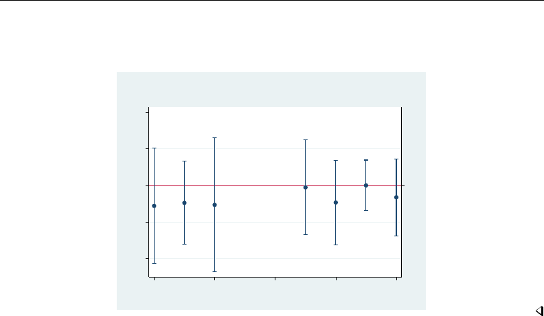
2118 serrbar — Graph standard error bar chart
. serrbar mean std date, scale(2) title("Observed Weight Variation")
> sub("San Francisco plant, 1/8 to 1/16") yline(195) yaxis(1 2)
> ylab(195, axis(2)) ytitle("", axis(2))
195
185 190 195 200 205
Package weight in lbs.
108 110 112 114 116
date
San Francisco plant, 1/8 to 1/16
Observed Weight Variation
Acknowledgment
serrbar was written by Nicholas J. Cox of the Department of Geography at Durham University,
UK, and coeditor of the Stata Journal.
Also see
[R]qc — Quality control charts

Title
set — Overview of system parameters
Syntax Description Remarks and examples Also see
Syntax
set setcommand . . .
set typed without arguments is equivalent to query typed without arguments.
Description
This entry provides a reference to Stata’s set commands. For many entries, more thorough
information is provided elsewhere; see the Reference field in each entry below for the location of
this information.
To reset system parameters to factory defaults, see [R]set defaults.
Remarks and examples
set adosize
Syntax: set adosize #, permanently
Default: 1,000
Description: sets the maximum amount of memory that automatically loaded do-files
may consume. 10 ≤#≤10000.
Reference: [P]sysdir
set autotabgraphs (Windows only)
Syntax: set autotabgraphs on |off , permanently
Default: off
Description: determines whether graphs are created as tabs within one window or as separate
windows.
set cformat
Syntax: set cformat fmt , permanently
Description: specifies the output format of coefficients, standard errors, and confidence limits
in coefficient tables. fmt is a numerical format; see [D]format.
Reference: [R]set cformat
set charset (Mac only)
Syntax: set charset mac |latin1 , permanently
Default: mac
Description: sets the character set used by Stata for Mac for rendering of ASCII text.
2119

2120 set — Overview of system parameters
set checksum
Syntax: set checksum on |off , permanently
Default: off
Description: determines whether files should be prevented from being downloaded from the
Internet if checksums do not match.
Reference: [D]checksum
set coeftabresults
Syntax: set coeftabresults on |off
Default: on
Description: determines whether coefficient table results are stored in r().
There is no permanently option because permanently is implied.
set conren (Unix console only)
Syntax 1: set conren
Syntax 2: set conren clear
Syntax 3: set conren sf |bf |it
result |txt |text|input |error |link |hilite
charchar. . .
Syntax 4: set conren {ulon |uloff}char char . . .
Syntax 5: set conren reset char char . . .
Description: can possibly make the output on your screen appear prettier.
set conren displays a list of the currently defined display codes.
set conren clear clears all codes.
set conren followed by a font type (bf,sf, or it) and display context (result,
error,link, or hilite) and then followed by a series of space-separated
characters sets the code for the specified font type and display context. If the font
type is omitted, the code is set to the same specified code for all three font types.
set conren ulon and set conren uloff set the codes for turning on and off
underlining.
set conren reset sets the code that will turn off all display and underlining codes.
Reference: [GSU]conren
set copycolor (Mac and Windows only)
Syntax: set copycolor automatic |asis |gs1 |gs2 |gs3 , permanently
Default: automatic
Description: determines how colors are handled when graphs are copied to the Clipboard.
Reference: [G-2]set printcolor
set dockable (Windows only)
Syntax: set dockable on |off , permanently
Default: on
Description: determines whether to enable the use of dockable window characteristics,
including the ability to dock or tab a window into another window.

set — Overview of system parameters 2121
set dockingguides (Windows only)
Syntax: set dockingguides on |off , permanently
Default: on
Description: determines whether to enable the use of dockable guides when repositioning
a dockable window.
set doublebuffer (Windows only)
Syntax: set doublebuffer on |off, permanently
Default: on
Description: enables or disables double buffering of the Results, Viewer, and Data Editor
windows. Double buffering prevents the windows from flickering when redrawn
or resized. Users who encounter performance problems such as the Results window
outputting very slowly should disable double buffering.
set dp
Syntax: set dp comma |period, permanently
Default: period
Description: determines whether a period or a comma is to be used as the decimal point.
Reference: [D]format
set emptycells
Syntax: set emptycells keep |drop, permanently
Default: keep
Description: sets what to do with empty cells in interactions.
Reference: [R]set emptycells
set eolchar (Mac only)
Syntax: set eolchar mac |unix, permanently
Default: unix
Description: sets the default end-of-line delimiter for text files created in Stata.
set fastscroll (Unix and Windows only)
Syntax: set fastscroll on |off, permanently
Default: on
Description: sets the scrolling method for new output in the Results window. Setting
fastscroll to on is faster but can be jumpy. Setting fastscroll to off
is slower but smoother.
set floatwindows (Windows only)
Syntax: set floatwindows on |off
Default: off
Description: determines whether to enable floating window behavior for dialog boxes and dockable
window. The term “float” in this context means that a window will always float
over the main Stata window; these windows cannot be placed behind the main Stata
window. There is no permanently option because permanently is implied.

2122 set — Overview of system parameters
set fvlabel
Syntax: set fvlabel {on |off }, permanently
Description: specifies whether to display factor-variable value labels in coefficient tables.
Reference: [R]set showbaselevels
set fvwrap
Syntax: set fvwrap #, permanently
Description: specifies that long value labels wrap #lines in coefficient tables.
Reference: [R]set showbaselevels
set fvwrapon
Syntax: set fvwrapon {word |width }, permanently
Description: specifies whether value labels that wrap will break at word bounderies or break
based on available space.
Reference: [R]set showbaselevels
set graphics
Syntax: set graphics on |off
Default: on; default is off for console Stata
Description: determines whether graphs are displayed on your monitor.
Reference: [G-2]set graphics
set haverdir
Syntax: set haverdir "path", permanently
Description: specifies the directory where the Haver databases are stored.
Reference: [D]import haver
set httpproxy
Syntax: set httpproxy on |off, init
Default: off
Description: turns on/off the use of a proxy server. There is no permanently option because
permanently is implied.
Reference: [R]netio
set httpproxyauth
Syntax: set httpproxyauth on |off
Default: off
Description: determines whether authorization is required for the proxy server.
There is no permanently option because permanently is implied.
Reference: [R]netio
set httpproxyhost
Syntax: set httpproxyhost "name"
Description: sets the name of a host to be used as a proxy server. There is no permanently
option because permanently is implied.
Reference: [R]netio

set — Overview of system parameters 2123
set httpproxyport
Syntax: set httpproxyport #
Default: 8080 if Stata cannot autodetect the proper setting for your computer.
Description: sets the port number for a proxy server. There is no permanently option
because permanently is implied.
Reference: [R]netio
set httpproxypw
Syntax: set httpproxypw "password"
Description: sets the appropriate password. There is no permanently option because
permanently is implied.
Reference: [R]netio
set httpproxyuser
Syntax: set httpproxyuser "name"
Description: sets the appropriate user ID. There is no permanently option because
permanently is implied.
Reference: [R]netio
set include bitmap (Mac only)
Syntax: set include bitmap on |off, permanently
Default: on
Description: sets the output behavior when copying an image to the Clipboard.
set level
Syntax: set level #, permanently
Default: 95
Description: sets the default confidence level for confidence intervals for all commands
that report confidence intervals. 10.00 ≤#≤99.99, and #can have at
most two digits after the decimal point.
Reference: [R]level
set linegap
Syntax: set linegap #
Default: 1
Description: sets the space between lines, in pixels, in the Results window. There is no
permanently option because permanently is implied.
set linesize
Syntax: set linesize #
Default: 1 less than the full width of the screen
Description: sets the line width, in characters, for both the screen and the log file.
Reference: [R]log

2124 set — Overview of system parameters
set locksplitters (Windows only)
Syntax: set locksplitters on |off , permanently
Default: off
Description: determines whether splitters should be locked so that docked windows
cannot be resized.
set logtype
Syntax: set logtype text |smcl, permanently
Default: smcl
Description: sets the default log filetype.
Reference: [R]log
set lstretch
Syntax: set lstretch on |off , permanently
Description: specifies whether to automatically widen the coefficient table up to the width of
the Results window to accommodate longer variable names.
set matacache,set matafavor,set matalibs,set matalnum,set matamofirst,
set mataoptimize, and set matastrict; see [M-3]mata set.
set matsize
Syntax: set matsize #, permanently
Default: 400 for Stata/MP, Stata/SE, and Stata/IC; 40 for Small Stata
Description: sets the maximum number of variables that can be included in any estimation
command. This setting cannot be changed in Small Stata.
10 ≤#≤11000 for Stata/MP and Stata/SE; 10 ≤#≤800 for Stata/IC.
Reference: [R]matsize
set max memory
Syntax: set max memory #b|k|m|g, permanently
Default: .(all the memory the operating system will supply)
Description: specifies the maximum amount of memory Stata can use to store your data.
2×segmentsize ≤#≤.
Reference: [D]memory
set maxdb
Syntax: set maxdb #, permanently
Default: 50
Description: sets the maximum number of dialog boxes whose contents are remembered
from one invocation to the next during a session. 5≤#≤1000
Reference: [R]db
set maxiter
Syntax: set maxiter #, permanently
Default: 16000
Description: sets the default maximum number of iterations for estimation commands.
0≤#≤16000
Reference: [R]maximize

set — Overview of system parameters 2125
set maxvar
Syntax: set maxvar #, permanently
Default: 5000 for Stata/MP and Stata/SE, 2048 for Stata/IC, and 99 for Small Stata
Description: sets the maximum number of variables. This can be changed only in Stata/MP and
Stata/SE. 2048 ≤#≤32767
Reference: [D]memory
set min memory
Syntax: set min memory #b|k|m|g, permanently
Default: 0
Description: specifies an amount of memory Stata will not fall below. This setting affects
efficiency, not the size of datasets you can analyze. 0≤#≤max memory
Reference: [D]memory
set more
Syntax: set more on |off, permanently
Default: on
Description: pauses when more is displayed, continuing only when the user presses a key.
Reference: [R]more
set niceness
Syntax: set niceness #, permanently
Default: 5
Description: affects how soon Stata gives back unused segments to the operating system.
0≤#≤10
Reference: [D]memory
set notifyuser (Mac only)
Syntax: set notifyuser on |off, permanently
Default: on
Description: sets the default Notification Manager behavior in Stata.
set obs
Syntax: set obs #
Default: current number of observations
Description: changes the number of observations in the current dataset. #must be at least
as large as the current number of observations. If there are variables in memory,
the values of all new observations are set to missing.
Reference: [D]obs
set odbcmgr (Unix only)
Syntax: set odbcmgr iodbc |unixodbc, permanently
Default: iodbc
Description: determines whether iODBC or unixODBC is your ODBC driver manager.
Reference: [D]odbc

2126 set — Overview of system parameters
set output
Syntax: set output proc |inform |error
Default: proc
Description: specifies the output to be displayed. proc means display all output; inform
suppresses procedure output but displays informative messages and error messages;
error suppresses all output except error messages. set output is seldom used.
Reference: [P]quietly
set pagesize
Syntax: set pagesize #
Default: 2 less than the physical number of lines on the screen
Description: sets the number of lines between more messages.
Reference: [R]more
set pformat
Syntax: set pformat fmt , permanently
Description: specifies the output format of p-values in coefficient tables.
fmt is a numerical format; see [D]format.
Reference: [R]set cformat
set pinnable (Windows only)
Syntax: set pinnable on |off , permanently
Default: on
Description: determines whether to enable the use of pinnable window characteristics for certain
windows in Stata.
set playsnd (Mac only)
Syntax: set playsnd on |off, permanently
Default: on
Description: sets the sound behavior for the Notification Manager behavior in Stata.
set printcolor
Syntax: set printcolor automatic |asis |gs1 |gs2 |gs3, permanently
Default: automatic
Description: determines how colors are handled when graphs are printed.
Reference: [G-2]set printcolor
set processors
Syntax: set processors #
Description: sets the number of processors or cores that Stata/MP will use. The default
is the number of processors available on the computer, or the number of
processors allowed by Stata/MP’s license, whichever is less.
set reventries
Syntax: set reventries #, permanently
Default: 5000
Description: sets the number of scrollback lines available in the Review window.
5≤#≤32000.

set — Overview of system parameters 2127
set revkeyboard (Mac only)
Syntax: set revkeyboard on |off, permanently
Default: on
Description: sets the keyboard navigation behavior for the Review window. on indicates
that you can use the keyboard to navigate and enter items from the Review
window into the Command window. off indicates that all keyboard input be
directed at the Command window; items can be entered from the Review
window only by using the mouse.
set rmsg
Syntax: set rmsg on |off, permanently
Default: off
Description: indicates whether a return message telling the execution time is to be displayed at
the completion of each command.
Reference: [P]rmsg
set scheme
Syntax: set scheme schemename , permanently
Default: s2color
Description: determines the overall look for graphs.
Reference: [G-2]set scheme
set scrollbufsize
Syntax: set scrollbufsize #
Default: 200000
Description: sets the scrollback buffer size, in bytes, for the Results window;
may be set between 10,000 and 2,000,000.
set searchdefault
Syntax: set searchdefault local |net |all, permanently
Default: local
Description: sets the default behavior of the search command. set searchdefault local
restricts search to use only Stata’s keyword database. set searchdefault net
restricts search to searching only the Internet. set searchdefault all
indicates that both the keyword database and the Internet are to be searched.
Reference: [R]search
set seed
Syntax: set seed #|code
Default: 123456789
Description: specifies initial value of the random-number seed used by the runiform() function.
Reference: [R]set seed
set segmentsize
Syntax: set segmentsize #b|k|m|g, permanently
Default: 32m for 64-bit machines; 16m for 32-bit machines
Description: Stata allocates memory for data in units of segmentsize. This setting changes the
amount of memory in a single segment.
1m ≤#≤32g for 64-bit machines; 1m ≤#≤1g for 32-bit machines
Reference: [D]memory

2128 set — Overview of system parameters
set sformat
Syntax: set sformat fmt , permanently
Description: specifies the output format of test statistics in coefficient tables.
fmt is a numerical format; see [D]format.
Reference: [R]set cformat
set showbaselevels
Syntax: set showbaselevels {on |off |all }, permanently
Description: specifies whether to display base levels of factor variables and their interactions
in coefficient tables.
Reference: [R]set showbaselevels
set showemptycells
Syntax: set showemptycells {on |off }, permanently
Description: specifies whether to display empty cells in coefficient tables.
Reference: [R]set showbaselevels
set showomitted
Syntax: set showomitted {on |off }, permanently
Description: specifies whether to display omitted coefficients in coefficient tables.
Reference: [R]set showbaselevels
set smoothfonts (Mac only)
Syntax: set smoothfonts on |off
Default: on
Description: determines whether to use font smoothing (antialiased text) in the Results, Viewer,
and Data Editor windows.
set timeout1
Syntax: set timeout1 #seconds , permanently
Default: 30
Description: sets the number of seconds Stata will wait for a remote host to respond to an initial
contact before giving up. In general, users should not modify this value unless
instructed to do so by Stata Technical Services.
Reference: [R]netio
set timeout2
Syntax: set timeout2 #seconds , permanently
Default: 180
Description: sets the number of seconds Stata will keep trying to get information from a remote
host after initial contact before giving up. In general, users should not modify this
value unless instructed to do so by Stata Technical Services.
Reference: [R]netio
set trace
Syntax: set trace on |off
Default: off
Description: determines whether to trace the execution of programs for debugging.
Reference: [P]trace

set — Overview of system parameters 2129
set tracedepth
Syntax: set tracedepth #
Default: 32000 (equivalent to ∞)
Description: if trace is set on, traces execution of programs and nested programs up to
tracedepth. For example, if tracedepth is 2, the current program and any
subroutine called would be traced, but subroutines of subroutines would not
be traced.
Reference: [P]trace
set traceexpand
Syntax: set traceexpand on |off, permanently
Default: on
Description: if trace is set on, shows lines both before and after macro expansion. If
traceexpand is set off, only the line before macro expansion is shown.
Reference: [P]trace
set tracehilite
Syntax: set tracehilite "pattern", word
Default: ""
Description: highlights pattern in the trace output.
Reference: [P]trace
set traceindent
Syntax: set traceindent on |off, permanently
Default: on
Description: if trace is set on, indents displayed lines according to their nesting level. The
lines of the main program are not indented. Two spaces of indentation are used for
each level of nested subroutine.
Reference: [P]trace
set tracenumber
Syntax: set tracenumber on |off, permanently
Default: off
Description: if trace is set on, shows the nesting level numerically in front of the line.
Lines of the main program are preceded by 01, lines of subroutines called by the
main program are preceded by 02, etc.
Reference: [P]trace
set tracesep
Syntax: set tracesep on |off, permanently
Default: on
Description: if trace is set on, displays a horizontal separator line that displays the name
of the subroutine whenever a subroutine is called or exits.
Reference: [P]trace

2130 set — Overview of system parameters
set type
Syntax: set type float |double, permanently
Default: float
Description: specifies the default storage type assigned to new variables.
Reference: [D]generate
set update interval (Mac and Windows only)
Syntax: set update interval #
Default: 7
Description: sets the number of days to elapse before performing the next automatic
update query.
Reference: [R]update
set update prompt (Mac and Windows only)
Syntax: set update prompt on |off
Default: on
Description: determines wheter a dialog is to be displayed before performing an automatic
update query. There is no permanently option because permanently is implied.
Reference: [R]update
set update query (Mac and Windows only)
Syntax: set update query on |off
Default: on
Description: determines whether update query is to be automatically performed when Stata
is launched. There is no permanently option because permanently is implied.
Reference: [R]update
set varabbrev
Syntax: set varabbrev on |off, permanently
Default: on
Description: indicates whether Stata should allow variable abbreviations.
Reference: [P]varabbrev
set varkeyboard (Mac only)
Syntax: set varkeyboard on |off, permanently
Default: on
Description: sets the keyboard navigation behavior for the Variables window. on indicates
that you can use the keyboard to navigate and enter items from the Variables
window into the Command window. off indicates that all keyboard input be
directed at the Command window; items can be entered from the Variables
window only by using the mouse.
Also see
[R]query — Display system parameters
[R]set defaults — Reset system parameters to original Stata defaults
[P]creturn — Return c-class values
[M-3]mata set — Set and display Mata system parameters

Title
set cformat — Format settings for coefficient tables
Syntax Description Option Remarks and examples Also see
Syntax
set cformat fmt , permanently
set pformat fmt , permanently
set sformat fmt , permanently
where fmt is a numerical format.
Description
set cformat specifies the output format of coefficients, standard errors, and confidence limits in
coefficient tables.
set pformat specifies the output format of p-values in coefficient tables.
set sformat specifies the output format of test statistics in coefficient tables.
Option
permanently specifies that, in addition to making the change right now, the setting be remembered
and become the default setting when you invoke Stata.
Remarks and examples
The formatting of the numbers in the coefficient table can be controlled by using the set cformat,
set pformat, and set sformat commands or by using the cformat(% fmt),pformat(% fmt), and
sformat(% fmt)options at the time of estimation or on replay of the estimation command. See
[R]estimation options.
The maximum format widths for set cformat,set pformat, and set sformat in coefficient
tables are 9, 5, and 8, respectively.
2131

2132 set cformat — Format settings for coefficient tables
Example 1
We use auto.dta to illustrate.
. use http://www.stata-press.com/data/r13/auto
(1978 Automobile Data)
. regress mpg weight displacement
Source SS df MS Number of obs = 74
F( 2, 71) = 66.79
Model 1595.40969 2 797.704846 Prob > F = 0.0000
Residual 848.049768 71 11.9443629 R-squared = 0.6529
Adj R-squared = 0.6432
Total 2443.45946 73 33.4720474 Root MSE = 3.4561
mpg Coef. Std. Err. t P>|t| [95% Conf. Interval]
weight -.0065671 .0011662 -5.63 0.000 -.0088925 -.0042417
displacement .0052808 .0098696 0.54 0.594 -.0143986 .0249602
_cons 40.08452 2.02011 19.84 0.000 36.05654 44.11251
. set cformat %9.2f
. regress mpg weight displacement
Source SS df MS Number of obs = 74
F( 2, 71) = 66.79
Model 1595.40969 2 797.704846 Prob > F = 0.0000
Residual 848.049768 71 11.9443629 R-squared = 0.6529
Adj R-squared = 0.6432
Total 2443.45946 73 33.4720474 Root MSE = 3.4561
mpg Coef. Std. Err. t P>|t| [95% Conf. Interval]
weight -0.01 0.00 -5.63 0.000 -0.01 -0.00
displacement 0.01 0.01 0.54 0.594 -0.01 0.02
_cons 40.08 2.02 19.84 0.000 36.06 44.11
. regress mpg weight displacement, cformat(%9.3f)
Source SS df MS Number of obs = 74
F( 2, 71) = 66.79
Model 1595.40969 2 797.704846 Prob > F = 0.0000
Residual 848.049768 71 11.9443629 R-squared = 0.6529
Adj R-squared = 0.6432
Total 2443.45946 73 33.4720474 Root MSE = 3.4561
mpg Coef. Std. Err. t P>|t| [95% Conf. Interval]
weight -0.007 0.001 -5.63 0.000 -0.009 -0.004
displacement 0.005 0.010 0.54 0.594 -0.014 0.025
_cons 40.085 2.020 19.84 0.000 36.057 44.113

set cformat — Format settings for coefficient tables 2133
To reset the cformat setting to its command-specific default, type
. set cformat
. regress mpg weight displacement
Source SS df MS Number of obs = 74
F( 2, 71) = 66.79
Model 1595.40969 2 797.704846 Prob > F = 0.0000
Residual 848.049768 71 11.9443629 R-squared = 0.6529
Adj R-squared = 0.6432
Total 2443.45946 73 33.4720474 Root MSE = 3.4561
mpg Coef. Std. Err. t P>|t| [95% Conf. Interval]
weight -.0065671 .0011662 -5.63 0.000 -.0088925 -.0042417
displacement .0052808 .0098696 0.54 0.594 -.0143986 .0249602
_cons 40.08452 2.02011 19.84 0.000 36.05654 44.11251
Also see
[R]estimation options — Estimation options
[R]query — Display system parameters
[R]set — Overview of system parameters
[U] 20.8 Formatting the coefficient table

Title
set defaults — Reset system parameters to original Stata defaults
Syntax Description Option Remarks and examples Also see
Syntax
set defaults category |all, permanently
where category is one of memory |output |interface |graphics |efficiency |
network |update |trace |mata |other
Description
set defaults resets settings made by set to the original default settings that were shipped with
Stata.
set defaults all resets all the categories, whereas set defaults category resets only the
settings for the specified category.
Option
permanently specifies that, in addition to making the change right now, the settings be remembered
and become the default settings when you invoke Stata.
Remarks and examples
Example 1
To assist us in debugging a new command, we modified some of the trace settings. To return
them to their original values, we type
. set_defaults trace
-> set trace off
-> set tracedepth 32000
-> set traceexpand on
-> set tracesep on
-> set traceindent on
-> set tracenumber off
-> set tracehilite ""
(preferences reset)
2134


Title
set emptycells — Set what to do with empty cells in interactions
Syntax Description Option Remarks and examples Also see
Syntax
set emptycells {keep |drop }, permanently
Description
set emptycells allows you to control how Stata handles interaction terms with empty cells.
Stata can keep empty cells or drop them. The default is to keep empty cells.
Option
permanently specifies that, in addition to making the change right now, the setting be remembered
and become the default setting when you invoke Stata.
Remarks and examples
By default, Stata keeps empty cells so they can be reported in the coefficient table. For example,
type
. use http://www.stata-press.com/data/r13/auto
. regress mpg rep78#foreign, baselevels
and you will see a regression of mpg on 10 indicator variables because rep78 takes on 5 values and
foreign takes on 2 values in the auto dataset. Two of those cells will be reported as empty because
the data contain no observations of foreign cars with a rep78 value of 1 or 2.
Many real datasets contain a large number of empty cells, and this could cause the “matsize too
small” error, r(908). In that case, type
. set emptycells drop
to get Stata to drop empty cells from the list of coefficients. If you commonly fit models with empty
cells, you can permanently set Stata to drop empty cells by typing the following:
. set emptycells drop, permanently
Also see
[R]set — Overview of system parameters
2136

Title
set seed — Specify initial value of random-number seed
Syntax Description Remarks and examples Also see
Syntax
set seed #
set seed statecode
where
#is any number between 0 and 231 −1(2,147,483,647), and
statecode is a random-number state previously obtained from creturn value c(seed).
Description
set seed #specifies the initial value of the random-number seed used by the random-number
functions, such as runiform() and rnormal().
set seed statecode resets the state of the random-number functions to the value specified, which
is a state previously obtained from creturn value c(seed).
Remarks and examples
Remarks are presented under the following headings:
Examples
Setting the seed
How to choose a seed
Do not set the seed too often
Preserving and restoring the random-number generator state
Examples
1. Specify initial value of random-number seed
. set seed 339487731
2. Create variable ucontaining uniformly distributed pseudorandom numbers on the interval [0,1)
. generate u = runiform()
3. Create variable zcontaining normally distributed random numbers with mean 0 and standard
deviation 1
. generate z = rnormal()
4. Obtain state of pseudorandom-number generator and store it in a local macro named state
. local state = c(seed)
5. Restore pseudorandom-number generator state to that previously stored in local macro named
state
. set seed ‘state’
2137

2138 set seed — Specify initial value of random-number seed
Setting the seed
Stata’s random-number generation functions, such as runiform() and rnormal(), do not really
produce random numbers. These functions are deterministic algorithms that produce numbers that
can pass for random. runiform() produces numbers that can pass for independent draws from a
rectangular distribution over [0,1);rnormal() produces numbers that can pass for independent draws
from N(0,1). Stata’s random-number functions are formally called pseudorandom-number functions.
The sequences these functions produce are determined by the seed, which is just a number and
which is set to 123456789 every time Stata is launched. This means that runiform() produces
the same sequence each time you start Stata. The first time you use runiform() after Stata is
launched, runiform() returns 0.136984078446403146. The second time you use it, runiform()
returns 0.643220667960122228. The third time you use it, . . . .
To obtain different sequences, you must specify different seeds using the set seed command.
You might specify the seed 472195:
. set seed 472195
If you were now to use runiform(), the first call would return 0.247166610788553953, the second
call would return 0.593119932804256678, and so on. Whenever you set seed 472195,runiform()
will return those numbers the first two times you use it.
Thus you set the seed to obtain different pseudorandom sequences from the pseudorandom-number
functions.
If you record the seed you set, pseudorandom results such as results from a simulation or imputed
values from mi impute can be reproduced later. Whatever you do after setting the seed, if you set
the seed to the same value and repeat what you did, you will obtain the same results.
How to choose a seed
Your best choice for the seed is an element chosen randomly from the set {0,1,...,2,147,483,647}.
We recommend that, but that is difficult to achieve because finding easy-to-access, truly random sources
is difficult.
One person we know uses digits from the serial numbers from dollar bills he finds in his wallet.
Of course, the numbers he obtains are not really random, but they are good enough, and they are
probably a good deal more random than the seeds most people choose. Some people use dates and
times, although we recommend against that because, over the day, it just gets later and later, and
that is a pattern. Others try to make up a random number, figuring if they include enough digits, the
result just has to be random. This is a variation on the five-second rule for dropped food, and we
admit to using both of these rules.
It does not really matter how you set the seed, as long as there is no obvious pattern in the seeds
that you set and as long as you do not set the seed too often during a session.
Nonetheless, here are two methods that we have seen used but you should not use:
1. The first time you set the seed, you set the number 1. The next time, you set 2, and then 3,
and so on. Variations on this included setting 1001, 1002, 1003, . . . , or setting 1001, 2001,
3001, and so on.
Do not follow any of these procedures. The seeds you set must not exhibit a pattern.

set seed — Specify initial value of random-number seed 2139
2. To set the seed, you obtain a pseudorandom number from runiform() and then use the
digits from that to form the seed.
This is a bad idea because the pseudorandom-number generator can converge to a cycle.
If you obtained the pseudorandom-number generator unrelated to those in Stata, this would
work well, but then you would have to find a rule to set the first generator’s seed. In any
case, the pseudorandom-number generators in Stata are all closely related, and so you must
not follow this procedure.
Choosing seeds that do not exhibit a pattern is of great importance. That the seeds satisfy the
other properties of randomness is minor by comparison.
Do not set the seed too often
We cannot emphasize this enough: Do not set the seed too often.
To see why this is such a bad idea, consider the limiting case: You set the seed, draw one
pseudorandom number, reset the seed, draw again, and so continue. The pseudorandom numbers you
obtain will be nothing more than the seeds you run through a mathematical function. The results you
obtain will not pass for random unless the seeds you choose pass for random. If you already had
such numbers, why are you even bothering to use the pseudorandom-number generator?
The definition of too often is more than once per problem.
If you are running a simulation of 10,000 replications, set the seed at the start of the simulation
and do not reset it until the 10,000th replication is finished. The pseudorandom-number generators
provided by Stata have long periods. The longer you go between setting the seed, the more random-like
are the numbers produced.
It is sometimes useful later to be able to reproduce in isolation any one of the replications, and so
you might be tempted to set the seed to a known value for each of the replications. We negatively
mentioned setting the seed to 1, 2, . . . , and it is in exactly such situations that we have seen this done.
The advantage, however, is that you could reproduce the fifth replication merely by setting the seed
to 5 and then repeating whatever it is that is to be replicated. If this is your goal, you do not need
to reset the seed. You can record the state of the random-number generator, save the state with your
replication results, and then use the recorded states later to reproduce whichever of the replications
that you wish. This will be discussed in Preserving and restoring the random-number generator state.
There is another reason you might be tempted to set the seed more than once per problem. It
sometimes happens that you run a simulation, let’s say for 5,000 replications, and then you decide
you should have run it for 10,000 replications. Instead of running all 10,000 replications afresh, you
decide to save time by running another 5,000 replications and then combining those results with
your previous 5,000 results. That is okay. We at StataCorp do this kind of thing. If you do this, it
is important that you set the seed especially well, particularly if you repeat this process to add yet
another 5,000 replications. It is also important that in each run there be a large enough number of
replications, which is say thousands of them.
Even so, do not do this: You want 500,000 replications. To obtain them, you run in batches of
1,000, setting the seed 500 times. Unless you have a truly random source for the seeds, it is unlikely
you can produce a patternless sequence of 500 seeds. The fact that you ran 1,000 replications in
between choosing the seeds does not mitigate the requirement that there be no pattern to the seeds
you set.
In all cases, the best solution is to set the seed only once and then use the method we suggest in
the next section.

2140 set seed — Specify initial value of random-number seed
Preserving and restoring the random-number generator state
In the previous section, we discussed the case in which you might be tempted to set the seed
more frequently than otherwise necessary, either to save time or to be able to rerun any one of the
replications. In such cases, there is an alternative to setting a new seed: recording the state of the
pseudorandom-number generator and then restoring the state later should the need arise.
The state of the random-number generator is a string that looks like this:
Xb5804563c43f462544a474abacbdd93d00021fb3
You can obtain the state from c(seed):
. display c(seed)
Xb5804563c43f462544a474abacbdd93d00021fb3
The name c(seed) is unfortunate because it suggests that
Xb5804563c43f462544a474abacbdd93d00021fb3 is nothing more than a seed such as 1073741823 in
a different guise. It is not. A better name for c(seed) would have been c(rng state). The state
string specifies an entry point into the sequence produced by the pseudorandom-number generator.
Let us explain.
The best way to use a pseudorandom-number generator would be to choose a seed once, draw
random numbers until you use up the generator, and then get a new generator and choose a new key.
Pseudorandom-number generators have a period, after which they repeat the original sequence. That
is what we mean by using up a generator. The period of the pseudorandom-number generator that
Stata is currently using is over 2123. Stata uses the KISS generator. It is difficult to imagine that you
could ever use up KISS.
The string reported by c(seed) reports an encoded form of the information necessary for Stata
to reestablish exactly where it is located in the pseudorandom-number generator’s sequence.
We are not seriously suggesting you choose only one seed over your entire lifetime, but let’s look
at how you might do that. Sometime after birth, when you needed your first random number, you
would set your seed,
. set seed 1073741823
On that day, you would draw, say, 10,000 pseudorandom numbers, perhaps to impute some missing
values. Being done for the day, you type
. display c(seed)
X15b512f3b2143ab434f1c92f4e7058e400023bc3
The next day, after launching Stata, you type
. set seed X15b512f3b2143ab434f1c92f4e7058e400023bc3
When you type set seed followed by a state string rather than a number, instead of setting the
seed, Stata reestablishes the previous state. Thus the next time you draw a pseudorandom number,
Stata will produce the 10,001st result after setting seed 1073741823. Let’s assume that you draw
100,000 numbers this day. Done for the day, you display c(seed).
. display c(seed)
X5d13d693a72ad0602b093cc4f61e07a500020381
On the third day, after setting the seed to the string above, you will be in a position to draw the
110,001st pseudorandom number.
In this way, you would eat your way though the 2123 random numbers, but you would be unlikely
ever to make it to the end. Assuming you did this every day for 100 years, to arrive at the end of
the sequence you would need to consume 2.9e+32 pseudorandom numbers per day.

set seed — Specify initial value of random-number seed 2141
We do not expect you to set the seed just once in your life, but using the state string makes it
easy to set the seed just once for a problem.
When we do simulations at StataCorp, we record c(seed) for each replication. Just like everybody
else, we record results from replications as observations in datasets; we just happen to have an extra
variable in the dataset, namely, a string variable named state. That string is filled in observation by
observation from the then-current values of c(seed), which is a function and so can be used in any
context that a function can be used in Stata.
Anytime we want to reproduce a particular replication, we thus have the information we need to
reset the pseudorandom-number generator, and having it in the dataset is convenient because we had
to go there anyway to determine which replication we wanted to reproduce.
In addition to recording each of the state strings for each replication, we record the closing value
of c(seed) as a note, which is easy enough to do:
. note: closing state ‘c(seed)’
If we want to add more replications later, we have a state string that we can use to continue from
where we left off.
Also see
[R]set — Overview of system parameters
[D]functions — Functions

Title
set showbaselevels — Display settings for coefficient tables
Syntax Description Option Remarks and examples Also see
Syntax
set showbaselevels {on |off |all }, permanently
set showemptycells {on |off }, permanently
set showomitted {on |off }, permanently
set fvlabel {on |off }, permanently
set fvwrap #, permanently
set fvwrapon {word |width }, permanently
Description
set showbaselevels specifies whether to display base levels of factor variables and their
interactions in coefficient tables. set showbaselevels on specifies that base levels be reported for
factor variables and for interactions whose bases cannot be inferred from their component factor
variables. set showbaselevels all specifies that all base levels of factor variables and interactions
be reported.
set showemptycells specifies whether to display empty cells in coefficient tables.
set showomitted specifies whether to display omitted coefficients in coefficient tables.
set fvlabel specifies whether to display factor-variable value labels in coefficient tables. set
fvlabel on, the default, specifies that the labels be displayed. set fvlabel off specifies that the
levels of factor variables rather than the labels be displayed.
set fvwrap #specifies that long value labels wrap #lines in the coefficient table. The default is
set fvwrap 1, which means that long value labels will be abbreviated to fit on one line.
set fvwrapon specifies whether value labels that wrap will break at word boundaries or break
based on available space. set fvwrapon word, the default, specifies that value labels break at word
boundaries. set fvwrapon width specifies that value labels break based on available space.
Option
permanently specifies that, in addition to making the change right now, the setting be remembered
and become the default setting when you invoke Stata.
2142

set showbaselevels — Display settings for coefficient tables 2143
Remarks and examples
Example 1
We illustrate the first three set commands using cholesterol2.dta.
. use http://www.stata-press.com/data/r13/cholesterol2
(Artificial cholesterol data, empty cells)
. generate x = race
. regress chol race##agegrp x
note: 2.race#2.agegrp identifies no observations in the sample
note: x omitted because of collinearity
Source SS df MS Number of obs = 70
F( 13, 56) = 13.51
Model 15751.6113 13 1211.66241 Prob > F = 0.0000
Residual 5022.71559 56 89.6913498 R-squared = 0.7582
Adj R-squared = 0.7021
Total 20774.3269 69 301.077201 Root MSE = 9.4706
chol Coef. Std. Err. t P>|t| [95% Conf. Interval]
race
white 12.84185 5.989703 2.14 0.036 .8430383 24.84067
other -.167627 5.989703 -0.03 0.978 -12.16644 11.83119
agegrp
20-29 17.24681 5.989703 2.88 0.006 5.247991 29.24562
30-39 31.43847 5.989703 5.25 0.000 19.43966 43.43729
40-59 34.86613 5.989703 5.82 0.000 22.86732 46.86495
60-79 44.43374 5.989703 7.42 0.000 32.43492 56.43256
race#agegrp
white 20-29 0 (empty)
white 30-39 -22.83983 8.470719 -2.70 0.009 -39.80872 -5.870939
white 40-59 -14.67558 8.470719 -1.73 0.089 -31.64447 2.293306
white 60-79 -10.51115 8.470719 -1.24 0.220 -27.48004 6.457735
other 20-29 -6.054425 8.470719 -0.71 0.478 -23.02331 10.91446
other 30-39 -11.48083 8.470719 -1.36 0.181 -28.44971 5.488063
other 40-59 -.6796112 8.470719 -0.08 0.936 -17.6485 16.28928
other 60-79 -1.578052 8.470719 -0.19 0.853 -18.54694 15.39084
x 0 (omitted)
_cons 175.2309 4.235359 41.37 0.000 166.7464 183.7153
. set showemptycells off
. set showomitted off
. set showbaselevels all

2144 set showbaselevels — Display settings for coefficient tables
. regress chol race##agegrp x
note: 2.race#2.agegrp identifies no observations in the sample
note: x omitted because of collinearity
Source SS df MS Number of obs = 70
F( 13, 56) = 13.51
Model 15751.6113 13 1211.66241 Prob > F = 0.0000
Residual 5022.71559 56 89.6913498 R-squared = 0.7582
Adj R-squared = 0.7021
Total 20774.3269 69 301.077201 Root MSE = 9.4706
chol Coef. Std. Err. t P>|t| [95% Conf. Interval]
race
black 0 (base)
white 12.84185 5.989703 2.14 0.036 .8430383 24.84067
other -.167627 5.989703 -0.03 0.978 -12.16644 11.83119
agegrp
10-19 0 (base)
20-29 17.24681 5.989703 2.88 0.006 5.247991 29.24562
30-39 31.43847 5.989703 5.25 0.000 19.43966 43.43729
40-59 34.86613 5.989703 5.82 0.000 22.86732 46.86495
60-79 44.43374 5.989703 7.42 0.000 32.43492 56.43256
race#agegrp
black 10-19 0 (base)
black 20-29 0 (base)
black 30-39 0 (base)
black 40-59 0 (base)
black 60-79 0 (base)
white 10-19 0 (base)
white 30-39 -22.83983 8.470719 -2.70 0.009 -39.80872 -5.870939
white 40-59 -14.67558 8.470719 -1.73 0.089 -31.64447 2.293306
white 60-79 -10.51115 8.470719 -1.24 0.220 -27.48004 6.457735
other 10-19 0 (base)
other 20-29 -6.054425 8.470719 -0.71 0.478 -23.02331 10.91446
other 30-39 -11.48083 8.470719 -1.36 0.181 -28.44971 5.488063
other 40-59 -.6796112 8.470719 -0.08 0.936 -17.6485 16.28928
other 60-79 -1.578052 8.470719 -0.19 0.853 -18.54694 15.39084
_cons 175.2309 4.235359 41.37 0.000 166.7464 183.7153

set showbaselevels — Display settings for coefficient tables 2145
To restore the display of empty cells, omitted predictors, and baselevels to their command-specific
default behavior, type
. set showemptycells
. set showomitted
. set showbaselevels
. regress chol race##agegrp x
note: 2.race#2.agegrp identifies no observations in the sample
note: x omitted because of collinearity
Source SS df MS Number of obs = 70
F( 13, 56) = 13.51
Model 15751.6113 13 1211.66241 Prob > F = 0.0000
Residual 5022.71559 56 89.6913498 R-squared = 0.7582
Adj R-squared = 0.7021
Total 20774.3269 69 301.077201 Root MSE = 9.4706
chol Coef. Std. Err. t P>|t| [95% Conf. Interval]
race
white 12.84185 5.989703 2.14 0.036 .8430383 24.84067
other -.167627 5.989703 -0.03 0.978 -12.16644 11.83119
agegrp
20-29 17.24681 5.989703 2.88 0.006 5.247991 29.24562
30-39 31.43847 5.989703 5.25 0.000 19.43966 43.43729
40-59 34.86613 5.989703 5.82 0.000 22.86732 46.86495
60-79 44.43374 5.989703 7.42 0.000 32.43492 56.43256
race#agegrp
white 20-29 0 (empty)
white 30-39 -22.83983 8.470719 -2.70 0.009 -39.80872 -5.870939
white 40-59 -14.67558 8.470719 -1.73 0.089 -31.64447 2.293306
white 60-79 -10.51115 8.470719 -1.24 0.220 -27.48004 6.457735
other 20-29 -6.054425 8.470719 -0.71 0.478 -23.02331 10.91446
other 30-39 -11.48083 8.470719 -1.36 0.181 -28.44971 5.488063
other 40-59 -.6796112 8.470719 -0.08 0.936 -17.6485 16.28928
other 60-79 -1.578052 8.470719 -0.19 0.853 -18.54694 15.39084
x 0 (omitted)
_cons 175.2309 4.235359 41.37 0.000 166.7464 183.7153

2146 set showbaselevels — Display settings for coefficient tables
Example 2
We illustrate the last three set commands using jaw.dta.
. use http://www.stata-press.com/data/r13/jaw, clear
(Table 4.6 Two-Way Unbalanced Data for Fractures of the Jaw -- Rencher (1998))
. mvreg y1 y2 y3 = i.fracture
Equation Obs Parms RMSE "R-sq" F P
y1 27 3 10.42366 0.2966 5.060804 0.0147
y2 27 3 6.325398 0.1341 1.858342 0.1777
y3 27 3 5.976973 0.1024 1.368879 0.2735
Coef. Std. Err. t P>|t| [95% Conf. Interval]
y1
fracture
two compou.. -8.833333 4.957441 -1.78 0.087 -19.06499 1.398322
one simple.. 6 5.394759 1.11 0.277 -5.134235 17.13423
_cons 37 3.939775 9.39 0.000 28.8687 45.1313
y2
fracture
two compou.. -5.761905 3.008327 -1.92 0.067 -11.97079 .446977
one simple.. -3.053571 3.273705 -0.93 0.360 -9.810166 3.703023
_cons 38.42857 2.390776 16.07 0.000 33.49425 43.36289
y3
fracture
two compou.. 4.261905 2.842618 1.50 0.147 -1.60497 10.12878
one simple.. .9285714 3.093377 0.30 0.767 -5.455846 7.312989
_cons 58.57143 2.259083 25.93 0.000 53.90891 63.23395

set showbaselevels — Display settings for coefficient tables 2147
. set fvwrap 2
. mvreg y1 y2 y3 = i.fracture
Equation Obs Parms RMSE "R-sq" F P
y1 27 3 10.42366 0.2966 5.060804 0.0147
y2 27 3 6.325398 0.1341 1.858342 0.1777
y3 27 3 5.976973 0.1024 1.368879 0.2735
Coef. Std. Err. t P>|t| [95% Conf. Interval]
y1
fracture
two compound
fractures -8.833333 4.957441 -1.78 0.087 -19.06499 1.398322
one simple
fracture 6 5.394759 1.11 0.277 -5.134235 17.13423
_cons 37 3.939775 9.39 0.000 28.8687 45.1313
y2
fracture
two compound
fractures -5.761905 3.008327 -1.92 0.067 -11.97079 .446977
one simple
fracture -3.053571 3.273705 -0.93 0.360 -9.810166 3.703023
_cons 38.42857 2.390776 16.07 0.000 33.49425 43.36289
y3
fracture
two compound
fractures 4.261905 2.842618 1.50 0.147 -1.60497 10.12878
one simple
fracture .9285714 3.093377 0.30 0.767 -5.455846 7.312989
_cons 58.57143 2.259083 25.93 0.000 53.90891 63.23395

2148 set showbaselevels — Display settings for coefficient tables
. set fvwrapon width
. mvreg y1 y2 y3 = i.fracture
Equation Obs Parms RMSE "R-sq" F P
y1 27 3 10.42366 0.2966 5.060804 0.0147
y2 27 3 6.325398 0.1341 1.858342 0.1777
y3 27 3 5.976973 0.1024 1.368879 0.2735
Coef. Std. Err. t P>|t| [95% Conf. Interval]
y1
fracture
two compound
fractures -8.833333 4.957441 -1.78 0.087 -19.06499 1.398322
one simple f
racture 6 5.394759 1.11 0.277 -5.134235 17.13423
_cons 37 3.939775 9.39 0.000 28.8687 45.1313
y2
fracture
two compound
fractures -5.761905 3.008327 -1.92 0.067 -11.97079 .446977
one simple f
racture -3.053571 3.273705 -0.93 0.360 -9.810166 3.703023
_cons 38.42857 2.390776 16.07 0.000 33.49425 43.36289
y3
fracture
two compound
fractures 4.261905 2.842618 1.50 0.147 -1.60497 10.12878
one simple f
racture .9285714 3.093377 0.30 0.767 -5.455846 7.312989
_cons 58.57143 2.259083 25.93 0.000 53.90891 63.23395

set showbaselevels — Display settings for coefficient tables 2149
. set showfvlabel off
. mvreg y1 y2 y3 = i.fracture
Equation Obs Parms RMSE "R-sq" F P
y1 27 3 10.42366 0.2966 5.060804 0.0147
y2 27 3 6.325398 0.1341 1.858342 0.1777
y3 27 3 5.976973 0.1024 1.368879 0.2735
Coef. Std. Err. t P>|t| [95% Conf. Interval]
y1
fracture
2 -8.833333 4.957441 -1.78 0.087 -19.06499 1.398322
3 6 5.394759 1.11 0.277 -5.134235 17.13423
_cons 37 3.939775 9.39 0.000 28.8687 45.1313
y2
fracture
2 -5.761905 3.008327 -1.92 0.067 -11.97079 .446977
3 -3.053571 3.273705 -0.93 0.360 -9.810166 3.703023
_cons 38.42857 2.390776 16.07 0.000 33.49425 43.36289
y3
fracture
2 4.261905 2.842618 1.50 0.147 -1.60497 10.12878
3 .9285714 3.093377 0.30 0.767 -5.455846 7.312989
_cons 58.57143 2.259083 25.93 0.000 53.90891 63.23395

2150 set showbaselevels — Display settings for coefficient tables
To restore these last three set commands to their defaults, type
. set showfvlabel on
. set fvwrap 1
. set fvwrapon word
. mvreg y1 y2 y3 = i.fracture
Equation Obs Parms RMSE "R-sq" F P
y1 27 3 10.42366 0.2966 5.060804 0.0147
y2 27 3 6.325398 0.1341 1.858342 0.1777
y3 27 3 5.976973 0.1024 1.368879 0.2735
Coef. Std. Err. t P>|t| [95% Conf. Interval]
y1
fracture
two compou.. -8.833333 4.957441 -1.78 0.087 -19.06499 1.398322
one simple.. 6 5.394759 1.11 0.277 -5.134235 17.13423
_cons 37 3.939775 9.39 0.000 28.8687 45.1313
y2
fracture
two compou.. -5.761905 3.008327 -1.92 0.067 -11.97079 .446977
one simple.. -3.053571 3.273705 -0.93 0.360 -9.810166 3.703023
_cons 38.42857 2.390776 16.07 0.000 33.49425 43.36289
y3
fracture
two compou.. 4.261905 2.842618 1.50 0.147 -1.60497 10.12878
one simple.. .9285714 3.093377 0.30 0.767 -5.455846 7.312989
_cons 58.57143 2.259083 25.93 0.000 53.90891 63.23395
Also see
[R]set — Overview of system parameters
[R]query — Display system parameters

Title
signrank — Equality tests on matched data
Syntax Menu Description Remarks and examples
Stored results Methods and formulas References Also see
Syntax
Wilcoxon matched-pairs signed-ranks test
signrank varname =exp if in
Sign test of matched pairs
signtest varname =exp if in
by is allowed with signrank and signtest; see [D] by.
Menu
signrank
Statistics >Nonparametric analysis >Tests of hypotheses >Wilcoxon matched-pairs signed-rank test
signtest
Statistics >Nonparametric analysis >Tests of hypotheses >Test equality of matched pairs
Description
signrank tests the equality of matched pairs of observations by using the Wilcoxon matched-pairs
signed-ranks test (Wilcoxon 1945). The null hypothesis is that both distributions are the same.
signtest also tests the equality of matched pairs of observations (Arbuthnott [1710], but better
explained by Snedecor and Cochran [1989]) by calculating the differences between varname and the
expression. The null hypothesis is that the median of the differences is zero; no further assumptions
are made about the distributions. This, in turn, is equivalent to the hypothesis that the true proportion
of positive (negative) signs is one-half.
For equality tests on unmatched data, see [R]ranksum.
Remarks and examples
Example 1: signrank
We are testing the effectiveness of a new fuel additive. We run an experiment with 12 cars. We
first run each car without the fuel treatment and measure the mileage. We then add the fuel treatment
and repeat the experiment. The results of the experiment are
2151

2152 signrank — Equality tests on matched data
Without With Without With
treatment treatment treatment treatment
20 24 18 17
23 25 24 28
21 21 20 24
25 22 24 27
18 23 23 21
17 18 19 23
We create two variables called mpg1 and mpg2, representing mileage without and with the treatment,
respectively. We can test the null hypothesis that the treatment had no effect by typing
. use http://www.stata-press.com/data/r13/fuel
. signrank mpg1=mpg2
Wilcoxon signed-rank test
sign obs sum ranks expected
positive 3 13.5 38.5
negative 8 63.5 38.5
zero 111
all 12 78 78
unadjusted variance 162.50
adjustment for ties -1.62
adjustment for zeros -0.25
adjusted variance 160.62
Ho: mpg1 = mpg2
z = -1.973
Prob > |z| = 0.0485
The output indicates that we can reject the null hypothesis at any level above 4.85%.
Example 2: signtest
signtest tests that the median of the differences is zero, making no further assumptions, whereas
signrank assumed that the distributions are equal as well. Using the data above, we type
. signtest mpg1=mpg2
Sign test
sign observed expected
positive 3 5.5
negative 8 5.5
zero 1 1
all 12 12
One-sided tests:
Ho: median of mpg1 - mpg2 = 0 vs.
Ha: median of mpg1 - mpg2 > 0
Pr(#positive >= 3) =
Binomial(n = 11, x >= 3, p = 0.5) = 0.9673
Ho: median of mpg1 - mpg2 = 0 vs.
Ha: median of mpg1 - mpg2 < 0
Pr(#negative >= 8) =
Binomial(n = 11, x >= 8, p = 0.5) = 0.1133

signrank — Equality tests on matched data 2153
Two-sided test:
Ho: median of mpg1 - mpg2 = 0 vs.
Ha: median of mpg1 - mpg2 != 0
Pr(#positive >= 8 or #negative >= 8) =
min(1, 2*Binomial(n = 11, x >= 8, p = 0.5)) = 0.2266
The summary table indicates that there were three comparisons for which mpg1 exceeded mpg2, eight
comparisons for which mpg2 exceeded mpg1, and one comparison for which they were the same.
The output below the summary table is based on the binomial distribution. The significance of the
one-sided test, where the alternative hypothesis is that the median of mpg2 −mpg1 is greater than
zero, is 0.1133. The significance of the two-sided test, where the alternative hypothesis is simply that
the median of the differences is different from zero, is 0.2266 =2×0.1133.
Stored results
signrank stores the following in r():
Scalars
r(N neg) number of negative comparisons r(sum neg) sum of the negative ranks
r(N pos) number of positive comparisons r(z) zstatistic
r(N tie) number of tied comparisons r(Var a) adjusted variance
r(sum pos) sum of the positive ranks
signtest stores the following in r():
Scalars
r(N neg) number of negative comparisons r(p 2) two-sided probability
r(N pos) number of positive comparisons r(p neg) one-sided probability of negative
comparison
r(N tie) number of tied comparisons r(p pos) one-sided probability of positive
comparison
Methods and formulas
For a practical introduction to these techniques with an emphasis on examples rather than theory,
see Bland (2000) or Sprent and Smeeton (2007). For a summary of these tests, see Snedecor and
Cochran (1989).
Methods and formulas are presented under the following headings:
signrank
signtest
signrank
Both the sign test and Wilcoxon signed-rank tests test the null hypothesis that the distribution
of a random variable D=varname −exp has median zero. The sign test makes no additional
assumptions, but the Wilcoxon signed-rank test makes the additional assumption that the distribution
of Dis symmetric. If D=X1−X2, where X1and X2have the same distribution, then it follows
that the distribution of Dis symmetric about zero. Thus the Wilcoxon signed-rank test is often
described as a test of the hypothesis that two distributions are the same, that is, X1∼X2.

2154 signrank — Equality tests on matched data
Let djdenote the difference for any matched pair of observations,
dj=x1j−x2j=varname −exp
for j=1,2, . . . , n.
Rank the absolute values of the differences, |dj|, and assign any tied values the average rank.
Consider the signs of dj, and let
rj=sign(dj)rank(|dj|)
be the signed ranks. The test statistic is
Tobs =
n
X
j=1
rj= (sum of ranks for +signs)−(sum of ranks for −signs)
The null hypothesis is that the distribution of djis symmetric about 0. Hence the likelihood is
unchanged if we flip signs on the dj, and thus the randomization datasets are the 2npossible sign
changes for the dj. Thus the randomization distribution of our test statistic Tcan be computed by
considering all the 2npossible values of
T=
n
X
j=1
Sjrj
where the rjare the observed signed ranks (considered fixed) and Sjis either +1 or −1.
With this distribution, the mean and variance of Tare given by
E(T) = 0 and Varadj(T) =
n
X
j=1
r2
j
The test statistic for the Wilcoxon signed-rank test is often expressed (equivalently) as the sum of
the positive signed-ranks, T+, where
E(T+) = n(n+ 1)
4and Varadj(T+) = 1
4
n
X
j=1
r2
j
Zeros and ties do not affect the theory above, and the exact variance is still given by the above
formula for Varadj(T+). When dj=0 is observed, djwill always be zero in each of the randomization
datasets (using sign(0) = 0). When there are ties, you can assign averaged ranks for each group of
ties and then treat them the same as the other ranks.
The “unadjusted variance” reported by signrank is the variance that the randomization distribution
would have had if there had been no ties or zeros:
Varunadj(T+) = 1
4
n
X
j=1
j2=n(n+ 1)(2n+ 1)
24
The adjustment for zeros is the change in the variance when the ranks for the zeros are signed to
make rj=0,
∆Varzero adj(T+) = −1
4
n0
X
j=1
j2=−n0(n0+ 1)(2n0+ 1)
24

signrank — Equality tests on matched data 2155
where n0is the number of zeros. The adjustment for ties is the change in the variance when the
ranks (for nonzero observations) are replaced by averaged ranks:
∆Varties adj(T+) = Varadj(T+)−Varunadj(T+)−∆Varzero adj(T+)
A normal approximation is used to calculate
z=T+−E(T+)
pVaradj(T+)
signtest
The test statistic for the sign test is the number n+of differences
dj=x1j−x2j=varname −exp
greater than zero. Assuming that the probability of a difference being equal to zero is exactly zero, then,
under the null hypothesis, n+∼binomial(n, p =1/2), where nis the total number of observations.
But what if some differences are zero? This question has a ready answer if you view the test
from the perspective of Fisher’s Principle of Randomization (Fisher 1935). Fisher’s idea (stated in a
modern way) was to look at a family of transformations of the observed data such that the a priori
likelihood (under the null hypothesis) of the transformed data is the same as the likelihood of the
observed data. The distribution of the test statistic is then produced by calculating its value for each
of the transformed “randomization” datasets, assuming that each dataset is equally likely.
For the sign test, the “data” are simply the set of signs of the differences. Under the null hypothesis
of the sign test, the probability that djis less than zero is equal to the probability that djis greater
than zero. Thus you can transform the observed signs by flipping any number of them, and the set of
signs will have the same likelihood. The 2npossible sign changes form the family of randomization
datasets. If you have no zeros, this procedure again leads to n+∼binomial(n, p =1/2).
If you do have zeros, changing their signs leaves them as zeros. So, if you observe n0zeros,
each of the 2nsign-change datasets will also have n0zeros. Hence, the values of n+calculated
over the sign-change datasets range from 0 to n−n0, and the “randomization” distribution of n+is
binomial(n−n0, p =1/2).
The work of Arbuthnott (1710) and later eighteenth-century contributions is discussed by Hald (2003,
chap. 17).
Frank Wilcoxon (1892–1965) was born in Ireland to American parents. After working in various
occupations (including merchant seaman, oil-well pump attendant, and tree surgeon), he settled in
chemistry, gaining degrees from Rutgers and Cornell and employment from various companies.
Working mainly on the development of fungicides and insecticides, Wilcoxon became interested
in statistics in 1925 and made several key contributions to nonparametric methods. After retiring
from industry, he taught statistics at Florida State until his death.

2156 signrank — Equality tests on matched data
References
Arbuthnott, J. 1710. An argument for divine providence, taken from the constant regularity observed in the births of
both sexes. Philosophical Transaction of the Royal Society of London 27: 186–190.
Bland, M. 2000. An Introduction to Medical Statistics. 3rd ed. Oxford: Oxford University Press.
Bradley, R. A. 2001. Frank Wilcoxon. In Statisticians of the Centuries, ed. C. C. Heyde and E. Seneta, 420–424.
New York: Springer.
Fisher, R. A. 1935. The Design of Experiments. Edinburgh: Oliver & Boyd.
Hald, A. 2003. A History of Probability and Statistics and Their Applications before 1750. New York: Wiley.
Harris, T., and J. W. Hardin. 2013. Exact Wilcoxon signed-rank and Wilcoxon Mann–Whitney ranksum tests.Stata
Journal 13: 337–343.
Kaiser, J. 2007. An exact and a Monte Carlo proposal to the Fisher–Pitman permutation tests for paired replicates
and for independent samples.Stata Journal 7: 402–412.
Newson, R. B. 2006. Confidence intervals for rank statistics: Somers’ D and extensions.Stata Journal 6: 309–334.
Snedecor, G. W., and W. G. Cochran. 1989. Statistical Methods. 8th ed. Ames, IA: Iowa State University Press.
Sprent, P., and N. C. Smeeton. 2007. Applied Nonparametric Statistical Methods. 4th ed. Boca Raton, FL: Chapman
& Hall/CRC.
Sribney, W. M. 1995. crc40: Correcting for ties and zeros in sign and rank tests. Stata Technical Bulletin 26: 2–4.
Reprinted in Stata Technical Bulletin Reprints, vol. 5, pp. 5–8. College Station, TX: Stata Press.
Wilcoxon, F. 1945. Individual comparisons by ranking methods. Biometrics 1: 80–83.
Also see
[R]ranksum — Equality tests on unmatched data
[R]ttest —ttests (mean-comparison tests)

Title
simulate — Monte Carlo simulations
Syntax Description Options Remarks and examples
References Also see
Syntax
simulate exp list , reps(#)options :command
options Description
nodots suppress replication dots
noisily display any output from command
trace trace command
saving( filename,. . .)save results to filename
nolegend suppress table legend
verbose display the full table legend
seed(#)set random-number seed to #
All weight types supported by command are allowed; see [U] 11.1.6 weight.
exp list contains (name:elist)
elist
eexp
elist contains newvar = (exp)
(exp)
eexp is specname
[eqno]specname
specname is b
b[]
se
se[]
eqno is ##
name
exp is a standard Stata expression; see [U] 13 Functions and expressions.
Distinguish between [ ], which are to be typed, and , which indicate optional arguments.
Description
simulate eases the programming task of performing Monte Carlo–type simulations. Typing
. simulate exp list, reps(#): command
runs command for #replications and collects the results in exp list.
2157

2158 simulate — Monte Carlo simulations
command defines the command that performs one simulation. Most Stata commands and user-
written programs can be used with simulate, as long as they follow standard Stata syntax; see
[U] 11 Language syntax. The by prefix may not be part of command.
exp list specifies the expression to be calculated from the execution of command. If no expressions
are given, exp list assumes a default, depending upon whether command changes results in e() or
r(). If command changes results in e(), the default is b. If command changes results in r() (but
not e()), the default is all the scalars posted to r(). It is an error not to specify an expression in
exp list otherwise.
Options
reps(#)is required—it specifies the number of replications to be performed.
nodots suppresses display of the replication dots. By default, one dot character is displayed for each
successful replication. A red ‘x’ is displayed if command returns an error or if one of the values
in exp list is missing.
noisily requests that any output from command be displayed. This option implies the nodots
option.
trace causes a trace of the execution of command to be displayed. This option implies the noisily
option.
saving( filename,suboptions )creates a Stata data file (.dta file) consisting of (for each statistic
in exp list) a variable containing the simulated values.
double specifies that the results for each replication be saved as doubles, meaning 8-byte reals.
By default, they are saved as floats, meaning 4-byte reals.
every(#)specifies that results be written to disk every #th replication. every() should be specified
only in conjunction with saving() when command takes a long time for each replication.
This will allow recovery of partial results should some other software crash your computer.
See [P]postfile.
replace specifies that filename be overwritten if it exists.
nolegend suppresses display of the table legend. The table legend identifies the rows of the table
with the expressions they represent.
verbose requests that the full table legend be displayed. By default, coefficients and standard errors
are not displayed.
seed(#)sets the random-number seed. Specifying this option is equivalent to typing the following
command before calling simulate:
. set seed #
Remarks and examples
For an introduction to Monte Carlo methods, see Cameron and Trivedi (2010, chap. 4). White (2010)
provides a command for analyzing results of simulation studies.

simulate — Monte Carlo simulations 2159
Example 1: Simulating basic summary statistics
We have a dataset containing means and variances of 100-observation samples from a lognormal
distribution (as a first step in evaluating, say, the coverage of a 95%, t-based confidence interval).
Then we perform the experiment 1,000 times.
The following command definition will generate 100 independent observations from a lognormal
distribution and compute the summary statistics for this sample.
program lnsim, rclass
version 13
drop _all
set obs 100
gen z = exp(rnormal())
summarize z
return scalar mean = r(mean)
return scalar Var = r(Var)
end
We can save 1,000 simulated means and variances from lnsim by typing
. set seed 1234
. simulate mean=r(mean) var=r(Var), reps(1000) nodots: lnsim
command: lnsim
mean: r(mean)
var: r(Var)
. describe *
storage display value
variable name type format label variable label
mean float %9.0g r(mean)
var float %9.0g r(Var)
. summarize
Variable Obs Mean Std. Dev. Min Max
mean 1000 1.638466 .214371 1.095099 2.887392
var 1000 4.63856 6.428406 .8626 175.3746
Technical note
Before executing our lnsim simulator, we can verify that it works by executing it interactively.
. set seed 1234
. lnsim
obs was 0, now 100
Variable Obs Mean Std. Dev. Min Max
z 100 1.597757 1.734328 .0625807 12.71548
. return list
scalars:
r(Var) = 3.007893773683719
r(mean) = 1.59775722913444

2160 simulate — Monte Carlo simulations
Example 2: Simulating a regression model
Consider a more complicated problem. Let’s experiment with fitting yj=a+bxj+ujwhen the
true model has a=1, b=2, uj=zj+cxj, and when zjis N(0,1). We will save the parameter
estimates and standard errors and experiment with varying c.xjwill be fixed across experiments but
will originally be generated as N(0,1). We begin by interactively making the true data:
. drop _all
. set obs 100
obs was 0, now 100
. set seed 54321
. gen x = rnormal()
. gen true_y = 1+2*x
. save truth
file truth.dta saved
Our program is
program hetero1
version 13
args c
use truth, clear
gen y = true_y + (rnormal() + ‘c’*x)
regress y x
end
Note the use of ‘c’ in our statement for generating y.cis a local macro generated from args c and
thus refers to the first argument supplied to hetero1. If we want c=3 for our experiment, we type
. simulate _b _se, reps(10000): hetero1 3
(output omitted )
Our program hetero1 could, however, be more efficient because it rereads the file truth once
every replication. It would be better if we could read the data just once. In fact, if we read in the data
right before running simulate, we really should not have to reread for each subsequent replication.
A faster version reads
program hetero2
version 13
args c
capture drop y
gen y = true_y + (rnormal() + ‘c’*x)
regress y x
end
Requiring that the current dataset has the variables true y and xmay become inconvenient.
Another improvement would be to require that the user supply variable names, such as in
program hetero3
version 13
args truey x c
capture drop y
gen y = ‘truey’ + (rnormal() + ‘c’*‘x’)
regress y x
end
Thus we can type
. simulate _b _se, reps(10000): hetero3 true_y x 3
(output omitted )
simulate — Monte Carlo simulations 2161
Example 3: Simulating a ratio of statistics
Now let’s consider the problem of simulating the ratio of two medians. Suppose that each sample
of size nicomes from a normal population with a mean µiand standard deviation σi, where i=1,2.
We write the program below and save it as a text file called myratio.ado (see [U] 17 Ado-files).
Our program is an rclass command that requires six arguments as input, identified by the local
macros n1,mu1,sigma1,n2,mu2, and sigma2, which correspond to n1,µ1,σ1,n2,µ2, and
σ2, respectively. With these arguments, myratio will generate the data for the two samples, use
summarize to compute the two medians and store the ratio of the medians in r(ratio).
program myratio, rclass
version 13
args n1 mu1 sigma1 n2 mu2 sigma2
// generate the data
drop _all
local N = ‘n1’+‘n2’
set obs ‘N’
tempvar y
generate ‘y’ = rnormal()
replace ‘y’ = cond(_n<=‘n1’,‘mu1’+‘y’*‘sigma1’,‘mu2’+‘y’*‘sigma2’)
// calculate the medians
tempname m1
summarize ‘y’ if _n<=‘n1’, detail
scalar ‘m1’ = r(p50)
summarize ‘y’ if _n>‘n1’, detail
// store the results
return scalar ratio = ‘m1’ / r(p50)
end
The result of running our simulation is
. set seed 19192
. simulate ratio=r(ratio), reps(1000) nodots: myratio 5 3 1 10 3 2
command: myratio 5 3 1 10 3 2
ratio: r(ratio)
. summarize
Variable Obs Mean Std. Dev. Min Max
ratio 1000 1.08571 .4427828 .3834799 6.742217
Technical note
Stata lets us do simulations of simulations and simulations of bootstraps. Stata’s bootstrap
command (see [R]bootstrap) works much like simulate, except that it feeds the user-written
program a bootstrap sample. Say that we want to evaluate the bootstrap estimator of the standard
error of the median when applied to lognormally distributed data. We want to perform a simulation,
resulting in a dataset of medians and bootstrap estimated standard errors.
As background, summarize (see [R]summarize) calculates summary statistics, leaving the mean
in r(mean) and the standard deviation in r(sd).summarize with the detail option also calculates
summary statistics, but more of them, and leaves the median in r(p50).
Thus our plan is to perform simulations by randomly drawing a dataset: we calculate the median
of our random sample, we use bootstrap to obtain a dataset of medians calculated from bootstrap
samples of our random sample, the standard deviation of those medians is our estimate of the standard
error, and the summary statistics are stored in the results of summarize.
2162 simulate — Monte Carlo simulations
Our simulator is
program define bsse, rclass
version 13
drop _all
set obs 100
gen x = rnormal()
tempfile bsfile
bootstrap midp=r(p50), rep(100) saving(‘bsfile’): summarize x, detail
use ‘bsfile’, clear
summarize midp
return scalar mean = r(mean)
return scalar sd = r(sd)
end
We can obtain final results, running our simulation 1,000 times, by typing
. set seed 48901
. simulate med=r(mean) bs_se=r(sd), reps(1000): bsse
command: bsse
med: r(mean)
bs_se: r(sd)
Simulations (1000)
12345
.................................................. 50
.................................................. 100
.................................................. 150
.................................................. 200
.................................................. 250
.................................................. 300
.................................................. 350
.................................................. 400
.................................................. 450
.................................................. 500
.................................................. 550
.................................................. 600
.................................................. 650
.................................................. 700
.................................................. 750
.................................................. 800
.................................................. 850
.................................................. 900
.................................................. 950
.................................................. 1000
. summarize
Variable Obs Mean Std. Dev. Min Max
med 1000 -.0008696 .1210451 -.3132536 .4058724
bs_se 1000 .126236 .029646 .0326791 .2596813
This is a case where the simulation dots (drawn by default, unless the nodots option is specified)
will give us an idea of how long this simulation will take to finish as it runs.
References
Cameron, A. C., and P. K. Trivedi. 2010. Microeconometrics Using Stata. Rev. ed. College Station, TX: Stata Press.
Gould, W. W. 1994. ssi6.1: Simplified Monte Carlo simulations.Stata Technical Bulletin 20: 22–24. Reprinted in
Stata Technical Bulletin Reprints, vol. 4, pp. 207–210. College Station, TX: Stata Press.

simulate — Monte Carlo simulations 2163
Hamilton, L. C. 2013. Statistics with Stata: Updated for Version 12. 8th ed. Boston: Brooks/Cole.
Hilbe, J. M. 2010. Creating synthetic discrete-response regression models.Stata Journal 10: 104–124.
Weesie, J. 1998. ip25: Parameterized Monte Carlo simulations: Enhancement to the simulation command.Stata
Technical Bulletin 43: 13–15. Reprinted in Stata Technical Bulletin Reprints, vol. 8, pp. 75–77. College Station,
TX: Stata Press.
White, I. R. 2010. simsum: Analyses of simulation studies including Monte Carlo error.Stata Journal 10: 369–385.
Also see
[R]bootstrap — Bootstrap sampling and estimation
[R]jackknife — Jackknife estimation
[R]permute — Monte Carlo permutation tests

Title
sj — Stata Journal and STB installation instructions
Description Remarks and examples Also see
Description
The Stata Journal (SJ) is a quarterly journal containing articles about statistics, data analysis,
teaching methods, and effective use of Stata’s language. The SJ publishes reviewed papers together
with shorter notes and comments, regular columns, tips, book reviews, and other material of interest
to researchers applying statistics in a variety of disciplines. You can read all about the Stata Journal
at http://www.stata-journal.com.
The Stata Journal is a printed and electronic journal with corresponding software. If you want
the journal, you must subscribe, but the software is available for no charge from our website at
http://www.stata-journal.com.PDF copies of SJ articles that are older than three years are available
for download for no charge at http://www.stata-journal.com/archives.html. More recent articles may
be individually purchased.
The predecessor to the Stata Journal was the Stata Technical Bulletin (STB). The STB was
also a printed and electronic journal with corresponding software. PDF copies of all STB journals
are available for download for no charge at http://www.stata-press.com/journals/stbj.html. The STB
software is available for no charge from our website at http://www.stata.com.
Below are instructions for installing the Stata Journal and the Stata Technical Bulletin software
from our website.
Remarks and examples
Remarks are presented under the following headings:
Installing the Stata Journal software
Obtaining from the Internet by pointing and clicking
Obtaining from the Internet via command mode
Installing the STB software
Obtaining from the Internet by pointing and clicking
Obtaining from the Internet via command mode
Installing the Stata Journal software
Each issue of the Stata Journal is labeled Volume #, Number #. Volume 1 refers to the first year
of publication, Volume 2 to the second, and so on. Issues are numbered 1, 2, 3, and 4 within each
year. The first issue of the Journal was published in the fourth quarter of 2001, and that issue is
numbered Volume 1, Number 1. For installation purposes, we refer to this issue as sj1-1.
The articles, columns, notes, and comments that make up the Stata Journal are assigned a letter-
and-number code, called an insert tag, such as st0001, an0034, or ds0011. The letters represent a
category: st is the statistics category, an is the announcements category, etc. The numbers are assigned
sequentially, so st0001 is the first article in the statistics category.
Sometimes inserts are subsequently updated, either to fix bugs or to add new features. A number
such as st0001 1 indicates that this article, column, note, or comment is an update to the original
st0001 article. Updates are complete; that is, installing st0001 1 provides all the features of the
original article and more.
2164

sj — Stata Journal and STB installation instructions 2165
The Stata Journal software may be obtained by pointing and clicking or by using command mode.
The sections below detail how to install an insert. In all cases, pretend that you wish to install
insert st0274 from sj12-4.
Obtaining from the Internet by pointing and clicking
1. Select Help > SJ and User-written Programs.
2. Click on Stata Journal.
3. Click on sj12-4.
4. Click on st0274.
5. Click on (click here to install).
Obtaining from the Internet via command mode
Type the following:
. net from http://www.stata-journal.com/software
. net cd sj12-4
. net describe st0274
. net install st0274
The above could be shortened to
. net from http://www.stata-journal.com/software/sj12-4
. net describe st0274
. net install st0274
Alternatively, you could type
. net sj 12-4
. net describe st0274
. net install st0274
but going about it the long way is more entertaining, at least the first time.
Installing the STB software
Each issue of the STB is numbered. STB-1 refers to the first issue (published May 1991), STB-2
refers to the second (published July 1991), and so on.
An issue of the STB consists of inserts—articles—and these are assigned letter-and-number
combinations, such as sg84, dm80, sbe26.1, etc. The letters represent a category; for example, sg
is the general statistics category and dm the data management category. The numbers are assigned
sequentially, so sbe39 is the 39th insert in the biostatistics and epidemiology series.
Insert sbe39, it turns out, provides a method of accounting for publication bias in meta-analysis; it
adds a new command called metatrim to Stata. If you installed sbe39, you would have that command
and its help file. Insert sbe39 was published in STB-57 (September 2000). Obtaining metatrim simply
requires going to STB-57 and getting sbe39.
Sometimes inserts were subsequently updated, either to fix bugs or to add new features. sbe39 was
updated: the first update is sbe39.1 and the second is sbe39.2. You could install insert sbe39.2, and
it would not matter whether you had previously installed sbe39.1. Updates are complete: installing
sbe39.2 provides all the features of the original insert and more.

2166 sj — Stata Journal and STB installation instructions
For computer naming purposes, insert sbe39.2 is referred to as sbe39 2. When referred to in
normal text, however, the insert is still called sbe39.2 because that looks nicer.
Inserts are easily available from the Internet. Inserts may be obtained by pointing and clicking or
by using command mode.
The sections below detail how to install an insert. In all cases, pretend that you wish to install
insert sbe39.2 from STB-61.
Obtaining from the Internet by pointing and clicking
1. Select Help > SJ and User-written Programs.
2. Click on STB.
3. Click on stb61.
4. Click on sbe39 2.
5. Click on (click here to install).
Obtaining from the Internet via command mode
Type the following:
. net from http://www.stata.com
. net cd stb
. net cd stb61
. net describe sbe39_2
. net install sbe39_2
The above could be shortened to
. net from http://www.stata.com/stb/stb61
. net describe sbe39_2
. net install sbe39_2
but going about it the long way is more entertaining, at least the first time.
Also see
[R]search — Search Stata documentation and other resources
[R]net — Install and manage user-written additions from the Internet
[R]net search — Search the Internet for installable packages
[R]update — Check for official updates
[U] 3.5 The Stata Journal
[U] 28 Using the Internet to keep up to date
[GSM] 19 Updating and extending Stata—Internet functionality
[GSU] 19 Updating and extending Stata—Internet functionality
[GSW] 19 Updating and extending Stata—Internet functionality

Title
sktest — Skewness and kurtosis test for normality
Syntax Menu Description Option
Remarks and examples Stored results Methods and formulas Acknowledgments
References Also see
Syntax
sktest varlist if in weight , noadjust
aweights and fweights are allowed; see [U] 11.1.6 weight.
Menu
Statistics >Summaries, tables, and tests >Distributional plots and tests >Skewness and kurtosis normality test
Description
For each variable in varlist,sktest presents a test for normality based on skewness and another
based on kurtosis and then combines the two tests into an overall test statistic. sktest requires a
minimum of 8 observations to make its calculations. See [MV]mvtest normality for multivariate
tests of normality.
Option
Main
noadjust suppresses the empirical adjustment made by Royston (1991c) to the overall χ2and
its significance level and presents the unaltered test as described by D’Agostino, Belanger, and
D’Agostino (1990).
Remarks and examples
Also see [R]swilk for the Shapiro–Wilk and Shapiro – Francia tests for normality. Those tests are,
in general, preferred for nonaggregated data (Gould and Rogers 1991;Gould 1992;Royston 1991c).
Moreover, a normal quantile plot should be used with any test for normality; see [R]diagnostic plots
for more information.
2167
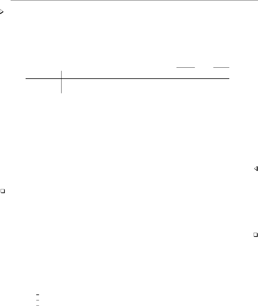
2168 sktest — Skewness and kurtosis test for normality
Example 1
Using our automobile dataset, we will test whether the variables mpg and trunk are normally
distributed:
. use http://www.stata-press.com/data/r13/auto
(1978 Automobile Data)
. sktest mpg trunk
Skewness/Kurtosis tests for Normality
joint
Variable Obs Pr(Skewness) Pr(Kurtosis) adj chi2(2) Prob>chi2
mpg 74 0.0015 0.0804 10.95 0.0042
trunk 74 0.9115 0.0445 4.19 0.1228
We can reject the hypothesis that mpg is normally distributed, but we cannot reject the hypothesis
that trunk is normally distributed, at least at the 12% level. The kurtosis for trunk is 2.19, as can
be verified by issuing the command
. summarize trunk, detail
(output omitted )
and the p-value of 0.0445 shown in the table above indicates that it is significantly different from
the kurtosis of a normal distribution at the 5% significance level. However, on the basis of skewness
alone, we cannot reject the hypothesis that trunk is normally distributed.
Technical note
sktest implements the test as described by D’Agostino, Belanger, and D’Agostino (1990) but with
the adjustment made by Royston (1991c). In the above example, if we had specified the noadjust
option, the χ2values would have been 13.13 for mpg and 4.05 for trunk. With the adjustment, the
χ2value might show as ‘.’. This result should be interpreted as an absurdly large number; the data
are most certainly not normal.
Stored results
sktest stores the following in r():
Scalars
r(chi2) χ2
r(P skew) Pr(skewness)
r(P kurt) Pr(kurtosis)
r(P chi2) Prob >chi2
Matrices
r(N) matrix of observations
r(Utest) matrix of test results, one row per variable

sktest — Skewness and kurtosis test for normality 2169
Methods and formulas
sktest implements the test described by D’Agostino, Belanger, and D’Agostino (1990) with the
empirical correction developed by Royston (1991c).
Let g1denote the coefficient of skewness and b2denote the coefficient of kurtosis as calculated
by summarize, and let ndenote the sample size. If weights are specified, then g1,b2, and n
denote the weighted coefficients of skewness and kurtosis and weighted sample size, respectively.
See [R]summarize for the formulas for skewness and kurtosis.
To perform the test of skewness, we compute
Y=g1(n+ 1)(n+ 3)
6(n−2) 1/2
β2(g1) = 3(n2+ 27n−70)(n+ 1)(n+ 3)
(n−2)(n+ 5)(n+ 7)(n+ 9)
W2=−1 + [2 {β2(g1)−1}]1/2
α=2/(W2−1)1/2
and
Then the distribution of the test statistic
Z1=1
√lnWln hY/α +(Y/α)2+ 11/2i
is approximately standard normal under the null hypothesis that the data are distributed normally.
To perform the test of kurtosis, we compute
E(b2) = 3(n−1)
n+ 1
var(b2) = 24n(n−2)(n−3)
(n+ 1)2(n+ 3)(n+ 5)
X={b2−E(b2)}/pvar(b2)
pβ1(b2) = 6(n2−5n+ 2)
(n+ 7)(n+ 9) 6(n+ 3)(n+ 5)
n(n−2)(n−3)1/2
A= 6 + 8
pβ1(b2)"2
pβ1(b2)+1 + 4
β1(b2)1/2#
and
Then the distribution of the test statistic
Z2=1
p2/(9A)
1−2
9A−(1−2/A
1 + Xp2/(A−4))1/3
is approximately standard normal under the null hypothesis that the data are distributed normally.
D’Agostino, Balanger, and D’Agostino Jr.’s omnibus test of normality uses the statistic
K2=Z2
1+Z2
2
which has approximately a χ2distribution with 2 degrees of freedom under the null of normality.

2170 sktest — Skewness and kurtosis test for normality
Royston (1991c) proposed the following adjustment to the test of normality, which sktest uses
by default. Let Φ(x)denote the cumulative standard normal distribution function for x, and let
Φ−1(p)denote the inverse cumulative standard normal function [that is, x= Φ−1{Φ(x)}]. Define
the following terms:
Zc=−Φ−1exp −1
2K2
Zt= 0.55n0.2−0.21
a1= (−5+3.46 lnn) exp(−1.37 lnn)
b1= 1 + (0.854 −0.148 lnn) exp(−0.55 lnn)
a2=a1− {2.13/(1 −2.37 lnn)}Zt
b2= 2.13/(1 −2.37 lnn) + b1and
If Zc<−1set Z=Zc; else if Zc< Ztset Z=a1+b1Zc; else set Z=a2+b2Zc. Define
P= 1 −Φ(Z). Then K2=−2lnPis approximately distributed χ2with 2 degrees of freedom.
The relative merits of the skewness and kurtosis test versus the Shapiro–Wilk and Shapiro–Francia
tests have been a subject of debate. The interested reader is directed to the articles in the Stata Technical
Bulletin. Our recommendation is to use the Shapiro–Francia test whenever possible, that is, whenever
dealing with nonaggregated or ungrouped data (Gould and Rogers 1991;Gould 1992); see [R]swilk.
If normality is rejected, use sktest to determine the source of the problem.
As both D’Agostino, Belanger, and D’Agostino (1990) and Royston (1991d) mention, researchers
should also examine the normal quantile plot to determine normality rather than blindly relying on a
few test statistics. See the qnorm command documented in [R]diagnostic plots for more information
on normal quantile plots.
sktest is similar in spirit to the Jarque–Bera (1987) test of normality. The Jarque–Bera test
statistic is also calculated from the sample skewness and kurtosis, though it is based on asymptotic
standard errors with no corrections for sample size. In effect, sktest offers two adjustments for
sample size, that of Royston (1991c) and that of D’Agostino, Belanger, and D’Agostino (1990).
Acknowledgments
sktest has benefited greatly by the comments and work of Patrick Royston of the MRC Clinical
Trials Unit, London, and coauthor of the Stata Press book Flexible Parametric Survival Analysis
Using Stata: Beyond the Cox Model. At this point, the program should be viewed as due as much to
Royston as to us, except, of course, for any errors. We are also indebted to Nicholas J. Cox of the
Department of Geography at Durham University, UK, and coeditor of the Stata Journal for his helpful
comments.
References
D’Agostino, R. B., A. J. Belanger, and R. B. D’Agostino, Jr. 1990. A suggestion for using powerful and informative
tests of normality. American Statistician 44: 316–321.
. 1991. sg3.3: Comment on tests of normality.Stata Technical Bulletin 3: 20. Reprinted in Stata Technical
Bulletin Reprints, vol. 1, pp. 105–106. College Station, TX: Stata Press.
Gould, W. W. 1991. sg3: Skewness and kurtosis tests of normality.Stata Technical Bulletin 1: 20–21. Reprinted in
Stata Technical Bulletin Reprints, vol. 1, pp. 99–101. College Station, TX: Stata Press.
. 1992. sg11.1: Quantile regression with bootstrapped standard errors.Stata Technical Bulletin 9: 19–21. Reprinted
in Stata Technical Bulletin Reprints, vol. 2, pp. 137–139. College Station, TX: Stata Press.

sktest — Skewness and kurtosis test for normality 2171
Gould, W. W., and W. H. Rogers. 1991. sg3.4: Summary of tests of normality.Stata Technical Bulletin 3: 20–23.
Reprinted in Stata Technical Bulletin Reprints, vol. 1, pp. 106–110. College Station, TX: Stata Press.
Jarque, C. M., and A. K. Bera. 1987. A test for normality of observations and regression residuals. International
Statistical Review 2: 163–172.
Marchenko, Y. V., and M. G. Genton. 2010. A suite of commands for fitting the skew-normal and skew-t models.
Stata Journal 10: 507–539.
Royston, P. 1991a. sg3.1: Tests for departure from normality.Stata Technical Bulletin 2: 16–17. Reprinted in Stata
Technical Bulletin Reprints, vol. 1, pp. 101–104. College Station, TX: Stata Press.
. 1991b. sg3.2: Shapiro–Wilk and Shapiro–Francia tests.Stata Technical Bulletin 3: 19. Reprinted in Stata
Technical Bulletin Reprints, vol. 1, p. 105. College Station, TX: Stata Press.
. 1991c. sg3.5: Comment on sg3.4 and an improved D’Agostino test.Stata Technical Bulletin 3: 23–24. Reprinted
in Stata Technical Bulletin Reprints, vol. 1, pp. 110–112. College Station, TX: Stata Press.
. 1991d. sg3.6: A response to sg3.3: Comment on tests of normality.Stata Technical Bulletin 4: 8–9. Reprinted
in Stata Technical Bulletin Reprints, vol. 1, pp. 112–114. College Station, TX: Stata Press.
Also see
[R]diagnostic plots — Distributional diagnostic plots
[R]ladder — Ladder of powers
[R]lv — Letter-value displays
[R]swilk — Shapiro–Wilk and Shapiro – Francia tests for normality
[MV]mvtest normality — Multivariate normality tests

Title
slogit — Stereotype logistic regression
Syntax Menu Description Options
Remarks and examples Stored results Methods and formulas References
Also see
Syntax
slogit depvar indepvars if in weight ,options
options Description
Model
dimension(#)dimension of the model; default is dimension(1)
baseoutcome(#|lbl)set the base outcome to #or lbl; default is the last outcome
constraints(numlist)apply specified linear constraints
collinear keep collinear variables
nocorner do not generate the corner constraints
SE/Robust
vce(vcetype)vcetype may be oim,robust,cluster clustvar,opg,bootstrap,
or jackknife
Reporting
level(#)set confidence level; default is level(95)
nocnsreport do not display constraints
display options control column formats, row spacing, line width, display of omitted
variables and base and empty cells, and factor-variable labeling
Maximization
maximize options control the maximization process; seldom used
initialize(initype)method of initializing scale parameters; initype can be constant,
random, or svd; see Options for details
nonormalize do not normalize the numeric variables
coeflegend display legend instead of statistics
indepvars may contain factor variables; see [U] 11.4.3 Factor variables.
bootstrap,by,fp,jackknife,rolling,statsby, and svy are allowed; see [U] 11.1.10 Prefix commands.
Weights are not allowed with the bootstrap prefix; see [R] bootstrap.
vce() and weights are not allowed with the svy prefix; see [SVY] svy.
fweights, iweights, and pweights are allowed; see [U] 11.1.6 weight.
coeflegend does not appear in the dialog box.
See [U] 20 Estimation and postestimation commands for more capabilities of estimation commands.
2172

slogit — Stereotype logistic regression 2173
Menu
Statistics >Categorical outcomes >Stereotype logistic regression
Description
slogit fits maximum-likelihood stereotype logistic regression models as developed by Ander-
son (1984). Like multinomial logistic and ordered logistic models, stereotype logistic models are for
use with categorical dependent variables. In a multinomial logistic model, the categories cannot be
ranked, whereas in an ordered logistic model the categories follow a natural ranking scheme. You
can view stereotype logistic models as a compromise between those two models. You can use them
when you are unsure of the relevance of the ordering, as is often the case when subjects are asked to
assess or judge something. You can also use them in place of multinomial logistic models when you
suspect that some of the alternatives are similar. Unlike ordered logistic models, stereotype logistic
models do not impose the proportional-odds assumption.
Options
Model
dimension(#)specifies the dimension of the model, which is the number of equations required
to describe the relationship between the dependent variable and the independent variables. The
maximum dimension is min(m−1, p), where mis the number of categories of the dependent
variable and pis the number of independent variables in the model. The stereotype model with
maximum dimension is a reparameterization of the multinomial logistic model.
baseoutcome(#|lbl)specifies the outcome level whose scale parameters and intercept are constrained
to be zero. The base outcome may be specified as a number of a label. By default, slogit assumes
that the outcome levels are ordered and uses the largest level of the dependent variable as the base
outcome.
constraints(numlist),collinear; see [R]estimation options.
By default, the linear equality constraints suggested by Anderson (1984), termed the corner
constraints, are generated for you. You can add constraints to these as needed, or you can turn off
the corner constraints by specifying nocorner. These constraints are in addition to the constraints
placed on the φparameters corresponding to baseoutcome(#).
nocorner specifies that slogit not generate the corner constraints. If you specify nocorner, you
must specify at least dimension() ×dimension() constraints for the model to be identified.
SE/Robust
vce(vcetype)specifies the type of standard error reported, which includes types that are derived from
asymptotic theory (oim,opg), that are robust to some kinds of misspecification (robust), that
allow for intragroup correlation (cluster clustvar), and that use bootstrap or jackknife methods
(bootstrap,jackknife); see [R]vce option.
If specifying vce(bootstrap) or vce(jackknife), you must also specify baseoutcome().
Reporting
level(#); see [R]estimation options.
nocnsreport; see [R]estimation options.

2174 slogit — Stereotype logistic regression
display options:noomitted,vsquish,noemptycells,baselevels,allbaselevels,nofvla-
bel,fvwrap(#),fvwrapon(style),cformat(%fmt),pformat(% fmt),sformat(% fmt), and
nolstretch; see [R]estimation options.
Maximization
maximize options:difficult,technique(algorithm spec),iterate(#),nolog,trace,
gradient,showstep,hessian,showtolerance,tolerance(#),ltolerance(#),
nrtolerance(#),nonrtolerance, and from(init specs); see [R]maximize. These options are
seldom used.
Setting the optimization type to technique(bhhh) resets the default vcetype to vce(opg).
initialize(constant |random |svd) specifies how initial estimates are computed. The default,
initialize(constant), is to set the scale parameters to the constant min(1/2,1/d), where d
is the dimension specified in dimension().
initialize(random) requests that uniformly distributed random numbers between 0 and 1 be
used as initial values for the scale parameters. If you specify this option, you should also use
set seed to ensure that you can replicate your results; see [R]set seed.
initialize(svd) requests that a singular value decomposition (SVD) be performed on the
matrix of regression estimates from mlogit to reduce its rank to the dimension specified in
dimension().slogit uses the reduced-rank components of the SVD as initial estimates for
the scale and regression coefficients. For details, see Methods and formulas.
nonormalize specifies that the numeric variables not be normalized. Normalization of the numeric
variables improves numerical stability but consumes more memory in generating temporary double-
precision variables. Variables that are of type byte are not normalized, and if initial estimates are
specified using the from() option, normalization of variables is not performed. See Methods and
formulas for more information.
The following option is available with slogit but is not shown in the dialog box:
coeflegend; see [R]estimation options.
Remarks and examples
Remarks are presented under the following headings:
Introduction
One-dimensional model
Higher-dimension models
Introduction
Stereotype logistic models are often used when subjects are requested to assess or judge something.
For example, consider a survey in which consumers may be asked to rate the quality of a product on
a scale from 1 to 5, with 1 indicating poor quality and 5 indicating excellent quality. If the categories
are monotonically related to an underlying latent variable, the ordered logistic model is appropriate.
However, suppose that consumers assess quality not just along one dimension, but rather weigh
two or three latent factors. Stereotype logistic regression allows you to specify multiple equations
to capture the effects of those latent variables, which you then parameterize in terms of observable
characteristics. Unlike with multinomial logit, the number of equations you specify could be less than
m−1, where mis the number of categories of the dependent variable.

slogit — Stereotype logistic regression 2175
Stereotype logistic models are also used when categories may be indistinguishable. Suppose that
a consumer must choose among A, B, C, or D. Multinomial logistic modeling assumes that the
four choices are distinct in the sense that a consumer choosing one of the goods can distinguish its
characteristics from the others. If goods A and B are in fact similar, consumers may be randomly
picking between the two. One alternative is to combine the two categories and fit a three-category
multinomial logistic model. A more flexible alternative is to use a stereotype logistic model.
In the multinomial logistic model, you estimate m−1 parameter vectors e
βk,k=1, . . . , m −1,
where mis the number of categories of the dependent variable. The stereotype logistic model is
a restriction on the multinomial model in the sense that there are dparameter vectors, where d
is between one and min(m−1, p), and pis the number of regressors. The relationship between
the stereotype model’s coefficients βj,j=1, . . . , d, and the multinomial model’s coefficients is
e
βk=−Pd
j=1 φjkβj. The φs are scale parameters to be estimated along with the βjs.
Given a row vector of covariates x, let ηk=θk−Pd
j=1 φjkxβj. The probability of observing
outcome kis
Pr(Yi=k) =
exp (ηk)
1 + Pm−1
l=1 exp (ηl)k < m
1
1 + Pm−1
l=1 exp (ηl)k=m
This model includes a set of θparameters so that each equation has an unrestricted constant term.
If d=m−1, the stereotype model is just a reparameterization of the multinomial logistic model.
To identify the φs and the βs, you must place at least d2restrictions on the parameters. By default,
slogit uses the “corner constraints” φjj = 1 and φjk = 0 for j6=k,k≤d, and j≤d.
For a discussion of the stereotype logistic model, see Lunt (2005).
One-dimensional model
Example 1
We have 2 years of repair rating data on the make, price, mileage rating, and gear ratio of 104
foreign and 44 domestic automobiles (with 13 missing values on repair rating). We wish to fit a
stereotype logistic model to discriminate between the levels of repair rating using mileage, price, gear
ratio, and origin of the manufacturer. Here is an overview of our data:
. use http://www.stata-press.com/data/r13/auto2yr
(Automobile Models)
. tabulate repair
Repair
rating Freq. Percent Cum.
Poor 5 3.70 3.70
Fair 19 14.07 17.78
Average 57 42.22 60.00
Good 38 28.15 88.15
Excellent 16 11.85 100.00
Total 135 100.00

2176 slogit — Stereotype logistic regression
The variable repair can take five values, 1, . . . , 5, which represent the subjective rating of the car
model’s repair record as Poor,Fair,Average,Good, and Excellent.
We wish to fit the one-dimensional stereotype logistic model
ηk=θk−φk(β1foreign +β2mpg +β3price +β4gratio)
for k < 5 and η5=0. To fit this model, we type
. slogit repair foreign mpg price gratio
Iteration 0: log likelihood = -173.78178 (not concave)
Iteration 1: log likelihood = -164.77316
Iteration 2: log likelihood = -161.7069
Iteration 3: log likelihood = -159.76138
Iteration 4: log likelihood = -159.34327
Iteration 5: log likelihood = -159.25914
Iteration 6: log likelihood = -159.25691
Iteration 7: log likelihood = -159.25691
Stereotype logistic regression Number of obs = 135
Wald chi2(4) = 9.33
Log likelihood = -159.25691 Prob > chi2 = 0.0535
( 1) [phi1_1]_cons = 1
repair Coef. Std. Err. z P>|z| [95% Conf. Interval]
foreign 5.947382 2.094126 2.84 0.005 1.84297 10.05179
mpg .1911968 .08554 2.24 0.025 .0235414 .3588521
price -.0000576 .0001357 -0.42 0.671 -.0003236 .0002083
gratio -4.307571 1.884713 -2.29 0.022 -8.00154 -.6136017
/phi1_1 1 (constrained)
/phi1_2 1.262268 .3530565 3.58 0.000 .5702904 1.954247
/phi1_3 1.17593 .3169397 3.71 0.000 .5547394 1.79712
/phi1_4 .8657195 .2411228 3.59 0.000 .3931275 1.338311
/phi1_5 0 (base outcome)
/theta1 -6.864749 4.21252 -1.63 0.103 -15.12114 1.391639
/theta2 -7.613977 4.861803 -1.57 0.117 -17.14294 1.914981
/theta3 -5.80655 4.987508 -1.16 0.244 -15.58189 3.968786
/theta4 -3.85724 3.824132 -1.01 0.313 -11.3524 3.637922
/theta5 0 (base outcome)
(repair=Excellent is the base outcome)
The coefficient associated with the first scale parameter, φ11, is 1, and its standard error and other
statistics are missing. This is the corner constraint applied to the one-dimensional model; in the header,
this constraint is listed as [phi1 1] cons = 1. Also, the φand θparameters that are associated
with the base outcome are identified. Keep in mind, though, that there are no coefficient estimates
for [phi1 5] cons or [theta5] cons in the ereturn matrix e(b). The Wald statistic is for a
test of the joint significance of the regression coefficients on foreign,mpg,price, and gratio.
The one-dimensional stereotype model restricts the multinomial logistic regression coefficients
e
βk,k=1, . . . ,m−1 to be parallel; that is, e
βk=−φkβ. As Lunt (2001) discusses, in the
one-dimensional stereotype model, one linear combination xiβbest discriminates the outcomes of
the dependent variable, and the scale parameters φkmeasure the distance between the outcome levels
and the linear predictor. If φ1≥φ2≥ ···φm−1≥φm≡0, the model suggests that the subjective
assessment of the dependent variable is indeed ordered. Here the maximum likelihood estimates of
the φs are not monotonic, as would be assumed in an ordered logit model.

slogit — Stereotype logistic regression 2177
We test that φ1=φ2by typing
. test [phi1_2]_cons = [phi1_1]_cons
( 1) - [phi1_1]_cons + [phi1_2]_cons = 0
chi2( 1) = 0.55
Prob > chi2 = 0.4576
Because the two parameters are not statistically different, we decide to add a constraint to force
φ1=φ2:
. constraint define 1 [phi1_2]_cons = [phi1_1]_cons
. slogit repair foreign mpg price gratio, constraint(1) nolog
Stereotype logistic regression Number of obs = 135
Wald chi2(4) = 21.28
Log likelihood = -159.65769 Prob > chi2 = 0.0003
( 1) [phi1_1]_cons = 1
( 2) - [phi1_1]_cons + [phi1_2]_cons = 0
repair Coef. Std. Err. z P>|z| [95% Conf. Interval]
foreign 7.166515 1.690177 4.24 0.000 3.853829 10.4792
mpg .2340043 .0807042 2.90 0.004 .0758271 .3921816
price -.000041 .0001618 -0.25 0.800 -.0003581 .000276
gratio -5.218107 1.798717 -2.90 0.004 -8.743528 -1.692686
/phi1_1 1 (constrained)
/phi1_2 1 (constrained)
/phi1_3 .9751096 .1286563 7.58 0.000 .7229478 1.227271
/phi1_4 .7209343 .1220353 5.91 0.000 .4817494 .9601191
/phi1_5 0 (base outcome)
/theta1 -8.293452 4.645182 -1.79 0.074 -17.39784 .8109368
/theta2 -6.958451 4.629292 -1.50 0.133 -16.0317 2.114795
/theta3 -5.620232 4.953981 -1.13 0.257 -15.32986 4.089392
/theta4 -3.745624 3.809189 -0.98 0.325 -11.2115 3.720249
/theta5 0 (base outcome)
(repair=Excellent is the base outcome)
The φestimates are now monotonically decreasing and the standard errors of the φs are small relative
to the size of the estimates, so we conclude that, with the exception of outcomes Poor and Fair,
the groups are distinguishable for the one-dimensional model and that the quality assessment can be
ordered.
Higher-dimension models
The stereotype logistic model is not limited to ordered categorical dependent variables; you can
use it on nominal data to reduce the dimension of the regressions. Recall that a multinomial model
fit to a categorical dependent variable with mlevels will have m−1 sets of regression coefficients.
However, a model with fewer dimensions may fit the data equally well, suggesting that some of the
categories are indistinguishable.

2178 slogit — Stereotype logistic regression
Example 2
As discussed in [R]mlogit, we have data on the type of health insurance available to 616
psychologically depressed subjects in the United States (Tarlov et al. 1989; Wells et al. 1989).
Patients may have either an indemnity (fee-for-service) plan or a prepaid plan, such as an HMO, or
may be uninsured. Demographic variables include age, gender, race, and site.
First, we fit the saturated, two-dimensional model that is equivalent to a multinomial logistic model.
We choose the base outcome to be 1 (indemnity insurance) because that is the default for mlogit.
. use http://www.stata-press.com/data/r13/sysdsn1
(Health insurance data)
. slogit insure age male nonwhite i.site, dim(2) base(1)
Iteration 0: log likelihood = -534.36165
Iteration 1: log likelihood = -534.36165
Stereotype logistic regression Number of obs = 615
Wald chi2(10) = 38.17
Log likelihood = -534.36165 Prob > chi2 = 0.0000
( 1) [phi1_2]_cons = 1
( 2) [phi1_3]_cons = 0
( 3) [phi2_2]_cons = 0
( 4) [phi2_3]_cons = 1
insure Coef. Std. Err. z P>|z| [95% Conf. Interval]
dim1
age .011745 .0061946 1.90 0.058 -.0003962 .0238862
male -.5616934 .2027465 -2.77 0.006 -.9590693 -.1643175
nonwhite -.9747768 .2363213 -4.12 0.000 -1.437958 -.5115955
site
2 -.1130359 .2101903 -0.54 0.591 -.5250013 .2989296
3 .5879879 .2279351 2.58 0.010 .1412433 1.034733
dim2
age .0077961 .0114418 0.68 0.496 -.0146294 .0302217
male -.4518496 .3674867 -1.23 0.219 -1.17211 .268411
nonwhite -.2170589 .4256361 -0.51 0.610 -1.05129 .6171725
site
2 1.211563 .4705127 2.57 0.010 .2893747 2.133751
3 .2078123 .3662926 0.57 0.570 -.510108 .9257327
/phi1_1 0 (base outcome)
/phi1_2 1 (constrained)
/phi1_3 0 (omitted)
/phi2_1 0 (base outcome)
/phi2_2 0 (omitted)
/phi2_3 1 (constrained)
/theta1 0 (base outcome)
/theta2 .2697127 .3284422 0.82 0.412 -.3740222 .9134476
/theta3 -1.286943 .5923219 -2.17 0.030 -2.447872 -.1260134
(insure=Indemnity is the base outcome)

slogit — Stereotype logistic regression 2179
For comparison, we also fit the model by using mlogit:
. mlogit insure age male nonwhite i.site, nolog
Multinomial logistic regression Number of obs = 615
LR chi2(10) = 42.99
Prob > chi2 = 0.0000
Log likelihood = -534.36165 Pseudo R2 = 0.0387
insure Coef. Std. Err. z P>|z| [95% Conf. Interval]
Indemnity (base outcome)
Prepaid
age -.011745 .0061946 -1.90 0.058 -.0238862 .0003962
male .5616934 .2027465 2.77 0.006 .1643175 .9590693
nonwhite .9747768 .2363213 4.12 0.000 .5115955 1.437958
site
2 .1130359 .2101903 0.54 0.591 -.2989296 .5250013
3 -.5879879 .2279351 -2.58 0.010 -1.034733 -.1412433
_cons .2697127 .3284422 0.82 0.412 -.3740222 .9134476
Uninsure
age -.0077961 .0114418 -0.68 0.496 -.0302217 .0146294
male .4518496 .3674867 1.23 0.219 -.268411 1.17211
nonwhite .2170589 .4256361 0.51 0.610 -.6171725 1.05129
site
2 -1.211563 .4705127 -2.57 0.010 -2.133751 -.2893747
3 -.2078123 .3662926 -0.57 0.570 -.9257327 .510108
_cons -1.286943 .5923219 -2.17 0.030 -2.447872 -.1260134
Apart from having opposite signs, the coefficients from the stereotype logistic model are identical
to those from the multinomial logit model. Recall the definition of ηkgiven in the Remarks and
examples, particularly the minus sign in front of the summation. One other difference in the output
is that the constant estimates labeled /theta in the slogit output are the constants labeled cons
in the mlogit output.
Next we examine the one-dimensional model.

2180 slogit — Stereotype logistic regression
. slogit insure age male nonwhite i.site, dim(1) base(1) nolog
Stereotype logistic regression Number of obs = 615
Wald chi2(5) = 28.20
Log likelihood = -539.75205 Prob > chi2 = 0.0000
( 1) [phi1_2]_cons = 1
insure Coef. Std. Err. z P>|z| [95% Conf. Interval]
age .0108366 .0061918 1.75 0.080 -.0012992 .0229723
male -.5032537 .2078171 -2.42 0.015 -.9105678 -.0959396
nonwhite -.9480351 .2340604 -4.05 0.000 -1.406785 -.489285
site
2 -.2444316 .2246366 -1.09 0.277 -.6847113 .1958481
3 .556665 .2243799 2.48 0.013 .1168886 .9964415
/phi1_1 0 (base outcome)
/phi1_2 1 (constrained)
/phi1_3 .0383539 .4079705 0.09 0.925 -.7612535 .8379613
/theta1 0 (base outcome)
/theta2 .187542 .3303847 0.57 0.570 -.4600001 .835084
/theta3 -1.860134 .2158898 -8.62 0.000 -2.28327 -1.436997
(insure=Indemnity is the base outcome)
We have reduced a two-dimensional multinomial model to one dimension, reducing the number of
estimated parameters by four and decreasing the model likelihood by ≈5.4.
slogit does not report a model likelihood-ratio test. The test of d=1 (a one-dimensional model)
versus d=0 (the null model) does not have an asymptotic χ2distribution because the unconstrained
φparameters (/phi1 3 in this example) cannot be identified if β=0. More generally, this problem
precludes testing any hierarchical model of dimension dversus d−1. Of course, the likelihood-ratio
test of a full-dimension model versus d=0 is valid because the full model is just multinomial
logistic, and all the φparameters are fixed at 0 or 1.
Technical note
The stereotype model is a special case of the reduced-rank vector generalized linear model discussed
by Yee and Hastie (2003). If we define ηik =θk−Pd
j=1 φjkxiβj, for k=1, . . . , m −1, we can
write the expression in matrix notation as
ηi=θ+Φ(xiB)0
where Φis a (m−1)×dmatrix containing the φjk parameters and Bis a p×dmatrix with
columns containing the βjparameters, j=1, . . . , d. The factorization ΦB0is not unique because
ΦB0=ΦMM−1B0for any nonsingular d×dmatrix M. To avoid this identifiability problem, we
choose M=Φ−1
1, where
Φ=Φ1
Φ2
and Φ1is d×dof rank dso that
ΦM=Id
Φ2Φ−1
1
and Idis a d×didentity matrix. Thus the corner constraints used by slogit are φjj ≡1 and
φjk ≡0 for j6=kand k, j ≤d.

slogit — Stereotype logistic regression 2181
Stored results
slogit stores the following in e():
Scalars
e(N) number of observations
e(k) number of parameters
e(k indvars) number of independent variables
e(k out) number of outcomes
e(k eq) number of equations in e(b)
e(k eq model) number of equations in overall model test
e(df m) Wald test degrees of freedom
e(df 0) null model degrees of freedom
e(k dim) model dimension
e(i base) base outcome index
e(ll) log likelihood
e(ll 0) null model log likelihood
e(N clust) number of clusters
e(chi2) χ2
e(p) significance
e(ic) number of iterations
e(rank) rank of e(V)
e(rc) return code
e(converged) 1 if converged, 0otherwise
Macros
e(cmd) slogit
e(cmdline) command as typed
e(depvar) name of dependent variable
e(indvars) independent variables
e(wtype) weight type
e(wexp) weight expression
e(title) title in estimation output
e(clustvar) name of cluster variable
e(out#)outcome labels, #= 1,..., e(k out)
e(chi2type) Wald; type of model χ2test
e(labels) outcome labels or numeric levels
e(vce) vcetype specified in vce()
e(vcetype) title used to label Std. Err.
e(opt) type of optimization
e(which) max or min; whether optimizer is to perform maximization or minimization
e(ml method) type of ml method
e(user) name of likelihood-evaluator program
e(technique) maximization technique
e(properties) b V
e(predict) program used to implement predict
e(marginsnotok) predictions disallowed by margins
e(footnote) program used to implement the footnote display
e(asbalanced) factor variables fvset as asbalanced
e(asobserved) factor variables fvset as asobserved
Matrices
e(b) coefficient vector
e(outcomes) outcome values
e(Cns) constraints matrix
e(ilog) iteration log (up to 20 iterations)
e(gradient) gradient vector
e(V) variance–covariance matrix of the estimators
e(V modelbased) model-based variance
Functions
e(sample) marks estimation sample

2182 slogit — Stereotype logistic regression
Methods and formulas
slogit obtains the maximum likelihood estimates for the stereotype logistic model by using ml;
see [R]ml. Each set of regression estimates, one set of βjs for each dimension, constitutes one ml
model equation. The d×(m−1)φs and the (m−1)θs are ml ancillary parameters.
Without loss of generality, let the base outcome level be the mth level of the dependent variable.
Define the row vector φk= (φ1k,. . . ,φdk )for k=1, . . . ,m−1, and define the p×dmatrix
B= (β1,...,βd). For observation i, the log odds of outcome level krelative to level m,k=1,
. . . ,m−1 is the index
ln Pr(Yi=k)
Pr(Yi=m)=ηik =θk−φk(xiB)0
=θk−φkν0
i
The row vector νican be interpreted as a latent variable reducing the p-dimensional vector of
covariates to a more interpretable d<pdimension.
The probability of the ith observation having outcome level kis then
Pr(Yi=k) = pik =
eηik
1 + Pm−1
j=1 eηij
, if k < m
1
1 + Pm−1
j=1 eηij
, if k=m
from which the log-likelihood function is computed as
L=
n
X
i=1
wi
m
X
k=1
Ik(yi)ln(pik) (1)
Here wiis the weight for observation iand
Ik(yi) = (1, if observation yihas outcome k
0, otherwise
Numeric variables are normalized for numerical stability during optimization where a new double-
precision variable exjis created from variable xj,j=1, . . . ,p, such that exj= (xj−¯xj)/sj. This
feature is turned off if you specify nonormalize, or if you use the from() option for initial estimates.
Normalization is not performed on byte variables, including the indicator variables generated by [R]xi.
The linear equality constraints for regression parameters, if specified, must be scaled also. Assume
that a constraint is applied to the regression parameter associated with variable jand dimension i,
βji, and the corresponding element of the constraint matrix (see [P]makecns) is divided by sj.
After convergence, the parameter estimates for variable jand dimension i—e
βji, say—are trans-
formed back to their original scale, βji =e
βji/sj. For the intercepts, you compute
θk=e
θk+
d
X
i=1
φik
p
X
j=1 e
βji ¯xj
sj

slogit — Stereotype logistic regression 2183
Initial values are computed using estimates obtained using mlogit to fit a multinomial logistic model.
Let the p×(m−1)matrix e
Bcontain the multinomial logistic regression parameters less the m−1
intercepts. Each φis initialized with constant values min (1/2,1/d), the initialize(constant)
option (the default), or, with uniform random numbers, the initialize(random) option. Constraints
are then applied to the starting values so that the structure of the (m−1)×dmatrix Φis
Φ=
φ1
φ2
.
.
.
φm−1
=
Id
e
Φ
where Idis a d×didentity matrix. Assume that only the corner constraints are used, but any
constraints you place on the scale parameters are also applied to the initial scale estimates, so the
structure of Φwill change accordingly. The φparameters are invariant to the scale of the covariates,
so initial estimates in [0,1]are reasonable. The constraints guarantee that the rank of Φis at least d,
so the initial estimates for the stereotype regression parameters are obtained from B=e
BΦ(Φ0Φ)−1.
One other approach for initial estimates is provided: initialize(svd). It starts with the mlogit
estimates and computes e
B0=UDV0, where Um−1×pand Vp×pare orthonormal matrices and
Dp×pis a diagonal matrix containing the singular values of e
B. The estimates for Φand Bare the
first dcolumns of Uand VD, respectively (Yee and Hastie 2003).
The score for regression coefficients is
ui(βj) = ∂Lik
∂βj
=xi m−1
X
l=1
φjlpil −φjk!
the score for the scale parameters is
ui(φjl) = ∂Lik
∂φjl
=(xiβj(pik −1),if l=k
xiβjpil,if l6=k
for l=1, . . . ,m−1; and the score for the intercepts is
ui(θl) = ∂Lik
∂θl
=(1−pik,if l=k
−pil,if l6=k
This command supports the Huber/White/sandwich estimator of the variance and its clustered
version using vce(robust) and vce(cluster clustvar), respectively. See [P]robust, particularly
Maximum likelihood estimators and Methods and formulas.
slogit also supports estimation with survey data. For details on VCEs with survey data, see
[SVY]variance estimation.
References
Anderson, J. A. 1984. Regression and ordered categorical variables (with discussion). Journal of the Royal Statistical
Society, Series B 46: 1–30.

2184 slogit — Stereotype logistic regression
Lunt, M. 2001. sg163: Stereotype ordinal regression.Stata Technical Bulletin 61: 12–18. Reprinted in Stata Technical
Bulletin Reprints, vol. 10, pp. 298–307. College Station, TX: Stata Press.
. 2005. Prediction of ordinal outcomes when the association between predictors and outcome differs between
outcome levels. Statistics in Medicine 24: 1357–1369.
Tarlov, A. R., J. E. Ware, Jr., S. Greenfield, E. C. Nelson, E. Perrin, and M. Zubkoff. 1989. The medical outcomes
study. An application of methods for monitoring the results of medical care. Journal of the American Medical
Association 262: 925–930.
Wells, K. B., R. D. Hays, M. A. Burnam, W. H. Rogers, S. Greenfield, and J. E. Ware, Jr. 1989. Detection of
depressive disorder for patients receiving prepaid or fee-for-service care. Results from the Medical Outcomes Survey.
Journal of the American Medical Association 262: 3298–3302.
Yee, T. W., and T. J. Hastie. 2003. Reduced-rank vector generalized linear models. Statistical Modelling 3: 15–41.
Also see
[R]slogit postestimation — Postestimation tools for slogit
[R]logistic — Logistic regression, reporting odds ratios
[R]mlogit — Multinomial (polytomous) logistic regression
[R]ologit — Ordered logistic regression
[R]oprobit — Ordered probit regression
[R]roc — Receiver operating characteristic (ROC) analysis
[SVY]svy estimation — Estimation commands for survey data
[U] 20 Estimation and postestimation commands

Title
slogit postestimation — Postestimation tools for slogit
Description Syntax for predict Menu for predict Options for predict
Remarks and examples Methods and formulas Also see
Description
The following postestimation commands are available after slogit:
Command Description
contrast contrasts and ANOVA-style joint tests of estimates
estat ic Akaike’s and Schwarz’s Bayesian information criteria (AIC and BIC)
estat summarize summary statistics for the estimation sample
estat vce variance–covariance matrix of the estimators (VCE)
estat (svy) postestimation statistics for survey data
estimates cataloging estimation results
lincom point estimates, standard errors, testing, and inference for linear combinations
of coefficients
lrtest1likelihood-ratio test
margins marginal means, predictive margins, marginal effects, and average marginal
effects
marginsplot graph the results from margins (profile plots, interaction plots, etc.)
nlcom point estimates, standard errors, testing, and inference for nonlinear combinations
of coefficients
predict predicted probabilities, estimated index and its approximate standard error
predictnl point estimates, standard errors, testing, and inference for generalized predictions
pwcompare pairwise comparisons of estimates
suest seemingly unrelated estimation
test Wald tests of simple and composite linear hypotheses
testnl Wald tests of nonlinear hypotheses
1lrtest is not appropriate with svy estimation results.
2185

2186 slogit postestimation — Postestimation tools for slogit
Syntax for predict
predict type stub*|newvar |newvarlist if in ,statistic outcome(outcome)
predict type stub*|newvarlist if in , scores
statistic Description
Main
pr probability of one or all of the dependent variable outcomes; the default
xb index for the kth outcome
stdp standard error of the index for the kth outcome
If you do not specify outcome(),pr (with one new variable specified), xb, and stdp assume outcome(#1).
You specify one or knew variables with pr, where kis the number of outcomes.
You specify one new variable with xb and stdp.
These statistics are available both in and out of sample; type predict . . . if e(sample) . . . if wanted only for
the estimation sample.
Menu for predict
Statistics >Postestimation >Predictions, residuals, etc.
Options for predict
Main
pr, the default, calculates the probability of each of the categories of the dependent variable or the
probability of the level specified in outcome(outcome). If you specify the outcome(outcome)
option, you need to specify only one new variable; otherwise, you must specify a new variable
for each category of the dependent variable.
xb calculates the index, θk−Pd
j=1 φjkxiβj, for outcome level k6=e(i base) and dimension
d=e(k dim). It returns a vector of zeros if k=e(i base). A synonym for xb is index. If
outcome() is not specified, outcome(#1) is assumed.
stdp calculates the standard error of the index. A synonym for stdp is seindex. If outcome() is
not specified, outcome(#1) is assumed.
outcome(outcome)specifies the outcome for which the statistic is to be calculated. equation() is
a synonym for outcome(): it does not matter which you use. outcome() or equation() can
be specified using
#1,#2,. . . , where #1 means the first category of the dependent variable, #2 means the
second category, etc.;
the values of the dependent variable; or
the value labels of the dependent variable if they exist.
scores calculates the equation-level score variables. For models with ddimensions and mlevels,
d+ (d+1)(m−1)new variables are created. Assume j=1, . . . ,dand k=1, . . . ,min the
following.
The first dnew variables will contain ∂lnL/∂(xβj).

slogit postestimation — Postestimation tools for slogit 2187
The next d(m−1)new variables will contain ∂lnL/∂φjk.
The last m−1 new variables will contain ∂lnL/∂θk.
Remarks and examples
Once you have fit a stereotype logistic model, you can obtain the predicted probabilities by using
the predict command for both the estimation sample and other samples; see [U] 20 Estimation and
postestimation commands and [R]predict.
predict without arguments (or with the pr option) calculates the predicted probability of each
outcome of the dependent variable. You must therefore give a new variable name for each of the
outcomes. To compute the estimated probability of one outcome, you use the outcome(outcome)
option where outcome is the level encoding the outcome. If the dependent variable’s levels are labeled,
the outcomes can also be identified by the label values (see [D]label).
The xb option in conjunction with outcome(outcome)specifies that the index be computed for
the outcome encoded by level outcome. Its approximate standard error is computed if the stdp option
is specified. Only one of the pr,xb, or stdp options can be specified with a call to predict.
Example 1
In example 2 of [R]slogit, we fit the one-dimensional stereotype model, where the depvar is
insure with levels k=1 for outcome Indemnity,k=2 for Prepaid, and k=3 for Uninsure. The
base outcome for the model is Indemnity, so for k6=1 the vector of indices for the kth level is
ηk=θk−φk(β1age +β2male +β3nonwhite +β42.site +β53.site)
We estimate the group probabilities by calling predict after slogit.
. use http://www.stata-press.com/data/r13/sysdsn1
(Health insurance data)
. slogit insure age male nonwhite i.site, dim(1) base(1) nolog
(output omitted )
. predict pIndemnity pPrepaid pUninsure, p
. list pIndemnity pPrepaid pUninsure insure in 1/10
pIndem~y pPrepaid pUnins~e insure
1. .5419344 .3754875 .0825782 Indemnity
2. .4359638 .496328 .0677081 Prepaid
3. .5111583 .4105107 .0783309 Indemnity
4. .3941132 .5442234 .0616633 Prepaid
5. .4655651 .4625064 .0719285 .
6. .4401779 .4915102 .0683118 Prepaid
7. .4632122 .4651931 .0715948 Prepaid
8. .3772302 .5635696 .0592002 .
9. .4867758 .4383018 .0749225 Uninsure
10. .5823668 .3295802 .0880531 Prepaid
Observations 5 and 8 are not used to fit the model because insure is missing at these points, but
predict estimates the probabilities for these observations since none of the independent variables is
missing. You can use if e(sample) in the call to predict to use only those observations that are
used to fit the model.

2188 slogit postestimation — Postestimation tools for slogit
Methods and formulas
predict
Let level bbe the base outcome that is used to fit the stereotype logistic regression model of
dimension d. The index for observation iand level k6=bis ηik =θk−Pd
j=1 φjkxiβj. This
is the log odds of outcome encoded as level krelative to that of bso that we define ηib ≡0.
The outcome probabilities for this model are defined as Pr(Yi=k) = eηik /Pm
j=1 eηij . Unlike in
mlogit,ologit, and oprobit, the index is no longer a linear function of the parameters. The
standard error of index ηik is thus computed using the delta method (see also [R]predictnl).
The equation-level score for regression coefficients is
∂lnLik
∂xiβj
= m−1
X
l=1
φjlpil −φjk!
the equation-level score for the scale parameters is
∂lnLik
∂φjl
=(xiβj(pik −1),if l=k
xiβjpil,if l6=k
for l=1, . . . ,m−1; and the equation-level score for the intercepts is
∂lnLik
∂θl
=(1−pik,if l=k
−pil,if l6=k
Also see
[R]slogit — Stereotype logistic regression
[U] 20 Estimation and postestimation commands

Title
smooth — Robust nonlinear smoother
Syntax Menu Description Option
Remarks and examples Methods and formulas Acknowledgments References
Also see
Syntax
smooth smoother, twice varname if in , generate(newvar)
where smoother is specified as SmSm. . . and Sm is one of
1|2|3|4|5|6|7|8|9R
3RSS|RS|R. . .
E
H
Letters may be specified in lowercase if preferred. Examples of smoother,twice include
3RSSH 3RSSH,twice 4253H 4253H,twice 43RSR2H,twice
3rssh 3rssh,twice 4253h 4253h,twice 43rsr2h,twice
Menu
Statistics >Nonparametric analysis >Robust nonlinear smoother
Description
smooth applies the specified resistant, nonlinear smoother to varname and stores the smoothed
series in newvar.
Option
generate(newvar)is required; it specifies the name of the new variable that will contain the
smoothed values.
Remarks and examples
Smoothing is an exploratory data-analysis technique for making the general shape of a series
apparent. In this approach (Tukey 1977), the observed data series is assumed to be the sum of an
underlying process that evolves smoothly (the smooth) and of an unsystematic noise component (the
rough); that is,
data =smooth +rough
2189

2190 smooth — Robust nonlinear smoother
Smoothed values ztare obtained by taking medians (or some other location estimate) of each point
in the original data ytand a few of the points around it. The number of points used is called the span
of the smoother. Thus a span-3 smoother produces ztby taking the median of yt−1,yt, and yt+1.
smooth provides running median smoothers of spans 1 to 9—indicated by the digit that specifies
their span. Median smoothers are resistant to isolated outliers, so they provide robustness to spikes
in the data. Because the median is also a nonlinear operator, such smoothers are known as robust (or
resistant) nonlinear smoothers.
smooth also provides the Hanning linear, nonrobust smoother, indicated by the letter H. Hanning
is a span-3 smoother with binomial weights. Repeated applications of H—HH,HHH, etc.— provide
binomial smoothers of span 5, 7, etc. See Cox (1997,2004) for a graphical application of this fact.
Because one smoother usually cannot adequately separate the smooth from the rough, compound
smoothers—multiple smoothers applied in sequence—are used. The smoother 35H, for instance, then
smooths the data with a span-3 median smoother, smooths the result with a span-5 median smoother,
and finally smooths that result with the Hanning smoother. smooth allows you to specify any number
of smoothers in any sequence.
Three refinements can be combined with the running median and Hanning smoothers. First, the
endpoints of a smooth can be given special treatment. This is specified by the Eoperator. Second,
smoothing by 3, the span-3 running median, tends to produce flat-topped hills and valleys. The
splitting operator, S, “splits” these repeated values, applies the endpoint operator to them, and then
“rejoins” the series. Finally, it is sometimes useful to repeat an odd-span median smoother or the
splitting operator until the smooth no longer changes. Following a digit or an Swith an Rspecifies
this type of repetition.
Even the best smoother may fail to separate the smooth from the rough adequately. To guard
against losing any systematic components of the data series, after smoothing, the smoother can be
reapplied to the resulting rough, and any recovered signal can be added back to the original smooth.
The twice operator specifies this procedure. More generally, an arbitrary smoother can be applied
to the rough (using a second smooth command), and the recovered signal can be added back to the
smooth. This more general procedure is called reroughing (Tukey 1977).
The details of each of the smoothers and operators are explained in Methods and formulas below.
Example 1
smooth is designed to recover the general features of a series that has been contaminated with
noise. To demonstrate this, we construct a series, add noise to it, and then smooth the noisy version
to recover an estimate of the original data. First, we construct and display the data:
. drop _all
. set obs 10
. set seed 123456789
. generate time = _n
. label variable time "Time"
. generate x = _n^3 - 10*_n^2 + 5*_n
. label variable x "Signal"
. generate z = x + 50*rnormal()
. label variable z "Observed series"
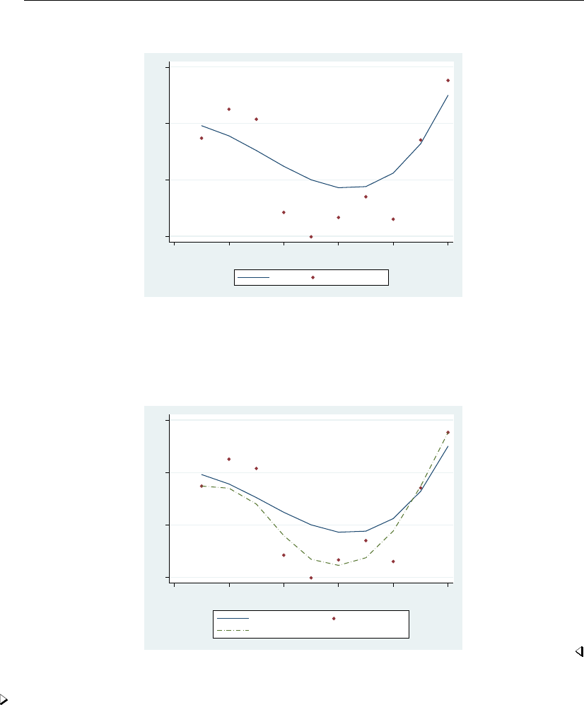
smooth — Robust nonlinear smoother 2191
. scatter x z time, c(l .) m(i o) ytitle("")
−200 −100 0 100
0 2 4 6 8 10
Time
Signal Observed series
Now we smooth the noisy series, z, assumed to be the only data we would observe:
. smooth 4253eh,twice z, gen(sz)
. label variable sz "Smoothed series"
. scatter x z sz time, c(l . l) m(i o i) ytitle("") || scatter sz time,
> c(l . l) m(i o i) ytitle("") clpattern(dash_dot)
−200 −100 0 100
0 2 4 6 8 10
Time
Signal Observed series
Smoothed series
Example 2
Salgado-Ugarte and Curts-Garc´
ıa (1993) provide data on the frequencies of observed fish lengths.
In this example, the series to be smoothed—the frequencies—is ordered by fish length rather than
by time.
. use http://www.stata-press.com/data/r13/fishdata, clear
. smooth 4253eh,twice freq, gen(sfreq)
. label var sfreq "4253EH,twice of frequencies"
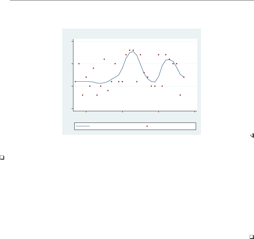
2192 smooth — Robust nonlinear smoother
. scatter sfreq freq length, c(l .) m(i o)
> title("Smoothed frequencies of fish lengths") ytitle("") xlabel(#4)
0 5 10 15
40 50 60 70
Standard body length
4253EH,twice of frequencies Frequency of indiv counts
Smoothed frequencies of fish lengths
Technical note
smooth allows missing values at the beginning and end of the series, but missing values in the
middle are not allowed. Leading and trailing missing values are ignored. If you wish to ignore missing
values in the middle of the series, you must drop the missing observations before using smooth.
Doing so, of course, would violate smooth’s assumption that observations are equally spaced—each
observation represents a year, a quarter, or a month (or a 1-year birth-rate category). In practice,
smooth produces good results as long as the spaces between adjacent observations do not vary too
much.
Smoothing is usually applied to time series, but any variable with a natural order can be smoothed.
For example, a smoother might be applied to the birth rate recorded by the age of the mothers (birth
rate for 17-year-olds, birth rate for 18-year-olds, and so on).
Methods and formulas
Methods and formulas are presented under the following headings:
Running median smoothers of odd span
Running median smoothers of even span
Repeat operator
Endpoint rule
Splitting operator
Hanning smoother
Twicing

smooth — Robust nonlinear smoother 2193
Running median smoothers of odd span
The smoother 3defines
zt=median(yt−1, yt, yt+1)
The smoother 5defines
zt=median(yt−2, yt−1, yt, yt+1, yt+2)
and so on. The smoother 1defines zt=median(yt), so it does nothing.
Endpoints are handled by using smoothers of shorter, odd span. Thus for 3,
z1=y1
z2=median(y1, y2, y3)
.
.
.
zN−1=median(yN−2, yN−1, yN)
ZN=yN
For 5,
z1=y1
z2=median(y1, y2, y3)
z3=median(y1, y2, y3, y4, y5)
z4=median(y2, y3, y4, y5, y6)
.
.
.
zN−2=median(yN−4, yN−3, yN−2, yN−1, yN)
zN−1=median(yN−2, yN−1, yN)
ZN=yN
and so on.
Running median smoothers of even span
Define the median() function as returning the linearly interpolated value when given an even
number of arguments. Thus the smoother 2defines
zt+0.5= (yt+yt+1)/2
The smoother 4defines zt+0.5as the linearly interpolated median of (yt−1, yt, yt+1, yt+2), and so
on. Endpoints are always handled using smoothers of shorter, even span. Thus for 4,

2194 smooth — Robust nonlinear smoother
z0.5=y1
z1.5=median(y1, y2)=(y1+y2)/2
z2.5=median(y1, y2, y3, y4)
.
.
.
zN−2.5=median(yN−4, yN−3, yN−2, yN)
zN−1.5=median(yN−2, yN−1)
zN−0.5=median(yN−1, yN)
zN+0.5=yN
As defined above, an even-span smoother increases the length of the series by 1 observation. However,
the series can be recentered on the original observation numbers, and the “extra” observation can be
eliminated by smoothing the series again with another even-span smoother. For instance, the smooth
of 4illustrated above could be followed by a smooth of 2to obtain
z∗
1= (z0.5+z1.5)/2
z∗
2= (z1.5+z2.5)/2
z∗
3= (z2.5+z3.5)/2
.
.
.
z∗
N−2= (zN−2.5+zN−1.5)/2
z∗
N−1= (zN−1.5+zN−0.5)/2
z∗
N= (zN−0.5+zN+0.5)/2
smooth keeps track of the number of even smoothers applied to the data and expands and shrinks the
length of the series accordingly. To ensure that the final smooth has the same number of observations
as varname,smooth requires you to specify an even number of even-span smoothers. However, the
pairs of even-span smoothers need not be contiguous; for instance, 4253 and 4523 are both allowed.
Repeat operator
Rindicates that a smoother is to be repeated until convergence, that is, until repeated applications
of the smoother produce the same series. Thus 3applies the smoother of running medians of span
3. 33 applies the smoother twice. 3R produces the result of repeating 3an infinite number of times.
Rshould be used only with odd-span smoothers because even-span smoothers are not guaranteed to
converge.
The smoother 453R2 applies a span-4 smoother, followed by a span-5 smoother, followed by
repeated applications of a span-3 smoother, followed by a span-2 smoother.

smooth — Robust nonlinear smoother 2195
Endpoint rule
The endpoint rule Emodifies the values z1and zNaccording to the following formulas:
z1=median(3z2−2z3, z1, z2)
zN=median(3zN−2−2zN−1, zN, zN−1)
When the endpoint rule is not applied, endpoints are typically “copied in”; that is, z1=y1and
zN=yN.
Splitting operator
The smoothers 3and 3R can produce flat-topped hills and valleys. The split operator attempts to
eliminate such hills and valleys by splitting the sequence, applying the endpoint rule E, rejoining the
series, and then resmoothing by 3R.
The Soperator may be applied only after 3,3R, or S.
We recommend that the Soperator be repeated once (SS) or until no further changes take place
(SR).
Hanning smoother
His the Hanning linear smoother:
zt= (yt−1+ 2yt+yt+1)/4
Endpoints are copied in: z1=y1and zN=yN.Hshould be applied only after all nonlinear
smoothers.
Twicing
A smoother divides the data into a smooth and a rough:
data =smooth +rough
If the smoothing is successful, the rough should exhibit no pattern. Twicing refers to applying the
smoother to the observed, calculating the rough, and then applying the smoother to the rough. The
resulting “smoothed rough” is then added back to the smooth from the first step.
Acknowledgments
smooth was originally written by William Gould (1992)—at which time it was named nlsm—and
was inspired by Salgado-Ugarte and Curts-Garc´
ıa (1992). Salgado-Ugarte and Curts-Garc´
ıa (1993)
subsequently reported anomalies in nlsm’s treatment of even-span median smoothers. smooth corrects
these problems and incorporates other improvements but otherwise is essentially the same as originally
published.

2196 smooth — Robust nonlinear smoother
References
Cox, N. J. 1997. gr22: Binomial smoothing plot.Stata Technical Bulletin 35: 7–9. Reprinted in Stata Technical
Bulletin Reprints, vol. 6, pp. 36–38. College Station, TX: Stata Press.
. 2004. gr22 1: Software update: Binomial smoothing plot.Stata Journal 4: 490.
. 2005. Speaking Stata: Smoothing in various directions.Stata Journal 5: 574–593.
Gould, W. W. 1992. sg11.1: Quantile regression with bootstrapped standard errors.Stata Technical Bulletin 9: 19–21.
Reprinted in Stata Technical Bulletin Reprints, vol. 2, pp. 137–139. College Station, TX: Stata Press.
Royston, P., and N. J. Cox. 2005. A multivariable scatterplot smoother.Stata Journal 5: 405–412.
Salgado-Ugarte, I. H., and J. Curts-Garc´
ıa. 1992. sed7: Resistant smoothing using Stata.Stata Technical Bulletin 7:
8–11. Reprinted in Stata Technical Bulletin Reprints, vol. 2, pp. 99–103. College Station, TX: Stata Press.
. 1993. sed7.2: Twice reroughing procedure for resistant nonlinear smoothing.Stata Technical Bulletin 11: 14–16.
Reprinted in Stata Technical Bulletin Reprints, vol. 2, pp. 108–111. College Station, TX: Stata Press.
Sasieni, P. D. 1998. gr27: An adaptive variable span running line smoother.Stata Technical Bulletin 41: 4–7. Reprinted
in Stata Technical Bulletin Reprints, vol. 7, pp. 63–68. College Station, TX: Stata Press.
Tukey, J. W. 1977. Exploratory Data Analysis. Reading, MA: Addison–Wesley.
Velleman, P. F. 1977. Robust nonlinear data smoothers: Definitions and recommendations. Proceedings of the National
Academy of Sciences 74: 434–436.
. 1980. Definition and comparison of robust nonlinear data smoothing algorithms. Journal of the American
Statistical Association 75: 609–615.
Velleman, P. F., and D. C. Hoaglin. 1981. Applications, Basics, and Computing of Exploratory Data Analysis. Boston:
Duxbury.
Also see
[R]lowess — Lowess smoothing
[R]lpoly — Kernel-weighted local polynomial smoothing
[TS]tssmooth — Smooth and forecast univariate time-series data

Title
spearman — Spearman’s and Kendall’s correlations
Syntax Menu Description Options for spearman
Options for ktau Remarks and examples Stored results Methods and formulas
Acknowledgment References Also see
Syntax
Spearman’s rank correlation coefficients
spearman varlist if in ,spearman options
Kendall’s rank correlation coefficients
ktau varlist if in ,ktau options
spearman options Description
Main
stats(spearman list)list of statistics; select up to three statistics; default is stats(rho)
print(#)significance level for displaying coefficients
star(#)significance level for displaying with a star
bonferroni use Bonferroni-adjusted significance level
sidak use ˇ
Sid´
ak-adjusted significance level
pw calculate all pairwise correlation coefficients by using all available data
matrix display output in matrix form
ktau options Description
Main
stats(ktau list)list of statistics; select up to six statistics; default is stats(taua)
print(#)significance level for displaying coefficients
star(#)significance level for displaying with a star
bonferroni use Bonferroni-adjusted significance level
sidak use ˇ
Sid´
ak-adjusted significance level
pw calculate all pairwise correlation coefficients by using all available data
matrix display output in matrix form
by is allowed with spearman and ktau; see [D] by.
where the elements of spearman list may be
rho correlation coefficient
obs number of observations
psignificance level
2197

2198 spearman — Spearman’s and Kendall’s correlations
and the elements of ktau list may be
taua correlation coefficient τa
taub correlation coefficient τb
score score
se standard error of score
obs number of observations
psignificance level
Menu
spearman
Statistics >Nonparametric analysis >Tests of hypotheses >Spearman’s rank correlation
ktau
Statistics >Nonparametric analysis >Tests of hypotheses >Kendall’s rank correlation
Description
spearman displays Spearman’s rank correlation coefficients for all pairs of variables in varlist or,
if varlist is not specified, for all the variables in the dataset.
ktau displays Kendall’s rank correlation coefficients between the variables in varlist or, if varlist is
not specified, for all the variables in the dataset. ktau is intended for use on small- and moderate-sized
datasets; it requires considerable computation time for larger datasets.
Options for spearman
Main
stats(spearman list)specifies the statistics to be displayed in the matrix of output. stats(rho)
is the default. Up to three statistics may be specified; stats(rho obs p) would display the
correlation coefficient, number of observations, and significance level. If varlist contains only two
variables, all statistics are shown in tabular form, and stats(),print(), and star() have no
effect unless the matrix option is specified.
print(#)specifies the significance level of correlation coefficients to be printed. Correlation coeffi-
cients with larger significance levels are left blank in the matrix. Typing spearman, print(.10)
would list only those correlation coefficients that are significant at the 10% level or lower.
star(#)specifies the significance level of correlation coefficients to be marked with a star. Typing
spearman, star(.05) would “star” all correlation coefficients significant at the 5% level or
lower.
bonferroni makes the Bonferroni adjustment to calculated significance levels. This adjustment affects
printed significance levels and the print() and star() options. Thus spearman, print(.05)
bonferroni prints coefficients with Bonferroni-adjusted significance levels of 0.05 or less.
sidak makes the ˇ
Sid´
ak adjustment to calculated significance levels. This adjustment affects printed
significance levels and the print() and star() options. Thus spearman, print(.05) sidak
prints coefficients with ˇ
Sid´
ak-adjusted significance levels of 0.05 or less.
pw specifies that correlations be calculated using pairwise deletion of observations with missing
values. By default, spearman uses casewise deletion, where observations are ignored if any of
the variables in varlist are missing.

spearman — Spearman’s and Kendall’s correlations 2199
matrix forces spearman to display the statistics as a matrix, even if varlist contains only two
variables. matrix is implied if more than two variables are specified.
Options for ktau
Main
stats(ktau list)specifies the statistics to be displayed in the matrix of output. stats(taua) is
the default. Up to six statistics may be specified; stats(taua taub score se obs p) would
display the correlation coefficients τa,τb, score, standard error of score, number of observations,
and significance level. If varlist contains only two variables, all statistics are shown in tabular
form and stats(),print(), and star() have no effect unless the matrix option is specified.
print(#)specifies the significance level of correlation coefficients to be printed. Correlation coef-
ficients with larger significance levels are left blank in the matrix. Typing ktau, print(.10)
would list only those correlation coefficients that are significant at the 10% level or lower.
star(#)specifies the significance level of correlation coefficients to be marked with a star. Typing
ktau, star(.05) would “star” all correlation coefficients significant at the 5% level or lower.
bonferroni makes the Bonferroni adjustment to calculated significance levels. This adjustment
affects printed significance levels and the print() and star() options. Thus ktau, print(.05)
bonferroni prints coefficients with Bonferroni-adjusted significance levels of 0.05 or less.
sidak makes the ˇ
Sid´
ak adjustment to calculated significance levels. This adjustment affects printed
significance levels and the print() and star() options. Thus ktau, print(.05) sidak prints
coefficients with ˇ
Sid´
ak-adjusted significance levels of 0.05 or less.
pw specifies that correlations be calculated using pairwise deletion of observations with missing values.
By default, ktau uses casewise deletion, where observations are ignored if any of the variables in
varlist are missing.
matrix forces ktau to display the statistics as a matrix, even if varlist contains only two variables.
matrix is implied if more than two variables are specified.
Remarks and examples
Example 1
We wish to calculate the correlation coefficients among marriage rate (mrgrate), divorce rate
(divorce rate), and median age (medage) in state data. We can calculate the standard Pearson
correlation coefficients and significance by typing
.use http://www.stata-press.com/data/r13/states2
(State data)
. pwcorr mrgrate divorce_rate medage, sig
mrgrate divorc~e medage
mrgrate 1.0000
divorce_rate 0.7895 1.0000
0.0000
medage 0.0011 -0.1526 1.0000
0.9941 0.2900

2200 spearman — Spearman’s and Kendall’s correlations
We can calculate Spearman’s rank correlation coefficients by typing
. spearman mrgrate divorce_rate medage, stats(rho p)
(obs=50)
Key
rho
Sig. level
mrgrate divorc~e medage
mrgrate 1.0000
divorce_rate 0.6933 1.0000
0.0000
medage -0.4869 -0.2455 1.0000
0.0003 0.0857
The large difference in the results is caused by one observation. Nevada’s marriage rate is almost 10
times higher than the state with the next-highest marriage rate. An important feature of the Spearman
rank correlation coefficient is its reduced sensitivity to extreme values compared with the Pearson
correlation coefficient.
We can calculate Kendall’s rank correlations by typing
. ktau mrgrate divorce_rate medage, stats(taua taub p)
(obs=50)
Key
tau_a
tau_b
Sig. level
mrgrate divorc~e medage
mrgrate 0.9829
1.0000
divorce_rate 0.5110 0.9804
0.5206 1.0000
0.0000
medage -0.3486 -0.1698 0.9845
-0.3544 -0.1728 1.0000
0.0004 0.0828
There are tied values for variables mrgrate,divorce rate, and medage, so tied ranks are used.
As a result, τa<1on the diagonal (see Methods and formulas for the definition of τa).

spearman — Spearman’s and Kendall’s correlations 2201
Technical note
According to Conover (1999, 323), “Spearman’s ρtends to be larger than Kendall’s τin absolute
value. However, as a test of significance, there is no strong reason to prefer one over the other because
both will produce nearly identical results in most cases.”
Example 2
We illustrate spearman and ktau with the auto data, which contains some missing values.
.use http://www.stata-press.com/data/r13/auto
(1978 Automobile Data)
. spearman mpg rep78
Number of obs = 69
Spearman’s rho = 0.3098
Test of Ho: mpg and rep78 are independent
Prob > |t| = 0.0096
Because we specified two variables, spearman displayed the sample size, correlation, and p-value in
tabular form. To obtain just the correlation coefficient displayed in matrix form, we type
. spearman mpg rep78, stats(rho) matrix
(obs=69)
mpg rep78
mpg 1.0000
rep78 0.3098 1.0000
The pw option instructs spearman and ktau to use all nonmissing observations between a pair
of variables when calculating their correlation coefficient. In the output below, some correlations are
based on 74 observations, whereas others are based on 69 because 5 observations contain a missing
value for rep78.
. spearman mpg price rep78, pw stats(rho obs p) star(0.01)
Key
rho
Number of obs
Sig. level
mpg price rep78
mpg 1.0000
74
price -0.5419* 1.0000
74 74
0.0000
rep78 0.3098* 0.1028 1.0000
69 69 69
0.0096 0.4008

2202 spearman — Spearman’s and Kendall’s correlations
Finally, the bonferroni and sidak options provide adjusted significance levels:
. ktau mpg price rep78, stats(taua taub score se p) bonferroni
(obs=69)
Key
tau_a
tau_b
score
se of score
Sig. level
mpg price rep78
mpg 0.9471
1.0000
2222.0000
191.8600
price -0.3973 1.0000
-0.4082 1.0000
-932.0000 2346.0000
192.4561 193.0682
0.0000
rep78 0.2076 0.0648 0.7136
0.2525 0.0767 1.0000
487.0000 152.0000 1674.0000
181.7024 182.2233 172.2161
0.0224 1.0000
Charles Edward Spearman (1863–1945) was a British psychologist who made contributions
to correlation, factor analysis, test reliability, and psychometrics. After several years’ military
service, he obtained a PhD in experimental psychology at Leipzig and became a professor at
University College London, where he sustained a long program of work on the interpretation of
intelligence tests. Ironically, the rank correlation version bearing his name is not the formula he
advocated.
Maurice George Kendall (1907–1983) was a British statistician who contributed to rank correlation,
time series, multivariate analysis, among other topics, and wrote many statistical texts. Most
notably, perhaps, his advanced survey of the theory of statistics went through several editions,
later ones with Alan Stuart; the baton has since passed to others. Kendall was employed in turn
as a government and business statistician, as a professor at the London School of Economics, as
a consultant, and as director of the World Fertility Survey. He was knighted in 1974.

spearman — Spearman’s and Kendall’s correlations 2203
Stored results
spearman stores the following in r():
Scalars
r(N) number of observations (last variable pair)
r(rho) ρ(last variable pair)
r(p) two-sided p-value (last variable pair)
Matrices
r(Nobs) number of observations
r(Rho) ρ
r(P) two-sided p-value
ktau stores the following in r():
Scalars
r(N) number of observations (last variable pair)
r(tau a) τa(last variable pair)
r(tau b) τb(last variable pair)
r(score) Kendall’s score (last variable pair)
r(se score) se of score (last variable pair)
r(p) two-sided p-value (last variable pair)
Matrices
r(Nobs) number of observations
r(Tau a) τa
r(Tau b) τb
r(Score) Kendall’s score
r(Se Score) standard error of score
r(P) two-sided p-value
Methods and formulas
Spearman’s (1904) rank correlation is calculated as Pearson’s correlation computed on the ranks
and average ranks (Conover 1999, 314 – 315). Ranks are as calculated by egen; see [D]egen. The
significance is calculated using the approximation
p= 2 ×ttail(n−2,|bρ|√n−2/p1−bρ2)
For any two pairs of ranks (xi, yi)and (xj, yj)of one variable pair (varname1,varname2),
1≤i, j ≤n, where nis the number of observations, define them as concordant if
(xi−xj)(yi−yj)>0
and discordant if this product is less than zero.
Kendall’s (1938; also see Kendall and Gibbons [1990] or Bland [2000], 222–225) score Sis
defined as C−D, where C(D) is the number of concordant (discordant) pairs. Let N=n(n−1)/2
be the total number of pairs, so τais given by
τa=S/N
and τbis given by
τb=S
√N−U√N−V

2204 spearman — Spearman’s and Kendall’s correlations
where
U=
N1
X
i=1
ui(ui−1)/2
V=
N2
X
j=1
vj(vj−1)/2
and where N1is the number of sets of tied xvalues, uiis the number of tied xvalues in the ith
set, N2is the number of sets of tied yvalues, and vjis the number of tied yvalues in the jth set.
Under the null hypothesis of independence between varname1and varname2, the variance of Sis
exactly (Kendall and Gibbons 1990, 66)
Var(S) = 1
18n(n−1)(2n+ 5) −
N1
X
i=1
ui(ui−1)(2ui+ 5) −
N2
X
j=1
vj(vj−1)(2vj+ 5)
+1
9n(n−1)(n−2)N1
X
i=1
ui(ui−1)(ui−2)N2
X
j=1
vj(vj−1)(vj−2)
+1
2n(n−1)N1
X
i=1
ui(ui−1)N2
X
j=1
vj(vj−1)
Using a normal approximation with a continuity correction,
z=|S| − 1
pVar(S)
For the hypothesis of independence, the statistics S,τa, and τbproduce equivalent tests and give the
same significance.
For Kendall’s τ, the normal approximation is surprisingly accurate for sample sizes as small as 8,
at least for calculating p-values under the null hypothesis for continuous variables. (See Kendall and
Gibbons [1990, chap. 4], who also present some tables for calculating exact p-values for n < 10.)
For Spearman’s ρ, the normal approximation requires larger samples to be valid.
Let vbe the number of variables specified so that k=v(v−1)/2 correlation coefficients are
to be estimated. If bonferroni is specified, the adjusted significance level is p0= min(1, kp). If
sidak is specified, p0= min 1,1−(1−p)n. See Methods and formulas in [R]oneway for a
more complete description of the logic behind these adjustments.
Early work on rank correlation is surveyed by Kruskal (1958).
Acknowledgment
The original version of ktau was written by Sean Becketti, a past editor of the Stata Technical
Bulletin and author of the Stata Press book Introduction to Time Series Using Stata.

spearman — Spearman’s and Kendall’s correlations 2205
References
Barnard, G. A. 1997. Kendall, Maurice George. In Leading Personalities in Statistical Sciences: From the Seventeenth
Century to the Present, ed. N. L. Johnson and S. Kotz, 130–132. New York: Wiley.
Bland, M. 2000. An Introduction to Medical Statistics. 3rd ed. Oxford: Oxford University Press.
Conover, W. J. 1999. Practical Nonparametric Statistics. 3rd ed. New York: Wiley.
David, H. A., and W. A. Fuller. 2007. Sir Maurice Kendall (1907–1983): A centenary appreciation. American
Statistician 61: 41–46.
Jeffreys, H. 1961. Theory of Probability. 3rd ed. Oxford: Oxford University Press.
Kendall, M. G. 1938. A new measure of rank correlation. Biometrika 30: 81–93.
Kendall, M. G., and J. D. Gibbons. 1990. Rank Correlation Methods. 5th ed. New York: Oxford University Press.
Kruskal, W. H. 1958. Ordinal measures of association. Journal of the American Statistical Association 53: 814–861.
Lovie, P., and A. D. Lovie. 1996. Charles Edward Spearman, F.R.S. (1863–1945). Notes and Records of the Royal
Society of London 50: 75–88.
Newson, R. B. 2000a. snp15: somersd—Confidence intervals for nonparametric statistics and their differences.Stata
Technical Bulletin 55: 47–55. Reprinted in Stata Technical Bulletin Reprints, vol. 10, pp. 312–322. College Station,
TX: Stata Press.
. 2000b. snp15.1: Update to somersd.Stata Technical Bulletin 57: 35. Reprinted in Stata Technical Bulletin
Reprints, vol. 10, pp. 322–323. College Station, TX: Stata Press.
. 2000c. snp15.2: Update to somersd.Stata Technical Bulletin 58: 30. Reprinted in Stata Technical Bulletin
Reprints, vol. 10, p. 323. College Station, TX: Stata Press.
. 2001. snp15.3: Update to somersd.Stata Technical Bulletin 61: 22. Reprinted in Stata Technical Bulletin
Reprints, vol. 10, p. 324. College Station, TX: Stata Press.
. 2003. snp15 4: Software update for somersd.Stata Journal 3: 325.
. 2005. snp15 5: Software update for somersd.Stata Journal 5: 470.
. 2006. Confidence intervals for rank statistics: Percentile slopes, differences, and ratios.Stata Journal 6: 497–520.
Seed, P. T. 2001. sg159: Confidence intervals for correlations.Stata Technical Bulletin 59: 27–28. Reprinted in Stata
Technical Bulletin Reprints, vol. 10, pp. 267–269. College Station, TX: Stata Press.
Spearman, C. E. 1904. The proof and measurement of association between two things. American Journal of Psychology
15: 72–101.
Wolfe, F. 1997. sg64: pwcorrs: Enhanced correlation display.Stata Technical Bulletin 35: 22–25. Reprinted in Stata
Technical Bulletin Reprints, vol. 6, pp. 163–167. College Station, TX: Stata Press.
. 1999. sg64.1: Update to pwcorrs.Stata Technical Bulletin 49: 17. Reprinted in Stata Technical Bulletin Reprints,
vol. 9, p. 159. College Station, TX: Stata Press.
Also see
[R]correlate — Correlations (covariances) of variables or coefficients
[R]nptrend — Test for trend across ordered groups

Title
spikeplot — Spike plots and rootograms
Syntax Menu Description Options
Remarks and examples Acknowledgments References Also see
Syntax
spikeplot varname if in weight ,options
options Description
Main
round(#)round varname to nearest multiple of #(bin width)
fraction make vertical scale the proportion of total values; default is frequencies
root make vertical scale show square roots of frequencies
Plot
spike options affect rendition of plotted spikes
Add plots
addplot(plot)add other plots to generated graph
Y axis, X axis, Titles, Legend, Overall, By
twoway options any options documented in [G-3]twoway options
fweights, aweights, and iweights are allowed; see [U] 11.1.6 weight.
Menu
Graphics >Distributional graphs >Spike plot and rootogram
Description
spikeplot produces a frequency plot for a variable in which the frequencies are depicted as
vertical lines from zero. The frequency may be a count, a fraction, or the square root of the count
(Tukey’s rootogram, circa 1965). The vertical lines may also originate from a baseline other than
zero at the user’s option.
Options
Main
round(#)rounds the values of varname to the nearest multiple of #. This action effectively specifies
the bin width.
fraction specifies that the vertical scale be the proportion of total values (percentage) rather than
the count.
root specifies that the vertical scale show square roots. This option may not be specified if fraction
is specified.
2206
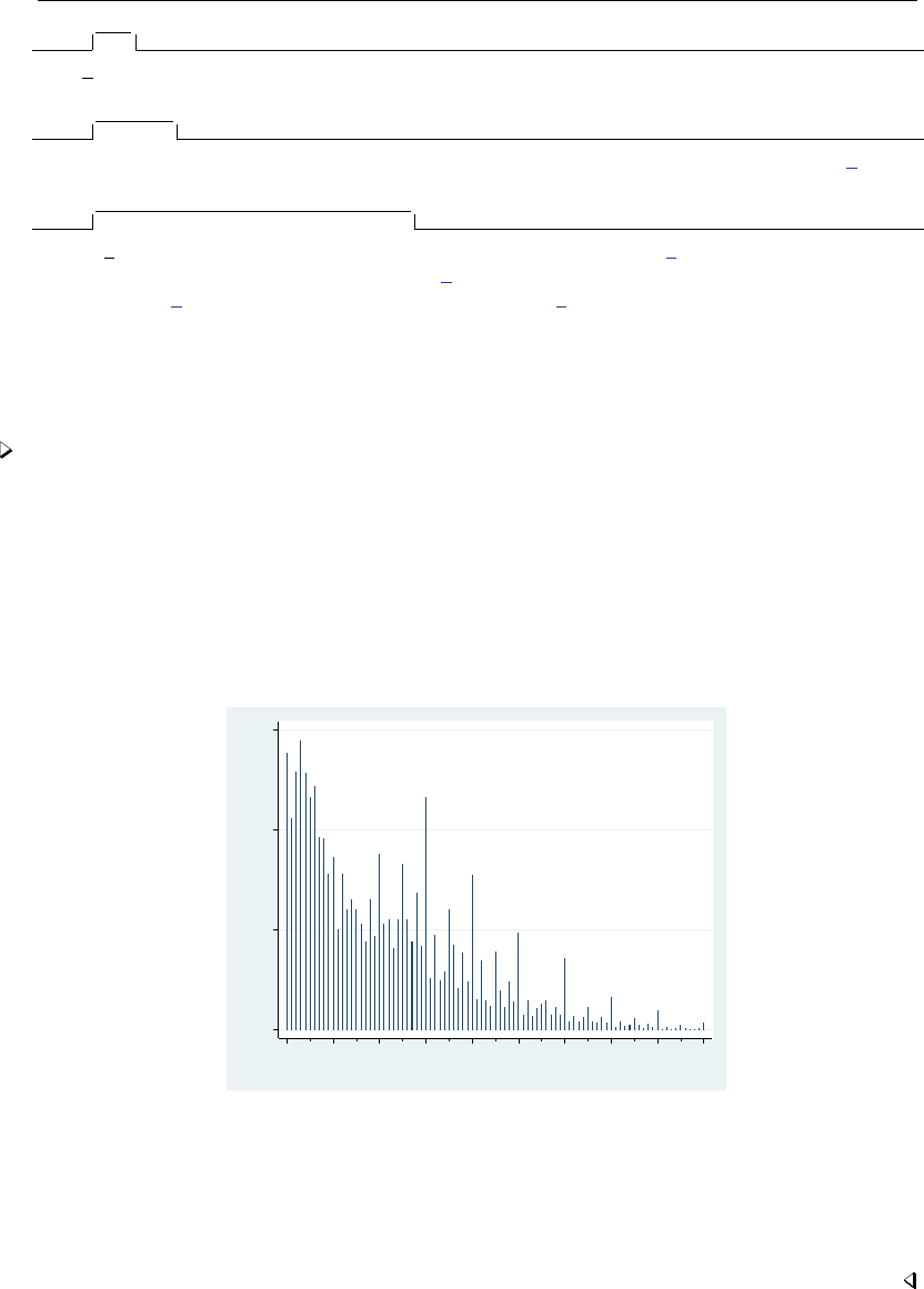
spikeplot — Spike plots and rootograms 2207
Plot
spike options affect the rendition of the plotted spikes; see [G-2]graph twoway spike.
Add plots
addplot(plot)provides a way to add other plots to the generated graph. See [G-3]addplot option.
Y axis, X axis, Titles, Legend, Overall, By
twoway options are any of the options documented in [G-3]twoway options. These include op-
tions for titling the graph (see [G-3]title options), options for saving the graph to disk (see
[G-3]saving option), and the by() option (see [G-3]by option).
Remarks and examples
Example 1
Cox and Brady (1997a) present an illustrative example using the age structure of the population
of Ghana from the 1960 census (rounded to the nearest 1,000). The dataset has ages from 0 (less
than 1 year) to 90. To view the distribution of ages, we would like to use each integer from 0 to 90
as the bins for the dataset.
. use http://www.stata-press.com/data/r13/ghanaage
. spikeplot age [fw=pop], ytitle("Population in 1000s") xlab(0(10)90)
> xmtick(5(10)85)
0 100 200 300
Population in 1000s
0 10 20 30 40 50 60 70 80 90
Age in years
The resulting graph shows a “heaping” of ages at the multiples of 5. Also, ages ending in even
numbers are more frequent than ages ending in odd numbers (except for 5). This preference for
reporting ages is well known in demography and other social sciences.
Note also that we used the ytitle() option to override the default title of “Frequency” and that
we used the xlab() and xmtick() options with numlists to further customize the resulting graph.
See [U] 11.1.8 numlist for details on specifying numlists.
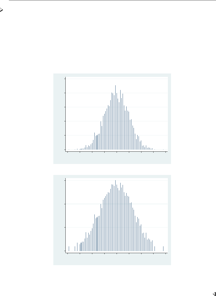
2208 spikeplot — Spike plots and rootograms
Example 2
The rootogram is a plot of the square-root transformation of the frequency counts. The square root
of a normal distribution is a multiple of another normal distribution.
. clear
. set seed 1234567
. set obs 5000
obs was 0, now 5000
. generate normal = rnormal()
. label variable normal "Gaussian(0,1) random numbers"
. spikeplot normal, round(.10) xlab(-4(1)4)
0 50 100 150 200 250
Frequency
−4 −3 −2 −1 0 1 2 3 4
Gaussian(0,1) random numbers
. spikeplot normal, round(.10) xlab(-4(1)4) root
0 5 10 15
Root of frequency
−4 −3 −2 −1 0 1 2 3 4
Gaussian(0,1) random numbers
Interpreting a histogram in terms of normality is thus similar to interpreting the rootogram for
normality.
This example also shows how the round() option is used to bin the values for a spike plot of a
continuous variable.

spikeplot — Spike plots and rootograms 2209
Example 3
spikeplot can also be used to produce time-series plots. varname should be the time variable,
and weights should be specified as the values for those times. To get a plot of daily rainfalls, we type
. spikeplot day [w=rain] if rain, ytitle("Daily rainfall in mm")
The base() option of graph twoway spike may be used to set a different baseline, such as
when we want to show variations relative to an average or to some other measure of level.
Acknowledgments
The original version of spikeplot was written by Nicholas J. Cox of the Department of Geography
at Durham University, UK, and coeditor of the Stata Journal and Anthony R. Brady of the Imperial
College School of Medicine (1997a,1997b).
References
Cox, N. J., and A. R. Brady. 1997a. gr25: Spike plots for histograms, rootograms, and time-series plots.Stata
Technical Bulletin 36: 8–11. Reprinted in Stata Technical Bulletin Reprints, vol. 6, pp. 50–54. College Station,
TX: Stata Press.
. 1997b. gr25.1: Spike plots for histograms, rootograms, and time-series plots: Update.Stata Technical Bulletin
40: 12. Reprinted in Stata Technical Bulletin Reprints, vol. 7, p. 58. College Station, TX: Stata Press.
Tukey, J. W. 1965. The future of processes of data analysis. In The Collected Works of John W. Tukey, Volume IV:
Philosophy and Principles of Data Analysis: 1965–1986, ed. L. V. Jones, 123–126. Monterey, CA: Wadsworth &
Brooks/Cole.
Also see
[R]histogram — Histograms for continuous and categorical variables

Title
ssc — Install and uninstall packages from SSC
Syntax Description Options Remarks and examples
Acknowledgments References Also see
Syntax
Summary of packages most recently added or updated at SSC
ssc new , saving(filename, replace ) type
Summary of most popular packages at SSC
ssc hot , n(#) author(name)
Describe a specified package at SSC
ssc describe pkgname |letter , saving(filename, replace )
Install a specified package from SSC
ssc install pkgname , all replace
Uninstall from your computer a previously installed package from SSC
ssc uninstall pkgname
Type a specific file stored at SSC
ssc type filename , asis
Copy a specific file from SSC to your computer
ssc copy filename , plus personal replace public binary
where letter in ssc describe is a–zor .
Description
ssc works with packages (and files) from the Statistical Software Components (SSC) archive,
which is often called the Boston College Archive and is provided by http://repec.org.
The SSC has become the premier Stata download site for user-written software on the web.
ssc provides a convenient interface to the resources available there. For example, on Statalist (see
http://www.statalist.org/), users will often write
The program can be found by typing ssc install newprogramname.
2210

ssc — Install and uninstall packages from SSC 2211
Typing that would load everything associated with newprogramname, including the help files.
If you are searching for what is available, type ssc new and ssc hot, and see [R]search.search
searches the SSC and other places, too. search provides a GUI interface from which programs can
be installed, including the programs at the SSC archive.
You can uninstall particular packages by using ssc uninstall. For the packages that you keep,
see [R]adoupdate for an automated way of keeping those packages up to date.
Command overview
ssc new summarizes the packages made available or updated recently. Output is presented in the
Stata Viewer, and from there you may click to find out more about individual packages or to
install them.
ssc hot lists the most popular packages—popular based on a moving average of the number of
downloads in the past three months. By default, 10 packages are listed.
ssc describe pkgname describes, but does not install, the specified package. Use search to find
packages; see [R]search. If you know the package name but do not know the exact spelling, type
ssc describe followed by one letter, a–zor (underscore), to list all the packages starting with
that letter.
ssc install pkgname installs the specified package. You do not have to describe a package before
installing it. (You may also install a package by using net install; see [R]net.)
ssc uninstall pkgname removes the previously installed package from your computer. It does not
matter how the package was installed. (ssc uninstall is a synonym for ado uninstall, so
either may be used to installed any package.)
ssc type filename types a specific file stored at SSC.ssc cat is a synonym for ssc type, which
may appeal to those familiar with Unix.
ssc copy filename copies a specific file stored at SSC to your computer. By default, the file is
copied to the current directory, but you can use options to change this. ssc copy is a rarely used
alternative to ssc install . . . , all.ssc cp is a synonym for ssc copy.
Options
Options are presented under the following headings:
Options for use with ssc new
Options for use with ssc hot
Option for use with ssc describe
Options for use with ssc install
Option for use with ssc type
Options for use with ssc copy
Options for use with ssc new
saving(filename, replace )specifies that the “what’s new” summary be saved in filename. If
filename is specified without a suffix, filename.smcl is assumed. If saving() is not specified,
saving(ssc results.smcl) is assumed.
type specifies that the “what’s new” results be displayed in the Results window rather than in the
Viewer.

2212 ssc — Install and uninstall packages from SSC
Options for use with ssc hot
n(#)specifies the number of packages to list; n(10) is the default. Specify n(.) to list all packages
in order of popularity.
author(name)lists the 10 most popular packages by the specified author. If n(#)is also specified,
the top #packages are listed.
Option for use with ssc describe
saving(filename, replace )specifies that, in addition to the descriptions being displayed on
your screen, it be saved in the specified file.
If filename is specified without an extension, .smcl will be assumed, and the file will be saved
as a SMCL file.
If filename is specified with an extension, no default extension is added. If the extension is .log,
the file will be stored as a text file.
If replace is specified, filename is replaced if it already exists.
Options for use with ssc install
all specifies that any ancillary files associated with the package be downloaded to your current
directory, in addition to the program and help files being installed. Ancillary files are files that
do not end in .ado or .sthlp and typically contain datasets or examples of the use of the new
command.
You can find out which files are associated with the package by typing ssc describe pkgname
before or after installing. If you install without using the all option and then want the ancillary
files, you can ssc install again.
replace specifies that any files being downloaded that already exist on your computer be replaced
by the downloaded files. If replace is not specified and any files already exist, none of the files
from the package is downloaded or installed.
It is better not to specify the replace option and wait to see if there is a problem. If there
is a problem, it is usually better to uninstall the old package by using ssc uninstall or ado
uninstall (which are, in fact, the same command).
Option for use with ssc type
asis affects how files with the suffixes .smcl and .sthlp are displayed. The default is to interpret
SMCL directives the file might contain. asis specifies that the file be displayed in raw, uninterpreted
form.
Options for use with ssc copy
plus specifies that the file be copied to the PLUS directory, the directory where user-written additions
are installed. Typing sysdir will display the identity of the PLUS directory on your computer;
see [P]sysdir.
personal specifies that the file be copied to your PERSONAL directory as reported by sysdir; see
[P]sysdir.
If neither plus nor personal is specified, the default is to copy the file to the current directory.

ssc — Install and uninstall packages from SSC 2213
replace specifies that, if the file already exists on your computer, the new file replace it.
public specifies that the new file be made readable by everyone; otherwise, the file will be created
according to the default permission you have set with your operating system.
binary specifies that the file being copied is a binary file and that it is to be copied as is. The default
is to assume that the file is a text file and change the end-of-line characters to those appropriate
for your computer/operating system.
Remarks and examples
Users can add new features to Stata, and some users choose to make new features that they have
written available to others via the web. The files that comprise a new feature are called a package, and
a package usually consists of one or more ado-files and help files. The net command (see [R]net)
makes it reasonably easy to install and uninstall packages regardless of where they are on the web.
One site, the SSC, has become particularly popular as a repository for additions to Stata. Command
ssc is an easier to use version of net designed especially for the SSC.
Many packages are available at the SSC. Packages have names, such as oaxaca,estout, or
egenmore. At SSC, capitalization is not significant, so Oaxaca,ESTOUT, and EGENmore are ways of
writing the same package names.
When you type
. ssc install oaxaca
the files associated with the package are downloaded and installed on your computer. Package names
usually correspond to the names of the command being added to Stata, so one would expect that
installing the package oaxaca will add command oaxaca to Stata on your computer, and expect
that typing help oaxaca will provide the documentation. That is the situation here, but that is not
always so. Before or after installing a package, type ssc describe pkgname to obtain the details.
Example 1
ssc new summarizes the packages most recently made available or updated. Output is presented in
the Viewer, from which you may click on a package name to find out more or install it. For example,
. ssc new
(contacting http://repec.org)
(output omitted )
GEOCODE3
module to retrieve coordinates or addresses from Google Geocoding API Version3
Authors: Stefan Bernhard Req: Stata version 12, insheetjson and libjson
> from SSC (q.v.)
Created: 2013-05-19
GGTAX
module to identify the most suitable GG family model
Authors: Andres L Gonzalez Rangel Req: Stata version 11
Created: 2013-05-19
ASL_NORM
module computing bootstrap Gaussianity tests
Authors: Maarten L. Buis Req: Stata version 11
Created: 2013-05-16
(output omitted )
End of recent additions and updates

2214 ssc — Install and uninstall packages from SSC
ssc hot provides a list of the most popular packages at SSC.
. ssc hot
Apr 2013
Rank # hits Package Author(s)
1 12621.4 estout Ben Jann
2 12606.8 outreg2 Roy Wada
3 8508.8 ranktest Mark E Schaffer, Frank Kleibergen
4 8061.9 ivreg2 Mark E Schaffer, Steven Stillman,
Christopher F Baum
5 3595.9 psmatch2 Edwin Leuven, Barbara Sianesi
6 2862.6 tabout Ian Watson
7 2358.2 outreg John Luke Gallup
8 2300.3 winsor Nicholas J. Cox
9 1743.0 xtabond2 David Roodman
10 1482.2 xtivreg2 Mark E Schaffer
(Click on package name for description)
Use the n(#)option to change the number of packages listed:
. ssc hot, n(20)
Apr 2013
Rank # hits Package Author(s)
1 12621.4 estout Ben Jann
2 12606.8 outreg2 Roy Wada
3 8508.8 ranktest Mark E Schaffer, Frank Kleibergen
4 8061.9 ivreg2 Mark E Schaffer, Steven Stillman,
Christopher F Baum
5 3595.9 psmatch2 Edwin Leuven, Barbara Sianesi
6 2862.6 tabout Ian Watson
7 2358.2 outreg John Luke Gallup
8 2300.3 winsor Nicholas J. Cox
9 1743.0 xtabond2 David Roodman
10 1482.2 xtivreg2 Mark E Schaffer
11 1481.7 fre Ben Jann
12 1361.7 cem Stefano Iacus, Gary King, Matthew
Blackwell, Giuseppe Porro
13 1279.3 xttest3 Christopher F Baum
14 1205.7 mdesc Rose Anne Medeiros, Dan Blanchette
15 1188.7 bcuse Christopher F Baum
16 1154.4 usespss Sergiy Radyakin
17 1113.3 distinct Gary Longton, Nicholas J. Cox
18 1111.1 egenmore Nicholas J. Cox
19 950.6 gllamm Sophia Rabe-Hesketh
20 948.3 hprescott Christopher F Baum
(Click on package name for description)

ssc — Install and uninstall packages from SSC 2215
The author(name)option allows you to list the most popular packages by a specific person:
. ssc hot, author(baum)
Apr 2013
Rank # hits Package Author(s)
4 8061.9 ivreg2 Mark E Schaffer, Steven Stillman,
Christopher F Baum
13 1279.3 xttest3 Christopher F Baum
15 1188.7 bcuse Christopher F Baum
20 948.3 hprescott Christopher F Baum
27 806.8 tscollap Christopher F Baum
31 742.7 whitetst Christopher F Baum, Nicholas J. Cox
34 696.3 xttest2 Christopher F Baum
42 574.0 overid Christopher F Baum, Mark E Schaffer,
Vince Wiggins, Steven Stillman
46 495.3 kpss Christopher F Baum
58 437.0 ivendog Christopher F Baum, Mark E Schaffer,
Steven Stillman
(Click on package name for description)
ssc describe pkgname describes, but does not install, the specified package. You must already
know the name of the package. See [R]search for assistance in searching for packages. Sometimes
you know the package name, but you do not know the exact spelling. Then you can type ssc
describe followed by one letter, a–zor , to list all the packages starting with that letter; even so,
using search is better.
. ssc describe bidensity
package from http://fmwww.bc.edu/repec/bocode/b
’BIDENSITY’: module to produce and graph bivariate density estimates
bidensity produces bivariate kernel density estimates and graphs
the result using a twoway contourline plot, optionally
overlaying a scatterplot. The default kernel is Epanechnikov;
all of the kernels provided by -kdensity- are also available.
Compared to Baum’s -kdens2- (SSC), which was recently enhanced to
produce contourline plots, -bidensity- computes the bivariate
kernel densities much more efficiently through use of Mata, and
provides a choice of kernel estimators. The estimated densities
can be saved in a Stata dataset or accessed as Mata matrices.
KW: density estimation
KW: bivariate density
KW: contourline plots
Requires: Stata version 12.1 and moremata from SSC (q.v.)
Distribution-Date: 20130119
Author: John Luke Gallup, Portland State University
Support: email jlgallup@pdx.edu
Author: Christopher F Baum, Boston College
Support: email baum@bc.edu
(type
bidensity.ado
bidensity.sthlp
(type - - to install)

2216 ssc — Install and uninstall packages from SSC
The default setting for the saving() option is for the output to be saved with the .smcl extension.
You could also save the file with a log extension, and in this case, the file would be stored as a text
file.
. ssc describe b, saving(b.index)
(output omitted )
. ssc describe bidensity, saving(bidensity.log)
(output omitted )
ssc install pkgname installs the specified package. You do not have to describe a package
before installing it. There are ways of installing packages other than ssc install, such as net; see
[R]net. It does not matter how a package is installed. For instance, a package can be installed using
net and still be uninstalled using ssc.
. ssc install bidensity
checking consistency and verifying not already installed...
installing into C:\ado\plus\...
installation complete.
ssc uninstall pkgname removes the specified, previously installed package from your computer.
You can uninstall immediately after installation or at any time in the future. (Technical note: ssc
uninstall is a synonym for ado uninstall, so it can uninstall any installed package, not just
packages obtained from the SSC.)
. ssc uninstall bidensity
package from http://fmwww.bc.edu/repec/bocode/b
(package uninstalled)
ssc type filename types a specific file stored at the SSC. Although not shown in the syntax
diagram, ssc cat is a synonym for ssc type, which may appeal to those familiar with Unix. To
view only the bidensity help file for the bidensity package, you would type
. ssc type bidensity.sthlp
help for bidensity
Bivariate kernel density estimation
bidensity varnameY varnameX [if exp] [in range] [, n(#)
kernel(kernelname) xwidth(#) ywidth(#) saving( name) replace
nograph scatter[(scatter_options)] contourline_options
mname(name)
(output omitted )
ssc copy filename copies a specific file stored at the SSC to your computer. By default, the file
is copied to the current directory, but you can use options to change this. ssc copy is a rarely used
alternative to ssc install . . . , all.ssc cp is a synonym for ssc copy.
. ssc copy bidensity.ado
(file bidensity.ado copied to current directory)
For more details on the SSC archive and for information on how to submit your own programs to
the SSC, see http://repec.org/bocode/s/sscsubmit.html.

ssc — Install and uninstall packages from SSC 2217
Acknowledgments
ssc is based on archutil by Nicholas J. Cox of the Department of Geography at Durham
University, UK, and coeditor of the Stata Journal and Christopher F. Baum of the Department of
Economics at Boston College and author of the Stata Press books An Introduction to Modern
Econometrics Using Stata and An Introduction to Stata Programming. The reworking of the original
was done with their blessing and their participation.
Christopher Baum maintains the Stata-related files stored at the SSC archive. We thank him for
this contribution to the Stata community.
References
Baum, C. F., and N. J. Cox. 1999. ip29: Metadata for user-written contributions to the Stata programming language.
Stata Technical Bulletin 52: 10–12. Reprinted in Stata Technical Bulletin Reprints, vol. 9, pp. 121–124. College
Station, TX: Stata Press.
Cox, N. J., and C. F. Baum. 2000. ip29.1: Metadata for user-written contributions to the Stata programming language.
Stata Technical Bulletin 54: 21–22. Reprinted in Stata Technical Bulletin Reprints, vol. 9, pp. 124–126. College
Station, TX: Stata Press.
Also see
[R]adoupdate — Update user-written ado-files
[R]net — Install and manage user-written additions from the Internet
[R]search — Search Stata documentation and other resources
[R]sj — Stata Journal and STB installation instructions
[P]sysdir — Query and set system directories

Title
stem — Stem-and-leaf displays
Syntax Menu Description Options
Remarks and examples Stored results References Also see
Syntax
stem varname if in ,options
options Description
Main
prune do not print stems that have no leaves
round(#)round data to this value; default is round(1)
truncate(#)truncate data to this value
digits(#)digits per leaf; default is digits(1)
lines(#)number of stems per interval of 10digits
width(#)stem width; equal to 10digits/width
by is allowed; see [D] by.
Menu
Statistics >Summaries, tables, and tests >Distributional plots and tests >Stem-and-leaf display
Description
stem displays stem-and-leaf plots.
Options
Main
prune prevents printing any stems that have no leaves.
round(#)rounds the data to this value and displays the plot in these units. If round() is not
specified, noninteger data will be rounded automatically.
truncate(#)truncates the data to this value and displays the plot in these units.
digits(#)sets the number of digits per leaf. The default is 1.
lines(#)sets the number of stems per every data interval of 10digits. The value of lines() must
divide 10digits; that is, if digits(1) is specified, then lines() must divide 10. If digits(2) is
specified, then lines() must divide 100, etc. Only one of lines() or width() may be specified.
If neither is specified, an appropriate value will be set automatically.
2218

stem — Stem-and-leaf displays 2219
width(#)sets the width of a stem. lines() is equal to 10digits/width, and this option is merely
an alternative way of setting lines(). The value of width() must divide 10digits. Only one of
width() or lines() may be specified. If neither is specified, an appropriate value will be set
automatically.
Note: If lines() or width() is not specified, digits() may be decreased in some circumstances
to make a better-looking plot. If lines() or width() is set, the user-specified value of digits()
will not be altered.
Remarks and examples
Example 1
Stem-and-leaf displays are a compact way to present considerable information about a batch of
data. For instance, using our automobile data (described in [U] 1.2.2 Example datasets):
. use http://www.stata-press.com/data/r13/auto
(1978 Automobile Data)
. stem mpg
Stem-and-leaf plot for mpg (Mileage (mpg))
1t 22
1f 44444455
1s 66667777
1. 88888888899999999
2* 00011111
2t 22222333
2f 444455555
2s 666
2. 8889
3* 001
3t
3f 455
3s
3.
4* 1
The stem-and-leaf display provides a way to list our data. The expression to the left of the vertical
bar is called the stem; the digits to the right are called the leaves. All the stems that begin with the
same digit and the corresponding leaves, written beside each other, reconstruct an observation of the
data. Thus, if we look at the four stems that begin with the digit 1 and their corresponding leaves,
we see that we have two cars rated at 12 mpg, 6 cars at 14, 2 at 15, and so on. The car with the
highest mileage rating in our data is rated at 41 mpg.
The above plot is a five-line plot with lines() equal to 5 (five lines per interval of 10) and
width() equal to 2 (two leaves per stem).
Instead, we could specify lines(2):
. stem mpg, lines(2)
Stem-and-leaf plot for mpg (Mileage (mpg))
1* 22444444
1. 556666777788888888899999999
2* 00011111222223334444
2. 555556668889
3* 0014
3. 55
4* 1
stem mpg, width(5) would produce the same plot as above.

2220 stem — Stem-and-leaf displays
The stem-and-leaf display provides a crude histogram of our data, one not so pretty as that produced
by histogram (see [R]histogram), but one that is nonetheless informative.
Example 2
The miles per gallon rating fits easily into a stem-and-leaf display because, in our data, it has two
digits. However, stem does not require two digits.
. stem price, lines(1) digits(3)
Stem-and-leaf plot for price (Price)
3*** 291,299,667,748,798,799,829,895,955,984,995
4*** 010,060,082,099,172,181,187,195,296,389,424,425,453,482,499, ... (26)
5*** 079,104,172,189,222,379,397,705,719,788,798,799,886,899
6*** 165,229,295,303,342,486,850
7*** 140,827
8*** 129,814
9*** 690,735
10*** 371,372
11*** 385,497,995
12*** 990
13*** 466,594
14*** 500
15*** 906
The (26) at the right of the second stem shows that there were 26 leaves on this stem —too many
to display on one line.
We can make a more compact stem-and-leaf plot by rounding. To display stem in units of 100,
we could type
. stem price, round(100)
Stem-and-leaf plot for price (Price)
price rounded to nearest multiple of 100
plot in units of 100
3* 33778889
4* 00001112222344455555667777899
5* 11222447788899
6* 2233359
7* 18
8* 18
9* 77
10* 44
11* 45
12* 0
13* 056
14* 5
15* 9
price, in our data, has four or five digits. stem presented the display in terms of units of 100, so a
car that cost $3,291 was treated for display purposes as $3,300.

stem — Stem-and-leaf displays 2221
Technical note
Stem-and-leaf diagrams have been used in Japanese railway timetables, as shown in Tufte (1990,
46–47).
Stored results
stem stores the following in r():
Scalars
r(width) width of a stem
r(digits) number of digits per leaf; default is 1
Macros
r(round) number specified in round()
r(truncate) number specified in truncate()
References
Cox, N. J. 2007. Speaking Stata: Turning over a new leaf.Stata Journal 7: 413–433.
Emerson, J. D., and D. C. Hoaglin. 1983. Stem-and-leaf displays. In Understanding Robust and Exploratory Data
Analysis, ed. D. C. Hoaglin, C. F. Mosteller, and J. W. Tukey, 7–32. New York: Wiley.
Tufte, E. R. 1990. Envisioning Information. Cheshire, CT: Graphics Press.
Tukey, J. W. 1972. Some graphic and semigraphic displays. In Statistical Papers in Honor of George W. Snedecor,
ed. T. A. Bancroft and S. A. Brown, 293–316. Ames, IA: Iowa State University Press.
. 1977. Exploratory Data Analysis. Reading, MA: Addison–Wesley.
Also see
[R]histogram — Histograms for continuous and categorical variables
[R]lv — Letter-value displays

Title
stepwise — Stepwise estimation
Syntax Menu Description Options
Remarks and examples Stored results Methods and formulas References
Also see
Syntax
stepwise ,options :command
options Description
Model
∗pr(#)significance level for removal from the model
∗pe(#)significance level for addition to the model
Model2
forward perform forward-stepwise selection
hierarchical perform hierarchical selection
lockterm1 keep the first term
lr perform likelihood-ratio test instead of Wald test
Reporting
display options control column formats and line width
∗At least one of pr(#)or pe(#)must be specified.
by and xi are allowed; see [U] 11.1.10 Prefix commands.
Weights are allowed if command allows them; see [U] 11.1.6 weight.
All postestimation commands behave as they would after command without the stepwise prefix; see the postestimation
manual entry for command.
See [U] 20 Estimation and postestimation commands for more capabilities of estimation commands.
Menu
Statistics >Other >Stepwise estimation
Description
stepwise performs stepwise estimation. Typing
. stepwise, pr(#): command
performs backward-selection estimation for command. The stepwise selection method is determined
by the following option combinations:
options Description
pr(#)backward selection
pr(#) hierarchical backward hierarchical selection
pr(#) pe(#)backward stepwise
pe(#)forward selection
pe(#) hierarchical forward hierarchical selection
pr(#) pe(#) forward forward stepwise
2222

stepwise — Stepwise estimation 2223
command defines the estimation command to be executed. The following Stata commands are
supported by stepwise:
clogit nbreg regress
cloglog ologit scobit
glm oprobit stcox
intreg poisson stcrreg
logistic probit streg
logit qreg tobit
stepwise expects command to have the following form:
command name depvar term term . . . if in weight ,command options
where term is either varname or (varlist)(a varlist in parentheses indicates that this group of
variables is to be included or excluded together). depvar is not present when command name is
stcox,stcrreg, or streg; otherwise, depvar is assumed to be present. For intreg,depvar is
actually two dependent variable names (depvar1and depvar2).
sw is a synonym for stepwise.
Options
Model
pr(#)specifies the significance level for removal from the model; terms with p≥pr() are eligible
for removal.
pe(#)specifies the significance level for addition to the model; terms with p < pe() are eligible
for addition.
Model 2
forward specifies the forward-stepwise method and may be specified only when both pr() and pe()
are also specified. Specifying both pr() and pe() without forward results in backward-stepwise
selection. Specifying only pr() results in backward selection, and specifying only pe() results
in forward selection.
hierarchical specifies hierarchical selection.
lockterm1 specifies that the first term be included in the model and not be subjected to the selection
criteria.
lr specifies that the test of term significance be the likelihood-ratio test. The default is the less
computationally expensive Wald test; that is, the test is based on the estimated variance–covariance
matrix of the estimators.
Reporting
display options:cformat(%fmt),pformat(% fmt),sformat(% fmt), and nolstretch; see [R]es-
timation options.

2224 stepwise — Stepwise estimation
Remarks and examples
Remarks are presented under the following headings:
Introduction
Search logic for a step
Full search logic
Examples
Estimation sample considerations
Messages
Programming for stepwise
Introduction
Typing
. stepwise, pr(.10): regress y1 x1 x2 d1 d2 d3 x4 x5
performs a backward-selection search for the regression model y1 on x1,x2,d1,d2,d3,x4, and
x5. In this search, each explanatory variable is said to be a term. Typing
. stepwise, pr(.10): regress y1 x1 x2 (d1 d2 d3) (x4 x5)
performs a similar backward-selection search, but the variables d1,d2, and d3 are treated as one
term, as are x4 and x5. That is, d1,d2, and d3 may or may not appear in the final model, but they
appear or do not appear together.
Example 1
Using the automobile dataset, we fit a backward-selection model of mpg:
. use http://www.stata-press.com/data/r13/auto
. generate weight2 = weight*weight
. stepwise, pr(.2): regress mpg weight weight2 displ gear turn headroom foreign
> price
begin with full model
p = 0.7116 >= 0.2000 removing headroom
p = 0.6138 >= 0.2000 removing displacement
p = 0.3278 >= 0.2000 removing price
Source SS df MS Number of obs = 74
F( 5, 68) = 33.39
Model 1736.31455 5 347.262911 Prob > F = 0.0000
Residual 707.144906 68 10.3991898 R-squared = 0.7106
Adj R-squared = 0.6893
Total 2443.45946 73 33.4720474 Root MSE = 3.2248
mpg Coef. Std. Err. t P>|t| [95% Conf. Interval]
weight -.0158002 .0039169 -4.03 0.000 -.0236162 -.0079842
weight2 1.77e-06 6.20e-07 2.86 0.006 5.37e-07 3.01e-06
foreign -3.615107 1.260844 -2.87 0.006 -6.131082 -1.099131
gear_ratio 2.011674 1.468831 1.37 0.175 -.9193321 4.94268
turn -.3087038 .1763099 -1.75 0.084 -.6605248 .0431172
_cons 59.02133 9.3903 6.29 0.000 40.28327 77.75938
This estimation treated each variable as its own term and thus considered each one separately. The
engine displacement and gear ratio should really be considered together:

stepwise — Stepwise estimation 2225
. stepwise, pr(.2): regress mpg weight weight2 (displ gear) turn headroom
> foreign price
begin with full model
p = 0.7116 >= 0.2000 removing headroom
p = 0.3944 >= 0.2000 removing displacement gear_ratio
p = 0.2798 >= 0.2000 removing price
Source SS df MS Number of obs = 74
F( 4, 69) = 40.76
Model 1716.80842 4 429.202105 Prob > F = 0.0000
Residual 726.651041 69 10.5311745 R-squared = 0.7026
Adj R-squared = 0.6854
Total 2443.45946 73 33.4720474 Root MSE = 3.2452
mpg Coef. Std. Err. t P>|t| [95% Conf. Interval]
weight -.0160341 .0039379 -4.07 0.000 -.0238901 -.0081782
weight2 1.70e-06 6.21e-07 2.73 0.008 4.58e-07 2.94e-06
foreign -2.758668 1.101772 -2.50 0.015 -4.956643 -.5606925
turn -.2862724 .176658 -1.62 0.110 -.6386955 .0661508
_cons 65.39216 8.208778 7.97 0.000 49.0161 81.76823
Search logic for a step
Before discussing the complete search logic, consider the logic for a step — the first step—in
detail. The other steps follow the same logic. If you type
. stepwise, pr(.20): regress y1 x1 x2 (d1 d2 d3) (x4 x5)
the logic is
1. Fit the model yon x1 x2 d1 d2 d3 x4 x5.
2. Consider dropping x1.
3. Consider dropping x2.
4. Consider dropping d1 d2 d3.
5. Consider dropping x4 x5.
6. Find the term above that is least significant. If its significance
level is ≥0.20, remove that term.
If you type
. stepwise, pr(.20) hierarchical: regress y1 x1 x2 (d1 d2 d3) (x4 x5)
the logic would be different because the hierarchical option states that the terms are ordered. The
initial logic would become
1. Fit the model yon x1 x2 d1 d2 d3 x4 x5.
2. Consider dropping x4 x5—the last term.
3. If the significance of this last term is ≥0.20, remove the term.
The process would then stop or continue. It would stop if x4 x5 were not dropped, and otherwise,
stepwise would continue to consider the significance of the next-to-last term, d1 d2 d3.
Specifying pe() rather than pr() switches to forward estimation. If you type
. stepwise, pe(.20): regress y1 x1 x2 (d1 d2 d3) (x4 x5)

2226 stepwise — Stepwise estimation
stepwise performs forward-selection search. The logic for the first step is
1. Fit a model of yon nothing (meaning a constant).
2. Consider adding x1.
3. Consider adding x2.
4. Consider adding d1 d2 d3.
5. Consider adding x4 x5.
6. Find the term above that is most significant. If its significance
level is <0.20, add that term.
As with backward estimation, if you specify hierarchical,
. stepwise, pe(.20) hierarchical: regress y1 x1 x2 (d1 d2 d3) (x4 x5)
the search for the most significant term is restricted to the next term:
1. Fit a model of yon nothing (meaning a constant).
2. Consider adding x1—the first term.
3. If the significance is <0.20, add the term.
If x1 were added, stepwise would next consider x2; otherwise, the search process would stop.
stepwise can also use a stepwise selection logic that alternates between adding and removing
terms. The full logic for all the possibilities is given below.

stepwise — Stepwise estimation 2227
Full search logic
Option Logic
pr() Fit the full model on all explanatory variables.
(backward selection) While the least-significant term is “insignificant”, remove it
and reestimate.
pr() hierarchical Fit full model on all explanatory variables.
(backward hierarchical selection) While the last term is “insignificant”, remove it
and reestimate.
pr() pe() Fit full model on all explanatory variables.
(backward stepwise) If the least-significant term is “insignificant”, remove it and
reestimate; otherwise, stop.
Do that again: if the least-significant term is “insignificant”,
remove it and reestimate; otherwise, stop.
Repeatedly,
if the most-significant excluded term is “significant”, add
it and reestimate;
if the least-significant included term is “insignificant”,
remove it and reestimate;
until neither is possible.
pe() Fit “empty” model.
(forward selection) While the most-significant excluded term is “significant”,
add it and reestimate.
pe() hierarchical Fit “empty” model.
(forward hierarchical selection) While the next term is “significant”, add it
and reestimate.
pr() pe() forward Fit “empty” model.
(forward stepwise) If the most-significant excluded term is “significant”,
add it and reestimate; otherwise, stop.
Do that again: if the most-significant excluded term is
“significant”, add it and reestimate; otherwise, stop.
Repeatedly,
if the least-significant included term is “insignificant”,
remove it and reestimate;
if the most-significant excluded term is “significant”,
add it and reestimate;
until neither is possible.

2228 stepwise — Stepwise estimation
Examples
The following two statements are equivalent; both include solely single-variable terms:
. stepwise, pr(.2): regress price mpg weight displ
. stepwise, pr(.2): regress price (mpg) (weight) (displ)
The following two statements are equivalent; the last term in each is r1,. . . ,r4:
. stepwise, pr(.2) hierarchical: regress price mpg weight displ (r1-r4)
. stepwise, pr(.2) hierarchical: regress price (mpg) (weight) (displ) (r1-r4)
To group variables weight and displ into one term, type
. stepwise, pr(.2) hierarchical: regress price mpg (weight displ) (r1-r4)
stepwise can be used with commands other than regress; for instance,
. stepwise, pr(.2): logit outcome (sex weight) treated1 treated2
. stepwise, pr(.2): logistic outcome (sex weight) treated1 treated2
Either statement would fit the same model because logistic and logit both perform logistic
regression; they differ only in how they report results; see [R]logit and [R]logistic.
We use the lockterm1 option to force the first term to be included in the model. To keep treated1
and treated2 in the model no matter what, we type
. stepwise, pr(.2) lockterm1: logistic outcome (treated1 treated2) ...
After stepwise estimation, we can type stepwise without arguments to redisplay results,
. stepwise
(output from logistic appears )
or type the underlying estimation command:
. logistic
(output from logistic appears )
At estimation time, we can specify options unique to the command being stepped:
. stepwise, pr(.2): logit outcome (sex weight) treated1 treated2, or
or is logit’s option to report odds ratios rather than coefficients; see [R]logit.
Estimation sample considerations
Whether you use backward or forward estimation, stepwise forms an estimation sample by taking
observations with nonmissing values of all the variables specified (except for depvar1and depvar2
for intreg). The estimation sample is held constant throughout the stepping. Thus if you type
. stepwise, pr(.2) hierarchical: regress amount sk edul sval
and variable sval is missing in half the data, that half of the data will not be used in the reported
model, even if sval is not included in the final model.
The function e(sample) identifies the sample that was used. e(sample) contains 1 for observations
used and 0 otherwise. For instance, if you type
. stepwise, pr(.2) pe(.10): logistic outcome x1 x2 (x3 x4) (x5 x6 x7)

stepwise — Stepwise estimation 2229
and the final model is outcome on x1,x5,x6, and x7, you could re-create the final regression by
typing
. logistic outcome x1 x5 x6 x7 if e(sample)
You could obtain summary statistics within the estimation sample of the independent variables by
typing
. summarize x1 x5 x6 x7 if e(sample)
If you fit another model, e(sample) will automatically be redefined. Typing
. stepwise, lock pr(.2): logistic outcome (x1 x2) (x3 x4) (x5 x6 x7)
would automatically drop e(sample) and re-create it.
Messages
note: dropped because of collinearity
Each term is checked for collinearity, and variables within the term are dropped if collinearity is
found. For instance, say that you type
. stepwise, pr(.2): regress y x1 x2 (r1-r4) (x3 x4)
and assume that variables r1 through r4 are mutually exclusive and exhaustive dummy
variables—perhaps r1,. . . ,r4 indicate in which of four regions the subject resides. One of the r1,
. . . ,r4 variables will be automatically dropped to identify the model.
This message should cause you no concern.
Error message: between-term collinearity, variable
After removing any within-term collinearity, if stepwise still finds collinearity between terms, it
refuses to continue. For instance, assume that you type
. stepwise, pr(.2): regress y1 x1 x2 (d1-d8) (r1-r4)
Assume that r1,. . . ,r4 identify in which of four regions the subject resides, and that d1,. . . ,d8
identify the same sort of information, but more finely. r1, say, amounts to d1 and d2;r2 to d3,d4,
and d5;r3 to d6 and d7; and r4 to d8. You can estimate the d* variables or the r* variables, but
not both.
It is your responsibility to specify noncollinear terms.
note: dropped because of estimability
note: obs. dropped because of estimability
You probably received this message in fitting a logistic or probit model. Regardless of estimation
strategy, stepwise checks that the full model can be fit. The indicated variable had a 0 or infinite
standard error.
For logistic, logit, and probit, this message is typically caused by one-way causation. Assume that
you type
. stepwise, pr(.2): logistic outcome (x1 x2 x3) d1

2230 stepwise — Stepwise estimation
and assume that variable d1 is an indicator (dummy) variable. Further assume that whenever d1 =1,
outcome =1 in the data. Then the coefficient on d1 is infinite. One (conservative) solution to this
problem is to drop the d1 variable and the d1==1 observations. The underlying estimation commands
probit,logit, and logistic report the details of the difficulty and solution; stepwise simply
accumulates such problems and reports the above summary messages. Thus if you see this message,
you could type
. logistic outcome x1 x2 x3 d1
to see the details. Although you should think carefully about such situations, Stata’s solution of
dropping the offending variables and observations is, in general, appropriate.
Programming for stepwise
stepwise requires that command name follow standard Stata syntax and allow the if qualifier;
see [U] 11 Language syntax. Furthermore, command name must have sw or swml as a program
property; see [P]program properties. If command name has swml as a property, command name
must store the log-likelihood value in e(ll) and model degrees of freedom in e(df m).
Stored results
stepwise stores whatever is stored by the underlying estimation command.
Also, stepwise stores stepwise in e(stepwise).
Methods and formulas
Some statisticians do not recommend stepwise procedures; see Sribney (1998) for a summary.
References
Afifi, A. A., S. May, and V. A. Clark. 2012. Practical Multivariate Analysis. 5th ed. Boca Raton, FL: CRC Press.
Beale, E. M. L. 1970. Note on procedures for variable selection in multiple regression. Technometrics 12: 909–914.
Bendel, R. B., and A. A. Afifi. 1977. Comparison of stopping rules in forward “stepwise” regression. Journal of the
American Statistical Association 72: 46–53.
Berk, K. N. 1978. Comparing subset regression procedures. Technometrics 20: 1–6.
Draper, N., and H. Smith. 1998. Applied Regression Analysis. 3rd ed. New York: Wiley.
Efroymson, M. A. 1960. Multiple regression analysis. In Mathematical Methods for Digital Computers, ed. A. Ralston
and H. S. Wilf, 191–203. New York: Wiley.
Gorman, J. W., and R. J. Toman. 1966. Selection of variables for fitting equations to data. Technometrics 8: 27–51.
Hocking, R. R. 1976. The analysis and selection of variables in linear regression. Biometrics 32: 1–49.
Hosmer, D. W., Jr., S. A. Lemeshow, and R. X. Sturdivant. 2013. Applied Logistic Regression. 3rd ed. Hoboken,
NJ: Wiley.
Kennedy, W. J., Jr., and T. A. Bancroft. 1971. Model-building for prediction in regression based on repeated significance
tests. Annals of Mathematical Statistics 42: 1273–1284.
Lindsey, C., and S. J. Sheather. 2010. Variable selection in linear regression.Stata Journal 10: 650–669.
Mantel, N. 1970. Why stepdown procedures in variable selection. Technometrics 12: 621–625.
. 1971. More on variable selection and an alternative approach (letter to the editor). Technometrics 13: 455–457.

stepwise — Stepwise estimation 2231
Sribney, W. M. 1998. FAQ: What are some of the problems with stepwise regression?
http://www.stata.com/support/faqs/stat/stepwise.html.
Wang, Z. 2000. sg134: Model selection using the Akaike information criterion.Stata Technical Bulletin 54: 47–49.
Reprinted in Stata Technical Bulletin Reprints, vol. 9, pp. 335–337. College Station, TX: Stata Press.
Williams, R. 2007. Stata tip 46: Step we gaily, on we go.Stata Journal 7: 272–274.
Also see
[R]nestreg — Nested model statistics

Title
stored results — Stored results
Syntax Description Option Remarks and examples References Also see
Syntax
List results from general commands, stored in r()
return list , all
List results from estimation commands, stored in e()
ereturn list , all
List results from parsing commands, stored in s()
sreturn list
Description
Results of calculations are stored by many Stata commands so that they can be easily accessed
and substituted into later commands.
return list lists results stored in r().
ereturn list lists results stored in e().
sreturn list lists results stored in s().
This entry discusses using stored results. Programmers wishing to store results should see [P]return
and [P]ereturn.
Option
all is for use with return list and ereturn list.all specifies that hidden and historical stored
results be listed along with the usual stored results. This option is seldom used. See Using hidden
and historical stored results and Programming hidden and historical stored results under Remarks
and examples of [P]return for more information. These sections are written in terms of return
list, but everything said there applies equally to ereturn list.
all is not allowed with sreturn list because s() does not allow hidden or historical results.
Remarks and examples
Stata commands are classified as being
r-class general commands that store results in r()
e-class estimation commands that store results in e()
s-class parsing commands that store results in s()
n-class commands that do not store in r(),e(), or s()
2232

stored results — Stored results 2233
There is also a c-class, c(), containing the values of system parameters and settings, along with
certain constants, such as the value of pi; see [P]creturn. A program, however, cannot be c-class.
You can look at the Stored results section of the manual entry of a command to determine whether
it is r-, e-, s-, or n-class, but it is easy enough to guess.
Commands producing statistical results are either r-class or e-class. They are e-class if they present
estimation results and r-class otherwise. s-class is a class used by programmers and is primarily used
in subprograms performing parsing. n-class commands explicitly state where the result is to go. For
instance, generate and replace are n-class because their syntax is generate varname =. . . and
replace varname =. . . .
After executing a command, you can type return list,ereturn list, or sreturn list to
see what has been stored.
Example 1
. use http://www.stata-press.com/data/r13/auto4
(1978 Automobile Data)
. describe
Contains data from http://www.stata-press.com/data/r13/auto4.dta
obs: 74 1978 Automobile Data
vars: 6 6 Apr 2013 00:20
size: 2,072
storage display value
variable name type format label variable label
price int %8.0gc Price
weight int %8.0gc Weight (lbs.)
mpg int %8.0g Mileage (mpg)
make str18 %-18s Make and Model
length int %8.0g Length (in.)
rep78 int %8.0g Repair Record 1978
Sorted by:
. return list
scalars:
r(changed) = 0
r(width) = 28
r(k) = 6
r(N) = 74
To view all stored results, including those that are historical or hidden, specify the all option.
. return list, all
scalars:
r(changed) = 0
r(width) = 28
r(k) = 6
r(N) = 74
scalars:
r(widthmax) = 1048576
r(k_max) = 2048
r(N_max) = 2147483646
r(widthmax),r(k max), and r(N max) are historical stored results. They are no longer relevant
because Stata dynamically adjusts memory beginning with Stata 12.

2234 stored results — Stored results
Technical note
In the above example, we stated that r(widthmax) and r(N max) are no longer relevant. In
fact, they are not useful. Stata no longer has a fixed memory size, so the methods used to calculate
r(widthmax) and r(N max) are no longer appropriate.
Example 2
You can use stored results in expressions.
. summarize mpg
Variable Obs Mean Std. Dev. Min Max
mpg 74 21.2973 5.785503 12 41
. return list
scalars:
r(N) = 74
r(sum_w) = 74
r(mean) = 21.2972972972973
r(Var) = 33.47204738985561
r(sd) = 5.785503209735141
r(min) = 12
r(max) = 41
r(sum) = 1576
. generate double mpgstd = (mpg-r(mean))/r(sd)
. summarize mpgstd
Variable Obs Mean Std. Dev. Min Max
mpgstd 74 -1.64e-16 1 -1.606999 3.40553
Be careful to use results stored in r() soon because they will be replaced the next time you execute
another r-class command. For instance, although r(mean) was 21.3 (approximately) after summarize
mpg, it is −1.64e–16 now because you just ran summarize with mpgstd.
Example 3
e-class is really no different from r-class, except for where results are stored and that, when an
estimation command stores results, it tends to store a lot of them:
. regress mpg weight length
(output omitted )
. ereturn list
scalars:
e(N) = 74
e(df_m) = 2
e(df_r) = 71
e(F) = 69.34050004300228
e(r2) = .6613903979336324
e(rmse) = 3.413681741382589
e(mss) = 1616.08062422659
e(rss) = 827.3788352328694
e(r2_a) = .6518520992838756
e(ll) = -194.3267619410807
e(ll_0) = -234.3943376482347
e(rank) = 3

stored results — Stored results 2235
macros:
e(cmdline) : "regress mpg weight length"
e(title) : "Linear regression"
e(marginsok) : "XB default"
e(vce) : "ols"
e(depvar) : "mpg"
e(cmd) : "regress"
e(properties) : "b V"
e(predict) : "regres_p"
e(model) : "ols"
e(estat_cmd) : "regress_estat"
matrices:
e(b) : 1 x 3
e(V) : 3 x 3
functions:
e(sample)
These e-class results will stick around until you run another estimation command. Typing return
list and ereturn list is the easy way to find out what a command stores.
Both r- and e-class results come in four flavors: scalars, macros, matrices, and functions. (s-class
results come in only one flavor—macros—and as earlier noted, s-class is used solely by programmers,
so ignore it.)
Scalars are just that—numbers by any other name. You can subsequently refer to r(mean) or
e(rmse) in numeric expressions and obtain the result to full precision.
Macros are strings. For instance, e(depvar) contains “mpg”. You can refer to it, too, in subsequent
expressions, but really that would be of most use to programmers, who will refer to it using constructs
like "‘e(depvar)’". In any case, macros are macros, and you obtain their contents just as you
would a local macro, by enclosing their name in single quotes. The name here is the full name, so
‘e(depvar)’ is mpg.
Matrices are matrices, and all estimation commands store e(b) and e(V) containing the coefficient
vector and variance–covariance matrix of the estimates (VCE).
Functions are stored by e-class commands only, and the only function existing is e(sample).
e(sample) evaluates to 1 (meaning true) if the observation was used in the previous estimation and
to 0 (meaning false) otherwise.
Technical note
Say that some command set r(scalar) and r(macro), the first being stored as a scalar and
the second as a macro. In theory, in subsequent use you are supposed to refer to r(scalar) and
‘r(macro)’. In fact, however, you can refer to either one with or without quotes, so you could refer
to ‘r(scalar)’ and r(macro). Programmers sometimes do this.
When you refer to r(scalar), you are referring to the full double-precision stored result. Think
of r(scalar) without quotes as a function returning the value of the stored result scalar. When you
refer to r(scalar) in quotes, Stata understands ‘r(scalar)’ to mean “substitute the printed result
of evaluating r(scalar)”. Pretend that r(scalar) equals the number 23. Then ‘r(scalar)’ is
23, the character 2followed by 3.
Referring to r(scalar) in quotes is sometimes useful. Say that you want to use the immediate
command ci with r(scalar). The immediate command ci requires its arguments to be numbers—
numeric literals in programmer’s jargon—and it will not take an expression. Thus you could not type

2236 stored results — Stored results
‘ci r(scalar) . . .’. You could, however, type ‘ci ‘r(scalar)’ . . .’ because ‘r(scalar)’ is just
a numeric literal.
For r(macro), you are supposed to refer to it in quotes: ‘r(macro)’. If, however, you omit the
quotes in an expression context, Stata evaluates the macro and then pretends that it is the result of
function-returning-string. There are side effects of this, the most important being that the result is
trimmed to 80 characters.
Referring to r(macro) without quotes is never a good idea; the feature was included merely for
completeness.
You can even refer to r(matrix) in quotes (assume that r(matrix) is a matrix). ‘r(matrix)’
does not result in the matrix being substituted; it returns the word matrix. Programmers sometimes
find that useful.
References
Jann, B. 2005. Making regression tables from stored estimates.Stata Journal 5: 288–308.
. 2007. Making regression tables simplified.Stata Journal 7: 227–244.
Also see
[P]ereturn — Post the estimation results
[P]return — Return stored results
[U] 18.8 Accessing results calculated by other programs
[U] 18.9 Accessing results calculated by estimation commands

Title
suest — Seemingly unrelated estimation
Syntax Menu Description Options
Remarks and examples Stored results Methods and formulas Acknowledgment
References Also see
Syntax
suest namelist ,options
where namelist is a list of one or more names under which estimation results were stored via
estimates store; see [R]estimates store. Wildcards may be used. *and all refer to all stored
results. A period (.) may be used to refer to the last estimation results, even if they have not (yet)
been stored.
options Description
SE/Robust
svy survey data estimation
vce(vcetype)vcetype may be robust or cluster clustvar
Reporting
level(#)set confidence level; default is level(95)
dir display a table describing the models
eform(string)report exponentiated coefficients and label as string
display options control column formats, row spacing, line width, display of omitted
variables and base and empty cells, and factor-variable labeling
coeflegend display legend instead of statistics
coeflegend does not appear in the dialog box.
Menu
Statistics >Postestimation >Tests >Seemingly unrelated estimation
Description
suest is a postestimation command; see [U] 20 Estimation and postestimation commands.
suest combines the estimation results—parameter estimates and associated (co)variance matrices—
stored under namelist into one parameter vector and simultaneous (co)variance matrix of the sand-
wich/robust type. This (co)variance matrix is appropriate even if the estimates were obtained on the
same or on overlapping data.
Typical applications of suest are tests for intramodel and cross-model hypotheses using test
or testnl, for example, a generalized Hausman specification test. lincom and nlcom may be used
after suest to estimate linear combinations and nonlinear functions of coefficients. suest may also
be used to adjust a standard VCE for clustering or survey design effects.
2237

2238 suest — Seemingly unrelated estimation
Different estimators are allowed, for example, a regress model and a probit model; the only
requirement is that predict produce equation-level scores with the score option after an estimation
command. The models may be estimated on different samples, due either to explicit if or in selection
or to missing values. If weights are applied, the same weights (type and values) should be applied to
all models in namelist. The estimators should be estimated without vce(robust) or vce(cluster
clustvar)options. suest returns the robust VCE, allows the vce(cluster clustvar)option, and
automatically works with results from the svy prefix command (only for vce(linearized)). See
example 7 in [SVY]svy postestimation for an example using suest with svy: ologit.
Because suest posts its results like a proper estimation command, its results can be stored
via estimates store. Moreover, like other estimation commands, suest typed without arguments
replays the results.
Options
SE/Robust
svy specifies that estimation results should be modified to reflect the survey design effects according
to the svyset specifications, see [SVY]svyset.
The svy option is implied when suest encounters survey estimation results from the svy prefix;
see [SVY]svy. Poststratification is allowed only with survey estimation results from the svy prefix.
vce(vcetype)specifies the type of standard error reported, which includes types that are robust
to some kinds of misspecification (robust) and that allow for intragroup correlation (cluster
clustvar; see [R]vce option.
The vce() option may not be combined with the svy option or estimation results from the svy
prefix.
Reporting
level(#)specifies the confidence level, as a percentage, for confidence intervals of the coefficients;
see [R]level.
dir displays a table describing the models in namelist just like estimates dir namelist.
eform(string)displays the coefficient table in exponentiated form: for each coefficient, exp(b)rather
than bis displayed, and standard errors and confidence intervals are transformed. string is the
table header that will be displayed above the transformed coefficients and must be 11 characters
or fewer, for example, eform("Odds ratio").
display options:noomitted,vsquish,noemptycells,baselevels,allbaselevels,nofvla-
bel,fvwrap(#),fvwrapon(style),cformat(%fmt),pformat(% fmt),sformat(% fmt), and
nolstretch; see [R]estimation options.
The following option is available with suest but is not shown in the dialog box:
coeflegend; see [R]estimation options.
Remarks and examples
Remarks are presented under the following headings:
Using suest
Remarks on regress
Testing the assumption of the independence of irrelevant alternatives
Testing proportionality
Testing cross-model hypotheses

suest — Seemingly unrelated estimation 2239
Using suest
If you plan to use suest, you must take precautions when fitting the original models. These
restrictions are relaxed when using svy commands; see [SVY]svy postestimation.
1. suest works with estimation commands that allow predict to generate equation-level score
variables when supplied with the score (or scores) option. For example, equation-level
score variables are generated after running mlogit by typing
. predict sc*, scores
2. Estimation should take place without the vce(robust) or vce(cluster clustvar)op-
tion. suest always computes the robust estimator of the (co)variance, and suest has a
vce(cluster clustvar)option.
The within-model covariance matrices computed by suest are identical to those obtained
by specifying a vce(robust) or vce(cluster clustvar)option during estimation. suest,
however, also estimates the between-model covariances of parameter estimates.
3. Finally, the estimation results to be combined should be stored by estimates store; see
[R]estimates store.
After estimating and storing a series of estimation results, you are ready to combine the estimation
results with suest,
. suest name1 name2 . . . , vce(cluster clustvar)
and you can subsequently use postestimation commands, such as test, to test hypotheses. Here an
important issue is how suest assigns names to the equations. If you specify one model name, the
original equation names are left unchanged; otherwise, suest constructs new equation names. The
coefficients of a single-equation model (such as logit and poisson) that was estimate stored
under name Xare collected under equation X. With a multiequation model stored under name X,
suest prefixes Xto an original equation name eq, forming equation name, X eq.
Technical note
Earlier we said that standard errors from suest are identical to those obtained by specifying the
vce(robust) option with each command individually. Thus if you fit a logistic model using logit
with the vce(robust) option, you will get the same standard errors when you type
. suest .
directly after logit using the same data without the vce(robust) option.
This is not true for multiple estimation results when the estimation samples are not all the same.
The standard errors from suest will be slightly smaller than those from individual model fits using the
vce(robust) option because suest uses a larger number of observations to estimate the simultaneous
(co)variance matrix.
Technical note
In rare circumstances, suest may have to truncate equation names to 32 characters. When
equation names are not unique because of truncation, suest numbers the equations within models,
using equations named X #.

2240 suest — Seemingly unrelated estimation
Remarks on regress
regress (see [R]regress) does not include its ancillary parameter, the residual variance, in its
coefficient vector and (co)variance matrix. Moreover, while the score option is allowed with predict
after regress, a score variable is generated for the mean but not for the variance parameter. suest
contains special code that assigns the equation name mean to the coefficients for the mean, adds the
equation lnvar for the log variance, and computes the appropriate two score variables itself.
Testing the assumption of the independence of irrelevant alternatives
The multinomial logit model and the closely related conditional logit model satisfy a probabilistic
version of the assumption of the independence of irrelevant alternatives (IIA), implying that the ratio
of the probabilities for two alternatives does not depend on what other alternatives are available.
Hausman and McFadden (1984) proposed a test for this assumption that is implemented in the
hausman command. The standard Hausman test has several limitations. First, the test statistic may be
undefined because the estimated VCE does not satisfy the required asymptotic properties of the test.
Second, the classic Hausman test applies only to the test of the equality of two estimators. Third, the
test requires access to a fully efficient estimator; such an estimator may not be available, for example,
if you are analyzing complex survey data. Using suest can overcome these three limitations.
Example 1
In our first example, we follow the analysis of the type of health insurance reported in [R]mlogit
and demonstrate the hausman command with the suest/test combination. We fit the full multinomial
logit model for all three alternatives and two restricted multinomial models in which one alternative
is excluded. After fitting each of these models, we store the results by using the store subcommand
of estimates.title() simply documents the models.
. use http://www.stata-press.com/data/r13/sysdsn4
(Health insurance data)
. mlogit insure age male
Iteration 0: log likelihood = -555.85446
Iteration 1: log likelihood = -551.32973
Iteration 2: log likelihood = -551.32802
Iteration 3: log likelihood = -551.32802
Multinomial logistic regression Number of obs = 615
LR chi2(4) = 9.05
Prob > chi2 = 0.0598
Log likelihood = -551.32802 Pseudo R2 = 0.0081
insure Coef. Std. Err. z P>|z| [95% Conf. Interval]
Indemnity (base outcome)
Prepaid
age -.0100251 .0060181 -1.67 0.096 -.0218204 .0017702
male .5095747 .1977893 2.58 0.010 .1219147 .8972346
_cons .2633838 .2787575 0.94 0.345 -.2829708 .8097383
Uninsure
age -.0051925 .0113821 -0.46 0.648 -.0275011 .0171161
male .4748547 .3618462 1.31 0.189 -.2343508 1.18406
_cons -1.756843 .5309602 -3.31 0.001 -2.797506 -.7161803
. estimates store m1, title(all three insurance forms)

suest — Seemingly unrelated estimation 2241
. quietly mlogit insure age male if insure != "Uninsure":insure
. estimates store m2, title(insure != "Uninsure":insure)
. quietly mlogit insure age male if insure != "Prepaid":insure
. estimates store m3, title(insure != "Prepaid":insure)
Having performed the three estimations, we inspect the results. estimates dir provides short
descriptions of the models that were stored using estimates store. Typing estimates table lists
the coefficients, displaying blanks for a coefficient not contained in a model.
. estimates dir
name command depvar npar title
m1 mlogit insure 9 all three insurance forms
m2 mlogit insure 6 insure != Uninsure :insure
m3 mlogit insure 6 insure != Prepaid :insure
. estimates table m1 m2 m3, star stats(N ll) keep(Prepaid: Uninsure:)
Variable m1 m2 m3
Prepaid
age -.01002511 -.01015205
male .50957468** .51440033**
_cons .26338378 .26780432
Uninsure
age -.00519249 -.00410547
male .47485472 .45910738
_cons -1.7568431*** -1.8017743***
Statistics
N 615 570 338
ll -551.32802 -390.48643 -131.76807
legend: * p<0.05; ** p<0.01; *** p<0.001
Comparing the coefficients between models does not suggest substantial differences. We can
formally test that coefficients are the same for the full model m1 and the restricted models m2 and m3
by using the hausman command. hausman expects the models to be specified in the order “always
consistent” first and “efficient under H0” second.
. hausman m2 m1, alleqs constant
Coefficients
(b) (B) (b-B) sqrt(diag(V_b-V_B))
m2 m1 Difference S.E.
age -.0101521 -.0100251 -.0001269 .
male .5144003 .5095747 .0048256 .0123338
_cons .2678043 .2633838 .0044205 .
b = consistent under Ho and Ha; obtained from mlogit
B = inconsistent under Ha, efficient under Ho; obtained from mlogit
Test: Ho: difference in coefficients not systematic
chi2(3) = (b-B)’[(V_b-V_B)^(-1)](b-B)
= 0.08
Prob>chi2 = 0.9944
(V_b-V_B is not positive definite)

2242 suest — Seemingly unrelated estimation
. hausman m3 m1, alleqs constant
Coefficients
(b) (B) (b-B) sqrt(diag(V_b-V_B))
m3 m1 Difference S.E.
age -.0041055 -.0051925 .001087 .0021355
male .4591074 .4748547 -.0157473 .
_cons -1.801774 -1.756843 -.0449311 .1333421
b = consistent under Ho and Ha; obtained from mlogit
B = inconsistent under Ha, efficient under Ho; obtained from mlogit
Test: Ho: difference in coefficients not systematic
chi2(3) = (b-B)’[(V_b-V_B)^(-1)](b-B)
= -0.18 chi2<0 ==> model fitted on these
data fails to meet the asymptotic
assumptions of the Hausman test;
see suest for a generalized test
According to the test of m1 against m2, we cannot reject the hypothesis that the coefficients of m1
and m2 are the same. The second Hausman test is not well defined—something that happens fairly
often. The problem is due to the estimator of the variance V(b-B) as V(b)-V(B), which is a feasible
estimator only asymptotically. Here it simply is not a proper variance matrix, and the Hausman test
becomes undefined.
suest m1 m2 estimates the simultaneous (co)variance of the coefficients of models m1 and m2.
Although suest is technically a postestimation command, it acts like an estimation command in that
it stores the simultaneous coefficients in e(b) and the full (co)variance matrix in e(V). We could have
used the estat vce command to display the full (co)variance matrix to show that the cross-model
covariances were indeed estimated. Typically, we would not have a direct interest in e(V).
. suest m1 m2, noomitted
Simultaneous results for m1, m2
Number of obs = 615
Robust
Coef. Std. Err. z P>|z| [95% Conf. Interval]
m1_Indemnity
m1_Prepaid
age -.0100251 .0059403 -1.69 0.091 -.0216679 .0016176
male .5095747 .1988159 2.56 0.010 .1199027 .8992467
_cons .2633838 .277307 0.95 0.342 -.280128 .8068956
m1_Uninsure
age -.0051925 .0109005 -0.48 0.634 -.0265571 .0161721
male .4748547 .3677326 1.29 0.197 -.2458879 1.195597
_cons -1.756843 .4971383 -3.53 0.000 -2.731216 -.78247
m2_Indemnity
m2_Prepaid
age -.0101521 .0058988 -1.72 0.085 -.0217135 .0014094
male .5144003 .1996133 2.58 0.010 .1231654 .9056352
_cons .2678043 .2744019 0.98 0.329 -.2700134 .8056221

suest — Seemingly unrelated estimation 2243
suest created equation names by combining the name under which we stored the results using
estimates store with the original equation names. Thus, in the simultaneous estimation result,
equation Prepaid originating in model m1 is named m1 Prepaid. According to the McFadden–
Hausman specification of a test for IIA, the coefficients of the equations m1 PrePaid and m2 PrePaid
should be equal. This equality can be tested easily with the test command. The cons option specifies
that the intercept cons be included in the test.
. test [m1_Prepaid = m2_Prepaid], cons
( 1) [m1_Prepaid]age - [m2_Prepaid]age = 0
( 2) [m1_Prepaid]male - [m2_Prepaid]male = 0
( 3) [m1_Prepaid]_cons - [m2_Prepaid]_cons = 0
chi2( 3) = 0.89
Prob > chi2 = 0.8266
The Hausman test via suest is comparable to that computed by hausman, but they use different
estimators of the variance of the difference of the estimates. The hausman command estimates V(b−B)
by V(b)−V(B), whereas suest estimates V(b−B)by V(b)−cov(b, B)−cov(B, b) + V(B).
One advantage of the second estimator is that it is always admissible, so the resulting test is always
well defined. This quality is illustrated in the Hausman-type test of IIA comparing models m1 and m3.
. suest m1 m3, noomitted
Simultaneous results for m1, m3
Number of obs = 615
Robust
Coef. Std. Err. z P>|z| [95% Conf. Interval]
m1_Indemnity
m1_Prepaid
age -.0100251 .0059403 -1.69 0.091 -.0216679 .0016176
male .5095747 .1988159 2.56 0.010 .1199027 .8992467
_cons .2633838 .277307 0.95 0.342 -.280128 .8068956
m1_Uninsure
age -.0051925 .0109005 -0.48 0.634 -.0265571 .0161721
male .4748547 .3677326 1.29 0.197 -.2458879 1.195597
_cons -1.756843 .4971383 -3.53 0.000 -2.731216 -.78247
m3_Indemnity
m3_Uninsure
age -.0041055 .0111185 -0.37 0.712 -.0258974 .0176865
male .4591074 .3601307 1.27 0.202 -.2467357 1.164951
_cons -1.801774 .5226351 -3.45 0.001 -2.82612 -.7774283
. test [m1_Uninsure = m3_Uninsure], cons
( 1) [m1_Uninsure]age - [m3_Uninsure]age = 0
( 2) [m1_Uninsure]male - [m3_Uninsure]male = 0
( 3) [m1_Uninsure]_cons - [m3_Uninsure]_cons = 0
chi2( 3) = 1.49
Prob > chi2 = 0.6845
Although the classic Hausman test computed by hausman is not defined here, the suest-based
test is just fine. We cannot reject the equality of the common coefficients across m1 and m3.
A second advantage of the suest approach is that we can estimate the (co)variance matrix of the
multivariate normal distribution of the estimators of the three models m1,m2, and m3 and test that
the common coefficients are equal.

2244 suest — Seemingly unrelated estimation
. suest m*, noomitted
Simultaneous results for m1, m2, m3
Number of obs = 615
Robust
Coef. Std. Err. z P>|z| [95% Conf. Interval]
m1_Indemnity
m1_Prepaid
age -.0100251 .0059403 -1.69 0.091 -.0216679 .0016176
male .5095747 .1988159 2.56 0.010 .1199027 .8992467
_cons .2633838 .277307 0.95 0.342 -.280128 .8068956
m1_Uninsure
age -.0051925 .0109005 -0.48 0.634 -.0265571 .0161721
male .4748547 .3677326 1.29 0.197 -.2458879 1.195597
_cons -1.756843 .4971383 -3.53 0.000 -2.731216 -.78247
m2_Indemnity
m2_Prepaid
age -.0101521 .0058988 -1.72 0.085 -.0217135 .0014094
male .5144003 .1996133 2.58 0.010 .1231654 .9056352
_cons .2678043 .2744019 0.98 0.329 -.2700134 .8056221
m3_Indemnity
m3_Uninsure
age -.0041055 .0111185 -0.37 0.712 -.0258974 .0176865
male .4591074 .3601307 1.27 0.202 -.2467357 1.164951
_cons -1.801774 .5226351 -3.45 0.001 -2.82612 -.7774283
. test [m1_Prepaid = m2_Prepaid] , cons notest
( 1) [m1_Prepaid]age - [m2_Prepaid]age = 0
( 2) [m1_Prepaid]male - [m2_Prepaid]male = 0
( 3) [m1_Prepaid]_cons - [m2_Prepaid]_cons = 0
. test [m1_Uninsure = m3_Uninsure], cons acc
( 1) [m1_Prepaid]age - [m2_Prepaid]age = 0
( 2) [m1_Prepaid]male - [m2_Prepaid]male = 0
( 3) [m1_Prepaid]_cons - [m2_Prepaid]_cons = 0
( 4) [m1_Uninsure]age - [m3_Uninsure]age = 0
( 5) [m1_Uninsure]male - [m3_Uninsure]male = 0
( 6) [m1_Uninsure]_cons - [m3_Uninsure]_cons = 0
chi2( 6) = 1.95
Prob > chi2 = 0.9240
Again we do not find evidence against the correct specification of the multinomial logit for type
of insurance. The classic Hausman test assumes that one of the estimators (named Bin hausman) is
efficient, that is, it has minimal (asymptotic) variance. This assumption ensures that V(b)−V(B)
is an admissible, viable estimator for V(b−B). The assumption that we have an efficient estimator
is a restrictive one. It is violated, for instance, if our data are clustered. We want to adjust for
clustering via a vce(cluster clustvar)option by requesting the cluster-adjusted sandwich estimator
of variance. Consequently, in such a case, hausman cannot be used. This problem does not exist
with the suest version of the Hausman test. To illustrate this feature, we suppose that the data are
clustered by city—we constructed an imaginary variable cityid for this illustration. If we plan to
apply suest, we would not specify the vce(cluster clustvar)option at the time of estimation.

suest — Seemingly unrelated estimation 2245
suest has a vce(cluster clustvar)option. Thus we do not need to refit the models; we can call
suest and test right away.
. suest m1 m2, vce(cluster cityid) noomitted
Simultaneous results for m1, m2
Number of obs = 615
(Std. Err. adjusted for 260 clusters in cityid)
Robust
Coef. Std. Err. z P>|z| [95% Conf. Interval]
m1_Indemnity
m1_Prepaid
age -.0100251 .005729 -1.75 0.080 -.0212538 .0012035
male .5095747 .1910496 2.67 0.008 .1351244 .884025
_cons .2633838 .2698797 0.98 0.329 -.2655708 .7923384
m1_Uninsure
age -.0051925 .0104374 -0.50 0.619 -.0256495 .0152645
male .4748547 .3774021 1.26 0.208 -.2648399 1.214549
_cons -1.756843 .4916613 -3.57 0.000 -2.720481 -.7932048
m2_Indemnity
m2_Prepaid
age -.0101521 .0057164 -1.78 0.076 -.0213559 .0010518
male .5144003 .1921385 2.68 0.007 .1378158 .8909848
_cons .2678043 .2682193 1.00 0.318 -.2578959 .7935045
. test [m1_Prepaid = m2_Prepaid], cons
( 1) [m1_Prepaid]age - [m2_Prepaid]age = 0
( 2) [m1_Prepaid]male - [m2_Prepaid]male = 0
( 3) [m1_Prepaid]_cons - [m2_Prepaid]_cons = 0
chi2( 3) = 0.79
Prob > chi2 = 0.8529
suest provides some descriptive information about the clustering on cityid. Like any other
estimation command, suest informs us that the standard errors are adjusted for clustering. The
Hausman-type test obtained from the test command uses a simultaneous (co)variance of m1 and m2
appropriately adjusted for clustering. In this example, we still do not have reason to conclude that
the multinomial logit model in this application is misspecified, that is, that IIA is violated.
The multinomial logistic regression model is a special case of the conditional logistic regression
model; see [R]clogit. Like the multinomial logistic regression model, the conditional logistic regression
model also makes the IIA assumption. Consider an example, introduced in [R]asclogit, in which
the demand for American, Japanese, and European cars is modeled in terms of the number of local
dealers of the respective brands and of some individual attributes incorporated in interaction with
the nationality of cars. We want to perform a Hausman-type test for IIA comparing the decision
between all nationalities with the decision between non-American cars. The following code fragment
demonstrates how to conduct a Hausman test for IIA via suest in this case.
. clogit choice japan europe maleJap maleEur incJap incEur dealer, group(id)
. estimates store allcars
. clogit choice japan maleJap incJap dealer if car!=1 , group(id)
. estimates store foreign

2246 suest — Seemingly unrelated estimation
. suest allcars foreign
. test [allcars_choice=foreign_choice], common
Testing proportionality
The applications of suest that we have discussed so far concern Hausman-type tests for mis-
specification. To test such a hypothesis, we compared two estimators that have the same probability
limit if the hypothesis holds true, but otherwise have different limits. We may also want to compare
the coefficients of models (estimators) for other substantive reasons. Although we most often want
to test whether coefficients differ between models or estimators, we may occasionally want to test
other constraints (see Hausman and Ruud [1987]).
Example 2
In this example, using simulated labor market data for siblings, we consider two dependent
variables, income (inc) and whether a person was promoted in the last year (promo). We apply
familiar economic arguments regarding human capital, according to which employees have a higher
income and a higher probability of being promoted, by having more human capital. Human capital is
acquired through formal education (edu) and on-the-job training experience (exp). We study whether
income and promotion are “two sides of the same coin”, that is, whether they reflect a common latent
variable, “human capital”. Accordingly, we want to compare the effects of different aspects of human
capital on different outcome variables.
We estimate fairly simple labor market equations. The income model is estimated with regress,
and the estimation results are stored under the name Inc.
. use http://www.stata-press.com/data/r13/income
. regress inc edu exp male
Source SS df MS Number of obs = 277
F( 3, 273) = 42.34
Model 2058.44672 3 686.148908 Prob > F = 0.0000
Residual 4424.05183 273 16.2053181 R-squared = 0.3175
Adj R-squared = 0.3100
Total 6482.49855 276 23.4873136 Root MSE = 4.0256
inc Coef. Std. Err. t P>|t| [95% Conf. Interval]
edu 2.213707 .243247 9.10 0.000 1.734828 2.692585
exp 1.47293 .231044 6.38 0.000 1.018076 1.927785
male .5381153 .4949466 1.09 0.278 -.436282 1.512513
_cons 1.255497 .3115808 4.03 0.000 .642091 1.868904
. est store Inc
Being sibling data, the observations are clustered on family of origin, famid. In the estimation
of the regression parameters, we did not specify a vce(cluster famid) option to adjust standard
errors for clustering on family (famid). Thus the standard errors reported by regress are potentially
flawed. This problem will, however, be corrected by specifying a vce(cluster clustvar)option
with suest.
Next we estimate the promotion equation with probit and again store the results under an
appropriate name.

suest — Seemingly unrelated estimation 2247
. probit promo edu exp male, nolog
Probit regression Number of obs = 277
LR chi2(3) = 49.76
Prob > chi2 = 0.0000
Log likelihood = -158.43888 Pseudo R2 = 0.1357
promo Coef. Std. Err. z P>|z| [95% Conf. Interval]
edu .4593002 .0898537 5.11 0.000 .2831901 .6354102
exp .3593023 .0805774 4.46 0.000 .2013735 .5172312
male .2079983 .1656413 1.26 0.209 -.1166527 .5326494
_cons -.464622 .1088166 -4.27 0.000 -.6778985 -.2513454
. est store Promo
The coefficients in the income and promotion equations definitely seem to be different. However,
because the scales of the two variables are different, we would not expect the coefficients to be equal.
The correct hypothesis here is that the proportionality of the coefficients of the two models, apart from
the constant, are equal. This formulation would still reflect that the relative effects of the different
aspects of human capital do not differ between the dependent variables. We can obtain a nonlinear
Wald test for the hypothesis of proportionality by using the testnl command on the combined
estimation results of the two estimators. Thus we first have to form the combined estimation results.
At this point, we specify the vce(cluster famid) option to adjust for the clustering of observations
on famid.
. suest Inc Promo, vce(cluster famid)
Simultaneous results for Inc, Promo
Number of obs = 277
(Std. Err. adjusted for 135 clusters in famid)
Robust
Coef. Std. Err. z P>|z| [95% Conf. Interval]
Inc_mean
edu 2.213707 .2483907 8.91 0.000 1.72687 2.700543
exp 1.47293 .1890583 7.79 0.000 1.102383 1.843478
male .5381153 .4979227 1.08 0.280 -.4377952 1.514026
_cons 1.255497 .3374977 3.72 0.000 .594014 1.916981
Inc_lnvar
_cons 2.785339 .079597 34.99 0.000 2.629332 2.941347
Promo_promo
edu .4593002 .0886982 5.18 0.000 .2854549 .6331454
exp .3593023 .079772 4.50 0.000 .2029522 .5156525
male .2079983 .1691053 1.23 0.219 -.1234419 .5394386
_cons -.464622 .1042169 -4.46 0.000 -.6688833 -.2603607

2248 suest — Seemingly unrelated estimation
The standard errors reported by suest are identical to those reported by the respective estimation
commands when invoked with the vce(cluster famid) option. We are now ready to test for
proportionality:
H0:βIncome
edu
βPromotion
edu
=βIncome
exp
βPromotion
exp
=βIncome
male
βPromotion
male
It is straightforward to translate this into syntax suitable for testnl, recalling that the coefficient of
variable vin equation eq is denoted by [eq]v.
. testnl [Inc_mean]edu/[Promo_promo]edu =
> [Inc_mean]exp/[Promo_promo]exp =
> [Inc_mean]male/[Promo_promo]male
(1) [Inc_mean]edu/[Promo_promo]edu = [Inc_mean]exp/[Promo_promo]exp
(2) [Inc_mean]edu/[Promo_promo]edu = [Inc_mean]male/[Promo_promo]male
chi2(2) = 0.61
Prob > chi2 = 0.7385
From the evidence, we fail to reject the hypotheses that the coefficients of the income and promotion
equations are proportional. Thus it is not unreasonable to assume that income and promotion can be
explained by the same latent variable, “labor market success”.
A disadvantage of the nonlinear Wald test is that it is not invariant with respect to representation:
a Wald test for a mathematically equivalent formulation of the nonlinear constraint usually leads to
a different test result. An equivalent formulation of the proportionality hypothesis is
H0:βIncome
edu βPromotion
exp =βPromotion
edu βIncome
exp and
βIncome
edu βPromotion
male =βPromotion
edu βIncome
male
This formulation is “more linear” in the coefficients. The asymptotic χ2distribution of the nonlinear
Wald statistic can be expected to be more accurate for this representation.
. testnl ([Inc_mean]edu*[Promo_promo]exp = [Inc_mean]exp*[Promo_promo]edu)
> ([Inc_mean]edu*[Promo_promo]male = [Inc_mean]male*[Promo_promo]edu)
(1) [Inc_mean]edu*[Promo_promo]exp = [Inc_mean]exp*[Promo_promo]edu
(2) [Inc_mean]edu*[Promo_promo]male = [Inc_mean]male*[Promo_promo]edu
chi2(2) = 0.46
Prob > chi2 = 0.7936
Here the two representations lead to similar test statistics and p-values. As before, we fail to reject
the hypothesis of proportionality of the coefficients of the two models.
Testing cross-model hypotheses
Example 3
In this example, we demonstrate how some cross-model hypotheses can be tested using the
facilities already available in most estimation commands. This demonstration will explain the intricate
relationship between the cluster adjustment of the robust estimator of variance and the suest command.
It will also be made clear that a new facility is required to perform more general cross-model testing.

suest — Seemingly unrelated estimation 2249
We want to test whether the effect of x1on the binary variable y1is the same as the effect of x2
on the binary y2; see Clogg, Petkova, and Haritou (1995). In this setting, x1may equal x2, and y1
may equal y2. We assume that logistic regression models can be used to model the responses, and
for simplicity, we ignore further predictor variables in these models. If the two logit models are fit on
independent samples so that the estimators are (stochastically) independent, a Wald test for b[x1]
= b[x2] rejects the null hypothesis if
b
b(x1)−b
b(x2)
bσ2nb
b(x1)o+bσ2nb
b(x2)o1/2
is larger than the appropriate χ2
1threshold. If the models are fit on the same sample (or on dependent
samples), so that the estimators are stochastically dependent, the above test that ignores the covariance
between the estimators is not appropriate.
It is instructive to see how this problem can be tackled by “stacking” data. In the stacked format,
we doubled the number of observations. The dependent variable is y1in the first half of the data and
is y2in the second half of the data. The predictor variable z1is set to x1in the first half of the
expanded data and to 0in the rest. Similarly, z2is 0 in the first half and x2in the second half. The
following diagram illustrates the transformation, in the terminology of the reshape command, from
wide to long format.
id y1y2x1x2
1y11 y21 x11 x21
2y12 y22 x12 x22
3y13 y23 x13 x23
=⇒
id y z1z2model
1y11 x11 0 1
2y12 x12 0 1
3y13 x13 0 1
1y21 0x21 2
2y22 0x22 2
3y23 0x23 2
The observations in the long format data organization are clustered on the original subjects and
are identified with the identifier id. The clustering on id has to be accounted for when fitting a
simultaneous model. The simplest way to deal with clustering is to use the cluster adjustment of the
robust or sandwich estimator; see [P]robust. The data manipulation can be accomplished easily with
the stack command; see [D]stack. Subsequently, we fit a simultaneous logit model and perform a
Wald test for the hypothesis that the coefficients of z1 and z2 are the same. A full setup to obtain
the cross-model Wald test could then be as follows:
. generate zero = 0 // a variable that is always 0
. generate one = 1 // a variable that is always 1
. generate two = 2 // a variable that is always 2
. stack id y1 x1 zero one id y2 zero x2 two, into(id y z1 z2 model)
. generate model2 = (model==2)
. logit y model2 z1 z2, vce(cluster id)
. test _b[z1] = _b[z2]
The coefficient of z1 represents the effect of x1 on y1, and similarly, z2 for the effect of x2
on y2. The variable model2 is a dummy for the “second model”, which is included to allow the
intercept in the second model to differ from that in the first model. The estimates of the coefficient
of z1 and its standard error in the combined model are the same as the estimates of the coefficient
of z1 and its standard error if we fit the model on the unstacked data.
. logit y1 x1, vce(robust)

2250 suest — Seemingly unrelated estimation
The vce(cluster clustvar)option specified with the logit command for the stacked data ensures
that the covariances of b[z1] and b[z2] are indeed estimated. This estimation ensures that the
Wald test for the equality of the coefficients is correct. If we had not specified the vce(cluster
clustvar)option, the (co)variance matrix of the coefficients would have been block-diagonal; that is,
the covariances of b[z1] and b[z2] would have been 0. Then test would have effectively used
the invalid formula for the Wald test for two independent samples.
In this example, the two logit models were fit on the same data. The same setup would apply,
without modification, when the two logit models were fit on overlapping data that resulted, for
instance, if the yor xvariables were missing in some observations.
The suest command allows us to obtain the above Wald test more efficiently by avoiding the
data manipulation, obviating the need to fit a model with twice the number of coefficients. The test
statistic produced by the above code fragment is identical to that obtained via suest on the original
(unstacked) data:
. logit y1 x1
. estimates store M1
. logit y2 x2
. estimates store M2
. suest M1 M2
. test [M1]x1=[M2]x2
The stacking method can be applied not only to the testing of cross-model hypotheses for logit
models but also to any estimation command that supports the vce(cluster clustvar)option. The
stacking approach clearly generalizes to stacking more than two logit or other models, testing more
general linear hypotheses, and testing nonlinear cross-model hypotheses (see [R]testnl). In all of these
cases, suest would yield identical statistical results but at smaller costs in terms of data management,
computer storage, and computer time.
Is suest nothing but a convenience command? No, there are two disadvantages to the stacking
method, both of which are resolved via suest. First, if the models include ancillary parameters
(in a regression model, the residual variance; in an ordinal response model, the cutpoints; and in
lognormal survival-time regression, the time scale parameter), these parameters are constrained to be
equal between the stacked models. In suest, this constraint is relaxed. Second, the stacking method
does not generalize to compare different statistical models, such as a probit model and a regression
model. As demonstrated in the previous section, suest can deal with this situation.

suest — Seemingly unrelated estimation 2251
Stored results
suest stores the following in e():
Scalars
e(N) number of observations
e(N clust) number of clusters
e(rank) rank of e(V)
Macros
e(cmd) suest
e(eqnames#)original names of equations of model #
e(names) list of model names
e(wtype) weight type
e(wexp) weight expression
e(clustvar) name of cluster variable
e(vce) vcetype specified in vce()
e(vcetype) title used to label Std. Err.
e(properties) b V
Matrices
e(b) stacked coefficient vector of the models
e(V) variance–covariance matrix of the estimators
Functions
e(sample) marks estimation sample
Methods and formulas
The estimation of the simultaneous (co)variance of a series of kestimators is a nonstandard
application of the sandwich estimator, as implemented by the command [P]robust. You may want
to read this manual entry before reading further.
The starting point is that we have fit kdifferent models on the same data—partially overlapping
or nonoverlapping data are special cases. We want to derive the simultaneous distribution of these k
estimators, for instance, to test a cross-estimator hypothesis H0. As in the framework of Hausman
testing, H0will often be of the form that different estimators have the same probability limit under
some hypothesis, while the estimators have different limits if the hypothesis is violated.
We consider (vector) estimators b
βito be defined as “the” solution of the estimation equations Gi,
Gi(bi) = X
j
wij uij (bi) = 0, i = 1, . . . , k
We refer to the uij as the “scores”. Specifying some weights wij = 0 trivially accommodates
for partially overlapping or even disjointed data. Under “suitable regularity conditions” (see White
[1982;1996] for details), the b
βiare asymptotically normally distributed, with the variance estimated
consistently by the sandwich estimator
Vi= Var(b
βi) = D−1
iX
j
wij uij u0
ij D−1
i

2252 suest — Seemingly unrelated estimation
where Diis the Jacobian of Gievaluated at b
βi. In the context of maximum likelihood estimation,
Dican be estimated consistently by (minus) the Hessian of the log likelihood or by the Fisher
information matrix. If the model is also well specified, the sandwiched term (Pjwij uij u0
ij ) converges
in probability to Di, so Vimay be consistently estimated by D−1
i.
To derive the simultaneous distribution of the estimators, we consider the “stacked” estimation
equation,
G(b
β) = G1(b
β1)0G1(b
β2)0. . . Gk(b
βk)00=0
Under “suitable regularity conditions” (see White [1996] for details), b
βis asymptotically jointly
normally distributed. The Jacobian and scores of the simultaneous equation are easily expressed in
the Jacobian and scores of the separate equations. The Jacobian of G,
D(b
β) = dG(β)
dββ=b
β
is block diagonal with blocks D1,. . . ,Dk. The inverse of D(b
β)is again block diagonal, with the
inverses of Dion the diagonal. The scores uof Gare simply obtained as the concatenated scores
of the separate equations:
uj= (u0
1ju0
2j. . . u0
kj )0
Out-of-sample (that is, where wij = 0) values of the score variables are defined as 0 (thus we drop the
isubscript from the common weight variable). The sandwich estimator for the asymptotic variance
of b
βreads
V= Var(b
β) = D(b
β)−1
X
j
wjuju0
j
D(b
β)−1
Taking a “partitioned” look at this expression, we see that V(b
βi)is estimated by
D−1
i
X
j
wjuij u0
ij
D−1
i
which is, yet again, the familiar sandwich estimator for b
βibased on the separate estimation equation
Gi. Thus considering several estimators simultaneously in this way does not affect the estimators
of the asymptotic variances of these estimators. However, as a bonus of stacking, we obtained a
sandwich-type estimate of the covariance Vih of estimators b
βiand b
βh,
Vih = Cov(b
βi,b
βh) = D−1
i
X
j
wjuij u0
ih
D−1
h
which is also obtained by White (1982).
This estimator for the covariance of estimators is an application of the cluster modification of the
sandwich estimator proposed by Rogers (1993). Consider the stacked data format as discussed in the
logit example, and assume that Stata would be able to estimate a “stacked model” in which different
models apply to different observations, for example, a probit model for the first half, a regression
model for the second half, and a one-to-one cluster relation between the first and second half. If there
are no common parameters to both models, the score statistics of parameters for the stacked models
are zero in the half of the data in which they do not occur. In Rogers’ method, we have to sum the
score statistics over the observations within a cluster. This step boils down to concatenating the score
statistics at the level of the cluster.

suest — Seemingly unrelated estimation 2253
We compare the sandwich estimator of the (co)variance V12 of two estimators with the estimator
of variance e
V12 applied in the classic Hausman test. Hausman (1978) showed that if b
β1is consistent
under H0and b
β2is efficient under H0, then asymptotically
Cov(b
β1,b
β2) = Var(b
β2)
and so var(b
β1−b
β2)is consistently estimated by V1−V2.
Acknowledgment
suest was written by Jeroen Weesie of the Department of Sociology at Utrecht University, The
Netherlands. This research is supported by grant PGS 50-370 by The Netherlands Organization for
Scientific Research.
An earlier version of suest was published in the Stata Technical Bulletin (1999). The current
version of suest is not backward compatible with the STB version because of the introduction of
new ways to manage estimation results via the estimates command.
References
Arminger, G. 1990. Testing against misspecification in parametric rate models. In Event History Analysis in Life
Course Research, ed. K. U. Mayer and N. B. Tuma, 146–158. Madison: University of Wisconsin Press.
Clogg, C. C., E. Petkova, and A. Haritou. 1995. Statistical methods for comparing regression coefficients between
models. American Journal of Sociology 100: 1261–1312. (With comments by P. D. Allison and a reply by C. C.
Clogg, E. Petkova, and T. Cheng).
Gourieroux, C. S., and A. Monfort. 1997. Time Series and Dynamic Models. Trans. ed. G. M. Gallo. Cambridge:
Cambridge University Press.
Hausman, J. A. 1978. Specification tests in econometrics. Econometrica 46: 1251–1271.
Hausman, J. A., and D. L. McFadden. 1984. Specification tests for the multinomial logit model. Econometrica 52:
1219–1240.
Hausman, J. A., and P. A. Ruud. 1987. Specifying and testing econometric models for rank-ordered data. Journal of
Econometrics 34: 83–104.
Huber, P. J. 1967. The behavior of maximum likelihood estimates under nonstandard conditions. In Vol. 1 of Proceedings
of the Fifth Berkeley Symposium on Mathematical Statistics and Probability, 221–233. Berkeley: University of
California Press.
Rogers, W. H. 1993. sg16.4: Comparison of nbreg and glm for negative binomial.Stata Technical Bulletin 16: 7.
Reprinted in Stata Technical Bulletin Reprints, vol. 3, pp. 82–84. College Station, TX: Stata Press.
Weesie, J. 1999. sg121: Seemingly unrelated estimation and the cluster-adjusted sandwich estimator.Stata Technical
Bulletin 52: 34–47. Reprinted in Stata Technical Bulletin Reprints, vol. 9, pp. 231–248. College Station, TX: Stata
Press.
White, H. L., Jr. 1982. Maximum likelihood estimation of misspecified models. Econometrica 50: 1–25.
. 1996. Estimation, Inference and Specification Analysis. Cambridge: Cambridge University Press.

2254 suest — Seemingly unrelated estimation
Also see
[R]estimates — Save and manipulate estimation results
[R]hausman — Hausman specification test
[R]lincom — Linear combinations of estimators
[R]nlcom — Nonlinear combinations of estimators
[R]test — Test linear hypotheses after estimation
[R]testnl — Test nonlinear hypotheses after estimation
[P]robust — Robust variance estimates

Title
summarize — Summary statistics
Syntax Menu Description Options
Remarks and examples Stored results Methods and formulas References
Also see
Syntax
summarize varlist if in weight ,options
options Description
Main
detail display additional statistics
meanonly suppress the display; calculate only the mean; programmer’s option
format use variable’s display format
separator(#)draw separator line after every #variables; default is separator(5)
display options control spacing, line width, and base and empty cells
varlist may contain factor variables; see [U] 11.4.3 Factor variables.
varlist may contain time-series operators; see [U] 11.4.4 Time-series varlists.
by,rolling, and statsby are allowed; see [U] 11.1.10 Prefix commands.
aweights, fweights, and iweights are allowed. However, iweights may not be used with the detail option; see
[U] 11.1.6 weight.
Menu
Statistics >Summaries, tables, and tests >Summary and descriptive statistics >Summary statistics
Description
summarize calculates and displays a variety of univariate summary statistics. If no varlist is
specified, summary statistics are calculated for all the variables in the dataset.
Also see [R]ci for calculating the standard error and confidence intervals of the mean.
Options
Main
detail produces additional statistics, including skewness, kurtosis, the four smallest and largest
values, and various percentiles.
meanonly, which is allowed only when detail is not specified, suppresses the display of results
and calculation of the variance. Ado-file writers will find this useful for fast calls.
2255

2256 summarize — Summary statistics
format requests that the summary statistics be displayed using the display formats associated with
the variables rather than the default gdisplay format; see [U] 12.5 Formats: Controlling how
data are displayed.
separator(#)specifies how often to insert separation lines into the output. The default is sepa-
rator(5), meaning that a line is drawn after every five variables. separator(10) would draw
a line after every 10 variables. separator(0) suppresses the separation line.
display options:vsquish,noemptycells,baselevels,allbaselevels,nofvlabel,
fvwrap(#), and fvwrapon(style); see [R]estimation options.
Remarks and examples
summarize can produce two different sets of summary statistics. Without the detail option,
the number of nonmissing observations, the mean and standard deviation, and the minimum and
maximum values are presented. With detail, the same information is presented along with the
variance, skewness, and kurtosis; the four smallest and four largest values; and the 1st, 5th, 10th,
25th, 50th (median), 75th, 90th, 95th, and 99th percentiles.
Example 1: summarize with the separator() option
We have data containing information on various automobiles, among which is the variable mpg,
the mileage rating. We can obtain a quick summary of the mpg variable by typing
. use http://www.stata-press.com/data/r13/auto2
(1978 Automobile Data)
. summarize mpg
Variable Obs Mean Std. Dev. Min Max
mpg 74 21.2973 5.785503 12 41
We see that we have 74 observations. The mean of mpg is 21.3 miles per gallon, and the standard
deviation is 5.79. The minimum is 12, and the maximum is 41.
If we had not specified the variable (or variables) we wanted to summarize, we would have obtained
summary statistics on all the variables in the dataset:
. summarize, separator(4)
Variable Obs Mean Std. Dev. Min Max
make 0
price 74 6165.257 2949.496 3291 15906
mpg 74 21.2973 5.785503 12 41
rep78 69 3.405797 .9899323 1 5
headroom 74 2.993243 .8459948 1.5 5
trunk 74 13.75676 4.277404 5 23
weight 74 3019.459 777.1936 1760 4840
length 74 187.9324 22.26634 142 233
turn 74 39.64865 4.399354 31 51
displacement 74 197.2973 91.83722 79 425
gear_ratio 74 3.014865 .4562871 2.19 3.89
foreign 74 .2972973 .4601885 0 1
There are only 69 observations on rep78, so some of the observations are missing. There are no
observations on make because it is a string variable.

summarize — Summary statistics 2257
The idea of the mean is quite old (Plackett 1958), but its extension to a scheme of moment-based
measures was not done until the end of the 19th century. Between 1893 and 1905, Pearson
discussed and named the standard deviation, skewness, and kurtosis, but he was not the first
to use any of these. Thiele (1889), in contrast, had earlier firmly grasped the notion that the
mrprovide a systematic basis for discussing distributions. However, even earlier anticipations
can also be found. For example, Euler in 1778 used m2and m3in passing in a treatment of
estimation (Hald 1998, 87), but seemingly did not build on that.
Similarly, the idea of the median is quite old. The history of the interquartile range is tangled
up with that of the probable error, a long-popular measure. Extending this in various ways to a
more general approach based on quantiles (to use a later term) occurred to several people in the
nineteenth century. Galton (1875) is a nice example, particularly because he seems so close to
the key idea of the quantiles as a function, which took another century to reemerge strongly.
Thorvald Nicolai Thiele (1838–1910) was a Danish scientist who worked in astronomy, math-
ematics, actuarial science, and statistics. He made many pioneering contributions to statistics,
several of which were overlooked until recently. Thiele advocated graphical analysis of residuals
checking for trends, symmetry of distributions, and changes of sign, and he even warned against
overinterpreting such graphs.
Example 2: summarize with the detail option
The detail option provides all the information of a normal summarize and more. The format
of the output also differs, as shown here:
. summarize mpg, detail
Mileage (mpg)
Percentiles Smallest
1% 12 12
5% 14 12
10% 14 14 Obs 74
25% 18 14 Sum of Wgt. 74
50% 20 Mean 21.2973
Largest Std. Dev. 5.785503
75% 25 34
90% 29 35 Variance 33.47205
95% 34 35 Skewness .9487176
99% 41 41 Kurtosis 3.975005
As in the previous example, we see that the mean of mpg is 21.3 miles per gallon and that the standard
deviation is 5.79. We also see the various percentiles. The median of mpg (the 50th percentile) is 20
miles per gallon. The 25th percentile is 18, and the 75th percentile is 25.
When we performed summarize, we learned that the minimum and maximum were 12 and 41,
respectively. We now see that the four smallest values in our dataset are 12, 12, 14, and 14. The four
largest values are 34, 35, 35, and 41. The skewness of the distribution is 0.95, and the kurtosis is
3.98. (A normal distribution would have a skewness of 0 and a kurtosis of 3.)
Skewness is a measure of the lack of symmetry of a distribution. If the distribution is symmetric,
the coefficient of skewness is 0. If the coefficient is negative, the median is usually greater than
the mean and the distribution is said to be skewed left. If the coefficient is positive, the median is
usually less than the mean and the distribution is said to be skewed right. Kurtosis (from the Greek
kyrtosis, meaning curvature) is a measure of peakedness of a distribution. The smaller the coefficient
of kurtosis, the flatter the distribution. The normal distribution has a coefficient of kurtosis of 3 and
provides a convenient benchmark.

2258 summarize — Summary statistics
Technical note
The convention of calculating the median of an even number of values by averaging the central
two order statistics is of long standing. (That is, given 8 values, average the 4th and 5th smallest
values, or given 42, average the 21st and 22nd smallest.) Stigler (1977) filled a much-needed gap
in the literature by naming such paired central order statistics as “comedians”, although it remains
unclear how far he was joking.
Example 3: summarize with the by prefix
summarize can usefully be combined with the by varlist:prefix. In our dataset, we have a
variable, foreign, that distinguishes foreign and domestic cars. We can obtain summaries of mpg
and weight within each subgroup by typing
. by foreign: summarize mpg weight
-> foreign = Domestic
Variable Obs Mean Std. Dev. Min Max
mpg 52 19.82692 4.743297 12 34
weight 52 3317.115 695.3637 1800 4840
-> foreign = Foreign
Variable Obs Mean Std. Dev. Min Max
mpg 22 24.77273 6.611187 14 41
weight 22 2315.909 433.0035 1760 3420
Domestic cars in our dataset average 19.8 miles per gallon, whereas foreign cars average 24.8.
Because by varlist:can be combined with summarize, it can also be combined with summarize,
detail:

summarize — Summary statistics 2259
. by foreign: summarize mpg, detail
-> foreign = Domestic
Mileage (mpg)
Percentiles Smallest
1% 12 12
5% 14 12
10% 14 14 Obs 52
25% 16.5 14 Sum of Wgt. 52
50% 19 Mean 19.82692
Largest Std. Dev. 4.743297
75% 22 28
90% 26 29 Variance 22.49887
95% 29 30 Skewness .7712432
99% 34 34 Kurtosis 3.441459
-> foreign = Foreign
Mileage (mpg)
Percentiles Smallest
1% 14 14
5% 17 17
10% 17 17 Obs 22
25% 21 18 Sum of Wgt. 22
50% 24.5 Mean 24.77273
Largest Std. Dev. 6.611187
75% 28 31
90% 35 35 Variance 43.70779
95% 35 35 Skewness .657329
99% 41 41 Kurtosis 3.10734
Technical note
summarize respects display formats if we specify the format option. When we type summarize
price weight, we obtain
. summarize price weight
Variable Obs Mean Std. Dev. Min Max
price 74 6165.257 2949.496 3291 15906
weight 74 3019.459 777.1936 1760 4840
The display is accurate but is not as aesthetically pleasing as we may wish, particularly if we plan to
use the output directly in published work. By placing formats on the variables, we can control how
the table appears:
. format price weight %9.2fc
. summarize price weight, format
Variable Obs Mean Std. Dev. Min Max
price 74 6,165.26 2,949.50 3,291.00 15,906.00
weight 74 3,019.46 777.19 1,760.00 4,840.00

2260 summarize — Summary statistics
If you specify a weight (see [U] 11.1.6 weight), each observation is multiplied by the value of the
weighting expression before the summary statistics are calculated so that the weighting expression is
interpreted as the discrete density of each observation.
Example 4: summarize with factor variables
You can also use summarize to obtain summary statistics for factor variables. For example, if
you type
. summarize i.rep78
Variable Obs Mean Std. Dev. Min Max
rep78
Fair 69 .115942 .3225009 0 1
Average 69 .4347826 .4993602 0 1
Good 69 .2608696 .4423259 0 1
Excellent 69 .1594203 .3687494 0 1
you obtain the sample proportions for four of the five levels of the rep78 variable. For example,
11.6% of the 69 cars with nonmissing values of rep78 have a fair repair record. When you use
factor-variable notation, the base category is suppressed by default. If you type
. summarize bn.rep78
Variable Obs Mean Std. Dev. Min Max
rep78
Poor 69 .0289855 .1689948 0 1
Fair 69 .115942 .3225009 0 1
Average 69 .4347826 .4993602 0 1
Good 69 .2608696 .4423259 0 1
Excellent 69 .1594203 .3687494 0 1
the notation bn.rep78 indicates that Stata should not suppress the base category so that we see the
proportions for all five levels.
We could have used tabulate oneway rep78 to obtain the sample proportions along with the
cumulative proportions. Alternatively, we could have used proportions rep78 to obtain the sample
proportions along with the standard errors of the proportions instead of the standard deviations of the
proportions.
Example 5: summarize with weights
We have 1980 census data on each of the 50 states. Included in our variables is medage, the
median age of the population of each state. If we type summarize medage, we obtain unweighted
statistics:
. use http://www.stata-press.com/data/r13/census
(1980 Census data by state)
. summarize medage
Variable Obs Mean Std. Dev. Min Max
medage 50 29.54 1.693445 24.2 34.7
Also among our variables is pop, the population in each state. Typing summarize medage [w=pop]
produces population-weighted statistics:

summarize — Summary statistics 2261
. summarize medage [w=pop]
(analytic weights assumed)
Variable Obs Weight Mean Std. Dev. Min Max
medage 50 225907472 30.11047 1.66933 24.2 34.7
The number listed under Weight is the sum of the weighting variable, pop, indicating that there
are roughly 226 million people in the United States. The pop-weighted mean of medage is 30.11
(compared with 29.54 for the unweighted statistic), and the weighted standard deviation is 1.67
(compared with 1.69).
Example 6: summarize with weights and the detail option
We can obtain detailed summaries of weighted data as well. When we do this, all the statistics
are weighted, including the percentiles.
. summarize medage [w=pop], detail
(analytic weights assumed)
Median age
Percentiles Smallest
1% 27.1 24.2
5% 27.7 26.1
10% 28.2 27.1 Obs 50
25% 29.2 27.4 Sum of Wgt. 225907472
50% 29.9 Mean 30.11047
Largest Std. Dev. 1.66933
75% 30.9 32
90% 32.1 32.1 Variance 2.786661
95% 32.2 32.2 Skewness .5281972
99% 34.7 34.7 Kurtosis 4.494223
Technical note
If you are writing a program and need to access the mean of a variable, the meanonly option
provides for fast calls. For example, suppose that your program reads as follows:
program mean
summarize ‘1’, meanonly
display " mean = " r(mean)
end
The result of executing this is
. use http://www.stata-press.com/data/r13/auto2
(1978 Automobile Data)
. mean price
mean = 6165.2568

2262 summarize — Summary statistics
Video example
Descriptive statistics in Stata
Stored results
summarize stores the following in r():
Scalars
r(N) number of observations r(p50) 50th percentile (detail only)
r(mean) mean r(p75) 75th percentile (detail only)
r(skewness) skewness (detail only) r(p90) 90th percentile (detail only)
r(min) minimum r(p95) 95th percentile (detail only)
r(max) maximum r(p99) 99th percentile (detail only)
r(sum w) sum of the weights r(Var) variance
r(p1) 1st percentile (detail only) r(kurtosis) kurtosis (detail only)
r(p5) 5th percentile (detail only) r(sum) sum of variable
r(p10) 10th percentile (detail only) r(sd) standard deviation
r(p25) 25th percentile (detail only)
Methods and formulas
Let xdenote the variable on which we want to calculate summary statistics, and let xi,i=1, . . . , n,
denote an individual observation on x. Let vibe the weight, and if no weight is specified, define
vi=1 for all i.
Define Vas the sum of the weight:
V=
n
X
i=1
vi
Define wito be vinormalized to sum to n,wi=vi(n/V ).
The mean,x, is defined as
x=1
n
n
X
i=1
wixi
The variance,s2, is defined as
s2=1
n−1
n
X
i=1
wi(xi−x)2
The standard deviation,s, is defined as √s2.
Define mras the rth moment about the mean x:
mr=1
n
n
X
i=1
wi(xi−x)r
The coefficient of skewness is then defined as m3m−3/2
2. The coefficient of kurtosis is defined as
m4m−2
2.
Let x(i)refer to the xin ascending order, and let w(i)refer to the corresponding weights of x(i).
The four smallest values are x(1),x(2),x(3), and x(4). The four largest values are x(n),x(n−1),
x(n−2), and x(n−3).

summarize — Summary statistics 2263
To obtain the pth percentile, which we will denote as x[p], let P=np/100. Let
W(i)=
i
X
j=1
w(j)
Find the first index isuch that W(i)> P . The pth percentile is then
x[p]=
x(i−1) +x(i)
2if W(i−1) =P
x(i)otherwise
References
Cox, N. J. 2010. Speaking Stata: The limits of sample skewness and kurtosis.Stata Journal 10: 482–495.
David, H. A. 2001. First (?) occurrence of common terms in statistics and probability. In Annotated Readings in the
History of Statistics, ed. H. A. David and A. W. F. Edwards, 209–246. New York: Springer.
Galton, F. 1875. Statistics by intercomparison, with remarks on the law of frequency of error. Philosophical Magazine
49: 33–46.
Gleason, J. R. 1997. sg67: Univariate summaries with boxplots.Stata Technical Bulletin 36: 23–25. Reprinted in
Stata Technical Bulletin Reprints, vol. 6, pp. 179–183. College Station, TX: Stata Press.
. 1999. sg67.1: Update to univar.Stata Technical Bulletin 51: 27–28. Reprinted in Stata Technical Bulletin
Reprints, vol. 9, pp. 159–161. College Station, TX: Stata Press.
Hald, A. 1998. A History of Mathematical Statistics from 1750 to 1930. New York: Wiley.
Hamilton, L. C. 1996. Data Analysis for Social Scientists. Belmont, CA: Duxbury.
. 2013. Statistics with Stata: Updated for Version 12. 8th ed. Boston: Brooks/Cole.
Kirkwood, B. R., and J. A. C. Sterne. 2003. Essential Medical Statistics. 2nd ed. Malden, MA: Blackwell.
Lauritzen, S. L. 2002. Thiele: Pioneer in Statistics. Oxford: Oxford University Press.
Plackett, R. L. 1958. Studies in the history of probability and statistics: VII. The principle of the arithmetic mean.
Biometrika 45: 130–135.
Stigler, S. M. 1977. Fractional order statistics, with applications. Journal of the American Statistical Association 72:
544–550.
Stuart, A., and J. K. Ord. 1994. Kendall’s Advanced Theory of Statistics: Distribution Theory, Vol I. 6th ed. London:
Arnold.
Thiele, T. N. 1889. Forelæsringer over Almindelig Iagttagelseslære: Sandsynlighedsregning og mindste Kvadraters
Methode. Kjøbenhavn: C.A. Reitzel. (English translation included in Lauritzen 2002).
Weisberg, H. F. 1992. Central Tendency and Variability. Newbury Park, CA: Sage.

2264 summarize — Summary statistics
Also see
[R]ameans — Arithmetic, geometric, and harmonic means
[R]centile — Report centile and confidence interval
[R]mean — Estimate means
[R]proportion — Estimate proportions
[R]ratio — Estimate ratios
[R]table — Flexible table of summary statistics
[R]tabstat — Compact table of summary statistics
[R]tabulate, summarize() — One- and two-way tables of summary statistics
[R]total — Estimate totals
[D]codebook — Describe data contents
[D]describe — Describe data in memory or in file
[D]inspect — Display simple summary of data’s attributes
[ST]stsum — Summarize survival-time data
[SVY]svy estimation — Estimation commands for survey data
[XT]xtsum — Summarize xt data

Title
sunflower — Density-distribution sunflower plots
Syntax Menu Description Options
Remarks and examples Acknowledgments References
Syntax
sunflower yvar xvar if in weight ,options
options Description
Main
nograph do not show graph
notable do not show summary table; implied when by() is specified
marker options affect rendition of markers drawn at the plotted points
Bins/Petals
binwidth(#)width of the hexagonal bins
binar(#)aspect ratio of the hexagonal bins
bin options affect rendition of hexagonal bins
light(#)minimum observations for a light sunflower; default is light(3)
dark(#)minimum observations for a dark sunflower; default is dark(13)
xcenter(#)x-coordinate of the reference bin
ycenter(#)y-coordinate of the reference bin
petalweight(#)observations in a dark sunflower petal
petallength(#)length of sunflower petal as a percentage
petal options affect rendition of sunflower petals
flowersonly show petals only; do not render bins
nosinglepetal suppress single petals
Add plots
addplot(plot)add other plots to generated graph
Y axis, X axis, Titles, Legend, Overall, By
twoway options any options documented in [G-3]twoway options
2265

2266 sunflower — Density-distribution sunflower plots
bin options Description
l|dbstyle(areastyle)overall look of hexagonal bins
l|dbcolor(colorstyle)outline and fill color
l|dbfcolor(colorstyle)fill color
l|dblstyle(linestyle)overall look of outline
l|dblcolor(colorstyle)outline color
l|dblwidth(linewidthstyle)thickness of outline
petal options Description
l|dflstyle(linestyle)overall style of sunflower petals
l|dflcolor(colorstyle)color of sunflower petals
l|dflwidth(linewidthstyle)thickness of sunflower petals
All options are rightmost; see [G-4] concept: repeated options.
fweights are allowed; see [U] 11.1.6 weight.
Menu
Graphics >Smoothing and densities >Density-distribution sunflower plot
Description
sunflower draws density-distribution sunflower plots (Plummer and Dupont 2003). These plots
are useful for displaying bivariate data whose density is too great for conventional scatterplots to be
effective.
A sunflower is several line segments of equal length, called petals, that radiate from a central point.
There are two varieties of sunflowers: light and dark. Each petal of a light sunflower represents 1
observation. Each petal of a dark sunflower represents several observations. Dark and light sunflowers
represent high- and medium-density regions of the data, and marker symbols represent individual
observations in low-density regions.
The plane defined by the variables yvar and xvar is divided into contiguous hexagonal bins. The
number of observations contained within a bin determines how the bin will be represented.
•When there are fewer than light(#)observations in a bin, each point is plotted using the
usual marker symbols in a scatterplot.
•Bins with at least light(#)but fewer than dark(#)observations are represented by a light
sunflower.
•Bins with at least dark(#)observations are represented by a dark sunflower.
Options
Main
nograph prevents the graph from being generated.

sunflower — Density-distribution sunflower plots 2267
notable prevents the summary table from being displayed. This option is implied when the by()
option is specified.
marker options affect the rendition of markers drawn at the plotted points, including their shape,
size, color, and outline; see [G-3]marker options.
Bins/Petals
binwidth(#)specifies the horizontal width of the hexagonal bins in the same units as xvar. By
default,
binwidth =max(rbw, nbw)
where
rbw =range of xvar/40
nbw =range of xvar/max(1,nb)
and
nb =int(min(sqrt(n),10 * log10(n)))
where
n=the number of observations in the dataset
binar(#)specifies the aspect ratio for the hexagonal bins. The height of the bins is given by
binheight =binwidth ×#×2/√3
where binheight and binwidth are specified in the units of yvar and xvar, respectively. The default
is binar(r), where rresults in the rendering of regular hexagons.
bin options affect how the hexagonal bins are rendered.
lbstyle(areastyle)and dbstyle(areastyle)specify the look of the light and dark hexagonal
bins, respectively. The options listed below allow you to change each attribute, but lbstyle()
and dbstyle() provide the starting points. See [G-4]areastyle for a list of available area styles.
lbcolor(colorstyle)and dbcolor(colorstyle)specify one color to be used both to outline the
shape and to fill the interior of the light and dark hexagonal bins, respectively. See [G-4]colorstyle
for a list of color choices.
lbfcolor(colorstyle)and dbfcolor(colorstyle)specify the color to be used to fill the interior of
the light and dark hexagonal bins, respectively. See [G-4]colorstyle for a list of color choices.
lblstyle(linestyle)and dblstyle(linestyle)specify the overall style of the line used to outline
the area, which includes its pattern (solid, dashed, etc.), thickness, and color. The other options
listed below allow you to change the line’s attributes, but lblstyle() and dblstyle() are
the starting points. See [G-4]linestyle for a list of choices.
lblcolor(colorstyle)and dblcolor(colorstyle)specify the color to be used to outline the light
and dark hexagonal bins, respectively. See [G-4]colorstyle for a list of color choices.
lblwidth(linewidthstyle)and dblwidth(linewidthstyle)specify the thickness of the line to be
used to outline the light and dark hexagonal bins, respectively. See [G-4]linewidthstyle for a
list of choices.

2268 sunflower — Density-distribution sunflower plots
light(#)specifies the minimum number of observations needed for a bin to be represented by a
light sunflower. The default is light(3).
dark(#)specifies the minimum number of observations needed for a bin to be represented by a dark
sunflower. The default is dark(13).
xcenter(#)and ycenter(#)specify the center of the reference bin. The default values are the
median values of xvar and yvar, respectively. The centers of the other bins are implicitly defined
by the location of the reference bin together with the common bin width and height.
petalweight(#)specifies the number of observations represented by each petal of a dark sunflower.
The default value is chosen so that the maximum number of petals on a dark sunflower is 14.
petallength(#)specifies the length of petals in the sunflowers. The value specified is interpreted
as a percentage of half the bin width. The default is 100%.
petal options affect how the sunflower petals are rendered.
lflstyle(linestyle)and dflstyle(linestyle)specify the overall style of the light and dark
sunflower petals, respectively.
lflcolor(colorstyle)and dflcolor(colorstyle)specify the color of the light and dark sunflower
petals, respectively.
lflwidth(linewidthstyle)and dflwidth(linewidthstyle)specify the width of the light and dark
sunflower petals, respectively.
flowersonly suppresses rendering of the bins. This option is equivalent to specifying lbcolor(none)
and dbcolor(none).
nosinglepetal suppresses flowers from being drawn in light bins that contain only 1 observation
and dark bins that contain as many observations as the petal weight (see the petalweight()
option).
Add plots
addplot(plot)provides a way to add other plots to the generated graph; see [G-3]addplot option.
Y axis, X axis, Titles, Legend, Overall, By
twoway options are any of the options documented in [G-3]twoway options. These include op-
tions for titling the graph (see [G-3]title options), options for saving the graph to disk (see
[G-3]saving option), and the by() option (see [G-3]by option).
Remarks and examples
See Dupont (2009, 87–92) for a discussion of sunflower plots and how to create them using Stata.
Example 1
Using the auto dataset, we want to examine the relationship between weight and mpg. To do that,
we type
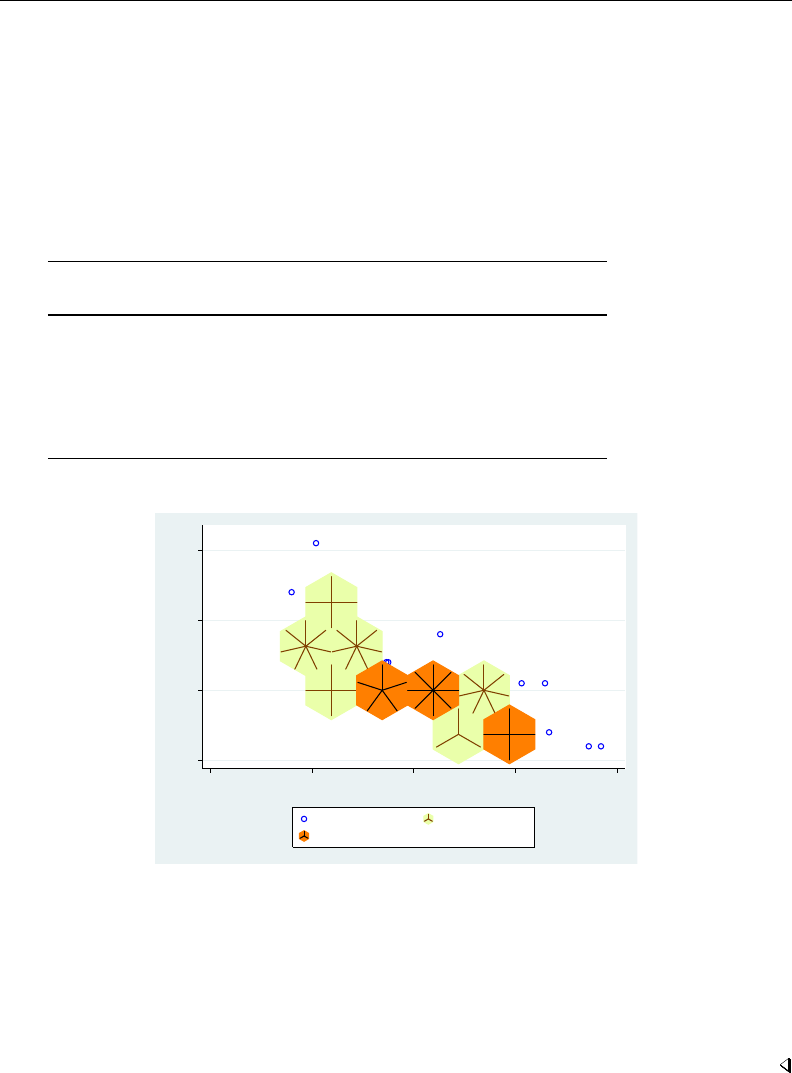
sunflower — Density-distribution sunflower plots 2269
. use http://www.stata-press.com/data/r13/auto
(1978 Automobile Data)
. sunflower mpg weight, binwid(500) petalw(2) dark(8) scheme(s2color)
Bin width = 500
Bin height = 8.38703
Bin aspect ratio = .0145268
Max obs in a bin = 15
Light = 3
Dark = 8
X-center = 3190
Y-center = 20
Petal weight = 2
flower petal No. of No. of estimated actual
type weight petals flowers obs. obs.
none 10 10
light 1 3 1 3 3
light 1 4 2 8 8
light 1 7 3 21 21
dark 2 4 1 8 8
dark 2 5 1 10 9
dark 2 8 1 16 15
76 74
10 20 30 40
Mileage (mpg)
1,000 2,000 3,000 4,000 5,000
Weight (lbs.)
Mileage (mpg) 1 petal = 1 obs.
1 petal = 2 obs.
The three darkly shaded sunflowers immediately catch our eyes, indicating a group of eight cars
that are heavy (nearly 4,000 pounds) and fuel inefficient and two groups of cars that get about 20
miles per gallon and weight in the neighborhood of 3,000 pounds, one with 10 cars and one with 8
cars. The lighter sunflowers with seven petals each indicate groups of seven cars that share similar
weight and fuel economy characteristics. To obtain the number of cars in each group, we counted
the number of petals in each flower and consulted the graph legend to see how many observations
each petal represents.

2270 sunflower — Density-distribution sunflower plots
Acknowledgments
We thank William D. Dupont and W. Dale Plummer Jr., both of the Department of Biostatistics at
Vanderbilt University, who are the authors of the original sunflower command, for their assistance
in producing this version.
References
Cleveland, W. S., and R. McGill. 1984. The many faces of a scatterplot. Journal of the American Statistical Association
79: 807–822.
Dupont, W. D. 2009. Statistical Modeling for Biomedical Researchers: A Simple Introduction to the Analysis of
Complex Data. 2nd ed. Cambridge: Cambridge University Press.
Dupont, W. D., and W. D. Plummer, Jr. 2005. Using density-distribution sunflower plots to explore bivariate relationships
in dense data.Stata Journal 5: 371–384.
Huang, C., J. A. McDonald, and W. Stuetzle. 1997. Variable resolution bivariate plots. Journal of Computational and
Graphical Statistics 6: 383–396.
Levy, D. E. 1999. 50 Years of Discovery: Medical Milestones from the National Heart, Lung, and Blood Institute’s
Framingham Heart Study. Hoboken, NJ: Center for Bio-Medical Communication.
Plummer, W. D., Jr., and W. D. Dupont. 2003. Density distribution sunflower plots. Journal of Statistical Software
8: 1–11.
Steichen, T. J., and N. J. Cox. 1999. flower: Stata module to draw sunflower plots. Boston College Department of
Economics, Statistical Software Components S393001. http://ideas.repec.org/c/boc/bocode/s393001.html.

Title
sureg — Zellner’s seemingly unrelated regression
Syntax Menu Description Options
Remarks and examples Stored results Methods and formulas References
Also see
Syntax
Basic syntax
sureg (depvar1varlist1) (depvar2varlist2). . . (depvarNvarlistN)
if in weight
Full syntax
sureg (eqname1:depvar1adepvar1b. . . =varlist1, noconstant )
(eqname2:depvar2adepvar2b. . . =varlist2, noconstant )
. . .
(eqnameN:depvarN a depvarN b . . . =varlistN, noconstant )
if in weight ,options
Explicit equation naming (eqname:) cannot be combined with multiple dependent variables in an
equation specification.
2271

2272 sureg — Zellner’s seemingly unrelated regression
options Description
Model
isure iterate until estimates converge
constraints(constraints)apply specified linear constraints
df adj.
small report small-sample statistics
dfk use small-sample adjustment
dfk2 use alternate adjustment
Reporting
level(#)set confidence level; default is level(95)
corr perform Breusch–Pagan test
nocnsreport do not display constraints
display options control column formats, row spacing, line width, display of omitted
variables and base and empty cells, and factor-variable labeling
Optimization
optimization options control the optimization process; seldom used
noheader suppress header table from above coefficient table
notable suppress coefficient table
coeflegend display legend instead of statistics
varlist1,. . . ,varlistNmay contain factor variables; see [U] 11.4.3 Factor variables. You must have the same levels
of factor variables in all equations that have factor variables.
depvars and the varlists may contain time-series operators; see [U] 11.4.4 Time-series varlists.
bootstrap,by,fp,jackknife,rolling, and statsby are allowed; see [U] 11.1.10 Prefix commands.
Weights are not allowed with the bootstrap prefix; see [R] bootstrap.
aweights are not allowed with the jackknife prefix; see [R] jackknife.
aweights and fweights are allowed; see [U] 11.1.6 weight.
noheader,notable, and coeflegend do not appear in the dialog box.
See [U] 20 Estimation and postestimation commands for more capabilities of estimation commands.
Menu
Statistics >Linear models and related >Multiple-equation models >Seemingly unrelated regression
Description
sureg fits seemingly unrelated regression models (Zellner 1962;Zellner and Huang 1962;Zell-
ner 1963). The acronyms SURE and SUR are often used for the estimator.

sureg — Zellner’s seemingly unrelated regression 2273
Options
Model
isure specifies that sureg iterate over the estimated disturbance covariance matrix and parameter
estimates until the parameter estimates converge. Under seemingly unrelated regression, this
iteration converges to the maximum likelihood results. If this option is not specified, sureg
produces two-step estimates.
constraints(constraints); see [R]estimation options.
df adj.
small specifies that small-sample statistics be computed. It shifts the test statistics from chi-squared
and zstatistics to Fstatistics and tstatistics. Although the standard errors from each equation are
computed using the degrees of freedom for the equation, the degrees of freedom for the tstatistics
are all taken to be those for the first equation.
dfk specifies the use of an alternate divisor in computing the covariance matrix for the equation
residuals. As an asymptotically justified estimator, sureg by default uses the number of sample
observations (n) as a divisor. When the dfk option is set, a small-sample adjustment is made and
the divisor is taken to be p(n−ki)(n−kj), where kiand kjare the numbers of parameters in
equations iand j, respectively.
dfk2 specifies the use of an alternate divisor in computing the covariance matrix for the equation
residuals. When the dfk2 option is set, the divisor is taken to be the mean of the residual degrees
of freedom from the individual equations.
Reporting
level(#); see [R]estimation options.
corr displays the correlation matrix of the residuals between equations and performs a Breusch–Pagan
test for independent equations; that is, the disturbance covariance matrix is diagonal.
nocnsreport; see [R]estimation options.
display options:noomitted,vsquish,noemptycells,baselevels,allbaselevels,nofvla-
bel,fvwrap(#),fvwrapon(style),cformat(%fmt),pformat(% fmt),sformat(% fmt), and
nolstretch; see [R]estimation options.
Optimization
optimization options control the iterative process that minimizes the sum of squared errors when
isure is specified. These options are seldom used.
iterate(#)specifies the maximum number of iterations. When the number of iterations equals #,
the optimizer stops and presents the current results, even if the convergence tolerance has not been
reached. The default value of iterate() is the current value of set maxiter (see [R]maximize),
which is iterate(16000) if maxiter has not been changed.
trace adds to the iteration log a display of the current parameter vector
nolog suppresses the display of the iteration log.
tolerance(#)specifies the tolerance for the coefficient vector. When the relative change in the
coefficient vector from one iteration to the next is less than or equal to #, the optimization process
is stopped. tolerance(1e-6) is the default.

2274 sureg — Zellner’s seemingly unrelated regression
The following options are available with sureg but are not shown in the dialog box:
noheader suppresses display of the table reporting Fstatistics, R-squared, and root mean squared
error above the coefficient table.
notable suppresses display of the coefficient table.
coeflegend; see [R]estimation options.
Remarks and examples
Seemingly unrelated regression models are so called because they appear to be joint estimates
from several regression models, each with its own error term. The regressions are related because the
(contemporaneous) errors associated with the dependent variables may be correlated. Chapter 5 of
Cameron and Trivedi (2010) contains a discussion of the seemingly unrelated regression model and
the feasible generalized least-squares estimator underlying it.
Example 1
When we fit models with the same set of right-hand-side variables, the seemingly unrelated
regression results (in terms of coefficients and standard errors) are the same as fitting the models
separately (using, say, regress). The same is true when the models are nested. Even in such cases,
sureg is useful when we want to perform joint tests. For instance, let us assume that we think
price =β0+β1foreign +β2length +u1
weight =γ0+γ1foreign +γ2length +u2
Because the models have the same set of explanatory variables, we could estimate the two equations
separately. Yet, we might still choose to estimate them with sureg because we want to perform the
joint test β1=γ1=0.
We use the small and dfk options to obtain small-sample statistics comparable with regress or
mvreg.
. use http://www.stata-press.com/data/r13/auto
(1978 Automobile Data)
. sureg (price foreign length) (weight foreign length), small dfk
Seemingly unrelated regression
Equation Obs Parms RMSE "R-sq" F-Stat P
price 74 2 2474.593 0.3154 16.35 0.0000
weight 74 2 250.2515 0.8992 316.54 0.0000
Coef. Std. Err. t P>|t| [95% Conf. Interval]
price
foreign 2801.143 766.117 3.66 0.000 1286.674 4315.611
length 90.21239 15.83368 5.70 0.000 58.91219 121.5126
_cons -11621.35 3124.436 -3.72 0.000 -17797.77 -5444.93
weight
foreign -133.6775 77.47615 -1.73 0.087 -286.8332 19.4782
length 31.44455 1.601234 19.64 0.000 28.27921 34.60989
_cons -2850.25 315.9691 -9.02 0.000 -3474.861 -2225.639

sureg — Zellner’s seemingly unrelated regression 2275
These two equations have a common set of regressors, and we could have used a shorthand syntax
to specify the equations:
. sureg (price weight = foreign length), small dfk
Here the results presented by sureg are the same as if we had estimated the equations separately:
. regress price foreign length
(output omitted )
. regress weight foreign length
(output omitted )
There is, however, a difference. We have allowed u1and u2to be correlated and have estimated the
full variance–covariance matrix of the coefficients. sureg has estimated the correlations, but it does
not report them unless we specify the corr option. We did not remember to specify corr when we
fit the model, but we can redisplay the results:
. sureg, notable noheader corr
Correlation matrix of residuals:
price weight
price 1.0000
weight 0.5840 1.0000
Breusch-Pagan test of independence: chi2(1) = 25.237, Pr = 0.0000
The notable and noheader options prevented sureg from redisplaying the header and coefficient
tables. We find that, for the same cars, the correlation of the residuals in the price and weight
equations is 0.5840 and that we can reject the hypothesis that this correlation is zero.
We can test that the coefficients on foreign are jointly zero in both equations—as we set out to
do—by typing test foreign; see [R]test. When we type a variable without specifying the equation,
that variable is tested for zero in all equations in which it appears:
. test foreign
( 1) [price]foreign = 0
( 2) [weight]foreign = 0
F( 2, 142) = 17.99
Prob > F = 0.0000
Example 2
When the models do not have the same set of explanatory variables and are not nested, sureg
may lead to more efficient estimates than running the models separately as well as allowing joint
tests. This time, let us assume that we believe
price =β0+β1foreign +β2mpg +β3displ +u1
weight =γ0+γ1foreign +γ2length +u2

2276 sureg — Zellner’s seemingly unrelated regression
To fit this model, we type
. sureg (price foreign mpg displ) (weight foreign length), corr
Seemingly unrelated regression
Equation Obs Parms RMSE "R-sq" chi2 P
price 74 3 2165.321 0.4537 49.64 0.0000
weight 74 2 245.2916 0.8990 661.84 0.0000
Coef. Std. Err. z P>|z| [95% Conf. Interval]
price
foreign 3058.25 685.7357 4.46 0.000 1714.233 4402.267
mpg -104.9591 58.47209 -1.80 0.073 -219.5623 9.644042
displacement 18.18098 4.286372 4.24 0.000 9.779842 26.58211
_cons 3904.336 1966.521 1.99 0.047 50.0263 7758.645
weight
foreign -147.3481 75.44314 -1.95 0.051 -295.2139 .517755
length 30.94905 1.539895 20.10 0.000 27.93091 33.96718
_cons -2753.064 303.9336 -9.06 0.000 -3348.763 -2157.365
Correlation matrix of residuals:
price weight
price 1.0000
weight 0.3285 1.0000
Breusch-Pagan test of independence: chi2(1) = 7.984, Pr = 0.0047
In comparison, if we had fit the price model separately,
. regress price foreign mpg displ
Source SS df MS Number of obs = 74
F( 3, 70) = 20.13
Model 294104790 3 98034929.9 Prob > F = 0.0000
Residual 340960606 70 4870865.81 R-squared = 0.4631
Adj R-squared = 0.4401
Total 635065396 73 8699525.97 Root MSE = 2207
price Coef. Std. Err. t P>|t| [95% Conf. Interval]
foreign 3545.484 712.7763 4.97 0.000 2123.897 4967.072
mpg -98.88559 63.17063 -1.57 0.122 -224.8754 27.10426
displacement 22.40416 4.634239 4.83 0.000 13.16146 31.64686
_cons 2796.91 2137.873 1.31 0.195 -1466.943 7060.763
The coefficients are slightly different, but the standard errors are uniformly larger. This would still be
true if we specified the dfk option to make a small-sample adjustment to the estimated covariance
of the disturbances.
Technical note
Constraints can be applied to SURE models using Stata’s standard syntax for constraints. For a
general discussion of constraints, see [R]constraint; for examples similar to seemingly unrelated
regression models, see [R]reg3.

sureg — Zellner’s seemingly unrelated regression 2277
Stored results
sureg stores the following in e():
Scalars
e(N) number of observations
e(k) number of parameters
e(k eq) number of equations in e(b)
e(mss #)model sum of squares for equation #
e(df m#)model degrees of freedom for equation #
e(rss #)residual sum of squares for equation #
e(df r) residual degrees of freedom
e(r2 #)R-squared for equation #
e(F #)Fstatistic for equation #(small only)
e(rmse #)root mean squared error for equation #
e(dfk2 adj) divisor used with VCE when dfk2 specified
e(ll) log likelihood
e(chi2 #)χ2for equation #
e(p #)significance for equation #
e(cons #) 1 if equation #has a constant, 0otherwise
e(chi2 bp) Breusch–Pagan χ2
e(df bp) degrees of freedom for Breusch–Pagan χ2test
e(cons #)1 when equation #has a constant; 0, otherwise
e(rank) rank of e(V)
e(ic) number of iterations
Macros
e(cmd) sureg
e(cmdline) command as typed
e(method) sure or isure
e(depvar) names of dependent variables
e(exog) names of exogenous variables
e(eqnames) names of equations
e(wtype) weight type
e(wexp) weight expression
e(corr) correlation structure
e(small) small
e(dfk) alternate divisor (dfk or dfk2 only)
e(properties) b V
e(predict) program used to implement predict
e(marginsok) predictions allowed by margins
e(marginsnotok) predictions disallowed by margins
e(asbalanced) factor variables fvset as asbalanced
e(asobserved) factor variables fvset as asobserved
Matrices
e(b) coefficient vector
e(Cns) constraints matrix
e(Sigma) b
Σmatrix
e(V) variance–covariance matrix of the estimators
Functions
e(sample) marks estimation sample
Methods and formulas
sureg uses the asymptotically efficient, feasible, generalized least-squares algorithm described in
Greene (2012, 292–304). The computing formulas are given on page 293–294.
The R-squared reported is the percent of variance explained by the predictors. It may be used for
descriptive purposes, but R-squared is not a well-defined concept when GLS is used.

2278 sureg — Zellner’s seemingly unrelated regression
sureg will refuse to compute the estimators if the same equation is named more than once or the
covariance matrix of the residuals is singular.
The Breusch and Pagan (1980)χ2statistic—a Lagrange multiplier statistic—is given by
λ=T
M
X
m=1
m−1
X
n=1
r2
mn
where rmn is the estimated correlation between the residuals of the Mequations and Tis the number
of observations. It is distributed as χ2with M(M−1)/2 degrees of freedom.
Arnold Zellner (1927–2010) was born in New York. He studied physics at Harvard and economics
at Berkeley, and then he taught economics at the Universities of Washington and Wisconsin
before settling in Chicago in 1966. Among his many major contributions to econometrics and
statistics are his work on seemingly unrelated regression, three-stage least squares, and Bayesian
econometrics.
References
Breusch, T. S., and A. R. Pagan. 1980. The Lagrange multiplier test and its applications to model specification in
econometrics. Review of Economic Studies 47: 239–253.
Cameron, A. C., and P. K. Trivedi. 2010. Microeconometrics Using Stata. Rev. ed. College Station, TX: Stata Press.
Greene, W. H. 2012. Econometric Analysis. 7th ed. Upper Saddle River, NJ: Prentice Hall.
McDowell, A. W. 2004. From the help desk: Seemingly unrelated regression with unbalanced equations.Stata Journal
4: 442–448.
Rossi, P. E. 1989. The ET interview: Professor Arnold Zellner. Econometric Theory 5: 287–317.
Weesie, J. 1999. sg121: Seemingly unrelated estimation and the cluster-adjusted sandwich estimator.Stata Technical
Bulletin 52: 34–47. Reprinted in Stata Technical Bulletin Reprints, vol. 9, pp. 231–248. College Station, TX: Stata
Press.
Zellner, A. 1962. An efficient method of estimating seemingly unrelated regressions and tests for aggregation bias.
Journal of the American Statistical Association 57: 348–368.
. 1963. Estimators for seemingly unrelated regression equations: Some exact finite sample results. Journal of the
American Statistical Association 58: 977–992.
Zellner, A., and D. S. Huang. 1962. Further properties of efficient estimators for seemingly unrelated regression
equations. International Economic Review 3: 300–313.
Also see
[R]sureg postestimation — Postestimation tools for sureg
[R]nlsur — Estimation of nonlinear systems of equations
[R]reg3 — Three-stage estimation for systems of simultaneous equations
[R]regress — Linear regression
[MV]mvreg — Multivariate regression
[SEM] example 12 — Seemingly unrelated regression
[SEM]intro 5 — Tour of models
[TS]dfactor — Dynamic-factor models
[U] 20 Estimation and postestimation commands

Title
sureg postestimation — Postestimation tools for sureg
Description Syntax for predict Menu for predict Options for predict
Remarks and examples Also see
Description
The following postestimation commands are available after sureg:
Command Description
contrast contrasts and ANOVA-style joint tests of estimates
estat ic Akaike’s and Schwarz’s Bayesian information criteria (AIC and BIC)
estat summarize summary statistics for the estimation sample
estat vce variance–covariance matrix of the estimators (VCE)
estimates cataloging estimation results
forecast dynamic forecasts and simulations
lincom point estimates, standard errors, testing, and inference for linear
combinations of coefficients
margins marginal means, predictive margins, marginal effects, and average marginal
effects
marginsplot graph the results from margins (profile plots, interaction plots, etc.)
nlcom point estimates, standard errors, testing, and inference for nonlinear
combinations of coefficients
predict predictions, residuals, influence statistics, and other diagnostic measures
predictnl point estimates, standard errors, testing, and inference for generalized predictions
pwcompare pairwise comparisons of estimates
test Wald tests of simple and composite linear hypotheses
testnl Wald tests of nonlinear hypotheses
Syntax for predict
predict type newvar if in , equation(eqno,eqno )statistic
statistic Description
Main
xb linear prediction; the default
stdp standard error of the linear prediction
residuals residuals
difference difference between the linear predictions of two equations
stddp standard error of the difference in linear predictions
These statistics are available both in and out of sample; type predict . . . if e(sample) . . . if wanted
only for the estimation sample.
2279

2280 sureg postestimation — Postestimation tools for sureg
Menu for predict
Statistics >Postestimation >Predictions, residuals, etc.
Options for predict
Main
equation(eqno,eqno )specifies to which equation(s) you are referring.
equation() is filled in with one eqno for the xb,stdp, and residuals options. equation(#1)
would mean that the calculation is to be made for the first equation, equation(#2) would mean
the second, and so on. You could also refer to the equations by their names. equation(income)
would refer to the equation named income and equation(hours) to the equation named hours.
If you do not specify equation(), the results are the same as if you specified equation(#1).
difference and stddp refer to between-equation concepts. To use these options, you must
specify two equations, for example, equation(#1,#2) or equation(income,hours). When
two equations must be specified, equation() is required.
xb, the default, calculates the linear prediction (fitted values)—the prediction of xjbfor the specified
equation.
stdp calculates the standard error of the prediction for the specified equation. It can be thought of as
the standard error of the predicted expected value or mean for the observation’s covariate pattern.
The standard error of the prediction is also referred to as the standard error of the fitted value.
residuals calculates the residuals.
difference calculates the difference between the linear predictions of two equations in the system.
With equation(#1,#2),difference computes the prediction of equation(#1) minus the
prediction of equation(#2).
stddp is allowed only after you have previously fit a multiple-equation model. The standard error of
the difference in linear predictions (x1jb−x2jb)between equations 1 and 2 is calculated.
For more information on using predict after multiple-equation estimation commands, see [R]predict.
Remarks and examples
For an example of cross-equation testing of parameters using the test command, see example 1
in [R]sureg.
Example 1
In example 1 of [R]sureg, we fit a seemingly unrelated regressions model of price and weight.
Here we obtain the fitted values.
. use http://www.stata-press.com/data/r13/auto
(1978 Automobile Data)
. sureg (price foreign length) (weight foreign length), small dfk
(output omitted )
. predict phat, equation(price)
(option xb assumed; fitted values)
. predict what, equation(weight)
(option xb assumed; fitted values)

sureg postestimation — Postestimation tools for sureg 2281
. summarize price phat weight what
Variable Obs Mean Std. Dev. Min Max
price 74 6165.257 2949.496 3291 15906
phat 74 6165.257 1656.407 1639.872 9398.138
weight 74 3019.459 777.1936 1760 4840
what 74 3019.459 736.9666 1481.199 4476.331
Just as in single-equation OLS regression, in a SURE model the sample mean of the fitted values
for an equation equals the sample mean of the dependent variable.
Example 2
Suppose that for whatever reason we were interested in the difference between the predicted values
of price and weight.predict has an option to compute this difference in one step:
. predict diff, equation(price, weight) difference
diff is the same as phat - what:
. generate mydiff = phat - what
. summarize diff mydiff
Variable Obs Mean Std. Dev. Min Max
diff 74 3145.797 1233.26 -132.2275 5505.914
mydiff 74 3145.797 1233.26 -132.2275 5505.914
Also see
[R]sureg — Zellner’s seemingly unrelated regression
[U] 20 Estimation and postestimation commands

Title
swilk — Shapiro–Wilk and Shapiro–Francia tests for normality
Syntax Menu Description Options for swilk
Options for sfrancia Remarks and examples Stored results Methods and formulas
Acknowledgment References Also see
Syntax
Shapiro–Wilk normality test
swilk varlist if in ,swilk options
Shapiro–Francia normality test
sfrancia varlist if in ,sfrancia options
swilk options Description
Main
generate(newvar)create newvar containing Wtest coefficients
lnnormal test for three-parameter lognormality
noties do not use average ranks for tied values
sfrancia options Description
Main
boxcox use the Box–Cox transformation for W0; the default is to use the
log transformation
noties do not use average ranks for tied values
by is allowed with swilk and sfrancia; see [D] by.
Menu
swilk
Statistics >Summaries, tables, and tests >Distributional plots and tests >Shapiro-Wilk normality test
sfrancia
Statistics >Summaries, tables, and tests >Distributional plots and tests >Shapiro-Francia normality test
Description
swilk performs the Shapiro–Wilk Wtest for normality, and sfrancia performs the
Shapiro–Francia W0test for normality. swilk can be used with 4 ≤n≤2000 observations,
and sfrancia can be used with 5 ≤n≤5000 observations; see [R]sktest for a test allowing more
observations. See [MV]mvtest normality for multivariate tests of normality.
2282

swilk — Shapiro–Wilk and Shapiro–Francia tests for normality 2283
Options for swilk
Main
generate(newvar)creates new variable newvar containing the Wtest coefficients.
lnnormal specifies that the test be for three-parameter lognormality, meaning that ln(X−k)is tested
for normality, where kis calculated from the data as the value that makes the skewness coefficient
zero. When simply testing ln(X)for normality, do not specify this option. See [R]lnskew0 for
estimation of k.
noties suppresses use of averaged ranks for tied values when calculating the Wtest coefficients.
Options for sfrancia
Main
boxcox specifies that the Box–Cox transformation of Royston (1983) for calculating W0test
coefficients be used instead of the default log transformation (Royston 1993a). Under the Box–Cox
transformation, the normal approximation to the sampling distribution of W0, used by sfrancia,
is valid for 5 ≤n≤1000. Under the log transformation, it is valid for 10≤n≤5000.
noties suppresses use of averaged ranks for tied values when calculating the W0test coefficients.
Remarks and examples
Example 1
Using our automobile dataset, we will test whether the variables mpg and trunk are normally
distributed:
. use http://www.stata-press.com/data/r13/auto
(1978 Automobile Data)
. swilk mpg trunk
Shapiro-Wilk W test for normal data
Variable Obs W V z Prob>z
mpg 74 0.94821 3.335 2.627 0.00430
trunk 74 0.97921 1.339 0.637 0.26215
. sfrancia mpg trunk
Shapiro-Francia W’ test for normal data
Variable Obs W’ V’ z Prob>z
mpg 74 0.94872 3.650 2.510 0.00604
trunk 74 0.98446 1.106 0.195 0.42271
We can reject the hypothesis that mpg is normally distributed, but we cannot reject that trunk is
normally distributed.
The values reported under Wand W0are the Shapiro– Wilk and Shapiro – Francia test statistics.
The tests also report Vand V0, which are more appealing indexes for departure from normality.
The median values of Vand V0are 1 for samples from normal populations. Large values indicate
nonnormality. The 95% critical values of V(V0), which depend on the sample size, are between 1.2
and 2.4 (2.0 and 2.8); see Royston (1991b). There is no more information in V(V0) than in W
(W0)—one is just the transform of the other.

2284 swilk — Shapiro–Wilk and Shapiro–Francia tests for normality
Example 2
We have data on a variable called studytime, which we suspect is distributed lognormally:
. use http://www.stata-press.com/data/r13/cancer
(Patient Survival in Drug Trial)
. generate lnstudytime = ln(studytime)
. swilk lnstudytime
Shapiro-Wilk W test for normal data
Variable Obs W V z Prob>z
lnstudytime 48 0.92731 3.311 2.547 0.00543
We can reject the lognormal assumption. We do not specify the lnnormal option when testing for
lognormality. The lnnormal option is for three-parameter lognormality.
Example 3
Having discovered that ln(studytime)is not distributed normally, we now test that
ln(studytime −k)is normally distributed, where kis chosen so that the resulting skewness is
zero. We obtain the estimate for kfrom lnskew0; see [R]lnskew0:
. lnskew0 lnstudytimek = studytime, level(95)
Transform k [95% Conf. Interval] Skewness
ln(studytim-k) -11.01181 -infinity -.9477328 -.0000173
. swilk lnstudytimek, lnnormal
Shapiro-Wilk W test for 3-parameter lognormal data
Variable Obs W V z Prob>z
lnstudytimek 48 0.97064 1.337 1.261 0.10363
We cannot reject the hypothesis that ln(studytime +11.01181)is distributed normally. We do
specify the lnnormal option when using an estimated value of k.
Stored results
swilk and sfrancia store the following in r():
Scalars
r(N) number of observations r(W) Wor W0
r(p) significance r(V) Vor V0
r(z) zstatistic
Methods and formulas
The Shapiro–Wilk test is based on Shapiro and Wilk (1965) with a new approximation accurate
for 4 ≤n≤2000 (Royston 1992). The calculations made by swilk are based on Royston (1982,
1992,1993b).

swilk — Shapiro–Wilk and Shapiro–Francia tests for normality 2285
The Shapiro–Francia test (Shapiro and Francia 1972;Royston 1983;Royston 1993a) is an
approximate test that is similar to the Shapiro–Wilk test for very large samples.
Samuel Sanford Shapiro (1930– ) earned degrees in statistics and engineering from City College
of New York, Columbia, and Rutgers. After employment in the U.S. Army and industry, he
joined the faculty at Florida International University in 1972. Shapiro has coauthored various
texts in statistics and published several papers on distributional testing and other statistical topics.
Acknowledgment
swilk and sfrancia were written by Patrick Royston of the MRC Clinical Trials Unit, London
and coauthor of the Stata Press book Flexible Parametric Survival Analysis Using Stata: Beyond the
Cox Model.
References
Brzezinski, M. 2012. The Chen–Shapiro test for normality.Stata Journal 12: 368–374.
Genest, C., and G. J. Brackstone. 2010. A conversation with Martin Bradbury Wilk. Statistical Science 25: 258–273.
Gould, W. W. 1992. sg3.7: Final summary of tests of normality.Stata Technical Bulletin 5: 10–11. Reprinted in Stata
Technical Bulletin Reprints, vol. 1, pp. 114–115. College Station, TX: Stata Press.
Royston, P. 1982. An extension of Shapiro and Wilks’s Wtest for normality to large samples. Applied Statistics 31:
115–124.
. 1983. A simple method for evaluating the Shapiro–Francia W’ test of non-normality. Statistician 32: 297–300.
. 1991a. sg3.2: Shapiro–Wilk and Shapiro–Francia tests.Stata Technical Bulletin 3: 19. Reprinted in Stata
Technical Bulletin Reprints, vol. 1, p. 105. College Station, TX: Stata Press.
. 1991b. Estimating departure from normality. Statistics in Medicine 10: 1283–1293.
. 1992. Approximating the Shapiro–Wilk W-test for non-normality. Statistics and Computing 2: 117–119.
. 1993a. A pocket-calculator algorithm for the Shapiro–Francia test for non-normality: An application to medicine.
Statistics in Medicine 12: 181–184.
. 1993b. A toolkit for testing for non-normality in complete and censored samples. Statistician 42: 37–43.
Shapiro, S. S., and R. S. Francia. 1972. An approximate analysis of variance test for normality. Journal of the
American Statistical Association 67: 215–216.
Shapiro, S. S., and M. B. Wilk. 1965. An analysis of variance test for normality (complete samples). Biometrika 52:
591–611.
Also see
[R]lnskew0 — Find zero-skewness log or Box–Cox transform
[R]lv — Letter-value displays
[R]sktest — Skewness and kurtosis test for normality
[MV]mvtest normality — Multivariate normality tests

Title
symmetry — Symmetry and marginal homogeneity tests
Syntax Menu Description Options
Remarks and examples Stored results Methods and formulas References
Also see
Syntax
Symmetry and marginal homogeneity tests
symmetry casevar controlvar if in weight ,options
Immediate form of symmetry and marginal homogeneity tests
symmi #11 #12 [...]\#21 #22 [...] [\...]if in ,options
options Description
Main
notable suppress output of contingency table
contrib report contribution of each off-diagonal cell pair
exact perform exact test of table symmetry
mh perform two marginal homogeneity tests
trend perform a test for linear trend in the (log) relative risk (RR)
cc use continuity correction when calculating test for linear trend
fweights are allowed; see [U] 11.1.6 weight.
Menu
symmetry
Statistics >Epidemiology and related >Other >Symmetry and marginal homogeneity test
symmi
Statistics >Epidemiology and related >Other >Symmetry and marginal homogeneity test calculator
Description
symmetry performs asymptotic symmetry and marginal homogeneity tests, as well as an exact
symmetry test on K×Ktables where there is a 1-to-1 matching of cases and controls (nonindepen-
dence). This testing is used to analyze matched-pair case–control data with multiple discrete levels
of the exposure (outcome) variable. In genetics, the test is known as the transmission/disequilibrium
test (TDT) and is used to test the association between transmitted and nontransmitted parental marker
alleles to an affected child (Spieldman, McGinnis, and Ewens 1993). For 2 ×2 tables, the asymptotic
test statistics reduce to the McNemar test statistic, and the exact symmetry test produces an exact
McNemar test; see [ST]epitab. For many exposure variables, symmetry can optionally perform a
test for linear trend in the log relative risk.
2286

symmetry — Symmetry and marginal homogeneity tests 2287
symmetry expects the data to be in the wide format; that is, each observation contains the matched
case and control values in variables casevar and controlvar. Variables can be numeric or string.
symmi is the immediate form of symmetry. The symmi command uses the values specified on
the command line; rows are separated by ‘\’, and options are the same as for symmetry. See
[U] 19 Immediate commands for a general introduction to immediate commands.
Options
Main
notable suppresses the output of the contingency table. By default, symmetry displays the n×n
contingency table at the top of the output.
contrib reports the contribution of each off-diagonal cell pair to the overall symmetry χ2.
exact performs an exact test of table symmetry. This option is recommended for sparse tables.
CAUTION: The exact test requires substantial amounts of time and memory for large tables.
mh performs two marginal homogeneity tests that do not require the inversion of the variance–covariance
matrix.
By default, symmetry produces the Stuart–Maxwell test statistic, which requires the inversion of the
nondiagonal variance–covariance matrix, V. When the table is sparse, the matrix may not be of full
rank, and then the command substitutes a generalized inverse V∗for V−1.mh calculates optional
marginal homogeneity statistics that do not require the inversion of the variance–covariance matrix.
These tests may be preferred in certain situations. See Methods and formulas and Bickeb¨
oller and
Clerget-Darpoux (1995) for details on these test statistics.
trend performs a test for linear trend in the (log) relative risk (RR). This option is allowed only for
numeric exposure (outcome) variables, and its use should be restricted to measurements on the
ordinal or the interval scales.
cc specifies that the continuity correction be used when calculating the test for linear trend. This
correction should be specified only when the levels of the exposure variable are equally spaced.
Remarks and examples
symmetry and symmi may be used to analyze 1-to-1 matched case–control data with multiple
discrete levels of the exposure (outcome) variable.
Example 1
Consider a survey of 344 individuals (BMDP 1990, 267–270) who were asked in October 1986
whether they agreed with President Reagan’s handling of foreign affairs. In January 1987, after the
Iran-Contra affair became public, these same individuals were surveyed again and asked the same
question. We would like to know if public opinion changed over this period.

2288 symmetry — Symmetry and marginal homogeneity tests
We first describe the dataset and list a few observations.
. use http://www.stata-press.com/data/r13/iran
. describe
Contains data from http://www.stata-press.com/data/r13/iran.dta
obs: 344
vars: 2 29 Jan 2013 02:37
size: 688
storage display value
variable name type format label variable label
before byte %8.0g vlab Public Opinion before IC
after byte %8.0g vlab Public Opinion after IC
Sorted by:
. list in 1/5
before after
1. agree agree
2. agree disagree
3. agree unsure
4. disagree agree
5. disagree disagree
Each observation corresponds to one of the 344 individuals. The data are in wide form so that
each observation has a before and an after measurement. We now perform the test without options.
. symmetry before after
Public
Opinion Public Opinion after IC
before IC agree disagree unsure Total
agree 47 56 38 141
disagree 28 61 31 120
unsure 26 47 10 83
Total 101 164 79 344
chi2 df Prob>chi2
Symmetry (asymptotic) 14.87 3 0.0019
Marginal homogeneity (Stuart-Maxwell) 14.78 2 0.0006
The test first tabulates the data in a K×Ktable and then performs Bowker’s (1948) test for table
symmetry and the Stuart–Maxwell (Stuart 1955;Maxwell 1970) test for marginal homogeneity.
Both the symmetry test and the marginal homogeneity test are highly significant, thus indicating
a shift in public opinion.
An exact test of symmetry is provided for use on sparse tables. This test is computationally
intensive, so it should not be used on large tables. Because we are working on a fast computer, we
will run the symmetry test again and this time include the exact option. We will suppress the output
of the contingency table by specifying notable and include the contrib option so that we may
further examine the cells responsible for the significant result.

symmetry — Symmetry and marginal homogeneity tests 2289
. symmetry before after, contrib exact mh notable
Contribution
to symmetry
Cells chi-squared
n1_2 & n2_1 9.3333
n1_3 & n3_1 2.2500
n2_3 & n3_2 3.2821
chi2 df Prob>chi2
Symmetry (asymptotic) 14.87 3 0.0019
Marginal homogeneity (Stuart-Maxwell) 14.78 2 0.0006
Marginal homogeneity (Bickenboller) 13.53 2 0.0012
Marginal homogeneity (no diagonals) 15.25 2 0.0005
Symmetry (exact significance probability) 0.0018
The largest contribution to the symmetry χ2is due to cells n12 and n21. These correspond to
changes between the agree and disagree categories. Of the 344 individuals, 56 (16.3%) changed from
the agree to the disagree response, whereas only 28 (8.1%) changed in the opposite direction.
For these data, the results from the exact test are similar to those from the asymptotic test.
Example 2
Breslow and Day (1980, 163) reprinted data from Mack et al. (1976) from a case–control study
of the effect of exogenous estrogen on the risk of endometrial cancer. The data consist of 59 elderly
women diagnosed with endometrial cancer and 59 disease-free control subjects living in the same
community as the cases. Cases and controls were matched on age, marital status, and time living
in the community. The data collected included information on the daily dose of conjugated estrogen
therapy. Breslow and Day analyzed these data by creating four levels of the dose variable. Here are
the data as entered into a Stata dataset:
. use http://www.stata-press.com/data/r13/bd163
. list, noobs divider
case control count
0 0 6
0 0.1-0.299 2
0 0.3-0.625 3
0 0.626+ 1
0.1-0.299 0 9
0.1-0.299 0.1-0.299 4
0.1-0.299 0.3-0.625 2
0.1-0.299 0.626+ 1
0.3-0.625 0 9
0.3-0.625 0.1-0.299 2
0.3-0.625 0.3-0.625 3
0.3-0.625 0.626+ 1
0.626+ 0 12
0.626+ 0.1-0.299 1
0.626+ 0.3-0.625 2
0.626+ 0.626+ 1

2290 symmetry — Symmetry and marginal homogeneity tests
This dataset is in a different format from that of the previous example. Instead of each observation
representing one matched pair, each observation represents possibly multiple pairs indicated by the
count variable. For instance, the first observation corresponds to six matched pairs where neither
the case nor the control was on estrogen, the second observation corresponds to two matched pairs
where the case was not on estrogen and the control was on 0.1 to 0.299 mg/day, etc.
To use symmetry to analyze this dataset, we must specify fweight to indicate that in our data
there are observations corresponding to more than one matched pair.
. symmetry case control [fweight=count]
control
case 0 0.1-0.299 0.3-0.625 0.626+ Total
0 6 2 3 1 12
0.1-0.299 9 4 2 1 16
0.3-0.625 9 2 3 1 15
0.626+ 12 1 2 1 16
Total 36 9 10 4 59
chi2 df Prob>chi2
Symmetry (asymptotic) 17.10 6 0.0089
Marginal homogeneity (Stuart-Maxwell) 16.96 3 0.0007
Both the test of symmetry and the test of marginal homogeneity are highly significant, thus leading
us to reject the null hypothesis that there is no effect of exposure to estrogen on the risk of endometrial
cancer.
Breslow and Day perform a test for trend assuming that the estrogen exposure levels were equally
spaced by recoding the exposure levels as 1, 2, 3, and 4.
We can easily reproduce their results by recoding our data in this way and by specifying the
trend option. Two new numeric variables were created, ca and co, corresponding to the variables
case and control, respectively. Below we list some of the data and our results from symmetry:
. encode case, gen(ca)
. encode control, gen(co)
. label values ca
. label values co
. list in 1/4
case control count ca co
1. 0 0 6 1 1
2. 0 0.1-0.299 2 1 2
3. 0 0.3-0.625 3 1 3
4. 0 0.626+ 1 1 4
. symmetry ca co [fw=count], notable trend cc
chi2 df Prob>chi2
Symmetry (asymptotic) 17.10 6 0.0089
Marginal homogeneity (Stuart-Maxwell) 16.96 3 0.0007
Linear trend in the (log) RR 14.43 1 0.0001

symmetry — Symmetry and marginal homogeneity tests 2291
We requested the continuity correction by specifying cc. Doing so is appropriate because our coded
exposure levels are equally spaced.
The test for trend was highly significant, indicating an increased risk of endometrial cancer with
increased dosage of conjugated estrogen.
You must be cautious: the way in which you code the exposure variable affects the linear trend
statistic. If instead of coding the levels as 1, 2, 3, and 4, we had instead used 0, 0.2, 0.46, and 0.7
(roughly the midpoint in the range of each level), we would have obtained a χ2statistic of 11.19 for
these data.
Stored results
symmetry stores the following in r():
Scalars
r(N pair) number of matched pairs
r(chi2) asymptotic symmetry χ2
r(df) asymptotic symmetry degrees of freedom
r(p) asymptotic symmetry p-value
r(chi2 sm) MH (Stuart–Maxwell) χ2
r(df sm) MH (Stuart–Maxwell) degrees of freedom
r(p sm) MH (Stuart–Maxwell) p-value
r(chi2 b) MH (Bickenb¨
oller) χ2
r(df b) MH (Bickenb¨
oller) degrees of freedom
r(p b) MH (Bickenb¨
oller) p-value
r(chi2 nd) MH (no diagonals) χ2
r(df nd) MH (no diagonals) degrees of freedom
r(p nd) MH (no diagonals) p-value
r(chi2 t) χ2for linear trend
r(p trend) p-value for linear trend
r(p exact) exact symmetry p-value
Methods and formulas
Methods and formulas are presented under the following headings:
Asymptotic tests
Exact symmetry test
Asymptotic tests
Consider a square table with Kexposure categories, that is, Krows and Kcolumns. Let nij be
the count corresponding to row iand column jof the table, Nij =nij +nji, for i, j =1,2, . . . , K,
and ni., and let n.j be the marginal totals for row iand column j, respectively. Asymptotic tests for
symmetry and marginal homogeneity for this K×Ktable are calculated as follows:
The null hypothesis of complete symmetry pij =pji,i6=j, is tested by calculating the test
statistic (Bowker 1948)
Tcs =X
i<j
(nij −nji)2
nij +nji
which is asymptotically distributed as χ2with K(K−1)/2−Rdegrees of freedom, where Ris
the number of off-diagonal cells with Nij =0.

2292 symmetry — Symmetry and marginal homogeneity tests
The null hypothesis of marginal homogeneity, pi. =p.i, is tested by calculating the Stuart–Maxwell
test statistic (Stuart 1955;Maxwell 1970),
Tsm =d0V−1d
where dis a column vector with elements equal to the differences di=ni. −n.i for i=1,2, . . . , K,
and Vis the variance–covariance matrix with elements
vii =ni. +n.i −2nii
vij =−(nij +nji), i 6=j
Tsm is asymptotically χ2with K−1 degrees of freedom.
This test statistic properly accounts for the dependence between the table’s rows and columns.
When the matrix Vis not of full rank, a generalized inverse V∗is substituted for V−1.
The Bickeb¨
oller and Clerget-Darpoux (1995) marginal homogeneity test statistic is calculated by
Tmh =X
i
(ni. −n.i)2
ni. +n.i
This statistic is asymptotically distributed, under the assumption of marginal independence, as χ2
with K−1 degrees of freedom.
The marginal homogeneity (no diagonals) test statistic T0
mh is calculated in the same way as Tmh,
except that the diagonal elements do not enter into the calculation of the marginal totals. Unlike the
previous test statistic, T0
mh reduces to a McNemar test statistic for 2 ×2 tables. The test statistic
{(K−1)/2}T0
mh is asymptotically distributed as χ2with K−1 degrees of freedom (Cleves, Olson,
and Jacobs 1997;Spieldman and Ewens 1996).
Breslow and Day’s test statistic for linear trend in the (log) of RR is
Pi<j (nij −nji)(Xj−Xi)−cc2
Pi<j (nij +nji)(Xj−Xi)2
where the Xjare the doses associated with the various levels of exposure and cc is the continuity
correction; it is asymptotically distributed as χ2with 1 degree of freedom.
The continuity correction option is applicable only when the levels of the exposure variable are
equally spaced.
Exact symmetry test
The exact test is based on a permutation algorithm applied to the null distribution. The distribution
of the off-diagonal elements nij ,i6=j, conditional on the sum of the complementary off-diagonal
cells, Nij =nij +nji, can be written as the product of K(K−1)/2 binomial random variables,
P(n) = Y
i<j Nij
nij πij nij (1 −πij )nij
where nis a vector with elements nij and πij =E(nij /Nij |Nij ). Under the null hypothesis of
complete symmetry, πij =πji =1/2, and thus the permutation distribution is given by

symmetry — Symmetry and marginal homogeneity tests 2293
P0(n) = Y
i<j Nij
nij 1
2Nij
The exact significance test is performed by evaluating
Pcs =X
n∈p
P0(n)
where p={n:P0(n)< P0(n∗)}and n∗is the observed contingency table data vector. The
algorithm evaluates pcs exactly. For information about permutation tests, see Good (2005,2006).
References
Bickeb¨
oller, H., and F. Clerget-Darpoux. 1995. Statistical properties of the allelic and genotypic transmis-
sion/disequilibrium test for multiallelic markers. Genetic Epidemiology 12: 865–870.
BMDP. 1990. BMDP Statistical Software Manual. Oakland, CA: University of California Press.
Bowker, A. H. 1948. A test for symmetry in contingency tables. Journal of the American Statistical Association 43:
572–574.
Breslow, N. E., and N. E. Day. 1980. Statistical Methods in Cancer Research: Vol. 1—The Analysis of Case–Control
Studies. Lyon: IARC.
Cleves, M. A. 1997. sg74: Symmetry and marginal homogeneity test/Transmission-Disequilibrium Test (TDT).Stata
Technical Bulletin 40: 23–27. Reprinted in Stata Technical Bulletin Reprints, vol. 7, pp. 193–197. College Station,
TX: Stata Press.
. 1999. sg110: Hardy–Weinberg equilibrium test and allele frequency estimation.Stata Technical Bulletin 48:
34–37. Reprinted in Stata Technical Bulletin Reprints, vol. 8, pp. 280–284. College Station, TX: Stata Press.
Cleves, M. A., J. M. Olson, and K. B. Jacobs. 1997. Exact transmission-disequilibrium tests with multiallelic markers.
Genetic Epidemiology 14: 337–347.
Cui, J. 2000. sg150: Hardy–Weinberg equilibrium test in case–control studies.Stata Technical Bulletin 57: 17–19.
Reprinted in Stata Technical Bulletin Reprints, vol. 10, pp. 218–220. College Station, TX: Stata Press.
Good, P. I. 2005. Permutation, Parametric, and Bootstrap Tests of Hypotheses: A Practical Guide to Resampling
Methods for Testing Hypotheses. 3rd ed. New York: Springer.
. 2006. Resampling Methods: A Practical Guide to Data Analysis. 3rd ed. Boston: Birkh¨
auser.
Mack, T. M., M. C. Pike, B. E. Henderson, R. I. Pfeffer, V. R. Gerkins, M. Arthur, and S. E. Brown. 1976. Estrogens
and endometrial cancer in a retirement community. New England Journal of Medicine 294: 1262–1267.
Mander, A. P. 2000. sbe38: Haplotype frequency estimation using an EM algorithm and log-linear modeling.Stata
Technical Bulletin 57: 5–7. Reprinted in Stata Technical Bulletin Reprints, vol. 10, pp. 104–107. College Station,
TX: Stata Press.
Maxwell, A. E. 1970. Comparing the classification of subjects by two independent judges. British Journal of Psychiatry
116: 651–655.
Spieldman, R. S., and W. J. Ewens. 1996. The TDT and other family-based tests for linkage disequilibrium and
association. American Journal of Human Genetics 59: 983–989.
Spieldman, R. S., R. E. McGinnis, and W. J. Ewens. 1993. Transmission test for linkage disequilibrium: The insulin
gene region and insulin-dependence diabetes mellitus (IDDM). American Journal of Human Genetics 52: 506–516.
Stuart, A. 1955. A test for homogeneity of the marginal distributions in a two-way classification. Biometrika 42:
412–416.
Also see
[ST]epitab — Tables for epidemiologists

Title
table — Flexible table of summary statistics
Syntax Menu Description Options
Remarks and examples Methods and formulas Also see
Syntax
table rowvar colvar supercolvar if in weight ,options
options Description
Main
contents(clist)contents of table cells; select up to five statistics; default is
contents(freq)
by(superrowvarlist)superrow variables
Options
cellwidth(#)cell width
csepwidth(#)column-separation width
stubwidth(#)stub width
scsepwidth(#)supercolumn-separation width
center center-align table cells; default is right-align
left left-align table cells; default is right-align
cw perform casewise deletion
row add row totals
column add column totals
scolumn add supercolumn totals
concise suppress rows with all missing entries
missing show missing statistics with period
replace replace current data with table statistics
name(string)name new variables with prefix string
format(%fmt)display format for numbers in cells; default is format(%9.0g)
by is allowed; see [D] by.
fweights, iweights, and pweights are allowed; see [U] 11.1.6 weight.pweights may not be used with sd,semean,
sebinomial, or sepoisson.iweights may not be used with semean,sebinomial, or sepoisson.
where the elements of clist may be
freq frequency nvarname same as count
mean varname mean of varname max varname maximum
sd varname standard deviation min varname minimum
semean varname standard error of the mean median varname median
(sd/sqrt(n))p1 varname 1st percentile
sebinomial varname standard error of the mean, binomial p2 varname 2nd percentile
distribution (sqrt(p(1-p)/n)). . . 3rd – 49th percentiles
sepoisson varname standard error of the mean, Poisson p50 varname 50th percentile (median)
distribution (sqrt(mean)). . . 51st – 97th percentiles
sum varname sum p98 varname 98th percentile
rawsum varname sums ignoring optionally specified weight p99 varname 99th percentile
count varname count of nonmissing observations iqr varname interquartile range
2294

table — Flexible table of summary statistics 2295
Rows, columns, supercolumns, and superrows are thus defined as
row 1 .
row 2 .
supercol 1 supercol 2
col 1 col 2 col 1 col 2
row 1 . . . .
row 2 . . . .
col 1 col 2
row 1 . .
row 2 . .
supercol 1 supercol 2
col 1 col 2 col 1 col 2
superrow 1:
row 1 . . . .
row 2 . . . .
superrow 2:
row 1 . . . .
row 2 . . . .
Menu
Statistics >Summaries, tables, and tests >Other tables >Flexible table of summary statistics
Description
table calculates and displays tables of statistics.
Options
Main
contents(clist)specifies the contents of the table’s cells; if not specified, contents(freq) is used
by default. contents(freq) produces a table of frequencies. contents(mean mpg) produces
a table of the means of variable mpg.contents(freq mean mpg sd mpg) produces a table of
frequencies together with the mean and standard deviation of variable mpg. Up to five statistics
may be specified.
by(superrowvarlist)specifies that numeric or string variables be treated as superrows. Up to four
variables may be specified in superrowvarlist. The by() option may be specified with the by
prefix.
Options
cellwidth(#)specifies the width of the cell in units of digit widths; 10 means the space occupied by
10 digits, which is 0123456789. The default cellwidth() is not a fixed number, but a number
chosen by table to spread the table out while presenting a reasonable number of columns across
the page.

2296 table — Flexible table of summary statistics
csepwidth(#)specifies the separation between columns in units of digit widths. The default is not
a fixed number, but a number chosen by table according to what it thinks looks best.
stubwidth(#)specifies the width, in units of digit widths, to be allocated to the left stub of the
table. The default is not a fixed number, but a number chosen by table according to what it
thinks looks best.
scsepwidth(#)specifies the separation between supercolumns in units of digit widths. The default
is not a fixed number, but a number chosen by table to present the results best.
center specifies that results be centered in the table’s cells. The default is to right-align results.
For centering to work well, you typically need to specify a display format as well. center
format(%9.2f) is popular.
left specifies that column labels be left-aligned. The default is to right-align column labels to
distinguish them from supercolumn labels, which are left-aligned.
cw specifies casewise deletion. If cw is not specified, all observations possible are used to calculate
each of the specified statistics. cw is relevant only when you request a table containing statistics
on multiple variables. For instance, contents(mean mpg mean weight) would produce a table
reporting the means of variables mpg and weight. Consider an observation in which mpg is known
but weight is missing. By default, that observation will be used in the calculation of the mean of
mpg. If you specify cw, the observation will be excluded in the calculation of the means of both
mpg and weight.
row specifies that a row be added to the table reflecting the total across the rows.
column specifies that a column be added to the table reflecting the total across columns.
scolumn specifies that a supercolumn be added to the table reflecting the total across supercolumns.
concise specifies that rows with all missing entries not be displayed.
missing specifies that missing statistics be shown in the table as periods (Stata’s missing-value
indicator). The default is that missing entries be left blank.
replace specifies that the data in memory be replaced with data containing 1 observation per cell
(row, column, supercolumn, and superrow) and with variables containing the statistics designated
in contents().
This option is rarely specified. If you do not specify this option, the data in memory remain
unchanged.
If you do specify this option, the first statistic will be named table1, the second table2, and so
on. For instance, if contents(mean mpg sd mpg) was specified, the means of mpg would be in
variable table1 and the standard deviations in table2.
name(string)is relevant only if you specify replace.name() allows changing the default stub
name that replace uses to name the new variables associated with the statistics. If you specify
name(stat), the first statistic will be placed in variable stat1, the second in stat2, and so on.
format(%fmt)specifies the display format for presenting numbers in the table’s cells. format(%9.0g)
is the default; format(%9.2f) and format(%9.2fc) are popular alternatives. The width of the
format you specify does not matter, except that %fmt must be valid. The width of the cells is
chosen by table to present the results best. The cellwidth() option allows you to override
table’s choice.

table — Flexible table of summary statistics 2297
Limits
Up to four variables may be specified in the by(), so with the three row, column, and supercolumn
variables, seven-way tables may be displayed.
Up to five statistics may be displayed in each cell of the table.
The sum of the number of rows, columns, supercolumns, and superrows is called the number of
margins. A table may contain up to 3,000 margins. Thus a one-way table may contain 3,000 rows. A
two-way table could contain 2,998 rows and two columns, 2,997 rows and three columns, . . ., 1,500
rows and 1,500 columns, . . ., two rows and 2,998 columns. A three-way table is similarly limited
by the sum of the number of rows, columns, and supercolumns. A r×c×dtable is feasible if
r+c+d≤3,000. The limit is set in terms of the sum of the rows, columns, supercolumns, and
superrows, and not, as you might expect, in terms of their product.
Remarks and examples
Remarks are presented under the following headings:
One-way tables
Two-way tables
Three-way tables
Four-way and higher-dimensional tables
Video example
One-way tables
Example 1
From the automobile dataset, here is a simple one-way table:
. use http://www.stata-press.com/data/r13/auto2
(1978 Automobile Data)
. table rep78, contents(mean mpg)
Repair
Record
1978 mean(mpg)
Poor 21
Fair 19.125
Average 19.4333
Good 21.6667
Excellent 27.3636
We are not limited to including only one statistic:
. table rep78, c(n mpg mean mpg sd mpg median mpg)
Repair
Record
1978 N(mpg) mean(mpg) sd(mpg) med(mpg)
Poor 2 21 4.24264 21
Fair 8 19.125 3.758324 18
Average 30 19.4333 4.141325 19
Good 18 21.6667 4.93487 22.5
Excellent 11 27.3636 8.732385 30

2298 table — Flexible table of summary statistics
We abbreviated contents() as c(). The format() option will allow us to better format the numbers
in the table:
. table rep78, c(n mpg mean mpg sd mpg median mpg) format(%9.2f)
Repair
Record
1978 N(mpg) mean(mpg) sd(mpg) med(mpg)
Poor 2 21.00 4.24 21.00
Fair 8 19.12 3.76 18.00
Average 30 19.43 4.14 19.00
Good 18 21.67 4.93 22.50
Excellent 11 27.36 8.73 30.00
The center option will center the results under the headings:
. table rep78, c(n mpg mean mpg sd mpg median mpg) format(%9.2f) center
Repair
Record
1978 N(mpg) mean(mpg) sd(mpg) med(mpg)
Poor 2 21.00 4.24 21.00
Fair 8 19.12 3.76 18.00
Average 30 19.43 4.14 19.00
Good 18 21.67 4.93 22.50
Excellent 11 27.36 8.73 30.00
Two-way tables
Example 2
In example 1, when we typed ‘table rep78, . . .’, we obtained a one-way table. If we were to
type ‘table rep78 foreign, . . .’, we would obtain a two-way table:
. table rep78 foreign, c(mean mpg)
Repair
Record Car type
1978 Domestic Foreign
Poor 21
Fair 19.125
Average 19 23.3333
Good 18.4444 24.8889
Excellent 32 26.3333
Note the missing cells. Certain combinations of repair record and car type do not exist in our dataset.
As with one-way tables, we can specify a display format for the cells and center the numbers
within the cells if we wish.

table — Flexible table of summary statistics 2299
. table rep78 foreign, c(mean mpg) format(%9.2f) center
Repair
Record Car type
1978 Domestic Foreign
Poor 21.00
Fair 19.12
Average 19.00 23.33
Good 18.44 24.89
Excellent 32.00 26.33
We can obtain row totals by specifying the row option and obtain column totals by specifying the
col option. We specify both below:
. table rep78 foreign, c(mean mpg) format(%9.2f) center row col
Repair
Record Car type
1978 Domestic Foreign Total
Poor 21.00 21.00
Fair 19.12 19.12
Average 19.00 23.33 19.43
Good 18.44 24.89 21.67
Excellent 32.00 26.33 27.36
Total 19.54 25.29 21.29
table can display multiple statistics within cells, but once we move beyond one-way tables, the
table becomes busy:
. table foreign rep78, c(mean mpg n mpg) format(%9.2f) center
Repair Record 1978
Car type Poor Fair Average Good Excellent
Domestic 21.00 19.12 19.00 18.44 32.00
2 8 27 9 2
Foreign 23.33 24.89 26.33
3 9 9
This two-way table with two statistics per cell works well here. That was, in part, helped along by our
interchanging the rows and columns. We turned the table around by typing table foreign rep78
rather than table rep78 foreign.

2300 table — Flexible table of summary statistics
Another way to display two-way tables is to specify a row and superrow rather than a row and
column. We do that below and display three statistics per cell:
. table foreign, by(rep78) c(mean mpg sd mpg n mpg) format(%9.2f) center
Repair
Record
1978 and
Car type mean(mpg) sd(mpg) N(mpg)
Poor
Domestic 21.00 4.24 2
Foreign
Fair
Domestic 19.12 3.76 8
Foreign
Average
Domestic 19.00 4.09 27
Foreign 23.33 2.52 3
Good
Domestic 18.44 4.59 9
Foreign 24.89 2.71 9
Excellent
Domestic 32.00 2.83 2
Foreign 26.33 9.37 9
Three-way tables
Example 3
We have data on the prevalence of byssinosis, a form of pneumoconiosis to which workers exposed
to cotton dust are susceptible. The dataset is on 5,419 workers in a large cotton mill. We know
whether each worker smokes, his or her race, and the dustiness of the work area. The categorical
variables are smokes Smoker or nonsmoker in the last five years.
race White or other.
workplace 1 (most dusty), 2 (less dusty), 3 (least dusty).
Moreover, this dataset includes a frequency-weight variable pop. Here is a three-way table showing
the fraction of workers with byssinosis:
. use http://www.stata-press.com/data/r13/byssin
(Byssinosis incidence)
. table workplace smokes race [fw=pop], c(mean prob)
Dustiness Race and Smokes
of other white
workplace no yes no yes
least .0107527 .0101523 .0081549 .0162774
less .02 .0081633 .0136612 .0143149
most .0820896 .1679105 .0833333 .2295082

table — Flexible table of summary statistics 2301
This table would look better if we showed the fraction to four digits:
. table workplace smokes race [fw=pop], c(mean prob) format(%9.4f)
Dustiness Race and Smokes
of other white
workplace no yes no yes
least 0.0108 0.0102 0.0082 0.0163
less 0.0200 0.0082 0.0137 0.0143
most 0.0821 0.1679 0.0833 0.2295
In this table, the rows are the dustiness of the workplace, the columns are whether the worker smokes,
and the supercolumns are the worker’s race.
Now we request that the table include the supercolumn totals by specifying the sctotal option,
which we can abbreviate as sc:
. table workplace smokes race [fw=pop], c(mean prob) format(%9.4f) sc
Dustiness Race and Smokes
of other white Total
workplace no yes no yes no yes
least 0.0108 0.0102 0.0082 0.0163 0.0090 0.0145
less 0.0200 0.0082 0.0137 0.0143 0.0159 0.0123
most 0.0821 0.1679 0.0833 0.2295 0.0826 0.1929
The supercolumn total is the total over race and is divided into its columns based on smokes. Here
is the table with the column rather than the supercolumn totals:
. table workplace smokes race [fw=pop], c(mean prob) format(%9.4f) col
Dustiness Race and Smokes
of other white
workplace no yes Total no yes Total
least 0.0108 0.0102 0.0104 0.0082 0.0163 0.0129
less 0.0200 0.0082 0.0135 0.0137 0.0143 0.0140
most 0.0821 0.1679 0.1393 0.0833 0.2295 0.1835
Here is the table with both column and supercolumn totals:
. table workplace smokes race [fw=pop], c(mean prob) format(%9.4f) sc col
Dustin
ess of Race and Smokes
workpl other white Total
ace no yes Total no yes Total no yes Total
least 0.0108 0.0102 0.0104 0.0082 0.0163 0.0129 0.0090 0.0145 0.0122
less 0.0200 0.0082 0.0135 0.0137 0.0143 0.0140 0.0159 0.0123 0.0138
most 0.0821 0.1679 0.1393 0.0833 0.2295 0.1835 0.0826 0.1929 0.1570
table is struggling to keep this table from becoming too wide—notice how it divided the words in
the title in the top-left stub. Here, if the table had more columns, or, if we demanded more digits,
table would be forced to segment the table and present it in pieces, which it would do:

2302 table — Flexible table of summary statistics
. table workplace smokes race [fw=pop], c(mean prob) format(%9.6f) sc col
Dustiness Race and Smokes
of other white
workplace no yes Total no yes Total
least 0.010753 0.010152 0.010417 0.008155 0.016277 0.012949
less 0.020000 0.008163 0.013483 0.013661 0.014315 0.014035
most 0.082090 0.167910 0.139303 0.083333 0.229508 0.183521
Dustiness Race and Smokes
of Total
workplace no yes Total
least 0.008990 0.014471 0.012174
less 0.015901 0.012262 0.013846
most 0.082569 0.192905 0.156951
Here three digits is probably enough, so here is the table including all the row, column, and supercolumn
totals:
. table workplace smokes race [fw=pop], c(mean prob) format(%9.3f) sc col row
Dustiness Race and Smokes
of other white Total
workplace no yes Total no yes Total no yes Total
least 0.011 0.010 0.010 0.008 0.016 0.013 0.009 0.014 0.012
less 0.020 0.008 0.013 0.014 0.014 0.014 0.016 0.012 0.014
most 0.082 0.168 0.139 0.083 0.230 0.184 0.083 0.193 0.157
Total 0.025 0.048 0.038 0.014 0.035 0.026 0.018 0.039 0.030
We can show multiple statistics:
. table workplace smokes race [fw=pop], c(mean prob n prob) format(%9.3f) sc
> col row
Dustiness Race and Smokes
of other white Total
workplace no yes Total no yes Total no yes Total
least 0.011 0.010 0.010 0.008 0.016 0.013 0.009 0.014 0.012
465 591 1,056 981 1,413 2,394 1,446 2,004 3,450
less 0.020 0.008 0.013 0.014 0.014 0.014 0.016 0.012 0.014
200 245 445 366 489 855 566 734 1,300
most 0.082 0.168 0.139 0.083 0.230 0.184 0.083 0.193 0.157
134 268 402 84 183 267 218 451 669
Total 0.025 0.048 0.038 0.014 0.035 0.026 0.018 0.039 0.030
799 1,104 1,903 1,431 2,085 3,516 2,230 3,189 5,419

table — Flexible table of summary statistics 2303
Four-way and higher-dimensional tables
Example 4
Let’s pretend that our byssinosis dataset also recorded each worker’s sex (it does not, and we have
made up this extra information). We obtain a four-way table just as we would a three-way table, but
we specify the fourth variable as a superrow by including it in the by() option:
. use http://www.stata-press.com/data/r13/byssin1
(Byssinosis incidence)
. table workplace smokes race [fw=pop], by(sex) c(mean prob) format(%9.3f) sc
> col row
Sex and
Dustiness Race and Smokes
of other white Total
workplace no yes Total no yes Total no yes Total
Female
least 0.006 0.009 0.008 0.009 0.021 0.016 0.009 0.018 0.014
less 0.020 0.008 0.010 0.015 0.015 0.015 0.016 0.012 0.014
most 0.057 0.154 0.141 0.057 0.154 0.141
Total 0.017 0.051 0.043 0.011 0.020 0.016 0.012 0.032 0.024
Male
least 0.013 0.011 0.012 0.006 0.007 0.006 0.009 0.008 0.009
less 0.020 0.000 0.019 0.000 0.013 0.011 0.016 0.013 0.014
most 0.091 0.244 0.136 0.083 0.230 0.184 0.087 0.232 0.167
Total 0.029 0.041 0.033 0.020 0.056 0.043 0.025 0.052 0.039
If our dataset also included work group and we wanted a five-way table, we could include both
the sex and work-group variables in the by() option. You may include up to four variables in by(),
and so produce up to 7-way tables.
Video example
Combining cross-tabulations and descriptives in Stata
Methods and formulas
The contents of cells are calculated by collapse and are displayed by tabdisp; see [D]collapse
and [P]tabdisp.

2304 table — Flexible table of summary statistics
Also see
[R]summarize — Summary statistics
[R]tabstat — Compact table of summary statistics
[R]tabulate oneway — One-way table of frequencies
[R]tabulate twoway — Two-way table of frequencies
[D]collapse — Make dataset of summary statistics
[P]tabdisp — Display tables

Title
tabstat — Compact table of summary statistics
Syntax Menu Description Options
Remarks and examples Acknowledgments Also see
Syntax
tabstat varlist if in weight ,options
options Description
Main
by(varname)group statistics by variable
statistics(statname. . . )report specified statistics
Options
labelwidth(#)width for by() variable labels; default is labelwidth(16)
varwidth(#)variable width; default is varwidth(12)
columns(variables) display variables in table columns; the default
columns(statistics) display statistics in table columns
format(%fmt)display format for statistics; default format is %9.0g
casewise perform casewise deletion of observations
nototal do not report overall statistics; use with by()
missing report statistics for missing values of by() variable
noseparator do not use separator line between by() categories
longstub make left table stub wider
save store summary statistics in r()
by is allowed; see [D] by.
aweights and fweights are allowed; see [U] 11.1.6 weight.
Menu
Statistics >Summaries, tables, and tests >Other tables >Compact table of summary statistics
Description
tabstat displays summary statistics for a series of numeric variables in one table, possibly broken
down on (conditioned by) another variable.
Without the by() option, tabstat is a useful alternative to summarize (see [R]summarize)
because it allows you to specify the list of statistics to be displayed.
With the by() option, tabstat resembles tabulate used with its summarize() option in that
both report statistics of varlist for the different values of varname.tabstat allows more flexibility
in terms of the statistics presented and the format of the table.
tabstat is sensitive to the linesize (see set linesize in [R]log); it widens the table if
possible and wraps if necessary.
2305

2306 tabstat — Compact table of summary statistics
Options
Main
by(varname)specifies that the statistics be displayed separately for each unique value of varname;
varname may be numeric or string. For instance, tabstat height would present the overall mean
of height. tabstat height, by(sex) would present the mean height of males, and of females,
and the overall mean height. Do not confuse the by() option with the by prefix (see [D]by); both
may be specified.
statistics(statname . . . )specifies the statistics to be displayed; the default is equivalent to
specifying statistics(mean). (stats() is a synonym for statistics().) Multiple statistics
may be specified and are separated by white space, such as statistics(mean sd). Available
statistics are
statname Definition statname Definition
mean mean p1 1st percentile
count count of nonmissing observations p5 5th percentile
nsame as count p10 10th percentile
sum sum p25 25th percentile
max maximum median median (same as p50)
min minimum p50 50th percentile (same as median)
range range =max −min p75 75th percentile
sd standard deviation p90 90th percentile
variance variance p95 95th percentile
cv coefficient of variation (sd/mean)p99 99th percentile
semean standard error of mean (sd/√n)iqr interquartile range =p75 −p25
skewness skewness qequivalent to specifying p25 p50 p75
kurtosis kurtosis
Options
labelwidth(#)specifies the maximum width to be used within the stub to display the labels of the
by() variable. The default is labelwidth(16).8≤#≤32.
varwidth(#)specifies the maximum width to be used within the stub to display the names of the vari-
ables. The default is varwidth(12).varwidth() is effective only with columns(statistics).
Setting varwidth() implies longstub.8≤#≤16.
columns(variables |statistics) specifies whether to display variables or statistics in the columns
of the table. columns(variables) is the default when more than one variable is specified.
format and format(%fmt)specify how the statistics are to be formatted. The default is to use a
%9.0g format.
format specifies that each variable’s statistics be formatted with the variable’s display format; see
[D]format.
format(% fmt)specifies the format to be used for all statistics. The maximum width of the specified
format should not exceed nine characters.
casewise specifies casewise deletion of observations. Statistics are to be computed for the sample
that is not missing for any of the variables in varlist. The default is to use all the nonmissing
values for each variable.
nototal is for use with by(); it specifies that the overall statistics not be reported.

tabstat — Compact table of summary statistics 2307
missing specifies that missing values of the by() variable be treated just like any other value and
that statistics should be displayed for them. The default is not to report the statistics for the by()==
missing group. If the by() variable is a string variable, by()=="" is considered to mean missing.
noseparator specifies that a separator line between the by() categories not be displayed.
longstub specifies that the left stub of the table be made wider so that it can include names of the
statistics or variables in addition to the categories of by(varname). The default is to describe the
statistics or variables in a header. longstub is ignored if by(varname)is not specified.
save specifies that the summary statistics be returned in r(). The overall (unconditional) statistics
are returned in matrix r(StatTotal) (rows are statistics, columns are variables). The conditional
statistics are returned in the matrices r(Stat1),r(Stat2),. . . , and the names of the corresponding
variables are returned in the macros r(name1),r(name2),. . . .
Remarks and examples
This command is probably most easily understood by going through a series of examples.
Example 1
We have data on the price, weight, mileage rating, and repair record of 22 foreign and 52 domestic
1978 automobiles. We want to summarize these variables for the different origins of the automobiles.
. use http://www.stata-press.com/data/r13/auto
(1978 Automobile Data)
. tabstat price weight mpg rep78, by(foreign)
Summary statistics: mean
by categories of: foreign (Car type)
foreign price weight mpg rep78
Domestic 6072.423 3317.115 19.82692 3.020833
Foreign 6384.682 2315.909 24.77273 4.285714
Total 6165.257 3019.459 21.2973 3.405797
More summary statistics can be requested via the statistics() option. The group totals can be
suppressed with the nototal option.
. tabstat price weight mpg rep78, by(foreign) stat(mean sd min max) nototal
Summary statistics: mean, sd, min, max
by categories of: foreign (Car type)
foreign price weight mpg rep78
Domestic 6072.423 3317.115 19.82692 3.020833
3097.104 695.3637 4.743297 .837666
3291 1800 12 1
15906 4840 34 5
Foreign 6384.682 2315.909 24.77273 4.285714
2621.915 433.0035 6.611187 .7171372
3748 1760 14 3
12990 3420 41 5
Although the header of the table describes the statistics running vertically in the “cells”, the table
may become hard to read, especially with many variables or statistics. The longstub option specifies
that a column be added describing the contents of the cells. The format option can be issued to

2308 tabstat — Compact table of summary statistics
specify that tabstat display the statistics by using the display format of the variables rather than
the overall default %9.0g.
. tabstat price weight mpg rep78, by(foreign) stat(mean sd min max) long format
foreign stats price weight mpg rep78
Domestic mean 6,072.4 3,317.1 19.8269 3.02083
sd 3,097.1 695.364 4.7433 .837666
min 3,291 1,800 12 1
max 15,906 4,840 34 5
Foreign mean 6,384.7 2,315.9 24.7727 4.28571
sd 2,621.9 433.003 6.61119 .717137
min 3,748 1,760 14 3
max 12,990 3,420 41 5
Total mean 6,165.3 3,019.5 21.2973 3.4058
sd 2,949.5 777.194 5.7855 .989932
min 3,291 1,760 12 1
max 15,906 4,840 41 5
We can specify a layout of the table in which the statistics run horizontally and the variables run
vertically by specifying the col(statistics) option.
. tabstat price weight mpg rep78, by(foreign) stat(min mean max) col(stat) long
foreign variable min mean max
Domestic price 3291 6072.423 15906
weight 1800 3317.115 4840
mpg 12 19.82692 34
rep78 1 3.020833 5
Foreign price 3748 6384.682 12990
weight 1760 2315.909 3420
mpg 14 24.77273 41
rep78 3 4.285714 5
Total price 3291 6165.257 15906
weight 1760 3019.459 4840
mpg 12 21.2973 41
rep78 1 3.405797 5
Finally, tabstat can also be used to enhance summarize so we can specify the statistics to
be displayed. For instance, we can display the number of observations, the mean, the coefficient of
variation, and the 25%, 50%, and 75% quantiles for a list of variables.
. tabstat price weight mpg rep78, stat(n mean cv q) col(stat)
variable N mean cv p25 p50 p75
price 74 6165.257 .478406 4195 5006.5 6342
weight 74 3019.459 .2573949 2240 3190 3600
mpg 74 21.2973 .2716543 18 20 25
rep78 69 3.405797 .290661 3 3 4
Because we did not specify the by() option, these statistics were not displayed for the subgroups
of the data formed by the categories of the by() variable.

tabstat — Compact table of summary statistics 2309
Video example
Descriptive statistics in Stata
Acknowledgments
The tabstat command was written by Jeroen Weesie and Vincent Buskens both of the Department
of Sociology at Utrecht University, The Netherlands.
Also see
[R]summarize — Summary statistics
[R]table — Flexible table of summary statistics
[R]tabulate, summarize() — One- and two-way tables of summary statistics
[D]collapse — Make dataset of summary statistics

Title
tabulate oneway — One-way table of frequencies
Syntax Menu Description Options
Remarks and examples Stored results References Also see
Syntax
One-way table
tabulate varname if in weight ,tabulate1 options
One-way table for each variable—a convenience tool
tab1 varlist if in weight ,tab1 options
tabulate1 options Description
Main
subpop(varname)exclude observations for which varname =0
missing treat missing values like other values
nofreq do not display frequencies
nolabel display numeric codes rather than value labels
plot produce a bar chart of the relative frequencies
sort display the table in descending order of frequency
Advanced
generate(stubname)create indicator variables for stubname
matcell(matname)save frequencies in matname; programmer’s option
matrow(matname)save unique values of varname in matname; programmer’s option
tab1 options Description
Main
subpop(varname)exclude observations for which varname =0
missing treat missing values like other values
nofreq do not display frequencies
nolabel display numeric codes rather than value labels
plot produce a bar chart of the relative frequencies
sort display the table in descending order of frequency
by is allowed with tabulate and tab1; see [D] by.
fweights, aweights, and iweights are allowed by tabulate.fweights are allowed by tab1. See [U] 11.1.6 weight.
2310

tabulate oneway — One-way table of frequencies 2311
Menu
tabulate oneway
Statistics >Summaries, tables, and tests >Frequency tables >One-way table
tabulate ..., generate()
Data >Create or change data >Other variable-creation commands >Create indicator variables
tab1
Statistics >Summaries, tables, and tests >Frequency tables >Multiple one-way tables
Description
tabulate produces a one-way table of frequency counts.
For information about a two-way table of frequency counts along with various measures of
association, including the common Pearson χ2, the likelihood-ratio χ2, Cram´
er’s V, Fisher’s exact
test, Goodman and Kruskal’s gamma, and Kendall’s τb, see [R]tabulate twoway.
tab1 produces a one-way tabulation for each variable specified in varlist.
Also see [R]table and [R]tabstat if you want one-, two-, or n-way table of frequencies and a wide
variety of summary statistics. See [R]tabulate, summarize() for a description of tabulate with the
summarize() option; it produces a table (breakdowns) of means and standard deviations. table is
better than tabulate, summarize(), but tabulate, summarize() is faster. See [ST]epitab for
a 2 ×2 table with statistics of interest to epidemiologists.
Options
Main
subpop(varname)excludes observations for which varname =0 in tabulating frequencies. The
mathematical results of tabulate . . ., subpop(myvar) are the same as tabulate . . . if myvar
!=0, but the table may be presented differently. The identities of the rows and columns will be
determined from all the data, including the myvar =0 group, so there may be entries in the table
with frequency 0.
Consider tabulating answer, a variable that takes on values 1, 2, and 3, but consider tabulating
it just for the male==1 subpopulation. Assume that answer is never 2 in this group. tabulate
answer if male==1 produces a table with two rows: one for answer 1 and one for answer 3.
There will be no row for answer 2 because answer 2 was never observed. tabulate answer,
subpop(male) produces a table with three rows. The row for answer 2 will be shown as having
0 frequency.
missing requests that missing values be treated like other values in calculations of counts, percentages,
and other statistics.
nofreq suppresses the printing of the frequencies.
nolabel causes the numeric codes to be displayed rather than the value labels.
plot produces a bar chart of the relative frequencies in a one-way table. (Also see [R]histogram.)
sort puts the table in descending order of frequency (and ascending order of the variable within
equal values of frequency).

2312 tabulate oneway — One-way table of frequencies
Advanced
generate(stubname)creates a set of indicator variables (stubname1,stubname2,. . . ) reflecting the
observed values of the tabulated variable. The generate() option may not be used with the by
prefix.
matcell(matname)saves the reported frequencies in matname. This option is for use by programmers.
matrow(matname)saves the numeric values of the r×1 row stub in matname. This option is for
use by programmers. matrow() may not be specified if the row variable is a string.
Limits
A one-way table may have a maximum of 12,000 rows (Stata/MP and Stata/SE), 3,000 rows
(Stata/IC), or 500 rows (Small Stata).
Remarks and examples
Remarks are presented under the following headings:
tabulate
tab1
Video example
For each value of a specified variable, tabulate reports the number of observations with that
value. The number of times a value occurs is called its frequency.
tabulate
Example 1
We have data summarizing the speed limit and the accident rate per million vehicle miles along
various Minnesota highways in 1973. The variable containing the speed limit is called spdlimit. If
we summarize the variable, we obtain its mean and standard deviation:
. use http://www.stata-press.com/data/r13/hiway
(Minnesota Highway Data, 1973)
. summarize spdlimit
Variable Obs Mean Std. Dev. Min Max
spdlimit 39 55 5.848977 40 70
The average speed limit is 55 miles per hour. We can learn more about this variable by tabulating it:
. tabulate spdlimit
Speed Limit Freq. Percent Cum.
40 1 2.56 2.56
45 3 7.69 10.26
50 7 17.95 28.21
55 15 38.46 66.67
60 11 28.21 94.87
65 1 2.56 97.44
70 1 2.56 100.00
Total 39 100.00

tabulate oneway — One-way table of frequencies 2313
We see that one highway has a speed limit of 40 miles per hour, three have speed limits of 45, 7
of 50, and so on. The column labeled Percent shows the percentage of highways in the dataset
that have the indicated speed limit. For instance, 38.46% of highways in our dataset have a speed
limit of 55 miles per hour. The final column shows the cumulative percentage. We see that 66.67%
of highways in our dataset have a speed limit of 55 miles per hour or less.
Example 2
The plot option places a sideways histogram alongside the table:
. tabulate spdlimit, plot
Speed Limit Freq.
40 1 *
45 3 ***
50 7 *******
55 15 ***************
60 11 ***********
65 1 *
70 1 *
Total 39
Of course, graph can produce better-looking histograms; see [R]histogram.
Example 3
tabulate labels tables using variable and value labels if they exist. To demonstrate how this
works, let’s add a new variable to our dataset that categorizes spdlimit into three categories. We
will call this new variable spdcat:
. generate spdcat=recode(spdlimit,50,60,70)
The recode() function divides spdlimit into 50 miles per hour or below, 51 – 60, and above 60;
see [D]functions. We specified the breakpoints in the arguments (spdlimit,50,60,70). The first
argument is the variable to be recoded. The second argument is the first breakpoint, the third argument
is the second breakpoint, and so on. We can specify as many breakpoints as we wish.
recode() used our arguments not only as the breakpoints but also to label the results. If spdlimit
is less than or equal to 50, spdcat is set to 50; if spdlimit is between 51 and 60, spdcat is 60;
otherwise, spdcat is arbitrarily set to 70. (See [U] 25 Working with categorical data and factor
variables.)
Because we just created the variable spdcat, it is not yet labeled. When we make a table using
this variable, tabulate uses the variable’s name to label it:
. tabulate spdcat
spdcat Freq. Percent Cum.
50 11 28.21 28.21
60 26 66.67 94.87
70 2 5.13 100.00
Total 39 100.00

2314 tabulate oneway — One-way table of frequencies
Even through the table is not well labeled, recode()’s coding scheme provides us with clues as to
the table’s meaning. The first line of the table corresponds to 50 miles per hour and below, the next
to 51 through 60 miles per hour, and the last to above 60 miles per hour.
We can improve this table by labeling the values and variables:
. label define scat 50 "40 to 50" 60 "55 to 60" 70 "Above 60"
. label values spdcat scat
. label variable spdcat "Speed Limit Category"
We define a value label called scat that attaches labels to the numbers 50, 60, and 70 using the
label define command; see [U] 12.6.3 Value labels. We label the value 50 as ‘40 to 50’, because
we looked back at our original tabulation in the first example and saw that the speed limit was never
less than 40. Similarly, we could have labeled the last category ‘65 to 70’ because the speed limit
is never greater than 70 miles per hour.
Next we requested that Stata label the values of the new variable spdcat using the value label
scat. Finally, we labeled our variable Speed Limit Category. We are now ready to tabulate the
result:
. tabulate spdcat
Speed Limit
Category Freq. Percent Cum.
40 to 50 11 28.21 28.21
55 to 60 26 66.67 94.87
Above 60 2 5.13 100.00
Total 39 100.00
Example 4
If we have missing values in our dataset, tabulate ignores them unless we explicitly indicate
otherwise. We have no missing data in our example, so let’s add some:
. replace spdcat=. in 39
(1 real change made, 1 to missing)
We changed the first observation on spdcat to missing. Let’s now tabulate the result:
. tabulate spdcat
Speed Limit
Category Freq. Percent Cum.
40 to 50 11 28.95 28.95
55 to 60 26 68.42 97.37
Above 60 1 2.63 100.00
Total 38 100.00
Comparing this output with that in the previous example, we see that the total frequency count is now
one less than it was—38 rather than 39. Also, the ‘Above 60’ category now has only one observation
where it used to have two, so we evidently changed a road with a high speed limit.
We want tabulate to treat missing values just as it treats numbers, so we specify the missing
option:

tabulate oneway — One-way table of frequencies 2315
. tabulate spdcat, missing
Speed Limit
Category Freq. Percent Cum.
40 to 50 11 28.21 28.21
55 to 60 26 66.67 94.87
Above 60 1 2.56 97.44
. 1 2.56 100.00
Total 39 100.00
We now see our missing value—the last category, labeled ‘.’, shows a frequency count of 1. The
table sum is once again 39.
Let’s put our dataset back as it was originally:
. replace spdcat=70 in 39
(1 real change made)
Technical note
tabulate also can automatically create indicator variables from categorical variables. We will
briefly review that capability here, but see [U] 25 Working with categorical data and factor variables
for a complete description. Let’s begin by describing our highway dataset:
. describe
Contains data from http://www.stata-press.com/data/r13/hiway.dta
obs: 39 Minnesota Highway Data, 1973
vars: 3 16 Nov 2012 12:39
size: 351
storage display value
variable name type format label variable label
spdlimit byte %8.0g Speed Limit
rate float %9.0g rcat Accident rate per million vehicle
miles
spdcat float %9.0g scat Speed Limit Category
Sorted by:
Note: dataset has changed since last saved
Our dataset contains three variables. We will type tabulate spdcat, generate(spd),describe
our data, and then explain what happened.
. tabulate spdcat, generate(spd)
Speed Limit
Category Freq. Percent Cum.
40 to 50 11 28.21 28.21
55 to 60 26 66.67 94.87
Above 60 2 5.13 100.00
Total 39 100.00

2316 tabulate oneway — One-way table of frequencies
. describe
Contains data from http://www.stata-press.com/data/r13/hiway.dta
obs: 39 Minnesota Highway Data, 1973
vars: 6 16 Nov 2012 12:39
size: 468
storage display value
variable name type format label variable label
spdlimit byte %8.0g Speed Limit
rate float %9.0g rcat Accident rate per million vehicle
miles
spdcat float %9.0g scat Speed Limit Category
spd1 byte %8.0g spdcat==40 to 50
spd2 byte %8.0g spdcat==55 to 60
spd3 byte %8.0g spdcat==Above 60
Sorted by:
Note: dataset has changed since last saved
When we typed tabulate with the generate() option, Stata responded by producing a one-way
frequency table, so it appeared that the option did nothing. Yet when we describe our dataset, we
find that we now have six variables instead of the original three. The new variables are named spd1,
spd2, and spd3.
When we specify the generate() option, we are telling Stata to not only produce the table but
also create a set of indicator variables that correspond to that table. Stata adds a numeric suffix to
the name we specify in the parentheses. spd1 refers to the first line of the table, spd2 to the second
line, and so on. Also Stata labels the variables so that we know what they mean. spd1 is an indicator
variable that is true (takes on the value 1) when spdcat is between 40 and 50; otherwise, it is zero.
(There is an exception: if spdcat is missing, so are the spd1,spd2, and spd3 variables. This did
not happen in our dataset.)
We want to prove our claim. Because we have not yet introduced two-way tabulations, we will
use the summarize statement:
. summarize spdlimit if spd1==1
Variable Obs Mean Std. Dev. Min Max
spdlimit 11 47.72727 3.437758 40 50
. summarize spdlimit if spd2==1
Variable Obs Mean Std. Dev. Min Max
spdlimit 26 57.11538 2.519157 55 60
. summarize spdlimit if spd3==1
Variable Obs Mean Std. Dev. Min Max
spdlimit 2 67.5 3.535534 65 70
Notice the indicated minimum and maximum in each of the tables above. When we restrict the
sample to spd1,spdlimit is between 40 and 50; when we restrict the sample to spd2,spdlimit
is between 55 and 60; when we restrict the sample to spd3,spdlimit is between 65 and 70.
Thus tabulate provides an easy way to create indicator (sometimes called dummy) variables.
For an overview of indicator and categorical variables, see [U] 25 Working with categorical data
and factor variables.

tabulate oneway — One-way table of frequencies 2317
tab1
tab1 is a convenience tool. Typing
. tab1 myvar thisvar thatvar, plot
is equivalent to typing
. tabulate myvar, plot
. tabulate thisvar, plot
. tabulate thatvar, plot
Video example
Tables and cross-tabulations in Stata
Stored results
tabulate and tab1 store the following in r():
Scalars
r(N) number of observations r(r) number of rows
References
Cox, N. J. 2009. Speaking Stata: I. J. Good and quasi-Bayes smoothing of categorical frequencies.Stata Journal 9:
306–314.
Harrison, D. A. 2006. Stata tip 34: Tabulation by listing.Stata Journal 6: 425–427.
Also see
[R]table — Flexible table of summary statistics
[R]tabstat — Compact table of summary statistics
[R]tabulate twoway — Two-way table of frequencies
[R]tabulate, summarize() — One- and two-way tables of summary statistics
[D]collapse — Make dataset of summary statistics
[ST]epitab — Tables for epidemiologists
[SVY]svy: tabulate oneway — One-way tables for survey data
[SVY]svy: tabulate twoway — Two-way tables for survey data
[XT]xttab — Tabulate xt data
[U] 12.6.3 Value labels
[U] 25 Working with categorical data and factor variables

Title
tabulate twoway — Two-way table of frequencies
Syntax Menu Description Options
Remarks and examples Stored results Methods and formulas References
Also see
Syntax
Two-way table
tabulate varname1varname2if in weight ,options
Two-way table for all possible combinations—a convenience tool
tab2 varlist if in weight ,options
Immediate form of two-way tabulations
tabi #11 #12 . . . \#21 #22 . . . \. . . ,options
options Description
Main
chi2 report Pearson’s χ2
exact(#)report Fisher’s exact test
gamma report Goodman and Kruskal’s gamma
lrchi2 report likelihood-ratio χ2
taub report Kendall’s τb
Vreport Cram´
er’s V
cchi2 report Pearson’s χ2in each cell
column report relative frequency within its column of each cell
row report relative frequency within its row of each cell
clrchi2 report likelihood-ratio χ2in each cell
cell report the relative frequency of each cell
expected report expected frequency in each cell
nofreq do not display frequencies
missing treat missing values like other values
wrap do not wrap wide tables
nokey report/suppress cell contents key
nolabel display numeric codes rather than value labels
nolog do not display enumeration log for Fisher’s exact test
∗firstonly show only tables that include the first variable in varlist
2318

tabulate twoway — Two-way table of frequencies 2319
Advanced
matcell(matname)save frequencies in matname; programmer’s option
matrow(matname)save unique values of varname1in matname; programmer’s option
matcol(matname)save unique values of varname2in matname; programmer’s option
‡replace replace current data with given cell frequencies
all equivalent to specifying chi2 lrchi2 V gamma taub
∗firstonly is available only for tab2.
‡replace is available only for tabi.
by is allowed with tabulate and tab2; see [D] by.
fweights, aweights, and iweights are allowed by tabulate.fweights are allowed by tab2. See [U] 11.1.6 weight.
all does not appear in the dialog box.
Menu
tabulate
Statistics >Summaries, tables, and tests >Frequency tables >Two-way table with measures of association
tab2
Statistics >Summaries, tables, and tests >Frequency tables >All possible two-way tables
tabi
Statistics >Summaries, tables, and tests >Frequency tables >Table calculator
Description
tabulate produces a two-way table of frequency counts, along with various measures of association,
including the common Pearson’s χ2, the likelihood-ratio χ2, Cram´
er’s V, Fisher’s exact test, Goodman
and Kruskal’s gamma, and Kendall’s τb.
Line size is respected. That is, if you resize the Results window before running tabulate,
the resulting two-way tabulation will take advantage of the available horizontal space. Stata for
Unix(console) users can instead use the set linesize command to take advantage of this feature.
tab2 produces all possible two-way tabulations of the variables specified in varlist.
tabi displays the r×ctable, using the values specified; rows are separated by ‘\’. If no options
are specified, it is as if exact were specified for a 2 ×2 table and chi2 were specified otherwise.
See [U] 19 Immediate commands for a general description of immediate commands. See Tables with
immediate data below for examples using tabi.
See [R]tabulate oneway if you want a one-way table of frequencies. See [R]table and [R]tabstat
if you want one-, two-, or n-way table of frequencies and a wide variety of summary statistics. See
[R]tabulate, summarize() for a description of tabulate with the summarize() option; it produces a
table (breakdowns) of means and standard deviations. table is better than tabulate, summarize(),
but tabulate, summarize() is faster. See [ST]epitab for a 2 ×2 table with statistics of interest
to epidemiologists.

2320 tabulate twoway — Two-way table of frequencies
Options
Main
chi2 calculates and displays Pearson’s χ2for the hypothesis that the rows and columns in a two-way
table are independent. chi2 may not be specified if aweights or iweights are specified.
exact(#)displays the significance calculated by Fisher’s exact test and may be applied to r×cas
well as to 2 ×2 tables. For 2 ×2 tables, both one- and two-sided probabilities are displayed. For
r×ctables, one-sided probabilities are displayed. The optional positive integer #is a multiplier on
the amount of memory that the command is permitted to consume. The default is 1. This option
should not be necessary for reasonable r×ctables. If the command terminates with error 910,
try exact(2). The maximum row or column dimension allowed when computing Fisher’s exact
test is the maximum row or column dimension for tabulate (see [R]limits).
gamma displays Goodman and Kruskal’s gamma along with its asymptotic standard error. gamma is
appropriate only when both variables are ordinal. gamma may not be specified if aweights or
iweights are specified.
lrchi2 displays the likelihood-ratio χ2statistic. lrchi2 may not be specified if aweights or
iweights are specified.
taub displays Kendall’s τbalong with its asymptotic standard error. taub is appropriate only when
both variables are ordinal. taub may not be specified if aweights or iweights are specified.
V(note capitalization) displays Cram´
er’s V.Vmay not be specified if aweights or iweights are
specified.
cchi2 displays each cell’s contribution to Pearson’s chi-squared in a two-way table.
column displays the relative frequency of each cell within its column in a two-way table.
row displays the relative frequency of each cell within its row in a two-way table.
clrchi2 displays each cell’s contribution to the likelihood-ratio chi-squared in a two-way table.
cell displays the relative frequency of each cell in a two-way table.
expected displays the expected frequency of each cell in a two-way table.
nofreq suppresses the printing of the frequencies.
missing requests that missing values be treated like other values in calculations of counts, percentages,
and other statistics.
wrap requests that Stata take no action on wide, two-way tables to make them readable. Unless wrap
is specified, wide tables are broken into pieces to enhance readability.
nokey suppresses or forces the display of a key above two-way tables. The default is to display the
key if more than one cell statistic is requested, and otherwise to omit it. key forces the display
of the key. nokey suppresses its display.
nolabel causes the numeric codes to be displayed rather than the value labels.
nolog suppresses the display of the log for Fisher’s exact test. Using Fisher’s exact test requires
counting all tables that have a probability exceeding that of the observed table given the observed
row and column totals. The log counts down each stage of the network computations, starting from
the number of columns and counting down to 1, displaying the number of nodes in the network
at each stage. A log is not displayed for 2 ×2 tables.
firstonly, available only with tab2, restricts the output to only those tables that include the first
variable in varlist. Use this option to interact one variable with a set of others.

tabulate twoway — Two-way table of frequencies 2321
Advanced
matcell(matname)saves the reported frequencies in matname. This option is for use by programmers.
matrow(matname)saves the numeric values of the r×1 row stub in matname. This option is for
use by programmers. matrow() may not be specified if the row variable is a string.
matcol(matname)saves the numeric values of the 1 ×ccolumn stub in matname. This option is
for use by programmers. matcol() may not be specified if the column variable is a string.
replace indicates that the immediate data specified as arguments to the tabi command be left as
the current data in place of whatever data were there.
The following option is available with tabulate but is not shown in the dialog box:
all is equivalent to specifying chi2 lrchi2 V gamma taub. Note the omission of exact. When
all is specified, no may be placed in front of the other options. all noV requests all association
measures except Cram´
er’s V(and Fisher’s exact). all exact requests all association measures,
including Fisher’s exact test. all may not be specified if aweights or iweights are specified.
Limits
Two-way tables may have a maximum of 1,200 rows and 80 columns (Stata/MP and Stata/SE),
300 rows and 20 columns (Stata/IC), or 160 rows and 20 columns (Small Stata). If larger tables are
needed, see [R]table.
Remarks and examples
Remarks are presented under the following headings:
tabulate
Measures of association
N-way tables
Weighted data
Tables with immediate data
tab2
Video examples
For each value of a specified variable (or a set of values for a pair of variables), tabulate
reports the number of observations with that value. The number of times a value occurs is called its
frequency.
tabulate
Example 1
tabulate will make two-way tables if we specify two variables following the word tabulate.
In our highway dataset, we have a variable called rate that divides the accident rate into three
categories: below 4, 4– 7, and above 7 per million vehicle miles. Let’s make a table of the speed
limit category and the accident-rate category:

2322 tabulate twoway — Two-way table of frequencies
. use http://www.stata-press.com/data/r13/hiway2
(Minnesota Highway Data, 1973)
. tabulate spdcat rate
Speed Accident rate per million
Limit vehicle miles
Category Below 4 4-7 Above 7 Total
40 to 50 3 5 3 11
55 to 50 19 6 1 26
Above 60 2 0 0 2
Total 24 11 4 39
The table indicates that three stretches of highway have an accident rate below 4 and a speed limit of
40 to 50 miles per hour. The table also shows the row and column sums (called the marginals). The
number of highways with a speed limit of 40 to 50 miles per hour is 11, which is the same result
we obtained in our previous one-way tabulations.
Stata can present this basic table in several ways— 16, to be precise — and we will show just a
few below. It might be easier to read the table if we included the row percentages. For instance, of
11 highways in the lowest speed limit category, three are also in the lowest accident-rate category.
Three-elevenths amounts to some 27.3%. We can ask Stata to fill in this information for us by using
the row option:
. tabulate spdcat rate, row
Key
frequency
row percentage
Speed Accident rate per million
Limit vehicle miles
Category Below 4 4-7 Above 7 Total
40 to 50 3 5 3 11
27.27 45.45 27.27 100.00
55 to 50 19 6 1 26
73.08 23.08 3.85 100.00
Above 60 2 0 0 2
100.00 0.00 0.00 100.00
Total 24 11 4 39
61.54 28.21 10.26 100.00
The number listed below each frequency is the percentage of cases that each cell represents out of
its row. That is easy to remember because we see 100% listed in the “Total” column. The bottom
row is also informative. We see that 61.54% of all the highways in our dataset fall into the lowest
accident-rate category, that 28.21% are in the middle category, and that 10.26% are in the highest.
tabulate can calculate column percentages and cell percentages, as well. It does so when we
specify the column or cell options, respectively. We can even specify them together. Below is a
table that includes everything:

tabulate twoway — Two-way table of frequencies 2323
. tabulate spdcat rate, row column cell
Key
frequency
row percentage
column percentage
cell percentage
Speed Accident rate per million
Limit vehicle miles
Category Below 4 4-7 Above 7 Total
40 to 50 3 5 3 11
27.27 45.45 27.27 100.00
12.50 45.45 75.00 28.21
7.69 12.82 7.69 28.21
55 to 50 19 6 1 26
73.08 23.08 3.85 100.00
79.17 54.55 25.00 66.67
48.72 15.38 2.56 66.67
Above 60 2 0 0 2
100.00 0.00 0.00 100.00
8.33 0.00 0.00 5.13
5.13 0.00 0.00 5.13
Total 24 11 4 39
61.54 28.21 10.26 100.00
100.00 100.00 100.00 100.00
61.54 28.21 10.26 100.00
The number at the top of each cell is the frequency count. The second number is the
row percentage—they sum to 100% going across the table. The third number is the column
percentage—they sum to 100% going down the table. The bottom number is the cell percentage—they
sum to 100% going down all the columns and across all the rows. For instance, highways with a
speed limit above 60 miles per hour and in the lowest accident rate category account for 100% of
highways with a speed limit above 60 miles per hour; 8.33% of highways in the lowest accident-rate
category; and 5.13% of all our data.
A fourth option, nofreq, tells Stata not to print the frequency counts. To construct a table consisting
of only row percentages, we type
. tabulate spdcat rate, row nofreq
Speed Accident rate per million
Limit vehicle miles
Category Below 4 4-7 Above 7 Total
40 to 50 27.27 45.45 27.27 100.00
55 to 50 73.08 23.08 3.85 100.00
Above 60 100.00 0.00 0.00 100.00
Total 61.54 28.21 10.26 100.00

2324 tabulate twoway — Two-way table of frequencies
Measures of association
Example 2
tabulate will calculate the Pearson χ2test for the independence of the rows and columns if we
specify the chi2 option. Suppose that we have 1980 census data on 956 cities in the United States
and wish to compare the age distribution across regions of the country. Assume that agecat is the
median age in each city and that region denotes the region of the country in which the city is
located.
. use http://www.stata-press.com/data/r13/citytemp2
(City Temperature Data)
. tabulate region agecat, chi2
Census agecat
Region 19-29 30-34 35+ Total
NE 46 83 37 166
N Cntrl 162 92 30 284
South 139 68 43 250
West 160 73 23 256
Total 507 316 133 956
Pearson chi2(6) = 61.2877 Pr = 0.000
We obtain the standard two-way table and, at the bottom, a summary of the χ2test. Stata informs us
that the χ2associated with this table has 6 degrees of freedom and is 61.29. The observed differences
are significant.
The table is, perhaps, easier to understand if we suppress the frequencies and print just the row
percentages:
. tabulate region agecat, row nofreq chi2
Census agecat
Region 19-29 30-34 35+ Total
NE 27.71 50.00 22.29 100.00
N Cntrl 57.04 32.39 10.56 100.00
South 55.60 27.20 17.20 100.00
West 62.50 28.52 8.98 100.00
Total 53.03 33.05 13.91 100.00
Pearson chi2(6) = 61.2877 Pr = 0.000
Example 3
We have data on dose level and outcome for a set of patients and wish to evaluate the association
between the two variables. We can obtain all the association measures by specifying the all and
exact options:

tabulate twoway — Two-way table of frequencies 2325
. use http://www.stata-press.com/data/r13/dose
. tabulate dose function, all exact
Enumerating sample-space combinations:
stage 3: enumerations = 1
stage 2: enumerations = 9
stage 1: enumerations = 0
Function
Dosage < 1 hr 1 to 4 4+ Total
1/day 20 10 2 32
2/day 16 12 4 32
3/day 10 16 6 32
Total 46 38 12 96
Pearson chi2(4) = 6.7780 Pr = 0.148
likelihood-ratio chi2(4) = 6.9844 Pr = 0.137
Cramr’s V = 0.1879
gamma = 0.3689 ASE = 0.129
Kendall’s tau-b = 0.2378 ASE = 0.086
Fisher’s exact = 0.145
We find evidence of association but not enough to be truly convincing.
If we had not also specified the exact option, we would not have obtained Fisher’s exact test.
Stata can calculate this statistic both for 2 ×2 tables and for r×c. For 2 ×2 tables, the calculation
is almost instant. On more general tables, however, the calculation can take longer.
We carefully constructed our example so that all would be meaningful. Kendall’s τband Goodman
and Kruskal’s gamma are relevant only when both dimensions of the table can be ordered, say, from
low to high or from worst to best. The other statistics, however, are always applicable.
Technical note
Be careful when attempting to compute the p-value for Fisher’s exact test because the number of
tables that contribute to the p-value can be extremely large and a solution may not be feasible. The
errors that are indicative of this situation are errors 910, exceeded memory limitations, and 1401,
integer overflow due to large row-margin frequencies. If execution terminates because of memory
limitations, use exact(2) to permit the algorithm to consume twice the memory, exact(3) for three
times the memory, etc. The default memory usage should be sufficient for reasonable tables.
N-way tables
If you need more than two-way tables, your best alternative to is use table, not tabulate; see
[R]table.
The technical note below shows you how to use tabulate to create a sequence of two-way tables
that together form, in effect, a three-way table, but using table is easy and produces prettier results:

2326 tabulate twoway — Two-way table of frequencies
. use http://www.stata-press.com/data/r13/birthcat
(City data)
. table birthcat region agecat, c(freq)
agecat and Census Region
birthcat 19-29 30-34
NE N Cntrl South West NE N Cntrl South West
29-136 11 23 11 11 34 27 10 8
137-195 31 97 65 46 48 58 45 42
196-529 4 38 59 91 1 3 12 21
agecat and Census Region
birthcat 35+
NE N Cntrl South West
29-136 34 26 27 18
137-195 3 4 7 4
196-529 4
Technical note
We can make n-way tables by combining the by varlist:prefix with tabulate. Continuing with
the dataset of 956 cities, say that we want to make a table of age category by birth-rate category by
region of the country. The birth-rate category variable is named birthcat in our dataset. To make
separate tables for each age category, we would type
. by agecat, sort: tabulate birthcat region
-> agecat = 19-29
Census Region
birthcat NE N Cntrl South West Total
29-136 11 23 11 11 56
137-195 31 97 65 46 239
196-529 4 38 59 91 192
Total 46 158 135 148 487
-> agecat = 30-34
Census Region
birthcat NE N Cntrl South West Total
29-136 34 27 10 8 79
137-195 48 58 45 42 193
196-529 1 3 12 21 37
Total 83 88 67 71 309

tabulate twoway — Two-way table of frequencies 2327
-> agecat = 35+
Census Region
birthcat NE N Cntrl South West Total
29-136 34 26 27 18 105
137-195 3 4 7 4 18
196-529 0 0 4 0 4
Total 37 30 38 22 127
Weighted data
Example 4
tabulate can process weighted as well as unweighted data. As with all Stata commands, we
indicate the weight by specifying the [weight]modifier; see [U] 11.1.6 weight.
Continuing with our dataset of 956 cities, we also have a variable called pop, the population of
each city. We can make a table of region by age category, weighted by population, by typing
. tabulate region agecat [freq=pop]
Census agecat
Region 19-29 30-34 35+ Total
NE 4,721,387 10,421,387 5,323,610 20,466,384
N Cntrl 16,901,550 8,964,756 4,015,593 29,881,899
South 13,894,254 7,686,531 4,141,863 25,722,648
West 16,698,276 7,755,255 2,375,118 26,828,649
Total 52,215,467 34,827,929 15,856,184 102899580
If we specify the cell,column, or row options, they will also be appropriately weighted. Below we
repeat the table, suppressing the counts and substituting row percentages:
. tabulate region agecat [freq=pop], nofreq row
Census agecat
Region 19-29 30-34 35+ Total
NE 23.07 50.92 26.01 100.00
N Cntrl 56.56 30.00 13.44 100.00
South 54.02 29.88 16.10 100.00
West 62.24 28.91 8.85 100.00
Total 50.74 33.85 15.41 100.00

2328 tabulate twoway — Two-way table of frequencies
Tables with immediate data
Example 5
tabi ignores the dataset in memory and uses as the table the values that we specify on the
command line:
. tabi 30 18 \ 38 14
col
row 1 2 Total
1 30 18 48
2 38 14 52
Total 68 32 100
Fisher’s exact = 0.289
1-sided Fisher’s exact = 0.179
We may specify any of the options of tabulate and are not limited to 2 ×2 tables:
. tabi 30 18 38 \ 13 7 22, chi2 exact
Enumerating sample-space combinations:
stage 3: enumerations = 1
stage 2: enumerations = 3
stage 1: enumerations = 0
col
row 1 2 3 Total
1 30 18 38 86
2 13 7 22 42
Total 43 25 60 128
Pearson chi2(2) = 0.7967 Pr = 0.671
Fisher’s exact = 0.707
. tabi 30 13 \ 18 7 \ 38 22, all exact col
Key
frequency
column percentage
Enumerating sample-space combinations:
stage 3: enumerations = 1
stage 2: enumerations = 3
stage 1: enumerations = 0
col
row 1 2 Total
1 30 13 43
34.88 30.95 33.59
2 18 7 25
20.93 16.67 19.53
3 38 22 60
44.19 52.38 46.88
Total 86 42 128
100.00 100.00 100.00

tabulate twoway — Two-way table of frequencies 2329
Pearson chi2(2) = 0.7967 Pr = 0.671
likelihood-ratio chi2(2) = 0.7985 Pr = 0.671
Cramr’s V = 0.0789
gamma = 0.1204 ASE = 0.160
Kendall’s tau-b = 0.0630 ASE = 0.084
Fisher’s exact = 0.707
For 2 ×2 tables, both one- and two-sided Fisher’s exact probabilities are displayed; this is true of
both tabulate and tabi. See Cumulative incidence data and Case–control data in [ST]epitab for
more discussion on the relationship between one- and two-sided probabilities.
Technical note
tabi, as with all immediate commands, leaves any data in memory undisturbed. With the replace
option, however, the data in memory are replaced by the data from the table:
. tabi 30 18 \ 38 14, replace
col
row 1 2 Total
1 30 18 48
2 38 14 52
Total 68 32 100
Fisher’s exact = 0.289
1-sided Fisher’s exact = 0.179
. list
row col pop
1. 1 1 30
2. 1 2 18
3. 2 1 38
4. 2 2 14
With this dataset, you could re-create the above table by typing
. tabulate row col [freq=pop], exact
col
row 1 2 Total
1 30 18 48
2 38 14 52
Total 68 32 100
Fisher’s exact = 0.289
1-sided Fisher’s exact = 0.179

2330 tabulate twoway — Two-way table of frequencies
tab2
tab2 is a convenience tool. Typing
. tab2 myvar thisvar thatvar, chi2
is equivalent to typing
. tabulate myvar thisvar, chi2
. tabulate myvar thatvar, chi2
. tabulate thisvar thatvar, chi2
Video examples
Pearson’s chi2 and Fisher’s exact test in Stata
Tables and cross-tabulations in Stata
Immediate commands in Stata: Cross-tabulations and chi-squared tests from summary data
Stored results
tabulate,tab2, and tabi store the following in r():
Scalars
r(N) number of observations r(p exact) Fisher’s exact p
r(r) number of rows r(chi2 lr) likelihood-ratio χ2
r(c) number of columns r(p lr) significance of likelihood-ratio χ2
r(chi2) Pearson’s χ2r(CramersV) Cram´
er’s V
r(p) significance of Pearson’s χ2r(ase gam) ASE of gamma
r(gamma) gamma r(ase taub) ASE of τb
r(p1 exact) one-sided Fisher’s exact pr(taub) τb
r(p1 exact) is defined only for 2×2tables. Also, the matrow(),matcol(), and matcell() options allow you to
obtain the row values, column values, and frequencies, respectively.
Methods and formulas
Let nij ,i=1, . . . , I and j=1, . . . , J, be the number of observations in the ith row and jth
column. If the data are not weighted, nij is just a count. If the data are weighted, nij is the sum of
the weights of all data corresponding to the (i, j)cell.
Define the row and column marginals as
ni·=
J
X
j=1
nij n·j=
I
X
i=1
nij
and let n=PiPjnij be the overall sum. Also, define the concordance and discordance as
Aij =X
k>i X
l>j
nkl +X
k<i X
l<j
nkl Dij =X
k>i X
l<j
nkl +X
k<i X
l>j
nkl
along with twice the number of concordances P=PiPjnij Aij and twice the number of discordances
Q=PiPjnij Dij .

tabulate twoway — Two-way table of frequencies 2331
The Pearson χ2statistic with (I−1)(J−1)degrees of freedom (so called because it is based
on Pearson (1900); see Conover [1999, 240] and Fienberg [1980, 9]) is defined as
X2=X
iX
j
(nij −mij )2
mij
where mij =ni·n·j/n.
The likelihood-ratio χ2statistic with (I−1)(J−1)degrees of freedom (Fienberg 1980, 40) is
defined as
G2= 2 X
iX
j
nij ln(nij /mij )
Cram´
er’s V(Cram´
er 1946) is a measure of association designed so that the attainable upper bound
is 1. For 2 ×2 tables, −1≤V≤1, and otherwise, 0 ≤V≤1.
V=((n11n22 −n12n21)/(n1·n2·n·1n·2)1/2for 2×2
(X2/n)/min(I−1, J −1)1/2otherwise
Gamma (Goodman and Kruskal 1954,1959,1963,1972; also see Agresti [2010,186 – 188])
ignores tied pairs and is based only on the number of concordant and discordant pairs of observations,
−1≤γ≤1,
γ= (P−Q)/(P+Q)
with asymptotic variance
16 X
iX
j
nij (QAij −P Dij )2/(P+Q)4
Kendall’s τb(Kendall 1945; also see Agresti 2010, 188– 189), −1≤τb≤1, is similar to gamma,
except that it uses a correction for ties,
τb= (P−Q)/(wrwc)1/2
with asymptotic variance
PiPjnij (2wrwcdij +τbvij )2−n3τ2
b(wr+wc)2
(wrwc)4

2332 tabulate twoway — Two-way table of frequencies
where
wr=n2−X
i
n2
i·
wc=n2−X
j
n2
·j
dij =Aij −Dij
vij =ni·wc+n·jwr
Fisher’s exact test (Fisher 1935;Finney 1948; see Zelterman and Louis [1992, 293–301] for
the 2 ×2 case) yields the probability of observing a table that gives at least as much evidence of
association as the one actually observed under the assumption of no association. Holding row and
column marginals fixed, the hypergeometric probability Pof every possible table Ais computed,
and the
P=X
T∈A
Pr(T)
where Ais the set of all tables with the same marginals as the observed table, T∗, such that
Pr(T)≤Pr(T∗). For 2 ×2 tables, the one-sided probability is calculated by further restricting Ato
tables in the same tail as T∗. The first algorithm extending this calculation to r×ctables was Pagano
and Halvorsen (1981); the one implemented here is the FEXACT algorithm by Mehta and Patel (1986).
This is a search-tree clipping method originally published by Mehta and Patel (1983) with further
refinements by Joe (1988) and Clarkson, Fan, and Joe (1993). Fisher’s exact test is a permutation
test. For more information on permutation tests, see Good (2005 and 2006) and Pesarin (2001).
References
Agresti, A. 2010. Analysis of Ordinal Categorical Data. 2nd ed. Hoboken, NJ: Wiley.
Campbell, M. J., D. Machin, and S. J. Walters. 2007. Medical Statistics: A Textbook for the Health Sciences. 4th
ed. Chichester, UK: Wiley.
Clarkson, D. B., Y.-A. Fan, and H. Joe. 1993. A remark on Algorithm 643: FEXACT: An algorithm for performing
Fisher’s exact test in r×ccontingency tables. ACM Transactions on Mathematical Software 19: 484–488.
Conover, W. J. 1999. Practical Nonparametric Statistics. 3rd ed. New York: Wiley.
Cox, N. J. 1996. sg57: An immediate command for two-way tables.Stata Technical Bulletin 33: 7–9. Reprinted in
Stata Technical Bulletin Reprints, vol. 6, pp. 140–143. College Station, TX: Stata Press.
. 1999. sg113: Tabulation of modes.Stata Technical Bulletin 50: 26–27. Reprinted in Stata Technical Bulletin
Reprints, vol. 9, pp. 180–181. College Station, TX: Stata Press.
. 2003. sg113 1: Software update: Tabulation of modes.Stata Journal 3: 211.
. 2009. Speaking Stata: I. J. Good and quasi-Bayes smoothing of categorical frequencies.Stata Journal 9:
306–314.
Cram´
er, H. 1946. Mathematical Methods of Statistics. Princeton: Princeton University Press.
Fienberg, S. E. 1980. The Analysis of Cross-Classified Categorical Data. 2nd ed. Cambridge, MA: MIT Press.
Finney, D. J. 1948. The Fisher–Yates test of significance in 2 ×2 contingency tables. Biometrika 35: 145–156.
Fisher, R. A. 1935. The logic of inductive inference. Journal of the Royal Statistical Society 98: 39–82.
Good, P. I. 2005. Permutation, Parametric, and Bootstrap Tests of Hypotheses: A Practical Guide to Resampling
Methods for Testing Hypotheses. 3rd ed. New York: Springer.
. 2006. Resampling Methods: A Practical Guide to Data Analysis. 3rd ed. Boston: Birkh¨
auser.
Goodman, L. A., and W. H. Kruskal. 1954. Measures of association for cross classifications. Journal of the American
Statistical Association 49: 732–764.

tabulate twoway — Two-way table of frequencies 2333
. 1959. Measures of association for cross classifications II: Further discussion and references. Journal of the
American Statistical Association 54: 123–163.
. 1963. Measures of association for cross classifications III: Approximate sampling theory. Journal of the American
Statistical Association 58: 310–364.
. 1972. Measures of association for cross classifications IV: Simplification of asymptotic variances. Journal of
the American Statistical Association 67: 415–421.
Harrison, D. A. 2006. Stata tip 34: Tabulation by listing.Stata Journal 6: 425–427.
Jann, B. 2008. Multinomial goodness-of-fit: Large-sample tests with survey design correction and exact tests for small
samples.Stata Journal 8: 147–169.
Joe, H. 1988. Extreme probabilities for contingency tables under row and column independence with application to
Fisher’s exact test. Communications in Statistics—Theory and Methods 17: 3677–3685.
Judson, D. H. 1992. sg12: Extended tabulate utilities.Stata Technical Bulletin 10: 22–23. Reprinted in Stata Technical
Bulletin Reprints, vol. 2, pp. 140–141. College Station, TX: Stata Press.
Kendall, M. G. 1945. The treatment of ties in rank problems. Biometrika 33: 239–251.
Longest, K. C. 2012. Using Stata for Quantitative Analysis. Thousand Oaks, CA: Sage.
Mehta, C. R., and N. R. Patel. 1983. A network algorithm for performing Fisher’s exact test in r×ccontingency
tables. Journal of the American Statistical Association 78: 427–434.
. 1986. Algorithm 643 FEXACT: A FORTRAN subroutine for Fisher’s exact test on unordered r×ccontingency
tables. ACM Transactions on Mathematical Software 12: 154–161.
Newson, R. B. 2002. Parameters behind “nonparametric” statistics: Kendall’s tau, Somers’ D and median differences.
Stata Journal 2: 45–64.
Pagano, M., and K. T. Halvorsen. 1981. An algorithm for finding the exact significance levels of r×ccontingency
tables. Journal of the American Statistical Association 76: 931–934.
Pearson, K. 1900. On the criterion that a given system of deviations from the probable in the case of a correlated
system of variables is such that it can be reasonably supposed to have arisen from random sampling. Philosophical
Magazine, Series 5 50: 157–175.
Pesarin, F. 2001. Multivariate Permutation Tests: With Applications in Biostatistics. Chichester, UK: Wiley.
Weesie, J. 2001. dm91: Patterns of missing values.Stata Technical Bulletin 61: 5–7. Reprinted in Stata Technical
Bulletin Reprints, vol. 10, pp. 49–51. College Station, TX: Stata Press.
Wolfe, R. 1999. sg118: Partitions of Pearson’s χ2for analyzing two-way tables that have ordered columns.Stata
Technical Bulletin 51: 37–40. Reprinted in Stata Technical Bulletin Reprints, vol. 9, pp. 203–207. College Station,
TX: Stata Press.
Zelterman, D., and T. A. Louis. 1992. Contingency tables in medical studies. In Medical Uses of Statistics, 2nd ed,
ed. J. C. Bailar III and C. F. Mosteller, 293–310. Boston: Dekker.

2334 tabulate twoway — Two-way table of frequencies
Also see
[R]table — Flexible table of summary statistics
[R]tabstat — Compact table of summary statistics
[R]tabulate oneway — One-way table of frequencies
[R]tabulate, summarize() — One- and two-way tables of summary statistics
[D]collapse — Make dataset of summary statistics
[ST]epitab — Tables for epidemiologists
[SVY]svy: tabulate oneway — One-way tables for survey data
[SVY]svy: tabulate twoway — Two-way tables for survey data
[XT]xttab — Tabulate xt data
[U] 12.6.3 Value labels
[U] 25 Working with categorical data and factor variables

Title
tabulate, summarize() — One- and two-way tables of summary statistics
Syntax Menu Description Options
Remarks and examples Also see
Syntax
tabulate varname1varname2if in weight ,options
options Description
Main
summarize(varname3)report summary statistics for varname3
nomeans include or suppress means
nostandard include or suppress standard deviations
nofreq include or suppress frequencies
noobs include or suppress number of observations
nolabel show numeric codes, not labels
wrap do not break wide tables
missing treat missing values of varname1and varname2as categories
by is allowed; see [D] by.
aweights and fweights are allowed; see [U] 11.1.6 weight.
Menu
Statistics >Summaries, tables, and tests >Other tables >Table of means, std. dev., and frequencies
Description
tabulate, summarize() produces one- and two-way tables (breakdowns) of means and standard
deviations. See [R]tabulate oneway and [R]tabulate twoway for one- and two-way frequency tables.
See [R]table for a more flexible command that produces one-, two-, and n-way tables of frequencies
and a wide variety of summary statistics. table is better, but tabulate, summarize() is faster.
Also see [R]tabstat for yet another alternative.
Options
Main
summarize(varname3)identifies the name of the variable for which summary statistics are to be
reported. If you do not specify this option, a table of frequencies is produced; see [R]tabulate
oneway and [R]tabulate twoway. The description here concerns tabulate when this option is
specified.
2335

2336 tabulate, summarize() — One- and two-way tables of summary statistics
[no]means includes or suppresses only the means from the table.
The summarize() table normally includes the mean, standard deviation, frequency, and, if the
data are weighted, number of observations. Individual elements of the table may be included or
suppressed by the [no]means,[no]standard,[no]freq, and [no]obs options. For example, typing
. tabulate category, summarize(myvar) means standard
produces a summary table by category containing only the means and standard deviations of
myvar. You could also achieve the same result by typing
. tabulate category, summarize(myvar) nofreq
[no]standard includes or suppresses only the standard deviations from the table; see [no]means
option above.
[no]freq includes or suppresses only the frequencies from the table; see [no]means option above.
[no]obs includes or suppresses only the reported number of observations from the table. If the data
are not weighted, the number of observations is identical to the frequency, and by default only the
frequency is reported. If the data are weighted, the frequency refers to the sum of the weights.
See [no]means option above.
nolabel causes the numeric codes to be displayed rather than the label values.
wrap requests that no action be taken on wide tables to make them readable. Unless wrap is specified,
wide tables are broken into pieces to enhance readability.
missing requests that missing values of varname1and varname2be treated as categories rather than
as observations to be omitted from the analysis.
Remarks and examples
tabulate with the summarize() option produces one- and two-way tables of summary statistics.
When combined with the by prefix, it can produce n-way tables as well.
Remarks are presented under the following headings:
One-way tables
Two-way tables
One-way tables
Example 1
We have data on 74 automobiles. Included in our dataset are the variables foreign, which marks
domestic and foreign cars, and mpg, the car’s mileage rating. Typing tabulate foreign displays a
breakdown of the number of observations we have by the values of the foreign variable.
. use http://www.stata-press.com/data/r13/auto
(1978 Automobile Data)
. tabulate foreign
Car type Freq. Percent Cum.
Domestic 52 70.27 70.27
Foreign 22 29.73 100.00
Total 74 100.00

tabulate, summarize() — One- and two-way tables of summary statistics 2337
We discover that we have 52 domestic cars and 22 foreign cars in our dataset. If we add the
summarize(varname)option, however, tabulate produces a table of summary statistics for varname:
. tabulate foreign, summarize(mpg)
Summary of Mileage (mpg)
Car type Mean Std. Dev. Freq.
Domestic 19.826923 4.7432972 52
Foreign 24.772727 6.6111869 22
Total 21.297297 5.7855032 74
We also discover that the average gas mileage for domestic cars is about 20 mpg and the average
foreign is almost 25 mpg. Overall, the average is 21 mpg in our dataset.
Technical note
We might now wonder if the difference in gas mileage between foreign and domestic cars is
statistically significant. We can use the oneway command to find out; see [R]oneway. To obtain an
analysis-of-variance table of mpg on foreign, we type
. oneway mpg foreign
Analysis of Variance
Source SS df MS F Prob > F
Between groups 378.153515 1 378.153515 13.18 0.0005
Within groups 2065.30594 72 28.6848048
Total 2443.45946 73 33.4720474
Bartlett’s test for equal variances: chi2(1) = 3.4818 Prob>chi2 = 0.062
The Fstatistic is 13.18, and the difference between foreign and domestic cars’ mileage ratings is
significant at the 0.05% level.
There are several ways that we could have statistically compared mileage ratings—see, for instance,
[R]anova,[R]oneway,[R]regress, and [R]ttest—but oneway seemed the most convenient.
Two-way tables
Example 2
tabulate, summarize can be used to obtain two-way as well as one-way breakdowns. For
instance, we obtained summary statistics on mpg decomposed by foreign by typing tabulate
foreign, summarize(mpg). We can specify up to two variables before the comma:

2338 tabulate, summarize() — One- and two-way tables of summary statistics
. generate wgtcat = autocode(weight,4,1760,4840)
. tabulate wgtcat foreign, summarize(mpg)
Means, Standard Deviations and Frequencies of Mileage (mpg)
Car type
wgtcat Domestic Foreign Total
2530 28.285714 27.0625 27.434783
3.0937725 5.9829619 5.2295149
7 16 23
3300 21.75 19.6 21.238095
2.4083189 3.4351128 2.7550819
16 5 21
4070 17.26087 14 17.125
1.8639497 0 1.9406969
23 1 24
4840 14.666667 . 14.666667
3.32666 . 3.32666
6 0 6
Total 19.826923 24.772727 21.297297
4.7432972 6.6111869 5.7855032
52 22 74
In addition to the means, standard deviations, and frequencies for each weight–mileage cell, also
reported are the summary statistics by weight, by mileage, and overall. For instance, the last row
of the table reveals that the average mileage of domestic cars is 19.83 and that of foreign cars is
24.77—domestic cars yield poorer mileage than foreign cars. But we now see that domestic cars
yield better gas mileage within weight class—the reason domestic cars yield poorer gas mileage is
because they are, on average, heavier.
Example 3
If we do not specify the statistics to be included in a table, tabulate reports the mean, standard
deviation, and frequency. We can specify the statistics that we want to see using the means,standard,
and freq options:
. tabulate wgtcat foreign, summarize(mpg) means
Means of Mileage (mpg)
Car type
wgtcat Domestic Foreign Total
2530 28.285714 27.0625 27.434783
3300 21.75 19.6 21.238095
4070 17.26087 14 17.125
4840 14.666667 . 14.666667
Total 19.826923 24.772727 21.297297
When we specify one or more of the means,standard, and freq options, only those statistics
are displayed. Thus we could obtain a table containing just the means and standard deviations by
typing means standard after the summarize(mpg) option. We can also suppress selected statistics
by placing no in front of the option name. Another way of obtaining only the means and standard
deviations is to add the nofreq option:

tabulate, summarize() — One- and two-way tables of summary statistics 2339
. tabulate wgtcat foreign, summarize(mpg) nofreq
Means and Standard Deviations of Mileage (mpg)
Car type
wgtcat Domestic Foreign Total
2530 28.285714 27.0625 27.434783
3.0937725 5.9829619 5.2295149
3300 21.75 19.6 21.238095
2.4083189 3.4351128 2.7550819
4070 17.26087 14 17.125
1.8639497 0 1.9406969
4840 14.666667 . 14.666667
3.32666 . 3.32666
Total 19.826923 24.772727 21.297297
4.7432972 6.6111869 5.7855032
Also see
[R]table — Flexible table of summary statistics
[R]tabstat — Compact table of summary statistics
[R]tabulate oneway — One-way table of frequencies
[R]tabulate twoway — Two-way table of frequencies
[D]collapse — Make dataset of summary statistics
[SVY]svy: tabulate oneway — One-way tables for survey data
[SVY]svy: tabulate twoway — Two-way tables for survey data
[U] 12.6 Dataset, variable, and value labels
[U] 25 Working with categorical data and factor variables

Title
test — Test linear hypotheses after estimation
Syntax Menu Description Options for testparm
Options for test Remarks and examples Stored results Methods and formulas
Acknowledgment References Also see
Syntax
Basic syntax
test coeflist (Syntax 1)
test exp=exp=. . . (Syntax 2 )
test [eqno]:coeflist (Syntax 3)
test [eqno=eqno=. . .]:coeflist (Syntax 4)
testparm varlist , equal equation(eqno)
Full syntax
test (spec)(spec). . . ,test options
test options Description
Options
mtest(opt)test each condition separately
coef report estimated constrained coefficients
accumulate test hypothesis jointly with previously tested hypotheses
notest suppress the output
common test only variables common to all the equations
constant include the constant in coefficients to be tested
nosvyadjust compute unadjusted Wald tests for survey results
minimum perform test with the constant, drop terms until the test
becomes nonsingular, and test without the constant on the
remaining terms; highly technical
matvlc(matname)save the variance–covariance matrix; programmer’s option
coeflist and varlist may contain factor variables and time-series operators; see [U] 11.4.3 Factor variables and
[U] 11.4.4 Time-series varlists.
matvlc(matname)does not appear in the dialog box.
Syntax 1 tests that coefficients are 0.
Syntax 2 tests that linear expressions are equal.
Syntax 3 tests that coefficients in eqno are 0.
Syntax 4 tests equality of coefficients between equations.
2340

test — Test linear hypotheses after estimation 2341
spec is one of
coeflist
exp=exp=exp
[eqno]:coeflist
[eqno1=eqno2=. . . ]:coeflist
coeflist is
coef coef . . .
[eqno]coef [eqno]coef . . .
[eqno] b[coef ][eqno] b[coef ]. . .
exp is a linear expression containing
coef
b[coef ]
b[eqno:coef ]
[eqno]coef
[eqno] b[coef ]
eqno is
##
name
coef identifies a coefficient in the model. coef is typically a variable name, a level indicator, an
interaction indicator, or an interaction involving continuous variables. Level indicators identify one
level of a factor variable and interaction indicators identify one combination of levels of an interaction;
see [U] 11.4.3 Factor variables.coef may contain time-series operators; see [U] 11.4.4 Time-series
varlists.
Distinguish between [ ], which are to be typed, and , which indicate optional arguments.
Although not shown in the syntax diagram, parentheses around spec are required only with multiple
specifications. Also, the diagram does not show that test may be called without arguments to
redisplay the results from the last test.
anova and manova (see [R]anova and [MV]manova) allow the test syntax above plus more
(see [R]anova postestimation for test after anova; see [MV]manova postestimation for test
after manova).
Menu
test
Statistics >Postestimation >Tests >Test linear hypotheses
testparm
Statistics >Postestimation >Tests >Test parameters

2342 test — Test linear hypotheses after estimation
Description
test performs Wald tests of simple and composite linear hypotheses about the parameters of the
most recently fit model.
test supports svy estimators (see [SVY]svy estimation), carrying out an adjusted Wald test by
default in such cases. test can be used with svy estimation results, see [SVY]svy postestimation.
testparm provides a useful alternative to test that permits varlist rather than a list of coefficients
(which is often nothing more than a list of variables), allowing the use of standard Stata notation,
including ‘-’ and ‘*’, which are given the expression interpretation by test.
test and testparm perform Wald tests. For likelihood-ratio tests, see [R]lrtest. For Wald-type
tests of nonlinear hypotheses, see [R]testnl. To display estimates for one-dimensional linear or
nonlinear expressions of coefficients, see [R]lincom and [R]nlcom.
See [R]anova postestimation for additional test syntax allowed after anova.
See [MV]manova postestimation for additional test syntax allowed after manova.
Options for testparm
equal tests that the variables appearing in varlist, which also appear in the previously fit model, are
equal to each other rather than jointly equal to zero.
equation(eqno)is relevant only for multiple-equation models, such as mvreg,mlogit, and heckman.
It specifies the equation for which the all-zero or all-equal hypothesis is tested. equation(#1)
specifies that the test be conducted regarding the first equation #1.equation(price) specifies
that the test concern the equation named price.
Options for test
Options
mtest(opt)specifies that tests be performed for each condition separately. opt specifies the method
for adjusting p-values for multiple testing. Valid values for opt are
bonferroni Bonferroni’s method
holm Holm’s method
sidak ˇ
Sid´
ak’s method
noadjust no adjustment is to be made
Specifying mtest without an argument is equivalent to mtest(noadjust).
coef specifies that the constrained coefficients be displayed.
accumulate allows a hypothesis to be tested jointly with the previously tested hypotheses.
notest suppresses the output. This option is useful when you are interested only in the joint test of
several hypotheses, specified in a subsequent call of test, accumulate.
common specifies that when you use the [eqno1=eqno2=. . .]form of spec, the variables common
to the equations eqno1,eqno2, etc., be tested. The default action is to complain if the equations
have variables not in common.
constant specifies that cons be included in the list of coefficients to be tested when using the
[eqno1=eqno2=. . .]or [eqno] forms of spec. The default is not to include cons.

test — Test linear hypotheses after estimation 2343
nosvyadjust is for use with svy estimation commands; see [SVY]svy estimation. It specifies that
the Wald test be carried out without the default adjustment for the design degrees of freedom. That
is, the test is carried out as W/k ∼F(k, d)rather than as (d−k+ 1)W/(kd)∼F(k, d −k+ 1),
where k= the dimension of the test and d= the total number of sampled PSUs minus the total
number of strata.
minimum is a highly technical option. It first performs the test with the constant added. If this test
is singular, coefficients are dropped until the test becomes nonsingular. Then the test without the
constant is performed with the remaining terms.
The following option is available with test but is not shown in the dialog box:
matvlc(matname), a programmer’s option, saves the variance–covariance matrix of the linear
combinations involved in the suite of tests. For the test of the linear constraints Lb =c,matname
contains LVL0, where Vis the estimated variance–covariance matrix of b.
Remarks and examples
Remarks are presented under the following headings:
Introductory examples
Special syntaxes after multiple-equation estimation
Constrained coefficients
Multiple testing
Introductory examples
test performs For χ2tests of linear restrictions applied to the most recently fit model (for
example, regress or svy: regress in the linear regression case; logit,stcox,svy: logit,. . .
in the single-equation maximum-likelihood case; and mlogit,mvreg,streg,. . . in the multiple-
equation maximum-likelihood case). test may be used after any estimation command, although for
maximum likelihood techniques, test produces a Wald test that depends only on the estimate of the
covariance matrix — you may prefer to use the more computationally expensive likelihood-ratio test;
see [U] 20 Estimation and postestimation commands and [R]lrtest.
There are several variations on the syntax for test. The second syntax,
test exp=exp=. . .
is allowed after any form of estimation. After fitting a model of depvar on x1,x2, and x3, typing
test x1+x2=x3 tests the restriction that the coefficients on x1 and x2 sum to the coefficient on x3.
The expressions can be arbitrarily complicated; for instance, typing test x1+2*(x2+x3)=x2+3*x3
is the same as typing test x1+x2=x3.
As a convenient shorthand, test also allows you to specify equality for multiple expressions; for
example, test x1+x2 = x3+x4 = x5+x6 tests that the three specified pairwise sums of coefficients
are equal.
test understands that when you type x1, you are referring to the coefficient on x1.
You could also more explicitly type test b[x1]+ b[x2]= b[x3]; or you could test
coef[x1]+ coef[x2]= coef[x3], or test [#1]x1+[#1]x2=[#1]x3, or many other things be-
cause there is more than one way to refer to an estimated coefficient; see [U] 13.5 Accessing coefficients
and standard errors. The shorthand involves less typing. On the other hand, you must be more explicit

2344 test — Test linear hypotheses after estimation
after estimation of multiple-equation models because there may be more than one coefficient associated
with an independent variable. You might type, for instance, test [#2]x1+[#2]x2=[#2]x3 to test
the constraint in equation 2 or, more readably, test [ford]x1+[ford]x2=[ford]x3, meaning that
Stata will test the constraint on the equation corresponding to ford, which might be equation 2. ford
would be an equation name after, say, sureg, or, after mlogit,ford would be one of the outcomes.
For mlogit, you could also type test [2]x1+[2]x2=[2]x3—note the lack of the #—meaning not
equation 2, but the equation corresponding to the numeric outcome 2. You can even test constraints
across equations: test [ford]x1+[ford]x2=[buick]x3.
The syntax
test coeflist
is available after all estimation commands and is a convenient way to test that multiple coefficients
are zero following estimation. A coeflist can simply be a list of variable names,
test varname varname . . .
and it is most often specified that way. After you have fit a model of depvar on x1,x2, and x3,
typing test x1 x3 tests that the coefficients on x1 and x3 are jointly zero. After multiple-equation
estimation, this would test that the coefficients on x1 and x3 are zero in all equations that contain
them. You can also be more explicit and type, for instance, test [ford]x1 [ford]x3 to test that
the coefficients on x1 and x3 are zero in the equation for ford.
In the multiple-equation case, there are more alternatives. You could also test that the coefficients
on x1 and x3 are zero in the equation for ford by typing test [ford]: x1 x3. You could test that
all coefficients except the coefficient on the constant are zero in the equation for ford by typing test
[ford]. You could test that the coefficients on x1 and x3 in the equation for ford are equal to the
corresponding coefficients in the equation corresponding to buick by typing test[ford=buick]:
x1 x3. You could test that all the corresponding coefficients except the constant in three equations
are equal by typing test [ford=buick=volvo].
testparm is much like the first syntax of test. Its usefulness will be demonstrated below.
The examples below use regress, but what is said applies equally after any single-equation
estimation command (such as logistic). It also applies after multiple-equation estimation commands
as long as references to coefficients are qualified with an equation name or number in square brackets
placed before them. The convenient syntaxes for dealing with tests of many coefficients in multiple-
equation models are demonstrated in Special syntaxes after multiple-equation estimation below.
Example 1: Testing for a single coefficient against zero
We have 1980 census data on the 50 states recording the birth rate in each state (brate), the
median age (medage), and the region of the country in which each state is located.
The region variable is 1 if the state is in the Northeast, 2 if the state is in the North Central, 3
if the state is in the South, and 4 if the state is in the West. We estimate the following regression:

test — Test linear hypotheses after estimation 2345
. use http://www.stata-press.com/data/r13/census3
(1980 Census data by state)
. regress brate medage c.medage#c.medage i.region
Source SS df MS Number of obs = 50
F( 5, 44) = 100.63
Model 38803.4208 5 7760.68416 Prob > F = 0.0000
Residual 3393.39921 44 77.1227094 R-squared = 0.9196
Adj R-squared = 0.9104
Total 42196.82 49 861.159592 Root MSE = 8.782
brate Coef. Std. Err. t P>|t| [95% Conf. Interval]
medage -109.0958 13.52452 -8.07 0.000 -136.3527 -81.83892
c.medage#
c.medage 1.635209 .2290536 7.14 0.000 1.173582 2.096836
region
N Cntrl 15.00283 4.252067 3.53 0.001 6.433353 23.57231
South 7.366445 3.953335 1.86 0.069 -.6009775 15.33387
West 21.39679 4.650601 4.60 0.000 12.02412 30.76946
_cons 1947.611 199.8405 9.75 0.000 1544.859 2350.363
test can now be used to perform a variety of statistical tests. Specify the coeflegend option
with your estimation command to see a legend of the coefficients and how to specify them; see
[R]estimation options. We can test the hypothesis that the coefficient on 3.region is zero by typing
. test 3.region=0
( 1) 3.region = 0
F( 1, 44) = 3.47
Prob > F = 0.0691
The Fstatistic with 1 numerator and 44 denominator degrees of freedom is 3.47. The significance
level of the test is 6.91% — we can reject the hypothesis at the 10% level but not at the 5% level.
This result from test is identical to one presented in the output from regress, which indicates
that the tstatistic on the 3.region coefficient is 1.863 and that its significance level is 0.069. The
tstatistic presented in the output can be used to test the hypothesis that the corresponding coefficient
is zero, although it states the test in slightly different terms. The Fdistribution with 1 numerator
degree of freedom is, however, identical to the t2distribution. We note that 1.8632≈3.47 and that
the significance levels in each test agree, although one extra digit is presented by the test command.
Technical note
After all estimation commands, including those that use the maximum likelihood method, the
test that one variable is zero is identical to that reported by the command’s output. The tests are
performed in the same way—using the estimated covariance matrix—and are known as Wald tests.
If the estimation command reports significance levels and confidence intervals using zrather than
tstatistics, test reports results using the χ2rather than the Fstatistic.

2346 test — Test linear hypotheses after estimation
Example 2: Testing the value of a single coefficient
If that were all test could do, it would be useless. We can use test, however, to perform other
tests. For instance, we can test the hypothesis that the coefficient on 2.region is 21 by typing
. test 2.region=21
( 1) 2.region = 21
F( 1, 44) = 1.99
Prob > F = 0.1654
We find that we cannot reject that hypothesis, or at least we cannot reject it at any significance level
below 16.5%.
Example 3: Testing the equality of two coefficients
The previous test is useful, but we could almost as easily perform it by hand using the results
presented in the regression output if we were well read on our statistics. We could type
. display Ftail(1,44,((_coef[2.region]-21)/4.252068)^2)
.16544873
So, now let’s test something a bit more difficult: whether the coefficient on 2.region is the same
as the coefficient on 4.region:
. test 2.region=4.region
( 1) 2.region - 4.region = 0
F( 1, 44) = 2.84
Prob > F = 0.0989
We find that we cannot reject the equality hypothesis at the 5% level, but we can at the 10% level.
Example 4
When we tested the equality of the 2.region and 4.region coefficients, Stata rearranged our
algebra. When Stata displayed its interpretation of the specified test, it indicated that we were testing
whether 2.region minus 4.region is zero. The rearrangement is innocuous and, in fact, allows
Stata to perform much more complicated algebra, for instance,
. test 2*(2.region-3*(3.region-4.region))=3.region+2.region+6*(4.region-3.region)
( 1) 2.region - 3.region = 0
F( 1, 44) = 5.06
Prob > F = 0.0295
Although we requested what appeared to be a lengthy hypothesis, once Stata simplified the algebra,
it realized that all we wanted to do was test whether the coefficient on 2.region is the same as the
coefficient on 3.region.
Technical note
Stata’s ability to simplify and test complex hypotheses is limited to linear hypotheses. If you
attempt to test a nonlinear hypothesis, you will be told that it is not possible:
. test 2.region/3.region=2.region+3.region
not possible with test
r(131);
To test a nonlinear hypothesis, see [R]testnl.

test — Test linear hypotheses after estimation 2347
Example 5: Testing joint hypotheses
The real power of test is demonstrated when we test joint hypotheses. Perhaps we wish to test
whether the region variables, taken as a whole, are significant by testing whether the coefficients on
2.region,3.region, and 4.region are simultaneously zero. test allows us to specify multiple
conditions to be tested, each embedded within parentheses.
. test (2.region=0) (3.region=0) (4.region=0)
( 1) 2.region = 0
( 2) 3.region = 0
( 3) 4.region = 0
F( 3, 44) = 8.85
Prob > F = 0.0001
test displays the set of conditions and reports an Fstatistic of 8.85. test also reports the degrees
of freedom of the test to be 3, the “dimension” of the hypothesis, and the residual degrees of freedom,
44. The significance level of the test is close to 0, so we can strongly reject the hypothesis of no
difference between the regions.
An alternative method to specify simultaneous hypotheses uses the convenient shorthand of
conditions with multiple equality operators.
. test 2.region=3.region=4.region=0
( 1) 2.region - 3.region = 0
( 2) 2.region - 4.region = 0
( 3) 2.region = 0
F( 3, 44) = 8.85
Prob > F = 0.0001
Technical note
Another method to test simultaneous hypotheses is to specify a test for each constraint and
accumulate it with the previous constraints:
. test 2.region=0
( 1) 2.region = 0
F( 1, 44) = 12.45
Prob > F = 0.0010
. test 3.region=0, accumulate
( 1) 2.region = 0
( 2) 3.region = 0
F( 2, 44) = 6.42
Prob > F = 0.0036
. test 4.region=0, accumulate
( 1) 2.region = 0
( 2) 3.region = 0
( 3) 4.region = 0
F( 3, 44) = 8.85
Prob > F = 0.0001
We tested the hypothesis that the coefficient on 2.region was zero by typing test 2.region=0.
We then tested whether the coefficient on 3.region was also zero by typing test 3.region=0,
accumulate. The accumulate option told Stata that this was not the start of a new test but a
continuation of a previous one. Stata responded by showing us the two equations and reporting an
Fstatistic of 6.42. The significance level associated with those two coefficients being zero is 0.36%.

2348 test — Test linear hypotheses after estimation
When we added the last constraint test 4.region=0, accumulate, we discovered that the three
region variables are significant. If all we wanted was the overall significance and we did not want to
bother seeing the interim results, we could have used the notest option:
. test 2.region=0, notest
( 1) 2.region = 0
. test 3.region=0, accumulate notest
( 1) 2.region = 0
( 2) 3.region = 0
. test 4.region=0, accumulate
( 1) 2.region = 0
( 2) 3.region = 0
( 3) 4.region = 0
F( 3, 44) = 8.85
Prob > F = 0.0001
Example 6: Quickly testing coefficients against zero
Because tests that coefficients are zero are so common in applied statistics, the test command
has a more convenient syntax to accommodate this case:
. test 2.region 3.region 4.region
( 1) 2.region = 0
( 2) 3.region = 0
( 3) 4.region = 0
F( 3, 44) = 8.85
Prob > F = 0.0001
Example 7: Specifying varlists
We will now show how to use testparm. In its first syntax, test accepts a list of variable names
but not a varlist.
. test i(2/4).region
i not found
r(111);
In the varlist, i(2/4).region means all the level variables from 2.region through 4.region,
yet we received an error. test does not actually understand varlists, but testparm does. In fact, it
understands only varlists.
. testparm i(2/4).region
( 1) 2.region = 0
( 2) 3.region = 0
( 3) 4.region = 0
F( 3, 44) = 8.85
Prob > F = 0.0001
Another way to test all the region variables is to type testparm i.region.
That testparm accepts varlists has other advantages that do not involve factor variables. Suppose
that we have a dataset that has dummy variables reg2,reg3, and reg4, rather than the categorical
variable region.

test — Test linear hypotheses after estimation 2349
. use http://www.stata-press.com/data/r13/census4
(birth rate, median age)
. regress brate medage c.medage#c.medage reg2 reg3 reg4
(output omitted )
. test reg2-reg4
- not found
r(111);
In a varlist, reg2-reg4 means variables reg2 and reg4 and all the variables between, yet we received
an error. test is confused because the -has two meanings: it means subtraction in an expression
and “through” in a varlist. Similarly, ‘*’ means “any set of characters” in a varlist and multiplication
in an expression. testparm avoids this confusion—it allows only a varlist.
. testparm reg2-reg4
( 1) reg2 = 0
( 2) reg3 = 0
( 3) reg4 = 0
F( 3, 44) = 8.85
Prob > F = 0.0001
testparm has another advantage. We have five variables in our dataset that start with the characters
reg:region,reg1,reg2,reg3, and reg4.reg* thus means those five variables:
. describe reg*
storage display value
variable name type format label variable label
region int %8.0g region Census Region
reg1 byte %9.0g region==NE
reg2 byte %9.0g region==N Cntrl
reg3 byte %9.0g region==South
reg4 byte %9.0g region==West
We cannot type test reg* because, in an expression, ‘*’ means multiplication, but here is what
would happen if we attempted to test all the variables that begin with reg:
. test region reg1 reg2 reg3 reg4
region not found
r(111);
The variable region was not included in our model, so it was not found. However, with testparm,
. testparm reg*
( 1) reg2 = 0
( 2) reg3 = 0
( 3) reg4 = 0
F( 3, 44) = 8.85
Prob > F = 0.0001
That is, testparm took reg* to mean all variables that start with reg that were in our model.
Technical note
Actually, reg* means what it always does—all variables in our dataset that begin with reg—in
this case, region reg1 reg2 reg3 reg4.testparm just ignores any variables you specify that are
not in the model.

2350 test — Test linear hypotheses after estimation
Example 8: Replaying the previous test
We just used test (testparm, actually, but it does not matter) to test the hypothesis that reg2,
reg3, and reg4 are jointly zero. We can review the results of our last test by typing test without
arguments:
. test
( 1) reg2 = 0
( 2) reg3 = 0
( 3) reg4 = 0
F( 3, 44) = 8.85
Prob > F = 0.0001
Technical note
test does not care how we build joint hypotheses; we may freely mix different forms of syntax.
(We can even start with testparm, but we cannot use it thereafter because it does not have an
accumulate option.)
Say that we type test reg2 reg3 reg4 to test that the coefficients on our region dummies
are jointly zero. We could then add a fourth constraint, say, that medage =100, by typing test
medage=100, accumulate. Or, if we had introduced the medage constraint first (our first test
command had been test medage=100), we could then add the region dummy test by typing test
reg2 reg3 reg4, accumulate or test (reg2=0) (reg3=0) (reg4=0), accumulate.
Remember that all previous tests are cleared when we do not specify the accumulate option. No
matter what tests we performed in the past, if we type test medage c.medage#c.medage, omitting
the accumulate option, we would test that medage and c.medage#c.medage are jointly zero.
Example 9: Testing the equality of multiple coefficients
Let’s return to our census3.dta dataset and test the hypothesis that all the included regions have
the same coefficient—that the Northeast is significantly different from the rest of the nation:
. use http://www.stata-press.com/data/r13/census3
(1980 Census data by state)
. regress brate medage c.medage#c.medage i.region
(output omitted )
. test 2.region=3.region=4.region
( 1) 2.region - 3.region = 0
( 2) 2.region - 4.region = 0
F( 2, 44) = 8.23
Prob > F = 0.0009
We find that they are not all the same. The syntax 2.region=3.region=4.region with multiple
=operators is just a convenient shorthand for typing that the first expression equals the second
expression and that the first expression equals the third expression,
. test (2.region=3.region) (2.region=4.region)
We performed the test for equality of the three regions by imposing two constraints: region 2 has
the same coefficient as region 3, and region 2 has the same coefficient as region 4. Alternatively, we
could have tested that the coefficients on regions 2 and 3 are the same and that the coefficients on
regions 3 and 4 are the same. We would obtain the same results in either case.
To test for equality of the three regions, we might, likely by mistake, type equality constraints for
all pairs of regions:

test — Test linear hypotheses after estimation 2351
. test (2.region=3.region) (2.region=4.region) (3.region=4.region)
( 1) 2.region - 3.region = 0
( 2) 2.region - 4.region = 0
( 3) 3.region - 4.region = 0
Constraint 3 dropped
F( 2, 44) = 8.23
Prob > F = 0.0009
Equality of regions 2 and 3 and of regions 2 and 4, however, implies equality of regions 3 and 4.
test recognized that the last constraint is implied by the other constraints and hence dropped it.
Technical note
Generally, Stata uses =for assignment, as in gen newvar =exp, and == as the operator for testing
equality in expressions. For your convenience, test allows both =and == to be used.
Example 10
The test for the equality of the regions is also possible with the testparm command. When we
include the equal option, testparm tests that the coefficients of all the variables specified are equal:
. testparm i(2/4).region, equal
( 1) - 2.region + 3.region = 0
( 2) - 2.region + 4.region = 0
F( 2, 44) = 8.23
Prob > F = 0.0009
We can also obtain the equality test by accumulating single equality tests.
. test 2.region=3.region, notest
( 1) 2.region - 3.region = 0
. test 2.region=4.region, accum
( 1) 2.region - 3.region = 0
( 2) 2.region - 4.region = 0
F( 2, 44) = 8.23
Prob > F = 0.0009
Technical note
If we specify a set of inconsistent constraints, test will tell us by dropping the constraint or
constraints that led to the inconsistency. For instance, let’s test that the coefficients on region 2 and
region 4 are the same, add the test that the coefficient on region 2 is 20, and finally add the test that
the coefficient on region 4 is 21:
. test (2.region=4.region) (2.region=20) (4.region=21)
( 1) 2.region - 4.region = 0
( 2) 2.region = 20
( 3) 4.region = 21
Constraint 1 dropped
F( 2, 44) = 1.29
Prob > F = 0.2868
test informed us that it was dropping constraint 1. All three equations cannot be simultaneously
true, so test drops whatever it takes to get back to something that makes sense.

2352 test — Test linear hypotheses after estimation
Special syntaxes after multiple-equation estimation
Everything said above about tests after single-equation estimation applies to tests after multiple-
equation estimation, as long as you remember to specify the equation name. To demonstrate, let’s
estimate a seemingly unrelated regression by using sureg; see [R]sureg.
. use http://www.stata-press.com/data/r13/auto
(1978 Automobile Data)
. sureg (price foreign mpg displ) (weight foreign length)
Seemingly unrelated regression
Equation Obs Parms RMSE "R-sq" chi2 P
price 74 3 2165.321 0.4537 49.64 0.0000
weight 74 2 245.2916 0.8990 661.84 0.0000
Coef. Std. Err. z P>|z| [95% Conf. Interval]
price
foreign 3058.25 685.7357 4.46 0.000 1714.233 4402.267
mpg -104.9591 58.47209 -1.80 0.073 -219.5623 9.644042
displacement 18.18098 4.286372 4.24 0.000 9.779842 26.58211
_cons 3904.336 1966.521 1.99 0.047 50.0263 7758.645
weight
foreign -147.3481 75.44314 -1.95 0.051 -295.2139 .517755
length 30.94905 1.539895 20.10 0.000 27.93091 33.96718
_cons -2753.064 303.9336 -9.06 0.000 -3348.763 -2157.365
To test the significance of foreign in the price equation, we could type
. test [price]foreign
( 1) [price]foreign = 0
chi2( 1) = 19.89
Prob > chi2 = 0.0000
which is the same result reported by sureg: 4.4602≈19.89. To test foreign in both equations, we
could type
. test [price]foreign [weight]foreign
( 1) [price]foreign = 0
( 2) [weight]foreign = 0
chi2( 2) = 31.61
Prob > chi2 = 0.0000
or
. test foreign
( 1) [price]foreign = 0
( 2) [weight]foreign = 0
chi2( 2) = 31.61
Prob > chi2 = 0.0000
This last syntax—typing the variable name by itself—tests the coefficients in all equations in which
they appear. The variable length appears in only the weight equation, so typing

test — Test linear hypotheses after estimation 2353
. test length
( 1) [weight]length = 0
chi2( 1) = 403.94
Prob > chi2 = 0.0000
yields the same result as typing test [weight]length. We may also specify a linear expression
rather than a list of coefficients:
. test mpg=displ
( 1) [price]mpg - [price]displacement = 0
chi2( 1) = 4.85
Prob > chi2 = 0.0277
or
. test [price]mpg = [price]displ
( 1) [price]mpg - [price]displacement = 0
chi2( 1) = 4.85
Prob > chi2 = 0.0277
A variation on this syntax can be used to test cross-equation constraints:
. test [price]foreign = [weight]foreign
( 1) [price]foreign - [weight]foreign = 0
chi2( 1) = 23.07
Prob > chi2 = 0.0000
Typing an equation name in square brackets by itself tests all the coefficients except the intercept
in that equation:
. test [price]
( 1) [price]foreign = 0
( 2) [price]mpg = 0
( 3) [price]displacement = 0
chi2( 3) = 49.64
Prob > chi2 = 0.0000
Typing an equation name in square brackets, a colon, and a list of variable names tests those variables
in the specified equation:
. test [price]: foreign displ
( 1) [price]foreign = 0
( 2) [price]displacement = 0
chi2( 2) = 25.19
Prob > chi2 = 0.0000
test [eqname1=eqname2]tests that all the coefficients in the two equations are equal. We cannot
use that syntax here because there are different variables in the model:
. test [price=weight]
variables differ between equations
(to test equality of coefficients in common, specify option )
r(111);
The common option specifies a test of the equality coefficients common to the equations price
and weight,

2354 test — Test linear hypotheses after estimation
. test [price=weight], common
( 1) [price]foreign - [weight]foreign = 0
chi2( 1) = 23.07
Prob > chi2 = 0.0000
By default, test does not include the constant, the coefficient of the constant variable cons, in
the test. The cons option specifies that the constant be included.
. test [price=weight], common cons
( 1) [price]foreign - [weight]foreign = 0
( 2) [price]_cons - [weight]_cons = 0
chi2( 2) = 51.23
Prob > chi2 = 0.0000
We can also use a modification of this syntax with the model if we also type a colon and the names
of the variables we want to test:
. test [price=weight]: foreign
( 1) [price]foreign - [weight]foreign = 0
chi2( 1) = 23.07
Prob > chi2 = 0.0000
We have only one variable in common between the two equations, but if there had been more, we
could have listed them.
Finally, a simultaneous test of multiple constraints may be specified just as after single-equation
estimation.
. test ([price]: foreign) ([weight]: foreign)
( 1) [price]foreign = 0
( 2) [weight]foreign = 0
chi2( 2) = 31.61
Prob > chi2 = 0.0000
test can also test for equality of coefficients across more than two equations. For instance, test
[eq1=eq2=eq3] specifies a test that the coefficients in the three equations eq1,eq2, and eq3 are
equal. This requires that the same variables be included in the three equations. If some variables are
entered only in some of the equations, you can type test [eq1=eq2=eq3], common to test that the
coefficients of the variables common to all three equations are equal. Alternatively, you can explicitly
list the variables for which equality of coefficients across the equations is to be tested. For instance,
test [eq1=eq2=eq3]: time money tests that the coefficients of the variables time and money do
not differ between the equations.
Technical note
test [eq1=eq2=eq3], common tests the equality of the coefficients common to all equations,
but it does not test the equality of all common coefficients. Consider the case where
eq1 contains the variables var1 var2 var3
eq2 contains the variables var1 var2 var4
eq3 contains the variables var1 var3 var4
Obviously, only var1 is common to all three equations. Thus test [eq1=eq2=eq3], common
tests that the coefficients of var1 do not vary across the equations, so it is equivalent to test
[eq1=eq2=eq3]: var1. To perform a test of the coefficients of variables common to two equations,
you could explicitly list the constraints to be tested,
. test ([eq1=eq2=eq3]:var1) ([eq1=eq2]:var2) ([eq1=eq3]:var3) ([eq2=eq3]:var4)

test — Test linear hypotheses after estimation 2355
or use test with the accumulate option, and maybe also with the notest option, to form the
appropriate joint hypothesis:
. test [eq1=eq2], common notest
. test [eq1=eq3], common accumulate notest
. test [eq2=eq3], common accumulate
Constrained coefficients
If the test indicates that the data do not allow you to conclude that the constraints are not satisfied,
you may want to inspect the constrained coefficients. The coef option specified that the constrained
results, estimated by GLS, are shown.
. test [price=weight], common coef
( 1) [price]foreign - [weight]foreign = 0
chi2( 1) = 23.07
Prob > chi2 = 0.0000
Constrained coefficients
Coef. Std. Err. z P>|z| [95% Conf. Interval]
price
foreign -216.4015 74.06083 -2.92 0.003 -361.558 -71.2449
mpg -121.5717 58.36972 -2.08 0.037 -235.9742 -7.169116
displacement 7.632566 3.681114 2.07 0.038 .4177148 14.84742
_cons 7312.856 1834.034 3.99 0.000 3718.215 10907.5
weight
foreign -216.4015 74.06083 -2.92 0.003 -361.558 -71.2449
length 30.34875 1.534815 19.77 0.000 27.34057 33.35693
_cons -2619.719 302.6632 -8.66 0.000 -3212.928 -2026.51
The constrained coefficient of foreign is −216.40 with standard error 74.06 in equations price
and weight. The other coefficients and their standard errors are affected by imposing the equality
constraint of the two coefficients of foreign because the unconstrained estimates of these two
coefficients were correlated with the estimates of the other coefficients.
Technical note
The two-step constrained coefficients bcdisplayed by test, coef are asymptotically equivalent to
the one-stage constrained estimates that are computed by specifying the constraints during estimation
using the constraint() option of estimation commands (Gourieroux and Monfort 1995, chap. 10).
Generally, one-step constrained estimates have better small-sample properties. For inspection and
interpretation, however, two-step constrained estimates are a convenient alternative. Moreover, some
estimation commands (for example, stcox, many xt estimators) do not have a constraint() option.

2356 test — Test linear hypotheses after estimation
Multiple testing
When performing the test of a joint hypothesis, you might want to inspect the underlying 1-degree-
of-freedom hypotheses. Which constraint “is to blame”? test displays the univariate as well as the
simultaneous test if the mtest option is specified. For example,
. test [price=weight], common cons mtest
( 1) [price]foreign - [weight]foreign = 0
( 2) [price]_cons - [weight]_cons = 0
chi2 df p
(1) 23.07 1 0.0000 #
(2) 11.17 1 0.0008 #
all 51.23 2 0.0000
# unadjusted p-values
Both coefficients seem to contribute to the highly significant result. The 1-degree-of-freedom test
shown here is identical to those if test had been invoked to test just this simple hypotheses. There is,
of course, a real risk in inspecting these simple hypotheses. Especially in high-dimensional hypotheses,
you may easily find one hypothesis that happens to be significant. Multiple testing procedures are
designed to provide some safeguard against this risk. p-values of the univariate hypotheses are modified
so that the probability of falsely rejecting one of the null hypotheses is bounded. test provides the
methods based on Bonferroni, ˇ
Sid´
ak, and Holm.
. test [price=weight], common cons mtest(b)
( 1) [price]foreign - [weight]foreign = 0
( 2) [price]_cons - [weight]_cons = 0
chi2 df p
(1) 23.07 1 0.0000 #
(2) 11.17 1 0.0017 #
all 51.23 2 0.0000
# Bonferroni-adjusted p-values
Stored results
test and testparm store the following in r():
Scalars
r(p) two-sided p-value r(chi2) χ2
r(F) Fstatistic r(ss) sum of squares (test)
r(df) test constraints degrees of freedom r(rss) residual sum of squares
r(df r) residual degrees of freedom r(drop) 1 if constraints were dropped, 0
r(dropped i) index of ith constraint dropped otherwise
Macros
r(mtmethod) method of adjustment for multiple
testing
Matrices
r(mtest) multiple test results
r(ss) and r(rss) are defined only when test is used for testing effects after anova.

test — Test linear hypotheses after estimation 2357
Methods and formulas
test and testparm perform Wald tests. Let the estimated coefficient vector be band the estimated
variance–covariance matrix be V. Let Rb =rdenote the set of qlinear hypotheses to be tested
jointly.
The Wald test statistic is (Judge et al. 1985, 20–28)
W= (Rb −r)0(RVR0)−1(Rb −r)
If the estimation command reports its significance levels using Zstatistics, a chi-squared distribution
with qdegrees of freedom,
W∼χ2
q
is used for computation of the significance level of the hypothesis test.
If the estimation command reports its significance levels using tstatistics with ddegrees of freedom,
an Fstatistic,
F=1
qW
is computed, and an Fdistribution with qnumerator degrees of freedom and ddenominator degrees
of freedom computes the significance level of the hypothesis test.
The two-step constrained estimates bcdisplayed by test with the coef option are the GLS estimates
of the unconstrained estimates bsubject to the specified constraints Rb =c(Gourieroux and Monfort
1995, chap. 10),
bc=b−R0(RVR0)−1R(Rb −r)
with variance–covariance matrix
Vc=V−VR0(RVR0)−1RV
If test displays a Wald test for joint (simultaneous) hypotheses, it can also display all 1-degree-of-
freedom tests, with p-values adjusted for multiple testing. Let p1, p2, . . . , pkbe the unadjusted p-values
of these 1-degree-of-freedom tests. The Bonferroni-adjusted p-values are defined as pb
i= min(1, kpi).
The ˇ
Sid´
ak-adjusted p-values are ps
i=1−(1−pi)k. Holm’s method for adjusting p-values is defined
as ph
i= min(1, kipi), where kiis the number of p-values at least as large as pi. Note that ph
i< pb
i,
reflecting that Holm’s method is strictly less conservative than the widely used Bonferroni method.
If test is used after a svy command, it carries out an adjusted Wald test—this adjustment should
not be confused with the adjustment for multiple testing. Both adjustments may actually be combined.
Specifically, the survey adjustment uses an approximate Fstatistic (d−k+1)W/(kd), where Wis the
Wald test statistic, kis the dimension of the hypothesis test, and d=the total number of sampled PSUs
minus the total number of strata. Under the null hypothesis, (d−k+1)F/(kd)∼F(k, d−k+1), where
F(k, d −k+1)is an Fdistribution with knumerator degrees of freedom and d−k+1 denominator
degrees of freedom. If nosvyadjust is specified, the p-value is computed using W/k ∼F(k, d).
See Korn and Graubard (1990) for a detailed description of the Bonferroni adjustment technique
and for a discussion of the relative merits of it and of the adjusted and unadjusted Wald tests.

2358 test — Test linear hypotheses after estimation
Acknowledgment
The svy adjustment code was adopted from another command developed in collaboration with
John L. Eltinge of the Bureau of Labor Statistics.
References
Beale, E. M. L. 1960. Confidence regions in non-linear estimation. Journal of the Royal Statistical Society, Series B
22: 41–88.
Eltinge, J. L., and W. M. Sribney. 1996. svy5: Estimates of linear combinations and hypothesis tests for survey data.
Stata Technical Bulletin 31: 31–42. Reprinted in Stata Technical Bulletin Reprints, vol. 6, pp. 246–259. College
Station, TX: Stata Press.
Gourieroux, C. S., and A. Monfort. 1995. Statistics and Econometric Models, Vol 1: General Concepts, Estimation,
Prediction, and Algorithms. Trans. Q. Vuong. Cambridge: Cambridge University Press.
Holm, S. 1979. A simple sequentially rejective multiple test procedure. Scandinavian Journal of Statistics 6: 65–70.
Judge, G. G., W. E. Griffiths, R. C. Hill, H. L¨
utkepohl, and T.-C. Lee. 1985. The Theory and Practice of Econometrics.
2nd ed. New York: Wiley.
Korn, E. L., and B. I. Graubard. 1990. Simultaneous testing of regression coefficients with complex survey data: Use
of Bonferroni tstatistics. American Statistician 44: 270–276.
Weesie, J. 1999. sg100: Two-stage linear constrained estimation.Stata Technical Bulletin 47: 24–30. Reprinted in
Stata Technical Bulletin Reprints, vol. 8, pp. 217–225. College Station, TX: Stata Press.
Also see
[R]anova — Analysis of variance and covariance
[R]anova postestimation — Postestimation tools for anova
[R]contrast — Contrasts and linear hypothesis tests after estimation
[R]lincom — Linear combinations of estimators
[R]lrtest — Likelihood-ratio test after estimation
[R]nestreg — Nested model statistics
[R]nlcom — Nonlinear combinations of estimators
[R]testnl — Test nonlinear hypotheses after estimation
[U] 13.5 Accessing coefficients and standard errors
[U] 20 Estimation and postestimation commands

Title
testnl — Test nonlinear hypotheses after estimation
Syntax Menu Description Options
Remarks and examples Stored results Methods and formulas References
Also see
Syntax
testnl exp =exp =exp . . . ,options
testnl (exp =exp =exp . . . )(exp =exp =exp . . . ). . . ,options
options Description
mtest(opt)test each condition separately
iterate(#)use maximum #of iterations to find the optimal step size
df(#)use Fdistribution with #denominator degrees of freedom for the
reference distribution of the test statistic
nosvyadjust carry out the Wald test as W/k ∼F(k, d); for use with svy
estimation commands when the df() option is also specified
df(#)and nosvyadjust do not appear in the dialog box.
The second syntax means that if more than one expression is specified, each must be surrounded by
parentheses.
exp is a possibly nonlinear expression containing
b[coef ]
b[eqno:coef ]
[eqno]coef
[eqno] b[coef ]
eqno is
##
name
coef identifies a coefficient in the model. coef is typically a variable name, a level indicator, an
interaction indicator, or an interaction involving continuous variables. Level indicators identify one
level of a factor variable and interaction indicators identify one combination of levels of an interaction;
see [U] 11.4.3 Factor variables.coef may contain time-series operators; see [U] 11.4.4 Time-series
varlists.
Distinguish between [ ], which are to be typed, and , which indicate optional arguments.
Menu
Statistics >Postestimation >Tests >Test nonlinear hypotheses
2359

2360 testnl — Test nonlinear hypotheses after estimation
Description
testnl tests (linear or nonlinear) hypotheses about the estimated parameters from the most recently
fit model.
testnl produces Wald-type tests of smooth nonlinear (or linear) hypotheses about the estimated
parameters from the most recently fit model. The p-values are based on the delta method, an
approximation appropriate in large samples.
testnl can be used with svy estimation results; see [SVY]svy postestimation.
The format (exp1=exp2=exp3. . . )for a simultaneous-equality hypothesis is just a convenient
shorthand for a list (exp1=exp2) (exp1=exp3), etc.
testnl may also be used to test linear hypotheses. test is faster if you want to test only
linear hypotheses; see [R]test.testnl is the only option for testing linear and nonlinear hypotheses
simultaneously.
Options
mtest(opt)specifies that tests be performed for each condition separately. opt specifies the method
for adjusting p-values for multiple testing. Valid values for opt are
bonferroni Bonferroni’s method
holm Holm’s method
sidak ˇ
Sid´
ak’s method
noadjust no adjustment is to be made
Specifying mtest without an argument is equivalent to specifying mtest(noadjust).
iterate(#)specifies the maximum number of iterations used to find the optimal step size in the
calculation of numerical derivatives of the test expressions. By default, the maximum number of
iterations is 100, but convergence is usually achieved after only a few iterations. You should rarely
have to use this option.
The following options are available with testnl but are not shown in the dialog box:
df(#)specifies that the Fdistribution with #denominator degrees of freedom be used for the reference
distribution of the test statistic. With survey data, #is the design degrees unless nosvyadjust is
specified.
nosvyadjust is for use with svy estimation commands when the df() option is also specified; see
[SVY]svy estimation. It specifies that the Wald test be carried out without the default adjustment
for the design degrees of freedom. That is, the test is carried out as W/k ∼F(k, d)rather than
as (d−k+1)W/(kd)∼F(k, d −k+1), where k=the dimension of the test and d=the
design degrees of freedom specified in the df() option.
Remarks and examples
Remarks are presented under the following headings:
Introduction
Using testnl to perform linear tests
Specifying constraints
Dropped constraints
Multiple constraints
Manipulability

testnl — Test nonlinear hypotheses after estimation 2361
Introduction
Example 1
We have just estimated the parameters of an earnings model on cross-sectional time-series data
using one of Stata’s more sophisticated estimators:
. use http://www.stata-press.com/data/r13/earnings
(NLS Women 14-24 in 1968)
. xtgee ln_w grade age c.age#c.age, corr(exchangeable) nolog
GEE population-averaged model Number of obs = 1326
Group variable: idcode Number of groups = 269
Link: identity Obs per group: min = 1
Family: Gaussian avg = 4.9
Correlation: exchangeable max = 9
Wald chi2(3) = 327.33
Scale parameter: .0976738 Prob > chi2 = 0.0000
ln_wage Coef. Std. Err. z P>|z| [95% Conf. Interval]
grade .0749686 .0066111 11.34 0.000 .062011 .0879261
age .1080806 .0235861 4.58 0.000 .0618526 .1543086
c.age#c.age -.0016253 .0004739 -3.43 0.001 -.0025541 -.0006966
_cons -.8788933 .2830899 -3.10 0.002 -1.433739 -.3240473
An implication of this model is that peak earnings occur at age - b[age]/(2* b[c.age#c.age]),
which here is equal to 33.2. Say that we have a theory that peak earnings should occur at age 16 +
1/ b[grade].
. testnl -_b[age]/(2*_b[c.age#c.age]) = 16 + 1/_b[grade]
(1) -_b[age]/(2*_b[c.age#c.age]) = 16 + 1/_b[grade]
chi2(1) = 1.71
Prob > chi2 = 0.1914
These data do not reject our theory.
Using testnl to perform linear tests
testnl may be used to test linear constraints, but test is faster; see [R]test. You could type
. testnl _b[x4] = _b[x1]
but it would take less computer time if you typed
. test _b[x4] = _b[x1]

2362 testnl — Test nonlinear hypotheses after estimation
Specifying constraints
The constraints to be tested can be formulated in many different ways. You could type
. testnl _b[mpg]*_b[weight] = 1
or
. testnl _b[mpg] = 1/_b[weight]
or you could express the constraint any other way you wished. (To say that testnl allows constraints
to be specified in different ways does not mean that the test itself does not depend on the formulation.
This point is briefly discussed later.) In formulating the constraints, you must, however, exercise one
caution: users of test often refer to the coefficient on a variable by specifying the variable name.
For example,
. test mpg = 0
More formally, they should type
. test _b[mpg] = 0
but test allows the b[] surrounding the variable name to be omitted. testnl does not allow this
shorthand. Typing
. testnl mpg=0
specifies the constraint that the value of variable mpg in the first observation is zero. If you make this
mistake, sometimes testnl will catch it:
. testnl mpg=0
equation (1) contains reference to X rather than _b[X]
r(198);
In other cases, testnl may not catch the mistake; then the constraint will be dropped because it
does not make sense:
. testnl mpg=0
Constraint (1) dropped
(There are reasons other than this for constraints being dropped.) The worst case, however, is
. testnl _b[weight]*mpg = 1
when what you mean is not that b[weight] equals the reciprocal of the value of mpg in the first
observation, but rather that
. testnl _b[weight]*_b[mpg] = 1
Sometimes this mistake will be caught by the “contains reference to X rather than b[X]” error, and
sometimes it will not. Be careful.
testnl, like test, can be used after any Stata estimation command, including the survey
estimators. When you use it after a multiple-equation command, such as mlogit or heckman, you
refer to coefficients by using Stata’s standard syntax: [eqname] b[varname].

testnl — Test nonlinear hypotheses after estimation 2363
Stata’s single-equation estimation output looks like this:
Coef . . .
weight 12.27 . . . <- coefficient is _b[weight]
mpg 3.21 . . .
Stata’s multiple-equation output looks like this:
Coef . . .
cat1 . . .
weight 12.27 . . . <- coefficient is [cat1]_b[weight]
mpg 3.21 . . .
8. . .
weight 5.83 . . . <- coefficient is [8]_b[weight]
mpg 7.43 . . .
Dropped constraints
testnl automatically drops constraints when
•They are nonbinding, for example, b[mpg]= b[mpg]. More subtle cases include
_b[mpg]*_b[weight] = 4
_b[weight] = 2
_b[mpg] = 2
In this example, the third constraint is nonbinding because it is implied by the first two.
•They are contradictory, for example, b[mpg]=2 and b[mpg]=3. More subtle cases include
_b[mpg]*_b[weight] = 4
_b[weight] = 2
_b[mpg] = 3
The third constraint contradicts the first two.
Multiple constraints
Example 2
We illustrate the simultaneous test of a series of constraints using simulated data on labor-market
promotion in a given year. We fit a probit model with separate effects for education, experience, and
experience-squared for men and women.

2364 testnl — Test nonlinear hypotheses after estimation
. use http://www.stata-press.com/data/r13/promotion
. probit promo male male#c.(yedu yexp yexp2), nolog
Probit regression Number of obs = 775
LR chi2(7) = 424.42
Prob > chi2 = 0.0000
Log likelihood = -245.42768 Pseudo R2 = 0.4637
promo Coef. Std. Err. z P>|z| [95% Conf. Interval]
male .6489974 .203739 3.19 0.001 .2496763 1.048318
male#c.yedu
0 .9730237 .1056136 9.21 0.000 .7660248 1.180023
1 1.390517 .1527288 9.10 0.000 1.091174 1.68986
male#c.yexp
0 .4559544 .0901169 5.06 0.000 .2793285 .6325803
1 1.422539 .1544255 9.21 0.000 1.11987 1.725207
male#c.yexp2
0 -.1027149 .0573059 -1.79 0.073 -.2150325 .0096026
1 -.3749457 .1160113 -3.23 0.001 -.6023236 -.1475677
_cons .9872018 .1148215 8.60 0.000 .7621559 1.212248
Note: 1 failure and 2 successes completely determined.
The effects of human capital seem to differ between men and women. A formal test confirms this.
. test (yedu#0.male = yedu#1.male) (yexp#0.male = yexp#1.male)
> (yexp2#0.male = yexp2#1.male)
( 1) [promo]0b.male#c.yedu - [promo]1.male#c.yedu = 0
( 2) [promo]0b.male#c.yexp - [promo]1.male#c.yexp = 0
( 3) [promo]0b.male#c.yexp2 - [promo]1.male#c.yexp2 = 0
chi2( 3) = 35.43
Prob > chi2 = 0.0000
How do we interpret this gender difference? It has repeatedly been stressed (see, for example, Long
[1997, 47–50]; Allison [1999]) that comparison of groups in binary response models, and similarly
in other latent-variable models, is hampered by an identification problem: with βthe regression
coefficients for the latent variable and σthe standard deviation of the latent residual, only the β/σ
are identified. In fact, in terms of the latent regression, the probit coefficients should be interpreted
as β/σ, not as the β. If we cannot claim convincingly that the residual standard deviation σdoes
not vary between the sexes, equality of the regression coefficients βimplies that the coefficients of
the probit model for men and women are proportional but not necessarily equal. This is a nonlinear
hypothesis in terms of the probit coefficients, not a linear one.
. testnl _b[yedu#1.male]/_b[yedu#0.male] = _b[yexp#1.male]/_b[yexp#0.male]
> = _b[yexp2#1.male]/_b[yexp2#0.male]
(1) _b[yedu#1.male]/_b[yedu#0.male] = _b[yexp#1.male]/_b[yexp#0.male]
(2) _b[yedu#1.male]/_b[yedu#0.male] = _b[yexp2#1.male]/_b[yexp2#0.male]
chi2(2) = 9.21
Prob > chi2 = 0.0100
We conclude that we find fairly strong evidence against the proportionality of the coefficients, and
hence we have to conclude that success in the labor market is produced in different ways by men
and women. (But remember, these were simulated data.)

testnl — Test nonlinear hypotheses after estimation 2365
Example 3
The syntax for specifying the equality of multiple expressions is just a convenient shorthand for
specifying a series of constraints, namely, that the first expression equals the second expression,
the first expression also equals the third expression, etc. The Wald test performed and the output
of testnl are the same whether we use the shorthand or we specify the series of constraints. The
lengthy specification as a series of constraints can be simplified using the continuation symbols ///.
. testnl (_b[yedu#1.male]/_b[yedu#0.male] = ///
> _b[yexp#1.male]/_b[yexp#0.male]) ///
> (_b[yedu#1.male]/_b[yedu#0.male] = ///
> _b[yexp2#1.male]/_b[yexp2#0.male])
(1) _b[yedu#1.male]/_b[yedu#0.male] = _b[yexp#1.male]/_b[yexp#0.male]
(2) _b[yedu#1.male]/_b[yedu#0.male] = _b[yexp2#1.male]/_b[yexp2#0.male]
chi2(2) = 9.21
Prob > chi2 = 0.0100
Having established differences between men and women, we would like to do multiple testing
between the ratios. Because we did not specify hypotheses in advance, we prefer to adjust the p-values
of tests using, here, Bonferroni’s method.
. testnl _b[yedu#1.male]/_b[yedu#0.male] = ///
> _b[yexp#1.male]/_b[yexp#0.male] = ///
> _b[yexp2#1.male]/_b[yexp2#0.male], mtest(b)
(1) _b[yedu#1.male]/_b[yedu#0.male] = _b[yexp#1.male]/_b[yexp#0.male]
(2) _b[yedu#1.male]/_b[yedu#0.male] = _b[yexp2#1.male]/_b[yexp2#0.male]
chi2 df p
(1) 6.89 1 0.0173 #
(2) 0.93 1 0.6713 #
all 9.21 2 0.0100
# Bonferroni-adjusted p-values
Manipulability
Although testnl allows you to specify constraints in different ways that are mathematically
equivalent, as noted above, this does not mean that the tests are the same. This difference is known as
the manipulability of the Wald test for nonlinear hypotheses; also see [R]boxcox. The test might even
be significant for one formulation but not significant for another formulation that is mathematically
equivalent. Trying out different specifications to find a formulation with the desired p-value is totally
inappropriate, though it may actually be fun to try. There is no variance under representation because
the nonlinear Wald test is actually a standard Wald test for a linearization of the constraint, which
depends on the particular specification. We note that the likelihood-ratio test is not manipulable in
this sense.
From a statistical point of view, it is best to choose a specification of the constraints that is as linear
is possible. Doing so usually improves the accuracy of the approximation of the null-distribution
of the test by a χ2or an Fdistribution. The example above used the nonlinear Wald test to test
whether the coefficients of human capital variables for men were proportional to those of women. A
specification of proportionality of coefficients in terms of ratios of coefficients is fairly nonlinear if
the coefficients in the denominator are close to 0. A more linear version of the test results from a
bilinear formulation. Thus instead of

2366 testnl — Test nonlinear hypotheses after estimation
. testnl _b[yedu#1.male]/_b[yedu#0.male] = _b[yexp#1.male]/_b[yexp#0.male]
(1) _b[yedu#1.male]/_b[yedu#0.male] = _b[yexp#1.male]/_b[yexp#0.male]
chi2(1) = 6.89
Prob > chi2 = 0.0087
perhaps
. testnl _b[yedu#1.male]*_b[yexp#0.male] = _b[yedu#0.male]*_b[yexp#1.male]
(1) _b[yedu#1.male]*_b[yexp#0.male] = _b[yedu#0.male]*_b[yexp#1.male]
chi2(1) = 13.95
Prob > chi2 = 0.0002
is better, and in fact it has been suggested that the latter version of the test is more reliable. This
assertion is confirmed by performing simulations and is in line with theoretical results of Phillips and
Park (1988). There is strong evidence against the proportionality of human capital effects between
men and women, implying for this example that differences in the residual variances between the
sexes can be ruled out as the explanation of the sex differences in the analysis of labor market
participation.
Stored results
testnl stores the following in r():
Scalars
r(df) degrees of freedom
r(df r) residual degrees of freedom
r(chi2) χ2
r(p) significance
r(F) Fstatistic
Macros
r(mtmethod) method specified in mtest()
Matrices
r(G) derivatives of R(b)with respect to b; see Methods and formulas below
r(R) R(b)−q; see Methods and formulas below
r(mtest) multiple test results
Methods and formulas
After fitting a model, define bas the resulting 1 ×kparameter vector and Vas the k×k
covariance matrix. The (linear or nonlinear) hypothesis is given by R(b) = q, where Ris a function
returning a j×1 vector. The Wald test formula is (Greene 2012, 528)
W=nR(b)−qo0GVG0−1nR(b)−qo
where Gis the derivative matrix of R(b)with respect to b.Wis distributed as χ2if Vis an
asymptotic covariance matrix. F=W/j is distributed as Ffor linear regression.
The adjustment methods for multiple testing are described in [R]test. The adjustment for survey
design effects is described in [SVY]svy postestimation.

testnl — Test nonlinear hypotheses after estimation 2367
References
Allison, P. D. 1999. Comparing logit and probit coefficients across groups. Sociological Methods and Research 28:
186–208.
Gould, W. W. 1996. crc43: Wald test of nonlinear hypotheses after model estimation.Stata Technical Bulletin 29:
2–4. Reprinted in Stata Technical Bulletin Reprints, vol. 5, pp. 15–18. College Station, TX: Stata Press.
Greene, W. H. 2012. Econometric Analysis. 7th ed. Upper Saddle River, NJ: Prentice Hall.
Long, J. S. 1997. Regression Models for Categorical and Limited Dependent Variables. Thousand Oaks, CA: Sage.
Phillips, P. C. B., and J. Y. Park. 1988. On the formulation of Wald tests of nonlinear restrictions. Econometrica 56:
1065–1083.
Also see
[R]contrast — Contrasts and linear hypothesis tests after estimation
[R]lincom — Linear combinations of estimators
[R]lrtest — Likelihood-ratio test after estimation
[R]nlcom — Nonlinear combinations of estimators
[R]test — Test linear hypotheses after estimation
[U] 13.5 Accessing coefficients and standard errors
[U] 20 Estimation and postestimation commands

Title
tetrachoric — Tetrachoric correlations for binary variables
Syntax Menu Description Options
Remarks and examples Stored results Methods and formulas References
Also see
Syntax
tetrachoric varlist if in weight ,options
options Description
Main
stats(statlist)list of statistics; select up to 4 statistics; default is stats(rho)
edwards use the noniterative Edwards and Edwards estimator; default is the
maximum likelihood estimator
print(#)significance level for displaying coefficients
star(#)significance level for displaying with a star
bonferroni use Bonferroni-adjusted significance level
sidak use ˇ
Sid´
ak-adjusted significance level
pw calculate all the pairwise correlation coefficients by using all available
data (pairwise deletion)
zeroadjust adjust frequencies when one cell has a zero count
matrix display output in matrix form
notable suppress display of correlations
posdef modify correlation matrix to be positive semidefinite
statlist Description
rho tetrachoric correlation coefficient
se standard error of rho
obs number of observations
pexact two-sided significance level
by is allowed; see [D] by.
fweights are allowed; see [U] 11.1.6 weight.
Menu
Statistics >Summaries, tables, and tests >Summary and descriptive statistics >Tetrachoric correlations
2368

tetrachoric — Tetrachoric correlations for binary variables 2369
Description
tetrachoric computes estimates of the tetrachoric correlation coefficients of the binary variables
in varlist. All of these variables should be 0, 1, or missing values.
Tetrachoric correlations assume a latent bivariate normal distribution (X1,X2) for each pair of
variables (v1,v2), with a threshold model for the manifest variables, vi=1 if and only if Xi>0.
The means and variances of the latent variables are not identified, but the correlation, r, of X1and
X2can be estimated from the joint distribution of v1and v2and is called the tetrachoric correlation
coefficient.
tetrachoric computes pairwise estimates of the tetrachoric correlations by the (iterative) maximum
likelihood estimator obtained from bivariate probit without explanatory variables (see [R]biprobit)
by using the Edwards and Edwards (1984) noniterative estimator as the initial value.
The pairwise correlation matrix is returned as r(Rho) and can be used to perform a factor analysis
or a principal component analysis of binary variables by using the factormat or pcamat commands;
see [MV]factor and [MV]pca.
Options
Main
stats(statlist)specifies the statistics to be displayed in the matrix of output. stats(rho) is the
default. Up to four statistics may be specified. stats(rho se p obs) would display the tetrachoric
correlation coefficient, its standard error, the significance level, and the number of observations. If
varlist contains only two variables, all statistics are shown in tabular form. stats(),print(),
and star() have no effect unless the matrix option is also specified.
edwards specifies that the noniterative Edwards and Edwards estimator be used. The default is the
maximum likelihood estimator. If you analyze many binary variables, you may want to use the fast
noniterative estimator proposed by Edwards and Edwards (1984). However, if you have skewed
variables, the approximation does not perform well.
print(#)specifies the maximum significance level of correlation coefficients to be printed. Correlation
coefficients with larger significance levels are left blank in the matrix. Typing tetrachoric . . . ,
print(.10) would list only those correlation coefficients that are significant at the 10% level or
lower.
star(#)specifies the maximum significance level of correlation coefficients to be marked with a
star. Typing tetrachoric . . . , star(.05) would “star” all correlation coefficients significant at
the 5% level or lower.
bonferroni makes the Bonferroni adjustment to calculated significance levels. This option af-
fects printed significance levels and the print() and star() options. Thus tetrachoric . . . ,
print(.05) bonferroni prints coefficients with Bonferroni-adjusted significance levels of 0.05
or less.
sidak makes the ˇ
Sid´
ak adjustment to calculated significance levels. This option affects printed
significance levels and the print() and star() options. Thus tetrachoric . . . , print(.05)
sidak prints coefficients with ˇ
Sid´
ak-adjusted significance levels of 0.05 or less.
pw specifies that the tetrachoric correlation be calculated by using all available data. By default,
tetrachoric uses casewise deletion, where observations are ignored if any of the specified
variables in varlist are missing.
zeroadjust specifies that when one of the cells has a zero count, a frequency adjustment be applied
in such a way as to increase the zero to one-half and maintain row and column totals.

2370 tetrachoric — Tetrachoric correlations for binary variables
matrix forces tetrachoric to display the statistics as a matrix, even if varlist contains only two
variables. matrix is implied if more than two variables are specified.
notable suppresses the output.
posdef modifies the correlation matrix so that it is positive semidefinite, that is, a proper correlation
matrix. The modified result is the correlation matrix associated with the least-squares approximation
of the tetrachoric correlation matrix by a positive-semidefinite matrix. If the correlation matrix is
modified, the standard errors and significance levels are not displayed and are returned in r().
Remarks and examples
Remarks are presented under the following headings:
Association in 2-by-2 tables
Factor analysis of dichotomous variables
Tetrachoric correlations with simulated data
Association in 2-by-2 tables
Although a wide variety of measures of association in cross tabulations have been proposed, such
measures are essentially equivalent (monotonically related) in the special case of 2 ×2 tables—there
is only 1 degree of freedom for nonindependence. Still, some measures have more desirable properties
than others. Here we compare two measures: the standard Pearson correlation coefficient and the
tetrachoric correlation coefficient. Given asymmetric row or column margins, Pearson correlations are
limited to a range smaller than −1 to 1, although tetrachoric correlations can still span the range
from −1 to 1. To illustrate, consider the following set of tables for two binary variables, X and Z:
Z = 0 Z = 1
X = 0 20 −a10 + a30
X = 1 a10 −a10
20 20 40
For aequal to 0, 1, 2, 5, 8, 9, and 10, the Pearson and tetrachoric correlations for the above table are
a0 1 2 5 8 9 10
Pearson 0.577 0.462 0.346 0 −0.346 −0.462 −0.577
Tetrachoric 1.000 0.792 0.607 0 −0.607 −0.792 −1.000
The restricted range for the Pearson correlation is especially unfortunate when you try to analyze
the association between binary variables by using models developed for continuous data, such as
factor analysis and principal component analysis.
The tetrachoric correlation of two variables (Y1, Y2)can be thought of as the Pearson correlation
of two latent bivariate normal distributed variables (Y∗
1, Y ∗
2)with threshold measurement models
Yi= (Y∗
i> ci)for unknown cutpoints ci. Or equivalently, Yi= (Y∗∗
i>0) where the latent bivariate
normal (Y∗∗
1, Y ∗∗
2)are shifted versions of (Y∗
1, Y ∗
2)so that the cutpoints are zero. Obviously, you
must judge whether assuming underlying latent variables is meaningful for the data. If this assumption
is justified, tetrachoric correlations have two advantages. First, you have an intuitive understanding of

tetrachoric — Tetrachoric correlations for binary variables 2371
the size of correlations that are substantively interesting in your field of research, and this intuition is
based on correlations that range from −1 to 1. Second, because the tetrachoric correlation for binary
variables estimates the Pearson correlation of the latent continuous variables (assumed multivariate
normal distributed), you can use the tetrachoric correlations to analyze multivariate relationships
between the dichotomous variables. When doing so, remember that you must interpret the model in
terms of the underlying continuous variables.
Example 1
To illustrate tetrachoric correlations, we examine three binary variables from the familyvalues
dataset (described in example 2).
. use http://www.stata-press.com/data/r13/familyvalues
(Attitudes on gender, relationships and family)
. tabulate RS075 RS076
fam att: fam att: trad
women in division of labor
charge bad 0 1 Total
0 1,564 979 2,543
1 119 632 751
Total 1,683 1,611 3,294
. correlate RS074 RS075 RS076
(obs=3291)
RS074 RS075 RS076
RS074 1.0000
RS075 0.0396 1.0000
RS076 0.1595 0.3830 1.0000
. tetrachoric RS074 RS075 RS076
(obs=3291)
RS074 RS075 RS076
RS074 1.0000
RS075 0.0689 1.0000
RS076 0.2480 0.6427 1.0000
As usual, the tetrachoric correlation coefficients are larger (in absolute value) and more dispersed
than the Pearson correlations.
Factor analysis of dichotomous variables
Example 2
Factor analysis is a popular model for measuring latent continuous traits. The standard estimators
are appropriate only for continuous unimodal data. Because of the skewness implied by Bernoulli-
distributed variables (especially when the probability is distributed unevenly), a factor analysis of a
Pearson correlation matrix can be rather misleading when used in this context. A factor analysis of
a matrix of tetrachoric correlations is more appropriate under these conditions (Uebersax 2000). We
illustrate this with data on gender, relationship, and family attitudes of spouses using the Households
in The Netherlands survey 1995 (Weesie et al. 1995). For attitude variables, it seems reasonable to
assume that agreement or disagreement is just a coarse measurement of more nuanced underlying
attitudes.
2372 tetrachoric — Tetrachoric correlations for binary variables
To demonstrate, we examine a few of the variables from the familyvalues dataset.
. use http://www.stata-press.com/data/r13/familyvalues
(Attitudes on gender, relationships and family)
. describe RS056-RS063
storage display value
variable name type format label variable label
RS056 byte %9.0g fam att: should be together
RS057 byte %9.0g fam att: should fight for relat
RS058 byte %9.0g fam att: should avoid conflict
RS059 byte %9.0g fam att: woman better nurturer
RS060 byte %9.0g fam att: both spouses money goo
RS061 byte %9.0g fam att: woman techn school goo
RS062 byte %9.0g fam att: man natural breadwinne
RS063 byte %9.0g fam att: common leisure good
. summarize RS056-RS063
Variable Obs Mean Std. Dev. Min Max
RS056 3298 .5630685 .4960816 0 1
RS057 3296 .5400485 .4984692 0 1
RS058 3283 .6387451 .4804374 0 1
RS059 3308 .654474 .4756114 0 1
RS060 3302 .3906723 .487975 0 1
RS061 3293 .7102946 .4536945 0 1
RS062 3307 .5857272 .4926705 0 1
RS063 3298 .5379018 .498637 0 1
. correlate RS056-RS063
(obs=3221)
RS056 RS057 RS058 RS059 RS060 RS061 RS062
RS056 1.0000
RS057 0.1350 1.0000
RS058 0.2377 0.0258 1.0000
RS059 0.1816 0.0097 0.2550 1.0000
RS060 -0.1020 -0.0538 -0.0424 0.0126 1.0000
RS061 -0.1137 0.0610 -0.1375 -0.2076 0.0706 1.0000
RS062 0.2014 0.0285 0.2273 0.4098 -0.0793 -0.2873 1.0000
RS063 0.2057 0.1460 0.1049 0.0911 0.0179 -0.0233 0.0975
RS063
RS063 1.0000

tetrachoric — Tetrachoric correlations for binary variables 2373
Skewness in these data is relatively modest. For comparison, here are the tetrachoric correlations:
. tetrachoric RS056-RS063
(obs=3221)
RS056 RS057 RS058 RS059 RS060 RS061 RS062
RS056 1.0000
RS057 0.2114 1.0000
RS058 0.3716 0.0416 1.0000
RS059 0.2887 0.0158 0.4007 1.0000
RS060 -0.1620 -0.0856 -0.0688 0.0208 1.0000
RS061 -0.1905 0.1011 -0.2382 -0.3664 0.1200 1.0000
RS062 0.3135 0.0452 0.3563 0.6109 -0.1267 -0.4845 1.0000
RS063 0.3187 0.2278 0.1677 0.1467 0.0286 -0.0388 0.1538
RS063
RS063 1.0000
Again we see that the tetrachoric correlations are generally larger in absolute value than the
Pearson correlations. The bivariate probit and Edwards and Edwards estimators (the edwards option)
implemented in tetrachoric may return a correlation matrix that is not positive semidefinite—a
mathematical property of any real correlation matrix. Positive definiteness is required by commands for
analyses of correlation matrices, such as factormat and pcamat; see [MV]factor and [MV]pca. The
posdef option of tetrachoric tests for positive definiteness and projects the estimated correlation
matrix to a positive-semidefinite matrix if needed.
. tetrachoric RS056-RS063, notable posdef
. matrix C = r(corr)
This time, we suppressed the display of the correlations with the notable option and requested
that the correlation matrix be positive semidefinite with the posdef option. Had the correlation matrix
not been positive definite, tetrachoric would have displayed a warning message and then adjusted
the matrix to be positive semidefinite. We placed the resulting tetrachoric correlation matrix into a
matrix, C, so that we can perform a factor analysis upon it.
tetrachoric with the posdef option asserted that Cwas positive definite because no warning
message was displayed. We can verify this by using a familiar characterization of symmetric positive-
definite matrices: all eigenvalues are real and positive.
. matrix symeigen eigenvectors eigenvalues = C
. matrix list eigenvalues
eigenvalues[1,8]
e1 e2 e3 e4 e5 e6 e7
r1 2.5974789 1.3544664 1.0532476 .77980391 .73462018 .57984565 .54754512
e8
r1 .35299228
We can proceed with a factor analysis on the matrix C. We use factormat and select iterated
principal factors as the estimation method; see [MV]factor.

2374 tetrachoric — Tetrachoric correlations for binary variables
. factormat C, n(3221) ipf factor(2)
(obs=3221)
Factor analysis/correlation Number of obs = 3221
Method: iterated principal factors Retained factors = 2
Rotation: (unrotated) Number of params = 15
Factor Eigenvalue Difference Proportion Cumulative
Factor1 2.06855 1.40178 0.7562 0.7562
Factor2 0.66677 0.47180 0.2438 1.0000
Factor3 0.19497 0.06432 0.0713 1.0713
Factor4 0.13065 0.10967 0.0478 1.1191
Factor5 0.02098 0.10085 0.0077 1.1267
Factor6 -0.07987 0.01037 -0.0292 1.0975
Factor7 -0.09024 0.08626 -0.0330 1.0645
Factor8 -0.17650 . -0.0645 1.0000
LR test: independent vs. saturated: chi2(28) = 4620.01 Prob>chi2 = 0.0000
Factor loadings (pattern matrix) and unique variances
Variable Factor1 Factor2 Uniqueness
RS056 0.5528 0.4120 0.5247
RS057 0.1124 0.4214 0.8098
RS058 0.5333 0.0718 0.7105
RS059 0.6961 -0.1704 0.4865
RS060 -0.1339 -0.0596 0.9785
RS061 -0.5126 0.2851 0.6560
RS062 0.7855 -0.2165 0.3361
RS063 0.2895 0.3919 0.7626
Example 3
We noted in example 2 that the matrix of estimates of the tetrachoric correlation coefficients need
not be positive definite. Here is an example:
. use http://www.stata-press.com/data/r13/familyvalues
(Attitudes on gender, relationships and family)
. tetrachoric RS056-RS063 in 1/20, posdef
(obs=18)
matrix with tetrachoric correlations is not positive semidefinite;
it has 2 negative eigenvalues
maxdiff(corr,adj-corr) = 0.2346
(adj-corr: tetrachoric correlations adjusted to be positive semidefinite)
adj-corr RS056 RS057 RS058 RS059 RS060 RS061 RS062
RS056 1.0000
RS057 0.5284 1.0000
RS058 0.3012 0.2548 1.0000
RS059 0.3251 0.2791 0.0550 1.0000
RS060 -0.5197 -0.4222 -0.7163 0.0552 1.0000
RS061 0.3448 0.4815 -0.0958 -0.1857 -0.0980 1.0000
RS062 0.1066 -0.0375 0.0072 0.3909 -0.2333 -0.7654 1.0000
RS063 0.3830 0.4939 0.4336 0.0075 -0.8937 -0.0337 0.4934
adj-corr RS063
RS063 1.0000

tetrachoric — Tetrachoric correlations for binary variables 2375
. mata:
mata (type to exit)
: C2 = st_matrix("r(corr)")
: eigenvecs = .
: eigenvals = .
: symeigensystem(C2, eigenvecs, eigenvals)
: eigenvals
1 2 3 4
1 3.156592567 2.065279398 1.324911199 .7554904485
5 6 7 8
1 .4845368741 .2131895139 -8.80914e-19 -1.90196e-16
: end
The estimated tetrachoric correlation matrix is rank-2 deficient. With this C2 matrix, we can only
use models of correlation that allow for singular cases.
Tetrachoric correlations with simulated data
Example 4
We use drawnorm (see [D]drawnorm) to generate a sample of 1,000 observations from a bivariate
normal distribution with means −1 and 1, unit variances, and correlation 0.4.
. clear
. set seed 11000
. matrix m = (1, -1)
. matrix V = (1, 0.4 \ 0.4, 1)
. drawnorm c1 c2, n(1000) means(m) cov(V)
(obs 1000)
Now consider the measurement model assumed by the tetrachoric correlations. We observe only
whether c1 and c2 are greater than zero,
. generate d1 = (c1 > 0)
. generate d2 = (c2 > 0)
. tabulate d1 d2
d2
d1 0 1 Total
0 176 6 182
1 656 162 818
Total 832 168 1,000
We want to estimate the correlation of c1 and c2 from the binary variables d1 and d2. Pearson’s
correlation of the binary variables d1 and d2 is 0.170—a seriously biased estimate of the underlying
correlation ρ=0.4.

2376 tetrachoric — Tetrachoric correlations for binary variables
. correlate d1 d2
(obs=1000)
d1 d2
d1 1.0000
d2 0.1704 1.0000
The tetrachoric correlation coefficient of d1 and d2 estimates the Pearson correlation of the latent
continuous variables, c1 and c2.
. tetrachoric d1 d2
Number of obs = 1000
Tetrachoric rho = 0.4790
Std error = 0.0700
Test of Ho: d1 and d2 are independent
2-sided exact P = 0.0000
The estimate of the tetrachoric correlation of d1 and d2, 0.4790, is much closer to the underlying
correlation, 0.4, between c1 and c2.
Stored results
tetrachoric stores the following in r():
Scalars
r(rho) tetrachoric correlation coefficient between variables 1 and 2
r(N) number of observations
r(nneg) number of negative eigenvalues (posdef only)
r(se rho) standard error of r(rho)
r(p) exact two-sided significance level
Macros
r(method) estimator used
Matrices
r(Rho) tetrachoric correlation matrix
r(Se Rho) standard errors of r(Rho)
r(Nobs) number of observations used in computing correlation
r(P) exact two-sided significance level matrix
Methods and formulas
tetrachoric provides two estimators for the tetrachoric correlation ρof two binary variables with
the frequencies nij ,i, j =0,1. tetrachoric defaults to the slower (iterative) maximum likelihood
estimator obtained from bivariate probit without explanatory variables (see [R]biprobit) by using
the Edwards and Edwards noniterative estimator as the initial value. A fast (noniterative) estimator is
also available by specifying the edwards option (Edwards and Edwards 1984;Digby 1983)
bρ=α−1
α+ 1

tetrachoric — Tetrachoric correlations for binary variables 2377
where
α=n00n11
n01n10 π/4
(π= 3.14 . . .)
if all nij >0. If n00 =0 or n11 =0, bρ=−1; if n01 =0 or n10 =0, bρ=1.
The asymptotic variance of the Edwards and Edwards estimator of the tetrachoric correlation is
easily obtained by the delta method,
avar(bρ) = πα
2(1 + α)221
n00
+1
n01
+1
n10
+1
n11
provided all nij >0, otherwise it is left undefined (missing). The Edwards and Edwards estimator
is fast, but may be inaccurate if the margins are very skewed.
tetrachoric reports exact p-values for statistical independence, computed by the exact option
of [R]tabulate twoway.
References
Brown, M. B. 1977. Algorithm AS 116: The tetrachoric correlation and its asymptotic standard error. Applied Statistics
26: 343–351.
Brown, M. B., and J. K. Benedetti. 1977. On the mean and variance of the tetrachoric correlation coefficient.
Psychometrika 42: 347–355.
Digby, P. G. N. 1983. Approximating the tetrachoric correlation coefficient. Biometrics 39: 753–757.
Edwards, J. H., and A. W. F. Edwards. 1984. Approximating the tetrachoric correlation coefficient. Biometrics 40:
563.
Golub, G. H., and C. F. Van Loan. 1996. Matrix Computations. 3rd ed. Baltimore: Johns Hopkins University Press.
Uebersax, J. S. 2000. Estimating a latent trait model by factor analysis of tetrachoric correlations.
http://ourworld.compuserve.com/homepages/jsuebersax/irt.htm.
Weesie, J., M. Kalmijn, W. Bernasco, and D. Giesen. 1995. Households in The Netherlands 1995. Utrecht, Netherlands:
Datafile, ISCORE, University of Utrecht.
Also see
[R]biprobit — Bivariate probit regression
[R]correlate — Correlations (covariances) of variables or coefficients
[R]spearman — Spearman’s and Kendall’s correlations
[R]tabulate twoway — Two-way table of frequencies
[MV]factor — Factor analysis
[MV]pca — Principal component analysis

Title
tnbreg — Truncated negative binomial regression
Syntax Menu Description Options
Remarks and examples Stored results Methods and formulas Acknowledgment
References Also see
Syntax
tnbreg depvar indepvars if in weight ,options
options Description
Model
noconstant suppress constant term
ll(#|varname)truncation point; default value is ll(0), zero truncation
dispersion(mean) parameterization of dispersion; the default
dispersion(constant) constant dispersion for all observations
exposure(varnamee)include ln(varnamee) in model with coefficient constrained to 1
offset(varnameo)include varnameoin model with coefficient constrained to 1
constraints(constraints)apply specified linear constraints
collinear keep collinear variables
SE/Robust
vce(vcetype)vcetype may be oim,robust,cluster clustvar,opg,bootstrap,
or jackknife
Reporting
level(#)set confidence level; default is level(95)
nolrtest suppress likelihood-ratio test
irr report incidence-rate ratios
nocnsreport do not display constraints
display options control column formats, row spacing, line width, display of omitted
variables and base and empty cells, and factor-variable labeling
Maximization
maximize options control the maximization process; seldom used
coeflegend display legend instead of statistics
indepvars may contain factor variables; see [U] 11.4.3 Factor variables.
depvar and indepvars may contain time-series operators; see [U] 11.4.4 Time-series varlists.
bootstrap,by,fp,jackknife,rolling,statsby, and svy are allowed; see [U] 11.1.10 Prefix commands.
Weights are not allowed with the bootstrap prefix; see [R] bootstrap.
vce() and weights are not allowed with the svy prefix; see [SVY] svy.
fweights, iweights, and pweights are allowed; see [U] 11.1.6 weight.
coeflegend does not appear in the dialog box.
See [U] 20 Estimation and postestimation commands for more capabilities of estimation commands.
2378

tnbreg — Truncated negative binomial regression 2379
Menu
Statistics >Count outcomes >Truncated negative binomial regression
Description
tnbreg estimates the parameters of a truncated negative binomial model by maximum likelihood.
The dependent variable depvar is regressed on indepvars, where depvar is a positive count variable
whose values are all above the truncation point.
Options
Model
noconstant; see [R]estimation options.
ll(#|varname)specifies the truncation point, which is a nonnegative integer. The default is zero
truncation, ll(0).
dispersion(mean |constant) specifies the parameterization of the model. dispersion(mean),
the default, yields a model with dispersion equal to 1+αexp(xjβ+offsetj); that is, the dispersion
is a function of the expected mean: exp(xjβ+offsetj).dispersion(constant) has dispersion
equal to 1 +δ; that is, it is a constant for all observations.
exposure(varnamee),offset(varnameo),constraints(constraints),collinear; see [R]esti-
mation options.
SE/Robust
vce(vcetype)specifies the type of standard error reported, which includes types that are derived from
asymptotic theory (oim,opg), that are robust to some kinds of misspecification (robust), that
allow for intragroup correlation (cluster clustvar), and that use bootstrap or jackknife methods
(bootstrap,jackknife); see [R]vce option.
Reporting
level(#); see [R]estimation options.
nolrtest suppresses fitting the Poisson model. Without this option, a comparison Poisson model is
fit, and the likelihood is used in a likelihood-ratio test of the null hypothesis that the dispersion
parameter is zero.
irr reports estimated coefficients transformed to incidence-rate ratios, that is, eβirather than βi.
Standard errors and confidence intervals are similarly transformed. This option affects how results
are displayed, not how they are estimated or stored. irr may be specified at estimation or when
replaying previously estimated results.
nocnsreport; see [R]estimation options.
display options:noomitted,vsquish,noemptycells,baselevels,allbaselevels,nofvla-
bel,fvwrap(#),fvwrapon(style),cformat(%fmt),pformat(% fmt),sformat(% fmt), and
nolstretch; see [R]estimation options.

2380 tnbreg — Truncated negative binomial regression
Maximization
maximize options:difficult,technique(algorithm spec),iterate(#),nolog,trace,
gradient,showstep,hessian,showtolerance,tolerance(#),ltolerance(#),
nrtolerance(#),nonrtolerance, and from(init specs); see [R]maximize. These options are
seldom used.
Setting the optimization type to technique(bhhh) resets the default vcetype to vce(opg).
The following option is available with tnbreg but is not shown in the dialog box:
coeflegend; see [R]estimation options.
Remarks and examples
Grogger and Carson (1991) showed that overdispersion causes inconsistent estimation of the
mean in the truncated Poisson model. To solve this problem, they proposed using the truncated
negative binomial model as an alternative. If data are truncated but do not exhibit overdispersion,
the truncated Poisson model is more appropriate; see [R]tpoisson. For an introduction to negative
binomial regression, see Cameron and Trivedi (2005,2010) and Long and Freese (2014). For an
introduction to truncated negative binomial models, see Cameron and Trivedi (2013) and Long (1997,
chap. 8).
tnbreg fits the mean-dispersion and the constant-dispersion parameterizations of truncated negative
binomial models. These parameterizations extend those implemented in nbreg; see [R]nbreg.
Example 1
We illustrate the truncated negative binomial model using the 1997 MedPar dataset (Hilbe 1999).
The data are from 1,495 patients in Arizona who were assigned to a diagnostic-related group (DRG)
of patients having a ventilator. Length of stay (los), the dependent variable, is a positive integer; it
cannot have zero values. The data are truncated because there are no observations on individuals who
stayed for zero days.
The objective of this example is to determine whether the length of stay was related to the binary
variables: died,hmo,type1,type2, and type3.
The died variable was recorded as a 0 unless the patient died, in which case, it was recorded
as a 1. The other variables also adopted this encoding. The hmo variable was set to 1 if the patient
belonged to a health maintenance organization (HMO).
The type1–type3 variables indicated the type of admission used for the patient. The type1
variable indicated an emergency admit. The type2 variable indicated an urgent admit—that is, the
first available bed. The type3 variable indicated an elective admission. Because type1–type3 were
mutually exclusive, only two of the three could be used in the truncated negative binomial regression
shown below.

tnbreg — Truncated negative binomial regression 2381
. use http://www.stata-press.com/data/r13/medpar
. tnbreg los died hmo type2-type3, vce(cluster provnum) nolog
Truncated negative binomial regression
Truncation point: 0 Number of obs = 1495
Dispersion = mean Wald chi2(4) = 36.01
Log likelihood = -4737.535 Prob > chi2 = 0.0000
(Std. Err. adjusted for 54 clusters in provnum)
Robust
los Coef. Std. Err. z P>|z| [95% Conf. Interval]
died -.2521884 .061533 -4.10 0.000 -.3727908 -.1315859
hmo -.0754173 .0533132 -1.41 0.157 -.1799091 .0290746
type2 .2685095 .0666474 4.03 0.000 .137883 .3991359
type3 .7668101 .2183505 3.51 0.000 .338851 1.194769
_cons 2.224028 .034727 64.04 0.000 2.155964 2.292091
/lnalpha -.630108 .0764019 -.779853 -.480363
alpha .5325343 .0406866 .4584734 .6185588
Because observations within the same hospital (provnum) are likely to be correlated, we specified
the vce(cluster provnum) option. The results show that whether the patient died in the hospital
and the type of admission have significant effects on the patient’s length of stay.
Example 2
To illustrate truncated negative binomial regression with more complex data than the previous
example, similar data were created from 100 hospitals. Each hospital had its own way of tracking
patient data. In particular, hospitals only recorded data from patients with a minimum length of stay,
denoted by the variable minstay.
Definitions for minimum length of stay varied among hospitals, typically, from 5 to 18 days. The
objective of this example is the same as before: to determine whether the length of stay, recorded in
los, was related to the binary variables: died,hmo,type1,type2, and type3.
The binary variables encode the same information as in example 1 above. The minstay variable
was used to allow for varying truncation points.

2382 tnbreg — Truncated negative binomial regression
. use http://www.stata-press.com/data/r13/medproviders
. tnbreg los died hmo type2-type3, ll(minstay) vce(cluster hospital) nolog
Truncated negative binomial regression
Truncation points: minstay Number of obs = 2144
Dispersion = mean Wald chi2(4) = 15.22
Log likelihood = -7864.0928 Prob > chi2 = 0.0043
(Std. Err. adjusted for 100 clusters in hospital)
Robust
los Coef. Std. Err. z P>|z| [95% Conf. Interval]
died .0781044 .0303596 2.57 0.010 .0186006 .1376081
hmo -.0731128 .0368897 -1.98 0.047 -.1454152 -.0008104
type2 .0294136 .0390167 0.75 0.451 -.0470578 .1058849
type3 .0626352 .054012 1.16 0.246 -.0432265 .1684969
_cons 3.014964 .0290886 103.65 0.000 2.957951 3.071977
/lnalpha -.9965131 .082867 -1.158929 -.8340967
alpha .3691645 .0305916 .313822 .4342666
In this analysis, two variables have a statistically significant relationship with length of stay.
On average, patients who died in the hospital had longer lengths of stay (p=0.01). Because the
coefficient for HMO is negative, that is, bHMO =−0.073, on average, patients who were insured by an
HMO had shorter lengths of stay (p=0.047). The type of admission was not statistically significant
(p > 0.05).

tnbreg — Truncated negative binomial regression 2383
Stored results
tnbreg stores the following in e():
Scalars
e(N) number of observations
e(k) number of parameters
e(k aux) number of auxiliary parameters
e(k eq) number of equations in e(b)
e(k eq model) number of equations in overall model test
e(k dv) number of dependent variables
e(df m) model degrees of freedom
e(r2 p) pseudo-R-squared
e(ll) log likelihood
e(ll 0) log likelihood, constant-only model
e(ll c) log likelihood, comparison model
e(alpha) value of alpha
e(N clust) number of clusters
e(chi2) χ2
e(chi2 c) χ2for comparison test
e(p) significance
e(rank) rank of e(V)
e(rank0) rank of e(V) for constant-only model
e(ic) number of iterations
e(rc) return code
e(converged) 1 if converged, 0otherwise
Macros
e(cmd) tnbreg
e(cmdline) command as typed
e(depvar) name of dependent variable
e(llopt) contents of ll(), or 0if not specified
e(wtype) weight type
e(wexp) weight expression
e(title) title in estimation output
e(clustvar) name of cluster variable
e(offset) linear offset variable
e(chi2type) Wald or LR; type of model χ2test
e(chi2 ct) Wald or LR; type of model χ2test corresponding to e(chi2 c)
e(dispers) mean or constant
e(vce) vcetype specified in vce()
e(vcetype) title used to label Std. Err.
e(opt) type of optimization
e(which) max or min; whether optimizer is to perform maximization or minimization
e(ml method) type of ml method
e(user) name of likelihood-evaluator program
e(technique) maximization technique
e(properties) b V
e(predict) program used to implement predict
e(asbalanced) factor variables fvset as asbalanced
e(asobserved) factor variables fvset as asobserved
Matrices
e(b) coefficient vector
e(Cns) constraints matrix
e(ilog) iteration log (up to 20 iterations)
e(gradient) gradient vector
e(V) variance–covariance matrix of the estimators
e(V modelbased) model-based variance
Functions
e(sample) marks estimation sample

2384 tnbreg — Truncated negative binomial regression
Methods and formulas
Methods and formulas are presented under the following headings:
Mean-dispersion model
Constant-dispersion model
Mean-dispersion model
A negative binomial distribution can be regarded as a gamma mixture of Poisson random variables.
The number of times an event occurs, yj, is distributed as Poisson(νjµj). That is, its conditional
likelihood is
f(yj|νj) = (νjµj)yje−νjµj
Γ(yj+ 1)
where µj= exp(xjβ+offsetj)and νjis an unobserved parameter with a Gamma(1/α, α)density:
g(ν) = ν(1−α)/αe−ν/α
α1/αΓ(1/α)
This gamma distribution has a mean of 1 and a variance of α, where αis our ancillary parameter.
The unconditional likelihood for the jth observation is therefore
f(yj) = Z∞
0
f(yj|ν)g(ν)dν =Γ(m+yj)
Γ(yj+ 1)Γ(m)pm
j(1 −pj)yj
where pj=1/(1+αµj)and m=1/α. Solutions for αare handled by searching for lnαbecause α
must be greater than zero. The conditional probability of observing yjevents given that yjis greater
than the truncation point τjis
Pr(Y=yj|yj> τj,xj) = f(yj)
Pr(Y > τj|xj)
The log likelihood (with weights wjand offsets) is given by
m= 1/α pj= 1/(1 + αµj)µj= exp(xjβ+ offsetj)
lnL=
n
X
j=1
wjln{Γ(m+yj)} − ln{Γ(yj+ 1)}
−ln{Γ(m)}+mln(pj) + yjln(1 −pj)−ln{Pr(Y > τj|pj, m)}

tnbreg — Truncated negative binomial regression 2385
Constant-dispersion model
The constant-dispersion model assumes that yjis conditionally distributed as Poisson(µ∗
j), where
µ∗
j∼Gamma(µj/δ, δ)for some dispersion parameter δ[by contrast, the mean-dispersion model
assumes that µ∗
j∼Gamma(1/α, αµj)]. The log likelihood is given by
mj=µj/δ p = 1/(1 + δ)
lnL=
n
X
j=1
wjln{Γ(mj+yj)} − ln{Γ(yj+ 1)}
−ln{Γ(mj)}+mjln(p) + yjln(1 −p)−ln{Pr(Y > τj|p, mj)}
with everything else defined as shown above in the calculations for the mean-dispersion model.
This command supports the Huber/White/sandwich estimator of the variance and its clustered
version using vce(robust) and vce(cluster clustvar), respectively. See [P]robust, particularly
Maximum likelihood estimators and Methods and formulas.
tnbreg also supports estimation with survey data. For details on variance–covariance estimates
with survey data, see [SVY]variance estimation.
Acknowledgment
We gratefully acknowledge the previous work by Joseph Hilbe (1999) at Arizona State University
and past editor of the Stata Technical Bulletin and coauthor of the Stata Press book Generalized
Linear Models and Extensions.
References
Cameron, A. C., and P. K. Trivedi. 2005. Microeconometrics: Methods and Applications. New York: Cambridge
University Press.
. 2010. Microeconometrics Using Stata. Rev. ed. College Station, TX: Stata Press.
. 2013. Regression Analysis of Count Data. 2nd ed. New York: Cambridge University Press.
Grogger, J. T., and R. T. Carson. 1991. Models for truncated counts. Journal of Applied Econometrics 6: 225–238.
Hilbe, J. M. 1998. sg91: Robust variance estimators for MLE Poisson and negative binomial regression.Stata Technical
Bulletin 45: 26–28. Reprinted in Stata Technical Bulletin Reprints, vol. 8, pp. 177–180. College Station, TX: Stata
Press.
. 1999. sg102: Zero-truncated Poisson and negative binomial regression.Stata Technical Bulletin 47: 37–40.
Reprinted in Stata Technical Bulletin Reprints, vol. 8, pp. 233–236. College Station, TX: Stata Press.
Long, J. S. 1997. Regression Models for Categorical and Limited Dependent Variables. Thousand Oaks, CA: Sage.
Long, J. S., and J. Freese. 2014. Regression Models for Categorical Dependent Variables Using Stata. 3rd ed. College
Station, TX: Stata Press.
Simonoff, J. S. 2003. Analyzing Categorical Data. New York: Springer.

2386 tnbreg — Truncated negative binomial regression
Also see
[R]tnbreg postestimation — Postestimation tools for tnbreg
[R]nbreg — Negative binomial regression
[R]poisson — Poisson regression
[R]tpoisson — Truncated Poisson regression
[R]zinb — Zero-inflated negative binomial regression
[R]zip — Zero-inflated Poisson regression
[SVY]svy estimation — Estimation commands for survey data
[XT]xtnbreg — Fixed-effects, random-effects, & population-averaged negative binomial models
[U] 20 Estimation and postestimation commands

Title
tnbreg postestimation — Postestimation tools for tnbreg
Description Syntax for predict Menu for predict Options for predict
Methods and formulas Also see
Description
The following postestimation commands are available after tnbreg:
Command Description
contrast contrasts and ANOVA-style joint tests of estimates
estat ic Akaike’s and Schwarz’s Bayesian information criteria (AIC and BIC)
estat summarize summary statistics for the estimation sample
estat vce variance–covariance matrix of the estimators (VCE)
estat (svy) postestimation statistics for survey data
estimates cataloging estimation results
forecast1dynamic forecasts and simulations
lincom point estimates, standard errors, testing, and inference for linear combinations
of coefficients
lrtest2likelihood-ratio test
margins marginal means, predictive margins, marginal effects, and average marginal
effects
marginsplot graph the results from margins (profile plots, interaction plots, etc.)
nlcom point estimates, standard errors, testing, and inference for nonlinear combinations
of coefficients
predict predictions, residuals, influence statistics, and other diagnostic measures
predictnl point estimates, standard errors, testing, and inference for generalized predictions
pwcompare pairwise comparisons of estimates
suest seemingly unrelated estimation
test Wald tests of simple and composite linear hypotheses
testnl Wald tests of nonlinear hypotheses
1forecast is not appropriate with svy estimation results.
2lrtest is not appropriate with svy estimation results.
2387

2388 tnbreg postestimation — Postestimation tools for tnbreg
Syntax for predict
predict type newvar if in ,statistic nooffset
predict type stub*|newvarreg newvardisp if in , scores
statistic Description
Main
nnumber of events; the default
ir incidence rate
cm conditional mean, E(yj|yj> τj)
pr(n)probability Pr(yj=n)
pr(a,b)probability Pr(a≤yj≤b)
cpr(n)conditional probability Pr(yj=n|yj> τj)
cpr(a,b)conditional probability Pr(a≤yj≤b|yj> τj)
xb linear prediction
stdp standard error of the linear prediction
These statistics are available both in and out of sample; type predict . . . if e(sample) . . . if wanted only for
the estimation sample.
Menu for predict
Statistics >Postestimation >Predictions, residuals, etc.
Options for predict
Main
n, the default, calculates the predicted number of events, which is exp(xjβ)if neither offset()
nor exposure() was specified when the model was fit; exp(xjβ+offsetj)if offset() was
specified; or exp(xjβ)×exposurejif exposure() was specified.
ir calculates the incidence rate exp(xjβ), which is the predicted number of events when exposure
is 1. This is equivalent to specifying both the nand the nooffset options.
cm calculates the conditional mean,
E(yj|yj> τj) = E(yj)
Pr(yj> τj)
where τjis the truncation point found in e(llopt).
pr(n)calculates the probability Pr(yj=n), where nis a nonnegative integer that may be specified
as a number or a variable.
pr(a,b)calculates the probability Pr(a≤yj≤b), where aand bare nonnegative integers that may
be specified as numbers or variables;
bmissing (b≥.) means +∞;
pr(20,.) calculates Pr(yj≥20);
pr(20,b)calculates Pr(yj≥20)in observations for which b≥.and calculates
Pr(20 ≤yj≤b)elsewhere.

tnbreg postestimation — Postestimation tools for tnbreg 2389
pr(.,b)produces a syntax error. A missing value in an observation of the variable acauses a
missing value in that observation for pr(a,b).
cpr(n)calculates the conditional probability Pr(yj=n|yj> τj), where τjis the truncation point
found in e(llopt).nis an integer greater than the truncation point that may be specified as a
number or a variable.
cpr(a,b)calculates the conditional probability Pr(a≤yj≤b|yj> τj), where τjis the truncation
point found in e(llopt). The syntax for this option is analogous to that used for pr(a,b)except
that amust be greater than the truncation point.
xb calculates the linear prediction, which is xjβif neither offset() nor exposure() was specified
when the model was fit; xjβ+offsetjif offset() was specified; or xjβ+ln(exposurej)if
exposure() was specified; see nooffset below.
stdp calculates the standard error of the linear prediction.
nooffset is relevant only if you specified offset() or exposure() when you fit the model. It
modifies the calculations made by predict so that they ignore the offset or exposure variable; the
linear prediction is treated as xjβrather than as xjβ+offsetjor xjβ+ln(exposurej). Specifying
predict . . . , nooffset is equivalent to specifying predict . . . , ir.
scores calculates equation-level score variables.
The first new variable will contain ∂ln L/∂(xjβ).
The second new variable will contain ∂ln L/∂(lnα)for dispersion(mean).
The second new variable will contain ∂ln L/∂(lnδ)for dispersion(constant).
Methods and formulas
In the following formulas, we use the same notation as in [R]tnbreg.
Methods and formulas are presented under the following headings:
Mean-dispersion model
Constant-dispersion model
Mean-dispersion model
The equation-level scores are given by
score(xβ)j=pj(yj−µj)−p(m+1)
jµj
Pr(Y > τj|pj, m)
score(ω)j=−mα(µj−yj)
1 + αµj−ln(1 + αµj) + ψ(yj+m)−ψ(m)
−pm
j
Pr(Y > τj|pj, m){mln(pj) + µjpj}
where ωj=lnαj,ψ(z)is the digamma function, and τjis the truncation point found in e(llopt).

2390 tnbreg postestimation — Postestimation tools for tnbreg
Constant-dispersion model
The equation-level scores are given by
score(xβ)j=mjψ(yj+mj)−ψ(mj) + ln(p) + pmjln(p)
Pr(Y > τj|p, mj)
score(ω)j=yj−(yj+mj)(1 −p)−score(xβ)j−µjp
Pr(Y > τj|p, mj)
where ωj=lnδjand τjis the truncation point found in e(llopt).
Also see
[R]tnbreg — Truncated negative binomial regression
[U] 20 Estimation and postestimation commands

Title
tobit — Tobit regression
Syntax Menu Description Options
Remarks and examples Stored results Methods and formulas References
Also see
Syntax
tobit depvar indepvars if in weight , ll(#)ul(#)options
options Description
Model
noconstant suppress constant term
∗ll(#)left-censoring limit
∗ul(#)right-censoring limit
offset(varname)include varname in model with coefficient constrained to 1
SE/Robust
vce(vcetype)vcetype may be oim,robust,cluster clustvar,bootstrap, or
jackknife
Reporting
level(#)set confidence level; default is level(95)
display options control column formats, row spacing, line width, display of omitted
variables and base and empty cells, and factor-variable labeling
Maximization
maximize options control the maximization process; seldom used
coeflegend display legend instead of statistics
∗You must specify at least one of ll(#)or ul(#).
indepvars may contain factor variables; see [U] 11.4.3 Factor variables.
depvar and indepvars may contain time-series operators; see [U] 11.4.4 Time-series varlists.
bootstrap,by,fp,jackknife,nestreg,rolling,statsby,stepwise, and svy are allowed; see [U] 11.1.10 Prefix
commands.
Weights are not allowed with the bootstrap prefix; see [R] bootstrap.
aweights are not allowed with the jackknife prefix; see [R] jackknife.
vce() and weights are not allowed with the svy prefix; see [SVY] svy.
aweights, fweights, iweights, and pweights are allowed; see [U] 11.1.6 weight.
coeflegend does not appear in the dialog box.
See [U] 20 Estimation and postestimation commands for more capabilities of estimation commands.
Menu
Statistics >Linear models and related >Censored regression >Tobit regression
2391

2392 tobit — Tobit regression
Description
tobit fits a model of depvar on indepvars where the censoring values are fixed.
Options
Model
noconstant; see [R]estimation options.
ll(#)and ul(#)indicate the lower and upper limits for censoring, respectively. You may specify
one or both. Observations with depvar ≤ll() are left-censored; observations with depvar ≥ul()
are right-censored; and remaining observations are not censored. You do not have to specify the
censoring values at all. It is enough to type ll,ul, or both. When you do not specify a censoring
value, tobit assumes that the lower limit is the minimum observed in the data (if ll is specified)
and the upper limit is the maximum (if ul is specified).
offset(varname); see [R]estimation options.
SE/Robust
vce(vcetype)specifies the type of standard error reported, which includes types that are derived
from asymptotic theory (oim), that are robust to some kinds of misspecification (robust), that
allow for intragroup correlation (cluster clustvar), and that use bootstrap or jackknife methods
(bootstrap,jackknife); see [R]vce option.
Reporting
level(#); see [R]estimation options.
display options:noomitted,vsquish,noemptycells,baselevels,allbaselevels,nofvla-
bel,fvwrap(#),fvwrapon(style),cformat(%fmt),pformat(% fmt),sformat(% fmt), and
nolstretch; see [R]estimation options.
Maximization
maximize options:iterate(#),nolog,trace,tolerance(#),ltolerance(#),
nrtolerance(#), and nonrtolerance; see [R]maximize. These options are seldom used.
Unlike most maximum likelihood commands, tobit defaults to nolog—it suppresses the iteration
log.
The following option is available with tobit but is not shown in the dialog box:
coeflegend; see [R]estimation options.
Remarks and examples
Tobit estimation was originally developed by Tobin (1958). A consumer durable was purchased if
a consumer’s desire was high enough, where desire was measured by the dollar amount spent by the
purchaser. If no purchase was made, the measure of desire was censored at zero.

tobit — Tobit regression 2393
Example 1: Censored from below
We will demonstrate tobit with an artificial example, which in the process will allow us to
emphasize the assumptions underlying the estimation. We have a dataset containing the mileage
ratings and weights of 74 cars. There are no censored variables in this dataset, but we are going to
create one. Before that, however, the relationship between mileage and weight in our complete data is
. use http://www.stata-press.com/data/r13/auto
(1978 Automobile Data)
. generate wgt = weight/1000
. regress mpg wgt
Source SS df MS Number of obs = 74
F( 1, 72) = 134.62
Model 1591.99024 1 1591.99024 Prob > F = 0.0000
Residual 851.469221 72 11.8259614 R-squared = 0.6515
Adj R-squared = 0.6467
Total 2443.45946 73 33.4720474 Root MSE = 3.4389
mpg Coef. Std. Err. t P>|t| [95% Conf. Interval]
wgt -6.008687 .5178782 -11.60 0.000 -7.041058 -4.976316
_cons 39.44028 1.614003 24.44 0.000 36.22283 42.65774
(We divided weight by 1,000 simply to make discussing the resulting coefficients easier. We find
that each additional 1,000 pounds of weight reduces mileage by 6 mpg.)
mpg in our data ranges from 12 to 41. Let us now pretend that our data were censored in the sense
that we could not observe a mileage rating below 17 mpg. If the true mpg is 17 or less, all we know
is that the mpg is less than or equal to 17:
. replace mpg=17 if mpg<=17
(14 real changes made)
. tobit mpg wgt, ll
Tobit regression Number of obs = 74
LR chi2(1) = 72.85
Prob > chi2 = 0.0000
Log likelihood = -164.25438 Pseudo R2 = 0.1815
mpg Coef. Std. Err. t P>|t| [95% Conf. Interval]
wgt -6.87305 .7002559 -9.82 0.000 -8.268658 -5.477442
_cons 41.49856 2.05838 20.16 0.000 37.39621 45.6009
/sigma 3.845701 .3663309 3.115605 4.575797
Obs. summary: 18 left-censored observations at mpg<=17
56 uncensored observations
0 right-censored observations
The replace before estimation was not really necessary—we remapped all the mileage ratings below
17 to 17 merely to reassure you that tobit was not somehow using uncensored data. We typed ll
after tobit to inform tobit that the data were left-censored. tobit found the minimum of mpg in
our data and assumed that was the censoring point. We could also have dispensed with replace and
typed ll(17), informing tobit that all values of the dependent variable 17 and below are really
censored at 17. In either case, at the bottom of the table, we are informed that there are, as a result,
18 left-censored observations.

2394 tobit — Tobit regression
On these data, our estimate is now a reduction of 6.9 mpg per 1,000 extra pounds of weight as
opposed to 6.0. The parameter reported as /sigma is the estimated standard error of the regression;
the resulting 3.8 is comparable with the estimated root mean squared error reported by regress of
3.4.
Technical note
You would never want to throw away information by purposefully censoring variables. The regress
estimates are in every way preferable to those of tobit. Our example is designed solely to illustrate
the relationship between tobit and regress. If you have uncensored data, use regress. If your
data are censored, you have no choice but to use tobit.
Example 2: Censored from above
tobit can also fit models that are censored from above. This time, let’s assume that we do not
observe the actual mileage rating of cars yielding 24 mpg or better—we know only that it is at least
24. (Also assume that we have undone the change to mpg we made in the previous example.)
. use http://www.stata-press.com/data/r13/auto, clear
(1978 Automobile Data)
. generate wgt = weight/1000
. regress mpg wgt
(output omitted )
. tobit mpg wgt, ul(24)
Tobit regression Number of obs = 74
LR chi2(1) = 90.72
Prob > chi2 = 0.0000
Log likelihood = -129.8279 Pseudo R2 = 0.2589
mpg Coef. Std. Err. t P>|t| [95% Conf. Interval]
wgt -5.080645 .43493 -11.68 0.000 -5.947459 -4.213831
_cons 36.08037 1.432056 25.19 0.000 33.22628 38.93445
/sigma 2.385357 .2444604 1.898148 2.872566
Obs. summary: 0 left-censored observations
51 uncensored observations
23 right-censored observations at mpg>=24

tobit — Tobit regression 2395
Example 3: Two-limit tobit model
tobit can also fit models that are censored from both sides (the so-called two-limit tobit):
. tobit mpg wgt, ll(17) ul(24)
Tobit regression Number of obs = 74
LR chi2(1) = 77.60
Prob > chi2 = 0.0000
Log likelihood = -104.25976 Pseudo R2 = 0.2712
mpg Coef. Std. Err. t P>|t| [95% Conf. Interval]
wgt -5.764448 .7245417 -7.96 0.000 -7.208457 -4.320438
_cons 38.07469 2.255917 16.88 0.000 33.57865 42.57072
/sigma 2.886337 .3952143 2.098676 3.673998
Obs. summary: 18 left-censored observations at mpg<=17
33 uncensored observations
23 right-censored observations at mpg>=24
Stored results
tobit stores the following in e():
Scalars
e(N) number of observations
e(N unc) number of uncensored observations
e(N lc) number of left-censored observations
e(N rc) number of right-censored observations
e(llopt) contents of ll(), if specified
e(ulopt) contents of ul(), if specified
e(k aux) number of auxiliary parameters
e(df m) model degrees of freedom
e(df r) residual degrees of freedom
e(r2 p) pseudo-R-squared
e(chi2) χ2
e(ll) log likelihood
e(ll 0) log likelihood, constant-only model
e(N clust) number of clusters
e(F) Fstatistic
e(p) significance
e(rank) rank of e(V)
e(converged) 1 if converged, 0otherwise

2396 tobit — Tobit regression
Macros
e(cmd) tobit
e(cmdline) command as typed
e(depvar) name of dependent variable
e(wtype) weight type
e(wexp) weight expression
e(title) title in estimation output
e(clustvar) name of cluster variable
e(offset) linear offset variable
e(chi2type) LR; type of model χ2test
e(vce) vcetype specified in vce()
e(vcetype) title used to label Std. Err.
e(properties) b V
e(predict) program used to implement predict
e(footnote) program and arguments to display footnote
e(asbalanced) factor variables fvset as asbalanced
e(asobserved) factor variables fvset as asobserved
Matrices
e(b) coefficient vector
e(V) variance–covariance matrix of the estimators
e(V modelbased) model-based variance
Functions
e(sample) marks estimation sample
James Tobin (1918–2002) was an American economist who after education and research at Harvard
moved to Yale, where he was on the faculty from 1950 to 1988. He made many outstanding
contributions to economics and was awarded the Nobel Prize in 1981 “for his analysis of financial
markets and their relations to expenditure decisions, employment, production and prices”. He
trained in the U.S. Navy with the writer in Herman Wouk, who later fashioned a character after
Tobin in the novel The Caine Mutiny (1951): “A mandarin-like midshipman named Tobit, with
a domed forehead, measured quiet speech, and a mind like a sponge, was ahead of the field by
a spacious percentage.”
Methods and formulas
See Methods and formulas in [R]intreg.
See Tobin (1958) for the original derivation of the tobit model. An introductory description
of the tobit model can be found in, for instance, Wooldridge (2013, sec. 17.2), Davidson and
MacKinnon (2004, 484–486), Long (1997, 196–210), and Maddala and Lahiri (2006, 333–336).
Cameron and Trivedi (2010, chap. 16) discuss the tobit model using Stata examples.
This command supports the Huber/White/sandwich estimator of the variance and its clustered
version using vce(robust) and vce(cluster clustvar), respectively. See [P]robust, particularly
Maximum likelihood estimators and Methods and formulas.
tobit also supports estimation with survey data. For details on VCEs with survey data, see
[SVY]variance estimation.

tobit — Tobit regression 2397
References
Amemiya, T. 1973. Regression analysis when the dependent variable is truncated normal. Econometrica 41: 997–1016.
. 1984. Tobit models: A survey. Journal of Econometrics 24: 3–61.
Burke, W. J. 2009. Fitting and interpreting Cragg’s tobit alternative using Stata.Stata Journal 9: 584–592.
Cameron, A. C., and P. K. Trivedi. 2010. Microeconometrics Using Stata. Rev. ed. College Station, TX: Stata Press.
Cong, R. 2000. sg144: Marginal effects of the tobit model.Stata Technical Bulletin 56: 27–34. Reprinted in Stata
Technical Bulletin Reprints, vol. 10, pp. 189–197. College Station, TX: Stata Press.
Davidson, R., and J. G. MacKinnon. 2004. Econometric Theory and Methods. New York: Oxford University Press.
Drukker, D. M. 2002. Bootstrapping a conditional moments test for normality after tobit estimation.Stata Journal 2:
125–139.
Goldberger, A. S. 1983. Abnormal selection bias. In Studies in Econometrics, Time Series, and Multivariate Statistics,
ed. S. Karlin, T. Amemiya, and L. A. Goodman, 67–84. New York: Academic Press.
Hurd, M. 1979. Estimation in truncated samples when there is heteroscedasticity. Journal of Econometrics 11: 247–258.
Long, J. S. 1997. Regression Models for Categorical and Limited Dependent Variables. Thousand Oaks, CA: Sage.
Maddala, G. S., and K. Lahiri. 2006. Introduction to Econometrics. 4th ed. New York: Wiley.
McDonald, J. F., and R. A. Moffitt. 1980. The use of tobit analysis. Review of Economics and Statistics 62: 318–321.
Shiller, R. J. 1999. The ET interview: Professor James Tobin. Econometric Theory 15: 867–900.
Stewart, M. B. 1983. On least squares estimation when the dependent variable is grouped. Review of Economic
Studies 50: 737–753.
Tobin, J. 1958. Estimation of relationships for limited dependent variables. Econometrica 26: 24–36.
Wooldridge, J. M. 2013. Introductory Econometrics: A Modern Approach. 5th ed. Mason, OH: South-Western.
Also see
[R]tobit postestimation — Postestimation tools for tobit
[R]heckman — Heckman selection model
[R]intreg — Interval regression
[R]ivtobit — Tobit model with continuous endogenous regressors
[R]regress — Linear regression
[R]truncreg — Truncated regression
[SVY]svy estimation — Estimation commands for survey data
[XT]xtintreg — Random-effects interval-data regression models
[XT]xttobit — Random-effects tobit models
[U] 20 Estimation and postestimation commands

Title
tobit postestimation — Postestimation tools for tobit
Description Syntax for predict Menu for predict Options for predict
Remarks and examples References Also see
Description
The following postestimation commands are available after tobit:
Command Description
contrast contrasts and ANOVA-style joint tests of estimates
estat ic Akaike’s and Schwarz’s Bayesian information criteria (AIC and BIC)
estat summarize summary statistics for the estimation sample
estat vce variance–covariance matrix of the estimators (VCE)
estat (svy) postestimation statistics for survey data
estimates cataloging estimation results
forecast1dynamic forecasts and simulations
hausman Hausman’s specification test
lincom point estimates, standard errors, testing, and inference for linear
combinations of coefficients
linktest link test for model specification
lrtest2likelihood-ratio test
margins marginal means, predictive margins, marginal effects, and average marginal
effects
marginsplot graph the results from margins (profile plots, interaction plots, etc.)
nlcom point estimates, standard errors, testing, and inference for nonlinear
combinations of coefficients
predict predictions, residuals, influence statistics, and other diagnostic measures
predictnl point estimates, standard errors, testing, and inference for generalized predictions
pwcompare pairwise comparisons of estimates
suest seemingly unrelated estimation
test Wald tests of simple and composite linear hypotheses
testnl Wald tests of nonlinear hypotheses
1forecast is not appropriate with svy estimation results.
2lrtest is not appropriate with svy estimation results.
2398

tobit postestimation — Postestimation tools for tobit 2399
Syntax for predict
predict type newvar if in ,statistic nooffset
predict type stub*|newvarreg newvarsigma if in , scores
statistic Description
Main
xb linear prediction; the default
stdp standard error of the linear prediction
stdf standard error of the forecast
pr(a,b)Pr(a< yj<b)
e(a,b)E(yj|a< yj<b)
ystar(a,b)E(y∗
j),y∗
j=max{a, min(yj, b)}
These statistics are available both in and out of sample; type predict . . . if e(sample) . . . if wanted only for
the estimation sample.
stdf is not allowed with svy estimation results.
where aand bmay be numbers or variables; amissing (a≥.) means −∞, and bmissing (b≥.)
means +∞; see [U] 12.2.1 Missing values.
Menu for predict
Statistics >Postestimation >Predictions, residuals, etc.
Options for predict
Main
xb, the default, calculates the linear prediction.
stdp calculates the standard error of the prediction, which can be thought of as the standard error of
the predicted expected value or mean for the observation’s covariate pattern. The standard error
of the prediction is also referred to as the standard error of the fitted value.
stdf calculates the standard error of the forecast, which is the standard error of the point prediction
for 1 observation. It is commonly referred to as the standard error of the future or forecast value.
By construction, the standard errors produced by stdf are always larger than those produced by
stdp; see Methods and formulas in [R]regress postestimation.
pr(a,b)calculates Pr(a<xjb+uj<b), the probability that yj|xjwould be observed in the
interval (a,b).
aand bmay be specified as numbers or variable names; lb and ub are variable names;
pr(20,30) calculates Pr(20 <xjb+uj<30);
pr(lb,ub)calculates Pr(lb <xjb+uj<ub); and
pr(20,ub)calculates Pr(20 <xjb+uj<ub).
amissing (a≥.) means −∞;pr(.,30) calculates Pr(−∞ <xjb+uj<30);
pr(lb,30) calculates Pr(−∞ <xjb+uj<30)in observations for which lb ≥.
and calculates Pr(lb < xjb+uj<30)elsewhere.

2400 tobit postestimation — Postestimation tools for tobit
bmissing (b≥.) means +∞;pr(20,.) calculates Pr(+∞>xjb+uj>20);
pr(20,ub)calculates Pr(+∞>xjb+uj>20)in observations for which ub ≥.
and calculates Pr(20 <xjb+uj<ub)elsewhere.
e(a,b)calculates E(xjb+uj|a<xjb+uj<b), the expected value of yj|xjconditional on
yj|xjbeing in the interval (a,b), meaning that yj|xjis truncated.
aand bare specified as they are for pr().
ystar(a,b)calculates E(y∗
j), where y∗
j=aif xjb+uj≤a,y∗
j=bif xjb+uj≥b, and
y∗
j=xjb+ujotherwise, meaning that y∗
jis censored. aand bare specified as they are for pr().
nooffset is relevant only if you specified offset(varname). It modifies the calculations made by
predict so that they ignore the offset variable; the linear prediction is treated as xjbrather than
as xjb+offsetj.
scores calculates equation-level score variables.
The first new variable will contain ∂ln L/∂(xjβ).
The second new variable will contain ∂ln L/∂σ.
Remarks and examples
Following Cong (2000), write the tobit model as
y∗
i=(yi,if a<yi< b
a, if yi≤a
b, if yi≥b
yiis a latent variable; instead, we observe y∗
i, which is bounded between aand bif yiis outside
those bounds.
There are four types of marginal effects that may be of interest in the tobit model, depending on
the application:
1. The βcoefficients themselves measure how the unobserved variable yichanges with respect
to changes in the regressors.
2. The marginal effects of the truncated expected value E(y∗
i|a<y∗
i< b)measure the changes
in yiwith respect to changes in the regressors among the subpopulation for which yiis not
at a boundary.
3. The marginal effects of the censored expected value E(y∗
i)describe how the observed
variable y∗
ichanges with respect to the regressors.
4. The marginal effects of Pr(a <y∗
i<b) describe how the probability of being uncensored
changes with respect to the regressors.
In the next example, we show how to obtain each of these.

tobit postestimation — Postestimation tools for tobit 2401
Example 1
In example 3 of [R]tobit, we fit a two-limit tobit model of mpg on wgt.
. use http://www.stata-press.com/data/r13/auto
(1978 Automobile Data)
. generate wgt = weight/1000
. tobit mpg wgt, ll(17) ul(24)
Tobit regression Number of obs = 74
LR chi2(1) = 77.60
Prob > chi2 = 0.0000
Log likelihood = -104.25976 Pseudo R2 = 0.2712
mpg Coef. Std. Err. t P>|t| [95% Conf. Interval]
wgt -5.764448 .7245417 -7.96 0.000 -7.208457 -4.320438
_cons 38.07469 2.255917 16.88 0.000 33.57865 42.57072
/sigma 2.886337 .3952143 2.098676 3.673998
Obs. summary: 18 left-censored observations at mpg<=17
33 uncensored observations
23 right-censored observations at mpg>=24
tobit reports the βcoefficients for the latent regression model. The marginal effect of xkon yis
simply the corresponding βk, because E(y|x)is linear in x. Thus a 1,000-pound increase in a car’s
weight (which is a 1-unit increase in wgt) would lower fuel economy by 5.8 mpg.
To estimate the means of the marginal effects on the expected value of the censored outcome,
conditional on weight being each of three values (2,000; 3,000; and 4,000 pounds), we type
. margins, dydx(wgt) predict(ystar(17,24)) at(wgt=(2 3 4))
Conditional marginal effects Number of obs = 74
Model VCE : OIM
Expression : E(mpg*|17<mpg<24), predict(ystar(17,24))
dy/dx w.r.t. : wgt
1._at : wgt = 2
2._at : wgt = 3
3._at : wgt = 4
Delta-method
dy/dx Std. Err. z P>|z| [95% Conf. Interval]
wgt
_at
1 -1.0861 .311273 -3.49 0.000 -1.696184 -.4760162
2 -4.45315 .4772541 -9.33 0.000 -5.388551 -3.51775
3 -1.412822 .3289702 -4.29 0.000 -2.057591 -.768052
The E(y∗|x)is nonlinear in x, so the marginal effect for a continuous covariate is not the same
as the change in y∗induced by a one-unit change in x. Recall that the marginal effect at a point
is the slope of the tangent line at that point. In our example, we estimate the mean of the marginal
effects for different values of wgt. The estimated mean of the marginal effects is −1.1 mpg for a
2,000 pound car; −4.5 mpg for a 3,000 pound car; and −1.4 mpg for a 4,000 pound car.

2402 tobit postestimation — Postestimation tools for tobit
To estimate the means of the marginal effects on the expected value of the truncated outcome at
the same levels of wgt, we type
. margins, dydx(wgt) predict(e(17,24)) at(wgt=(2 3 4))
Conditional marginal effects Number of obs = 74
Model VCE : OIM
Expression : E(mpg|17<mpg<24), predict(e(17,24))
dy/dx w.r.t. : wgt
1._at : wgt = 2
2._at : wgt = 3
3._at : wgt = 4
Delta-method
dy/dx Std. Err. z P>|z| [95% Conf. Interval]
wgt
_at
1 -1.166572 .0827549 -14.10 0.000 -1.328768 -1.004375
2 -2.308842 .4273727 -5.40 0.000 -3.146477 -1.471207
3 -1.288896 .0889259 -14.49 0.000 -1.463188 -1.114604
The mean of the marginal effects of a change in wgt on yi(which is bounded between 17 and 24)
is about −1.2 mpg for a 2,000 pound car; −2.3 mpg for a 3,000 pound car; and −1.3 for a 4,000
pound car.
References
Cong, R. 2000. sg144: Marginal effects of the tobit model.Stata Technical Bulletin 56: 27–34. Reprinted in Stata
Technical Bulletin Reprints, vol. 10, pp. 189–197. College Station, TX: Stata Press.
McDonald, J. F., and R. A. Moffitt. 1980. The use of tobit analysis. Review of Economics and Statistics 62: 318–321.
Also see
[R]tobit — Tobit regression
[U] 20 Estimation and postestimation commands

Title
total — Estimate totals
Syntax Menu Description Options
Remarks and examples Stored results Methods and formulas References
Also see
Syntax
total varlist if in weight ,options
options Description
if/in/over
over(varlist, nolabel )group over subpopulations defined by varlist; optionally,
suppress group labels
SE/Cluster
vce(vcetype)vcetype may be analytic,cluster clustvar,bootstrap, or
jackknife
Reporting
level(#)set confidence level; default is level(95)
noheader suppress table header
nolegend suppress table legend
display options control column formats and line width
coeflegend display legend instead of statistics
bootstrap,jackknife,mi estimate,rolling,statsby, and svy are allowed; see [U] 11.1.10 Prefix commands.
vce(bootstrap) and vce(jackknife) are not allowed with the mi estimate prefix.
Weights are not allowed with the bootstrap prefix; see [R] bootstrap.
vce() and weights are not allowed with the svy prefix; see [SVY] svy.
fweights, iweights, and pweights are allowed; see [U] 11.1.6 weight.
coeflegend does not appear in the dialog box.
See [U] 20 Estimation and postestimation commands for more capabilities of estimation commands.
Menu
Statistics >Summaries, tables, and tests >Summary and descriptive statistics >Totals
Description
total produces estimates of totals, along with standard errors.
2403

2404 total — Estimate totals
Options
if/in/over
over(varlist , nolabel )specifies that estimates be computed for multiple subpopulations, which
are identified by the different values of the variables in varlist.
When this option is supplied with one variable name, such as over(varname), the value labels of
varname are used to identify the subpopulations. If varname does not have labeled values (or there
are unlabeled values), the values themselves are used, provided that they are nonnegative integers.
Noninteger values, negative values, and labels that are not valid Stata names are substituted with
a default identifier.
When over() is supplied with multiple variable names, each subpopulation is assigned a unique
default identifier.
nolabel specifies that value labels attached to the variables identifying the subpopulations be
ignored.
SE/Cluster
vce(vcetype)specifies the type of standard error reported, which includes types that are derived from
asymptotic theory (analytic), that allow for intragroup correlation (cluster clustvar), and that
use bootstrap or jackknife methods (bootstrap,jackknife); see [R]vce option.
vce(analytic), the default, uses the analytically derived variance estimator associated with the
sample total.
Reporting
level(#); see [R]estimation options.
noheader prevents the table header from being displayed. This option implies nolegend.
nolegend prevents the table legend identifying the subpopulations from being displayed.
display options:cformat(%fmt)and nolstretch; see [R]estimation options.
The following option is available with total but is not shown in the dialog box:
coeflegend; see [R]estimation options.
Remarks and examples
Example 1
Suppose that we collected data on incidence of heart attacks. The variable heartatk indicates
whether a person ever had a heart attack (1 means yes; 0 means no). We can then estimate the total
number of persons who have had heart attacks for each sex in the population represented by the data
we collected.

total — Estimate totals 2405
. use http://www.stata-press.com/data/r13/total
. total heartatk [pw=swgt], over(sex)
Total estimation Number of obs = 4946
Male: sex = Male
Female: sex = Female
Over Total Std. Err. [95% Conf. Interval]
heartatk
Male 944559 104372.3 739943 1149175
Female 581590 82855.59 419156.3 744023.7
Stored results
total stores the following in e():
Scalars
e(N) number of observations
e(N over) number of subpopulations
e(N clust) number of clusters
e(k eq) number of equations in e(b)
e(df r) sample degrees of freedom
e(rank) rank of e(V)
Macros
e(cmd) total
e(cmdline) command as typed
e(varlist) varlist
e(wtype) weight type
e(wexp) weight expression
e(title) title in estimation output
e(cluster) name of cluster variable
e(over) varlist from over()
e(over labels) labels from over() variables
e(over namelist) names from e(over labels)
e(vce) vcetype specified in vce()
e(vcetype) title used to label Std. Err.
e(properties) b V
e(estat cmd) program used to implement estat
e(marginsnotok) predictions disallowed by margins
Matrices
e(b) vector of total estimates
e(V) (co)variance estimates
e( N) vector of numbers of nonmissing observations
e(error) error code corresponding to e(b)
Functions
e(sample) marks estimation sample

2406 total — Estimate totals
Methods and formulas
Methods and formulas are presented under the following headings:
The total estimator
Survey data
The survey total estimator
The poststratified total estimator
Subpopulation estimation
The total estimator
Let ydenote the variable on which to calculate the total and yj, j =1, . . . , n, denote an individual
observation on y. Let wjbe the frequency weight (or iweight), and if no weight is specified, define
wj=1 for all j. See the next section for pweighted data. The sum of the weights is an estimate
of the population size:
b
N=
n
X
j=1
wj
If the population values of yare denoted by Yj, j =1, . . . , N , the associated population total is
Y=
N
X
j=1
Yj=Ny
where yis the population mean. The total is estimated as
b
Y=b
Ny
The variance estimator for the total is
b
V(b
Y) = b
N2b
V(y)
where b
V(y)is the variance estimator for the mean; see [R]mean. The standard error of the total is
the square root of the variance.
If x,xj,x, and b
Xare similarly defined for another variable (observed jointly with y), the
covariance estimator between b
Xand b
Yis
d
Cov( b
X, b
Y) = b
N2d
Cov(x, y)
where d
Cov(x, y)is the covariance estimator between two means; see [R]mean.
Survey data
See [SVY]variance estimation and [SVY]poststratification for discussions that provide background
information for the following formulas.

total — Estimate totals 2407
The survey total estimator
Let Yjbe a survey item for the jth individual in the population, where j=1, . . . , M and Mis
the size of the population. The associated population total for the item of interest is
Y=
M
X
j=1
Yj
Let yjbe the survey item for the jth sampled individual from the population, where j=1, . . . , m
and mis the number of observations in the sample.
The estimator b
Yfor the population total Yis
b
Y=
m
X
j=1
wjyj
where wjis a sampling weight. The estimator for the number of individuals in the population is
c
M=
m
X
j=1
wj
The score variable for the total estimator is the variable itself,
zj(b
Y) = yj
The poststratified total estimator
Let Pkdenote the set of sampled observations that belong to poststratum k, and define IPk(j)
to indicate if the jth observation is a member of poststratum k, where k=1, . . . , LPand LPis
the number of poststrata. Also, let Mkdenote the population size for poststratum k.Pkand Mkare
identified by specifying the poststrata() and postweight() options on svyset; see [SVY]svyset.
The estimator for the poststratified total is
b
YP=
LP
X
k=1
Mk
c
Mkb
Yk=
LP
X
k=1
Mk
c
Mk
m
X
j=1
IPk(j)wjyj
where
c
Mk=
m
X
j=1
IPk(j)wj
The score variable for the poststratified total is
zj(b
YP) =
LP
X
k=1
IPk(j)Mk
c
Mk yj−b
Yk
c
Mk!

2408 total — Estimate totals
Subpopulation estimation
Let Sdenote the set of sampled observations that belong to the subpopulation of interest, and
define IS(j)to indicate if the jth observation falls within the subpopulation.
The estimator for the subpopulation total is
b
YS=
m
X
j=1
IS(j)wjyj
and its score variable is
zj(b
YS) = IS(j)yj
The estimator for the poststratified subpopulation total is
b
YP S =
LP
X
k=1
Mk
c
Mkb
YS
k=
LP
X
k=1
Mk
c
Mk
m
X
j=1
IPk(j)IS(j)wjyj
and its score variable is
zj(b
YP S ) =
LP
X
k=1
IPk(j)Mk
c
Mk(IS(j)yj−b
YS
k
c
Mk)
References
Cochran, W. G. 1977. Sampling Techniques. 3rd ed. New York: Wiley.
Stuart, A., and J. K. Ord. 1994. Kendall’s Advanced Theory of Statistics: Distribution Theory, Vol I. 6th ed. London:
Arnold.
Also see
[R]total postestimation — Postestimation tools for total
[R]mean — Estimate means
[R]proportion — Estimate proportions
[R]ratio — Estimate ratios
[MI]estimation — Estimation commands for use with mi estimate
[SVY]direct standardization — Direct standardization of means, proportions, and ratios
[SVY]poststratification — Poststratification for survey data
[SVY]subpopulation estimation — Subpopulation estimation for survey data
[SVY]svy estimation — Estimation commands for survey data
[SVY]variance estimation — Variance estimation for survey data
[U] 20 Estimation and postestimation commands

Title
total postestimation — Postestimation tools for total
Description Remarks and examples Also see
Description
The following postestimation commands are available after total:
Command Description
estat vce variance–covariance matrix of the estimators (VCE)
estat (svy) postestimation statistics for survey data
estimates cataloging estimation results
lincom point estimates, standard errors, testing, and inference for linear combinations
of coefficients
nlcom point estimates, standard errors, testing, and inference for nonlinear combinations
of coefficients
test Wald tests of simple and composite linear hypotheses
testnl Wald tests of nonlinear hypotheses
Remarks and examples
Example 1
Continuing with our data on incidence of heart attacks from example 1 in [R]total, we want to
test whether there are twice as many heart attacks among men than women in the population.
. use http://www.stata-press.com/data/r13/total
. total heartatk [pw=swgt], over(sex)
(output omitted )
. test _b[Male] = 2*_b[Female]
( 1) [heartatk]Male - 2*[heartatk]Female = 0
F( 1, 4945) = 1.25
Prob > F = 0.2643
Thus we do not reject our hypothesis that the total number of heart attacks for men is twice that for
women in the population.
Also see
[R]total — Estimate totals
[U] 20 Estimation and postestimation commands
2409

Title
tpoisson — Truncated Poisson regression
Syntax Menu Description Options
Remarks and examples Stored results Methods and formulas Acknowledgment
References Also see
Syntax
tpoisson depvar indepvars if in weight ,options
options Description
Model
noconstant suppress constant term
ll(#|varname)truncation point; default value is ll(0), zero truncation
exposure(varnamee)include ln(varnamee) in model with coefficient constrained to 1
offset(varnameo)include varnameoin model with coefficient constrained to 1
constraints(constraints)apply specified linear constraints
collinear keep collinear variables
SE/Robust
vce(vcetype)vcetype may be oim,robust,cluster clustvar,opg,bootstrap,
or jackknife
Reporting
level(#)set confidence level; default is level(95)
irr report incidence-rate ratios
nocnsreport do not display constraints
display options control column formats, row spacing, line width, display of omitted
variables and base and empty cells, and factor-variable labeling
Maximization
maximize options control the maximization process; seldom used
coeflegend display legend instead of statistics
indepvars may contain factor variables; see [U] 11.4.3 Factor variables.
depvar and indepvars may contain time-series operators; see [U] 11.4.4 Time-series varlists.
bootstrap,by,fp,jackknife,rolling,statsby, and svy are allowed; see [U] 11.1.10 Prefix commands.
Weights are not allowed with the bootstrap prefix; see [R] bootstrap.
vce() and weights are not allowed with the svy prefix; see [SVY] svy.
fweights, iweights, and pweights are allowed; see [U] 11.1.6 weight.
coeflegend does not appear in the dialog box.
See [U] 20 Estimation and postestimation commands for more capabilities of estimation commands.
Menu
Statistics >Count outcomes >Truncated Poisson regression
2410

tpoisson — Truncated Poisson regression 2411
Description
tpoisson estimates the parameters of a truncated Poisson model by maximum likelihood. The
dependent variable depvar is regressed on indepvars, where depvar is a positive count variable whose
values are all above the truncation point.
Options
Model
noconstant; see [R]estimation options.
ll(#|varname)specifies the truncation point, which is a nonnegative integer. The default is zero
truncation, ll(0).
exposure(varnamee),offset(varnameo),constraints(constraints),collinear; see [R]esti-
mation options.
SE/Robust
vce(vcetype)specifies the type of standard error reported, which includes types that are derived from
asymptotic theory (oim,opg), that are robust to some kinds of misspecification (robust), that
allow for intragroup correlation (cluster clustvar), and that use bootstrap or jackknife methods
(bootstrap,jackknife); see [R]vce option.
Reporting
level(#); see [R]estimation options.
irr reports estimated coefficients transformed to incidence-rate ratios, that is, eβirather than βi.
Standard errors and confidence intervals are similarly transformed. This option affects how results
are displayed, not how they are estimated. irr may be specified at estimation or when replaying
previously estimated results.
nocnsreport; see [R]estimation options.
display options:noomitted,vsquish,noemptycells,baselevels,allbaselevels,nofvla-
bel,fvwrap(#),fvwrapon(style),cformat(%fmt),pformat(% fmt),sformat(% fmt), and
nolstretch; see [R]estimation options.
Maximization
maximize options:difficult,technique(algorithm spec),iterate(#),nolog,trace,
gradient,showstep,hessian,showtolerance,tolerance(#),ltolerance(#),
nrtolerance(#),nonrtolerance, and from(init specs); see [R]maximize. These options are
seldom used.
Setting the optimization type to technique(bhhh) resets the default vcetype to vce(opg).
The following option is available with tpoisson but is not shown in the dialog box:
coeflegend; see [R]estimation options.

2412 tpoisson — Truncated Poisson regression
Remarks and examples
Truncated Poisson regression is used to model the number of occurrences of an event when that
number is restricted to be above the truncation point. If the dependent variable is not truncated,
standard Poisson regression may be more appropriate; see [R]poisson. Truncated Poisson regression
was first proposed by Grogger and Carson (1991). For an introduction to Poisson regression, see
Cameron and Trivedi (2005,2010) and Long and Freese (2014). For an introduction to truncated
Poisson models, see Cameron and Trivedi (2013) and Long (1997, chap. 8).
Suppose that the patients admitted to a hospital for a given condition form a random sample from
a population of interest and that each admitted patient stays at least one day. You are interested in
modeling the length of stay of patients in days. The sample is truncated at zero because you only
have data on individuals who stayed at least one day. tpoisson accounts for the truncated sample,
whereas poisson does not.
Truncation is not the same as censoring. Right-censored Poisson regression was implemented in
Stata by Raciborski (2011).
Example 1
Consider the Simonoff (2003) dataset of running shoes for a sample of runners who registered
an online running log. A running-shoe marketing executive is interested in knowing how the number
of running shoes purchased relates to other factors such as gender, marital status, age, education,
income, typical number of runs per week, average miles run per week, and the preferred type of
running. These data are naturally truncated at zero. A truncated Poisson model is fit to the number
of shoes owned on runs per week, miles run per week, gender, age, and marital status.
No options are needed because zero truncation is the default for tpoisson.
. use http://www.stata-press.com/data/r13/runshoes
. tpoisson shoes rpweek mpweek male age married
Iteration 0: log likelihood = -88.328151
Iteration 1: log likelihood = -86.272639
Iteration 2: log likelihood = -86.257999
Iteration 3: log likelihood = -86.257994
Truncated Poisson regression Number of obs = 60
Truncation point: 0 LR chi2(5) = 22.75
Prob > chi2 = 0.0004
Log likelihood = -86.257994 Pseudo R2 = 0.1165
shoes Coef. Std. Err. z P>|z| [95% Conf. Interval]
rpweek .1575811 .1097893 1.44 0.151 -.057602 .3727641
mpweek .0210673 .0091113 2.31 0.021 .0032094 .0389252
male .0446134 .2444626 0.18 0.855 -.4345246 .5237513
age .0185565 .0137786 1.35 0.178 -.008449 .045562
married -.1283912 .2785044 -0.46 0.645 -.6742498 .4174674
_cons -1.205844 .6619774 -1.82 0.069 -2.503296 .0916078
Using the zero-truncated Poisson regression with these data, only the coefficient on average miles
per week is statistically significant at the 5% level.

tpoisson — Truncated Poisson regression 2413
Example 2
Semiconductor manufacturing requires that silicon wafers be coated with a layer of metal oxide.
The depth of this layer is strictly controlled. In this example, a critical oxide layer is designed for
300 ±20 angstroms ( ˚
A).
After the oxide layer is coated onto a wafer, the wafer enters a photolithography step in which the
lines representing the electrical connections are printed on the oxide and later etched and filled with
metal. The widths of these lines are measured. In this example, they are controlled to 90±5 micrometers
(µm).
After these and other steps, each wafer is electrically tested at probe. If too many failures are
discovered, the wafer is rejected and sent for engineering analysis. In this example, the maximum
number of probe failures tolerated for this product is 10.
A major failure at probe has been encountered—88 wafers had more than 10 failures each. The
88 wafers that failed were tested using 4 probe machines. The engineer suspects that the failures
were a result of faulty probe machines, poor depth control, or poor line widths. The line widths and
depths in these data are the actual measurement minus its specification target, 300 ˚
A for the oxide
depths and 90 µm for the line widths.
The following table tabulates the average failure rate for each probe using Stata’s mean command;
see [R]mean.
. use http://www.stata-press.com/data/r13/probe
. mean failures, over(probe) nolegend
Mean estimation Number of obs = 88
Over Mean Std. Err. [95% Conf. Interval]
failures
1 15.875 1.186293 13.51711 18.23289
2 14.95833 .5912379 13.78318 16.13348
3 16.47059 .9279866 14.62611 18.31506
4 23.09677 .9451117 21.21826 24.97529
The 95% confidence intervals in this table suggest that there are about 5–11 additional failures
per wafer on probe 4. These are unadjusted for varying line widths and oxide depths. Possibly, probe
4 received the wafers with larger line widths or extreme oxide depths.
Truncated Poisson regression more clearly identifies the root causes for the increased failures by
estimating the differences between probes adjusted for the line widths and oxide depths. It also allows
us to determine whether the deviations from specifications in line widths or oxide depths might be
contributing to the problem.

2414 tpoisson — Truncated Poisson regression
. tpoisson failures i.probe depth width, ll(10) nolog
Truncated Poisson regression Number of obs = 88
Truncation point: 10 LR chi2(5) = 73.70
Prob > chi2 = 0.0000
Log likelihood = -239.35746 Pseudo R2 = 0.1334
failures Coef. Std. Err. z P>|z| [95% Conf. Interval]
probe
2 -.1113037 .1019786 -1.09 0.275 -.3111781 .0885707
3 .0114339 .1036032 0.11 0.912 -.1916245 .2144924
4 .4254115 .0841277 5.06 0.000 .2605242 .5902989
depth -.0005034 .0033375 -0.15 0.880 -.0070447 .006038
width .0330225 .015573 2.12 0.034 .0025001 .063545
_cons 2.714025 .0752617 36.06 0.000 2.566515 2.861536
The coefficients listed for the probes are testing the null hypothesis: H0:probei=probe1, where i
equals 2, 3, and 4. Because the only coefficient that is statistically significant is the one for testing for
H0:probe4=probe1,p < 0.001, and because the p-values for the other probes are not statistically
significant, that is, p≥0.275, the implication is that there is a difference between probe 4 and the
other machines. Because the coefficient for this test is positive, 0.425, the conclusion is that the
average failure rate for probe 4, after adjusting for line widths and oxide depths, is higher than the
other probes. Possibly, probe 4 needs calibration or the head used with this machine is defective.
Line-width control is statistically significant, p=0.034, but variation in oxide depths is not causing
the increased failure rate. The engineer concluded that the sudden increase in failures is the result of
two problems. First, probe 4 is malfunctioning, and second, there is a possible lithography or etching
problem.

tpoisson — Truncated Poisson regression 2415
Stored results
tpoisson stores the following in e():
Scalars
e(N) number of observations
e(k) number of parameters
e(k eq) number of equations in e(b)
e(k eq model) number of equations in overall model test
e(k dv) number of dependent variables
e(df m) model degrees of freedom
e(r2 p) pseudo-R-squared
e(ll) log likelihood
e(ll 0) log likelihood, constant-only model
e(N clust) number of clusters
e(chi2) χ2
e(p) significance
e(rank) rank of e(V)
e(ic) number of iterations
e(rc) return code
e(converged) 1 if converged, 0otherwise
Macros
e(cmd) tpoisson
e(cmdline) command as typed
e(depvar) name of dependent variable
e(llopt) contents of ll(), or 0if not specified
e(wtype) weight type
e(wexp) weight expression
e(title) title in estimation output
e(clustvar) name of cluster variable
e(offset) linear offset variable
e(chi2type) Wald or LR; type of model χ2test
e(vce) vcetype specified in vce()
e(vcetype) title used to label Std. Err.
e(opt) type of optimization
e(which) max or min; whether optimizer is to perform maximization or minimization
e(ml method) type of ml method
e(user) name of likelihood-evaluator program
e(technique) maximization technique
e(properties) b V
e(predict) program used to implement predict
e(asbalanced) factor variables fvset as asbalanced
e(asobserved) factor variables fvset as asobserved
Matrices
e(b) coefficient vector
e(Cns) constraints matrix
e(ilog) iteration log (up to 20 iterations)
e(gradient) gradient vector
e(V) variance–covariance matrix of the estimators
e(V modelbased) model-based variance
Functions
e(sample) marks estimation sample

2416 tpoisson — Truncated Poisson regression
Methods and formulas
The conditional probability of observing yjevents given that yj> τj, where τjis the truncation
point, is given by
Pr(Y=yj|yj> τj,xj) = exp(−λ)λyj
yj!Pr(Y > τj|xj)
The log likelihood (with weights wjand offsets) is given by
ξj=xjβ+offsetj
f(yj) = exp{−exp(ξj)}exp(ξjyj)
yj!Pr(Y > τj|ξj)
lnL=
n
X
j=1
wj[−exp(ξj) + ξjyj−ln(yj!) −ln {Pr(Y > τj|ξj)}]
This command supports the Huber/White/sandwich estimator of the variance and its clustered
version using vce(robust) and vce(cluster clustvar), respectively. See [P]robust, particularly
Maximum likelihood estimators and Methods and formulas.
tpoisson also supports estimation with survey data. For details on variance–covariance estimates
with survey data, see [SVY]variance estimation.
Acknowledgment
We gratefully acknowledge the previous work by Joseph Hilbe (1999) at Arizona State University
and past editor of the Stata Technical Bulletin and coauthor of the Stata Press book Generalized
Linear Models and Extensions.
References
Cameron, A. C., and P. K. Trivedi. 2005. Microeconometrics: Methods and Applications. New York: Cambridge
University Press.
. 2010. Microeconometrics Using Stata. Rev. ed. College Station, TX: Stata Press.
. 2013. Regression Analysis of Count Data. 2nd ed. New York: Cambridge University Press.
Farbmacher, H. 2011. Estimation of hurdle models for overdispersed count data.Stata Journal 11: 82–94.
Grogger, J. T., and R. T. Carson. 1991. Models for truncated counts. Journal of Applied Econometrics 6: 225–238.
Hilbe, J. M. 1998. sg91: Robust variance estimators for MLE Poisson and negative binomial regression.Stata Technical
Bulletin 45: 26–28. Reprinted in Stata Technical Bulletin Reprints, vol. 8, pp. 177–180. College Station, TX: Stata
Press.
. 1999. sg102: Zero-truncated Poisson and negative binomial regression.Stata Technical Bulletin 47: 37–40.
Reprinted in Stata Technical Bulletin Reprints, vol. 8, pp. 233–236. College Station, TX: Stata Press.
Hilbe, J. M., and D. H. Judson. 1998. sg94: Right, left, and uncensored Poisson regression.Stata Technical Bulletin
46: 18–20. Reprinted in Stata Technical Bulletin Reprints, vol. 8, pp. 186–189. College Station, TX: Stata Press.
Long, J. S. 1997. Regression Models for Categorical and Limited Dependent Variables. Thousand Oaks, CA: Sage.
Long, J. S., and J. Freese. 2014. Regression Models for Categorical Dependent Variables Using Stata. 3rd ed. College
Station, TX: Stata Press.
Raciborski, R. 2011. Right-censored Poisson regression model.Stata Journal 11: 95–105.
Simonoff, J. S. 2003. Analyzing Categorical Data. New York: Springer.

tpoisson — Truncated Poisson regression 2417
Also see
[R]tpoisson postestimation — Postestimation tools for tpoisson
[R]poisson — Poisson regression
[R]nbreg — Negative binomial regression
[R]tnbreg — Truncated negative binomial regression
[R]zinb — Zero-inflated negative binomial regression
[R]zip — Zero-inflated Poisson regression
[SVY]svy estimation — Estimation commands for survey data
[XT]xtpoisson — Fixed-effects, random-effects, and population-averaged Poisson models
[U] 20 Estimation and postestimation commands

Title
tpoisson postestimation — Postestimation tools for tpoisson
Description Syntax for predict Menu for predict Options for predict
Methods and formulas Also see
Description
The following postestimation commands are available after tpoisson:
Command Description
contrast contrasts and ANOVA-style joint tests of estimates
estat ic Akaike’s and Schwarz’s Bayesian information criteria (AIC and BIC)
estat summarize summary statistics for the estimation sample
estat vce variance–covariance matrix of the estimators (VCE)
estat (svy) postestimation statistics for survey data
estimates cataloging estimation results
forecast1dynamic forecasts and simulations
lincom point estimates, standard errors, testing, and inference for linear combinations
of coefficients
lrtest2likelihood-ratio test
margins marginal means, predictive margins, marginal effects, and average marginal
effects
marginsplot graph the results from margins (profile plots, interaction plots, etc.)
nlcom point estimates, standard errors, testing, and inference for nonlinear combinations
of coefficients
predict predictions, residuals, influence statistics, and other diagnostic measures
predictnl point estimates, standard errors, testing, and inference for generalized predictions
pwcompare pairwise comparisons of estimates
suest seemingly unrelated estimation
test Wald tests of simple and composite linear hypotheses
testnl Wald tests of nonlinear hypotheses
1forecast is not appropriate with svy estimation results.
2lrtest is not appropriate with svy estimation results.
2418

tpoisson postestimation — Postestimation tools for tpoisson 2419
Syntax for predict
predict type newvar if in ,statistic nooffset
statistic Description
Main
nnumber of events; the default
ir incidence rate
cm conditional mean, E(yj|yj> τj)
pr(n)probability Pr(yj=n)
pr(a,b)probability Pr(a≤yj≤b)
cpr(n)conditional probability Pr(yj=n|yj> τj)
cpr(a,b)conditional probability Pr(a≤yj≤b|yj> τj)
xb linear prediction
stdp standard error of the linear prediction
score first derivative of the log likelihood with respect to xjβ
These statistics are available both in and out of sample; type predict . . . if e(sample) . . . if wanted
only for the estimation sample.
Menu for predict
Statistics >Postestimation >Predictions, residuals, etc.
Options for predict
Main
n, the default, calculates the predicted number of events, which is exp(xjβ)if neither offset()
nor exposure() was specified when the model was fit; exp(xjβ+offsetj)if offset() was
specified; or exp(xjβ)×exposurejif exposure() was specified.
ir calculates the incidence rate exp(xjβ), which is the predicted number of events when exposure
is 1. This is equivalent to specifying both the nand the nooffset options.
cm calculates the conditional mean,
E(yj|yj> τj) = E(yj)
Pr(yj> τj)
where τjis the truncation point found in e(llopt).
pr(n)calculates the probability Pr(yj=n), where nis a nonnegative integer that may be specified
as a number or a variable.
pr(a,b)calculates the probability Pr(a≤yj≤b), where aand bare nonnegative integers that may
be specified as numbers or variables;
bmissing (b≥.) means +∞;
pr(20,.) calculates Pr(yj≥20);
pr(20,b)calculates Pr(yj≥20)in observations for which b≥.and calculates
Pr(20 ≤yj≤b)elsewhere.

2420 tpoisson postestimation — Postestimation tools for tpoisson
pr(.,b)produces a syntax error. A missing value in an observation of the variable acauses a
missing value in that observation for pr(a,b).
cpr(n)calculates the conditional probability Pr(yj=n|yj> τj), where τjis the truncation point
found in e(llopt).nis an integer greater than the truncation point that may be specified as a
number or a variable.
cpr(a,b)calculates the conditional probability Pr(a≤yj≤b|yj> τj), where τjis the truncation
point found in e(llopt). The syntax for this option is analogous to that used for pr(a,b)except
that amust be greater than the truncation point.
xb calculates the linear prediction, which is xjβif neither offset() nor exposure() was specified
when the model was fit; xjβ+offsetjif offset() was specified; or xjβ+ln(exposurej)if
exposure() was specified; see nooffset below.
stdp calculates the standard error of the linear prediction.
score calculates the equation-level score, ∂ln L/∂(xjβ).
nooffset is relevant only if you specified offset() or exposure() when you fit the model. It
modifies the calculations made by predict so that they ignore the offset or exposure variable; the
linear prediction is treated as xjβrather than as xjβ+offsetjor xjβ+ln(exposurej). Specifying
predict . . . , nooffset is equivalent to specifying predict . . . , ir.
Methods and formulas
In the following formula, we use the same notation as in [R]tpoisson.
The equation-level scores are given by
score(xβ)j=yj−eξj−e−eξjeξj
Pr(Y > τj|ξj)
where τjis the truncation point found in e(llopt).
Also see
[R]tpoisson — Truncated Poisson regression
[U] 20 Estimation and postestimation commands

Title
translate — Print and translate logs
Syntax Description Options for print Options for translate
Remarks and examples Stored results Also see
Syntax
Print log and SMCL files
print filename , like(ext) name(windowname)override options
Translate log files to SMCL files and vice versa
translate filenamein filenameout , translator(tname) name(windowname)
override options replace
View translator parameter settings
translator query tname
Change translator parameter settings
translator set tname setopt setval
Return translator parameter settings to default values
translator reset tname
List current mappings from one extension to another
transmap query .ext
Specify that files with one extension be treated the same as files with another extension
transmap define .extnew .extold
filename in print, in addition to being a filename to be printed, may be specified as @Results to
mean the Results window and @Viewer to mean the Viewer window.
filenamein in translate may be specified just as filename in print.
tname in translator specifies the name of a translator; see the translator() option under Options
for translate.
Description
print prints log, SMCL, and text files. Although there is considerable flexibility in how print
(and translate, which print uses) can be set to work, they have already been set up and should
just work:
. print mylog.smcl
. print mylog.log
2421

2422 translate — Print and translate logs
Unix users may discover that they need to do a bit of setup before print works; see Printing files,
Unix below. International Unix users may also wish to modify the default paper size. All users can
tailor print and translate to their needs.
print may also be used to print the current contents of the Results window or the Viewer. For
instance, the current contents of the Results window could be printed by typing
. print @Results
translate translates log and SMCL files from one format to another, the other typically being
suitable for printing. translate can also translate SMCL logs (logs created by typing, say, log using
mylog) to plain text:
. translate mylog.smcl mylog.log
You can use translate to recover a log when you have forgotten to start one. You may type
. translate @Results mylog.txt
to capture as plain text what is currently shown in the Results window.
This entry provides a general overview of print and translate and covers in detail the printing
and translation of text (nongraphic) files.
translator query,translator set, and translator reset show, change, and restore the
default values of the settings for each translator.
transmap define and transmap query create and show mappings from one file extension to
another for use with print and translate.
For example, print myfile.txt knows to use a translator appropriate for printing text files
because of the .txt extension. However, it does not know what to do with .xyz files. If you have
.xyz files and always wish to treat them as .txt files, you can type transmap define .xyz .txt.
Options for print
like(ext)specifies how the file should be translated to a form suitable for printing. The default is to
determine the translation method from the extension of filename. Thus mylog.smcl is translated
according to the rule for translating smcl files, myfile.txt is translated according to the rule for
translating txt files, and so on. (These rules are, in fact, translate’s smcl2prn and txt2prn
translators, but put that aside for the moment.)
Rules for the following extensions are predefined:
.txt assume input file contains plain text
.log assume input file contains Stata log text
.smcl assume input file contains SMCL
To print a file that has an extension different from those listed above, you can define a new
extension, but you do not have to do that. Assume that you wish to print the file read.me, which
you know to contain plain text. If you were just to type print read.me, you would be told that
Stata cannot translate .me files. (You would actually be told that the translator for me2prn was
not found.) You could type print read.me, like(txt) to tell print to print read.me like a
.txt file.
On the other hand, you could type
. transmap define .me .txt

translate — Print and translate logs 2423
to tell Stata that .me files are always to be treated like .txt files. If you did that, Stata would
remember the new rule, even in future sessions.
When you specify the like() option, you override the recorded rules. So, if you were to type
print mylog.smcl, like(txt), the file would be printed as plain text (meaning that all the
SMCL commands would show).
name(windowname)specifies which window to print when printing a Viewer. The default is for
Stata to print the topmost Viewer [Unix(GUI) users: See the second technical note in Printing files,
Unix]. The name() option is ignored when printing the Results window.
The window name is located inside parentheses in the window title. For example, if the title for
a Viewer window is Viewer (#1) [help print], the name for the window is #1.
override options refers to translate’s options for overriding default values. print uses translate
to translate the file into a format suitable for sending to the printer, and thus translate’s
override options may also be used with print. The settings available vary between each translator
(for example, smcl2ps will have different settings than smcl2txt) and may also differ across
operating systems (for example, Windows may have different printing options than Mac OS X).
To find out what you can override when printing .smcl files, type
. translator query smcl2prn
(output omitted )
In the omitted output, you might learn that there is an rmargin #tunable value, which specifies
the right margin in inches. You could specify the override option rmargin(#)to temporarily
override the default value, or you could type translator set smcl2prn rmargin #beforehand
to permanently reset the value.
Alternatively, on some computers with some translators, you might discover that nothing can be
set.
Options for translate
translator(tname)specifies the name of the translator to be used to translate the file. The available
translators are
tname Input Output
smcl2ps SMCL PostScript
log2ps Stata text log PostScript
txt2ps generic text file PostScript
Viewer2ps Viewer window PostScript
Results2ps Results window PostScript
smcl2prn SMCL default printer format
log2prn Stata text log default printer format
txt2prn generic text log default printer format
Results2prn Results window default printer format
Viewer2prn Viewer window default printer format
smcl2txt SMCL generic text file
smcl2log SMCL Stata text log
Results2txt Results window generic text file
Viewer2txt Viewer window generic text file
smcl2pdf SMCL PDF
log2pdf Stata text log PDF
txt2pdf generic text log PDF
Results2pdf Results window PDF
Viewer2pdf Viewer window PDF

2424 translate — Print and translate logs
If translator() is not specified, translate determines which translator to use from extensions
of the filenames specified. Typing translate myfile.smcl myfile.ps would use the smcl2ps
translator. Typing translate myfile.smcl myfile.ps, translate(smcl2prn) would override
the default and use the smcl2prn translator.
Actually, when you type translate a.b c.d,translate looks up .bin the transmap extension-
synonym table. If .bis not found, the translator b2dis used. If .bis found in the table, the
mapped extension is used (call it b0), and then the translator b02dis used. For example,
Command Translator used
. translate myfile.smcl myfile.ps smcl2ps
. translate myfile.odd myfile.ps odd2ps, which does not exist, so error
. transmap define .odd .txt
. translate myfile.odd myfile.ps txt2ps
You can list the mappings that translate uses by typing transmap query.
name(windowname)specifies which window to translate when translating a Viewer. The default is for
Stata to translate the topmost Viewer. The name() option is ignored when translating the Results
window.
The window name is located inside parentheses in the window title. For example, if the title for
a Viewer window is Viewer (#1) [help print], the name for the window is #1.
override options override any of the default options of the specified or implied translator. To find
out what you can override for, say, log2ps, type
. translator query log2ps
(output omitted )
In the omitted output, you might learn that there is an rmargin #tunable value, which, for
log2ps, specifies the right margin in inches. You could specify the override option rmargin(#)
to temporarily override the default value or type translator set log2ps rmargin #beforehand
to permanently reset the value.
replace specifies that filenameout be replaced if it already exists.
Remarks and examples
Remarks are presented under the following headings:
Printing files
Printing files, Mac and Windows
Printing files, Unix
Translating files from one format to another
Printing files
Printing should be easy; just type
. print mylog.smcl
. print mylog.log
You can use print to print SMCL files, plain text files, and even the contents of the Results and
Viewer windows:

translate — Print and translate logs 2425
. print @Results
. print @Viewer
. print @Viewer, name(#2)
For information about printing and translating graph files, see [G-2]graph print and see [G-2]graph
export.
Printing files, Mac and Windows
When you type print, you are using the same facility that you would be using if you had selected
Print from the File menu. If you try to print a file that Stata does not know about, Stata will complain:
. print read.me
translator me2prn not found
(perhaps you need to specify the like() option)
r(111);
Then you could type
. print read.me, like(txt)
to indicate that you wanted read.me sent to the printer in the same fashion as if the file were named
readme.txt, or you could type
. transmap define .me .txt
. print read.me
Here you are telling Stata once and for all that you want files ending in .me to be treated in the
same way as files ending in .txt. Stata will remember this mapping, even across sessions. To clear
the .me mapping, type
. transmap define .me
To see all the mappings, type
. transmap query
To print to a file, use the translate command, not print:
. translate mylog.smcl mylog.prn
translate prints to a file by using the Windows print driver when the new filename ends in .prn.
Under Mac, the prn translators are the same as the pdf translators. We suggest that you simply use
the .pdf file extension when printing to a file.
Printing files, Unix
Stata assumes that you have a PostScript printer attached to your Unix computer and that the Unix
command lpr(1) can be used to send PostScript files to it, but you can change this. On your Unix
system, typing
mycomputer$ lpr < filename
may not be sufficient to print PostScript files. For instance, perhaps on your system you would need
to type
mycomputer$ lpr -Plexmark < filename

2426 translate — Print and translate logs
or
mycomputer$ lpr -Plexmark filename
or something else. To set the print command to be lpr -Plexmark filename and to state that the
printer expects to receive PostScript files, type
. printer define prn ps "lpr -Plexmark @"
To set the print command to lpr -Plexmark < filename and to state that the printer expects to receive
plain text files, type
. printer define prn txt "lpr -Plexmark < @"
That is, just type the command necessary to send files to your printer and include an @sign where
the filename should be substituted. Two file formats are available: ps and txt. The default setting,
as shipped from the factory, is
. printer define prn ps "lpr < @"
We will return to the printer command in the technical note that follows because it has some other
capabilities you should know about.
In any case, after you redefine the default printer, the following should just work:
. print mylog.smcl
. print mylog.log
If you try to print a file that Stata does not know about, it will complain:
. print read.me
translator me2prn not found
r(111);
Here you could type
. print read.me, like(txt)
to indicate that you wanted read.me sent to the printer in the same fashion as if the file were named
readme.txt, or you could type
. transmap define .me .txt
. print read.me
Here you are telling Stata once and for all that you want files ending in .me to be treated in the
same way as files ending in .txt. Stata will remember this setting for .me, even across sessions.
If you want to clear the .me setting, type
. transmap define .me
If you want to see all your settings, type
. transmap query
Technical note
The syntax of the printer command is
printer define printername ps |txt "Unix command with @"
printer query printername

translate — Print and translate logs 2427
You may define multiple printers. By default, print uses the printer named prn, but print has the
syntax
print filename , like(ext) printer(printername)override options
so, if you define multiple printers, you may route your output to them.
For instance, if you have a second printer on your system, you might type
. printer define lexmark ps "lpr -Plexmark < @"
After doing that, you could type
. print myfile.smcl, printer(lexmark)
Any printers that you set will be remembered even across sessions. You can delete printers:
. printer define lexmark
You can list all the defined printers by typing printer query, and you can list the definition of a
particular printer, say, prn, by typing printer query prn.
The default printer prn we have predefined for you is
. printer define prn ps "lpr < @"
meaning that we assume that it is a PostScript printer and that the Unix command lpr(1), without
options, is sufficient to cause files to print. Feel free to change the default definition. If you change
it, the change will be remembered across sessions.
Technical note
Unix(GUI) users should note that X-Windows does not have the concept of a window z-order, which
prevents Stata from determining which window is the topmost window. Instead, Stata determines
which window is topmost based on which window has the focus. However, some window managers
will set the focus to a window without bringing the window to the top. What Stata considers the
topmost window may not appear topmost visually. For this reason, you should always use the name()
option to ensure that the correct window is printed.
Technical note
When you select the Results window to print from the Print menu or toolbar button, the result is
the same as if you were to issue the print command. When you select a Viewer window to print
from the Print menu or toolbar button, the result is the same as if you were to issue the print
command with a name() option.
The translation to PostScript format is done by translate and, in particular, is performed by
the translators smcl2ps,log2ps, and txt2ps. There are many tunable parameters in each of these
translators. You can display the current values of these tunable parameters for, say, smcl2ps by
typing
. translator query smcl2ps
(output omitted )

2428 translate — Print and translate logs
and you can set any of the tunable parameters (for instance, setting smcl2ps’s rmargin value to 1)
by typing
. translator set smcl2ps rmargin 1
(output omitted )
Any settings you make will be remembered across sessions. You can reset smcl2ps to be as it was
when Stata was shipped by typing
. translator reset smcl2ps
Translating files from one format to another
If you have a SMCL log, which you might have created by previously typing log using mylog,
you can translate it to an text log by typing
. translate myfile.smcl myfile.log
and you can translate it to a PostScript file by typing
. translate myfile.smcl myfile.ps
translate translates files from one format to another, and, in fact, print uses translate to
produce a file suitable for sending to the printer.
When you type
. translate a.b c.d
translate looks for the predefined translator b2dand uses that to perform the translation. If there
is a transmap synonym for b, however, the mapped value b0is used: b02d.
Only certain translators exist, and they are listed under the description of the translate() option
in Options for translate above, or you can type
. translator query
for a complete (and perhaps more up-to-date) list.
Anyway, translate forms the name b2dor b02d, and if the translator does not exist, translate
issues an error message. With the translator() option, you can specify exactly which translator
to use, and then it does not matter how your files are named.
The only other thing to know is that some translators have tunable parameters that affect how they
perform their translation. You can type
. translator query translator_name
to find out what those parameters are. Some translators have no tunable parameters, and some have
many:

translate — Print and translate logs 2429
. translator query smcl2ps
header on
headertext
logo on
user
projecttext
cmdnumber on
fontsize 9 lmargin 1.00
pagesize letter rmargin 1.00
pagewidth 8.50 tmargin 1.00
pageheight 11.00 bmargin 1.00
scheme monochrome
cust1_result_color 0 0 0 cust2_result_color 0 0 0
cust1_standard_color 0 0 0 cust2_standard_color 0 0 0
cust1_error_color 0 0 0 cust2_error_color 255 0 0
cust1_input_color 0 0 0 cust2_input_color 0 0 0
cust1_link_color 0 0 0 cust2_link_color 0 0 255
cust1_hilite_color 0 0 0 cust2_hilite_color 0 0 0
cust1_result_bold on cust2_result_bold on
cust1_standard_bold off cust2_standard_bold off
cust1_error_bold on cust2_error_bold on
cust1_input_bold off cust2_input_bold off
cust1_link_bold off cust2_link_bold off
cust1_hilite_bold on cust2_hilite_bold on
cust1_link_underline on cust2_link_underline on
cust1_hilite_underline off cust2_hilite_underline off
You can temporarily override any setting by specifying the setopt(setval)option on the translate
(or print) command. For instance, you can type
. translate . . . ,. . . cmdnumber(off)
or you can reset the value permanently by typing
. translator set smcl2ps setopt setval
For instance,
. translator set smcl2ps cmdnumber off
If you reset a value, Stata will remember the change, even in future sessions.
Mac and Windows users: The smcl2ps (and the other *2ps translators) are not used by print,
even when you have a PostScript printer attached to your computer. Instead, the Mac or Windows print
driver is used. Resetting smcl2ps values will not affect printing; instead, you change the defaults
in the Printers Control Panel in Windows and by selecting Page Setup... from the File menu in
Mac. You can, however, translate files yourself using the smcl2ps translator and the other *2ps
translators.
Stored results
transmap query .ext stores in macro r(suffix) the mapped extension (without the leading
period) or stores ext if the ext is not mapped.
translator query translatorname stores setval in macro r(setopt)for every setopt,setval pair.

2430 translate — Print and translate logs
printer query printername (Unix only) stores in macro r(suffix) the “filetype” of the input
that the printer expects (currently “ps” or “txt”) and, in macro r(command), the command to send
output to the printer.
Also see
[R]log — Echo copy of session to file
[G-2]graph export — Export current graph
[G-2]graph print — Print a graph
[G-2]graph set — Set graphics options
[P]smcl — Stata Markup and Control Language
[U] 15 Saving and printing output—log files

Title
truncreg — Truncated regression
Syntax Menu Description Options
Remarks and examples Stored results Methods and formulas References
Also see
Syntax
truncreg depvar indepvars if in weight ,options
options Description
Model
noconstant suppress constant term
ll(varname |#)lower limit for left-truncation
ul(varname |#)upper limit for right-truncation
offset(varname)include varname in model with coefficient constrained to 1
constraints(constraints)apply specified linear constraints
collinear keep collinear variables
SE/Robust
vce(vcetype)vcetype may be oim,robust,cluster clustvar,opg,bootstrap,
or jackknife
Reporting
level(#)set confidence level; default is level(95)
noskip perform likelihood-ratio test
nocnsreport do not display constraints
display options control column formats, row spacing, line width, display of omitted
variables and base and empty cells, and factor-variable labeling
Maximization
maximize options control the maximization process; seldom used
coeflegend display legend instead of statistics
indepvars may contain factor variables; see [U] 11.4.3 Factor variables.
depvar and indepvars may contain time-series operators; see [U] 11.4.4 Time-series varlists.
bootstrap,by,fp,jackknife,mi estimate,rolling,statsby, and svy are allowed; see [U] 11.1.10 Prefix
commands.
vce(bootstrap) and vce(jackknife) are not allowed with the mi estimate prefix; see [MI] mi estimate.
Weights are not allowed with the bootstrap prefix; see [R] bootstrap.
aweights are not allowed with the jackknife prefix; see [R] jackknife.
vce(),noskip, and weights are not allowed with the svy prefix; see [SVY] svy.
aweights, fweights, iweights, and pweights are allowed; see [U] 11.1.6 weight.
coeflegend does not appear in the dialog box.
See [U] 20 Estimation and postestimation commands for more capabilities of estimation commands.
2431

2432 truncreg — Truncated regression
Menu
Statistics >Linear models and related >Truncated regression
Description
truncreg fits a regression model of depvar on indepvars from a sample drawn from a restricted
part of the population. Under the normality assumption for the whole population, the error terms in
the truncated regression model have a truncated normal distribution, which is a normal distribution
that has been scaled upward so that the distribution integrates to one over the restricted range.
Options
Model
noconstant; see [R]estimation options.
ll(varname |#)and ul(varname |#)indicate the lower and upper limits for truncation, respectively.
You may specify one or both. Observations with depvar ≤ll() are left-truncated, observations
with depvar ≥ul() are right-truncated, and the remaining observations are not truncated. See
[R]tobit for a more detailed description.
offset(varname),constraints(constraints),collinear; see [R]estimation options.
SE/Robust
vce(vcetype)specifies the type of standard error reported, which includes types that are derived from
asymptotic theory (oim,opg), that are robust to some kinds of misspecification (robust), that
allow for intragroup correlation (cluster clustvar), and that use bootstrap or jackknife methods
(bootstrap,jackknife); see [R]vce option.
Reporting
level(#); see [R]estimation options.
noskip specifies that a full maximum-likelihood model with only a constant for the regression equation
be fit. This model is not displayed but is used as the base model to compute a likelihood-ratio test
for the model test statistic displayed in the estimation header. By default, the overall model test
statistic is an asymptotically equivalent Wald test of all the parameters in the regression equation
being zero (except the constant). For many models, this option can substantially increase estimation
time.
nocnsreport; see [R]estimation options.
display options:noomitted,vsquish,noemptycells,baselevels,allbaselevels,nofvla-
bel,fvwrap(#),fvwrapon(style),cformat(%fmt),pformat(% fmt),sformat(% fmt), and
nolstretch; see [R]estimation options.
Maximization
maximize options:difficult,technique(algorithm spec),iterate(#),nolog,trace,
gradient,showstep,hessian,showtolerance,tolerance(#),ltolerance(#),
nrtolerance(#),nonrtolerance, and from(init specs); see [R]maximize. These options are
seldom used, but you may use the ltol(#)option to relax the convergence criterion; the default
is 1e-6 during specification searches.
Setting the optimization type to technique(bhhh) resets the default vcetype to vce(opg).

truncreg — Truncated regression 2433
The following option is available with truncreg but is not shown in the dialog box:
coeflegend; see [R]estimation options.
Remarks and examples
Truncated regression fits a model of a dependent variable on independent variables from a restricted
part of a population. Truncation is essentially a characteristic of the distribution from which the sample
data are drawn. If xhas a normal distribution with mean µand standard deviation σ, the density of
the truncated normal distribution is
f(x|a<x<b) = f(x)
Φb−µ
σ−Φa−µ
σ
=
1
σφx−µ
σ
Φb−µ
σ−Φa−µ
σ
where φand Φare the density and distribution functions of the standard normal distribution.
Compared with the mean of the untruncated variable, the mean of the truncated variable is greater
if the truncation is from below, and the mean of the truncated variable is smaller if the truncation is
from above. Moreover, truncation reduces the variance compared with the variance in the untruncated
distribution.
Example 1
We will demonstrate truncreg with part of the Mroz dataset distributed with Berndt (1996). This
dataset contains 753 observations on women’s labor supply. Our subsample is of 250 observations,
with 150 market laborers and 100 nonmarket laborers.
. use http://www.stata-press.com/data/r13/laborsub
. describe
Contains data from http://www.stata-press.com/data/r13/laborsub.dta
obs: 250
vars: 6 25 Sep 2012 18:36
size: 1,750
storage display value
variable name type format label variable label
lfp byte %9.0g 1 if woman worked in 1975
whrs int %9.0g Wife’s hours of work
kl6 byte %9.0g # of children younger than 6
k618 byte %9.0g # of children between 6 and 18
wa byte %9.0g Wife’s age
we byte %9.0g Wife’s educational attainment
Sorted by:

2434 truncreg — Truncated regression
. summarize, sep(0)
Variable Obs Mean Std. Dev. Min Max
lfp 250 .6 .4908807 0 1
whrs 250 799.84 915.6035 0 4950
kl6 250 .236 .5112234 0 3
k618 250 1.364 1.370774 0 8
wa 250 42.92 8.426483 30 60
we 250 12.352 2.164912 5 17
We first perform ordinary least-squares estimation on the market laborers.
. regress whrs kl6 k618 wa we if whrs > 0
Source SS df MS Number of obs = 150
F( 4, 145) = 2.80
Model 7326995.15 4 1831748.79 Prob > F = 0.0281
Residual 94793104.2 145 653745.546 R-squared = 0.0717
Adj R-squared = 0.0461
Total 102120099 149 685369.794 Root MSE = 808.55
whrs Coef. Std. Err. t P>|t| [95% Conf. Interval]
kl6 -421.4822 167.9734 -2.51 0.013 -753.4748 -89.48953
k618 -104.4571 54.18616 -1.93 0.056 -211.5538 2.639668
wa -4.784917 9.690502 -0.49 0.622 -23.9378 14.36797
we 9.353195 31.23793 0.30 0.765 -52.38731 71.0937
_cons 1629.817 615.1301 2.65 0.009 414.0371 2845.597
Now we use truncreg to perform truncated regression with truncation from below zero.
. truncreg whrs kl6 k618 wa we, ll(0)
(note: 100 obs. truncated)
Fitting full model:
Iteration 0: log likelihood = -1205.6992
Iteration 1: log likelihood = -1200.9873
Iteration 2: log likelihood = -1200.9159
Iteration 3: log likelihood = -1200.9157
Iteration 4: log likelihood = -1200.9157
Truncated regression
Limit: lower = 0 Number of obs = 150
upper = +inf Wald chi2(4) = 10.05
Log likelihood = -1200.9157 Prob > chi2 = 0.0395
whrs Coef. Std. Err. z P>|z| [95% Conf. Interval]
kl6 -803.0042 321.3614 -2.50 0.012 -1432.861 -173.1474
k618 -172.875 88.72898 -1.95 0.051 -346.7806 1.030579
wa -8.821123 14.36848 -0.61 0.539 -36.98283 19.34059
we 16.52873 46.50375 0.36 0.722 -74.61695 107.6744
_cons 1586.26 912.355 1.74 0.082 -201.9233 3374.442
/sigma 983.7262 94.44303 10.42 0.000 798.6213 1168.831

truncreg — Truncated regression 2435
If we assume that our data were censored, the tobit model is
. tobit whrs kl6 k618 wa we, ll(0)
Tobit regression Number of obs = 250
LR chi2(4) = 23.03
Prob > chi2 = 0.0001
Log likelihood = -1367.0903 Pseudo R2 = 0.0084
whrs Coef. Std. Err. t P>|t| [95% Conf. Interval]
kl6 -827.7657 214.7407 -3.85 0.000 -1250.731 -404.8008
k618 -140.0192 74.22303 -1.89 0.060 -286.2129 6.174547
wa -24.97919 13.25639 -1.88 0.061 -51.08969 1.131317
we 103.6896 41.82393 2.48 0.014 21.31093 186.0683
_cons 589.0001 841.5467 0.70 0.485 -1068.556 2246.556
/sigma 1309.909 82.73335 1146.953 1472.865
Obs. summary: 100 left-censored observations at whrs<=0
150 uncensored observations
0 right-censored observations
Technical note
Whether truncated regression is more appropriate than the ordinary least-squares estimation depends
on the purpose of that estimation. If we are interested in the mean of wife’s working hours conditional
on the subsample of market laborers, least-squares estimation is appropriate. However if we are
interested in the mean of wife’s working hours regardless of market or nonmarket labor status,
least-squares estimates could be seriously misleading.
Truncation and censoring are different concepts. A sample has been censored if no observations
have been systematically excluded but some of the information contained in them has been suppressed.
In a truncated distribution, only the part of the distribution above (or below, or between) the truncation
points is relevant to our computations. We need to scale it up by the probability that an observation
falls in the range that interests us to make the distribution integrate to one. The censored distribution
used by tobit, however, is a mixture of discrete and continuous distributions. Instead of rescaling
over the observable range, we simply assign the full probability from the censored regions to the
censoring points. The truncated regression model is sometimes less well behaved than the tobit model.
Davidson and MacKinnon (1993) provide an example where truncation results in more inconsistency
than censoring.

2436 truncreg — Truncated regression
Stored results
truncreg stores the following in e():
Scalars
e(N) number of observations
e(N bf) number of obs. before truncation
e(chi2) model χ2
e(k eq) number of equations in e(b)
e(k eq model) number of equations in overall model test
e(k aux) number of auxiliary parameters
e(df m) model degrees of freedom
e(ll) log likelihood
e(ll 0) log likelihood, constant-only model
e(N clust) number of clusters
e(sigma) estimate of sigma
e(p) significance
e(rank) rank of e(V)
e(ic) number of iterations
e(rc) return code
e(converged) 1 if converged, 0otherwise
Macros
e(cmd) truncreg
e(cmdline) command as typed
e(llopt) contents of ll(), if specified
e(ulopt) contents of ul(), if specified
e(depvar) name of dependent variable
e(wtype) weight type
e(wexp) weight expression
e(title) title in estimation output
e(clustvar) name of cluster variable
e(offset1) offset
e(chi2type) Wald or LR; type of model χ2test
e(vce) vcetype specified in vce()
e(vcetype) title used to label Std. Err.
e(opt) type of optimization
e(which) max or min; whether optimizer is to perform maximization or minimization
e(ml method) type of ml method
e(user) name of likelihood-evaluator program
e(technique) maximization technique
e(properties) b V
e(predict) program used to implement predict
e(asbalanced) factor variables fvset as asbalanced
e(asobserved) factor variables fvset as asobserved
Matrices
e(b) coefficient vector
e(Cns) constraints matrix
e(ilog) iteration log (up to 20 iterations)
e(gradient) gradient vector
e(V) variance–covariance matrix of the estimators
e(V modelbased) model-based variance
e(means) means of independent variables
e(dummy) indicator for dummy variables
Functions
e(sample) marks estimation sample
Methods and formulas
Greene (2012, 833–839) and Davidson and MacKinnon (1993, 534–537) provide introductions to
the truncated regression model.

truncreg — Truncated regression 2437
Let y=Xβ+be the model. yrepresents continuous outcomes either observed or not observed.
Our model assumes that ∼N(0, σ2I).
Let abe the lower limit and bbe the upper limit. The log likelihood is
lnL=−n
2log(2πσ2)−1
2σ2
n
X
j=1
(yj−xjβ)2−
n
X
j=1
log Φb−xjβ
σ−Φa−xjβ
σ
This command supports the Huber/White/sandwich estimator of the variance and its clustered
version using vce(robust) and vce(cluster clustvar), respectively. See [P]robust, particularly
Maximum likelihood estimators and Methods and formulas.
truncreg also supports estimation with survey data. For details on VCEs with survey data, see
[SVY]variance estimation.
References
Berndt, E. R. 1996. The Practice of Econometrics: Classic and Contemporary. New York: Addison–Wesley.
Cong, R. 1999. sg122: Truncated regression.Stata Technical Bulletin 52: 47–52. Reprinted in Stata Technical Bulletin
Reprints, vol. 9, pp. 248–255. College Station, TX: Stata Press.
Davidson, R., and J. G. MacKinnon. 1993. Estimation and Inference in Econometrics. New York: Oxford University
Press.
Greene, W. H. 2012. Econometric Analysis. 7th ed. Upper Saddle River, NJ: Prentice Hall.
Also see
[R]truncreg postestimation — Postestimation tools for truncreg
[R]regress — Linear regression
[R]tobit — Tobit regression
[MI]estimation — Estimation commands for use with mi estimate
[SVY]svy estimation — Estimation commands for survey data
[U] 20 Estimation and postestimation commands

Title
truncreg postestimation — Postestimation tools for truncreg
Description Syntax for predict Menu for predict Options for predict Also see
Description
The following postestimation commands are available after truncreg:
Command Description
contrast contrasts and ANOVA-style joint tests of estimates
estat ic Akaike’s and Schwarz’s Bayesian information criteria (AIC and BIC)
estat summarize summary statistics for the estimation sample
estat vce variance–covariance matrix of the estimators (VCE)
estat (svy) postestimation statistics for survey data
estimates cataloging estimation results
forecast1dynamic forecasts and simulations
lincom point estimates, standard errors, testing, and inference for linear combinations
of coefficients
lrtest2likelihood-ratio test
margins marginal means, predictive margins, marginal effects, and average marginal
effects
marginsplot graph the results from margins (profile plots, interaction plots, etc.)
nlcom point estimates, standard errors, testing, and inference for nonlinear combinations
of coefficients
predict predictions, residuals, influence statistics, and other diagnostic measures
predictnl point estimates, standard errors, testing, and inference for generalized predictions
pwcompare pairwise comparisons of estimates
suest seemingly unrelated estimation
test Wald tests of simple and composite linear hypotheses
testnl Wald tests of nonlinear hypotheses
1forecast is not appropriate with mi or svy estimation results.
2lrtest is not appropriate with svy estimation results.
2438

truncreg postestimation — Postestimation tools for truncreg 2439
Syntax for predict
predict type newvar if in ,statistic nooffset
predict type stub*|newvarreg newvarlnsigma if in , scores
statistic Description
Main
xb linear prediction; the default
stdp standard error of the prediction
stdf standard error of the forecast
pr(a,b)Pr(a< yj<b)
e(a,b)E(yj|a< yj<b)
ystar(a,b)E(y∗
j),y∗
j=max{a, min(yj, b)}
These statistics are available both in and out of sample; type predict . . . if e(sample) . . . if wanted only for
the estimation sample.
stdf is not allowed with svy estimation results.
where aand bmay be numbers or variables; amissing (a≥.) means −∞, and bmissing (b≥.)
means +∞; see [U] 12.2.1 Missing values.
Menu for predict
Statistics >Postestimation >Predictions, residuals, etc.
Options for predict
Main
xb, the default, calculates the linear prediction.
stdp calculates the standard error of the prediction, which can be thought of as the standard error of
the predicted expected value or mean for the observation’s covariate pattern. The standard error
of the prediction is also referred to as the standard error of the fitted value.
stdf calculates the standard error of the forecast, which is the standard error of the point prediction
for 1 observation. It is commonly referred to as the standard error of the future or forecast value.
By construction, the standard errors produced by stdf are always larger than those produced by
stdp; see Methods and formulas in [R]regress postestimation.
pr(a,b)calculates Pr(a<xjb+uj<b), the probability that yj|xjwould be observed in the
interval (a,b).
aand bmay be specified as numbers or variable names; lb and ub are variable names;
pr(20,30) calculates Pr(20 <xjb+uj<30);
pr(lb,ub)calculates Pr(lb <xjb+uj<ub); and
pr(20,ub)calculates Pr(20 <xjb+uj<ub).
amissing (a≥.) means −∞;pr(.,30) calculates Pr(−∞ <xjb+uj<30);
pr(lb,30) calculates Pr(−∞ <xjb+uj<30)in observations for which lb ≥.
and calculates Pr(lb < xjb+uj<30)elsewhere.

2440 truncreg postestimation — Postestimation tools for truncreg
bmissing (b≥.) means +∞;pr(20,.) calculates Pr(+∞>xjb+uj>20);
pr(20,ub)calculates Pr(+∞>xjb+uj>20)in observations for which ub ≥.
and calculates Pr(20 <xjb+uj<ub)elsewhere.
e(a,b)calculates E(xjb+uj|a<xjb+uj<b), the expected value of yj|xjconditional on
yj|xjbeing in the interval (a,b), meaning that yj|xjis truncated.
aand bare specified as they are for pr().
ystar(a,b)calculates E(y∗
j), where y∗
j=aif xjb+uj≤a,y∗
j=bif xjb+uj≥b, and
y∗
j=xjb+ujotherwise, meaning that y∗
jis censored. aand bare specified as they are for pr().
nooffset is relevant only if you specified offset(varname). It modifies the calculations made by
predict so that they ignore the offset variable; the linear prediction is treated as xjbrather than
as xjb+offsetj.
scores calculates equation-level score variables.
The first new variable will contain ∂ln L/∂(xjβ).
The second new variable will contain ∂ln L/∂σ.
Also see
[R]truncreg — Truncated regression
[U] 20 Estimation and postestimation commands

Title
ttest — ttests (mean-comparison tests)
Syntax Menu Description Options
Remarks and examples Stored results Methods and formulas References
Also see
Syntax
One-sample t test
ttest varname == #if in , level(#)
Two-sample t test using groups
ttest varname if in , by(groupvar)options1
Two-sample t test using variables
ttest varname1== varname2if in , unpaired unequal welch level(#)
Paired t test
ttest varname1== varname2if in , level(#)
Immediate form of one-sample t test
ttesti #obs #mean #sd #val , level(#)
Immediate form of two-sample t test
ttesti #obs1 #mean1 #sd1 #obs2 #mean2 #sd2 ,options2
options1Description
Main
∗by(groupvar)variable defining the groups
unequal unpaired data have unequal variances
welch use Welch’s approximation
level(#)set confidence level; default is level(95)
∗by(groupvar)is required.
options2Description
Main
unequal unpaired data have unequal variances
welch use Welch’s approximation
level(#)set confidence level; default is level(95)
by is allowed with ttest; see [D] by.
2441

2442 ttest —ttests (mean-comparison tests)
Menu
ttest
Statistics >Summaries, tables, and tests >Classical tests of hypotheses >t test (mean-comparison test)
ttesti
Statistics >Summaries, tables, and tests >Classical tests of hypotheses >t test calculator
Description
ttest performs ttests on the equality of means. In the first form, ttest tests that varname has
a mean of #. In the second form, ttest tests that varname has the same mean within the two groups
defined by groupvar. In the third form, ttest tests that varname1and varname2have the same
mean, assuming unpaired data. In the fourth form, ttest tests that varname1and varname2have
the same mean, assuming paired data.
ttesti is the immediate form of ttest; see [U] 19 Immediate commands.
For the equivalent of a two-sample ttest with sampling weights (pweights), use the svy: mean
command with the over() option, and then use lincom; see [R]mean and [SVY]svy postestimation.
Options
Main
by(groupvar)specifies the groupvar that defines the two groups that ttest will use to test the
hypothesis that their means are equal. Specifying by(groupvar)implies an unpaired (two sample)
ttest. Do not confuse the by() option with the by prefix; you can specify both.
unpaired specifies that the data be treated as unpaired. The unpaired option is used when the two
sets of values to be compared are in different variables.
unequal specifies that the unpaired data not be assumed to have equal variances.
welch specifies that the approximate degrees of freedom for the test be obtained from Welch’s formula
(1947) rather than from Satterthwaite’s approximation formula (1946), which is the default when
unequal is specified. Specifying welch implies unequal.
level(#)specifies the confidence level, as a percentage, for confidence intervals. The default is
level(95) or as set by set level; see [U] 20.7 Specifying the width of confidence intervals.
Remarks and examples
Remarks are presented under the following headings:
One-sample t test
Two-sample t test
Paired t test
Two-sample t test compared with one-way ANOVA
Immediate form
Video examples

ttest —ttests (mean-comparison tests) 2443
One-sample t test
Example 1
In the first form, ttest tests whether the mean of the sample is equal to a known constant under
the assumption of unknown variance. Assume that we have a sample of 74 automobiles. We know
each automobile’s average mileage rating and wish to test whether the overall average for the sample
is 20 miles per gallon.
. use http://www.stata-press.com/data/r13/auto
(1978 Automobile Data)
. ttest mpg==20
One-sample t test
Variable Obs Mean Std. Err. Std. Dev. [95% Conf. Interval]
mpg 74 21.2973 .6725511 5.785503 19.9569 22.63769
mean = mean(mpg) t = 1.9289
Ho: mean = 20 degrees of freedom = 73
Ha: mean < 20 Ha: mean != 20 Ha: mean > 20
Pr(T < t) = 0.9712 Pr(|T| > |t|) = 0.0576 Pr(T > t) = 0.0288
The test indicates that the underlying mean is not 20 with a significance level of 5.8%.
Two-sample t test
Example 2: Two-sample ttest using groups
We are testing the effectiveness of a new fuel additive. We run an experiment in which 12 cars
are given the fuel treatment and 12 cars are not. The results of the experiment are as follows:
treated mpg
0 20
0 23
0 21
0 25
0 18
0 17
0 18
0 24
0 20
0 24
0 23
0 19
1 24
1 25
1 21
1 22
1 23
1 18
1 17
1 28
1 24
1 27
1 21
1 23

2444 ttest —ttests (mean-comparison tests)
The treated variable is coded as 1 if the car received the fuel treatment and 0 otherwise.
We can test the equality of means of the treated and untreated group by typing
. use http://www.stata-press.com/data/r13/fuel3
. ttest mpg, by(treated)
Two-sample t test with equal variances
Group Obs Mean Std. Err. Std. Dev. [95% Conf. Interval]
0 12 21 .7881701 2.730301 19.26525 22.73475
1 12 22.75 .9384465 3.250874 20.68449 24.81551
combined 24 21.875 .6264476 3.068954 20.57909 23.17091
diff -1.75 1.225518 -4.291568 .7915684
diff = mean(0) - mean(1) t = -1.4280
Ho: diff = 0 degrees of freedom = 22
Ha: diff < 0 Ha: diff != 0 Ha: diff > 0
Pr(T < t) = 0.0837 Pr(|T| > |t|) = 0.1673 Pr(T > t) = 0.9163
We do not find a statistically significant difference in the means.
If we were not willing to assume that the variances were equal and wanted to use Welch’s formula,
we could type
. ttest mpg, by(treated) welch
Two-sample t test with unequal variances
Group Obs Mean Std. Err. Std. Dev. [95% Conf. Interval]
0 12 21 .7881701 2.730301 19.26525 22.73475
1 12 22.75 .9384465 3.250874 20.68449 24.81551
combined 24 21.875 .6264476 3.068954 20.57909 23.17091
diff -1.75 1.225518 -4.28369 .7836902
diff = mean(0) - mean(1) t = -1.4280
Ho: diff = 0 Welch’s degrees of freedom = 23.2465
Ha: diff < 0 Ha: diff != 0 Ha: diff > 0
Pr(T < t) = 0.0833 Pr(|T| > |t|) = 0.1666 Pr(T > t) = 0.9167
Technical note
In two-sample using groups randomized designs, subjects will sometimes refuse the assigned
treatment but still be measured for an outcome. In this case, take care to specify the group properly.
You might be tempted to let varname contain missing where the subject refused and thus let ttest
drop such observations from the analysis. Zelen (1979) argues that it would be better to specify that
the subject belongs to the group in which he or she was randomized, even though such inclusion will
dilute the measured effect.

ttest —ttests (mean-comparison tests) 2445
Example 3: Two-sample ttest using variables
There is a second, inferior way to organize the data in the preceding example. We ran a test on
24 cars, 12 without the additive and 12 with. We now create two new variables, mpg1 and mpg2.
mpg1 mpg2
20 24
23 25
21 21
25 22
18 23
17 18
18 17
24 28
20 24
24 27
23 21
19 23
This method is inferior because it suggests a connection that is not there. There is no link between
the car with 20 mpg and the car with 24 mpg in the first row of the data. Each column of data could
be arranged in any order. Nevertheless, if our data are organized like this, ttest can accommodate
us.
. use http://www.stata-press.com/data/r13/fuel
. ttest mpg1==mpg2, unpaired
Two-sample t test with equal variances
Variable Obs Mean Std. Err. Std. Dev. [95% Conf. Interval]
mpg1 12 21 .7881701 2.730301 19.26525 22.73475
mpg2 12 22.75 .9384465 3.250874 20.68449 24.81551
combined 24 21.875 .6264476 3.068954 20.57909 23.17091
diff -1.75 1.225518 -4.291568 .7915684
diff = mean(mpg1) - mean(mpg2) t = -1.4280
Ho: diff = 0 degrees of freedom = 22
Ha: diff < 0 Ha: diff != 0 Ha: diff > 0
Pr(T < t) = 0.0837 Pr(|T| > |t|) = 0.1673 Pr(T > t) = 0.9163
Paired t test
Example 4
Suppose that the preceding data were actually collected by running a test on 12 cars. Each car
was run once with the fuel additive and once without. Our data are stored in the same manner as in
example 3, but this time, there is most certainly a connection between the mpg values that appear
in the same row. These come from the same car. The variables mpg1 and mpg2 represent mileage
without and with the treatment, respectively.

2446 ttest —ttests (mean-comparison tests)
. use http://www.stata-press.com/data/r13/fuel
. ttest mpg1==mpg2
Paired t test
Variable Obs Mean Std. Err. Std. Dev. [95% Conf. Interval]
mpg1 12 21 .7881701 2.730301 19.26525 22.73475
mpg2 12 22.75 .9384465 3.250874 20.68449 24.81551
diff 12 -1.75 .7797144 2.70101 -3.46614 -.0338602
mean(diff) = mean(mpg1 - mpg2) t = -2.2444
Ho: mean(diff) = 0 degrees of freedom = 11
Ha: mean(diff) < 0 Ha: mean(diff) != 0 Ha: mean(diff) > 0
Pr(T < t) = 0.0232 Pr(|T| > |t|) = 0.0463 Pr(T > t) = 0.9768
We find that the means are statistically different from each other at any level greater than 4.6%.
Two-sample t test compared with one-way ANOVA
Example 5
In example 2, we saw that ttest can be used to test the equality of a pair of means; see [R]oneway
for an extension that allows testing the equality of more than two means.
Suppose that we have data on the 50 states. The dataset contains the median age of the population
(medage) and the region of the country (region) for each state. Region 1 refers to the Northeast,
region 2 to the North Central, region 3 to the South, and region 4 to the West. Using oneway, we
can test the equality of all four means.
. use http://www.stata-press.com/data/r13/census
(1980 Census data by state)
. oneway medage region
Analysis of Variance
Source SS df MS F Prob > F
Between groups 46.3961903 3 15.4653968 7.56 0.0003
Within groups 94.1237947 46 2.04616945
Total 140.519985 49 2.8677548
Bartlett’s test for equal variances: chi2(3) = 10.5757 Prob>chi2 = 0.014
We find that the means are different, but we are interested only in testing whether the means for the
Northeast (region==1) and West (region==4) are different. We could use oneway:
. oneway medage region if region==1 | region==4
Analysis of Variance
Source SS df MS F Prob > F
Between groups 46.241247 1 46.241247 20.02 0.0002
Within groups 46.1969169 20 2.30984584
Total 92.4381638 21 4.40181733
Bartlett’s test for equal variances: chi2(1) = 2.4679 Prob>chi2 = 0.116

ttest —ttests (mean-comparison tests) 2447
We could also use ttest:
. ttest medage if region==1 | region==4, by(region)
Two-sample t test with equal variances
Group Obs Mean Std. Err. Std. Dev. [95% Conf. Interval]
NE 9 31.23333 .3411581 1.023474 30.44662 32.02005
West 13 28.28462 .4923577 1.775221 27.21186 29.35737
combined 22 29.49091 .4473059 2.098051 28.56069 30.42113
diff 2.948718 .6590372 1.57399 4.323445
diff = mean(NE) - mean(West) t = 4.4743
Ho: diff = 0 degrees of freedom = 20
Ha: diff < 0 Ha: diff != 0 Ha: diff > 0
Pr(T < t) = 0.9999 Pr(|T| > |t|) = 0.0002 Pr(T > t) = 0.0001
The significance levels of both tests are the same.
Immediate form
Example 6
ttesti is like ttest, except that we specify summary statistics rather than variables as arguments.
For instance, we are reading an article that reports the mean number of sunspots per month as 62.6
with a standard deviation of 15.8. There are 24 months of data. We wish to test whether the mean
is 75:
. ttesti 24 62.6 15.8 75
One-sample t test
Obs Mean Std. Err. Std. Dev. [95% Conf. Interval]
x 24 62.6 3.225161 15.8 55.92825 69.27175
mean = mean(x) t = -3.8448
Ho: mean = 75 degrees of freedom = 23
Ha: mean < 75 Ha: mean != 75 Ha: mean > 75
Pr(T < t) = 0.0004 Pr(|T| > |t|) = 0.0008 Pr(T > t) = 0.9996
Example 7
There is no immediate form of ttest with paired data because the test is also a function of the
covariance, a number unlikely to be reported in any published source. For nonpaired data, however,
we might type

2448 ttest —ttests (mean-comparison tests)
. ttesti 20 20 5 32 15 4
Two-sample t test with equal variances
Obs Mean Std. Err. Std. Dev. [95% Conf. Interval]
x 20 20 1.118034 5 17.65993 22.34007
y 32 15 .7071068 4 13.55785 16.44215
combined 52 16.92308 .6943785 5.007235 15.52905 18.3171
diff 5 1.256135 2.476979 7.523021
diff = mean(x) - mean(y) t = 3.9805
Ho: diff = 0 degrees of freedom = 50
Ha: diff < 0 Ha: diff != 0 Ha: diff > 0
Pr(T < t) = 0.9999 Pr(|T| > |t|) = 0.0002 Pr(T > t) = 0.0001
If we had typed ttesti 20 20 5 32 15 4, unequal, the test would have assumed unequal variances.
Video examples
One-sample ttest in Stata
ttest for two independent samples in Stata
ttest for two paired samples in Stata
Immediate commands in Stata: One-sample ttest from summary data
Immediate commands in Stata: Two-sample ttest from summary data
Stored results
ttest and ttesti store the following in r():
Scalars
r(N 1) sample size n1r(sd 1) standard deviation for first variable
r(N 2) sample size n2r(sd 2) standard deviation for second variable
r(p l) lower one-sided p-value r(sd) combined standard deviation
r(p u) upper one-sided p-value r(mu 1) ¯x1mean for population 1
r(p) two-sided p-value r(mu 2) ¯x2mean for population 2
r(se) estimate of standard error r(df t) degrees of freedom
r(t) tstatistic r(level) confidence level
Methods and formulas
See, for instance, Hoel (1984, 140–161) or Dixon and Massey (1983, 121–130) for an introduction
and explanation of the calculation of these tests. Acock (2014, 162–173) and Hamilton (2013, 145–150)
describe ttests using applications in Stata.
The test for µ=µ0for unknown σis given by
t=(x−µ0)√n
s
The statistic is distributed as Student’s twith n−1 degrees of freedom (Gosset [Student, pseud.] 1908).

ttest —ttests (mean-comparison tests) 2449
The test for µx=µywhen σxand σyare unknown but σx=σyis given by
t=x−y
(nx−1)s2
x+(ny−1)s2
y
nx+ny−21/21
nx+1
ny1/2
The result is distributed as Student’s twith nx+ny−2 degrees of freedom.
You could perform ttest (without the unequal option) in a regression setting given that regression
assumes a homoskedastic error model. To compare with the ttest command, denote the underlying
observations on xand yby xj,j=1, . . . , nx, and yj,j=1, . . . , ny. In a regression framework,
typing ttest without the unequal option is equivalent to
1. creating a new variable zjthat represents the stacked observations on xand y(so that zj=xj
for j=1, . . . , nxand znx+j=yjfor j=1, . . . , ny)
2. and then estimating the equation zj=β0+β1dj+j, where dj=0 for j=1, . . . , nxand
dj=1 for j=nx+1, . . . , nx+ny(that is, dj=0 when the zobservations represent x, and
dj=1 when the zobservations represent y).
The estimated value of β1,b1, will equal y−x, and the reported tstatistic will be the same tstatistic
as given by the formula above.
The test for µx=µywhen σxand σyare unknown and σx6=σyis given by
t=x−y
s2
x/nx+s2
y/ny1/2
The result is distributed as Student’s twith νdegrees of freedom, where νis given by (with
Satterthwaite’s [1946] formula) s2
x/nx+s2
y/ny2
s2
x/nx2
nx−1+s2
y/ny2
ny−1
With Welch’s formula (1947), the number of degrees of freedom is given by
−2 + s2
x/nx+s2
y/ny2
s2
x/nx2
nx+1 +s2
y/ny2
ny+1
The test for µx=µyfor matched observations (also known as paired observations, correlated
pairs, or permanent components) is given by
t=d√n
sd
where drepresents the mean of xi−yiand sdrepresents the standard deviation. The test statistic t
is distributed as Student’s twith n−1 degrees of freedom.

2450 ttest —ttests (mean-comparison tests)
You can also use ttest without the unpaired option in a regression setting because a paired
comparison includes the assumption of constant variance. The ttest with an unequal variance
assumption does not lend itself to an easy representation in regression settings and is not discussed
here. (xj−yj) = β0+j.
William Sealy Gosset (1876–1937) was born in Canterbury, England. He studied chemistry and
mathematics at Oxford and worked as a chemist with the brewers Guinness in Dublin. Gosset
became interested in statistical problems, which he discussed with Karl Pearson and later with
Fisher and Neyman. He published several important papers under the pseudonym “Student”, and
he lent that name to the ttest he invented.
References
Acock, A. C. 2014. A Gentle Introduction to Stata. 4th ed. College Station, TX: Stata Press.
Boland, P. J. 2000. William Sealy Gosset—alias ‘Student’ 1876–1937. In Creators of Mathematics: The Irish Connection,
ed. K. Houston, 105–112. Dublin: University College Dublin Press.
Dixon, W. J., and F. J. Massey, Jr. 1983. Introduction to Statistical Analysis. 4th ed. New York: McGraw–Hill.
Gleason, J. R. 1999. sg101: Pairwise comparisons of means, including the Tukey wsd method.Stata Technical Bulletin
47: 31–37. Reprinted in Stata Technical Bulletin Reprints, vol. 8, pp. 225–233. College Station, TX: Stata Press.
Gosset, W. S. 1943. “Student’s” Collected Papers. London: Biometrika Office, University College.
Gosset [Student, pseud.], W. S. 1908. The probable error of a mean. Biometrika 6: 1–25.
Hamilton, L. C. 2013. Statistics with Stata: Updated for Version 12. 8th ed. Boston: Brooks/Cole.
Hoel, P. G. 1984. Introduction to Mathematical Statistics. 5th ed. New York: Wiley.
Pearson, E. S., R. L. Plackett, and G. A. Barnard. 1990. ‘Student’: A Statistical Biography of William Sealy Gosset.
Oxford: Oxford University Press.
Preece, D. A. 1982. t is for trouble (and textbooks): A critique of some examples of the paired-samples t-test.
Statistician 31: 169–195.
Satterthwaite, F. E. 1946. An approximate distribution of estimates of variance components. Biometrics Bulletin 2:
110–114.
Senn, S. J., and W. Richardson. 1994. The first t-test. Statistics in Medicine 13: 785–803.
Welch, B. L. 1947. The generalization of ‘student’s’ problem when several different population variances are involved.
Biometrika 34: 28–35.
Zelen, M. 1979. A new design for randomized clinical trials. New England Journal of Medicine 300: 1242–1245.
Also see
[R]bitest — Binomial probability test
[R]ci — Confidence intervals for means, proportions, and counts
[R]esize — Effect size based on mean comparison
[R]mean — Estimate means
[R]oneway — One-way analysis of variance
[R]prtest — Tests of proportions
[R]sdtest — Variance-comparison tests
[MV]hotelling — Hotelling’s T-squared generalized means test

Title
update — Check for official updates
Syntax Menu Description Options
Remarks and examples Stored results Also see
Syntax
Report on update level of currently installed Stata
update
Set update source
update from location
Compare update level of currently installed Stata with that of source
update query , from(location)
Perform update if necessary
update all , from(location) detail force exit
Set automatic updates (Mac and Windows only)
set update query on |off
set update interval #
set update prompt on |off
Menu
Help >Check for Updates
Description
The update command reports on the current update level and installs official updates to Stata. Official
updates are updates to Stata as it was originally shipped from StataCorp, not the additions to
Stata published in, for instance, the Stata Journal (SJ). Those additions are installed using the net
command and updated using the adoupdate command; see [R]net and [R]adoupdate.
update without arguments reports on the update level of the currently installed Stata.
update from sets an update source, where location is a directory name or URL. If you are on the
Internet, type update from http://www.stata.com.
update query compares the update level of the currently installed Stata with that available from the
update source and displays a report.
2451

2452 update — Check for official updates
update all updates all necessary files. This is what you should type to check for and install updates.
set update query determines if update query is to be automatically performed when Stata is
launched. Only Mac and Windows platforms can be set for automatic updating.
set update interval #sets the number of days to elapse before performing the next automatic
update query. The default #is 7. The interval starts from the last time an update query was
performed (automatically or manually). Only Mac and Windows platforms can be set for automatic
updating.
set update prompt determines whether a dialog is to be displayed before performing an automatic
update query. The dialog allows you to perform an update query now, perform one the next
time Stata is launched, perform one after the next interval has passed, or disable automatic update
query. Only Mac and Windows platforms can be set for automatic updating.
Options
from(location)specifies the location of the update source. You can specify the from() option on
the individual update commands or use the update from command. Which you do makes no
difference. You typically do not need to use this option.
detail specifies to display verbose output during the update process.
force specifies to force downloading of all files even if, based on the date comparison, Stata does
not think it is necessary. There is seldom a reason to specify this option.
exit instructs Stata to exit when the update has successfully completed. There is seldom a reason
to specify this option.
Remarks and examples
update updates the official components of Stata from the official source: http://www.stata.com.
If you are connected to the Internet, the easy thing to do is to type
. update all
and follow the instructions. If Stata is up to date, update all will do nothing. Otherwise, it will
download whatever is necessary and install the files. If you just want to know what updates are
available, type
. update query
update query will check if any updates are available and report that information. If updates are
available, it will recommend that you type update all.
If you want to report the current update level, type
. update
update will report the update level of the Stata installation. update will also show you the date that
updates were last checked and if any updates were available at that time.

update — Check for official updates 2453
Stored results
update without a subcommand, update from, and update query store the following in r():
Scalars
r(inst exe) date of executable installed (*)
r(avbl exe) date of executable available over web (*) (**)
r(inst ado) date of ado-files installed (*)
r(avbl ado) date of ado-files available over web (*) (**)
r(inst utilities) date of utilities installed (*)
r(avbl utilities) date of utilities available over web (*) (**)
r(inst docs) date of documentation installed (*)
r(avbl docs) date of documentation available over web (*) (**)
Macros
r(name exe) name of the Stata executable
r(dir exe) directory in which executable is stored
r(dir ado) directory in which ado-files are stored
r(dir utilities) directory in which utilities are stored
r(dir docs) directory in which PDF documentation is stored
Notes:
* Dates are stored as integers counting the number of days since January 1, 1960; see [D] datetime.
** These dates are not stored by update without a subcommand because update by itself reports information
solely about the local computer and does not check what is available on the web.
Also see
[R]adoupdate — Update user-written ado-files
[R]net — Install and manage user-written additions from the Internet
[R]ssc — Install and uninstall packages from SSC
[P]sysdir — Query and set system directories
[U] 28 Using the Internet to keep up to date
[GSM] 19 Updating and extending Stata—Internet functionality
[GSU] 19 Updating and extending Stata—Internet functionality
[GSW] 19 Updating and extending Stata—Internet functionality

Title
vce option — Variance estimators
Syntax Description Options Remarks and examples
Methods and formulas Also see
Syntax
estimation cmd . . . , vce(vcetype). . .
vcetype Description
Likelihood based
oim observed information matrix (OIM)
opg outer product of the gradient (OPG) vectors
Sandwich estimators
robust Huber/White/sandwich estimator
cluster clustvar clustered sandwich estimator
Replication based
bootstrap ,bootstrap options bootstrap estimation
jackknife ,jackknife options jackknife estimation
Description
This entry describes the vce() option, which is common to most estimation commands. vce()
specifies how to estimate the variance–covariance matrix (VCE) corresponding to the parameter
estimates. The standard errors reported in the table of parameter estimates are the square root of the
variances (diagonal elements) of the VCE.
Options
SE/Robust
vce(oim) is usually the default for models fit using maximum likelihood. vce(oim) uses the observed
information matrix (OIM); see [R]ml.
vce(opg) uses the sum of the outer product of the gradient (OPG) vectors; see [R]ml. This is the
default VCE when the technique(bhhh) option is specified; see [R]maximize.
vce(robust) uses the robust or sandwich estimator of variance. This estimator is robust to some
types of misspecification so long as the observations are independent; see [U] 20.21 Obtaining
robust variance estimates.
2454
vce option — Variance estimators 2455
If the command allows pweights and you specify them, vce(robust) is implied; see
[U] 20.23.3 Sampling weights.
vce(cluster clustvar)specifies that the standard errors allow for intragroup correlation, relaxing the
usual requirement that the observations be independent. That is, the observations are independent
across groups (clusters) but not necessarily within groups. clustvar specifies to which group each
observation belongs, for example, vce(cluster personid) in data with repeated observations
on individuals. vce(cluster clustvar)affects the standard errors and variance–covariance matrix
of the estimators but not the estimated coefficients; see [U] 20.21 Obtaining robust variance
estimates.
vce(bootstrap ,bootstrap options )uses a bootstrap; see [R]bootstrap. After estimation with
vce(bootstrap), see [R]bootstrap postestimation to obtain percentile-based or bias-corrected
confidence intervals.
vce(jackknife ,jackknife options )uses the delete-one jackknife; see [R]jackknife.
Remarks and examples
Remarks are presented under the following headings:
Prefix commands
Passing options in vce()
Prefix commands
Specifying vce(bootstrap) or vce(jackknife) is often equivalent to using the corresponding
prefix command. Here is an example using jackknife with regress.
. use http://www.stata-press.com/data/r13/auto
(1978 Automobile Data)
. regress mpg turn trunk, vce(jackknife)
(running regress on estimation sample)
Jackknife replications (74)
12345
.................................................. 50
........................
Linear regression Number of obs = 74
Replications = 74
F( 2, 73) = 66.26
Prob > F = 0.0000
R-squared = 0.5521
Adj R-squared = 0.5395
Root MSE = 3.9260
Jackknife
mpg Coef. Std. Err. t P>|t| [95% Conf. Interval]
turn -.7610113 .150726 -5.05 0.000 -1.061408 -.4606147
trunk -.3161825 .1282326 -2.47 0.016 -.5717498 -.0606152
_cons 55.82001 5.031107 11.09 0.000 45.79303 65.84699

2456 vce option — Variance estimators
. jackknife: regress mpg turn trunk
(running regress on estimation sample)
Jackknife replications (74)
12345
.................................................. 50
........................
Linear regression Number of obs = 74
Replications = 74
F( 2, 73) = 66.26
Prob > F = 0.0000
R-squared = 0.5521
Adj R-squared = 0.5395
Root MSE = 3.9260
Jackknife
mpg Coef. Std. Err. t P>|t| [95% Conf. Interval]
turn -.7610113 .150726 -5.05 0.000 -1.061408 -.4606147
trunk -.3161825 .1282326 -2.47 0.016 -.5717498 -.0606152
_cons 55.82001 5.031107 11.09 0.000 45.79303 65.84699
Here it does not matter whether we specify the vce(jackknife) option or instead use the jackknife
prefix.
However, vce(jackknife) should be used in place of the jackknife prefix whenever available
because they are not always equivalent. For example, to use the jackknife prefix with clogit
properly, you must tell jackknife to omit whole groups rather than individual observations. Specifying
vce(jackknife) does this automatically.
. use http://www.stata-press.com/data/r13/clogitid
. jackknife, cluster(id): clogit y x1 x2, group(id)
(output omitted )
This extra information is automatically communicated to jackknife by clogit when the vce()
option is specified.
. clogit y x1 x2, group(id) vce(jackknife)
(running clogit on estimation sample)
Jackknife replications (66)
12345
.................................................. 50
................
Conditional (fixed-effects) logistic regression
Number of obs = 369
Replications = 66
F( 2, 65) = 4.58
Prob > F = 0.0137
Log likelihood = -123.41386 Pseudo R2 = 0.0355
(Replications based on 66 clusters in id)
Jackknife
y Coef. Std. Err. t P>|t| [95% Conf. Interval]
x1 .653363 .3010608 2.17 0.034 .052103 1.254623
x2 .0659169 .0487858 1.35 0.181 -.0315151 .1633489

vce option — Variance estimators 2457
Passing options in vce()
If you wish to specify more options to the bootstrap or jackknife estimation, you can include them
within the vce() option. Below we request 300 bootstrap replications and save the replications in
bsreg.dta:
. use http://www.stata-press.com/data/r13/auto
(1978 Automobile Data)
. regress mpg turn trunk, vce(bootstrap, nodots seed(123) rep(300) saving(bsreg))
Linear regression Number of obs = 74
Replications = 300
Wald chi2(2) = 127.28
Prob > chi2 = 0.0000
R-squared = 0.5521
Adj R-squared = 0.5395
Root MSE = 3.9260
Observed Bootstrap Normal-based
mpg Coef. Std. Err. z P>|z| [95% Conf. Interval]
turn -.7610113 .1361786 -5.59 0.000 -1.027916 -.4941062
trunk -.3161825 .1145728 -2.76 0.006 -.540741 -.0916239
_cons 55.82001 4.69971 11.88 0.000 46.60875 65.03127
. bstat using bsreg
Bootstrap results Number of obs = 74
Replications = 300
command: regress mpg turn trunk
Observed Bootstrap Normal-based
Coef. Std. Err. z P>|z| [95% Conf. Interval]
turn -.7610113 .1361786 -5.59 0.000 -1.027916 -.4941062
trunk -.3161825 .1145728 -2.76 0.006 -.540741 -.0916239
_cons 55.82001 4.69971 11.88 0.000 46.60875 65.03127
Methods and formulas
By default, Stata’s maximum likelihood estimators display standard errors based on variance
estimates given by the inverse of the negative Hessian (second derivative) matrix. If vce(robust),
vce(cluster clustvar), or pweights is specified, standard errors are based on the robust variance
estimator (see [U] 20.21 Obtaining robust variance estimates); likelihood-ratio tests are not appropriate
here (see [SVY]survey), and the model χ2is from a Wald test. If vce(opg) is specified, the standard
errors are based on the outer product of the gradients; this option has no effect on likelihood-ratio
tests, though it does affect Wald tests.
If vce(bootstrap) or vce(jackknife) is specified, the standard errors are based on the chosen
replication method; here the model χ2or Fstatistic is from a Wald test using the respective replication-
based covariance matrix. The tdistribution is used in the coefficient table when the vce(jackknife)
option is specified. vce(bootstrap) and vce(jackknife) are also available with some commands
that are not maximum likelihood estimators.


Title
view — View files and logs
Syntax Menu Description Options
Remarks and examples Also see
Syntax
Display file in Viewer
view file "filename", asis adopath
Bring up browser pointed to specified URL
view browse "url"
Display help results in Viewer
view help topic or command name
Display search results in Viewer
view search keywords
Display news results in Viewer
view news
Display net results in Viewer
view net netcmd
Display ado-results in Viewer
view ado adocmd
Display update results in Viewer
view update updatecmd
Menu
File >View...
2459

2460 view — View files and logs
Description
view displays file contents in the Viewer.
view file displays the specified file. file is optional, so if you had a SMCL session log created
by typing log using mylog, you could view it by typing view mylog.smcl.view file can
properly display .smcl files (logs and the like), .sthlp files, and text files. view file’s asis
option specifies that the file be displayed as plain text, regardless of the filename’s extension.
view browse opens your browser pointed to url. Typing
view browse http://www.stata.com would bring up your browser pointed to the
http://www.stata.com website.
view help displays the specified topic in the Viewer. For example, to review the help for Stata’s
print command, you could type help print. See [R]help for more details.
view search displays the results of the search command in the Viewer. For instance, to search
the system help for information on robust regression, you could type search robust regression.
See [R]search for more details.
view news does the same as the news command—see [R]news—but displays the results in the
Viewer. (news displays the latest news from http://www.stata.com.)
view net does the same as the net command—see [R]net—but displays the result in the Viewer.
For instance, typing view net search hausman test would search the Internet for additions to
Stata related to the Hausman test. Typing view net from http://www.stata.com would go to
the Stata additions download site at http://www.stata.com.
view ado does the same as the ado command—see [R]net—but displays the result in the Viewer.
For instance, typing view ado dir would show a list of files you have installed.
view update does the same as the update command—see [R]update—but displays the result in
the Viewer. Typing view update would show the dates of what you have installed, and from there
you could click to compare those dates with the latest updates available. Typing view update
query would skip the first step and show the comparison.
Options
asis, allowed with view file, specifies that the file be displayed as text, regardless of the filename’s
extension. view file’s default action is to display files ending in .smcl and .sthlp as SMCL;
see [P]smcl.
adopath, allowed with view file, specifies that Stata search the S ADO path for filename and
display it, if found.
Remarks and examples
Most users access the Viewer by selecting File > View... and proceeding from there. Some com-
mands allow you to skip that step. Some common interactive uses of commands that display their
results in the Viewer are the following:

view — View files and logs 2461
. view mysession.smcl
. view mysession.log
. help print
. help regress
. view news
. view browse http://www.stata.com
. search hausman test
. view net
. view ado
. view update query
Also see
[R]help — Display help in Stata
[R]net — Install and manage user-written additions from the Internet
[R]news — Report Stata news
[R]search — Search Stata documentation and other resources
[R]update — Check for official updates
[D]type — Display contents of a file
[GSM] 3 Using the Viewer
[GSU] 3 Using the Viewer
[GSW] 3 Using the Viewer

Title
vwls — Variance-weighted least squares
Syntax Menu Description Options
Remarks and examples Stored results Methods and formulas References
Also see
Syntax
vwls depvar indepvars if in weight ,options
options Description
Model
noconstant suppress constant term
sd(varname)variable containing estimate of conditional standard deviation
Reporting
level(#)set confidence level; default is level(95)
display options control column formats, row spacing, line width, display of omitted
variables and base and empty cells, and factor-variable labeling
coeflegend display legend instead of statistics
indepvars may contain factor variables; see [U] 11.4.3 Factor variables.
bootstrap,by,jackknife,rolling, and statsby are allowed; see [U] 11.1.10 Prefix commands.
Weights are not allowed with the bootstrap prefix; see [R] bootstrap.
fweights are allowed; see [U] 11.1.6 weight.
coeflegend does not appear in the dialog box.
See [U] 20 Estimation and postestimation commands for more capabilities of estimation commands.
Menu
Statistics >Linear models and related >Other >Variance-weighted least squares
Description
vwls estimates a linear regression using variance-weighted least squares. It differs from ordinary
least-squares (OLS) regression in that it does not assume homogeneity of variance, but requires that
the conditional variance of depvar be estimated prior to the regression. The estimated variance need
not be constant across observations. vwls treats the estimated variance as if it were the true variance
when it computes the standard errors of the coefficients.
You must supply an estimate of the conditional standard deviation of depvar to vwls by using
the sd(varname)option, or you must have grouped data with the groups defined by the indepvars
variables. In the latter case, vwls treats all indepvars as categorical variables, computes the mean
and standard deviation of depvar separately for each subgroup, and computes the regression of the
subgroup means on indepvars.
2462

vwls — Variance-weighted least squares 2463
regress with analytic weights can be used to produce another kind of “variance-weighted least
squares”; see Remarks and examples for an explanation of the difference.
Options
Model
noconstant; see [R]estimation options.
sd(varname)is an estimate of the conditional standard deviation of depvar (that is, it can vary
observation by observation). All values of varname must be >0. If you specify sd(), you cannot
use fweights.
If sd() is not given, the data will be grouped by indepvars. Here indepvars are treated as categorical
variables, and the means and standard deviations of depvar for each subgroup are calculated and
used for the regression. Any subgroup for which the standard deviation is zero is dropped.
Reporting
level(#); see [R]estimation options.
display options:noomitted,vsquish,noemptycells,baselevels,allbaselevels,nofvla-
bel,fvwrap(#),fvwrapon(style),cformat(%fmt),pformat(% fmt),sformat(% fmt), and
nolstretch; see [R]estimation options.
The following option is available with vwls but is not shown in the dialog box:
coeflegend; see [R]estimation options.
Remarks and examples
The vwls command is intended for use with two special—and different—types of data. The first
contains data that consist of measurements from physical science experiments in which all error is
due solely to measurement errors and the sizes of the measurement errors are known.
You can also use variance-weighted least-squares linear regression for certain problems in categorical
data analysis, such as when all the independent variables are categorical and the outcome variable is
either continuous or a quantity that can sensibly be averaged. If each of the subgroups defined by
the categorical variables contains a reasonable number of subjects, then the variance of the outcome
variable can be estimated independently within each subgroup. For the purposes of estimation, vwls
treats each subgroup as one observation, with the dependent variable being the subgroup mean of the
outcome variable.
The vwls command fits the model
yi=xiβ+εi
where the errors εiare independent normal random variables with the distribution εi∼N(0, νi).
The independent variables xiare assumed to be known without error.
As described above, vwls assumes that you already have estimates s2
ifor the variances νi. The
error variance is not estimated in the regression. The estimates s2
iare used to compute the standard
errors of the coefficients; see Methods and formulas below.
In contrast, weighted OLS regression assumes that the errors have the distribution εi∼N(0, σ2/wi),
where the wiare known weights and σ2is an unknown parameter that is estimated in the regression.
This is the difference from variance-weighted least squares: in weighted OLS, the magnitude of the
error variance is estimated in the regression using all the data.

2464 vwls — Variance-weighted least squares
Example 1
An artificial, but informative, example illustrates the difference between variance-weighted least
squares and weighted OLS.
We measure the quantities xiand yiand estimate that the standard deviation of yiis si. We enter
the data into Stata:
. use http://www.stata-press.com/data/r13/vwlsxmpl
. list
x y s
1. 1 1.2 .5
2. 2 1.9 .5
3. 3 3.2 1
4. 4 4.3 1
5. 5 4.9 1
6. 6 6.0 2
7. 7 7.2 2
8. 8 7.9 2
Because we want observations with smaller variance to carry larger weight in the regression, we
compute an OLS regression with analytic weights proportional to the inverse of the squared standard
deviations:
. regress y x [aweight=s^(-2)]
(sum of wgt is 1.1750e+01)
Source SS df MS Number of obs = 8
F( 1, 6) = 702.26
Model 22.6310183 1 22.6310183 Prob > F = 0.0000
Residual .193355117 6 .032225853 R-squared = 0.9915
Adj R-squared = 0.9901
Total 22.8243734 7 3.26062477 Root MSE = .17952
y Coef. Std. Err. t P>|t| [95% Conf. Interval]
x .9824683 .0370739 26.50 0.000 .8917517 1.073185
_cons .1138554 .1120078 1.02 0.349 -.1602179 .3879288
If we compute a variance-weighted least-squares regression by using vwls, we get the same results
for the coefficient estimates but very different standard errors:
. vwls y x, sd(s)
Variance-weighted least-squares regression Number of obs = 8
Goodness-of-fit chi2(6) = 0.28 Model chi2(1) = 33.24
Prob > chi2 = 0.9996 Prob > chi2 = 0.0000
y Coef. Std. Err. z P>|z| [95% Conf. Interval]
x .9824683 .170409 5.77 0.000 .6484728 1.316464
_cons .1138554 .51484 0.22 0.825 -.8952124 1.122923

vwls — Variance-weighted least squares 2465
Although the values of yiwere nicely linear with xi, the vwls regression used the large estimates
for the standard deviations to compute large standard errors for the coefficients. For weighted OLS
regression, however, the scale of the analytic weights has no effect on the standard errors of the
coefficients—only the relative proportions of the analytic weights affect the regression.
If we are sure of the sizes of our error estimates for yi, using vwls is valid. However, if we can
estimate only the relative proportions of error among the yi, then vwls is not appropriate.
Example 2
Let’s now consider an example of the use of vwls with categorical data. Suppose that we have
blood pressure data for n=400 subjects, categorized by gender and race (black or white). Here is
a description of the data:
. use http://www.stata-press.com/data/r13/bp
. table gender race, c(mean bp sd bp freq) row col format(%8.1f)
Race
Gender White Black Total
Female 117.1 118.5 117.8
10.3 11.6 10.9
100.0 100.0 200.0
Male 122.1 125.8 124.0
10.6 15.5 13.3
100.0 100.0 200.0
Total 119.6 122.2 120.9
10.7 14.1 12.6
200.0 200.0 400.0
Performing a variance-weighted regression using vwls gives
. vwls bp gender race
Variance-weighted least-squares regression Number of obs = 400
Goodness-of-fit chi2(1) = 0.88 Model chi2(2) = 27.11
Prob > chi2 = 0.3486 Prob > chi2 = 0.0000
bp Coef. Std. Err. z P>|z| [95% Conf. Interval]
gender 5.876522 1.170241 5.02 0.000 3.582892 8.170151
race 2.372818 1.191683 1.99 0.046 .0371631 4.708473
_cons 116.6486 .9296297 125.48 0.000 114.8266 118.4707

2466 vwls — Variance-weighted least squares
By comparison, an OLS regression gives the following result:
. regress bp gender race
Source SS df MS Number of obs = 400
F( 2, 397) = 15.24
Model 4485.66639 2 2242.83319 Prob > F = 0.0000
Residual 58442.7305 397 147.210908 R-squared = 0.0713
Adj R-squared = 0.0666
Total 62928.3969 399 157.71528 Root MSE = 12.133
bp Coef. Std. Err. t P>|t| [95% Conf. Interval]
gender 6.1775 1.213305 5.09 0.000 3.792194 8.562806
race 2.5875 1.213305 2.13 0.034 .2021938 4.972806
_cons 116.4862 1.050753 110.86 0.000 114.4205 118.552
Note the larger value for the race coefficient (and smaller p-value) in the OLS regression. The
assumption of homogeneity of variance in OLS means that the mean for black men pulls the regression
line higher than in the vwls regression, which takes into account the larger variance for black men
and reduces its effect on the regression.
Stored results
vwls stores the following in e():
Scalars
e(N) number of observations
e(df m) model degrees of freedom
e(chi2) model χ2
e(df gf) goodness-of-fit degrees of freedom
e(chi2 gf) goodness-of-fit χ2
e(rank) rank of e(V)
Macros
e(cmd) vwls
e(cmdline) command as typed
e(depvar) name of dependent variable
e(properties) b V
e(predict) program used to implement predict
e(asbalanced) factor variables fvset as asbalanced
e(asobserved) factor variables fvset as asobserved
Matrices
e(b) coefficient vector
e(V) variance–covariance matrix of the estimators
Functions
e(sample) marks estimation sample
Methods and formulas
Let y= (y1, y2, . . . , yn)0be the vector of observations of the dependent variable, where nis
the number of observations. When sd() is specified, let s1,s2,. . . ,snbe the standard deviations
supplied by sd(). For categorical data, when sd() is not given, the means and standard deviations
of yfor each subgroup are computed, and nbecomes the number of subgroups, yis the vector of
subgroup means, and siare the standard deviations for the subgroups.

vwls — Variance-weighted least squares 2467
Let V= diag(s2
1, s2
2, . . . , s2
n)denote the estimate of the variance of y. Then the estimated
regression coefficients are
b= (X0V−1X)−1X0V−1y
and their estimated covariance matrix is
d
Cov(b)=(X0V−1X)−1
A statistic for the goodness of fit of the model is
Q= (y−Xb)0V−1(y−Xb)
where Qhas a χ2distribution with n−kdegrees of freedom (kis the number of independent
variables plus the constant, if any).
References
Gini, R., and J. Pasquini. 2006. Automatic generation of documents.Stata Journal 6: 22–39.
Grizzle, J. E., C. F. Starmer, and G. G. Koch. 1969. Analysis of categorical data by linear models. Biometrics 25:
489–504.
Press, W. H., S. A. Teukolsky, W. T. Vetterling, and B. P. Flannery. 2007. Numerical Recipes: The Art of Scientific
Computing. 3rd ed. New York: Cambridge University Press.
Also see
[R]vwls postestimation — Postestimation tools for vwls
[R]regress — Linear regression
[U] 11.1.6 weight
[U] 20 Estimation and postestimation commands

Title
vwls postestimation — Postestimation tools for vwls
Description Syntax for predict Menu for predict Options for predict Also see
Description
The following postestimation commands are available after vwls:
Command Description
contrast contrasts and ANOVA-style joint tests of estimates
estat summarize summary statistics for the estimation sample
estat vce variance–covariance matrix of the estimators (VCE)
estimates cataloging estimation results
forecast dynamic forecasts and simulations
lincom point estimates, standard errors, testing, and inference for linear
combinations of coefficients
linktest link test for model specification
margins marginal means, predictive margins, marginal effects, and average marginal
effects
marginsplot graph the results from margins (profile plots, interaction plots, etc.)
nlcom point estimates, standard errors, testing, and inference for nonlinear
combinations of coefficients
predict predictions, residuals, influence statistics, and other diagnostic measures
predictnl point estimates, standard errors, testing, and inference for generalized predictions
pwcompare pairwise comparisons of estimates
test Wald tests of simple and composite linear hypotheses
testnl Wald tests of nonlinear hypotheses
Syntax for predict
predict type newvar if in , xb stdp
These statistics are available both in and out of sample; type predict . . . if e(sample) . . . if wanted
only for the estimation sample.
Menu for predict
Statistics >Postestimation >Predictions, residuals, etc.
2468


Title
which — Display location and version for an ado-file
Syntax Description Option Remarks and examples Also see
Syntax
which fname.ftype, all
Description
which looks for fname.ftype along the S ADO path. If Stata finds the file, which displays the full
path and filename, along with, if the file is text, all lines in the file that begin with “*!” in the first
column. If Stata cannot find the file, which issues the message “file not found along ado-path” and
sets the return code to 111. ftype must be a file type for which Stata usually looks along the ado-path
to find. Allowable ftypes are
.ado,.class,.dlg,.idlg,.sthlp,.ihlp,.hlp,.key,.maint,.mata,.mlib,.mo,.mnu,
.plugin,.scheme,.stbcal, and .style
If ftype is omitted, which assumes .ado. When searching for .ado files, if Stata cannot find the
file, Stata then checks to see if fname is a built-in Stata command, allowing for valid abbreviations.
If it is, the message “built-in command” is displayed; if not, the message “command not found as
either built-in or ado-file” is displayed and the return code is set to 111.
For information about internal version control, see [P]version.
Option
all forces which to report the location of all files matching the fname.ftype found along the search
path. The default is to report just the first one found.
Remarks and examples
If you write programs, you know that you make changes to the programs over time. If you are like
us, you also end up with multiple versions of the program stored on your disk, perhaps in different
directories. You may even have given copies of your programs to other Stata users, and you may not
remember which version of a program you or your friends are using. The which command helps
you solve this problem.
Example 1
The which command displays the path for filename.ado and any lines in the code that begin
with “*!”. For example, we might want information about the test command, described in [R]test,
which is an ado-file written by StataCorp. Here is what happens when we type which test:
. which test
C:\Program Files\Stata13\ado\base\t\test.ado
*! version 2.2.2 07feb2012
2470

which — Display location and version for an ado-file 2471
which displays the path for the test.ado file and also a line beginning with “*!” that indicates the
version of the file. This is how we, at StataCorp, do version control—see [U] 18.11.1 Version for an
explanation of our version control numbers.
We do not need to be so formal. which will display anything typed after lines that begin with
‘*!’. For instance, we might write myprog.ado:
. which myprog
.\myprog.ado
*! first written 1/03/2013
*! bug fix on 1/05/2013 (no variance case)
*! updated 1/24/2013 to include noconstant option
*! still suspicious if variable takes on only two values
It does not matter where in the program the lines beginning with *! are—which will list them (in
particular, our “still suspicious” comment was buried about 50 lines down in the code). All that is
important is that the *! marker appear in the first two columns of a line.
Example 2
If we type which command, where command is a built-in command rather than an ado-file, Stata
responds with
. which summarize
built-in command: summarize
If command was neither a built-in command nor an ado-file, Stata would respond with
. which junk
command junk not found as either built-in or ado-file
r(111);
Also see
[P]findfile — Find file in path
[P]version — Version control
[U] 17 Ado-files
[U] 18.11.1 Version

Title
xi — Interaction expansion
Syntax Menu Description Options
Remarks and examples Stored results References Also see
Syntax
xi , prefix(string) noomit term(s)
xi , prefix(string) noomit :any stata command varlist with terms . . .
where a term has the form
i.varname or I.varname
i.varname1*i.varname2I.varname1*I.varname2
i.varname1*varname3I.varname1*varname3
i.varname1|varname3I.varname1|varname3
varname,varname1, and varname2denote numeric or string categorical variables. varname3denotes
a continuous, numeric variable.
Menu
Data >Create or change data >Other variable-creation commands >Interaction expansion
Most commands in Stata now allow factor variables; see [U] 11.4.3 Factor variables. To determine
if a command allows factor variables, see the information printed below the options table for the
command. If the command allows factor variables, it will say something like “indepvars may
contain factor variables”.
We recommend that you use factor variables instead of xi if a command allows factor variables.
We include [R]xi in our documentation so that readers can consult it when using a Stata command
that does not allow factor variables.
Description
xi expands terms containing categorical variables into indicator (also called dummy) variable sets
by creating new variables and, in the second syntax (xi: any stata command ), executes the specified
command with the expanded terms. The dummy variables created are
i.varname creates dummies for categorical variable varname
i.varname1*i.varname2creates dummies for categorical variables varname1
and varname2:
all interactions and main effects
i.varname1*varname3creates dummies for categorical variable varname1
and continuous variable varname3:
all interactions and main effects
i.varname1|varname3creates dummies for categorical variable varname1
and continuous variable varname3:
all interactions and main effect of varname3,
but no main effect of varname1
2472

xi — Interaction expansion 2473
Options
prefix(string)allows you to choose a prefix other than Ifor the newly created interaction variables.
The prefix cannot be longer than four characters. By default, xi will create interaction variables
starting with I. When you use xi, it drops all previously created interaction variables starting
with the prefix specified in the prefix(string)option or with Iby default. Therefore, if you
want to keep the variables with a certain prefix, specify a different prefix in the prefix(string)
option.
noomit prevents xi from omitting groups. This option provides a way to generate an indicator
variable for every category having one or more variables, which is useful when combined with
the noconstant option of an estimation command.
Remarks and examples
Remarks are presented under the following headings:
Background
Indicator variables for simple effects
Controlling the omitted dummy
Categorical variable interactions
Interactions with continuous variables
Using xi: Interpreting output
How xi names variables
xi as a command rather than a command prefix
Warnings
xi provides a convenient way to include dummy or indicator variables when fitting a model (say,
with regress or logistic). For instance, assume that the categorical variable agegrp contains 1
for ages 20–24, 2 for ages 25–39, 3 for ages 40–44, etc. Typing
. xi: logistic outcome weight i.agegrp bp
estimates a logistic regression of outcome on weight, dummies for each agegrp category, and bp.
That is, xi searches out and expands terms starting with “i.” or “I.” but ignores the other variables.
xi will expand both numeric and string categorical variables, so if you had a string variable race
containing “white”, “black”, and “other”, typing
. xi: logistic outcome weight bp i.agegrp i.race
would include indicator variables for the race group as well.
The i. indicator variables xi expands may appear anywhere in the varlist, so
. xi: logistic outcome i.agegrp weight i.race bp
would fit the same model.
You can also create interactions of categorical variables; typing
xi: logistic outcome weight bp i.agegrp*i.race
fits a model with indicator variables for all agegrp and race combinations, including the agegrp and
race main-effect terms (that is, the terms that are created when you just type i.agegrp i.race).
You can interact dummy variables with continuous variables; typing
xi: logistic outcome bp i.agegrp*weight i.race

2474 xi — Interaction expansion
fits a model with indicator variables for all agegrp categories interacted with weight, plus the
main-effect terms weight and i.agegrp.
You can get the interaction terms without the agegrp main effect (but with the weight main
effect) by typing
xi: logistic outcome bp i.agegrp|weight i.race
You can also include multiple interactions:
xi: logistic outcome bp i.agegrp*weight i.agegrp*i.race
We will now back up and describe the construction of dummy variables in more detail.
Background
The terms continuous,categorical, and indicator or dummy variables are used below. Continuous
variables measure something—such as height or weight—and at least conceptually can take on any
real number over some range. Categorical variables, on the other hand, take on a finite number of
values, each denoting membership in a subclass—for example, excellent, good, and poor, which
might be coded 0, 1, 2, or 1, 2, 3, or even “Excellent”, “Good”, and “Poor”. An indicator or
dummy variable—the terms are used interchangeably—is a special type of two-valued categorical
variable that contains values 0, denoting false, and 1, denoting true. The information contained in
any k-valued categorical variable can be equally well represented by kindicator variables. Instead
of one variable recording values representing excellent, good, and poor, you can have three indicator
variables, indicating the truth or falseness of “result is excellent”, “result is good”, and “result is
poor”.
xi provides a convenient way to convert categorical variables to dummy or indicator variables
when you fit a model (say, with regress or logistic).
Example 1
For instance, assume that the categorical variable agegrp contains 1 for ages 20–24, 2 for ages
25–39, and 3 for ages 40–44. (There is no one over 44 in our data.) As it stands, agegrp would be
a poor candidate for inclusion in a model even if we thought age affected the outcome. The reason
is that the coding would restrict the effect of being in the second age group to be twice the effect of
being in the first, and, similarly, the effect of being in the third to be three times the first. That is, if
we fit the model,
y=β0+β1agegrp +Xβ2
the effect of being in the first age group is β1, the second 2β1, and the third 3β1. If the coding 1, 2,
and 3 is arbitrary, we could just as well have coded the age groups 1, 4, and 9, making the effects
β1, 4β1, and 9β1.
The solution is to convert the categorical variable agegrp to a set of indicator variables, a1,a2,
and a3, where aiis 1 if the individual is a member of the ith age group and 0 otherwise. We can
then fit the model
y=β0+β11a1+β12a2+β13a3+Xβ2
The effect of being in age group 1 is now β11; 2, β12; and 3, β13; and these results are independent
of our (arbitrary) coding. The only difficulty at this point is that the model is unidentified in the sense
that there are an infinite number of (β0, β11, β12, β13)that fit the data equally well.

xi — Interaction expansion 2475
To see this, pretend that (β0, β11, β12, β13)=(1,1,3,4). The predicted values of yfor the various
age groups are
y=(1+1+Xβ2=2+Xβ2(age group 1)
1+3+Xβ2=4+Xβ2(age group 2)
1+4+Xβ2=5+Xβ2(age group 3)
Now pretend that (β0, β11, β12, β13)=(2,0,2,3). The predicted values of yare
y=(2+0+Xβ2=2+Xβ2(age group 1)
2+2+Xβ2=4+Xβ2(age group 2)
2+3+Xβ2=5+Xβ2(age group 3)
These two sets of predictions are indistinguishable: for age group 1, y=2+Xβ2regardless of
the coefficient vector used, and similarly for age groups 2 and 3. This arises because we have three
equations and four unknowns. Any solution is as good as any other, and, for our purposes, we merely
need to choose one of them. The popular selection method is to set the coefficient on the first indicator
variable to 0 (as we have done in our second coefficient vector). This is equivalent to fitting the model
y=β0+β12a2+β13a3+Xβ2
How we select a particular coefficient vector (identifies the model) does not matter. It does, however,
affect the interpretation of the coefficients.
For instance, we could just as well choose to omit the second group. In our artificial example,
this would yield (β0, β11, β12, β13)=(4,−2,0,1)instead of (2,0,2,3). These coefficient vectors
are the same in the sense that
y=(2+0+Xβ2=2+Xβ2=4−2+Xβ2(age group 1)
2+2+Xβ2=4+Xβ2=4+0+Xβ2(age group 2)
2+3+Xβ2=5+Xβ2=4+1+Xβ2(age group 3)
But what does it mean that β13 can just as well be 3 or 1? We obtain β13 =3 when we set β11 =0,
so β13 =β13 −β11 and β13 measures the difference between age groups 3 and 1.
In the second case, we obtain β13 =1 when we set β12 = 0, so β13 −β12 =1 and β13 measures
the difference between age groups 3 and 2. There is no inconsistency. According to our β12 =0
model, the difference between age groups 3 and 1 is β13 −β11 =1−(−2) = 3, the same result we
got in the β11 =0 model.
Example 2
The issue of interpretation is important because it can affect the way we discuss results. Imagine
that we are studying recovery after a coronary bypass operation. Assume that the age groups are
children under 13 (we have two of them), young adults under 25 (we have a handful of them), adults
under 46 (of which we have even more), mature adults under 56, older adults under 65, and elderly
adults. We follow the prescription of omitting the first group, so all our results are reported relative
to children under 13. While there is nothing statistically wrong with this, readers will be suspicious
when we make statements like “compared with young children, older and elder adults . . . ”. Moreover,
we will probably have to end each statement with “although results are not statistically significant”
because we have only two children in our comparison group. Of course, even with results reported in
this way, we can do reasonable comparisons (say, with mature adults), but we will have to do extra
work to perform the appropriate linear hypothesis test using Stata’s test command.

2476 xi — Interaction expansion
Here it would be better to force the omitted group to be more reasonable, such as mature adults.
There is, however, a generic rule for automatic comparison group selection that, although less popular,
tends to work better than the omit-the-first-group rule. That rule is to omit the most prevalent group.
The most prevalent is usually a reasonable baseline.
In any case, the prescription for categorical variables is
1. Convert each k-valued categorical variable to kindicator variables.
2. Drop one of the kindicator variables; any one will do, but dropping the first is popular,
dropping the most prevalent is probably better in terms of having the computer guess at a
reasonable interpretation, and dropping a specified one often eases interpretation the most.
3. Fit the model on the remaining k−1 indicator variables.
xi automates this procedure.
We will now consider each of xi’s features in detail.
Indicator variables for simple effects
When you type i.varname,xi internally tabulates varname (which may be a string or a numeric
variable) and creates indicator (dummy) variables for each observed value, omitting the indicator for
the smallest value. For instance, say that agegrp takes on the values 1, 2, 3, and 4. Typing
xi: logistic outcome i.agegrp
creates indicator variables named Iagegrp 2,Iagegrp 3, and Iagegrp 4. (xi chooses the
names and tries to make them readable; xi guarantees that the names are unique.) The expanded
logistic model is
. logistic outcome _Iagegrp_2 _Iagegrp_3 _Iagegrp_4
Afterward, you can drop the new variables xi leaves behind by typing ‘drop I*’ (note the
capitalization).
xi provides the following features when you type i.varname:
•varname may be string or numeric.
•Dummy variables are created automatically.
•By default, the dummy-variable set is identified by dropping the dummy corresponding to
the smallest value of the variable (how to specify otherwise is discussed below).
•The new dummy variables are left in your dataset. By default, the names of the new dummy
variables start with I; therefore, you can drop them by typing ‘drop I*’. You do not
have to do this; each time you use xi, any automatically generated dummies with the same
prefix as the one specified in the prefix(string)option, or Iby default, are dropped and
new ones are created.
•The new dummy variables have variable labels so that you can determine what they correspond
to by typing ‘describe’.
•xi may be used with any Stata command (not just logistic).

xi — Interaction expansion 2477
Controlling the omitted dummy
By default, i.varname omits the dummy corresponding to the smallest value of varname; for
a string variable, this is interpreted as dropping the first in an alphabetical, case-sensitive sort. xi
provides two alternatives to dropping the first: xi will drop the dummy corresponding to the most
prevalent value of varname, or xi will let you choose the particular dummy to be dropped.
To change xi’s behavior to dropping the most prevalent dummy, type
. char _dta[omit] prevalent
although whether you type “prevalent” or “yes” or anything else does not matter. Setting this
characteristic affects the expansion of all categorical variables in the dataset. If you resave your
dataset, the prevalent preference will be remembered. If you want to change the behavior back to the
default drop-the-first rule, type
. char _dta[omit]
to clear the characteristic.
Once you set dta[omit],i.varname omits the dummy corresponding to the most prevalent
value of varname. Thus the coefficients on the dummies have the interpretation of change from the
most prevalent group. For example,
. char _dta[omit] prevalent
. xi: regress y i.agegrp
might create Iagegrp 1 through Iagegrp 4, resulting in Iagegrp 2 being omitted if agegrp =
2 is most common (as opposed to the default dropping of Iagegrp 1). The model is then
y=b0+b1Iagegrp 1 +b3Iagegrp 3 +b4Iagegrp 4 +u
Then Predicted yfor agegrp 1=b0+b1Predicted yfor agegrp 3=b0+b3
Predicted yfor agegrp 2=b0Predicted yfor agegrp 4=b0+b4
Thus the model’s reported tor Zstatistics are for a test of whether each group is different from the
most prevalent group.
Perhaps you wish to omit the dummy for agegrp 3 instead. You do this by setting the variable’s
omit characteristic:
. char agegrp[omit] 3
This overrides dta[omit] if you have set it. Now when you type
. xi: regress y i.agegrp
Iagegrp 3 will be omitted, and you will fit the model
y=b0
0+b0
1Iagegrp 1 +b0
2Iagegrp 2 +b0
4Iagegrp 4 +u
Later if you want to return to the default omission, type
. char agegrp[omit]
to clear the characteristic.
In summary, i.varname omits the first group by default, but if you define
. char _dta[omit] prevalent

2478 xi — Interaction expansion
the default behavior changes to dropping the most prevalent group. Either way, if you define a
characteristic of the form
. char varname[omit] #
or, if varname is a string,
. char varname[omit] string-literal
the specified value will be omitted.
Examples: . char agegrp[omit] 1
. char race[omit] White (for race, a string variable)
. char agegrp[omit] (to restore default for agegrp)
Categorical variable interactions
i.varname1*i.varname2creates the dummy variables associated with the interaction of the cate-
gorical variables varname1and varname2. The identification rules—which categories are omitted—are
the same as those for i.varname. For instance, assume that agegrp takes on four values and race
takes on three values. Typing
. xi: regress y i.agegrp*i.race
results in
model : dummies for:
y=a+b2Iagegrp 2 +b3Iagegrp 3 +b4Iagegrp 4 (agegrp)
+c2Irace 2 +c3Irace 3 (race)
+d22 IageXrac 2 2 +d23 IageXrac 2 3
+d32 IageXrac 3 2 +d33 IageXrac 3 3 (agegrp*race)
+d42 IageXrac 4 2 +d43 IageXrac 4 3
+u
That is, typing
. xi: regress y i.agegrp*i.race
is the same as typing
. xi: regress y i.agegrp i.race i.agegrp*i.race
Although there are many other ways the interaction could have been parameterized, this method has
the advantage that you can test the joint significance of the interactions by typing
. testparm _IageXrac*
When you perform the estimation step, whether you specify i.agegrp*i.race or i.race*i.agegrp
makes no difference (other than in the names given to the interaction terms; in the first case, the
names will begin with IageXrac; in the second, IracXage). Thus
. xi: regress y i.race*i.agegrp
fits the same model.
You may also include multiple interactions simultaneously:
. xi: regress y i.agegrp*i.race i.agegrp*i.sex

xi — Interaction expansion 2479
The model fit is
model : dummies for:
y=a+b2Iagegrp 2 +b3Iagegrp 3 +b4Iagegrp 4 (agegrp)
+c2Irace 2 +c3Irace 3 (race)
+d22 IageXrac 2 2 +d23 IageXrac 2 3
+d32 IageXrac 3 2 +d33 IageXrac 3 3 (agegrp*race)
+d42 IageXrac 4 2 +d43 IageXrac 4 3
+e2Isex 2 (sex)
+f22 IageXsex 2 2 +f23 IageXsex 2 3 +f24 IageXsex 2 4 (agegrp*sex)
+u
The agegrp dummies are (correctly) included only once.
Interactions with continuous variables
i.varname1*varname2(as distinguished from i.varname1*i.varname2—note the second i.)
specifies an interaction of a categorical variable with a continuous variable. For instance,
. xi: regress y i.agegr*wgt
results in the model
y=a+b2Iagegrp 2 +b3Iagegrp 3 +b4Iagegrp 4 (agegrp dummies)
+cwgt (continuous wgt effect)
+d2IageXwgt 2 +d3IageXwgt 3 +d4IageXwgt 4 (agegrp*wgt interactions)
+u
A variation on this notation, using |rather than *, omits the agegrp dummies. Typing
. xi: regress y i.agegrp|wgt
fits the model
y=a0+c0wgt (continuous wgt effect)
+d0
2IageXwgt 2 +d0
3IageXwgt 3 +d0
4IageXwgt 4 (agegrp*wgt interactions)
+u0
The predicted values of yare
agegrp*wgt model agegrp|wgt model
y=a+cwgt a0+c0wgt if agegrp =1
a+cwgt +b2+d2wgt a0+c0wgt +d0
2wgt if agegrp =2
a+cwgt +b3+d3wgt a0+c0wgt +d0
3wgt if agegrp =3
a+cwgt +b4+d4wgt a0+c0wgt +d0
4wgt if agegrp =4
That is, typing
. xi: regress y i.agegrp*wgt

2480 xi — Interaction expansion
is equivalent to typing
. xi: regress y i.agegrp i.agegrp|wgt
In either case, you do not need to specify separately the continuous variable wgt; it is included
automatically.
Using xi: Interpreting output
. xi: regress mpg i.rep78
i.rep78 _Irep78_1-5 (naturally coded; _Irep78_1 omitted)
(output from regress appears )
Interpretation: i.rep78 expanded to the dummies Irep78 1,Irep78 2,. . . ,Irep78 5. The
numbers on the end are “natural” in the sense that Irep78 1 corresponds to rep78 =1, Irep78 2
to rep78 =2, and so on. Finally, the dummy for rep78 =1 was omitted.
. xi: regress mpg i.make
i.make _Imake_1-74 (_Imake_1 for make==AMC Concord omitted)
(output from regress appears )
Interpretation: i.make expanded to Imake 1,Imake 2,. . . ,Imake 74. The coding is not
natural because make is a string variable. Imake 1 corresponds to one make, Imake 2 to another,
and so on. You can find out the coding by typing describe.Imake 1 for the AMC Concord was
omitted.
How xi names variables
By default, xi assigns to the dummy variables it creates names having the form
Istub groupid
You may subsequently refer to the entire set of variables by typing ‘Istub*’. For example,
name = I+stub + + groupid Entire set
Iagegrp 1 I agegrp 1 Iagegrp*
Iagegrp 2 I agegrp 2 Iagegrp*
IageXwgt 1 I ageXwgt 1 IageXwgt*
IageXrac 1 2 I ageXrac 1 2 IageXrac*
IageXrac 2 1 I ageXrac 2 1 IageXrac*
If you specify a prefix in the prefix(string)option, say, S, then xi will name the variables
starting with the prefix
Sstub groupid

xi — Interaction expansion 2481
xi as a command rather than a command prefix
xi can be used as a command prefix or as a command by itself. In the latter form, xi merely
creates the indicator and interaction variables. Typing
. xi: regress y i.agegrp*wgt
i.agegrp _Iagegrp_1-4 (naturally coded; _Iagegrp_1 omitted)
i.agegrp*wgt _IageXwgt_1-4 (coded as above)
(output from regress appears )
is equivalent to typing
. xi i.agegrp*wgt
i.agegrp _Iagegrp_1-4 (naturally coded; _Iagegrp_1 omitted)
i.agegrp*wgt _IageXwgt_1-4 (coded as above)
. regress y _Iagegrp* _IageXwgt*
(output from regress appears )
Warnings
1. xi creates new variables in your dataset; most are bytes, but interactions with continuous
variables will have the storage type of the underlying continuous variable. You may get
the message “insufficient memory”. If so, you will need to increase the amount of memory
allocated to Stata’s data areas; see [U] 6 Managing memory.
2. When using xi with an estimation command, you may get the message “matsize too small”.
If so, see [R]matsize.
Stored results
xi stores the following characteristics:
dta[ xi Vars Prefix ] prefix names
dta[ xi Vars To Drop ] variables created
References
Hendrickx, J. 1999. dm73: Using categorical variables in Stata.Stata Technical Bulletin 52: 2–8. Reprinted in Stata
Technical Bulletin Reprints, vol. 9, pp. 51–59. College Station, TX: Stata Press.
. 2000. dm73.1: Contrasts for categorical variables: Update.Stata Technical Bulletin 54: 7. Reprinted in Stata
Technical Bulletin Reprints, vol. 9, pp. 60–61. College Station, TX: Stata Press.
. 2001a. dm73.2: Contrasts for categorical variables: Update.Stata Technical Bulletin 59: 2–5. Reprinted in Stata
Technical Bulletin Reprints, vol. 10, pp. 9–14. College Station, TX: Stata Press.
. 2001b. dm73.3: Contrasts for categorical variables: Update.Stata Technical Bulletin 61: 5. Reprinted in Stata
Technical Bulletin Reprints, vol. 10, pp. 14–15. College Station, TX: Stata Press.
Also see
[U] 11.1.10 Prefix commands
[U] 20 Estimation and postestimation commands

Title
zinb — Zero-inflated negative binomial regression
Syntax Menu Description Options
Remarks and examples Stored results Methods and formulas References
Also see
Syntax
zinb depvar indepvars if in weight ,
inflate(varlist, offset(varname)|cons) options
options Description
Model
∗inflate( ) equation that determines whether the count is zero
noconstant suppress constant term
exposure(varnamee)include ln(varnamee) in model with coefficient constrained to 1
offset(varnameo)include varnameoin model with coefficient constrained to 1
constraints(constraints)apply specified linear constraints
collinear keep collinear variables
probit use probit model to characterize excess zeros; default is logit
SE/Robust
vce(vcetype)vcetype may be oim,robust,cluster clustvar,opg,bootstrap,
or jackknife
Reporting
level(#)set confidence level; default is level(95)
irr report incidence-rate ratios
vuong perform Vuong test
zip perform ZIP likelihood-ratio test
nocnsreport do not display constraints
display options control column formats, row spacing, line width, display of omitted
variables and base and empty cells, and factor-variable labeling
Maximization
maximize options control the maximization process; seldom used
coeflegend display legend instead of statistics
∗inflate(varlist, offset(varname)|cons) is required.
indepvars and varlist may contain factor variables; see [U] 11.4.3 Factor variables.
bootstrap,by,fp,jackknife,rolling,statsby, and svy are allowed; see [U] 11.1.10 Prefix commands.
Weights are not allowed with the bootstrap prefix; see [R] bootstrap.
vce(),vuong,zip, and weights are not allowed with the svy prefix; see [SVY] svy.
fweights, iweights, and pweights are allowed; see [U] 11.1.6 weight.
coeflegend does not appear in the dialog box.
See [U] 20 Estimation and postestimation commands for more capabilities of estimation commands.
2482

zinb — Zero-inflated negative binomial regression 2483
Menu
Statistics >Count outcomes >Zero-inflated negative binomial regression
Description
zinb estimates a zero-inflated negative binomial (ZINB) regression of depvar on indepvars, where
depvar is a nonnegative count variable.
Options
Model
inflate(varlist, offset(varname)|cons) specifies the equation that determines whether the
observed count is zero. Conceptually, omitting inflate() would be equivalent to fitting the model
with nbreg.
inflate(varlist, offset(varname))specifies the variables in the equation. You may optionally
include an offset for this varlist.
inflate( cons) specifies that the equation determining whether the count is zero contains only
an intercept. To run a zero-inflated model of depvar with only an intercept in both equations, type
zinb depvar, inflate( cons).
noconstant,exposure(varnamee),offset(varnameo),constraints(constraints),collinear;
see [R]estimation options.
probit requests that a probit, instead of logit, model be used to characterize the excess zeros in the
data.
SE/Robust
vce(vcetype)specifies the type of standard error reported, which includes types that are derived from
asymptotic theory (oim,opg), that are robust to some kinds of misspecification (robust), that
allow for intragroup correlation (cluster clustvar), and that use bootstrap or jackknife methods
(bootstrap,jackknife); see [R]vce option.
Reporting
level(#); see [R]estimation options.
irr reports estimated coefficients transformed to incidence-rate ratios, that is, eβirather than βi.
Standard errors and confidence intervals are similarly transformed. This option affects how results
are displayed, not how they are estimated or stored. irr may be specified at estimation or when
replaying previously estimated results.
vuong specifies that the Vuong (1989) test of ZINB versus negative binomial be reported. This test
statistic has a standard normal distribution with large positive values favoring the ZINB model and
large negative values favoring the negative binomial model.
zip requests that a likelihood-ratio test comparing the ZINB model with the zero-inflated Poisson
model be included in the output.
nocnsreport; see [R]estimation options.
display options:noomitted,vsquish,noemptycells,baselevels,allbaselevels,nofvla-
bel,fvwrap(#),fvwrapon(style),cformat(%fmt),pformat(% fmt),sformat(% fmt), and
nolstretch; see [R]estimation options.

2484 zinb — Zero-inflated negative binomial regression
Maximization
maximize options:difficult,technique(algorithm spec),iterate(#),nolog,trace,
gradient,showstep,hessian,showtolerance,tolerance(#),ltolerance(#),
nrtolerance(#),nonrtolerance, and from(init specs); see [R]maximize. These options are
seldom used.
Setting the optimization type to technique(bhhh) resets the default vcetype to vce(opg).
The following option is available with zinb but is not shown in the dialog box:
coeflegend; see [R]estimation options.
Remarks and examples
See Long (1997, 242–247) and Greene (2012, 821–826) for a discussion of zero-modified count
models. For information about the test developed by Vuong (1989), see Greene (2012, 823–824) and
Long (1997). Greene (1994) applied the test to zero-inflated Poisson and negative binomial models,
and there is a description of that work in Greene (2012).
Negative binomial regression fits models of the number of occurrences (counts) of an event. You
could use nbreg for this (see [R]nbreg), but in some count-data models, you might want to account
for the prevalence of zero counts in the data.
For instance, you could count how many fish each visitor to a park catches. Many visitors may
catch zero, because they do not fish (as opposed to being unsuccessful). You may be able to model
whether a person fishes depending on several covariates related to fishing activity and model how
many fish a person catches depending on several covariates having to do with the success of catching
fish (type of lure/bait, time of day, temperature, season, etc.). This is the type of data for which the
zinb command is useful.
The zero-inflated (or zero-altered) negative binomial model allows overdispersion through the
splitting process that models the outcomes as zero or nonzero.
Example 1
We have data on the number of fish caught by visitors to a national park. Some of the visitors do
not fish, but we do not have the data on whether a person fished; we have data merely on how many
fish were caught, together with several covariates. Because our data have a preponderance of zeros
(142 of 250), we use the zinb command to model the outcome.

zinb — Zero-inflated negative binomial regression 2485
. use http://www.stata-press.com/data/r13/fish
. zinb count persons livebait, inf(child camper) vuong
Fitting constant-only model:
Iteration 0: log likelihood = -519.33992
(output omitted )
Iteration 8: log likelihood = -442.66299
Fitting full model:
Iteration 0: log likelihood = -442.66299 (not concave)
(output omitted )
Iteration 8: log likelihood = -401.54776
Zero-inflated negative binomial regression Number of obs = 250
Nonzero obs = 108
Zero obs = 142
Inflation model = logit LR chi2(2) = 82.23
Log likelihood = -401.5478 Prob > chi2 = 0.0000
count Coef. Std. Err. z P>|z| [95% Conf. Interval]
count
persons .9742984 .1034938 9.41 0.000 .7714543 1.177142
livebait 1.557523 .4124424 3.78 0.000 .7491503 2.365895
_cons -2.730064 .476953 -5.72 0.000 -3.664874 -1.795253
inflate
child 3.185999 .7468551 4.27 0.000 1.72219 4.649808
camper -2.020951 .872054 -2.32 0.020 -3.730146 -.3117567
_cons -2.695385 .8929071 -3.02 0.003 -4.44545 -.9453189
/lnalpha .5110429 .1816816 2.81 0.005 .1549535 .8671323
alpha 1.667029 .3028685 1.167604 2.380076
Vuong test of zinb vs. standard negative binomial: z = 5.59 Pr>z = 0.0000
In general, Vuong test statistics that are significantly positive favor the zero-inflated models, whereas
those that are significantly negative favor the non–zero-inflated models. Thus, in the above model,
the zero inflation is significant.

2486 zinb — Zero-inflated negative binomial regression
Stored results
zinb stores the following in e():
Scalars
e(N) number of observations
e(N zero) number of zero observations
e(k) number of parameters
e(k eq) number of equations in e(b)
e(k eq model) number of equations in overall model test
e(k aux) number of auxiliary parameters
e(k dv) number of dependent variables
e(df m) model degrees of freedom
e(ll) log likelihood
e(ll 0) log likelihood, constant-only model
e(df c) degrees of freedom for comparison test
e(N clust) number of clusters
e(chi2) χ2
e(p) significance of model test
e(chi2 cp) χ2for test of α=0
e(vuong) Vuong test statistic
e(rank) rank of e(V)
e(ic) number of iterations
e(rc) return code
e(converged) 1 if converged, 0otherwise
Macros
e(cmd) zinb
e(cmdline) command as typed
e(depvar) name of dependent variable
e(inflate) logit or probit
e(wtype) weight type
e(wexp) weight expression
e(title) title in estimation output
e(clustvar) name of cluster variable
e(offset1) offset
e(offset2) offset for inflate()
e(chi2type) Wald or LR; type of model χ2test
e(chi2 cpt) Wald or LR; type of model χ2test corresponding to e(chi2 cp)
e(vce) vcetype specified in vce()
e(vcetype) title used to label Std. Err.
e(opt) type of optimization
e(which) max or min; whether optimizer is to perform maximization or minimization
e(ml method) type of ml method
e(user) name of likelihood-evaluator program
e(technique) maximization technique
e(properties) b V
e(predict) program used to implement predict
e(asbalanced) factor variables fvset as asbalanced
e(asobserved) factor variables fvset as asobserved
Matrices
e(b) coefficient vector
e(Cns) constraints matrix
e(ilog) iteration log (up to 20 iterations)
e(gradient) gradient vector
e(V) variance–covariance matrix of the estimators
e(V modelbased) model-based variance
Functions
e(sample) marks estimation sample

zinb — Zero-inflated negative binomial regression 2487
Methods and formulas
Several models in the literature are (correctly) described as zero inflated. The zinb command
maximizes the log likelihood lnL, defined by
m= 1/α
pj= 1/(1 + αµj)
ξβ
j=xjβ+ offsetβ
j
ξγ
j=zjγ+ offsetγ
j
µj= exp(ξβ
j)
lnL=X
j∈S
wjln F(ξγ
j) + 1−F(ξγ
j)pm
j
+X
j6∈S
wjhln1−F(ξγ
j)+lnΓ(m+yj)−lnΓ(yj+ 1)
−lnΓ(m) + mlnpj+yjln(1 −pj)i
where wjare the weights, Fis the inverse of the logit link (or the inverse of the probit link if
probit was specified), and Sis the set of observations for which the outcome yj=0.
This command supports the Huber/White/sandwich estimator of the variance and its clustered
version using vce(robust) and vce(cluster clustvar), respectively. See [P]robust, particularly
Maximum likelihood estimators and Methods and formulas.
zinb also supports estimation with survey data. For details on VCEs with survey data, see
[SVY]variance estimation.
References
Desmarais, B. A., and J. J. Harden. 2013. Testing for zero inflation in count models: Bias correction for the Vuong
test.Stata Journal 13: 810–835.
Greene, W. H. 1994. Accounting for excess zeros and sample selection in Poisson and negative binomial regression
models. Working paper EC-94-10, Department of Economics, Stern School of Business, New York University.
http://ideas.repec.org/p/ste/nystbu/94-10.html.
. 2012. Econometric Analysis. 7th ed. Upper Saddle River, NJ: Prentice Hall.
Long, J. S. 1997. Regression Models for Categorical and Limited Dependent Variables. Thousand Oaks, CA: Sage.
Long, J. S., and J. Freese. 2001. Predicted probabilities for count models.Stata Journal 1: 51–57.
. 2014. Regression Models for Categorical Dependent Variables Using Stata. 3rd ed. College Station, TX: Stata
Press.
Mullahy, J. 1986. Specification and testing of some modified count data models. Journal of Econometrics 33: 341–365.
Vuong, Q. H. 1989. Likelihood ratio tests for model selection and non-nested hypotheses. Econometrica 57: 307–333.

2488 zinb — Zero-inflated negative binomial regression
Also see
[R]zinb postestimation — Postestimation tools for zinb
[R]zip — Zero-inflated Poisson regression
[R]nbreg — Negative binomial regression
[R]poisson — Poisson regression
[R]tnbreg — Truncated negative binomial regression
[R]tpoisson — Truncated Poisson regression
[SVY]svy estimation — Estimation commands for survey data
[XT]xtnbreg — Fixed-effects, random-effects, & population-averaged negative binomial models
[U] 20 Estimation and postestimation commands

Title
zinb postestimation — Postestimation tools for zinb
Description Syntax for predict Menu for predict Options for predict
Methods and formulas Reference Also see
Description
The following postestimation commands are available after zinb:
Command Description
contrast contrasts and ANOVA-style joint tests of estimates
estat ic Akaike’s and Schwarz’s Bayesian information criteria (AIC and BIC)
estat summarize summary statistics for the estimation sample
estat vce variance–covariance matrix of the estimators (VCE)
estat (svy) postestimation statistics for survey data
estimates cataloging estimation results
forecast1dynamic forecasts and simulations
lincom point estimates, standard errors, testing, and inference for linear
combinations of coefficients
lrtest2likelihood-ratio test
margins marginal means, predictive margins, marginal effects, and average marginal
effects
marginsplot graph the results from margins (profile plots, interaction plots, etc.)
nlcom point estimates, standard errors, testing, and inference for nonlinear
combinations of coefficients
predict predictions, residuals, influence statistics, and other diagnostic measures
predictnl point estimates, standard errors, testing, and inference for generalized predictions
pwcompare pairwise comparisons of estimates
suest seemingly unrelated estimation
test Wald tests of simple and composite linear hypotheses
testnl Wald tests of nonlinear hypotheses
1forecast is not appropriate with svy estimation results.
2lrtest is not appropriate with svy estimation results.
2489

2490 zinb postestimation — Postestimation tools for zinb
Syntax for predict
predict type newvar if in ,statistic nooffset
predict type stub*|newvarreg newvarinflate newvarlnalpha if in , scores
statistic Description
Main
nnumber of events; the default
ir incidence rate
pr probability of a degenerate zero
pr(n)probability Pr(yj=n)
pr(a,b)probability Pr(a≤yj≤b)
xb linear prediction
stdp standard error of the linear prediction
These statistics are available both in and out of sample; type predict . . . if e(sample) . . . if wanted only for
the estimation sample.
Menu for predict
Statistics >Postestimation >Predictions, residuals, etc.
Options for predict
Main
n, the default, calculates the predicted number of events, which is (1−pj) exp(xjβ)if neither
offset() nor exposure() was specified when the model was fit, where pjis the predicted
probability of a zero outcome; (1−pj) exp{(xjβ) + offsetj}if offset() was specified; or
(1−pj){exp(xjβ)×exposurej}if exposure() was specified.
ir calculates the incidence rate exp(xjβ), which is the predicted number of events when exposure
is 1. This is equivalent to specifying both the nand the nooffset options.
pr calculates the probability Pr(yj=0), where this zero was obtained from the degenerate distribution
F(zjγ). If offset() was specified within the inflate() option, then F(zjγ+ offsetγ
j)is
calculated.
pr(n)calculates the probability Pr(yj=n), where nis a nonnegative integer that may be specified
as a number or a variable. Note that pr is not equivalent to pr(0).
pr(a,b)calculates the probability Pr(a≤yj≤b), where aand bare nonnegative integers that may
be specified as numbers or variables;
bmissing (b≥.) means +∞;
pr(20,.) calculates Pr(yj≥20);
pr(20,b)calculates Pr(yj≥20)in observations for which b≥.and calculates
Pr(20 ≤yj≤b)elsewhere.
pr(.,b)produces a syntax error. A missing value in an observation of the variable acauses a
missing value in that observation for pr(a,b).

zinb postestimation — Postestimation tools for zinb 2491
xb calculates the linear prediction, which is xjβif neither offset() nor exposure() was specified;
xjβ+offsetjif offset() was specified; or xjβ+ln(exposurej)if exposure() was specified;
see nooffset below.
stdp calculates the standard error of the linear prediction.
nooffset is relevant only if you specified offset() or exposure() when you fit the model. It
modifies the calculations made by predict so that they ignore the offset or exposure variable; the
linear prediction is treated as xjβrather than as xjβ+offsetjor xjβ+ln(exposurej). Specifying
predict . . . , nooffset is equivalent to specifying predict . . . , ir.
scores calculates equation-level score variables.
The first new variable will contain ∂ln L/∂(xjβ).
The second new variable will contain ∂ln L/∂(zjγ).
The third new variable will contain ∂ln L/∂ lnα.
Methods and formulas
The probabilities calculated using the pr(n)option are the probability Pr(yi=n). These are
calculated using
Pr(0|xi) = ωi+ (1 −ωi)p2(0|xi)
Pr(n|xi) = (1 −ωi)p2(n|xi)for n= 1,2, . . .
where ωiis the probability of obtaining an observation from the degenerate distribution whose mass
is concentrated at zero, and p2(n|xi)is the probability of yi=nfrom the nondegenerate, negative
binomial distribution. ωican be obtained from the pr option.
See Cameron and Trivedi (2013, sec. 4.6) for further details.
Reference
Cameron, A. C., and P. K. Trivedi. 2013. Regression Analysis of Count Data. 2nd ed. New York: Cambridge
University Press.
Also see
[R]zinb — Zero-inflated negative binomial regression
[U] 20 Estimation and postestimation commands

Title
zip — Zero-inflated Poisson regression
Syntax Menu Description Options
Remarks and examples Stored results Methods and formulas References
Also see
Syntax
zip depvar indepvars if in weight ,
inflate(varlist, offset(varname)|cons) options
options Description
Model
∗inflate( ) equation that determines whether the count is zero
noconstant suppress constant term
exposure(varnamee)include ln(varnamee) in model with coefficient constrained to 1
offset(varnameo)include varnameoin model with coefficient constrained to 1
constraints(constraints)apply specified linear constraints
collinear keep collinear variables
probit use probit model to characterize excess zeros; default is logit
SE/Robust
vce(vcetype)vcetype may be oim,robust,cluster clustvar,opg,bootstrap,
or jackknife
Reporting
level(#)set confidence level; default is level(95)
irr report incidence-rate ratios
vuong perform Vuong test
nocnsreport do not display constraints
display options control column formats, row spacing, line width, display of omitted
variables and base and empty cells, and factor-variable labeling
Maximization
maximize options control the maximization process; seldom used
coeflegend display legend instead of statistics
∗inflate(varlist, offset(varname)|cons) is required.
indepvars and varlist may contain factor variables; see [U] 11.4.3 Factor variables.
bootstrap,by,fp,jackknife,rolling,statsby, and svy are allowed; see [U] 11.1.10 Prefix commands.
Weights are not allowed with the bootstrap prefix; see [R] bootstrap.
vce(),vuong, and weights are not allowed with the svy prefix; see [SVY] svy.
fweights, iweights, and pweights are allowed; see [U] 11.1.6 weight.
coeflegend does not appear in the dialog box.
See [U] 20 Estimation and postestimation commands for more capabilities of estimation commands.
2492

zip — Zero-inflated Poisson regression 2493
Menu
Statistics >Count outcomes >Zero-inflated Poisson regression
Description
zip estimates a zero-inflated Poisson (ZIP) regression of depvar on indepvars, where depvar is a
nonnegative count variable.
Options
Model
inflate(varlist, offset(varname)|cons) specifies the equation that determines whether the
observed count is zero. Conceptually, omitting inflate() would be equivalent to fitting the model
with poisson; see [R]poisson.
inflate(varlist, offset(varname))specifies the variables in the equation. You may optionally
include an offset for this varlist.
inflate( cons) specifies that the equation determining whether the count is zero contains only
an intercept. To run a zero-inflated model of depvar with only an intercept in both equations, type
zip depvar, inflate( cons).
noconstant,exposure(varnamee),offset(varnameo),constraints(constraints),collinear;
see [R]estimation options.
probit requests that a probit, instead of logit, model be used to characterize the excess zeros in the
data.
SE/Robust
vce(vcetype)specifies the type of standard error reported, which includes types that are derived from
asymptotic theory (oim,opg), that are robust to some kinds of misspecification (robust), that
allow for intragroup correlation (cluster clustvar), and that use bootstrap or jackknife methods
(bootstrap,jackknife); see [R]vce option.
Reporting
level(#); see [R]estimation options.
irr reports estimated coefficients transformed to incidence-rate ratios, that is, ebrather than b.
Standard errors and confidence intervals are similarly transformed. This option affects how results
are displayed, not how they are estimated or stored. irr may be specified at estimation or when
replaying previously estimated results.
vuong specifies that the Vuong (1989) test of ZIP versus Poisson be reported. This test statistic has a
standard normal distribution with large positive values favoring the ZIP model and large negative
values favoring the Poisson model.
nocnsreport; see [R]estimation options.
display options:noomitted,vsquish,noemptycells,baselevels,allbaselevels,nofvla-
bel,fvwrap(#),fvwrapon(style),cformat(%fmt),pformat(% fmt),sformat(% fmt), and
nolstretch; see [R]estimation options.

2494 zip — Zero-inflated Poisson regression
Maximization
maximize options:difficult,technique(algorithm spec),iterate(#),nolog,trace,
gradient,showstep,hessian,showtolerance,tolerance(#),ltolerance(#),
nrtolerance(#),nonrtolerance, and from(init specs); see [R]maximize. These options are
seldom used.
Setting the optimization type to technique(bhhh) resets the default vcetype to vce(opg).
The following option is available with zip but is not shown in the dialog box:
coeflegend; see [R]estimation options.
Remarks and examples
See Long (1997, 242–247) and Greene (2012, 821–826) for a discussion of zero-modified count
models. For information about the test developed by Vuong (1989), see Greene (2012, 823–824) and
Long (1997). Greene (1994) applied the test to ZIP and ZINB models, as described in Greene (2012,
824).
Poisson regression fits models of the number of occurrences (counts) of an event. You could use
poisson for this (see [R]poisson), but in some count-data models, you might want to account for
the prevalence of zero counts in the data.
For instance, you might count how many fish each visitor to a park catches. Many visitors may
catch zero, because they do not fish (as opposed to being unsuccessful). You may be able to model
whether a person fishes depending on several covariates related to fishing activity and model how
many fish a person catches depending on several covariates having to do with the success of catching
fish (type of lure/bait, time of day, temperature, season, etc.). This is the type of data for which the
zip command is useful.
The zero-inflated (or zero-altered) Poisson model allows overdispersion through the splitting process
that models the outcomes as zero or nonzero.
Example 1
We have data on the number of fish caught by visitors to a national park. Some of the visitors do
not fish, but we do not have the data on whether a person fished; we merely have data on how many
fish were caught together with several covariates. Because our data have a preponderance of zeros
(142 of 250), we use the zip command to model the outcome.

zip — Zero-inflated Poisson regression 2495
. use http://www.stata-press.com/data/r13/fish
. zip count persons livebait, inf(child camper) vuong
Fitting constant-only model:
Iteration 0: log likelihood = -1347.807
(output omitted )
Iteration 4: log likelihood = -1103.9425
Fitting full model:
Iteration 0: log likelihood = -1103.9425
(output omitted )
Iteration 5: log likelihood = -850.70142
Zero-inflated Poisson regression Number of obs = 250
Nonzero obs = 108
Zero obs = 142
Inflation model = logit LR chi2(2) = 506.48
Log likelihood = -850.7014 Prob > chi2 = 0.0000
count Coef. Std. Err. z P>|z| [95% Conf. Interval]
count
persons .8068853 .0453288 17.80 0.000 .7180424 .8957281
livebait 1.757289 .2446082 7.18 0.000 1.277866 2.236713
_cons -2.178472 .2860289 -7.62 0.000 -2.739078 -1.617865
inflate
child 1.602571 .2797719 5.73 0.000 1.054228 2.150913
camper -1.015698 .365259 -2.78 0.005 -1.731593 -.2998038
_cons -.4922872 .3114562 -1.58 0.114 -1.10273 .1181558
Vuong test of zip vs. standard Poisson: z = 3.95 Pr>z = 0.0000
In general, Vuong test statistics that are significantly positive favor the zero-inflated models, while
those that are significantly negative favor the non–zero-inflated models. Thus, in the above model,
the zero inflation is significant.

2496 zip — Zero-inflated Poisson regression
Stored results
zip stores the following in e():
Scalars
e(N) number of observations
e(N zero) number of zero observations
e(k) number of parameters
e(k eq) number of equations in e(b)
e(k eq model) number of equations in overall model test
e(k dv) number of dependent variables
e(df m) model degrees of freedom
e(ll) log likelihood
e(ll 0) log likelihood, constant-only model
e(ll c) log likelihood, comparison model
e(df c) degrees of freedom for comparison test
e(N clust) number of clusters
e(chi2) χ2
e(p) significance of model test
e(vuong) Vuong test statistic
e(rank) rank of e(V)
e(ic) number of iterations
e(rc) return code
e(converged) 1 if converged, 0otherwise
Macros
e(cmd) zip
e(cmdline) command as typed
e(depvar) name of dependent variable
e(inflate) logit or probit
e(wtype) weight type
e(wexp) weight expression
e(title) title in estimation output
e(clustvar) name of cluster variable
e(offset1) offset
e(offset2) offset for inflate()
e(chi2type) Wald or LR; type of model χ2test
e(vce) vcetype specified in vce()
e(vcetype) title used to label Std. Err.
e(opt) type of optimization
e(which) max or min; whether optimizer is to perform maximization or minimization
e(ml method) type of ml method
e(user) name of likelihood-evaluator program
e(technique) maximization technique
e(properties) b V
e(predict) program used to implement predict
e(asbalanced) factor variables fvset as asbalanced
e(asobserved) factor variables fvset as asobserved
Matrices
e(b) coefficient vector
e(Cns) constraints matrix
e(ilog) iteration log (up to 20 iterations)
e(gradient) gradient vector
e(V) variance–covariance matrix of the estimators
e(V modelbased) model-based variance
Functions
e(sample) marks estimation sample

zip — Zero-inflated Poisson regression 2497
Methods and formulas
Several models in the literature are (correctly) described as zero inflated. The zip command
maximizes the log-likelihood lnL, defined by
ξβ
j=xjβ+ offsetβ
j
ξγ
j=zjγ+ offsetγ
j
lnL=X
j∈S
wjln F(ξγ
j) + 1−F(ξγ
j)exp(−λj)+
X
j6∈S
wjhln1−F(ξγ
j)−λj+ξβ
jyj−ln(yj!)i
where wjare the weights, Fis the inverse of the logit link (or the inverse of the probit link if
probit was specified), and Sis the set of observations for which the outcome yj=0.
This command supports the Huber/White/sandwich estimator of the variance and its clustered
version using vce(robust) and vce(cluster clustvar), respectively. See [P]robust, particularly
Maximum likelihood estimators and Methods and formulas.
zip also supports estimation with survey data. For details on VCEs with survey data, see [SVY]vari-
ance estimation.
References
Desmarais, B. A., and J. J. Harden. 2013. Testing for zero inflation in count models: Bias correction for the Vuong
test.Stata Journal 13: 810–835.
Greene, W. H. 1994. Accounting for excess zeros and sample selection in Poisson and negative binomial regression
models. Working paper EC-94-10, Department of Economics, Stern School of Business, New York University.
http://ideas.repec.org/p/ste/nystbu/94-10.html.
. 2012. Econometric Analysis. 7th ed. Upper Saddle River, NJ: Prentice Hall.
Lambert, D. 1992. Zero-inflated Poisson regression, with an application to defects in manufacturing. Technometrics
34: 1–14.
Long, J. S. 1997. Regression Models for Categorical and Limited Dependent Variables. Thousand Oaks, CA: Sage.
Long, J. S., and J. Freese. 2001. Predicted probabilities for count models.Stata Journal 1: 51–57.
. 2014. Regression Models for Categorical Dependent Variables Using Stata. 3rd ed. College Station, TX: Stata
Press.
Mullahy, J. 1986. Specification and testing of some modified count data models. Journal of Econometrics 33: 341–365.
Vuong, Q. H. 1989. Likelihood ratio tests for model selection and non-nested hypotheses. Econometrica 57: 307–333.

2498 zip — Zero-inflated Poisson regression
Also see
[R]zip postestimation — Postestimation tools for zip
[R]zinb — Zero-inflated negative binomial regression
[R]nbreg — Negative binomial regression
[R]poisson — Poisson regression
[R]tnbreg — Truncated negative binomial regression
[R]tpoisson — Truncated Poisson regression
[SVY]svy estimation — Estimation commands for survey data
[XT]xtpoisson — Fixed-effects, random-effects, and population-averaged Poisson models
[U] 20 Estimation and postestimation commands

Title
zip postestimation — Postestimation tools for zip
Description Syntax for predict Menu for predict Options for predict
Remarks and examples Methods and formulas Reference Also see
Description
The following postestimation commands are available after zip:
Command Description
contrast contrasts and ANOVA-style joint tests of estimates
estat ic Akaike’s and Schwarz’s Bayesian information criteria (AIC and BIC)
estat summarize summary statistics for the estimation sample
estat vce variance–covariance matrix of the estimators (VCE)
estat (svy) postestimation statistics for survey data
estimates cataloging estimation results
forecast1dynamic forecasts and simulations
lincom point estimates, standard errors, testing, and inference for linear
combinations of coefficients
lrtest2likelihood-ratio test
margins marginal means, predictive margins, marginal effects, and average marginal
effects
marginsplot graph the results from margins (profile plots, interaction plots, etc.)
nlcom point estimates, standard errors, testing, and inference for nonlinear
combinations of coefficients
predict predictions, residuals, influence statistics, and other diagnostic measures
predictnl point estimates, standard errors, testing, and inference for generalized predictions
pwcompare pairwise comparisons of estimates
suest seemingly unrelated estimation
test Wald tests of simple and composite linear hypotheses
testnl Wald tests of nonlinear hypotheses
1forecast is not appropriate with svy estimation results.
2lrtest is not appropriate with svy estimation results.
2499

2500 zip postestimation — Postestimation tools for zip
Syntax for predict
predict type newvar if in ,statistic nooffset
predict type stub*|newvarreg newvarinflate if in , scores
statistic Description
Main
nnumber of events; the default
ir incidence rate
pr probability of a degenerate zero
pr(n)probability Pr(yj=n)
pr(a,b)probability Pr(a≤yj≤b)
xb linear prediction
stdp standard error of the linear prediction
These statistics are available both in and out of sample; type predict . . . if e(sample) . . . if wanted only for
the estimation sample.
Menu for predict
Statistics >Postestimation >Predictions, residuals, etc.
Options for predict
Main
n, the default, calculates the predicted number of events, which is (1−pj) exp(xjβ)if neither
offset() nor exposure() was specified when the model was fit, where pjis the predicted
probability of a zero outcome; (1−pj) exp{(xjβ) + offsetj}if offset() was specified; or
(1−pj){exp(xjβ)×exposurej}if exposure() was specified.
ir calculates the incidence rate exp(xjβ), which is the predicted number of events when exposure
is 1. This is equivalent to specifying both the nand the nooffset options.
pr calculates the probability Pr(yj=0), where this zero was obtained from the degenerate distribution
F(zjγ). If offset() was specified within the inflate() option, then F(zjγ+ offsetγ
j)is
calculated.
pr(n)calculates the probability Pr(yj=n), where nis a nonnegative integer that may be specified
as a number or a variable. Note that pr is not equivalent to pr(0).
pr(a,b)calculates the probability Pr(a≤yj≤b), where aand bare nonnegative integers that may
be specified as numbers or variables;
bmissing (b≥.) means +∞;
pr(20,.) calculates Pr(yj≥20);
pr(20,b)calculates Pr(yj≥20)in observations for which b≥.and calculates
Pr(20 ≤yj≤b)elsewhere.
pr(.,b)produces a syntax error. A missing value in an observation of the variable acauses a
missing value in that observation for pr(a,b).

zip postestimation — Postestimation tools for zip 2501
xb calculates the linear prediction, which is xjβif neither offset() nor exposure() was specified;
xjβ+offsetjif offset() was specified; or xjβ+ln(exposurej)if exposure() was specified;
see nooffset below.
stdp calculates the standard error of the linear prediction.
nooffset is relevant only if you specified offset() or exposure() when you fit the model. It
modifies the calculations made by predict so that they ignore the offset or exposure variable; the
linear prediction is treated as xjβrather than as xjβ+offsetjor xjβ+ln(exposurej). Specifying
predict . . . , nooffset is equivalent to specifying predict . . . , ir.
scores calculates equation-level score variables.
The first new variable will contain ∂ln L/∂(xjβ).
The second new variable will contain ∂ln L/∂(zjγ).
Remarks and examples
Example 1
Continuing with example 1 from [R]zip, we will use predict to compute the predicted number
of fish captured by each individual.
. use http://www.stata-press.com/data/r13/fish
. zip count persons livebait, inf(child camper) vuong
(output omitted )
. predict numfished
(option n assumed; predicted number of events)
predict with the pr option computes the probability that an individual does not fish.
. predict pr, pr
On the other hand, predict with the pr(n)option computes the probability of catching nfish;
particularly, the probability of catching zero fish will be
. predict pr0, pr(0)
. list pr pr0 in 1
pr pr0
1. .3793549 .8609267
Notice that pr0 is always equal to or greater than pr. For example, for the first individual, the
probability of not fishing is 0.38; on the other hand, the probability of catching zero fish (0.86) is
equal to the sum of the probability of not fishing and the probability of fishing but not catching any
fish. pr0 can be also computed as one minus the probability of catching at least one fish, that is:
. predict pr_catch, pr(1,.)
. gen pr0b = 1-pr_catch

2502 zip postestimation — Postestimation tools for zip
Methods and formulas
The probabilities calculated using the pr(n)option are the probability Pr(yi=n). These are
calculated using
Pr(0|xi) = ωi+ (1 −ωi) exp(−λi)
Pr(n|xi) = (1 −ωi)λn
iexp(−λi)
n!for n= 1,2, . . .
where ωiis the probability of obtaining an observation from the degenerate distribution whose mass
is concentrated at zero. ωican be obtained from the pr option.
See Cameron and Trivedi (2013, sec. 4.6) for further details.
Reference
Cameron, A. C., and P. K. Trivedi. 2013. Regression Analysis of Count Data. 2nd ed. New York: Cambridge
University Press.
Also see
[R]zip — Zero-inflated Poisson regression
[U] 20 Estimation and postestimation commands
Author index
This is the author index for the Stata Base Reference
Manual.
A
Abramowitz, M., [R] contrast,[R] orthog
Abrams, K. R., [R] meta
Abramson, J. H., [R] kappa
Abramson, Z. H., [R] kappa
Abrevaya, J., [R] boxcox postestimation
Achen, C. H., [R] scobit
Acock, A. C., [R] anova,[R] correlate,[R] nestreg,
[R] oneway,[R] prtest,[R] ranksum,[R] ttest
Adkins, L. C., [R] heckman,[R] regress,[R] regress
postestimation
Afifi, A. A., [R] anova,[R] stepwise
Agresti, A., [R] ci,[R] expoisson,[R] tabulate twoway
Aigner, D. J., [R] frontier
Aiken, L. S., [R] pcorr
Aitchison, J., [R] ologit,[R] oprobit
Aitken, A. C., [R] reg3
Aivazian, S. A., [R] ksmirnov
Akaike, H., [R] BIC note,[R] estat ic,[R] glm
Aldrich, J. H., [R] logit,[R] probit
Alexandersson, A., [R] regress
Alf, E., Jr., [R] rocfit,[R] rocreg
Algina, J., [R] esize
Alldredge, J. R., [R] pk,[R] pkcross
Allison, P. D., [R] rologit,[R] testnl
Alm˚
as, I., [R] inequality
Alonzo, T. A., [R] rocreg,[R] rocreg postestimation,
[R] rocregplot
Altman, D. G., [R] anova,[R] fp,[R] kappa,
[R] kwallis,[R] meta,[R] mfp,[R] nptrend,
[R] oneway
Ambler, G., [R] fp,[R] fp postestimation,[R] mfp,
[R] regress
Amemiya, T., [R] glogit,[R] intreg,[R] ivprobit,
[R] nlogit,[R] tobit
Andersen, E. B., [R] clogit
Andersen, P. K., [R] glm
Anderson, J. A., [R] ologit,[R] slogit
Anderson, R. E., [R] rologit
Anderson, R. L., [R] anova
Anderson, S., [R] pkequiv
Anderson, T. W., [R] ivregress postestimation
Andrews, D. F., [R] rreg
Andrews, D. W. K., [R] ivregress
¨
Angquist, L., [R] bootstrap,[R] permute
Angrist, J. D., [R] ivregress,[R] ivregress
postestimation,[R] qreg,[R] regress
Anscombe, F. J., [R] binreg postestimation,[R] glm,
[R] glm postestimation
Arbuthnott, J., [R] signrank
Archer, K. J., [R] estat gof,[R] logistic,[R] logit
Arellano, M., [R] areg postestimation,[R] gmm
Arminger, G., [R] suest
Armitage, P., [R] ameans,[R] expoisson,[R] pkcross,
[R] sdtest
Armstrong, R. D., [R] qreg
Arthur, M., [R] symmetry
Atella, V., [R] frontier
Atkinson, A. C., [R] boxcox,[R] nl
Azen, S. P., [R] anova
B
Babin, B. J., [R] rologit
Baker, R. J., [R] glm
Baker, R. M., [R] ivregress postestimation
Bakker, A., [R] mean
Balaam, L. N., [R] pkcross
Baltagi, B. H., [R] hausman
Bamber, D., [R] rocfit,[R] rocregplot,[R] roctab
Bancroft, T. A., [R] stepwise
Barnard, G. A., [R] spearman,[R] ttest
Barnett, A. G., [R] glm
Barrison, I. G., [R] binreg
Bartlett, M. S., [R] oneway
Bartus, T., [R] margins
Basmann, R. L., [R] ivregress,[R] ivregress
postestimation
Basu, A., [R] glm
Bauldry, S., [R] ivregress
Baum, C. F., [R] gmm,[R] heckman,[R] heckoprobit,
[R] heckprobit,[R] ivregress,[R] ivregress
postestimation,[R] margins,[R] net,[R] net
search,[R] regress postestimation,[R] regress
postestimation time series,[R] ssc
Bayart, D., [R] qc
Beale, E. M. L., [R] stepwise,[R] test
Beaton, A. E., [R] rreg
Becketti, S., [R] fp,[R] fp postestimation,[R] regress,
[R] runtest,[R] spearman
Beggs, S., [R] rologit
Belanger, A. J., [R] sktest
Bellocco, R., [R] glm,[R] logit
Belotti, F., [R] frontier
Belsley, D. A., [R] regress postestimation,[R] regress
postestimation diagnostic plots
Bendel, R. B., [R] stepwise
Benedetti, J. K., [R] tetrachoric
Beniger, J. R., [R] cumul
Bera, A. K., [R] sktest
Beran, R. J., [R] regress postestimation time series
Berk, K. N., [R] stepwise
Berk, R. A., [R] rreg
Berkson, J., [R] logit,[R] probit
Bern, P. H., [R] nestreg
Bernasco, W., [R] tetrachoric
Berndt, E. K., [R] glm
Berndt, E. R., [R] truncreg
2503

2504 Author index
Berry, G., [R] ameans,[R] expoisson,[R] sdtest
Berry, K. J., [R] ranksum
Bewley, R., [R] reg3
Beyer, W. H., [R] qc
Bickeb¨
oller, H., [R] symmetry
Bickel, P. J., [R] rreg
Birdsall, T. G., [R] lroc
Black, W. C., [R] rologit
Blackwell, J. L., III, [R] areg
Bland, M., [R] ranksum,[R] sdtest,[R] signrank,
[R] spearman
Blevins, J. R., [R] hetprobit
Bliese, P. D., [R] icc
Bliss, C. I., [R] probit
Bloch, D. A., [R] brier
Bloomfield, P., [R] qreg
Blundell, R., [R] gmm,[R] ivprobit
BMDP, [R] symmetry
Bofinger, E., [R] qreg
Boice, J. D., Jr., [R] bitest
Boland, P. J., [R] ttest
Bolduc, D., [R] asmprobit
Bollen, K. A., [R] regress postestimation
Bond, S., [R] gmm
Bonferroni, C. E., [R] correlate
Borenstein, M., [R] meta
Bottai, M., [R] qreg
Bound, J., [R] ivregress postestimation
Bowker, A. H., [R] symmetry
Box, G. E. P., [R] anova,[R] boxcox,[R] lnskew0
Box, J. F., [R] anova
Boyd, N. F., [R] kappa
Brackstone, G. J., [R] diagnostic plots,[R] swilk
Bradley, R. A., [R] signrank
Brady, A. R., [R] logistic,[R] spikeplot
Brant, R., [R] ologit
Breslow, N. E., [R] clogit,[R] dstdize,[R] symmetry
Breusch, T. S., [R] regress postestimation,[R] regress
postestimation time series,[R] sureg
Brier, G. W., [R] brier
Brillinger, D. R., [R] jackknife
Brook, R. H., [R] brier
Brown, D. R., [R] anova,[R] contrast,[R] loneway,
[R] oneway,[R] pwcompare
Brown, L. D., [R] ci
Brown, M. B., [R] sdtest,[R] tetrachoric
Brown, S. E., [R] symmetry
Brown, W., [R] icc
Bru, B., [R] poisson
Brzezinski, M., [R] swilk
Buchner, D. M., [R] ladder
Buis, M. L., [R] constraint,[R] eform option,
[R] logistic,[R] logit,[R] margins
Bunch, D. S., [R] asmprobit
Burke, W. J., [R] tobit
Burnam, M. A., [R] lincom,[R] mlogit,[R] mprobit,
[R] mprobit postestimation,[R] predictnl,
[R] slogit
Burr, I. W., [R] qc
Buskens, V., [R] tabstat
C
Cai, T., [R] rocreg
Cai, T. T., [R] ci
Cameron, A. C., [R] asclogit,[R] asmprobit,
[R] bootstrap,[R] gmm,[R] heckman,
[R] heckoprobit,[R] intreg,[R] ivpoisson,
[R] ivregress,[R] ivregress postestimation,
[R] logit,[R] mprobit,[R] nbreg,[R] ologit,
[R] oprobit,[R] poisson,[R] probit,[R] qreg,
[R] regress,[R] regress postestimation,
[R] simulate,[R] sureg,[R] tnbreg,[R] tobit,
[R] tpoisson,[R] zinb postestimation,[R] zip
postestimation
Campbell, M. J., [R] ci,[R] kappa,[R] poisson,
[R] tabulate twoway
Canette, I., [R] nl,[R] nlsur
Cappellari, L., [R] asmprobit
Cardell, S., [R] rologit
Carlile, T., [R] kappa
Carlin, J. B., [R] ameans
Carpenter, J. R., [R] bootstrap,[R] bstat
Carroll, R. J., [R] boxcox,[R] rreg,[R] sdtest
Carson, R. T., [R] tnbreg,[R] tpoisson
Carter, S. L., [R] frontier,[R] lrtest,[R] nbreg
Caudill, S. B., [R] frontier
Caulcutt, R., [R] qc
Chadwick, J., [R] poisson
Chaimani, A., [R] meta
Chakraborti, S., [R] ksmirnov
Chamberlain, G., [R] clogit,[R] gmm,[R] qreg
Chambers, J. M., [R] diagnostic plots,[R] grmeanby,
[R] lowess
Chang, I. M., [R] margins
Charlett, A., [R] fp
Chatfield, M., [R] anova
Chatterjee, S., [R] poisson,[R] regress,[R] regress
postestimation,[R] regress postestimation
diagnostic plots
Chen, X., [R] logistic,[R] logistic postestimation,
[R] logit
Chiburis, R., [R] heckman,[R] heckoprobit,
[R] heckprobit,[R] oprobit
Choi, B. C. K., [R] rocfit,[R] rocreg postestimation,
[R] rocregplot,[R] roctab
Chow, G. C., [R] contrast
Chow, S.-C., [R] pk,[R] pkcross,[R] pkequiv,
[R] pkexamine,[R] pkshape
Christakis, N., [R] rologit
Clark, V. A., [R] stepwise
Clarke, R. D., [R] poisson
Clarke-Pearson, D. L., [R] roccomp,[R] rocreg,
[R] roctab

Author index 2505
Clarkson, D. B., [R] tabulate twoway
Clayton, D. G., [R] cloglog,[R] cumul
Clerget-Darpoux, F., [R] symmetry
Cleveland, W. S., [R] diagnostic plots,[R] lowess,
[R] lpoly,[R] sunflower
Cleves, M. A., [R] binreg,[R] dstdize,[R] logistic,
[R] logit,[R] roccomp,[R] rocfit,[R] rocreg,
[R] rocreg postestimation,[R] rocregplot,
[R] roctab,[R] sdtest,[R] symmetry
Clogg, C. C., [R] suest
Clopper, C. J., [R] ci
Cobb, G. W., [R] anova
Cochran, W. G., [R] ameans,[R] anova,[R] correlate,
[R] dstdize,[R] mean,[R] oneway,[R] poisson,
[R] probit,[R] proportion,[R] ranksum,
[R] ratio,[R] signrank,[R] total
Coelli, T. J., [R] frontier
Cohen, J., [R] esize,[R] kappa,[R] pcorr
Cohen, P., [R] pcorr
Coleman, J. S., [R] poisson
Collett, D., [R] clogit,[R] logistic,[R] logistic
postestimation
Cone-Wesson, B., [R] rocreg,[R] rocreg
postestimation,[R] rocregplot
Cong, R., [R] tobit,[R] tobit postestimation,
[R] truncreg
Conover, W. J., [R] centile,[R] ksmirnov,[R] kwallis,
[R] nptrend,[R] sdtest,[R] spearman,
[R] tabulate twoway
Conroy, R. M., [R] intreg,[R] ranksum
Consonni, D., [R] dstdize
Cook, A., [R] ci
Cook, N. R., [R] rocreg
Cook, R. D., [R] boxcox,[R] regress postestimation
Coster, D., [R] contrast
Coull, B. A., [R] ci
Cox, D. R., [R] boxcox,[R] exlogistic,[R] expoisson,
[R] lnskew0
Cox, G. M., [R] anova
Cox, N. J., [R] ci,[R] cumul,[R] diagnostic plots,
[R] histogram,[R] inequality,[R] kappa,
[R] kdensity,[R] ladder,[R] lowess,
[R] lpoly,[R] net,[R] net search,[R] regress
postestimation,[R] regress postestimation
diagnostic plots,[R] search,[R] serrbar,
[R] sktest,[R] smooth,[R] spikeplot,[R] ssc,
[R] stem,[R] summarize,[R] sunflower,
[R] tabulate oneway,[R] tabulate twoway
Cragg, J. G., [R] ivregress postestimation
Cram´
er, H., [R] tabulate twoway
Cramer, J. S., [R] logit
Cronbach, L. J., [R] icc
Croux, C., [R] rreg
Crowther, M. J., [R] meta
Cui, J., [R] symmetry
Cumming, G., [R] esize,[R] regress postestimation
Cummings, P., [R] binreg,[R] glm,[R] margins
Curts-Garc´
ıa, J., [R] smooth
Cuzick, J., [R] kappa,[R] nptrend
D
D’Agostino, R. B., [R] sktest
D’Agostino, R. B., Jr., [R] sktest
Daidone, S., [R] frontier
Daniel, C., [R] diagnostic plots,[R] oneway
Danuso, F., [R] nl
DasGupta, A., [R] ci
Davey Smith, G., [R] meta
David, F. N., [R] correlate
David, H. A., [R] spearman,[R] summarize
Davidson, R., [R] boxcox,[R] cnsreg,[R] gmm,
[R] intreg,[R] ivregress,[R] ivregress
postestimation,[R] mlogit,[R] nl,[R] nlsur,
[R] reg3,[R] regress,[R] regress postestimation
time series,[R] tobit,[R] truncreg
Davison, A. C., [R] bootstrap
Day, N. E., [R] clogit,[R] dstdize,[R] symmetry
de Irala-Est´
evez, J., [R] logistic
De Luca, G., [R] biprobit,[R] heckoprobit,
[R] heckprobit,[R] oprobit,[R] probit
de Wolf, I., [R] rologit
Deaton, A. S., [R] nlsur
Deb, P., [R] nbreg
Debarsy, N., [R] lpoly
Dehon, C., [R] correlate
DeLong, D. M., [R] roccomp,[R] rocreg,[R] roctab
DeLong, E. R., [R] roccomp,[R] rocreg,[R] roctab
DeMaris, A., [R] regress postestimation
Desbordes, R., [R] ivregress
Desmarais, B. A., [R] zinb,[R] zip
Dewey, M. E., [R] correlate
Didelez, V., [R] ivregress
Digby, P. G. N., [R] tetrachoric
Dixon, W. J., [R] ttest
Djulbegovic, B., [R] meta
Dobson, A. J., [R] glm
Dodd, L. E., [R] rocreg
Dohoo, I., [R] regress
Doll, R., [R] poisson
Donald, A., [R] meta
Donald, S. G., [R] ivregress postestimation
Donner, A., [R] loneway
Donoho, D. L., [R] lpoly
Dore, C. J., [R] fp
Dorfman, D. D., [R] rocfit,[R] rocreg
Doris, A., [R] gmm,[R] inequality
Draper, N., [R] eivreg,[R] oneway,[R] regress,
[R] stepwise
Drukker, D. M., [R] asmprobit,[R] boxcox,
[R] frontier,[R] lrtest,[R] nbreg,[R] tobit
Duan, N., [R] boxcox postestimation,[R] heckman
Duncan, A. J., [R] qc
Dunn, G., [R] kappa
Dunnett, C. W., [R] mprobit,[R] pwcompare
Dunnington, G. W., [R] regress
Dupont, W. D., [R] logistic,[R] mkspline,
[R] sunflower

2506 Author index
Durbin, J., [R] ivregress postestimation,[R] regress
postestimation time series
Duren, P., [R] regress
Duval, R. D., [R] bootstrap,[R] jackknife,[R] rocreg,
[R] rocregplot
E
Edgington, E. S., [R] runtest
Edwards, A. L., [R] anova
Edwards, A. W. F., [R] tetrachoric
Edwards, J. H., [R] tetrachoric
Efron, B., [R] bootstrap,[R] qreg
Efroymson, M. A., [R] stepwise
Egger, M., [R] meta
Eisenhart, C., [R] correlate,[R] runtest
Ellis, C. D., [R] poisson
Ellis, P. D., [R] esize,[R] regress postestimation
Eltinge, J. L., [R] test
Emerson, J. D., [R] lv,[R] stem
Ender, P. B., [R] marginsplot
Engel, A., [R] boxcox,[R] marginsplot
Engle, R. F., [R] regress postestimation time series
Erdreich, L. S., [R] roccomp,[R] rocfit,[R] roctab
Eubank, R. L., [R] lpoly
Evans, M. A., [R] pk,[R] pkcross
Everitt, B. S., [R] gllamm,[R] glm
Ewens, W. J., [R] symmetry
Ezekiel, M., [R] regress postestimation diagnostic
plots
F
Fagerland, M. W., [R] estat gof,[R] mlogit
postestimation
Fan, J., [R] lpoly
Fan, Y.-A., [R] tabulate twoway
Fang, K.-T., [R] asmprobit
Farbmacher, H., [R] tpoisson
Feiveson, A. H., [R] nlcom,[R] ranksum
Feldt, L. S., [R] anova
Ferri, H. A., [R] kappa
Festinger, L., [R] ranksum
Field, C. A., [R] bootstrap
Fieller, E. C., [R] pkequiv
Fienberg, S. E., [R] kwallis,[R] tabulate twoway
Filon, L. N. G., [R] correlate
Filoso, V., [R] regress
Finch, S., [R] esize
Findley, D. F., [R] estat ic
Findley, T. W., [R] ladder
Finlay, K., [R] ivprobit,[R] ivregress,[R] ivtobit
Finney, D. J., [R] probit,[R] tabulate twoway
Fiorio, C. V., [R] kdensity
Fiser, D. H., [R] estat gof,[R] lroc
Fishell, E., [R] kappa
Fisher, L. D., [R] anova,[R] dstdize,[R] oneway
Fisher, N. I., [R] regress postestimation time series
Fisher, R. A., [R] anova,[R] anova,[R] esize,
[R] ranksum,[R] signrank,[R] tabulate
twoway
Flannery, B. P., [R] dydx,[R] vwls
Fleiss, J. L., [R] dstdize,[R] icc,[R] kappa
Fletcher, K., [R] rocreg,[R] rocreg postestimation,
[R] rocregplot
Flynn, Z. L., [R] gmm
Folsom, R. C., [R] rocreg,[R] rocreg postestimation,
[R] rocregplot
Ford, J. M., [R] frontier
Forsythe, A. B., [R] sdtest
Forthofer, R. N., [R] dstdize
Foster, A., [R] regress
Fouladi, R. T., [R] esize
Fourier, J. B. J., [R] cumul
Fox, J., [R] kdensity,[R] lv
Fox, W. C., [R] lroc
Francia, R. S., [R] swilk
Freese, J., [R] asroprobit,[R] clogit,[R] cloglog,
[R] logistic,[R] logit,[R] mlogit,[R] mprobit,
[R] nbreg,[R] ologit,[R] oprobit,[R] poisson,
[R] probit,[R] regress,[R] regress
postestimation,[R] tnbreg,[R] tpoisson,
[R] zinb,[R] zip
Fr¨
olich, M., [R] qreg
Frome, E. L., [R] qreg
Frydenberg, M., [R] dstdize,[R] roccomp,[R] roctab
Fu, V. K., [R] ologit
Fuller, W. A., [R] regress,[R] spearman
G
Gail, M. H., [R] rocreg,[R] rocreg postestimation
Gall, J.-R. L., [R] estat gof,[R] logistic
Gallant, A. R., [R] ivregress,[R] nl
Gallup, J. L., [R] estimates table
Galton, F., [R] correlate,[R] cumul,[R] regress,
[R] summarize
Gan, F. F., [R] diagnostic plots
Garrett, J. M., [R] logistic,[R] logistic postestimation,
[R] regress postestimation
Garsd, A., [R] exlogistic
Gasser, T., [R] lpoly
Gastwirth, J. L., [R] sdtest
Gates, R., [R] asmprobit
Gauss, J. C. F., [R] regress
Gauvreau, K., [R] dstdize,[R] logistic
Geisser, S., [R] anova
Gel, Y. R., [R] sdtest
Gelbach, J., [R] ivprobit,[R] ivtobit
Gelman, R., [R] margins
Genest, C., [R] diagnostic plots,[R] swilk
Gentle, J. E., [R] anova,[R] nl
Genton, M. G., [R] sktest
Genz, A., [R] asmprobit
Gerkins, V. R., [R] symmetry

Author index 2507
Geweke, J., [R] asmprobit
Gibbons, J. D., [R] ksmirnov,[R] spearman
Giesen, D., [R] tetrachoric
Gijbels, I., [R] lpoly
Gillham, N. W., [R] regress
Gillispie, C. C., [R] regress
Gini, R., [R] vwls
Glass, G. V., [R] esize
Gleason, J. R., [R] anova,[R] bootstrap,[R] ci,
[R] correlate,[R] loneway,[R] summarize,
[R] ttest
Glidden, D. V., [R] logistic
Gnanadesikan, R., [R] cumul,[R] diagnostic plots
Godfrey, L. G., [R] regress postestimation time series
Goeden, G. B., [R] kdensity
Goerg, S. J., [R] ksmirnov
Goldberger, A. S., [R] intreg,[R] mlexp,[R] tobit
Goldstein, R., [R] brier,[R] correlate,[R] inequality,
[R] nl,[R] ologit,[R] oprobit,[R] ranksum,
[R] regress postestimation
Golub, G. H., [R] orthog,[R] tetrachoric
Good, P. I., [R] permute,[R] symmetry,[R] tabulate
twoway
Goodall, C., [R] lowess,[R] rreg
Goodman, L. A., [R] tabulate twoway
Gordon, M. G., [R] binreg
Gorga, M. P., [R] rocreg,[R] rocreg postestimation,
[R] rocregplot
Gorman, J. W., [R] stepwise
Gosset [Student, pseud.], W. S., [R] ttest
Gosset, W. S., [R] ttest
Gould, W. W., [R] bootstrap,[R] bsample,[R] dydx,
[R] frontier,[R] gmm,[R] grmeanby,
[R] jackknife,[R] kappa,[R] logistic,
[R] margins,[R] maximize,[R] mkspline,
[R] ml,[R] mlexp,[R] net search,[R] nlcom,
[R] ologit,[R] oprobit,[R] poisson,
[R] predictnl,[R] qreg,[R] regress,[R] rreg,
[R] simulate,[R] sktest,[R] smooth,[R] swilk,
[R] testnl
Gourieroux, C. S., [R] hausman,[R] suest,[R] test
Graubard, B. I., [R] margins,[R] ml,[R] test
Graybill, F. A., [R] centile
Green, D. M., [R] lroc
Greene, W. H., [R] asclogit,[R] asmprobit,
[R] biprobit,[R] clogit,[R] cnsreg,[R] frontier,
[R] gmm,[R] heckman,[R] heckoprobit,
[R] heckprobit,[R] hetprobit,[R] ivregress,
[R] logit,[R] lrtest,[R] margins,[R] mkspline,
[R] mlexp,[R] mlogit,[R] nlogit,[R] nlsur,
[R] pcorr,[R] probit,[R] reg3,[R] regress,
[R] regress postestimation time series,
[R] sureg,[R] testnl,[R] truncreg,[R] zinb,
[R] zip
Greenfield, S., [R] lincom,[R] mlogit,[R] mprobit,
[R] mprobit postestimation,[R] predictnl,
[R] slogit
Greenhouse, S. W., [R] anova
Greenland, S., [R] ci,[R] glogit,[R] mkspline,
[R] ologit,[R] poisson
Gregoire, A., [R] kappa
Grieve, R., [R] bootstrap,[R] bstat
Griffith, J. L., [R] brier
Griffith, R., [R] gmm
Griffiths, W. E., [R] cnsreg,[R] estat ic,[R] glogit,
[R] ivregress,[R] ivregress postestimation,
[R] logit,[R] probit,[R] regress,[R] regress
postestimation,[R] test
Grissom, R. J., [R] esize,[R] regress postestimation
Grizzle, J. E., [R] vwls
Grogger, J. T., [R] tnbreg,[R] tpoisson
Gronau, R., [R] heckman
Gropper, D. M., [R] frontier
Guan, W., [R] bootstrap
Gutierrez, R. G., [R] frontier,[R] lpoly,[R] lrtest,
[R] nbreg
H
Haan, P., [R] asmprobit,[R] mlogit,[R] mprobit
Hadi, A. S., [R] poisson,[R] regress,[R] regress
postestimation,[R] regress postestimation
diagnostic plots
Hadorn, D. C., [R] brier
Hahn, J., [R] ivregress postestimation
Hair, J. F., Jr., [R] rologit
Hajian-Tilaki, K. O., [R] rocreg
Hajivassiliou, V. A., [R] asmprobit
Hald, A., [R] qreg,[R] regress,[R] signrank,
[R] summarize
Haldane, J. B. S., [R] ranksum
Hall, A. D., [R] frontier
Hall, A. R., [R] gmm,[R] gmm postestimation,
[R] ivpoisson,[R] ivpoisson postestimation,
[R] ivregress,[R] ivregress postestimation
Hall, B. H., [R] glm
Hall, N. S., [R] anova
Hall, P., [R] bootstrap,[R] qreg,[R] regress
postestimation time series
Hall, R. E., [R] glm
Hall, W. J., [R] roccomp,[R] rocfit,[R] roctab
Hallock, K., [R] qreg
Halvorsen, K. T., [R] tabulate twoway
Hamerle, A., [R] clogit
Hamilton, J. D., [R] gmm
Hamilton, L. C., [R] bootstrap,[R] diagnostic plots,
[R] estat vce,[R] ladder,[R] lv,[R] mlogit,
[R] regress,[R] regress postestimation,
[R] regress postestimation diagnostic plots,
[R] rreg,[R] simulate,[R] summarize,[R] ttest
Hampel, F. R., [R] rreg
Hanley, J. A., [R] roccomp,[R] rocfit,[R] rocreg,
[R] rocreg postestimation,[R] rocregplot,
[R] roctab
Hansen, L. P., [R] gmm,[R] ivregress,[R] ivregress
postestimation
Hao, L., [R] qreg

2508 Author index
Harbord, R. M., [R] roccomp,[R] roctab
Harden, J. J., [R] zinb,[R] zip
Hardin, J. W., [R] binreg,[R] biprobit,[R] estat ic,
[R] glm,[R] glm postestimation,[R] lroc,
[R] poisson,[R] ranksum,[R] regress
postestimation,[R] signrank
Haritou, A., [R] suest
Harkness, J., [R] ivprobit,[R] ivtobit
Harrell, F. E., Jr., [R] mkspline,[R] ologit
Harris, R. L., [R] qc
Harris, T., [R] poisson,[R] qreg,[R] ranksum,
[R] signrank
Harrison, D. A., [R] histogram,[R] tabulate oneway,
[R] tabulate twoway
Harrison, J. A., [R] dstdize
Hartmann, D. P., [R] icc
Harvey, A. C., [R] hetprobit
Hastie, T. J., [R] grmeanby,[R] slogit
Hauck, W. W., [R] pkequiv
Haughton, J. H., [R] inequality
Hausman, J. A., [R] glm,[R] hausman,[R] ivregress
postestimation,[R] nlogit,[R] rologit,[R] suest
Havnes, T., [R] inequality
Hayashi, F., [R] gmm,[R] ivpoisson,[R] ivregress,
[R] ivregress postestimation
Hayes, R. J., [R] permute
Hays, R. D., [R] lincom,[R] mlogit,[R] mprobit,
[R] mprobit postestimation,[R] predictnl,
[R] slogit
Hays, W. L., [R] esize,[R] regress postestimation
Heagerty, P. J., [R] anova,[R] dstdize,[R] oneway
Heckman, J., [R] biprobit,[R] heckman,[R] heckman
postestimation,[R] heckoprobit,[R] heckprobit
Hedges, L. V., [R] esize,[R] meta
Heiss, F., [R] nlogit
Henderson, B. E., [R] symmetry
Hendrickx, J., [R] mlogit,[R] xi
Hensher, D. A., [R] nlogit
Hickam, D. H., [R] brier
Higgins, J. E., [R] anova
Higgins, J. P. T., [R] meta
Hilbe, J. M., [R] cloglog,[R] estat ic,[R] glm,[R] glm
postestimation,[R] logistic,[R] logit,[R] lroc,
[R] nbreg,[R] poisson,[R] probit,[R] simulate,
[R] tnbreg,[R] tpoisson
Hill, A. B., [R] poisson
Hill, R. C., [R] cnsreg,[R] estat ic,[R] glogit,
[R] heckman,[R] ivregress,[R] ivregress
postestimation,[R] logit,[R] probit,
[R] regress,[R] regress postestimation,[R] test
Hills, M., [R] cloglog,[R] cumul
Hinchliffe, S. R., [R] meta
Hinkley, D. V., [R] bootstrap
Hirji, K. F., [R] exlogistic,[R] expoisson
Hoaglin, D. C., [R] diagnostic plots,[R] lv,[R] regress
postestimation,[R] regress postestimation
diagnostic plots,[R] smooth,[R] stem
Hochberg, Y., [R] oneway
Hocking, R. R., [R] stepwise
Hoel, P. G., [R] bitest,[R] ttest
Hoffmann, J. P., [R] glm
Hole, A. R., [R] asmprobit,[R] clogit,[R] mlogit,
[R] mprobit
Holloway, L., [R] brier
Holm, S., [R] test
Holmes, S., [R] bootstrap
Hood, W. C., [R] ivregress
Hosmer, D. W., Jr., [R] clogit,[R] clogit
postestimation,[R] estat classification,[R] estat
gof,[R] glm,[R] glogit,[R] lincom,[R] logistic,
[R] logistic postestimation,[R] logit,[R] logit
postestimation,[R] lroc,[R] lrtest,[R] lsens,
[R] mlogit,[R] mlogit postestimation,
[R] predictnl,[R] stepwise
Hotelling, H., [R] roccomp,[R] rocfit,[R] roctab
Hozo, I., [R] meta
Huang, C., [R] sunflower
Huang, D. S., [R] nlsur,[R] sureg
Huber, C., [R] esize,[R] regress postestimation
Huber, P. J., [R] qreg,[R] rreg,[R] suest
Hunter, D. R., [R] qreg
Hurd, M., [R] intreg,[R] tobit
Hutto, C., [R] exlogistic
Huynh, H., [R] anova
I
Iglewicz, B., [R] lv
Ilardi, G., [R] frontier
Isaacs, D., [R] fp
Ishiguro, M., [R] BIC note
J
Jackman, R. W., [R] regress postestimation
Jacobs, K. B., [R] symmetry
Jaeger, D. A., [R] ivregress postestimation
James, B. R., [R] rocreg,[R] rocreg postestimation
James, K. L., [R] rocreg,[R] rocreg postestimation
Janes, H., [R] rocfit,[R] rocreg,[R] rocreg
postestimation,[R] rocregplot
Jann, B., [R] estimates store,[R] ksmirnov,[R] stored
results,[R] tabulate twoway
Jarque, C. M., [R] sktest
Jeffreys, H., [R] ci,[R] spearman
Jenkins, S. P., [R] asmprobit,[R] do,[R] inequality
Joe, H., [R] tabulate twoway
Johnson, D. E., [R] anova,[R] contrast,
[R] pwcompare
Johnson, M. E., [R] sdtest
Johnson, M. M., [R] sdtest
Johnson, N. L., [R] ksmirnov,[R] nbreg,[R] poisson
Johnston, J. E., [R] ranksum
Jolliffe, D., [R] inequality,[R] qreg,[R] regress
Jolliffe, I. T., [R] brier
Jones, A., [R] heckman,[R] logit,[R] probit

Author index 2509
Jones, D. R., [R] meta
Jones, M. C., [R] kdensity,[R] lpoly
Judge, G. G., [R] estat ic,[R] glogit,[R] ivregress,
[R] ivregress postestimation,[R] logit,
[R] probit,[R] regress postestimation,[R] test
Judson, D. H., [R] poisson,[R] tabulate twoway,
[R] tpoisson
Juul, S., [R] dstdize,[R] roccomp,[R] roctab
K
Kahn, H. A., [R] dstdize
Kaiser, J., [R] ksmirnov,[R] permute,[R] signrank
Kalmijn, M., [R] tetrachoric
Keane, M. P., [R] asmprobit
Keeler, E. B., [R] brier
Kelley, K., [R] esize,[R] regress postestimation
Kemp, A. W., [R] nbreg,[R] poisson
Kempthorne, P. J., [R] regress postestimation
Kendall, M. G., [R] centile,[R] spearman,
[R] tabulate twoway
Kennedy, W. J., Jr., [R] anova,[R] nl,[R] regress,
[R] stepwise
Kerlinger, F. N., [R] esize,[R] regress postestimation
Keselman, H. J., [R] esize
Kettenring, J. R., [R] diagnostic plots
Keynes, J. M., [R] ameans
Khan, S., [R] hetprobit
Khandker, S. R., [R] inequality
Kiernan, M., [R] kappa
Kim, J. J., [R] esize,[R] regress postestimation
Kirk, R. E., [R] esize,[R] regress postestimation
Kirkwood, B. R., [R] dstdize,[R] summarize
Kish, L., [R] loneway
Kitagawa, G., [R] BIC note
Klar, J., [R] estat gof
Kleiber, C., [R] inequality
Klein, L. R., [R] reg3,[R] reg3 postestimation,
[R] regress postestimation time series
Klein, M., [R] binreg,[R] clogit,[R] logistic,
[R] lrtest,[R] mlogit,[R] ologit
Kleinbaum, D. G., [R] binreg,[R] clogit,[R] logistic,
[R] lrtest,[R] mlogit,[R] ologit
Kleiner, B., [R] diagnostic plots,[R] lowess
Kline, R. B., [R] esize,[R] regress postestimation
Kmenta, J., [R] eivreg,[R] ivregress,[R] regress
Koch, G. G., [R] anova,[R] kappa,[R] vwls
Koehler, K. J., [R] diagnostic plots
Koenker, R., [R] qreg,[R] regress postestimation
Kohler, U., [R] estat classification,[R] kdensity,
[R] regress,[R] regress postestimation,
[R] regress postestimation diagnostic plots
Kolmogorov, A. N., [R] ksmirnov
Kontopantelis, E., [R] meta
Koopman, S. J., [R] regress postestimation time series
Koopmans, T. C., [R] ivregress
Korn, E. L., [R] margins,[R] ml,[R] test
Kotz, S., [R] inequality,[R] ksmirnov,[R] nbreg,
[R] nlogit,[R] poisson
Kreuter, F., [R] estat classification,[R] kdensity,
[R] regress,[R] regress postestimation,
[R] regress postestimation diagnostic plots
Krushelnytskyy, B., [R] inequality,[R] qreg
Kruskal, W. H., [R] kwallis,[R] ranksum,
[R] spearman,[R] tabulate twoway
Kuehl, R. O., [R] anova,[R] contrast,[R] icc,
[R] oneway
Kuh, E., [R] regress postestimation,[R] regress
postestimation diagnostic plots
Kumbhakar, S. C., [R] frontier,[R] frontier
postestimation
Kung, D. S., [R] qreg
Kutner, M. H., [R] pkcross,[R] pkequiv,[R] pkshape,
[R] regress postestimation
L
Lachenbruch, P. A., [R] diagnostic plots
Lacy, M. G., [R] permute
Lafontaine, F., [R] boxcox
Lahiri, K., [R] tobit
Lai, S., [R] exlogistic
Laird, N. M., [R] expoisson
Lambert, D., [R] zip
Lambert, P. C., [R] poisson
Landis, J. R., [R] kappa
Lane, P. W., [R] margins
Langan, D., [R] meta
Lange, K., [R] qreg
Laplace, P.-S., [R] regress
Larsen, W. A., [R] regress postestimation diagnostic
plots
Lash, T. L., [R] ci,[R] glogit,[R] poisson
Lauritzen, S. L., [R] summarize
Lee, E. S., [R] dstdize
Lee, E. T., [R] roccomp,[R] rocfit,[R] roctab
Lee, T.-C., [R] estat ic,[R] glogit,[R] ivregress,
[R] ivregress postestimation,[R] logit,
[R] probit,[R] regress postestimation,[R] test
Lee, W. C., [R] roctab
Legendre, A.-M., [R] regress
Lehmann, E. L., [R] oneway
Lemeshow, S. A., [R] clogit,[R] clogit postestimation,
[R] estat classification,[R] estat gof,
[R] glm,[R] glogit,[R] lincom,[R] logistic,
[R] logistic postestimation,[R] logit,[R] logit
postestimation,[R] lroc,[R] lrtest,[R] lsens,
[R] mlogit,[R] predictnl,[R] stepwise
Leroy, A. M., [R] qreg,[R] regress postestimation,
[R] rreg
Levene, H., [R] sdtest
Levin, B., [R] dstdize,[R] kappa
Levinsohn, J. A., [R] frontier
Levy, D. E., [R] sunflower
Lewis, H. G., [R] heckman
Lewis, I. G., [R] binreg

2510 Author index
Lewis, J. D., [R] fp
Li, G., [R] rreg
Li, W., [R] pkcross,[R] pkequiv,[R] pkshape
Libois, F., [R] fp
Lim, G. C., [R] cnsreg,[R] regress,[R] regress
postestimation
Lindley, D. V., [R] ci
Lindsey, C., [R] boxcox,[R] lowess,[R] regress
postestimation,[R] regress postestimation
diagnostic plots,[R] stepwise
Linhart, J. M., [R] lpoly
Lipset, S. M., [R] histogram
Liu, J.-P., [R] pk,[R] pkcross,[R] pkequiv,
[R] pkexamine,[R] pkshape
Locke, C. S., [R] pkequiv
Lockwood, J. R., [R] areg
Lokshin, M., [R] biprobit,[R] heckman,
[R] heckoprobit,[R] heckprobit,[R] oprobit
Long, J. S., [R] asroprobit,[R] clogit,[R] cloglog,
[R] intreg,[R] logistic,[R] logit,[R] mlogit,
[R] mprobit,[R] nbreg,[R] ologit,[R] oprobit,
[R] poisson,[R] probit,[R] regress,[R] regress
postestimation,[R] testnl,[R] tnbreg,[R] tobit,
[R] tpoisson,[R] zinb,[R] zip
Longest, K. C., [R] tabulate twoway
Longley, J. D., [R] kappa
Longton, G. M., [R] rocfit,[R] rocreg,[R] rocreg
postestimation,[R] rocregplot
L´
opez-Feldman, A., [R] inequality
Lorenz, M. O., [R] inequality
Louis, T. A., [R] tabulate twoway
Lovell, C. A. K., [R] frontier,[R] frontier
postestimation
Lovie, A. D., [R] spearman
Lovie, P., [R] spearman
Lucas, H. L., [R] pkcross
Luce, R. D., [R] rologit
Lumley, T. S., [R] anova,[R] dstdize,[R] oneway
Lunt, M., [R] ologit,[R] slogit
L¨
utkepohl, H., [R] estat ic,[R] glogit,[R] ivregress,
[R] ivregress postestimation,[R] logit,
[R] probit,[R] regress postestimation,[R] test
M
Ma, G., [R] roccomp,[R] rocfit,[R] roctab
Machin, D., [R] ci,[R] kappa,[R] tabulate twoway
Mack, T. M., [R] symmetry
MacKinnon, J. G., [R] boxcox,[R] cnsreg,[R] gmm,
[R] intreg,[R] ivregress,[R] ivregress
postestimation,[R] mlogit,[R] nl,[R] nlsur,
[R] reg3,[R] regress,[R] regress postestimation
time series,[R] tobit,[R] truncreg
MacRae, K. D., [R] binreg
Madansky, A., [R] runtest
Maddala, G. S., [R] nlogit,[R] tobit
Magnusson, L. M., [R] gmm,[R] ivprobit,
[R] ivregress,[R] ivtobit
Mallows, C. L., [R] regress postestimation diagnostic
plots
Mander, A. P., [R] anova,[R] symmetry
Mann, H. B., [R] kwallis,[R] ranksum
Manning, W. G., [R] heckman
Manski, C. F., [R] gmm
Mantel, N., [R] stepwise
Marchenko, Y. V., [R] anova,[R] loneway,
[R] oneway,[R] sktest
Marden, J. I., [R] rologit
Markowski, C. A., [R] sdtest
Markowski, E. P., [R] sdtest
Marschak, J., [R] ivregress
Martin, W., [R] regress
Mart´
ınez, M. A., [R] logistic
Mascher, K., [R] rocreg,[R] rocreg postestimation,
[R] rocregplot
Massey, F. J., Jr., [R] ttest
Massey, J. T., [R] boxcox,[R] marginsplot
Master, I. M., [R] exlogistic
Mastrucci, M. T., [R] exlogistic
Matthews, J. N. S., [R] ameans,[R] expoisson,
[R] sdtest
M´
aty´
as, L., [R] gmm
Maurer, K., [R] boxcox,[R] marginsplot
Maxwell, A. E., [R] symmetry
May, S., [R] stepwise
McCaffrey, D. F., [R] areg
McCleary, S. J., [R] regress postestimation diagnostic
plots
McClish, D. K., [R] rocreg
McCullagh, P., [R] binreg,[R] binreg postestimation,
[R] glm,[R] glm postestimation,[R] ologit,
[R] rologit
McCulloch, C. E., [R] logistic
McDonald, J. A., [R] sunflower
McDonald, J. F., [R] tobit,[R] tobit postestimation
McDowell, A., [R] boxcox,[R] marginsplot
McDowell, A. W., [R] sureg
McFadden, D. L., [R] asclogit,[R] asmprobit,
[R] clogit,[R] hausman,[R] maximize,
[R] nlogit,[R] suest
McGill, R., [R] sunflower
McGinnis, R. E., [R] symmetry
McGraw, K. O., [R] icc
McGuire, T. J., [R] dstdize
McKelvey, R. D., [R] ologit
McNeil, B. J., [R] roccomp,[R] rocfit,[R] rocreg,
[R] rocreg postestimation,[R] rocregplot,
[R] roctab
McNeil, D., [R] poisson
Meeusen, W., [R] frontier
Mehta, C. R., [R] exlogistic,[R] exlogistic
postestimation,[R] expoisson,[R] tabulate
twoway
Melly, B., [R] qreg
Mensing, R. W., [R] anova postestimation
Metz, C. E., [R] lroc

Author index 2511
Miao, W., [R] sdtest
Michels, K. M., [R] anova,[R] contrast,[R] loneway,
[R] oneway,[R] pwcompare
Mielke, P. W., Jr., [R] brier,[R] ranksum
Mihaly, K., [R] areg
Miladinovic, B., [R] meta
Miller, A. B., [R] kappa
Miller, R. G., Jr., [R] diagnostic plots,[R] oneway,
[R] pwcompare
Milliken, G. A., [R] anova,[R] contrast,[R] margins,
[R] pwcompare
Miranda, A., [R] gllamm,[R] heckoprobit,
[R] heckprobit,[R] ivprobit,[R] ivtobit,
[R] logistic,[R] logit,[R] nbreg,[R] ologit,
[R] oprobit,[R] poisson,[R] probit
Mitchell, C., [R] exlogistic
Mitchell, M. N., [R] anova,[R] anova postestimation,
[R] contrast,[R] logistic,[R] logistic
postestimation,[R] logit,[R] margins,
[R] marginsplot,[R] pwcompare,[R] regress
Moffitt, R. A., [R] tobit,[R] tobit postestimation
Mogstad, M., [R] inequality
Monfort, A., [R] hausman,[R] suest,[R] test
Monson, R. R., [R] bitest
Montoya, D., [R] rocreg,[R] rocreg postestimation,
[R] rocregplot
Mood, A. M., [R] centile
Mooney, C. Z., [R] bootstrap,[R] jackknife,
[R] rocreg,[R] rocregplot
Moran, J. L., [R] dstdize
Morris, C., [R] bootstrap
Morris, N. F., [R] binreg
Moskowitz, M., [R] kappa
Mosteller, C. F., [R] jackknife,[R] regress,[R] regress
postestimation diagnostic plots,[R] rreg
Moulton, L. H., [R] permute
Muellbauer, J., [R] nlsur
Mullahy, J., [R] gmm,[R] ivpoisson,[R] zinb,[R] zip
M¨
uller, H.-G., [R] lpoly
Muro, J., [R] heckoprobit,[R] heckprobit
Murphy, A. H., [R] brier
Murray-Lyon, I. M., [R] binreg
Mu˜
noz, J., [R] exlogistic
N
Nachtsheim, C. J., [R] pkcross,[R] pkequiv,
[R] pkshape,[R] regress postestimation
Nadarajah, S., [R] nlogit
Nadaraya, E. A., [R] lpoly
Nagler, J., [R] scobit
Naiman, D. Q., [R] qreg
Narula, S. C., [R] qreg
Nee, J. C. M., [R] kappa
Neely, S. T., [R] rocreg,[R] rocreg postestimation,
[R] rocregplot
Nelder, J. A., [R] binreg,[R] binreg postestimation,
[R] glm,[R] glm postestimation,[R] margins,
[R] ologit
Nelson, C. R., [R] ivregress postestimation
Nelson, E. C., [R] lincom,[R] mlogit,[R] mprobit,
[R] mprobit postestimation,[R] predictnl,
[R] slogit
Nelson, F. D., [R] logit,[R] probit
Neter, J., [R] pkcross,[R] pkequiv,[R] pkshape,
[R] regress postestimation
Newey, W. K., [R] glm,[R] gmm,[R] ivpoisson,
[R] ivprobit,[R] ivregress,[R] ivtobit
Newman, S. C., [R] poisson
Newson, R. B., [R] centile,[R] glm,[R] glm
postestimation,[R] inequality,[R] kwallis,
[R] logistic postestimation,[R] logit
postestimation,[R] margins,[R] mkspline,
[R] ranksum,[R] signrank,[R] spearman,
[R] tabulate twoway
Newton, H. J., [R] kdensity
Neyman, J., [R] ci
Ng, E. S.-W., [R] bootstrap,[R] bstat
Nicewander, W. A., [R] correlate
Nichols, A., [R] ivregress,[R] reg3
Nickell, S. J., [R] gmm
Nolan, D., [R] diagnostic plots
Norton, S. J., [R] rocreg,[R] rocreg postestimation,
[R] rocregplot
O
O’Fallon, W. M., [R] logit
O’Neill, D., [R] gmm,[R] inequality
Oehlert, G. W., [R] nlcom,[R] rocreg postestimation,
[R] rocregplot
Olivier, D., [R] expoisson
Olkin, I., [R] kwallis
Olson, J. M., [R] symmetry
Ord, J. K., [R] centile,[R] mean,[R] proportion,
[R] qreg,[R] ratio,[R] summarize,[R] total
Orsini, N., [R] glm,[R] logit,[R] mkspline,[R] qreg
Ostle, B., [R] anova postestimation
Over, M., [R] regress
P
Pacheco, J. M., [R] dstdize
Pagan, A. R., [R] frontier,[R] regress postestimation,
[R] sureg
Pagano, M., [R] dstdize,[R] logistic,[R] margins,
[R] tabulate twoway
Paik, M. C., [R] dstdize,[R] kappa
Palmer, T. M., [R] ivregress
Pampel, F. C., [R] logistic,[R] logit,[R] probit
Panis, C., [R] mkspline
Park, H. J., [R] regress
Park, J. Y., [R] boxcox,[R] margins,[R] nlcom,
[R] predictnl,[R] rocreg postestimation,
[R] rocregplot,[R] testnl
Parks, W. P., [R] exlogistic
Parner, E. T., [R] glm

2512 Author index
Parzen, E., [R] estat ic,[R] kdensity
Pasquini, J., [R] vwls
Patel, N. R., [R] exlogistic,[R] exlogistic
postestimation,[R] expoisson,[R] tabulate
twoway
Patterson, H. D., [R] pkcross
Paul, C., [R] logistic
Pearce, M. S., [R] logistic
Pearson, E. S., [R] ci,[R] ttest
Pearson, K., [R] correlate,[R] correlate,[R] esize,
[R] tabulate twoway
Penfield, R. D., [R] esize
Pepe, M. S., [R] roc,[R] roccomp,[R] rocfit,
[R] rocreg,[R] rocreg postestimation,
[R] rocregplot,[R] roctab
Peracchi, F., [R] regress,[R] regress postestimation
P´
erez-Hern´
andez, M. A., [R] kdensity
P´
erez-Hoyos, S., [R] lrtest
Perkins, A. M., [R] ranksum
Perotti, V., [R] heckoprobit,[R] heckprobit,
[R] oprobit
Perrin, E., [R] lincom,[R] mlogit,[R] mprobit,
[R] mprobit postestimation,[R] predictnl,
[R] slogit
Pesarin, F., [R] tabulate twoway
Peterson, B., [R] ologit
Peterson, W. W., [R] lroc
Petitclerc, M., [R] kappa
Petkova, E., [R] suest
Petrin, A. K., [R] frontier
Pfeffer, R. I., [R] symmetry
Phillips, P. C. B., [R] boxcox,[R] margins,[R] nlcom,
[R] predictnl,[R] regress postestimation
time series,[R] rocreg postestimation,
[R] rocregplot,[R] testnl
Pickles, A., [R] gllamm,[R] glm
Pike, M. C., [R] symmetry
Pindyck, R. S., [R] biprobit,[R] heckprobit
Pischke, J.-S., [R] ivregress,[R] ivregress
postestimation,[R] qreg,[R] regress
Pitblado, J. S., [R] frontier,[R] gmm,[R] lpoly,
[R] maximize,[R] ml,[R] mlexp
Plackett, R. L., [R] ameans,[R] regress,[R] rologit,
[R] summarize,[R] ttest
Plummer, W. D., Jr., [R] sunflower
Poi, B. P., [R] bootstrap,[R] bstat,[R] frontier,
[R] gmm,[R] ivregress,[R] ivregress
postestimation,[R] maximize,[R] ml,
[R] mlexp,[R] nl,[R] nlsur,[R] reg3
Poirier, D. J., [R] biprobit
Poisson, S. D., [R] poisson
Pollock, P. H., III, [R] histogram
Ponce de Leon, A., [R] roccomp,[R] roctab
Porter, T. M., [R] correlate
Powers, D. A., [R] logistic postestimation,[R] logit,
[R] logit postestimation,[R] probit
Preacher, K. J., [R] esize,[R] regress postestimation
Preece, D. A., [R] ttest
Pregibon, D., [R] glm,[R] linktest,[R] logistic,
[R] logistic postestimation,[R] logit,[R] logit
postestimation
Press, W. H., [R] dydx,[R] vwls
Punj, G. N., [R] rologit
R
Rabe-Hesketh, S., [R] gllamm,[R] glm,
[R] heckoprobit,[R] heckprobit,[R] ivprobit,
[R] ivtobit,[R] logistic,[R] logit,[R] nbreg,
[R] ologit,[R] oprobit,[R] poisson,[R] probit
Raciborski, R., [R] poisson,[R] tpoisson
Raftery, A. E., [R] BIC note,[R] estat ic,[R] glm
Ramalheira, C., [R] ameans
Ramsahai, R. R., [R] ivregress
Ramsey, J. B., [R] regress postestimation
Ratkowsky, D. A., [R] nl,[R] pk,[R] pkcross
Redelmeier, D. A., [R] brier
Reeves, D., [R] meta
Reichenheim, M. E., [R] kappa,[R] roccomp,
[R] roctab
Reid, C., [R] ci
Reilly, M., [R] logistic
Relles, D. A., [R] rreg
Rencher, A. C., [R] anova postestimation
Revankar, N. S., [R] frontier
Richardson, W., [R] ttest
Riffenburgh, R. H., [R] ksmirnov,[R] kwallis
Riley, A. R., [R] net search
Ringquist, E. J., [R] meta
Rivers, D., [R] ivprobit
Roberson, P. K., [R] estat gof,[R] lroc
Robyn, D. L., [R] cumul
Rodgers, J. L., [R] correlate
Rodr´
ıguez, G., [R] nbreg,[R] poisson
Rogers, W. H., [R] brier,[R] glm,[R] heckman,
[R] lincom,[R] mlogit,[R] mprobit,
[R] mprobit postestimation,[R] nbreg,
[R] poisson,[R] predictnl,[R] qreg,[R] regress,
[R] rocreg,[R] rreg,[R] sktest,[R] slogit,
[R] suest
Ronning, G., [R] clogit
Rose, J. M., [R] nlogit
Rosenthal, R., [R] contrast
Rosnow, R. L., [R] contrast
Ross, G. J. S., [R] nl
Rossi, P. E., [R] sureg
Rothman, K. J., [R] ci,[R] dstdize,[R] glogit,
[R] poisson
Rothstein, H. R., [R] meta
Rousseeuw, P. J., [R] qreg,[R] regress postestimation,
[R] rreg
Rovine, M. J., [R] correlate

Author index 2513
Royston, P., [R] bootstrap,[R] centile,[R] cusum,
[R] diagnostic plots,[R] dotplot,[R] dydx,
[R] estat ic,[R] fp,[R] fp postestimation,
[R] glm,[R] kdensity,[R] lnskew0,[R] lowess,
[R] marginsplot,[R] mfp,[R] ml,[R] nl,
[R] regress,[R] sktest,[R] smooth,[R] swilk
Rubin, D. B., [R] contrast
Rubin, H., [R] ivregress postestimation
Rubinfeld, D. L., [R] biprobit,[R] heckprobit
Rudebusch, G. D., [R] ivregress postestimation
Ruppert, D., [R] boxcox,[R] rreg
Rutherford, E., [R] poisson
Rutherford, M. J., [R] poisson
Ruud, P. A., [R] gmm,[R] rologit,[R] suest
Ryan, T. P., [R] qc
S
Sajaia, Z., [R] biprobit,[R] heckprobit
Sakamoto, Y., [R] BIC note
Salgado-Ugarte, I. H., [R] kdensity,[R] lowess,
[R] smooth
Salim, A., [R] logistic
Sanders, F., [R] brier
Santos Silva, J. M. C., [R] gmm,[R] ivpoisson
Sargan, J. D., [R] ivregress postestimation
Sasieni, P. D., [R] dotplot,[R] glm,[R] lowess,
[R] nptrend,[R] poisson,[R] smooth
Sass, T. R., [R] areg
Satterthwaite, F. E., [R] esize,[R] ttest
Sauerbrei, W., [R] bootstrap,[R] estat ic,[R] fp,
[R] mfp
Savin, N. E., [R] regress postestimation time series
Saw, S. L. C., [R] qc
Sawa, T., [R] estat ic
Saxl, I., [R] correlate
Schaalje, G. B., [R] anova postestimation
Schaffer, M. E., [R] ivregress,[R] ivregress
postestimation
Scheff´
e, H., [R] anova,[R] oneway
Schlesselman, J. J., [R] boxcox
Schlossmacher, E. J., [R] qreg
Schmidt, C. H., [R] brier
Schmidt, P., [R] frontier,[R] regress postestimation
Schneider, H., [R] sdtest
Schnell, D., [R] regress
Schonlau, M., [R] glm,[R] logistic,[R] logit,
[R] poisson,[R] regress
Schuirmann, D. J., [R] pkequiv
Schwarz, G., [R] BIC note,[R] estat ic
Scott, D. W., [R] kdensity
Scott, E. L., [R] intro
Scott, G. B., [R] exlogistic
Scotto, M. G., [R] diagnostic plots
Searle, S. R., [R] contrast,[R] margins,
[R] pwcompare,[R] pwmean
Seed, P. T., [R] ci,[R] correlate,[R] roccomp,
[R] roctab,[R] sdtest,[R] spearman
Seidler, J., [R] correlate
Selvin, S., [R] poisson
Sempos, C. T., [R] dstdize
Semykina, A., [R] inequality,[R] qreg
Seneta, E., [R] correlate
Senn, S. J., [R] glm,[R] ttest
Shapiro, S. S., [R] swilk
Shea, J. S., [R] ivregress postestimation
Sheather, S. J., [R] boxcox,[R] lowess,[R] lpoly,
[R] qreg,[R] regress postestimation,[R] regress
postestimation diagnostic plots,[R] stepwise
Sheehan, N. A., [R] ivregress
Sheldon, T. A., [R] meta
Shewhart, W. A., [R] qc
Shiboski, S. C., [R] logistic
Shiller, R. J., [R] tobit
Shimizu, M., [R] kdensity,[R] lowess
Shrout, P. E., [R] icc,[R] kappa
ˇ
Sid´
ak, Z., [R] correlate,[R] oneway
Silverman, B. W., [R] kdensity,[R] qreg
Silvey, S. D., [R] ologit,[R] oprobit
Simonoff, J. S., [R] kdensity,[R] tnbreg,[R] tpoisson
Simor, I. S., [R] kappa
Singleton, K. J., [R] gmm
Sininger, Y., [R] rocreg,[R] rocreg postestimation,
[R] rocregplot
Sitgreaves, R., [R] icc
Sj¨
olander, P. C., [R] glm,[R] logit
Skrondal, A., [R] gllamm,[R] glm
Smeeton, N. C., [R] ranksum,[R] signrank
Smirnov, N. V., [R] ksmirnov
Smith, C. A. B., [R] ranksum
Smith, H., [R] eivreg,[R] oneway,[R] regress,
[R] stepwise
Smith, J. M., [R] fp
Smith, M. L., [R] esize
Smith, R. J., [R] ivprobit
Smithson, M., [R] esize,[R] regress postestimation
Snedecor, G. W., [R] ameans,[R] anova,[R] correlate,
[R] oneway,[R] ranksum,[R] signrank
Snell, E. J., [R] exlogistic,[R] expoisson
Song, F., [R] meta
Soon, T. W., [R] qc
Spearman, C. E., [R] icc,[R] spearman
Speed, F. M., [R] margins
Speed, T., [R] diagnostic plots
Spiegelhalter, D. J., [R] brier
Spieldman, R. S., [R] symmetry
Spitzer, J. J., [R] boxcox
Sprent, P., [R] ranksum,[R] signrank
Sribney, W. M., [R] orthog,[R] ranksum,
[R] signrank,[R] stepwise,[R] test
Staelin, R., [R] rologit
Staiger, D. O., [R] ivregress postestimation
Starmer, C. F., [R] vwls
Startz, R., [R] ivregress postestimation
Stegun, I. A., [R] contrast,[R] orthog

2514 Author index
Steichen, T. J., [R] kappa,[R] kdensity,[R] sunflower
Steiger, J. H., [R] esize
Steiger, W., [R] qreg
Stein, C., [R] bootstrap
Stephenson, D. B., [R] brier
Stepniewska, K. A., [R] nptrend
Sterne, J. A. C., [R] dstdize,[R] meta,[R] summarize
Stevenson, R. E., [R] frontier
Stewart, M. B., [R] intreg,[R] oprobit,[R] tobit
Stigler, S. M., [R] ameans,[R] ci,[R] correlate,
[R] kwallis,[R] qreg,[R] regress,
[R] summarize
Stillman, S., [R] ivregress,[R] ivregress postestimation
Stine, R., [R] bootstrap
Stock, J. H., [R] areg postestimation,[R] ivregress,
[R] ivregress postestimation
Stoto, M. A., [R] lv
Stover, L., [R] rocreg,[R] rocreg postestimation,
[R] rocregplot
Street, J. O., [R] rreg
Stryhn, H., [R] regress
Stuart, A., [R] centile,[R] mean,[R] proportion,
[R] qreg,[R] ratio,[R] summarize,
[R] symmetry,[R] total
Student, see Gosset, W. S.
Stuetzle, W., [R] sunflower
Sturdivant, R. X., [R] clogit,[R] clogit postestimation,
[R] estat classification,[R] estat gof,
[R] glm,[R] glogit,[R] lincom,[R] logistic,
[R] logistic postestimation,[R] logit,[R] logit
postestimation,[R] lroc,[R] lrtest,[R] lsens,
[R] mlogit,[R] predictnl,[R] stepwise
Su´
arez, C., [R] heckoprobit,[R] heckprobit
Suen, H. K., [R] icc
Sullivan, G., [R] regress
Sutton, A. J., [R] meta
Swed, F. S., [R] runtest
Sweetman, O., [R] gmm,[R] inequality
Swets, J. A., [R] lroc
Szroeter, J., [R] regress postestimation
T
Taka, M. T., [R] pkcross
Tamhane, A. C., [R] oneway
Taniuchi, T., [R] kdensity
Tanner, W. P., Jr., [R] lroc
Tanur, J. M., [R] kwallis
Tapia, R. A., [R] kdensity
Tarlov, A. R., [R] lincom,[R] mlogit,[R] mprobit,
[R] mprobit postestimation,[R] predictnl,
[R] slogit
Tauchmann, H., [R] frontier
Taylor, C., [R] gllamm,[R] glm
Teukolsky, S. A., [R] dydx,[R] vwls
Theil, H., [R] ivregress,[R] reg3
Thiele, T. N., [R] summarize
Thompson, B., [R] esize,[R] regress postestimation
Thompson, J. C., [R] diagnostic plots
Thompson, J. R., [R] kdensity,[R] poisson
Thompson, M. L., [R] rocreg
Thorndike, F., [R] poisson
Thurstone, L. L., [R] rologit
Tibshirani, R. J., [R] bootstrap,[R] qreg
Tidmarsh, C. E., [R] fp
Tilford, J. M., [R] estat gof,[R] lroc
Tob´
ıas, A., [R] lrtest,[R] poisson,[R] roccomp,
[R] roctab,[R] sdtest
Tobin, J., [R] tobit
Toman, R. J., [R] stepwise
Tong, H., [R] estat ic
Toplis, P. J., [R] binreg
Tosetto, A., [R] logistic,[R] logit
Train, K. E., [R] asmprobit
Trapido, E., [R] exlogistic
Treiman, D. J., [R] eivreg,[R] mlogit
Trivedi, P. K., [R] asclogit,[R] asmprobit,
[R] bootstrap,[R] gmm,[R] heckman,
[R] heckoprobit,[R] intreg,[R] ivpoisson,
[R] ivregress,[R] ivregress postestimation,
[R] logit,[R] mprobit,[R] nbreg,[R] ologit,
[R] oprobit,[R] poisson,[R] probit,[R] qreg,
[R] regress,[R] regress postestimation,
[R] simulate,[R] sureg,[R] tnbreg,[R] tobit,
[R] tpoisson,[R] zinb postestimation,[R] zip
postestimation
Tsiatis, A. A., [R] exlogistic
Tufte, E. R., [R] stem
Tukey, J. W., [R] jackknife,[R] ladder,[R] linktest,
[R] lv,[R] regress,[R] regress postestimation
diagnostic plots,[R] rreg,[R] smooth,
[R] spikeplot,[R] stem
Tukey, P. A., [R] diagnostic plots,[R] lowess
Tyler, J. H., [R] regress
U
Uebersax, J. S., [R] tetrachoric
Uhlendorff, A., [R] asmprobit,[R] mlogit,[R] mprobit
University Group Diabetes Program, [R] glogit
Utts, J. M., [R] ci
V
Valman, H. B., [R] fp
van Belle, G., [R] anova,[R] dstdize,[R] oneway
Van de Ven, W. P. M. M., [R] biprobit,
[R] heckoprobit,[R] heckprobit
van den Broeck, J., [R] frontier
Van der Reyden, D., [R] ranksum
Van Kerm, P., [R] inequality,[R] kdensity
Van Loan, C. F., [R] orthog,[R] tetrachoric
Van Pragg, B. M. S., [R] biprobit,[R] heckoprobit,
[R] heckprobit
Velleman, P. F., [R] regress postestimation,[R] smooth
Venables, W., [R] esize

Author index 2515
Verardi, V., [R] correlate,[R] fp,[R] ivregress,
[R] lpoly,[R] rreg
Vetterling, W. T., [R] dydx,[R] vwls
Vidmar, S., [R] ameans
Vittinghoff, E., [R] logistic
Vohr, B. R., [R] rocreg,[R] rocreg postestimation,
[R] rocregplot
von Bortkiewicz, L., [R] poisson
von Eye, A., [R] correlate
Von Storch, H., [R] brier
Vondr´
aˇ
cek, J., [R] correlate
Vuong, Q. H., [R] ivprobit,[R] zinb,[R] zip
W
Wacholder, S., [R] binreg
Wagner, H. M., [R] qreg
Wallis, W. A., [R] kwallis
Walters, S. J., [R] ci,[R] kappa,[R] tabulate twoway
Wand, M. P., [R] kdensity
Wang, D., [R] ci,[R] dstdize,[R] prtest
Wang, Q., [R] ivregress
Wang, Y., [R] asmprobit
Wang, Z., [R] logistic postestimation,[R] lrtest,
[R] stepwise
Ware, J. E., Jr., [R] lincom,[R] mlogit,[R] mprobit,
[R] mprobit postestimation,[R] predictnl,
[R] slogit
Waterson, E. J., [R] binreg
Watson, G. S., [R] lpoly,[R] regress postestimation
time series
Watson, M. W., [R] areg postestimation,[R] ivregress
Weber, S., [R] correlate
Webster, A. D., [R] fp
Wedderburn, R. W. M., [R] glm
Weesie, J., [R] constraint,[R] hausman,
[R] ladder,[R] reg3,[R] regress,[R] regress
postestimation,[R] rologit,[R] simulate,
[R] suest,[R] sureg,[R] tabstat,[R] tabulate
twoway,[R] test,[R] tetrachoric
Weisberg, H. F., [R] summarize
Weisberg, S., [R] boxcox,[R] regress,[R] regress
postestimation
Weiss, M., [R] estimates table
Weisstein, E. W., [R] rocreg postestimation
Welch, B. L., [R] esize,[R] ttest
Wellington, J. F., [R] qreg
Wells, K. B., [R] lincom,[R] mlogit,[R] mprobit,
[R] mprobit postestimation,[R] predictnl,
[R] slogit
Welsch, R. E., [R] regress postestimation,[R] regress
postestimation diagnostic plots
Welsh, A. H., [R] bootstrap
West, K. D., [R] glm,[R] gmm,[R] ivregress
West, S. G., [R] pcorr
Westlake, W. J., [R] pkequiv
White, H. L., Jr., [R] regress,[R] regress
postestimation,[R] rocreg,[R] suest
White, I. R., [R] meta,[R] simulate
White, K. J., [R] boxcox,[R] regress postestimation
time series
Whitehouse, E., [R] inequality
Whitfield, J. W., [R] ranksum
Whiting, P., [R] roccomp,[R] roctab
Whitney, D. R., [R] kwallis,[R] ranksum
Widen, J. E., [R] rocreg,[R] rocreg postestimation,
[R] rocregplot
Wieand, S., [R] rocreg,[R] rocreg postestimation
Wiggins, V. L., [R] regress postestimation,[R] regress
postestimation time series
Wilcox, D. W., [R] ivregress postestimation
Wilcoxon, F., [R] kwallis,[R] ranksum,[R] signrank
Wilde, J., [R] gmm
Wilk, M. B., [R] cumul,[R] diagnostic plots,[R] swilk
Wilks, D. S., [R] brier
Williams, R., [R] glm,[R] margins,[R] marginsplot,
[R] ologit,[R] oprobit,[R] pcorr,[R] stepwise
Wilson, E. B., [R] ci
Wilson, S. R., [R] bootstrap
Windmeijer, F., [R] gmm,[R] ivpoisson
Winer, B. J., [R] anova,[R] contrast,[R] loneway,
[R] oneway,[R] pwcompare
Wolfe, F., [R] correlate,[R] spearman
Wolfe, R., [R] ologit,[R] oprobit,[R] tabulate twoway
Wolfson, C., [R] kappa
Wolpin, K. I., [R] asmprobit
Wong, S. P., [R] icc
Wood, F. S., [R] diagnostic plots
Woodard, D. E., [R] contrast
Wooldridge, J. M., [R] areg postestimation,[R] gmm,
[R] heckoprobit,[R] intreg,[R] ivpoisson,
[R] ivprobit,[R] ivregress,[R] ivregress
postestimation,[R] ivtobit,[R] margins,
[R] margins, contrast,[R] qreg,[R] regress,
[R] regress postestimation,[R] regress
postestimation time series,[R] tobit
Working, H., [R] roccomp,[R] rocfit,[R] roctab
Wright, J. H., [R] ivregress,[R] ivregress
postestimation
Wright, J. T., [R] binreg
Wright, P. G., [R] ivregress
Wu, C. F. J., [R] qreg
Wu, D.-M., [R] ivregress postestimation
Wu, N., [R] ivregress
X
Xie, Y., [R] logit,[R] probit
Xu, J., [R] cloglog,[R] logistic,[R] logit,[R] mlogit,
[R] ologit,[R] oprobit,[R] probit
Y
Yang, Z., [R] poisson
Yates, J. F., [R] brier
Yee, T. W., [R] slogit

2516 Author index
Yellott, J. I., Jr., [R] rologit
Yogo, M., [R] ivregress,[R] ivregress postestimation
Yoshioka, H., [R] logistic postestimation,[R] logit
postestimation
Yun, M.-S., [R] logistic postestimation,[R] logit
postestimation
Z
Zabell, S. L., [R] kwallis
Zamora, M., [R] heckoprobit,[R] heckprobit
Zavoina, W., [R] ologit
Zelen, M., [R] ttest
Zellner, A., [R] frontier,[R] nlsur,[R] reg3,[R] sureg
Zelterman, D., [R] tabulate twoway
Zheng, X., [R] gllamm
Zimmerman, F., [R] regress
Zubkoff, M., [R] lincom,[R] mlogit,[R] mprobit,
[R] mprobit postestimation,[R] predictnl,
[R] slogit
Zucchini, W., [R] rocreg
Zwiers, F. W., [R] brier

Subject index
This is the subject index for the Base Reference Manual.
Readers may also want to consult the combined subject
index (and the combined author index) in the Glossary
and Index.
A
about command, [R] about
absorption in regression, [R] areg
acprplot command, [R] regress postestimation
diagnostic plots
added-variable plots, [R] regress postestimation
diagnostic plots
adjusted
margins, [R] margins,[R] marginsplot
means, [R] contrast,[R] margins,[R] marginsplot
partial residual plot, [R] regress postestimation
diagnostic plots
ado command, [R] net
ado describe command, [R] net
ado dir command, [R] net
ado uninstall command, [R] net
ado,view subcommand, [R] view
ado d,view subcommand, [R] view
ado-files,
editing, [R] doedit
installing, [R] net,[R] sj,[R] ssc
location of, [R] which
official, [R] update
searching for, [R] search,[R] ssc
updating user-written, [R] adoupdate
adosize,set subcommand, [R] set
adoupdate command, [R] adoupdate
agreement, interrater, [R] kappa
AIC, see Akaike information criterion
Akaike information criterion, [R] BIC note,[R] estat,
[R] estat ic,[R] estimates stats,[R] glm,
[R] lrtest
all,update subcommand, [R] update
alternative-specific
conditional logit (McFadden’s choice) model,
[R] asclogit
multinomial probit regression, [R] asmprobit
rank-ordered probit regression, [R] asroprobit
alternatives,estat subcommand, [R] asclogit
postestimation,[R] asmprobit postestimation,
[R] asroprobit postestimation,[R] nlogit
postestimation
ameans command, [R] ameans
analysis of covariance, [R] anova
analysis of variance, [R] anova,[R] contrast,[R] icc,
[R] loneway,[R] oneway
Kruskal–Wallis, [R] kwallis
plots, [R] marginsplot
repeated measures, [R] anova
analysis-of-variance test of normality, [R] swilk
ANCOVA, see analysis of covariance
ANOVA, see analysis of variance
anova command, [R] anova,[R] anova postestimation
ARCH effects, testing for, [R] regress postestimation
time series
archlm,estat subcommand, [R] regress
postestimation time series
area under the curve, [R] lroc,also see pharmacokinetic
data,also see receiver operating characteristic
analysis
areg command, [R] areg,[R] areg postestimation
asclogit command, [R] asclogit,[R] asclogit
postestimation
asmprobit command, [R] asmprobit,[R] asmprobit
postestimation
asroprobit command, [R] asroprobit,[R] asroprobit
postestimation
association test, [R] correlate,[R] spearman,
[R] tabulate twoway,[R] tetrachoric
association, measures of, [R] tabulate twoway
asymmetry, see skewness
AUC, also see area under the curve
augmented
component-plus-residual plot, [R] regress
postestimation diagnostic plots
partial residual plot, [R] regress postestimation
diagnostic plots
autocorrelation, [R] regress postestimation time series,
also see HAC variance estimate
autoregressive conditional heteroskedasticity test,
[R] regress postestimation time series
autotabgraphs,set subcommand, [R] set
average
marginal effects, [R] margins,[R] marginsplot
partial effects (APEs), [R] margins,[R] marginsplot
predictions, [R] margins,[R] marginsplot
averages, see means
avplot and avplots commands, [R] regress
postestimation diagnostic plots
B
backed up message, [R] maximize
Bartlett’s test for equal variances, [R] oneway
base,fvset subcommand, [R] fvset
Bayesian information criterion, [R] BIC note,[R] estat,
[R] estat ic,[R] estimates stats,[R] glm,
[R] lrtest
bcskew0 command, [R] lnskew0
Berndt–Hall–Hall–Hausman algorithm, [R] ml
beta coefficients, [R] regress
BFGS algorithm, see Broyden–Fletcher–Goldfarb–
Shanno algorithm
bgodfrey,estat subcommand, [R] regress
postestimation time series
BHHH algorithm, see Berndt–Hall–Hall–Hausman
algorithm
bias corrected and accelerated, [R] bootstrap
postestimation,[R] bstat
2519

2520 Subject index
BIC, see Bayesian information criterion
Bickenb¨
oller test statistic, [R] symmetry
binary outcome model, see outcomes, binary
binomial
distribution, confidence intervals, [R] ci
family regression, [R] binreg
probability test, [R] bitest
binreg command, [R] binreg,[R] binreg
postestimation
bioequivalence test, [R] pk,[R] pkequiv
biopharmaceutical data, see pharmacokinetic data
biprobit command, [R] biprobit,[R] biprobit
postestimation
bitest and bitesti commands, [R] bitest
bivariate probit regression, [R] biprobit
biweight kernel function, [R] kdensity,[R] lpoly,
[R] qreg
biweight regression estimates, [R] rreg
blogit command, [R] glogit,[R] glogit postestimation
Bonferroni’s multiple-comparison adjustment, see
multiple comparisons, Bonferroni’s method
bootstrap
sampling and estimation, [R] bootstrap,
[R] bsample,[R] bstat,[R] qreg,[R] rocreg,
[R] simulate
standard errors, [R] vce option
bootstrap prefix command, [R] bootstrap,
[R] bootstrap postestimation
bootstrap,estat subcommand, [R] bootstrap
postestimation
Boston College archive, see Statistical Software
Components archive
Box–Cox
power transformations, [R] lnskew0
regression, [R] boxcox
boxcox command, [R] boxcox,[R] boxcox
postestimation
Box’s conservative epsilon, [R] anova
bprobit command, [R] glogit,[R] glogit
postestimation
Breusch–Godfrey test, [R] regress postestimation time
series
Breusch–Pagan test, [R] sureg
Breusch–Pagan/Cook–Weisberg test for
heteroskedasticity, [R] regress postestimation
brier command, [R] brier
Brier score decomposition, [R] brier
browse,view subcommand, [R] view
Broyden–Fletcher–Goldfarb–Shanno algorithm, [R] ml
bsample command, [R] bsample
bsqreg command, [R] qreg,[R] qreg postestimation
bstat command, [R] bstat
C
c(cformat) c-class value, [R] set cformat
c(pformat) c-class value, [R] set cformat
c(seed) c-class value, [R] set emptycells,[R] set seed
c(sformat) c-class value, [R] set cformat
c(showbaselevels) c-class value, [R] set
showbaselevels
c(showemptycells) c-class value, [R] set
showbaselevels
c(showomitted) c-class value, [R] set showbaselevels
calculator, [R] display
carryover effects, [R] pk,[R] pkcross,[R] pkshape
case–control data, [R] clogit,[R] logistic,[R] rocreg,
[R] symmetry
categorical, also see factor variables
contrasts after anova, [R] contrast
covariates, [R] anova
data, agreement, measures for, [R] kappa
graphs, [R] grmeanby,[R] spikeplot
outcomes, see outcomes, categorical,also see
outcomes, binary,also see outcomes, ordinal
regression, also see outcomes subentry
absorbing one categorical variable, [R] areg
tabulations, [R] table,[R] tabstat,[R] tabulate
oneway,[R] tabulate twoway,[R] tabulate,
summarize()
variable creation, [R] tabulate oneway,[R] xi
cchart command, [R] qc
cd,net subcommand, [R] net
censored observations, [R] heckman,[R] heckoprobit,
[R] heckprobit,[R] intreg,[R] ivtobit,[R] tobit,
also see truncated observations
censored-normal regression, see interval regression
centile command, [R] centile
centiles, see percentiles, displaying
central tendency, measures of, see means,see medians
cformat,set subcommand, [R] set,[R] set cformat
charset,set subcommand, [R] set
check,ml subcommand, [R] ml
checksum,set subcommand, [R] set
chi-squared
hypothesis test, [R] hausman,[R] lrtest,[R] sdtest,
[R] tabulate twoway,[R] test,[R] testnl
probability plot, [R] diagnostic plots
quantile plot, [R] diagnostic plots
test for marginal homogeneity, [R] symmetry
test of independence, [R] tabulate twoway
choice models, [R] asclogit,[R] asmprobit,
[R] asroprobit,[R] clogit,[R] cloglog,
[R] exlogistic,[R] glm,[R] glogit,
[R] heckoprobit,[R] heckprobit,[R] hetprobit,
[R] ivprobit,[R] logistic,[R] logit,[R] mlogit,
[R] mprobit,[R] nlogit,[R] ologit,[R] oprobit,
[R] probit,[R] rologit,[R] scobit,[R] slogit,
[R] suest
Chow test, [R] anova,[R] contrast,[R] lrtest
ci and cii commands, [R] ci
classification
data, see receiver operating characteristic analysis
interrater agreement, [R] kappa
table, [R] estat classification
classification,estat subcommand, [R] estat
classification

Subject index 2521
clear,
estimates subcommand, [R] estimates store
fvset subcommand, [R] fvset
ml subcommand, [R] ml
clearing estimation results, [R] estimates store
clogit command, [R] bootstrap,[R] clogit,[R] clogit
postestimation,[R] exlogistic,[R] rologit
cloglog command, [R] cloglog,[R] cloglog
postestimation
close,
cmdlog subcommand, [R] log
log subcommand, [R] log
cls command, [R] cls
cluster estimator of variance, [R] vce option
alternative-specific
conditional logit model, [R] asclogit
multinomial probit regression, [R] asmprobit
rank-ordered probit regression, [R] asroprobit
complementary log-log regression, [R] cloglog
generalized linear models, [R] glm
for binomial family, [R] binreg
generalized method of moments, [R] gmm,
[R] ivpoisson
heckman selection model, [R] heckman
instrumental-variables regression, [R] ivregress
interval regression, [R] intreg
linear regression, [R] regress
constrained, [R] cnsreg
truncated, [R] truncreg
with dummy-variable set, [R] areg
logistic regression, [R] logistic,[R] logit,also see
logit regression subentry
conditional, [R] clogit
multinomial, [R] mlogit
ordered, [R] ologit
rank-ordered, [R] rologit
skewed, [R] scobit
stereotype, [R] slogit
logit regression, [R] logit,also see logistic regression
subentry
for grouped data, [R] glogit
nested, [R] nlogit
maximum likelihood estimation, [R] ml,[R] mlexp
multinomial
logistic regression, [R] mlogit
probit regression, [R] mprobit
negative binomial regression
truncated, [R] nbreg
zero-inflated, [R] zinb
nonlinear
least-squares estimation, [R] nl
systems of equations, [R] nlsur
Poisson regression, [R] poisson
truncated, [R] tpoisson
with endogenous regressors, [R] ivpoisson
zero-inflated, [R] zip
cluster estimator of variance, continued
probit regression, [R] probit
bivariate, [R] biprobit
for grouped data, [R] glogit
heteroskedastic, [R] hetprobit
multinomial, [R] mprobit
ordered, [R] oprobit
ordered heckman selection model,
[R] heckoprobit
with endogenous regressors, [R] ivprobit
with sample selection, [R] heckprobit
summary statistics,
mean, [R] mean
proportion, [R] proportion
ratio, [R] ratio
total, [R] total
tobit model, [R] tobit
with endogenous regressors, [R] ivtobit
truncated
negative binomial regression, [R] tnbreg
Poisson regression, [R] tpoisson
regression, [R] truncreg
with endogenous regressors,
instrumental-variables regression, [R] ivregress
Poisson regression, [R] ivpoisson
probit model, [R] ivprobit
tobit model, [R] ivtobit
zero-inflated
negative binomial regression, [R] zinb
Poisson regression, [R] zip
cluster sampling, [R] bootstrap,[R] bsample,
[R] jackknife
cmdlog
close command, [R] log
command, [R] log
off command, [R] log
on command, [R] log
using command, [R] log
cnsreg command, [R] cnsreg,[R] cnsreg
postestimation
coefficient of variation, [R] tabstat
coefficients (from estimation),
cataloging, [R] estimates
linear combinations of, see linear combinations of
estimators
nonlinear combinations of, see nonlinear
combinations of estimators
testing equality of, [R] test,[R] testnl
coeftabresults,set subcommand, [R] set
collinearity,
display of omitted variables, [R] set showbaselevels
handling by regress,[R] regress
retaining collinear variables, [R] estimation options,
[R] orthog
variance inflation factors, [R] regress postestimation
command line, launching dialog box from, [R] db
commands, reviewing, [R] #review

2522 Subject index
comparative scatterplot, [R] dotplot
comparison test between nested models, [R] nestreg
complementary log-log regression, [R] cloglog,[R] glm
completely determined outcomes, [R] logit
component-plus-residual plot, [R] regress
postestimation diagnostic plots
conditional
logistic regression, [R] asclogit,[R] clogit,
[R] rologit,[R] slogit
marginal effects, [R] margins,[R] marginsplot
margins, [R] margins,[R] marginsplot
confidence interval
for bioequivalence, [R] pkequiv
for bootstrap statistics, [R] bootstrap
postestimation,[R] rocreg,[R] rocreg
postestimation
for combinations of coefficients,
linear, [R] lincom
nonlinear, [R] nlcom
for contrasts, [R] contrast
for counts, [R] ci
for false-positive rates, [R] rocregplot
for incidence-rate ratios, [R] expoisson,[R] glm,
[R] nbreg,[R] poisson,[R] tnbreg,[R] tpoisson,
[R] zinb,[R] zip
for intragroup correlations, [R] loneway
for margins, [R] margins
for means, [R] ci,[R] ameans,[R] esize,[R] mean,
[R] ttest
for medians and percentiles, [R] centile
for odds ratios, [R] exlogistic,[R] glm,[R] glogit,
[R] logistic,[R] logit,[R] ologit,[R] scobit
for proportions, [R] ci,[R] proportion
for ratios, [R] ratio
for relative-risk ratios, [R] mlogit
for ROC area, [R] roccomp,[R] rocfit,[R] rocreg,
[R] roctab
for ROC values, [R] rocregplot
for standardized mortality ratios, [R] dstdize
for totals, [R] total
confidence interval, set default, [R] level
confidence levels, [R] level
conjoint analysis, [R] rologit
conren,set subcommand, [R] set
console, controlling scrolling of output, [R] more
constrained estimation, [R] constraint,[R] estimation
options
alternative-specific
conditional logistic model, [R] asclogit
multinomial probit regression, [R] asmprobit
rank-ordered probit regression, [R] asroprobit
complementary log-log regression, [R] cloglog
generalized linear models, [R] glm
for binomial family, [R] binreg
generalized negative binomial regression, [R] nbreg
heckman selection model, [R] heckman,
[R] heckoprobit
interval regression, [R] intreg
constrained estimation, continued
linear regression, [R] cnsreg
seemingly unrelated, [R] sureg
stochastic frontier, [R] frontier
three-stage least squares, [R] reg3
truncated, [R] truncreg
logistic regression, [R] logistic,[R] logit,also see
logit regression subentry
conditional, [R] clogit
multinomial, [R] mlogit
ordered, [R] ologit
skewed, [R] scobit
stereotype, [R] slogit
logit regression, [R] logit,also see logistic regression
subentry
for grouped data, [R] glogit
nested, [R] nlogit
maximum likelihood estimation, [R] ml
multinomial
logistic regression, [R] mlogit
probit regression, [R] mprobit
negative binomial regression, [R] nbreg
truncated, [R] tnbreg
zero-inflated, [R] zinb
Poisson regression, [R] poisson
truncated, [R] tpoisson
zero-inflated, [R] zip
probit regression, [R] probit
bivariate, [R] biprobit
for grouped data, [R] glogit
heteroskedastic, [R] hetprobit
multinomial, [R] mprobit
ordered, [R] oprobit
with endogenous regressors, [R] ivprobit
with sample selection, [R] heckprobit
tobit model with endogenous regressors, [R] ivtobit
truncated
negative binomial regression, [R] tnbreg
Poisson regression, [R] tpoisson
regression, [R] truncreg
with endogenous regressors
probit regression, [R] ivprobit
tobit model, [R] ivtobit
zero-inflated
negative binomial regression, [R] zinb
Poisson regression, [R] zip
constraint
command, [R] constraint
define command, [R] constraint
dir command, [R] constraint
drop command, [R] constraint
free command, [R] constraint
get command, [R] constraint
list command, [R] constraint
contingency tables, [R] roctab,[R] symmetry,
[R] table,[R] tabulate twoway

Subject index 2523
contrast command, [R] anova postestimation,
[R] contrast,[R] contrast postestimation,
[R] margins, contrast
contrasts, [R] contrast,[R] margins, contrast,
[R] marginsplot
control charts, [R] qc
convergence criteria, [R] maximize
Cook–Weisberg test for heteroskedasticity, [R] regress
postestimation
Cook’s D,[R] glm postestimation,[R] regress
postestimation
copy,ssc subcommand, [R] ssc
copycolor,set subcommand, [R] set
copyright
Apache, [R] copyright apache
boost, [R] copyright boost
freetype, [R] copyright freetype
icu, [R] copyright icu
JagPDF, [R] copyright jagpdf
lapack, [R] copyright lapack
libpng, [R] copyright libpng
MiG Layout, [R] copyright miglayout
scintilla, [R] copyright scintilla
ttf2pt1, [R] copyright ttf2pt1
zlib, [R] copyright zlib
copyright command, [R] copyright
correlate command, [R] correlate
correlated errors, see robust, Huber/White/sandwich
estimator of variance,also see autocorrelation
correlation, [R] correlate
binary variables, [R] tetrachoric
continuous variables, [R] correlate
intraclass, [R] icc
intracluster, [R] loneway
Kendall’s rank, [R] spearman
matrices, [R] correlate,[R] estat,[R] estat vce
pairwise, [R] correlate
partial and semipartial, [R] pcorr
serial, [R] runtest
Spearman’s rank, [R] spearman
structure, [R] asmprobit,[R] asroprobit,[R] reg3
tetrachoric, [R] tetrachoric
correlation,estat subcommand, [R] asmprobit
postestimation,[R] asroprobit postestimation
cosine kernel function, [R] kdensity,[R] lpoly,
[R] qreg
cost frontier model, [R] frontier
count data,
confidence intervals for counts, [R] ci
estimation, [R] expoisson,[R] glm,[R] gmm,
[R] ivpoisson,[R] nbreg,[R] poisson,
[R] tnbreg,[R] tpoisson,[R] zinb,[R] zip
graphs, [R] histogram,[R] kdensity,[R] spikeplot
interrater agreement, [R] kappa
summary statistics of, [R] table,[R] tabstat,
[R] tabulate oneway,[R] tabulate twoway,
[R] tabulate, summarize()
count data, continued
symmetry and marginal homogeneity tests,
[R] symmetry
count,ml subcommand, [R] ml
covariance
matrix of estimators, [R] estat,[R] estat vce,
[R] estimates store
of variables or coefficients, [R] correlate
covariance, analysis of, [R] anova
covariance,estat subcommand, [R] asmprobit
postestimation,[R] asroprobit postestimation
covariate patterns, [R] logistic postestimation,[R] logit
postestimation,[R] probit postestimation
COVRATIO, [R] regress postestimation
cprplot command, [R] regress postestimation
diagnostic plots
Cram´
er’s V,[R] tabulate twoway
crossover designs, [R] pk,[R] pkcross,[R] pkshape
cross-tabulations, see tables
cumul command, [R] cumul
cumulative distribution, empirical, [R] cumul
cumulative incidence data, [R] poisson
cusum command, [R] cusum
cusum test, [R] cusum
D
data,
autocorrelated, see autocorrelation
case–control, see case–control data
categorical, see categorical data, agreement,
measures for
experimental, see experimental data
matched case–control, see matched case–control data
observational, see observational data
range of, see range of data
ranking, see ranking data
sampling, see sampling
summarizing, see summarizing data
survival-time, see survival analysis
time-series, see time-series analysis
data manipulation, [R] fvrevar,[R] fvset
Davidon–Fletcher–Powell algorithm, [R] ml
db command, [R] db
default settings of system parameters, [R] query,
[R] set defaults
define,
constraint subcommand, [R] constraint
transmap subcommand, [R] translate
delta beta influence statistic, [R] clogit postestimation,
[R] logistic postestimation,[R] logit
postestimation
delta chi-squared influence statistic, [R] clogit
postestimation,[R] logistic postestimation,
[R] logit postestimation
delta deviance influence statistic, [R] clogit
postestimation,[R] logistic postestimation,
[R] logit postestimation

2524 Subject index
delta method, [R] margins,[R] nlcom,[R] predictnl,
[R] testnl
density estimation, kernel, [R] kdensity
density-distribution sunflower plot, [R] sunflower
derivatives, numeric, [R] dydx,[R] testnl
describe,
ado subcommand, [R] net
estimates subcommand, [R] estimates describe
net subcommand, [R] net
ssc subcommand, [R] ssc
descriptive statistics,
CIs for means, proportions, and counts, [R] ci
correlations, [R] correlate,[R] pcorr,
[R] tetrachoric
displaying, [R] grmeanby,[R] lv,[R] summarize
estimation, [R] mean,[R] proportion,[R] ratio,
[R] total
means, [R] ameans,[R] summarize
percentiles, [R] centile
pharmacokinetic data,
make dataset of, [R] pkcollapse
summarize, [R] pksumm
tables, [R] table,[R] tabstat,[R] tabulate oneway,
[R] tabulate twoway,[R] tabulate, summarize()
design,fvset subcommand, [R] fvset
design effects, [R] loneway
deviance residual, [R] binreg postestimation,[R] fp
postestimation,[R] glm postestimation,
[R] logistic postestimation,[R] logit
postestimation,[R] probit postestimation
DFBETA, [R] regress postestimation
dfbeta command, [R] regress postestimation
DFITS, [R] regress postestimation
DFP algorithm, [R] ml
diagnostic plots, [R] diagnostic plots,[R] logistic
postestimation,[R] regress postestimation
diagnostic plots
diagnostics, regression, see regression diagnostics
dialog box, [R] db
dichotomous outcome model, see outcomes, binary
difference of estimated coefficients, see linear
combinations of estimators
difficult option, [R] maximize
dir,
ado subcommand, [R] net
constraint subcommand, [R] constraint
estimates subcommand, [R] estimates store
direct standardization, [R] dstdize,[R] mean,
[R] proportion,[R] ratio
dispersion, measures of, see percentiles, displaying,see
range of data,see standard deviations, displaying,
see variance, displaying
display
settings, [R] set showbaselevels
width and length, [R] log
display command, as a calculator, [R] display
display,ml subcommand, [R] ml
displaying, also see printing, logs (output)
previously typed lines, [R] #review
stored results, [R] stored results
distributions,
examining, [R] ameans,[R] centile,[R] kdensity,
[R] mean,[R] pksumm,[R] summarize,
[R] total
income, [R] inequality
plots, [R] cumul,[R] cusum,[R] diagnostic plots,
[R] dotplot,[R] histogram,[R] kdensity,
[R] ladder,[R] lv,[R] spikeplot,[R] stem
standard population, [R] dstdize
testing equality of, [R] ksmirnov,[R] kwallis,
[R] ranksum,[R] signrank
testing for normality, [R] sktest,[R] swilk
transformations
to achieve normality, [R] boxcox,[R] ladder
to achieve zero skewness, [R] lnskew0
do command, [R] do
dockable,set subcommand, [R] set
dockingguides,set subcommand, [R] set
documentation, keyword search on, [R] search
doedit command, [R] doedit
do-files, [R] do
editing, [R] doedit
dose–response models, [R] binreg,[R] glm,[R] logistic
dotplot command, [R] dotplot
doublebuffer,set subcommand, [R] set
dp,set subcommand, [R] set
drop,
constraint subcommand, [R] constraint
estimates subcommand, [R] estimates store
dstdize command, [R] dstdize
dummy variables, see indicator variables
Duncan’s multiple-comparison adjustment, see multiple
comparisons, Duncan’s method
Dunnett’s multiple comparison adjustment, see multiple
comparisons, Dunnett’s method
duration analysis, see survival analysis
Durbin–Watson statistic, [R] regress postestimation
time series
durbinalt,estat subcommand, [R] regress
postestimation time series
Durbin’s alternative test, [R] regress postestimation
time series
dwatson,estat subcommand, [R] regress
postestimation time series
dydx command, [R] dydx
E
e() stored results, [R] stored results
e(sample), resetting, [R] estimates save
e-class command, [R] stored results
editing
ado-files and do-files, [R] doedit
files while in Stata, [R] doedit
efficiency,query subcommand, [R] query

Subject index 2525
eform option,[R] eform option
eivreg command, [R] eivreg,[R] eivreg
postestimation
empirical cumulative distribution function, [R] cumul
emptycells,set subcommand, [R] set,[R] set
emptycells
ending a Stata session, [R] exit
endless loop, see loop, endless
endogeneity test, [R] ivregress postestimation
endogenous covariates, [R] gmm,[R] ivpoisson,
[R] ivprobit,[R] ivregress,[R] ivtobit,[R] reg3
endogenous,estat subcommand, [R] ivregress
postestimation
Engle’s LM test, [R] regress postestimation time series
eolchar,set subcommand, [R] set
Epanechnikov kernel function, [R] kdensity,[R] lpoly,
[R] qreg
epidemiology and related,
Brier score decomposition, [R] brier
interrater agreement, [R] kappa
meta-analysis, [R] meta
pharmacokinetic data, see pharmacokinetic data
ROC analysis, see receiver operating characteristic
analysis
standardization, [R] dstdize
symmetry and marginal homogeneity tests,
[R] symmetry
tables, [R] tabulate twoway
equality test of
binomial proportions, [R] bitest
coefficients, [R] pwcompare,[R] sureg,[R] test,
[R] testnl
distributions, [R] ksmirnov,[R] kwallis,
[R] ranksum,[R] signrank
margins, [R] margins,[R] pwcompare
means, [R] contrast,[R] esize,[R] pwmean,
[R] ttest
medians, [R] ranksum
proportions, [R] bitest,[R] prtest
ROC areas, [R] roccomp,[R] rocreg
variances, [R] sdtest
equivalence test, [R] pk,[R] pkequiv
ereturn list command, [R] stored results
error messages and return codes, [R] error messages
searching, [R] search
error-bar charts, [R] serrbar
errors-in-variables regression, [R] eivreg
esample,estimates subcommand, [R] estimates save
esize and esizei commands, [R] esize
esize,estat subcommand, [R] regress
postestimation
estat
alternatives command, [R] asclogit
postestimation,[R] asmprobit postestimation,
[R] asroprobit postestimation,[R] nlogit
postestimation
archlm command, [R] regress postestimation time
series
estat,continued
bgodfrey command, [R] regress postestimation
time series
bootstrap command, [R] bootstrap postestimation
classification command, [R] estat classification
correlation command, [R] asmprobit
postestimation,[R] asroprobit postestimation
covariance command, [R] asmprobit
postestimation,[R] asroprobit postestimation
durbinalt command, [R] regress postestimation
time series
dwatson command, [R] regress postestimation time
series
endogenous command, [R] ivregress
postestimation
esize command, [R] regress postestimation
facweights command, [R] asmprobit
postestimation,[R] asroprobit postestimation
firststage command, [R] ivregress
postestimation
gof command, [R] estat gof,[R] poisson
postestimation
hettest command, [R] regress postestimation
ic command, [R] estat,[R] estat ic
imtest command, [R] regress postestimation
mfx command, [R] asclogit postestimation,
[R] asmprobit postestimation,[R] asroprobit
postestimation
nproc command, [R] rocreg postestimation
overid command, [R] gmm postestimation,
[R] ivpoisson postestimation,[R] ivregress
postestimation
ovtest command, [R] regress postestimation
predict command, [R] exlogistic postestimation
se command, [R] exlogistic postestimation,
[R] expoisson postestimation
summarize command, [R] estat,[R] estat
summarize
szroeter command, [R] regress postestimation
vce command, [R] estat,[R] estat vce
vif command, [R] regress postestimation
estimates
clear command, [R] estimates store
command, [R] suest
introduction, [R] estimates
describe command, [R] estimates describe
dir command, [R] estimates store
drop command, [R] estimates store
esample command, [R] estimates save
for command, [R] estimates for
notes command, [R] estimates notes
query command, [R] estimates store
replay command, [R] estimates replay
restore command, [R] estimates store
save command, [R] estimates save
stats command, [R] estimates stats
store command, [R] estimates store
table command, [R] estimates table

2526 Subject index
estimates,continued
title command, [R] estimates title
use command, [R] estimates save
estimation
options, [R] estimation options
results,
clearing, [R] estimates store
storing and restoring, [R] estimates store
tables of, [R] estimates table
sample, summarizing, [R] estat,[R] estat
summarize
estimators,
covariance matrix of, [R] correlate,[R] estat,
[R] estat vce
linear combinations of, [R] lincom
nonlinear combinations of, [R] nlcom
event history analysis, see survival analysis
exact statistics,
binary confidence intervals, [R] ci,[R] exlogistic,
[R] roctab
centiles, [R] centile
indirect standardization, [R] dstdize
one-way anova, [R] loneway
regression, [R] exlogistic,[R] expoisson
test,
binomial probability, [R] bitest
equality of distributions, [R] ksmirnov
equality of medians, [R] ranksum
Fisher’s, [R] tabulate twoway
symmetry and marginal homogeneity,
[R] symmetry
tetrachoric correlations, [R] tetrachoric
exit command, [R] exit
exiting Stata, see exit command
exlogistic command, [R] exlogistic,[R] exlogistic
postestimation
exogeneity test, see endogeneity test
experimental data, [R] anova,[R] contrast,
[R] correlate,[R] kwallis,[R] logit,[R] mean,
[R] regress,[R] summarize,[R] tabulate
oneway,[R] tabulate twoway,[R] ttest
exploded logit model, [R] rologit
expoisson command, [R] expoisson,[R] expoisson
postestimation
exponentiated coefficients, [R] eform option
F
factor variables, [R] fvrevar,[R] fvset
factorial design, [R] anova
factor-variable settings, [R] fvset
facweights,estat subcommand, [R] asmprobit
postestimation,[R] asroprobit postestimation
failure-time model, see survival analysis
false-positive rate, [R] estat classification,[R] roc,
[R] rocreg,[R] rocreg postestimation,
[R] rocregplot
FAQs, search, [R] search
fastscroll,set subcommand, [R] set
feasible generalized least squares, [R] reg3,[R] sureg
feasible generalized nonlinear least squares, [R] nlsur
fences, [R] lv
FGLS, see feasible generalized least squares
FGNLS, see feasible generalized nonlinear least squares
files, downloading, [R] adoupdate,[R] net,[R] sj,
[R] ssc,[R] update
firststage,estat subcommand, [R] ivregress
postestimation
Fisher’s exact test, [R] tabulate twoway
fixed-effects model, [R] anova,[R] areg,[R] asclogit,
[R] clogit
flexible functional form, [R] boxcox,[R] fp,[R] mfp
floatwindows,set subcommand, [R] set
footnote,ml subcommand, [R] ml
for,estimates subcommand, [R] estimates for
forecast, standard error of, [R] regress postestimation
format settings, [R] set cformat
fp generate command, [R] fp
fp plot command, [R] fp postestimation
fp predict command, [R] fp postestimation
fp prefix command, [R] fp,[R] fp postestimation
fraction defective, [R] qc
fractional polynomial regression, [R] fp
multivariable, [R] mfp
free,constraint subcommand, [R] constraint
frequencies,
graphical representation, [R] histogram,
[R] kdensity
table of, [R] table,[R] tabstat,[R] tabulate
oneway,[R] tabulate twoway,[R] tabulate,
summarize()
from,
net subcommand, [R] net
update subcommand, [R] update
from() option, [R] maximize
frontier command, [R] frontier,[R] frontier
postestimation
frontier model, see stochastic frontier model
functions,
combinations of estimators, [R] lincom,[R] nlcom
cumulative distribution, [R] cumul
derivatives and integrals of, [R] dydx
estimable, [R] margins
evaluator program, [R] gmm,[R] nl,[R] nlsur
fractional polynomial, [R] fp,[R] mfp
index, [R] logistic postestimation,[R] logit
postestimation,[R] probit postestimation
kernel, [R] kdensity,[R] lpoly
link, [R] glm
maximizing likelihood, [R] maximize,[R] ml
obtaining help for, [R] help
orthogonalization, [R] orthog
parameters, [R] nlcom
piecewise cubic and piecewise linear, [R] mkspline
prediction, [R] predict,[R] predictnl

Subject index 2527
functions, continued
production and cost, [R] frontier
variance, [R] glm
fvlabel,set subcommand, [R] set,[R] set
showbaselevels
fvrevar command, [R] fvrevar
fvset
base command, [R] fvset
clear command, [R] fvset
design command, [R] fvset
report command, [R] fvset
fvwrap,set subcommand, [R] set,[R] set
showbaselevels
fvwrapon,set subcommand, [R] set,[R] set
showbaselevels
G
Gaussian kernel function, [R] kdensity,[R] lpoly,
[R] qreg
generalized
least squares,
feasible, see feasible generalized least squares
linear latent and mixed models, [R] gllamm
linear models, [R] binreg,[R] glm
method of moments, see gmm command
negative binomial regression, [R] nbreg
get,
constraint subcommand, [R] constraint
net subcommand, [R] net
gladder command, [R] ladder
GLLAMM, see generalized linear latent and mixed
models
gllamm command, [R] gllamm
GLM, see generalized linear models
glm command, [R] glm,[R] glm postestimation
glogit command, [R] glogit,[R] glogit postestimation
gmm command, [R] gmm,[R] gmm postestimation
gnbreg command, [R] nbreg,[R] nbreg
postestimation
gof,estat subcommand, [R] estat gof,[R] poisson
postestimation
Goodman and Kruskal’s gamma, [R] tabulate twoway
goodness of fit, [R] brier,[R] diagnostic plots,
[R] estat gof,[R] ksmirnov,[R] linktest,
[R] logistic postestimation,[R] lrtest,
[R] poisson postestimation,[R] regress
postestimation,also see deviance residual,also
see normal distribution and normality, test for
gprobit command, [R] glogit,[R] glogit
postestimation
gradient option, [R] maximize
graph,ml subcommand, [R] ml
graphics,
query subcommand, [R] query
set subcommand, [R] set
graphs,
added-variable plot, [R] regress postestimation
diagnostic plots
graphs, continued
adjusted partial residual plot, [R] regress
postestimation diagnostic plots
augmented component-plus-residual plot, [R] regress
postestimation diagnostic plots
augmented partial residual plot, [R] regress
postestimation diagnostic plots
binary variable cumulative sum, [R] cusum
component-plus-residual, [R] regress postestimation
diagnostic plots
cumulative distribution, [R] cumul
density, [R] kdensity
density-distribution sunflower, [R] sunflower
derivatives, [R] dydx,[R] testnl
diagnostic, [R] diagnostic plots
dotplot, [R] dotplot
error-bar charts, [R] serrbar
fractional polynomial, [R] fp postestimation
histograms, [R] histogram,[R] kdensity
integrals, [R] dydx
interaction plots, [R] marginsplot
ladder-of-power histograms, [R] ladder
letter-value display, [R] lv
leverage-versus-(squared)-residual, [R] regress
postestimation diagnostic plots
logistic diagnostic, [R] logistic postestimation,
[R] lsens
lowess smoothing, [R] lowess
margins plots, [R] marginsplot
means and medians, [R] grmeanby
normal probability, [R] diagnostic plots
partial residual, [R] regress postestimation
diagnostic plots
partial-regression leverage, [R] regress
postestimation diagnostic plots
profile plots, [R] marginsplot
quality control, [R] qc
quantile, [R] diagnostic plots
quantile–normal, [R] diagnostic plots
quantile–quantile, [R] diagnostic plots
regression diagnostic, [R] regress postestimation
diagnostic plots
residual versus fitted, [R] regress postestimation
diagnostic plots
residual versus predictor, [R] regress postestimation
diagnostic plots
ROC curve, [R] lroc,[R] roccomp,[R] rocfit
postestimation,[R] rocregplot,[R] roctab
rootograms, [R] spikeplot
smoothing, [R] kdensity,[R] lowess,[R] lpoly
spike plot, [R] spikeplot
stem-and-leaf, [R] stem
sunflower, [R] sunflower
symmetry, [R] diagnostic plots
time-versus-concentration curve, [R] pk,
[R] pkexamine
Greenhouse–Geisser epsilon, [R] anova

2528 Subject index
grmeanby command, [R] grmeanby
group-data regression, [R] glogit,[R] intreg
H
HAC variance estimate, [R] binreg,[R] glm,[R] gmm,
[R] ivregress,[R] nl
Hansen’s Jstatistic, [R] gmm,[R] gmm
postestimation,[R] ivpoisson,[R] ivpoisson
postestimation,[R] ivregress
harmonic mean, [R] ameans
hat matrix, see projection matrix, diagonal elements of
hausman command, [R] hausman
Hausman specification test, [R] hausman
haverdir,set subcommand, [R] set
hazard ratio, [R] eform option,[R] lincom
health ratio, [R] binreg
heckman command, [R] heckman,[R] heckman
postestimation
Heckman selection model, [R] heckman,
[R] heckoprobit,[R] heckprobit
heckoprobit command, [R] heckoprobit,
[R] heckoprobit postestimation
heckprobit command, [R] heckprobit,
[R] heckprobit postestimation
Helmert contrasts, [R] contrast
help command, [R] help
help,view subcommand, [R] view
help d,view subcommand, [R] view
hessian option, [R] maximize
heteroskedastic probit regression, [R] hetprobit
heteroskedasticity, also see HAC variance estimate
conditional, [R] regress postestimation time series
robust variances, see robust, Huber/White/sandwich
estimator of variance
test, [R] hetprobit,[R] regress postestimation,
[R] regress postestimation time series
heteroskedasticity test, [R] sdtest
hetprobit command, [R] hetprobit,[R] hetprobit
postestimation
hettest,estat subcommand, [R] regress
postestimation
hierarchical
regression, [R] nestreg,[R] stepwise
samples, [R] anova,[R] gllamm,[R] loneway,
[R] areg
histogram command, [R] histogram
histograms, [R] histogram
dotplots, [R] dotplot
kernel density estimator, [R] kdensity
ladder-of-powers, [R] ladder
of categorical variables, [R] histogram
rootograms, [R] spikeplot
stem-and-leaf, [R] stem
Holm’s multiple-comparison adjustment, see multiple
comparisons, Holm’s method
homogeneity of variances, [R] oneway,[R] sdtest
homoskedasticity tests, [R] regress postestimation
Hosmer–Lemeshow
delta chi-squared influence statistic, see delta chi-
squared influence statistic
delta deviance influence statistic, see delta deviance
influence statistic
goodness-of-fit test, [R] estat gof
hot,ssc subcommand, [R] ssc
httpproxy,set subcommand, [R] netio,[R] set
httpproxyauth,set subcommand, [R] netio,[R] set
httpproxyhost,set subcommand, [R] netio,[R] set
httpproxyport,set subcommand, [R] netio,[R] set
httpproxypw,set subcommand, [R] netio,[R] set
httpproxyuser,set subcommand, [R] netio,[R] set
Huber weighting, [R] rreg
Huber/White/sandwich estimator of variance, see robust,
Huber/White/sandwich estimator of variance
Huynh–Feldt epsilon, [R] anova
hypertext help, [R] help
I
ic,estat subcommand, [R] estat,[R] estat ic
icc command, [R] icc
IIA, see independence of irrelevant alternatives
immediate commands, [R] bitest,[R] ci,[R] esize,
[R] prtest,[R] sdtest,[R] symmetry,
[R] tabulate twoway,[R] ttest
imtest,estat subcommand, [R] regress
postestimation
incidence rate,
negative binomial regression, [R] nbreg
postestimation,[R] tnbreg postestimation,
[R] zinb postestimation
Poisson regression, [R] poisson postestimation,
[R] tpoisson postestimation,[R] zip
postestimation
incidence-rate ratio, [R] eform option
estimation,
negative binomial regression, [R] nbreg,
[R] tnbreg,[R] zinb
Poisson regression, [R] expoisson,[R] ivpoisson,
[R] poisson,[R] tpoisson,[R] zip
postestimation, [R] contrast,[R] expoisson
postestimation,[R] lincom
include bitmap,set subcommand, [R] set
income distributions, [R] inequality
independence of irrelevant alternatives,
assumption, [R] clogit,[R] mlogit
relaxing assumption, [R] asclogit,[R] asmprobit,
[R] asroprobit,[R] nlogit
test for, [R] hausman,[R] nlogit,[R] suest
independence test, [R] correlate,[R] spearman,
[R] tabulate twoway
index of probit and logit, [R] logit postestimation,
[R] predict,[R] probit postestimation
index search, [R] search
indicator variables, [R] tabulate oneway,[R] xi,also
see factor variables
indirect standardization, [R] dstdize

Subject index 2529
inequality measures, [R] inequality
influence statistics, see delta beta influence statistic,
see delta chi-squared influence statistic,see delta
deviance influence statistic,see DFBETA
information
criteria, see Akaike information criterion,see
Bayesian information criterion
matrix, [R] correlate,[R] maximize
matrix test, [R] regress postestimation
init,ml subcommand, [R] ml
inner fence, [R] lv
install,
net subcommand, [R] net
ssc subcommand, [R] ssc
installation
of official updates, [R] update
of SJ and STB, [R] net,[R] sj
of user-written commands (updating), [R] adoupdate
instrumental-variables regression, [R] gmm,
[R] ivpoisson,[R] ivprobit,[R] ivregress,
[R] ivtobit,[R] reg3
integ command, [R] dydx
integrals, numeric, [R] dydx
interaction, [R] anova,[R] contrast,[R] fvrevar,
[R] margins,[R] margins, contrast,
[R] margins, pwcompare,[R] marginsplot,
[R] pwcompare,[R] set emptycells,[R] xi
interaction expansion, [R] xi
interaction plots, [R] marginsplot
interface,query subcommand, [R] query
Internet,
commands to control connections to, [R] netio
installation of updates from, [R] adoupdate,[R] net,
[R] sj,[R] update
search, [R] net search
interquantile range, [R] qreg
interquartile range, [R] lv,[R] table,[R] tabstat
interrater agreement, [R] kappa
interval regression, [R] intreg
intraclass correlation, see correlation, intraclass
intracluster correlation, see correlation, intracluster
intreg command, [R] intreg,[R] intreg
postestimation
IQR, see interquartile range
iqreg command, [R] qreg,[R] qreg postestimation
IRLS, see iterated, reweighted least squares
istdize command, [R] dstdize
iterate() option, [R] maximize
iterated, reweighted least squares, [R] binreg,[R] glm,
[R] reg3,[R] sureg
iterations, controlling the maximum number,
[R] maximize
ivpoisson command, [R] ivpoisson,[R] ivpoisson
postestimation
ivprobit command, [R] ivprobit,[R] ivprobit
postestimation
ivregress command, [R] ivregress,[R] ivregress
postestimation
ivtobit command, [R] ivtobit,[R] ivtobit
postestimation
J
jackknife
estimation, [R] jackknife
standard errors, [R] vce option
jackknife prefix command, [R] jackknife,
[R] jackknife postestimation
jackknifed residuals, [R] regress postestimation
K
kap command, [R] kappa
kappa command, [R] kappa
kapwgt command, [R] kappa
kdensity command, [R] kdensity
Kendall’s tau, [R] spearman,[R] tabulate twoway
kernel density estimator, [R] kdensity
kernel-weighted local polynomial estimator, [R] lpoly
Kish design effects, [R] loneway
Kolmogorov–Smirnov test, [R] ksmirnov
Kruskal–Wallis test, [R] kwallis
ksmirnov command, [R] ksmirnov
ktau command, [R] spearman
kurtosis, [R] lv,[R] pksumm,[R] regress
postestimation,[R] sktest,[R] summarize,
[R] tabstat
kwallis command, [R] kwallis
L
L1-norm models, [R] qreg
LAD regression, [R] qreg
ladder command, [R] ladder
ladder of powers, [R] ladder
Lagrange multiplier test, [R] regress postestimation
time series
Latin-square designs, [R] anova,[R] pkshape
LAV regression, [R] qreg
least absolute
deviations, [R] qreg
residuals, [R] qreg
value regression, [R] qreg
least squared deviations, see linear regression
least squares, see linear regression
generalized, see feasible generalized least squares
least-squares means, [R] margins,[R] marginsplot
letter values, [R] lv
level,set subcommand, [R] level,[R] set
Levene’s robust test statistic, [R] sdtest
leverage, [R] logistic postestimation,[R] regress
postestimation diagnostic plots
leverage-versus-(squared)-residual plot, [R] regress
postestimation diagnostic plots
license, [R] about
likelihood, see maximum likelihood estimation

2530 Subject index
likelihood-ratio
chi-squared of association, [R] tabulate twoway
test, [R] lrtest
limited dependent variables, [R] asclogit,
[R] asmprobit,[R] asroprobit,[R] binreg,
[R] biprobit,[R] brier,[R] clogit,[R] cloglog,
[R] cusum,[R] exlogistic,[R] expoisson,
[R] glm,[R] glogit,[R] heckoprobit,
[R] heckprobit,[R] hetprobit,[R] ivpoisson,
[R] ivprobit,[R] logistic,[R] logit,[R] mlogit,
[R] mprobit,[R] nbreg,[R] nlogit,[R] ologit,
[R] oprobit,[R] poisson,[R] probit,[R] rocfit,
[R] rocreg,[R] rologit,[R] scobit,[R] slogit,
[R] tnbreg,[R] tpoisson,[R] zinb,[R] zip
limits, [R] limits,[R] matsize
lincom command, [R] lincom
linear
combinations of estimators, [R] lincom
hypothesis test after estimation, [R] contrast,
[R] lrtest,[R] margins,[R] margins, contrast,
[R] margins, pwcompare,[R] pwcompare,
[R] test
regression, [R] anova,[R] areg,[R] binreg,
[R] cnsreg,[R] eivreg,[R] frontier,
[R] glm,[R] gmm,[R] heckman,[R] intreg,
[R] ivregress,[R] ivtobit,[R] qreg,[R] reg3,
[R] regress,[R] rreg,[R] sureg,[R] tobit,
[R] vwls
splines, [R] mkspline
linegap,set subcommand, [R] set
linesize,set subcommand, [R] log,[R] set
link function, [R] glm
link,net subcommand, [R] net
linktest command, [R] linktest
list,
constraint subcommand, [R] constraint
ereturn subcommand, [R] stored results
return subcommand, [R] stored results
sreturn subcommand, [R] stored results
lnskew0 command, [R] lnskew0
local linear, [R] lpoly
local polynomial, [R] lpoly
locally weighted smoothing, [R] lowess
location, measures of, [R] lv,[R] summarize,[R] table
locksplitters,set subcommand, [R] set
log
close command, [R] log
command, [R] log,[R] view
off command, [R] log
on command, [R] log
query command, [R] log
using command, [R] log
log files, printing, [R] translate,also see log command
log or nolog option, [R] maximize
log transformations, [R] boxcox,[R] lnskew0
logistic and logit regression, [R] logistic,[R] logit
complementary log-log, [R] cloglog
conditional, [R] asclogit,[R] clogit,[R] rologit
exact, [R] exlogistic
fixed-effects, [R] asclogit,[R] clogit
fractional polynomial, [R] fp
generalized linear model, [R] glm
multinomial, [R] asclogit,[R] clogit,[R] mlogit
nested, [R] nlogit
ordered, [R] ologit
polytomous, [R] mlogit
rank-ordered, [R] rologit
skewed, [R] scobit
stereotype, [R] slogit
with grouped data, [R] glogit
logistic command, [R] logistic,[R] logistic
postestimation
logit command, [R] logit,[R] logit postestimation
logit regression, see logistic and logit regression
log-linear model, [R] expoisson,[R] glm,[R] ivpoisson,
[R] poisson,[R] tpoisson,[R] zip
logtype,set subcommand, [R] log,[R] set
loneway command, [R] loneway
loop, endless, see endless loop
Lorenz curve, [R] inequality
lowess, see locally weighted smoothing
lowess command, [R] lowess
lpoly command, [R] lpoly
L-R plots, [R] regress postestimation diagnostic plots
lroc command, [R] lroc
lrtest command, [R] lrtest
lsens command, [R] lsens
lstat command, see estat classification
command
lstretch,set subcommand, [R] set
ltolerance() option, [R] maximize
lv command, [R] lv
lvr2plot command, [R] regress postestimation
diagnostic plots
M
MAD regression, [R] qreg
main effects, [R] anova
man command, [R] help
Mann–Whitney two-sample statistics, [R] ranksum
marginal
effects, [R] margins,[R] marginsplot
homogeneity, test of, [R] symmetry
means, [R] contrast,[R] margins,[R] margins,
contrast,[R] margins, pwcompare,
[R] marginsplot,[R] pwcompare
margins command, [R] margins,[R] margins
postestimation,[R] margins, contrast,
[R] margins, pwcompare,[R] marginsplot
margins test, [R] margins,[R] pwcompare
marginsplot command, [R] marginsplot

Subject index 2531
mata
query command, [R] set
set matacache command, [R] set
set matafavor command, [R] set
set matalibs command, [R] set
set matalnum command, [R] set
set matamofirst command, [R] set
set mataoptimize command, [R] set
set matastrict command, [R] set
mata,query subcommand, [R] query
matched case–control data, [R] asclogit,[R] clogit,
[R] symmetry
matched-pairs tests, [R] signrank,[R] ttest
matsize,set subcommand, [R] matsize,[R] set
max memory,set subcommand, [R] set
maxdb,set subcommand, [R] db,[R] set
maximization technique explained, [R] maximize,
[R] ml
maximize,ml subcommand, [R] ml
maximum
likelihood estimation, [R] maximize,[R] ml,
[R] mlexp
limits, [R] limits
number of variables in a model, [R] matsize
maximums and minimums, reporting, [R] lv,
[R] summarize,[R] table
maxiter,set subcommand, [R] maximize,[R] set
maxvar,set subcommand, [R] set
McFadden’s choice model, [R] asclogit
McNemar’s chi-squared test, [R] clogit
mean command, [R] mean,[R] mean postestimation
means,
arithmetic, geometric, and harmonic, [R] ameans
confidence interval and standard error, [R] ci
displaying, [R] ameans,[R] summarize,[R] table,
[R] tabstat,[R] tabulate, summarize()
estimating, [R] mean
graphing, [R] grmeanby
marginal, [R] margins
pairwise comparisons of, [R] pwmean
pharmacokinetic data, [R] pksumm
robust, [R] rreg
testing equality of, see equality test of means
measurement error, [R] vwls
measures of
association, [R] tabulate twoway
central tendency, see means,see medians
dispersion, see percentiles, displaying,see range
of data,see standard deviations, displaying,see
variance, displaying
inequality, [R] inequality
location, [R] lv,[R] summarize
median command, [R] ranksum
median regression, [R] qreg
median test, [R] ranksum
medians,
displaying, [R] centile,[R] lv,[R] summarize,
[R] table,[R] tabstat
graphing, [R] grmeanby
testing equality of, see equality test of medians
memory, matsize, see matsize,set subcommand
memory,query subcommand, [R] query
messages and return codes, see error messages and
return codes
meta-analysis, [R] meta
mfp prefix command, [R] mfp,[R] mfp postestimation
mfx,estat subcommand, [R] asclogit postestimation,
[R] asmprobit postestimation,[R] asroprobit
postestimation
midsummaries, [R] lv
mild outliers, [R] lv
Mills’ ratio, [R] heckman,[R] heckman
postestimation
min memory,set subcommand, [R] set
minimum
absolute deviations, [R] qreg
squared deviations, [R] areg,[R] cnsreg,[R] nl,
[R] regress,[R] regress postestimation
minimums and maximums, see maximums and
minimums, reporting
missing values, [R] misstable
misstable
nested command, [R] misstable
patterns command, [R] misstable
summarize command, [R] misstable
tree command, [R] misstable
mixed designs, [R] anova
mkspline command, [R] mkspline
ml
check command, [R] ml
clear command, [R] ml
count command, [R] ml
display command, [R] ml
footnote command, [R] ml
graph command, [R] ml
init command, [R] ml
maximize command, [R] ml
model command, [R] ml
plot command, [R] ml
query command, [R] ml
report command, [R] ml
score command, [R] ml
search command, [R] ml
trace command, [R] ml
mleval command, [R] ml
mlexp command, [R] mlexp,[R] mlexp postestimation
mlmatbysum command, [R] ml
mlmatsum command, [R] ml
mlogit command, [R] mlogit,[R] mlogit
postestimation
mlsum command, [R] ml
mlvecsum command, [R] ml

2532 Subject index
MNP, see outcomes, multinomial
model coefficients test, [R] lrtest,[R] test,[R] testnl
model specification test, see specification test
model,ml subcommand, [R] ml
models, maximum number of variables in, [R] matsize
modulus transformations, [R] boxcox
monotone-missing pattern, [R] misstable
Monte Carlo simulations, [R] permute,[R] simulate
more command and parameter, [R] more
more,set subcommand, [R] more,[R] set
mprobit command, [R] mprobit,[R] mprobit
postestimation
multilevel model, [R] gllamm
multinomial outcome model, see outcomes, multinomial
multiple comparisons, [R] contrast,[R] margins,
[R] pwcompare,[R] pwmean,[R] anova
postestimation,[R] correlate,[R] oneway,
[R] regress postestimation,[R] roccomp,
[R] spearman,[R] test,[R] testnl,
[R] tetrachoric
Bonferroni’s method, [R] contrast,[R] margins,
[R] pwcompare,[R] pwmean,[R] anova
postestimation,[R] correlate,[R] oneway,
[R] regress postestimation,[R] roccomp,
[R] spearman,[R] test,[R] testnl,
[R] tetrachoric
Duncan’s method, [R] pwcompare,[R] pwmean
Dunnett’s method, [R] pwcompare,[R] pwmean
Holm’s method, [R] anova postestimation,
[R] regress postestimation,[R] test,[R] testnl
multiple-range method, see Dunnett’s method
subentry
Scheff´
e’s method, [R] contrast,[R] margins,
[R] pwcompare,[R] pwmean,[R] oneway
ˇ
Sid´
ak’s method, [R] contrast,[R] margins,
[R] pwcompare,[R] pwmean,[R] anova
postestimation,[R] correlate,[R] oneway,
[R] regress postestimation,[R] roccomp,
[R] spearman,[R] test,[R] testnl,
[R] tetrachoric
Studentized-range method, see Tukey’s method
subentry
Student–Newman–Keuls’ method, [R] pwcompare,
[R] pwmean
Tukey’s method, [R] pwcompare,[R] pwmean
multiple regression, see linear regression
multiple-range multiple-comparison adjustment, see
multiple comparisons, Dunnett’s method
multivariable fractional polynomial regression, [R] mfp
multivariate analysis,
bivariate probit, [R] biprobit
three-stage least squares, [R] reg3
Zellner’s seemingly unrelated, [R] nlsur,[R] sureg
N
natural splines, [R] mkspline
nbreg command, [R] nbreg,[R] nbreg postestimation
needle plot, [R] spikeplot
negative binomial regression, [R] nbreg
generalized linear models, [R] glm
truncated, [R] tnbreg
zero-inflated, [R] zinb
nested
designs, [R] anova
effects, [R] anova
logit, [R] nlogit
model statistics, [R] nestreg
regression, [R] nestreg
nested,misstable subcommand, [R] misstable
nestreg prefix command, [R] nestreg
net
cd command, [R] net
describe command, [R] net
from command, [R] net
get command, [R] net
install command, [R] net
link command, [R] net
query command, [R] net
search command, [R] net search
set ado command, [R] net
set other command, [R] net
sj command, [R] net
stb command, [R] net
net,view subcommand, [R] view
net d,view subcommand, [R] view
network,query subcommand, [R] query
new,ssc subcommand, [R] ssc
Newey–West standard errors, [R] glm
news command, [R] news
news,view subcommand, [R] view
Newton–Raphson algorithm, [R] ml
niceness,set subcommand, [R] set
nl command, [R] nl,[R] nl postestimation
nlcom command, [R] nlcom
nlogit command, [R] nlogit,[R] nlogit
postestimation
nlogitgen command, [R] nlogit
nlogittree command, [R] nlogit
nlsur command, [R] nlsur,[R] nlsur postestimation
nolog or log option, [R] maximize
nonconformities, quality control, [R] qc
nonconstant variance, see robust, Huber/White/sandwich
estimator of variance
nonlinear
combinations of estimators, [R] nlcom
hypothesis test after estimation, [R] lrtest,
[R] margins,[R] margins, contrast,
[R] margins, pwcompare,[R] nlcom,
[R] predictnl,[R] testnl
least squares, [R] nl
regression, [R] boxcox,[R] nl,[R] nlsur
nonparametric analysis,
hypothesis tests,
agreement, [R] kappa
association, [R] spearman,[R] tabulate twoway

Subject index 2533
nonparametric analysis, hypothesis tests, continued
cusum, [R] cusum
equality of distributions, [R] ksmirnov,
[R] kwallis,[R] ranksum,[R] signrank
medians, [R] ranksum
proportions, [R] bitest,[R] prtest
random order, [R] runtest
trend, [R] nptrend
percentiles, [R] centile
quantile regression, [R] qreg
ROC analysis, [R] roc
estimation, [R] rocreg
graphs, [R] rocregplot
test equality of areas, [R] roccomp
without covariates, [R] roctab
smoothing, [R] kdensity,[R] lowess,[R] lpoly,
[R] smooth
nonrtolerance option, [R] maximize
nonselection hazard, [R] heckman,[R] heckman
postestimation
normal distribution and normality,
examining distributions for, [R] diagnostic plots,
[R] lv
probability and quantile plots, [R] diagnostic plots
test for, [R] sktest,[R] swilk
transformations to achieve, [R] boxcox,[R] ladder,
[R] lnskew0
not concave message, [R] maximize
notes on estimation results, [R] estimates notes
notes,estimates subcommand, [R] estimates notes
notifyuser,set subcommand, [R] set
nproc,estat subcommand, [R] rocreg postestimation
nptrend command, [R] nptrend
NR algorithm, [R] ml
nrtolerance() option, [R] maximize
N-way analysis of variance, [R] anova
O
obs,set subcommand, [R] set
observational data, [R] correlate,[R] heckman,
[R] ivregress,[R] logit,[R] mean,[R] regress,
[R] summarize,[R] tabulate oneway,
[R] tabulate twoway,[R] ttest
observed information matrix, [R] ml,[R] vce option
odbcmgr,set subcommand, [R] set
odds ratio, [R] eform option
estimation, [R] asclogit,[R] binreg,[R] clogit,
[R] cloglog,[R] exlogistic,[R] glm,[R] glogit,
[R] logistic,[R] logit,[R] mlogit,[R] scobit
postestimation, [R] contrast,[R] exlogistic
postestimation,[R] lincom
off,
cmdlog subcommand, [R] log
log subcommand, [R] log
OIM, see observed information matrix
ologit command, [R] ologit,[R] ologit postestimation
OLS regression, see linear regression
omitted variables test, [R] regress postestimation,also
see specification test
on,
cmdlog subcommand, [R] log
log subcommand, [R] log
one-way analysis of variance, [R] kwallis,[R] loneway,
[R] oneway
oneway command, [R] oneway
OPG, see outer product of the gradient
oprobit command, [R] oprobit,[R] oprobit
postestimation
order statistics, [R] lv
ordered
logit, [R] ologit
probit, [R] heckoprobit,[R] oprobit
ordinal outcome model, see outcomes, ordinal
ordinary least squares, see linear regression
orthog command, [R] orthog
orthogonal polynomial, [R] contrast,[R] margins,
contrast,[R] orthog
orthpoly command, [R] orthog
other,query subcommand, [R] query
outcomes,
binary,
complementary log-log, [R] cloglog
glm for binomial family, [R] binreg,[R] glm
grouped data, [R] glogit
logistic, [R] exlogistic,[R] logistic,[R] logit,
[R] scobit
probit, [R] biprobit,[R] heckprobit,
[R] hetprobit,[R] ivprobit,[R] probit
ROC analysis, [R] rocfit,[R] rocreg
categorical,
logistic, [R] asclogit,[R] clogit,[R] mlogit,
[R] nlogit,[R] slogit
probit, [R] asmprobit,[R] mprobit
count,
negative binomial, [R] nbreg,[R] tnbreg,
[R] zinb
Poisson, [R] expoisson,[R] ivpoisson,
[R] poisson,[R] tpoisson,[R] zip
multinomial, see categorical subentry,see ordinal
subentry,see rank subentry
ordinal,
logistic, [R] ologit,[R] slogit
probit, [R] heckoprobit,[R] oprobit
polytomous, see categorical subentry,see ordinal
subentry,see rank subentry
rank,
logistic, [R] rologit
probit, [R] asroprobit
outer fence, [R] lv
outer product of the gradient, [R] ml,[R] vce option
outliers, [R] lv,[R] qreg,[R] regress postestimation,
[R] rreg
out-of-sample predictions, [R] predict,[R] predictnl

2534 Subject index
output,
query subcommand, [R] query
set subcommand, [R] set
output,
coefficient table,
automatically widen, [R] set
display settings, [R] set showbaselevels
format settings, [R] set cformat
controlling the scrolling of, [R] more
printing, [R] translate
recording, [R] log
outside values, [R] lv
overid,estat subcommand, [R] gmm postestimation,
[R] ivpoisson postestimation,[R] ivregress
postestimation
overidentifying restrictions test, [R] gmm
postestimation,[R] ivpoisson postestimation,
[R] ivregress postestimation
ovtest,estat subcommand, [R] regress
postestimation
P
P–P plot, [R] diagnostic plots
pagesize,set subcommand, [R] more,[R] set
paging of screen output, controlling, [R] more
pairwise comparisons, [R] margins, pwcompare,
[R] marginsplot,[R] pwcompare,[R] pwmean
pairwise correlation, [R] correlate
parameters, system, see system parameters
partial
correlation, [R] pcorr
effects, [R] margins,[R] marginsplot
regression leverage plot, [R] regress postestimation
diagnostic plots
regression plot, [R] regress postestimation
diagnostic plots
residual plot, [R] regress postestimation diagnostic
plots
Parzen kernel function, [R] kdensity,[R] lpoly,
[R] qreg
pattern of missing values, [R] misstable
patterns,misstable subcommand, [R] misstable
pausing until key is pressed, [R] more
pchart command, [R] qc
pchi command, [R] diagnostic plots
pcorr command, [R] pcorr
PDF, [R] translate
Pearson goodness-of-fit test, [R] estat gof,[R] logistic
postestimation,[R] poisson postestimation
Pearson product-moment correlation coefficient,
[R] correlate
Pearson residual, [R] binreg postestimation,[R] estat
gof,[R] glm postestimation,[R] logistic
postestimation,[R] logit postestimation
percentiles, displaying, [R] centile,[R] lv,
[R] summarize,[R] table,[R] tabstat
permutation test, [R] permute
permute prefix command, [R] permute
pformat,set subcommand, [R] set,[R] set cformat
pharmaceutical statistics, [R] pk,[R] pksumm
pharmacokinetic data, [R] pk,[R] pkcollapse,
[R] pkcross,[R] pkequiv,[R] pkexamine,
[R] pkshape,[R] pksumm
piecewise
cubic functions, [R] mkspline
linear functions, [R] mkspline
pinnable,set subcommand, [R] set
pk, see pharmacokinetic data
pkcollapse command, [R] pkcollapse
pkcross command, [R] pkcross
pkequiv command, [R] pkequiv
pkexamine command, [R] pkexamine
.pkg filename suffix, [R] net
pkshape command, [R] pkshape
pksumm command, [R] pksumm
Plackett–Luce model, [R] rologit
playsnd,set subcommand, [R] set
plot,ml subcommand, [R] ml
pnorm command, [R] diagnostic plots
poisson command, [R] nbreg,[R] poisson,
[R] poisson postestimation
Poisson distribution,
confidence intervals, [R] ci
regression, see Poisson regression
Poisson regression, [R] nbreg,[R] poisson
generalized linear model, [R] glm
truncated, [R] tpoisson
zero-inflated, [R] zip
polynomials,
fractional, [R] fp,[R] mfp
orthogonal, [R] orthog
smoothing, see local polynomial
polytomous outcome model, see outcomes, polytomous
populations,
diagnostic plots, [R] diagnostic plots
examining, [R] histogram,[R] lv,[R] spikeplot,
[R] stem,[R] summarize,[R] table
standard, [R] dstdize
testing equality of, see distributions, testing equality
of
testing for normality, [R] sktest,[R] swilk
postestimation command, [R] contrast,[R] estat,
[R] estat ic,[R] estat summarize,[R] estat
vce,[R] estimates,[R] hausman,[R] lincom,
[R] linktest,[R] lrtest,[R] margins,
[R] margins, contrast,[R] margins,
pwcompare,[R] marginsplot,[R] nlcom,
[R] predict,[R] predictnl,[R] pwcompare,
[R] suest,[R] test,[R] testnl
poverty indices, [R] inequality
power transformations, [R] boxcox,[R] lnskew0
predict command, [R] predict,[R] regress
postestimation
predict,estat subcommand, [R] exlogistic
postestimation

Subject index 2535
predictions, [R] predict,[R] predictnl
predictions, standard error of, [R] glm,[R] predict,
[R] regress postestimation
predictnl command, [R] predictnl
prefix command, [R] bootstrap,[R] fp,[R] jackknife,
[R] mfp,[R] nestreg,[R] permute,[R] simulate,
[R] stepwise,[R] xi
Pregibon delta beta influence statistic, see delta beta
influence statistic
preprocessor commands, [R] #review
prevalence studies, see case–control data
print command, [R] translate
printcolor,set subcommand, [R] set
printing, logs (output), [R] translate
probit command, [R] probit,[R] probit
postestimation
probit regression, [R] probit
alternative-specific multinomial probit,
[R] asmprobit
alternative-specific rank-ordered, [R] asroprobit
bivariate, [R] biprobit
generalized linear model, [R] glm
heteroskedastic, [R] hetprobit
multinomial, [R] mprobit
ordered, [R] heckoprobit,[R] oprobit
two-equation, [R] biprobit
with endogenous regressors, [R] ivprobit
with grouped data, [R] glogit
with sample selection, [R] heckprobit
processors,set subcommand, [R] set
production frontier model, [R] frontier
product-moment correlation, [R] correlate
between ranks, [R] spearman
profile plots, [R] marginsplot
programming, limits, [R] limits
programs, user-written, see ado-files
projection matrix, diagonal elements of, [R] binreg
postestimation,[R] clogit postestimation,
[R] glm postestimation,[R] logistic
postestimation,[R] logit postestimation,
[R] regress postestimation,[R] rreg
postestimation
proportion command, [R] proportion,
[R] proportion postestimation
proportional
hazards models, see survival analysis
odds assumption, [R] ologit
relaxed, [R] slogit
odds model, [R] ologit
sampling, [R] bootstrap
proportions,
confidence intervals for, [R] ci
estimating, [R] proportion
testing equality of, [R] bitest,[R] prtest
prtest command, [R] prtest
prtesti command, [R] prtest
pseudo R-squared, [R] maximize
pseudosigmas, [R] lv
pwcompare command, [R] pwcompare,
[R] pwcompare postestimation
pwcorr command, [R] correlate
pwmean command, [R] pwmean,[R] pwmean
postestimation
Q
Q–Q plot, [R] diagnostic plots
qc charts, see quality control charts
qchi command, [R] diagnostic plots
qladder command, [R] ladder
qnorm command, [R] diagnostic plots
qqplot command, [R] diagnostic plots
qreg command, [R] qreg,[R] qreg postestimation
qtolerance() option, [R] maximize
qualitative dependent variables, [R] asclogit,
[R] asmprobit,[R] asroprobit,[R] binreg,
[R] biprobit,[R] brier,[R] clogit,[R] cloglog,
[R] cusum,[R] exlogistic,[R] glm,[R] glogit,
[R] heckoprobit,[R] heckprobit,[R] hetprobit,
[R] ivprobit,[R] logistic,[R] logit,[R] mlogit,
[R] mprobit,[R] nlogit,[R] ologit,[R] oprobit,
[R] probit,[R] rocfit,[R] rocreg,[R] rologit,
[R] scobit,[R] slogit
quality control charts, [R] qc,[R] serrbar
quantile command, [R] diagnostic plots
quantile–normal plots, [R] diagnostic plots
quantile plots, [R] diagnostic plots
quantile–quantile plots, [R] diagnostic plots
quantile regression, [R] qreg
quantiles, see percentiles, displaying
query
command, [R] query
efficiency command, [R] query
graphics command, [R] query
interface command, [R] query
mata command, [R] query
memory command, [R] query
network command, [R] query
other command, [R] query
output command, [R] query
trace command, [R] query
update command, [R] query
query,
estimates subcommand, [R] estimates store
log subcommand, [R] log
ml subcommand, [R] ml
net subcommand, [R] net
translator subcommand, [R] translate
transmap subcommand, [R] translate
update subcommand, [R] update
quitting Stata, see exit command
R
r() stored results, [R] stored results
Ramsey test, [R] regress postestimation

2536 Subject index
random
order, test for, [R] runtest
sample, [R] bootstrap
random-effects model, [R] anova,[R] loneway
random-order test, [R] runtest
range chart, [R] qc
range of data, [R] lv,[R] stem,[R] summarize,
[R] table,[R] tabstat
rank correlation, [R] spearman
ranking data, [R] rologit
rank-order statistics, [R] signrank,[R] spearman
rank-ordered logistic regression, see outcomes, rank
ranksum command, [R] ranksum
rate ratio, see incidence-rate ratio
ratio command, [R] ratio,[R] ratio postestimation
ratios, estimating, [R] ratio
rc (return codes), see error messages and return codes
rchart command, [R] qc
receiver operating characteristic analysis, [R] roc
area under ROC curve, [R] lroc
nonparametric analysis without covariates,
[R] roctab
parametric analysis without covariates, [R] rocfit
regression models, [R] rocreg
ROC curves after rocfit,[R] rocfit postestimation
ROC curves after rocreg,[R] rocregplot
test equality of ROC areas, see equality test of ROC
areas
rectangle kernel function, [R] kdensity,[R] lpoly,
[R] qreg
reexpression, [R] boxcox,[R] ladder,[R] lnskew0
reg3 command, [R] reg3,[R] reg3 postestimation
regress command, [R] regress,[R] regress
postestimation,[R] regress postestimation
diagnostic plots,[R] regress postestimation time
series
regression
diagnostics, [R] estat classification,[R] estat gof,
[R] logistic postestimation,[R] lroc,[R] lsens,
[R] poisson postestimation,[R] predict,
[R] predictnl,[R] regress postestimation
diagnostic plots,[R] regress postestimation time
series
function, estimating, [R] lpoly
regression,
constrained, [R] cnsreg
creating orthogonal polynomials for, [R] orthog
dummy variables, with, [R] anova,[R] areg,[R] xi
fixed-effects, [R] areg
fractional polynomial, [R] fp,[R] mfp
graphing, [R] logistic,[R] regress postestimation
diagnostic plots
grouped data, [R] intreg
increasing number of variables allowed, [R] matsize
instrumental variables, [R] gmm,[R] ivpoisson,
[R] ivprobit,[R] ivregress,[R] ivtobit
linear, see linear regression
regression, continued
system, [R] gmm,[R] ivpoisson,[R] ivregress,
[R] nlsur,[R] reg3,[R] sureg
truncated, [R] truncreg
relative-risk ratio, [R] eform option,[R] lincom,
[R] mlogit
reliability, [R] brier,[R] eivreg,[R] icc,[R] intreg,
[R] loneway,[R] poisson
reliability theory, see survival analysis
repeated-measures ANOVA, [R] anova
repeating and editing commands, [R] #review
replay,estimates subcommand, [R] estimates
replay
report,fvset subcommand, [R] fvset
report,ml subcommand, [R] ml
RESET test, [R] regress postestimation
reset,translator subcommand, [R] translate
residuals, [R] logistic,[R] predict,[R] regress
postestimation diagnostic plots,[R] rreg
postestimation
residual-versus-fitted plot, [R] regress postestimation
diagnostic plots
residual-versus-predictor plot, [R] regress
postestimation diagnostic plots
resistant smoothers, [R] smooth
restore,estimates subcommand, [R] estimates
store
restricted cubic splines, [R] mkspline
Results window, clearing, [R] cls
results,
saving, [R] estimates save
stored, [R] stored results
return codes, see error messages and return codes
return list command, [R] stored results
reventries,set subcommand, [R] set
#review command, [R] #review
revkeyboard,set subcommand, [R] set
risk ratio, [R] binreg
rmsg,set subcommand, [R] set
robust regression, [R] regress,[R] rreg,also see robust,
Huber/White/sandwich estimator of variance
robust test for equality of variance, [R] sdtest
robust, Huber/White/sandwich estimator of variance,
[R] vce option
alternative-specific
conditional logit model, [R] asclogit
multinomial probit regression, [R] asmprobit
rank-ordered probit regression, [R] asroprobit
complementary log-log regression, [R] cloglog
generalized linear models, [R] glm
for binomial family, [R] binreg
generalized method of moments, [R] gmm,
[R] ivpoisson
heckman selection model, [R] heckman
instrumental-variables regression, [R] ivregress
interval regression, [R] intreg

Subject index 2537
robust, Huber/White/sandwich estimator of variance,
continued
linear regression, [R] regress
constrained, [R] cnsreg
truncated, [R] truncreg
with dummy-variable set, [R] areg
logistic regression, [R] logistic,[R] logit,also see
logit regression subentry
conditional, [R] clogit
multinomial, [R] mlogit
ordered, [R] ologit
rank-ordered, [R] rologit
skewed, [R] scobit
stereotype, [R] slogit
logit regression, [R] logistic,[R] logit,also see
logistic regression subentry
for grouped data, [R] glogit
nested, [R] nlogit
maximum likelihood estimation, [R] ml,[R] mlexp
multinomial
logistic regression, [R] mlogit
probit regression, [R] mprobit
negative binomial regression, [R] nbreg
truncated, [R] tnbreg
zero-inflated, [R] zinb
nonlinear
least-squares estimation, [R] nl
systems of equations, [R] nlsur
Poisson regression, [R] poisson
truncated, [R] tpoisson
with endogenous regressors, [R] ivpoisson
zero-inflated, [R] zip
probit regression, [R] probit
bivariate, [R] biprobit
for grouped data, [R] glogit
heteroskedastic, [R] hetprobit
multinomial, [R] mprobit
ordered, [R] heckoprobit,[R] oprobit
with endogenous regressors, [R] ivprobit
with sample selection, [R] heckprobit
quantile regression, [R] qreg
summary statistics,
mean, [R] mean
proportion, [R] proportion
ratio, [R] ratio
total, [R] total
tobit model, [R] tobit
with endogenous regressors, [R] ivtobit
truncated
negative binomial regression, [R] tnbreg
Poisson regression, [R] tpoisson
regression, [R] truncreg
with endogenous regressors,
instrumental-variables regression, [R] ivregress
Poisson regression, [R] ivpoisson
probit regression, [R] ivprobit
tobit regression, [R] ivtobit
robust, Huber/White/sandwich estimator of variance,
continued
zero-inflated
negative binomial regression, [R] zinb
Poisson regression, [R] zip
robust, other methods of, [R] rreg,[R] smooth
robvar command, [R] sdtest
ROC, see receiver operating characteristic analysis
roccomp command, [R] roc,[R] roccomp
rocfit command, [R] rocfit,[R] rocfit postestimation
rocgold command, [R] roc,[R] roccomp
rocplot command, [R] rocfit postestimation
rocreg command, [R] rocreg,[R] rocreg
postestimation,[R] rocregplot
rocregplot command, [R] rocregplot
roctab command, [R] roc,[R] roctab
roh, [R] loneway
rologit command, [R] rologit,[R] rologit
postestimation
rootograms, [R] spikeplot
rreg command, [R] rreg,[R] rreg postestimation
run command, [R] do
runiform() function, [R] set seed
runtest command, [R] runtest
rvfplot command, [R] regress postestimation
diagnostic plots
rvpplot command, [R] regress postestimation
diagnostic plots
S
s() stored results, [R] stored results
sample, random, see random sample
sampling, [R] bootstrap,[R] bsample,also see cluster
sampling
sandwich/Huber/White estimator of variance, see robust,
Huber/White/sandwich estimator of variance
save,estimates subcommand, [R] estimates save
saved results, see stored results
saving results, [R] estimates save
Scheff´
e’s multiple-comparison adjustment, see multiple
comparisons, Scheff´
e’s method
scheme,set subcommand, [R] set
Schwarz information criterion, see Bayesian information
criterion
s-class command, [R] stored results
scobit command, [R] scobit,[R] scobit
postestimation
score,ml subcommand, [R] ml
scores, [R] predict
scrollbufsize,set subcommand, [R] set
scrolling of output, controlling, [R] more
sdtest command, [R] sdtest
sdtesti command, [R] sdtest
se,estat subcommand, [R] exlogistic postestimation,
[R] expoisson postestimation

2538 Subject index
search,
ml subcommand, [R] ml
net subcommand, [R] net
view subcommand, [R] view
search command, [R] search
search Internet, [R] net search
search d,view subcommand, [R] view
searchdefault,set subcommand, [R] search,[R] set
seed,set subcommand, [R] set,[R] set seed
seemingly unrelated
estimation, [R] suest
regression, [R] nlsur,[R] reg3,[R] sureg
segmentsize,set subcommand, [R] set
selection models, [R] heckman,[R] heckoprobit,
[R] heckprobit
sensitivity, [R] estat classification,[R] lroc,[R] lsens,
also see receiver operating characteristic analysis
model, [R] regress postestimation,[R] rreg
serial correlation, see autocorrelation
serial independence test, [R] runtest
serrbar command, [R] serrbar
session, recording, [R] log
set
adosize command, [R] set
autotabgraphs command, [R] set
cformat command, [R] set,[R] set cformat
charset command, [R] set
checksum command, [R] set
coeftabresults command, [R] set
command, [R] query,[R] set
conren command, [R] set
copycolor command, [R] set
dockable command, [R] set
dockingguides command, [R] set
doublebuffer command, [R] set
dp command, [R] set
emptycells command, [R] set,[R] set emptycells
eolchar command, [R] set
fastscroll command, [R] set
floatwindows command, [R] set
fvlabel command, [R] set,[R] set showbaselevels
fvwrap command, [R] set,[R] set showbaselevels
fvwrapon command, [R] set,[R] set
showbaselevels
graphics command, [R] set
haverdir command, [R] set
httpproxy command, [R] netio,[R] set
httpproxyauth command, [R] netio,[R] set
httpproxyhost command, [R] netio,[R] set
httpproxyport command, [R] netio,[R] set
httpproxypw command, [R] netio,[R] set
httpproxyuser command, [R] netio,[R] set
include bitmap command, [R] set
level command, [R] level,[R] set
linegap command, [R] set
linesize command, [R] log,[R] set
locksplitters command, [R] set
set,continued
logtype command, [R] log,[R] set
lstretch command, [R] set
matsize command, [R] matsize,[R] set
maxdb command, [R] db,[R] set
maxiter command, [R] maximize,[R] set
max memory command, [R] set
maxvar command, [R] set
min memory command, [R] set
more command, [R] more,[R] set
niceness command, [R] set
notifyuser command, [R] set
obs command, [R] set
odbcmgr command, [R] set
output command, [R] set
pagesize command, [R] more,[R] set
pformat command, [R] set,[R] set cformat
pinnable command, [R] set
playsnd command, [R] set
printcolor command, [R] set
processors command, [R] set
reventries command, [R] set
revkeyboard command, [R] set
rmsg command, [R] set
scheme command, [R] set
scrollbufsize command, [R] set
searchdefault command, [R] search,[R] set
seed command, [R] set,[R] set seed
segmentsize command, [R] set
sformat command, [R] set,[R] set cformat
showbaselevels command, [R] set,[R] set
showbaselevels
showemptycells command, [R] set,[R] set
showbaselevels
showomitted command, [R] set,[R] set
showbaselevels
smoothfonts command, [R] set
timeout1 command, [R] netio,[R] set
timeout2 command, [R] netio,[R] set
trace command, [R] set
tracedepth command, [R] set
traceexpand command, [R] set
tracehilite command, [R] set
traceindent command, [R] set
tracenumber command, [R] set
tracesep command, [R] set
type command, [R] set
update interval command, [R] set,[R] update
update prompt command, [R] set,[R] update
update query command, [R] set,[R] update
varabbrev command, [R] set
varkeyboard command, [R] set
set ado,net subcommand, [R] net
set matacache,mata subcommand, [R] set
set matafavor,mata subcommand, [R] set
set matalibs,mata subcommand, [R] set
set matalnum,mata subcommand, [R] set

Subject index 2539
set matamofirst,mata subcommand, [R] set
set mataoptimize,mata subcommand, [R] set
set matastrict,mata subcommand, [R] set
set other,net subcommand, [R] net
set,translator subcommand, [R] translate
set defaults command, [R] set defaults
settings,
display, [R] set showbaselevels
format, [R] set cformat
sformat,set subcommand, [R] set,[R] set cformat
sfrancia command, [R] swilk
Shapiro–Francia test for normality, [R] swilk
Shapiro–Wilk test for normality, [R] swilk
shewhart command, [R] qc
showbaselevels,set subcommand, [R] set,[R] set
showbaselevels
showemptycells,set subcommand, [R] set,[R] set
showbaselevels
shownrtolerance option, [R] maximize
showomitted,set subcommand, [R] set,[R] set
showbaselevels
showstep option, [R] maximize
showtolerance option, [R] maximize
ˇ
Sid´
ak’s multiple-comparison adjustment, see multiple
comparisons, ˇ
Sid´
ak’s method
signrank command, [R] signrank
signtest command, [R] signrank
simulate prefix command, [R] simulate
simulation, Monte Carlo, [R] permute,[R] simulate
simultaneous
quantile regression, [R] qreg
systems, [R] reg3
SIR, see standardized incidence ratio
SJ, see Stata Journal and Stata Technical Bulletin
sj,net subcommand, [R] net
skewed logistic regression, [R] scobit
skewness, [R] ladder,[R] regress postestimation,
[R] summarize,[R] lnskew0,[R] lv,
[R] pksumm,[R] sktest,[R] tabstat
sktest command, [R] sktest
slogit command, [R] slogit,[R] slogit postestimation
Small Stata, [R] limits
smooth command, [R] smooth
smoothfonts,set subcommand, [R] set
smoothing, [R] lpoly,[R] smooth
graphs, [R] kdensity,[R] lowess
SMR, see standardized mortality ratio
spearman command, [R] spearman
Spearman’s rho, [R] spearman
specification test, [R] gmm postestimation,
[R] hausman,[R] ivpoisson postestimation,
[R] ivregress postestimation,[R] linktest,
[R] lnskew0,[R] regress postestimation,
[R] suest
specificity, [R] estat classification,[R] lroc,[R] lsens,
also see receiver operating characteristic analysis
Spiegelhalter’s Zstatistic, [R] brier
spike plot, [R] spikeplot
spikeplot command, [R] spikeplot
splines
linear, [R] mkspline
restricted cubic, [R] mkspline
split-plot designs, [R] anova
spread, [R] lv
sqreg command, [R] qreg,[R] qreg postestimation
sreturn list command, [R] stored results
ssc
copy command, [R] ssc
describe command, [R] ssc
hot command, [R] ssc
install command, [R] ssc
new command, [R] ssc
type command, [R] ssc
uninstall command, [R] ssc
SSC archive, see Statistical Software Components
archive
standard deviations,
displaying, [R] lv,[R] summarize,[R] table,
[R] tabstat,[R] tabulate, summarize()
testing equality of, [R] sdtest
standard errors,
for general predictions, [R] predictnl
forecast, [R] predict,[R] regress postestimation
mean, [R] ci,[R] mean
prediction, [R] glm,[R] predict,[R] regress
postestimation
residuals, [R] predict,[R] regress postestimation
robust, see robust, Huber/White/sandwich estimator
of variance
standardized
incidence ratio, [R] dstdize
margins, [R] margins
means, [R] mean
mortality ratio, [R] dstdize
proportions, [R] proportion
rates, [R] dstdize
ratios, [R] ratio
residuals, [R] binreg postestimation,[R] glm
postestimation,[R] logistic postestimation,
[R] logit postestimation,[R] predict,[R] regress
postestimation
Stata Journal and Stata Technical Bulletin
installation of, [R] net,[R] sj
keyword search of, [R] search
Stata limits, [R] limits
Stata/IC, [R] limits
Stata/MP, [R] limits
Stata/SE, [R] limits
stata.key file, [R] search
Statistical Software Components archive, [R] ssc
stats,estimates subcommand, [R] estimates stats
STB, see Stata Journal and Stata Technical Bulletin
stb,net subcommand, [R] net
stcox, fractional polynomials, [R] fp,[R] mfp
stem command, [R] stem

2540 Subject index
stem-and-leaf displays, [R] stem
stepwise estimation, [R] stepwise
stepwise prefix command, [R] stepwise
stereotype logistic regression, [R] slogit
stochastic frontier model, [R] frontier
store,estimates subcommand, [R] estimates store
stored results, [R] stored results
storing and restoring estimation results, [R] estimates
store
stratified
graphs, [R] dotplot
models, [R] asclogit,[R] asmprobit,[R] asroprobit,
[R] clogit,[R] exlogistic,[R] expoisson,
[R] rocreg,[R] rologit
resampling, [R] bootstrap,[R] bsample,[R] bstat,
[R] permute
standardization, [R] dstdize
summary statistics, [R] mean,[R] proportion,
[R] ratio,[R] total
structural vector autoregressive
postestimation, [R] regress postestimation time
series
Stuart–Maxwell test statistic, [R] symmetry
Studentized residuals, [R] predict,[R] regress
postestimation
Studentized-range multiple-comparison adjustment, see
multiple comparisons, Tukey’s method
Student–Newman–Keuls’ multiple-comparison
adjustment, see multiple comparisons, Student–
Newman–Keuls’ method
Student’s tdistribution, see tdistribution
subhazard ratio, [R] eform option,[R] lincom
suest command, [R] suest
summarize,
estat subcommand, [R] estat,[R] estat summarize
misstable subcommand, [R] misstable
summarize command, [R] summarize,[R] tabulate,
summarize()
summarizing data, [R] summarize,[R] tabstat,[R] lv,
[R] table,[R] tabulate oneway,[R] tabulate
twoway,[R] tabulate, summarize()
summary statistics, see descriptive statistics
sums, over observations, [R] summarize
sunflower command, [R] sunflower
sunflower plots, [R] sunflower
sureg command, [R] sureg,[R] sureg postestimation
survey sampling, see cluster sampling
survival analysis, [R] intreg,[R] logistic,[R] poisson
survival-time data, see survival analysis
swilk command, [R] swilk
symbolic forms, [R] anova
symmetry command, [R] symmetry
symmetry plots, [R] diagnostic plots
symmetry test, [R] symmetry
symmi command, [R] symmetry
symplot command, [R] diagnostic plots
syntax diagrams explained, [R] intro
system
estimators, [R] gmm,[R] ivpoisson,[R] ivregress,
[R] nlsur,[R] reg3,[R] sureg
parameters, [R] query,[R] set,[R] set defaults
szroeter,estat subcommand, [R] regress
postestimation
Szroeter’s test for heteroskedasticity, [R] regress
postestimation
T
tdistribution
confidence interval for mean, [R] ci,[R] mean
testing equality of means, [R] esize,[R] ttest
tab1 command, [R] tabulate oneway
tab2 command, [R] tabulate twoway
tabi command, [R] tabulate twoway
table command, [R] table
table,estimates subcommand, [R] estimates table
tables,
coefficient,
display in exponentiated form, [R] eform option
display settings, [R] estimation options,[R] set
showbaselevels
format settings, [R] set cformat
maximum likelihood display options, [R] ml
system parameter settings, [R] set
contingency, [R] table,[R] tabulate twoway
estimation results, [R] estimates table
frequency, [R] tabulate oneway,[R] tabulate
twoway,[R] table,[R] tabstat,[R] tabulate,
summarize()
missing values, [R] misstable
summary statistics, [R] table,[R] tabstat,
[R] tabulate, summarize()
tabstat command, [R] tabstat
tabulate command, [R] tabulate oneway,
[R] tabulate twoway
summarize(),[R] tabulate, summarize()
tau, [R] spearman
TDT test, see transmission-disequilibrium test
technique() option, [R] maximize
test,
ARCH, see autoregressive conditional
heteroskedasticity test
association, see association test
autoregressive conditional heteroskedasticity, see
autoregressive conditional heteroskedasticity test
binomial probability, see binomial probability test
bioequivalence, see bioequivalence test
Breusch–Godfrey, see Breusch–Godfrey test
Breusch–Pagan, see Breusch–Pagan test
chi-squared hypothesis, see chi-squared hypothesis
test
Chow, see Chow test
comparison (between nested models), see
comparison test between nested models
cusum, see cusum test

Subject index 2541
test, continued
Durbin’s alternative, see Durbin’s alternative test
endogeneity, see endogeneity test
Engle’s LM, see Engle’s LM test
equality of
binomial proportions, see equality test of
binomial proportions
coefficients, see equality test of coefficients
distributions, see distributions, testing equality of
margins, see equality test of margins
means, see equality test of means
medians, see equality test of medians
proportions, see equality test of proportions
ROC areas, see equality test of ROC areas
variances, see equality test of variances
equivalence, see equivalence test
exogeneity, see endogeneity test
Fisher’s exact, see Fisher’s exact test
goodness-of-fit, see goodness of fit
Hausman specification, see Hausman specification
test
heteroskedasticity, see heteroskedasticity test
independence, see independence test,also see
Breusch–Pagan test
independence of irrelevant alternatives, see
independence of irrelevant alternatives
information matrix, see information matrix test
interrater agreement, see interrater agreement
Kolmogorov–Smirnov, see Kolmogorov–Smirnov test
Kruskal–Wallis, see Kruskal–Wallis test
kurtosis, see kurtosis
likelihood-ratio, see likelihood-ratio test
linear hypotheses after estimation, see linear
hypothesis test after estimation
marginal homogeneity, see marginal homogeneity,
test of
margins, see margins test
model coefficients, see model coefficients test
model specification, see specification test
nonlinear hypotheses after estimation, see nonlinear
hypothesis test after estimation
normality, see normal distribution and normality
omitted variables, see omitted variables test
overidentifying restrictions, see overidentifying
restrictions test
permutation, see permutation test
Ramsey, see Ramsey test
random-order, see random-order test
RESET, see RESET test
serial correlation, see autocorrelation
serial independence, see serial independence test
Shapiro–Francia, see Shapiro–Francia test for
normality
Shapiro–Wilk, see Shapiro–Wilk test for normality
skewness, see skewness
symmetry, see symmetry test
Szroeter’s, see Szroeter’s test for heteroskedasticity
TDT, see transmission-disequilibrium test
test, continued
transmission-disequilibrium test, see transmission-
disequilibrium test
trend, see trend, test for
variance-comparison, see variance-comparison test
Vuong, see Vuong test
weak instrument, see weak instrument test
test command, [R] anova postestimation,[R] test
testnl command, [R] testnl
testparm command, [R] test
tetrachoric command, [R] tetrachoric
three-stage least squares, [R] reg3
timeout1,set subcommand, [R] netio,[R] set
timeout2,set subcommand, [R] netio,[R] set
time-series analysis, [R] regress postestimation time
series
time-versus-concentration curve, [R] pk
title,estimates subcommand, [R] estimates title
tnbreg command, [R] tnbreg,[R] tnbreg
postestimation
tobit command, [R] tobit,[R] tobit postestimation
tobit regression, [R] ivtobit,[R] tobit,also see intreg
command,also see truncreg command
.toc filename suffix, [R] net
tolerance() option, [R] maximize
total command, [R] total,[R] total postestimation
totals, estimation, [R] total
tpoisson command, [R] tpoisson,[R] tpoisson
postestimation
trace,
ml subcommand, [R] ml
query subcommand, [R] query
set subcommand, [R] set
trace option, [R] maximize
tracedepth,set subcommand, [R] set
traceexpand,set subcommand, [R] set
tracehilite,set subcommand, [R] set
traceindent,set subcommand, [R] set
tracenumber,set subcommand, [R] set
tracesep,set subcommand, [R] set
tracing iterative maximization process, [R] maximize
transformations
log, [R] lnskew0
modulus, [R] boxcox
power, [R] boxcox,[R] lnskew0
to achieve normality, [R] boxcox,[R] ladder
to achieve zero skewness, [R] lnskew0
translate command, [R] translate
translate logs, [R] translate
translator
query command, [R] translate
reset command, [R] translate
set command, [R] translate
transmap
define command, [R] translate
query command, [R] translate
transmission-disequilibrium test, [R] symmetry

2542 Subject index
tree,misstable subcommand, [R] misstable
trend, test for, [R] nptrend,[R] symmetry
triangle kernel function, [R] kdensity,[R] lpoly,
[R] qreg
truncated
negative binomial regression, [R] tnbreg
observations, [R] truncreg,also see censored
observations
Poisson regression, [R] tpoisson
regression, [R] truncreg
truncreg command, [R] truncreg,[R] truncreg
postestimation
ttest and ttesti commands, [R] ttest
Tukey’s multiple-comparison adjustment, see multiple
comparisons, Tukey’s method
tuning constant, [R] rreg
two-stage least squares, [R] ivregress
two-way
analysis of variance, [R] anova
scatterplots, [R] lowess
type,
set subcommand, [R] set
ssc subcommand, [R] ssc
U
Ustatistic, [R] ranksum
uniformly distributed random-number function, [R] set
seed
uninstall,
net subcommand, [R] net
ssc subcommand, [R] ssc
unique values, counting, [R] table,[R] tabulate oneway
univariate
distributions, displaying, [R] cumul,[R] diagnostic
plots,[R] histogram,[R] ladder,[R] lv,
[R] stem
kernel density estimation, [R] kdensity
update
all command, [R] update
command, [R] update
from command, [R] update
query command, [R] update
update,
query subcommand, [R] query
view subcommand, [R] view
update d,view subcommand, [R] view
update interval,set subcommand, [R] set,
[R] update
update prompt,set subcommand, [R] set,
[R] update
update query,set subcommand, [R] set,[R] update
updates to Stata, [R] adoupdate,[R] net,[R] sj,
[R] update
use,estimates subcommand, [R] estimates save
user-written additions,
installing, [R] net,[R] ssc
searching for, [R] net search,[R] ssc
using,
cmdlog subcommand, [R] log
log subcommand, [R] log
V
varabbrev,set subcommand, [R] set
variables,
categorical, see categorical data, agreement,
measures for
dummy, see indicator variables
factor, see factor variables
in model, maximum number, [R] matsize
orthogonalize, [R] orthog
variance,
analysis of, [R] anova,[R] loneway,[R] oneway
displaying, [R] summarize,[R] tabstat
estimators, [R] vce option
Huber/White/sandwich estimator, see robust,
Huber/White/sandwich estimator of variance
inflation factors, [R] regress postestimation
nonconstant, see robust, Huber/White/sandwich
estimator of variance
stabilizing transformations, [R] boxcox
testing equality of, [R] sdtest
variance–covariance matrix of estimators, [R] correlate,
[R] estat,[R] estat vce
variance-comparison test, [R] sdtest
variance-weighted least squares, [R] vwls
varkeyboard,set subcommand, [R] set
vce,estat subcommand, [R] estat,[R] estat vce
vce() option, [R] vce option
version of ado-file, [R] which
version of Stata, [R] about
view
ado command, [R] view
ado d command, [R] view
browse command, [R] view
command, [R] view
help command, [R] view
help d command, [R] view
net command, [R] view
net d command, [R] view
news command, [R] view
search command, [R] view
search d command, [R] view
update command, [R] view
update d command, [R] view
view d command, [R] view
view d,view subcommand, [R] view
viewing previously typed lines, [R] #review
vif,estat subcommand, [R] regress postestimation
Vuong test, [R] zinb,[R] zip
vwls command, [R] vwls,[R] vwls postestimation

Subject index 2543
W
Wald test, [R] contrast,[R] predictnl,[R] test,
[R] testnl
weak instrument test, [R] ivregress postestimation
weighted least squares, [R] regress
for grouped data, [R] glogit
generalized linear models, [R] glm
generalized method of moments estimation,
[R] gmm,[R] ivpoisson
instrumental-variables regression, [R] gmm,
[R] ivregress
nonlinear least-squares estimation, [R] nl
nonlinear systems of equations, [R] nlsur
variance, [R] vwls
Welsch distance, [R] regress postestimation
which command, [R] which
White/Huber/sandwich estimator of variance, see robust,
Huber/White/sandwich estimator of variance
White’s test for heteroskedasticity, [R] regress
postestimation
Wilcoxon
rank-sum test, [R] ranksum
signed-ranks test, [R] signrank
X
xchart command, [R] qc
xi prefix command, [R] xi
Z
Zellner’s seemingly unrelated regression, [R] sureg,
[R] reg3,[R] suest
zero-altered, see zero-inflated
zero-inflated
negative binomial regression, [R] zinb
Poisson regression, [R] zip
zero-skewness transform, [R] lnskew0
zinb command, [R] zinb,[R] zinb postestimation
zip command, [R] zip,[R] zip postestimation
