[IG] Installation Guide Stata V13
User Manual:
Open the PDF directly: View PDF ![]() .
.
Page Count: 28
- Contents
- [IG] Installation Guide
- Simple installation
- Installing Stata for Windows
- Installing Stata for Mac
- Installing Stata for Unix
- Installation overview
- Find your installation media and license
- Obtain superuser access
- Create a directory for Stata
- Upgrading
- Install Stata
- Initialize the license
- Set the message of the day (optional)
- Verify that Stata is working
- Modify shell start-up script
- Update Stata if necessary
- Starting Stata
- Exiting Stata
- Troubleshooting Unix installation
- Troubleshooting Unix start-up
- Stata(console) starts but Stata(GUI) does not
- Platforms and flavors
- Documentation
- [GS] Getting Started
- [GSM] Mac
- Contents
- 1 Introducing Stata---sample session
- 2 The Stata user interface
- 3 Using the Viewer
- The Viewer's purpose
- Viewer buttons
- Viewer's function
- Viewing local text files, including SMCL files
- Viewing remote files over the Internet
- Navigating within the Viewer
- Printing
- Tabs in the Viewer
- Right-clicking on the Viewer window
- Searching for help in the Viewer
- Commands in the Viewer
- Using the Viewer from the Command window
- 4 Getting help
- 5 Opening and saving Stata datasets
- 6 Using the Data Editor
- 7 Using the Variables Manager
- 8 Importing data
- 9 Labeling data
- 10 Listing data and basic command syntax
- 11 Creating new variables
- 12 Deleting variables and observations
- 13 Using the Do-file Editor---automating Stata
- 14 Graphing data
- 15 Editing graphs
- 16 Saving and printing results by using logs
- 17 Setting font and window preferences
- 18 Learning more about Stata
- 19 Updating and extending Stata---Internet functionality
- A Troubleshooting Stata
- B Advanced Stata usage
- C More on Stata for Mac
- Subject index
- [GSU] Unix
- Contents
- 1 Introducing Stata---sample session
- 2 The Stata user interface
- 3 Using the Viewer
- The Viewer in Stata(GUI)
- The Viewer's purpose
- Viewer buttons
- Viewer's function
- Viewing local text files, including SMCL files
- Viewing remote files over the Internet
- Navigating within the Viewer
- Printing
- Tabs in the Viewer
- Right-clicking on the Viewer window
- Searching for help in the Viewer
- Commands in the Viewer
- Using the Viewer from the Command window
- 4 Getting help
- 5 Opening and saving Stata datasets
- 6 Using the Data Editor
- 7 Using the Variables Manager
- 8 Importing data
- 9 Labeling data
- 10 Listing data and basic command syntax
- 11 Creating new variables
- 12 Deleting variables and observations
- 13 Using the Do-file Editor---automating Stata
- 14 Graphing data
- 15 Editing graphs
- 16 Saving and printing results by using logs
- 17 Setting font and window preferences
- 18 Learning more about Stata
- 19 Updating and extending Stata---Internet functionality
- A Troubleshooting Stata
- B Advanced Stata usage
- C Stata manual pages for Unix
- conren
- stata
- Subject index
- [GSW] Windows
- Contents
- 1 Introducing Stata---sample session
- 2 The Stata user interface
- 3 Using the Viewer
- The Viewer's purpose
- Viewer buttons
- Viewer's function
- Viewing local text files, including SMCL files
- Viewing remote files over the Internet
- Navigating within the Viewer
- Printing
- Tabs in the Viewer
- Right-clicking on the Viewer window
- Searching for help in the Viewer
- Commands in the Viewer
- Using the Viewer from the Command window
- 4 Getting help
- 5 Opening and saving Stata datasets
- 6 Using the Data Editor
- 7 Using the Variables Manager
- 8 Importing data
- 9 Labeling data
- 10 Listing data and basic command syntax
- 11 Creating new variables
- 12 Deleting variables and observations
- 13 Using the Do-file Editor---automating Stata
- 14 Graphing data
- 15 Editing graphs
- 16 Saving and printing results by using logs
- 17 Setting font and window preferences
- 18 Learning more about Stata
- 19 Updating and extending Stata---Internet functionality
- A Troubleshooting Stata
- B Advanced Stata usage
- C More on Stata for Windows
- Subject index
- [GSM] Mac
- [U] User's Guide
- Contents
- Stata basics
- Elements of Stata
- 11 Language syntax
- 12 Data
- 13 Functions and expressions
- 13.1 Overview
- 13.2 Operators
- 13.3 Functions
- 13.4 System variables (_variables)
- 13.5 Accessing coefficients and standard errors
- 13.6 Accessing results from Stata commands
- 13.7 Explicit subscripting
- 13.8 Indicator values for levels of factor variables
- 13.9 Time-series operators
- 13.10 Label values
- 13.11 Precision and problems therein
- 13.12 References
- 14 Matrix expressions
- 14.1 Overview
- 14.2 Row and column names
- 14.3 Vectors and scalars
- 14.4 Inputting matrices by hand
- 14.5 Accessing matrices created by Stata commands
- 14.6 Creating matrices by accumulating data
- 14.7 Matrix operators
- 14.8 Matrix functions
- 14.9 Subscripting
- 14.10 Using matrices in scalar expressions
- 14.11 Reference
- 15 Saving and printing output---log files
- 16 Do-files
- 17 Ado-files
- 17.1 Description
- 17.2 What is an ado-file?
- 17.3 How can I tell if a command is built in or an ado-file?
- 17.4 How can I look at an ado-file?
- 17.5 Where does Stata look for ado-files?
- 17.6 How do I install an addition?
- 17.7 How do I add my own ado-files?
- 17.8 How do I install official updates?
- 17.9 How do I install updates to user-written additions?
- 17.10 Reference
- 18 Programming Stata
- 18.1 Description
- 18.2 Relationship between a program and a do-file
- 18.3 Macros
- 18.4 Program arguments
- 18.5 Scalars and matrices
- 18.6 Temporarily destroying the data in memory
- 18.7 Temporary objects
- 18.8 Accessing results calculated by other programs
- 18.9 Accessing results calculated by estimation commands
- 18.10 Storing results
- 18.11 Ado-files
- 18.12 Tools for interacting with programs outside Stata and with other languages
- 18.13 A compendium of useful commands for programmers
- 18.14 References
- 19 Immediate commands
- 20 Estimation and postestimation commands
- 20.1 All estimation commands work the same way
- 20.2 Standard syntax
- 20.3 Replaying prior results
- 20.4 Cataloging estimation results
- 20.5 Saving estimation results
- 20.6 Specifying the estimation subsample
- 20.7 Specifying the width of confidence intervals
- 20.8 Formatting the coefficient table
- 20.9 Obtaining the variance--covariance matrix
- 20.10 Obtaining predicted values
- 20.11 Accessing estimated coefficients
- 20.12 Performing hypothesis tests on the coefficients
- 20.13 Obtaining linear combinations of coefficients
- 20.14 Obtaining nonlinear combinations of coefficients
- 20.15 Obtaining marginal means, adjusted predictions, and predictive margins
- 20.16 Obtaining conditional and average marginal effects
- 20.17 Obtaining pairwise comparisons
- 20.18 Obtaining contrasts, tests of interactions, and main effects
- 20.19 Graphing margins, marginal effects, and contrasts
- 20.20 Dynamic forecasts and simulations
- 20.21 Obtaining robust variance estimates
- 20.22 Obtaining scores
- 20.23 Weighted estimation
- 20.24 A list of postestimation commands
- 20.25 References
- Advice
- 21 Entering and importing data
- 22 Combining datasets
- 23 Working with strings
- 24 Working with dates and times
- 25 Working with categorical data and factor variables
- 26 Overview of Stata estimation commands
- 26.1 Introduction
- 26.2 Means, proportions, and related statistics
- 26.3 Linear regression with simple error structures
- 26.4 Structural equation modeling (SEM)
- 26.5 ANOVA, ANCOVA, MANOVA, and MANCOVA
- 26.6 Generalized linear models
- 26.7 Binary-outcome qualitative dependent-variable models
- 26.8 ROC analysis
- 26.9 Conditional logistic regression
- 26.10 Multiple-outcome qualitative dependent-variable models
- 26.11 Count dependent-variable models
- 26.12 Exact estimators
- 26.13 Linear regression with heteroskedastic errors
- 26.14 Stochastic frontier models
- 26.15 Regression with systems of equations
- 26.16 Models with endogenous sample selection
- 26.17 Models with time-series data
- 26.18 Panel-data models
- 26.19 Multilevel mixed-effects models
- 26.20 Survival-time (failure-time) models
- 26.21 Treatment-effect models
- 26.22 Generalized method of moments (GMM)
- 26.23 Estimation with correlated errors
- 26.24 Survey data
- 26.25 Multiple imputation
- 26.26 Multivariate and cluster analysis
- 26.27 Pharmacokinetic data
- 26.28 Specification search tools
- 26.29 Power and sample-size analysis
- 26.30 Obtaining new estimation commands
- 26.31 References
- 27 Commands everyone should know
- 28 Using the Internet to keep up to date
- Subject and author index
- [D] Data Management
- Contents
- intro
- data management
- append
- assert
- bcal
- by
- cd
- cf
- changeeol
- checksum
- clear
- clonevar
- codebook
- collapse
- compare
- compress
- contract
- copy
- corr2data
- count
- cross
- data types
- datasignature
- datetime
- Syntax
- Types of dates and their human readable forms (HRFs)
- Stata internal form (SIF)
- HRF-to-SIF conversion functions
- Displaying SIFs in HRF
- Building SIFs from components
- SIF-to-SIF conversion
- Extracting time-of-day components from SIFs
- Extracting date components from SIFs
- Conveniently typing SIF values
- Obtaining and working with durations
- Using dates and times from other software
- Description
- Remarks and examples
- References
- Also see
- Syntax
- datetime business calendars
- datetime business calendars creation
- Syntax
- Description
- Remarks and examples
- Introduction
- Concepts
- The preliminary commands
- The omit commands: from/to and if
- The omit commands: and
- The omit commands: omit date
- The omit commands: omit dayofweek
- The omit commands: omit dowinmonth
- Creating stbcal-files with bcal create
- Where to place stbcal-files
- How to debug stbcal-files
- Ideas for calendars that may not occur to you
- Also see
- datetime display formats
- datetime translation
- Syntax
- Description
- Remarks and examples
- Introduction
- Specifying the mask
- How the HRF-to-SIF functions interpret the mask
- Working with two-digit years
- Working with incomplete dates and times
- Translating run-together dates, such as 20060125
- Valid times
- The clock() and Clock() functions
- Why there are two SIF datetime encodings
- Advice on using datetime/c and datetime/C
- Determining when leap seconds occurred
- The date() function
- The other translation functions
- Also see
- describe
- destring
- dir
- drawnorm
- drop
- ds
- duplicates
- edit
- egen
- encode
- erase
- expand
- expandcl
- export
- filefilter
- fillin
- format
- functions
- Description
- Mathematical functions
- Probability distributions and density functions
- Beta and noncentral beta distributions
- ibeta()
- betaden()
- ibetatail()
- invibeta()
- invibetatail()
- nibeta()
- invnibeta()
- Binomial distribution
- binomial()
- binomialp()
- binomialtail()
- invbinomial()
- invbinomialtail()
- Chi-squared and noncentral chi-squared distributions
- chi2()
- chi2den()
- chi2tail()
- invchi2()
- invchi2tail()
- nchi2()
- nchi2den()
- nchi2tail()
- invnchi2()
- invnchi2tail()
- npnchi2()
- Dunnett's multiple range distribution
- dunnettprob()
- invdunnettprob()
- F and noncentral F distributions
- F()
- Fden()
- Ftail()
- invF()
- invFtail()
- nF()
- nFtail()
- invnFtail()
- npnF()
- Gamma distribution
- gammap()
- gammaden()
- gammaptail()
- invgammap()
- invgammaptail()
- dgammapda()
- dgammapdada()
- dgammapdadx()
- dgammapdx()
- dgammapdxdx()
- Hypergeometric distribution
- hypergeometric()
- hypergeometricp()
- Negative binomial distribution
- nbinomial()
- nbinomialp()
- nbinomialtail()
- invnbinomial()
- invnbinomiailtail()
- Normal (Gaussian), log of the normal, and binormal distributions
- binormal()
- normal()
- normalden()
- invnormal()
- lnnormal()
- Poisson distribution
- poisson()
- poissonp()
- poissontail()
- invpoisson()
- invpoissontail()
- Student's t and noncentral Student's t distributions
- t()
- tden()
- ttail()
- invt()
- invttail()
- nt()
- ntden()
- nttail()
- invnttail()
- npnt()
- Tukey's Studentized range distribution
- tukeyprob()
- invtukeyprob()
- Random-number functions
- String functions
- abbrev()
- char()
- indexnot()
- itrim()
- length()
- lower()
- ltrim()
- plural()
- proper()
- real()
- regexm()
- regexr()
- regexs()
- reverse()
- rtrim()
- soundex()
- soundex_nara()
- strcat()
- strdup()
- string()
- strlen()
- strlower()
- strltrim()
- strmatch()
- strofreal()
- strpos()
- strproper()
- strreverse()
- strrtrim()
- strtoname()
- strtrim()
- strupper()
- subinstr()
- subinword()
- substr()
- trim()
- upper()
- word()
- wordcount()
- Programming functions
- autocode()
- byteorder()
- c()
- _caller()
- chop()
- clip()
- cond()
- e()
- e(sample)
- epsdouble()
- epsfloat()
- fileexists()
- fileread()
- filereaderror()
- filewrite()
- float()
- fmtwidth()
- has_eprop()
- inlist()
- inrange()
- irecode()
- matrix()
- maxbyte()
- maxdouble()
- maxfloat()
- maxint()
- maxlong()
- mi()
- minbyte()
- mindouble()
- minfloat()
- minint()
- minlong()
- missing()
- r()
- recode()
- replay()
- return()
- s()
- scalar()
- smallestdouble()
- Date and time functions
- bofd()
- Cdhms()
- clock()
- Cmdyhms()
- Cofc()
- cofC()
- Cofd()
- cofd()
- daily()
- date()
- day()
- dhms()
- dofb()
- dofC()
- dofc()
- dofh()
- dofm()
- dofq()
- dofw()
- dofy()
- dow()
- doy()
- halfyear()
- halfyearly()
- hh()
- hhC()
- hms()
- hofd()
- hours()
- mdy()
- mdyhms()
- minutes()
- mm()
- mmC()
- mofd()
- month()
- monthly()
- msofhours()
- msofminutes()
- msofseconds()
- qofd()
- quarter()
- quarterly()
- seconds()
- ss()
- ssC()
- tC()
- tc()
- td()
- th()
- tm()
- tq()
- tw()
- week()
- weekly()
- wofd()
- year()
- yearly()
- yh()
- ym()
- yofd()
- yq()
- yw()
- Selecting time spans
- Matrix functions returning a matrix
- Matrix functions returning a scalar
- Acknowledgments
- References
- Also see
- Description
- generate
- gsort
- hexdump
- icd9
- import
- import delimited
- import excel
- import haver
- import sasxport
- infile (fixed format)
- infile (free format)
- infix (fixed format)
- input
- inspect
- ipolate
- isid
- joinby
- label
- label language
- labelbook
- list
- lookfor
- memory
- merge
- missing values
- mkdir
- mvencode
- notes
- obs
- odbc
- order
- outfile
- pctile
- putmata
- range
- recast
- recode
- rename
- rename group
- reshape
- Syntax
- Menu
- Description
- Options
- Remarks and examples
- Description of basic syntax
- Wide and long data forms
- Avoiding and correcting mistakes
- reshape long and reshape wide without arguments
- Missing variables
- Advanced issues with basic syntax: i()
- Advanced issues with basic syntax: j()
- Advanced issues with basic syntax: xij
- Advanced issues with basic syntax: String identifiers for j()
- Advanced issues with basic syntax: Second-level nesting
- Description of advanced syntax
- Stored results
- Acknowledgment
- References
- Also see
- rmdir
- sample
- save
- separate
- shell
- snapshot
- sort
- split
- stack
- statsby
- sysuse
- type
- use
- varmanage
- webuse
- xmlsave
- xpose
- zipfile
- Subject and author index
- [G] Graphics
- Contents
- Introduction
- Commands
- graph
- graph bar
- Syntax
- Menu
- Description
- Options
- Remarks and examples
- Introduction
- Examples of syntax
- Treatment of bars
- Treatment of data
- Multiple bars (overlapping the bars)
- Controlling the text of the legend
- Multiple over()s (repeating the bars)
- Nested over()s
- Charts with many categories
- How bars are ordered
- Reordering the bars
- Putting the bars in a prespecified order
- Putting the bars in height order
- Putting the bars in a derived order
- Reordering the bars, example
- Use with by()
- Video example
- History
- References
- Also see
- graph box
- graph combine
- graph copy
- graph describe
- graph dir
- graph display
- graph dot
- graph drop
- graph export
- graph manipulation
- graph matrix
- graph other
- graph pie
- graph play
- graph print
- graph query
- graph rename
- graph save
- graph set
- graph twoway
- graph twoway area
- graph twoway bar
- graph twoway connected
- graph twoway contour
- graph twoway contourline
- graph twoway dot
- graph twoway dropline
- graph twoway fpfit
- graph twoway fpfitci
- graph twoway function
- graph twoway histogram
- graph twoway kdensity
- graph twoway lfit
- graph twoway lfitci
- graph twoway line
- graph twoway lowess
- graph twoway lpoly
- graph twoway lpolyci
- graph twoway mband
- graph twoway mspline
- graph twoway pcarrow
- graph twoway pcarrowi
- graph twoway pccapsym
- graph twoway pci
- graph twoway pcscatter
- graph twoway pcspike
- graph twoway qfit
- graph twoway qfitci
- graph twoway rarea
- graph twoway rbar
- graph twoway rcap
- graph twoway rcapsym
- graph twoway rconnected
- graph twoway rline
- graph twoway rscatter
- graph twoway rspike
- graph twoway scatter
- Syntax
- Menu
- Description
- Options
- Remarks and examples
- Typical use
- Scatter syntax
- The overall look for the graph
- The size and aspect ratio of the graph
- Titles
- Axis titles
- Axis labels and ticking
- Grid lines
- Added lines
- Axis range
- Log scales
- Multiple axes
- Markers
- Weighted markers
- Jittered markers
- Connected lines
- Graphs by groups
- Saving graphs
- Video example
- Appendix: Styles and composite styles
- References
- Also see
- graph twoway scatteri
- graph twoway spike
- graph twoway tsline
- graph use
- palette
- set graphics
- set printcolor
- set scheme
- Options
- added_line_options
- added_text_options
- addplot_option
- advanced_options
- area_options
- aspect_option
- axis_choice_options
- Syntax
- Description
- Options
- Remarks and examples
- Usual case: one set of axes
- Special case: multiple axes due to multiple scales
- yaxis(1) and xaxis(1) are the defaults
- Notation style is irrelevant
- yaxis() and xaxis() are plot options
- Specifying the other axes options with multiple axes
- Each plot may have at most one x scale and one y scale
- Special case: Multiple axes with a shared scale
- Reference
- Also see
- axis_label_options
- axis_options
- axis_scale_options
- axis_title_options
- barlook_options
- blabel_option
- by_option
- cat_axis_label_options
- cat_axis_line_options
- clegend_option
- cline_options
- connect_options
- eps_options
- fcline_options
- fitarea_options
- legend_options
- line_options
- marker_label_options
- marker_options
- name_option
- nodraw_option
- play_option
- png_options
- pr_options
- ps_options
- rcap_options
- region_options
- rspike_options
- saving_option
- scale_option
- scheme_option
- std_options
- textbox_options
- tif_options
- title_options
- twoway_options
- Styles/concepts/schemes
- addedlinestyle
- alignmentstyle
- anglestyle
- areastyle
- axisstyle
- bystyle
- clockposstyle
- colorstyle
- compassdirstyle
- concept: gph files
- concept: lines
- concept: repeated options
- connectstyle
- gridstyle
- intensitystyle
- justificationstyle
- legendstyle
- linepatternstyle
- linestyle
- linewidthstyle
- marginstyle
- markerlabelstyle
- markersizestyle
- markerstyle
- orientationstyle
- plotregionstyle
- pstyle
- relativesize
- ringposstyle
- schemes intro
- scheme economist
- scheme s1
- scheme s2
- scheme sj
- shadestyle
- stylelists
- symbolstyle
- text
- textboxstyle
- textsizestyle
- textstyle
- ticksetstyle
- tickstyle
- Subject and author index
- [ME] Multilevel Mixed Effects
- Contents
- me
- mecloglog
- mecloglog postestimation
- meglm
- meglm postestimation
- melogit
- melogit postestimation
- menbreg
- menbreg postestimation
- meologit
- meologit postestimation
- meoprobit
- meoprobit postestimation
- mepoisson
- mepoisson postestimation
- meprobit
- meprobit postestimation
- meqrlogit
- meqrlogit postestimation
- meqrpoisson
- meqrpoisson postestimation
- mixed
- Syntax
- Menu
- Description
- Options
- Remarks and examples
- Introduction
- Two-level models
- Covariance structures
- Likelihood versus restricted likelihood
- Three-level models
- Blocked-diagonal covariance structures
- Heteroskedastic random effects
- Heteroskedastic residual errors
- Other residual-error structures
- Crossed-effects models
- Diagnosing convergence problems
- Survey data
- Stored results
- Methods and formulas
- Acknowledgments
- References
- Also see
- mixed postestimation
- Glossary
- Subject and author index
- [MI] Multiple Imputation
- Contents
- intro substantive
- intro
- estimation
- mi add
- mi append
- mi convert
- mi copy
- mi describe
- mi erase
- mi estimate
- Syntax
- Menu
- Description
- Options
- Remarks and examples
- Using mi estimate
- Example 1: Completed-data logistic analysis
- Example 2: Completed-data linear regression analysis
- Example 3: Completed-data survival analysis
- Example 4: Panel data and multilevel models
- Example 5: Estimating transformations
- Example 6: Monte Carlo error estimates
- Potential problems that can arise when using mi estimate
- Stored results
- Methods and formulas
- Acknowledgments
- References
- Also see
- mi estimate using
- mi estimate postestimation
- mi expand
- mi export
- mi export ice
- mi export nhanes1
- mi extract
- mi import
- mi import flong
- mi import flongsep
- mi import ice
- mi import nhanes1
- mi import wide
- mi impute
- Syntax
- Menu
- Description
- Options
- Remarks and examples
- Stored results
- Methods and formulas
- References
- Also see
- mi impute chained
- mi impute intreg
- mi impute logit
- mi impute mlogit
- mi impute monotone
- mi impute mvn
- mi impute nbreg
- mi impute ologit
- mi impute pmm
- mi impute poisson
- mi impute regress
- mi impute truncreg
- mi merge
- mi misstable
- mi passive
- mi predict
- Syntax
- Menu
- Description
- Options
- Remarks and examples
- Introduction
- Using mi predict and mi predictnl
- Example 1: Obtain MI linear predictions and other statistics
- Example 2: Obtain MI linear predictions for the estimation sample
- Example 3: Obtain MI estimates of probabilities
- Example 4: Obtain other MI predictions
- Example 5: Obtain MI predictions after multiple-equation commands
- Methods and formulas
- References
- Also see
- mi ptrace
- mi rename
- mi replace0
- mi reset
- mi reshape
- mi select
- mi set
- mi stsplit
- mi test
- mi update
- mi varying
- mi xeq
- mi XXXset
- noupdate option
- styles
- technical
- Description
- Remarks and examples
- Notation
- Definition of styles
- Adding new commands to mi
- Outline for new commands
- Utility routines
- u_mi_assert_set
- u_mi_certify_data
- u_mi_no_sys_vars and u_mi_no_wide_vars
- u_mi_zap_chars
- u_mi_xeq_on_tmp_flongsep
- u_mi_get_flongsep_tmpname
- mata: u_mi_flongsep_erase()
- u_mi_sortback
- u_mi_save and u_mi_use
- mata: u_mi_wide_swapvars()
- u_mi_fixchars
- mata: u_mi_cpchars_get() and mata: u_mi_cpchars_put()
- mata: u_mi_get_mata_instanced_var()
- mata: u_mi_ptrace_*()
- How to write other set commands to work with mi
- Also see
- workflow
- Glossary
- Subject and author index
- [MV] Multivariate Statistics
- Contents
- intro
- multivariate
- alpha
- biplot
- ca
- ca postestimation
- ca postestimation plots
- candisc
- canon
- canon postestimation
- cluster
- Syntax
- Description
- Remarks and examples
- Introduction to cluster analysis
- Stata's cluster-analysis system
- Data transformations and variable selection
- Similarity and dissimilarity measures
- Partition cluster-analysis methods
- Hierarchical cluster-analysis methods
- Hierarchical cluster analysis applied to a dissimilarity matrix
- Postclustering commands
- Cluster-management tools
- References
- Also see
- clustermat
- cluster dendrogram
- cluster generate
- cluster kmeans and kmedians
- cluster linkage
- cluster notes
- cluster programming subroutines
- cluster programming utilities
- cluster stop
- cluster utility
- discrim
- discrim estat
- discrim knn
- discrim knn postestimation
- discrim lda
- discrim lda postestimation
- discrim logistic
- discrim logistic postestimation
- discrim qda
- discrim qda postestimation
- factor
- factor postestimation
- hotelling
- manova
- manova postestimation
- matrix dissimilarity
- mca
- mca postestimation
- mca postestimation plots
- mds
- mds postestimation
- mds postestimation plots
- mdslong
- mdsmat
- measure_option
- mvreg
- mvreg postestimation
- mvtest
- mvtest correlations
- mvtest covariances
- mvtest means
- mvtest normality
- pca
- pca postestimation
- procrustes
- procrustes postestimation
- rotate
- rotatemat
- scoreplot
- screeplot
- Glossary
- Subject and author index
- [PSS] Power and Sample Size
- Contents
- intro
- GUI
- power
- power, graph
- power, table
- power onemean
- power twomeans
- power pairedmeans
- power oneproportion
- power twoproportions
- power pairedproportions
- power onevariance
- power twovariances
- power onecorrelation
- power twocorrelations
- power oneway
- power twoway
- power repeated
- unbalanced designs
- Glossary
- Subject and author index
- [R] Base Reference
- Contents
- Introduction
- A
- about
- adoupdate
- ameans
- anova
- anova postestimation
- areg
- areg postestimation
- asclogit
- asclogit postestimation
- asmprobit
- asmprobit postestimation
- asroprobit
- asroprobit postestimation
- B
- C
- centile
- ci
- clogit
- clogit postestimation
- cloglog
- cloglog postestimation
- cls
- cnsreg
- cnsreg postestimation
- constraint
- contrast
- Syntax
- Menu
- Description
- Options
- Remarks and examples
- Stored results
- Methods and formulas
- References
- Also see
- contrast postestimation
- copyright
- copyright apache
- copyright boost
- copyright freetype
- copyright icu
- copyright jagpdf
- copyright lapack
- copyright libpng
- copyright miglayout
- copyright scintilla
- copyright ttf2pt1
- copyright zlib
- correlate
- cumul
- cusum
- D
- E
- eform_option
- eivreg
- eivreg postestimation
- error messages
- esize
- estat
- estat classification
- estat gof
- estat ic
- estat summarize
- estat vce
- estimates
- estimates describe
- estimates for
- estimates notes
- estimates replay
- estimates save
- estimates stats
- estimates store
- estimates table
- estimates title
- estimation options
- exit
- exlogistic
- exlogistic postestimation
- expoisson
- expoisson postestimation
- F
- G
- gllamm
- glm
- glm postestimation
- glogit
- glogit postestimation
- gmm
- Syntax
- Menu
- Description
- Options
- Remarks and examples
- Introduction
- Substitutable expressions
- The weight matrix and two-step estimation
- Obtaining standard errors
- Exponential (Poisson) regression models
- Specifying derivatives
- Exponential regression models with panel data
- Rational-expectations models
- System estimators
- Dynamic panel-data models
- Details of moment-evaluator programs
- Stored results
- Methods and formulas
- References
- Also see
- gmm postestimation
- grmeanby
- H
- hausman
- heckman
- heckman postestimation
- heckoprobit
- heckoprobit postestimation
- heckprobit
- heckprobit postestimation
- help
- hetprobit
- hetprobit postestimation
- histogram
- I
- icc
- inequality
- intreg
- intreg postestimation
- ivpoisson
- ivpoisson postestimation
- ivprobit
- ivprobit postestimation
- ivregress
- ivregress postestimation
- ivtobit
- ivtobit postestimation
- J
- K
- L
- ladder
- level
- limits
- lincom
- linktest
- lnskew0
- log
- logistic
- logistic postestimation
- Description
- Syntax for predict
- Menu for predict
- Options for predict
- Remarks and examples
- predict without options
- predict with the xb and stdp options
- predict with the residuals option
- predict with the number option
- predict with the deviance option
- predict with the rstandard option
- predict with the hat option
- predict with the dx2 option
- predict with the ddeviance option
- predict with the dbeta option
- Methods and formulas
- References
- Also see
- logit
- logit postestimation
- loneway
- lowess
- lpoly
- lroc
- lrtest
- lsens
- lv
- M
- margins
- Syntax
- Menu
- Description
- Options
- Remarks and examples
- Introduction
- Obtaining margins of responses
- Example 1: A simple case after regress
- Example 2: A simple case after logistic
- Example 3: Average response versus response at average
- Example 4: Multiple margins from one command
- Example 5: Margins with interaction terms
- Example 6: Margins with continuous variables
- Example 7: Margins of continuous variables
- Example 8: Margins of interactions
- Example 9: Decomposing margins
- Example 10: Testing margins---contrasts of margins
- Example 11: Margins of a specified prediction
- Example 12: Margins of a specified expression
- Example 13: Margins with multiple outcomes (responses)
- Example 14: Margins with multiple equations
- Example 15: Margins evaluated out of sample
- Obtaining margins of derivatives of responses (a.k.a. marginal effects)
- Do not specify marginlist when you mean over()
- Use at() freely, especially with continuous variables
- Expressing derivatives as elasticities
- Derivatives versus discrete differences
- Example 16: Average marginal effect (partial effects)
- Example 17: Average marginal effect of all covariates
- Example 18: Evaluating marginal effects over the response surface
- Obtaining margins with survey data and representative samples
- Standardizing margins
- Obtaining margins as though the data were balanced
- Obtaining margins with nested designs
- Special topics
- Video examples
- Glossary
- Stored results
- Methods and formulas
- References
- Also see
- margins postestimation
- margins, contrast
- margins, pwcompare
- marginsplot
- Syntax
- Menu
- Description
- Options
- Remarks and examples
- Introduction
- Dataset
- Profile plots
- Interaction plots
- Contrasts of margins---effects (discrete marginal effects)
- Three-way interactions
- Continuous covariates
- Plots at every value of a continuous covariate
- Contrasts of at() groups---discrete effects
- Controlling the graph's dimensions
- Pairwise comparisons
- Horizontal is sometimes better
- Marginal effects
- Plotting a subset of the results from margins
- Advanced usage
- Video examples
- Addendum: Advanced uses of dimlist
- Acknowledgments
- References
- Also see
- matsize
- maximize
- mean
- mean postestimation
- meta
- mfp
- mfp postestimation
- misstable
- mkspline
- ml
- Syntax
- Description
- Options
- Options for use with ml model in interactive or noninteractive mode
- Options for use with ml model in noninteractive mode
- Options for use when specifying equations
- Options for use with ml search
- Option for use with ml plot
- Options for use with ml init
- Options for use with ml maximize
- Option for use with ml graph
- Options for use with ml display
- Options for use with mleval
- Option for use with mlsum
- Option for use with mlvecsum
- Option for use with mlmatsum
- Options for use with mlmatbysum
- Options for use with ml score
- Remarks and examples
- Stored results
- Methods and formulas
- References
- Also see
- mlexp
- mlexp postestimation
- mlogit
- mlogit postestimation
- more
- mprobit
- mprobit postestimation
- margins
- N
- nbreg
- nbreg postestimation
- nestreg
- net
- Syntax
- Description
- Options
- Remarks and examples
- Definition of a package
- The purpose of the net and ado commands
- Content pages
- Package-description pages
- Where packages are installed
- A summary of the net command
- A summary of the ado command
- Relationship of net and ado to the point-and-click interface
- Creating your own site
- Format of content and package-description files
- Example 1
- Example 2
- Additional package directives
- SMCL in content and package-description files
- Error-free file delivery
- References
- Also see
- net search
- netio
- news
- nl
- nl postestimation
- nlcom
- nlogit
- nlogit postestimation
- nlsur
- nlsur postestimation
- nptrend
- O
- P
- pcorr
- permute
- pk
- pkcollapse
- pkcross
- pkequiv
- pkexamine
- pkshape
- pksumm
- poisson
- poisson postestimation
- predict
- predictnl
- probit
- probit postestimation
- proportion
- proportion postestimation
- prtest
- pwcompare
- Syntax
- Menu
- Description
- Options
- Remarks and examples
- Stored results
- Methods and formulas
- References
- Also see
- pwcompare postestimation
- pwmean
- pwmean postestimation
- Q
- R
- ranksum
- ratio
- ratio postestimation
- reg3
- reg3 postestimation
- regress
- regress postestimation
- Description
- Predictions
- DFBETA influence statistics
- Tests for violation of assumptions
- Syntax for estat hettest
- Menu for estat
- Description for estat hettest
- Options for estat hettest
- Syntax for estat imtest
- Menu for estat
- Description for estat imtest
- Options for estat imtest
- Syntax for estat ovtest
- Menu for estat
- Description for estat ovtest
- Option for estat ovtest
- Syntax for estat szroeter
- Menu for estat
- Description for estat szroeter
- Options for estat szroeter
- Remarks and examples for estat hettest, estat imtest, estat ovtest, and estat szroeter
- Stored results for estat hettest, estat imtest, and estat ovtest
- Variance inflation factors
- Measures of effect size
- Methods and formulas
- Acknowledgments
- References
- Also see
- regress postestimation diagnostic plots
- regress postestimation time series
- #review
- roc
- roccomp
- rocfit
- rocfit postestimation
- rocreg
- rocreg postestimation
- rocregplot
- roctab
- rologit
- rologit postestimation
- rreg
- rreg postestimation
- runtest
- S
- T
- U
- V
- W
- X
- Z
- Author index
- Subject index
- [SEM] Structural Equation Modeling
- Contents
- Acknowledgments
- intro 1
- intro 2
- Description
- Remarks and examples
- Using path diagrams to specify standard linear SEMs
- Specifying correlation
- Using the command language to specify standard linear SEMs
- Specifying generalized SEMs: Family and link
- Specifying generalized SEMs: Family and link, multinomial logistic regression
- Specifying generalized SEMs: Family and link, paths from response variables
- Specifying generalized SEMs: Multilevel mixed effects (2 levels)
- Specifying generalized SEMs: Multilevel mixed effects (3 levels)
- Specifying generalized SEMs: Multilevel mixed effects (4+ levels)
- Specifying generalized SEMs: Multilevel mixed effects with random intercepts
- Specifying generalized SEMs: Multilevel mixed effects with random slopes
- Reference
- Also see
- intro 3
- intro 4
- Description
- Remarks and examples
- Differences in assumptions between sem and gsem
- sem: Choice of estimation method
- gsem: Choice of estimation method
- Treatment of missing values
- Variable types: Observed, latent, endogenous, exogenous, and error
- Constraining parameters
- Identification 1: Substantive issues
- Identification 2: Normalization constraints (anchoring)
- References
- Also see
- intro 5
- Description
- Remarks and examples
- Single-factor measurement models
- Item--response theory (IRT) models
- Multiple-factor measurement models
- Confirmatory factor analysis (CFA) models
- Structural models 1: Linear regression
- Structural models 2: Gamma regression
- Structural models 3: Binary-outcome models
- Structural models 4: Count models
- Structural models 5: Ordinal models
- Structural models 6: Multinomial logistic regression
- Structural models 7: Dependencies between response variables
- Structural models 8: Unobserved inputs, outputs, or both
- Structural models 9: MIMIC models
- Structural models 10: Seemingly unrelated regression (SUR)
- Structural models 11: Multivariate regression
- Structural models 12: Mediation models
- Correlations
- Higher-order CFA models
- Correlated uniqueness model
- Latent growth models
- Models with reliability
- Multilevel mixed-effects models
- References
- Also see
- intro 6
- Description
- Remarks and examples
- The generic SEM model
- Fitting the model for different groups of the data
- Which parameters vary by default, and which do not
- Specifying which parameters are allowed to vary in broad, sweeping terms
- Adding constraints for path coefficients across groups
- Adding constraints for means, variances, or covariances across groups
- Adding constraints for some groups but not others
- Adding paths for some groups but not others
- Relaxing constraints
- Reference
- Also see
- intro 7
- Description
- Remarks and examples
- Replaying the model (sem and gsem)
- Displaying odds ratios, incidence-rate ratios, etc. (gsem only)
- Obtaining goodness-of-fit statistics (sem and gsem)
- Performing tests for including omitted paths and relaxing constraints (sem only)
- Performing tests of model simplification (sem and gsem)
- Displaying other results, statistics, and tests (sem and gsem)
- Obtaining predicted values (sem)
- Obtaining predicted values (gsem)
- Using contrast, pwcompare, and margins (sem and gsem)
- Accessing stored results
- Also see
- intro 8
- intro 9
- intro 10
- intro 11
- intro 12
- Description
- Remarks and examples
- Is your model identified?
- Convergence solutions generically described
- Temporarily eliminate option reliability()
- Use default normalization constraints
- Temporarily eliminate feedback loops
- Temporarily simplify the model
- Try other numerical integration methods (gsem only)
- Get better starting values (sem and gsem)
- Get better starting values (gsem)
- Also see
- Builder
- Builder, generalized
- estat eform
- estat eqgof
- estat eqtest
- estat framework
- estat ggof
- estat ginvariant
- estat gof
- estat mindices
- estat residuals
- estat scoretests
- estat stable
- estat stdize
- estat summarize
- estat teffects
- example 1
- example 2
- example 3
- example 4
- example 5
- example 6
- example 7
- example 8
- example 9
- example 10
- example 11
- example 12
- example 13
- example 14
- example 15
- example 16
- example 17
- example 18
- example 19
- example 20
- example 21
- example 22
- example 23
- example 24
- example 25
- example 26
- example 27g
- example 28g
- example 29g
- example 30g
- example 31g
- example 32g
- example 33g
- example 34g
- example 35g
- example 36g
- example 37g
- example 38g
- Description
- Remarks and examples
- Random-intercept model, single-equation formulation
- Random-intercept model, within-and-between formulation
- Random-slope model, single-equation formulation
- Random-slope model, within-and-between formulation
- Fitting the random-intercept model with the Builder
- Fitting the random-slope model with the Builder
- Reference
- Also see
- example 39g
- example 40g
- example 41g
- example 42g
- example 43g
- example 44g
- example 45g
- example 46g
- gsem
- gsem estimation options
- gsem family-and-link options
- gsem model description options
- gsem path notation extensions
- gsem postestimation
- gsem reporting options
- lincom
- lrtest
- methods and formulas for gsem
- methods and formulas for sem
- nlcom
- predict after gsem
- predict after sem
- sem
- sem and gsem option constraints()
- sem and gsem option covstructure()
- sem and gsem option from()
- sem and gsem option reliability()
- sem and gsem path notation
- sem and gsem syntax options
- sem estimation options
- sem group options
- sem model description options
- sem option method()
- sem option noxconditional
- sem option select()
- sem path notation extensions
- sem postestimation
- sem reporting options
- sem ssd options
- ssd
- test
- testnl
- Glossary
- Subject and author index
- [ST] Survival Analysis
- Contents
- intro
- survival analysis
- Description
- Remarks and examples
- Introduction
- Declaring and converting count data
- Converting snapshot data
- Declaring and summarizing survival-time data
- Manipulating survival-time data
- Obtaining summary statistics, confidence intervals, tables, etc.
- Fitting regression models
- Sample size and power determination for survival analysis
- Converting survival-time data
- Programmer's utilities
- Epidemiological tables
- Reference
- Also see
- ct
- ctset
- cttost
- discrete
- epitab
- Syntax
- Menu
- Description
- Options
- Remarks and examples
- Incidence-rate data
- Stratified incidence-rate data
- Standardized estimates with stratified incidence-rate data
- Cumulative incidence data
- Stratified cumulative incidence data
- Standardized estimates with stratified cumulative incidence data
- Case--control data
- Stratified case--control data
- Case--control data with multiple levels of exposure
- Case--control data with confounders and possibly multiple levels of exposure
- Standardized estimates with stratified case--control data
- Matched case--control data
- Video examples
- Stored results
- Methods and formulas
- Unstratified incidence-rate data (ir and iri)
- Unstratified cumulative incidence data (cs and csi)
- Unstratified case--control data (cc and cci)
- Unstratified matched case--control data (mcc and mcci)
- Stratified incidence-rate data (ir with the by() option)
- Stratified cumulative incidence data (cs with the by() option)
- Stratified case--control data (cc with by() option, mhodds, tabodds)
- Acknowledgments
- References
- Also see
- ltable
- snapspan
- st
- st_is
- stbase
- stci
- stcox
- Syntax
- Menu
- Description
- Options
- Remarks and examples
- Cox regression with uncensored data
- Cox regression with censored data
- Treatment of tied failure times
- Cox regression with discrete time-varying covariates
- Cox regression with continuous time-varying covariates
- Robust estimate of variance
- Cox regression with multiple-failure data
- Stratified estimation
- Cox regression as Poisson regression
- Cox regression with shared frailty
- Stored results
- Methods and formulas
- Acknowledgment
- References
- Also see
- stcox PH-assumption tests
- stcox postestimation
- stcrreg
- stcrreg postestimation
- stcurve
- stdescribe
- stfill
- stgen
- stir
- stpower
- stpower cox
- stpower exponential
- Syntax
- Menu
- Description
- Options
- Remarks and examples
- Introduction
- Other ways of specifying the effect size
- Sample-size determination by using different approximations
- Sample-size determination in the presence of censoring
- Nonuniform accrual and exponential losses to follow-up
- The conditional versus unconditional approaches
- Link to the sample-size and power computation for the log-rank test
- Power determination
- Stored results
- Methods and formulas
- References
- Also see
- stpower logrank
- stptime
- strate
- streg
- streg postestimation
- sts
- sts generate
- sts graph
- sts list
- sts test
- stset
- Syntax
- Menu
- Description
- Options for use with stset and streset
- Options unique to streset
- Options for st
- Remarks and examples
- What are survival-time data?
- Key concepts
- Survival-time datasets
- Using stset
- Two concepts of time
- The substantive meaning of analysis time
- Setting the failure event
- Setting multiple failures
- First entry times
- Final exit times
- Intermediate exit and reentry times (gaps)
- if() versus if exp
- Past and future records
- Using streset
- Performance and multiple-record-per-subject datasets
- Sequencing of events within t
- Weights
- Data warnings and errors flagged by stset
- Using survival-time data in Stata
- References
- Also see
- stsplit
- stsum
- sttocc
- sttoct
- stvary
- Glossary
- Subject and author index
- [SVY] Survey Data
- Contents
- intro
- survey
- bootstrap_options
- brr_options
- direct standardization
- estat
- jackknife_options
- ml for svy
- poststratification
- sdr_options
- subpopulation estimation
- svy
- svy bootstrap
- svy brr
- svy estimation
- svy jackknife
- svy postestimation
- svy sdr
- svy: tabulate oneway
- svy: tabulate twoway
- svydescribe
- svymarkout
- svyset
- variance estimation
- Glossary
- Subject and author index
- [TE] Treatment Effects
- Contents
- treatment effects
- etpoisson
- etpoisson postestimation
- etregress
- etregress postestimation
- teffects
- teffects intro
- teffects intro advanced
- Description
- Remarks and examples
- Introduction
- Defining treatment effects
- The potential-outcome model
- Assumptions needed for estimation
- Comparing the ATE and ATET
- Overview of treatment-effect estimators
- RA estimators
- IPW estimators
- AIPW estimators
- IPWRA estimators
- Nearest-neighbor matching estimators
- Propensity-score matching estimators
- Choosing among estimators
- Model choice
- Acknowledgments
- References
- Also see
- teffects aipw
- teffects ipw
- teffects ipwra
- teffects multivalued
- teffects nnmatch
- teffects overlap
- teffects postestimation
- teffects psmatch
- teffects ra
- Glossary
- Subject and author index
- [TS] Time Series
- Contents
- intro
- time series
- arch
- arch postestimation
- arfima
- arfima postestimation
- arima
- arima postestimation
- corrgram
- cumsp
- dfactor
- dfactor postestimation
- dfgls
- dfuller
- estat acplot
- estat aroots
- fcast compute
- fcast graph
- forecast
- forecast adjust
- forecast clear
- forecast coefvector
- forecast create
- forecast describe
- forecast drop
- forecast estimates
- forecast exogenous
- forecast identity
- forecast list
- forecast query
- forecast solve
- irf
- irf add
- irf cgraph
- irf create
- Syntax
- Menu
- Description
- Options
- Remarks and examples
- Methods and formulas
- Impulse--response function formulas for VARs
- Dynamic-multiplier function formulas for VARs
- Forecast-error variance decomposition formulas for VARs
- Impulse{--}response function formulas for VECMs
- Algorithms for bootstrapping the VAR IRF and FEVD standard errors
- Impulse--response function formulas for ARIMA and ARFIMA
- References
- Also see
- irf ctable
- irf describe
- irf drop
- irf graph
- irf ograph
- irf rename
- irf set
- irf table
- mgarch
- mgarch ccc
- mgarch ccc postestimation
- mgarch dcc
- mgarch dcc postestimation
- mgarch dvech
- mgarch dvech postestimation
- mgarch vcc
- mgarch vcc postestimation
- newey
- newey postestimation
- pergram
- pperron
- prais
- prais postestimation
- psdensity
- rolling
- sspace
- sspace postestimation
- tsappend
- tsfill
- tsfilter
- Syntax
- Description
- Remarks and examples
- An example dataset
- A baseline method: Symmetric moving-average (SMA) filters
- An overview of filtering in the frequency domain
- SMA revisited: The Baxter--King filter
- Filtering a random walk: The Christiano--Fitzgerald filter
- A one-parameter high-pass filter: The Hodrick--Prescott filter
- A two-parameter high-pass filter: The Butterworth filter
- Methods and formulas
- Acknowledgments
- References
- Also see
- tsfilter bk
- tsfilter bw
- tsfilter cf
- tsfilter hp
- tsline
- tsreport
- tsrevar
- tsset
- tssmooth
- tssmooth dexponential
- tssmooth exponential
- tssmooth hwinters
- tssmooth ma
- tssmooth nl
- tssmooth shwinters
- ucm
- ucm postestimation
- var intro
- var
- var postestimation
- var svar
- var svar postestimation
- varbasic
- varbasic postestimation
- vargranger
- varlmar
- varnorm
- varsoc
- varstable
- varwle
- vec intro
- vec
- vec postestimation
- veclmar
- vecnorm
- vecrank
- vecstable
- wntestb
- wntestq
- xcorr
- Glossary
- Subject and author index
- [XT] Longitudinal Data/Panel Data
- Contents
- intro
- xt
- quadchk
- vce_options
- xtabond
- xtabond postestimation
- xtcloglog
- xtcloglog postestimation
- xtdata
- xtdescribe
- xtdpd
- xtdpd postestimation
- xtdpdsys
- xtdpdsys postestimation
- xtfrontier
- xtfrontier postestimation
- xtgee
- xtgee postestimation
- xtgls
- xtgls postestimation
- xthtaylor
- xthtaylor postestimation
- xtintreg
- xtintreg postestimation
- xtivreg
- xtivreg postestimation
- xtline
- xtlogit
- xtlogit postestimation
- xtnbreg
- xtnbreg postestimation
- xtologit
- xtologit postestimation
- xtoprobit
- xtoprobit postestimation
- xtpcse
- xtpcse postestimation
- xtpoisson
- xtpoisson postestimation
- xtprobit
- xtprobit postestimation
- xtrc
- xtrc postestimation
- xtreg
- xtreg postestimation
- xtregar
- xtregar postestimation
- xtset
- xtsum
- xttab
- xttobit
- xttobit postestimation
- xtunitroot
- Glossary
- Subject and author index
- [P] Programming
- Contents
- Combined subject table of contents
- intro
- automation
- break
- byable
- capture
- char
- class
- Description
- Remarks and examples
- 1. Introduction
- 2. Definitions
- 3. Version control
- 4. Member variables
- 5. Inheritance
- 6. Member programs' return values
- 7. Assignment
- 8. Built-ins
- 9. Prefix operators
- 10. Using object values
- 11. Object destruction
- 12. Advanced topics
- Appendix A. Finding, loading, and clearing class definitions
- Appendix B. Jargon
- Appendix C. Syntax diagrams
- Also see
- class exit
- classutil
- comments
- confirm
- continue
- creturn
- _datasignature
- #delimit
- dialog programming
- Description
- Remarks and examples
- 1. Introduction
- 2. Concepts
- 3. Commands
- 3.1 VERSION
- 3.2 INCLUDE
- 3.3 DEFINE
- 3.4 POSITION
- 3.5 LIST
- 3.6 DIALOG
- 3.6.1 CHECKBOX on/off input control
- 3.6.2 RADIO on/off input control
- 3.6.3 SPINNER numeric input control
- 3.6.4 EDIT string input control
- 3.6.5 VARLIST and VARNAME string input controls
- 3.6.6 FILE string input control
- 3.6.7 LISTBOX list input control
- 3.6.8 COMBOBOX list input control
- 3.6.9 BUTTON special input control
- 3.6.10 TEXT static control
- 3.6.11 TEXTBOX static control
- 3.6.12 GROUPBOX static control
- 3.6.13 FRAME static control
- 3.6.14 COLOR input control
- 3.6.15 EXP expression input control
- 3.6.16 HLINK hyperlink input control
- 3.7 OK, SUBMIT, CANCEL, and COPY u-action buttons
- 3.8 HELP and RESET helper buttons
- 3.9 Special dialog directives
- 4. SCRIPT
- 5. PROGRAM
- 5.1 Concepts
- 5.1.1 Vnames
- 5.1.2 Enames
- 5.1.3 rstrings: cmdstring and optstring
- 5.1.4 Adding to an rstring
- 5.2 Flow-control commands
- 5.2.1 if
- 5.2.2 while
- 5.2.3 call
- 5.2.4 exit
- 5.2.5 close
- 5.3 Error-checking and presentation commands
- 5.3.1 require
- 5.3.2 stopbox
- 5.4 Command-construction commands
- 5.4.1 by
- 5.4.2 bysort
- 5.4.3 put
- 5.4.4 varlist
- 5.4.5 ifexp
- 5.4.6 inrange
- 5.4.7 weight
- 5.4.8 beginoptions and endoptions
- 5.4.8.1 option
- 5.4.8.2 optionarg
- 5.5 Command-execution commands
- 5.5.1 stata
- 5.5.2 clear
- 5.6 Special scripts and programs
- 6. Properties
- 7. Child dialogs
- 7.1 Referencing the parent
- 8. Example
- Appendix A: Jargon
- Appendix B: Class definition of dialog boxes
- Appendix C: Interface guidelines for dialog boxes
- Frequently asked questions
- Also see
- discard
- display
- ereturn
- error
- estat programming
- _estimates
- exit
- file
- Syntax
- Description
- Options
- Remarks and examples
- Use of file
- Use of file with tempfiles
- Writing ASCII text files
- Reading ASCII text files
- Use of seek when writing or reading ASCII text files
- Writing and reading binary files
- Writing binary files
- Reading binary files
- Use of seek when writing or reading binary files
- Appendix A.1 $mskip hinmuskip $ Useful commands and functions for use with file
- Appendix A.2 $mskip hinmuskip $ Actions of binary output formats with out-of-range values
- Stored results
- Reference
- Also see
- file formats .dta
- findfile
- foreach
- Syntax
- Description
- Remarks and examples
- Introduction
- foreach { elax $mathsurround hbox {$Z$}@ mathinner {ldotp ldotp ldotp }mskip hinmuskip $} of local and foreach { elax $mathsurround hbox {$Z$}@ mathinner {ldotp ldotp ldotp }mskip hinmuskip $} of global
- foreach { elax $mathsurround hbox {$Z$}@ mathinner {ldotp ldotp ldotp }mskip hinmuskip $} of varlist
- foreach { elax $mathsurround hbox {$Z$}@ mathinner {ldotp ldotp ldotp }mskip hinmuskip $} of newlist
- foreach { elax $mathsurround hbox {$Z$}@ mathinner {ldotp ldotp ldotp }mskip hinmuskip $} of numlist
- Use of foreach with continue
- The unprocessed list elements
- Also see
- forvalues
- fvexpand
- gettoken
- if
- include
- java
- javacall
- levelsof
- macro
- Syntax
- Description
- Remarks and examples
- Formal definition of a macro
- Global and local macro names
- Macro assignment
- Macro extended functions
- Macro extended function for extracting program properties
- Macro extended functions for extracting data attributes
- Macro extended function for naming variables
- Macro extended functions for filenames and file paths
- Macro extended function for accessing operating-system parameters
- Macro extended functions for names of stored results
- Macro extended function for formatting results
- Macro extended function for manipulating lists
- Macro extended functions related to matrices
- Macro extended function related to time-series operators
- Macro extended function for copying a macro
- Macro extended functions for parsing
- Macro expansion operators and function
- The tempvar, tempname, and tempfile commands
- Manipulation of macros
- Macros as arguments
- Also see
- macro lists
- makecns
- mark
- matlist
- matrix
- matrix accum
- matrix define
- matrix dissimilarity
- matrix eigenvalues
- matrix get
- matrix mkmat
- matrix rownames
- matrix score
- matrix svd
- matrix symeigen
- matrix utility
- more
- nopreserve option
- numlist
- pause
- plugin
- postfile
- _predict
- preserve
- program
- program properties
- Project Manager
- putexcel
- quietly
- _return
- return
- _rmcoll
- rmsg
- _robust
- scalar
- serset
- signestimationsample
- sleep
- smcl
- Description
- Remarks and examples
- Introduction
- SMCL modes
- Command summary---general syntax
- Help file preprocessor directive for substituting repeated material
- Formatting directives for use in line and paragraph modes
- Link directives for use in line and paragraph modes
- Formatting directives for use in line mode
- Formatting directives for use in paragraph mode
- Directive for entering the as-is mode
- Directive for entering the Stata 6 help mode
- Inserting values from constant and current-value class
- Displaying characters using ASCII code
- Advice on using display
- Advice on formatting help files
- Also see
- sortpreserve
- syntax
- sysdir
- tabdisp
- timer
- tokenize
- trace
- unab
- unabcmd
- varabbrev
- version
- viewsource
- while
- window programming
- window fopen
- window manage
- Syntax
- Description
- Remarks and examples
- Also see
- window menu
- Syntax
- Description
- Remarks and examples
- Overview
- Clear previously defined menu additions
- Define submenus
- Define menu items
- Define separator bars
- Activate menu changes
- Add files to the Open Recent menu
- Keyboard shortcuts (Windows only)
- Examples
- Advanced features: Dialogs and built-in actions
- Advanced features: Creating checked menu items
- Putting it all together
- Also see
- window push
- window stopbox
- Subject and author index
- [M] Mata
- Contents
- Introduction to the Mata manual
- Introduction and advice
- intro
- ado
- first
- Description
- Remarks and examples
- Invoking Mata
- Using Mata
- Making mistakes: Interpreting error messages
- Working with real numbers, complex numbers, and strings
- Working with scalars, vectors, and matrices
- Working with functions
- Distinguishing real and complex values
- Working with matrix and scalar functions
- Performing element-by-element calculations: Colon operators
- Writing programs
- More functions
- Mata environment commands
- Exiting Mata
- Also see
- help
- how
- interactive
- Description
- Remarks and examples
- 1. Start in Stata; load the data
- 2. Create any time-series variables
- 3. Create a constant variable
- 4. Drop unnecessary variables
- 5. Drop observations with missing values
- 6. Put variables on roughly the same numeric scale
- 7. Enter Mata
- 8. Use Mata's st_view() function to access your data
- 9. Perform your matrix calculations
- Review
- Reference
- Also see
- LAPACK
- limits
- naming
- permutation
- returnedargs
- source
- tolerance
- Language definition
- intro
- break
- class
- Syntax
- Description
- Remarks and examples
- Notation and jargon
- Declaring and defining a class
- Saving classes in files
- Workflow recommendation
- When you need to recompile
- Obtaining instances of a class
- Constructors and destructors
- Setting member variable and member function exposure
- Making a member final
- Making a member static
- Virtual functions
- Referring to the current class using this
- Using super to access the parent's concept
- Casting back to a parent
- Accessing external functions from member functions
- Pointers to classes
- Also see
- comments
- continue
- declarations
- do
- errors
- exp
- for
- ftof
- goto
- if
- op_arith
- op_assignment
- op_colon
- op_conditional
- op_increment
- op_join
- op_kronecker
- op_logical
- op_range
- op_transpose
- optargs
- pointers
- pragma
- reswords
- return
- semicolons
- struct
- Syntax
- Description
- Remarks and examples
- Introduction
- Structures and functions must have different names
- Structure variables must be explicitly declared
- Declare structure variables to be scalars whenever possible
- Vectors and matrices of structures
- Structures of structures
- Pointers to structures
- Operators and functions for use with structure members
- Operators and functions for use with entire structures
- Listing structures
- Use of transmorphics as passthrus
- Saving compiled structure definitions
- Saving structure variables
- Reference
- Also see
- subscripts
- syntax
- version
- void
- while
- Commands for controlling Mata
- Index and guide to functions
- Mata functions
- intro
- abbrev()
- abs()
- adosubdir()
- all()
- args()
- asarray()
- ascii()
- assert()
- blockdiag()
- bufio()
- byteorder()
- C()
- c()
- callersversion()
- cat()
- chdir()
- cholesky()
- cholinv()
- cholsolve()
- comb()
- cond()
- conj()
- corr()
- cross()
- crossdev()
- cvpermute()
- date()
- deriv()
- designmatrix()
- det()
- _diag()
- diag()
- diag0cnt()
- diagonal()
- dir()
- direxists()
- direxternal()
- display()
- displayas()
- displayflush()
- Dmatrix()
- _docx*()
- dsign()
- e()
- editmissing()
- edittoint()
- edittozero()
- editvalue()
- eigensystem()
- eigensystemselect()
- eltype()
- epsilon()
- _equilrc()
- error()
- errprintf()
- exit()
- exp()
- factorial()
- favorspeed()
- ferrortext()
- fft()
- fileexists()
- _fillmissing()
- findexternal()
- findfile()
- floatround()
- fmtwidth()
- fopen()
- fullsvd()
- geigensystem()
- ghessenbergd()
- ghk()
- ghkfast()
- gschurd()
- halton()
- hash1()
- hessenbergd()
- Hilbert()
- I()
- inbase()
- indexnot()
- invorder()
- invsym()
- invtokens()
- isdiagonal()
- isfleeting()
- isreal()
- isrealvalues()
- issymmetric()
- isview()
- J()
- Kmatrix()
- lapack()
- liststruct()
- Lmatrix()
- logit()
- lowertriangle()
- lud()
- luinv()
- lusolve()
- makesymmetric()
- matexpsym()
- matpowersym()
- mean()
- mindouble()
- minindex()
- minmax()
- missing()
- missingof()
- mod()
- moptimize()
- Syntax
- Step 1: Initialization
- Step 2: Definition of maximization or minimization problem
- Step 3: Perform optimization or perform a single function evaluation
- Step 4: Post, display, or obtain results
- Utility functions for use in all steps
- Definition of M
- Setting the sample
- Specifying dependent variables
- Specifying independent variables
- Specifying constraints
- Specifying weights or survey data
- Specifying clusters and panels
- Specifying optimization technique
- Specifying initial values
- Performing one evaluation of the objective function
- Performing optimization of the objective function
- Tracing optimization
- Specifying convergence criteria
- Accessing results
- Stata evaluators
- Advanced functions
- Syntax of evaluators
- Syntax of type lf evaluators
- Syntax of type d evaluators
- Syntax of type lf* evaluators
- Syntax of type gf evaluators
- Syntax of type q evaluators
- Passing extra information to evaluators
- Utility functions
- Description
- Remarks and examples
- Conformability
- Diagnostics
- References
- Also see
- Syntax
- more()
- _negate()
- norm()
- normal()
- optimize()
- panelsetup()
- pathjoin()
- pinv()
- polyeval()
- printf()
- qrd()
- qrinv()
- qrsolve()
- quadcross()
- range()
- rank()
- Re()
- reldif()
- rows()
- rowshape()
- runiform()
- runningsum()
- schurd()
- select()
- setbreakintr()
- sign()
- sin()
- sizeof()
- solve_tol()
- solvelower()
- solvenl()
- sort()
- soundex()
- spline3()
- sqrt()
- st_addobs()
- st_addvar()
- st_data()
- st_dir()
- st_dropvar()
- st_global()
- st_isfmt()
- st_isname()
- st_local()
- st_macroexpand()
- st_matrix()
- st_numscalar()
- st_nvar()
- st_rclear()
- st_store()
- st_subview()
- st_tempname()
- st_tsrevar()
- st_updata()
- st_varformat()
- st_varindex()
- st_varname()
- st_varrename()
- st_vartype()
- st_view()
- st_viewvars()
- st_vlexists()
- stata()
- stataversion()
- strdup()
- strlen()
- strmatch()
- strofreal()
- strpos()
- strreverse()
- strtoname()
- strtoreal()
- strtrim()
- strupper()
- subinstr()
- sublowertriangle()
- _substr()
- substr()
- sum()
- svd()
- svsolve()
- swap()
- Toeplitz()
- tokenget()
- tokens()
- trace()
- _transpose()
- transposeonly()
- trunc()
- uniqrows()
- unitcircle()
- unlink()
- valofexternal()
- Vandermonde()
- vec()
- xl()
- Mata glossary of common terms
- Subject and author index
- [I] Index
- Subject index

i
Stata R
Release 13 Installation Guide
Contents
Simple installation ........................................ 1
Installing Stata for Windows ................................ 3
Installing Stata for Mac .................................... 9
Installing Stata for Unix .................................... 13
Platforms and flavors ...................................... 23
Documentation ........................................... 24
®
Copyright c
1985–2013 by StataCorp LP
All rights reserved
Version 13
Simple installation
Before you install
Before you begin the installation procedure:
1. Make sure you have a License and Activation Key.
2. Determine from the License and Activation Key whether you should install
Stata/MP, Stata/SE, Stata/IC, or Small Stata.
Stata for Windows installation
1. Insert the installation media.
2. If you have Auto-insert Notification enabled, the installer will start au-
tomatically. Otherwise, you will want to navigate to your installation
media and double-click on Setup.exe to start the installer.
3. Go to page 3for detailed instructions about the rest of the installation.
Stata for Mac installation
1. Insert the installation media.
2. Open the installation media on the Desktop, and double-click on the
Installer application.
3. Go to page 9for detailed instructions about the rest of the installation.
Stata for Unix installation
1. Become superuser, and then insert and mount the installation media.
2. Create the installation directory (we recommend /usr/local/stata13),
and change to that directory.
3. Type /media/Stata/install (assuming that /media/Stata is the path to
the installation media), and follow the prompts. Nothing will be written
to disk until you say it is okay to do so.
4. Go to page 13 for detailed instructions about the rest of the installation.
1
Installing Stata for Windows
Upgrade or update?
If you are using an earlier Stata release and you are upgrading to Stata 13, or
if you have never installed Stata before on this computer, you need to read
this Installation Guide. If you have already installed Stata 13 and you would
like to install the latest updates to Stata 13, please refer to [GSW] 19 Updating
and extending Stata—Internet functionality.
Upgrading to Stata/MP, Stata/SE, or Stata/IC
If you have already installed a flavor of Stata 13 and have purchased an
upgrade to Stata/MP, Stata/SE, or Stata/IC, run the installer again. Check
Modify, click on Next, and choose the flavor(s) of Stata you wish to install.
Your existing copy will not be affected.
Make sure that you have your License and Activation Key before doing this.
After installation, you will immediately want to update Stata because your
executable will most likely be out of sync with your ado-files.
Before you install
Before you begin the installation procedure:
1. Make sure you have the Stata installation media.
2. Make sure you have a License and Activation Key.
3. Determine from the License and Activation Key whether you should install
Stata/MP, Stata/SE, Stata/IC, or Small Stata.
4. Decide where you want to install the Stata software. We recommend
C:\Program Files (x86)\Stata13 on 64-bit Windows and
C:\Program Files\Stata13 on 32-bit Windows.
5. If you already have an old version of Stata on your system, decide
whether you want to keep it or uninstall it. We do not recommend
having more than one version of Stata installed at a time, because it can
cause confusing file-association behavior.
3

4[ IG ] Installing Stata for Windows
Installation
Have your Stata License and Activation Key with you.
1. Insert the installation media.
2. If you have Auto-insert Notification enabled, the installer will start au-
tomatically. Otherwise, you will want to navigate to your installation
media and double-click on Setup.exe to start the installer.
3. You might be asked to verify that you want to install the software; if
so, confirm that you wish to do so.
4. The Stata 13 Installation Wizard will start. Proceed as you would with
any other software installation.
5. Read and accept the software license agreement to proceed with the
installation.
6. The installer will display options for personalizing your installation and
making Stata accessible to all users who share your computer. The default
choices are probably what you want. If not, make any necessary changes,
and click on Next.
7. At the Select Executable step, you can choose which type and flavor of
Stata to install.
a. Choose the flavor of Stata that matches your License and Activation
Key.
b. If you have a 64-bit computer with 64-bit Microsoft Windows
installed, you must install a 64-bit version. For network instal-
lations which require both 64-bit and 32-bit versions for clients,
after completing the installation of the 64-bit version, run the
installer again, as described in step 11 below, and install the
32-bit version.
c. If you have a 32-bit computer, you may only install a 32-bit
version of Stata.
8. The installer will ask you where you want to install Stata.
a. We recommend that you choose the default directory.
b. If you want to install Stata on a network drive, you will need a
network license. You can install Stata from the server, or if you
have the appropriate privileges, you can install Stata directly to
the network drive.
c. When you have chosen an installation directory, click on Next.

[ IG ] Installing Stata for Windows 5
9. The installer will then ask you where you want to set the default working
directory.
a. The default working directory is the default location for your
datasets, graphs, and other Stata-related files.
b. We recommend that you choose Use Each User’s Documents Folder.
c. When you have chosen a default working directory, click on
Next to begin the installation.
10. When the installation is complete, click on Finish to exit the installer.
11. If you would like to modify your installation or install other flavors of
Stata that are below the flavor of your license, you can run the installer
a second time. It will bring up the Application Maintenance dialog. Check
Modify, and click on the Next button. You can then choose the flavor(s)
of Stata that you would like to add.
If you would like to install Stata by using the command line, please consult
http://www.stata.com/support/faqs/win/autoinstall.html. Do this even if you
have installed previous versions of Stata via the command line, because the
arguments have changed.
Initialize the license
You now need to start Stata so that you can initialize the license. Go to the
Stata 13 program group in the Start menu, and click on the version of Stata
you installed.
The first time that you start Stata, it will prompt you for the information on
your License and Activation Key. You must enter something for all fields in
the dialog before you can continue. The code and authorization are not case
sensitive. If you make a mistake typing the codes, you will be prompted to
try again.
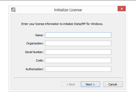
6[ IG ] Installing Stata for Windows
If you get the message “The serial number, code, and authorization are
inconsistent”, try the initialization again. Be careful when typing your code
and authorization. Anything that looks like “o” is the letter oh, anything like
“0” is a zero, anything like “1” is the number one, and anything like “L” is
the letter el.
Important: Do not lose your License and Activation Key. You may need it
again in the future.
Update Stata if necessary
StataCorp releases updates to Stata often. These updates may include new
features and bug fixes that can be automatically downloaded and installed by
Stata from the Internet. There may be updates to Stata more recent than the
version of Stata on your installation media.
The first time Stata is launched, a dialog will open asking you if you would
like to check for updates now. Click on OK to do so. If an update is available,
follow the instructions. If you have trouble connecting to the Internet from
Stata, visit http://www.stata.com/support/faqs/web/ for help.
By default, automatic update checking is enabled. This ensures that your
Stata is up to date, it is convenient, and it causes no problems even if you are
not connected to the Internet. If you disable automatic update checking, it is
a good idea to periodically check for updates to Stata. See [GSW] 19 Updating
and extending Stata—Internet functionality for more information about updating.

[ IG ] Installing Stata for Windows 7
Register your copy
Make sure that your copy of Stata is registered. As a registered Stata user,
you are entitled to free technical assistance should you have any questions,
and we will keep you informed of any new products or advancements that
have been announced. To register your copy of Stata, fill out the online
registration form at http://www.stata.com/register/, or return the registration
card that came with your Stata software.
Creating network shortcuts
If you installed Stata on a network drive, you will need to create shortcuts
on the workstations that will be using Stata.
1. Mount the network drive that Stata is installed on from a workstation.
Right-click on the Desktop or on the Windows Start menu, and select
New > Shortcut. Type the path for the Stata executable into the edit
field, or click on Browse... to locate it. Enter “Stata” for the name of the
shortcut.
2. Once a shortcut for Stata has been created, right-click on it, and select
Properties. Set the default working directory for Stata by changing the
Start in field to a local drive that users have write access to. This is
where Stata will store datasets, graphs, and other Stata-related files. If
the workstation will be used by more than one user, consider changing
the Start in field to the environment variable %HOMEDRIVE%%HOMEPATH%.
Doing so will set the default working directory to each user’s home
directory.
Other ways to start Stata
You can start Stata in multiple ways:
•From the Start menu.
•Double-click on its application icon (as with any other application).
•Double-click on a Stata do-file. See [GSW] 13 Using the Do-file Editor—
automating Stata and [U] 16 Do-files for more information.
•Double-click on a Stata data file. Stata data files are files created by Stata
and have the extension .dta. When you double-click on a Stata data file,
Stata is started and the data file is loaded into Stata; see [GSW] 5 Opening
and saving Stata datasets.
If you experience any problems when trying to start Stata, see [GSW] A Trou-
bleshooting Stata. (We are assuming that you have successfully installed Stata
and have initialized the license. Please see page 24 for how to access the
PDF documentation from outside Stata.)

8[ IG ] Installing Stata for Windows
Exiting Stata
To exit Stata, select Exit from the File menu or press Alt+F4. If you have
made any changes to the data in your dataset, including creating a new
dataset, you will be prompted to save the changes.
If you exit Stata by typing the equivalent exit command, you will see the
following in the Results window if you have made changes to your data:
no; data in memory would be lost
r(4);
If you would like to save your changes, you could save the dataset as you
save any other file by using File > Save or Ctrl +S. You can also save the
dataset by typing save filename. You could then type exit again, and Stata
will exit. If you do not wish to save your changes, you can force Stata to
exit without saving the dataset by typing exit, clear.
Verifying installation
If you need to create a report to verify that Stata has been installed properly,
point your browser to http://www.stata.com/support/installation-qualification/.
There you will find instructions for downloading and using the Stata Installation
Qualification Tool (IQT). The tool will verify your installation not only after
you initially install Stata, but also after every update you apply.
Installing Stata for Mac
Upgrade or update?
If you are using an earlier Stata release and you are upgrading to Stata 13, or
if you have never installed Stata before on this computer, you need to read
this Installation Guide. If you have already installed Stata 13 and you would
like to install the latest updates to Stata 13, please refer to [GSM] 19 Updating
and extending Stata—Internet functionality.
Upgrading to Stata/MP, Stata/SE, or Stata/IC
If you have already installed a flavor of Stata 13 and have purchased an
upgrade to Stata/MP, Stata/SE, or Stata/IC, run the installer again and select
Add Stata/MP,Add Stata/SE, or Add Stata/IC for the Installation Type.
Make sure that you have your License and Activation Key before doing this.
After installation, you will immediately want to update Stata because your
executable will most likely be out of sync with your ado-files.
Warning against multiple Stata applications
We recommend against having more than one Stata application installed on
the same computer, because it can confuse the Finder. Why? Because when
you double-click on a Stata file, the Mac may choose the wrong Stata to run.
You will not be able to predict which one will start. If you typically do not
start Stata by double-clicking on Stata files, you can have multiple versions,
but be forewarned that the first time you start Stata by double-clicking, you
may be confused.
Before you install
Before you begin the installation procedure:
1. Make sure you have the Stata installation media.
2. Make sure you have a License and Activation Key.
3. Determine from the License and Activation Key whether you should install
Stata/MP, Stata/SE, Stata/IC, or Small Stata.
9

10 [ IG ] Installing Stata for Mac
4. You should not have any of your personal files in the Stata folder. But
if you do and wish to keep them, move them out of the Stata folder
first.
5. If you are upgrading, drag the current Stata folder to the Trash, and
empty the Trash. Note: You must empty the Trash before proceeding.
6. You are now ready to install.
Installation
1. Insert the installation media.
2. Open the installation media from the Desktop, and double-click on the
Installer application to start the installation.
3. After you have carefully read the Read Me file and have agreed to the
software license agreement, click on Continue.
4. By default, Stata will be installed in /Applications/Stata. You can
change the folder that Stata will be installed in by changing the Destination,
but we recommend using the default destination. Click on Continue.
5. Choose the flavor of Stata that matches your license.
6. Click on the Install button.
7. Click on Quit after you see the message Installation was successful.
Initialize the license
You now need to start Stata so that you can initialize the license.
The first time that you start Stata, it will prompt you for the information on
your License and Activation Key. You must enter something for all fields in
the dialog before you can continue. The code and authorization are not case
sensitive. If you make a mistake typing the codes, you will be prompted to
try again.
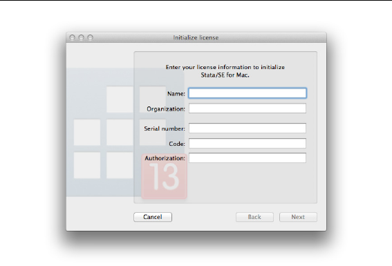
[ IG ] Installing Stata for Mac 11
If you get the message “The serial number, code, and authorization are
inconsistent”, try the initialization again. Be careful when typing your code
and authorization. Anything that looks like “o” is the letter oh, anything like
“0” is a zero, anything like “1” is the number one, and anything like “L” is
the letter el.
Important: Do not lose your License and Activation Key. You may need it
again in the future.
Update Stata if necessary
StataCorp releases updates to Stata often. These updates may include new
features and bug fixes that can be automatically downloaded and installed by
Stata from the Internet. There may be updates to Stata more recent than the
version of Stata on your installation media.
The first time Stata is launched, a dialog will open asking you if you would
like to check for updates now. Click on OK to do so. If an update is available,
follow the instructions. If you have trouble connecting to the Internet from
Stata, visit http://www.stata.com/support/faqs/web/ for help.
By default, automatic update checking is enabled. This ensures that your
Stata is up to date, it is convenient, and it causes no problems even if you are
not connected to the Internet. If you disable automatic update checking, it is
a good idea to periodically check for updates to Stata. See [GSM] 19 Updating
and extending Stata—Internet functionality for more information about updating.

12 [ IG ] Installing Stata for Mac
Register your copy
Make sure that your copy of Stata is registered. As a registered Stata user,
you are entitled to free technical assistance should you have any questions,
and we will keep you informed of any new products or advancements that
have been announced. To register your copy of Stata, fill out the online
registration form at http://www.stata.com/register/, or return the registration
card that came with your Stata software.
Other ways to start Stata
You can start Stata in multiple ways:
•Double-click on its application icon (as with any other application).
•Double-click on a Stata do-file. See [GSM] 13 Using the Do-file Editor—
automating Stata and [U] 16 Do-files for more information.
•Double-click on a Stata data file. Stata data files are files created by Stata
and have the extension .dta. When you double-click on a Stata data file,
Stata is started and the data file is loaded into Stata; see [GSM] 5 Opening
and saving Stata datasets.
If you experience any problems when trying to start Stata, see [GSM] A Trou-
bleshooting Stata. (We are assuming that you have successfully installed Stata
and have initialized the license. Please see page 24 for how to access the
PDF documentation from outside Stata.)
Quitting Stata
To quit Stata, select Quit from the Stata menu or press Command –Q. If you
have made any changes to the data in your dataset, including creating a new
dataset, you will be prompted to save the changes.
If you quit Stata by typing the equivalent exit command, you will see the
following in the Results window if you have made changes to your data:
no; data in memory would be lost
r(4);
If you would like to save your changes, you could save the dataset as you
save any other file by using File > Save or Command –S. You can also save the
dataset by typing save filename. You could then type exit again, and Stata
will quit. If you do not wish to save your changes, you can force Stata to
quit without saving the dataset by typing exit, clear.
Installing Stata for Unix
Installation overview
The outline of the installation process is as follows:
1. Ensure that you have the Stata installation media and the License and
Activation Key.
2. As superuser, create the directory in which you want to install Stata.
3. Change to that directory and run the installation script that is on the
Stata installation media.
4. Follow the instructions during the installation process.
5. Once the installation is complete, enter your license codes.
The details for each of these steps are below, with some pointers for
troubleshooting.
Find your installation media and license
You should have received the installation media and a License and Activation
Key. You will need both to install Stata. The codes in the License and Activation
Key are necessary for initializing the Stata software.
Obtain superuser access
You must be logged in as superuser (root) to install Stata. For varieties of
Unix that disable the root account by default, issue either the command sudo
su - or the command su - to run as superuser during the installation. The #
prompt below indicates that you are running as superuser.
Create a directory for Stata
We recommend that you install Stata in /usr/local/stata13.
If you would like the path to the executables as seen by users to remain stable
as you upgrade Stata in the future, you can create a symbolic link (type man
ln for more information) from /usr/local/stata13 to /usr/local/stata:
# ln -s /usr/local/stata13 /usr/local/stata
If you wish to install Stata in a different directory, you are free to do so.
13

14 [ IG ] Installing Stata for Unix
Users who want to access Stata must modify their .profile or .cshrc or
.login shell start-up scripts to include the Stata installation directory in their
PATH. Throughout this manual, we will assume that you have installed Stata
in /usr/local/stata13 and used a symbolic link to /usr/local/stata.
Upgrading
If you are upgrading from Stata 12, you can leave Stata 12 installed where
it is, allowing you to have both Stata 12 and Stata 13. Install Stata 13 in
/usr/local/stata13 and leave Stata 12 alone.
Have your users modify their shell start-up scripts to use the proper PATH for
Stata 13. Otherwise, when they run Stata, they will be running Stata 12.
If you want to uninstall Stata 12, type
# rm -r /usr/local/stata12
to remove it. If Stata 12 is installed in a different directory, you will have
to change the above command accordingly.
Install Stata
Set your current directory to /usr/local/stata13 and run the installation
script,
# cd /usr/local/stata13
# /media/Stata/install
replacing /media/Stata with the path to the installation media if your device
path differs (other common paths are /dev/cdrom and /mount/stata). If you
have trouble running the installer, it could be because your version of Unix
will not, by default, allow you to run applications from a installation media.
Please see page 18 for more help.
Follow the prompts. Nothing will be written until you say it is OK to do so.
Initialize the license
Initialize the license by typing
# cd /usr/local/stata13
# ./stinit

[ IG ] Installing Stata for Unix 15
You will be asked if you accept the software license agreement, which can
be found in the file license.pdf on your installation media. Read and accept
the software license agreement to proceed with the installation.
You will be asked for your serial number, code, and authorization, which are
provided in your License and Activation Key. The code and authorization are
not case sensitive. You will also be asked to specify your name and address
if you have a single-user license, or the institution name and department or
address if you have a multiple-user license. When you invoke Stata in the
future, the license information will be displayed along with the name and
address you enter. This information will also be written in system files that
Stata creates so that, should you ever need to send a file to us, we will know
whom it is from. Whenever you or any of your users calls our technical
support line, we will ask for this information, all of which Stata reports when
it begins execution.
If, for some reason, you need to reinitialize the license for an installed
copy of Stata, you will have to contact Stata Technical Support for special
instructions.
Set the message of the day (optional)
Every time Stata is invoked, the contents of /usr/local/stata13/stata.msg
are displayed. This feature provides a convenient way to communicate with
Stata users if you are administering a large site. As superuser, you may edit
the file or erase it if you wish.
Verify that Stata is working
Now that you have completed the installation process, you should verify that
everything has been installed properly. You must log out as superuser and log
in again as a regular Stata user. The prompts below change to $to indicate
your regular user status.
To use Stata as a user, your path must include the Stata installation directory,
and to run the GUI version, you must be running X Windows. For our quick
test, we are going to be crude. The following will work whether you use sh,
csh,bash, or ksh:
% sh
$ PATH=$PATH:/usr/local/stata
$ export PATH
For Stata(console):
$ stata

16 [ IG ] Installing Stata for Unix
For Stata(GUI):
$ xstata
Stata should launch. Use stata-se or xstata-se if you have Stata/SE, stata-
mp or xstata-mp if you have Stata/MP, and stata-sm or xstata-sm if you
have Small Stata. If Stata does not start properly, see page 18.
Assuming that nothing is wrong, type
. exit
$ exit
The first exit took us out of Stata. The second exit took us out of the sh
that we temporarily invoked.
Modify shell start-up script
Once you have verified that Stata is working, modify your shell start-up
script to include Stata in your path. We will assume that you have created a
symbolic link from /usr/local/stata to your Stata installation directory. If
you did not create the recommended symbolic link, substitute your installation
directory for /usr/local/stata in the paths below.
If you use csh or tcsh, there is a line in your .cshrc file (in your home
directory) that looks like
set path = (/bin /usr/bin /usr/local/bin ~/bin)
Edit the file and add /usr/local/stata to the end of the list:
set path = (/bin /usr/bin /usr/local/bin ~/bin /usr/local/stata)
If you use bash,sh, or ksh, there is a line in your .profile (in your home
directory) that looks like
PATH="/bin:/usr/bin:/usr/local/bin:$HOME/bin"
Edit the file and add /usr/local/stata to the list:
PATH="/bin:/usr/bin:/usr/local/bin:$HOME/bin:/usr/local/stata"
If you are using a symbolic link to your Stata installation directory and you
have included the path to the Stata installation directory, be sure that the
symbolic link appears before the true directory in the path.
Log out and log back in so that the changes you have made will take effect.
Stata should now work from any directory on your computer.

[ IG ] Installing Stata for Unix 17
Update Stata if necessary
StataCorp releases updates to Stata often. These updates may include new
features and bug fixes that can be automatically downloaded and installed by
Stata from the Internet. There may be updates to Stata more recent than the
version of Stata on your installation media. You should check for updates to
Stata before you use it for the first time. You can do this one of two ways:
•Select Help > Check for Updates.
•Enter update query from the command line.
It is also a good idea to periodically check for updates to Stata. See [GSU] 19 Up-
dating and extending Stata—Internet functionality for more information about
updating. If you have trouble connecting to the Internet from Stata, visit
http://www.stata.com/support/faqs/web/ for help.
Starting Stata
With Stata for Unix, you can choose between two user interfaces. The first
option is the graphical user interface, or GUI, which we will refer to as
Stata(GUI). The second option is the nongraphical user interface, which we
will refer to as Stata(console). If instructions apply to either interface, we
will simply refer to Stata.
Upon installation, both interfaces are installed, but only the GUI version can
display graphs. If you use X Windows, you will be able to invoke either
interface, GUI or console, at each session. See [GSU] 2 The Stata user interface
for more information about the Stata user interface.
To start Stata from a Unix prompt, type
•xstata or xstata-se or xstata-mp or xstata-sm to start Stata(GUI), or
•stata or stata-se or stata-mp or stata-sm to start Stata(console).
If you see a message telling you that Stata could not find the license file or
if you receive any other error when you try to start Stata, please see page 18.
Stata(GUI) requires X Windows to run.
Stata(console) has a nongraphical interface; it is run in a terminal window,
and output is displayed on the terminal.

18 [ IG ] Installing Stata for Unix
Exiting Stata
To exit Stata(GUI), select Exit from the File menu or press Ctrl +Q. If you
have made any changes to the data in your dataset, including creating a new
dataset, you will be prompted to save the changes.
If you exit Stata by typing the equivalent exit command, which is the only
way to exit the console version of Stata, you will see the following in the
Results window if you have made changes to your data:
no; data in memory would be lost
r(4);
If you would like to save your changes in Stata(GUI), you could save the
dataset as you save any other file by using File > Save or Ctrl +S. In either
Stata, you can also save the dataset by typing save filename. You could then
type exit again, and Stata will exit. If you do not wish to save your changes,
you can force Stata to exit without saving the dataset by typing exit, clear.
Troubleshooting Unix installation
If you had trouble with the installation of Stata, it could be because you
have a recent copy of Unix that will not allow you to run applications from
aDVD or USB drive. Type df -l to see what local devices are mounted; one
should look like the Stata installation media. For example, you could see
something like
$ df -l
Filesystem 1K-blocks Used Available Use% Mounted on
/dev/hda6 23054660 5528268 16336380 26% /
/dev/hdc 274158 274158 0 100% /media/Stata
/dev/hdc is the device name, and /media/Stata is the mount point.
If you see something indicating that the Stata installation media is successfully
mounted, you need to see if you are being prevented from running applications
directly from the installation media. Type mount to get information about any
mounted file systems. Somewhere on the list, you should see information
about your installation media. Continuing with the above example, you should
see your device name and mount point in the output:
$ mount
omitted output
/dev/hdc on /media/Stata type iso9660 (ro,noexec,nosuid,nodev,uid=220)

[ IG ] Installing Stata for Unix 19
If you see the term noexec appear, you are not allowed to run applications from
aDVD or USB drive. Your best course of action is to copy everything from
the Stata installation media to a temporary directory and run the installation
from there. Substitute your mount point for /media/Stata below.
$ mkdir /tmp/statainstall
$ cp -r /media/Stata /tmp/statainstall
$ mkdir /usr/local/stata13
$ cd /usr/local/stata13
$ sudo /tmp/statainstall/Stata/install
After you have Stata running and initialized, you can delete the temporary
directory /tmp/statainstall.
If you are still having problems installing or if you have any other troubles,
see the Unix FAQs on our website at http://www.stata.com/support/faqs/unix/.
If this does not help, contact Stata Technical Support. Please gather all the
information you can about your system, including your computer model and
the type and version of Unix that you are using.
Troubleshooting Unix start-up
If you have attempted to invoke Stata(GUI) by typing xstata,xstata-se,
xstata-mp, or xstata-sm at the Unix prompt and it has failed, attempt to
invoke Stata(console) by typing stata,stata-se,stata-mp, or stata-sm at
the Unix prompt. If Stata(console) fails, continue here. If Stata(console) starts
without problems, see the next section of this chapter.
You tried to start Stata and it refused; Stata or your operating system presented
a message explaining that something is wrong. Here are the possibilities:
Cannot find Stata directory
Stata first checks in /usr/local/stata13 and then checks in /usr/local/stata
to find the license file. If Stata does not find the license in either of these
locations, it looks in every directory in the Unix PATH. If you receive this
message, most likely the directory where Stata is installed is not in your
PATH. You need to add this directory to your PATH.
Cannot find license file
This message means just what it says; nothing is too seriously wrong. Stata
simply could not find what it is looking for. The two most common reasons
for this are that you did not complete the installation process or that Stata
is not installed where it should be.
Did you insert the codes on your License and Activation Key to unlock Stata?
If not, go back and complete the initialization procedure.
Assuming that you did unlock Stata, Stata is merely mislocated, or the
location has not been filled in.

20 [ IG ] Installing Stata for Unix
Error opening or reading the file
Something is distinctly wrong and for purely technical reasons. Stata found
the file that it was looking for, but either the operating system refused to let
Stata open it or there was an I/O error.
The stata.lic file could have incorrect permissions. Verify that stata.lic is
in /usr/local/stata (or at least in the directory linked to /usr/local/stata)
and that everybody has been granted read permission. To change the permis-
sions, become superuser by logging in as root (using su or sudo) and type
chmod a+r /usr/local/stata13/stata.lic.
Other messages
The other messages indicate that Stata thinks you are attempting to do
something that you are not licensed to do. Most commonly, you are attempting
to run Stata over a network when you do not have a network license, but there
are many other alternatives. There are two possibilities: either you really are
attempting to do something that you are not licensed to do, or Stata is wrong.
In either case, you are going to have to contact us. Your license can be
upgraded, or, if Stata is wrong, we can provide codes to make Stata stop
thinking that you are violating the license; see [U] 3.9 Technical support.
Stata(console) starts but Stata(GUI) does not
Trouble with libraries
Stata, like many other programs designed for Unix machines, needs certain
system libraries to run. Most of the standard library routines that Stata
needs are included in the Stata binary. However, Stata does rely on a few
external libraries. For example, Stata assumes that your system will have
the standard C library available. Stata(GUI) assumes that you have the X
Windows libraries as well. These libraries are often located in different places
on different implementations of Unix. For example, under Linux, the standard
C libraries can be found in /lib, whereas the X Windows libraries are in
/usr/lib; under Solaris, both the standard libraries and the X libraries are
in /usr/lib. The operating system needs to know where to find the libraries
that Stata needs to run. The Unix environment variable LD LIBRARY PATH
tells the operating system where to find libraries. If you get an error message
that says something like
ld.so.1: xstata: fatal: some library.so.#: can’t open file
the likely reason is that the operating system cannot find the necessary
libraries. Stata does not rely on any unique libraries; you can rest assured
that the libraries you need are on your system. You should look for the
library in question on your system and make sure the environment variable
LD LIBRARY PATH includes the path to the directory where the library in
question is located. Your system administrator may be able to help with this
task.

[ IG ] Installing Stata for Unix 21
Setting the DISPLAY environment variable
Sometimes when executing Stata in a networked environment, Stata(GUI) will
produce the error message
You need X Windows for this version of Stata.
This means that Stata has not found the DISPLAY environment variable. You
need to set the DISPLAY variable to be the screen on which you want Stata(GUI)
to appear. For example, in csh, type setenv DISPLAY machine:0.0.
xhost permissions
Another related error message can occur with Stata(GUI). When Stata is being
run in a networked environment, the computer on which Stata(GUI) is actually
executing may not have permission to draw on the screen of the computer
on which you have asked Stata to draw. Then you may see the following:
Xlib: connection to machine name:0.0 refused by server
Xlib: Client is not authorized to connect to Server
xhost: unable to open display
This means that the machine that is actually executing the Stata instructions
(the x-client in X Windows parlance) does not have permission to draw on
the screen of the computer that you have asked it to (the x-server). On the
machine on which you want to display Stata(GUI), type
% xhost +client machine
This will give the client permission to draw on the server.
Getting more help
If you continue to experience problems invoking Stata(GUI), please see
the Unix FAQs on our website at http://www.stata.com/support/faqs/unix/, or
contact Stata Technical Support.
Platforms and flavors
Available platforms
Stata for Mac is available for 64-bit Intel-based Macs running Mac OS X
version 10.6.8 or newer.
Stata for Windows is available for 64-bit x86-64 and 32-bit x86 versions of
Windows 8 and 7, Vista, XP, and server versions of Windows.
Stata for Unix is available for 64-bit Linux for x86-64, 32-bit Linux for x86,
64-bit Solaris for SPARC, and 64-bit Solaris for x86-64.
Support for other platforms may have been added; contact us for the latest
information.
Available flavors
Stata/MP Professional version of Stata.
Parallel-processing capable.
Fastest on multiple-core/multiple-processor machines.
Maximum of 32,767 variables; observations limited only by
computer memory.
Stata/SE Professional version of Stata.
Fastest on a single-processor machine.
Maximum of 32,767 variables; observations limited only by
computer memory.
Stata/IC Professional version of Stata.
Very fast.
Maximum of 2,047 variables; observations limited only by com-
puter memory.
Small Stata Stata for small computers.
Slower than Stata/MP, Stata/SE, and Stata/IC.
Maximum of 99 variables and 1,200 observations.
23
Documentation
All the documentation for Stata is included in PDF format. You can open
it from within Stata by clicking on Help > PDF Documentation. It is also
linked into Stata’s system help. If you want to get to the PDF documents
directly, they can be found in the docs subdirectory of the Stata instal-
lation directory. There is also a copy of the manuals at the top level
of the installation installation media. For information about how to opti-
mally set up Adobe Reader for viewing the PDF manuals, please visit
http://www.stata.com/support/faqs/res/documentation.html.
When reading the manuals, you will find references to other Stata manuals.
For example,
[U] 26 Overview of Stata estimation commands
[R]regress
The first example is a reference to chapter 26, Overview of Stata estima-
tion commands, in the User’s Guide; and the second is a reference to the
regress entry in the Base Reference Manual. All of these are clickable in the
PDF documentation.
24

[ IG ] Documentation 25
All the manuals in the Stata Documentation have a shorthand notation:
[GSM]Getting Started with Stata for Mac
[GSU]Getting Started with Stata for Unix
[GSW]Getting Started with Stata for Windows
[U]Stata User’s Guide
[R]Stata Base Reference Manual
[D]Stata Data Management Reference Manual
[G]Stata Graphics Reference Manual
[XT]Stata Longitudinal-Data/Panel-Data Reference Manual
[ME]Stata Multilevel Mixed-Effects Reference Manual
[MI]Stata Multiple-Imputation Reference Manual
[MV]Stata Multivariate Statistics Reference Manual
[PSS]Stata Power and Sample-Size Reference Manual
[P]Stata Programming Reference Manual
[SEM]Stata Structural Equation Modeling Reference Manual
[SVY]Stata Survey Data Reference Manual
[ST]Stata Survival Analysis and Epidemiological Tables Reference Manual
[TS]Stata Time-Series Reference Manual
[TE]Stata Treatment-Effects Reference Manual:
Potential Outcomes/Counterfactual Outcomes
[I]Stata Glossary and Index
[M]Mata Reference Manual
