Stellarium User Guide 0.18.0 1
User Manual:
Open the PDF directly: View PDF ![]() .
.
Page Count: 353 [warning: Documents this large are best viewed by clicking the View PDF Link!]
Stellarium 0.18.0 User Guide
Georg Zotti, Alexander Wolf (editors)
2017
Copyright c
2014-2017 Georg Zotti.
Copyright c
2011-2017 Alexander Wolf.
Copyright c
2006-2013 Matthew Gates.
Copyright c
2013-2014 Barry Gerdes (†2014).
STELLARIUM.ORG
Permission is granted to copy, distribute and/or modify this document under the terms
of the GNU Free Documentation License, Version 1.3 or any later version published by
the Free Software Foundation; with no Invariant Sections, no Front-Cover Texts, and no
Back-Cover Texts. A copy of the license is included in the appendix G entitled “GNU Free
Documentation License”.
All trademarks, third party brands, product names, trade names, corporate names and company
names mentioned may be trademarks of their respective owners or registered trademarks of other
companies and are used for purposes of explanation and to the readers’ benefit, without implying a
violation of copyright law.
Version 0.18.0-1, March 25, 2018
Contents
IBasic Use
1Introduction ................................................ 3
1.1 Historical notes 3
2Getting Started ............................................. 7
2.1 System Requirements 7
2.1.1 Minimum ...................................................... 7
2.1.2 Recommended ................................................ 7
2.2 Downloading 8
2.3 Installation 8
2.3.1 Windows ...................................................... 8
2.3.2 OSX .......................................................... 8
2.3.3 Linux .......................................................... 8
2.4 Running Stellarium 9
2.4.1 Windows ...................................................... 9
2.4.2 OSX .......................................................... 9
2.4.3 Linux .......................................................... 9
2.5 Troubleshooting 9
3A First Tour ................................................. 11
3.1 Time Travel 12
3.2 Moving Around the Sky 13

3.3 The Main Tool Bar 14
3.4 Taking Screenshots 17
4The User Interface ........................................ 19
4.1 Setting the Date and Time 19
4.2 Setting Your Location 20
4.3 The Configuration Window 21
4.3.1 TheMainTab ................................................. 21
4.3.2 TheInformationTab ............................................ 21
4.3.3 TheNavigationTab ............................................ 21
4.3.4 TheToolsTab .................................................. 21
4.3.5 TheScriptsTab ................................................ 25
4.3.6 ThePluginsTab ................................................ 26
4.4 The View Settings Window 26
4.4.1 TheSkyTab ................................................... 26
4.4.2 The Deep-Sky Objects (DSO) Tab . . . . . . . . . . . . . . . . . . . . . . . . . . . . . . . . 27
4.4.3 TheMarkingsTab .............................................. 27
4.4.4 TheLandscapeTab ............................................ 29
4.4.5 TheStarloreTab ............................................... 30
4.4.6 TheSurveysTab ............................................... 31
4.5 The Object Search Window 32
4.6 The Astronomical Calculations Window 34
4.6.1 ThePositionsTab............................................... 34
4.6.2 TheEphemerisTab ............................................. 34
4.6.3 ThePhenomenaTab ........................................... 37
4.6.4 The“Altitudevs.Time”Tab ...................................... 37
4.6.5 TheGraphsTab ............................................... 38
4.6.6 The “What’s Up Tonight” (WUT) Tab . . . . . . . . . . . . . . . . . . . . . . . . . . . . . . . 38
4.6.7 The “Planetary Calculator” (PC) Tab . . . . . . . . . . . . . . . . . . . . . . . . . . . . . 39
4.7 Help Window 40
4.7.1 Editing Keyboard Shortcuts . . . . . . . . . . . . . . . . . . . . . . . . . . . . . . . . . . . . . 40
II Advanced Use
5Files and Directories ...................................... 45
5.1 Directories 45
5.1.1 Windows ..................................................... 45
5.1.2 MacOSX .................................................... 46
5.1.3 Linux ......................................................... 46
5.2 Directory Structure 46
5.3 The Logfile 47
5.4 The Main Configuration File 47
5.5 Getting Extra Data 48
5.5.1 MoreStars .................................................... 48
5.5.2 MoreDeep-SkyObjects ........................................ 48
5.5.3 Alternative Planet Ephemerides: DE430, DE431 . . . . . . . . . . . . . . . . . . . . 48
5.5.4 GPSPosition .................................................. 49
6Command Line Options .................................. 51
6.1 Examples 53
6.2 Special Options 53
6.2.1 Spout ........................................................ 53
7Landscapes ............................................... 55
7.1 Stellarium Landscapes 55
7.1.1 Locationinformation ........................................... 56
7.1.2 Polygonallandscape .......................................... 57
7.1.3 Sphericallandscape ........................................... 58
7.1.4 High resolution (“Old Style”) landscape . . . . . . . . . . . . . . . . . . . . . . . . . . . 59
7.1.5 Fisheyelandscape............................................. 63
7.1.6 Description ................................................... 64
7.1.7 Gazetteer .................................................... 65
7.1.8 PackingandPublishing ......................................... 65
7.2 Creating Panorama Photographs for Stellarium 66
7.2.1 PanoramaPhotography ........................................ 66
7.2.2 HuginPanoramaSoftware ...................................... 67
7.2.3 Regular creation of panoramas . . . . . . . . . . . . . . . . . . . . . . . . . . . . . . . . . 68
7.3 Panorama Postprocessing 71
7.3.1 TheGIMP ..................................................... 71
7.3.2 ImageMagick ................................................. 72
7.3.3 FinalCalibration ............................................... 74
7.3.4 ArtificialPanoramas............................................ 76
7.3.5 NightscapeLayer.............................................. 76
7.4 Other recommended software 77
7.4.1 IrfanView ..................................................... 77
7.4.2 FSPViewer .................................................... 77
7.4.3 Clink ......................................................... 77
7.4.4 Cygwin ...................................................... 78
7.4.5 GNUWin32.................................................... 78
8Deep-Sky Objects ........................................ 79
8.1 Stellarium DSO Catalog 79
8.1.1 Modifyingcatalog.dat ......................................... 80
8.1.2 Modifyingnames.dat .......................................... 82
8.1.3 Modifyingtextures.json ......................................... 82
8.1.4 Modifyingoutlines.dat.......................................... 84

8.2 Adding Extra Nebulae Images 84
8.2.1 Preparing a photo for inclusion to the textures.json file............. 84
8.2.2 PlateSolving .................................................. 86
8.2.3 Processing into a textures.json insert ............................ 86
9Adding Sky Cultures ...................................... 89
9.1 Basic Information 89
9.2 Skyculture Description Files 90
9.3 Constellation Names 90
9.4 Star Names 90
9.5 Planet Names 91
9.6 Deep-Sky Objects Names 91
9.7 Stick Figures 91
9.8 Constellation Boundaries 92
9.9 Constellation Artwork 92
9.10 Seasonal Rules 92
9.11 References 93
9.12 Asterisms and help rays 93
9.13 Publish Your Work 93
10 Surveys .................................................... 95
10.1 Introduction 95
10.2 Hipslist file and default surveys 95
10.3 Solar system HiPS survey 96
III Extending Stellarium
11 Plugins: An Introduction .................................. 99
11.1 Enabling plugins 99
11.2 Data for plugins 99
12 Interface Extensions ..................................... 101
12.1 Angle Measure Plugin 101
12.2 Compass Marks Plugin 102
12.3 Equation of Time Plugin 103
12.3.1 Section EquationOfTimeinconfig.inifile........................ 103
12.4 Field of View Plugin 104
12.4.1 Section FOVinconfig.inifile .................................. 104
12.5 Pointer Coordinates Plugin 105
12.5.1 Section PointerCoordinatesin config.ini file . . . . . . . . . . . . . . . . . . . . . 105
12.6 Text User Interface Plugin 106
12.6.1 Using the Text User Interface . . . . . . . . . . . . . . . . . . . . . . . . . . . . . . . . . . . . 106
12.6.2 TUICommands ............................................... 106
12.6.3 Section tuiinconfig.inifile.................................... 108
12.7 Remote Control Plugin 109
12.7.1 Usingtheplugin .............................................. 109
12.7.2 Remote Control Web Interface . . . . . . . . . . . . . . . . . . . . . . . . . . . . . . . . . 110
12.7.3 Remote Control Commandline API . . . . . . . . . . . . . . . . . . . . . . . . . . . . . . 110
12.7.4 Developerinformation ........................................ 110
12.8 Remote Sync Plugin 111
12.9 Solar System Editor Plugin 114
13 Object Catalog Plugins ................................. 117
13.1 Bright Novae Plugin 117
13.1.1 Section Novaeinconfig.inifile ................................ 117
13.1.2 Format of bright novae catalog . . . . . . . . . . . . . . . . . . . . . . . . . . . . . . . . 118
13.1.3 Lightcurves.................................................. 118
13.2 Historical Supernovae Plugin 119
13.2.1 List of supernovae in default catalog . . . . . . . . . . . . . . . . . . . . . . . . . . . . 119
13.2.2 Lightcurves.................................................. 121
13.2.3 Section Supernovaeinconfig.inifile ........................... 121
13.2.4 Format of historical supernovae catalog . . . . . . . . . . . . . . . . . . . . . . . . . 122
13.3 Exoplanets Plugin 123
13.3.1 Potential habitable exoplanets . . . . . . . . . . . . . . . . . . . . . . . . . . . . . . . . . 123
13.3.2 Propernames ................................................ 124
13.3.3 Section Exoplanetsinconfig.inifile ............................ 126
13.3.4 Format of exoplanets catalog . . . . . . . . . . . . . . . . . . . . . . . . . . . . . . . . . . 127
13.4 Pulsars Plugin 129
13.4.1 Section Pulsarsinconfig.inifile ................................ 129
13.4.2 Formatofpulsarscatalog...................................... 130
13.5 Quasars Plugin 131
13.5.1 Section Quasarsinconfig.inifile .............................. 131
13.5.2 Format of quasars catalog . . . . . . . . . . . . . . . . . . . . . . . . . . . . . . . . . . . . . 132
13.6 Meteor Showers Plugin 133
13.6.1 Terms ....................................................... 133
13.6.2 Section MeteorShowersinconfig.inifile ........................ 134
13.6.3 Format of Meteor Showers catalog . . . . . . . . . . . . . . . . . . . . . . . . . . . . . 135
13.6.4 FurtherInformation ........................................... 136
13.7 Navigational Stars Plugin 137
13.7.1 Section NavigationalStarsinconfig.inifile ...................... 137
13.8 Satellites Plugin 138
13.8.1 SatelliteProperties ............................................ 138
13.8.2 IridiumFlaresprediction ....................................... 139
13.8.3 SatelliteCatalog ............................................. 139
13.8.4 Configuration ................................................ 140
13.8.5 SourcesforTLEdata........................................... 140
13.9 ArchaeoLines Plugin 141
13.9.1 Introduction ................................................. 141
13.9.2 Characteristic Declinations . . . . . . . . . . . . . . . . . . . . . . . . . . . . . . . . . . . . 141
13.9.3 AzimuthLines ................................................ 143
13.9.4 Arbitrary Declination Lines . . . . . . . . . . . . . . . . . . . . . . . . . . . . . . . . . . . . . 143
13.9.5 ConfigurationOptions......................................... 143
14 Scenery3d – 3D Landscapes ........................... 145
14.1 Introduction 145
14.2 Usage 145
14.3 Hardware Requirements & Performance 146
14.3.1 Performancenotes ........................................... 147
14.4 Model Configuration 147
14.4.1 Exporting OBJ from Sketchup . . . . . . . . . . . . . . . . . . . . . . . . . . . . . . . . . . . 147
14.4.2 Notes on OBJ file format limitations . . . . . . . . . . . . . . . . . . . . . . . . . . . . . . 148
14.4.3 Configuring OBJ for Scenery3d . . . . . . . . . . . . . . . . . . . . . . . . . . . . . . . . . 150
14.4.4 ConcatenatingOBJfiles ....................................... 153
14.4.5 Beyond 3D: Temporally evolving Models . . . . . . . . . . . . . . . . . . . . . . . . . 153
14.4.6 Working with non-georeferenced OBJ files . . . . . . . . . . . . . . . . . . . . . . . 153
14.4.7 Rotating OBJs with recognized survey points . . . . . . . . . . . . . . . . . . . . . 154
14.5 Predefined views 154
14.6 Example 155
15 Stellarium at the Telescope ............................. 159
15.1 Oculars Plugin 159
15.1.1 UsingtheOcularplugin........................................ 160
15.1.2 Configuration ................................................ 164
15.1.3 Scaling the eyepiece view . . . . . . . . . . . . . . . . . . . . . . . . . . . . . . . . . . . . . 169
15.2 TelescopeControl Plugin 172
15.2.1 Abilities and limitations . . . . . . . . . . . . . . . . . . . . . . . . . . . . . . . . . . . . . . . . 172
15.2.2 Usingthisplug-in.............................................. 172
15.2.3 Main window (’Telescopes’) . . . . . . . . . . . . . . . . . . . . . . . . . . . . . . . . . . . 172
15.2.4 Telescope configuration window . . . . . . . . . . . . . . . . . . . . . . . . . . . . . . . 173
15.2.5 Supporteddevices ........................................... 175
15.3 RTS2 176
15.4 INDI 177
15.5 StellariumScope 178
15.6 Other telescope servers and Stellarium 178

15.7 Observability Plugin 180
16 Scripting .................................................. 183
16.1 Introduction 183
16.2 Script Console 184
16.3 Includes 184
16.4 Minimal Scripts 184
16.5 Example: Retrograde motion of Mars 184
16.5.1 Scriptheader ................................................ 184
16.5.2 Abodyofscript .............................................. 185
16.6 More Examples 187
IV Practical Astronomy
17 Astronomical Concepts ................................. 191
17.1 The Celestial Sphere 191
17.2 Coordinate Systems 192
17.2.1 Altitude/Azimuth Coordinates . . . . . . . . . . . . . . . . . . . . . . . . . . . . . . . . . . 192
17.2.2 Right Ascension/Declination Coordinates . . . . . . . . . . . . . . . . . . . . . . . . 193
17.2.3 EclipticalCoordinates ......................................... 195
17.2.4 GalacticCoordinates ......................................... 196
17.3 Distance 196
17.4 Time 196
17.4.1 SiderealTime ................................................ 197
17.4.2 JulianDayNumber ........................................... 197
17.4.3 DeltaT ...................................................... 198
17.5 Angles 201
17.5.1 Notation .................................................... 201
17.5.2 HandyAngles ................................................ 201
17.6 The Magnitude Scale 202
17.7 Luminosity 202
17.8 Precession 203
17.9 Parallax 205
17.9.1 Geocentric and Topocentric Observations . . . . . . . . . . . . . . . . . . . . . . . 205
17.9.2 StellarParallax ............................................... 205
17.10 Proper Motion 206
18 Astronomical Phenomena .............................. 207
18.1 The Sun 207
18.2 Stars 207
18.2.1 MultipleStarSystems .......................................... 208
18.2.2 Constellations ................................................ 208
18.2.3 StarNames .................................................. 209
18.2.4 Spectral Type & Luminosity Class . . . . . . . . . . . . . . . . . . . . . . . . . . . . . . . . 210
18.2.5 VariableStars ................................................ 211
18.3 Our Moon 213
18.3.1 PhasesoftheMoon........................................... 213
18.4 The Major Planets 214
18.4.1 TerrestrialPlanets ............................................. 214
18.4.2 JovianPlanets................................................ 214
18.5 The Minor Bodies 215
18.5.1 Asteroids .................................................... 215
18.5.2 Comets ..................................................... 215
18.6 Meteoroids 216
18.7 Zodiacal Light and Gegenschein 216
18.8 The Milky Way 216
18.9 Nebulae 217
18.9.1 TheMessierObjects ........................................... 217
18.10 Galaxies 217
18.11 Eclipses 218
18.11.1SolarEclipses................................................. 218
18.11.2LunarEclipses ................................................ 218
18.12 Observing Hints 218
18.13 Atmospheric effects 219
18.13.1AtmosphericExtinction ........................................ 219
18.13.2AtmosphericRefraction ....................................... 219
18.13.3LightPollution ................................................ 222
19 A Little Sky Guide ........................................ 223
19.1 Dubhe and Merak, The Pointers 223
19.2 M31, Messier 31, The Andromeda Galaxy 223
19.3 The Garnet Star, µCephei 224
19.4 4 and 5 Lyrae, εLyrae 224
19.5 M13, Hercules Cluster 224
19.6 M45, The Pleiades, The Seven Sisters 224
19.7 Algol, The Demon Star, βPersei 225
19.8 Sirius, αCanis Majoris 225
19.9 M44, The Beehive, Praesepe 225
19.10 27 Cephei, δCephei 225
19.11 M42, The Great Orion Nebula 225
19.12 La Superba, Y Canum Venaticorum, HIP 62223 226
19.13 52 and 53 Bootis, ν1and ν2Bootis 226
19.14 PZ Cas, HIP 117078 226
19.15 VV Cephei, HIP 108317 226

19.16 AH Scorpii, HIP 84071 226
19.17 Albireo, βCygni 227
19.18 31 and 32 Cygni, o1and o2Cygni 227
19.19 The Coathanger, Brocchi’s Cluster, Cr 399 227
19.20 Kemble’s Cascade 228
19.21 The Double Cluster, χand hPersei, NGC 884 and NGC 869 228
19.22 Large Magellanic Cloud, PGC 17223 228
19.23 Tarantula Nebula, C 103, NGC 2070 228
19.24 Small Magellanic Cloud, NGC 292, PGC 3085 229
19.25 ωCentauri cluster, C 80, NGC 5139 229
19.26 47 Tucanae, C 106, NGC 104 230
19.27 The Coalsack Nebula, C 99 230
19.28 Mira, oCeti, 68 Cet 230
19.29 αPersei Cluster, Cr 39, Mel 20 230
19.30 M7, The Ptolemy Cluster 231
19.31 M24, The Sagittarius Star Cloud 231
19.32 IC 4665, The Summer Beehive Cluster 232
19.33 The E Nebula, Barnard 142 and 143 232
20 Exercises ................................................. 233
20.1 Find M31 in Binoculars 233
20.1.1 Simulation ................................................... 233
20.1.2 ForReal ..................................................... 233
20.2 Handy Angles 233
20.3 Find a Lunar Eclipse 234
20.4 Find a Solar Eclipse 234
20.5 Find a retrograde motion of Mars 234
20.6 Analemma 234
20.7 Transit of Venus 235
20.8 Transit of Mercury 235
20.9 Triple shadows on Jupiter 235
20.10 Jupiter without satellites 235
20.11 Mutual occultations of planets 235
20.12 The proper motion of stars 236
VAppendices
ADefault Hotkeys .......................................... 239
A.1 Mouse actions with combination of the keyboard keys 239
A.2 Display Options 239
A.3 Miscellaneous 240
A.4 Movement and Selection 241
A.5 Date and Time 241
A.6 Scripts 242
A.7 Windows 242
A.8 Plugins 242
A.8.1 AngleMeasure............................................... 242
A.8.2 ArchaeoLines ................................................ 242
A.8.3 CompassMarks .............................................. 242
A.8.4 EquationofTime ............................................. 242
A.8.5 Exoplanets................................................... 243
A.8.6 FieldofView ................................................. 243
A.8.7 MeteorShowers .............................................. 243
A.8.8 Oculars ..................................................... 243
A.8.9 Pulsars ...................................................... 243
A.8.10 Quasars ..................................................... 244
A.8.11 Satellites..................................................... 244
A.8.12 Scenery3d: 3D landscapes . . . . . . . . . . . . . . . . . . . . . . . . . . . . . . . . . . . . 244
A.8.13 SolarSystemEditor ............................................ 244
A.8.14 TelescopeControl ............................................ 244
BThe Bortle Scale of Light Pollution ...................... 247
B.1 Excellent dark sky site 247
B.2 Typical truly dark site 247
B.3 Rural sky 248
B.4 Rural/suburban transition 248
B.5 Suburban sky 249
B.6 Bright suburban sky 249
B.7 Suburban/urban transition 249
B.8 City sky 249
B.9 Inner-city sky 249
CStar Catalogues ......................................... 251
C.1 Stellarium’s Sky Model 251
C.1.1 Zones ....................................................... 251
C.2 Star Catalogue File Format 251
C.2.1 GeneralDescription .......................................... 251
C.2.2 FileSections.................................................. 252
C.2.3 RecordTypes ................................................ 253
C.3 Variable Stars 255
C.3.1 Variable Star Catalog File Format . . . . . . . . . . . . . . . . . . . . . . . . . . . . . . . 255
C.3.2 GCVSVariabilityTypes ........................................ 256
C.4 Double Stars 268
C.4.1 Double Star Catalog File Format . . . . . . . . . . . . . . . . . . . . . . . . . . . . . . . . 269
C.5 Cross-Identification Data 269
C.5.1 Cross-Identification Catalog File Format . . . . . . . . . . . . . . . . . . . . . . . . . 269
DConfiguration Files ....................................... 271
D.1 Program Configuration 271
D.1.1 astro...................................................... 271
D.1.2 astrocalc.................................................. 274
D.1.3 color...................................................... 275
D.1.4 custom_selected_info....................................... 278
D.1.5 custom_time_correction..................................... 278
D.1.6 devel..................................................... 278
D.1.7 dso_catalog_filters.......................................... 279
D.1.8 dso_type_filters............................................. 279
D.1.9 gui....................................................... 280
D.1.10 init_location............................................... 282
D.1.11 landscape................................................. 282
D.1.12 localization................................................ 283
D.1.13 main...................................................... 283
D.1.14 navigation................................................. 283
D.1.15 plugins_load_at_startup..................................... 284
D.1.16 projection................................................. 285
D.1.17 proxy..................................................... 285
D.1.18 scripts..................................................... 286
D.1.19 search.................................................... 286
D.1.20 spheric_mirror.............................................. 286
D.1.21 stars...................................................... 287
D.1.22 tui........................................................ 287
D.1.23 video..................................................... 288
D.1.24 viewing................................................... 288
D.1.25 DialogPositions............................................. 289
D.1.26 DialogSizes................................................ 289
D.1.27 hips....................................................... 290
D.2 Solar System Configuration Files 291
D.2.1 Filessystem_major.ini .......................................... 291
D.2.2 Filessystem_minor.ini .......................................... 295
EPlanetary nomenclature ................................ 299
E.1 Format of nomenclature data file 300
E.2 How names are approved by the IAU 300
E.3 IAU rules and conventions 301
E.4 Naming conventions 302
E.5 Descriptor terms (feature types) 303
FAccuracy ................................................ 305
F.1 Date Range 305
F.2 Stellar Proper Motion 305
F.3 Planetary Positions 306
F.4 Minor Bodies 306
F.5 Precession and Nutation 307
F.6 Planet Axes 307
F.7 Eclipses 307
F.8 The Calendar 307
GGNU Free Documentation License ..................... 309
G.1 PREAMBLE 309
G.2 APPLICABILITY AND DEFINITIONS 309
G.3 VERBATIM COPYING 311
G.4 COPYING IN QUANTITY 311
G.5 MODIFICATIONS 311
G.6 COMBINING DOCUMENTS 313
G.7 COLLECTIONS OF DOCUMENTS 313
G.8 AGGREGATION WITH INDEPENDENT WORKS 313
G.9 TRANSLATION 314
G.10 TERMINATION 314
G.11 FUTURE REVISIONS OF THIS LICENSE 314
G.12 RELICENSING 314
HAcknowledgements ..................................... 317
H.1 Contributors 317
H.2 How you can help 317
H.3 Technical Articles 318
H.4 Included Source Code 319
H.5 Data 319
H.6 Image Credits 321
H.6.1 Full credits for “earthmap” texture . . . . . . . . . . . . . . . . . . . . . . . . . . . . . . 323
H.6.2 License for the JPL planets images . . . . . . . . . . . . . . . . . . . . . . . . . . . . . . 324
H.6.3 DSS ......................................................... 325

I
1Introduction .................................3
1.1 Historical notes
2Getting Started .............................. 7
2.1 System Requirements
2.2 Downloading
2.3 Installation
2.4 Running Stellarium
2.5 Troubleshooting
3A First Tour ..................................11
3.1 Time Travel
3.2 Moving Around the Sky
3.3 The Main Tool Bar
3.4 Taking Screenshots
4The User Interface ......................... 19
4.1 Setting the Date and Time
4.2 Setting Your Location
4.3 The Configuration Window
4.4 The View Settings Window
4.5 The Object Search Window
4.6 The Astronomical Calculations Window
4.7 Help Window
Basic Use
1. Introduction
Stellarium is a software project that allows people to use their home computer as a virtual plan-
etarium. It calculates the positions of the Sun and Moon, planets and stars, and draws how the
sky would look to an observer depending on their location and the time. It can also draw the
constellations and simulate astronomical phenomena such as meteor showers or comets, and solar
or lunar eclipses.
Stellarium may be used as an educational tool for teaching about the night sky, as an ob-
servational aid for amateur astronomers wishing to plan a night’s observing or even drive their
telescopes to observing targets, or simply as a curiosity (it’s fun!). Because of the high quality
of the graphics that Stellarium produces, it is used in some real planetarium projector products
and museum projection setups. Some amateur astronomy groups use it to create sky maps for
describing regions of the sky in articles for newsletters and magazines, and the exchangeable sky
cultures feature invites its use in the field of Cultural Astronomy research and outreach.
Stellarium is still under development, and by the time you read this guide, a newer version may
have been released with even more features than those documented here. Check for updates to
Stellarium at the Stellarium website1.
If you have questions and/or comments about this guide, or about Stellarium itself, visit the
Stellarium site at Github2or our Google Groups forum3.
1.1 Historical notes
Fabien Chéreau started the project during the summer 2000, and throughout the years found
continuous support by a small team of enthusiastic developers.
Here is a list of past and present major contributors sorted roughly by date of arrival on the
project:
1http://stellarium.org
2https://github.com/Stellarium/stellarium
3https://groups.google.com/forum/#!forum/stellarium

4Chapter 1. Introduction
Fabien Chéreau original creator, maintainer, general development
Matthew Gates maintainer, original user guide, user support, general development
Johannes Gajdosik astronomical computations, large star catalogs support
Johan Meuris GUI design, website creation, drawings of our 88 Western constellations
Nigel Kerr Mac OSX port
Rob Spearman funding for planetarium support
Barry Gerdes
user support, tester, Windows support. Barry passed away in October 2014 at age
80. He was a major contributor on the forums, wiki pages and mailing list where his good
will and enthusiasm is strongly missed. RIP Barry.
Timothy Reaves ocular plugin
Bogdan Marinov GUI, telescope control, other plugins
Diego Marcos SVMT plugin
Guillaume Chéreau display, optimization, Qt upgrades, HiPS surveys
Alexander Wolf maintainer, DSO catalogs, user guide, general development
Georg Zotti
astronomical computations, Scenery 3D and ArchaeoLines plugins, general develop-
ment, user guide, user support
Marcos Cardinot MeteorShowers plugin
Florian Schaukowitsch
Scenery 3D plugin, Remote Control plugin, RemoteSync plugin, OBJ
rendering, Qt/OpenGL internals
Teresa Huertas Roldán Planetary nomenclature
Unfortunately time is evolving, and most members of the original development team are no
longer able to devote most of their spare time to the project (some are still available for limited
work which requires specific knowledge about the project).
As of 2017, the project’s maintainer is Alexander Wolf, doing most maintenance and regular
releases. Major new features are contributed mostly by Georg Zotti and his team focussing on
extensions of Stellarium’s applicability in the fields of historical and cultural astronomy research
(which means Stellarium is getting more accurate) and outreach (making it usable for museum
installations), but also on graphic items like comet tails or the Zodiacal Light.
A detailed track of development can be found in the
ChangeLog
file in the installation folder. A
few important milestones for the project:
2000 first lines of code for the project
2001-06
first public mention (and users feedbacks!) of the software on the French newsgroup
fr.sci.astronomie.amateur 4
2003-01 Stellarium reviewed by Astronomy magazine
2003-07 funding for developing planetarium features (fisheye projection and other features)
2005-12 use accurate (and fast) planetary model
2006-05 Stellarium “Project Of the Month” on SourceForge
2006-08 large stars catalogs
2007-01 funding by ESO for development of professional astronomy extensions (VirGO)
2007-04 developers’ meeting near Munich, Germany
2007-05 switch to the Qt library as main GUI and general purpose library
2009-09 plugin system, enabling a lot of new development
2010-07 Stellarium ported on Maemo mobile device
2010-11 artificial satellites plugin
2014-06 high quality satellites and Saturn rings shadows, normal mapping for moon craters
2014-07
v0.13.0: adapt to OpenGL evolutions in the Qt framework, now requires more modern
4https://groups.google.com/d/topic/fr.sci.astronomie.amateur/OT7K8yogRlI/
discussion

1.1 Historical notes 5
graphic hardware than earlier versions
2015-04 v0.13.3: Scenery 3D plugin
2015-10 v0.14.0: Accurate precession
2016-07 v0.15.0: Remote Control plugin
2016-12 v0.15.1: DE430&DE431, AstroCalc, DSS layer, and Stellarium acting as SpoutSender
2017-06
v0.16.0: Remote Sync plugin, polygonal OBJ models for minor bodies, RTS2 telescope
support
2017-09 v0.16.1: Standard and extended DSO catalog, new subcatalogues for DSO
2017-12 v0.17.0: Nomenclature labels for planets and moons, INDI telescope support
2018-03 v0.18.0: Multiple image surveys
Stellarium has been kindly supported by ESA in their Summer of Code in Space initiatives,
which so far has resulted in better planetary rendering (2012), the Meteor Showers plugin (2013),
the web-based remote control and an alternative solution for planetary positions based on the
DE430/DE431 ephemeris (2015), the RemoteSync plugin and OBJ models (2016), and the planet
nomenclature labels (2017).
This guide is based on the user guide written by Matthew Gates for version 0.10 around 2008.
The guide was then ported to the Stellarium wiki and continuously updated by Barry Gerdes
and Alexander Wolf up to version 0.12. Unfortunately, some new features were not properly
documented in the wiki, and generally, without Barry the wiki started to fall out of sync with the
actual program. In late 2015 we (Alexander and Georg) started porting the texts back to L
A
T
E
X and
updated and added information where necessary, or wrote new chapters for the features which were
introduced in the last years. We feel that a single book is the better format for offline reading. The
PDF version of this guide has a clickable table of contents and clickable hyperlinks.
These new editions of the Guide (since V0.15) will not contain notes about using earlier
versions than 0.13 or using very outdated hardware. New features are marked with a version
number like 0.15.2 in the margin. Some references to previous versions may still be made for
completeness, but if you are using earlier versions of Stellarium for particular reasons, please use
the older guides.
2. Getting Started
2.1 System Requirements
Stellarium has been seen to run on most systems where Qt5 is available, from tiny ARM computers
like the Raspberry Pi 2/3
1
or Odroid C1 to big museum installations with multiple projectors and
planetaria with fish-eye projectors. The most important hardware requirement is a contemporary
graphics subsystem.
2.1.1 Minimum
•
Linux/Unix; Windows 7 and later (It may run on Vista, but unsupported. A special version
for XP is still available); Mac OS X 10.10.0 and later
•
3D graphics capabilities which support OpenGL 3.0 and GLSL 1.3 (2008 GeForce 8xxx and
later, ATI/AMD Radeon HD-2xxx and later; Intel HD graphics (Core-i 2xxx and later)) or
OpenGL ES 2.0 and GLSL ES 1.0 (e.g., ARM SBCs like Raspberry Pi 2/3). On Windows,
some older cards may be supported via ANGLE when they support DirectX10.
•512 MB RAM
•250 MB free on disk
2.1.2 Recommended
•Linux/Unix; Windows 7 and later; Mac OS X 10.10.0 and later
•3D graphics card which supports OpenGL 3.3 and above and GLSL1.3 and later
•1 GB RAM or more
•1.5 GB free on disk (About 3GB extra required for the optional DE430/DE431 files).
•
A dark room for realistic rendering — details like the Milky Way, Zodiacal Light or star
twinkling can’t be seen in a bright room.
1
As of autumn 2017, you need to enable the experimental OpenGL driver and compile the drm and
Mesa 17 libraries from sources. See 2.3.3

8Chapter 2. Getting Started
2.2 Downloading
Download the correct package for your operating system directly from the main page,
http://stellarium.org
. An archive of all available versions is available at
https://sourceforge.
net/projects/stellarium/files/.
2.3 Installation
2.3.1 Windows
1. Double click on the installer file you downloaded:
•stellarium-0.18.0-win64.exe for 64-bit Windows 7 and later.
•stellarium-0.18.0-win32.exe for 32-bit Windows 7 and later.
•stellarium-0.18.0-classic-win32.exe for Windows XP and later.
2. Follow the on-screen instructions.
2.3.2 OS X
1.
Locate the
Stellarium-0.18.0.dmg
file in Finder and double click on it or open it using
the Disk Utility application. Now, a new disk appears on your desktop and Stellarium is in it.
2.
Open the new disk and please take a moment to read the
ReadMe
file. Then drag
Stellarium
to the Applications folder.
3.
Note: You should copy Stellarium to the Applications folder before running it — some users
have reported problems running it directly from the disk image (.dmg).
2.3.3 Linux
Check if your distribution has a package for Stellarium already — if so you’re probably best off
using it. If not, you can download and build the source.
For Ubuntu we provide a package repository with the latest stable releases. Open a terminal
and type:
sudo add - apt - repository ppa : ste llarium / stellarium - releases
sudo apt - get upd at e
sudo apt - get insta ll s tella rium
Raspberry Pi 2/3
These tiny ARM-based computers are very popular for small and energy-efficient applications like
controlling push-to Dobsonians. A new open-source OpenGL driver stack has been made available
recently, but as of October 2017 the default Raspbian operating system comes with an outdated
version. Stellarium requires Mesa 17 or later. To set up a Raspberry Pi 2 or 3 with Raspbian
Stretch for use with Stellarium, activate the OpenGL driver in
raspi-config
and follow instructions
from the VC4 wiki.
2
The
libdrm
upgrade is required and does not harm, but you can also install
Mesa 17 in addition to the stock Mesa 13 following another set of instructions.3
For Ubuntu 16.04 LTS, follow instructions4.
Note that as of October 2017 (Mesa 17.4) the 3D planets do not work.
2https://github.com/anholt/mesa/wiki/VC4-complete-Raspbian-upgrade
. You only need
to follow the instructions on first boot, libdrm and Mesa.
3https://github.com/anholt/mesa/wiki/Building-Mesa-for-VC4
. Note that you may
need to add a symbolic link to the VC4 library. With all paths from these instructions,
ln -s ~/prefix/dri/vc4_dri.so ~/prefix/vc4_dri.so should do the trick.
4https://ubuntu-mate.community/t/tutorial-activate-opengl-driver-for-ubuntu-mate-16-04/
7094

2.4 Running Stellarium 9
2.4 Running Stellarium
2.4.1 Windows
The Stellarium installer creates a whole list of items in the Start Menu under the Programs/Stel-
larium
section. The list evolves over time, not all entries listed here may be installed on your
system. Select one of these to run Stellarium:
Stellarium
OpenGL version. This is the most efficient for modern PCs and should be used
when you have installed appropriate OpenGL drivers. Note that some graphics cards are
“blacklisted” by Qt to immediately run via ANGLE (Direct3D), you cannot force OpenGL in
this case. This should not bother you.
Stellarium (ANGLE mode)
Uses Direct3D translation of the OpenGL rendering via ANGLE
library. Forces Direct3D version 9.
Stellarium (MESA mode)
Uses software rendering via MESA library. This should work on any
PC without dedicated graphics card.
On startup, a diagnostic check is performed to test whether the graphics hardware is capable of
running. If all is fine, you will see nothing of it. Else you may see an error panel informing you
that your computer is not capable of running Stellarium (“No OpenGL 2 found”), or a warning
that there is only OpenGL 2.1 support. The latter means you will be able to see some graphics,
but depending on the type of issue you will have some bad graphics. For example, on an Intel
GMA4500 there is only a minor issue in Night Mode, while on other systems we had reports of
missing planets or even crashes as soon as a planet comes into view. If you see this, try running in
Direct3D 9 or MESA mode, or upgrade your system. The warning, once ignored, will not show
again.
When you have found a mode that works on your system, you can delete the other links.
2.4.2 OS X
Double click on the Stellarium application. Add it to your Dock for quick access.
2.4.3 Linux
If your distribution had a package you’ll probably already have an item in the GNOME or KDE
application menus. If not, just open a terminal and type stellarium.
2.5 Troubleshooting
Stellarium writes startup and other diagnostic messages into a logfile. Please see section 5.3 where
this file is located on your system. This file is essential in case when you feel you need to report a
problem with your system which has not been found before.
If you don’t succeed in running Stellarium, please see the online forum
5
. It includes FAQ
(Frequently Asked Questions, also Frequently Answered Questions) and a general question section
which may include further hints. Please make sure you have read and understood the FAQ before
asking the same questions again.
5https://github.com/Stellarium/stellarium
3. A First Tour
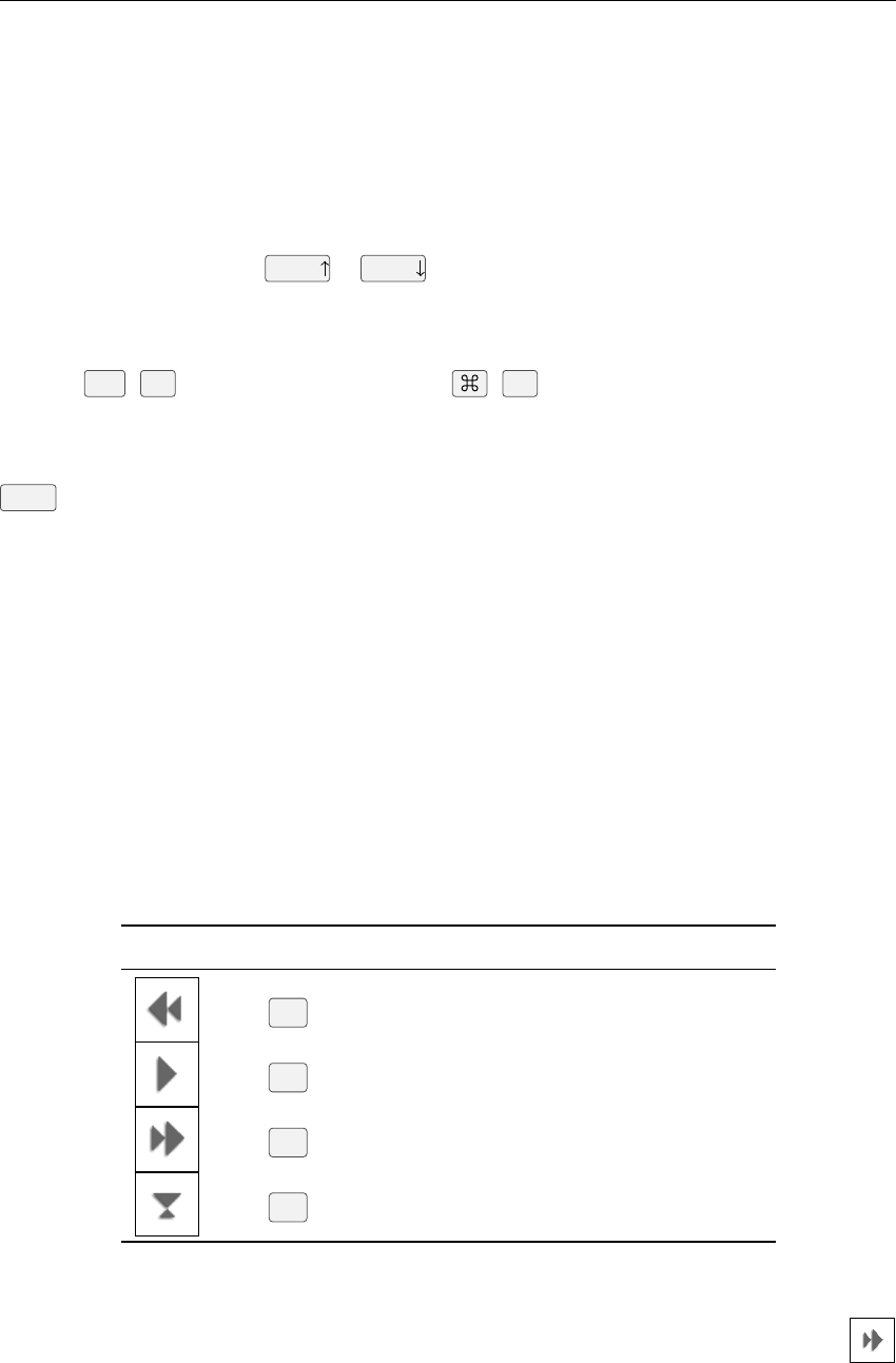
Figure 3.1: Stellarium main view. (Combination of day and night views.)
When Stellarium first starts, we see a green meadow under a sky. Depending on the time of day, it
is either a day or night scene. If you are connected to the Internet, an automatic lookup will attempt
to detect your approximate position.1
1See section 4.2 if you want to switch this off.
12 Chapter 3. A First Tour
At the bottom left of the screen, you can see the status bar. This shows the current observer
location, field of view (FOV), graphics performance in frames per second (FPS) and the current
simulation date and time. If you move the mouse over the status bar, it will move up to reveal a tool
bar which gives quick control over the program.
The rest of the view is devoted to rendering a realistic scene including a panoramic landscape
and the sky. If the simulation time and observer location are such that it is night time, you will see
stars, planets and the moon in the sky, all in the correct positions.
You can drag with the mouse on the sky to look around or use the cursor keys. You can zoom
with the mouse wheel or the Page or Page keys.
Much of Stellarium can be controlled very intuitively with the mouse. Many settings can
additionally be switched with shortcut keys (hotkeys). Advanced users will learn to use these
shortcut keys. Sometimes a key combination will be used. For example, you can quit Stellarium by
pressing
Ctrl +Q
on Windows and Linux, and
+Q
on Mac OS X. For simplicity, we will
show only the Windows/Linux version. We will present the default hotkeys in this guide. However,
almost all hotkeys can be reconfigured to match your taste. Note that some listed shortkeys are only
available as key combinations on international keyboard layouts, e.g., keys which require pressing
AltGr on a German keyboard. These must be reconfigured, please see 4.7.1 for details.
The way Stellarium is shown on the screen is primarily governed by the menus. These are
accessed by dragging the mouse to the left or bottom edge of the screen, where the menus will slide
out. In case you want to see the menu bars permanently, you can press the small buttons right in the
lower left corner to keep them visible.
3.1 Time Travel
When Stellarium starts up, it sets its clock to the same time and date as the system clock. However,
Stellarium’s clock is not fixed to the same time and date as the system clock, or indeed to the
same speed. We may tell Stellarium to change how fast time should pass, and even make time
go backwards! So the first thing we shall do is to travel into the future! Let’s take a look at the
time control buttons on the right hand ride of the tool-bar. If you hover the mouse cursor over the
buttons, a short description of the button’s purpose and keyboard shortcut will appear.
Button Shortcut key Description
JDecrease the rate at which time passes
KMake time pass as normal
LIncrease the rate at which time passes
8Return to the current time & date
Table 3.1: Time Travel
OK, so lets go see the future! Click the mouse once on the increase time speed button .
Not a whole lot seems to happen. However, take a look at the clock in the status bar. You should
see the time going by faster than a normal clock! Click the button a second time. Now the time is
going by faster than before. If it’s night time, you might also notice that the stars have started to
3.2 Moving Around the Sky 13
move slightly across the sky. If it’s daytime you might be able to see the sun moving (but it’s less
apparent than the movement of the stars). Increase the rate at which time passes again by clicking
on the button a third time. Now time is really flying!
Let time move on at this fast speed for a little while. Notice how the stars move across the sky.
If you wait a little while, you’ll see the Sun rising and setting. It’s a bit like a time-lapse movie.
Stellarium not only allows for moving forward through time – you can go backwards too! Click
on the real time speed button . The stars and/or the Sun should stop scooting across the sky.
Now press the decrease time speed button once. Look at the clock. Time has stopped. Click
the decrease time speed button four or five more times. Now we’re falling back through time at
quite a rate (about one day every ten seconds!).
Time Dragging, Time Scrolling
Another way to quickly change time is time dragging. Press
Ctrl
and slide the mouse along the
direction of daily motion to go forward, or to the other direction to go backward. 0.15.1
Similarly, pressing
Ctrl
and scrolling the mouse wheel will advance time by minutes, pressing
Ctrl +
and scrolling the mouse wheel will advance time by hours,
Ctrl +Alt
by days, and finally
Ctrl + + Alt by calendar years.
Enough time travel for now. Wait until it’s night time, and then click the real time speed button
. With a little luck you will now be looking at the night sky.
3.2 Moving Around the Sky
Key Description
Cursor keys Pan the view left, right, up and down
Page /Page ,Ctrl +/Ctrl +Zoom in and out
Left mouse button Select an object in the sky
Right mouse button Clear selected object
Centre mouse button (wheel press) Centre selected object and start tracking
Mouse wheel Zoom in and out
Centre view on selected object
Forward-slash ( /) Auto-zoom in to selected object
Backslash ( \) Auto-zoom out to original field of view
Table 3.2: Moving Around the Sky
As well as travelling through time, Stellarium lets to look around the sky freely, and zoom in
and out. There are several ways to accomplish this listed in table 3.2.
Let’s try it. Use the cursors to move around left, right, up and down. Zoom in a little using
the
Page
key, and back out again using the
Page
. Press the
\
key and see how Stellarium
returns to the original field of view (how “zoomed in” the view is), and direction of view.
It’s also possible to move around using the mouse. If you left-click and drag somewhere on the
sky, you can pull the view around.
Another method of moving is to select some object in the sky (left-click on the object), and
press the Space key to centre the view on that object. Similarly, selecting an object and pressing
the forward-slash key /will centre on the object and zoom right in on it.
14 Chapter 3. A First Tour
The forward-slash
/
and backslash
\
keys auto-zoom in an out to different zoom levels
depending on what is selected. If the object selected is a planet or moon in a sub-system with a lot of
moons (e.g. Jupiter), the initial zoom in will go to an intermediate level where the whole sub-system
should be visible. A second zoom will go to the full zoom level on the selected object. Similarly, if
you are fully zoomed in on a moon of Jupiter, the first auto-zoom out will go to the sub-system
zoom level. Subsequent auto-zoom out will fully zoom out and return the initial direction of view.
For objects that are not part of a sub-system, the initial auto-zoom in will zoom right in on the
selected object (the exact field of view depending on the size/type of the selected object), and the
initial auto-zoom out will return to the initial FOV and direction of view.
3.3 The Main Tool Bar
Figure 3.2: Night scene with constellation artwork and moon.
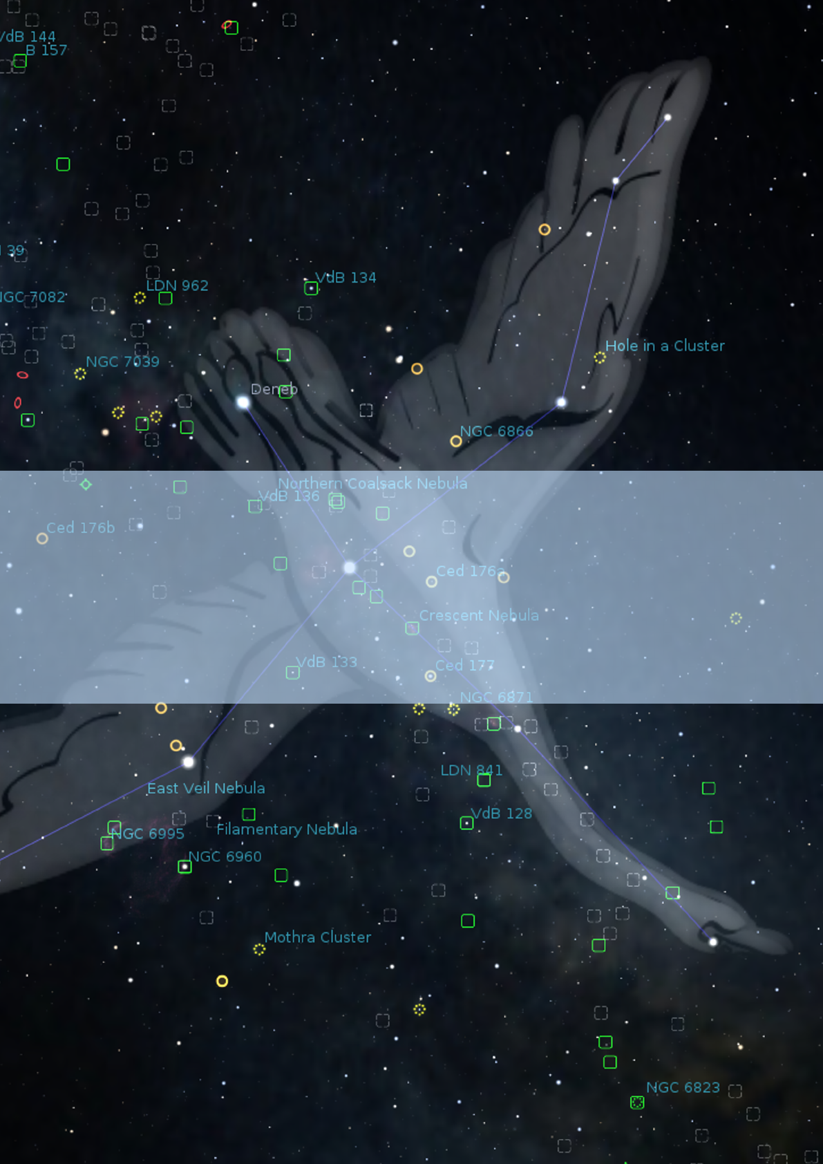
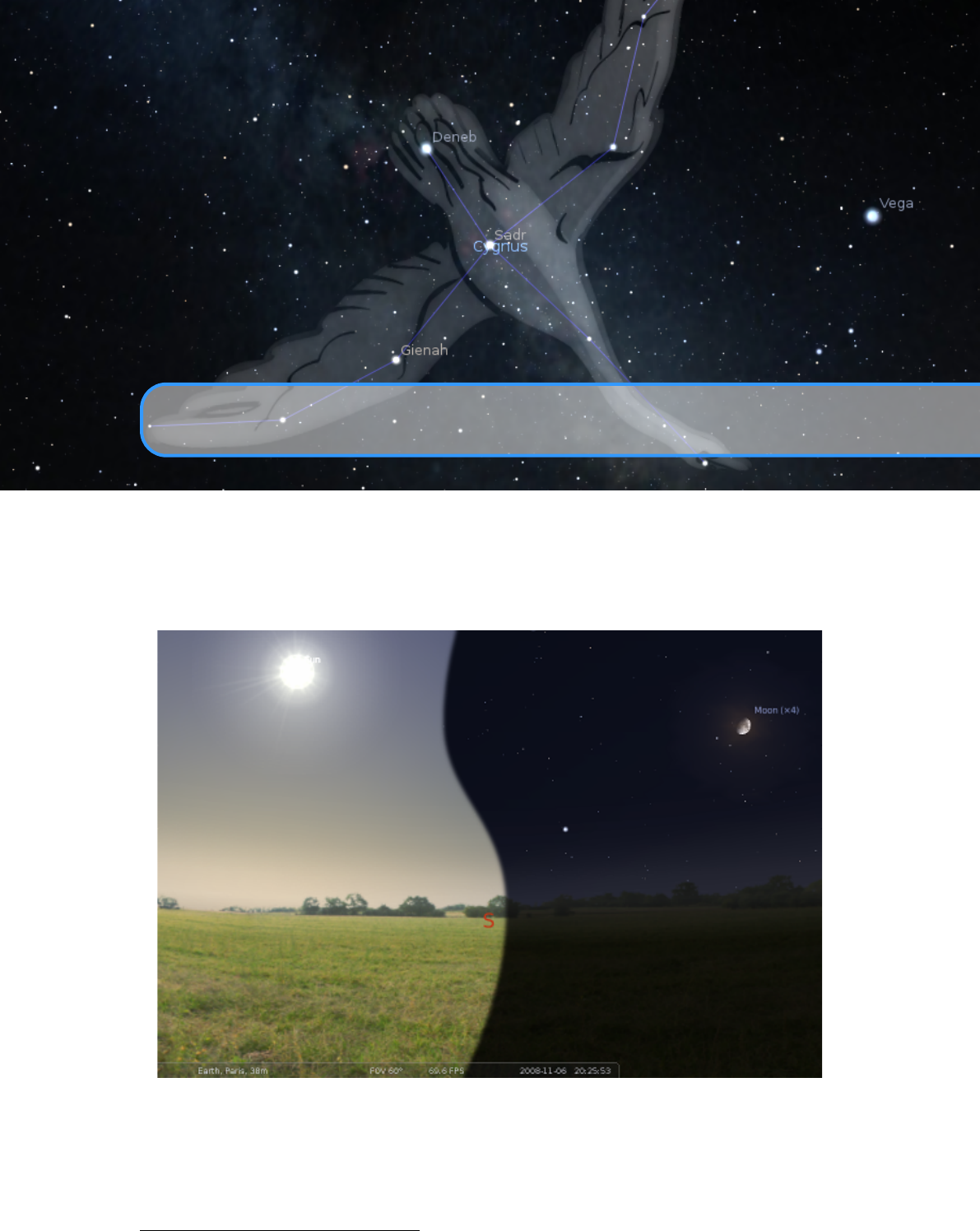
Stellarium can do a whole lot more than just draw the stars. Figure 3.2 shows some of
Stellarium’s visual effects including constellation line and boundary drawing, constellation art,
planet hints, and atmospheric halo around the bright Moon. The controls in the main tool bar
provide a mechanism for turning on and off the visual effects.
When the mouse if moved to the bottom left of the screen, a second tool bar becomes visible.
All the buttons in this side tool bar open and close dialog boxes which contain controls for further
configuration of the program. The dialogs will be described in the next chapter.
Table 3.3 describes the operations of buttons on the main tool bar and the side tool bar, and
gives their default keyboard shortcuts.
3.3 The Main Tool Bar 15
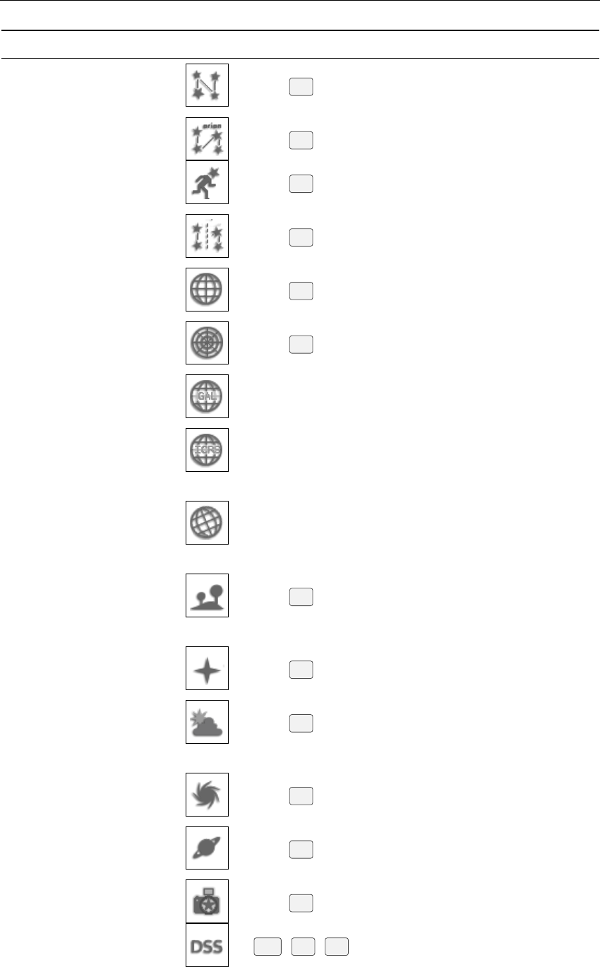
Feature Button Key Description
Constellations C
Draw constellations as “stick fig-
ures”
Constellation Names VDraw name of the constellations
Constellation Art R
Superimpose artistic representations
of the constellations
Constellation Boundaries B
Draw boundaries of the constella-
tions 1
Equatorial Grid E
Draw grid lines for the equatorial
coordinate system (RA/Dec)
Azimuth Grid Z
Draw grid lines for the horizontal
coordinate system (Alt/Azi)
Galactic Grid
Draw grid lines for the galactic coor-
dinate system (Long/Lat) 1
Equatorial J2000 Grid
Draw grid lines for the equatorial
coordinate system at standard epoch
J2000.0 (RA/Dec) 1
Ecliptic Grid
Draw grid lines for the ecliptic co-
ordinate system of date (Long/Lat)
1
Toggle Ground G
Toggle drawing of the ground. Turn
this off to see objects that are below
the horizon.
Toggle Cardinal Points Q
Toggle marking of the North, South,
East and West points on the horizon.
Toggle Atmosphere A
Toggle atmospheric effects. Most
notably makes the stars visible in the
daytime.
Deep-Sky Objects D
Toggle marking the positions of
Deep-Sky Objects.
Planet Hints P
Toggle indicators to show the posi-
tion of planets.
Nebula images IToggle “nebula images”. 1
Digitized Sky Survey Ctrl +Alt +DToggle “Digitized Sky Survey”.1
16 Chapter 3. A First Tour
Coordinate System Ctrl +M
Toggle between horizontal (Alt/Azi)
& equatorial (RA/Dec) coordinate
systems.
Goto
Center the view on the selected ob-
ject
Night Mode Ctrl +N
Toggle “night mode”, which applies
a red-only filter to the view to be
easier on the dark-adapted eye.
Full Screen Mode F11 Toggle full screen mode.
Bookmarks Alt +BToggle bookmarks window. 1
Flip view (horizontal) Ctrl +Shift +H
Flip the image in the horizontal
plane. 1
Flip view (vertical) Ctrl +Shift +V
Flip the image in the vertical plane.
1
Quit Stellarium Ctrl +QClose Stellarium.
Help Window F1
Show the help window, with key
bindings and other useful informa-
tion
Configuration Window F2 Show the configuration window
Search Window F3 or Ctrl +FShow the object search window
View Window F4 Show the view window
Time Window F5 Show the time window
Location Window F6 Show the observer location window
(map)
AstroCalc Window F10
Show the astronomical calculations
window
Table 3.3: Stellarium’s standard menu buttons. Those marked
1
must be enabled first, see section 4.3.4.

3.4 Taking Screenshots 17
3.4 Taking Screenshots
You can save what is on the screen to a file by pressing
Ctrl +S
. Screenshots are taken in
PNG format, and have filenames like
stellarium-000.png
,
stellarium-001.png
(the number
increments to prevent overwriting existing files).
Stellarium creates screenshots in a directory depending on your operating system, see section
5.1 Files and Directories.
4. The User Interface
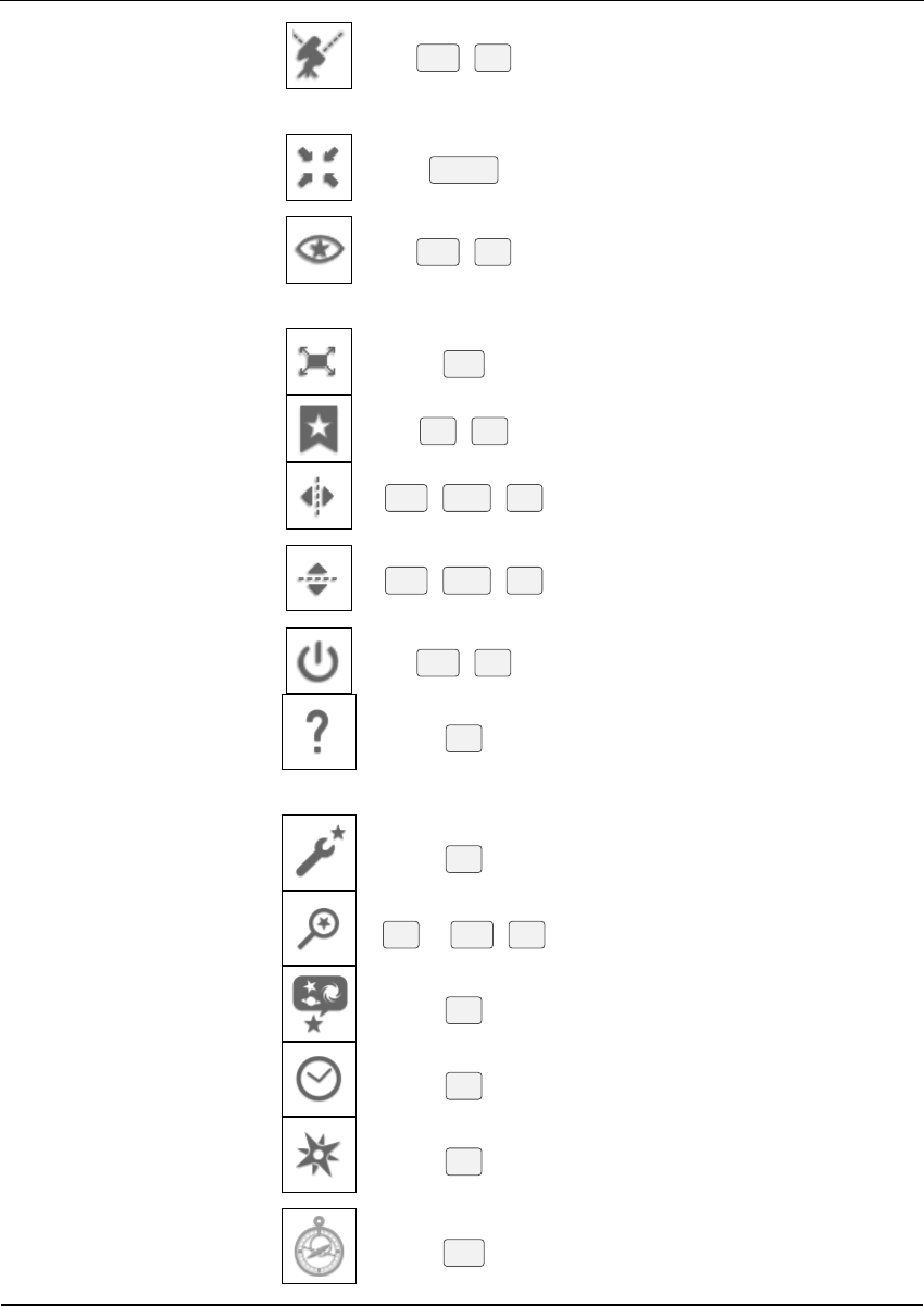
This chapter describes the dialog windows which can be accessed from the left menu bar.
Most of Stellarium’s settings can be changed using the view window (press or
F4
) and
the configuration window ( or
F2
). Most settings have short labels. To learn more about
some settings, more information is available as tooltips, small text boxes which appear when you
hover the mouse cursor over a button.10.15
You can drag the windows around, and the position will be used again when you restart
Stellarium. If this would mean the window is off-screen (because you start in windowed mode, or
with a different screen), the window will be moved so that at least a part is visible.
Some options are really rarely changed and therefore may only be configured by editing the
configuration file. See 5.4 The Main Configuration File for more details.
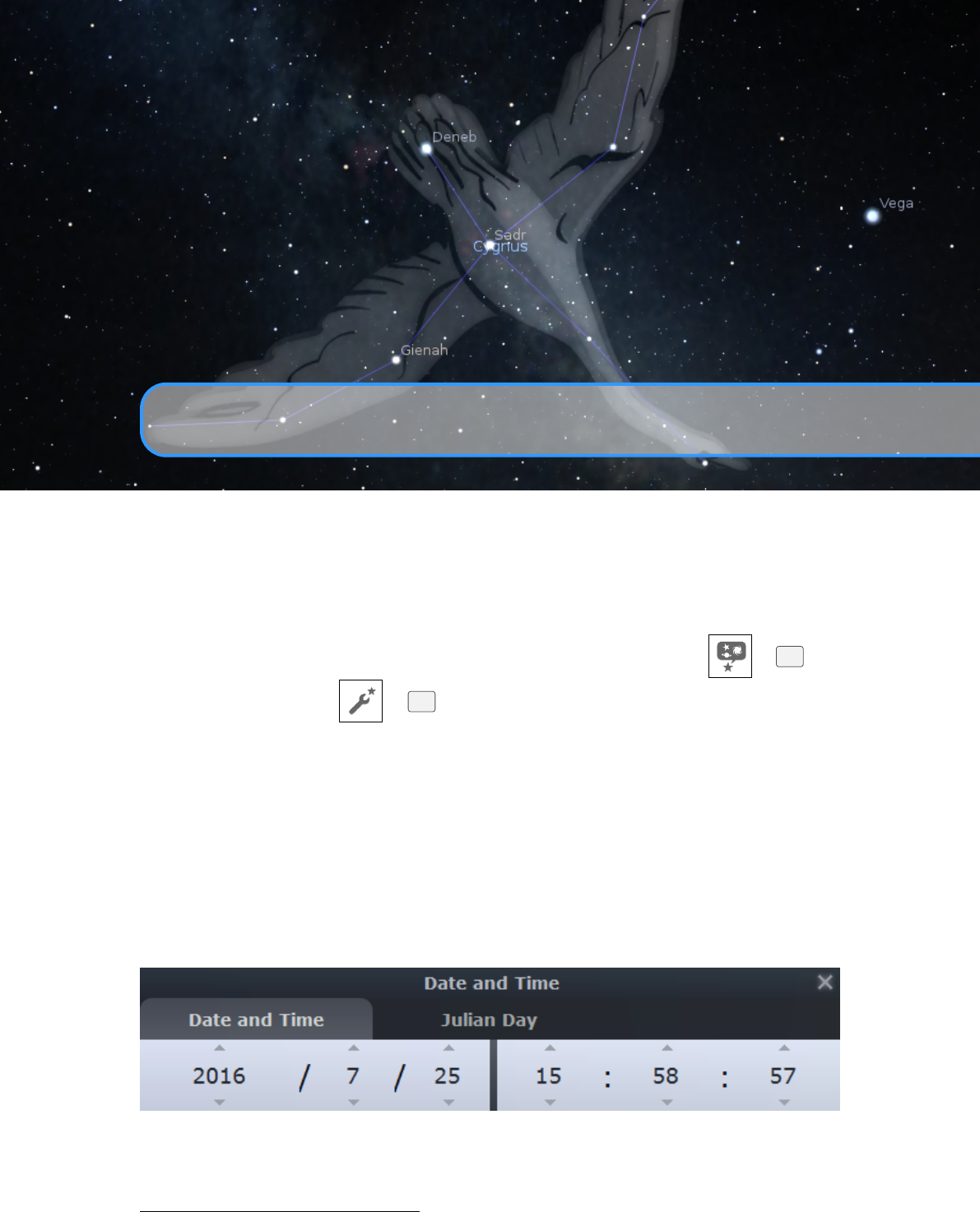
4.1 Setting the Date and Time
Figure 4.1: Date and Time dialog
In addition to the time rate control buttons on the main toolbar, you can use the date and time
1
Unfortunately, on Windows 7 and later, with some NVidia and AMD GPUs in OpenGL mode, these
tooltips often do not work.
20 Chapter 4. The User Interface
window (open with the button or
F5
) to set the simulation time. The values for year, month,
day, hour, minutes and seconds may be modified by typing new values, by clicking the up and down
arrows above and below the values, and by using the mouse wheel.
The other tab in this window allows you to see or set Julian Day and/or Modified Julian Day
numbers (see 17.4.2).
4.2 Setting Your Location
Figure 4.2: Location window
The positions of the stars in the sky is dependent on your location on Earth (or other planet) as well
as the time and date. For Stellarium to show accurately what is (or will be/was) in the sky, you
must tell it where you are. You only need to do this once – Stellarium can save your location so
you won’t need to set it again until you move.0.13.1
After installation, Stellarium uses an online service which tries to find your approximate
location based on the IP address you are using. This seems very practical, but if you feel this causes
privacy issues, you may want to switch this feature off. You should also consider switching it off
on a computer which does not move, to save network bandwidth.
To set your location more accurately, or if the lookup service fails, press
F6
to open the
location window (Fig. 4.2). There are a few ways you can set your location:
1. Just click on the map.
2.
Search for a city where you live using the search edit box at the top right of the window, and
select the right city from the list.
3.
Click on the map to filter the list of cities in the vicinity of your click, then choose from the
shortlist.
4.3 The Configuration Window 21
4. Enter a new location using the longitude, latitude and other data.
5.
Click on
Get Location from GPS
if you have a GPS receiver. See section 5.5.4 for configuration
0.16
details. Sometimes you have to try several times to get a valid 3D fix including altitude.
If you want to use the current location permanently, click on the “use as default” checkbox, disable
“Get location from Network”, and close the location window.
4.3 The Configuration Window
The configuration window contains general program settings, and many other settings which do not
concern specific display options. Press the tool button or F2 to open.
4.3.1 The Main Tab
The Main tab in the configuration window provides controls for changing separately the program
and sky culture languages.
The next setting group allows to enable using DE430/DE431 ephemeris files. These files have
to be installed separately. Most users do not require this. See section 5.5.3 if you are interested.
The tab also provides the buttons for saving the current view direction as default for the next
startup, and for saving the program configuration. Most display settings have to be explicitly stored
to make a setting change permanent.
4.3.2 The Information Tab
The Information tab allows you to set the type and amount of information displayed about a selected
object.
•Ticking or unticking the relevant boxes will control this.
•
The information displays in various colours depending on the type and level of the stored
data
•Additional settings for the information display
4.3.3 The Navigation Tab
The Navigation tab (Fig. 4.5) allows for enabling/disabling of keyboard shortcuts for panning and
zooming the main view, and also how to specify what simulation time should be used when the
program starts:
System date and time
Stellarium will start with the simulation time equal to the operating system
clock.
System date at
Stellarium will start with the same date as the operating system clock, but the
time will be fixed at the specified value. This is a useful setting for those people who use
Stellarium during the day to plan observing sessions for the upcoming evening.
Other some fixed time can be chosen which will be used every time Stellarium starts.
The lowest field allows selection of the correction model for the time correction
∆T
(see sec-
tion 17.4.3). Default is “Espenak and Meeus (2006)”. Please use other values only if you know
what you are doing.
4.3.4 The Tools Tab
The Tools tab (Fig. 4.6) contains miscellaneous utility features, and also allows to hide or show
additional buttons in the lower button bar. If your screen is too narrow to show all buttons, you may
have to choose your optimal setup.
22 Chapter 4. The User Interface
Figure 4.3: Configuration Window: Main Tab
Figure 4.4: Configuration Window: Information Tab
4.3 The Configuration Window 23
Figure 4.5: Configuration Window: Navigation Tab
Figure 4.6: Configuration Window: Tools Tab
24 Chapter 4. The User Interface
Figure 4.7: Configuration Window: Scripts Tab
Figure 4.8: Configuration Window: Plugins Tab

4.3 The Configuration Window 25
Spheric mirror distortion
This option pre-warps the main view such that it may be projected
onto a spherical mirror using a projector. The resulting image will be reflected up from the
spherical mirror in such a way that it may shine onto a small planetarium dome (or even just
the ceiling of your dining room), making a cheap planetarium projection system.
Select single constellation
When active, clicking on a star that is member in the constellation
lines will make the constellation stand out. You can select several constellations, but clicking
onto a star which is not member of a constellation line will display all constellations.
Show nebula background button
You can disable display of DSO photographs with this button.
Show bookmarks button You can enable display of Bookmarks dialog with this button.
Show ICRS grid button
You can toggle display of equatorial J2000 coordinate grid with this
button.
Show ecliptic grid button You can toggle display of ecliptic coordinate grid with this button.
Auto-enabling for the atmosphere
When changing planet during location change, atmosphere
will be switched as required.
Include nutation
Compute the slight wobble of earth’s axis. This feature is active only about 500
years around J2000.0.
Azimuth from South Some users may be used to counting azimuth from south.
Use buttons background Applies a gray background under the buttons on the bottom bar.
Auto zoom out returns to initial direction of view
When enabled, this option changes the be-
haviour of the zoom out key
\
so that it resets the initial direction of view in addition to
the field of view.
Disc viewport
This option masks the main view producing the effect of a telescope eyepiece. It is
also useful when projecting Stellarium’s output with a fish-eye lens planetarium projector.
Gravity labels
This option makes labels of objects in the main view align with the nearest horizon.
This means that labels projected onto a dome are always aligned properly.
Show flip buttons
When enabled, two buttons will be added to the main tool bar which allow
the main view to be mirrored in the vertical and horizontal directions. This is useful when
observing through telecopes which may cause the image to be mirrored.
Show DSS button You can toggle display of Digitized Sky Survey with this button.
Show galactic grid button You can toggle display of galactic coordinate grid with this button.
Show constellation boundaries button
You can toggle display of constellation boundaries with
this button.
Use decimal degrees You can toggle usage of decimal degree format for coordinates.
Topocentric coordinates
If you require planetocentric coordinates, you may switch this off. Usu-
ally it should be enabled. (See 17.9.1)
Auto select landscapes
When changing the planet in the location panel, a fitting landscape
panorama will be shown when available.
Indication for mount mode
You can activate the short display of a message when switching type
of used mount.
In addition, you can set the directory where screenshots will be stored, and you can download more
star catalogs on this tab.
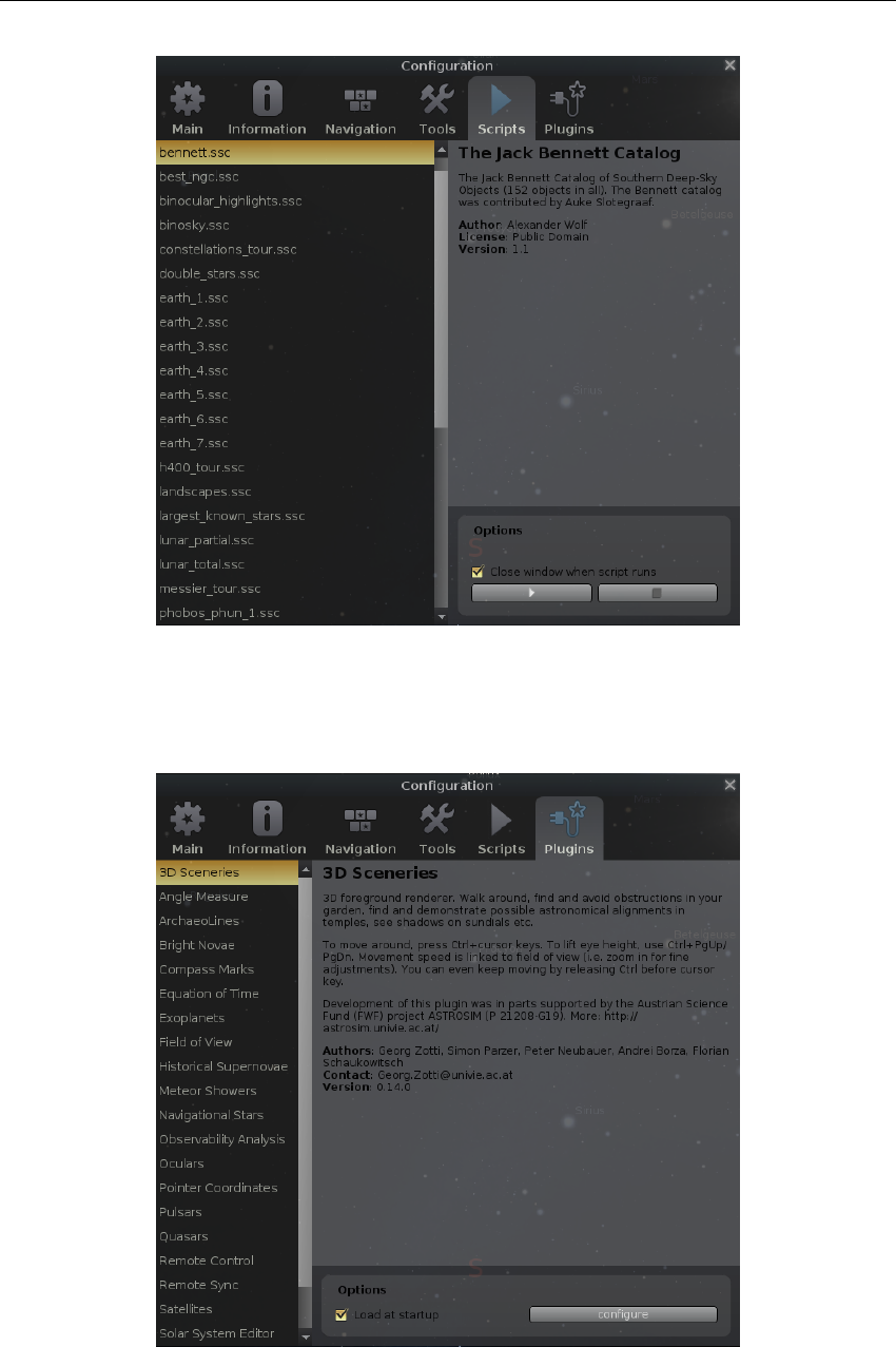
4.3.5 The Scripts Tab
The Scripts tab (Fig. 4.7) allows the selection of pre-assembled scripts bundled with Stellarium that
can be run (See chapter 16 for an introduction to the scripting capabilities and language). This list
can be expanded by your own scripts as required. See section 5.2 where to store your own scripts.
When a script is selected it can be run by pressing the arrow button and stopped with the stop
button. With some scripts the stop button is inhibited until the script is finished.
Scripts that use sound or embedded videos will need a version of Stellarium configured at
26 Chapter 4. The User Interface
Figure 4.9: View Settings Window: Sky Tab
compile time with multimedia support enabled. It must be pointed out here that sound or video
codecs available depends on the sound and video capabilities of you computer platform and may
not work.
4.3.6 The Plugins Tab
Plugins (see chapter 11 for an introduction) can be enabled here (Fig. 4.8) to be loaded the next
time you start Stellarium. When loaded, many plugins allow additional configuration which is
available by pressing the configure button on this tab.
4.4 The View Settings Window
The View settings window controls many display features of Stellarium which are not available via
the main toolbar.
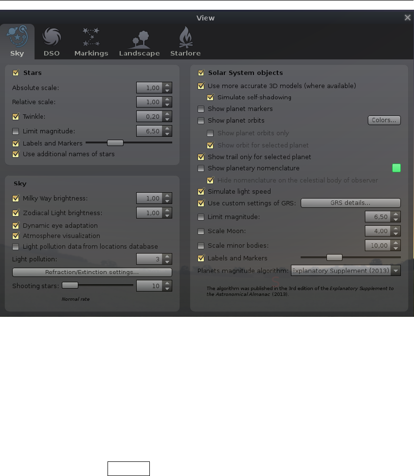
4.4.1 The Sky Tab
The Sky tab of the View window (Fig. 4.9) contains settings for changing the general appearance of
the main sky view. Some hightlights:
Absolute scale
is the size of stars as rendered by Stellarium. If you increase this value, all stars
will appear larger than before.
Relative scale
determines the difference in size of bright stars compared to faint stars. Values
higher than 1.00 will make the brightest stars appear much larger than they do in the sky.
This is useful for creating star charts, or when learning the basic constellations.

4.4 The View Settings Window 27
Twinkle
controls how much the stars twinkle when atmosphere is enabled (scintillation, see
section 18.13.2). Since v0.15.0, the twinkling is reduced in higher altitudes, where the star
light passes the atmosphere in a steeper angle and is less distorted.
Limit magnitude
Inhibits automatic addition of fainter stars when zooming in. This may be
helpful if you are interested in naked eye stars only.
Dynamic eye adaptation
When enabled this feature reduces the brightness of faint objects when
a bright object is in the field of view. This simulates how the eye can be dazzled by a bright
object such as the moon, making it harder to see faint stars and galaxies.
Light pollution
In urban and suburban areas, the sky is brightned by terrestrial light pollution
reflected in the atmophere. Stellarium simulates light pollution and is calibrated to the Bortle
Dark Sky Scale where 1 means a good dark sky, and 9 is a very badly light-polluted sky. See
Appendix B for more information.
Solar System objects
this group of options lets you turn on and off various features related to
the planets. Simulation of light speed will give more precise positions for planetary bodies
which move rapidly against backround stars (e.g. the moons of Jupiter). The Scale Moon
option will increase the apparent size of the moon in the sky, which can be nice for wide
field of view shots.
Labels and markers
you can independantly change the amount of labels displayed for planets,
stars and nebulae. The further to the right the sliders are set, the more labels you will see.
Note that more labels will also appear as you zoom in.
Shooting stars
Stellarium has a simple meteor simulation option. This setting controls how many
shooting stars will be shown. Note that shooting stars are only visible when the time rate is 1,
and might not be visiable at some times of day. Meteor showers are not currently simulated.
Atmosphere settings
An auxiliary dialog contains detail settings for the atmosphere. Here you can set atmospheric
pressure and temperature which influence refraction (see section 18.13.2), and the opacity factor
kv
for extinction, magnitude loss per airmass (see section 18.13.1).
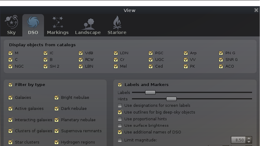
4.4.2 The Deep-Sky Objects (DSO) Tab
Deep-sky objects or DSO are extended objects which are external to the solar system, and are not
point sources like stars. DSO include galaxies, planetary nebulae and star clusters. These objects
may or may not have images associated with them. Stellarium comes with a catalogue of over
90,000 extended objects containing the combined data from many catalogues, with 200 images.
The DSO tab (Fig. 4.10) allows you to specify which catalogs or which object types you are
interested in. This selection will also be respected in other parts of the program, most notably
Search (section 4.5) and AstroCalc/WUT (section 4.6.6) will not find objects from catalogs which
you have not selected here.
See chapter 8 for details about the catalog, and how to extend it with your own photographs.
4.4.3 The Markings Tab
The Markings tab of the View window (Fig. 4.11) controls the following features:
Celestial sphere
this group of options makes it possible to plot various grids and lines in the main
view.
Projection
Selecting items in this list changes the projection method which Stellarium uses to
draw the sky (Snyder, 1987). Options are:
Perspective
Perspective projection maps the horizon and other great circles like equator,
ecliptic, hour lines, etc. into straight lines. The maximum field of view is 150
◦
. The
mathematical name for this projection method is gnomonic projection.
28 Chapter 4. The User Interface
Figure 4.10: View Settings Window: DSO Tab
Stereographic
Stereographic projection has been known since antiquity and was originally
known as the planisphere projection. It preserves the angles at which curves cross each
other but it does not preserve area. Else it is similar to fish-eye projection mode. The
maximum field of view in this mode is 235◦.
Fish-Eye
Stellarium draws the sky using azimuthal equidistant projection. In fish-eye
projection, straight lines become curves when they appear a large angular distance
from the centre of the field of view (like the distortions seen with very wide angle
camera lenses). This is more pronounced as the user zooms out. The maximum field
of view in this mode is 180◦.
Orthographic
Orthographic projection is related to perspective projection, but the point of
perspective is set to an infinite distance. The maximum field of view is 180◦.
Equal Area
The full name of this projection method is Lambert azimuthal equal-area
projection. It preserves the area but not the angle. The maximum field of view is 360
◦
.
Hammer-Aitoff
The Hammer projection is an equal-area map projection, described by
ERNST VON HAMMER (1858–1925) in 1892 and directly inspired by the Aitoff
projection. The maximum field of view in this mode is 360◦.
Sinusoidal
The sinusoidal projection is a pseudocylindrical equal-area map projection,
sometimes called the Sanson–Flamsteed or the Mercator equal-area projection. Merid-
ians are mapped to sine curves.
Mercator
Mercator projection is a cylindrical projection developed by GERARDUS MER-
CATOR (1512–1594) which preserves the angles between objects, and the scale around
an object is the same in all directions. The poles are mapped to infinity. The maximum
field of view in this mode is 233◦.
Miller cylindrical
The Miller cylindrical projection is a modified Mercator projection,
proposed by OSBORN MAITLAND MILLER (1897–1979) in 1942. The poles are no
longer mapped to infinity.
Cylinder
The full name of this simple projection mode is cylindrical equidistant projection
or Plate Carrée. The maximum field of view in this mode is 233◦.
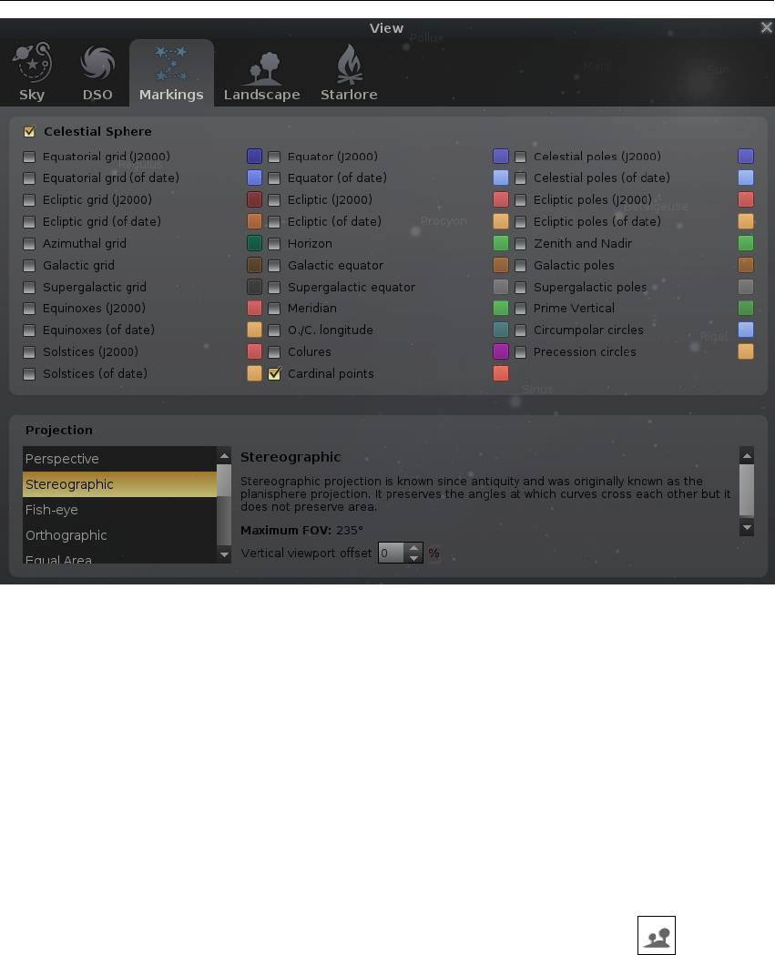
4.4 The View Settings Window 29
Figure 4.11: View Settings Window: Markings Tab
4.4.4 The Landscape Tab
The Landscape tab of the View window (Fig. 4.12) controls the landscape graphics (the horizon
which surrounds you). To change the landscape graphics, select a landscape from the list on the left
side of the window. A description of the landscape will be shown on the right.
Note that while a landscape can include information about where the landscape graphics were
taken (planet, longitude, latitude and altitude), this location does not have to be the same as the
location selected in the Location window, although you can set up Stellarium such that selection of
a new landscape will alter the location for you.
The controls at the bottom right of the window operate as follows:
Show ground
This turns on and off landscape rendering (same as the button in the main
tool-bar).
Show_fog
This turns on and off rendering of a band of fog/haze along the horizon, when available
in this landscape.
Use associated planet and position
When enabled, selecting a new landscape will automatically
update the observer location.
Use this landscape as default
Selecting this option will save the landscape into the program
configuration file so that the current landscape will be the one used when Stellarium starts.
Minimal brightness
Use some minimal brightness setting. Moonless night on very dark locations
may appear too dark on your screen. You may want to configure some minimal brightness
here.
from landscape, if given
Landscape authors may decide to provide such a minimal brightness
value in the landscape.ini file.
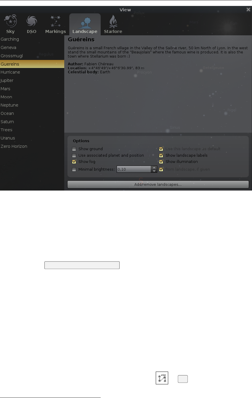
30 Chapter 4. The User Interface
Figure 4.12: View Settings Window: Landscape Tab
Show landscape labels
Landscapes can be configured with a gazetteer of interesting points, e.g.,
mountain peaks, which can be labeled with this option.
Show illumination
to reflect the ugly developments of our civilisation, landscapes can be config-
ured with a layer of light pollution, e.g., streetlamps, bright windows, or the sky glow of a
nearby city. This layer, if present, will be mixed in when it is dark enough.
Using the button
Add/remove landscapes. . .
, you can also install new landscapes from ZIP files
which you can download e.g. from the Stellarium website
2
or create yourself (see ch. 7 Landscapes),
or remove these custom landscapes.
Loading large landscapes may take several seconds. If you like to switch rapidly between
v0.15.2
several landscapes and have enough memory, you can increase the default cache size to keep more
landscapes loaded previously available in memory. Note that a large landscape can take up 200MB
or more! See section D.1.11.
4.4.5 The Starlore Tab
The Starlore tab of the View window (Fig. 4.13) controls what culture’s constellations and bright
star names will be used in the main display. Some cultures have constellation art (e.g., Western and
Inuit), and the rest do not. Configurable options include
Use this skyculture as default
Activate this option to load this skyculture when Stellarium starts.
Show labels
Activate display of constellation labels, like or
V
. You can further select
whether you want to display abbreviated, original or translated names.
2http://stellarium.sourceforge.net/wiki/index.php/Landscapes
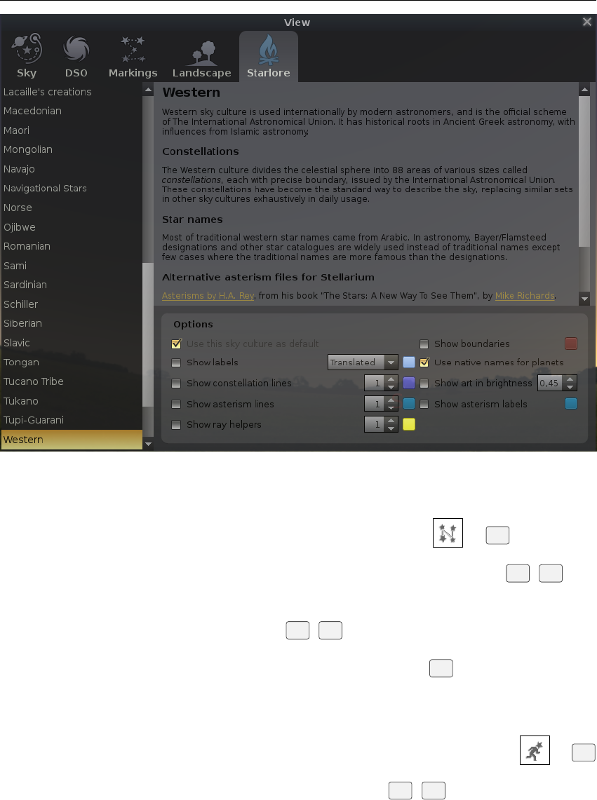
4.4 The View Settings Window 31
Figure 4.13: View Settings Window: Starlore Tab
Show lines with thickness. . .
Activate display of stick figures, like or
C
, and you can
configure constellation line thickness here.
Show asterism lines. . .
Activate display of asterism stick figures (like the shortcut
Alt +A
), and
you can configure asterism line thickness here. v0.16.0
Show ray helpers. . .
Activate display of special navigational lines which connect stars often from
different constellations (like the shortcut
Alt +R
), and you can configure thickness of those
lines here. v0.17.0
Show boundaries
Activate display of constellation boundaries, like
B
. Currently, boundaries
have been defined only for “Western” skycultures.
Use native names for planets
If provided, show the planet names as used in this skyculture (also
shows modern planet name for reference).
Show art in brightness. . .
Activate display of constellation art (if available), like or
R
.
You can also select the brightness here.
Show asterism labels Activate display of asterism labels, like Alt +V. v0.16.0
4.4.6 The Surveys Tab v0.18.0
The Surveys tab (Fig. 4.14) allows to toggle the visibility of online sky or solar system surveys (see
chapter 10 for description of the surveys format). Currently, only HiPS surveys are supported.
On the left side of the window we see the list of available surveys from the configured sources
(See section D.1.27 for how to change the default sources). On the right side a description of the
selected survey and its properties are displayed.
Surveys are grouped by types. The top combobox allows to filter the listed surveys according
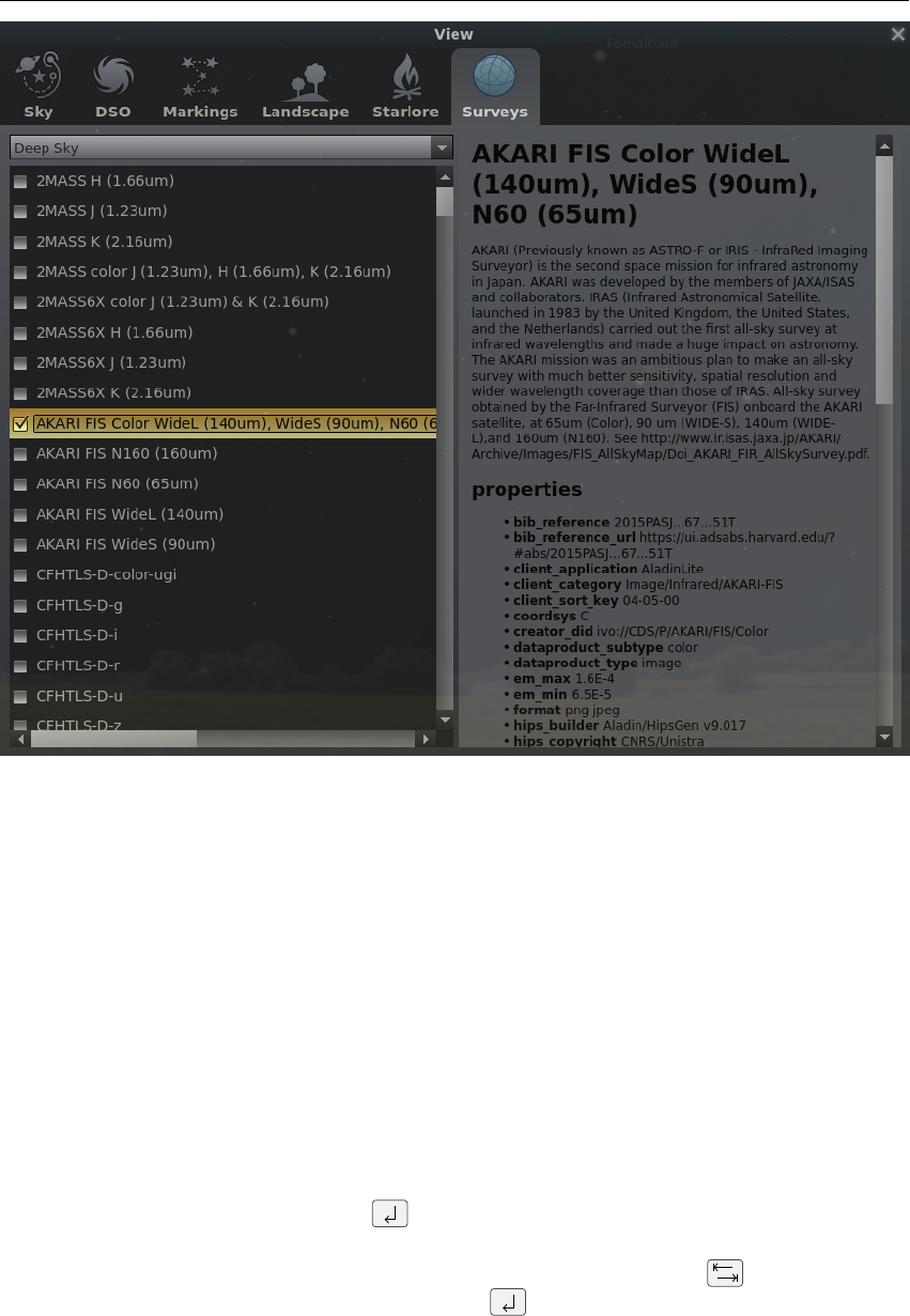
32 Chapter 4. The User Interface
Figure 4.14: View Settings Window: Surveys Tab
to a given type (Deep Sky or Solar System).
You can toggle the visibility of a survey by checking the box on the left of the survey name
in the list. (Note that as of v0.18.0, only a single deep sky survey can be rendered at a time, so it
makes no sense to select more than one in the list!) Once a survey is visible you should be able to
see its loading status in the loading bar area of the sky view.
Deep sky surveys will be rendered aligned with the sky view, while solar system surveys
automatically map on the proper body.
4.5 The Object Search Window
The Object Search window provides a convenient way to locate objects in the sky. Simply type in
the name of an object to find, and press . Stellarium will point you at that object in the sky.
As you type, Stellarium will make a list of objects which contains what you have typed so far.
The first of the list of matching objects will be highlighted. If you press the key, the selection
will change to the next item in the list. Hitting the key will go to the currently highlighted
object and close the search dialog.
For example, suppose we want to locate Saturn’s moon Mimas. Type the first letter of the name,
m, to see a list of objects whose name contains m: Haumea, Miranda, Umbriel, . . .
You may want at this point to have Stellarium rather propose object names with start with the
string you enter. Do that in the Options tab of this panel. Now repeat searching (delete, and re-enter
4.5 The Object Search Window 33
Figure 4.15: The Search Window: Objects
Figure 4.16: The Search Window: Positions
Figure 4.17: The Search Window: Lists
34 Chapter 4. The User Interface
Figure 4.18: The Search Window: Options
mto start over). Now the list is shorter and contains only objects which start with m:Maia, Mars,
. . . The first item in this list, Maia, is highlighted. Pressing now would go to Maia, but we
want Mimas. We can either press a few times to highlight Mimas and then hit , or we can
continue to type the name until it is the first/only object in the list.
The Position tab (Fig. 4.16) provides a convenient way to enter a set of coordinates.
The List Search tab (Fig. 4.18) allows selection of an object from predefined sets. The number
of choices is governed by the loaded DSO catalogs and plug-ins. Scroll down the first window to
select the type. Click on the name and Stellarium will go to that object.
The Options tab (Fig. 4.18) provides a few settings to fine-tune your search experience. When
the name of an object to find is typed in the object window and you are connected to the internet and
“Extend search” is ticked, Stellarium will search the SIMBAD on-line data bases for its coordinates.
You can then click the button or press return. Stellarium will point you at that object in the sky
even if there is no object displayed on the screen. The SIMBAD server being used can be selected
from the scroll window.
4.6 The Astronomical Calculations Window
This window provides advanced functionality, some of which is still in an experimental phase.
v0.15.0
You can call it by pressing
F10
or the button on the left menu bar. The Astronomical
Calculations window shows six tabs with different functionality.
4.6.1 The Positions Tab
This tab shows J2000.0 or horizontal positions, magnitudes and additional parameters (e.g. surface
v0.16.0
brightness for deep-sky objects or angular separation for double stars) for various lists of celestial
objects above the horizon at the simulated time, filtered by magnitude. Double-clicking on an entry
brings the object into focus (Figure 4.19). You may also export the list of positions into a CSV file.
4.6.2 The Ephemeris Tab
Select an object, start and end time, and compute an ephemeris (list of positions and magnitudes
evolving over time) for that object. The positions are marked in the sky with yellow circles
(Figure 4.20).
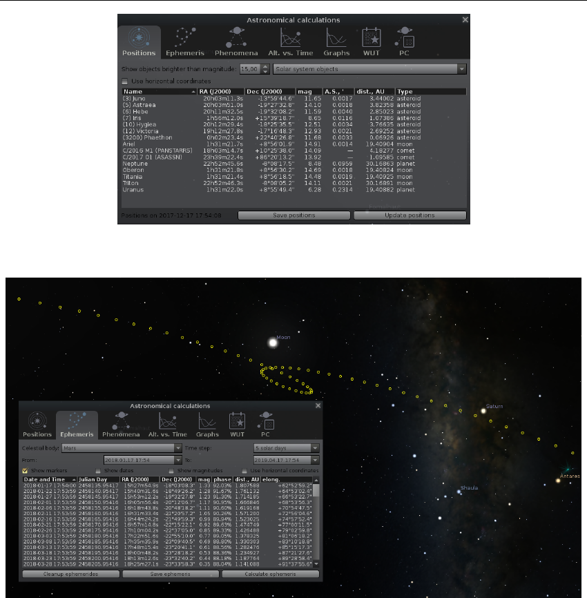
4.6 The Astronomical Calculations Window 35
Figure 4.19: Astronomical Calculations (AstroCalc): Celestial positions
Figure 4.20: Astronomical Calculations (AstroCalc): Plot trace of planet
When you click on a date, an orange circle indicates this date and/or magnitude. Double-
clicking sets the respective date and brings the object to focus. Dates and/or magnitudes will show
near position markers when Show dates and/or Show magnitudes checkboxes are active.
You can export the calculated ephemeris into a CSV file.
Another interesting option in this tool: using horizontal coordinates for plotting traces of the
Solar system objects. In this mode, the circle marks are not linked to the sky, but to the horizontal
coordinate system. For example, you can get an analemma of the Sun for any location (Figures 4.21
and 4.22), or observe the visibility of Mercury, Venus or a comet in the twilight sky.
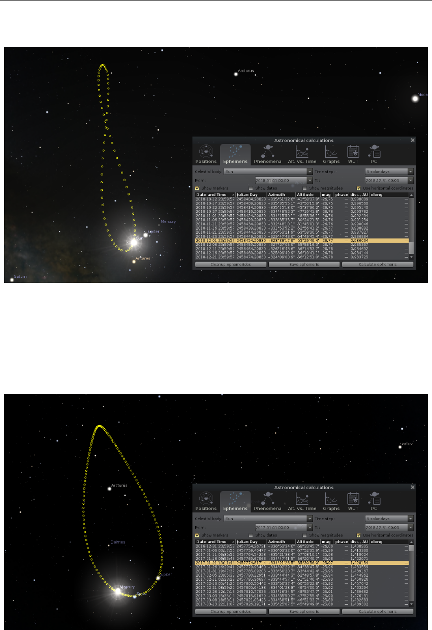
36 Chapter 4. The User Interface
Figure 4.21: Astronomical Calculations (AstroCalc): Analemma on the Earth
Figure 4.22: Astronomical Calculations (AstroCalc): Analemma on Mars
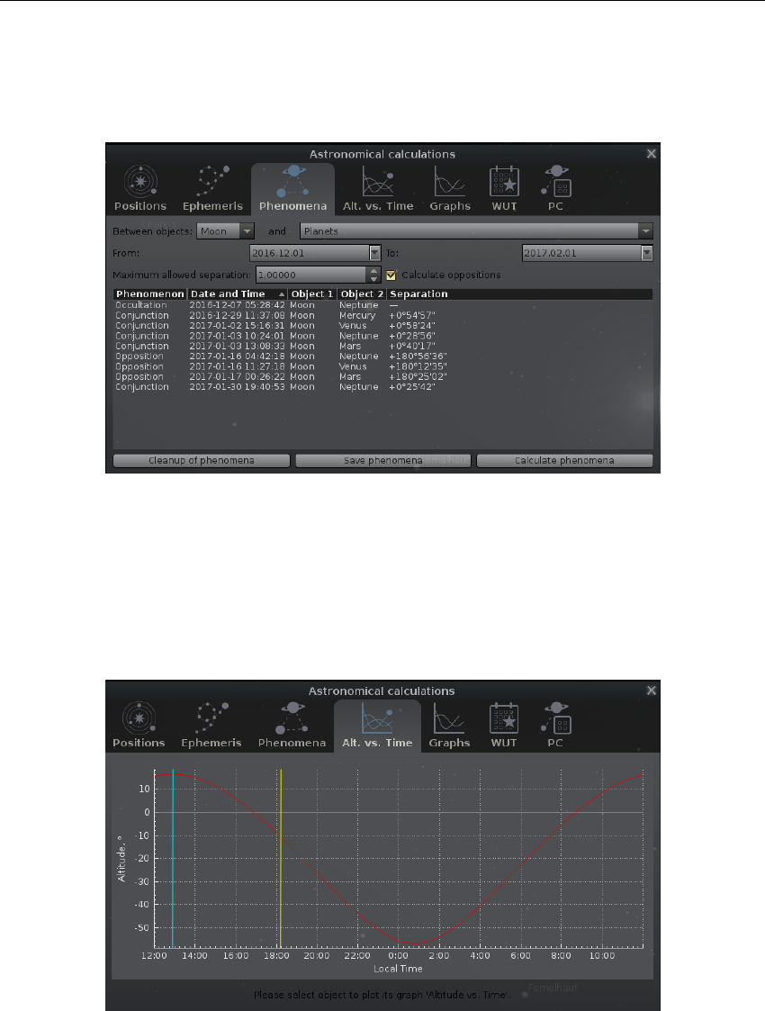
4.6 The Astronomical Calculations Window 37
4.6.3 The Phenomena Tab
This tab allows you to compute phenomena like conjunctions, oppositions, occultations and eclipses
(in special cases) between planetary objects (Figure 4.23). You can export the calculated phenomena
into a CSV file.
Figure 4.23: Astronomical Calculations (AstroCalc): Phenomena
4.6.4 The “Altitude vs. Time” Tab
On this tab you can compute the geometrical altitude of the currently selected object and date and
draw it as a graph (Figure 4.24).
Figure 4.24: Astronomical Calculations (AstroCalc): Altitude vs. Time
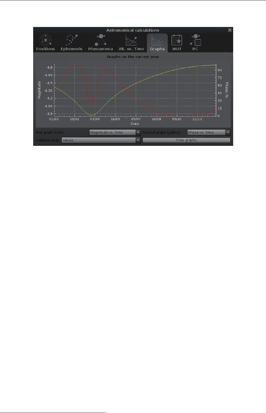
38 Chapter 4. The User Interface
4.6.5 The Graphs Tab
Figure 4.25: Astronomical Calculations (AstroCalc): Graphs
This tab can show two functions over time for the current year and draw graphs for them in one
v0.16.0
screen (Figure 4.25). You can select from
•Magnitude vs. Time
•Phase vs. Time
•Distance vs. Time
•Elongation vs. Time
•Angular size vs. Time
•Phase angle vs. Time
This tool may be very helpful for educational and statistics purposes.3
4.6.6 The “What’s Up Tonight” (WUT) Tab
The “What’s Up Tonight” (WUT) tool
4
displays a list of objects that will be visible at night for the
v0.16.0
current date and location.
The objects are organized into type categories. Select an object type in the box labeled Select
a Category, and all objects of that type which are above the horizon on the selected night will be
displayed in the box labeled Matching Objects. For example, in the screenshot, the Planets category
has been selected, and three planets which are up in the selected night are displayed (Jupiter, Mars
and Mercury).
By default, the WUT will display objects which are above the horizon between sunset and
midnight (i.e. in the evening). You can choose to show objects which are up between midnight and
dawn (in the morning), around midnight, or any time between dusk and dawn (any time tonight)
using the combobox near the top of the window. You can also choose to see only those objects
that are brighter than a certain magnitude by setting a minimum magnitude using the Show objects
brighter than magnitude spinbox. You may center an object from the right list in the sky map just
by selecting it.
Note that only DSO from catalogs which you have selected in the DSO panel (section 4.4.2)
will be found.
3The idea for this tool has been obtained from SkytechX:http://www.skytechx.eu/
4This tool has been partially ported from the KStars planetarium: https://edu.kde.org/kstars/
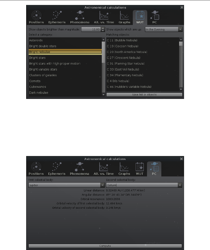
4.6 The Astronomical Calculations Window 39
Figure 4.26: Astronomical Calculations (AstroCalc): What’s Up Tonight (WUT)
4.6.7 The “Planetary Calculator” (PC) Tab
The “Planetary Calculator” (PC) tool has been added after user requests. It computes the relations
v0.17.0
between two Solar system bodies for the current date and location — linear and angular distances,
orbital resonances and orbital velocities.
Figure 4.27: Astronomical Calculations (AstroCalc): Planetary Calculator (PC)
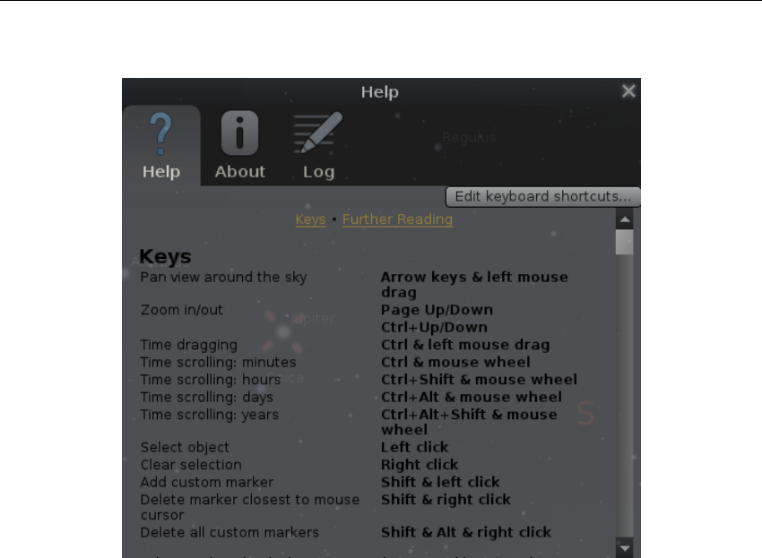
40 Chapter 4. The User Interface
4.7 Help Window
Figure 4.28: Help Window
The Help window lists all of Stellarium’s keystrokes. Note that some features are only available as
keystrokes, so it’s a good idea to have a browse of the information in this window.
4.7.1 Editing Keyboard Shortcuts
You can edit the shortcut keys here. Each available function can be configured with up to two key
combinations. You may want to reconfigure keys for example if you have a non-English keyboard
layout and some keys either do not work at all, or feel unintuitive for you, or if you are familiar with
other software and want to use the same hotkeys for similar functions. Simply select the function
and click with the mouse into the edit field, then press your key of choice. If the key has been taken
already, a message will tell you.
The About Tab (Fig. 4.29) shows version and licensing information, and a list of people who
helped to produce the program.
The Log Tab (Fig. 4.30) shows messages like the loading confirmations carried out when
stellarium runs. It is useful to locate the files that stellarium writes to your computer. The same
information is written to the file log.txt that you will find in your user directory (see 5.1).
4.7 Help Window 41
Figure 4.29: Help Window: About
Figure 4.30: Help Window: Logfile

II 5Files and Directories ...................... 45
5.1 Directories
5.2 Directory Structure
5.3 The Logfile
5.4 The Main Configuration File
5.5 Getting Extra Data
6Command Line Options ...................51
6.1 Examples
6.2 Special Options
7Landscapes ............................... 55
7.1 Stellarium Landscapes
7.2 Creating Panorama Photographs for Stellarium
7.3 Panorama Postprocessing
7.4 Other recommended software
8Deep-Sky Objects ........................ 79
8.1 Stellarium DSO Catalog
8.2 Adding Extra Nebulae Images
9Adding Sky Cultures ...................... 89
9.1 Basic Information
9.2 Skyculture Description Files
9.3 Constellation Names
9.4 Star Names
9.5 Planet Names
9.6 Deep-Sky Objects Names
9.7 Stick Figures
9.8 Constellation Boundaries
9.9 Constellation Artwork
9.10 Seasonal Rules
9.11 References
9.12 Asterisms and help rays
9.13 Publish Your Work
10 Surveys ..................................... 95
10.1 Introduction
10.2 Hipslist file and default surveys
10.3 Solar system HiPS survey
Advanced Use
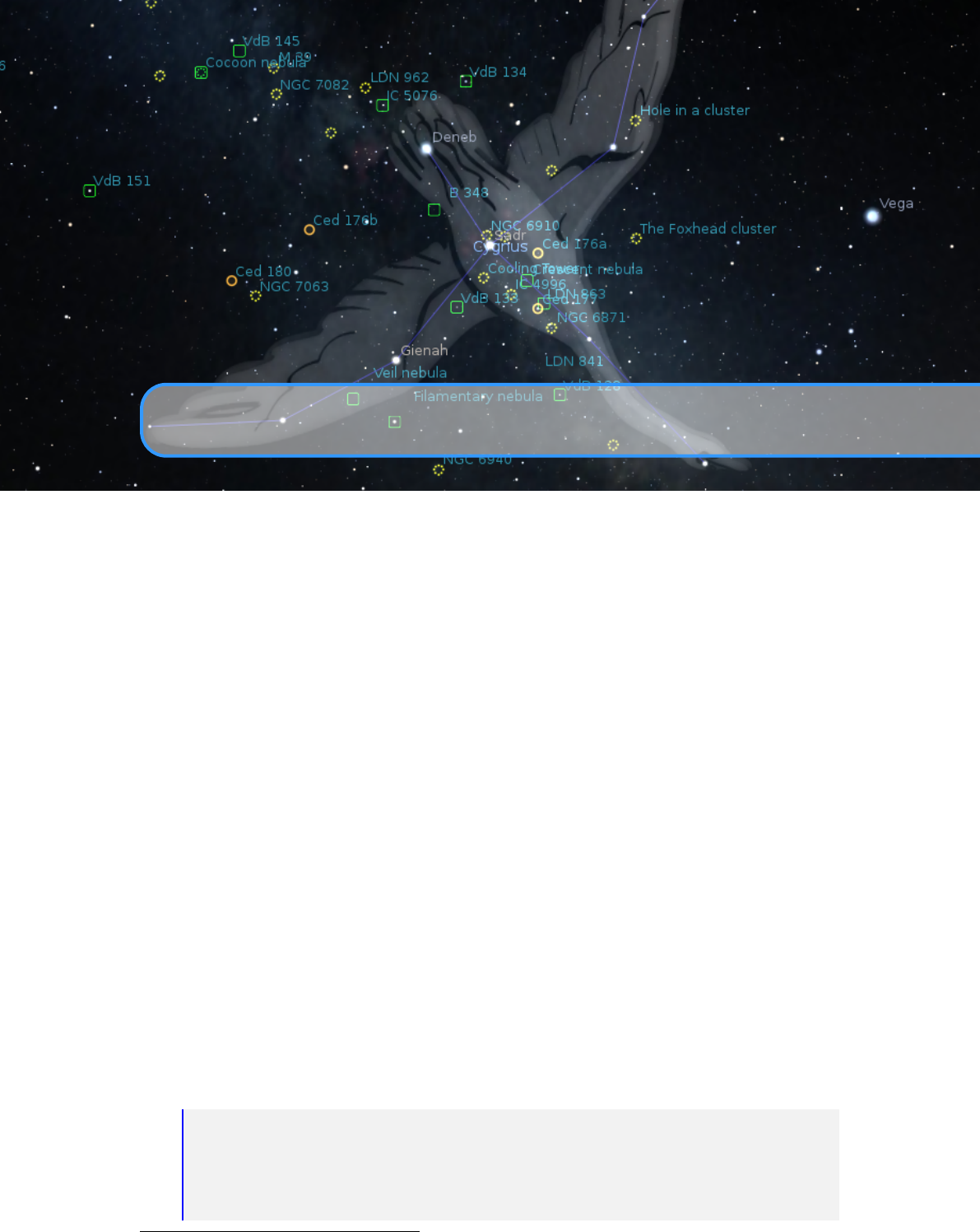
5. Files and Directories
5.1 Directories
Stellarium has many data files containing such things as star catalogue data, nebula images, button
icons, font files and configuration files. When Stellarium looks for a file, it looks in two places.
First, it looks in the user directory for the account which is running Stellarium. If the file is not
found there, Stellarium looks in the installation directory
1
. Thus it is possible for Stellarium to be
installed by an administrative user and yet have a writable configuration file for non-administrative
users. Another benefit of this method is on multi-user systems: Stellarium can be installed by
the administrator, and different users can maintain their own configuration and other files in their
personal user accounts.
In addition to the main search path, Stellarium saves some files in other locations, for example
screens shots and recorded scripts.
The locations of the user directory, installation directory, screenshot save directory and script
save directory vary according to the operating system and installation options used. The following
sections describe the locations for various operating systems.
5.1.1 Windows
installation directory
By default this is
C:\Program Files\Stellarium\
, although this can
be adjusted during the installation process.
user directory
This is the Stellarium sub-folder in the Application Data folder for the user account
which is used to run Stellarium. Depending on the version of Windows and its configuration,
this could be any of the following (each of these is tried, if it fails, the next in the list if tried).
% APPDATA %\ Stellarium \
% USER PROFILE %\ Stellarium \
% HOMEDRIVE %\% HOMEPATH %\ Stellari um \
% HOME %\ St ella rium \
Stellarium ’s instal lat ion directory
1The installation directory was referred to as the config root directory in previous versions of this guide

46 Chapter 5. Files and Directories
Thus, on a typical Windows Vista/7/10 system with user “Bob Dobbs”, the user directory
will be:
C :\ Users \ Bob Dobbs \ AppData \ Roaming \ Stellarium \
The user data directory is unfortunately hidden by default. To make it accessible in the Win-
dows file explorer, open an
Explorer
window and select
Organize... Folder and search options
.
Make sure folders marked as hidden are now displayed. Also, deselect the checkbox to “hide
known file name endings”.2
screenshot save directory
Screenshots will be saved to the
Pictures/Stellarium
directory,
although this can be changed in the GUI (see section 4.3.4) or with a command line option
(see section 6).
5.1.2 Mac OS X
installation directory
This is found inside the application bundle,
Stellarium.app
. See Inside
Application Bundles3for more information.
user directory This is the sub-directory Library/Preferences/Stellarium/ (or
~/Library/Application Support/Stellarium
on newest versions of Mac OS X) of
the user’s home directory.
screenshot save directory Screenshots are saved to the user’s Desktop.
5.1.3 Linux
installation directory
This is in the
share/stellarium
sub-directory of the installation prefix,
i.e., usually /usr/share/stellarium or /usr/local/share/stellarium/.
user directory
This is the
.stellarium
sub-directory of user’s home directory, i.e.,
~/.stellarium/
.
This is a hidden folder, so if you are using a graphical file browser, you may want to change
its settings to “display hidden folders”.
screenshot save directory Screenshots are saved to the user’s home directory.
5.2 Directory Structure
Within the installation directory and user directory defined in section 5.1, files are arranged in the
following sub-directories.
landscapes/
contains data files and textures used for Stellarium’s various landscapes. Each
landscape has its own sub-directory. The name of this sub-directory is called the landscape
ID, which is used to specify the default landscape in the main configuration file, or in script
commands.
skycultures/
contains constellations, common star names and constellation artwork for Stel-
larium’s many sky cultures. Each culture has its own sub-directory in the skycultures
directory.
nebulae/
contains data and image files for nebula textures. In the future Stellarium may be able
to support multiple sets of nebula images and switch between them at runtime. This feature
is not implemented for version 0.18.0, although the directory structure is in place - each set
of nebula textures has its own sub-directory in the nebulae directory.
2
This is a very confusing default setting and in fact a security risk: Consider you receive an email
with some file
funny.png.exe
attached. Your explorer displays this as
funny.png
. You double-click it,
expecting to open some image browser with a funny image. However, you start some unknown program
instead, and running this .exe executable program may turn out to be anything but funny!
3http://www.mactipsandtricks.com/articles/Wiley_HT_appBundles.lasso

5.3 The Logfile 47
stars/
contains Stellarium’s star catalogues. In the future Stellarium may be able to support
multiple star catalogues and switch between them at runtime. This feature is not implemented
for version 0.18.0, although the directory structure is in place – each star catalogue has its
own sub-directory in the stars directory.
data/ contains miscellaneous data files including fonts, solar system data, city locations, etc.
textures/
contains miscellaneous texture files, such as the graphics for the toolbar buttons, planet
texture maps, etc.
ephem/
(optional) may contain data files for planetary ephemerides DE430 and DE431 (see 5.5.3).
If any file exists in both the installation directory and user directory, the version in the user
directory will be used. Thus it is possible to override settings which are part of the main Stellarium
installation by copying the relevant file to the user area and modifying it there.
It is recommended to add new landscapes or sky cultures by creating the relevant files and
directories within the user directory, leaving the installation directory unchanged. In this manner
different users on a multi-user system can customise Stellarium without affecting the other users,
and updating Stellarium will not risk the loss of your own data.
5.3 The Logfile
Stellarium reports various events and confirmations to a logfile,
log.txt
, in the user directory.
This has the same content as you can see on the console on Linux when you start Stellarium on the
command line. Normally you don’t need to bother with its contents, however, if Stellarium behaves
unexpectedly, crashes, or shows other problems, a quick look into this file may help to identify the
problem. Also when you report a problem to the developers in the hope that they (we) can ’fix’
anything, this logfile is an essential ingredient to your report. The logfile can also be displayed
within the program: press F1 to call the help panel, and select the Logfile tab.
5.4 The Main Configuration File
The main configuration file is read each time Stellarium starts, and settings such as the observer’s
location and display preferences are taken from it. Ideally this mechanism should be totally
transparent to the user – anything that is configurable should be configured “in” the program GUI.
However, at time of writing Stellarium isn’t quite complete in this respect, despite improvements in
each version. Some settings, esp. color values for lines, grids, etc. can only be changed by directly
editing the configuration file.
4
This section describes some of the settings a user may wish to
modify in this way, and how to do it.
If the configuration file does not exist in the user directory when Stellarium is started (e.g., the
first time the user starts the program), one will be created with default values for all settings (refer
to section 5 Files and Directories for the location of the user directory on your operating system).
The name of the configuration file is config.ini5.
The configuration file is a regular text file, so all you need to edit it is a text editor like
Notepad
on Windows, Text Edit on the Mac, or nano/vi/gedit/emacs/leafpad etc. on Linux.
A complete list of configuration file options and values may be found in appendix D.1 Configu-
ration File.
4Color values can be edited interactively by the Text User Interface plugin (see 12.6).
5
It is possible to specify a different name for the main configuration file using the
--config-file
command line option. See section 6 Command Line Options for details.

48 Chapter 5. Files and Directories
5.5 Getting Extra Data
5.5.1 More Stars
Stellarium is packaged with over 600 thousand stars in the normal program download, but much
larger star catalogues may be downloaded in the Tools tab of the Configuration dialog ( or
F2 ).
5.5.2 More Deep-Sky Objects
Stellarium is packaged with over 90 thousand deep-sky objects6in the normal program downloadv0.16.1
(the standard edition of Stellarium DSO catalog, see section 8.1), but an extended DSO catalog
with over one million objects (up to
19.0m
) may be downloaded from Stellarium’s SourceForge
website7:
Version Filename MD5 hash Size
3.3; extended edition catalog.dat b703354655d7d7f109f2ed97100b8de5 28.6 MB
The file can be placed in a folder named
nebulae/default
inside either the installation
directory (replacing of standard catalog) or the user directory (see section 5.2).
5.5.3 Alternative Planet Ephemerides: DE430, DE431
By default, Stellarium uses the VSOP87 planetary theory, an analytical solution which is able to
v0.15.0
deliver planetary positions for any input date (P. Bretagnon and Francou, 1988). However, its use is
recommended only for the year range
−4000. .. +8000
. Outside this range, it seems to be usable
for a few more millennia without too great errors, but with degrading accuracy. Likewise for the
moon, Stellarium by default uses ELP 2000-82B (Chapront-Touze, 1982; Chapront-Touzé and
Chapront, 1983; Chapront-Touzé and Chapront, 1988b).
Since v0.15.0 you can install extra data files which allow access to the numerical integration runs
DE430 and DE431 from NASA’s Jet Propulsion Laboratory (JPL) (Folkner et al., 2014). The data
files have to be downloaded separately, and most users will likely not need them. DE430 provides
highly accurate data for the years
+1550... +2650
, while DE431 covers years
−13000... +17000
,
which allows e.g. archaeoastronomical research on Mesolithic landscapes. Outside these year
ranges, positional computation falls back to VSOP87.
The integration of this feature is still somewhat experimental, and some other current approxi-
mations will lead to numerical data which differ slightly from best possible ephemerides. Please at
least compare with JPL Horizons8for dependable results.
To enable use of these data, download the files from JPL9:
Ephemeris Filename MD5 hash Size
DE430 linux_p1550p2650.430 707c4262533d52d59abaaaa5e69c5738 97.5 MB
DE431 lnxm13000p17000.431 fad0f432ae18c330f9e14915fbf8960a 2.59 GB
The files can be placed in a folder named
ephem
inside either the installation directory or the
user directory (see 5.2). Alternatively, if you have them already stored elsewhere, you may add the
path to config.ini like:
6Over 83 thousand deep-sky objects in version 0.16.0.
7https://sourceforge.net/projects/stellarium/files/Extra-data-files/DSO/3.3/
8https://ssd.jpl.nasa.gov/horizons.cgi
9ftp://ssd.jpl.nasa.gov/pub/eph/planets/Linux/
. (Also download from this directory if you
are not running Linux!)
5.5 Getting Extra Data 49
[ astro ]
de430_ path = C :/ Astrodata / JPL_DE43x / lin ux_p155 0p26 50 .430
de431_ path = C :/ Astrodata / JPL_DE43x / lnx m13 000p170 00 .431
For fast access avoid storing them on a network drive or USB pendrive!
You activate use of either ephemeris in the Configuration panel (
F2
). If you activate both,
preference will be given for DE430 if the simulation time allows it. Outside of the valid times,
VSOP87 will always be used.
Acknowledgement
The optional use of DE430/431 has been supported by the ESA Summer of Code in Space 2015
initiative.
5.5.4 GPS Position
In the Location panel (see section 4.2) you can receive your location from a GPS device. The exact
0.16
way to receive GPS location depends on your operating system.
GPSD (Linux, Mac OS X only)
On Linux, Mac-OS X and other Unixoid platforms, Stellarium preferrably should not connect
directly to a GPS USB device, serial device, bluetooth device, etc., but uses a connection to the
gpsd
daemon running on a computer in your network which provides GPS services concurrently for
any interested application. In most cases, this will be a
gpsd
running on your localhost, receiving
data from some GPS device plugged in via USB.
Please follow instructions by the
gpsd
authors
10
to properly configure this system daemon. A
few hints:
•
On Ubuntu 16.04 and likely other systems, USB hotplug devices are handled by the
udev
daemon which detects newly plugged-in devices and creates device files in the
/dev
di-
rectory. Unfortunately, most GPS devices use the Prolific 2303 chipset in their serial-to-
USB converter and are identified as such, without other unique information like serial
numbers. This chipset is also used in other Serial-to-USB converter cables, and to avoid
conflicts the according rule has been disabled by the release managers of Ubuntu. In
/lib/udev/60-gpsd.rules, find the commented line and re-activate it.
•
If you have such an USB GPS mouse and USB-to-serial converters for other purposes like
for your telescope control, you must solve the “
udev
crisis” in some other way to get
gpsd
running. You may be able to find some property in your device to uniquely identify this
device and write an
udev
rule to create the symlink in
/dev/gps0
to which
gpsd
can then
connect.
•
You can also connect to another computer which runs
gpsd
. This could be a little Raspberry
Pi computer which happens to be in your WiFi to allow localisation and time service. To
configure this, you must manually edit config.ini. Find the [gui] section and edit
[ gui ]
# These values are used on non - Windows systems
# supporting GPSD
gpsd_hostname = " localhost "
gpsd_port = 2947
Also, gpsd must be started with the -G parameter to enable this.
10http://catb.org/gpsd/index.html

50 Chapter 5. Files and Directories
•
Even your smartphone can be used as GPS data source
11
: Apps like
BlueNMEA
can provide
these data for
gpsd
, but you must make sure to configure hostname/IP Address and port
number correctly, for example
sudo gpsd -n - D8 -S 1001 tcp ://1 92.1 6 8.1. 101:4 352
which means
-n to start without a device connection
-D8 maximum debug level. When it works, use what suits you
-S 1001 provide service on port 1001
tcp
Use this address:port combination to receive data from (IP of your smartphone, port
shown on BlueNMEA screen).
•In case you really don’t want to use the gpsd, you can use a directly connected device, see
below. This is however not recommended when you have gpsd available.
NMEA Device
This mode is primarily for Windows users, but also for Linux and Mac users who don’t want to use
gpsd.
Virtually all GPS receivers are able to emit the standardized NMEA-0183 messages which
encode time, position, speed, satellite information and other data. The standard originally required
connection settings of 4800 baud, 8 bit, no parity, one stop bit (8N1), however some devices come
with faster transfer.
Compatible devices today are connected on a “virtual COM port” via USB. Unfortunately the
COM number seems to depend on the USB plug where you attach the receiver. You can identify
the port name (COM3, COM4, . . . ) in the Windows system configuration (Device Manager) or
with the software that came with your device.12
If this is the only serial device, Stellarium should automatically connect to it regardless of
configuration entries. You cannot change the USB plug after you first have received a location
fix. If you have a device with non-standard baudrate or several serial devices on serial ports (e.g.,
your telescope?), you must find out which serial port is used by the GPS device and manually edit
config.ini. Find the [gui] section and edit
[ gui ]
# These values are used on Windows primarily .
gps_interface = "COM3"
gps_ bau drate = 4800
From now on, always use the same USB plug configuration to connect GPS and telescope.
13
If
GPS lookup fails, see the logfile for diagnostic messages.
Bluetooth GPS
Most smartphones provide GPS and Bluetooth hardware. You can install a virtual COM port in
your Windows Bluetooth settings and use a smartphone app like
BlueNMEA
to provide the NMEA
strings.
11Thanks to user Caysho for this hint.
12On Linux, this may read /dev/ttyUSB0,/dev/gps0 or similar.
13
Again, for Linux the port number is defined in order of hotplugging by
udev
. You should develop an
udev
rule which adds a unique name and use this. In this case, you may also need to add your user to the
dialout group (or whichever group owns your serial port). Better yet, use gpsd (see above).
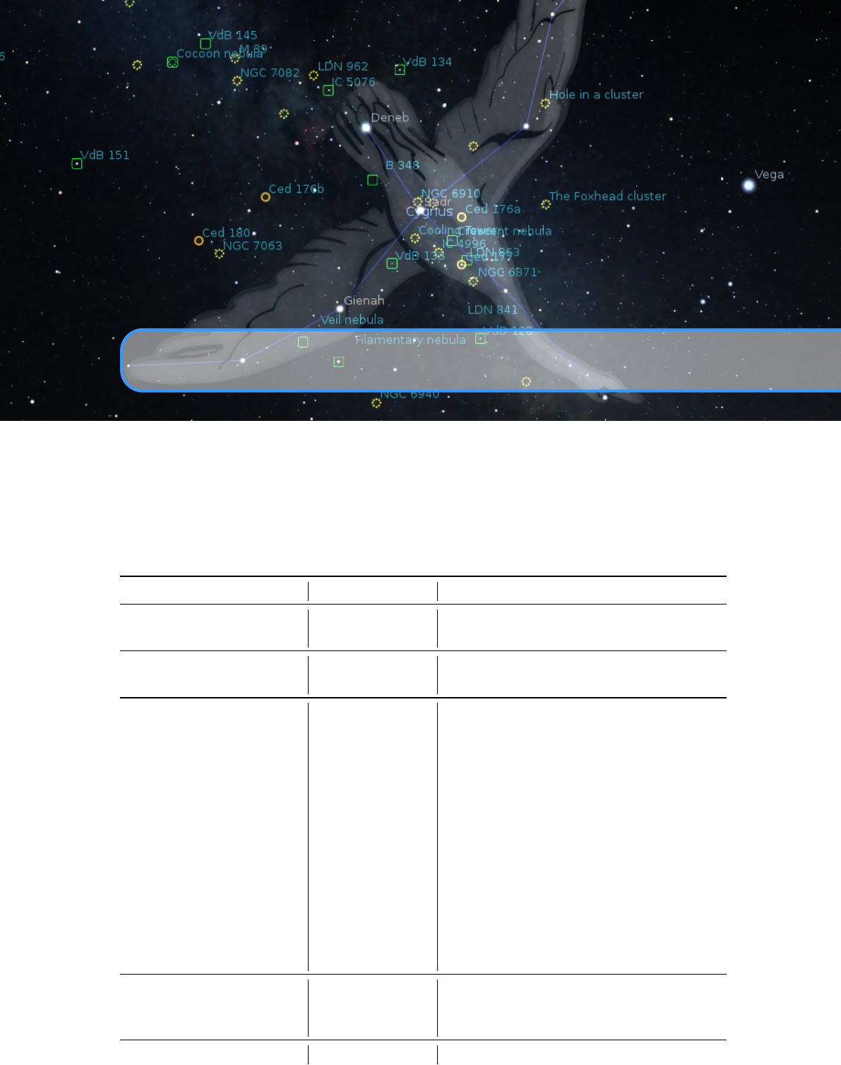
6. Command Line Options
Stellarium’s behaviour can be modified by providing parameters to the program when it is called
via the command line. See table for a full list:
Option Option Parameter Description
--help or -h [none]
Print a quick command line help message,
and exit.
--version or -v [none]
Print the program name and version informa-
tion, and exit.
--config-file or -c config file name
Specify the configuration file name. The de-
fault value is config.ini.
The parameter can be a full path (which will
be used verbatim) or a partial path.
Partial paths will be searched for inside the
regular search paths unless they start with a
“
.
”, which may be used to explicitly specify
a file in the current directory or similar.
For example, using the option
-c
my_config.ini
would resolve to the
file
<user directory>/my_config.ini
whereas
-c ./my_config.ini
can be used
to explicitly say the file
my_config.ini
in
the current working directory.
--restore-defaults [none]
Stellarium will start with the default configu-
ration. Note: The old configuration file will
be overwritten.
--user-dir path Specify the user data directory.

52 Chapter 6. Command Line Options
--screenshot-dir path
Specify the directory to which screenshots
will be saved.
--full-screen yes or no
Over-rides the full screen setting in the config
file.
--home-planet planet Specify observer planet (English name).
--longitude longitude Specify latitude, e.g. +53d58’16.65"
--latitude latitude Specify longitude, e.g. -1d4’27.48"
--altitude altitude Specify observer altitude in meters.
--list-landscapes [none]
Print a list of available landscape IDs and
exit.
--landscape landscape ID
Start using landscape whose ID matches the
passed parameter (dir name of landscape).
--sky-date date The initial date in yyyymmdd format.
--sky-time time The initial time in hh:mm:ss format.
--startup-script script name
The name of a script to run after the program
has started. [startup.ssc]
--fov angle The initial field of view in degrees.
--projection-type ptype
The initial projection type (e.g.
perspective).
--spout or -S all or sky Act as Spout sender (See section 6.2.1).12
--spout-name name
Use
name
as name of the Spout sender. De-
fault name: Stellarium.1
--verbose
Even more diagnostic output in logfile (esp.
multimedia handling)
--dump-opengl-details or -d [none]
Dump information about OpenGL support to
logfile. Use this is you have graphics prob-
lems and want to send a bug report.
--angle-mode or -a [none]
Use ANGLE as OpenGL ES2 rendering en-
gine (autodetect Direct3D version).1
--angle-d3d9 or -9 [none]
Force use Direct3D 9 for ANGLE OpenGL
ES2 rendering engine.1
--angle-d3d11 [none]
Force use Direct3D 11 for ANGLE OpenGL
ES2 rendering engine.1
--angle-warp [none]
Force use the Direct3D 11 software rasterizer
for ANGLE OpenGL ES2 rendering engine.
1
--mesa-mode or -m [none]
Use MESA as software OpenGL rendering
engine.1
--safe-mode or -s [none] Synonymous to --mesa-mode.1
--compat33 or -C [none]
Request OpenGL 3.3 Compatibility Profile.
May help for certain driver configurations.
Mac?
1On Windows only
2This function requires running in OpenGL mode.
6.1 Examples 53
--fix-text or -t [none]
Alternative way of creating the Info text, re-
quired on some systems.3
If you want to avoid adding the same switch every time when you start Stellarium from the
0.15
command line, you can also set an environment variable STEL_OPTS with your default options.
6.1 Examples
•
To start Stellarium using the configuration file,
configuration_one.ini
situated in the
user directory (use either of these):
stel lari um -- config - file = conf igu rat ion _on e . ini
st ella riu m - c con figu rat ion_ one . ini
•To list the available landscapes, and then start using the landscape with the ID “ocean”
stellarium --list-landscapes
stel lari um -- landsca pe = ocean
Note that console output (like --list-landscapes) on Windows is not possible.
6.2 Special Options
6.2.1 Spout 0.15.1
Apart from stand-alone use, Stellarium can be used as multimedia source in larger installations,
in museums or science exhibitions.
Spout4
is a technology which enables use of Stellarium’s
output window as texture in DirectX applications on Windows. Simply start Stellarium with the
--spout=sky
command line option. (Currently
Spout
output is limited to the main window without
GUI panels, but this may change in future versions.) Your master application must obviously embed
a
Spout
receiver. The default name of the
Spout
sender is
Stellarium
. If you need more than
one instance of Stellarium acting as source, you can use option
--spout-name=StelSpout2
in
addition to create another
Spout
sender without a name conflict. In such cases, it may be useful to
also have separate user data directories and use option --user-dir.
This mode does not work in ANGLE mode and requires modern graphics hardware with
the
WGL_NV_DX_interop
driver extension running in OpenGL mode. Some NVidia GPUs work
without this extension listed explicitly. On a notebook with NVidia Optimus technology, make sure
to launch Stellarium on the NVidia hardware. For permanent setting, use the NVidia configuration
dialog to configure Stellarium explicitly to run always on the NVidia card.
3E.g., Raspberry Pi 2/3 with Raspbian Jessie and VC4 drivers from Mesa 11 (2016).
4http://spout.zeal.co/
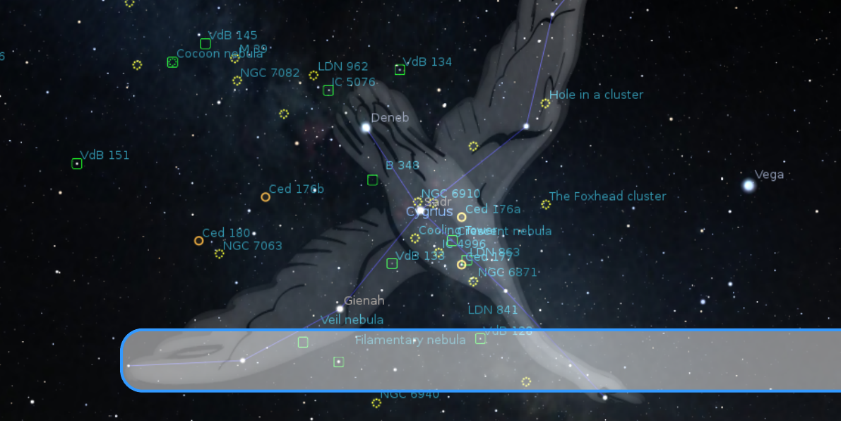
7. Landscapes
GEORG ZOTTI
Landscapes are one of the key features that make Stellarium popular. Originally just used for
decoration, since version 10.6 they can be configured accurately for research and demonstra-
tion in “skyscape astronomy”, a term which describes the connection of landscape and the sky
above (Brown, 2015). Configured properly, they can act as reliable proxies of the real landscapes,
so that you can take e.g. measurements of sunrise or stellar alignments (Zotti and Neubauer, 2015),
or prepare your next moonrise photograph, as though you were on-site.
In this chapter you can find relevant information required to accurately configure Stellarium
landscapes, using panoramas created from photographs taken on-site, optionally supported by
horizon measurements with a theodolite.
Creating an accurate panorama requires some experience with photography and image process-
ing. However, great open-source tools have been developed to help you on the job. If you already
know other tools, you should be able to easily transfer the presented concepts to those other tools.
7.1 Stellarium Landscapes
As of version 0.15, the available landscape types are:
polygonal
A point list of measured azimuth/altitude pairs, used to define a sharp horizon polygon.
The area below the horizon line is colored in a single color (Section 7.1.2).
spherical
The simple form to configure a photo-based panorama: A single image is used as texture
map for the horizon (Section 7.1.3).
old_style
The original photo panorama. This is the most difficult to configure, but allows highest
resolution by using several texture maps (Section 7.1.4).
fisheye
Another 1-texture approach, utilizing an image made with a fisheye lens. This land-
scape suffers from calibration uncertainties and can only be recommended for decoration
(Section 7.1.5).
A landscape consists of a
landscape.ini
plus the data files that are referenced from there,

56 Chapter 7. Landscapes
like a coordinate list or the textures. Those reside in a subdirectory of the
landscape
folder inside
the Stellarium program directory, or, for own work, in a subdirectory of the
landscape
folder
inside your Stellarium user data directory (see section 5.1).
Let us ssume we want to create a landscape for a place called Rosenburg. The location for the
files of our new custom landscape Rosenburg depends on the operating system (see 5.1). Create a
new subdirectory, and for maximum compatibility, use small letters and no spaces:
Windows C:/Users/YOU/AppData/Roaming/Stellarium/landscapes/rosenburg
Linux ~/.stellarium/landscapes/rosenburg
Mac $HOME/Library/Preferences/Stellarium/landscapes/rosenburg
7.1.1 Location information
This optional section in
landscape.ini
allows automatic loading of site coordinates if this option
is activated in the program GUI (see 4.4.4). For our purposes we should consider especially the
coordinates in the location section mandatory!
[location]
planet = Earth
country = Austria
name = KGA Rosenburg
latitud e = +48 d38 ’3.3 "
long itud e ␣= ␣ +15 d38 ’2.8 "
altitude = 266
light_pollution = 1
at m ospher i c_exti n ction_ c oeffic i ent = 0.2
display_fog = 0
atmospheric_temperature = 10.0
at mosp heri c _pre ssur e = 1013.0
Where:
planet Is the English name of the solar system body for the landscape.
latitude
Is the latitude of site of the landscape in degrees, minutes and seconds. Positive values
represent North of the equator, negative values South of the equator.
longitude
Is the longitude of site of the landscape. Positive values represent East of the Green-
wich Meridian on Earth (or equivalent on other bodies), Negative values represent Western
longitude.
altitude Is the altitude of the site of the landscape in meters.
country (optional) Name of the country the location is in.
state (optional) Name of the state the location is in.
name
(optional) Name of the location. This may contain spaces, but keep it short to have it fully
visible in the selection box.
Since v0.11.0, there are a few more optional parameters that can be loaded if the according switch
is active in the landscape selection panel. If they are missing, the parameters do not change to
defaults.
light_pollution (optional) Light pollution of the site, given on the Bortle Scale (1: none . . . 9:
metropolitan; see Appendix B). If negative or absent, no change will be made.
atmospheric_extinction_coefficient
(optional, no change if absent.) Extinction coefficient
(mag/airmass) for this site.
atmospheric_temperature
(optional, no change if absent.) Surface air temperature (Degrees
Celsius). Used for refraction. Set to -1000 to explicitly declare "no change".

7.1 Stellarium Landscapes 57
atmospheric_pressure
(optional, no change if absent.) Surface air pressure (mbar; would be
1013 for "normal" sea-level conditions). Used for refraction. Set to -2 to declare "no change",
or -1 to compute from altitude.
display_fog
(optional, -1/0/1, default=-1) You may want to preconfigure setting 0 for a landscape
on the Moon. Set -1 to declare "no change".
7.1.2 Polygonal landscape
This landscape type has been added only recently (since 0.13) to allow the use of measured horizons.
Users of
Cartes du Ciel1
will be happy to hear that the format of the list of measurements is
compatible.
This is the technically simplest of the landscapes, but may be used to describe accurately
measured horizon lines. The file that encodes horizon altitudes can also be used in all other
landscape types. If present there, it will be used to define object visibility (instead of the opacity of
the landscape photo textures) and, if horizon_line_color is defined, will be plotted.
There is a small caveat: Sometimes, there may appear vertical lines from some corners towards
the zenith or the mathematical horizon, e.g. if there is a vertex including azimuth 0 or 180. If this
irritates you, just offset this azimuth minimally (e.g., 180.00001).
The
landscape.ini
file for a polygonal type landscape looks like this (this example is based
on the Geneve landscape which was borrowed from Cartes du Ciel and comes with Stellarium):
[landscape]
name = Geneve
type = polygonal
author = Georg Zotti ; Horizon definition by Patrick Chevalley
descripti on = Horizon line of Geneve .
Demonstrates compatibility with
horizon desc ription s from Cartes du Ciel .
po ly gon al_ ho riz on_l is t = ho riz on_ Gen eve . txt
polygonal_angle_rotatez = 0
grou nd_ color = .15 ,.45 ,.45
horizon_line_color = .75,.45,.45
Where:
name appears in the landscape tab of the configuration window.
type identifies the method used for this landscape. polygonal in this case.
author lists the author(s) responsible for images and composition.
description
gives a short description visible in the selection panel. The text can be superseded
by optional description.<lang>.utf8 files.
polygonal_horizon_list is the name of the horizon data file for this landscape.
polygonal_horizon_list_mode
(optional) the two first columns in the list are numbers: az-
imuth and altitude or zenith distance, in either degrees or radians or gradians(gon). The value
must be one of
azDeg_altDeg
,
azDeg_zdDeg
,
azRad_altRad
,
azRad_zdRad
,
azGrad_altGrad
,
azGrad_zdGrad. Default: azDeg_altDeg
polygonal_angle_rotatez
(optional, default=0) Angle (degrees) to adjust azimuth. This may
be used to apply a (usually) small offset rotation, e.g. when you have measured the horizon
in a grid-based coordinate system like UTM and have to compensate for the meridian
convergence.
1SkyChart / Cartes du Ciel planetarium: http://www.ap-i.net/skychart/en/start

58 Chapter 7. Landscapes
ground_color
(optional, default=
0,0,0
, i.e., black) Color for the area below the horizon line.
Each R,G,B component is a float within 0..1.
horizon_line_color
(optional, default: invisible) used to draw a polygonal horizon line. Each
R,G,B component is a float within 0..1.
minimal_brightness
(optional) Some minimum brightness to keep landscape visible. Default=-
1, i.e., use
minimal_brightness
from the
[landscape]
section in the global
config.ini
.
minimal_altitude
(optional, default=-2) Some sky elements, e.g. stars, are not drawn below
this altitude to increase performance. Under certain circumstances you may want to specify
something else here. (since v0.14.0)
polygonal_horizon_inverted
(optional, default=false) In rare cases like horizon lines for high
mountain peaks with many negative horizon values this should be set to true. (since v0.15.0)
7.1.3 Spherical landscape
This method uses a more usual type of panorama – the kind which is produced directly from
software such as
autostitch
or
Hugin2
. The Moon landscape which comes with Stellarium
provides a minimal example of a landscape.ini file for a spherical type landscape:
[landscape]
name = Moon
type = spherical
maptex = apol lo17 . png
A more elaborate example is found with the Grossmugl landscape:
[landscape]
name = Grossmugl
type = spherical
aut hor = G uent her Wu ch te rl , K uf fner - S ter nwa rte . at ;
Lights cape : Georg Zotti
descripti on = Field near Leeberg , Grossmugl ( Riesentumulus ),
Austria - Primary Observing Spot of the Grossmugl
Star ligh t Oasis - http :// star lig hto asi s . org
maptex = gross mugl_ l eebe r g_cr o p11 .25. png
maptex_top=11.25
maptex_fog = grossmugl_leeberg_fog_crop22.5.png
maptex_f og_ top = 22.5
maptex_fo g_bo ttom = -22.5
maptex_illum = grossmugl_leeberg_illum_crop0.png
maptex_illum_bottom = 0
angle_rotatez=-89.1
minimal_brightness = 0.0075
po ly gon al_ ho riz on_l is t = ho riz on_g ros smug l . txt
polygonal_angle_rotatez=0
horizon_line_color = .75,.45,.45
minimal_altitude = -1
Where:
name appears in the landscape tab of the configuration window. This name may be translated.
type identifies the method used for this landscape. spherical in this case.
2http://hugin.sourceforge.net/

7.1 Stellarium Landscapes 59
author lists the author(s) responsible for images and composition.
description
gives a short description visible in the selection panel. The text will be superseded
by optional description.<lang>.utf8 files.
maptex is the name of the image file for this landscape.
maptex_top (optional; default=90) is the altitude angle of the top edge.
maptex_bottom
(optional; default=-90) is the altitude angle of the bottom edge. Usually you will
not require this, or else there will be a hole at your feet. ;-)
maptex_fog (optional; default: no fog) is the name of the fog image file for this landscape.
maptex_fog_top
(optional; default=90) is the altitude angle of the top edge of the fog texture.
Useful to crop away parts of the image to conserve texture memory.
maptex_fog_bottom (optional; default=-90) is the altitude angle of the bottom edge.
maptex_illum
(optional; default: no illumination layer) is the name of the nocturnal illumina-
tion/light pollution image file for this landscape.
maptex_illum_top
(optional; default=90) is the altitude angle of the top edge, if you have light
pollution only close to the horizon.
maptex_illum_bottom (optional; default=-90) is the altitude angle of the bottom edge.
angle_rotatez
(optional, default=0) Angle (degrees) to adjust azimuth. If 0, the left/right edge
is due east.
tesselate_rows
(optional, default=20) This is the number of rows for the maptex. If straight
vertical edges in your landscape appear broken, try increasing this value, but higher values
require more computing power. Fog and illumination textures will have a similar vertical
resolution.
tesselate_cols
(optional, default=40) If straight horizontal edges in your landscape appear
broken, try increasing.
polygonal_horizon_list
(optional) is the name of the (measured) horizon data file for this
landscape. Can be used to define the exact position of the horizon. If missing, the texture
can be queried for horizon transparency (for accurate object rising/setting times)
polygonal_horizon_list_mode (optional) see 7.1.2
polygonal_angle_rotatez (optional, default=0) see 7.1.2
horizon_line_color see 7.1.2
minimal_brightness see 7.1.2
minimal_altitude
(optional, default=-2) Some sky elements, e.g. stars, are not drawn below
this altitude for efficiency. Under certain circumstances (e.g. for space station panoramas
where you may have sky below your feet, or for deep valleys/high mountains, you may want
to specify something else here. (since v0.14.0)
To save texture memory, you can trim away the transparent sky and define the angle maptex_top.
Likewise,
fogtex_top
,
fogtex_bottom
,
maptex_illum_top
and
maptex_illum_top
. You
should then stretch the texture to a full power of 2, like
4096×1024
(but note that some hardware
is even limited to 2048 pixels). The easiest method to create perfectly aligned fog and illumination
layers is with an image editor that supports layers like the
GIMP
or
Photoshop
. Fog and Light
images should have black background.
7.1.4 High resolution (“Old Style”) landscape
The
old_style
or multiple image method works by having the 360
◦
panorama of the horizon
(without wasting too much texture memory with the sky) split into a number of reasonably small
side textures, and a separate ground texture. This has the advantage over the single-image method
that the detail level of the horizon can be increased without ending up with a single very large image
file, so this is usable for either very high-resolution panoramas or for older hardware with limited
capabilities. The ground texture can be a different resolution than the side textures. Memory usage
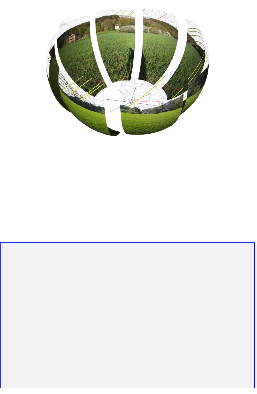
60 Chapter 7. Landscapes
Figure 7.1: Old_style landscape: eight parts delivering a high-resolution panorama. The
bottom (ground) texture, drawn on a flat plane, is not shown here.
may be more efficient because there are no unused texture parts like the corners of the texture file
in the fish-eye method. It is even possible to repeat the horizon several times (for purely decorative
purpose). The side textures are mapped onto curved (spherical ring or cylinder) walls (Fig. 7.1).
On the negative side, it is more difficult to create this type of landscape – merging the ground
texture with the side textures can prove tricky. (
Hugin
can be used to create also this file, though.
And on the other hand, you can replace this by something else like a site map.) The contents of
the
landscape.ini
file for this landscape type is also somewhat more complicated than for other
landscape types. Here is the landscape.ini file which describes our Rosenburg landscape3:
[landscape]
name = KGA Rosenburg
author = Georg Zotti , VIAS / ASTROSIM
descripti on = KGA Rosenburg
type = old_style
nbsidetex = 8
tex0 = Horiz -0. png
tex1 = Horiz -1. png
tex2 = Horiz -2. png
tex3 = Horiz -3. png
tex4 = Horiz -4. png
tex5 = Horiz -5. png
tex6 = Horiz -6. png
tex7 = Horiz -7. png
nbside = 8
side0 = tex0 :0:0:1:1
side1 = tex1 :0:0:1:1
side2 = tex2 :0:0:1:1
3the groundtex grassground.png mentioned here has been taken from the Guereins landscape.

7.1 Stellarium Landscapes 61
side3 = tex3 :0:0:1:1
side4 = tex4 :0:0:1:1
side5 = tex5 :0:0:1:1
side6 = tex6 :0:0:1:1
side7 = tex7 :0:0:1:1
grou ndte x = gra ssg round . png
ground = groundtex :0:0:1:1
nb_decor_repeat = 1
decor_alt_angle = 82
decor_angle_shift = -62
; Rotatez deviates from -90 by the Meridian Conver gence .
; The original landscape pano is grid - aligned , not north - aligned !
de cor_ angl e_ro tatez = -90.525837223
ground_angle_shift = -62
gr ound _ang l e_ro tate z = 44.4 741 62777
draw_ground_first = 1
fogtex = fog . png
fog_alt_angle = 20
fog_angle_shift = -3
fog = fogtex :0:0:1:1
calibrated = true
[location]
planet = Earth
latitud e = +48 d38 ’3.3 "
long itud e ␣= ␣ +15 d38 ’2.8 "
altitude = 266
light_pollution = 1
at m ospher i c_exti n ction_ c oeffic i ent = 0.2
display_fog = 0
atmospheric_temperature = 10.0
at mosp heri c _pre ssur e = 1013.0
Where:
name
is the name that will appear in the landscape tab of the configuration window for this
landscape
type should be old_style for the multiple image method.
author lists the author(s) responsible for images and composition.
description
gives a short description visible in the selection panel. The text will be superseded
by optional description.<lang>.utf8 files.
nbsidetex is the number of side textures for the landscape.
tex0 ... tex<nbsidetex-1>
are the side texture file names. These should exist in the
textures / landscapes / landscape directory in PNG format.
light0 ... light<nbsidetex-1>
are optional textures. If they exist, they are used as overlays
on top of the respective
tex<...>
files and represent nocturnal illumination, e.g. street
lamps, lit windows, red dots on towers, sky glow by city light pollution, . . . Empty (black)
panels can be omitted. They are rendered exactly over the
tex<...>
files even when the
PNG files have different size. If you need your light pollution higher in the sky, you must
use a spherical or fisheye landscape. v0.13.1
nbside is the number of side textures

62 Chapter 7. Landscapes
side0 ...side<nbside-1>
are the descriptions of how the side textures should be arranged in
the program. Each description contains five fields separated by colon characters (
:
). The
first field is the ID of the texture (e.g.
tex0
), the remaining fields are the texture coordinates
(
x0:y0:x1:y1
) used to place the texture in the scene. If you want to use all of the image,
this will just be 0:0:1:1.
groundtex
is the name of the ground texture file. (This could also be a diagram e.g. indicating
the mountain peaks!)
fogtex
is the name of the texture file for fog in this landscape. Fog is mapped onto a simple
cylinder.
4
Note that for this landscape, accurate overlay of fog and landscape is only
guaranteed if calibrated=true and tan_mode=true.
nb_decor_repeat
is the number of times to repeat the side textures in the 360 panorama. (Useful
photo panoramas should have 1here)
decor_alt_angle
(degrees) is the vertical angular extent of the textures (i.e. how many degrees
of the full altitude range they span).
decor_angle_shift
(degrees) vertical angular offset of the scenery textures, at which height the
bottom line of the side textures is placed.
decor_angle_rotatez
(degrees) angular rotation of the panorama around the vertical axis. This
is handy for rotating the landscape so North is in the correct direction. Note that for historical
reasons, a landscape with this value set to zero degrees has its leftmost edge pointing towards
east.
ground_angle_shift
(degrees) vertical angular offset of the ground texture, at which height the
ground texture is placed.
ground_angle_rotatez
(degrees) angular rotation of the ground texture around the vertical axis.
When the sides are rotated, the ground texture may need to be rotated as well to match up
with the sides.
fog_alt_angle
(degrees) vertical angular size of the fog cylinder - how fog looks. Accurate
vertical size requires calibrated=true.
fog_angle_shift
(degrees) vertical angular offset of the fog texture - at what height is it drawn.
Accurate vertical placement requires calibrated=true.
draw_ground_first
if 1 the ground is drawn in front of the scenery, i.e. the side textures will
overlap over the ground texture.
calibrated
(optional). Only if true,
decor_alt_angle
etc. really work as documented above.
v0.10.6
The (buggy) old code was left to work with the landscapes already existing. Note that with
“uncalibrated” landscapes, sunrise computations and similar functionality which requires an
accurate horizon line will not work.
tan_mode
(optional, not used in this file). If true, the panorama image must be in in cylindrical,
not equirectangular projection. Finding
decor_alt_angle
and
decor_angle_shift
may
be a bit more difficult with this, but now (v0.13.0) works also with calibrated. A fog image
created as overlay on the pano will be perfectly placed.
decor_angle_rotatez
angular rotation of the scenery around the vertical axis. This is handy for
rotating the landscape so North is in the correct direction. If 0, the left edge of
tex0
is due
east.
ground_angle_shift
vertical angular offset of the ground texture, at which height the ground
texture is placed. Values above -10 are not recommended for non-photographic content (e.g.,
a map) due to high distortion.
ground_angle_rotatez
angular rotation of the ground texture around the vertical axis. When
the sides are rotated, the ground texture may need to be rotated as well to match up with the
sides. If 0, east is up. if North is up in your image, set this to 90. Note that adjustments of
4In very wide-angle views, the fog cylinder may become visible in the corners.

7.1 Stellarium Landscapes 63
decor_angle_rotatez require adjustments of this angle in the opposite direction!
fog_alt_angle vertical angular size of the fog cylinder.
fog_angle_shift vertical angular offset of the fog cylinder.
draw_ground_first
if 1, the ground is drawn before the sides, i.e. the side textures may overlap
the ground texture if ground_angle_shift >decor_angle_shift.
polygonal_horizon_list (optional) see 7.1.2
polygonal_horizon_list_mode (optional) see 7.1.2
polygonal_angle_rotatez (optional, default=0) see 7.1.2
horizon_line_color see 7.1.2
minimal_brightness see 7.1.2
minimal_altitude see 7.1.2
7.1.5 Fisheye landscape
The Trees landscape that is provided with Stellarium is an example of the single fish-eye method,
and provides a good illustration. The centre of the image is the spot directly above the observer
(the zenith). The point below the observer (the nadir) becomes a circle that just touches the edges
of the image. The remaining areas of the image (the corners outside the circle) are not used.
The image file (Fig. 7.2) should be saved in PNG format with alpha transparency. Whereever
the image is transparent Stellarium will render the sky.
The
landscape.ini
file for a fish-eye type landscape looks like this (this example is based on
the Trees landscape which comes with Stellarium):
[landscape]
name = Trees
type = fisheye
author = Robert Spearman . Light pollution image : Georg Zotti
descripti on = Trees in Greenlake Park , Seattle
maptex = trees_5 12 . png
ma pte x_ill um = t ree s_i llu m_5 12 . png
ma ptex _fo g = tree s_f og_ 512 . png
texturefov = 210
angle_rotatez = 17
tesselat e_r ows = 28
tesselat e_c ols = 60
Where:
name appears in the landscape tab of the configuration window.
type identifies the method used for this landscape. fisheye in this case.
author lists the author(s) responsible for images and composition.
description
gives a short description visible in the selection panel. The text will be superseded
by optional description.<lang>.utf8 files.
maptex is the name of the image file for this landscape.
maptex_fog (optional) is the name of the fog image file for this landscape.
maptex_illum
(optional) is the name of the nocturnal illumination/light pollution image file for
this landscape.
texturefov is the field of view that the image covers in degrees.
angle_rotatez (optional) Angle (degrees) to adjust azimuth.
tesselate_rows
(optional, default=20) If straight edges in your landscape appear broken, try
increasing.
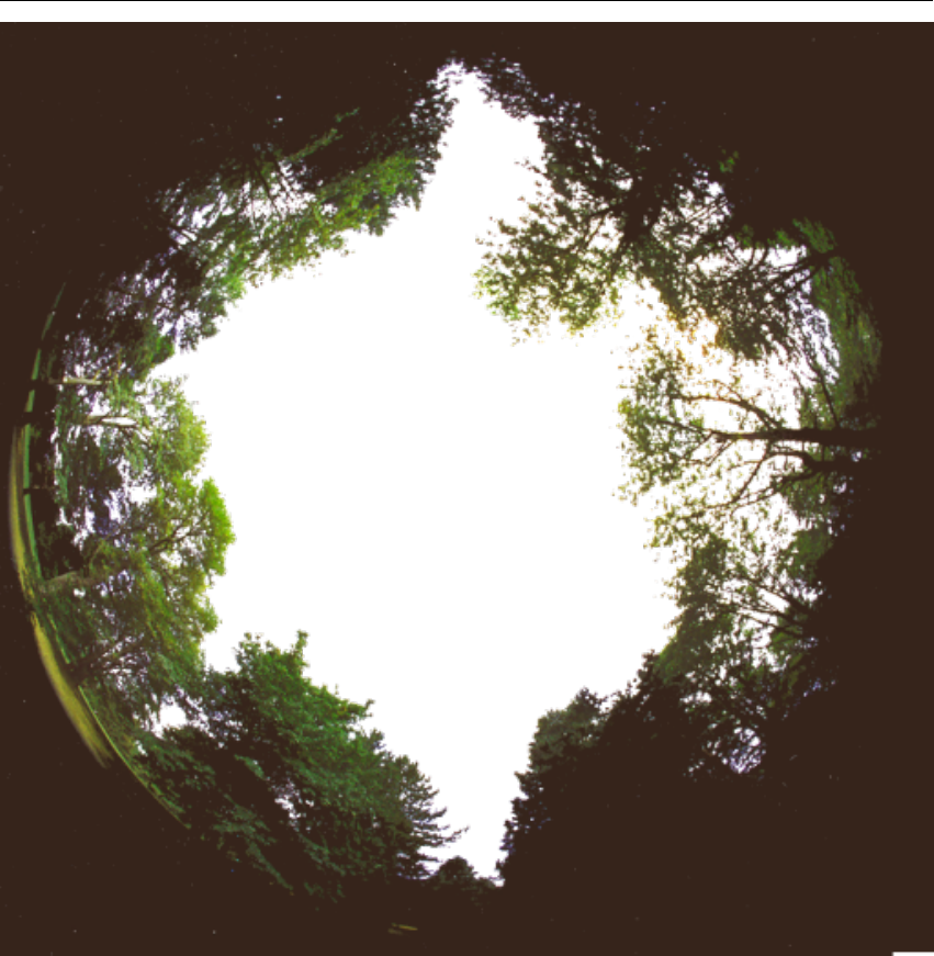
64 Chapter 7. Landscapes
Figure 7.2: Texture for the Trees Fisheye landscape.
tesselate_cols
(optional, default=40) If straight edges in your landscape appear broken, try
increasing.
polygonal_horizon_list (optional) see 7.1.2
polygonal_horizon_list_mode (optional) see 7.1.2
polygonal_angle_rotatez (optional, default=0) see 7.1.2
horizon_line_color see 7.1.2
minimal_brightness see 7.1.2
minimal_altitude see 7.1.2
7.1.6 Description
The short
description
entry in
landscape.ini
will be replaced by the contents of an optional
file
description.<LANG>.utf8
.
<LANG>
is the ISO 639-1 language code, or its extension which
contains language and country code, like
pt_BR
for Brazilian Portuguese. The long description
requires the file
description.en.utf8
, this is
en=english
text with optional HTML tags for

7.1 Stellarium Landscapes 65
sections, tables, etc. You can also have embedded images in the HTML (Views of sacred landscapes,
other informative images, . . . ?), just make them PNG format please. The length of the description
texts is not limited, you have room for a good description, links to external resources, whatever
seems suitable.
If you can provide other languages supported by Stellarium, you can provide translations
yourself, else Stellarium translators may translate the English version for you. (It may take years
though.) The file ending
.utf8
indicates that for special characters like ÄÖÜßáé you should use
UTF8 encoding. If you write only English/ASCII, this may not be relevant.
7.1.7 Gazetteer 0.14
An optional feature for landscapes is a gazetteer function, i.e., labels for landscape features. The
Grossmugl landscape demonstrates an example and should be self-explanatory. This is again
multilingual, so the files are called gazetteer.<LANG>.utf8.
# demo gaz ett eer for Gros smu gl land sca pe .
# Can be used to bette r des cri be the landscape ,
# i.e. show label s on la ndscape f eatu res .
# Fields must be s epar ate d by vertica l line ,
# lab el must not have s uch a ver tic al line .
# Comm ent s have this hash mark in firs t col umn .
# coo rdina tes in de gree s from true No rth .
# line to war ds zenith draw s a s ingle line st ric tly upwa rd .
# l abel is c ente red on line endpoin t .
# Az imu th | Al tit ude | degrees | azimuth | label
# | | towar ds z enith | shift |
11 3.66 | 5.5 | 4 | -6 | Leeberg
35 | 1.5 | 2.5 | 0 | Gro ssmu gl
335 | 2 | 2 | 0 | S tein abru nn
305 | 2 | 1 | 0 | R ing endo rf
18 0 | 2 | 2 | 0 | V ie nn a (3 0 km )
135 | 2 | 0.5 | 0 | Wind power plant Stra ssh of
7.1.8 Packing and Publishing
You likely have developed your landscape already in your own Stellarium user data directory,
but when you are happy with your work, you may consider sharing it with other users. For easy
distribution and installation via Stellarium’s GUI (see section 4.4.4), you should create a ZIP
file. This must contain
landscape.ini
and any textures and auxiliary files described above
(
description.en.utf8
,
gazetteer.en.utf8
and their translations, horizon files, images for
the description . . . ) used by your landscape. If you want to release the landscape for download,
consider adding a
README.txt
clarifying license and usage conditions. It does not matter whether
the ZIP file contains a directory name inside the ZIP. If not, the directory name (ID) of the landscape
will be taken from the ZIP file name.
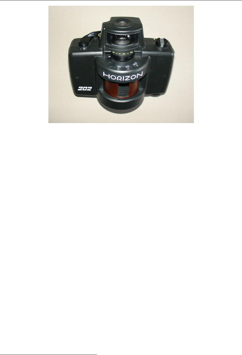
66 Chapter 7. Landscapes
Figure 7.3: Zenit “Horizon 202” panorama camera with rotating lens for 35mm film.
(Source: Wikipedia, “Horizon202” by BillC - Own Work. Licensed under CC BY-SA 3.0 via Wikimedia
Commons - https://commons.wikimedia.org/wiki/File:Horizon202.jpg)
7.2 Creating Panorama Photographs for Stellarium
7.2.1 Panorama Photography
Traditional film-based panorama photography required dedicated cameras with curved film holders
and specialized lenses (Figure 7.3).
Digital photography has brought a revolution also in this field, and it has become quite easy to
create panoramas simply by taking a series of photographs with a regular camera on the same spot
and combining them with dedicated software.
A complete panorama photo visually encloses the observer like the mental image that as-
tronomers have been using for millennia: the celestial sphere. If we want to document the view,
say, in a big hall like a church, optimal results will be gained with a camera on a tripod with a
specialized panorama head (Figure 7.4) which assures the camera rotates around the entrance
pupil
5
of the lens in order to avoid errors by the parallax shift observed on photographs taken on
adjacent but separate positions.
Often however, both the upper half of the observer’s environment (the sky) and the ground
the photographer is standing on, are regarded of lesser importance, and only a series of laterally
adjacent photographs is taken and combined into a cylindrical or spherical ring that shows the
landscape horizon, i.e., where ground and sky meet. If the closest object of interest is farther
away that a few metres, requirements on parallax avoidance are far less critical, and the author has
taken lots of landscape panoramas with a camera on the usual tripod screw, and even more entirely
without a tripod. However, any visible errors that are caused by a shifted camera will require more
effort in postprocessing.
When you have no tripod, note that you must not rotate the camera on your outstretched arm!
Rather, the camera’s entrance pupil must be rotated, so you should appear to dance around the
5
In many references you will find “Nodal Point” mentioned here. But see these:
http://en.
wikipedia.org/wiki/Cardinal_point_%28optics%29#Nodal_points
,
http://web.archive.
org/web/20060513074042/http://doug.kerr.home.att.net/pumpkin/Pivot_Point.pdf
,
http://www.janrik.net/PanoPostings/NoParallaxPoint/TheoryOfTheNoParallaxPoint.pdf
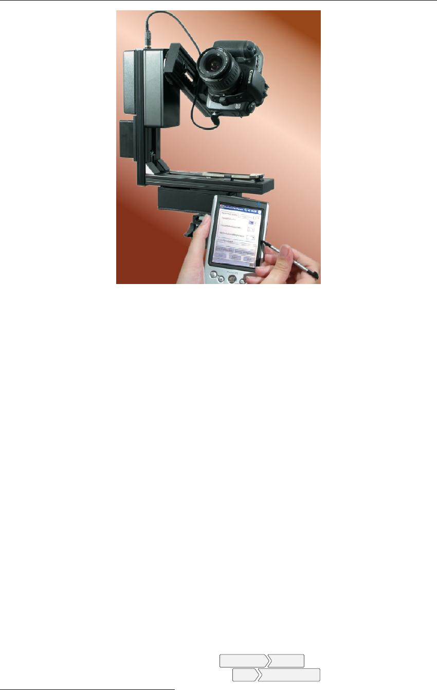
7.2 Creating Panorama Photographs for Stellarium 67
Figure 7.4: Automated panorama head. (Source: Wikipedia
https://commons.wikimedia.org/
wiki/File:Rodeon_vr_head_01.jpg)
camera!
The images should match in brightness and white balance. If you can shoot in RAW, do so to
be able to change white balance later. If the camera can only create JPG, ensure you have set the
camera to a suitable white balance before taking the photos and not to “auto”, because this may
find different settings and thus give colour mismatches. Exposure brightness differences can be
largely removed during stitching, but good, well-exposed original shots always give better results.
As a general recommendation, the images of a panorama should be taken from left to right,
else please accordingly invert some of the instructions given below.
There are several panorama making programs. Often they are included in the software that
comes with a digital camera and allow the creation of simple panoramas. Other software titles are
available for purchase. However, there is one cost-free open-source program that does everything
we need for our task, and much more:
7.2.2 Hugin Panorama Software
Hugin6
, named after one of the ravens that sits on Odin’s shoulder and tells him about the world,
is a user-friendly catch-all package with graphical user interface that allows creating panoramas
with a single application. Actually,
Hugin
is a GUI application which calls several specialized
sub-programs with fitting parameters. The instructions are based on Hugin V2014.0 and 2015.0.
Typically digital images come in JPG format with information about camera, lens, and settings
stored in invisible metadata in the EXIF format. When
Hugin
reads such images, it can automati-
cally derive focal length, field of view, and exposure differences (exposure time, aperture, color
balance) to create panoramas as easily as possible.
After starting
Hugin
for the first time, select
Interface Expert
to release several options not
visible to “beginners”. In the Preferences dialog (
Files Preferences
), edit number of CPU to
6http://hugin.sourceforge.net/
68 Chapter 7. Landscapes
match the number of cores in your computer and allow parallel processing. E.g., if you have an
Intel Core-i7, you usually can set up to 8 cores (4 cores with hyperthreading; but maybe leave
one core for your other tasks while you wait for a processing job?). If your PC is equipped with a
modern programmable graphics card, you can enable its use in the
Programs
tab with activating
“Use GPU for remapping”.
After that, we are ready for creating our panoramas.
7.2.3 Regular creation of panoramas
The graphical user interface (GUI) consists of a main menu, symbols, and 4 tabs. We start on the
tab Photos.
•Add images. . .
Opens a file browser. Select the images which you want to stitch. Usually,
lens data (focal length, field of view, . . . ) are read from the EXIF data. If those are not
available (e.g. cheap cameras, images scanned from film), you can enter those data on
loading or later. The images are now listed in the file list, and you can edit image parameters
by marking one or more, and then choosing from the context menu which you get from
pressing the right mouse button. In case you have used different lenses (or inadvertently
used different focal lengths of a zoom lens), you can assign separate lenses to the images.
Caveat: If you have resized the images, or produced copied on your RAW converter with
non-native resolution, the Field of View (FoV) in
Hugin
may be misidentified. You must
edit lens parameters and fill in the field of view from a full-size image. Else the first round
of optimisation will run into unsolvable trouble.
•
Select one image as position anchor (usually the center image), and one as exposure anchor
(this can be the same image). For our purpose, the anchor image should face south.
•
Next, we must find common feature points. The next field below provides the required
settings. It is recommended to use the
CPFind
command. To avoid finding control points
in (moving) clouds, select setting
Hugin’s CPFind + Celeste 7
. Then press
Create control points
.
This opens a dialog box in which you can see output of the selected feature point extractor.
It should finish with a box telling you the number of identified points. In rare cases some
images cannot be linked to others, you will have to manually add or edit feature points in
those cases.
•
Now it’s time to start optimisations. On the
Geometric Optimimisation
combo, start with
the button
Positions, incremental from anchor
, and press
Calculate
. Moments later, a first
rough match is available for inspection.
•
First open the Preview window (press
Ctrl +P
or click the blue icon). Assumed your
images cover the full horizon, the window shows an equirectangular area (360 degrees along
the horizon and 180 degrees from zenith to nadir). The anchor image should be close to the
image center, and the other images should be already well-aligned to both sides. You can set
the exact center point by clicking it in the image. If the horizon appears badly warped, use
the right mouse key and click on the horizon roughly near
−90
or
+90
degrees (halfway to
the left or right).
•
Open the OpenGL preview window (press
Ctrl +Shift +P
or click the blue icon with GL
inside). This panel provides several important views:
–
The
Preview
tab is similar to the non-OpenGL preview. You can display an overlay of
the control points, which are colored according to match quality. Also, with button
Identify
activated, you see the overlapping image frames when you move the mouse
over the image.
–The Layout tab helps finding links between images.
–The Move/Drag dialog may help to interactively adjust a panorama.
7If you forget this, you can remove cloud points by calling Celeste in the control point editor later
7.2 Creating Panorama Photographs for Stellarium 69
Sometimes the preview image may however be distorted and unusable.
•
Open the Control Points Table dialog (press
F3
or click the “table” button). Here you see
the points listed which link two images. Clicking a column label sorts by this column. It is
recommended that only neighboring overlapping images should be included here. If you
have very large overlap, it is possible that points are found between two images which are
not directly adjacent. In the OpenGL preview window, you can use the
Preview
or the
Layout
tabs to identify those image pairs. Such points should be deleted. In the point table,
click on columns “Right Img.”, then “Left Img.”, and then find pairs like 0/2, 1/3, 2/4 etc.
Mark those lines, and delete the points.
•
To re-run the optimisation, press the double-arrow icon or the
calculate
button in the
Optimise/Geometric area.
Preliminary Geometric Optimisation
Now the (usually) longest part begins: Iterative optimisation of the photo matchpoints. If your
images were taken on a panorama tripod head, there should only be very few bad matchpoints, e.g.
those found on persons or clouds
8
which have moved between photos. For handheld photos, the
following considerations should be observed.
The most important line which we want to create in all perfection is the visible horizon, where
sky and earth meet. The foreground, usually grassy or rocky, is of lesser interest, and stitching
errors in those areas may not even be relevant.
Therefore, matchpoints with large errors in the foreground can be safely removed, while, if
necessary, points on the horizon should be added manually. Use the
Control Points
tab, select
adjacent images (start with 0 on the left and 1 on the right side), and delete the worst-fitting
matchpoints closest to the camera (near the bottom of the images). We now start a long phase of
re-optimizing and deletion of ill-matching points as long as those are far from the horizon. When
all near matchpoints are deleted, the result should already look not too bad.
For continued optimisation, the number of parameters to optimize can be extended. To begin, I
recommend
Positions and View (y, p, r, v)
, which may find a new focal length slightly different from
the data in the EXIF tags. Again, delete further foreground points. If after a few rounds you
still have bad point distances, try
Positions and Barrel Distortion (y, p, r, b)
to balance distortion by bad
optics, or even go up to
Everything without translation
. Optimisation can only reach perfect results if
you did not move between exposures. Else, find a solution which shows the least error.
In case you took your photos not on a tripod and moved too much, you may even want to play
with the translation options, but errors will be increasingly hard to avoid.
Using Straight Edges as Guides
If the panorama contains straight lines like vertical edges of buildings, these can be used to
automatically get a correctly levelled horizon: Vertical lines are mapped to vertical lines in
equirectangular panos! In the
Control Points
tab, select the image with the vertical edge in both
subframes, and mark points on the vertical edge. (switch off auto-estimate!). Likewise, horizontal
lines may help, but make sure lines like rooves are perpendicular to your line of view, else the
perspective effect causes an inclination.
Multi-ring Panoramas
If you are trying to create a panorama with several rings (horizon, one or two rings below, and
nadir area), you must try to create/keep control points that best give a result without visible seams.
In this case, and esp. if you have only used a regular tripod or even dared to go for a free-handed
panorama, you may observe that it is best to remove control points in neighboring photos in the
8You should have created control points with the Celeste option!
70 Chapter 7. Landscapes
lower rings, but keep only the “vertical” links between images with similar azimuth.
In total, and if the foreground is not important but only grassy or sandy, the rule of thumb is
that the horizon images must be strongly linked with good quality (small errors), while images in
the lower rings should be linked mostly to their respective upper photos, but not necessarily to the
images to its sides. The resulting panorama will then show a good horizon line, while stitching
artifacts in a grassy or otherwise only decorative ground will usually be acceptable and can, if
needed, be camouflaged in postprocessing.
This optimisation and editing of control points is likely a longish iterative process, and these
are the late night hours where you will finally wish you had used a panorama head. . .
Masking
If you have images with overlapping areas, you can usually not force
Hugin
to take pixels from the
image which you find best. you can however mask off an area from an image which you don’t want
to see in the output under any circumstances, e.g. a person’s arm or foot in one image. Just open
the image in the
Mask
tab and either press
Add new mask
and draw the mask polygon covering
the unwanted area, or use the crop settings to define rectangular areas to use.
Exposure disbalance
In the
Photos
tab, select
Photometric parameters
on the right side. The EV column lists the
Exposure Value. If you see disbalance here and in the preview window, you can run a photometric
optimisation with the lowest button on the
Photos
tab. Simply select Low dynamic range and press
Calculate
. The preview should now show a seamless image. If all else fails, you can edit the EV
values directly.
Advanced photographers may want to correct exposures in their RAW images before creating
JPG or TIF images to combine with
Hugin
. This unfortunately may create exposure disbalance
because the EXIF tags may not be adjusted accordingly, so based on different exposure/f-stop
conbinations
Hugin
may think it has to re-balance the values. In these cases, don’t run the
photometric optimiser. Some image exposure values have to be changed manually, and the effect
supervised in the preview window. Usually the smooth blending in the subprogam
enblend
called
by Hugin will hide remaining differences.
Stitching
When you are happy with the panorama in the preview window and the matchpoints promise a good
fit, it is time to finally create the panorama image.
Hugin
can create a large number of different
projections which all have their application. For Stellarium, we can only use the equirectangular
projection. You still have 2 options:
spherical
landscapes (see 7.1.3) require single equirectangular images, the maximum size depends
on your graphics hardware and
Qt
limitations and is likely not larger than
8192 ×4096
pixels.
old_style
landscapes (see 7.1.4) can use several textures for the ring along the horizon, and one
image for the nadir zone. If you need high resolution, you should aim for creating this one.
Sometimes, creating the nadir zone is difficult: this is where usually the view is blocked by the
tripod, and we are not interested in views of tripod or our own feet. For our purpose it is usually
enough to fill in the feet area using the clone stamp, or a monochrome color, or, for
old_style
landscapes, you can instead insert an oriented site map or wind rose.
There is a button
create optimal size
in
Hugin
. It may recommend a panorama width around
13.000 pixels for an average camera and photos taken with a wide-angle lens. Increasing this size
will most likely not lead to higher optical resolution! The panorama width which you can most
usefully create depends on the resolution of the source images (which leads to the result given by
Hugin
) and on your needs. If you need arcminute resolution, you would aim for
360 ×60 =21600

7.3 Panorama Postprocessing 71
pixels, which cannot be loaded into graphics memory in a single piece, i.e., is too large for
Stellarium, and must be configured as
old_style
landscape. In this case, 10 or 11 tiles of
2048 ×2048
pixels (totalling 20480 or 22528 pixels) is the closest meaningful setting, i.e., you
could create an image of 20480 pixels width and cut this into usable pieces. Usually, a size
of
4096 ×2048
or
8192 ×4096
pixels (for better computers) is enough, and can be used in a
spherical landscape.
We have to edit the file after stitching, therefore select creation of an image in the TIFF format.
LZW compression is non-lossy, so use this to keep file size reasonably small.
For regular images, it is enough to create “Exposure corrected, low dynamic range”. If you
have a problem with persons that have moved between your images, you may want to post-process
the final result with import of the distorted sub-images and manually defining the best blending line.
For this, find the “Remapped Images” group and again activate “Exposure corrected, low dynamic
range”.
Now, press the
Stitch!
button in the lower right corner. This opens a helper program which
supervises the stitching process. Depending on your computer and size of the image, it will require
a few minutes of processing.
In case stitching fails with a cryptic error message, try to add the option --fine-mask to the
enblend options.
Store a copy of the
Hugin
project file to always be able to go back to the settings you used to
create the last panorama. We will get back to it when we want to make a truly calibrated panorama
(see 7.3.3).
7.3 Panorama Postprocessing
The image created has to be further processed to be used in Stellarium. The most obvious change is
the need for a transparent sky, which we can easily create in programs like
Adobe Photoshop
or
the free and open-source GIMP. I will describe only the free and open-source solution.
After that, we have to bring the image into shape for Stellarium, which may include some
trimming. While we could also slice an image with interactive tools, higher accuracy and repeatable
results can be achieved with command-line programs, which makes the
ImageMagick
suite the
tool of our choice.
7.3.1 The GIMP
The
GIMP
(GNU Image Manipulation Program) has been developed as free alternative to the
leading commercial product,
Adobe Photoshop
. While it may look a bit different, basic concepts
are similar. Not everybody can (or wants to) afford Photoshop, therefore let’s use the GIMP.
Like
Photoshop
, the
GIMP
is a layer-aware image editor. To understand the concept, it is
easiest to imagine you operate on a growing stack of overhead slides. You can put a new transparent
slide (“layer”) on top of the stack and paint on this without modifying the lower layers.
A few important commands:
Zooming Ctrl +Mouse Wheel
Layer visibility and transparency
Make sure to have layer dialog shown (
Windows Dockable Dialogs
).
A gray bar indicates opacity for the currently active layer. Note the mouse cursor in this
opacity bar (often also called transparency bar): near the top of the bar the upward pointer
immediately sets percentage. A bit lower the pointer looks different and can be used for
fine-tuning.
The most obvious postprocessing need for our panorama is making the sky transparent. The
optimal tool usually is the “Fuzzy Select”, which is equivalent to the “Magic Wand” tool in

72 Chapter 7. Landscapes
Photoshop
. Simply mark the sky, and then delete it. The checkerboard background indicates
transparent pixels.
It sometimes helps to put an intensive bright red or blue background layer under the panorama
photo to see the last remaining clouds and other specks. In the layer dialog, create a new layer,
bucket-fill with blue or red, and drag it in the layer dialog below the pano layer. Write-protect this
layer, work on the image layer, and before exporting the image layer with transparent sky to PNG,
don’t forget to switch off the background.
We need this layer functionality especially to align the panorama on a calibration grid, see
section 7.3.3.
7.3.2 ImageMagick
ImageMagick
(
IM
)
9
can be described as “Swiss Army Knife of image manipulation”. It can do
most operations usually applied to images in a GUI program, but is called from the command line.
This allows also to include
IM
in your own command scripts
10
. We will use it to do our final cut
and resize operations. I cannot give an exhaustive tutorial about more than a few of
IM
’s functions,
but the commands given here should be enough for our purpose.
To open a command window (console, a.k.a. DOS window), press the Windows key and enter
cmd, then press . (On Linux and Mac, you surely know how to open a console window.)
There are some things you might need to know:
•The command line is not your enemy, but a way to call expert tools.
•The Windows command line processor cmd.exe is far from user friendly.
•
There are remedies and alternatives. See notes on
clink
(7.4.3) for a considerable improve-
ment, and Cygwin (7.4.4) for experts.
Command-line magick for spherical landscapes
Let’s start with the commands for final dressing of an equirectangular panorama to be used as
spherical landscape which has been created in size
4096 ×2048
, but where you have seen that
nothing interesting is in the image above 11.25
◦
. This means we can cut away the sky area and
compress the image to 4096 ×1024 to save graphics memory.11
To understand the numbers in the example, consider that in a panorama image of
4096 ×2048
pixels, 1024 pixels represent 90
◦
,
512px =45◦
,
256px =22.5◦
,
128px =11.25◦
. To keep a top
line of
11.25◦
, we keep an image height of
1024 +128 =1152px
, but the crop starts at pixel
Y=1024 −128 =896.
co nve rt l an dsc ape . png - crop 4096 x 11 52 +0 +896
- res ize 4096 x 1024 ! l and sc ape _c rop pe d . png
Note the exclamation mark in the -resize argument, which is required to stretch the image in a
non-proportional way.
Alternatively, you can operate with
IM
’s “gravity”, which indicates the corner or edge geometric
offsets are referred to. Given that we want the lower part of the image to exist completely, you only
need to compute the size of the cropped image:
convert landscape . png - gravity SouthWest - crop 4096 x1152 +0+0
- res ize 4096 x 1024 ! l and sc ape _c rop pe d . png
You still need the addition
+0+0
in the -crop option, else the image will be cut into several pieces.
In the file landscape.ini, you then have to set maptex_top=11.25.
9http://www.imagemagick.org/
10These may typically be .BAT files on Windows, or various shell scripts on Linux or Mac.
11
Most modern graphics cards no longer require the “powers of two” image sizes, but we keep this practice
to increase compatibility.

7.3 Panorama Postprocessing 73
Command-line magick for old_style landscapes
Let us assume we want to create a high-resolution landscape from a pano image of width 16384
which we have carefully aligned and calibrated on an oversized grid template that also shows a
measured horizon line (see 7.3.3). Usually it is not necessary to create the full-size image, but only
the horizon range, in this high resolution. Assume this image has been aligned and justified on
our grid image and is
HEIGHT
pixels high, the left border is at pixel
X_LEFT
, and top border (i.e.,
the point where relevant content like the highest tree is visible) is on pixel
Y_TOP
. Assume our
graphics card is a bit oldish or you aim for maximum compatibility, so we can load only textures of
at most 2048 pixels in size. Given that the horizon area usually only covers a few degrees, a vertical
extent of
2048px
seem a pretty good range for that most interesting zone. The ground can then be
filled with some low-resolution image of grass, soil, or a properly oriented site map, or you can use
Hugin
to create a ground image (and using the maximum of
2048×2048
also here usually is far
more than enough).
In
GIMP
(or
Photoshop
, . . . ), we must find the values for
X_LEFT
,
Y_TOP
and
HEIGHT
.
HEIGHT
is being resized to 2048, strictly, by the exclamation mark in the resize command. We can create
our image tiles now with this singular beast of a command line (write all in 1 line!), which puts our
files directly into STELLARIUM_LANDSCAPEPATH/LANDSCAPE_NAME:
convert PANO . png -crop 16384 xHEIGHT + X_LEFT + Y_TOP + repage
- res ize 1 63 84 x204 8 !
- type Tr ueC ol or Mat te - d epth 8
- crop 2 04 8 x 2048 + r epa ge
png : S TELL AR IUM _L AND SCAP EP ATH / L AND SCA PE_ NAM E / Horiz -% d. png
This creates 8 images. See section 7.1.4 for the
landscape.ini
where these images can be
referenced. Don’t forget to read off top and bottom lines (altitudes in degrees) from your grid,
the vertical extent will form the
decor_alt_angle
, and the bottom line the
decor_angle_shift
entries in this file.
Creating a ground image for old_style landscapes
When you want a good ground image for an
old_style
landscape from your panorama and not
just fill the
groundtex
with a monochrome texture or a map, you have to create a ground view in
Hugin
. But you may have already created a huge pano! This can also be used as source image, and
a ground shot can be extracted with a reversed operation. In principle, all you need to know is the
field of view around the nadir. Figure 7.5 shows a simple configuration file.
# hugin project file
#hugin_ptoversion 2
p f0 w2048 h 2048 v92 E0 R0 n " TIFF_m ␣ c: LZW ␣ r: CROP "
m g1 i0 f0 m2 p0 .00784314
# image lines
# - hug in cr opF ac tor =1
i w16384 h8192 f4 v360 Ra0 Rb0 Rc0 Rd0 Re0 Eev0 Er1 Eb1 r0
p90 y0 TrX0 TrY0 TrZ0 Tpy0 Tpp0 j0 a0 b0 c0 d0 e0 g0 t0
Va1 Vb0 Vc0 Vd0 Vx0 Vy0 Vm5 n" Eq irect_P ano360 . png "
Figure 7.5: Project file
ground.pto
usable to create the ground image with
Hugin
or, on
the command line, its
nona
stitcher. The last line, starting with
i
, has been wrapped, but
must be 1 line.
74 Chapter 7. Landscapes
Say, the side panels extend down to
decor_angle_shift=-44
degrees, which means you
must close the ground with a Nadir
FoV =2×(90 −44) = 92
. For maximum compatibility, we
will again make an image of width and height both 2048
px
. These values can be found in the
p
line
in Figure 7.5. The
i
line describes the input image, which is our full equirectangular pano of width
w=16384 and height h=8192. The last argument of that line is the image file name.
For processing, we do not use the
Hugin
GUI, but simply the command line. The actual
program to call is
nona
. If your stitched panorama is a 16-bit TIFF,
nona
will also make a 16-bit
image, but our textures are limited to 8-bit PNGs. We apply our most useful tool,
convert
from the
ImageMagick suite.
nona -v -m PNG grou nd . pto -o gro un d . png
con vert groun d . png - depth 8 gro und _8bi t . png
The file ground_8bit.png is then used in the groundtex field on landscape.ini.
7.3.3 Final Calibration
The creation of a calibrated panorama (which can be regarded as dependable proxy for further
measurements taken inside Stellarium) requires reference measurements to match the photos against.
We must take azimuth/altitude measurements with a theodolite or total station, in the optimal case
along the full horizon, and in addition I recommend to take azimuth and altitudes of some distinct
features along the horizon which must also be visible in the photographs: mountain summits,
electrical towers, church towers, .. .
I recommend you create grid templates of the sizes you are going to create, e.g. 4096, 8192,
16386 and 20480 pixels wide with some diagram tool. On these, you can then also draw the
measured horizon line.
Now, load a panorama on top of this in the
GIMP
, i.e., copy it into a separate layer over the
grid image, and set it semi-transparent.
Try to align the center of the image (where the geometric anchor has been defined; remember:
this should be the image pointing south!) with the measured horizon line or the distinct features.
The optimal solution consists of a photo panorama which aligns perfectly with the measured
line and features. We now have to iteratively bring deviations to a minimum. The process depends
on processor speed, image size, your training and – most of all – your requirements in accuracy!
In the
GIMP
, load your grid image with horizon line. Now select
File Open as Layers. . .
,
load your photo panorama, and then set layer transparency in the Layers dialog to about 50%.
Select the double-arrow tool to move the panorama via mouse drag and cursor keys over the
grid, and align the outline of the photo horizon’s southern point with the measured line. Now it’s
time to estimate the quality of the panorama.
In
Hugin
’s
Photos
tab, select the
Positions
view on the right side. Now you see “Yaw”, “Pitch”
and “Roll” values of camera-to-world orientation listed in the photos list. It should now be possible,
by changing the values only for the anchor image and re-optimizing, to come to a panorama with
only minimal error. In the process, start with Optimising
Positions incremental from anchor
,
then go for view and barrel optimisation, and so on. Always try to remove foreground match points
which have large error and are irrelevant for the task to match the horizon. Those are especially
cross-matches of horizon and subhorizon rows of images. Only vertically and horizontally adjacent
images should be required to match. For handheld panoramas, also links between adjacent images
in the non-horizontal rows are usually too erroneous to be useful, just remove these match points.
Use the
Layout
tab in the Fast Panorama Preview to see the relations between images (Fig. 7.6):
Red lines have big errors, green lines are good, thin gray lines indicate possible overlap without
specified match points. After each optimisation step, export a new pano image, load as layer in
GIMP, and check again.
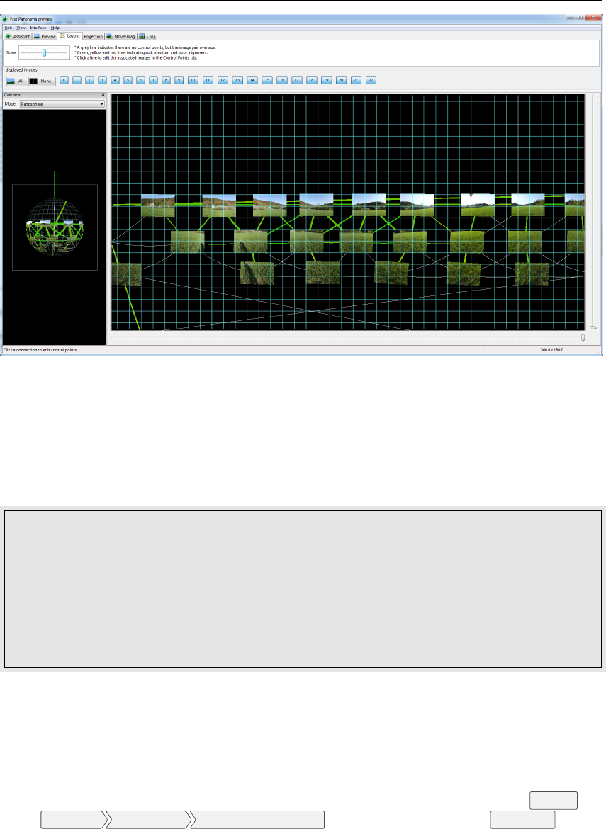
7.3 Panorama Postprocessing 75
Figure 7.6:
Hugin
’s Fast Panorama Preview can be used to check which images are
connected to its neighbours. Most important are good matches along the horizon, the
images in the lower rows are clearly less important. If captured on a tripod, they should
still match.
Basic rules to observe (use obvious inverses).
•
If image aligns well in azimuth but overshoots the grid to the right: Increase yaw accord-
ingly (0.022◦/pixel if image is 16384 pixels wide).
•
If the north end (left and right borders) is higher than the southern contact point: Increase
pitch angle.
•
If north and south points are OK, but the western (right) half is higher than the eastern
(left) half: Increase Roll angle.
The corrections required for pitch and roll may be surprisingly small!
Within a few rounds of adjustments, panorama creation, adding as layer in the image editor,
and comparing to the reference data, you should achieve a match to fit your needs.
In case you have taken photographs in several rings but without a panorama tripod, you
may have to first align only the horizontal images (deselect the lower images to exclude from
optimisation), and when the horizon ring is aligned perfectly, deactivate further optimisation in
Hugin
for those photos while “attaching” (optimising) the lower photos. In
Hugin
’s
Photos
tab,
select
Optimise Geometric Custom Parameters
. This opens an extra tab
Optimiser
, where
you can fine-tune your needs: Switch off all variables for the photos in the horizon ring, and make
sure the lower photos fit in the preview after optimisation.
It may even help to define that the lower rows have been taken with a different Lens, so the
field of view and distortion settings of the horizon row will be used as it had been found during the
horizon-only match.
By now you should have enough experience what level of error may be acceptable for you.

76 Chapter 7. Landscapes
7.3.4 Artificial Panoramas
I have created a website
12
where you can enter geographical coordinates and download a file
pano.kml
which helps with image creation from
Google Earth
imagery. Store this file for a site,
let us call it MYPLACE, into a new directory GE_MYPLACE inside your landscapes directory.
Store all scenes visible from the respective viewpoint MYPLACE as picture into one common
folder in your
landscapes/GE_MYPLACE
under the viewpoint name, e.g.,
75-30.jpg
, which
means 75 degrees from Nadir, azimuth 30 degrees. Also, double-click the pano entry or the marker
in
Google Earth
to open a window with the basic content of your
landscape.ini
. Copy and
paste from there into a new file
landscape.ini
and adjust the obvious entries. Complete as
required with the entries described in section 7.1.3.
On loading of the images, Hugin will not be able to detect any EXIF lens data and ask you
for the horizontal field of view. Enter 60 degrees, which is the standard value for
Google Earth
screenshots13.
The viewpoint names translate almost directly to the yaw and pitch angles which you can enter
in the image list in
Hugin
’s
Photos
tab. For example, switch to the
Positions
display on the right
window edge in the
Photo
tab, mark all images that start with
25-
and assign a pitch angle of
−90 +25 =−65
. The second part of the names is directly the azimuth. In this case, don’t run
the optimizer, but you can immediately set an output resolution and stitch (see 7.2.3). To get rid
of the image decorations (compass etc), apply masks
14
. Postprocessing steps are the same as for
photo-panoramas: make sky invisible, crop, etc.
It is also interesting to switch on the 3D buildings layer before creating the images. If temples
or other buildings are accurate, this will give an even closer approximation to what would be visible
on-site. Note however that not every building will be modelled in usable quality, and that usually
vegetation is not included in the 3D buildings layer. Also, if you are too close to buildings, they
may be cut away by the near clipping plane of the rendering.
These images, based on
Google Earth
imagery and the SRTM topographic model, seem usable
as first rough approximation to a photo-based or surveyed panorama. Note that it is definitely not
accurate enough for representing nearby horizon features or critically important mountain peaks,
and please note that Google has image copyright which at least requires you to acknowledge when
displaying these pictures.
7.3.5 Nightscape Layer
Since version 0.13, Stellarium can simulate artificial illumination, like streetlamps, bright windows,
or the skyglow over cities (Zotti and Wuchterl, 2016). One way to create this layer is to make 2
panorama series during the day and night and process these in the same
Hugin
project to align
those photos, and then stitch two separate images by selecting either the daylight or the nighttime
shots. The night panorama has to be processed to remove stars, airplanes, etc.
The other way is a simple layer overpainted in the image processing program. As rough
recommendation, use several layers to prepare this feature:
•
Put a semitransparent black layer over your daylight image, this helps you to place your
painted pixels.
•Paint windows, street lamps, signs, . . . . You may apply a layer style to produce some glow.
•
To draw an impression of more light in the atmosphere (city skyglow), use a gradient with
some brownish color. Generally the color depends on the appropriate mix of city lights
(sodium, mercury vapour, etc.). Note that on the city outskirts a simple vertical gradient will
12http://homepage.univie.ac.at/Georg.Zotti/php/panoCam.php
13Note that if you work with Google Earth Pro, you can create different FoV!
14There is a wide overlap in the images to allow generous trimming.

7.4 Other recommended software 77
not work, towards the city the horizon is much brighter. Use a huge but weak brush to make
a more spotty sky.
•
Use the existing landscape as template for the layer mask for this gradient sky layer. (You
want to hide skyglow by leaves in the foreground!)
•
If you want to add only a few lights to an
old_style
landscape, you need to provide only
the panels showing those lights. Just load a side panel for reference, place a new layer on top,
and paint the lights on windows, lamps etc. There is no light option for the ground texture.
This makes
old_style
landscapes best suited for localized light pollution, not city skyglow.
The resulting image is then declared in the
maptex_illum
line of
landscape.ini
. Try also
to balance the global strength of light pollution with the
light_pollution
key, and a probable
minimal brightness with the minimal_brightness key.
Try to match the visual appearance, not necessarily what photographs may have recorded.
E.g., the Grossmugl sky shows horizon glow mostly towards the city of Vienna, where long-time
exposures may already be saturated.
The possibilities seem limited only by your time and skills!
7.4 Other recommended software
Here is a short collection of other useful programs for (panorama) image manipulation and other
tasks on Windows.
7.4.1 IrfanView
IrfanView
is a free image viewer for Windows with many options. It can show almost any image
format, including several camera RAW formats, in windowed and full-screen mode. It is definitely
preferrable over any image viewer built into Windows. Unfortunately however, it has no panorama
viewer function!
7.4.2 FSPViewer
FSPViewer15
by Fulvio Senore is an excellent panorama viewer for equirectanglar images. Images
centered along the horizon can be viewed directly, while settings for images with different minimum
and maximum angles, as well as “hotspots” (similar to hyperlinks) which move to neighboring
panoramas, can be configured in an .FSV text file like figure 7.7.
Imag eNam e = H ori zon _Ro senb urg . jpg
WindowTit le = Hor izon _Rosenb urg
hFov =70
# Formula : HP =100*( h /2 - upper )/( lower - upper ) in Hugin crop , or
# HP =100* zeroRow / imgHeight
HorizonPosition=33.8
Figure 7.7: FSP configuration file (example)
7.4.3 Clink
Clink16
is a command line enhancement for Windows developed by Martin Ridgers. If you have
ever worked under a Linux
bash
-like command line, you will easily feel that Windows’
cmd.exe
15Further details are available on its home page http://www.fsoft.it/FSPViewer/.
16http://mridgers.github.io/clink/

78 Chapter 7. Landscapes
is extremely limited.
Clink
provides several useful features, most notably a really usable command-
line completion. It is not essential for our tasks, but a general improvement of usability of the
Windows command line which else has not caused me any trouble.
7.4.4 Cygwin
Compared to Linux, the command line of Windows can be a humbling experience. None of the
wonderful helpers taken for granted on Linux are available.
Cygwin17
provides a command line
console with
bash
shell and all the niceties like
make
,
awk
,
sed
, etc. which seem essential for
routine work. If you are used to Linux tools, use inline scripts in your
Makefile
s and need more
than Clink can offer, you should install Cygwin.
7.4.5 GNUWin32
Alternative to
Cygwin
, several of those nice tools (
sed
,
awk
etc.) have also been made available as
standalone commands for Windows. If you don’t need the inline scripting capabilities in
Makefile
s
which you would get from
Cygwin
but just want to call
awk
or
sed
inside your
.BAT
scripts, maybe
this is enough.
17https://cygwin.com/index.html
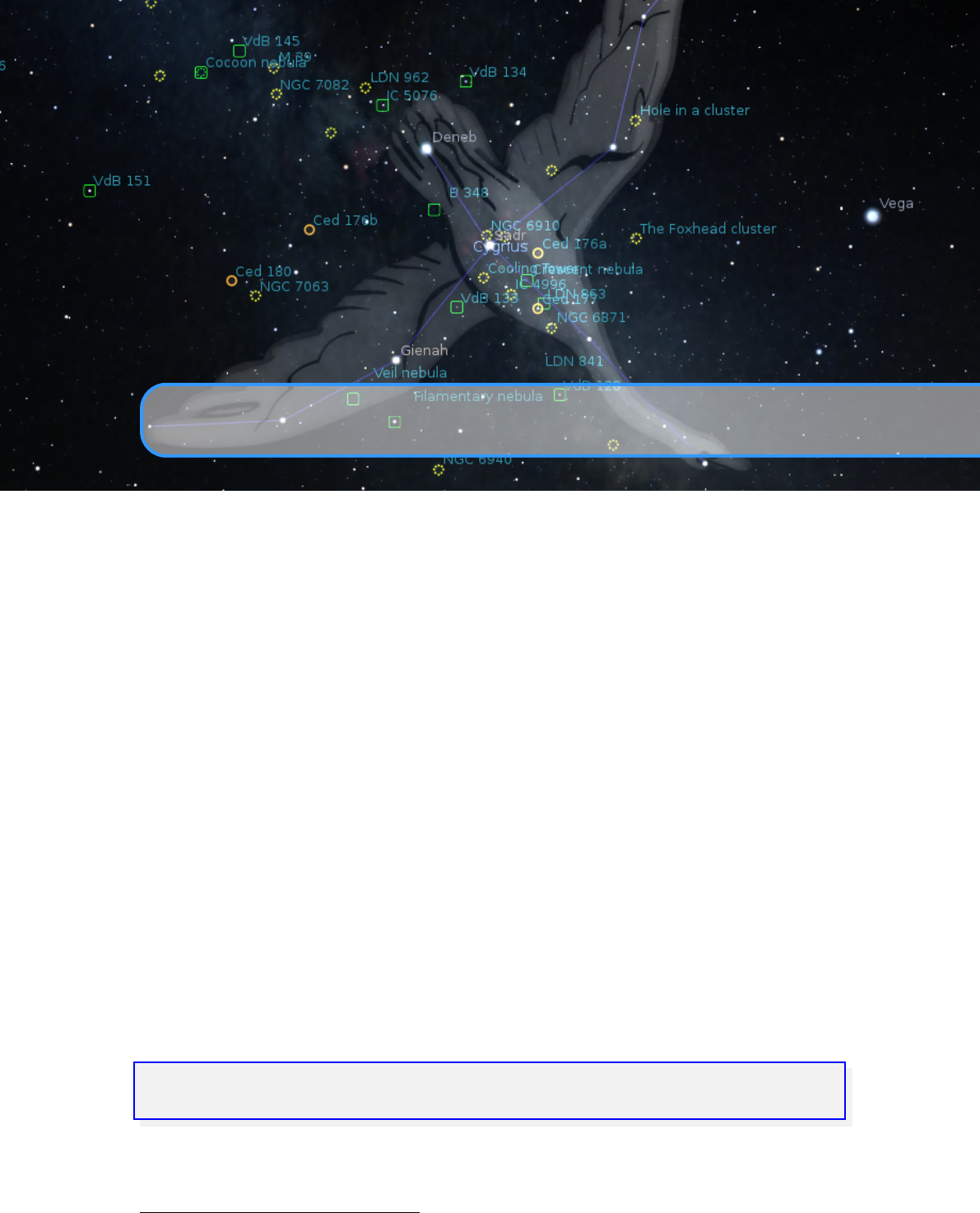
8. Deep-Sky Objects
Since version 0.10.0 Stellarium uses the “json” cataloguing system of configuring textures. At
the same time the Simbad online catalogue was added to the search feature, making the catalog
somewhat redundant and used now only as a first search point or if there is no internet connection.
If the object has a name (not just a catalogue number), you should add one or more records to
the
.../nebulae/default/names.dat
file (where
...
is either the installation directory or the
user directory). See section 8.1.2 Modifying names.dat for details of the file format.
If you wish to associate a texture (image) with the object, you must add a record to the
.../nebulae/default/textures.json file. See section 8.1.3 for details of the file format.
If you wish to associate an outline with the object, you must add the series of lines to the
.../nebulae/default/outlines.dat file. See section 8.1.4 for details of the file format.
8.1 Stellarium DSO Catalog
Stellarium’s DSO Catalog contains over 90000 objects
1
(up to
15.5m
for galaxies) and is available
for end users as collection of files:
catalog.txt Stellarium DSO Catalog in ASCII format for editing data
catalog.dat Stellarium DSO Catalog in zipped binary format for usage within Stellarium
names.dat List of proper names of the objects from file catalog.dat
ASCII file can be converted into binary format through enabling an option in the file
config.ini
(See 5.4):
[ devel ]
convert_dso_catalog = true
The file
catalog.txt
should be put into the directory
.../nebulae/default/
and you
should create an empty file
catalog.pack
to storing the binary catalog. After converting the data
into binary format you should gzip them by the command
1
An extended edition of this catalog with over one million objects may be downloaded and installed
manually (see section 5.5.2).

80 Chapter 8. Deep-Sky Objects
gzip -nc catalog . pack > catalog . dat
Stellarium DSO Catalog contains data and supports the designations for follow catalogues:
NGC New General Catalogue
IC Index Catalogue
MMessier Catalog
CCaldwell Catalogue
BBarnard Catalogue (Barnard, 1927)
SH2 Sharpless Catalogue (Sharpless, 1959)
VdB Van den Bergh Catalogue of reflection nebulae (van den Bergh, 1966)
RCW
A catalogue of H
α
-emission regions in the southern Milky Way (Rodgers, Campbell,
and Whiteoak, 1960)
LDN Lynds’ Catalogue of Dark Nebulae (Lynds, 1962)
LBN Lynds’ Catalogue of Bright Nebulae (Lynds, 1965)
Cr Collinder Catalogue (Collinder, 1931)
Mel Melotte Catalogue of Deep Sky Objects (Melotte, 1915)
PGC HYPERLEDA. I. Catalog of galaxies2
UGC The Uppsala General Catalogue of Galaxies
Ced Cederblad Catalog of bright diffuse Galactic nebulae (Cederblad, 1946)
Arp Atlas of peculiar galaxies (Arp, 1966)V0.16.0
VV
The catalogue of interacting galaxies by Vorontsov-Velyaminov (Vorontsov-Velyaminov,
Noskova, and Arkhipova, 2001)V0.16.0
PK Version 2000 of the Catalogue of Galactic Planetary Nebulae (Kohoutek, 2001)
V0.16.0
PN G The Strasbourg-ESO Catalogue of Galactic Planetary Nebulae (Acker et al., 1992)
V0.16.1
SNR G A catalogue of Galactic supernova remnants (Green, 2014)
V0.16.1
ACO A Catalog of Rich Clusters of Galaxies (Abell, Corwin, and Olowin, 1989)
V0.16.1
Cross-index data for Stellarium’s DSO Catalog is partially obtained from “Merged catalogue of
reflection nebulae” (Magakian, 2003) and astronomical databases SIMBAD
3
(Wenger et al., 2000)
and NED4.
8.1.1 Modifying catalog.dat
This section describes the inner structure of the files
catalog.dat
(binary format) and
catalog.txt
(ASCII format). Stellarium can convert ASCII file into the binary format file for faster usage within
the program.
Each line contains one record, each record consisting of the following fields with tab char as
delimiter:
Column Type Description
1 integer Deep-Sky Object Identificator
2 float RA (decimal degrees)
3 float Dec (decimal degrees)
4 float B magnitude
5 float V magnitude
6 string Object type (See section 8.1.1 for details).
7 string Morphological type of object
8 float Major axis size or radius (arcmin)
2The PGC and UGC catalogues are partially supported
3SIMBAD Astronomical Database — http://simbad.u-strasbg.fr/simbad/
4NASA/IPAC Extragalactic Database (NED) — https://ned.ipac.caltech.edu/

8.1 Stellarium DSO Catalog 81
9 float Minor axis size (arcmin)
10 integer Orientation angle (degrees)
11 float Redshift
12 float Error of redshift
13 float Parallax (mas)
14 float Error of parallax (mas)
15 float Non-redshift distance (Mpc for galaxies, kpc for other objects)
16 float Error of non-redsift distance (Mpc for galaxies, kpc for other objects)
17 integer NGC number (New General Catalogue)
18 integer IC number (Index Catalogue)
19 integer M number (Messier Catalog)
20 integer C number (Caldwell Catalogue)
21 integer B number (Barnard Catalogue)
22 integer SH2 number (Sharpless Catalogue)
23 integer VdB number (van den Bergh Catalogue of reflection nebulae)
24 integer
RCW number (A catalogue of H
α
-emission regions in the southern
Milky Way)
25 integer LDN number (Lynds’ Catalogue of Dark Nebulae)
26 integer LBN number (Lynds’ Catalogue of Bright Nebulae)
27 integer Cr number (Collinder Catalogue)
28 integer Mel number (Melotte Catalogue of Deep Sky Objects)
29 integer PGC number (HYPERLEDA. I. Catalog of galaxies); partial
30 integer UGC number (The Uppsala General Catalogue of Galaxies); partial
31 string
Ced identificator (Cederblad Catalog of bright diffuse Galactic nebulae)
32 integer Arp number (Atlas of Peculiar Galaxies)
33 integer VV number (The catalogue of interacting galaxies)
34 string PK identificator (Catalogue of Galactic Planetary Nebulae)
35 string
PN G identificator (The Strasbourg-ESO Catalogue of Galactic Planetary
Nebulae)
36 string SNR G identificator (A catalogue of Galactic supernova remnants)
37 string ACO identificator (A Catalog of Rich Clusters of Galaxies)
Types of Objects
Possible values for type of objects in the file catalog.dat.
Type Description
G Galaxy
GX Galaxy
AGX Active Galaxy
RG Radio Galaxy
IG Interacting Galaxy
GC Globular Cluster
OC Open Cluster
NB Nebula
PN Planetary Nebula
DN Dark Nebula
RN Reflection Nebula
C+N Cluster associated with nebulosity
HII HII Region
82 Chapter 8. Deep-Sky Objects
SNR Supernova Remnant
SNC Supernova Candidate
SNRC Supernova Remnant Candidate
BN Bipolar Nebula
EN Emission Nebula
SA Stellar Association
SC Star Cloud
CL Cluster
IR Infra-Red Object
QSO Quasar
Q? Possible Quasar
ISM Interstellar Matter
EMO Emission Object
LIN LINEAR-type Active Galaxies
BLL BL Lac Object
BLA Blazar
MOC Molecular Cloud
YSO Young Stellar Object
PN? Possible Planetary Nebula
PPN Protoplanetary Nebula
∗Star
∗∗ Double Star
MUL Multiple Star
SY∗Symbiotic Star
EM∗Emission-line Star
CLG Cluster of galaxies
empty Unknown type, catalog errors, Unidentified Southern Objects etc.
8.1.2 Modifying names.dat
Each line in the file
names.dat
contains one record. A record relates an extended object catalogue
number (from
catalog.dat
) with a name. A single catalogue number may have more than one
record in this file.
The record structure is as follows:
Offset Length Type Description
0 5 %5s Designator for catalogue (prefix)
5 15 %d Identificator for object in the catalog
20 60 %s Proper name of the object (translatable)
If an object has more than one record in the file
names.dat
, the last record in the file will be used
for the nebula label.
8.1.3 Modifying textures.json
This file is used to describe each nebula image. The file structure follows the JSON format, a
detailed description of which may be found at
www.json.org
. The
textures.json
file which
ships with Stellarium has the following structure:
serverCredits (optional) a structure containing the following key/value pairs:
short a short identifier of a server where the json file is found, e.g. “ESO”
full a longer description of a server, e.g. “ESO Online Digitised Sky Survey Server”
infoURL a URL pointing at a page with information about the server

8.1 Stellarium DSO Catalog 83
imageCredits
a structure containing the same parts as a serverCredits structure but referring to
the image data itself
shortName an identifier for the set of images, to be used inside Stellarium
minResolution
minimum resolution, applies to all images in the set, unless otherwise specified at
the image level
maxBrightness
the maximum brightness of an image, applies to all images in the set, unless
otherwise specified at the image level
subTiles
a list of structures describing indiviual image tiles, or referring to another json file. Each
subTile may contain:
minResolution
maxBrightness
worldCoords
subTiles
imageCredits
imageUrl
textureCoords
shortName (name for the whole set of images, e.g. “Nebulae”)
miniResolution (applies to all images in set)
alphaBlend (applies to all images in set)
subTiles list of images. Each image record has the following properties:
imageCredits (itself a list of key/pairs)
imageUrl (e.g. file name)
worldCoords (a list of four pairs of coordinates representing the corners of the image)
textureCoords
(a list of four pairs of corner descriptions. i.e. which is top left of image
etc)
minResolution (over-rides file-level setting)
maxBrightness
Items enclosed in Quotation marks are strings for use in the program. Syntax is extremely
important. Look at the file with a text editor to see the format. Items in <> are user provided strings
and values to suit the texture and source.
{
" i m ag eC r ed it s " : { " s ho rt " : " < au th or ␣ n ame > " ,
" in foUr l " : " htt p :// < mysit e .org > "
},
" i ma ge U rl " : " < m yP ho to . png > " ,
" w o rl dC oo r ds " : [[ [ X0 , Y0 ] , [ X1 , Y 1 ], [ X2 , Y 2 ], [ X3 , Y3 ] ]] ,
" tex ture Coor ds " : [[[ 0 ,0] ,[1 ,0] ,[1 ,1] ,[0 ,1]]] ,
" Min Resol utio n " : 0. 214 881 046 3 ,
" max Brigh tnes s " : < mag >
},
where
worldCoords
Decimal numerical values of the J2000 coordinates (RA and dec both in degrees) of
the corners of the texture. These values are usually given to 4 decimal places.
textureCoords
Where 0,0 is South Left, 1,0 the South Right, 1,1 North Right, 0,1 North Left
corners of the texture.
MinResolution UNDOCUMENTED VALUE! Sorry!
maxBrightness total object brightness, magnitude
Calculating of the coords of the corners of the images (plate solving) is a time consuming
project and needs to be fine tuned from the screen display. As most images will be two dimensional,
display on a spherical display will limit the size to about 1 degree before distortion becomes evident.
Larger images should be sectioned into a mosaic of smaller textures for a more accurate display.
84 Chapter 8. Deep-Sky Objects
8.1.4 Modifying outlines.dat
Each line in the file
outlines.dat
contains three “columns” of data for outline elements. The
V0.16.1
structure for each line is as follows:
Offset Length Type Description
0 8 %d Right ascension (decimal hours)
10 18 %d Declination (decimal degrees)
20 60 %s Command
Coordinates for each point of outline is represented in the equatorial coordinate system for epoch
J2000.0. The possible values of the third “column” (Command) are:
start
This command marks a start point of the outline. This command should also contain the
designation of the deep-sky object.
vertex This command marks an intermediate point of the outline.
end This command marks an end point of the outline.
Example for outline of M42:
05.56401 -05.49880 start M 42
05.56759 -05.39201 vertex
05.56635 -05.31749 vertex
05.57158 -05.21922 vertex
05.57601 -05.21716 vertex
05.58830 -05.30164 vertex
05.59140 -05.34341 vertex
05.59028 -05.37076 vertex
05.59008 -05.38175 vertex
05.59581 -05.37159 vertex
05.59943 -05.47123 vertex
05.59912 -05.65838 vertex
05.59520 -05.73212 vertex
05.58490 -05.68102 vertex
05.56948 -05.57675 end
The format of the file
outlines.dat
is compatible with the similar file of the
SkyChart/-
Cartes du Ciel planetarium.
8.2 Adding Extra Nebulae Images
BARRY GERDES
8.2.1 Preparing a photo for inclusion to the textures.json file
The first step is to take a photo of the object you wish to display in Stellarium. When you have
the picture you will need to align it with the equatorial coordinate system so that north is directly
up and not inverted side to side or up and down as can happen with photos taken with a diagonal
mirror in the path. Next you will need to crop the picture, setting the main feature at the centre
and making the cropped size a factor of
2n
eg. 64, 128, 256, 512, 1024 or 2048 pixels square
(or elongated like 512x1024). If this requirement is not met, your textures may not be visible, or
graphics performance may be seriously impacted. Textures larger than 2048 may only be supported
on high-end hardware. Images must be in PNG format. When cropping, make sure you leave at
least six prominent background stars.
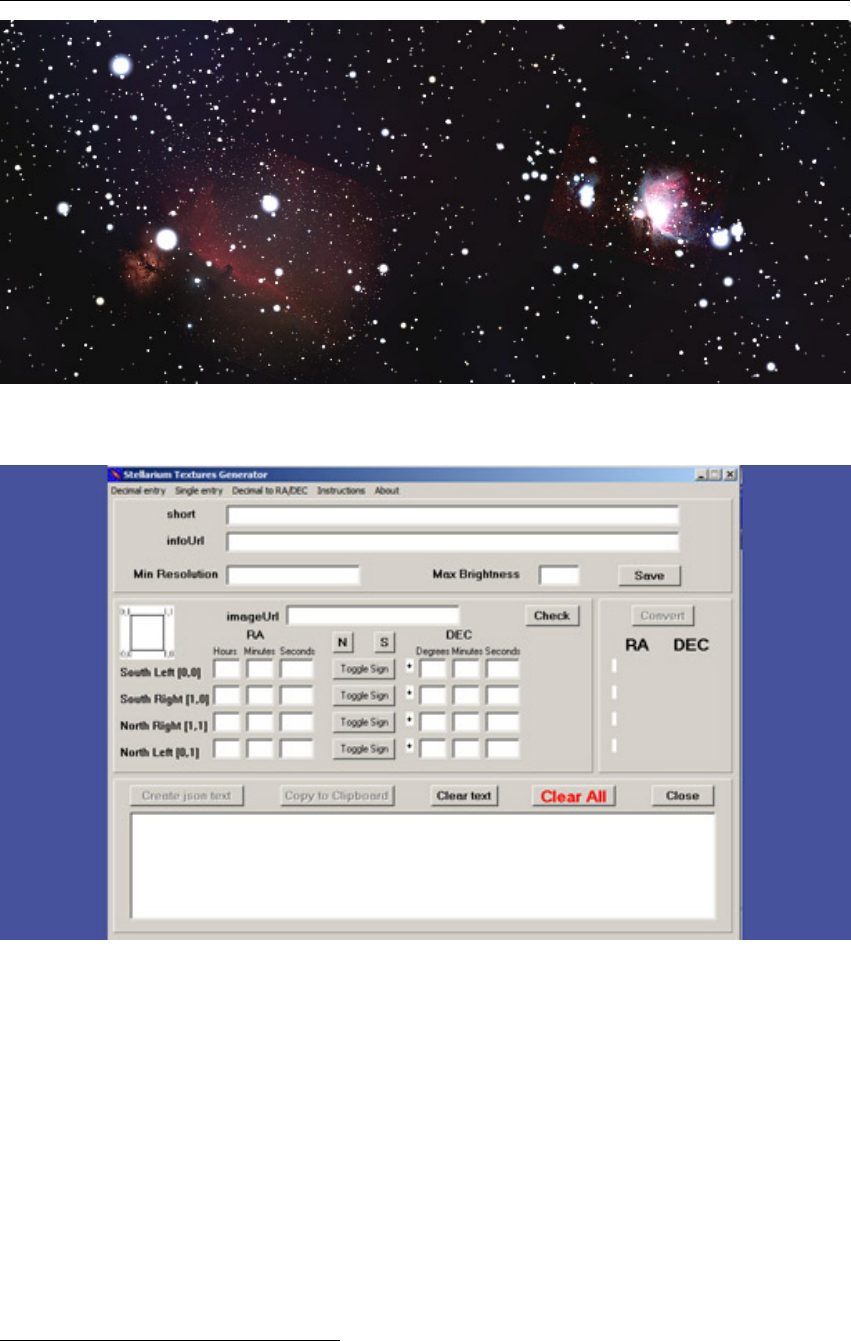
8.2 Adding Extra Nebulae Images 85
Figure 8.1: Screen shot of nebula images displayed in Stellarium
Figure 8.2:
Stellarium Textures Generator
: A program to convert Equatorial coordinates
into decimal form and write a textures.json insert
The next step is to process your photo to make the background black, really black. This will
ensure that your background will meld with the Stellarium background and not be noticed as gray
square. Suitable programs to do all this are The GIMP5or Photoshop if you can afford it.
When you have your image prepared you will need to plate solve it using at least 6 known GSC
stars that can be identified. That is why the cropping with plenty of stars was necessary. When
the plate is solved you will need to find the J2000 coordinates of the corners and convert them to
decimal values to form the world coordinates in the textures.json file.
The program
Stellarium Textures Generator
by Peter Vasey (Fig. 8.2) can convert the corner
coordinates of a texture found in your plate solving program into decimal values and write an insert
5free in keeping with the Stellarium spirit; available from http://www.gimp.org
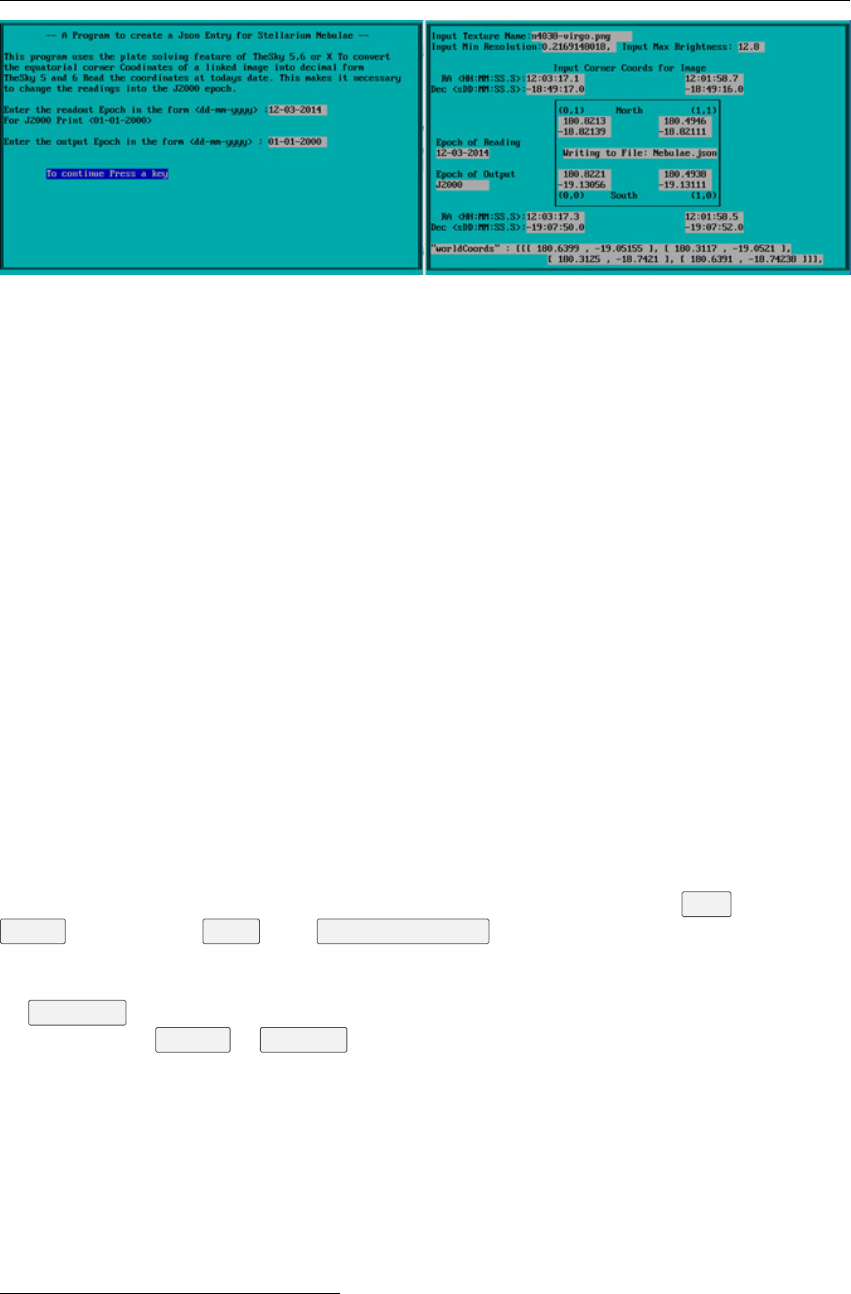
86 Chapter 8. Deep-Sky Objects
Figure 8.3:
ReadDSS
: A program to write a
textures.json
insert with epoch manipula-
tion.
for the textures.json file.6
There is another program,
ReadDSS
(Fig. 8.3), written by Barry Gerdes in Qb64(gl), that will
perform the same task but allows manipulation of the epochs.7
8.2.2 Plate Solving
Suitable programs that can accept your picture and calculate its corner coordinates are hard to
find. I have only found one that suits our purpose and it is another expensive planetarium program,
TheSky X Pro
. However the older versions
TheSky 5
and
6 Pro
will also do the job if suitably
configured, although I could not solve the test program with
TheSky 6
that uses the same procedure
as TheSky 5.
These programs have a link feature that can match your photo to the selected area of the screen
and superimpose it on the display with a box around your photo provided it can match at least 6
stars from the GSC that is included with the program. When this is fitted you can read the corner
coordinates of your texture in the Status bar by selecting them with a mouse.
TheSky X
can read
these coordinates in J2000 values and uses textures in the FITS format, but the earlier programs
only read the coordinates of the current program date. To read the J2000 coordinates it is necessary
to re-start the program with the date set to 1-1-2000.
To add the picture to
TheSky 5
you need first make a mono 8 bit version of the photo and place
it on the clipboard. Run
TheSky
and centre on the object centre. Look in the
Tools
menu for the
image link and select setup . Tick show image frame to put a frame around the image.
Paste the clipboard image on the display and use the zoom and position controls to get it as
close to the size and position as possible by visually matching stars. Go to the menu again and click
on
link wizard
. If you have been successful the window will show the number of stars matched
and the option to
accept
or
continue
. Accept and you will now see all the matched stars have
overlaid the picture. You can now read off the corner coordinates from the status bar starting at the
bottom (south) left and continuing counterclockwise to the top (north) left.
8.2.3 Processing into a textures.json insert
Place your image in the
*.png
format in the
.../nebulae/default/
folder. Ensure that the name
matches the textures.json entry.
Once you have the corner coordinates of your photo you can add them to the decimal converter
program and it will write an insert
nebula.json
as a text file that you can paste directly into the
6
It is available as a freebee from
http://www.madpc.co.uk/~peterv/astroplover/equipnbits/
Stellariumtextures.zip.
7http://barry.sarcasmogerdes.com/stellarium/uploads/writejsoninsert.zip

8.2 Adding Extra Nebulae Images 87
textures.json file that is in the .../nebulae/default/ folder.
Save the
textures.json
file with the new insert and run Stellarium. Find the object in the
F3
Object selection window and slew to it. Your image should be there and with a bit of luck
it will nicely overlay the stars in Stellarium. However this only rarely happens, so a little bit of
tweaking of the JSON
worldcoords
will be needed to get a perfect match. Select equatorial mode
( or
Ctrl +M
). This will show the area with north up. Select each corner in sequence and
make small changes to the coordinates. Restart Stellarium each time and check if you have moved
into the right direction. Continue with each corner until all the stars match. With a little bit of
practice this will be done in about 10 minutes.
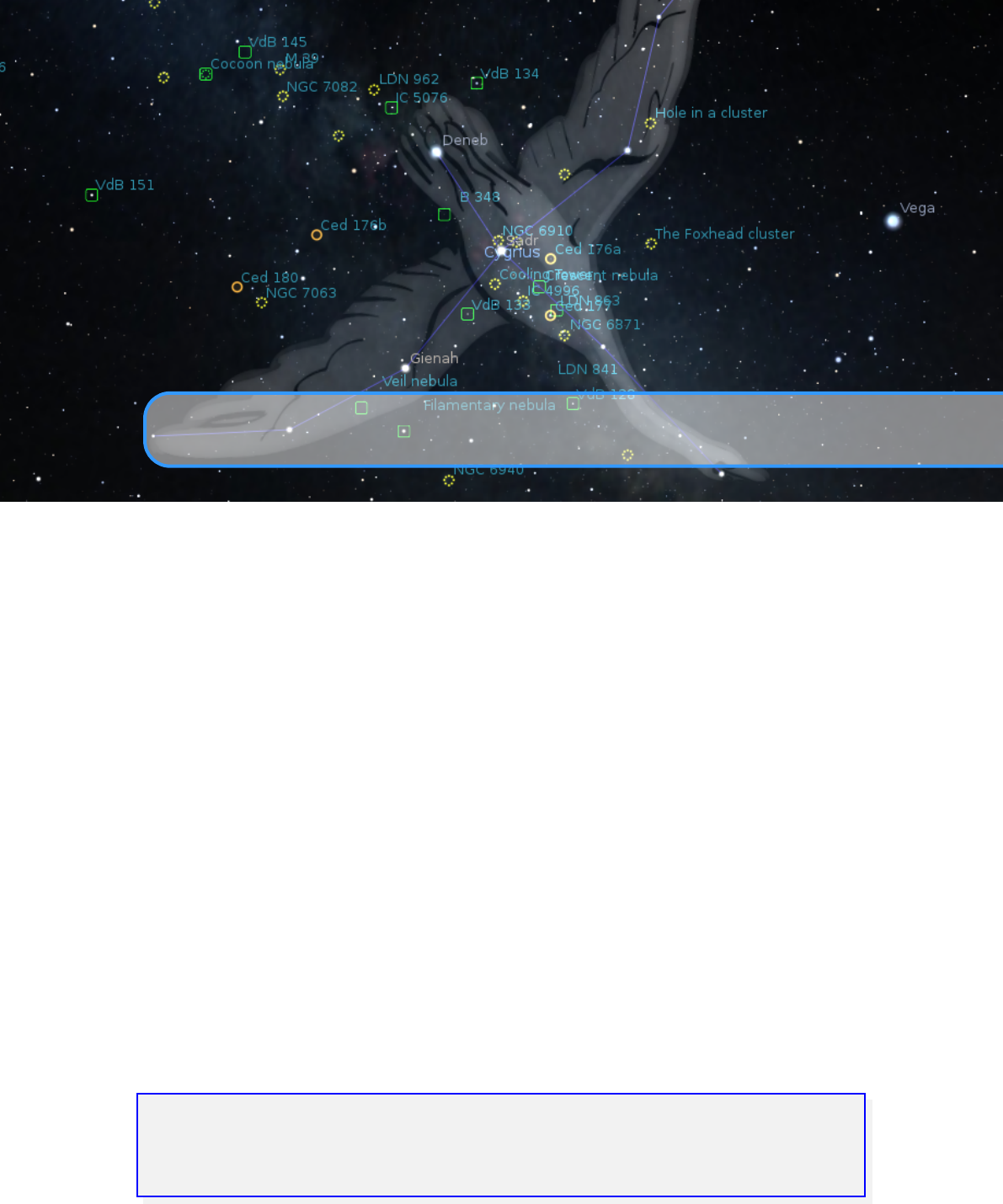
9. Adding Sky Cultures
GEORG ZOTTI,WITH ADDITIONS BY ALEXANDER WOLF
Stellarium comes with a nice set of skycultures. For ethnographers or historians of science it may
be a worthwile consideration to illustrate the sky culture of the people they are studying. It is not
very hard to do so, but depending on your data, may require some skills in image processing.
Some features regarding translation and multilinguality have evolved over the years, and not
all skycultures currently included in Stellarium adhere to the standards described in the following
sections. If you add a new skyculture, please do so for an optimal result!
In the Stellarium program folder you can see a folder
skycultures
. Let us assume you work
on Windows and want to create a new Skyculture, say, myCulture.
You can take the
inuit
directory as template to start with. Just copy the folder
C:\Program
Files\Stellarium\skycultures\inuit
to
C:\Users\[YOU]\AppData\Roaming\Stellarium\
skycultures\myculture
In the folder you see image files for the constellation artwork, and all other files with various
extensions are text files.
9.1 Basic Information
In myculture\info.ini, change the entries to
[ info ]
name = myC ulture
aut hor = me
boundaries=none
(or what seems best for you). The name is used for the list entry in the Starlore tab in the View
dialog (see 4.4.5).
The option “boundaries” is optional and may contain the follow values:

90 Chapter 9. Adding Sky Cultures
none
— this value is enabled by default and it designates that this culture doesn’t have boundaries
of constellations.
generic
— please use this value for subset of “western” cultures to enable using default boundaries.
own — please use it for culture who has own set of boundaries for constellations.
9.2 Skyculture Description Files
In order to have translated texts we have files
description.<LANG>.utf8
, where
<LANG>
is
the two-letter ISO 639-1 language code, or its extension which contains language and coun-
try code, like
pt_BR
for Brazilian Portuguese. A minimum skyculture must contain the file
description.en.utf8
, this is
en=english
text with optional HTML tags for sections, tables,
etc. You can also have embedded images in the HTML (your book cover? Views of sacred land-
scapes/buildings/artwork/. . . ?), just make them PNG format please. The length of the description
texts is not limited, you have room for a good description, tables of names/translations, links to
external resources, whatever seems suitable. When you started from a copied skyculture, delete the
other description.*.utf8 files.
If you can provide other languages supported by Stellarium, you can provide translations
yourself, else Stellarium translators may translate the English version for you. (It may take years
though.) The file ending
.utf8
indicates that for special characters like ÄÖÜßáé you should use
UTF8 encoding. If you write only English/ASCII, this may not be relevant.
9.3 Constellation Names
The native constellations are listed in
constellation_names.eng.fab
. It consists of 3 simple
columns: Abbreviation (or just a serial number), native name, and english translation. The writing
_("name")
allows automatic translation of the English strings to other languages. These strings
will be used as constellation labels.
The first column (abbreviation) in the Western sky culture provides the canonical 3-letter
abbreviation for constellations as used by the International Astronomical Union. Such abbreviations
may not be available for the skyculture you are working with, so you must invent your own. These
abbreviations are used as keys in the other files, so they must be unique within your skyculture. It
is not necessary to have 3-letter keys.
The keys can be displayed on screen when labels are requested in the Starlore GUI (sec-
tion 4.4.5). If you want to prevent certain abbreviations from being displayed, let them start with a
dot. See the effect in the
Western (H.A.Rey)
skyculture: In
Abbreviated
mode, only the official
abbreviations are displayed. In
Native
mode, the second column of
constellation_names.eng.fab
is shown. Only with setting
Translated
, the text translated from the text shown in the third column
is shown. If your skyculture is a variant of the Western skyculture, please use the canonical Latin
names, they have all been translated already.
If your skyculture is not a variant of the generally known Western skyculture, please include an
English translation to the name given in the native language. Else translators will not be able to
translate the name. See a good example in the Mongolian skyculture.
9.4 Star Names
The file
star_names.fab
contains a list of HIP catalogue numbers and common names for those
stars. Each line of the file contains one record of two fields (separated by the pipe character (
|
)) or
three fields (the first pair is separated by the pipe character (
|
) and the last one separated by the
space character). The first field is the Hipparcos catalogue number of the star, the second is the

9.5 Planet Names 91
common name of the star in a format that enables translation support, the third is an optional list of
references (see 9.11) to the source of the information about this name, e.g:
# P iscis Aus trin us ( PsA )
113368| _ ( " Fomalhaut ") 1 ,2 ,6 ,11 ,12
113368| _ (" Thalim ")
In the sample you can see 3 lines: the first line is a comment, the second line has 3 fields and
the third line has 2 fields. Both lines with data have the same Hipparcos number of the star —
Fomalhaut is the well-known name of HIP 113368, and Thalim is an additional (not well-known)
name of this star.
9.5 Planet Names
The file
planet_names.fab
contains a list of native names of the planets. Each line of the file
contains one record of 3 fields, separated by the white space or tab character. The first field is
the English name of the planet, the second is the native name of the planet (can be in the native
language, but please for maximum utability use an english transliteration) and the third is the
translatable version of the native name of the planet (translated into English). Here is an example
from the Egyptian skyculture:
Mars "Horus - D esher " _( " Red ␣ Horus ␣ ( Mars ) ")
9.6 Deep-Sky Objects Names
The file
dso_names.fab
contains a list of native names for deep-sky objects (DSO). The format
v0.15.1
of this file is similar to the
star_names.fab
format (see 9.4). Each line of the file contains one
record of two fields (separated by the pipe character (
|
)) or three fields (first pair is separated by the
pipe character (
|
) and the last one separated by the space character). The first field is an identifier
of the deep-sky object, the second is the native name of the DSO in a format that enables translation
support, the optional third is a list of references (see 9.11) to the source of the information about
this name, e.g.:
PGC 17223| _ (" N ative ␣ name ␣ for ␣ LMC ") 1 ,2 ,3
NGC 292 |_ (" Nati ve ␣ name ␣ for ␣ SML " ) 1 ,3
NGC 292 |_(" Small ␣ Magel lanic ␣ Cloud " )
9.7 Stick Figures
The modern-style stick figures are coded in constellationship.fab. Lines look like:
Abbr pairs pair1_star1 pair1_star2 pair2_star1 pair2_star2 ...
In this file,
Abbr is the abbreviation defined in constellation_names.eng.fab
pairs is the number of line pairs which follow.
pairN_starA
Hipparcos numbers for the stars which form the constellation stick figure. We need
two entries per line, longer line segments are not supported. To find the HIP number, just
have Stellarium open and click on the star in Stellarium while editing this file.

92 Chapter 9. Adding Sky Cultures
9.8 Constellation Boundaries
The optional file
1constellations_boundaries.dat
includes data for the boundary lines drawn
between constellations. The default boundaries for western constellations are defined in the
data/constellations_boundaries.dat file.
The format for this file is a bit more dificult than the other files. It contains sections which may
consist of multiple lines, of the format:
N RA_1 DE_1 RA_2 DE_2 ... RA_N DE_N 2 CON1 CON2
where
Nnumber of segments for boundary
RA_n, DE_n
right ascension (decimal hours) and declination (decimal degrees) of the points of
segments in J2000 coordinates.
2 CON1 CON2
this data indicate “border between 2 constellations CON1 and CON2”. They
are used to define isolated boundaries for each constellation (for proper working of the
Select single constellation option).
9.9 Constellation Artwork
Constellation artwork is optional, but may give your skyculture the final touch, if it requires artwork
at all. E.g., H. A. Rey’s variant of the Western skyculture deliberately does not contain artwork.
Each constellation artwork is linked to 3 stars in its constellation. This is programmed in the
file constellationsart.fab. You have to write lines
Abbr image_name . png x1 y1 HIP1 x2 y2 HIP2 x3 y3 HIP3
where
Abbr is the abbreviation defined in constellation_names.eng.fab
image_name.png
is the file name of your texture. It should be sized in a power of two, like
512×512
,
1024×2048
etc. Avoid dimensions larger than 2048, they are not supported on
all systems. You can distort images to better exploit the pixels, the texture will be stretched
back. The background of the artwork image must be absolutely black.
xn, yn, HIPn
pixel locations of the star in the constellation drawing (find those in any image
editor) and HIPnis the star number in the Hipparcos catalog, which you find when you click
on the star in Stellarium.
In case the artwork is only available in a certain projection (e.g., an all-sky map), or is otherwise
heavily distorted so that the match is not satisfactory, you may have to reproject the image somehow.
For aligning, you should switch Stellarium to Stereographic projection for optimal results.
You don’t have to shutdown and restart Stellarium during creation/matching, just switch
skyculture to something else and back to the new one to reload.
9.10 Seasonal Rules
File
seasonal_rules.fab
(optional) contains possible seasonal rules for the visibility of constel-
lations. There is one rule per line. Each rule contains three elements separated with white space (or
tab character): constellation ID, start of visibility (month) and end of visibility (month), e.g:
Emu 6 3
1Please define “boundaries = own” in the file info.ini to enable using custom boundaries.
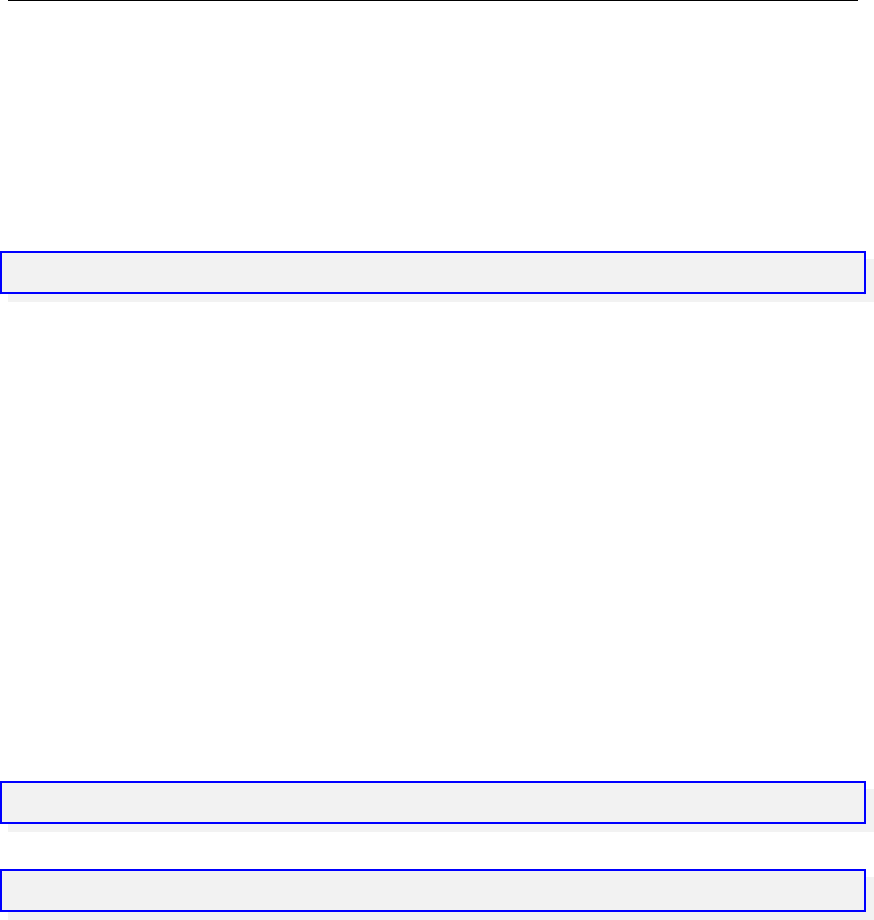
9.11 References 93
This specifies that constellation Emu (abbreviated also as “Emu”) is visible only from June to
March.
9.11 References
The file
reference.fab
contains a list of information sources. Each line of the file contains one
v0.15.1
record of 3 fields, separated by the pipe character (
|
) — number of source, description of source
and optional URL, e.g.:
9| Kruger 60| https :// en . wikipedia . org / wiki / Krug er_60
9.12 Asterisms and help rays
Sometimes there is a need to extract some part of a constellation into a figure in its own right, or to
v0.16.1
merge parts from different constellations into one big figure — e.g. “Big Dipper” as part of Ursa
Major or the “Summer Triangle” consisting of 3 stars from the constellations Cygnus, Lyra and
Aquila. Those features are called “asterisms”.
Other simple figures might be used as navigation helpers — the help rays. As example to
help in orientation in sky the additional lines between constellations Ursa Major, Ursa Minor and
Cassiopeia might be useful. The asterisms and help rays are listed in
asterism_names.eng.fab
.
This file consists of 2 simple columns: Abbreviation (or just a serial number) and English name
of asterism. The writing
_("name")
allows automatic translation of the English strings to other
languages. These strings will be used as asterisms labels. In addition, after a hash mark (
#
) marking
a comment sign, some reference information should be noted. Collecting sources and giving such
references is always a good idea. Some later versions of Stellarium may use this information.
The stick figures of asterisms are similar to constellation figures and coded in
asterism_lines.fab
.
Lines look like:
Abbr type pairs pa ir1_star1 pair1 _star2 pair2_st ar1 pair2_ star2 ...
or
Abbr 2 pairs pair1_RA1 pair1_DE1 pair1_RA2 pair1_DE2 pair2_RA1 ...
In this file,
Abbr is the abbreviation defined in asterism_names.eng.fab
type
is the type of line. Use 1 or 2 to define an asterisms and 0 for the help rays (0 and 1 uses HIP
numbers, and 2 uses coordinates).
pairs is the number of line pairs which follow.
pairN_starA
Hipparcos numbers for the stars which form the asterism/help ray stick figure (similar
to constellations), or equatorial coordinates for epoch J2000.0 of the stars (decimal hours for
right ascension and decimal degrees for declination). The help rays are actually a special
form of asterisms in Stellarium.
9.13 Publish Your Work
If you are willing to let other users enjoy the result of your hard work (and we certainly hope you
do!), when you are done, please write a note in the Forum or at Launchpad. Please be prepared to
put the imagery and text under some compatible open-source license (Creative Commons). Else the
skyculture cannot be hosted by us.
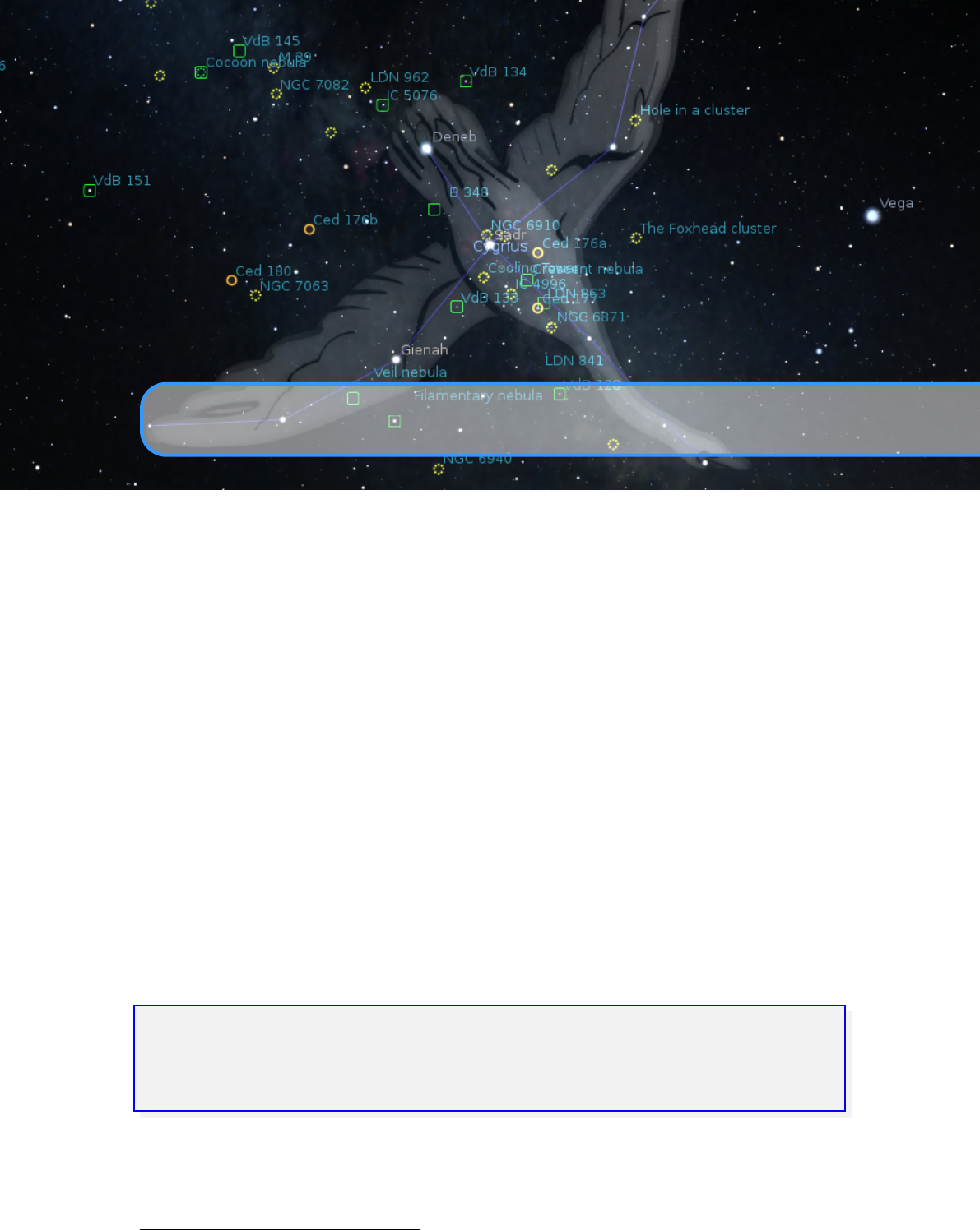
10. Surveys
GUILLAUME CHÉREAU
10.1 Introduction
Asky survey is a map of the sky stored as a hierarchical set of a potentially large number of smaller
v0.18.0
images (called tiles). The advantage compared to a regular texture is that we need to render only
the visible tiles of a potentially gigantic image at the lowest resolution needed. This is particularly
interesting for rendering online images that can be stored on a server, while the client only has to
download the parts he currently uses.
Since version 0.18.0, Stellarium added some preliminary support for loading and rendering on-
line surveys in the Hierarchical Progressive Surveys (HiPS) format, developed by the International
Virtual Observatory Alliance. A full description of the format can be found on the IVOA website
1
.
10.2 Hipslist file and default surveys
Hipslist files are text files used to describe catalogs of HiPS surveys. The full specification is part
of the HiPS format, and looks like that:
# Ex ampl e of a hi ps list fi le .
# Date : 2018 -03 -19
hip s_s er vic e_ url = h ttp s :/ / da ta . s te ll ar iu m . org / su rv ey s / cal li sto
hip s _rel e ase_ d ate = 2018 -03 -18 T14 :01 Z
hip s_st atus = pu blic m irror c lona b leO n ce
As of v0.18.0, by default Stellarium tries to load HiPS from two sources:
http://alaskybis.
unistra.fr/hipslist
and
https://data.stellarium.org/surveys/hipslist
. This can
be changed with the hips/sources options in the configuration file (see also section D.1.27). For
example:
1http://www.ivoa.net/documents/HiPS/20170519/REC-HIPS-1.0-20170519.pdf

96 Chapter 10. Surveys
[ hips ]
sources / size = 1
sources /1/ url = " https :// myownhips / hipslist "
10.3 Solar system HiPS survey
Though not specified in the HiPS standard, Stellarium recognises HiPS surveys representing planet
textures, as opposed to sky surveys. If the
obs_frame
property of a survey is set to the name of a
planet or other solar system body, Stellarium will render it in place of the default texture used for
the body.

III
11 Plugins: An Introduction .................. 99
12 Interface Extensions ..................... 101
13 Object Catalog Plugins ................. 117
14 Scenery3d – 3D Landscapes ............ 145
15 Stellarium at the Telescope ............. 159
16 Scripting .................................. 183
Extending Stellarium
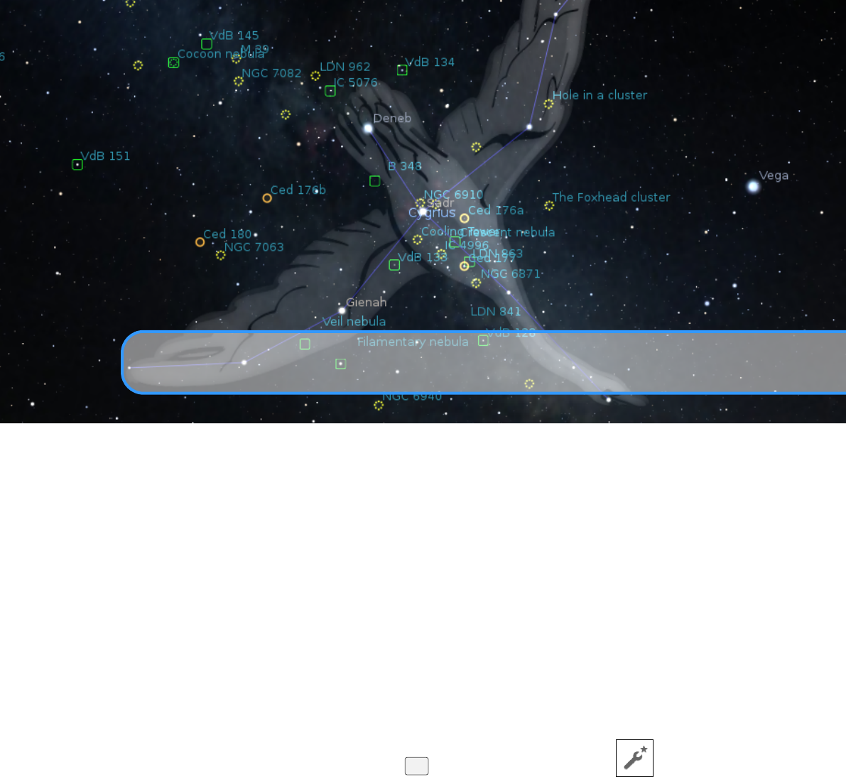
11. Plugins: An Introduction
Starting with version 0.10.3, Stellarium’s packages have included a steadily growing number
of optional extensions called plug-ins: Angle Measure, Compass Marks, Oculars, Telescope
Control, Text User Interface, Satellites, Solar System Editor, Historical Novae and Supernovae,
Quasars, Pulsars, Exoplanets, Observability analysis, ArchaeoLines, Scenery3D, RemoteControl
and RemoteSync. All these plug-ins are “built-in” in the standard Stellarium distribution and don’t
need to be downloaded separately.
11.1 Enabling plugins
To enable a plugin:
1. Open the Configuration dialog (press F2 or use the left tool bar button )
2. Select the Plugins tab
3. Select the plugin you want to enable from the list
4. Check the Load at startup option
5. Restart Stellarium
If the plugin has configuration options, the
configuration
button will be enabled when the plugin
has been loaded and clicking it will open the plugin’s configuration dialog. When you only just
activated loading of a plugin, you must restart Stellarium to access the plugin’s configuration dialog.
11.2 Data for plugins
Some plugins contain files with different data, e.g., catalogs. JSON is a typical format for those
files, and you can edit its contents manually. Of course, each plugin has a specific format of data for
its own catalogs, and you should read the documentation for the plugin before editing its catalog.
You can read some common instructions for editing catalogs of plugins below. In this example
we use file name catalog.json for identification of the catalog for a typical plugin.

100 Chapter 11. Plugins: An Introduction
You can modify the
catalog.json
files manually using a text editor.
If you are using
Windows, it is strongly recommended to use an advanced text editor such as Notepad++1to
avoid problems with end-of-line characters.
(It will also color the JSON code and make it easier
to read.)
Warning
: Before editing your
catalog.json
file, make a backup copy. Leaving out the
smallest detail (such as a comma or forgetting to close a curly bracket) may prevent Stellarium
from starting.
As stated in section 5, the path to the directory
2
which contains
catalog.json
file is something
like:
Windows C:\Users\UserName\AppData\Roaming\Stellarium\modules\PluginName
Mac OS X HomeDirectory/Library/Preferences/Stellarium/modules/PluginName
Linux and UNIX-like OS ~/.stellarium/modules/PluginName
1http://notepad-plus-plus.org/
2
This is a hidden folder, so in order to find it you may need to change your computer’s settings to display
hidden files and folders.
12. Interface Extensions
Most users will soon be familiar with the usual user interface. A few plugins are available which
extend the regular user interface with a few small additions which are presented first. However, some
applications and installations of Stellarium require completely different user interfaces. Mostly,
these serve to avoid showing the user interface panels to an audience, be that in your astronomy
club presentations, a domed planetarium or in a museum installation.
12.1 Angle Measure Plugin
goes misty eyed
I recall measuring the size of the Cassini Division when I was a student. It was not
the high academic glamor one might expect. . . It was cloudy. . . It was rainy. . . The
observatory lab had some old scopes set up at one end, pointing at a photograph of
Saturn at the other end of the lab. We measured. We calculated. We wished we were
in Hawaii. A picture is worth a thousand words.
The Angle Measure plugin is a small tool which is used to measure the angular distance between
two points on the sky.
1.
Enable the tool by clicking the tool-bar button, or by pressing
Ctrl +A
. A message will
appear at the bottom of the screen to tell you that the tool is active.
2. Drag a line from the first point to the second point using the left mouse button
3. To clear the measurement, click the right mouse button
4.
To deactivate the angle measure tool, press the tool-bar button again, or press
Ctrl +A
on
the keyboard.
In the configuration dialog, you can configure if you want to have distances given on the rotating
sphere, or in horizontal (alt-azimuthal) coordinates. You can also link one point to the resting
horizon, the other to the sky and observe how angles change.
102 Chapter 12. Interface Extensions
12.2 Compass Marks Plugin
Stellarium helps the user get their bearings using the cardinal point feature – the North, South, East
and West markers on the horizon. Compass Marks takes this idea and extends it to add markings
every few degrees along the horizon, and includes compass bearing values in degrees.
When activated (see section 11.1), there is a tool bar button for toggling the compass
markings. Note that when you enable compass marks, the cardinal points will be turned off.
Figure 12.1: Markings of Compass Marks Plugin
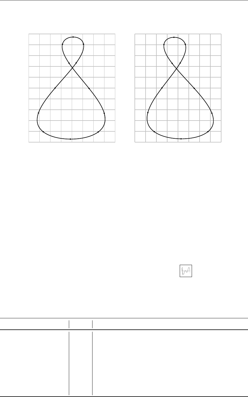
12.3 Equation of Time Plugin 103
12.3 Equation of Time Plugin
-20 -15 -10 -5 0 5 10 15 20
-25
-20
-15
-10
-5
0
5
10
15
20
25
Ari
Tau
Gem
Cnc
Leo
Vir
Lib
Sco
Sgr
Cap
Aqr
Psc
-20 -15 -10 -5 0 5 10 15 20
-25
-20
-15
-10
-5
0
5
10
15
20
25
Ari
Tau
Gem
Cnc
Leo
Vir
Lib
Sco
Sgr
Cap
Aqr
Psc
Figure 12.2: Figure-8 plots for Equation of Time, for years 1000 (left) and 2000 (right).
These plots, often found on sundials, link solar declination (vertical axis) and its deviation
at mean noon from the meridian, in minutes. Labeled dots indicate when the sun entered
the respective Zodiacal sign (30◦section of the ecliptic). Figures by Georg Zotti.
The Equation of Time plugin shows the solution of the equation of time. This describes the
discrepancy between two kinds of solar time:
Apparent solar time directly tracks the motion of the sun. Most sundials show this time.
Mean solar time tracks a fictitious “mean” sun with noons 24 hours apart.
There is no universally accepted definition of the sign of the equation of time. Some publications
show it as positive when a sundial is ahead of a clock; others when the clock is ahead of the sundial.
In the English-speaking world, the former usage is the more common, but is not always followed.
Anyone who makes use of a published table or graph should first check its sign usage.
If enabled (see section 11.1), click on the Equation of Time button on the bottom toolbar
to display the value for the equation of time on top of the screen.
12.3.1 Section EquationOfTimein config.ini file
You can edit
config.ini
file by yourself for changes of the settings for the Equation of Time
plugin – just make it carefully!
ID Type Description
enable_at_startup bool
Display solution of the equation of time at startup of Stel-
larium
flag_use_ms_format bool
Set format for the displayed solution – minutes and seconds
or decimal minutes
flag_use_inverted_value bool Change sign of the equation of time
flag_show_button bool Show the tool’s button on the bottom toolbar
text_color R,G,B
Font color for the displayed solution of the equation of time
font_size int
Font size for the displayed solution of the equation of time
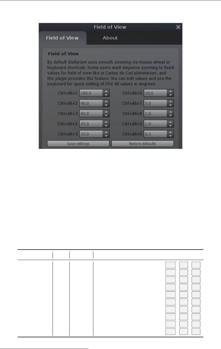
104 Chapter 12. Interface Extensions
12.4 Field of View Plugin
Figure 12.3: Configuration dialog of Field of View plugin
By default Stellarium uses smooth zooming via mouse wheel or keyboard shortcuts. Some users may
want stepwise zooming to fixed values for field of view like in the
Cartes du Ciel1
planetarium
program, and this plugin provides this feature. You can edit values and use the keyboard for
quick-setting of FOV. All values in degrees.
1. Enable the tool by configuring it to “Load at startup”.
2. Press shortkeys for quick changes of FOV.
12.4.1 Section FOVin config.ini file
You can configure the plugin with its dialog (Fig. 12.3) or edit
config.ini
file by yourself for
changes of the settings for the Field of View plugin – just make it carefully!
ID Type Default Description
fov_quick_0 float 0.5 Value of FOV for the shortcut Ctrl +Alt +0
fov_quick_1 float 180 Value of FOV for the shortcut Ctrl +Alt +1
fov_quick_2 float 90 Value of FOV for the shortcut Ctrl +Alt +2
fov_quick_3 float 60 Value of FOV for the shortcut Ctrl +Alt +3
fov_quick_4 float 45 Value of FOV for the shortcut Ctrl +Alt +4
fov_quick_5 float 20 Value of FOV for the shortcut Ctrl +Alt +5
fov_quick_6 float 10 Value of FOV for the shortcut Ctrl +Alt +6
fov_quick_7 float 5 Value of FOV for the shortcut Ctrl +Alt +7
fov_quick_8 float 2 Value of FOV for the shortcut Ctrl +Alt +8
fov_quick_9 float 1 Value of FOV for the shortcut Ctrl +Alt +9
1SkyChart / Cartes du Ciel planetarium: http://www.ap-i.net/skychart/en/start
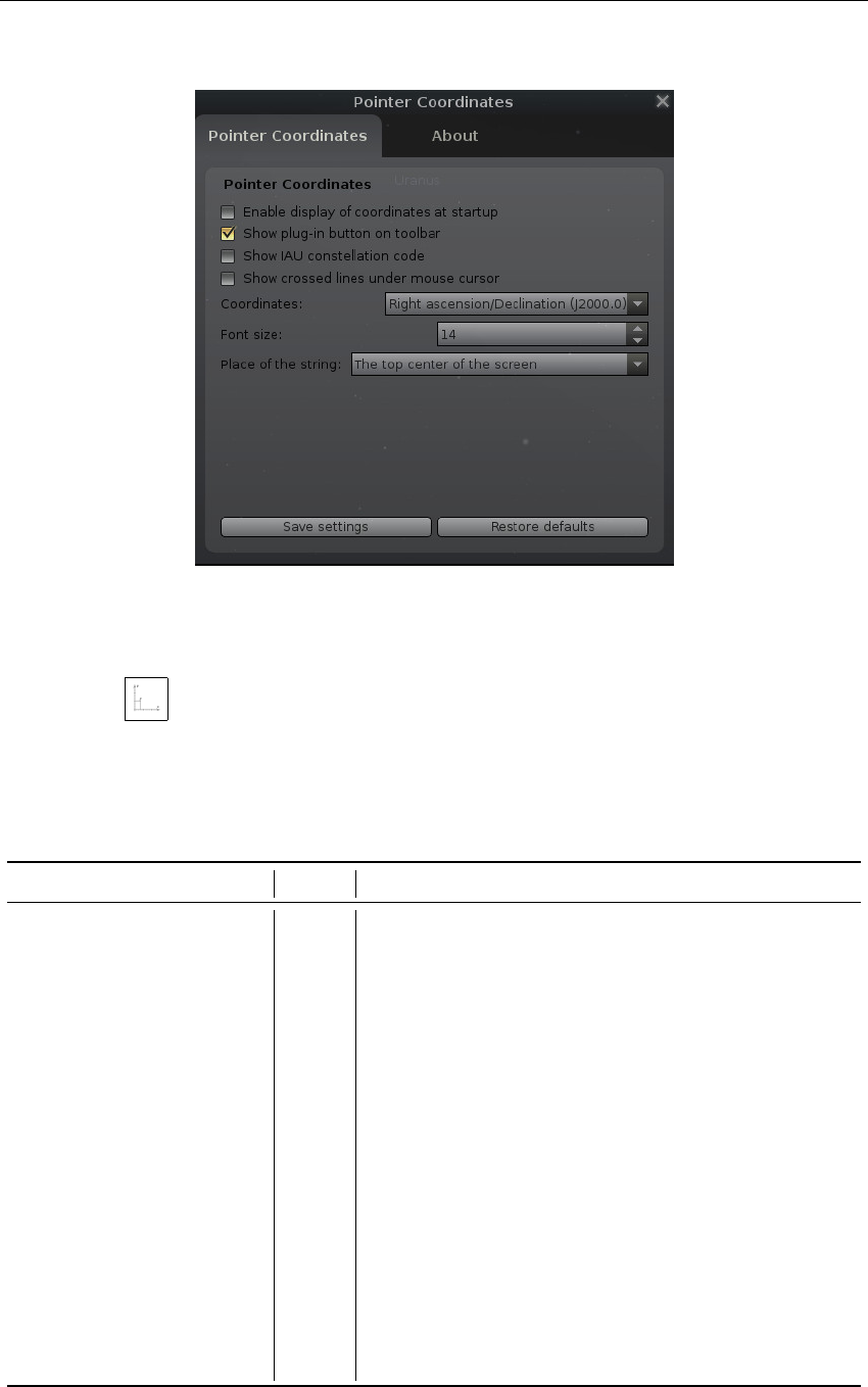
12.5 Pointer Coordinates Plugin 105
12.5 Pointer Coordinates Plugin
Figure 12.4: Interface of Pointer Coordinates plugin
The Pointer Coordinates plugin shows the coordinates of the mouse pointer. If enabled, click on the
plugin button on the bottom toolbar to display the coordinates of the mouse pointer.
12.5.1 Section PointerCoordinatesin config.ini file
You can edit
config.ini
file by yourself for changes of the settings for the Pointer Coordinates
plugin – just make it carefully!
ID Type Description
enable_at_startup bool
Enable displaying mouse pointer coordinates at pro-
gram startup
flag_show_button bool Show the plugin’s tool button on the bottom toolbar
text_color R,G,B Color for coordinates text of the mouse pointer
font_size int Font size for the displayed mouse pointer coordinates
current_displaying_place string
Specifies the place of displaying coordinates of
the mouse pointer. Possible values:
TopRight
,
TopCenter
,
RightBottomCorner
,
Custom
.Default
value:TopRight.
custom_coordinates int,int
Specifies the screen coordinates of the custom place
for displaying coordinates of the mouse pointer
current_coordinate_system string
Specifies the coordinate system. Possible values:
RaDecJ2000
,
RaDec
,
HourAngle
,
Ecliptic
,
AltAzi
,
Galactic.Default value:RaDecJ2000.
flag_show_constellation bool
Add the 3-letter IAU abbreviation for the constellation
of the mouse pointer location (Roman, 1987).
flag_show_crossed_lines bool Show crossed lines under mouse cursor.
106 Chapter 12. Interface Extensions
12.6 Text User Interface Plugin
This plugin re-implements the “TUI” of the pre-0.10 versions of Stellarium, an unobtrusive menu
used primarily by planetarium system operators to change settings, run scripts and so on.
Given that color configuration for lines and texts cannot be found elsewhere, an interesting part
for general use (at least for extended configuration sessions) is the way to interactively select colors
in this menu.
A full list of the commands for the TUI plugin is given in section 12.6.2.
12.6.1 Using the Text User Interface
1. Activate the text menu using the Alt +Tkey.2
2. Navigate the menu using the cursors keys.
3.
To edit a value, press the right cursor until the value you wish to change it highlighted with
> and < marks, e.g. >3.142<. Then press the cursor keys and to change the value.
You may also type in a new value with the other keys on the keyboard.
12.6.2 TUI Commands
1 Location (menu group)
1.1 Latitude Set the latitude of the observer in degrees
1.2 Longitude Set the longitude of the observer in degrees
1.3 Altitude Set the altitude of the observer in meters
1.4 Solar System Body Select the solar system body on which the observer is
2 Set Time (menu group)
2.1 Current date/time
Set the time and date for which Stellarium will generate
the view
2.2 Set Time Zone (disabled in 0.15)
2.3 Days keys (disabled in 0.15)
2.4 Startup date/time preset
Select the time which Stellarium starts with (if the “Sky
Time At Start-up” setting is “Preset Time”
2.5 Startup date and time
The setting “system” sets Stellarium’s time to the com-
puter clock when Stellarium runs. The setting “preset”
selects a time set in menu item “2.4 - Startup date/time
preset”
2.6 Date Display Format
Change how Stellarium formats date values. “sys-
tem_default” takes the format from the computer set-
tings, or it is possible to select “yyyymmdd”, “ddm-
myyyy” or “mmddyyyy” modes
2.7 Time Display Format
Change how Stellarium formats time values. “sys-
tem_default” takes the format from the computer set-
tings, or it is possible to select “24h” or “12h” clock
modes
3 General (menu group)
3.1 Starlore
Select the sky culture to use (changes constellation lines,
names, artwork)
2
This used to be hard-coded to
M
before version 0.15, but
Alt +T
is better to remember as it runs
parallel with
Ctrl +T
for switching the GUI panels, and frees up
M
for the Milky Way. The
Alt +T
keybinding is hardcoded, i.e., cannot be reconfigured by the user, and should not be used for another function.

12.6 Text User Interface Plugin 107
3.2 Sky Language
Change the language used to describe objects in the sky
3.3 App Language Change the application language (used in GUIs)
4 Stars (menu group)
4.1 Show stars Turn on/off star rendering
4.2 Relative Scale
Change the relative brightness of the stars. Larger values
make bright stars much larger.
4.3 Absolute Scale
Change the absolute brightness of the stars. Large values
show more stars. Leave at 1 for realistic views.
4.4 Twinkle
Sets how strong the star twinkling effect is - zero is off,
the higher the value the more the stars will twinkle.
5 Colors (menu group) change color/brightness of the. . .
5.1 Constellation lines constellation lines
5.2 Constellation labels labels used to name stars
5.3 Art brightness constellation art
5.4 Constellation boundaries constellation boundary lines
5.5 Cardinal points cardinal points markers
5.6 Planet labels labels for planets
5.7 Planet orbits orbital guide lines for planets
5.8 Planet trails planet trails lines
5.9 Meridian Line meridian line
5.10 Azimuthal Grid lines and labels for the azimuthal grid
5.11 Equatorial Grid lines and labels for the equatorial grid
5.12 Equatorial J2000 Grid lines and labels for the equatorial J2000.0 grid
5.13 Equator Line equator line
5.14 Ecliptic Line ecliptic line
5.15 Ecliptic Line (J2000) J2000 ecliptic line
5.16 Nebula names labels for nebulae
5.17 Nebula hints circles used to mark positions of unspecified nebulae
5.18 Galaxy hints ellipses used to mark positions of galaxies
5.19 Bright nebula hints squares used to mark positions of bright nebulae
5.20 Dark nebula hints squares used to mark positions of dark nebulae
5.21 Clusters hints symbols used to mark positions of clusters
5.22 Horizon line horizon line
5.23 Galactic grid galactic grid
5.24 Galactic equator line galactic equator line
5.25
Opposition/conjunction longi-
tude line
opposition/conjunction line
5.26 Sky background
sky background. Note that anything but black is only
useful for artistic works.
6 Effects (menu group)
6.1 Light Pollution
Changes the intensity of the light pollution (see Ap-
pendix B Bortle Scale index)
6.2 Landscape
Select the landscape which Stellarium draws when
ground drawing is enabled. Press to activate.
6.3 Setting Landscape Sets Loca-
tion
If “Yes” then changing the landscape will move the
observer location to the location for that landscape (if
one is known). Setting this to “No” means the observer
location is not modified when the landscape is changed.

108 Chapter 12. Interface Extensions
6.4
Auto zoom out returns to ini-
tial . . . view
Changes the behaviour when zooming out from a se-
lected object. When set to “Off”, selected object will
stay in center. When set to “On”, view will return to
startup view.
6.5 Zoom Duration Sets the time for zoom operations to take (in seconds)
6.6 Milky Way intensity Changes the brightness of the Milky Way
6.7 Zodiacal light intensity Changes the brightness of the Zodiacal light
7 Scripts (menu group)
7.1 Run local script
Run a script from the scripts sub-directory of the User
Directory or Installation Directory (see section 5 (Files
and Directories))
7.1 Stop running script Stop execution of a currently running script
8 Administration (menu group)
8.1 Load default configuration
Reset all settings according to the main configuration
file
8.2 Save current configuration Save the current settings to the main configuration file
8.3 Shutdown Emits a command configured in
12.6.3 Section tuiin config.ini file
The section in
config.ini
for this plugin is named only
[tui]
for historical reasons. As always,
be careful when editing!
ID Type Description
tui_font_color R,G,B Font color for TUI text
tui_font_size int Font size for the TUI
flag_show_gravity_ui bool
Bend menu text around the screen center. May be
useful in planetarium setups, and should then be used
together with “Disc viewport” in the configuration
menu (see 4.3.4).
flag_show_tui_datetime bool Show date and time in lower center.
flag_show_tui_short_obj_info bool
Show some object info in lower right, or (in plane-
tarium setups with “Disc viewport” active,) wrapped
along the outer circle border.
admin_shutdown_cmd string executable command to shutdown your system. Best
used on Linux or Mac systems. E.g.
shutdown -h
now

12.7 Remote Control Plugin 109
12.7 Remote Control Plugin
The Remote Control plugin enables the user to control Stellarium through an external web interface
using a standard web browser like Firefox or Chrome, instead of using the main GUI. This works
on the same computer Stellarium runs as well as over the network. Even more, multiple “remote
controls” can access the same Stellarium instance at the same time, without getting in the way of
each other. Apart from system configuration options, most of the functionality the main interface
provides is available through it (Zotti, Schaukowitsch, and Wimmer, 2017).
The plugin may be most useful for presentation scenarios, hiding the GUI from the audience
and allowing the presenter to change settings on a separate monitor without showing distracting
dialog windows. It also allows to start and stop scripts remotely. Because the web interface can be
customized (or completely replaced) with some knowledge of HTML, CSS and JavaScript, another
possibility is a kiosk mode, where untrusted users can execute a variety of predefined actions (like
starting recorded tours) without having access to all Stellarium settings. The web API can also be
accessed directly (without using a browser and the HTML interface), allowing control of Stellarium
with external programs and scripts using HTTP calls like with the tools wget and curl.
12.7.1 Using the plugin
Figure 12.5: The default remote control web interface
After enabling the plugin, you can set it up through the configuration dialog. You can configure
it to start the web server automatically whenever Stellarium starts or manually start/stop the server
using the “Server enabled” checkbox or the button in the toolbar.
The plugin starts an HTTP server on the specified port. The default port is 8090, so you should
reach the remote control after enabling it by starting a web browser on the same computer and
entering
http://localhost:8090
in the address bar. When trying to access the remote control
from another computer, you need the IP address or the hostname of the server on which Stellarium
runs. The plugin shows the locally detected address, but depending on your network or if you need
external access you might need to use a different one — contact your network administrator if you
need help with that.

110 Chapter 12. Interface Extensions
The access to the remote control may optionally be restricted with a simple password.
Warning:
currently no network encryption is used, meaning that an attacker having access to
your network can easily find out the password by waiting for a user entering it. Access from the
Internet to the plugin should generally be restricted, except if countermeasures such as VPN usage
are taken! If you are in a home network using NAT (network access translation), this should be
enough for basic security except if port forwarding or a DMZ is configured.
12.7.2 Remote Control Web Interface
If you are familiar with the main Stellarium interface, you should easily find your way around the
web interface. Tabs at the top allow access to different settings and controls.
Main
Contains the time controls and most of the buttons of the main bottom toolbar. An additional
control allows moving the view like when dragging the mouse or using the arrow keys in
Stellarium, and a slider enables the changing of the field of view. There are also buttons to
quickly execute time jumps using the commonly used astronomical time intervals.
Selection
Allows searching and selecting objects like in section 4.5. SIMBAD search is also
supported. Quick select buttons are available for the primary solar system objects. It also
displays the information text for current selection.
Sky
Settings related to the sky display as shown in the “View” dialog as shown in subsection 4.4.1.
DSO The deep-sky object catalog, filter and display settings like in subsection 4.4.3.
Landscape Changing and configuring the background landscape, see subsection 4.4.4
Actions and scripts
Lists all registered actions, and allows starting and stopping of scripts (chap-
ter 16). If there is no button for the action you want in another tab, you can find all actions
which can be configured as a keyboard shortcut (section 4.3) here.
Location
Allows changing the location, like in section 4.2. Custom location saving is currently
not supported.
Projection Switch the projection method used, like subsection 4.4.3.
12.7.3 Remote Control Commandline API
It is also possible to send commands via command line, e.g.,
wg et -q -- post - data ’ id = sho w .ssc ’ http :/ / ste lla : 809 0/ api / s cr ipt s / run >/ dev / null 2 >&1
cu rl -- dat a ’ id = m yScr ip t . ssc ’ http :// lo ca lh os t : 80 90/ api / s crip ts / r un >/ de v / nul l 2 >&1
cu rl -d ’ id = m yS crip t . ssc ’ ht tp : // l oc al ho st :80 90/ a pi / scr ipts / r un >/ de v / nul l 2 >&1
curl -d ’ id = La ndsca peMg r . fogDi splay ed & value = false ’ \
ht tp :// lo ca lh os t : 80 90/ a pi / s te lp ro pe rt y / se t
This allows triggering automatic show setups for museums etc. via some centralized schedulers
like cron.
You can retrieve a complete pretty-printed list of properties:
cu rl - G - d ’ id = p ro pI d = - 1& a c ti on Id = -2 ’ h ttp :/ / l o ca lh os t :8 09 0/ ap i / ma in / st at us | \
py thon - m js on . tool
Depending on your operating system or command shell, you may have to use double quotes in the
--data argument to curl.
12.7.4 Developer information
If you are a developer and would like to add functionality to the Remote Control API, customize
the web interface or access the API through another program, further information can be found in
the plugin’s developer documentation3.
This plugin was created by Florian Schaukowitsch in the 2015 campaign of the ESA Summer
of Code in Space programme.
3http://stellarium.org/doc/head/remoteControlDoc.html

12.8 Remote Sync Plugin 111
12.8 Remote Sync Plugin 0.16.0
The Remote Sync plugin enables setups which connect several instances of Stellarium running on a
network. This may be useful in installations where one presenter wants to allow a larger audience
to follow the actions on several dim screens (e.g., when you need to avoid a projector’s bright light
in a public observatory). The actions performed on a “master” instance, which acts as a server, are
automatically replicated on all connected clients. These clients may run on the same device the
server runs, or may access the server over a network.
The plugin is still quite experimental, but is provided for testing purposes. You can configure it
through the standard plugin settings dialog (Figure 12.6). One Stellarium instance can either run in
the server mode or connect to an existing server as a client. A custom TCP protocol is used for the
connection. The port used by the server is configurable, and the clients must know the IP address
or host name and the port of the server.
Figure 12.6: RemoteSync settings window
Alternatively, you may start the plugin through command line arguments. This is useful
for automated setups or when multiple instances are running on the same computer. To start
the instance as a server, use the
--syncMode=server
argument with the optional
--syncPort
parameter to specify the port to listen on. To start a client instance, use
--syncMode=client
and
use --syncHost and --syncPort to specify the server to connect to.
In the settings window, you can also specify what should happen when the client loses the
connection to its server, and what to do when the server quits normally. You can choose between

112 Chapter 12. Interface Extensions
Do nothing:
connection is lost and will not be re-established. Stellarium client keeps running in
whatever state it was, waiting for keyboard/mouse interaction.
Try reconnecting:
Assume Stellarium is switched off on the server but may come back online
again, or assume some temporary network problem. Stellarium client just keeps running in
whatever state it was, but tries to reconnect.
Quit:
Assume the server always runs until switched off at the end of operating hours. This is
intended for pure client screens without keyboards. When the server is shut down, assume
this is the end of the day, and exit Stellarium. An enclosing run script can then shutdown the
client computer before power is switched off with some main switch.
By default, the following things are synchronized:
•simulation time
•viewer location
•the selected object
•view direction
•current field of view
•
all StelProperty-based settings except for GUI-related properties. This includes almost all
settings visible in the configuration dialogs such as projection type, sky and view options,
landscape settings, line colors, etc.
Because there is currently no full time synchronisation implemented, for the best results all
client computers should make sure their system clocks are set as close as possible to the server
computer’s clock (preferably a few milliseconds difference at most). This can be done for example
by using an NTP server.
4
If all your Stellarium instances run on the same device, this is of course
not necessary.
It is also possible to exclude some state from being synchronized. On each client, the client
configuration GUI (Figure 12.7) allows to disable specific settings from being synchronized on this
client.
The lower part of this dialog allows you to fine-tune which named StelProperties (which hold
parts of the internal program state) should be excluded from synchronization. The configuration
dialog lists all available properties which usually have easy to understand names on the left side.
Highlight one or more properties which you don’t want synchronized and press the arrow button to
move them to the list of excluded properties.
For historic reasons there are two kinds of Properties: Actions (Boolean switches, for which
also hotkeys can be assigned) and (genuine) StelProperties. The latter have names indicating which
module they belong to and may have other data types (numbers, colors, . . . ). Note that the actions
frequently are just alias names of Boolean StelProperties, so in order to inhibit a certain property
from being synchronized, you must find both entries.
Properties of plugins will only be visible when the respective plugin has been enabled. When
a plugin has been disabled, its properties may vanish from the stored list of non-synchronized
properties.
Each client can have different settings. This could allow installations with several screens
where on one screen you show the constellation figures, another screen shows the distribution of
deep-sky objects in the same frame, and a third screen may show a close-up view of the currently
centered object. Or just show several sky cultures, or show the sky at different locations, .. . .
The names of all available StelProperties from which you might want to select a few to exclude
from synchronisation can also be found with a little scripting (see chapter 16). Open the script
console F12 and enter the following call:
4
Instructions on how to use the public NTP server pool for the most common operating systems can be
found at http://www.pool.ntp.org/en/use.html.
12.8 Remote Sync Plugin 113
Figure 12.7: RemoteSync client settings window
core .output (core .getPropertyList());
Run the script and inspect the output tab. It may take a little guesswork to select the right names,
but the general structure of property names like
<Module>.<Property>
should help you to find
your way around.
Author and Acknowledgements
This plugin was created mostly by Florian Schaukowitsch in the 2015-16 campaigns of the ESA
Summer of Code in Space programme.
114 Chapter 12. Interface Extensions
12.9 Solar System Editor Plugin
Stellarium stores its data (orbital elements and other details) about solar system objects (planets,
their moons, minor bodies) in two files. File
data/ssystem_major.ini
in the installation direc-
tory contains data for the planets and their moons. File
data/ssystem_minor.ini
contains data
for minor bodies, i.e., planetoids and comets. The file will be taken from the user data directory if it
also exists there, which means, users can add minor planets or comets as they become observable
by editing this file.
This plugin provides a window to the Minor Planet Center (MPC
5
) where the latest Solar
System information can be found. When this plugin is loaded (see section 11.1) and you call the
configuration dialog, the first tab allows to import, export or reset your
ssystem_minor.ini
, and
also to load extra data for minor bodies in Stellarium’s
.ini
format. For example, the installation
directory contains a file
ssystem_1000comets.ini
which contains data for over 1000 historical
comets. Currently it is not possible to select only a few from that, so try loading this only on a
reasonably fast computer, and think about deleting comets again (or resetting the file) when you
don’t require them.
The second tab lists all currently loaded minor bodies (see figure 12.9). It is recommended to
remove old entries of yesteryear’s comets if you don’t need them any longer. Just select one or
more objects and press
Remove
. If you have a very weak computer, you may want to reduce the
number of minor bodies to just a handful to improve performance.
On this tab, you also find the option to connect to the MPC and download current orbital
elements, or load a text file in the format provided by MPC (see figures 12.10 and 12.11).
Figure 12.8: Interface of Solar System Editor plugin: Configuration file tab
5https://www.minorplanetcenter.net
12.9 Solar System Editor Plugin 115
Figure 12.9: Interface of Solar System Editor plugin: Solar System tab
Figure 12.10: Interface of Solar System Editor plugin: Import data dialog
116 Chapter 12. Interface Extensions
Figure 12.11: Interface of Solar System Editor plugin: Import data dialog — view after
downloading and parsing the MPC data.
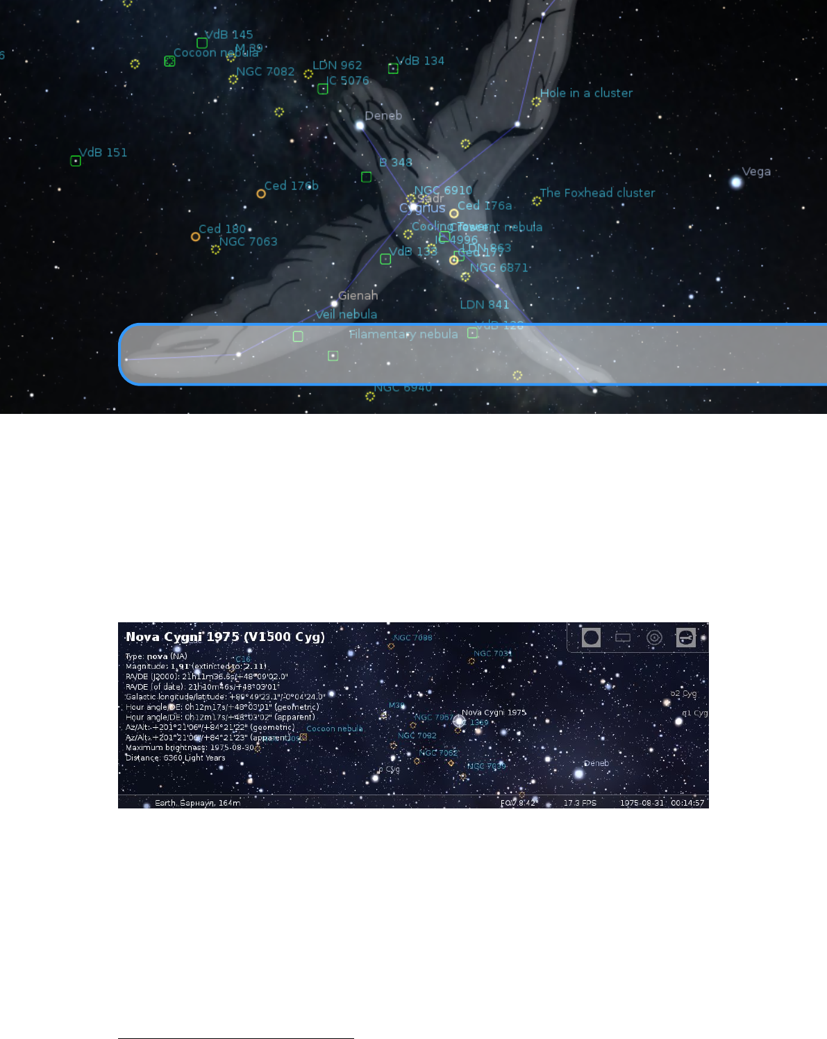
13. Object Catalog Plugins
Several plugins provide users with some more object classes.
13.1 Bright Novae Plugin
Figure 13.1: Nova Cygni 1975 (also known as V1500 Cyg)
The Bright Novae plugin provides visualization of some bright novae in the Milky Way galaxy. If
enabled (see section 11.1), bright novae from the past will be presented in the sky at the correct
times. For example, set date and time to 30 August 1975, look at the constellation Cygnus to see
Nova Cygni 19751(Fig. 13.1).
13.1.1 Section Novaein config.ini file
You can edit
config.ini
file by yourself for changes of the settings for the Bright Novae plugin –
just make it carefully!
1http://en.wikipedia.org/wiki/V1500_Cygni

118 Chapter 13. Object Catalog Plugins
ID Type Description
last_update string Date and time of last update
update_frequency_days int Frequency of updates, in days
updates_enable bool Enable updates of bright novae catalog from Internet
url string URL of bright novae catalog
13.1.2 Format of bright novae catalog
To add a new nova, open a new line after line 5 and paste the following, note commas and brackets,
they are important:
" Nova ␣ d esign atio n ":
{
" name " : " name ␣ of ␣ nova " ,
" type " : " type ␣ of ␣ nova " ,
" maxM agn itude ": value of maximal visual magnitude ,
" minM agn itude ": value of minimal visual magnitude ,
" peakJD " : JD for maximal visual magnitude ,
" m2 ": Time to d ecli ne by 2 mag from ma ximu m ( in days ) ,
" m3 ": Time to d ecli ne by 3 mag from ma ximu m ( in days ) ,
" m6 ": Time to d ecli ne by 6 mag from ma ximu m ( in days ) ,
" m9 ": Time to d ecli ne by 9 mag from ma ximu m ( in days ) ,
" distance ": value of distance between nova and
Earth ( in thousands of Light Years ) ,
" RA ": " Right ␣ asc ension ␣( J2000 ) ",
" Dec " : " Declination ␣( J2000 ) "
},
For example, the record for Nova Cygni 1975 (V1500 Cyg) looks like:
" V15 00 ␣ Cyg " :
{
" name " : " Nova ␣ Cygni ␣ 1975 " ,
" ty pe " : " NA " ,
" maxM agn itude ": 1.69 ,
" minM agn itude ": 21 ,
" peakJD " : 2442655 ,
" m2 ": 2 ,
" m3 ": 4 ,
" m6 ": 32 ,
" m9 ": 2 63
" distance ": 6.36 ,
" RA ": " 21 h1 1m36 .6 s" ,
" Dec " : " 48 d09 m02 s "
},
13.1.3 Light curves
This plugin uses a very simple model for calculation of light curves for novae stars. This model is
based on time for decay by
N
magnitudes from the maximum value, where
N
is 2, 3, 6 and 9. If a
nova has no values for decay of magnitude then this plugin will use generalized values for it.
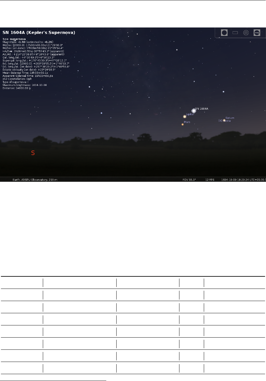
13.2 Historical Supernovae Plugin 119
13.2 Historical Supernovae Plugin
Figure 13.2: Supernova 1604 (also known as
Kepler’s Supernova
,
Kepler’s Nova
or
Kepler’s Star)
Similar to the Historical Novae plugin (section 13.1), the Historical Supernovae plugin provides
visualization of bright historical supernovae (Fig. 13.2) from the table below. If enabled (see
section 11.1), bright supernovae from the past will be presented in the sky at the correct times. For
example, set date and time to 29 April 1006, and look at the constellation Lupus to see SN 1006A.
13.2.1 List of supernovae in default catalog
Supernova Date of max. brightness Max. apparent mag. Type Name
SN 185A27 December -6.0 Ia
SN 386A 24 April 1.5 II
SN 1006A329 April -7.5 I
SN 1054A43 July -6.0 II
SN 1181A54 August -2.0 II
SN 1572A65 November -4.0 I Tycho’s Supernova
SN 1604A78 October -2.0 I Kepler’s Supernova
2https://en.wikipedia.org/wiki/SN_185
3https://en.wikipedia.org/wiki/SN_1006
4https://en.wikipedia.org/wiki/SN_1054
5https://en.wikipedia.org/wiki/SN_1181
6https://en.wikipedia.org/wiki/SN_1572
7https://en.wikipedia.org/wiki/SN_1604

120 Chapter 13. Object Catalog Plugins
SN 1680A815 August 6.0 IIb Cassiopeia A
SN 1885A917 August 5.8 IPec S Andromedae
SN 1895B 5 July 8.0 I
SN 1919A 14 March 11.0 I
SN 1920A 17 December 11.7 II
SN 1921C 11 December 11.0 I
SN 1937C 21 August 8.5 Ia
SN 1937D 15 September 11.87 Ia
SN 1960F 21 April 11.6 Ia
SN 1960R 19 December 12.0 I
SN 1961H 8 May 11.8 Ia
SN 1962M 26 November 11.5 II
SN 1965I 19 Juni 11.8 Ia
SN 1966J 2 December 11.3 I
SN 1968L 12 July 11.9 IIP
SN 1970G 30 July 11.4 IIL
SN 1971I 29 May 11.9 Ia
SN 1972E10 8 May 8.4 Ia
SN 1974G 27 April 11.8 Ia
SN 1979C 15 April 11.6 IIL
SN 1980K 31 October 11.6 IIL
SN 1981B 9 March 12.0 Ia
SN 1983N 17 July 11.4 Ib
SN 1986G 12 May 11.44 Ia Pec
SN 1987A11 24 February 2.9 IIPec
SN 1989B 6 February 11.9 Ia
SN 1991T 26 April 11.6 IaPec
SN 1993J12 30 March 10.8 IIb
SN 1994ae 12 January 12.0 Ia
SN 1994D 31 March 11.8 Ia
SN 1998bu 21 May 11.9 Ia
SN 2004dj 31 July 11.3 IIP
SN 2004et 2 October 11.57 II
SN 2011fe13 13 September 10.06 Ia
SN 2012cg 6 Juni 11.954 Ia
SN 2012fr 16 November 11.95 Ia
SN 2013aa 13 February 11.9 Ia
SN 2014j 30 January 10.5 Ia
8https://en.wikipedia.org/wiki/Cassiopeia_A
9https://en.wikipedia.org/wiki/S_Andromedae
10https://en.wikipedia.org/wiki/SN1972e
11https://en.wikipedia.org/wiki/SN_1987A
12https://en.wikipedia.org/wiki/SN_1993J
13https://en.wikipedia.org/wiki/SN_2011fe
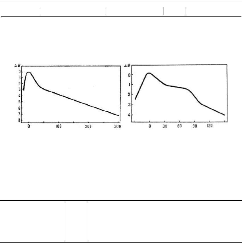
13.2 Historical Supernovae Plugin 121
SN 2017cbv 22 March 11.5 Ia
13.2.2 Light curves
In this plugin a simple model of light curves for different supernovae has been implemented
(Figure 13.3). While Type I supernovae show a peak and slow but steady decay, Type II supernovae
show a longer “plateau” in the decay curve.
Figure 13.3: Light Curves of Supernovae Types I (left) and II (right)
In both images for light curves the maximum brightness is marked as day 0.
13.2.3 Section Supernovaein config.ini file
You can edit
config.ini
file by yourself for changes of the settings for the Historical Supernovae
plugin – just make it carefully!
ID Type Description
last_update string Date and time of last update
update_frequency_days int Frequency of updates, in days
updates_enable bool Enable updates of bright novae catalog from Internet
url string URL of bright novae catalog

122 Chapter 13. Object Catalog Plugins
13.2.4 Format of historical supernovae catalog
To add a new nova, open a new line after line 5 and paste the following, note commas and brackets,
they are important:
" Supernova ␣ designation " :
{
" type " : " type ␣ of ␣ s uperno va " ,
" maxM agn itude ": value of maximal visual magnitude ,
" peakJD " : JD for maximal visual magnitude ,
" alpha ": " Right ␣ ascension ␣( J2000 )" ,
" delta ": " Declin atio n ␣( J2000 ) ",
" distance ": value of distance between supernova and
Earth ( in thousands of Light Years ) ,
" note " : " notes ␣ for ␣ su pern ova "
},
For example, the record for SN 1604A (Kepler’s Supernova) looks like:
" 1604 A ":
{
" type " : "I" ,
" maxM agn itude ": -2,
" peakJD " : 2307190 ,
" a lpha " : " 17 h3 0m 36 .00 s " ,
" d elta " : " -21 d2 9m00 .0 s " ,
" distance ": 14 ,
" note " : " Kepler ’s␣ Super nova "
},
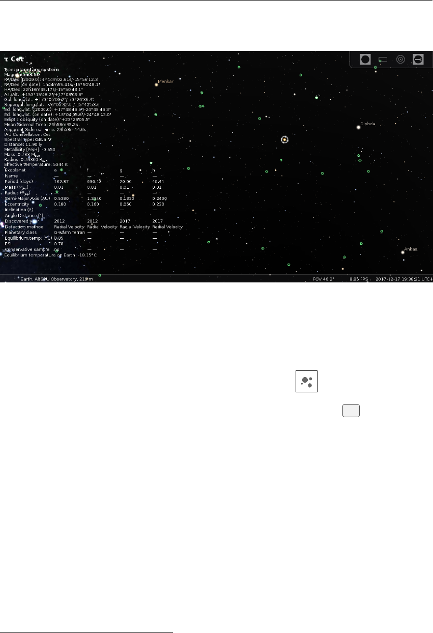
13.3 Exoplanets Plugin 123
13.3 Exoplanets Plugin
Figure 13.4: Planetary system τCeti
This plugin plots the position of stars with exoplanets. Exoplanets data is derived from “The
Extrasolar Planets Encyclopaedia”
14
. List of potential habitable exoplanets and data about them
were taken from “The Habitable Exoplanets Catalog”
15
by the Planetary Habitability Laboratory
16
.
If enabled (see section 11.1), just click on the Exoplanet button on the bottom toolbar to
display markers for the stars with known exoplanets. You can then either click on such a marked
star or find the stars with exoplanets by their designation (e.g., 24 Sex) in the F3 dialog (see 4.5).
13.3.1 Potential habitable exoplanets
This plugin can display potential habitable exoplanets (orange marker) and some information about
those planets.
Planetary Class
Planet classification from host star spectral type (F, G, K, M; see section 18.2.4),
habitable zone (hot, warm, cold) and size (miniterran, subterran, terran, superterran, jovian,
neptunian) (Earth = G-Warm Terran).
Equilibrium Temperature The planetary equilibrium temperature17 is a theoretical temperature
(in ◦C) that the planet would be at when considered simply as if it were a black body being
heated only by its parent star (assuming a 0.3 bond albedo). As example the planetary
equilibrium temperature of Earth is -18.15◦C (255 K).
Earth Similarity Index (ESI)
Similarity to Earth
18
on a scale from 0 to 1, with 1 being the
most Earth-like. ESI depends on the planet’s radius, density, escape velocity, and surface
temperature.
14http://exoplanet.eu/
15http://phl.upr.edu/projects/habitable-exoplanets-catalog
16http://phl.upr.edu/home
17http://lasp.colorado.edu/~bagenal/3720/CLASS6/6EquilibriumTemp.html
18http://phl.upr.edu/projects/earth-similarity-index-esi

124 Chapter 13. Object Catalog Plugins
13.3.2 Proper names
In December 2015, the International Astronomical Union (IAU) has officially approved names for
several exoplanets after a public vote.
Veritate
* (14 And) – From the latin Veritas, truth. The ablative form means where there is truth
19
.
Spe * (14 And b) – From the latin Spes, hope. The ablative form means where there is hope.
Musica (18 Del) – Musica is Latin for music.
Arion
(18 Del b) – Arion was a genius of poetry and music in ancient Greece. According to
legend, his life was saved at sea by dolphins after attracting their attention by the playing of
his kithara.
Fafnir (42 Dra) – Fafnir was a Norse mythological dwarf who turned into a dragon.
Orbitar
(42 Dra b) – Orbitar is a contrived word paying homage to the space launch and orbital
operations of NASA.
Chalawan (47 UMa) – Chalawan is a mythological crocodile king from a Thai folktale.
Taphao Thong
(47 UMa b) – Taphao Thong is one of two sisters associated with the Thai folk
tale of Chalawan.
Taphao Kaew
(47 UMa c) – Taphao Kae is one of two sisters associated with the Thai folk tale of
Chalawan.
Helvetios
(51 Peg) – Helvetios is Celtic for the Helvetian and refers to the Celtic tribe that lived in
Switzerland during antiquity.
Dimidium
(51 Peg b) – Dimidium is Latin for half, referring to the planet’s mass of at least half
the mass of Jupiter.
Copernicus
(55 Cnc) – NICOLAUS COPERNICUS or MIKOLAJ KOPERNIK (1473-1543) was a
Polish astronomer who proposed the heliocentric model of the solar system in his book “De
revolutionibus orbium coelestium”.
Galileo
(55 Cnc b) – GALILEO GALILEI (1564-1642) was an Italian astronomer and physicist
often called the father of observational astronomy and the father of modern physics. Using
a telescope, he discovered the four largest satellites of Jupiter, and the reported the first
telescopic observations of the phases of Venus, among other discoveries.
Brahe
(55 Cnc c) – TYCHO BRAHE (1546-1601) was a Danish astronomer and nobleman who
recorded accurate astronomical observations of the stars and planets. These observations
were critical to Kepler’s formulation of his three laws of planetary motion.
Lipperhey
* (55 Cnc d) – HANS LIPPERHEY (1570-1619) was a German-Dutch lens grinder
and spectacle maker who is often attributed with the invention of the refracting telescope in
160820.
Janssen
(55 Cnc e) – JACHARIAS JANSSEN (1580s-1630s) was a Dutch spectacle maker who
is often attributed with invention of the microscope, and more controversially with the
invention of the telescope.
Harriot
(55 Cnc f) – THOMAS HARRIOT (ca. 1560-1621) was an English astronomer, mathe-
matician, ethnographer, and translator, who is attributed with the first drawing of the Moon
through telescopic observations.
Amateru
* (
ε
Tau b) – Amateru is a common Japanese appellation for shrines when they enshrine
Amaterasu, the Shinto goddess of the Sun, born from the left eye of the god Izanagi21.
Hypatia
(
ι
Dra b) – HYPATIA was a famous Greek astronomer, mathematician, and philosopher.
She was head of the Neo-Platonic school at Alexandria in the early 5th century, until
19The original name proposed, Veritas, is that of an asteroid important for the study of the solar system.
20
The original spelling of Lippershey was corrected to Lipperhey on 15.01.2016. The commonly seen
spelling Lippershey (with an s) results in fact from a typographical error dating back from 1831, thus should
be avoided.
21The name originally proposed, Amaterasu, is already used for an asteroid.

13.3 Exoplanets Plugin 125
murdered by a Christian mob in 415.
Ran
* (
ε
Eri) – Ran is the Norse goddess of the sea, who stirs up the waves and captures sailors
with her net.
AEgir
* (
ε
Eri b) – Ægir is Ran’s husband, the personified god of the ocean. Ægir and Ran both
represent the Jotuns who reign in the outer Universe; together they had nine daughters22.
Tadmor * (γCep b) – Ancient Semitic name and modern Arabic name for the city of Palmyra, a
UNESCO World Heritage Site.
Dagon (αPsA b) – Dagon was a Semitic deity, often represented as half-man, half-fish.
Tonatiuh (HD 104985) – Tonatiuh was the Aztec god of the Sun.
Meztli (HD 104985 b) – Meztli was the Aztec goddess of the Moon.
Ogma
* (HD 149026) – Ogma was a deity of eloquence, writing, and great physical strength in
the Celtic mythologies of Ireland and Scotland, and may be related to the Gallo-Roman deity
Ogmios23.
Smertrios (HD 149026 b) – Smertrios was a Gallic deity of war.
Intercrus
(HD 81688) – Intercrus means between the legs in Latin style, referring to the star’s
position in the constellation Ursa Major.
Arkas (HD 81688 b) – Arkas was the son of Callisto (Ursa Major) in Greek mythology.
Cervantes
(
µ
Ara) – Miguel de Cervantes Saavedra (1547-1616) was a famous Spanish writer
and author of “El Ingenioso Hidalgo Don Quixote de la Mancha”.
Quijote
(
µ
Ara b) – Lead fictional character from CERVANTES’s “El Ingenioso Hidalgo Don
Quixote de la Mancha”.
Dulcinea
(
µ
Ara c) — Fictional character and love interest of Don Quijote (or Quixote) in
CERVANTES’s “El Ingenioso Hidalgo Don Quixote de la Mancha”.
Rocinante
(
µ
Ara d) – Fictional horse of Don Quijote in CERVANTES’s “El Ingenioso Hidalgo
Don Quixote de la Mancha”.
Sancho
(
µ
Ara e) – Fictional squire of Don Quijote in CERVANTES’s “El Ingenioso Hidalgo Don
Quixote de la Mancha”.
Thestias
* (
β
Gem b) – Thestias is the patronym of Leda and her sister Althaea, the daughters of
Thestius. Leda was a Greek queen, mother of Pollux and of his twin Castor, and of Helen
and Clytemnestra24.
Lich
(PSR B1257+12) – Lich is a fictional undead creature known for controlling other undead
creatures with magic.
Draugr (PSR B1257+12 b) – Draugr refers to undead creatures in Norse mythology.
Poltergeist
(PSR B1257+12 c) – Poltergeist is a name for supernatural beings that create physical
disturbances, from German for noisy ghost.
Phobetor
(PSR B1257+12 d) – Phobetor is a Greek mythological deity of nightmares, the son of
Nyx, the primordial deity of night.
Titawin
(
υ
And) – Titawin (also known as Medina of Tetouan) is a settlement in northern Morocco
and UNESCO World Heritage Site. Historically it was an important point of contact between
two civilizations (Spanish and Arab) and two continents (Europe and Africa) after the
8th
century.
Saffar
(
υ
And b) – Saffar is named for ABU AL-QASIM AHMED IBN-ABD ALLAH IBN-OMAR
AL GHAFIQI IBN-AL-SAFFAR, who taught arithmetic, geometry, and astronomy in 11th
century Cordova in Andalusia (modern Spain), and wrote an influential treatise on the uses
22
Note the typographical difference between Ægir and Aegir, the Norwegian transliteration. The same
name, with the spelling Aegir, has been attributed to one of Saturn’s satellites, discovered in 2004.
23Ogmios is a name already attributed to an asteroid.
24
The original proposed name Leda is already attributed to an asteroid and to one of Jupiter’s satellites.
The name Althaea is also attributed to an asteroid.

126 Chapter 13. Object Catalog Plugins
of the astrolabe.
Samh
(
υ
And c) – Samh is named for ABU AL-QASIM ’ASBAGH IBN MUHAMMAD IBN AL-
SAMH AL-MAHRI (or Ibn al-Samh), a noted 11th century astronomer and mathematician in
the school of al Majriti in Cordova (Andalusia, now modern Spain).
Majriti
(
υ
And d) – Majriti is named for ABU AL-QASIM AL-QURTUBI AL-MAJRITI, a notable
mathematician, astronomer, scholar, and teacher in
10th
century and early
11th
century
Andalusia (modern Spain).
Libertas
* (
ξ
Aql) – Libertas is Latin for liberty. Liberty refers to social and political freedoms,
and a reminder that there are people deprived of liberty in the world even today. The
constellation Aquila represents an eagle – a popular symbol of liberty.
Fortitudo
* (
ξ
Aql b) – Fortitudo is Latin for fortitude. Fortitude means emotional and mental
strength in the face of adversity, as embodied by the eagle (represented by the constellation
Aquila).
All names with asterix mark (*) are modified based on the original proposals, to be consistent
with the IAU rules.
13.3.3 Section Exoplanetsin config.ini file
You can edit
config.ini
file by yourself for changes of the settings for the Exoplanets plugin –
just make it carefully!
ID Type Description
last_update string Date and time of last update
update_frequency_hours int Frequency of updates, in hours
updates_enable bool
Enable updates of exoplanets catalog from Inter-
net
url string URL of exoplanets catalog
flag_show_exoplanets_button bool
Enable showing button of exoplanets on bottom
bar
distribution_enabled bool Enable distribution mode of display
timeline_enabled bool Enable timeline mode of display
habitable_enabled bool Enable habitable mode of display
enable_at_startup bool
Enable displaying exoplanets at startup of the
plugin
exoplanet_marker_color R,G,B Color for marker of star with planetary system
habitable_exoplanet_marker_color R,G,B
Color for marker of star with planetary system
with potential habitable exoplanets
temperature_scale string
Temperature scale for equilibrium temperature
of exoplanets. Possible values: Kelvin,Celsius,
Fahrenheit. Default value: Celsius.

13.3 Exoplanets Plugin 127
13.3.4 Format of exoplanets catalog
To add a new exoplanet system, open a new line after line 5 and paste the following, note commas
and brackets, they are important:
" Star ␣ d esign atio n ":
{
"exoplanets":
[
{
" mass " : mass of e xoplanet (M jup ),
" ra di us ": r adius of ex opla net (R jup ) ,
" period ": period of exo plan et ( days ),
" se miA xis " : semi - m ajor axi s ( AU ) ,
" ecce ntr icity ": orbit ’ s eccentricity ,
" in clination " : orbit ’s in clinatio n ( degree ) ,
" angleDistance ": angle distance from star
(arcseconds),
" discov ered ": exoplanet disc overed year ,
" de tection Method ": " exoplanet ␣ detection ␣ method " ,
" pclass ": " planetary ␣ class " ,
" EqTemp ": equ ilibrium tempera ture (K),
" cons erv ative ": con servative or optimistic
habi tab ility of the exoplanet ,
" ESI " : Earth Simil arity Index (*100) ,
" pla netProp erName ": " proper ␣ name ␣ of ␣ planet " ,
" planet Name ": " designation ␣ of ␣ planet "
},
{
" mass " : mass of e xoplanet (M jup ),
" ra di us ": r adius of ex opla net (R jup ) ,
" period ": period of exo plan et ( days ),
" se miA xis " : semi - m ajor axi s ( AU ) ,
" ecce ntr icity ": orbit ’ s eccentricity ,
" in clination " : orbit ’s in clinatio n ( degree ) ,
" angleDistance ": angle distance from star
(arcseconds),
" discov ered ": exoplanet disc overed year ,
" de tection Method ": " exoplanet ␣ detection ␣ method " ,
" pclass ": " planetary ␣ class " ,
" EqTemp ": equ ilibrium tempera ture (K),
" cons erv ative ": con servative or optimistic
habi tab ility of the exoplanet ,
" ESI " : Earth Simil arity Index (*100) ,
" pla netProp erName ": " proper ␣ name ␣ of ␣ planet " ,
" planet Name ": " designation ␣ of ␣ planet "
}
],
" d is tan ce " : va lu e of d ista nce to star ( pc ) ,
" s ty pe " : " sp ectr al ␣ t yp e ␣ of ␣ star " ,
" smass ": value of mass of star (M sun ),

128 Chapter 13. Object Catalog Plugins
" smetal ": value of metalli city of star ,
" Vmag " : value of visual m agnitu de of star ,
" sradius " : value of radius of star ( R sun ),
" effectiveTemp ": value of effective temperature
of star ( K ) ,
" s ta rPr op erN am e " : " pro per ␣ n ame ␣ of ␣ the ␣ st ar " ,
" hasHP ": boolean ( has potential habitable planets ),
" RA ": " Right ␣ asc ension ␣( J2000 ) ",
" DE ": " Declina tion ␣( J2000 )"
},
For example, the record for 24 Sex looks like:
" 24 ␣ Sex ":
{
"exoplanets":
[
{
" mass " : 1.99 ,
" period " : 452.8 ,
" semiAxis ": 1.333 ,
" ecce ntr icity ": 0.09 ,
" angleDistance ": 0.017821 ,
" discov ered ": 2010 ,
"planetName": "b"
},
{
" mass " : 0.86 ,
" period " : 883.0 ,
" semiAxis ": 2.08 ,
" ecce ntr icity ": 0.29 ,
" angleDistance ": 0.027807 ,
" discov ered ": 2010 ,
"planetName": "c"
}
],
" distance ": 74.8 ,
" s ty pe " : " G5 " ,
" smass ": 1.54 ,
" smetal ": -0.03 ,
" Vmag " : 7.38 ,
" sradius " : 4.9 ,
"effectiveTemp": 5098,
" RA ": " 10 h 23m2 8s " ,
" DE ": " -00 d 54m 08s "
},
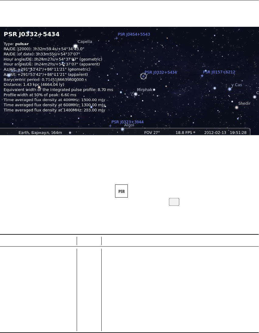
13.4 Pulsars Plugin 129
13.4 Pulsars Plugin
Figure 13.5: PSR J0332-5434
This plugin plots the position of various pulsars, with object information about each one. Pulsar
data is derived from “The Australia Telescope National Facility Pulsar Catalogue” (Manchester
et al., 2005).
If enabled (see section 11.1), use the button to activate display of pulsars. The GUI
allows a few configuration options. You can also find a pulsar (
F3
) by its designation (e.g., PSR
J0437-4715).
13.4.1 Section Pulsarsin config.ini file
ID Type Description
last_update string Date and time of last update
update_frequency_days int Frequency of updates [days]
updates_enable bool Enable updates of pulsars catalog from Internet
url string URL of pulsars catalog
enable_at_startup bool Enable displaying of pulsars at startup of Stellarium
distribution_enabled bool Enable distribution mode for the pulsars
flag_show_pulsars_button bool Enable displaying pulsars button on toolbar
marker_color R,G,B Color for marker of the pulsars
glitch_color R,G,B Color for marker of the pulsars with glitches
use_separate_colors bool Use separate colors for different types of the pulsars
130 Chapter 13. Object Catalog Plugins
13.4.2 Format of pulsars catalog
To add a new pulsar, open a new line after line 5 and paste the following, note commas and brackets,
they are important:
" Pulsar ␣ designation ":
{
" RA ": " Right ␣ asc ension ␣( J2000 ) ",
" DE ": " D ec lin ati on ␣ ( J2 000 ) " ,
" n ot es " : " t yp e ␣ of ␣ p ulsar " ,
" distance ": value of distance based on electron density
model ( kpc ) ,
" period " : value of bary centric period of the pulsar (s),
" p arallax " : value of annula r pa rall ax ( mas ) ,
" bperiod " : value of binary period of pulsar ( days ),
" pder ivative ": value of time derivative of bar cyc entric
period ,
" d meas ure " : v al ue of d is per sio n m ea sur e ( pc /( cm * cm * cm )) ,
" f requ enc y " : v al ue of b ary ce ntr ic r ota tio n f requ enc y ( Hz ) ,
" pfrequ ency ": value of time derivat ive of barycent ric
ro tat ion fr equ enc y (1/( s * s ))
" ecce ntr icity ": value of eccentricity ,
" w50 " : va lue of p rofi le wi dt h at 50% of peak ( ms ) ,
" s400 " : value of time a veraged flux density at
400 MHz ( mJy ) ,
" s600 " : value of time a veraged flux density at
600 MHz ( mJy ) ,
" s1400 ": value of time averaged flux density at
1400 MHz ( mJy )
},
For example, the record for PSR J0014+4746 looks like:
" PSR ␣ J001 4 + 47 46 " :
{
" distance ": 1.82 ,
" dmeasure ": 30.85 ,
" frequency ": 0.805997239145 ,
" pf requ ency ": -3.6669 E -16 ,
" w50 ": 88.7 ,
" s400 " : 14 ,
" s600 " : 9,
" s1400 ": 3,
" RA ": " 00 h1 4m17 .75 s " ,
" DE ": " 47 d4 6m33 .4 s"
},
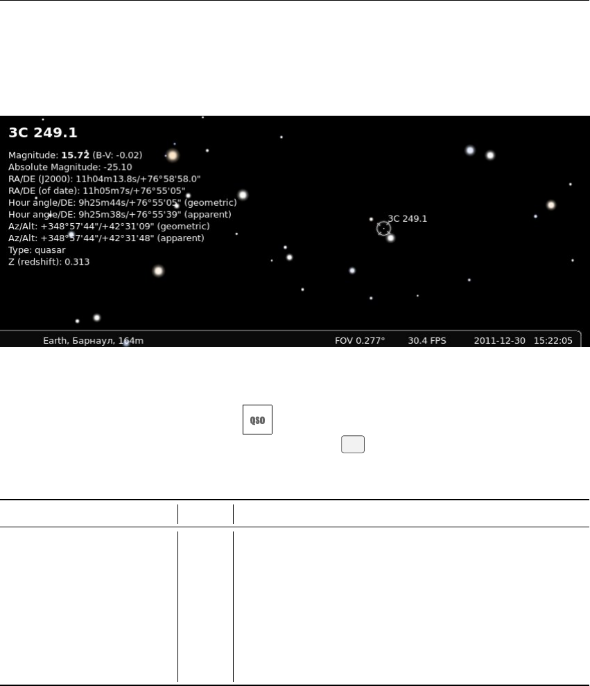
13.5 Quasars Plugin 131
13.5 Quasars Plugin
The Quasars plugin provides visualization of some quasars brighter than 16 visual magnitude. The
catalogue of quasars has been compiled from “A catalogue of quasars and active nuclei: 13th
edition” (Véron-Cetty and Véron, 2010).
Figure 13.6: 3C 249.1, also known as LEDA 2821945 or 4C 77.09
If enabled (see section 11.1), use the button to activate display of quasars. The GUI allows
a few configuration options. You can also find a quasar ( F3 ) by its designation (e.g., 3C 273).
13.5.1 Section Quasarsin config.ini file
ID Type Description
last_update string Date and time of last update
update_frequency_days int Frequency of updates, in days
updates_enable bool Enable updates of quasars catalog from Internet
url string URL of quasars catalog
enable_at_startup bool Enable displaying of quasars at startup of Stellarium
distribution_enabled bool Enable distribution mode for the quasars
flag_show_quasars_button bool Enable displaying quasars button on toolbar
marker_color R,G,B Color for marker of the quasars

132 Chapter 13. Object Catalog Plugins
13.5.2 Format of quasars catalog
To add a new quasar, open a new line after line 5 and paste the following, note commas and brackets,
they are important:
" Quasar ␣ designation ":
{
" RA ": " Right ␣ asc ension ␣( J2000 ) ",
" DE ": " D ec lin ati on ␣ ( J2 000 ) " ,
" Amag " : value of absolute magnitude ,
" Vmag " : value of visual magnitude ,
"z ": value of Z ( redshift ),
" bV ": value of B -V colo ur
},
For example, the record for 3C 249.1 looks like:
"3 C␣ 249.1 " :
{
" RA ": " 11 h0 4m13 .8 s" ,
" DE ": " +76 d5 8m58 s " ,
" Amag " : -25.1 ,
" Vmag " : 15.72 ,
"z ": 0.313 ,
" bV ": -0.02
},
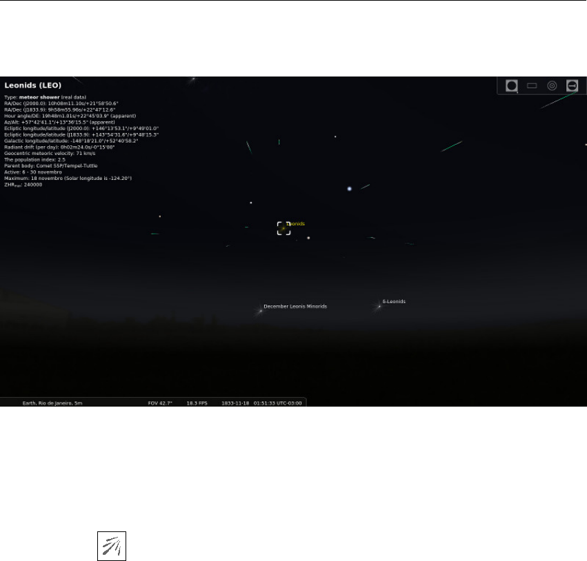
13.6 Meteor Showers Plugin 133
13.6 Meteor Showers Plugin
Figure 13.7: The 1833 Leonids replayed with the Meteor Showers plugin.
In contrast and extension of the random shooting stars feature of Stellarium (see section 18.6),
this plugin provides data for real meteor showers and a marker for each active and inactive radiant,
showing real information about its activity. If enabled (see section 11.1), just click on the Meteor
Showers button on the bottom toolbar to display markers for the radiants.
13.6.1 Terms
Meteor shower
Ameteor shower is a celestial event in which a number of meteors are observed to radiate, or
originate, from one point in the night sky. These meteors are caused by streams of cosmic debris
called meteoroids entering Earth’s atmosphere at extremely high speeds on parallel trajectories.
Most meteors are smaller than a grain of sand, so almost all of them disintegrate and never hit
the Earth’s surface. Intense or unusual meteor showers are known as meteor outbursts and meteor
storms, which may produce greater than 1,000 meteors an hour.
Radiant
The radiant or apparent radiant of a meteor shower is the point in the sky from which (to a planetary
observer) meteors appear to originate. The Perseids, for example, are meteors which appear to
come from a point within the constellation of Perseus.
An observer might see such a meteor anywhere in the sky but the direction of motion, when
traced back, will point to the radiant. A meteor that does not point back to the known radiant for a
given shower is known as a sporadic and is not considered part of that shower.
Many showers have a radiant point that changes position during the interval when it appears.
For example, the radiant point for the Delta Aurigids drifts by more than a degree per night.

134 Chapter 13. Object Catalog Plugins
Zenithal Hourly Rate (ZHR)
The Zenithal Hourly Rate (ZHR) of a meteor shower is the number of meteors a single observer
would see in one hour under a clear, dark sky (limiting apparent magnitude of 6.5) if the radiant
of the shower were at the zenith. The rate that can effectively be seen is nearly always lower and
decreases the closer the radiant is to the horizon.
Population index
The population index indicates the magnitude distribution of the meteor showers. Values below
2.5 correspond to distributions where bright meteors are more frequent than average, while values
above 3.0 mean that the share of faint meteors is larger than usual.
13.6.2 Section MeteorShowersin config.ini file
You can edit
config.ini
file by yourself for changes of the settings for the Meteor Showers
plugin – just make it carefully!
ID Type Description
last_update string Date and time of last update
update_frequency_hours int Frequency of updates, in hours
updates_enable bool
Enable updates of the meteor showers catalog from Internet
url string URL of the meteor showers catalog
flag_show_ms_button bool
Enable showing button of the meteor showers on bottom
bar
flag_show_radiants bool
Enable displaying markers for the radiants of the meteor
showers
flag_active_radiants bool
Flag for displaying markers for the radiants of the active
meteor showers only
enable_at_startup bool Enable displaying meteor showers at starup plugin
show_radiants_labels bool
Flag for displaying labels near markers of the radiants of
the meteor showers
font_size int
Font size for label of markers of the radiants of the meteor
showers
colorARG R,G,B
Color for marker of active meteor showers with generic
data
colorARR R,G,B Color for marker of active meteor showers with real data
colorIR R,G,B Color for marker of inactive meteor showers

13.6 Meteor Showers Plugin 135
13.6.3 Format of Meteor Showers catalog
To add a new meteor shower, you just need to:
1. Copy the code of some valid meteor shower;
2. Paste it in the line 6 (right after the "showers": {) of the showers.json document;
3. Replace the information according with your needs.
Note commas and brackets, they are very important! For example, below is a record for Northern
Taurids:
" NTA ":
{
" designation ": " Northern ␣ Taurids " ,
"activity":
[
{
" year " : " generic " ,
" zhr ": 5,
" start ": " 09.25 " ,
" finish ": " 11.25 " ,
" peak " : " 11.12 "
},
{
" year " : " 2014 " ,
" start ": " 10.20 " ,
" finish ": " 12.10 "
},
{
" year " : " 2013 " ,
" start ": " 10.20 " ,
" finish ": " 12.10 "
},
{
" year " : " 2012 " ,
" start ": " 10.20 " ,
" finish ": " 12.10 "
},
{
" year " : " 2011 " ,
" start ": " 10.20 " ,
" finish ": " 12.10 "
}
],
" sp ee d " : 29 ,
" r adi an tAl pha ": " 58 " ,
" radi ant Delta ": "+22 ",
"driftAlpha": "5",
"driftDelta": "1",
" colors " :
[
{
" c ol or " : " y ello w " ,

136 Chapter 13. Object Catalog Plugins
"intensity": 80
},
{
" color ": " white " ,
"intensity": 20
}
],
" parentObj " : " Comet ␣ C /1917 ␣ F1 ␣( Mellish )" ,
" pidx " : 2.3
},
13.6.4 Further Information
You can get more info about meteor showers here:
•
Wikipedia about Meteor showers:
https://en.wikipedia.org/wiki/Meteor_Showers
•International Meteor Organization: http://www.imo.net/
Acknowledgements
This plugin was created as project of ESA Summer of Code in Space 201325.
25http://sophia.estec.esa.int/socis2013/?q=about
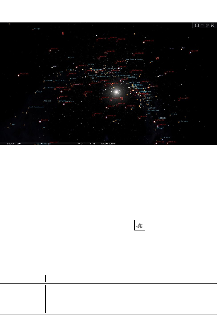
13.7 Navigational Stars Plugin 137
13.7 Navigational Stars Plugin
Figure 13.8: Navigational stars on the screen
This plugin marks navigational stars from a selected set:
Anglo-American
— the 57 "selected stars" that are listed in The Nautical Almanac
26
jointly
published by Her Majesty’s Nautical Almanac Office and the US Naval Observatory since
1958; consequently, these stars are also used in navigational aids such as the 2102-D Star
Finder27 and Identifier.
French
— the 81 stars that are listed in the Ephémérides Nautiques published by the French
Bureau des Longitudes.
Russian — the 160 stars that are listed in the Russian Nautical Almanac.
If enabled (see section 11.1), just click on the Sextant button on the bottom toolbar to display
markers for the navigational stars. This can help you in training your skills in astronomical
navigation before you cruise the ocean in the traditional way, with your sextant and chronometer.
13.7.1 Section NavigationalStarsin config.ini file
You can edit
config.ini
file by yourself for changes of the settings for the Navigational Stars
plugin – just make it carefully!
ID Type Description
navstars_color R,G,B Color of markers of navigational stars
enable_at_startup bool Set to true to display navigational stars at startup of planetarium
current_ns_set string
Current set of navigational stars. Possible values: AngloAmerican,
French and Russian.
26The Nautical Almanac website – http://aa.usno.navy.mil/publications/docs/na.php
27
Rude Starfinder 2102-D description and usage instruction –
http://oceannavigation.blogspot.
ru/2008/12/rude-starfinder-2102-d.html
138 Chapter 13. Object Catalog Plugins
13.8 Satellites Plugin
The Satellites plugin displays the positions of artifical satellites in Earth’s orbit based on a catalog
of orbital data. It allows automatic updates from online sources and manages a list of update file
URLs.
To calculate satellite positions, the plugin uses an implementation of the SGP4/SDP4 algorithms
(J.L. Canales’
gsat
library), using as its input data in NORAD’s two-line element set (TLE
28
)
format. Lists with TLEs for hundreds of satellites are available online and are regularly updated.
The plugin downloads the lists prepared by
http://celestrak.com
to keep itself up-to-date, but
the users can specify other sources online or load updates from local files.
If enabled (see section 11.1), just click on the Satellite button on the bottom toolbar to
display markers for the satellites.
It should now be possible to search for artificial satellites using the regular search dialog (
F3
).
Note that at any given time, most Satellites will be below the horizon.
Figure 13.9: Configuration of the Satellites plugin.
13.8.1 Satellite Properties
Name and identifiers
Each satellite has a name. It’s displayed as a label of the satellite hint and
in the list of satellites. Names are not unique though, so they are used only for presentation
purposes.
Satellite Catalog
In the Satellite Catalog satellites are uniquely identified by their NORAD
number, which is encoded in TLEs.
Grouping
A satellite can belong to one or more groups such as “amateur”, “geostationary” or
“navigation”. They have no other function but to help the user organize the satellite collection.
Group names are arbitrary strings defined in the Satellite Catalog for each satellite and are
more similar to the concept of tags than a hierarchical grouping. A satellite may also not
belong to any group at all.
By convention, group names are in lowercase. The GUI translates some of the groups used
in the default catalog.
28TLE: https://en.wikipedia.org/wiki/Two-line_element_set
13.8 Satellites Plugin 139
13.8.2 Iridium Flares prediction
The Satellite plugin might predict Iridium flares for the current location up to 2 weeks in the future
from the current moment. The calculations of visual magnitude based on standard magnitude,
orientation of satellite and places an observer and Sun. Of course all predictions can be saved in the
CSV file (Figure 13.10).
Figure 13.10: Prediction of Iridium flares in the Satellites plugin.
13.8.3 Satellite Catalog
The satellite catalog is stored on the disk in JSON
29
format, in a file named
satellites.json
. A
default copy is embedded in the plug-in at compile time. A working copy is kept in the user data
directory.
To add a new satellite, open a new line after line 5 and paste the following, note commas and
brackets, they are important:
" NO RAD ␣ n umbe r ":
{
" na me ": " name ␣ of ␣ the ␣ sat el lite "
" d escr ip ti on " : " de sc ri ptio n ␣ go es ␣ here " ,
" co mms " : [
{
" d e sc ri p ti on " : " d ow n li nk ␣ 1 " ,
" fre que ncy ": 437.49 ,
" m odul at io n ": " AFSK ␣ 1200 ␣ bps "
},
{
" d e sc ri p ti on " : " d ow n li nk ␣ 2 " ,
" fre que ncy ": 145.825
}
],
" gr oups " : [ " gro up1 ", " gro up2 " ],
" st dMag " : 2.0 ,
" tl e1 ": " 1␣ 1234 5 U␣ 9 000 5 D␣ ␣␣ 090 80 .8 52 36 26 5 ␣␣ .00 00 0014 ␣ ␣ 00000 -0 ␣ ␣ 20602 -4 ␣ 0␣␣ 5 632 " ,
" tle2 ": "2␣ 12345 ␣ 98.2700 ␣ ␣ 53 .27 02 ␣ 001 191 8 ␣␣ 7 1.1 776 ␣ 28 9.07 05 ␣ 14.3 1818 920 ␣ ␣␣ 653 ",
" vi sibl e ": true
},
29http://www.json.org/

140 Chapter 13. Object Catalog Plugins
Explanation of the fields:
NORAD number
required parameter, surrounded by double quotes (
"
), followed by a colon (
:
).
It is used internally to identify the satellite. You should replace the text
"NORAD number"
with the first number on both lines of the TLE set (in this case,
"12345"
). It must match
the number of the satellite in the source you are adding from if you want the TLE to be
automatically updated.
The remaining parameters should be listed between two curly brackets and the closing curly bracket
must be followed by a comma to separate it from the next satellite in the list:
name
required parameter. It will be displayed on the screen and used when searching for the
satellite with the Find window. Use the description field for a more readable name if you like.
(The description field can accept HTML tags such as
<br/>
(new line),
<b></b>
(bold),
etc.)
description optional parameter, double quoted. Appears when you click on the satellite
comms
optional parameter, square bracketed list of curly bracketed communications information.
groups
optional parameter, comma separated list of double quoted group names contained in
square brackets. Used for grouping satellites in the drop down box on the config (see above)
tle1 required, line 1 of the TLE, must be contained in double quotes and begin with "1 "
tle2 required, line 2 of the TLE, must be contained in double quotes and begin with "2 "
visible
required parameter, set to true if you want to see it, this can be toggled from the configura-
tion window once the satellite is loaded.
stdMag optional parameter, contained standard magnitude of satellite.
You can edit the tags for a satellite, modify the description and comms data, and even add new
satellites.
13.8.4 Configuration
The plug-in’s configuration data is stored in Stellarium’s main configuration file.
13.8.5 Sources for TLE data
Celestrak 30
used as default update source, it also has TLE lists beyond those included by default
in Satellite plug-in
TLE.info 31
Space Track 32
the definitive source, requires signup, operated by United States Department of
Defense
30http://celestrak.com/NORAD/elements/
31http://www.tle.info/joomla/index.php
32http://www.space-track.org/
13.9 ArchaeoLines Plugin 141
13.9 ArchaeoLines Plugin
GEORG ZOTTI
Figure 13.11: Declination Lines provided by the ArchaeoLines plugin
13.9.1 Introduction
In the archaeoastronomical literature, several astronomically derived orientation schemes are
prevalent. Often prehistorical and historical buildings are described as having been built with a
main axis pointing to a sunrise on summer or winter solstice. There can hardly be a better tool than
Scenery3D (see chapter 14) to investigate a 3D model of such a building, and this plugin has been
introduced in version 0.13.3 as a further tool in the archaeoastronomer’s toolbox (Zotti, 2016b).
When activated (see section 11.1), you can find a a tool bar button (in the shape of a
trilithon with the sun shining through it). Press this, or
Ctrl +U
, to display the currently selected
set of characteristical diurnal arcs.
13.9.2 Characteristic Declinations
The ArchaeoLines plugin displays any combination of declination arcs
δ
most relevant to archaeo-
or ethnoastronomical studies. Of course, principles used in this context are derived from natural
observations, and many of these declinations are still important in everyday astronomy.
•Declinations of equinoxes (i.e., the equator, δ=0) and the solstices (δ=±ε)
•Declinations of the crossquarter days (days between solstices and equinoxes, δ=±ε/√2)
•Declinations of the Major Lunar Standstills (δ=±(ε+i))
•Declinations of the Minor Lunar Standstills (δ=±(ε−i))
•Declination of the Zenith passage (δ=ϕ)
•Declination of the Nadir passage (δ=−ϕ)
•Declination δof the currently selected object
•Current declination δÀof the sun
•Current declination δÁof the moon
•Current declination δPof a naked-eye planet
142 Chapter 13. Object Catalog Plugins
0 10 20 30 40 50 60 70 80 90 100 110 120 130 140 150 160 170 180
0
5
10
15
20
25
30
35
40
45
50
55
60
65
70
75
0
5
10
15
20
25
30
35
40
45
50
55
60
65
70
75
Solstices, Equinoxes
Solar Crossquarters
Major Standstills
Minor Standstills
Zenith Passage
Nadir Passage
Rising Azimuths, Year 2000
Figure 13.12: Rising azimuths of a few important events for sun and moon, and zenith and
nadir passages depending on geographic latitudes (vertical axis).
The principal relation between declinations
δ
, geographic latitude
ϕ
, and the rising azimuth
A
is computed from
cosA=−sinδ
cosϕ.(13.1)
This formula does not take into account local horizon elevation nor atmospheric refraction nor
lunar parallax correction. The effect applied to characteristic declinations is shown graphically for
the present time (J2000.0) in figure 13.12. For example, in a latitude of 30◦, an object which goes
through the zenith rises at azimuth 55
◦
. Lunar major standstill risings occur at azimuths 56.7
◦
and
123.5
◦
, lunar minor standstill risings at azimuths 69
◦
and 111
◦
. The summer sun rises at 62.6
◦
, the
winter sun at 117.3◦. An object which goes through the nadir rises at 125◦.
The blue lines seem to vanish at
ϕ=45◦
: while there are still objects going through the zenith
in higher latitudes, they are circumpolar and do not cross the horizon.
For the lunar events, there are two lines each drawn by the plugin, for maximum and minimum
distance of the moon. The lunar extreme declinations are computed taking horizon parallax effects
into account. For technical reasons however, the derived declinations are then used to draw small
circles of constant declinations on the sphere, without taking the change of lunar horizontal parallax
into account. Note that therefore the observed declination of the moon at the major standstill can
exceed the indicated limits if it is high in the sky. The main purpose of this plugin is however to
show an indication of the intersection of the standstill lines with the horizon.
It may be very instructive to let the time run quite fast and observe the declination line of
“current moon” swinging between its north and south limits each month. These limits grow and
shrink between the Major and Minor Standstills in the course of 18.6 years.
13.9 ArchaeoLines Plugin 143
The sun likewise swings between the solstices. Over centuries, the solstice declinations very
slightly move as well due to the slightly changing obliquity of the ecliptic.
13.9.3 Azimuth Lines
Some religions, e.g., Islam or Bahai, adhere to a practice of observing a prayer direction towards a
particular location. Azimuth lines for two locations can be shown, these lines indicate the great
circle direction towards the locations which can be edited in the configuration window. Default
locations are Mecca (Kaaba) and Jerusalem. The azimuth
q
towards a location
T= (λT,ϕT)
can
be computed for an observer at
O= (λO,ϕO)
based on spherical trigonometry on a spherical
Earth (Abdali, 1997) as
q=arctan sin(λT−λO)
cosϕOtanϕT−sinϕOcos(λT−λO)(13.2)
In addition, up to two vertical lines with arbitrary azimuth and custom label can be shown.
13.9.4 Arbitrary Declination Lines
Up to two arbitrary declination lines can be shown with a custom label. 0.15.1
13.9.5 Configuration Options
The configuration dialog allows the selection of the lines which are of interest to you. In addition,
you can select the color of the lines by clicking on the color swatches.33
Section ArchaeoLinesin config.ini file
Apart from changing settings using the plugin configuration dialog, you can also edit
config.ini
file by yourself for changes of the settings for the ArchaeoLines plugin – just make it carefully!
ID Type Default
enable_at_startup bool false
color_equinox float R,G,B 1.00,1.00,0.50
color_solstices float R,G,B 1.00,1.00,0.25
color_crossquarters float R,G,B 1.00,0.75,0.25
color_major_standstill float R,G,B 0.25,1.00,0.25
color_minor_standstill float R,G,B 0.20,0.75,0.20
color_zenith_passage float R,G,B 1.00,0.75,0.75
color_nadir_passage float R,G,B 1.00,0.75,0.75
color_selected_object float R,G,B 1.00,1.00,1.00
color_current_sun float R,G,B 1.00,1.00,0.75
color_current_moon float R,G,B 0.50,1.00,0.50
color_current_planet float R,G,B 0.25,0.80,1.00
color_geographic_location_1 float R,G,B 0.25,1.00,0.25
color_geographic_location_2 float R,G,B 0.25,0.25,1.00
color_custom_azimuth_1 float R,G,B 0.25,1.00,0.25
color_custom_azimuth_2 float R,G,B 0.25,0.50,0.75
33
Unfortunately, on some systems with Windows in OpenGL mode, the color dialog hides behind the
Stellarium window when in fullscreen mode. So, before editing line colors, please leave fullscreen mode!
144 Chapter 13. Object Catalog Plugins
color_custom_declination_1 float R,G,B 0.45,1.00,0.15
color_custom_declination_2 float R,G,B 0.45,0.50,0.65
show_equinox bool true
show_solstices bool true
show_crossquarters bool true
show_major_standstills bool true
show_minor_standstills bool true
show_zenith_passage bool true
show_nadir_passage bool true
show_selected_object bool true
show_current_sun bool true
show_current_moon bool true
show_current_planet string none
show_geographic_location_1 bool false
show_geographic_location_2 bool false
geographic_location_1_longitude double 39.826175
geographic_location_1_latitude double 21.4276
geographic_location_1_label string Mecca (Qibla)
geographic_location_2_longitude double 35.235774
geographic_location_2_latitude double 31.778087
geographic_location_2_label string Jerusalem
show_custom_azimuth_1 bool false
show_custom_azimuth_2 bool false
custom_azimuth_1_angle double 0.0
custom_azimuth_2_angle double 0.0
custom_azimuth_1_label string custAzi1
custom_azimuth_2_label string custAzi2
custom_altitude_1_angle double 0.0
custom_altitude_2_angle double 0.0
custom_altitude_1_label string custAlt1
custom_altitude_2_label string custAlt2
show_custom_declination_1 bool false
show_custom_declination_2 bool false
custom_declination_1_angle double 0.0
custom_declination_1_label string custDec1
custom_declination_2_angle double 0.0
custom_declination_2_label string custDec2
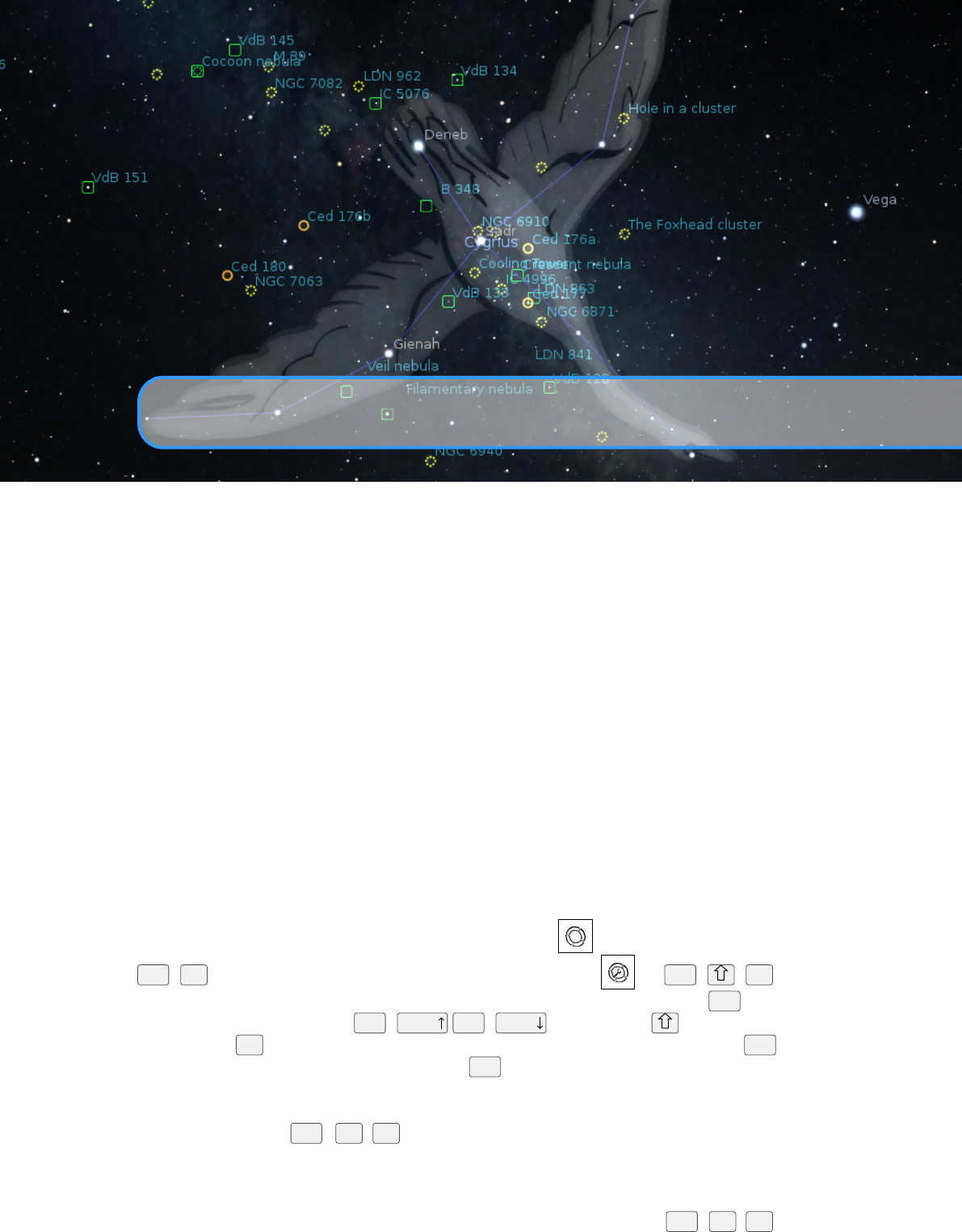
14. Scenery3d – 3D Landscapes
GEORG ZOTTI AND FLORIAN SCHAUKOWITSCH
14.1 Introduction
Have you ever wished to be able to walk through Stonehenge or other ancient building structures de-
scribed as being constructed with astronomical orientation in mind, and experience such orientation
in a 3D virtual environment that also provides a good sky simulation?
The Stellarium Scenery3d plugin allows you to see architectural 3D models embedded in a
landscape combined with the excellent representation of the sky provided by Stellarium. You can
walk around, check for (or demonstrate) possible astronomical alignments of ancient architecture,
see sundials and other shadow casters in action, etc.
14.2 Usage
You activate the plugin with the circular enclosure button at screen bottom or by pressing
Ctrl +W
. The other button with circular enclosure and tool icon (or
Ctrl + + W
) opens
the settings dialog. Once loaded and displaying, you can walk around pressing
Ctrl
plus cursor
keys. Change eye height with
Ctrl +Page
/
Ctrl +Page
keys. Adding key increases speed
by 10, adding
Alt
multiplies by 5 (pressing both keys multiplies by 50!). If you release
Ctrl
before
the cursor key, animation will continue. (Press Ctrl +any cursor key to stop moving.)
Further key bindings exist which can be configured using the Stellarium default key-binding
interface. Some options are also available in the Scenery3d dialog. For example, coordinate display
can be enabled with
Ctrl +R
+
T
. If your models are georeferenced in a true geographical
coordinate grid, e.g. UTM or Gauss-Krueger, you will especially like this, and this makes the plugin
usable for scientific purposes. Display shows grid name, Easting, Northing, Altitude of ground, and
eye height above ground.
Other features include a virtual “torchlight”, which can be enabled with
Ctrl +R
+
L
to give

146 Chapter 14. Scenery3d – 3D Landscapes
additional local illumination around the viewer to help to see in the dark. Interesting points of view
can be saved and restored later by the user, including a description of the view. Scene authors can
also distribute predefined viewpoints in their scene.
The plugin also simulates the shadows of the scene’s objects cast by the Sun, Moon and even
Venus (only 1 shadow caster used at a time, you will never see shadows cast by Venus in moonlight),
so you could use it for examining sundials, or analyze and simulate light-and-shadow interactions
in archaeological structures.
14.3 Hardware Requirements & Performance
In order to work with the non-linear projection models in Stellarium, this plugin uses a trick to
create the foreground renderings: it renders the scene into the six planes of a so-called cubemap,
which is then correctly reprojected onto the sides of a cube, depending on the current projection
settings. Your graphics card must be able to do this, i.e. it must support the OpenGL extension
called
EXT_framebuffer_object
. Typical modern 3D cards (by NVidia or ATI/AMD) support
this extension. In case your graphics hardware does not suppport it, the plugin will still work, but
you are limited to perspective projection.
You can influence rendering quality, but also speed, using the plugin’s GUI, which provides
some options such as enabling the use of shadows, bumpmapping (provides more realistic surface
lighting) or configuring the sizes of the textures used for the cubemap or shadowmaps. Larger
values there improve the quality, but require faster hardware and more video memory for smooth
results.
Because the “cubemap trick” requires quite a large amount of performance (in essence, the
scene has to be rendered 6 times), there are some options available that try to reduce this burden.
The first option is to change the type of the “cubemap”. The most compatible setting is 6 textures,
which seems to work best on older integrated Intel GPUs. The recommended default is the second
setting, Cubemap, which uses a more modern OpenGL feature and generally works a bit faster
than 6 textures on more modern graphics cards. Finally, the Geometry shader option tries to render
all 6 cube faces at once. This requires a more recent GPU + drivers (at least OpenGL 3.2 must
be supported), the setting is disabled otherwise. Depending on your hardware and the scene’s
complexity, this method may give a speedup or may be slower, you must find this out yourself.
Another option prevents re-rendering of the cubemap if nothing relevant has changed. You can
define the interval (in Stellarium’s simulation time) in which nothing is updated in the GUI. You
can still rotate the camera without causing a re-draw, giving a subjective performance that is close
to Stellarium’s performance without Scenery3d. When moving, the cubemap will be updated. You
can enable another option that only causes 1 or 2 sides of the cubemap to be updated while you
move, giving a speedup but causing some parts of the image to be outdated and discontinuous. The
cubemap will be completed again when you stop moving.
Shadow rendering may also cause quite a performance impact. The Simple shadows option
can speed this up a lot, at the cost of shadow quality especially in larger scenes. Another perfor-
mance/quality factor is shadow filtering. The sharpest (and fastest) possible shadows are achieved
with filtering Off, but depending on shadowmap resolution and scene size the shadows may look
quite “blocky”. Hardware shadow filtering is usually very fast, but may not improve appearance
a lot. Therefore, there are additional filter options available, the High filter option is relatively
expensive. Finally, the PCSS option allows to approximate the increase of solar and lunar shadow
penumbras relative to the distance from their shadow casters, i.e. shadows are sharp near contact
points, and more blurred further away. This again requires quite a bit of performance, and only
works if the shadow filter option is set to Low or High (without Hardware).
The configuration GUI shows tooltips for most of its settings, which can explain what a setting

14.4 Model Configuration 147
Geometry Yes
Lights Yes
Clay No
Photomatched Yes
DefaultUVs No
Instanced No
Table 14.1: Kerkythea Export Settings
does. All settings are saved automatically, and restored when you reopen Stellarium.
14.3.1 Performance notes
This plugin clearly runs better with proper 3D graphics cards. On reasonably good hardware (tested
on a notebook PC with NVidia M960), models with over 10.000.000 triangles are working nicely
with shadows and bumpmaps, although your mileage may vary. On very small hardware like
single-board computers with native OpenGL ES2, models may be limited to 64k vertices (points).
If display is too slow, switch to perspective projection: all other projections require almost sixfold
effort! Or try the “lazy” cubemap mode and lazy updates of tiles, where the scene is only rendered
in specific timesteps or when movement happens.
14.4 Model Configuration
The model format supported in Scenery3d is Wavefront .OBJ, which is pretty common for 3D
models. You can use several modeling programs to build your models. Software such as Blender,
Maya,3D Studio Max etc. can export OBJ.
14.4.1 Exporting OBJ from Sketchup
A simple to use and cost-free modeling program is
Sketchup
, commonly used to create the 3D
buildings seen in
Google Earth
. It can be used to create georeferenced models. OBJ is not a native
export format for the standard version of
Sketchup
. If you are not willing to afford
Sketchup Pro
,
you have to find another way to export a textured OBJ model.
One good exporter is available in the
Kerkythea
renderer project
1
. You need
SU2KT 3.17
or
better, and
KT2OBJ 1.1.0
or better. Deselect any selection, then export your model to the
Kerkythea
XML format with settings shown in 14.1. (Or, with selection enabled, make sure settings are No-
Yes-Yes-No-Yes-No-No.) You do not have to launch
Kerkythea
unless you want to create nice
renderings of your model. Then, use the
KT2OBJ
converter to create an OBJ. You can delete the
XML after the conversion. Note that some texture coordinates may not be exported correctly. The
setting
Photomatched:Yes
seems now to have corrected this issue, esp. with distorted/manually
shifted textures.
Another free OBJ exporter has been made available by TIG:
OBJexporter.rb2
. This is the
only OBJ exporter tested so far capable of handling large TIN landscapes (
>450.000
triangles).
As of version 2.6 it seems to be the best OBJ exporter available for Sketchup.
This exporter swaps Y/Z coordinates, but you can add a key to the config file to correct swapped
axes, see below. Other exporters may also provide coordinates in any order of X, Y, Z – all those
can be properly configured.
1Available at http://www.kerkythea.net/cms/
2Available from http://forums.sketchucation.com/viewtopic.php?f=323&t=33448
148 Chapter 14. Scenery3d – 3D Landscapes
Another quirk has to be fixed manually though: in the material description file (MTL), TIG’s
exporter writes both
d
and
Tr
lines with the same value. Actually,
Tr =1.0−d
according to
OBJ/MTL documentation, so you should edit away one line, or else the later line overwrites the
value given earlier. Moreover, given that
Tr=1
should actually specify fully transparent objects,
such a line will make your object entirely invisible!
Another (almost) working alternative:
ObjExporter.rb
by author Honing. Here, export with
settings
0xxx00
. This will not create a
TX...
folder but dump all textures in the same directory as
the OBJ and MTL files. Unfortunately, currently some material assignments seem to be bad.
14.4.2 Notes on OBJ file format limitations
The OBJ format supported is only a subset of the full OBJ format: Only (optionally textured)
triangle meshes are supported, i.e., only lines containing statements:
mtllib
,
usemtl
,
v
,
vn
,
vt
,
f
(with three elements only!),
g
. Negative vertex numbers (i.e., a specification of relative positions)
are not supported.
A further recommendation for correct illumination is that all vertices should have vertex
normals.
Sketchup
models exported with the
Kerkythea
or TIG plugins should have correct
normals. If your model does not provide them, default normals can be reconstructed from the
triangle edges, resulting in a faceted look.
If possible, the model should also be triangulated, but the current loader may also work with
non-triangle geometry. The correct use of objects (
o
) and groups (
g
) will improve performance: it
is best if you pre-combine all objects that use the same material into a single one. The loader will
try to optimize it anyways if this is not the case, but can do this only partly (to combine 2 objects
with the same material into 1, it requires them to follow directly after each other in the OBJ). A
simple guide to use Blender3for this task follows:
1. File Import Wavefront .obj
- you may need to change the forward/up axes for correct
orientation, try “-Y forward” and “Z up”
2. Select an object which has a shared material
3. Press +Land select ’By Material’
4. Select ’Join’ in the left (main) tool window
5. Repeat for other objects that have shared materials
6.
Export the .obj, making sure to select the same forward/up axes as in the import, also make
sure “Write Normals”, “Write Materials” and “Include UVs” are checked
For transparent objects (with a
d
or
Tr
value, alpha testing does NOT need this), this recommenda-
tion does NOT hold: for optimal results, each separate transparent object should be exported as a
separate “OBJ object”. This is because they need to be sorted during rendering to achieve correct
transparency. If the objects are combined already, you can separate them using Blender:
1. Import .obj (see above)
2. Select the combined transparent object
3. Enter “Edit” mode with and make sure everything is selected (press Aif not)
4.
Press
P
and select “By loose parts”, this should separate the object into its unconnected
regions
5. Export .obj (see above), also check “Objects as OBJ Objects”
The MTL file specified by
mtllib
contains the material parameters. The minimum that should
be specified is either
map_Kd
or a
Kd
line specifying color values used for the respective faces.
But there are other options in MTL files, and the supported parameters and defaults are listed in
Table 14.2.
If no ambient color is specified, the diffuse color values are taken for the ambient color. An
optional emissive term
Ke
can be added, which is modulated to only be visible during nighttime.
3http://www.blender.org

14.4 Model Configuration 149
Parameter Default Range Meaning
Ka set to Kd values 0. .. 1 each R/G/B Ambient color
Kd 0.8 0.8 0.8 0.. .1 each R/G/B Diffuse color
Ke 0.0 0.0 0.0 0.. .1 each R/G/B Emissive color
Ks 0.0 0.0 0.0 0.. .1 each R/G/B Specular color
Ns 8.0 0. .. ∞shinyness
dor Tr 1.0 0. .. 1 opacity
bAlphatest 0 0 or 1 perform alpha test
bBackface 0 0 or 1 render backface
map_Kd (none) filename texture map to be mixed with Ka, Kd
map_Ke (none) filename texture map to be mixed with Ke
map_bump (none) filename normal map for surface roughness
illum 2 integer illumination mode in the standard MTL format.
vis_fadeIn (none) double see 14.4.5
vis_fadeOut (none) double see 14.4.5
Table 14.2: MTL parameters evaluated
This also requires the landscape’s self-illumination layer to be enabled. It allows to model self-
illuminating objects such as street lights, windows etc. It can optionally also be modulated by the
emissive texture map_Ke.
If a value for
Ks
is specified, specularity is evaluated using the Phong reflection model
4
with
Ns
as the exponential shininess constant. Larger shininess means smaller specular highlights (more
metal-like appearance). Specularity is not modulated by the texture maps. Unfortunately, some 3D
editors export unusable default value combinations for
Ks
and
Ns
.
Blender
may create lines with
Ks
=1/1/1 and
Ns
=0. This creates a look of “partial overexposed snow fields”. While the values are
allowed in the specification, in most cases the result looks ugly. Make sure to set
Ns
to 1 or higher,
or disable those two lines.
If a value for
d
or
Tr
exists, alpha blending is enabled for this material. This simulates
transparency effects. Transparency can be further controlled using the alpha channel of the
map_Kd
texture.
A simpler and usually more performant way to achieve simple “cutout” transparency effects is
alpha-testing, by setting
bAlphatest
to 1. This simply discards all pixels of the model where the
alpha value of the
map_Kd
is below the
transparency_threshold
value from
scenery3d.ini
,
making “holes” in the model. This also produces better shadows for such objects. If required, alpha
testing can be combined with “real” blending-based transparency.
Sometimes, exported objects only have a single side (“paper wall”), and are only visible from
one side when looked at in Scenery3d. This is caused by an optimization called back-face culling,
which skips drawing the back sides of objects because they are usually not visible anyway. If
possible, avoid such “thin” geometry, this will also produce better shadows on the object. As a
workaround, you can also set bBackface to 1 to disable back-face culling for this material.
The optional
map_bump
enables the use of a tangent-space normal maps
5
, which provides a
dramatic improvement in surface detail under illumination.
4https://en.wikipedia.org/wiki/Phong_reflection_model
5https://en.wikipedia.org/wiki/Normal_mapping

150 Chapter 14. Scenery3d – 3D Landscapes
14.4.3 Configuring OBJ for Scenery3d
The walkaround in your scene can use a ground level (piece of terrain) on which the observer can
walk. The observer eye will always stay “eye height” above ground. Currently, there is no collision
detection with walls implemented, so you can easily walk through walls, or jump on high towers, if
their platform or roof is exported in the ground layer. If your model has no explicit ground layer,
walk will be on the highest surface of the scenery layer. If you use the special name
NULL
as ground
layer, walk will be above zero_ground_height level.
Technically, if your model has cavities or doors, you should export your model twice. Once,
just the ground plane, i.e. where you will walk. Of course, for a temple or other building, this
includes its socket above soil, and any steps, but pillars should not be included. This plane is
required to compute eye position above ground. Note that it is not possible to walk in several floors
of a building, or in a multi-plane staircase. You may have to export several “ground” planes and
configure several scenery directories for those rare cases. For optimal performance, the ground
model should consist of as few triangles as you can tolerate.
The second export includes all visible model parts, and will be used for rendering. Of course,
this requires the ground plane again, but also all building elements, walls, roofs, etc.
If you have not done so by yourself, it is recommended to separate ground and buildings into
Sketchup layers (or similar concepts in whichever editor you are using) in order to easily switch the
model to the right state prior to exporting.
Filename recommendations:
<Temple>.skp
Name of a Sketchup Model file. (The
<>
brackets signal “use your
own name here!”) The SKP file is not used by Scenery3d, but you
may want to leave it in the folder for later improvements.
<Temple>.obj Model in OBJ format.
<Temple>_ground.obj Ground layer, if different from Model file.
OBJ export may also create folders
TX_<Temple>
and
TX_<Temple>_ground
. You can delete the
TX_<Temple>_ground folder, <Temple>_ground.obj is just used to compute vertical height.
Put the OBJ, MTL and TX directories into a subdirectory of your user directory (see sec-
tion 5.1), e.g.
<USERDATA>/Stellarium/scenery3d/<Temple>
, and add a text file into it called
scenery3d.ini (This name is mandatory!) with content described as follows.
[model]
name=<Temple>
Unique ID within all models in scenery3d directory. Recom-
mendation: use directory name.
landscape=<landscapename> Name of an available Stellarium landscape.
This is required if the landscape file includes geographical coordinates and your model does not:
First, the location coordinates of the
landscape.ini
file are used, then location coordinates given
here. The landscape also provides the background image of your scenery. If you want a zero-height
(mathematical) horizon, use the provided landscape called Zero Horizon.
scenery=<Temple>.obj The complete model, including visible ground.
ground=<Temple>_ground.obj
Optional: separate ground plane. (NULL for zero altitude.)
description=<Description> A basic scene description (including HTML tags)
The
scenery3d.ini
may contain a simple scene description, but it is recommended to use the
localizable description format: in the scene’s directory (which contains
scenery3d.ini
) create
files in the format
description.<lang>.utf8
which can contain arbitrary UTF-8–encoded
HTML content. <lang> stands for the ISO 639 language code.
author=<Your Name yourname@yourplace.com>
copyright=<Copyright Info>

14.4 Model Configuration 151
obj_order=XYZ
Use this if you have used an exporter which swaps Y/Z
coordinates. Defaults to
XYZ
, other options:
XZY
,
YZX
,
YXZ
,
ZXY,ZYX
camNearZ=0.3
This defines the distance of the camera near plane, default
0.3. Everything closer than this value to the camera can not
be displayed. Must be larger than zero. It may seem tempting
to set this very small, but this will lead to accuracy issues.
Recommendation is not to go under 0.1
camFarZ=10000 Defines the maximal viewing distance, default 10000.
shadowDistance=<val>
The maximal distance shadows are displayed. If left out, the
value from
camFarZ
is used here. If this is set to a smaller
value, this may increase the quality of the shadows that are
still visible.
shadowSplitWeight=0..1
Decimal value for further shadow tweaking. If you require
better shadows up close, try setting this to higher values. The
default is calculated using a heuristic that incorporates scene
size.
[general]
The general section defines some further import/rendering options.
transparency_threshold=0.5
Defines the alpha threshold for alpha-testing, as described
in section 14.4.2. Default 0.5
scenery_generate_normals=0
Boolean, if true normals are recalculated by the plugin,
instead of imported. Default false
ground_generate_normals=0
Boolean, same as above, for ground model. Default
false
.
[location]
Optional section to specify geographic longitude
λ
, latitude
ϕ
, and altitude. The section is required
if coord/convergence_angle=from_grid, else location is inherited from landscape.
planet = Earth
latitude = +48d31’30.4" Required if coord/convergence_angle=from_grid
longitude = +16d12’25.5" "–"
altitude =from_model|<int>
altitude (for astronomical computations) can be computed
from the model: if
from_model
, it is computed as
(zmin +
zmax)/2+orig_H
, i.e. from the model bounding box centre
height.
display_fog = 0
atmospheric_extinction_coefficient = 0.2
atmospheric_temperature = 10.0
atmospheric_pressure = -1
light_pollution = 1
[coord]
Entries in the
[coord]
section are again optional, default to zero when not specified, but are
required if you want to display meaningful eye coordinates in your survey (world) coordinate
system, like UTM or Gauss-Krüger.
grid_name=<string>
Name of grid coordinates, e.g.
"UTM 33 U
(WGS 84)"
,
"Gauss-Krüger M34"
or
"Relative to
<Center>"
This name is only displayed, there is no
evaluation of its contents.
orig_E=<double> | (Easting) East-West-distance to zone central meridian

152 Chapter 14. Scenery3d – 3D Landscapes
orig_N=<double> | (Northing) North distance from Equator
orig_H=<double> | (Height) Altitude above Mean Sea Level of model origin
These entries describe the offset, in metres, of the model coordinates relative to coordinates in a
geographic grid, like Gauss-Krüger or UTM. If you have your model vertices specified in grid
coordinates, do not specify orig_... data, but please definitely add start_... data, below.
Note that using grid coordinates without offset for the vertices is usually a bad idea for real-
world applications like surveyed sites in UTM coordinates. Coordinate values are often very large
numbers (ranging into millions of meters from equator and many thousands from the zone meridian).
If you want to assign millimetre values to model vertices, you will hit numerical problems with the
usual single-precision floating point arithmetic. Therefore we can specify this offset which is only
necessary for coordinate display.
Typically, digital elevation models and building structures built on those are survey-grid aligned,
so true geographical north for a place with geographical longitude
λ
and latitude
ϕ
will in general
not coincide with grid north, the difference is known as meridian convergence6.
γ(λ,ϕ) = arctan(tan(λ−λ0)sinϕ)(14.1)
This amount can be given in
convergence_angle
(degrees), so that your model will be rotated
clockwise by this amount around the vertical axis to be aligned with True North7.
convergen ce_a ngle = from_grid |< double >
gr id _me ri dia n = < double >|+ < int >d < int > ’< float > "
grid_meridian
is the central meridian
λ0
of grid zone, e.g. for UTM or Gauss-Krüger, and is only
required to compute convergence angle if convergence_angle=from_grid.
zero_ground_height=<double>
height of terrain outside
<Temple>_ground.OBJ
, or if
ground=NULL
. Allows smooth approach
from outside. This value is relative to the model origin, or typically close to zero, i.e., use a Z
value in model coordinates, not world coordinates! (If you want the terrain height surrounding your
model to be orig_H, use 0, not the correct mean height above sea level!) Defaults to minimum of
height of ground level (or model, resp.) bounding box.
start_E=<double>
start_N=<double>
start_H=<double> only meaningful if ground==NULL, else His derived from ground
start_Eye=<double> default: 1.65m
start_az_alt_fov=<az_deg>,<alt_deg>,<fov_deg>
initial view direction and field of view.
start_...
defines the view position to be set after loading the scenery. Defaults to center of
model boundingbox.
It is advisable to use the grid coordinates of the location of the panoramic photo (landscape) as
start_...
coordinates, or the correct coordinates and some carefully selected
start_az_alt_fov
in case of certain view corridors (temple axes, . . . ).
6http://en.wikipedia.org/wiki/Transverse_Mercator_projection
7
Note that Sketchup’s georeferencing dictionary provides a NorthAngle entry, which is
360 −
convergence_angle.

14.4 Model Configuration 153
14.4.4 Concatenating OBJ files
Some automated workflows may involve tiled landscape areas, e.g. to overcome texture limitations
or triangle count limits in simpler tools like
Sketchup
. In this case you can create separate meshes
in the same coordinate system, but you need to concatenate them. One powerful program to
assemble your parts is again Blender.
In
Blender
, import the OBJ files
File Import Wavefront .obj
. If your OBJ coordinates have
Z as vertical axis (common for terrestrial models), use “Z up”, “-Y Forward” as import settings for
the coordinate axes. The model will appear south-up. Switch on textured view if required (
Alt +
Z
). If the scene looks almost black now, reconfigure the light to be sunlight. If you have created
a VRML of some structures in
ArcScene
, export that without shifting to center, and import the
WRL file in
Blender
with default orientation “Y up”, “Z forward”. Models from other sources
may still be different. In the end, all parts should fit neatly together.
Blender
is a very powerful
program, you can enhance your model as you wish.
In the end, select all relevant parts which you want to have visible in Stellarium (click on
the lines in the outline view containing the object names to light them up gray, then Rightclick-
Select) and press
Ctrl +J
to optionally join them, then export to a single OBJ
File Export
Wavefront .obj . In the export options, apply “Selection Only”, and “-Y Forward” and “Z Up”8.
Verify the new model loads correctly, e.g. in Meshlab9!
14.4.5 Beyond 3D: Temporally evolving Models
Stellarium working as “time machine” can display the sky for any calendar date in its range of
0.16.1
valid dates. Also landscapes and human-built structures evolve. Temples are being rebuilt, changed,
re-dedicated or repurposed, new windows are cut, old windows closed. To show landscape and
buildings in the right shape for the time in question, we can make material transparent, so that parts
of the model are not displayed. To allow for archaeological uncertainties in dating construction and
destruction, we can gradually fade in and fade out the model parts in question (Zotti, Schaukowitsch,
and Wimmer, To Appear 2018).
To enable this magic, you must combine all your models into one (see section 14.4.4), export as
one OBJ/MTL as usual, and manually edit the MTL file. It is wise to give the material for the parts
in question a reasonable name that you can later identify in the MTL file. Then you simply add
one or both of the new keywords
vis_fadeIn
or
vis_fadeOut
to the material description, with 2
arguments which are the Julian days of begin and end of a phase transition. For sharp transitions,
just use the same JD dates.
# Some structure has been put up around -3100/ -3000
vis_fadeIn 588783.5 625308.5
# Fade away between 500 AD /700 AD
vis_fadeOut 1903682.5 1976732.5
14.4.6 Working with non-georeferenced OBJ files
There exists modeling software which produces nice models, but without concept of georeference.
One spectacular example is
AutoDesk PhotoFly
, a cloud application which delivers 3D models
from a bunch of photos uploaded via its program interface. This “technological preview” is in
version 2 and free of cost as of mid-2011.
The problem with these models is that you cannot assign surveyed coordinates to points in
the model, so either you can georeference the models in other applications, or you must find the
8http://blender.stackexchange.com/questions/3352/merging-multiple-obj-files
9http://www.meshlab.org
154 Chapter 14. Scenery3d – 3D Landscapes
correct transformation matrix. Importing the OBJ in
Sketchup
may take a long time for detailed
photo-generated models, and the texturing may suffer, so you can cut the model down to the
minimum necessary e.g. in
Meshlab
, and import just a stub required to georeference the model in
Sketchup.
Now, how would you find the proper orientation? The easiest chance would be with a structure
visible in the photo layer of
Google Earth
. So, start a new model and immediately
add location
from the
Google Earth
interface. Then you can import the OBJ with TIG’s importer plugin. If
the imported model looks perfect, you may just place the model into the
Sketchup
landscape and
export a complete landscape just like above. If not, or if you had to cut/simplify the OBJ to be
able to import it, you can rotate/scale the OBJ (it must be grouped!). If you see a shadow in the
photos, you may want to set the date/time of the original photos in the scene and verify that the
shadows created by
Sketchup
illuminating the model match those in the model’s photo texture.
When you are satisfied with placement/orientation, you create a
scenery3d.ini
like above with
the command Plugins ASTROSIM/Stellarium scenery3d helpers Create scenery3d.ini .
Then, you select the OBJ group, open the
Windows Ruby Console
and readout data by calling
Plugins ASTROSIM/Stellarium scenery3d helpers Export transformation of selected group .
On the Ruby console, you will find a line of numbers (the
4×4
transformation matrix) which
you copy/paste (all in one line!) into the [model] section in scenery3d.ini.
obj2grid _tr afo =< a11 > , < a12 >, < a13 >,< a14 > , < a21 >, < a22 >, < a23 > , < a24 >,
<a31 > , < a32 >,< a33 > , < a34 >, < a41 >, < a42 > , < a43 >, < a44 >
You edit the
scenery3d.ini
to use your full (unmodified)
PhotoFly
model and, if you don’t have a
panorama, take
Zero Horizon
landscape as (no-)background. It depends on the model if you want
to be able to step on it, or to declare
ground=NULL
for a constant-height ground. Run Stellarum
once and adjust the start_N,start_E and zero_ground_height.
14.4.7 Rotating OBJs with recognized survey points
If you have survey points measured in a survey grid plus an image-based model with those points
visible, you can use Meshlab to find the model vertex coordinates in the photo model, and some
other program like
CoordTrans
in the
JavaGraticule3D
suite to find either the matrix values to
enter in
scenery3d.ini
or even rotate the OBJ points. However, this involves more math than can
be described here; if you came that far, you likely know the required steps. Here it really helps if
you know how to operate automatic text processors like AWK.
14.5 Predefined views
You can also configure and distribute some predefined views with your model in a
viewpoints.ini
file. The viewpoints can be loaded and stored with the viewpoint dialog which you can call with the
button. See the provided “Sterngarten” scene for an example. These entries are not editable
by the user through the interface. The user can always save his own views, they will be saved into
the file userviews.ini in the user’s Stellarium user directory, and are editable.
[ Sto redV iews ]
si ze =<int > D efin es how many e ntri es are in this file .
Pr efix each ent ry with its index !
1/ lab el = < string > The name of this entry
1/ de sc ri pt io n = < stri ng > A d es cr ip ti on of t his entry ( can i nclu de HTML )
1/ po si ti on =< x ,y , z ,h > Th e x , y ,z gr id c oo rd in a te s
( like ori g_ * or start_ * in s cen ery3d . ini )
+ the c urr ent eye h eight h
1/ view_fov = < az_deg , alt_deg , fov_deg > The view dir ection + FOV
( li ke sta rt _az _a lt_ fo v in sc en er y3 d . ini )
14.6 Example 155
; an e xa mple for a se cond entry ( note the 2 at the be gi nn ing of each li ne !)
2/ label = Signs
2/ de scri ptio n = Two signs that d esc rib e the Ste rnga rten
2/position = 593155.2421,5333348.6304,325.7295809038 ,0.8805
2/ view_fov = 84.315399 , - 8.1 870 78 ,8 3.0 000 00
14.6 Example
Let us add a quick example here. A recent paper (Pollard, 2017) claims that the Uffington White
Horse, a geoglyph carved into a hillsite in England during the Bronze Age, may depict the mythical
“Sun Horse”, a common conception of that period.
Unfortunately, as of 2017, the official UK Lidar repository does not include the Uffington
area, so a detailed GIS-based model is not available. We could use EUdem25 data with aerial
imagery, or for a quick look, we just use
Sketchup
. Yet another unfortunate development: Trimble
declared that after the 5-year transition period from Google to Trimble is over in May 2017, terrain
modelling will be limited to
Sketchup Pro
. But note that a fresh installation comes with a 30-day
Pro trial time, this should be enough for this example.
First, locate the site in
Google Earth
at
λ=−1.56718,ϕ=51.582843
. (Or just search for
“Uffington”.) Try to identify which parts of the landscape may be visible from your site, so you
can estimate which parts of terrain should be included in the model. Open
Sketchup
, select the
meter-based “Landscape Architecture” template, add
View Toolbars. . .
: Locations. Click on the
“Add Location” button of that toolbar. Enter “Uffington” into the location search dialog. This brings
you close to our site of interest. Clip a part of terrain to import it to Sketchup. Optionally, add more
terrain.
If installed, TIG’s OBJ exporter is available from the
File
menu, or you can use
Sketchup Pro
’s
built-in OBJ export. Export
UffingtonHorse.obj
to a subdirectory
scenery3d/Uffington
in
your Stellarium user data directory. The geolocation is stored in an “AttributeDictionary”. To read
this, press
Window Ruby Console
to open the Ruby Console. Then write a few lines of Ruby to
get access to the Georeference dictionary and other data:
model = Sketchup . active_mode l
attrdicts = model . at tribute _di cti onaries
at trd ict s . each {| d |
puts " A ttrib uteD icti onar y : ␣ % s " % d. name
d . e ach_ pai r { |k , v| p ut s " ␣␣ %s =% s " % [k , v ] }
}
mod el . sh ado w_ inf o . e ac h {| k ,v | puts "␣ #{ k }␣ #{ v} "}
utm = model . point_to_ utm Geom :: Point3d . new (0 ,0 ,0)
puts (" grid_name = UTM ␣%i␣%s␣ (% s)" %
[ utm . zone_number , utm . zone_letter , model . get_da tum ])
Note the
ModelTranslation
values. Those are inches (of all units!) in the UTM reference
frame and define the model coordinate origin in world coordinates. (Actually, it uses the negative
values.) Multiplication by 2.54 gives cm, and by 0.0254, meters in the UTM coordinate system. We
will use the negatives of these values as
orig_E
,
orig_N
,
orig_H
. Additionally, we have found
information about meridian convergence correction (
Sketchup
’s
NorthAngle
), UTM zone number
etc. All this goes into our configuration file. Create this file
scenery3d.ini
with the content seen
in fig. 14.1

156 Chapter 14. Scenery3d – 3D Landscapes
[ model ]
name = U ffingt onHor se
; Either a fitting landscape or just ’ Zero Horizon ’:
landscap e = Zero Horizon
scenery = Uffing ton Horse . obj
; activate the next line if you have a separate ground layer
; gr ou nd = U ffi ng ton Hors e_gr ou nd . obj
; If model Y - a xi s poi nt s up , act ivat e the next line
;obj_order=XZY
author = Georg Zotti
co pyr igh t =( c ) 2017 Geo rg Zo tt i
descripti on = Uffington Horse may represent the Sun Horse . \
See Joshua Pollard in Antiquity 91 356(2017): 406 -20.
[location]
name = U ffingt onHor se
co untr y = UK
planetName=Earth
; Set the fo llowing to a fitt ing la ndsc ape
land scape Key = Zero Horizon
longitude=-1.56718254089355
latitude =51 .582 8432 7498 23
altitude =137
[ coord ]
grid _nam e = UTM 30 U ( WGS 84)
gridTyp e = UTM
orig_E =599 273. 0211957 8
orig_N = 5715 615.150 7910 6
orig_H = 136. 2952976 2673 6
convergence_angle=1.12284363771988
; He ig ht used out side the terrain , to not " fall ␣ off " the rim .
zero_ground_height=137
; You may want to re se t these c oord ina tes .
; Observer is set to those on loading the scenery .
start_E =599 273.021 19578
start_N =571 5615 .150 791 06
start _az_ alt _fov =50 ,10 ,83
Figure 14.1: scenery3d.ini for the Uffington example.

14.6 Example 157
Authors and Acknowledgements
Scenery3d was conceived by Georg Zotti for the ASTROSIM
10
project. A first prototype was
implemented in 2010/2011 by Simon Parzer and Peter Neubauer as student work supervised
by Michael Wimmer (TU Wien). Models for accuracy tests (Sterngarten, Testscene), and later
improvements in integration, user interaction,
.ini
option handling, OBJ/MTL loader bugfixes
and georeference testing by Georg Zotti.
Andrei Borza in 2011/12 further improved rendering quality (shadow mapping, normal map-
ping) and speed (Zotti, 2015; Zotti and Neubauer, 2012a; Zotti and Neubauer, 2012b).
In 2014–17, Florian Schaukowitsch adapted the code to work with Qt 5 and the Stellarium 0.13
codebase, replaced the renderer with a more efficient, fully shader-based system, implemented
various performance, quality and usability enhancements, and did some code cleanup. Both
Andrei and Florian were again supervised by Michael Wimmer (Zotti, 2016a; Zotti, 2016b; Zotti,
Schaukowitsch, and Wimmer, To Appear 2018).
This work has been originally created during the ASTROSIM project supported 2008-2012 by
the Austrian Science Fund (FWF) under grant number P 21208-G19.
10http://astrosim.univie.ac.at

15. Stellarium at the Telescope
Stellarium is great for indoor use on the desktop, but it is also very useful outdoors under the real
sky, and several plugins enhance its usability particularly for observers.
Two plugins are bundled with Stellarium which are designed to be used at the telescope:
Oculars (section 15.1), which provides field of view hints for telescopes, oculars and sensors, and
TelescopeControl (section 15.2), which allows you to send GOTO commands to many motorized
telescope mounts. Other GOTO telescopes are supported by external programs which you must
install separately:
StellariumScope
(section 15.5),
RTS2
(section 15.3) or
INDI
(section 15.4). This
can also help DIY hardware tinkerers who like to build their own control systems (section 15.6).
In addition, the Observability plugin (section 15.7) can be used for planning the best times to
observe your favourite objects.
15.1 Oculars Plugin
TIMOTHY REAVES,WITH ADDITIONS BY ALEXANDER WOLF
This plugin serves several purposes:
•
to see what the sky looks like through a particular combination of eyepiece, lense (Barlow or
Shapley types) and telescope. This plugin helps to get an idea of what you should see when
looking through a physical telescope, and understand why one eyepiece may be better suited
to observe a particular target than another. This can also be very useful for deciding what
telescope is best suited to a style of viewing. And with the support for binoculars, you also
have the ability to understand just about any type of optics-enhanced visual observing.
•
to show what a particular combination of camera and lens or telescope would be able to
photograph of the sky.
•
lastly, with the help of the Telrad sight, understand where object in the sky are in relation to
each other. This can be helpful for star-hopping with a non-GOTO telescope.
None of these activities can take the place of hands-on experience, but they are a good way to
supplement your visual astronomy interests.
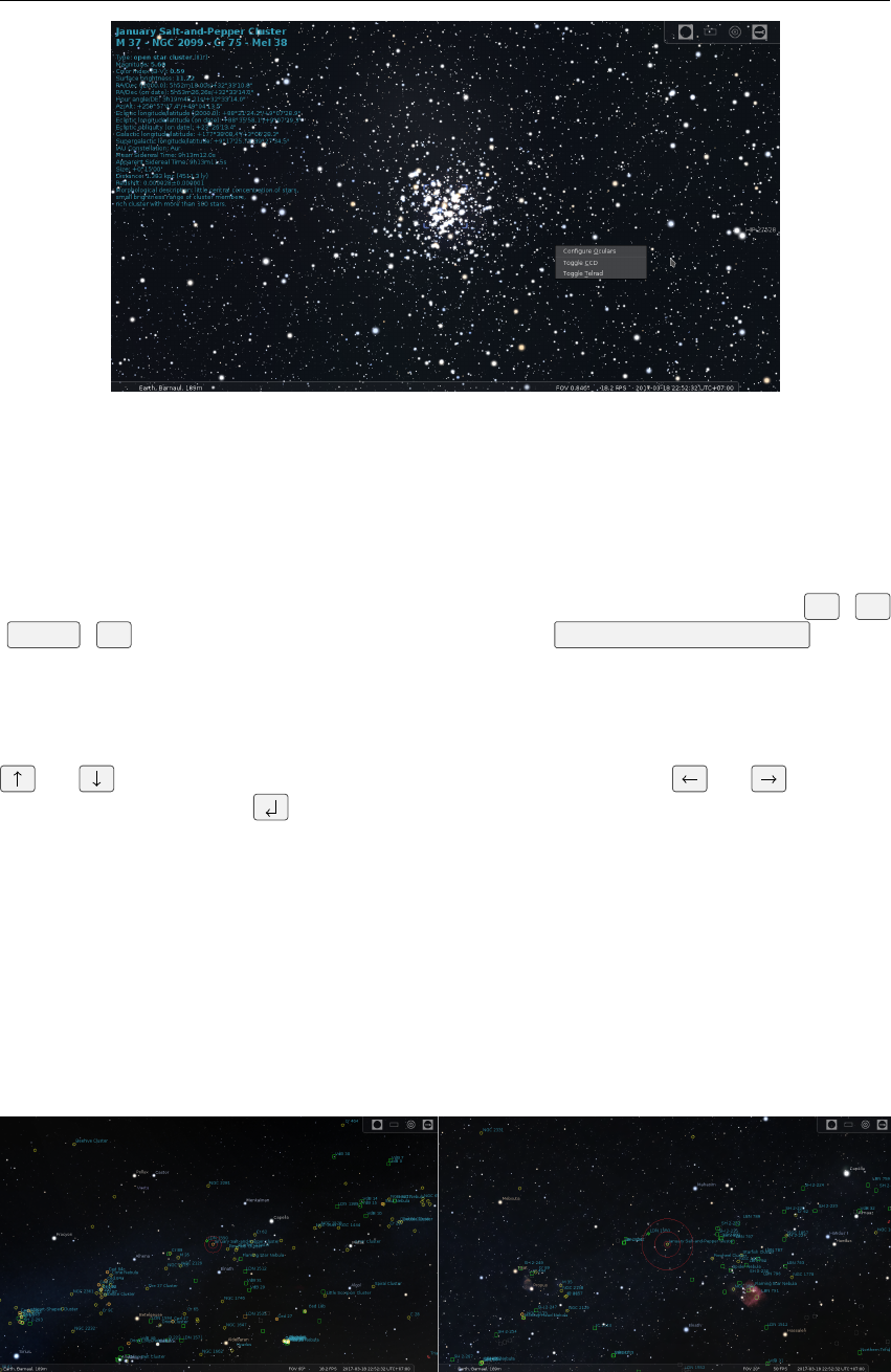
160 Chapter 15. Stellarium at the Telescope
Figure 15.1: The on-screen menu (top right) and popup menu (lower right) of the Oculars
plugin.
15.1.1 Using the Ocular plugin
The plugin is controlled through a popup menu or through an on-screen control panel (see top
right corner on screens in fig. 15.17). By default, the hot key to display the popup is
Alt +O
(
Option +O
for Mac users). This can be changed in the
Editing Keyboard Shortcuts
window
(see section 4.7.1). The menu will popup where your cursor is located.
The options available in the popup menu depend on what you are currently doing. In the default
menu, you can choose to configure the plugin, activate a CCD, or activate the Telrad finder (see
fig. 15.1). The menu is navigated by either the arrow keys on your keyboard or by your mouse. The
and arrow keys move the selection up or down the menu, and the and arrow keys
display or hide sub-menus. activates an option.
Telrad Finder
The Telrad view can be used without defining any of the items below. As a reflex sight is non-
magnifying, this feature can only be enabled when no eyepiece is selected. You still may want to
zoom in a bit to better see which stars are in the circles (fig. 15.2). The three circles that appear in
the center of the screen are
0.5◦
,
2.0◦
, and
4.0◦
in diameter. They stay centered in the screen, so
move the “telescope” (click-drag the background) to center the circles on the object of interest.
While the Telrad finder is active, you can not activate a CCD with the popup menu, but only
with the on-screen menu.
Figure 15.2: The left image is the default 60◦, and the right one is 40◦.
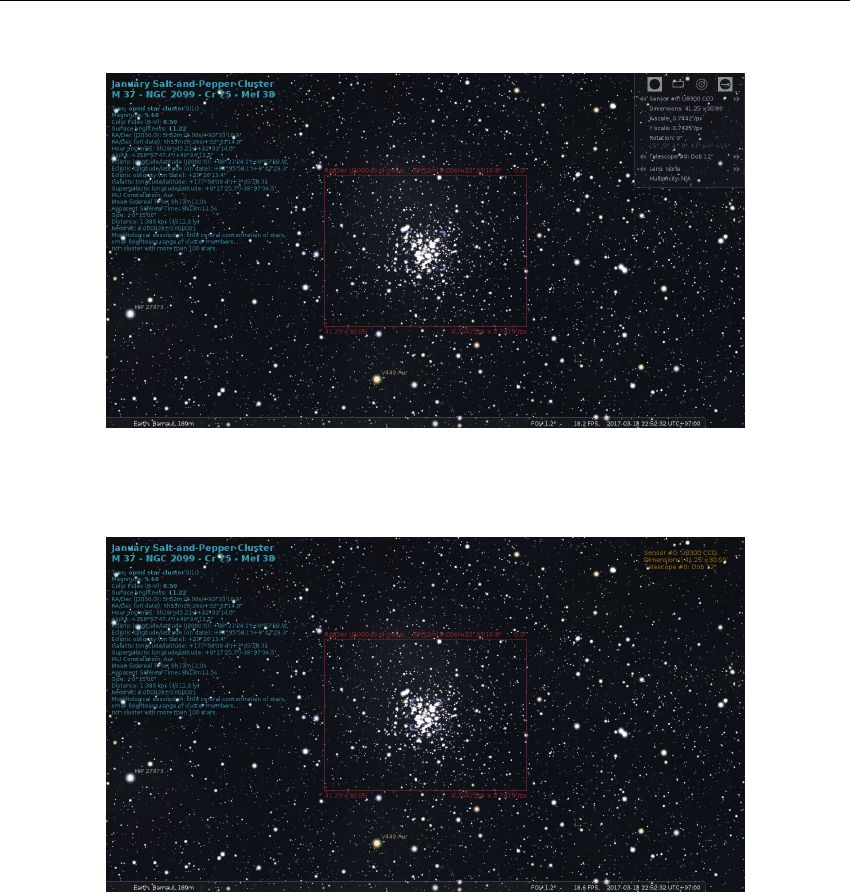
15.1 Oculars Plugin 161
CCD Sensors
Figure 15.3: View of M37 through a CCD sensor of the Oculars plugin.
Figure 15.4: View of M37 through a CCD sensor of the Oculars plugin (without on-screen
control panel).
This is a great way to get an idea of what a particular camera will be able to capture when attached
to a particular telescope or lens. For using camera lenses, you must describe them as telescope with
the appropriate values for the lens. When active, this feature will display a red bounding box of the
area that will be captured, as well as zoom in to give a better view of the surroundings. You can
manually zoom in or out from there.
The default CCD view will appear similar to fig. 15.3 or, when you are working without the
on-screen control panel, the information area in the upper right hand corner also shows angular size
captured by the CCD (see fig. 15.4).
When a CCD view is displayed, the popup menu changes as seen in fig. 15.5. You can select
what telescope to use, as well as progress to the previous or next CCD, or go to a specific CCD.
You can also rotate the CCD to better frame your subject, or to see if the CCD can be rotated in
such a way as to catch your area of interest (see fig. 15.6). Once rotated, the CCD frame on screen
displays the new orientation (see fig. 15.7).
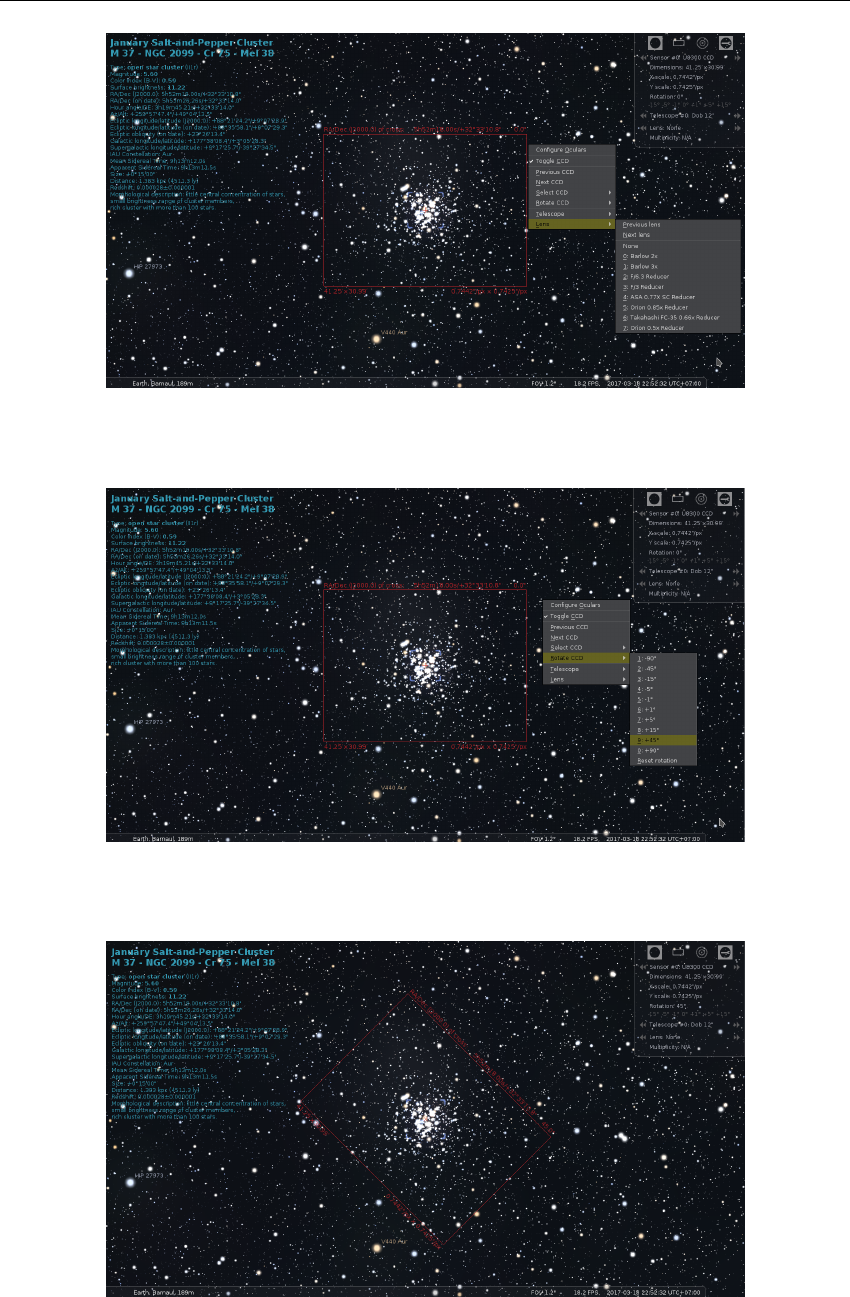
162 Chapter 15. Stellarium at the Telescope
Figure 15.5: The CCD sensor popup menu of the Oculars plugin.
Figure 15.6: Setting rotation of CCD sensor in the popup menu.
Figure 15.7: A rotated CCD sensor frame of the Oculars plugin.
15.1 Oculars Plugin 163
Oculars
•Define some eyepieces and telescope (see section 15.1.2).
•Select an object to view (i.e. a star, planet, etc.)
•
Click the toolbar button for toggling the Ocular view, or press
Ctrl +O
(
+O
for
Mac users).
•Swap between eye pieces and telescopes to see how the view changes.
This is really the area of interest to most telescopic observers. It is a great way to compare
different eyepiece/telescope combinations, to see how they change the view of the sky. And it is
easy to do so with binoculars too. To show this, let us use the M37 cluster as target. Through a pair
of Celestron 15x70 binoculars, it would look like in fig. 15.8.
Figure 15.8: The M37 cluster through a Celestron 15x70 binocular.
A very pretty sight. Now, what would it look like through a Celestron 80 mm EDF finder ’scope,
with an Explore Scientific 14 mm 100◦eyepiece? See fig. 15.9!
Figure 15.9: The M37 cluster through a Celestron 80 mm EDF with Explore Scientific
14 mm eyepiece.
Not bad at all. But we like to see more! So we move the eyepiece to a C1400. See fig. 15.10 for the
resulting view.
164 Chapter 15. Stellarium at the Telescope
Figure 15.10: The M37 cluster through a Celestron C1400 with Tele Vue Nagler 31 mm
eyepiece.
Very nice indeed! So for this target, the C1400 is going to be the best bet. However, if my
target was the Pleiades, the C1400 with that eyepiece would not be good – the 80EDF would do
much better!
When an eyepiece is active, the popup menu again changes. With a non-binocular eyepiece
selected, you also have the ability to select a particular eyepiece or telescope. When a binocular is
active, you can not select a telescope, as it is not relevant. Changing the eyepiece to a non-binocular
will again allow the telescope to be selected. Also notice that when your mouse cursor is very near
the right hand border of the screen, the popup menu’s sub-menus display to the left, not the right.
Star Scales
0.16.0
As you know from section 4.4.1, the number and relative size of stars of various magnitudes can be
adjusted to your personal preferences in the view settings window to approximate the appearance
of the stars as seen by the naked eye. Some observers prefer to have a simulated ocular view with
very small, or more, stars, quite different from what Stellarium usually shows. The Oculars plugin
therefore keeps two additional sets of scaling values for ocular views and CCD views, which are
activated automatically when you switch to ocular or CCD view, and which are stored immediately
and permanently in the plugin’s ocular.ini file.1
15.1.2 Configuration
All configuration is done through the user interface in the application. To open the configuration
dialog hit the
Alt +O
key, or click the
configure
button on the plugin setup dialog (available
in the
Plugins
tab of Stellarium’s Configuration window (opened by pressing
F2
or the
button in the left toolbar)), or the rightmost button of the on-screen panel (if displayed in the top
right corner of screen). There are six tabs in the configuration dialog: General,Eyepieces,Lenses,
Sensors,Telescopes, and About. The first five are the ones we are interested in here.
1
The appearance of stars may depend on various other factors: telescope type, ocular type, quality of
optics, seeing, . . . Such details with all combinations cannot meaningfully be stored, though. These values
should allow a rapid toggle on any single night.
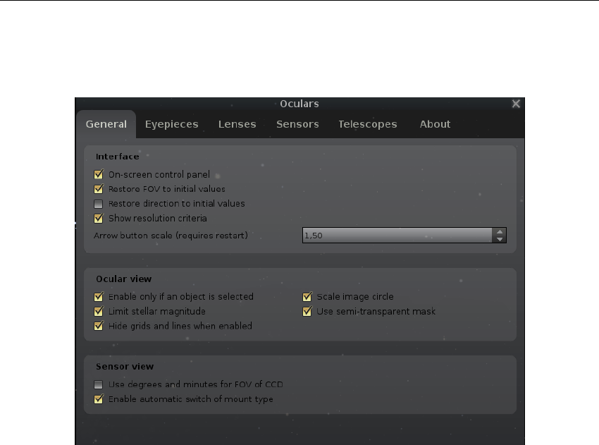
15.1 Oculars Plugin 165
General
The first option allows you to define the general behaviour of the plugin. The options are grouped
by areas of usage: Interface,Ocular view and Sensor view (see figure 15.11).
Figure 15.11: General tab of the Oculars plugin configuration dialog.
Interface: this group of options allows to change behaviour of the plugin in general.
On-screen control panel:
show an additional GUI panel in the top-right corner of the
screen to allow switching features of the plugin (in addition to the popup window).
Restore FOV to initial values and
Restore direction to initial values
options allow restoration field of view and direction of
view, resp., to the initial values at program start at the end of the plugin usage (e.g.,
when disabling the view through CCD frame).
Show resolution criteria
compute and show Rayleigh criterion, Dawes’, Abbe’s and Spar-
row’s limits for combination of telescope, lens and eyepiece. In addition, this option
will show visual resolution for selected “setup”. This option may be very helpful for
double star observers.
Arrow button scale
allows to change the size of the arrow buttons in the ocular GUI panel.
Ocular view
is a group of options that allows to change the plugin’s behaviour in visual observation
mode.
Enable only if an object is selected
– uncheck this option if you want to use the visual
observation mode when no object is selected.
Limit stellar magnitude
allows to hide faint stars, which are invisible for the selected
combination of eyepiece, lens and telescope.
Hide grids and lines when enabled
allows to hide grids and lines when you observe the
sky through the eyepiece and re-enables their visibility when leaving visual observation
mode.
Scale image circle
option allows you to define whether or not to scale the images based on
apparent FOV. When deactivated, the image circle will fill your screen. In general,
we recommend you not select this, unless you have a need to, because it can really

166 Chapter 15. Stellarium at the Telescope
reduce the image size on the screen. It can however be very useful in comparing
two eyepieces. If you set this option, the on-screen image will be scaled based on
the eyepieces and telescopes you define. See section 15.1.3 for information on what
scaling means, and why you might want to use it.
Use semi-transparent mask:
uncheck this option if you want to see visible field of view
as in real telescope.
Sensor view
is group of options allows to change behaviour of the plugin for photographic
observations mode.
Use degrees and minutes for FOV of CCD
– for many cases the use of decimal degrees
for the value of the field of view is not comfortable, and this option allows to use the
more human readable format for FOV.
Enable automatic switch of mount type
allows to store the CCD frame orientation when
the type of telescope mount is changed.
Eyepieces
This is the tab used to enter your own eyepieces (see figures 15.12 and 15.13). By default, a few
sample ones have been added; feel free to delete those once you’ve entered your own.
The fields on this tab are:
Name
– a free-text description of the eye piece. You could modify this to match your personal
descriptions of eyepieces.
aFOV – apparent field of view in degrees.
Focal Length – eyepiece focal length in mm.
Field Stop
– the field stop of the eyepiece in mm. This is used to calculate the true field of view of
an eyepiece. If you do not know what it is just leave it the default zero. Not all manufacturers
provide this value; TeleVue is one that does.
Binoculars
– selecting this checkbox tells the system that this eyepiece is binoculars or finders;
this means that this eyepiece can be used without defining a telescope.
Has permanent cross-hairs
– selecting this checkbox tells the system that this eyepiece or binoc-
ular (finder) has also simple cross-hairs2.
When Binoculars are described, the relevant fields change to
tFOV – true field of view in degrees.
Magnification factor – the magnification of the binocular.
Diameter – the diameter of the binocular objective in mm.
Lenses
This is the tab used to enter your own lenses (see figure 15.14). By default, a few sample ones have
been added; feel free to delete them once you’ve entered your own.
The fields on this tab are:
Name
– a free-text description of the lense. You could modify this to match your personal
descriptions of lenses.
Multiplier
– a factor larger than 1 expands the focal length, and lenses with this type are named
Barlow lense; a factor less than 1 reduces the focal length, and lenses with this type are
named Shapley lense or focus reducer.
Sensors
This tab allows you to define sensors for any camera you may have (see figure 15.15). When defined
and selected, this will draw a red bounding rectangle in the center of the eye piece view, showing
2
The Oculars plugin supports eyepieces with reticle patterns – both special eyepieces are available in the
default list of eyepieces, and the option Has permanent cross-hairs is not related to those eyepieces.
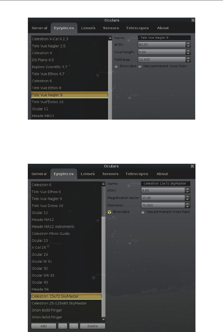
15.1 Oculars Plugin 167
Figure 15.12: Eyepieces tab of Oculars plugin configuration dialog.
Figure 15.13: Eyepieces tab of Oculars plugin configuration dialog (settings for binocular).
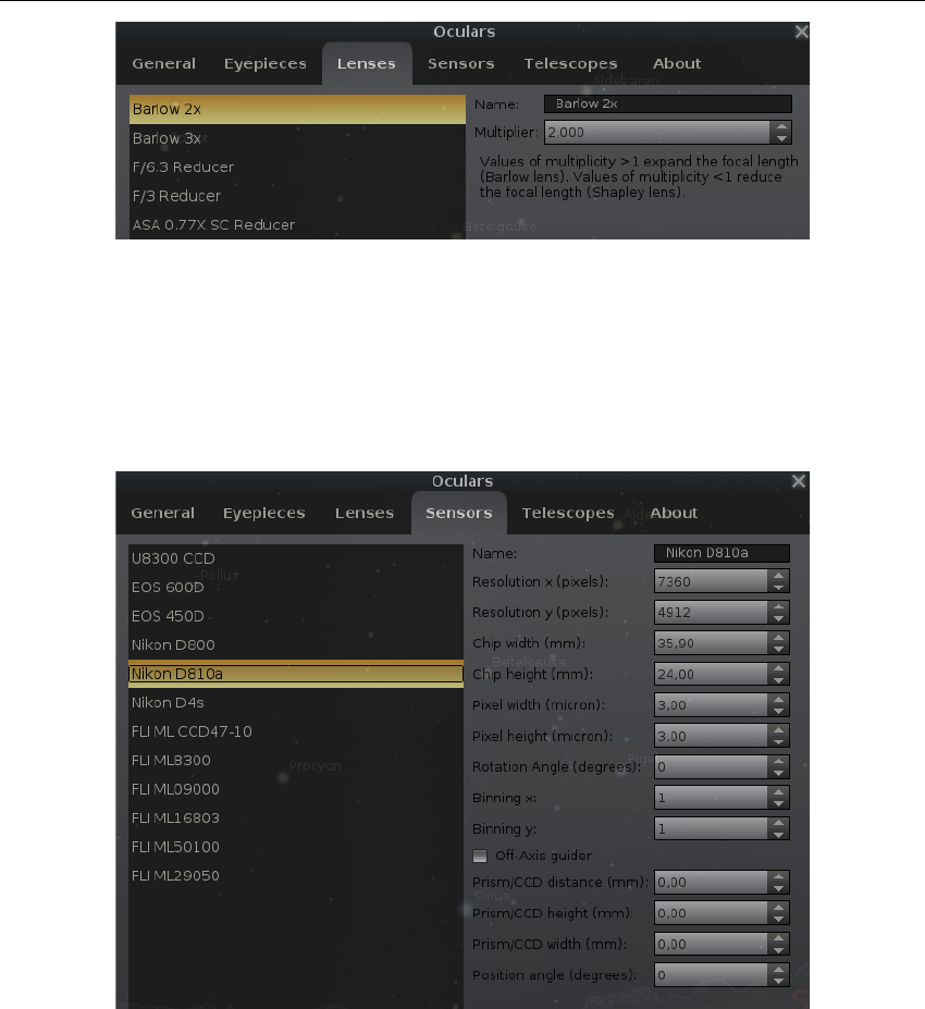
168 Chapter 15. Stellarium at the Telescope
Figure 15.14: Lenses tab of Oculars plugin configuration dialog.
what the CCD will capture. Because of the way floating point numbers are stored, sometimes you
may see one of your defined values change (for example from 2.2 to 2.19999) but this should not
affect what you see.
Figure 15.15: Sensors tab of Oculars plugin configuration dialog.
The fields on this tab are:
Name – A free-text description of the sensor.
Resolution x – the width of the sensor in pixels.
Resolution y – the height of the sensor in pixels.
Chip width – the width of the sensor in mm.
Chip height – the height of the sensor in mm.
Pixel width – the width of an individual pixel, in µm.
Pixel height – the height of an individual pixel, in µm.
Rotation Angle – the rotation angle of the sensor, in degrees.
Binning x – the binning factor for the width of the sensor.
Binning y – the binning factor for the height of the sensor.
Off-Axis guider
– selecting this checkbox tells the system that this sensor has support an off-axis
guider also.
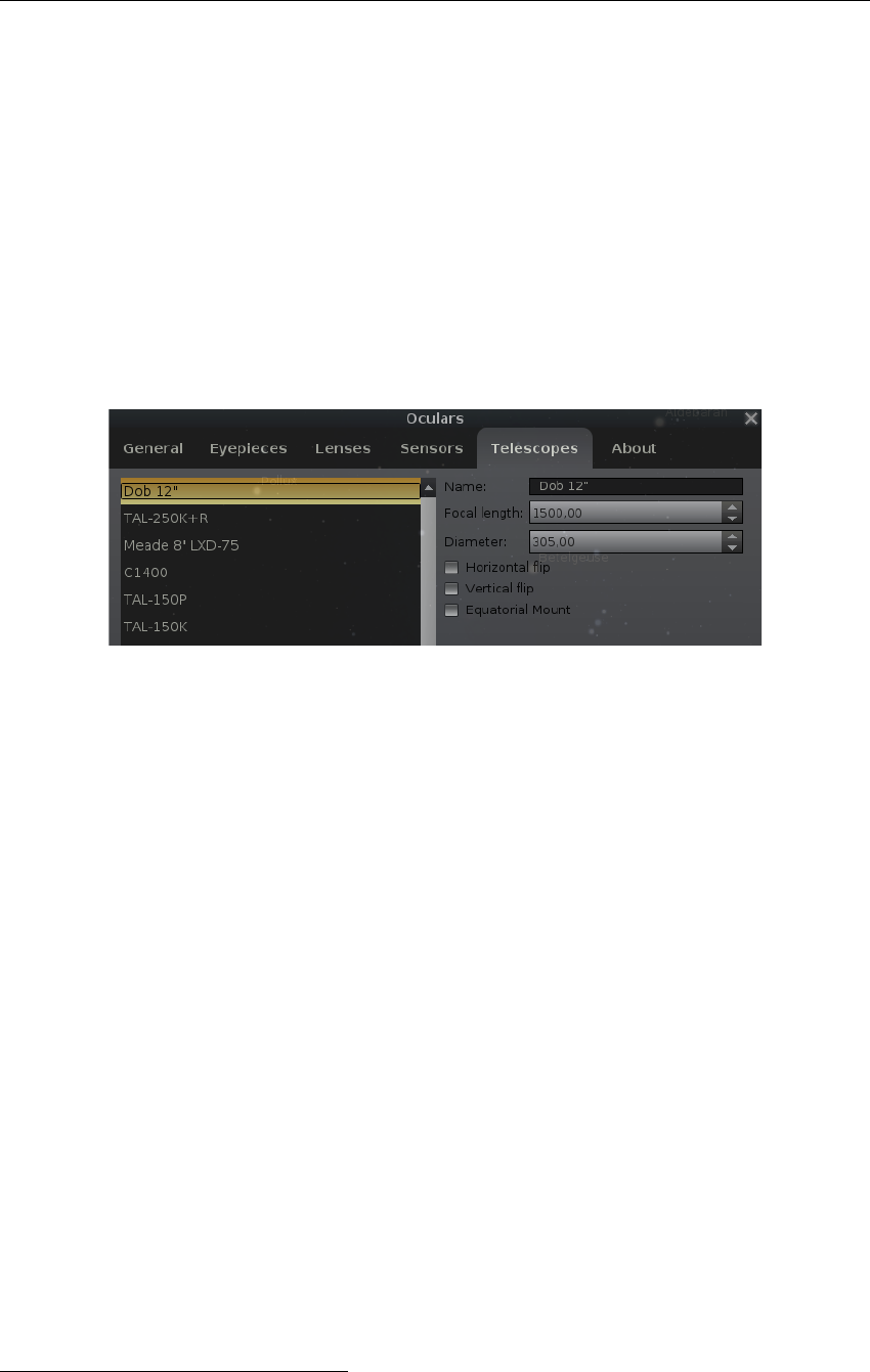
15.1 Oculars Plugin 169
Prism/CCD distance
– distance between center of prism/CCD of Off-Axis Guider and optical
axis of telescope in mm.
Prism/CCD width – the width of the prism/CCD of Off-Axis Guider in mm.
Prism/CCD height – the height of the prism/CCD of Off-Axis Guider in mm.
Position Angle – the position angle of the prism/CCD of Off-Axis Guider, in degrees.
The resolution is easy to find: these are simply the image dimensions of a (non-binned) frame. The
chip size and pixel size may be more difficult, but the manual, or searching the Internet, should turn
up these values. For a “full-frame” DSLR, this should be close to 36x24
mm
, while APS-C should
be around 22.5x15
mm
. Pixel size is simply image size divided by resolution. Some cameras may
have unsquare pixels.
Telescopes
This is the tab used to enter your own telescopes (see fig. 15.16). The fields on this tab are:
Figure 15.16: Telescopes tab of Oculars plugin configuration dialog.
Name – A free-text description of the telescope.
Focal Length – telescope focal length in mm.
Diameter – telescope diameter (aperture) in mm.
Horizontal flip – if the view through this telescope should flip horizontally.
Vertical flip – if the view through this telescope should flip vertically.
Equatorial Mount – select it if this telescope has an equatorial mount.
15.1.3 Scaling the eyepiece view
I (TR) would like to thank Al Nagler over at TeleVue
3
for helping to set me straight on the topic of
eyepieces. They are a lot more complicated than you might think!
By default, the view drawn on your computer screen when the plugin is active fills the screen.
That is, there is a circle drawn to represent the view through the eyepiece, and this circle will fill
the screen. For general use, this is what most people would want. There will be times that it’s not.
If you are going to be observing any deep space object, it can be very important to choose the
best eyepiece for that object. You will typically want an eyepiece that will magnify the object as
much as possible, while showing all of the object in the eyepiece view. Getting this can be tricky,
especially if you do not like changing eyepieces at the telescope. Or maybe you want to understand
why one type of telescope may be better than another type for observing what you are interested in.
This is where you will want to scale the image on screen based on your eyepiece.
Different eyepieces generally have a different apparent field of view (aFOV). An easy way
to think about this is: the larger the aFOV, the bigger the picture you see in the eyepiece. Older
types of eyepiece (some types still built and in wide use today have been constructed in the 19th
3http://televue.com/

170 Chapter 15. Stellarium at the Telescope
century) generally have their aFOV in the
50◦
range. Today, there are massive eyepieces available
with
82◦
, and recently even
100◦
aFOV! These eyepieces are huge, as they require a lot of very
special glass to achieve their incredible fields of view. An eyepiece of the same focal length with a
100◦
aFOV will produce an image through the eyepiece that is twice as wide as one produced by a
50◦eyepiece.
Different telescopes, with an eyepiece of a given aFOV, will also produce a different true field
of view. This is the actual size of the piece of sky that you see through the eyepiece. Getting these
two “just right” can be very important. It’s easy to assume that you want the biggest telescope
you can get, with the eyepiece that gives you the highest magnification. This is never true in
reality. Depending on where you live, and especially what you like to look at, a 100-120
mm
quality
refractor with a wide aFOV eyepiece may very well be better than a large SCT with the same
eyepiece. This is something I learned the hard way.
So how does scaling the eyepiece view help? The plugin will find the eyepiece you have with
the largest aFOV. This aFOV becomes
100%
of the computer screen diameter. Then, any other
eyepiece will have its aFOV compared, and the view on screen will be scaled down accordingly.
These
100◦
aFOV eyepieces makes the math here easy. If you have one, then when that eyepiece
is used, the circle that represents the view through the eyepiece will take up
100%
of the screen
diameter. Next, if you select an eyepiece with an
82◦
aFOV, its view will be scaled to
82%
of the
screen, and a 62◦aFOV eyepiece will be scaled to 62% of the screen.
Example in action
This is easier to understand in action, so let us look at an example that uses three eyepieces all with
the same 17
mm
focal length, so they all produce the same level of magnification (well, one has
an 17.3
mm
focal length, but its magnification is nearly identical) and see how the view changes.
These example all use a Celestron C8 8" SCT telescope, and the target is the Great Orion Nebula.
We can see from the images in fig. 15.17 that the target is all three images is the same size.
The
100◦
image fills the screen, the
82◦
is smaller, and the
62◦
is smallest yet, filling
62%
of the
computer screen. Note that in each image, the field of view that you see changes. The larger the
aFOV, the more you can see of the sky. So in this example, if you had an 8" telescope, you would
want to use the 17mm 100◦Ethos eyepiece to see as much of the nebula as possible.
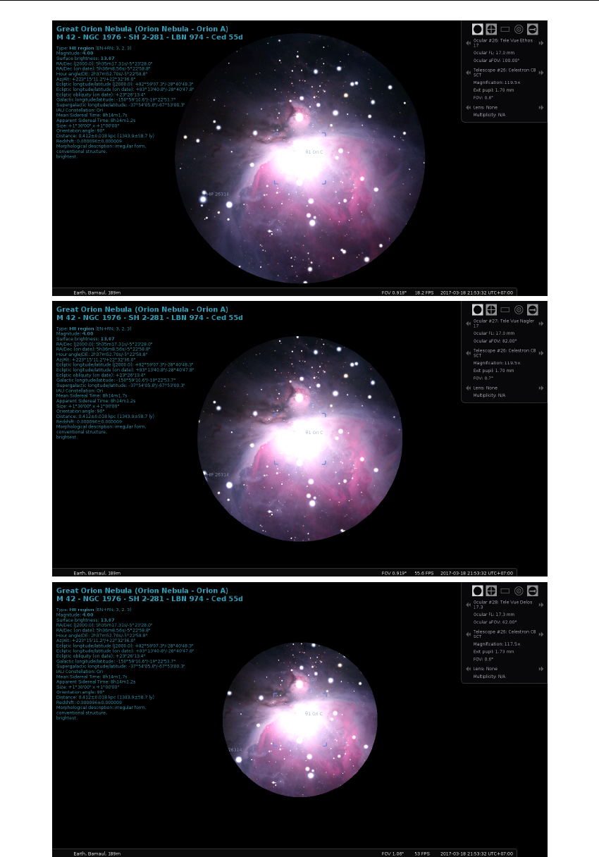
15.1 Oculars Plugin 171
Figure 15.17: Comparing apparent fields of view of (top) a 17
mm
Tele Vue Ethos eyepiece
with an aFOV of
100◦
. Magnification is
119.5×
. (center) a 17
mm
Tele Vue Nagler
eyepiece with an aFOV of
82◦
. Magnification is
119.5×
. (bottom) a 17.3
mm
Tele Vue
Delos eyepiece with an aFOV of 62◦. Magnification is 117.5×.

172 Chapter 15. Stellarium at the Telescope
15.2 TelescopeControl Plugin
This plugin provides a simple control mechanism for motorised telescope mounts. The user selects
an object (i.e. by clicking on something – a planet, a star etc.) and presses the telescope go-to key,
and the telescope will be guided to the object.
Multiple telescopes may be controlled simultaneously.
WARNING
Stellarium cannot prevent your telescope from being pointed at the Sun. It is up to you to ensure
proper filtering and safety measures are applied!
Never point your telescope at the Sun without a proper solar filter installed. The powerful light
amplified by the telescope WILL cause irreversible damage to your eyes and/or your equipment.
Even if you don’t do it deliberately, a slew during daylight hours may cause your telescope to
point at the sun on its way to the given destination, so it is strongly recommended to avoid using
the telescope control feature before sunset without appropriate protection.
15.2.1 Abilities and limitations
This plug-in allows Stellarium to send only ’slew’ (’go to’) commands to the device and to receive
its current position. It cannot issue any other commands, so users should be aware of the possibility
for mount collisions and similar situations. (To abort a slew, you can start another one to a safe
position.)
Currently this plug-in does not allow satellite tracking unless the controlled telescope is an
RTS2 system (see section 15.3), and is not very suitable for lunar or planetary observations. Many
mounts can be set to a ’lunar’ tracking speed, you may prefer this.
15.2.2 Using this plug-in
Here are two general ways to control a device with this plug-in, depending on the situation:
DIRECT CONNECTION
A device supported by the plug-in is connected with a cable to the
computer running Stellarium
INDIRECT CONNECTION
local
A device is connected to the same computer but it is driven by a stand-alone telescope
server program or a third-party application that can ’talk’ to Stellarium;
remote
A device is connected to a remote computer and the software that drives it can
’talk’ to Stellarium over the network; this software can be either one of Stellarium’s
stand-alone telescope servers, or a third party application.
Most older telescopes use cables that connect to a serial port (RS-232), the newer ones use USB
(Universal Serial Bus). On Linux and Max OS X, both cases are handled identically by the plug-in.
On Windows, a USB connection may require a ’virtual serial port’ software, if it is not supplied
with the cable or the telescope. Such a software creates a virtual (’fake’) COM port that corresponds
to the real USB port so it can be used by the plug-in. On all three platforms, if the computer
has no ’classic’ serial ports and the telescope can connect only to a serial port, a serial-to-USB
(RS-232-to-USB) adapter may be necessary.
Telescope set-up (setting geographical coordinates, performing alignment, etc.) should be done
before connecting the telescope to Stellarium.
15.2.3 Main window (’Telescopes’)
The plug-in’s main window can be opened:
•
By pressing the
configure
button for the plug-in in the
Plugins
tab of Stellarium’s Configu-
ration window (opened by pressing F2 or the button in the left toolbar).
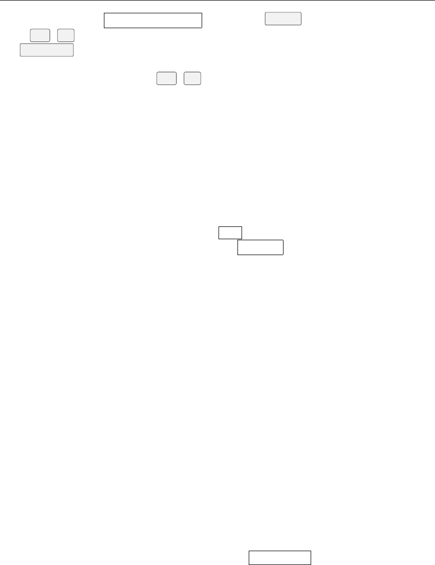
15.2 TelescopeControl Plugin 173
•
By pressing the
Configure telescopes...
button in the
Slew to
window (opened by pressing
Ctrl +0or the respective button on the bottom toolbar).
The Telescopes tab displays a list of the telescope connections that have been set up:
•
The number (#) column shows the number used to control this telescope. For example, for
telescope #2, the shortcut is Ctrl +2.
•
The Status column indicates if this connection is currently active or not. Unfortunately, there
are some cases in which ’Connected’ is displayed when no working connection exists.
•The Type field indicates what kind of connection this is:
virtual means a virtual telescope (test mode).
local, Stellarium means a DIRECT connection to the telescope (see above).
local, external
means an INDIRECT connection to a program running on the same com-
puter.
remote, unknown means an INDIRECT connection over a network to a remote machine.
remote, RTS2 means an INDIRECT connection over a network to an RTS2 server.
remote, INDI means an INDIRECT connection over a network to an INDI server.
To set up a new telescope connection, press the
Add
button. To modify the configuration of an
existing connection, select it in the list and press the
Configure
button. In both cases, a telescope
connection configuration window will open.
15.2.4 Telescope configuration window
Connection type
The topmost field represents the choice between the types of connections (see section 15.2.2):
Telescope controlled by:
Stellarium, directly through a serial port is the DIRECT case
External software or a remote computer is an INDIRECT case
RTS2 Telescope is another INDIRECT case v0.16.0
INDI is another INDIRECT case v0.17.0
Nothing, just simulate one (a moving reticle) is a virtual telescope (no connection)
Telescope properties
Name is the label that will be displayed on the screen next to the telescope reticle.
Connection delay
If the movement of the telescope reticle on the screen is uneven, you can try
increasing or decreasing this value.
Coordinate system
Some Celestron telescopes have had their firmware updated and now interpret
the coordinates they receive as coordinates that use the equinox of the date (EOD, also
known as JNow), making necessary this setting.
Start/connect at startup
Check this option if you want Stellarium to attempt to connect to the
telescope immediately after it starts. Otherwise, to start the telescope, you need to open the
main window, select that telescope and press the Start/Connect button.
Device settings
This section is active only for DIRECT connections (see above).
Serial port
sets the serial port used by the telescope. There is a pop-up box that suggests some
default values:
•On Windows, serial ports COM1 to COM10
•
On Linux, serial ports
/dev/ttyS0
to
/dev/ttyS3
and USB ports
/dev/ttyUSB0
to
/dev/ttyUSB3. Make sure you have read/write access to the tty device. Depending
on your flavour of Linux, this may e.g. require some group membership.
•
On Mac OS X, the list is empty as it names its ports in a peculiar way. If you are using
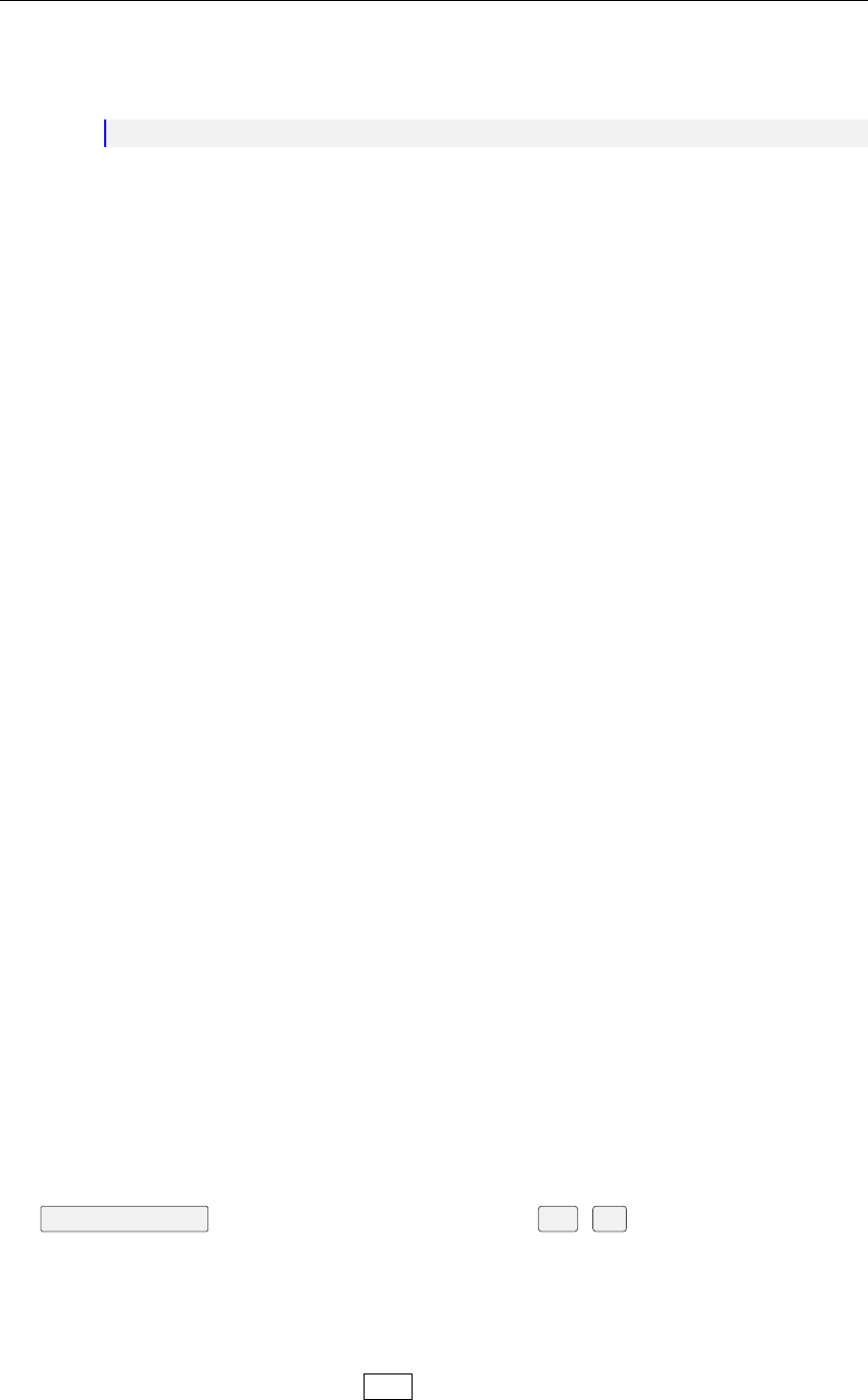
174 Chapter 15. Stellarium at the Telescope
an USB cable, the default serial port of your telescope most probably is not in the list
of suggestions. To list all valid serial port names in Mac OS X, open a terminal and
type:
ls / dev /*
This will list all devices, the full name of your serial port should be somewhere in the
list (for example, /dev/cu.usbserial-FTDFZVMK).
Device model : see 15.2.5 Supported devices.
Connection settings
Both fields here refer to INDIRECT connections, which implies communication over a network
(TCP/IP).
Host
can be either a host name or an IPv4 address such as ’127.0.0.1’. The default value of
’localhost’ means ’this computer’.
Modifying the default host name value makes sense only if you are attempting a remote
connection over a network. In this case, it should be the name or IP address of the computer
that runs a program that runs the telescope.
Port
refers to the TCP port used for communication. The default value depends on the telescope
number and ranges between 10001 and 10009.
RTS2 settings
(see also 15.3) You will need access to an RTS2 HTTPD server through HTTP/JSON calls. Please
v0.16.0
see RTS2 documentation (man rts2-httpd) for details. You will as well need username and password
for HTTPD. Please be aware that in order to move the telescope, your user must have the telescope
in the list of allowed devices in the database. Please see
man rts2-user
for details on how to
manipulate RTS2 users.
URL
points to RTS2 HTTPD. Can include anything a URL can have - port (:8889) and prefix path
for RTS2 access.
Username username used for login to RTS2 HTTPD.
Password password for login to RTS2 HTTPD.
INDI settings
(see also 15.4) You will need access to an INDI server through a TCP/IP connection. Please see
v0.17.0
INDI documentation for details. You will need to select the correct INDI device to manage it.
User Interface Settings: Field of view indicators
A series of circles representing different fields of view can be added around the telescope marker.
This is a relic from the times before the Oculars plug-in (see 15.1) existed.
Activate the ’Use field of view indicators’ option, then enter a list of values separated with
commas in the field below. The values are interpreted as degrees of arc.
These marks can be used in combination with a virtual telescope to display a moving reticle
with the Telrad circles.
’Slew telescope to’ window
The
Slew telescope to
window can be opened by pressing
Ctrl +0
or the respective button in
the bottom toolbar.
It contains two fields for entering celestial coordinates, selectors for the preferred format
(Hours-Minutes-Seconds, Degrees-Minutes-Seconds, or Decimal degrees), a drop-down list and
two buttons.
The drop-down list contains the names of the currently connected devices. If no devices are
connected, it will remain empty, and the Slew button will be disabled.
15.2 TelescopeControl Plugin 175
Pressing the
Slew
button slews the selected device to the selected set of coordinates. See the
section about keyboard commands below for other ways of controlling the device.
Pressing the Configure telescopes. . . button opens the main window of the plug-in.
TIP: Inside the ’Slew’ window, underlined letters indicate that pressing
Alt +underlined letter
can be used instead of clicking. For example, pressing
Alt +S
is equivalent to clicking the
Slew
button, pressing Alt +Eswitches to decimal degree format, etc.
Sending commands
Once a telescope is successfully started/connected, Stellarium displays a telescope reticle labelled
with the telescope’s name on its current position in the sky. The reticle is an object like every other
in Stellarium - it can be selected with the mouse, it can be tracked and it appears as an object in the
’Search’ window.
To point a device to an object: Select an object (e.g. a star) and press the number of the device
while holding down the
Ctrl
key. (For example,
Ctrl +1
for telescope #1.) This will move the
telescope to the selected object. Note that most telescopes can only execute a single command
to move to that object’s position, but if the telescope is an RTS2 telescope, you can even track a
satellite (if the mount then is fast enough to support it).4
To point a device to the center of the view: Press the number of the device while holding down
the Alt key. (For example,
Alt +1
for telescope #1.) This will slew the device to the point in
the center of the current view. (If you move the view after issuing the command, the target won’t
change unless you issue another command.)
To point a device to a given set of coordinates: Use the Slew to window (press Ctrl +0).
15.2.5 Supported devices
Directly connected telescopes
All devices listed in the ’Device model’ list are convenience definitions using one of the two built-in
interfaces: the Meade LX200 (the Meade Autostar controller) interface and the Celestron NexStar
interface.
The device list contains the following:
Celestron NexStar (compatible) Any device using the NexStar interface.
Losmandy G-11
A computerized telescope mount made by Losmandy (Meade LX-200/Autostar
interface).
Meade Autostar compatible Any device using the LX-200/Autostar interface.
Meade ETX-70 (#494 Autostar, #506 CCS)
The Meade ETX-70 telescope with the #494 Au-
tostar controller and the #506 Connector Cable Set. According to the tester, it is a bit slow,
so its default setting of ’Connection delay’ is 1.5 seconds instead of 0.5 seconds.
Meade LX200 (compatible) Any device using the LX-200/Autostar interface.
Sky-Watcher SynScan AZ mount
The Sky-Watcher SynScan AZ GoTo mount is used in a num-
ber of telescopes.
Sky-Watcher SynScan (version 3 or later)
SynScan is also the name of the hand controller used
in other Sky-Watcher GoTo mounts, and it seems that any mount that uses a SynScan
controller version 3.0 or greater is supported by the plug-in, as it uses the NexStar protocol.
Wildcard Innovations Argo Navis (Meade mode)
Argo Navis is a ’Digital Telescope Computer’
by Wildcard Innovations. It is an advanced digital setting circle that turns an ordinary
telescope (for example, a dobsonian) into a ’Push To” telescope (a telescope that uses a
computer to find targets and human power to move the telescope itself). Just don’t forget to
set it to Meade compatibility mode and set the baud rate to 9600B1.
4
Actually, the TLE orbital elements of the selected satellite are transmitted to RTS2, which does then
compute the satellite position itself.

176 Chapter 15. Stellarium at the Telescope
RTS2 telescopes
v0.16.0
Setting up a robotic telescope and dome control system with RTS2 is beyond the scope of this
handbook, but see section 15.3 for a few notes to be able to connect and command the telescope
with Stellarium. Please refer to the RTS2 Web pages5for further details.
Please be aware that some RTS2 usernames might have only read-only access. If this is case for
your username, the telescope marker will be painted red (or
color_telescope_readonly
from
Stellarium’s settings file).
INDI telescopes
v0.17.0
Setting up a robotic telescope and dome control system with INDI is beyond the scope of this
handbook, but see section 15.4 for a few notes to be able to connect and command the telescope
with Stellarium. Please refer to the INDI web pages6for further details.
Virtual telescope
If you want to test this plug-in without an actual device connected to the computer, choose “Nothing,
just simulate one (a moving reticle)” in the
Telescope controlled by:
field. It will show a telescope
reticle that will react in the same way as the reticle of a real telescope controlled by the plug-in.
See the section above about field of view indicators for a possible practical application (emulating
’Telrad’ circles).
15.3 RTS2
RTS2, the Remote Telescope System 2, is a complete robotic observatory control system for Linux
v0.16.0
by Petr Kubánek, who kindly provided the plugin code to make RTS2 interoperate with Stellarium.
We cannot give a full manual or any further support for RTS2 here, please refer to its website
7
for
complete instructions about dome control, cameras, filter wheels, weather sensors, etc. A few notes
may be useful for beginners, though.
RTS2’s central piece is a daemon. Start the system:
sudo service rts2 start
RTS2’s main control screen is text-based,
rts2-mon
. For a quick check, switch on the system using
F9
. Telescope
T0
is a dummy telescope which you can select and operate with commands like
move 120 35
(this moves to RA=120
◦
=8h, DEC=35
◦
, but only when this position is above your
horizon).
Stellarium’s Telescope plugin can communicate with RTS2 using the RTS2 web interface. You
must run
rts2-httpd
for this, which may require the right permissions to write the lock files in
/var/run
. This program requires that a database has been created as described in the file
RUN
in
RTS2’s source directory and on the RTS2 website
8
. Also, you must create a ’user’ for RTS2. This
is not a regular Linux account, but an entry in the RTS2 database. Create a user with
rts2-user -a
<user>
. You should use a password different from your regular Linux password, as this will be
transmitted in plain text between the computer running Stellarium and the RTS2 control computer,
and may also be written into Stellarium’s logfile. Then you can enable device control for the
respective user. If you want to send slew commands from Stellarium, make sure to allow access to
telescope
T0
. If not, Stellarium will be able to show the telescope marker, but you will not be able
to control the telescope. To enable control for existing users in the default stars database,
5http://rts2.org/
6http://indilib.org
7http://rts2.org
8http://rts2.org/faq.html
15.4 INDI 177
psql stars
up da te u sers set a ll ow ed _d evi ce s = ’* ’;
In case you cannot properly connect to the RTS2 telescope or cannot send slew commands,
check Stellarium’s logfile log.txt for some diagnostic messages.
RTS2 is the only type of telescope supported by Stellarium which can autonomously track
satellites. Tracking accuracy fully depends on Stellarium’s TLE satellite elements being up-to-date
(see section 13.8) and the accuracy of your RTS2 installation.
15.4 INDI
INDI, the Instrument Neutral Distributed Interface, is a distributed control system (DCS) protocol
v0.17.0
to enable control, data acquisition and exchange among hardware devices and software front ends,
emphasizing astronomical instrumentation9.
INDI client (v1.6.0) has been incorporated into Stellarium’s Telescope Control plugin by
Alessandro Siniscalchi to allow Stellarium to communicate with INDI hardware drivers via INDI
server. INDI server is a hub that sits between drivers and clients. It reroutes traffic for control
and data across distributed networks. Each device or client in the network is a node and may
communicate with other nodes whenever desired. The server supports broadcasting, chaining, and
marshalling of data.
Stellarium only supports INDI mounts (no other INDI devices), and you will need to select the
correct INDI device to manage it at the stage of configuration of telescope. For this purpose the
plug-in has a tool to getting the list of connected devices from the INDI server (when the server is
working!). Please define hostname and port
10
in the “INDI Settings” block, press
Refresh devices
and select the required device in the list “Devices”.
List of telescope types supported by INDI11:
•Meade Autostar
•Meade LX200 (Classic/GPS/16)
•Celestron NexStar
•Celestron NexStar Evolution
•Orion Synscan Telescope
•EQ-6 MCU Update
•HEQ-5 MCU Update
•LittleFoot Vpower
•LittleFoot Elegance Photo
•Astro-Electronic FS-2
•EQMod
•Pulsar2
•SkySensor2000PC
•Takahashi Temma
•10 Micron
•Losmandy Gemini
•Astrophysics
•Skywatcher Virtuoso (Alt/Az)
•IOptron IEQPro/CEM60
9https://en.wikipedia.org/wiki/Instrument_Neutral_Distributed_Interface
10
The Internet Assigned Numbers Authority (IANA) has assigned to INDI the Transmission Control
Protocol and User Datagram Protocol (TCP/UDP) port 7624.
11http://indilib.org/devices/telescopes/all.html

178 Chapter 15. Stellarium at the Telescope
•IOptron ZEQ25/SmartEQ
•IOptron GotoNova Upgrade Kit 8400
15.5 StellariumScope
StellariumScope is a free add-on that enables you to control your telescope with Stellarium.
Features
•Provides an interface between Stellarium and ASCOM telescope drivers.
•
Provides the ability to both “Sync” and “Slew” the telescope. It’s also possible to issue a
stop/cancel command from Stellarium.
•
You can easily host Stellarium on one computer linked to another control computer that
hosts the telescope driver.
•
The installation program will automatically install the documentation, but the link to the
documentation is provided by developer12 so you can read it before installation.
•
There are earlier releases still available on the downloads page on Welsh Dragon Computing
site.
The original
StellariumScope
program was designed and implemented by Scott of ByteArts
and is still available for download
13
. If you have difficulties with the releases available on the Welsh
Dragon Computing site14, you may want to consider using the original version.
Figure 15.18 shows the interface and some of the options. Use this application (like all software
that controls your mount) with supervision of your mount’s movements.
15.6 Other telescope servers and Stellarium
Other developers have also been busy creating hard- and software often involving Arduino or
Raspberry Pi boards which can control GOTO or PUSHTO (manually driven but position-aware,
usually Dobsonian) telescopes and are ultimately controlled from Stellarium. Those are not related
nor authored by the Stellarium team, so while we welcome such development (esp. open-sourced)
in general, we cannot provide documentation nor any support.
A few examples:
iTelescope http://simonbox.info/index.php/astronomy/93-raspberry-pi-itelescope
node-telescope-server https://www.npmjs.com/package/node-telescope-server
One anonymous user sent a troubleshooting solution when connecting Stellarium to the Cele-
stron NexRemote software:
One tricky Window XP issue I fixed was that my older laptop would transiently lose
connection with Stellarium although the status would still be “Connected” and all
looked normal. [. . . ]
I boosted the NexRemote.exe process in Windows XP to High under Set Priority under
the Windows Task Manager via Ctrl +Alt +Del .
All slews now proceed normally. Problem went away.15
12StellariumScope
User’s Guide —
http://welshdragoncomputing.ca/x/st/misc/
stellariumscope_user_guide.2015.10.24.pdf
13http://www.bytearts.com/stellarium/
14http://welshdragoncomputing.ca/x/index.php/home/stellariumscope/
about-stellariumscope
15https://sourceforge.net/p/stellarium/discussion/278769/thread/16e4c054/
?limit=25#8ffa

15.6 Other telescope servers and Stellarium 179
Figure 15.18: StellariumScope interface

180 Chapter 15. Stellarium at the Telescope
15.7 Observability Plugin
This Plugin is activated with the button . It analyzes the observability of the selected object (or
the screen center, if no object is selected). The plugin can show rise, transit, and set times, as well
as the best epoch of the year (i.e., largest angular separation from the Sun), the date range when
the source is above the horizon at dark night, and the dates of Acronychal and Cosmical rise/set.
Ephemerides of the Solar-System objects and parallax effects are taken into account.
Explanation of some parameters
Sun altitude at twilight
Any celestial object will be considered visible when the Sun is below this
altitude. The altitude at astronomical twilight ranges usually between -12 and -18 degrees.
This parameter is only used for the estimate of the range of observable epochs (see below).
Horizon altitude
Minimum observable altitude (due to mountains, buildings, or just a limited
telescope mount).
Today ephemeris
Self-explanatory. The program will show the rise, set, and culmination (transit)
times. The exact times for these ephemeris are given in two ways: as time spans (referred to
the current time) and as clock hours (in local time).
Acronychal/Cosmical/Heliacal rise/set
The days of Cosmical rise/set of an object are estimated
as the days when the object rises (or sets) together with the rise/set of the Sun. The exact
dates of these ephemeris depend on the Observer’s location. On the contrary, the Acronycal
rise (or set) happens when the star rises/sets with the setting/rising of the Sun (i.e., opposite
to the Sun). On the one hand, it is obvious that the source is hardly observable (or not
observable at all) in the dates between Cosmical set and Cosmical rise. On the other hand,
the dates around the Acronychal set and rise are those when the altitude of the celestial
object uses to be high when the Sun is well below the horizon (hence the object can be
well observed). The date of Heliacal rise is the first day of the year when a star becomes
visible. It happens when the star is close to the eastern horizon roughly before the end of the
astronomical night (i.e., at the astronomical twilight). In the following nights, the star will
be visibile during longer periods of time, until it reaches its Heliacal set (i.e., the last night
of the year when the star is still visible). At the Heliacal set, the star sets roughly after the
beginning of the astronomical night.
Largest Sun separation
Happens when the angular separation between the Sun and the celestial
object are maximum. In most cases, this is equivalent to say that the Equatorial longitudes of
the Sun and the object differ by 180 degrees, so the Sun is in opposition to the object. When
an object is at its maximum possible angular separation from the Sun (no matter if it is a
planet or a star), it culminates roughly at midnight, and on the darkest possible area of the
Sky at that declination. Hence, that is the ’best’ night to observe a particular object.
Nights with source above horizon
The program computes the range of dates when the celestial
object is above the horizon at least during one moment of the night. By ’night’, the program
considers the time span when the Sun altitude is below that of the twilight (which can be set
by the user; see above). When the objects are fixed on the sky (or are exterior planets), the
range of observable epochs for the current year can have two possible forms: either a range
from one date to another (e.g., 20 Jan to 15 Sep) or in two steps (from 1 Jan to a given date
and from another date to 31 Dec). In the first case, the first date (20 Jan in our example) shall
be close to the so-called ’Heliacal rise of a star’ and the second date (15 Sep in our example)
shall be close to the ’Heliacal set’. In the second case (e.g., a range in the form 1 Jan to 20
May and 21 Sep to 31 Dec), the first date (20 May in our example) would be close to the
Heliacal set and the second one (21 Sep in our example) to the Heliacal rise. More exact
equations to estimate the Heliacal rise/set of stars and planets (which will not depend on the

15.7 Observability Plugin 181
mere input of a twilight Sun elevation by the user) will be implemented in future versions of
this plugin.
Full Moon
When the Moon is selected, the program can compute the exact closest dates of the
Moon’s opposition to the Sun.
Note on Terminology
The (sparse) literature on terminology about computing these Heliacal, Acronychal or Cosmic
events seems to disagree on which end of the night is to be computed. While all agree about Heliacal
rises taking place in the morning, Acronychal and Cosmic are sometimes applied in reverse order
from those described here. In case you use these data, make sure you keep this definition as well.
Author
This plugin has been contributed by Ivan Marti-Vidal (Onsala Space Observatory)
16
with some
advice by Alexander Wolf and Georg Zotti.
16mailto:i.martividal@gmail.com
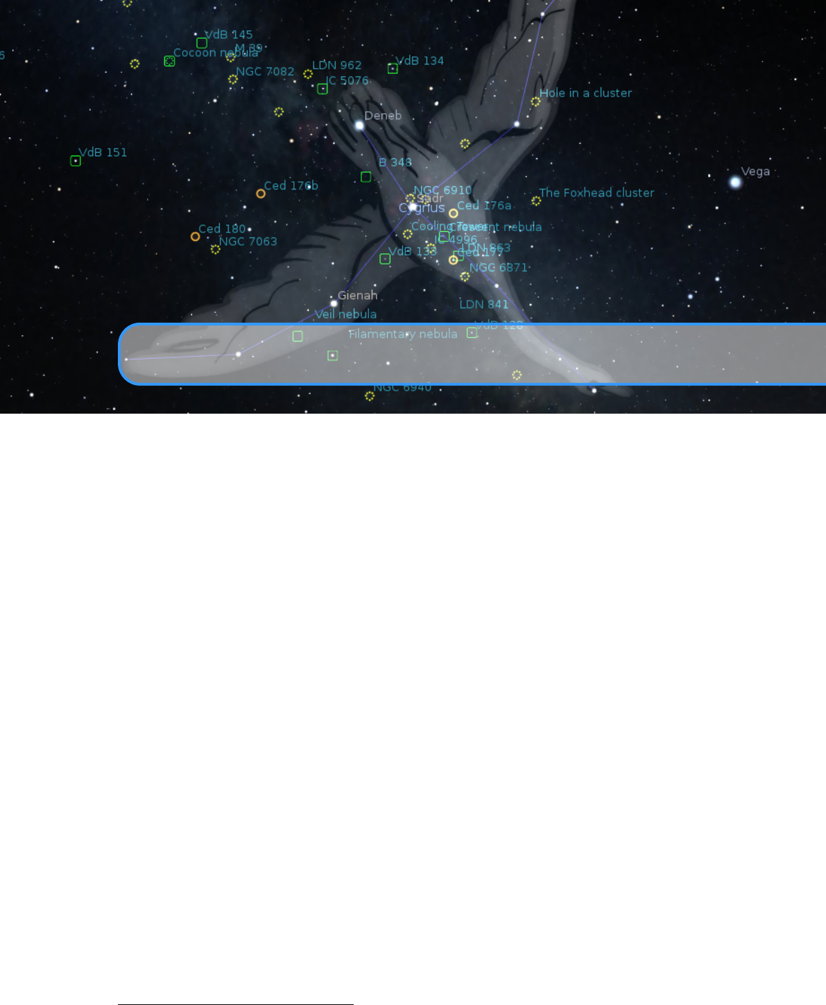
16. Scripting
16.1 Introduction
The development of a powerful scripting system has been continuing for a number of years now
and can now be called operational. The use of a script was recognised as a perfect way of arranging
a display of a sequence of astronomical events from the earliest versions of Stellarium and a simple
system called Stratoscript was implemented. The scripting facility is Stellarium’s version of a
Presentation, a feature that may be used to run an astronomical or other presentation for instruction
or entertainment from within the Stellarium program. The original Stratoscript was quite limited in
what it could do so a new Stellarium Scripting System has been developed.
Since version 0.10.1, Stellarium has included a scripting feature based on the Qt Scripting
Engine
1
. This makes it possible to write small programs within Stellarium to produce automatic
presentations, set up custom configurations, and to automate repetitive tasks.
As of version 0.14.0 a new scripting engine has reached a level where it has all required features
for usage, however new commands may be added from time to time. Since version 0.14.0 support
of scripts for the Stratoscript engine has been discontinued.
The programming language ECMAscript
2
(also known as JavaScript) gives users access to all
basic ECMAScript language features such as flow control, variables, string manipulation and so on.
Interaction with Stellarium-specific features is done via a collection of objects which represent
components of Stellarium itself. The various modules of Stellarium, and also activated plugins, can
be called in scripts to calculate, move the scene, switch on and off display of objects, etc. You can
write text output into text files with the
output()
command. You can call all public slots which
are documented in the scripting API documentation3.
1http://doc.qt.io/qt-5/qtscript-index.html
2https://en.wikipedia.org/wiki/ECMAScript
3http://www.stellarium.org/doc/0.18.0/scripting.html
184 Chapter 16. Scripting
16.2 Script Console
It is possible to open, edit run and save scripts using the script console window. To toggle the script
console, press
F12
. The script console also provides an output window in which script debugging
output is visible.
16.3 Includes
Stellarium provides a mechanism for splitting scripts into different files. Typical functions or lists
of variables can be stored in separate
.inc
files and used within other scripts through the
include()
command:
include (" co mm on_ ob jec ts . inc " );
16.4 Minimal Scripts
This script prints “Hello Universe” in the Script Console log window and into log.txt:
core .debug(" H el lo U nive rse " );
This script prints “Hello Universe” in the Script Console output window and into the file
output.txt
which you will also find in the user data directory. The absolute path to the file will also be given in
log.txt.
core .output (" H ello Un ive rse " );
The file
output.txt
will be rewritten on each run of Stellarium. In case you need to save a copy
of the current output file to another file, call
core .sa veO utputAs ("myImportantData.txt");
core .resetOutput();
This script uses the LabelMgr module to display “Hello Universe” in red, fontsize 20, on the screen
for 3 seconds.
var label =LabelMgr.labelScreen(" He ll o Un ive rse " , 200 , 200 ,
true , 20 , "# ff0000 " );
core .wait (3);
LabelMgr.deleteLabel(label);
16.5 Example: Retrograde motion of Mars
A good way begin writing of scripts: set yourself a specific goal and try to achieve it with the help
of few simple steps. Any complex script can be split into simple parts or tasks, which may solve
any newbie problems in scripting.
Let me explain it with examples.
Imagine that you have set a goal to make a demonstration of a very beautiful, but longish
phenomenon — the retrograde motion of the planet Mars (Fig. 16.1).
16.5.1 Script header
Any “complex” script should contain a few lines in the first part of the file, which contains important
data for humans — the name of the script and its description — and some rules for Stellarium.
You can even assign default shortcuts in the script header, but make sure you assign a key not used
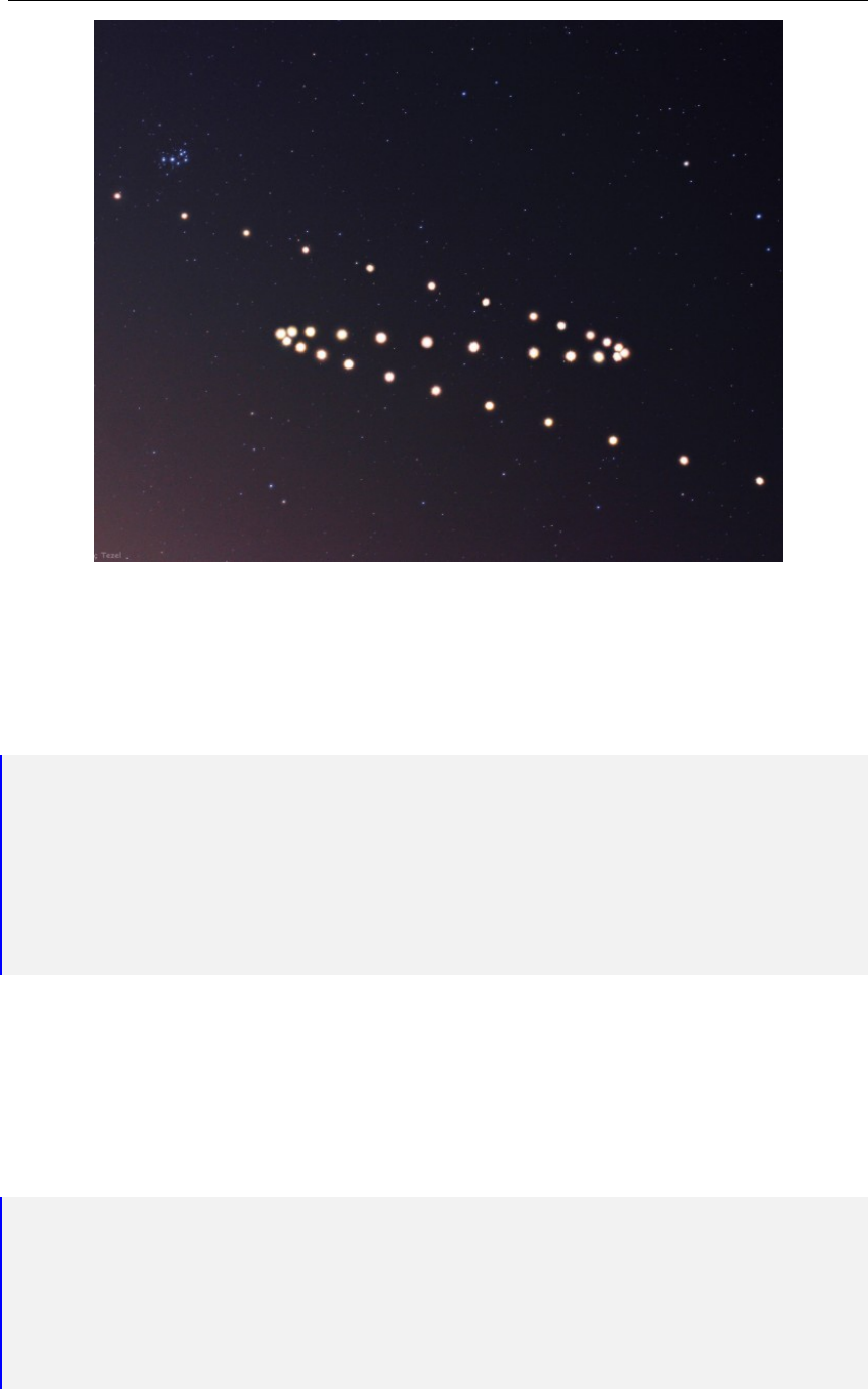
16.5 Example: Retrograde motion of Mars 185
Figure 16.1: Retrograde motion of Mars in 2005. (Credit & Copyright: Tunc Tezel — APOD:
2006 April 22 – Z is for Mars.)
elsewhere! The description may cover several lines (until the end of the commented header) and
should therefore be the last entry of the header.
//
// Name :Retrogra de motion of Mars
// Author :John Doe
// License :Public Domain
// Version : 1.0
// Shortcut:Ctrl+M
// Description:A demo of retro grade motion of Mars .
//
16.5.2 A body of script
At the first stage of writing of the script for a demo of retrograde motion of Mars we should set
some limits for our demo. For example we want to see motion of Mars every day during 250 days
since October
1st
, 2009. Choosing a value of field of view and of the coordinates of the center of
the screen should be done at the this stage also.
Let’s add few lines of code into the script after the header and run it:
core .setDate (" 2009 -10 -01 T10 :00:00 ");
core .moveToRaDec(" 08 h 44m 41s " ," +18 d09m1 3s " ,1);
StelMovementMgr.zoomTo (40 , 1);
for (i=0; i<250; i++)
{
core . setDate ( " + 1 days " );
core . wait (0.2);

186 Chapter 16. Scripting
}
OK, Stellarium is doing something, but what exactly is it doing? The ground and atmosphere is
enabled and any motion of Mars is invisible. Let’s add an another few lines into the script (hiding
the landscape and atmosphere) after setting date and time:
Land sca peMgr .setFlagLandscape(false);
Land sca peMgr .setFlagAtmosphere(false);
The whole sky is moving now — let’s lock it! Add this line after previous lines:
StelMovementMgr.setFlagLockEquPos(true);
It looks better now, but what about cardinal points, elements of GUI and some “glitch of
movement”? Let’s change the script:
core .setDate (" 2009 -10 -01 T10 :00:00 ");
Land sca peMgr .setFlagCardinalsPoints(false);
Land sca peMgr .setFlagLandscape(false);
Land sca peMgr .setFlagAtmosphere(false);
core .setGuiVisible(false);
core .moveToRaDec(" 08 h 44m 41s " ," +18 d09m1 3s " ,1);
StelMovementMgr.setFlagLockEquPos(true);
StelMovementMgr.zoomTo (40 , 1);
core .wait (2);
for (i=0; i<250; i++)
{
core . setDate ( " + 1 days " );
core . wait (0.2);
}
core . s etGui Visib le ( true );
It’s better, but let’s draw the “path” of Mars! Add those line before the loop:
core .selectObjectByName(" Mars " ,false);
SolarSystem.setFlagIsolatedTrails(true );
SolarSystem.setFlagTrails(true);
Hmm. . . let’s add a few strings with info for users (insert those lines after the header):
var color =" # ff9900 ";
var info =LabelMgr.labelScreen(" A m otio n of Mars " , 20 , 20 ,
false , 24 , color);
var apx =LabelMgr.labelScreen(" Setup best viewing angle , FOV
and date / time . ", 20 , 50 , false , 18 , color);
LabelMgr.se tLabelShow (info ,true );
LabelMgr.se tLabelShow (apx ,true );
core .wait (2);
LabelMgr.se tLabelShow (apx ,false);
Let’s add some improvements to display info for users — change in the loop:
var label =LabelMgr.labelObject(" Normal motion , West to
East " ," M ar s " ,true , 16 , color ," SE " );
for (i=0; i<250; i++)
{

16.6 More Examples 187
core . setDate ( " + 1 days " );
if (( i% 10) == 0)
{
var strDate = " Day " +i;
LabelMgr . setLa bel Show ( apx , false );
var apx = L abe lMgr . l abe lSc ree n ( strDate , 20 ,
50 , false , 16 , color);
LabelMgr . setLa bel Show ( apx , true );
}
if (i== 75)
{
LabelMgr . de leteLabel ( label);
label = LabelMgr . labelObje ct (" Retrograde or
op pos ite m otio n beg ins " ," Mars " ,
true , 16 , color ," SE " );
core . wait (2);
LabelMgr . de leteLabel ( label);
label = LabelMgr . labelObje ct (" Retrograde
mot ion " ," M ar s " , true , 16 , color ,
" SE " );
}
if (i== 160)
{
LabelMgr . de leteLabel ( label);
label = LabelMgr . labelObje ct (" Normal motion
re turn s " ," Ma rs " , true , 16 , color ,
" SE " );
core . wait (2);
LabelMgr . de leteLabel ( label);
label = LabelMgr . labelObje ct (" Norma l mo ti on " ,
" Mars " , true , 16 , color ," SE " );
}
core . wait (0.2);
}
16.6 More Examples
The best source of examples is the
scripts
sub-directory of the main Stellarium source tree. This
directory contains a sub-directory called
tests
which are not installed with Stellarium, but are
nonetheless useful sources of example code for various scripting features.

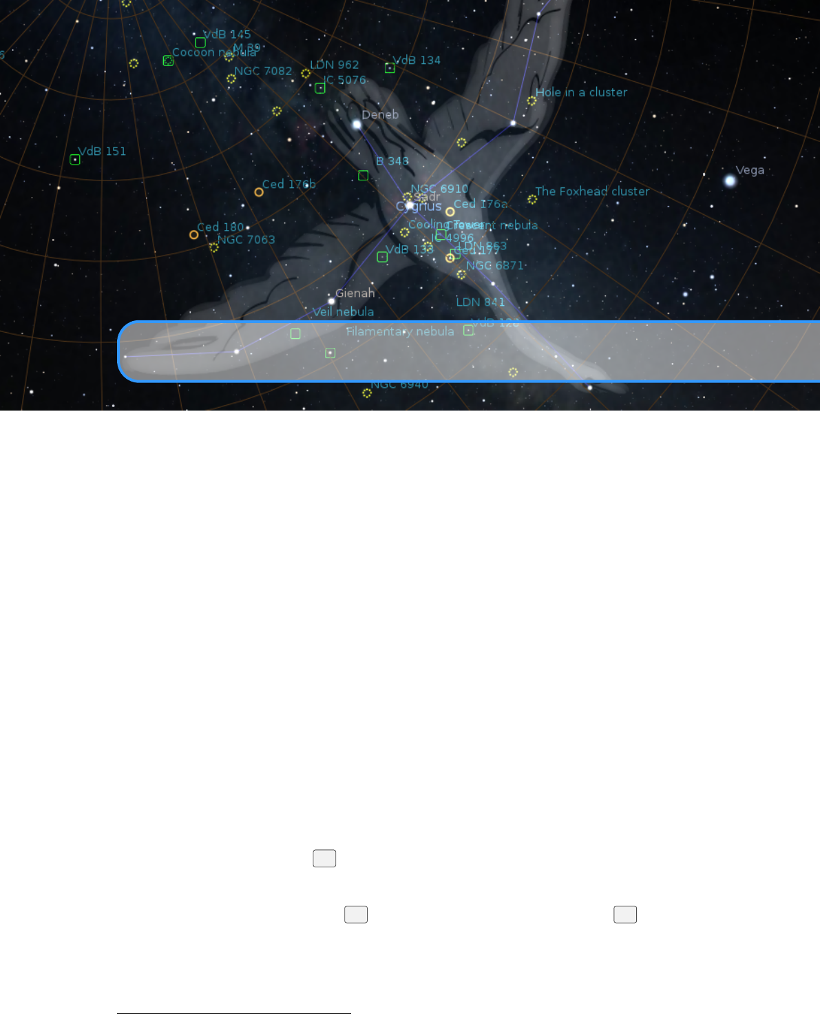
17. Astronomical Concepts
BARRY GERDES,WITH ADDITIONS BY GEORG ZOTTI
This section includes some general notes on astronomy in an effort to outline some concepts that
are helpful to understand features of Stellarium. Material here is only an overview, and the reader is
encouraged to get hold of a couple of good books on the subject. A good place to start is a compact
guide and ephemeris such as the National Audubon Society Field Guide to the Night Sky
1
. Also
recommended is a more complete textbook such as Universe. There are also some nice resources
on the net, like the Wikibooks Astronomy book2.
17.1 The Celestial Sphere
The Celestial Sphere is a concept which helps us think about the positions of objects in the sky.
Looking up at the sky, you might imagine that it is a huge dome or top half of a sphere, and the
stars are points of light on that sphere. Visualising the sky in such a manner, it appears that the
sphere moves, taking all the stars with it — it seems to rotate. Watching the movement of the stars
we can see that they seem to rotate around a static point about once a day. Stellarium is the perfect
tool to demonstrate this!
1.
Open the location dialog (
F6
). Set the location to be somewhere in mid-Northern latitudes.
(Just click on the map to select a location, or fine-tune with the settings.) The United
Kingdom is an ideal location for this demonstration.
2.
Turn off atmospheric rendering
A
and ensure cardinal points are turned on (
Q
). This will
keep the sky dark so the Sun doesn’t prevent us from seeing the motion of the stars when it
is above the horizon.
3. Pan round to point North, and make sure the field of view is about 90◦.
4. Pan up so the ‘N’ cardinal point on the horizon is at the bottom of the screen.
1http://www.amazon.com/National-Audubon-Society-Field-Series/dp/0679408525
2http://en.wikibooks.org/wiki/Subject:Astronomy

192 Chapter 17. Astronomical Concepts
5.
Now increase the time rate. Press
K
,
L
,
L
,
L
,
L
– this should set the time rate so
the stars can be seen to rotate around a point in the sky about once every ten seconds. If
you watch Stellarium’s clock you’ll see this is the time it takes for one day to pass at this
accelerated rate.
The point which the stars appear to move around is one of the Celestial Poles.
The apparent movement of the stars is due to the rotation of the Earth. Our location as the
observer on the surface of the Earth affects how we perceive the motion of the stars. To an observer
standing at Earth’s North Pole, the stars all seem to rotate around the zenith (the point directly
upward). As the observer moves South towards the equator, the location of the celestial pole moves
down towards the horizon. At the Earth’s equator, the North celestial pole appears to be on the
Northern horizon.
Similarly, observers in the Southern hemisphere see the Southern celestial pole at the zenith
when they are at the South pole, and it moves to the horizon as the observer travels towards the
equator.
1.
Leave time moving on nice and fast, and open the configuration window. Go to the location
tab and click on the map right at the top – i.e., set your location to the North pole. See how
the stars rotate parallel to the horizon, around a point right at the top of the screen. With the
field of view set to
90◦
and the horizon at the bottom of the screen, the top of the screen is
the zenith.
2.
Now click on the map again, this time a little further South. You should see the positions of
the stars jump, and the centre of rotation has moved a little further down the screen.
3.
Click on the map even further towards and equator. You should see the centre of rotation
having moved down again.
To help with the visualisation of the celestial sphere, turn on the equatorial grid by clicking the
button on the main tool-bar or pressing the
E
key. Now you can see grid lines drawn on the sky.
These lines are like lines of longitude and latitude on the Earth, but drawn for the celestial sphere.
The Celestial Equator is the line around the celestial sphere that is half way between the
celestial poles – just as the Earth’s equator is the line half way between the Earth’s poles.
17.2 Coordinate Systems
17.2.1 Altitude/Azimuth Coordinates
The Horizontal Coordinate System (also called Altitude/Azimuth coordinate system) can be used
to describe a direction of view (the azimuth angle) and an angular height in the sky (the altitude
angle). The azimuth angle is measured clockwise round from due North
3
. Hence North itself is 0
◦
,
East
90◦
, Southwest is
225◦
and so on. The altitude angle is measured up from the mathematical
horizon, which is just halfway between “straight up” and “straight down”, without regard to the
landscape. Looking directly up (at the zenith) would be
90◦
, half way between the zenith and the
horizon is 45◦and so on. The point opposite the zenith is called the nadir.
The Altitude/Azimuth coordinate system is attractive in that it is intuitive – most people are
familiar with azimuth angles from bearings in the context of navigation, and the altitude angle is
something most people can visualise pretty easily.
However, the altitude/azimuth coordinate system is not suitable for describing the general
position of stars and other objects in the sky – the altitude and azimuth values for a celestial object
change with time and the location of the observer.
3
In some textbooks azimuth is counted from south. There is no global authority to decide upon this issue,
just be aware of this when you compare numbers with other sources.
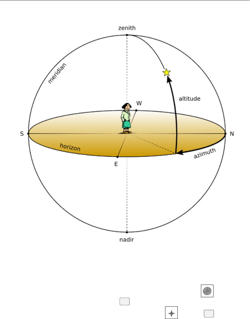
17.2 Coordinate Systems 193
Figure 17.1: Altitude/Azimuth (Horizontal) Coordinate System
Stellarium can draw grid lines for altitude/azimuth coordinates. Use the button on the
main tool-bar to activate this grid, or press the Zkey.
In addition, the cardinal points can be highlighted using the button or Qkey.
There are a few great circles with special names which Stellarium can draw (see section 4.4.3).
Meridian
This is the vertical line which runs from the North point towards the zenith and further
to the South point.
(Mathematical) Horizon This is the line exactly 90◦away from the zenith.
First Vertical
This is the vertical line which runs from the East point towards the zenith and
further to the West point.
17.2.2 Right Ascension/Declination Coordinates
Like the Altitude/Azimuth system, the Right Ascension/Declination (RA/Dec) Coordinate System
(or Equatorial Coordinate System) uses two angles to describe positions in the sky. These angles

194 Chapter 17. Astronomical Concepts
Figure 17.2: Equatorial Coordinates
are measured from standard points on the celestial sphere. Right ascension
α
and declination
δ
are
to the celestial sphere what longitude and latitude are to terrestrial map makers.
The Northern celestial pole has a declination of
δ=90◦
, the celestial equator has a declination
of δ=0◦, and the Southern celestial pole has a declination of δ=−90◦.
Right ascension is measured as an angle round from a point in the sky known as the First Point
of Aries, in the same way that longitude is measured around the Earth from Greenwich. Figure 17.2
illustrates RA/Dec coordinates. The angle
α
is usually expressed as time with minute and seconds,
with 15◦equalling one hour.
Unlike Altitude/Azimuth coordinates, RA/Dec coordinates of a star do not change if the
observer changes latitude, and do not change noticeably over the course of the day due to the
rotation of the Earth. RA/Dec coordinates are generally used nowadays in star catalogues such as
the Hipparcos catalogue.
However, the story is complicated a little by precession (section 17.8) and parallax (sec-
tion 17.9). Precession causes a slow drift of the coordinates almost parallel to the ecliptic, and

17.2 Coordinate Systems 195
therefore star catalogues always have to specify their equinox of validity. Current catalogs and
atlases use coordinates for J2000.0.
Stellarium can draw grid lines for Equatorial coordinates. Use the button on the main
tool-bar to activate this grid, or press the
E
key to draw the equatorial grid for the simulation
time. The Markings dialog (4.4.3) allows you to set also the grid for J2000.0 standard coordinates.
In case you are observing from another celestial object, the equatorial coordinates use a system
similar to the one referring to the earth-based coordinates, but parallel to the planet’s rotational axis.
There are again a few great circles with special names which Stellarium can draw in addition,
both for simulation time and for J2000.0 (see section 4.4.3).
Celestial Equator
the line directly above the earth’s (or more generally, the observer’s planet’s)
equator.
Colures
These are lines similar to meridian and first vertical in the azimuthal system. The
Equinoctial Colure runs from the North Celestial Pole NCP through the First Point of Aries
à
, South Celstial Pole SCP and First Point of Libra
æ
while the Solstitial Colure runs from
the NCP through First Point of Cancer ã, SCP and First Point of Capricorn é.
17.2.3 Ecliptical Coordinates
The earth’s orbit around the sun, i.e., the ecliptic, defines the “equatorial line” of this coordinate
system, which is traditionally used when computing the coordinates for planets.
The zero point of ecliptical longitude
λ
is the same as for equatorial coordinates, and the eclip-
tical latitude
β
is counted positive towards the Northern Ecliptical Pole NEP in the constellation of
Draco.
Moon and sun (and to a much lesser extent, the other planets) pull on the equatorial bulge and
try to put Earth’s axis normal to its orbital plane. Earth acts like a spinning top and evades this pull
in a sideways motion, so that earth’s axis seems to describe a small circle over a period of almost
26.000 years (see section 17.8).
In addition, ecliptic obliquity against the equatorial coordinates, which mirrors the earth’s axial
tilt, slowly changes.
Therefore, also for ecliptical coordinates is is required to specify which date the coordinates
refer to. Stellarium can draw two grids for Ecliptical coordinates. Use the
,
key to draw the
ecliptic for the simulation time. The Markings dialog (4.4.3) allows you to show also a line for
epoch J2000.0 and grids for the ecliptical coordinates for current epoch and epoch J2000.0. You
can assign your own shortcut keys (section 4.7.1) if you frequently operate with these coordinates.
Since version 0.14.0 Stellarium can very accurately show the motions between the coordinate
systems (Vondrák, Capitaine, and Wallace, 2011; Vondrák, Capitaine, and Wallace, 2012), and it is
quite interesting to follow these motions for several millennia. To support such demonstrations,
Stellarium can also draw the precession circles between celestial and ecliptical poles (activate them
in the Markings dialog (4.4.3). If you observe long enough, you will see that these circles vary in
size, reflecting the changes in ecliptic obliquity.
Many of the minor bodies are best observed around the times of their opposition. Stellarium
can display a great circle in the ecliptical coordinates which runs through the ecliptic poles and
through the sun, thereby allowing to estimate opposition and conjunction. Activate display of this
Opposition/Conjunction Line in the Markings dialog (Labeled “O./C. longitude”; 4.4.3).
It is interesting to note that star catalogs before TYCHO BRAHE’s (1546–1601), most notably
the one in PTOLEMY’s Almagest, used Ecliptical coordinates. The reason is simple: It was known
since HIPPARCHUS that stellar coordinates slowly move along the ecliptic through precession, and
the correction to coordinates of a date of interest was a simple addition of a linear correction to the
ecliptical longitude in the catalog. Changes of ecliptic obliquity was discovered much later.

196 Chapter 17. Astronomical Concepts
17.2.4 Galactic Coordinates
The Milky Way appears to run along a great circle over the sky, mirroring the fact that the sun
is a star in it. Coordinates for non-stellar objects which belong to the Milky Way like pulsars
or planetary nebulae are often mapped in Galactic Coordinates, where galactic longitude
l
and
galactic latitude
b
are usually given in decimal degrees. Here, the zero point of galactic longitudes
lies in the Galactic Center.
Stellarium can also draw a galactic grid and the galactic equator by activating the respective
options in the Markings dialog (see section 4.4.3). You can assign a keyboard shortcut if you
frequently use these coordinates (see 4.7.1).
17.3 Distance
As DOUGLAS ADAMS (1952–2001) pointed out in The Hitchhiker’s Guide to the Galaxy (Adams,
1981),
Space [. . . ] is big. Really big. You just won’t believe how vastly, hugely, mind-
bogglingly big it is. I mean, you may think it’s a long way down the road to the
chemist, but that’s just peanuts to space.[p.76]
Astronomers use a variety of units for distance that make sense in the context of the mind-boggling
vastness of space.
Astronomical Unit (AU)
This is the mean Earth-Sun distance. Roughly 150 million kilometres
(
1.49598×10⁸km
). The AU is used mainly when discussing the solar system – for example
the distance of various planets from the Sun.
Light year (LY)
A light year is not, as some people believe, a measure of time. It is the distance
that light travels in a year. The speed of light being approximately 300,000 kilometres per
second means a light year is a very large distance indeed, working out at about 9.5 trillion
kilometres (
9.46073 ×10¹² km
). Light years are most frequently used when describing the
distance of stars and galaxies or the sizes of large-scale objects like galaxies, nebulae etc.
Parsec (pc)
A parsec is defined as the distance of an object that has an annual parallax of 1 second
of arc. This equates to 3.26156 light years (
3.08568 ×10¹³ km
). Parsecs (and derivatives:
kiloparsec
kpc
, megaparsec
Mpc
) are most frequently used when describing the distance of
stars or the sizes of large-scale objects like galaxies, nebulae etc.
17.4 Time
The length of a day is defined as the amount of time that it takes for the Sun to travel from the
highest point in the sky at mid-day to the next high-point on the next day. In astronomy this is
called a solar day. The apparent motion of the Sun is caused by the rotation of the Earth. However,
in this time, the Earth not only spins, it also moves slightly round its orbit. Thus in one solar day
the Earth does not spin exactly
360◦
on its axis. Another way to measure day length is to consider
how long it takes for the Earth to rotate exactly 360◦. This is known as one sidereal day.
Figure 17.3 illustrates the motion of the Earth as seen looking down on the Earth orbiting the
Sun. The red triangle on the Earth represents the location of an observer. The figure shows the
Earth at four times:
1. The Sun is directly overhead - it is mid-day.
2.
Twelve hours have passed since 1. The Earth has rotated round and the observer is on the
opposite side of the Earth from the Sun. It is mid-night. The Earth has also moved round in
its orbit a little.
3. The Earth has rotated exactly 360◦. Exactly one sidereal day has passed since 1.
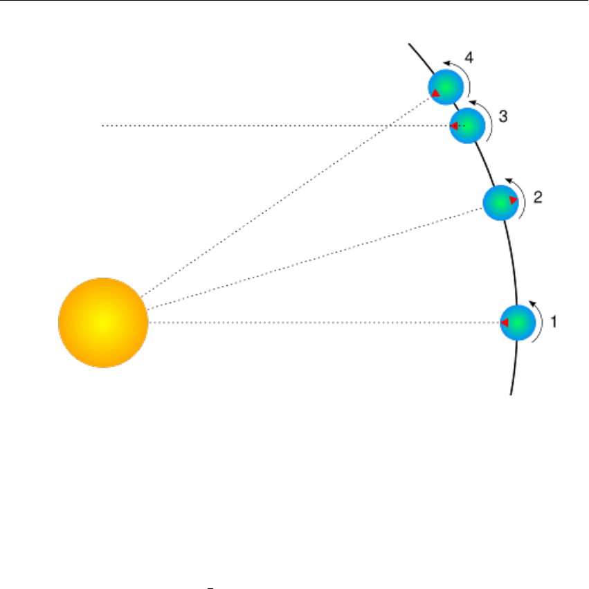
17.4 Time 197
Figure 17.3: Sidereal day
4.
It is mid-day again – exactly one solar day since 1. Note that the Earth has rotated more than
360◦since 1.
It should be noted that in figure 17.3 the sizes of the Sun and Earth and not to scale. More
importantly, the distance the Earth moves around its orbit is much exaggerated. The Earth takes a
year to travel round the Sun –
3651
4
solar days. The length of a sidereal day is about 23 hours, 56
minutes and 4 seconds.
17.4.1 Sidereal Time
It takes exactly one sidereal day for the celestial sphere to make one revolution in the sky. As-
tronomers find sidereal time useful when observing. This is the Right Ascension which is currently
passing the meridian line. When visiting observatories, look out for doctored alarm clocks that
have been set to run in sidereal time!
17.4.2 Julian Day Number
In the 19th century, astronomer JOHN HERSCHEL (1792–1871) introduced the use of Julian Day
numbers (invented around the time of the Gregorian calendar reform). This is a simple continuous
day count starting on January 1, -4712 (4713 BC). There are no years, months etc., and the integral
day number switches at noon, so during a single night of observation (in Europe) the date never
changes.
The fractional part of the number is just the fraction of day that has elapsed since last noon.
Given that a day has 86400 seconds, we should give a JD with 5 decimal places to capture the
nearest second.
This causes a problem for modern computers: even a “double precision float” can keep

198 Chapter 17. Astronomical Concepts
only about 13 decimal places. More than 2.4 million days have passed, so that e.g. Jan-
uary 1, 2000, 12:00UT is 2451545.0, which is an accurately storable number with 7 decimal
places, but 12:34:56UT is computed as 2451545.02426. A more accurate result would yield
2451545.024259259259... So, for a field where sub-second accuracy became crucial like spacecraft
operations, the Modified Julian Day (MJD) has been introduced. It is simply
MJD =JD −2400000.5.(17.1)
This means, days start at midnight, and the (constant, in our era) decimal places of the “big numbers”
at the begin of the number have been traded in for more decimal places at the end.
Don’t put your expectations too high when you see MJD displayed (section 4.1): Stellarium
uses a double-precision floating point number for JD for internal timekeeping, and Stellarium’s
display of MJD is simply computed from it. So you cannot set temporal increments smaller than a
second, and it hardly would make sense to expect more accuracy from the simulation algorithms.
17.4.3 Delta T
Until around 1900, the earth’s rotation was regarded as perfect standard of time. There were
86400 seconds per mean solar day, and the accuracy of reproducing time with mechanical clocks
only in this time started to become as good as the earth’s rotation itself.
Astronomers who computed solar eclipses reported in texts from antiquity wondered about a
required time shift which they originally attributed to a yet-unknown “secular acceleration of the
lunar motion”. However, it turned out that indeed the gravitational effect of the moon which causes
the tides also has effects on earth’s rotation: the tides slowly break earth’s rotational speed. The
energy is also transferred to the moon, and the acceleration leads to the moon slowly moving away
from the earth4.
This led to the introduction of a time named Ephemeris Time (ET) with progresses in the speed
of the second in the year 1900, to be used for positional computation in our solar system, in addition
to Greenwich Mean Time (GMT), from which all zone times and “civil” clock times were derived.
The introduction of Atomic Clocks in the middle of the 20th century led to a redefinition of the
(temporal) second, which has been de-coupled from earth’s rotation. This time, the International
Atomic Time TAI, is the basis for Terrestrial Time TT which can be considered as constantly
progressing at constant speed5, and is used for computation of the planetary positions.
Still, people living on earth prefer to have the mean solar noon governing the run of day and
night. Therefore all forms of civil time are linked to Coordinated Universal Time UTC. Seconds
in UTC and TAI are of equal length. The slow and irregular divergence between TAI and UTC is
observed by a few standardisation institutes. When necessary, a leap second can be introduced to
the UTC to bring the earth’s rotation back in sync so that the Mean Sun again culminates at noon.
The difference
∆T=T T −UT
(or “Delta T”) describes the temporal offset which amounts
already to more than a minute in the 21st century. There have been many attempts to properly model
∆T
, and Stellarium offers several models you can choose from in the configuration dialog (see
section 4.3.3). The default, “Espenak and Meeus (2006)”, is a widely accepted standard. But if you
are a researcher and want to experiment with alternative models, you will hopefully like this feature.
you can even specify your own data for
a
,
b
,
c
,
y
and the secular term for lunar acceleration
n
4
No need to worry, the moon recedes from the earth only a few centimeters per year as measured with
the laser reflectors left by the Apollo astronauts in the 1970s. In a very far future, however, there will only be
annular solar eclipses as a consequence!
5
We don’t discuss relativity here. The advanced reader is referred to the presentation in the Wikipedia,
https://en.wikipedia.org/wiki/Delta_T.

17.4 Time 199
(actually
˙n=dn/dt
in units of
arcseconds/century2
) if you can model
∆T
according to the formula
∆T=a+b·u+c·u2where (17.2)
u=year −y
100 (17.3)
List of ∆Tmodels in Stellarium
The following list describes sources and a few details about the models for
∆T
implemented in
Stellarium.
Without correction. Correction is disabled. Use only if you know what you are doing!
Schoch (1931).
This historical formula was obtained by Schoch (1931) and was also used in “A
New Test of Einstein’s Theory of Relativity by Ancient Solar Eclipses” (Henriksson, 2009).
See for more in Peters (2010). ˙n=−29.6800/cy2.
Clemence (1948).
This empirical equation was published in “On the system of astronomical
constants” (Clemence, 1948). Valid range of usage: between years 1681 and 1900.
˙n=
−22.4400/cy2.
IAU (1952).
This formula is based on a study of post-1650 observations of the Sun, the Moon and
the planets (Spencer Jones, 1939) and reproduced in Astronomical Formulae for Calculators
(Meeus, 1988). It was also adopted in the PC program
SunTracker Pro
. Valid range of usage:
between years 1681 and 1936. ˙n=−22.4400/cy2.
Astronomical Ephemeris (1960).
This is a slightly modified version of the IAU 1952 (Spencer
Jones, 1939) formula which was adopted in the “Astronomical Ephemeris” (Wilkins, 1961)
and in the Canon of Solar Eclipses -2003 to +2526 (Mucke and Meeus, 1983). Valid range
of usage: between years -500 and 2000. ˙n=−22.4400/cy2.
Tuckerman (1962, 1964) & Goldstine (1973).
The famous tables (Tuckerman, 1962; Tuckerman,
1964) list the positions of the Sun, the Moon and the planets at 5- and 10-day intervals from
601 BCE to 1649 CE. The same relation was also implicitly adopted in the syzygy tables of
Goldstine (1973). Valid range of usage: between years -600 and 1649.
Muller & Stephenson (1975).
This equation was published in “The accelerations of the earth and
moon from early astronomical observations” (Muller and F. R. Stephenson, 1975). Valid
range of usage: between years -1375 and 1975. ˙n=−37.500/cy2.
Stephenson (1978).
This equation was published in “Pre-Telescopic Astronomical Observations”
(F. R. Stephenson, 1978). ˙n=−30.000/cy2.
Schmadel & Zech (1979).
This 12th-order polynomial equation (outdated and superseded by
Schmadel and Zech (1988)) was published in “Polynomial approximations for the correction
delta T E.T.-U.T. in the period 1800-1975” (Schmadel and Zech, 1979) as fit through data
published by Brouwer (1952). Valid range of usage: between years 1800 and 1975, with
meaningless values outside this range. ˙n=−23.894600/cy2.
Morrison & Stephenson (1982).
This algorithm Morrison and F. R. Stephenson, 1982 was
adopted in Planetary Programs and Tables from –4000 to +2800 (Pierre Bretagnon and
Simon, 1986) and in the PC planetarium program
RedShift
. Valid range of usage: between
years -4000 and 2800. ˙n=−26.000/cy2.
Stephenson & Morrison (1984).
This formula was published in “Long-term changes in the rota-
tion of the earth - 700 B.C. to A.D. 1980” (F. R. Stephenson and Morrison, 1984). Valid
range of usage: between years -391 and 1600. ˙n=−26.000/cy2.
Stephenson & Houlden (1986).
This algorithm (Houlden and F. Stephenson, 1986) is used in the
PC planetarium program
Guide 7
. Valid range of usage: between years -600 and 1600.
˙n=−26.000/cy2.
Espenak (1987, 1989).
This algorithm was given in Fifty Year Canon of Solar Eclipses: 1986 –
2035 (Espenak, 1987) and in Fifty Year Canon of Lunar Eclipses: 1986 – 2035 (Espenak,
1989). Valid range of usage: between years 1950 and 2100.

200 Chapter 17. Astronomical Concepts
Borkowski (1988).
This formula was obtained by Borkowski (1988) from an analysis of 31 solar
eclipse records dating between 2137 BCE and 1715 CE. Valid range of usage: between years
-2136 and 1715. ˙n=−23.89500/cy2.
Schmadel & Zech (1988).
This 12th-order polynomial equation was published in “Empirical
Transformations from U.T. to E.T. for the Period 1800-1988” (Schmadel and Zech, 1988)
as data fit through values given by F. R. Stephenson and Morrison (1984). Valid range of
usage: between years 1800 and 1988, with a mean error of less than one second, max. error
1.9s, and meaningless values outside this range. ˙n=−26.000/cy2.
Chapront-Touze & Chapront (1991).
This formula was adopted by M. Chapront-Touze & J.
Chapront in the shortened version of the ELP 2000-85 lunar theory in their Lunar Tables and
Programs from 4000 B.C. to A.D. 8000 (Chapront-Touzé and Chapront, 1991). The relations
are based on those of F. R. Stephenson and Morrison (1984), but slightly modified to make
them compatible with the tidal acceleration parameter of
˙n=−23.894600/cy2
adopted in the
ELP 2000-85 lunar theory (Chapront-Touzé and Chapront, 1988a).
Stephenson & Morrison (1995).
This equation was published in “Long-Term Fluctuations in the
Earth’s Rotation: 700 BC to AD 1990” (F. R. Stephenson and Morrison, 1995). Valid range
of usage: between years -700 and 1600. ˙n=−26.000/cy2.
Stephenson (1997).
F. R. Stephenson published this formula in his book Historical Eclipses and
Earth’s Rotation (F. Richard Stephenson, 1997). Valid range of usage: between years -500
and 1600. ˙n=−26.000/cy2.
Meeus (1998) (with Chapront, Chapront-Touze & Francou (1997)).
From Astronomical Algo-
rithms (Meeus, 1998), and widely used. Table for 1620..2000, and includes a variant of
Chapront, Chapront-Touze & Francou (1997) for dates outside 1620..2000. Valid range of
usage: between years -400 and 2150. ˙n=−25.737600/cy2.
JPL Horizons.
The JPL Solar System Dynamics Group of the NASA Jet Propulsion Laboratory
use this formula in their interactive website JPL Horizons
6
. Valid range of usage: between
years -2999 and 1620, with zero values outside this range. ˙n=−25.737600/cy2.
Meeus & Simons (2000).
This polynome was published in “Polynomial approximations to Delta
T, 1620-2000 AD” (Meeus and Simons, 2000). Valid range of usage: between years 1620
and 2000, with zero values outside this range. ˙n=−25.737600/cy2.
Montenbruck & Pfleger (2000).
The fourth edition of Astronomy on the Personal Computer
(Montenbruck and Pfleger, 2000) provides simple 3rd-order polynomial data fits for the
recent past. Valid range of usage: between years 1825 and 2005, with a typical 1-second
accuracy and zero values outside this range.
Reingold & Dershowitz (2002, 2007).
E. M. Reingold & N. Dershowitz present this polynomial
data fit in Calendrical Calculations (Reingold and Dershowitz, 2007) and in their Calendrical
Tabulations 1900-2200 (Reingold and Dershowitz, 2002). It is based on Astronomical
Algorithms (Meeus, 1991).
Morrison & Stephenson (2004, 2005).
This important solution was published in “Historical val-
ues of the Earth’s clock error
∆
T and the calculation of eclipses” (Morrison and F. R.
Stephenson, 2004) with addendum (Morrison and F. R. Stephenson, 2005). Valid range of
usage: between years -1000 and 2000. ˙n=−26.000/cy2.
Stephenson, Morrison & Hohenkerk (2016).
This important new solution was published in
“Measurement of the Earth’s rotation: 720 BC to AD 2015” (F. R. Stephenson, Morri-
son, and Hohenkerk, 2016). The solution combines a spline fit to observations (used between
the given limits) with a parabolic fit (used as fallback outside the range, but without smooth
transitions at the limits, i.e., values for 2016 and later deviate notably from current estimates,
and should not be used for dates after 2015). Recommended range of usage: between years
6http://ssd.jpl.nasa.gov/?horizons

17.5 Angles 201
-720.0 and 2016.0 ˙n=−25.8200/cy2.
Espenak & Meeus (2006).
This solution
7
by F. Espenak and J. Meeus, based on Morrison and
F. R. Stephenson (2004) and a polynomial fit through tabulated values for 1600-2000, is
used for the NASA Eclipse Web Site
8
and in their Five Millennium Canon of Solar Eclipses:
-1900 to +3000 (Espenak and Meeus, 2006). This formula is also used in the solar, lunar and
planetary ephemeris program SOLEX. Valid range of usage: between years -1999 and 3000.
˙n=−25.85800/cy2.
Reijs (2006).
From the Length of Day (LOD; as determined by Morrison and F. R. Stephenson
(2004)), Victor Reijs derived a
∆T
formula by using a Simplex optimisation with a cosine
and square function
9
. This is based on a possible periodicy described by Morrison and F. R.
Stephenson (2004). Valid range of usage: between years -1500 and 1100. ˙n=−26.000/cy2.
Banjevic (2006).
This solution is based on F. R. Stephenson and Morrison (1984) and was
published in “Ancient eclipses and dating the fall of Babylon” (Banjevic, 2006). Valid
range of usage: between years -2020 and 1620, with zero values outside this range.
˙n=
−26.000/cy2.
Islam, Sadiq & Qureshi (2008, 2013).
This solution by S. Islam, M. Sadiq and M. S. Qureshi,
based on Meeus and Simons (2000), was published in “Error Minimization of Polynomial
Approximation of Delta T” (Islam, Sadiq, and Qureshi, 2008) and revisited by Sana Islam
in 2013. Valid range of usage: between years 1620 and 2007, with zero values outside this
range.
Khalid, Sultana & Zaidi (2014).
This polynomial approximation with 0.6 seconds of accuracy
was published in “Delta T: Polynomial Approximation of Time Period 1620–2013” (Khalid,
Sultana, and Zaidi, 2014). Valid range of usage: between years 1620 and 2013, with zero
values outside this range.
Custom equation of ∆T.
This is a quadratic formula for calculation of
∆T
with coefficients
defined by the user.
17.5 Angles
Astronomers typically use degrees to measure angles. Since many observations require very precise
measurement, the degree is subdivided into sixty minutes of arc also known as arc-minutes. Each
minute of arc is further subdivided into sixty seconds of arc, or arc-seconds. Thus one degree is
equal to 3600 seconds of arc. Finer grades of precision are usually expressed using the SI prefixes
with arc-seconds, e.g. milli arc-seconds (one milli arc-second is one thousandth of an arc-second).
17.5.1 Notation
Degrees are denoted using the
◦
symbol after a number. Minutes of arc are denoted with a
0
, and
seconds of arc are denoted using 00. Angles are frequently given in two formats:
1.
DMS format — degrees, minutes and seconds. For example
90◦1501200
. When more precision
is required, the seconds component may include a decimal part, for example
90◦15012.43200
.
2. Decimal degrees, for example 90.2533◦
17.5.2 Handy Angles
Being able to estimate angular distance can be very useful when trying to find objects from star
maps in the sky. One way to do this with a device called a crossbow.
7This solution is used by default.
8http://eclipse.gsfc.nasa.gov/eclipse.html
9http://www.iol.ie/~geniet/eng/DeltaTeval.htm

202 Chapter 17. Astronomical Concepts
Crossbows are a nice way get an idea of angular distances, but carrying one about is a little
cumbersome. A more convenient alternative is to hold up an object such as a pencil at arm’s length.
If you know the length of the pencil,
d
, and the distance of it from your eye,
D
, you can calculate
its angular size, θusing this formula:
θ=2·arctand
2·D(17.4)
Another, more handy (ahem!) method is to use the size of your hand at arm’s length:
Tip of little finger About 1◦
Middle three fingers About 4◦
Across the knuckles of the fist About 10◦
Open hand About 18◦
Using you hand in this way is not very precise, but it’s close enough to give you some way
to translate an idea like “Mars will be
45◦
above the Southeastern horizon at 21:30”. Of course,
there is variation from person to person, but the variation is compensated for somewhat by the fact
that people with long arms tend to have larger hands. In exercise 20.2 you will work out your own
“handy angles”.
17.6 The Magnitude Scale
When astronomers talk about magnitude, they are referring to the brightness of an object. How
bright an object appears to be depends on how much light it is giving out and how far it is from the
observer. Astronomers separate these factors by using two measures: absolute magnitude (Mag or
M
) which is a measure of how much light is being given out by an object, and apparent magnitude
(mag or m) which is how bright something appears to be in the sky.
For example, consider two 100 watt lamps, one which is a few meters away, and one which is a
kilometre away. Both give out the same amount of light – they have the same absolute magnitude.
However the nearby lamp seems much brighter – it has a much greater apparent magnitude. When
astronomers talk about magnitude without specifying whether they mean apparent or absolute
magnitude, they are usually referring to apparent magnitude.
The magnitude scale has its roots in antiquity. The Greek astronomer HIPPARCHUS defined the
brightest stars in the sky to be first magnitude, and the dimmest visible to the naked eye to be sixth
magnitude. In the 19th century British astronomer NORMAN POGSON (1829–1891) quantified the
scale more precisely, defining it as a logarithmic scale where a magnitude 1 object is 100 times
as bright as a magnitude 6 object (a difference of five magnitudes). The zero-point of the modern
scale was originally defined as the brightness of the star Vega, however this was re-defined more
formally in 1982 (Aller et al., 1989). Objects brighter than Vega are given negative magnitudes.
The absolute magnitude of a star is defined as the magnitude a star would appear if it were 10
parsecs from the observer.
Table 17.1 lists several objects that may be seen in the sky, their apparent magnitude and their
absolute magnitude where applicable (only stars have an absolute magnitude value. The planets
and the Moon don’t give out light like a star does – they reflect the light from the Sun).
17.7 Luminosity
Luminosity is an expression of the total energy radiated by a star. It may be measured in watts,
however, astronomers tend to use another expression — solar luminosities where an object with
twice the Sun’s luminosity is considered to have two solar luminosities and so on. Luminosity is
related to absolute magnitude.
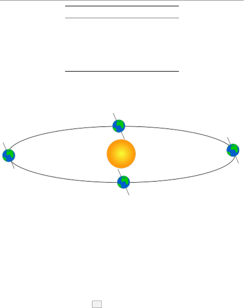
17.8 Precession 203
Object m M
The Sun -27 4.8
Vega 0.05 0.6
Betelgeuse 0.47 -7.2
Sirius (the brightest star) -1.5 1.4
Venus (at brightest) -4.4 —
Full Moon (at brightest) -12.6 —
Table 17.1: Magnitudes of a few objects
17.8 Precession
Figure 17.4: Ecliptic obliquity
As the Earth orbits the Sun throughout the year, the axis of rotation (the line running through
the rotational poles of the Earth) seems to point towards the same position on the celestial sphere,
as can be seen in figure 17.4. The angle between the axis of rotation and the perpendicular of the
orbital plane is called the obliquity of the ecliptic. It is currently about
23◦270
and is the angle
between equatorial coordinates (17.2.2) and ecliptical coordinates (17.2.3).
Observed over very long periods of time the direction the axis of rotation points to does actually
change. The angle between the axis of rotation and the orbital plane stays fairly constant, but the
direction the axis points — the position of the celestial pole — transcribes a figure similar to a
circle on the stars in the celestial sphere. The motion is similar to the way in which a gyroscope
slowly twists, as figure 17.5 illustrates. This process is called precession. The circles can be shown
in Stellarium: From the View menu (
F4
), tab “Markings”, switch on “Precession Circles” (4.4.3).
Precession is a slow process. The axis of rotation twists through a full
360◦
about once
every 26,000 years. However, over these long times other gravitational perturbations (“planetary
precession”) play a role, and what may be thought of as rigid “precession circle” can actually only
show the instantaneous (current) state. Over millennia the circle slightly varies.
Precession has some important implications:
1.
RA/Dec coordinates change over time, albeit slowly. Measurements of the positions of
stars recorded using RA/Dec coordinates must also include a date (“equinox”) for those
coordinates. Therefore the current star catalogues list their objects for the epoch and equinox
J2000.0.
2.
Polaris, the pole star, won’t stay a good indicator of the location of the Northern celestial
pole. In 14,000 years time Polaris will be nearly 47◦away from the celestial pole!
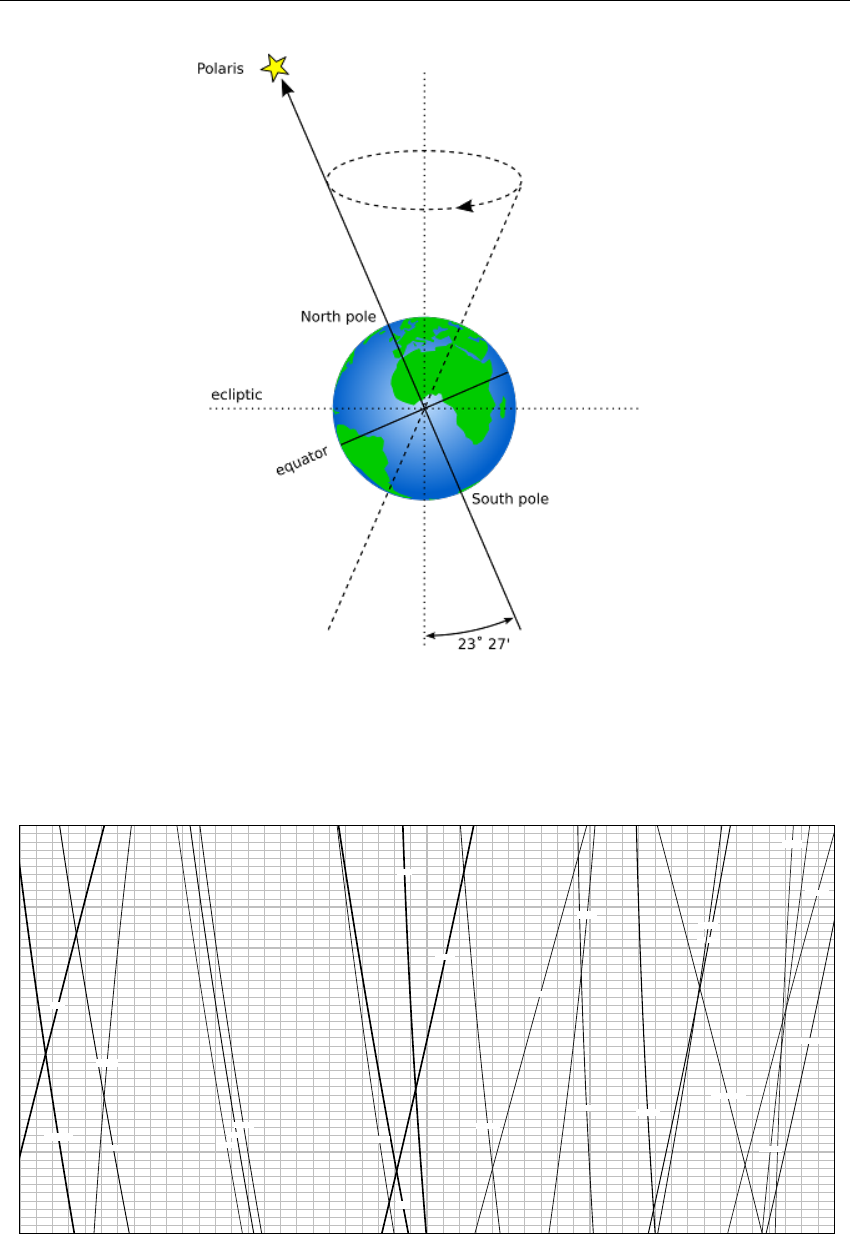
204 Chapter 17. Astronomical Concepts
Figure 17.5: Precession
90 95 100 105 110 115 120 125 130 135
85 90 95 100 105 110 115 120 125 130 135
Azimuth
-1000
-900
-800
-700
-600
-500
-400
-300
-200
-100
0
Deneb Kaitos
Rigel
Gam Ori Mintaka
Alnilam
Alnitak
Kap Ori
Betelgeuse
Bet CMa
Sirius
Eps CMa
Del CMa
Zet Pup
Lam Vel
Alphard
Gam Cen
Spica
The Cen
Antares
Lam Sco
The Sco
Eps Sgr
Sig Sgr
Precession Shift of Stars on the Horizon
Geograpical Latitude: 30°0’ 0’’. Stars to mag=2.25. Azimuths from North, without refraction. © Georg Zotti 2010, http://astrosim.univie.ac.at
Figure 17.6: Precession: Change of rising positions of the stars along the eastern horizon
from azimuths 85 to 135 degrees, between years 1000 BC and 0, for latitude ϕ=30◦.

17.9 Parallax 205
3.
The change in declination causes a shift in the rising and setting positions of the stars along
the horizon. Figure 17.6 shows part of the horizon for latitude
ϕ=30◦
North. For a given
year (left vertical labels), make a horizontal line to find rising azimuth of the bright stars
indicated by the twisting lines. Depending on where on the celestial sphere a star is located,
it may appear to move north or south, or be almost stationary for several centuries.
17.9 Parallax
Parallax is the change of angular position of two stationary points relative to each other as seen by
an observer, due to the motion of said observer. Or more simply put, it is the apparent shift of an
object against a background due to a change in observer position.
This can be demonstrated by holding ones thumb up at arm’s length. Closing one eye, note the
position of the thumb against the background. After swapping which eye is open (without moving),
the thumb appears to be in a different position against the background.
17.9.1 Geocentric and Topocentric Observations
When computing planetary positions was done manually by adding numbers tabulated in yearly
almanacs, computing the Earth’s position and, say, position of a minor planet was usually good
enough to find the object in the sky. In both cases, the exact numbers refer to the gravitational
centres of the respective bodies. However, we are sitting on Earth’s surface, so the observed planet
will be seen in a slightly shifted location. The amount for objects in the inner solar system is usually
just a few arcseconds and is mostly negligible when we just want to find an object. But it makes
a difference when it comes to observations of stellar occultations by planets or asteroids. Such a
body may measure only a few tens of kilometres, and the shadow track which it leaves on Earth’s
surface is of approximately the same size.10
A much closer and bigger object is the Moon, which can also occult stars. It can even occult
the one big star we call the Sun: this is a Solar Eclipse. And here it makes a huge difference where
on the planet you are located.
If you are interested in astronomical computing, you may still be interested in geocentric
numerical results. From the Settings panel (
F2
), tab “Tools”, there is a checkbox for “Topocentric
Coordinates”. Switch it off to put yourself into the center of the planet you are located.
17.9.2 Stellar Parallax
A similar thing happens due to the Earth’s motion around the Sun. Nearby stars appear to move
against more distant background stars, as illustrated in figure 17.7. The movement of nearby stars
against the background is called stellar parallax, or annual parallax.
Since we know the distance the radius of the Earth’s orbit around the Sun from other methods,
we can use simple geometry to calculate the distance of the nearby star if we measure annual
parallax.
As can be seen from figure 17.7, the annual parallax
p
is half the angular distance between the
apparent positions of the nearby star. The distance of the nearby object is
d
. Astronomers use a unit
of distance called the parsec (
pc
) which is defined as the distance at which a nearby star has
p=100
.
Even the nearest stars exhibit very small movement due to parallax. The closest star to the
Earth other than the Sun is Proxima Centauri. It has an annual parallax of
0.7719900
, corresponding
to a distance of 1.295pc (4.22 light years).
10
Unfortunately Stellarium (as of v0.15.0) is not accurate enough to reliably compute such occultations.
Even a deviation of 0.5 arcseconds is too much here.
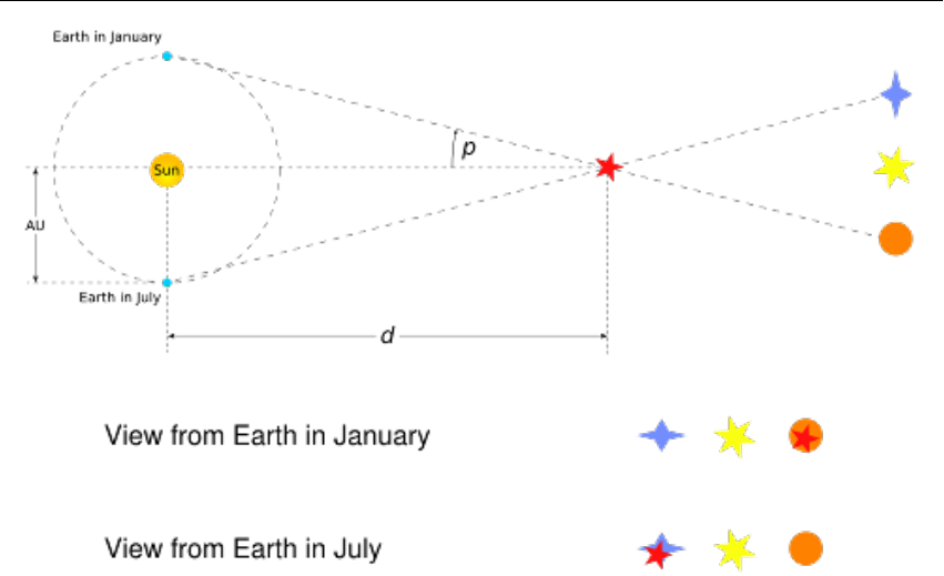
206 Chapter 17. Astronomical Concepts
Figure 17.7: Stellar Parallax
Even with the most sensitive instruments for measuring the positions of the stars it is only
possible to use parallax to determine the distance of stars up to about 1,600 light years from the
Earth, after which the annual parallax is so small it cannot be measured accurately enough.
In Stellarium, the annual parallax can be listed in the object information for stars when available.
It is not used for the positional calculations.
17.10 Proper Motion
Proper motion is the change in the position of a star over time as a result of its motion through
space relative to the Sun. It does not include the apparent shift in position of star due to annular
parallax. The star exhibiting the greatest proper motion is Barnard’s Star which moves more than
ten seconds of arc per year.
If you want to simulate the effect of proper motion with Stellarium, put the map into equatorial
view mode, switch off ground and cardinal marks, and set some high time lapse speed. You will see
a few stars change their locations quite soon, those are usually stars in our galactic neighbourhood
(see section 20.12).
Note however some limitations:
1.
Stellarium will stop at
±100.000
years. This limit may be still suitable for most stellar
locations. The planetary locations are not trustworthy outside of a much narrower temporal
window (see section F). You cannot simulate the sky over the dinosaurs or such things.
2.
Proper motion is only modelled by the linear components. True 3D motion in space requires
more computation, which would slow down the program.
3.
Double stars are listed in catalogs as two individual stars with their current proper motion
which consists of spatial motion and the orbital motion around their center of gravity. They
may be seen flying apart, which is of course not realistic.

18. Astronomical Phenomena
BARRY GERDES,WITH ADDITIONS BY GEORG ZOTTI
This chapter focuses on the observational side of astronomy — what we see when we look at the
sky.
18.1 The Sun
Without a doubt, the most prominent object in the sky is the Sun. The Sun is so bright that when it
is in the sky, its light is scattered by the atmosphere to such an extent that almost all other objects in
the sky are rendered invisible.
The Sun is a star like many others but it is much closer to the Earth at approximately 150
million kilometres (a distance also called 1 Astronomical Unit). The next nearest star, Proxima
Centauri is approximately 260,000 times further away from us than the Sun! The Sun is also known
by its Latin name, Sol.
Over the course of a year, the Sun appears to move round the celestial sphere in a great circle
known as the ecliptic. Stellarium can draw the ecliptic on the sky. To toggle drawing of the ecliptic,
press the ,key.
WARNING: Looking at the Sun can permanently damage the eye. Never look at the Sun without
using the proper filters! By far the safest way to observe the Sun it to look at it on a computer
screen, courtesy of Stellarium!
18.2 Stars
The Sun is just one of billions of stars. Even though many stars have a much greater absolute
magnitude than the Sun (they give out more light), they have an enormously smaller apparent
magnitude due to their large distance. Stars have a variety of forms — different sizes, brightnesses,
temperatures, and colours. Measuring the position, distance and attributes of the stars is known as
astrometry, and is a major part of observational astronomy.

208 Chapter 18. Astronomical Phenomena
18.2.1 Multiple Star Systems
Many stars have stellar companions. As many as six stars can be found orbiting one-another in close
associations known as multiple star systems —binary systems being the most common with two
stars. Multiple star systems are more common than solitary stars, putting our Sun in the minority
group.
Sometimes multiple stars orbit each other in a way that means one will periodically eclipse the
other. These are eclipsing binaries or Algol variables.
Optical Doubles & Optical Multiples
Sometimes two or more stars appear to be very close to one another in the sky, but in fact have
great separation, being aligned from the point of view of the observer but of different distances.
Such pairings are known as optical doubles and optical multiples.
18.2.2 Constellations
The constellations are groupings of stars that are visually close to one another in the sky. The
actual groupings are fairly arbitrary — different cultures have grouped stars together into different
constellations. In many cultures, the various constellations have been associated with mythological
entities. As such people have often projected pictures into the skies as can be seen in figure 18.1
which shows the constellation of Ursa Major. On the left is a picture with the image of the mythical
Great Bear, on the right only a line-art version (or stick figure) is shown. The seven bright stars of
Ursa Major are widely recognised, known variously as “the plough”, the “pan-handle”, and the
“big dipper”. This sub-grouping is known as an asterism — a distinct grouping of stars. On the
right, the picture of the bear has been removed and only a constellation diagram remains.
Figure 18.1: Ursa Major
Stellarium can draw both constellation diagrams and artistic representations of the constellations.
Multiple sky cultures are supported: Western, Polynesian, Egyptian, Chinese, and several other sky
cultures are available, although at time of writing the non-Western constellations are not complete,
and as yet there are no artistic representations of these sky-cultures.
Aside from historical and mythological value, to the modern astronomer the constellations
provide a way to segment the sky for the purposes of describing locations of objects, indeed one of
the first tasks for an amateur observer is learning the constellations — the process of becoming
familiar with the relative positions of the constellations, at what time of year a constellation is
visible, and in which constellations observationally interesting objects reside. The International

18.2 Stars 209
Astronomical Union has adopted 88 “Western” constellations as a common system for segmenting
the sky. They are based on Greek/Roman mythology, but with several additions from Renaissance
and later centuries. As such some formalisation has been adopted, each constellation having
aproper name, which is in Latin, and a three letter abbreviation of that name. For example,
Ursa Major has the abbreviation UMa. Also, the “Western” constellation have clearly defined
boundaries (Delporte, 1930), which you can draw in Stellarium when you press the
B
key
1
. The
IAU constellation a selected object is placed in is also available in the object information data
(Roman, 1987), regardless of the currently active skyculture. On the other hand, the shapes of
mythological figures, and also stick figures, have not been canonized, so you will find deviations
between Stellarium and printed atlases.
18.2.3 Star Names
Stars can have many names. The brighter stars often have common names relating to mythical
characters from the various traditions. For example the brightest star in the sky, Sirius is also known
as The Dog Star (the name Canis Major — the constellation Sirius is found in — is Latin for “The
Great Dog”).
Most bright names have been given names in antiquity. PTOLEMY’s most influential book, the
Syntaxis, was translated to the Arab language in the age of early Muslim scientists. When, centuries
later, the translation, called Almagest, was re-introduced to the re-awakening European science,
those names, which often only designated the position of the star within the figure, were taken from
the books, often misspelled, and used henceforth as proper names.
A few more proper names have been added later, sometimes dedicatory names added by court
astronomers into their maps. There are also 3 stars named after the victims of the Apollo 1 disaster
in 1967. Today, the International Astronomical Union (IAU) is the only scientifically accepted
authority which can give proper names to stars. Some companies offer a paid name service for
commemoration or dedication of a star for deceased relatives or such, but all you get here is a piece
of paper with coordinates of (usually) an unremarkably dim star only visible in a telescope, and a
name to remember, stored (at best) in the company’s database.
There are several more formal naming conventions that are in common use.
Bayer Designation
German astronomer JOHANN BAYER (1572–1625) devised one such system for his atlas, the
Uranographia, first published in 1603. His scheme names the stars according to the constellation in
which they lie prefixed by a lower case Greek letter, starting at
α
for (usually) the brightest star
in the constellation and proceeding with
β,γ,...
in descending order of apparent magnitude. For
example, such a Bayer Designation for Sirius is “
α
Canis Majoris” (note that the genitive form
of the constellation name is used; today also the short form
α
CMa is in use). There are some
exceptions to the descending magnitude ordering, and some multiple stars (both real and optical)
are named with a numerical superscript after the Greek letter, e.g. π1... π6Orionis.
Flamsteed Designation
English astronomer JOHN FLAMSTEED (1646–1719) numbered stars in each constellation in order
of increasing right ascension followed by the genitive form of the constellation name, for example
“61 Cygni” (or short: “61 Cyg”).
1
These boundaries or borders have been drawn using star maps from 1875. Due to the effect of precession,
these borders are no longer parallel to today’s coordinates.
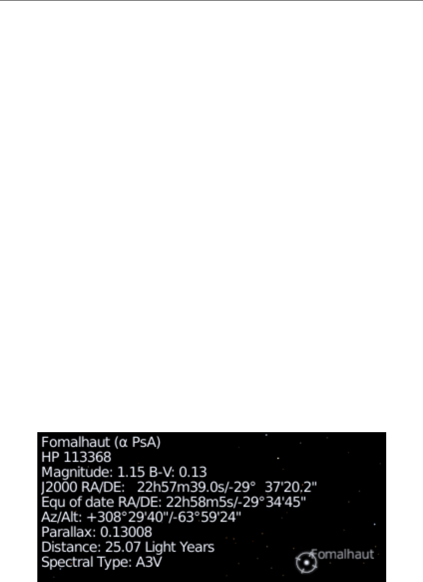
210 Chapter 18. Astronomical Phenomena
Hipparcos
Hipparcos (for High Precision Parallax Collecting Satellite) was an astrometry mission of the
European Space Agency (ESA) dedicated to the measurement of stellar parallax and the proper
motions of stars. The project was named in honour of the Greek astronomer HIPPARCHUS.
Ideas for such a mission dated from 1967, with the mission accepted by ESA in 1980. The
satellite was launched by an Ariane 4 on 8 August 1989. The original goal was to place the satellite
in a geostationary orbit above the earth, however a booster rocket failure resulted in a highly
elliptical orbit from 315 to 22,300 miles altitude. Despite this difficulty, all of the scientific goals
were accomplished. Communications were terminated on 15 August 1993.
The program was divided in two parts: the Hipparcos experiment whose goal was to measure
the five astrometric parameters of some 120,000 stars to a precision of some 2 to 4 milli arc-seconds
and the Tycho experiment, whose goal was the measurement of the astrometric and two-colour
photometric properties of some 400,000 additional stars to a somewhat lower precision.
The final Hipparcos Catalogue (120,000 stars with 1 milli arc-second level astrometry) and the
final Tycho Catalogue (more than one million stars with 20-30 milli arc-second astrometry and
two-colour photometry) were completed in August 1996. The catalogues were published by ESA in
June 1997. The Hipparcos and Tycho data have been used to create the Millennium Star Atlas: an
all-sky atlas of one million stars to visual magnitude 11, from the Hipparcos and Tycho Catalogues
and 10,000 non-stellar objects included to complement the catalogue data.
There were questions over whether Hipparcos has a systematic error of about 1 milli arc-second
in at least some parts of the sky. The value determined by Hipparcos for the distance to the Pleiades
is about 10% less than the value obtained by some other methods. By early 2004, the controversy
remained unresolved.
Stellarium uses the Hipparcos Catalogue for star data, as well as having traditional names
for many of the brighter stars. The stars tab of the search window allows for searching based
on a Hipparcos Catalogue number (as well as traditional names), e.g. the star Sadalmelik in the
constellation of Aquarius can be found by searching for the name, or its Hipparcos number, 109074.
Figure 18.2 shows the information Stellarium displays when a star is selected. At the top, the
common name, Bayer/Flamsteed designations and Hipparcos number are shown, followed by the
RA/Dec coordinates, apparent magnitude, distance and other data.
Figure 18.2: Star Names and Data
18.2.4 Spectral Type & Luminosity Class
Stars have many different colours. Seen with the naked eye most appear to be white, but this is
due to the response of the eye — at low light levels the eye is not sensitive to colour. Typically

18.2 Stars 211
Spectral Type Surface Temperature (K) Star Colour
O 28,000—50,000 Blue
B 10,000—28,000 Blue-white
A 7,500—10,000 White-blue
F 6,000—7,500 Yellow-white
G 4,900—6,000 Yellow
K 3,500—4,900 Orange
M 2,000—3,500 Red
Table 18.1: Spectral Types
the unaided eye can start to see differences in colour only for stars that have apparent magnitude
brighter than 1. Betelgeuse, for example has a distinctly red tinge to it, and Sirius appears to be
blue, while Vega is the prototype “white” star.
By splitting the light from a star using a prism attached to a telescope and measuring the
relative intensities of the colours of light the star emits — the spectrum — a great deal of interesting
information can be discovered about a star including its surface temperature, and the presence of
various elements in its atmosphere.
Astronomers groups stars with similar spectra into spectral types, denoted by one of the
following letters: O, B, A, F, G, K and M.
2
Type O stars have a high surface temperature (up to
around 50,000 K) while the at other end of the scale, the M stars are red and have a much cooler
surface temperature, typically 3000 K. The Sun is a type G star with a surface temperature of
around 5,500 K. Spectral types may be further sub-divided using a numerical suffix ranging from
0-9 where 0 is the hottest and 9 is the coolest. Table 18.1 shows the details of the various spectral
types.
For about 90% of stars, the absolute magnitude increases as the spectral type tends to the O
(hot) end of the scale. Thus the whiter, hotter stars tend to have a greater luminosity. These stars
are called main sequence stars. There are however a number of stars that have spectral type at the
M end of the scale, and yet they have a high absolute magnitude. These stars are close to the ends
of their lives and have a very large size, and consequently are known as giants, the largest of these
known as super-giants.
There are also stars whose absolute magnitude is very low regardless of the spectral class.
These are known as dwarf stars, among them white dwarfs (dying stars) and brown dwarfs (“failed
stars”).
The luminosity class is an indication of the type of star — whether it is main sequence, a
giant or a dwarf. Luminosity classes are denoted by a number in roman numerals, as described in
table 18.2.
Plotting the luminosity of stars against their spectral type/surface temperature gives a diagram
called a Hertzsprung-Russell diagram (after the two astronomers EJNAR HERTZSPRUNG (1873–
1967) and HENRY NORRIS RUSSELL (1877–1957) who devised it). A slight variation of this is
shown in figure 18.3 (which is technically a colour/magnitude in figure 18.3 (which is technically a
colour/magnitude plot).
18.2.5 Variable Stars
Most stars are of nearly constant luminosity. The Sun is a good example of one which goes through
relatively little variation in brightness (usually about 0.1% over an 11 year solar cycle). Many stars,
2The classic mnemonic for students of astrophysics says: “Oh, Be A Fine Girl, Kiss Me”.
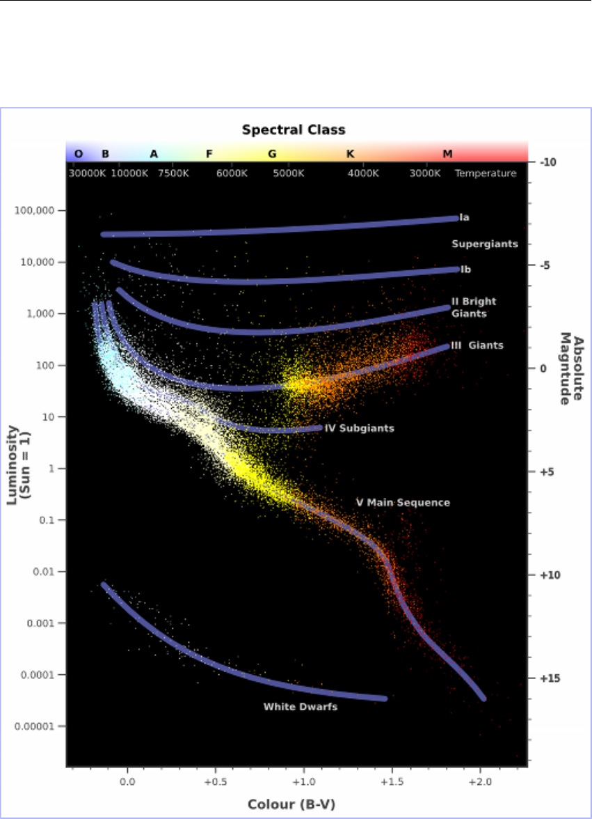
212 Chapter 18. Astronomical Phenomena
Figure 18.3: Hertzsprung-Russell Diagram

18.3 Our Moon 213
Luminosity class Description
Ia, Ib Super-giants
II Bright giants
III Normal giants
IV Sub-giants
V Main sequence
VI Sub-dwarfs
VII White-dwarfs
Table 18.2: Luminosity Classification
however, undergo significant variations in luminosity, and these are known as variable stars. There
are many types of variable stars falling into two categories, intrinsic and extrinsic.
Intrinsic variables are stars which have intrinsic variations in brightness, that is, the star itself
gets brighter and dimmer. There are several types of intrinsic variables, probably the best-known
and most important of which is the Cepheid variable whose luminosity is related to the period
with which its brightness varies. Since the luminosity (and therefore absolute magnitude) can be
calculated, Cepheid variables may be used to determine the distance of the star when the annual
parallax is too small to be a reliable guide. This is especially welcome because they are giant stars,
and so they are even visible in neighboring galaxies.
Extrinsic variables are stars of constant brightness that show changes in brightness as seen from
the Earth. These include rotating variables, stars whose apparent brightness change due to rotation,
and eclipsing binaries.
Stellarium’s catalogs include many kinds variable stars. See section C.3 for more details.
18.3 Our Moon
The Moon is the large satellite which orbits the Earth approximately every 28 days. It is seen as a
large bright disc in the early night sky that rises later each day and changes shape into a crescent
until it disappears near the Sun. After this it rises during the day then gets larger until it again
becomes a large bright disc again.
18.3.1 Phases of the Moon
As the moon moves round its orbit, the amount that is illuminated by the sun as seen from a vantage
point on Earth changes. The result of this is that approximately once per orbit, the moon’s face
gradually changes from being totally in shadow to being fully illuminated and back to being in
shadow again. This process is divided up into various phases as described in table 18.3.

214 Chapter 18. Astronomical Phenomena
18.4 The Major Planets
Unlike the stars whose relative positions remain more or less constant, the planets seem to move
across the sky over time (the word “planet” comes from the Greek for “wanderer”). The planets
are siblings of the Earth, massive bodies that are in orbit around the Sun. Until 2006 there was no
formal definition of a planet, leading to some confusion about the classification for some bodies
traditionally regarded as being planets, but which didn’t seem to fit with the others.
In 2006 the International Astronomical Union (IAU) defined a planet as a celestial body that,
within the Solar System:
1. is in orbit around the Sun
2.
has sufficient mass for its self-gravity to overcome rigid body forces so that it assumes a
hydrostatic equilibrium (nearly round) shape; and
3. has cleared the neighbourhood around its orbit
or within another system:
1. is in orbit around a star or stellar remnants
2. has a mass below the limiting mass for thermonuclear fusion of deuterium; and
3. is above the minimum mass/size requirement for planetary status in the Solar System.
Moving from the Sun outwards, the 8 major planets are: Mercury, Venus, Earth, Mars, Jupiter,
Saturn, Uranus and Neptune. Since the formal definition of a planet in 2006 Pluto has been relegated
to having the status of dwarf planet, along with bodies such as Ceres and Eris. See figure 18.4.
18.4.1 Terrestrial Planets
The planets closest to the sun are called collectively the terrestrial planets. The terrestrial planets
are: Mercury, Venus, Earth and Mars.
The terrestrial planets are relatively small, comparatively dense, and have solid rocky surface.
Most of their mass is made from solid matter, which is mostly rocky and/or metallic in nature.
18.4.2 Jovian Planets
Jupiter, Saturn, Uranus and Neptune make up the Jovian planets, also called gas giants. They are
much more massive than the terrestrial planets, and do not have a solid surface. Jupiter is the largest
of all the planets with a diameter of about 12, and mass over 300 times that of the Earth!
The Jovian planets do not have a solid surface – the vast majority of their mass being in
gaseous form (although they may have rocky or metallic cores). Because of this, they have an
average density which is much less than the terrestrial planets. Saturn’s mean density is only about
0.7g/cm3– it would float in water!
New Moon
The moon’s disc is fully in shadow, or there is just a slither of illuminated
surface on the edge.
Waxing Crescent Less than half the disc is illuminated, but more is illuminated each night.
First Quarter Approximately half the disc is illuminated, and increasing each night.
Waxing Gibbous More than half of the disc is illuminated, and still increasing each night.
Full Moon The whole disc of the moon is illuminated.
Waning Gibbous
More than half of the disc is illuminated, but the amount gets smaller each
night.
Last Quarter Approximately half the disc is illuminated, but this gets less each night.
Waning Crescent
Less than half the disc of the moon is illuminated, and this gets less each
night.
Table 18.3: Lunar Phases
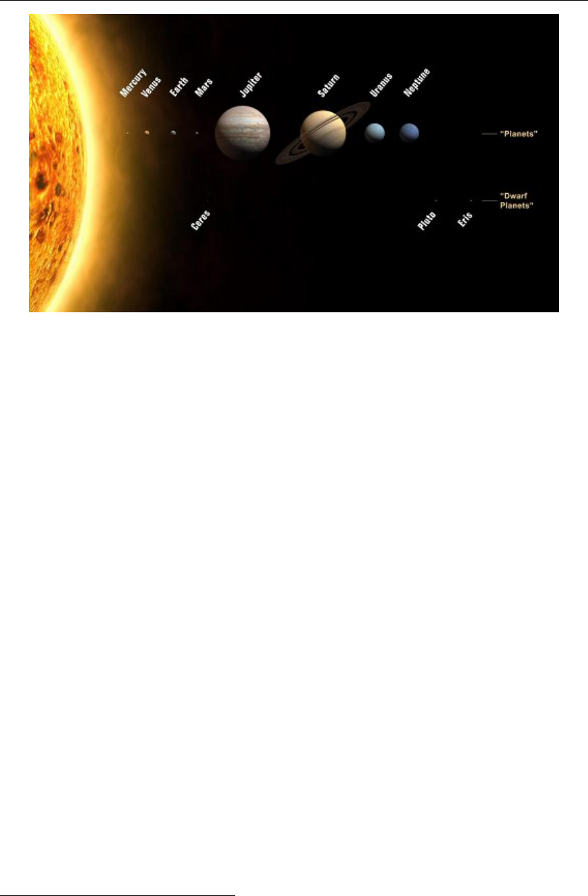
18.5 The Minor Bodies 215
Figure 18.4: The Planets
18.5 The Minor Bodies
As well as the Major Planets, the solar system also contains innumerable smaller bodies in orbit
around the Sun. These are generally the dwarf planets (Ceres, Pluto, Eris), the other minor planets,
also known as planetoids or asteroids, and comets.
18.5.1 Asteroids
Asteroids are celestial bodies orbiting the Sun in more or less regular orbits mostly between Mars
and Jupiter. They are generally rocky bodies like the inner (terrestrial) planets, but of much smaller
size. They are countless in number ranging in size from about ten meters to hundreds of kilometres.
18.5.2 Comets
A comet is a small body in the solar system that orbits the Sun and (at least occasionally) exhibits a
coma (or atmosphere) and/or a tail.
Most comets have a very eccentric orbit (featuring a highly flattened ellipse, or even a parabolic
track), and as such spend most of their time a very long way from the Sun. Comets are composed
of rock, dust and ices. When they come close to the Sun, the heat evaporates the ices, causing a
gaseous release. This gas and loose material which comes away from the body of the comet is
swept away from the Sun by the Solar wind, forming the tail.
Most larger comets exhibit two kinds of tail: a straight gas tail (often blue-green in photographs),
and a wider, occasionally curved dust tail (reflecting whitish sunlight).
Comets whose orbit brings them close to the Sun more frequently than every 200 years are
considered to be short period comets, the most famous of which is probably Comet Halley, named
after the British astronomer EDMUND HALLEY (1656–1741/42
3
), which has an orbital period of
roughly 76 years.
3
Halley lived in a time when Great Britain still used the Julian calendar and started the years in March.
He died January 14th, 1741 (Julian), which was called January 25th 1742 (Gregorian) in most other European
countries.

216 Chapter 18. Astronomical Phenomena
18.6 Meteoroids
These objects are small pieces of space debris left over from the early days of the solar system or
which crumbled off a comet when it came close to the sun. These particles orbit the Sun and come
in a variety of shapes, sizes an compositions, ranging from microscopic dust particles up to about
ten meters across.
Sometimes these objects collide with the Earth. The closing speed of these collisions is
generally extremely high (tens of kilometres per second). When such an object ploughs through the
Earth’s atmosphere, a large amount of kinetic energy is converted into heat and light, and a visible
flash or streak can often be seen with the naked eye. Even the smallest particles can cause these
events which are commonly known as shooting stars.
While smaller objects tend to burn up in the atmosphere, larger, denser objects can penetrate
the atmosphere and strike the surface of the planet, sometimes leaving meteor craters.
Sometimes the angle of the collision means that larger objects pass through the atmosphere but
do not strike the Earth. When this happens, spectacular fireballs are sometimes seen.
To clarify some terminology:
Meteoroids are the objects when they are floating in space.
Meteor is the name given to the visible atmospheric phenomenon.
Shooting Star colloquial term for a small meteor
Fireball, Bolide
term for a very bright meteor. These illuminate the landscape, sometimes
for several seconds, and occasionally even cause sounds. These are also candidates for
Meteorites , the objects that penetrate the atmosphere and land (or impact) on the surface.
In some nights over the year you can observe increased meteorite activity. Those meteors seem
to come from a certain point in the sky, the Radiant. But what we see is similar to driving through a
mosquito swarm which all seem to come head-on. Earth itself moves through space, and sweeps up
a dense cloud of particles which originates from a comet’s tail. Stellarium’s Meteor Shower plugin
(see section 13.6) can help you planning your next meteor observing night.
18.7 Zodiacal Light and Gegenschein
In very clear nights on the best observing sites, far away from the light pollution of our cities, you
can observe a feeble glow also known as “false twilight” after evening twilight in the west, or
before dawn in the east. The glow looks like a wedge of light along the ecliptic. Exactly opposite
the sun, there is another dim glow that can be observed with dark-adapted eyes in perfect skies: the
Gegenschein (counterglow).
This is sunlight reflected off the same dust and meteoroids in the plane of our solar system
which is the source of meteors. Stellarium’s sky can show the Zodiacal light (Kwon, Hong, and
Weinberg, 2004), but observe how quickly light pollution kills its visibility!
18.8 The Milky Way
There is a band of very dense stars running right round the sky in huge irregular stripe. Most of
these stars are very dim, but the overall effect is that on very dark clear nights we can see a large,
beautiful area of diffuse light in the sky. It is this for which we name our galaxy the Milky Way.
The reason for this effect is that our galaxy is somewhat like a disc, and we are off to one side.
Thus when we look towards the centre of the disc, we see more a great concentration of stars (there
are more star in that direction). As we look out away from the centre of the disc we see fewer stars -
we are staring out into the void between galaxies!
It’s a little hard to work out what our galaxy would look like from far away, because when we
look up at the night sky, we are seeing it from the inside. All the stars we can see are part of the

18.9 Nebulae 217
Milky Way, and we can see them in every direction. However, there is some structure. There is a
higher density of stars in particular places.
18.9 Nebulae
Seen with the naked eye, binoculars or a small telescope, a nebula (plural nebulae) is a fuzzy patch
on the sky. Historically, the term referred to any extended object, but the modern definition excludes
some types of object such as galaxies.
Observationally, nebulae are popular objects for amateur astronomers – they exhibit complex
structure, spectacular colours (in most cases only visible in color photography) and a wide variety
of forms. Many nebulae are bright enough to be seen using good binoculars or small to medium
sized telescopes, and are a very photogenic subject for astro-photographers.
Nebulae are associated with a variety of phenomena, some being clouds of interstellar dust and
gas in the process of collapsing under gravity, some being envelopes of gas thrown off during a
supernova event (so called supernova remnants), yet others being the remnants of dumped outer
layers around dying stars (planetary nebulae).
Examples of nebulae for which Stellarium has images include the Crab Nebula (M1), which
is a supernova remnant, and the Dumbbell Nebula (M27) and the Ring Nebula (M57) which are
planetary nebulae.
18.9.1 The Messier Objects
The Messier objects are a set of astronomical objects catalogued by CHARLES MESSIER (1730–
1817) in his catalogue of Nebulae and Star Clusters first published in 1774. The original motivation
behind the catalogue was that Messier was a comet hunter, and he was frustrated by objects which
resembled but were not comets. He therefore compiled a list of these annoying objects.
The first edition covered 45 objects numbered M1 to M45. The total list consists of 110
objects, ranging from M1 to M110. The final catalogue was published in 1781 and printed in the
Connaissance des Temps in 1784. Many of these objects are still known by their Messier number.
Because the Messier list was compiled by astronomers in the Northern Hemisphere, it contains
only objects from the north celestial pole to a celestial latitude of about
−35◦
. Many impressive
Southern objects, such as the Large and Small Magellanic Clouds are excluded from the list.
Because all of the Messier objects are visible with binoculars or small telescopes (under favourable
conditions), they are popular viewing objects for amateur astronomers. In early spring, astronomers
sometimes gather for “Messier Marathons”, when all of the objects can be viewed over a single
night.
Stellarium includes images of many Messier objects.
18.10 Galaxies
Stars, it seems, are gregarious – they like to live together in groups. These groups are called galaxies.
The number of stars in a typical galaxy is literally astronomical – many billions – sometimes over
hundreds of billions of stars!
Our own star, the sun, is part of a galaxy. When we look up at the night sky, all the stars we
can see are in the same galaxy. We call our own galaxy the Milky Way (or sometimes simply “the
Galaxy”4).
Other galaxies appear in the sky as dim fuzzy blobs. Only four are normally visible to the
naked eye. The Andromeda galaxy (M31) visible in the Northern hemisphere, the two Magellanic
4Which means closely the same thing, the word deriving from Greek gala=milk.

218 Chapter 18. Astronomical Phenomena
clouds, visible in the Southern hemisphere, and the home galaxy Milky Way, visible in parts from
north and south under dark skies.
There are thought to be billions of galaxies in the universe comprised of an unimaginably large
number of stars.
The vast majority of galaxies are so far away that they are very dim, and cannot be seen without
large telescopes, but there are dozens of galaxies which may be observed in medium to large sized
amateur instruments. Stellarium includes images of many galaxies, including the Andromeda
galaxy (M31), the Pinwheel Galaxy (M101), the Sombrero Galaxy (M104) and many others.
Astronomers classify galaxies according to their appearance. Some classifications include
spiral galaxies,elliptical galaxies,lenticular galaxies and irregular galaxies.
18.11 Eclipses
Eclipses occur when an apparently large celestial body (planet, moon etc.) moves between the
observer (that’s you!) and a more distant object – the more distant object being eclipsed by the
nearer one.
18.11.1 Solar Eclipses
Solar eclipses occur when our Moon moves between the Earth and the Sun. This happens when the
inclined orbit of the Moon causes its path to cross our line of sight to the Sun. In essence it is the
observer falling under the shadow of the moon.
There are three types of solar eclipses:
Partial The Moon only covers part of the Sun’s surface.
Total The Moon completely obscures the Sun’s surface.
Annular
The Moon is at apogee (furthest from Earth in its elliptic orbit) and its disc is too
small to completely cover the Sun. In this case most of the Sun’s disc is obscured – all except a
thin ring around the edge.
18.11.2 Lunar Eclipses
Lunar eclipses occur when the Earth moves between the Sun and the Moon, and the Moon is in the
Earth’s shadow. They occur under the same basic conditions as the solar eclipse but can occur more
often because the Earth’s shadow is so much larger than the Moon’s.
Total lunar eclipses are more noticeable than partial eclipses because the Moon moves fully
into the Earth’s shadow and there is very noticeable darkening. However, the Earth’s atmosphere
refracts light (bends it) in such a way that some sunlight can still fall on the Moon’s surface even
during total eclipses. The blue parts of sunlight are scattered and filtered away, so that there is a
marked reddening of the light as it passes through the atmosphere, and this makes the Moon appear
in a deep red colour. The darkness and colors are notably influenced by atmospheric clarity and
clouds. After big volcanic eruptions eclipses are often reported darker.
18.12 Observing Hints
When stargazing, there’s a few little things which make a lot of difference, and are worth taking
into account.
Dark skies
For many people getting away from light pollution isn’t an easy thing. At best it means
a drive away from the towns, and for many the only chance to see a sky without significant
glow from street lighting is on vacation. If you can’t get away from the cities easily, make
the most of it when you are away.

18.13 Atmospheric effects 219
Wrap up warm
The best observing conditions are the same conditions that make for cold nights,
even in the summer time. Observing is not a strenuous physical activity, so you will feel the
cold a lot more than if you were walking around. Wear a lot of warm clothing, don’t sit/lie
on the floor (at least use a camping mat, consider taking a deck-chair), and take a flask of
hot drink.
Dark adaptation
The true majesty of the night sky only becomes apparent when the eye has had
time to become accustomed to the dark. This process, known as dark adaptation, can take up
to half an hour, and as soon as the observer sees a bright light they must start the process
over. Red light doesn’t compromise dark adaptation as much as white light, so use a red
torch if possible (and one that is as dim as you can manage with). A dim single red LED
light is ideal, also to have enough light to take notes.
The Moon
Unless you’re particularly interested in observing the Moon on a given night, it can be
a nuisance—it can be so bright as to make observation of dimmer objects such as nebulae
impossible. When planning what you want to observe, take the phase and position of the
Moon into account. Of course Stellarium is the ideal tool for finding this out!
Averted vision
A curious fact about the eye is that it is more sensitive to dim light towards the
edge of the field of view. If an object is slightly too dim to see directly, looking slightly off
to the side but concentrating on the object’s location can often reveal it.
Angular distance
Learn how to estimate angular distances. Learn the angular distances described
in section 17.5.2. If you have a pair of binoculars, find out the angular distance across the
field of view and use this as a standard measure.
18.13 Atmospheric effects
18.13.1 Atmospheric Extinction
Atmospheric Extinction is the attenuation of light of a celestial body by Earth’s atmosphere. In
the last split-second of its travel into our eyes or detectors, light from outer space has to pass our
atmosphere, through layers of mixed gas, water vapour and dust. If a star is in the zenith, its light
must pass one air mass and is reduced by whatever amount of water and dust is above you. When
the star is on the horizon, it has to pass about 40 times longer through the atmosphere: 40 air masses
(Fig. 18.5). The number of air masses increases fast in low altitudes, this is why we see so few
stars along the horizon. Usually blue light is extinguished more, this is why the sun and moon (and
brigher stars) appear reddish on the horizon.
Stellarium can simulate extinction, and you can set the opacity of your atmosphere with a
global factor
k
, the magnitude loss per airmass (see section 4.4.1). The best mountaintop sites may
have k=0.15, while k=0.25 seems a value usable for good locations in lower altitudes.
18.13.2 Atmospheric Refraction
Atmospheric Refraction is a lifting effect of our atmosphere which can be observed by the fact that
objects close to the horizon appear higher than they should be if computed only with spherical
trigonometry. Stellarium simulates refraction for terrestrial locations when the atmosphere is
switched on. Refraction depends on air pressure and temperature. Figure 18.6 has been created
from the same formulae that are employed in Stellarium. You can see how fast refraction grows
very close to the mathematical horizon.
Note that these models can only give approximate conditions. There are many weird effects in
the real atmosphere, when temperature inversion layers can create light ducts, double sunsets etc.
Also note that the models give meaningful results only for altitudes above approximately
−2◦
.
Below that, in nature, there is always ground which blocks our view. In Stellarium you can switch
off the ground, and you can observe a sunset with a strange egg-shaped sun below the horizon. This

220 Chapter 18. Astronomical Phenomena
0 10 20 30 40 Airmass
−2−10123456
mag =
0°
5°
10°
15°
0.4
0.3
0.25
0.2
0.175
0.15
0.125
Star invisible at k_v
0.4
0.3
0.25
0.2
0.175
0.15
0.125
Absorption [Dmag] k_v
Airmass, Absorption and Extinction Angle (m_z=6.5; apparent altitudes)
(Model: Schaefer, S&T4/1987; Airmass: Rozenberg 1966; Observations: Müller 1970) © Georg Zotti 2009−2010, ASTROSIM
Figure 18.5: Airmass and Extinction. The figure shows Airmass (blue) along the line of
sight in the altitude labeled on the left side. The green curves show how many magnitudes
an object is dimmed down, depending on extinction factor
k
(called
kv
in the figure). The
red curves indicate at which altitude a star of given magnitude can be seen with good
eyesight, again depending on
k
. The black dots are observed values found in the literature.
is of course nonsense. Stellarium is also not able to properly recreate the atmospheric distortions as
seen from a stratosphere balloon, where the height of earth’s surface is several degrees below the
mathematical horizon.
Scintillation
Scintillation is the scientific name of the twinkling which stars show in turbulent atmosphere. The
twinkling is caused by moving pockets of air with different temperature. Observe a star low on the
horizon with a telescope, and you will note it does not stand still but dances around a bit, often also
changing color to show red or blue hues. While the twinkling of stars may look fine and comforting
to the naked eye on a nice warm summer evening, telescopic observers and astrophotographers
don’t like it at all. They rather complain about “bad seeing”, because it deteriorates the optical
resolution of their instruments and photographs.
Just like extinction and refraction are stronger along the horizon, stars in low altitude in general
show more twinkling than stars higher up in the sky.
Note that planets seem to be affected less by scintillation: they are not point sources, but little
disks, and so the effect of the turbulent pockets of air distorting different parts of the disks cancels
out a bit when observing with the naked eye: planets appear to be more stable. Of course, the view
18.13 Atmospheric effects 221
−1.3° −1.2° −1.1° −1.0° −0.9° −0.8° −0.7° −0.6° −0.5° −0.4° −0.3° −0.2° −0.1° 0.0° 0.1° 0.2° 0.3° 0.4° 0.5° 0.6° 0.7° 0.8° 0.9° Dalt
−10°
−5°
0°
5°
10°
15°
20°
25°
1013.25 mbar, 10°C
Temperature: −60..10..50°C
Pressure: −500..100..1100 mbar
Bennett’s Formula
Correction of observed altitudes
Sæmundsson’s Formula
Correction of geometric altitudes
Refraction
(Model: Meeus, Astr.Alg.1994) © Georg Zotti 2010, ASTROSIM
Figure 18.6: Refraction. The figure shows corrective values (degrees) which are subtracted from observed altitudes (left side) to reach geometric
altitudes, or values to be added to computed values (right side). The models used are not directly inverse operations.

222 Chapter 18. Astronomical Phenomena
in a telescope will still be deteriorated by the turbulent atmosphere.
While bad seeing was one key motivation of sending telescopes into earth orbit since the 1970s,
the latest generation of ground-based giant telescopes is able to compensate for the turbulent motion
by rapidly deforming their secondary mirror.
18.13.3 Light Pollution
An ugly side effect of civilisation is a steady increase in outdoor illumination. Many people
think it increases safety, but while this statement can be questioned, one definite result, aside
from environmental issues like dangers for the nocturnal fauna, are ever worsening conditions for
astronomical observations or just enjoyment of the night sky.
Stellarium can simulate the effect of light pollution on the visibility of celestial objects. This
is controlled from the light pollution section of the Sky tab of the View window (see section 4.9).
Light pollution levels are set using a numerical value between 1 and 9 which corresponds to the
Bortle Dark Sky Scale (see Appendix B). Given that public lighting became bright enough to cause
adverse effects on observability only during the 19th century, Stellarium presents an unpolluted
sky for dates before 1825. Note that of course light pollution was not switched on over night, but
became gradually noticeable over decades, but you have to estimate the appropriate level.
In addition, local variations of the amount of light pollution can be included in a light pollution
layer in the landscapes, see section 7 for details. This foreground layer may include all kinds of
light, e.g. campfires, so this is also available for earlier dates.
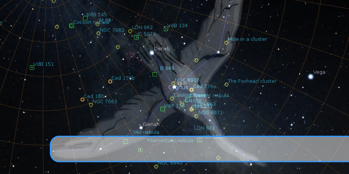
19. A Little Sky Guide
PAUL ROBINSON,WITH ADDITIONS BY ALEXANDER WOLF
This chapter lists some astronomical objects that can be located using Stellarium. All of them
can be seen with the naked eye or binoculars. Since many astronomical objects have more than
one name (often having a “proper name”, a “common name” and various catalogue numbers), the
chapter lists the name as it appears in Stellarium — use this name when using Stellarium’s search
function — and any other commonly used names.
The Location Guide entry gives brief instructions for finding each object using nearby bright
stars or groups of stars when looking at the real sky — a little time spent learning the major
constellations visible from your latitude will pay dividends when it comes to locating fainter (and
more interesting!) objects. When trying to locate these objects in the night sky, keep in mind that
Stellarium displays many stars that are too faint to be visible without optical aid, and even bright
stars can be dimmed by poor atmospheric conditions and light pollution.
19.1 Dubhe and Merak, The Pointers
Type: Stars
Magnitude: 1.83, 2.36
Location Guide:
The two “rightmost” of the seven stars that form the main shape of “The Plough”
(or “Big Dipper”, part of Ursa Major).
Northern hemisphere observers are very fortunate to have two stars that point towards Polaris
which lie very close to the northern celestial pole. Whatever the time of night or season of the year
they are always an immediate clue to the location of Polaris, the Pole Star.
19.2 M31, Messier 31, The Andromeda Galaxy
Type: Spiral Galaxy
Magnitude: 3.4

224 Chapter 19. A Little Sky Guide
Location Guide:
Find the three bright stars that constitute the main part of the constellation of
Andromeda. From the middle of these look toward the constellation of Cassiopeia.
M31 is the most distant object visible to the naked eye, and among the few nebulae that can be
seen without a telescope or powerful binoculars. Under good conditions it appears as a large fuzzy
patch of light. It is a galaxy containing billions of stars whose distance is roughly 2.5 million light
years from Earth.
19.3 The Garnet Star, µCephei
Type: Variable Star
Magnitude: 4.25 (Avg.)
Location Guide:
Cephius lies “above” the W-shape of Cassiopeia. The Garnet Star lies slightly
to one side of a point halfway between 5 Cephei and 21 Cephei.
A “supergiant” (1035 Solar radii) of spectral class M with a strong red colour. Given its name
by Sir William Herschel in the 18th century, the colour is striking in comparison to its blue-white
neighbours.
19.4 4 and 5 Lyrae, εLyrae
Type: Double Star
Magnitude: 4.7
Location Guide: Close to Vega (αLyrae), one of the brightest stars in the sky.
In binoculars
ε
Lyrae is resolved into two separate stars. Remarkably, each of these is also a
double star (although this will only be seen with a telescope) and all four stars form a physical
system.
19.5 M13, Hercules Cluster
Type: Globular Cluster
Magnitude: 5.8
Location Guide:
Located approximately 1/3 of the way along a line from 44 (
η
) to 40 (
ζ
) Herculis.
This cluster of hundreds of thousands of mature stars appears as a circular “cloud” using the
naked eye or binoculars (a large telescope is required to resolve individual stars). Oddly the cluster
appears to contain one young star and several areas that are almost devoid of stars.
19.6 M45, The Pleiades, The Seven Sisters
Type: Open Cluster
Magnitude: 1.2 (Avg.)
Location Guide:
Lies on the Bull’s back, about 1/3 between Aldebaran in Taurus and Almaak in
Andromeda.
Depending upon conditions, six to 9 of the blueish stars in this famous cluster will be visible to
someone with average eyesight, and in binoculars it is a glorious sight. The cluster has more than
500 members in total, many of which are shown to be surrounded by nebulous material in long
exposure photographs.

19.7 Algol, The Demon Star, βPersei 225
19.7 Algol, The Demon Star, βPersei
Type: Variable Star
Magnitude: 3.0 (Avg.)
Location Guide:
Halfway between Aldebaran in Taurus and the middle star of the “W” of
Cassiopeia.
Once every three days or so, Algol’s brightness changes from 2.1 to 3.4 and back within a
matter of hours. The reason for this change is that Algol has a dimmer giant companion star, with an
orbital period of about 2.8 days, that causes a regular partial eclipse. Although Algol’s fluctuations
in magnitude have been known since at least the 17th century, it was the first to be proved to be due
to an eclipsing companion — it is therefore the prototype Eclipsing Variable.
19.8 Sirius, αCanis Majoris
Type: Star
Magnitude: -1.47
Location Guide:
Sirius is easily found by following the line of three stars in Orion’s belt south-
wards.
Sirius is a white dwarf star at a comparatively close 8.6 light years. This proximity and its high
innate luminance makes it the brightest star in our sky. Sirius is a double star; its companion is a
White Dwarf, much dimmer but very hot, and is believed to be smaller than the earth.
19.9 M44, The Beehive, Praesepe
Type: Open Cluster
Magnitude: 3.7
Location Guide:
Cancer lies about halfway between the twins (Castor & Pollux) in Gemini and
Regulus, the brightest star in Leo. The Beehive can be found between Asellus Borealis and Asellus
Australis.
There are probably 350 or so stars in this cluster, although it appears to the naked eye simply as
a misty patch. It contains a mixture of stars from red giants to white dwarf and is estimated to be
some 700 million years old.
19.10 27 Cephei, δCephei
Type: Variable Star
Magnitude: 4.0 (Avg.)
Location Guide:
Locate the four stars that form the square of Cepheus. One corner of the square
has two other bright stars nearby forming a distinctive triangle —
δ
is at the head of this triangle
in the direction of Cassiopeia.
δ
Cephei gives its name to a whole class of variables, all of which are pulsating high-mass stars
in the later stages of their evolution.
δ
Cephei is also a double star with a companion of magnitude
6.3 visible in binoculars.
19.11 M42, The Great Orion Nebula
Type: Nebula
Magnitude: 4.0
Location Guide:
Almost in the middle of the area bounded by Orion’s belt and lower stars, Saiph
and Rigel.

226 Chapter 19. A Little Sky Guide
The Great Orion Nebula is the brightest nebula visible in the night sky and lies at about 1.500
light years from earth. It is a truly gigantic gas and dust cloud that extends for several hundred light
years, reaching almost halfway across the constellation of Orion. The nebula contains a cluster
of hot young stars known as the Trapezium, and more stars are believed to be forming within the
cloud.
19.12 La Superba, Y Canum Venaticorum, HIP 62223
Type: Star
Magnitude: 5.4 (Avg.)
Location Guide:
Almost the center of the arch of stars of Ursa Major’s tail. Forms a neat triangle
with Phekda (γ) and Alkaid (η, tail tip) in Ursa Major towards Canes Venatici.
La Superba (215 Solar radii) is a “Carbon Star” — a group of relatively cool gigantic (usually
variable) stars that have an outer shell containing high levels of carbon. This shell is very efficient
at absorbing short wavelength blue light, giving carbon stars a distinctive red or orange tint. One of
the coolest and reddest known stars.
19.13 52 and 53 Bootis, ν1and ν2Bootis
Type: Double Star
Magnitude: 5.0, 5.0
Location Guide:
Follow a line from Seginus (
γ
Boo, left shoulder) to Nekkar (
β
Boo, the head)
and then continue for the same distance again to arrive at this double star.
This optical double star consists of a pair of different spectral type, and 52 Bootis, at approxi-
mately 800 light years, is twice as far away as 53.
19.14 PZ Cas, HIP 117078
Type: Variable Star
Magnitude: 8.2 (Avg.)
Location Guide:
Lies about 1/3 between Caph (
β
Cas, the top right star of “W”) in Cassiopeia
and ιCephei (32 Cep, top left star in “rectangle” of Cepheus).
This faint red star is one of the biggest known stars — its average size parameter is 1565 Solar
radii (the true value is from 1340 to 1940 Solar radii). PZ Cas is a pulsating variable star located in
a region with heavy dust extinction.
19.15 VV Cephei, HIP 108317
Type: Variable Star, Double Star
Magnitude: 5.1 (Avg.)
Location Guide: Lies near the center of the “rectangle” of Cepheus).
This is an interesting eclipsing binary system — VV Cep A (1457 Solar radii) is a highly
distorted star in a binary system, losing mass to its B-type companion VV Cephei B (10 Solar radii)
for at least part of its orbit.
19.16 AH Scorpii, HIP 84071
Type: Variable Star
Magnitude: 7.1 (Avg.)
19.17 Albireo, βCygni 227
Location Guide: Lies in Scorpius, about 1 1
4of a continuation of the Scorpion’s “tail”.
AH Sco (1411 Solar radii) is variable by nearly 3 magnitudes in the visual range, and an
estimated 20% in total luminosity. The variation in diameter is not clear because the temperature
also varies.
19.17 Albireo, βCygni
Type: Double Star
Magnitude: 3.4, 5.1
Location Guide: The “head” of Cygni.
When viewed with the naked eye, it appears to be a single star. However, in a telescope it
readily resolves into a double star, consisting of Albireo A (amber), and Albireo B (blue-green).
Separated by 35
00
, the two components provide one of the best contrasting double stars in the sky
due to their different colors.
Figure 19.1: Albireo: A Bright and Beautiful Double. Credit & Copyright: Richard
Yandrick.
19.18 31 and 32 Cygni, o1and o2Cygni
Type: Multiple Star
Magnitude: 3.8, 4.0
Location Guide:
The two bright stars about 1/2 between Deneb (
α
Cygni, “tail” of Cygnus) and
Rukh (δCygni, middle of the left “wing” of Cygnus).
The wide binary
o1
Cygni and
o2
Cygni is separated 61
0
(NNE), and this star is an easy naked-
eye double.
o1
Cygni with 30 Cyg and HD 192579 (HIP 99676) is a moderately difficult triple
system. And surprise — each of o1Cyg and o2Cyg are also Algol-type eclipsing binaries!
19.19 The Coathanger, Brocchi’s Cluster, Cr 399
Type: Asterism
Location Guide:
It is best found by slowly sweeping across the Milky Way along an imaginary
line from the bright star Altair toward the even brighter star Vega (around 1/3 between Altair and
Vega).

228 Chapter 19. A Little Sky Guide
The asterism is made up of 10 stars ranging from 5th to 7th magnitude which form the
conspicuous “coathanger”, a straight line of 6 stars with a “hook” of 4 stars on the south side. Under
a dark sky, Collinder 399 can be seen with the naked eye as an unresolved patch of light; binoculars
or a telescope at very low power are usually needed in order to view the “coathanger” asterism.
19.20 Kemble’s Cascade
Type: Asterism
Location Guide:
The asterism lies in the constellation Camelopardalis, about 1/3 between CS
Cam and αCam — HIP 18505 has magnitude 5 and can be found in the center of the chain.
Kemble’s Cascade is a chain of stars which are visible in binocular even in light-polluted skies.
19.21 The Double Cluster, χand hPersei, NGC 884 and NGC 869
Type: Open Clusters
Location Guide: The two open clusters near stars χand h in the constellation Perseus.
The Double Cluster (also known as Caldwell 14 or C14) is the common name for the naked-eye
open clusters NGC 869 and NGC 884 (often designated hPersei and
χ
Persei, respectively). The
Double Cluster is approximately the radiant of the Perseid meteor shower, which peaks annually
around August 12 or 13. Although easy to locate in the northern sky, observing the Double
Cluster in its two parts requires optical aid. They are described as being an “awe-inspiring” and
“breathtaking” sight, and are often cited as targets in astronomical observers’ guides.
19.22 Large Magellanic Cloud, PGC 17223
Type: Dwarf Spiral Galaxy
Magnitude: 0.9
Location Guide:
It is visible as a faint “cloud” in the night sky of the southern hemisphere
straddling the border between the constellations of Dorado and Mensa, and it appears from Earth
more than 20 times the width of the full moon.
The Large Magellanic Cloud (LMC) is a satellite galaxy of the Milky Way. The Large
Magellanic Cloud is usually considered an irregular galaxy. However, it shows signs of a bar
structure, and has more recently been reclassified as a Magellanic-type dwarf spiral galaxy. At
a distance of 50 kiloparsecs, the LMC is the third closest galaxy to the Milky Way, after the
Sagittarius Dwarf Spheroidal (~16 kiloparsecs) and the putative Canis Major Dwarf Galaxy (~12.9
kiloparsecs, though its status as a galaxy is under dispute) lying closer to the center of the Milky
Way. The LMC has a diameter of about 14,000 light-years (~4.3 kpc) and a mass of approximately
10 billion (
1010
) solar masses, making it roughly 1/100 as massive as the Milky Way. The LMC has
a wide range of galactic objects and phenomena — surveys of the galaxy have found roughly 60
globular clusters, 400 planetary nebulae, and 700 open clusters, along with hundreds of thousands
of giant and supergiant stars.
19.23 Tarantula Nebula, C 103, NGC 2070
Type: Nebula
Magnitude: 7.3
Location Guide: Part of Large Magellanic Cloud.
The Tarantula Nebula (also known as 30 Doradus) is an H II region in the Large Magellanic
Cloud (LMC). 30 Doradus has at its centre the star cluster NGC 2070 which includes the compact
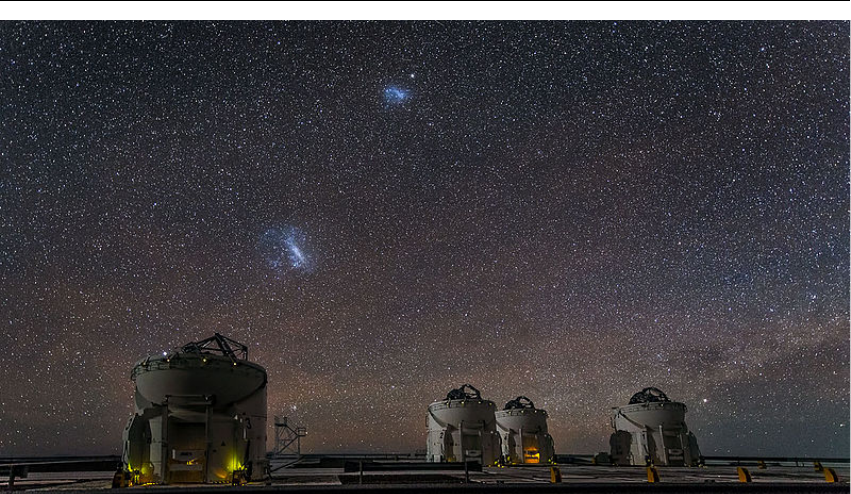
19.24 Small Magellanic Cloud, NGC 292, PGC 3085 229
Figure 19.2: Small and Large Magellanic Clouds over Paranal Observatory. Credit: ESO/J.
Colosimo.
concentration of stars known as R136 that produces most of the energy that makes the nebula
visible. The estimated mass of the cluster is 450,000 solar masses, suggesting it will likely become
a globular cluster in the future (Bosch, E. Terlevich, and R. Terlevich, 2009). The closest supernova
observed since the invention of the telescope, Supernova 1987A, occurred in the outskirts of the
Tarantula Nebula.
19.24 Small Magellanic Cloud, NGC 292, PGC 3085
Type: Dwarf Irregular Galaxy
Magnitude: 2.2
Location Guide:
It is located mostly in the constellation of Tucana and appears as a hazy, light
patch in the night sky about 3
◦
across, looking like a detached piece of the Milky Way. Since it has
a very low surface brightness, it is best viewed from a dark site away from city lights.
The Small Magellanic Cloud (SMC) is a dwarf galaxy near the Milky Way. It is classified
as a dwarf irregular galaxy. It has a diameter of about 7,000 light-years and has a total mass of
approximately 7 billion times the mass of the Sun. The SMC contains a central bar structure and it
is speculated that it was once a barred spiral galaxy that was disrupted by the Milky Way to become
somewhat irregular. At a distance of about 200,000 light-years, it is one of the Milky Way’s nearest
neighbors. It is also one of the most distant objects that can be seen with the naked eye.
19.25 ωCentauri cluster, C 80, NGC 5139
Type: Globular Cluster
Magnitude: 5.3
Location Guide: It is located around 1/3 between ζand γCentauri.
Omega Centauri (
ω
Cen), or NGC 5139, is a globular cluster in the constellation of Centaurus
that was first identified as a non-stellar object by Edmond Halley in 1677. Located at a distance

230 Chapter 19. A Little Sky Guide
of 15,800 light-years (4,850 pc), it is the largest globular cluster in the Milky Way at a diameter
of roughly 150 light-years. It is estimated to contain approximately 10 million stars and a total
mass equivalent to 4 million solar masses. Omega Centauri is so distinctive from the other galactic
globular clusters that it is thought to have an alternate origin as the core remnant of a disrupted
dwarf galaxy (Noyola, Gebhardt, and Bergmann, 2008).
19.26 47 Tucanae, C 106, NGC 104
Type: Globular Cluster
Magnitude: 4.1
Location Guide: It can be seen with the naked eye near Small Magellanic Cloud.
It is the one of brightest globular cluster in the sky, and is noted for having a very bright and
dense core. It is also one of the most massive globular clusters in the Milky Way Galaxy, containing
millions of stars. The cluster appears roughly the size of the full moon in the sky under ideal
conditions.
19.27 The Coalsack Nebula, C 99
Type: Dark Nebula
Location Guide: Dark region between αand βCrux.
The Coalsack Nebula is the most prominent dark nebula in the skies, easily visible to the
naked eye as a dark patch silhouetted against the southern Milky Way. It is located at a distance of
approximately 600 light years away from Earth. The Coalsack is important in Australian Aboriginal
astronomy, and forms the head of the Emu in the sky in several Aboriginal cultures.
19.28 Mira, oCeti, 68 Cet
Type: Variable Star
Magnitude: 2.0–10.1
Location Guide: It is located around 1/3 between δand θCeti.
Mira (
o
Ceti) is a star estimated 200–400 light years away in the constellation Cetus. Mira is a
binary star system that consists of a red giant (Mira A) undergoing mass loss and a high temperature
white dwarf companion (Mira B) that is accreting mass from the primary. Such an arrangement of
stars is known as a symbiotic system, and this is the closest such symbiotic pair to the Sun. Mira is
the brightest periodic variable in the sky that is not visible to the naked eye for part of its cycle. Its
distance is uncertain. Mira A is a well-known example of a category of long-period variable stars
known as Mira variables, which are named after it.
19.29 αPersei Cluster, Cr 39, Mel 20
Type: Open Cluster
Magnitude: 1.2
Location Guide:
Around the white-yellow supergiant Mirfak, also known as
α
Persei in direction
to δPersei.
The Alpha Persei Cluster, also known as Melotte 20 or Collinder 39, is an open cluster in the
constellation of Perseus. To the naked eye, the cluster consists of several blue (spectral class B)
stars.
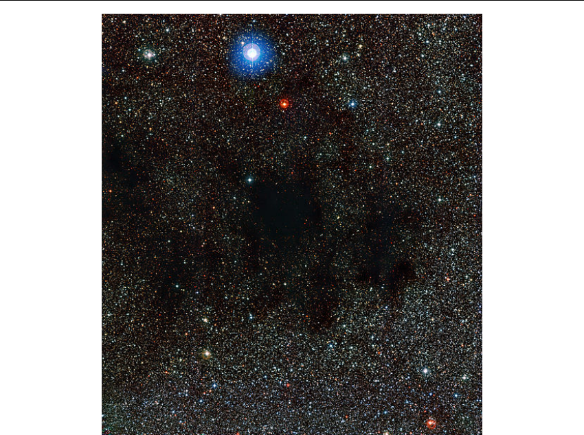
19.30 M7, The Ptolemy Cluster 231
Figure 19.3: The Coalsack Nebula taken by the Wide Field Imager on the MPG/ESO
2.2-metre telescope. Credit: ESO.
19.30 M7, The Ptolemy Cluster
Type: Open Cluster
Magnitude: 3.3
Location Guide:
The cluster is easily detectable with the naked eye, close to the “sting” of
Scorpius — near the center of the line between Shaula (λScorpii) and Kaus Media (δSagittarii).
M7 has been known since antiquity — it was first recorded by the 2nd-century Greek-Roman
astronomer Ptolemy, who described it as a nebula in 130 AD. Telescopic observations of the cluster
reveal about 80 stars within a field of view of 1.3
◦
across. At the cluster’s estimated distance of 980
light years this corresponds to an actual diameter of 25 light years.
19.31 M24, The Sagittarius Star Cloud
Type: Star Cloud
Magnitude: 4.6
Location Guide: In the Milky Way region near Polis (µSagittarii).
The Sagittarius Star Cloud is a star cloud in the constellation of Sagittarius, approximately 600
light years wide. The stars, clusters and other objects comprising M24 are part of the Sagittarius or
Sagittarius-Carina arms of the Milky Way galaxy. Messier described M24 as a “large nebulosity
containing many stars” and gave its dimensions as being some 1.5◦across.

232 Chapter 19. A Little Sky Guide
19.32 IC 4665, The Summer Beehive Cluster
Type: Open Cluster
Magnitude: 4.2
Location Guide: Visible to the naked eye near Cebalrai (βOphiuchi).
IC 4665 is an open cluster in the constellation Ophiuchus which is easily visible in the smallest
of telescopes and also with binoculars. From a sufficiently dark place it is also visible to the naked
eye.
19.33 The E Nebula, Barnard 142 and 143
Type: Dark Nebula
Location Guide:
A well-defined dark area on a background of Milky Way near Tarazed (
γ
Aquilae).
The “E” or “Barnard’s E” Nebula (officially designated as B142 and B143) is a pair of dark
nebulae in the constellation Aquila. It is a well-defined dark area on a background of the Milky
Way. The size of the nebula is roughly 0.5
◦
, and its distance from earth is estimated at about 2000
light years.

20. Exercises
PAUL ROBINSON,WITH ADDITIONS BY ALEXANDER WOLF
20.1 Find M31 in Binoculars
M31 – the Andromeda Galaxy – is the most distant object visible to the naked eye. Finding it in
binoculars is a rewarding experience for new-comers to observing.
20.1.1 Simulation
1.
Set the location to a mid-Northern latitude if necessary (M31 isn’t always visible for Southern
hemisphere observers). The UK is ideal.
2.
Find M31 and set the time so that the sky is dark enough to see it. The best time of year for
this at Northern latitudes is Autumn/Winter, although there should be a chance to see it at
some time of night throughout the year.
3.
Set the field of view to
6◦
(or the field of view of your binoculars if they’re different.
6◦
is
typical for 7x50 binoculars).
4.
Practise finding M31 from the bright stars in Cassiopeia and the constellation of Andromeda.
Learn the chain of stars that extends from Andromeda’s central star perpendicular to her
body.
20.1.2 For Real
This part is not going to be possible for many people. First, you need a good night and a dark sky.
In urban areas with a lot of light pollution it’s going to be very hard to see Andromeda.
20.2 Handy Angles
As described in section 17.5.2, your hand at arm’s length provides a few useful estimates for
angular size. It’s useful to know whether your handy angles are typical, and if not, what they are.

234 Chapter 20. Exercises
The method here below is just one way to do it – feel free to use another method of your own
construction!
Hold your hand at arm’s length with your hand open – the tips of your thumb and little finger
as far apart as you can comfortably hold them. Get a friend to measure the distance between your
thumb and your eye, we’ll call this
D
. There is a tendency to over-stretch the arm when someone
is measuring it – try to keep the thumb-eye distance as it would be if you were looking at some
distant object.
Without changing the shape of your hand, measure the distance between the tips of your thumb
and little finger. It’s probably easiest to mark their positions on a piece of paper and measure the
distance between the marks, we’ll call this
d
. Using some simple trigonometry, we can estimate the
angular distance θusing equation (17.4).
Repeat the process for the distance across a closed fist, three fingers and the tip of the little
finger.
For example, for one author D=72cm, d=21cm, so:
θ=2·arctan21
144≈161
2
◦(20.1)
Remember that handy angles are not very precise – depending on your posture at a given time
the values may vary by a fair bit.
20.3 Find a Lunar Eclipse
Stellarium comes with two scripts for finding lunar eclipses, but can you find one on a different
date?
20.4 Find a Solar Eclipse
Find a Solar Eclipse using Stellarium and take a screenshot of it. Use the location panel and see
how the eclipse look on different locations at the same time. Don’t forget to have “Topocentric
coordinates” enabled in the settings (see section 17.9.1).
20.5 Find a retrograde motion of Mars
Find Mars using Stellarium and take a series of screenshots of its position at different times. Use
the date and time panel and see how the motion of Mars changes over the time. Find periods of
direct and retrograde motion of Mars (see also section 16.5).
20.6 Analemma
Set a time around noon and set time rate to pause, turn on the azimuthal grid. Find the Sun and
check its horizontal coordinates. Use the date and time panel and see how the horizontal coordinates
of the Sun change over time (please use one time step for simulation — look at the position of the
Sun every 7 days for example). Use the location panel and see how the positions of the Sun look
from different location at the same times. Check the change of positions of the Sun on Mars at the
same times.

20.7 Transit of Venus 235
20.7 Transit of Venus
Set date to
6th
of June, 2012, find Venus near the Sun and change scale of the view (zoom in). Find
time of all four contacts and maximum of transit for your location. Because the Sun appears to
rotate as it crosses the sky, Venus will appear to move on some curve — for example it will be an
inverted “U” shape for eastern states of Australia. Check difference of path shape of Venus for
equatorial and azimuthal mounts. Find a few dates and times for transit of Venus in past and in
future. Notice how they usually come in pairs 8 years apart, with gaps of over 100 years between
pairs.
20.8 Transit of Mercury
Set date to
9th
of May, 2016, find Mercury near the Sun and change scale of the view (zoom in).
Find time of all four contacts and maximum of transit for your location. Because the Sun appears
to rotate as it crosses the sky, Mercury will appear to move on some curve — for example it will be
an inverted “U” shape for observers from Europe. Check difference of path shape of Mercury for
equatorial and azimuthal mounts. Find few dates and times for transit of Mercury in past and in
future.
20.9 Triple shadows on Jupiter
Set date to
24th
of January, 2015, find Jupiter and change scale of the view (zoom in). Find the
time when three shadows will be visible on the disk of Jupiter. Which moons cast those shadows?
Check which moons cause triple shadows on Jupiter at 3 June 2014. Details for this phenomenon
you can find in the book Mathematical astronomy morsels (Meeus, 1997).
20.10 Jupiter without satellites
Set date to
9th
November, 2019, find Jupiter and change scale of the view (zoom in). Find time
limits for the disappearance of the moons. Which moons are on the back of the planet, and which
— in front of it? Please give answer on the same questions for 3 September 2009. Details for this
phenomenon you can find in the book Mathematical astronomy morsels (Meeus, 1997)
20.11 Mutual occultations of planets
Set date to
13th
October, 1590, find Venus and change scale of the view (zoom in). Find time of
minimal separation of Venus and Mars on this date. Set typical scale of view for visual observation
and check Venus and Mars again. What would the typical observer of that time had said? Find the
minimal separation between Venus and Saturn near end of August 1771. What would the typical
observer on Earth had said? Find the minimal separation between Mars and Mercury in first half of
August 2079.
Find mutual occultation of Earth and Mercury as seen from Mars near the end of November
2022. Find mutual occultation of Saturn and Mercury as seen from Venus near the middle of May
1967.
Details for this phenomenon you can find in the books More mathematical astronomy morsels
(Meeus, 2002) and Mathematical astronomy morsels III (Meeus, 2004)

236 Chapter 20. Exercises
20.12 The proper motion of stars
Turn off ground and atmosphere, set time rate on pause, find the star HIP 87937 and change the
scale of the view to better see Barnard’s Star. Use the date and time panel and see how the location
of the star is changing in time (please try use one time step for simulation — look at the position of
the star every year for example). When will Barnard’s star cross the border of constellation? When
has Barnard’s star crossed the border of constellation in the past?
Please check the proper motions of Sirius (HIP 32349), Procyon (HIP 37279), 61 Cyg (HIP
104214) and
τ
Cet (HIP 8102). Which star has the fastest proper motion? Which star has the
slowest rate of proper motion?
When will observers see Arcturus and HIP 68706 as close optical binary? Find the minimal
angular separation between θand εInd in the past.
How will the appearance of following constellations change over a wide range of time (-
100000..100000 years for example): Ursa Major, Orion, Bootes?
A note of caution, however: the proper motions are only modelled by extrapolating their current
shift rates in right ascension and declination, but don’t take radial velocity into account. The results
in very far times should be seen only as approximations.

V
ADefault Hotkeys .......................... 239
BThe Bortle Scale of Light Pollution ....... 247
CStar Catalogues .......................... 251
DConfiguration Files ....................... 271
EPlanetary nomenclature ................ 299
FAccuracy ................................. 305
GGNU Free Documentation License . . . . . 309
HAcknowledgements ..................... 317
Bibliography .............................. 327
Index ...................................... 335
Appendices
A. Default Hotkeys
The currently configured hotkeys are visible in the Help dialog (
F1
). Here is the default list for
reference.
A.1 Mouse actions with combination of the keyboard keys
Actions Description
Arrow keys & left mouse drag Pan view around the sky
Page Up/Down &Ctrl +Page Up/Down Zoom in/out
Ctrl & left mouse drag Time dragging
Ctrl & mouse wheel Time scrolling: minutes
Ctrl +Shift & mouse wheel Time scrolling: hours
Ctrl +Alt & mouse wheel Time scrolling: days
Ctrl +Alt +Shift & mouse wheel Time scrolling: years
Left click Select object
Right click Clear selection
Shift & left click Add custom marker
Shift & right click Delete the one closest marker to mouse cursor
Alt +Shift & right click Delete all custom markers
A.2 Display Options
Shortcut key Description
PPlanets
Alt +PPlanet labels
Ctrl +PPlanet markers
240 Appendix A. Default Hotkeys
OPlanet orbits
Shift +TPlanet trails
Ctrl +Shift +PPlanet selection marker
SStars
Alt +SStars labels
DDeep-sky objects (symbols)
IDeep-sky objects background images
Ctrl +Alt +DDigitized Sky Survey (experimental)
MMilky Way
Ctrl +Shift +ZZodiacal Light
GGround
FFog
Shift +GLandscape Illumination
Ctrl +Shift +GLandscape Labels
AAtmosphere
QCardinal points
,Ecliptic line
.Equator line
EEquatorial grid
ZAzimuthal grid
HHorizon line
;Meridian line
CConstellation lines
VConstellation labels
RConstellation art
BConstellation boundaries
Ctrl +Alt +Shift +VSelect single constellation
Tab Remove selection of constellations
Ctrl +Shift +NNative planet names (from starlore)
F11 Full-screen mode
Ctrl +NNight mode
Ctrl +Shift +HFlip scene horizontally
Ctrl +Shift +VFlip scene vertically
A.3 Miscellaneous
Shortcut key Description
Ctrl +CCopy selected object information to clipboard
Ctrl +QQuit
Ctrl +SSave screenshot
Ctrl +MSwitch between equatorial and azimuthal mount
Ctrl +TToggle visibility of GUI
A.4 Movement and Selection 241
A.4 Movement and Selection
Shortcut key Description
Center on selected object
Ctrl +HGo to home
Ctrl +GSet home planet to selected planet (“go there”)
Shift +ELook towards East
Shift +NLook towards North
Shift +SLook towards South
Shift +WLook towards West
Shift +ZLook towards Zenith
TTrack object
/Zoom in on selected object
\Zoom out
A.5 Date and Time
Shortcut key Description
=Add 1 solar day
-Subtract 1 solar day
Ctrl +=Add 1 solar hour
Ctrl +-Subtract 1 solar hour
Alt +=Add 1 sidereal day
Alt +-Subtract 1 sidereal day
]Add 7 solar days
[Subtract 7 solar days
Ctrl +Alt +Shift +]Add 1 sidereal year
Ctrl +Alt +Shift +[Subtract 1 sidereal year
JDecrease time speed
Shift +JDecrease time speed (a little)
KSet normal time rate
LIncrease time speed
Shift +LIncrease time speed (a little)
7Set time rate to zero
8Set time to now
Ctrl +D,PPause script execution
Ctrl +D,RResume script execution
Ctrl +D,SStop script execution
242 Appendix A. Default Hotkeys
A.6 Scripts
Shortcut key Description
Ctrl +D,0Run script “Solar System Screensaver”
Ctrl +D,1Run script “Constellations Tour”
Ctrl +D,2Run script “Sky Culture Tour”
Ctrl +D,3Run script “Screensaver”
A.7 Windows
Shortcut key Description
F1 Toggle Help window
F2 Toggle Configuration window
F3 Toggle Search window
F4 Toggle Sky and viewing options window
F5 Toggle Date/time window
F6 Toggle Location window
F7 Toggle Shortcuts window
F10 Toggle AstroCalc window
F12 Toggle Script Console window
Alt +BToggle Bookmarks window
A.8 Plugins
A.8.1 Angle Measure
Shortcut key Description
Ctrl +AToggle angle measurement
A.8.2 ArchaeoLines
Shortcut key Description
Ctrl +UToggle archaeolines
Ctrl +Shift +UToggle archaeolines dialog
A.8.3 Compass Marks
Shortcut key Description
Ctrl +Alt +CToggle compass marks
A.8.4 Equation of Time
Shortcut key Description
Ctrl +Alt +TShow solution for Equation of Time
A.8 Plugins 243
A.8.5 Exoplanets
Shortcut key Description
Ctrl +Alt +EShow exoplanets
Alt +EToggle Exoplanets configuration window
A.8.6 Field of View
Shortcut key Description
Ctrl +Alt +1Set FOV to 180◦
Ctrl +Alt +2Set FOV to 90◦
Ctrl +Alt +3Set FOV to 60◦
Ctrl +Alt +4Set FOV to 45◦
Ctrl +Alt +5Set FOV to 20◦
Ctrl +Alt +6Set FOV to 10◦
Ctrl +Alt +7Set FOV to 5◦
Ctrl +Alt +8Set FOV to 2◦
Ctrl +Alt +9Set FOV to 1◦
Ctrl +Alt +0Set FOV to 0.5◦
A.8.7 Meteor Showers
Shortcut key Description
Ctrl +Shift +MToggle meteor showers
Shift +MToggle radiant labels
Ctrl +Alt +MShow search dialog
Ctrl +Alt +Shift +MShow settings dialog
A.8.8 Oculars
Shortcut key Description
Ctrl +OOcular view
Alt +OOculars popup menu
Alt +CShow crosshairs
Ctrl +BTelrad sight
A.8.9 Pulsars
Shortcut key Description
Ctrl +Alt +PShow pulsars
244 Appendix A. Default Hotkeys
A.8.10 Quasars
Shortcut key Description
Ctrl +Alt +QShow quasars
A.8.11 Satellites
Shortcut key Description
Ctrl +ZToggle satellite hints
Alt +Shift +ZToggle satellite labels
Alt +ZToggle Satellites configuration window
A.8.12 Scenery3d: 3D landscapes
Shortcut key Description
Ctrl +WToggle 3D landscape
Ctrl +Shift +WShow settings dialog
Ctrl +Alt +WShow viewpoint dialog
Ctrl +R,TToggle location text
Ctrl +R,SToggle shadows
Ctrl +R,LToggle torchlight
Ctrl +R,DToggle debug information
Ctrl +R,PReload shaders
A.8.13 Solar System Editor
Shortcut key Description
Ctrl +Alt +SImport orbital elements in MPC format...
A.8.14 Telescope Control
Shortcut key Description
Ctrl +0Move a telescope to a given set of coordinates (shows dialog)
Ctrl +1Move telescope #1 to selected object
Ctrl +2Move telescope #2 to selected object
Ctrl +3Move telescope #3 to selected object
Ctrl +4Move telescope #4 to selected object
Ctrl +5Move telescope #5 to selected object
Ctrl +6Move telescope #6 to selected object
Ctrl +7Move telescope #7 to selected object
Ctrl +8Move telescope #8 to selected object
Ctrl +9Move telescope #9 to selected object
Alt +1Move telescope #1 to the point currently in the center of the screen
Alt +2Move telescope #2 to the point currently in the center of the screen
Alt +3Move telescope #3 to the point currently in the center of the screen
Alt +4Move telescope #4 to the point currently in the center of the screen
Alt +5Move telescope #5 to the point currently in the center of the screen

A.8 Plugins 245
Alt +6Move telescope #6 to the point currently in the center of the screen
Alt +7Move telescope #7 to the point currently in the center of the screen
Alt +8Move telescope #8 to the point currently in the center of the screen
Alt +9Move telescope #9 to the point currently in the center of the screen
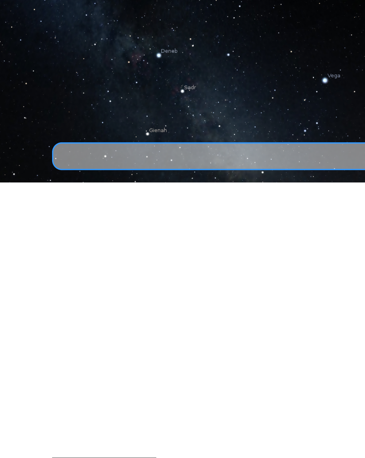
B. The Bortle Scale of Light Pollution
The Bortle scale is a nine-level numeric scale that measures the night sky’s brightness of a particular
location. It quantifies the astronomical observability of celestial objects and the interference
caused by light pollution. JOHN E. BORTLE created the scale and published it in Sky & Telescope
magazine (Bortle, 2001) to help amateur astronomers evaluate the darkness of an observing site,
and secondarily, to compare the darkness of observing sites. The scale ranges from Class 1, the
darkest skies available on Earth, through Class 9, inner-city skies. It gives several criteria for each
level beyond naked-eye limiting magnitude (NELM). The accuracy and utility of the scale have
been questioned in recent research (Crumey, 2014).
B.1 Excellent dark sky site
Level: 1
Naked-eye limiting magnitude: 7.6 – 8.0
Approx. SQM mag/arcsec2:21.7 – 22.01
Zodiacal light, gegenschein, zodiacal band visible; M33 direct vision naked-eye object; Scorpius
and Sagittarius regions of the Milky Way cast obvious shadows on the ground; Airglow is readily
visible; Jupiter and Venus affect dark adaptation; surroundings basically invisible.
B.2 Typical truly dark site
Level: 2
Naked-eye limiting magnitude: 7.1 – 7.5
Approx. SQM mag/arcsec2:21.5 – 21.7
Airglow weakly visible near horizon; M33 easily seen with naked eye; highly structured
Summer Milky Way; distinctly yellowish zodiacal light bright enough to cast shadows at dusk and
dawn; clouds only visible as dark holes; surroundings still only barely visible silhouetted against
the sky; many Messier globular clusters still distinct naked-eye objects.
1Dark Skies Awareness – http://www.darkskiesawareness.org/nomogram.php
248 Appendix B. The Bortle Scale of Light Pollution
Figure B.1: Light Pollution Simulation / Bortle Scale
B.3 Rural sky
Level: 3
Naked-eye limiting magnitude: 6.6 – 7.0
Approx. SQM mag/arcsec2:21.3 – 21.5
Some light pollution evident at the horizon; clouds illuminated near horizon, dark overhead;
Milky Way still appears complex; M15, M4, M5, M22 distinct naked-eye objects; M33 easily
visible with averted vision; zodiacal light striking in spring and autumn, color still visible; nearer
surroundings vaguely visible.
B.4 Rural/suburban transition
Level: 4
Naked-eye limiting magnitude: 6.1 – 6.5
Approx. SQM mag/arcsec2:20.4 – 21.3
Light pollution domes visible in various directions over the horizon; zodiacal light is still
visible, but not even halfway extending to the zenith at dusk or dawn; Milky Way above the horizon
still impressive, but lacks most of the finer details; M33 a difficult averted vision object, only
visible when higher than 55
◦
; clouds illuminated in the directions of the light sources, but still dark
overhead; surroundings clearly visible, even at a distance.

B.5 Suburban sky 249
B.5 Suburban sky
Level: 5
Naked-eye limiting magnitude: 5.6 – 6.0
Approx. SQM mag/arcsec2:19.1 – 20.4
Only hints of zodiacal light are seen on the best nights in autumn and spring; Milky Way is
very weak or invisible near the horizon and looks washed out overhead; light sources visible in
most, if not all, directions; clouds are noticeably brighter than the sky.
B.6 Bright suburban sky
Level: 6
Naked-eye limiting magnitude: 5.1 – 5.5
Approx. SQM mag/arcsec2:18.0 – 19.1
Zodiacal light is invisible; Milky Way only visible near the zenith; sky within 35
◦
from the
horizon glows grayish white; clouds anywhere in the sky appear fairly bright; surroundings easily
visible; M33 is impossible to see without at least binoculars, M31 is modestly apparent to the
unaided eye.
B.7 Suburban/urban transition
Level: 7
Naked-eye limiting magnitude: 4.6 – 5.0
Approx. SQM mag/arcsec2:18.0 – 19.1
Entire sky has a grayish-white hue; strong light sources evident in all directions; Milky Way
invisible; M31 and M44 may be glimpsed with the naked eye, but are very indistinct; clouds are
brightly lit; even in moderate-sized telescopes the brightest Messier objects are only ghosts of their
true selves.
B.8 City sky
Level: 8
Naked-eye limiting magnitude: 4.1 – 4.5
Approx. SQM mag/arcsec2:<18.0
Sky glows white or orange — you can easily read; M31 and M44 are barely glimpsed by an
experienced observer on good nights; even with telescope, only bright Messier objects can be
detected; stars forming familiar constellation patterns may be weak or completely invisible.
B.9 Inner-city sky
Level: 9
Naked-eye limiting magnitude: 4.0 at best
Approx. SQM mag/arcsec2:<18.0
Sky is brilliantly lit with many stars forming constellations invisible and many weaker constel-
lations invisible; aside from Pleiades, no Messier object is visible to the naked eye; only objects to
provide fairly pleasant views are the Moon, the Planets and a few of the brightest star clusters.

C. Star Catalogues
This chapter provides technical descriptions on how Stellarium records its star catalogues, and the
related file formats.
C.1 Stellarium’s Sky Model
C.1.1 Zones
The celestial sphere is split into zones, which correspond to the triangular faces of a geodesic sphere.
The number of zones (faces) depends on the level of sub-division of this sphere. The lowest level,
0, is an icosahedron (20 faces), subsequent levels Lof sub-division give the number of zones nas:
n=20 ·4L(C.1)
Stellarium uses levels 0 to 7 in the existing star catalogues. Star Data Records contain the
position of a star as an offset from the central position of the zone in which that star is located, thus
it is necessary to determine the vector from the observer to the centre of a zone, and add the star’s
offsets to find the absolute position of the star on the celestial sphere.
This position for a star is expressed as a 3-dimensional vector which points from the observer
(at the centre of the geodesic sphere) to the position of the star as observed on the celestial sphere.
C.2 Star Catalogue File Format
C.2.1 General Description
Stellarium’s star catalogue data is kept in the
stars/default
sub-directory of the Installation
Directory and/or User Directory (see section 5.1).
The main catalogue data is split into several files:
stars_0_0v0_7.cat
stars_1_0v0_7.cat

252 Appendix C. Star Catalogues
stars_2_0v0_7.cat
stars_3_1v0_4.cat
stars_4_1v0_2.cat
stars_5_2v0_1.cat
stars_6_2v0_1.cat
stars_7_2v0_1.cat
stars_8_2v0_1.cat
There also exist some control and reference files:
stars_hip_cids_0v0_0.cat
stars_hip_sp_0v0_3.cat
gcvs_hip_part.dat
wds_hip_part.dat
cross-id.dat
stars.ini
name.fab
When Stellarium starts, it reads the
stars.ini
file, from which it determines the names of the
other files, which it then loads.
The files
stars_hip_cids_0v0_0.cat
and
stars_hip_sp_0v0_2.cat
contain reference
data for the main catalogue files. The file
gcvs_hip_part.dat
contains data about variables stars
(see section C.3) and file
wds_hip_part.dat
contains data about double stars (see section C.4)
which again contains references into the main catalogue files.
The file
cross-id.dat
(see section C.5) contains cross-identification data between HIP, SAO,
HD and HR designations.
A given catalogue file models stars for one and only one level (i.e. for a fixed number of zones),
which is recorded in the header of the file. Individual star records do not contain full positional
coordinates, instead they contain coordinates relative to the central position of the zone they occupy.
Thus, when parsing star catalogues, it is necessary to know about the zone model to be able to
extract positional data.
File Data Data Geodesic #Records Notes
Type Record Size Level
stars_0_0v0_7.cat 0 28 bytes 0 4,979 Hipparcos
stars_1_0v0_7.cat 0 28 bytes 1 21,806 Hipparcos
stars_2_0v0_7.cat 0 28 bytes 2 150,850 Hipparcos
stars_3_1v0_4.cat 1 10 bytes 3 425,807 Tycho 2
stars_4_1v0_2.cat 1 10 bytes 4 1,692,779 Tycho 2
stars_5_2v0_1.cat 2 8 bytes 5 7,083,058 NOMAD
stars_6_2v0_1.cat 2 8 bytes 6 24,670,782 NOMAD
stars_7_2v0_1.cat 2 8 bytes 7 50,733,321 NOMAD
stars_8_2v0_1.cat 2 8 bytes 7 92,304,337 NOMAD
For a given catalogue file, there may be one of three formats for the actual star data. The
variation comes from the source of the data – the larger catalogues of fainter stars providing less
data per star than the brighter star catalogues. See tables Stellarium’s star catalogue and for details.
Stellarium’s star catalogues are based on Hipparcos (Anderson and Francis, 2012; ESA, 1997),
Tycho 2 (Høg et al., 2000) and NOMAD (Zacharias et al., 2004) catalogues.
C.2.2 File Sections
The catalogue files are split into three main sections as described in table File sections.

C.2 Star Catalogue File Format 253
Section Offset Description
File Header Record 0
Contains magic number, geodesic subdivision level, and magni-
tude range
Zone Records 32
A list of how many records there are for each zone. The length
of the zones section depends on the level value from the header
Star Data Records 32+4n
This section of the file contains fixed-size star records, as de-
scribed below. Records do not contain zone information, which
must be inferred by counting how many records have been read
so far and switching zones when enough have been read to fill
the number of stars for the zone, as specified in the zones section
above. The value of
n
used in the offset description is the number
of zones, as described above.
C.2.3 Record Types
File Header Record
The File Header Record describes file-wide settings. It also contains a magic number which servers
as a file type identifier. See table C.1.
Name Offset Type Size Description
Magic 0 int 4
magic number which identifies the file as
a star catalogue. 0xde0955a3
Data Type 4 int 4
type of the file, which defines the size
and structure of the Star Data record for
the file.
Major Version 8 int 4 file format major version number
Minor Version 12 int 4 file format minor version number
Level 16 int 4
sets the level of sub-division of the
geodesic sphere used to create the zones.
0 means an icosahedron (20 triangular
faces), subsequent levels of sub-division
lead to numbers of zones as described in
section C.2.3
Magnitude Minimum 20 int 4
low bound of the magnitude scale for val-
ues in this file. Note that this is still an
integer in Stellarium’s own internal rep-
resentation
Magnitude Range 24 int 4
range of magnitudes expressed in this file
Magnitude Steps 28 int 4
number of steps used to describes values
in the range
Table C.1: Header Record
Zone Records
The Zone Records section of the file lists the number of star records there are per zone. The number
of zones is determined from the level value in the File Header Record, as described in section

254 Appendix C. Star Catalogues
Zones. The Zones section is simply a list of integer values which describe the number of stars for
each zone. The total length of the Zones section depends on the number of zones. See table C.2.
Name Offset Type Size Description
num stars in zone 0 0 int 4
number of records in this file which are in
zone 0
num stars in zone 1 4 int 4
number of records is this file which are in
zone 1
...
num stars in zone n4nint 4
number of records is this file which are in
zone n
Table C.2: Zones section
Star Data Records
After the Zones section, the actual star data starts. The star data records themselves do not contain
the zone in which the star belongs. Instead, the zone is inferred from the position of the record
in the file. For example, if the Zone Records section of the file says that the first 100 records are
for zone 0, the next 80 for zone 1 and so on, it is possible to infer the zone for a given record by
counting how many records have been read so far.
The actual record structure depends on the value of the Data Type, as found in the File Header
Record. See tables C.3, C.4 and C.5 for record structure details.
It should be noted that although the positional data loses accuracy as one progresses though the
Star Record Types, this is compensated for by the face that the number of zones is much higher for
the files where the smaller precision position fields are used, so the actual resolution on the sky
isn’t significantly worse for the type 1 and 2 records in practice.
Name Offset Type Size Description
hip 0 int 3 Hipparcos catalogue number
component_ids 3 unsigned char 1
index to an array of catalogue num-
ber suffixes. The list is read from the
stars_hip_component_ids.cat
file. The value of this field turns out
to be the line number in the file - 1
x0 4 int 4
position of the star relative to the
central point in the star’s zone, in
axis 1
x1 8 int 4
position of the star relative to the
central point in the star’s zone, in
axis 2
b_v 9 unsigned char 1
magnitude level in B-V colour. This
value refers to one of 256 discrete
steps in the magnitude range for the
file
mag 10 unsigned char 1
magnitude level in the V-I colour.
This value refers to one of 256 dis-
crete steps in the magnitude range
for the file

C.3 Variable Stars 255
sp_int 11 unsigned short int 2
index into an array of spectral type
descriptions which is taken from the
file
stars_hip_sp.cat
, the index
corresponds to the line number in
the file - 1
dx0 13 int 4 proper motion of the star in axis 1
dx1 17 int 4 proper motion of the star in axis 2
plx 21 int 4
parallax of the star. To get the actual
value, divide by 10000.
Table C.3: Star Data Record Type 0
Name Offset Type Size Description
x0 0 int 20 bits
position of the star relative to the central point
in the star’s zone, in axis 1
x1 20 bits int 20 bits
position of the star relative to the central point
in the star’s zone, in axis 2
dx0 40 bits int 14 bits proper motion of the star in axis 1
dx1 54 bits int 14 bits proper motion of the star in axis 2
b_v 68 bits unsigned int 7 bits
magnitude level in B-V colour. This value
refers to one of 128 discrete steps in the mag-
nitude range for the file
mag 75 bits unsigned int 5 bits
magnitude level in the V-I colour. This value
refers to one of 32 discrete steps in the mag-
nitude range for the file
Table C.4: Star Data Record Type 1
C.3 Variable Stars
Since version 0.12.2 Stellarium supports the subset of variable stars from GCVS
1
which have HIP
identificators (i.e., stars from the Hipparcos catalog). Stellarium’s Catalog of Variable Stars is based
on the “General Catalogue of Variable Stars (Samus+ 2007-2015)” (Samus et al., 2015).
C.3.1 Variable Star Catalog File Format
General Description
Stellarium’s Variable Stars catalog data is kept in the
stars/default
sub-directory of the Installa-
tion Directory and/or User Directory (see section 5.1).
File Format
The
gcvs_hip_part.dat
file contains data about 6916 Variable Stars (see section 18.2.5) which
have HIP identificators and are stored in a plain text format with tab delimiter (Table C.6).
1http://www.sai.msu.su/gcvs/gcvs/

256 Appendix C. Star Catalogues
Name Offset Type Size Description
x0 0 int 18 bits
position of the star relative to the central point
in the star’s zone, in axis 1
x1 18 bits int 18 bits
position of the star relative to the central point
in the star’s zone, in axis 2
b_v 36 bits unsigned int 7 bits
magnitude level in B-V colour. This value
refers to one of 128 discrete steps in the mag-
nitude range for the file
mag 43 bits unsigned int 5 bits
magnitude level in the V-I colour. This value
refers to one of 32 discrete steps in the mag-
nitude range for the file
Table C.5: Star Data Record Type 2
Name Type Description
HIP int
This is the HIP identificator for the star. Used for reference to the
main star catalogue.
GCVS string This is the GCVS designation for the variable star.
Type string Type of variability.
Max float Magnitude at maximum brightness.
MFlag int
Magnitude flag code (0=No flag; 1="(" if max. magnitude is an
amplitude; 2="<" if max. magnitude is a bright limit; 3=">" is max.
magnitude is a faint limit).
Min I float First minimum magnitude or amplitude.
Min II float Second minimum magnitude.
V char The photometric system for magnitudes.
Epoch float Epoch for maximum or minimum light (in Julian days).
Period float Period for the variable star (in days).
M-m float Rising time or duration of the eclipse (in percent).
Spectrum string Spectral class of the variable star.
Table C.6: Variable Star Catalog File Format
C.3.2 GCVS Variability Types
An improved system of variability classification is used in the fourth edition of the GCVS, based
on recent developments in classification principles and taking into account the suggestions of a
number of specialists. Variability types are grouped according to the major astrophysical reasons
for variability.
All of these classes include objects of a dissimilar nature that belong to different types of light
variability. On the other hand, an object may be variable because of almost all of the possible
reasons or because of any combination of them. If a variable belongs to several types of variability,
the types are joined in the data field by a “+” sign, e.g., E+UG, UV+BY.
Despite considerable success in understanding stellar variability processes, the classification
adopted in the Catalogue is far from perfect. This is especially the case for explosive, symbiotic
and novalike variables; X-ray sources; and peculiar objects.

C.3 Variable Stars 257
You can read about latest different types of variability at VIZIER2.
Eruptive Variable Stars
Eruptive variables are stars varying in brightness because of violent processes and flares occurring
in their chromospheres and coronae. The light changes are usually accompanied by shell events
or mass outflow in the form of stellar winds of variable intensity and/or by interaction with the
surrounding interstellar medium. This class includes the following types:
BE
It becomes more and more clear that, although the majority of Be stars are photometrically
variable, not all of them could be properly called GCAS variables. Quite a number of
them show small-scale variations not necessarily related to shell events; in some cases the
variations are quasi-periodic. By now we are not able to present an elaborated system of
classification for Be variables, but we adopt a decision that in the cases when a Be variable
cannot be readily described as a GCAS star we give simply BE for the type of variability.
FU
Orion variables of the FU Orionis type. Characterized by gradual increases in brightness by
about 6 mag in several months, followed by either almost complete constancy at maximum
that is sustained for long periods of time or slow decline by 1-2 mag. Spectral types at
maximum are in the range Ae(alpha) - Gpe(alpha). After an outburst, a gradual development
of an emission spectrum is observed and the spectral type becomes later. These variables
probably mark one of the evolutionary stages of T Tauri-type Orion variables (INT), as
evidenced by an outburst of one member, V1057 Cyg, but its decline (2.5 mag in 11 years)
commenced immediately after maximum brightness was attained. All presently known FU
Ori variables are coupled with reflecting cometary nebulae.
GCAS
Eruptive irregular variables of the Gamma Cas type. These are rapidly rotating B III-IVe
stars with mass outflow from their equatorial zones. The formation of equatorial rings or
disks is often accompanied by temporary fading. Light amplitudes may reach 1.5 mag in V.
I
Poorly studied irregular variables with unknown features of light variations and spectral types.
This is a very inhomogeneous group of objects.
IA Poorly studied irregular variables of early (O-A) spectral type.
IB Poorly studied irregular variables of intermediate (F-G) to late (K-M) spectral type.
IN
Orion variables. Irregular, eruptive variables connected with bright or dark diffuse
nebulae or observed in the regions of these nebulae. Some of them may show cyclic
light variations caused by axial rotation. In the Spectrum-Luminosity diagram, they
are found in the area of the main sequence and subgiants. They are probably young
objects that, during the course of further evolution, will become light-constant stars on
the zero-age main sequence (ZAMS). The range of brightness variations may reach
several magnitudes. In the case of rapid light variations having been observed (up to 1
mag in 1-10 days), the letter “S” is added to the symbol for the type (INS). This type
may be divided into the following subtypes:
INA
Orion variables of early spectral types (B-A or Ae). They are often characterized
by occasional abrupt Algol-like fadings (T Ori);
INB
Orion variables of intermediate and late spectral types, F-M or Fe-Me (BH Cep,
AH Ori). F-type stars may show Algol-like fadings similar to those of many INA
stars; K-M stars may produce flares along with irregular light variations;
INT,IT
Orion variables of the T Tauri type. Stars are assigned to this type on the
basis of the following (purely spectroscopic) criteria: spectral types are in the
range Fe-Me. The spectra of most typical stars resemble the spectrum of the solar
chromosphere. The feature specific to the type is the presence of the flourescent
emission lines Fe II 4046, 4132 A (anomalously intense in the spectra of these
2http://cdsarc.u-strasbg.fr/vizier/ftp/cats/B/gcvs/vartype.txt

258 Appendix C. Star Catalogues
stars), emission lines [Si II] and [O I], as well as the absorption line Li I 6707 A.
These variables are usually observed only in diffuse nebulae. If it is not apparent
that the star is associated with a nebula, the letter “N” in the symbol for the type
may be omitted, e.g., IT (RW AUR);
IN(YY)
Some Orion variables (YY Ori) show the presence of absorption components
on the redward sides of emission lines, indicating the infall of matter toward the
stars’ surfaces. In such cases, the symbol for the type may be accompanied by
the symbol “YY”.
IS
Rapid irregular variables having no apparent connection with diffuse nebulae and showing
light changes of about 0.5 - 1.0 mag within several hours or days. There is no strict
boundary between rapid irregular and Orion variables. If a rapid irregular star is
observed in the region of a diffuse nebula, it is considered an Orion variable and
designated by the symbol INS. To attribute a variable to the IS type, it is necessary
to take much care to be certain that its light changes are really not periodic. Quite a
number of the stars assigned to this type in the third edition of the GCVS turned out
to be eclipsing binary systems, RR Lyrae variables, and even extragalactic BL Lac
objects.
ISA Rapid irregular variables of the early spectral types, B-A or Ae;
ISB
Rapid irregular variables of the intermediate and late spectral types, F-M and
Fe-Me.
RCB
Variables of the R Coronae Borealis type. These are hydrogen-poor, carbon- and helium-
rich, high-luminosity stars belonging to the spectral types Bpe-R, which are simultaneously
eruptive and pulsating variables. They show slow nonperiodic fadings by 1-9 mag in V
lasting from a month or more to several hundred days. These changes are superposed on
cyclic pulsations with amplitudes up to several tenths of a magnitude and periods in the
range 30-100 days.
RS
Eruptive variables of the RS Canum Venaticorum type. This type is ascribed to close binary
systems with spectra showing Ca II H and K in emission, their components having enhanced
chromospheric activity that causes quasi-periodic light variability. The period of variation
is close to the orbital one, and the variability amplitude is usually as great as 0.2 mag in V
(UX Ari). They are X-ray sources and rotating variables. RS CVn itself is also an eclipsing
system (see below).
SDOR
Variables of the S Doradus type. These are eruptive, high-luminosity Bpec-Fpec stars
showing irregular (sometimes cyclic) light changes with amplitudes in the range 1-7 mag in
V. They belong to the brightest blue stars of their parent galaxies. As a rule, these stars are
connected with diffuse nebulae and surrounded by expanding envelopes (P Cyg, Eta Car).
UV
Eruptive variables of the UV Ceti type, these are K Ve-M Ve stars sometimes displaying flare
activity with amplitudes from several tenths of a magnitude up to 6 mag in V. The amplitude
is considerably greater in the ultraviolet spectral region. Maximum light is attained in several
seconds or dozens of seconds after the beginning of a flare; the star returns to its normal
brightness in several minutes or dozens of minutes.
UVN
Flaring Orion variables of spectral types Ke-Me. These are phenomenologically almost
identical to UV Cet variables observed in the solar neighborhood. In addition to being related
to nebulae, they are normally characterized by being of earlier spectral type and greater
luminosity, with slower development of flares (V389 Ori). They are possibly a specific
subgroup of INB variables with irregular variations superimposed by flares.
WR
Eruptive Wolf-Rayet variables. Stars with broad emission features of He I and He II as well as
C II-C IV, O II-O IV, and N III-N V. They display irregular light changes with amplitudes up
to 0.1 mag in V, which are probably caused by physical processes, in particular, by nonstable

C.3 Variable Stars 259
mass outflow from their atmospheres.
Pulsating Variable Stars
Pulsating variables are stars showing periodic expansion and contraction of their surface layers.
The pulsations may be radial or nonradial. A radially pulsating star remains spherical in shape,
while in the case of nonradial pulsations the star’s shape periodically deviates from a sphere, and
even neighboring zones of its surface may have opposite pulsation phases.
Depending on the period value, on the mass and evolutionary status of the star, and on the scale
of pulsational phenomena, the following types of pulsating variables may be distinguished:
ACYG
Variables of the Alpha Cygni type, which are nonradially pulsating supergiants of Bep-
AepIa spectral types. The light changes with amplitudes of the order of 0.1 mag often seem
irregular, being caused by the superposition of many oscillations with close periods. Cycles
from several days to several weeks are observed.
BCEP
Variables of the Beta Cephei type (Beta Cep, Beta CMa), which are pulsating O8-B6 I-V
stars with periods of light and radial-velocity variations in the range of 0.1 - 0.6 days and
light amplitudes from 0.01 to 0.3 mag in V. The light curves are similar in shape to average
radial-velocity curves but lag in phase by a quarter of the period, so that maximum brightness
corresponds to maximum contraction, i.e., to minimum stellar radius. The majority of these
stars probably show radial pulsations, but some (V469 Per) display nonradial pulsations;
multiperiodicity is characteristic of many of these stars.
BCEPS
A short-period group of Beta Cep variables. The spectral types are B2-B3 IV-V;
periods and light amplitudes are in the ranges 0.02 - 0.04 days and 0.015 - 0.025 days,
respectively, i.e., an order of magnitude smaller than the normally observed ones.
BLBOO
The so-called “anomalous Cepheids”, i.e. stars with periods characteristic of compar-
atively long-period RRAB variables, but considerably brighter by luminosity (BL Boo =
NGC 5466 V19).
CEP
Cepheids. Radially pulsating, high luminosity (classes Ib-II) variables with periods in the
range of 1-135 days and amplitudes from several hundredths to 2 mag in V (in the B band,
the amplitudes are greater). Spectral type at maximum light is F; at minimum, the types are
G-K. The longer the period of light variation, the later is the spectral type. The maximum of
the surface-layer expansion velocity almost coinciding with maximum light.
CEP(B)
Cepheids (TU Cas, V 367 Sct) displaying the presence of two or more simultane-
ously operating pulsation modes (usually the fundamental tone with the period P0 and
the first overtone P1). The periods P0 are in the range from 2 to 7 days, with the ratio
P1/P0 approx. 0.71.
CW
Variables of the W Virginis type. These are pulsating variables of the galactic spherical
component (old disk) population with periods of approximately 0.8 to 35 days and amplitudes
from 0.3 to 1.2 mag in V. They obey a period-luminosity relation different from that for Delta
Cep variables (see DCEP). For an equal period value, the W Vir variables are fainter than the
Delta Cep stars by 0.7 - 2 mag. The light curves of W Vir variables for some period intervals
differ from those of Delta Cep variables for corresponding periods either by amplitudes or
by the presence of humps on their descending branches, sometimes turning into broad flat
maxima. W Vir variables are present in globular clusters and at high galactic latitudes. They
may be separated into the following subtypes:
CWA W Vir variables with periods longer than 8 days (W Vir);
CWB W Vir variables with periods shorter than 8 days (BL Her).
DCEP
These are the classical cepheids, or Delta Cep-type variables. Comparatively young objects
that have left the main sequence and evolved into the instability strip of the Hertzsprung-
Russell (H-R) diagram, they obey the well-known Cepheid period-luminosity relation and

260 Appendix C. Star Catalogues
belong to the young disk population. DCEP stars are present in open clusters. They display
a certain relation between the shapes of their light curves and their periods.
DCEPS
These are Delta Cep variables having light amplitudes <0.5 mag in V (<0.7 mag
in B) and almost symmetrical light curves (M-m approx. 0.4 - 0.5 periods); as a rule,
their periods do not exceed 7 days. They are probably first-overtone pulsators and/or
are in the first transition across the instability strip after leaving the main sequence
(SU Cas).
Traditionally, both Delta Cep and W Vir stars are quite often called Cepheids because
it is often impossible to discriminate between them on the basis of the light curves for
periods in the range 3 - 10 days. However, these are distinct groups of entirely different
objects in different evolutionary stages. One of the significant spectral differences
between W Vir stars and Cepheids is the presence, during a certain phase interval, of
hydrogen-line emission in the former and of Ca II H and K emission in the latter.
DSCT
Variables of the Delta Scuti type. These are pulsating variables of spectral types A0-F5
III-V displaying light amplitudes from 0.003 to 0.9 mag in V (usually several hundredths of
a magnitude) and periods from 0.01 to 0.2 days. The shapes of the light curves, periods, and
amplitudes usually vary greatly. Radial as well as nonradial pulsations are observed. The
variability of some members of this type appears sporadically and sometimes completely
ceases, this being a consequence of strong amplitude modulation with the lower value of
the amplitude not exceeding 0.001 mag in some cases. The maximum of the surface layer
expansion does not lag behind the maximum light for more than 0.1 periods. DSCT stars are
representatives of the galactic disk (flat component) and are phenomenologically close to the
SX Phe variables.
DSCTC
Low amplitude group of Delta Sct variables (light amplitude <0.1 mag in V). The
majority of this type’s representatives are stars of luminosity class V; objects of this
subtype generally are representative of the Delta Sct variables in open clusters.
GDOR
Gamma Doradus stars. Early type F dwarfs showing (multiple) periods from several
tenths of a day to slightly in excess of one day. Amplitudes usually do not exceed 0.1 mag.
Presumably low degree g-mode non-radial pulsators. Prototype: gamma Dor.
L
Slow irregular variables. The light variations of these stars show no evidence of periodicity, or
any periodicity present is very poorly defined and appears only occasionally. Like for the
type I, stars are often attributed to this type because of being insufficiently studied. Many
type L variables are really semiregulars or belong to other types.
LB
Slow irregular variables of late spectral types (K, M, C, S); as a rule, they are giants
(CO Cyg). This type is also ascribed, in the GCVS, to slow red irregular variables in
the case of unknown spectral types and luminosities.
LC
Irregular variable supergiants of late spectral types having amplitudes of about 1 mag in
V (TZ Cas).
LPB
The comparatively long-period pulsating B stars (periods exceeding (LBV) one day).
M
Mira (Omicron) Ceti-type variables. These are long-period variable giants with characteristic
late-type emission spectra (Me, Ce, Se) and light amplitudes from 2.5 to 11 mag in V. Their
periodicity is well pronounced, and the periods lie in the range between 80 and 1000 days.
Infrared amplitudes are usually less than in the visible and may be <2.5 mag. For example,
in the K band they usually do not exceed 0.9 mag. If the amplitudes exceed 1 - 1.5 mag , but
it is not certain that the true light amplitude exceeds 2.5 mag, the symbol “M” is followed by
a colon, or the star is attributed to the semiregular class with a colon following the symbol
for that type (SR).
PVTEL
Variables of the PV Telescopii type. These are helium supergiant Bp stars with weak
hydrogen lines and enhanced lines of He and C. They pulsate with periods of approximately

C.3 Variable Stars 261
0.1 to 1 days, or vary in brightness with an amplitude of 0.1 mag in V during a time interval
of about a year.
RPHS
Very rapidly pulsating hot (subdwarf B) stars. Typical periods are hundreds of seconds,
amplitudes are within several hundredths of a magnitude. Prototype: V361 Hya = EC
14026-2647.
RR
Variables of the RR Lyrae type, which are radially-pulsating giant A-F stars having amplitudes
from 0.2 to 2 mag in V. Cases of variable light-curve shapes as well as variable periods are
known. If these changes are periodic, they are called the Blazhko effect.
Traditionally, RR Lyrae stars are sometimes called short-period Cepheids or cluster-type
variables. The majority of these stars belong to the spherical component of the Galaxy; they
are present, sometimes in large numbers, in some globular clusters, where they are known as
pulsating horizontal-branch stars. Like Cepheids, maximum expansion velocities of surface
layers for these stars practically coincide with maximum light.
RR(B)
RR Lyrae variables showing two simultaneously operating pulsation modes, the
fundamental tone with the period P0 and the first overtone, P1 (AQ Leo). The ratio
P1/P0 is approximately 0.745;
RRAB
RR Lyrae variables with asymmetric light curves (steep ascending branches), periods
from 0.3 to 1.2 days, and amplitudes from 0.5 to 2 mag in V;
RRC
RR Lyrae variables with nearly symmetric, sometimes sinusoidal, light curves, periods
from 0.2 to 0.5 days, and amplitudes not greater than 0.8 mag in V (SX UMa).
RV
Variables of the RV Tauri type. These are radially pulsating supergiants having spectral types
F-G at maximum light and K-M at minimum. The light curves are characterized by the
presence of double waves with alternating primary and secondary minima that can vary in
depth so that primary minima may become secondary and vice versa. The complete light
amplitude may reach 3-4 mag in V. Periods between two adjacent primary minima (usually
called formal periods) lie in the range 30-150 days (these are the periods appearing in the
Catalogue). Two subtypes, RVA and RVB, are recognized:
RVA RV Tauri variables that do not vary in mean magnitude (AC Her);
RVB
RV Tauri variables that periodically (with periods from 600 to 1500 days and ampli-
tudes up to 2 mag in V) vary in mean magnitude (DF Cyg, RV Tau).
SR
Semiregular variables, which are giants or supergiants of intermediate and late spectral types
showing noticeable periodicity in their light changes, accompanied or sometimes interrupted
by various irregularities. Periods lie in the range from 20 to >2000 days, while the shapes of
the light curves are rather different and variable, and the amplitudes may be from several
hundredths to several magnitudes (usually 1-2 mag in V).
SRA
Semiregular late-type (M, C, S or Me, Ce, Se) giants displaying persistent periodicity
and usually small (<2.5 mag in V) light amplitudes (Z Aqr). Amplitudes and light-
curve shapes generally vary and periods are in the range of 35-1200 days. Many of
these stars differ from Miras only by showing smaller light amplitudes;
SRB
Semiregular late-type (M, C, S or Me, Ce, Se) giants with poorly defined periodicity
(mean cycles in the range of 20 to 2300 days) or with alternating intervals of periodic
and slow irregular changes, and even with light constancy intervals (RR CrB, AF Cyg).
Every star of this type may usually be assigned a certain mean period (cycle), which is
the value given in the Catalogue. In a number of cases, the simultaneous presence of
two or more periods of light variation is observed;
SRC
Semiregular late-type (M, C, S or Me, Ce, Se) supergiants (Mu Cep) with amplitudes
of about 1 mag and periods of light variation from 30 days to several thousand days;
SRD
Semiregular variable giants and supergiants of F, G, or K spectral types, sometimes
with emission lines in their spectra. Amplitudes of light variation are in the range from

262 Appendix C. Star Catalogues
0.1 to 4 mag, and the range of periods is from 30 to 1100 days (SX Her, SV UMa).
SRS
Semiregular pulsating red giants with short period (several days to a month), probably
high-overtone pulsators. Prototype: AU Ari.
SXPHE
Phenomenologically, these resemble DSCT (Delta Sct) variables and are pulsating subd-
warfs of the spherical component, or old disk galactic population, with spectral types in the
range A2-F5. They may show several simultaneous periods of oscillation, generally in the
range 0.04-0.08 days, with variable-amplitude light changes that may reach 0.7 mag in V.
These stars are present in globular clusters.
ZZ
ZZ Ceti variables. These are nonradially pulsating white dwarfs that change their brightnesses
with periods from 30 s to 25 min and amplitudes from 0.001 to 0.2 mag in V. They usually
show several close period values. Flares of 1 mag are sometimes observed; however, these
may be explained by the presence of close UV Ceti companions.
These variables are divided into the following subtypes:
ZZA
ZZ Cet-type variables of DA spectral type (ZZ Cet) having only hydrogen absorption
lines in their spectra;
ZZB
ZZ Cet-type variables of DB spectral type having only helium absorption lines in their
spectra.
ZZO
ZZ Cet-type variables of the DO spectral type showing HeII and and CIV absorpion
lines in their spectra.
Rotating Variable Stars
Variable stars with nonuniform surface brightness and/or ellipsoidal shapes, whose variability is
caused by axial rotation with respect to the observer. The nonuniformity of surface brightness
distributions may be caused by the presence of spots or by some thermal or chemical inhomogeneity
of the atmosphere caused by a magnetic field whose axis is not coincident with the rotation axis.
These stars are subdivided into the following types:
ACV
Alpha2 Canum Venaticorum variables. These are main-sequence stars with spectral types
B8p-A7p and displaying strong magnetic fields. Spectra show abnormally strong lines of
Si, Sr, Cr, and rare earths whose intensities vary with rotation. They exhibit magnetic field
and brightness changes (periods of 0.5-160 days or more). The amplitudes of the brightness
changes are usually within 0.01-0.1 mag in V.
ACVO
Rapidly oscillating Alpha2 CVn variables. These are nonradially pulsating, rotating
magnetic variables of Ap spectral type (DO Eri). Pulsation periods are in the range
of 6-12 mmag (0.004-0.01 days), while amplitudes of light variation caused by the
pulsation are about 0.01 mag in V. The pulsational variations are superposed on those
caused by rotation.
BY
BY Draconis-type variables, which are emission-line dwarfs of dKe-dMe spectral type showing
quasiperiodic light changes with periods from a fraction of a day to 120 days and amplitudes
from several hundredths to 0.5 mag in V. The light variability is caused by axial rotation
of a star with a variable degree of nonuniformity of the surface brightness (spots) and
chromospheric activity. Some of these stars also show flares similar to those of UV Cet
stars, and in those cases they also belong to the latter type and are simultaneously considered
eruptive variables.
ELL
Rotating ellipsoidal variables (b Per, Alpha Vir). These are close binary systems with
ellipsoidal components, which change combined brightnesses with periods equal to those
of orbital motion because of changes in emitting areas toward an observer, but showing no
eclipses. Light amplitudes do not exceed 0.1 mag in V.
FKCOM
FK Comae Berenices-type variables. These are rapidly rotating giants with nonuniform
surface brightnesses, which have G-K spectral types with broad H and K Ca II emission

C.3 Variable Stars 263
and sometimes Halpha. They may also be spectroscopic binary systems. Periods of light
variation (up to several days) are equal to rotational periods, and amplitudes are several
tenths of a magnitude. It is not excluded that these objects are the product of further evolution
of EW (W UMa) close binary systems (see below).
PSR
Optically variable pulsars (CM Tau), which are rapidly rotating neutron stars with strong
magnetic fields, radiating in the radio, optical, and X-ray regions. Pulsars emit narrow beams
of radiation, and periods of their light changes coincide with rotational periods (from 0.004
to 4 s), while amplitudes of the light pulses reach 0.8 mag.
R
Close binary systems characterized by the presence of strong reflection (re-radiation) of the light
of the hot star illuminating the surface of the cooler companion. Light curves are sinusoidal
with the period equal to Porb, maximum brightness coinciding with the passage of the hot
star in front of the companion. The eclipse may be absent. The range of light variation is
about 0.5-1.0mag V (KV Vel).
SXARI
SX Arietis-type variables. These are main-sequence B0p-B9p stars with variable-intensity
He I and Si III lines and magnetic fields. They are sometimes called helium variables.
Periods of light and magnetic field changes (about 1 day) coincide with rotational periods,
while amplitudes are approximately 0.1 mag in V. These stars are high-temperature analogs
of the ACV variables.
Cataclysmic (Explosive and Novalike) Variables
These are variable stars showing outbursts caused by thermonuclear burst processes in their surface
layers (novae) or deep in their interiors (supernovae). We use the term “novalike” for variables
that show novalike outbursts caused by rapid energy release in the surrounding space (UG-type
stars - see below) and also for objects not displaying outbursts but resembling explosive variables at
minimum light by their spectral (or other) characteristics. The majority of explosive and novalike
variables are close binary systems, their components having strong mutual influence on the evolution
of each star. It is often observed that the hot dwarf component of the system is surrounded by an
accretion disk formed by matter lost by the other, cooler, and more extended component. This
category is subdivided into the following types:
N
Novae. Close binary systems with orbital periods from 0.05 to 230 days. One of the components
of these systems is a hot dwarf star that suddenly, during a time interval from one to several
dozen or several hundred days, increases its brightness by 7-19 mag in V, then returns
gradually to its former brightness over several months, years, or decades. Small changes
at minimum light may be present. Cool components may be giants, subgiants, or dwarfs
of K-M type. The spectra of novae near maximum light resemble A-F absorption spectra
of luminous stars at first. Then broad emission lines (bands) of hydrogen, helium, and
other elements with absorption components indicating the presence of a rapidly expanding
envelope appear in the spectrum. As the light decreases, the composite spectrum begins to
show forbidden lines characteristic of the spectra of gas nebulae excited by hot stars. At
minimum light, the spectra of novae are generally continuous or resemble the spectra of
Wolf-Rayet stars. Only spectra of the most massive systems show traces of cool components.
Some novae reveal pulsations of hot components with periods of approximately 100 s and
amplitudes of about 0.05 mag in V after an outburst. Some novae eventually turn out to be
eclipsing systems. According to the features of their light variations, novae are subdivided
into fast (NA), slow (NB), very slow (NC), and recurrent (NR) categories.
NA
Fast novae displaying rapid light increases and then, having achieved maximum light,
fading by 3 mag in 100 or fewer days (GK Per);
NB
Slow novae that fade after maximum light by 3 mag in >= 150 days (RR Pic). Here the
presence of the well-known “dip” in the light curves of novae similar to T Aur and DQ

264 Appendix C. Star Catalogues
Her is not taken into account: The rate of fading is estimated on the basis of a smooth
curve, its parts before and after the “dip” being a direct continuation of one another;
NC
Novae with a very slow development and remaining at maximum light for more than
a decade, then fading very slowly. Before an outburst these objects may show long-
period light changes with amplitudes of 1-2 mag in V (RR Tel); cool components of
these systems are probably giants or supergiants, sometimes semiregular variables,
and even Mira variables. Outburst amplitudes may reach 10 mag. High excitation
emission spectra resemble those of planetary nebulae, Wolf-Rayet stars, and symbiotic
variables. The possibility that these objects are planetary nebulae in the process of
formation is not excluded;
NL
Novalike variables, which are insufficiently studied objects resembling novae by the
characteristics of their light changes or by spectral features. This type includes, in
addition to variables showing novalike outbursts, objects with no bursts ever observed;
the spectra of novalike variables resemble those of old novae, and small light changes
resemble those typical for old novae at minimum light. However, quite often a
detailed investigation makes it possible to reclassify some representatives of this highly
inhomogeneous group of objects into other types;
NR
Recurrent novae, which differ from typical novae by the fact that two or more outbursts
(instead of a single one) separated by 10-80 years have been observed (T CrB).
SN
Supernovae (B Cas, CM Tau). Stars that increase, as a result of an outburst, their brightnesses
by 20 mag and more, then fade slowly. The spectrum during an outburst is characterized
by the presence of very broad emission bands, their widths being several times greater than
those of the bright bands observed in the spectra of novae. The expansion velocities of SN
envelopes are in the thousands of km/s. The structure of a star after outburst alters completely.
An expanding emission nebula results and a (not always observable) pulsar remains at the
position of the original star. According to the light curve shape and the spectral features,
supernovae are subdivided into types I and II.
SNI
Type I supernovae. Absorption lines of Ca II, Si, etc., but no hydrogen lines are present
in the spectra. The expanding envelope almost lacks hydrogen. During 20-30 days
following maximum light, the brightness decreases by approximately 0.1 mag per day,
then the rate of fading slows and reaches a constant value of 0.014/day;
SNII
Type II supernovae. Lines of hydrogen and other elements are apparent in their
spectra. The expanding envelope consists mainly of H and He. Light curves show
greater diversity than those of type I supernovae. Usually after 40-100 days since
maximum light, the rate of fading is 0.1 mag per day.
UG
U Geminorum-type variables, quite often called dwarf novae. They are close binary systems
consisting of a dwarf or subgiant K-M star that fills the volume of its inner Roche lobe and a
white dwarf surrounded by an accretion disk. Orbital periods are in the range 0.05-0.5 days.
Usually only small, in some cases rapid, light fluctuations are observed, but from time to
time the brightness of a system increases rapidly by several magnitudes and, after an interval
of from several days to a month or more, returns to the original state. Intervals between two
consecutive outbursts for a given star may vary greatly, but every star is characterized by a
certain mean value of these intervals, i.e., a mean cycle that corresponds to the mean light
amplitude. The longer the cycle, the greater the amplitude. These systems are frequently
sources of X-ray emission. The spectrum of a system at minimum is continuous, with broad
H and He emission lines. At maximum these lines almost disappear or become shallow
absorption lines. Some of these systems are eclipsing, possibly indicating that the primary
minimum is caused by the eclipse of a hot spot that originates in the accretion disk from the
infall of a gaseous stream from the K-M star. According to the characteristics of the light

C.3 Variable Stars 265
changes, U Gem variables may be subdivided into three types: SS Cyg, SU UMa, and Z
Cam.
UGSS
SS Cygni-type variables (SS Cyg, U Gem). They increase in brightness by 2-6 mag
in V in 1-2 days and in several subsequent days return to their original brightnesses.
The values of the cycle are in the range 10 days to several thousand;
UGSU
SU Ursae Majoris-type variables. These are characterized by the presence of two
types of outbursts called “normal” and “supermaxima”. Normal, short outbursts
are similar to those of UGSS stars, while supermaxima are brighter by 2 mag, are
more than five times longer (wider), and occur several times less frequently. During
supermaxima the light curves show superposed periodic oscillations (superhumps),
their periods being close to the orbital ones and amplitudes being about 0.2-0.3 mag in
V. Orbital periods are shorter than 0.1 days; companions are of dM spectral type;
UGZ
Z Camelopardalis-type stars. These also show cyclic outbursts, differing from UGSS
variables by the fact that sometimes after an outburst they do not return to the original
brightness, but during several cycles retain a magnitude between maximum and mini-
mum. The values of cycles are from 10 to 40 days, while light amplitudes are from 2
to 5 mag in V.
ZAND
Symbiotic variables of the Z Andromedae type. They are close binaries consisting of a hot
star, a star of late type, and an extended envelope excited by the hot star’s radiation. The
combined brightness displays irregular variations with amplitudes up to 4 mag in V. A very
inhomogeneous group of objects.
Close Binary Eclipsing Systems
We adopt a triple system of classifying eclipsing binary systems: according to the shape of the
combined light curve, as well as to physical and evolutionary characteristics of their components.
The classification based on light curves is simple, traditional, and suits the observers; the second
and third classification methods take into account positions of the binary-system components in the
(MV ,B-V) diagram and the degree of inner Roche lobe filling. Estimates are made by applying the
simple criteria proposed by Svechnikov and Istomin (1979). The symbols for the types of eclipsing
binary systems that we use are given below.
Classification based on the shape of the light curve
E
Eclipsing binary systems. These are binary systems with orbital planes so close to the observer’s
line of sight (the inclination i of the orbital plane to the plane orthogonal to the line of sight
is close to 90 deg) that the components periodically eclipse each other. Consequently, the
observer finds changes of the apparent combined brightness of the system with the period
coincident with that of the components’ orbital motion.
EA
Algol (Beta Persei)-type eclipsing systems. Binaries with spherical or slightly ellip-
soidal components. It is possible to specify, for their light curves, the moments of
the beginning and end of the eclipses. Between eclipses the light remains almost
constant or varies insignificantly because of reflection effects, slight ellipsoidality of
components, or physical variations. Secondary minima may be absent. An extremely
wide range of periods is observed, from 0.2 to >= 10000 days. Light amplitudes are
also quite different and may reach several magnitudes.
EB
Beta Lyrae-type eclipsing systems. These are eclipsing systems having ellipsoidal
components and light curves for which it is impossible to specify the exact times
of onset and end of eclipses because of a continuous change of a system’s apparent
combined brightness between eclipses; secondary minimum is observed in all cases,
its depth usually being considerably smaller than that of the primary minimum; periods
are mainly longer than 1 day. The components generally belong to early spectral types

266 Appendix C. Star Catalogues
(B-A). Light amplitudes are usually <2 mag in V.
EP Stars showing eclipses by their planets. Prototype: V0376 Peg.
EW
W Ursae Majoris-type eclipsing variables. These are eclipsers with periods shorter than
1 days, consisting of ellipsoidal components almost in contact and having light curves
for which it is impossible to specify the exact times of onset and end of eclipses. The
depths of the primary and secondary minima are almost equal or differ insignificantly.
Light amplitudes are usually <0.8 mag in V. The components generally belong to
spectral types F-G and later.
Classification according to the components’ physical characteristics
GS
Systems with one or both giant and supergiant components; one of the components may be a
main sequence star.
PN Systems having, among their components, nuclei of planetary nebulae (UU Sge).
RS
RS Canum Venaticorum-type systems. A significant property of these systems is the presence
in their spectra of strong Ca II H and K emission lines of variable intensity, indicating
increased chromospheric activity of the solar type. These systems are also characterized
by the presence of radio and X-ray emission. Some have light curves that exhibit quasi
sine waves outside eclipses, with amplitudes and positions changing slowly with time. The
presence of this wave (often called a distortion wave) is explained by differential rotation of
the star, its surface being covered with groups of spots; the period of the rotation of a spot
group is usually close to the period of orbital motion (period of eclipses) but still differs from
it, which is the reason for the slow change (migration) of the phases of the distortion wave
minimum and maximum in the mean light curve. The variability of the wave’s amplitude
(which may be up to 0.2 mag in V) is explained by the existence of a long-period stellar
activity cycle similar to the 11-year solar activity cycle, during which the number and total
area of spots on the star’s surface vary.
WD Systems with white-dwarf components.
WR Systems having Wolf-Rayet stars among their components (V444 Cyg).
Classification based on the degree of filling of inner Roche lobes
AR
Detached systems of the AR Lacertae type. Both components are subgiants not filling their
inner equipotential surfaces.
DDetached systems, with components not filling their inner Roche lobes.
DM
Detached main-sequence systems. Both components are main-sequence stars and do
not fill their inner Roche lobes.
DS
Detached systems with a subgiant. The subgiant also does not fill its inner critical
surface.
DW
Systems similar to W UMa systems in physical properties (KW, see below), but not in
contact.
KContact systems, both components filling their inner critical surfaces.
KE
Contact systems of early (O-A) spectral type, both components being close in size to
their inner critical surfaces.
KW
Contact systems of the W UMa type, with ellipsoidal components of F0-K spectral
type. Primary components are main-sequence stars and secondaries lie below and to
the left of the main sequence in the (MV,B-V) diagram.
SD
Semidetached systems in which the surface of the less massive component is close to its inner
Roche lobe.
The combination of the above three classification systems for eclipsers results in the assignment
of multiple classifications for object types. These are separated by a solidus ("/") in the data field.
Examples are: E/DM, EA/DS/RS, EB/WR, EW/KW, etc.

C.3 Variable Stars 267
Optically Variable Close Binary Sources of Strong, Variable X-ray Radiation (X-ray
Sources)
AM
AM Her type variables; close binary systems consisting of a dK-dM type dwarf and of a
compact object with strong magnetic field, characterized by variable linear and circular
polarization of light. The total range of light variations may reach 4-5 mag V.
X
Close binary systems that are sources of strong, variable X-ray emission and which do not
belong to or are not yet attributed to any of the above types of variable stars. One of the
components of the system is a hot compact object (white dwarf, neutron star, or possibly a
black hole). X-ray emission originates from the infall of matter onto the compact object or
onto an accretion disk surrounding the compact object. In turn, the X-ray emission is incident
upon the atmosphere of the cooler companion of the compact object and is reradiated in the
form of optical high-temperature radiation (reflection effect), thus making that area of the
cooler companion’s surface an earlier spectral type. These effects lead to quite a peculiar
complex character of optical variability in such systems. These objects may be subdivided
into the following types:
XB
X-ray bursters. Close binary systems showing X-ray and optical bursts, their duration
being from several seconds to ten minutes, with amplitudes of about 0.1 mag in V (V
801 Ara, V 926 Sco);
XF
Fluctuating X-ray systems showing rapid variations of X-ray (Cygnus X-1 = V1357
Cyg) and optical (V821 Ara) radiation on time scalesof dozens of milliseconds;
XI
X-ray irregulars. Close binary systems consisting of a hot compact object surrounded by
an accretion disk and a dA - dM-type dwarf. These display irregular light changes on
time scales of minutes and hours, and amplitudes of about 1 mag in V. Superposition
of a periodic variation because of orbital motion is possible (V818 Sco);
XJ
X-ray binaries characterized by the presence of relativistic jets evident at X-ray and radio
wavelengths, as well as in the optical spectrum in the form of emission components
showing periodic displacements with relativistic velocities (V1343 Aql);
XND
X-ray, novalike (transient) systems containing, along with a hot compact object, a
dwarf or subgiant of G-M spectral type. These systems occasionally rapidly increase
in brightness by 4-9 mag in V, in the visible simultaneously with the X-ray range, with
no envelope ejected. The duration of the outburst may be up to several months (V616
Mon);
XNG
X-ray, novalike (transient) systems with an early-type supergiant or giant primary
component and a hot compact object as a companion. Following the main component’s
outburst, the material ejected by it falls onto the compact object and causes, with a
significant delay, the appearance of X rays. The amplitudes are about 1-2 mag in V
(V725 Tau);
XP
X-ray pulsar systems. The primary component is usually an ellipsoidal early-type
supergiant. The reflection effect is very small and light variability is mainly caused by
the ellipsoidal primary component’s rotation. Periods of light changes are between
1 and 10 days; the period of the pulsar in the system is from 1 s to 100 min. Light
amplitudes usually do not exceed several tenths of a magnitude (Vela X-1 = GP Vel);
XPR
X-ray pulsar systems featuring the presence of the reflection effect. They consist of a
dB-dF-type primary and an X-ray pulsar, which may also be an optical pulsar. The
mean light of the system is brightest when the primary component is irradiated by X
rays; it is faintest during a low state of the X-ray source. The total light amplitude may
reach 2-3 mag in V (HZ Her);
XPRM,XM
X-ray systems consisting of a late-type dwarf (dK-dM) and a pulsar with a
strong magnetic field. Matter accretion on the compact object’s magnetic poles is

268 Appendix C. Star Catalogues
accompanied by the appearance of variable linear and circular polarization; hence,
these systems are sometimes known as “polars”. The amplitudes of the light changes
are usually about 1 mag in V but, provided that the primary component is irradiated by
X rays, the mean brightness of a system may increase by 3 mag in V. The total light
amplitude may reach 4-5 mag in V (AM Her, AN UMa).
If the beam of X-ray emission originating at the magnetic poles of the rotating hot compact
object does not pass through the observer’s position and the system is not observed as a pulsar, the
letter “P” in the above symbols for X-ray-system types is not used. If an X-ray system is also an
eclipsing or an ellipsoidal variable, the X-ray symbol is preceded by “E” or “ELL” joined with the
X-ray symbol by a "+" sign (e.g., E+X, ELL+X).
Other Symbols
In addition to the variable-star types described above, certain other symbols that need to be explained
will be found in the Type data field:
BLLAC
Extragalactic BL Lacertae-type objects. These are compact quasistellar objects showing
almost continuous spectra with weak emission and absorption lines and relatively rapid
irregular light changes with amplitudes up to 3 mag in V or more. Sources of strong X-ray
radiation and radio waves, their emission displays strong and variable linear polarization in
the visible and infrared spectral regions. Some objects of this type, considered erroneously to
be variable stars and designated in the GCVS system, will probably sometimes be included
in the main table of the Catalogue in the future, too.
CST
Nonvariable stars, formerly suspected to be variable and hastily designated. Further observa-
tions have not confirmed their variability.
GAL
Optically variable quasistellar extragalactic objects (active galactic nuclei [AGNs]) consid-
ered to be variable stars by mistake.
L: Unstudied variable stars with slow light changes.
QSO
Optically variable quasistellar extragalactic sources (quasars) that earlier were erroneously
considered to be variable stars.
SUnstudied variable stars with rapid light changes.
*
Unique variable stars outside the range of the classifications described above. These probably
represent either short stages of transition from one variability type to another or the earliest
and latest evolutionary stages of these types, or they are insufficiently studied members of
future new types of variables.
+
If a variable star belongs to several types of light variability simultaneously, the types are joined
in the Type field by a “+” sign (e.g., E+UG, UV+BY).
:Uncertainty flag on Type of Variability
C.4 Double Stars
Since version 0.15.0 Stellarium supports the subset of double stars from WDS
3
which have HIP
identificators (i.e., stars from the Hipparcos catalog). Stellarium’s Catalog of Double Stars is based
on the “The 2001 US Naval Observatory Double Star CD-ROM. I. The Washington Double Star
Catalog” (Mason et al., 2001). Cross reference data for WDS and HIP designations is based on the
XHIP catalog (Anderson and Francis, 2012) through the astronomical database SIMBAD (Wenger
et al., 2000).
3http://ad.usno.navy.mil/wds/

C.5 Cross-Identification Data 269
C.4.1 Double Star Catalog File Format
General Description
Stellarium’s Double Stars catalog data is kept in the
stars/default
sub-directory of the Installa-
tion Directory and/or User Directory (see section 5.1).
File Format
The
wds_hip_part.dat
file contains data about 16411 double stars which have HIP identificators
and stored in plain text format with tab delimiters.
Name Type Description
HIP int
HIP identificator for the star. Used for reference to the main
star catalogue.
WDS string WDS designation for the double star.
Observation int Date of last satisfactory observation (in years).
Position Angle float
Position Angle at date of last satisfactory observation (in
decimal degrees).
Separation float
Separation at date of last satisfactory observation (in arcsec).
C.5 Cross-Identification Data
Since version 0.14.0 Stellarium supports cross-identification between stars from Hipparcos (HIP) (An-
derson and Francis, 2012), Smithsonian Astrophysical Observatory (SAO) Star Catalog J2000.0,
Henry Draper Catalogue and Extension (HD) (Cannon and Pickering, 1993) and Catalogue of
bright stars (Hoffleit, 1964) (BSC5 or HR) catalogues.
C.5.1 Cross-Identification Catalog File Format
General Description
Stellarium’s Cross-Identification catalog data is kept in the
stars/default
sub-directory of the
Installation Directory and/or User Directory (see section 5.1).
File Format
The file
cross-id.dat
contains cross reference data for catalogues HIP, SAO, HD and HR, which
stored in the plain text format with tab delimiter.
Name Type Description
HIP int
HIP identificator for the star. Used for reference to the main star cata-
logue.
SAO int SAO identificator for the star.
HD int HD identificator for the star.
HR int HR identificator for the star.
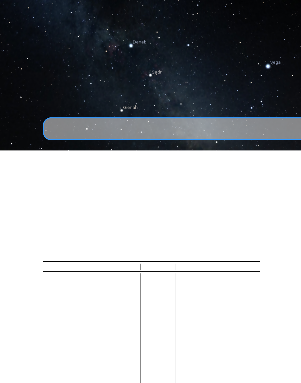
D. Configuration Files
D.1 Program Configuration
First, see 5.4 (The Main Configuration File) for information about the file
config.ini
, including
its default installed location, and command line options that can affect how it is processed.
The file
config.ini
(or a file which you can load instead with the
--config <file>
option)
is structured into the following parts. In addition, plugins can add a section named like the plugin
(Exception: The Text User Interface plugin’s section is named [tui] for historical reasons).
D.1.1 astro
This section includes settings for the commonly displayed objects.
ID Type Default Description
apparent_magnitude_algorithm string ExpSup2013
Set algorithm for computation of
apparent magnitude of the planets.
Possible values: ExpSup2013,
ExpSup1992,AstrAlm1984,
Mueller1893 and Generic.
nebula_magnitude_limit float 8.5
Value of limiting magnitude for the
deep-sky objects.
star_magnitude_limit float 6.5
Value of limiting magnitude for the
stars. Sometimes you don’t want to
display more stars when zooming in.
planet_magnitude_limit float 6.5
Value of limiting magnitude for the
planets. Sometimes you don’t want
to display more planets when zoom-
ing in.
planets_orbits_color_style string one_color
Set the style of orbits color. Possible
values: one_color,groups and max.
272 Appendix D. Configuration Files
flag_nebula_magnitude_limit bool false
Set to true to activate limit for show-
ing deep-sky objects.
flag_star_magnitude_limit bool false
Set to true to activate limit for show-
ing stars
flag_planet_magnitude_limit bool false
Set to true to activate limit for show-
ing planets.
extinction_mode_below_horizon string zero
Set extinction mode for atmosphere
below horizon. Possible values:
zero,mirror and major_planets.
flag_stars bool true
Set to false to hide the stars on start-
up
flag_star_name bool true
Set to false to hide the star labels on
start-up
flag_star_additional_names bool true
Set true to use additional names
(also known as) for stars.
flag_planets bool true
Set to false to hide the planet labels
on start-up
flag_planets_hints bool true
Set to false to hide the planet hints
on startup (names and circular high-
lights)
flag_planets_orbits bool false
Set to true to show the planet orbits
on startup
flag_permanent_orbits bool false
Set to true to show the orbit of
planet, when planet is out of the
viewport also.
flag_planets_pointers bool false
Set to true to show the planet pointer
markers on startup
flag_planets_nomenclature bool false
Set to true to show the planetary
nomenclature markers and labels
flag_hide_local_nomenclature bool true
Set to true to hide the plane-
tary nomenclature items on the ob-
server’s celestial body
flag_light_travel_time bool true
Should be true to improve accuracy
in the movement of the planets by
compensating for the time it takes
for light to travel. This has a slight
impact on performance, but is essen-
tial e.g. for Jupiter’s moons.
flag_object_trails bool false
Turns on and off drawing of object
trails (which show the movement of
the planets over time).
flag_isolated_trails bool true
Turns on and off drawing of isolated
trails.
flag_isolated_orbits bool true
Turns on and off drawing of isolated
orbits.
flag_nebula bool true
Set to false to hide the nebulae on
start-up.

D.1 Program Configuration 273
flag_nebula_name bool false
Set to true to show the nebula labels
on start-up.
flag_nebula_display_no_texture bool false
Set to true to suppress displaying of
nebula textures.
nebula_hints_amount float 3.0 Sets the amount of hints [0. . . 10].
nebula_labels_amount float 3.0 Sets the amount of labels [0.. . 10].
flag_milky_way bool true Set to false to hide the Milky Way.
milky_way_intensity float 1.0
Sets the relative brightness with
which the milky way is drawn. Typi-
cal [1. . . 3].
flag_zodiacal_light bool true
Set to false to hide the zodiacal light
zodiacal_light_intensity float 1.0
Sets the relative brightness with
which the zodiacal light is drawn.
max_mag_nebula_name float 8.0
Sets the magnitude of the nebulae
whose name is shown.
flag_nebula_hints_proportional bool false
Enables/disables proportional mark-
ers for deep-sky objects.
flag_surface_brightness_usage bool false
Enables/disables usage surface
brightness for markers for deep-sky
objects.
flag_size_limits_usage bool false
Enables/disables usage angular size
filter for markers for deep-sky ob-
jects.
size_limit_min int 1
Minimal angular size of visible deep-
sky objects in arcminutes.
size_limit_max int 600
Maximum angular size of visible
deep-sky objects in arcminutes.
flag_use_type_filter bool false
Enables/disables usage of the type
filters for deep-sky objects.
flag_nutation bool true Enables/disables usage nutation.
flag_topocentric_coordinates bool true
Enables/disables usage topocentric
coordinates.
flag_dso_designation_usage bool false
If true, use designations of deep-sky
objects on the sky instead of their
common names.
flag_dso_outlines_usage bool false
If true, use outlines for big deep-sky
objects on the sky instead of their
hints.
flag_dso_additional_names bool true
Set true to use additional names
(also known as) for deep-sky ob-
jects.
flag_grs_custom bool false
Turns on and off to using custom
settings for calculation of position
of Great Red Spot on Jupiter.
grs_longitude int 216
Longitude of Great Red Spot on
Jupiter in degrees.

274 Appendix D. Configuration Files
grs_drift float 15.0
Annual drift of Great Red Spot on
Jupiter in degrees.
grs_jd float 2456901.5
Initial JD for calculation of position
of Great Red Spot on Jupiter.
grs_measurements_url string
URL of recent measurements of
GRS’ position1.
meteor_zhr int 10 ZHR for sporadic meteors.
de430_path string
Path to JPL DE430 ephemerides file.
flag_use_de430 bool false
Enables/disables usage JPL DE430
ephemerides (if available).
de431_path string
Path to JPL DE431 ephemerides file.
flag_use_de431 bool false
Enables/disables usage JPL DE431
ephemerides (if available).
flag_toast_survey bool false
Enables/disables usage Digitized
Sky Survey in TOAST format.
toast_survey_host string
Host of Digitized Sky Survey stor-
age data.
toast_survey_directory string results
Directory name of Digitized Sky
Survey storage data.
toast_survey_levels int 11
Count of levels for Digitized Sky
Survey storage data.
D.1.2 astrocalc
This section includes settings for the Astronomical Calculations feature.
ID Type Default Description
flag_ephemeris_markers bool true
Set to true to show the calculated
ephemeris markers for Solar system bodies.
flag_ephemeris_dates bool false
Set to true to show the dates of calculated
ephemeris for Solar system bodies.
flag_ephemeris_magnitudes bool false
Set to true to show the magnitude of Solar
system body for the calculated ephemeride.
flag_ephemeris_horizontal bool false
Set to true to use horizontal coordinates for
ephemerides.
ephemeris_celestial_body string Moon
Default celestial body for computation of
ephemerides.
ephemeris_time_step int 6 Identificator for time step category.
celestial_magnitude_limit float 6.0
Value of limiting magnitude for the celes-
tial objects in computation of their posi-
tions.
celestial_category int 200
Identificator for default category of celes-
tial bodies.
flag_horizontal_coordinates bool false
Set to true to use horizontal coordinates
for compute of positions for the celestial
objects.
1Default value is http://jupos.privat.t-online.de/rGrs.htm
D.1 Program Configuration 275
flag_phenomena_opposition bool false
Set to true to compute of opposition phe-
nomenon between the Solar system bodies.
phenomena_angular_separation float 1.0
Allowed angular separation between celes-
tial bodies for computation of phenomena.
phenomena_celestial_body string Venus
Default celestial body for computation of
phenomena.
phenomena_celestial_group int 0
Identificator for group of celestial bodies
for computation of phenomenae.
wut_magnitude_limit float 10.0
Value of limiting magnitude for calcula-
tions within What’s Up Tonight feature.
wut_time_interval int 0
Identificator for time interval within What’s
Up Tonight feature computations.
graphs_celestial_body string Moon Default celestial body for draw of graphs.
graphs_first_id int 1 Identificator for left graph (blue line).
graphs_second_id int 2 Identificator for right graph (yellow line).
D.1.3 color
This section defines the RGB colors for the various objects, lines, grids, labels etc. Values are given
in float from 0 to 1. e.g. 1.0,1.0,1.0 for white, or 1,0,0 for red. Leave no whitespace between the
numbers!
ID Default Colour of the. . .
default_color 0.5,0.5,0.7 default colour.
daylight_text_color 0.0,0.0,0.0 info text at daylight.
sky_background_color 0.0,0.0,0.0
sky background (non-black is useful
for artists only).
ecliptical_J2000_color 0.4,0.1,0.1 ecliptical grid (J2000.0 frame).
ecliptic_J2000_color 0.7,0.2,0.2 ecliptic line (J2000.0 frame).
equinox_J2000_points_color 0.7,0.2,0.2 equinox points (J2000.0 frame).
solstice_J2000_points_color 0.7,0.2,0.2 solstice points (J2000.0 frame).
ecliptic_J2000_poles_color 0.7,0.2,0.2 ecliptic poles (J2000.0 frame).
ecliptical_color 0.6,0.3,0.1 ecliptical grid (of date).
ecliptic_color 0.9,0.6,0.2 ecliptic line (of date).
equinox_points_color 0.9,0.6,0.2 equinox points (of date).
solstice_points_color 0.9,0.6,0.2 solstice points (of date).
ecliptic_poles_color 0.9,0.6,0.2 ecliptic poles (of date).
precession_circles_color 0.9,0.6,0.2 precession circles.
equator_J2000_color 0.2,0.2,0.6 equator line (J2000.0 frame).
equatorial_J2000_color 0.1,0.1,0.5 equatorial grid (J2000.0 frame).
celestial_J2000_poles_color 0.2,0.2,0.6 celestial poles (J2000.0 frame).
equator_color 0.3,0.5,1.0 equator line (of date).
equatorial_color 0.2,0.3,0.8 equatorial grid (of date).
celestial_poles_color 0.3,0.5,1.0 celestial poles (of date).
276 Appendix D. Configuration Files
circumpolar_circles_color 0.3,0.5,1.0 circumpolar circles.
galactic_color 0.3,0.2,0.1 galactic grid.
galactic_equator_color 0.5,0.3,0.1 galactic equator line.
galactic_poles_color 0.5,0.3,0.1 galactic poles.
supergalactic_color 0.2,0.2,0.2 supergalactic grid.
supergalactic_equator_color 0.4,0.4,0.4 supergalactic equator line.
supergalactic_poles_color 0.4,0.4,0.4 supergalactic poles.
azimuthal_color 0.0,0.3,0.2 azimuthal grid.
horizon_color 0.2,0.6,0.2 horizon line.
meridian_color 0.2,0.6,0.2 meridian line.
prime_vertical_color 0.2,0.5,0.2 prime vertical.
zenith_nadir_color 0.2,0.6,0.2 zenith and nadir.
cardinal_color 0.8,0.2,0.1 cardinal points.
colures_color 0.5,0.0,0.5 colures.
longitude_color 0.2,0.4,0.4 opposition/conjunction longitude.
asterism_lines_color 0.4,0.4,0.8 asterism lines.
asterism_names_color 0.4,0.4,0.8 asterism names.
rayhelper_lines_color 1.0,1.0,0.0 the ray helper lines.
const_lines_color 0.2,0.2,0.6 constellation lines.
const_names_color 0.4,0.6,0.9 constellation names.
const_boundary_color 0.3,0.1,0.1 constellation boundaries.
dso_label_color 0.2,0.6,0.7 deep-sky objects labels.
dso_circle_color 1.0,0.7,0.2
deep-sky objects symbols, if not of
the types below.
dso_galaxy_color 1.0,0.2,0.2 galaxies symbols.
dso_radio_galaxy_color 0.3,0.3,0.3 radio galaxies symbols.
dso_active_galaxy_color 1.0,0.5,0.2 active galaxies symbols.
dso_interacting_galaxy_color 0.2,0.8,1.0 clusters of galaxies symbols.
dso_galaxy_cluster_color 0.2,0.5,1.0 interacting galaxies symbols.
dso_quasar_color 1.0,0.2,0.2 quasars symbols.
dso_possible_quasar_color 1.0,0.2,0.2 possible quasars symbols.
dso_bl_lac_color 1.0,0.2,0.2 BL Lac objects symbols.
dso_blazar_color 1.0,0.2,0.2 blazars symbols.
dso_nebula_color 0.1,1.0,0.1 nebulae symbols.
dso_planetary_nebula_color 0.1,1.0,0.1 planetary nebulae symbols.
dso_reflection_nebula_color 0.1,1.0,0.1 reflection nebulae symbols.
dso_bipolar_nebula_color 0.1,1.0,0.1 bipolar nebulae symbols.
dso_emission_nebula_color 0.1,1.0,0.1 emission nebulae symbols.
dso_dark_nebula_color 0.3,0.3,0.3 dark nebulae symbols.
dso_hydrogen_region_color 0.1,1.0,0.1 hydrogen regions symbols.
dso_supernova_remnant_color 0.1,1.0,0.1 supernovae remnants symbols.
D.1 Program Configuration 277
dso_supernova_candidate_color 0.1,1.0,0.1 supernova candidates symbols.
dso_supernova_remnant_cand_color 0.1,1.0,0.1
supernova remnant candidates sym-
bols.
dso_interstellar_matter_color 0.1,1.0,0.1 interstellar matter symbols.
dso_cluster_with_nebulosity_color 0.1,1.0,0.1
clusters associated with nebulosity
symbols.
dso_molecular_cloud_color 0.1,1.0,0.1 molecular clouds symbols.
dso_possible_planetary_nebula_color 0.1,1.0,0.1
possible planetary nebulae symbols.
dso_protoplanetary_nebula_color 0.1,1.0,0.1 protoplanetary nebulae symbols.
dso_cluster_color 1.0,1.0,0.1 star clusters symbols.
dso_open_cluster_color 1.0,1.0,0.1 open star clusters symbols.
dso_globular_cluster_color 1.0,1.0,0.1 globular star clusters symbols.
dso_stellar_association_color 1.0,1.0,0.1 stellar associations symbols.
dso_star_cloud_color 1.0,1.0,0.1 star clouds symbols.
dso_star_color 1.0,0.7,0.2 star symbols.
dso_symbiotic_star_color 1.0,0.7,0.2 symbiotic star symbols.
dso_emission_star_color 1.0,0.7,0.2 emission-line star symbols.
dso_emission_object_color 1.0,0.7,0.2 emission objects symbols.
dso_young_stellar_object_color 1.0,0.7,0.2 young stellar objects symbols.
star_label_color 0.4,0.3,0.5 star labels.
planet_names_color 0.5,0.5,0.7 planet names.
planet_pointers_color 1.0,0.3,0.3 planet pointers.
planet_nomenclature_color 0.1,1.0,0.1
planetary nomenclature hints and la-
bels.
sso_orbits_color 0.7,0.2,0.2 default orbits.
major_planet_orbits_color 0.7,0.2,0.2 major planet orbits.
minor_planet_orbits_color 0.7,0.5,0.5 minor planet orbits.
dwarf_planet_orbits_color 0.7,0.5,0.5 dwarf planet orbits.
moon_orbits_color 0.7,0.2,0.2 moon of planet orbits.
cubewano_orbits_color 0.7,0.5,0.5 cubewano orbits.
plutino_orbits_color 0.7,0.5,0.5 plutino orbits.
sdo_orbits_color 0.7,0.5,0.5 scattered disk object orbits.
oco_orbits_color 0.7,0.5,0.5 Oort cloud object orbits.
comet_orbits_color 0.7,0.8,0.8 comet orbits.
mercury_orbit_color 0.5,0.5,0.5 orbit of Mercury.
venus_orbit_color 0.9,0.9,0.7 orbit of Venus.
earth_orbit_color 0.0,0.0,1.0 orbit of Earth.
mars_orbit_color 0.8,0.4,0.1 orbit of Mars.
jupiter_orbit_color 1.0,0.6,0.0 orbit of Jupiter.
saturn_orbit_color 1.0,0.8,0.0 orbit of Saturn.
uranus_orbit_color 0.0,0.7,1.0 orbit of Uranus.
neptune_orbit_color 0.0,0.3,1.0 orbit of Neptune.
object_trails_color 1.0,0.7,0.0 planet trails.

278 Appendix D. Configuration Files
custom_marker_color 0.1,1.0,0.1 custom marker.
script_console_keyword_color 1.0,0.0,1.0
syntax highlight for keywords in the
script console.
script_console_module_color 0.0,1.0,1.0
syntax highlight for modules in the
script console.
script_console_comment_color 1.0,1.0,0.0
syntax highlight for comments in the
script console.
script_console_function_color 0.0,1.0,0.0
syntax highlight for functions in the
script console.
script_console_constant_color 1.0,0.5,0.5
syntax highlight for constants in the
script console.
D.1.4 custom_selected_info
You can fine-tune the bits of information to display for the selected object in this section. Set the
entry to true to display it.
ID Type Description
flag_show_absolutemagnitude bool absolute magnitude for objects.
flag_show_altaz bool horizontal coordinates for objects.
flag_show_catalognumber bool catalog designations for objects.
flag_show_distance bool distance to object.
flag_show_extra bool extra info for object.
flag_show_hourangle bool hour angle for object.
flag_show_magnitude bool magnitude for object.
flag_show_name bool common name for object.
flag_show_radecj2000 bool equatorial coordinates (J2000.0 frame) of object.
flag_show_radecofdate bool equatorial coordinates (of date) of object.
flag_show_galcoord bool galactic coordinates (System II) of object.
flag_show_supergalcoord bool supergalactic coordinates of object.
flag_show_eclcoordj2000 bool ecliptic coordinates (J2000.0 frame) of object.
flag_show_eclcoordofdate bool ecliptic coordinates (of date) of object.
flag_show_type bool type of object.
flag_show_size bool size of object.
flag_show_constellation bool show 3-letter IAU constellation label.
D.1.5 custom_time_correction
Stellarium allows experiments with ∆T. See 17.4.3 for details.
ID Type Description
coefficients [float,float,float] Coefficients a,b,cfor custom equation of ∆T
ndot float n-dot value for custom equation of ∆T
year int Year for custom equation of ∆T
D.1.6 devel
This section is for developers only.

D.1 Program Configuration 279
ID Type Description
convert_dso_catalog bool
Set to true to convert file
catalog.txt
into file
catalog.dat. Default value: false.
convert_dso_decimal_coord bool
Set to true to use decimal values for coordinates in source
catalog. Default value: true.
D.1.7 dso_catalog_filters
In this section you can fine-tune which of the deep-sky catalogs should be selected on startup.
ID Type Default Description
flag_show_ngc bool true New General Catalogue (NGC).
flag_show_ic bool true Index Catalogue (IC).
flag_show_m bool true Messier Catalog (M).
flag_show_c bool false Caldwell Catalogue (C).
flag_show_b bool false Barnard Catalogue (B).
flag_show_sh2 bool false Sharpless Catalogue (Sh-II).
flag_show_vdb bool false Van den Bergh Catalogue of reflection nebulae (VdB).
flag_show_rcw bool false
The RCW catalogue of H
α
-emission regions in the southern
Milky Way.
flag_show_lbn bool false Lynds’ Catalogue of Bright Nebulae (LBN).
flag_show_ldn bool false Lynds’ Catalogue of Dark Nebulae (LDN).
flag_show_cr bool false Collinder Catalogue (Cr).
flag_show_mel bool false Melotte Catalogue of Deep Sky Objects (Mel).
flag_show_pgc bool false HYPERLEDA. I. Catalog of galaxies (PGC).
flag_show_ced bool false
Cederblad Catalog of bright diffuse Galactic nebulae (Ced).
flag_show_ugc bool false The Uppsala General Catalogue of Galaxies (UGC).
flag_show_arp bool false Atlas of Peculiar Galaxies (Arp).
flag_show_vv bool false The Catalogue of Interacting Galaxies (VV).
flag_show_pk bool false The Catalogue of Galactic Planetary Nebulae (PK).
flag_show_png bool false
The Strasbourg-ESO Catalogue of Galactic Planetary Neb-
ulae (PN G).
flag_show_snrg bool false A catalogue of Galactic supernova remnants (SNR G).
flag_show_aco bool false A Catalog of Rich Clusters of Galaxies (ACO).
D.1.8 dso_type_filters
In this section you can fine-tune which types of the deep-sky objects should be selected on startup.

280 Appendix D. Configuration Files
ID Type Default Description
flag_show_galaxies bool true display galaxies.
flag_show_active_galaxies bool true display active galaxies.
flag_show_interacting_galaxies bool true display interacting galaxies.
flag_show_clusters bool true display star clusters.
flag_show_bright_nebulae bool true display bright nebulae.
flag_show_dark_nebulae bool true display dark nebulae.
flag_show_planetary_nebulae bool true display planetary nebulae.
flag_show_hydrogen_regions bool true display hydrogen regions.
flag_show_supernova_remnants bool true display supernovae remnants.
flag_show_galaxy_clusters bool true display clusters of galaxies.
flag_show_other bool true display other deep-sky objects.
D.1.9 gui
This section includes settings for the graphical user interface.
ID Type Default Description
flag_show_gui bool true If true, display GUI.
base_font_size int 13
Sets the font size. Typical value: 15
base_font_name string Verdana Selects the name
(Windows) for base font
DejaVu Sans
(others)
base_font_file string
Selects the name for font file, e.g.
DejaVuSans.ttf
flag_mouse_cursor_timeout bool true
Set to false if you want to have cur-
sor visible at all times.
mouse_cursor_timeout float 10
Set to 0if you want to keep the
mouse cursor visible at all times.
non-0 values mean the cursor will
be hidden after that many seconds of
inactivity
flag_show_flip_buttons bool false
Enables/disables display of the im-
age flipping buttons in the main tool-
bar (see section 4.3.4)
flag_show_nebulae_
background_button
bool false
Set to true if you want to have access
to the button for enabling/disabling
backgrounds for deep-sky objects
flag_show_toast_survey_button bool false
Set to true if you want to have access
to the button for enabling/disabling
Digitized Sky Survey for deep-sky
objects
selected_object_info string all
Values: all,short,none, and custom
(since V0.12.0; see 4.3.2).
custom_marker_size float 5.0 Size of custom marker.
D.1 Program Configuration 281
custom_marker_radius_limit int 15
Limit the click radius for mouse cur-
sor position in any direction for re-
moving of closest custom marker.
auto_hide_horizontal_toolbar bool true
Set to true if you want auto hide the
horizontal toolbar.
auto_hide_vertical_toolbar bool true
Set to true if you want auto hide the
vertical toolbar.
flag_use_window_transparency bool false If false, show menu bars opaque
flag_show_buttons_background bool true
If true, use background under but-
tons on bottom bar.
flag_show_datetime bool true
display date and time in the bottom
bar
flag_time_jd bool false
use JD format for time in the bottom
bar
flag_show_tz bool false
show time zone info in the bottom
bar
flag_show_location bool true display location in the bottom bar
flag_show_fps bool true
show at how many frames per sec-
ond Stellarium is rendering
flag_show_fov bool true
show how many degrees your verti-
cal field of view is
flag_fov_dms bool false
use DMS format for FOV in the bot-
tom bar
flag_show_decimal_degrees bool false
If true, use decimal degrees for co-
ordinates
flag_use_azimuth_from_south bool false
If true, calculate azimuth from south
towards west (as in some astronomi-
cal literature)
flag_surface_brightness_arcsec bool false
Toggle usage the measure unit
mag/0
(
mag/arcmin2
) or
mag/00
(
mag/arcsec2
) for the surface bright-
ness of deep-sky objects.
flag_surface_brightness_short bool false
Toggle usage the short notation for
the surface brightness of deep-sky
objects.
flag_enable_kinetic_scrolling bool true
If true, use kinetic scrolling in the
GUI2.
pointer_animation_speed float 1.0 Animation speed of pointers.
gpsd_hostname string "localhost"
hostname of server running
gpsd
(non-Windows only)
gpsd_port int 2947
port number of
gpsd
(non-Windows
only)
gps_interface string "COM3"
Port number of serial/USB GPS de-
vice (Windows only)
2This option is available on Windows tablets only.

282 Appendix D. Configuration Files
gps_baudrate int 4800
baudrate of serial/USB GPS device
(Windows only)
D.1.10 init_location
ID Type Description
landscape_name string
Sets the landscape you see. Built-in options are garching, geneva,
grossmugl, guereins, hurricane, jupiter, mars, moon, neptune, ocean,
saturn, trees, uranus, zero.
location string Name of location on which to start stellarium.
last_location string Coordinates of last used location in stellarium.
D.1.11 landscape
ID Type Description
atmosphere_fade_duration float
Sets the time (seconds) it takes for the atmosphere to
fade when de-selected
flag_landscape bool
Set to false if you don’t want to see the landscape at
all
flag_fog bool Set to false if you don’t want to see fog on start-up
flag_atmosphere bool
Set to false if you don’t want to see atmosphere on
start-up
flag_landscape_sets_location bool
Set to true if you want Stellarium to modify the ob-
server location when a new landscape is selected
(changes planet and longitude/latitude/altitude if lo-
cation data is available in the landscape.ini file)
minimal_brightness float
Set minimal brightness for landscapes. [0. . . 1] Typi-
cal value: 0.01
atmosphereybin int Set atmosphere binning coefficient for axis Y.
flag_minimal_brightness bool Set to true to use minimal brightness for landscape.
flag_landscape_sets_minimal_brightness bool
Set to true to use value for minimal brightness for
landscape from landscape settings.
flag_enable_illumination_layer bool Set to true to use illumination layer for landscape.
flag_enable_labels bool
Set to true to use landscape labels from gazetteer
layer.
atmospheric_extinction_coefficient float
Set atmospheric extinction coefficient
k
[mag/air-
mass]
temperature_C float Set atmospheric temperature [Celsius]
pressure_mbar float Set atmospheric pressure [mbar]
cache_size_mb int
Set the cache size for landscapes [megabytes]. De-
fault: 100

D.1 Program Configuration 283
D.1.12 localization
ID Type Description
sky_culture string
Sets the sky culture to use. E.g. western, polynesian, egyptian,
chinese, lakota, navajo, inuit, korean, norse, tupi, maori, aztec,
sami.
sky_locale string
Sets language used for names of objects in the sky (e.g. planets).
The value is a short locale code, e.g. en, de, en_GB
app_locale string
Sets language used for Stellarium’s user interface. The value is
a short locale code, e.g. en, de, en_GB.
time_zone string
Sets the time zone. Valid values: system_default, or some
region/location combination, e.g. Pacific/Marquesas
time_display_format string time display format: can be system_default,24h or 12h.
date_display_format string
date display format: can be system_default,mmddyyyy,ddm-
myyyy or yyyymmdd (ISO8601).
D.1.13 main
ID Type Description
invert_screenshots_colors bool
If true, Stellarium will saving the screenshorts with in-
verted colors.
restore_defaults bool
If true, Stellarium will restore default settings at
startup. This is equivalent to calling Stellarium with the
–restore-defaults option.
screenshot_dir string Path for saving screenshots
version string
Version of Stellarium. This parameter may be used to
detect necessary changes in config.ini file, do not edit.
use_separate_output_file bool
Set to true if you want to create a new file for script output
for each start of Stellarium
ignore_opengl_warning bool
Set to true if you don’t want to see OpenGL warnings for
each start of Stellarium.
check_requirements bool
Set to false if you want to disable and permanently ig-
nore checking hardware requirements at startup. Expect
problems if hardware is below requirements!
D.1.14 navigation
This section controls much of the look&feel of Stellarium. Be careful if you change something
here.
ID Type Description
preset_sky_time float
Preset sky time used by the dome version. Unit is
Julian Day. Typical value: 2451514.250011573
startup_time_mode string
Set the start-up time mode, can be actual (start
with current real world time), or Preset (start at
time defined by preset_sky_time)
flag_enable_zoom_keys bool Set to false if you want to disable the zoom

284 Appendix D. Configuration Files
flag_manual_zoom bool
Set to false for normal zoom behaviour as described
in this guide. When set to true, the auto zoom
feature only moves in a small amount and must be
pressed many times
flag_enable_move_keys bool Set to false if you want to disable the arrow keys
flag_enable_mouse_navigation bool
Set to false if you want to disable the mouse navi-
gation.
init_fov float
Initial field of view, in degrees, typical value: ”60”.
min_fov float
Minimal field of view, in degrees, typical value:
”0.001389” (5").
init_view_pos floats
Initial viewing direction. This is a vector with x,y,z-
coordinates. x being N-S (S +ve), y being E-W (E
+ve), z being up-down (up +ve). Thus to look South
at the horizon use 1,0,0. To look Northwest and up
at 45◦, use -1,-1,1 and so on.
auto_move_duration float
Duration (seconds) for the program to move to
point at an object when the space bar is pressed.
Typical value: 1.4
mouse_zoom float Sets the mouse zoom amount (mouse-wheel)
move_speed float Sets the speed of movement
zoom_speed float Sets the zoom speed
viewing_mode string
If set to horizon, the viewing mode simulate an
alt/azi mount, if set to equator, the viewing mode
simulates an equatorial mount
flag_manual_zoom bool
Set to true if you want to auto-zoom in incremen-
tally.
auto_zoom_out_resets_direction bool
Set to true if you want to auto-zoom restoring di-
rection.
time_correction_algorithm string Algorithm of DeltaT correction.
D.1.15 plugins_load_at_startup
This section lists which plugins are loaded at startup (those with true values). Each plugin can
add another section into this file with its own content, which is described in the respective plugin
documentation, see 11. You activate loading of plugins in the
F2
settings dialog, tab “Plugins”.
After selection of which plugins to load, you must restart Stellarium.
ID Type Description
AngleMeasure bool 12.1 Angle Measure plugin
ArchaeoLines bool 13.9 ArchaeoLines plugin
CompassMarks bool 12.2 Compass Marks plugin
MeteorShowers bool 13.6 Meteor Showers plugin
Exoplanets bool 13.3 Exoplanets plugin
Observability bool 15.7 Observability Analysis
Oculars bool 15.1 Oculars plugin
Pulsars bool 13.4 Pulsars plugin
Quasars bool 13.5 Quasars plugin
RemoteControl bool 12.7 Remote Control plugin
RemoteSync bool 12.8 Remote Sync plugin
D.1 Program Configuration 285
Satellites bool 13.8 Satellites plugin
SolarSystemEditor bool 12.9 Solar System Editor plugin
Supernovae bool 13.2 Historical Supernovae plugin
TelescopeControl bool 15.2 Telescope Control plugin
TextUserInterface bool 12.6 Text User Interface plugin
Novae bool 13.1 Bright Novae plugin
Scenery3dMgr bool 14 Scenery 3D plugin
D.1.16 projection
This section contains the projection of your choice and several advanced settings important if you
run Stellarium on a single screen, multi-projection, dome projection, or other setups.
ID Type Description
type string
Sets projection mode. Values: ProjectionPerspective,
ProjectionEqualArea, ProjectionStereographic, Pro-
jectionFisheye, ProjectionHammer, ProjectionCylin-
der, ProjectionMercator, ProjectionOrthographic,
ProjectionMiller, or ProjectionSinusoidal.
flip_horz bool
flip_vert bool
viewport string
How the view-port looks. Values: none (regular rect-
angular screen), disk (circular screen, useful for plan-
etarium setup).
viewportMask string How the view-port looks. Values: none.
viewport_fov_diameter float
viewport_x float Usually 0.
viewport_y float Usually 0.
viewport_width float
viewport_height float
viewport_center_x float Usually half of viewport_width.
viewport_center_y float Usually half of viewport_height.
viewport_center_offset_x float [-0.5. . . +0.5] Usually 0.
viewport_center_offset_y float
[-0.5. . . +0.5] Use negative values to move the hori-
zon lower.
D.1.17 proxy
This section has setting for connection to network through proxy server (proxy will be using when
host of proxy is filled).
ID Type Description
host_name string Name of host for proxy. E.g. proxy.org
type string Type of proxy. E.g. socks
port int Port of proxy. E.g. 8080
user string Username for proxy. E.g. michael_knight
password string Password for proxy. E.g. xxxxx

286 Appendix D. Configuration Files
D.1.18 scripts
ID Type Default Description
startup_script string startup.ssc name of script executed on program start
D.1.19 search
ID Type Description
flag_search_online bool If true, Stellarium will be use SIMBAD for search.
simbad_server_url string URL for SIMBAD mirror
flag_start_words bool
If false, Stellarium will be search phrase only from start of words
coordinate_system string
Specifies the coordinate system. Possible values: equatorialJ2000,
equatorial, horizontal, galactic. Default value: equatorialJ2000.
D.1.20 spheric_mirror
Stellarium can be used in planetarium domes. You can use a projector with a hemispheric mirror
with geometric properties given in this section. Note: These functions are only rarely used or tested,
some may not work as expected.
ID Type Default Description
flip_horz bool true Flip the projection horizontally
flip_vert bool false Flip the projection vertically
projector_alpha float 0
This parameter controls the properties of the
spheric mirror projection mode.
projector_gamma float
This parameter controls the properties of the
spheric mirror projection mode.
projector_delta float -1e100
This parameter controls the properties of the
spheric mirror projection mode.
projector_phi float 0
This parameter controls the properties of the
spheric mirror projection mode.
projector_position_x float 0
projector_position_y float 1
projector_position_z float -0.2
mirror_position_x float 0
mirror_position_y float 2
mirror_position_z float 0
image_distance_div_height float -1e100
mirror_radius float 0.25
dome_radius float 2.5
custom_distortion_file string
texture_triangle_base_length float
zenith_y float 0.125 deprecated
scaling_factor float 0.8 deprecated
distorter_max_fov float 175.0
Set the maximum field of view for the spheric
mirror distorter in degrees. Typical value:
180
viewportCenterWidth float projected image width, pixels
viewportCenterHeight float projected image height, pixels

D.1 Program Configuration 287
viewportCenterX float projected image center X, pixels
viewportCenterY float projected image center Y, pixels
D.1.21 stars
This section controls how stars are rendered.
ID Type Description
relative_scale float
relative size of bright and faint stars. Higher values mean that
bright stars are comparitively larger when rendered. Typical
value: 1.0
absolute_scale float
Changes how large stars are rendered. larger value lead to
larger depiction. Typical value: 1.0
star_twinkle_amount float amount of twinkling. Typical value: 0.3
flag_star_twinkle bool
true to allow twinkling (but only when atmosphere is active!).
flag_forced_twinkle bool
true to allow twinkling stars even without atmosphere. This
is obvious nonsense and contrary to nature, but some users
seem to like it.
flag_star_halo bool
false to not draw a halo around the brightest stars. This looks
poor, but some users seem to prefer it.
mag_converter_max_fov float
maximum field of view for which the magnitude conversion
routine is used. Typical value: 90.0.
mag_converter_min_fov float
minimum field of view for which the magnitude conversion
routine is used. Typical value: 0.001.
labels_amount float amount of labels. Typical value: 3.0
init_bortle_scale int
initial value of light pollution on the Bortle scale. Typical
value: 3.
D.1.22 tui
The built-in text user interface (TUI) plugin (see chapter 12.6) is most useful for planetariums. You
can even configure a system shutdown command. For historical reasons, the section is not called
[TextUserInterface] but simply [tui].
ID Type Default Description
tui_font_size float 15 Font size for TUI.
tui_font_color floatRGB 0.3,1,0.3 Font color for TUI.
flag_show_gravity_ui bool false
Enables or disables gravity mode for
UI
flag_show_tui_datetime bool false
Set to true if you want to see a date
and time label suited for dome pro-
jections
flag_show_tui_short_obj_info bool
set to true if you want to see object
info suited for dome projections
tui_admin_shutdown_command string
e.g. for Linux:
shutdown
–poweroff +2

288 Appendix D. Configuration Files
D.1.23 video
ID Type Description
fullscreen bool
If true, Stellarium will start up in full-screen mode, else windowed
mode
screen_w int Display width when in windowed mode. Value in pixels, e.g. 1024
screen_h int Display height when in windowed mode. Value in pixels, e.g. 768
screen_x int
Horizontal position of the top-left corner in windowed mode. Value
in pixels, e.g. 0
screen_y int
Vertical position of the top-left corner in windowed mode. Value in
pixels, e.g. 0
viewport_effect string
This is used when the spheric mirror display mode is activated. Values
include none and sphericMirrorDistorter.
minimum_fps int
Sets the minimum number of frames per second to display at (hard-
ware performance permitting)
maximum_fps int
Sets the maximum number of frames per second to display at. This
is useful to reduce power consumption in laptops.
D.1.24 viewing
This section defines which objects, labels, lines, grids etc. you want to see on startup. Set those to
true. Most items can be toggled with hotkeys or switched in the GUI.
ID Type Description
flag_asterism_drawing bool Display asterism line drawing
flag_asterism_name bool Display asterism names
flag_rayhelper_drawing bool Display the ray helper line drawing
flag_constellation_drawing bool Display constellation line drawing
flag_constellation_name bool Display constellation names
flag_constellation_art bool Display constellation art
flag_constellation_boundaries bool Display constellation boundaries
flag_constellation_isolate_selected bool
If true, constellation lines, boundaries and art will
be limited to the constellation of the selected star,
if that star is “on” one of the constellation lines.
flag_constellation_pick bool
Set to true if you only want to see the line drawing,
art and name of the selected constellation star
flag_isolated_trails bool
Set to true if you only want to see the trail line
drawn for the selected planet (asteroid, comet,
moon)
flag_isolated_orbits bool
Set to true if you want to see orbits only for selected
planet and their moons.
flag_azimutal_grid bool Display azimuthal grid
flag_equatorial_grid bool Display equatorial grid (of date)
flag_equatorial_J2000_grid bool Display equatorial grid (J2000)
flag_ecliptic_grid bool Display ecliptic grid (of date)
flag_ecliptic_J2000_grid bool Display ecliptic grid (J2000)
flag_galactic_grid bool Display galactic grid (System II)
flag_galactic_equator_line bool Display galactic equator line
flag_equator_line bool Display celestial equator line (of date)

D.1 Program Configuration 289
flag_equator_J2000_line bool Display celestial equator line (J2000)
flag_ecliptic_line bool Display ecliptic line (of date)
flag_ecliptic_J2000_line bool Display ecliptic line (J2000)
flag_meridian_line bool Display meridian line
flag_prime_vertical_line bool Display Prime Vertical line (East-Zenith-West)
flag_colure_lines bool Display colure lines (Celestial Pole-à/ã/æ/é)
flag_cardinal_points bool Display cardinal points
cardinal_font_size int Font size for cardinal points. Typical value: 24
subcardinal_font_size int
Font size for subcardinal points. Typical value: 18
flag_gravity_labels bool
Set to true if you want labels to undergo gravity
(top side of text points toward zenith). Useful with
dome projection.
flag_moon_scaled bool Set to false if you want to see the real moon size
moon_scale float
Sets the moon scale factor, sometimes useful to cor-
relate to our perception of the moon’s size. Typical
value: 4
constellation_art_intensity float
brightness [0. . . 1] of the constellation art images.
Typical value: 0.5
constellation_art_fade_duration float
time the constellation art takes to fade in or out, in
seconds. Typical value: 1.5
constellation_font_size int font size for constellation labels
constellation_line_thickness int
thickness of lines of the constellations [1. . . 5]. Typ-
ical value: 1
asterism_font_size int font size for asterism labels
asterism_line_thickness int
thickness of lines of the asterisms [1. . . 5]. Typical
value: 1
rayhelper_line_thickness int
thickness of lines of the ray helpers [1. . . 5]. Typi-
cal value: 1
flag_night bool Enable night mode (red-only mode) on startup
light_pollution_luminance float Sets the level of the light pollution simulation
use_luminance_adaptation bool Enable dynamic eye adaptation.
D.1.25 DialogPositions
By default, GUI panels appear centered in the screen. You can move them to your favorite location,
and on next start they will appear on that location instead. The entries in this section define the
upper left pixel coordinate where panels are stored.
Examples:
ID Type Example Description
Help int,int 58,39 Position of Help panel
DateTime int,int 1338,944 Position of time panel
D.1.26 DialogSizes0.15.1
GUI panels can be resized by dragging on their lower corners or borders. Enlarged sizes are stored
here, and on next start they will appear in this size. The entries in this section define the size.
Examples:

290 Appendix D. Configuration Files
ID Type Example Description
Help int,int 895,497 Size of Help panel
AstroCalc int,int 913,493 Size of AstroCalc panel
D.1.27 hips
This section defines the source list of the HiPS surveys, as well as other HiPS related options.0.18.0
ID Type Description
show bool show HiPS at startup?
sources/size int Number of HiPS survey sources
sources/n/url string uri of the nth source hipslist file (n∈[1...sources/size])
visible/url bool
HiPS configured to be displayed. (Stores current setting on program
exit)

D.2 Solar System Configuration Files 291
D.2 Solar System Configuration Files
The files
3ssystem_major.ini
and
ssystem_minor.ini
(in the
data/
subdirectory of the pro-
gram directory, contain orbital and rotational data from which Stellarium configures the Solar
System objects.
The minor bodies can be modified by placing a privately modified copy of
ssystem_minor.ini
into your own
data/
directory (see Chapter 5). You can edit the file either manually, or with the
Solar System Editor plugin (see Section 12.9).
Each object’s data are described in its own section which is typically named after the object
name. Some section names (e.g. those using diacriticals, spaces or other problematic characters)
appear a bit mangled.
We list here examples for the major planets, larger moons with special coordinate functions,
minor moons with generic orbital elements, minor planets and comets with elliptical and parabolic
orbit elements.
All elements are stored in alphabetic order in the files, however it makes more sense to present
the elements in another structure which better reflects the meaning. The actual order of the objects
in the files, and order of entries inside an object section, is irrelevant.
D.2.1 File ssystem_major.ini
Planet section
Example:
[ jupiter ]
name = Jupi te r
type = planet
coord_func=jupiter_special
albedo =0.51
atmosphere=1
color =1. , 0.983 , 0.934
tex_map = jupiter . png # texture courtesy of Bj \ xf6rn J\ xf3nsson
halo = true
oblateness=0.064874
or bit_v i suali zatio n _peri od =4331.87
parent = Sun
radius=71492
ro t_equ a tor_a scend i ng_no de = -22.203
rot_obliquity=2.222461
rot_perio de =9.92491
rot_pole_ de =64.49
rot_pole_ ra =268.05
rot_rotation_offset=-1 # use JupiterGRS patch
where
name English name of the planet. May appear translated.
type Mandatory for planets:
parent =Sun. The body which this object is running around. Default: Sun
coord_func The planet positions are all computed with a dedicated function (VSOP or DE43x).
3Before v0.16, there was a single file, ssystem.ini, with slightly different rules.

292 Appendix D. Configuration Files
orbit_visualization_period
number of (earth) days for how long the orbit should be made visible.
Typically Stellarium shows one orbit line. The orbit slowly drifts, however.
atmosphere
(0 or 1) flag to indicate whether observer locations should enable atmosphere drawing.
radius Equator radius, km.
oblateness Flattening of the polar diameter. (rpole/req)
albedo
total albedo (reflectivity) of the planet. Used for “generic” magnitude computation, but
the major planets usually have dedicated magnitude formulas, so the value is not evaluated
unless you are observing from a location outside Earth.
color Used to colorize halo. At least one of the components should be 1.
tex_halo
File name of texture map for halo texture in
textures
folder. (Used when zoomed out
far enough so that the actual sphere is not visible.)
tex_map File name of texture map in textures folder.
halo Should be true to draw a halo (simple light disk) when object too small to draw a sphere.
Elements for the Physical Ephemeris
rot_equator_ascending_node deprecated
rot_obliquity deprecated
rot_pole_ra constant of axis right ascension in ICRF, degrees
rot_pole_ra1 change per century of axis right ascension in ICRF, degrees
rot_pole_de constant of axis declination in ICRF, degrees
rot_pole_de1 change per century of axis declination in ICRF, degrees
rot_rotation_offset
longitude of central meridian at J2000.0. The special value here indicates
special treatment for the Great Red Spot.
rot_periode Duration of one sidereal rotation, in earth hours.
rot_equator_ascending_node and rot_obliquity are the generic values to specify the axis orien-
tation with respect to the parent object’s equator, or the VSOP87 inertial plane in case of planets.
However, for planets the IAU has been using right ascension and declination of the pole in the
ICRF for decades now. The elements to use for planets should therefore be the rot_pole_* values.
In many cases, the attitude/rotation formula is given like
α0=rot_pole_ra +T∗rot_pole_ra1 (D.1)
δ0=rot_pole_de +T∗rot_pole_de1 (D.2)
W=rot_rotation_offset +d∗rot_periode (D.3)
These cases are covered by the data in
ssystem_major.ini
. Other cases are dealt with in a
different way.
Moon section
All planet moons are defined only in ssystem_major.ini.
Moons are special in that they orbit another planet. Therefore, the rotational elements used to
be specified relative to the equatorial plane of the parent planet, and
orbit_SemiMajorAxis
are
specified in kilometers. However, current IAU reference material gives axis orientation with right
ascension and declination values for the pole in ICRF coordinates, with some of them in motion.
So again, if one of the
rot_pole_...
values exist, we assume the current standard. For more
complicated motion, again some special functions are applied.
[amalthea]
name=Amalthea
type = moon
parent = Jupiter
iau_moon_number=JV

D.2 Solar System Configuration Files 293
coord_ func = ell_orbit
orbit_AscendingNode=141.5521520794674
orbit_Eccentricity=0.006175744402949701
orbit_Epo ch =2 454 619.50000
orbit_Inclination=0.3864576103404582
orbit_LongOfPericenter=245.4222355150120000
or bit_ Mean Long itude = 224. 79248 9355 2 5500 00
orbi t_P eriod =0 .501 637046211 6355
orbit_SemiMajorAxis=181994.8658358799
or bit_v i suali zatio n _peri od =0.5 0163 7046 2116 355
radius =73
ro t_equ a tor_a scend i ng_no de =213.7
rot_obliquity=15.5
rot_perio de =1 2.039 2891 0907 9252
rot_rotation_offset=235.50
albedo =0.06
color =1. , 0.627 , 0.492
halo = true
tex_map = amalthea . png
model = j5amalt hea_ MLfix . obj
where
name English name of planet moon. No number, just the name. May be translated.
type moon
parent English name of planet or parent body.
iau_moon_number
a short label (string) consisting of the planet’s initial and the moon’s Roman
number in order of discovery. v0.16.1
coord_func
Must be
ell_orbit
for moons with orbital elements given, or
<name>_special
for
orbit_AscendingNode Ω
orbit_Eccentricity e
orbit_Epoch
orbit_Inclination i[degrees]
orbit_LongOfPericenter
orbit_MeanLongitude
orbit_Period [days]
orbit_SemiMajorAxis a[km]
orbit_visualization_period
[days] Defaults to
orbit_Period
to show orbit as closed line. This
is in fact only useful in case of special functions for positioning where
orbit_Period
is
not given.
radius Equator radius, km.
oblateness Flattening of the polar diameter. (rpole/req)
rot_equator_ascending_node =213.7 TRY TO AVOID!
rot_obliquity =15.5 TRY TO AVOID!
rot_pole_ra constant of axis right ascension in ICRF, degrees
rot_pole_ra1 change per century of axis right ascension in ICRF, degrees
rot_pole_de constant of axis declination in ICRF, degrees
294 Appendix D. Configuration Files
rot_pole_de1 change per century of axis declination in ICRF, degrees
rot_rotation_offset longitude of central meridian at J2000.0.
rot_periode
Duration of one sidereal rotation, in earth hours. For moons in bound rotation (which
always show one face towards their parent planet), it is best to omit this value: it defaults to
orbit_Period * 24.
albedo total reflectivity [0..1]
color for drawing halo (default: 1,1,1)
halo [=true|false] to draw a simple diffuse dot when zoomed out. Default: true
tex_map name of spherical texture map. Many moons have been mapped by visiting spacecraft!
v0.16.0
model
(optional) name of a 3D model for a non-spherical body in the
model
subdirectory of the
program directory.
Solar System Observer
Stellarium is great for excursions to the surface of any object with known orbital elements. Con-
figuring a viewpoint away from a planet requires a special kind of location. The Solar System
Observer has been provided as a neutral view location high above the North pole of the Solar
System. It has been configured like this:
[solar_system_observer]
name = Solar System Observer
parent = Sun
albedo =0.
color =0. , 0. , 0.
halo = false
hidden = true
coord_ func = ell_orbit
orbit_AscendingNode=0
orbit_Eccentricity=0
orbit_Epoch=2451545.0
orbit_Inclination=90
orbit_LongOfPericenter=0
orbit_MeanLongitude=90
orbi t_P eriod =700000000 00
or bit_ Semi Majo rAxis =70000 000 000
radius =1.
rot_obliquity=90
type=observer
Note the inclination and mean longitude of 90 degrees, and that it is hidden and has no halo.
Earth Observer
This is another “observer” location. The Earth Observer has been provided as a neutral view
location above the Northern hemisphere of the Earth. It has been configured like this:
[ earth_ob ser ver ]
name = Earth Observer
parent = Earth
albedo =0.
color =0. , 0. , 0.
halo = false
hidden = true

D.2 Solar System Configuration Files 295
coord_ func = ell_orbit
orbit_AscendingNode=0
orbit_Eccentricity=0
orbit_Epoch=2451545.0
orbit_Inclination=43
orbit_LongOfPericenter=0
orbit_MeanLongitude=90
orbit_Period=100000000000
orbit_SemiMajorAxis=1000000
radius =1.
rot_obliquity=90
type=observer
D.2.2 File ssystem_minor.ini
Minor Planet section
[4 vesta ]
type=asteroid
minor_planet_number=4
name = Vesta
coord_ func = co met_orbit
parent = Sun
or bit_ ArgOf Peric ente r =151.19843
or bit_ Asce ndin gNode =103.85141
orbit_Eccentricity=0.0887401
orbit_Epoch=2457000.5
orbit_Inc lina tion =7.14043
orbit_Mea nAno maly =20.86389
orbit _Mea nMo tion = 0.27154465
or bit_ Semi Majo rAxis =2.3617933
or bit_v i suali zatio n _peri od =1325.46
color =1. , 1. , 1.
halo = true
oblateness=0.0
albedo=0.423
radius =280
absolute_magnitude=3.2
slope_parameter=0.32
tex _map = ve sta . png
model =4 ve sta _21 _ML fix . obj
type
can be
asteroid, dwarf planet, cubewano, plutino, scattered disc object,
Oort cloud object
. With the exception of Pluto (which is included in
ssystem_major.ini
and cannot be changed), all positions for minor bodies are computed with the orbiting elements
given in this way.

296 Appendix D. Configuration Files
Note that although all minor planets orbit the sun in an elliptical orbit, the
coord_func=comet_orbit
.
However, it is more common for minor planets to specify epoch, mean anomaly and mean motion.
Visual magnitude is modelled from absolute magnitude Hand slope parameter G.
Elements for rotational axis may be given just like for planets when they are known. It is
recommended to use the modern specification (elements rot_pole_...).
A few asteroids have been visited by spacecraft, and for many other asteroids visual observations
v0.16.0
of stellar occultations by asteroids and light curve measurements have enabled researchers to derive
3D shape models of asteroids. If a model is available in the
models
subdirectory of the program
directory, this can be configured with a model entry.
Comet section
Comets are tiny, and their outgassing and close approaches to the major planets cause fast changes
in their orbital elements, so that each apparition should be specified with a dedicated section in
ssystem_minor.ini.
The coord_func is always specified as
comet_orbit
. Note the specification of a time (JDE) at
pericenter which is typical for comets.
Comet brightness is evaluated from
mag =absolute_magnitude+5·logdistance+2.5·slope_parameter·log(CometSunDistance)
(D.4)
The term
slope_parameter
may be a misnomer in case of comets. From the literature (Meeus,
1998) (equation 33.13) we find
mag =g+5log∆+κlogr(D.5)
from which
κ=2·slope_parameter
. In any case,
κ
is typically [5. . . 15] and specific for each
comet.
albedo is used to set the brightness for rendering the body, if you are close enough.
A large number of elements for historical comets is provided in the file
ssystem_1000comets.ini
in the installation directory. You can copy&paste what you need into your
ssystem_minor.ini
or add all with the Solar System Editor plugin (section 12.9). Unfortunately it is not possible to
specify several sets of orbital elements for different epochs of one apparition which would allow
automatic changes.
Periodic Comet
[1 phalley ]
type = comet
name =1 P / H alley
coord_ func = co met_orbit
parent = Sun [ can be omit ted ]
or bit_ ArgOf Peric ente r =111.7154
orbit_AscendingNode=58.8583
orbit_Eccentricity=0.968004
orbit_Inc lina tion =162.2453
orbit_PericenterDistance=0.57136
or bit_T imeA t Peri cente r =244 6463 .12979167
orbit_good=780

D.2 Solar System Configuration Files 297
color =1.0 , 1.0 , 1.0
dust_brightnessfactor=1.5
dust_lengthfactor=0.4
dust_ widt hfa ctor =1.5
albedo =0.1
radius =5
absolute_magnitude=5.5
slope_parameter=3.2
tex _map = no map . png
model =1682 q 1halley_MLfix . obj [ optional ]
You may want to e.g. change the name in this entry to
name=1P/Halley (1982i)
. Note a
rather short duration of
orbit_good
, which means the comet is only displayed 780 days before
and after perihel.
Some comets have been visited by spacecraft so that shape models of their cores may be
available and can be configured with a model entry. v0.16.0
Parabolic/Hyperbolic Comet
[ c2013us10 %28 catalina %29]
type = comet
name =C /2013 US10 ( Catalina )
coord_ func = co met_orbit
parent = Sun
or bit_ ArgOf Peric ente r =340.3533
orbit_AscendingNode=186.141
orbit_Eccentricity=1.000372
orbit_Inc lina tion =148.8766
orbit_PericenterDistance=0.822958
or bit_T imeA t Peri cente r =245 7342 .20748843
orbit_good=1000
color =1.0 , 1.0 , 1.0
dust_brightnessfactor=1.5
dust_lengthfactor=0.4
dust_ widt hfa ctor =1.5
albedo =0.1
radius =5
absolute_magnitude=4.4
slope_parameter=4
tex _map = no map . png
This has basically the same format. Note eccentricity is larger 1, this means the comet is
running on a slightly hyperbolic orbit. Stellarium shows data for this comet for almost 3 years
(orbit_good=1000 days) from perihel.
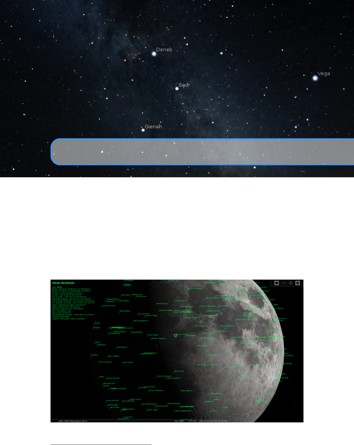
E. Planetary nomenclature
v0.17.0
Planetary nomenclature, like terrestrial nomenclature, is a system of uniquely identifying features
on the surface of a planet or natural satellite so that the features can be easily located, described, and
discussed. Since the invention of the telescope, astronomers have given names to the surface features
they have discerned, especially on the Moon and Mars. To standardize planetary nomenclature, the
International Astronomical Union (IAU) was assigned in 1919 the task of selecting official names
for features on solar system bodies1.
Figure E.1: Feature nomenclature of the Moon.
1History of Planetary Nomenclature – https://planetarynames.wr.usgs.gov/Page/History
300 Appendix E. Planetary nomenclature
Since version 0.17.0 Stellarium supports planetary nomenclature, which allows using the
planetarium for educational and informative purposes on the one hand, and as tool for recognition
and targeting of the planetary features for advanced amateurs on the other hand, avoiding the need
for additional cartographic software in the field.
All planetary nomenclature items are stored in a dedicated internal format, and all names are
translatable to provide better understanding of those names by average users and newbies – for
example in schools or universities. Of course all nomenclature items are available for finding in
the Search Tool after enabling the display of nomenclature (this feature is rather costly in terms of
computing power and therefore is by default disabled in the GUI).
The information in sections E.2–E.5, included here for reference, has been taken from the
“Gazetteer of Planetary Nomenclature” website by the International Astronomical Union (IAU)
Working Group for Planetary System Nomenclature (WGPSN)2.
E.1 Format of nomenclature data file
File
data/nomenclature.fab
is a plain text file in UTF-8 encoding and has a very simple data
format:
•One item per line;
•
Each item contains seven elements with white space (“space” or “tab” character) as delimiter.
Item Type Comment
planet name string
English name of the planet, moon or minor
body carrying the named feature
ID of planetary feature integer
unique integer, equal to Feature ID obtained
from Gazetteer of Planetary Nomenclature
translatable name of planetary feature string
English name, containing context data for
translators
type of planetary feature string
2-char code (see designation column in table
in section E.5)
center latitude of planetary feature float decimal degrees
center longitude of planetary feature float decimal degrees
size of planetary feature float kilometers
Example:
Vesta 15201 _( " Caesonia " ," crater ") AA 31.20117 249.93457 104.23
E.2 How names are approved by the IAU
When images are first obtained of the surface of a planet or satellite, a theme for naming features
is chosen and a few important features are named, usually by members of the appropriate IAU
task group (a commonly accepted planet-naming group). Later, as higher resolution images and
maps become available, additional features are named at the request of investigators mapping or
describing specific surfaces, features, or geologic formations. Anyone may suggest that a specific
name be considered by a task group. If the members of the task group agree that the name is
appropriate, it can be retained for use when there is a request from a member of the scientific
community that a specific feature be named. Names successfully reviewed by a task group are
2https://planetarynames.wr.usgs.gov, visited on 2017-10-30

E.3 IAU rules and conventions 301
submitted to the IAU Working Group for Planetary System Nomenclature (WGPSN)
3
. Upon
successful review by the members of the WGPSN, names are considered provisionally approved
and can be used on maps and in publications as long as the provisional status is clearly stated.
Provisional names are then presented for adoption to the IAU’s General Assembly, which met
triennially in the past, and which now adopts nomenclature for planetary surface features as required.
A name is not considered to be official – that is, “adopted” – until the General Assembly has given
its approval.
E.3 IAU rules and conventions
Names adopted by the IAU must follow various rules and conventions established and amended
through the years by the Union. These include:
1.
Nomenclature is a tool and the first consideration should be to make it simple, clear, and
unambiguous.
2.
In general, official names will not be given to features whose longest dimensions are less
than 100 meters, although exceptions may be made for smaller features having exceptional
scientific interest.
3.
The number of names chosen for each body should be kept to a minimum. Features should
be named only when they have special scientific interest, and when the naming of such
features is useful to the scientific and cartographic communities at large.
4.
Duplication of the same surface feature name on two or more bodies, and of the same name
for satellites and minor planets, is discouraged. Duplications may be allowed when names
are especially appropriate and the chances for confusion are very small.
5.
Individual names chosen for each body should be expressed in the language of origin.
Transliteration for various alphabets should be given, but there will be no translation from
one language to another.
6.
Where possible, the themes established in early solar system nomenclature should be used
and expanded on.
7.
Solar system nomenclature should be international in its choice of names. Recommendations
submitted to the IAU national committees will be considered, but final selection of the
names is the responsibility of the International Astronomical Union. Where appropriate, the
WGPSN strongly supports an equitable selection of names from ethnic groups, countries,
and gender on each map; however, a higher percentage of names from the country planning
a landing is allowed on landing site maps.
8.
No names having political, military or religious significance may be used, except for names
of political figures prior to the 19th century.
9.
Commemoration of persons on planetary bodies should not normally be a goal in itself, but
may be employed in special circumstances and is reserved for persons of high and enduring
international standing. Persons being so honored must have been deceased for at least three
years, before a proposal may be submitted.
10.
When more than one spelling of a name is extant, the spelling preferred by the person, or
used in an authoritative reference, should be used. Diacritical marks are a necessary part of a
name and will be used.
11.
Ring and ring-gap nomenclature and names for newly discovered satellites are developed in
joint deliberation between WGPSN and IAU Commission X2. Names will not be assigned
to satellites until their orbital elements are reasonably well known or definite features have
been identified on them.
3Working Group for Planetary System Nomenclature – https://planetarynames.wr.usgs.gov/

302 Appendix E. Planetary nomenclature
12.
Accessible and authoritative sources, including Internet sources, are required for adopted
names. Wikipedia is not sufficient as a source, but may be useful for identifying appropriate
sources.
In addition to these general rules, each task group develops additional conventions as it formulates an
interesting and meaningful nomenclature for individual planetary bodies. Most of these conventions
are self evident from study of the appendixes that follow.
E.4 Naming conventions
Names for all planetary features include a descriptor term, with a few exceptions. For craters, the
descriptor term is implicit. Some features named on Io and Triton do not carry a descriptor term
because they are ephemeral.
In general, the naming convention for a feature type remains the same regardless of its size.
Exceptions to this rule are channels (valles) on Mars and Venus, and craters on the Moon, Mars, and
Venus; naming conventions for these features differ according to size. The categories for naming
features on each planet or satellite (and the exceptions) are listed in Categories for Naming Features
on Planets and Satellites
4
. One feature classification, regio, was originally used on early maps of
the Moon and Mercury (drawn from telescopic observations) to describe vague albedo features. It
is now also used to delineate a broad geographic region.
Named features on bodies so small that coordinates have not yet been determined are identified
on drawings or images of the body that are included in the IAU Transactions volume of the year
when the names were adopted. Satellite rings and gaps in the rings are named for scientists who
have studied these features; drawings that show these names are also included in the pertinent
Transactions volume. Names for atmospheric features are informal at present; a formal system will
be chosen in the future.
The boundaries of many large features (such as terrae, regiones, planitiae, and plana) are not
topographically or geomorphically distinct; the coordinates of these features are identified from
an arbitrarily chosen center point. Boundaries (and thus coordinates) may be determined more
accurately from geochemical and geophysical data obtained by future missions.
During active missions, small surface features are often given informal names. These may
include landing sites, spacecraft impact sites, and small topographic features, such as craters, hills,
and rocks. Such names will not be given official status by the IAU, except as provided for by Rule 2
above. As for the larger objects, official names for any such small features would have to conform
to established IAU rules and categories.
When a satellite has been discovered through the efforts of a large scientific team, the list of
individual team members may be too long to include all contributors. In such cases, credit for the
discovery will go to the science team.
4Surface Feature Categories – https://planetarynames.wr.usgs.gov/Page/Categories

E.5 Descriptor terms (feature types) 303
E.5 Descriptor terms (feature types)
Descriptor terms are intended to represent morphological characteristics, not geological origin. The
WGPSN does not endorse any specific scientific hypotheses when assigning descriptors.
Feature Designation Description
Albedo Feature AL
Geographic area distinguished by amount of
reflected light
Arcus, arc¯
us AR Arc-shaped feature
Astrum, astra AS Radial-patterned features on Venus
Catena, catenae CA Chain of craters
Cavus, cavi CB
Hollows, irregular steep-sided depressions usu-
ally in arrays or clusters
Chaos, chaoses CH Distinctive area of broken terrain
Chasma, chasmata CM A deep, elongated, steep-sided depression
Collis, colles CO Small hills or knobs
Corona, coronae CR Ovoid-shaped feature
Crater, craters AA A circular depression
Dorsum, dorsa DO Ridge
Eruptive center ER Active volcanic centers on Io
Facula, faculae FA Bright spot
Farrum, farra FR
Pancake-like structure, or a row of such struc-
tures
Flexus, flex¯
us FE
A very low curvilinear ridge with a scalloped
pattern
Fluctus, fluct¯
us FL Flow terrain
Flumen, flumina FM Channel on Titan that might carry liquid
Fossa, fossae FO Long, narrow depression
Fretum, freta FT
Strait, a narrow passage of liquid connecting
two larger areas of liquid
Insula, insulae IN
Island (islands), an isolated land area (or group
of such areas) surrounded by, or nearly sur-
rounded by, a liquid area (sea or lake)
Labes, lab¯
es LA Landslide
Labyrinthus, labyrinthi LB Complex of intersecting valleys or ridges
Lacuna, lacunae LU
Irregularly shaped depression on Titan having
the appearance of a dry lake bed
Lacus, lac¯
us LC
“Lake” or small plain; on Titan, a “lake” or
small, dark plain with discrete, sharp boundaries
Landing site name LF Lunar features at or near Apollo landing sites
Large ringed feature LG Cryptic ringed features
Lenticula, lenticulae LE Small dark spots on Europa
Linea, lineae LI
A dark or bright elongate marking, may be
curved or straight
Lingula, lingulae LN
Extension of plateau having rounded lobate or
tongue-like boundaries
Macula, maculae MA Dark spot, may be irregular

304 Appendix E. Planetary nomenclature
Mare, maria ME
“Sea”; on the Moon, low albedo, relatively
smooth plain, generally of large extent; on Mars,
dark albedo areas of no known geological sig-
nificance; on Titan, large expanses of dark ma-
terials thought to be liquid hydrocarbons
Mensa, mensae MN A flat-topped prominence with cliff-like edges
Mons, montes MO Mountain
Oceanus, oceani OC A very large dark area on the moon
Palus, paludes PA “Swamp”; small plain
Patera, paterae PE
An irregular crater, or a complex one with scal-
loped edges
Planitia, planitiae PL Low plain
Planum, plana PM Plateau or high plain
Plume, plumes PU Cryo-volcanic features on Triton
Promontorium, promontoria PR “Cape”; headland promontoria
Regio, regiones RE
A large area marked by reflectivity or color dis-
tinctions from adjacent areas, or a broad geo-
graphic region
Reticulum, reticula RT Reticular (netlike) pattern on Venus
Rima, rimae RI Fissure
Rupes, rup¯
es RU Scarp
Satellite Feature SF
A feature that shares the name of an associated
feature. For example, on the Moon the craters
referred to as “Lettered Craters” are classified
in the gazetteer as “Satellite Features”
Scopulus, scopuli SC Lobate or irregular scarp
Serpens, serpentes SE
Sinuous feature with segments of positive and
negative relief along its length
Sinus, sin¯
us SI
“Bay”; small plain; on Titan, bays within seas
or lakes of liquid hydrocarbons
Sulcus, sulci SU Subparallel furrows and ridges
Terra, terrae TA Extensive land mass
Tessera, tesserae TE Tile-like, polygonal terrain
Tholus, tholi TH Small domical mountain or hill
Unda, undae UN Dunes
Vallis, valles VA Valley
Vastitas, vastitates VS Extensive plain
Virga, virgae VI A streak or stripe of color
Author and Acknowledgement
The nomenclature feature has been implemented by Teresa Huertas Roldán supported by the “ESA
Summer of Code in Space 2017” programme.
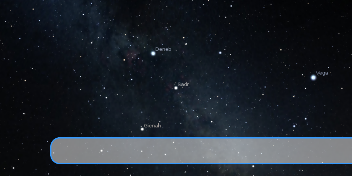
F. Accuracy
Stellarium originally was developed to present a beautiful simulation of the night sky, mostly
to understand what is visible in the sky when you leave your house, i.e., for present times. To
save computation time, some concessions were made in astronomical accuracy by using simplified
models which seemed acceptable at that time. However, many users started to overstress Stellarium’s
capabilities to simulate the historical sky of many centuries in the past, and found — or even worse:
did not find, but simply published — the resulting inconsistencies and errors. Unfortunately, celestial
motions are indeed more complicated than a simple clockwork, and the process of retrofitting
detailed and accurate models which started around v0.11.0 is not completed yet. Therefore, when
using Stellarium for scientific work like eclipse simulation to illustrate records found in Cuneiform
tablets, always also use some other reference to compare, and of course specify the program version
you used for your work. (The next version may be more accurate or at least provide different
results!) You can of course contact us if you are willing and able to help improving Stellarium’s
accuracy!
F.1 Date Range
The calendar dates are limited to a very wide interval of years, -100.000. . . 100.000. This is mostly
useful to visualize the effect of stellar proper motions or the wobbling motion of Earth’s axis known
as precession. If you observe the other planets, this is way beyond what current models are able to
show! Observe for example the Moon: you will find that it seems to run on a polar orbit around
+78.000 and even retrograde on a highly elongated orbit a few millennia after that. This is obvious
nonsense, caused by extrapolating mathematical models in inappropriate ways.
F.2 Stellar Proper Motion
Even though you can follow stellar proper motion for tens of thousands of years, please note that
the computation only takes the linear components
∆α
,
∆δ
into account. For times far from today,
a true 3D computation would be required, so that also changes in distance (and thus, brighness)

306 Appendix F. Accuracy
Object(s) Method Notes
Mercury, Venus, Earth-Moon
barycenter, Mars
VSOP87
Accuracy is 1 arc-second from
2000 B.C. – 6000 A.D.
Jupiter, Saturn VSOP87
Accuracy is 1 arc-second from 0
A.D. – 4000 A.D.
Uranus, Neptune VSOP87
Accuracy is 1 arc-second from
4000 B.C. – 8000 A.D.
Pluto ?
Pluto’s position is valid only from
1885 A.D. – 2099 A.D.
Earth’s Moon ELP2000-82B
Fit against JPL DE200, which pro-
vides date range 1850–2050. Po-
sitions should be usable for some
(unspecified) longer interval.
Galilean satellites L2
Valid from 500 A.D. – 3500 A.D.
Table F.1: Orbit-centric accuracy of used algorithms
could be simulated. Still, the simulation here should give a good impression which close and/or
fast stars will move over time, and thus how constellations become deformed.
Note that due to the way the stars are stored in catalogs, zooming in on fast stars like Arcturus
may even cease to display such stars when their original area in the sky is no longer in view.
Also, binary stars seem to break apart because Stellarium does not store them as systems
revolving about their combined center of gravity.
F.3 Planetary Positions
Stellarium uses the VSOP87 theory (P. Bretagnon and Francou, 1988) to calculate the positions of
the planets over time. This is an analytical ephemeris modeled to match the numerical integration run
DE200 from NASA JPL, which by itself gives positions for 1850.. . 2050. Its use is recommended
for the years -4000. . . +8000. You can observe the sun leaving the “ecliptic of date” and running
on the “ecliptic J2000” outside this date range. This is obviously a mathematical trick to keep
continuity. Still, positions may be somewhat useful outside this range, but don’t expect anything
reliable 50,000 years in the past!
The optionally usable JPL DE431 delivers planet positions strictly for -13000. . . +17000 only,
and nothing outside, but likely with higher accuracy. Outside of this range, positions from VSOP87
will be shown again.
As far as Stellarium is concerned, the user should bear in mind the limits of the VSOP87 and
other models (Table F.1). Accuracy values for VSOP87 are heliocentric as given by P. Bretagnon
and Francou (1988).
Note that Stellarium models light-time correction (if enabled), but does not yet model aberration of
light. Therefore seasons’ beginnings are off by a few minutes.
F.4 Minor Bodies
Positions for the Minor Bodies (Dwarf Planets, Asteroids, Comets) are computed with standard
algorithms found in astronomical text books. The generally used method of orbital elements allows
to compute the positions of the respective object on an undisturbed Kepler orbit around the sun.

F.5 Precession and Nutation 307
However, gravitational, and in the case of comets, non-gravitational (outgassing) disturbances slowly
change these orbital elements. Therefore an epoch is given for such elements, and computation of
positions for times far from this epoch will lead to positional errors. Therefore, when searching for
asteroids or comets, always update your orbital elements (See section 12.9), and use elements with
an epoch as close to your time of observation as possible! Stellarium does not simulate gravitational
perturbances and orbital changes of minor bodies passing major planets.
F.5 Precession and Nutation
Since v0.14.0, Stellarium computes the orientation of earth’s axis according to the IAU2006
Precession in a long-time variant developed by Vondrák, Capitaine, and Wallace (2011), and
IAU2000B Nutation (McCarthy and Luzum, 2003). This also now allows proper depiction of the
changes in ecliptic obliquity and display of “instantaneous precession circles” around the ecliptic
poles. These circles are indeed varying according to ecliptical obliquity. Nutation is only computed
for about 500 years around J2000.0. Nobody could have observed it before 1609, and it is unclear
for how long this model is applicable.
F.6 Planet Axes
Orientation for the other planets is still simplified. Future versions should implement modern
IAU-approved models.
F.7 Eclipses
The moon’s motion is very complicated, and eclipse computations can be tricky. One aspect which
every student of history, prehistory and archaeology should know but as it seems not every does,
is at least a basic understanding of the irregular slow-down of earth’s rotation known as
∆T
(see
section 17.4.3).
Eclipse records on cuneiform tablets go back to the 8th century BC, some Chinese records go
back a bit further. Experts on Earth rotation have provided models for
∆T
based on such observa-
tions. These are usually given as parabolic fit, with some recommended time span. Extrapolating
parabolic fits to erratic curves too far into the past is dangerous, pointless and inevitably leads to
errors or invalid results. Models differ by many hours (exceeding a whole day!) when applied too
far in the past. This means, there was certainly an eclipse, and latitude will be OK, but you cannot
say which longitude the eclipse was covering. The probability to have seen a total eclipse at a
certain interesting location will be very small and should by itself not be used as positive argument
for any reasonable statement. This is not a problem of Stellarium, but of current knowledge. To
repeat, you may find a solar eclipse in the 6th millennium BC, but you cannot even be sure which
side of Earth could observe it!
WANTED: A model for ∆Tthat works in the Mesolithic!
F.8 The Calendar
Stellarium follows the widely accepted convention that dates before the Gregorian calendar reform
are given in the Julian calendar, introduced by JULIUS CAESAR in 46 BC. This calendar introduces
a leap day every fourth year, which is a bit too much. If you want to show summer solstice in
the year -2500, you will notice it is not on June 21st. This is not an error of Stellarium – the
Gregorian reform had a reason! In prehistoric times, it may be more useful to work with solar
ecliptic longitudes. For example, summer solstice is at λ=90.

308 Appendix F. Accuracy
JULIUS CAESAR was assassinated in March 44 BC=-43 (see below). His simple 4-year leap rule
was then misapplied by the high priests of Rome by adding a leap day every third year. AUGUSTUS
fixed the calendar, and only 8 AD was the first correctly applied leap year as we know them. Be
careful if you are working in Augustean times: Stellarium does not model these issues!
Some authors (esp. for Mesoamerican dates) give dates in the proleptic Gregorian calendar
(which means, they apply the Gregorian leap year rules before 1582). This is a convention, they may
of course do that, but you must do the conversion to the Julian calendar to visualize the sky with
Stellarium. Hopefully they also give Julian Day numbers (JD), you can use them with Stellarium.
JD numbers are independent from calendar systems.
Some have noted a difference of one between dates given as BC versus Stellarium’s negative
years. Note that historical chronology does not know a year Zero! (Try to write this date in Roman
numbers!) Year 1 AD was preceded by year 1 BC. Astronomers want to simplify computations
and therefore use a year 0 (equivalent to 1 BC). It is simple: 1 BC=0, 2 BC=-1, . . . . 100 BC=-99.
Stellarium is an astronomy program. Just accept this.

G. GNU Free Documentation License
Version 1.3, 3 November 2008
Copyright c
2000, 2001, 2002, 2007, 2008 Free Software Foundation, Inc. http://fsf.org/
Everyone is permitted to copy and distribute verbatim copies of this license document, but changing
it is not allowed.
G.1 PREAMBLE
The purpose of this License is to make a manual, textbook, or other functional and useful document
“free” in the sense of freedom: to assure everyone the effective freedom to copy and redistribute it,
with or without modifying it, either commercially or noncommercially. Secondarily, this License
preserves for the author and publisher a way to get credit for their work, while not being considered
responsible for modifications made by others.
This License is a kind of “copyleft”, which means that derivative works of the document must
themselves be free in the same sense. It complements the GNU General Public License, which is a
copyleft license designed for free software.
We have designed this License in order to use it for manuals for free software, because free
software needs free documentation: a free program should come with manuals providing the same
freedoms that the software does. But this License is not limited to software manuals; it can be used
for any textual work, regardless of subject matter or whether it is published as a printed book. We
recommend this License principally for works whose purpose is instruction or reference.
G.2 APPLICABILITY AND DEFINITIONS
This License applies to any manual or other work, in any medium, that contains a notice placed by
the copyright holder saying it can be distributed under the terms of this License. Such a notice grants
a world-wide, royalty-free license, unlimited in duration, to use that work under the conditions
stated herein. The “Document”, below, refers to any such manual or work. Any member of the

310 Appendix G. GNU Free Documentation License
public is a licensee, and is addressed as “you”. You accept the license if you copy, modify or
distribute the work in a way requiring permission under copyright law.
A “Modified Version” of the Document means any work containing the Document or a portion
of it, either copied verbatim, or with modifications and/or translated into another language.
A “Secondary Section” is a named appendix or a front-matter section of the Document that deals
exclusively with the relationship of the publishers or authors of the Document to the Document’s
overall subject (or to related matters) and contains nothing that could fall directly within that overall
subject. (Thus, if the Document is in part a textbook of mathematics, a Secondary Section may
not explain any mathematics.) The relationship could be a matter of historical connection with the
subject or with related matters, or of legal, commercial, philosophical, ethical or political position
regarding them.
The “Invariant Sections” are certain Secondary Sections whose titles are designated, as being
those of Invariant Sections, in the notice that says that the Document is released under this License.
If a section does not fit the above definition of Secondary then it is not allowed to be designated as
Invariant. The Document may contain zero Invariant Sections. If the Document does not identify
any Invariant Sections then there are none.
The “Cover Texts” are certain short passages of text that are listed, as Front-Cover Texts or
Back-Cover Texts, in the notice that says that the Document is released under this License. A
Front-Cover Text may be at most 5 words, and a Back-Cover Text may be at most 25 words.
A “Transparent” copy of the Document means a machine-readable copy, represented in a
format whose specification is available to the general public, that is suitable for revising the
document straightforwardly with generic text editors or (for images composed of pixels) generic
paint programs or (for drawings) some widely available drawing editor, and that is suitable for
input to text formatters or for automatic translation to a variety of formats suitable for input to
text formatters. A copy made in an otherwise Transparent file format whose markup, or absence
of markup, has been arranged to thwart or discourage subsequent modification by readers is not
Transparent. An image format is not Transparent if used for any substantial amount of text. A copy
that is not “Transparent” is called “Opaque”.
Examples of suitable formats for Transparent copies include plain ASCII without markup,
Texinfo input format, LaTeX input format, SGML or XML using a publicly available DTD, and
standard-conforming simple HTML, PostScript or PDF designed for human modification. Examples
of transparent image formats include PNG, XCF and JPG. Opaque formats include proprietary
formats that can be read and edited only by proprietary word processors, SGML or XML for which
the DTD and/or processing tools are not generally available, and the machine-generated HTML,
PostScript or PDF produced by some word processors for output purposes only.
The “Title Page” means, for a printed book, the title page itself, plus such following pages as
are needed to hold, legibly, the material this License requires to appear in the title page. For works
in formats which do not have any title page as such, “Title Page” means the text near the most
prominent appearance of the work’s title, preceding the beginning of the body of the text.
The “publisher” means any person or entity that distributes copies of the Document to the
public.
A section “Entitled XYZ” means a named subunit of the Document whose title either is precisely
XYZ or contains XYZ in parentheses following text that translates XYZ in another language.
(Here XYZ stands for a specific section name mentioned below, such as “Acknowledgements”,
“Dedications”, “Endorsements”, or “History”.) To “Preserve the Title” of such a section when you
modify the Document means that it remains a section “Entitled XYZ” according to this definition.
The Document may include Warranty Disclaimers next to the notice which states that this
License applies to the Document. These Warranty Disclaimers are considered to be included by
reference in this License, but only as regards disclaiming warranties: any other implication that

G.3 VERBATIM COPYING 311
these Warranty Disclaimers may have is void and has no effect on the meaning of this License.
G.3 VERBATIM COPYING
You may copy and distribute the Document in any medium, either commercially or noncommercially,
provided that this License, the copyright notices, and the license notice saying this License applies
to the Document are reproduced in all copies, and that you add no other conditions whatsoever to
those of this License. You may not use technical measures to obstruct or control the reading or
further copying of the copies you make or distribute. However, you may accept compensation in
exchange for copies. If you distribute a large enough number of copies you must also follow the
conditions in section 3.
You may also lend copies, under the same conditions stated above, and you may publicly
display copies.
G.4 COPYING IN QUANTITY
If you publish printed copies (or copies in media that commonly have printed covers) of the
Document, numbering more than 100, and the Document’s license notice requires Cover Texts, you
must enclose the copies in covers that carry, clearly and legibly, all these Cover Texts: Front-Cover
Texts on the front cover, and Back-Cover Texts on the back cover. Both covers must also clearly
and legibly identify you as the publisher of these copies. The front cover must present the full title
with all words of the title equally prominent and visible. You may add other material on the covers
in addition. Copying with changes limited to the covers, as long as they preserve the title of the
Document and satisfy these conditions, can be treated as verbatim copying in other respects.
If the required texts for either cover are too voluminous to fit legibly, you should put the first
ones listed (as many as fit reasonably) on the actual cover, and continue the rest onto adjacent
pages.
If you publish or distribute Opaque copies of the Document numbering more than 100, you must
either include a machine-readable Transparent copy along with each Opaque copy, or state in or
with each Opaque copy a computer-network location from which the general network-using public
has access to download using public-standard network protocols a complete Transparent copy of
the Document, free of added material. If you use the latter option, you must take reasonably prudent
steps, when you begin distribution of Opaque copies in quantity, to ensure that this Transparent
copy will remain thus accessible at the stated location until at least one year after the last time you
distribute an Opaque copy (directly or through your agents or retailers) of that edition to the public.
It is requested, but not required, that you contact the authors of the Document well before
redistributing any large number of copies, to give them a chance to provide you with an updated
version of the Document.
G.5 MODIFICATIONS
You may copy and distribute a Modified Version of the Document under the conditions of sections
2 and 3 above, provided that you release the Modified Version under precisely this License, with
the Modified Version filling the role of the Document, thus licensing distribution and modification
of the Modified Version to whoever possesses a copy of it. In addition, you must do these things in
the Modified Version:
•
A. Use in the Title Page (and on the covers, if any) a title distinct from that of the Document,
and from those of previous versions (which should, if there were any, be listed in the History

312 Appendix G. GNU Free Documentation License
section of the Document). You may use the same title as a previous version if the original
publisher of that version gives permission.
•
B. List on the Title Page, as authors, one or more persons or entities responsible for authorship
of the modifications in the Modified Version, together with at least five of the principal
authors of the Document (all of its principal authors, if it has fewer than five), unless they
release you from this requirement.
•
C. State on the Title page the name of the publisher of the Modified Version, as the publisher.
•D. Preserve all the copyright notices of the Document.
•
E. Add an appropriate copyright notice for your modifications adjacent to the other copyright
notices.
•
F. Include, immediately after the copyright notices, a license notice giving the public
permission to use the Modified Version under the terms of this License, in the form shown in
the Addendum below.
•
G. Preserve in that license notice the full lists of Invariant Sections and required Cover Texts
given in the Document’s license notice.
•H. Include an unaltered copy of this License.
•
I. Preserve the section Entitled “History”, Preserve its Title, and add to it an item stating at
least the title, year, new authors, and publisher of the Modified Version as given on the Title
Page. If there is no section Entitled “History” in the Document, create one stating the title,
year, authors, and publisher of the Document as given on its Title Page, then add an item
describing the Modified Version as stated in the previous sentence.
•
J. Preserve the network location, if any, given in the Document for public access to a
Transparent copy of the Document, and likewise the network locations given in the Document
for previous versions it was based on. These may be placed in the “History” section. You
may omit a network location for a work that was published at least four years before the
Document itself, or if the original publisher of the version it refers to gives permission.
•
K. For any section Entitled “Acknowledgements” or “Dedications”, Preserve the Title of
the section, and preserve in the section all the substance and tone of each of the contributor
acknowledgements and/or dedications given therein.
•
L. Preserve all the Invariant Sections of the Document, unaltered in their text and in their
titles. Section numbers or the equivalent are not considered part of the section titles.
•
M. Delete any section Entitled “Endorsements”. Such a section may not be included in the
Modified Version.
•
N. Do not retitle any existing section to be Entitled “Endorsements” or to conflict in title
with any Invariant Section.
•O. Preserve any Warranty Disclaimers.
If the Modified Version includes new front-matter sections or appendices that qualify as
Secondary Sections and contain no material copied from the Document, you may at your option
designate some or all of these sections as invariant. To do this, add their titles to the list of Invariant
Sections in the Modified Version’s license notice. These titles must be distinct from any other
section titles.
You may add a section Entitled “Endorsements”, provided it contains nothing but endorsements
of your Modified Version by various parties — for example, statements of peer review or that the
text has been approved by an organization as the authoritative definition of a standard.
You may add a passage of up to five words as a Front-Cover Text, and a passage of up to
25 words as a Back-Cover Text, to the end of the list of Cover Texts in the Modified Version.
Only one passage of Front-Cover Text and one of Back-Cover Text may be added by (or through
arrangements made by) any one entity. If the Document already includes a cover text for the same
cover, previously added by you or by arrangement made by the same entity you are acting on behalf

G.6 COMBINING DOCUMENTS 313
of, you may not add another; but you may replace the old one, on explicit permission from the
previous publisher that added the old one.
The author(s) and publisher(s) of the Document do not by this License give permission to use
their names for publicity for or to assert or imply endorsement of any Modified Version.
G.6 COMBINING DOCUMENTS
You may combine the Document with other documents released under this License, under the terms
defined in section 4 above for modified versions, provided that you include in the combination all
of the Invariant Sections of all of the original documents, unmodified, and list them all as Invariant
Sections of your combined work in its license notice, and that you preserve all their Warranty
Disclaimers.
The combined work need only contain one copy of this License, and multiple identical Invariant
Sections may be replaced with a single copy. If there are multiple Invariant Sections with the same
name but different contents, make the title of each such section unique by adding at the end of
it, in parentheses, the name of the original author or publisher of that section if known, or else a
unique number. Make the same adjustment to the section titles in the list of Invariant Sections in
the license notice of the combined work.
In the combination, you must combine any sections Entitled “History” in the various original
documents, forming one section Entitled “History”; likewise combine any sections Entitled “Ac-
knowledgements”, and any sections Entitled “Dedications”. You must delete all sections Entitled
“Endorsements”.
G.7 COLLECTIONS OF DOCUMENTS
You may make a collection consisting of the Document and other documents released under this
License, and replace the individual copies of this License in the various documents with a single
copy that is included in the collection, provided that you follow the rules of this License for verbatim
copying of each of the documents in all other respects.
You may extract a single document from such a collection, and distribute it individually under
this License, provided you insert a copy of this License into the extracted document, and follow
this License in all other respects regarding verbatim copying of that document.
G.8 AGGREGATION WITH INDEPENDENT WORKS
A compilation of the Document or its derivatives with other separate and independent documents
or works, in or on a volume of a storage or distribution medium, is called an “aggregate” if the
copyright resulting from the compilation is not used to limit the legal rights of the compilation’s
users beyond what the individual works permit. When the Document is included in an aggregate,
this License does not apply to the other works in the aggregate which are not themselves derivative
works of the Document.
If the Cover Text requirement of section 3 is applicable to these copies of the Document, then
if the Document is less than one half of the entire aggregate, the Document’s Cover Texts may be
placed on covers that bracket the Document within the aggregate, or the electronic equivalent of
covers if the Document is in electronic form. Otherwise they must appear on printed covers that
bracket the whole aggregate.

314 Appendix G. GNU Free Documentation License
G.9 TRANSLATION
Translation is considered a kind of modification, so you may distribute translations of the Document
under the terms of section 4. Replacing Invariant Sections with translations requires special permis-
sion from their copyright holders, but you may include translations of some or all Invariant Sections
in addition to the original versions of these Invariant Sections. You may include a translation of
this License, and all the license notices in the Document, and any Warranty Disclaimers, provided
that you also include the original English version of this License and the original versions of those
notices and disclaimers. In case of a disagreement between the translation and the original version
of this License or a notice or disclaimer, the original version will prevail.
If a section in the Document is Entitled “Acknowledgements”, “Dedications”, or “History”, the
requirement (section 4) to Preserve its Title (section 1) will typically require changing the actual
title.
G.10 TERMINATION
You may not copy, modify, sublicense, or distribute the Document except as expressly provided
under this License. Any attempt otherwise to copy, modify, sublicense, or distribute it is void, and
will automatically terminate your rights under this License.
However, if you cease all violation of this License, then your license from a particular copyright
holder is reinstated (a) provisionally, unless and until the copyright holder explicitly and finally
terminates your license, and (b) permanently, if the copyright holder fails to notify you of the
violation by some reasonable means prior to 60 days after the cessation.
Moreover, your license from a particular copyright holder is reinstated permanently if the
copyright holder notifies you of the violation by some reasonable means, this is the first time you
have received notice of violation of this License (for any work) from that copyright holder, and you
cure the violation prior to 30 days after your receipt of the notice.
Termination of your rights under this section does not terminate the licenses of parties who
have received copies or rights from you under this License. If your rights have been terminated and
not permanently reinstated, receipt of a copy of some or all of the same material does not give you
any rights to use it.
G.11 FUTURE REVISIONS OF THIS LICENSE
The Free Software Foundation may publish new, revised versions of the GNU Free Documentation
License from time to time. Such new versions will be similar in spirit to the present version, but
may differ in detail to address new problems or concerns. See
http://www.gnu.org/copyleft/
.
Each version of the License is given a distinguishing version number. If the Document specifies
that a particular numbered version of this License “or any later version” applies to it, you have the
option of following the terms and conditions either of that specified version or of any later version
that has been published (not as a draft) by the Free Software Foundation. If the Document does
not specify a version number of this License, you may choose any version ever published (not as a
draft) by the Free Software Foundation. If the Document specifies that a proxy can decide which
future versions of this License can be used, that proxy’s public statement of acceptance of a version
permanently authorizes you to choose that version for the Document.
G.12 RELICENSING
“Massive Multiauthor Collaboration Site” (or “MMC Site”) means any World Wide Web server
that publishes copyrightable works and also provides prominent facilities for anybody to edit

G.12 RELICENSING 315
those works. A public wiki that anybody can edit is an example of such a server. A “Massive
Multiauthor Collaboration” (or “MMC”) contained in the site means any set of copyrightable works
thus published on the MMC site.
“CC-BY-SA” means the Creative Commons Attribution-Share Alike 3.0 license published by
Creative Commons Corporation, a not-for-profit corporation with a principal place of business in
San Francisco, California, as well as future copyleft versions of that license published by that same
organization.
“Incorporate” means to publish or republish a Document, in whole or in part, as part of another
Document.
An MMC is “eligible for relicensing” if it is licensed under this License, and if all works
that were first published under this License somewhere other than this MMC, and subsequently
incorporated in whole or in part into the MMC, (1) had no cover texts or invariant sections, and (2)
were thus incorporated prior to November 1, 2008.
The operator of an MMC Site may republish an MMC contained in the site under CC-BY-SA
on the same site at any time before August 1, 2009, provided the MMC is eligible for relicensing.
H. Acknowledgements
H.1 Contributors
When not listed as chapter authors, the following were the main contributors to the User Guide,
mostly for versions before V0.15:
Matthew Gates
Primary author of the first User Guide (versions 0.9
to 0.12)
Paul Robinson Sky guide; exercise ideas
Andras Mohari Celestial sphere diagrams; numerous corrections
Rudy Gobits, Dirk Schwarzhans Mac platform specifics
Barry Gerdes Windows platform specifics
Customisation of .fab files
Documentation Maintainer up to V0.12
Sigma Japanese translation; many corrections
Richard Powell
Figure 18.3 (colour/magnitude diagram) is a modifi-
cation of his diagram; he kindly granted permission
for it to be distributed under the FDL
John Twin Many spelling corrections
Georg Zotti Lead author of the 0.15+ editions
Alexander Wolf
New layout, many contributions for the 0.15+ edi-
tions
The rest of the Stellarium developer team You know who you are.. . :-)
Additional material has been incorporated into the guide from sources that are published under
the GNU FDL, including material from Wikipedia and the Astronomy book at Wikibooks.
H.2 How you can help
We especially welcome contributions, but also bug reports, feature requests and other feedback
through the usual channels (trackers, forums and so on):

318 Appendix H. Acknowledgements
Stellarium on Github https://github.com/Stellarium/
Bug tracker https://bugs.launchpad.net/stellarium
Questions for Stellarium (FAQ) https://answers.launchpad.net/stellarium
Feedback forum https://sourceforge.net/p/stellarium/discussion/278769/
H.3 Technical Articles
Stellarium would not look the same and work without these works from computer graphics and
astronomy.
The tone reproductor class
The class mainly performs a fast implementation of the algorithm
from Tumblin and Rushmeier (1993), with more accurate values from Devlin et al. (2002).
The blue shift formula is taken from Jensen et al. (2000) and combined with the Scotopic
vision formula from Larson, Rushmeier, and Piatko (1997).
The skylight class
The class governs sky colors and is a fast implementation of the algorithm by
Preetham, Shirley, and Smits (1999).
The skybright class
The class governs physical sky brightness values based on Bradley Schaefer’s
VISLIMIT.BAS
basic source code (Schaefer, 1998). The basic sources are available on the Sky
and Telescope web site (code “offered as-is and without support”).
The ∆Tcalculations
For implementation of calculation routines for
∆T
we used the following
sources:
1. ∆T
webpage by Rob van Gent:
http://www.staff.science.uu.nl/~gent0113/
deltat/deltat.htm
2.
Five Millennium Canon of Solar Eclipses: -1900 to +3000 (Espenak and Meeus, 2006)
(http://eclipse.gsfc.nasa.gov/SEhelp/deltatpoly2004.html)
3. “On the system of astronomical constants” (Clemence, 1948)
4.
“The rotation of the earth, and the secular accelerations of the sun, moon and planets”
(Spencer Jones, 1939)
5.
“Polynomial approximations for the correction delta T E.T.-U.T. in the period 1800-
1975” (Schmadel and Zech, 1979)
6. “ELP 2000-85 and the dynamic time-universal time relation” (Borkowski, 1988)
7.
“Empirical Transformations from U.T. to E.T. for the Period 1800-1988” (Schmadel
and Zech, 1988)
8.
“Historical values of the Earth’s clock error
∆
T and the calculation of eclipses” (Mor-
rison and F. R. Stephenson, 2004) with Addendum (Morrison and F. R. Stephenson,
2005)
9. “Polynomial approximations to Delta T, 1620-2000 AD” (Meeus and Simons, 2000)
10. Canon of Solar Eclipses -2003 to +2526 (Mucke and Meeus, 1983)
11.
“The accelerations of the earth and moon from early astronomical observations”
(Muller and F. R. Stephenson, 1975)
12. “Pre-Telescopic Astronomical Observations” (F. R. Stephenson, 1978)
13.
“Long-term changes in the rotation of the earth - 700 B.C. to A.D. 1980” (F. R.
Stephenson and Morrison, 1984)
14.
“Long-Term Fluctuations in the Earth’s Rotation: 700 BC to AD 1990” (F. R. Stephen-
son and Morrison, 1995)
15. Historical Eclipses and Earth’s Rotation (F. Richard Stephenson, 1997)
16. Astronomical Algorithms (Meeus, 1998)
17. Astronomy on the Personal Computer (Montenbruck and Pfleger, 2000)
18.
Calendrical Calculations (The Millennium Edition) (Reingold and Dershowitz, 2001)
19. ∆Twebpage by V. Reijs: http://www.iol.ie/~geniet/eng/DeltaTeval.htm

H.4 Included Source Code 319
Precession:
“New precession expressions, valid for long time intervals” (Vondrák, Capitaine, and
Wallace, 2011) with correction (Vondrák, Capitaine, and Wallace, 2012)
Nutation:
“An abridged model of the precession-nutation of the celestial pole” (McCarthy and
Luzum, 2003) This model provides accuracy better than 1 milli-arcsecond in the time
1995-2050. It is applied for years 1500..2500 only.
H.4 Included Source Code
•
Some computation of the sidereal time (
sidereal_time.h/c
) and Pluto orbit contains code
from the libnova library (LGPL) by Liam Girdwood.
•
The
orbit.cpp/h
and
solve.h
files were directly borrowed from
Celestia
(Chris Laurel;
GPL license). They have now evolved a bit.
•
Several implementations of IMCCE theories for planet and satellite movement by Johannes
Gajdosik (MIT-style license, see the corresponding files for the license text)
•
The tesselation algorithms were originally extracted from the glues library version 1.4 by
Mike Gorchak <mike@malva.ua> (SGI FREE SOFTWARE LICENSE B).
•OBJ loader in the Scenery3D plugin based on glObjViewer (c) 2007 dhpoware
•
Parts of the code to work with DE430 and DE431 data files have been taken from Project
Pluto (GPL license).
•
The
SpoutLibrary.dll
and header from the SpoutSDK version 2.005 available at
http:
//spout.zeal.co (BSD license).
H.5 Data
1.
The Hipparcos star catalog From ESA (European Space Agency) and the Hipparcos mission.
ref. ESA, 1997, The Hipparcos and Tycho Catalogues, ESA SP-1200
http://cdsweb.
u-strasbg.fr/ftp/cats/I/239
2. The solar system data mainly comes from IMCCE and partly from Celestia.
3. Polynesian constellations are based on diagrams from the Polynesian Voyaging Society
4. Chinese constellations are based on diagrams from the Hong Kong Space Museum
5.
Egyptian constellations are based on the work of Juan Antonio Belmonte, Instituto de
Astrofisica de Canarias
6.
The Tycho-2 Catalogue of the 2.5 Million Brightest Stars Hog E., Fabricius C., Makarov
V.V., Urban S., Corbin T., Wycoff G., Bastian U., Schwekendiek P., Wicenec A. Astron.
Astrophys. 355, L27 (2000) http://cdsweb.u-strasbg.fr/ftp/cats/I/259
7.
Naval Observatory Merged Astrometric Dataset (NOMAD) version 1 (
http://www.nofs.
navy.mil/nomad) Norbert Zacharias writes:
“There are no fees, both UCAC and NOMAD are freely available with
the only requirement that the source of the data (U.S. Naval Observatory) and
original product name need to be provided with any distribution, as well as a
description about any changes made to the data, if at all.”
The changes made to the data are:
•try to compute visual magnitude and color from the b,v,r values
•compute nr_of_measurements =thenumbero f validb,v,rvalues
•
throw away or keep stars (depending on magnitude, nr_of_measurements, combination
of flags, tycho2 number)
•
add all stars from Hipparcos (incl. component solutions), and tycho2+1st supplement
•
reorganize the stars in several brigthness levels and triangular zones according to
position and magnitude

320 Appendix H. Acknowledgements
The programs that are used to generate the star files are called "MakeCombinedCatalogue",
"ParseHip", "ParseNomad", and can be found in the util subdirectory in source code. The
position, magnitudes, and proper motions of the stars coming from NOMAD are unchanged,
except for a possible loss of precision, especially in magnitude. When there is no v-
magnitude, it is estimated from r or b magnitude. When there is no b- or v- magnitude, the
color B-V is estimated from the other magnitudes. Also proper motions of faint stars are
neglected at all.
8.
Stellarium’s Catalog of Variable Stars based on General Catalog of Variable Stars (GCVS)
version 2013Apr.
http://www.sai.msu.su/gcvs/gcvs/
Samus N.N., Durlevich O.V.,
Kazarovets E V., Kireeva N.N., Pastukhova E.N., Zharova A.V., et al., General Catalogue
of Variable Stars (Samus+ 2007-2012)
http://cdsarc.u-strasbg.fr/viz-bin/Cat?
cat=B%2Fgcvs&
9. Consolidated DSO catalog was created from various data:
(a)
NGC/IC data taken from SIMBAD Astronomical Database
http://simbad.u-strasbg.
fr
(b)
Distance to NGC/IC data taken from NED (NASA/IPAC EXTRAGALACTIC DATABASE)
http://ned.ipac.caltech.edu
(c)
Catalogue of HII Regions (Sharpless, 1959) taken from VizieR
http://vizier.
u-strasbg.fr/viz-bin/VizieR?-source=VII/20
(d)
H-
α
emission regions in the Southern Milky Way (Rodgers+, 1960) taken from VizieR
http://vizier.u-strasbg.fr/viz-bin/VizieR?-source=VII/216
(e)
Catalogue of Reflection Nebulae (Van den Bergh, 1966) taken from VizieR
http:
//vizier.u-strasbg.fr/viz-bin/VizieR?-source=VII/21
(f)
Lynds’ Catalogue of Dark Nebulae (LDN) (Lynds, 1962) taken from VizieR
http:
//vizier.u-strasbg.fr/viz-bin/VizieR?-source=VII/7A
(g)
Lynds’ Catalogue of Bright Nebulae (Lynds, 1965) taken from VizieR
http://
vizier.u-strasbg.fr/viz-bin/VizieR?-source=VII/9
(h)
Catalog of bright diffuse Galactic nebulae (Cederblad, 1946) taken from VizieR
http://vizier.u-strasbg.fr/viz-bin/VizieR?-source=VII/231
(i)
Barnard’s Catalogue of 349 Dark Objects in the Sky (Barnard, 1927) taken from
VizieR http://vizier.u-strasbg.fr/viz-bin/VizieR?-source=VII/220A
(j)
A Catalogue of Star Clusters shown on Franklin-Adams Chart Plates (Melotte, 1915)
taken from NASA ADS
http://adsabs.harvard.edu/abs/1915MmRAS..60..175M
(k)
On Structural Properties of Open Galactic Clusters and their Spatial Distribution.
Catalog of Open Galactic Clusters (Collinder, 1931). Taken from NASA ADS
http:
//adsabs.harvard.edu/abs/1931AnLun...2....1C
(l)
The Collinder Catalog of Open Star Clusters. An Observer’s Checklist. Edited
by Thomas Watson. Taken from CloudyNights
http://www.cloudynights.com/
page/articles/cat/articles/the-collinder-catalog-updated-r2467
10. Cross-identification of objects in consolidated DSO catalog was maked with:
(a) SIMBAD Astronomical Database http://simbad.u-strasbg.fr
(b)
Merged catalogue of reflection nebulae (Magakian, 2003)
http://vizier.u-strasbg.
fr/viz-bin/VizieR-3?-source=J/A+A/399/141
(c)
Messier Catalogue was taken from Wikipedia (includes morphological classification
and distances) https://en.wikipedia.org/wiki/List_of_Messier_objects
(d)
Caldwell Catalogue was taken from Wikipedia (includes morphological classification
and distances) https://en.wikipedia.org/wiki/Caldwell_catalogue
11.
Morphological classification and magnitudes (partially) for Melotte catalogue was taken
from DeepSkyPedia http://deepskypedia.com/wiki/List:Melotte

H.6 Image Credits 321
H.6 Image Credits
All graphics are copyrighted by the Stellarium’s Team (GPL) except the ones mentioned below:
•
The “earthmap” texture was created by NASA (Reto Stockli, NASA Earth Observatory)
using data from the MODIS instrument aboard the Terra satellite (Public Domain). See
section H.6.1 for details.
•
Moon texture map was combined from maps by USGS Astrogeology Research Program,
(
http://astrogeology.usgs.gov
; Public Domain, DFSG-free) and by Lunar surface
textures from Celestia, based on Clementine data (Public Domain).
•
Saturn map and ring textures created by Björn Jónsson: “All the planetary maps available on
these pages are publicly available. You do not need a special permission to use them but if
you do then please mention their origin in your work [..]”
•
Jupiter map created by James Hastings-Trew from Cassini data. “The maps are free to
download and use as source material or resource in artwork or rendering (CGI or real time).”
•
The Venus, Amalthea, Proteus, Iapetus and Phoebe maps and rings of Uranus and Neptune
are from Celestia (
http://shatters.net/celestia/
) under the GNU General Purpose
License, version 2 or any later version:
–Venus is from Björn Jónsson and modified by RVS.
–
Amalthea is a shaded relief map by Phil Stooke, colored by Wm. Robert John-
ston (
http://www.johnstonsarchive.net/spaceart/cylmaps.html
), and fur-
ther modified by Jens Meyer and Grant Hutchison.
–The Proteus map is from Phil Stooke.
–
Triton is probably from David Seal’s site (see below), modified by Chris Laurel and
Grant Hutchison.
–Iapetus and Phoebe maps are from dr. Fridger Schrempp (t00fri).
•
Mercury map is produced by NASA from Messenger data (
https://astrogeology.usgs.
gov/search/map/Mercury/Messenger/Global/Mercury_MESSENGER_MDIS_Basemap_
BDR_Mosaic_Global_166m) and modified and colored by RVS. License: public domain.
•
Europa, Io and Callisto maps are created by John van Vliet from PDS data and modified by
RVS. License: cc-by-sa.
•Ganymede map is from USGS and modified by RVS. Public domain.
•
Tethys, Dione, Rhea, Enceladus and Mimas maps are created by NASA (CICLOPS team)
from Cassini data, colored by RVS. Public domain.
•
Hyperion map created by John van Vliet from PDS data, modified by RVS. License: cc-by-sa.
•
Triton: Image selection, radiometric calibration, geographic registration and photometric
correction, and final mosaic assembly were performed by Dr. Paul Schenk at the Lunar and
Planetary Institute, Houston, Texas. Image data from Voyager 2 (NASA, JPL). Original
texture has “white spots”, which was filled by Dizel777 (
http://spaceengine.org/
forum/19-563-25069-16-1409101585).
•
Pluto map is produced by NASA from New Horizons data and colored by RVS. (Courtesy
NASA/Johns Hopkins University Applied Physics Laboratory/Southwest Research Institute,
http://photojournal.jpl.nasa.gov/catalog/PIA19858).
•
Charon map is produced by NASA from New Horizons data and colored by RVS. (Courtesy
NASA/Johns Hopkins University Applied Physics Laboratory/Southwest Research Institute
(http://photojournal.jpl.nasa.gov/catalog/PIA19866).
•
All other planet maps from David Seal’s site:
http://maps.jpl.nasa.gov/
; see license
in section H.6.2.
•
The fullsky milky way panorama has been created by Axel Mellinger, University of Pots-
dam, Germany. Further information and more pictures available from
http://home.
arcor-online.de/axel.mellinger/
. License: permission given to “Modify and re-

322 Appendix H. Acknowledgements
distribute this image if proper credit to the original image is given.”
•
All messiers nebula pictures except those mentioned below from the Grasslands Observatory:
“Images courtesy of Tim Hunter and James McGaha, Grasslands Observatory at
http:
//www.3towers.com
.” License: permission given to “use the image freely” (including right
to modify and redistribute) “as long as it is credited.”
•
M31, and the Pleiades pictures come from Herm Perez:
http://home.att.net/~hermperez/
default.htm
License: “Feel free to use these images, if you use them in a commercial
setting please attribute the source.”
•Images of M8, M33, NGC253, NGC1499, NGC2244 from Jean-Pierre Bousquet
•Images of M1, M15, M16, M27, M42, M57, M97, NGC6946 from Stephane Dumont
•Images of M17, M44, NGC856, NGC884 from Maxime Spano
•
Constellation art, GUI buttons, logo created by Johan Meuris (Jomejome) (
jomejome(at)
users.sourceforge.net
)
http://www.johanmeuris.eu/
. License: released under the
Free Art License (http://artlibre.org/licence.php/lalgb.html).
Icon created by Johan Meuris, License: Creative Commons Attribution-ShareAlike 3.0
Unported.
•
The “earth-clouds” texture includes imagery owned by NASA. See NASA’s Visible Earth
project at http://visibleearth.nasa.gov/.
License:
1. The imagery is free of licensing fees
2. NASA requires that they be provided a credit as the owners of the imagery.
The cloud texturing was taken from Celestia (GPL;
http://www.shatters.net/celestia/
).
•
The folder icon derived from the Tango Desktop Project, used under the terms of the Creative
Commons Attribution Share-Alike license.
•
Images of NGC281, NGC5139, NGC6543, NGC6960, NGC7023, NGC7317, NGC7319,
NGC7320 from Andrey Kuznetsov, Kepler Observatory (
http://kepler-observatorium.
ru). License: Creative Commons Attribution 3.0 Unported.
•
Images of NGC891, NGC1333, NGC2903, NGC3185, NGC3187, NGC3189, NGC3190,
NGC3193, NGC3718, NGC3729, NGC4490, NGC5981, NGC5982, NGC5985, NGC7129
from Oleg Bryzgalov (
http://olegbr.astroclub.kiev.ua/
). License: Creative Com-
mons Attribution 3.0 Unported.
•
Image of solar corona from eclipse 2008-08-01 and image of
η
Carinae by Georg Zotti
http://www.waa.at/. License: Creative Commons Attribution 3.0 Unported.
•Images of IC1805, IC1848, NGC6888 from Steve Tuttle (http://www.stuttle1.com/).
•
Images of IC4628, M20, M21, M47, NGC2467, IC2948, NGC3324, NGC3293, NGC7590,
RCW158 from Trevor Gerdes (http://www.sarcasmogerdes.com/).
•
Images of IC2118, NGC1532 from users of Ice In Space (
http://www.iceinspace.com.
au/).
•Image of IC5146 from James A Weier.
•Images of SMC, LMC (Magellanic Clouds) and ρOph from Albert Van Donkelaar.
•
Images of NGC55, NGC300, NGC1365, NGC3628, NGC4945, NGC5128, NGC6726,
NGC6744, NGC6752, NGC6822, NGC7293, NGC2070 from Philip Montgomery (
http:
//www.kenthurst.bigpondhosting.com/).
•
The Vesta and Ceres map was taken from USGS website
https://astrogeology.usgs.
gov/ and colored by RVS. License: public domain.
•
Images of NGC7318, NGC7331, M3, M13, M51, M63, M64, M74, M78, M81, M82, M96,
M101, M105, Barnard 22, Barnard 142, Barnard 173, IC405, IC443, NGC1514, NGC1961,
NGC2371, NGC2403, NGC246, NGC2841, NGC3310, NGC3938, NGC4559, NGC7008,
NGC7380, NGC7479, NGC7635, Sh2-101 from Peter Vasey, Plover Hill Observatory

H.6 Image Credits 323
(http://www.madpc.co.uk/~peterv/).
•Image of IC434 from Marc Aragnou.
•
Images of IC59, IC63, IC410, NGC2359, Sadr region from Carole Pope (
https://sites.
google.com/site/caroleastroimaging/).
•
Images of NGC3690, NGC5257, NGC6050, IC883, UGC8335 and UGC9618 from NASA,
ESA, the Hubble Heritage (STScI/AURA)-ESA/Hubble Collaboration. License: public
domain; (http://hubblesite.org/copyright/)
•Images of NGC40, NGC4631, NGC4627, NGC4656, NGC4657 from Steven Bellavia.
•Images of Barnard Loop, IC342 from Sun Shuwei. License: public domain.
•Images of M77, Sh2-264, Sh2-308 from Wang Lingyi. License: public domain.
•
Images of IC10 from Lowell Observatory (
http://www2.lowell.edu/
). License: public
domain.
•
Images of IC2177, NGC6334, NGC6357, Fornax Cluster from ESO/Digitized Sky Survey 2
(http://eso.org/public/). License: Creative Commons Attribution 4.0 International.
•
Images of NGC3603 from ESO/La Silla Observatory (
http://eso.org/public/
). Li-
cense: Creative Commons Attribution 4.0 International.
•
Images of NGC4244 from Ole Nielsen. License: Creative Commons Attribution-Share Alike
2.5 Generic.
•Images of NGC7000 from NASA. License: public domain.
•
Images of IC1396 from Giuseppe Donatiello. License: Creative Commons CC0 1.0 Universal
Public Domain Dedication.
•
Images of Sh2-155 from Hewholooks (
https://commons.wikimedia.org/wiki/
). Li-
cense: Creative Commons Attribution-Share Alike 3.0 Unported.
•
Images of NGC4565 from Ken Crawford (
http://www.imagingdeepsky.com/
). License:
“This work is free and may be used by anyone for any purpose. If you wish to use this content,
you do not need to request permission as long as you follow any licensing requirements
mentioned on this page.”
•
Images of Coma Cluster from Caelum Observatory (
http://www.caelumobservatory.
com/). License: Creative Commons Attribution-Share Alike 3.0 Unported.
•
Images of NGC1316 from ESO (
http://eso.org/public/
). License: Creative Commons
Attribution 4.0 International.
H.6.1 Full credits for “earthmap” texture
Author: Reto Stockli, NASA Earth Observatory, rstockli(at)climate.gsfc.nasa.gov
Address of correspondence: Reto Stockli
ETH/IAC (NFS Klima) & NASA/GSFC Code 913 (SSAI)
University Irchel
Building 25 Room J53
Winterthurerstrasse 190
8057 Zurich, Switzerland
Phone: +41 (0)1 635 5209
Fax: +41 (0)1 362 5197
Email: rstockli(at)climate.gsfc.nasa.gov
URL: http://earthobservatory.nasa.gov,http://www.iac.ethz.ch/staff/stockli
Supervisors: Fritz Hasler and David Herring, NASA/Goddard Space Flight Center
Funding: This project was realized under the SSAI subcontract 2101-01-027 (NAS5-01070)
License:
“Any and all materials published on the Earth Observatory are freely available for
re-publication or re-use, except where copyright is indicated.”

324 Appendix H. Acknowledgements
H.6.2 License for the JPL planets images
From http://www.jpl.nasa.gov/images/policy/index.cfm:
Unless otherwise noted, images and video on JPL public web sites (public sites
ending with a
jpl.nasa.gov
address) may be used for any purpose without prior
permission, subject to the special cases noted below. Publishers who wish to have
authorization may print this page and retain it for their records; JPL does not issue
image permissions on an image by image basis. By electing to download the material
from this web site the user agrees:
1.
that Caltech makes no representations or warranties with respect to ownership
of copyrights in the images, and does not represent others who may claim to be
authors or owners of copyright of any of the images, and makes no warranties
as to the quality of the images. Caltech shall not be responsible for any loss or
expenses resulting from the use of the images, and you release and hold Caltech
harmless from all liability arising from such use.
2.
to use a credit line in connection with images. Unless otherwise noted in
the caption information for an image, the credit line should be “Courtesy
NASA/JPL-Caltech.”
3.
that the endorsement of any product or service by Caltech, JPL or NASA must
not be claimed or implied.
Special Cases:
•
Prior written approval must be obtained to use the NASA insignia logo (the blue
“meatball” insignia), the NASA logotype (the red “worm” logo) and the NASA
seal. These images may not be used by persons who are not NASA employees
or on products (including Web pages) that are not NASA sponsored. In addition,
no image may be used to explicitly or implicitly suggest endorsement by NASA,
JPL or Caltech of commercial goods or services. Requests to use NASA logos
may be directed to Bert Ulrich, Public Services Division, NASA Headquarters,
Code POS, Washington, DC 20546, telephone (202) 358-1713, fax (202) 358-
4331, email bert.ulrich(at)hq.nasa.gov.
•
Prior written approval must be obtained to use the JPL logo (stylized JPL letters
in red or other colors). Requests to use the JPL logo may be directed to the
Television/Imaging Team Leader, Media Relations Office, Mail Stop 186-120,
Jet Propulsion Laboratory, Pasadena CA 91109, telephone (818) 354-5011, fax
(818) 354-4537.
•
If an image includes an identifiable person, using the image for commercial
purposes may infringe that person’s right of privacy or publicity, and permission
should be obtained from the person. NASA and JPL generally do not permit
likenesses of current employees to appear on commercial products. For more
information, consult the NASA and JPL points of contact listed above.
•
JPL/Caltech contractors and vendors who wish to use JPL images in advertising
or public relation materials should direct requests to the Television/Imaging
Team Leader, Media Relations Office, Mail Stop 186-120, Jet Propulsion Labo-
ratory, Pasadena CA 91109, telephone (818) 354-5011, fax (818) 354-4537.
•
Some image and video materials on JPL public web sites are owned by orga-
nizations other than JPL or NASA. These owners have agreed to make their
images and video available for journalistic, educational and personal uses, but
restrictions are placed on commercial uses. To obtain permission for commer-
cial use, contact the copyright owner listed in each image caption. Ownership

H.6 Image Credits 325
of images and video by parties other than JPL and NASA is noted in the caption
material with each image.
H.6.3 DSS
From http://archive.stsci.edu/dss/acknowledging.html:
The Digitized Sky Surveys were produced at the Space Telescope Science Institute
under U.S. Government grant NAG W-2166. The images of these surveys are based
on photographic data obtained using the Oschin Schmidt Telescope on Palomar
Mountain and the UK Schmidt Telescope. The plates were processed into the present
compressed digital form with the permission of these institutions.
The National Geographic Society - Palomar Observatory Sky Atlas (POSS-I)
was made by the California Institute of Technology with grants from the National
Geographic Society.
The Second Palomar Observatory Sky Survey (POSS-II) was made by the Cali-
fornia Institute of Technology with funds from the National Science Foundation, the
National Geographic Society, the Sloan Foundation, the Samuel Oschin Foundation,
and the Eastman Kodak Corporation.
The Oschin Schmidt Telescope is operated by the California Institute of Technol-
ogy and Palomar Observatory.
The UK Schmidt Telescope was operated by the Royal Observatory Edinburgh,
with funding from the UK Science and Engineering Research Council (later the UK
Particle Physics and Astronomy Research Council), until 1988 June, and thereafter by
the Anglo-Australian Observatory. The blue plates of the southern Sky Atlas and its
Equatorial Extension (together known as the SERC-J), as well as the Equatorial Red
(ER), and the Second Epoch [red] Survey (SES) were all taken with the UK Schmidt.
All data are subject to the copyright given in the copyright summary. Copyright
information specific to individual plates is provided in the downloaded FITS headers.
Supplemental funding for sky-survey work at the ST ScI is provided by the
European Southern Observatory.

Bibliography
Abdali, S. Kamal (Sept. 1997). The Correct Quibla (cited on page 143).
Abell, G. O., H. G. Corwin Jr., and R. P. Olowin (May 1989). “A catalog of rich clusters
of galaxies”. In: Astrophysical Journal Supplement 70, pages 1–138. DOI:
10.1086/
191333 (cited on page 80).
Acker, A. et al. (1992). The Strasbourg-ESO Catalogue of Galactic Planetary Nebulae.
Parts I, II. (Cited on page 80).
Adams, Douglas (1981). The Hitchhiker’s Guide to the Galaxy. Pocket Books (cited on
page 196).
Aller, L. H. et al. (1989). Landolt-Börnstein: Numerical Data and Functional Relationships
in Science and Technology - New Series (cited on page 202).
Anderson, E. and C. Francis (May 2012). “XHIP: An extended hipparcos compilation”. In:
Astronomy Letters 38, pages 331–346. DOI:
10.1134/S1063773712050015
. arXiv:
1108.4971 (cited on pages 252, 268, 269).
Arp, H. (Nov. 1966). “Atlas of Peculiar Galaxies”. In: Astrophysical Journal Supplement
14, page 1. DOI:10.1086/190147 (cited on page 80).
Banjevic, B. (May 2006). “Ancient eclipses and dating the fall of Babylon”. In: Pub-
lications de l’Observatoire Astronomique de Beograd 80, pages 251–257 (cited on
page 201).
Barnard, Edward Emerson (1927). Catalogue of 349 dark objects in the sky (cited on
page 80).
Borkowski, K. M. (Oct. 1988). “ELP 2000-85 and the dynamic time-universal time re-
lation”. In: Astronomy and Astrophysics 205, pages L8–L10 (cited on pages 200,
318).
Bortle, John E. (Feb. 2001). “Introducing the Bortle Dark-Sky Scale”. In: Sky & Tele-
scope, pages 126–129. URL:
http://www.skyandtelescope. com/astronomy -
resources / light - pollution - and - astronomy - the - bortle - dark - sky -
scale/ (cited on page 247).

328 BIBLIOGRAPHY
Bosch, G., E. Terlevich, and R. Terlevich (Feb. 2009). “Gemini/GMOS Search for Mas-
sive Binaries in the Ionizing Cluster of 30 Dor”. In: The Astronomical Journal 137,
pages 3437–3441. DOI:
10.1088/0004-6256/137/2/3437
. arXiv:
0811.4748
(cited
on page 229).
Bretagnon, P. and G. Francou (Aug. 1988). “Planetary theories in rectangular and spherical
variables - VSOP 87 solutions”. In: Astronomy and Astrophysics 202, pages 309–315.
URL:
http://vizier.cfa.harvard.edu/viz-bin/ftp-index?/ftp/cats/VI/
81 (cited on pages 48, 306).
Bretagnon, Pierre and Jean-Louis Simon (1986). Planetary Programs and Tables from
–4000 to +2800. Richmond: Willmann-Bell (cited on page 199).
Brouwer, D. (Sept. 1952). “A study of the changes in the rate of rotation of the earth”. In:
Astronomical Journal 57, page 125. DOI:10.1086/106723 (cited on page 199).
Brown, Daniel (2015). “Exploring Skyscape in Stellarium”. In: Journal of Skyscape
Archaeology 1.1, pages 93–111 (cited on page 55).
Cannon, Annie Jump and Edward C. Pickering (1993). “VizieR Online Data Catalog: Henry
Draper Catalogue and Extension, published in Ann. Harvard Obs. 91-100 (1918-1925)”.
In: VizieR Online Data Catalog 3135 (cited on page 269).
Cederblad, S. (1946). “Studies of bright diffuse galactic nebulae with special regard to
their spatial distribution.” In: Meddelanden fran Lunds Astronomiska Observatorium
Serie II 119, pages 1–166 (cited on page 80).
Chapront-Touze, M. (Jan. 1982). “The ELP solution for the main problem of the moon
and some applications”. In: Celestial Mechanics 26, pages 63–69. DOI:
10.1007/
BF01233183 (cited on page 48).
Chapront-Touzé, Michelle and Jean Chapront (July 1983). “The lunar ephemeris ELP
2000”. In: Astronomy and Astrophysics 124, pages 50–62 (cited on page 48).
—
(Jan. 1988a). “ELP 2000-85: a semi-analytical lunar ephemeris adequate for historical
times”. In: Astronomy and Astrophysics 190, pages 342–352 (cited on page 200).
—
(1988b). Lunar Solution ELP 2000-82B. Paris: Bureau des Longitudes - URA707.
URL:
http://vizier.cfa.harvard.edu/viz-bin/ftp-index?VI/79
(cited on
page 48).
—
(1991). Lunar Tables and Programs from 4000 B.C. to A.D. 8000. Richmond: Willmann-
Bell (cited on page 200).
Clemence, G. M. (May 1948). “On the system of astronomical constants”. In: Astronomical
Journal 53, page 169. DOI:10.1086/106088 (cited on pages 199, 318).
Collinder, P. (1931). “On Structural Properties of Open Galactic Clusters and their Spatial
Distribution. Catalog of Open Galactic Clusters.” In: Annals of the Observatory of
Lund 2, B1–B46 (cited on page 80).
Crumey, A. (Aug. 2014). “Human contrast threshold and astronomical visibility”. In:
Monthly Notices of the Royal Astronomical Society 442, pages 2600–2619. DOI:
10.
1093/mnras/stu992. arXiv: 1405.4209 [astro-ph.IM] (cited on page 247).
Delporte, Eugène (1930). Délimitation Scientifique des Constellations. Cambridge: Cam-
bridge University Press (cited on page 209).
Devlin et al. (2002). “Tone Reproduction and Physically Based Spectral Rendering”. In:
EUROGRAPHICS 2002 (cited on page 318).

BIBLIOGRAPHY 329
ESA, editor (1997). The HIPPARCOS and TYCHO catalogues. Astrometric and photo-
metric star catalogues derived from the ESA HIPPARCOS Space Astrometry Mission.
Volume 1200. ESA Special Publication (cited on page 252).
Espenak, Fred (1987). Fifty Year Canon of Solar Eclipses: 1986 – 2035. Washington:
NASA (cited on page 199).
—
(1989). Fifty Year Canon of Lunar Eclipses: 1986 – 2035. Washington: NASA (cited
on page 199).
Espenak, Fred and Jean Meeus (2006). Five Millennium Canon of Solar Eclipses: -1900
to +3000. NASA. URL:
https://eclipse.gsfc.nasa.gov/SEpubs/5MCSE.html
(cited on pages 201, 318).
Folkner, William M. et al. (Feb. 2014). The Planetary and Lunar Ephemerides DE430 and
DE431. IPN Progress Report 42-196. JPL/NASA. URL:
https://ipnpr.jpl.nasa.
gov/progress_report/42-196/196C.pdf (cited on page 48).
Goldstine, Herman Heine (1973). New and Full Moons 1001 B.C. to A.D. 1651. Volume 94.
American Philosophical Society: Memoirs of the American Philosophical Society.
American Philosophical Society. ISBN: 9780871690944. URL:
https : / / books .
google.com/books?id=lgsNAAAAIAAJ (cited on page 199).
Green, D. A. (Sept. 2014). “VizieR Online Data Catalog: A catalogue of Galactic supernova
remnants (Green, 2014)”. In: VizieR Online Data Catalog 7272 (cited on page 80).
Henriksson, G. (Aug. 2009). “A New Test of Einstein’s Theory of Relativity by Ancient
Solar Eclipses”. In: Cosmology Across Cultures. Volume 409. Astronomical Society of
the Pacific Conference Series, page 166 (cited on page 199).
Hoffleit, D. (1964). Catalogue of bright stars (cited on page 269).
Høg, E. et al. (Mar. 2000). “The Tycho-2 catalogue of the 2.5 million brightest stars”. In:
Astronomy and Astrophysics 355, pages L27–L30 (cited on page 252).
Houlden, M.A. and F.R. Stephenson (1986). A Supplement to the Tuckerman Tables.
Volume 170. American Philosophical Society. ISBN: 9780871691705. URL:
https:
//books.google.ru/books?id=JwsNAAAAIAAJ (cited on page 199).
Islam, Sana, Muhammad Sadiq, and Muhammad Shahid Qureshi (2008). “Error Mini-
mization of Polynomial Approximation of Delta T”. In: Journal of Astrophysics and
Astronomy 29 (3-4), pages 363–366. URL:
http://www.ias.ac.in/describe/
article/joaa/029/03-04/0363-0366 (cited on page 201).
Jensen, Henrik Wann et al. (2000). Night Rendering. Technical report UUCS-00-016.
University of Utah (cited on page 318).
Khalid, M., Mariam Sultana, and Faheem Zaidi (2014). “Delta T: Polynomial Approxi-
mation of Time Period 1620–2013”. In: Journal of Astrophysics 2014. DOI:
10.1155/
2014/480964 (cited on page 201).
Kohoutek, L. (Nov. 2001). “Version 2000 of the Catalogue of Galactic Planetary Nebulae”.
In: Astronomy and Astrophysics 378, pages 843–846. DOI:
10.1051/0004-6361:
20011162 (cited on page 80).
Kwon, S. M., S. S. Hong, and J. L. Weinberg (2004). “An observational model of the
zodiacal light brightness distribution”. In: New Astronomy 10, pages 91–107. DOI:
doi:10.1016/j.newast.2004.05.004 (cited on page 216).
Larson, Gregory Ward, Holly Rushmeier, and Christine Piatko (Jan. 1997). A Visibility
Matching Tone Reproduction Operator for High Dynamic Range Scenes. Technical

330 BIBLIOGRAPHY
report LBNL-39882, UC-400. Lawrence Berkeley National Laboratory. URL:
http:
//radsite.lbl.gov/radiance/papers (cited on page 318).
Lynds, B. T. (May 1962). “Catalogue of Dark Nebulae.” In: Astrophysical Journal Supple-
ment 7, page 1. DOI:10.1086/190072 (cited on page 80).
—
(Aug. 1965). “Catalogue of Bright Nebulae.” In: Astrophysical Journal Supplement 12,
page 163. DOI:10.1086/190123 (cited on page 80).
Magakian, T. Y. (Feb. 2003). “Merged catalogue of reflection nebulae”. In: Astronomy and
Astrophysics 399, pages 141–145. DOI:
10.1051/0004-6361:20021743
(cited on
page 80).
Manchester, R. N. et al. (Apr. 2005). “The Australia Telescope National Facility Pulsar
Catalogue”. In: The Astronomical Journal 129, pages 1993–2006. DOI:
10.1086/
428488. eprint: astro-ph/0412641 (cited on page 129).
Mason, B. D. et al. (Dec. 2001). “The 2001 US Naval Observatory Double Star CD-ROM. I.
The Washington Double Star Catalog”. In: The Astronomical Journal 122, pages 3466–
3471. DOI:10.1086/323920 (cited on page 268).
McCarthy, Dennis D. and Brian J. Luzum (2003). “An abridged model of the precession-
nutation of the celestial pole”. In: Celestial Mechanics and Dynamical Astronomy 85,
pages 37–49 (cited on pages 307, 319).
Meeus, Jean (1988). Astronomical Formulae for Calculators. 4th. Richmond: Willmann-
Bell (cited on page 199).
— (1991). Astronomical Algorithms. Richmond: Willmann-Bell (cited on page 200).
—
(1997). Mathematical astronomy morsels. Richmond: Willmann-Bell. ISBN: 0-943396-
51-4 (cited on page 235).
—
(1998). Astronomical Algorithms. 2nd. Richmond: Willmann-Bell (cited on pages 200,
296, 318).
—
(2002). More mathematical astronomy morsels. Richmond: Willmann-Bell (cited on
page 235).
—
(2004). Mathematical astronomy morsels III. Richmond: Willmann-Bell. ISBN: 0-
943396-81-6 (cited on page 235).
Meeus, Jean and L. Simons (Dec. 2000). “Polynomial approximations to Delta T, 1620-
2000 AD”. In: Journal of the British Astronomical Association 110 (cited on pages 200,
201, 318).
Melotte, P. J. (1915). “A Catalogue of Star Clusters shown on Franklin-Adams Chart
Plates”. In: Memoirs of the Royal Astronomical Society 60, page 175 (cited on page 80).
Montenbruck, O. and T. Pfleger (2000). Astronomy on the Personal Computer. fourth
edition. Berlin: Springer. ISBN: 3-540-67221-4 (cited on pages 200, 318).
Morrison, L. V. and F. R. Stephenson (1982). “Secular and decade fluctuations in the earth’s
rotation - 700 BC - AD 1978”. In: Sun and Planetary System. Edited by W. Fricke and
G. Teleki. Volume 96. Astrophysics and Space Science Library, pages 173–178 (cited
on page 199).
—
(Aug. 2004). “Historical values of the Earth’s clock error
∆
T and the calculation
of eclipses”. In: Journal for the History of Astronomy 35, pages 327–336 (cited on
pages 200, 201, 318).
—
(Aug. 2005). “Addendum: Historical values of the Earth’s clock error”. In: Journal for
the History of Astronomy 36, page 339 (cited on pages 200, 318).

BIBLIOGRAPHY 331
Mucke, Hermann and Jean Meeus (1983). Canon of Solar Eclipses -2003 to +2526. Vienna:
Astronomisches Büro (cited on pages 199, 318).
Muller, P. M. and F. R. Stephenson (1975). “The accelerations of the earth and moon from
early astronomical observations”. In: Growth Rhythms and the History of the Earth’s
Rotation. Edited by G. D. Rosenberg and S. K. Runcorn, pages 459–533 (cited on
pages 199, 318).
Noyola, E., K. Gebhardt, and M. Bergmann (Apr. 2008). “Gemini and Hubble Space
Telescope Evidence for an Intermediate-Mass Black Hole in
ω
Centauri”. In: The
Astrophysical Journal 676, 1008-1015, pages 1008–1015. DOI:
10.1086/529002
.
arXiv: 0801.2782 (cited on page 230).
Peters, Anton R. (2010). “Ancient Records Silent on Theory of Relativity. A Refutation
of Henriksson’s Article.” In: Journal of Cosmology 9, pages 2245–2258 (cited on
page 199).
Pollard, Joshua (2017). “The Uffington White Horse geoglyph as sun-horse”. In: Antiquity
91.356, pages 406–420. DOI:10.15184/aqy.2016.269 (cited on page 155).
Preetham, Arcot J., Peter Shirley, and Brian Smits (1999). “A Practical Analytic Model for
Daylight”. In: SIGGRAPH ’99: Proceedings of the 26th Annual Conference on Com-
puter Graphics and Interactive Techniques. New York, NY, USA: ACM Press/Addison-
Wesley Publishing Co., pages 91–100. ISBN: ISBN 0-201-48560-5. DOI:
http://doi.
acm.org/10.1145/311535.311545 (cited on page 318).
Reingold, Edward M. and Nachum Dershowitz (2001). Calendrical Calculations (The
Millennium Edition). 2rd. Cambridge: Cambridge University Press (cited on page 318).
—
(2002). Calendrical Tabulations 1900-2200. Cambridge: Cambridge University Press
(cited on page 200).
—
(2007). Calendrical Calculations. 3rd. Cambridge: Cambridge University Press (cited
on page 200).
Rodgers, A. W., C. T. Campbell, and J. B. Whiteoak (1960). “A catalogue of H
α
-emission
regions in the southern Milky Way”. In: Monthly Notices of the Royal Astronomical
Society 121, page 103. DOI:10.1093/mnras/121.1.103 (cited on page 80).
Roman, Nancy (July 1987). “Identification of a Constellation from a Position”. In: Publica-
tions of the Astronomical Society of the Pacific 99, pages 695–699 (cited on pages 105,
209).
Samus, N. N. et al. (2015). “General Catalogue of Variable Stars (Samus+ 2007-2015)”.
In: VizieR On-line Data Catalog B/gcvs, page 1 (cited on page 255).
Schaefer, Bradley (May 1998). “To the Visual Limits”. In: Sky&Telescope, pages 57–60
(cited on page 318).
Schmadel, L. D. and G. Zech (1979). “Polynomial approximations for the correction delta
T E.T.-U.T. in the period 1800-1975”. In: Acta Astronomica 29, pages 101–104 (cited
on pages 199, 318).
—
(1988). “Empirical Transformations from U.T. to E.T. for the Period 1800-1988”.
In: Astronomische Nachrichten 309. DOI:
10. 1002/ asna. 2113090316
(cited on
pages 199, 200, 318).
Schoch, Carl (1931). “Die säkulare Acceleration des Mondes und der Sonne”. In: Astro-
nomische Abhandlungen. Ergänzungshefte zu den Astronomischen Nachrichten 8 (cited
on page 199).

332 BIBLIOGRAPHY
Sharpless, S. (Dec. 1959). “A Catalogue of H II Regions.” In: Astrophysical Journal
Supplement 4, page 257. DOI:10.1086/190049 (cited on page 80).
Snyder, John P. (1987). Map Projections – A Working Manual. USGS Professional Papers
1395. Washington: U.S. Geological Survey (cited on page 27).
Spencer Jones, H. (May 1939). “The rotation of the earth, and the secular accelerations of
the sun, moon and planets”. In: Monthly Notices of the Royal Astronomical Society 99,
page 541. DOI:10.1093/mnras/99.7.541 (cited on pages 199, 318).
Stephenson, F. R. (1978). “Pre-Telescopic Astronomical Observations”. In: Tidal Friction
and the Earth’s Rotation. Edited by P. Brosche and J. Suendermann, page 5 (cited on
pages 199, 318).
Stephenson, F. R. and L. V. Morrison (Nov. 1984). “Long-term changes in the rotation
of the earth - 700 B.C. to A.D. 1980”. In: Philosophical Transactions of the Royal
Society of London Series A 313, pages 47–70. DOI:
10.1098/rsta.1984.0082
(cited
on pages 199–201, 318).
—
(Apr. 1995). “Long-Term Fluctuations in the Earth’s Rotation: 700 BC to AD 1990”.
In: Philosophical Transactions of the Royal Society of London Series A 351, pages 165–
202. DOI:10.1098/rsta.1995.0028 (cited on pages 200, 318).
Stephenson, F. R., L. V. Morrison, and C. Y. Hohenkerk (Dec. 2016). “Measurement of the
Earth’s rotation: 720 BC to AD 2015”. In: Proc. R. Soc. A 472, page 20160404. DOI:
10.1098/rspa.2016.0404 (cited on page 200).
Stephenson, F. Richard (1997). Historical Eclipses and Earth’s Rotation. Cambridge
Books Online. Cambridge University Press. ISBN: 9780511525186. DOI:
10.1017/
CBO9780511525186
.URL:
http://ebooks.cambridge.org/ebook.jsf?bid=
CBO9780511525186 (cited on pages 200, 318).
Tuckerman, Bryant (1962). Planetary, Lunar, and Solar Positions, 601 B.C. to A.D. 1, at
Five-day and Ten-day Intervals. Volume 56. American Philosophical Society: Memoirs
of the American Philosophical Society. American Philosophical Society. URL:
https:
//books.google.com/books?id=ZyUWAAAAIAAJ (cited on page 199).
—
(1964). Planetary, Lunar and Solar Positions A.D. 2 to A.D. 1649 at Five Day and Ten
Day Intervals. Volume 59. American Philosophical Society: Memoirs of the American
Philosophical Society. American Philosophical Society. ISBN: 9780871690593. URL:
https://books.google.com/books?id=cDQLAAAAIAAJ (cited on page 199).
Tumblin, Greg and Holly Rushmeier (Nov. 1993). “Tone Reproduction for Realistic
Images”. In: IEEE Computer Graphics & Application (cited on page 318).
van den Bergh, S. (Dec. 1966). “A study of reflection nebulae.” In: Astronomical Journal
71, pages 990–998. DOI:10.1086/109995 (cited on page 80).
Véron-Cetty, M.-P. and P. Véron (July 2010). “A catalogue of quasars and active nuclei:
13th edition”. In: Astronomy and Astrophysics 518, A10, A10. DOI:
10.1051/0004-
6361/201014188 (cited on page 131).
Vondrák, J., N. Capitaine, and P. Wallace (2011). “New precession expressions, valid
for long time intervals”. In: Astronomy and Astrophysics 534.A22, pages 1–19. DOI:
10.1051/0004-6361/201117274 (cited on pages 195, 307, 319).
—
(2012). “New precession expressions, valid for long time intervals (Corrigendum)”. In:
Astronomy and Astrophysics 541.C1. DOI:
10.1051/0004-6361/201117274e
(cited
on pages 195, 319).

BIBLIOGRAPHY 333
Vorontsov-Velyaminov, B. A., R. I. Noskova, and V. P. Arkhipova (2001). “The catalogue
of interacting galaxies by Vorontsov-Velyaminov”. In: Astronomical and Astrophysical
Transactions 20 (5), pages 717–959. DOI:
10.1080/10556790108208213
(cited on
page 80).
Wenger, M. et al. (Apr. 2000). “The SIMBAD astronomical database. The CDS reference
database for astronomical objects”. In: Astronomy and Astrophysics Supplement 143,
pages 9–22. DOI:
10.1051/aas:2000332
. eprint:
astro- ph/0002110
(cited on
pages 80, 268).
Wilkins, G. A., editor (1961). Explanatory Supplement to the Astronomical Ephemeris.
London. ISBN: 0-11-880578-9 (cited on page 199).
Zacharias, N. et al. (Dec. 2004). “The Naval Observatory Merged Astrometric Dataset (NO-
MAD)”. In: American Astronomical Society Meeting Abstracts. Volume 36. Bulletin of
the American Astronomical Society, page 1418 (cited on page 252).
Zotti, Georg (2015). “Visualization Tools and Techniques”. In: Handbook for Archaeoas-
tronomy and Ethnoastronomy. Edited by Clive L.N. Ruggles. Volume 1. New York:
Springer Reference. Chapter 29, pages 445–457 (cited on page 157).
—
(2016a). “Archaeoastronomical Simulations in a Desktop Planetarium”. In: Proc.
CHNT2015. Edited by Wolfgang Börner. ISBN: 978-3-200-04698-6. URL:
http://
www.chnt.at/wp-content/uploads/eBook_CHNT20_Zotti_2015.pdf
(cited on
page 157).
—
(2016b). “Open-Source Virtual Archaeoastronomy”. In: Mediterranean Archaeology
and Archaeometry 16.4, pages 17–24. DOI:
10.5281/zenodo.207260
.URL:
http:
//maajournal.com/Issues/2016/Vol16-4/Full3.pdf
(cited on pages 141, 157).
Zotti, Georg and Wolfgang Neubauer (Sept. 2012a). “A Virtual Reconstruction Approach
for Archaeoastronomical Research”. In: Proc. VSMM2012 (Virtual Systems in the
Information Society). Edited by Gabriele Guidi and Alonzo C. Addison. IEEE. Milano:
IEEE, pages 33–40. ISBN: 978-1-4673-2563-9 (cited on page 157).
— (Nov. 2012b). “Virtual Reconstructions in a Desktop Planetarium for Demonstrations
in Cultural Astronomy”. In: Progress in Cultural Heritage Preservation (Proc. 4th
International Conference EuroMed 2012, Limassol, Cyprus, Oct. 29–Nov. 3, 2012).
Edited by M. Ioannides et al. Volume 7616. Lecture Notes in Computer Science.
Heidelberg: Springer, pages 170–180. ISBN: 978-3-642-34233-2 (cited on page 157).
—
(2015). “Astronomical and Topographical Orientation of Kreisgrabenanlagen in Lower
Austria”. In: SEAC2011 Stars and Stones: Voyages in Archaeoastronomy and Cultural
Astronomy. Edited by Fernando Pimenta et al. BAR International Series 2720. Oxford:
Archaeopress, pages 188–193. ISBN: 978 1 4073 1373 3 (cited on page 55).
Zotti, Georg, Florian Schaukowitsch, and Michael Wimmer (To Appear 2018). “Beyond
3D Models: Simulation of Phased Models in Stellarium”. In: Proceedings SEAC2017
(cited on pages 153, 157).
—
(2017). “The Skyscape Planetarium”. In: The Marriage of Astronomy and Culture:
Theory and Method in the Study of Cultural Astronomy (Papers from the 2016 SEAC
Conference). Edited by Liz Henty et al. Volume 21. Culture and Cosmos 1&2. Lampeter,
Ceredigion, Wales: Culture and Cosmos & Sophia Centre Press, pages 269–281 (cited
on page 109).
Zotti, Georg and Günther Wuchterl (2016). “Raising Awareness of Light Pollution by
Simulation of Nocturnal Light of Astronomical Cultural Heritage Sites”. In: The

Index
A
absolute magnitude . . . . . . . . . . . . . . . . . . . . 202
Adams,Douglas.......................196
airmass...............................219
al-Majriti, Abu al-Qasim al-Qurtubi. . . . . .126
al-Saffar, Abu al-Qasim Ahmed Ibn-Abd Allah
Ibn-Omar al Ghafiqi Ibn- . . . . . . . 125
al-Samh al-Mahri, Abu al-Qasim ’Asbagh ibn
Muhammad ibn . . . . . . . . . . . . . . . 126
Almagest..............................195
altitude...............................192
Andromeda Galaxy . . . . . . . . . . . . . . . . . . . . 233
apparent magnitude . . . . . . . . . . . . . . . . . . . . 202
apparentradiant....................... 133
ASCOM..............................178
Atmospheric Extinction . . . . . . . . . . . . . . . . 219
Atmospheric Refraction . . . . . . . . . . . . . . . . 219
Augustus..............................308
azimuth...............................192
B
Barnard’s Star. . . . . . . . . . . . . . . . . . . . .206, 236
Bayer,Johann.........................209
binoculars.............................233
Blazhkoeffect.........................261
Bortle,JohnE. ........................247
Brahe,Tycho.....................124,195
browndwarfs..........................211
C
Caesar, Julius . . . . . . . . . . . . . . . . . . . . . 307, 308
cardinalpoints.........................193
CelestialEquator......................192
CelestialPoles.........................192
CelestialSphere........................191
Cervantes.............................125
Colure
Equinoctial........................195
Solstitial..........................195
Coordinate System
Ecliptical.........................195
Equatorial.........................193
Galactic..........................196
Horizontal........................192
Copernicus, Nicolaus. . . . . . . . . . . . . . . . . . .124
crossbow..............................201
D
DE430.................................48
DE431.................................48
declination............................194
Deep-skyobjects........................27
doublestars...........................269
dwarfstars............................211

336 INDEX
E
ecliptic...........................194,195
ecliptical latitude . . . . . . . . . . . . . . . . . . . . . . 195
ecliptical longitude. . . . . . . . . . . . . . . . . . . . .195
equator...............................192
equinox...............................195
F
FAQ................................9,318
First Point of Aries. . . . . . . . . . . . . . . . . . . . .194
First Point of Cancer . . . . . . . . . . . . . . . . . . . 195
First Point of Capricorn. . . . . . . . . . . . . . . . .195
Flamsteed,John.......................209
G
galacticlatitude........................196
galactic longitude . . . . . . . . . . . . . . . . . . . . . . 196
Galilei,Galileo........................124
giants.................................211
GPS...................................49
H
Halley,Edmund.......................215
Hammer,Ernstvon......................28
HandyAngles.....................201,233
Harriot,Thomas.......................124
Herschel,John.........................197
Hertzsprung, Ejnar . . . . . . . . . . . . . . . . . . . . . 211
Hierarchical Progressive Surveys . . . . . . . . . 95
Hipparchus. . . . . . . . . . . . . . . . . . .195, 202, 210
Hypatia...............................124
I
IAU . . 105, 124, 199, 209, 214, 278, 299–302,
307
INDI.................................177
Installation..............................8
International Virtual Observatory Alliance . 95
J
Janssen, Jacharias . . . . . . . . . . . . . . . . . . . . . . 124
JulianDay.........................20,197
Modified......................20,198
K
Kopernik, Mikolaj . . . . . . . . . . . . . . . . . . . . . 124
L
Lipperhey,Hans.......................124
luminosityclass........................211
M
M31.............................218,233
Magellanic Cloud
Large........................217,228
Small........................217,229
mainsequence.........................211
mathematical horizon . . . . . . . . . . . . . . . . . . 192
Mercator,Gerardus......................28
meridian convergence . . . . . . . . . . . . . . . . . . 152
Messier,Charles.......................217
meteorshower.........................133
meteoroids............................133
MilkyWay............................216
Miller, Osborn Maitland . . . . . . . . . . . . . . . . . 28
N
nadir.................................192
NMEA.................................50
Northern Ecliptical Pole . . . . . . . . . . . . . . . . 195
O
obliquity..............................195
obliquity of the ecliptic . . . . . . . . . . . . . . . . . 203
Opposition/Conjunction Line . . . . . . . . . . . 195
P
parallax...............................194
planetarynebulae......................196
Pogson,Norman.......................202
populationindex.......................134
precession . . . . . . . . . . . . . . . . . . . 194, 195, 203
precession circles . . . . . . . . . . . . . . . . . . . . . . 195
Propermotion.........................206
Ptolemy..........................195,209
pulsars................................196

INDEX 337
R
radiant................................133
Rightascension........................194
Right Ascension/Declination . . . . . . . . . . . . 193
RTS2.................................176
Russell, Henry Norris . . . . . . . . . . . . . . . . . . 211
S
scintillation........................27,220
siderealtime...........................197
skysurvey..............................95
spectraltypes..........................211
spectrum..............................211
super-giants...........................211
T
timedragging...........................13
V
VSOP87...............................48
W
whitedwarfs...........................211
Z
zenith.................................192
Zenithal Hourly Rate . . . . . . . . . . . . . . . . . . . 134
