Swe Guide
User Manual:
Open the PDF directly: View PDF ![]() .
.
Page Count: 117 [warning: Documents this large are best viewed by clicking the View PDF Link!]
- Preface
- Acknowledgements
- 14 Introduction
- 14 Philosophy of Computation
- 14 Theory of Computation
- 3 Automata Theory
- 4 Computability Theory
- 5 Computational Complexity Theory
- 14 Types and Structures
- 14 Algorithms
- 14 Programming Language Theory
- 14 Implementation, Featuring an Exploration of Java
- 14 Additional Technologies
- 14 Software Development and Philosophies
- 14 Appendices
INTUITION FOR
COMPUTATION
A Guide for Programmers and Curious Minds
1011001000
1101101011
0001000111
1101011010
1011101001
0001001 1 0 0
00100010 0 0
010001101 1
1111101001
1000010001
0010010110
(tommy monson )

contents 2
contents
Preface 7
Acknowledgements 8
=Introduction 10
=Philosophy of Computation 11
1 Information and Communication 12
1.1 CategoriesofBeing............................. 13
1.1.1 Properties.............................. 14
1.1.2 Classes ............................... 14
1.1.3 Objects ............................... 14
1.1.4 Relations .............................. 15
1.2 ClassicalMetaphysics............................ 15
1.2.1 Henosis and Arche ......................... 15
1.2.2 Democritus’ Atomism . . . . . . . . . . . . . . . . . . . . . . . 15
1.2.3 Plato’s Theory of Forms . . . . . . . . . . . . . . . . . . . . . . 15
1.2.4 Aristotle’s Hylomorphism . . . . . . . . . . . . . . . . . . . . . 17
1.3 TheoriesandModels ............................ 20
1.4 Modeling Physical Reality . . . . . . . . . . . . . . . . . . . . . . . . . 20
1.4.1 Pre-scientific Thought . . . . . . . . . . . . . . . . . . . . . . . 20
1.4.2 Point Particles and Forces . . . . . . . . . . . . . . . . . . . . . 20
1.4.3 WavesandFields.......................... 20
1.4.4 Quantum States and Operators . . . . . . . . . . . . . . . . . . . 20
1.5 InformationTheory............................. 20
1.6 SignalsandSystems ............................ 20
1.7 Semiotics, Language, and Code . . . . . . . . . . . . . . . . . . . . . . . 24
2 Reasoning and Logic 25
2.1 The Syntax and Semantics of Argument . . . . . . . . . . . . . . . . . . 25
2.2 TheStructureofProof ........................... 27
2.3 The Oracle, the Seer, and the Sage . . . . . . . . . . . . . . . . . . . . . 29
2.4 The Mathematician and the Scientist . . . . . . . . . . . . . . . . . . . . 32
2.5 Mechanical Computation . . . . . . . . . . . . . . . . . . . . . . . . . . 33
=Theory of Computation 35
3 Automata Theory 35
3.1 Exploring the Link Between Concrete and Abstract Machines . . . . . . . 36
3.2 Formalization of an Abstract Machine . . . . . . . . . . . . . . . . . . . 38
3.3 Classes of Automata and the Languages They Can Understand . . . . . . 39
3.3.1 Finite-state Machines . . . . . . . . . . . . . . . . . . . . . . . . 40
3.3.2 PushdownAutomata ........................ 42

contents 3
3.3.3 Linear Bounded Automata . . . . . . . . . . . . . . . . . . . . . 43
3.3.4 TuringMachines .......................... 43
3.4 The Importance of Turing Machines to Modern Computing . . . . . . . . 47
3.5 Modern Hardware Implementation . . . . . . . . . . . . . . . . . . . . . 51
4 Computability Theory 51
4.1 The Scope of Problem Solving . . . . . . . . . . . . . . . . . . . . . . . 52
4.1.1 InformalLogic ........................... 52
4.1.2 FormalLogic............................ 52
4.1.3 Decision Problems and Function Problems . . . . . . . . . . . . 53
4.1.4 "Effective Calculability" . . . . . . . . . . . . . . . . . . . . . . 54
4.2 The Ballad of Georg Cantor . . . . . . . . . . . . . . . . . . . . . . . . 55
4.2.1 The First Article on Set Theory . . . . . . . . . . . . . . . . . . 55
4.2.2 Ordinals and Cardinals . . . . . . . . . . . . . . . . . . . . . . . 57
4.2.3 The Continuum Hypothesis . . . . . . . . . . . . . . . . . . . . 58
4.2.4 Cantor’s Later Years and Legacy . . . . . . . . . . . . . . . . . . 61
4.3 The Diagonal Argument for Computable Functions . . . . . . . . . . . . 62
4.3.1 Uncountably Many Languages . . . . . . . . . . . . . . . . . . . 63
4.3.2 Countably Many Turing Machines . . . . . . . . . . . . . . . . . 64
4.3.3 Computable Functions and Computable Numbers . . . . . . . . . 67
4.4 Hilbert’s Program and Gödel’s Refutation of It . . . . . . . . . . . . . . . 68
4.4.1 Hilbert’s Second Problem . . . . . . . . . . . . . . . . . . . . . 68
4.4.2 Gödel’s Completeness Theorem . . . . . . . . . . . . . . . . . . 69
4.4.3 Gödel’s Incompleteness Theorems . . . . . . . . . . . . . . . . . 71
4.5 The Entscheidungsproblem and the Church-Turing Thesis . . . . . . . . . 71
4.5.1 𝜇-recursiveFunctions ....................... 71
4.5.2 The Untyped 𝜆-calculus ...................... 71
4.5.3 The Halting Problem . . . . . . . . . . . . . . . . . . . . . . . . 71
4.6 TuringDegrees ............................... 71
5 Computational Complexity Theory 71
5.1 BigONotation ............................... 71
5.2 ComplexityClasses............................. 71
=Types and Structures 72
6 Type Theory and Category Theory 72
6.1 The Curry-Howard-Lambek Isomorphism . . . . . . . . . . . . . . . . . 72
7 Abstract Data Types and the Data Structures that Implement Them 72
7.1 Lists..................................... 74
7.1.1 Arrays................................ 74
7.1.2 LinkedLists ............................ 75
7.1.3 SkipLists.............................. 77
7.2 Stacks .................................... 77
7.3 Queues ................................... 78

contents 4
7.4 Deques ................................... 79
7.5 PriorityQueues............................... 79
7.6 Graphs.................................... 79
7.7 Trees..................................... 80
7.7.1 Binary Search Trees . . . . . . . . . . . . . . . . . . . . . . . . 81
7.7.2 BinaryHeaps............................ 87
7.7.3 Tries ................................ 87
7.8 Maps .................................... 88
7.8.1 HashMaps ............................. 88
7.8.2 TreeMaps ............................. 89
7.9 Sets ..................................... 90
7.10Multisets(orBags) ............................. 90
=Algorithms 91
8 Searching 91
8.1 Depth-FirstSearch ............................. 91
8.2 Breadth-FirstSearch ............................ 94
8.3 BidirectionalSearch............................. 97
8.4 Dijkstra’sAlgorithm ............................ 98
8.5 BinarySearch................................ 99
8.6 Rabin-KarpAlgorithm ........................... 99
9 Sorting 99
9.1 SelectionSort................................ 99
9.2 InsertionSort ................................ 99
9.3 MergeSort ................................. 99
9.4 QuickSort.................................. 99
9.5 RadixSort.................................. 99
9.6 TopologicalSort .............................. 99
10 Miscellaneous 99
10.1 Cache Replacement Algorithms . . . . . . . . . . . . . . . . . . . . . . 100
10.2Permutations ................................100
10.3Combinations................................100
10.4BitwiseAlgorithms.............................100
=Programming Language Theory 101
11 Elements of Programming Languages 101
11.1Syntax....................................101
11.2TypeSystems ................................101
11.3ControlStructures..............................101
11.4Libraries...................................101
11.5Exceptions..................................101
11.6Comments..................................101

contents 5
12 Program Execution 101
13 A History of Programming Languages 101
14 Programming Paradigms 101
14.1 Imperative versus Declarative . . . . . . . . . . . . . . . . . . . . . . . . 101
14.1.1 Functional Programming . . . . . . . . . . . . . . . . . . . . . . 101
14.1.2 Logic Programming . . . . . . . . . . . . . . . . . . . . . . . . 101
14.2 Procedural versus Object-Oriented . . . . . . . . . . . . . . . . . . . . . 101
15 Programming Techniques 101
15.1 Higher-Order Programming . . . . . . . . . . . . . . . . . . . . . . . . . 101
15.1.1 Lambda Expressions . . . . . . . . . . . . . . . . . . . . . . . . 101
15.2Currying...................................101
15.3Metaprogramming .............................101
=Implementation, Featuring an Exploration of Java 102
16 How does Java work? 102
17 Java Standard Library 102
17.1java.lang...................................102
17.2java.util ...................................102
17.3java.io....................................102
17.4java.net ...................................102
18 Java Techniques 102
18.1 Static Initialization Blocks . . . . . . . . . . . . . . . . . . . . . . . . . 102
18.2LambdaExpressions ............................102
19 Java Frameworks 102
=Additional Technologies 103
20 Computer Networks, Including The Internet 103
21 Unit Testing 103
21.1JUnit.....................................103
22 Version Control 103
22.1Git......................................103
23 Build Automation 103
23.1Make ....................................103
23.2Maven....................................103

contents 6
24 Unix 104
24.1 History of Unix and GNU/Linux . . . . . . . . . . . . . . . . . . . . . . 104
24.2 A Tour of the Unix File System . . . . . . . . . . . . . . . . . . . . . . . 104
24.3 Common Commands and Tasks . . . . . . . . . . . . . . . . . . . . . . 104
24.4 Making a Personalized Linux Installation . . . . . . . . . . . . . . . . . 104
25 Virtualization & Containerization 105
25.1Docker....................................105
26 Markup and Style Languages 105
26.1TeX .....................................105
26.2HMTL....................................105
26.3CSS .....................................105
27 Data Formats 105
27.1XML ....................................105
27.2JSON ....................................105
28 Query Languages 106
28.1SQL.....................................106
=Software Development and Philosophies 107
29 Software Engineering Processes and Principles 107
30 Design Patterns 107
=Appendices 108
AMathematical Fundamentals 108
BSystem Design 109
B.1 ServerTechnologies.............................109
B.2 Persistent Storage Technologies . . . . . . . . . . . . . . . . . . . . . . 109
B.3 NetworkTechniques ............................112
CSources, Not Citations 113
DLessons Learned 114
EThoughts on Education 115
FPassion 116
GThe Future of this Guide 117

7
Preface
I wrote my first novel because I wanted to read it.
—Toni Morrison
In December of 2018, I graduated from Duke University, feeling like I knew simulta-
neously very much and nothing at all.

8
Acknowledgements

9
The very word intuition has to be understood.
You know the word tuition—tuition comes from outside, somebody teaches you, the tutor.
Intuition means something that arises within your being;
it is your potential, that’s why it is called intuition.
Wisdom is never borrowed, and that which is borrowed is never wisdom.
Unless you have your own wisdom, your own vision,
your own clarity, your own eyes to see,
you will not be able to understand the mystery of existence.
—Osho

10
Introduction
What is this thing that flickers past my gaze?
No more, no less than what my mind hath wrought.
I find it difficult to describe what this book is. And yet, I find it easy to express why I
think it is worth your time and contemplation.

11
Philosophy of Computation
We’re presently in the midst of a third intellectual revolution. The first came
with Newton: the planets obey physical laws. The second came with Darwin:
biology obeys genetic laws. In today’s third revolution, we’re coming to re-
alize that even minds and societies emerge from interacting laws that can be
regarded as computations. Everything is a computation.
—Rudy Rucker
Computation is an essential part of being human. Just as we act on our perceptions, feel
our emotions, and daydream in our imaginations, we also compute with our reasoning in
order to find answers to the questions we have about life.
One can describe computation in a variety of ways. Some are poetic, others are more
formal, and many we will discuss at length. In doing so, we will generally flow from po-
etry to formality, starting with broad statements and colorful examples and progressing
toward a formal understanding. For now, we will say that computation is a process that
resolves uncertainty.
In his Theogony, the Ancient Greek poet Hesiod (fl. 750 BCE) depicts a fascinating un-
certainty known as Chaos: a vast nothingness that preceded the creation of the Universe.
From this void emerged the primordial deities, personifications of nature who gave life
to the Titans and, by extension, to the Olympian gods. Curiously, the modern definition
of chaos has nearly inverted. Now, one might say that a situation is chaotic if there is so
much going on that it is hard to make sense of anything. Despite their great conceptual
difference, these meanings share a common property: they both evoke confusion.
This place in which we find ourselves may indeed be post-Chaos, but confusion remains
a familiar state for us. In fact, it is our natural state. We come into life confused about
everything, crying, open-eyed in reaction to how much is going on around us. Slowly, we
figure a few things out. Later, we consider many things certain. As time ticks on and we
carve our separate paths in the world, the wise ones among us come to realize the true
depth of their confusion.
Although we are initially confused, we naturally pursue an understanding of the chaos
that surrounds us. We perceive the goings-on of our environment and draw information
from them, piecing together a knowledge that orients us and gives meaning to the disor-
der of our existence. This is the crux of computation. It is the structured manipulation
of data into information for the purpose of acquiring knowledge. It shines a light into the
darkness we call home.
These terms—data, information, and knowledge—are broad enough to apply to a va-
riety of systems. In fact, they appear in nearly every academic field and certainly within
those that strive for objectivity. One can have data on, information about, and knowledge
of anything that can be observed or experienced. As such, it is difficult to confine these

information and communication 12
terms to short and tidy definitions that are free of controversy. We will have to settle then
for long, pragmatic definitions.
In this chapter, we will explore what computation is and why it matters. In some sense,
computation is a kind of game in which pieces are moved and transformed within a game
space according to a predetermined set of rules. However, unlike most games, computa-
tion has no set goal. Nature shuffles its hazy pieces about, following arbitrary rules for
reasons we cannot ascertain. Man, on the other hand, explicitly defines its pieces and
rules, modeling them after Nature’s strange mechanics. We invent win conditions and
play toward them, hoping that our computations will result in general solutions that will
elucidate the knowledge we seek.
section 1: Information and Communication, covers the pieces . . .
section 2: Reasoning and Logic, covers the rules . . .
Here, we learn how this game is played and how it is woven into the fabric of our real-
ity. In the chapter following this one, we model the game of computation mathematically
and find the theoretical limits of what it can tell us. Beyond that, we learn how to be an
excellent player, covering techniques for efficient problem solving and tools for designing
beautiful, maintainable systems.
1 information and communication
For Wiener, entropy was a measure of disorder; for Shannon, of uncertainty.
Fundamentally, as they were realizing, these were the same.
—James Gleick
Say you want to communicate an idea 𝑋to someone. That is, you would like to convey
some information to them so that you might together establish a shared body of knowl-
edge.𝑋is on the tip of your tongue, but you cannot quite put it into words. Accordingly,
you express a related idea 𝑌0, hoping that you might be able to suss out your target 𝑋with
the help of your fellow interlocutor. This proxy idea is either too specific or too general,
asubclass or superclass of the class 𝑋, and you must replace it with another idea, prefer-
ably 𝑋or at least some 𝑌1that is closer to 𝑋than 𝑌0. And so on and so forth, ideas are
proposed until some candidate 𝑌𝑛=𝑋is found. The conversation could go as follows:
"Dude, what’s that thing with the moving parts that beeps
sometimes? And it, like, gets hot if it moves too fast?
⋅ ⋅ ⋅
It’s like a Machine of some sort, but more specific."

information and communication 13
"Oh yeah, those things with the engine in the front and the four
doors? And it has two rows of seats, right? That’s a Sedan."
"No, not a sedan. It’s more general than that. But it does
transport people and objects. It’s definitely a type of Vehicle."
"A Car?"
"Oh, that’s right, I’m thinking of a Car. Ok, now that we’re on
the same page, remember how you lent me your car?
My bad, man, I crashed it."
In this scenario, Interlocutor introduces the problem: there is information to commu-
nicate, and it defines a class 𝑋. And a class, we understand, is a collection of individual
objects and is itself an object in abstracto, an idea in our mind’s eye of such a collection.
grasps for 𝑋, throwing out descriptions to lure it closer, but it evades. then takes the
class 𝑌0,Machine, as a starting point and states that it is a superclass of 𝑋.
Interlocutor responds with specification, adding assumed details to the definition
of 𝑌0. Thus, 𝑌1is proposed: the class Sedan. Luckily, the assumptions are not totally
off-base; 𝑌1turns out to be a subclass of 𝑋.confirms this and so returns with a gener-
alization that conjures 𝑌2, the class Vehicle.specifies again, offering up as 𝑌3a subclass
of Vehicle called Car. Finally, accepts this class as the target 𝑋and ends the search.
And with this mutual knowledge of Car established, then goes on to specify an instance
of Car, a particular car that belongs to . And with both interlocutors now cognizant of
exactly what is being discussed, swiftly informs that his ride is totaled.
The process of generalization is a boon to experts and a bane to amateurs. It is the
unification of multiple types into a single category, a one from many, e pluribus unum.
The opposite concept, partitioning a single category into multiple types, many from one,
ex uno plura, is the process of specification, which tends to be the easier of the two to un-
derstand. On the other hand, generalization tends to produce a richer and more detailed
understanding.
Generalization and specification are also called bottom-up and top-down strategies re-
spectively in the field of information processing. A question naturally arises: what do we
mean by top and bottom?
1.1 Categories of Being
In order to clear the chaos, we must first ask what there is. What can we say about the
things that exist? Can we fundamentally distinguish some from others, or is it all just a
information and communication 14
big, soupy mess? Furthermore, if we indeed say that some things are 𝐴and the rest are
𝐵, can we also claim that such a distinction is actually present in reality or are things 𝐴
and 𝐵only because that is how our minds perceive them? These are some of the oldest
questions in metaphysics, the study of what is.
1.1.1 Properties
A common approach to this challenge is creating a system of categories that partition
reality at the highest level. For example, one could suggest that there is a fundamental
difference between a quantity and a quality. If these are considered distinct categories,
we can classify measurable or countable stuff like length,mass,number, and monetary
value as quantitative and experiential stuff like softness,roundness,flavor, and beauty as
qualitative.
The quantity-quality distinction is a generally accepted one. However, the dichotomy is
not so absolute. For example, softness is listed above as a quality. We might expect, then,
that hardness is a quality. For example, rocks are hard and puppy ears are soft. But hard-
ness is also a quantitative measurement of resistance to plastic deformation. Thus, the
word hardness can refer to both quantitative and qualitative phenomena. The categorical
difference between these hardnesses, which exists independent of language, is identified
through the context in which the word is used. A hardness can be measured with numbers,
but it can also simply be experienced via touch.
1.1.2 Classes
The Universal and Particular Notions of Chess
As an illustrative example, consider all of the games of chess that are being played
right now, currently progressing or left half-finished and awaiting the next move.
Consider also all of the historical games of chess that have been played to comple-
tion or total abandonment since the invention of chess.
1.1.3 Objects
This curiosity aside, we could also design our category system such that quantities and
qualities are both considered properties of some very general sort of thing. Philosophers
have long considered the idea of a highest-level category and have ascribed a variety of
names to its members: entity,being,thing,term,individual, etc. Each carries its own sub-
tle connotations. We will use the name object because it is the default choice in current
philosophical practice and because it has bled into the technical language of computer
science with its meaning largely unchanged.

information and communication 15
How general is this category of objects? Namely, are properties objects? If they are,
then our system collapses to a single category, which really means that no distinctions
about reality can be made at all. The category of objects thus becomes the soupy mess
we are trying to escape. For now, let us assume that properties are not objects. Instead,
they are something else, and they relate to objects in some way, giving them their charac-
teristics. From these relations, the diversity of existence unfolds.
1.1.4 Relations
1.2 Classical Metaphysics
1.2.1 Henosis and Arche
1.2.2 Democritus’ Atomism
1.2.3 Plato’s Theory of Forms
Plato (c. 428/427 – c. 348/347 BCE) was the first to expound a metaphysics of objects
with his theory of Forms, which proposed a solution to the problem of universals. This
problem is subtle, but important: how can one general property appear in many individual
objects? For example, when we say that a floor and a bowl are smooth, are we referring to
some singular paradigm of smoothness that is independent of each? For Plato, universals
or Forms, such as smoothness, are indeed distinct from the particulars that partake of
them, such as floors and bowls and other smooth objects. He posits that the essence of an
object, its sine qua non, is the result of its partaking of these Forms.
Forms, as conceptualized by Plato, are ideal, abstract entities that exist in the hyper-
ouranos, the realm beyond the heavens. In the times of Homer and Hesiod, the Ancient
Greeks understood a cosmology that closely mirrored that of the Hebrew Bible. They en-
visioned the Earth as a flat disc surrounded by endless ocean and the sky as a solid dome
with gem-like stars embedded in it, much as it all appears from a naive perspective on the
ground. Under the Earth was the underworld, where the dead live, and beyond the dome
were the heavens, where the divine live.
Plato, however, was influenced by the philosophy of Pythagoras (c. 570 – c. 495 BCE),
who championed a spherical Earth for aesthetic reasons. Thus, he instead modeled the
Earth as a "round body in the center of the heavens," and he imagined the Forms as part
of a different, eternal world that transcends physical space and time. Whereas physical
reality is the domain of perception and opinion, the realm of the Forms is, as he paints it
in Phaedrus, the domain of reason:
Of that place beyond the heavens none of our earthly poets has yet sung, and
none shall sing worthily. But this is the manner of it, for assuredly we must
be bold to speak what is true, above all when our discourse is upon truth.
It is there that true Being dwells, without colour or shape, that cannot be
touched; reason alone, the soul’s pilot, can behold it, and all true knowledge
is knowledge thereof. Now even as the mind of a god is nourished by rea-
son and knowledge, so also is it with every soul that has a care to receive

information and communication 16
her proper food; wherefore when at last she has beheld Being she is well
content, and contemplating truth she is nourished and prospers, until the
heaven’s revolution brings her back full circle. And while she is borne round
she discerns justice, its very self, and likewise temperance, and knowledge,
not the knowledge that is neighbor to Becoming and varies with the various
objects to which we commonly ascribe being, but the veritable knowledge of
Being that veritably is. And when she has contemplated likewise and feasted
upon all else that has true being, she descends again within the heavens and
comes back home. And having so come, her charioteer sets his steeds at their
manger, and puts ambrosia before them and draught of nectar to drink withal.
Plato makes a revolutionary statement here about the nature of scientific knowledge.
He declares that one cannot know the physical world directly because it is, in fact, less
real than the hyperouranos. As he puts it in Timaeus, a Form is "what always is and never
becomes," and a particular is "what becomes and never is." Further, physical reality is
merely the "receptacle of all Becoming," a three-dimensional space that affords spatial
extension and location to all particulars. Unlike Forms, particulars are subject to change,
and thus cannot be sources of absolute knowledge. They are slippery, metaphysically un-
definable, and explainable only in terms of the unchanging Forms of which they partake.
The above passage can be interpreted as an early argument for basing human knowledge
in abstract mathematics rather than in subjective evaluations of concrete observations. For
example, to know what a triangle is, one cannot simply point to a triangular rock or even
to a very carefully drawn diagram of a triangle. One must instead use abstract reasoning
to express the Form of a triangle by means of a formal definition: a three-sided shape in
a two-dimensional plane. This is the essence of a triangle. In contrast, the triangular rock
and diagram each partake of multiple Forms, and neither are perfectly triangular. We
may still call them triangles, but only those who know the Form of a triangle will under-
stand what we mean when we do so. Therefore, it is knowledge of the unambiguous Form
that gives insight into the complex and ever-changing particular, not the other way around.
Here, our object-property distinction blurs. Because while Forms may define universal
properties, are they not also objects in an abstract sense? And while concrete particulars
may be objects, are they not also fully characterized by a set of properties? In Plato’s
metaphysics, the categories of interest are really the concrete and the abstract, that which
we perceive and that which we conceive. Plato further claims that humans come from the
abstract realm, where they familiarize themselves with the Forms, and they are born into
the concrete realm, where particulars are abundant and Forms are only latent memories.
It is through philosophy then, the exploration of the rational mind, that we unearth our
innate understanding.
To explain the link between the realms, Plato also postulates a demiurge, a transcendent
artisan who shapes an initially chaotic space into an ordered, material reality, using the
Forms as models. This entity is benevolent and wishes to craft a world like the ideal one
he sees, but the objects that he instantiates are always imperfect copies. Like that of a

information and communication 17
master portraitist, his work is beautiful, but it is, in the end, a mere image of his subject.
So it is for programmers. Before us lies the space of computer memory, uniform and
featureless, a receptacle of Becoming. Our Forms are types, our particulars are values,
and the behavior in the space is dictated by the code that we execute. In object-oriented
programming (OOP), values can be of an object type that is formally defined by a class.
For example, my cat Mystic belongs to the class of entities known as Cat, the set of all
possible cats. She is an object known as a cat, and her catness is defined by the class
Cat. In Plato’s terms, she is a particular, partaking of the Form Cat. Just as the demiurge
instantiates particulars from Forms, so the programmer instantiates objects from classes.
Both bridge the gap between what is possible and what is.
That said, while Plato’s metaphysics gives good insight into OOP and other abstract
(or high-level) programming concepts, it cannot explain concrete (or low-level) ideas like
data that is represented with bits. This is because Plato was not overly concerned with the
substance of objects, the stuff that makes them physical. Thus, in our pursuit of a holis-
tic understanding of information, we must also consider substance theories, philosophies
that give metaphysical weight to matter.
1.2.4 Aristotle’s Hylomorphism
Blah
Euclid’s Elements
Although arithmetic has been practiced since prehistory, theoretical mathematics
was founded by the Ancient Greeks. The Greeks, in contrast to earlier peoples,
applied deductive reasoning to the study of mathematics. While sophisticated
arithmetic, geometry, and algebra was done before this period by the Babylonians
and the Egyptians, this work was all based on evidence collected from the physical
world. The Greeks were the first to recognize the need for proof of mathematical
statements using logic.
While various proofs were written by Greeks in the centuries before his birth,
Euclid of Alexandria is nonetheless credited with formalizing the concept of proof
due to his use of the axiomatic method in his groundbreaking treatise, Elements.
This work was the first of its kind, serving as both a comprehensive compilation of
Greek mathematical knowledge and as an introductory text suitable for students.
Additionally, it was a product of a synthesis of Greek thought, founded on the
epistemology and metaphysics of Plato and Aristotle.
Elements is divided into thirteen books. Books I–IV and VI cover plane geometry,
the study of shape, size, and position in two-dimensional space. Books V and
VII–X cover elementary number theory (classically known as arithmetic) in a
geometric way, expressing numbers as lengths of line segments. Finally, Books

information and communication 18
XI–XIII cover solid geometry by applying principles of plane geometry to three-
dimensional space. Each book begins with a list of definitions (if necessary) that
assign names to abstract mathematical ideas that are expressed in unambiguous
terms. These ideas are then used to prove propositions, mathematical statements
that warrant proof.
Euclid’s proofs in Elements can be described as axiomatic. That is, they start
from axioms, statements that are taken as true without proof. Axioms solve a
problem in logical argumentation known as infinite regress, which often occurs,
for example, when children ask questions. A curious child, seeking knowledge,
might ask his parent why something is the way it is. That is, he requests a proof
of some proposition 𝑃0. The parent would respond with some proposition 𝑃1that
supports the truth of 𝑃0. The child, unsatisfied, would subsequently ask why 𝑃1
is true. The parent would respond with the assertion that 𝑃2is true and implies
𝑃1, and the child would similarly question whence 𝑃2arises. This dialogue could
continue in this manner forever with the child endlessly searching for an anchor
with which he can ground his understanding. However, patience waning, the
parent must end this line of questioning by giving an unquestionable answer.
Common examples include "Because that’s just the way it is" or "Because I said
so."
Some Greek philosophers considered infinite regress to be a serious epistemo-
logical issue. If we assume that all knowledge must be demonstrable by a proof
or logical argument, we cannot know anything because our axioms cannot be
satisfactorily proven. And yet, there are things that we claim to know. In his
Posterior Analytics, Aristotle challenges this notion that all knowledge must be
provable, averring that
All instruction given or received by way of argument proceeds from
pre-existent knowledge.
Aristotle continues his text in support of this statement. He discusses the nature of
premises in his syllogistic logic and how they differ from the conclusions that they
derive. Namely, he states that the premises of a knowledge-producing deductive
argument or syllogism must be true, to ensure the truth of their conclusion,
indemonstrable, to ensure that they are independent of proof, and causal, to
ensure that their conclusion logically follows:
Assuming then that my thesis as to the nature of scientific knowl-
edge is correct, the premises of demonstrated knowledge must be true,
primary, immediate, better known than and prior to the conclusion,
which is further related to them as effect to cause. Unless these con-
ditions are satisfied, the basic truths will not be ’appropriate’ to the
conclusion. Syllogism there may indeed be without these conditions,

information and communication 19
but such syllogism, not being productive of scientific knowledge, will
not be demonstration. The premises must be true: for that which is
non-existent cannot be known—we cannot know, e.g. that the diag-
onal of a square is commensurate with its side. The premises must
be primary and indemonstrable; otherwise they will require demon-
stration in order to be known, since to have knowledge, if it be not
accidental knowledge, of things which are demonstrable, means pre-
cisely to have a demonstration of them. The premises must be causes,
since we posess scientific knowledge of a thing only when we know
its cause; prior, in order to be causes; antecedently known, this an-
tecedent knowledge being not our mere understanding of the meaning,
but knowledge of the fact as well.
Thus, Aristotle differentiates pre-existent knowledge from scientific knowledge.
Whereas the latter is produced by means of a logical proof, the former is produced
by one’s intuition. He goes on to argue that what we intuitively understand
is indeed knowledge, in the same way that what we prove is knowledge. The
difference, he argues, is that axioms are self-evident. For example, the reflexive
property of the natural numbers (i.e. for every natural 𝑥,𝑥=𝑥) is typically
considered so obvious that proof is unnecessary. At the same time, the statement
is so fundamental that it cannot really be proven. Despite their unprovability,
Aristotle argues that axioms such as these constitute knowledge that is simply,
unquestionably known:
Our own doctrine is that not all knowledge is demonstrative: on
the contrary, knowledge of the immediate premises is independent of
demonstration. (The necessity of this is obvious; for since we must
know the prior premises from which the demonstration is drawn, and
since the regress must end in immediate truths, those truths must be
indemonstrable.) Such, then, is our doctrine, and in addition we main-
tain that besides scientific knowledge there is its originative source
which enables us to recognize the definitions.
Euclid apparently agreed with this epistemology because Book I of Elements, in
addition to its definitions and propositions, contains a number of axioms, which
are labeled either as postulates or common notions. In antiquity, a postulate
denoted an axiom of a particular science, whereas a common notion denoted an
axiom common to all sciences. Today, we do not think of axioms in this way.
Rather, we simply consider them starting points for proofs. Euclid’s axioms are
given below:
Postulates
1. Hi
information and communication 20
Common Notions
1. Hi
Euclid’s proofs can also be described as constructive.
1.3 Theories and Models
1.4 Modeling Physical Reality
1.4.1 Pre-scientific Thought
1.4.2 Point Particles and Forces
1.4.3 Waves and Fields
1.4.4 Quantum States and Operators
1.5 Information Theory
1.6 Signals and Systems
Data are the building blocks of signals, which are mathematical models of quantities that
change over time. Signals are carriers of information about these quantities. A piece of
information, known as a message, is encoded as data of a certain medium, either physical
or numerical. In this sense, one can consider information a meaningful pattern that is
embedded in a phenomenon. Philosophically, information is the essence of a substance,
a set of properties that defines what a thing is. Mathematically, signals are functions 𝑓
that map a set of times 𝑡to a set of amplitudes 𝐴, and they are classified according to the
properties of these sets.
Sample rate is a property that is related to time. Continuous signals are functions of
continuous time. That is, 𝑡is either the real number line Ror an interval of it. In this case,
𝑡is also called a linear continuum. This definition of continuity is different from those
given in real analysis, which describe functions for which sufficiently small changes in
input result in arbitrarily small changes in output. For this reason, these signals are also
called continuous-time in order to avoid any confusion with the continuous functions that
are described in mathematics. If a signal is not continuous, it is discrete or discrete-time.
Continuous signals that have an infinite number of possible amplitude values (i.e. those
that are modeled by Ror C) are called analog signals because an infinite-valued output
can be viewed as analogous to the seemingly infinite complexity of real-world phenom-
ena. At any instant in its time domain, an analog signal can exactly model a time-varying,
real-world quantity, such as voltage, pressure, distance, mass, color, or anything else that
is quantifiable. All continuous signals are analog, but not all analog signals are continu-
ous. For example, the analog data of a continuous signal can be sampled at a finite rate
information and communication 21
in order to construct a discrete, analog signal.
In general, signals can be viewed as messages encoded in data whose decoded content
is information. Like traditional written messages, ... Any signal can be expressed as an
ordered sequence of data, each of which can be expressed as a tuple (𝑡, 𝐴(𝑡)). Because
there are an infinite number of "instants" in any given interval of continuous time, the con-
tinuous signal shown above can be expressed as an infinite, ordered sequence of analog
data.
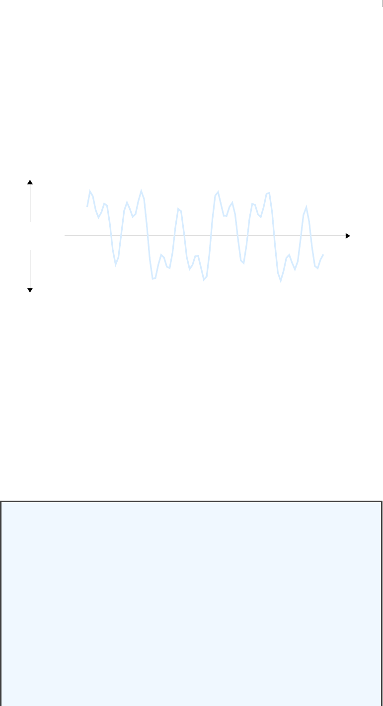
Consider an arbitrary continuous signal:
0
𝐴𝑡
Analog data are special because they exist in continuous space and thus theoretically
have an infinite degree of precision. If we assume a classical model of physics in which
time flows continuously, we can model physical quantities with real numbers by writing
an equation 𝐴=𝑓(𝑡)where 𝑡, 𝐴 ∈R. In this sense, a complete set of analog data over a
given time interval (i.e. an analog signal) can perfectly describe a physical quantity over
the same interval. However, handling analog data can be very difficult.
Imagine that you throw a ball in the air and somehow exactly measure its height above
the ground at every instant before it lands. If you were to organize these height data with
respect to time, you would construct an analog signal that perfectly describes the height
of the ball at any point during the throw. In practice, however, no measuring instrument
has the required speed or precision necessary to do this. Additionally, you would need an
infinite amount of memory to store continuous-time data that is collected at every instant.
The Rationale for Binary Numbers
Binary encoding of data is not a requirement for computation. Rather, it is a
concession that is made toward digital electronics. Computers have been designed
for other bases, and, in some cases, a non-binary encoding is actually preferable.
As long as the data can be encoded with a finite number of symbols, it can be
handled by a digital computer (i.e. a computer that manipulates digits). A digital
computer receives and operates on a discrete signal of data, a value or set of
values that updates at regular time intervals (e.g. every second, every minute, etc.).
One could argue that analog computers process data that are encoded with an
infinite number of symbols. However, this would require a loose definition of
"symbol" because analog data cannot be perfectly represented by digits. Rather,
information and communication 22
analog data is represented in a real, physical medium, like position, pressure, or
voltage. An analog computer receives and operates on this continuous signal of
data that updates instantaneously with real-world time.
Consider the Mark 1A Fire Control Computer, a device, more appropriately
termed a "calculator" by modern definitions, that was installed on United States
battleships in World War II. This machine used mechanical parts, such as gears,
cams, followers, differentials, and integrators, to perform the arithmetic and
calculus necessary to hit an enemy ship with a projectile, even if both ships were
moving in different directions. It also used smooth components that gradually
translated rotational motion into linear motion along a continuum.
Despite being labeled with decimal (base-10) integers, this tool actually received
continuous,analog quantities, such as physical position, as input. If each of
its mechanical positions were considered a different "symbol," this system
would theoretically be able to represent uniquely every real number to a infinite
degree of precision and, thus, compute continuous functions without error.
Such analog computation is performed also in slide rules, as well as in early
electronic computers, which used voltage to represent numbers instead of position.
01 2 345 6 78910
7.7741
Any digital encoding of numbers is possible in computing, and the choice does
not affect what a computer theoretically can or cannot do. Rather, it has practical
consequences. Decimal encoding was implemented in a number of early electronic
and electro-mechanical computers, such as the Harvard Mark I and the ENIAC.
Regardless of which encoding is used, data is data.
Data are unorganized facts or statistical values that may reveal something of interest.
They are collected by sampling the properties of phenomena from the observable Uni-
verse. Once collected, they can be cleaned, organized, and then analyzed in the hope of
gaining a better understanding of reality. When a set of structured data is put into context,
it can be interpreted as information that explains what has been observed. This informa-
tion can then be encoded as an ordered sequence of data known as a message. Messages
are transmitted and received both by Nature and by Man. In the latter case, this process
can be viewed as the communication of abstract, human thought.
Data can describe a variety of things, such as quantities, qualities, and relations. In
computer science, data are quantitative. That is, they describe quantities, which are prop-
erties that can be modeled with numbers. A quantity can be further classified as either a
information and communication 23
multitude or a magnitude. The former is a discrete quantity that is counted. One would
ask "how many" elements belong to a multitude. In contrast, a magnitude is a continuous
quantity that is measured. It is the size of something that is modeled as a continuum (e.g.
by fields such as Ror C), and one would accordingly inquire as to "how much" of it there
is.
A set of data collected at a finite rate (e.g. by a measuring instrument) is technically a
multitude of samples, even if the quantity being measured is a magnitude. For example, if
a ball were thrown in the air, one could ask "how much" height it has at regular intervals of
time. Once the data collection ends, one can also ask "how many" samples were acquired.
Furthermore, one can ask "how often" samples were taken. This is an evaluation of the
sampling rate, and it is really just an alternative way of asking with "how much" speed
samples were taken. Rates and ratios are still quantities. The existence of the rational
numbers Qare evidence enough of this.
Data can be represented by various media, both symbolic and physical. In the age
of modern computing, data are often assumed to be digital in nature, expressed in the
symbolic medium of numerical digits. This is the case for data processed by modern,
electronic computers, which charge capacitors in order to generate voltages that represent
logic levels. A transistor acts as a gate to each capacitor, staying closed to retain electric
charge during storage and opening to measure or modify voltage on reads and writes re-
spectively.
The ratio of a capacitor’s charge to its capacitance determines its voltage (i.e. 𝑉=𝑞
𝐶).
This voltage is then mapped to a logic level, which corresponds to a range of voltage
values. These logic levels represent digits. In modern computer memory, data are repre-
sented as binary digits or bits (i.e. the digits 0 and 1), each of which represents a binary
number. In this case, there are two logic levels, low and high.
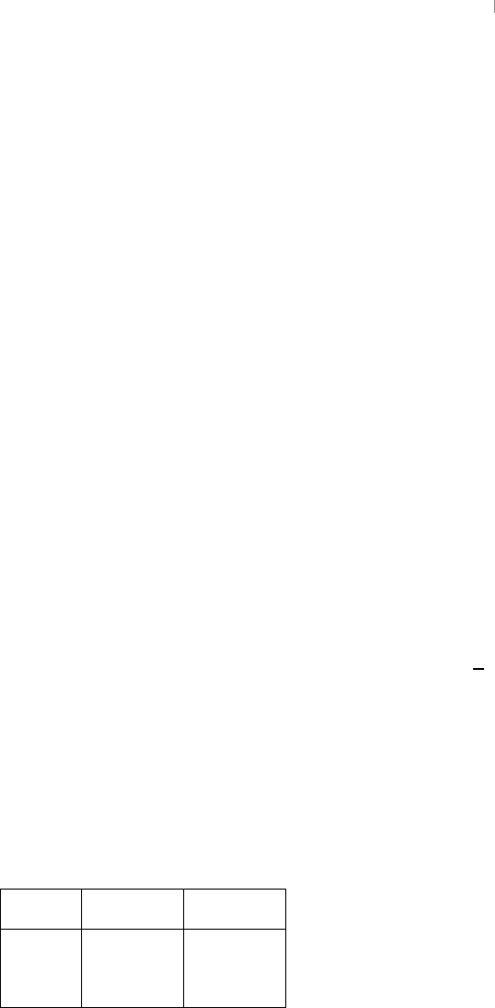
Table 1: Voltage Ranges for CMOS Logic Levels (V)
Signals Low (0) High (1)
Input 0.00–1.50 3.50–5.00
Output 0.00–0.05 4.95–5.00
However, quantitative data need not be expressed with symbolic digits. They can in-
stead be defined in terms of an analogous physical quantity. For example, the unit of
measurement known as the millimeter of mercury (mmHg) defines pressure in terms of
the height of a column of mercury in a manometer. It is used to quantify blood pressure,
and it does so by considering height an analog or model of pressure measuring that instead.
Using this method, data about one phenomenon can be encoded as data of a different phe-
nomenon, provided that the quantities involved are somehow related to each other. In this
case, a height of 1 mm is related to a pressure of 133.322 Pa above atmospheric pressure.
information and communication 24
1.7 Semiotics, Language, and Code
However, the term "universal language" is also often used in other contexts to describe a
hypothetical language that all of the world speaks and understands. This is an old idea,
and it is addressed in a number of myths and religious texts. In Genesis, the myth of the
Tower of Babel explains the diversity of language as a result of God thwarting the Baby-
lonians’ plan to build a tower that would extend into the heavens. As punishment for their
blasphemy, God "confused their tongues" and dispersed them across the world, shattering
their once universal language. Similar myths are told by cultures across the world, such as
the Native American Tohono O’odham people, who tell tales of Montezuma attempting
to do the same, attracting the ire of the Great Spirit.
Alas, no such language exists and it is unlikely that one has ever existed. Rather, hu-
man language is generally believed to have evolved independently around the world from
prelinguistic systems of communication such as gesturing, touching, and vocalization
about 100,000 years ago. Similarly, written language evolved from proto-writing, the
repeated use of symbols to identify objects or events.
Writing is distinct from speaking in that it is a reliable method of storing and transmit-
ting information. Before the invention of written language, important pieces of history
and literature were preserved through oral tradition, passing from one generation to the
next through repetition and memorization. However, oral tradition is prone to data loss
and unintended changes. Like messages in a game of telephone spanning centuries, sto-
ries were at risk of losing old details and gaining extraneous ones. Additionally, if a
society fell apart, their stories could be lost forever. Writing is a tool that mitigates these
issues by encoding speech into a symbolic code that can be inscribed onto durable media,
such as clay tablets or stone, or onto more delicate, portable media such as parchment or
paper.
Symbology in Natural Languages
Asymbol is a syntactic mark that is understood to represent a semantic idea. For
example, the numeral "2" is a symbol for the abstract concept of the number
known as "two," the quantity of items in a pair. Symbology is universal for
mankind, as it is an exercise of our capacity for abstract thought. Humans can
leverage the pattern-recognizing power of the brain to associate symbols or
sequences of symbols (also known as strings) with ideas. Thus, we can proliferate
information textually by means of a writing system.
Languages are diverse, and so are their writing systems.
An argument of any kind must be expressed in a language. In the case of an informal ar-
gument, such as a debate, a natural language is typically used (i.e. a language, spoken or
written, that evolved naturally as an aspect of human culture). This is done in the name of
universality. For example, a political debate that is held and perhaps broadcast in Poland

reasoning and logic 25
would likely be conducted in Polish because Polish politics are primarily of interest to
Polish people. Many Poles speak English in addition to Polish, but there is no language
more widely spoken in Poland than Polish, with a whopping 97% of the country declaring
it as their first language. For media directed toward the population of Poland, there is no
language that will better ensure an effective dissemination of ideas. It is a nearly universal
language in this context, a language understood by all intended recipients.
Formal proofs, on the other hand, require a formal language for clarity and precision.
In practice, formal proofs are rarely written or read by logicians or mathematicians. Typi-
cally, mathematical proofs are written using a combination of formal and natural language.
However, computer programs, written in programming languages, are considered formal.
A formal language is constructed from an alphabet Σ, which is a set of symbols. The
set of all possible finite-length words or formulas that can be built from this alphabet is de-
noted Σ∗. A formal language 𝐿over an alphabet Σis then defined as a subset of Σ∗. Thus,
a language is a set of purely syntactic objects. It may conform to a grammar that specifies
how words can be produced or arranged in a sentence, but a language is never inherently
meaningful. The semantics of a language is always interpreted separately from the syntax.
2 reasoning and logic
2.1 The Syntax and Semantics of Argument
Reasoning is a cognitive act performed by rational beings. It involves the absorption and
synthesis of presently available information for the purpose of elucidating knowledge. It
may require the ingenuity of thought, but in some cases the rote application of simple
rules is sufficient. Reasoning could also be described as the providing of good reasons
to explain or justify things. However, as you might expect, there is much debate over
whether or not any particular reason is "good." Reasoning is broad, and it comes in differ-
ent flavors, but ultimately it is the pursuit of truth.
Reasoning may involve the application of logic. This logical reasoning is the kind of
reasoning that can be expressed in the form of an argument. However, this argument does
not need to be "correct." Such reasoning simply must be explainable in steps, whether that
be through informal speech or formal writing.
In logic, an argument has two parts: a set of two or more premises and a conclusion.
If the conclusion necessarily follows from the premises, the argument is called valid. To
know whether or not an argument is valid, one must produce a step-by-step deduction of
the conclusion from its premises.
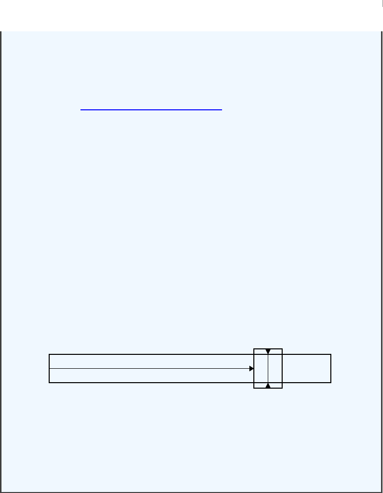
A deduction is constructed within a deductive system, which also has two parts: a set of
two or more premises and a set of rules of inference. A rule of inference can be thought of
as a kind of logical function. It takes statements (such as premises) as input and outputs
either an intermediate result or the conclusion. A deduction, then, has three parts: a set of

reasoning and logic 26
two or more premises, a conclusion, and a set of intermediates. A single-step deduction
is represented below, along with a suitable rule of inference labeled 𝑀𝑃 . Note that the
set of intermediates is empty in the case of deductions with only one step.
𝑃𝑄
𝑃
𝑄
1st
2nd
Con.
M
P
This is the quintessential rule of inference used in logical reasoning, expressed here
in symbols. It is known as modus ponens (Latin for "a method that affirms"). The first
premise 𝑃→𝑄is called a conditional statement where →is the implies operator. It
states that if the antecedent 𝑃were true, it would imply that the consequent 𝑄would also
be true. The second premise 𝑃simply states that the statement 𝑃is indeed true. Thus,
by means of modus ponens, we can infer from the premises 𝑃→𝑄and 𝑃that the con-
clusion 𝑄must be true.
Inference is also called entailment. Though these terms describe the same logical con-
cept, the latter more aptly describes the relationship between statements that are con-
nected in a deduction. To infer is to come to a conclusion that is not explicitly stated in
the premises. To entail is to require that something follows. If 𝑃entails 𝑄, this suggests
that 𝑄is a logical consequence of 𝑃, which we can express using a turnstile:𝑃 ⊢ 𝑄.
Inference is an action that humans perform. Entailment is a relationship between logical
rules.
When the inferences made mirror the entailment, you’ve got yourself a valid argument.
However, this does not necessarily mean that your argument is sound.Validity is a prop-
erty of arguments with a conclusion that can be deduced from its premises according to
rules of inference. However, validity says nothing about whether or not the premises have
ameaning that accurately describes reality. Soundness, on the other hand, is a property of
valid arguments whose premises are known truths or axioms. The deduction of a sound
argument is called a proof.
Validity and soundness complicate entailment. Now, an argument can be evaluated ei-
ther in terms of its syntax or in terms of its semantics. Syntax refers to the arrangement
of symbolic words (or, more generally, tokens) in a body of text. Semantics, on the other
hand, refers to the meaning that can be interpreted from the text. Both of these concepts

reasoning and logic 27
are integral to human language and indeed to the communication of information in gen-
eral.
Consider the following valid deduction:
"If it is raining, it is Tuesday." 𝑃→𝑄
"It is raining." 𝑃
"Therefore, it is Tuesday." ∴𝑄
This conclusion is a syntactic consequence of the premises (𝑃 ⊢ 𝑄). That is, when
the argument is evaluated simply as a collection of symbolic strings that are manipulated
according to rules, 𝑃entails 𝑄.
Syntactic consequence is sometimes expressed with the following statement: "If the
premises are true, the conclusion must also be true." However, while this statement does
hold for all valid arguments, text evaluated syntactically does not have any notion of truth.
It is simply a sequence of tokens. Thus, it may be better to think of valid arguments as
"games that are played according to the rules." For example, chess has no inherent mean-
ing associated with it, but it still has rules, and valid games of chess are those that comply
with those rules.
Now, it might be Tuesday and raining as you are reading this. However, semantically,
it is not required to be Tuesday if it is raining. The first premise given above is, in reality,
false. However, if we change it to something that we consider true, we can come to a
conclusion that is both valid and sound:
"If it is raining, it is wet outside." 𝑃→𝑄
"It is raining." 𝑃
"Therefore, it is wet outside." ∴𝑄
In this case, the conclusion is a semantic consequence of the premises (𝑃 ⊨ 𝑄). In
addition to the argument being syntactically logical, it is also semantically true "in all uni-
verses." That is, there is no possible scenario where it is raining, and it is not wet outside.
This syntactic-semantic difference will come up repeatedly throughout this guide.
2.2 The Structure of Proof
Of course, arguments can have more than one step. An argument can involve many in-
ferences, some of which may use intermediate conclusions as premises for further con-
clusions. Multiple threads of reasoning can extend from the premises, weaving through
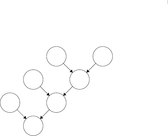
reasoning and logic 28
intermediate conclusions and intertwining via inference until they all meet at a final con-
clusion. This is the tree structure that is inherent in a formal proof.
𝐹
𝑃1𝐼2
𝑃2𝐼1
𝑃3𝑃4
In this tree, the first premises are labeled as 𝑃𝑛where 𝑛∈ {1,2,3,4}, the intermediate
conclusions are labeled as 𝐼𝑚where 𝑚∈ {1,2}, and the final conclusion is labeled 𝐹.
Though one can make a distinction between first premises and intermediate conclusions,
it is important to note that they are all premises with regard to the eventual final conclu-
sion. Thus, there are no restrictions on combining them beyond those dictated by the rules
of inference.
In modern proof theory, proofs like these are studied not only for their semantic mean-
ing, but also for their mathematical structure. They are treated like data structures, which
are abstract objects that are used in computer science to model the storage and flow of
digital information. Similarly, a proof is an abstract text that models the flow of logical
information as it is manipulated by rules of inference toward a final conclusion.
Information, in the context of computer science and, more generally, information the-
ory, refers to a syntactic message. Formally, it is an order sequence of symbols
In computer science, the data structures of interest are recursive. That is, the structure
can be defined "in terms of itself." Recursion is a deep topic, and we will spend much of
the next part characterizing it, but a practical way to think about a recursive structure is
in terms of type.
Types are a widespread feature in programming languages. As a concept, they are
founded in a logical system called a type theory. There are multiple type theories, and
some of them are used as alternative foundations for mathematics. We will cover all of
this in detail later, but, essentially, a type is a label that can be given to
However, not all forms of reasoning have such strict rules. There are other methods
of reasoning that cannot be modeled by an argument. In contrast to logical reasoning,
intuitive reasoning has steps that are not understood. Although the question might seem
peculiar, it is worth asking whether or not computation can be intuitive. So, to begin our
journey of understanding computation in a modern, logical sense, we will first walk in
the other direction, considering it instead in a mystical, otherworldly sense.

reasoning and logic 29
2.3 The Oracle, the Seer, and the Sage
Intuition is the capacity to create conclusions without evidence, proof, or a combination
of the two. If any premises are involved, they may appear to an onlooker as if they were
plucked out of thin air. If any method is involved, it is esoteric or hidden from sight. Acts
of intuition range from the mundane procedures we perform without thinking to great
feats of intellectual, artistic, and athletic achievement. And while it is often associated
with magic or supernatural ability, intuition is a real, observable phenomenon, and it is a
form of reasoning.
Like that of reasoning, the definition of intuition is fuzzy. There are a variety of events
that one might label as the product of intuition that are actually quite functionally distinct
from one another. For this reason, I would like to consider and compare three archetypes
that are known for their intuitive skills: the Oracle, the Seer, and the Sage. For the skep-
tics among you, I ask that you suspend your disbelief for a moment and assume that our
characters are acting in good faith. There is no lying here; the conclusions are sincere.
the oracle
An Oracle is a person who predicts the future by acting as a vessel for a god or a set
of gods. They are considered by believers to be portals through which the divine speaks
directly. They are found in histories all over the world, but most people associate the role
with the priestesses of Ancient Greece. Picture a woman with eyes that roll back into her
head as she speaks in a possessed, thundering voice.
For an Oracle, the conclusions come straight from the source. She may not even do
any reasoning herself, save for the unconscious reasoning that is performed while she is
possessed. However, conscious or not, she provides a great service to mankind. There is
no clearer answer than the one given to you directly from the gods themselves, even if it
has to be sent through what is essentially the human version of a telephone.
For those seeking counsel, the premises of the Oracle’s conclusion are unnecessary be-
cause they just know that the statement must be true. For them, the connection the Oracle
has with the gods and with reality is part of life itself. We all have deep beliefs like this.
For example, most people do not feel that gravity needs to be proven to them in order for
them to accept it as fact. Their perception of gravity in the world around them is proof
enough. This is the kind of intuition characterized by subconscious reasoning, the rea-
soning you do without being aware of doing it.
the seer
A Seer is a person who predicts the future by interpreting signs from a god or a set
of gods. Unlike an Oracle, a Seer speaks divine truth in his own words, drawing from
an innate, sometimes god-given power to see meaning in natural events or occult objects.
There are various methods of divination that are used by Seers, such scrying (the gazing
into magical things, like crystal balls, for the purpose of seeing visions), auspicy (the in-
terpretation of bird migration), or dowsing (the use of magic to find water, often with the

reasoning and logic 30
aid of a dowsing rod). The acceptance of any particular method is cultural, but beliefs in
divination vary greatly, even within a single society.
The Seer has premises for his conclusion, but the rules of inference involved in his
reasoning are incomprehensible to others. He
the sage
What is Truth?
Truth, in the absolute sense, has been discussed and debated since the dawn of
man. It is a concept that seems obvious to us, and yet it always seems to elude
our understanding. Philosophers have formulated dozens of theories of truth over
the years, with some asserting that truth is an objective property of our universe
and others asserting that truth is a useful lie that mankind has invented. And
while there is merit in those claims that truth is not real, we still see around us the
technology that was born out of our intuitive sense of true and false. Especially
in computer science where everything is represented in binary.
The traditional theories of truth have been termed substantive. That is, they assert
that truth has some basis in reality and that it is a meaningful thing to discuss.
Early theories of truth from Ancient Greece are considered the foundation of
correspondence theory, the idea that statements are true if their symbols are
arranged in such a way that they express an abstract thought that accurately
describes reality. This theory defines truth in the context of a relationship between
language and objective reality. It is a useful philosophy that allows us to orient
ourselves in the world around us. However, many philosophers believe that truth
cannot be explained by such a simple rule. In fact, there are many more factors
that could play a role in the concept.
Objections to a strict correspondence theory usually take issue with the treatment
of language as something monolithic and easy to classify within a true-false
dichotomy. For example, a statement encoded as a sentence in a language is only
meaningful to people who can read that language. What does this imply about a
particular language’s relationship with truth? Is a statement only true for those
who understand it? Furthermore, there is no guarantee that readers of the same
language will even be able to agree on the meaning expressed by a particular
sentence. Languages often encompass multiple dialects that might parse words
differently. Words themselves also may not be precise, and some abstract thoughts
may not have suitable words in some languages. These are the points raised in
social constructivism, a theory which avers that human knowledge is historically
and culturally specific. Social constructivists also believe that truth is constructed
and that language cannot faithfully represent any kind of objective reality.
Other substantive theories find the essence of truth nestled in other abstract
concepts. Consensus theory, as the name implies, defines truth as something that
is agreed upon either by all human beings or by a subset (such as academic groups

reasoning and logic 31
or standards bodies). This is another anthropocentric definition that is at constant
risk of philosophical division on any given topic. Coherence theory takes a more
objective approach, claiming that a statement can only be true if it fits into a
system of statements that support each other’s truth. This is similar to the notion
of formal systems, which we will discuss in depth later. However, traditional
coherence theories attempt to explain all of reality within a single coherent system
of truths, which is incompatible with our modern understanding of formal systems.
Modern developments in philosophy have resulted in theories that deviate from
the long-held, substantive opinions on the nature of truth. These minimalist
theories assert instead that truth is either not real or not a necessary property
of language or logic. They claim that statements are assertions and thus are
implicitly understood to be true. For example, it is understood that by putting
forth the sentence "2 + 2 = 4," you are endorsing the semantic meaning "2 + 2 = 4
is true." The clause "is true" is called a truth predicate, and minimalist theories of
truth often consider its use redundant.
This idea of a truth predicate is borrowed from Alfred Tarski’s semantic theory of
truth, which is a substantive theory that refines the correspondence concepts es-
poused by Socrates, Plato, and Aristotle for formal languages. This theory makes
a distinction between a statement made in a formal language and a truth predicate,
which evaluates the truth of the statement. Tarski made this distinction in order
to circumvent the liar’s paradox, which is often presented with the following ex-
ample: "This sentence is false." If the predicate "is false" is considered to be part
of "this sentence," the truth of this statement cannot be decided. For this reason,
Tarski states that a language cannot contain its own truth predicate. This is en-
forced by requiring that "this sentence" be written in an object language and that
"is false" be written in a metalanguage.Convention T, the general form of this
rule, can be expressed as
"𝑃" is true if and only if 𝑃
where "𝑃" is simply the metalanguage sentence 𝑃rendered in the object language.
That is, the syntactic representation is assigned a truth value of true if and only
if the semantic meaning it represents is considered true (according to whatever
theory of truth you employ). By this rule, we say that "2 + 2 = 4" is true if
and only if the sum of the number 2with the number 2is equal to the number 4.
Minimalist redundancy theories modify Tarski’s theory by interpreting "𝑃" as an
implicit assertion of the truth of 𝑃. The sentence "𝑃," which asserts that 𝑃is
true, is then false if and only if its semantic meaning 𝑃is false.
F9f
The debate on the nature of truth rages on in perpetuum. However, for our pur-
poses, we must be practical. There is truth in logic and mathematics and computer
science as well, but, in practice, it has little to do with the debates on absolute
reasoning and logic 32
truth described above. Their truth is relative. That is, it relies on the assumption
that our premises are true. Cognizant of this, we move forward with our thinking,
searching for truths within these arbitrary boundaries.
2.4 The Mathematician and the Scientist
Logical reasoning is the inference of new information from present information. It in-
volves rule of inferences that are used to relate sets of premises to conclusions. There are
three kinds of logical reasoning: deductive,inductive, and abductive. Each is classified
according to which piece of information (premises, rule, or conclusion) is missing and
must be inferred from the others.
Inductive arguments exist on a spectrum between weak and strong. Those that are
stronger and more persuasive have a higher probability of having a true conclusion. In-
ductive reasoning is associated with science and critical thinking because it allows one to
make generalizations about complex phenomena given limited evidence. Unlike deduc-
tive reasoning, it attempts to find new knowledge that is not simply contained within its
premises.
Statements made by induction are bolstered with evidence whereas deductive state-
ments are as true as their premises. This leaves inductive reasoning susceptible to faulty
generalizations and biased sampling. Induction must also assume that future events will
occur exactly as they have in the past, which is not always the case. For example, a turkey
that is fed every morning with the ring of a bell may infer by induction that bell →food.
However, he will see the error in his reasoning when the farmer rings the bell on Thanks-
giving Day and instead slits his throat.
abductive reasoning
Abductive reasoning is the inference of a premise, given a conclusion and a rule. It
is investigative in nature. For example, given a conclusion "The grass is wet" and a rule
"When it rains, the grass gets wet," we might determine that rain is the best explanation
for the wetness of the grass. Thus, we abduce that "It might have rained."
Like induction, abduction can also produce a hypothesis. However, abduction does not
seek a new relationship between two previously unconnected statements. Rather, it uses
established relationships to find a reasonable explanation for a statement that is assumed
to be true. It is often used by detectives or diagnosticians who need to find a probable
cause of an event. It is also used in Bayesian statistics. While multiple premises may be
abduced, typically we want to abduce a single, "best" premise.
Abductive reasoning allows us to ignore the many causes that are unlikely in favor of
those few that may be relevant to the problem at hand. For example, doctors are often
reasoning and logic 33
taught to heed the following proverb: "When you hear hoofbeats, think of horses, not
zebras." That is, when a patient exhibits certain symptoms, a doctor should abduce from
them a commonplace disease before considering more exotic possibilities. However, "ze-
bras" do exist. Sometimes the most likely cause is not the actual cause. For this reason,
abduction is also considered to be equivalent to a deductive fallacy called affirming the
consequent, which is like a modus ponens performed in reverse. That is, given a condi-
tional 𝑃→𝑄and the consequent 𝑄, abduction infers 𝑃from 𝑄by assuming that the
converse 𝑄→𝑃of the conditional is also true. This is not a deductively valid infer-
ence. Considering our example again, the grass might be wet from rain, but this is not
necessarily true. It is also possible that the sprinkler system is on. Or perhaps there is a
zebra-esque scenario like a flood.
Induction and Abduction
2.5 Mechanical Computation
Before we discuss and classify automata in depth, we should first consider what is not an
automaton. What is an example of something that might perform some kind of calcula-
tion, but is not a computer? What about a microwave? Is a microwave a computer? No,
it is not. A computer can be programmed in some meaningful, robust way. A microwave
contains a microprocessor, which uses combinational logic and basic binary inputs to set
timers and operate the oven. It cannot be programmed in any meaningful way. What
about a calculator? Is a calculator a computer? If we are being formal, the answer is no,
but it depends on what kind of "calculator" we are talking about.
Calculators, such as counting boards and the abacus, have been around since pre-
history. Calculators with four-function capabilities have been around since the invention
of Wilhelm Schickard’s mechanical calculator in 1642. In the late 19th century, the arith-
mometer and comptometers, two kinds of digital, mechanical calculator, were being used
in offices. The Dalton Adding Machine introduced buttons to the calculator in 1902, and
pocket mechanical calculators became widespread in 1948 with the Curta. None of these
are computers.
The difference between a calculator and a computer is that a computer can be pro-
grammed and a calculator cannot. What does it mean to be programmable? That is per-
haps the central question of automata theory, and we will discuss in this section several
levels of "programmability." However, for now, we can certainly say that a simple, four-
function electronic calculator is not a computer. It simply uses combinational circuits
like full-adders, full-subtractors, multipliers, and dividers to implement its functions, and
there is no potential for modifications or user-defined functions.
reasoning and logic 34
Surprisingly enough, special-purpose computers have also been around for a long time.
Early examples include the Antikythera mechanism (an Ancient Greek analog computer),
Al-Jazari’s 1206 water-powered astronomical clock, the 1774 Writer Automaton (a me-
chanical doll that could be programmed to write messages), the 1801 Jacquard loom, and
slide rules. Some later mechanical computers were quite powerful, such as differential
analyzers (special-purpose computers for solving differential equations) and fire control
computers. Charles Babbage designed the Analytical Engine, a general-purpose com-
puter, in 1837, and Ada Lovelace wrote a program for it, but it was never built. General-
purpose computing would not reemerge until the 1940s.
The line between calculator and computer began to blur with the introduction of pro-
grammable calculators in the 1960s. Many modern high-end calculators are programmable
in Turing-complete languages such as TI-BASIC or even C or C++, which officially
makes them computers. Once we start implementing sequential logic with components
like SR latches or D flip-flops, we are storing state, and state is a requirement for com-
puting. Circuits that use sequential logic can be considered automata and, given enough
complexity, computers.
Modern Computing is American
TEXT

35
Theory of Computation
Theory is relevant to you because it shows you a new, simpler, and more
elegant side of computers, which we normally consider to be complicated
machines. The best computer designs and applications are conceived with
elegance in mind. A theoretical course can heighten your aesthetic sense and
help you build more beautiful systems.
—Michael Sipser
The theory of computation is a field of study that is related to both mathematics and
computer science. It is concerned with a process known as computation, which refers to
any kind of calculation (the transformation of one or more inputs into one or more out-
puts) that is accomplished by following an algorithm (a set of rigorously defined steps). It
is also concerned with the formalization of theoretical models of computation known as
abstract machines or abstract automata. Also of interest are the computational problems
that can be solved by these abstract machines and how efficiently they can be solved. The
theory of computation gives us the formal definition of a computer and the scope of what
a computer can accomplish.
Much of the work in the theory of computation is…quite abstract. While calculation
and computation have been practiced by humans for thousands of years, the concept was
only formalized by mathematicians, logicians, philosophers, linguists, and computer sci-
entists in the past 150 years. This part of the guide will delve into some fairly academic
topics with a decent amount of mathematical rigor, but it is written to be accessible and
entertaining.
The field has three branches: automata theory,computability theory, and computa-
tional complexity theory, each of which asks fundamental questions pertaining to how
mathematical calculations can be automated, which kinds of problems can be solved by
a machine, and how many resources are required to solve a particular problem. We will
touch on the major discoveries made in each of these branches and discuss why they are
significant to computer science and programming in general.
3 automata theory
Automata theory is the study of automata and their behavior. An automaton is a self-
operating machine designed to follow or respond to a predetermined sequence of oper-
ations. Automata include physical devices such as cuckoo clocks, mechanical watches,
robots, and computer processors as well as abstract machines. An abstract machine is
any formal description of mechanical behavior. An abstract machine that is used to for-
mally describe computation is called a model of computation. This is a mathematical
description of what a computer is, and it models the computation that a real, concrete
computer could actually perform, if you were to implement that computer according to

automata theory 36
the model’s specifications. Like their concrete counterparts, abstract machines have state,
a set of information in the present that was acquired due to past events. All automata be-
gin with a starting state, receive some sort of input, and transition to another state based
on the value of that input and the value of its current state.
One abstract automaton in particular fully models not only the computation that is per-
formed by today’s state-of-the-art computers, but also the very process of computation
itself. We will spend a lot of time in this guide discussing the structure and behavior of
this model as well as what its limitations imply regarding the future of computing, soft-
ware, mathematics, and the meaning of life. We will also briefly explore the abstract
automata that exist in pure mathematics and model computation that is not physically re-
alizable.
3.1 Exploring the Link Between Concrete and Abstract Machines
Let’s take a simple, concrete machine and try to visualize the abstract machine that un-
derlies it. Consider a cuckoo clock. Every day, at noon, a small plank with a mechanical
bird perched on its lip will extend from a hole above the clock face, powered by a working
motor. Once the plank is fully extended, the bird will flap its metal wings and maybe turn
its head as a song is played from a revolving music box inside the clock. Then, when it is
12:01 PM, the music will stop, the bird will still, and the plank will retract. The process
will occur again the next day, at noon.
The machine’s components here are the plank, the bird, and the music box. The compo-
nents each have two states: the plank can be retracted or extended, the bird can be still or
flapping its wings, and the music box can be paused or playing. The input to this machine
is whether or not the clock hands both point straight at 12. We can say that this automaton
has a state that can be expressed in terms of the states of its components. We can represent
its starting state with the sequence (0,0,0) (i.e. the plank is retracted, the bird is still, and
the music box is paused). The automaton can receive one of two inputs, 1 or 0 (i.e. both
clock hands point straight at 12 or they do not). This input might be implemented with
an electromechanical switch that turns the motor on or off.
(0,0,0) -> (1,0,0) We start at state (0,0,0). As the morning passes, the automaton
receives a constant input of 0, which keeps it in its starting state. At noon, the input
switches to 1, and the automaton transitions to the state (1,0,0). As the plank extends and
transitions its own state from 0 to 1, the bird remains still, and the music box remains
paused. Once the plank is fully extended, we are in state (1,0,0).
(1,0,0) -> (1,1,1) We expect that the plank will be fully extended well before 12:01
PM, so the input should still be 1. However, if for some reason the input is 0, we should
transition back to (0,0,0), as the machine should only operate outside of its starting state
between 12:00 and 12:01 PM. This is a simple example of strange input. The input 0 at this
state is unexpected, but it is technically possible. It is a better idea to define the behavior
for this unexpected case, rather than to allow the input to cause unexpected behavior. On
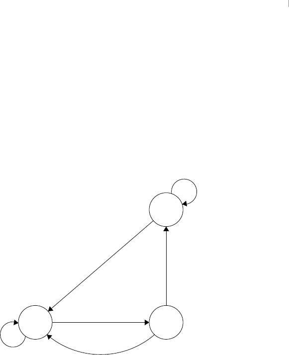
automata theory 37
the other hand, if the input is 1 at this state, the automaton transitions to the state (1,1,1).
The plank is fully extended, the bird is flapping its wings, and the music box is playing.
(1,1,1) -> (0,0,0) Before 12:01 PM, the input is still 1, and that input should keep
the automaton in its current state of (1,1,1). When 12:01 PM rolls around, the input will
now be 0. In this case, we would like to return to the original state. On receipt of the
input 0 while in state (1,1,1), the automaton transitions back to its starting state, (0,0,0).
This abstract machine is shown below with a state format of (plank, bird, music) and an
input specifying if the clock hands point exactly toward 12.
(0,0,0) (1,0,0)
(1,1,1)
1
1
0
0
1
0
This is a perfectly reasonable abstract machine, but something isn’t right. It does not
accurately simulate the behavior of the cuckoo clock we described. What happens when
the clock strikes midnight? The clock hands will point at 12, producing an input of 1,
but we don’t want the bird to wake everyone up at midnight. We could use two bits of
input: whether or not the hands are between 12:00 and 12:01, and whether it is AM or
PM. Additionally, the music never plays unless the bird is flapping its wings, so we can
combine those states. The abstract machine is better represented by the diagram below
with a state format of (plank, bird/music) and an input format of (hands are toward 12, is
PM).
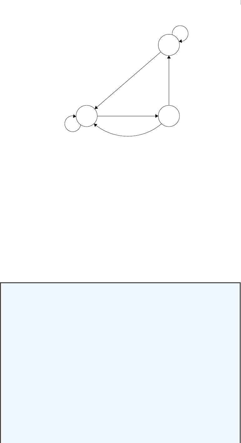
automata theory 38
(0,0) (1,0)
(1,1)
(1,1)
(1,1)
not (1,1)
𝑛𝑜𝑡 (1,1)
(1,1)
𝑛𝑜𝑡 (1,1)
Note that the actual complexity of the concrete cuckoo clock would be a bit more com-
plicated than the automaton above. For example, what does the bird do specifically when
it is on? Perhaps it raises and lowers its wings three times, turns its head to the right
twice, and repeats. This process can be modeled by a different automaton. To fully model
a concrete automaton, we must reduce it to an abstract machine, a system of states and
transitions that account for every intended behavior. Abstract machines are capable of
modeling systems of any arbitrary complexity. The automaton above is a model of com-
putation called a finite-state machine (FSM), and it will be the first abstract machine that
we will discuss.
3.2 Formalization of an Abstract Machine
A Brief Introduction to Formal Grammars
A formal grammar is a finite set of production rules that specifies what a particular
language is supposed to look like. It formalizes the structure of "grammatical
units" in a language. This is done in order to enforce a specific alphabet, a
consistent lexicon, and a predictable sentence structure, all of which contribute to
how useful and distinct any given language is.
A grammar 𝐺consists of the following components:
∙A finite set 𝑁of nonterminal symbols.
∙A finite set Σof terminal symbols that is disjoint from 𝑁.
∙A symbol 𝑆∈𝑁, designated as the start symbol.
∙A finite set 𝑃of production rules where each rule is of the form
(Σ ∪ 𝑁)∗𝑁(Σ ∪ 𝑁)∗→(Σ ∪ 𝑁)∗.

automata theory 39
Put another way, a production rule converts a sequence of symbols to another
sequence of symbols. If a rule is of the form left-hand side →right-hand side,
each side can contain terminals and nonterminals, but its left-hand side must
contain at least one nonterminal. A nonterminal is a symbol that is replaced by
other symbols when an appropriate rule is applied. Unlike a terminal, it does
not belong to the alphabet of the language, but rather represents a sequence of
symbols that do. Terminals cannot be replaced by other symbols once chosen.
Let’s construct a simple formal grammar. It is typical for the nonterminals to be
uppercase and for the terminals to be lowercase. Let 𝑁={SENTENCE, NOUN,
ADJ}, Σ = {the, dog, building, plays, fluffy, good}, and 𝑆=SENTENCE. The
rules of 𝑃are given below.
∙SENTENCE →the NOUN plays
∙NOUN →ADJ NOUN
∙NOUN →dog
∙NOUN →building
∙ADJ →fluffy
∙ADJ →good
We can now start with SENTENCE and apply these rules to construct a "sentence"
that is valid in this language. Example sentences and their derivations are given
below.
∙SENTENCE →the NOUN plays →the ADJ NOUN plays →the good
NOUN plays →the good dog plays
∙SENTENCE →the NOUN plays →the ADJ NOUN plays →the ADJ ADJ
NOUN plays →the ADJ ADJ ADJ NOUN plays →the fluffy ADJ ADJ
NOUN plays →the fluffy good ADJ NOUN plays →the fluffy good fluffy
NOUN plays →the fluffy good fluffy building plays
Notice that the first example expresses an actual thought whereas the second exam-
ple, while still syntactically a sentence, is nonsensical. Because it allows meaning-
less sentences, the grammar described above belongs to the class of context-free
grammars.
3.3 Classes of Automata and the Languages They Can Understand
Automata, in general, are machines that receive, interpret, and follow instructions that are
written according to the grammar of a formal language. Formal languages are similar to
the natural languages that humans speak in that they have words that conform to a syntax

automata theory 40
that is specified in terms of symbols from an alphabet. These words can be arranged ac-
cording to a grammar to form sentences, from which semantic meaning can be interpreted.
However, unlike natural languages, they are defined in precise, unambiguous terms.
A formal language 𝐿over an alphabet Σis a set of words that is a subset of Σ∗, the
set of all possible words that can be composed using Σ. Typically, formal languages con-
form to a formal grammar, which is a set of precise grammatical rules. However, not
all formal grammars are equal. Grammars determine how words can be arranged into
sentences, which determines the kinds of thoughts that can be expressed. Thus, grammar
controls how powerful or expressive a language is. If we intend to use a particular formal
language to instruct a computer to solve a problem, the expressiveness of the language
will determine the kinds of instructions we are able to give. If we cannot express a given
instruction, we will not be able to solve any problems requiring that instruction.
In this section, we will examine automata with different mechanical structures. The
data that are stored in components of these structures can be interpreted as words, and
the structures themselves can be used to represent the rules of a formal grammar. How-
ever, some expressive grammars cannot be represented by simpler structures. Thus, the
mechanical structure of an automaton acts as an upper bound on its capacity to under-
stand language, and, by extension, its computational versatility.
We will now discuss four classes of automata, in increasing order of complexity. As
they become more complex, automata are able to recognize more powerful and expressive
languages. They can be told to execute instructions in these languages, and they will be
able to accomplish more complex tasks if their language is more expressive. When we
reach the last of these four automata, we will be talking about the most powerful model of
computation that is feasible to build, the automaton that models modern general-purpose
computers. Once we explore this particularly important automaton in depth, we will learn
how it can be modified to model more exotic forms of computation.
3.3.1 Finite-state Machines
A finite-state machine is a model of computation that can be in exactly one state from a
finite set of states at any given time. Given its current state and an input, an FSM can
transition to another state. Deterministic finite automata (DFA) are FSMs that transition
to at most one state for each input. In contrast, nondeterministic finite automata (NFA)
can transition to zero or more states for each input. It follows then that a DFA is a special
kind of NFA. An FSM may also have a subset of states that are considered final states.
When the machine transitions to one of these states, it will finish its work and cease oper-
ation.
FSMs can read and understand regular languages, which are languages that can be ex-
pressed using a regular expression or regex. A regex consists of constants (which denote
sets of strings) and operators (which denote operations on those sets). If an FSM receives
an input (such as a regex) at a given state, and its state-transition function maps that state
and input to another state, we say that the FSM matches that input. That is, it considers
that input valid and will perform an action accordingly.

automata theory 41
A Quick Summary of Regular Expressions
Given a finite, non-empty input alphabet Σ, there are three constants defined as
regexes:
∙The empty set,∅, which denotes the set containing no elements.
∙The empty string,𝜀, which denotes the set containing only the empty string
"."
∙Aliteral character (e.g. the character 𝑎denotes the set containing only the
character "𝑎").
These constants can be combined and manipulated with operators to create long,
complex regular expressions. There are three operators that operate on regexes,
which are described below in increasing order of priority. Given regular expres-
sions 𝐴and 𝐵, the operations include:
∙The concatenation of 𝐴and 𝐵,𝐴𝐵, which denotes the set of strings that can
be created by concatenating a string in 𝐴with a string in 𝐵.
∙The alternation of 𝐴and 𝐵,𝐴|𝐵, which denotes the union set of 𝐴and 𝐵.
∙The Kleene star of 𝐴,𝐴∗, which denotes the set of all strings that can be
created by concatenating a finite number of strings (including zero strings)
from the set 𝐴.
Two additional operators are added as "syntactic sugar": +and ?. Whereas the
literal character 𝑎denotes the set of strings that contain a single 𝑎and nothing
else, the regex 𝑎+denotes the set of strings that contain at least one 𝑎and nothing
else and the regex 𝑎?denotes the set of strings that contain at most one 𝑎and
nothing else. Thus, 𝑎+ = 𝑎𝑎∗and 𝑎? = 𝑎|𝜀.
A variety of metacharacters are also often used in order to create more concise
regexes. Common metacharacters include:
∙̂, which matches the starting position in a line of text.
∙$, which matches the ending position in a line of text.
∙., the wildcard, which matches any character.
∙−, which, when placed between two regexes in brackets, denotes a range of
characters.
∙[̂], which matches a single character which is not in the brackets.

automata theory 42
Not only is it correct to say that a finite-state machine can understand any regular ex-
pression, but also it is true that FSMs and regexes are equivalent. That is, a regex can
be written in the form of an FSM and vice versa. Indeed, a regular language "program"
can be expressed as a regex, a DFA, or an NFA. For example, the regex [A-Z][a-z]∗[0-9]
describes any string that starts with a single uppercase letter, is followed by zero or more
lowercase letters, and ends with a single digit. This expression can also be represented
by the following DFA. Note that state 3is circled twice to indicate that it is a final state.
The automaton will continue to run until it receives a sequence of input that allows it to
transition to its final state.
1 2 3
[A-Z] [0-9]
[a-z]∗
Regular languages and, by extension, finite-state machines are often used in string
searching algorithms. FSMs and regular languages are also often used in the lexical analy-
sis (lexing) done by a compiler. That is, they give language designers the power to specify
which words are valid in their programming language.
3.3.2 Pushdown Automata
Pushdown automata (PDA) are finite-state machines that also have access to a stack.
These automata introduce a notion of history or memory. A PDA can push a symbol
onto its stack on every transition, which will provide information in the future about ac-
tions in the past. It can also pop or peek at the stack to decide which transition to take next.
Pushdown automata can distinguish syntactically correct sentences from random se-
quences of valid words, something finite-state automata cannot do because they have no
notion of what comes earlier than a given point in a given sentence. For example, a push-
down automaton would be able to tell that "my dog bites red toys" is a valid English
sentence and "red my toys dog bites" is not. However, PDA cannot understand semantics.
It would also consider "my dog barks red toys" a valid English sentence, even though it
has no meaning.
Pushdown automata can read context-free languages, which are languages that follow
acontext-free grammar. Context-free languages are formal languages whose production
rules are of the form 𝐴→𝛼where 𝐴is a nonterminal and 𝛼is a sequence that may contain
terminals and nonterminals. A PDA pops terminals from its stack. When a nonterminal 𝐴
is at the top of the stack, the PDA can pop it and push the 𝛼of some production rule onto
the stack. In a sense, the stack of the PDA contains the unprocessed data of the grammar.
Context-free grammars can be written to formalize languages such as the language
of matching parentheses or the language of infix algebraic expressions (e.g. (2+4)/7*8).

automata theory 43
PDA and context-free languages are often used in the syntactic analysis (parsing) done
by a compiler. That is, they give language designers the power to specify how valid sen-
tences are structured in their programming language.
3.3.3 Linear Bounded Automata
Imagine that, instead of a stack, an automaton could have access to a finite-length list.
Linear bounded automata (LBA) have a finite number of states, a finite length of tape,
and a head that can read and write symbols on the tape and move left or right along it,
one symbol at a time. The length of the tape is a linear function of the length of the input,
so we can say that the tape has 𝑘𝑛 cells, where 𝑛is the length of the input instructions and
𝑘is a constant.
This machine is similar to the idea of a modern computer. The tape represents a fi-
nite amount of memory, and the head is able to read and write to it. LBA can understand
context-sensitive languages, which are languages that follow a context-sensitive grammar.
Sophisticated programming languages are context-sensitive, so a linear bounded automa-
ton would be able to read and understand modern software. The 𝑘𝑛-length tape acts as a
sufficient environment for computationally demanding programming tasks, given a large
enough 𝑘. Similarly, given enough memory, real computers can also solve very computa-
tionally difficult problems.
A context-sensitive language is a language where semantics matter. Using our earlier
example, "my dog barks red toys" would not be a valid sentence in a context-sensitive
version of English. An LBA then is actually able to differentiate data types and can tell
when an operation is defined for one type and undefined for another. LBA and context-
sensitive languages are often used in the semantic analysis (type checking) done by a
compiler. That is, they give language designers the power to specify whether or not a syn-
tactically correct sentence actually has any real meaning in their programming language.
Where can we go from here? LBA are suitable models of real-world computers, and
they can process semantic language. What more can we do? Let’s try making the tape
infinitely long…
3.3.4 Turing Machines
ATuring machine (TM) not only models real-world computers, but computation itself.
The concept, which was formalized in 1936 by Alan Turing, generalizes automata and
defines the limitations of mechanical computing. It specifies a set of components that
are necessary and sufficient for creating a "problem-solving machine" that is capable of
solving any problem that can be solved by a machine. Weaker automata can solve some
of these machine-solvable problems, but only Turing-complete automata (those that are
functionally equivalent to TMs) have the expressive power to solve any of them. The
components of a Turing machine are listed below.

automata theory 44
∙An infinitely long tape that is divided into cells, each of which contains a symbol
from some finite alphabet. One symbol from this alphabet is considered blank, and
the tape is initially filled with these symbols.
∙Ahead that can read and write symbols on the tape and move left or right along it,
one symbol at a time.
∙Astate register that stores its current state and initially stores its starting state.
∙Afinite table of instructions that, given the machine’s current state and tape symbol,
tells the machine to do the following sequence of actions:
1. Erase or write a symbol at the current tape cell (or do nothing)
2. Move the head one tape cell to the left or right (or do nothing).
3. Depending on the current state and input, transition to a different state (or the
same state) or halt computation.
A machine like this need not be a real-world computer. In fact, in his original proof, On
Computable Numbers, with an Application to the Entscheidungsproblem, Turing refers to
a person, whom he calls the "computer," as an example of a Turing machine. If we break
down these components into the resources they represent, it becomes clear that many
systems could be considered Turing machines.
∙The infinitely long tape represents infinite space for computation or infinite memory.
∙The head represents three abilities:
1. Reading memory,
2. Writing to memory,
3. Traversing the memory freely, with no side effects.
∙The state register represents the ability to know what "step" you are on in the
problem-solving process. We will clarify this ambiguous idea in a second, but
for now just think of it as having an idea of your progress.
∙The finite table of instructions represents a sequence of commands or program that
can be followed unambiguously. The automaton can follow and obey these com-
mands in order without any actual thought.
As long as you have unlimited space to work in, the freedom to read and write symbols
anywhere in that space, a list of instructions to follow exactly, and the knowledge of what
to do next, you have a Turing machine. We can now visualize the person Turing referred
to as a "computer." It is a man with an infinitely large piece of paper, a pen that he writes
symbols with, a list of instructions that tells him which symbols to write, where on the
paper to move his pen tip, which instruction to perform next, and a knowledge of which
instruction he is currently performing. Many systems of logic, such as programming lan-
guages, are Turing-complete. Many things not traditionally thought of as "systems of
logic" are also Turing-complete.

automata theory 45
Turing Machines and Consciousness
In 1950, Turing developed the Turing test, a test of a machine’s ability to exhibit
behavior indistinguishable from that of a human. It involves an interrogator who
is tasked with having two separate text conversations and determining which of
the two participants is actually a machine. If the interrogator cannot distinguish
a difference, the machine has passed the test. Despite its importance to the
philosophy of computer science, the test is not a good indicator of whether or not
a computer can think. The test says more about how gullible the interrogator is
than how conscious the computer is. At the end of the day, the computer is still
following its programming.
What about this man whom Turing calls a "computer"? Would he pass the test,
given the right programming? Perhaps he would. But that would not make him
aperson. What kind of person is this man if he follows whatever instructions
he is given? He is a slave, a person who always obeys. Could we say then that
machines are also, in a certain sense of the word, slaves? Perhaps this is where
the term master-slave technology came from. Regardless, it is important to make
a philosophical distinction here about what separates humans from machines or,
more precisely, what distinguishes thought from computation.
Essentially, this boils down to the question of consciousness. There is much
debate about consciousness. Philosophers have proposed a variety of concepts
that partially define it such as free will (the ability to choose) or qualia (the raw
experience of existence, e.g. sounds, colors, emotions). However, intentionality is
one characteristic that is generally agreed upon as necessary for conscious thought.
Intentionality is the ability of the mind to think about something. Computers can
think things, but they cannot think about things. They lack intentionality.
For a Turing machine, the list of instructions is an essential component. It is
capable of "thinking" if and only if some one tells it what to think. That effort is
more accurately defined by the term "computation." We would also refer to the
man’s efforts with his pen and infinite paper as computations because they require
no thought. If he were nothing more than a Turing machine, the man would
not be able to perform mathematics on his own. In fact, he would not be able
to do anything without instructions. It is the moment when he does something
without being explicitly told to do it that he first displays consciousness. When
unprompted computation is performed for some purpose, we can talk about
consciousness.
So calling computers slaves is a bit of an anthropomorphization. A slave is a
conscious being who is forced to act like a machine. Computers don’t have
the prerequisite consciousness. No matter how complicated its architecture
or sophisticated its artificial intelligence software, a computer is a tool like a
microwave or a calculator. Could it ever be more than that? Could a technology
ever think? Perhaps. But such a thing would be quite different from a Turing
automata theory 46
machine or any modern computer.
F9f
In attempting to construct such machines we should not be irreverently
usurping His power of creating souls, any more than we are in the
procreation of children: rather we are, in either case, instruments of
His will providing mansions for the souls that He creates.
—Alan Turing (1950),
in response to a theological objection to artificial consciousness.
A single-tape Turing machine is formally defined as a septuple (𝑄, Γ, 𝑏, Σ, 𝛿, 𝑞0, 𝐹 ),
where
∙𝑄is a finite, non-empty set of states,
∙Γis a finite, non-empty tape alphabet,
∙𝑏∈ Γ is the blank symbol,
∙Σ⊆Γ⧵{𝑏}is the set of symbols that can be written on the tape,
∙𝛿is a partial function 𝛿∶ (𝑄⧵𝐹)×Γ ↛Γ×{𝐿, 𝑅} × 𝑄called the transition
function, which inputs the current state and tape symbol and outputs the symbol to
write to the tape, the direction to move the head, and the next state to transition to,
∙𝑞0∈𝑄is the starting state, and
∙𝐹 ⊆ 𝑄 is the set of final states. The contents of the tape are accepted if the Turing
machine halts computation in a state from 𝐹.
We should now address what exactly "state" is in regard to computing. Many people
associate it with the current instruction being fed to the machine. However, Turing made
a distinction between this interpretation of state and the interpretation of state as the com-
puter’s "progress" or "state of mind." Turing’s complete configuration of state includes
not only the current instruction, but the current symbol configuration of the entire tape as
well and all the instructions yet to be executed. In this way, state is defined by the results
of past instructions and the inevitable execution of future instructions.
Now we have defined what a Turing machine is, but it is still not clear why it is consid-
ered such a landmark concept in computer science. For example, if real-world computers
can be sufficiently modeled by linear bounded automata, why do we instead focus so heav-
ily on Turing machines?

automata theory 47
Turing machines are the class of automata that can read recursively enumerable lan-
guages. A formal language is called recursively enumerable, if it is a recursively enu-
merable subset in the set of all possible words over the alphabet of the language. This
essentially means that, for a language of this type, there exists an algorithm that can output
a list of every word in the language. Consider what would be required for such an algo-
rithm. How many valid words are there in a given language? Depending on its rules for
constructing words, there may be an infinite amount. This is the case for some program-
ming languages. A variable name could theoretically be as long as you want, provided
you have enough memory to store it. In order to list all of the words in a recursively enu-
merable language, you would need infinite memory, which only a Turing machine can
provide.
This does not imply that TMs can handle infinite lists of instructions. Rather, they can
handle infinite looping over a finite set of instructions. A Turing machine can "success-
fully" run a never-ending program. A real machine would use up all of its memory trying
to run such a program, eventually crashing due to a stack overflow (an attempt to write
data outside of the limits of the memory). A TM would never run out of memory and,
given infinite time, could run the program forever.
As previously stated, the Turing machine models not only computers, but computa-
tion. It abstracts away the physical limitations of computers such as memory constraints,
overheating, or hardware failure and asks what the fundamental limits of algorithmic com-
putation are. It makes a statement on which mathematical problems are decidable. It is
an ideal computer, and, as such, it is not only a model of what real-world computers are to-
day, but a model of what they could be in the future, given sufficient advances in hardware.
3.4 The Importance of Turing Machines to Modern Computing
The automata we have discussed so far (finite-state machines, pushdown automata, linear
bounded automata, and Turing machines) form a sort of hierarchy of machine capabil-
ity. The formal grammars and languages that these automata can understand likewise
constitute a hierarchy that was first described by Noam Chomsky in 1956. The Chomsky
hierarchy, a classification of the expressiveness of language according to grammatical
rules, is summarized below by a table with columns for grammars, the languages those
grammars build, and the class of automaton that can understand those languages.
automata theory 48
Table 2: The Chomsky Hierarchy
Grammar Language Automaton
Type-0 Recursively enumerable Turing machine
Type-1 Context-sensitive Linear bounded automaton
Type-2 Context-free Pushdown automaton
Type-3 Regular Finite-state machine
As this is a hierarchy, higher-ranking automata are capable of doing anything that lower-
ranking automata can. For example, an LBA can do anything that a PDA or FSM can and
more. To give a linguistic analogy, an LBA would be fluent in all of the languages that
the PDA and FSM are fluent in, but would also be fluent in additional languages. What
causes this difference in language facility? It is the structure of the automaton’s memory.
Let’s recap how these four automata handle memory.
∙An FSM has no memory. It simply has a finite number of states, perhaps represented
by a finite list of instructions. It can transition between states, but it has no notion
of how it got to any particular state. It records no history.
∙A PDA has a stack of memory, but this form of memory is restricted. It cannot read
or write its memory in any order it likes. It can read the top entry on the stack, but
it must delete data to read entries located elsewhere.
∙An LBA has a finite array of memory. It can read or write this memory in any order
it likes, but it has limitations on how much information it can store.
∙A TM has an infinite array of memory. It can read or write this memory in any
order it likes, and it can also store as much as it likes.
It is no coincidence that real-world computers today use array-based memory. Arrays
are both an intuitive and Turing-complete way to store information. Now, technically,
LBA and TMs use "tape" instead of arrays, but the differences are minimal. In tape mem-
ory, cells have relative position, but they are not labeled. Modern computers are actually
modeled by register machines. Register machines are equivalent in expressive power to
Turing machines, but their memory is composed of an infinite-length array of uniquely
addressed registers. Like a tape of cells, an array of registers can be freely accessed.
A subset of register machines known as random-access machines allow for JUMP in-
structions (e.g. jump to register #5623) in addition to standard sequential traversal of
memory (e.g. move right, move right, move right, etc). This allows computers to accom-
plish a task with fewer instructions, but the expressive powers of random-access machines
and Turing machines are equivalent because both are capable of eventually solving the
task. Modern computers can be described as random-access machines because they use
random-access memory (RAM). In RAM, the time to access information is independent
automata theory 49
of physical location. From a performance perspective, this means that we do not have
to consider where we store things in memory. It’s all uniformly fast. This allows for the
construction of node-based data structures, which we will discuss in a later section.
Exploring Exotic Automata
It is worth thinking about automata whose memory is modeled by non-list data
structures. For example, a pushdown automaton uses a stack to model its memory
and because of this, it is not Turing-complete. What if it used a queue instead? In
this case, it would be Turing-complete because it could dequeue items to traverse
the memory and then enqueue them to avoid data loss. One could envision this as
a Turing machine whose infinite tape ends are glued together to form an infinite
loop. The machine can only move in one direction, but it can still access every
cell because its tape is circular.
The memory can also be modeled by non-sequential data structures to create
some bizarre models of computation. What if the memory of a computer was
laid out not as an array, but as an undirected tree? What if it was organized
according to an algebraic structure like a monoid or a ring? I’m not even going to
pretend that I understand what kind of behavior this would result in. But it is an
area of active research.
Other tweaks can be made to the properties of a Turing machine to create new,
interesting automata. For example, 𝜔-automata (or stream automata) are Turing
machines that expect an infinite sequence of instructions. 𝜔-automata never stop
running because an infinite sequence of instructions requires an infinite sequence
of instruction executions. Because they never terminate, they never move into
acceptance (final) states. Rather than a set of final states 𝐹, they have a set of
acceptance conditions 𝐴𝑐𝑐.
For ordinary automata, every run 𝜌(i.e. a sequence of 𝑛states) ends with a
state 𝑟𝑛, and the input is only accepted if this state is final (i.e. 𝑟𝑛∈𝐹). For
𝜔-automata, runs are infinite sequences, so they do not end with a state 𝑟𝑛at all.
How do we tell if a run 𝜌should be accepted as a valid set of instructions? We
require that 𝜌∈𝐴𝑐𝑐. That is, if the run is a member of the "set of acceptable
runs," it should be accepted. What is the "set of acceptable runs"? That depends
on which variant of 𝜔-automaton you are talking about.
The class of 𝜔-automata contains multiple automata with different definitions of
𝐴𝑐𝑐. For example, for some subset 𝐹(final states) of 𝑄(all states), the Büchi
automaton accepts those runs 𝜌, for which there exists a final state that occurs
"infinitely often" in 𝜌. What is a state that is visited "infinitely often"? Given an
infinite amount of runtime, some states in 𝑄will be visited an infinite amount of
times, and others will not. For example, what if you can transition away from your
starting state 𝑞0, but you are not allowed to transition into it. Even given infinite

automata theory 50
time, 𝑞0would not be visited infinitely often, and if it were the only state in 𝐹, you
would never be able to construct a run that would be considered valid by a Büchi
automaton. Nondeterministic Büchi automata have applications in "always-on"
or "always listening" software, such as those used in highly-autonomous robots or
smart speakers like the Amazon Echo, both of which receive instructions based
on a never-ending, real-time stream of sensory data.
Wow, that’s a lot of abstract mathematics. Why is any of this important for gaining
a fundamental understanding of Turing machines or real-world computers? It is
important because we can only really grasp their scope if we explore outside of it.
Some automata can have properties that are not practical or possible to implement
in the real-world. Mathematically, they could have infinite states or continuous
alphabets or hyperdimensional memory. But here, once and for all, let’s define
the scope of computation we will be considering for the rest of this guide.
A modern computer has:
∙Afinite set of states Q. If it were instead infinite, the automaton would have
a state for every possible input, and thus would be able to understand any
conceivable language. This is far too powerful a machine to build. This
would essentially be a universal problem solver.
∙Afinite alphabet Σ. If it were instead infinite, the automaton could have
a continuous alphabet. What kind of alphabet’s symbols exist on a spec-
trum? Perhaps you could call sound a "language" with a continuous alpha-
bet known as frequency. An automaton with an infinite alphabet would not
be digital and would not use bits. It would be an analog computer. Analog
computers do exist, and they were popular in the 1950s and 1960s, but nowa-
days we write software for digital computers. Fun fact: analog synthesizers,
which are still commonly used in electronic music, are considered a kind of
analog computer.
∙A transition function 𝛿. If it were instead a relation (i.e. inputs are mapped
to more than one output), the automaton would be nondeterministic. It is
suspected that nondeterministic Turing machines would be able to solve
NP-complete problems, which is a computational feat that has not yet been
accomplished in a tractable way by a deterministic Turing machine.
While more exotic memory structures are theoretically possible, real-world computers
use arrays of memory. Since Turing machines can solve any computable problem and data
structures are used by computers to solve problems, it follows that data structures can be
simulated by Turing machines. Because register machines use array-based memory and
are Turing-equivalent, it also follows that all data structures can be implemented using
arrays. This is a very useful insight, and it will be discussed further in Section 3.

computability theory 51
The selection of Turing machines (or register machines) as the model for real-world
computers has also influenced decisions in computer architecture. In early computers,
the instructions were not integrated into the machine. Code was written on punch cards,
which were fed into computers. Eventually, code was stored digitally in programs that
were uploaded to the computer’s memory. This type of machine is known as a stored-
program computer.
Where should one store instructions or code in a stored-program computer? Those
that have a Harvard architecture store their instructions in an instruction memory that is
separate from the data memory. Those that have a von Neumann architecture store their
instructions and data in the same physical memory, but partition the memory somehow to
avoid overwriting the instructions. The von Neumann architecture allows "programs that
write programs," such as assemblers, compilers, linkers, and loaders. Modern computers
are more von Neumann than they are Harvard because their instructions and data share
an address space, but they are not strictly either. We can describe modern computers as
random-access stored-program (RASP) machines with split-cache modified Harvard ar-
chitectures.
3.5 Modern Hardware Implementation
4 computability theory
Thirty years ago, we used to ask: Can a computer simulate all processes of
logic? The answer was yes, but the question was surely wrong. We should
have asked: Can logic simulate all sequences of cause and effect? And the
answer would have been no.
—Gregory Bateson
Computation is mathematical in nature. Underneath its shiny UI and immersive appli-
cations, a computer is simply a machine that can be programmed to calculate numbers
(and do it very quickly in the case of modern computers). With that said, let me pose
the central question of computability theory: could a machine (or computer) theoretically
solve any given math problem, if given the correct input (or code)? We will consider this
question more formally in this section, but it turns out that the answer is no. There exist
problems that a computer will never be able to solve with computation, even given infinite
resources.
In this section, we will discuss what makes a problem solvable and thus within the
scope of computational analysis. We will also briefly discuss unsolvable problems and
how they can be organized into a hierarchy of unsolvability. That said, before we discuss
either solvable or unsolvable problems, we need to formalize our definition of the term
problem with regard to the field of computer science.

computability theory 52
4.1 The Scope of Problem Solving
Since computation is mathematical, it follows that the natural use of computers is to solve
mathematical problems. A mathematical problem is a problem that is amenable to being
represented with mathematics. Are there problems that are not mathematical? That is,
are there problems that either cannot be formalized with mathematics or should not be
formalized with mathematics because the result would produce no valuable insight? Of
course. You might say that certain "human" problems are not mathematical in nature. For
example, can an ethical problem be solved mathematically? Furthermore, what does it
mean for a problem to have a mathematical solution? It turns out that the answer lies in
the difference between reasoning and logic.
4.1.1 Informal Logic
4.1.2 Formal Logic
Logic is a long-standing, far-reaching field, and its definition has changed over the ages,
but it can be broadly described as the study of argument.
The practice and analysis of logic can be done in many different ways. For example,
the early study of logic was mostly done in the context of natural language arguments
made during oration.
Modern logic, however, is formal. That is, it observes the abstract forms of arguments
instead of the arguments themselves.
Formal logic is the study of inference with regard to formulæ. Formulæ, Latin for
"small forms" or "small rules," are finite sequences of symbols from an alphabet. They
are purely syntactic objects, much like strings of text. Inference is the act of processing
a formula 𝐴and deducing that a formula 𝐵is a logical consequence of 𝐴. This means
that, given a set of rules of inference, the string 𝐴can be transformed into the string 𝐵by
means of a finite series of applications of said rules.
and they are studied in within formal systems. These systems of abstract thoughts are
used to infer the existence of formulæ by means of logical deduction starting from a given
set of axioms. A formal system has:
1. A finite alphabet of symbols, from which a formula may be constructed
2. A formal grammar, to which a formula must conform if it is to be considered well-
formed in the system
3. A set of initial formulæ, known as axioms, from which inferences can be made
4. A set of inference rules, known as a logical calculus, which prescribe how infer-
ences are to be made
Formulæ, which are finite sequences of symbols from a system’s alphabet, are purely
syntactic objects, but, given an interpretation, they can be endowed with semantic mean-
ing. For example, an interpretation of first-order logic requires the following assignments
of semantic meaning:

computability theory 53
1. Variables are assigned objects (things that can be modeled) from a domain of dis-
course (a well-defined set of objects)
2. Predicates are assigned properties of objects
3. Formulæ, which contain variables and predicates, are assigned a truth value of true
or false
A well-formed formula with such an interpretation is called a sentence, and the mean-
ing expressed by a sentence is called a statement or proposition. A sentence expressing
a true statement (according to the axioms and inference rules of the formal system) is
called a theorem, and a set of theorems is called a theory. For example, ZFC set theory
is a first-order theory of sets. It has a collection of theorems written in first-order logic
that form an axiomatic set, and these theorems are used to prove other theorems that also
belong to the theory using a set of inference rules.
4.1.3 Decision Problems and Function Problems
First-order logic is also called predicate calculus. It is a system for calculating predicates,
which are Boolean-valued functions. In mathematics, a predicate maps propositions writ-
ten in first-order logic to Boolean values (i.e. 𝑃∶𝑋→{TRUE,FALSE}). In linguistics, a
proposition can be written in the form of a yes-no question without sacrificing any seman-
tic meaning. For example, evaluating the proposition "The sky is blue." as true or false is
the same thing as answering the question "Is the sky blue?" with either yes or no.
More generally, a predicate is a function that receives an input and makes a binary deci-
sion about it. In computability theory, the analogous concept is called a decision problem,
a problem that can be posed as a yes-no question. Decision problems are fundamental to
mathematical practice. A proof of a mathematical statement is a decision problem. Ad-
ditionally, formal verification of a proof involves solving a series of decision problems
regarding whether or not each statement in the proof can be reduced to its axioms. The
proof is valid if and only if all of its statements are. Decision problems are problems that
can be solved by making a decision (mapping the question to a yes-no answer).
It is natural to expect that computers, which are tools for doing math, should be able to
solve decision problems. That said, computers can handle more than just Boolean-valued
functions. They can represent functions of arbitrary return type (e.g. integers, words,
objects, etc.). This allows them to solve the broader class of function problems, problems
where a single output is expected for every valid input. Function problems are problems
that can be solved by calculating a function (mapping the problem input to a solution
output).
One important example of a decision problem is whether or not a given function prob-
lem is solvable. Let 𝐹be a function problem, and let 𝐷be the decision problem of whether
or not 𝐹is solvable for each of its inputs. Let 𝑓∶𝑋→𝑌be a function that solves 𝐹,
where 𝑋is the set of all problem inputs and 𝑌is the set of all problem outputs. Let 𝐺(𝑓)
denote the set of all ordered pairs (𝑥, 𝑓 (𝑥)) such that 𝑥∈𝑋.𝐺(𝑓)is known as the graph
of the function 𝑓. Let 𝑑∶𝑋→{TRUE,FALSE}be a decision that solves 𝐷. For each

computability theory 54
𝑥∈𝑋,𝑑(𝑥)is TRUE if and only if there exists an ordered pair (𝑥, 𝑓 (𝑥)) in 𝐺(𝑓). Other-
wise, 𝑑(𝑥)is FALSE.
Here’s a more concrete example. Let 𝑥be any natural number (including 0). 𝐹asks
"What is 2
∕𝑥for all 𝑥?." 𝐷asks "Does 2
∕𝑥exist for all 𝑥?." In both cases, 𝑓(𝑥) = 2
∕𝑥, but
𝐹is interested in the value of each of the outputs while 𝐷is interested in the existence
of each of the outputs. There is one input for which 𝑓has no defined output and that is
𝑥= 0. In this case, the answer to 𝐷is negative, and 𝐹is technically unsolvable. That
said, we can just move the goalposts a little bit to make 𝐹solvable by allowing 𝑓to be a
partial function: 𝑓∶N↛N. Partial functions do not necessarily map every member
of their domain to a value. Thus, they can be undefined for some input values. As long as
"undefined" is considered a valid answer to 𝐹,𝐹can be considered solvable for its whole
domain.
In computability theory, we are interested in determining whether or not an output ex-
ists for each of a problem’s inputs. If an output exists, we can be sure it has avalue, but
the particular value is inconsequential. While computers do solve function problems, it
is enough to consider only the corresponding decision problem when proving whether a
function problem is solvable or not.
4.1.4 "Effective Calculability"
Before the study of computer science, mathematicians sometimes informally described
functions as effectively calculable. This meant that a correct output could be calculated
for any input from the domain of the function, using an effective method. A method, in
general, is just a "procedure" that does "something." A method is effective if it consists of
a finite number of instructions and solves a particular problem.
A particular method can be effective for some problems and ineffective for others. For
example, typing is a method. If I want to put characters into a text document, typing is an
effective method. If I want to plant a flower, typing is not an effective method. However,
if I want to plant a flower, building a flower-planting robot and programming it, via typ-
ing, to plant a flower is an effective method because it actually accomplishes the objective.
An effective method that is used to calculate the values of a function is called an algorithm.
Much work was done in the 1930s to formalize "effective calculability." The results
established Turing computability as the correct formalization. This model gives the fol-
lowing fundamental definition: any function whose outputs can be calculated by an algo-
rithm is a computable function. Computable functions are precisely those functions that
can be computed by a Turing machine. In the mathematical sense, they could also be
called solvable. A computable or solvable decision is predictably called decidable. If the
functions model mathematical proofs, they could also be called provable. Despite a few
minor differences, all of these terms get at the same idea.
We will now discuss the history preceding and the circumstances of this foundational
work in formalizing "effective calculability" as computability. Much of this work was
done between the 1930s and the 1950s, but it built heavily on set-theoretical concepts dis-
computability theory 55
covered by German mathematician Georg Cantor in the late 19th century. After a crash
course in Cantorian set theory, we will examine computable functions from a variety of
angles. Computability is interdisciplinary. The concept permeates our reality, and as
such its eventual formalization was made possibly by the collective efforts of mathemati-
cians, logicians, linguists, and computer scientists. Today, research on computability is
widespread in the study of anything scientific.
After a rigorous study of what is computable, we will conclude this section with a brief
exploration of what is not computable. This is a topic that is important to theoretical
computer science. By assuming that certain aspects of an abstract machine are hyper-
computational, we can envision the kind of problems that could be solved if computation
were ever to transcend Turing machines.
4.2 The Ballad of Georg Cantor
Georg Cantor (1845-1918) was a German mathematician whose work established set the-
ory, a fundamental theory in mathematics. Much of his work was built on generalizations
of the set of natural numbers, namely the ordinal numbers and the cardinal numbers.
These sets include both finite and infinite quantities, a concept that was considered very
controversial in the late 19th century. Despite an extreme amount of backlash, Cantor
stood by his set theory and formalized what has been called "the first truly original idea
in mathematics since those of the Greeks."
4.2.1 The First Article on Set Theory
Cantor began his work in number theory, until his mentor, Leopold Kronecker, suggested
that he answer an open question in real analysis: "If a given function can be represented by
a trigonometric series, is that representation unique?." A trigonometric series is a series
of the form
𝐴0
2+
∞
∑
𝑛=1
(𝐴𝑛cos 𝑛𝑥 +𝐵𝑛sin 𝑛𝑥).
One common example of a trigonometric series is a Fourier series, which has coefficients
𝐴𝑛and 𝐵𝑛of the form
𝐴𝑛=1
𝜋∫2𝜋
0
𝑓(𝑥) cos 𝑛𝑥 𝑑𝑥,
𝐵𝑛=1
𝜋∫2𝜋
0
𝑓(𝑥) sin 𝑛𝑥 𝑑𝑥,
where 𝑓is an integrable function. That said, Cantor’s work concerned the general def-
inition of a trigonometric series. He proved that any countable, closed set of natural
numbers could encode a trigonometric series that uniquely represents a function. The
qualifiers countable and closed are significant. A countable set is a set whose elements
can be counted or enumerated. A closed set is a set that contains its limit points. For a

computability theory 56
trigonometric series, this means the set of all 𝑛must contain a countable number of ele-
ments, two of which must be 1and ∞.1is no problem, but what does it mean for a set
to contain ∞? And, for example, how can the natural numbers between and including 1
and ∞be "countable"?
The concept of infinity had been around for a long time by the 1870s, but it had, until
this point, been considered a philosophical topic. Aristotle identified a dichotomy be-
tween the "potential infinite" and the "actual infinite" in which the former can always
have elements added to it while the latter is instead considered "complete." This mind-
set persisted for around two-thousand years with the majority of scholars believing that
"actual infinity" was outside of the purview of mathematics. It was used in mathemati-
cal practice, but only in a non-rigorous, conceptual way, as seen in the characterization
of limits "tending toward infinity." Actual infinity was considered an "ideal entity," not
something that could be studied like finite numbers.
Here, however, Cantor had found a rigorous mathematical object containing infinity as
an actual numerical quantity. If a set could represent a countable number of terms in a
trigonometric series and was closed on [1,∞], it could look like {1,2,3,…,∞}. It was
this discovery that caused Cantor to think about the differences between a set like this, and
a set like the real numbers, which, in addition to these values, could contain many more.
He published his first article on set theory in 1874, stating two theorems that ushered in
a new epoch of mathematical thought.
Cantor’s first theorem from his 1874 article states that the set of real algebraic numbers
can be put into one-to-one correspondence with the set of positive integers. An alge-
braic number is any complex number that is a root of a non-zero polynomial with rational
coefficients. That is, it is any 𝑥∈Cthat satisfies the following equation:
𝑎𝑛𝑥𝑛+𝑎𝑛−1𝑥𝑛−1 +⋯+𝑎2𝑥2+𝑎1𝑥+𝑎0= 0,
where 𝑎0,…, 𝑎𝑛∈Q, at least one of which must be non-zero. A real algebraic num-
ber or algebraic real is then, logically, any algebraic number with an imaginary part of
0. Complementary to the algebraic numbers are the transcendental numbers, the real or
complex numbers that are not roots of any such polynomials, such as 𝜋or 𝑒.
Cantor is stating here then that there exists a one-to-one correspondence or bijection
between these algebraic reals and the positive integers (also known as the natural or count-
ing numbers). An intuitive example of a bijection occurs when you touch the fingertips
of your left hand to those of your right hand. Each left fingertip is paired with exactly one
right fingertip, and vice versa. No fingertip is left unpaired. With this theorem, Cantor
proves that the algebraic reals and the naturals are like the left and right hand. When
paired one-to-one, no number from either set is left unpaired.
This discovery is almost unbelievable, and it is totally foreign to anything in finite
mathematics. To put this into perspective, consider the fact that the algebraic reals contain
the rational numbers. One would think that there would be far more rational numbers
than positive integers, but when discussing infinite sets, it turns out that that is not the
case. The rationals Q, algebraic reals AR, integers Z, and naturals Nare all examples
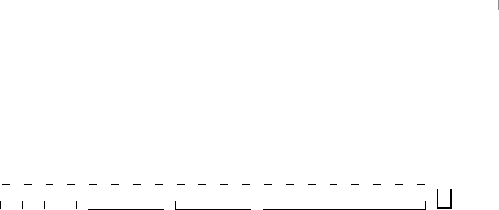
computability theory 57
of countably infinite sets. That is, all of their elements can be put into a list. While it may
be difficult to see this quality in the rational numbers, it is made easier when you consider
that the rational numbers are also called the measuring numbers. While there are an
infinite number of positive fractional measurements you could make while woodworking
or cooking, these measurements can also be listed:
{0
1
0
,1
1
1
,1
2,2
1
2
,1
3,2
3,3
1,3
2
3
,1
4,3
4,4
1,4
3
4
,1
5,2
5,3
5,4
5,5
1,5
2,5
3,5
4
5
,⋯
𝑛
}
Note that each bracket has a number 𝑛associated with it. Starting with 𝑛= 1, the numbers
in each bracket begin with 1
∕𝑛and the numerator is incremented until you reach 𝑛
∕𝑛. Then,
you continue with 𝑛
∕1, incrementing the denominator until you reach 𝑛
∕𝑛again. Fractions
whose values are already in the list are skipped. Negative rational numbers can be added
by simply placing a number’s complement immediately after itself in the list. Thus, Qis
enumerable and countably infinite.
In his second theorem from his 1874 article, Cantor states that, given any sequence of
real numbers 𝑥1, 𝑥2, 𝑥3,…in a closed interval [𝑎, 𝑏], there exists a number in [𝑎, 𝑏]that
is not contained in the given sequence. Essentially, this means that, unlike the sets we just
discussed, the set of real numbers Ris not enumerable or countably infinite. It cannot be
expressed as a list or sequence because there will always be a real number missing. There
exists no proper way to "count" the reals. With these two theorems, Cantor discovered
that differences can exist between infinite sets. There are distinct infinities. He comments
on this in the same article:
I have found the clear difference between a so-called continuum and a col-
lection like the totality of real algebraic numbers.
The truth of this "so-called continuum" of the real numbers would continue to evade
Cantor for the rest of his life. In the years following his first article of set theory, he made
a number of foundational discoveries related to this territory he termed the transfinite. He
began looking for a bijection between the unit line segment [0,1] ∈ Rand the unit square
(i.e. a square with sides of length 1). In 1877, in a letter to his friend Richard Dedekind
(of Dedekind cuts fame), Cantor instead wrote a proof for the existence of a bijection be-
tween the unit line and all of the points in an 𝑛-dimensional space. Not only could the real
numbers between 0and 1map one-to-one with those in a 1 × 1 grid, they could map to all
of the points in the plane, all of the points in 3-dimensional space, and all of the points in
any arbitrary dimension. Such was the nature of uncountably infinite sets. Cantor wrote
to Dedekind below his proof: "I see it, but I don’t believe it!"
4.2.2 Ordinals and Cardinals
To aid his exploration into the continuous nature of the real numbers, he formulated the
transfinite arithmetic, the arithmetic of infinite numbers whose size is somewhere be-
tween finite and uncountably infinite. He generalized the natural numbers, introducing

computability theory 58
two countably infinite sets, those of the ordinal and cardinal numbers.
Ordinal numbers describe order in a collection. More specifically, they describe the
ordinality of a number in an ordered set (e.g. 1st,2nd,3rd,…). They include both finite
natural numbers such as 1,2,3,…and transfinite numbers such as
𝜔, 𝜔 + 1, 𝜔 + 2,…,2𝜔, 3𝜔, 4𝜔, …, 𝜔2, 𝜔3, 𝜔4,…, 𝜔𝜔, 𝜔𝜔𝜔, 𝜔𝜔𝜔𝜔
,…
where 𝜔is the "first infinite ordinal." Note that this sequence of transfinite quantities never
ends. Cantor commented on this property, stating that the set of all ordinals Ωcannot have
a greatest member. Because Ωis well-ordered, there must exist some number 𝛿that would
be greater than all of the numbers in Ω. But 𝛿would belong to Ωbecause Ωcontains all
ordinal numbers. This implies that 𝛿 > 𝛿, which is a contradiction. Cantor, a devout
Lutheran, called this illusive Ωthe Absolute Infinite, a number or set that is bigger than
any conceivable quantity, finite or transfinite. This kind of thinking later led to the dis-
covery of a number of mathematical paradoxes or contradictions in set theory, many of
which still exist today.
Cardinal numbers describe the size or cardinality of a set (i.e. a set could contain 1
element, 2elements, 3elements, …). Like the ordinals, the cardinals include both finite
natural numbers and transfinite numbers, the smallest of which is ℵ0(aleph-null). ℵ0is
the cardinality of any countably infinite set, such as the natural numbers. In contrast to
this, Cantor describes uncountably infinite sets, such as the real numbers, as having car-
dinality ℵ1(aleph-one). There are other greater aleph numbers that are studied for their
own sake such as ℵ𝜔, the first uncountable cardinal number not equal to ℵ1. That said,
ℵ0and ℵ1are sufficient for our purposes. Like the set of all ordinal numbers, the set
of all cardinal numbers cannot be completed in any meaningful way and thus it can be
described as a set of Absolute Infinite cardinality.
4.2.3 The Continuum Hypothesis
For much of his career, Cantor tried to prove the continuum hypothesis, which states that
there is no set whose cardinality is strictly between that of the integers and the real num-
bers. This would imply that there is no cardinal number between ℵ0and ℵ1. If this
hypothesis were true, the cardinality of R(ℵ1) would be equal to the cardinality of the
continuum 𝔠(a "continuum" being a set whose numbers "blend" into each other seam-
lessly).
To prove that 𝔠=ℵ1, Cantor sought to relate 𝔠to ℵ0, and in doing so, he formulated
a concept that is very relevant to combinatorics. He defined the power set operator ,
which maps any set 𝑆to its power set (𝑆), the set of all subsets of 𝑆. For example, for
a set 𝑆= {1,2,3},(𝑆)contains the following sets:
{} {1} {2} {3} {1,2} {1,3} {2,3} {1,2,3}
Notice that 𝑆has cardinality 3and that (𝑆)has cardinality 23= 8. For any set 𝑆
with cardinality 𝑥,(𝑆)has cardinality 2𝑥, and it turns out that this holds for transfinite
cardinals as well. Thus, (Z)=2ℵ0. This expression is denoted with the character ℶ1

computability theory 59
(beth-one) according to the following rule: ℶ𝛼+1 = 2ℵ𝛼. By Cantor’s theorem,ℶ1> ℵ0,
so we can define 𝔠= 2ℵ0=ℶ1and state that 𝔠> ℵ0. The continuum has a greater
cardinality than a discrete set like the integers. The question then becomes: Could 𝔠be
anything less than ℵ1, the cardinality of the real numbers? Or is the set of real numbers
the smallest example of a continuum?
With the work of Kurt Gödel in 1940 and of Paul Cohen in 1963, it was established that
the continuum hypothesis cannot be proven or disproven. It is independent of the axioms
of Cantor’s set theory. It is also independent of the axioms of the current foundation of
mathematics, the Zermelo-Fraenkel set theory with the axiom of choice (ZFC set theory).
That said, since set theory works regardless of whether or not the continuum hypothesis is
true, most mathematicians operate assuming that it is true because the set of real numbers
does appear to exhibit the behavior we would expect from a "continuum." Thus, indepen-
dent of any particular set theory, we may assume that, for any transfinite cardinal 𝜆, there
is no cardinal 𝜅such that 𝜆 < 𝜅 < 2𝜆.
Backlash Against Cantor’s Set Theory
Typically, when a proof is submitted, it is either quickly accepted by the mathe-
matical community or quickly shown to be flawed. In the case of Georg Cantor’s
set theory, controversy loomed for many decades and objections came from many
different angles. Most of the grievances came from the constructivists, a group
that was partially founded by Cantor’s mentor, Leopold Kronecker.
Constructivism is a philosophy of mathematics that asserts that it is necessary to
find or construct a mathematical object in order to prove that it exists. Unlike
classical mathematics,constructive mathematics does not adhere to the law of
the excluded middle, which states that a well-formed proposition must be either
true or false. According to this philosophy, a proof by contradiction (a proof of
an object’s existence founded in disproving the object’s non-existence) is invalid.
Constructivists took issue with the characterization of actual infinities (e.g. the
uncountably infinite set R) as legitimate mathematical objects worthy of study.
Their mathematical philosophy only permitted the existence of potential infinities
(e.g. the countably infinite set N). Kronecker did not consider Cantor’s original
1874 proof of a difference in cardinality between Nand Ras constructive. He
remained staunchly opposed to Cantorian set theory and its hierarchy of the
infinite, stating that
God created the natural numbers; all else is the work of man.
There were other mathematical objections to Cantor’s findings, such as those
directed toward the uncountability of the transcendental numbers. By 1874, only
a handful of transcendentals had been discovered. The constant 𝑒was proven to be
transcendental the year prior, and 𝜋would not be proven to be transcendental until

computability theory 60
1882. In stating that the algebraic reals were countable and the reals were not,
Cantor implied that almost all real numbers were transcendental. That is, if you
remove a countable subset (AR) from an uncountable set (R), you are left with an
uncountable subset (A𝑐
R, the complement of the algebraic reals, also known as the
transcendental reals). Many could not accept that something previously thought
to be incredibly rare had instead an uncountably infinite number of examples.
Other mathematicians, including Kronecker, refused even to accept Cantor’s work
as mathematical in nature, believing it to be, at best, philosophical.
In addition to objections from mathematicians, Cantor’s set theory received a
number of complaints from Christian theologians. Some saw the formalization of
an uncountable infinity as a challenge to the uniqueness of the absolute infinity
of God. Some associated the transfinite hierarchy with pantheism. Cantor felt
strongly that his set theory could exist harmoniously within a Christian framework.
Even his notational choices (ℵ,𝜔, and Ω) can be considered an homage to the
title of "Alpha and Omega." He associated the Absolute Infinite with God, and
felt that transfinite quantities, while infinite, were no challenge to the supremacy
of the Lord, averring that
…the transfinite species are just as much at the disposal of the inten-
tions of the Creator and His absolute boundless will as are the finite
numbers.
Furthermore, Cantor wrote to numerous prominent theologians, including the
Pope, in an attempt to clear up this confusion between the abstract notion of
infinity and the actuality of infinity, as he saw it, in God and in Nature:
The actual infinite was distinguished by three relations: first, as it is
realized in the supreme perfection, in the completely independent, ex-
traworldly existence, in Deo, where I call it absolute infinite or simply
absolute; second to the extent that it is represented in the dependent,
creatural world; third as it can be conceived in abstracto in thought
as a mathematical magnitude, number or ordertype. In the latter two
relations, where it obviously reveals itself as limited and capable for
further proliferation and hence familiar to the finite, I call it Trans-
finitum and strongly contrast it with the absolute.
The onslaught of criticism began to wear Cantor down. Frustrated with the
disapproval from his mentor and high-ranking members of his faith and with his
inability to solve the continuum hypothesis, he fell into a chronic depression that
persisted until his death. He ceased mathematical study for years at a time, writing
and lecturing instead on Shakespeare. Nevertheless, some mathematicians, such
as David Hilbert, supported his set theory.
computability theory 61
Hilbert championed the transfinitist philosophy, which claims that infinite sets
are legitimate mathematical objects. He believed that Cantor’s set theory was the
key to axiomatizing all of mathematics, a goal that he would pursue for much of
his life. He gave lectures on transfinite arithmetic after Cantor’s death, employing
an intuitive thought experiment known as Hilbert’s Grand Hotel. Ultimately, set
theory was generally accepted, thanks in large part to Hilbert, who believed in
Cantor’s work even in the face of a considerable opposition to its fundamental
principles.
F9f
No one will drive us from the paradise which Cantor created for us.
—David Hilbert
4.2.4 Cantor’s Later Years and Legacy
In the early 20th century, mathematicians and philosophers had found a variety of para-
doxes within Cantor’s set theory. The most famous example was Russell’s paradox, which
was discovered by Bertrand Russell in 1901. It posits that, given a set 𝑆that is "the set
of all sets that are not members of themselves," it is unclear whether 𝑆contains itself. If
it does, it contains a set that is a member of itself. If it does not, it does not contain all
sets. An alternative, colloquial form of this is the barber’s paradox: Given a barber who
shaves all those, and only those, who do not shave themselves, does the barber shave him-
self? There is no answer to this question. It cannot be answered within its own axiomatic
system.
When he was not hospitalized for disease or depression, Cantor lectured on these para-
doxes of his set theory until his retirement in 1913. He lived in poverty, suffering from
malnourishment during World War I before succumbing to a heart attack in a sanatorium
in 1918.
Georg Cantor’s work was revolutionary and had far reaching consequences in every
field that made use of mathematics. It drew a line in the sand between discrete and con-
tinuous phenomena. It was Cantor’s investigation into and formalization of the infinite
that laid the groundwork for ZFC set theory, the current "common language" of mathe-
matics. More than that, however, he shifted the collective perception of the purpose of
mathematics.
Before this point, mathematics was typically done to understand the natural world. Can-
tor believed not only that mathematics could describe what he saw around him, but that it
could also solve problems that were purely logical, those that existed in the mind. Mathe-

computability theory 62
matics was a universe in the abstract, worthy of exploring in the same way that the natural
one was. For Cantor, mathematics allowed one to see beyond the limitations of the human
senses into worlds of arbitrary dimension, unshackled by physical laws. This philosophy
has encouraged the continued development of abstract theories, many of which are later
found to have concrete implications for the nature of our reality. Cantor stood firm in op-
position to the "oppression and authoritarian close-mindedness" he faced from Kronecker
et al. and called for objectivity and truth among his peers, bringing humanity, kicking and
screaming, into the modern era of mathematical thought.
The essence of mathematics is in its freedom.
—Georg Cantor
4.3 The Diagonal Argument for Computable Functions
While the story of Georg Cantor and his set theory is interesting in its own right, its
relevance to Turing computability and to computer science in general may not be readily
apparent. For this reason, I would like to discuss the implications of one final topic related
to Cantor, his 1891 constructive proof of transfinite cardinality known as the diagonal
argument. The theorem and its short, elegant proof are recreated below.
Theorem: Given the set 𝑇of all infinite sequences of binary digits, if
𝑠0, 𝑠1, 𝑠2,…, 𝑠𝑛,…is any enumeration of elements from 𝑇, there
exists an element 𝑠∈𝑇which does not correspond to any 𝑠𝑛in the
enumeration.
Proof: We start with an enumeration of elements from 𝑇:
𝑠0= (1,0,1,1,0,0,1,0,0,0,⋯)
𝑠1= (1,1,0,1,1,0,1,0,1,1,⋯)
𝑠2= (0,0,0,1,0,0,0,1,1,1,⋯)
𝑠3= (1,1,0,1,0,1,1,0,1,0,⋯)
𝑠4= (1,0,1,1,1,0,1,0,0,1,⋯)
𝑠5= (0,0,0,1,0,0,1,1,0,0,⋯)
𝑠6= (0,0,1,0,0,0,1,0,0,0,⋯)
𝑠7= (0,1,0,0,0,1,1,0,1,1,⋯)
𝑠8= (1,1,1,1,1,0,1,0,0,1,⋯)
𝑠9= (1,0,0,0,0,1,0,0,0,1,⋯)
⋮
We then construct a sequence of binary digits 𝑠⋆by making the 𝑛th digit
of 𝑠⋆equal to the negation of the 𝑛th digit of the 𝑛th sequence given

computability theory 63
above. Put more simply, we highlight the digits along a diagonal, and
flip their values to make 𝑠⋆:
𝑠0= ( 1 ,0,1,1,0,0,1,0,0,0,⋯)
𝑠1= (1,1,0,1,1,0,1,0,1,1,⋯)
𝑠2= (0,0,0,1,0,0,0,1,1,1,⋯)
𝑠3= (1,1,0,1,0,1,1,0,1,0,⋯)
𝑠4= (1,0,1,1,1,0,1,0,0,1,⋯)
𝑠5= (0,0,0,1,0,0,1,1,0,0,⋯)
𝑠6= (0,0,1,0,0,0,1,0,0,0,⋯)
𝑠7= (0,1,0,0,0,1,1,0,1,1,⋯)
𝑠8= (1,1,1,1,1,0,1,0,0,1,⋯)
𝑠9= (1,0,0,0,0,1,0,0,0,1,⋯)
⋮
𝑠⋆= ( 0,0,1,0,0,1,0,1,1,0,⋯)
𝑠⋆must differ from each 𝑠𝑛because their 𝑛th digits differ. Thus, 𝑠⋆does
not belong to the given enumeration of 𝑇. Given any enumeration of
𝑇, you can always construct an infinite binary sequence that does not
appear in it. □
With this information, we can go a step further and say that 𝑇is uncountably infinite.
Note that this result requires that the sequences be countably infinite. This argument has
become a common technique in proofs to prove the uncountability of a set whose mem-
bers are countably infinite. Turing used a diagonal argument to formalize the notion of
computability and to prove that the Entscheidungsproblem, one of the most important
mathematical problems of the 20th century, is undecidable. Next, we will use the diago-
nal argument to formalize the set of computable functions.
4.3.1 Uncountably Many Languages
Consider the alphabet {0,1}. With this alphabet, one can construct the set of all binary
strings 𝑆using the regular expression {0,1}∗(i.e. {𝜀, 0,1,00,01,10,11,000,001,⋯}).
Strings like these are often called words in computability theory, but they could potentially
represent very long pieces of text that you might not think of as "words." It may be help-
ful to think of them instead as syntactically valid building blocks of a particular language.
Two other things to note:
1. These binary strings are finite in length, by definition of the Kleene star ∗. They
are the set of finite words that can be constructed using the alphabet {0,1}.

computability theory 64
2. While this example uses a binary alphabet, the set 𝑆could be constructed similarly
over a ternary alphabet or an 𝑛-ary alphabet where 𝑛∈N. Formally, the set of
all words over an alphabet Σis denoted Σ∗. Likewise, the symbols of Σneed not
be numbers. An alphabet can contain any symbols, as long as they are distinct and
there are a finite number of them.
We can then consider the power set of 𝑆,
(𝑆) = {{𝜀},{0},{1},{10},{0,1},{0,10},{1,10},{0,1,10},⋯}
to be the set of all languages that can be created using these binary words. A language 𝐿
is simply a subset of the set of all possible words over a finite alphabet. Stated formally,
𝐿 ⊆ Σ∗. As we discussed previously in the section on automata, languages can conform to
a grammar, but for now we will consider them simply as countable sets of words. Words
that belong to a given language are called well-formed words and those that do not are
called ill-formed words, but only in relation to that language.
Because 𝑆is a countably infinite set and because the power set of a countably infinite
set is uncountably infinite (by Cantor’s theorem), we know that (𝑆)is an uncountably
infinite set. Each member of (𝑆)is a countable set of words, also known as a language.
Thus, there exists an uncountable number of languages of binary words (and of languages
in general). The diagonal argument supports this.
Let each sequence 𝑠𝑛from the above proof represent a language. The "columns of the
matrix" each correspond to a binary word from 𝑆. Thus, the digits in each sequence rep-
resent whether or not a particular word is well-formed (1) or ill-formed (0) with regard to
the language the sequence represents. For example, the language {0,1,01,10,11} would
have a 1in its sequence for the columns corresponding to words 0,1,01,10,11 and a
0everywhere else. We can enumerate the languages as in the proof and flip the values
along the diagonal of the enumeration to construct a new language. Thus, the set of all lan-
guages of binary words is not enumerable. Rather, there are uncountably many languages.
4.3.2 Countably Many Turing Machines
Now, let’s require that the sequences be finite. Because a Turing machine has a finite num-
ber of states and transitions, it can be represented with a finite binary string. Similarly,
every natural number can be represented with a finite binary string. Thus, there is a one-
to-one correspondence between the set of all Turing machines and the set of all natural
numbers. So while there are uncountably many languages, there are only countably many
Turing machines to recognize those languages.
We know that Turing machines recognize exactly the recursively enumerable languages
𝑅, so we know there are also countably many of these. Taking the complement of 𝑅im-
plies that there are also uncountably many non-recursively enumerable languages that a
Turing machine cannot recognize. In fact, almost all languages cannot be recognized by
a Turing machine.
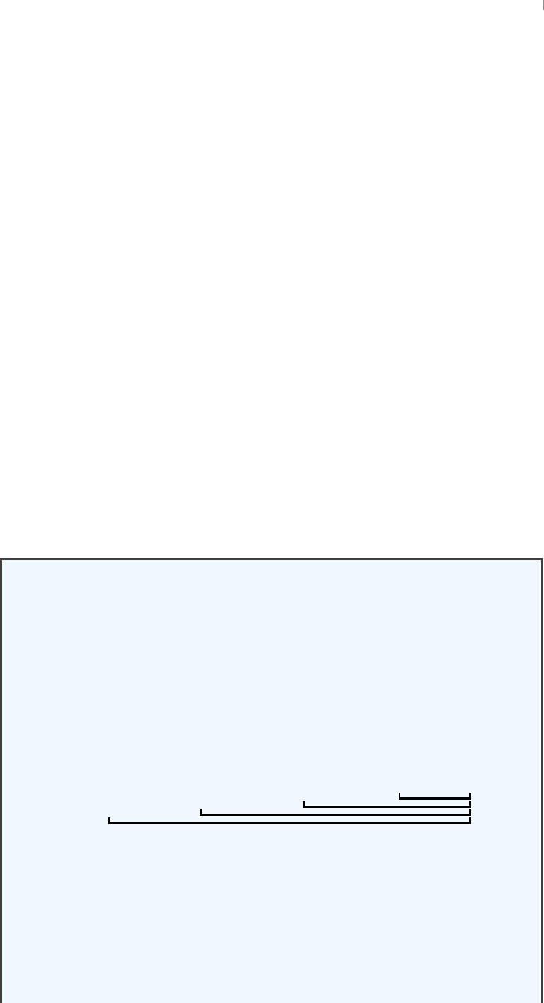
computability theory 65
Before we define the recursively enumerable languages, we should first define a strict
subset of them known as the recursive languages. A recursive language can be represented
by a recursive set of natural numbers. A subset 𝐿of the natural numbers is called recursive
if there exists a total function 𝑓such that
𝑓(𝑤) = {1if 𝑤∈𝐿
0otherwise
Such a function represents the following decision problem: "Let 𝐿be a language repre-
sented by a set. Given a word 𝑤, is 𝑤a well-formed word in 𝐿?" In the case of a recursive
𝐿, this decision problem is called decidable.
Similarly, a recursively enumerable language can be represented by a recursively enu-
merable set of natural numbers. A subset 𝐿of the natural numbers is called recursively
enumerable if there exists a partial function 𝑓such that
𝑓(𝑤) = {1if 𝑤∈𝐿
undefined otherwise
The decision problem can be phrased in the same way, but, in the case of a recursively
enumerable 𝐿, it is called partially decidable or semidecidable. That is, we can decide
a word is in the language, but we cannot formally decide that it is not. In mathematical
terms, statements like this can be proven, but not disproven. If that sounds incredibly
unintuitive, that’s because it is. This concept will come up later in a discussion of Kurt
Gödel’s contribution to computability.
Decidability and Semidecidability for Humans and Computers
Recall that recursive languages are also recursively enumerable. That is, their
recursive nature is countable. This is because recursive languages can construct
only finite sentences that have an end. On the other hand, a recursively enumerable
language can have sentences that expand forever, always ready to accept another
clause before its period.
The following sentence is recursive (and, thus, also recursively enumerable):
Alice said that Betty said that Charlie said that David got a kitten.
This sentence is composed of a countable, finite number of building blocks called
clauses that each contain a subject and a predicate. In this case, the subjects are
the names and their respective predicates are marked by brackets.
All but one of these clauses are nested in the predicate of a previous clause. If
a sentence can be defined in terms of smaller sentences, it is said to be defined
recursively. This sentence qualifies: it contains a full sentence starting with
computability theory 66
Betty, which contains a full sentence starting with Charlie, which contains a
full sentence starting with David. It can also be called recursively enumerable,
because the clauses can be counted.
This next "sentence," on the other hand, is recursively enumerable, but it is not
recursive:
Alice said that Betty said that Charlie said that David said that …
In this case, you can count the potentially infinite number of recursions that occur.
However, this "sentence" cannot be called recursive because, due to the absence
of a period, it actually contains no full sentences.
How can we understand this concept in the context of computation? We can think
about sentences as programs. When someone says a sentence to you, you process
information as the sentence is being said. When the sentence finally ends, you
have all of the information necessary to understand the thought this person is
trying to convey to you. As a result, you gain insight from this person. Similarly,
when a programmer executes a program, the computer processes information as
it moves forward through the instructions. When the program terminates, the
computer has all of the information it needs to compute an answer. It is then
able to return a value, which is the kind of insight that is produced by an algorithm.
What if, instead, someone said a sentence to you that never ended? You could
listen intently, trying to keep track of everything they’ve said, but the punchline
will never come. You will never understand what they are trying to tell you.
Similarly, if a program’s instructions never end, a computer will never be able to
produce any meaningful answer. This is called an infinite recursion, which is a
kind of infinite loop.
This conclusion assumes that the computer we are talking about is a real computer
in the real world, where time and space are finite. The reason that a Turing
machine is a helpful abstraction is that it has an infinite amount of time and space
at its disposal. Theoretically, it could run a program composed of a set of infinitely
looping instructions to its "completion." Note the choice of the phrase "a set of
infinitely looping instructions" instead of "an infinite set of instructions." The
latter is called a stream, and it is not Turing-recognizable. 𝜔-automata, however,
can recognize it.
Many well-known functions can be defined recursively, such as the factorial func-
tion 𝑓(𝑛) = 𝑛!. What is an example of a function that is recursively enumerable,
but not recursive? To answer this, I would like to recommend this video, in which
a mechanical calculator is instructed to divide a number by zero. The calculator
knows the method for division, but this method is only effective in the cases where
the denominator is not zero. In the case where the denominator is zero, it attempts
computability theory 67
to carry out the calculation, faithfully incrementing its count of how many times
the denominator fits into the numerator. Of course, zero fits into any number an
infinite amount of times, so the calculator will continue to calculate until, as the
videographer suggests, it potentially catches fire. The program will never termi-
nate, and a result will never be returned, so we can say that division over any set
including zero is only semidecidable.
The problems that Turing machines can solve are either decidable or semidecidable.
What, then, is undecidable? What kinds of problems do non-recursively enumerable lan-
guages describe? Consider the same decision problem from before: "Let 𝐿be a lan-
guage represented by a set. Given a word 𝑤, is 𝑤a well-formed word in 𝐿?" If 𝐿is
non-recursively enumerable, a Turing machine cannot ever decide this problem because
it cannot recognize 𝐿. Thus, such decision problems are undecidable for all inputs, and
any related function problems have no answer.
4.3.3 Computable Functions and Computable Numbers
Because all recursive languages are recursively enumerable, a Turing machine can recog-
nize a language from either class. 𝑓in both cases is known as a computable function, a
function whose output can be correctly computed by an algorithm performed by a Tur-
ing machine. This means that a Turing machine can be considered a formalization of the
countable set of computable functions:
A partial function 𝑓∶N𝑘↛Nis computable if and only if ∃a
Turing-recognizable computer program with the following properties:
1. If 𝑓(𝐱)is defined, the program will eventually halt on the input 𝐱
with 𝑓(𝐱)stored in the tape memory.
2. If 𝑓(𝐱)is undefined, the program never halts on the input 𝐱.
While algorithms are typically written using natural numbers or integers, this is not a
requirement. The finite-length 𝑘-tuple 𝐱can belong to any 𝐴𝑘where 𝐴is a countable set.
Likewise, the codomain of 𝑓can be any countable set. This generalization allows us to
investigate computable numbers, the numbers that an algorithm can produce.
Consider a partial function 𝑔∶Q𝑘↛Q. Like N,Qhas cardinality ℵ0. Thus, if a
program, as defined above, exists, 𝑔is computable. If we add a countably infinite set of
numbers to Q, we can construct AR, the algebraic reals. Because ARalso has cardinal-
ity ℵ0, a function 𝑔∶A𝑘
R↛ARis also potentially computable. This coheres with our
informal notion of computability, as well: The algebraic reals are those real numbers that
are the roots of a non-zero polynomial, and an algorithm can compute them by solving
their corresponding polynomial equation.
computability theory 68
From here, we can add a countably infinite set of transcendental reals to our set of al-
gebraic reals to form the set of computable numbers. These are the real numbers that
can be computed with an arbitrary level of precision by a finite, terminating algorithm.
This implies that a countable number of transcendental reals can be computed. It may
be surprising to hear, for example, that the transcendental constant 𝜋is computable, but
its algorithm is simple. Given a circle, 𝜋is the ratio of the circle’s circumference to its
diameter. These quantities can be stored with an arbitrary level of precision in a TM’s
countably infinite memory, and instructions can be written to divide one by the other. In
general, computable transcendentals can be found by enumerating 𝑆∶= ARand using
the diagonal argument to construct a computable real 𝑠∉𝑆. Add 𝑠to 𝑆, apply the argu-
ment again, and repeat to add a countably infinite number of computable transcendentals
to 𝑆.
The set of computable numbers is countably infinite, which means that almost all real
numbers are uncomputable. The question naturally arises: Does a number really exist (or
have any worth) if it is impossible to compute its value? A constructivist would argue that
it does not. There are efforts to use the computable numbers instead of the real numbers
for all of mathematics, and the resulting theory is called computable analysis. Regardless,
one could argue that theoretical computer science is an exploration of the mathematics
that can be done within this set.
4.4 Hilbert’s Program and Gödel’s Refutation of It
In 1900, David Hilbert gave an address to the International Congress of Mathematicians
in Paris. In his speech, he described twenty-three problems that he felt would be some
of the most important of the century. While these problems are diverse in subject mat-
ter, they are all deep questions. In each of their answers (or lack of answers) lies some
fundamental truth about the structure of mathematics itself. They are known as Hilbert’s
problems, and many of them remained unsolved and of great interest today.
4.4.1 Hilbert’s Second Problem
This presentation of problems was, in essence, the inception of Hilbert’s program, a world-
wide goal to solve what was known at the time as the foundational crisis of mathematics.
With the general acceptance of Cantor’s set theory came the discovery of many para-
doxes and inconsistencies that called into question the consistency of mathematics. It
had been assumed until this point that mathematics was something that could be trusted,
that a statement could be proven true from previous mathematical truths. The creation of
Zermelo-Fraenkel set theory in the late 1920s resolved some of these paradoxes, such as
Russell’s paradox, but not all inconsistencies were resolved. Mathematics was still curi-
ously "broken" in certain ways.
Metamathematics
computability theory 69
TEXT
As a proponent of the philosophy of mathematics known as formalism, Hilbert believed
that mathematics was not a description of some abstract part of reality, but was rather akin
to a game where pieces could be moved according to a set of rules. He believed that a
mathematical "game" was played with "pieces" from an arbitrary set of a priori truths.
These pieces are called axioms, and they are manipulated according to an arbitrary set of
inference rules to construct conclusions. These conclusions can then be used as premises
for the inference of further conclusions. Thus, formalism avers that mathematics is purely
syntactic. It is nothing more than the manipulation of strings of symbols by logical rules,
and any sort of semantic meaning derived from these strings is merely the product of an
interpretation.
In the early 20th century, Hilbert made it his life’s goal to construct a set of axioms,
from which all existing and future mathematical theories could be derived in a consistent
manner. His peers agreed that the search for such an axiomatization was direly needed.
By this point, no one had been able to prove the consistency of the standard Peano arith-
metic, which includes basic axioms such as 𝑥+𝑦=𝑦+𝑥and 𝑥× 0 = 0. Proving a
consistent set of axioms of arithmetic was the second of Hilbert’s famous twenty-three
problems, preceded only by the problem of deciding Cantor’s continuum hypothesis.
Stated more generally, Hilbert intended to construct a formal system that was complete,
consistent,
In order for Hilbert’s program to succeed, there would have to exist a formal system
with the following properties:
∙Completeness, the ability to prove all true mathematical statements
∙Consistency, the absence of contradictions
∙Conservation, the ability to prove results involving countable quantities without the
use of uncountable ones
∙Decidability, the existence of an algorithm that could decide the truth or falsity of
any mathematical statement
As a professor at the prestigious University of Göttingen, Hilbert gave many lectures on
his program, both inside and outside of Germany. At one such lecture given in Bologna
in 1928, Kurt Gödel was in attendance. The concepts of mathematical logic discussed at
this lecture would inspire Gödel throughout his career, but in only three years he would
deal a fatal blow to Hilbert’s program.
4.4.2 Gödel’s Completeness Theorem
In 1929, Gödel published his completeness theorem of mathematical logic as his doctoral
thesis. This was a mathematical proof that elucidated something fundamental about the
first-order logic mathematics is based on. Although it is a bit difficult to understand at first,

computability theory 70
the result is ultimately quite simple, and it supports what mathematicians have implicitly
understood about abstract, general proofs since about 300 BCE, when Euclid introduced
the axiomatic method.
All of Gödel’s theorems that we will discuss in this section are statements about theo-
ries, which are represented as mathematical objects so that they can be studied mathemat-
ically. A theory is similar to a formal system, but it does not necessarily have inference
rules. However, it is a set of axioms written in a language, which has an alphabet and
a grammar. A theory can be coupled with a set of inference rules and often these rules
are understood from context (e.g. by examining the logical structure of the language
that the axioms are written in). Mathematical theories, for example, typically employ a
first-order logical calculus because first-order logic is the standard formalization of math-
ematics. However, theories need not be mathematical. Political theories are still theories.
They are composed of theorems expressed with the alphabet and grammar of a natural
language. They have sets of fundamental beliefs from which other beliefs are derived,
and they may be coupled with some form of deductive reasoning, though this reasoning
may not necessarily be first-order logical. That said, we will focus on first-order logical
theories written in the syntax of mathematics.
A theory coupled with a deductive logical calculus is called a deductive system. A for-
mula that is found to be true, independent of interpretation, by means of this system (i.e.
via a series of inferences that starts at the axioms) is called logically valid. The axioms
of a theory are assumed to be true, so a logically valid formula deduced within a truth-
preserving system must also be true, but only within the theory. All truth is relative, and,
as such, the truth value of any given formula is necessarily dependent on the choice of
axioms and the inference rules that are allowed. There is more than one way to reason
about a given theory, and, as such, a theory can be coupled with different logical calculi
to form different deductive systems. Examples of first-order logical deductive systems
include natural deduction, the Hilbert-Ackermann system, and sequent calculus.
A theory is syntactic in nature. It is a set of strings written in a language , and these
strings are called -formulæ. Any logical calculus that is applied to a theory will
simply map these strings to other strings according to some set of rules. Theories have
no inherent meaning. On the other hand, a model is semantic in nature. A model is
an ordered pair (, 𝐼)where is a theory (a set of -formulæ) and 𝐼is an interpretation
function with domain the set of all constant,function, and relation symbols of such that
1. If 𝑐is a constant symbol, then 𝐼(𝑐)is a constant (a statement) in
2. If 𝐹is a function symbol, then 𝐼(𝐹)is a function on the domain
3. If 𝑅is a relation symbol, then 𝐼(𝑅)is a relation on the domain
computational complexity theory 71
4.4.3 Gödel’s Incompleteness Theorems
4.5 The Entscheidungsproblem and the Church-Turing Thesis
4.5.1 𝜇-recursive Functions
4.5.2 The Untyped 𝜆-calculus
4.5.3 The Halting Problem
Computability is Recursion
TEXT
4.6 Turing Degrees
5 computational complexity theory
Blah, blah, blah...
5.1 Big O Notation
5.2 Complexity Classes

72
Types and Structures
6 type theory and category theory
6.1 The Curry-Howard-Lambek Isomorphism
7 abstract data types and the data structures that
implement them
In this section, we evaluate data structures from a theoretical standpoint, describing their
essential properties and why one may be preferable to another for some task. There is no
single, best way of storing data. The optimal layout varies depending on the nature of the
task. The rules and requirements that define these data structures can be implemented in
code, and many programming languages have their own implementations of these struc-
tures.
Some operations are common among many different data structures. The time com-
plexity of any of these operations will depend on the choice of data structure. We will
discuss how these operations are performed concretely for each data structure listed be-
low, but first we will give an abstract description of these operations.
access To access an item in a data structure is to provide an index to denotes the desired
element’s location relative to the other elements (1st, 2nd, ..., Nth) and to use that element
to acquire the element’s data. The action is only applicable to data structures that have
order.
search To search for an element in a data structure is to provide some sort of informa-
tion about the element (like its value) and to use that information to acquire the element’s
data.
insert To insert an element into a data structure is to find a valid location to insert the
element, to allocate that memory for use by the data structure, and to store the element’s
data there. Requirements for proper insertion depend on the data structure in question.
For example, if the structure requires that its elements be sorted, an element must be
inserted into that structure in sorted order. It also may be possible to insert an element
into a specified location in the structure, with different locations taking different amounts
of time.
The reassign operation is similar to insert, but simpler. It consists of finding a valid
location and storing data there, no new memory is allocated. Instead, memory that is
already a part of the data structure is overwritten.
delete To delete an element from a data structure is to find where the element is stored
in memory and to deallocate that section of memory from the total memory controlled
by the data structure. The data structure may also have to be reorganized in some way
after this deallocation. Like insert, this operation has a runtime that depends heavily on
where the element in located within the structure.
abstract data types and the data structures that implement them 73
Note also that, in many cases, a name can be used to refer to both an abstract data type
and a data structure that is an implementation of that type. For this reason, a table of
relevant abstract data types is given below.
Table 3: Abstract Data Types
Abstract Data Type Structure Description
Set An unordered collection of unique values.
Multiset (or Bag) An unordered collection of elements that are not nec-
essarily unique.
List An ordered collection of elements that are not neces-
sarily unique.
Map A collection of key-value pairs such that the keys are
unique.
Graph A set of elements (called nodes) and a set of pairs
of those nodes (called edges). The pairs are un-
ordered for an undirected graph or ordered for a di-
rected graph.
Tree A directed, acyclic graph in which all nodes have an
in-degree of 1 (except the root node, which has an in-
degree of 0).
Stack A LIFO-ordered collection of elements that are not
necessarily unique.
Queue A FIFO-ordered collection of elements that are not
necessarily unique.
Priority Queue A priority-ordered collection of elements that are not
necessarily unique.
Double-ended Queue A queue that can add/remove elements from both
ends.
Double-ended Priority Queue A priority queue that can add/remove elements from
both ends.
Each data structure described below could implement one or more of these abstract
data types. However, each name used below refers to a data structure of one of these
types, not to the type itself, unless specified otherwise.

abstract data types and the data structures that implement them 74
7.1 Lists
Alist is an abstract data type that represents an ordered collection of elements that are
not necessarily unique. It is typically implemented with either static or dynamic arrays or
with linked lists. The major difference between these data structures has to do with how
the data is stored in memory (i.e. whether data is stored contiguously or not and whether
the amount of allocated memory is fixed or not).
7.1.1 Arrays
*** Talk about how strings are often implemented with arrays.
An array is a collection of elements that are stored contiguously in memory. Each ele-
ment in the array is assigned an index which describes its relative position in the array.
The elements should take up the same amount of space in memory. This is required
to allow indexing to function correctly. To find an element, you must find the beginning
of that element’s data in memory and then fetch a number of bits that corresponds to the
element’s size. To find the element with index 𝑖, you would start at the memory address
where the array begins, skip forward 𝑖×elementSize bits, and then fetch elementSize
bits. In addition to elements taking up the same amount of space, they should also have
the same type. This allows the bits to be interpreted in an unambiguous way.
Arrays can be static or dynamic. A static array takes up a fixed amount of size in
memory while a dynamic array can be resized. The difficulty with increasing the size of
an array is that an array must remain contiguous, but the memory just ahead of the end
of the array could contain important data that cannot be erased. For this reason, dynamic
arrays are often implemented as static arrays that are destroyed and recreated with a larger
size elsewhere in memory when they exceed their previous size.
abstract data types and the data structures that implement them 75
Table 4: Dynamic Array Time Complexity
Operation Time Reasoning
Access 𝑂(1) Indicies allow for direct access
Search 𝑂(𝑛)Have to check elements linearly
Insert (beginning) 𝑂(𝑛)Have to shift all elements one to the right
Insert (middle) 𝑂(𝑛)Same as above in the worst case
Insert (end) 𝑂(1) amortized If there is allocated space at the end, it takes
constant time. If not, you may have to copy all
elements to a new, bigger array.
Delete (beginning) 𝑂(𝑛)Have to shift all elements one to the left
Delete (middle) 𝑂(𝑛)Same as above in the worst case
Delete (end) 𝑂(1) Free the memory at the end of the array
Worst-Case Summary
Access = 𝑂(1) Search = 𝑂(𝑛)Insert/Delete = 𝑂(𝑛)
A static array has the same search properties, but it cannot insert or delete items, be-
cause those operations involve changing the size of the array.
7.1.2 Linked Lists
Alinked list is a collection of nodes that are not stored contiguously in memory. A node
contains some data and a pointer to the next node in the sequence. To point a node A to
another node B means to assign A’s pointer the value of B’s location in memory. The first
node is called the head of the linked list and the last node is called the tail. The tail has
no next node, so its pointer points to null.
The data contained in the nodes of a linked list do not need to have the same type or
size. Because the nodes are stored non-contiguously and are accessed via pointers, there
is no need for nodes to be of the same size.
Linked lists allow for insertion and deletion of elements without restructuring the entire
data structure. This means that linked lists are dynamic. To insert an element X between
elements P and N, traverse the list to find P, save P’s pointer to N as temp, point P to X,
and point X to temp. Deleting is a similar process: traverse the list to find P and point it
to N.
Because you have to traverse the list to insert or delete, it is common practice to keep
track of where the tail is located in memory. This allows for constant time insertion of
abstract data types and the data structures that implement them 76
elements at the end of the list. For constant time deletion of the tail, you would also have
to cache the penultimate node, Pen, in order to point it to null and make it the new tail.
However, keeping track of Pen is 𝑂(𝑛)for a singly linked list because there is no way of
directly finding the new Pen after deleting the tail once.
A linked list can be singly or doubly linked. A doubly linked list has nodes with pointers
to both the previous and next nodes in the sequence. This allows for traversal of the list
in both directions. It also allows for constant time deletion of the tail, as long as the tail
is cached.
Table 5: Linked List Time Complexity
Operation Time Reasoning
Access 𝑂(𝑛)Linked lists do not really have indicies,
but you can iterate through a certain
amount of pointers, starting at the head
Search 𝑂(𝑛)Have to check elements linearly
Insert (beginning) 𝑂(1) Point the new node to the head
Insert (middle) 𝑂(𝑖)Search for the previous node at index i-1,
then reassign pointers
Insert (end) 𝑂(1) with caching,
𝑂(𝑛)otherwise
If you know where the tail is stored, you
can just point it to the new node. If not,
you must first traverse the entire list to find
the tail, which is an 𝑂(𝑛)operation.
Delete (beginning) 𝑂(1) Point head to null
Delete (middle) 𝑂(𝑖)Search for node at index i, then reassign
pointers
Delete (end) 𝑂(1) with caching
and double links,
𝑂(𝑛)otherwise
To delete the tail, you need to know where
the penultimate node, Pen, is. If you cache
the tail and have double links, you can al-
ways find Pen. Otherwise, you must tra-
verse the list to Pen, which is 𝑂(𝑛).
Worst-Case Summary (singly linked, no caching)
Access = 𝑂(𝑛)Search = 𝑂(𝑛)Insert/Delete = 𝑂(𝑛)
Worst-Case Summary (doubly linked, cached tail)
Access = 𝑂(𝑛)Search = 𝑂(𝑛)Insert/Delete = 𝑂(1)
abstract data types and the data structures that implement them 77
7.1.3 Skip Lists
Blah
7.2 Stacks
Astack is a collection of elements with two operations: push and pop. To push an element
onto a stack is to add it to the stack. To pop an element from the stack is to remove its most
recently added element and return it. Peek is an operation that is sometimes implemented
for convenience. It allows access to the most recently added element without removing
it from the stack. The most recently added element is located at the top of the stack, and
the least recently added element is located at the bottom of the stack.
A stack is similar to a linked list, but its operations are stricter. It can only insert and
delete elements at the head of the list (top of the stack), and searching for or accessing an
element located somewhere other than the head requires removing elements from head to
tail until the desired element is the head. A stack can be implemented using an array or a
linked list, so whether or not it is contiguous depends on the implementation details.
Stacks Implemented at the Hardware Level
Stacks are also used in the architecture of computer memory. Classically, the
bottom of the stack will be placed at a high address in memory and a stack pointer
will be assigned its location. When data is pushed onto this stack, the stack will
grow downward to lower addresses in memory, and the stack pointer will keep
track of the top of the stack (lower addresses). When data is popped, the stack
pointer will move accordingly toward the bottom (higher addresses).
Local function variables are stored on the stack. If a call to another function
is made, that function’s local variables will be stored on the stack in a frame.
From top to bottom (low to high address), the frame of a callee function typically
stores local variables, the return address to the code being executed by the caller
function, and then parameters of the callee function. The frame pointer marks the
location of the return address in the frame. This implements the concept of scope
in computing.
abstract data types and the data structures that implement them 78
Table 6: Stack Time Complexity
Operation Time Reasoning
Access 𝑂(𝑛)To access the bottom element, you must pop every other element
Search 𝑂(𝑛)If the element you are searching for is at the bottom, you must
pop every other element
Push 𝑂(1) Make the new node the head of the list
Pop 𝑂(1) Remove and return the head and make the next element the new
head
Peek 𝑂(1) Return the head
7.3 Queues
A queue is a collection of elements with two operations: enqueue and dequeue. To en-
queue an element is to add it to the queue. To dequeue an element is to remove its least
recently added element and return it. As with the stack, peek is often implemented for
convenience, and it returns the least recently added element. The least recently added el-
ement is located at the front of the queue, and the most recently added element is located
at the back of the queue.
While a queue can be implemented using an array, it is more commonly implemented
using either a singly or doubly linked list or using a dynamic array variant called an "array
deque." If implemented using a singly linked list, it must insert elements at the tail and
remove them at the head. A queue may or may not be contiguous, depending on the
implementation.
Table 7: Queue Time Complexity
Operation Time Reasoning
Access 𝑂(𝑛)To access the back element, you must dequeue every other ele-
ment
Search 𝑂(𝑛)If the element you are searching for is at the back, you must de-
queue every other element
Enqueue 𝑂(1) Add the new node to the tail of the list
Dequeue 𝑂(1) Remove and return the head and make the next element the new
head
Peek 𝑂(1) Return the head
abstract data types and the data structures that implement them 79
7.4 Deques
Blah
7.5 Priority Queues
Blah
7.6 Graphs
A graph is a set of vertices (nodes) and edges between those vertices. Graphs are either
undirected or directed, which means their edges are unidirectional or bidirectional, respec-
tively. It is usually implemented using either an adjacency list or an adjacency matrix.
With an adjacency list, the vertices are stored as objects, and each vertex stores a list of
its adjacent vertices. The edges could also be stored as objects, in which case, each vertex
would store a list of its incident edges, and each edge would store a list of its incident ver-
tices. This implementation could, for example, sufficiently represent a hypergraph, which
is a generalization of a graph in which an edge can join any number of vertices.
With an adjacency matrix, the rows would represent the source vertices and the columns
would represent the destination vertices. The matrix simply stores how many edges are
incident to both the source vertex and destination vertex. The data pertaining to the ver-
tices and edges is stored outside of the matrix. The adjacency matrix for an undirected
graph must be symmetrical, whereas this is not the case for directed graphs.
Adjacency lists are better at representing sparse graphs (graphs with few edges) while
adjacency matrices are better at representing dense graphs (graphs with close to the max-
imum number of edges).
Table 8: Adjacency List Time Complexity
Operation Time Reasoning
Insert vertex 𝑂(1) Store vertex in hash table, map it to adjacent vertices
Insert edge 𝑂(1) Add an adjacent vertex
Remove vertex 𝑂(|𝑉|)Visit all adjacent vertices of the given vertex, remove
the given vertex from their adjacency lists, remove given
vertex from map
Remove edge 𝑂(1) Remove destination vertex from source vertex’s list of
adjacent vertices
Check adjacency 𝑂(|𝑉|)In the worst case, a vertex could have an adjacency list
containing all vertices in the graph
Space complexity: 𝑂(|𝑉|+|𝐸|)

abstract data types and the data structures that implement them 80
Table 9: Adjacency Matrix Time Complexity
Operation Time Reasoning
Insert vertex 𝑂(|𝑉2|)Matrix must be resized
Insert edge 𝑂(1) Increment value in matrix
Remove vertex 𝑂(|𝑉2|)Matrix must be resized
Remove edge 𝑂(1) Decrement value in matrix
Check adjacency 𝑂(1) Check if value in matrix is greater than zero
Space complexity: 𝑂(|𝑉|2)
***Talk about graph coloring and MSTs and stuff***
7.7 Trees
Atree is a collection of nodes that contain data and pointers to child nodes. Each child
can only have one parent node. There are many descriptors that can be applied to trees.
Those that describe some of the most useful tree implementations are listed below.
Table 10: Tree Descriptors
Descriptor Meaning
Binary Each node in the tree has at most 2 children
Balanced The left and right subtrees of each node differ in height by no
more than one
Ordered (or sorted) The nodes are sorted in some way, such that they can be searched
in 𝑂(𝑙𝑜𝑔 𝑛)time
Complete* Every level of the tree has the maximum amount of nodes pos-
sible, except for, perhaps, the last level
Full* Each node in the tree has either zero or two children
Perfect* Each non-leaf node has two children, and all leaves have the
same depth
*These terms are not standardized, but they are often defined this way.
We will now discuss a variety of tree-based abstract data types and data structures that
have proven to be very useful in software design. We will cover the binary search tree,
the binary heap, and the trie, as well the preferred implementations for each.
abstract data types and the data structures that implement them 81
7.7.1 Binary Search Trees
Abinary search tree (BST) refers to an ordered binary tree that satisfies the binary search
property, which states that each parent node must be greater than or equal to the nodes
in its left subtree and less than the nodes in its right subtree. This is a sorted order that
is imposed on the tree to give it 𝑂(𝑙𝑜𝑔 𝑛)search, insert, and delete operations, as long as
the tree is also balanced.
Inserting a node, 𝑁, into a binary search tree involves searching for it in the tree until
you arrive at a leaf and then making 𝑁a child of that leaf. Deleting a node, 𝑁, is more
complicated. If 𝑁has no children, simply remove it. If it has one child, replace it with
that child. If it has two children, copy the data of 𝐶, which can be either 𝑁’s in-order
predecessor or in-order successor, to 𝑁. If 𝐶is a leaf, remove it. Otherwise, 𝐶has one
child. Replace 𝐶with that child.
Table 11: Binary Search Tree Time Complexity
Operation Time Reasoning
Search 𝑂(𝑙𝑜𝑔 𝑛)Perform a binary search
Insert 𝑂(𝑙𝑜𝑔 𝑛)Perform a binary search for the closest node and insert the
given node as its leaf
Delete 𝑂(𝑙𝑜𝑔 𝑛)Perform a binary search to find the given node, delete it, and
rearrange the tree
As nodes are inserted into and deleted from a binary search tree, the tree may become
unbalanced. For this reason, self-balancing BSTs, such as AVL trees and red-black trees,
are often the preferred BST implementations because a BST’s search, insert, and delete
operations are only 𝑂(𝑙𝑜𝑔 𝑛)if the tree remains balanced.
avl trees
In an AVL tree, each node, 𝑁, stores the heights of its left and right subtrees, 𝐿and 𝑅.
The difference between these heights (𝐿.height -𝑅.height) is called 𝑁’s balance. If
its balance is less than -1 or greater than 1, 𝑁is unbalanced and must be fixed using tree
rotation. In practice, if a node becomes unbalanced after an insertion, its balance will be
either 2 (L is taller) or -2 (R is taller). An AVL tree is only balanced when all of its nodes
are balanced.
There are two types of rotations, left and right, and they are inverse operations of each
other. A rotation is a way to move a parent (𝐴) down the tree while moving its child (𝐵)
up and preserving the order of the tree. Regardless of the direction, this results in 𝐵aban-
doning its child 𝐶to adopt 𝐴as its child and 𝐴adopting 𝐶as its child. During a right
rotation, 𝐵starts as 𝐴’s left child, 𝐶starts as 𝐵’s right child, 𝐴becomes 𝐵’s right child,
abstract data types and the data structures that implement them 82
and 𝐶becomes 𝐴’s left child. During a left rotation, 𝐵starts as 𝐴’s right child, 𝐶starts
as 𝐵’s left child, 𝐴becomes 𝐵’s left child, and 𝐶becomes 𝐴’s right child. The rotation
operation takes the parent node, 𝐴, as input.
If node 𝑁is unbalanced, rotations must be performed to balance its subtrees. The pseu-
docode for this algorithm is given below.
Algorithm 1: Balancing a node in an AVL Tree
Data: A tree rooted at 𝑁
begin
if N is not balanced then
𝐿⟵𝑁.𝑙𝑒𝑓 𝑡;
𝑅⟵𝑁.𝑟𝑖𝑔ℎ𝑡;
if 𝐿is taller than 𝑅then
if 𝐿’s extra node is on the right then
leftRotation(𝐿);
end
rightRotation(𝑁);
end
else if 𝑅is taller than 𝐿then
if 𝑅’s extra node is on the left then
rightRotation(𝑅);
end
leftRotation(𝑁);
end
end
end
When a node is added to the AVL tree with a BST insert operation, this algorithm is ap-
plied to all of its ancestors as the recursive call stack moves up the tree. This ensures that
the tree is balanced. Deletion is handled similarly. A BST delete operation is performed
on a node, and then the balancing algorithm is applied to all of its ancestors recursively.
red-black trees
A red-black tree is another kind of self-balancing binary search tree in which each node
stores an extra bit that colors the node red or black. A red-black tree maintains its balance
such that search, insert, and delete operations remain 𝑂(𝑙𝑜𝑔 𝑛), but its balances require-
ments are looser. Whereas an AVL tree can only have a max difference in height of 1
between subtrees, a red-black tree can have subtrees whose heights differ by up to a factor
of two.
In addition to the standard properties of a binary search tree, a red-black tree has five
properties that enforce its balance:
1. Each node is either red or black.

abstract data types and the data structures that implement them 83
2. The root is black.
3. All leaves, which are null nodes, are black.
4. Every red node must have two black children.
5. Every path from a given node to a descendant leaf must have the same number of
black nodes.
Consider two paths from a node to its leaves, one with the minimum possible number
of red nodes and one with the maximum possible number of red nodes. Each path must
have the same number of black nodes, 𝑏. The minimum number of red nodes is zero, so
the first path has 𝑏nodes. Because red nodes must have black children and because each
path must have 𝑏black nodes, the second path has a maximum number of 𝑏red parents
and 2𝑏nodes total. Thus, two paths from a given node to its leaves differ in height by at
most a factor of 2, which preserves the efficiency of the BST’s operations.
Inserting and deleting nodes can be complicated with red-black trees because all five
red-black properties must be preserved. The operations required to preserve them depend
on the colors of nodes related to the node being inserted or deleted.
Red-Black Insertion
A new node, 𝑁, replaces a leaf and is always initially colored red. It is also given two
black, null leaves as children. Because we are inserting a red node, Property 5 is not at
risk of being violated, but Property 4 is. We must rebalance the tree in cases where the
insertion of 𝑁causes a red node to have a red child. In these cases, 𝑁’s parent, 𝑃, must
be red. We can also assume that 𝑁’s grandparent, 𝐺, is black, because its child, 𝑃, is red.
However, 𝐺’s other child (𝑁’s uncle), 𝑈, could be red or black.
Case 1: 𝑁is the root of the tree.
Just change 𝑁’s color to black to comply with Property 2.
Case 2: 𝑃is black.
Property 4 cannot be violated, so no rebalancing is required.
Case 3: 𝑃is red and 𝑈is red.
Property 4 is violated because 𝑃is red and its child, 𝑁, is also red. This can be
fixed by flipping 𝐺to red and flipping 𝑃and 𝑈to black. However, 𝐺may now vi-
olate Property 2 (if it is the root) or Property 4 (if its parent is red). For this reason,
the rebalancing function (which was called on 𝑁) should be called recursively on
𝐺whenever a Case 3 situation occurs.
abstract data types and the data structures that implement them 84
Case 4: 𝑃is red and 𝑈is black.
Property 4 is violated because 𝑃is red and its child, 𝑁, is also red. In this case, it
is significant whether or not 𝑁and 𝑃are left or right children of their respective
parents. This leads to four subcases that are all handled with tree rotations, similar
to AVL insertion.
Case 4.A: 𝑁and 𝑃are left children.
Perform a right rotation on 𝐺and flip the colors of 𝑃and 𝐺.
Case 4.B: 𝑁is a right child, and 𝑃is a left child.
Perform a left rotation on 𝑃to create a Case 4.A subtree rooted at 𝐺. Per-
form the Case 4.A steps.
Case 4.C: 𝑁and 𝑃are right children.
Perform a left rotation on 𝐺and flip the colors of 𝑃and 𝐺.
Case 4.D: 𝑁is a left child, and 𝑃is a right child.
Perform a right rotation on 𝑃to create a Case 4.C subtree rooted at 𝐺. Per-
form the Case 4.C steps.
The logic of red-black balancing after insertion can be summarized by the following
algorithms:
abstract data types and the data structures that implement them 85
Algorithm 2: Red-Black Balancing After Insertion
void rbInsertBalance(𝑁):
Data: A red node, 𝑁, that was just inserted into the red-black tree
begin
𝑃⟵parent(𝑁);
𝐺⟵grandparent(𝑁);
𝑈⟵uncle(𝑁);
if 𝑃== NULL then
case1(𝑁);
end
else if 𝑃is black then
case2(𝑁);
end
else if 𝑃is red and 𝑈is red then
case3(𝑁,𝑃,𝑈,𝐺);
end
else \\ 𝑃is red and 𝑈is black
case4(𝑁,𝑃,𝐺);
end
end

abstract data types and the data structures that implement them 86
Algorithm 3: Red-Black Balancing Cases
void case1(𝑁):
begin
Color 𝑁black;
end
void case2(𝑁):
begin
return;// tree is already balanced
end
void case3(𝑁,𝑃,𝑈,𝐺):
begin
Color 𝑃black;
Color 𝑈black;
Color 𝐺red;
rbInsertBalance(𝐺);
end
void case4(𝑁,𝑃,𝐺):
begin
if 𝑃is a left child then
if 𝑁is a right child then
leftRotation(𝑃);
end
case4A(𝑃,𝐺);
end
else
if 𝑁is a left child then
rightRotation(𝑃);
end
case4C(𝑃,𝐺);
end
end
void case4A(𝑃,𝐺):
begin
rightRotation(G);
Color 𝑃black;
Color 𝐺red;
end
void case4C(𝑃,𝐺):
begin
leftRotation(G);
Color 𝑃black;
Color 𝐺red;
end
The process for balancing after deleting is similar, but it is more complicated and in-
volves more cases. As such, it is not worth the space required to expound on it here. Refer
instead to the description on Wikipedia’s red-black tree page.
abstract data types and the data structures that implement them 87
7.7.2 Binary Heaps
Abinary heap is a complete ordered binary tree that satisfies the heap property, which
states that each parent node is either greater than or equal to its children (in the case of a
max-heap) or less than or equal to its children (in the case of a min-heap).
Binary heaps are often implemented using static or dynamic arrays. The root of the
heap is stored at index 0. Each of the other nodes is stored at an index 𝑖 > 0such that
the locations of its parent, left child, and right child can be calculated according to the
following expressions.
Table 12: Relative Indices for a Heap Represented by An Array
Node Index
Current Node 𝑖
Parent (𝑖− 1)∕2
Left Child (2 × 𝑖) + 1
Right Child (2 × 𝑖) + 2
Assuming an array implementation, we can insert a new node in the heap by adding it
to the end of the array and resolving any violations of the heap property that occur, if any.
We can also delete any node in the heap (including the root) by removing it, replacing
it with the last node in the array, and resolving any violations of the heap property that
occur, if any. A heap is an optimal choice for implementing a priority queue, which has
fundamental operations such as insert, find min/max, and delete min/max.
Table 13: Binary Heap Time Complexity
Operation Time Reasoning
Insert 𝑂(𝑙𝑜𝑔 𝑛)Insert node at end of array and "bubble up"
Find Min/Max 𝑂(1) The min/max (depends on heap order) is always stored
at index 0
Delete Min/Max 𝑂(𝑙𝑜𝑔 𝑛)Replace root with last node and "bubble down"
7.7.3 Tries
Atrie is an ordered tree that is typically not binary. It is similar to a map, but the keys
(which are usually strings) are not necessarily associated with every node. Instead, a node
may store a prefix of a key (such as the first character of a key) and have an incident edge
that points to a key or to another prefix that adds a single character to the original prefix.
abstract data types and the data structures that implement them 88
The root node stores an empty string.
This allows for the compact storage and convenient search of strings that share prefixes.
This would be useful for storing a dictionary of English words and recommending valid
words given a prefix. For this reason, it is often used for autocompleting words and stor-
ing new, custom words.
Table 14: Trie Time Complexity
Operation Time Reasoning
Search 𝑂(𝑛)Traverse the trie character-by-character until the full 𝑛-length
string is found or you hit a leaf
Insert 𝑂(𝑛)Add new prefix nodes to the trie character-by-character until there
is an 𝑛-length path leading from the root to the given word
Delete 𝑂(𝑛)Traverse the trie toward the given string and delete the first node
you encounter with an out-degree of 1.
7.8 Maps
Amap, also known as an associative array, is a collection of key-value pairs, such that
keys are unique. A key can be used to search the map to find its corresponding value. Maps
are typically implemented with a hash table (to make a hash map) or a tree (to make a tree
map). Whether or not a map has order depending on its implementation. Hash maps are
not ordered while tree maps are ordered.
7.8.1 Hash Maps
A hash table uses a hash function to map keys to buckets in an array. It does this by
hashing a key and reducing that hash to an index in the array, using a modulo operator
(index = hash % array_size). It must also handle collisions, which occur when two
or more keys map to the same bucket. The two common ways of handling this are separate
chaining and open addressing.
separate chaining
In separate chaining, buckets hold pointers to linked lists, which hold the key-value pairs
in nodes. A bucket without a collision will point to a single node, whereas a bucket with
a collision will point to a chain of nodes. The buckets could also instead hold the heads
of the linked lists, which would decrease the number of pointer traversals by 1, but would
also increase the size of the buckets, including the empty ones, if the values take up more
space than a pointer.
open addressing
In open addressing, all key-value pairs are stored in the bucket array. When a new pair has
abstract data types and the data structures that implement them 89
to be inserted, the bucket corresponding to its hashed key (preferred bucket) is checked for
occupancy. If there is a collision, more buckets are checked in a probe sequence. The most
common probe sequence is linear probing, which means you check buckets separated by
a fixed interval, which is usually 1 (bucket x, bucket x+1, bucket x+2, ...). When an
unoccupied bucket is found, the pair is stored there. When a key is used to access a value,
the key is compared to the key stored in the preferred bucket. If it matches, the value in
that bucket is returned. Otherwise, the process is repeated with other buckets according
to the probe sequence and will return either when the keys match (item found) or when
the bucket is empty (item not found).
dynamic resizing
A hash table that is quite full is slower than one that is quite empty, regardless of the style
of collision resolution. If table that uses separate chaining is quite full, it is more likely
that future items will have to be chained to existing items, which leads to longer search
times. If a table that uses open addressing is quite full, a future item whose preferred
bucket is filled will spend longer looking for an empty bucket, and it will take longer to
search for it as well.
The load factor of a hash table is the ratio of the number of keys stored in the table
to the number of buckets in the table. When the load factor exceeds some limit (0.75 is
commonly used), the hash table will be rehashed, which involves creating a new hash
table and remapping all of the elements to it. There are other techniques that allow for
incremental resizing instead of this all-at-once method, which can be useful for highly
available systems.
Table 15: Hash Map Time Complexity
Operation Time Reasoning
Access N/A Hash maps have no total order
Search 𝑂(1)* The hash tells you where the data is located
Insert 𝑂(1)* The hash tells you where to put the data
Delete 𝑂(1)* The hash tells you which bucket to empty
*This time complexity assumes a good hash function with minimal collisions. A very bad hash function
with result in an 𝑂(𝑛)time complexity.
7.8.2 Tree Maps
A perfect hash function results in an 𝑂(1) search time. A particularly bad hash function
could cause a hash table with separate chaining to put all key-value pairs into the same
bucket, which would result in an 𝑂(𝑛)search time. A tree implementation lands in be-
tween these scenario with an 𝑂(𝑙𝑜𝑔 𝑛)search time. It can be visualized as a hash table
with one bucket which contains the root of a tree instead of the head of a linked list.
abstract data types and the data structures that implement them 90
Maps like this are often implemented using self-balancing binary search trees like AVL
trees or red-black trees. While they are less time-efficient than maps that have good hash
functions, they are sorted by key, and thus allow for fast enumeration of items in key order.
However, their search algorithms become complicated with the presence of collisions.
Table 16: Tree Map Time Complexity
Operation Time Reasoning
Access N/A Tree maps have no single unambiguous total order
Search 𝑂(𝑙𝑜𝑔 𝑛)Traverse the search tree
Insert 𝑂(𝑙𝑜𝑔 𝑛)Traverse the search tree and insert the value
Delete 𝑂(𝑙𝑜𝑔 𝑛)Traverse the search tree and delete the value, reorganizing the
tree if necessary
7.9 Sets
A set is an unordered collection of unique elements. It is typically implemented in a simi-
lar way to a map. A hash table is used for unsorted sets to achieve 𝑂(1) search/insert/delete.
A self-balancing binary search tree is used for sorted sets to achieve 𝑂(𝑙𝑜𝑔𝑛)search/insert/delete
and fast enumeration in sorted order.
A set can also be implemented using a map. In this case, the keys are the elements and
the values are flags, such as 1or true.
7.10 Multisets (or Bags)
Blah

91
Algorithms
How can you classify algorithms? By problem, time complexity, paradigm?
brute-force description
greedy description
divide and conquer description
dynamic programming description
8 searching
While data structures are used for storing data, they are only useful if their data can be
quickly retrieved. Given a collection of data, how would you find a particular item in it?
That is, given a key (something that identifies the item), how would you find the value (the
actual item)? Search algorithms are also used to determine if a data structure contains a
certain value. In this case, instead of returning the value you searched for, you would
simply return whether or not the value was found.
There are many different kinds of search algorithms and one may be preferable to an-
other depending on the data structure, how the data is ordered, and the key you are given.
For data structures like hash maps, searching takes constant time. That is, given a key,
you can perform a constant time operation (i.e. hashing) to find the value. Data structures
with non-constant search times are more interesting and will be the subjects of this sec-
tion. Trees and graphs in particular have many possible search algorithms that are useful
in different scenarios.
8.1 Depth-First Search
Depth-first search (DFS) is a method of traversing trees and graphs. While it is often
implemented for the purpose of searching, it is more generally a method of visiting all of
the nodes in a tree or graph. It involves starting at a root node and exploring each path as
far as possible before searching another path. At each node, you can perform some kind
of action (such as comparing the node’s data to your key) or move on to another node.
For binary trees, each node has two paths. At any node, you can recursively traverse its
left path (L), recursively traverse its right path (R), or process the node itself (N). The or-
der in which these actions are performed determine the order in which the tree is searched.
Below are some different tree traversals (pre-order,in-order,out-order,post-order) that
implement these actions in different orders.

searching 92
Algorithm 4: Pre-order traversal (NLR)
void preorder(𝑁):
begin
if 𝑁!= NULL then
visit(𝑁);
preorder(𝑁.left);
preorder(𝑁.right);
end
end
Algorithm 5: In-order traversal (LNR)
void inorder(𝑁):
begin
if 𝑁!= NULL then
inorder(𝑁.left);
visit(𝑁);
inorder(𝑁.right);
end
end
Algorithm 6: Out-order traversal (RNL)
void outorder(𝑁):
begin
if 𝑁!= NULL then
outorder(𝑁.right);
visit(𝑁);
outorder(𝑁.left);
end
end
Algorithm 7: Post-order traversal (LRN)
void postorder(𝑁):
begin
if 𝑁!= NULL then
postorder(𝑁.left);
postorder(𝑁.right);
visit(𝑁);
end
end
In a pre-order traversal, every node is visited before its children. This is an example
of a topological sort or topological ordering. In an in-order traversal, nodes are visited
left to right. For a binary search tree, an in-order traversal would process nodes in sorted
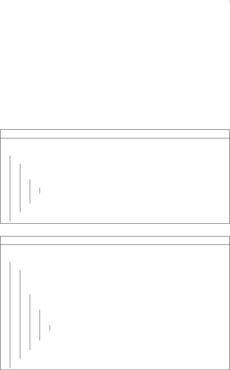
searching 93
order. Out-order is the opposite of in-order. Nodes are visited right to left, and a binary
search tree would be processed in reverse sorted order. In a post-order traversal, every
node is visited after its children. It is often used to delete an entire tree, node by node.
DFS can also be applied to graphs. Instead of having a left and right path, a node
in a graph may have many paths, each of which needs to be explored completely before
moving on to the next. However, depth-first searching a graph with a cycle will result
in looping through the nodes in that cycle indefinitely. This can be dealt with by ignor-
ing previously visited nodes and/or by stopping the search at a certain depth. Iterative
deepening is a process that involves depth-first searching to a certain depth and repeating
the search with a deeper depth until a given node is found. Recursive and iterative DFS
algorithms are given below. They handle cycles by keeping track of visited nodes.
Algorithm 8: DFS (recursive)
Data: A graph 𝐺and a node 𝑢in 𝐺
void dfs-recursive(𝐺,𝑢):
begin
Visit 𝑢;
foreach node 𝑣in 𝐺.adjacentNodes(𝑢)do
if 𝑣is not visited then
dfs-recursive(𝐺,𝑣);
end
end
end
Algorithm 9: DFS (iterative)
Data: A graph 𝐺and a node 𝑢in 𝐺
void dfs-iterative(𝐺,𝑢):
begin
Let 𝑆be a stack;
𝑆.push(𝑢);
while 𝑆is not empty do
𝑢⟵𝑆.pop();
if 𝑢is not visited then
Visit 𝑢;
foreach node 𝑣in 𝐺.adjacentNodes(𝑢)do
𝑆.push(v);
end
end
end
end
It is important to note that the recursive and iterative implementations of DFS do not
search in the same order. For example, if a binary tree is traversed using recursive DFS,
nodes at the same depth will be visited left to right. If it is traversed using iterative DFS,
nodes at the same depth will be visited right to left because storing them with a stack will
invert their order. It seems then that it might be preferable to implement DFS recursively.
searching 94
Table 17: DFS Computational Complexities
Resource Complexity Reasoning
Time 𝑂(|𝑉|+|𝐸|)The search must visit every node and walk every path.
Space 𝑂(|𝑉|)The call stack would hold |𝑉|frames if the tree was a
path. The stack would have to hold |𝑉|− 1 nodes if the
root were connected to every other node.
8.2 Breadth-First Search
Breadth-first search (BFS) is another way of traversing trees and graphs. Like DFS, it is
often used as a method of searching trees, but in general it is just a method to visit every
node in a tree or graph. Unlike DFS, it visits all neighbors of a node before visiting deeper
nodes.
Unlike DFS, BFS does not have a variety of orders like pre-order, in-order, etc. when
applied to a tree. Typically, nodes in the same level will be visited left to right and shallow
levels will be processed before deep levels, but the latter rule is the only true requirement
of a BFS. Like DFS, BFS can be written recursively, but it is much more natural to write
it iteratively, so that algorithm will be given first.
Algorithm 10: BFS (iterative)
Data: A graph 𝐺and a node 𝑢in 𝐺
void bfs-iterative(𝐺,𝑢):
begin
Let 𝑄be a queue;
𝑄.enqueue(𝑢);
while 𝑄is not empty do
𝑢⟵𝑄.dequeue();
if 𝑢is not visited then
Visit 𝑢;
foreach node 𝑣in G.adjacentNodes(𝑢)do
𝑄.enqueue(𝑣);
end
end
end
end
Note that the only difference between the iterative implementations of DFS and BFS is
the choice of data structure. DFS uses a stack to hold the next nodes to visit while BFS
uses a queue. This explains why DFS is natural to write recursively, and BFS is not. In
dfs-iterative, a stack is used to store the next nodes to visit. In dfs-recursive, the
algorithm stores its recursive subroutines on the call stack which is a stack data structure.
Instead of storing the next nodes to visit, dfs-recursive stores a subroutine that will
searching 95
find and visit the next nodes.
BFS can be written using recursion, but it will essentially require implementing a stack
(the call stack) into the algorithm. This is not a very meaningful way to implement BFS.
In fact, it is more like implementing DFS and running it on a single-branch tree in which
each node contains the BFS queue’s state at some particular step during a regular, itera-
tive BFS. Despite its inherent awkwardness, a recursive implementation of BFS is shown
below.
Algorithm 11: BFS (recursive)
Data: A graph 𝐺and a node 𝑢in 𝐺
void bfs-recursive(𝐺,𝑢):
begin
Let 𝑄be a queue;
𝑄.enqueue(𝑢);
bfs-recursive-helper(𝐺,𝑄);
end
Data: 𝑄
void bfs-recursive-helper(𝐺,𝑄):
begin
if Q is not empty then
𝑢⟵𝑄.dequeue();
Visit 𝑢;
foreach node 𝑣in G.adjacentNodes(𝑢)do
𝑄.enqueue(𝑣);
end
bfs-recursive-helper(𝐺,𝑄);
end
end
The space complexity of this implementation is particularly bad. If you needed to visit
|𝑉|nodes, you would have to store |𝑉|queues at once. In a binary tree, when a full node
is visited, one node is dequeued and two are enqueued, which increments the size of the
queue by 1. When the node has one child, the queue does not change size. When the node
has no children, the queue’s size decrements by 1. In the worst-case (which occurs if the
tree is perfect), the queue would increment in size by 1 until the last level. As BFS visits
the nodes in the last level, the queue would decrement by 1, starting at a size of 𝑙𝑜𝑔 |𝑉|
and ending empty when the final node is explored. At this point, the call stack would
start unwinding. The average queue size in this case would be 1
∕2⋅𝑙𝑜𝑔 |𝑉|, so the space
complexity would be 𝑂(|𝑉|𝑙𝑜𝑔 |𝑉|)instead of the 𝑂(|𝑉|)space complexity achieved by
the iterative implementation.

searching 96
Table 18: BFS Computational Complexities
Resource Complexity Reasoning
Time 𝑂(|𝑉|+|𝐸|)The search must visit every node and walk every path.
Space 𝑂(|𝑉|)The queue would have to hold |𝑉|− 1 nodes if the root
were connected to every other node.
DFS and BFS are Intertwined
DFS and BFS are two sides of the same coin. DFS is more natural to write
recursively, and BFS is more natural to write iteratively. DFS uses a stack, and
BFS uses a queue. Both searches are 𝑂(|𝑉|+|𝐸|), so they will theoretically
finish traversing the same tree in the same amount of time. However, in general,
DFS will search for nodes that are far away from the source before BFS will.
And, in general, BFS will search for nodes that are near the source before DFS. If
you have an idea of "how distant" your desired item likely is from your source,
it might be worth choosing one over the other to improve your search performance.
The time complexity of DFS and BFS on trees can also be expressed as 𝑂(𝑏𝑑)
where 𝑏is the branching factor of the tree and 𝑑is the depth of the tree. This
suggests that a search is faster if the tree is narrower or shorter. To put it another
way, the search is faster the closer the desired node is to the top and the left of the
tree.
DFS and BFS are used to solve a variety of fundamental computer science
problems. Either one can be used to find the number of connected components
in a graph. The idea is to iterate over every node in a graph and, if it has not yet
been visited, to perform a DFS or BFS. The number of searches made equals the
number of connected components. DFS and BFS can also be used to test if a
graph is bipartite. This is done by checking if the graph can be 2-colored. DFS is
used to solve mazes. BFS is used to solve shortest path problems.
It is interesting to think of DFS and BFS as two different kinds of personalities.
DFS is like a person who is overly confident and always pressing forward, even if
they are going in the wrong direction. They only take a step back if they are forced
to. BFS is like a person who is overly cautious and always investigating every
option before moving forward. They only move on if there is nothing else to learn
around them. Both approaches are useful, but they are useful in different scenarios.

searching 97
8.3 Bidirectional Search
A bidirectional search involves performing two searches on the same graph simultane-
ously. They can be DFS or BFS, but they are typically BFS. This algorithm is often used
to check if two nodes are connected or to solve the shortest path problem. If two breadth-
first searches start at two different roots, they will search outward until one reaches a node
that the other visited already. If this happens, the two roots are connected, and the shortest
path goes through that intersection. The shortest path can be traced from that intersection
by moving up through the intersection node’s ancestry. In one search, the intersection’s
oldest ancestor is 𝑠. In the other search, it is 𝑡. If you wish to know not only that 𝑠and 𝑡
are connected but also the details of their shortest path, you must keep track of the parent
of every node you visit, perhaps with a map.
Why is this more useful approach than a regular BFS? Let 𝑠and 𝑡be two nodes that are
𝑑edges away from each other. If you BFS starting from s, you would have to search to
a depth of 𝑑to find 𝑡, which would result in an 𝑂(𝑏𝑑)search time. However, if you BFS
starting from both 𝑠and 𝑡, each process would have to search to a depth of 𝑑∕2to find the
intersection, which would result in an 𝑂(2𝑏𝑑∕2) = 𝑂(𝑏𝑑∕2)search time, which is a major
searching 98
improvement.
Algorithm 12: Bidirectional Search
Data: A graph 𝐺and node 𝑠and 𝑡in 𝐺
void bidirectional(𝐺,𝑠,𝑡):
begin
Let sParentMap and tParentMap be maps;
Let sQ and tQ be queues;
Let sParent and tParent be null nodes;
Let sCurr and tCurr be null nodes;
sQ.enqueue(𝑠);
tQ.enqueue(𝑡);
while sQ is not empty and tQ is not empty do
sCurr ⟵sQ.dequeue();
tCurr ⟵tQ.dequeue();
sParentMap.put(sCurr, sParent);
tParentMap.put(tCurr, tParent);
if sCurr is visited then
printShortestPath(sCurr,sParentMap,tParentMap);
return;
end
else if tCurr is visited then
printShortestPath(tCurr,sParentMap,tParentMap);
return;
end
Visit sCurr;
Visit tCurr;
for node sAdj in G.adjacentNodes(sCurr) do
sQ.enqueue(sAdj);
end
for node tAdj in G.adjacentNodes(tCurr) do
tQ.enqueue(tAdj);
end
sParent ⟵sCurr;
tParent ⟵tCurr;
end
end
Consider using a bidirectional BFS to solve the search problem instead of the shortest
path problem. A breadth-first search will find nearby nodes quickly. Therefore, if you
had multiple guesses of where your search item might be located, it would make sense to
perform breadth-first searches in all of those areas.
8.4 Dijkstra’s Algorithm
Blah

sorting 99
8.5 Binary Search
Blah
8.6 Rabin-Karp Algorithm
Blah
9 sorting
Blah
9.1 Selection Sort
Blah
9.2 Insertion Sort
Blah
9.3 Merge Sort
Blah
9.4 Quick Sort
Blah
9.5 Radix Sort
Blah
9.6 Topological Sort
Blah
10 miscellaneous
Blah

miscellaneous 100
10.1 Cache Replacement Algorithms
Blah
10.2 Permutations
Blah
10.3 Combinations
Blah
10.4 Bitwise Algorithms
Blah

101
Programming Language Theory
11 elements of programming languages
11.1 Syntax
11.2 Type Systems
11.3 Control Structures
11.4 Libraries
11.5 Exceptions
11.6 Comments
12 program execution
13 a history of programming languages
14 programming paradigms
14.1 Imperative versus Declarative
14.1.1 Functional Programming
14.1.2 Logic Programming
14.2 Procedural versus Object-Oriented
15 programming techniques
15.1 Higher-Order Programming
15.1.1 Lambda Expressions
15.2 Currying
15.3 Metaprogramming

102
Implementation, Featuring an
Exploration of Java
Blah
16 how does java work?
17 java standard library
17.1 java.lang
17.2 java.util
17.3 java.io
17.4 java.net
18 java techniques
Blah
18.1 Static Initialization Blocks
Blah
18.2 Lambda Expressions
Blah
19 java frameworks

103
Additional Technologies
"Stupid Computer Shit"
20 computer networks, including the internet
21 unit testing
Blah
21.1 JUnit
Blah
22 version control
Blah
22.1 Git
How do you download stuff from GitHub? There are a few methods that might be avail-
able, depending on the software.
∙git clone the directory
∙wget raw files
∙Grab it from a package repo with something like pacman
∙Get it from the AUR with something like yay or yaourt
∙Download a tarball, unzip it, extract it, and build the source files into an executable
23 build automation
23.1 Make
GNU Make compiles source files into executables.
23.2 Maven
Blah

unix 104
24 unix
24.1 History of Unix and GNU/Linux
24.2 A Tour of the Unix File System
24.3 Common Commands and Tasks
∙chmod +x
∙.bash_profile is executed at login for the current user
∙.bashrc is executed every time a shell is opened for the current user
∙INI files
∙Run command (rc) files.
∙Shell scripts. Shebangs.
∙Config files (plain text)
∙Handling swap files in Vim. You accidentally deleted a terminal where you were
editing a file, and now you have a file with a previous save and the autosaved file.
Which one do you want to look at? You probably want to recover (R) the swap
file, save its changes to the main file (:w), reload the file content (:e), and when
prompted about the existence of a swap file, delete the swap file (D). If the delete
option is not available, that means that the file is being edited elsewhere. Go close
those windows.
∙Daemon - background process
∙File Descriptors
24.4 Making a Personalized Linux Installation
∙Install Arch
∙Download Desktop Environment
∙Download Window Manager
∙Download Login Manager (or use startx)
∙Learn pacman
∙Download from the AUR
∙urxvt terminal has its perl extensions and configuration in ~/.Xresources (run xrdb
~/.Xresources to have the window system grab the changes without a reboot)
∙urxvt needs monospaced font and fonts that support Unicode
∙feh

virtualization & containerization 105
∙compton
∙polybar
∙vim
∙Change desktop environment on startup by adding exec ds_name to the bottom of
~/.xinitrc
25 virtualization & containerization
Blah
25.1 Docker
Blah
26 markup and style languages
26.1 TeX
Blah
26.2 HMTL
Blah
26.3 CSS
Blah
27 data formats
Blah
27.1 XML
Blah
27.2 JSON
Blah

query languages 106
28 query languages
28.1 SQL
Blah

107
Software Development and
Philosophies
29 software engineering processes and principles
∙Agile
∙Test Driven Development
∙"Software development process"
∙Single Responsibility Principle
∙Open Closed Principle
30 design patterns
∙Singleton
∙Abstract Factory

108
Appendices
Summarize the appendices below...
a mathematical fundamentals

system design 109
b system design
b.1 Server Technologies
domain name system (dns) server Translates a domain name to an IP address
of a server containing the information on the requested website. Could use round-robin,
load balancing, or geography to choose a server associated with a certain domain name.
An OS or browser can cache DNS results until the result’s time to live (TTL) expires.
If a local DNS server does not know the IP address of some domain name, it can ask a
nearby, larger DNS server if it knows. The biggest DNS servers are called root servers,
and they are distributed across the world’s continents. They return lists of servers that
would recognize your requested domain name. These are authoritative name servers for
the appropriate top-level domain (.com, .org, .edu, .ca, .uk, etc.).
There are many kinds of results that can be returned by a DNS server:
ns record Name server. Specifies the names of the DNS servers that can translate
a given domain.
mx record Mail exchange. Specifies the mail servers that will accept a message.
a record Address. Points a name to an IP address.
cname Canonical. Points a name to another name (google.com to www.google.com)
or to an A record.
load balancer Decides which servers to send requests to based on some criteria (ran-
dom, round-robin, load, session, Layer 4, Layer 7). Can be implemented in software or
hardware. Can generate cookies to send to the user. The user can then send those cook-
ies back to return to the server they were using. Multiple load balancers are needed for
horizontal scaled systems.
reverse proxy A web server that acts as an intermediary between clients and backend
servers. Forwards requests to the backend and returns their responses. This hides the
backend server IPs from the client and allows for a centralized source of information.
However, it is a single point of failure, so load balancers are a better choice for horizontally
scaled systems.
application layer It may be useful to have a layer of application servers separate
from your web servers. This allows you to scale the layers independently. A web server
serves content to clients using the HTTP. An application server hosts the logic of the
application, which could generate an HTTP file to send to a web server. Web servers are
often used as reverse proxies for application servers.
b.2 Persistent Storage Technologies
caches Caching involves putting data that is referenced often on a separate, small mem-
ory component. For example, when you stay on the same domain, your OS can cache an
IP address so it doesn’t have to look up the same IP address every time.
file-based caching The data that you want is saved in a local file. For example,
you could cache an HTML file instead of dynamically creating a website with data
from a database. Not recommended for scalable solutions

system design 110
in-memory caching Copy the most popular pieces of data from an application’s
database and put it in RAM for faster access times. If you choose to cache a database
query as a key and the result as a value, it is hard to determine when to delete this pair
when the data becomes stale. Alternatively, you could cache objects. When an object
is instantiated, make the necessary database requests to initialize values, and store the
object in memory. If a piece of data changes, delete all objects that use that piece
of data from cache. This allows for asynchronous processing (the application only
touches the database when creating objects). Popular systems include Memcached
and Redis.
cache update strategies
cache-aside The cache does not interact with storage directly. The applica-
tion looks for data in the cache. Upon a cache miss, it finds its data in storage,
adds it to the cache, and returns the data. Only requested data is cached. Data in
the cache can become stale if it is updated in storage but not in cache.
write-through The application uses the cache as its primary data store, and
the cache reads and writes to the database. Application adds data to cache, cache
writes to data store and returns value to the application. Writes are synchronous
and slow, but data is consistent. Reads of cached data are fast. However, most
data written to the cache will not be read.
write-back The application adds data to the cache, and the data is asynchronously
written to the database. Data loss could occur if the cache fails before new data
is written to the database.
raid Redundant Array of Independent Disks is a technique that uses many physical disk
drives to improve the redundancy or performance of a system.
raid0 Writes a portion of a file on one drive and the other portion on another drive
concurrently. This doubles write speed but has no redundancy.
raid1 Writes the whole file on both drives. No write speed improvements, but
improves redundancy.
raid10 A combination of RAID0 and RAID1. If you have 4 drives, a file is striped
between 2 drives and the same striped data is written concurrently to the other 2
drives.
raid5 Given N drives, you stripe data across N-1 drives and stores a full copy of
the file on 1 drive.
raid6 Given N drives, you stripe data across N-2 drives and stores a full copy of
the file on 2 drives.
relational database management system (rdbms) Arelational database is
a collection of items organized in tables. A database transaction is a change in a database.
All transactions are ACID: Atomic (all or nothing), Consistent (moves the database from
one valid state to another), Isolated (concurrent transactions produce the same results as
serial transactions), and Durable (changes do not revert). Various techniques for scaling
databases are described below.
replication

system design 111
master-slave replication A master serves reads and writes, replicating
writes to the slaves, which can only serve reads. If a master goes offline, the
system is read-only until a slave is promoted.
master-master replication There are multiple masters that can serve
both reads and writes and coordinate with each other on writes. A master can
fail and the system can still be fully-functional. However, writes need to be load
balanced. Master-master systems are usually either eventually consistent (not
ACID) or have high-latency, synchronized writes.
replication disadvantages If a master dies before it can replicate a write,
data loss occurs. Lots of write replication to slaves means that slaves cannot
serve reads as effectively. More slaves means more replication lag on writes.
federation Splits up databases by function instead of using a monolithic database.
Reads and writes go to the appropriate database, resulting in less replication lag.
Smaller databases can fit a greater percentage of results in memory, which allows
for more cache hits. Parallel writing is possible between databases. Not effective for
large tables.
sharding Data is distributed across different databases (shards) such that each
database can only manage a subset of the data (like submitting tests to piles labeled
A-M and N-Z). Less traffic, less replication, more cache hits, parallel writes between
shards. If one shard goes down, the others can continue to work (however, replication
is still necessary to prevent data loss). Load balancing between shards is important.
Sharing data between shards could be complicated.
denormalization Improves read performance at the expense of write performance.
Redundant copies of data are written in multiple tables to avoid expensive joins.
sql tuning Benchmark your database system and optimize it by restructuring ta-
bles and using appropriate variables.
nosql A NoSQL database stores and retrieves data in ways other than tabular relations.
Its transactions are BASE: Basically Available (the system guarantees availability), Soft
state (the state of the system may change over time, even without input), and eventually
consistent (will become consistent over a period of time, if no further input is received).
NoSQL prioritizes availability over consistency. Some configurations are described be-
low.
key-value store Stores data using keys and values. O(1) reads and writes. Used
for simple data model or for rapidly changing data, such as a cache. Complex opera-
tions are done in the application layer.
document store All information about an object is stored in a document (XML,
JSON, binary, etc.). A document store database provides APIs or a query language
to query the documents themselves.
wide column store The basic unit of data is a column (name/value pair). Columns
can be grouped in column families. Super column families can further group column
families. Useful for very large data sets.
graph database Each node is a record and each edge is a relationship between
records. Good for many-to-many relationships. Not widely used and relatively new.

system design 112
b.3 Network Techniques
horizontal scaling Distributes your data over many servers. Alleviates the load on
a single server, but now requests have to be distributed across these servers. Introduces
complexity: load balancers are required, and servers should now be stateless.
asynchronism Asynchronous tasks are done to prevent the user from waiting for their
results. One example is anticipating user requests and pre-computing their results. An-
other example is having a worker handle a complicated user job in the background and
allowing the user to interact with the application in the meantime. The worker will then
signal when the job is complete. A job could also "appear" complete to the user, but
require a few additional seconds to actually complete.
firewalling A network security system typically used to create a controlled barrier
between a trusted internal network and an untrusted external network like the Internet.
For example, if you want your server to listen for HTTP and HTTPS requests, you could
restrict incoming traffic to only ports 80 and 443. This prevents clients from having, for
example, full read and write access to your databases.
consistency patterns When many servers hold copies of the same data, we must
find an acceptable method of updating them.
weak consistency After a write, reads may or may not see it. A best effort
approach is taken. Works when the application must continue running and data can
be lost during outages (VoIP, video chat, multiplayer games). Good for any sort of
"live" service.
eventual consistency After a write, read will eventually see it. Works when
the application must continue running, but data cannot be lost, even during outages
(email, blogs, Reddit). Good when writes are important, but reading stale data for a
short period of time is acceptable.
strong consistency After a write, reads will see it. Works when everyone
needs to see the most up-to-date information at all times, even if it slows the whole
system down (file systems, databases). Good when stale data is unacceptable.
shared session state If users can access a website from many different servers,
how do you keep track of their session data? If a user logs in on one server, how can the
network know they are logged in when they move to another server? Store all session
data on a single server. Use RAID for redundancy.
microservices An application can be structured as a collection of microservices that
have their own well-defined independent functions. These microservices can be combined
in a modular fashion to create the full application. Each microservice could have its own
network architecture. This allows for modular scaling of an application. Software like
Apache Zookeeper is used to keep track of microservices and how they interact.
content delivery network (cdn) A CDN is a globally distributed network of
proxy servers that serves content to users from nearby nodes. A push CDN only updates
some piece of data when the developer pushes data to it. It’s faster, but requires more
storage on the CDN. A pull CDN get content from the developer’s server whenever a
client requests it. It’s slower, but requires less space on the CDN.

sources, not citations 113
c sources, not citations
The origin of concepts, even for a scholar, is very difficult to trace. For a
nonscholar such as me, it is easier. But less accurate.
—Peter Freyd

lessons learned 114
d lessons learned

thoughts on education 115
e thoughts on education

passion 116
f passion

the future of this guide 117
g the future of this guide
