Thesis Guide
User Manual:
Open the PDF directly: View PDF ![]() .
.
Page Count: 121 [warning: Documents this large are best viewed by clicking the View PDF Link!]
- Introduction
- Tips and tricks
- Submitting your thesis
- Useful packages
- Figures
- Tables
- References
- Layout and language
- Changes and plans
- TeX setup and packages
- Print shops
- Making a glossary or list of acronyms
- Plots with TikZ
- Long tables
- A famous equation is E = mc2
- Old or obsolete information and instructions
- Bibliography
- List of Figures
- List of Tables
- Glossary
- Acronyms
- Acknowledgements
Users Guide to Writing a Thesis in a
Physics/Astronomy Institute of the University of
Bonn
Hinweise und Tipps
zur
Produktion einer Bachelor/Master/Diplom/Doktorarbeit
in der
Mathematisch-Naturwissenschaftlichen-Fakultät
der
Rheinischen Friedrich-Wilhelms-Universität Bonn
vorgelegt von
Ian C. Brock
aus
Stoke-on-Trent
Version 6.0
8th December 2018
Bonn 2018
1. Gutachter: Prof. Dr. John Smith
2. Gutachterin: Prof. Dr. Anne Jones
Tag der Promotion:
Erscheinungsjahr:

Acknowledgements
I would like to thank the members of my group who read and criticised different versions of this
guide. Questions and suggestions from students who used previous versions of the guide have led
to a number of improvements. The authors of the book “Physics at the Terascale” provided many
examples of different L
A
T
E
X usage and conventions that were also very helpful. Andrii Verbytskyi
provided the tikz examples. Miriam Ramos provided advice and input on how to implement references
in the style usually used in astronomy publications and theses. Kaven Yau suggested the new (as of
version 4.0) way of steering which cover and title pages are included. Jan Schmidt provided many
useful suggestions that found their way into version 6.0.
Acknowledgements at the beginning should be a
\chapter*
so that they do not appear in the Table
of Contents.
iii

Contents
1 Introduction 1
2 Tips and tricks 5
2.1 How to use the ubonn-thesis style ........................... 5
2.2 Options that can be passed to ubonn-thesis ..................... 7
2.3 Do ............................................ 9
2.4 Do not .......................................... 11
2.5 Units ........................................... 13
2.5.1 siunitx package ................................. 13
2.5.2 SIunits/hepunits packages ........................... 15
2.6 Definitions in particle physics .............................. 16
2.7 Hints ........................................... 17
2.8 Common English mistakes ............................... 18
2.9 Line numbering ..................................... 19
2.10 Updating ubonn-thesis ................................. 20
3 Submitting your thesis 21
3.1 PhD thesis ........................................ 21
3.1.1 Submission ................................... 21
3.1.2 Printing the final version ............................ 21
3.2 Master/Diplom/Bachelor thesis ............................. 22
3.2.1 Submission ................................... 22
3.2.2 MSc/Diplom theses for the department library ................. 23
3.2.3 BSc theses ................................... 23
4 Useful packages 25
4.1 Layout and language .................................. 25
4.2 Appearance ....................................... 26
4.3 Other packages ..................................... 26
4.4 ToDo Notes ....................................... 29
5 Figures 31
5.1 Simple figures ...................................... 31
5.2 Fancier figures ...................................... 32
5.3 Figure formats ...................................... 33
v
5.4 TikZ and PGF ...................................... 34
5.4.1 Accelerator lattices ............................... 35
5.5 Placement ........................................ 35
5.5.1 standalone package and class ......................... 38
5.6 Feynman graphs ..................................... 38
5.6.1 PyFeyn ..................................... 38
5.6.2 FeynMF and FeynMP .............................. 39
5.6.3 Feynman graphs with TikZ........................... 41
6 Tables 43
6.1 Use of \phantom .................................... 43
6.2 Using siunitx and the Scolumn option ......................... 44
6.3 Using dcolumn ..................................... 47
7 References 51
7.1 Formatting by hand ................................... 51
7.2 Using BibT
EX and biblatex ............................... 52
7.3 BibT
EX entries ..................................... 53
7.3.1 Entry types ................................... 54
7.3.2 Entries from Inspire and CDS ......................... 54
7.3.3 More on names ................................. 55
7.4 Formatting references .................................. 55
7.4.1 biblatex styles .................................. 55
7.4.2 Traditional BibT
EX styles ............................ 57
7.5 Errata .......................................... 57
7.6 Sources for references .................................. 58
7.7 Common wishes ..................................... 59
7.8 Using mcite ....................................... 60
8 Layout and language 61
8.1 Page layout ....................................... 61
8.2 Footnotes ........................................ 61
8.3 Thesis in German .................................... 63
8.4 Fonts .......................................... 64
8.5 Other languages ..................................... 64
8.6 Coloured links ...................................... 64
8.7 Chapter headings .................................... 65
A Changes and plans 67
B T
E
X setup and packages 71
B.1 Integrated environments ................................ 71
B.1.1 T
EXstudio .................................... 72
B.1.2 Visual Studio Code ............................... 72
B.1.3 Kile ....................................... 72
vi
B.2 MacOS ......................................... 73
B.3 (Ku|Xu|U)buntu ..................................... 73
B.4 Windows ........................................ 75
B.4.1 MiKT
EX.................................... 76
B.4.2 T
EX Live .................................... 77
C Print shops 79
D Making a glossary or list of acronyms 81
D.1 ZEUS detector description ............................... 82
E Plots with TikZ85
F Long tables 87
G A famous equation is E=m c291
G.1 A slightly less famous equation F=ma ........................ 91
G.2 The cross-section is given by σ=N/L ........................ 91
H Old or obsolete information and instructions 93
H.1 More on feynmf ..................................... 93
H.2 Windows ........................................ 94
H.2.1 Windows XP .................................. 94
H.2.2 T
EXnic Center ................................. 95
Bibliography 97
List of Figures 99
List of Tables 101
Glossary 103
Acronyms 105
Acknowledgements 113
vii

CHAPTER 1
Introduction
L
A
T
EX file: ./guide_intro.tex
When you want to start writing your thesis you usually ask a (more senior) colleague if he or she has a
L
A
T
E
Xframework that you can start with. He or she in turn had asked their (more senior) colleague for
an example thesis several years earlier etc.! Maybe it is surprising that we are actually using L
A
T
E
X
and not T
EX to write theses!
L
A
T
E
X (or more precisely the packages that one can use in L
A
T
E
X) is actually in a state of continual
development and improvement, so it certainly makes sense to review what packages are available, how
they should be used and whether there are better ways of doing things than methods used 10 or more
years ago.
The aim of this guide is to break with the tradition of just adapting what your predecessor used and
provide up-to-date guidelines on the layout and packages that can or should be used for thesis writing.
The guide should also provide you with enough information for you to concentrate on the content of
your thesis, rather than having to spend too much time making it look nice!
You may ask why bother? First and foremost a thesis is something that you should be proud of!
I therefore think it is actually worth devoting some effort to not only making it look good, but also
to using correct and consistent notation when you write it. Figures and tables should be legible and
understandable (including the size of the axis labels!). You should, however, not have to spend too
much time working out how to make the thesis look the way you want it to. It is also good if you can
avoid annoying or irritating your supervisor if he or she also thinks that
GeV/c2
should be written like
this and not as GeV/c2or GeV/c2etc. or some mixture of the two.
The recommendations are based on experience I gained:
•preparing the lecture course „EDV für Physiker“ for many years;
•editing the book “Physics at the Terascale”, which was published in April 2011;
•rewriting and maintaining the ATLAS L
A
T
EX document class and style files;
•
regular reading of the „TeXnische Komödie“, which is published by Dante (Deutschsprachige
Anwendervereinigung T
EX) 4 times a year;
•general interest in preparing good quality documents;
1

Chapter 1 Introduction
•reading quite a lot of theses!
This document does not attempt to explain how to write L
A
T
E
X. I assume a basic level of knowledge.
The aim is more to give some practical tips and solutions to solve problems that often occur when you
are writing your thesis. There are many books and online documents to help you get started, so many
in fact that it is difficult to know where to start. My favourite is “Guide to L
A
T
E
X” from Kopka [KD04].
Be sure to read the Fourth Edition though. It was originally written in German where the title is „L
A
T
E
X:
Eine Einführung“. When you want to know what packages exist, what they can do and how to use them,
consult “The L
A
T
E
X Companion” from M. Goossens et al. [MG04]. A fairly comprehensive online
guide is the “A (Not So) Short Introduction to LaTeX2e.” [Oet+], which is available in many languages.
Help on getting started and a list of online documents can be found on the CTAN (Comprehensive T
E
X
Archive Network) information page
http://tug.ctan.org/starter.html
. Other useful sources
of information that I and others use are:
•http://www.tex.ac.uk/faq
: This contains an extensive FAQ (maybe even a bit better than
the German one maintained by Dante). An interesting feature is the “Visual FAQ” that serves as a
rather unorthodox, but very intuitive kind of index:
http://www.tex.ac.uk/tex-archive/
info/visualFAQ/visualFAQ.pdf.
•http://tex.stackexchange.com
often comes up in Google searches and contains a lot of
very useful tips.
•http://detexify.kirelabs.org/classify.html
contains a little online tool to find L
A
T
E
X
names of symbols. It works quite well and can be a lot quicker than searching through the
written documentation.
Not everyone knows about the
texdoc
command which should be available for Linux and MacOS
T
E
X installations. To get help on a package, you can simply give the command
texdoc geometry
,
etc. Note that to see the KOMA-Script manual you have to know the name of the PDF file:
texdoc
scrguide
or
texdoc scrguien
for the German and English versions, respectively. The AMS Math
users guide also does not have a totally obvious name — try
texdoc amsldoc
. It contains a whole
host of useful information on typesetting (complicated) equations.
The Physikalisches Institut is a member of Dante and so receives three copies of each issue of „der
TeXnische Komödie“, one of which is available in the department library in PI. The booklet often
contains useful hints on typesetting. We also get a DVD every year with T
E
X distributions for Unix,
MacOS and Windows. Details on how to install a L
A
T
EX distribution can be found in Appendix B.
If you write your thesis in English, questions are sure to occur on how things should be written
in English, what is the correct punctuation and hyphenation, and what do you have to worry about
when you construct sentences. I will not attempt to answer such questions here. “The guide to writing
ZEUS papers” from Brian Foster [Fos] contains a wealth of useful information. Brian kindly gave me
permission to package a PDF file of the note with this guide.
This document is structured as follows. Chapter 2tells you how to get started with the files and the
package. It also contains several tips and tricks that it is probably good to include early. It is sometimes
not clear which version of the cover should be used when submitting and/or printing your thesis. Some
instructions are given in Chapter 3. This is followed by Chapter 4, which lists the packages used in
this document and says what they are good for. Chapters 5and 6give some guidelines for figures and
tables. Chapter 7discusses the tricky business of references and their formatting. Some hints on how
2

to solve common layout problems, which fonts one can use and how to handle multiple languages in a
document are given in Chapter 8. In the appendix I include some more information on the T
E
X setup I
have used to test things. I have seen a glossary (list of acronyms) in a few theses and think this is a
nice idea. The appendix shows how you can create such a list. As big tables are often moved to the
appendix, an example of how to create such tables is given there as well.
While this guide is structured pretty much like a thesis, I have included a couple of extra features
that are usually not needed in a thesis. The first is a link to the relevant L
A
T
E
X file at the beginning
of each chapter. I have also added an index, as that is probably a useful complement to the table of
contents.
Regular updates are made to the guide, so it is worth checking every so often to see if a new version
is available. Corrections and suggestions for improvements are very welcome.
3

CHAPTER 2
Tips and tricks
L
A
T
EX file: ./guide_tips.tex
Over time I have collected quite a lengthy list of things you should “Do” and “Not Do” (at least in my
head) that I think it is useful to write down early in the document, so that you may actually read them!
In this chapter I first tell you how to get and use the style file and then give some tips. I have also
started to add a list of common English mistakes, especially those made by German speakers!
2.1 How to use the ubonn-thesis style
The idea with this document is that you also look at the L
A
T
E
X that is used to create it, in order to
find out how things are done. I will therefore usually not give the L
A
T
E
X commands in the printed
document, but assume that you will have a look at the L
A
T
E
X source. To help you with this, each
chapter contains a link to the relevant file at the top. This link should work if you have compiled the
guide yourself and are in the
guide
subdirectory of the
ubonn-thesis
directory tree. The files that
make up this document are available in a Git repository and as a
tar
file. To get the latest Git entries
give the command:
git clone https://git.physik.uni-bonn.de/cgit/projects/ubonn-thesis.git
If you want to checkout a particular version you can give the command:
git clone --branch vN.M https://git.physik.uni-bonn.de/cgit/projects/ubonn-thesis.git
The tar file (and the tag tree (as of version 1.5)) also includes the guide as a PDF file:
thesis_guide.pdf
.
It can be obtained from:
http://www.pi.uni-bonn.de/teaching/uni-bonn-thesis and
http://www.pi.uni-bonn.de/lehre/uni-bonn-thesis.
Once you have the files, you can then give the command:
make new [THESIS=dirname] [TEXLIVE=YYYY]
to create a new directory with several files to help you get started. By default the directory name will be
mythesis
. If you want to write a thesis that uses the astronomy style of references (
authoryear
style
and a bibliography at the end of each chapter) give the command “
make astro [THESIS=dirname]
”.
To compile your thesis try:
5

Chapter 2 Tips and tricks
cd mythesis [or dirname]
make thesis
If your version of T
E
X Live is older than 2011, you should really update to a newer version! If this
is not possible, use the command “
make new09
” followed by “
make thesis09
” or “
make thesis
BIBTEX=bibtex”. See Section 2.2 for a list of the options that can be passed to the package.
As of version 6.0,
make thesis
uses the
latexmk
command for compilation.
latexmk
looks at
your logfile and decides how many times
pdflatex
etc. have to be run. If you use feynmf or feynmp
you should use the commented out version of the
LATEXMK
variable that includes the
-shell-escape
option.
1
For details on how to compile a glossary with
latexmk
see Appendix D. If for some reason
latexmk
does not work you can use the command
make thesis11
instead. The tool
pplatex2
is
supposed to provide a nicely formatted version of the L
A
T
EX output on the command line.
My original idea was that the style file should work for all recent T
E
X installations. However, some
of the packages I recommend have been changing quite a lot over the past few years. You should
therefore set the T
E
X Live version you are using appropriately. The default setting is 2016.
3
This
is also the setting to use for an up-to-date version of MikTeX (2.9). Things should compile without
any changes if you use T
E
X Live 2013 or later. Look in the style file to see what changes are made
depending on the year you use. You can change the T
E
X Live version when you make a new thesis by
giving a command like “
make new TEXLIVE=2011
”.
4
If you switch T
E
X Live versions do a “
make
clean cleanbbl cleanblx” in between.
Note that as of version 2.1, the main file for the thesis (
mythesis.tex
), the
Makefile
and the
style file (
ubonn-thesis.sty
) are copied into your
mythesis
subdirectory. This means that if you
update the ubonn-thesis you can look for differences between the new style file and the one you have. It
also implies that if you want the update to have an effect on your thesis you should copy the
Makefile
and ubonn-thesis.sty into the directory with your thesis. For more details see Section 2.10.
As of version 4.0 of the package, you specify the type of thesis and the stage as options to the
\documentclass
or to the ubonn-thesis package. These options select the appropriate title and cover
pages. The following thesis types exist:
PhD a PhD thesis;
Master a Master thesis;
Diplom a Diplom thesis;
Bachelor a Bachelor thesis.
The following stages exist:
Draft you are still writing your thesis;
Submit you are ready to submit your thesis;
Final the final version of your thesis. For PhD theses this is the version that goes to ULB;
PILibrary
final version of your thesis with an extra cover page including an abstract for the PI library.
1
I got this information from
https://tex.stackexchange.com/questions/374160/how-to-have-latexmk-
always-use-shell-escape.
2Can be downloaded from https://github.com/stefanhepp/pplatex.
3Setting the T
EX Live version to one that is lower than your installation should not cause any problems.
4For even older versions of T
EX Live use the command “make new09”. This turns off the use of biblatex.
6
2.2 Options that can be passed to ubonn-thesis
See Chapter 3for some more details about thesis submission.
If you are not a member of the „Physikalisches Institut“ you should also change
\InstituteName
,
\inInstitute
and
\InstituteAddress
. The style file
ubonn-thesis.sty
already contains the
appropriate definitions for PI, HISKP, IAP and AIfA.
All packages that are needed should be part of your T
E
X installation. If not you may have to install
them or ask your system administrator to do so.
If you just want to make the cover pages, use the file
cover_only.tex
. Be sure to adapt the font
selected in
ubonn-thesis.sty
to the font you actually used in your thesis. Be aware that not all font
sizes are available in all font collections. If you used the default L
A
T
E
X font in your thesis, then choose
lmodern in the style file.
The main file for this guide is
guide/thesis_guide.tex
and it includes the L
A
T
E
X files in the
directory
./guide
and some of the Feynman graphs in the directories
./feynmf
and
./tikz
. Again
this guide should compile without changes for T
E
X Live 2013 or later. For earlier versions set
\texlive
in
thesis_guide.tex
to the appropriate value. Set the default font to txfonts for T
E
X
Live 2011 and older. If you want to compile the guide with T
E
X Live older than 2011, it is probably
easier to switch from biblatex to traditional BibT
EX. This is done via the make new09 command.
2.2 Options that can be passed to ubonn-thesis
From version 3.0 onwards it is possible to change things in the style file by passing options to it. A
few default packages also changed with this version. subfig
→
subcaption and longtable
→
xtab. The
syntax
siunitx
and
siunitx=true
is equivalent. Use
siunitx=false
to turn off an option. The
following options exist:
Option Default Description
PhD false A PhD thesis.
Master false A Master thesis.
Diplom false A Diplom thesis.
Bachelor false A Bachelor thesis.
Draft true Draft version of the thesis.
Submit false Version of the thesis to be submitted.
Final false Final version of the thesis (for PhD theses ready to go to ULB).
PILibrary false Final version including an extra cover page for the PI library.
thesistype Unknown Specify the thesis type.
thesisversion Draft Specify the stage of the thesis.
texlive 2016
Specify the T
E
X Live version. You can also use the older command
\newcommand*{\texlive}{2016}.
siunitx true Use the siunitx package for typesetting units.
eVkern false
Apply a kern of -0.1em to
eV
in order to move “e” and “V” closer together.
This is not necessary if you use the newtx font package.
dcolumn true A package for helping to align things in tables.
7
Chapter 2 Tips and tricks
Option Default Description
physics false Useful mathematical constructions for physics.
hepparticles true
Standardised names and formatting for particle physics. This loads
hepnicenames and heppennames.
hepitalic true Use italics rather than upright letters for particles.
mhchem true A nice package for chemical elements and processes.
feynmf false Include the feynmf package for Feynman graphs.
feynmp false Include the feynmp package for Feynman graphs.
subcaption true
A package for making sub-figures (and sub-tables) and captions for them.
subfig false A package for making sub-figures and captions for them.
subfigure false A package for making sub-figures and captions for them (deprecated).
xtab true A package for tables that are longer than one page.
longtable false Another package for tables that are longer than one page.
supertabular false Another package for tables that are longer than one page.
newtx true Use the newtx font packages (newer version of txfonts).
txfonts false Use a Times-Roman-like font.
palatino false Use a combination of Palatino, Courier and Helvetica fonts.
titlesec false Use the titlesec package for formatting chapter titles.
floatopt true Adjust settings that control the number and placement of floats.
biblatex true Include biblatex.
astrobib false Adjust biblatex options to conform to the usual astronomy style.
todonotes false Turn on use of the todonotes package and define \mynote.
shownotes false Show the ToDo notes (also turns on todonotes).
cleveref false Turn on use of the cleveref package.
clevercaps true Capitalise Fig., Table etc.
backend biber
Specify the backend to use for biblatex. Possibilities are
biber
,
bibtex
or bibtex8.
backref true
The bibliography lists where the reference is cited. This option is very
useful when writing your thesis, but should probably be turned off for the
final version.
bibencoding Set the encoding for the bibliography (usually not needed).
bibstyle numeric-comp
Specify the style to use for the references. Standard values are
numeric-comp or alphabetic.
firstinits false Use firstinits instead of giveninits for biblatex.
Some default option values are adjusted depending on the T
E
X Live version. See the
ubonn-thesis
style file to find out what is changed.
Depending on the font you use, you may find that the “e” and “V” in
eV
,
MeV
etc. are too far apart.
You can pass the option eVkern to ubonn-thesis in order to move them 0.1em closer together.5
5
This option has no effect for T
E
X Live 2011 and older, as siunitx adjusted the spacing internally using the parameter
eVcorra. It is not needed if you use the newtx font package.
8

2.3 Do
2.3 Do
•
Have 1–2 other people read your thesis well before you are supposed to submit it. Do not ask
too many; everyone has their own opinions on how things should be written, how much detail
should be included etc. and these opinions will not necessarily agree with each other!
•
Write “nice” L
A
T
E
X. It makes it much easier to find mistakes in your document. If you like to use
the keyboard rather than the mouse when moving round in a document, turn on “auto-fill-mode
(emacs)” or its equivalent in any other editor, so that line breaks are inserted.
•
Make sure every table and figure is referenced in the text. I get very irritated when I suddenly
find a figure that is not described in the text. A useful package to check this is refcheck.
6
You
need to run L
A
T
E
X one more time for it to work. It indicates both in the log file and the resulting
PDF which figures, tables, equations and sections are referenced.
•
Use a units package to format numbers and their units. Recent versions of L
A
T
E
X include the
siunitx package, which is a superior replacement of SIunits. I used to use SIunits, or rather
hepunits which is built on top of SIunits, and defines common particle physics units such as
GeV. Use of these packages is discussed in Section 2.5. An alternative is the units package.
•Define any complicated symbols once you use them more than once:
\newcommand*{\etajet}{\ensuremath{\eta_{\text{jet}}}\xspace}
If you decide at a later date that jet should be a superscript rather than a subscript you only have
to change this in one place!
Note that Kopka [KD04] recommends using
\newcommand*
rather than
\newcommand
for
short commands.
•
If you use normal words in superscripts or subscripts (or anything else in math mode) enclose
them in
\text
. You can also use
\mathrm
or
\textrm
. However, if you then use the same
symbols in slides with a sans-serif font, the text may well continue to be in a serif font.
Compare: A common jet energy cut at the LHC is now
pjet
T>20 GeV
, while at HERA we typically
used
pjet
T>6 GeV
.The
GeV
in the first expression is in sans-serif. This is because the
\sisetup{detect-family=true}7
option is set in
ubonn-thesis.sty
(see Section 2.5.1).
I used the option
detect-family=false8
for the
\SI
command in the 2nd expression. In the
first expression I use \text for “jet”, while I use \mathrm in the second expression.
•
Use
\xspace
and
\ensuremath
in all commands where you would like to use a symbol both
in text mode and in math mode. Without
\xspace
you have to make sure that you end every
symbol with
\
or
{}
, otherwise the space is used to signify the end of the symbol, e.g. in
L
A
T
EXwe have to pay attention otherwise the symbol and the next word run together.
6
There is a conflict if you use refcheck,subcaption and hyperref together. See
http://tex.stackexchange.com/
questions/273970/conflict-refcheck-subcaption-packages-for-label-with-underscores
for a work-
around.
7obeyall in T
EX Live 2009.
8obeyfamily=false in T
EX Live 2009.
9

Chapter 2 Tips and tricks
•
Decide how you want to write abbreviations for particles and stick to it — you should probably
define the particle names in your style file and always use them (also for quarks). There are
packages hepnicenames and heppennames, which use hepparticles.
9
These packages have
many predefined particles and a standard convention for naming. It is easy to add further
definitions. See Section 2.6 for some more details on how to write particles that are relevant for
particle physics.
•
Decide how you want to write coordinate axes and stick to it. Far too often I see text like: “The
proton beam defines the Z direction, while the interaction point is denoted as
(x0,y0,z0)
. The
polar angle is measured with respect to the z axis and
cot θ=pZ/pT
”. Which is the best way
of writing the coordinates? As
x
,
y
and
z
are often used for kinematic variables, there are
arguments in favour of (X,Y,Z).
•
Use
\enquote
from the csquotes package to quote text rather than using explicit quotation
marks. This has the advantage that consistent quotation marks are used everywhere (also if they
are nested) and that they are also correct for the language (and dialect
10
) you are writing your
thesis in. You can also see in the Chapter 1how this works, even when switching languages
inside a paragraph.
•
Use sizes that depend on the font size,
em
(width of “M”) and
ex
(height of “x”), for spacing
that should change with the text size. Use absolute sizes
cm, mm, pt
etc. where they are
appropriate, e.g. title pages, boxes, etc.
\quad
and
\qquad
are also useful sizes in tables and
equations.
•
Add a \ (or {}) after abbreviations that end with a full stop such as e.g. if followed directly by
text. If you do not, an end of sentence space is added rather than a normal interword space. Note
that \ is not needed (but does no harm) after abbreviations that only consist of capital letters:
compare “e.g. my name is Ian C. Brock” and “e.g. my name is Ian C. Brock”, where \ was
included in the second version. In this example the difference is small. However, if L
A
T
E
X
increases the spacing between words to fill a line the effect is more obvious.
•
If a capital letter ends a sentence you should add the command
\@
before the full stop, e.g.
\ldots as discussed in the chapter on QCD\@.
which produces . . . as discussed in
the chapter on QCD. This is necessary, as otherwise only an interword space is used before the
next sentence.
•Ask someone (me) if you cannot easily find out how to solve formatting problems. I once saw
a thesis in German, where the author wanted to use commas instead of full stops in numbers
and wrote numbers as
$2,\!47$
to produce 2
,
47 instead of 2
,
47. There are usually much
better solutions, e.g.
\num{2.47}
with the siunitx package produces
2.47
in English and
2,47
in German. In the end such solutions will save you time!
9
Note that hepnicenames automatically includes heppennames, so it is sufficient to include hepnicenames to be able to
use both sets of definitions.
10
By default, British (UK) English uses ‘British quoted text’ for outer quotation marks, while American (US) English uses
“American quoted text”. In this guide (and in
ubonn-thesis.sty
) “American (US) quotes” are used even if you write in
British (UK) English.
10

2.4 Do not
•Use punctuation in equations and “d”, i.e. \dif for derivatives, e.g.
∫ydx.
This is also one of the the very few places, where it makes sense to put some spacing in by hand
— normally you should leave this to T
E
X. Note that the physics package provides the command
\dd{x}, which does the spacing for you.
•
Pay attention to the alignment of numbers in tables. siunitx provides the
S
column specifier to
help with this. Packages such as dcolumn also provide assistance.
Not really a strict “Do”: I highly recommend that you use an integrated environment for editing and
compiling your thesis. If you are on a Mac or under Windows you probably get TEXshop or T
E
X Live
by default. T
E
Xstudio is based on Texmaker and is available for Linux, Windows and MacOS. It used
to be my preferred L
A
T
E
X environment under all systems! In the past couple of years, I have switched to
the Visual Studio Code editor instead. The main reason for this is so that I can use the same program
for editing scripts, e.g. a
Makefile
as I use for L
A
T
E
X code. The L
A
T
E
X Workshop extension is being
actively developed and is very nice. The Spell Right spelling checker works very well and I have
also activated the use of ChkTeX to improve my L
A
T
E
X syntax. Under Linux you can also use Kile or
the way I used to work was to use
emacs
and AUCTeX. Note that the RefTeX mode in
emacs
also
provides powerful tools for finding cross-references and the names of citations easily.
One advantage of such environments is that it is usually possible to switch between a position in
your output file and the relevant place in the source code and vice versa. This makes it much quicker to
fix things when you spot an error in your output PDF file. You can usually also step through the errors
when you try to compile your file and fix them directly. In addition, they know which environments
and mathematical symbols exist, which can speed things up if you have not been working with L
A
T
E
X
for the past 20 years!
More details on integrated environments and installing T
E
X for different systems can be found in
Appendix B.
2.4 Do not
•
Don’t write symbols differently in math mode and in text. One of my pet hates is: “The most
famous equation in the world is:
E=mc2(2.1)
where E is the energy of the particle and m is its mass”, i.e.
E
and
m
are in math mode in the
equation, but in text mode in the text where they are explained.
•
Do not start a new paragraph when describing the elements in an equation. The equation above
is described correctly. Wrong would be: The most famous equation in the world is:
E=mc2(2.2)
where
E
is the energy of the particle and
m
is its mass. Using the paragraph options of this
guide, you add extra space. If your paragraphs are indented, “where” would also be indented.
11

Chapter 2 Tips and tricks
If you want to leave a blank line in your L
A
T
E
X file for clarity, you should make it a comment
line, i.e. “%”.
•
Another example of how not to write things is something like “The scale factor, SF, used to correct
the MC is determined in an independent dataset using
SF =Ndata/NMC
”. Note the wrong
font and spacing of SF,data and MC. All should be enclosed in \text: SF =Ndata/NMC.
•
Do not include the directory (or at least the top-level directory) or the extension of the file in
\includegraphics
commands. Use
\graphicspath
instead to set up a list of directories
that hold the figures. Let L
A
T
E
X or PDFL
A
T
E
X pick the extension for the figure, so that you can
(in principle) easily switch between the two.
•
Do not use the old font commands
\rm
,
\tt
,
\sc
etc. If you are running a recent version of
T
EX Live, you may have seen warnings of the form:
Class scrartcl Warning: Usage of deprecated font command ‘\sc’!
(scrartcl) You should note, that in 1994 font command ‘\sc’ has
(scrartcl) been defined for compatibility to Script 2.0 only.
(scrartcl) Now, after two decades of LaTeX2e and NFSS2, you
(scrartcl) shouldn’t use such commands any longer and within
(scrartcl) KOMA-Script usage of ‘\sc’ is definitely deprecated.
(scrartcl) See ‘fntguide.pdf’ for more information about
(scrartcl) recommended font commands.
(scrartcl) Note also, that KOMA-Script will remove the definition
(scrartcl) of ‘\sc’ anytime until release of about version 3.20.
(scrartcl) But for now, KOMA-Script will replace deprecated ‘\sc’
(scrartcl) by ‘\normalfont \scshape ’ on input line 94.
If you have T
E
X Live 2016 or later, you will find that KOMA-Script has gone ahead with its
threat and
\sc
etc. now give errors and compilation stops! Instead you should use
\textsc
etc. You should also use
\mathcal{L}
instead of
{\cal L}
. A nice, brief explanation of
the differences can be found in „Das L
A
T
E
X2e Sündenregister“, which you can find with the
command
texdoc l2tabu
. The English variant is called “An essential guide to L
A
T
E
X2e usage:
Obsolete commands and packages” and can be found with the command
texdoc l2tabuen
. I
highly recommend you read this document to find out what constructs you should avoid in your
documents. You can read the font guide by giving the command texdoc fntguide.
•
Do not try to end paragraphs with \\. These should be used sparingly when for some reason you
really have to start a new line. Just leave an empty line for a new paragraph.
•
Do not draw conclusions or interpret figures in the caption. The caption should just describe
what is in the figure. Interpretation belongs in the main body of the text.
•
Do not start trying to format figure and table captions inside each caption — use the options
available in KOMA- Script to set such things at the beginning of the document.
•
Do not worry about overfull boxes, positions of figures and tables, etc. until you reach the final
version of your thesis.
12

2.5 Units
2.5 Units
As mentioned above, but I’ll say it again just to make the point, one of my pet hates is inconsistent and
poor typesetting and spacing of units. At least three standard packages exist to solve this problem:
siunitx,SIunits and units. My favourite is siunitx as it offers many extra features in addition to the
correct typesetting of numbers and their units.
Instead of SIunits, I used to use hepunits, which is based on SIunits but includes units commonly used
in particle physics such as
GeV
and
pb
. Unfortunately the syntax of the hepunits and units packages
is different even though they use the same macro name. In hepunits you write
\unit{10}{\GeV}
,
while in units you write
\unit[10]{\GeV}
. The siunitx package is quite new and older versions were
supposed to have compatibility modes for both SIunits and units, but I had problems getting them
working. It uses the macros \SI and \num rather than \unit.
2.5.1 siunitx package
This package is a more modern and complete package than either SIunits or units. There were quite
a few changes from version 1 (T
E
X Live 2009) to version 2 (T
E
X Live 2011 or later), which means
that several of the examples I include here have somewhat different syntaxes depending on which
version of T
E
X Live is being used to compile this guide. If you use T
E
X Live 2011 or later, but want
to use units which were available in T
E
X Live 2009 or the older syntax you can include the option
version-1-compatibility
. Note that T
E
X Live 2009 was the default version for Ubuntu releases
up to and including 12.04. I will give the siunitx version 2 options in the text and the version 1 options
as footnotes.
One very attractive feature is that it allows you to format computer-generated numbers such as
1.4E4
automatically, e.g.
\num{1.4E4}
produces
1.4 ×10⁴
. Depending on the language or using
the option
exponent-product11
you can also get
−3.4 ·10−6
. It is even possible to set the number
of decimal places, cf.
2.99467 ×10⁸m s−1
and
3.0 ×10⁸m s−1
, which only differ by the use of the
round-mode and round-precision12 options, and even rounds correctly!
Another extremely nice feature of the package is that you can typeset numbers in a single way and
then a full stop or a comma will be used as the decimal point, depending on which language you
set for your document. This means that computer generated decimal numbers can be output with
commas in a German thesis just by changing the language of your thesis — this for me is L
A
T
E
X at its
best! For example, writing
\num{1.2345E-3}
produces
1.2345 ×10⁻³
in the default language of the
document and 1,2345 ·10−3if I say that this piece of text is in German (ngerman to be exact).
In keeping with L
A
T
E
X philosophy, you can specify a number and its error using
\num{2.88(32)}
to produce
2.88 ±0.32
with the
separate-uncertainty13
option (which I specify) or 2
.
88
(
32
)
with
the default option. Errors and powers can also be combined, e.g.
\num{2.88(32)E-3}
produces
(2.88 ±0.32) ×10−3
. You also give as an option how units with negative powers of units should be
shown, e.g. per second. This can be changed for a single command.
Some examples are given below:
•cis 3 ×10⁸m s−1— default \per;
11 expproduct in T
EX Live 2009.
12 dp in T
EX Live 2009
13 seperr in T
EX Live 2009.
13

Chapter 2 Tips and tricks
•cis 3 ×10⁸m/s— using per-mode=fraction,fraction-function=\sfrac14
•written in displaymath or preferably equation*:
c=2.99 ×10⁸m/s
with per-mode=symbol15;
•~is 1.054 ×10⁻³⁴ J s.
You use “.” or “,” to make a space between the units, as illustrated in the last bullet. Angles are also
very straightforward — just use \ang as in 90°.
If you want to write something like
90(99)%
, include the option
parse-numbers=false
with the
\SI command, so that it does not try to interpret 90(99).
If you also want to use siunitx in slides, where one usually uses a sans serif font, you may at
first be disappointed that siunitx uses a serif font for the units! Do not despair! You can use the
command
\sisetup{detect-family=true}16
to ensure that the package uses the current font (in
all its aspects) rather than its default.
Have a look at the manual,
texdoc siunitx
, for many more examples. siunitx also contains useful
and powerful tools for typesetting tables and as mentioned above can be used to round numbers. These
aspects are discussed in Chapter 6.
Note that the
\clight
symbol that is used in the macro
\MeVovercsq
to produce
MeV/c2
is
defined as
c0
in siunitx version 2. As this is not the way it is usually written in particle physics I
redefined it using:
\DeclareSIUnit\clight{\text{\ensuremath{c}}}
Two things that are currently not built in are separate statistical and systematic errors and asymmetric
errors. From the author I got some suggestions on how to define such things. They are included
in
guide_defs.sty
at present and can be added to
thesis_defs.sty
. Two versions of a few of
the commands are defined depending on the value of
\texlive
, as some of the options changed
when moving from version 1 to version 2 of siunitx. Several new macros have been defined there:
\numerrt
,
\numpmerr
and
\numpmerrt
to write errors with a description, which are asymmetric
and both, respectively. The corresponding macros for values and errors are
\SIerrt
,
\SIpmerr
and
\SIpmerrt
. For the macros whose names end with “
t
”, you also have to provide the descriptive text.
If you have two errors then use
\SIerrtt
or
\SIpmerrtt
, which have two or three more arguments,
respectively. For the standard case of statistical and systematic errors, you can use the macros
\SIerrs
and \SIpmerrs. Examples of their use are:
•σ=(3.42 ±0.46 (stat.) ±0.32 (sys.))pb
•σ=(3.42 +0.46
−0.32)pb
•σ=(3.42 +0.46
−0.32 (stat.))pb
•σ=(3.42 +0.46
−0.32 (stat.) +0.06
−0.04 (sys.))pb
14 per=fraction,fraction=nice in T
EX Live 2009
15 per=slash in T
EX Live 2009
16 obeyall in T
EX Live 2009.
14

2.5 Units
•σ=(3.42 +0.46
−0.32 (stat.) +0.06
−0.04 (sys.))pb
The last two examples use
\SIpmerrs
and
\SIpmerrtt
just to show that they can both give the same
output. If you need even more complicated combinations of errors, or more errors, have a look at the
definitions, e.g.
σt¯
t=(164.6±8.7(stat.) +6.4
−5.3(sys.) ±8.2(lumi.))pb
2.5.2 SIunits/hepunits packages
Before I found siunitx these used to be my preferred units packages. This section therefore gives
examples on how to use hepunits and what you should be careful about. As siunitx has got stricter
about what it allows for a syntax, I have had to cheat in the L
A
T
E
X code several times to show the effect.
Even though
\xspace
is used for some units in hepunits it does not appear to have the usual effect.
Hence, if you use units in normal text it is probably wise to terminate them with “\” or “{}”. Compare
•
The
GeV
is a heavily used unit in particle physics and cross-sections measured in
pb
or
nb
are
quite common. Masses can be given in either MeV/c2or MeV.
•The GeV is a heavily used unit in particle physics and cross-sections measured in pb or nb are
quite common. Masses can be given in either MeV/c2or MeV.
In the first bullet the units were not terminated, while in the second they were.
Note that SIunits typesets the value in text mode and the unit in math mode. You only have to worry
about this if you want to use math mode symbols e.g. 10
8
in the value. Three different ways of writing
the velocity of light are:
•cis \unit{$3 \cdot 10^{8}$}{\metre\per\second}
•cis \unit{3$\cdot$\power{10}{8}}{\metre\reciprocal\second}
•cis \unit{3 $\cdot$ \power{10}{8}}{\metre\usk\reciprocal\second}
•Written in displaymath or preferably equation*:
\begin{equation*}
c = \unit{$3 \times \power{10}{8}$}{\metre\usk\reciprocal\second}
\end{equation*}
If you try these examples you will see differences in the spacing. The first example gives the best
result. Two different ways of handling the value are used in the second and third examples, either
without or with space between the number and
$\cdot$
. In the fourth example, where you use
\unit
in math mode, you still need to enclose the value in $. . . $ if it includes characters from math mode.
Conversely if for some reason you want normal text in your units, you should put it inside
\text
, e.g.
the velocity of light is 3×10⁸metres per second. If you forgot the \text command using
\unit{$3 \cdot \power{10}{8}$}{metres per second}
you would get: 3
·
10
8metrespersecond
or if you tried to write the units yourself you would get 3×10⁸ms−1.
If you have negative powers then you can play around with the
\power
command and the usual
superscript:
•~is \unit{$1.054 \times 10^{-34}$}{\joule\usk\second}
•~is \unit{1.054 $\times$ \power{10}{-34}}{\joule\usk\second}
15
Chapter 2 Tips and tricks
•~is \unit{1.054 $\times$ \power{10}{$-34$}}{\joule\usk\second}
Note the use of
\usk
to get a bit of space between the units. In the second example the minus sign
appears as a dash, “-”, rather than “
−
”, which is too small. Hence, if you use
\power
you should put
the power in math mode.
Just to complicate things further, if you use the Palatino font for example, then the standard T
E
X font
is used in math mode. You thus have to decide from the very beginning whether numbers should
ALL
be in text or in math mode. This is clearly one of the disadvantages of using a font for which the math
mode is different from the text mode. ATLAS uses either the newtx or txfonts package, which do not
have this problem. This is why I use newtx in this guide. If you compile the guide with a different font
and the numbers 1234
.
56 and 1234.56 look the same then you do not have to worry! Recent versions
of this guide contain a Palatino font combination that works in both text and math mode — see the
style file. There are other ways to get around the problem with Palatino. You can try either the pxfonts
or the mathpazo packages — for my taste the sans serif font used in pxfonts looks a bit better.
2.6 Definitions in particle physics
At some point the CERN Computer Newsletter claimed that all particles should be written upright,
e.g.
Z
boson,
b
quark. However, nowadays it seems to be much more common to use italics. This
is also how the particles are written in the PDG. While ATLAS usually uses italics, CMS (and the
CERN Courier) use upright letters.
If you use the hepnicenames,heppennames and/or hepparticles packages, you can use the option
italic
to switch from upright and italics. This is of course very nice! You just have to get used to
the conventions used there for particle names. Many particles are available in hepnicenames, while
heppennames is more complete.
Some examples from heppennames: \Pe
produces
e
;
\Pl
produces
`
;
\Pqt
produces
t
;
\PZ
produces
Z
;
\PWpm
produces
W±
;
\PBz
produces
B0
;
\PBpm
produces
B±
;
\PacB
produces
B−
c
;
\PBz{}\PaBz produces B0B0, while \PBz\PaBz produces B0B0.
Some examples from hepnicenames: \APelectron
produces
e+
;
\Plepton
produces
`
;
\Ptop
produces
t
;
\PZ
produces
Z
;
\PWpm
produces
W±
;
\PBzero
produces
B0
;
\PBpm
produces
B±
;
\APBc
produces
B−
c
;
\PBzero
{}
\PaBzero
produces
B0B0
, while
\PBzero\*APBzero
produces B0B0.
You can use commands like
\HepParticle
to define particles that are missing. There are also
macros for antiparticles and supersymmetric particles. If you define particles yourself, I would
recommend one of the following definitions:
\newcommand*{\Zo}{\ensuremath{Z}\xspace}
\newcommand*{\Zo}{\ensuremath{\text{Z}}\xspace}
\newcommand*{\bbarQ}{\ensuremath{\bar{b}}\xspace}
\newcommand*{\bbarQ}{\ensuremath{\bar{\text{b}}}\xspace}
which produce
Z
,
Z
,
¯
b
,
¯
b
. Note that you are not allowed to include numbers in the names of commands,
so
\Z0
or
\U1S
are not valid commands. For
B±
c
and other particles whose names are capital letters,
16
2.7 Hints
it can be debated whether it better to use
\overline
than
\bar
. Compare
B±
c
and
¯
B±
c
. If you use
upright letters the choice is maybe easier: B±
cand ¯
B±
cor K0
Sand ¯
K0
L.
Another problem is that, depending on the font you use, the spacing between “e” and “V” on
eV
and its derivatives, e.g.
GeV
, can be larger than you would like. As this is font dependent the siunitx
package does not try to fix this.
17
The ubonn-thesis package contains an option
eVkern
that introduces
a -0.1em kerning, i.e. shift of “V” closer to “e” by 0.1em, which you can turn on if necessary.
2.7 Hints
xspace is great, but how do you write
B0¯
B0
when you have defined the symbols
\Bo
and
\Bobar
with
\xspace
at the end. Here you need
{}
between the two commands, e.g.
\Bo{}\Bobar
produces
B0¯
B0while \Bo\Bobar produces B0¯
B0.
How should you write “between 10
4
and 10
5
”? If you use math mode it looks like 10
4−
10
5
, which is
not really what you want. Although it is rather clumsy, the best way to do it is
$10^{4}$--$10^{5}$
which produces “104–105”.
With siunitx and \num there is a built-in option. You simply write
\numrange{3e4}{7e4} to produce “3 ×10⁴to 7 ×10⁴” or
\SIrange[range-phrase=- -]{5}{7}{\GeV}
to produce “
5
–
7 GeV
”. If you only want the unit to
appear once write
\SIrange[range-units = single, range-phrase=- -]{5}{7}{\GeV}
to produce
5
–
7 GeV
.
In a single range, such settings are rather long-winded! However, they can be applied to the whole
document using the \sisetup macro.
With SIunits and
\unit
you can write
\unit{\power{10}{4}--\power{10}{5}}{}
, which
would look almost correct, but leaves some space for the unit! If you want to write between 5 and
7 GeV, then \unit works well: \unit{5--7}{\GeV}.
A similar problem is how do you write “about 10%”? Again the simple solution ∼10% or ∼10%
have too much space. In the file
thesis_defs.sty
two macros
\mysim
and
\mysymeq
are defined
that add some negative space so that you can simply put everything in math mode:
∼
10% or
'
0
.
2.
An alternative is to use
\SI
or
\unit
, as there should actually be some space between the number and
the % sign, e.g.
$\sim$\SI{10}{\%}
, which produces
∼10 %
, is completely correct and does not
need the use of \mysim.
What is the difference between
\textrm
and
\mathrm
? I used to worry about this and found a few
examples (which I then forgot) where the font size was better using one or the other. Then I learnt
about
\text
, converted all my predefined symbols to use
\text
rather than
\mathrm
or
\textrm
,
and don’t have to worry any more. However, I can given an example: the transverse energy of the
highest energy jet is denoted
p1stjet
T
if one uses
\mathrm
, while it is denoted by
p1st jet
T
if you use
\textrm
, where I used
\text
to produce 1
st
. As you can see from this example, the key difference is
that
\mathrm
switches to an upright font, but keeps you in math mode — hence ignoring any spaces.
\textrm switches to text mode (with a serif font) and therefore pays attention to spaces.
A perennial problem is bold math when it is needed in section headings etc. This is further
complicated by the fact that the table of contents is usually not typeset using a bold font (except for
17
A discussion of this can be found in
http://tex.stackexchange.com/questions/219854/can-i-declare-a-
new-automatic-kern-for-ev-without-modifying-font-metrics.
17

Chapter 2 Tips and tricks
chapter titles, or whatever the highest level(s) of sectioning are). One way to get this right in both
cases is to give the heading twice, once with
\boldmath
for the real title and once without as the
optional title for the table of contents. An alternative solution is to add the command
\def\bfseries{\fontseries\bfdefault\selectfont\boldmath}
. As of version 3.0 of ubonn-
thesis this command is included, so
\boldmath
should no longer be needed. An illustration of how
this works is given in Appendix G.
2.8 Common English mistakes
Several constructs are often used by German (and other non-native) speakers that are not grammatically
correct in English. Additions to the list are welcome. These are the ones I remember coming across
so far:
•
“He has been living here since five years.” Correct: “He has been living here for five years.”
An example of the correct use of “since”: “Since becoming ATLAS spokesperson he has
implemented . . . .”
•
“This allows to measure
mH
very accurately.” Correct: “This allows
mH
to be measured very
accurately.”
•“The table contains lots of informations.” Correct: “The table contains a lot of information.”
•
“The table contains a lot of information, that is redundant.” Correct: “The table contains a lot
of information that is redundant.” You do not need a comma before “that” in English.
•
“The main topics to discuss include: Building a new detector; . . . ” Correct: “The main topics
to discuss include: building a new detector; . . . ” Do not capitalise the word after a colon.
•
“less” and “fewer”: use “fewer” for things that you can count and “less” for things you cannot
count: “less energy” and “fewer jets”.
•
“The interaction occurs with a highly energetic hadron.” Correct: “The interaction occurs with
a high energy hadron.” One could argue that: “The interaction occurs with a high-energy
hadron.” is even better, as it makes clear that “high” is describing the energy of the hadron.
•
“Energy is measured in the hadronic calorimeter.” Correct: “Energy is measured in the hadron
calorimeter.” This is somewhat controversial. There are in fact ATLAS publications that use
the term “hadronic calorimeter”.
•“We are not sensible to this effect.” Correct: “We are not sensitive to this effect.”
•
“We have to choose between Xenon (Xe) and Argon (Ar).” Correct: “We have to choose between
xenon (Xe) and argon (Ar).”
•
“We loose
50 %
of the signal due to this cut.” Correct: “We lose
50%
of the signal due to this
cut.”
18

2.9 Line numbering
One further important point: decide early on if you are going to write your thesis in American or
British English. Typical American spellings include: flavor, color, hadronize. The British English
spellings are: flavour, colour, hadronise. Choose one or the other and do not mix them. Note that
the conventions on punctuation and where references appear relative to punctuation are different in
American and British English.
You should also decide how to capitalise your chapter and section headings. You can either capitalise
just the first word (and proper names and acronyms), or every important word. Most journals have
moved to the first option, but there are some that use the latter (most notably APS journals). Both are
fine — just be consistent!
2.9 Line numbering
You probably do not need line numbers when writing your thesis (who knows?). However, as this is a
very useful package that occasionally has some problems, I thought I would include some information
here.
lineno is the package to use to get line numbers in your text, but sometimes a block of lines is not
numbered — see Fig. 2.1a.
(a) (b)
Figure 2.1: Example of (a) a problem with line numbers and (b) its solution.
Such problems are associated with text that is close to math mode environments. Some of the
problems can be solved by using a new version of the lineno package. However, this only works for
“standard” L
A
T
E
X math environments:
displaymath
,
equation
and
eqnarray
, while it does not
work for recommended amsmath environments such as equation*,align(*) and alignat(*).
The solution is to enclose the equation in linenomath environment, e.g.
The total visible cross section for inclusive heavy-quark jet
production, $\sigma^{q}$, with $q\in\{b,c\}$ is given by
\begin{linenomath}
\begin{equation*}
\sigma^{q} = \frac{N_{q}^{\text{rec,Data}}}%
{\mathcal{A}_{q}\cdot\mathcal{L}_{\text{Data}}}.
\end{equation*}
\end{linenomath}
19

Chapter 2 Tips and tricks
Here, $\mathcal{L}_{\text{Data}}$ denotes the integrated luminosity,
$\mathcal{A}_{q}$ is the acceptance and $N_{q}^{\text{rec,Data}}$ the
number of reconstructed heavy-quark jets in data, which was determined
Then the line numbering will be correct, see Fig. 2.1b.
2.10 Updating ubonn-thesis
When you make a new thesis skeleton (as of version 2.1) the files
thesis_skel/Makefile
and
ubonn-thesis.sty
(and
ubonn-biblatex.sty
) are copied to your
mythesis
directory. As of
version 6.0, your
mythesis
directory should be completely standalone and does not rely on any files
in the parent directory. If you want to profit from updates to ubonn-thesis, you therefore need to copy
the new version into
mythesis
again. The advantage of this scheme is that you can easily check what
the differences are before you do the copy. More importantly, if you have made your own changes to
the style file, it should be relatively easy to merge the two versions. Having all files in the
mythesis
subdirectory also makes it much easier for you to use your own version manager for your thesis.
What is therefore the best way to update ubonn-thesis? If you are using Git, then you first need to
do a
git pull
in the
ubonn-thesis
directory. If you use a tar file, then you should unpack it and
copy over your
mythesis
directory tree to the new
ubonn-thesis
tree. As of version 6.0, you can
then use a command like
make update THESIS=mythesis
to copy the style files, the
Makefile
,
the bib file with the standard references and the covers to your
mythesis
directory. You will be asked
before existing files are overwritten. If you overwrite the
Makefile
make sure you update the value
of THESIS afterwards.
As a side remark, I would also recommend that you put all Feynman graphs etc. in subdirectories of
mythesis
. You may have to change some variables that are set at the beginning of the
Makefile
so
that this works if you use feynmf. If you use feynmp just add
\write18
statements. See Section 5.6
for some more details.
20

CHAPTER 3
Submitting your thesis
L
A
T
EX file: ./guide_submit.tex
Questions often come up when your thesis is finished and now you have to print it and submit it.
Both the „Promotionsbüro“ and the „Prüfungsamt“ have instructions on what you have to do, but it is
sometimes not clear what this means in terms of the cover pages offered by this thesis framework.
For the printed version of your thesis, you probably want hyperref links and the table of contents to
be black. In order to do this, you should uncomment the
\hypersetup
command that is in the thesis
main file, just after the \usepackage{thesis_defs}.
3.1 PhD thesis
3.1.1 Submission
1.
Use the file
PhD_Submit_Title.tex
for the title pages. This is selected by passing the options
PhD, Submit
. to the
\documentclass
or the ubonn-thesis package. Leave the „Tag der
Promotion“ and „Erscheinungsjahr“ blank.
2.
You are required to also submit a CV and a summary of your thesis. A skeleton CV is provided
as the file
thesis_cv.tex
which you then include at the end of your thesis. The summary
should also be printed separately.
3.
You have to print and bind five copies of your thesis for the Promotionsbüro. Nowadays these
are usually in colour. One of these copies will go to the department library.
4.
The first and second referees for your thesis often like to also have an extra copy of the thesis so
that they can make comments when they read your thesis — ask them if they want one. You can
usually save the institute some money and print these copies in black & white.
3.1.2 Printing the final version
1. Use the file PhD_Final_Title.tex for the title page. This is selected by passing the options
PhD, Final. to the \documentclass or the ubonn-thesis package.
2. Do not include your CV.
21

Chapter 3 Submitting your thesis
3.
There are probably some small corrections you or the referees found during the time between
submission and your examination. These should be corrected before you submit your thesis to
the university library (ULB).
4.
Almost everyone submits their thesis electronically to the ULB. You still have to print two
copies for them as well.
1
The ULB is quite strict on the quality of the binding etc. The university
print shop is not able to fulfil the requirements, so you have to print these versions externally.
When you do this do not forget to uncomment the
\hypersetup
command as mentioned above,
if you want to print them in colour.
5.
The department library (in the Physikalisches Institut) needs seven printed copies with the
file
PhD_Cover.tex
as the cover and
PhD_Final_Title.tex
for the title pages. These are
selected by passing the options
PhD, PILibrary
to the
\documentclass
or the ubonn-thesis
package. You have to get the “BONN-IR-YYYY-nnn” number from the librarian. You should
also include an abstract (in English) on the cover page. You can also use this abstract when you
submit your thesis electronically to the ULB.
6.
The department library version of the thesis is the one that you usually print if you need extra
copies for your experiment or research group.
Note that when you want to get your degree certificate, you will get some forms from the
Promotionsbüro that have to fill out. These forms have to be signed by your supervisor. One of the
forms asks you if you have published significant parts of your thesis elsewhere. This means your actual
thesis and not a paper that uses the results from your thesis. If you submit your thesis electronically to
the ULB, then you should not fill out this form. It only applies if you actually publish your thesis
elsewhere (which is allowed by the Promotionsordnung).
Appendix Csuggests some print shops that can make copies of your thesis in good enough quality
to be accepted by the university library.
3.2 Master/Diplom/Bachelor thesis
3.2.1 Submission
1. Use the file Master_Submit_Title.tex,Diplom_Submit_Title.tex or
Bachelor_Title.tex
for the title pages. These are selected by passing one of the options
Master
,
Diplom
or
Bachelor
to the
\documentclass
or the ubonn-thesis package. In
addition, pass the option Submit to to the \documentclass or the ubonn-thesis package.
2.
You have to print and bind three copies of your thesis to be submitted to the Prüfungsamt.
Nowadays these are usually in colour.
3.
The first and second referees for your thesis often like to have an extra copy of the thesis so that
they can make comments when they read your thesis — ask them if they want one. You can
usually save the institute some money and print these copies in black & white.
Note that a CV does not have to be included in a Master/Diplom/Bachelor thesis. This is only
needed when you submit a PhD thesis.
1This used to be five, but has recently (2015) been reduced.
22

3.2 Master/Diplom/Bachelor thesis
3.2.2 MSc/Diplom theses for the department library
1.
Use the file
Master_Cover.tex
for the cover and
Master_Final_Title.tex2
for the title
pages. These are selected by passing the options
Master, PILibrary3
to the
\documentclass
or the ubonn-thesis package.
2.
There are probably some small corrections you or the referees found during the time between
submission and the completion of the referees’ reports and grades. These should be corrected
before you submit your thesis to the department library.
3. The department library (in the Physikalisches Institut) needs 1 printed copies with the file
Master_Cover.tex
as the cover. This is selected by passing the options
Master, PILibrary
to the
\documentclass
or the ubonn-thesis package. You have to get the “BONN-IB-YYYY-
nnn” number from the librarian. You should also include an abstract (in English) on the cover
page.
4.
This version of the thesis is the one that you usually print if you need extra copies for your
experiment or research group.
3.2.3 BSc theses
1.
There are probably some small corrections you or the referees found during the time between
submission and the completion of the referees’ reports and grades. These should be corrected
before you print some extra copies of your thesis if your group wants them.
2Replace Master with Diplom as appropriate.
3or Diplom, PILibrary
23

CHAPTER 4
Useful packages
L
A
T
EX file: ./guide_package.tex
L
A
T
E
X has so many packages that it is often hard to find the correct or most useful ones. It is also not a
good idea to just take one of your friend’s theses and use his/her packages and conventions, as there is
a steady and regular improvement in the packages available.
This chapter lists some useful packages — maybe also some that are not so commonly known. Here
I only say what the package is used for. More detailed instructions on the usage can be found in the
relevant chapters. I first list the packages used in this guide and then give a bit of information on other
packages that may be useful.
From all that I have read, KOMA-Script seems to be the way to go for the overall classes. I have
therefore based the ubonn-thesis style on this. You replace article,report and book by scrartcl,scrreprt
and scrbook. For theses I think it is best to use scrbook, as this class also includes the commands
\frontmatter,\mainmatter and \backmatter that set up page numbering etc. appropriately.
Please try to use KOMA- Script version 3.0 or higher. The
\KOMAoptions
command is not available
in earlier versions, so you would have to modify the style file.
4.1 Layout and language
There are quite a few packages related to layout and also to handling of text input and languages. As
far as layout goes, KOMA- Script has many options with which you can already do a lot. You can either
use the built-in typearea package to do the page layout, which also includes nice options to allow for
the binding, or use the geometry package which also contains more than enough options. In the past I
have used geometry, but I also see no reason not to just use typearea. Note that you should not include
the typearea package, you should simply set the options using
\KOMAoptions
. Generally, all you
need to do is specify
DIV
(set by default to 12), which divides the page into a number of divisions and
BCOR
(set by default to
5 mm
), which leaves some space for the binding. The packages are listed in
Table 4.1.
The package scrlayer-scrpage has superseded scrpage2. If your version of L
A
T
E
X is so old that it
does not know about scrlayer-scrpage adjust the ubonn-thesis style file accordingly.
25
Chapter 4 Useful packages
geometry
Provides simple options for page layout such as
scale=0.75
to cover
75 %
of
the page.
typearea
Does much the same, but here you specify how many elements to split the page
into, e.g.
DIV=12
. You do not have to include this package explicitly if you use
KOMA-Script.
setspace Useful options to change spacing.
fontenc The encoding used for fonts. Recommended is T1, which is given as an option.
inputenc
Use either
utf8
or
latin1
so that you can input German letters such as ä, ü and
ß directly.
babel Language specific typesetting.
csquotes
Package for quoting things using the correct language-dependent quotation marks.
scrlayer-scrpage Set headers and footer.
xspace Avoid having to put “\” or “{}” after a macro.
Table 4.1: Useful packages for layout.
4.2 Appearance
It used to be the case that nearly all L
A
T
E
X documents used the Computer Modern Fonts. That is no
longer necessary. There are rather complete font sets that are also free that you can use instead. The
default font for theses is newtx that is available as of T
E
X Live 2013. If you have this package, then
I would recommend using it. txfonts is an older version of this package that can be used instead,
if necessary. Some of the spacings in equations have been improved in newtx and there is a better
balance of the sizes of serif, sans serif and
typewriter
fonts. Other fonts that look quite nice (e.g.
Palatino) can also be used. The option
palatino
in ubonn-thesis can be used to select this. The
option actually selects the font packages mathpazo,courier and helvet. Another alternative is a package
such as pxfonts to get both text and math fonts in the same style. Some examples of other possible font
packages are given in the style file. As mentioned above, certain fonts can be selected directly via
options: txfonts,newtx or palatino.
Commonly used packages associated with fonts, tables and figures are listed in Table 4.2.
As alternatives to xtab, one can also use supertabular or longtable. All these packages also have the
advantage that you can specify header and footer text. If you use the
mpxtabuar
environment from
xtab you can include footnotes in a table. See the xtab documentation for more details. It is probably
best to only use one of these three packages to avoid conflicts.
Use of the titlesec package gives a warning when using KOMA -Script; hence as of version 3.0 the
chapter title formatting is done by hand in ubonn-thesis. You can switch back to using titlesec by
giving the option titlesec.
The package microtype declares itself to be responsible for “Subliminal refinements towards
typographical perfection”. Need I say more?
4.3 Other packages
Some other useful packages, some of which are included in
ubonn-thesis.sty
are listed in Table 4.3.
26
4.3 Other packages
siunitx Typeset units properly with correct spacing.
graphicx The package to use for including graphics.
rotating
Package to use for rotating tables etc. The
\includegraphics
command
can rotate figures directly.
array Adds extra column formatting capabilities.
xtab Can produce tables that extend over more than one page.
booktabs Help for producing nicer tables.
amsmath,amssymb Extra math commands and symbols from AMS.
hepnicenames A somewhat restricted list of predefined elementary particles.
heppennames
A more complete list of predefined elementary particles. Note that hepnice-
names also loads heppennames. The packages are based on hepparticles,
which you can use to define further particles.
mhchem Nice package for typesetting chemical elements correctly.
xfrac Some more options for typesetting fractions.
xcolor Add colour commands.
titlesec
Change the appearance of chapter and section headings. See below for more
information.
microtype Small adjustments to word spacings.
Table 4.2: Useful packages for appearance.
While the amsmath package solves many problems that occur if you just use the normal L
A
T
E
X
math mode commands, there are some things that are not so nice with long and complicated multiline
equations. IEEEtrantools, in particular the
IEEEeqnarray
environment, can help here. See Ref. [Oet+]
or the package documentation for more details.
The packages physics,commath and skmath provide some additional maths commands. Differentials
etc. are particularly useful. The physics package contains a lot of nice and flexible definitions and also
handles the spacing around things like
dx
well, if you use the
\dd{x}
construction. The commath
package has not been updated for a while. skmath does quite a lot more then commath and even
modifies/enhances some standard commands.
The todonotes is a very nice package that enables you to add notes to your text. By default they will
be put in the margin of your document. More details can be found in Section 4.4.
The cleveref package is a great package for specifying references to figures, tables, sections etc.
You just give the command
\cref{fig:plot}
and it will add “Fig.” or whatever you set to the figure
number and an unbreakable space. This guide has been converted to use the cleveref everywhere.
standalone is both a package and a document class. It is available from T
E
X Live 2012 onwards.
It allows you to have a standalone document for a tikz or feynmf figure and also input this file into
another document. If you run PDFL
A
T
E
X on the file it also automatically crops the resulting picture.
This is one of those packages where you think “Why didn’t someone create this years ago?”. The tikz
figures included in this guide make use of it.
I do not recommend the subfiles package by default as it is not included in T
E
X Live by default.
Have a look at
http://en.wikibooks.org/wiki/LaTeX/General_Guidelines
for example for
more information. If you want to use the package you have to download it and install for yourself.
You can do much the same thing using AUCTeX inside emacs.
27
Chapter 4 Useful packages
ifthen Provides the \ifthenelse command.
IEEEtrantools Contains useful environments for multiline equations.
feynmp Draw Feynman graphs with Metapost.
axodraw Draw Feynman graphs.
tikz General drawing package that can also be used for Feynman graphs.
standalone
Allows you to have a document that you can directly compile for each figure and
also input to another document.
hyperref
Adds
\url
command as well as ability to click on entries on table of contents etc.
cleveref Provides “Fig.”, “Table” etc. when you use the \cref{fig:plot} syntax.
todonotes
Nice package to add notes to your text. You can also use it to indicate missing
figures.
background Allows you to add things like DRAFT across the whole document page.
subfiles Provides a nice alternative to \include.
subcaption A newer alternative to subfig.
tabularx Allows fixed table width with flexible column widths.
floatrow Add ability to define own floats.
physics Some useful extra maths commands, especially for differentials.
commath Some useful extra maths commands — has not been updated for a while.
skmath More maths commands that could be useful.
adjustbox Add much more sophisticated clipping capabilities than offered by graphicx.
wrapfig Allow text to flow around figures.
floatflt Similar capabilities to wrapfig — allow text to flow around figures.
glossaries
Provide commands for creating a glossary. This is intended to replace the glossary
package.
dcolumn
Very helpful for lining up columns on character strings such as a decimal point.
siunitx offers similar and better functionality.
refcheck Check whether labels are used, i.e. if figures and tables are actually referenced.
Table 4.3: Other useful packages.
Note that there is a conflict if you use refcheck,subcaption and hyperref to-
gether. See
http://tex.stackexchange.com/questions/273970/conflict-refcheck-
subcaption-packages-for-label-with-underscores for a workaround.
It is often useful to indicate whether your thesis is in the draft stage. The thesis skeleton uses the
package background for this. It is only available as of T
E
X Live 2011. Hence “Draft” is instead put in
the heading for older versions. As an alternative, you can try the package draftwatermark.1
A list of other packages that are commonly used is given in Table 4.4. They are not included in the
list above, because they are either not really needed or have been superseded by other packages.
As indicated, the ziffer package is advertised as providing the correct spacing after a comma in math
mode if you use the comma as the decimal separator. Compare 2
,
5with 2,5 and 2
,
5. The first spacing
is wrong. If you use the ziffer package it will be correct. However, it does seem to conflict with the use
1
draftwatermark needs
\unitlength
to be set to
1 pt
. This is not the default setting in ubonn-thesis. The 2009 thesis
skeleton contains
\setlength{\unitlength}{1pt}
(commented out). Given that this is a global setting, neither it nor
draftwatermark are included by default.
28
4.4 ToDo Notes
hepunits Typeset units properly with correct spacing.
units Typeset units properly with correct spacing.
SIunits
Typeset units properly with correct spacing. hepunits uses this package, so it does
not need to be added explicitly
fancyhdr
As the name suggests, do your own header and footer configuration. Within
KOMA-Script it is recommended to use scrlayer-scrpage instead.
feynmf Draw Feynman graphs with Metafont.
draftwatermark Another package that allows you to add DRAFT to the background each page.
subfig
As the name suggests make sub-figures and add separate captions for them. This
package has apparently been deprecated.
subfigure
As the name suggests make sub-figures and add separate captions for them. This
package is deprecated.
color Add colour commands — xcolor is needed to colour boxes around links.
float As far as I can tell floatflt offers more options.
caption
Much more control on captions — as KOMA-Script also has many options, not
sure this is necessary.
ziffer Spacing with a comma as decimal separator is correct.
nomencl Another package for creating a glossary.
fncychap Another package for changing the style of the chapter heading.
quotchap Another package for changing the style of the chapter heading.
Table 4.4: Other packages that are often used, but I have already given alternatives.
of the dcolumn package, so I cannot compile this guide if ziffer is included. Some workarounds are
discussed in Section 8.3. In addition, the siunitx package contains the same functionality, which can
simply be steered by changing the document language, as discussed in Section 6.2. Hence, ziffer is not
really needed anymore.
4.4 ToDo Notes
If you include the option
todonotes
with ubonn-thesis, the margin of the thesis will also be adjusted
a bit to leave more space for such notes. As an example, the \mynote command is defined.
If you turn on the option
todonotes
, the package will be loaded. With the option
shownotes
they
will also be displayed. The shownotes
also turns on
todonotes.
Another nice feature of the todonotes package is that you can use
\missingfigure{text}
to
indicate figures that you still want to include. See for example Fig. 4.1. You can get a list of your
notes by adding the \listoftodos command somewhere.
The macro
\todo
has some problems inside floats. You should pass the option
inline
to
\mynote
if you want a comment inside a caption. If you also include a “List of Tables” or “List of Figures”,
then you have to provide a short caption as an option or move the note outside (after) the caption.
29
Chapter 4 Useful packages
Still need to create the plot to be included here.
Missing
figure
Figure 4.1: This figure still has to be added.
Use the option inline to include a note in a caption, as this is floating. A note that does not point to a block of text needs a
blank first argument.
30

CHAPTER 5
Figures
L
A
T
EX file: ./guide_figs.tex
This chapter discusses what you need to know to include graphics in your thesis. The basic command
to use is \includegraphics.
I recently found a pretty complete guide (in German) called
l2piqfaq
which can be obtained from
http://www.ctan.org/tex-archive/info/l2picfaq/german
. It contains a lot of detailed
information and tricks.
The chapter also contains some suggestions as to how to create Feynman graphs with a number of
different packages.
5.1 Simple figures
A simple figure and its associated caption is straightforward to include. For example, the layout of the
LHC and its experiments is shown in Fig. 5.1.
Note the use of
\centering
rather than the environment
\begin{center}
...
\end{center}
to
centre the figure. This avoid adding extra vertical space. It is also important that the
\label
be either
inside the caption or after it. If your caption is more than 1 (or 2) lines, you should also give a short
form that will appear in the “List of Figures”.
One tricky question is how to best format the caption. This document uses a smaller font and no
extra indentation. Often italics are used. I dislike this, as symbols are then formatted in different ways
in the main text and in the caption. One can also reduce the width of the caption. The font for the
caption can be specified using the
\setkomafont{caption}
command. You can specify how to
label the figure by changing the
\figureformat
command. The captions in this document follow the
standard KOMA-Script convention: if they are one line long they are centred; if they are longer they
are left-adjusted. If you want them all to be left-adjusted set the
KOMAoptions caption=nooneline
in ubonn-thesis.sty. Some examples of the possibilities are included in the style file.
Another thing to consider is whether the text should be indented or not. For short captions,
indentation is OK. I do not think it looks good for long captions. Hence the style file sets
\setcapindent{0pt}.
31
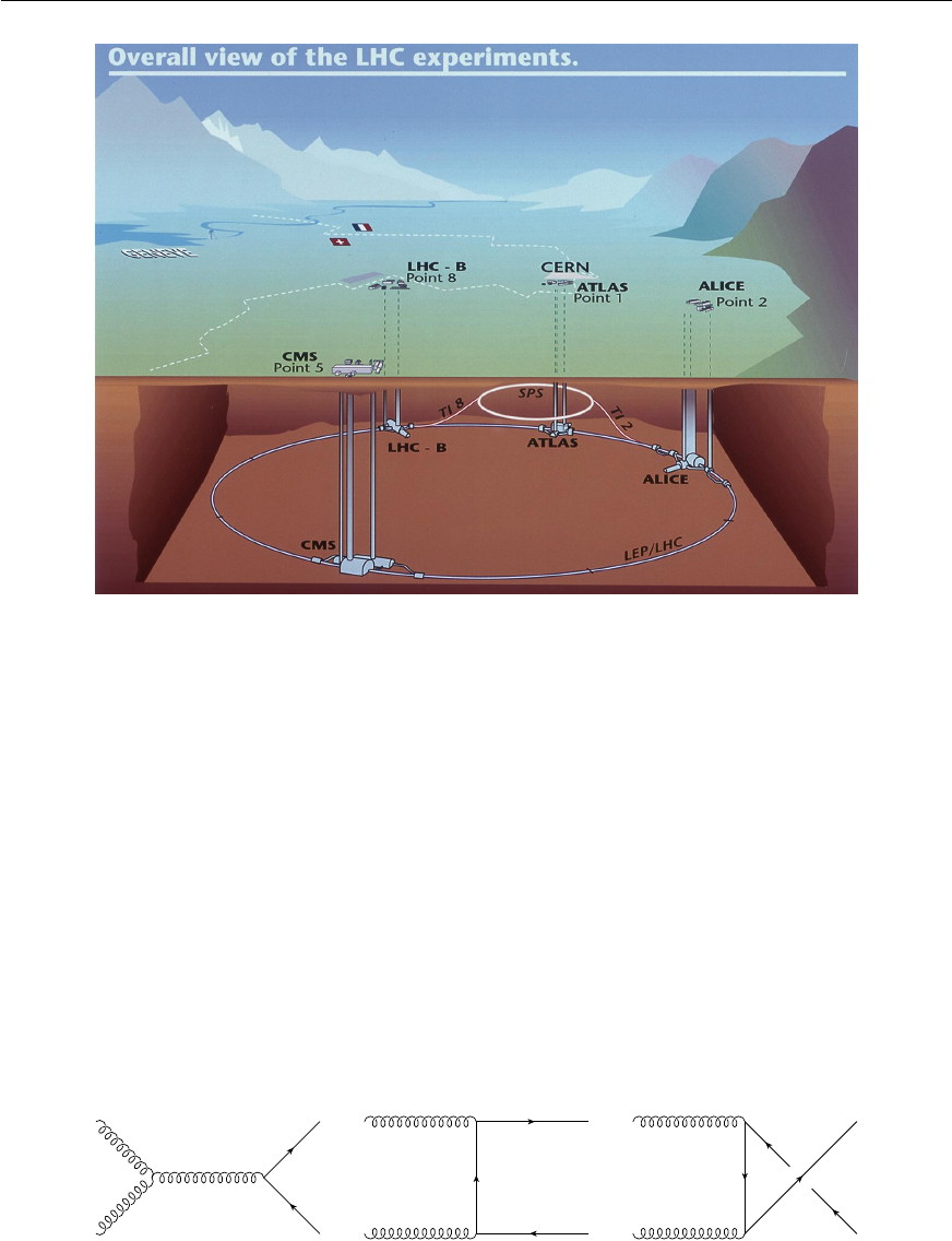
Chapter 5 Figures
Figure 5.1: Sketch of the LHC ring, the position of the experiments and the surrounding countryside. The four
big LHC experiments are indicated. The location of the injection lines and the SPS are also shown.
5.2 Fancier figures
Life gets more complicated if you want to include several plots in one figure, if you want the caption
next to the figure, or if you want the text to “flow” around the figure. For the first case I like to use the
tabular environment to place the plots, although there are other ways of doing it.
Another very nice way to add (a), (b) etc. to the figure is to use the
\put
command. This has
the big advantage that you can display the letters in the figure without actually having to add them
to the EPS/PDF file. Figure 5.2 shows how this is done. Note that the origin of the coordinate
system is the bottom right-hand corner of the file that you have included (assuming that the
\put
command comes just after the
\includegraphics
). The units for the
\put
command are set with
the
\setlength{\unitlength}
command, which is by default set to
1 mm
in
ubonn-thesis.sty
.
The same units are also used for Feynman graphs made with the feynmf and/or feynmp package — see
Section 5.6.2.
t
g
t
g
t
g
(a) (b) (c)
Figure 5.2: Adding letters to figures with \put.
Another way of achieving the same thing, but this time with the letter outside the figure is to use
32
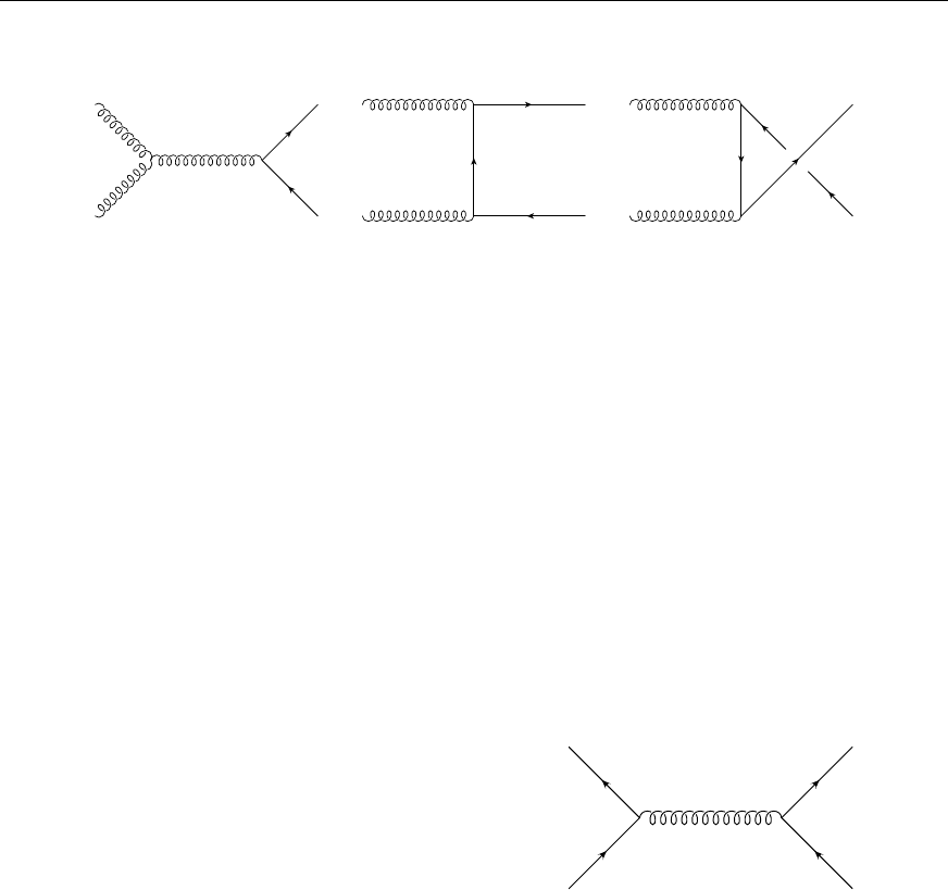
5.3 Figure formats
tabular. An example of this is shown in Fig. 5.3.
t
g
t
g
t
g
(a) (b) (c)
Figure 5.3: Adding letters to figures with tabular.
If you want to save space it is sometimes nice to put the caption next to the figure. While packages
exist to do this, KOMA-Script has its own built-in
captionbeside
environment. The placement
option comes after the caption itself and can be one of:
lLeft of figure
rRight of figure
iInner margin in two-sided layout
oOuter margin in two-sided layout
Note that this is an environment rather than a macro and that the figure itself is inside the environment.
Also the placement does not seem to work exactly how it is advertised in the manual. I set the width
equal to \figwidth and then the offset to -\figwidth.
Figure 5.4: A small figure with a simple caption beside
it.
t
g
If you want different (partial) captions for a figure then the subfig package used to be the way to go.
An alternative, and successor, to subfig is subcaption. It works in much the same way as subfig. A nice
tutorial on its use can be found in
http://www.peteryu.ca/tutorials/publishing/latex_
captions
. An example of its use can be seen in Fig. 5.5. The L
A
T
E
X file
guide_figs.tex
contains
examples for both subfig and subcaption, as the way subcaption should be used was different for T
E
X
Live 2011 and earlier. You can see how to reference the different parts of the figure in Section 5.6. If
you want the captions of the sub-figures to also appear in the “List of Figures” you should include the
package with the option lofdepth. For tables use the option lotdepth.
If you run out of space (applies more often to proceedings than to theses) you can use the wrapfig
package.
5.3 Figure formats
If you use plain L
A
T
E
X, you are pretty much stuck with encapsulated postscript (EPS) as your figure
format. If you use PDFL
A
T
E
X, then you have much more freedom, with the notable exception that you
33
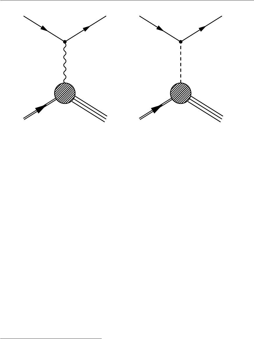
Chapter 5 Figures
p(P)
e(k)
γ, Z(q)
e0(k0)
X
1
(a) NC scattering
p(P)
e(k)
W±(q)
νe(k0)
X
1
(b) CC scattering
Figure 5.5: Processes in ep scattering.
cannot include EPS files!
1
I would still recommend that you always try to use a vector graphic format.
What usually works well is to either create PDF directly or to create EPS and then convert from EPS
to PDF.
The tool I use for conversion is
epstopdf
. Occasionally this fails; in that case
eps2eps
can help.
It is important that the bounding box is set correctly in the EPS file before you run epstopdf.
If these fail, you can try the
convert
command which is part of
ImageMagick
. A more powerful
tool is inkscape which is a successor to xfig. Professionals use Adobe Illustrator!
5.4 TikZ and PGF
pgfplots and tikz are packages to help with creating graphics “inline”. For 3D figures you also need
tikz-3dplot. PGF is the backend, while TikZ is what the user interacts with directly. The manual
contains all the information you should need, but was 1161 pages long at the last count, so it may not
to be too easy to find what you want!
I do not have much experience with using these packages so far, so this section will certainly not
cover all possibilities. There may also be better ways of doing things than I illustrate here. The
examples I give come from Andrii Verbytskyi or are adapted from questions and answers found
on
http://tex.stackexchange.com/
. The examples included in this guide and a few more are
collected in the
tikz
subdirectory. If you want to get started with TikZ you can copy this directory
into your thesis directory, e.g. mythesis.2
TikZ is not included by default in a new skeleton thesis. See the commented out packages in a new
1This restriction has finally been lifted with T
EX Live 2011. It simply converts the EPS files to PDF inline.
2
Note that some of the examples only work with T
E
X Live 2011 and later. This is indicated in the file. I also did not
manage to compile the guide without errors when including tikz with T
E
X Live 2009, so some of the figures may be
missing if you compile your own version of the guide with T
EX Live 2009.
34
5.5 Placement
thesis skeleton or
thesis_guide.tex
for the packages and TikZ libraries that you should include if
you want to use it.
You often want to include a figure of your experiment’s coordinate system in your thesis. One way
to do this is illustrated in Fig. 5.6.
z
x
y
θφ
e
p
Figure 5.6: The ZEUS coordinate system.
It is also possible to make flow charts with TikZ. This is illustrated in Fig. 5.7.
There are many more possibilities, including plots which you would otherwise make with
root
or
some other graphics program. An example plot showing the effect of systematic variations can be
found in Appendix E. Making Feynman graphs with TikZ is covered in Section 5.6.3.
5.4.1 Accelerator lattices
If you want to include an accelerator lattice in your thesis you can try tikz-palattice
3
He used the
package to make lattices of particle accelerators for his PhD thesis.
5.5 Placement
Even after many years of including figures into L
A
T
E
X files, I still think there is a fair amount of black
magic involved in getting them into the place that you want them to be.
In general, you are advised to give L
A
T
E
X as much freedom as possible in the placing, so it is usual
to use the options
[htbp]
for the placement. In particular, be very careful with using just
[h]
or
[H]
as the placement option. It very easily leads to L
A
T
E
X putting single lines of text either above or below
a figure. One way to get rid of single lines is to remove the option
h
, as the figure must then be placed
at the top or bottom of the page (or on a page of floats). You can also add an
!
in the list of options,
which suspends spacing and number restrictions.
A nice summary of the logic behind the placement can be found in T
E
X/L
A
T
E
X Stack Exchange
(click on the link!). A couple of points from there that are worth mentioning here:
3https://ctan.org/pkg/tikz-palattice
written by Jan Schmidt, who gave me a number of useful tips for this
guide.
35

Chapter 5 Figures
Event
generator Collision
MOZART Detector
ZGANA Trigger
Event
rejection
ZEPHYR
ORANGE
and
PHANTOM
NTuples
Analysis
MOZART control cards
MOZART GAFs
ZGANA control cards
ZGANA GAFs
ZEPHYR control cards
ZEPHYR GAFs
ORANGE control cards
ORANGE GAFs
Figure 5.7: Event reconstruction and simulation in ZEUS.
36

5.5 Placement
•The order of the options htbp has no effect!
•
If a float is placed in the middle of a paragraph, the reference point for deciding where it will
appear is the next line break or page break in the paragraph, following the float.
•
The order of figures (and tables) is fixed to the order that they are included in a document.
However, the order of figures and tables relative to each other is not fixed.
The UK List of FAQ recommends changing several default L
A
T
E
X options so that there are fewer
problems with figure and table placement. It is certainly worth reading that page for further advice. As
it is very hard to really test how well these options work they can be turned on or off in ubonn-thesis
via the option floatopt=true|false. The default value is set to true.
I used to think it was better to attach the figure to a paragraph:
The distribution is shown in \cref{fig:funny1}.
%
\begin{figure}[htbp]
\centering
\includegraphics[width=\figwidth]{file}
\caption{An odd plot that I don’t understand.}
\label{fig:funny1}
\end{figure}
%
The distribution shows something that I do not understand.
Given that this is not understood we went to the pub for a beer to
think about it a bit more.
More recently it appears to me to be better to separate the figure from the paragraph:
The distribution is shown in \cref{fig:funny2}.
The distribution shows something that I do not understand.
\begin{figure}[htbp]
\centering
\includegraphics[width=\figwidth]{file}
\caption{An odd plot that I don’t understand.}
\label{fig:funny2}
\end{figure}
Given that this is not understood we went to the pub for a beer to
think about it a bit more.
However, it is hard to give a hard and fast rule here. As indicated above, the effect of these different
ways of including a figure (and table) is the point in the text (reference point) that L
A
T
EX uses to start
trying to place the figure. In general, you should only try to tweak the position of figures and tables
when your text is final, as a change in the text way well move some of the floats.
37

Chapter 5 Figures
5.5.1 standalone package and class
The standalone package provides a great way of developing figures in small files and then inputting
these files directly, without making any changes, into your thesis!
It is in fact both a package and a document class. It is available from T
E
X Live 2012 onward. It
allows you to have a standalone document for a tikz or feynmf figure and also input this file into another
document. If you run PDFL
A
T
E
X on the file it also automatically crops the resulting picture. This is
one of those packages where you think “Why didn’t someone create this years ago?”. The TikZ figures
that I include in this guide (see subdirectory
tikz
) make use of this package. If you want to use it,
make sure that you also include this package in your thesis.
5.6 Feynman graphs
You have lots of Feynman graphs you want to include, but how do you generate them? Recently I
have moved to a Python package PyFeyn (
https://pyfeyn.hepforge.org
) that works quite nicely.
Before that I followed the example of many people, where I found one way doing it and never changed!
I used to use
Mn_Fit
, mainly because I wrote it and therefore know inside out how it works. Examples
can be found on my web page: http://pi.physik.uni-bonn.de/~brock/feynman.
Alternatives include axodraw and the feynmf or feynmp packages. It is also possible to use tikz. The
use of feynmf and feynmp is described in Section 5.6.2, while a few examples of usage of tikz are
given in Section 5.6.3. Examples of Feynman graphs made with feynmf and feynmp can be found in
the feynmf directory, while those made with tikz can be found in the tikz subdirectory.
Instructions on how to use axodraw may come at a later date — contributions would be welcome!
Several people have claimed that
jaxodraw
is the way to go. This is a Java package which you can
download from
http://jaxodraw.sourceforge.net/
. It has a Graphical User Interface (GUI) to
axodraw and so is simple and straightforward to use.
This paragraph illustrates how to reference different parts of a figure that uses the environment
subfigure
from the package subcaption. If you compile the guide with T
E
X Live 2011 or earlier the
environment
subcaption
from the package subfig is used. The NC and CC graphs shown in Fig. 5.5,
or more accurately in Fig. 5.5(a) and Fig. 5.5(b) were made with feynmp. Another way of saying the
same thing is that typical Feynman graphs for
ep
scattering are shown in Fig. 5.5, where (a) shows a
neutral current and (b) show a charged current process.
5.6.1 PyFeyn
As the name suggests, PyFeyn (
https://pyfeyn.hepforge.org
) is a Python package for drawing
Feynman graphs. It combines the advantages of using a programming language to draw the graphs
with the ability to use L
A
T
E
X and the same fonts as you use in your thesis for the text. I also wanted to
improve my Python skills, so now use this package for my graphs.
The package hepnicename is included by PyFeyn. If you want your particles to be written with
italics, you have to add this option to __init__.py in the pyfeyn directory.
PyFeyn should work pretty much out of the box, but may need a specific version of the pyx package.
If you want to use the newtx fonts, you may have to apply a patch. In order to install the package using
Homebrew Python under MacOS, I did:
38

5.6 Feynman graphs
pip(3) install PyX==0.12.1 (Python 2 needs 0.12.1)
pip(3) install PyFeyn
Stuff goes in /usr/local/lib/python2.7/site-packages/... etc.
To use newtx fonts had to patch pyx/dvi/vffiles.py
https://sourceforge.net/p/pyx/code/3678/
So far I have not tested its use with operating systems other than MacOS, but it should work.
While functions exist to draw a number of lines, I added my own wrapper functions that adjust the
style as I wanted. Have a look at
pyfeyn/myPyFeyn/__init__.py
to see what default settings I use
to get the font and colours that I want. Examples of Feynman graphs drawn using the package can be
found in Fig. 5.8 and are included in the
pyfeyn
directory. If you want to get started with PyFeyn you
can copy this directory into your thesis directory, e.g. mythesis.
u d
W
b
b
t
Z
u d
W
W
b t
Z
Figure 5.8: Example Feynman graphs for the associated production of a top quark and a Zboson.
5.6.2 FeynMF and FeynMP
In order to use feynmf or feynmp, you have to put the commands to draw the graph in a L
A
T
E
X file and
then process this file with L
A
T
E
X and either Metafont or Metapost.
4
You can either make a separate
L
A
T
E
X file containing the Feynman graph or include the commands inside your normal L
A
T
E
X file.
Metapost is a bit easier to use than Metafont. You should be able to just run
mpost
after
(pdf)latex
and then run
pdflatex
again twice. Note that you have to run
mpost
on all the files whose names are
defined at the beginning of the
fmffile
environment. While Metapost works well as of T
E
X Live
2011, I did not get it to work properly with T
EX Live 2009 for unknown reasons.
Metafont is a bit trickier. On Unix systems the
feynmf
perl script exists that runs both L
A
T
E
X
and Metafont for you. This will produce a
dvi
file that you then then look at or use to make a
Postscript/PDF file.
I think a better way to proceed is the following:
•make a separate L
A
T
EX file for each of the Feynman graphs;
•input this file in your figure;
•
use the
Makefile
described below to automatically run over one or all feynmp/feynmf L
A
T
E
X
files by giving the command make feynmp or make feynmf.
4ubonn-thesis.sty
now includes feynmp by default for T
E
X Live 2011 and later. If you want to use feynmf instead just
change the name.
39

Chapter 5 Figures
Check
./feynmf/feynmf_all.dvi
or
./feynmf/feynmf_all.pdf
to see if the graphs are
OK;
•run L
A
T
EX or PDFL
A
T
EX;
•run bibtex or biber;
•run L
A
T
EX or PDFL
A
T
EX again, at least twice.
The last three steps are done with the command
make thesis
,
make thesis11
or
make thesis09
.
The big advantage of this procedure is that the graphs are included “properly” in the thesis, their fonts
should automatically match the fonts used in the thesis and you don’t have to worry about converting
and clipping. I have written a small script that is executed by the
Makefile
to do the third step.
The script is
run_mf
for feynmf and
run_mp
for feynmp. These are included in the main directory
ubonn-thesis
. The scripts assume that all Feynman graphs are in a
feynmf
subdirectory. This can
clearly be adjusted in the
Makefile
as necessary. To get started you can copy the
feynmf
directory
from ubonn-thesis.
The
run_mf
script assumes that all files of type
tex
(except those that start with
feynmf_
) are
Feynman graphs to process with
feynmf
. Note that it may be necessary to give the command
make
cleanfeynmf to get rid of temporary files before make feynmf if you change the sizes of things.
The
run_mp
script works a bit differently. It creates a temporary directory
mpost_tmp
in which it
processes the figures (
tex
files) in the
feynmf
subdirectory. The resulting PDF files are copied back
to the feynmf subdirectory.
You can also use the package standalone together with feynmp. The files in the
feynmf
directory
contain commented out code that shows how this can be done. I do not do this by default for the guide,
as the package is very new and I also want to test making the Feynman graphs with feynmf. Note
that the name in the
fmffile
environment (and the
\write18
command) should be the same and
different from the name of the L
A
T
E
X file. If you use this option, you should probably also adjust the
Makefile
target for
feynmp
to work in the same way as the target
tikz
. You have to run
pdflatex
twice on each file.
Figure 5.9 shows the same neutral current and charged current graphs, but this time inputting the
appropriate feynmf commands directly. The graphs are enclosed in
\fbox
for illustration purposes
only. The plots are made using feynmp, where an appropriate
\write18
statement is included in
the L
A
T
E
X source code, e.g.
\write18 mpost gluon
, after the figure, where the figure starts with
\begin{fmffile}{gluon}.5
With the T
E
X Live 2011 and later setups I use to test this guide, this is all you need. If
mpost
does not run automatically, you must execute the command
pdflatex shell-escape mythesis
when you compile your thesis. This can be achieved by including the
EXTRACMD
definition that is
commented out in the
Makefile
. In this guide I put the Feynman graph in its own file and the
\write18
statement in the main file so that I can test feynmf and feynmp with the same L
A
T
E
X code.
In your thesis, you should probably put the
\write18
statement in the file with the Feynman graph. If
you use
latexmk
to compile you probably need to use the commented out version of the
latexmk
command in the Makefile.
5
If you use T
E
Xstudio you may have to give the full pathname for
mpost
, e.g.
/usr/texbin/mpost
, as T
E
Xstudio does
not parse your PATH properly.
40
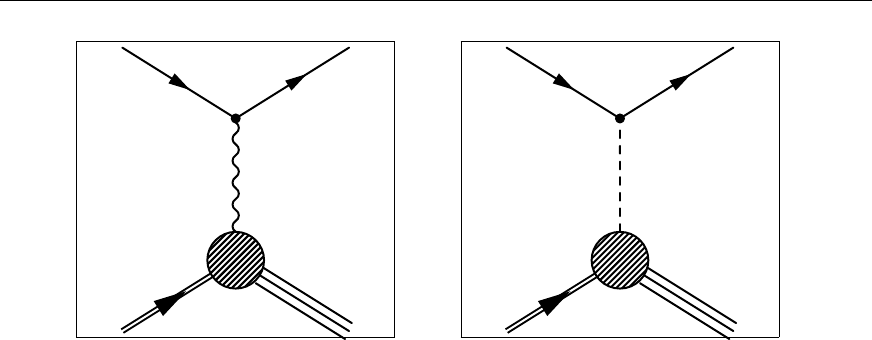
5.6 Feynman graphs
p(P)
e(k)
γ, Z(q)
e0(k0)
X
p(P)
e(k)
W±(q)
νe(k0)
X
Figure 5.9: NC and CC graphs for ep scattering using feynmf code directly.
As mentioned above, you probably want to first draw the graphs outside of your thesis to get
them into the form that you need. If you give the command
make feynmf
, it will run
feynmf
on
all
tex
files in the subdirectory
feynmf
. If you give the command
make feynmf file=ep_nc
it
will run over
./feynmf/ep_nc.tex
etc. As indicated above, the graphs can then be looked at in
feynmf_all.dvi or
feynmf_all.pdf. You can use the same syntax for make feynmp and make tikz.
5.6.3 Feynman graphs with TikZ
In order to draw Feynman graphs with TikZ, you need to include some extra TikZ packages and
libraries. In addition it makes sense to define things like gluons, photons and incoming and outgoing
particles once, as these are objects that are often needed.
Given the multitude of possibilities that exist to draw things with TikZ, it is not surprising that there
are several ways of achieving the same end. It is also debatable whether feymp or tikz is better. If
you use TikZ for drawing other things, then it is probably easier to use it also for Feynman graphs.
However, if you want things like gluons on an arc, this may well only be available, if at all, with very
recent versions of tikz.
As a start we can directly compare a scattering graph made with feynmp and tikz. This is shown in
Fig. 5.10. As you can see the quality of the graphs is very similar. Further tweaking can probably
make them almost identical.
41
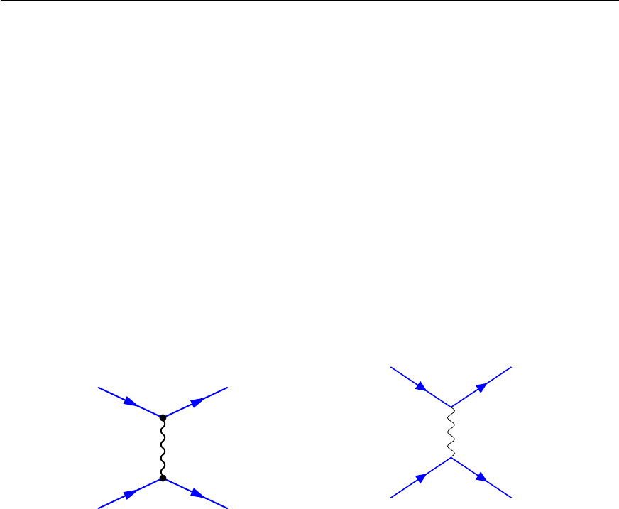
Chapter 5 Figures
γ
e−
e−
e−
e−
(a) Feynmp
e−e−
e−e−
γ
(b) TikZ
Figure 5.10: Feynman graphs drawn with feynmp and tikz.
42

CHAPTER 6
Tables
L
A
T
EX file: ./guide_tables.tex
You almost certainly have tables with results that you want to include in your thesis. You probably
even know about the
tabular
environment, but what about fine-tuning to get the tables exactly in the
form that you want? How do you line up the decimal points in a list of cross-sections and/or
±
for the
errors? How can you handle a table that goes over more than one page and what if it is so wide that
you would like to rotate it by 90°?
Also, how can you make your tables look more professional with for example thick and thin lines
in appropriate places? This is easy to solve — use the
\toprule
,
\midrule
and
\bottomrule
commands from the booktabs package. These commands also produce much better spacing between
these lines and the rows above and below. The booktabs package gives you some advice on how good
tables should look, as well as some guidelines on how to make your tables look better.
The
\rule
command is very useful for adding more space between rows. Kopka has several examples
of its usage. You can also use
\arraystretch
, e.g.
\renewcommand{\arraystretch}{1.5}
to
increase the spacing by
50 %
. This command is often useful if table cells contain subscripts and/or
superscripts. \toprule etc. mean that it is usually not needed in headers.
If you want columns of expandable width you can use the tabularx package. The environment
tabular* has instead expandable intercolumn spacing.
Tables usually go inside the table environment so their position can “float”. In this chapter I use
some tables inside table and some inline.
Trying to include footnotes in tables can be tricky. See Section 8.2 for some guidance on how this
can be done.
6.1 Use of \phantom
Although extra packages can help, a very useful command is
\phantom
. This inserts white space
corresponding to the width of the argument. Compare the results in the following table with two
numbers 0.76 and 83.1:
43
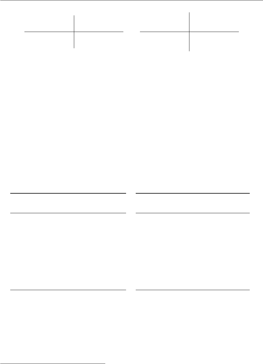
Chapter 6 Tables
Centred Right justified
Phantom Phantom
0.76 0.76 0.76 0.76
83.1 83.1 83.1 83.1
Centred Right justified
Phantom Phantom
0.76 0.76 0.76 0.76
83.1 83.1 83.1 83.1
The difference between the two tables is that the one on the right has the length
\extrarowheight
set to 0.5ex. The first two columns are centred, the last two are right justified. This is clearly a bit
clumsy, but it does work!
6.2 Using siunitx and the Scolumn option
The siunitx package contains some nice tools that make the correct alignment of numbers simpler.
The syntax of some of the options changed between version 1 (
≤
2009) and version 2 (
≥
2011). I
discuss the version 2 options in the main text and give the equivalent version 1 options as a footnote. If
you look at the L
A
T
E
X code, the T
E
X Live 2009 version is inside
\ifthenelse{\texlive < 2011}
,
while the T
EX Live 2011 version is in the second block.
A first simple example is shown in Table 6.1. In fact I show the table twice, once with the language
set to default and once with it set to German. The
tabular
contents are identical, the second tabular
is inside a
\foreignlanguage
. Note the use of
table-format1
to centre the temperatures as the
heading is wider than the numbers.
Liquid Temp. Viscosity η
[◦C] (m Pa s)
Blood 37 4.0
Glycerine 0 10 000
20 1 410
60 81
Oil (SAE 10) 30 200
Water 0 1.8
20 1.00
60 0.65
Air 20 0.018
Flüssigkeit Temp. Viskosität η
[◦C] (m Pa s)
Blut 37 4,0
Glyzerin 0 10 000
20 1 410
60 81
Öl (SAE 10) 30 200
Wasser 0 1,8
20 1,00
60 0,65
Luft 20 0,018
Table 6.1: A table of viscosities in the default language and German.
Table 6.2 shows a more complicated table set using the tools. You can either enclose all numbers
in
\num
or use the
S
column descriptor. If you use
S
, note that it usually centres the contents of the
column. You can use the
table-number-alignment2
option to change this.
S
and
\num
cannot
generally be mixed in a single column though. If you want to use
\num
in an
S
column you have
to enclose it in braces. You also need to do this with regular text, such as column headings — see
Table 6.1.
1tabformat in T
EX Live 2009
2tabnumalign in T
EX Live 2009
44
6.2 Using siunitx and the Scolumn option
ηjet dσb/dηbdσNLO
b/dηbChad
b
[pb] [pb GeV−1]
−1.60 : −1.10 57.4 ±9.4 +13
−372 +22
−13 0.70
−1.10 : −0.80 121 ±21 +16
−16 182 +50
−30 0.78
−0.80 : −0.50 214 ±22 +22
−12 255 +69
−42 0.79
−0.50 : −0.20 233 ±21 +28
−21 307 +83
−50 0.79
−0.20 : 0.10 264 ±22 +28
−23 342 +91
−55 0.81
0.10 : 0.50 316 ±21 +23
−17 346 +96
−57 0.85
0.50 : 1.40 288 ±15 +20
−30 265 +82
−48 0.93
Table 6.2: A selection of cross-section measurements!
With
\num
you can also specify the precision with which each number is shown separately. With
S
you specify the format for the whole column. With siunitx version 1 this is done using the
dp
option
and gives the number of decimal places for the rounding. With siunitx version 2 you should also make
sure that you specify the rounding mode in the preamble of the table (usually
figures
or
places
—
you can also choose off).
If you know that you are going to make such a table, it is very easy to use either of these options to
write it out in this format using a program. Using
\num
solves the very common problem of your
program writing out the results with too many significant digits and you have to correct them all by
hand later (as well as every time they get updated)! A slightly different approach that one could follow
is to use
S
for simple numbers in tables and
\num
for more complicated number typesetting. For
asymmetric errors you could consider defining something similar to
\numpmerr
, which internally
uses \num.
A common and closely related problem that occurs is that your analysis spits out a result such as
24
.
36789
+0.36423
−0.45236
. You copy and paste this into a table and then a referee (or your supervisor) complains
that you clearly don’t understand statistics, as you should never quote an error to 5 significant digits.
You can go ahead and edit all the numbers by hand, but what do you do if you rerun your analysis
and all the numbers change. Reformatting by hand is then an error prone and lengthy process. As
discussed above, you can either use options such as
round-precision3
in the
S
command or use the
macro \num and dp/round-precision to do the rounding for you.
Table 6.3 shows and compares two different approaches on how this can be done, even for asymmetric
errors. While the form may appear to be a bit clumsy at first, it is easy enough to get your program to
write out the lines. In siunitx version 1 you should use option
dp
for the rounding. In version 2 you
should use the options
round-mode
and
round-precision
. In the first line of the left-hand part of
the table I show what to do if you need to change the precision of a single number. As you can see this
is rather trivial. However, then the alignment on the decimal point is no longer perfect. While this is
probably OK for internal notes etc., theses or papers (should) have tougher requirements. Another
way of achieving the same thing and avoiding the use of
round-mode
and
round-precision4
is
3dp in T
EX Live 2009
4dp in T
EX Live 2009. The round-mode should be set in the preamble of the table and not for every number.
45
Chapter 6 Tables
shown in the right half. Note the use of options for the
S
command and the use of
\num
enclosed in
braces to format the row that requires a different precision.
It takes a while to learn what the different options mean and their consequences. I hope that these
examples cover most problems and at least give ideas as to what is possible. In particular the solution
on the right-hand side of Table 6.3 is very nice, as all numbers except the one that requires an extra
digit are written without any special formatting!
ηjet dσb/dηb
[pb]
−1.60 : −1.10 0.574 ±0.094 +0.035
−0.031
−1.10 : −0.80 1.21 ±0.21 +0.16
−0.16
−0.80 : −0.50 2.14 ±0.22 +0.22
−0.12
−0.50 : −0.20 2.33 ±0.21 +0.28
−0.21
−0.20 : +0.10 2.64 ±0.22 +0.28
−0.23
+0.10 : +0.50 3.16 ±0.21 +0.23
−0.17
+0.50 : +1.40 2.88 ±0.15 +0.20
−0.30
ηjet dσb/dηb
[pb]
−1.60 : −1.10 0.574 ±0.094 +0.035
−0.031
−1.10 : −0.80 1.21 ±0.21 +0.16
−0.16
−0.80 : −0.50 2.14 ±0.22 +0.22
−0.12
−0.50 : −0.20 2.33 ±0.21 +0.28
−0.21
−0.20 : +0.10 2.64 ±0.22 +0.28
−0.23
+0.10 : +0.50 3.16 ±0.21 +0.23
−0.17
+0.50 : +1.40 2.88 ±0.15 +0.20
−0.30
Table 6.3: Another selection of cross-section measurements! Note the use of
\sisetup
to keep the plus signs
on the positive errors.
Another example using siunitx tools that contains a similar problem is:
English German1 German2
Value ±Error Wert Messung
0.76 ±0.14 0,89 ±0,16 0,89 ±0,16
83.1 ±7.6 94,2 ±8,3 94,2 ±8,3
As you can see, the “English” column formats things nicely using the
S
column descriptor. The
“German1” column successfully converts the decimal point to a comma and also the parentheses
with the error to
±
. However, the alignment of the numbers is now messed up. The “German2”
column looks better. I had to do some dirty tricks with the formatting of the intercolumn separator
@{\,\pm\!\!}
to get the spacing nice! This confirms my statement above that the
S
format is most
useful for aligning simple numbers easily, while
\num
is very nice for rounding to a given precision —
note that you can use either the dp or sf options to achieve what you want.
If your header is wider than the content, you may also have to tweak a few things to get the correct
alignment. A good way of doing this is to insert some
\hspace*
into the header. The table on the
left is without
\hspace
, while the one on the right is with an
\hspace
of 2em. The tables contain
vertical lines that I would normally not include to illustrate the alignment.
46
6.3 Using dcolumn
dσNLO
b/dηb
[pb GeV−1]
72 +22
−13
182 +50
−30
255 +69
−42
dσNLO
b/dηb
[pb GeV−1]
72 +22
−13
182 +50
−30
255 +69
−42
6.3 Using dcolumn
An alternative is the dcolumn package. You can also use this package to convert numbers written with
“.” as the decimal point into German-style numbers with “,”.
5
You can line up measurements and
errors by putting each of them in its own column. If your errors are symmetric you can put
±
as the
intercolumn separator:
English German Val ±Err Val Err
0.76 0.76 0,76 0,76 0.76 ±0.14 0.76 ±0.04
83.1 83.183,1 83,183.1 ±4.2 83.1±4.2
Table 6.4 shows quite a complicated table set in 2 different ways. It is rotated by
90°
to illustrate
how that can be done.
The 2nd version (right) is certainly simpler to typeset and does not really use any tricks to line
things up. Note the use of
array
rather than
tabular
which means that the contents are typeset in
math mode rather than text mode. For tables of numbers this is often preferred. You just have to
enclose the array in
\(...\)
or
\begin{math}
. . .
\end{math}
. Close inspection of the right-hand
table shows that it is, however, not perfect. It is questionable whether one wants to to write
+
0
.
5or
just 0
.
5. The fact that both
pT
as well as
η
cross-sections are in a single tabular, but the numerical
values are so different makes it difficult to line things up perfectly. An alternative, which uses the
headers to fix the width of the columns is given in Table 6.5. Note that this uses
sidewaystable
rather than sideways inside table, which also rotates the caption.
This version of the table also adds a few extra bells and whistles. It uses a
\rule
of zero width
to give a bit more space above and below the cross-sections.
p{...}
switches to paragraph mode,
so
\centering
is needed to get centred headers. It adds a bit more space between the rows using
\arraystretch
. You have to play around a bit with the column widths. If you set one of them
too small it gets expanded anyway, so the two parts of the table would not line up. Just for fun the
bottom half of the table uses “,” instead of “.” for the decimal point! Admittedly the header is a bit
complicated, but the numbers are nice and easy to write!
5See Section 8.3 for hints on how to get around problems with the ziffer package
47
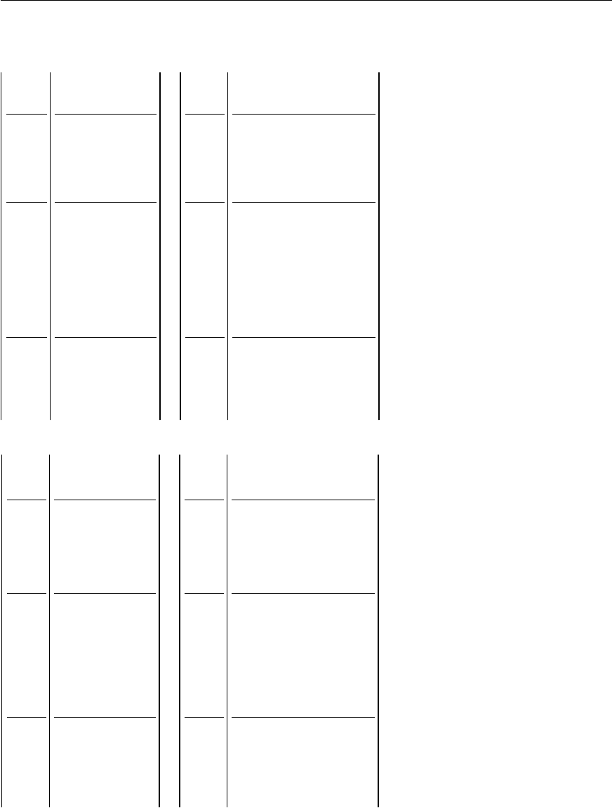
Chapter 6 Tables
pjet
Tdσb/dpb
TdσNLO
b/dpb
TChad
b
(GeV) (pb/GeV) (pb/GeV)
6 : 11 95.6±4.9+9.8
−7.0109 +31
−19 0.83
11 : 16 24.8±1.2+1.8
−1.429.1+7.9
−4.70.89
16 : 21 6.02 ±0.49+0.6
−0.67.1+2.0
−1.20.92
21 : 27 0.93 ±0.22+0.31
−0.20 1.87+0.54
−0.34 0.95
27 : 35 0.30 ±0.12+0.14
−0.12 0.46+0.13
−0.08 1.05
ηjet dσb/dηbdσNLO
b/dηbChad
b
(pb) (pb)
−1.6:−1.1 57 ±22+13
−372+22
−13 0.70
−1.1:−0.8 121 ±21+16
−16 182+50
−30 0.78
−0.8:−0.5 214 ±22+22
−12 255+69
−42 0.79
−0.5:−0.2 233 ±21+28
−21 307+83
−50 0.79
−0.2:0.1 264 ±22+28
−23 342+91
−55 0.81
0.1:0.5 316 ±21+23
−17 346+96
−57 0.86
0.5:1.4 288 ±15+20
−30 265+82
−48 0.93
pjet
Tdσb/dpb
TdσNLO
b/dpb
TChad
b
[GeV] [pb GeV−1] [pb GeV−1]
6 : 11 95.6±4.9+9.8
−7.0109 +31
−19 0.83
11 : 16 24.8±1.2+1.8
−1.429.1+7.9
−4.70.89
16 : 21 6.02 ±0.49 +0.6
−0.67.1+2.0
−1.20.92
21 : 27 0.93 ±0.22 +0.31
−0.20 1.87 +0.54
−0.34 0.95
27 : 35 0.30 ±0.12 +0.14
−0.12 0.46 +0.13
−0.08 1.05
ηjet dσb/dηbdσNLO
b/dηbChad
b
[pb] [pb]
−1.6 : −1.1 57 ±22 +13
−372 +22
−13 0.70
−1.1 : −0.8 121 ±21 +16
−16 182 +50
−30 0.78
−0.8 : −0.5 214 ±22 +22
−12 255 +69
−42 0.79
−0.5 : −0.2 233 ±21 +28
−21 307 +83
−50 0.79
−0.2 : +0.1 264 ±22 +28
−23 342 +91
−55 0.81
+0.1 : +0.5 316 ±21 +23
−17 346 +96
−57 0.86
+0.5 : +1.4 288 ±15 +20
−30 265 +82
−48 0.93
Table 6.4: Cross-section measurements!
48
6.3 Using dcolumn
pjet
Tdσb/dpb
TdσNLO
b/dpb
TChad
b
[GeV] [pb GeV−1] [pb GeV−1]
6 : 11 95.6±4.9+9.8
−7.0109 +31
−19 0.83
11 : 16 24.8±1.2+1.8
−1.429.1+7.9
−4.70.89
16 : 21 6.02 ±0.49 +0.6
−0.67.1+2.0
−1.20.92
21 : 27 0.93 ±0.22 +0.31
−0.20 1.87 +0.54
−0.34 0.95
27 : 35 0.30 ±0.12 +0.14
−0.12 0.46 +0.13
−0.08 1.05
ηjet dσb/dηbdσNLO
b/dηbChad
b
[pb] [pb]
−1,6 : −1,1 57 ±22 +13
−372 +22
−13 0,70
−1,1 : −0,8 121 ±21 +16
−16 182 +50
−30 0,78
−0,8 : −0,5 214 ±22 +22
−12 255 +69
−42 0,79
−0,5 : −0,2 233 ±21 +28
−21 307 +83
−50 0,79
−0,2 : 0,1 264 ±22 +28
−23 342 +91
−55 0,81
0,1 : 0,5 316 ±21 +23
−17 346 +96
−57 0,86
0,5 : 1,4 288 ±15 +20
−30 265 +82
−48 0,93
Table 6.5: Cross-sections using
sidewaystable
, which also rotates the caption. Just for fun the numbers indicating the
η
range of the bins in the lower
half have been converted to German format! Note also the dirty trick used to get the Chad
bvalues nicely in the centre of the column.
49
CHAPTER 7
References
L
A
T
EX file: ./guide_refs.tex
Every thesis should also include a list of references, called the bibliography in L
A
T
E
X terminology.
You “cite” a reference using the
\cite
command. For example, the book of Kopka [KD04] is my
favourite L
A
T
E
X book. In general you should include a non-breaking space, i.e. “~” between the text
and the
\cite
command. In British (UK) English the reference should come before the punctuation;
in American English it comes after it.1
That is the easy part! Where do you get the references from and how do you format them? Sources
of references are discussed in Section 7.6. There are two options for the formatting. Either you do it
by hand, formatting
\bibitem
entries yourself or you use BibT
E
X. More precisely you should use the
biblatex package. which is a replacement for traditional BibT
E
X. While biblatex and/or BibT
E
X may
appear to be the more complicated option at the beginning, I strongly recommend that you use it.
In addition, you have to make sure that authors’ names are printed consistently, you include the
appropriate collaboration name, the title is formatted correctly and journals are given consistent
abbreviations. Such topics are discussed in Section 7.3.
What about citing a series of articles? Can you include them in one reference or do you want to
keep one article per reference? I give some hints on useful options and settings for biblatex below
(Section 7.4.1). If you use traditional BibT
E
X (which I do not recommend), then you probably have
to use the mcite package — see Section 7.8. Just to take a silly example. The ZEUS collaboration
publications in 2010 [ZA+10;Abr+10a;Abr+10b] were not as numerous as in previous years. If you
use the standard
\cite
command and the
unsrt
option or its equivalent, you get a list of numbers. In
the past one could use the mcite package to make the references nicer, put them all in one, write the
list as [m–n] etc.
7.1 Formatting by hand
Don’t! The number of references that you will need will probably grow fast. It is quite likely that
at some point you will decide that they are not really formatted as you would like them to be. You
will almost certainly add references when you correct your thesis. How do you make sure they are
1
After some research, it appears to me that the footnote number should come after the punctuation, unless the footnote
only refers to the last word of the phrase or sentence.
51

Chapter 7 References
in the order you want? How do you make sure that only articles that you actually refer to are in the
bibliography?
Suppose you want to use some of the references in your thesis in conference proceedings or a paper
in a journal. Every place where you publish will have it’s own preferred format for the references that
almost certainly will not be the one you chose for your thesis.
If you insist on following this route, consult a book on L
A
T
EX!
7.2 Using BibT
E
X and biblatex
I won’t pretend that BibT
E
X is the most user-friendly way of handling references and there are several
things that you have to pay attention to when you use it for your references.
The two big advantages of biblatex and/or BibT
E
X are: only references that you actually refer to
appear in the bibliography; you can change the format (consistently) of all articles in the bibliography
simply by changing the style!
The first step is to put your references in one or more
.bib
files. For this document they can be
found in:
•../guide/guide_refs.bib;
•../refs/standard_refs-biber.bib or ../refs/standard_refs-bibtex.bib;
•../guide/refs/example_refs-utf8.bib
or
../guide/refs/example_refs-ascii.bib
;
•../guide/refs/zeus_2009.bib and ../guide/refs/zeus_2010.bib.
For each article you specify things like its title, author, journal etc.
You then include these files into your L
A
T
E
X document and specify which style should be used. You
also have to indicate where you want the bibliography to appear.
At this point you also have to decide which interface to the contents of the
.bib
files you want to
use. You have a choice of the original BibT
E
X or the more modern biblatex. If you use biblatex you
need something like:
% Use biblatex for the bibliography
\usepackage[backend=biber,
style=numeric-comp, sorting=none, block=ragged, giveninits=true]{biblatex}
% \usepackage[backend=bibtex, hyperref=true,
% style=numeric-comp, sorting=none, block=ragged, giveninits=true]{biblatex}
% Adjustments to output are in this style file:
\usepackage{ubonn-biblatex}
\addbibresource{../mythesis/thesis_refs.bib}
\addbibresource{../refs/standard_refs-biber.bib}
in the document preamble and
\printbibliography
where they should be printed.
2
Note that as of
version 3.0 of the thesis package, the biblatex command is included in ubonn-thesis directly. To turn it
off add the option biblatex=false.
2If you use an older version of T
EX Live you may have to replace giveninits by firstinits.
52

7.3 BibT
EX entries
If you use traditional BibT
EX you need something like:
% Use BibTeX for the bibliography
\bibliographystyle{../refs/atlasBibStyleWithTitle.bst}
% \bibliographystyle{unsrt}
\bibliography{../mythesis/thesis_refs,%
../refs/standard_refs-bibtex}
at the point where the references should be printed. Note that L
A
T
E
X is sometimes picky about spaces
in lists of files, so you either terminate each line in
\bibliography
with a % or include all files on
one line.
Which should you use? Traditional BibT
E
X has been around for a long time and is therefore better
known. However, it has many problems when it comes to sorting, handling more modern sources of
information (e.g. the web), etc. By now (written in 2015) biblatex is rather stable, so future changes
should be minor. It supports things like online references and enables you to click on references using
the preprint number or DOI to look at a reference. It is also easier to change the way your references
look. I therefore strongly recommend that you use biblatex.
Another serious problem with BibT
E
X is that it cannot handle umlauts etc. properly. While I
have said elsewhere in this document that you should use UTF-8 encoding so that you can enter ä
etc. directly, this does not work with BibT
E
X. You can use the old syntax
\"{a}
.
3
This problem is
completely solved if you use biblatex and the biber backend.4As indicated above, the references in
the guide include two versions of the file with some example references:
•./guide/refs/examples_refs-utf8.bib with UTF-8 encoding;
•./guide/refs/examples_refs-ascii.bib without any umlauts.
If you try to compile the guide with the wrong file using BibT
E
X, you will get some errors as I have
included some umlauts in the example references. The thesis skeletons use traditional BibT
E
X with
T
E
X Live older than 2011 and biblatex with the
biber
backend for newer versions. See the skeleton
thesis_skel/thesis_2009_skel.tex
for the complete syntax if you want to use traditional
BibT
EX.
That’s it? Well almost! First, you will have to make sure that the entry type that you use corresponds
to the type of document that you are citing. Second, you will probably get some or all of your
references from standard sources such as Spires
5
, Inspire or CDS, you will have to change the entries
a bit so that they get formatted the way you want.
7.3 BibT
E
X entries
In this section I discuss how to format your BibT
E
X databases, i.e. the
.bib
files. In the following
section I talk about how you make your references look the way you want them to be in your thesis.
3
In fact you have to write this as
author = "Br{\"{u}}ning, Oliver"
for it to work properly! As an aside, if you look
at the L
A
T
E
X source code for this footnote, it might seem natural to use
\verb
for
author = ...
. However, verbatim
does not work in footnotes, unless you include other packages such as fancyvrb.
4
If for some reason you want to use biblatex with the
bibtex8
backend you have to encode your
.bib
files with latin1
instead of UTF-8 if they includes umlauts and use the line:
\usepackage[backend=bibtex8,bibencoding=latin1]{biblatex}.
5I will refer to both as Inspire in this chapter.
53

Chapter 7 References
7.3.1 Entry types
One question is what entry type you should use for what? I give here recommendations on what to use
for biblatex. Some of the entry types that biblatex has are not part of BibT
EX.
@article This is easy — use it for articles published in journals, e.g. [ZA+10].
@book Just as easy — use it for books, e.g. [KD04].
@proceedings, @inproceedings
The name says it all. Use
@inproceedings
for a paper in the
proceedings and @proceedings for the whole volume.
@collection
Use it for things such as the ATLAS Technical Design Report [Brü+04a] where the
names that you find are the editors. Use @incollection for a single article in a collection.
@report
Use it for conference and internal notes. This is probably also the best type to use for
preprints. You can also use @booklet or @online.
@online Use it for things that are only available online, e.g. [Oet+].
@thesis
The name says it all.
@phdthesis
and
@mastersthesis
also exist. If you are using
biblatex you can and should specify the thesis type, e.g.
type = {PhD}
, see for example a PhD
thesis [Lod12].
biblatex also knows about multivolume proceedings etc. See the manual for more details.
Note that Inspire will always give you a BibT
E
X entry of type
@article
, so you should adjust it by
hand according to what the document you refer to really is. CDS tries a bit harder, but you probably
still have to set the entry type by hand.
As indicated above, biblatex knows about preprint archives, online references with a url etc. and
can format the references so that you can click on a DOI or arXiv number. Details of how these are
handled are well documented in the manual. In order to make use of these abilities you have to modify
the Inspire format of the references a bit so that it is fully compatible with what biblatex expects for
preprints etc. More details on this are given below.
What else do you have to be careful about? The first thing to know is that biblatex and BibT
E
X will
try to format your author names and titles. Thus, if you want the title to remain in exactly the form you
have typed it in include it in “"{Title}"”, i.e. both double quotes and braces. If not, collaborations and
accelerators tend to be converted to lowercase, e.g. “lhc” instead of “LHC”. If you use an author such
as “ATLAS Collaboration” it gets printed as “A. Collaboration”. If part of a title should not have its
case changed enclose it in {. . . }, e.g. “"The {ATLAS} Detector"”
7.3.2 Entries from Inspire and CDS
Things like the LHC Design Report are by default called
@article
in Inspire [Bru+04] or
@book
in
CDS [Brü+04b]. They are in fact best declared as
@collection
with the
author
field replaced by
editor
and a field indicating the
institution
instead of
publisher
[Brü+04c]. You can also add
the CDS link as a url field.
Conference notes, e.g. from ATLAS, are defined as
@techreport
by CDS [11]. It is bet-
ter to just call them
@report
. You should add an author, usually just
author = "{ATLAS
54

7.4 Formatting references
Collaboration}",
[ATL11a]. You may also have to change the month format to avoid error
messages. For internal notes, also call them report and add
type = internal report
to the entry.
Again you could add the CDS link as a
url
field. For preprints, I also think it is best to use the
@report entry type.
Books need to be changed from
@article
to
@book
and it is better to give the ISBN in the
isbn
field [HM84a] rather than the reportNumber field as given in Inspire [HM84b].
Theses should used the
@thesis
entry type and then add a
type
field. Alternatively you can use
@mastersthesis or @phdthesis.
In all cases you probably have to edit the titles a bit to get things like
√s=7 TeV
printed properly.
An open question is whether you should assume the use of a units package in the formatting of the title.
If you want to make your
.bib
files usable by others, it is probably best to do the formatting by hand.
An example of a typical ATLAS paper as it comes from Inspire [Aad+11] needs a bit of work. With
T
E
X Live 2011 the link to DOI and arXiv both work well [ATL11b]. Note that the LHC collaborations
specify that the first author should not be included, i.e. author = "{ATLAS Collaboration}",.
7.3.3 More on names
The best way to format author names so that they appear correctly whatever BibT
E
X style you use is
Surname, Name. Any other syntax is likely to get mangled.
What about collaboration names? If you use Inspire as the source of your BibT
E
X entries, you will
see that it has a field for the collaboration. This is often, but not always, formatted correctly. However,
very few BibT
E
X styles, and as far as I know no biblatex styles, pay any attention to this field. The
ones from Inpire listed below will work properly. The only other reliable alternative I have found is to
use the following syntax:
@Article{Chekanov:2009qja,
author = "{ZEUS Collab.} and Chekanov, S. and others",
which then usually gets formatted as “ZEUS Collab., S. Chekanov et al.,”. I went through and changed
the references in zeus_2009.bib accordingly.
7.4 Formatting references
While BibT
E
X or biblatex format the references for you from the
.bib
files, you have to tell them what
format you want! For a start, you have to choose between an alphabetic and a numeric scheme for the
references. Most journals use a numeric style. This corresponds to style
unsrt
or a variant thereof
using traditional BibT
E
X. If you use biblatex you include the package with option
numeric-comp
or
numeric
.
numeric-comp
produces more compact citations (e.g. [1–4,7,9]) than
numeric
(e.g.
[1,2,3,4,7,9]).
For this guide (for a change) I use an alphabetic style:
alpha
with BibT
E
X or option
alphabetic
with biblatex. In the thesis skeleton I use a more usual unsorted numeric style.
7.4.1 biblatex styles
My experience with biblatex took off when I started rewriting the ATLAS L
A
T
E
X templates in 2014.
The first official stable release of biblatex was 19 Oct 2010. Active and rapid development is ongoing
55
Chapter 7 References
— there were many updates in 2011. Some things I recommend below may work a bit differently
depending on which version you have. See Appendix Bon how to install a newer version of T
E
X Live
if you want a more up-do-date version of L
A
T
EX.
Looking for numeric styles you can either use the built-in
numeric
or
numeric-comp
. The
numeric-comp
style is used by default in the thesis skeleton. I made a few adjustments that are
included in the file ubonn-biblatex.sty.6
You can change some of the things in the style file by passing options to it. The syntax
articletitle
and
articletitle=true
is equivalent. Use
articletitle=false
to turn off an option. The
following options exist:
Option Default Description
texlive 2014
Specify the T
E
X Live version. You can also use the older command
\newcommand*{\texlive}{2014}.
block ragged Specify the justification of each reference;
maxbibnames 5 Numbers of authors to list before switching to “et al.”;
articletitle true Show the titles of articles and reports;
titlequote false Enclose the title in quotes rather than using a slanted font.
boldvol false Show the volume in bold face.
showurl true Show the URL field.
showdoi false
Show the DOI separately. Otherwise it is linked from the journal
reference.
eprint true Show the arXiv entry.
address false Print the address, if given.
location false Print the location, if given.
You can fine tune things even more by using hooks that are available. For example, the way I turn
off the URL field is to include the command:
\AtEveryBibitem{\clearfield{url}}
in the preamble or in the relevant style file given in the previous paragraph. It is not clear to me if you
also need \AtEveryCitekey{\clearfield{url}}.
A fairly nice-looking style is
ieee
. This is only be available in recent releases (
≥
2011) of T
E
X
Live. After playing around a bit with the
ieee
style, I decided it is too new and has too many settings
that depend on having a new version of biblatex for now.
There are slowly more and more biblatex styles around, but not as many as traditional BibT
E
X.
It is, however, much easier to change things (usually you can just change an option) with biblatex
than it was for traditional BibT
E
X, so you can probably start with a standard file and just make
adjustments in your preamble. I have found a number of very useful hints on how to make changes in
http://tex.stackexchange.com/ — just search for biblatex.
If you include ubonn-thesis with the option
astrobib
, the references will be formatted in the style
usually used in astrophysics publications. Version 3.0 contains a first version of this option. A few
more tweaks may still be needed. You can use the command
make astro
instead of
make new
to
6
In the past (before version 3.0) these files were called
./biblatex/biblatex-num-v2009.sty
and
./biblatex/biblatex-num-v2011.sty
. Which file was used by default was steered by the
\texlive
macro
which is set in the main file.
56

7.5 Errata
make a thesis skeleton with the appropriate options set and the template introduction uses typical
citation commands. The option
astrobib
only works for T
E
X Live 2011 and later, i.e. with biblatex.
If it is available,
biber
is the preferred backend over
bibtex
or
bibtex8
. However, the backend
is mostly relevant for sorting, so it probably does not matter which you use if you use an option that
gives the references in the order that they were cited.
biber
seems to work well with T
E
X Live 2012
and later and hence is the default. For older versions of T
E
X Live, a better solution is probably
make
new09 followed by make thesis09 that then uses traditional BibT
EX.7
If you want to find out where your references are actually cited, you can include the option
backref=true.
If you get an error such as:
biber thesis_guide
data source /tmp/par-62726f636b/cache-ab06f20732bfab23dfa35f56998ad4edca61bee1//inc/lib/Biber/LaTeX/recode_data.xml not found in .
Compilation failed in require at Biber/Utils.pm line 21.
then you should delete the directory
/tmp/par-...
and try to run again. The directory name depends
on the operating system you are using. Use the command
biber --cache
to find out where it is. If
you are adventurous, the command rm -rf $(biber --cache) will do it all for you!
7.4.2 Traditional BibT
E
X styles
I strongly recommend that you use biblatex and biber, but if you insist. . .
If you use references directly from Spires or Inspire, then it is probably best to use one of the style
files that is compatible with their format. A list can be found on
http://www.slac.stanford.
edu/spires/hep/refs/bibstyles.shtml
. I have used
utphys
a few times and it works OK. I
see that there are also style files available there for common HEP journals, which could save quite a
bit of work. The big advantage of utphys is that it also knows about the arXiv and preprints.
The equivalent of biblatex’s
ieee
style in BibT
E
X is
ieeetr
. It also knows about arXiv and
preprints. However, it does not know about collaborations.
There are also standard ATLAS style files that work fairly well:
atlasBibStyleWithTitle.bst
and atlasBibStyleWoTitle.bst These are included in the refs directory.
7.5 Errata
What is the best way to include errata? biblatex offers a nice mechanism for this using the
related
field. For example, Ref [ATL15] has an erratum. This is achieved using the following:
@Article{EXOT-2013-13,
author = "{ATLAS Collaboration}",
title = "{Search for new phenomena in final states ...}",
journal = "Eur. Phys. J. C",
volume = "75",
year = "2015",
pages = "299",
7
You can still try to use biblatex if you want to — use
make new
to create a new skeleton — as
ubonn-thesis
switches to
bibtex
automatically for T
E
X Live versions earlier than 2011. Compile the thesis with
make thesis09
though. If you
want to set the backend yourself, use the option backend. Set the encoding with the option bibencoding if necessary.
57
Chapter 7 References
doi = "10.1140/epjc/s10052-015-3517-3",
reportNumber = "CERN-PH-EP-2014-299",
eprint = "1502.01518",
archivePrefix = "arXiv",
primaryClass = "hep-ex",
related = "EXOT-2013-13-err",
relatedstring = "Erratum:",
}
@Article{EXOT-2013-13-err,
author = "{ATLAS Collaboration}",
journal = "Eur. Phys. J. C",
volume = "75",
year = "2015",
pages = "408",
doi = "10.1140/epjc/s10052-015-3639-7",
reportNumber = "CERN-PH-EP-2014-299",
}
This mechanism is used in
ATLAS.bib
and will be extended to
CMS.bib
once I have a list of the
CMS Errata.
The mechanism only works if the
biber
backend is used. Using the standard files with the
bibtex
backend and/or traditional BibT
E
X does not cause errors when compiling. However, the Errata are
simply ignored.
7.6 Sources for references
ATLAS keeps a checked list of ATLAS and CMS publications in BibT
E
X format. The ZEUS
collaboration also kept a reasonably up-to-date list of ZEUS and H1 publications (as well as some
others), and I assume that other collaborations keep similar lists.
Within experimental high energy physics the standard way to get a reference is to use Inspire
(http://inspirehep.net).8You can get the appropriate Inspire entry by using the Inspire search
engine. Alternatively if you know the arXiv preprint number you can go from its entry to Inspire
directly.
To get the ZEUS references I used above I first tried the following command in Inspire:
find exp zeus and date 2009
This does not really give you the references you expect though! It seems much more reliable to use an
author name so I used:
find a chekanov and date 2009
8
This has now replaced Spires (
http://www.slac.stanford.edu/spires/
). One problem with Spires was that it was
very slow and regularly timed out when you perform searches.
58

7.7 Common wishes
and then selecting BibT
E
X format, saving the resulting page in a file and removing the
<pre>
and
</pre>
entries between references. This worked better, even though I got a whole load of ATLAS
papers as well.
If you then try to use the references, you get complaints that something is not in math mode. You
have to go through by hand and change things such as Q^2 to $Q^{2}$.
7.7 Common wishes
It is possible that you would like to combine several articles into a single reference. The mcite package
was designed to do this, but is not compatible with biblatex and hyperref.biblatex has another solution
that it calls sets.
In
standard_refs-biber.bib
and
standard_refs-bibtex.bib
I have put in the three stand-
ard references for the Standard Model [Gla61]. They are combined by using
@Set
and the relevant
keys. If you use a recent version of
biber
(T
E
X Live 2012 and later) this is all you have to do. If,
however, you are using T
E
X Live 2011 or earlier with biblatex, and therefore the
bibtex
or
bibtex8
backend, the crossref field must contain the same key as the first one in entryset.
One thing you should always do is include all references in a single
\cite
, e.g. there were quite a
few ZEUS publications in 2009 [ZC+10a;ZC+09;ZC+10b] is better than [ZC+10a][ZC+09][ZC+10b].
If you want to get a list of references printed in the form “[m–n]”, then with biblatex you should use the
style
numeric-comp
. In 2009 there were many papers published by the ZEUS collaboration [ZC+10a;
ZC+09;ZC+10b] as well as several articles from both the H1 and ZEUS collaborations[HA+10a;
HA+10b]. See Section 7.8 on how to do this with BibT
EX.
In some areas, it is more common to give a bibliography per chapter, rather than collecting all
references at the end of the thesis. This is straightforward to achieve with biblatex. Simply add the
option
refsection=chapter
when you include biblatex. This and more can be done by passing the
option astrobib to ubonn-thesis. In addition you have give the command
\printbibliography[heading=subbibliography]
at the end of each chapter. The thesis skel-
eton contains such commands commented out. The command
make astro
uses a skeleton with
a bibliography per chapter. The option
astrobib
also sets things up so that the natbib citation
commands
\citep
,
\citet
and
\citealt
can be used, so that the citation appears as expected for
astronomy publications. If you use
\citep
and an old version of biblatex, you may see an extra comma
between the author name and the year in parentheses. This can been removed by uncommenting the
lines:
% \ifUBN@astrobib
% \renewcommand*{\nameyeardelim}{\addspace}
% \fi
in ubonn-biblatex.sty
You are nearing the end of your thesis and have to properly format all the references that you have.
However, they are spread over several files and these files also contain many references that you do not
use or want to correct. How best to proceed?
bibtool -x mythesis.aux -o refs.bib
59

Chapter 7 References
will extract the entries that you use and in future you can use and correct
refs.bib
, which only
contains the references that you actually cite.9
7.8 Using mcite
As mentioned above, the mcite package used to be a good way of combining several articles into a
single references and also getting them to be printed out in the form “[m–n]”, rather than “[l,m,n]” or
“[l],[m],[n]”. How do you achieve this? Just put all the articles in a single
\cite
and prefix those that
should be lumped together with a “*”,
e.g.
\cite{Chekanov:2009wt,*Aaron:2009wg,*Aaron:2009sma}
. The problem is that this
package does not appear to be compatible with the hyperref package, so you have to choose between
the two. Given the ability that the hyperref package offers to jump directly to sections, equations,
references referred to in a document, I guess most of you will go with hyperref rather than mcite.
As mentioned above the biblatex package offers a more modern alternative and different ways of
achieving the same results! It is also not compatible with mcite.
A modified version mcite is used by ZEUS in its LaTeX4ZEUS environment, which is why I include
a short description here.
9
I got this tip from
http://tex.stackexchange.com/questions/417/how-to-split-all-bibtex-
referenced-entries-from-a-big-bibtex-database-to-a-copy
. Do not forget to change
mythesis.tex
to
use refs.bib instead of the previous sources.
60

CHAPTER 8
Layout and language
L
A
T
EX file: ./guide_layout.tex
If you are not happy with the layout, fonts, etc. that are used in this guide or the thesis skeleton, this
chapter includes some examples on how you can change things.
8.1 Page layout
Page geometry can be changed using either the typearea or the geometry package. In this guide I use
typearea as it is closely tied into KOMA-Script. The basic command is to specify how many pieces to
divide the page into. This guide uses
DIV=12
by default with a binding correction of
BCOR=5mm
. You
can then let KOMA - Script and typearea sort out the rest. Note that typearea will issue a warning that
you have “Bad type area settings” when using
DIV=14
. If you want to avoid this warning, you can set
DIV
to 11 or smaller, but then the amount of text on each page is reduced by quite a bit and your thesis
will cover more pages.
The alternative is to use geometry, where by default I say that the text should cover about 75% of
the page. In practice, I have found geometry easier to use if you want to specify exactly the layout, e.g.
making single Feynman graphs with feynmf.typearea is probably to be preferred for documents on
normal paper sizes.
See the beginning of the KOMA-Script guide for a detailed introduction on how a page should be
laid out.
The setspace package has a number of useful options to change spacing in a fairly easy way, if such
options are not already available in KOMA- Script.
8.2 Footnotes
A few tweaks may well be useful in order to get footnotes looking the way you want them rather than
using the default KOMA - Script settings.
The default setting of KOMA-Script is:
\deffootnote[1em]{1.5em}{1em}{\textsuperscript{\thefootnotemark}}
In this guide and in ubonn-thesis.sty I have changed this to:
61

Chapter 8 Layout and language
\deffootnote{1em}{1em}{\textsuperscript{\thefootnotemark}\ }
The differences are:
•
The optional argument is missing that sets the box width for the footnote mark (which is
right-adjusted). In this case the width of the first required argument is used instead, which
also defines how much all other lines are indented. Hence all lines in the footnote are now
left-aligned, while in the default setting the first line is indented more than the others.
•
In the last argument an extra space has been added so that the footnote mark is not quite so
close to the text.
You might think that a nice way to write footnotes is:
We want to include a footnote
\footnote{
This is the footnote text.
}
about what the footnote should look like.
If you do this you will find some extra space where it should not be. This is illustrated in footnote
1
. To
try out footnotes we try first an example which is probably how you would first try to write a footnote:
1
As you can see this is not really satisfactory. You have a spurious space between the colon and the
footnote mark
1
. If may even be the case that the footnote mark appears on the next line! To get the
spacing correct and still have “nice” L
A
T
EX you have to add some judicious %signs:
We want to include a footnote%
\footnote{%
This is the footnote text.
}
about what the footnote should look like.
To show how this works2have a look at the footnote referred to above.
In standard L
A
T
E
X you can use
\footnotemark
to set the symbol for a footnote and refer to it.
KOMA-Script has a better solution for this. You define a
\label
inside the footnote and then refer
to it via the label and
\footref
. You can see how to do this in footnote
2
and if you were paying
attention you will have seen that I also used it to refer to footnote
1
. Using this mechanism it is even
possible to click on the reference if you use PDFL
A
T
EX.
When a footnote contains a complete sentence, people still often forget to add a full stop at the end
of it — try not to!
If you try to use footnotes in tables, you will probably have some problems. The ctable package
allows you to include footnotes that are part of the table. It also supports booktabs, so it should
be possible to keep the same format. If you use the package xtab you can use the environment
mpxtabular
instead of
xtabular
to get footnotes — see Appendix Ffor an example. If you use
the longtable package, use
longtable
rather than
table
and
tabular
in order to easily include
footnotes. Another recent package (T
E
X Live 2011) is tablefootnote which provides the command
\tablefootnote. This is advertised to also work in sideways tables.
1This is an example of a footnote with extra space at the beginning.
2
This is a longer footnote about nothing in particular that goes over more than one line to make sure that we can also have
a proper look at the effect of indentation.
62
8.3 Thesis in German
8.3 Thesis in German
babel is a powerful package for handling different languages. The languages to be used in a document
can either be given as options to
\documentclass
or to babel. I choose to use
\documentclass
here so that the style file
ubonn-thesis.sty
is independent of the thesis language. If you give more
than one language make sure that the default language comes last.
Your thesis is in German rather than English. What do you have to worry about? First, set the
languages in the \documentclass to UKenglish,ngerman rather than the other way round.
Second, if you want to use a comma rather than a full stop for the decimal point you may notice that
numbers are sometimes not written properly. In text mode they are OK, e.g. 91,1234, while in math
mode there is a small space after the comma, e.g. 91,1234.
If you use the siunitx package, you can simply specify the locale:
\sisetup{locale = DE}
.
This is already done for you in
ubonn-thesis.sty
in such a way that if you select
ngerman
as the
language of your document
\num{2.3}
will be printed as
2,3
. I find this by far the best way to handle
such things.
You can also do such things locally in a single table for example by using constructions such as
“
S[decimalsymbol=comma]
” in the column description of a table to change full stops into commas
— see Chapter 6.
Another way to avoid this problem by using the ziffer package. It is commented out in
ubonn-thesis.sty
. An alternative is to remove the comments on the T
E
X code snippet at the top of
the file thesis_defs.sty:
\mathchardef\CommaOrdinary="013B
\mathchardef\CommaPunct ="613B
\mathcode‘,="8000 % , im Math-Mode aktiv ("8000) machen
{\catcode‘\,=\active
\gdef ,{\obeyspaces\futurelet\next\CommaCheck}}
\def\CommaCheck{\if\space\next\CommaPunct\else\CommaOrdinary\fi}
As far as I have able to tell this above code does just what one wants and so is probably better than
trying to use ziffer.
I have spent some effort to try to get around the problems that occur if you try to use ziffer and
dcolumn together. A way that seems to work is to use the full stop as the decimal point in columns that
are formatted using dcolumn and then just change full stop to a comma, i.e. use the form
D{.}{,}{2}
.
The table below illustrates this usage:
Teilchen Masse [GeV/c2]
Zboson 91,0372 ±0,0002
Wboson 83 ±0,035
Top quark 173,3±1,1
If you use ziffer and want to keep the decimal symbol, e.g.
D{.}{.}
or
D{,}{,}
this does not seem
to work. Hence if you try to use ziffer with this guide you will get error messages.
The other question is whether to use the traditional T
E
X way of writing letter with umlauts:
\"{u}
to get ü, or
\"a
to get ä, or just to type in the character directly. I strongly recommend typing the
characters directly. It makes your L
A
T
E
X much easier to read and spell-check. You can either switch
63

Chapter 8 Layout and language
your keyboard to German (this is simple under Windows, MacOS, KDE or Gnome (Unity)) or set the
compose key and then type the sequence Compose " a to get ä for example.
8.4 Fonts
Fonts to use for the various parts of a document can usually be set using the
\setkomafont
command.
I have set a few such fonts in
ubonn-thesis.sty
. In particular I set the fonts for the title page so
that it conforms more closely to the requirements for theses and also have a few more commented out
examples there.
Which font should I use?
http://tug.ctan.org/tex-archive/info/Free_Math_Font_
Survey/en/survey.html
has a list of fonts that one can consider using. I have included commented
out packages that use some of these in the style file. Good alternatives to newtx and txfonts (with the
varg
option) seem to be either lmodern or pxfonts. See Section 2.5 for some of the things you have to
worry about if you use a font for which the text mode and math mode display numbers differently.
8.5 Other languages
If you have a few words in the foreign language just use \foreignlanguage,
e.g.
\foreignlanguage{ngerman}{Das Physikalische Institut der Universität Bonn}
to produce Das Physikalische Institut der Universität Bonn. You might ask why bother? Hyphenation,
in particular, is not the same in different languages, so telling L
A
T
E
X which language the text is in
certainly helps. To change the language at a certain point in the document use
\selectlanguage
.
To set a block of text (inside an environment) use the
otherlanguage
environment. I used this in the
title pages, as (except for the cover page) they are in German. It certainly does no harm to specify the
language of the abstract within \thesisabstract.
The csquotes package advertises itself as the way to cope with quoting things in different languages.
The basic command to use is
\enquote
for quoting things in the current default language, while you
use
\foreignquote
to quote things in another language. For example, John said “I have too much
to do at the moment”, while Johannes sagte „ich habe im Moment alle Zeit der Welt“. Note that
babel uses
ngerman
for “new” German spelling, while csquotes options calls the same thing
german
.
However, this only affects the setting of options. If you use commands such as
\foreignquote
you
can specify ngerman as the language.
Having used csquotes for several years now, I find it a really nice way of quoting things properly in
the language you are writing your text in without having to worry about using the correct opening and
closing quotes, so I warmly recommend it.
8.6 Coloured links
In the default version of the thesis, links in the table of contents are coloured blue, citations are
coloured dark magenta and URLs are coloured dark green. These settings are in
ubonn-thesis.sty
.
For the printed version you probably do not want these things to be coloured. You can change the
hyperref options using the
\hypersetup
command as indicated in the main file of your thesis. Using
64
8.7 Chapter headings
these changes, such links will be surrounded by a coloured box when viewed on the screen, while the
box will not be shown when the thesis is printed.
8.7 Chapter headings
The standard appearance of the chapter headings is not very exciting! You can make some changes
with the KOMA-Script options, but nothing very radical. A number of packages exist that can make
larger changes. I tried out fncychap,quotchap and titlesec. A variant of titlesec was used for this
guide and for theses (version 3.0). As combining titlesec with KOMA-Script is not recommended, the
settings are now done by hand by default. The problem with this version was that the bibliography
was given a chapter number, if it was part of
\mainmatter
rather than
\backmatter
. As of version
4.0, I use a very similar style, but this time the changes are made using KOMA-Script adjustment as
suggested by the author.
3
This seems to work better. If you want to get back to the usual style, just
comment out the appropriate lines in
ubonn-thesis.sty
. See the documentation on titlesec on how
to make further adjustments.
3http://www.komascript.de/chapterwithlines
65
APPENDIX A
Changes and plans
L
A
T
EX file: ./guide_appendix.tex
In this section I document briefly the major changes to this guide. I also indicate other topics for
which I would like to add some more information.
Table A.1: Changes to the ubonn-thesis and ubonn-biblatex style files.
Date Version Comment
05 Dec 2018 6.0
T
E
X Live 2016 is now the default. After a
make new
the
mythesis
directory should now be standalone. This make it easier to use Git
etc. Bibliography files now go in the
bib
subdirectory. Use
latexmk
by default to compile. Add a command
make update
to update to a
newer version of the style files. Switch to newtx as the default font.
Add a section on “Typical English mistakes”. Add documentation on
todonotes and cleveref packages. Switch from scrpage2 to scrlayer-
scrpage package. Add information on how to handle errata. Improve
bar width in heppennames and hepnicenames. Switch to version 4 of
mhchem. The thesis guide no longer compiles using T
E
X Live versions
earlier than 2011, as it uses some packages that were not available then.
30 Jun 2016 5.1
Add hepnicenames and heppennames packages. Add a bit more
documentation on particle definitions. Add some more information
and updated the guidelines on positioning of figures. Month and
address/location are not included in references by default.
15 Mar 2016 5.0
Move from SVN to Git repository. Update documentation accordingly.
Small fix so comma is not part of link from journal entry to DOI. Add a
workaround for conflicts involving refcheck,subcaption and refcheck.
67

Appendix A Changes and plans
Table A.1: Changes to the ubonn-thesis and ubonn-biblatex style files.
27 Aug 2015 4.0
Add options for thesis type and stage. This simplifies and improves how
the different cover and title pages are included. Put bibliography before
appendix (this seems to be more standard). With this the bibliography
moves into
\mainmatter
. Use KOMA-Script options to add lines
around chapter headings — small change to the style. Add a skeleton
that compiles with T
E
X Live 2009 —
make new09
command. Remove
most advice and switches to use
bibtex8
. The 2009 version of the
skeleton now uses traditional BibT
E
X. Add ATLAS bibliography style
files. Small updates to submission instructions and operating systems.
02 Feb 2015 3.0
Add ability to pass options to
ubonn-thesis.sty
using the keyval
package. T
E
X Live 2014 is now the default. The T
E
X Live version can
be passed as an option. Improve its handling. Change a few default
packages: longtable
→
xtab;subfig
→
subcaption (for T
E
X Live 2012
and later). Add options for different fonts. Stick with txfonts as default,
but encourage use of newtx if it is available. Add inclusion of biblatex
package into style file. Put biblatex fine tuning into a new style file
ubonn-biblatex.sty
. Add options so that bibliography in standard
astronomy style can be produced. Add
\boldmath
command to bold
font by default. Remove inclusion of feynmf/feynmp by default.
10 Jul 2013 2.1
Move thesis main file to
mythesis
subdirectory. Also put
Makefile
and copy
ubonn-thesis.sty
into
mythesis
subdirectory. Split main
Makefile
into several files, one for thesis, one for the guide an done
for pictures and Feynman graphs.
06 Jul 2013
Use the standalone package in the TikZ figures. Add commented out
code to feynmp figures to show how to use standalone for them as well.
Move the guide main file to the
guide
subdirectory so that this works
properly.
04 Jul 2013
Add a few examples of using the tikz package. Switch to using feynmp
rather than feynmf by default (as of T
E
X Live 2011). Add
\write18
statements for Feynman graphs with feynmp and adapt Makefile.
18 May 2013
Add some information on the refcheck package and back-referencing
with biblatex.
23 Apr 2013 2.0
Rename pibonn-thesis to ubonn-thesis. Make thesis submission a separ-
ate chapter (so that PhD submission can also be a separate document).
Make T
E
X Live 2011 the default. Make Inspire rather than Spires
default.
Table A.2 summarises the changes that were made during the development of the pibonn-thesis
package.
Table A.2: Changes to the pibonn-thesis style files.
68
Table A.2: Changes to the pibonn-thesis style files.
Date Comment
31 Mar 2013 Add instructions on how to use L
A
T
EX backport under Ubuntu variants.
28 Mar 2013
Updated and hopefully complete and correct instructions on thesis submission.
Move to USenglish and UKenglish as languages rather than american and british.
14 Mar 2013
Change the style of the chapter heading. Add some more instructions which cover
pages are needed when.
24 Jan 2013 Add watermark possibility with background package.
14 Dec 2012
Added a glossary and a list of acronyms as well as instructions on how to make
them. Skeleton CV for PhD thesis added — has still to be cross-checked with the
Promotionsbüro.
04 Dec 2012
Add some hints on what title pages to use when and what you have to worry about
when printing and submitting your thesis.
02 Dec 2012
Use American-style quotation marks by default with the csquotes package. This
means outer “double quote and inner ‘single quote’”, which seems to be quite
common, even in British (UK) English publications such as CERN Courier.
22 Oct 2012 Replace color by xcolor so that one can colour boxes around links.
12 Oct 2012
Add some more information on installing T
E
X Live 2011. Add some thesis
examples. Add some hints on using Kile. Sorting of references turned off for T
E
X
Live 2011. Some more information on which reference types to use added.
24 Aug 2012 Update SVN information due to PI changes.
19 Jun 2012 Make a separate file for cover so that page numbering starts properly.
18 Jun 2012 Add instructions for T
EX Live under Windows.
05 Jun 2012
Move current version into the trunk subdirectory to conform to usual SVN
structure.
24 May 2012
Made the guide more generic so that it can be sent to other institutes. Used
\ifthenelse
everywhere rather than having separate files for different T
E
X Live
versions.
15 May 2012
Reorganised switching between T
E
X Live 2009 and 2011. The version should be
set first before loading the style file. Without the option T
E
X Live 2009 is assumed.
Some changes to adapt to stricter siunitx version 2 requirements and new options.
Added some comments on ways of writing axis names for coordinates. Added
some information on using feynmp rather than feynmf.
14 May 2012
Only include one title page for Bachelor theses. Add some more sources of
information. Reorganise and improve a bit the references chapter. Reorganise
information on installing a T
E
X setup. Move Windows XP to a separate subsection.
Add a bit of information for MacOS. Add a bit of information on the subfiles
package.
06 Mar 2012 Add more information on formatting footnotes.
23 Jan 2012 Added more and better examples of using the Scolumn format in tables.
20 Jan 2012
Add more information on biblatex and make this the default (unsorted, numeric)
for a thesis.
11 Jul 2011 Removed dot after chapter and figure/table numbers.
69

Appendix A Changes and plans
Table A.2: Changes to the pibonn-thesis style files.
17 Jun 2011
Added discussion of siunitx package. Added some extra tables that also use this
package. Added booktabs package which include
\toprule
,
\midrule
and
\bottomrule
to get better looking tables. Also switched from
\usepackage
to
\RequirePackage in ubonn-thesis.sty.
23 May 2011 Changed default font to txfonts. Added more font options and explanation.
Here is a list of ideas for more information that could be added to this guide:
•Add drawing of Feynman graphs with axodraw and/or jaxodraw.
•Add instructions on content of CV and summary for PhD thesis.
70

APPENDIX B
T
E
X setup and packages
L
A
T
EX file: ./guide_appendix.tex
If you have an older L
A
T
E
X installation (with a KOMA-Script version less than 3.0) you will probably
have to make a few changes to the style file and your main thesis file. In particular the
\KOMAoptions
macro does not exist. In this case, you have to put the options into the document class options. Also
some of the names have changed. Consult the KOMA- Script manual for more information.
Other packages that I recommend and that are subject to rapid development still are biblatex and
siunitx. If you want to fully exploit their capabilities, you should make sure you L
A
T
E
X installation is as
recent as possible — I recommend at least T
EX Live 2013 and preferably later.
As I mentioned in the introduction, the institute is a member of Dante and I therefore receive a copy
of the T
E
X Collection DVD every year. You can also download the installation you need from the T
E
X
Users (TUG) group web page: http://www.tug.org/texcollection.
B.1 Integrated environments
As already mentioned in Section 2.3, I highly recommend that you use an integrated environment for
editing and compiling your thesis. All such tools allow you to define projects, which then know about
which files should be included when compiling.
T
E
Xstudio and Texmaker can be installed under Windows, MacOS or Linux. I have tried T
E
Xstudio in
all three systems and it works nicely. It can be downloaded from
http://texstudio.sourceforge.
net/
. Others report good experience with Texmaker (under Ubuntu). It is available as an Ubuntu
package or from
http://www.xm1math.net/texmaker
. Texmaker and T
E
Xstudio (T
E
XmakerX)
split in 2009, so both packages contain a lot of similarities. Visual Studio Code
1
has a very nice
extension for L
A
T
E
X documents. Kile is quite popular, especially if you use the KDE desktop
environment.
I used to use
emacs
and AUCTeX, as I can then use the same editor for everything. Note that the
RefTeX mode in
emacs
also provides powerful tools for finding and inserting cross-references and the
names of citations easily.
1https://code.visualstudio.com
71

Appendix B T
EX setup and packages
B.1.1 T
E
Xstudio
I have been using T
E
Xstudio as my main tool for creating L
A
T
E
X documents since 2013. One very
nice feature is that it works under MacOS, Windows and Linux. It is fairly easy to adapt to your
preferences. Additional keyboard shortcuts can be added and the editor can be customised. I usually
change the TAB behaviour so that spaces rather than TABs are inserted.
If you use the integrated PDF viewer, it is very easy to switch between the PDF file and the L
A
T
E
X
source code, which is extremely helpful. You can also usually click on an error in the Message window
and the cursor will jump to the right spot. This makes debugging and proofreading much easier.
You can configure T
E
Xstudio to use
latexmk
by default. It is easy to switch between
biber
and
bibtex using the Build preferences.
You can also make a glossary from within T
E
Xstudio. In order to do this you have to define a user
build command. You can find such commands under: Options
→
Configure TeXstudio
→
Build. I
defined a new command which I called “BuildWithGlossary”. This executes
pdflatex, biber,
makeindex, makeglossary, pdflatex, pdflatex.
B.1.2 Visual Studio Code
I currently use Visual Studio Code as my editor for both L
A
T
E
X and other programs. It is available for
Windows, MacOS and Linux. The big advantage is that you have one editor for both documentation
and code. It works quite well for writing L
A
T
E
X, but assumes that you know the L
A
T
E
X commands that
you want to include. Rapid development is ongoing, also for the L
A
T
E
X extension L
A
T
E
X Workshop that
you should certainly install. If you have
chktex
installed you should also enable it, as it helps you to
find errors and gives a lot of information on the quality of your L
A
T
EX.
B.1.3 Kile
Many people use Kile as their environment for editing and compiling L
A
T
E
X. I have not used it for a
number of years, so some of the instructions I give here may be out of date.
If you use
bibtex
for your references then the default setup does not have to be changed. If you
want to use the biber backend then you should integrate the command into Kile.
To do this you need to do the following: In Kile:
Settings →Configure Kile →Tools
→Build
and then insert a new tool (Biber) on the left-hand side. It is probably best to define the
class of the tool as BibT
E
X. Then on the right-hand side in the
General
tab the command should be
biber
and the option
%S
. In the
Advanced
tab you should set the
Source extension
to
aux
and
the Target extension to bbl.
I would then recommend adding a new configuration to the
QuickBuild
called
PDFLaTeX+Biber+ViewPDF
that executes the commands:
PDFLaTeX, Biber, PDFLaTeX, PDFLaTeX, ViewPDF
. This is also
the series of commands that the Makefile executes.
I have not yet investigated how to also make the glossary from within Kile, but it should be possible
to do it in the same way as you add a biber command.
72

B.2 MacOS
B.2 MacOS
For the past several years, I have been installing and running L
A
T
E
X on a MacBook Pro. The standard
package you start with is T
E
XShop. Together with BasicT
E
X this provides a basic environment.
However, if you want to do more (like write a thesis), you should install T
E
X Live. There is a complete
T
E
X Live installation call MacT
E
X that you can download from
http://www.tug.org/mactex/
.
The Dante T
E
X Collection DVD also includes MacT
E
X, which is what the T
E
XShop web page
recommends as the best combination to install.
As discussed above, there are MacOS versions of T
E
Xstudio and Texmaker which you can try. I
have been using T
EXstudio.
B.3 (Ku|Xu|U)buntu
For most of my tests with Ubuntu I have been using Xubuntu 14.04 and T
E
X Live 2013. More recently
I have also used Xubuntu 16.04 and T
EX Live 015.
I also made the guide on a plain Xubuntu 12.04 installation, which used the default packages from
the Xubuntu image. At installation time I enabled the usage of 3rd party non-free software. This is be
needed for
acroread
among other things.
2
If you want to write your thesis in British (UK) English
you should make sure that that language is fully installed. If you want to write your thesis in German,
then also install German as a language, even if your system is in English.
I explicitly installed the following packages in addition:
(k|x)ubuntu-restricted-extras
git #Used to be subversion
texlive
texlive-doc-en
texlive-science
texlive-science-doc
texlive-lang-german
texlive-fonts-recommended
texlive-fonts-extra
texlive-latex-extra
feynmf
texlive-bibtex-extra
biber
For Ubuntu 13.04 and later I also had to install
texlive-metapost
in order to compile the guide.
The guide also needs texlive-generic-extra, at least for T
EX Live 2015.
(Ku|Xu|U)buntu 12.04 has T
E
X Live 2009 installed by default. You will need to install
texlive-latex3
.
Later versions include the relevant packages in
texlive-latex-recommended
which is installed
by default. You also have to install
biblatex
rather than
texlive-bibtex-extra
. I recommend
using traditional BibT
EXrather than biber with such an old version,so do not install biber.
Using these packages I was able to issue to following commands to produce the guide (assuming that
you have T
EX Live 2011 or later):
2Nowadays you have to download acroread from the Adobe web page.
73

Appendix B T
EX setup and packages
git clone https://git.physik.uni-bonn.de/cgit/projects/ubonn-thesis.git
cd ubonn-thesis
Set the
\texlive
variable appropriately in
guide/thesis_guide.tex
. Then the following worked:
cd guide
make guide
so all packages are there as well as at least the default font which I selected. If your version of T
E
X
Live is older than 2013, you should set
\texlive
accordingly and not pass the option
newtx
to
ubonn-thesis. In addition, I had to download and install the package physics from CTAN when using
T
EX Live 2011 and Scientific Linux 6.
The default version of the guide uses biber for the biblatex package and includes
./guide/refs/example_refs-utf8.bib
which contains some umlauts.
3
You give the command
make guide to compile, which uses biber rather than bibtex to process the .bib files.
The default version of the guide also compiles on ATLAS Bonn desktop computers (Ubuntu 18.04
with T
E
X Live 2017). If you want to use feynmf instead of feynmp to compile the guide, you have
to pass the option
feynmf
instead of
feynmp
to
ubonn-thesis.sty
and give the command
make
feynmf before make guide.
If you want to switch from
biber
to
bibtex
or
bibtex8
or vice versa, give the commands
make
cleanguide cleanbbl cleanblx before you try to compile the guide (or your thesis).
In order to edit L
A
T
E
X you need an editor such as
emacs
or use a program such as
kile
(and the
associated
kile-doc
), T
E
Xstudio or Texmaker. These were discussed briefly in the previous section.
If your L
A
T
E
X installation is old, you may want to bring it up-to-date. For Ubuntu variants
there is a simple solution. Just add T
E
X Live backports to your list of sources (use the
sudo
apt-add-repository ppa:texlive-backports/ppa
command). You should then be able to
give the command
sudo apt-get update; sudo apt-get upgrade
. Note that this variant will
overwrite your current L
A
T
E
X installation. An alternative is the method discussed in the following
paragraphs, which allows you to have two different installations in parallel.
A T
E
Xnische Komödie issue (3/2011) contained detailed instructions on how to install a newer
version of T
E
X Live in parallel to the default version in Kubuntu (Ubuntu works in almost exactly
the same way). For a while, I did this as standard practice on my laptop and it worked very
well. Another useful source of information on how to install T
E
X Live can be found under
http:
//tug.org/texlive/quickinstall.html.
A brief summary of how to do the installation by hand: you must have
perl-tk
installed. Go to a
directory where you want the install script to be and then execute the following chain of commands:
wget http://mirror.ctan.org/systems/texlive/tlnet/install-tl-unx.tar.gz
tar zxvf install-tl-unx.tar.gz
cd install-tl-...
sudo ./install-tl -gui perltk
Turn off some of the languages
Make sure installation is in /usr/local/texlive
Install
3
The same references using normal ascii test (suitable for
bibtex
) can be found in
./guide/refs/example_refs-ascii.bib.
74

B.4 Windows
I installed the scheme
scheme-tetex
and added the collections:
BibTeX additional styles
,
Generic additional packages
,
LaTeX additional packages
and
Natural and computer
sciences. When the installation is complete (can easily take 1 to 2 hours):
cd ..
echo ’export PATH=/opt/texbin:${PATH}’ > texlive.sh
sudo cp texlive.sh /etc/profile.d/
sudo ln -s /usr/local/texlive/2011/bin/i386-linux /opt/texbin
If you have a 64-bit installation replace
i386-linux
with
x86_64-linux
. Note that the last 3
commands set things up so that
/opt/texbin
is at the beginning of your
PATH
and that L
A
T
E
X is then
taken from there rather than the usual /usr/bin.
With Kubuntu 13.04, I had to install
texdoc
in addition in order to be able to use it to access the
documentation with it.4
For updating, additions of packages etc., it is useful to define an alias in your
.bashrc
or
.bash_aliases:
function sutlmgr () {
if [[ -z "$@" ]]; then
sudo /opt/texbin/tlmgr -gui
else
sudo /opt/texbin/tlmgr "$@"
fi
}
You then give the command
sutlmgr
to start the T
E
X Live manager interface. You can use this
interface to install new packages as well as to update the ones you have installed. If you want to update
things, you should first click on “Load default” to load a repository and then you can do things such as
“Update all installed”.
If you are using Ubuntu 11.10, you may well get an error: “
sh: gnome-open: not found
”
when you try to give a
texdoc
command. I fixed this by making a link from
/usr/local/bin/gnome-open
to /usr/bin/xdg-open.
B.4 Windows
I also tried to to make the guide and a skeleton thesis under Windows. My tests have been done
with Windows 7 and more recently Windows 10. I simply downloaded the MiKT
E
X installer from
http://miktex.org
. This is discussed in Appendix B.4.1. You can also install T
E
X Live for
Windows. Some hints on how to do this are given below (Appendix B.4.2).5
Once you have a T
E
X installation, you have to get the thesis style files and the guide. To do this I
used
TortoiseGit
which is available from
https://tortoisegit.org
as the interface between
Windows and Git.
4This was not necessary for earlier (K)Ubuntu versions. I found it a bit strange, but it seems to be needed.
5
I have had success with the 2010 T
E
X Collection DVD from Dante to install proT
E
Xt, which is based on MiKT
E
X. Newer
versions should also work without problems. What the user sees is T
E
Xworks which is deliberately supposed to look like
the Mac’s T
EXShop.
75

Appendix B T
EX setup and packages
To checkout the files, simply start Windows Explorer and go to the top-level directory where you
want to do the checkout, right-click on the mouse and enter
https://git.physik.uni-bonn.de/cgit/projects/ubonn-thesis.git
as the URL. If you
do this you can stay at the cutting edge! If you want a particular version then specify the branch you
want, e.g. “v5.0”. You can of course simply download the appropriate tar file from the PI webpages.
To set up your thesis, you have to do by hand what the
Makefile
does under Linux or in-
stall GNU Make. If you want to do it by hand, you should make a new directory
mythesis
,
copy
thesis_skel/thesis_skel.tex
to
mythesis/mythesis.tex
, and copy the rest of the
files you need from
thesis_skel
into
mythesis
. In addition you should copy the style files
ubonn-thesis.sty and ubonn-biblatex.sty into the mythesis directory.
To compile things, I ran the sequence PDFL
A
T
E
X, BibT
E
X, PDFL
A
T
E
X, PDFL
A
T
E
X to get the output
file for the skeleton thesis. If you want to use
biber
instead of traditional BibT
E
X, then you should
change the BibT
EX command from bibtex to biber in T
EXstudio or T
EXworks.
If you want to install GNU Make you can try the following: You should install the “Minimal Gnu for
Windows” from
http://www.mingw.org
. I downloaded and ran
mingw-get-setup.exe
. Once
you have installed it you can run the “MinGW Installer” to install the software you want. I think you
should install msys-base from “Basic Setup”. This installs
make
and quite a lot of other typical Unix
commands. Finally you have to add
C:\MinGW\msys\1.0\bin
to your
PATH
. One way to do this
is with the command
setx PATH %PATH%;C:\MinGW\msys\1.0\bin
using a Windows Command
Prompt, i.e.
cmd.exe
. You can also use the GUI in the System Administration to set environment
variables. If you get
make
to work properly you start
cmd.exe
, navigate to the correct directory and
give the usual commands to create and compile your thesis:
make new
make
T
E
Xstudio knows about indexes and glossaries. You have to set up a user command to execute
makeindex
and
makeglossaries
as discussed in Appendix B.1. With the addition of these
commands, you should also be able to compile this guide.
If you run PDFL
A
T
E
X with the option
-enable-write18
and include appropriate
mpost
commands
in your L
A
T
E
X file(s), as discussed in Section 5.6.2, Feynman graphs made using feynmp work well.
With T
E
Xstudio, you can simply include this option in the PDFL
A
T
E
X command: Options
→
Configure
TeXstudio →Commands.
I have not invested any effort in trying to get
feynmf
working under Windows. The output files are
produced, but I have not tried to run Metafont on them.
B.4.1 MiKT
E
X
I have installed T
E
X under Windows both from the T
E
X Collection 2010 DVD and via a download
from Internet. For the DVD I logged in as an Administrator and then opened the DVD. It opened a
T
E
X Collection window and I then clicked on proT
E
Xt Quick Install and installed MiKT
E
X (minimal
version), Ghostscript and Ghostview for all users. Once the installation was finished, I also updated all
the packages using the MiKT
E
X Maintenance (Admin)
→
Update (Admin) program. Be patient —
these updates always take a while!
With the minimal version of MiKT
E
X you are then asked whether to install the missing packages
when first compiling a file that needs them. Note that such missing packages are installed in your local
76

B.4 Windows
directory tree and not in the central directory tree. This means that if you want to update MiKT
E
X in
the future you should run the MiKT
E
X Update both as Admin and as a normal user. Be patient if the
first compilation of a document appears to hang. This usually means that new packages are being
installed.
Note that the Dante T
E
X Collection 2011 DVD has dropped T
E
Xnic Center within proT
E
Xt and is
using the T
E
XmakerX front-end instead. T
E
XmakerX has recently been superseded by T
E
Xstudio, My
comments on T
E
Xnic Center have been relegated to Appendix H. There is also the package Texmaker.
B.4.2 T
E
X Live
You can install T
E
X Live instead of proT
E
Xt. To do that you can either use the T
E
X Collection
DVD or download T
E
X Live. If you download T
E
X Live you should unzip the file that you get
and go to the directory
install-tl/install-tl-YYYYMMDD
. In that directory you should run
install-tl-advanced.bat as Administrator if you want to install T
EX Live in a system directory.
I installed the “medium” scheme. The following extra collections were needed:
•BibTeX additional styles
•Generic additional packages
•LaTeX additional packages — needed for csquotes
•Natural and computer sciences
I also added the German documentation. Do not forget to toggle the option
All users
if you want
more than one user to be able to use L
A
T
E
X on your machine. If you forget one of the above collections,
you can install the missing packages later.
While MiKT
E
X can install missing packages on the fly, this does not seem to be the case for T
E
X
Live. To install extra packages you should start the T
E
X Live manager and before doing anything else
you should load the default repository.
You can either use T
EXworks as the front end or you can install T
EXstudio or Texmaker.
77

APPENDIX C
Print shops
For a PhD thesis, as mentioned in Section 3.1, you have to print and bind the five copies that are
needed by the university library externally. Some print shops in the Bonn region that can supply the
required quality at a reasonable price are:
•Typo-Druck & Verlags-GmbH
Irmintrudisstr. 1b
53111 Bonn
Telefon 0228-650905
http://www.typo-druck.de
•Buchbinderei Hennemann
Paulusplatz 12
53119 Bonn
Telefon 0228-223521
http://www.buchbinderei-hennemann.de
It is also possible to order online, e.g.:
•http://www.druckerei-eberwein.de/shop
•http://www.kunsthaus-schwanheide.de
•http://www.druckterminal
•http://www.sedruck.de
•http://hundt-druck.de
•http://copyteamcologne.de
•http://dr.hut-verlag.de
We have tried out „Druckerei Eberwein“. Their price was reasonable and they delivered quickly and
in good quality.
79

APPENDIX D
Making a glossary or list of acronyms
L
A
T
EX file: ./guide_appendix.tex
What is the difference between a glossary and a list of acronyms? They are in fact very similar. A
list of acronyms is probably most appropriate for defining the abbreviations used for detector names,
e.g. the electromagnetic calorimeter (EMC). A glossary is used for defining terms, e.g. “
transition
radiation
: transition radiation can be emitted when a particle crosses the boundary between two
media with different dielectric constants”. A list of acronyms is probably a good idea to include in any
thesis; a glossary may be helpful as well.
Several packages are available to help in the creation of a glossary:
glossaries A new glossary package that can do everything! This is what I use here.
nomencl Another glossary package that I used in the book “Physics at the Terascale”.
glossary Replaced by glossaries in T
EX Live 2012 and also available with T
EX Live 2009.
glosstex Rather an old package that looks to be quite simple to use.
A short introduction to these packages can be found in the T
EXnische Komödie 4/2012.
The nomencl package is maybe the easiest to use for creating a simple list of acronyms. If you
want to change the formatting or do anything other than create a simple list, it is probably worth
investigating glossaries.
The nice thing about glossaries is that it works with hyperref so that you can even click on an
acronym and find its definition. In this guide I included the package with the option
acronym
, in
order to get both a glossary and a list of acronyms. I also included the option
toc
, so that the glossary
and list of acronyms are included in the table of contents. You tell it to to make a glossary (and
list of acronyms) by giving the command
\makeglossaries
in the preamble and you print the
glossary (usually at the end of the document) with the
\printglossaries
command. I have not
included these commands in the thesis skeleton, as the glossaries package is rather new and may not
be available in older T
E
X installations. In order to process the glossary, you need to run the command
makeglossaries filename
. This is included in the
Makefile
for the commands
make guide
and should be added to
make thesis
and/or
make thesis09
if you want to make a glossary for
your thesis.
81

Appendix D Making a glossary or list of acronyms
If you use the package xtab for long tables, then you should include glossaries with the option
nosuper
to avoid it loading supertabular. Use styles with a
long
rather than a
super
variant if you
want such features.
If you have a glossary and want it to compile it using
latexmk
you should add the following lines
to /.latexmkrc or to /.config/latexmk/latexmkrc:1
add_cus_dep(’glo’, ’gls’, 0, ’run_makeglossaries’);
add_cus_dep(’acn’, ’acr’, 0, ’run_makeglossaries’);
sub run_makeglossaries {
if ( $silent ) {
system "makeglossaries -q ’$_[0]’";
}
else {
system "makeglossaries ’$_[0]’";
};
}
push @generated_exts, ’glo’, ’gls’, ’glg’;
push @generated_exts, ’acn’, ’acr’, ’alg’;
$clean_ext .= ’ %R.ist %R.xdy’;
I illustrate the use with the standard description of the ZEUS detector, which includes the
abbreviations that are used in the rest of a ZEUS paper. As a first step you define the terms for the
glossary and the acronyms. In this guide, the acronyms and the glossary entries are defined in the file
guide_glossary.tex. These definitions must come before they are used. You can decide whether
it is best to have them in a single file, or define them just before they are used. When they are printed
at the end, they will be sorted alphabetically.
Once an acronym is defined, the first time the acronym is used,
\gls
{acronym}, the full text and
the abbreviation is printed. Every time after that only the abbreviation is printed.
D.1 ZEUS detector description
In the kinematic range of the analysis, charged particles were tracked in the central tracking detector
(CTD) and the MVD silicon tracker (MVD). These components operated in a magnetic field of
1.43 T
provided by a thin superconducting solenoid. The CTD consisted of 72 cylindrical drift-chamber
layers, organised in nine superlayers covering the polar-angle region
15°< θ < 164°
. The MVD
consisted of a barrel (BMVD) and a forward (FMVD) section. The BMVD contained three layers
and provided polar-angle coverage for tracks from
30°
to
150°
. The four-layer FMVD extended the
polar-angle coverage in the forward region to
7°
. After alignment, the single-hit resolution of the
MVD was
24 µm
. The transverse distance of closest approach (DCA) of tracks to the nominal vertex
in
X
–
Y
was measured to have a resolution, averaged over the azimuthal angle, of
(
46
⊕
122
/pT)µm
,
1
I got this information from
https://tex.stackexchange.com/questions/1226/how-to-make-latexmk-use-
makeglossaries
82

D.1 ZEUS detector description
with
pT
in
GeV
. For CTD-MVD tracks that pass through all nine CTD superlayers, the momentum
resolution was σ(pT)/pT=0.0029pT⊕0.0081 ⊕0.0012/pT, with pTin GeV.
The high-resolution uranium–scintillator calorimeter (CAL) consisted of three parts: the forward
(FCAL), the barrel (BCAL) and the rear (RCAL) calorimeters. Each part was subdivided transversely
into towers and longitudinally into one electromagnetic section (EMC) and either one (in RCAL)
or two (in BCAL and FCAL) hadronic sections (HAC). The smallest subdivision of the calorimeter
was called a cell. The CAL energy resolutions, as measured under test-beam conditions, were
σ(E)/E=0.18/√Efor electrons and σ(E)/E=0.35/√Efor hadrons, with Ein GeV.
83

Appendix D Making a glossary or list of acronyms
We start a new page so that you can see how the cross-referencing works. ZEUS had quite a large
assortment of tracking detectors. In the forward direction there was the forward tracking detector
(FTD) and the transition radiation detector (TRD). The TRD was replaced by the straw-tube tracker
(STT) for the HERA 2 running period. In the middle of the detector, the CTD was always there, while
the MVD was also installed later.
84

APPENDIX E
Plots with TikZ
Figure E.1 shows how you can produce a plot showing the contributions of many different systematic
uncertainties to a result. Note that this plot uses some modern features of the tikz and pgfplots packages.
Hence it is only included if this guide is compiled with T
EX Live 2011 or later.
85
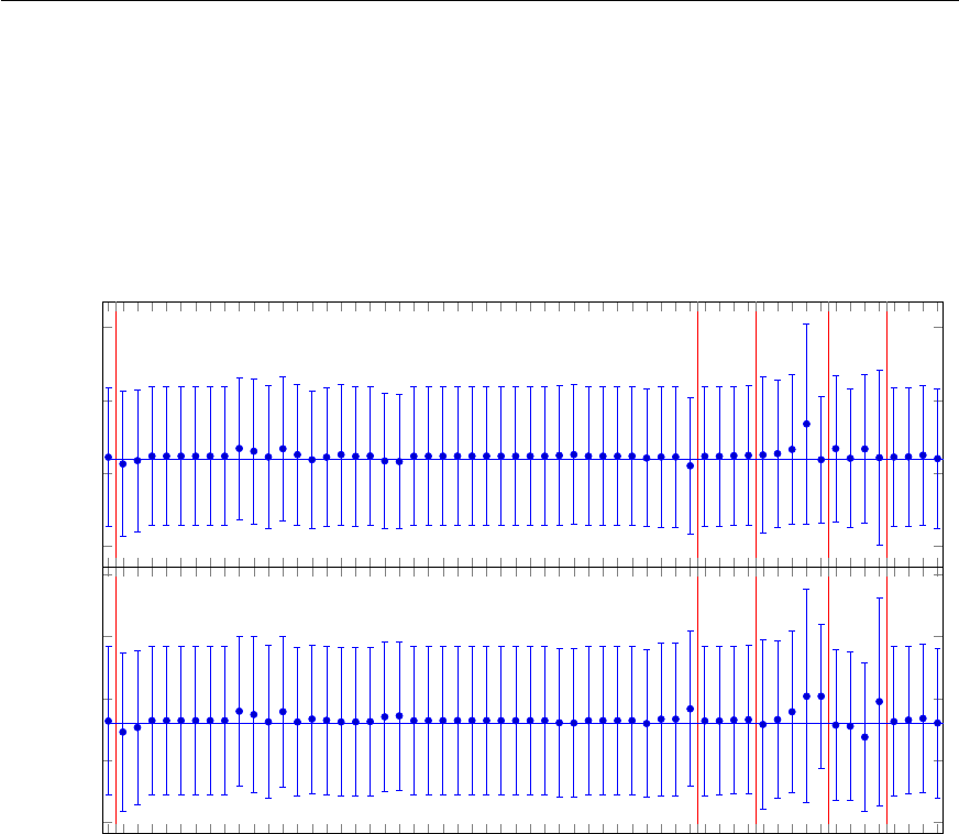
Appendix E Plots with TikZ
1
1.5
2
2.5
δ1δ2δ3δ4δ5
BD+
s1→D∗+K0
S/BD+
s1→D∗0K+
Central value
Cut on cos θ∗−0.050 for D0
Cut on cos θ∗−0.025 for D0
Cut on cos θ∗+0.025 for D0
Cut on cos θ∗+0.050 for D0
Cut on cos θ∗−0.050 for D∗+(2p,4p)
Cut on cos θ∗−0.0250 for D∗+(2p,4p)
Cut on cos θ∗−0.0250 for D∗+(2p,4p)
Cut on cos θ∗+0.050 for D∗+(2p,4p)
Cut on cos θ∗−0.050 for D0(K)
Cut on cos θ∗−0.025 for D0(K)
Cut on cos θ∗+0.025 for D0(K)
Cut on cos θ∗+0.050 for D0(K)
Window of M(D∗+) − M(D0) − 2%
Window of M(D∗+) − M(D0) − 4%
Window of M(D∗+) − M(D0)+2%
Window of M(D∗+) − M(D0)+4%
Window of M(D∗+)(2p,4p) − 2.5%
Window of M(D∗+)(2p,4p) − 5%
Window of M(D∗+)(2p,4p)+2.5%
Window of M(D∗+)(2p,4p)+5%
Window of M(D0)−5 MeV
Window of M(D0)−10 MeV
Window of M(D0)+5 MeV
Window of M(D0)+10 MeV
Cut on pT(D0) −0.05 GeV
Cut on pT(D0) −0.10 GeV
Cut on pT(D0)+0.05 GeV
Cut on pT(D0)+0.10 GeV
Cut on pT(D∗+)(2p) −0.05 GeV
Cut on pT(D∗+)(2p) −0.10 GeV
Cut on pT(D∗+)(2p)+0.05 GeV
Cut on pT(D∗+)(2p)+0.10 GeV
Cut on pT(πe)D∗+(2p,4p) −0.010 GeV
Cut on pT(πe)D∗+(2p,4p) −0.005 GeV
Cut on pT(πe)D∗+(2p,4p)+0.005 GeV
Cut on pT(πe)D∗+(2p,4p)+0.010 GeV
Cut on pT(πe)D0−0.02 GeV
Cut on pT(πe)D0−0.04 GeV
Cut on pT(πe)D0+0.02 GeV
Cut on pT(πe)D0+0.04 GeV
CAL energy scale−1%
CAL energy scale−2%
CAL energy scale+1%
CAL energy scale+2%
Change BG pars
Separate BG parameters
−16 MeV fit range
−1 MeV resolution
+1 MeV resolution
MPDG(D∗+)+0.14 MeV
MPDG(D∗+) −0.14 MeV
MPDG(D0)+0.16 MeV
MPDG(D0) −0.16 MeV
MC beauty contribution ×0.0
MC beauty contribution ×0.5
MC beauty contribution ×1.5
MC beauty contribution ×2.0
0.6
0.7
0.8
0.9
1
f(c→D+
s1)
Figure E.1: The results of strange excited charm meson fragmentation fraction and branching ratio with
systematic variations. The individual systematic variations are put into groups δ1−δ5.
86

APPENDIX F
Long tables
L
A
T
EX file: ./guide_appendix.tex
Long and complicated tables, such as tables containing the breakdown of the systematic error for each
data point are usually put into the appendices. Code or data cards can also be included here. Examples
of complicated typesetting have been given already in Chapter 6. In this appendix I give an example
of a table (Table F.1) that goes over more than one page using the xtab package. If instead you use
longtable, note that it is a combination of
tabular
and
table
in one environment. As mentioned in
Chapter 4, an alternative is the supertabular package.
While footnotes do not work properly in a normal
tabular
, but they do work in
longtable
if you
use longtable. You can use the
mpxtabuar
environment to include footnotes in a table if you use xtab.
If you use the xtab package, note that you should specify the table header and footer outside the
table itself. Do not include
xtabular
inside a
table
environment, as the table will then be output on
one page, which is not what you want! Such packages sometimes need a bit of help to get the page
breaks in the right place. According to the xtab documentation you should first try to play around with
the variable
\xentrystretch
. The default value is
0.1
. Decrease this to put more on a page and
increase it to get less. You can even set it to a negative value! The value can be set per table. As an
alternative you can use the \shrinkheight command.
87
Appendix F Long tables
Number Letter Explanation
1 a The lowercase 1st letter in the alphabeta
2 b The lowercase 2nd letter in the alphabet
3 c The lowercase 3rd letter in the alphabet
4 d The lowercase 4th letter in the alphabet
5 e The lowercase 5th letter in the alphabet
6 f The lowercase 6th letter in the alphabet
7 g The lowercase 7th letter in the alphabet
8 h The lowercase 8th letter in the alphabet
9 i The lowercase 9th letter in the alphabet
10 j The lowercase 10th letter in the alphabetb
11 k The lowercase 11th letter in the alphabet
12 l The lowercase 12th letter in the alphabet
13 m The lowercase 13th letter in the alphabet
14 n The lowercase 14th letter in the alphabet
15 o The lowercase 15th letter in the alphabet
16 p The lowercase 16th letter in the alphabet
17 q The lowercase 17th letter in the alphabet
18 r The lowercase 18th letter in the alphabet
19 s The lowercase 19th letter in the alphabet
20 t The lowercase 20th letter in the alphabet
21 u The lowercase 21st letter in the alphabet
22 v The lowercase 22nd letter in the alphabet
23 w The lowercase 23rd letter in the alphabet
24 x The lowercase 24th letter in the alphabet
25 y The lowercase 25th letter in the alphabet
26 z The lowercase 26th letter in the alphabet
1 A The uppercase 1st letter in the alphabet
2 B The uppercase 2nd letter in the alphabet
3 C The uppercase 3rd letter in the alphabet
4 D The uppercase 4th letter in the alphabet
5 E The uppercase 5th letter in the alphabet
6 F The uppercase 6th letter in the alphabet
7 G The uppercase 7th letter in the alphabet
8 H The uppercase 8th letter in the alphabet
9 I The uppercase 9th letter in the alphabet
10 J The uppercase 10th letter in the alphabet
11 K The uppercase 11th letter in the alphabet
12 L The uppercase 12th letter in the alphabet
Continued on next page
a“a” deserves a footnote
b“j” deserves another footnote
88
Number Letter Explanation
13 M The uppercase 13th letter in the alphabet
14 N The uppercase 14th letter in the alphabet
15 O The uppercase 15th letter in the alphabet
16 P The uppercase 16th letter in the alphabet
17 Q The uppercase 17th letter in the alphabet
18 R The uppercase 18th letter in the alphabet
19 S The uppercase 19th letter in the alphabet
20 T The uppercase 20th letter in the alphabet
21 U The uppercase 21st letter in the alphabet
22 V The uppercase 22nd letter in the alphabet
23 W The uppercase 23rd letter in the alphabet
24 X The uppercase 24th letter in the alphabet
25 Y The uppercase 25th letter in the alphabet
26 Z The uppercase 26th letter in the alphabet
Table F.1: The alphabet.
89

APPENDIX G
A famous equation is E=mc2
L
A
T
EX file: ./guide_appendix.tex
This chapter was included to check that one gets bold mathematics in a chapter/section title, but not in
the table of contents.
As of release of the ubonn-thesis package, no special handling of titles should be necessary. This is
because the following line was added:
\def\bfseries{\fontseries\bfdefault\selectfont\boldmath}
G.1 A slightly less famous equation F=m a
The title here does not include
\boldmath
, as the bold font series turns on bold math by default. Note
that the section in the table of contents is typeset in a normal font when writing a book or report.
G.2 The cross-section is given by σ=N/L
This attempt includes
\boldmath
by hand and uses Greek letters and some specific font. It appears to
also work OK.
91

APPENDIX H
Old or obsolete information and instructions
With time things change! Some of the instruction or packages that I recommended at an earlier time
are superseded. Operating systems and T
E
X installations also change with time. In order to avoid
cluttering up the main chapters of the guide with outdated or obsolete information, such things are
collected in this appendix.
H.1 More on feynmf
I relegate this section to the chapter on obsolete instructions, because I think it is much easier to just
use feynmp than feynmf. If you have T
E
X Live 2012, you can combine feynmp with standalone for a
very convenient way to develop and include Feynman graphs, as discussed in Section 5.6.2.
If you use feynmp you can just give the command
make feynmp
and it will produce PDF files of
all the tex files in the feynmf subdirectory.
If you do not want to include the feynmf commands for Feynman graphs in the thesis (or input the
file containing them), you can try to make encapsulated Postscript (or PDF) files that contain a single
Feynman graph and then include these as usual in your thesis.
If you want to use feynmf you can start with the
feynmf
command on the
tex
file containing the
graph.
1
This produces a
dvi
file that you then have to convert to Encapsulated Postscript and/or PDF.
This is not totally trivial.
The best way is to specify the options to the geometry package so that the page size corresponds to
the Feynman graph. For a graph with size
(
50
,
50
)
, as specified at the beginning of the
fmfgraph*
environment (within \unitlength in mm), the following wrapper works well:
\documentclass{article}
%
\usepackage[papersize={60mm,56mm},text={58mm,52mm},centering]{geometry}
\usepackage{feynmf}
\usepackage{color}
%
\pagestyle{empty}
1
Note that the example files that are included in this document tree are missing the
\documentclass
and
\usepackage
commands.
93

Appendix H Old or obsolete information and instructions
\begin{document}
\setlength{\parindent}{0pt}
\setlength{\parskip}{0pt}
\setlength{\unitlength}{1mm}
\begin{center}
\fbox{\input{figs/feynmf/ep_nc.tex}}
\end{center}
\end{document}
I also had success with the command chain:
feynmf ep_nc
dvips ep_nc
ps2epsi ep_nc.ps
and then you can include ep_nc.epsi in your L
A
T
EXfile.2To get PDF you need one more step:
epstopdf ep_nc.epsi
An alternative with explicit Metafont calls is:
pdflatex ep_nc
mf ’\mode=localfont; input ep_nc;’
pdflatex ep_nc
pdflatex ep_nc
The trouble with this is that the Feynman graph is not clipped, unless you have specified the page size
appropriately as discussed above.
H.2 Windows
H.2.1 Windows XP
As I no longer have access to a Windows XP machine, and Windows XP is slowly disappearing, my
experience with Windows XP stopped 2011.
I started the T
E
X Collection 2010 DVD. I started it as an Administrator, it opened a T
E
X Collection
window and I then clicked on proTeXt Quick Install and installed MiKT
E
X (minimal version), T
E
Xnic
Center, Ghostscript and Ghostview for all users. Once the installation was finished, I also updated all
the packages using the MiKT
E
X Maintenance (Admin)
→
Update (Admin) program. Be patient —
these updates always take a while!
You should then be able to double-click on
mythesis.tex
and try to compile it! My first attempt
at this failed. I had set MiKT
E
X to install missing packages, but it was supposed to ask me first. This
seems to work well if you are logged in as the same user (with Administration rights) as the one who
installed MiKT
E
X. The package updating does not seem to work properly (it only asks you for the
first missing package I think) if you are a normal user. After going through the exercise once as an
2
By default L
A
T
E
X will not find
.epsi
files with the
\includegraphics
command. Rename them to
.eps
instead or add
.epsi to the list of file types that \includegraphics can handle.
94

H.2 Windows
Administrator to compile the skeleton thesis, I could also compile both the thesis and the guide as a
normal user.
The second attempt was a complete MiKT
E
X installation. I told it to install missing packages
without asking. This also failed at the first attempt as it was missing the package logreq and somehow
did not install it automatically. I had to use the MiKT
E
X Maintenance (Admin)
→
Package Manager
(Admin) to install logreq.
H.2.2 T
E
Xnic Center
I tried out the T
EXnic Center, which is also available. You first have to tell it where to find the L
A
T
EX
executables. In my case this is
C:\Program Files\MiKTeX 2.8\mktex\bin
. You also have to tell
the program where to find Acrobat (Reader) although it should find it automatically.
In the T
E
Xnic Center I opened one of the main files, i.e.
mythesis.tex
or
thesis_guide.tex
and then in the
Project
menu I declared this file to be the main file for a new project. You should
declare the file format to be Unix. You can then compile the project and look at the output by hitting
Ctrl + F5
. It is also possible to set some options such that you do not have to close the file in
Acrobat Reader before compiling.
There is a small problem and irritation with T
E
Xnic Center and Acrobat Reader X. Under
Build →
Define Output Profiles →Viewer
you have to change
acroview
to
acroviewR10
in the three
places where it is given. If you then try to compile Adobe Reader opens but you get an error message.
Just view the output again
F5
and the PDF file will be shown. Via Google, I found some tricks that are
supposed to fix this problem, but they did not work for me. You can also just start Adobe Reader first
and then T
EXnic Center.
In general, I thought I liked the T
E
Xnic Center somewhat more than T
E
Xworks, which is the direct
MiKT
E
X interface. It allows you to set up projects and you then have the ability to navigate easily
through all your files via the Navigator. However, it has a serious problem in that it does not handle
UTF-8 files properly. Although support for UTF-8 has been advertised for almost two years I do not
see much signs of progress.
As T
E
Xnic Center has been dropped on the Dante T
E
X Collection 2011 DVD I have relegated this
information to a subsection.
95

Bibliography
[KD04] H. Kopka and P. W. Daly, Guide to L
A
TEX, 4th ed., Addison-Wesley, 2004
(cit. on pp. 2,9,51,54).
[MG04] F. Mittelbach and M. Goossens, The L
A
TEX Companion, 2nd ed., Addison-Wesley, 2004
(cit. on p. 2).
[Oet+] T. Oetiker et al., A (Not So) Short Introduction to LaTeX2e,
url:http://ctan.org/tex-archive/info/lshort (cit. on pp. 2,27,54).
[Fos]
B. Foster, The guide to writing ZEUS papers,url:
http://pi.physik.uni-bonn.de
(cit. on p. 2).
[ZA+10] ZEUS Collab., H. Abramowicz et al.,
Inclusive dijet cross sections in neutral current deep inelastic scattering at HERA,
Eur. Phys. J. C70 (2010) 965, arXiv: 1010.6167 [hep-ex] (cit. on pp. 51,54).
[Abr+10a] H. Abramowicz et al., Measurement of high-Q2charged current deep inelastic
scattering cross sections with a longitudinally polarised positron beam at HERA,
Eur. Phys. J. C70 (2010) 945, arXiv: 1008.3493 [hep-ex] (cit. on p. 51).
[Abr+10b] H. Abramowicz et al.,
Measurement of D+and Λ+
cproduction in deep inelastic scattering at HERA,
JHEP 11 (2010) 009, arXiv: 1007.1945 [hep-ex] (cit. on p. 51).
[Brü+04a] O. S. Brüning et al., eds., LHC Design Report. 1. The LHC Main Ring,
CERN-2004-003-V-1, CERN-2004-003, 2004,
url:https://cdsweb.cern.ch/record/782076 (cit. on p. 54).
[Lod12] T. Loddenkötter,
Implementation of a kinematic fit of single top-quark production in association with a
W
boson and its application in a neural-network-based analysis in ATLAS,
BONN-IR-2012-06, PhD Thesis: University of Bonn, 2012,
url:http://hss.ulb.uni-bonn.de/diss_online (cit. on p. 54).
[Bru+04] (. Bruning Oliver S. et al., LHC Design Report. 1. The LHC Main Ring,
(2004), Entry directly From InSpire (cit. on p. 54).
[Brü+04b] O. S. Brüning et al., LHC Design Report,Entry directly From CDS, CERN, 2004
(cit. on p. 54).
[Brü+04c] O. S. Brüning et al., eds., LHC Design Report. 1. The LHC Main Ring,
CERN-2004-003-V-1, CERN-2004-003, 2004,
url:https://cdsweb.cern.ch/record/782076 (cit. on p. 54).
97
Bibliography
[11] Determination of the muon reconstruction efficiency in ATLAS at the Z resonance in
proton-proton collisions at sqrt(s)=7 TeV, tech. rep. ATLAS-CONF-2011-008,
Entry directly from CDS: CERN, 2011 (cit. on p. 54).
[ATL11a]
ATLAS Collaboration, Determination of the muon reconstruction efficiency in ATLAS at
the Zresonance in proton–proton collisions at √s=7 TeV, ATLAS-CONF-2011-008,
CERN, 2011 (cit. on p. 55).
[HM84a] F. Halzen and A. D. Martin,
Quarks and Leptons: An Introductory Course in Modern Particle Physics, Wiley, 1984,
isbn: 9780471887416 (cit. on p. 55).
[HM84b]
F. Halzen and A. D. Martin, QUARKS AND LEPTONS: AN INTRODUCTORY COURSE
IN MODERN PARTICLE PHYSICS, (1984), Entry directly From InSpire (cit. on p. 55).
[Aad+11] G. Aad et al., Measurement of the top quark-pair production cross section with ATLAS
in pp collisions at
√s=
7TeV,Eur.Phys.J.
C71
(2011) 1577,Entry directly From InSpire,
arXiv: 1012.1792 [hep-ex] (cit. on p. 55).
[ATL11b]
ATLAS Collaboration, Measurement of the top quark-pair production cross section with
ATLAS in pp collisions at √s=7TeV,Eur. Phys. J. C 71 (2011) 1577,
arXiv: 1012.1792 (cit. on p. 55).
[ATL15] ATLAS Collaboration, Search for new phenomena in final states ...,
Eur. Phys. J. C 75 (2015) 299, arXiv: 1502.01518 [hep-ex] (cit. on p. 57),
Erratum: Eur. Phys. J. C 75 (2015) 408.
[Gla61] S. Glashow, Partial Symmetries of Weak Interactions, Nucl. Phys. 22 (1961) 579;
A. Salam, “Weak and Electromagnetic Interactions”, Elementary particle theory.
Relativistic groups and analyticity. Proceedings of the Eighth Nobel Symposium,
ed. by N. Svartholm, Stockholm: Almquist & Wiksell, 1968 367; S. Weinberg,
A Model of Leptons, Phys. Rev. Lett. 19 (1967) 1264, cit. on p. 59.
[ZC+10a] ZEUS Collab., S. Chekanov et al., A QCD analysis of ZEUS diffractive data,
Nucl. Phys. B831 (2010) 1, arXiv: 0911.4119 [hep-ex] (cit. on p. 59).
[ZC+09] ZEUS Collab., S. Chekanov et al.,
Exclusive photoproduction of upsilon mesons at HERA,Phys. Lett. B680 (2009) 4,
arXiv: 0903.4205 [hep-ex] (cit. on p. 59).
[ZC+10b] ZEUS Collab., S. Chekanov et al.,
Measurement of J/ψphotoproduction at large momentum transfer at HERA,
JHEP 05 (2010) 085, arXiv: 0910.1235 [hep-ex] (cit. on p. 59).
[HA+10a]
H1 and ZEUS Collab., F. D. Aaron et al., Combined Measurement and QCD Analysis of
the Inclusive ep Scattering Cross Sections at HERA,JHEP 01 (2010) 109,
arXiv: 0911.0884 [hep-ex] (cit. on p. 59).
[HA+10b] H1 and ZEUS Collab., F. D. Aaron et al., Events with an Isolated Lepton and Missing
Transverse Momentum and Measurement of W Production at HERA,
JHEP 03 (2010) 035, arXiv: 0911.0858 [hep-ex] (cit. on p. 59).
98

List of Figures
2.1 Example of (a) a problem with line numbers and (b) its solution. ........... 19
4.1 Optional caption without \mynote so that “List of Figures” does not break. . . . . . 30
5.1
Sketch of the LHC ring, the position of the experiments and the surrounding countryside.
32
5.2 Adding letters to figures with \put........................... 32
5.3 Adding letters to figures with tabular......................... 33
5.4 A small figure with a simple caption beside it. ..................... 33
5.5 Processes in ep scattering. ............................... 34
5.6 The ZEUS coordinate system. ............................. 35
5.7 Event reconstruction and simulation in ZEUS ..................... 36
5.8 Example Feynman graphs for the associated production of a top quark and a Zboson. 39
5.9 NC and CC graphs for ep scattering using feynmf code directly. ............ 41
5.10 Feynman graphs drawn with feynmp and tikz...................... 42
E.1 Strange D∗∗ systematics, fragmentation fractions ................... 86
99

List of Tables
4.1 Useful packages for layout. ............................... 26
4.2 Useful packages for appearance. ............................ 27
4.3 Other useful packages. ................................. 28
4.4 Other packages that are often used, but I have already given alternatives. ....... 29
6.1 A table of viscosities in the default language and German. ............... 44
6.2 A selection of cross-section measurements! ...................... 45
6.3
Another selection of cross-section measurements! Note the use of
\sisetup
to keep
the plus signs on the positive errors. .......................... 46
6.4 Cross-section measurements! .............................. 48
6.5 Cross-sections using sidewaystable, which also rotates the caption. ........ 49
A.1 Changes to the ubonn-thesis and ubonn-biblatex style files. .............. 67
A.1 Changes to the ubonn-thesis and ubonn-biblatex style files. .............. 68
A.2 Changes to the pibonn-thesis style files. ........................ 68
A.2 Changes to the pibonn-thesis style files. ........................ 69
A.2 Changes to the pibonn-thesis style files. ........................ 70
F.1 The alphabet. ...................................... 89
101


Index
\*APBzero, 16
\missingfigure, 29
\printbibliography, 59
adjustbox, 28
align(*), 19
alignat(*), 19
American English, 10
AMS math, 2
amsmath, 19,27
amssymb, 27
\ang, 14
array, 27,47
\arraystretch, 43,47
article, 25,54
astronomy, 56
astrophysics, 56
axodraw, 28,38,70
babel, 26,63,64
background, 28,69
\backmatter, 25,65
\bar, 17
biber, 57,72–74
\bibitem, 51
biblatex, 6–8,51–57,59,60,68,69,71,74
@Set option, 59
\bibliography, 53
BibT
EX, 52
bibtex, 74
bibtex8, 74
bibtool, 60
\Bo, 17
\Bobar, 17
\boldmath, 18,68,91
book, 25,54,55
booktabs, 27,43,62,70
\bottomrule, 43,70
British English, 10
BSc, 6,22
caption, 29
captionbeside, 33
CDS, 54
\centering, 31,47
chapter
heading, 65
\chapter, 113
\chapter*, iii
ChkTeX, 11
\cite, 51,59,60
\citealt, 59
\citep, 59
\citet, 59
cleveref, 8,27,28,67
\clight, 14
color, 29,69
link, 64
commath, 27,28
compiling, 5
conference note, 54
coordinates, 10
courier, 26
cover, 6
\cref{fig:plot}, 27,28
csquotes, 10,26,64,69,77
ctable, 62
CV, 21
dcolumn, 11,28,29,47,63
107

Index
department library, 22,23
derivative, 11
design report, 54
\dif, 11
Diplom, 6,22
displaymath, 14,15,19
\documentclass, 6,21–23,63,93
draft, 28
draftwatermark, 28,29
em, 10
emacs, 9,11,71
English, 2
English mistakes, 18
\enquote, 10,64
\ensuremath, 9
eqnarray, 19
equation, 19
equation*, 14,15,19
Errata, 57
ex, 10
\extrarowheight, 44
fancyhdr, 29
fancyvrb, 53
\fbox, 40
feymp, 41
Feynman graphs, 38
feynmf, 6,8,20,27,29,32,38–41,61,68,69,
74,93
feynmp, 6,8,20,28,32,38–42,68,69,74,76,
93
\figureformat, 31
figures, 31
directories, 12
Feynman graphs, 38
multiple, 32
figures formats, 33
\figwidth, 33
float, 29
floatflt, 28,29
floatrow, 28
fmffile, 39,40
fmfgraph*, 93
fncychap, 29,65
font
lmodern, 7
fontenc, 26
footnote, 61
\footnotemark, 62
\footref, 62
\foreignlanguage, 44,64
\foreignquote, 64
\frontmatter, 25
geometry, 25,26,61,93
German, 63
ghostscript, 76
ghostview, 76
Git, 75
glossaries, 28,81,82
glossary, 28,81
glosstex, 81
\gls, 82
\graphicspath, 12
graphicx, 27,28
helvet, 26
hepnicename, 38
hepnicenames, 8,10,16,27,67
\HepParticle, 16
hepparticles, 10,16,27
heppennames, 8,10,16,27,67
hepunits, 9,13,15,29
\hspace, 46
\hspace*, 46
hyperref, 9,21,28,59,60,64,81
\hypersetup, 21,22,64
IEEEeqnarray, 27
IEEEtrantools, 27,28
ifthen, 28
\ifthenelse, 28,69
\ifthenelse{\texlive < 2011}, 44
\include, 28
\includegraphics, 12,27,31,32,94
\inInstitute, 7
inputenc, 26
inspire, 54
\InstituteAddress, 7
\InstituteName, 7
108

Index
internal note, 54
jaxodraw, 70
keyval, 68
kile, 11,71,72
\KOMAoptions, 25,71
KOMA-Script,25
Kubuntu, 73
\label, 31,62
L
A
T
EX, 1
L
A
T
EX Workshop, 11,72
latexmk, 6,40,72,82
library
department, 22,23
university, 22
line numbers, 19
lineno, 19
linenomath, 19
Linux, 73
\listoftodos, 29
lmodern, 7,64
logreq, 95
longtable, 7,26,62,68,87
MacOS, 73
\mainmatter, 25,65,68
\makeglossaries, 81
Master thesis, 54
math
bold, 17,91
mathpazo, 16,26
\mathrm, 9,17
mcite, 51,59,60
metafont, 39
metapost, 39
\MeVovercsq, 14
mhchem, 27,67
microtype, 26,27
\midrule, 43,70
MiKTeX, 76,94
mpxtabuar, 26,87
mpxtabular, 62
MSc, 6,22
msys-base, 76
\mynote, 8,29,99
\mysim, 17
\mysymeq, 17
natbib, 59
\newcommand, 9
\newcommand*, 9
newtx, 7,8,16,26,38,64,67,68
nomencl, 29,81
note
conference, 54
internal, 54
\num, 13,17,44–46,63
\numerrt, 14
\numpmerr, 14,45
\numpmerrt, 14
options, 7
otherlanguage, 64
\overline, 17
page, 61
particles, 16
\per, 13
pgfplots, 34,85
\phantom, vi,43
PhD, 6,21
PhD thesis, 54
physics, 11,27,28,74
pibonn-thesis, 68–70
\power, 15,16
preprint, 55
\printbibliography, 52
\printglossaries, 81
proceedings, 54
\put, 32,99
pxfonts, 16,26,64
PyFeyn, 38,39
pyx, 38
\qquad, 10
\quad, 10
quotation marks, 64
quotchap, 29,65
quotes, 64
109

Index
range, 17
refcheck, 9,28,67,68
RefTeX, 11,71
report, 25
technical, 54
\RequirePackage, 70
\rm, 12
rotating, 27
rounding, 45
\rule, 43,47
\sc, 12
scrartcl, 25
scrbook, 25
scrlayer-scrpage, 25,26,29,67
scrpage2, 25,67
scrreprt, 25
\selectlanguage, 64
\setcapindent, 31
\setkomafont, 31,64
\setlength, 32
\setlength{\unitlength}{1pt},28
setspace, 26,61
\sfrac, 14
\shrinkheight, 87
\SI, 9,13,14,17
sideways, 47
sidewaystable, 47,49
\SIerrs, 14
\SIerrt, 14
\SIerrtt, 14
\SIpmerr, 14
\SIpmerrs, 14,15
\SIpmerrt, 14
\SIpmerrtt, 14,15
\sisetup, 9,14,17,46,63,101
SIunits, 9,13,15,17,29
siunitx, 7–11,13–15,17,27–29,44–46,63,
69–71
skmath, 27,28
Spell Right, 11
spires, 54
standalone, 27,28,38,40,68,93
subcaption, 7,9,28,33,38,67,68
subfig, 7,28,29,33,38,68
subfigure, 29,38
subfiles, 27,28,69
submit, 21
BSc thesis, 22
Diplom thesis, 22
MSc thesis, 22
PhD thesis, 21
supertabular, 26,82,87
table, 43,47,62,87
tablefootnote, 62
\tablefootnote, 62
tabular, 32,33,43,44,47,62,87
tabular*, 43
tabularx, 28,43
T
EX distribution, 2
texdoc, 2
T
EX Live
2009, 13
2011, 13
\texlive, 7,14,56,74
TeXmaker, 71
TeXnic Center, 94,95
TeXStudio, 72
TeXstudio, 71
\text, 9,12,15,17
\textrm, 9,17
\textsc, 12
thesis, 54,55
Bachelor, 6
Diplom, 6
Master, 6,54
PhD, 6,54
\thesisabstract, 64
TikZ, 85
TikZ, 34,41
tikz, 27,28,34,38,41,42,68,85
tikz-3dplot, 34
tikz-palattice, 35
tips, 5
titlesec, 8,26,27,65
\todo, 29
todonotes, 8,27–29,67
\toprule, 43,70
tortoisegit, 75
110

Index
\tt, 12
txfonts, 7,8,16,26,64,68
typearea, 25,26,61
\U1S, 16
ubonn-biblatex, 67,68
ubonn-biblatex.sty, 59
ubonn-thesis, 5,6,8,17,18,20–23,25,26,28,
29,37,52,56,59,67,68,74,91
updating, 20
Ubuntu, 73
ubuntu
12.04, 13
UK English, 10
ULB, 22
\unit, 13,15,17
\unitlength, 28,93
\unitlength}{1pt}, 28,110
units, 9,13,29
university library, 22
upadting, 20
\url, 28
US English, 10
\usepackage, 21,70,93
\usk, 16
\verb, 53
Visual Studio Code, 11,71,72
vscode, see Visual Studio Code
windows, 75
wrapfig, 28,33
\write18, 20,40,68
xcolor, 27,29,69
\xentrystretch, 87
xfrac, 27
xspace, 17,26
\xspace, 9,15,17
xtab, 7,26,27,62,68,82,87
xtabular, 62,87
Xubuntu, 73
\Z0, 16
ZEUS paper guide, 2
ziffer, 28,29,47,63
111

Acknowledgements
There is plenty of discussion as to where the acknowledgements should go in a thesis. The two most
common places are just after the title and dedication or right at the end. For the purpose of this guide I
include both options.
Acknowledgements at the end should be in
\chapter
so that they appear in the Table of Contents.
113
