Tmod: Analysis Of Transcriptional Modules Tmod User Manual
User Manual:
Open the PDF directly: View PDF ![]() .
.
Page Count: 95
- Introduction
- Dive into tmod: analysis of transcriptomic responses to tuberculosis
- Statistical tests in tmod
- Visualisation and presentation of results in tmod
- Working with limma
- Using tmod for other types of GSEA analyses
- Using and creating modules and gene sets
- Case studies
- References
tmod: Analysis of Transcriptional
Modules
January Weiner
2018-11-28
Abstract
The package tmod provides blood transcriptional modules described by Chaussabel et
al. (2008) and by Li et al. (2014) as well as metabolic profiling clusters from Weiner et
al. (2012). Furthermore, the package includes several tools for testing the significance of
enrichment of modules or other gene sets as well as visualisation of the features (genes,
metabolites etc.) and modules. This user guide is a tutorial and main documentation for
the package.
Contents
1 Introduction 3
2 Dive into tmod: analysis of transcriptomic responses to tuberculosis 5
2.1 Introduction . . . . . . . . . . . . . . . . . . . . . . . . . . . . . . . . 5
2.2 The Gambia data set . . . . . . . . . . . . . . . . . . . . . . . . . . . . 5
2.3 Transcriptional module analysis with GSEA . . . . . . . . . . . . . . . . 7
2.4 Visualizing results . . . . . . . . . . . . . . . . . . . . . . . . . . . . . 9
3 Statistical tests in tmod 11
3.1 Introduction . . . . . . . . . . . . . . . . . . . . . . . . . . . . . . . . 11
3.2 First generation tests . . . . . . . . . . . . . . . . . . . . . . . . . . . . 12
3.3 Second generation tests . . . . . . . . . . . . . . . . . . . . . . . . . . . 14
3.3.1 U-test (tmodUtest) . . . . . . . . . . . . . . . . . . . . . . . . . 14
3.3.2 CERNO test (tmodCERNOtest and tmodZtest) . . . . . . . . . . 15
3.3.3 PLAGE . . . . . . . . . . . . . . . . . . . . . . . . . . . . . . . 16
3.4 Permutation tests . . . . . . . . . . . . . . . . . . . . . . . . . . . . . . 18
3.4.1 Introduction . . . . . . . . . . . . . . . . . . . . . . . . . . . . . 18
3.4.2 Permutation testing – a general case . . . . . . . . . . . . . . . . . 18
3.4.3 Permutation testing with tmodGeneSetTest . . . . . . . . . . . . 21
3.5 Comparison of different tests . . . . . . . . . . . . . . . . . . . . . . . . 22
4 Visualisation and presentation of results in tmod 23
4.1 Introduction . . . . . . . . . . . . . . . . . . . . . . . . . . . . . . . . 23
4.2 Evidence plots . . . . . . . . . . . . . . . . . . . . . . . . . . . . . . . 23
4.3 Summary tables . . . . . . . . . . . . . . . . . . . . . . . . . . . . . . . 25
4.4 Panel plots with tmodPanelPlot . . . . . . . . . . . . . . . . . . . . . . 26
5 Working with limma 30
1
5.1 Limma and tmod . . . . . . . . . . . . . . . . . . . . . . . . . . . . . . 30
5.2 Minimum significant difference (MSD) . . . . . . . . . . . . . . . . . . . 31
5.3 Comparing tests across experimental conditions . . . . . . . . . . . . . . 35
6 Using tmod for other types of GSEA analyses 41
6.1 Correlation analysis . . . . . . . . . . . . . . . . . . . . . . . . . . . . . 41
6.2 Functional multivariate analysis . . . . . . . . . . . . . . . . . . . . . . 43
6.3 PCA and tag clouds . . . . . . . . . . . . . . . . . . . . . . . . . . . . . 48
7 Using and creating modules and gene sets 53
7.1 Using built-in gene sets (transcriptional modules) . . . . . . . . . . . . . 53
7.2 Accessing the tmod module data directly . . . . . . . . . . . . . . . . . . 54
7.2.1 Module operations . . . . . . . . . . . . . . . . . . . . . . . . . 55
7.2.2 Using tmod modules in other programs . . . . . . . . . . . . . . . 56
7.2.3 Custom module definitions . . . . . . . . . . . . . . . . . . . . . 65
7.3 Obtaining other gene sets . . . . . . . . . . . . . . . . . . . . . . . . . . 66
7.3.1 MSigDB . . . . . . . . . . . . . . . . . . . . . . . . . . . . . . . 67
7.3.2 Using the ENSEMBL databases through biomaRt . . . . . . . . . . 69
7.3.3 Gene ontologies (GO) . . . . . . . . . . . . . . . . . . . . . . . . 70
7.3.4 KEGG pathways . . . . . . . . . . . . . . . . . . . . . . . . . . . 73
7.3.5 Manual creation of tmod module objects: MSigDB . . . . . . . . . 74
8 Case studies 77
8.1 Metabolic profiling of TB patients . . . . . . . . . . . . . . . . . . . . . . 77
8.1.1 Introduction . . . . . . . . . . . . . . . . . . . . . . . . . . . . . 77
8.1.2 Differential analysis . . . . . . . . . . . . . . . . . . . . . . . . . 78
8.1.3 Functional multivariate analysis . . . . . . . . . . . . . . . . . . . 84
8.2 Case study: RNASeq . . . . . . . . . . . . . . . . . . . . . . . . . . . . 89
References 92
2
Chapter 1
Introduction
Gene set enrichment analysis (GSEA) is an increasingly important tool in the biological
interpretation of high throughput data, versatile and powerful. In general, there are three
generations of GSEA algorithms and packages.
First generation approaches test for enrichment in defined sets of differentially ex-
pressed genes (often called “foreground”) against the set of all genes (“background”). The
statistical test involved is usually a hypergeometric or Fisher’s exact test. The main prob-
lem with this kind of approach is that it relies on arbitrary thresholds (like p-value or log
fold change cut-offs), and the number of genes that go into the “foreground” set depends
on the statistical power involved. Comparison between the same experimental condition
will thus yield vastly different results depending on the number of samples used in the
experiment.
The second generation of GSEA involve tests which do not rely on such arbitrary defi-
nitions of what is differentially expressed, and what not, and instead directly or indirectly
employ the information about the statistical distribution of individual genes. A popular
implementation of this type of GSEA is the eponymous GSEA program (Subramanian et
al. 2005). While popular and quite powerful for a range of applications, this software has
important limitations due to its reliance on bootstrapping to obtain an exact p-value. For
one thing, the performance of GSEA dramatically decreases for small sample numbers
(Weiner 3rd and Domaszewska 2016). Moreover, the specifics of the approach prevent it
from being used in applications where a direct test for differential expression is either not
present (for example, in multivariate functional analysis, see Section “Functional multi-
variate analysis”).
3

The tmod package and the included CERNO1test belong to the second generation of
algorithms. However, unlike the program GSEA, the CERNO relies exclusively on an
ordered list of genes, and the test statistic has a χ² distribution. Thus, it is suitable for
any application in which an ordered list of genes is generated: for example, it is possible
to apply tmod to weights of PCA components or to variable importance measure of a
machine learning model.
tmod was created with the following properties in mind: (i) test for enrichment which
relies on a list of sorted genes, (ii) with an analytical solution, (iii) flexible, allowing custom
gene sets and analyses, (iv) with visualizations of multiple analysis results, suitable for
time series and suchlike, (v) including transcriptional module definitions not present in
other databases and, finally, (vi) to be suitable for use in R.
1Coincident Extreme Ranks in Numerical Observations (Yamaguchi et al. 2008)
4

Chapter 2
Dive into tmod: analysis of
transcriptomic responses to tuberculosis
2.1 Introduction
In this chapter, I will use an example data set included in tmod to show the application
of tmod to the analysis of differential gene expression. The data set has been generated
by Maerdorf et al. (2011) and has the GEO ID GSE28623. Is based on whole blood RNA
microarrays from tuberculosis (TB) patients and healthy controls.
Although microarrays were used to generate the data, the principle is the same as in
RNASeq.
2.2 The Gambia data set
In the following, we will use the Egambia data set included in the package. The data
is already background corrected and normalized, so we can proceed with a differential
gene expression analysis. Note that only a bit over 5000 genes from the original set of
over 45000 probes is included.
library(limma)
library(tmod)
5

data(Egambia)
design <- cbind(Intercept=rep(1,30), TB=rep(c(0,1), each= 15))
E <- as.matrix(Egambia[,-c(1:3)])
fit <- eBayes(lmFit(E, design))
tt <- topTable(fit, coef=2,number=Inf,
genelist=Egambia[,1:3])
The table below shows first couple of results from the table tt.
GENE_SYMBOL
GENE_NAME logFC adj.P.Val
FAM20A family with sequence similarity 20,
member A”
2.956 0.001899
FCGR1B Fc fragment of IgG, high affinity Ib,
receptor (CD64)”
2.391 0.002095
BATF2 basic leucine zipper transcription
factor, ATF-like 2
2.681 0.002216
ANKRD22 ankyrin repeat domain 22 2.764 0.002692
SEPT4 septin 4 3.287 0.002692
CD274 CD274 molecule 2.377 0.002692
OK, we see some of the genes known to be prominent in the human host response
to TB. We can display one of these using tmod’s showGene function (it’s just a boxplot
combined with a beeswarm, nothing special):
group <- rep(c("CTRL","TB"), each=15)
showGene(E["20799",], group,
main=Egambia["20799","GENE_SYMBOL"])
6
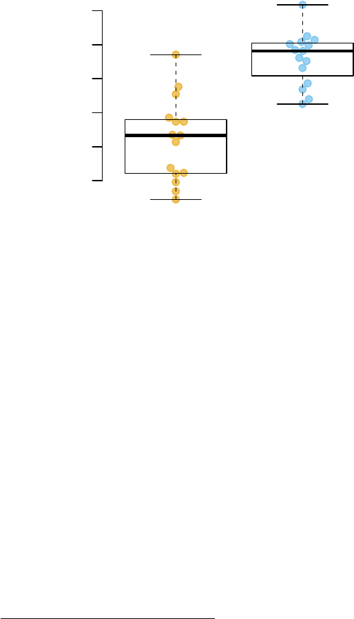
FCGR1B
log2 expression
11
12
13
14
15
16
CTRL
TB
Fine, but what about the modules?
2.3 Transcriptional module analysis with GSEA
There are two main functions in tmod to understand which modules or gene sets are sig-
nificantly enriched1. There are several statistical tests which can be used from within
tmod (see chapter “Statistical tests in tmod” below), but here we will use the CERNO test,
which is the main reason this package exist. CERNO is particularly fast and robust second
generation approach, recommended for most applications.
CERNO works with an ordered list of genes (only ranks maer, no other statistic is
necessary); the idea is to test, for each gene set, whether the genes in this gene set are
more likely than others to be at the beginning of that list. The CERNO statistic has a χ2
distribution and therefore no randomization is necessary, making the test really fast.
1If you work with limma, there are other, more efficient and simpler to use functions. See “Working with
limma” below.
7

l <- tt$GENE_SYMBOL
resC <- tmodCERNOtest(l)
head(resC, 15)
## ID Title cerno
## LI.M37.0 LI.M37.0 immune activation - generic cluster 426.4
## LI.M11.0 LI.M11.0 enriched in monocytes (II) 113.8
## LI.S4 LI.S4 Monocyte surface signature 76.4
## LI.M112.0 LI.M112.0 complement activation (I) 73.7
## LI.M75 LI.M75 antiviral IFN signature 65.3
## LI.M16 LI.M16 TLR and inflammatory signaling 46.3
## LI.M67 LI.M67 activated dendritic cells 49.5
## LI.M165 LI.M165 enriched in activated dendritic cells (II) 91.7
## LI.M37.1 LI.M37.1 enriched in neutrophils (I) 68.0
## LI.M118.0 LI.M118.0 enriched in monocytes (IV) 54.6
## LI.S5 LI.S5 DC surface signature 123.2
## LI.M4.3 LI.M4.3 myeloid cell enriched receptors and transporters 34.4
## LI.M20 LI.M20 AP-1 transcription factor network 31.9
## LI.M81 LI.M81 enriched in myeloid cells and monocytes 57.0
## LI.M150 LI.M150 innate antiviral response 31.8
## N1 AUC cES P.Value adj.P.Val
## LI.M37.0 100 0.746 2.13 1.82e-18 6.31e-16
## LI.M11.0 20 0.777 2.85 5.26e-09 9.09e-07
## LI.S4 10 0.897 3.82 1.61e-08 1.85e-06
## LI.M112.0 11 0.846 3.35 1.72e-07 1.49e-05
## LI.M75 10 0.893 3.26 1.05e-06 7.19e-05
## LI.M16 5 0.979 4.63 1.25e-06 7.19e-05
## LI.M67 6 0.971 4.13 1.69e-06 8.36e-05
## LI.M165 19 0.720 2.41 2.44e-06 1.06e-04
## LI.M37.1 12 0.870 2.83 4.32e-06 1.66e-04
## LI.M118.0 9 0.877 3.03 1.49e-05 5.17e-04
## LI.S5 34 0.683 1.81 4.78e-05 1.50e-03
## LI.M4.3 5 0.886 3.44 1.59e-04 4.58e-03
## LI.M20 5 0.876 3.19 4.09e-04 9.96e-03
## LI.M81 13 0.756 2.19 4.22e-04 9.96e-03
## LI.M150 5 0.950 3.18 4.32e-04 9.96e-03
8

Only first 15 results are shown above.
Columns in the above table contain the following:
•ID The module ID. IDs starting with “LI” come from Li et al. (S. Li et al. 2014),
while IDs starting with “DC” have been defined by Chaussabel et al. (Chaussabel
et al. 2008).
•Title The module description
•cerno The CERNO statistic
•N1 Number of genes in the module
•AUC The area under curve – main size estimate
•cES CERNO statistic divided by 2×N1
•P.Value P-value from the hypergeometric test
•adj.P.Val P-value adjusted for multiple testing using the Benjamini-Hochberg cor-
rection
These results make a lot of sense: the transcriptional modules found to be enriched in a
comparison of TB patients with healthy individuals are in line with the published findings.
In especially, we see the interferon response, complement system as well as T-cell related
modules.
2.4 Visualizing results
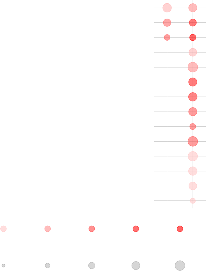
The main working horse for visualizing the results in tmod is the function tmodPanelPlot.
This is really a glorified heatmap which shows both the effect size (size of the blob on
the figure below) and the p-value (intensity of the color). Each column corresponds to a
different comparison. Here, there will be only one column for the only comparison we
made, however we need to wrap it in a list object. However, we can also use a slightly
different representation to also show how many significantly up- and down-regulated2
genes are found in the enriched modules (right panel on the figure below).
2Formally, we don’t test for regulation here. “Differentially expressed” is the correct expression. I will
use, however, the word “regulated” throughout this manual with the understanding that it only means
“there is a difference between two conditions” because it is shorter.
9
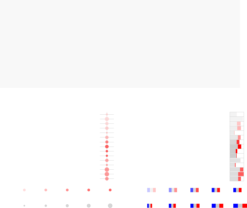
par(mfrow=c(1,2))
tmodPanelPlot(list(Gambia=resC))
## calculate the number of significant genes
## per module
pie <- tmodDecideTests(g=tt$GENE_SYMBOL,
lfc=tt$logFC,
pval=tt$adj.P.Val)
names(pie) <- "Gambia"
tmodPanelPlot(list(Gambia=resC), pie=pie, grid="b")
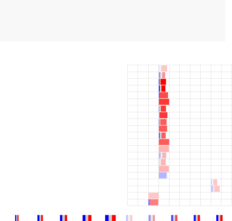
enriched in myeloid cells and monocytes (LI.M81)
innate antiviral response (LI.M150)
AP−1 transcription factor network (LI.M20)
myeloid cell enriched receptors and transporters (LI.M4.3)
DC surface signature (LI.S5)
enriched in monocytes (IV) (LI.M118.0)
complement activation (I) (LI.M112.0)
Monocyte surface signature (LI.S4)
enriched in monocytes (II) (LI.M11.0)
immune activation − generic cluster (LI.M37.0)
enriched in neutrophils (I) (LI.M37.1)
enriched in activated dendritic cells (II) (LI.M165)
activated dendritic cells (LI.M67)
TLR and inflammatory signaling (LI.M16)
antiviral IFN signature (LI.M75)
Gambia
Effect size:
P value:
0.68 0.98
0.01 0.001 10−410−510−6
On the right hand side, the red color on the bars indicates that all signficantly regulated
in the enriched modules. The size of the bar corresponds to the AUC, and intensity of the
color corresponds to the p-value. See chapter “Visualisation and presentation of results
in tmod” for more information on this and other functions.
10

Chapter 3
Statistical tests in tmod
3.1 Introduction
There is a substantial numer of different gene set enrichment tests. Several are imple-
mented in tmod (see Table below for a summary). This chapter gives an overview of the
possibilities for gene set enrichment analysis with tmod.
Test Description Input type
tmodHGtest First generation test Two sets, foreground and
background
tmodUtest Wilcoxon U test Ordered gene list
tmodCERNOtest CERNO test Ordered gene list
tmodZtest variant of the CERNO
test
Ordered gene list
tmodPLAGEtest eigengene-based Expression matrix
tmodAUC general permutation
based testing
Matrix of ranks
tmodGeneSetTest permutation based on a
particular statistic
A statistic (e.g. logFC)
In the following, I will briefly describe the various tests and show examples of usage
on the Gambia data set.
11

3.2 First generation tests
First generation tests were based on an overrepresentation analysis (ORA). In essence,
they rely on spliing the genes into two groups: the genes of interest (foreground), such
as genes that we consider to be significantly regulated in an experimental condition, and
all the rest (background). For a given gene set, this results in a 2×2contingency table. If
these two factors are independent (i.e., the probability of a gene belonging to a gene set is
independent of the probability of a gene being regulated in the experimental condition),
then we can easily derive expected frequencies for each cell of the table. Several statistical
tests exist to test whether the expected frequencies differ significantly from the observed
frequencies.
In tmod, the function tmodHGtest(), performs a hypergeometric test on two groups
of genes: ‘foreground’ (fg), or the list of differentially expressed genes, and ‘background’
(bg) – the gene universe, i.e., all genes present in the analysis. The gene identifiers used
currently by tmod are HGNC identifiers, and we will use the GENE_SYMBOL field from
the Egambia data set.
In this particular example, however, we have almost no genes which are significantly
differentially expressed after correction for multiple testing: the power of the test with 10
individuals in each group is too low. For the sake of the example, we will therefore relax
our selection. Normally, I’d use a q-value threshold of at least 0.001.
fg <- tt$GENE_SYMBOL[tt$adj.P.Val < 0.05 &abs( tt$logFC ) > 1]
resHG <- tmodHGtest(fg=fg, bg=tt$GENE_SYMBOL)
options(width=60)
resHG
## ID
## LI.M112.0 LI.M112.0
## LI.M11.0 LI.M11.0
## LI.M75 LI.M75
## LI.S4 LI.S4
## LI.S5 LI.S5
## LI.M165 LI.M165
## LI.M4.3 LI.M4.3
## LI.M16 LI.M16
## Title
12
## LI.M112.0 complement activation (I)
## LI.M11.0 enriched in monocytes (II)
## LI.M75 antiviral IFN signature
## LI.S4 Monocyte surface signature
## LI.S5 DC surface signature
## LI.M165 enriched in activated dendritic cells (II)
## LI.M4.3 myeloid cell enriched receptors and transporters
## LI.M16 TLR and inflammatory signaling
## b B n N E P.Value adj.P.Val
## LI.M112.0 4 11 47 4826 37.3 2.48e-06 0.000858
## LI.M11.0 4 20 47 4826 20.5 3.41e-05 0.005907
## LI.M75 3 10 47 4826 30.8 9.91e-05 0.008569
## LI.S4 3 10 47 4826 30.8 9.91e-05 0.008569
## LI.S5 4 34 47 4826 12.1 2.96e-04 0.020465
## LI.M165 3 19 47 4826 16.2 7.52e-04 0.039413
## LI.M4.3 2 5 47 4826 41.1 9.11e-04 0.039413
## LI.M16 2 5 47 4826 41.1 9.11e-04 0.039413
The columns in the above table contain the following:
•ID The module ID. IDs starting with “LI” come from Li et al. (S. Li et al. 2014),
while IDs starting with “DC” have been defined by Chaussabel et al. (Chaussabel
et al. 2008).
•Title The module description
•bNumber of genes from the given module in the fg set
•BNumber of genes from the module in the bg set
•nSize of the fg set
•NSize of the bg set
•EEnrichment, calcualted as (b/n)/(B/N)
•P.Value P-value from the hypergeometric test
•adj.P.Val P-value adjusted for multiple testing using the Benjamini-Hochberg cor-
rection
Well, IFN signature in TB is well known. However, the numbers of genes are not high:
n is the size of the foreground, and b the number of genes in fg that belong to the given
module. N and B are the respective totals – size of bg+fg and number of genes that belong
13

to the module that are found in this totality of the analysed genes. If we were using the
full Gambia data set (with all its genes), we would have a different situation.
Lack of significant genes is the main problem of ORA: spliing the genes into fore-
ground and background relies on an arbitrary threshold which will yield very different
results for different sample sizes.
3.3 Second generation tests
3.3.1 U-test (tmodUtest)
Another approach is to sort all the genes (for example, by the respective p-value) and
perform a U-test on the ranks of (i) genes belonging to the module and (ii) genes that do
not belong to the module. This is a bit slower, but often works even in the case if the power
of the statistical test for differential expression is low. That is, even if only a few genes or
none at all are significant at acceptable thresholds, sorting them by the p-value or another
similar metric can nonetheless allow to get meaningful enrichments1.
Moreover, we do not need to set arbitrary thresholds, like p-value or logFC cutoff.
The main issue with the U-test is that it detects enrichments as well as depletions –
that is, modules which are enriched at the boom of the list (e.g. modules which are
never, ever regulated in a particular comparison) will be detected as well. This is often
undesirable. Secondly, large modules will be reported as significant even if the actual
effect size (i.e., AUC) is modest or very small, just because of the sheer number of genes in
a module. Unfortunately, also the reverse is true: modules with a small number of genes,
even if they consist of highly up- or down-regulated genes from the top of the list will not
be detected.
l <- tt$GENE_SYMBOL
resU <- tmodUtest(l)
head(resU)
## ID Title U N1 AUC
1The rationale is that the non-significant p-values are not associated with the test that we are actually
performing, but merely used to sort the gene list. Thus, it does not maer whether they are significant or
not.
14

## LI.M37.0 LI.M37.0 immune activation - generic cluster 352659 100 0.746
## LI.M37.1 LI.M37.1 enriched in neutrophils (I) 50280 12 0.870
## LI.S4 LI.S4 Monocyte surface signature 43220 10 0.897
## LI.M75 LI.M75 antiviral IFN signature 42996 10 0.893
## LI.M11.0 LI.M11.0 enriched in monocytes (II) 74652 20 0.777
## LI.M67 LI.M67 activated dendritic cells 28095 6 0.971
## P.Value adj.P.Val
## LI.M37.0 1.60e-17 5.53e-15
## LI.M37.1 4.53e-06 6.57e-04
## LI.S4 6.85e-06 6.57e-04
## LI.M75 8.63e-06 6.57e-04
## LI.M11.0 9.49e-06 6.57e-04
## LI.M67 3.20e-05 1.81e-03
nrow(resU)
## [1] 25
This list makes a lot of sense, and also is more stable than the other one: it does not
depend on modules that contain just a few genes. Since the statistics is different, the b, B,
n, N and E columns in the output have been replaced by the following:
•UThe Mann-Whitney U statistics
•N1 Number of genes in the module
•AUC Area under curve – a measure of the effect size
A U-test has been also implemented in limma in the wilcoxGST() function.
3.3.2 CERNO test (tmodCERNOtest and tmodZtest)
There are two tests in tmod which both operate on an ordered list of genes: tmodUtest
and tmodCERNOtest. The U test is simple, however has two main issues. Firstly, The
CERNO test, described by Yamaguchi et al. (2008), is based on Fisher’s method of com-
bining probabilities. In summary, for a given module, the scaled ranks of genes from the
15

module are treated as probabilities. These are then logarithmized, summed and multi-
plied by -2:
fCERN O =−2·
N
∑
i=1
ln Ri
Ntot
This statitic has the χ2distribution with 2·Ndegrees of freedom, where Nis the
number of genes in a given module and Ntot is the total number of genes (Yamaguchi et
al. 2008).
The CERNO test is actually much more practical than other tests for most purposes and
is the recommended approach. A variant called tmodZtest exists in which the p-values
are combined using Stouffer’s method rather than the Fisher’s method.
3.3.3 PLAGE
PLAGE (Tomfohr, Lu, and Kepler 2005) is a gene set enrichment method based on singular
value decomposition (SVD). The idea is that instead of running a statistical test (such as a
t-test) on each gene separately, information present in the gene expression of all genes in a
gene set is first extracted using SVD, and the resulting vector (one per gene set) is treated
as a “pseudo gene” and analysed using the approppriate statistical tool.
In the tmod implementation, for each module a gene expression matrix subset is gener-
ated and decomposed using PCA using the eigengene() function. The first component
is returned and a t-test comparing two groups is then performed. This limits the imple-
mentation to only two groups, but extending it for more than one group is trivial.
tmodPLAGEtest(Egambia$GENE_SYMBOL, Egambia[,-c(1:3)], group=group)
## Converting group to factor
## Calculating eigengenes...
## ID Title
## LI.S4 LI.S4 Monocyte surface signature
## LI.M11.0 LI.M11.0 enriched in monocytes (II)
16
## LI.M16 LI.M16 TLR and inflammatory signaling
## LI.M20 LI.M20 AP-1 transcription factor network
## LI.M67 LI.M67 activated dendritic cells
## LI.M37.0 LI.M37.0 immune activation - generic cluster
## LI.M4.3 LI.M4.3 myeloid cell enriched receptors and transporters
## LI.M118.0 LI.M118.0 enriched in monocytes (IV)
## LI.M37.1 LI.M37.1 enriched in neutrophils (I)
## LI.M97 LI.M97 enriched for SMAD2/3 signaling
## LI.M112.0 LI.M112.0 complement activation (I)
## LI.M105 LI.M105 TBA
## LI.M75 LI.M75 antiviral IFN signature
## LI.M165 LI.M165 enriched in activated dendritic cells (II)
## LI.M81 LI.M81 enriched in myeloid cells and monocytes
## LI.M112.1 LI.M112.1 complement activation (II)
## LI.M86.0 LI.M86.0 chemokines and inflammatory molecules in myeloid cells
## LI.M66 LI.M66 TBA
## t.t D.CTRL AbsD.CTRL P.Value adj.P.Val
## LI.S4 -7.17 -2.62 2.62 9.96e-08 3.45e-05
## LI.M11.0 -6.45 -2.35 2.35 5.51e-07 9.53e-05
## LI.M16 -5.34 -1.95 1.95 1.09e-05 1.26e-03
## LI.M20 -4.95 -1.81 1.81 3.21e-05 2.78e-03
## LI.M67 -4.69 -1.71 1.71 6.59e-05 3.88e-03
## LI.M37.0 -4.73 -1.73 1.73 6.89e-05 3.88e-03
## LI.M4.3 -4.63 -1.69 1.69 9.74e-05 3.88e-03
## LI.M118.0 -4.62 -1.69 1.69 9.75e-05 3.88e-03
## LI.M37.1 -4.53 -1.66 1.66 1.01e-04 3.88e-03
## LI.M97 -4.33 -1.58 1.58 1.74e-04 5.52e-03
## LI.M112.0 -4.36 -1.59 1.59 1.75e-04 5.52e-03
## LI.M105 -4.10 -1.50 1.50 3.28e-04 9.44e-03
## LI.M75 -3.91 -1.43 1.43 5.63e-04 1.50e-02
## LI.M165 -3.77 -1.38 1.38 7.80e-04 1.93e-02
## LI.M81 -3.80 -1.39 1.39 9.29e-04 2.14e-02
## LI.M112.1 -3.52 -1.29 1.29 1.64e-03 3.43e-02
## LI.M86.0 -3.50 -1.28 1.28 1.68e-03 3.43e-02
## LI.M66 -3.36 -1.23 1.23 2.24e-03 4.30e-02
17

3.4 Permutation tests
3.4.1 Introduction
The GSEA approach (Subramanian et al. 2005) is based on similar premises as the other
approaches described here. In principle, GSEA is a combination of an arbitrary scoring
of a sorted list of genes and a permutation test. Although the GSEA approach has been
criticized from statistical standpoint (Damian and Gorfine 2004), it remains one of the
most popular tools to analyze gene sets amongst biologists. In the following, it will be
shown how to use a permutation-based test with tmod.
A permutation test is based on a simple principle. The labels of observations (that is,
their group assignments) are permutated and a statistic siis calculated for each i-th per-
mutation. Then, the same statistic sois calculated for the original data set. The proportion
of the permutated sets that yielded a statistic siequal to or higher than sois the p-value
for a statistical hypothesis test.
3.4.2 Permutation testing – a general case
First, we will set up a function that creates a permutation of the Egambia data set and
repeats the limma procedure for this permutation, returning the ordering of the genes.
permset <- function(data, design) {
require(limma)
data <- data[, sample(1:ncol(data)) ]
fit <- eBayes(lmFit(data, design))
tt <- topTable(fit, coef=2,number=Inf,sort.by="n")
order(tt$P.Value)
}
In the next step, we will generate 100 random permutations. The sapply function
will return a matrix with a column for each permutation and a row for each gene. The
values indicate the order of the genes in each permutation. We then use the tmod function
tmodAUC to calculate the enrichment of each module for each permutation.
18

# same design as before
design <- cbind(Intercept=rep(1,30),
TB=rep(c(0,1), each= 15))
E <- as.matrix(Egambia[,-c(1:3)])
N <- 250 # small number for the sake of example
set.seed(54321)
perms <- sapply(1:N, function(x) permset(E, design))
pauc <- tmodAUC(Egambia$GENE_SYMBOL, perms)
dim(perms)
## [1] 5547 250
We can now calculate the true values of the AUC for each module and compare them
to the results of the permutation. The parameters “order.by” and “qval” ensure that we
will calculate the values for all the modules (even those without any genes in our gene
list!) and in the same order as in the perms variable.
fit <- eBayes(lmFit(E, design))
tt <- topTable(fit, coef=2,number=Inf,
genelist=Egambia[,1:3])
res <- tmodCERNOtest(tt$GENE_SYMBOL, qval=Inf,order.by="n")
all(res$ID == rownames(perms))
## [1] TRUE
fnsum <- function(m) sum(pauc[m,] >= res[m,"AUC"])
sums <- sapply(res$ID, fnsum)
res$perm.P.Val <- sums / N
res$perm.P.Val.adj <- p.adjust(res$perm.P.Val)
res <- res[order(res$AUC, decreasing=T),]
head(res[order(res$perm.P.Val),
c("ID","Title","AUC","adj.P.Val","perm.P.Val.adj") ])
## ID Title AUC adj.P.Val
## LI.M16 LI.M16 TLR and inflammatory signaling 0.979 7.19e-05
19
## LI.M59 LI.M59 CCR1, 7 and cell signaling 0.977 5.75e-02
## LI.M67 LI.M67 activated dendritic cells 0.971 8.36e-05
## LI.M150 LI.M150 innate antiviral response 0.950 9.96e-03
## LI.M127 LI.M127 type I interferon response 0.946 1.16e-02
## LI.S4 LI.S4 Monocyte surface signature 0.897 1.85e-06
## perm.P.Val.adj
## LI.M16 0
## LI.M59 0
## LI.M67 0
## LI.M150 0
## LI.M127 0
## LI.S4 0
Although the results are based on a small number of permutations, the results are
nonetheless strikingly similar. For more permutations, they improve further. The table
below is a result of calculating 100,000 permutations.
ID Title AUC adj.P.Val
LI.M37.0 immune activation - generic cluster 0.7462103 0.00000
LI.M11.0 enriched in monocytes (II) 0.7766542 0.00000
LI.M112.0 complement activation (I) 0.8455773 0.00000
LI.M37.1 enriched in neutrophils (I) 0.8703781 0.00000
LI.M105 TBA 0.8949512 0.00000
LI.S4 Monocyte surface signature 0.8974252 0.00000
LI.M150 innate antiviral response 0.9498859 0.00000
LI.M67 activated dendritic cells 0.9714730 0.00000
LI.M16 TLR and inflammatory signaling 0.9790500 0.00000
LI.M118.0 enriched in monocytes (IV) 0.8774710 0.00295
LI.M75 antiviral IFN signature 0.8927741 0.00295
LI.M127 type I interferon response 0.9455715 0.00295
LI.S5 DC surface signature 0.6833387 0.02336
LI.M188 TBA 0.8684647 0.09894
LI.M165 enriched in activated dendritic cells (II) 0.7197180 0.11600
LI.M240 chromosome Y linked 0.8157171 0.11849
LI.M20 AP-1 transcription factor network 0.8763327 0.12672
LI.M81 enriched in myeloid cells and monocytes 0.7562851 0.13202
LI.M3 regulation of signal transduction 0.7763995 0.14872
LI.M4.3 myeloid cell enriched receptors and transporters 0.8859573 0.15675
20

Unfortunately, the permutation approach has two main drawbacks. Firstly, it requires
a sufficient number of samples – for example, with three samples in each group there are
only 6! = 720 possible permutations. Secondly, the computational load is substantial.
3.4.3 Permutation testing with tmodGeneSetTest
Another approach to permutation testing is through the tmodGeneSetTest() function.
This is an implementation of geneSetTest from the limma package2. Here, a statistic is
used – for example the fold changes or -log10(pvalue). For each module, the average
value of this statistic in the module is calculated and compared to a number of random
samples of the same size as the module. Below, we are using again the tt object containing
the results of the analysis in the Gambia data set.
tmodGeneSetTest(tt$GENE_SYMBOL, abs(tt$logFC))
## ID Title d
## LI.M4.3 LI.M4.3 myeloid cell enriched receptors and transporters 4.15
## LI.M11.0 LI.M11.0 enriched in monocytes (II) 5.09
## LI.M20 LI.M20 AP-1 transcription factor network 5.55
## LI.M37.0 LI.M37.0 immune activation - generic cluster 9.14
## LI.M67 LI.M67 activated dendritic cells 6.42
## LI.M75 LI.M75 antiviral IFN signature 6.03
## LI.M112.0 LI.M112.0 complement activation (I) 6.64
## LI.M165 LI.M165 enriched in activated dendritic cells (II) 5.23
## LI.M240 LI.M240 chromosome Y linked 5.39
## LI.S4 LI.S4 Monocyte surface signature 5.90
## LI.S5 LI.S5 DC surface signature 4.86
## LI.M16 LI.M16 TLR and inflammatory signaling 5.24
## LI.M37.1 LI.M37.1 enriched in neutrophils (I) 3.36
## LI.M118.0 LI.M118.0 enriched in monocytes (IV) 3.75
## LI.M188 LI.M188 TBA 3.71
## M N1 AUC P.Value adj.P.Val
## LI.M4.3 1.216 5 0.886 0.000 0.0000
## LI.M11.0 0.902 20 0.777 0.000 0.0000
## LI.M20 1.414 5 0.876 0.000 0.0000
2Only the actual geneSetTest part, the wilcoxGST part is implemented in tmodUtest
21
## LI.M37.0 0.815 100 0.746 0.000 0.0000
## LI.M67 1.480 6 0.971 0.000 0.0000
## LI.M75 1.222 10 0.893 0.000 0.0000
## LI.M112.0 1.273 11 0.846 0.000 0.0000
## LI.M165 0.931 19 0.720 0.000 0.0000
## LI.M240 1.222 8 0.816 0.000 0.0000
## LI.S4 1.224 10 0.897 0.000 0.0000
## LI.S5 0.774 34 0.683 0.000 0.0000
## LI.M16 1.381 5 0.979 0.001 0.0288
## LI.M37.1 0.855 12 0.870 0.002 0.0461
## LI.M118.0 0.959 9 0.877 0.002 0.0461
## LI.M188 1.067 6 0.868 0.002 0.0461
In the above table, dis the difference between the mean value of the statistic
(abs(tt$logFC)) in the given module and the mean of the means of the statistic in the
random samples, divided by standard deviation.
The drawback of this approach is that we are permuting the genes (rather than the
samples). This may easily lead to unstable and spurious results, so care should be taken.
3.5 Comparison of different tests
22

Chapter 4
Visualisation and presentation of results
in tmod
4.1 Introduction
By default, results produced by tmod are data frames containing one row per tested gene
set / module. In certain circumstances, when multiple tests are performed, the returned
object is a list in which each element is a results table. In other situations a list can be
created manually. In any case, it is often necessary to extract, compare or summarize one
or more result tables.
4.2 Evidence plots
Let us first investigate in more detail the module LI.M75, the antiviral interferon signature.
We can use the evidencePlot function to see how the module is enriched in the list l.
l <- tt$GENE_SYMBOL
evidencePlot(l, "LI.M75")
23
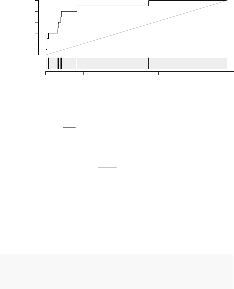
0 1000 2000 3000 4000 5000
List of genes
Fraction of genes in module
0.0 0.4 0.8
In essence, this is a receiver-operator characteristic (ROC) curve, and the area under
the curve (AUC) is related to the U-statistic, from which the P-value in the tmodUtest is
calculated, as AUC =U
n1·n2. Both the U statistic and the AUC are reported. Moreover,
the AUC can be used to calculate effect size according to the Wendt’s formula(Wendt 1972)
for rank-biserial correlation coefficient:
r= 1 −
2·U
n1·n2
= 1 −2·AUC
In the above diagram, we see that nine out of the 10 genes that belong to the LI.M75
module and which are present in the Egambia data set are ranked among the top 1000
genes (as sorted by p-value).
There are three options of interest for generating evidence plots, shown below. Firstly,
by using the option labels=... it is possible to indicate gene of interest on the plot.
Secondly, option style="g" shows a plot similar to the K-S plots of GSEA. Thirdly, it is
possible to show more than one module on a single plot.
par(mfrow=c(1,2))
evidencePlot(l, m="LI.M75",style="g")
evidencePlot(l, m=c("LI.M37.0","LI.M75"),
gene.labels=l[1:4], col=c(2,4), legend="right")
24
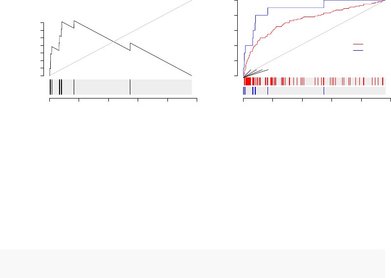
0 1000 2000 3000 4000 5000
List of genes
Fraction of genes in module
0.0 0.2 0.4 0.6
0 1000 2000 3000 4000 5000
List of genes
Fraction of genes in module
0.0 0.2 0.4 0.6 0.8 1.0
FAM20A
FCGR1B
BATF2
ANKRD22
LI.M37.0
LI.M75
4.3 Summary tables
We can summarize the output from the previously run tests (tmodUtest,tmodCERNOtest
and tmodHGtest) in one table using tmodSummary. For this, we will create a list contain-
ing results from all comparisons.
resAll <- list(CERNO=resC, U=resU, HG=resHG)
head(tmodSummary(resAll))
## ID Title AUC.CERNO
## LI.M11.0 LI.M11.0 enriched in monocytes (II) 0.777
## LI.M112.0 LI.M112.0 complement activation (I) 0.846
## LI.M118.0 LI.M118.0 enriched in monocytes (IV) 0.877
## LI.M127 LI.M127 type I interferon response 0.946
## LI.M13 LI.M13 innate activation by cytosolic DNA sensing 0.913
## LI.M150 LI.M150 innate antiviral response 0.950
## q.CERNO AUC.U q.U E.HG q.HG
## LI.M11.0 9.09e-07 0.777 0.000657 20.5 0.005907
## LI.M112.0 1.49e-05 0.846 0.001811 37.3 0.000858
## LI.M118.0 5.17e-04 0.877 0.001926 NA NA
## LI.M127 1.16e-02 0.946 0.007486 NA NA
## LI.M13 3.66e-02 NA NA NA NA
## LI.M150 9.96e-03 0.950 0.007162 NA NA
The table below shows the results.
25

4.4 Panel plots with tmodPanelPlot
A list of result tables (or even of a single result table) can be visualized using a heatmap-
like plot called here “panel plot”. The idea is to show both, effect sizes and p-values, and,
optionally, also the direction of gene regulation.
In the example below, we will use the resAll object created above, containing the
results from three different tests for enrichment, to compare the results of the individual
tests. However, since the Ecolumn of HG test is not easily comparable to the AUC values
(which are between 0 and 1), we need to scale it down.
resAll$HG$E <- log10(resAll$HG$E) - 0.5
tmodPanelPlot(resAll)
26
DC surface signature (LI.S5)
complement activation (I) (LI.M112.0)
enriched in monocytes (II) (LI.M11.0)
antiviral IFN signature (LI.M75)
Monocyte surface signature (LI.S4)
myeloid cell enriched receptors and transporters (LI.M4.3)
TLR and inflammatory signaling (LI.M16)
enriched in activated dendritic cells (II) (LI.M165)
enriched in monocytes (IV) (LI.M118.0)
activated dendritic cells (LI.M67)
immune activation − generic cluster (LI.M37.0)
enriched in neutrophils (I) (LI.M37.1)
AP−1 transcription factor network (LI.M20)
type I interferon response (LI.M127)
innate antiviral response (LI.M150)
enriched in myeloid cells and monocytes (LI.M81)
CERNO
U
HG
Effect size:
P value:
0.5 1.1
0.01 0.001 10−410−510−6
Each enrichment result corresponds to a reddish blob. The size of the blob corresponds
to the effect size (AUC or log10(Enrichment), as it may be), and color intensity corre-
sponds to the p-value – pale colors show p-values closer to 0.01. It is easily seen how
tmodCERNOtest is the more sensitive option.
We can see that also the intercept term is enriched for genes found in monocytes and
neutrophils. Note that by default, tmodPanelPlot only shows enrichments with p < 0.01,
hence a slight difference from the tmodSummary output. This behavior can be modified
by the pval.thr option.
However, one is usually interested in the direction of regulation. If a gene list is sorted
27
by p-value, the enriched modules may contain both up- or down-regulated genes1. It
is often desirable to visualize whether genes in a module go up, or go down between
experimental conditions. For this, the function tmodDecideTests is used to obtain the
number of significantly up- or down-regulated genes in a module.
This information must be obtained separately from the differential gene expression
analysis and provided as a list to tmodPanelPlot. The names of this list must be identical
to the names in the results list.
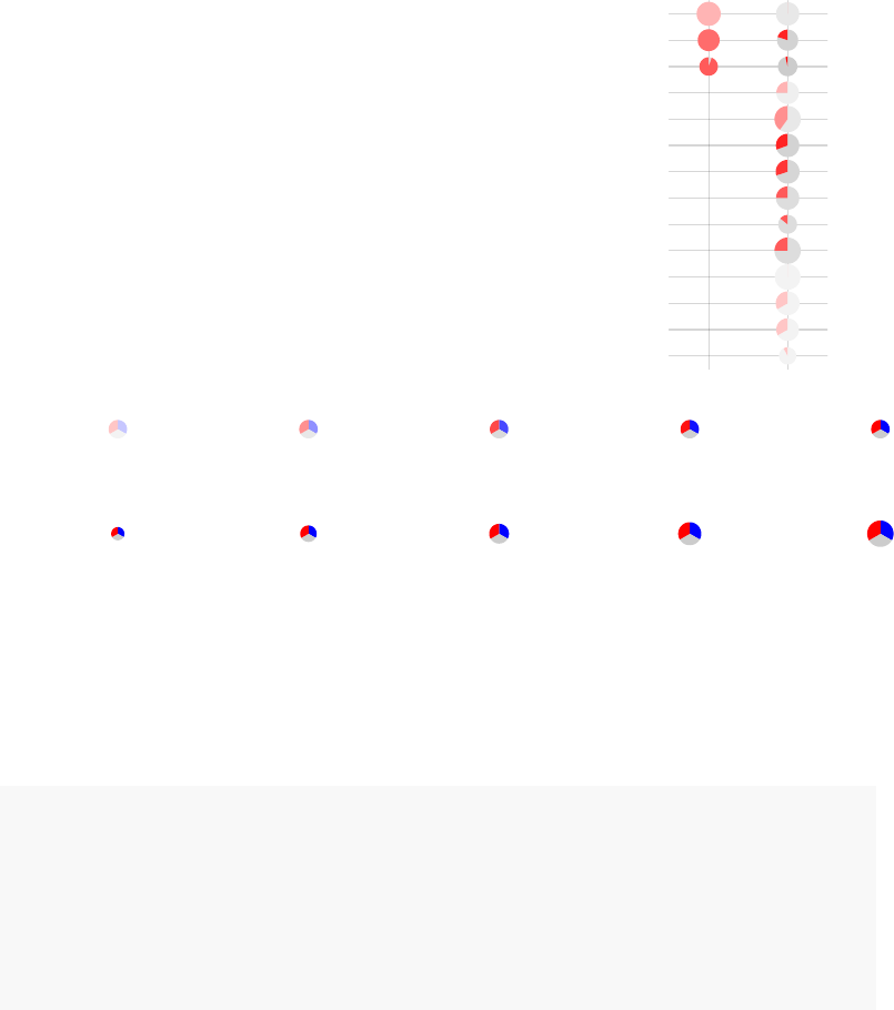
There are three default representations (rug-like, pie and a square pie).
par(mfrow=c(1,3))
pie <- tmodDecideTests(g=tt$GENE_SYMBOL, lfc=tt$logFC, pval=tt$adj.P.Val)
names(pie) <- "CERNO"
tmodPanelPlot(resAll["CERNO"], pie=pie, grid="b")
tmodPanelPlot(resAll["CERNO"], pie=pie, grid="b",pie.style="pie")
tmodPanelPlot(resAll["CERNO"], pie=pie, grid="b",pie.style="boxpie")
enriched in myeloid cells and monocytes (LI.M81)
innate antiviral response (LI.M150)
AP−1 transcription factor network (LI.M20)
myeloid cell enriched receptors and transporters (LI.M4.3)
DC surface signature (LI.S5)
enriched in monocytes (IV) (LI.M118.0)
complement activation (I) (LI.M112.0)
Monocyte surface signature (LI.S4)
enriched in monocytes (II) (LI.M11.0)
immune activation − generic cluster (LI.M37.0)
enriched in neutrophils (I) (LI.M37.1)
enriched in activated dendritic cells (II) (LI.M165)
activated dendritic cells (LI.M67)
TLR and inflammatory signaling (LI.M16)
antiviral IFN signature (LI.M75)
CERNO
Effect size:
P value:
0.68 0.98
0.01 0.001 10−410−510−6
Each mini-plot shows the effect size of the enrichment and the corresponding p-value,
as before. Additionally, the fraction of up-regulated and down-regulated genes is visual-
ized by coloring a fraction of the area of the mini-plot red or blue, respectively2.
The tmodPanelPlot function has several parameters, notably for filtering and la-
belling:
1Searching for enrichment only in up- or only in down-regulated genes depends on how the gene list is
sorted; this is described in Section “Testing for up- or down-regulated genes separately”.
2The colors can be modified by the parameter pie.colors
28
• Filtering:
–filter.empty.rows and filter.empty.cols remove, respectively, mod-
ules and result tables with no enrichment above pval.thr
–filter.rows.pval and filter.rows.auc removes rows that do not con-
tain at least one p value or AUC above the specified threshold
–filter.by.id shows only a selected subset of modules
• Labelling:
–row.labels.auto: by default, the row labels of the panel plot are generated
automatically from the module descriptions. This option specifies how.
–row.labels: alternatively, labels for the modules shown can be provided
manually as a named vector
–col.labels: alternative labels for the columns (in order of appearance in
the results list)
–col.labels.style: where the column labels should be put (top, boom,
both, none)
Internally, tmodPanelPlot is a convenient wrapper for the much more customizable
function pvalEffectPlot, operating directly on matrices of effect sizes and p values.
29

Chapter 5
Working with limma
5.1 Limma and tmod
Given the popularity of the limma package, tmod includes functions to easily integrate
with limma. In fact, if you fit a design / contrast with limma function lmFit and calculate
the p-values with eBayes(), you can directly use the resulting object in tmodLimmaTest
and tmodLimmaDecideTests1.
res.l <- tmodLimmaTest(fit, Egambia$GENE_SYMBOL)
length(res.l)
## [1] 2
names(res.l)
## [1] "Intercept" "TB"
head(res.l$TB)
1The function tmodLimmaDecideTests is described in the next section
30
## ID Title cerno N1 AUC
## LI.M37.0 LI.M37.0 immune activation - generic cluster 414.3 100 0.726
## LI.M11.0 LI.M11.0 enriched in monocytes (II) 105.6 20 0.786
## LI.M112.0 LI.M112.0 complement activation (I) 75.6 11 0.867
## LI.S4 LI.S4 Monocyte surface signature 70.0 10 0.884
## LI.M75 LI.M75 antiviral IFN signature 66.1 10 0.865
## LI.M67 LI.M67 activated dendritic cells 50.4 6 0.971
## cES P.Value adj.P.Val
## LI.M37.0 2.07 4.57e-17 1.58e-14
## LI.M11.0 2.64 7.92e-08 9.67e-06
## LI.M112.0 3.44 8.39e-08 9.67e-06
## LI.S4 3.50 1.84e-07 1.59e-05
## LI.M75 3.31 7.78e-07 5.38e-05
## LI.M67 4.20 1.21e-06 6.97e-05
5.2 Minimum significant difference (MSD)
The tmodLimmaTest function uses coefficients and p-values from the limma object to or-
der the genes. By default, the genes are ordered by MSD (Minimum Significant Differ-
ence), rather than p-value or log fold change.
The MSD is defined as follows:
MSD =
CI.L if logFC >0
−CI.R if logFC <0
Where logFC is the log fold change, CI.L is the left boundary of the 95% confidence
interval of logFC and CI.R is the right boundary. MSD is always greater than zero and
is equivalent to the absolute distance between the confidence interval and the x axis. For
example, if the logFC is 0.7 with 95% CI = [0.5, 0.9], then MSD=0.5; if logFC is -2.5 with
95% CI = [-3.0, -2.0], then MSD = 2.0.
The idea behind MSD is as follows. Ordering genes by decreasing absolute log fold
change will include on the top of the list some genes close to background, for which log
fold changes are grand, but so are the errors and confidence intervals, just because mea-
suring genes with low expression is loaded with errors. Ordering genes by decreasing
absolute log fold change should be avoided.
31

On the other hand, in a list ordered by p-values, many of the genes on the top of the
list will have strong signals and high expression, which results in beer statistical power
and ultimately with lower p-values – even though the actual fold changes might not be
very impressive.
However, by using MSD and using the boundary of the confidence interval to order
the genes, the genes on the top of the list are those for which we can confidently that the
actual log fold change is large. That is because the 95% confidence intervals tells us that
in 95% cases, the real log fold change will be anywhere within that interval. Using its
bountary closer to the x-axis (zero log fold change), we say that in 95% of the cases the log
fold change will have this or larger magnitude (hence, “minimal significant difference”).
This can be visualized as follows, using the drop-in replacement for limma’s topTable
function, tmodLimmaTopTable, which calculates msd as well as confidence intervals. We
will consider only genes with positive log fold changes and we will show top 50 genes as
ordered by the three different measures:
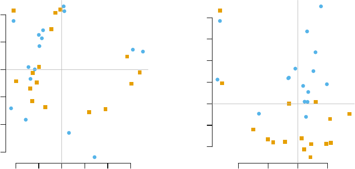
plotCI <- function(x, ci.l, ci.r, title="") {
n <- length(x)
plot(x,
ylab="logFC",xlab="Index",
pch=19,ylim=c(min(x-ci.l), max(x+ci.r)),
main=title)
segments(1:n, ci.l, 1:n, ci.r, lwd=5,col="#33333333")
}
par(mfrow=c(1,3))
x <- tmodLimmaTopTable(fit, coef="TB")
print(head(x))
## logFC.TB t.TB msd.TB SE.TB d.TB ciL.TB ciR.TB qval.TB
## 34 0.0282 0.0756 -0.728 0.373 0.0288 -0.728 0.784 0.9954
## 36 1.5242 3.8798 0.728 0.393 1.6398 0.728 2.320 0.0439
## 41 0.0789 0.1783 -0.817 0.442 0.0955 -0.817 0.975 0.9950
## 44 0.1532 0.3239 -0.806 0.473 0.1985 -0.806 1.112 0.9950
## 52 -0.2350 -0.6170 -0.537 0.381 -0.2451 -1.007 0.537 0.9950
## 62 -0.3195 -0.5585 -0.840 0.572 -0.5007 -1.479 0.840 0.9950
32
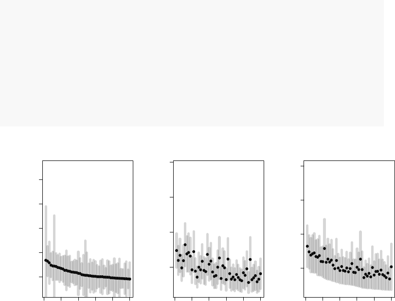
x <- x[ x$logFC.TB > 0, ] # only to simplify the output!
x2 <- x[ order(abs(x$logFC.TB), decreasing=T),][1:50,]
plotCI(x2$logFC.TB, x2$ciL.TB, x2$ciR.TB, "logFC")
x2 <- x[ order(x$qval.TB),][1:50,]
plotCI(x2$logFC.TB, x2$ciL.TB, x2$ciR.TB, "q-value")
x2 <- x[ order(x$msd.TB, decreasing=T),][1:50,]
plotCI(x2$logFC.TB, x2$ciL.TB, x2$ciR.TB, "MSD")
0 10 20 30 40 50
2 4 6 8 10
logFC
Index
logFC
0 10 20 30 40 50
2468
q−value
Index
logFC
0 10 20 30 40 50
2 4 6 8
MSD
Index
logFC
Black dots are logFCs, and grey bars denote 95% confidence intervals. On the left panel,
the top 50 genes ordered by the fold change include several genes with broad confidence
intervals, which, despite having a large log fold change, are not significantly up- or down-
regulated.
On the middle panel the genes are ordered by p-value. It is clear that the log fold
changes of the genes vary considerably, and that the list includes genes which are more
and less strongly regulated in TB.
The third panel shows genes ordered by decreasing MSD. There is less variation in
the logFC than on the second panel, but at the same time the fallacy of the first panel
is avoided. MSD is a compromise between considering the effect size and the statistical
significance.
What about enrichments?
33

x <- tmodLimmaTopTable(fit, coef="TB",genelist=Egambia[,1:3])
x.lfc <- x[ order(abs(x$logFC.TB), decreasing=T),]
x.qval <- x[ order(x$qval.TB),]
x.msd <- x[ order(x$msd.TB, decreasing=T),]
comparison <- list(
lfc=tmodCERNOtest(x.lfc$GENE_SYMBOL),
qval=tmodCERNOtest(x.qval$GENE_SYMBOL),
msd=tmodCERNOtest(x.msd$GENE_SYMBOL))
tmodPanelPlot(comparison)
34
enriched in neutrophils (I) (LI.M37.1)
innate antiviral response (LI.M150)
chromosome Y linked (LI.M240)
enriched in monocytes (IV) (LI.M118.0)
myeloid cell enriched receptors and transporters (LI.M4.3)
AP−1 transcription factor network (LI.M20)
TLR and inflammatory signaling (LI.M16)
DC surface signature (LI.S5)
enriched in monocytes (II) (LI.M11.0)
enriched in activated dendritic cells (II) (LI.M165)
Monocyte surface signature (LI.S4)
activated dendritic cells (LI.M67)
antiviral IFN signature (LI.M75)
complement activation (I) (LI.M112.0)
immune activation − generic cluster (LI.M37.0)
lfc
qval
msd
Effect size:
P value:
0.5 0.98
0.01 0.001 10−410−510−6
In this case, the results of p-value and msd-ordering are very similar.
While MSD is a general method, it relies on a construction of confidence intervals,
which might not be possible in some cases.
5.3 Comparing tests across experimental conditions
In the above example with the Gambian data set there were only two coefficients calcu-
lated in limma, the intercept and the TB. However, often there are several coefficients
35

or contrasts which are analysed simultaneously, for example different experimental con-
ditions or different time points. tmod includes several functions which make it easy to
visualize such sets of enrichments.
The object res.l created above using the tmod function tmodLimmaTest is a list of tmod
results. Any such list can be directly passed on to functions tmodSummary and tmod-
PanelPlot, as long as each element of the list has been created with tmodCERNOtest or a
similar function. tmodSummary creates a table summarizing module information in each
of the comparisons made. The values for modules which are not found in a result object
(i.e., which were not found to be significantly enriched in a given comparison) are shown
as NA’s:
head(tmodSummary(res.l), 5)
## ID Title AUC.Intercept
## LI.M11.0 LI.M11.0 enriched in monocytes (II) 0.815
## LI.M112.0 LI.M112.0 complement activation (I) NA
## LI.M118.0 LI.M118.0 enriched in monocytes (IV) NA
## LI.M124 LI.M124 enriched in membrane proteins 0.881
## LI.M127 LI.M127 type I interferon response NA
## q.Intercept AUC.TB q.TB
## LI.M11.0 0.000114 0.786 9.67e-06
## LI.M112.0 NA 0.867 9.67e-06
## LI.M118.0 NA 0.838 2.85e-03
## LI.M124 0.011487 NA NA
## LI.M127 NA 0.945 1.04e-02
We can neatly visualize the above information on a heatmap-like representation:
tmodPanelPlot(res.l, text.cex=0.8)
36
enriched in neutrophils (I) (LI.M37.1)
enriched in monocytes (II) (LI.M11.0)
immune activation − generic cluster (LI.M37.0)
enriched in monocytes (IV) (LI.M118.0)
TLR and inflammatory signaling (LI.M16)
complement activation (I) (LI.M112.0)
Monocyte surface signature (LI.S4)
antiviral IFN signature (LI.M75)
enriched in activated dendritic cells (II) (LI.M165)
activated dendritic cells (LI.M67)
innate antiviral response (LI.M150)
myeloid cell enriched receptors and transporters (LI.M4.3)
AP−1 transcription factor network (LI.M20)
DC surface signature (LI.S5)
Intercept
TB
Effect size:
P value:
0.5 0.97
0.01 0.001 10−410−510−6
The function tmodPanelPlot has many optional arguments for customization, includ-
ing options for label sizes, p value thresholds and custom functions for ploing the test
37

results instead of just red blobs.
It is often of interest to see which enriched modules go up, and which go down? Specif-
ically, we would like to see, for each module, how many genes are up-, and how many
genes are down-regulated. tmodPanelPlot takes an optional argument, pie, which con-
tains information on significantly regulated genes in modules. We can conveniently gen-
erate it from a limma linear fit object with the tmodLimmaDecideTests function:
pie <- tmodLimmaDecideTests(fit, genes=Egambia$GENE_SYMBOL)
head(pie$TB[ order( pie$TB[,"Up"], decreasing=T), ])
## Down Zero Up
## DC.M3.4 0 11 9
## DC.M4.2 0 16 7
## LI.M11.0 0 16 4
## LI.M37.0 0 110 4
## LI.M112.0 0 9 4
## LI.M165 0 24 4
data(tmod)
tmod$MODULES["DC.M3.4",]
## ID Title Category Annotated
## DC.M3.4 DC.M3.4 Interferon DC.M3 Yes
## URL
## DC.M3.4 http://www.biir.net/public_wikis/module_annotation/V2_Trial_8_Modules_M3.4
## Source SourceID original.ID B
## DC.M3.4 http://www.biir.net/ DC M3.4 53
The pie object is a list. Each element of the list corresponds to one coefficient and is a
data frame with the columns “Down”, “Zero” and “Up” (in that order). Importantly, all
names of the “res.l” list must correspond to an item in the pie list.
all(names(pie) %in% names(res.l))
## [1] TRUE
38

We can now use this information in tmodPanelPlot:
tmodPanelPlot(res.l, pie=pie, text.cex=0.8,grid="b")
enriched in neutrophils (I) (LI.M37.1)
enriched in monocytes (II) (LI.M11.0)
immune activation − generic cluster (LI.M37.0)
enriched in monocytes (IV) (LI.M118.0)
TLR and inflammatory signaling (LI.M16)
complement activation (I) (LI.M112.0)
Monocyte surface signature (LI.S4)
antiviral IFN signature (LI.M75)
enriched in activated dendritic cells (II) (LI.M165)
activated dendritic cells (LI.M67)
innate antiviral response (LI.M150)
myeloid cell enriched receptors and transporters (LI.M4.3)
AP−1 transcription factor network (LI.M20)
DC surface signature (LI.S5)
Intercept
TB
Effect size:
P value:
0.5 0.97
0.01 0.001 10−410−510−6
A pie-like plot can be also generated:
tmodPanelPlot(res.l,
pie=pie, pie.style="pie")
39
enriched in neutrophils (I) (LI.M37.1)
enriched in monocytes (II) (LI.M11.0)
immune activation − generic cluster (LI.M37.0)
enriched in monocytes (IV) (LI.M118.0)
TLR and inflammatory signaling (LI.M16)
complement activation (I) (LI.M112.0)
Monocyte surface signature (LI.S4)
antiviral IFN signature (LI.M75)
enriched in activated dendritic cells (II) (LI.M165)
activated dendritic cells (LI.M67)
innate antiviral response (LI.M150)
myeloid cell enriched receptors and transporters (LI.M4.3)
AP−1 transcription factor network (LI.M20)
DC surface signature (LI.S5)
Intercept
TB
Effect size:
P value:
0.5 0.97
0.01 0.001 10−410−510−6
There is also a more general function, tmodDecideTests that also produces a
tmodPanelPlot-compatible object, a list of data frames with gene counts. However,
instead of taking a limma object, it requires (i) a gene name, (ii) a vector or a matrix of
log fold changes, and (iii) a vector or a matrix of p-values. We can replicate the result of
tmodLimmaDecideTests above with the following commands:
tt.I <-
topTable(fit, coef="Intercept",number=Inf,sort.by="n")
tt.TB <- topTable(fit, coef="TB",number=Inf,sort.by="n")
pie2 <- tmodDecideTests(Egambia$GENE_SYMBOL,
lfc=cbind(tt.I$logFC, tt.TB$logFC),
pval=cbind(tt.I$adj.P.Val, tt.TB$adj.P.Val))
identical(pie[[1]], pie2[[1]])
## [1] TRUE
40

Chapter 6
Using tmod for other types of GSEA
analyses
The fact that tmod relies on a single ordered list of genes makes it useful in many other
situations in which such a list presents itself.
6.1 Correlation analysis
Genes can be ordered by their absolute correlation with a variable or even a data set or a
module. For example, one can ask the question about a function of a particular unknown
gene – such as ANKRD22, annotated as “ankyrin repeat domain 22”.
x <- E[ match("ANKRD22", Egambia$GENE_SYMBOL), ]
cors <- t(cor(x, t(E)))
ord <- order(abs(cors), decreasing=TRUE)
head(tmodCERNOtest(Egambia$GENE_SYMBOL[ ord ]))
## ID Title cerno N1
## LI.M37.0 LI.M37.0 immune activation - generic cluster 431.4 100
## LI.M165 LI.M165 enriched in activated dendritic cells (II) 113.1 19
## LI.M11.0 LI.M11.0 enriched in monocytes (II) 113.9 20
## LI.M112.0 LI.M112.0 complement activation (I) 80.5 11
41

## LI.M75 LI.M75 antiviral IFN signature 74.5 10
## LI.M16 LI.M16 TLR and inflammatory signaling 52.1 5
## AUC cES P.Value adj.P.Val
## LI.M37.0 0.719 2.16 4.71e-19 1.63e-16
## LI.M165 0.781 2.98 2.18e-09 3.77e-07
## LI.M11.0 0.807 2.85 5.14e-09 5.92e-07
## LI.M112.0 0.849 3.66 1.32e-08 1.14e-06
## LI.M75 0.901 3.72 3.30e-08 2.28e-06
## LI.M16 0.991 5.21 1.11e-07 6.41e-06
Clearly, ANKRD22 correlates to other immune related genes, most of all these which
are interferon inducible.
In another example, consider correlation between genes and the first principal com-
ponent (“eigengene”) of a group of genes of unknown function1. To demonstrate the
method, we will select the genes from the module “LI.M75”. For this, we use the function
getGenes with the optional argument genelist used to filter the genes in the module
by the genes present in the data set.
g <- getGenes("LI.M75",genelist=Egambia$GENE_SYMBOL, as.list=T)
sel <- Egambia$GENE_SYMBOL %in% g[[1]]
x <- E[sel, ]
## calculating the "eigengene"
pca <- prcomp(t(x), scale.=T)
eigen <- pca$x[,1]
cors <- t(cor(eigen, t(E)))
ord <- order(abs(cors), decreasing=TRUE)
head(tmodCERNOtest(Egambia$GENE_SYMBOL[ ord ]))
## ID Title cerno N1
## LI.M165 LI.M165 enriched in activated dendritic cells (II) 156.0 19
## LI.M75 LI.M75 antiviral IFN signature 106.1 10
## LI.M37.0 LI.M37.0 immune activation - generic cluster 353.4 100
## LI.M127 LI.M127 type I interferon response 66.2 5
## LI.M150 LI.M150 innate antiviral response 65.4 5
1More on eigengenes in the Chapter on modules
42

## LI.M67 LI.M67 activated dendritic cells 67.7 6
## AUC cES P.Value adj.P.Val
## LI.M165 0.826 4.11 3.06e-16 1.06e-13
## LI.M75 0.940 5.31 9.91e-14 1.71e-11
## LI.M37.0 0.658 1.77 1.29e-10 1.49e-08
## LI.M127 0.998 6.62 2.43e-10 2.10e-08
## LI.M150 0.998 6.54 3.34e-10 2.31e-08
## LI.M67 0.994 5.64 8.65e-10 4.99e-08
6.2 Functional multivariate analysis
Transcriptional modules can help to understand the biological meaning of the calculated
multivariate transformations. For example, consider a principal component analysis
(PCA), visualised using the pca3d package (Weiner 2013):
mypal <- c("#E69F00","#56B4E9")
pca <- prcomp(t(E), scale.=TRUE)
col <- mypal[ factor(group) ]
par(mfrow=c(1,2))
l<-pcaplot(pca, group=group, col=col)
legend("topleft",as.character(l$groups),
pch=l$pch,
col=l$colors, bty="n")
l<-pcaplot(pca, group=group, col=col, components=3:4)
legend("topleft",as.character(l$groups),
pch=l$pch,
col=l$colors, bty="n")
43
−40 −20 0 20 40 60
−60 −40 −20 0 20 40
PC 1
PC 2
CTRL
TB
−40 −20 0 20
−20 0 10 20 30 40
PC 3
PC 4
CTRL
TB
The fourth component looks really interesting. Does it correspond to the modules
which we have found before? Each principal component is, after all, a linear combination
of gene expression values multiplied by weights (or scores) which are constant for a given
component. The i-th principal component for sample jis given by
P Ci,j =∑
k
wi,k ·xk,j
where kis the index of the variables (genes in our case), wi,k is the weight associated
with the i-th component and the k-th variable (gene), and xk,j is the value of the variable
kfor the sample j; that is, the gene expression of gene kin the sample j. Genes influence
the position of a sample along a given component the more the larger their absolute weight
for that component.
For example, on the right-hand figure above, we see that samples which were taken
from TB patients have a high value of the principal component 4; the opposite is true for
the healthy controls. The genes that allow us to differentiate between these two groups
will have very large, positive weights for genes highly expressed in TB patients, and very
large, negative weights for genes which are highly expressed in NID, but not TB.
We can sort the genes by their weight in the given component, since the weights are
stored in the pca object in the “rotation” slot, and use the tmodUtest function to test for
enrichment of the modules.
44

o <- order(abs(pca$rotation[,4]), decreasing=TRUE)
l <- Egambia$GENE_SYMBOL[o]
res <- tmodUtest(l)
head(res)
## ID Title U N1 AUC
## LI.M37.0 LI.M37.0 immune activation - generic cluster 339742 100 0.719
## LI.M37.1 LI.M37.1 enriched in neutrophils (I) 50096 12 0.867
## LI.M75 LI.M75 antiviral IFN signature 43379 10 0.901
## LI.M11.0 LI.M11.0 enriched in monocytes (II) 74343 20 0.773
## LI.S5 LI.S5 DC surface signature 115007 34 0.706
## LI.M67 LI.M67 activated dendritic cells 28291 6 0.978
## P.Value adj.P.Val
## LI.M37.0 3.13e-14 1.08e-11
## LI.M37.1 5.41e-06 6.70e-04
## LI.M75 5.81e-06 6.70e-04
## LI.M11.0 1.19e-05 1.03e-03
## LI.S5 1.71e-05 1.18e-03
## LI.M67 2.51e-05 1.45e-03
Perfect, this is what we expected: we see that the neutrophil / interferon signature
which is the hallmark of the TB biosignature. What about other components? We can
run the enrichment for each component and visualise the results using tmod’s functions
tmodSummary and tmodPanelPlot. Below, we use the filter.empty option to omit the
principal components which show no enrichment at all.
# Calculate enrichment for each component
gs <- Egambia$GENE_SYMBOL
# function calculating the enrichment of a PC
gn.f <- function(r) {
tmodCERNOtest(gs[order(abs(r), decreasing=T)],
qval=0.01)
}
x <- apply(pca$rotation, 2, gn.f)
tmodSummary(x, filter.empty=TRUE)[1:5,]
## ID Title AUC.PC3 q.PC3 AUC.PC4
45
## LI.M11.0 LI.M11.0 enriched in monocytes (II) NA NA 0.773
## LI.M112.0 LI.M112.0 complement activation (I) NA NA 0.751
## LI.M118.0 LI.M118.0 enriched in monocytes (IV) NA NA 0.853
## LI.M127 LI.M127 type I interferon response NA NA 0.959
## LI.M144 LI.M144 cell cycle, ATP binding 0.989 0.00605 NA
## q.PC4 AUC.PC9 q.PC9 AUC.PC14 q.PC14 AUC.PC30 q.PC30
## LI.M11.0 2.14e-07 NA NA NA NA NA NA
## LI.M112.0 4.91e-05 NA NA NA NA NA NA
## LI.M118.0 5.03e-05 NA NA NA NA NA NA
## LI.M127 3.71e-03 NA NA NA NA NA NA
## LI.M144 NA NA NA NA NA NA NA
The following plot shows the same information in a visual form. The size of the blobs
corresponds to the effect size (AUC value), and their color – to the q-value.
tmodPanelPlot(x)
extracellular matrix (II) (LI.M2.1)
cell movement, Adhesion & Platelet activation (LI.M30)
cell cycle, ATP binding (LI.M144)
regulation of transcription, transcription factors (LI.M213)
immune activation − generic cluster (LI.M37.0)
enriched in neutrophils (I) (LI.M37.1)
DC surface signature (LI.S5)
enriched in monocytes (II) (LI.M11.0)
antiviral IFN signature (LI.M75)
TLR and inflammatory signaling (LI.M16)
enriched in activated dendritic cells (II) (LI.M165)
Monocyte surface signature (LI.S4)
enriched in monocytes (IV) (LI.M118.0)
complement activation (I) (LI.M112.0)
activated dendritic cells (LI.M67)
innate antiviral response (LI.M150)
complement and other receptors in DCs (LI.M40)
type I interferon response (LI.M127)
enriched in B cells (I) (LI.M47.0)
platelet activation − actin binding (LI.M196)
enriched in myeloid cells and monocytes (LI.M81)
PC1
PC2
PC3
PC4
PC5
PC6
PC7
PC8
PC9
PC10
PC11
PC12
PC13
PC14
PC15
PC16
PC17
PC18
PC19
PC20
PC21
PC22
PC23
PC24
PC25
PC26
PC27
PC28
PC29
PC30
Effect size: P value:
0.5 0.990.01 0.001 10−410−510−6
46
However, we might want to ask, for each module, how many of the genes in that
module have a negative, and how many have a positive weight? We can use the function
tmodDecideTests for that. For each principal component shown, we want to know how
many genes have very large (in absolute terms) weights – we can use the “lfc” parameter
of tmodDecideTests for that. We define here “large” as being in the top 25% of all weights
in the given component. For this, we need first to calculate the 3rd quartile (top 25%
threshold). We will show only 10 components:
qfnc <- function(r) quantile(r, 0.75)
qqs <- apply(pca$rotation[,1:10], 2, qfnc)
pie <- tmodDecideTests(gs, lfc=pca$rotation[,1:10], lfc.thr=qqs)
tmodPanelPlot(x[1:10], pie=pie,
pie.style="rug",grid="between")
platelet activation − actin binding (LI.M196)
DC surface signature (LI.S5)
enriched in monocytes (II) (LI.M11.0)
immune activation − generic cluster (LI.M37.0)
antiviral IFN signature (LI.M75)
TLR and inflammatory signaling (LI.M16)
enriched in activated dendritic cells (II) (LI.M165)
enriched in neutrophils (I) (LI.M37.1)
Monocyte surface signature (LI.S4)
enriched in monocytes (IV) (LI.M118.0)
complement activation (I) (LI.M112.0)
activated dendritic cells (LI.M67)
innate antiviral response (LI.M150)
complement and other receptors in DCs (LI.M40)
enriched in myeloid cells and monocytes (LI.M81)
type I interferon response (LI.M127)
enriched in B cells (I) (LI.M47.0)
extracellular matrix (II) (LI.M2.1)
cell movement, Adhesion & Platelet activation (LI.M30)
cell cycle, ATP binding (LI.M144)
regulation of transcription, transcription factors (LI.M213)
PC1
PC2
PC3
PC4
PC5
PC6
PC7
PC8
PC9
PC10
Effect size: P value:
0.5 0.99 0.01 0.001 10−410−510−6
47

6.3 PCA and tag clouds
For another way of visualizing enrichment, we can use the tagcloud package (Weiner
2014). P-Values will be represented by the size of the tags, while AUC – which is a proxy
for the effect size – will be shown by the color of the tag, from grey (AUC=0.5, random) to
black (1):
library(tagcloud)
w <- -log10(res$P.Value)
c <- smoothPalette(res$AUC, min=0.5)
tags <- strmultline(res$Title)
tagcloud(tags, weights=w, col=c)
immune activation
− generic cluster
TLR and inflammatory
signaling
enriched in activated
dendritic cells (II)
platelet activation
− actin binding
myeloid cell enriched
receptors and transporters
enriched in
monocytes (II)
enriched in
neutrophils (I)
complement and other
receptors in DCs
antiviral
IFN signature
Monocyte surface
signature
enriched in myeloid
cells and monocytes
DC surface
signature
type I interferon
response
activated
dendritic cells
innate antiviral
response
enriched in
monocytes (IV)
transmembrane and
ion transporters (I)
enriched in
B cells (I)
complement
activation (I)
enriched in
B cells (II)
TBA
TBA
We can now annotate the PCA axes using the tag clouds; however, see below for a
shortcut in tmod.
48

par(mar=c(1,1,1,1))
o3 <- order(abs(pca$rotation[,3]), decreasing=TRUE)
l3 <- Egambia$GENE_SYMBOL[o3]
res3 <- tmodUtest(l3)
layout(matrix(c(3,1,0,2),2,2,byrow=TRUE),
widths=c(1/3,2/3), heights=c(2/3,1/3))
col <- mypal[ factor(group) ]
# note -- PC4 is now x axis!!
l <- pcaplot(pca, group=group, components=4:3,
col=col, cex=1.8)
legend("topleft",
as.character(l$groups),
pch=l$pch,
col=l$colors, bty="n")
tagcloud(tags, weights=w, col=c, fvert= 0)
tagcloud(strmultline(res3$Title),
weights=-log10(res3$P.Value),
col=smoothPalette(res3$AUC, min=0.5),
fvert=1)
49
−20 −10 0 10 20 30 40
−40 −20 0 20
PC 4
PC 3
CTRL
TB
immune activation
− generic cluster
TLR and inflammatory
signaling
enriched in activated
dendritic cells (II)
myeloid cell enriched
receptors and transporters
platelet activation
− actin binding
enriched in
monocytes (II)
enriched in
neutrophils (I)
antiviral
IFN signature
complement and other
receptors in DCs
type I interferon
response
DC surface
signature
innate antiviral
response
enriched in myeloid
cells and monocytes
transmembrane and
ion transporters (I)
enriched in
monocytes (IV)
Monocyte surface
signature
activated
dendritic cells
enriched in
B cells (I)
complement
activation (I)
enriched in
B cells (II)
TBA
TBA
regulation of transcription,
transcription factors
NK cell surface
signature
heme
biosynthesis (I)
transmembrane
transport (I)
enriched in
dendritic cells
cell cycle,
ATP binding
enriched in
NK cells (II)
TBA
TBA
TBA
TBA
TBA
TBA
TBA
TBA
As mentioned previously, there is a way of doing it all with tmod much more quickly,
in just a few lines of code:
Note that plot.params are just parameters which will be passed to the pca2d function.
However, remember that is must be a list.
To plot the PCA, tmod uses the function pcaplot(), but you can actually do it yourself
by providing tmodPCA with a suitable function. The only requirement is that the function
takes named parameters “pca” and “components”:
50
plotf <- function(pca, components) {
id1 <- components[1]
id2 <- components[2]
print(id1)
print(id2)
plot(pca$x[,id1], pca$x[,id2])
}
ret <- tmodPCA(pca, genes=Egambia$GENE_SYMBOL,
components=3:4,plotfunc=plotf)
## [1] 3
## [1] 4
inflammasome receptors
and signaling
regulation of transcription,
transcription factors
phosphatidylinositol
signaling system
cell cycle,
ATP binding
enriched in
cell cycle
heme
biosynthesis intracellular
transport
enriched in
dendritic cells
TLR and inflammatory
signaling myeloid cell enriched
receptors and transporters
activated
dendritic cells
type I interferon
response
innate antiviral
response
innate activation by
cytosolic DNA sensing
complement and other
receptors in DCs
platelet activation
− actin binding
antiviral
IFN signature
Monocyte surface
signature
enriched in activated
dendritic cells enriched in myeloid
cells and monocytes
enriched in
neutrophils
recruitment
of neutrophils
immune activation
− generic cluster
AP−1 transcription
factor network
chemokines and inflammatory
molecules in myeloid cells
enriched
in B cells
complement
activation
enriched in
monocytes
DC surface
signature
−40 −20 0 20
−20 −10 0 10 20 30 40
pca$x[, id1]
pca$x[, id2]
51
Alternatively, you can use the function “pca2d” from the pca3d package:
if(require(pca3d)) plotf <- pca2d
ret <- tmodPCA(pca, genes=Egambia$GENE_SYMBOL,
components=3:4,plotfunc=plotf, plot.params=list(group=group))
inflammasome receptors
and signaling
regulation of transcription,
transcription factors
phosphatidylinositol
signaling system
cell cycle,
ATP binding
enriched in
cell cycle
heme
biosynthesis
intracellular
transport
enriched in
dendritic cells
TLR and inflammatory
signaling
myeloid cell enriched
receptors and transporters
activated
dendritic cells
type I interferon
response
innate antiviral
response
innate activation by
cytosolic DNA sensing
complement and other
receptors in DCs
platelet activation
− actin binding
antiviral
IFN signature
Monocyte surface
signature
enriched in activated
dendritic cells
enriched in myeloid
cells and monocytes
enriched in
neutrophils
recruitment
of neutrophils
immune activation
− generic cluster
AP−1 transcription
factor network
chemokines and inflammatory
molecules in myeloid cells
enriched
in B cells
complement
activation
enriched in
monocytes
DC surface
signature
−40 −20 0 20
−20 −10 0 10 20 30 40
PC 3
PC 4
52

Chapter 7
Using and creating modules and gene
sets
Tmod was created with transcriptional modules in mind. This is why the word “module”
is used throughout tmod. However, any gene or variable set – depending on application –
is a “module” in tmod. These data sets can be used with most of tmod functions (including
the gene set enrichment test functions) by specifying it with the option mset=, for example
tmodCERNOtest(..., mset=mytmodobject).
7.1 Using built-in gene sets (transcriptional modules)
By default, tmod uses the modules published by Li et al. (S. Li et al. 2014) (LI). A second
set of modules was published by Chaussabel et al. (Chaussabel et al. 2008) (DC); new
module definitions were described by Banchereau et al. (Banchereau et al. 2012) and can
be found on a public website1.
Depending on the mset parameter to the test functions, either the LI or DC sets are
used, or both, if the mset=all has been specified.
l <- tt$GENE_SYMBOL
res2 <- tmodUtest(l, mset="all")
head( res2 )
1http://www.biir.net/public_wikis/module_annotation/G2_Trial_8_Modules
53
## ID Title U N1 AUC
## LI.M37.0 LI.M37.0 immune activation - generic cluster 352659 100 0.746
## DC.M4.2 DC.M4.2 Inflammation 91352 20 0.950
## DC.M1.2 DC.M1.2 Interferon 73612 17 0.900
## DC.M3.2 DC.M3.2 Inflammation 96366 24 0.836
## DC.M5.15 DC.M5.15 Neutrophils 65289 16 0.848
## DC.M7.29 DC.M7.29 Undetermined 77738 20 0.809
## P.Value adj.P.Val
## LI.M37.0 1.60e-17 9.68e-15
## DC.M4.2 1.67e-12 5.07e-10
## DC.M1.2 5.70e-09 9.62e-07
## DC.M3.2 6.35e-09 9.62e-07
## DC.M5.15 7.24e-07 8.77e-05
## DC.M7.29 9.08e-07 9.18e-05
As you can see, the information contained in both module sets is partially redundant.
7.2 Accessing the tmod module data directly
The tmod package stores its data in two data frames and two lists. This object is contained
in a list called tmod, which is loaded with data("tmod"). The names mimick the various
environments from Annotation.dbi packages, but currently the objects are just two lists
and two data frames.
•tmod$MODULES is a data frame which contains general module information as de-
fined in the supplementary materials for Li et al. (S. Li et al. 2014) and Chaussabel
et al. (Chaussabel et al. 2008)
•tmod$GENES is a data frame which contains general gene information, including
columns with HGNC (“primary”), as well as ENTREZ and REFSEQ identifiers.
•tmod$MODULES2GENES is a list with module IDs (same as in the “ID” column of
tmod$MODULES) as names. Every element of the list is a character vector with IDs
(“primary” column of tmod$GENES) of the genes which are included in this mod-
ule.
•tmod$GENES2MODULES is a list with gene IDs (same as in the “primary” column of
tmod$GENES) as names. Every element of the list is a character vector with IDs of
the modules in which the gene is found.
54

7.2.1 Module operations
The gene sets used by tmod are objects of class tmod. The default object used in the gene
set enrichment tests in the tmod package can be loaded into the environment with the
command data(tmod):
data(tmod)
tmod
## An object of class "tmod"
## 606 modules, 12712 genes
Objects of the class tmod can be easily generated from a number of data sources (see
below). Several functions can be used on the objects:
length(tmod)
## [1] 606
sel <- grep("Interferon", tmod$MODULES$Title, ignore.case=TRUE)
ifn <- tmod[sel]
ifn
## An object of class "tmod"
## 6 modules, 161 genes
length(ifn)
## [1] 6
55

7.2.2 Using tmod modules in other programs
Using these variables, one can apply any other tool for the analysis of enriched module
sets available, for example, the geneSetTest function from the limma package (Smyth
et al. (2005))2. We will first run tmodCERNOtest seing the qval to Inf to get p-values
for all modules. Then, we apply the geneSetTest function to each module. Note that
we are using the actual geneSetTest function3.
data(tmod)
res <- tmodCERNOtest(tt$GENE_SYMBOL, qval=Inf)
gstest <- function(x) {
sel <- tt$GENE_SYMBOL %in% tmod$MODULES2GENES[[x]]
geneSetTest(sel, tt$logFC, ranks.only=FALSE)
}
gst <- sapply(res$ID, gstest)
## [1] 0.799
## [1] 0.902
## [1] 1.22
## [1] 1.2
## [1] 1.26
## [1] 1.38
## [1] 1.57
## [1] 0.884
## [1] 0.846
## [1] 1.02
## [1] 0.631
## [1] 1.1
## [1] 1.39
## [1] 0.715
## [1] 1.15
## [1] 1.19
2The geneSetTest function from limma is implemented in the tmod function tmodGeneSetTest, and
limma’s wilcoxon.GST is essentially the same as tmodUtest
3Note that somewhat confusingly, limma’s both functions, geneSetTest and wilcoxGST, are identical.
The laer function is a synonym for geneSetTest with the option rank.only=TRUE. However, this is the
default seing for geneSetTest, which means that with the default seing, both functions return the same
results.
56
## [1] 0.731
## [1] 0.894
## [1] 0.87
## [1] 0.919
## [1] 0.717
## [1] 1.42
## [1] 1.02
## [1] 0.574
## [1] 0.533
## [1] 0.946
## [1] 1.19
## [1] 1.15
## [1] 0.879
## [1] 0.656
## [1] 0.546
## [1] 0.973
## [1] 1.55
## [1] 0.809
## [1] 0.926
## [1] 1.13
## [1] 0.989
## [1] 0.737
## [1] 0.691
## [1] 1.08
## [1] 0.775
## [1] 0.551
## [1] 1.02
## [1] 0.681
## [1] 0.994
## [1] 0.687
## [1] 0.717
## [1] 0.662
## [1] 0.668
## [1] 0.994
## [1] 0.862
## [1] 0.917
## [1] 0.563
## [1] 0.842
57
## [1] 0.637
## [1] 0.807
## [1] 0.935
## [1] 0.605
## [1] 0.815
## [1] 0.501
## [1] 0.984
## [1] 0.715
## [1] 0.676
## [1] 0.778
## [1] 0.582
## [1] 0.683
## [1] 0.589
## [1] 0.521
## [1] 0.748
## [1] 0.826
## [1] 0.706
## [1] 0.509
## [1] 0.751
## [1] 0.923
## [1] 0.632
## [1] 0.533
## [1] 0.555
## [1] 0.626
## [1] 0.944
## [1] 0.709
## [1] 0.533
## [1] 0.734
## [1] 0.844
## [1] 0.608
## [1] 0.564
## [1] 0.529
## [1] 0.518
## [1] 0.532
## [1] 0.623
## [1] 0.561
## [1] 0.962
## [1] 0.461
58
## [1] 0.58
## [1] 0.525
## [1] 0.586
## [1] 0.481
## [1] 0.702
## [1] 0.642
## [1] 0.622
## [1] 0.634
## [1] 0.533
## [1] 0.693
## [1] 0.485
## [1] 0.607
## [1] 0.555
## [1] 0.579
## [1] 0.57
## [1] 0.523
## [1] 0.653
## [1] 0.553
## [1] 0.548
## [1] 0.479
## [1] 0.543
## [1] 0.539
## [1] 0.682
## [1] 0.615
## [1] 0.492
## [1] 0.478
## [1] 0.532
## [1] 0.412
## [1] 0.597
## [1] 0.692
## [1] 0.603
## [1] 0.957
## [1] 0.548
## [1] 0.46
## [1] 0.452
## [1] 0.443
## [1] 0.326
## [1] 0.352
59
## [1] 0.57
## [1] 0.547
## [1] 0.671
## [1] 0.394
## [1] 0.597
## [1] 0.473
## [1] 0.627
## [1] 0.627
## [1] 0.497
## [1] 0.494
## [1] 0.443
## [1] 0.629
## [1] 0.463
## [1] 0.45
## [1] 0.455
## [1] 0.426
## [1] 0.853
## [1] 0.438
## [1] 0.388
## [1] 0.37
## [1] 0.456
## [1] 0.453
## [1] 0.518
## [1] 0.378
## [1] 0.6
## [1] 0.395
## [1] 0.452
## [1] 0.473
## [1] 0.461
## [1] 0.394
## [1] 0.405
## [1] 0.419
## [1] 0.463
## [1] 0.523
## [1] 0.473
## [1] 0.417
## [1] 0.59
## [1] 0.661
60
## [1] 0.49
## [1] 0.546
## [1] 0.495
## [1] 0.453
## [1] 0.466
## [1] 0.276
## [1] 0.39
## [1] 0.426
## [1] 0.272
## [1] 0.433
## [1] 0.446
## [1] 0.457
## [1] 0.36
## [1] 0.342
## [1] 0.353
## [1] 0.365
## [1] 0.385
## [1] 0.482
## [1] 0.384
## [1] 0.53
## [1] 0.417
## [1] 0.347
## [1] 0.409
## [1] 0.485
## [1] 0.376
## [1] 0.316
## [1] 0.362
## [1] 0.384
## [1] 0.412
## [1] 0.436
## [1] 0.345
## [1] 0.363
## [1] 0.273
## [1] 0.471
## [1] 0.312
## [1] 0.377
## [1] 0.368
## [1] 0.282
61
## [1] 0.423
## [1] 0.269
## [1] 0.302
## [1] 0.394
## [1] 0.302
## [1] 0.299
## [1] 0.429
## [1] 0.181
## [1] 0.301
## [1] 0.376
## [1] 0.318
## [1] 0.193
## [1] 0.193
## [1] 0.193
## [1] 0.193
## [1] 0.193
## [1] 0.193
## [1] 0.193
## [1] 0.196
## [1] 0.194
## [1] 0.454
## [1] 0.189
## [1] 0.504
## [1] 0.3
## [1] 0.386
## [1] 0.361
## [1] 0.335
## [1] 0.43
## [1] 0.368
## [1] 0.364
## [1] 0.308
## [1] 0.343
## [1] 0.326
## [1] 0.333
## [1] 0.326
## [1] 0.432
## [1] 0.138
## [1] 0.349
62
## [1] 0.312
## [1] 0.345
## [1] 0.284
## [1] 0.218
## [1] 0.333
## [1] 0.3
## [1] 0.212
## [1] 0.255
## [1] 0.309
## [1] 0.186
## [1] 0.197
## [1] 0.309
## [1] 0.319
## [1] 0.302
## [1] 0.248
## [1] 0.252
## [1] 0.113
## [1] 0.322
## [1] 0.139
## [1] 0.143
## [1] 0.219
## [1] 0.21
## [1] 0.238
## [1] 0.087
## [1] 0.383
## [1] 0.102
## [1] 0.102
## [1] 0.102
## [1] 0.216
## [1] 0.221
## [1] 0.271
## [1] 0.157
## [1] 0.392
## [1] 0.334
## [1] 0.212
## [1] 0.0931
## [1] 0.193
## [1] 0.206
63

## [1] 0.254
## [1] 0.271
## [1] 0.295
## [1] 0.313
## [1] 0.0526
## [1] 0.25
## [1] 0.0442
## [1] 0.071
## [1] 0.152
## [1] 0.261
## [1] 0.13
## [1] 0.239
## [1] 0.0498
## [1] 0.0259
## [1] 0.123
## [1] 0.146
## [1] 0.0908
## [1] 0.105
## [1] 0.172
## [1] 0.123
## [1] 0.188
## [1] 0.0962
Are the results from CERNO and geneSetTest similar?
plot(res$P.Value, gst,
log="xy",pch=19,
col="#33333366",
xlab="P Values from tmod",
ylab="P Values from geneSetTest")
abline(0,1)
abline(h=0.01,col="grey")
abline(v=0.01,col="grey")
64
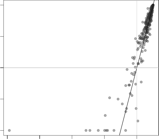
1e−18 1e−14 1e−10 1e−06 1e−02
1e−04 1e−03 1e−02 1e−01 1e+00
P Values from tmod
P Values from geneSetTest
On the plot above, the p-values from tmod are ploed against the p-values from
geneSetTest. As you can see, in this particular example, both methods give very similar
results.
7.2.3 Custom module definitions
It is possible to use any kind of arbitrary or custom gene set definitions. These custom
definition of gene sets takes form of a list which is then provided as the mset parameter
to the test functions. The list in question must have the following members:
•MODULES A data frame which contains at least the columns “ID” and “Title”.
The IDs must correspond to the names of MODULES2GENES.
65

•GENES (optional) A data frame which contains at least the column “ID”. The gene
IDs must correspond to the gene IDs used in MODULES2GENES.
•MODULES2GENES A list. The names of the list are the IDs from the MODULES
data frame. The items in the list are character vectors with names of the genes that
are associated with each module.
•GENES2MODULES (optional) A list with the reverse mapping from genes to mod-
ules. Names on that list must correspond to GENES$ID, and the character vector
members of the list must correspond to MODULES$ID.
The tests in the tmod package will accept a simple list that contains the above fields.
However, the function makeTmod can be used conveniently to create a tmod object.
Here is a minimal definition of such a set:
mymset <- makeTmod(
modules=data.frame(ID=c("A","B"),
Title=c("A title",
"B title")),
modules2genes=list(
A=c("G1","G2"),
B=c("G3","G4"))
)
mymset
## An object of class "tmod"
## 2 modules, 4 genes
Both GENES and GENES2MODULES will be automatically created by makeTmod.
Whether the gene IDs are Entrez, or something else entirely does not maer, as long
as they matched the provided input to the test functions.
7.3 Obtaining other gene sets
The tests in the tmod package can take any arbitrary module definitions. While tmod –
for many reasons – cannot distribute all module sets, it can easily import gene sets from
many sources. A few of these will be discussed below.
66

7.3.1 MSigDB
The MSigDB database from the Broad institute is an interesting collection of gene sets
(actually, multiple collections), including Reactome pathways, gene ontologies (GO) and
many other data sets. Moreover, it is the basis for the GSEA program.
Unfortunately, MSigDB cannot be distributed or even accessed without a free regis-
tration, which imposes a heavy limination on third party tools such as tmod. Use the
following guide to download and parse the database such that you can use it with R and
tmod.
First, you will need to download the MSigDB in XML format4. This file can be
accessed at the URL http://software.broadinstitute.org/gsea/msigdb/download_file.jsp?
filePath=/resources/msigdb/6.1/msigdb_v6.1.xml – follow the link, register and log in,
and save the file on your disk (roughly 113 MB).
Importing MSigDB is easy – tmod has a function specifically for that purpose. Once
you have downloaded the MSigDB file, you can create the tmod-compatible R object with
one command5. However, the tmod function tmodImportMsigDB() can also use this for-
mat, look up the manual page:
msig <- tmodImportMSigDB("msigdb_v6.1.xml")
msig
## An object of class "tmod"
## 14645 modules, 32403 genes
That’s it – now you can use the full MSigDB for enrichment tests:
res <- tmodCERNOtest(tt$GENE_SYMBOL, mset=msig)
head(res)
## ID Title cerno N1 AUC
## M3408 M3408 GSE1432 ctrl vs ifng 24h microglia dn 239 39 0.801
4Note that even if you register with MSig, it is not possible to download the database directly from R in
the XML format.
5MSigDB gene sets can be also downloaded as “GMT” files. This format contains less information and
is therefore less usable.
67

## M14329 M14329 Go immune response 857 267 0.623
## M3010 M3010 Hecker ifnb1 targets 244 43 0.846
## M3286 M3286 GSE13485 ctrl vs day3 yf17d vaccine pbmc dn 247 45 0.729
## M3288 M3288 GSE13485 ctrl vs day7 yf17d vaccine pbmc dn 272 54 0.722
## M11976 M11976 Go defense response 948 311 0.600
## cES P.Value adj.P.Val
## M3408 3.07 2.97e-18 4.35e-14
## M14329 1.61 1.87e-17 1.37e-13
## M3010 2.84 4.56e-17 2.22e-13
## M3286 2.75 1.41e-16 5.16e-13
## M3288 2.52 3.63e-16 1.06e-12
## M11976 1.52 5.29e-16 1.29e-12
The results are quite typical for MSigDB, which is quite abundant with similar or over-
lapping gene sets. As the first results, we see, again, interferon response, as well as sets
of genes which are significantly upregulated after yellow fever vaccination – and which
are also interferon related. We might want to limit our analysis only to the 50 “hallmark”
module categories:
sel <- msig$MODULES$Category == "H"
tmodCERNOtest(tt$GENE_SYMBOL, mset=msig[sel] )
## ID Title cerno N1 AUC cES
## M5913 M5913 Hallmark interferon gamma response 221.7 41 0.779 2.70
## M5921 M5921 Hallmark complement 217.8 56 0.698 1.94
## M5911 M5911 Hallmark interferon alpha response 108.4 20 0.756 2.71
## M5946 M5946 Hallmark coagulation 179.2 50 0.678 1.79
## M5890 M5890 Hallmark tnfa signaling via nfkb 149.0 47 0.648 1.58
## M5930 M5930 Hallmark epithelial mesenchymal transition 212.5 73 0.637 1.46
## M5932 M5932 Hallmark inflammatory response 184.5 62 0.621 1.49
## M5953 M5953 Hallmark kras signaling up 221.8 82 0.605 1.35
## M5892 M5892 Hallmark cholesterol homeostasis 49.1 14 0.614 1.76
## P.Value adj.P.Val
## M5913 8.51e-15 4.25e-13
## M5921 8.61e-09 2.15e-07
## M5911 3.19e-08 5.32e-07
## M5946 1.97e-06 2.46e-05
68

## M5890 2.66e-04 2.25e-03
## M5930 2.70e-04 2.25e-03
## M5932 3.46e-04 2.47e-03
## M5953 1.79e-03 1.12e-02
## M5892 8.04e-03 4.47e-02
We see both – the prominent interferon response and the complement activation. Also,
in addition, TNF-αsignalling via NF-κβ.
Other particularly interesting subsets of MSigDB are shown in the table below. “Cate-
gory” and “Subcategory” are columns in the msig$MODULES data frame.
Subset Description Category Subcategory
Hallmark Curated set of gene sets H
GO / BP Gene ontology, biological process C5 BP
GO / CC Gene ontology, cellular component C5 CC
GO / MF Gene ontology, molecular function C5 MF
Biocarta Molecular pathways from Biocarta C2 CP:BIOCARTA
KEGG Pathways from Kyoto Encyclopedia of Genes and Genomes C2 CP:KEGG
Reactome Pathways from the Reactome pathway database C2 CP:REACTOME
7.3.2 Using the ENSEMBL databases through biomaRt
ENSEMBL databases for a multitude of organisms can be accessed using the R package
biomaRt.
Importantly, biomaRt allows to map different types of identifiers onto each other; this
allows for example to obtain Entrez gene identifiers (required by KEGG or GO) .
Below, we will use biomaRt to obtain gene ontology (GO) terms and Reactome path-
way IDs for genes in the Egambia data set, using the Entrez gene ID’s (column EG in the
Egambia data set).
library(biomaRt)
mart <- useMart("ensembl",dataset = "hsapiens_gene_ensembl")
bm <- getBM(filters="hgnc_symbol",
values = Egambia$GENE_SYMBOL,
69

attributes = c("hgnc_symbol","entrezgene","reactome","go_id","name_1006","go_linkage_type"),
mart=mart)
In the following code, we construct the modules data frame mand the gene set to gene
mappings m2g (each twice: once for GO, and once for Reactome). We only keep the terms
that have at least 10 and not more than 100 associated Entrez gene ID’s.
m2g_r <- with(bm[ bm$reactome != "", ], split(hgnc_symbol, reactome))
m2g_g <- with(bm[ bm$go_id != "", ], split(hgnc_symbol, go_id))
ll <- lengths(m2g_r)
m2g_r <- m2g_r[ ll >= 5& ll <= 250 ]
ll <- lengths(m2g_g)
m2g_g <- m2g_g[ ll >= 5& ll <= 250 ]
m_r <- data.frame(ID=names(m2g_r), Title=names(m2g_r))
m_g <- data.frame(ID=names(m2g_g),
Title=bm$name_1006[ match(names(m2g_g), bm$go_id)])
ensemblR <- makeTmod(modules=m_r, modules2genes=m2g_r)
ensemblGO <- makeTmod(modules=m_g, modules2genes=m2g_g)
## these objects are no longer necessary
rm(bm, m_g, m_r, m2g_r, m2g_g)
7.3.3 Gene ontologies (GO)
GO terms are perhaps the most frequently used type of gene sets in GSEA, in particular
because they are available for a much larger number of organisms than other gene sets
(like KEGG pathways).
There are many sources to obtain GO definitions. As described in the previous sec-
tions, GO’s can be also obtained from ENSEMBL via biomaRt and from MSigDB. In fact,
MSigDB may be the easiest way.
However, GO annotations can also be obtained from AnnotationDBI Bioconductor
packages as shown below. Note that the Entrez gene IDs are in the EG column of the
70

Egambia object.
library(org.Hs.eg.db)
mtab <- toTable(org.Hs.egGO)
There are over 15,000 GO terms and 250,000 genes in the mtab mapping; however,
many of them map to either a very small or a very large number of genes. At this stage,
it could also be useful to remove any genes not present in our particular data set, but that
would make the resulting tmod object less flexible. However, we may be interested only
in the “biological process” ontology for now.
mtab <- mtab[ mtab$Ontology == "BP", ]
m2g <- split(mtab$gene_id, mtab$go_id)
## remove the rather large object
rm(mtab)
ll <- lengths(m2g)
m2g <- m2g[ ll >= 10 & ll <= 100 ]
length(m2g)
## [1] 2224
Using the mapping and the GO.db it is easy to create a module set suitable for tmod:
library(GO.db)
gt <- toTable(GOTERM)
m <- data.frame(ID=names(m2g))
m$Title <- gt$Term[ match(m$ID, gt$go_id) ]
goset <- makeTmod(modules=m, modules2genes=m2g)
rm(gt, m2g, m)
This approach allows an offline mapping to GO terms, assuming the necessary DBI
is installed. Using AnnotationDBI databases such as org.Hs.eg.db has, however, also
two major disadvantages: firstly, the annotations are available for a small number of or-
ganisms. Secondly, the annotations in ENSEMBL may be more up to date.
71

We can now compare the results of the analysis with MSigDB. There is one hitch,
though. The authors of MSigDB decided to use their own identifiers instead of GO identi-
fiers. The GO identifiers can still be extracted from MSigDB, but can only be found in the
field EXTERNAL_DETAILS_URL. Below, the function renameMods is used to replace the
MSigDB identifiers with GO identifiers.
msig.bp <- msig[ msig$MODULES$Subcategory == "BP" ]
go_ids <- gsub(".*/","", msig.bp$MODULES$EXTERNAL_DETAILS_URL)
names(go_ids) <- msig.bp$MODULES$ID
msig.bp <- renameMods(msig.bp, go_ids)
Now we can run the enrichment on tt with both data sets and compare the results.
Note, however, that while systematic gene names are used in MSigDB, the object goset
was created from org.Hs.eg.db and uses Entrez identifiers. Also, we will make both
sets directly comparable by filtering for the common genes, and we will request a result
for all modules, even if they are not significant.
both <- intersect(msig.bp$MODULES$ID, goset$MODULES$ID)
msig.bp <- msig.bp[both]
goset.both <- goset[both]
rescomp <- list()
rescomp$orghs <-
tmodCERNOtest(tt$EG, mset=goset.both, qval=Inf,order.by="n")
rescomp$msigdb <-
tmodCERNOtest(tt$GENE_SYMBOL, mset=msig.bp, qval=Inf,order.by="n")
all(rownames(rescomp$msigdb) == rownames(rescomp$orghs))
## [1] TRUE
plot(rescomp$msigdb$P.Value, rescomp$orghs$P.Value, log="xy",
xlab="MSigDB GO",ylab="org.Hs.eg.db GO",bty="n")
abline(0,1,col="grey")
72
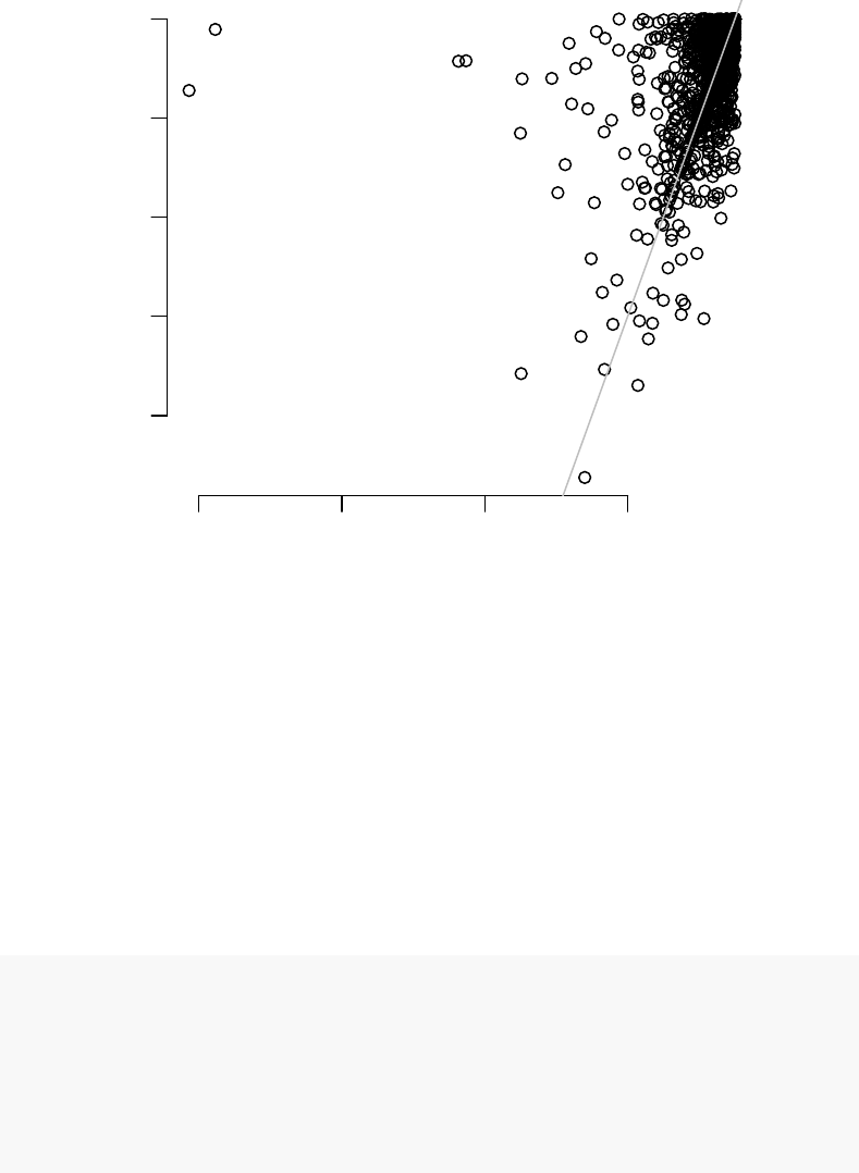
1e−15 1e−11 1e−07 1e−03
1e−04 1e−03 1e−02 1e−01 1e+00
MSigDB GO
org.Hs.eg.db GO
The differences are quite apparent, and most likely due to the differences in the ver-
sions of the GO database.
7.3.4 KEGG pathways
One way to obtain KEGG pathway gene sets is to use the MSigDB as described above.
However, alternatively and for other organisms it is possible to directly obtain the path-
way definitions from KEGG. The code below might take a lot of time on a slow connection.
library(KEGGREST)
pathways <- keggLink("pathway","hsa")
## get pathway Names in addition to IDs
paths <- sapply(unique(pathways), function(p) keggGet(p)[[1]]$NAME)
m <- data.frame(ID=unique(pathways), Title=paths)
73

## m2g is the mapping from modules (pathways) to genes
m2g <- split(names(pathways), pathways)
## kegg object can now be used with tmod
kegg <- makeTmod(modules=m, modules2genes=m2g)
Note that KEGG uses a slightly modified version of Entrez identifiers – each numeric
identifier is preceded by a three leer species code (e.g. “hsa” for humans) followed by a
colon:
eg <- paste0("hsa:", tt$EG)
tmodCERNOtest(eg, mset="kegg")
Again, the most important part is to ensure that the gene identifiers in the tmod object
(kegg in this case) correspond to the gene identifiers in in the ordered list.
7.3.5 Manual creation of tmod module objects: MSigDB
For the purposes of an example, the code below shows how to parse the XML MSigDB
file using the R package XML. Essentially, this is the same code that tmodImportMsigDB
is using:
library(XML)
foo <- xmlParse("msigdb_v6.1.xml" )
foo2 <- xmlToList(foo)
There are over 10,000 “gene sets” (equivalent to modules in tmod) defined. Each mem-
ber of foo2 is a named character vector:
path1 <- foo2[[1]]
class(path1)
## [1] "character"
74

names(path1)
## [1] "STANDARD_NAME" "SYSTEMATIC_NAME" "HISTORICAL_NAMES"
## [4] "ORGANISM" "PMID" "AUTHORS"
## [7] "GEOID" "EXACT_SOURCE" "GENESET_LISTING_URL"
## [10] "EXTERNAL_DETAILS_URL" "CHIP" "CATEGORY_CODE"
## [13] "SUB_CATEGORY_CODE" "CONTRIBUTOR" "CONTRIBUTOR_ORG"
## [16] "DESCRIPTION_BRIEF" "DESCRIPTION_FULL" "TAGS"
## [19] "MEMBERS" "MEMBERS_SYMBOLIZED" "MEMBERS_EZID"
## [22] "MEMBERS_MAPPING" "FOUNDER_NAMES" "REFINEMENT_DATASETS"
## [25] "VALIDATION_DATASETS"
For our example analysis, we will use only human gene sets. We further need to make
sure there are no NULLs in the list.
orgs <- sapply(foo2, function(x) x["ORGANISM"])
unique(orgs)
## [1] "Homo sapiens" "Mus musculus" "Rattus norvegicus"
## [4] "Danio rerio" "Macaca mulatta" NA
foo3 <- foo2[ orgs == "Homo sapiens" ]
foo3 <- foo3[ ! sapply(foo3, is.null) ]
Next, construct the MODULES data frame. We will use four named fields for each
vector, which contain the ID (systematic name), description, category and subcategory:
modules <- t(sapply(foo3,
function(x)
x[ c("SYSTEMATIC_NAME","STANDARD_NAME","CATEGORY_CODE","SUBCATEGORY_CODE") ]))
colnames(modules) <- c("ID","Title","Category","Subcategory" )
modules <- data.frame(modules, stringsAsFactors=FALSE)
Then, we create the modules to genes mapping and the GENES data frame. For this,
we use the MEMBERS_SYMBOLIZED field, which is a comma separated list of gene symbols
belonging to a particular module:
75

m2g <- lapply(foo3,
function(x) strsplit( x["MEMBERS_SYMBOLIZED"], "," )[[1]])
names(m2g) <- modules$ID
mymsig <- makeTmod(modules=modules, modules2genes=m2g)
mymsig
## An object of class "tmod"
## 14645 modules, 32403 genes
From now on, you can use the object mymsig with tmod enrichment tests.
Note that it is not necessary to create the members GENES and GENES2MODULES
manually. The reverse mapping from genes to modules, GENES2MODULES, will be auto-
matically inferred from MODULES2GENES. If no meta-information on genes is provided
in GENES, then a minimal data frame will be created with one column only (ID).
76

Chapter 8
Case studies
8.1 Metabolic profiling of TB patients
8.1.1 Introduction
One of the main objectives in writing tmod was the ability to analyse metabolic profil-
ing data and other uncommon data sets. In 2012, we have analysed metabolic profiles
of serum collected from patients suffering from tuberculosis (TB) and healthy controls
(Weiner 3rd et al. 2012). It turned out that there are huge differences between these two
groups of individuals, involving amino acid metabolism, lipid metabolism and many oth-
ers. In the course of the analysis, we found correlations between the metabolites which are
not explained fully by the metabolic pathways. For example, cortisol is correlated with
kynurenine due to the immunoactive function of these molecules indicating an activation
of the immune system, and not because these two molecules are linked by a synthesis pro-
cess. Vice versa, kynurenine and tryptophan were not directly correlated, even though
these molecules are clearly linked by a metabolic process, because tryptophan is not an
immune signalling molecule, while kynurenine is.
The tmod package includes both, the data set used in the Weiner et al. paper and
the cluster definitions (modules) published therein. In the following, we will use these
modules to analyse the metabolic profiles1.
1Formally, this is not correct, as the modules were derived from the data set that we are going to analyse,
however it serves for demonstration purposes
77

First, we load the data modules and the data set to analyse.
data(modmetabo) ## modules
data(tbmprof)
ids <- rownames(tbmprof)
tb <- factor(gsub("\\..*","", ids))
sex <- factor(gsub(".*\\.([MF])\\..*","\\1", ids))
table(tb, sex)
## sex
## tb F M
## HEALTHY 58 34
## TB 25 19
8.1.2 Differential analysis
The metabolic profiling data has not exactly a normal distribution, but that varies from
one compound to another. It is possible to normalize it by ranking, but we can simply use
the wilcoxon test to see differences between males and females as well as TB patients and
healthy individuals.
wcx.tb <- apply(tbmprof, 2, function(x) wilcox.test(x ~ tb, conf.int=T))
wcx.tb <- t(sapply(wcx.tb, function(x) c(x$estimate, x$p.value)))
wcx.sex <- apply(tbmprof, 2, function(x) wilcox.test(x ~ sex, conf.int=T))
wcx.sex <- t(sapply(wcx.sex, function(x) c(x$estimate, x$p.value)))
wcx <- data.frame(ID=colnames(tbmprof),
E.tb=wcx.tb[,1], pval.tb=wcx.tb[,2],
E.sex=wcx.sex[,1], pval.sex=wcx.sex[,2],
row.names=colnames(tbmprof))
The data frame contains the results of all tests. We can now test both the healthy/tb
comparison and the male/female comparison for enrichment in metabolic profiling mod-
ules. Instead ordering the feature identifiers, we use the option “input.order” to deter-
mine the sorting.
78

ids <- wcx$ID
res <- list()
res$tb <- tmodCERNOtest(ids[order(wcx$pval.tb)], mset=modmetabo)
res$tb
## ID Title cerno N1
## ME.107 ME.107 Amino acids cluster 104.6 18
## ME.37 ME.37 Kynurenines, taurocholates and cortisol cluster 116.9 25
## MP.2 MP.2 Amino Acid 99.2 28
## AUC cES P.Value adj.P.Val
## ME.107 0.882 2.91 1.28e-08 5.39e-07
## ME.37 0.884 2.34 2.82e-07 5.91e-06
## MP.2 0.706 1.77 3.36e-04 4.70e-03
res$sex <- tmodCERNOtest(ids[order(wcx$pval.sex)], mset=modmetabo)
res$sex
## ID Title cerno N1 AUC cES P.Value adj.P.Val
## ME.26 ME.26 Hormones cluster 62.5 10 0.920 3.12 2.92e-06 0.000123
## MS.1 MS.1 Steroid 61.0 11 0.873 2.77 1.59e-05 0.000335
## ME.69 ME.69 Cholesterol cluster 45.1 11 0.819 2.05 2.55e-03 0.035649
Both these result tables are concordant with previous findings. The enriched modules
in male vs female comparison are what one would expect. In TB, a cluster consisting of
kynurenine, bile acids and cortisol is up-regulated, while amino acids go down. We can
take a closer look at it using the evidencePlot function.
Why is there a module called “Amino acid cluster” and another one called “Amino
acid”? The “cluster” in the name of the module indicates that it has been build by cluster-
ing of the profiles, while the other module has been based on the biochemical classification
of the molecules. This information is contained in the Category column of the MODULES
data frame:
modmetabo$MODULES[ c("ME.107","MP.2"), ]
## ID Title Category
## ME.107 ME.107 Amino acids cluster Cluster
## MP.2 MP.2 Amino Acid Pathway
79
To get an overview for both of these comparisons at the same time, we can use the
tmodPanelPlot function. The size of the blobs below corresponds to the AUC values from
the tables above.
tmodPanelPlot(res)
Amino Acid (MP.2)
Amino acids cluster (ME.107)
Kynurenines, taurocholates and cortisol cluster (ME.37)
Hormones cluster (ME.26)
Steroid (MS.1)
tb
sex
Effect size:
P value:
0.5 0.92
0.01 0.001 10−410−510−6
This, unfortunately, does not tell us in which group the metabolites from a given mod-
ules are higher. For this, we can use the “estimate” from the wilcox.test above and a
parameter for tmodPanelPlot called “pie”. To create the value for this parameter – a list
that describes, for each condition and for each module, how many metabolites change in
one direction, and how many change in the other.
pie.data <- wcx[,c("E.sex","E.tb")]
colnames(pie.data) <- c("sex","tb")
pie <- tmodDecideTests(wcx$ID, lfc=pie.data, lfc.thr=0.2,mset=modmetabo)
tmodPanelPlot(res, pie=pie, pie.style="rug",grid="between")
80
Amino Acid (MP.2)
Amino acids cluster (ME.107)
Kynurenines, taurocholates and cortisol cluster (ME.37)
Hormones cluster (ME.26)
Steroid (MS.1)
tb
sex
Effect size:
P value:
0.5 0.92
0.01 0.001 10−410−510−6
We see now that the cortisol cluster is higher in TB, while amino acids are found at
lower concentration in the patients. Also, we see that most of the steroids found (cluster
ME.26 and module MS.1) are lower in females. The laer is not surprising if we inspect it
closely.
wcx <- wcx[order(wcx$pval.sex),]
showModule(wcx[,c("E.sex","pval.sex")], wcx$ID, "MS.1",mset=modmetabo)
## E.sex pval.sex ID
## HMDB00493 -0.87 3.04e-06 HMDB00493
## HMDB00365 -0.64 4.03e-05 HMDB00365
## HMDB02759 -0.62 1.07e-04 HMDB02759
## M.37186 -0.50 1.49e-04 M.37186
## HMDB03818.1 -0.39 1.54e-04 HMDB03818.1
## M.32619 -0.36 3.42e-04 M.32619
## HMDB03818 -0.46 4.35e-03 HMDB03818
## HMDB01032 -0.27 5.28e-03 HMDB01032
## HMDB02802 -0.10 8.85e-02 HMDB02802
## HMDB00063 -0.12 1.55e-01 HMDB00063
## HMDB04026 -0.08 3.35e-01 HMDB04026
## Name Pathway
## HMDB00493 5alpha-androstan-3beta,17beta-diol disulfate Lipid
81

## HMDB00365 epiandrosterone sulfate Lipid
## HMDB02759 androsterone sulfate Lipid
## M.37186 5alpha-androstan-3alpha,17beta-diol monosulfate (1) Lipid
## HMDB03818.1 4-androsten-3beta,17beta-diol disulfate (2) Lipid
## M.32619 pregn steroid monosulfate* Lipid
## HMDB03818 4-androsten-3beta,17beta-diol disulfate (1) Lipid
## HMDB01032 dehydroisoandrosterone sulfate (DHEA-S) Lipid
## HMDB02802 cortisone Lipid
## HMDB00063 cortisol Lipid
## HMDB04026 21-hydroxypregnenolone disulfate Lipid
## Subpathway HMDB KEGG MetabolonID
## HMDB00493 Steroid HMDB00493 C12525 M.37190
## HMDB00365 Steroid HMDB00365 C07635 M.33973
## HMDB02759 Steroid HMDB02759 M.31591
## M.37186 Steroid M.37186
## HMDB03818.1 Steroid HMDB03818 C04295 M.37203
## M.32619 Steroid M.32619
## HMDB03818 Steroid HMDB03818 C04295 M.37202
## HMDB01032 Steroid HMDB01032 C04555 M.32425
## HMDB02802 Steroid HMDB02802 C00762 M.1769
## HMDB00063 Steroid HMDB00063 C00735 M.1712
## HMDB04026 Steroid HMDB04026 C05485 M.46115
i <- "HMDB00493" # what is it?
modmetabo$GENES[i,]
## ID Name Pathway
## HMDB00493 HMDB00493 5alpha-androstan-3beta,17beta-diol disulfate Lipid
## Subpathway HMDB KEGG MetabolonID
## HMDB00493 Steroid HMDB00493 C12525 M.37190
par(mfrow=c(1,2))
showGene(tbmprof[,i], sex, main=modmetabo$GENES[i, "Name"],
ylab="Relative abundance")
## now for cortisol cluster
i <- "HMDB00063"
82

wcx <- wcx[order(wcx$pval.tb),]
showModule(wcx[,c("E.tb","pval.tb")], wcx$ID, "ME.37",
mset=modmetabo)[1:10,] # only first 10!
## E.tb pval.tb ID Name
## M.47908 -7.00e-01 2.67e-14 M.47908 Unknown
## M.32599 -8.00e-01 2.32e-10 M.32599 glycocholenate sulfate*
## HMDB00169 -6.30e-01 5.12e-09 HMDB00169 mannose
## Mx.22110 -6.45e-05 1.38e-08 Mx.22110 3-hydroxykynurenine
## HMDB00063 -5.40e-01 1.99e-08 HMDB00063 cortisol
## HMDB00159 -2.90e-01 2.49e-08 HMDB00159 phenylalanine
## M.32807 -1.22e+00 3.58e-08 M.32807 taurocholenate sulfate
## M.46637 -1.03e+00 6.66e-08 M.46637 Unknown
## M.46652 -8.40e-01 1.42e-07 M.46652 Unknown
## HMDB00684 -3.10e-01 1.79e-07 HMDB00684 kynurenine
## Pathway Subpathway
## M.47908
## M.32599 Lipid Secondary Bile Acid Metabolism
## HMDB00169 Carbohydrate Fructose, Mannose and Galactose Metabolism
## Mx.22110 Amino acid Tryptophan Metabolism
## HMDB00063 Lipid Steroid
## HMDB00159 Amino Acid Phenylalanine and Tyrosine Metabolism
## M.32807 Lipid Secondary Bile Acid Metabolism
## M.46637
## M.46652
## HMDB00684 Amino Acid Tryptophan Metabolism
## HMDB KEGG MetabolonID
## M.47908 M.47908
## M.32599 M.32599
## HMDB00169 HMDB00169 C00159 M.584
## Mx.22110 C02794 Mx.22110
## HMDB00063 HMDB00063 C00735 M.1712
## HMDB00159 HMDB00159 C00079 M.64
## M.32807 M.32807
## M.46637 M.46637
## M.46652 M.46652
## HMDB00684 HMDB00684 C00328 M.15140
83
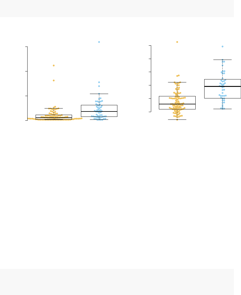
showGene(tbmprof[,i], tb, main=modmetabo$GENES[i, "Name"],
ylab="Relative abundance")
5alpha−androstan−3beta,17beta−diol disulfate
Relative abundance
0
5
10
15
F
M
cortisol
Relative abundance
0.5
1.0
1.5
2.0
2.5
3.0
HEALTHY
TB
8.1.3 Functional multivariate analysis
We can practically circumvent a gene-by-gene analysis. In fact, we are rarely interested in
the p-values associated with single genes or metabolites. There is too many of them, and
the statistical power is limited by the sheer number of tests and the requirement of correc-
tion for multiple testing. In case you have not read the part on FMA above, “Functional
multivariate analysis”, in its simplest form, is simply combining a principal component
analysis (PCA) with enrichment analysis. PCA lets us explore where the variance in the
data is; enrichment analysis allows us to interprete the principal components in functional
terms.
In tmod, it can be done in a few lines of code:
pca <- prcomp(tbmprof, scale.=T)
ret <- tmodPCA(pca, genes=colnames(tbmprof), mset=modmetabo,
plot.params=list(group=tb))
84

Polyunsaturated Fatty
Acid (n3 and n6)
Long Chain
Fatty Acid
Medium Chain
Fatty Acid
Medium−chain fatty
acids cluster
Long chain fatty
acid cluster Amino acids
cluster
Lysolipid
Lipid
Kynurenines, taurocholates
and cortisol cluster
Long chain fatty
acid cluster
Secondary Bile
Acid Metabolism Long Chain
Fatty Acid
Polyunsaturated Fatty
Acid (n3 and n6)
Lipid
−10 −5 0 5 10 15
−10 −5 0 5 10 15 20
PC 1
PC 2
The ret object now contains the results of enrichments (in the ret$enrichments mem-
ber) and we can directly throw it on a panel plot:
tmodPanelPlot(ret$enrichments)
85
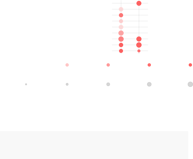
Kynurenines, taurocholates and cortisol cluster (ME.37)
Lysolipid (MS.47)
Medium−chain fatty acids cluster (ME.6)
Amino acids cluster (ME.107)
Medium Chain Fatty Acid (MS.37)
Polyunsaturated Fatty Acid (n3 and n6) (MS.40)
Long Chain Fatty Acid (MS.36)
Long chain fatty acid cluster (ME.2)
Lipid (MP.1)
Component1
Component2
Effect size:
P value:
0.5 0.95
0.01 0.001 10−410−510−6
OK, but which of the terms are characteristic for TB patients? Which for the healthy
controls? In the above, the enrichments were based on a list sorted by the absolute PCA
weights. However, we can split it into a list ordered by signed weights ordered once from
small to large values, and once from large to small values.
pca <- prcomp(tbmprof, scale.=T)
ret <- tmodPCA(pca, genes=colnames(tbmprof), mset=modmetabo,
plot.params=list(group=tb),
mode="cross")
86
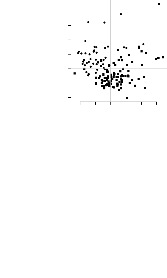
Kynurenines, taurocholates
and cortisol cluster
Putative
hypoxia−related cluster
Secondary Bile
Acid Metabolism
Pyrophosphates
cluster
Carbohydrate
Peptide
Polyunsaturated Fatty
Acid (n3 and n6)
Long Chain
Fatty Acid
Medium Chain
Fatty Acid
Medium−chain fatty
acids cluster
Long chain fatty
acid cluster
Amino acids
cluster
Lysolipid
Lipid
Urea cycle; Arginine
and Proline Metabolism
Amino acids
cluster
Hippurate
cluster
Nicotine
metabolites cluster
Amino
Acid
Kynurenines, taurocholates
and cortisol cluster
Long chain fatty
acid cluster
Secondary Bile
Acid Metabolism
Polyunsaturated Fatty
Acid (n3 and n6)
Long Chain
Fatty Acid
Lipid
−10 −5 0 5 10 15
−10 −5 0 5 10 15 20
PC 1
PC 2
In essence, reading this plot is simple. First, note that this time the tag clouds on the
top and the boom correspond to the two ends of the vertical, y axis (second component);
and the tag clouds at the left and right correspond to the two ends of the horizontal, x axis
(first PCA component).
Now, take the amino acid cluster (boom of the plot): it is enriched at the lower end of
the y axis, which means, that features in that cluster are higher in the yellow points which
are at the boom of the plot (lower end of the y). In other words, amino acids are higher
in healthy persons – a finding which corroborates the differential analysis above.
Similarly, “kynurenines” are at the left, lower side of the x axis, which means, that
features from this cluster are at higher levels in TB patients.
What about the male-female differences? They probably can be found in other, less
important2components. We could look for them manually, but we can also search which
2That is, components which include a smaller fraction of the total variance in the data set
87

of the responses (turned to orthogonal PCA components) is best predicted by the sex
factor.
foo <- summary(lm(pca$x ~ sex))
foo <- t(sapply(foo,
function(x) c(r=x$r.squared, pval=x$coefficients[2,4])))
head(foo[ order(foo[,2]), ])
## r pval
## Response PC5 0.2457 8.49e-10
## Response PC10 0.2146 1.36e-08
## Response PC7 0.0328 3.48e-02
## Response PC8 0.0221 8.39e-02
## Response PC107 0.0199 1.02e-01
## Response PC6 0.0192 1.08e-01
We can use the components 1 (which corresponds to TB/healthy) and components 5,
which corresponds to male/female differences, as suggested by the above calculations.
ret <- tmodPCA(pca, genes=colnames(tbmprof), mset=modmetabo,
plot.params=list(group=paste(sex, tb)),
components=c(2,5))
88
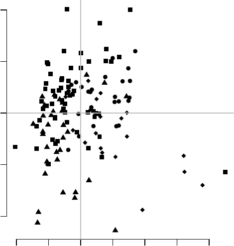
Kynurenines, taurocholates
and cortisol cluster
Long chain fatty
acid cluster
Secondary Bile
Acid Metabolism
Long Chain
Fatty Acid
Polyunsaturated Fatty
Acid (n3 and n6)
Lipid
Hormones
cluster
Long Chain
Fatty Acid
Lysophosphatidylcholines
and bilirubines cluster
Steroid
Lysolipid
Lipid
−10 −5 0 5 10 15 20
−10 −5 0 5 10
PC 2
PC 5
Orange circles and blue triangles are females, located mostly in Q1 and Q2 (top half);
this corresponds to differences on the y axis and the tagcloud next to it (hormone cluster,
steroids etc.). On the other hand, TB patients (blue triangles and yellow circles) are in Q1
and Q4 (right-hand side), which corresponds to the TB-specific tag cloud below the y axis.
8.2 Case study: RNASeq
The example below has been extended from the edgeR package users manual.
The code below loads the data and, using org.Hs.eg.db, adds Entrez IDs and HGNC
symbols.
89

library(edgeR)
rawdata <- read.csv("rnaseq_example.csv",stringsAsFactors=FALSE)
y <- DGEList(counts=rawdata[,4:9], genes=rawdata[,1:3])
map <- toTable(org.Hs.egREFSEQ2EG)
y$genes$EG <- map$gene_id[ match(y$genes$idRefSeq, map$accession) ]
map <- toTable(org.Hs.egSYMBOL)
y$genes$Symbol <- map$symbol[ match(y$genes$EG, map$gene_id) ]
Next, we perform differential gene expression to test for the difference between normal
tissue (N) and tumor (T).
Patient <- paste0("P.",rep(c(8,33,51), each=2))
Tissue <- rep(c("N","T"), 3)
design <- model.matrix(~Patient+Tissue)
y <- calcNormFactors(y)
design <- model.matrix(~Patient+Tissue)
y <- estimateDisp(y, design, robust=TRUE)
fit <- glmQLFit(y, design)
## calculate the results for coefficient of interest
lrt <- glmQLFTest(fit, coef="TissueT")
Since there are no confidence intervals for log fold changes in edgeR, we cannot com-
pute MSD, and therefore we will use the p-values to order the genes in the following code:
ord <- order(lrt$table$PValue)
res.rnaseq <- list()
res.rnaseq$tmod <- tmodCERNOtest(lrt$genes$Symbol[ord])
res.rnaseq$goset <- tmodCERNOtest(lrt$genes$EG[ord], mset=goset)
So far, so good. However, an alternative to using MSD is test the log fold change of
the selected contrast not against 0, but against a pre-selected threshold using the TREAT
method (McCarthy and Smyth 2009), implemented in edgeR in the function glmTreat:
90
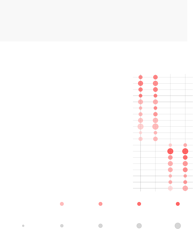
lrt.treat <- glmTreat(fit, coef="TissueT",lfc=log2(2))
ord <- order(lrt.treat$table$PValue)
res.rnaseq$treat.tmod <- tmodCERNOtest(lrt$genes$Symbol[ord])
res.rnaseq$treat.goset <- tmodCERNOtest(lrt$genes$EG[ord], mset=goset)
res.rnaseq <- res.rnaseq[c(1,3,2,4)]
tmodPanelPlot(res.rnaseq, filter.rows.pval=1e-3)
cell adhesion (LI.M51)
enriched for cell migration (LI.M122)
extracellular matrix, collagen (LI.M210)
cell cycle and transcription (LI.M4.0)
cytoskeleton/actin (SRF transcription targets) (LI.M145.1)
immune activation − generic cluster (LI.M37.0)
B cell surface signature (LI.S2)
complement activation (I) (LI.M112.0)
complement activation (II) (LI.M112.1)
enriched in monocytes (II) (LI.M11.0)
enriched in myeloid cells and monocytes (LI.M81)
platelet degranulation (GO:0002576)
muscle filament sliding (GO:0030049)
cardiac muscle contraction (GO:0060048)
skeletal muscle contraction (GO:0003009)
sarcomere organization (GO:0045214)
muscle organ development (GO:0007517)
epidermis development (GO:0008544)
peptide cross−linking (GO:0018149)
tmod
treat.tmod
goset
treat.goset
Effect size:
P value:
0.5 0.93
0.01 0.001 10−410−510−6
The results are very similar, but the p-values are lower.
91
References
Banchereau, Romain, Alejandro Jordan-Villegas, Monica Ardura, Asuncion Mejias,
Nicole Baldwin, Hui Xu, Elizabeth Saye, et al. 2012. “Host Immune Transcriptional
Profiles Reflect the Variability in Clinical Disease Manifestations in Patients with
Staphylococcus Aureus Infections.” PLoS One 7 (4). Public Library of Science: e34390.
Chaussabel, Damien, Charles Quinn, Jing Shen, Pinakeen Patel, Casey Glaser, Nicole
Baldwin, Dorothee Stichweh, et al. 2008. “A Modular Analysis Framework for Blood
Genomics Studies: Application to Systemic Lupus Erythematosus.” Immunity 29 (1). El-
sevier: 150–64.
Damian, Doris, and Malka Gorfine. 2004. “Statistical Concerns About the GSEA Pro-
cedure.” Nature Genetics 36 (7). Nature Publishing Group: 663–63.
Li, Shuzhao, Nadine Rouphael, Sai Duraisingham, Sandra Romero-Steiner, Sco Pres-
nell, Carl Davis, Daniel S Schmidt, et al. 2014. “Molecular Signatures of Antibody Re-
sponses Derived from a Systems Biology Study of Five Human Vaccines.” Nature Immunol-
ogy 15 (2). Nature Publishing Group: 195–204.
Maerdorf, Jeroen, Martin Ota, Dirk Repsilber, Hans J Mollenkopf, January Weiner,
Philip C Hill, and Stefan HE Kaufmann. 2011. “Functional Correlations of Pathogenesis-
Driven Gene Expression Signatures in Tuberculosis.” PloS One 6 (10). Public Library of
Science: e26938.
McCarthy, Davis J, and Gordon K Smyth. 2009. “Testing Significance Relative to a
Fold-Change Threshold Is a TREAT.” Bioinformatics 25 (6). Oxford University Press: 765–
71.
Smyth, Gordon K. 2005. “Limma: Linear Models for Microarray Data.” In Bioinformat-
ics and Computational Biology Solutions Using R and Bioconductor, edited by R. Gentleman,
92
V. Carey, S. Dudoit, R. Irizarry, and W. Huber, 397–420. New York: Springer.
Subramanian, Aravind, Pablo Tamayo, Vamsi K Mootha, Sayan Mukherjee, Benjamin
L Ebert, Michael A Gillee, Amanda Paulovich, et al. 2005. “Gene Set Enrichment Anal-
ysis: A Knowledge-Based Approach for Interpreting Genome-Wide Expression Profiles.”
Proceedings of the National Academy of Sciences of the United States of America 102 (43). Na-
tional Acad Sciences: 15545–50.
Tomfohr, John, Jun Lu, and Thomas B Kepler. 2005. “Pathway Level Analysis of Gene
Expression Using Singular Value Decomposition.” BMC Bioinformatics 6 (1). BioMed Cen-
tral: 225.
Weiner 3rd, January, and Teresa Domaszewska. 2016. “Tmod: An R Package for Gen-
eral and Multivariate Enrichment Analysis.” PeerJ Preprints 2016 (09). PeerJ, Inc.
Weiner 3rd, January, Shreemanta K Parida, Jeroen Maerdorf, Gillian F Black, Dirk
Repsilber, Anna Telaar, Robert P Mohney, et al. 2012. “Biomarkers of Inflammation, Im-
munosuppression and Stress with Active Disease Are Revealed by Metabolomic Profiling
of Tuberculosis Patients.” PloS One 7 (7). Public Library of Science: e40221.
Weiner, January. 2013. Pca3d: Three Dimensional PCA Plots.
———. 2014. Tagcloud: Tag Clouds.
Wendt, Hans W. 1972. “Dealing with a Common Problem in Social Science: A Simpli-
fied Rank-Biserial Coefficient of Correlation Based on the U Statistic.” European Journal of
Social Psychology 2 (4). Wiley Online Library: 463–65.
Yamaguchi, Ken D, Daniel L Ruderman, Ed Croze, T Charis Wagner, Sharlene
Velichko, Anthony T Reder, and Hugh Salamon. 2008. “IFN-β-Regulated Genes Show
Abnormal Expression in Therapy-Naïve Relapsing–remiing MS Mononuclear Cells:
Gene Expression Analysis Employing All Reported Protein–protein Interactions.” Journal
of Neuroimmunology 195 (1). Elsevier: 116–20.
93
