TR 102 273 2 V1.2.1 Electromagnetic Compatibility And Radio Spectrum Matters (ERM); Improvement On Radiated Methods Of Measu 102299 10227302v010201p

User Manual: 102299

Open the PDF directly: View PDF .
Page Count: 107 [warning: Documents this large are best viewed by clicking the View PDF Link!]

ETSI TR 102 273-2 V1.2.1 (2001-

1

2)

Technical Report

E

lectromagnetic compatibility

a

nd Radio spectrum Matters (ERM);

I

mprovement on Radiated Methods

o

f Measurement (using test site) and evaluation

o

f the corresponding measurement uncertainties;

Part

2: Anechoic chamber

ETSI

E

TSI TR 102 273

-

2

V1.2.1 (2001

-

1

2)

2

Reference

RTR/ERM-RP02-057-2

Keywords

analogue, data, measurement uncertainty,

mobile, radio, testing

ETSI

650 Route des Lucioles

F-06921 Sophia Antipolis Cedex - FRANCE

Tel.: +33 4 92 94 42 00 Fax: +33 4 93 65 47 16

Siret N° 348 623 562 00017 - NAF 742 C

Association à but non lucratif enregistrée à la

Sous-Préfecture de Grasse (06) N° 7803/88

Important notice

Individual copies of the present document can be downloaded from:

http://www.etsi.org

The present document may be made available in more than one electronic version or in print. In any case of existing or

perceived difference in contents between such versions, the reference version is the Portable Document Format (PDF).

In case of d

i

spute, the reference shall be the printing on ETSI printers of the PDF version kept on a specific network drive

within ETSI Secretariat.

Users of the present document should be aware that the document may be subject to revision or change of status.

Information on the current status of this and other ETSI documents is available at

http://portal.etsi.org/tb/status/status.asp

If you find errors in the present document, send your comment to:

editor@etsi.fr

Copyright Notification

No part may be reproduced except as authorized by written permission.

The copyright and the foregoing restriction extend to reproduction in all media.

© European Telecommunications Standards Institute 2001.

All rights reserved.

ETSI

E

TSI TR 102 273

-

2

V1.2.1 (2001

-

1

2)

3

Contents

Intellectual Property Rights................................................................................................................................6

Foreword.............................................................................................................................................................6

1 Scope........................................................................................................................................................7

2 References................................................................................................................................................7

3 Definitions, symbols and abbreviations ...................................................................................................8

3.1 Definitions..........................................................................................................................................................8

3.2 Symbols............................................................................................................................................................12

3.3 Abbreviations ...................................................................................................................................................14

4 Introduction............................................................................................................................................15

5 Uncertainty contributions specific to an Anechoic Chamber.................................................................16

5.1 Effects of the metal shielding...........................................................................................................................16

5.1.1 Resonances .................................................................................................................................................16

5.1.2 Imaging of antennas (or an EUT) ...............................................................................................................16

5.2 Effects of the radio absorbing materials...........................................................................................................17

5.2.1 Introduction.................................................................................................................................................17

5.2.2 Pyramidal absorbers....................................................................................................................................18

5.2.3 Wedge absorbers.........................................................................................................................................19

5.2.4 Ferrite tiles..................................................................................................................................................20

5.2.5 Ferrite grids.................................................................................................................................................20

5.2.6 Urethane/ferrite hybrids..............................................................................................................................21

5.2.7 Floor absorbers ...........................................................................................................................................21

5.2.8 Performance comparison ............................................................................................................................21

5.2.9 Reflection in an Anechoic Chamber...........................................................................................................22

5.2.10 Mutual coupling due to imaging in the absorbing material ........................................................................24

5.3 Other effects.....................................................................................................................................................25

5.3.1 Extraneous reflections.................................................................................................................................25

5.3.2 Mutual coupling between antennas (or antenna and EUT).........................................................................25

5.3.3 Turntable and antenna mounting fixtures ...................................................................................................26

5.3.4 Antenna cabling..........................................................................................................................................27

5.3.5 Positioning of the EUT and antennas..........................................................................................................27

5.3.6 Equipment cabling......................................................................................................................................28

6 Verification procedure for an Anechoic Chamber .................................................................................28

6.1 Introduction ......................................................................................................................................................28

6.2 Normalized site attenuation..............................................................................................................................29

6.2.1 NSA for the ideal Anechoic Chamber ........................................................................................................30

6.2.2 Mutual coupling..........................................................................................................................................31

6.3 Overview of the verification procedure............................................................................................................32

6.3.1 Apparatus required......................................................................................................................................32

6.3.2 Site preparation...........................................................................................................................................33

6.3.3 Measurement configuration ........................................................................................................................34

6.3.4 What to record ............................................................................................................................................36

6.4 Verification procedure......................................................................................................................................36

6.4.1 Procedure 1: 30 MHz to 1 000 MHz...........................................................................................................36

6.4.2 Alternative Procedure 1: 30 MHz to 1 000 MHz........................................................................................41

6.4.3 Procedure 2: 1 GHz to 12,75 GHz..............................................................................................................41

6.5 Processing the results of the verification procedure.........................................................................................45

6.5.1 Introduction.................................................................................................................................................45

6.5.2 Procedure 1: 30 MHz to 1 000 MHz...........................................................................................................45

6.5.3 Procedure 2 (1 GHz to 12,75 GHz) ............................................................................................................47

6.5.4 Report format..............................................................................................................................................49

6.6 Calculation of measurement uncertainty (Procedure 1) ...................................................................................49

6.6.1 Uncertainty contribution, direct attenuation measurement .........................................................................49

6.6.2 Uncertainty contribution, NSA measurement.............................................................................................50

ETSI

E

TSI TR 102 273

-

2

V1.2.1 (2001

-

1

2)

4

6.6.3 Expanded uncertainty of the verification procedure ...................................................................................51

6.7 Calculation of measurement uncertainty (Procedure 2) ...................................................................................51

6.7.1 Uncertainty contribution, direct attenuation measurement .........................................................................52

6.7.2 Uncertainty contribution, NSA measurement.............................................................................................53

6.7.3 Expanded uncertainty of the verification procedure ...................................................................................54

6.8 Summary ..........................................................................................................................................................54

7 Test methods ..........................................................................................................................................54

7.1 Introduction ......................................................................................................................................................54

7.1.1 Site preparation...........................................................................................................................................55

7.1.2 Preparation of the EUT...............................................................................................................................56

7.1.3 Standard antennas .......................................................................................................................................56

7.1.4 Mutual coupling and mismatch loss correction factors...............................................................................57

7.1.5 Power supplies to the EUT .........................................................................................................................57

7.1.6 Restrictions .................................................................................................................................................57

7.2 Transmitter tests ...............................................................................................................................................57

7.2.1 Frequency error (30 MHz to 1 000 MHz)...................................................................................................57

7.2.1.1 Apparatus required................................................................................................................................57

7.2.1.2 Method of measurement........................................................................................................................58

7.2.1.3 Procedure for completion of the results sheets......................................................................................59

7.2.1.4 Log book entries....................................................................................................................................59

7.2.1.5 Statement of results...............................................................................................................................59

7.2.2 Expanded uncertainty for frequency error test............................................................................................60

7.2.3 Effective radiated power (30 MHz to 1 000 MHz).....................................................................................60

7.2.3.1 Apparatus required................................................................................................................................60

7.2.3.2 Method of measurement........................................................................................................................61

7.2.3.3 Procedure for the completion of the results sheets................................................................................63

7.2.3.4 Log book entries....................................................................................................................................65

7.2.3.5 Statement of results...............................................................................................................................66

7.2.4 Measurement uncertainty for effective radiated power...............................................................................66

7.2.4.1 Uncertainty contributions: Stage 1: EUT measurement........................................................................66

7.2.4.2 Uncertainty contributions: Stage two: Substitution measurement ........................................................67

7.2.4.3 Expanded uncertainty of the ERP measurement ...................................................................................68

7.2.5 Spurious emissions (30 MHz to 4 GHz or 12,75 GHz) ..............................................................................68

7.2.5.1 Apparatus required................................................................................................................................69

7.2.5.2 Method of measurement........................................................................................................................70

7.2.5.3 Procedure for completion of the results sheets......................................................................................74

7.2.5.4 Log book entries....................................................................................................................................75

7.2.5.5 Statement of results...............................................................................................................................76

7.2.6 Measurement uncertainty for Spurious emissions ......................................................................................76

7.2.6.1 Uncertainty contributions: Stage 1: EUT measurement........................................................................76

7.2.6.2 Uncertainty contributions: Stage 2: Substitution measurement ............................................................77

7.2.6.3 Expanded uncertainty of the spurious emission....................................................................................78

7.2.7 Adjacent channel power..............................................................................................................................79

7.3 Receiver tests....................................................................................................................................................79

7.3.1 Sensitivity tests (30 MHz to 1 000 MHz)...................................................................................................79

7.3.1.1 Apparatus required................................................................................................................................80

7.3.1.2 Method of measurement........................................................................................................................81

7.3.1.3 Procedure for completion of the results sheets......................................................................................86

7.3.1.4 Log book entries....................................................................................................................................86

7.3.1.5 Statement of results...............................................................................................................................88

7.3.2 Measurement uncertainty for Receiver sensitivity......................................................................................89

7.3.2.1 Uncertainty contributions: Stage 1: Determination of Transform Factor..............................................89

7.3.2.2 Uncertainty contributions: Stage 2: EUT measurement........................................................................90

7.3.2.3 Expanded uncertainty of the receiver sensitivity measurement ............................................................91

7.3.3 Co-channel rejection...................................................................................................................................91

7.3.4 Adjacent channel selectivity .......................................................................................................................91

7.3.5 Intermodulation immunity ..........................................................................................................................91

7.3.6 Blocking immunity or desensitization ........................................................................................................91

7.3.7 Spurious response immunity to radiated fields (30 MHz to 4 GHz)...........................................................91

7.3.7.1 Apparatus required................................................................................................................................91

7.3.7.2 Method of measurement........................................................................................................................93

ETSI

E

TSI TR 102 273

-

2

V1.2.1 (2001

-

1

2)

5

7.3.7.3 Procedure for completion of the results sheets......................................................................................98

7.3.7.4 Log book entries....................................................................................................................................99

7.3.7.5 Statement of results.............................................................................................................................101

7.3.8 Measurement uncertainty for Spurious response immunity......................................................................102

7.3.8.1 Uncertainty contributions: Stage 1: Transform factor.........................................................................102

7.3.8.2 Uncertainty contributions: Stage 2: EUT measurement......................................................................103

7.3.8.3 Expanded uncertainty of the spurious response immunity measurement............................................104

Annex A: Bibliography........................................................................................................................105

History............................................................................................................................................................107

ETSI

E

TSI TR 102 273

-

2

V1.2.1 (2001

-

1

2)

6

Intellectual Property Rights

IPRs essential or potentially essential to the present document may have been declared to ETSI. The information

pertaining to these essential IPRs, if any, is publicly available for ETSI members and non-members, and can be found

in ETSI SR 000 314: "Intellectual Property Rights (IPRs); Essential, or potentially Essential, IPRs notified to ETSI in

respect of ETSI standards", which is available from the ETSI Secretariat. Latest updates are available on the ETSI Web

server (http://webapp.etsi.org/IPR/home.asp).

Pursuant to the ETSI IPR Policy, no investigation, including IPR searches, has been carried out by ETSI. No guarantee

can be given as to the existence of other IPRs not referenced in ETSI SR 000 314 (or the updates on the ETSI Web

server) which are, or may be, or may become, essential to the present document.

Foreword

This Technical Report (TR) has been produced by ETSI Technical Committee Electromagnetic compatibility and Radio

spectrum Matters (ERM).

The present document is part 2 of a multi-part deliverable covering Improvement on radiated methods of measurement

(using test site) and evaluation of the corresponding measurement uncertainties, as identified below:

Part 1: "Uncertainties in the measurement of mobile radio equipment characteristics";

Sub-part 1: "Introduction";

Sub-part 2: "Examples and annexes";

Part 2: "Anechoic chamber";

Part 3: "Anechoic chamber with a ground plane";

Part 4: "Open area test site";

Part 5: "Striplines";

Part 6: "Test fixtures";

Part 7: "Artificial human beings".

ETSI

E

TSI TR 102 273

-

2

V1.2.1 (2001

-

1

2)

7

1 Scope

The present document provides background to the subject of measurement uncertainty and proposes extensions and

improvements relevant to radiated measurements. It also details the methods of radiated measurements (test methods for

mobile radio equipment parameters and verification procedures for test sites) and additionally provides the methods for

evaluating the associated measurement uncertainties.

The present document provides a method to be used together with all the applicable standards and (E)TRs, supports

TR 100 027 [13] and can be used with TR 100 028 [12].

The present document covers the test methods for performing radiated measurements on mobile radio equipment in an

Anechoic Chamber and also provides the methods for evaluation and calculation of the measurement uncertainties for

each of the measured parameters.

2 References

For the purposes of this Technical Report (TR), the following references apply:

[1] ANSI C63.5 (1988): "Electromagnetic Compatibility-Radiated Emission Measurements in

Electromagnetic Interference (EMI) Control - Calibration of Antennas".

[2] "Antenna Theory: Analysis and Design", 2nd Edition, Constantine A. Balanis (1996).

[3] "Calculation of site attenuation from antenna factors", A. A. Smith Jr, RF German and J B Pate.

IEEE transactions EMC. Vol. EMC 24 pp 301-316, Aug 1982.

[4] ITU-T Recommendation O.153: "Basic parameters for the measurement of error performance at

bit rates below the primary rate".

[5] ITU-T Recommendation O.41: "Psophometer for use on telephone-type circuits".

[6] CISPR 16-1: "Specification for radio disturbance and immunity measuring apparatus and

methods - Part 1: Radio disturbance and immunity measuring apparatus".

[7] EN 50147-2 (1996): "Anechoic Chambers - Part 2: Alternative test site suitability with respect to

site attenuation".

[8] ETSI TR 102 273-1-1: "ElectroMagnetic Compatibility and Radio Spectrum Matters (ERM);

Improvement on Radiated Methods of Measurement (using test site) and evaluation of the

corresponding measurement uncertainties Part 1: Uncertainties in the measurement of mobile radio

equipment characteristics; Sub-part 1: Introduction".

[9] ETSI TR 102 273-1-2: "ElectroMagnetic Compatibility and Radio Spectrum Matters (ERM);

Improvement on Radiated Methods of Measurement (using test site) and evaluation of the

corresponding measurement uncertainties; Part 1: Uncertainties in the measurement of mobile

radio equipment characteristics; Sub-part 2: Examples and annexes".

[10] "The gain resistance product of the half-wave dipole", W. Scott Bennet Proceedings of IEEE

vol. 72 No. 2 Dec 1984 pp 1824-1826.

[11] "The new IEEE standard dictionary of electrical and electronic terms" Fifth edition, IEEE

Piscataway, NJ USA 1993.

[12] ETSI TR 100 028 (V1.4.1) (Parts 1 and 2): "Electromagnetic compatibility and Radio spectrum

Matters (ERM); Uncertainties in the measurement of mobile radio equipment characteristics".

[13] ETSI TR 100 027: "Methods of measurement for private mobile radio equipment".

ETSI

E

TSI TR 102 273

-

2

V1.2.1 (2001

-

1

2)

8

3 Definitions, symbols and abbreviations

3.1 Definitions

For the purposes of the present document, the following terms and definitions apply:

accuracy: this term is defined, in relation to the measured value, in clause 4.1.1; it has also been used in the remainder

of the document in relation to instruments

Audio Frequency (AF) load: normally a resistor of sufficient power rating to accept the maximum audio output power

from the EUT. The value of the resistor is normally that stated by the manufacturer and is normally the impedance of

the audio transducer at 1 000 Hz

NOTE: In some cases it may be necessary to place an isolating transformer between the output terminals of the

receiver under test and the load.

AF termination: any connection other than the audio frequency load which may be required for the purpose of testing

the receiver (i.e. in a case where it is required that the bit stream be measured, the connection may be made, via a

suitable interface, to the discriminator of the receiver under test)

NOTE: The termination device is normally agreed between the manufacturer and the testing authority and details

included in the test report. If special equipment is required then it is normally provided by the

manufacturer.

A-M1: test modulation consisting of a 1 000 Hz tone at a level which produces a deviation of 12 % of the channel

separation

A-M2: test modulation consisting of a 1 250 Hz tone at a level which produces a deviation of 12 % of the channel

separation

A-M3: test modulation consisting of a 400 Hz tone at a level which produces a deviation of 12 % of the channel

separation. This signal is used as an unwanted signal for analogue and digital measurements

antenna: that part of a transmitting or receiving system that is designed to radiate or to receive electromagnetic waves

antenna factor: quantity relating the strength of the field in which the antenna is immersed to the output voltage across

the load connected to the antenna. When properly applied to the meter reading of the measuring instrument, yields the

electric field strength in V/m or the magnetic field strength in A/m

antenna gain: ratio of the maximum radiation intensity from an (assumed lossless) antenna to the radiation intensity

that would be obtained if the same power were radiated isotropically by a similarly lossless antenna

bit error ratio: ratio of the number of bits in error to the total number of bits

combining network: network allowing the addition of two or more test signals produced by different sources (e.g. for

connection to a receiver input)

NOTE: Sources of test signals are normally connected in such a way that the impedance presented to the receiver

is 50 Ω. Combining networks are designed so that effects of any intermodulation products and noise

produced in the signal generators are negligible.

correction factor: numerical factor by which the uncorrected result of a measurement is multiplied to compensate for

an assumed systematic error

confidence level: probability of the accumulated error of a measurement being within the stated range of uncertainty of

measurement

directivity: ratio of the maximum radiation intensity in a given direction from the antenna to the radiation intensity

averaged over all directions (i.e. directivity = antenna gain + losses)

DM-0: test modulation consisting of a signal representing an infinite series of "0" bits

DM-1: test modulation consisting of a signal representing an infinite series of "1" bits

ETSI

E

TSI TR 102 273

-

2

V1.2.1 (2001

-

1

2)

9

DM-2: test modulation consisting of a signal representing a pseudorandom bit sequence of at least 511 bits in

accordance with ITU-T Recommendation O.153

D-M3: test signal agreed between the testing authority and the manufacturer in the cases where it is not possible to

measure a bit stream or if selective messages are used and are generated or decoded within an equipment

NOTE: The agreed test signal may be formatted and may contain error detection and correction. Details of the

test signal are be supplied in the test report.

duplex filter: device fitted internally or externally to a transmitter/receiver combination to allow simultaneous

transmission and reception with a single antenna connection.

error of measurement (absolute): result of a measurement minus the true value of the measurand

error (relative): ratio of an error to the true value

estimated standard deviation: from a sample of n results of a measurement the estimated standard deviation is given

by the formula:

1

1

2

−

−

=

∑

=

n

)x(x

n

i

i

σ

xi being the ith result of measurement (i = 1, 2, 3, ..., n) and xthe arithmetic mean of the n results considered.

A practical form of this formula is:

1

2

−

−

=n

n

X

Y

σ

where X is the sum of the measured values and Y is the sum of the squares of the measured values.

The term standard deviation has also been used in the present document to characterize a particular probability

density. Under such conditions, the term standard deviation may relate to situations where there is only one result for a

measurement.

expansion factor: multiplicative factor used to change the confidence level associated with a particular value of a

measurement uncertainty

The mathematical definition of the expansion factor can be found in clause D.5.6.2.2 of the TR 100 028-2 [12].

extreme test conditions: conditions defined in terms of temperature and supply voltage. Tests are normally made with

the extremes of temperature and voltage applied simultaneously. The upper and lower temperature limits are specified

in the relevant testing standard. The test report states the actual temperatures measured

error (of a measuring instrument): indication of a measuring instrument minus the (conventional) true value

free field: field (wave or potential) which has a constant ratio between the electric and magnetic field intensities

free space: region free of obstructions and characterized by the constitutive parameters of a vacuum

impedance: measure of the complex resistive and reactive attributes of a component in an alternating current circuit

impedance (wave): complex factor relating the transverse component of the electric field to the transverse component

of the magnetic field at every point in any specified plane, for a given mode

influence quantity: quantity which is not the subject of the measurement but which influences the value of the quantity

to be measured or the indications of the measuring instrument

intermittent operation: operation where the manufacturer states the maximum time that the equipment is intended to

transmit and the necessary standby period before repeating a transmit period

isotropic radiator: hypothetical, lossless antenna having equal radiation intensity in all directions

ETSI

E

TSI TR 102 273

-

2

V1.2.1 (2001

-

1

2)

1

0

limited frequency range: limited frequency range is a specified smaller frequency range within the full frequency

range over which the measurement is made

NOTE: The details of the calculation of the limited frequency range are normally given in the relevant testing

standard.

maximum permissible frequency deviation: maximum value of frequency deviation stated for the relevant channel

separation in the relevant testing standard

measuring system: complete set of measuring instruments and other equipment assembled to carry out a specified

measurement task

measurement repeatability: closeness of the agreement between the results of successive measurements of the same

measurand carried out subject to all the following conditions:

- the same method of measurement;

- the same observer;

- the same measuring instrument;

- the same location;

- the same conditions of use;

- repetition over a short period of time.

measurement reproducibility: closeness of agreement between the results of measurements of the same measurand,

where the individual measurements are carried out changing conditions such as:

- method of measurement;

- observer;

- measuring instrument;

- location;

- conditions of use;

- time.

measurand: quantity subjected to measurement

noise gradient of EUT: function characterizing the relationship between the RF input signal level and the performance

of the EUT, e.g. the SINAD of the AF output signal

nominal frequency: one of the channel frequencies on which the equipment is designed to operate.

nominal mains voltage: declared voltage or any of the declared voltages for which the equipment was designed.

normal test conditions: conditions defined in terms of temperature, humidity and supply voltage stated in the relevant

testing standard

normal deviation: frequency deviation for analogue signals which is equal to 12 % of the channel separation

psophometric weighting network: as described in ITU-T Recommendation O.41

polarization: for an electromagnetic wave, the figure traced as a function of time by the extremity of the electric vector

at a fixed point in space

quantity (measurable): attribute of a phenomenon or a body which may be distinguished qualitatively and determined

quantitatively

rated audio output power: maximum audio output power under normal test conditions, and at standard test

modulations, as declared by the manufacturer

ETSI

E

TSI TR 102 273

-

2

V1.2.1 (2001

-

1

2)

1

1

rated radio frequency output power: maximum carrier power under normal test conditions, as declared by the

manufacturer

shielded enclosure: structure that protects its interior from the effects of an exterior electric or magnetic field, or

conversely, protects the surrounding environment from the effect of an interior electric or magnetic field

SINAD sensitivity: minimum standard modulated carrier-signal input required to produce a specified SINAD ratio at

the receiver output

stochastic (random) variable: variable whose value is not exactly known, but is characterized by a distribution or

probability function, or a mean value and a standard deviation (e.g. a measurand and the related measurement

uncertainty)

test load: test load is a 50 Ω substantially non-reactive, non-radiating power attenuator which is capable of safely

dissipating the power from the transmitter

test modulation: test modulating signal is a baseband signal which modulates a carrier and is dependent upon the type

of EUT and also the measurement to be performed

trigger device: circuit or mechanism to trigger the oscilloscope timebase at the required instant. It may control the

transmit function or inversely receive an appropriate command from the transmitter

uncertainty (random): component of the uncertainty of measurement which, in the course of a number of

measurements of the same measurand, varies in an unpredictable way (to be considered as a component for the

calculation of the combined uncertainty when the effects it corresponds to have not been taken into consideration

otherwise)

uncertainty (systematic): component of the uncertainty of measurement which, in the course of a number of

measurements of the same measurand remains constant or varies in a predictable way

uncertainty (limits of uncertainty of a measuring instrument): extreme values of uncertainty permitted by

specifications, regulations etc. for a given measuring instrument

NOTE: This term is also known as "tolerance".

uncertainty (standard): expression characterizing, for each individual uncertainty component, the uncertainty for that

component

It is the standard deviation of the corresponding distribution.

uncertainty (combined standard): combined standard uncertainty is calculated by combining appropriately the

standard uncertainties for each of the individual contributions identified in the measurement considered or in the part of

it, which has been considered

NOTE: In the case of additive components (linearly combined components where all the corresponding

coefficients are equal to one) and when all these contributions are independent of each other (stochastic),

this combination is calculated by using the Root of the Sum of the Squares (the RSS method). A more

complete methodology for the calculation of the combined standard uncertainty is given in clause D.3.12

of TR 100 028-2 [12].

uncertainty (expanded): expanded uncertainty is the uncertainty value corresponding to a specific confidence level

different from that inherent to the calculations made in order to find the combined standard uncertainty

The combined standard uncertainty is multiplied by a constant to obtain the expanded uncertainty limits (see clause 5.3

of TR 100 028-1 [12], and also clause D.5 (and more specifically clause D.5.6.2) of TR 100 028-2 [12]).

upper specified AF limit: maximum audio frequency of the audio pass-band. It is dependent on the channel separation

wanted signal level: for conducted measurements a level of +6 dBµV emf referred to the receiver input under normal

test conditions. Under extreme test conditions the value is +12 dBµV emf

NOTE: For analogue measurements the wanted signal level has been chosen to be equal to the limit value of the

measured usable sensitivity. For bit stream and message measurements the wanted signal has been chosen

to be +3 dB above the limit value of measured usable sensitivity.

ETSI

E

TS

I

TR 102 273

-

2

V1.2.1 (2001

-

1

2)

1

2

3.2 Symbols

For the purposes of the present document, the following symbols apply:

β

2π/λ (radians/m)

γ

incidence angle with ground plane (°)

λ

wavelength (m)

φ

H phase angle of reflection coefficient (°)

η

120π Ohms - the intrinsic impedance of free space (Ω)

µ

permeability (H/m)

AFR Antenna Factor of the receive antenna (dB/m)

AFT Antenna Factor of the transmit antenna (dB/m)

AFTOT mutual coupling correction factor (dB)

c calculated on the basis of given and measured data

Ccross cross correlation coefficient

d derived from a measuring equipment specification

D(

θ

,

φ

) directivity of the source

d distance between dipoles (m)

δ skin depth (m)

d1 an antenna or EUT aperture size (m)

d2 an antenna or EUT aperture size (m)

ddir path length of the direct signal (m)

drefl path length of the reflected signal (m)

E Electric field intensity (V/m)

EDHmax calculated maximum electric field strength in the receiving antenna height scan from a half

wavelength dipole with 1 pW of radiated power (for horizontal polarization) (µV/m)

EDVmax calculated maximum electric field strength in the receiving antenna height scan from a half

wavelength dipole with 1 pW of radiated power (for vertical polarization) (µV/m)

eff antenna efficiency factor

φ

angle (°)

∆

f bandwidth (Hz)

f frequency (Hz)

G(

θ

,

φ

) gain of the source (which is the source directivity multiplied by the antenna efficiency factor)

H magnetic field intensity (A/m)

I0 the (assumed constant) current (A)

Im the maximum current amplitude

k 2π/λ

k a factor from Student's t distribution

k Boltzmann's constant (1,38 x 10-23 Joules/° Kelvin)

K relative dielectric constant

l the length of the infinitesimal dipole (m)

L the overall length of the dipole (m)

l the point on the dipole being considered (m)

m measured

p power level value

Pe (n) Probability of error n

Pp (n) Probability of position n

Pr antenna noise power (W)

Prec Power received (W)

Pt Power transmitted (W)

θ

angle (°)

ρ

reflection coefficient

r the distance to the field point (m)

ρ

g reflection coefficient of the generator part of a connection

ρ

l reflection coefficient of the load part of the connection

ETSI

E

TSI TR 102 273

-

2

V1.2.1 (2001

-

1

2)

1

3

Rs equivalent surface resistance (Ω)

σ

conductivity (S/m)

σ

standard deviation

r indicates rectangular distribution

SNRb* Signal to Noise Ratio at a specific BER

SNRb Signal to Noise Ratio per bit

TA antenna temperature (° Kelvin)

u indicates U-distribution

U the expanded uncertainty corresponding to a confidence level of x %: U = k

×

uc

uc the combined standard uncertainty

ui general type A standard uncertainty

ui01 random uncertainty

uj general type B uncertainty

uj01 reflectivity of absorbing material: EUT to the test antenna

uj02 reflectivity of absorbing material: substitution or measuring antenna to the test antenna

uj03 reflectivity of absorbing material: transmitting antenna to the receiving antenna

uj04 mutual coupling: EUT to its images in the absorbing material

uj05 mutual coupling: de-tuning effect of the absorbing material on the EUT

uj06 mutual coupling: substitution, measuring or test antenna to its image in the absorbing material

uj07 mutual coupling: transmitting or receiving antenna to its image in the absorbing material

uj08 mutual coupling: amplitude effect of the test antenna on the EUT

uj09 mutual coupling: de-tuning effect of the test antenna on the EUT

uj10 mutual coupling: transmitting antenna to the receiving antenna

uj11 mutual coupling: substitution or measuring antenna to the test antenna

uj12 mutual coupling: interpolation of mutual coupling and mismatch loss correction factors

uj13 mutual coupling: EUT to its image in the ground plane

uj14 mutual coupling: substitution, measuring or test antenna to its image in the ground plane

uj15 mutual coupling: transmitting or receiving antenna to its image in the ground plane

uj16 range length

uj17 correction: off boresight angle in the elevation plane

uj18 correction: measurement distance

uj19 cable factor

uj20 position of the phase centre: within the EUT volume

uj21 positioning of the phase centre: within the EUT over the axis of rotation of the turntable

uj22 position of the phase centre: measuring, substitution, receiving, transmitting or test antenna

uj23 position of the phase centre: LPDA

uj24 stripline: mutual coupling of the EUT to its images in the plates

uj25 stripline: mutual coupling of the 3-axis probe to its image in the plates

uj26 stripline: characteristic impedance

uj27 stripline: non-planar nature of the field distribution

uj28 stripline: field strength measurement as determined by the 3-axis probe

uj29 stripline: transform factor

uj30 stripline: interpolation of values for the transform factor

uj31 stripline: antenna factor of the monopole

uj32 stripline: correction factor for the size of the EUT

uj33 stripline: influence of site effects

uj34 ambient effect

uj35 mismatch: direct attenuation measurement

uj36 mismatch: transmitting part

uj37 mismatch: receiving part

uj38 signal generator: absolute output level

ETSI

E

TSI TR 102 273

-

2

V1.2.1 (2001

-

1

2)

1

4

uj39 signal generator: output level stability

uj40 insertion loss: attenuator

uj41 insertion loss: cable

uj42 insertion loss: adapter

uj43 insertion loss: antenna balun

uj44 antenna: antenna factor of the transmitting, receiving or measuring antenna

uj45 antenna: gain of the test or substitution antenna

uj46 antenna: tuning

uj47 receiving device: absolute level

uj48 receiving device: linearity

uj49 receiving device: power measuring receiver

uj50 EUT: influence of the ambient temperature on the ERP of the carrier

uj51 EUT: influence of the ambient temperature on the spurious emission level

uj52 EUT: degradation measurement

uj53 EUT: influence of setting the power supply on the ERP of the carrier

uj54 EUT: influence of setting the power supply on the spurious emission level

uj55 EUT: mutual coupling to the power leads

uj56 frequency counter: absolute reading

uj57 frequency counter: estimating the average reading

uj58 salty man/salty-lite: human simulation

uj59 salty man/salty-lite: field enhancement and de-tuning of the EUT

uj60 test fixture: effect on the EUT

uj61 test fixture: climatic facility effect on the EUT

Vdirect received voltage for cables connected via an adapter (dBµV/m)

Vsite received voltage for cables connected to the antennas (dBµV/m)

W0 radiated power density (W/m2)

3.3 Abbreviations

For the purposes of the present document, the following abbreviations apply:

AF Audio Frequency

BER Bit Error Ratio

CD Citizen's Band

emf electromotive force

EUT Equipment Under Test

FSK Frequency Shift Keying

GMSK Gaussian Minimum Shift Keying

GSM Global System for Mobile telecommunication (Pan European digital telecommunication system)

IF Intermediate Frequency

LPDA Log Periodic Dipole Antenna

m measured

NaCl Sodium chloride

NSA Normalized Site Attenuation

r indicates rectangular distribution

RF Radio Frequency

rms root mean square

RSS Root-Sum-of-the-Squares

TEM Transverse Electro-Magnetic

u indicates U-distribution

VSWR Voltage Standing Wave Ratio

ETSI

E

TSI TR 102 273

-

2

V1.2.1 (2001

-

1

2)

1

5

4 Introduction

An Anechoic Chamber is an enclosure whose internal walls, floor and ceiling are covered with radio absorbing material,

normally of the pyramidal urethane foam type. It is normally shielded against local ambients. The chamber contains an

antenna support at one end and a turntable at the other. A typical Anechoic Chamber is shown in figure 1 with dipole

antennas at both ends.

Range length 3m or 10 m

Turntable

Antenna support

Antenna support

Radio

absorbing

material

Dipole antennas

Figure 1: A typical Anechoic Chamber

The chamber shielding and radio absorbing material work together to provide a controlled environment for testing

purposes. This type of test chamber attempts to simulate free space conditions. The shielding provides a test space, with

reduced levels of interference from ambient signals and other outside effects, whilst the radio absorbing material

minimizes unwanted reflections from the walls, floor and ceiling which could influence the measurements.

In practice whilst it is relatively easy for the shielding to provide high levels (80 dB to 140 dB) of ambient interference

rejection (normally making ambient interference negligible), no design of radio absorbing material satisfies the

requirement of complete absorption of all the incident power. For example it cannot be perfectly manufactured and

installed and its return loss (a measure of its efficiency) varies with frequency, angle of incidence and in some cases, is

influenced by high power levels of incident radio energy. To improve the return loss over a broader frequency range,

ferrite tiles, ferrite grids and hybrids of urethane foam and ferrite tiles are used with varying degrees of success.

The Anechoic Chamber generally has several advantages over other test facilities. There is minimal ambient

interference, minimal floor, ceiling and wall reflections and it is independent of the weather. It does however have some

disadvantages which include limited measuring distance (due to available room size, cost, etc.) and limited lower

frequency usage due to the size of the room and the pyramidal absorbers.

Both absolute and relative measurements can be performed in an Anechoic Chamber. Where absolute measurements are

to be carried out, or where the test facility is to be used for accredited measurements, the chamber should be verified.

Verification involves comparison of the measured performance to that of an ideal theoretical chamber, with

acceptability being decided on the basis of the maximum difference between the two.

ETSI

E

TSI TR 102 273

-

2

V1.2.1 (2001

-

1

2)

1

6

5 Uncertainty contributions specific to an Anechoic

Chamber

A typical Anechoic Chamber comprises two main components:

- a metallic shield;

- radio absorbing material.

Whilst each component is included to improve the quality of the testing environment within the chamber, each has

negative effects as well. Below, some positive effects are mentioned as a brief introduction to a discussion of the

negative effects and their impact on measurement uncertainty.

5.1 Effects of the metal shielding

The benefits of shielding a testing area can be seen by considering the situation on a typical Open Area Test Site where

ambient RF interference can add considerable uncertainty to the measurements. Such RF ambient signals can be

continuous sources e.g. commercial radio and television, link services, navigation etc. or intermittent ones e.g. CB,

emergency services, DECT, GSM, paging systems, machinery and a variety of others. The interference can be either

narrowband or broadband.

The Anechoic Chamber overcomes these problems by the provision of a shielded enclosure. A shielded enclosure is

defined as any structure that protects its interior from the effects of an exterior electric or magnetic field, or conversely,

protects the surrounding environment from the effects of an interior field. The shielding is normally provided by metal

panels with continuous electrical contact between them and any opening provided in the shield (e.g. doors and breakout

panels).

Further advantages of the shield are protection from the weather and the general degradation effects it can have.

5.1.1 Resonances

Any metal shield will act as a reflecting surface and grouping six of them together to form a metal box makes it possible

for the chamber to act like a resonant waveguide cavity. Whilst these resonance effects tend to be narrowband, their

peak magnitudes can be high, resulting in a significant disruption of the desired field distribution.

A resonant waveguide cavity mode can, in theory, be excited at any frequency which satisfies the following formula:

fx

l

y

b

z

h

= + +150

222

MHz (5.1)

where l, b and h are respectively the length, breadth and height of the chamber in metres and x, y and z are mode

numbers of which only one is allowed to be zero at any time. As an example, the lowest frequency at which a resonance

could occur in a facility which measures 5 m by 5 m by 7 m is 36,87 MHz.

Caution should be exercised whenever measurements are attempted close to any frequencies predicted by this formula,

particularly for the lowest values, for which the absorber might offer poor performance. To improve confidence in the

chamber, these lower calculated frequencies could be included in the verification procedure.

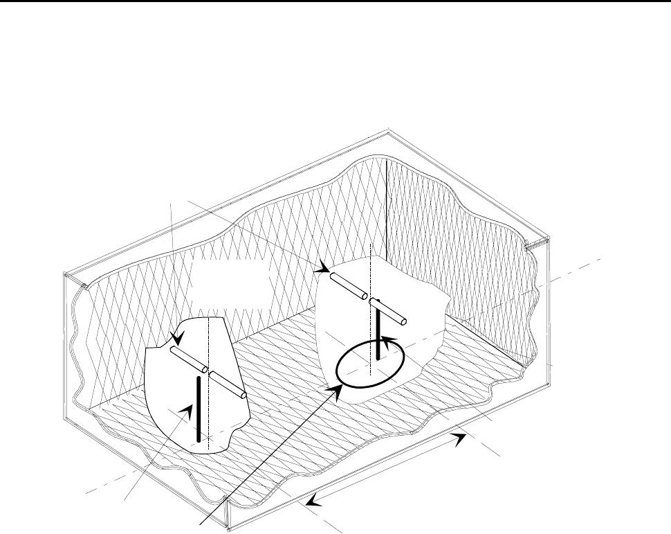
5.1.2 Imaging of antennas (or an EUT)

The shield will have a significant impact on the overall performance of the chamber if it is not adequately "masked"

from the test volume by the absorbing material i.e. if the absorbing material has inadequate absorption characteristics.

For example, in the extreme case of 0 dB return loss from the absorbing materials (i.e. zero absorption/perfect

reflection) an antenna (or EUT) will "see" an image of itself in the end wall close behind, the two side walls, the ceiling,

the floor and, to a lesser extent, the far end wall (see figure 2).

ETSI

E

TSI TR 102 273

-

2

V1.2.1 (2001

-

1

2)

1

7

In this multi-image environment, the one driven (real) antenna is, in effect, powering a seven element array (of which it

is one). Major changes result to all of the antenna's (or the EUT's) electrical characteristics such as input impedance,

gain and radiation pattern.

EUT

Images

Images

Transmitting

dipole

Figure 2: Imaging in the shielded enclosure

Whilst no chamber would be used at any frequency for which the absorbing material performs so badly as to appear

"invisible", this example illustrates that any finite value of reflectivity will produce this imaging to some extent.

Good absorption (low reflectivity) will minimize all internal reflections, whereas poor absorption (high reflectivity) will

not only produce imaging of the antennas (or the EUT), but can also contribute numerous high amplitude reflections.

5.2 Effects of the radio absorbing materials

5.2.1 Introduction

As discussed in clause 5.1.2 the absorbing material plays a critical role in the chamber's performance. Absorption is the

irreversible conversion of the energy of an electromagnetic wave into another form of energy as a result of wave

interaction with matter [11] (i.e. it gets hot). The efficiency with which the material absorbs energy is determined by the

absorption coefficient. This is defined as the ratio of the energy absorbed by the surface to the energy incident upon it

[11]. It is more usual, however, for the reflectivity (i.e. return loss) of an absorbing material to be quoted rather than its

absorption, the assumption being that any incident power not reflected is absorbed.

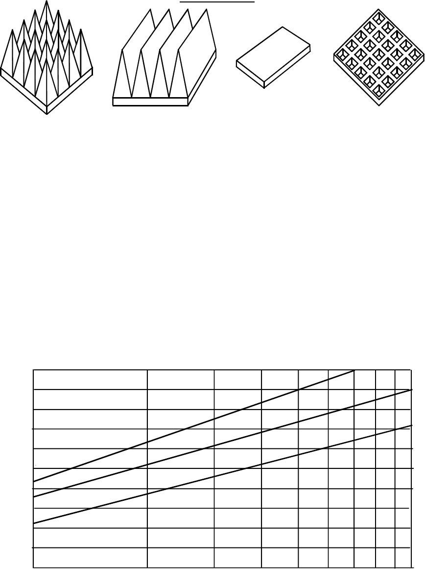
Different types of RF absorbers are available (see figure 3). They all absorb radiated energy to a greater or lesser extent,

but possess different mechanical and electrical properties making certain types more suitable for some applications than

others.

ETSI

E

TSI TR 102 273

-

2

V1.2.1 (2001

-

1

2)

1

8

Ferrite Grid

Ferrite tileWedge

Pyramidal

NOT TO SCALE

Figure 3: Typical RF absorbers

A review of commonly available types is now given.

5.2.2 Pyramidal absorbers

This type of absorber is manufactured from polyurethane foam impregnated with carbon, and moulded into a pyramidal

shape (see figure 3). This shape provides inherently wide bandwidth, small polarization dependence and gives

reasonably wide angular coverage.

Pyramidal absorbers behave as lossy, tapered transitions, ranging from low impedance at the base to 377 Ω at the tip (to

match the impedance of free space). They work on the principle that if all of the energy is converted to heat before the

base is reached, there is nothing to reflect from the shield.

A line, drawn from the centre of the base through the centre of the tip of the pyramid is termed the normal angle of

incidence (0°) and the pyramidal shape maximizes the absorber performance at this angle of incidence. As the angle of

incidence increases, however, the return loss degrades, as illustrated in figure 4 for 50°, 60° and 70° angles against

absorber thickness.

0

10

20

30

40

50

1 2 3 4 5 6 78910

50

°

70

°

60

°

Thickness of absorber in wavelengths

Return loss (dB)

Figure 4: Typical return loss of pyramidal absorber at various incidence angles

This absorption characteristic leads to large reflection coefficients at large angles of incidence where the incident radio

energy approaches broadside to the side faces of the pyramids. The reflection is primarily due to impedance mismatch

between the incident wave and the absorber impedance taper.

ETSI

E

TSI TR 102 273

-

2

V1.2.1 (2001

-

1

2)

1

9

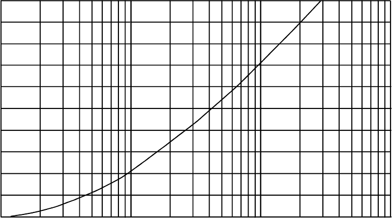
The actual performance varies according to the degree of carbon loading and the shape and size of the cones. Its

effectiveness in suppressing surface reflections is mainly a function of the cone height to wavelength ratio, the

absorption improving as this ratio increases (see figure 5).

0

Thickness of absorber in wavelengths

0,01 0,1 1 10

Return loss (dB)

50

40

30

20

10

Figure 5: Typical return loss of pyramidal absorber at normal incidence

Larger cones therefore, have better low frequency performance e.g. 0,6 m length cones can only be used effectively

down to about 120 MHz, whereas, for comparable performance, 1,778 m cones can be used effectively down to about

40 MHz. This improved performance can, however, only be attained at significantly increased cost and reduction in

space efficiency (see table 1).

The high frequency performance of the pyramidal absorbers seems unlimited (see figure 5), but this is not the case. In

practice, it is limited by resonant effects of the spacing between the peaks of the pyramids, absorber layout pattern and

surface finish of the absorber in general. It is unreasonable to assume any absorber will give more than 50 dB return

loss. In some chambers, mixed size pyramids are used to randomize the absorber pattern to improve its high frequency

performance with only minimum degradation at the lower frequencies.

Flammability, space inefficiency and performance degradation over time caused by drooping under their own weight,

breaking of the absorber tips and rounding of the valleys are major disadvantages of this type of absorber. However, a

hollow cone version is available which reduces the overall weight and improves the mechanical stability. Flame

retarding types are also available, but space inefficiency and "fragility" remain major problems with this type of

absorber.

5.2.3 Wedge absorbers

Wedge absorbers (see figure 3), are a variation of the polyurethane pyramidal foam type, which tends to overcome the

degradation of reflectivity with increasing angle of incidence, but at some performance cost.

This improvement is only for cases where the incident wave direction is parallel to the ridge of the wedge as no

broadside presents itself at off normal angles as is the case with pyramidal absorbers.

Disadvantages of this type of absorber are degraded performance compared to pyramidal types at normal incidence and

when used with the ridge perpendicular to the incident wave.

These effects make wedge absorbers more suitable for use in chambers with range lengths of 10 m or more where they

are used to good advantage in the middle sections of the ceilings, floor and side walls.

ETSI

E

TSI TR 102 273

-

2

V1.2.1 (2001

-

1

2)

2

0

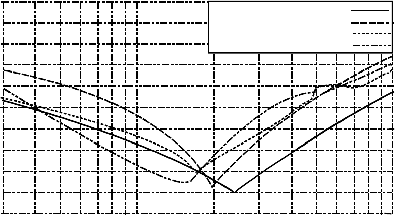
5.2.4 Ferrite tiles

Ferrite is a ferromagnetic ceramic material. Its susceptibility and permeability are dependant on the field strength and

magnetization curves (which have hysterisis). Its magnetic characteristics can be affected by pressure, temperature, field

strength, frequency and time. Its mechanical and electromagnetic characteristics depend heavily on the sintering process

used to form the ferrite. It is hard (physically), brittle (as are all ceramics) and will chip and break if handled roughly.

Ferrite tiles are thin, flat, ceramic blocks typically 15 cm by 8 cm by 1 cm thick (see figure 3). Both thickness and

composition of the ferrite material affect their absorption performance. In practice, their layout is also very critical as

small air gaps between adjacent tiles can considerably degrade performance at the lowest frequencies (30 MHz to

100 MHz). However, when properly installed this is the frequency range for which they give the most benefit over

pyramidal foam absorbers. They are generally manufactured to give about 15 dB to 20 dB return loss at 30 MHz (see

figure 6).

Return loss (dB)

0

Frequency (MHz)

30 100 500

1

000

10

20

30

40

Ferrite grid

Ferrite tile (type 1)

Ferrite tile (type 2)

Ferrite tile (type 3)

Figure 6: Normal incidence return loss variation of three different designs of ferrite tile

and a ferrite grid against frequency

Their main advantages are that they are thin (typically 1 cm) so the shielded enclosure outside dimensions are relatively

small compared to pyramidal foam for the same internal volume (see table 1). Ferrite tiles also have a durable surface

and have stable performance with time.

Disadvantages are cost, the strong dependence of the reflectivity performance on both polarization and angle of

incidence and possible non linear performance due to saturation at high field strengths.

Due to their relatively high cost ferrite tiles are mainly built up into 1 m or 2 m square blocks which are placed

strategically in the chamber under pyramidal foam absorbers in the middle sections of the side walls, floor and ceiling,

the main reflection paths between antennas (or between an antenna and EUT). They are also used on the end walls to

improve absorption and to reduce image coupling.

This combination of ferrite tiles and pyramidal foam absorbers is more cost effective in performance terms than a fully

ferrited room.

5.2.5 Ferrite grids

Ferrite grids are typically 10 cm by 10 cm by 2,5 cm thick. They provide absorption from 30 MHz to 1 000 MHz. The

grid structure provides better power handling characteristics and avoids the installation problems associated with plain

tiles. Their absorption characteristics are basically the same as for ferrite tiles (see figure 6).

ETSI

E

TSI TR 102 273

-

2

V1.2.1 (2001

-

1

2)

2

1

5.2.6 Urethane/ferrite hybrids

Urethane/ferrite hybrid absorbers (as introduced in clause 5.2.4) consist of pyramidal foam absorber bonded to a ferrite

tile backing. They are designed in such a way that the ferrite tiles are active at the low frequencies, where the pyramidal

foam absorbers are not very efficient, whilst the pyramidal absorbers take over at higher frequencies.

A disadvantage is the impedance mismatch between the ferrite base and the foam pyramids which results in

performance degradation in some frequency ranges.

In a similar manner to the ferrite tile, the hybrid absorber is used in the middle sections of the side walls floor and

ceilings - the main reflection paths between antennas (or between an antenna and EUT). They are also used on the end

walls to improve absorption and to reduce image coupling.

5.2.7 Floor absorbers

Anechoic materials (except ferrite tiles and grids) cannot, in general, support loads. Normally, therefore, a false floor of

RF transparent material is built above the anechoic materials, to enable access to the test antenna and turntable. It is,

however, very difficult to obtain a floor that is truly RF transparent and the floor is often "visible". This tends to be

revealed when the performance of the chamber is being verified and has been known to lead to constructional

modifications.

Special types of floor absorbers can be used. These are constructed of normal pyramidal absorbers whose external

profiled sections have been filled with a low loss rigid foam so as to form a solid block. This is usually capable of

supporting the weight of a man, but with usage, degradation in performance occurs.

The most common solution is not to have a floor for access, but to arrange access to the antenna support, either with

another access door (degrades chamber performance) or by making the antenna mount such that it can be easily moved

to the turntable end to facilitate antenna changes, etc.

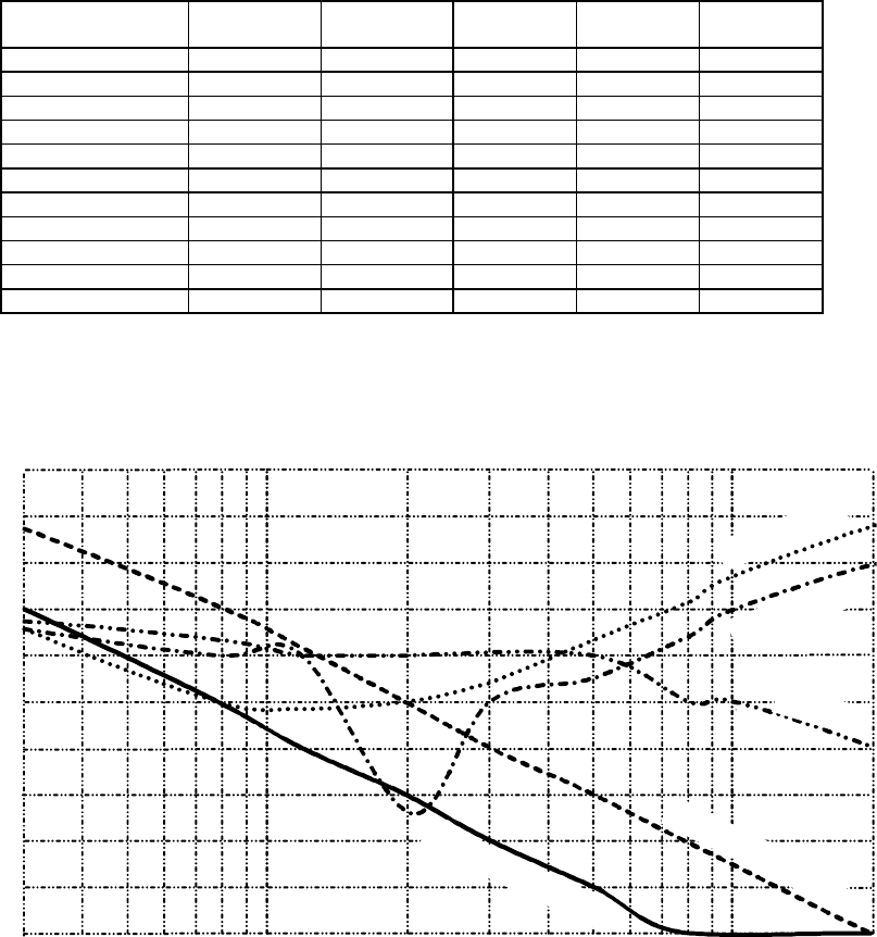
5.2.8 Performance comparison

Tables 1 and 2 detail numerous relative parameters for the different absorber types discussed above. Table 1 gives the

physical parameters relating to an Anechoic Chamber of internal testing dimensions of 8 m by 3 m by 3 m. Table 2

details the return loss (at 0° angle of incidence) for the various absorber types considered in table 1. The data in table 2

is shown graphically in figure 7.

Table 1: Typical physical parameters of an 8 m by 3 m by 3 m Anechoic Chamber

for various absorber types

Features Pyramidal

0,66 m Pyramidal

1,778 m Ferrite

tiles Ferrite

grid Hybrid

Inside

dimensions

8 m by

3 m by

3 m

8 m by

3 m by

3 m

8 m by

3 m by

3 m

8 m by

3 m by

3 m

8 m by

3 m by

3 m

Outside

dimensions

(approx.)

9,32 m by

4,32 m by

4,32 m

11,56 m by

6,56 m by

6,56 m

8,02 m by

3,02 m by

3,02 m

8,05 m by

3,05 m by

3,05 m

9,35 m by

4,35 m by

4,35 m

Overall volume 174 m3 497m3 73 m3 75 m3 177 m3

Flammable yes yes no no yes

Risk of damage high high low low high

Floor absorbers moveable fixed fixed fixed fixed

Frequency

range (MHz) 80 to

>1 000 30 to

>1 000 30 to

>500 30 to

>1 000 30 to

>1 000

ETSI

E

TSI TR 102 273

-

2

V1.2.1 (2001

-

1

2)

2

2

Table 2: Typically return loss at 0°

°°

° incidence for various absorbers against frequency

Frequency Pyramidal

0,66 m Pyramidal

1,778 m Ferrite

tiles Ferrite

grid Hybrid

30 MHz 7 dB 15 dB 17 dB 17 dB 16 dB

80 MHz 15 dB 25 dB 25 dB 20 dB 18 dB

120 MHz 19 dB 30 dB 26 dB 20 dB 20 dB

200 MHz 25 dB 35 dB 25 dB 37 dB 20 dB

300 MHz 30 dB 40 dB 23 dB 25 dB 20 dB

500 MHz 35 dB 45 dB 18 dB 23 dB 20 dB

800 MHz 40 dB 50 dB 14 dB 18 dB 25 dB

1 GHz 50 dB 50 dB 12 dB 15 dB 25 dB

3 GHz 50 dB 50 dB 6 dB 10 dB 30 dB

10 GHz 50 dB 50 dB - - 30 dB

18 GHz 50 dB 50 dB - - 35 dB

All of these types of absorber dissipate the energy incident on their surfaces in the form of heat. When in the presence

of high value fields, the power absorbed in the foam variety can exceed its ability to dissipate the heat, and the resulting

increase in temperature degrades its performance. This is not normally a problem with ferrite types.

0

Frequency (MHz)

30 100 1 000

Return loss (dB)

Ferrite tiles

Ferrite grids

Hybrid

Pyramidal 0,66 m

Pyramidal 1,778 m

50

40

30

20

10

Figure 7: Return loss variation with frequency of the absorber performance given in table 2

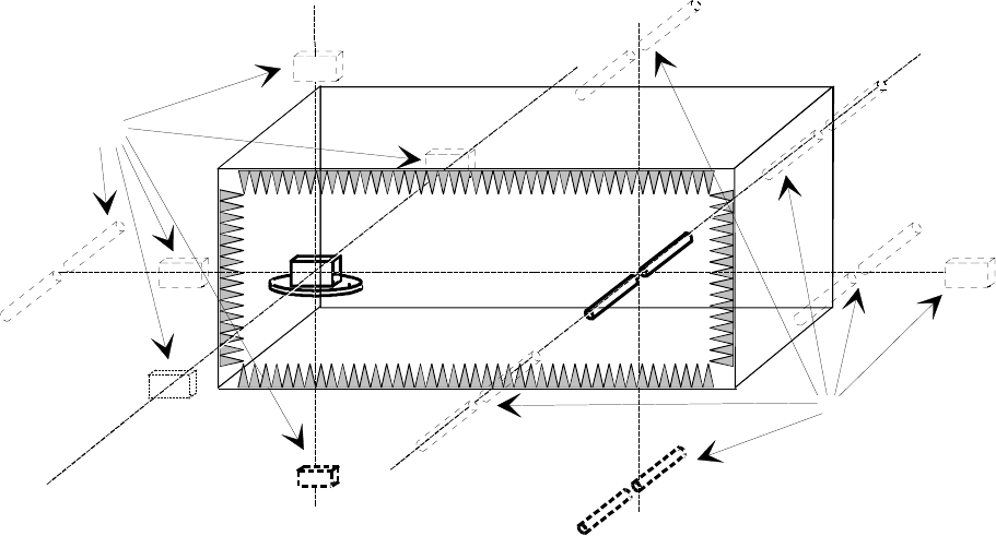
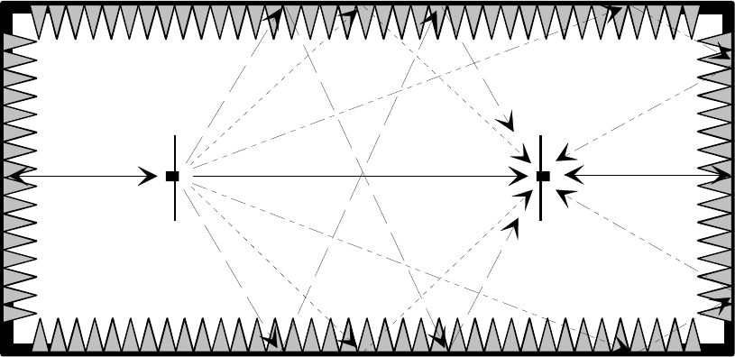
5.2.9 Reflection in an Anechoic Chamber

As has been stated, the absorbing materials used and their layout play a critical role in the chamber's performance. A

plan view of an Anechoic Chamber with its end and side walls covered in pyramidal foam absorbers is shown in

figure 8. Mounted in the chamber are two dipoles (shown for illustration purposes only, although this is a common

arrangement found in test methods and the verification procedure). Various single and double bounce reflection paths

are also illustrated.

The single bounce reflection paths via the end walls are at normal incidence to the absorbers, and since the absorbers

are at maximum efficiency at normal incidence the reflections are of a low amplitude. However the amplitude of the

worst case reflections, the single bounce paths between the antennas via the side walls, are dependant on the angles of

incidence, which themselves are dependant on the geometry (cross section and range length) of the chamber. The

ceiling and floor provides other single bounce reflection paths.

ETSI

E

TSI TR 102 273

-

2

V1.2.1 (2001

-

1

2)

2

3

Figure 8: Plan view of an Anechoic Chamber which uses pyramidal absorber

The direct path between the antennas is the only wanted signal and all other signals, whether the result of reflections

from the absorber or from extraneous sources (see clause 5.3.1) interfere with the required field and result in

measurement uncertainty. The situation is further complicated by the directional nature of the dipoles, reflections in the

E-plane of the dipole being reduced in amplitude when compared to the case for the orthogonal polarization, as a result

of the dipole's radiation pattern.

As an example of the magnitude of the problem, the following is calculated for illustrative purposes. A typical chamber

of 5 m by 5 m by 7 m, employing 0,66 m pyramidal foam absorbers is used over a 3 m range length. The angles of

incidence on the side walls, floor and ceiling of the main single bounce reflection paths are:

tan-1(1,5 / 2,5) = 31,0° (5.2)

Assuming a frequency of 80 MHz, the reflectivity at this angle of incidence is approximately 15 dB. If the polarization

of the transmitting dipole is taken as horizontal, then its directivity in the horizontal plane reduces the magnitude of the

side wall reflections by 1,9 dB which, in addition to the extra path length loss (relative to the direct ray) of 5,8 dB, leads

to the amplitudes of the four main one-bounce reflections being -22,7 dB, -22,7 dB, -20,8 dB and -20,8 dB for the two

side walls, floor and ceiling respectively (these levels being relative to the amplitude of the direct path).

NOTE: In a chamber of identical cross section but offering a 10 m range length, these four main interfering rays

have greater amplitudes of approximately -13,4 dB, -13,4 dB, -12,0 dB and -12,0 dB as a result of

increased reflectivity from the absorbing materials (grazing angle of incidence), less relative path loss (the

path lengths are more nearly equal) and less benefit from the directivity of the dipole pattern.

Whilst the addition of these rays is rather more complex than just a straightforward addition (and for a full analysis one

should also include multiple bounce reflections), their amplitudes serve to illustrate the potential problem of signal level

uncertainty since, again for illustrative purposes only, a single -20 dB interfering signal can, at its maximum relative

phasing, enhance or reduce the received signal strength by +0,83 dB or -0,92 dB respectively. Table 3 illustrates the

uncertainty caused by a single unwanted interfering signal.

ETSI

E

TSI TR 102 273

-

2

V1.2.1 (2001

-

1

2)

2

4

Table 3: Uncertainty in received signal level due to a single unwanted interfering signal

Ratio of unwanted

to wanted

signal level

Received

level uncertainty Ratio of unwanted

to wanted

signal level

Received

level uncertainty

-30,0 dB +0,27 dB -0,28 dB -9,0 dB +2,64 dB -3,81 dB

-25,0 dB +0,48 dB -0,50 dB -8,0 dB +2,91 dB -4,41 dB

-20,0 dB +0,83 dB -0,92 dB -7,0 dB +3,21 dB -5,14 dB

-17,5 dB +1,09 dB -1,24 dB -6,0 dB +3,53 dB -6,04 dB

-15,0 dB +1,42 dB -1,70 dB -5,0 dB +3,88 dB -7,18 dB

-14,0 dB +1,58 dB -1,93 dB -4,0 dB +4,25 dB -8,66 dB

-13,0 dB +1,75 dB -2,20 dB -3,0 dB +4,65 dB -10,69 dB

-12,0 dB +1,95 dB -2,51 dB -2,0 dB +5,08 dB -13,74 dB

-11,0 dB +2,16 dB -2,88 dB -1,0 dB +5,53 dB -19,27 dB

-10,0 dB +2,39 dB -3,30 dB 0,0 dB +6,04 dB -∞ dB

For optimized chamber performance therefore, the middle sections of the ceiling, floor and side walls should be

carefully constructed to provide the highest values of absorption in the chamber, especially for range lengths greater

than 3 m. From a measurement viewpoint the amount of reflection from the walls has a direct effect on the "quality" of

the measurement.

Experience has shown that in chambers which have 0,66 m pyramidal absorbers the overall performance has three

distinct stages:

- below about 150 MHz or so the amplitude of reflections from the walls, floor and ceiling can be observed to

degrade the operation of the facility. The shielded enclosure may act as a large cavity resonator, although all

possible modes may not be excited as they are dependant on the configurations of the test equipment and EUT;

- from about 150 MHz up to a few hundred MHz most of the components (e.g. absorber dimensions) return to full

specification and the chamber tends to "behave" quite well;

- at very high frequencies, arbitrarily hundreds of MHz to well above 1 000 MHz resonances can be set up by the

physical dimensions of the absorber material which can negate the fact that the absorber materials themselves

have good performance characteristics at these frequencies.

In the present document, the uncertainty contributions due to reflectivity of the absorbers are estimated in

TR 102 273-1-1 [8], annex A and given representative symbols as follows:

uj01 is used for the contribution associated with the reflectivity of the absorbing material between the EUT and

the test antenna in test methods;

uj02 is used for the contribution associated with the reflectivity of the absorbing material between the substitution

or measuring antenna and the test antenna in test methods;

uj03 is used for the contribution associated with the reflectivity of the absorbing material between the transmitting

antenna and the receiving antenna in verification procedures.

5.2.10 Mutual coupling due to imaging in the absorbing material

Mutual coupling is the mechanism which produces changes in the electrical behaviour of an antenna (or EUT) when

placed close to a conducting surface, another antenna, etc. The changes can include, amongst others, de-tuning, gain

variation and changes to the radiation pattern. Whilst the absorbing material helps to reduce these effects, it does not

remove them completely. To avoid the major effects of any such performance changes, it is a stipulation in all tests, that

no part of any antenna, or EUT, should at any time, approach to within less than 1 m of any absorbing material. Where

this condition cannot be satisfied, testing should not be carried out.

The magnitude of the effects on the electrical characteristics due to the degree of imaging in the absorber/shield of the

chamber are estimated in TR 102 273-1-1 [8], annex A and the uncertainty contributions due to the mutual coupling

effects to the absorber materials are given representative symbols as follows:

uj04 is used for the uncertainty contribution associated with the EUT and its images in the absorbing material in

test methods;

ETSI

E

TSI TR 102 273

-

2

V1.2.1 (2001

-

1

2)

2

5

uj05 is used for the uncertainty contribution associated with the de-tuning effect of the absorbing material on the

EUT in test methods;

uj06 is used for the uncertainty contribution associated with the substitution, measuring or test antenna and its

images in the absorbing material in test methods;

uj07 is used for the uncertainty contribution associated with the transmitting or receiving antenna and its images in

the absorbing material in verification procedures.

5.3 Other effects

5.3.1 Extraneous reflections

Within the chamber, reflecting objects such as internal lighting, cameras and safety circuits (which are normally used in

chambers where high power fields are generated) should be avoided (or their effects minimized) as they will have a

direct effect on the quality of the measurement at that site. Similarly, the materials from which the antenna mount and

turntable are constructed should be of low relative dielectric constant.

5.3.2 Mutual coupling between antennas (or antenna and EUT)

Mutual coupling, as stated in clause 5.2.10, is the mechanism which produces changes in the electrical behaviour of an

EUT (or antenna) when placed close to a conducting surface, another antenna, etc. The changes can include detuning,

gain variation and distortion of the radiation pattern.

To illustrate the mutual coupling effects between antennas it is useful to start by considering the interaction between

two closely spaced resonant dipoles in free space. Some texts [2] show that in this condition, noticeable changes to the

dipole's input impedance result for dipole to dipole spacing of up to 10 wavelengths (assuming side by side orientation).

In a transmit/receive system between two resonant dipoles the input impedance of the driven dipole (Zin1) can be

calculated as a combination of its own self impedance (Z11), the self impedance of the other dipole (Z22) and a

contribution from the mutual interaction between them which comprises both resistive (R12) and reactive (X12)

components. The relationship between them can be shown to be:

ZZ

(R jX )

Z

in111 12 12 2

22

=− + (5.3)

The variations with spacing of the mutual resistance and reactance for two half wavelength dipoles are shown in

figure 9.

EXAMPLE 1: if the spacing is 3 m and the frequency is 30 MHz, from figure 9, R12 = 29,11 Ω and

X12 = -34,36 Ω. As a result, Zin1 = 88,32 + j 60,98 Ω whereas with no coupling it would have been

73 + j 42,5 Ω.

EXAMPLE 2: the input impedance of the transmitting antenna for two half wavelength dipoles spaced half a

wavelength apart, becomes 70 + j 30,5 Ω as a result of the mutual coupling.

Along with the change in input impedances arising from mutual coupling, there will be a signal strength loss due to the

associated mismatch to the line. However, it is not only the dipole impedance that changes as a result of its proximity to

another. The radiation pattern and gain (or antenna factor) will also change. Indeed, the gain change has been shown

[10] to have an unexpected relationship with the radiation resistance - namely that their product remains constant no

matter how much either quantity may vary. Specifically:

Gain = 120 / Resistance

As a result, for the first example above (30 MHz dipoles spaced 3 m apart) a gain loss of 0,83 dB occurs whilst for the

second example of two dipoles half a wavelength apart an increase of 0,19 dB results. Simply increasing the spacing to

minimize mutual coupling, requires a receiver with sufficient sensitivity to cope with the increased path loss.

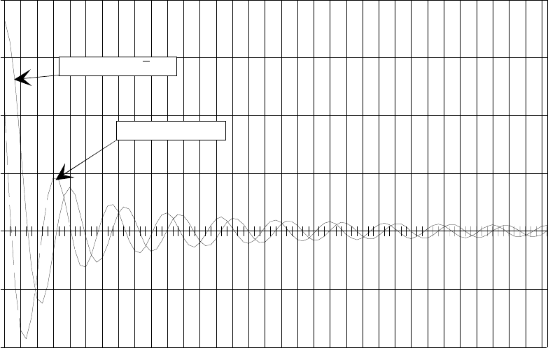
ETSI

E

TSI TR 102 273

-

2

V1.2.1 (2001

-

1

2)

2

6

Spacing in wavelengths

-40

-20

0

20

40

60

80

0

0,3

0,6

0,9

1,2

1,8

1,5

2,1

2,4

2,7

3,0

3,3

3,6

3,9

4,2

4,5

4,8

5,1

5,4

5,7

6,0

6,3

6,6

6,9

7,2

7,5

7,8

8,1

8,4

8,7

9,0

9,3

9,6

9,9

Resistance (R )

12

Reactance (X )

12

Ohms

Figure 9: The mutual resistance and reactance of 2 side-by-side dipoles, each λ

λλ

λ/2

The magnitude of the effects on the electrical characteristics of the EUT (or antenna) due to the mutual coupling

between them are estimated in TR 102 273-1-1 [8] annex A and the uncertainty contributions which result are given

representative symbols as follows:

uj08 is used for the uncertainty contribution associated with the amplitude effect of the test antenna on the EUT in

test methods;

uj09 is used for the uncertainty contribution associated with the de-tuning effect of the test antenna on the EUT in

test methods;

uj10 is used for the uncertainty contribution associated with the mutual coupling between transmitting antenna and

receiving antenna in verification procedures;

uj11 is used for the uncertainty contribution associated with the mutual coupling between substitution or

measuring antenna and test antenna in test methods.

5.3.3 Turntable and antenna mounting fixtures

As the turntable and mounting fixtures are in close proximity to the EUT/antenna they can significantly change its

performance. The antenna mount likewise for the test antenna. The antenna mount, turntable and mounting fixtures

should, therefore, be constructed from non-conducting, low relative dielectric constant plastics or wood to reduce

reflections and interactions. It is recommended that materials with dielectric constants of less than 1,5 be used for all

supporting structures.

Structurally, the antenna mount should be sufficiently strong to prevent twisting under load, since the antenna pattern

might move "off axis" with the result that the signal level may not be maximized (see figure 10). In a substitution type

measurement, however, provided the antenna is not repositioned between the two stages of the test, any such error in

alignment should cancel itself out.

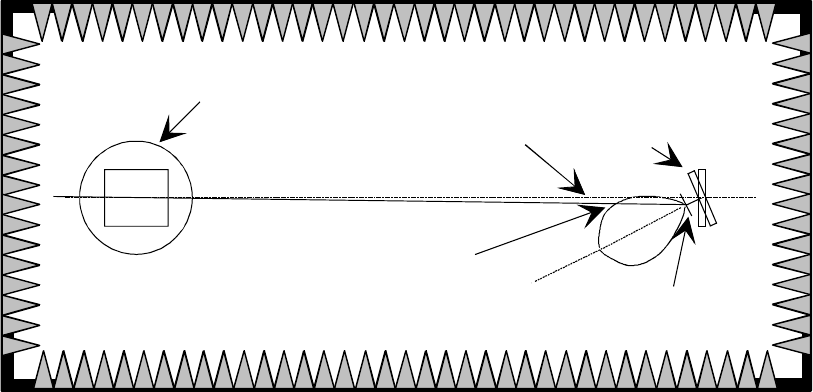
ETSI

E

TSI TR 102 273

-

2

V1.2.1 (2001

-

1

2)

2

7

Antenna mast

twisted

Antenna offset

from site axis

Turntable and EUT

Signal from

antenna

reduced

Centre line

Figure 10: Signal reduction due to a twisted mast (plan view)

The stability of the turntable is also important since an unstable, or non uniform turntable will change the measurement

distance as it is rotated.

The controller for the turntable should also be carefully considered to avoid measurement errors. For example, rapid

changes in speed of rotation can lead to missing peak values. Settling times are important for measuring equipment in

some tests e.g. SINAD measurement. The controller should, therefore, be designed with fixed, acceptable speeds to

avoid problems of this sort.

5.3.4 Antenna cabling

There are radiating mechanisms by which RF cables can introduce uncertainties into radiated measurements:

- leakage;

- acting as a parasitic element to the antenna;

- introducing common mode current to the balun of the antenna.

Leakage allows electromagnetic coupling into the cables. Because the electromagnetic wave contains both electric and

magnetic fields, mixed coupling can occur and the voltage induced is very dependant on the orientation, with respect to

the cable, of the fields. This coupling can have different effects depending on the length of the cable and where it is in

the system. Cables are usually the longest part of the test equipment configuration and, as such, leakage can make them

act as efficient receiving or transmitting antennas thereby contributing significantly to the uncertainty of a

measurement.

The parasitic effect of the cable can potentially be the most significant of the three effects and can cause major changes

to the antenna's radiation pattern, gain and input impedance. The common mode current problem has similar effects on

the antenna's performance.

All three effects can be largely eliminated by routeing and loading the cables with ferrite beads as detailed in the test

methods. A cable for which no precautions have been taken to prevent these effects can cause different results to be

obtained simply by being repositioned.

uj19 is used for the uncertainty contribution associated with cable factor (the combined uncertainty which results

from interaction between any antenna and its cable).

5.3.5 Positioning of the EUT and antennas

The phase centre of an EUT (or antenna) is the point within the EUT (or antenna) from which it radiates. If the EUT (or

antenna) was rotated about this point, the phase of the received/transmitted signal would not change. For some test

procedures, especially those which require an accurate knowledge of the measurement distance, it is vital to be able to

identify the phase centre.

ETSI

E

TSI TR 102 273

-

2

V1.2.1 (2001

-

1

2)

2

8

Where an EUT is being tested the uncertainty in the position of the phase centre of the source within the EUT volume

can lead to signal level uncertainties since all calculations deriving emission or sensitivity levels will be based on the

precise measurement distance.

uj20 is used for the uncertainty contribution associated with not knowing the exact position of the phase centre

within the EUT volume.

The positioning, on the turntable, of the phase centre of the EUT's radiating source, can lead to uncertainties if it is

offset from the table's axis of rotation. Any offset will cause the source to describe a circle about the axis as the EUT is

rotated. Variations in path lengths (both direct and reflected) are thereby introduced leading directly to changes in the

received/transmitted field strength.

uj21 is used for the uncertainty contribution associated with the positioning of the EUT's phase centre over the

axis of rotation of the turntable.

The phase centre of an antenna (or any other radiating structure) is the point from which it can be considered to radiate.

If the antenna (or radiating structure) was rotated about this point, the phase of the received/transmitted signal would

not change. The phase centre of both a dipole and biconic antenna is in the centre of its two arms, for a Log Periodic

Dipole Antenna (LPDA) it should be assumed to be halfway along its longitudinal axis and for a waveguide horn it is

the centre of its open mouth.

uj22 is used for the uncertainty contribution associated with the positioning of the phase centre of the measuring,

substitution, receiving, transmitting or test antenna.

Certain antennas, most notably the LPDA, possess a phase centre which is difficult to pinpoint at any particular

frequency. Further, for this type of antenna the phase centre moves along the array with changing frequency resulting in

a measurement distance uncertainty (e.g. an LPDA with a 0,3 m length contributes a standard uncertainty level due to

range length uncertainty of uj = 1,0 dB). To use such an antenna for site verification, for example, could introduce large

uncertainties.

uj23 is used for the uncertainty contribution associated with not knowing the exact position of the phase centre for

LPDAs.

5.3.6 Equipment cabling

EUT cable layout can contribute significantly to the uncertainty of a measurement. Large variations can occur when

measuring spurious emissions for example as a result of the positions of the supply and control cables.

These cables can act as parasitic elements and can receive, transmit or reflect radiated fields. The effects vary with cable

type, the configuration and use, but they may strongly influence the outcome of a measurement. A number of schemes

can be used to reduce these problems, amongst which are a total replacement by fibre optic cables and twisting wires

together and loading them with ferrite beads.

uj55 is used for the uncertainty contribution which results from interaction between the EUT and the power leads.

6 Verification procedure for an Anechoic Chamber

6.1 Introduction

The verification procedure is a process carried out in Anechoic Chambers, Anechoic Chambers with Ground Planes,

Open Area Test Sites and Striplines to prove their suitability as free field test sites.

Anechoic Chambers and Open Area Test Sites

For both types of Anechoic Chamber (i.e. both with and without a ground plane) and Open Area Test Sites the

verification procedure involves the transmission of a known signal level from one calibrated antenna (usually a dipole)

and the measurement of the received signal level in a second calibrated antenna (also usually a dipole).

ETSI

E

TSI TR 102 273

-

2

V1.2.1 (2001

-

1

2)

2

9

By comparison of the transmitted and received signal levels, an "insertion loss" can be deduced. After inclusion of any

correction factors for the measurement, the figure of loss which results from the verification procedure, is known as

"site attenuation".

Site attenuation is defined [11] as "the ratio of the power input of a matched, balanced, lossless, tuned dipole radiator to

that at the output of a similarly matched, balanced, lossless, tuned dipole receiving antenna for specified polarization,

separation and heights above a flat reflecting surface. It is a measure of the transmission path loss between two

antennas".

As the definition states ".... above a flat reflecting surface", it is usual for the verification procedure to involve one

antenna (the transmitting antenna) remaining fixed in height whilst a second antenna (the receiving antenna) is scanned

through a specified height range looking for a peak in the received signal level.

The parameter of site attenuation originated for Open Area Test Sites, hence the reference to a reflective ground plane

in the definition. The term is, however, also used in association with Anechoic Chambers. The measurement of site

attenuation in such an Anechoic Chamber provides an equally good measure of the facility's quality as it does for an

Open Area Test Site. Without a "flat reflecting surface", an Anechoic Chamber has no ground reflection and hence a

vertical height scan is unnecessary.

The determination of site attenuation involves two different measurements of received signal level. The first is with all

the items of test equipment connected directly together via an adapter, whilst the second involves replacing the adapter

with a pair of antennas. The difference in received levels (after allowance for any relevant correction factors which may

be appropriate), for the same signal generator output level, is the site attenuation.

The verification procedure for an Anechoic Chamber is based on EN 50147-2 [7], which itself is based on that given in

CISPR 16-1 [6] and clauses 15.4 to 16.6.3 inclusive. Both procedures call for the determination of Normalized Site

Attenuation (NSA) which is equivalent to site attenuation after subtraction of the antenna factors and any mutual

coupling effects. It should be noted that both publications EN 50147-2 [7] and CISPR 16-1 [6] only detail verification

procedures in the 30 MHz to 1 000 MHz frequency band.

It is particularly for the verification of Open Area Test Sites that NSA has historically found use. However, the same

approach has also been adopted in the verification procedure which follows for the Anechoic Chamber.

6.2 Normalized site attenuation

NSA is determined from the value of site attenuation by subtraction of the antenna factors and mutual coupling effects.

The subtraction of the antenna factors makes NSA independent of antenna type.

NOTE: The uncertainty of the resulting value for NSA depends directly on the uncertainty with which the

antenna factors are known.

Symbolically,

NSA = Vdirect - Vsite - AFT - AFR - AFTOT

where:

V

direct = received voltage for cables connected via the "in-line" adapter;

Vsite = received voltage for cables connected to the antennas;

AFT = antenna factor of the transmit antenna;

AFR = antenna factor of the receive antenna;

AFTOT = mutual coupling correction factor.

The verification procedure compares the measured NSA (after relevant corrections) against the theoretical

figure calculated for an ideal Anechoic Chamber. The difference between the two values at any specific frequency is a

measure of the quality of the chamber at that frequency.

The relevant theory for deriving the NSA of an ideal Anechoic Chamber is given below.

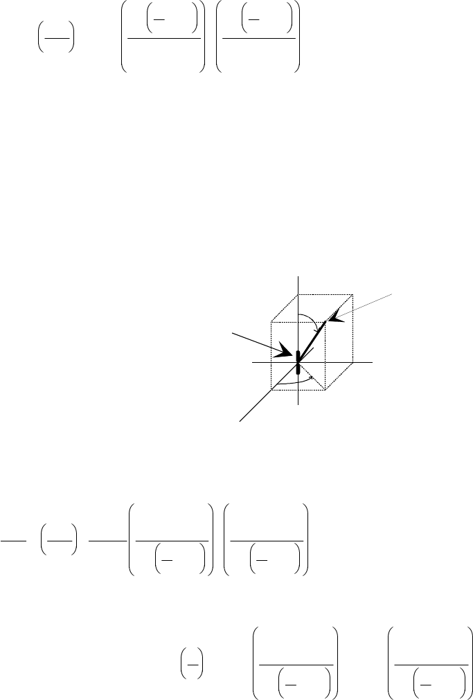
ETSI

E

TSI TR 102 273

-

2

V1.2.1 (2001

-

1

2)

3

0

6.2.1 NSA for the ideal Anechoic Chamber

In an ideal Anechoic Chamber where there are:

- no unwanted reflections (ground reflected or others);

- no interaction between transmit and receive dipoles;

- no coupling of the dipoles to the absorbing material;

- perfectly aligned, loss-less, matched tuned dipoles are used;

the coupling between the dipoles (assumed to be half wavelength) is given by the Friis transmission equation (as

derived in clause 7 of TR 102 273-1-1 [8]):

PdP

rec t

=

λ

π

πθ

θ

πθ

θ

41643 22

22

22

,

cos cos

sin

cos cos

sin (6.1)

where:

P

t = power transmitted (W);

Prec = power received (W);

λ

= wavelength (m);

d = distance between dipoles (m);

and

θ

is a spherical co-ordinate, as shown in figure 11.

r

z

y

x

θ

φ

Dipole

Field point

P( r,

θ

,

φ

)

Figure 11: Spherical co-ordinates

For this ideal site, the site attenuation (the inverse of the Friis transmission equation) is given by:

P

P

d

t

rec =41

1643

22

2

2

22

π

λ

θ

πθ

θ

πθ

,

sin

cos cos

sin

cos cos

(6.2)

More usually, this formula is given in logarithmic terms as follows:

Site Attenuation d

=,+17 67 20 20

2

20

2

log log sin

cos cos

log sin

cos cos

λ

θ

πθ

θ

πθ

+ + dB (6.3)

ETSI

E

TSI TR 102 273

-

2

V1.2.1 (2001

-

1

2)

3

1

For an Anechoic Chamber, since both transmit and receive antennas are assumed to be at the same height,

θ

=

π

/2 and

the formula reduces to:

Site Attenuation = 17,67 + 20 log (d/λ) dB

NOTE 1: In an actual measurement, the value of site attenuation is likely to be greater than given by this formula

due to mismatch and resistive losses, mutual coupling effects, etc.

An alternative formulation for site attenuation, based on field strengths and antenna factors has been derived in [3]. The

resulting formulae are for use with ground reflection sites but they are easily adapted for the fully Anechoic Chamber.

The general formula given for site attenuation, A, is:

()

A,AFAF

fE

TR

mDHor V

=2791

max (6.4)

where:

AFT = Antenna Factor of the transmitting antenna (m-1),

AFR = Antenna Factor of the receiving antenna (m-1),

fm = frequency (MHz) and

E

D(H or V)max = calculated maximum electric field strength (µV/m) in the receiving antenna height scan from a

half wavelength dipole with 1 pW of radiated power.

E

D(H or V)max takes the form EDHmax for horizontal polarization and EDVmax for vertical polarization.

NOTE 2: The stipulations of a half wavelength dipole and 1 pW of radiated power in ED(H or V)max do not limit the

use of the site attenuation equation to those conditions. The definition of ED(H or V)max in the text of [3] is

for convenience only and the stipulated conditions cancel out in the final formulae for site attenuation and

NSA, both of which apply generally.

For the Anechoic Chamber, ED(H or V)max (a term whose amplitude is generally peaked on a ground reflection range by

height scanning on a mast) is simply replaced by ED(H or V) since no maximization is involved. Also both polarizations

behave similarly and ED(H or V) can be shown to be:

EDH = EDV = 7,01/d

In decibel terms, the site attenuation formula becomes:

A = 48,92 + 20 log (AFT) + 20 log (AFR) - 20 log fm - 20 log (7,01/d) dB

The formula for NSA then follows as:

NSA = A - 20 log (AFT) - 20 log (AFR ) dB

i.e. NSA = 48,92 - 20 log fm - 20 log (7,01/d) dB

6.2.2 Mutual coupling

Mutual coupling may exist between the antennas during the verification procedure. This will serve to modify the results

since it can change antenna input impedance/voltage standing wave ratio and gain/antenna factors of both dipoles.

Figure 12 shows schematically mutual coupling as it occurs between dipoles in a reflection-free environment.

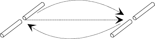
ETSI

E

TSI TR 102 273

-

2

V1.2.1 (2001

-

1

2)

3

2

Direct path

Mutual coupling

between dipoles

Transmitting

dipole

Receiving

dipole

Figure 12: Direct path and mutual coupling

For accurate determination of NSA these additional effects needs to be taken into consideration and correction factors

should be applied to the measured results to compensate.

In the verification procedure that follows, tables of correction factors are provided for mutual coupling between dipoles,

where appropriate, for 3 m and 10 m range lengths.

6.3 Overview of the verification procedure

The first steps in the verification procedure are the gathering of all the appropriate test equipment (see clause 6.3.1) and

preparation of the site (see clause 6.3.2).

The test equipment should then be configured (see clause 6.3.3), and the verification procedure carried out (see

clause 6.4).

On completion of the verification procedure, the results need to be processed (see clause 6.5) so that at each test

frequency a value for the deviation of the chamber performance from the ideal can be calculated and plotted (see

figure 23) and the measurement uncertainties calculated (see clauses 6.6 and 6.7).

The verification procedure (see clause 6.4) recommends an antenna scheme in the 30 MHz to 1 000 MHz frequency

band which uses tuned, half wavelength dipoles for all frequencies in the range 80 MHz to1 000 MHz and shortened

dipoles (see clause 6.3.3) below 80 MHz.

NOTE: For cases in which this is not suitable, an alternative scheme using dipoles and bicones (possibly also

LPDAs) is suggested in clause 6.3.2. It should be noted that measurement uncertainty is likely to be

degraded if the recommended dipole scheme is not used.

For the 1 GHz to 12,75 GHz band, broadband antennas (LPDAs) are recommended.

Throughout the whole band of 30 MHz to 12,75 GHz, the procedure involves discrete frequencies only. For the

frequency range 30 MHz to 1 000 MHz, the frequencies have been taken from CISPR 16-1 [6], annex G.

Figure 13 shows a typical verification testing arrangement of antennas (for the lower band) and test equipment.

6.3.1 Apparatus required

- attenuator pads, 10 dB;

- connecting cables;

- ferrite beads;

- receiving device (measuring receiver or spectrum analyser);

- signal generator;

- transmit antenna;

- receive antenna.

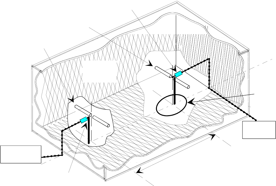
ETSI

E

TSI TR 102 273

-

2

V1.2.1 (2001

-

1

2)

3

3

For frequencies from 30 MHz to 1 000 MHz:

- transmit antenna (half wavelength dipole as detailed in ANSI C63.5 [1] recommended);

- receive antenna (half wavelength dipole as detailed in ANSI C63.5 [1] recommended).

NOTE 1: Alternatively dipoles plus bicones or dipoles plus bicones and LPDAs may be used.

NOTE 2: The reference dipole antennas, incorporating matching/transforming baluns, for the procedure are

available in the following bands: 20 MHz - 65 MHz, 65 MHz - 180 MHz, 180 MHz - 400 MHz,

400 MHz - 1 000 MHz. Constructional details are contained in ANSI C63.5 [1]. In the recommended

antenna scheme for verification in this band, a shortened dipole is used at all frequencies from 30 MHz to

70 MHz inclusive.

For frequencies above 1 000 MHz:

- Transmit antenna (LPDA 1 GHz to 12,75 GHz);

- Receive antenna (LPDA 1 GHz to 12,75 GHz).

The type and serial numbers of all items of test equipment should be recorded in the results sheet relevant to the

frequency band i.e. table 7 for the 30 MHz - 1 000 MHz band, table 8 for the 1 MHz - 12,75 GHz band.

Range length 3 m or 10 m

Turntable

Receiving

dipole

Transmitting

dipole

10 dB attenuator

10 dB attenuator

Signal

generator

Receiving

device

Radio

absorbing

material

Figure 13: Site layout for the verification procedure using horizontally polarized dipoles

in an Anechoic Chamber

6.3.2 Site preparation

Prior to the start of the verification procedure, system checks should be made on the test equipment to be used. All

items of test equipment where appropriate, should be connected to power supplies, switched on and allowed adequate

time to stabilize, as recommended by the manufacturers. Where a stabilization period is not given by the manufacturer,

30 minutes should be allowed.

ETSI

E

TSI TR 102 273

-

2

V1.2.1 (2001

-

1

2)

3

4

The cables for both ends of the chamber should be routed behind and away from the antennas, parallel to the side walls

and floor of the chamber, towards the back walls for a minimum of 2 m (unless the back wall is reached). They should

then be allowed to drop vertically towards the floor, preferably behind the anechoic panels, and routed out through the

screen (normally via a breakout panel) to the test equipment.

These cables should be dressed with ferrite beads, spaced 0,15 m apart for their entire lengths within the screen of the

chamber. The cables, their routeing and dressing should be the same as for the normal operation of the chamber.

Calibration data for all items of test equipment should be available and valid. For all non-ANSI dipoles, the data should

include VSWR and antenna factor (or gain) against frequency. The calibration data for all cables and attenuators should

include insertion loss and VSWR throughout the entire frequency range of the tests. Where any correction factors/tables

are required, these should be immediately available.

6.3.3 Measurement configuration

For the frequency band 30 MHz to 1 000 MHz, both antennas should be tuned half-wavelength dipoles (constructed as

detailed in ANSI C63.5 [1]) aligned for the same polarization.

NOTE 1: Due to size constraints a shortened dipole is used over part of this frequency band. For uniformity of

verification procedure across Open Area Test Sites and both types of Anechoic Chamber, a shortened

dipole is used from 30 MHz - 70 MHz inclusive. At all these frequencies the 80 MHz arm length

(0,889 m) is used attached to the 20 MHz - 65 MHz balun for all test frequencies in the

30 MHz - 60 MHz band and to the 65 MHz - 180 MHz balun for 70 MHz. Tuned half wavelength

dipoles, attached to their matching baluns are used for all frequencies in the band 80 MHz - 1 000 MHz

inclusive. Table 4 details dipole arm lengths (as measured from the centre of the balun block) and balun

type against frequency.

Table 4: Dipole arm length and balun type against frequency

Frequency

(MHz) Dipole arm length

(m) Balun

type Frequency

(MHz) Dipole arm length

(m) Balun

type

30 0,889 160 0,440 65 MHz to

35 0,889 180 0,391 180 MHz

40 0,889 20 MHz to 200 0,352

45 0,889 65 MHz 250 0,283 180 MHz to

50 0,889 300 0,235 400 MHz

60 0,889 400 0,175

70 0,889 500 0,143

80 0,889 600 0,117

90 0,791 65 MHz to 700 0,102 400 MHz to

100 0,714 180 MHz 800 0,089 1 000 MHz

120 0,593 900 0,079

140 0,508 1 000 0,076

For the 30 MHz - 1 000 MHz band, the restriction that no part of an antenna should come within 1 metre of any part of

the absorbing panels puts a limit on the number of combinations of transmitting antenna positions and polarizations for

this procedure. For each polarization, five positions within the chamber are verified. These are shown in figures 14 and

15. Optionally, four further positions, shown in outline in these figures and figure 19 (where the H and V suffices refer

to horizontal and vertical polarizations respectively) can be tested for each polarization if required. Correction factors

(where appropriate) and NSA data are supplied for all positions, including the optional ones.

The same antenna positions/polarization scheme is used in the 1 GHz - 12,75 GHz band for which both antennas should

be LPDAs, aligned for the same polarization.

NOTE 2: When the transmitting LPDA is used at positions other than on the central axis of the chamber, the

transmitting and receiving antennas should be aligned for maximum signal i.e. they should point directly

towards each other.

For both bands, the measured NSA is determined for all positions/polarizations.

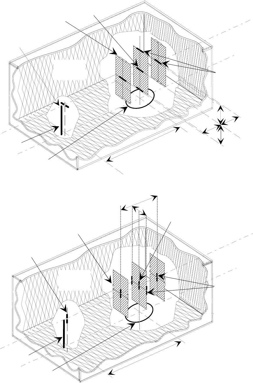
ETSI

E

TSI TR 102 273

-

2

V1.2.1 (2001

-

1

2)

3

5

Antenna

mount

Receiving

dipole

Transmitting dipole

position 1H

Transmitting

dipole position

s

Range length 3 m or 10 m

Turntable

d

d

d

d

Central axis

Optional transmitting

dipole positions (outlined)

Radio

absorbing

material

Figure 14: Antenna arrangements for horizontal polarization

Transmitting

dipole position

s

Antenna

mount

Turntable

Transmitting dipole

position 1V

Receiving dipole

Range length 3 m or 10 m

Optional transmitting

dipole positions (outlined)

Central axis

2d

2d

Radio

absorbing

material

Figure 15: Antenna arrangements for vertical polarization

ETSI

E

TSI TR 102 273

-

2

V1.2.1 (2001

-

1

2)

3

6

6.3.4 What to record

During the course of the procedure the chamber ambient temperature and relative humidity should be recorded.

Also during the course of the procedure, the output level of the signal generator, the received level, the tuned frequency

and polarization of the antennas should be recorded along with ALL equipment used signal generator, receiver, cables,

connectors, etc. An example of the results sheet is shown in table 5. A set of 10 results sheets (optionally 18), one

corresponding to each position/polarization of the transmitting antenna, should be completed for each frequency band.

NOTE: The results sheet for 1,0 GHz to 12,75 GHz verification (see table 8) is identical to table 5 except for the

omission of the column for mutual coupling correction factor AFTOT. Where LPDAs are used, no

corrections for mutual coupling are necessary.

Table 5: Example of an Anechoic Chamber verification results sheet

Anechoic Chamber verification procedure results sheet 30 MHz to 1 000 MHz

Range length: 3 m Polarization: Horizontal Date:

Ambient temperature: 20°C Position No.: 1H Relative humidity: 60 %

Freq.

(MHz)

Direct

Vdirect

(dBµV)

Site

Vsite

(dBµV)

Transmit

Antenna

factor

AFT

(dB)

Receive

Antenna

factor

AFR

(dB)

Mutual

coupling

correction

AFTOT

(dB)

Overall

value

(dB)

Ideal

value

(dB)

Difference

(dB)

Transmit antenna: Dipole S/No. D 001 Receive antenna: Dipole S/No. D 002

Transmit antenna cable: Ref. No. C 128 Receive antenna cable: Ref. No. C 129

Signal generator: Ref. No. SG 001 Receiving device: Ref. No. SA 001

Attenuator: S/No. AT 01 Attenuator: S/No. AT 02

Ferrite type: Worry beads Ferrite manufacturer: Rusty co. Ltd.

6.4 Verification procedure

Introduction

Two different procedures, one for each frequency band, are involved in verifying the performance of an Anechoic

Chamber which is used for the band 30 MHz to 12,75 GHz. The first procedure covers 30 MHz to 1 000 MHz and the

second covers 1 GHz to 12,75 GHz.

6.4.1 Procedure 1: 30 MHz to 1 000 MHz

Direct attenuation

1) The two antenna cables should be connected together, via attenuator pads and an "in-line" adapter as shown in

figure 16. Alternatively, if this is not practical, a calibrated cable may be used instead of the adapter.

NOTE 1: The use of a cable will increase the overall measurement uncertainty.

"In line"

adapter Attenuator 2

10 dB Receiving

device

Attenuator 1

10 dB

Signal

generator

cable 1 cable 2

ferrite beads ferrite beads

Figure 16: Initial equipment arrangement for the verification tests

2) The output of the signal generator should be adjusted to an appropriate level. The minimum acceptable level for

any frequency in the band of interest may be calculated from:

- 20 dB above the maximum expected radiated path loss (20 log ((4π range length)/λ)), plus the ambient noise

floor, the value of the attenuator pads and the cable losses, minus the antenna gains.

ETSI

E

TSI TR 102 273

-

2

V1.2.1 (2001

-

1

2)

3

7

NOTE 2: For practical purposes it is advisable to set a single output level for all frequencies in the band, since this

avoids level changes during the verification. Therefore this calculation should be evaluated at 30 MHz,

the worst frequency, since the reduced sensitivity of the shortened dipoles at this frequency requires an

enhanced signal level 53 dB above that required for tuned half wavelength dipoles. Table 6 indicates the

enhancement required for other frequencies where shortened dipoles are used.

EXAMPLE: 20 dB + 22 dB (radiated path loss) - 110 dBm (ambient noise floor) + 20 dB (attenuator

pads) + 1 dB (cable losses) - 4 dB (antenna gains) + 53 dB (enhancement) = + 2 dBm (109 dBµV).

Table 6: Enhancement figures for shortened dipoles

Frequency

(MHz) Enhancement

(dB)

30 53

35 48

40 43

45 38

50 32

60 19

70 4

If the calculated level is not available then the verification cannot proceed.

Once set, this signal generator output level should not be adjusted again for the entire duration of the verification

process.

3) The receiving device and signal generator should be tuned to the appropriate frequency (starting at the first

frequency given in the result sheet shown in table 7). The output level of the signal generator should be checked

(to be certain that the original set level has been maintained) and the received level on the receiving device

should be noted. For each frequency, the value to be entered in the column headed "Direct" on the results sheet is

the sum of this received level plus the loss of the "in-line" adapter or cable at this frequency i.e.:

"Direct" value = received level + loss of "in-line" adapter or cable.

4) Step 3 should be repeated for all the frequencies in the results sheet shown in table 7.

Radiated attenuation: Horizontal polarization

5) The adapter used to make the direct connection between the attenuator pads should be removed and the transmit

and receive dipoles connected as shown schematically in figure 17.

6) The signal generator, receiving device and dipoles should be tuned to the appropriate frequency (starting at the

top of the results sheet shown in table 7).

NOTE 3: For all frequencies below 80 MHz, a shortened dipole (as defined in clause 6.3.3) should be used. The

dipole arm length is defined as the measured distance from the centre of the balun block to the tip of the

arm. From a fully extended state, each telescopic element, in turn, should be "pushed in" from the tip until

the required length is obtained. The outermost section needs to fully compress before any of the others,

and so on.

7) The receiving dipole should be mounted on the central axis of the chamber and its phase centre should lie in the

plane of symmetry of the chamber (see figure 18). The dipole should be oriented for horizontal polarization.

8) The range length (3 m or 10 m) is defined as the horizontal distance between the receiving dipole and the axis of

rotation of the turntable. This should be set to an accuracy of ±0,01 m.

9) The transmitting dipole should be mounted in position 1H as shown in figures 14 and 19 and oriented for

horizontal polarization. It should be positioned with its phase centre:

a) in the plane of symmetry of the chamber (see figure 18);

b) on the axis of rotation of the turntable.

ETSI

E

TSI TR 102 273

-

2

V1.2.1 (2001

-

1

2)

3

8

10) The output level of the signal generator should be checked (to ensure that an inadvertent change to the original

set level has not occurred) and the received level on the receiving device should be noted. This value should be

entered in the results sheet (see table 7) under the column headed "Site".

11) Steps 6 to 10 should be repeated until all the frequencies in the results sheet have been completed, changing the

dipoles as appropriate.

Table 7: Anechoic Chamber verification results sheet (30 MHz to 1 000 MHz)

Anechoic Chamber verification procedure results sheet 30 MHz to 1 000 MHz

Range length: Polarization: Date:

Ambient temperature: Position No.: Relative humidity:

Freq.

(MHz)

Direct

Vdirect

(dBµV)

Site

Vsite

(dBµV)

Transmit

Antenna

factor

AFT

(dB)

Receive

Antenna

factor

AFR

(dB)

Mutual

coupling

correction

AFTOT

(dB)

Overall

value

(dB)

Ideal

value

(dB)

Difference

(dB)

30

35

40

45

50

60

70

80

90

100

120

140

160

180

200

250

300

400

500

600

700

800

900

1 000

Transmit antenna: Receive antenna:

Transmit antenna cable: Receive antenna cable:

Signal generator: Receiving device:

Attenuator: Attenuator:

Ferrite type: Ferrite manufacturer:

12) Steps 6 to 11 should be repeated with the transmitting dipole at the four other positions illustrated in figure 14

and shown as 2H, 3H, 4H and 5H in figure 19. Optionally, steps 6 to 11 should also be repeated for the four extra

positions (6H, 7H, 8H and 9H).

NOTE 4: In figures 14 and 19, for both 3 m and 10 m range verification d = 0,7 m. The positioning accuracy of all

positions relative to position 1H should be ±0,01 m.

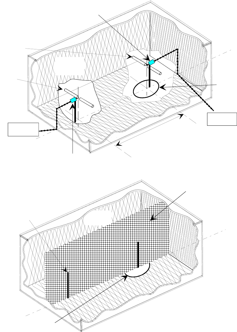
ETSI

E

TSI TR 102 273

-

2

V1.2.1 (20

0

1

-

1

2)

3

9

Range length 3 m or 10 m

Turntable

Receiving

dipole

Transmitting

dipole

10 dB attenuator

10 dB attenuator

Signal

generator

Receiving

device

Radio

absorbing

material

Figure 17: Equipment configuration for verification of an Anechoic Chamber

Turntable

Plane of symmetry

of chamber

Antenna

mast absorbing

Radio

material

Figure 18: The plane of symmetry of the Anechoic Chamber

Radiated attenuation: Vertical polarization

13) The equipment should be connected as shown in figure 17 with the dipoles vertically polarized.

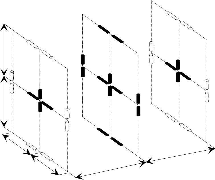
ETSI

E

TSI TR 102 273

-

2

V1.2.1 (2001

-

1

2)

4

0

14) The signal generator, receiving device and dipoles should be tuned to the appropriate frequency (starting at the

top of the results sheet shown in table 7).

NOTE 5: For all frequencies below 80 MHz, a shortened dipole (as defined in clause 6.3.3) should be used. The

dipole arm length is defined as the measured distance from the centre of the balun block to the tip of the

arm. From a fully extended state, each telescopic element, in turn, should be "pushed in" from the tip until

the required length is obtained. The outermost section needs to fully compress before any of the others,

and so on.

15) The receiving dipole should be mounted on the central axis of the chamber and the whole of its body should lie

in the plane of symmetry of the chamber (see figure 18).

16) The range length (3 m or 10 m) is defined as the horizontal distance between the receiving dipole and the axis of

rotation of the turntable. This should be set to an accuracy of ±0,01 m.

17) The transmitting dipole should be mounted in position 1V as shown in figures 15 and 19 and the whole of its

body should lie in the plane of symmetry of the chamber. Its axis should lie on the axis of rotation of the

turntable.

1V

2V

3V

4V

4H

1H

2H

3H

5V

5H

6H

7H

9H

6V

7V

9V

8H

8V

d

d

d

d

d

d

Figure 19: Expanded view of the 5 (optionally 9) transmitting dipole positions

18) The output level of the signal generator should be checked (to ensure that an inadvertent change to the original

set level has not occurred) and the received level on the receiving device should be noted. This value should be

entered in the result sheet (see table 7) under the column headed "Site".

19) Steps 14 to 18 should be repeated until all the frequencies in the result sheet have been completed, changing the

dipoles as appropriate.

20) Steps 14 to 19 should be repeated with the transmitting dipole at the four other positions as illustrated in

figure 15 and shown as 2V, 3V, 4V and 5V in figure 19. Optionally, steps 14 to 19 should also be repeated for

the four extra positions (6V, 7V, 8V and 9V).

NOTE 6: In figures 15 and 19, for both 3 m and 10 m range verification d = 0,7 m. The positioning accuracy of all

positions relative to position 1V should be ±0,01 m.

ETSI

E

TSI TR 102 273

-

2

V1.2.1 (2001

-

1

2)

4

1

6.4.2 Alternative Procedure 1: 30 MHz to 1 000 MHz

The procedure contained in clause 6.4.1 is the most accurate procedure considered for verification in the

30 MHz - 1 000 MHz band - the use of ANSI C63.5 [1] dipoles enabling precise correction figures for mutual coupling

to be incorporated into the results. The procedure can be very time consuming however and, as a quicker alternative

scheme, the following, less accurate procedure could be adopted.

1) The procedure, as detailed in clause 6.4.1 should be completed for positions 1H (for horizontal polarization) and

1V (for vertical polarization).

2) Both transmitting and receiving dipoles should be replaced with bicones for the full 30 MHz - 1 000 MHz band.

NOTE 1: As a further alternative, bicones 30 MHz - 200 MHz (possibly 300 MHz) can be used with LPDAs for the

rest of the band. Note, however, that the range length uncertainty associated with the moving phase centre

of the latter can significantly increase measurement uncertainty (e.g. a typical design of LPDA with

length approximately 1 m, could contribute a range length uncertainty of uj = 1,73 dB over a 3 m range

length. This would reduce to uj = 0,5 dB for a 10 m range length but would remain a significant

contribution to the overall uncertainty).

CAUTION: For reduced uncertainty in the verification procedure, measurements using alternative antennas should

be carried out in the far-fields of the antennas (see clause 7 of TR 102 273-1-1 [8]). For a typical

bicone of length 1,315 m, far-field conditions over a 3 m range length only exist from 30 MHz to

60 MHz and not at 70 MHz or above. For a 10 m range length, the corresponding usable frequency

range is 30 MHz to 270 MHz.

3) The entire verification procedure, as described in steps 1 - 20 of clause 6.4.1, should be repeated including

positions 1H and 1V for the transmitting antenna.

NOTE 2: This alternative procedure does not include any correction factors to account for mutual coupling effects.

Whilst these effects are smaller for broadband antennas than for dipoles, there will be increased

uncertainty in this alternative verification process because the effects cannot be calculated out of the

measurements.

6.4.3 Procedure 2: 1 GHz to 12,75 GHz

Direct attenuation

1) Connect the two antenna cables together, including the attenuator pads via an "in-line" adapter as shown in

figure 20. Alternatively, if this is not practical, a calibrated cable may be used instead of the adapter.

NOTE 1: The use of a cable will increase the overall measurement uncertainty.

"In line"

adapter Attenuator 2

10 dB Receiving

device

Attenuator 1

10 dB

Signal

generator

cable 1 cable 2

ferrite beads ferrite beads

Figure 20: Initial equipment arrangement for the verification tests

2) The output of the signal generator should be adjusted to an appropriate level. The minimum acceptable level for

any frequency in the band of interest may be calculated from:

- 20 dB above the maximum expected radiated path loss (20 log ((4π range length)/λ)), plus the ambient noise

floor, the value of the attenuator pads and the cable losses, minus the antenna gains.

NOTE 2: For practical purposes it is advisable to set a single output level for all frequencies in the band, since this

avoids level changes during the verification.

EXAMPLE: 20 dB + 75 dB (maximum expected path loss) + (- 110 dB) (ambient noise floor) + 20 dB

(attenuator pads) + 15 dB (cable losses) - 10 dB (antenna gains) = +10 dBm (117 dBµV).

If the calculated level is not available then the verification cannot proceed.

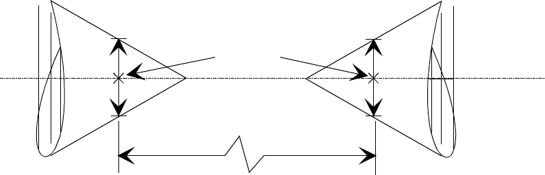
ETSI

E

TSI TR 102 273

-

2

V1.2.1 (2001

-

1

2)

4

2

Once set, this signal generator output level should not be adjusted again for the entire duration of the verification

procedure.

3) The receiving device and signal generator should be tuned to the appropriate frequency (starting at the first

frequency given in the result sheet shown in table 8). The output level of the signal generator should be checked

(to be certain that the original set level has been maintained) and the received level on the receiving device

should be noted. For each frequency, the value to be entered under the column headed "Direct" on the results

sheet is the sum of this received level plus the loss of the "in-line" adapter or cable i.e.:

"Direct" value = received level + loss of "In-line" adapter or cable.

4) Step 3 should be repeated for all frequencies in the results sheet shown in table 8.

Radiated attenuation: Horizontal polarization

5) The adapter used to make the direct connection between the attenuator pads should be removed and the transmit

and receive antennas should be connected as shown in figure 22 with the LPDAs horizontally polarized.

NOTE 3: In order to minimize the uncertainty in range length which results from using LPDAs (the radiating phase

centre moves with frequency), the radiating phase centre is defined, for the purposes of these

measurements only, as the point on the log periodic central axis where its thickness is 0,08 m. This is

shown in figure 21.

0,08m 0,08m

Transmitting

log periodic Receiving

log periodic

Central axis

of chamber

Phase

centres

Range length

Figure 21: Definition of phase centres of the LPDA

6) The receiving antenna should be positioned with its central axis coincident with the central axis of the chamber.

7) The horizontal spacing between the phase centre of the receiving LPDA and the centre of the turntable is the

range length. This should be set to an accuracy of ±0,01 m.

8) The transmitting antenna should be mounted in position 1H as shown in figures 14 and 19, with its central axis

coincident with the central axis of the chamber. The phase centre of the transmitting antenna should lie on the

axis of rotation of the turntable.

9) The signal generator and receiving device should be tuned to the appropriate frequency (starting at the top of the

results sheet shown in table 8).

10) The output level of the signal generator should be checked (to ensure that an inadvertent change to the original

set level has not occurred) and the received level on the receiving device should be noted. This value should be

entered in the results sheet (see table 8) under the column headed "Site".

11) Steps 9 and 10 should be repeated until all the frequencies in the results sheet (see table 8) have been completed.

12) Steps 9, 10 and 11 should be repeated with the transmitting antenna at the four other positions as illustrated in

figure 14 and shown as 2H, 3H, 4H and 5H in figure 19. Optionally, steps 9, 10 and 11 should also be repeated

for the four extra positions (6H, 7H, 8H and 9H).

NOTE 4: In figures 12 and 17 for both 3 m and 10 m range length verifications, d = 0,7m. The positioning accuracy

of the phase centres of all positions relative to position 1H should be ±0,01 m.

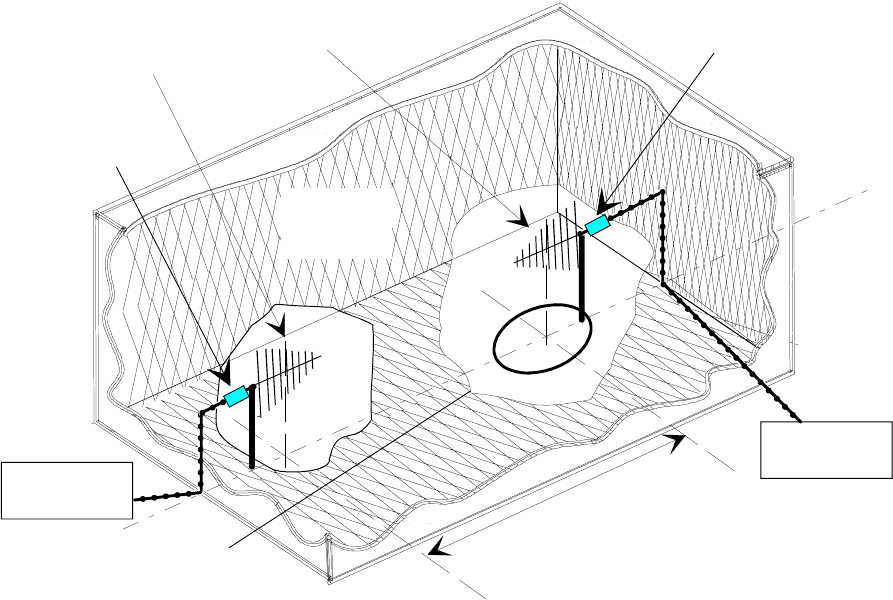
ETSI

E

TSI TR 102 273

-

2

V1.2.1 (2001

-

1

2)

4

3

NOTE 5: For all positions, both antennas needs to point directly towards each other, consistent with keeping their

central axes parallel to the floor. For all transmitting positions other than 1H, 2H and 3H in figure 19, this

will involve small angle rotation of both receiving and transmitting antennas. For both antennas, this

rotation should be about the phase centre.

Radiated attenuation: Vertical polarization

13) The equipment should be connected as shown in figure 22.

NOTE 6: In order to minimize the uncertainty in range length which results from using LPDAs (the radiating phase

centre moves with frequency), the radiating phase centre is defined, for the purposes of these

measurements, as the point on the LPDA's central axis where its thickness is 0,08 m. This is shown in

figure 21.

Range length 3 m or 10 m

Turntable

Receiving

LPDA

Transmitting

LPDA 10 dB attenuator

10 dB attenuator

Signal

generator

Receiving

device

Radio

absorbing

material

Figure 22: Anechoic Chamber layout for verification with LPDAs

14) The receiving antenna should be positioned with its central axis coincident with the central axis of the chamber.

It should be oriented for vertical polarization.

15) The horizontal spacing between the phase centre of the LPDA and the centre of the turntable is the range length.

This should be set to an accuracy of ±0,01 m.

16) The transmitting antenna should be mounted in position 1V as shown in figures 15 and 19 with its central axis

coincident with the central axis of the chamber. The phase centre of the transmitting antenna should lie on the

axis of rotation of the turntable. The transmitting antenna should be oriented for vertical polarization.

17) The signal generator and receiving device should be tuned to the appropriate frequency (starting at the top of the

results sheet shown in table 8).

18) The output level of the signal generator should be checked (to ensure that an inadvertent change to the original

set level has not occurred) and the received level on the receiving device should be noted. This value should be

entered in the results sheet (see table 8) under the column headed "Site".

19) Steps 17 and 18 should be repeated until all the frequencies in the results sheet (see table 8) have been

completed.

ETSI

E

TSI TR 102 273

-

2

V1.2.1 (2001

-

1

2)

4

4

20) Steps 17, 18 and 19 should be repeated with the transmitting dipole at the four other positions as illustrated in

figure 15 and shown as 2V, 3V, 4V and 5V in figure 19. Optionally, steps 17, 18 and 19 should also be repeated

for the four extra positions (6V, 7V, 8V and 9V).

NOTE 7: In figures 13 and 17, for both 3 m and 10 m range length verifications d = 0,7 m. The positioning

accuracy of the phase centres of all positions relative to position 1V should be ±0,01 m.

NOTE 8: For all positions, both antennas needs to point directly towards each other, consistent with keeping their

central axes parallel to the floor. For all transmitting positions other than 1V, 2V and 3V in figure 19, this

will involve small angle rotation of both receiving and transmitting antennas. For both antennas, this

rotation should be about the phase centre.

Table 8: Anechoic Chamber verification results sheet (1 GHz - 12,75 GHz)

Anechoic Chamber verification procedure results sheet 1 GHz to 12,75 GHz

Range length: Polarization: Date:

Ambient temperature: Position No.: Relative humidity:

Freq.

(GHz)

Direct

Vdirect

(dBµV)

Site

Vsite

(dBµV)

Transmit

Antenna

factor

AFT

(dB)

Receive

Antenna

factor

AFR

(dB)

Overall

value

(dB)

Ideal

value

(dB)

Difference

(dB)

1,0

1,25

1,5

1,75

2,0

2,25

2,5

2,75

3,0

3,25

3,5

3,75

4,0

4,5

5,0

5,5

6,0

6,5

7,0

7,5

8,0

8,5

9,0

9,5

10,0

10,5

11,0

11,5

12,0

12,75

Transmit antenna: Receive antenna:

Transmit antenna cable: Receive antenna cable:

Signal generator: Receiving device:

Attenuator: Attenuator:

Ferrite type: Ferrite manufacturer:

ETSI

E

TSI TR 102 273

-

2

V1.2.1 (2001

-

1

2)

4

5

6.5 Processing the results of the verification procedure

6.5.1 Introduction

Having carried out the verification procedures as detailed in clause 6.4 the results sheets should have values filling the

first three columns, namely those headed "Freq", "Direct" and "Site". This clause details the values to be incorporated in

all the remaining columns.

The processing of the results finally reveals how well the measured performance of the Anechoic Chamber compares to

the ideal case.

Firstly, the figures for entering under the column headings of "Transmit Antenna factor, AFT" and "Receive Antenna

factor, AFR" are discussed and values are provided. Secondly, for the 30 MHz to 1 000 MHz verification procedure

only, correction factors are provided for the recommended antenna scheme (ANSI C63.5 [1] dipoles) to allow for the

effects of mutual coupling and mismatch loss. These effects are regarded as not significant at frequencies above

180 MHz and enable the column headed "Mutual coupling correction, AFTOT" to be completed. The "Overall value"

column can then be calculated. This column reveals the measured NSA for the Anechoic Chamber.

Finally, having extracted the relevant values (from tables provided) to complete the "Ideal value" column, the difference

between the measured performance and the ideal can be calculated by simple subtraction of the values in the columns

"Overall value" and "Ideal value".

6.5.2 Procedure 1: 30 MHz to 1 000 MHz

Antenna factors

For dipoles, the antenna factor of each dipole is given by:

Antenna factor = 20 log f - 31,4 dB

where f is the frequency in MHz.

NOTE 1: A resistive loss of 0,5 dB is incorporated into this formula.

Whilst the above formula for antenna factor applies only to a tuned half wavelength dipole, it should still be used in this

verification procedure, even where shortened dipoles have been used (the 30 MHz - 70 MHz band). Table 9 gives the

values at the test frequencies. The relevant values should be entered in the verification results sheet (see table 7) in the

columns headed "Transmit Antenna factor, AFT" and "Receive Antenna factor, AFR".

NOTE 2: Table 9 applies for both horizontal and vertical polarization.

When antennas other than dipoles are used, antenna factors are usually provided by the manufacturers. Where gain

figures, rather than antenna factors, have been given, these can be converted into antenna factor by the following

equation:

Antenna factor = 20log 9,734

G dB

λ

(6.5)

where:

λ

is the wavelength (m);

G is the numeric gain.

NOTE 3: The gain figure to be used should be relative to an isotropic radiator - not relative to a dipole.

ETSI

E

TSI TR 102 273

-

2

V1.2

.

1 (2001

-

1

2)

4

6

Table 9: Antenna factor for a dipole used in the verification procedure.

Frequency

(MHz) Antenna factor

(dB) Frequency

(MHz) Antenna factor

(dB)

30 -1,9

160 12,7

35 -0.5

180 13,7

40 0,6

200 14,6

45 1,7

250 16,6

50 2,6

300 18,1

60 4,2

400 20,6

70 5,5

500 22,6

80 6,7

600 24,2

90 7,7

700 25,5

100 8,6

800 26,7

120 10,2

900 27,7

140 11,5

1 000 28,6

Mutual coupling and mismatch loss correction factors

Table 10 gives the factors necessary to correct the measured figures not only for mutual coupling, but also for mismatch

transmission loss - this being the dominant term for frequencies up to 70 MHz. The table applies for both vertical and

horizontal polarization.

NOTE 4: Particularly at low frequencies (i.e. up to 180 MHz) the performance of each antenna used in the

verification procedure is affected by the presence of the other antenna. This interaction between antennas

is termed mutual coupling and has been modelled by computer simulation for the recommended antenna

scheme (ANSI dipoles) only.

For the recommended dipole antenna scheme only, the relevant figures should be taken from table 10 and entered in the

results sheet (see table 7) in the column headed "Mutual coupling correction AFTOT". For all frequencies above

180 MHz, the correction factor should be taken as 0,0 dB.

For the alternative antenna schemes (bicones only or bicones and log periodics) all entries in the "Mutual coupling

correction AFTOT" column should be 0,0 dB.

Table 10: Mutual coupling and mismatch loss correction factors

Range lengths and transmitting dipole positions:

Range length: 3 m

Various positions Range length: 10 m

Various positions

Freq

(MHz) 1H

1V 2H

2V 3H

3V 4H, 4V

5H, 5V

6H, 6V

7H, 7V

8H, 8V

9H, 9V

1H

1V 2H

2V 3H

3V 4H, 4V

5H, 5V

6H, 6V

7H, 7V

8H, 8V

9H, 9V

30 52,7 53,3 52,3 52,6 53,1 52,3 51,5 51,5 51,5 51,5 51,5 51,5

35 47,5 48,1 47,1 47,4 48,0 47,1 46,5 46,5 46,4 46,5 46,5 46,4

40 42,4 42,9 42,1 42,3 42,8 42,0 41,5 41,5 41,5 41,5 41,5 41,5

45 37,1 37,6 36,8 37,1 37,5 36,8 36,3 36,3 36,3 36,3 36,3 36,3

50 31,5 31,9 31,2 31,4 31,8 31,2 30,7 30,8 30,7 30,7 30,8 30,7

60 18,7 19,1 18,5 18,7 19,0 18,5 18,1 18,1 18,1 18,1 18,1 18,1

70 3,8 4,4 3,6 3,7 4,3 3,6 3,2 3,3 3,3 3,3 3,3 3,3

80 0,7 1,0 0,7 0,9 0,9 0,7 0,2 0,3 0,2 0,2 0,3 0,2

90 0,6 0,9 0,3 0,6 0,5 0,3 0,1 0,0 0,0 0,1 0,0 0,0

100 0,6 0,5 0,2 0,5 0,5 0,2 0,1 0,1 0,1 0,1 0,1 0,1

120 0,3 0,8 0,5 0,3 0,8 0,4 0,2 0,2 0,2 0,2 0,2 0,2

140 0,5 0,6 0,4 0,2 0,5 0,3 0,2 0,2 0,2 0,2 0,2 0,3

160 0,4 0,4 0,4 0,4 0,4 0,4 0,3 0,3 0,2 0,3 0,3 0,3

180 0,3 0,5 0,3 0,3 0,5 0,3 0,2 0,2 0,2 0,2 0,2 0,2

ETSI

E

TSI TR 102 273

-

2

V1.2.1 (2001

-

1

2)

4

7

Completion of the results sheet

The next stage is to enter values in the column headed "Overall value". This is achieved by performing the following

calculation:

"Overall value" = "Vdirect" - Vsite" - " AFT " - " AFR" - " AFTOT"

The resulting value is the measured NSA for the Anechoic Chamber.

The final stages in determining the quality of the site are to complete the column headed "Ideal value" in the results

sheet (see table 7) by taking the relevant values from table 11 and to calculate the entries for the "Difference" column

from:

"Difference" "Overall value" - "Ideal value"

The values in the "Difference" column represent the variation between the theoretical and the measured NSA of the

Anechoic Chamber.

Table 11: Theoretical ideal values for NSA

Ideal NSA (dB)

Range length: 3 m

Various positions Range length: 10 m

Various positions

Freq.

(MHz) 1H

1V 2H

2V 3H

3V 4H, 4V

5H, 5V 6H, 6V

7H, 7V 8H, 8V

9H, 9V 1H

1V 2H

2V 3H

3V 4H, 4V

5H, 5V 6H, 6V

7H, 7V 8H, 8V

9H, 9V

30 12,0 9,7 13,8 12,2 10,1 14,0 22,5 21,8 23,1 22,5 21,9 23,1

35 10,7 8,4 12,5 10,9 8,7 12,6 21,1 20,5 21,7 21,1 20,5 21,7

40 9,5 7,2 11,3 9,7 7,6 11,5 20,0 19,3 20,6 20,0 19,4 20,6

45 8,5 6,2 10,3 8,7 6,6 10,5 19,0 18,3 19,5 19,0 18,3 19,5

50 7,6 5,3 9,4 7,8 5,6 9,5 18,0 17,4 18,6 18,0 17,4 18,6

60 6,0 3,7 7,8 6,2 4,1 8,0 16,4 15,8 17,0 16,5 15,8 17,0

70 4,6 2,3 6,5 4,9 2,7 6,6 15,1 14,5 15,7 15,1 14,5 15,7

80 3,5 1,2 5,3 3,7 1,6 5,5 13,9 13,3 14,5 14,0 13,3 14,6

90 2,5 0,2 4,3 2,7 0,5 4,4 12,9 12,3 13,5 13,0 12,3 13,5

100 1,5 -0,8 3,4 1,8 -0,4 3,5 12,0 11,4 12,6 12,0 11,4 12,6

120 0,0 -2,4 1,8 0,2 -2,0 1,9 10,4 9,8 11,0 10,4 9,8 11,0

140 -1,4 -3,7 0,4 -1,2 -3,3 0,6 9,1 8,5 9,7 9,1 8,5 9,7

160 -2,5 -4,9 -0,7 -2,3 -4,5 -0,6 7,9 7,3 8,5 8,0 7,3 8,5

180 -3,6 -5,9 -1,7 -3,3 -5,5 -1,6 6,9 6,3 7,5 7,0 6,3 7,5

200 -4,5 -6,8 -2,7 -4,3 -6,4 -2,5 6,0 5,4 6,6 6,0 5,4 6,6

250 -6,4 -8,7 -4,6 -6,2 -8,3 -4,4 4,0 3,4 4,6 4,1 3,4 4,7

300 -8,0 -10,3 -6,2 -7,8 -9,9 -6,0 2,5 1,8 3,1 2,5 1,9 3,1

400 -10,5 -12,8 -8,7 -10,3 -12,4 -8,5 -0,0 -0,7 0,6 0,0 -0,7 0,6

500 -12,4 -14,7 -10,6 -12,2 -14,4 -10,5 -2,0 -2,6 -1,4 -2,0 -2,6 -1,4

600 -14,0 -16,3 -12,2 -13,8 -15,9 -12,1 -3,6 -4,2 -3,0 -3,5 -4,2 -3,0

700 -15,4 -17,7 -13,5 -15,1 -17,3 -13,4 -4,9 -5,5 -4,3 -4,9 -5,5 -4,3

800 -16,5 -18,8 -14,7 -16,3 -18,4 -14,5 -6,1 -6,7 -5,5 -6,0 -6,7 -5,5

900 -17,5 -19,9 -15,7 -17,3 -19,5 -15,6 -7,1 -7,7 -6,5 -7,1 -7,7 -6,5

1 000 -18,5 -20,8 -16,6 -18,2 -20,4 -16,5 -8,0 -8,6 -7,4 -8,0 -8,6 -7,4

6.5.3 Procedure 2 (1 GHz to 12,75 GHz)

Antenna factors

Generally, the manufacturers of the LPDAs will supply figures for either the gain or antenna factor variation with

frequency. Where the gain variation is given, this should be converted to antenna factor by the following formula:

Antenna factor = 20log 9,734

G dB

λ

(6.6)

where:

λ is the wavelength (m);

ETSI

E

TSI TR 102 273

-

2

V1.2.1 (2001

-

1

2)

4

8

G is the numeric gain.

NOTE: The gain figure to be used should be relative to an isotropic radiator - not relative to a dipole.

Whether directly or indirectly (by using this formula), the antenna factor columns in the results sheet headed "Transmit

Antenna factor, AFT" and "Receive Antenna factor, AFR" should now be filled in with the relevant values.

Completion of the results sheet

The next stage is to fill in the column headed "Overall value". The relevant values are determined by subtracting the

values in the "Site, Vsite", "Transmit Antenna factor, AFT" and "Receive Antenna factor, AFR" columns from the values

in the "Direct, Vdirect" column i.e.:

"Overall value" = "Vdirect " - "Vsite" - "AFT" - "AFR"

The resulting value is the measured NSA for the Anechoic Chamber.

The final stages in determining the quality of the chamber are to complete the column headed "Ideal value" in the

results sheet by taking the relevant values from table 12 and to calculate the entries for the "Difference" column from:

"Difference" = "Overall value" - "Ideal value"

The resulting values in the "Difference" column represent the variation between the ideal and the measured performance

of the Anechoic Chamber.

Table 12: Theoretical ideal values for NSA

Ideal NSA (dB)

Range length: 3 m

Various positions Range length: 10 m

Various positions

Freq.

(GHz) 1H

1V 2H

2V 3H

3V 4H, 4V

5H, 5V 6H, 6V

7H, 7V 8H, 8V

9H, 9V

1H

1V 2H

2V 3H

3V 4H, 4V

5H, 5V 6H, 6V

7H, 7V 8H, 8V

9H, 9V

1 -18,5 -20,8 -16,6 -18,2 -20,4 -16,5 -8,0 -8,6 -7,4 -8,0 -8,6 -7,4

1,25 -20,4 -22,7 -18,6 -20,0 -22,3 -18,4 -9,9 -10,6 -9,4 -9,9 -10,5 -9,3

1,5 -22,0 -24,3 -20,2 -21,7 -23,9 -20,0 -11,5 -12,2 -10,9 -11,5 -12,1 -10,9

1,75 -23,3 -25,6 -21,5 -23,1 -25,2 -21,3 -12,9 -13,5 -12,3 -12,8 -13,5 -12,3

2 -24,5 -26,8 -22,7 -24,2 -26,4 -22,5 -14,0 -14,7 -13,4 -14,0 -14,6 -13,4

2,25 -25,5 -27,8 -23,7 -25,3 -27,4 -23,5 -15,0 -15,7 -14,5 -15,0 -15,6 -14,4

2,5 -26,4 -28,7 -24,6 -26,2 -28,3 -24,4 -16,0 -16,6 -15,4 -15,9 -16,6 -15,4

2,75 -27,2 -29,6 -25,4 -27,0 -29,2 -25,3 -16,8 -17,4 -16,2 -16,8 -17,4 -16,2

3 -28,0 -30,3 -26,2 -27,8 -29,9 -26,0 -17,5 -18,2 -17,0 -17,5 -18,1 -16,9

3,25 -28,7 -31,0 -26,9 -28,5 -30,6 -26,7 -18,2 -18,9 -17,6 -18,2 -18,8 -17,6

3,5 -29,3 -31,6 -27,5 -29,1 -31,3 -27,4 -18,9 -19,5 -18,3 -18,9 -19,5 -18,3

3,75 -29,9 -32,2 -28,1 -29,7 -31,9 -28,0 -19,5 -20,1 -18,9 -19,5 -20,1 -18,9

4 -30,5 -32,8 -28,7 -30,3 -32,4 -28,5 -20,0 -20,7 -19,5 -20,0 -20,6 -19,4

4,5 -31,5 -33,8 -29,7 -31,3 -33,4 -29,5 -21,1 -21,7 -20,5 -21,0 -21,7 -20,5

5 -32,4 -34,7 -30,6 -32,2 -34,4 -30,5 -22,0 -22,6 -21,4 -22,0 -22,6 -21,4

5,5 -33,3 -35,6 -31,4 -33,0 -35,2 -31,3 -22,8 -23,4 -22,2 -22,8 -23,4 -22,2

6 -34,0 -36,3 -32,2 -33,8 -35,9 -32,0 -23,6 -24,2 -23,0 -23,5 -24,2 -23,0

6,5 -34,7 -37,0 -32,9 -34,5 -36,6 -32,7 -24,3 -24,9 -23,7 -24,3 -24,9 -23,7

7 -35,4 -37,7 -33,5 -35,1 -37,3 -33,4 -24,9 -25,5 -24,3 -24,9 -25,5 -24,3

7,5 -36,0 -38,3 -34,1 -35,7 -37,9 -34,0 -25,5 -26,1 -24,9 -25,5 -26,1 -24,9

8 -36,5 -38,8 -34,7 -36,3 -38,4 -34,5 -26,1 -26,7 -25,5 -26,0 -26,7 -25,5

8,5 -37,0 -39,4 -35,2 -36,8 -39,0 -35,1 -26,6 -27,2 -26,0 -26,6 -27,2 -26,0

9 -37,5 -39,8 -35,7 -37,3 -39,5 -35,6 -27,1 -27,7 -26,5 -27,1 -27,7 -26,5

9,5 -38,0 -40,3 -36,2 -37,8 -39,9 -36,0 -27,6 -28,2 -27,0 -27,5 -28,2 -26,9

10 -38,5 -40,8 -36,6 -38,2 -40,0 -36,5 -28,0 -28,6 -27,4 -28,0 -28,6 -27,4

10,5 -38,9 -41,2 -37,1 -38,7 -40,8 -36,9 -28,4 -29,1 -27,8 -28,4 -29,0 -27,8

11 -39,3 -41,6 -37,5 -39,1 -41,2 -37,3 -28,8 -29,5 -28,2 -28,8 -29,4 -28,2

11,5 -39,7 -42,0 -37,8 -39,4 -41,6 -37,7 -29,2 -29,8 -28,6 -29,2 -29,8 -28,6

12 -40,0 -42,3 -38,2 -39,8 -42,0 -38,1 -29,6 -30,2 -29,0 -29,6 -30,2 -29,0

12,75 -40,6 -42,9 -38,7 -40,3 -42,5 -38,6 -30,1 -30,7 -29,5 -30,1 -30,7 -29,5

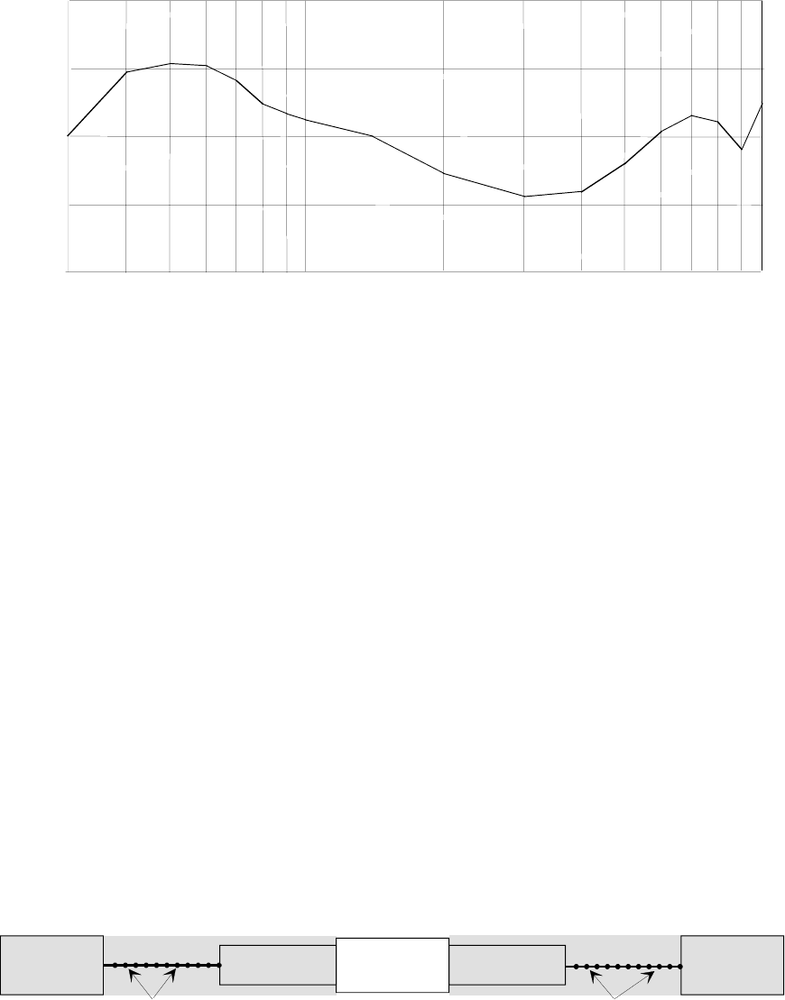
ETSI

E

TSI TR 102 273

-

2

V1.2.1 (2001

-

1

2)

4

9

6.5.4 Report format

It is suggested that the results of the verification are presented in two ways, firstly in the format of a completed results

sheet, and secondly in the form of a plot of the "Difference" column against frequency for each polarization as shown in

figure 23.

30 100 300 1 000

Frequency (MHz)

0

1

2

-1

-2

Difference between measured

and ideal NSA (dB)

Figure 23: Plot of the difference between the measured and ideal NSA against frequency

6.6 Calculation of measurement uncertainty (Procedure 1)

The column headed "Overall" in the results sheet is completed during the processing of the results for the verification

procedure. The values entered in this column are the measured NSA figures for the Anechoic Chamber.

The value, at any particular frequency, for the measured NSA is "Direct" (reference value) less "Site" (the value

appearing on the receiver during the measurement) less the sum of "Transmit Antenna factor AFT", "Receive Antenna

factor AFR" and "Mutual coupling correction AFTOT" i.e.:

NSA = "Direct" - "Site" - "Transmit Antenna factor " - "Receive Antenna factor " - "Mutual coupling correction"

As an example, let the direct attenuation be +10 dBm and the received level during the site measurement be -33 dBm.

Putting both the antenna factors at 3,9 dB and the mutual coupling correction at 2,1 dB gives a measured NSA value of:

NSA = (10 dBm - (-33 dBm)) - (3,9 dB + 3,9 dB + 2,1 dB) = 33,1 dB

There are uncertainties in each of these components for the NSA and an example of a typical calculation of the

expanded uncertainty is now given. A fully worked example calculation can be found in clause 4 of

TR 102 273-1-2 [9].

6.6.1 Uncertainty contribution, direct attenuation measurement

The verification procedure involves two different measurement stages and the derivation of NSA. The first stage (the

reference) is with all the items of test equipment connected directly together via an adapter between the attenuators as

shown in figure 24 (components shown shaded are common to both stages of the procedure).

"In line"

adapter Attenuator 2

10 dB Receiving

device

Attenuator 1

10 dB

Signal

generator

cable 1 cable 2

ferrite beads ferrite beads

Figure 24: Stage 1: Direct attenuation measurement for the verification procedure

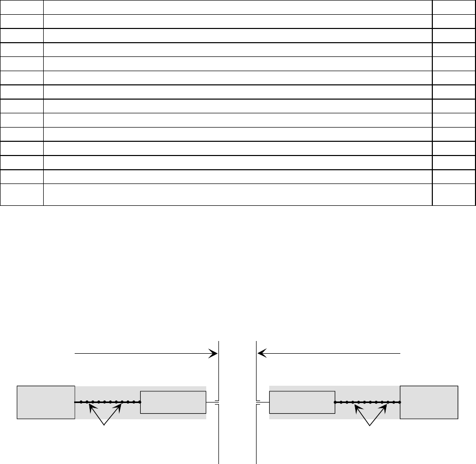
ETSI

E

TSI TR 102 273

-

2

V1.2.1 (2001

-

1

2)

5

0

Despite the commonality of most of the components to both stages of this procedure, the mismatch uncertainty

contribution from both stages has to be calculated and included in the uncertainty calculations, since the load conditions

vary i.e. antennas replace the adapter in the second stage. Conversely, as a result of this commonality, the uncertainty

contribution of some of the individual components will cancel.

The magnitude of the random uncertainty contribution to this stage of the procedure can be assessed from multiple

repetition of the direct attenuation measurement. All the uncertainty components which contribute to this stage of the

test are listed in table 13. Annex A should be consulted for the sources and/or magnitudes of the uncertainty

contributions.

Table 13: Contributions from the direct attenuation measurement

uj or i Description of uncertainty contributions dB

uj35 mismatch: direct attenuation measurement

uj38 signal generator: absolute output level

uj39 signal generator: output level stability

uj19 cable factor: receiving antenna 0,00

uj19 cable factor: transmitting antenna 0,00

uj41 insertion loss: receiving antenna cable 0,00

uj41 insertion loss: transmitting antenna cable 0,00

uj40 insertion loss: receiving antenna attenuator 0,00

uj40 insertion loss: transmitting antenna attenuator 0,00

uj42 insertion loss: adapter

uj47 receiving device: absolute level 0,00

uj48 receiving device: linearity 0,00

ui01 random uncertainty (see note in clause A.18 of TR 102 273-1-2 and note in clause 6.4.7 of

TR 102 273-1-1)

The standard uncertainties from table 13 should be combined by RSS in accordance with clause 5 of

TR 102 273-1-1 [8]. This gives the combined standard uncertainty (uc direct attenuation measurement) for the direct

attenuation measurement in dB.

6.6.2 Uncertainty contribution, NSA measurement

This stage involves removing the adapter and connecting each attenuator to an antenna as shown in figure 25, and

recording the new level on the receiving device.

cable 1

ferrite beads

Attenuator 1

10 dB

Signal

generator

Transmitting antenna Receiving antenna

cable 2

ferrite beads

Receiving

device

Attenuator 2

10 dB

Figure 25: Stage 2: NSA measurement

The difference in received levels (after allowance for any correction factors which may be appropriate), for the same

signal generator output level, reveals the NSA. All the uncertainty components which contribute to this stage of the test

are listed in table 14. Annex A should be consulted for the sources and/or magnitudes of the uncertainty contributions.

ETSI

E

TSI TR 102 273

-

2

V1.2.1 (2001

-

1

2)

5

1

Table 14: Contributions from the NSA measurement

uj or i Description of uncertainty contributions dB

uj36 mismatch: transmitting part

uj37 mismatch: receiving part

uj38 signal generator: absolute output level

uj39 signal generator: output level stability

uj19 cable factor: receiving antenna

uj19 cable factor: transmitting antenna

uj41 insertion loss: receiving antenna cable 0,00

uj41 insertion loss: transmitting antenna cable 0,00

uj40 insertion loss: receiving antenna attenuator 0,00

uj40 insertion loss: transmitting antenna attenuator 0,00

uj47 receiving device: absolute level

uj48 receiving device: linearity

uj16 range length

uj03 reflectivity of absorber material: transmitting antenna to the receiving antenna

uj44 antenna: antenna factor of the receiving antenna

uj44 antenna: antenna factor of the transmitting antenna

uj46 antenna: tuning of the receiving antenna

uj46 antenna: tuning of the transmitting antenna

uj22 position of the phase centre: receiving antenna

uj22 position of the phase centre: transmitting antenna

uj07 mutual coupling: transmitting antenna to its images in the absorbing material

uj07 mutual coupling: receiving antenna to its images in the absorbing material

uj10 mutual coupling: transmitting antenna to the receiving antenna

uj12 mutual coupling: interpolation of mutual coupling and mismatch loss correction factors

uj34 ambient effect

ui01 random uncertainty (see note in clause A.18 of TR 102 273-1-2 and note in clause 6.4.7 of

TR 102 273-1-1)

The standard uncertainties from table 14 should be combined by RSS in accordance with clause 5 of

TR 102 273-1-1 [8]. This gives the combined standard uncertainty (uc NSA measurement) for the NSA measurement in dB.

6.6.3 Expanded uncertainty of the verification procedure

The combined standard uncertainty of the results of the verification procedure is the combination of the components

outlined in clauses 6.6.1 and 6.6.2. The components to be combined are: uc direct attenuation measurement and uc NSA

measurement

__dB__, =

22 tmeasuremenNSActmeasuremennattenuatiodirectcc uuu += (6.7)

The expanded uncertainty is ±1,96 × uc = ± __,__ dB at a 95 % confidence level.

6.7 Calculation of measurement uncertainty (Procedure 2)

The column headed "Overall" in the results sheet is completed during the processing of the results for the verification

procedure. The values entered in this column are the measured NSA figures for the Anechoic Chamber.

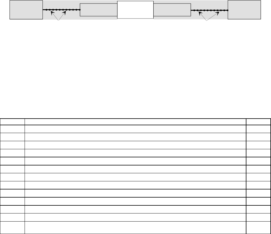
ETSI

E

TSI TR 102 273

-

2

V1.2.1 (2001

-

1

2)

5

2

The value, at any particular frequency, for the measured NSA is "Direct" (reference value) less "Site" (the value

appearing on the receiver during the NSA measurement) less the sum of "Transmit Antenna factor AFT" and "Receive

Antenna factor AFR" i.e.:

NSA = "Direct" - "Site" - "Transmit Antenna factor" - "Receive Antenna factor" (6.8)

As an example, let the direct attenuation value be 10 dBm and the received level during the site measurement be

-33 dBm. Putting each antenna factor at 3,9 dB gives a measured NSA value of:

NSA = [10 dBm - (-33 dBm)] - (7,8 dB) = 35,2 dB (6.9)

There are uncertainties in each of these components for the NSA and an example of a typical calculation of the

expanded uncertainty is now given. A fully worked example calculation can be found in clause 4 of

TR 102 273-1-2 [9].

6.7.1 Uncertainty contribution, direct attenuation measurement

The verification procedure involves two different measurement stages and the derivation of NSA. The first stage (the

reference) is with all the items of test equipment connected directly together via an adapter between the attenuators as

shown in figure 26 (components shown shaded are common to both stages of the procedure).

"In line"

adapter Attenuator 2

10 dB Receiving

device

Attenuator 1

10 dB

Signal

generator

cable 1 cable 2

ferrite beads ferrite beads

Figure 26: Stage 1: Direct attenuation measurement for the verification procedure

Despite the commonality of most of the components to both stages of this procedure, the mismatch uncertainty

contribution for both stages of the test has to be calculated and included in the uncertainty calculations. This is the result

of load conditions varying (i.e. antennas replacing the adapter in the second stage). Conversely, as a result of this

commonality, the uncertainty contributions of some of the individual components will cancel.

The magnitude of the random uncertainty contribution to each stage of the procedure can be assessed from multiple

repetition of the respective measurements. All the uncertainty components which contribute to this stage of the test are

listed in table 15. Annex A should be consulted for the sources and/or magnitudes of the uncertainty contributions.

Table 15: Contributions from the direct attenuation measurement

uj or i Description of uncertainty contributions dB

uj35 mismatch: direct attenuation measurement

uj38 signal generator: absolute output level 0,00

uj39 signal generator: output level stability

uj19 cable factor: receiving LPDA 0,00

uj19 cable factor: transmitting LPDA 0,00

uj41 insertion loss: receiving LPDA cable 0,00

uj41 insertion loss: transmitting LPDA cable 0,00

uj40 insertion loss: receiving LPDA attenuator 0,00

uj40 insertion loss: transmitting LPDA attenuator 0,00

uj42 insertion loss: adapter

uj47 receiving device: absolute level 0,00

uj48 receiving device: linearity 0,00

ui01 random uncertainty (see note in clause A.18 of TR 102 273-1-2 and note in clause 6.4.7 of

TR 102 273-1-1)

The standard uncertainties from table 15 should be combined by RSS in accordance with clause 5 of

TR 102 273-1-1 [8]. This gives the combined standard uncertainty (uc direct attenuation measurement) for the direct

attenuation measurement in dB.

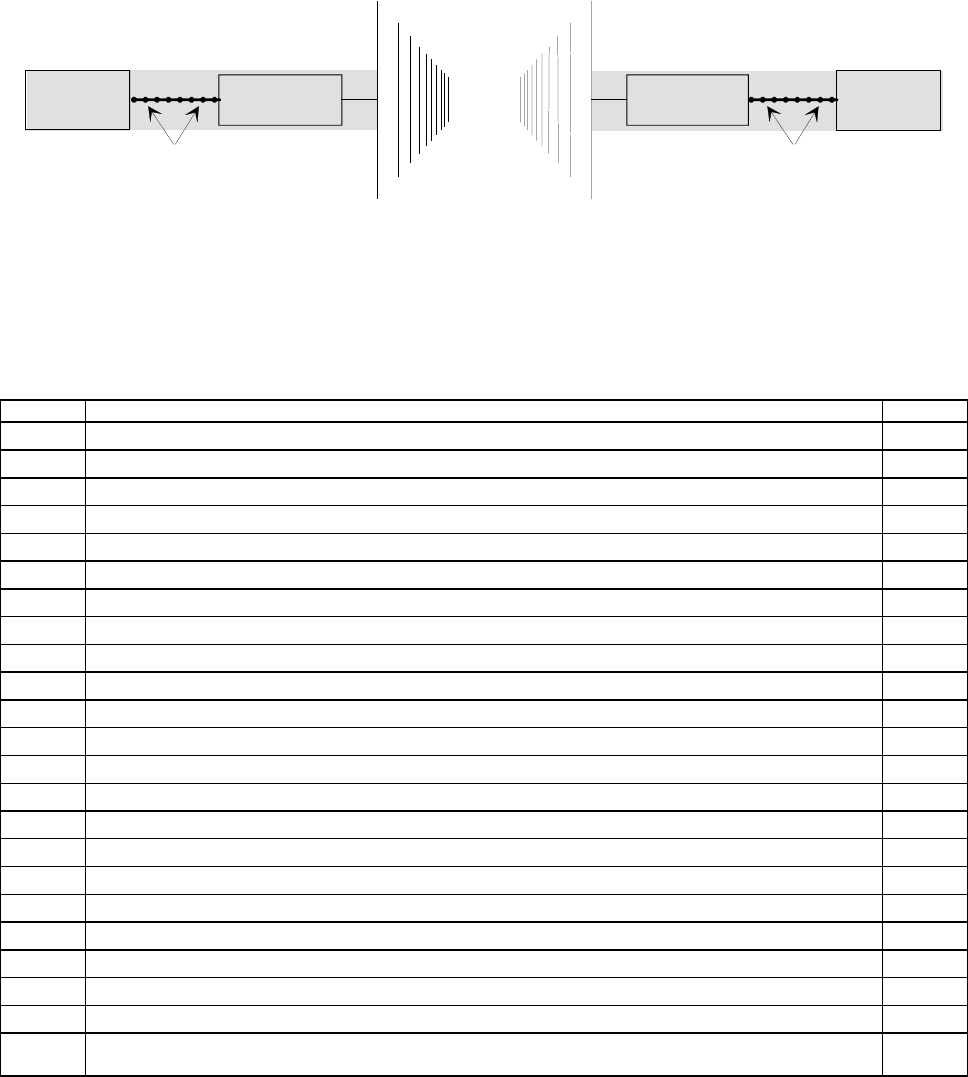
ETSI

E

TSI TR 102 273

-

2

V1.2.1 (2001

-

1

2)

5

3

6.7.2 Uncertainty contribution, NSA measurement

This stage involves removing the adapter and connecting each attenuator to an antenna as shown in figure 27, and

recording the new level on the receiving device.

cable 2

Attenuator 2

10 dB

Receiving

device

ferrite beads

cable 1 Attenuator 1

10 dB

ferrite beads

Signal

generator

Figure 27: Stage 2: NSA measurement

The difference in received levels (after allowance for any correction factors which may be appropriate), for the same

signal generator output level, reveals the NSA. All the components which contribute to this stage of the test are listed in

table 16. Annex A should be consulted for the sources and/or magnitudes of the uncertainty contributions.

Table 16: Contributions from the measurement

uj or i Description of uncertainty contributions dB

uj36 mismatch: transmitting part

uj37 mismatch: receiving part

uj38 signal generator: absolute output level 0,00

uj39 signal generator: output level stability

uj19 cable factor: receiving LPDA

uj19 cable factor: transmitting LPDA

uj41 insertion loss: receiving LPDA cable 0,00

uj41 insertion loss: transmitting LPDA cable 0,00

uj40 insertion loss: receiving LPDA attenuator 0,00

uj40 insertion loss: transmitting LPDA attenuator 0,00

uj47 receiving device: absolute level

uj48 receiving device: linearity

uj16 range length 0,00

uj03 reflectivity of absorber material: transmitting antenna to the receiving antenna

uj44 antenna: antenna factor of the receiving LPDA

uj44 antenna: antenna factor of the transmitting LPDA

uj22 position of the phase centre: receiving LPDA

uj22 position of the phase centre: transmitting LPDA

uj23 position of the phase centre: LPDA

uj07 mutual coupling: receiving LPDA and its images in the absorbing material

uj07 mutual coupling: transmitting LPDA and its images in the absorbing material

uj34 ambient effect 0,00

ui01 random uncertainty (see note in clause A.18 of TR 102 273-1-2 and note in clause 6.4.7 of

TR 102 273-1-1)

The standard uncertainties from table 16 should be combined by RSS in accordance with clause 5 of

TR 102 273-1-1 [8]. This gives the combined standard uncertainty (uc NSA measurement) for the NSA measurement of

in dB.

ETSI

E

TSI TR 102 273

-

2

V1.2.1 (2001

-

1

2)

5

4

6.7.3 Expanded uncertainty of the verification procedure

The combined standard uncertainty of the results of the verification procedure is the combination of the components

outlined in clauses 6.7.1 and 6.7.2. The components to be combined are uc direct attenuation measurement and uc NSA

measurement.

__dB__, =

22 tmeasuremenNSActmeasuremennattenuatiodirectcc uuu += (6.10)

The expanded uncertainty is ± 1,96 x uc = ± __,__ dB at a 95 % confidence level.

6.8 Summary

The expanded uncertainty values derived in clauses 6.6.3 and 6.7.3 reveal the uncertainty with which the NSA can be

measured. Any value of NSA which varies by more than these uncertainty values from the theoretical value is probably

due to imperfection(s) in the site. These imperfections may be due to reflections from a range of possible sources in the

Anechoic Chamber at the time the verification procedure is carried out.

7 Test methods

7.1 Introduction

The following test methods apply to integral antenna devices only i.e. EUTs not fitted with either a permanent or a

temporary external antenna connector. The Spurious emissions test also applies to EUTs with a detachable antenna.

The range length of the Anechoic Chamber should be adequate to allow for testing in the far-field of the EUT i.e. the

range length should be equal to or exceed:

()

212

2

dd+

λ

(7.1)

where:

d1 is the largest dimension of the EUT/dipole after substitution (m);

d2 is the largest dimension of the test antenna (m);

λ

is the test frequency wavelength (m).

It should be noted that in the substitution part of these tests, where both test and substitution/measuring antennas are

half wavelength dipoles, this minimum range length for far-field testing would be (2

λ

).

It should be stated in the test report when either of these conditions is not met. The additional contributions to the

measurement uncertainty which result can be incorporated into the analysis of the results.

No part of the volume of the EUT should, at any angle of rotation, fall outside the "quiet zone" of the chamber at the

nominal frequency of test. Where this condition cannot be met, the measurement should not be carried out.

NOTE: The "quiet zone" is a volume within the chamber in which a specified performance has either been proven

by test, or is guaranteed by the designer/manufacture. The specified performance is usually the

reflectivity of the absorbing panels or a directly related parameter (e.g. signal uniformity in amplitude and

phase). It should be noted however that the defining levels of the quiet zone tend to vary.

An additional requirement of the chamber construction is to ensure that no part of any antenna or EUT should come

within 1 m of the absorbing panels (this is to avoid "electrical loading"). For the EUT, this condition needs to be

satisfied for all angles of rotation. Where this condition cannot be met, the measurement should not be carried out.

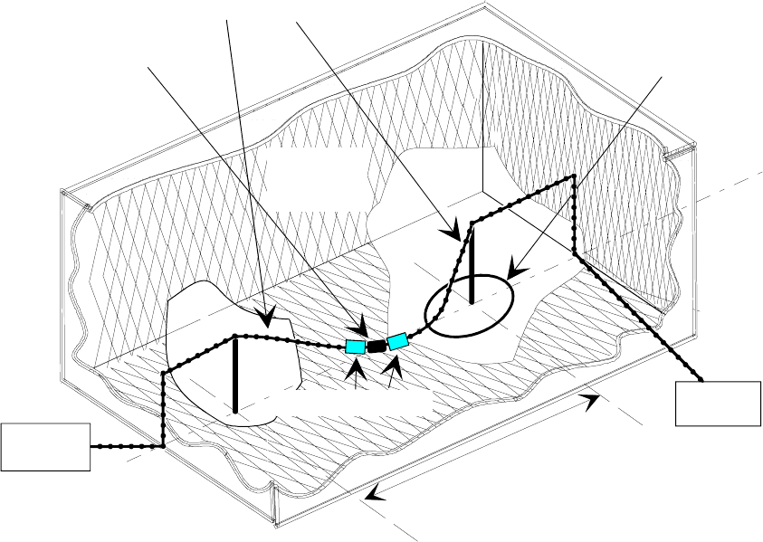
ETSI

E

TSI TR 102 273

-

2

V1.2.1 (2001

-

1

2)

5

5

Further, measurements should not be carried out if the reflectivity of the absorbing material within the chamber is worse

than -5 dB at the frequency of test.

7.1.1 Site preparation

The cables for both ends of the test chamber should be routed behind and away from the antennas, parallel to the side

walls and floor of the chamber, towards the back walls for a minimum of 2 m (unless the back wall is reached). They

should then be allowed to drop vertically towards the floor, preferably behind the anechoic panels, and routed out

through the screen (normally via a breakout panel) to the test equipment.

These cables should be dressed with ferrite beads, spaced 0,15 m apart for their entire lengths within the screen of the

chamber. The routeing and dressing of the cables should be identical to the verification procedure set-up.

Calibration data for items of test equipment used should be available and valid. For both the test and

substitution/measuring antennas, the data should include gain relative to an isotropic radiator (or antenna factor) against

frequency. Also, the VSWR of the substitution/measuring antenna should be known.

The calibration data for all cables and attenuators used should include insertion loss and VSWR throughout the entire

frequency range of the tests. All VSWR and insertion loss figures should be recorded in the log book results sheet for

the specific test.

Where correction factors/tables are required, these should be immediately available.

For all items of test equipment, the maximum errors they exhibit should be known along with the distribution of the

error e.g.:

- cable loss:

±0,5 dB with a rectangular distribution;

- measuring receiver: 1,0 dB (standard deviation) signal level accuracy with a Gaussian error distribution.

Cabling

Adaptor

Range length 3 m or 10 m

Turntable

Receiving

device

10 dB attenuators

Radio

absorbing

material

Signal

generator

Figure 28: Anechoic Chamber set-up for daily system checking

At the start of each day, system checks should be made on the equipment used in the Anechoic Chamber. The following

checking procedures, as a minimum requirement, should be carried out.

ETSI

E

TSI TR 102 273

-

2

V1.2.1 (2001

-

1

2)

5

6

1) All items of test equipment requiring electrical supplies should be connected to their power sources, switched on

and allowed adequate time to stabilize, as recommended by the manufacturers. Where a stabilization period is

not given by the manufacturer, 30 minutes should be allowed. After this time period those items of test

equipment which possess the facility should have their self test/self calibration procedures performed.

2) A signal generator should be connected to the existing cabling at the turntable end. The other end of this cable

should be connected via a calibrated coaxial cable/10 dB attenuator/adapter/10 dB attenuator/calibrated coaxial

cable combination to existing cabling at the other end of the chamber. This existing cable should be connected to

a receiving device (see figure 28). Where the use of a cable is impractical due to the arrangements within the

chamber, bicones or other suitable antennas could be connected at both ends as appropriate. The signal generator

should be scanned across the appropriate frequency range and the response of the receiving device noted. It

should be compared with previous tests carried out under similar conditions. Any anomalies should be

investigated.

7.1.2 Preparation of the EUT

The manufacturer should supply information about the EUT covering the operating frequency, polarization, supply

voltage(s) and the reference face. Additional information, specific to the type of EUT should include, where relevant,

carrier power, channel spacing, whether different operating modes are available (e.g. high and low power modes) and if

operation is continuous or is subject to a maximum test duty cycle (e.g. one minute on, four minutes off).

Where necessary, a mounting bracket of minimal size should be available for mounting the EUT on the turntable. This

bracket should be made from low conductivity, low relative dielectric constant (i.e. less than 1,5) material(s) such as

expanded polystyrene, balsawood, etc.

The presence of the cables supplying power can affect the measured performance of the EUT. For this reason, attempts

should be made to make them "transparent" as far as the testing is concerned. This can be achieved by routeing them by

the shortest possible paths down to, and out from, the chamber screen. Additionally, where possible, these leads should

be twisted together and loaded with ferrite beads at 0,15 m spacing.

7.1.3 Standard antennas

In the frequency band 30 MHz to 1 000 MHz, except where stipulated, both test and substitution/measuring antennas

should be tuned half-wavelength dipoles (constructed as detailed in ANSI C63.5 [1]) aligned for the same polarization.

NOTE: Due to size constraints a shortened dipole is used over part of this frequency band. For uniformity of

procedures across Open Area Test Sites and both types of Anechoic Chamber, a shortened dipole is used

from 30 MHz up to 80 MHz. At all these frequencies the 80 MHz arm length (0,889 m) is used attached

to the 20 MHz to 65 MHz balun for all test frequencies from 30 MHz to 65 MHz inclusive or to the

65 MHz to 180 MHz balun for 65 MHz to 80 MHz. Tuned half wavelength dipoles, attached to their

matching baluns are used for all frequencies in the band 80 MHz to 1 000 MHz inclusive. Table 17 details

dipole arm lengths (as measured from the centre of the balun block) and balun type against frequency.

Where the test frequency does not correspond to a set frequency in the table the arm length to be used

should be determined by linear interpolation between the closest set values.

Table 17: Dipole arm length and balun type against frequency

Frequency

(MHz) Dipole arm length

(m) Balun type Frequency

(MHz) Dipole arm length

(m) Balun type

30 0,889 160 0,440 65 MHz to

35 0,889 180 0,391 180 MHz

40 0,889 20 MHz to 200 0,352

45 0,889 65 MHz 250 0,283 180 MHz to

50 0,889 300 0,235 400 MHz

60 0,889 400 0,175

70 0,889 500 0,143

80 0,889 600 0,117

90 0,791 65 MHz to 700 0,102 400 MHz to

100 0,714 180 MHz 800 0,089 1 000 MHz

120 0,593 900 0,079

140 0,508 1 000 0,076

ETSI

E

TSI TR 102 273

-

2

V1.2.1 (2001

-

1

2)

5

7

7.1.4 Mutual coupling and mismatch loss correction factors

Correction factors are included where relevant, to allow for mutual coupling and mismatch loss for the 30 MHz to

180 MHz band, based on using the recommended ANSI C63.5 [1] dipoles. These have been calculated by computer

modelling of their baluns, sectional arms and the range length using MiniNEC. The factors are only valid for this

particular type of dipole. However, if this type is unavailable, an alternative could be used. This alternative should be a

tuned half wavelength dipole at the particular test frequency. Since correction factors have not been calculated in this

document for any type other than the ANSI C63.5 [1] dipoles this will result in a greater expanded uncertainty for the

measurement unless the test house/manufacturer has performed equivalent modelling on the dipoles used.

7.1.5 Power supplies to the EUT

All tests should be performed using power supplies wherever possible, including tests on EUTs designed for battery-

only use. In all cases, power leads should be connected to the EUT's supply terminals (and monitored with a digital

voltmeter) but the battery should remain present, electrically isolated from the rest of the EUT, possibly by putting tape

over its contacts. All leads involved should be taken down to the floor of the facility by the shortest possible routes,

twisting pairs together and loading with ferrite beads at 0,15 m spacing.

7.1.6 Restrictions

The restriction that no part of an antenna should come within 1 m of any part of the absorbing panels should be applied

at all times throughout these test methods.

7.2 Transmitter tests

7.2.1 Frequency error (30 MHz to 1 000 MHz)

Definition

The frequency error of a transmitter is the difference between the measured carrier frequency in the absence of

modulation and the nominal frequency of the transmitter as stated by the manufacturer.

7.2.1.1 Apparatus required

- digital voltmeter;

- ferrite beads;

- 10 dB attenuators;

- power supply;

- connecting cables;

- Anechoic Chamber;

- test antenna (a half wavelength dipole, bicone or LPDA);

- frequency counter.

The type and serial numbers of all items of test equipment should be recorded in the log book results sheet (see

table 18).

NOTE: The half wavelength dipole antennas, incorporating matching/transforming baluns, for the procedure are

available in the following bands: 20 MHz to 65 MHz, 65 MHz to 180 MHz, 180 MHz to 400 MHz,

400 MHz to 1 000 MHz. Constructional details are contained in ANSI C63.5 [1]. In the recommended

antenna scheme for this band, a shortened dipole is used at all frequencies from 30 MHz up to 80 MHz.

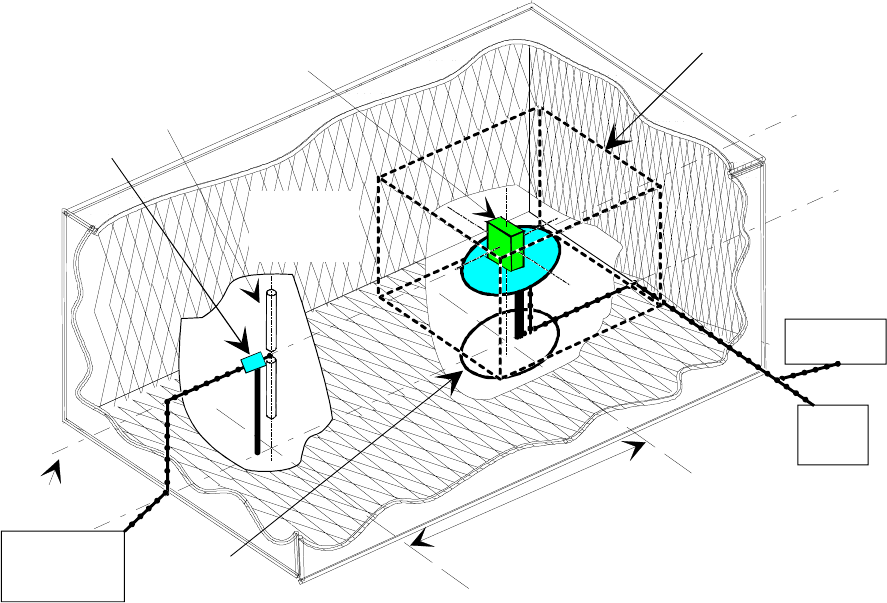
ETSI

E

TSI TR 102 273

-

2

V1.2.1 (2001

-

1

2)

5

8

7.2.1.2 Method of measurement

1) The measurement should always be performed in the absence of modulation.

2) The EUT should be mounted on the turntable, whose surface is at the height specified in the relevant Standard

or, where not stated, at a convenient height within the "quiet zone" of the Anechoic Chamber. The EUT should

be mounted in an orientation which matches that of its normal usage as stated by the manufacturer. This

orientation and mounting configuration should be recorded on page 1 of the log book results sheet (see table 18).

NOTE 1: The turntable should be constructed from non-conducting, low relative dielectric constant (preferably less

than 1,5) material(s).

3) The test antenna (dipole, bicone or LPDA) should be oriented for the stated polarization of the EUT. For cases in

which the test antenna is a tuned half wavelength dipole, this should be tuned to the nominal frequency. The

output of the test antenna should be connected to the frequency counter via a 10 dB attenuator and the calibrated,

ferrited coaxial cable associated with that end of the chamber (see figure 29). The phase centre of the test

antenna should be at the same height above the floor as the mid point of the EUT.

NOTE 2: Where a dipole is used, frequencies below 80 MHz require a shortened version (as defined in

clause 7.1.3) to be used. For any frequency, the dipole arm length (given in table 17) is defined from the

centre of the balun block to the tip of the arm. From a fully extended state, each telescopic element, in

turn, should be "pushed in" from the tip until the required length is obtained. The outermost section needs

to fully compress before any of the others, and so on. Table 17 also gives the choice of balun for set

frequencies. Where the test frequency does not correspond to a set frequency in the table, the arm length

to be used should be determined by linear interpolation between the closest set values.

Range length 3 m or 10 m

Turntable

Test

antenna

EUT

Central axis

of chamber

Quiet zone

10 dB attenuator

Frequency

counter

Power

supply

unit

Digital

voltmeter

Radio

absorbing

material

Figure 29: Anechoic Chamber set-up for the Frequency error test

4) The EUT should be switched on without modulation, allowed adequate time to stabilize and the resolution of the

frequency counter adjusted to read to the nearest Hz.

5) The value of the frequency displayed on the counter should be recorded in the log book results sheet (see

table 18).

ETSI

E

TSI TR 102 273

-

2

V1.2.1 (2001

-

1

2)

5

9

NOTE 3: In cases where the frequency does not appear stable, this might require observations over a 30 second or

1 minute time period, noting the highest and lowest readings and estimating the average value. In these

cases it is the average value that should be recorded in the log book results sheet (see table 18).

7.2.1.3 Procedure for completion of the results sheets

There are two values that need to be derived before the overall results sheet (see table 19) can be completed. Firstly the

value for frequency error (from a straightforward calculation of recorded frequency minus the nominal frequency) and

secondly, the value of the expanded uncertainty for the test. This should be carried out as given in clause 7.2.2 and the

resulting value entered in the overall results sheet (see table 19).

7.2.1.4 Log book entries

Table 18: Log book results sheet

FREQUENCY ERROR Date: PAGE 1 of 1

Temperature:.........°

°°

°C Humidity:...............% Frequency:.............MHz

Manufacturer of EUT:..................... Type No:.............. Serial No:..................

Range length:.......................

Test equipment item Type No. Serial No. VSWR Insertion loss

Antenna

factor/gain

Test antenna N/A

Test antenna attenuator N/A

Test antenna cable N/A

Digital voltmeter

N/A N/A N/A

Power supply

N/A N/A N/A

Ferrite beads

N/A N/A N/A

Frequency counter N/A N/A

Mounting configuration of EUT

Reading on frequency counter: Hz

7.2.1.5 Statement of results

The results should be presented in tabular form as shown in table 19.

Table 19: Overall results sheet

FREQUENCY ERROR Date: PAGE 1 of 1

Frequency error Hz

Expanded uncertainty (95 %) Hz

ETSI

E

TSI TR 102 273

-

2

V1.2.1 (2001

-

1

2)

6

0

7.2.2 Expanded uncertainty for frequency error test

The method of calculating the expanded uncertainty for tests in which signal levels in dB are involved is equally

adopted for the frequency error test in which all the uncertainties are in the units of Hz. That is, all the uncertainty

contributions are converted into standard uncertainties and combined by the RSS method under the assumption that they

are all stochastic. All the uncertainty components which contribute to the test are listed in table 20. Annex A should be

consulted for the sources and/or magnitudes of the uncertainty contributions.

Table 20: Contributions from the measurement

uj or i Description of uncertainty contributions Hz

ui01 random uncertainty (see note in clause A.18 of TR 102 273-1-2 and note in clause 6.4.7 of

TR 102 273-1-1)

uj56 frequency counter: absolute reading

uj05 mutual coupling: detuning effect of the absorbing material on the EUT

uj09 mutual coupling: detuning effect of the test antenna on the EUT

The standard uncertainties from table 20 should be combined by RSS in accordance with clause 5 of

TR 102 273-1-1 [8]. The combined standard uncertainty of the frequency measurement (uc contributions from the

measurement) is the combination of the components outlined above.

uc = uc contributions from the measurement = __,__ Hz

The expanded uncertainty is ±1,96 x uc = ± __,__ Hz at a 95 % confidence level.

7.2.3 Effective radiated power (30 MHz to 1 000 MHz)

Definition

The effective radiated power is the power radiated in the direction of the maximum field strength under specified

conditions of measurement, in the absence of modulation.

7.2.3.1 Apparatus required

- digital voltmeter;

- ferrite beads;

- 10 dB attenuators;

- power supply;

- connecting cables;

- Anechoic Chamber;

- test antenna (half wavelength dipole as detailed in ANSI C63.5 [1] recommended);

- substitution antenna (half wavelength dipole as detailed in ANSI C63.5 [1] recommended);

- receiving device (measuring receiver or spectrum analyser);

- signal generator.

The type and serial numbers of all items of test equipment should be recorded on page 1 of the log book results sheet

(see table 22).

NOTE: The half wavelength dipole antennas, incorporating matching/transforming baluns, for the procedure are

available in the following bands: 20 MHz to 65 MHz, 65 MHz to 180 MHz, 180 MHz to 400 MHz,

400 MHz to 1 000 MHz. Constructional details are contained in ANSI C63.5 [1]. In the recommended

antenna scheme for this band, a shortened dipole is used at all frequencies from 30 MHz up to 80 MHz.

ETSI

E

TSI TR 102 273

-

2

V1.2.1 (2001

-

1

2)

6

1

7.2.3.2 Method of measurement

1) The measurement should always be performed in the absence of modulation.

2) The EUT should be mounted directly onto the turntable, whose surface is at the height specified in the relevant

standard or, where not stated, at a convenient height within the "quiet zone" of the Anechoic Chamber. The EUT

should be mounted in an orientation which matches that of its normal usage as stated by the manufacturer. The

normal to the reference face of the EUT should point directly down the chamber towards the test antenna

support. This is the 0° reference angle for the test. This orientation and mounting configuration should be

recorded on page 1 of the log book results sheet (see table 22). The items of test equipment should be set-up as

shown in figure 30.

NOTE 1: The turntable should be constructed from non-conducting, low relative dielectric constant (preferably less

than 1,5) material(s).

3) In cases where the position of the phase centre of the EUT's antenna is known, the EUT should be positioned on

the turntable such that this phase centre is as coincident with the axis of rotation of the turntable as possible and

either on the central axis of the chamber or at a convenient height within the quiet zone. Alternatively, if the

position of the phase centre is unknown, but the antenna is a single rod which is visible and vertical in normal

usage, the axis of the antenna should lie on the axis of rotation whilst its base should be positioned on the

chamber's central axis (or at a convenient height within the quiet zone). If the phase centre of the EUT is

unknown and no antenna is visible, the volume centre of the EUT should be used instead. The offset from the

central axis of the chosen phase centre datum, should be entered on page 2 of the log book results sheet (see

table 22).

4) The test antenna (in the recommended scheme a tuned ANSI C63.5 [1] half wavelength dipole for frequencies of

80 MHz and above, a shortened dipole for frequencies from 30 MHz up to 80 MHz) should be tuned to the

appropriate frequency and oriented for vertical polarization. Its output should be connected to the receiving

device via a 10 dB attenuator and the calibrated, ferrited coaxial cable associated with that end of the chamber.

The height of the phase centre of the test antenna should be at the same offset (if any) from the central axis of the

chamber as the phase centre/antenna base/volume centre of the EUT, so that the measurement axis is parallel to

the central axis.

NOTE 2: The measurement axis is the straight line between the phase centres of transmitting and receiving devices.

NOTE 3: For all frequencies below 80 MHz, a shortened dipole (as defined in clause 7.1.3) should be used. The

dipole arm length is defined from the centre of the balun block to the tip of the arm. From a fully

extended state, each telescopic element, in turn, should be "pushed in" from the tip until the required

length is obtained. The outermost section needs to fully compress before any of the others, and so on.

Table 17 gives the dipole arm lengths and choice of balun for set frequencies. Where the test frequency

does not correspond to a set frequency in the table, the arm length to be used should be determined by

linear interpolation between the closest set values.

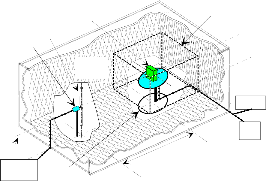
ETSI

E

TSI TR 102 273

-

2

V1.2.1 (2001

-

1

2)

6

2

Range length 3 m or 10 m

Turntable

Test

antenna

EUT

Central axis

of chamber

Quiet zone

10 dB attenuator

Receiving

device

Digital

voltmeter

Power

supply

unit

Radio

absorbing

material

Figure 30: Anechoic Chamber set-up for the effective radiated power measurement on the EUT

5) The EUT should be switched on without modulation, and the receiving device tuned to the appropriate

frequency.

6) The EUT should be rotated through 360° in the horizontal plane until the maximum signal is detected on the

receiving device. The angle with reference to the nominal orientation of the EUT and the maximum signal level

(dBm) detected by the receiving device should be recorded on page 2 of the log book results sheet (see table 22).

7) The EUT should be replaced on the turntable by the substitution antenna (identical to the test antenna), which

has been adjusted to correspond to the frequency of the EUT (see figure 31).

8) The phase centre of the substitution antenna should lie directly over the axis of rotation of the turntable, whilst

its height should be at the same offset from the central axis of the chamber as the phase centre of the test

antenna, so that the measurement axis is again parallel to the central axis.

9) The substitution antenna should be oriented for vertical polarization and connected via a 10 dB attenuator to a

calibrated signal generator using the calibrated, ferrited coaxial cable associated with the turntable end of the

chamber.

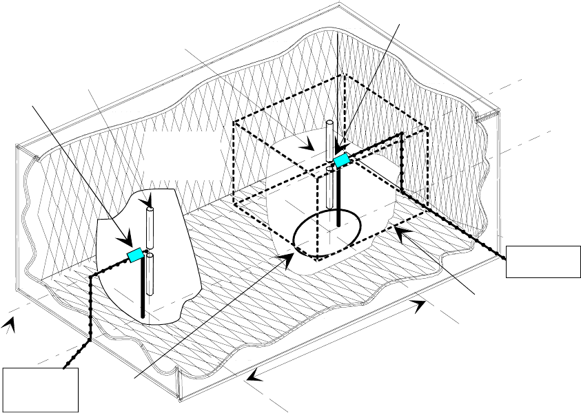
ETSI

E

TSI TR 102 273

-

2

V1.2.1 (20

0

1

-

1

2)

6

3

Range length 3 m or 10 m

Turntable

Test

antenna

Substitution

antenna

Central axis

of chamber

Quiet zone

10 dB attenuator

10 dB attenuator

Receiving

device

Radio

absorbing

material

Signal

generator

Figure 31: Substitution antenna replacing the EUT

10) The signal generator should be tuned to the appropriate frequency and its output level adjusted until the level

measured on the receiving device, is at least 20 dB above the level with the output from the signal generator

switched off.

11) The substitution antenna should be rotated until the maximum level is detected on the receiving device.

NOTE 4: This is to correct for possible misalignment of a directional beam i.e. dipoles used in horizontally

polarized tests. This step can be omitted when dipoles are used in vertically polarized tests.

12) The output level of the signal generator should be adjusted until the level, measured on the receiving device, is

identical to that recorded in step 6. This output signal level (dBm) from the signal generator should be recorded

on page 2 of the log book results sheet (see table 22).

NOTE 5: In the event of insufficient range of signal generator output level, the receiving device input attenuation

should be decreased to compensate. The signal generator output level (dBm) and the change in

attenuation (dB) should both be recorded on page 2 of the log book results sheet (see table 22) in this

case.

13) The EUT should be remounted on the turntable as stipulated in steps 2 and 3, the test antenna oriented for

horizontal polarization and steps 4 to 12 repeated with the substitution antenna also oriented for horizontal

polarization.

7.2.3.3 Procedure for the completion of the results sheets

There are two values that need to be derived before the overall results sheet (see table 23) can be completed. These are

the overall measurement correction and the expanded uncertainty values.

Guidance for deriving the values of the correction factors is given in table 21.

ETSI

E

TSI TR 102 273

-

2

V1.2.1 (2001

-

1

2)

6

4

When the correction factors have been derived, they should be entered on page 2 of the log book results sheet (see

table 22) as a result of which the overall correction can be calculated as follows:

overall correction = substitution antenna cable loss

+ substitution antenna attenuator loss

+ substitution antenna balun loss

+ mutual coupling and mismatch loss (where applicable)

- gain of substitution antenna

NOTE: For frequencies greater than 180 MHz the mutual coupling and mismatch loss factor should be taken as

0,00 dB.

The resulting value for the overall correction factor should then be entered on page 2 of the log book result sheet (see

table 22). The effective radiated power can then be calculated:

effective radiated power = signal generator output level

- reduction in the input attenuation of receiving device (if any)

+ overall correction

The only calculation that remains to be performed before the overall results sheet (see table 23) can be completed is the

determination of the expanded measurement uncertainty. This should be carried out as given in clause 7.2.4 and the

resulting value entered in the overall results sheet (see table 23).

Table 21: Guidance for deriving correction factors

Figures for correction factors

Substitution antenna cable loss Obtained directly from the calibration data

Substitution antenna attenuator loss Obtained from calibration data

Substitution antenna balun loss If not known from calibration data, the value should be

taken as 0,30 dB

Mutual coupling and mismatch loss factors between the

test antenna and substitution antenna For ANSI dipoles (30 MHz to 180 MHz) values can be

obtained from TR 102 273-1-1 [8] table A.19.For

frequencies greater than 180 MHz, this value is 0,00 dB.

For non-ANSI dipoles this value is 0,00 dB.

Gain of substitution antenna For ANSI dipoles (30 MHz to 1 000 MHz) the value is

2,10 dBi. For other types, the value can be obtained from

calibration data

ETSI

E

TSI TR 102 273

-

2

V1.2.1 (2001

-

1

2)

6

5

7.2.3.4 Log book entries

Table 22: Log book results sheet

EFFECTIVE RADIATED POWER Date: PAGE 1 of 2

Temperature:.........°

°°

°C Humidity:...............% Frequency:.............MHz

Manufacturer of EUT:..................... Type No:.............. Serial No:..................

Bandwidth of Receiving Device...................Hz

Range length:.......................

Test equipment item Type No. Serial No. VSWR Insertion loss

Antenna

factor/gain

Test antenna N/A

Test antenna attenuator N/A

Test antenna cable N/A

Substitution antenna N/A

Substitution antenna attenuator N/A

Substitution antenna cable N/A

Digital voltmeter N/A N/A N/A

Power supply N/A N/A N/A

Receiver device N/A N/A

Signal generator N/A N/A

Ferrite beads N/A N/A N/A

Mounting configuration of EUT

(continued)

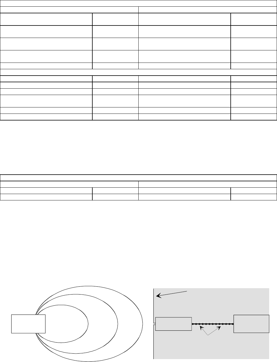
ETSI

E

TSI TR 102 273

-

2

V1.2.1 (2001

-

1

2)

6

6

Table 22 (concluded): Log book results sheet

EFFECTIVE RADIATED POWER Date: PAGE 2 of 2

Vertical Polarization Horizontal Polarization

Offset of EUT's phase centre from the

central axis Offset of EUT's phase centre from the

central axis

Maximum signal level on receiving

device dBm Maximum signal level on receiving

device (dBm) dBm

Angle at which the maximum signal is

received Angle at which the maximum signal is

received

Output level from signal generator into

substitution antenna (dBm) dBm Output level from signal generator into

substitution antenna (dBm) dBm

Change in receiver attenuator dB Change in receiver attenuator dB

Correction factors

Substitution antenna cable loss(es) Substitution antenna cable loss(es)

Substitution antenna attenuator loss Substitution antenna attenuator loss

Substitution antenna balun loss Substitution antenna balun loss

Mutual coupling and mismatch loss

(30 MHz to 180 MHz) Mutual coupling and mismatch loss

(30 MHz to 180 MHz)

Gain of the substitution antenna Gain of the substitution antenna

Overall measurement correction dB Overall measurement correction dB

7.2.3.5 Statement of results

The results should be presented in tabular form as shown in table 23.

Table 23: Overall results sheet

EFFECTIVE RADIATED POWER Date: PAGE 1 of 1

Vertical Polarization Horizontal Polarization

Effective radiated power dBm Effective radiated power dBm

Expanded uncertainty (95 %) dB Expanded uncertainty (95 %) dB

7.2.4 Measurement uncertainty for effective radiated power

A fully worked example illustrating the methodology to be used can be found in clause 4 of TR 102 273-1-2 [9].

7.2.4.1 Uncertainty contributions: Stage 1: EUT measurement

For the measurement of effective radiated power two stages of test are involved. The first stage (the EUT measurement)

is to measure on the receiving device, a level from the EUT as shown in figure 32 (shaded components are common to

both stages of the test).

Test

antenna

cable 2

Test antenna

ferrite beads

Attenuator 2

10 dB Receiving

device

EUT

Figure 32: Stage 1: EUT measurement

Due to the commonality of all of the components from the test antenna to the receiver in both stages of the test, the

mismatch uncertainty contributes identically in each stage and hence cancels. Similarly, the systematic uncertainty

contributions (e.g. test antenna cable loss, etc.) of the individual components also cancel.

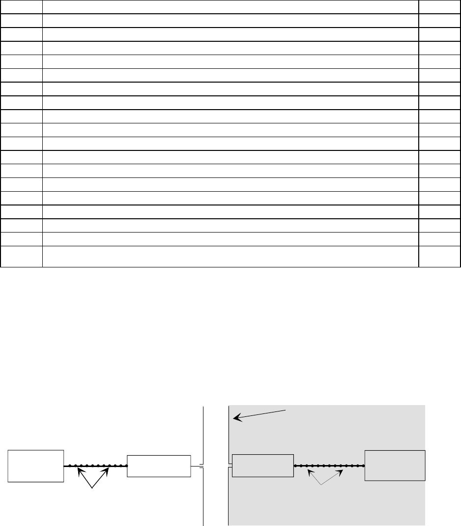
ETSI

E

TSI TR 102 273

-

2

V1.2.1 (2001

-

1

2)

6

7

The magnitude of the random uncertainty contribution to each stage of the procedure can be assessed from multiple

repetition of the EUT measurement. All the uncertainty components which contribute to this stage of the test are listed

in table 24. Annex A should be consulted for the sources and/or magnitudes of the uncertainty contributions.

Table 24: Contributions from the EUT measurement

uj or i Description of uncertainty contributions dB

uj37 mismatch: receiving part

uj19 cable factor: test antenna cable

uj41 insertion loss: test antenna cable 0,00

uj40 insertion loss: test antenna attenuator 0,00

uj47 receiving device: absolute level

uj53 EUT: influence of setting the power supply on the ERP of the carrier

uj20 position of the phase centre: within the EUT volume

uj21 positioning of the phase centre: within the EUT over the axis of rotation of the turntable

uj50 EUT: influence of the ambient temperature on the ERP of the carrier

uj16 range length 0,00

uj01 reflectivity of absorbing material: EUT to the test antenna 0,00

uj45 antenna: gain of the test antenna 0,00

uj46 antenna: tuning of the test antenna 0,00

uj55 EUT: mutual coupling to the power leads

uj08 mutual coupling: amplitude effect of the test antenna on the EUT

uj04 mutual coupling: EUT to its images in the absorbing material

uj06 mutual coupling: test antenna to its images in the absorbing material

ui01 random uncertainty (see note in clause A.18 of TR 102 273-1-2 and note in clause 6.4.7 of

TR 102 273-1-1)

The standard uncertainties from table 24 should be combined by RSS in accordance with clause 5 of

TR 102 273-1-1 [8]. This gives the combined standard uncertainty (uc contribution from the EUT measurement) for the EUT

measurement in dB.

7.2.4.2 Uncertainty contributions: Stage two: Substitution measurement

The second stage (the substitution) involves replacing the EUT with a substitution antenna and signal source as shown

in figure 33 and adjusting the output level of the signal generator until the same level as in stage one is achieved on the

receiving device.

Test

antenna

cable 2

Test antenna

ferrite beads

Attenuator 2

10 dB Receiving

device

cable 1

ferrite beads

Attenuator 1

10 dB

Signal

generator

Figure 33: Stage 2: Substitution measurement

All the uncertainty components which contribute to this stage of the test are listed in table 25. Annex A should be

consulted for the sources and/or magnitudes of the uncertainty contributions.

ETSI

E

TSI TR 102 273

-

2

V1.2.1 (2001

-

1

2)

6

8

Table 25: Contributions from the substitution

uj or i Description of uncertainty contributions dB

uj36 mismatch: transmitting part

uj37 mismatch: receiving part

uj38 signal generator: absolute output level

uj39 signal generator: output level stability

uj19 cable factor: substitution antenna cable

uj19 cable factor: test antenna cable

uj41 insertion loss: substitution antenna cable

uj41 insertion loss: test antenna cable 0,00

uj40 insertion loss: substitution antenna attenuator

uj40 insertion loss: test antenna attenuator 0,00

uj47 receiving device: absolute level 0,00

uj16 range length 0,00

uj02 reflectivity of absorbing material: substitution antenna to the test antenna 0,00

uj45 antenna: gain of the substitution antenna 0,50

uj45 antenna: gain of the test antenna 0,00

uj46 antenna: tuning of the test antenna 0,00

uj22 position of the phase centre: substitution antenna

uj06 mutual coupling: substitution antenna to its images in the absorbing material

uj06 mutual coupling: test antenna to its images in the absorbing material 0,50

uj11 mutual coupling: substitution antenna to the test antenna 0,00

uj12 mutual coupling: interpolation of mutual coupling and mismatch loss correction factors 0,00

ui01 random uncertainty (see note in clause A.18 of TR 102 273-1-2 and note in clause 6.4.7 of

TR 102 273-1-1)

The standard uncertainties from table 25 should be combined by RSS in accordance with clause 5 of

TR 102 273-1-1 [8]. This gives the combined standard uncertainty (uc contributions from the substitution) for the substitution

measurement in dB.

7.2.4.3 Expanded uncertainty of the ERP measurement

The combined standard uncertainty of the effective radiated power measurement is the RSS combination of the

components outlined in clauses 7.2.4.1 and 7.2.4.2. The components to be combined are uc contribution from the EUT

measurement and uc contribution from the substitution.

uu u

c ccontribution fromthe EUT measurement ccontribution fromthe substitution

=+=

22

_ _ ,_ _ dB (7.2)

The expanded uncertainty is ±1,96 x uc = ± __,__ dB at a 95 % confidence level.

7.2.5 Spurious emissions (30 MHz to 4 GHz or 12,75 GHz)

Spurious emissions are unwanted sources of radiation from an EUT. They are at frequencies other than those of the

carrier and sidebands associated with normal modulation and by definition, their radiating mechanisms and locations

within the equipment, as well as their directivities, polarizations and directions are unknown.

An EUT which is large in terms of wavelength, may possess highly directive (i.e. narrow beam) spurious, particularly at

high frequencies, which could radiate at angles that are difficult to detect. Mainly for this reason, a "characterization"

procedure, i.e. the identification of all frequencies at which an EUT radiates, should be performed in a shielded

enclosure (i.e. an enclosure with metal walls but no absorbing material) prior to testing in the Anechoic Chamber. An

additional benefit of the characterization procedure, is that it ensures that no ambient is mistaken for a spurious

emission in a poorly shielded chamber. Characterization should cover the full 30 MHz to 4 GHz or 12,75 GHz band (as

stated in the relevant standard).

ETSI

E

TSI TR 102 273

-

2

V1.2.1 (2001

-

1

2)

6

9

Spurious emission testing is performed on all radio equipment possessing an integral antenna. For EUTs fitted with an

external antenna connector, spurious emission testing is carried out with a broadband 50 Ω load (sometimes known as

an artificial antenna) connected instead of the antenna. The test is then referred to as cabinet radiation testing.

NOTE: For integral antenna devices, the measurement of a spurious emission (for transmitters) is unavoidably

performed in the presence of the carrier at full power level. Care should always be exercised under this

condition to prevent overloading the input of the receiving device. For these receiving devices, for both

characterization and spurious emission testing, a high "Q" notch filter (centred on the carrier frequency)

should be used for frequencies up to approximately 1,5 times the carrier frequency and a high pass filter

for frequencies above this (the cut-off being approximately 1,5 times the carrier frequency). This should

be connected between the test antenna and the input to the receiving device as appropriate.

Definition

Spurious emissions are emissions at frequencies other than those of the carrier and sidebands associated with normal

modulation.

The level of a spurious emission should be measured as either:

- the effective radiated power of the cabinet and integral antenna together, in the case of EUTs not fitted with an

external antenna connector; or

- the effective radiated power of the cabinet and structure of the equipment combined (this is termed cabinet

radiation) in the case of EUTs fitted with an external antenna connector.

7.2.5.1 Apparatus required

- digital voltmeter;

- ferrite beads;

- 10 dB attenuators;

- power supply;

- connecting cables;

- Anechoic Chamber;

- shielded chamber (non-anechoic);

- broadband test antenna (biconic, typically 30 MHz to 200 MHz, LPDAs, typically 200 MHz to 1 GHz and

1 GHz to 12,75 GHz or waveguide horns, typically 1 GHz to 12,75 GHz);

- substitution antenna (half wavelength dipole as detailed in ANSI C63.5 [1] recommended 30 MHz to1 000 MHz

and waveguide horns for 1 GHz to 12,75 GHz);

- receiving device (measuring receiver or spectrum analyser);

- signal generator;

- high "Q" notch filter and high pass filter - only for tests on equipment not fitted with a permanent antenna

connector;

- 50 Ω load - only for tests on EUTs fitted with a permanent antenna connector. This load should perform well

throughout the entire frequency band (typically VSWR 1,25:1 up to 1 000 MHz, better than 2,0:1 for 1 GHz to

4 GHz or 12,75 GHz). It should be able to absorb the maximum carrier power at the nominal frequency of the

EUT.

The types and serial numbers of all items of test equipment should be recorded on page 1 of the log book results sheet

(see table 27).

NOTE: The half wavelength dipole antennas, incorporating matching/transforming baluns, for the procedure are

available in the following bands: 20 MHz to 65 MHz, 65 MHz to 180 MHz, 180 MHz to 400 MHz,

400 MHz to 1 000 MHz. Constructional details are contained in ANSI C63.5 [1]. In the recommended

antenna scheme for this band, a shortened dipole is used at all frequencies from 30 MHz up to 80 MHz.

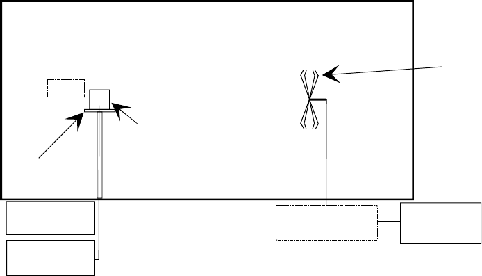
ETSI

E

TSI TR 102 273

-

2

V1.2

.

1 (2001

-

1

2)

7

0

7.2.5.2 Method of measurement

Characterization

The process of characterization should take place within a shielded, totally reflecting enclosure where no absorbing

material is present.

C1) The EUT should be mounted on a non-conducting turntable of low relative dielectric constant (preferably

less than 1,5) material(s) in a shielded enclosure (i.e. no absorber).

C2) The test equipment should be arranged as shown in figure 34. The protecting filter should only be used for

EUTs which are not fitted with an external antenna connector. For those which do have such a connector, the

broadband 50 Ω load should be connected to the EUT and the filter becomes unnecessary.

Turntable

Broadband

test

antenna

EUT

Receiving

device

Protecting

filter

Digital

voltmeter

Power

supply

Load

Figure 34: Elevation view of shielded chamber set up for the characterization tests

C3) The EUT should be mounted in the position closest to normal use as declared by the manufacturer. This

mounting configuration should be recorded on page 1 of the log book results sheet (see table 27).

C4) The broadband test antenna should be aligned for vertical polarization and spaced a convenient distance away

from the EUT.

NOTE 1: For the purposes of this characterization procedure, the range length does not have to meet the conditions

for far-field testing given earlier.

C5) The EUT should be switched on, without modulation, and the receiving device scanned through the

appropriate frequency band, avoiding the carrier frequency and its adjacent channels. All frequencies

producing a response on the receiving device should be recorded on page 2 of the log book results sheet

(see table 27).

NOTE 2: The test antenna should be changed as necessary to ensure that the complete frequency range is covered.

C6) The broadband test antenna should be aligned for horizontal polarization and step C5 repeated.

NOTE 3: The only information provided by the characterization procedure is which frequencies should be

measured in the Anechoic Chamber.

Measurement

NOTE 4: The following procedure steps involve, for every frequency identified in the characterization procedure,

scanning for the peak of the spurious emission in both horizontal and vertical planes around the EUT. The

amplitude peak in both planes is measured in both horizontal and vertical polarizations. Large EUTs,

however, may possess highly directional spurious emissions particularly at high frequencies and, despite

the two plane scanning, there remains for these cases, a small probability that no spurious can be detected.

1) The measurement should always be performed in the absence of modulation.

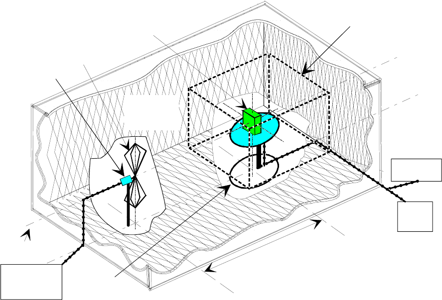
ETSI

E

TSI TR 102 273

-

2

V1.2.1 (2001

-

1

2)

7

1

2) The EUT should be mounted directly onto the turntable, whose surface is at the height specified in the relevant

standard or, where not stated, at a convenient height within the "quiet zone" of the Anechoic Chamber. The EUT

should be mounted in an orientation which matches that of its normal usage as stated by the manufacturer. The

normal to the reference face of the EUT should point directly down the chamber towards the test antenna

support. This is the 0° reference angle for the test. This orientation and mounting configuration should be

recorded on page 1 of the log book results sheet (see table 27). The items of test equipment should be set-up as

shown in figure 35.

NOTE 5: The turntable should be constructed from non-conducting, low relative dielectric constant (preferably less

than 1,5) material(s).

3) The EUT should be positioned such that its volume centre lies on the axis of rotation of the turntable and either

on the central axis of the chamber or at a convenient height within the quiet zone (see figure 35). The offset from

the central axis of the volume centre should be entered on page 2 of the log book results sheet (see table 27).

4) For EUTs fitted with an external antenna connector, the broadband 50 Ω load should be connected in place of

the antenna.

Range length 3 m or 10 m

Turntable

Test

antenna

EUT

Central axis

of chamber

Quiet zone

10 dB attenuator

Receiving

device

Digital

voltmeter

Power

supply

unit

Radio

absorbing

material

Figure 35: Anechoic Chamber set up for Spurious emissions testing on the EUT

5) The test antenna (biconic, LPDA or waveguide horn) should be oriented for vertical polarization. Its output

should be connected to the receiving device via a 10 dB attenuator and the calibrated, ferrited coaxial cable

associated with that end of the chamber, and a protective filter (only if the EUT does not possess an external

antenna connector). The height of the phase centre of the test antenna should be at the same offset (as recorded in

Step 3) from the central axis of the chamber as the volume centre of the EUT, so that the measurement axis is

parallel to the central axis.

NOTE 6: The measurement axis is the straight line between the phase centres of transmitting and receiving devices.

6) The EUT should be switched on, without modulation, and the receiving device tuned to the first frequency

recorded on page 2 of the log book results sheet (see table 27).

7) The EUT should be rotated through 360° in the azimuth plane until the maximum signal level is observed on the

receiving device. The corresponding received level (dBm1) and the angle of the turntable (angle1) should be

recorded on page 2 of the log book results sheet (see table 27).

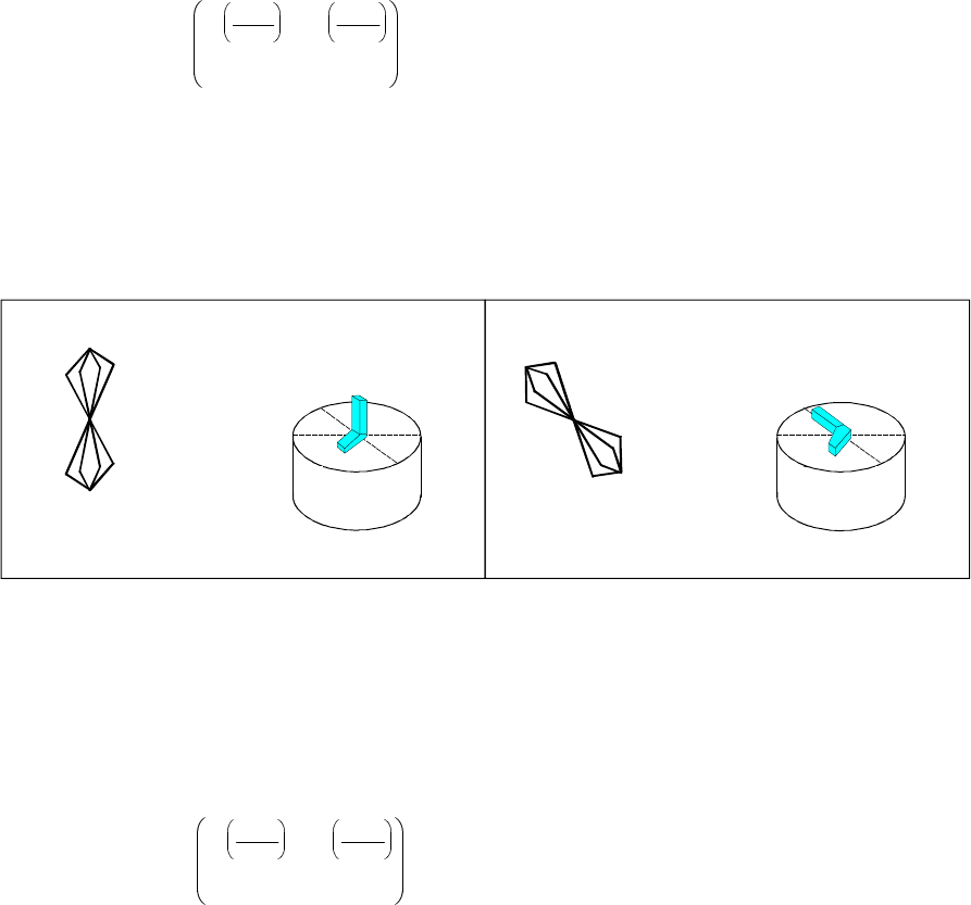
ETSI

E

TSI TR 102 273

-

2

V1.2.1 (2001

-

1

2)

7

2

8) The polarization of the test antenna should be changed to horizontal and the received signal level (dBm2) again

recorded on page 2 of the log book results sheet (see table 27). If this value of signal level is more than 20 dB

below that measured in Step 7, the peak of this spurious, to be entered on page 2 of the log book results sheet

(see table 27) as "Spurious level 1", is simply the level measured in Step 7. Equally, if dBm2 exceeds dBm1 by

more than 20 dB, "Spurious level 1" is simply dBm2. Alternatively, the spurious level should be calculated as:

Spurious level

dBm dBm

= dBm12010 10

12

20 20

log + (7.3)

The resulting value should be entered in the log book results sheet as "Spurious level 1".

9) Retaining the test antenna polarization (horizontal), the EUT should be rotated about its volume centre to lie on

its side as shown in figure 36. The EUT should again be rotated through 360° in the azimuth plane until the

maximum signal level is observed on the receiving device. The corresponding received level (dBm3) and the

angle of the turntable (angle2) should be recorded on page 2 of the log book results sheet (see table 27).

Figure 36: Turning the EUT

10) The polarization of the test antenna should be changed to vertical and the received signal level (dBm4) again

recorded on page 2 of the log book results sheet (see table 27). If this value of signal level is more than 20 dB

below that measured in Step 9, the peak of this spurious, to be entered on page 2 of the log book results sheet

(see table 27) as "Spurious level 2", is simply the level measured in Step 9. Equally, if dBm4 exceeds dBm3 by

more than 20 dB, "Spurious level 2" is simply dBm4. Alternatively, the spurious level should be calculated as:

Spurious level

dBm dBm

= dBm22010 10

34

20 20

log + (7.4)

The resulting value should be entered in the log book results sheet as "Spurious level 2".

Whichever value is the larger of "Spurious level 1" and "Spurious level 2", it should be entered as "Overall

spurious level" on page 2 of the log book results sheet (see table 27).

11) The EUT should be replaced on the turntable by the substitution antenna (a tuned half wavelength dipole which

has been adjusted to correspond to the appropriate frequency or waveguide horn) (see figure 37).

NOTE 7: For all frequencies below 80 MHz, a shortened dipole (as defined in clause 7.1.3) should be used. The

dipole arm length is defined from the centre of the balun block to the tip of the arm. From a fully

extended state, each telescopic element, in turn, should be "pushed in" from the tip until the required

length is obtained. The outermost section needs to fully compress before any of the others, and so on.

Table 17 gives the dipole arm lengths and choice of balun for set frequencies. Where the test frequency

does not correspond to a set frequency in the table, the arm length to be used should be determined by

linear interpolation between the closest set values.

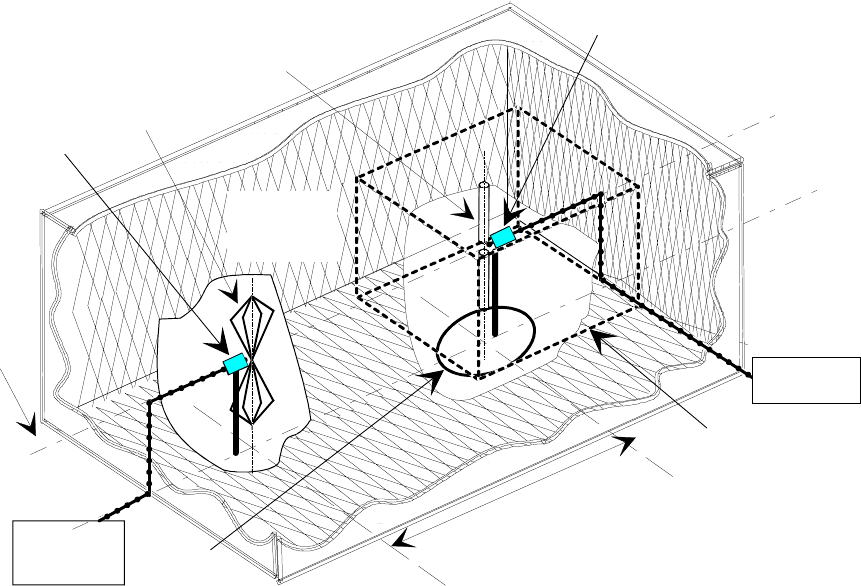
ETSI

E

TSI TR 102 273

-

2

V1.2.1 (2001

-

1

2)

7

3

12) The phase centre of the substitution antenna should lie directly over the axis of rotation of the turntable, whilst

its height should be at the same offset (as recorded in Step 3) from the central axis of the chamber, so that the

measurement axis is again parallel to the central axis.

NOTE 8: The phase centre of a dipole is in the centre of its two rods and for a waveguide horn it is in the centre of

its open mouth.

Range length 3 or 10 m

Turntable

Test

antenna

Substitution

antenna

Central axis

of chamber

Quiet zone

10 dB attenuator

10 dB attenuator

Receiving

device

Signal

generator

Radio

absorbing

material

Figure 37: Substitution antenna replacing the EUT for spurious emission testing

in an Anechoic Chamber

13) The substitution antenna should be oriented for vertical polarization and connected to a calibrated signal

generator via a 10 dB attenuator and the calibrated, ferrited coaxial cable associated with that end of the

chamber.

14) The signal generator should be tuned to the appropriate frequency and its output level adjusted until the level

measured on the receiving device, is at least 20 dB above the level with the output from the signal generator

switched off.

15) The substitution antenna should be rotated until the maximum level is detected on the receiving device.

NOTE 9: This is to correct for possible misalignment of a directional beam (i.e. as produced by waveguide horns in

all tests and by dipoles when used in horizontally polarized tests only). This step can be omitted for

dipoles used in vertically polarized tests.

16) The output level of the signal generator should be adjusted until the level, measured on the receiving device, is

identical to the "Overall spurious level" recorded in Step 10. This output signal level should be recorded (dBm5)

on page 2 of the log book results sheet (see table 27).

NOTE 10: In the event of insufficient range of signal generator output level, the input attenuation to the receiving

device should be decreased to compensate. The signal generator output level (dBm6) and the change in

attenuation (dB, where a decrease is taken as + dB, an increase is taken as - dB) should be recorded on

page 2 of the log book results sheet (see table 27).

17) Steps 2 to 16 should be repeated for all the other frequencies recorded in the log book results sheet (see table 27),

changing the antennas as necessary.

ETSI

E

TSI TR 102 273

-

2

V1.2.1 (2001

-

1

2)

7

4

7.2.5.3 Procedure for completion of the results sheets

There are several values that remain to be entered in the overall results sheet (see table 28). These are the overall

spurious emission levels (corrected for the systematic offsets involved in the measurement) and the expanded

measurement uncertainty.

Guidance for deriving the values of the correction factors is given in table 26.

When the correction factors have been derived, they should be entered on page 2 of the log book results sheet (see

table 27). The overall correction for each spurious frequency can be calculated as follows:

overall correction = substitution antenna cable loss

+ substitution antenna attenuator loss

+ substitution antenna balun loss

+ mutual coupling and mismatch loss (where applicable)

- gain of substitution antenna

NOTE: For frequencies greater than 180 MHz the mutual coupling and mismatch loss factor should be taken as

0,00 dB.

The resulting values should be entered on page 2 of the results sheet (see table 27) and the effective radiated power of

each spurious emission calculated from:

spurious ERP = signal generator output level

- reduction in the input attenuation of receiving device (if any)

+ overall correction

Each value of spurious emission effective radiated power should be entered on page 2 of the log book results sheet (see

table 27) and in the overall results sheet (see table 28).

The final value to be entered in the overall results sheet (see table 28) is that for the expanded uncertainty. This should

be calculated according to clause 7.2.6.

Table 26: Guidance for deriving correction factors

Figures for correction factors

Substitution antenna cable loss Obtained directly from the calibration data

Substitution antenna attenuator loss Obtained from calibration data

Substitution antenna balun loss For dipoles: if not known from calibration data, the value

should be taken as 0,30 dB. For waveguide horns: taken

as 0,00 dB

Mutual coupling and mismatch loss factors between the

test antenna and substitution antenna For ANSI dipoles (30 MHz to 180 MHz) values can be

obtained from TR 102 273-1-1 [8] table A.19. For

frequencies greater than 180 MHz, this value is 0,00 dB.

For non-ANSI dipoles and waveguide horns this value is

0,00 dB

Gain of substitution antenna For ANSI dipoles (30 MHz to 1 000 MHz) the value is

2,10 dBi. For other types of antennas (non-ANSI dipoles or

waveguide horns), the value can be obtained from

calibration data

ETSI

E

TSI TR 102 273

-

2

V1.2.1 (2001

-

1

2)

7

5

7.2.5.4 Log book entries

Table 27: Log book results sheet

SPURIOUS EMISSIONS Date: PAGE 1 of 2

Temperature:…......°

°°

°C Humidity:…............% Frequency:…..........MHz

Manufacturer of EUT:….................. Type No:…........... Serial No:…...............

Bandwidth of Receiving Device…................Hz

Range length:…....................

Test equipment item Type No. Serial No. VSWR Insertion loss

Antenna

factor/gain

Broadband test antenna

(typically 30 MHz to 200 MHz) N/A

Broadband test antenna

(typically 200 MHz to 1 GHz) N/A

Broadband test antenna

(typically 1 GHz to 12,75 GHz) N/A

Test antenna attenuator N/A

Test antenna cable N/A

Substitution antenna (typically

ANSI C63.5 [1] 30 MHz to 1 000 MHz) N/A

Substitution antenna (typically

waveguide horns 1 GHz to 12,75 GHz)

N/A

Substitution antenna attenuator N/A

Substitution antenna cable N/A

Digital voltmeter N/A N/A N/A

Power supply N/A N/A N/A

Receiving device N/A N/A

Signal generator N/A N/A

Ferrite beads N/A N/A N/A

High "Q" notch filter N/A

High pass filter N/A

Mounting configuration of EUT (Characterization)

Mounting configuration of EUT (Measurement)

(continued)

ETSI

E

TSI TR 102 273

-

2

V1.2.1 (2001

-

1

2)

7

6

Table 27 (concluded): Log book results sheet

SPURIOUS EMISSIONS Date: PAGE 2 of 2

Offset of volume centre of the EUT from the central axis of the chamber:……………..m

Frequency (MHz)

dBm1

angle1

dBm2

Spurious level 1 (dBm)

dBm3

angle2

dBm4

Spurious level 2 (dBm)

Overall spurious level (dBm)

Signal generator

output level dBm5 (dBm)

Change in attenuator level (dB)

Spurious emission ERP (dBm)

Correction factors

Frequency (MHz)

Substitution antenna cable loss

Substitution antenna attenuator loss

Substitution antenna balun loss

Mutual coupling and mismatch loss

(30 MHz - 180 MHz)

Gain of the substitution antenna

Overall measurement correction dB dB dB dB dB dB dB

7.2.5.5 Statement of results

The results should be presented in tabular form as shown in table 28.

Table 28: Overall results sheet

SPURIOUS EMISSIONS Date: PAGE 1 of 1

Frequency (MHz)

Spurious emission ERP (dBm)

Expanded uncertainty (95 %) dB dB dB dB dB dB dB

7.2.6 Measurement uncertainty for Spurious emissions

A fully worked example illustrating the methodology to be used can be found in clause 4 of TR 102 273-1-2 [9].

7.2.6.1 Uncertainty contributions: Stage 1: EUT measurement

For the measurement of spurious effective radiated power two stages of test are involved. The first stage (the EUT

measurement) is to measure on the receiving device, a level from the EUT as shown in figure 38 (shaded components

are common to both stages of the test).

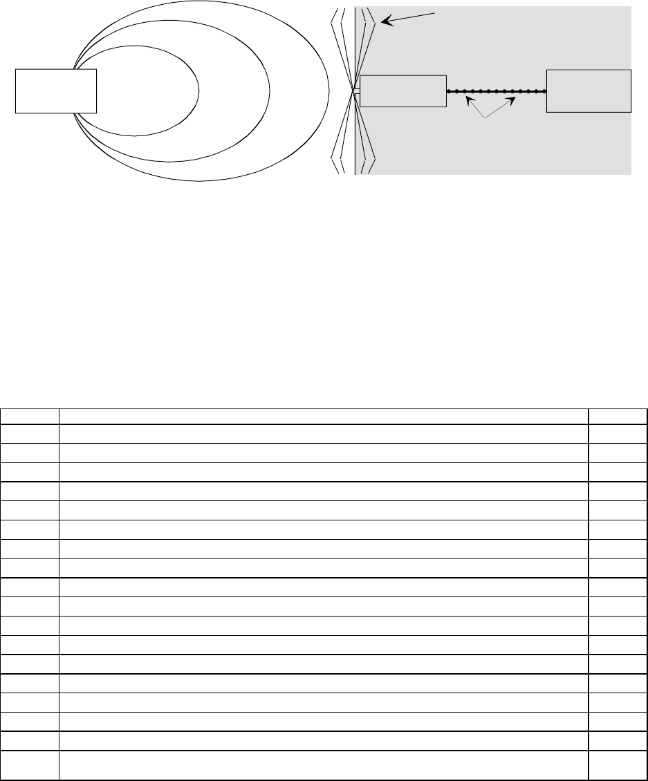
ETSI

E

TSI TR 102 273

-

2

V1.2.1 (2001

-

1

2)

7

7

Test

antenna

cable 2

Test antenna

ferrite beads

Attenuator 2

10 dB Receiving

device

EUT

Figure 38: Stage 1: EUT measurement

Due to the commonality of all of the components from the test antenna to the receiver in both stages of the test, the

mismatch uncertainty contributes identically in each stage and hence cancels. Similarly, the systematic uncertainty

contributions (e.g. test antenna cable loss, etc.) of the individual components also cancel.

The magnitude of the random uncertainty contribution to this stage of the procedure can be assessed from multiple

repetition of the EUT measurement.

All the uncertainty components which contribute to this stage of the test are listed in table 29. Annex A should be

consulted for the sources and/or magnitudes of the uncertainty contributions.

Table 29: Contributions from the EUT measurement

uj or i Description of uncertainty contributions dB

uj37 mismatch: receiving part 0,00

uj40 insertion loss: test antenna attenuator 0,00

uj41 insertion loss: test antenna cable 0,00

uj19 cable factor: test antenna cable

uj47 receiving device: absolute level 0,00

uj54 EUT: influence of setting the power supply on the spurious emission level 0,03

uj20 position of the phase centre: within the EUT volume

uj21 positioning of the phase centre: within the EUT over the axis of rotation of the turntable

uj51 EUT: influence of the ambient temperature on the spurious emission level 0,03

uj16 range length 0,00

uj01 reflectivity of absorbing material: EUT to the test antenna 0,00

uj45 antenna: gain of the test antenna 0,00

uj46 antenna: tuning of the test antenna 0,00

uj55 EUT: mutual coupling to the power leads

uj08 mutual coupling: amplitude effect of the test antenna on the EUT 0,00

uj04 mutual coupling: EUT to its images in the absorbing material

uj06 mutual coupling: test antenna to its images in the absorbing material 0,00

ui01 random uncertainty (see note in clause A.18 of TR 102 273-1-2 and note in clause 6.4.7 of

TR 102 273-1-1)

The standard uncertainties from table 29 should be combined by RSS in accordance with clause 5 of

TR 102 273-1-1 [8]. This gives the combined standard uncertainty (uc contribution from the EUT measurement) for the EUT

measurement in dB.

7.2.6.2 Uncertainty contributions: Stage 2: Substitution measurement

The second stage (the substitution) involves replacing the EUT with a substitution antenna and signal source as shown

in figure 39 and adjusting the output level of the signal generator until the same level as in stage one is achieved on the

receiving device.

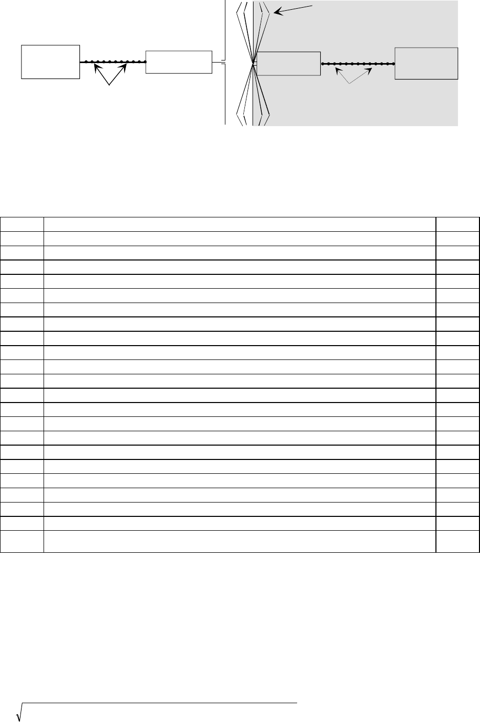
ETSI

E

TSI TR 102 273

-

2

V1.2.1 (2001

-

1

2)

7

8

Test

antenna

cable 2

Test antenna

ferrite beads

Receiving

device

Attenuator

10 dB

cable 2

ferrite beads

Attenuator

10 dB

Signal

generator

Figure 39: Stage 2: Substitution measurement

All the uncertainty components which contribute to this stage of the test are listed in table 30. Annex A should be

consulted for the sources and/or magnitudes of the uncertainty contributions.

Table 30: Contributions from the substitution

uj or i Description of uncertainty contributions dB

uj36 mismatch: transmitting part

uj37 mismatch: receiving part

uj38 signal generator: absolute output level

uj39 signal generator: output level stability

uj19 cable factor: substitution antenna cable

uj19 cable factor: test antenna cable

uj41 insertion loss: substitution antenna cable

uj41 insertion loss: test antenna cable 0,00

uj40 insertion loss: substitution antenna attenuator

uj40 insertion loss: test antenna attenuator 0,00

uj47 receiving device: absolute level 0,00

uj16 range length 0,00

uj02 reflectivity of absorbing material: substitution antenna to the test antenna 0,00

uj45 antenna: gain of the substitution antenna

uj45 antenna: gain of the test antenna 0,00

uj46 antenna: tuning of the test antenna 0,00

uj22 position of the phase centre: substitution antenna

uj06 mutual coupling: substitution antenna to its images in the absorbing material

uj06 mutual coupling: test antenna to its images in the absorbing material

uj11 mutual coupling: substitution antenna to the test antenna 0,00

uj12 mutual coupling: interpolation of mutual coupling and mismatch loss correction factors 0,00

ui01 random uncertainty (see note in clause A.18 of TR 102 273-1-2 and note in clause 6.4.7 of

TR 102 2731-1)

The standard uncertainties from table 30 should be combined by RSS in accordance with clause 5 of

TR 102 273-1-1 [8]. This gives the combined standard uncertainty (uc contribution from the substitution) for the EUT

measurement in dB.

7.2.6.3 Expanded uncertainty of the spurious emission

The combined standard uncertainty of the ERP measurement of the spurious emission is the combination of the

components outlined in clauses 7.2.6.1 and 7.2.6.2. The components to be combined are uc contribution from the EUT

measurement and uc contribution from the substitution.

uu u

c ccontribution fron the EUT measurement ccontribtution fromthe substitution

=+

22

= _ _,_ _dB (7.5)

ETSI

E

TSI TR 102 273

-

2

V1.2.1 (2001

-

1

2)

7

9

The expanded uncertainty is ± 1,96 x uc = ± __,__ dB at a 95 % confidence level.

7.2.7 Adjacent channel power

This test is normally carried out using a Test Fixture and as a result has not been considered for the Anechoic Chamber.

7.3 Receiver tests

The tests carried out on receivers can be divided into two categories, namely sensitivity and immunity. However, only

sensitivity tests are considered here.

7.3.1 Sensitivity tests (30 MHz to 1 000 MHz)

The test method for measuring the maximum or average usable sensitivity of a receiver is in two parts. In the first part,

a transform factor for the chamber (i.e. the relationship in decibels between the output power level (in dBm) from the

signal generator to the resulting electric field strength (in dBµV/m) at the point of test) is determined. In the second

part, the sensitivity of the EUT is measured by finding the lowest output level from the signal generator which produces

the required response at each of eight angles in the horizontal plane.

The receiver output depends on the type of information the receiver has been designed to demodulate. There are

principally three different types of information: analogue speech, bit stream and messages.

Definitions:

For analogue speech:

- the

maximum usable sensitivity expressed as field strength is the minimum of 8 field strength (in dBµV/m)

measurements (at 45° increments in the horizontal plane) at the nominal frequency of the receiver and with

specified test modulation, which produces a SINAD ratio of 20 dB measured at the receiver input through a

telephone psophometric weighting network. The starting horizontal angle is the reference orientation as stated by

the manufacturer.

- the

average usable sensitivity expressed as field strength is the average of eight field strength (in dBµV/m)

measurements (at 45° increments in the horizontal plane) at the nominal frequency of the receiver and with

specified test modulation, which produces a SINAD ratio of 20 dB measured at the receiver input through a

telephone psophometric weighting network. The starting horizontal angle is the reference orientation as stated by

the manufacturer.

For bit stream:

- the

maximum usable sensitivity expressed as field strength is the minimum of eight field strength (in dBµV/m)

measurements (at 45° increments in the horizontal plane) at the nominal frequency of the receiver and with

specified test modulation, which produces, after demodulation, a data signal with a bit error ratio of 10-2

measured at the receiver input. The starting horizontal angle is the reference orientation as stated by the

manufacturer.

- the

average usable sensitivity expressed as field strength is the average of eight field strength (in dBµV/m)

measurements (at 45° increments in the horizontal plane) at the nominal frequency of the receiver and with

specified test modulation, which produces, after demodulation, a data signal with a bit error ratio of 10-2

measured at the receiver input. The starting horizontal angle is the reference orientation as stated by the

manufacturer.

For messages:

- the

maximum usable sensitivity expressed as field strength is the minimum of eight field strength (in dBµV/m)

measurements (at 45° increments in the horizontal plane) at the nominal frequency of the receiver, and with

specified test modulation, which produces, after demodulation, a message acceptance ratio of 80 % measured at

the receiver input. The starting horizontal angle is the reference orientation as stated by the manufacturer.

ETSI

E

TSI TR 102 273

-

2

V1.2.1 (2001

-

1

2)

8

0

- the average usable sensitivity expressed as field strength is the average of eight field strength (in dBµV/m)

measurements (at 45° increments in the horizontal plane) at the nominal frequency of the receiver and with

specified test modulation, which produces, after demodulation, a message acceptance ratio of 80 % measured at

the receiver input. The starting horizontal angle is the reference orientation as stated by the manufacturer.

7.3.1.1 Apparatus required

- digital voltmeter;

- ferrite beads;

- 10 dB attenuators;

- power supply;

- connecting cables;

- Anechoic Chamber;

- test antenna (half wavelength dipole as detailed in ANSI C63.5 [1] recommended);

- measuring antenna (half wavelength dipole as detailed in ANSI C63.5 [1] recommended);

- RF Signal generator;

- receiving device (measuring receiver or spectrum analyser).

Additional requirements for analogue speech:

- AF source;

- SINAD meter (incorporating telephone psophometric weighting network);

- acoustic coupler (alternatively: audio load).

Additional requirements for bit stream:

- bit stream generator;

- bit error measuring test set.

Additional requirements for messages:

- acoustic coupler;

- message generator;

- response measuring test set.

The types and serial numbers of all items of test equipment should be recorded on page 1 of the log book results sheet

(see table 32).

NOTE: The half wavelength dipole antennas, incorporating matching/transforming baluns, for the procedure are

available in the following bands: 20 MHz to 65 MHz, 65 MHz to 180 MHz, 180 MHz to 400 MHz,

400 MHz to 1 000 MHz. Constructional details are contained in ANSI C63.5 [1]. In the recommended

antenna scheme for this band, a shortened dipole is used at all frequencies from 30 MHz up to 80 MHz.

ETSI

E

TSI TR 102 273

-

2

V1.2.1 (2001

-

1

2)

8

1

7.3.1.2 Method of measurement

Determination of the transform factor for the test site

1) For this part of the test, it is necessary to position the measuring antenna within the chamber, such that its phase

centre is at the same point that the phase centre of the EUT will occupy in the second part of the test (the EUT

being mounted in an orientation which matches that of its normal usage as declared by the manufacturer). The

precise point should always be on the axis of rotation of the turntable, and either on the central axis of the

chamber or at a convenient height within the quiet zone. The vertical offset of the phase centre of the EUT from

the central axis (if any) should be either measured remotely or determined by sitting the EUT on the turntable.

The vertical offset should be recorded on page 2 of the log book results sheet (see table 32).

NOTE 1: If the position of the phase centre within the EUT is unknown but the antenna is visible, then the vertical

offset from the central axis of the point at which the antenna meets the case of the EUT should be used. If

the phase centre is unknown and there is no visible antenna the volume centre of the EUT should be used

instead.

2) The measuring antenna (in the recommended scheme: a tuned ANSI C63.5 [1] half wavelength dipole for

frequencies of 80 MHz and above, a shortened dipole for frequencies from 30 MHz up to 80 MHz) should be

adjusted to correspond to the nominal frequency of the EUT and positioned with its phase centre on the axis of

rotation of the turntable and at the same vertical offset from the central axis of the chamber (if any) as

determined for the EUT in Step 1. The measuring antenna should be oriented for vertical polarization.

NOTE 2: For all frequencies below 80 MHz, a shortened dipole (as defined in clause 7.1.3) should be used. The

dipole arm length is defined from the centre of the balun block to the tip of the arm. From a fully

extended state, each telescopic element, in turn, should be "pushed in" from the tip until the required

length is obtained. The outermost section needs to fully compress before any of the others, and so on.

Table 17 gives the dipole arm lengths and choice of balun for set frequencies. Where the test frequency

does not correspond to a set frequency in the table, the arm length to be used should be determined by

linear interpolation between the closest set values.

NOTE 3: The turntable should be constructed from non-conducting, low relative dielectric constant (preferably less

than 1,5) material(s).

3) The measuring antenna should be connected via a 10 dB attenuator and the calibrated, ferrited coaxial cable

associated with that end of the chamber, to the receiving device.

4) The test antenna (identical to the measuring antenna) should be tuned to the nominal frequency of the EUT and

mounted with the height of its phase centre at the same vertical offset from the central axis of the chamber (if

any) as the measuring antenna, so that the measurement axis is parallel to the central axis of the chamber. The

test antenna should be oriented to the same polarization as the measuring antenna.

NOTE 4: The measurement axis is the straight line joining the phase centres of the transmitting and receiving

devices.

5) The test antenna should be connected via a 10 dB attenuator and the calibrated, ferrited coaxial cable associated

with that end of the chamber, to the signal generator whose output is unmodulated (see figure 40). The signal

generator should be tuned to the nominal frequency of the EUT.

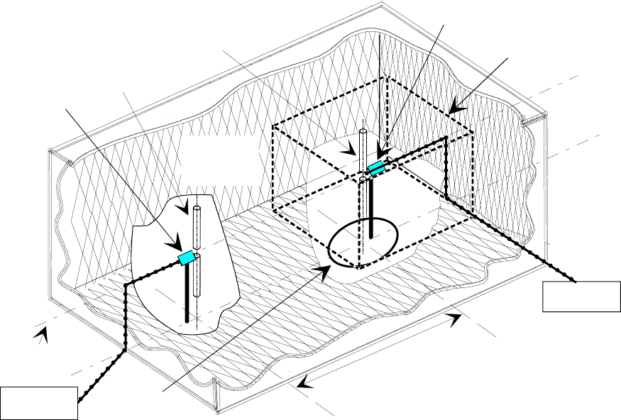
ETSI

E

TSI TR 102 273

-

2

V1.2.1 (2001

-

1

2)

8

2

Range length 3 m or 10 m

Turntable

Test

antenna

Measuring

antenna

Central axis

of chamber

Quiet zone

10 dB attenuator

10 dB attenuator

Receiving

device

Signal

generator

Radio

absorbing

material

Figure 40: Equipment layout for determining the transform factor during sensitivity tests

in an Anechoic Chamber

6) The output level of the signal generator should be adjusted until a received signal level at least 20 dB above the

noise floor is observed on the receiving device.

7) The received signal level (dBµV) appearing on the receiving device along with the output level from the signal

generator (dBm) should be recorded on page 2 of the log book results sheet (see table 32). The transform factor

for the chamber (i.e. the factor relating the output power level from the signal generator (dBm) to the resulting

field strength (dBµV/m) at the point of measurement) should then be calculated according to the following

formula:

Transform Factor (dB) = received signal level (dBµV)

+ measuring antenna cable loss

+ measuring antenna attenuator loss

+ measuring antenna balun loss

+ mutual coupling and mismatch loss correction factor (if applicable)

+ antenna factor of the measuring antenna

- signal generator output level (dBm)

NOTE 5: Guidance for deriving/calculating/finding the unknown values in the above formula for transform factor

are given in table 31. These values should be entered on page 2 of the log book results sheet (see

table 32).

The resulting value for the transform factor should be entered on page 2 of the log book results sheet (see

table 32).

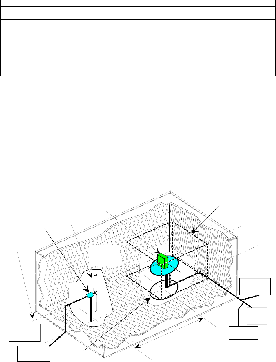
ETSI

E

TSI TR 102 273

-

2

V1.2.1 (2001

-

1

2)

8

3

Table 31: Guidance for deriving Transform Factor

Values in the formula for Transform Factor

Measuring antenna cable loss Obtained directly from the calibration data

Measuring antenna attenuator loss Obtained from calibration data

Measuring antenna balun loss

Mutual coupling and mismatch loss correction factors

between the test antenna and the measuring antenna For ANSI dipoles (30 MHz to 180 MHz) values can be

obtained from TR 102 273-1-1 [8] table A.19. For

frequencies greater than 180 MHz, this value is 0,00 dB.

For non-ANSI dipoles this value is 0,00 dB

Antenna factor of the measuring antenna For ANSI dipoles:

Antenna factor = 20 log10 (f) - 31,4 dB dB/m

(where f is the frequency in MHz) For other types the

value can be obtained from calibration data

Sensitivity measurement on the EUT

8) The measuring antenna should be replaced on the turntable by the EUT. The EUT should be positioned on the

turntable such that its phase centre is in the same place as formerly occupied by the phase centre of the

measuring antenna.

NOTE 6: If the position of the phase centre within the EUT is unknown but the antenna is a single rod which is

visible and vertical in normal usage, the axis of the antenna should be aligned with the axis of rotation of

the turntable. If the phase centre is not known and there is no visible antenna the volume centre of the

EUT should be aligned with the axis of rotation of the turntable.

9) The EUT should be mounted in an orientation which matches that of its normal usage as declared by the

manufacturer. The normal to its reference face should point directly towards the antenna mast. This is the 0°

reference angle for this test. This orientation and mounting configuration should be recorded on page 1 of the log

book results sheet (see table 32).

Range length 3 m or 10 m

Turntable

Test

antenna

EUT

Central axis

of chamber

Quiet zone

10 dB attenuator

Signal

generator

Modulation

detection

Modulation

source

Power

supply

unit

Digital

voltmeter

Radio

absorbing

material

Figure 41: Anechoic Chamber set-up for sensitivity tests on the EUT

ETSI

E

TSI TR 102 273

-

2

V1.2.1 (2001

-

1

2)

8

4

For analogue speech:

10a) The EUT should be connected to the modulation detector (a SINAD meter incorporating a telephone

psophometric weighting network) through an AF load or by an acoustic coupler which is made from low

dielectric constant (i.e. less than 1,5) material(s) for EUTs not fitted with a direct connection (see figure 41).

10b) The signal generator output should be modulated with test modulation AM-1 (produced by the AF source)

and its output level should be adjusted until a psophometrically weighted SINAD ratio of 20 dB is obtained

from the EUT. The corresponding signal generator output power level should be recorded on page 2 of the

log book results sheet (see table 32).

10c) The EUT should be successively rotated through 45° in the horizontal plane to new testing angles of 45°, 90°,

135°, 180°, 225°, 270°, 315° (thereby covering the entire 360° in eight measurements). At each angle

Step 10b should be repeated.

10d) The eight values of signal generator output power level resulting from Steps 10b and 10c should be converted

into field strength values by firstly adding the transform factor to produce the field strength in dBµV/m and

then secondly converting dBµV/m to µV/m i.e.:

1) field strength (dBµV/m) = signal generator level (dBm) + transform factor (dB);

2) field strength (µV/m) = 10(field strength(dBµV/m)/20).

The resulting values in µV/m should be entered on page 2 of the log book results sheet (see table 32).

10e) The test procedure should now continue with Step 11.

For bit stream:

10a) The EUT should be connected to the modulation detector (a bit error measuring test set, which should also

receive a direct input from the bit stream generator) by a direct connection (see figure 41).

10b) The signal generator output should be modulated with test modulation DM-2 (produced by the bit stream

generator) and its output level should be adjusted until a bit error ratio of 10-2 is obtained from the EUT. The

corresponding signal generator output power level should be recorded on page 2 of the log book results sheet

(see table 32).

10c) The EUT should be successively rotated through 45° in the horizontal plane to new testing angles of 45°, 90°,

135°, 180°, 225°, 270°, 315° (thereby covering the entire 360° in eight measurements). At each angle

Step 10b should be repeated.

10d) The eight values of signal generator output power level resulting from Steps 10b and 10c should be converted

into field strength values by firstly adding the transform factor to produce the field strength in dBµV/m and

then secondly converting dBµV/m to µV/m i.e.:

1) field strength (dBµV/m) = signal generator level (dBm) + transform factor (dB);

2) field strength (µV/m) = 10(field strength(dBµV/m)/20).

The resulting values in µV/m should be entered on page 2 of the log book results sheet (see table 32).

10e) The test procedure should now continue with Step 11.

For messages:

10a) The EUT should be connected to the modulation detector (a response measuring test set) via an acoustic

coupler (pipe) which is made from low dielectric constant (i.e. less than 1,5) material(s) (see figure 41).

10b) The signal generator output should be modulated with test modulation DM-3 (produced by the message

generator) and its output level should be adjusted until a message acceptance ratio of <10 % is obtained from

the EUT.

10c) The test message should be transmitted repeatedly from the test antenna, whilst observing for each message

whether a successful response is obtained. The output level of the signal generator should be increased by

2 dB for each occasion that a successful response is NOT obtained.

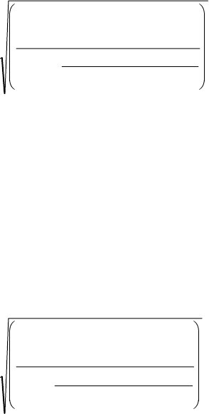
ETSI

E

TSI TR 102 273

-

2

V1.2.1 (2001

-

1

2)

8

5

10d) Step 10c should be repeated until three consecutive successful responses are observed at the same output

level from the signal generator. The output level from the signal generator should be recorded on page 2 of

the log book results sheet (see table 32).

10e) The output signal level from the signal generator should be reduced by 1 dB. The new signal level should be

recorded on page 2 of the log book results sheet (see table 32) and the response of the EUT observed.

10f) If a successful response is NOT obtained, the output signal level should be increased by 1 dB and the new

level recorded in the results sheet. If a successful response IS obtained, the input level should not be changed

until three consecutive successful responses have been observed. In this case, the output signal level from the

signal generator should be reduced by 1 dB and the new level recorded in the results sheet. No signal levels

should be recorded unless preceded by a change of level.

10g) Step 10f should be repeated until a total of 10 recorded values for the signal generator output level have been

entered on page 2 of the log book results sheet (see table 32).

10h) The EUT should be successively rotated through 45° in the horizontal plane to new testing angles of 45°, 90°,

135°, 180°, 225°, 270°, 315° (thereby covering the entire 360° in 8 measurements). At each angle Steps 10b

to 10g should be repeated.

10i) For each angle, the ten recorded values of the signal generator output level (dBm) should be converted to

field strength (µV/m) by firstly adding the transform factor to produce the field strength in dBµV/m and then

secondly converting dBµV/m to µV/m i.e.:

1) field strength (dBµV/m) = signal generator level (dBm) + transform factor (dB);

2) field strength (µV/m) = 10(field strength(dBµV/m)/20).

The resulting values in µV/m should be entered on page 2 of the log book results sheet (see table 32).

10j) For each angle, the ten new recorded values of field strength in µV/m should be averaged according to the

following formula:

Average field strength (µV/m) =

()

10

1

2

1

10

field strength V/m i

i

i

µ

=

=

∑ (7.6)

The resulting eight average values should also be entered on page 2 of the log book results sheet (see table 32).

10k) The procedure should continue with Step 11.

11) For the maximum sensitivity test only, the lowest of the eight values of field strength (µV/m) calculated during

the multiple-stage Step 10 represents the minimum field strength to which the EUT responds. This minimum

value of field strength (µV/m) should be entered on page 2 of the log book results sheet (see table 32) as the

maximum sensitivity.

12) For the average sensitivity test only, the average of the eight values of field strength (dBµV/m) calculated during

the multiple-stage Step 10 represents the average field strength to which the EUT responds. This average value

of field strength in µV/m should now be calculated by the following:

Average field strength (µV/m) =

()

8

1

2

1

8

field strength V/m i

i

i

µ

=

=

∑ (7.7)

This average value of field strength (µV/m) should be entered on page 2 of the log book results sheet (see

table 32) as the average sensitivity.

13) Steps 2 to 12 should be repeated with both the test and measuring antennas oriented for horizontal polarization.

ETSI

E

TSI TR 102 273

-

2

V1.2.1 (2001

-

1

2)

8

6

7.3.1.3 Procedure for completion of the results sheets

All the necessary processing of the measured results is carried out during the course of the test procedure. The only

calculation that remains to be performed before the overall results sheet (see table 33) can be completed is the

determination of the expanded uncertainty of the measurement. This should be performed as given in clause 7.3.2 and

the resulting value entered in the overall results sheet (see table 33).

7.3.1.4 Log book entries

Table 32: Log book results sheet

RECEIVER SENSITIVITY Date: PAGE 1 of 2

Temperature:.........°

°°

°C Humidity:...............% Frequency:.............MHz

Manufacturer of EUT:..................... Type No:.............. Serial No:..................

Range length:.......................

Test equipment item Type No. Serial No. VSWR Insertion

loss Antenna

factor

Test antenna N/A

Test antenna attenuator N/A

Test antenna cable N/A

Measuring antenna N/A

Measuring antenna attenuator N/A

Measuring antenna cable N/A

Ferrite beads

N/A N/A N/A

Receiving device N/A N/A

Signal generator N/A N/A

Digital voltmeter

N/A N/A N/A

Power supply

N/A N/A N/A

AF source (if applicable)

N/A N/A N/A

SINAD meter (if applicable)

N/A N/A N/A

AF load (if applicable)

N/A N/A N/A

Bit stream generator (if applicable)

N/A N/A N/A

Bit error measuring test set (if applicable)

N/A N/A N/A

Acoustic coupler (if applicable)

N/A N/A N/A

Message generator (if applicable)

N/A N/A N/A

Response measuring test set (if

applicable)

N/A N/A N/A

Mounting configuration of EUT

ETSI

E

TSI TR 102 273

-

2

V1.2.1 (20

0

1

-

1

2)

8

7

RECEIVER SENSITIVITY (analogue speech) Date: PAGE 2 of 2

Vertical polarization Horizontal polarization

Vertical offset from the central axis m Vertical offset from the central axis m

Received signal level dBµV Received signal level dBµV

Output level from signal generator dBm Output level from signal generator dBm

Transform Factor dB Transform Factor dB

Signal generator level (dBm) against angle for

20 dB SINAD Signal generator level (dBm) against angle for

20 dB SINAD

0°

°°

° 45°

°°

° 90°

°°

° 135°

°°

°

180°

°°

°

225°

°°

°

270°

°°

°

325°

°°

°

0°

°°

° 45°

°°

° 90°

°°

° 135°

°°

°

180°

°°

°

225°

°°

°

270°

°°

°

325°

°°

°

level

level

Conversion to µ

µµ

µV/m Conversion to µ

µµ

µV/m

0°

°°

° 45°

°°

° 90°

°°

° 135°

°°

°

180°

°°

°

225°

°°

°

270°

°°

°

325°

°°

°

0°

°°

° 45°

°°

° 90°

°°

° 135°

°°

°

180°

°°

°

225°

°°

°

270°

°°

°

325°

°°

°

level

level

MAXIMUM Sensitivity µV/m MAXIMUM Sensitivity µV/m

AVERAGE Sensitivity µV/m AVERAGE Sensitivity µV/m

Values in the formula for Transform Factor

Measuring antenna cable loss Measuring antenna cable loss

Measuring antenna attenuator loss Measuring antenna attenuator loss

Measuring antenna balun loss Measuring antenna balun loss

Mutual coupling and mismatch loss

(30 MHz - 180 MHz) Mutual coupling and mismatch loss

(30 MHz - 180 MHz)

Antenna factor of the measuring

antenna Antenna factor of the measuring

antenna

Vertical offset from the central axis m Vertical offset from the central axis m

Received signal level dBµV Received signal level dBµV

Output level from signal generator dBm Output level from signal generator dBm

Transform Factor dB Transform Factor dB

RECEIVER SENSITIVITY (bit stream) Date: PAGE 2 of 2

Vertical polarization Horizontal polarization

Vertical offset from the central axis m Vertical offset from the central axis m

Received signal level dBµV Received signal level dBµV

Output level from signal generator dBm Output level from signal generator dBm

Transform Factor dB Transform Factor dB

Signal generator level (dBm) against angle for

10-2 BER

Signal generator level (dBm) against angle for

10-2 BER

0°

°°

° 45°

°°

° 90°

°°

° 135°

°°

°

180°

°°

°

225°

°°

°

270°

°°

°

325°

°°

°

0°

°°

° 45°

°°

° 90°

°°

° 135°

°°

°

180°

°°

°

225°

°°

°

270°

°°

°

325°

°°

°

level

level

Conversion to µ

µµ

µV/m Conversion to µ

µµ

µV/m

0°

°°

° 45°

°°

° 90°

°°

° 135°

°°

°

180°

°°

°

225°

°°

°

270°

°°

°

325°

°°

°

0°

°°

° 45°

°°

° 90°

°°

° 135°

°°

°

180°

°°

°

225°

°°

°

270°

°°

°

325°

°°

°

level

level

MAXIMUM Sensitivity µV/m MAXIMUM Sensitivity µV/m

AVERAGE Sensitivity µV/m AVERAGE Sensitivity µV/m

Values in the formula for Transform Factor

Measuring antenna cable loss Measuring antenna cable loss

Measuring antenna attenuator loss Measuring antenna attenuator loss

Measuring antenna balun loss Measuring antenna balun loss

Mutual coupling and mismatch loss

(30 MHz - 180 MHz) Mutual coupling and mismatch loss

(30 MHz - 180 MHz)

Antenna factor of the measuring

antenna Antenna factor of the measuring

antenna

ETSI

E

TSI TR 102 273

-

2

V1.2.1 (2001

-

1

2)

8

8

RECEIVER SENSITIVITY (messages) Date: PAGE 2 of 2

Vertical polarization Horizontal polarization

Vertical offset from the central axis m Vertical offset from the central axis m

Received signal level dBµV Received signal level dBµV

Output level from signal generator dBm Output level from signal generator dBm

Transform Factor dB Transform Factor dB

Signal generator level (dBm) against angle Signal generator level (dBm) against angle

level

0°

°°

° 45°

°°

° 90°

°°

° 135°

°°

°

180°

°°

°

225°

°°

°

270°

°°

°

325°

°°

°

level

0°

°°

° 45°

°°

° 90°

°°

° 135°

°°

°

180°

°°

°

225°

°°

°

270°

°°

°

325°

°°

°

1 1

2 2

3 3

4 4

5 5

6 6

7 7

8 8

9 9

10 10

Conversion to µ

µµ

µV/m Conversion to µ

µµ

µV/m

level

0°

°°

° 45°

°°

° 90°

°°

° 135°

°°

°

180°

°°

°

225°

°°

°

270°

°°

°

325°

°°

°

level

0°

°°

° 45°

°°

° 90°

°°

° 135°

°°

°

180°

°°

°

225°

°°

°

270°

°°

°

325°

°°

°

1 1

2 2

3 3

4 4

5 5

6 6

7 7

8 8

9 9

10 10

Ave.

Ave.

MAXIMUM Sensitivity µV/m MAXIMUM Sensitivity µV/m

AVERAGE Sensitivity µV/m AVERAGE Sensitivity µV/m

Values in the formula for Transform Factor

Measuring antenna cable loss Measuring antenna cable loss

Measuring antenna attenuator loss Measuring antenna attenuator loss

Measuring antenna balun loss Measuring antenna balun loss

Mutual coupling and mismatch loss

(30 MHz - 180 MHz) Mutual coupling and mismatch loss

(30 MHz - 180 MHz)

Antenna factor of the measuring

antenna Antenna factor of the measuring

antenna

7.3.1.5 Statement of results

The results should be presented in tabular form as shown in table 33.

Table 33: Overall results sheet

RECEIVER SENSITIVITY Date: PAGE 1 of 1

Vertical polarization Horizontal polarization

MAXIMUM Usable Sensitivity µV/m MAXIMUM Usable Sensitivity µV/m

AVERAGE Usable Sensitivity µV/m AVERAGE Usable Sensitivity µV/m

Expanded uncertainty (95 %) dB Expanded uncertainty (95 %) dB

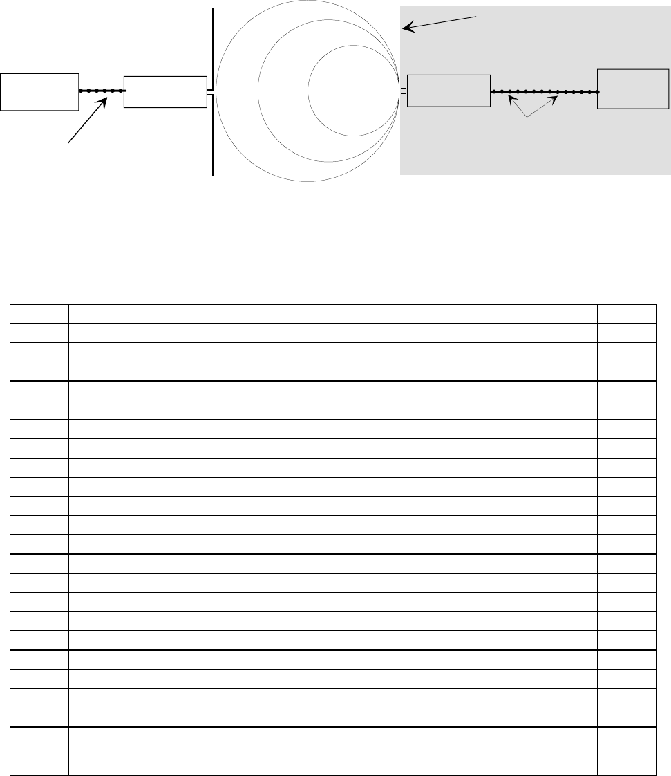
ETSI

E

TSI TR 102 273

-

2

V1.2.1 (2001

-

1

2)

8

9

7.3.2 Measurement uncertainty for Receiver sensitivity

A fully worked example illustrating the methodology to be used can be found in clause 4 of TR 102 273-1-2 [9].

7.3.2.1 Uncertainty contributions: Stage 1: Determination of Transform Factor

The first stage (determining the transform factor) involves placing a measuring antenna as shown in figure 42 and

determining the relationship between the signal generator output power level and the resulting field strength (the shaded

areas in figure 42 represent components common to both stages of the test).

Test

antenna

cable 2

ferrite beads

Test antenna

Signal

generator

Attenuator 2

10 dB

Measuring

antenna

Measuring

antenna

cable 1

Receiving

device Attenuator 1

10 dB

Figure 42: Stage 1: Transform Factor

All the uncertainty components which contribute to this stage of the test are listed in table 34. Annex A should be

consulted for the sources and/or magnitudes of the uncertainty contributions.

Table 34: Contributions for the Transform Factor

uj or i Description of uncertainty contributions dB

uj36 mismatch: transmitting part 0,00

uj37 mismatch: receiving part

uj38 signal generator: absolute output level

uj39 signal generator: output level stability

uj19 cable factor: measuring antenna cable

uj19 cable factor: test antenna cable 0,00

uj41 insertion loss: measuring antenna cable

uj41 insertion loss: test antenna cable 0,00

uj40 insertion loss: measuring antenna attenuator

uj40 insertion loss: test antenna attenuator 0,00

uj47 receiving device: absolute level

uj16 range length 0,00

uj02 reflectivity of absorber material: measuring antenna to the test antenna 0,00

uj44 antenna: antenna factor of the measuring antenna

uj45 antenna: gain of the test antenna 0,00

uj46 antenna: tuning of the measuring antenna

uj46 antenna: tuning of the test antenna 0,00

uj22 position of the phase centre: measuring antenna

uj06 mutual coupling: measuring antenna to its images in the absorbing material

uj06 mutual coupling: test antenna to its images in the absorbing material 0,00

uj11 mutual coupling: measuring antenna to the test antenna 0,00

uj12 mutual coupling: interpolation of mutual coupling and mismatch loss correction factors 0,00

ui01 random uncertainty (see note in clause A.18 of TR 102 273-1-2 and note in clause 6.4.7 of

TR 102 273-1-1)

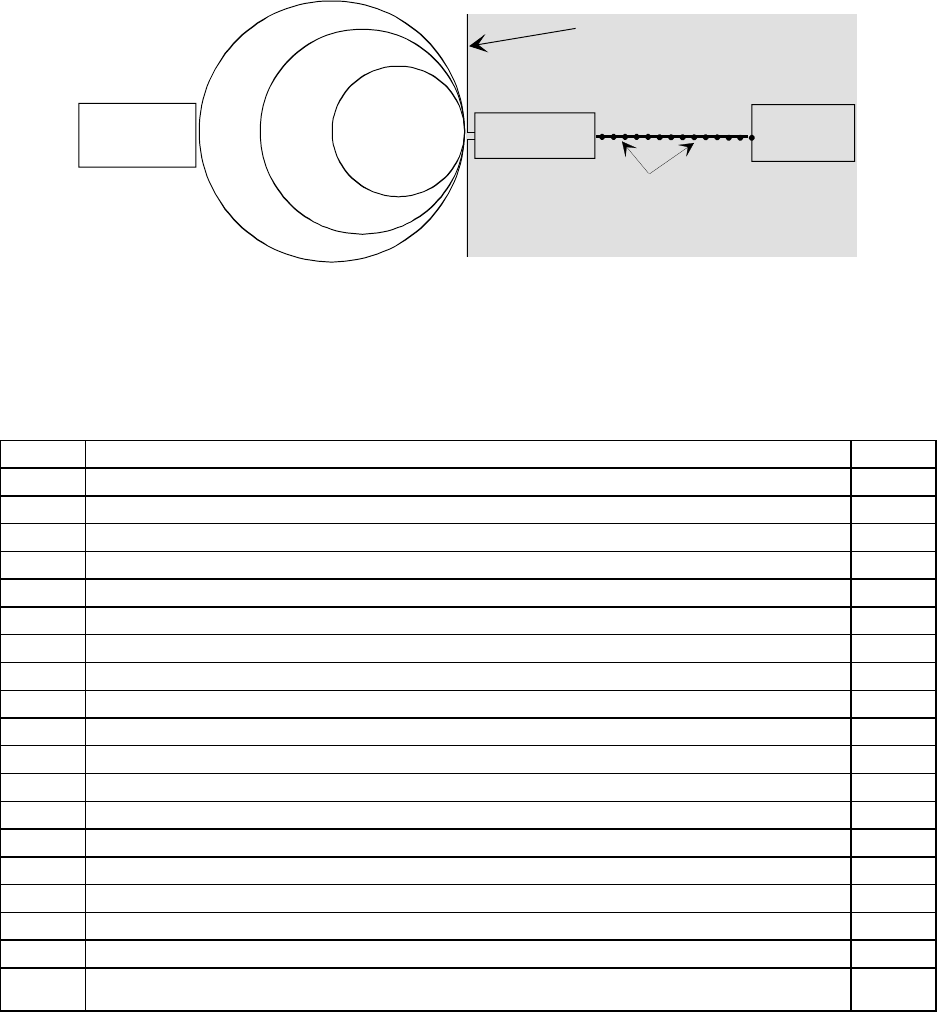
ETSI

E

TSI TR 102 273

-

2

V1.2.1 (2001

-

1

2)

9

0

The standard uncertainties from table 34 should be combined by RSS in accordance with clause 5 of

TR 102 273-1-1 [8]. This gives the combined standard uncertainty (uc contributions from the Transform Factor) for the

Transform Factor in dB.

7.3.2.2 Uncertainty contributions: Stage 2: EUT measurement

The second stage (the EUT measurement) is to determine the minimum signal generator output level which produces

the required response from the EUT as shown in figure 43 (the shaded areas represent components common to both

stages of the test).

Test

antenna

cable 2

ferrite beads

Test antenna

Signal

generator

Attenuator 2

10 dB

EUT

Figure 43: Stage 2: EUT measurement

All the uncertainty components which contribute to this stage of the test are listed in table 35. Annex A should be

consulted for the sources and/or magnitudes of the uncertainty contributions.

Table 35: Contributions from the EUT measurement

uj or i Description of uncertainty contributions dB

uj36 mismatch: transmitting part

uj37 mismatch: receiving part

uj38 signal generator: absolute output level

uj39 signal generator: output level stability

uj19 cable factor: test antenna cable 0,00

uj41 insertion loss: test antenna cable 0,00

uj40 insertion loss: test antenna attenuator 0,00

uj20 position of the phase centre: within the EUT volume

uj22 positioning of the phase centre: within the EUT over the axis of rotation of the turntable

uj52 EUT: modulation detection

uj16 range length 0,00

uj01 reflectivity of absorber material: EUT to the test antenna

uj45 antenna: gain of the test antenna 0,00

uj46 antenna: tuning of the test antenna 0,00

uj55 EUT: mutual coupling to the power leads

uj08 mutual coupling: amplitude effect of the test antenna on the EUT 0,00

uj04 mutual coupling: EUT to its images in the absorbing material

uj06 mutual coupling: test antenna to its images in the absorbing material 0,00

ui01 random uncertainty (see note in clause A.18 of TR 102 273-1-2 and note in clause 6.4.7 of

TR 102 273-1-1)

The standard uncertainties from table 35 should be combined by RSS in accordance with clause 5 of

TR 102 273-1-1 [8]. This gives the combined standard uncertainty (uc contribution from the EUT measurement) for the EUT

measurement in dB.

ETSI

E

TSI TR 102 273

-

2

V1.2.1 (2001

-

1

2)

9

1

7.3.2.3 Expanded uncertainty of the receiver sensitivity measurement

The combined uncertainty of the sensitivity measurement is the combination of the components outlined in

clauses 7.3.2.1 and 7.3.2.2. The components to be combined are uc contribution from the Transform Factor and uc contribution

from the EUT measurement.

uu u

c ccontribution fromtheTransform Factor c contribution fromthe EUT measurement

=+

22

= _ _,_ _ dB (7.8)

The expanded uncertainty is ± 1,96 x uc = ± __,__ dB at a 95 % confidence level.

7.3.3 Co-channel rejection

This test is normally carried out using a Test Fixture and as a result has not been considered for the Anechoic Chamber.

7.3.4 Adjacent channel selectivity

This test is normally carried out using a Test Fixture and as a result has not been considered for the Anechoic Chamber.

7.3.5 Intermodulation immunity

This test is normally carried out using a Test Fixture and as a result has not been considered for the Anechoic Chamber.

7.3.6 Blocking immunity or desensitization

This test is normally carried out using a Test Fixture and as a result has not been considered for the Anechoic Chamber.

7.3.7 Spurious response immunity to radiated fields (30 MHz to 4 GHz)

In this test method, two signals are transmitted simultaneously towards the EUT. One is the wanted signal, whilst the

other is an unwanted, interfering signal. Both signals are transmitted from the same test antenna, into which they are fed

through a combining network. The wanted signal (in the range 30 MHz - 1 000 MHz) is at the nominal frequency of the

receiver and is transmitted at the level specified in the ETS. The unwanted signal has a different modulation to the

wanted signal and is at a very much higher power level.

Definition

The spurious response immunity to radiated fields is a measure of the capability of the receiver to discriminate between

the wanted modulated radiated field at the nominal frequency and an unwanted radiated field at any other frequency at

which a response is obtained.

For analogue speech: it is specified as the ratio, in decibels, of an unwanted signal level expressed as field

strength to a specified wanted signal level expressed as field strength producing, through a telephone

psophometric weighting network, a SINAD ratio of 14 dB.

For bit stream: it is specified as the ratio, in decibels, of an unwanted signal level expressed as field strength to

a specified wanted signal level expressed as field strength producing a data signal with a bit error ratio of 10-2.

For messages: it is specified as the ratio, in decibels, of an unwanted signal level expressed as field strength to a

specified wanted signal level expressed as field strength producing after demodulation a message acceptance

ratio of 80 %.

7.3.7.1 Apparatus required

- digital voltmeter;

- ferrite beads;

- 10 dB attenuators;

ETSI

E

TSI TR 102 273

-

2

V1.2.1 (2001

-

1

2)

9

2

- power supply;

- connecting cables;

- combining network;

- RF load;

- power amplifier;

- 3 axis field probe;

- Anechoic Chamber;

- test antenna (broadband antenna recommended e.g. biconic, typically 30 MHz to 200 MHz, LPDAs,

- typically 200 MHz to 1 GHz and 1 GHz to 4 GHz);

- measuring antenna (half wavelength dipole as detailed in ANSI C63.5 [1] recommended);

- swept frequency RF signal generator;

- receiving device (measuring receiver or spectrum analyser);

- AF source.

Additional requirements for analogue speech:

- AF source;

- SINAD Meter (incorporating telephone psophometric weighting network);

- acoustic coupler (alternatively: audio load).

Additional requirements for bit stream:

- bit stream generator;

- bit error measuring test set.

Additional requirements for messages:

- acoustic coupler;

- message generator;

- response measuring test set.

The types and serial numbers of all items of test equipment should be recorded on page 1 of the log book results sheet

(see table 37).

NOTE: The half wavelength dipole antennas, incorporating matching/transforming baluns, for the procedure are

available in the following bands: 20 MHz to 65 MHz, 65 MHz to 180 MHz, 180 MHz to 400 MHz,

400 MHz to 1 000 MHz. Constructional details are contained in ANSI C63.5 [1]. In the recommended

antenna scheme for this band, a shortened dipole is used at all frequencies from 30 MHz up to 80 MHz.

ETSI

E

TSI TR 102 273

-

2

V1.2.1 (2001

-

1

2)

9

3

7.3.7.2 Method of measurement

Determination of the transform factor for the Anechoic Chamber

1) For this part of the test, it is necessary to position either the 3-axis probe (if it possesses adequate dynamic range

to allow the wanted field strength to be measured) or the measuring antenna (in the recommended scheme: a

tuned ANSI C63.5 [1] half wavelength dipole for frequencies of 80 MHz and above, a shortened dipole for

frequencies from 30 MHz up to 80 MHz) within the chamber such that its phase centre is at the same point that

the phase centre of the EUT will occupy in the second part of the test (the EUT being mounted in an orientation

which matches that of its normal usage as declared by the manufacturer). The precise point should always be on

the axis of rotation of the turntable, and either on the central axis of the chamber or at a convenient height within

the quiet zone. The vertical offset of the phase centre of the EUT from the central axis (if any) should be either

measured remotely or determined by sitting the EUT on the turntable. The offset should be recorded on page 2 of

the log book results sheet (see table 37).

NOTE 1: If the position of the phase centre within the EUT is unknown but the antenna is visible, then the vertical

offset from the central axis of the point at which the antenna meets the case of the EUT should be used. If

the phase centre is unknown and there is no visible antenna the volume centre of the EUT should be used

instead.

NOTE 2: If a 3-axis probe is being used to measure the field strength of the wanted signal, Steps 2 and 3 should be

omitted.

2) The measuring antenna should be adjusted to correspond to the nominal frequency of the EUT and positioned

with its phase centre on the axis of rotation of the turntable and at the same vertical offset from the central axis

of the chamber (if any) as determined for the EUT in Step 1. The measuring antenna should be oriented for

vertical polarization.

NOTE 3: For all frequencies below 80 MHz, a shortened dipole (as defined in clause 7.1.3) should be used. The

dipole arm length is defined from the centre of the balun block to the tip of the arm. From a fully

extended state, each telescopic element, in turn, should be "pushed in" from the tip until the required

length is obtained. The outermost section needs to fully compress before any of the others, and so on.

Table 17 gives the dipole arm lengths and choice of balun for set frequencies. Where the test frequency

does not correspond to a set frequency in the table, the arm length to be used should be determined by

linear interpolation between the closest set values.

NOTE 4: The turntable should be constructed from non-conducting, low relative dielectric constant (preferably less

than 1,5) material(s).

3) The measuring antenna should be connected via a 10 dB attenuator and the calibrated, ferrited coaxial cable

associated with that end of the chamber, to the receiving device.

4) The test antenna (a broadband antenna which is functional at both the nominal frequency of the EUT as well as

covering either the calculated frequency at which a spurious response may occur or part of the limited frequency

range) should be tuned to the nominal frequency of the EUT and mounted with the height of its phase centre at

the same vertical offset from the central axis of the chamber (if any) as recorded in Step 1, so that the

measurement axis is parallel to the central axis of the chamber. The test antenna should be oriented to the same

polarization as the measuring antenna.

NOTE 5: The measurement axis is the straight line joining the phase centres of the transmitting and receiving

devices.

5) The test antenna should be connected via a 10 dB attenuator and the calibrated, ferrited coaxial cable associated

with that end of the chamber, to signal generator A (see figure 44) via the combiner whose other port should be

terminated with the RF load. The output from signal generator A should be unmodulated and tuned to the

nominal frequency of the EUT.

NOTE 6: Steps 6 and 7 should be omitted if a 3-axis probe is being used to measure the wanted field strength.

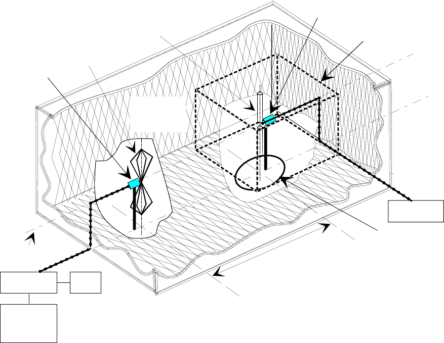
ETSI

E

TSI TR 102 273

-

2

V1.2

.

1 (2001

-

1

2)

9

4

Range length 3 m or 10 m

Turntable

Test

antenna

Measuring

antenna

Central axis

of chamber

Quiet zone

10 dB attenuator

10 dB attenuator

Radio

absorbing

material

Combiner

Signal

generator

A

Load

Receiving

device

Figure 44: Equipment layout for determining the transform factor in an Anechoic Chamber

(using a measuring antenna)

6) The output level of the signal generator A should be adjusted until a received signal level at least 20 dB above

the noise floor is observed on the receiving device.

7) The received signal level (dBµV) appearing on the receiving device along with the output level from the signal

generator (dBm) should be recorded on page 2 of the log book results sheet (see table 37). The transform factor

for the chamber (i.e. the factor relating the output power level from the signal generator (dBm) to the resulting

field strength (dBµV/m) at the point of measurement) should then be calculated according to the following

formula:

Transform Factor (dB) = received signal level (dBµV)

+ measuring antenna cable loss

+ measuring antenna attenuator loss

+ measuring antenna balun loss

+ mutual coupling and mismatch loss correction factor (if applicable)

+ antenna factor of the measuring antenna

- signal generator output level (dBm)

NOTE 7: Guidance for deriving/calculating/finding the unknown values in the above formula for transform factor

are given in table 36. The resulting values should be entered on page 2 of the log book results sheet (see

table 37).

The resulting value for the transform factor should be entered on page 2 of the log book results sheet

(see table 37).

ETSI

E

TSI TR 102 273

-

2

V1.2.1 (2001

-

1

2)

9

5

Table 36: Guidance for deriving Transform Factor

Values in the formula for Transform Factor

Measuring antenna cable loss Obtained directly from the calibration data

Measuring antenna attenuator loss Obtained from calibration data

Measuring antenna balun loss If not known from calibration data, the value should be

taken as 0,30 dB.

Mutual coupling and mismatch loss correction factors

between the test antenna and the measuring antenna For ANSI dipoles (30 MHz to 180 MHz) values can be

obtained from TR 102 273-1-1 [8] table A19. For

frequencies greater than 180 MHz, this value is 0,00 dB.

For non-ANSI dipoles this value is 0,00 dB

Antenna factor of the measuring antenna For ANSI dipoles:

Antenna factor = 20 log10 (f) - 31,4 dB dB/m

(where f is the frequency in MHz)

For other types the value can be obtained from calibration

data

8) If a measuring antenna is being used, the output power level of the signal generator (dBm) should be adjusted,

using the calculated value for the transform factor, to provide the wanted signal level (dBµV/m, as specified in

the relevant testing standard) in the vicinity of the EUT. Alternatively, if a 3-axis probe is being used to measure

the field strength, the output power level of the signal generator (dBm) should be adjusted to provide the wanted

signal level (dBµV/m, as specified in the relevant testing standard).

EUT set-up

9) The 3-axis probe or measuring antenna should be replaced on the turntable by the EUT. The EUT should be

positioned on the turntable such that its phase centre is in the same place as formerly occupied by the centre of

the 3-axis probe or the phase centre of the measuring antenna.

NOTE 8: If the position of the phase centre within the EUT is unknown but the antenna is a single rod which is

visible and vertical in normal usage, the axis of the antenna should be aligned with the axis of rotation of

the turntable. If the phase centre is not known and there is no visible antenna the volume centre of the

EUT should be aligned with the axis of rotation of the turntable.

10) The EUT should be mounted in an orientation which matches that of its normal usage as declared by the

manufacturer. The normal to its reference face should point directly towards the test antenna. This is the 0°

reference angle for the test. This orientation and mounting configuration should be recorded on page 1 of the log

book results sheet (see table 37).

Measurement of the EUT

11) The two signal generators should be connected to the test antenna as shown in figure 45. Signal generator A

provides the wanted signal. It should remain at the level set in Step 8 and at the nominal frequency of the

EUT. Signal generator B and the power amplifier provide the interfering, unwanted signal. Test modulation

A-M3, produced by an AF source, should be applied to the modulator input of signal generator B which should

be tuned to the lowest frequency of the limited frequency range (defined in the relevant testing standard).

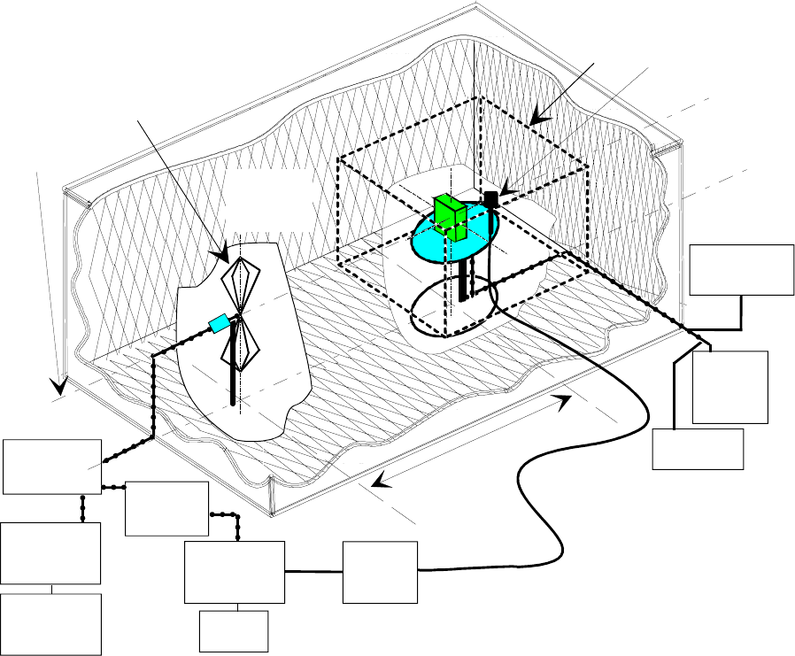
ETSI

E

TSI TR 102 273

-

2

V1.2.1 (2001

-

1

2)

9

6

Range length 3 m or 10 m

Test

antenna

Central axis

3-axis

probe

Modulation

Quiet

zone

Combining

network

Modulation

source AF

Power

amplifier

probe

meter

3-axis

Digital

voltmeter

Radio

absorbing

material

Source

of chamber

detection

Power

supply

unit

Signal

generator

AB

Signal

generator

Figure 45: Anechoic Chamber set-up for Spurious response immunity tests

For analogue speech:

12a) Signal generator A should be modulated with test modulation A-M1 produced by the AF source. Signal

generator B should then have its level adjusted to give a field strength, as measured by the 3-axis probe,

which is 80 dB in excess of the wanted signal level. The output power of signal generator B should then be

levelled at this field strength, using the 3-axis probe, to ensure that at any frequency, the generated field

strength is the same. The frequency of the unwanted signal should then be continuously varied over the entire

limited frequency range noting any frequencies which degrade the SINAD ratio below 20 dB. These

frequencies should be recorded on page 2 of the log book results sheet (see table 37).

NOTE 9: The response time of the SINAD meter should be taken into account when deciding the sweep speed for

signal generator B.

12b) In turn, signal generator B should be tuned to each of the frequencies recorded in Step 12a as well as to those

frequencies outside the limited frequency range at which it has been calculated that a response may occur. At

each frequency, the output power level of signal generator B should be adjusted to provide a 14 dB SINAD

ratio from the EUT. The corresponding value of field strength (µV/m), as measured on the 3-axis probe,

should be recorded on page 2 of the log book results sheet (see table 37).

NOTE 10: The field strength measurement on the unwanted signal can be made despite the presence of the wanted

signal since its magnitude is greatly in excess of that for the wanted signal.

12c) The spurious response immunity ratio to radiated fields for analogue speech should be calculated, for each of

the frequencies concerned, as the ratio in dB of the field strength of the unwanted signal to the wanted signal

level at the receiver input and should be recorded on page 2 of the log book results sheet (see table 37).

12d) The procedure should continue with clause 7.3.7.3.

ETSI

E

TSI TR 102 273

-

2

V1.2.1 (2001

-

1

2)

9

7

For bit stream:

12a) Signal generator A should be modulated with test modulation D-M2 produced by the bit stream generator.

The reference bit stream output from the bit stream generator should be connected to the reference bit stream

input on the bit error detector. Signal generator B should then be adjusted to give a field strength, as

measured by the 3-axis probe, which is 80 dB in excess of the wanted signal level. The output power of

signal generator B should then be levelled at this field strength, using the 3-axis probe, to ensure that at any

frequency, the generated field strength is the same. The frequency of the unwanted signal should then be

continuously varied over the entire limited frequency range noting any frequencies which produce a response

i.e. a change in bit error ratio. These frequencies should be recorded on page 2 of the log book results sheet

(see table 37).

NOTE 11: The response time of the bit error measuring test set should be taken into account when deciding the

sweep speed for signal generator B.

12b) In turn, signal generator B should be tuned to each of the frequencies recorded in Step 12a as well as to those

frequencies outside the limited frequency range at which it has been calculated that a response may occur. At

each frequency, the output power level of signal generator B should be adjusted to provide a bit error ratio of

10-2 from the EUT. The corresponding value of field strength (µV/m), as measured on the 3-axis probe,

should be recorded on page 2 of the log book results sheet (see table 37).

12c) The spurious response immunity ratio to radiated fields for bit stream should be calculated, for each of the

frequencies concerned, as the ratio in dB of the field strength of the unwanted signal to the wanted signal

level at the receiver input and should be recorded on page 2 of the log book results sheet (see table 37).

12d) The procedure should continue with clause 7.3.7.3.

For messages:

12a) The EUT should be monitored via an acoustic coupler (pipe) which is made from low dielectric constant

(i.e. less than 1,5) material(s) for message acceptance.

NOTE 12: The test sequence which ensures the 80 % message acceptance criterion is very time consuming. It is

considered impractical to combine this test sequence with a continuous frequency sweep (as occurs in the

corresponding procedures for analogue speech and bit stream data) since the sweep speed for signal

generator B would have to be extremely slow to allow capture of narrow band spurious responses.

Therefore the test is carried out for the calculated response frequencies only.

12b) Signal generator A should be modulated with test modulation D-M3 produced by the message generator and

signal generator B should be tuned to the first frequency for which it has been calculated that a response

might occur.

12c) The wanted signal should then be transmitted repeatedly and the unwanted signal switched on. The input

level of the unwanted signal should be adjusted until a message acceptance ratio of less than 10 % is

obtained.

12d) The level of the unwanted signal should be reduced by 2 dB for each occasion that a successful response is

not observed. This procedure should be continued until three consecutive successful responses have been

observed. The value of field strength as indicated by the 3-axis probe should then be recorded on page 2 of

the log book results sheet (see table 37).

12e) The unwanted signal level should be increased by 1 dB and the new value of field strength recorded on

page 2 of the log book results sheet (see table 37). The wanted signal should then be continuously

repeated. In each case if a response is NOT obtained the level of the unwanted signal should be reduced by

1 dB and the new field strength value recorded in the results sheet. If a successful response IS obtained, the

level of the unwanted signal should not be changed until three consecutive successful responses have been

obtained. In this case the unwanted signal should be increased by 1 dB and the new field strength value

recorded on page 2 of the log book results sheet (see table 37). No levels of the field strength should be

recorded unless preceded by a change in level. The measurement should be stopped after a total of 10 values

have been recorded.

ETSI

E

TSI TR 102 273

-

2

V1.2.1 (2001

-

1

2)

9

8

12f) The ten values of field strength recorded during Steps 12d and 12e should then be averaged according to the

following formulation:

Average field strength (µV/m) =

()

10

1

2

1

10

field strength V/m i

i

i

µ

=

=

∑ (7.9)

12g) Steps 12c to 12f should be repeated at each frequency within the specified frequency range at which it is

calculated that a spurious response could occur.

12h) The spurious response immunity to radiated fields for messages should be calculated, for the frequency

concerned, as the ratio in dB of the average field strength of the unwanted signal (Step 12f) to the wanted

signal level at the receiver input and should be recorded on page 2 of the log book results sheet (see table 37).

12i) The procedure should continue with clause 7.3.7.3.

7.3.7.3 Procedure for completion of the results sheets

No special processing of the results is necessary to provide the spurious response immunity, since all calculations are

performed during the procedure. However, to complete the overall results sheet (see table 38) it is necessary, firstly to

transfer some or all of the response frequencies and their corresponding values for spurious response immunity and

secondly to calculate the expanded measurement uncertainty associated with the procedure. This should be carried out

as detailed in clause 7.3.8.

ETSI

E

TSI TR 102 273

-

2

V1.2.1 (2001

-

1

2)

9

9

7.3.7.4 Log book entries

Table 37: Log book results sheet

SPURIOUS RESPONSE IMMUNITY Date: Page 1 of 2

Temperature:…......°

°°

°C Humidity:…............% Frequency:…..........MHz

Manufacturer of EUT:….................. Type No:…........... Serial No:…...............

Range length:…....................

Test equipment item Type No. Serial No. VSWR Insertion

loss Antenna

factor

Test antenna N/A

Test antenna attenuator N/A

Test antenna cable N/A

Measuring antenna N/A

Measuring antenna attenuator N/A

Measuring antenna cable N/A

Ferrite beads N/A N/A N/A

Combining network N/A N/A

RF load N/A N/A

Signal generator N/A N/A

Digital voltmeter N/A N/A N/A

Power supply N/A N/A N/A

Frequency modulation source N/A N/A N/A

AF source (if applicable) N/A N/A N/A

SINAD meter (if applicable) N/A N/A N/A

AF load (if applicable) N/A N/A N/A

Bit stream generator (if applicable) N/A N/A N/A

Bit error measuring test set (if applicable)

N/A N/A N/A

Acoustic coupler (if applicable) N/A N/A N/A

Message generator (if applicable) N/A N/A N/A

Response measuring test set

(if applicable) N/A N/A N/A

Mounting configuration of EUT

(continued)

ETSI

E

TSI TR 102 273

-

2

V1.2.1 (2001

-

1

2)

1

00

Table 37 (continued): Log book results sheet

SPURIOUS RESPONSE IMMUNITY (analogue speech) Date: Page 2 of 2

Vertical offset from the central axis m

Received signal level dBµV

Signal generator output level dBm

Transform Factor dB

Wanted signal level: µV/m Limited frequency range: MHz

Response and calculated

frequencies (MHz)

F

ield strength of unwanted

signal for

14 dB SINAD (µ

µµ

µV/m)

Spurious response immunity:

Field strength of unwanted signal -

Wanted signal level

(dB)

Values in the formula for Transform Factor

Measuring antenna cable loss Measuring antenna cable loss

Measuring antenna attenuator loss Measuring antenna attenuator loss

Measuring antenna balun loss Measuring antenna balun loss

Mutual coupling and mismatch loss

(30 MHz to 180 MHz) Mutual coupling and mismatch loss

(30 MHz to 180 MHz)

Antenna factor of the measuring

antenna Antenna factor of the measuring

antenna

SPURIOUS RESPONSE IMMUNITY (bit stream) Date: Page 2 of 2

Vertical offset from the central axis m

Received signal level dBµV

Signal generator output level dBm

Transform Factor dB

Wanted signal level: µV/m Limited frequency range: MHz

Response and calculated

frequencies (MHz)

F

ield strength of unwanted

signal for

10-2 BER (µ

µµ

µV/m)

Spurious response immunity:

Field strength of unwanted signal -

Wanted signal level

(dB)

Values in the formula for Transform Factor

Measuring antenna cable loss Measuring antenna cable loss

Measuring antenna attenuator loss Measuring antenna attenuator loss

Measuring antenna balun loss Measuring antenna balun loss

Mutual coupling and mismatch loss

(30 MHz to 180 MHz) Mutual coupling and mismatch loss

(30 MHz to 180 MHz)

Antenna factor of the measuring

antenna Antenna factor of the measuring

antenna

(continued)

ETSI

E

TSI TR 102 273

-

2

V1.2.1 (2001

-

1

2)

1

01

Table 37 (concluded): Log book results sheet

SPURIOUS RESPONSE IMMUNITY (messages) Date: Page 2 of 2

Vertical offset from the central axis m

Received signal level dBµV

Signal generator output level dBm

Transform Factor dB

Wanted signal level: µV/m Limited frequency range: MHz

Calculated frequencies

(MHz)

F

ield strength of unwanted

signal for

80 % acceptance (µ

µµ

µV/m)

Spurious response immunity:

Field strength of unwanted signal -

Wanted signal level

(dB)

Values in the formula for Transform Factor

Measuring antenna cable loss

Measuring antenna cable loss

Measuring antenna attenuator loss

Measuring antenna attenuator loss

Measuring antenna balun loss

Measuring antenna balun loss

Mutual coupling and mismatch loss

(30 MHz to 180 MHz)

Mutual coupling and mismatch loss

(30 MHz to 180 MHz)

Antenna factor of the measuring

antenna

Antenna factor of the measuring

antenna

7.3.7.5 Statement of results

The results should be presented in tabular form as shown in table 38.

Table 38: Overall results sheet

SPURIOUS RESPONSE IMMUNITY Date: Page 1 of 1

Frequency (MHz) Spurious response immunity (dB)

Expanded uncertainty (95 %) dB

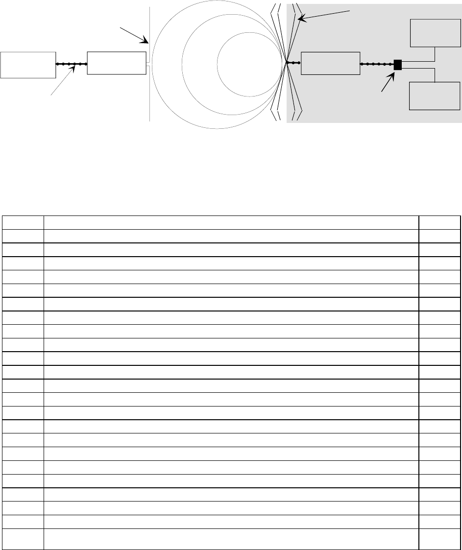
ETSI

E

TSI TR 102 273

-

2

V1.2.1 (2001

-

1

2)

1

02

7.3.8 Measurement uncertainty for Spurious response immunity

A fully worked example for the measurement uncertainty involved in this test has not been given in clause 4 of

TR 102 273-1-2 [9], although the procedure is basically the same as those given.

7.3.8.1 Uncertainty contributions: Stage 1: Transform factor

If the first stage involved measuring the transform factor (as shown in figure 46) i.e. the relationship between the output

level of the signal generator (dBm) and the resulting field strength (dBµV/m) in the vicinity of the turntable, then the

shaded areas in figure 46 represent components common to both stages of the test.

Test

antenna

cable 2

Test antenna

Measuring

antenna

Signal combiner

Wanted

signal

Attenuator 2

10 dB

Load

Attenuator 1

10 dB

receiving

device

Measuring

antenna

cable 1

Figure 46: Stage 1: Transform factor

All the uncertainty components which contribute to this stage of the test are listed in table 39. Annex A should be

consulted for the sources and/or magnitudes of the uncertainty contributions.

Table 39: Contributions for the Transform Factor

uj or i Description of uncertainty contributions dB

uj36 mismatch: transmitting part

uj37 mismatch: receiving part

uj38 signal generator: absolute output level

uj39 signal generator: output level stability

uj19 cable factor: measuring antenna cable

uj19 cable factor: test antenna cable

uj41 insertion loss: measuring antenna cable

uj41 insertion loss: test antenna cable 0,00

uj40 insertion loss: measuring antenna attenuator

uj40 insertion loss: test antenna attenuator 0,00

uj47 receiving device: absolute level

uj16 range length 0,00

uj02 reflectivity of absorber material: measuring antenna to the test antenna 0,00

uj44 antenna: antenna factor of the measuring antenna

uj45 antenna: gain of the test antenna 0,00

uj46 antenna: tuning of the measuring antenna

uj46 antenna: tuning of the test antenna 0,00

uj22 position of the phase centre: measuring antenna

uj06 mutual coupling: measuring antenna to its images in the absorbing material

uj06 mutual coupling: test antenna to its images in the absorbing material 0,00

uj11 mutual coupling: measuring antenna to the test antenna 0,00

uj12 mutual coupling: interpolation of mutual coupling and mismatch loss correction factors 0,00

ui01 random uncertainty (see note in clause A.18 of TR 102 273-1-2 and note in clause 6.4.7 of

TR 102 273-1-1)

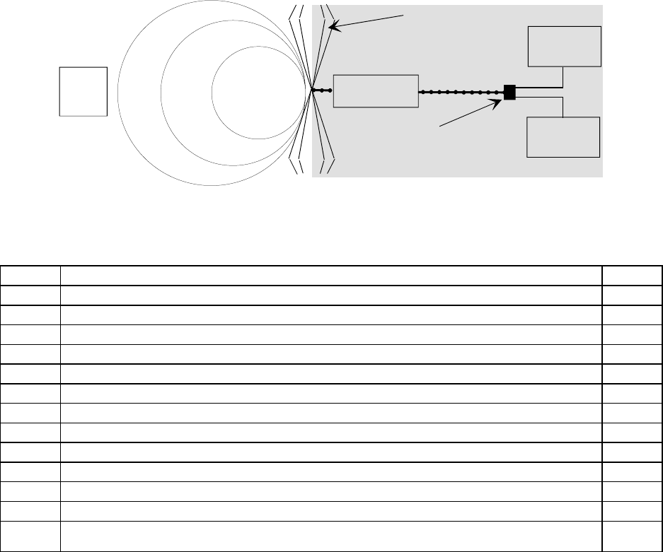
ETSI

E

TSI TR 102 273

-

2

V1.2.1 (2001

-

1

2)

1

03

Alternatively, if the 3-axis probe was used, then figure 47 illustrates the test equipment set-up and table 40 lists the

uncertainty components that contribute.

Test

antenna

cable 2

Test antenna

Signal combiner

Wanted

signal

Attenuator 2

10 dB

Load

3-axis

probe

meter

Figure 47: Stage 1: 3-axis probe

Table 40: Contributions for the 3-axis probe

uj or i Description of uncertainty contributions dB

uj36 mismatch: transmitting part 0,00

uj38 signal generator: absolute output level 0,00

uj39 signal generator: output level stability

uj19 cable factor: test antenna cable

uj41 insertion loss: test antenna cable 0,00

uj40 insertion loss: test antenna attenuator 0,00

uj16 range length

uj45 antenna: gain of the test antenna 0,00

uj46 antenna: tuning of the test antenna 0,00

uj06 mutual coupling: test antenna to its images in the absorbing material 0,00

uj12 mutual coupling: interpolation of mutual coupling and mismatch loss correction factors 0,00

uj28 field strength measurement as determined by the 3-axis probe

ui01 random uncertainty (see note in clause A.18 of TR 102 273-1-2 and note in clause 6.4.7 of

TR 102 273-1-1)

The standard uncertainties from table 39 of table 40 should be combined by RSS in accordance with clause 5 of

TR 102 273-1-1 [8]. This gives the combined standard uncertainty (uc contributions from the Transform Factor) for the

transform factor in dB.

7.3.8.2 Uncertainty contributions: Stage 2: EUT measurement

In this stage, the wanted signal is set to the level specified in the standard using either the transform factor of the

three-axis probe. The unwanted signal is then switched on and the level adjusted until the level of the unwanted signal,

as measured on the three-axis probe, is at the wanted signal level plus the spurious response rejection ratio required. The

schematic of the equipment set-up is shown in figure 48.

All the uncertainty components that contribute to this stage of the test are listed in table 41. Annex A should be

consulted for the sources and/or magnitudes of the uncertainty contributions.

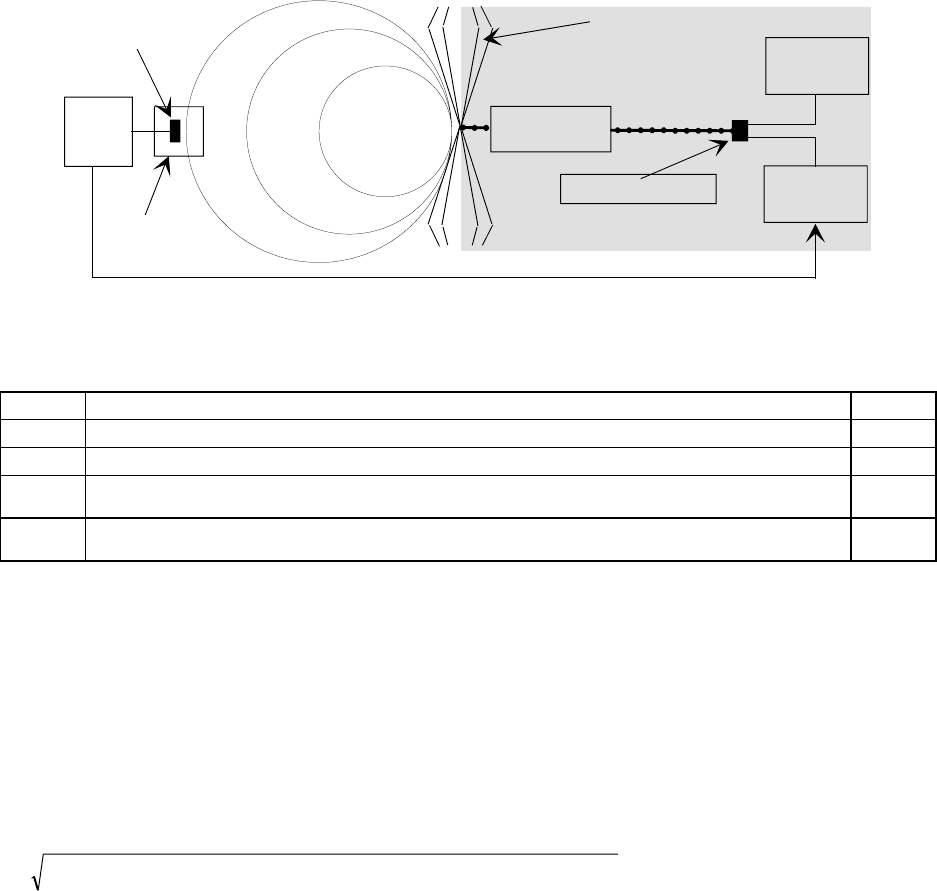
ETSI

E

TSI TR 102 273

-

2

V1.2.1 (20

0

1

-

1

2)

1

04

Test

antenna

cable 2

Test antenna

Measuring

antenna

EUT

3-axis

probe

meter

Signal combiner Unwanted

signal

Wanted

signal

Attenuator 2

10 dB

Figure 48: Stage 2: EUT measurement

Table 41: Contributions from the EUT measurement

uj or i Description of uncertainty contributions dB

uj20 position of the phase centre: within the EUT volume

uj52 EUT: modulation detection

uj28 field strength measurement as determined by the 3-axis probe (unwanted signal

measurement)

ui01 random uncertainty (see note in clause A.18 of TR 102 273-1-2 and note in clause 6.4.7 of

TR 102 273-1-1)

The standard uncertainties from table 41 should be combined by RSS in accordance with clause 5 of

TR 102 273-1-1 [8]. This gives the combined standard uncertainty (uc contribution from the EUT measurement) for the EUT

measurement in dB.

7.3.8.3 Expanded uncertainty of the spurious response immunity measurement

The combined uncertainty of the spurious response immunity measurement is the combination of the components

outlined in clauses 7.3.8.1 and 7.3.8.2. The components to be combined are (uc contribution from the Transform Factor and uc

contribution from the EUT measurement.

uu u

c ccontribution fromtheTransform Factor c contribution fromthe EUT measurement

=+

22

= __,__ dB (7.10)

The expanded uncertainty is ± 1,96 x uc = ± __,__ dB at a 95 % confidence level.

ETSI

E

TSI TR 102 273

-

2

V1.2.1 (2001

-

1

2)

1

05

Annex A:

Bibliography

- "A designers guide to shielding", Hewlett Packard: RF and microwave measurement symposium and exhibition.

- "Analysis of trials on Artificial Human Body", I. L. Gallan and P. R. Brown Interference technology

international consultants ltd. Contract ref MC/078.

- "Calculation of site attenuation from antenna factors" A. A. Smith Jr, RF German and J B Pate. IEEE

transactions EMC. Vol. EMC 24 pp 301-316 Aug 1982.

- "Computer simulation and measurements of electromagnetic fields close to phantom Humans", Electricity and

magnetism in biology and medicine by Martin Blank, Ed 1993 San Francisco Press.

- "Control of errors on Open Area Test Sites", A. A. Smith Jnr. EMC technology October 1982 page 50-58.

- "Fundamentals of RF and Microwave Power Measurements", Hewlett Packard: Application note 64-1

August 1977.

- "Getting better results from an Open Area Test Site", Joseph DeMarinus.

- "Guide to the evaluation and expression of the uncertainties associated with the results of electrical

measurements", Ministry of Defence: 00-26/Issue 2: September 1988.

- "Measurement uncertainty generally", Statens Tekniske Provenaevn, The Danish Accreditation Committee

(STP). June 1988 (Danish).

- "Specifications for equipment's for use in the Land Mobile Service" CEPT Recommendation T/R 24-01.

- "Techniques for measuring narrowband and broadband EMI signals using spectrum analysers", Hewlett Packard

RF and microwave measurement symposium and exhibition.

- "The expression of uncertainty in electrical measurement", B3003, November 1987 National Measurement

Accreditation Service (NAMAS).

- "The gain resistance product of the half-wave dipole", W. Scott Bennet Proceedings of IEEE vol. 72 No. 2

Dec 1984 pp 1824-1826.

- "Uncertainties of Measurement for NATLAS electrical testing laboratories. NAMAS policy and general notes",

National Testing Laboratory Accreditation Scheme (NATLAS), NIS20 July 1986 (English)

- "Use of Simulated Human Bodies in pager receiver sensitivity measurements", K.Siwiak and W.Elliott III.

Southcom /92 conference, Orlando 1992. pp 189/92.

- "Usikkerhed pa maleresultater" (Per Bennich, Institute for Product Development: "Uncertainty of measured

results"). October 1988. (Danish).

- "Standard site method for determining antenna factors", A. A. Smith Jr. IEEE transactions EMC. Vol EMC 24

pp 316-322 Aug 1982.

- 50(161) IEC 1990.

- Advanced National certificate mathematics, PEDOE, Hodder and Stoughton Volumes I and II.

- "Antenna engineering handbook", R. C. Johnson, H. Jasik.

- "Antennas and radio wave propagation", R. E. Collin, McGraw Hill.

- "Antennas", John D. Kraus, Second edition, McGraw Hill.

- "Chambers Science and Technology dictionary", 1988. Published by Chambers Cambridge.

- "Digital Communications", John G. Proakis, McGraw-Hill International Editions, second edition.

ETSI

E

TSI TR 102 273

-

2

V1.2.1 (2001

-

1

2)

1

06

- Guide to the Expression of Uncertainty in Measurement (International Organization for Standardization, Geneva,

Switzerland, 1995).

- "Radiowave propagation and antennas for personal communications", K. Siwiak, Artech House Publications.

- "The telecommunications factbook and illustrated dictionary", Kahn, Delmar publications Inc. New York 1992.

- "Vocabulary of metrology", British Standard Institution (BSI): PD 6461: Part 2: September 1980.

- "Wave transmission", F. R. Conner, Arnold 1978.

ETSI

E

TSI TR 102 273

-

2

V1.2.1 (2001

-

1

2)

1

07

History

Document history

Edition 1 February 1998 Publication as ETR 273-2

V1.2.1 December 2001 Publication