UFVM V1.0 U FVM User Guide
User Manual:
Open the PDF directly: View PDF ![]() .
.
Page Count: 56
9/6/2017
uFVM v1.0
CFD Academic Tool developed in
MATLAB® – User Manual
Computational Mechanics Lab
AMERICAN UNIVERSITY OF BEIRUT

1
1 CONTENTS
2 Introduction ............................................................................................................................. 3
2.1 Using The Manual ............................................................................................................ 3
2.1.1 About The Manual ................................................................................................... 3
2.1.2 Terms of Use ............................................................................................................ 3
2.2 About The Code Development and Authors ................................................................... 3
2.2.1 What’s uFVM? ......................................................................................................... 3
2.2.2 The Place and Time of Development ....................................................................... 3
2.2.3 Developers ............................................................................................................... 3
2.3 Range of Applicability ...................................................................................................... 4
2.4 A Glance into uFVM’s Discretization and Solution Methods .......................................... 4
3 Structure of The Code ............................................................................................................. 6
3.1 Source Files ...................................................................................................................... 6
3.2 Tutorials ........................................................................................................................... 6
4 Introductory Test Case ............................................................................................................ 7
4.1 Main File: Running a Case ............................................................................................... 7
4.2 Example ........................................................................................................................... 7
4.2.1 Header ..................................................................................................................... 7
4.2.2 Setup Solver Class .................................................................................................... 8
4.2.3 Read OpenFOAM Files ............................................................................................. 8
4.2.4 Setup Time ............................................................................................................... 9
4.2.5 Setup Equations ....................................................................................................... 9
4.2.6 Initialize Case ........................................................................................................... 9
4.2.7 Running the Case ..................................................................................................... 9
5 Reading and Plotting OpenFOAM Mesh ................................................................................ 10
6 An Introductory Presentation of uFVM Functions ................................................................ 15
6.1 Application Class ............................................................................................................ 15
6.2 Reading OpenFOAM Files and Translation to uFVM ..................................................... 15
6.3 Fixing Time Settings ....................................................................................................... 16
6.4 Interpreting the Model/Equations ................................................................................ 16
6.5 Running the Case ........................................................................................................... 20
6.5.1 Time Loop/Convergence Loop ............................................................................... 20
2
6.5.2 Assembling Equation Terms .................................................................................. 21
6.5.2.1 Transient Term .................................................................................................. 23
6.5.2.2 Convection Term ............................................................................................... 24
6.5.2.3 Diffusion Term ................................................................................................... 24
6.5.2.4 Source Term....................................................................................................... 25
6.5.2.5 ‘mdot_f’ Term .................................................................................................... 26
6.5.2.6 Pressure Correction Treatment for Free Surface Flow ...................................... 28
6.5.2.7 False Transience ................................................................................................ 28
6.5.2.8 Gradient Computation ....................................................................................... 29
6.5.2.9 Implicit Under-Relaxation .................................................................................. 31
6.5.2.10 Residual Form of the Equation ...................................................................... 32
6.5.2.11 Residual Computation ................................................................................... 32
6.5.2.12 Assembling Fluxes to Global Assembly Matrix .............................................. 34
6.5.3 Solving the Equation Algebraic System ................................................................. 39
6.5.3.1 SOR Solver ......................................................................................................... 40
6.5.3.2 ILU Solver ........................................................................................................... 40
6.5.3.3 AMG Linear Solver ............................................................................................. 40
6.5.4 Correcting Equation Solution ................................................................................ 41
6.6 Convergence .................................................................................................................. 43
6.7 Post-processing ............................................................................................................. 44
7 Tutorials ................................................................................................................................. 45
7.1 Basic ............................................................................................................................... 45
7.2 Incompressible .............................................................................................................. 48
7.3 Heat Transfer ................................................................................................................. 53

3
2 INTRODUCTION
2.1 USING THE MANUAL
2.1.1 About The Manual
This manual provides an overview about uFVM code. The manual describes with sufficient
details the structure of the code, the range of applicability and who may use it. The way through
which a CFD case is prepared is then described and plenty of tutorials are accordingly provided.
In other words, this manual presents a complete set of instructions for the user to follow in
order to setup a CFD problem.
2.1.2 Terms of Use
uFVM is an academic CFD tool made for learning purposes. It provides a package of libraries and
algorithms that the user can comfortably follow up. Handling, distributing or modifying is fully
permissible; the user has the full permission to add any piece of code or modify an existing one.
2.2 ABOUT THE CODE DEVELOPMENT AND AUTHORS
2.2.1 What’s uFVM?
The name of the code presents an abbreviation letters of the finite volume method (FVM) that
the code is based on. The “u” at the beginning of the name points for a fluid flow. The code is
developed in Matlab® environment because it is assumed that the majority of interested people
are familiar with this environment.
2.2.2 The Place and Time of Development
The code is developed in the computational mechanics lab at the American University of Beirut,
Beirut, Lebanon. The development has started in 2003 and was built and updated gradually
through years. Lots of versions were made each of them had a different structure but
necessarily the same theoretical background.
2.2.3 Developers
The code is a direct accomplishment of the CFD group at the American University of Beirut. The
CFD group is a team of professors, graduate and undergraduate students. Their main objective is
to build computational knowledge and work on plenty of related topics in both tracks
development and application. The team is very familiar with Ansys Fluent® and OpenFOAM®;
they utilize these packages for many purposes. uFVM for example was validated in reference to
these packages. The group’s accomplishments, research topics and published work are posted
on their website https://feaweb.aub.edu.lb/research/cfd. The major contributor to the code is

4
Professor Marwan Darwish
1
. A co-contributor to the code is Professor Fadl Moukalled
2
. The
other contributors to the code are Master and PhD students who accomplished their theses and
dissertations from the computational mechanics lab at the American University of Beirut.
2.3 RANGE OF APPLICABILITY
uFVM works for incompressible fluid flows with any type of mesh (structured and unstructured).
For consistency, the code doesn’t include any geometry modeling or meshing capabilities. It
accepts mesh files of OpenFOAM format.
It is worth mentioning that uFVM is a solver which solves the conservation equations (transport
equations) where the user is able to investigate any physical quantity of interest which is
transported by means of a physical phenomenon like convection and diffusion. It is possible also
to set any form of an explicit term into the conservation equation like external forces; these are
treated as source terms. A transient treatment is also included. The domain usually assumes a
fluid flow. However, the code may still apply to solid domains if the user seeks certain transport
quantities in a solid, obviously the temperature distribution.
The code may also handle multi-phase flows. The current distributed version of uFVM doesn’t
include compressible and multi-phase solvers as they are still under construction and revision.
For further information about the status of multi-phase solver, the user may contact any of the
contributors.
It is not the purpose of this code to provide a CFD tool for conducting fluid flow simulations for
heavy/complex applications. There are two issues to raise here. First, this code is made for those
who are mainly learning CFD and/or interested in CFD code development. This code provides a
very useful and helpful means for those people. Second, the user should necessarily realize that
Matlab is a highly user friendly language; this makes it very convenient for learning issues much
more than it is for conducting real life engineering applications. However, this friendly user
specialty had an expense at the computational time; Matlab is slower than other lower level
languages.
2.4 A GLANCE INTO UFVM’S DISCRETIZATION AND SOLUTION METHODS
Only pressure-based methods are available in uFVM with SIMPLE method as the default scheme.
The default convection scheme is the Upwind scheme, but however, different convection
schemes are also available like (SOU, QUICK, SMART, etc.). Gradient computation is based on
the first-order Gauss approximation whether it is cell-based or nodal-based. The “ILU” and
“SOR” solvers are available along with a multi-grid (AMG) solver which utilizes any of the fixed
cycles (V, F, or W Cycle). Under-relaxation factors for any given quantity are treated implicitly in
1
Professor Darwish has gained his PhD from Brunel University in 1985. His major research topics are
computational fluid dynamics, classical fluid mechanics and material sciences. He’s currently acting as a
full time professor at the American University of Beirut.
2
Professor Moukalled has gained his PhD from Louisiana University in 1987. His major research topics are
compressible flows, computational fluid dynamics, modeling energy systems. He’s currently acting as a
full time professor at the American University of Beirut.
5
the equations. All these solution methods and controls are presented in a more detailed
framework in later parts of the manual.

6
3 STRUCTURE OF THE CODE
The uFVM directories are distributed into sources, which are the routines that make up the
code, and tutorials that include the test cases.
3.1 SOURCE FILES
The source code is available in the ‘ufvm/src’ directory. It is distributed to different folders,
‘fvm’ and ‘utilities’. ‘fvm’ contains the finites volume methods, algorithms and solution. ‘utilities’
contains all auxiliary functions.
3.2 TUTORIALS
There are set of tutorials that allows the user to work with ufvm. These tutorials are classified as
basic, incompressible, compressible, multiphase and heatTransfer. Cases that are to be
simulated are to be made in OpenFOAM format. OpenFOAM cases include 3 main directories:
‘0’, ‘system’ and ‘constant’. The ‘0’ directory is where initial and boundary conditions are
specified. The ‘system’ directory includes the solution methods, the finite volume schemes and
the time and write controls of the simulation. The ‘constant’ directory includes the mesh files,
the fluid properties (transport and/or thermophysical), gravity properties and turbulence
properties. For further information, refer to the tutorials.

7
4 INTRODUCTORY TEST CASE
4.1 MAIN FILE: RUNNING A CASE
The code runs from a main script, usually called ‘run’. The ‘run’ file has to be located in an
OpenFOAM case as mentioned earlier. It represents the case study or the problem definition.
This is the only file of importance for the user. The main file contains a set of functions that build
up the model. However, the user has to add the path of uFVM source files by typing the
following command into the command window:
addpath(genpath('~location of uFVM~/uFVM/src'));
4.2 EXAMPLE
The incompressible ‘elbow’ example will be presented here.
Listing 1 - Run file of the case named ‘elbow’ in the incompressible tutorials directory
4.2.1 Header
The script starts by few words expressing a header and providing a summary of the case:
%--------------------------------------------------------------------------
%
% written by the CFD Group @ AUB, 2017
% contact us at: cfd@aub.edu.lb
%==========================================================================
% Case Description:
% In this test case a water flow in an elbow is simulated
%--------------------------------------------------------------------------
%--------------------------------------------------------------------------
%
% written by the CFD Group @ AUB, 2017
% contact us at: cfd@aub.edu.lb
%==========================================================================
% Case Description:
% In this test case a water flow in an elbow is simulated
%--------------------------------------------------------------------------
% Setup Case
cfdSetupSolverClass('incompressible');
% Read OpenFOAM Files
cfdReadOpenFoamFiles;
% Setup Time Settings
cfdSetupTime;
% Setup Equations
cfdDefineEquation('U', 'ddt(rho*U) + div(rho*U*U) = laplacian(mu*U) + div(mu*transp(grad(U)))
- grad(p) + rho*g'); % Momentum
cfdDefineEquation('p', 'div(U) = 0'); % Continuity
cfdDefineEquation('T', 'ddt(rho*Cp*T) + div(rho*Cp*U*T) = laplacian(k*T)'); % Energy
% Initialize case
cfdInitializeCase;
% Run case
cfdRunCase;

8
4.2.2 Setup Solver Class
The user has to set the class of the application. The application can be one of the following:
basic-incompressible-compressible-multiphase-heatTransfer. These are the standard
OpenFOAM tutorial classes.
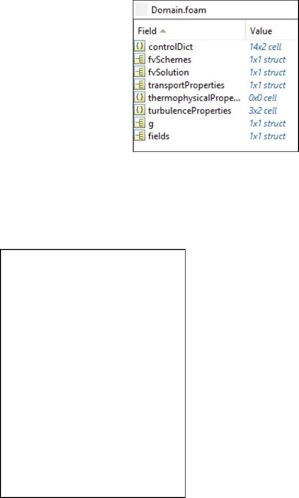
4.2.3 Read OpenFOAM Files
OpenFOAM files are imported at this level to Matlab and stored in a global variable called
‘Domain’. In fact, all OpenFOAM input information are stored in a structure called foam within
the global Domain variable. The table below presents the settings that the user must or may
include in the OpenFOAM files:
Option/Setting Name
Description
Location
residualControl
The equations’ tolerances
(convergence criteria)
system/fvSolution
relaxationFactors
The under-relaxation factors
to be applied to the
equations
system/fvSolution
ddtSchemes
The transient scheme (steady
or transient). The options
are:
steadyState
Euler
system/fvSchemes
divSchemes
The convection scheme. The
options are:
Gauss upwind
Gauss linear
system/fvSchemes
startFrom
This tells the solver from
where to start. The options
are:
firstTime
startTime
latestTime
system/controlDict
startTime
The initial time of the
simulation
system/controlDict
stopAt
This tells the solver until
when to stop. The options
are:
endTime
system/controlDict
endTime
The final time of the
simulation
system/controlDict
deltaT
The time step of the
simulation
system/controlDict
writeControl
The criterion that the solver
writes the results based on.
The options are:
timeStep
system/controlDict
writeInterval
Write results every specified
number of time steps (if the
system/controlDict
9
writeControl is set to
timeStep)
4.2.4 Setup Time
The function cfdSetupTime sets time controls and other conditions for the simulation. Other
conditions of the simulation are related to multiphase flow model which will not be considered
in the current uFVM version. The following table presents the valid arguments of the function:
4.2.5 Setup Equations
The user has to define the equations that are to be solved. The equations that are being solved
in the above example are described below.
Momentum:
Continuity:
Energy:
4.2.6 Initialize Case
The case is initialized after that by evaluating all the fields with their corresponding values on
the mesh. For example, the field variables (variables to be solved for), have initial values that are
imported from the OpenFOAM ‘0’ directory. The properties are evaluated based on their values
dictated by the ‘transportProperties’ file or ‘thermophysicalProperties’ file in case of a
compressible flow; these are found in the ‘constant’ directory.
4.2.7 Running the Case
The case is made to run at this level, iterating over the equations until convergence. The
convergence criteria can be found in the ‘fvSolution’ file in the ‘system’ directory within
OpenFOAM folders.
10
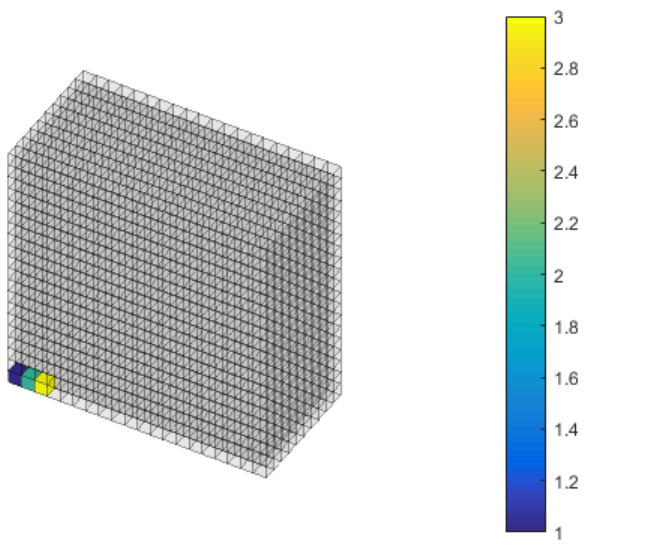
5 READING AND PLOTTING OPENFOAM MESH
When in the case, a user may read the OpenFOAM mesh and visualize it before running the
case. The following commands are all what the user needs to do so:
To read the mesh, the function cfdReadPolyMesh has to be called. The uFVM will go to the
‘constant/polyMesh’ directory, read the files there, and store the mesh information in the
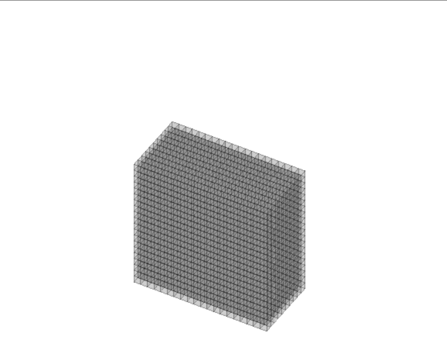
database. To plot the mesh, the user has to use the function cfdPlotMesh; the mesh will then
be plotted:
Figure 1 - Plotted mesh
To witness the details of the read mesh, the user has to call for the mesh from the database by
writing:
mesh = cfdGetMesh

11
The mesh will be printed out such as:
The information printed out above are structures and values that store the quantitative and
qualitative details of the mesh. For instance, see the number of elements (numberOfElements:
4000) and the number of patches (numberOfPatches: 3). The information of any element or face
can be witnessed by accessing it from the corresponding structure. If I want to see the details of
element number 100 in the mesh, I can simply write mesh.elements(100)and the output is:
mesh =
struct with fields:
nodes: [1×4851 struct]
numberOfNodes: 4851
caseDirectory: 'constant/polyMesh'
numberOfFaces: 12800
numberOfElements: 4000
faces: [1×12800 struct]
numberOfInteriorFaces: 11200
boundaries: [1×3 struct]
numberOfBoundaries: 3
numberOfPatches: 3
elements: [1×4000 struct]
numberOfBElements: 1600
numberOfBFaces: 1600
cconn: {4000×1 cell}
csize: [4000×1 double]

12
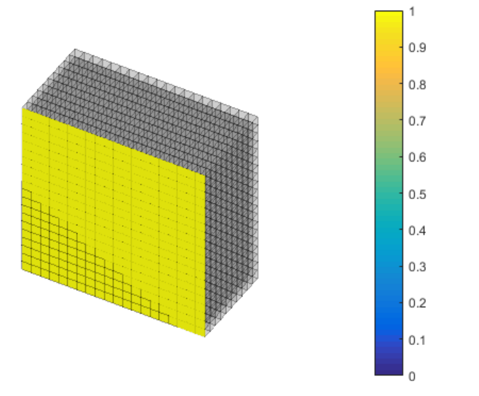
The previous commands can also be applied to faces and nodes. The user may also visualize the
elements, faces and patches. In order to plot patch #1 for instance, the function
cfdPlotPatches(1) has to be called. The output figure is:
>> theMesh.elements(100)
ans =
struct with fields:
index: 100
iNeighbours: [80 99 120 300]
iFaces: [235 291 294 295 12205 12595]
iNodes: [104 335 336 105 125 356 357 126]
volume: 0.1250
faceSign: [-1 -1 1 1 1 1]
numberOfNeighbours: 4
OldVolume: 0.1250
centroid: [3×1 double]
13
Figure 2 - Plotted mesh and patch number 1
Elements and faces may also be visualized using the functions cfdPlotElements and
cfdPlotFaces. If more than an entity are to be plotted, say 3 entities of indecis 1, 2 and 3, and
considering plotting the elements, the user has to call cfdPlotElements([1 2 3]). The
output figure is:
14
Figure 3 - Visualizing elements 1, 2 and 3

15
6 AN INTRODUCTORY PRESENTATION OF UFVM FUNCTIONS
6.1 APPLICATION CLASS
Different applications give rise to different ways of treating the fluid flow equations. Thus a user
has to set an application class by choosing any of the following applications (basic,
incompressible, compressible, heatTransfer and multiphase). It is significantly important to set
the right application class because it is the basis of many things inside the code.
6.2 READING OPENFOAM FILES AND TRANSLATION TO UFVM
As mentioned previously, uFVM cases are prepared in OpenFOAM format. This choice was made
because OpenFOAM is a widely used CFD library (C++ based). Preparing an OpenFOAM case is
quite straight forward for each application class. Refer to the tutorials and check the way in
which each application is being prepared.
uFVM’s function cfdReadOpenFoamFiles reads all the files that exist in the 3 standard
OpenFOAM directories ‘0’, ‘constant’ and ‘system’. It searches for specific entries and blocks
within the files and stores them in the uFVM’s data base. See the following table for details
about the read files:
The above FOAM details are imported and stored in the data base ‘Domain’ under the structure
‘foam’ as such:
OpenFOAM
Case
Directory
'system'
Directory
fvSolution block: solvers
block: SIMPLE/PISO/ALGORITHM
block: relaxationFactors
fvSchemes block: ddtSchemes
block: divSchemes
block: laplcaianSchemes
Other Finite Volume Operators
controlDict key: startFrom
key: startTime
key: stopAt
key: endTime
other control options
'constant'
Directory
polyMesh boundary
points
faces
owner
neighbour
Others
transportProperties/thermophysicalProperties Collect all properties and their attributes (values,
dimensions, models, expressions)
turbulenceProperties key: simulationType i.e. RAS
key: RASModel
key: turbulence
key: printCoeffs
g Collect gravitational acceleration vale i.e. (0 0 -9.8)
'0'
Directory
U class
internalField
boundaryField
p class
internalField
boundaryField
T class
internalField
boundaryField
Other fields
16
6.3 FIXING TIME SETTINGS
Of the imported control settings, the time controls which exist in the controlDict structure in the
global Domain variable, are stored again in a more useful way in another structure called time.
The structure ‘time’ contains the following info for the arbitrary case of elbow:
The above settings will be used later on to set the start and end of the time loop or convergence
loop. If the case is transient, ‘deltaT’ in the above structure is the time step.
6.4 INTERPRETING THE MODEL/EQUATIONS
The equations in uFVM are interpreted in such a way that each term of the equation has its own
attributes. Generally, any conservation equation has the following form:
>> Domain.time
ans =
struct with fields:
startFrom: 'latestTime'
startTime: 0
stopAt: 'endTime'
endTime: 10000
deltaT: 10
fdt: 1.0000e+09
type: 'Transient'

17
Note: The diffusion term can only be written as when the diffusion coefficient
is constant. However, when implementing the diffusion term in uFVM, it is always written as
laplacian(tau*phi) whether is constant or not.
The general conservation equation above is expressed in uFVM as follows:
cfdDefineEquation('phi', 'ddt(rho*phi) + div(rho*U*phi) = laplacian(tau*phi) + Q');
in the above implementation has to be an explicit expression that includes fields and/or
properties. Inside uFVM, each of the above terms is interpreted in a different way. Each term
consists of an explicit part and an implicit one; the explicit part is the part which holds the
previous iteration value, and the implicit part is kept as an unknown to be assembled with other
implicit parts of other terms in a global matrix. The explicit part is roughly all the parameters
that are multiplied with and the implicit part is . In the case of a general conservation
equation, the explicit part of the transient term
is and the implicit part is. In addition,
the explicit part of the transient term, is called the rho field. For the convection and diffusion
terms, the explicit parts are and respectively, and the names of the latter explicit fields are
the psi field and the gamma field respectively. The source term is treated explicitly; it is
evaluated based on available field values.
The table below summarizes the treatment of the terms of a general conservation equation:
The term type: Transient Term
the rho field:
the variable field:
The term type: Convection Term
the psi field:
the variable field:
The term type: DiffusionTerm
the gamma field:
the variable name:
The term type: Source term

18
Example1:
Take the momentum equation in the elbow case as an example:
It is written in uFVM in the following form:
'ddt(rho*U) + div(rho*U*U) = laplacian(mu*U) + div(mu*transp(grad(U))) - grad(p) + rho*g'
The momentum equation above includes 6 terms, each of them is interpreted in uFVM as shown
here:
Example2:
Take the Energy equation in the elbow case as another example:
It is written in uFVM in the following form:
'ddt(rho*Cp*T) + div(rho*Cp*U*T) = laplacian(k*T)'
The Energy equation above includes 3 terms, each of them is interpreted in uFVM as shown
here:
ddt(rho*U) The term type: Transient Term
Finite Volume Operation: Implicit
the rho field: rho
the variable field: U
term sign: 1
div(rho*U*U) The term type: Convection Term
Finite Volume Operation: Implicit
the psi field: rho*U
the variable field: U
term sign: 1
laplacian(mu*U) The term type: Stress Term
Finite Volume Operation: Implicit
the gamma field: mu
the variable name: U
term sign = -1
div(mu*transp(grad(U))) The term type: Source term
Finite Volume Operation: Explicit
explicit operators available: grad
term sign: -1
grad(p) The term type: Source term
Finite Volume Operation: Explicit
explicit operators available: grad
term sign: 1
rho*g The term type: Source term
Finite Volume Operation: Explicit
explicit operators available: none
term sign: -1

19
However, a special case arises for the continuity equation which is usually called also the
pressure equation ‘p’. The ‘p’ equation is treated in a different way. The pressure equation for
an incompressible application class is the same for any fluid flow problem within the
incompressible category. Thus, the user may ignore the pressure equation expression keeping
only the equation name (‘p’). The reason that the pressure equation expression is included in
the Matlab listing above and we are repeating it here is just for showing the exact models that
this code is solving:
cfdDefineEquation('p', 'div(U) = 0');
While it is sufficient to write:
cfdDefineEquation('p');
Automatically, all the terms of the continuity equation are treated in a single term assembly
process, this term is called ‘mdot’. For incompressible fluid flows, the continuity equation stated
above is theoretically converted into another equation called the pressure equation, and that’s
why the name ‘p’ corresponds to the continuity equation.
A summary of how the pressure equation is derived from the continuity equation is presented
here:
The continuity equation for an incompressible flow:
ddt(rho*Cp*T) The term type: Transient Term
Finite Volume Operation: Implicit
the rho field: rho*Cp
the variable field: T
term sign: 1
div(rho*Cp*U*T) The term type: Convection Term
Finite Volume Operation: Implicit
the psi field: rho*Cp*U
the variable field: T
term sign: 1
laplacian(k*T) The term type: Stress Term
Finite Volume Operation: Implicit
the gamma field: k
the variable name: T
term sign = -1

20
Dividing into a predicted and correction components:
So,
The Rhie-Chow interpolation for is
and for is
Therefore, the equation of the incompressible pressure equation is:
For a compressible continuity equation, the resulting pressure equation is a follows (you may
find the proof in the book):
6.5 RUNNING THE CASE
6.5.1 Time Loop/Convergence Loop
The time loop and the convergence loop are located in the cfdRunCase where the time
settings are utilized. The following listing shows the time and convergence loops for a transient
simulation:

21
Listing 2 – Time loop
Note that the time settings startTime, endTime and deltaT are retrieved from the structure
called ‘time’ in the data base.
6.5.2 Assembling Equation Terms
The main function which includes all the finite volume methods (assembling equation terms,
solving and correcting) is cfdAssembleAndCorrectEquation. The aim of discretizing is to
assemble the algebraic coefficients and build the algebraic system of the model equation:
And after that, the function proceeds to solve a set of algebraic system which yields a
solution of the system.
The following listing shows the main content of this function:
time = cfdGetTime;
startTime = time.startTime;
endTime = time.endTime;
deltaT = time.deltaT;
% Time Loop: Loop until the final time
timeIter = 1;
cumulativeIter = 1;
for t=startTime:deltaT:endTime
% Time settings
currentTime = t + deltaT;
cfdSetCurrentTime(currentTime);
% Update previous time step fields
cfdTransientUpdate;
cfdPrintCurrentTime(currentTime);
% Convergence Loop: Loop until convergence for the current time step
for iter=1:20
cfdPrintIteration(cumulativeIter);
cfdPrintResidualsHeader;
%
cfdUpdateFields;
%
for iEquation=1:theNumberOfEquations
% Assemble the current equation and correct it
[rmsResidual, maxResidual, lsResBefore, lsResAfter] = cfdAssembleAndCorrectEquation(theEquationNames{iEquation});
% Print the equation residuals
cfdPrintResiduals(cfdGetBaseName(theEquationNames{iEquation}),rmsResidual,maxResidual,lsResBefore,lsResAfter);
% If multigrid solver is assigned, print the AMG solver
% settings
theEquation = cfdGetModel(theEquationNames{iEquation});
isMultigrid = theEquation.multigrid.isActive;
if isMultigrid
cfdPrintLinearSolver(theEquationNames{iEquation});
if iEquation<theNumberOfEquations
cfdPrintResidualsHeader;
end
end
% Store RMS residuals to check for convergence later on
convergenceCriterion{iEquation}(1:length(maxResidual)) = rmsResidual;
end
fprintf('|==========================================================================|\n');
cfdPrintCPUTime;
cfdPlotRealTimeResiduals(cumulativeIter);
% Check for convergence at each iteration at the current time
% step
isConverged = cfdCheckConvergence(convergenceCriterion);
if isConverged
fprintf('Solution is converged!\n')
break;
end
cumulativeIter = cumulativeIter + 1;
end
cfdWriteResults(timeIter, currentTime);
timeIter = timeIter + 1;
end
22
Listing 3 - Assembling, solving, correcting the equation and storing its residuals
Starting with assembling the equation, the function cfdAssembleEquation executes the
following commands:
Listing 4 - Assembling equation terms and post assembling
The function cfdAssembleEquationTerms is in fact the function that includes the term
assembly and it is shown in the listing below, while the function cfdPostAssembleEquation
includes some methods that are done after assembling.
Listing 5 - Assembling of the terms in cfdAssembleEquationTerms
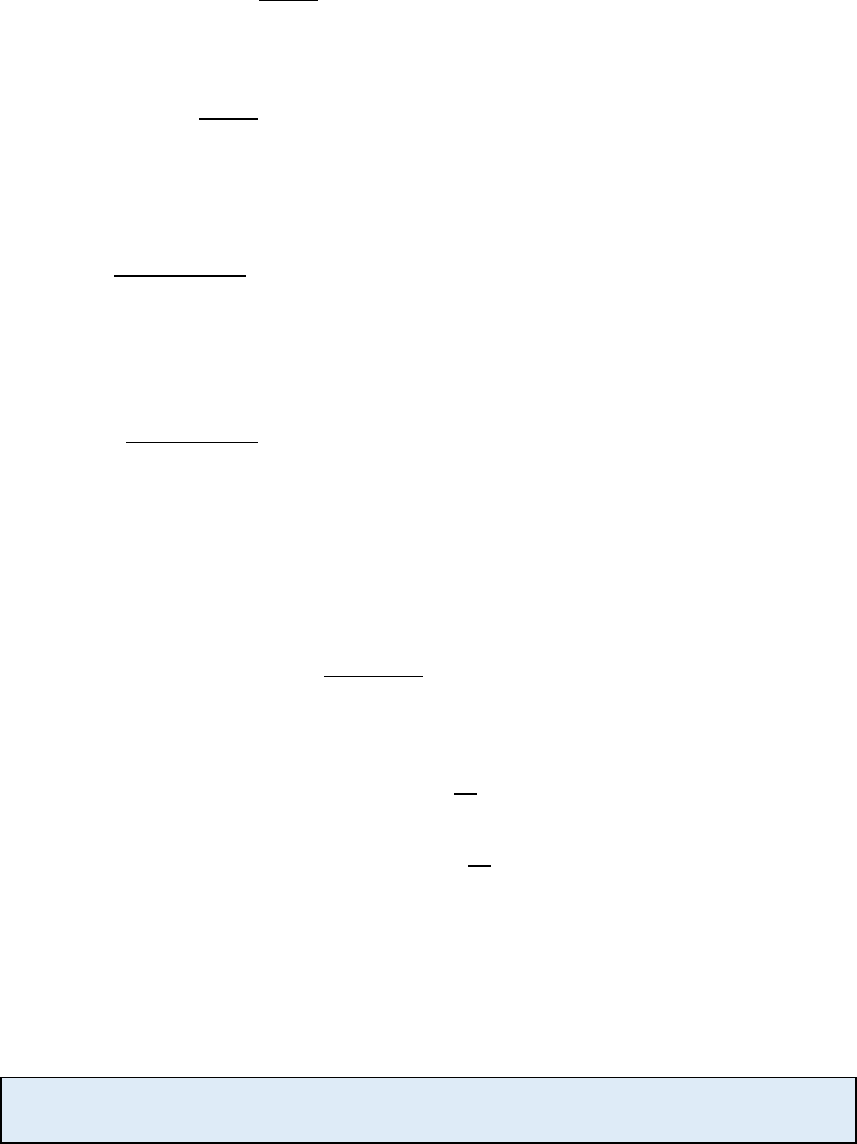
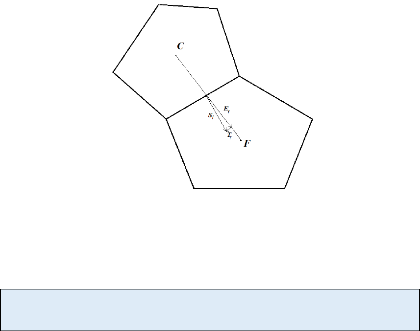
The assembling of the terms is made according to the finite volume method. The finite volume
method states that the conservation equation is integrated on an element of volume . The
figure below shows an element with neighboring element :
for iCorrector=1:nCorrectors
% Assemble Equation
[rmsResidual(iComponent), maxResidual(iComponent)] = cfdAssembleEquation(theEquationName,iComponent);
% Solve Equation
[initialResidual(iComponent),finalResidual(iComponent)] = cfdSolveEquation(theEquationName);
% Correct Equation
cfdCorrectEquation(theEquationName,iComponent);
end
% Store rms residual in the equation model
cfdStoreResiduals(theEquationName, iComponent, rmsResidual(iComponent));
end
% Assemble Equation Terms
[rmsResidual, maxResidual] = cfdAssembleEquationTerms(theEquationName,iComponent);
% Post Assemble Equation
cfdPostAssembleEquation(theEquationName,iComponent);
for iTerm = 1:theNumberOfTerms
theTerm = theEquation.terms{iTerm};
if strcmp(theTerm.name,'Transient')
cfdAssembleTransientTerm(theEquationName,theTerm,iComponent);
elseif strcmp(theTerm.name,'Convection')
cfdAssembleConvectionTerm(theEquationName,theTerm,iComponent);
elseif strcmp(theTerm.name,'Diffusion')
cfdAssembleDiffusionTerm(theEquationName,theTerm);
elseif strcmp(theTerm.name,'Stress')
cfdAssembleStressTerm(theEquationName,theTerm,iComponent);
elseif strcmp(theTerm.name,'mdot_f')
cfdAssembleMdotTerm(theEquationName,theTerm);
elseif strcmp(theTerm.name,'Source')
cfdAssembleSourceTerm(theEquationName,theTerm,iComponent);
elseif strcmp(theTerm.name,'Implicit Source')
cfdAssembleSourceTerm(theEquationName,theTerm,iComponent);
else
error('\n%s\n',[theTerm.name,' term is not defined']);
end
end
23
The general conservation equation is:
Integrating the equation over the volume of element :
Applying finite volume time discretization approach for transient term and Greens’ theorem to
convection and diffusion terms:
The coefficient in the second term (convection term) is referred to as ; this is
mentioned earlier. So, the equation is now:
For each element, this is the semi-discretized equation. The terms above are now distributed
into element and face fluxes.
6.5.2.1 Transient Term
The semi-discretized transient term
is a contribution from the element itself but
not from the surrounding (through faces) like the convection and diffusion terms, so it is added
to the element flux such as follows:
In uFVM, the function cfdAssembleTransientTermEuler calculates the above fluxes as
shown in the listing below:
Listing 6 - Assmebling transient term based on Euler's method
theFluxes.FLUXCE = theTerm.sign * vol .* rho / deltaT;
theFluxes.FLUXCEOLD = - theTerm.sign * vol .* rho_old / deltaT;
theFluxes.FLUXTE = theFluxes.FLUXCE .* phi' + theFluxes.FLUXCEOLD .* phi_old';

24
6.5.2.2 Convection Term
The face fluxes of the convection term
based on a first order upwind scheme
are calculated as follows:
The listing below is retrieved from cfdAssembleConvectionTerm:
Listing 7 - Calculating face fluxes from the convection term contribution. It is retrieved from the function
The above assembly is based on a first order upwind convection scheme. If a higher order
scheme is required and additional non-linear face flux arises. For a second order upwind
convection scheme, we have in addition to the above fluxes:
A glance to the implementation is shown here:
Listing 8 - Assembling of the correction term for higher order convection scheme (SOU)
6.5.2.3 Diffusion Term
The face fluxes of the diffusion term
are calculated as follows. The linear
face fluxes are:
is the geometric difference at the face; it is calculated as:
theFluxes.FLUXC1f(iFaces,1) = theTerm.sign * max(psi,0);
theFluxes.FLUXC2f(iFaces,1) = - theTerm.sign * max(-psi,0);
theFluxes.FLUXVf(iFaces,1) = 0;
theFluxes.FLUXTf(iFaces,1) = theFluxes.FLUXC1f(iFaces) .* phi(iOwners) + theFluxes.FLUXC2f(iFaces) .*
phi(iNeighbours) + theFluxes.FLUXVf(iFaces);
rC = [theMesh.elements(iUpwind).centroid]';
rf = [theMesh.faces(iFaces).centroid]';
rCf = rf - rC;
corr = psi .* dot(2*phiGradC' - phiGradf(iUpwind, :)',rCf')';
theFluxes.FLUXTf(iFaces) = theFluxes.FLUXTf(iFaces) + corr;
25
Where is the norm of the vector , which is the non-orthogonal component of :
The non-linear face flux is:
The above non-linear face flux includes the previous iteration value of as well as the non-
orthogonal component of the face surface vector which is shown in the figure below:
The total flux is then:
The following piece of code is retrieved from the function cfdAssembleDiffusionTerm:
Listing 9 - Assembling diffusion term to face fluxes
6.5.2.4 Source Term
The source terms are all terms that are to be treated explicitly in the equation assembly. Any
source term is discretized and assembled as an element flux as follows:
theFluxes.FLUXC1f(iFaces,1) = - theTerm.sign * gamma .* gDiff_f;
theFluxes.FLUXC2f(iFaces,1) = theTerm.sign * gamma .* gDiff_f;
theFluxes.FLUXVf(iFaces,1) = theTerm.sign * gamma .* dot(grad_f(:,:)',Tf(:,:)')';
theFluxes.FLUXTf(iFaces,1) = theFluxes.FLUXC1f(iFaces) .* phi(iOwners) + theFluxes.FLUXC2f(iFaces) .*
phi(iNeighbours) + theFluxes.FLUXVf(iFaces);
26
It is worth mentioning that in uFVM, source terms are either recognized as standard source
terms or non-standard source terms. Of the standard source terms are gradients of equation
fields (). In the momentum equation for example, there’s a pressure gradient
term . Instead of calculating the pressure gradient to assemble it, it is available in the data
base. So it is only called from the data base; this saves some time.
The non-standard source terms are evaluated directly as they appear in the equation. Of the
non-standard terms are:
The second part of shear stress term. It appears in the momentum equation
The third part of the shear stress term which includes the bulk viscosity for
compressible flows. It appears in the momentum equation.
A body force (weight of fluid) which appears in the momentum equation
The following listing shows the assembly of a non-standard term retrieved from the function
cfdAssembleSourceTerm:
Listing 10 - Assembling non-standard source term
6.5.2.5 ‘mdot_f’ Term
The pressure correction equation is treated within a single term called ‘mdot_f’ term. The
incompressible pressure equation
consists of a diffusion-like term
of a gamma coefficient
. It also includes a source term
.
The diffusion-like term is discretized into face fluxes such as:
We introduce here :
% If source term is not standard
S = cfdEvaluateNonstandardSourceTerm(theTerm, iComponent);
% Assemble Source Term as element flux
theFluxes.FLUXTE = theTerm.sign * S .* volume;
cfdAssembleIntoGlobalMatrixElementFluxes(theEquationName,theFluxes,iComponent);
27
So,
Usually, the non-linear flux of the diffusion term
is neglected, because it doesn’t
affect the final solution as it is a correction term, so the non-linear flux contribution of the
diffusion-like term .
The source term
can be regarded as face fluxes contribution instead of element
fluxes. So, the face flux contribution of the source term is:
The total flux is:
Whereas for the compressible pressure correction equation
there are additional terms (transient and convection). They are discretized regularly.
The transient term
element flux contribution is:
The convection term
has a psi coefficient
, so the face fluxes
are:
28
The source term includes an additional component. It is the
term which is in fact a result of
the transient term but will be here regarded as a source term because it is not standard.
The corresponding code will be presented in the algebraic system section for convenience.
6.5.2.6 Pressure Correction Treatment for Free Surface Flow
In case the application is ‘multiphase’, uFVM is able to simulate homogeneous flows with a well-
defined interface. In this case, the OpenFOAM case to be prepared is quite different, you may
refer to the ‘damBreak’ case in the tutorials directory.
6.5.2.7 False Transience
For steady simulations, it is usually advantageous to insert a transient-like treatment. It acts as
an under-relaxation to the equation yet is enhances diagonal dominance. It also adds a non-zero
contribution to the diagonal coefficient even in the extreme cases where the diagonal
coefficient is zero. Consider the following system:
A false transient contributes to the equation above as shown here:
where
The following listing is a retrieved from the function cfdAssembleFalseTransientTerm in
the source files:
29
Listing 11 - Assembling false transience term
6.5.2.8 Gradient Computation
The gradient of a field can be calculated using Green-Gauss method. The gradient is
calculated as follows:
However, the face value can be calculated in two approaches, a cell-based method and a
node-base method. In the cell based method, the face value is calculated as the average values
of the two cells sharing the face:
where is the geometric weighing factor equal to
The listing below shows the calculation of the face values and the gradient in the function
cfdComputeGradientGauss0:
Listing 12 - Calculation of gradient based on Green-Gauss method
volumes = [theMesh.elements(iElements).volume]';
theFluxes.FLUXCE(iElements,1) = volumes .* rho / fdt;
theFluxes.FLUXCEOLD(iElements,1) = - volumes .* rho_old / fdt;
theFluxes.FLUXTE(iElements,1) = theFluxes.FLUXCE(iElements,1) .* phi;
theFluxes.FLUXTEOLD(iElements,1) = theFluxes.FLUXCEOLD(iElements,1) .* phi_old;
cfdAssembleIntoGlobalMatrixElementFluxes(theEquationName,theFluxes,iComponent);
for iComponent=1:theNumberOfComponents
phi_f = gf.*phi(iNeighbours,iComponent) + (1-gf).*phi(iOwners,iComponent);
for iFace=iFaces
phiGrad(iOwners(iFace),:,iComponent) = phiGrad(iOwners(iFace),:,iComponent) +
phi_f(iFace)*Sf(iFace,:);
phiGrad(iNeighbours(iFace),:,iComponent) = phiGrad(iNeighbours(iFace),:,iComponent) -
phi_f(iFace)*Sf(iFace,:);
end
end
%-----------------------------------------------------
% BOUNDARY FACES contribution to gradient
%-----------------------------------------------------
iBOwners = [theMesh.faces(iBFaces).iOwner]';
phi_b = phi(iBElements,:);
Sb = [theMesh.faces(iBFaces).Sf]';
for iComponent=1:theNumberOfComponents
%
for k=1:theMesh.numberOfBFaces
phiGrad(iBOwners(k),:,iComponent) = phiGrad(iBOwners(k),:,iComponent) + phi_b(k)*Sb(k,:);
end
end
%-----------------------------------------------------
% Get Average Gradient by dividing with element volume
%-----------------------------------------------------
volumes = [theMesh.elements(iElements).volume]';
for iComponent=1:theNumberOfComponents
for iElement =1:theMesh.numberOfElements
phiGrad(iElement,:,iComponent) = phiGrad(iElement,:,iComponent)/volumes(iElement);
end
end
30
The node-based method requires that the node value is first calculated from the elements
surrounding the node
And then the face value is calculated from the values of its nodes
The listing below in the function cfdInterpolateFromElementsToNodes calculates the
values at the nodes:
Listing 13 - Interpolating the cell values to the nodes
Then the following code calculates the node values to the faces, and can be found in the
function cfdInterpolateFromNodesToFaces:
for iNode = 1:numberOfNodes
theNode = fvmNodes(iNode);
N = theNode.centroid;
localPhiNode=0;
localInverseDistanceSum = 0;
if(isempty(theNode.iFaces(theNode.iFaces>numberOfInteriorFaces)))
localElementIndices = theNode.iElements;
for iElement = localElementIndices
theElement = fvmElements(iElement);
C = theElement.centroid;
d = cfdMagnitude(N-C);
localPhi = phi(iElement);
localPhiNode = localPhiNode + localPhi/d;
localInverseDistanceSum = localInverseDistanceSum + 1/d;
end
else
localBFacesIndices = theNode.iFaces(theNode.iFaces>numberOfInteriorFaces);
for iBFace = localBFacesIndices
theFace = fvmFaces(iBFace);
C = theFace.centroid;
iBElement = numberOfElements+(iBFace-numberOfInteriorFaces);
d = cfdMagnitude(N-C);
localPhi = phi(iBElement);
localPhiNode = localPhiNode + localPhi/d;
localInverseDistanceSum = localInverseDistanceSum + 1/d;
end
end
localPhiNode = localPhiNode/localInverseDistanceSum;
%
%
phi_n(iNode) = localPhiNode;
%
end
31
Listing 14 - Interpolating the node values to the faces
Finally, we calculate the gradient according to the Green-Gauss method which can be found in
the function cfdComputeGradientNodal:
Listing 15 - Calculation of the Green-Gauss gradient based on the face values calculated from node values
6.5.2.9 Implicit Under-Relaxation
As suggested by Patankar’s approach, a relaxation factor is introduced into the algebraic
system.
for iFace=1:numberOfFaces
theFace = fvmFaces(iFace);
iNodes = theFace.iNodes;
C = theFace.centroid;
localSumOfInverseDistance=0;
localPhi=0;
for iNode=iNodes
theNode = fvmNodes(iNode);
N=theNode.centroid;
d=cfdMagnitude(C-N);
localPhi = localPhi + phiNodes(iNode)/d;
localSumOfInverseDistance = localSumOfInverseDistance+1/d;
end
localPhi = localPhi/localSumOfInverseDistance;
phi_f(iFace) = localPhi;
end
for iFace=1:theNumberOfInteriorFaces
%
theFace = fvmFaces(iFace);
%
iElement1 = theFace.iOwner;
iElement2 = theFace.iNeighbour;
%
Sf = theFace.Sf;
%
%
phiGrad(:,iElement1) = phiGrad(:,iElement1) + phi_f(iFace)*Sf;
phiGrad(:,iElement2) = phiGrad(:,iElement2) - phi_f(iFace)*Sf;
end
%=====================================================
% BOUNDARY FACES contribution to gradient
%=====================================================
for iBPatch=1:theNumberOfBElements
%
iBFace = theNumberOfInteriorFaces+iBPatch;
iBElement = theNumberOfElements+iBPatch;
theFace = fvmFaces(iBFace);
%
iElement1 = theFace.iOwner;
%
Sb = theFace.Sf;
phi_b = phi(iBElement);
%
phiGrad(:,iElement1) = phiGrad(:,iElement1) + phi_b*Sb;
end
%-----------------------------------------------------
% Get Average Gradient by dividing with element volume
%-----------------------------------------------------
for iElement =1:theNumberOfElements
theElement = fvmElements(iElement);
phiGrad(:,iElement) = phiGrad(:,iElement)/theElement.volume;
end
32
However, for an equation in the correction form, an implicit under-relaxation is made as follows:
In uFVM, it is done in the function cfdApplyURF:
Listing 16 - Introducing under-relaxation to the algebraic equation
6.5.2.10 Residual Form of the Equation
In fact, uFVM assembles a residual or correction form of the equation instead of the direct
equation. This correction makes use of the previous iteration values of such that:
Satisfying in the standard equation form:
Once the algebraic system is calculated and is determined, the exact value is updated as:
6.5.2.11 Residual Computation
The residuals are criteria upon which the user decides to consider the results correct enough.
The residual of the algebraic equation at element is calculated as:
The maximum residual over the cells is calculated as:
theEquation = cfdGetModel(theEquationName);
urf = theEquation.urf;
theCoefficients = cfdGetCoefficients;
theCoefficients.ac = theCoefficients.ac/urf;
cfdSetCoefficients(theCoefficients);

33
And the root-mean-squared of the residuals over the cells is:
Normalized residuals provide better insight of the convergence. They are calculated as follows:
After that, you we calculate the maximum and root-mean square scaled residual.
However, since in uFVM the equations are assembled in the residual (correction) form as
mentioned earlier, the residual at element is simply:
So,
The following listing presents the residual calculation; it is available in the function
cfdComputeNormalizedResidual:
Listing 17 - Residual calculation
A special case arises with the pressure correction equation as it is by default in the correction
form as shown here:
% Loop over elements and calculate residual at each element
Rc = abs(bc);
% Residuals. Calculate for convenience. Otherwise, they are not used
Rc_max = max(Rc);
Rc_rms = sqrt(sum(Rc.^2)/theNumberOfElements);
% Get phi scale from data base.
% phi_scale = max(abs(phi)). And if phi is zero, phi_scale is set to 1
phi_scale = cfdGetScale(theEquationUserName);
% Normalized Residuals
Rc_scaled = Rc / (max(abs(ac))*phi_scale);
Rc_max_scaled = max(Rc_scaled);
Rc_rms_scaled = sqrt(sum(Rc_scaled.^2)/theNumberOfElements);
MAXResidual = Rc_max_scaled;
RMSResidual = Rc_rms_scaled;

34
However, the residual of this equation is determined as a continuity criterion
Thus, a quantity called is calculated at each iteration to judge the
convergence of the continuity equation, so, we have for the continuity equation:
The corresponding implementation can be found in the function:
cfdComputeEffectiveDivergence:
Listing 18 - Calculating the effective divergence as a residual criterion for the continuity equation
6.5.2.12 Assembling Fluxes to Global Assembly Matrix
After calculating the face or/and element fluxes from each term, these fluxes are to be summed
to construct the algebraic system coefficients.
6.5.2.12.1 Algebraic Systems Representation
The algebraic system is constructed:
% Interior Faces Contribution
theNumberOfInteriorFaces = cfdGetNumberOfInteriorFaces;
iFaces = 1:theNumberOfInteriorFaces;
owners = [theMesh.faces(iFaces).iOwner]';
neighbours = [theMesh.faces(iFaces).iNeighbour]';
for iFace=1:theNumberOfInteriorFaces
iOwner = owners(iFace);
iNeighbour = neighbours(iFace);
%
effDiv(iOwner) = effDiv(iOwner) + mdot_f(iFace);
effDiv(iNeighbour) = effDiv(iNeighbour) - mdot_f(iFace);
end
% Boundary Faces Contribution
theNumberOfPatches = cfdGetNumberOfPatches;
for iPatch=1:theNumberOfPatches
theBoundary = theMesh.boundaries(iPatch);
numberOfBFaces = theBoundary.numberOfBFaces;
% cfdGetBoundaryIndex
iFaceStart = theBoundary.startFace;
iFaceEnd = iFaceStart+numberOfBFaces-1;
iBFaces = iFaceStart:iFaceEnd;
owners = [theMesh.faces(iBFaces).iOwner]';
mdot_b = theMdotField.phi(iBFaces);
for iBFace=1:numberOfBFaces
iOwner = owners(iBFace);
effDiv(iOwner) = effDiv(iOwner) + mdot_b(iBFace);
end
end
35
The coefficient matrix is a highly sparse matrix, so it is stored as an array for the diagonal
coefficients in addition of a data structure containing the non-zeros at each row (off-diagonal
coefficients). The diagonal array is named in uFVM as ac and the off-diagonal coefficient data
structure as anb.
6.5.2.12.2 Assembling Algebraic System coefficients
If the discretized term gives rise to element fluxes like the transient and source terms, the fluxes
, , and are assembled as follows given that the algebraic equation is
in the residual (correction) form:
If the term includes faces fluxes (, , and ) like the convection and
diffusion terms, the assembling is done such as:
Recall that for element fluxes:
And for face fluxes,
Therefore, the algebraic equation has the general form:
So,

36
The pressure equation again has a special case since it is already in the residual form. The
discretized incompressible pressure correction equation:
So, the fluxes here are to be calculated as:
1) Diagonal coefficient :
and
2) Off-diagonal coefficients :
3) Right-hand-side:
and
For the compressible pressure correction equation, the discretized equation is:
So, the fluxes of the compressible pressure correction equation are calculated as:
1) Diagonal coefficient :
37
and
2) Off-diagonal coefficients :
3) Right-hand-side:
and
The listing below shows the calculation of the fluxes of the pressure correction equation:

38
Listing 19 - Calculating fluxes of the pressure correction equation
In uFVM, the assembling of element fluxes is shown here in the listing below retrieved from the
function cfdAssembleIntoGlobalMatrixElementFluxes:
%
% assemble term I
% rho_f [v]_f.Sf
%
U_bar_f = dot(vel_bar_f(:,:)',Sf(:,:)')';
FLUXVf = FLUXVf + rho_f.*U_bar_f;
%
% Assemble term II and linearize it
% - rho_f ([DPVOL]_f.P_grad_f).Sf
%
DUSf = [DU1_f.*Sf(:,1),DU2_f.*Sf(:,2),DU3_f.*Sf(:,3)]; % S'f
eDUSf = [DUSf(:,1)./cfdMagnitude(DUSf),DUSf(:,2)./cfdMagnitude(DUSf),DUSf(:,3)./cfdMagnitude(DUSf)];
DUEf =
[cfdMagnitude(DUSf).*eCN(:,1)./dot(eCN(:,:)',eDUSf(:,:)')',cfdMagnitude(DUSf).*eCN(:,2)./dot(eCN(:,:)',eDUSf(:,:)'
)',cfdMagnitude(DUSf).*eCN(:,3)./dot(eCN(:,:)',eDUSf(:,:)')'];
geoDiff = cfdMagnitude(DUEf)./cfdMagnitude(CN);
DUTf = DUSf - DUEf;
FLUXCf = FLUXCf + rho_f.*geoDiff;
FLUXFf = FLUXFf - rho_f.*geoDiff;
FLUXVf = FLUXVf - rho_f.*dot(p_grad_f(iFaces,:)',DUTf(:,:)')';
%
% assemble term III
% rho_f ([P_grad]_f.([DPVOL]_f.Sf))
%
FLUXVf = FLUXVf + rho_f.*dot(p_grad_bar_f(iFaces,:)',DUSf(:,:)')';
%
% assemble terms VIII and IX
% (1-URF)(U_f -[v]_f.S_f)
%
FLUXVf = FLUXVf + (1.0 - mdot_f_URF)*(mdot_f_previous - rho_f.*U_bar_f);
%
% compute Rhie-Chow interpolation of mdot_f and updated it in the data base
%
mdot_f = FLUXCf .* pressureC + FLUXFf .* pressureN + FLUXVf;
theMdotField.phi(iFaces) = mdot_f;
cfdSetMeshField(theMdotField);
%
% assemble total flux
%
FLUXTf = mdot_f;
%
% assemble terms X (for compressible flow)
%
applicationClass = cfdGetApplicationClass;
if strcmp(applicationClass, 'compressible')
theDrhodpField = cfdGetMeshField('C_rho');
C_rho = theDrhodpField.phi;
C_rho_f = cfdInterpolateFromElementsToFaces('Average', C_rho);
C_rho_f = C_rho_f(iFaces);
FLUXCf = FLUXCf + (C_rho_f ./ rho_f) .* max(mdot_f, 0);
FLUXFf = FLUXFf - (C_rho_f ./ rho_f) .* max(-mdot_f, 0);
% Add transient contribution
if isTransient
deltaT = cfdGetDt;
volume = [theMesh.elements.volume]';
FLUXCE = volume(iElements) .* C_rho(iElements) / deltaT;
FLUXTE = (rho(iElements) - density_old(iElements)) .* volume(iElements) / deltaT ;
end
end
39
Listing 20 - Assembling element fluxes
The assembly of face fluxes is shown here, and it is retrieved from the function
cfdAssembleIntoGlobalMatrixFaceFluxes:
Listing 21 - Assembling face fluxes
6.5.3 Solving the Equation Algebraic System
The algebraic system is solved iteratively. Direct solving of the system using Gaussian
elimination is very expensive because the matrix is usually large and highly sparse. There are
plenty of solvers which iteratively try to approximate the solution of the system. In uFVM, two
iterative solvers are implemented, Successive Over-relaxation (SOR) and Incomplete Lower
Upper (ILU).
% Call coefficients
ac = theCoefficients.ac;
ac_old = theCoefficients.ac_old;
bc = theCoefficients.bc;
% Assemble element fluxes
for iElement = 1:numberOfElements
ac(iElement) = ac(iElement) + theFluxes.FLUXCE(iElement);
ac_old(iElement) = ac_old(iElement) + theFluxes.FLUXCEOLD(iElement);
bc(iElement) = bc(iElement) - theFluxes.FLUXTE(iElement);
end
% Store updated coefficients
theCoefficients.ac = ac;
theCoefficients.ac_old = ac_old;
theCoefficients.bc = bc;
% Call coefficients
ac = theCoefficients.ac;
anb = theCoefficients.anb;
bc = theCoefficients.bc;
%
% Assemble fluxes of interior faces
%
for iFace = 1:numberOfInteriorFaces
theFace = theMesh.faces(iFace);
iOwner = theFace.iOwner;
iOwnerNeighbourCoef = theFace.iOwnerNeighbourCoef;
iNeighbour = theFace.iNeighbour;
iNeighbourOwnerCoef = theFace.iNeighbourOwnerCoef;
%
% assemble fluxes for owner cell
%
ac(iOwner) = ac(iOwner) + theFluxes.FLUXC1f(iFace);
anb{iOwner}(iOwnerNeighbourCoef) = anb{iOwner}(iOwnerNeighbourCoef) + theFluxes.FLUXC2f(iFace);
bc(iOwner) = bc(iOwner) - theFluxes.FLUXTf(iFace);
%
% assemble fluxes for neighbour cell
%
ac(iNeighbour) = ac(iNeighbour) - theFluxes.FLUXC2f(iFace);
anb{iNeighbour}(iNeighbourOwnerCoef) = anb{iNeighbour}(iNeighbourOwnerCoef) - theFluxes.FLUXC1f(iFace);
bc(iNeighbour) = bc(iNeighbour) + theFluxes.FLUXTf(iFace);
end
%
% assemble fluxes of boundary faces
%
for iBFace=numberOfInteriorFaces+1:numberOfFaces
theBFace = theMesh.faces(iBFace);
iOwner = theBFace.iOwner;
%
% assemble fluxes for owner cell
%
ac(iOwner) = ac(iOwner) + theFluxes.FLUXC1f(iBFace);
bc(iOwner) = bc(iOwner) - theFluxes.FLUXTf(iBFace);
end
% Store updated coefficients
theCoefficients.ac = ac;
theCoefficients.anb = anb;
theCoefficients.bc = bc;

40
6.5.3.1 SOR Solver
The SOR is a Gauss-Seidal solver except that it includes a factor which enhances the progress
of the solver. Check the function cfdSORSolver:
Listing 22 - SOR solver
6.5.3.2 ILU Solver
Incomplete factorization of the matrix is an efficient preconditioner which allows for an
accelerated convergence rate of the solver. The corresponding function is: cfdILUSolver
Listing 23 - ILU solver
6.5.3.3 AMG Linear Solver
An algebraic multigrid solver remove low-frequency error components. In the context of
multigrid solvers, the direct iterative solvers like ILU solver are regarded as smoothers. Below is
for iElement=1:numberOfElements
cconn = theCoefficients.cconn{iElement};
local_dphi = bc(iElement);
for iLocalNeighbour = 1:length(cconn)
iNeighbour = cconn(iLocalNeighbour);
local_dphi = local_dphi - anb{iElement}(iLocalNeighbour)*dphi(iNeighbour);
end
dphi(iElement) = local_dphi/ac(iElement);
end
for iElement=numberOfElements:-1:1
cconn = theCoefficients.cconn{iElement};
local_dphi = bc(iElement);
for iLocalNeighbour = 1:length(cconn)
iNeighbour = cconn(iLocalNeighbour);
local_dphi = local_dphi - anb{iElement}(iLocalNeighbour)*dphi(iNeighbour);
end
dphi(iElement) = local_dphi/ac(iElement);
end
for i1=1:numberOfElements
dc(i1) = ac(i1);
end
for i1=1:numberOfElements
dc(i1) = 1.0/dc(i1);
rc(i1) = bc(i1);
i1NbList = theCoefficients.cconn{i1};
i1NNb = length(i1NbList);
if(i1~=numberOfElements-1)
% loop over neighbours of iElement
j1_ = 1;
while(j1_<=i1NNb)
jj1 = i1NbList(j1_);
% for all neighbour j > i do
if((jj1>i1) && (jj1<=numberOfElements))
j1NbList = theCoefficients.cconn{jj1};
j1NNb = length(j1NbList);
i1_= 0;
k1 = -1;
% find _i index to get A[j][_i]
while((i1_<=j1NNb) && (k1 ~= i1))
i1_ = i1_ + 1;
k1 = j1NbList(i1_);
end
% Compute A[j][i]*D[i]*A[i][j]
if(k1 == i1)
dc(jj1) = dc(jj1) - anb{jj1}(i1_)*dc(i1)*anb{i1}(j1_);
else
disp('the index for i in j is not found');
end
end
j1_ = j1_ + 1;
end
end
end

41
a glance to the AMG code, it is advisable to access the code to see much more details about it.
Refer to cfdApplyAMG.
Listing 24 - Multigrid solver
Note: uFVM utilizes the AMG solver by default for the pressure equation only, while applies
direct iterative solvers for all other equations.
6.5.4 Correcting Equation Solution
All the equations are corrected just after solving the algebraic system such that:
However, after solving the pressure correction equation, the other fields have also to be
corrected:
For incompressible flow:
For compressible flow:
gridLevel = 1;
nCycle = 1;
if(strcmp(cycleType,'V-Cycle'))
while ((nCycle<=maxCycles)&&(finalResidual>rrf*initialResidual))
%
% Apply V-Cycle
%
finalResidual = cfdApplyVCycle(gridLevel,smootherType,maxLevels,preSweep,postSweep,rrf);
%
nCycle = nCycle + 1;
end
elseif(strcmp(cycleType,'F-Cycle'))
while ((nCycle<=maxCycles)&&(finalResidual>rrf*initialResidual))
%
% Apply F-Cycle
%
finalResidual = cfdApplyFCycle(gridLevel,smootherType,maxLevels,preSweep,postSweep,rrf);
%
nCycle = nCycle + 1;
end
elseif(strcmp(cycleType,'W-Cycle'))
while ((nCycle<=maxCycles)&&(finalResidual>rrf*initialResidual))
%
% Apply W-Cycle
%
finalResidual = cfdApplyWCycle(gridLevel,smootherType,maxLevels,preSweep,postSweep,rrf);
%
nCycle = nCycle + 1;
end
end

42
Listing of correcting :
Listing 25 - Correcting
Listing of correcting
:
Listing 26 – Correcting
Listing of correcting :
Listing 27 – Correcting
Further details of the implementation of field corrections can be found at
cfdCorrectEquation.
applicationClass = cfdGetApplicationClass;
if strcmp(applicationClass, 'compressible')
% Get density field
theDensityField = cfdGetMeshField('rho');
rho = theDensityField.phi;
% Get the convected density at the faces
pos = zeros(size(mdot_f));
pos(mdot_f>0) = 1;
rho_f = rho(iOwners).*pos(iFaces) + rho(iNeighbours).*(1 - pos(iFaces));
% Get drhodp field
theDrhodpField = cfdGetMeshField('C_rho');
C_rho = theDrhodpField.phi;
C_rho_f = cfdInterpolateFromElementsToFaces('Average', C_rho);
C_rho_f = C_rho_f(iFaces);
% Correct bt adding compressible contribution
mdot_f(iFaces) = mdot_f(iFaces) + (mdot_f(iFaces) ./ rho_f) .* C_rho_f .* pp(iOwners);
end
% Correct
mdot_f(iFaces) = mdot_f(iFaces) + FLUXC1f(iFaces).*pp(iOwners) + FLUXC2f(iFaces).*pp(iNeighbours);
thePPField = cfdGetMeshField('PP');
ppGrad = thePPField.phiGradient;
%
DUPPGRAD = [DU1.*ppGrad(iElements,1),DU2.*ppGrad(iElements,2),DU3.*ppGrad(iElements,3)];
%
theVelocityField = cfdGetMeshField('U');
vel = theVelocityField.phi;
%
vel(iElements,:) = vel(iElements,:) - DUPPGRAD(iElements,:);
thePressureCorrectionField = cfdGetMeshField('PP');
pp = thePressureCorrectionField.phi;
theDensityField = cfdGetMeshField('rho');
rho = theDensityField.phi;
theDrhodpField = cfdGetMeshField('C_rho');
C_rho = theDrhodpField.phi;
theEquation = cfdGetModel('rho');
URFRho = theEquation.urf;
rho = rho + 0.7 .* C_rho .* pp;
43
6.6 CONVERGENCE
Once the case is run, the solution will be updated at each iteration while at the mean time a
real-time plot will be displayed showing the residuals of the equations. A sample is shown in the
figure below:
Figure 4 - Real-time residuals monitor
Once the case is run until convergence, or the maximum number of iterations are reached in a
steady state simulation, a phrase ‘Solution is converged!’ will show up on the screen notifying
the user.
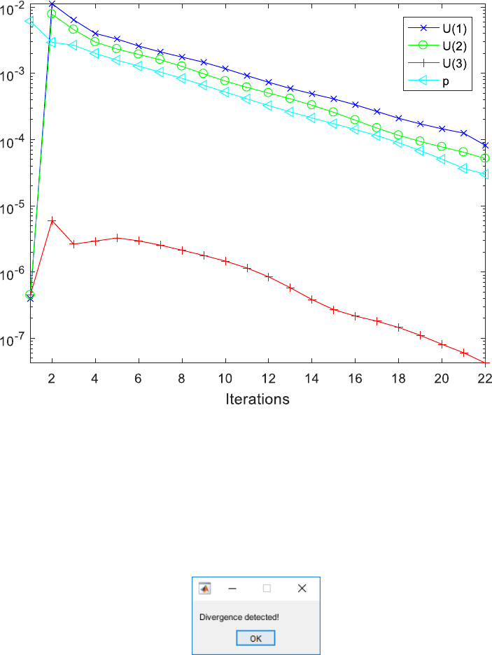
In case of divergence, a pop-up message box will be displayed notifying the user that the
program has detected divergence. The box is presented below:
Figure 5 - Divergence notification
44
6.7 POST-PROCESSING
The user may plot the results on figures. The corresponding functions to plot the resulting fields
is cfdPlotField. The function takes an argument the name of the field to be plotted.
Considering that the user wants to plot the velocity field, they have to call the following in the
command window:
cfdPlotField('U')
To plot the velocity vectors, the function to be used is cfdPlotVelocity. The function takes
as arguments the vector scale, the transparency of the faces and the vector skipping criterion. If
the user wants to plot the vector field with vector scale of 1, full transparency and 10 vector
skips (skip a vector every 10 vectors), they have to call the following in the command window:
cfdPlotVelocity('vectorScale',1,'faceAlpha',0,'vectorSkip',0);
45
7 TUTORIALS
In this chapter, some tutorials will be provided from each application class. 5 application classes
can be simulated so far within uFVM: basic, incompressible, compressible, Heat Transfer and
multiphase.
7.1 BASIC
The ‘stepProfile’ case is considered here. The mesh is a square domain with 20 by 20 structured
cells. A constant velocity profile () is assumed over the domain as shown in the figure
below. We attempt to solve a pure convection problem in order to evaluate the quality of
convection schemes. The convected quantity is and has dirichlet boundary conditions at two
patches shown below in the figure, while on the other part of the boundary, the quantity is
set to zero gradient.
The equation that is to be solved is
where is the velocity field set as constant field (Refer to the 0 directory in the tutorials and
look at the file named ‘U’). The corresponding run file is as shown here:
46
In addition, we set the default option of the divSchemes in the ‘fvShemes’ directory to ‘Gauss
upwind’ which corresponds to first order upwind. Running the case generates the following
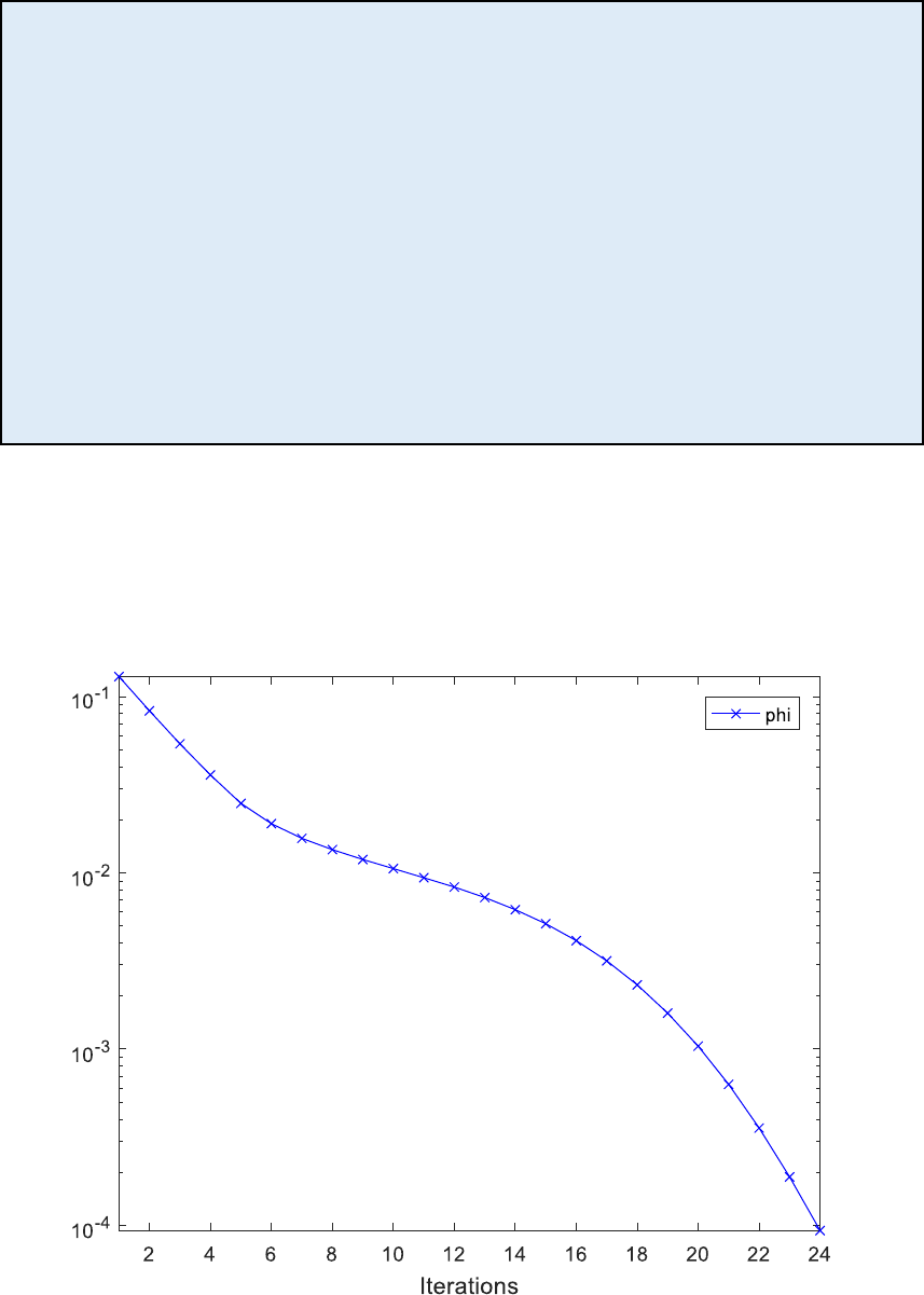
residuals plot:
Figure 6 - Residuals monitor for the upwind convection of the quantity
%--------------------------------------------------------------------------
%
% written by the CFD Group @ AUB, 2017
% contact us at: cfd@aub.edu.lb
%==========================================================================
% Case Description:
% In this test case the square cavity problem is considered with a
% uniform velocity profile throughout the domain. The objective is to
% investigate the convection schemes (the default now is set to first
% order upwind).
%--------------------------------------------------------------------------
% Setup Case
cfdSetupSolverClass('basic');
% Read OpenFOAM Files
cfdReadOpenFoamFiles;
% Setup Time Settings
cfdSetupTime;
% Setup Equations
cfdDefineEquation('phi', 'div(rho*U*phi) = 0'); % Convection
% Initialize case
cfdInitializeCase;
% Run case
cfdRunCase;
47
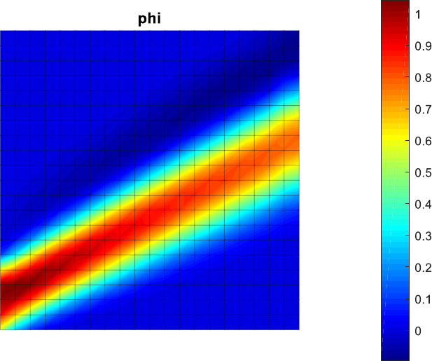
The contour of is as follows:
Figure 7 - Contour plot of phi subject to first order upwind convection
48
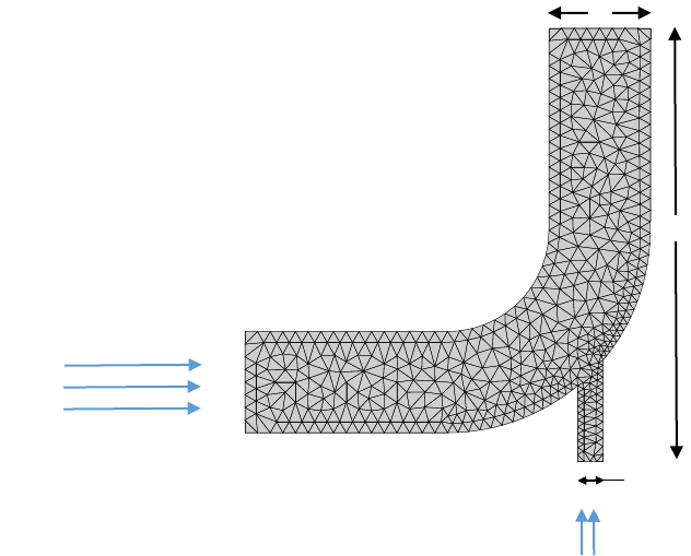
7.2 INCOMPRESSIBLE
The ‘elbow’ case is considered here. The following is the mesh with inlet velocities shown:
This case simulates a water flow in the elbow at steady state conditions with no gravitational
acceleration. The governing equations are:
Momentum:
Continuity:
Energy:
The corresponding run case is:
16
64
4
1 m/s
3 m/s
49
Listing 28 - Run file of the 'elbow' case
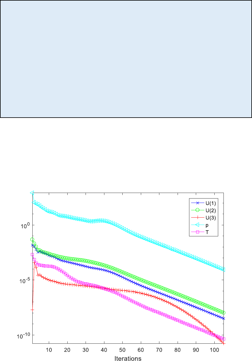
Refer to the ‘elbow’ case in the tutorials directory. Running the case will solve the problem
where it converges after 105 iterations, and the figure below shows the residuals history of the
equations (U, p, and T):
Figure 8 - Residuals history of the elbow case
%--------------------------------------------------------------------------
%
% written by the CFD Group @ AUB, 2017
% contact us at: cfd@aub.edu.lb
%==========================================================================
% Case Description:
% In this test case a water flow in an elbow is simulated at steady state
%--------------------------------------------------------------------------
% Setup Case
cfdSetupSolverClass('incompressible');
% Read OpenFOAM Files
cfdReadOpenFoamFiles;
% Setup Time Settings
cfdSetupTime;
% Setup Equations
cfdDefineEquation('U', 'div(rho*U*U) = laplacian(mu*U) + div(mu*transp(grad(U))) - grad(p)'); % Momentum
cfdDefineEquation('p', 'div(U) = 0'); % Continuity
cfdDefineEquation('T', 'div(rho*Cp*U*T) = laplacian(k*T)'); % Energy
% Initialize case
cfdInitializeCase;
% Run case
cfdRunCase;
50
We call the following functions:
cfdPlotField('U')
cfdPlotField('p')
cfdPlotField('T')
cfdPlotVelocity('vectorScale',1,'faceAlpha',0,'vectorSkip',0);
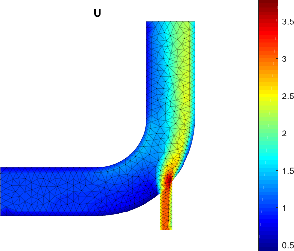
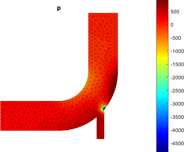
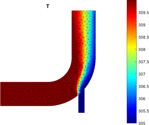
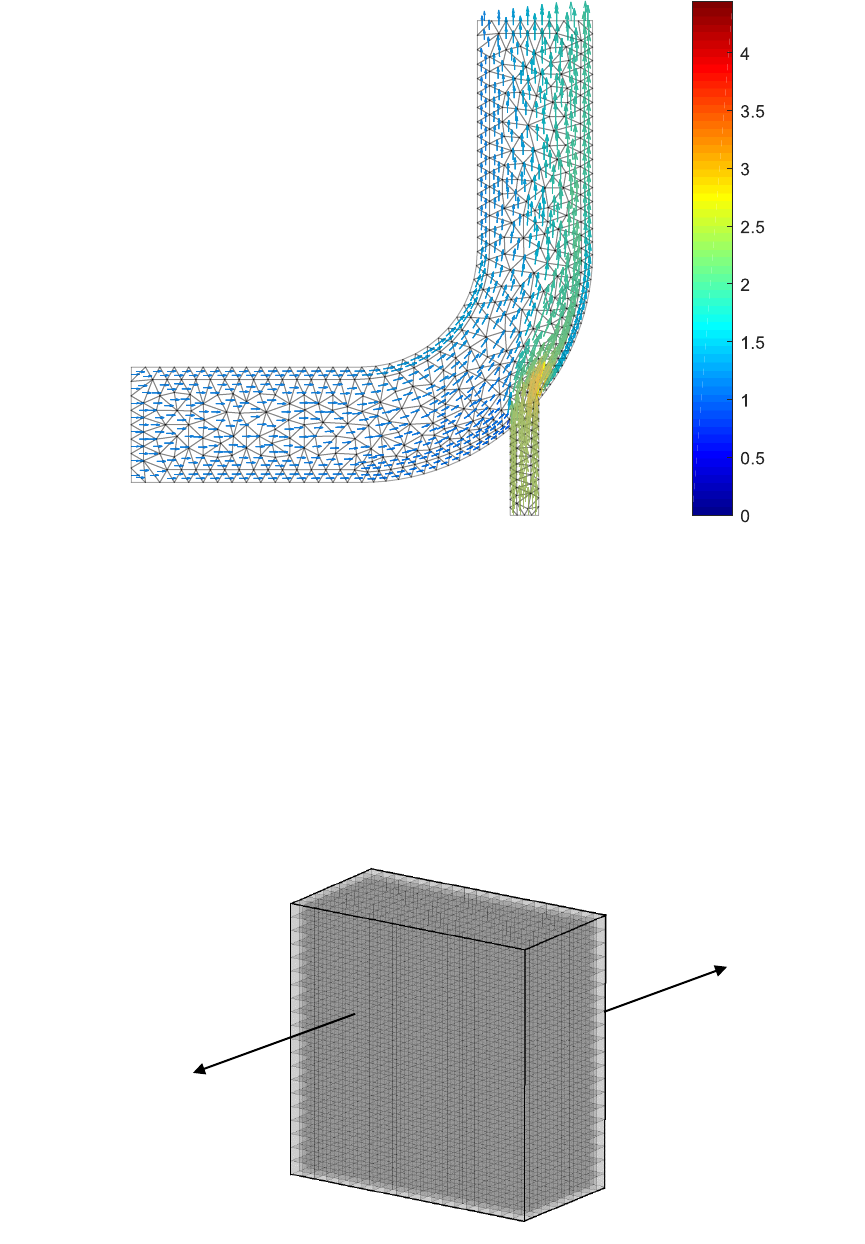
The results for velocity ‘U’, pressure ‘p’ and temperature ‘T’ in addition to the velocity vector
field will be plotted. Presented below are the results:
Figure 9 - Velocity magnitude contour (m/s)
51
Figure 10 - Pressure contour (pa)
52
Figure 11 - Temperature contour (k)
53
Figure 12 - Velocity vectors
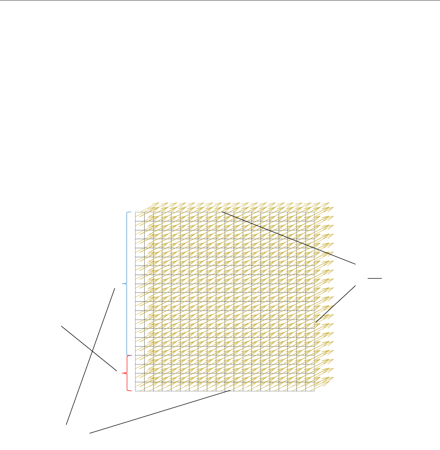
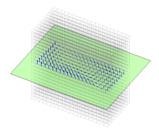
7.3 HEAT TRANSFER
A hot room case will be presented here. A buoyancy driven air flow is simulated in a room which
has different temperature values on its floor and ceiling while the walls are adiabatic. The mesh
is shown here:
Floor
Ceiling

54
In this problem, Boussinesq approximation is implemented to account for buoyancy effects due
to temperature gradients.
The governing equations are:
Momentum:
Continuity:
Energy:
The corresponding run case is:
Running the case, gives the following velocity field at an arbitrary section plane:
%--------------------------------------------------------------------------
%
% written by the CFD Group @ AUB, 2017
% contact us at: cfd@aub.edu.lb
%==========================================================================
% Case Description:
% In this test case a hot room is simulated with boussinesq
% approximation
%--------------------------------------------------------------------------
% Setup Case
cfdSetupSolverClass('heatTransfer');
% Read OpenFOAM Files
cfdReadOpenFoamFiles;
% Setup Time Settings
cfdSetupTime;
% Define new properties
cfdSetupProperty('alpha', 'model', 'nu/Pr');
% Setup Equations
cfdDefineEquation('U', 'div(U*U) = laplacian(nu*U) + div(nu*transp(grad(U))) - grad(p) - g*beta*(T - TRef)'); %
Momentum
cfdDefineEquation('p', 'div(U) = 0'); % Continuity
cfdDefineEquation('T', 'div(U*T) = laplacian(alpha*T)'); % Energy
% Initialize case
cfdInitializeCase;
% Run case
cfdRunCase;
55
Figure 13 - Velocity field at a section plane
