Vivado HLS Optimization Methodology Guide (UG1270) Ug1270 Opt
User Manual:
Open the PDF directly: View PDF ![]() .
.
Page Count: 136 [warning: Documents this large are best viewed by clicking the View PDF Link!]
- Vivado HLS Optimization Methodology Guide
- Revision History
- Table of Contents
- Ch. 1: Introduction
- Ch. 2: Optimizing the Hardware Function
- Ch. 3: Optimize Structures for Performance
- Ch. 4: Data Access Patterns
- Ch. 5: Standard Horizontal Convolution
- Appx. A: OpenCL Attributes
- Appx. B: HLS Pragmas
- pragma HLS allocation
- pragma HLS array_map
- pragma HLS array_partition
- pragma HLS array_reshape
- pragma HLS clock
- pragma HLS data_pack
- pragma HLS dataflow
- pragma HLS dependence
- pragma HLS expression_balance
- pragma HLS function_instantiate
- pragma HLS inline
- pragma HLS interface
- pragma HLS latency
- pragma HLS loop_flatten
- pragma HLS loop_merge
- pragma HLS loop_tripcount
- pragma HLS occurrence
- pragma HLS pipeline
- pragma HLS protocol
- pragma HLS reset
- pragma HLS resource
- pragma HLS stream
- pragma HLS top
- pragma HLS unroll
- Appx. C: Additional Resources and Legal Notices


Table of Contents
Revision History...............................................................................................................3
Chapter 1: Introduction.............................................................................................. 9
HLS Pragmas................................................................................................................................9
OpenCL Attributes.....................................................................................................................11
Directives....................................................................................................................................12
Chapter 2: Optimizing the Hardware Function........................................... 15
Hardware Function Optimization Methodology....................................................................16
Baseline The Hardware Functions...........................................................................................18
Optimization for Metrics.......................................................................................................... 19
Pipeline for Performance......................................................................................................... 20
Chapter 3: Optimize Structures for Performance...................................... 25
Reducing Latency...................................................................................................................... 28
Reducing Area............................................................................................................................29
Design Optimization Workflow................................................................................................31
Chapter 4: Data Access Patterns..........................................................................33
Algorithm with Poor Data Access Patterns............................................................................ 33
Algorithm With Optimal Data Access Patterns......................................................................42
Chapter 5: Standard Horizontal Convolution............................................... 45
Optimal Horizontal Convolution..............................................................................................48
Optimal Vertical Convolution...................................................................................................50
Optimal Border Pixel Convolution.......................................................................................... 52
Optimal Data Access Patterns................................................................................................. 54
Appendix A: OpenCL Attributes............................................................................55
always_inline.............................................................................................................................. 56
opencl_unroll_hint..................................................................................................................... 57
reqd_work_group_size.............................................................................................................. 58
vec_type_hint..............................................................................................................................60
Vivado HLS Optimization Methodology Guide 5
UG1270 (v2017.4) December 20, 2017 www.xilinx.com [placeholder text]

work_group_size_hint................................................................................................................61
xcl_array_partition..................................................................................................................... 63
xcl_array_reshape...................................................................................................................... 65
xcl_data_pack............................................................................................................................. 68
xcl_dataflow................................................................................................................................69
xcl_dependence......................................................................................................................... 71
xcl_max_work_group_size.........................................................................................................73
xcl_pipeline_loop........................................................................................................................75
xcl_pipeline_workitems.............................................................................................................76
xcl_reqd_pipe_depth..................................................................................................................77
xcl_zero_global_work_offset.....................................................................................................79
Appendix B: HLS Pragmas........................................................................................81
pragma HLS allocation..............................................................................................................82
pragma HLS array_map............................................................................................................84
pragma HLS array_partition.....................................................................................................87
pragma HLS array_reshape......................................................................................................89
pragma HLS clock......................................................................................................................91
pragma HLS data_pack............................................................................................................. 93
pragma HLS dataflow............................................................................................................... 95
pragma HLS dependence.........................................................................................................98
pragma HLS expression_balance.......................................................................................... 100
pragma HLS function_instantiate..........................................................................................101
pragma HLS inline...................................................................................................................103
pragma HLS interface.............................................................................................................106
pragma HLS latency................................................................................................................111
pragma HLS loop_flatten........................................................................................................113
pragma HLS loop_merge........................................................................................................115
pragma HLS loop_tripcount................................................................................................... 116
pragma HLS occurrence.........................................................................................................118
pragma HLS pipeline.............................................................................................................. 120
pragma HLS protocol..............................................................................................................122
pragma HLS reset....................................................................................................................123
pragma HLS resource............................................................................................................. 124
pragma HLS stream................................................................................................................ 126
pragma HLS top.......................................................................................................................128
pragma HLS unroll.................................................................................................................. 129
Appendix C: Additional Resources and Legal Notices........................... 133
Vivado HLS Optimization Methodology Guide 6
UG1270 (v2017.4) December 20, 2017 www.xilinx.com [placeholder text]

References................................................................................................................................133
Please Read: Important Legal Notices................................................................................. 134
Vivado HLS Optimization Methodology Guide 7
UG1270 (v2017.4) December 20, 2017 www.xilinx.com [placeholder text]


Chapter 1
Introduction
This guide provides details on how to perform opmizaons using Vivado HLS. The opmizaon
process consists of direcves which specify which opmizaons are performed and a
methodology which shows how opmizaons may be applied in a determinisc and ecient
manner.
HLS Pragmas
Optimizations in Vivado HLS
In both SDAccel and SDSoC projects, the hardware kernel must be synthesized from the OpenCL,
C, or C++ language, into RTL that can be implemented into the programmable logic of a Xilinx
device. Vivado HLS synthesizes the RTL from the OpenCL, C, and C++ language descripons.
Vivado HLS is intended to work with your SDAccel or SDSoC Development Environment project
without interacon. However, Vivado HLS also provides pragmas that can be used to opmize
the design: reduce latency, improve throughput performance, and reduce area and device
resource ulizaon of the resulng RTL code. These pragmas can be added directly to the source
code for the kernel.
IMPORTANT!:
Although the SDSoC environment supports the use of HLS pragmas, it does not support pragmas
applied to any argument of the funcon interface (interface, array paron, or data_pack pragmas).
Refer to "Opmizing the Hardware Funcon" in the SDSoC Environment Opmizaon Guide (UG1235)
for more informaon.
The Vivado HLS pragmas include the opmizaon types specied below:
Vivado HLS Optimization Methodology Guide 9
UG1270 (v2017.4) December 20, 2017 www.xilinx.com [placeholder text]

Table 1: Vivado HLS Pragmas by Type
Type Attributes
Kernel Optimization •pragma HLS allocation
•pragma HLS clock
•pragma HLS expression_balance
•pragma HLS latency
•pragma HLS reset
•pragma HLS resource
•pragma HLS top
Function Inlining •pragma HLS inline
•pragma HLS function_instantiate
Interface Synthesis •pragma HLS interface
•pragma HLS protocol
Task-level Pipeline •pragma HLS dataflow
•pragma HLS stream
Pipeline •pragma HLS pipeline
•pragma HLS occurrence
Loop Unrolling •pragma HLS unroll
•pragma HLS dependence
Loop Optimization •pragma HLS loop_flatten
•pragma HLS loop_merge
•pragma HLS loop_tripcount
Array Optimization •pragma HLS array_map
•pragma HLS array_partition
•pragma HLS array_reshape
Structure Packing •pragma HLS data_pack
Chapter 1: Introduction
Vivado HLS Optimization Methodology Guide 10
UG1270 (v2017.4) December 20, 2017 www.xilinx.com [placeholder text]

OpenCL Attributes
Optimizations in OpenCL
This secon describes OpenCL aributes that can be added to source code to assist system
opmizaon by the SDAccel compiler, xocc, the SDSoC system compilers, sdscc and sds++,
and Vivado HLS synthesis.
SDx provides OpenCL aributes to opmize your code for data movement and kernel
performance. The goal of data movement opmizaon is to maximize the system level data
throughput by maximizing interface bandwidth ulizaon and DDR bandwidth ulizaon. The
goal of kernel computaon opmizaon is to create processing logic that can consume all the
data as soon as they arrive at kernel interfaces. This is generally achieved by expanding the
processing code to match the data path with techniques such as funcon inlining and pipelining,
loop unrolling, array paroning, dataowing, etc.
The OpenCL aributes include the types specied below:
Table 2: OpenCL __attributes__ by Type
Type Attributes
Kernel Size •reqd_work_group_size
•vec_type_hint
•work_group_size_hint
•xcl_max_work_group_size
•xcl_zero_global_work_offset
Function Inlining •always_inline
Task-level Pipeline •xcl_dataflow
•xcl_reqd_pipe_depth
Pipeline •xcl_pipeline_loop
•xcl_pipeline_workitems
Loop Unrolling •opencl_unroll_hint
Array Optimization •xcl_array_partition
•xcl_array_reshape
Note: Array variables only accept a single array
opmizaon aribute.
Chapter 1: Introduction
Vivado HLS Optimization Methodology Guide 11
UG1270 (v2017.4) December 20, 2017 www.xilinx.com [placeholder text]

TIP: The SDAccel and SDSoC compilers also support many of the standard aributes supported by
gcc
, such as
always_inline
,
noinline
,
unroll
, and
nounroll
.
Directives
To view details on the aributes in the following table see the Command Reference secon in
UG902.
Note: Refer to Vivado Design Suite User Guide: High-Level Synthesis (UG902) for more details.
Table 3: Vivado HLS Pragmas by Type
Type Attributes
Kernel Optimization •set_directive_allocation
•set_directive_clock
•set_directive_expression_balance
•set_directive_latency
•set_directive_reset
•set_directive_resource
•set_directive_top
Function Inlining •set_directive_inline
•set_directive_function_instantiate
Interface Synthesis •set_directive_interface
•set_directive_protocol
Task-level Pipeline •set_directive_dataflow
•set_directive_stream
Pipeline •set_directive_pipeline
•set_directive_occurrence
Loop Unrolling •set_directive_unroll
•set_directive_dependence
Loop Optimization •set_directive_loop_flatten
•set_directive_loop_merge
•set_directive_loop_tripcount
Chapter 1: Introduction
Vivado HLS Optimization Methodology Guide 12
UG1270 (v2017.4) December 20, 2017 www.xilinx.com [placeholder text]

Table 3: Vivado HLS Pragmas by Type (cont'd)
Type Attributes
Array Optimization •set_directive_array_map
•set_directive_array_partition
•set_directive_array_reshape
Structure Packing •set_directive_data_pack
Chapter 1: Introduction
Vivado HLS Optimization Methodology Guide 13
UG1270 (v2017.4) December 20, 2017 www.xilinx.com [placeholder text]


Chapter 2
Optimizing the Hardware Function
The SDSoC environment employs heterogeneous cross-compilaon, with ARM CPU-specic
cross compilers for the Zynq-7000 SoC and Zynq UltraScale+ MPSoC CPUs, and Vivado HLS as a
PL cross-compiler for hardware funcons. This secon explains the default behavior and
opmizaon direcves associated with the Vivado HLS cross-compiler.
The default behavior of Vivado HLS is to execute funcons and loops in a sequenal manner
such that the hardware is an accurate reecon of the C/C++ code. Opmizaon direcves can
be used to enhance the performance of the hardware funcon, allowing pipelining which
substanally increases the performance of the funcons. This chapter outlines a general
methodology for opmizing your design for high performance.
There are many possible goals when trying to opmize a design using Vivado HLS. The
methodology assumes you want to create a design with the highest possible performance,
processing one sample of new input data every clock cycle, and so addresses those opmizaons
before the ones used for reducing latency or resources.
Detailed explanaons of the opmizaons discussed here are provided in Vivado Design Suite
User Guide: High-Level Synthesis (UG902).
It is highly recommended to review the methodology and obtain a global perspecve of hardware
funcon opmizaon before reviewing the details of specic opmizaon.
Vivado HLS Optimization Methodology Guide 15
UG1270 (v2017.4) December 20, 2017 www.xilinx.com [placeholder text]

Hardware Function Optimization
Methodology
Hardware funcons are synthesized into hardware in the Programmable Logic (PL) by the Vivado
HLS compiler. This compiler automacally translates C/C++ code into an FPGA hardware
implementaon, and as with all compilers, does so using compiler defaults. In addion to the
compiler defaults, Vivado HLS provides a number of opmizaons that are applied to the C/C++
code through the use of pragmas in the code. This chapter explains the opmizaons that can be
applied and a recommended methodology for applying them.
The are two ows for opmizing the hardware funcons.
• Top-down ow: In this ow, program decomposion into hardware funcons proceeds top-
down within the SDSoC environment, leng the system compiler create pipelines of
funcons that automacally operate in dataow mode. The microarchitecture for each
hardware funcon is opmized using Vivado HLS.
•Boom-up ow: In this ow, the hardware funcons are opmized in isolaon from the
system using the Vivado HLS compiler provided in the Vivado Design suite. The hardware
funcons are analyzed, opmizaons direcves can be applied to create an implementaon
other than the default, and the resulng opmized hardware funcons are then incorporated
into the SDSoC environment.
The boom-up ow is oen used in organizaons where the soware and hardware are
opmized by dierent teams and can be used by soware programmers who wish to take
advantage of exisng hardware implementaons from within their organizaon or from partners.
Both ows are supported, and the same opmizaon methodology is used in either case. Both
workows result in the same high-performance system. Xilinx sees the choice as a workow
decision made by individual teams and organizaons and provides no recommendaon on which
ow to use. Examples of both ows are provided in this link in the SDSoC Environment
Opmizaon Guide (UG1235).
The opmizaon methodology for hardware funcons is shown in the gure below.
Chapter 2: Optimizing the Hardware Function
Vivado HLS Optimization Methodology Guide 16
UG1270 (v2017.4) December 20, 2017 www.xilinx.com [placeholder text]

Simulate Design - Validate The C function
Synthesize Design - Baseline design
1: Initial Optimizations - Define interfaces (and data packing)
- Define loop trip counts
2: Pipeline for Performance - Pipeline and dataflow
3: Optimize Structures for Performance - Partition memories and ports
- Remove false dependencies
4: Reduce Latency - Optionally specify latency requirements
5: Improve Area - Optionally recover resources through sharing
X15638-110617
The gure above details all the steps in the methodology and the subsequent secons in this
chapter explain the opmizaons in detail.
IMPORTANT!: Designs will reach the opmum performance aer step 3.
Step 4 is used to minimize, or specically control, the latency through the design and is only
required for applicaons where this is of concern. Step 5 explains how to reduce the resources
required for hardware implementaon and is typically only applied when larger hardware
funcons fail to implement in the available resources. The FPGA has a xed number of resources,
and there is typically no benet in creang a smaller implementaon if the performance goals
have been met.
Chapter 2: Optimizing the Hardware Function
Vivado HLS Optimization Methodology Guide 17
UG1270 (v2017.4) December 20, 2017 www.xilinx.com [placeholder text]

Baseline The Hardware Functions
Before seeking to perform any hardware funcon opmizaon, it is important to understand the
performance achieved with the exisng code and compiler defaults, and appreciate how
performance is measured. This is achieved by selecng the funcons to implement hardware and
building the project.
Aer the project has been built, a report is available in the reports secon of the IDE (and
provided at <project name>/<build_config>/_sds/vhls/<hw_function>/
solution/syn/report/<hw_function>.rpt). This report details the performance
esmates and ulizaon esmates.
The key factors in the performance esmates are the ming, interval, and latency in that order.
• The ming summary shows the target and esmated clock frequency. If the esmated clock
frequency is greater than the target, the hardware will not funcon at this clock frequency. The
clock frequency should be reduced by using the Data Moon Network Clock Frequency
opon in the Project Sengs. Alternavely, because this is only an esmate at this point in
the ow, it might be possible to proceed through the remainder of the ow if the esmate
only exceeds the target by 20%. Further opmizaons are applied when the bitstream is
generated, and it might sll be possible to sasfy the ming requirements. However, this is an
indicaon that the hardware funcon is not guaranteed to meet ming.
• The iniaon interval (II) is the number of clock cycles before the funcon can accept new
inputs and is generally the most crical performance metric in any system. In an ideal hardware
funcon, the hardware processes data at the rate of one sample per clock cycle. If the largest
data set passed into the hardware is size N (e.g., my_array[N]), the most opmal II is N + 1.
This means the hardware funcon processes N data samples in N clock cycles and can accept
new data one clock cycle aer all N samples are processed. It is possible to create a hardware
funcon with an II < N, however, this requires greater resources in the PL with typically lile
benet. The hardware funcon will oen be ideal as it consumes and produces data at a rate
faster than the rest of the system.
• The loop iniaon interval is the number of clock cycles before the next iteraon of a loop
starts to process data. This metric becomes important as you delve deeper into the analysis to
locate and remove performance bolenecks.
• The latency is the number of clock cycles required for the funcon to compute all output
values. This is simply the lag from when data is applied unl when it is ready. For most
applicaons this is of lile concern, especially when the latency of the hardware funcon
vastly exceeds that of the soware or system funcons such as DMA. It is, however, a
performance metric that you should review and conrm is not an issue for your applicaon.
• The loop iteraon latency is the number of clock cycles it takes to complete one iteraon of a
loop, and the loop latency is the number of cycles to execute all iteraons of the loop.
Chapter 2: Optimizing the Hardware Function
Vivado HLS Optimization Methodology Guide 18
UG1270 (v2017.4) December 20, 2017 www.xilinx.com [placeholder text]
The Area Esmates secon of the report details how many resources are required in the PL to
implement the hardware funcon and how many are available on the device. The key metric here
is the Ulizaon (%). The Ulizaon (%) should not exceed 100% for any of the resources. A gure
greater than 100% means there are not enough resources to implement the hardware funcon,
and a larger FPGA device might be required. As with the ming, at this point in the ow, this is an
esmate. If the numbers are only slightly over 100%, it might be possible for the hardware to be
opmized during bitstream creaon.
You should already have an understanding of the required performance of your system and what
metrics are required from the hardware funcons. However, even if you are unfamiliar with
hardware concepts such as clock cycles, you are now aware that the highest performing
hardware funcons have an II = N + 1, where N is the largest data set processed by the funcon.
With an understanding of the current design performance and a set of baseline performance
metrics, you can now proceed to apply opmizaon direcves to the hardware funcons.
Optimization for Metrics
The following table shows the rst direcve you should think about adding to your design.
Table 4: Optimization Strategy Step 1: Optimization For Metrics
Directives and Configurations Description
LOOP_TRIPCOUNT Used for loops that have variable bounds. Provides an
estimate for the loop iteration count. This has no impact on
synthesis, only on reporting.
A common issue when hardware funcons are rst compiled is report les showing the latency
and interval as a queson mark “?” rather than as numerical values. If the design has loops with
variable loop bounds, the compiler cannot determine the latency or II and uses the “?” to indicate
this condion. Variable loop bounds are where the loop iteraon limit cannot be resolved at
compile me, as when the loop iteraon limit is an input argument to the hardware funcon,
such as variable height, width, or depth parameters.
To resolve this condion, use the hardware funcon report to locate the lowest level loop which
fails to report a numerical value and use the LOOP_TRIPCOUNT direcve to apply an esmated
tripcount. The tripcount is the minimum, average, and/or maximum number of expected
iteraons. This allows values for latency and interval to be reported and allows implementaons
with dierent opmizaons to be compared.
Because the LOOP_TRIPCOUNT value is only used for reporng, and has no impact on the
resulng hardware implementaon, any value can be used. However, an accurate expected value
results in more useful reports.
Chapter 2: Optimizing the Hardware Function
Vivado HLS Optimization Methodology Guide 19
UG1270 (v2017.4) December 20, 2017 www.xilinx.com [placeholder text]
Pipeline for Performance
The next stage in creang a high-performance design is to pipeline the funcons, loops, and
operaons. Pipelining results in the greatest level of concurrency and the highest level of
performance. The following table shows the direcves you can use for pipelining.
Table 5: Optimization Strategy Step 1: Optimization Strategy Step 2: Pipeline for
Performance
Directives and Configurations Description
PIPELINE Reduces the initiation interval by allowing the concurrent
execution of operations within a loop or function.
DATAFLOW Enables task level pipelining, allowing functions and loops
to execute concurrently. Used to minimize interval.
RESOURCE Specifies pipelining on the hardware resource used to
implement a variable (array, arithmetic operation).
Config Compile Allows loops to be automatically pipelined based on their
iteration count when using the bottom-up flow.
At this stage of the opmizaon process, you want to create as much concurrent operaon as
possible. You can apply the PIPELINE direcve to funcons and loops. You can use the
DATAFLOW direcve at the level that contains the funcons and loops to make them work in
parallel. Although rarely required, the RESOURCE direcve can be used to squeeze out the
highest levels of performance.
A recommended strategy is to work from the boom up and be aware of the following:
• Some funcons and loops contain sub-funcons. If the sub-funcon is not pipelined, the
funcon above it might show limited improvement when it is pipelined. The non-pipelined
sub-funcon will be the liming factor.
• Some funcons and loops contain sub-loops. When you use the PIPELINE direcve, the
direcve automacally unrolls all loops in the hierarchy below. This can create a great deal of
logic. It might make more sense to pipeline the loops in the hierarchy below.
• For cases where it does make sense to pipeline the upper hierarchy and unroll any loops lower
in the hierarchy, loops with variable bounds cannot be unrolled, and any loops and funcons
in the hierarchy above these loops cannot be pipelined. To address this issue, pipeline these
loops wih variable bounds, and use the DATAFLOW opmizaon to ensure the pipelined
loops operate concurrently to maximize the performance of the tasks that contains the loops.
Alternavely, rewrite the loop to remove the variable bound. Apply a maximum upper bound
with a condional break.
The basic strategy at this point in the opmizaon process is to pipeline the tasks (funcons and
loops) as much as possible. For detailed informaon on which funcons and loops to pipeline,
refer to Hardware Funcon Pipeline Strategies.
Chapter 2: Optimizing the Hardware Function
Vivado HLS Optimization Methodology Guide 20
UG1270 (v2017.4) December 20, 2017 www.xilinx.com [placeholder text]

Although not commonly used, you can also apply pipelining at the operator level. For example,
wire roung in the FPGA can introduce large and unancipated delays that make it dicult for
the design to be implemented at the required clock frequency. In this case, you can use the
RESOURCE direcve to pipeline specic operaons such as mulpliers, adders, and block RAM
to add addional pipeline register stages at the logic level and allow the hardware funcon to
process data at the highest possible performance level without the need for recursion.
Note: The Cong commands are used to change the opmizaon default sengs and are only available
from within Vivado HLS when using a boom-up ow. Refer to Vivado Design Suite User Guide: High-Level
Synthesis (UG902) for more details.
Hardware Function Pipeline Strategies
The key opmizaon direcves for obtaining a high-performance design are the PIPELINE and
DATAFLOW direcves. This secon discusses in detail how to apply these direcves for various
C code architectures.
Fundamentally, there are two types of C/C++ funcons: those that are frame-based and those
that are sampled-based. No maer which coding style is used, the hardware funcon can be
implemented with the same performance in both cases. The dierence is only in how the
opmizaon direcves are applied.
Frame-Based C Code
The primary characterisc of a frame-based coding style is that the funcon processes mulple
data samples - a frame of data – typically supplied as an array or pointer with data accessed
through pointer arithmec during each transacon (a transacon is considered to be one
complete execuon of the C funcon). In this coding style, the data is typically processed
through a series of loops or nested loops.
An example outline of frame-based C code is shown below.
void foo(
data_t in1[HEIGHT][WIDTH],
data_t in2[HEIGHT][WIDTH],
data_t out[HEIGHT][WIDTH] {
Loop1: for(int i = 0; i < HEIGHT; i++) {
Loop2: for(int j = 0; j < WIDTH; j++) {
out[i][j] = in1[i][j] * in2[i][j];
Loop3: for(int k = 0; k < NUM_BITS; k++) {
. . . .
}
}
}
Chapter 2: Optimizing the Hardware Function
Vivado HLS Optimization Methodology Guide 21
UG1270 (v2017.4) December 20, 2017 www.xilinx.com [placeholder text]

When seeking to pipeline any C/C++ code for maximum performance in hardware, you want to
place the pipeline opmizaon direcve at the level where a sample of data is processed.
The above example is representave of code used to process an image or video frame and can be
used to highlight how to eecvely pipeline hardware funcons. Two sets of input are provided
as frames of data to the funcon, and the output is also a frame of data. There are mulple
locaons where this funcon can be pipelined:
• At the level of funcon foo.
• At the level of loop Loop1.
• At the level of loop Loop2.
• At the level of loop Loop3.
Reviewing the advantages and disadvantages of placing the PIPELINE direcve at each of these
locaons helps explain the best locaon to place the pipeline direcve for your code.
Funcon Level: The funcon accepts a frame of data as input (in1 and in2). If the funcon is
pipelined with II = 1—read a new set of inputs every clock cycle—this informs the compiler to
read all HEIGHT*WIDTH values of in1 and in2 in a single clock cycle. It is unlikely this is the
design you want.
If the PIPELINE direcve is applied to funcon foo, all loops in the hierarchy below this level
must be unrolled. This is a requirement for pipelining, namely, there cannot be sequenal logic
inside the pipeline. This would create HEIGHT*WIDTH*NUM_ELEMENT copies of the logic,
which would lead to a large design.
Because the data is accessed in a sequenal manner, the arrays on the interface to the hardware
funcon can be implemented as mulple types of hardware interface:
• Block RAM interface
• AXI4 interface
• AXI4-Lite interface
• AXI4-Stream interface
• FIFO interface
A block RAM interface can be implemented as a dual-port interface supplying two samples per
clock. The other interface types can only supply one sample per clock. This would result in a
boleneck. There would be a large highly parallel hardware design unable to process all the data
in parallel and would lead to a waste of hardware resources.
Chapter 2: Optimizing the Hardware Function
Vivado HLS Optimization Methodology Guide 22
UG1270 (v2017.4) December 20, 2017 www.xilinx.com [placeholder text]

Loop1 Level: The logic in Loop1 processes an enre row of the two-dimensional matrix. Placing
the PIPELINE direcve here would create a design which seeks to process one row in each clock
cycle. Again, this would unroll the loops below and create addional logic. However, the only way
to make use of the addional hardware would be to transfer an enre row of data each clock
cycle: an array of HEIGHT data words, with each word being WIDTH*<number of bits in data_t>
bits wide.
Because it is unlikely the host code running on the PS can process such large data words, this
would again result in a case where there are many highly parallel hardware resources that cannot
operate in parallel due to bandwidth limitaons.
Loop2 Level: The logic in Loop2 seeks to process one sample from the arrays. In an image
algorithm, this is the level of a single pixel. This is the level to pipeline if the design is to process
one sample per clock cycle. This is also the rate at which the interfaces consume and produce
data to and from the PS.
This will cause Loop3 to be completely unrolled but to process one sample per clock. It is a
requirement that all the operaons in Loop3 execute in parallel. In a typical design, the logic in
Loop3 is a shi register or is processing bits within a word. To execute at one sample per clock,
you want these processes to occur in parallel and hence you want to unroll the loop. The
hardware funcon created by pipelining Loop2 processes one data sample per clock and creates
parallel logic only where needed to achieve the required level of data throughput.
Loop3 Level: As stated above, given that Loop2 operates on each data sample or pixel, Loop3 will
typically be doing bit-level or data shiing tasks, so this level is doing mulple operaons per
pixel. Pipelining this level would mean performing each operaon in this loop once per clock and
thus NUM_BITS clocks per pixel: processing at the rate of mulple clocks per pixel or data
sample.
For example, Loop3 might contain a shi register holding the previous pixels required for a
windowing or convoluon algorithm. Adding the PIPELINE direcve at this level informs the
complier to shi one data value every clock cycle. The design would only return to the logic in
Loop2 and read the next inputs aer NUM_BITS iteraons resulng in a very slow data
processing rate.
The ideal locaon to pipeline in this example is Loop2.
When dealing with frame-based code you will want to pipeline at the loop level and typically
pipeline the loop that operates at the level of a sample. If in doubt, place a print command into
the C code and to conrm this is the level you wish to execute on each clock cycle.
For cases where there are mulple loops at the same level of hierarchy—the example above
shows only a set of nested loops—the best locaon to place the PIPELINE direcve can be
determined for each loop and then the DATAFLOW direcve applied to the funcon to ensure
each of the loops executes in a concurrent manner.
Chapter 2: Optimizing the Hardware Function
Vivado HLS Optimization Methodology Guide 23
UG1270 (v2017.4) December 20, 2017 www.xilinx.com [placeholder text]

Sample-Based C Code
An example outline of sample-based C code is shown below. The primary characterisc of this
coding style is that the funcon processes a single data sample during each transacon.
void foo (data_t *in, data_t *out) {
static data_t acc;
Loop1: for (int i=N-1;i>=0;i--) {
acc+= ..some calculation..;
}
*out=acc>>N;
}
Another characterisc of sample-based coding style is that the funcon oen contains a stac
variable: a variable whose value must be remembered between invocaons of the funcon, such
as an accumulator or sample counter.
With sample-based code, the locaon of the PIPELINE direcve is clear, namely, to achieve an II
= 1 and process one data value each clock cycle, for which the funcon must be pipelined.
This unrolls any loops inside the funcon and creates addional hardware logic, but there is no
way around this. If Loop1 is pipelined, it takes a minimum of N clock cycles to complete. Only
then can the funcon read the next x input value.
When dealing with C code that processes at the sample level, the strategy is always to pipeline
the funcon.
In this type of coding style, the loops are typically operang on arrays and performing a shi
register or line buer funcons. It is not uncommon to paron these arrays into individual
elements as discussed in Chapter 3: Opmize Structures for Performance to ensure all samples
are shied in a single clock cycle. If the array is implemented in a block RAM, only a maximum of
two samples can be read or wrien in each clock cycle, creang a data processing boleneck.
The soluon here is to pipeline funcon foo. Doing so results in a design that processes one
sample per clock.
Chapter 2: Optimizing the Hardware Function
Vivado HLS Optimization Methodology Guide 24
UG1270 (v2017.4) December 20, 2017 www.xilinx.com [placeholder text]

Chapter 3
Optimize Structures for
Performance
C code can contain descripons that prevent a funcon or loop from being pipelined with the
required performance. This is oen implied by the structure of the C code or the default logic
structures used to implement the PL logic. In some cases, this might require a code modicaon,
but in most cases these issues can be addressed using addional opmizaon direcves.
The following example shows a case where an opmizaon direcve is used to improve the
structure of the implementaon and the performance of pipelining. In this inial example, the
PIPELINE direcve is added to a loop to improve the performance of the loop. This example code
shows a loop being used inside a funcon.
#include "bottleneck.h"
dout_t bottleneck(...) {
...
SUM_LOOP: for(i=3;i<N;i=i+4) {
#pragma HLS PIPELINE
sum += mem[i] + mem[i-1] + mem[i-2] + mem[i-3];
}
...
}
When the code above is compiled into hardware, the following message appears as output:
INFO: [SCHED 61] Pipelining loop 'SUM_LOOP'.
WARNING: [SCHED 69] Unable to schedule 'load' operation ('mem_load_2',
bottleneck.c:62) on array 'mem' due to limited memory ports.
INFO: [SCHED 61] Pipelining result: Target II: 1, Final II: 2, Depth: 3.
I
The issue in this example is that arrays are implemented using the ecient block RAM resources
in the PL fabric. This results in a small cost-ecient fast design. The disadvantage of block RAM
is that, like other memories such as DDR or SRAM, they have a limited number of data ports,
typically a maximum of two.
In the code above, four data values from mem are required to compute the value of sum. Because
mem is an array and implemented in a block RAM that only has two data ports, only two values
can be read (or wrien) in each clock cycle. With this conguraon, it is impossible to compute
the value of sum in one clock cycle and thus consume or produce data with an II of 1 (process
one data sample per clock).
Vivado HLS Optimization Methodology Guide 25
UG1270 (v2017.4) December 20, 2017 www.xilinx.com [placeholder text]
The memory port limitaon issue can be solved by using the ARRAY_PARTITION direcve on the
mem array. This direcve parons arrays into smaller arrays, improving the data structure by
providing more data ports and allowing a higher performance pipeline.
With the addional direcve shown below, array mem is paroned into two dual-port memories
so that all four reads can occur in one clock cycle. There are mulple opons to paroning an
array. In this case, cyclic paroning with a factor of two ensures the rst paron contains
elements 0, 2, 4, etc., from the original array and the second paron contains elements 1, 3, 5,
etc. Because the paroning ensures there are now two dual-port block RAMs (with a total of
four data ports), this allows elements 0, 1, 2, and 3 to be read in a single clock cycle.
Note: The ARRAY_PARTITION direcve cannot be used on arrays which are arguments of the funcon
selected as an accelerator.
#include "bottleneck.h"
dout_t bottleneck(...) {
#pragma HLS ARRAY_PARTITION variable=mem cyclic factor=2 dim=1
...
SUM_LOOP: for(i=3;i<N;i=i+4) {
#pragma HLS PIPELINE
sum += mem[i] + mem[i-1] + mem[i-2] + mem[i-3];
}
...
}
Other such issues might be encountered when trying to pipeline loops and funcons. The
following table lists the direcves that are likely to address these issues by helping to reduce
bolenecks in data structures.
Table 6: Optimization Strategy Step 3: Optimize Structures for Performance
Directives and Configurations Description
ARRAY_PARTITION Partitions large arrays into multiple smaller arrays or into
individual registers to improve access to data and remove
block RAM bottlenecks.
DEPENDENCE Provides additional information that can overcome loop-
carry dependencies and allow loops to be pipelined (or
pipelined with lower intervals).
INLINE Inlines a function, removing all function hierarchy. Enables
logic optimization across function boundaries and improves
latency/interval by reducing function call overhead.
UNROLL Unrolls for-loops to create multiple independent operations
rather than a single collection of operations, allowing
greater hardware parallelism. This also allows for partial
unrolling of loops.
Config Array Partition This configuration determines how arrays are automatically
partitioned, including global arrays, and if the partitioning
impacts array ports.
Config Compile Controls synthesis specific optimizations such as the
automatic loop pipelining and floating point math
optimizations.
Chapter 3: Optimize Structures for Performance
Vivado HLS Optimization Methodology Guide 26
UG1270 (v2017.4) December 20, 2017 www.xilinx.com [placeholder text]

Table 6: Optimization Strategy Step 3: Optimize Structures for Performance (cont'd)
Directives and Configurations Description
Config Schedule Determines the effort level to use during the synthesis
scheduling phase, the verbosity of the output messages,
and to specify if II should be relaxed in pipelined tasks to
achieve timing.
Config Unroll Allows all loops below the specified number of loop
iterations to be automatically unrolled.
In addion to the ARRAY_PARTITION direcve, the conguraon for array paroning can be
used to automacally paron arrays.
The DEPENDENCE direcve might be required to remove implied dependencies when pipelining
loops. Such dependencies are reported by message SCHED-68.
@W [SCHED-68] Target II not met due to carried dependence(s)
The INLINE direcve removes funcon boundaries. This can be used to bring logic or loops up
one level of hierarchy. It might be more ecient to pipeline the logic in a funcon by including it
in the funcon above it, and merging loops into the funcon above them where the DATAFLOW
opmizaon can be used to execute all the loops concurrently without the overhead of the
intermediate sub-funcon call. This might lead to a higher performing design.
The UNROLL direcve might be required for cases where a loop cannot be pipelined with the
required II. If a loop can only be pipelined with II = 4, it will constrain the other loops and
funcons in the system to be limited to II = 4. In some cases, it might be worth unrolling or
parally unrolling the loop to creang more logic and remove a potenal boleneck. If the loop
can only achieve II = 4, unrolling the loop by a factor of 4 creates logic that can process four
iteraons of the loop in parallel and achieve II = 1.
The Cong commands are used to change the opmizaon default sengs and are only available
from within Vivado HLS when using a boom-up ow. Refer to Vivado Design Suite User Guide:
High-Level Synthesis (UG902) for more details.
If opmizaon direcves cannot be used to improve the iniaon interval, it might require
changes to the code. Examples of this are discussed in Vivado Design Suite User Guide: High-Level
Synthesis (UG902).
Chapter 3: Optimize Structures for Performance
Vivado HLS Optimization Methodology Guide 27
UG1270 (v2017.4) December 20, 2017 www.xilinx.com [placeholder text]
Reducing Latency
When the compiler nishes minimizing the iniaon interval (II), it automacally seeks to
minimize the latency. The opmizaon direcves listed in the following table can help specify a
parcular latency or inform the compiler to achieve a latency lower than the one produced,
namely, instruct the compiler to sasfy the latency direcve even if it results in a higher II. This
could result in a lower performance design.
Latency direcve are generally not required because most applicaons have a required
throughput but no required latency. When hardware funcons are integrated with a processor,
the latency of the processor is generally the liming factor in the system.
If the loops and funcons are not pipelined, the throughput is limited by the latency because the
task does not start reading the next set of inputs unl the current task has completed.
Table 7: Optimization Strategy Step 4: Reduce Latency
Directive Description
LATENCY Allows a minimum and maximum latency constraint to be
specified.
LOOP_FLATTEN Allows nested loops to be collapsed into a single loop. This
removes the loop transition overhead and improves the
latency. Nested loops are automatically flattened when the
PIPELINE directive is applied.
LOOP_MERGE Merges consecutive loops to reduce overall latency, increase
logic resource sharing, and improve logic optimization.
The loop opmizaon direcves can be used to aen a loop hierarchy or merge consecuve
loops together. The benet to the latency is due to the fact that it typically costs a clock cycle in
the control logic to enter and leave the logic created by a loop. The fewer the number of
transions between loops, the lesser number of clock cycles a design takes to complete.
Chapter 3: Optimize Structures for Performance
Vivado HLS Optimization Methodology Guide 28
UG1270 (v2017.4) December 20, 2017 www.xilinx.com [placeholder text]

Reducing Area
In hardware, the number of resources required to implement a logic funcon is referred to as the
design area. Design area also refers to how much area the resource used on the xed-size PL
fabric. The area is of importance when the hardware is too large to be implemented in the target
device, and when the hardware funcon consumes a very high percentage (> 90%) of the
available area. This can result in dicules when trying to wire the hardware logic together
because the wires themselves require resources.
Aer meeng the required performance target (or II), the next step might be to reduce the area
while maintaining the same performance. This step can be opmal because there is nothing to be
gained by reducing the area if the hardware funcon is operang at the required performance
and no other hardware funcons are to be implemented in the remaining space in the PL.
The most common area opmizaon is the opmizaon of dataow memory channels to reduce
the number of block RAM resources required to implement the hardware funcon. Each device
has a limited number of block RAM resources.
If you used the DATAFLOW opmizaon and the compiler cannot determine whether the tasks
in the design are streaming data, it implements the memory channels between dataow tasks
using ping-pong buers. These require two block RAMs each of size N, where N is the number of
samples to be transferred between the tasks (typically the size of the array passed between
tasks). If the design is pipelined and the data is in fact streaming from one task to the next with
values produced and consumed in a sequenal manner, you can greatly reduce the area by using
the STREAM direcve to specify that the arrays are to be implemented in a streaming manner
that uses a simple FIFO for which you can specify the depth. FIFOs with a small depth are
implemented using registers and the PL fabric has many registers.
For most applicaons, the depth can be specied as 1, resulng in the memory channel being
implemented as a simple register. If, however, the algorithm implements data compression or
extrapolaon where some tasks consume more data than they produce or produce more data
than they consume, some arrays must be specied with a higher depth:
• For tasks which produce and consume data at the same rate, specify the array between them
to stream with a depth of 1.
• For tasks which reduce the data rate by a factor of X-to-1, specify arrays at the input of the
task to stream with a depth of X. All arrays prior to this in the funcon should also have a
depth of X to ensure the hardware funcon does not stall because the FIFOs are full.
• For tasks which increase the data rate by a factor of 1-to-Y, specify arrays at the output of the
task to stream with a depth of Y. All arrays aer this in the funcon should also have a depth
of Y to ensure the hardware funcon does not stall because the FIFOs are full.
Chapter 3: Optimize Structures for Performance
Vivado HLS Optimization Methodology Guide 29
UG1270 (v2017.4) December 20, 2017 www.xilinx.com [placeholder text]
Note: If the depth is set too small, the symptom will be the hardware funcon will stall (hang) during
Hardware Emulaon resulng in lower performance, or even deadlock in some cases, due to full FIFOs
causing the rest of the system to wait.
The following table lists the other direcves to consider when aempng to minimize the
resources used to implement the design.
Table 8: Optimization Strategy Step 5: Reduce Area
Directives and Configurations Description
ALLOCATION Specifies a limit for the number of operations, hardware
resources, or functions used. This can force the sharing of
hardware resources but might increase latency.
ARRAY_MAP Combines multiple smaller arrays into a single large array to
help reduce the number of block RAM resources.
ARRAY_RESHAPE Reshapes an array from one with many elements to one
with greater word width. Useful for improving block RAM
accesses without increasing the number of block RAM.
DATA_PACK Packs the data fields of an internal struct into a single scalar
with a wider word width, allowing a single control signal to
control all fields.
LOOP_MERGE Merges consecutive loops to reduce overall latency, increase
sharing, and improve logic optimization.
OCCURRENCE Used when pipelining functions or loops to specify that the
code in a location is executed at a lesser rate than the code
in the enclosing function or loop.
RESOURCE Specifies that a specific hardware resource (core) is used to
implement a variable (array, arithmetic operation).
STREAM Specifies that a specific memory channel is to be
implemented as a FIFO with an optional specific depth.
Config Bind Determines the effort level to use during the synthesis
binding phase and can be used to globally minimize the
number of operations used.
Config Dataflow This configuration specifies the default memory channel
and FIFO depth in dataflow optimization.
The ALLOCATION and RESOURCE direcves are used to limit the number of operaons and to
select which cores (hardware resources) are used to implement the operaons. For example, you
could limit the funcon or loop to using only one mulplier and specify it to be implemented
using a pipelined mulplier.
If the ARRAY_PARITION direcve is used to improve the iniaon interval you might want to
consider using the ARRAY_RESHAPE direcve instead. The ARRAY_RESHAPE opmizaon
performs a similar task to array paroning, however, the reshape opmizaon recombines the
elements created by paroning into a single block RAM with wider data ports. This might
prevent an increase in the number of block RAM resources required.
Chapter 3: Optimize Structures for Performance
Vivado HLS Optimization Methodology Guide 30
UG1270 (v2017.4) December 20, 2017 www.xilinx.com [placeholder text]

If the C code contains a series of loops with similar indexing, merging the loops with the
LOOP_MERGE direcve might allow some opmizaons to occur. Finally, in cases where a
secon of code in a pipeline region is only required to operate at an iniaon interval lower than
the rest of the region, the OCCURENCE direcve is used to indicate that this logic can be
opmized to execute at a lower rate.
Note: The Cong commands are used to change the opmizaon default sengs and are only available
from within Vivado HLS when using a boom-up ow. Refer to Vivado Design Suite User Guide: High-Level
Synthesis (UG902) for more details.
Design Optimization Workflow
Before performing any opmizaons it is recommended to create a new build conguraon
within the project. Using dierent build conguraons allows one set of results to be compared
against a dierent set of results. In addion to the standard Debug and Release conguraons,
custom conguraons with more useful names (e.g., Opt_ver1 and UnOpt_ver) might be created
in the Project Sengs window using the Manage Build Conguraons for the Project toolbar
buon.
Dierent build conguraons allow you to compare not only the results, but also the log les and
even output RTL les used to implement the FPGA (the RTL les are only recommended for
users very familiar with hardware design).
The basic opmizaon strategy for a high-performance design is:
• Create an inial or baseline design.
• Pipeline the loops and funcons. Apply the DATAFLOW opmizaon to execute loops and
funcons concurrently.
• Address any issues that limit pipelining, such as array bolenecks and loop dependencies (with
ARRAY_PARTITION and DEPENDENCE direcves).
• Specify a specic latency or reduce the size of the dataow memory channels and use the
ALLOCATION and RESOUCES direcves to further reduce area.
Note: It might somemes be necessary to make adjustments to the code to meet performance.
In summary, the goal is to always meet performance rst, before reducing area. If the strategy is
to create a design with the fewest resources, simply omit the steps to improving performance,
although the baseline results might be very close to the smallest possible design.
Throughout the opmizaon process it is highly recommended to review the console output (or
log le) aer compilaon. When the compiler cannot reach the specied performance goals of an
opmizaon, it automacally relaxes the goals (except the clock frequency) and creates a design
with the goals that can be sased. It is important to review the output from the compilaon log
les and reports to understand what opmizaons have been performed.
Chapter 3: Optimize Structures for Performance
Vivado HLS Optimization Methodology Guide 31
UG1270 (v2017.4) December 20, 2017 www.xilinx.com [placeholder text]


Chapter 4
Data Access Patterns
An FPGA is selected to implement the C code due to the superior performance of the FPGA - the
massively parallel architecture of an FPGA allows it to perform operaons much faster than the
inherently sequenal operaons of a processor, and users typically wish to take advantage of
that performance.
The focus here is on understanding the impact that the access paerns inherent in the C code
might have on the results. Although the access paerns of most concern are those into and out
of the hardware funcon, it is worth considering the access paerns within funcons as any
bolenecks within the hardware funcon will negavely impact the transfer rate into and out of
the funcon.
To highlight how some data access paerns can negavely impact performance and demonstrate
how other paerns can be used to fully embrace the parallelism and high performance
capabilies of an FPGA, this secon reviews an image convoluon algorithm.
• The rst part reviews the algorithm and highlights the data access aspects that limit the
performance in an FPGA.
• The second part shows how the algorithm might be wrien to achieve the highest
performance possible.
Algorithm with Poor Data Access Patterns
A standard convoluon funcon applied to an image is used here to demonstrate how the C
code can negavely impact the performance that is possible from an FPGA. In this example, a
horizontal and then vercal convoluon is performed on the data. Because the data at the edge
of the image lies outside the convoluon windows, the nal step is to address the data around
the border.
The algorithm structure can be summarized as follows:
• A horizontal convoluon.
• Followed by a vercal convoluon.
Vivado HLS Optimization Methodology Guide 33
UG1270 (v2017.4) December 20, 2017 www.xilinx.com [placeholder text]

• Followed by a manipulaon of the border pixels.
static void convolution_orig(
int width,
int height,
const T *src,
T *dst,
const T *hcoeff,
const T *vcoeff) {
T local[MAX_IMG_ROWS*MAX_IMG_COLS];
// Horizontal convolution
HconvH:for(int col = 0; col < height; col++){
HconvWfor(int row = border_width; row < width - border_width; row++){
Hconv:for(int i = - border_width; i <= border_width; i++){
}
}
}
// Vertical convolution
VconvH:for(int col = border_width; col < height - border_width; col++){
VconvW:for(int row = 0; row < width; row++){
Vconv:for(int i = - border_width; i <= border_width; i++){
}
}
}
// Border pixels
Top_Border:for(int col = 0; col < border_width; col++){
}
Side_Border:for(int col = border_width; col < height - border_width; col+
+){
}
Bottom_Border:for(int col = height - border_width; col < height; col++){
}
}
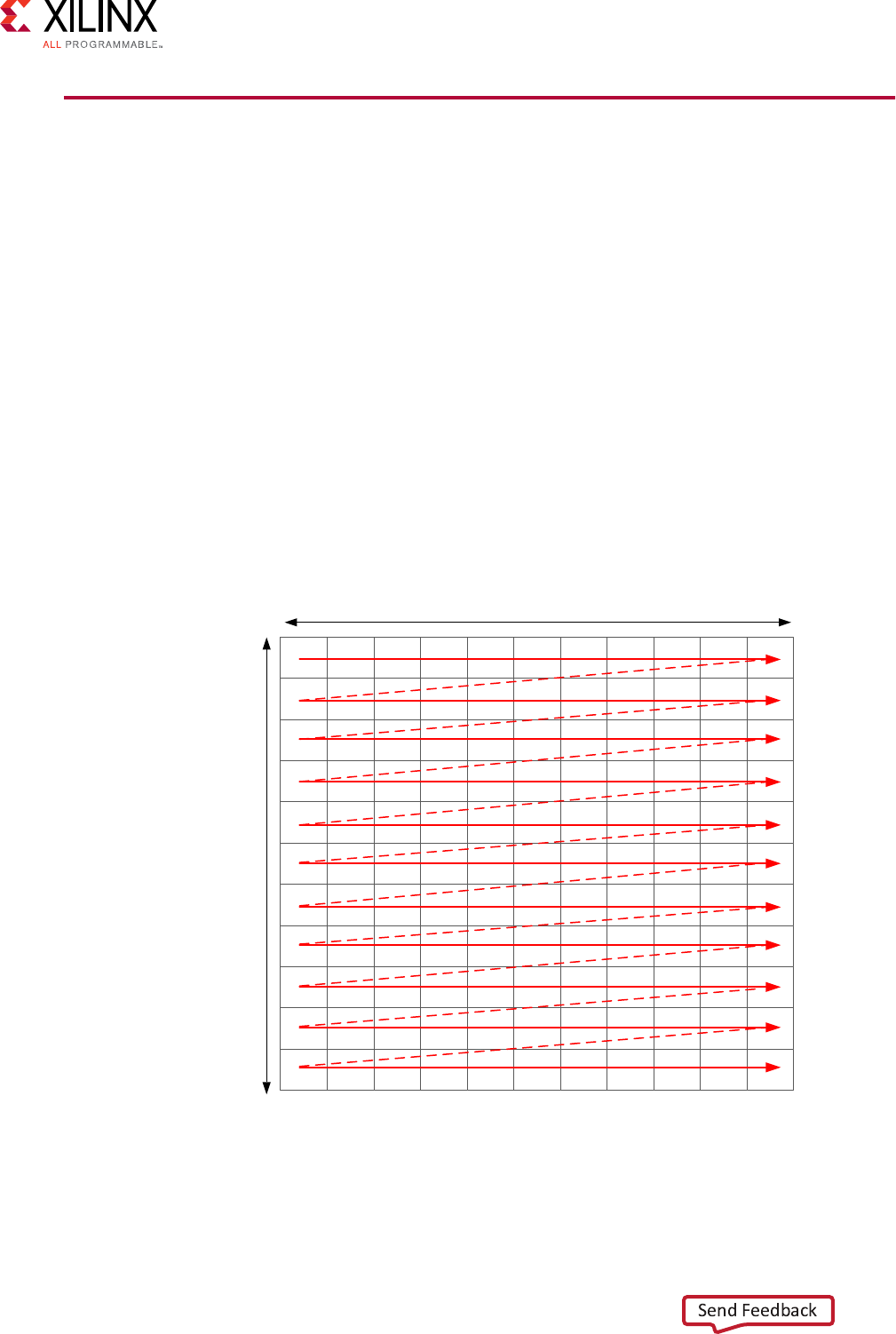
Standard Horizontal Convolution
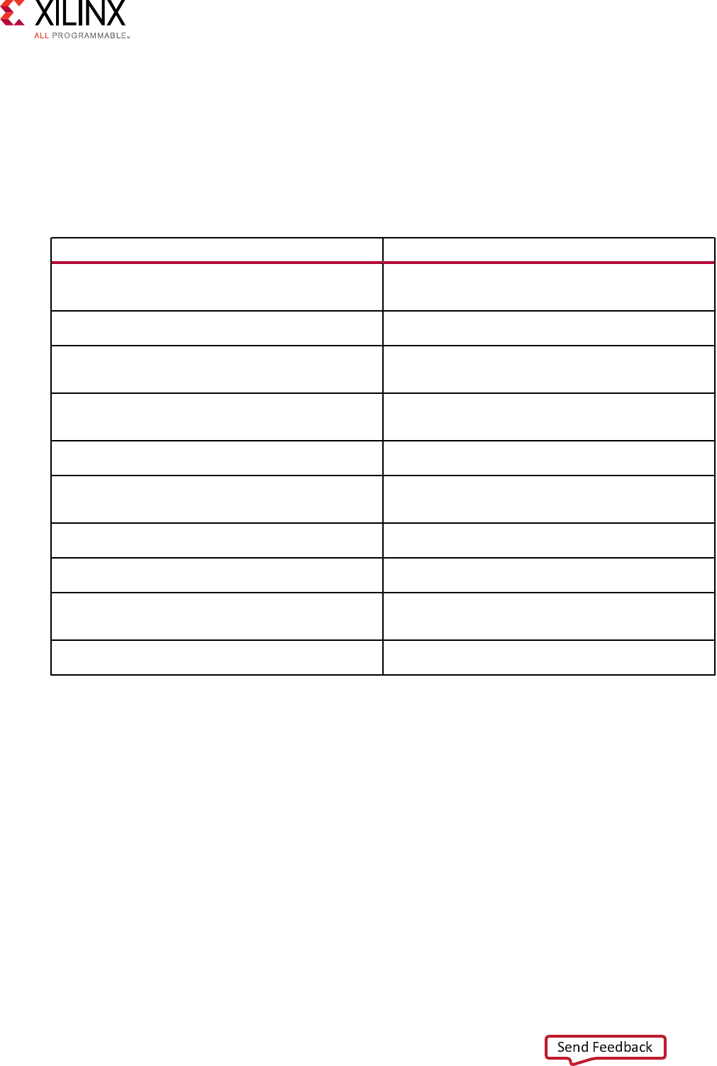
The rst step in this is to perform the convoluon in the horizontal direcon as shown in the
following gure.
Chapter 4: Data Access Patterns
Vivado HLS Optimization Methodology Guide 34
UG1270 (v2017.4) December 20, 2017 www.xilinx.com [placeholder text]
First Output Second Output Final Output
src
Hsamp
local
Hcoeff
Hsamp
Hcoeff
Hsamp
Hcoeff
X14296-121417
The convoluon is performed using K samples of data and K convoluon coecients. In the
gure above, K is shown as 5, however, the value of K is dened in the code. To perform the
convoluon, a minimum of K data samples are required. The convoluon window cannot start at
the rst pixel because the window would need to include pixels that are outside the image.
By performing a symmetric convoluon, the rst K data samples from input src can be
convolved with the horizontal coecients and the rst output calculated. To calculate the second
output, the next set of K data samples is used. This calculaon proceeds along each row unl the
nal output is wrien.
The C code for performing this operaon is shown below.
const int conv_size = K;
const int border_width = int(conv_size / 2);
#ifndef __SYNTHESIS__
Chapter 4: Data Access Patterns
Vivado HLS Optimization Methodology Guide 35
UG1270 (v2017.4) December 20, 2017 www.xilinx.com [placeholder text]

T * const local = new T[MAX_IMG_ROWS*MAX_IMG_COLS];
#else // Static storage allocation for HLS, dynamic otherwise
T local[MAX_IMG_ROWS*MAX_IMG_COLS];
#endif
Clear_Local:for(int i = 0; i < height * width; i++){
local[i]=0;
}
// Horizontal convolution
HconvH:for(int col = 0; col < height; col++){
HconvWfor(int row = border_width; row < width - border_width; row++){
int pixel = col * width + row;
Hconv:for(int i = - border_width; i <= border_width; i++){
local[pixel] += src[pixel + i] * hcoeff[i + border_width];
}
}
}
The code is straighorward and intuive. There are, however, some issues with this C code that
will negavely impact the quality of the hardware results.
The rst issue is the large storage requirements during C compilaon. The intermediate results in
the algorithm are stored in an internal local array. This requires an array of HEIGHT*WIDTH,
which for a standard video image of 1920*1080 will hold 2,073,600 values.
• For the cross-compilers targeng Zynq®-7000 All Programmable SoC or Zynq UltraScale+™
MPSoC, as well as many host systems, this amount of local storage can lead to stack
overows at run me (for example, running on the target device, or running co-sim ows
within Vivado HLS). The data for a local array is placed on the stack and not the heap, which is
managed by the OS. When cross-compiling with arm-linux-gnueabihf-g++ use the -
Wl,"-z stacksize=4194304" linker opon to allocate sucent stack space. (Note that
the syntax for this opon varies for dierent linkers.) When a funcon will only be run in
hardware, a useful way to avoid such issues is to use the __SYNTHESIS__ macro. This macro is
Chapter 4: Data Access Patterns
Vivado HLS Optimization Methodology Guide 36
UG1270 (v2017.4) December 20, 2017 www.xilinx.com [placeholder text]

automacally dened by the system compiler when the hardware funcon is synthesized into
hardware. The code shown above uses dynamic memory allocaon during C simulaon to
avoid any compilaon issues and only uses stac storage during synthesis. A downside of
using this macro is the code veried by C simulaon is not the same code that is synthesized.
In this case, however, the code is not complex and the behavior will be the same.
• The main issue with this local array is the quality of the FPGA implementaon. Because this is
an array it will be implemented using internal FPGA block RAM. This is a very large memory to
implement inside the FPGA. It might require a larger and more costly FPGA device. The use of
block RAM can be minimized by using the DATAFLOW opmizaon and streaming the data
through small ecient FIFOs, but this will require the data to be used in a streaming
sequenal manner. There is currently no such requirement.
The next issue relates to the performance: the inializaon for the local array. The loop
Clear_Local is used to set the values in array local to zero. Even if this loop is pipelined in the
hardware to execute in a high-performance manner, this operaon sll requires approximately
two million clock cycles (HEIGHT*WIDTH) to implement. While this memory is being inialized,
the system cannot perform any image processing. This same inializaon of the data could be
performed using a temporary variable inside loop HConv to inialize the accumulaon before the
write.
Finally, the throughput of the data, and thus the system performance, is fundamentally limited by
the data access paern.
• To create the rst convolved output, the rst K values are read from the input.
• To calculate the second output, a new value is read and then the same K-1 values are re-read.
One of the keys to a high-performance FPGA is to minimize the access to and from the PS. Each
access for data, which has previously been fetched, negavely impacts the performance of the
system. An FPGA is capable of performing many concurrent calculaons at once and reaching
very high performance, but not while the ow of data is constantly interrupted by re-reading
values.
Note: To maximize performance, data should only be accessed once from the PS and small units of local
storage - small to medium sized arrays - should be used for data which must be reused.
With the code shown above, the data cannot be connuously streamed directly from the
processor using a DMA operaon because the data is required to be re-read me and again.
Chapter 4: Data Access Patterns
Vivado HLS Optimization Methodology Guide 37
UG1270 (v2017.4) December 20, 2017 www.xilinx.com [placeholder text]
Standard Vertical Convolution
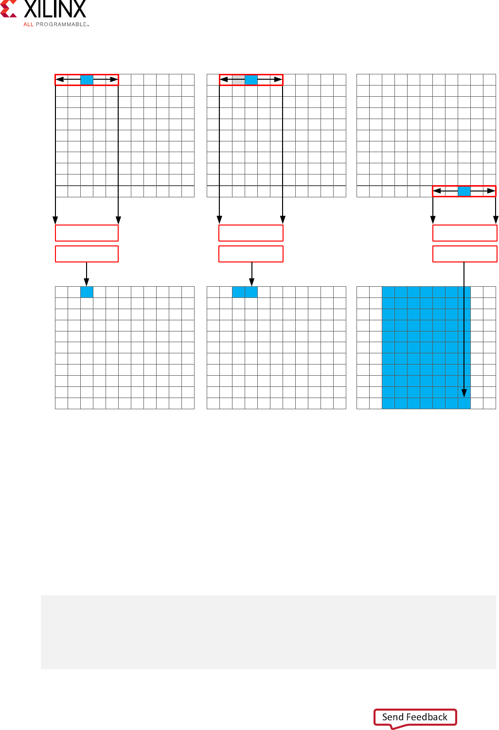
The next step is to perform the vercal convoluon shown in the following gure.
First Output Second Output Final Output
local
Vsamp
dst
Vcoeff
Vsamp
Vcoeff
Vsamp
Vconv
X14299-110617
The process for the vercal convoluon is similar to the horizontal convoluon. A set of K data
samples is required to convolve with the convoluon coecients, Vcoe in this case. Aer the
rst output is created using the rst K samples in the vercal direcon, the next set of K values is
used to create the second output. The process connues down through each column unl the
nal output is created.
Aer the vercal convoluon, the image is now smaller than the source image src due to both
the horizontal and vercal border eect.
The code for performing these operaons is shown below.
Clear_Dst:for(int i = 0; i < height * width; i++){
dst[i]=0;
}
Chapter 4: Data Access Patterns
Vivado HLS Optimization Methodology Guide 38
UG1270 (v2017.4) December 20, 2017 www.xilinx.com [placeholder text]

// Vertical convolution
VconvH:for(int col = border_width; col < height - border_width; col++){
VconvW:for(int row = 0; row < width; row++){
int pixel = col * width + row;
Vconv:for(int i = - border_width; i <= border_width; i++){
int offset = i * width;
dst[pixel] += local[pixel + offset] * vcoeff[i + border_width];
}
}
}
This code highlights similar issues to those already discussed with the horizontal convoluon
code.
• Many clock cycles are spent to set the values in the output image dst to zero. In this case,
approximately another two million cycles for a 1920*1080 image size.
• There are mulple accesses per pixel to re-read data stored in array local.
• There are mulple writes per pixel to the output array/port dst.
The access paerns in the code above in fact creates the requirement to have such a large local
array. The algorithm requires the data on row K to be available to perform the rst calculaon.
Processing data down the rows before proceeding to the next column requires the enre image
to be stored locally. This requires that all values be stored and results in large local storage on the
FPGA.
In addion, when you reach the stage where you wish to use compiler direcves to opmize the
performance of the hardware funcon, the ow of data between the horizontal and vercal loop
cannot be managed via a FIFO (a high-performance and low-resource unit) because the data is
not streamed out of array local: a FIFO can only be used with sequenal access paerns.
Instead, this code which requires arbitrary/random accesses requires a ping-pong block RAM to
improve performance. This doubles the memory requirements for the implementaon of the local
array to approximately four million data samples, which is too large for an FPGA.
Chapter 4: Data Access Patterns
Vivado HLS Optimization Methodology Guide 39
UG1270 (v2017.4) December 20, 2017 www.xilinx.com [placeholder text]
Standard Border Pixel Convolution
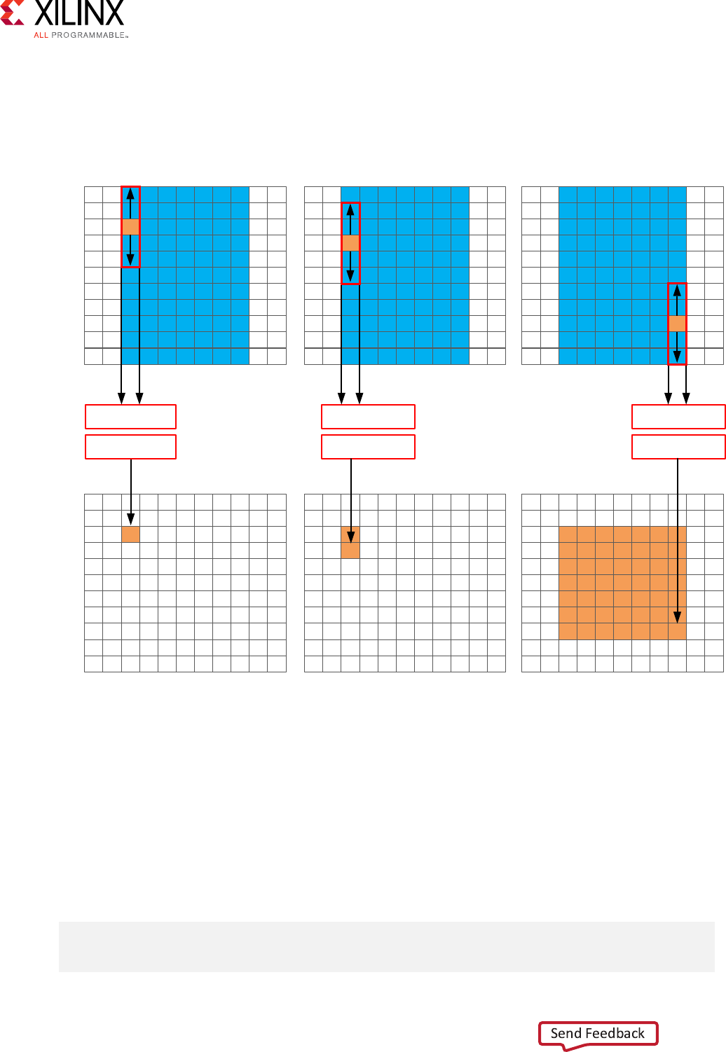
The nal step in performing the convoluon is to create the data around the border. These pixels
can be created by simply reusing the nearest pixel in the convolved output. The following gures
shows how this is achieved.
Top Left Top Row Top Right
Left and Right Edges Bottom Left and Bottom Row Bottom Right
dst
dst
X14294-121417
The border region is populated with the nearest valid value. The following code performs the
operaons shown in the gure.
int border_width_offset = border_width * width;
int border_height_offset = (height - border_width - 1) * width;
// Border pixels
Top_Border:for(int col = 0; col < border_width; col++){
int offset = col * width;
for(int row = 0; row < border_width; row++){
int pixel = offset + row;
dst[pixel] = dst[border_width_offset + border_width];
}
for(int row = border_width; row < width - border_width; row++){
int pixel = offset + row;
dst[pixel] = dst[border_width_offset + row];
}
Chapter 4: Data Access Patterns
Vivado HLS Optimization Methodology Guide 40
UG1270 (v2017.4) December 20, 2017 www.xilinx.com [placeholder text]

for(int row = width - border_width; row < width; row++){
int pixel = offset + row;
dst[pixel] = dst[border_width_offset + width - border_width - 1];
}
}
Side_Border:for(int col = border_width; col < height - border_width; col++)
{
int offset = col * width;
for(int row = 0; row < border_width; row++){
int pixel = offset + row;
dst[pixel] = dst[offset + border_width];
}
for(int row = width - border_width; row < width; row++){
int pixel = offset + row;
dst[pixel] = dst[offset + width - border_width - 1];
}
}
Bottom_Border:for(int col = height - border_width; col < height; col++){
int offset = col * width;
for(int row = 0; row < border_width; row++){
int pixel = offset + row;
dst[pixel] = dst[border_height_offset + border_width];
}
for(int row = border_width; row < width - border_width; row++){
int pixel = offset + row;
dst[pixel] = dst[border_height_offset + row];
}
for(int row = width - border_width; row < width; row++){
int pixel = offset + row;
dst[pixel] = dst[border_height_offset + width - border_width - 1];
}
}
The code suers from the same repeated access for data. The data stored outside the FPGA in
the array dst must now be available to be read as input data re-read mulple mes. Even in the
rst loop, dst[border_width_offset + border_width] is read mulple mes but the
values of border_width_offset and border_width do not change.
This code is very intuive to both read and write. When implemented with the SDSoC
environment it is approximately 120M clock cycles, which meets or slightly exceeds the
performance of a CPU. However, as shown in the next secon, opmal data access paerns
ensure this same algorithm can be implemented on the FPGA at a rate of one pixel per clock
cycle, or approximately 2M clock cycles.
The summary from this review is that the following poor data access paerns negavely impact
the performance and size of the FPGA implementaon:
•Mulple accesses to read and then re-read data. Use local storage where possible.
• Accessing data in an arbitrary or random access manner. This requires the data to be stored
locally in arrays and costs resources.
•Seng default values in arrays costs clock cycles and performance.
Chapter 4: Data Access Patterns
Vivado HLS Optimization Methodology Guide 41
UG1270 (v2017.4) December 20, 2017 www.xilinx.com [placeholder text]
Algorithm With Optimal Data Access
Patterns
The key to implemenng the convoluon example reviewed in the previous secon as a high-
performance design with minimal resources is to:
• Maximize the ow of data through the system. Refrain from using any coding techniques or
algorithm behavior that inhibits the connuous ow of data.
• Maximize the reuse of data. Use local caches to ensure there are no requirements to re-read
data and the incoming data can keep owing.
• Embrace condional branching. This is expensive on a CPU, GPU, or DSP but opmal in an
FPGA.
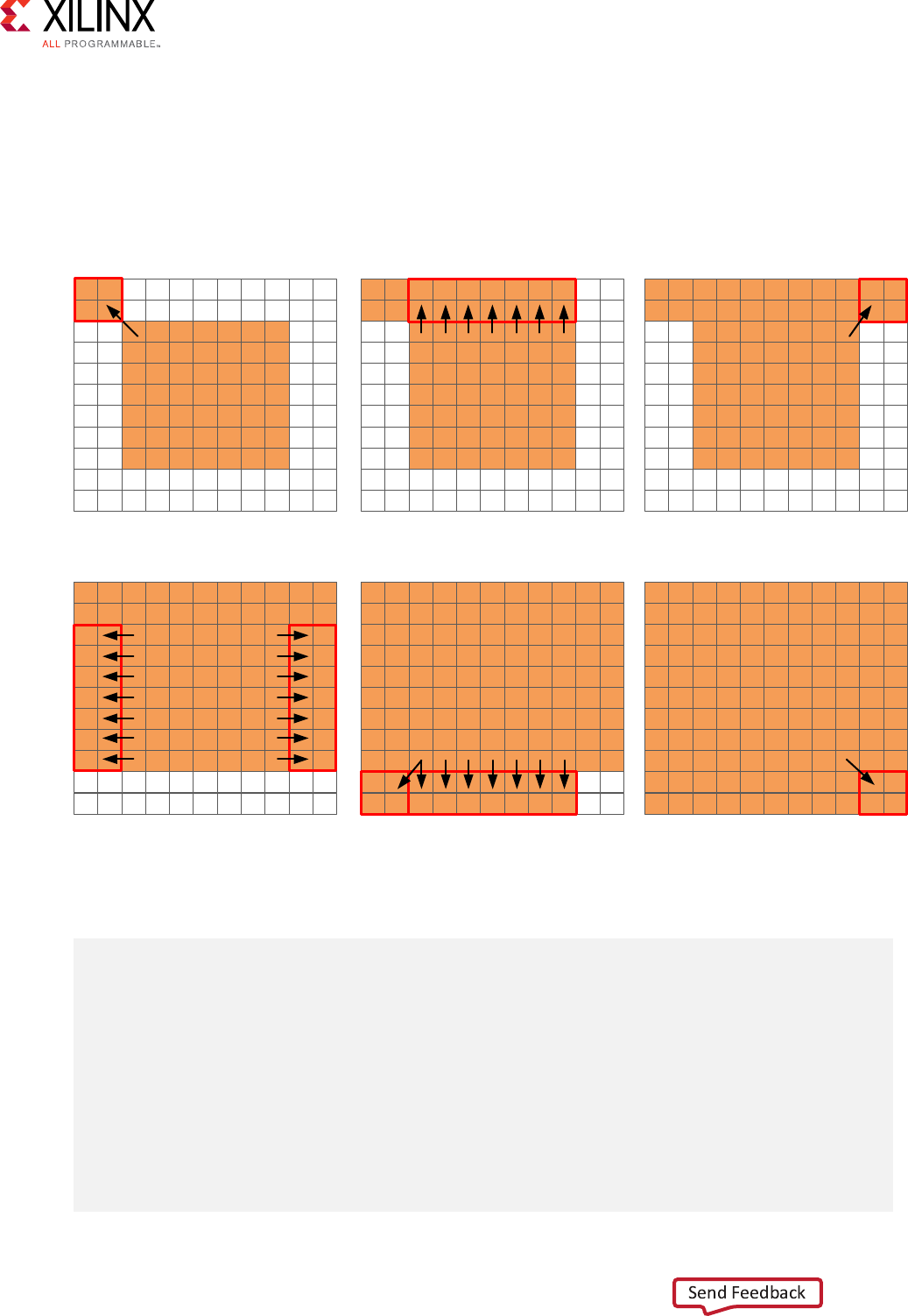
The rst step is to understand how data ows through the system into and out of the FPGA. The
convoluon algorithm is performed on an image. When data from an image is produced and
consumed, it is transferred in a standard raster-scan manner as shown in the following gure.
Width
Height
X14298-121417
If the data is transferred to the FPGA in a streaming manner, the FPGA should process it in a
streaming manner and transfer it back from the FPGA in this manner.
Chapter 4: Data Access Patterns
Vivado HLS Optimization Methodology Guide 42
UG1270 (v2017.4) December 20, 2017 www.xilinx.com [placeholder text]

The convoluon algorithm shown below embraces this style of coding. At this level of abstracon
a concise view of the code is shown. However, there are now intermediate buers, hconv and
vconv, between each loop. Because these are accessed in a streaming manner, they are
opmized into single registers in the nal implementaon.
template<typename T, int K>
static void convolution_strm(
int width,
int height,
T src[TEST_IMG_ROWS][TEST_IMG_COLS],
T dst[TEST_IMG_ROWS][TEST_IMG_COLS],
const T *hcoeff,
const T *vcoeff)
{
T hconv_buffer[MAX_IMG_COLS*MAX_IMG_ROWS];
T vconv_buffer[MAX_IMG_COLS*MAX_IMG_ROWS];
T *phconv, *pvconv;
// These assertions let HLS know the upper bounds of loops
assert(height < MAX_IMG_ROWS);
assert(width < MAX_IMG_COLS);
assert(vconv_xlim < MAX_IMG_COLS - (K - 1));
// Horizontal convolution
HConvH:for(int col = 0; col < height; col++) {
HConvW:for(int row = 0; row < width; row++) {
HConv:for(int i = 0; i < K; i++) {
}
}
}
// Vertical convolution
VConvH:for(int col = 0; col < height; col++) {
VConvW:for(int row = 0; row < vconv_xlim; row++) {
VConv:for(int i = 0; i < K; i++) {
}
}
}
Border:for (int i = 0; i < height; i++) {
for (int j = 0; j < width; j++) {
}
}
All three processing loops now embrace condional branching to ensure the connuous
processing of data.
Chapter 4: Data Access Patterns
Vivado HLS Optimization Methodology Guide 43
UG1270 (v2017.4) December 20, 2017 www.xilinx.com [placeholder text]


First Output Second Output Final Output
src
Hsamp
local
Hcoeff
Hsamp
Hcoeff
Hsamp
Hcoeff
X14296-121417
The convoluon is performed using K samples of data and K convoluon coecients. In the
gure above, K is shown as 5, however, the value of K is dened in the code. To perform the
convoluon, a minimum of K data samples are required. The convoluon window cannot start at
the rst pixel because the window would need to include pixels that are outside the image.
By performing a symmetric convoluon, the rst K data samples from input src can be
convolved with the horizontal coecients and the rst output calculated. To calculate the second
output, the next set of K data samples is used. This calculaon proceeds along each row unl the
nal output is wrien.
The C code for performing this operaon is shown below.
const int conv_size = K;
const int border_width = int(conv_size / 2);
#ifndef __SYNTHESIS__
Chapter 5: Standard Horizontal Convolution
Vivado HLS Optimization Methodology Guide 46
UG1270 (v2017.4) December 20, 2017 www.xilinx.com [placeholder text]

T * const local = new T[MAX_IMG_ROWS*MAX_IMG_COLS];
#else // Static storage allocation for HLS, dynamic otherwise
T local[MAX_IMG_ROWS*MAX_IMG_COLS];
#endif
Clear_Local:for(int i = 0; i < height * width; i++){
local[i]=0;
}
// Horizontal convolution
HconvH:for(int col = 0; col < height; col++){
HconvWfor(int row = border_width; row < width - border_width; row++){
int pixel = col * width + row;
Hconv:for(int i = - border_width; i <= border_width; i++){
local[pixel] += src[pixel + i] * hcoeff[i + border_width];
}
}
}
The code is straighorward and intuive. There are, however, some issues with this C code that
will negavely impact the quality of the hardware results.
The rst issue is the large storage requirements during C compilaon. The intermediate results in
the algorithm are stored in an internal local array. This requires an array of HEIGHT*WIDTH,
which for a standard video image of 1920*1080 will hold 2,073,600 values.
• For the cross-compilers targeng Zynq®-7000 All Programmable SoC or Zynq UltraScale+™
MPSoC, as well as many host systems, this amount of local storage can lead to stack
overows at run me (for example, running on the target device, or running co-sim ows
within Vivado HLS). The data for a local array is placed on the stack and not the heap, which is
managed by the OS. When cross-compiling with arm-linux-gnueabihf-g++ use the -
Wl,"-z stacksize=4194304" linker opon to allocate sucent stack space. (Note that
the syntax for this opon varies for dierent linkers.) When a funcon will only be run in
hardware, a useful way to avoid such issues is to use the __SYNTHESIS__ macro. This macro is
Chapter 5: Standard Horizontal Convolution
Vivado HLS Optimization Methodology Guide 47
UG1270 (v2017.4) December 20, 2017 www.xilinx.com [placeholder text]

automacally dened by the system compiler when the hardware funcon is synthesized into
hardware. The code shown above uses dynamic memory allocaon during C simulaon to
avoid any compilaon issues and only uses stac storage during synthesis. A downside of
using this macro is the code veried by C simulaon is not the same code that is synthesized.
In this case, however, the code is not complex and the behavior will be the same.
• The main issue with this local array is the quality of the FPGA implementaon. Because this is
an array it will be implemented using internal FPGA block RAM. This is a very large memory to
implement inside the FPGA. It might require a larger and more costly FPGA device. The use of
block RAM can be minimized by using the DATAFLOW opmizaon and streaming the data
through small ecient FIFOs, but this will require the data to be used in a streaming
sequenal manner. There is currently no such requirement.
The next issue relates to the performance: the inializaon for the local array. The loop
Clear_Local is used to set the values in array local to zero. Even if this loop is pipelined in the
hardware to execute in a high-performance manner, this operaon sll requires approximately
two million clock cycles (HEIGHT*WIDTH) to implement. While this memory is being inialized,
the system cannot perform any image processing. This same inializaon of the data could be
performed using a temporary variable inside loop HConv to inialize the accumulaon before the
write.
Finally, the throughput of the data, and thus the system performance, is fundamentally limited by
the data access paern.
• To create the rst convolved output, the rst K values are read from the input.
• To calculate the second output, a new value is read and then the same K-1 values are re-read.
One of the keys to a high-performance FPGA is to minimize the access to and from the PS. Each
access for data, which has previously been fetched, negavely impacts the performance of the
system. An FPGA is capable of performing many concurrent calculaons at once and reaching
very high performance, but not while the ow of data is constantly interrupted by re-reading
values.
Note: To maximize performance, data should only be accessed once from the PS and small units of local
storage - small to medium sized arrays - should be used for data which must be reused.
With the code shown above, the data cannot be connuously streamed directly from the
processor using a DMA operaon because the data is required to be re-read me and again.
Optimal Horizontal Convolution
To perform the calculaon in a more ecient manner for FPGA implementaon, the horizontal
convoluon is computed as shown in the following gure.
Chapter 5: Standard Horizontal Convolution
Vivado HLS Optimization Methodology Guide 48
UG1270 (v2017.4) December 20, 2017 www.xilinx.com [placeholder text]
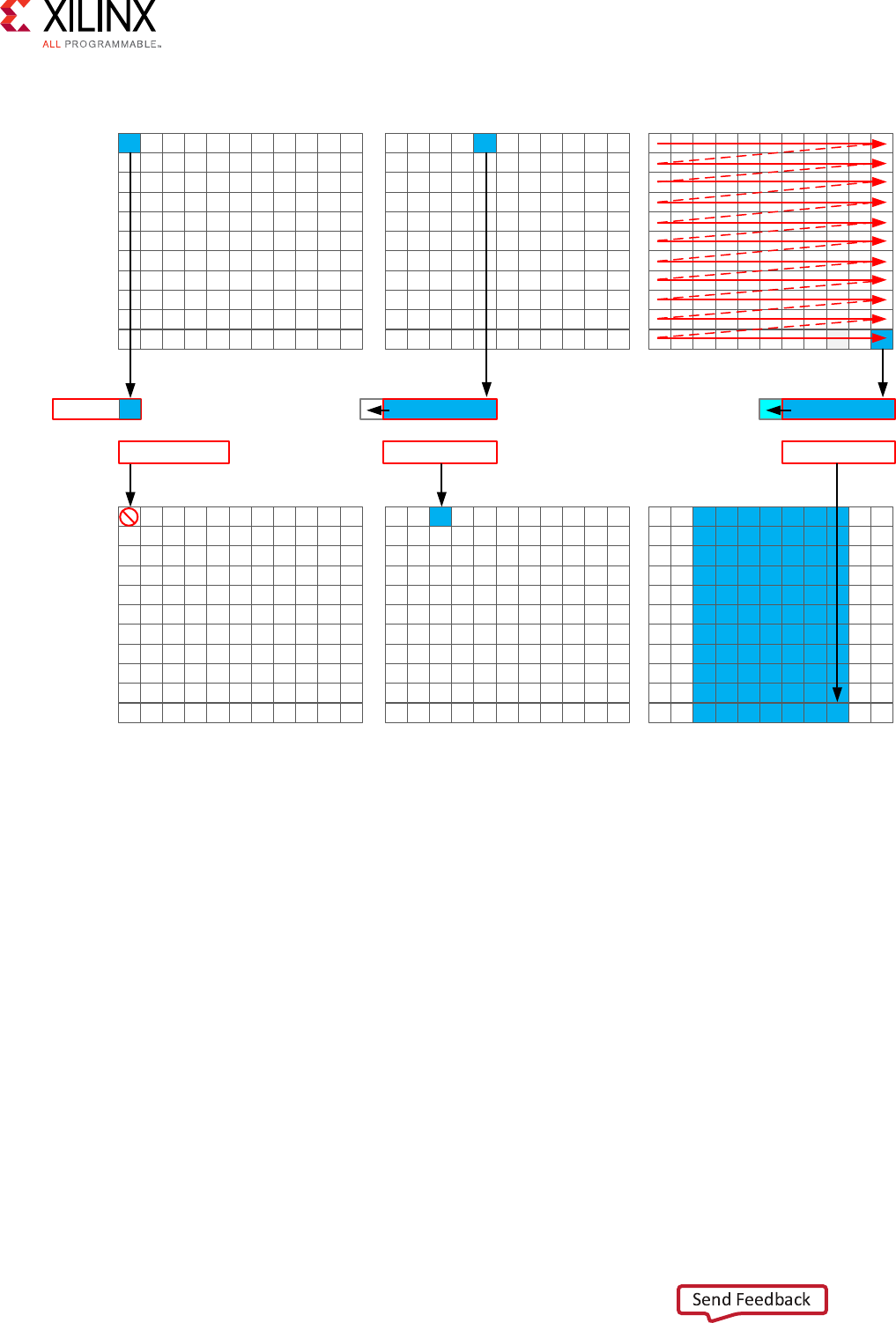
First Calculation First Output Final Output
src
Hwin
hconv
Hconv
Hsamp
Hconv
Hsamp
Hconv
X14297-110617
The algorithm must use the K previous samples to compute the convoluon result. It therefore
copies the sample into a temporary cache hwin. This use of local storage means there is no need
to re-read values from the PS and interrupt the ow of data. For the rst calculaon there are
not enough values in hwin to compute a result, so condionally, no output values are wrien.
The algorithm keeps reading input samples and caching them into hwin. Each me it reads a new
sample, it pushes an unneeded sample out of hwin. The rst me an output value can be wrien
is aer the Kth input has been read. An output value can now be wrien. The algorithm proceeds
in this manner along the rows unl the nal sample has been read. At that point, only the last K
samples are stored in hwin: all that is required to compute the convoluon.
Chapter 5: Standard Horizontal Convolution
Vivado HLS Optimization Methodology Guide 49
UG1270 (v2017.4) December 20, 2017 www.xilinx.com [placeholder text]

As shown below, the code to perform these operaons uses both local storage to prevent re-
reads from the PL – the reads from local storage can be performed in parallel in the nal
implementaon – and the extensive use of condional branching to ensure each new data
sample can be processed in a dierent manner.
// Horizontal convolution
phconv=hconv_buffer; // set / reset pointer to start of buffer
// These assertions let HLS know the upper bounds of loops
assert(height < MAX_IMG_ROWS);
assert(width < MAX_IMG_COLS);
assert(vconv_xlim < MAX_IMG_COLS - (K - 1));
HConvH:for(int col = 0; col < height; col++) {
HConvW:for(int row = 0; row < width; row++) {
#pragma HLS PIPELINE
T in_val = *src++;
// Reset pixel value on-the-fly - eliminates an O(height*width) loop
T out_val = 0;
HConv:for(int i = 0; i < K; i++) {
hwin[i] = i < K - 1 ? hwin[i + 1] : in_val;
out_val += hwin[i] * hcoeff[i];
}
if (row >= K - 1) {
*phconv++=out_val;
}
}
}
An interesng point to note in the code above is the use of the temporary variable out_val to
perform the convoluon calculaon. This variable is set to zero before the calculaon is
performed, negang the need to spend two million clock cycles to reset the values, as in the
previous example.
Throughout the enre process, the samples in the src input are processed in a raster-streaming
manner. Every sample is read in turn. The outputs from the task are either discarded or used, but
the task keeps constantly compung. This represents a dierence from code wrien to perform
on a CPU.
Optimal Vertical Convolution
The vercal convoluon represents a challenge to the streaming data model preferred by an
FPGA. The data must be accessed by column but you do not wish to store the enre image. The
soluon is to use line buers, as shown in the following gure.
Chapter 5: Standard Horizontal Convolution
Vivado HLS Optimization Methodology Guide 50
UG1270 (v2017.4) December 20, 2017 www.xilinx.com [placeholder text]
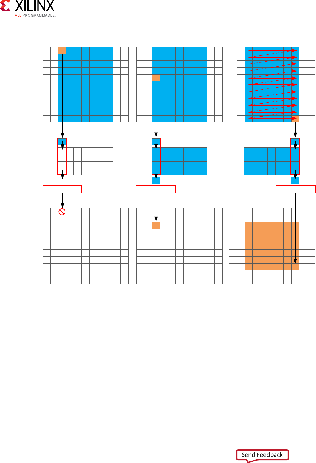
First Calculation First Output Final Output
hconv
vconv
Vconv Vconv Vconv
X14300-110617
Once again, the samples are read in a streaming manner, this me from the local buer hconv.
The algorithm requires at least K-1 lines of data before it can process the rst sample. All the
calculaons performed before this are discarded through the use of condionals.
A line buer allows K-1 lines of data to be stored. Each me a new sample is read, another
sample is pushed out the line buer. An interesng point to note here is that the newest sample
is used in the calculaon, and then the sample is stored into the line buer and the old sample
ejected out. This ensures that only K-1 lines are required to be cached rather than an unknown
number of lines, and minimizes the use of local storage. Although a line buer does require
mulple lines to be stored locally, the convoluon kernel size K is always much less than the
1080 lines in a full video image.
Chapter 5: Standard Horizontal Convolution
Vivado HLS Optimization Methodology Guide 51
UG1270 (v2017.4) December 20, 2017 www.xilinx.com [placeholder text]

The rst calculaon can be performed when the rst sample on the Kth line is read. The
algorithm then proceeds to output values unl the nal pixel is read.
// Vertical convolution
phconv=hconv_buffer; // set/reset pointer to start of buffer
pvconv=vconv_buffer; // set/reset pointer to start of buffer
VConvH:for(int col = 0; col < height; col++) {
VConvW:for(int row = 0; row < vconv_xlim; row++) {
#pragma HLS DEPENDENCE variable=linebuf inter false
#pragma HLS PIPELINE
T in_val = *phconv++;
// Reset pixel value on-the-fly - eliminates an O(height*width) loop
T out_val = 0;
VConv:for(int i = 0; i < K; i++) {
T vwin_val = i < K - 1 ? linebuf[i][row] : in_val;
out_val += vwin_val * vcoeff[i];
if (i > 0)
linebuf[i - 1][row] = vwin_val;
}
if (col >= K - 1) {
*pvconv++ = out_val;
}
}
The code above once again processes all the samples in the design in a streaming manner. The
task is constantly running. Following a coding style where you minimize the number of re-reads
(or re-writes) forces you to cache the data locally. This is an ideal strategy when targeng an
FPGA.
Optimal Border Pixel Convolution
The nal step in the algorithm is to replicate the edge pixels into the border region. To ensure the
constant ow of data and data reuse, the algorithm makes use of local caching. The following
gure shows how the border samples are aligned into the image.
• Each sample is read from the vconv output from the vercal convoluon.
• The sample is then cached as one of four possible pixel types.
• The sample is then wrien to the output stream.
Chapter 5: Standard Horizontal Convolution
Vivado HLS Optimization Methodology Guide 52
UG1270 (v2017.4) December 20, 2017 www.xilinx.com [placeholder text]
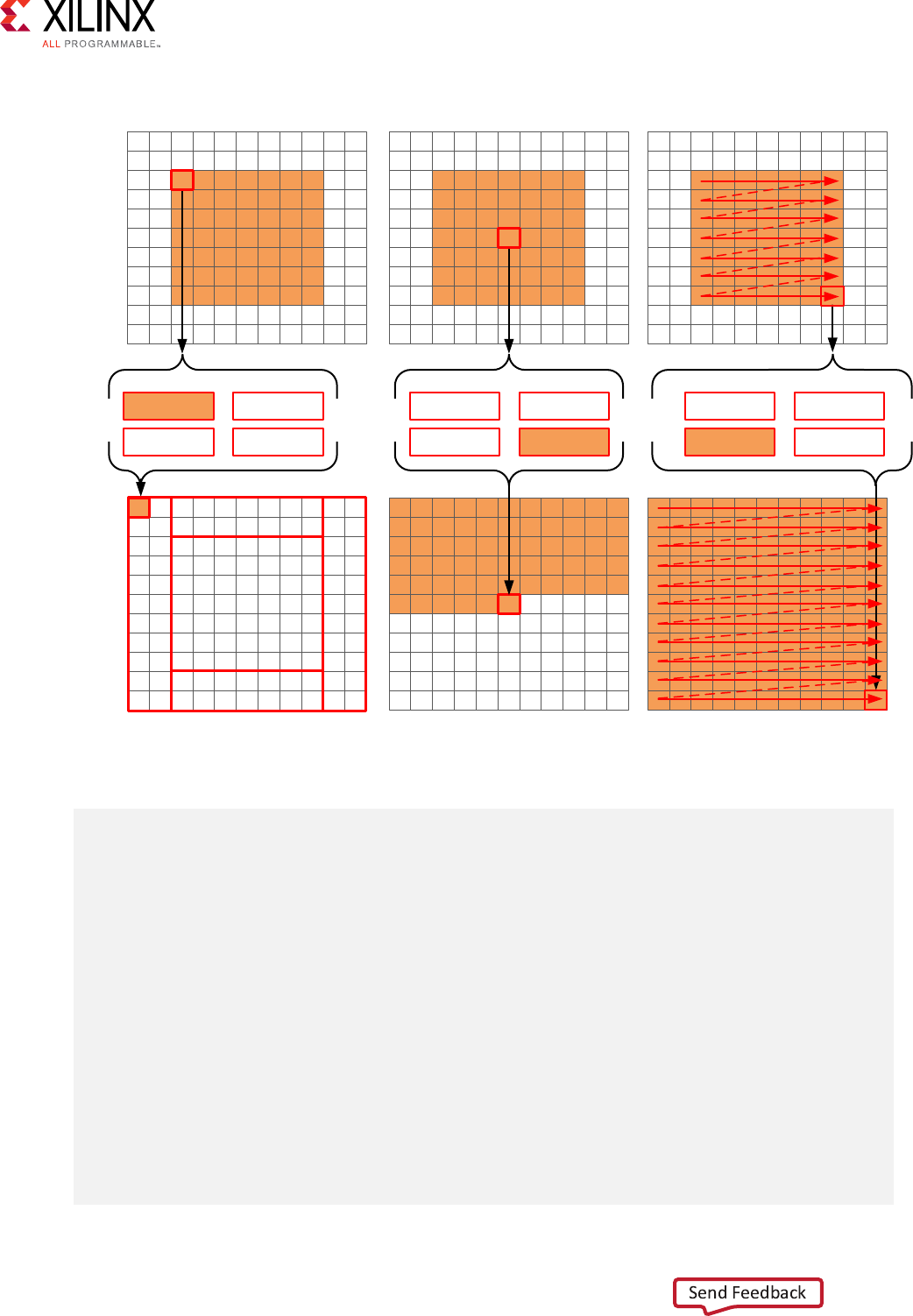
First Output Middle Output Final Output
vconv
Left Edge Border
dst
Right Edge Raw Pixel
Left Edge Border
Right Edge Raw Pixel
Left Edge Border
Right Edge Raw Pixel
Border
Raw Pixel
Border
Right Edge
Left Edge
X14295-110617
The code for determining the locaon of the border pixels is shown here.
// Border pixels
pvconv=vconv_buffer; // set/reset pointer to start of buffer
Border:for (int i = 0; i < height; i++) {
for (int j = 0; j < width; j++) {
T pix_in, l_edge_pix, r_edge_pix, pix_out;
#pragma HLS PIPELINE
if (i == 0 || (i > border_width && i < height - border_width)) {
// read a pixel out of the video stream and cache it for
// immediate use and later replication purposes
if (j < width - (K - 1)) {
pix_in = *pvconv++;
borderbuf[j] = pix_in;
}
if (j == 0) {
l_edge_pix = pix_in;
}
if (j == width - K) {
r_edge_pix = pix_in;
}
}
// Select output value from the appropriate cache resource
if (j <= border_width) {
Chapter 5: Standard Horizontal Convolution
Vivado HLS Optimization Methodology Guide 53
UG1270 (v2017.4) December 20, 2017 www.xilinx.com [placeholder text]

pix_out = l_edge_pix;
} else if (j >= width - border_width - 1) {
pix_out = r_edge_pix;
} else {
pix_out = borderbuf[j - border_width];
}
*dst++=pix_out;
}
}
A notable dierence with this new code is the extensive use of condionals inside the tasks. This
allows the task, aer it is pipelined, to connuously process data. The result of the condionals
does not impact the execuon of the pipeline. The result will impact the output values, but the
pipeline with keep processing as long as input samples are available.
Optimal Data Access Patterns
The following summarizes how to ensure your data access paerns result in the most opmal
performance on an FPGA.
• Minimize data input reads. Aer data has been read into the block, it can easily feed many
parallel paths but the inputs to the hardware funcon can be bolenecks to performance.
Read data once and use a local cache if the data must be reused.
• Minimize accesses to arrays, especially large arrays. Arrays are implemented in block RAM
which like I/O ports only have a limited number of ports and can be bolenecks to
performance. Arrays can be paroned into smaller arrays and even individual registers but
paroning large arrays will result in many registers being used. Use small localized caches to
hold results such as accumulaons and then write the nal result to the array.
• Seek to perform condional branching inside pipelined tasks rather than condionally execute
tasks, even pipelined tasks. Condionals are implemented as separate paths in the pipeline.
Allowing the data from one task to ow into the next task with the condional performed
inside the next task will result in a higher performing system.
• Minimize output writes for the same reason as input reads, namely, that ports are bolenecks.
Replicang addional accesses only pushes the issue further back into the system.
For C code which processes data in a streaming manner, consider employing a coding style that
promotes read-once/write-once to funcon arguments because this ensures the funcon can be
eciently implemented in an FPGA. It is much more producve to design an algorithm in C that
results in a high-performance FPGA implementaon than debug why the FPGA is not operang
at the performance required.
Chapter 5: Standard Horizontal Convolution
Vivado HLS Optimization Methodology Guide 54
UG1270 (v2017.4) December 20, 2017 www.xilinx.com [placeholder text]

Appendix A
OpenCL Attributes
Optimizations in OpenCL
This secon describes OpenCL aributes that can be added to source code to assist system
opmizaon by the SDAccel compiler, xocc, the SDSoC system compilers, sdscc and sds++,
and Vivado HLS synthesis.
SDx provides OpenCL aributes to opmize your code for data movement and kernel
performance. The goal of data movement opmizaon is to maximize the system level data
throughput by maximizing interface bandwidth ulizaon and DDR bandwidth ulizaon. The
goal of kernel computaon opmizaon is to create processing logic that can consume all the
data as soon as they arrive at kernel interfaces. This is generally achieved by expanding the
processing code to match the data path with techniques such as funcon inlining and pipelining,
loop unrolling, array paroning, dataowing, etc.
The OpenCL aributes include the types specied below:
Table 9: OpenCL __attributes__ by Type
Type Attributes
Kernel Size •reqd_work_group_size
•vec_type_hint
•work_group_size_hint
•xcl_max_work_group_size
•xcl_zero_global_work_offset
Function Inlining •always_inline
Task-level Pipeline •xcl_dataflow
•xcl_reqd_pipe_depth
Pipeline •xcl_pipeline_loop
•xcl_pipeline_workitems
Loop Unrolling •opencl_unroll_hint
Vivado HLS Optimization Methodology Guide 55
UG1270 (v2017.4) December 20, 2017 www.xilinx.com [placeholder text]

Table 9: OpenCL __attributes__ by Type (cont'd)
Type Attributes
Array Optimization •xcl_array_partition
•xcl_array_reshape
Note: Array variables only accept a single array
opmizaon aribute.
TIP: The SDAccel and SDSoC compilers also support many of the standard aributes supported by
gcc
, such as
always_inline
,
noinline
,
unroll
, and
nounroll
.
always_inline
Description
The always_inline aribute indicates that a funcon must be inlined. This aribute is a
standard feature of GCC, and a standard feature of the SDx compilers.
This aribute enables a compiler opmizaon to have a funcon inlined into the calling funcon.
The inlined funcon is dissolved and no longer appears as a separate level of hierarchy in the
RTL.
In some cases, inlining a funcon allows operaons within the funcon to be shared and
opmized more eecvely with surrounding operaons in the calling funcon. However, an
inlined funcon can no longer be shared with other funcons, so the logic may be duplicated
between the inlined funcon and a separate instance of the funcon which can be more broadly
shared. While this can improve performance, this will also increase the area required for
implemenng the RTL.
In some cases the compiler may choose to ignore the always_inline aribute and not inline a
funcon.
By default, inlining is only performed on the next level of funcon hierarchy, not sub-funcons.
Syntax
Place the aribute in the OpenCL source before the funcon denion to always have it inlined
whenever the funcon is called.
__attribute__((always_inline))
Appendix A: OpenCL Attributes
Vivado HLS Optimization Methodology Guide 56
UG1270 (v2017.4) December 20, 2017 www.xilinx.com [placeholder text]

Examples
This example adds the always_inline aribute to funcon foo:
__attribute__((always_inline))
void foo ( a, b, c, d ) {
...
}
See Also
•hps://gcc.gnu.org
•SDAccel Environment Opmizaon Guide (UG1207)
opencl_unroll_hint
Description
IMPORTANT!: This is a compiler hint which the compiler may ignore.
Loop unrolling is the rst opmizaon technique available in SDAccel. The purpose of the loop
unroll opmizaon is to expose concurrency to the compiler. This newly exposed concurrency
reduces latency and improves performance, but also consumes more FPGA fabric resources.
The opencl_unroll_hint aribute is part of the OpenCL Language Specicaon, and
species that loops (for, while, do) can be unrolled by the OpenCL compiler. See "Unrolling
Loops" in SDAccel Environment Opmizaon Guide (UG1207) for more informaon.
The opencl_unroll_hint aribute qualier must appear immediately before the loop to be
aected. You can use this aribute to specify full unrolling of the loop, paral unrolling by a
specied amount, or to disable unrolling of the loop.
Syntax
Place the aribute in the OpenCL source before the loop denion:
__attribute__((opencl_unroll_hint(
n
)))
Where:
•n is an oponal loop unrolling factor and must be a posive integer, or compile me constant
expression. An unroll factor of 1 disables unrolling.
TIP: If n is not specied, the compiler automacally determines the unrolling factor for the loop.
Appendix A: OpenCL Attributes
Vivado HLS Optimization Methodology Guide 57
UG1270 (v2017.4) December 20, 2017 www.xilinx.com [placeholder text]

Example 1
The following example unrolls the for loop by a factor of 2. This results in two parallel loop
iteraons instead of four sequenal iteraons for the compute unit to complete the operaon.
__attribute__((opencl_unroll_hint(2)))
for(int i = 0; i < LENGTH; i++) {
bufc[i] = bufa[i] * bufb[i];
}
Conceptually the compiler transforms the loop above to the code below:
for(int i = 0; i < LENGTH; i+=2) {
bufc[i] = bufa[i] * bufb[i];
bufc[i+1] = bufa[i+1] * bufb[i+1];
}
See Also
•SDAccel Environment Opmizaon Guide (UG1207)
•hps://www.khronos.org/
•The OpenCL C Specicaon
reqd_work_group_size
Description
When OpenCL kernels are submied for execuon on an OpenCL device, they execute within an
index space, called an ND range, which can have 1, 2, or 3 dimensions. This is called the global
size in the OpenCL API. The work-group size denes the amount of the ND range that can be
processed by a single invocaon of a kernel compute unit. The work-group size is also called the
local size in the OpenCL API. The OpenCL compiler can determine the work-group size based on
the properes of the kernel and selected device. Once the work-group size (local size) has been
determined, the ND range (global size) is divided automacally into work-groups, and the work-
groups are scheduled for execuon on the device.
Although the OpenCL compiler can dene the work-group size, the specicaon of the
reqd_work_group_size aribute on the kernel to dene the work-group size is highly
recommended for FPGA implementaons of the kernel. The aribute is recommended for
performance opmizaon during the generaon of the custom logic for a kernel. See "OpenCL
Execuon Model" in SDAccel Environment Opmizaon Guide (UG1207) for more informaon.
TIP: In the case of an FPGA implementaon, the specicaon of the
reqd_work_group_size
aribute is highly recommended as it can be used for performance opmizaon during the generaon
of the custom logic for a kernel.
Appendix A: OpenCL Attributes
Vivado HLS Optimization Methodology Guide 58
UG1270 (v2017.4) December 20, 2017 www.xilinx.com [placeholder text]

OpenCL kernel funcons are executed exactly one me for each point in the ND range index
space. This unit of work for each point in the ND range is called a work-item. Work-items are
organized into work-groups, which are the unit of work scheduled onto compute units. The
oponal reqd_work_group_size denes the work-group size of a compute unit that must be
used as the local_work_size argument to clEnqueueNDRangeKernel. This allows the
compiler to opmize the generated code appropriately for this kernel.
Syntax
Place this aribute before the kernel denion, or before the primary funcon specied for the
kernel:
__attribute__((reqd_work_group_size(
X
,
Y
,
Z
)))
Where:
•X, Y, Z: Species the ND range of the kernel. This represents each dimension of a three
dimensional matrix specifying the size of the work-group for the kernel.
Examples
The following OpenCL API C kernel code shows a vector addion design where two arrays of
data are summed into a third array. The required size of the work-group is 16x1x1. This kernel
will execute 16 mes to produce a valid result.
#include <clc.h>
// For VHLS OpenCL C kernels, the full work group is synthesized
__attribute__ ((reqd_work_group_size(16, 1, 1)))
__kernel void
vadd(__global int* a,
__global int* b,
__global int* c)
{
int idx = get_global_id(0);
c[idx] = a[idx] + b[idx];
}
See Also
•SDAccel Environment Opmizaon Guide (UG1207)
•hps://www.khronos.org/
•The OpenCL C Specicaon
Appendix A: OpenCL Attributes
Vivado HLS Optimization Methodology Guide 59
UG1270 (v2017.4) December 20, 2017 www.xilinx.com [placeholder text]
vec_type_hint
Description
IMPORTANT!: This is a compiler hint which the compiler may ignore.
The oponal __attribute__((vec_type_hint(
<type>
))) is part of the OpenCL
Language Specicaon, and is a hint to the OpenCL compiler represenng the computaonal
width of the kernel, providing a basis for calculang processor bandwidth ulizaon when the
compiler is looking to autovectorize the code.
By default, the kernel is assumed to have the __attribute__((vec_type_hint(int)))
qualier. This lets you specify a dierent vectorizaon type.
Implicit in autovectorizaon is the assumpon that any libraries called from the kernel must be
re-compilable at run me to handle cases where the compiler decides to merge or separate
workitems. This probably means that such libraries can never be hard coded binaries or that hard
coded binaries must be accompanied either by source or some re-targetable intermediate
representaon. This may be a code security queson for some.
Syntax
Place this aribute before the kernel denion, or before the primary funcon specied for the
kernel:
__attribute__((vec_type_hint(
<type>
)))
Where:
•<type>: is one of the built-in vector types listed in the following table, or the constuent scalar
element types.
Note: When not specied, the kernel is assumed to have an INT type.
Table 10: Vector Types
Type Description
charnA vector of n 8-bit signed two’s complement integer values.
ucharnA vector of n 8-bit unsigned integer values.
shortnA vector of n 16-bit signed two’s complement integer values.
ushortnA vector of n 16-bit unsigned integer values.
intnA vector of n 32-bit signed two’s complement integer values.
uintnA vector of n 32-bit unsigned integer values.
longnA vector of n 64-bit signed two’s complement integer values.
ulongnA vector of n 64-bit unsigned integer values.
Appendix A: OpenCL Attributes
Vivado HLS Optimization Methodology Guide 60
UG1270 (v2017.4) December 20, 2017 www.xilinx.com [placeholder text]
Table 10: Vector Types (cont'd)
Type Description
floatnA vector of n 32-bit floating-point values.
doublenA vector of n 64-bit floating-point values.
Note: n is assumed to be 1 when not specied. The vector data type names dened above where n is any
value other than 2, 3, 4, 8 and 16, are also reserved. That is to say, n can only be specied as 2,3,4,8, and
16.
Examples
The following example autovectorizes assuming double-wide integer as the basic computaon
width:
#include <clc.h>
// For VHLS OpenCL C kernels, the full work group is synthesized
__attribute__((vec_type_hint(double)))
__attribute__ ((reqd_work_group_size(16, 1, 1)))
__kernel void
...
See Also
•SDAccel Environment Opmizaon Guide (UG1207)
•hps://www.khronos.org/
•The OpenCL C Specicaon
work_group_size_hint
Description
IMPORTANT!: This is a compiler hint which the compiler may ignore.
The work-group size in the OpenCL standard denes the size of the ND range space that can be
handled by a single invocaon of a kernel compute unit. When OpenCL kernels are submied for
execuon on an OpenCL device, they execute within an index space, called an ND range, which
can have 1, 2, or 3 dimensions. See "OpenCL Execuon Model" in SDAccel Environment
Opmizaon Guide (UG1207) for more informaon.
Appendix A: OpenCL Attributes
Vivado HLS Optimization Methodology Guide 61
UG1270 (v2017.4) December 20, 2017 www.xilinx.com [placeholder text]

OpenCL kernel funcons are executed exactly one me for each point in the ND range index
space. This unit of work for each point in the ND range is called a work-item. Unlike for loops in
C, where loop iteraons are executed sequenally and in-order, an OpenCL runme and device is
free to execute work-items in parallel and in any order.
Work-items are organized into work-groups, which are the unit of work scheduled onto compute
units. The oponal work_group_size_hint aribute is part of the OpenCL Language
Specicaon, and is a hint to the compiler that indicates the work-group size value most likely to
be specied by the local_work_size argument to clEnqueueNDRangeKernel. This allows
the compiler to opmize the generated code according to the expected value.
TIP: In the case of an FPGA implementaon, the specicaon of the
reqd_work_group_size
aribute instead of the
work_group_size_hint
is highly recommended as it can be used for
performance opmizaon during the generaon of the custom logic for a kernel.
Syntax
Place this aribute before the kernel denion, or before the primary funcon specied for the
kernel:
__attribute__((work_group_size_hint(
X
,
Y
,
Z
)))
Where:
•X, Y, Z: Species the ND range of the kernel. This represents each dimension of a three
dimensional matrix specifying the size of the work-group for the kernel.
Examples
The following example is a hint to the compiler that the kernel will most likely be executed with a
work-group size of 1:
__attribute__((work_group_size_hint(1, 1, 1)))
__kernel void
...
See Also
•SDAccel Environment Opmizaon Guide (UG1207)
•hps://www.khronos.org/
•The OpenCL C Specicaon
Appendix A: OpenCL Attributes
Vivado HLS Optimization Methodology Guide 62
UG1270 (v2017.4) December 20, 2017 www.xilinx.com [placeholder text]

xcl_array_partition
Description
IMPORTANT!: Array variables only accept one aribute. While
xcl_array_partition
does
support mul-dimensional arrays, you can only reshape one dimension of the array with a single
aribute.
One of the advantages of the FPGA over other compute devices for OpenCL programs is the
ability for the applicaon programmer to customize the memory architecture all throughout the
system and into the compute unit. By default, The SDAccel compiler generates a memory
architecture within the compute unit that maximizes local and private memory bandwidth based
on stac code analysis of the kernel code. Further opmizaon of these memories is possible
based on aributes in the kernel source code, which can be used to specify physical layouts and
implementaons of local and private memories. The aribute in the SDAccel compiler to control
the physical layout of memories in a compute unit is array_partition.
For one dimensional arrays, the array_partition aribute implements an array declared
within kernel code as mulple physical memories instead of a single physical memory. The
selecon of which paroning scheme to use depends on the specic applicaon and its
performance goals. The array paroning schemes available in the SDAccel compiler are
cyclic, block, and complete.
Syntax
Place the aribute with the denion of the array variable:
__attribute__((xcl_array_partition(
<type>
,
<factor>
,
<dimension>
)))
Where:
•<type>: Species one of the following paron types:
○cyclic: Cyclic paroning is the implementaon of an array as a set of smaller physical
memories that can be accessed simultaneously by the logic in the compute unit. The array
is paroned cyclically by pung one element into each memory before coming back to
the rst memory to repeat the cycle unl the array is fully paroned.
○block: Block paroning is the physical implementaon of an array as a set of smaller
memories that can be accessed simultaneously by the logic inside of the compute unit. In
this case, each memory block is lled with elements from the array before moving on to the
next memory.
○complete: Complete paroning decomposes the array into individual elements. For a
one-dimensional array, this corresponds to resolving a memory into individual registers.
Appendix A: OpenCL Attributes
Vivado HLS Optimization Methodology Guide 63
UG1270 (v2017.4) December 20, 2017 www.xilinx.com [placeholder text]

○The default type is complete.
•<factor>: For cyclic type paroning, the factor species how many physical memories to
paron the original array into in the kernel code. For Block type paroning, the factor
species the number of elements from the original array to store in each physical memory.
IMPORTANT!: For
complete
type paroning, the factor is not specied.
•<dimension>: Species which array dimension to paron. Specied as an integer from 1 to N.
SDAccel supports arrays of N dimensions and can paron the array on any single dimension.
Example 1
For example, consider the following array declaraon:
int buffer[16];
The integer array, named buer, stores 16 values that are 32-bits wide each. Cyclic paroning
can be applied to this array with the following declaraon:
int buffer[16] __attribute__((xcl_array_partition(cyclic,4,1)));
In this example, the cyclic paron_type aribute tells SDAccel to distribute the contents of the
array among four physical memories. This aribute increases the immediate memory bandwidth
for operaons accessing the array buer by a factor of four.
All arrays inside of a compute unit in the context of SDAccel are capable of sustaining a
maximum of two concurrent accesses. By dividing the original array in the code into four physical
memories, the resulng compute unit can sustain a maximum of eight concurrent accesses to the
array buer.
Example 2
Using the same integer array as found in Example 1, block paroning can be applied to the array
with the following declaraon:
int buffer[16] __attribute__((xcl_array_partition(block,4,1)));
Since the size of the block is four, SDAccel will generate four physical memories, sequenally
lling each memory with data from the array.
Appendix A: OpenCL Attributes
Vivado HLS Optimization Methodology Guide 64
UG1270 (v2017.4) December 20, 2017 www.xilinx.com [placeholder text]

Example 3
Using the same integer array as found in Example 1, complete paroning can be applied to the
array with the following declaraon:
int buffer[16] __attribute__((xcl_array_partition(complete, 1)));
In this example the array is completely paroned into distributed RAM, or 16 independent
registers in the programmable logic of the kernel. Because complete is the default, the same
eect can also be accomplished with the following declaraon:
int buffer[16] __attribute__((xcl_array_partition));
While this creates an implementaon with the highest possible memory bandwidth, it is not
suited to all applicaons. The way in which data is accessed by the kernel code through either
constant or data dependent indexes aects the amount of supporng logic that SDx has to build
around each register to ensure funconal equivalence with the usage in the original code. As a
general best pracce guideline for SDx, the complete paroning aribute is best suited for
arrays in which at least one dimension of the array is accessed through the use of constant
indexes.
See Also
•xcl_array_reshape
•pragma HLS array_paron
•SDAccel Environment Opmizaon Guide (UG1207)
•Vivado Design Suite User Guide: High-Level Synthesis (UG902)
xcl_array_reshape
Description
IMPORTANT!: Array variables only accept one aribute. While
xcl_array_reshape
does support
mul-dimensional arrays, you can only reshape one dimension of the array with a single aribute.
Combines array paroning with vercal array mapping.
The ARRAY_RESHAPE aribute combines the eect of ARRAY_PARTITION, breaking an array
into smaller arrays, and concatenang elements of arrays by increasing bit-widths. This reduces
the number of block RAM consumed while providing parallel access to the data. This aribute
creates a new array with fewer elements but with greater bit-width, allowing more data to be
accessed in a single clock cycle.
Appendix A: OpenCL Attributes
Vivado HLS Optimization Methodology Guide 65
UG1270 (v2017.4) December 20, 2017 www.xilinx.com [placeholder text]
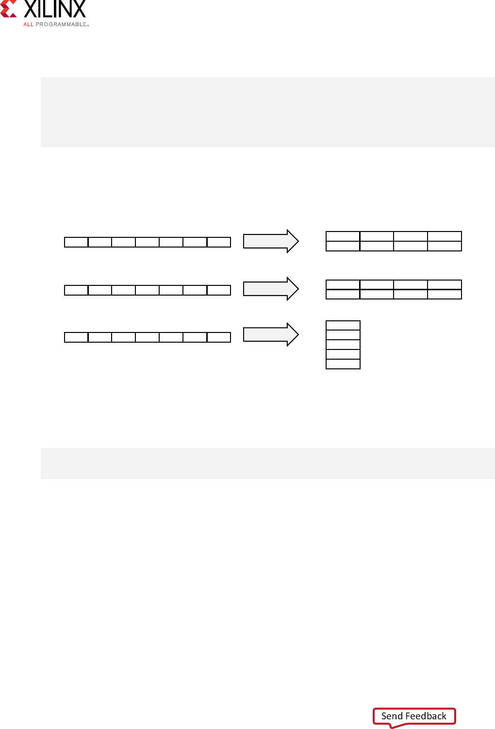
Given the following code:
void foo (...) {
int array1[N] __attribute__((xcl_array_reshape(block, 2, 1)));
int array2[N] __attribute__((xcl_array_reshape(cycle, 2, 1)));
int array3[N] __attribute__((xcl_array_reshape(complete, 1)));
...
}
The ARRAY_RESHAPE aribute transforms the arrays into the form shown in the following
gure:
Figure 1: ARRAY_RESHAPE
0 1 2 ... N-3 N-2 N-1
N/2 ... N-2 N-1
0 1 ... (N/2-1)
1 ... N-3 N-1
0 2 ... N-2
block
cyclic
complete
X14307-110217
0 1 2 ... N-3 N-2 N-1
0 1 2 ... N-3 N-2 N-1
array1[N]
array2[N]
array3[N] N-1
N-2
...
1
0
MSB
LSB
MSB
LSB
MSB
LSB
array4[N/2]
array5[N/2]
array6[1]
Syntax
Place the aribute with the denion of the array variable:
__attribute__((xcl_array_reshape(
<type>
,
<factor>
,
<dimension>
)))
Where:
•<type>: Species one of the following paron types:
○cyclic: Cyclic paroning is the implementaon of an array as a set of smaller physical
memories that can be accessed simultaneously by the logic in the compute unit. The array
is paroned cyclically by pung one element into each memory before coming back to
the rst memory to repeat the cycle unl the array is fully paroned.
○block: Block paroning is the physical implementaon of an array as a set of smaller
memories that can be accessed simultaneously by the logic inside of the compute unit. In
this case, each memory block is lled with elements from the array before moving on to the
next memory.
Appendix A: OpenCL Attributes
Vivado HLS Optimization Methodology Guide 66
UG1270 (v2017.4) December 20, 2017 www.xilinx.com [placeholder text]
○complete: Complete paroning decomposes the array into individual elements. For a
one-dimensional array, this corresponds to resolving a memory into individual registers.
○The default type is complete.
•<factor>: For cyclic type paroning, the factor species how many physical memories to
paron the original array into in the kernel code. For Block type paroning, the factor
species the number of elements from the original array to store in each physical memory.
IMPORTANT!: For
complete
type paroning, the factor should not be specied.
•<dimension>: Species which array dimension to paron. Specied as an integer from 1 to N.
SDAccel supports arrays of N dimensions and can paron the array on any single dimension.
Example 1
Reshapes (paron and maps) an 8-bit array with 17 elements, AB[17], into a new 32-bit array
with ve elements using block mapping.
int AB[17] __attribute__((xcl_array_reshape(block,4,1)));
TIP: A factor of 4 indicates that the array should be divided into four. So 17 elements is reshaped into
an array of 5 elements, with four mes the bit-width. In this case, the last element, AB[17], is mapped
to the lower eight bits of the h element, and the rest of the h element is empty.
Example 2
Reshapes the two-dimensional array AB[6][4] into a new array of dimension [6][2], in which
dimension 2 has twice the bit-width:
int AB[6][4] __attribute__((xcl_array_reshape(block,2,2)));
Example 3
Reshapes the three-dimensional 8-bit array, AB[4][2][2] in funcon foo, into a new single
element array (a register), 128 bits wide (4*2*2*8):
int AB[4][2][2] __attribute__((xcl_array_reshape(complete,0)));
TIP: A dimension of 0 means to reshape all dimensions of the array.
See Also
•xcl_array_paron
•pragma HLS array_reshape
•SDAccel Environment Opmizaon Guide (UG1207)
Appendix A: OpenCL Attributes
Vivado HLS Optimization Methodology Guide 67
UG1270 (v2017.4) December 20, 2017 www.xilinx.com [placeholder text]

•Vivado Design Suite User Guide: High-Level Synthesis (UG902)
xcl_data_pack
Description
Packs the data elds of a struct into a single scalar with a wider word width.
The xcl_data_pack aribute is used for packing all the elements of a struct into a single
wide vector to reduce the memory required for the variable. This allows all members of the
struct to be read and wrien to simultaneously. The bit alignment of the resulng new wide-
word can be inferred from the declaraon order of the struct elds. The rst eld takes the
LSB of the vector, and the nal element of the struct is aligned with the MSB of the vector.
TIP: Any arrays declared inside the
struct
are completely paroned and reshaped into a wide
scalar and packed with other scalar elds.
If a struct contains arrays, those arrays can be opmized using the xcl_array_partition
aribute to paron the array. The xcl_data_pack aribute performs a similar operaon as
the complete paroning of the xcl_array_partition aribute, reshaping the elements in
the struct to a single wide vector.
A struct cannot be opmized with xcl_data_pack and also paroned. The
xcl_data_pack and xcl_array_partition aributes are mutually exclusive.
You should exercise some cauon when using the xcl_data_pack opmizaon on structs with
large arrays. If an array has 4096 elements of type int, this will result in a vector (and port) of
width 4096*32=131072 bits. SDx can create this RTL design, however it is very unlikely logic
synthesis will be able to route this during the FPGA implementaon.
Syntax
Place within the region where the struct variable is dened:
__attribute__((xcl_data_pack(
<variable>
,
<name>
)))
Where:
•<variable>: is the variable to be packed.
•<name>: Species the name of resultant variable aer packing. If no <name> is specied, the
input <variable> is used.
Appendix A: OpenCL Attributes
Vivado HLS Optimization Methodology Guide 68
UG1270 (v2017.4) December 20, 2017 www.xilinx.com [placeholder text]

Example 1
Packs struct array AB[17] with three 8-bit eld elds (typedef struct {unsigned char R, G, B;}
pixel) in funcon foo, into a new 17 element array of 24 bits.
typedef struct{
unsigned char R, G, B;
} pixel;
pixel AB[17] __attribute__((xcl_data_pack(AB)));
See Also
•pragma HLS data_pack
•SDAccel Environment Opmizaon Guide (UG1207)
xcl_dataflow
Description
The xcl_dataflow aribute enables task-level pipelining, allowing funcons and loops to
overlap in their operaon, increasing the concurrency of the RTL implementaon, and increasing
the overall throughput of the design.
All operaons are performed sequenally in a C descripon. In the absence of any direcves that
limit resources (such as pragma HLS allocation), Vivado HLS seeks to minimize latency and
improve concurrency. However, data dependencies can limit this. For example, funcons or loops
that access arrays must nish all read/write accesses to the arrays before they complete. This
prevents the next funcon or loop that consumes the data from starng operaon. The dataow
opmizaon enables the operaons in a funcon or loop to start operaon before the previous
funcon or loop completes all its operaons.
When dataow opmizaon is specied, Vivado HLS analyzes the dataow between sequenal
funcons or loops and create channels (based on pingpong RAMs or FIFOs) that allow consumer
funcons or loops to start operaon before the producer funcons or loops have completed.
This allows funcons or loops to operate in parallel, which decreases latency and improves the
throughput of the RTL.
If no iniaon interval (number of cycles between the start of one funcon or loop and the next)
is specied, Vivado HLS aempts to minimize the iniaon interval and start operaon as soon
as data is available.
Appendix A: OpenCL Attributes
Vivado HLS Optimization Methodology Guide 69
UG1270 (v2017.4) December 20, 2017 www.xilinx.com [placeholder text]
TIP: Vivado HLS provides dataow conguraon sengs. The
config_dataflow
command
species the default memory channel and FIFO depth used in dataow opmizaon. Refer to the
Vivado Design Suite User Guide: High-Level Synthesis (UG902) for more informaon.
For the DATAFLOW opmizaon to work, the data must ow through the design from one task
to the next. The following coding styles prevent Vivado HLS from performing the DATAFLOW
opmizaon, refer to UG902 for more informaon:
• Single-producer-consumer violaons
•Bypassing tasks
•Feedback between tasks
•Condional execuon of tasks
•Loops with mulple exit condions
IMPORTANT!: If any of these coding styles are present, Vivado HLS issues a message and does not
perform DATAFLOW opmizaon.
Finally, the DATAFLOW opmizaon has no hierarchical implementaon. If a sub-funcon or
loop contains addional tasks that might benet from the DATAFLOW opmizaon, you must
apply the opmizaon to the loop, the sub-funcon, or inline the sub-funcon.
Syntax
Assign the dataflow aribute before the funcon denion or the loop denion:
__attribute__((xcl_dataflow))
Examples
Species dataow opmizaon within funcon foo.
#pragma HLS dataflow
See Also
•pragma HLS dataow
•SDAccel Environment Opmizaon Guide (UG1207)
•Vivado Design Suite User Guide: High-Level Synthesis (UG902)
Appendix A: OpenCL Attributes
Vivado HLS Optimization Methodology Guide 70
UG1270 (v2017.4) December 20, 2017 www.xilinx.com [placeholder text]

xcl_dependence
Description
The xcl_dependence aribute is used to provide addional informaon that can overcome
loop-carry dependencies and allow loops to be pipelined (or pipelined with lower intervals).
Vivado HLS automacally detects dependencies:
• Within loops (loop-independent dependence), or
• Between dierent iteraons of a loop (loop-carry dependence).
These dependencies impact when operaons can be scheduled, especially during funcon and
loop pipelining.
• Loop-independent dependence: The same element is accessed in the same loop iteraon.
for (i=0;i<N;i++) {
A[i]=x;
y=A[i];
}
• Loop-carry dependence: The same element is accessed in a dierent loop iteraon.
for (i=0;i<N;i++) {
A[i]=A[i-1]*2;
}
Under certain complex scenarios automac dependence analysis can be too conservave and fail
to lter out false dependencies. Under certain circumstances, such as variable dependent array
indexing, or when an external requirement needs to be enforced (for example, two inputs are
never the same index), the dependence analysis might be too conservave. The
xcl_dependence aribute allows you to explicitly specify the dependence and resolve a false
dependence.
IMPORTANT!: Specifying a false dependency, when in fact the dependency is not false, can result in
incorrect hardware. Be sure dependencies are correct (true or false) before specifying them.
Syntax
This aribute must be assigned at the declaraon of the variable:
__attribute__((xcl_dependence(
<class>
<type>
<direction>
distance=
<int>
<dependent>
)))
Appendix A: OpenCL Attributes
Vivado HLS Optimization Methodology Guide 71
UG1270 (v2017.4) December 20, 2017 www.xilinx.com [placeholder text]

Where:
•<class>: Species a class of variables in which the dependence needs claricaon. Valid values
include array or pointer.
TIP: <class> is mutually exclusive with
variable=
as you can either specify a variable or a class of
variables.
•<type>: Valid values include intra or inter. Species whether the dependence is:
○intra: dependence within the same loop iteraon. When dependence <type> is specied
as intra, and <dependent> is false, Vivado HLS may move operaons freely within a loop,
increasing their mobility and potenally improving performance or area. When
<dependent> is specied as true, the operaons must be performed in the order specied.
○inter: dependence between dierent loop iteraons. This is the default <type>. If
dependence <type> is specied as inter, and <dependent> is false, it allows Vivado HLS
to perform operaons in parallel if the funcon or loop is pipelined, or the loop is unrolled,
or parally unrolled, and prevents such concurrent operaon when <dependent> is
specied as true.
•<direcon>: Valid values include RAW, WAR, or WAW. This is relevant for loop-carry
dependencies only, and species the direcon for a dependence:
○RAW (Read-Aer-Write - true dependence) The write instrucon uses a value used by the
read instrucon.
○WAR (Write-Aer-Read - an dependence) The read instrucon gets a value that is
overwrien by the write instrucon.
○WAW (Write-Aer-Write - output dependence) Two write instrucons write to the same
locaon, in a certain order.
•distance=
<int>
: Species the inter-iteraon distance for array access. Relevant only for
loop-carry dependencies where dependence is set to true.
•<dependent>: Species whether a dependence needs to be enforced (true) or removed
(false). The default is true.
Example 1
In the following example, Vivado HLS does not have any knowledge about the value of cols and
conservavely assumes that there is always a dependence between the write to buff_A[1]
[col] and the read from buff_A[1][col]. In an algorithm such as this, it is unlikely cols will
ever be zero, but Vivado HLS cannot make assumpons about data dependencies. To overcome
this deciency, you can use the xcl_dependence aribute to state that there is no
dependence between loop iteraons (in this case, for both buff_A and buff_B).
void foo(int rows, int cols, ...)
for (row = 0; row < rows + 1; row++) {
for (col = 0; col < cols + 1; col++)
__attribute__((xcl_pipeline_loop(II=1)))
{
if (col < cols) {
Appendix A: OpenCL Attributes
Vivado HLS Optimization Methodology Guide 72
UG1270 (v2017.4) December 20, 2017 www.xilinx.com [placeholder text]

buff_A[2][col] = buff_A[1][col] __attribute__((xcl_dependence(inter
false))); // read from buff_A
buff_A[1][col] = buff_A[0][col]; // write to buff_A
buff_B[1][col] = buff_B[0][col] __attribute__((xcl_dependence(inter
false)));
temp = buff_A[0][col];
}
Example 2
Removes the dependence between Var1 in the same iteraons of loop_1 in funcon foo.
__attribute__((xcl_dependence(intra false)));
Example 3
Denes the dependence on all arrays in loop_2 of funcon foo to inform Vivado HLS that all
reads must happen aer writes (RAW) in the same loop iteraon.
__attribute__((xcl_dependence(array intra RAW true)));
See Also
•pragma HLS dependence
•SDAccel Environment Opmizaon Guide (UG1207)
•Vivado Design Suite User Guide: High-Level Synthesis (UG902)
xcl_max_work_group_size
Description
Use this aribute instead of reqd_work_group_size when you need to specify a larger kernel
than the 4K size.
Extends the default maximum work group size supported in SDx by the
reqd_work_group_size aribute. SDx supports work size larger than 4096 with the Xilinx
aribute xcl_max_work_group_size.
Note: The actual workgroup size limit is dependent on the Xilinx device selected for the plaorm.
Appendix A: OpenCL Attributes
Vivado HLS Optimization Methodology Guide 73
UG1270 (v2017.4) December 20, 2017 www.xilinx.com [placeholder text]

Syntax
Place this aribute before the kernel denion, or before the primary funcon specied for the
kernel:
__attribute__((xcl_max_work_group_size(
X
,
Y
,
Z
)))
Where:
•X, Y, Z: Species the ND range of the kernel. This represents each dimension of a three
dimensional matrix specifying the size of the work-group for the kernel.
Example 1
Below is the kernel source code for an un-opmized adder. No aributes were specied for this
design other than the work size equal to the size of the matrices (i.e., 64x64). That is, iterang
over an enre workgroup will fully add the input matrices a and b and output the result to
output. All three are global integer pointers, which means each value in the matrices is four bytes
and is stored in o-chip DDR global memory.
#define RANK 64
__kernel __attribute__ ((reqd_work_group_size(RANK, RANK, 1)))
void madd(__global int* a, __global int* b, __global int* output) {
int index = get_local_id(1)*get_local_size(0) + get_local_id(0);
output[index] = a[index] + b[index];
}
This local work size of (64, 64, 1) is the same as the global work size. It should be noted that this
seng creates a total work size of 4096.
Note: This is the largest work size that SDAccel supports with the standard OpenCL aribute
reqd_work_group_size. SDAccel supports work size larger than 4096 with the Xilinx aribute
xcl_max_work_group_size.
Any matrix larger than 64x64 would need to only use one dimension to dene the work size.
That is, a 128x128 matrix could be operated on by a kernel with a work size of (128, 1, 1), where
each invocaon operates on an enre row or column of data.
See Also
•SDAccel Environment Opmizaon Guide (UG1207)
•hps://www.khronos.org/
•The OpenCL C Specicaon
Appendix A: OpenCL Attributes
Vivado HLS Optimization Methodology Guide 74
UG1270 (v2017.4) December 20, 2017 www.xilinx.com [placeholder text]

xcl_pipeline_loop
Description
Pipeline a loop to improve latency and throughput. Although loop unrolling exposes concurrency,
it does not address the issue of keeping all elements in a kernel data path busy at all mes. This is
necessary for maximizing kernel throughput and performance. Even in an unrolled case, loop
control dependencies can lead to sequenal behavior. The sequenal behavior of operaons
results in idle hardware and a loss of performance.
Xilinx addresses this issue by introducing a vendor extension on top of the OpenCL 2.0
specicaon for loop pipelining. The Xilinx aribute for loop pipelining is xcl_pipeline_loop.
By default, the SDAccel™ compiler automacally applies this aribute on the innermost loop
with trip count more than 64 or its parent loop when its trip count is less than or equal 64.
Syntax
Place the aribute in the OpenCL source before the loop denion:
__attribute__((xcl_pipeline_loop))
Examples
The following example pipelines LOOP_1 of funcon vaccum to improve performance:
__kernel __attribute__ ((reqd_work_group_size(1, 1, 1)))
void vaccum(__global const int* a, __global const int* b, __global int*
result)
{
int tmp = 0;
__attribute__((xcl_pipeline_loop))
LOOP_1: for (int i=0; i < 32; i++) {
tmp += a[i] * b[i];
}
result[0] = tmp;
}
See Also
•pragma HLS pipeline
•SDAccel Environment Opmizaon Guide (UG1207)
•Vivado Design Suite User Guide: High-Level Synthesis (UG902)
Appendix A: OpenCL Attributes
Vivado HLS Optimization Methodology Guide 75
UG1270 (v2017.4) December 20, 2017 www.xilinx.com [placeholder text]

xcl_pipeline_workitems
Description
Pipeline a work item to improve latency and throughput. Work item pipelining is the extension of
loop pipelining to the kernel work group. This is necessary for maximizing kernel throughput and
performance.
Syntax
Place the aribute in the OpenCL source before the elements to pipeline:
__attribute__((xcl_pipeline_workitems))
Example 1
In order to handle the reqd_work_group_size aribute in the following example, SDAccel
automacally inserts a loop nest to handle the three-dimensional characteriscs of the ND range
(3,1,1). As a result of the added loop nest, the execuon prole of this kernel is like an
unpipelined loop. Adding the xcl_pipeline_workitems aribute adds concurrency and
improves the throughput of the code.
kernel
__attribute__ ((reqd_work_group_size(3,1,1)))
void foo(...)
{
...
__attribute__((xcl_pipeline_workitems)) {
int tid = get_global_id(0);
op_Read(tid);
op_Compute(tid);
op_Write(tid);
}
...
}
Example 2
The following example adds the work-item pipeline to the appropriate elements of the kernel:
__kernel __attribute__ ((reqd_work_group_size(8, 8, 1)))
void madd(__global int* a, __global int* b, __global int* output)
{
int rank = get_local_size(0);
__local unsigned int bufa[64];
__local unsigned int bufb[64];
__attribute__((xcl_pipeline_workitems)) {
int x = get_local_id(0);
int y = get_local_id(1);
Appendix A: OpenCL Attributes
Vivado HLS Optimization Methodology Guide 76
UG1270 (v2017.4) December 20, 2017 www.xilinx.com [placeholder text]

bufa[x*rank + y] = a[x*rank + y];
bufb[x*rank + y] = b[x*rank + y];
}
barrier(CLK_LOCAL_MEM_FENCE);
__attribute__((xcl_pipeline_workitems)) {
int index = get_local_id(1)*rank + get_local_id(0);
output[index] = bufa[index] + bufb[index];
}
}
See Also
•pragma HLS pipeline
•SDAccel Environment Opmizaon Guide (UG1207)
•Vivado Design Suite User Guide: High-Level Synthesis (UG902)
xcl_reqd_pipe_depth
Description
IMPORTANT!: Pipes must be declared in lower case alphanumerics. In addion,
printf()
is not
supported with variables used in pipes.
The OpenCL 2.0 specicaon introduces a new memory object called pipe. A pipe stores data
organized as a FIFO. Pipes can be used to stream data from one kernel to another inside the
FPGA device without having to use the external memory, which greatly improves the overall
system latency.
In the SDAccel development environment, pipes must be stacally dened outside of all kernel
funcons:. The depth of a pipe must be specied by using the xcl_reqd_pipe_depth
aribute in the pipe declaraon:
pipe int p0 __attribute__((xcl_reqd_pipe_depth(512)));
Pipes can only be accessed using standard OpenCL read_pipe() and write_pipe() built-in
funcons in non-blocking mode, or using Xilinx extended read_pipe_block() and
write_pipe_block() funcons in blocking mode.
IMPORTANT!: A given pipe, can have one and only one producer and consumer in dierent kernels.
Pipe objects are not accessible from the host CPU. The status of pipes can be queried using
OpenCL get_pipe_num_packets() and get_pipe_max_packets() built-in funcons. See
The OpenCL C Specicaon from Khronos OpenCL Working Group for more details on these built-
in funcons.
Appendix A: OpenCL Attributes
Vivado HLS Optimization Methodology Guide 77
UG1270 (v2017.4) December 20, 2017 www.xilinx.com [placeholder text]

Syntax
This aribute must be assigned at the declaraon of the pipe object:
pipe int
id
__attribute__((xcl_reqd_pipe_depth(
n
)));
Where:
•id: Species an idener for the pipe, which must consist of lower-case alphanumerics. For
example infifo1 not inFifo1.
•n: Species the depth of the pipe. Valid depth values are 16, 32, 64, 128, 256, 512, 1024,
2048, 4096, 8192, 16384, 32768.
Examples
The following is the dataflow_pipes_ocl example from Xilinx GitHub that use pipes to pass
data from one processing stage to the next using blocking read_pipe_block() and
write_pipe_block() funcons:
pipe int p0 __attribute__((xcl_reqd_pipe_depth(32)));
pipe int p1 __attribute__((xcl_reqd_pipe_depth(32)));
// Input Stage Kernel : Read Data from Global Memory and write into Pipe P0
kernel __attribute__ ((reqd_work_group_size(1, 1, 1)))
void input_stage(__global int *input, int size)
{
__attribute__((xcl_pipeline_loop))
mem_rd: for (int i = 0 ; i < size ; i++)
{
//blocking Write command to pipe P0
write_pipe_block(p0, &input[i]);
}
}
// Adder Stage Kernel: Read Input data from Pipe P0 and write the result
// into Pipe P1
kernel __attribute__ ((reqd_work_group_size(1, 1, 1)))
void adder_stage(int inc, int size)
{
__attribute__((xcl_pipeline_loop))
execute: for(int i = 0 ; i < size ; i++)
{
int input_data, output_data;
//blocking read command to Pipe P0
read_pipe_block(p0, &input_data);
output_data = input_data + inc;
//blocking write command to Pipe P1
write_pipe_block(p1, &output_data);
}
}
// Output Stage Kernel: Read result from Pipe P1 and write the result to
// Global Memory
kernel __attribute__ ((reqd_work_group_size(1, 1, 1)))
void output_stage(__global int *output, int size)
{
__attribute__((xcl_pipeline_loop))
mem_wr: for (int i = 0 ; i < size ; i++)
Appendix A: OpenCL Attributes
Vivado HLS Optimization Methodology Guide 78
UG1270 (v2017.4) December 20, 2017 www.xilinx.com [placeholder text]

{
//blocking read command to Pipe P1
read_pipe_block(p1, &output[i]);
}
}
See Also
•SDAccel Environment Proling and Opmizaon Guide (UG1207)
•hps://www.khronos.org/
•The OpenCL C Specicaon
xcl_zero_global_work_offset
Description
If you use clEnqueueNDRangeKernel with the global_work_offset set to NULL or all
zeros, you can use this aribute to tell the compiler that the global_work_offset is always
zero.
This aribute can improve memory performance when you have memory accesses like:
A[get_global_id(x)] = ...;
Note: You can specify reqd_work_group_size, vec_type_hint, and
xcl_zero_global_work_offset together to maximize performance.
Syntax
Place this aribute before the kernel denion, or before the primary funcon specied for the
kernel:
__kernel __attribute__((xcl_zero_global_work_offset))
void test (__global short *input, __global short *output, __constant short
*constants) { }
See Also
•reqd_work_group_size
•vec_type_hint
•clEnqueueNDRangeKernel
•SDAccel Environment Proling and Opmizaon Guide (UG1207)
Appendix A: OpenCL Attributes
Vivado HLS Optimization Methodology Guide 79
UG1270 (v2017.4) December 20, 2017 www.xilinx.com [placeholder text]

Appendix B
HLS Pragmas
Optimizations in Vivado HLS
In both SDAccel and SDSoC projects, the hardware kernel must be synthesized from the OpenCL,
C, or C++ language, into RTL that can be implemented into the programmable logic of a Xilinx
device. Vivado HLS synthesizes the RTL from the OpenCL, C, and C++ language descripons.
Vivado HLS is intended to work with your SDAccel or SDSoC Development Environment project
without interacon. However, Vivado HLS also provides pragmas that can be used to opmize
the design: reduce latency, improve throughput performance, and reduce area and device
resource ulizaon of the resulng RTL code. These pragmas can be added directly to the source
code for the kernel.
IMPORTANT!:
Although the SDSoC environment supports the use of HLS pragmas, it does not support pragmas
applied to any argument of the funcon interface (interface, array paron, or data_pack pragmas).
Refer to "Opmizing the Hardware Funcon" in the SDSoC Environment Opmizaon Guide (UG1235)
for more informaon.
The Vivado HLS pragmas include the opmizaon types specied below:
Table 11: Vivado HLS Pragmas by Type
Type Attributes
Kernel Optimization •pragma HLS allocation
•pragma HLS clock
•pragma HLS expression_balance
•pragma HLS latency
•pragma HLS reset
•pragma HLS resource
•pragma HLS top
Function Inlining •pragma HLS inline
•pragma HLS function_instantiate
Vivado HLS Optimization Methodology Guide 81
UG1270 (v2017.4) December 20, 2017 www.xilinx.com [placeholder text]

Table 11: Vivado HLS Pragmas by Type (cont'd)
Type Attributes
Interface Synthesis •pragma HLS interface
•pragma HLS protocol
Task-level Pipeline •pragma HLS dataflow
•pragma HLS stream
Pipeline •pragma HLS pipeline
•pragma HLS occurrence
Loop Unrolling •pragma HLS unroll
•pragma HLS dependence
Loop Optimization •pragma HLS loop_flatten
•pragma HLS loop_merge
•pragma HLS loop_tripcount
Array Optimization •pragma HLS array_map
•pragma HLS array_partition
•pragma HLS array_reshape
Structure Packing •pragma HLS data_pack
pragma HLS allocation
Description
Species instance restricons to limit resource allocaon in the implemented kernel. This denes,
and can limit, the number of RTL instances and hardware resources used to implement specic
funcons, loops, operaons or cores. The ALLOCATION pragma is specied inside the body of a
funcon, a loop, or a region of code.
For example, if the C source has four instances of a funcon foo_sub, the ALLOCATION pragma
can ensure that there is only one instance of foo_sub in the nal RTL. All four instances of the C
funcon are implemented using the same RTL block. This reduces resources ulized by the
funcon, but negavely impacts performance.
Appendix B: HLS Pragmas
Vivado HLS Optimization Methodology Guide 82
UG1270 (v2017.4) December 20, 2017 www.xilinx.com [placeholder text]

The operaons in the C code, such as addions, mulplicaons, array reads, and writes, can be
limited by the ALLOCATION pragma. Cores, which operators are mapped to during synthesis, can
be limited in the same manner as the operators. Instead of liming the total number of
mulplicaon operaons, you can choose to limit the number of combinaonal mulplier cores,
forcing any remaining mulplicaons to be performed using pipelined mulpliers (or vice versa).
The ALLOCATION pragma applies to the scope it is specied within: a funcon, a loop, or a
region of code. However, you can use the -min_op argument of the config_bind command
to globally minimize operators throughout the design.
TIP: For more informaon refer to "Controlling Hardware Resources" and
config_bind
in Vivado
Design Suite User Guide: High-Level Synthesis (UG902).
Syntax
Place the pragma inside the body of the funcon, loop, or region where it will apply.
#pragma HLS allocation instances=
<list>
\
limit=
<value>
<type>
Where:
•instances=
<list>
: Species the names of funcons, operators, or cores.
•limit=
<value>
: Oponally species the limit of instances to be used in the kernel.
•
<type>
: Species that the allocaon applies to a funcon, an operaon, or a core (hardware
component) used to create the design (such as adders, mulpliers, pipelined mulpliers, and
block RAM). The type is specied as one of the following::
○function: Species that the allocaon applies to the funcons listed in the instances=
list. The funcon can be any funcon in the original C or C++ code that has NOT been:
- Inlined by the pragma HLS inline, or the set_directive_inline command, or
- Inlined automacally by Vivado HLS.
○operation: Species that the allocaon applies to the operaons listed in the
instances= list. Refer to Vivado Design Suite User Guide: High-Level Synthesis (UG902) for
a complete list of the operaons that can be limited using the ALLOCATION pragma.
○core: Species that the ALLOCATION applies to the cores, which are the specic hardware
components used to create the design (such as adders, mulpliers, pipelined mulpliers,
and block RAM). The actual core to use is specied in the instances= opon. In the case
of cores, you can specify which the tool should use, or you can dene a limit for the
specied core.
Appendix B: HLS Pragmas
Vivado HLS Optimization Methodology Guide 83
UG1270 (v2017.4) December 20, 2017 www.xilinx.com [placeholder text]

Example 1
Given a design with mulple instances of funcon foo, this example limits the number of
instances of foo in the RTL for the hardware kernel to 2.
#pragma HLS allocation instances=foo limit=2 function
Example 2
Limits the number of mulplier operaons used in the implementaon of the funcon my_func
to 1. This limit does not apply to any mulpliers outside of my_func, or mulpliers that might
reside in sub-funcons of my_func.
TIP: To limit the mulpliers used in the implementaon of any sub-funcons, specify an allocaon
direcve on the sub-funcons or inline the sub-funcon into funcon
my_func
.
void my_func(data_t angle) {
#pragma HLS allocation instances=mul limit=1 operation
...
}
See Also
•pragma HLS funcon_instanate
•pragma HLS inline
•Vivado Design Suite User Guide: High-Level Synthesis (UG902)
pragma HLS array_map
Description
Combines mulple smaller arrays into a single large array to help reduce block RAM resources.
Designers typically use the pragma HLS array_map command (with the same instance=
target) to combine mulple smaller arrays into a single larger array. This larger array can then be
targeted to a single larger memory (RAM or FIFO) resource.
Each array is mapped into a block RAM or UltraRAM, when supported by the device. The basic
block RAM unit provided in an FPGA is 18K. If many small arrays do not use the full 18K, a beer
use of the block RAM resources is to map many small arrays into a single larger array.
TIP: If a block RAM is larger than 18K, they are automacally mapped into mulple 18K units.
The ARRAY_MAP pragma supports two ways of mapping small arrays into a larger one:
Appendix B: HLS Pragmas
Vivado HLS Optimization Methodology Guide 84
UG1270 (v2017.4) December 20, 2017 www.xilinx.com [placeholder text]

• Horizontal mapping: this corresponds to creang a new array by concatenang the original
arrays. Physically, this gets implemented as a single array with more elements.
•Vercal mapping: this corresponds to creang a new array by concatenang the original
words in the array. Physically, this gets implemented as a single array with a larger bit-width.
The arrays are concatenated in the order that the pragmas are specied, starng at:
• Target element zero for horizontal mapping, or
• Bit zero for vercal mapping.
Syntax
Place the pragma in the C source within the boundaries of the funcon where the array variable
is dened.
#pragma HLS array_map variable=
<name>
instance=
<instance>
\
<mode>
offset=
<int>
Where:
•variable=
<name>
: A required argument that species the array variable to be mapped into
the new target array <instance>.
•instance=
<instance>
: Species the name of the new array to merge arrays into.
•<mode>: Oponally species the array map as being either horizontal or vertical.
○Horizontal mapping is the default <mode>, and concatenates the arrays to form a new array
with more elements.
○Vercal mapping concatenates the array to form a new array with longer words.
•offset=
<int>
: Applies to horizontal type array mapping only. The oset species an
integer value oset to apply before mapping the array into the new array <instance>. For
example:
○Element 0 of the array variable maps to element <int> of the new target.
○Other elements map to <int+1>, <int+2>... of the new target.
IMPORTANT!: If an oset is not specied, Vivado HLS calculates the required oset automacally to
avoid overlapping array elements.
Appendix B: HLS Pragmas
Vivado HLS Optimization Methodology Guide 85
UG1270 (v2017.4) December 20, 2017 www.xilinx.com [placeholder text]

Example 1
Arrays array1 and array2 in funcon foo are mapped into a single array, specied as array3
in the following example:
void foo (...) {
int8 array1[M];
int12 array2[N];
#pragma HLS ARRAY_MAP variable=array1 instance=array3 horizontal
#pragma HLS ARRAY_MAP variable=array2 instance=array3 horizontal
...
loop_1: for(i=0;i<M;i++) {
array1[i] = ...;
array2[i] = ...;
...
}
...
}
Example 2
This example provides a horizontal mapping of array A[10] and array B[15] in funcon foo into a
single new array AB[25].
• Element AB[0] will be the same as A[0].
• Element AB[10] will be the same as B[0] because no offset= opon is specied.
• The bit-width of array AB[25] will be the maximum bit-width of either A[10] or B[15].
#pragma HLS array_map variable=A instance=AB horizontal
#pragma HLS array_map variable=B instance=AB horizontal
Example 3
The following example performs a vercal concatenaon of arrays C and D into a new array CD,
with the bit-width of C and D combined. The number of elements in CD is the maximum of the
original arrays, C or D:
#pragma HLS array_map variable=C instance=CD vertical
#pragma HLS array_map variable=D instance=CD vertical
See Also
•pragma HLS array_paron
•pragma HLS array_reshape
•Vivado Design Suite User Guide: High-Level Synthesis (UG902)
Appendix B: HLS Pragmas
Vivado HLS Optimization Methodology Guide 86
UG1270 (v2017.4) December 20, 2017 www.xilinx.com [placeholder text]

pragma HLS array_partition
Description
Parons an array into smaller arrays or individual elements.
This paroning:
• Results in RTL with mulple small memories or mulple registers instead of one large memory.
•Eecvely increases the amount of read and write ports for the storage.
•Potenally improves the throughput of the design.
• Requires more memory instances or registers.
Syntax
Place the pragma in the C source within the boundaries of the funcon where the array variable
is dened.
#pragma HLS array_partition variable=
<name>
\
<type>
factor=
<int>
dim=
<int>
where
•variable=
<name>
: A required argument that species the array variable to be paroned.
•<type>: Oponally species the paron type. The default type is complete. The following
types are supported:
○cyclic: Cyclic paroning creates smaller arrays by interleaving elements from the
original array. The array is paroned cyclically by pung one element into each new array
before coming back to the rst array to repeat the cycle unl the array is fully paroned.
For example, if factor=3 is used:
- Element 0 is assigned to the rst new array
- Element 1 is assigned to the second new array.
- Element 2 is assigned to the third new array.
- Element 3 is assigned to the rst new array again.
○block: Block paroning creates smaller arrays from consecuve blocks of the original
array. This eecvely splits the array into N equal blocks, where N is the integer dened by
the factor= argument.
○complete: Complete paroning decomposes the array into individual elements. For a
one-dimensional array, this corresponds to resolving a memory into individual registers.
This is the default <type>.
Appendix B: HLS Pragmas
Vivado HLS Optimization Methodology Guide 87
UG1270 (v2017.4) December 20, 2017 www.xilinx.com [placeholder text]
•factor=
<int>
: Species the number of smaller arrays that are to be created.
IMPORTANT!: For complete type paroning, the factor is not specied. For block and cyclic
paroning the
factor=
is required.
•dim=
<int>
: Species which dimension of a mul-dimensional array to paron. Specied as
an integer from 0 to N, for an array with N dimensions:
○If a value of 0 is used, all dimensions of a mul-dimensional array are paroned with the
specied type and factor opons.
○Any non-zero value parons only the specied dimension. For example, if a value 1 is
used, only the rst dimension is paroned.
Example 1
This example parons the 13 element array, AB[13], into four arrays using block paroning:
#pragma HLS array_partition variable=AB block factor=4
TIP:
Because four is not an integer factor of 13:
• Three of the new arrays have three elements each,
• One array has four elements (AB[9:12]).
Example 2
This example parons dimension two of the two-dimensional array, AB[6][4] into two new
arrays of dimension [6][2]:
#pragma HLS array_partition variable=AB block factor=2 dim=2
Example 3
This example parons the second dimension of the two-dimensional in_local array into
individual elements.
int in_local[MAX_SIZE][MAX_DIM];
#pragma HLS ARRAY_PARTITION variable=in_local complete dim=2
See Also
•pragma HLS array_map
•pragma HLS array_reshape
•Vivado Design Suite User Guide: High-Level Synthesis (UG902)
•xcl_array_paron
Appendix B: HLS Pragmas
Vivado HLS Optimization Methodology Guide 88
UG1270 (v2017.4) December 20, 2017 www.xilinx.com [placeholder text]
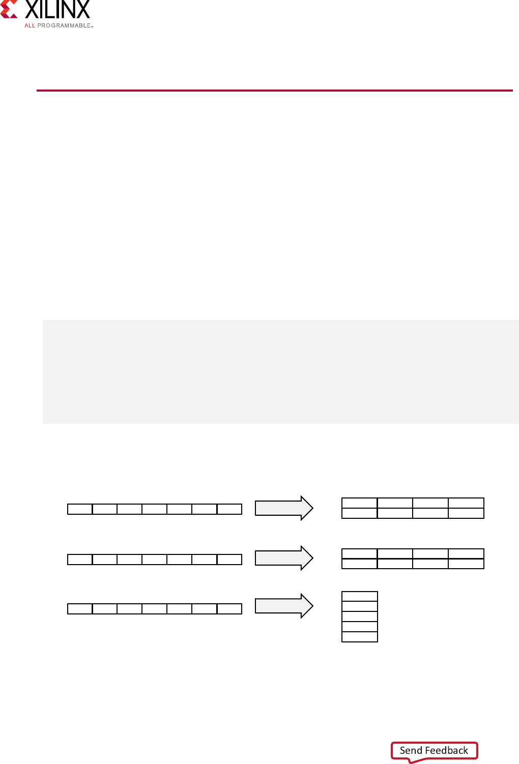
•SDAccel Environment Opmizaon Guide (UG1207)
pragma HLS array_reshape
Description
Combines array paroning with vercal array mapping.
The ARRAY_RESHAPE pragma combines the eect of ARRAY_PARTITION, breaking an array
into smaller arrays, with the eect of the vercal type of ARRAY_MAP, concatenang elements of
arrays by increasing bit-widths. This reduces the number of block RAM consumed while
providing the primary benet of paroning: parallel access to the data. This pragma creates a
new array with fewer elements but with greater bit-width, allowing more data to be accessed in a
single clock cycle.
Given the following code:
void foo (...) {
int array1[N];
int array2[N];
int array3[N];
#pragma HLS ARRAY_RESHAPE variable=array1 block factor=2 dim=1
#pragma HLS ARRAY_RESHAPE variable=array2 cycle factor=2 dim=1
#pragma HLS ARRAY_RESHAPE variable=array3 complete dim=1
...
}
The ARRAY_RESHAPE pragma transforms the arrays into the form shown in the following gure:
Figure 2: ARRAY_RESHAPE Pragma
01 2 ... N-3 N-2 N-1
N/2 ... N-2 N-1
0 1 ... (N/2-1)
1 ... N-3 N-1
0 2 ... N-2
block
cyclic
complete
X14307-110217
0 1 2 ... N-3 N-2 N-1
0 1 2 ... N-3 N-2 N-1
array1[N]
array2[N]
array3[N] N-1
N-2
...
1
0
MSB
LSB
MSB
LSB
MSB
LSB
array4[N/2]
array5[N/2]
array6[1]
Appendix B: HLS Pragmas
Vivado HLS Optimization Methodology Guide 89
UG1270 (v2017.4) December 20, 2017 www.xilinx.com [placeholder text]

Syntax
Place the pragma in the C source within the region of a funcon where the array variable is
denes.
#pragma HLS array_reshape variable=
<name>
\
<type>
factor=
<int>
dim=
<int>
Where:
•<name>: A required argument that species the array variable to be reshaped.
•<type>: Oponally species the paron type. The default type is complete. The following
types are supported:
○cyclic: Cyclic reshaping creates smaller arrays by interleaving elements from the original
array. For example, if factor=3 is used, element 0 is assigned to the rst new array,
element 1 to the second new array, element 2 is assigned to the third new array, and then
element 3 is assigned to the rst new array again. The nal array is a vercal concatenaon
(word concatenaon, to create longer words) of the new arrays into a single array.
○block: Block reshaping creates smaller arrays from consecuve blocks of the original
array. This eecvely splits the array into N equal blocks where N is the integer dened by
factor=, and then combines the N blocks into a single array with word-width*N.
○complete: Complete reshaping decomposes the array into temporary individual elements
and then recombines them into an array with a wider word. For a one-dimension array this
is equivalent to creang a very-wide register (if the original array was N elements of M bits,
the result is a register with N*M bits). This is the default type of array reshaping.
•factor=
<int>
: Species the amount to divide the current array by (or the number of
temporary arrays to create). A factor of 2 splits the array in half, while doubling the bit-width.
A factor of 3 divides the array into three, with triple the bit-width.
IMPORTANT!: For complete type paroning, the factor is not specied. For block and cyclic
reshaping the
factor=
is required.
•dim=
<int>
: Species which dimension of a mul-dimensional array to paron. Specied as
an integer from 0 to N, for an array with N dimensions:
○If a value of 0 is used, all dimensions of a mul-dimensional array are paroned with the
specied type and factor opons.
○Any non-zero value parons only the specied dimension. For example, if a value 1 is
used, only the rst dimension is paroned.
•object: A keyword relevant for container arrays only. When the keyword is specied the
ARRAY_RESHAPE pragma applies to the objects in the container, reshaping all dimensions of
the objects within the container, but all dimensions of the container itself are preserved.
When the keyword is not specied the pragma applies to the container array and not the
objects.
Appendix B: HLS Pragmas
Vivado HLS Optimization Methodology Guide 90
UG1270 (v2017.4) December 20, 2017 www.xilinx.com [placeholder text]
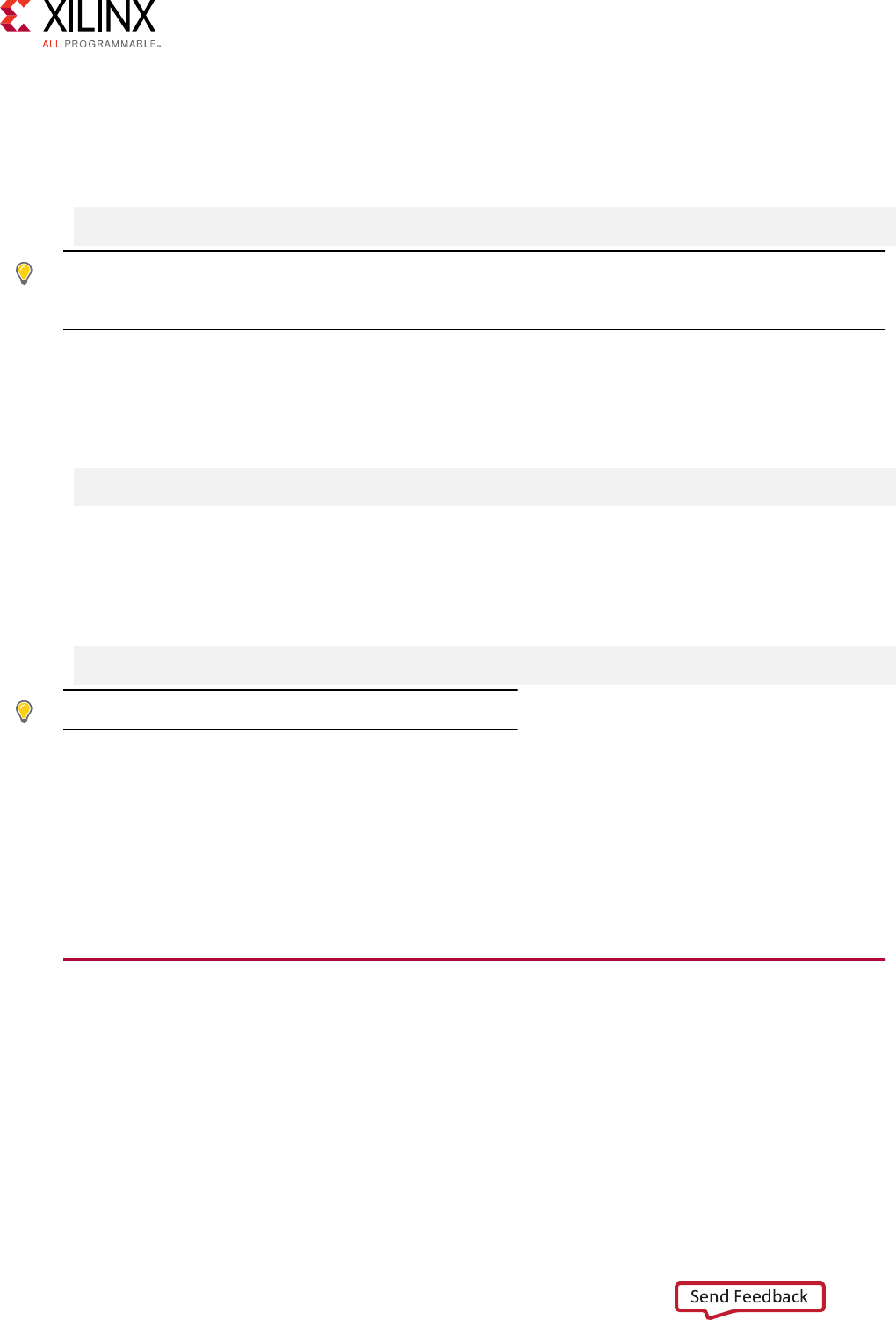
Example 1
Reshapes (paron and maps) an 8-bit array with 17 elements, AB[17], into a new 32-bit array
with ve elements using block mapping.
#pragma HLS array_reshape variable=AB block factor=4
TIP: factor=4 indicates that the array should be divided into four. So 17 elements is reshaped into an
array of 5 elements, with four mes the bit-width. In this case, the last element, AB[17], is mapped to
the lower eight bits of the h element, and the rest of the h element is empty.
Example 2
Reshapes the two-dimensional array AB[6][4] into a new array of dimension [6][2], in which
dimension 2 has twice the bit-width:
#pragma HLS array_reshape variable=AB block factor=2 dim=2
Example 3
Reshapes the three-dimensional 8-bit array, AB[4][2][2] in funcon foo, into a new single
element array (a register), 128 bits wide (4*2*2*8):
#pragma HLS array_reshape variable=AB complete dim=0
TIP: dim=0 means to reshape all dimensions of the array.
See Also
•pragma HLS array_map
•pragma HLS array_paron
•Vivado Design Suite User Guide: High-Level Synthesis (UG902)
•SDAccel Environment Proling and Opmizaon Guide (UG1207)
pragma HLS clock
Description
Applies the named clock to the specied funcon.
C and C++ designs support only a single clock. The clock period specied by create_clock is
applied to all funcons in the design.
Appendix B: HLS Pragmas
Vivado HLS Optimization Methodology Guide 91
UG1270 (v2017.4) December 20, 2017 www.xilinx.com [placeholder text]

SystemC designs support mulple clocks. Mulple named clocks can be specied using the
create_clock command and applied to individual SC_MODULEs using pragma HLS clock.
Each SC_MODULE is synthesized using a single clock.
Syntax
Place the pragma in the C source within the body of the funcon.
#pragma HLS clock domain=<clock>
Where:
• domain=<clock>: Species the clock name.
IMPORTANT!: The specied clock must already exist by the
create_clock
command. There is no
pragma equivalent of the create_clock command. See the Vivado Design Suite User Guide: High-Level
Synthesis (UG902) for more informaon.
Example 1
Assume a SystemC design in which the top-level, foo_top, has clocks ports fast_clock and
slow_clock. However, foo_top uses only fast_clock within its funcon. A sub-block,
foo_sub, uses only slow_clock.
In this example, the following create_clock commands are specied in the script.tcl le
which is specied when the Vivado HLS tool is launched:
create_clock -period 15 fast_clk
create_clock -period 60 slow_clk
Then the following pragmas are specied in the C source le to assign the clock to the specied
funcons, foo_sub and foo_top:
foo_sub (p, q) {
#pragma HLS clock domain=slow_clock
...
}
void foo_top { a, b, c, d} {
#pragma HLS clock domain=fast_clock
...
See Also
•Vivado Design Suite User Guide: High-Level Synthesis (UG902)
Appendix B: HLS Pragmas
Vivado HLS Optimization Methodology Guide 92
UG1270 (v2017.4) December 20, 2017 www.xilinx.com [placeholder text]

pragma HLS data_pack
Description
Packs the data elds of a struct into a single scalar with a wider word width.
The DATA_PACK pragma is used for packing all the elements of a struct into a single wide
vector to reduce the memory required for the variable, while allowing all members of the
struct to be read and wrien to simultaneously. The bit alignment of the resulng new wide-
word can be inferred from the declaraon order of the struct elds. The rst eld takes the
LSB of the vector, and the nal element of the struct is aligned with the MSB of the vector.
If the struct contains arrays, the DATA_PACK pragma performs a similar operaon as the
ARRAY_RESHAPE pragma and combines the reshaped array with the other elements in the
struct. Any arrays declared inside the struct are completely paroned and reshaped into a
wide scalar and packed with other scalar elds. However, a struct cannot be opmized with
DATA_PACK and ARRAY_PARTITION or ARRAY_RESHAPE, as those pragmas are mutually
exclusive.
IMPORTANT!: You should exercise some cauon when using the
DATA_PACK
opmizaon on
struct
objects with large arrays. If an array has 4096 elements of type int, this will result in a vector
(and port) of width 4096*32=131072 bits. Vivado HLS can create this RTL design, however it is very
unlikely logic synthesis will be able to route this during the FPGA implementaon.
In general, Xilinx recommends that you use arbitrary precision (or bit-accurate) data types.
Standard C types are based on 8-bit boundaries (8-bit, 16-bit, 32-bit, 64-bit), however, using
arbitrary precision data types in a design lets you specify the exact bit-sizes in the C code prior to
synthesis. The bit-accurate widths result in hardware operators that are smaller and faster. This
allows more logic to be placed in the FPGA and for the logic to execute at higher clock
frequencies. However, the DATA_PACK pragma also lets you align data in the packed struct
along 8-bit boundaries if needed.
If a struct port is to be implemented with an AXI4 interface you should consider using the
DATA_PACK
<byte_pad>
opon to automacally align member elements of the struct to 8-
bit boundaries. The AXI4-Stream protocol requires that TDATA ports of the IP have a width in
mulples of 8. It is a specicaon violaon to dene an AXI4-Stream IP with a TDATA port width
that is not a mulple of 8, therefore, it is a requirement to round up TDATA widths to byte
mulples. Refer to "Interface Synthesis and Structs" in Vivado Design Suite User Guide: High-Level
Synthesis (UG902) for more informaon.
Appendix B: HLS Pragmas
Vivado HLS Optimization Methodology Guide 93
UG1270 (v2017.4) December 20, 2017 www.xilinx.com [placeholder text]

Syntax
Place the pragma near the denion of the struct variable to pack:
#pragma HLS data_pack variable=
<variable>
\
instance=
<name>
<byte_pad>
Where:
•variable=
<variable>
: is the variable to be packed.
•instance=
<name>
: Species the name of resultant variable aer packing. If no <name> is
specied, the input <variable> is used.
•
<byte_pad>
: Oponally species whether to pack data on an 8-bit boundary (8-bit, 16-bit,
24-bit...). The two supported values for this opon are:
○struct_level: Pack the whole struct rst, then pad it upward to the next 8-bit
boundary.
○field_level: First pad each individual element (eld) of the struct on an 8-bit
boundary, then pack the struct.
TIP: Deciding whether mulple elds of data should be concatenated together before
(
field_level
) or aer (
struct_level
) alignment to byte boundaries is generally determined by
considering how atomic the data is. Atomic informaon is data that can be interpreted on its own,
whereas non-atomic informaon is incomplete for the purpose of interpreng the data. For example,
atomic data can consist of all the bits of informaon in a oang point number. However, the exponent
bits in the oang point number alone would not be atomic. When packing informaon into
TDATA
,
generally non-atomic bits of data are concatenated together (regardless of bit width) unl they form
atomic units. The atomic units are then aligned to byte boundaries using pad bits where necessary.
Example 1
Packs struct array AB[17] with three 8-bit eld elds (R, G, B) into a new 17 element array of
24 bits.
typedef struct{
unsigned char R, G, B;
} pixel;
pixel AB[17];
#pragma HLS data_pack variable=AB
Appendix B: HLS Pragmas
Vivado HLS Optimization Methodology Guide 94
UG1270 (v2017.4) December 20, 2017 www.xilinx.com [placeholder text]

Example 2
Packs struct pointer AB with three 8-bit elds (typedef struct {unsigned char R, G, B;} pixel) in
funcon foo, into a new 24-bit pointer.
typedef struct{
unsigned char R, G, B;
} pixel;
pixel AB;
#pragma HLS data_pack variable=AB
Example 3
In this example the DATA_PACK pragma is specied for in and out arguments to rgb_to_hsv
funcon to instruct the compiler to do pack the structure on an 8-bit boundary to improve the
memory access:
void rgb_to_hsv(RGBcolor* in, // Access global memory as RGBcolor struct-
wise
HSVcolor* out, // Access Global Memory as HSVcolor struct-
wise
int size) {
#pragma HLS data_pack variable=in struct_level
#pragma HLS data_pack variable=out struct_level
...
}
See Also
•pragma HLS array_paron
•pragma HLS array_reshape
•Vivado Design Suite User Guide: High-Level Synthesis (UG902)
pragma HLS dataflow
Description
The DATAFLOW pragma enables task-level pipelining, allowing funcons and loops to overlap in
their operaon, increasing the concurrency of the RTL implementaon, and increasing the overall
throughput of the design.
Appendix B: HLS Pragmas
Vivado HLS Optimization Methodology Guide 95
UG1270 (v2017.4) December 20, 2017 www.xilinx.com [placeholder text]
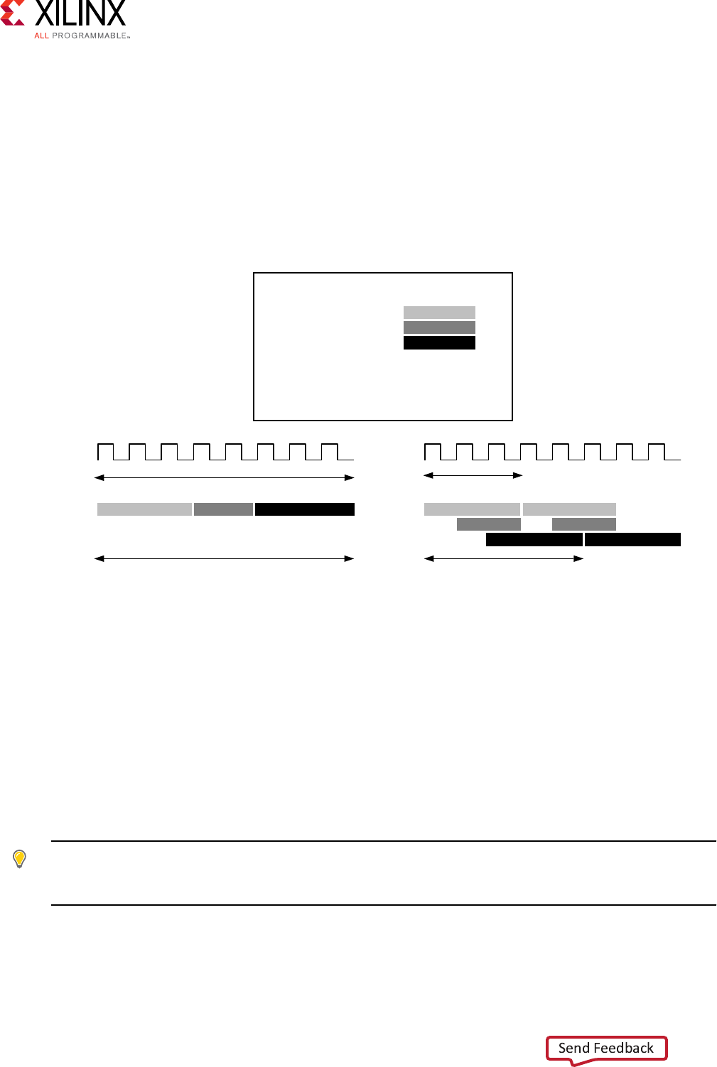
All operaons are performed sequenally in a C descripon. In the absence of any direcves that
limit resources (such as pragma HLS allocation), Vivado HLS seeks to minimize latency and
improve concurrency. However, data dependencies can limit this. For example, funcons or loops
that access arrays must nish all read/write accesses to the arrays before they complete. This
prevents the next funcon or loop that consumes the data from starng operaon. The
DATAFLOW opmizaon enables the operaons in a funcon or loop to start operaon before
the previous funcon or loop completes all its operaons.
Figure 3: DATAFLOW Pragma
void top (a,b,c,d) {
...
func_A(a,b,i1);
func_B(c,i1,i2);
func_C(i2,d)
return d;
}
func_A
func_B
func_C
8 cycles
func_A func_B func_C
8 cycles
3 cycles
func_A
func_B
func_C
func_A
func_B
func_C
5 cycles
(A) Without Dataflow Pipelining (B) With Dataflow Pipelining
X14266-110217
When the DATAFLOW pragma is specied, Vivado HLS analyzes the dataow between sequenal
funcons or loops and create channels (based on pingpong RAMs or FIFOs) that allow consumer
funcons or loops to start operaon before the producer funcons or loops have completed.
This allows funcons or loops to operate in parallel, which decreases latency and improves the
throughput of the RTL.
If no iniaon interval (number of cycles between the start of one funcon or loop and the next)
is specied, Vivado HLS aempts to minimize the iniaon interval and start operaon as soon
as data is available.
TIP: The
config_dataflow
command species the default memory channel and FIFO depth used
in dataow opmizaon. Refer to the
config_dataflow
command in the Vivado Design Suite User
Guide: High-Level Synthesis (UG902) for more informaon.
For the DATAFLOW opmizaon to work, the data must ow through the design from one task to
the next. The following coding styles prevent Vivado HLS from performing the DATAFLOW
opmizaon:
Appendix B: HLS Pragmas
Vivado HLS Optimization Methodology Guide 96
UG1270 (v2017.4) December 20, 2017 www.xilinx.com [placeholder text]

• Single-producer-consumer violaons
• Bypassing tasks
• Feedback between tasks
•Condional execuon of tasks
• Loops with mulple exit condions
IMPORTANT!: If any of these coding styles are present, Vivado HLS issues a message and does not
perform DATAFLOW opmizaon.
Finally, the DATAFLOW opmizaon has no hierarchical implementaon. If a sub-funcon or loop
contains addional tasks that might benet from the DATAFLOW opmizaon, you must apply
the opmizaon to the loop, the sub-funcon, or inline the sub-funcon.
Syntax
Place the pragma in the C source within the boundaries of the region, funcon, or loop.
#pragma HLS dataflow
Example 1
Species DATAFLOW opmizaon within the loop wr_loop_j.
wr_loop_j: for (int j = 0; j < TILE_PER_ROW; ++j) {
#pragma HLS DATAFLOW
wr_buf_loop_m: for (int m = 0; m < TILE_HEIGHT; ++m) {
wr_buf_loop_n: for (int n = 0; n < TILE_WIDTH; ++n) {
#pragma HLS PIPELINE
// should burst TILE_WIDTH in WORD beat
outFifo >> tile[m][n];
}
}
wr_loop_m: for (int m = 0; m < TILE_HEIGHT; ++m) {
wr_loop_n: for (int n = 0; n < TILE_WIDTH; ++n) {
#pragma HLS PIPELINE
outx[TILE_HEIGHT*TILE_PER_ROW*TILE_WIDTH*i
+TILE_PER_ROW*TILE_WIDTH*m+TILE_WIDTH*j+n] = tile[m][n];
}
}
See Also
•pragma HLS allocaon
•Vivado Design Suite User Guide: High-Level Synthesis (UG902)
•xcl_dataow
•SDAccel Environment Opmizaon Guide (UG1207)
Appendix B: HLS Pragmas
Vivado HLS Optimization Methodology Guide 97
UG1270 (v2017.4) December 20, 2017 www.xilinx.com [placeholder text]

pragma HLS dependence
Description
The DEPENDENCE pragma is used to provide addional informaon that can overcome loop-
carry dependencies and allow loops to be pipelined (or pipelined with lower intervals).
Vivado HLS automacally detects dependencies:
• Within loops (loop-independent dependence), or
• Between dierent iteraons of a loop (loop-carry dependence).
These dependencies impact when operaons can be scheduled, especially during funcon and
loop pipelining.
• Loop-independent dependence: The same element is accessed in the same loop iteraon.
for (i=0;i<N;i++) {
A[i]=x;
y=A[i];
}
• Loop-carry dependence: The same element is accessed in a dierent loop iteraon.
for (i=0;i<N;i++) {
A[i]=A[i-1]*2;
}
Under certain complex scenarios automac dependence analysis can be too conservave and fail
to lter out false dependencies. Under certain circumstances, such as variable dependent array
indexing, or when an external requirement needs to be enforced (for example, two inputs are
never the same index), the dependence analysis might be too conservave. The DEPENDENCE
pragma allows you to explicitly specify the dependence and resolve a false dependence.
IMPORTANT!: Specifying a false dependency, when in fact the dependency is not false, can result in
incorrect hardware. Be sure dependencies are correct (true or false) before specifying them.
Syntax
Place the pragma within the boundaries of the funcon where the dependence is dened.
#pragma HLS dependence variable=
<variable>
<class>
\
<type>
<direction>
distance=
<int>
<dependent>
Where:
•variable=
<variable>
: Oponally species the variable to consider for the dependence.
Appendix B: HLS Pragmas
Vivado HLS Optimization Methodology Guide 98
UG1270 (v2017.4) December 20, 2017 www.xilinx.com [placeholder text]

•<class>: Oponally species a class of variables in which the dependence needs claricaon.
Valid values include array or pointer.
TIP: <class> and
variable=
do not need to be specied together as you can either specify a variable
or a class of variables within a funcon.
•<type>: Valid values include intra or inter. Species whether the dependence is:
○intra: dependence within the same loop iteraon. When dependence <type> is specied
as intra, and <dependent> is false, Vivado HLS may move operaons freely within a loop,
increasing their mobility and potenally improving performance or area. When
<dependent> is specied as true, the operaons must be performed in the order specied.
○inter: dependence between dierent loop iteraons. This is the default <type>. If
dependence <type> is specied as inter, and <dependent> is false, it allows Vivado HLS
to perform operaons in parallel if the funcon or loop is pipelined, or the loop is unrolled,
or parally unrolled, and prevents such concurrent operaon when <dependent> is
specied as true.
•<direcon>: Valid values include RAW, WAR, or WAW. This is relevant for loop-carry
dependencies only, and species the direcon for a dependence:
○RAW (Read-Aer-Write - true dependence) The write instrucon uses a value used by the
read instrucon.
○WAR (Write-Aer-Read - an dependence) The read instrucon gets a value that is
overwrien by the write instrucon.
○WAW (Write-Aer-Write - output dependence) Two write instrucons write to the same
locaon, in a certain order.
•distance=
<int>
: Species the inter-iteraon distance for array access. Relevant only for
loop-carry dependencies where dependence is set to true.
•<dependent>: Species whether a dependence needs to be enforced (true) or removed
(false). The default is true.
Example 1
In the following example, Vivado HLS does not have any knowledge about the value of cols and
conservavely assumes that there is always a dependence between the write to buff_A[1]
[col] and the read from buff_A[1][col]. In an algorithm such as this, it is unlikely cols will
ever be zero, but Vivado HLS cannot make assumpons about data dependencies. To overcome
this deciency, you can use the DEPENDENCE pragma to state that there is no dependence
between loop iteraons (in this case, for both buff_A and buff_B).
void foo(int rows, int cols, ...)
for (row = 0; row < rows + 1; row++) {
for (col = 0; col < cols + 1; col++) {
#pragma HLS PIPELINE II=1
#pragma HLS dependence variable=buff_A inter false
#pragma HLS dependence variable=buff_B inter false
if (col < cols) {
Appendix B: HLS Pragmas
Vivado HLS Optimization Methodology Guide 99
UG1270 (v2017.4) December 20, 2017 www.xilinx.com [placeholder text]

buff_A[2][col] = buff_A[1][col]; // read from buff_A[1][col]
buff_A[1][col] = buff_A[0][col]; // write to buff_A[1][col]
buff_B[1][col] = buff_B[0][col];
temp = buff_A[0][col];
}
Example 2
Removes the dependence between Var1 in the same iteraons of loop_1 in funcon foo.
#pragma HLS dependence variable=Var1 intra false
Example 3
Denes the dependence on all arrays in loop_2 of funcon foo to inform Vivado HLS that all
reads must happen aer writes (RAW) in the same loop iteraon.
#pragma HLS dependence array intra RAW true
See Also
•pragma HLS pipeline
•Vivado Design Suite User Guide: High-Level Synthesis (UG902)
•xcl_pipeline_loop
•SDAccel Environment Opmizaon Guide (UG1207)
pragma HLS expression_balance
Description
Somemes a C-based specicaon is wrien with a sequence of operaons resulng in a long
chain of operaons in RTL. With a small clock period, this can increase the latency in the design.
By default, Vivado HLS rearranges the operaons using associave and commutave properes.
This rearrangement creates a balanced tree that can shorten the chain, potenally reducing
latency in the design at the cost of extra hardware.
The EXPRESSION_BALANCE pragma allows this expression balancing to be disabled, or to be
expressly enabled, within a specied scope.
Appendix B: HLS Pragmas
Vivado HLS Optimization Methodology Guide 100
UG1270 (v2017.4) December 20, 2017 www.xilinx.com [placeholder text]

Syntax
Place the pragma in the C source within the boundaries of the required locaon.
#pragma HLS expression_balance off
Where:
•off: Turns o expression balancing at this locaon.
TIP: Leaving this opon out of the pragma enables expression balancing, which is the default mode.
Example 1
This example explicitly enables expression balancing in funcon my_Func:
void my_func(char inval, char incr) {
#pragma HLS expression_balance
Example 2
Disables expression balancing within funcon my_Func:
void my_func(char inval, char incr) {
#pragma HLS expression_balance off
See Also
•Vivado Design Suite User Guide: High-Level Synthesis (UG902)
pragma HLS function_instantiate
Description
The FUNCTION_INSTANTIATE pragma is an opmizaon technique that has the area benets
of maintaining the funcon hierarchy but provides an addional powerful opon: performing
targeted local opmizaons on specic instances of a funcon. This can simplify the control logic
around the funcon call and potenally improve latency and throughput.
By default:
•Funcons remain as separate hierarchy blocks in the RTL.
• All instances of a funcon, at the same level of hierarchy, make use of a single RTL
implementaon (block).
Appendix B: HLS Pragmas
Vivado HLS Optimization Methodology Guide 101
UG1270 (v2017.4) December 20, 2017 www.xilinx.com [placeholder text]

The FUNCTION_INSTANTIATE pragma is used to create a unique RTL implementaon for each
instance of a funcon, allowing each instance to be locally opmized according to the funcon
call. This pragma exploits the fact that some inputs to a funcon may be a constant value when
the funcon is called, and uses this to both simplify the surrounding control structures and
produce smaller more opmized funcon blocks.
Without the FUNCTION_INSTANTIATE pragma, the following code results in a single RTL
implementaon of funcon foo_sub for all three instances of the funcon in foo. Each
instance of funcon foo_sub is implemented in an idencal manner. This is ne for funcon
reuse and reducing the area required for each instance call of a funcon, but means that the
control logic inside the funcon must be more complex to account for the variaon in each call of
foo_sub.
char foo_sub(char inval, char incr) {
#pragma HLS function_instantiate variable=incr
return inval + incr;
}
void foo(char inval1, char inval2, char inval3,
char *outval1, char *outval2, char * outval3)
{
*outval1 = foo_sub(inval1, 1);
*outval2 = foo_sub(inval2, 2);
*outval3 = foo_sub(inval3, 3);
}
In the code sample above, the FUNCTION_INSTANTIATE pragma results in three dierent
implementaons of funcon foo_sub, each independently opmized for the incr argument,
reducing the area and improving the performance of the funcon. Aer
FUNCTION_INSTANTIATE opmizaon, foo_sub is eecvely be transformed into three
separate funcons, each opmized for the specied values of incr.
Syntax
Place the pragma in the C source within the boundaries of the required locaon.
#pragma HLS function_instantiate variable=
<variable>
Where:
•variable=
<variable>
: A required argument that denes the funcon argument to use as
a constant.
Appendix B: HLS Pragmas
Vivado HLS Optimization Methodology Guide 102
UG1270 (v2017.4) December 20, 2017 www.xilinx.com [placeholder text]

Example 1
In the following example, the FUNCTION_INSTANTIATE pragma placed in funcon swInt)
allows each instance of funcon swInt to be independently opmized with respect to the maxv
funcon argument:
void swInt(unsigned int *readRefPacked, short *maxr, short *maxc, short
*maxv){
#pragma HLS function_instantiate variable=maxv
uint2_t d2bit[MAXCOL];
uint2_t q2bit[MAXROW];
#pragma HLS array partition variable=d2bit,q2bit cyclic factor=FACTOR
intTo2bit<MAXCOL/16>((readRefPacked + MAXROW/16), d2bit);
intTo2bit<MAXROW/16>(readRefPacked, q2bit);
sw(d2bit, q2bit, maxr, maxc, maxv);
}
See Also
•pragma HLS allocaon
•pragma HLS inline
•Vivado Design Suite User Guide: High-Level Synthesis (UG902)
pragma HLS inline
Description
Removes a funcon as a separate enty in the hierarchy. Aer inlining, the funcon is dissolved
into the calling funcon and no longer appears as a separate level of hierarchy in the RTL. In
some cases, inlining a funcon allows operaons within the funcon to be shared and opmized
more eecvely with surrounding operaons. An inlined funcon cannot be shared. This can
increase area required for implemenng the RTL.
The INLINE pragma applies dierently to the scope it is dened in depending on how it is
specied:
•INLINE: Without arguments, the pragma means that the funcon it is specied in should be
inlined upward into any calling funcons or regions.
•INLINE OFF: Species that the funcon it is specied in should NOT be inlined upward into
any calling funcons or regions. This disables the inline of a specic funcon that may be
automacally inlined, or inlined as part of a region or recursion.
•INLINE REGION: This applies the pragma to the region or the body of the funcon it is
assigned in. It applies downward, inlining the contents of the region or funcon, but not
inlining recursively through the hierarchy.
Appendix B: HLS Pragmas
Vivado HLS Optimization Methodology Guide 103
UG1270 (v2017.4) December 20, 2017 www.xilinx.com [placeholder text]

•INLINE RECURSIVE: This applies the pragma to the region or the body of the funcon it is
assigned in. It applies downward, recursively inlining the contents of the region or funcon.
By default, inlining is only performed on the next level of funcon hierarchy, not sub-funcons.
However, the recursive opon lets you specify inlining through levels of the hierarchy.
Syntax
Place the pragma in the C source within the body of the funcon or region of code.
#pragma HLS inline <region | recursive | off>
Where:
•region: Oponally species that all funcons in the specied region (or contained within the
body of the funcon) are to be inlined, applies to the scope of the region.
•recursive: By default, only one level of funcon inlining is performed, and funcons within
the specied funcon are not inlined. The recursive opon inlines all funcons recursively
within the specied funcon or region.
•off: Disables funcon inlining to prevent specied funcons from being inlined. For example,
if recursive is specied in a funcon, this opon can prevent a parcular called funcon
from being inlined when all others are.
TIP: Vivado HLS automacally inlines small funcons and using the INLINE pragma with the
off
opon may be used to prevent this automac inlining.
Example 1
This example inlines all funcons within the region it is specied in, in this case the body of
foo_top, but does not inline any lower level funcons within those funcons.
void foo_top { a, b, c, d} {
#pragma HLS inline region
...
Example 2
The following example, inlines all funcons within the body of foo_top, inlining recursively
down through the funcon hierarchy, except funcon foo_sub is not inlined. The recursive
pragma is placed in funcon foo_top. The pragma to disable inlining is placed in the funcon
foo_sub:
foo_sub (p, q) {
#pragma HLS inline off
int q1 = q + 10;
foo(p1,q);// foo_3
...
Appendix B: HLS Pragmas
Vivado HLS Optimization Methodology Guide 104
UG1270 (v2017.4) December 20, 2017 www.xilinx.com [placeholder text]

}
void foo_top { a, b, c, d} {
#pragma HLS inline region recursive
...
foo(a,b);//foo_1
foo(a,c);//foo_2
foo_sub(a,d);
...
}
Note: Noce in this example, that INLINE applies downward to the contents of funcon foo_top, but
applies upward to the code calling foo_sub.
Example 3
This example inlines the copy_output funcon into any funcons or regions calling
copy_output.
void copy_output(int *out, int out_lcl[OSize * OSize], int output) {
#pragma HLS INLINE
// Calculate each work_item's result update location
int stride = output * OSize * OSize;
// Work_item updates output filter/image in DDR
writeOut: for(int itr = 0; itr < OSize * OSize; itr++) {
#pragma HLS PIPELINE
out[stride + itr] = out_lcl[itr];
}
See Also
•pragma HLS allocaon
•pragma HLS funcon_instanate
•Vivado Design Suite User Guide: High-Level Synthesis (UG902)
Appendix B: HLS Pragmas
Vivado HLS Optimization Methodology Guide 105
UG1270 (v2017.4) December 20, 2017 www.xilinx.com [placeholder text]

pragma HLS interface
Description
In C based design, all input and output operaons are performed, in zero me, through formal
funcon arguments. In an RTL design these same input and output operaons must be
performed through a port in the design interface and typically operate using a specic I/O (input-
output) protocol. For more informaon, refer to "Managing Interfaces" in the Vivado Design Suite
User Guide: High-Level Synthesis (UG902).
The INTERFACE pragma species how RTL ports are created from the funcon denion during
interface synthesis.
The ports in the RTL implementaon are derived from:
• Any funcon-level protocol that is specied.
•Funcon arguments.
• Global variables accessed by the top-level funcon and dened outside its scope.
Funcon-level protocols, also called block-level I/O protocols, provide signals to control when
the funcon starts operaon, and indicate when funcon operaon ends, is idle, and is ready for
new inputs. The implementaon of a funcon-level protocol:
• Is specied by the <mode> values ap_ctrl_none, ap_ctrl_hs or ap_ctrl_chain. The
ap_ctrl_hs block-level I/O protocol is the default.
• Are associated with the funcon name.
Each funcon argument can be specied to have its own port-level (I/O) interface protocol, such
as valid handshake (ap_vld) or acknowledge handshake (ap_ack). Port Level interface protocols
are created for each argument in the top-level funcon and the funcon return, if the funcon
returns a value. The default I/O protocol created depends on the type of C argument. Aer the
block-level protocol has been used to start the operaon of the block, the port-level IO protocols
are used to sequence data into and out of the block.
If a global variable is accessed, but all read and write operaons are local to the design, the
resource is created in the design. There is no need for an I/O port in the RTL. If the global
variable is expected to be an external source or desnaon, specify its interface in a similar
manner as standard funcon arguments. See the examples below.
When the INTERFACE pragma is used on sub-funcons, only the register opon can be used.
The <mode> opon is not supported on sub-funcons.
Appendix B: HLS Pragmas
Vivado HLS Optimization Methodology Guide 106
UG1270 (v2017.4) December 20, 2017 www.xilinx.com [placeholder text]
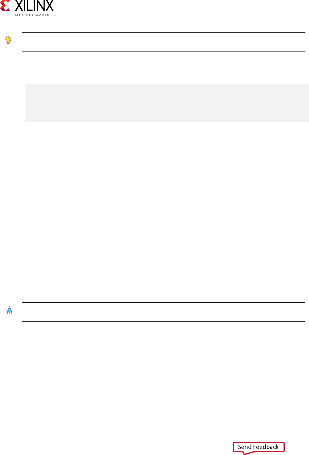
TIP: Vivado HLS automacally determines the I/O protocol used by any sub-funcons. You cannot
control these ports except to specify whether the port is registered.
Syntax
Place the pragma within the boundaries of the funcon.
#pragma HLS interface
<mode>
port=
<name>
bundle=
<string>
\
register register_mode=
<mode>
depth=
<int>
offset=
<string>
\
clock=
<string>
name=
<string>
\
num_read_outstanding=
<int>
num_write_outstanding=
<int>
\
max_read_burst_length=
<int>
max_write_burst_length=
<int>
Where:
•<mode>: Species the interface protocol mode for funcon arguments, global variables used
by the funcon, or the block-level control protocols. For detailed descripons of these
dierent modes see "Interface Synthesis Reference" in the Vivado Design Suite User Guide:
High-Level Synthesis (UG902). The mode can be specied as one of the following:
○ap_none: No protocol. The interface is a data port.
○ap_stable: No protocol. The interface is a data port. Vivado HLS assumes the data port is
always stable aer reset, which allows internal opmizaons to remove unnecessary
registers.
○ap_vld: Implements the data port with an associated valid port to indicate when the
data is valid for reading or wring.
○ap_ack: Implements the data port with an associated acknowledge port to acknowledge
that the data was read or wrien.
○ap_hs: Implements the data port with associated valid and acknowledge ports to
provide a two-way handshake to indicate when the data is valid for reading and wring and
to acknowledge that the data was read or wrien.
○ap_ovld: Implements the output data port with an associated valid port to indicate
when the data is valid for reading or wring.
IMPORTANT!: Vivado HLS implements the input argument or the input half of any read/write
arguments with mode
ap_none
.
○ap_fifo: Implements the port with a standard FIFO interface using data input and output
ports with associated acve-Low FIFO empty and full ports.
Note: You can only use this interface on read arguments or write arguments. The ap_fifo mode does
not support bidireconal read/write arguments.
○ap_bus: Implements pointer and pass-by-reference ports as a bus interface.
○ap_memory: Implements array arguments as a standard RAM interface. If you use the RTL
design in Vivado IP integrator, the memory interface appears as discrete ports.
○bram: Implements array arguments as a standard RAM interface. If you use the RTL design
in Vivado IP integrator, the memory interface appears as a single port.
Appendix B: HLS Pragmas
Vivado HLS Optimization Methodology Guide 107
UG1270 (v2017.4) December 20, 2017 www.xilinx.com [placeholder text]

•○axis: Implements all ports as an AXI4-Stream interface.
○s_axilite: Implements all ports as an AXI4-Lite interface. Vivado HLS produces an
associated set of C driver les during the Export RTL process.
○m_axi: Implements all ports as an AXI4 interface. You can use the config_interface
command to specify either 32-bit (default) or 64-bit address ports and to control any
address oset.
○ap_ctrl_none: No block-level I/O protocol.
Note: Using the ap_ctrl_none mode might prevent the design from being veried using the C/RTL co-
simulaon feature.
○ap_ctrl_hs: Implements a set of block-level control ports to start the design operaon
and to indicate when the design is idle, done, and ready for new input data.
Note: The ap_ctrl_hs mode is the default block-level I/O protocol.
○ap_ctrl_chain: Implements a set of block-level control ports to start the design
operaon, continue operaon, and indicate when the design is idle, done, and ready
for new input data.
Note: The ap_ctrl_chain interface mode is similar to ap_ctrl_hs but provides an addional input
signal ap_continue to apply back pressure. Xilinx recommends using the ap_ctrl_chain block-
level I/O protocol when chaining Vivado HLS blocks together.
•port=
<name>
: Species the name of the funcon argument, funcon return, or global
variable which the INTERFACE pragma applies to.
TIP: Block-level I/O protocols (
ap_ctrl_none
,
ap_ctrl_hs
, or
ap_ctrl_chain
) can be
assigned to a port for the funcon
return
value.
•bundle=
<string>
: Groups funcon arguments into AXI interface ports. By default, Vivado
HLS groups all funcon arguments specied as an AXI4-Lite (s_axilite) interface into a
single AXI4-Lite port. Similarly, all funcon arguments specied as an AXI4 (m_axi) interface
are grouped into a single AXI4 port. This opon explicitly groups all interface ports with the
same bundle=
<string>
into the same AXI interface port and names the RTL port the value
specied by <string>.
•register: An oponal keyword to register the signal and any relevant protocol signals, and
causes the signals to persist unl at least the last cycle of the funcon execuon. This opon
applies to the following interface modes:
○ap_none
○ap_ack
○ap_vld
○ap_ovld
○ap_hs
○ap_stable
Appendix B: HLS Pragmas
Vivado HLS Optimization Methodology Guide 108
UG1270 (v2017.4) December 20, 2017 www.xilinx.com [placeholder text]

○axis
○s_axilite
TIP: The
-register_io
opon of the
config_interface
command globally controls registering
all inputs/outputs on the top funcon. Refer to Vivado Design Suite User Guide: High-Level Synthesis
(UG902) for more informaon.
•register_mode= <forward|reverse|both|off>: Used with the register keyword,
this opon species if registers are placed on the forward path (TDATA and TVALID), the
reverse path (TREADY), on both paths (TDATA, TVALID, and TREADY), or if none of the
port signals are to be registered (off). The default register_mode is both. AXI-Stream
(axis) side-channel signals are considered to be data signals and are registered whenever the
TDATA is registered.
•depth=
<int>
: Species the maximum number of samples for the test bench to process. This
seng indicates the maximum size of the FIFO needed in the vericaon adapter that Vivado
HLS creates for RTL co-simulaon.
TIP: While
depth
is usually an opon, it is required for
m_axi
interfaces.
•offset=
<string>
: Controls the address oset in AXI4-Lite (s_axilite) and AXI4
(m_axi) interfaces.
○For the s_axilite interface, <string> species the address in the register map.
○For the m_axi interface, <string> species on of the following values:
-direct: Generate a scalar input oset port.
-slave: Generate an oset port and automacally map it to an AXI4-Lite slave interface.
-off: Do not generate an oset port.
TIP: The
-m_axi_offset
opon of the
config_interface
command globally controls the
oset ports of all M_AXI interfaces in the design.
•clock=
<name>
: Oponally specied only for interface mode s_axilite. This denes the
clock signal to use for the interface. By default, the AXI-Lite interface clock is the same clock
as the system clock. This opon is used to specify a separate clock for the AXI-Lite
(s_axilite) interface.
TIP: If the
bundle
opon is used to group mulple top-level funcon arguments into a single AXI-Lite
interface, the clock opon need only be specied on one of the bundle members.
•num_read_outstanding=
<int>
: For AXI4 (m_axi) interfaces, this opon species how
many read requests can be made to the AXI4 bus, without a response, before the design stalls.
This implies internal storage in the design, a FIFO of size:
num_read_outstanding*max_read_burst_length*word_size.
Appendix B: HLS Pragmas
Vivado HLS Optimization Methodology Guide 109
UG1270 (v2017.4) December 20, 2017 www.xilinx.com [placeholder text]

•num_write_outstanding=
<int>
: For AXI4 (m_axi) interfaces, this opon species how
many write requests can be made to the AXI4 bus, without a response, before the design
stalls. This implies internal storage in the design, a FIFO of size:
num_write_outstanding*max_write_burst_length*word_size
•max_read_burst_length=
<int>
: For AXI4 (m_axi) interfaces, this opon species the
maximum number of data values read during a burst transfer.
•max_write_burst_length=
<int>
: For AXI4 (m_axi) interfaces, this opon species the
maximum number of data values wrien during a burst transfer.
•name=
<string>
: This opon is used to rename the port based on your own specicaon.
The generated RTL port will use this name.
Example 1
In this example, both funcon arguments are implemented using an AXI4-Stream interface:
void example(int A[50], int B[50]) {
//Set the HLS native interface types
#pragma HLS INTERFACE axis port=A
#pragma HLS INTERFACE axis port=B
int i;
for(i = 0; i < 50; i++){
B[i] = A[i] + 5;
}
}
Example 2
The following turns o block-level I/O protocols, and is assigned to the funcon return value:
#pragma HLS interface ap_ctrl_none port=return
The funcon argument InData is specied to use the ap_vld interface, and also indicates the
input should be registered:
#pragma HLS interface ap_vld register port=InData
This exposes the global variable lookup_table as a port on the RTL design, with an
ap_memory interface:
pragma HLS interface ap_memory port=lookup_table
Appendix B: HLS Pragmas
Vivado HLS Optimization Methodology Guide 110
UG1270 (v2017.4) December 20, 2017 www.xilinx.com [placeholder text]

Example 3
This example denes the INTERFACE standards for the ports of the top-level transpose
funcon. Noce the use of the bundle= opon to group signals.
// TOP LEVEL - TRANSPOSE
void transpose(int* input, int* output) {
#pragma HLS INTERFACE m_axi port=input offset=slave bundle=gmem0
#pragma HLS INTERFACE m_axi port=output offset=slave bundle=gmem1
#pragma HLS INTERFACE s_axilite port=input bundle=control
#pragma HLS INTERFACE s_axilite port=output bundle=control
#pragma HLS INTERFACE s_axilite port=return bundle=control
#pragma HLS dataflow
See Also
•pragma HLS protocol
•Vivado Design Suite User Guide: High-Level Synthesis (UG902)
pragma HLS latency
Description
Species a minimum or maximum latency value, or both, for the compleon of funcons, loops,
and regions. Latency is dened as the number of clock cycles required to produce an output.
Funcon latency is the number of clock cycles required for the funcon to compute all output
values, and return. Loop latency is the number of cycles to execute all iteraons of the loop. See
"Performance Metrics Example" of Vivado Design Suite User Guide: High-Level Synthesis (UG902).
Vivado HLS always tries to the minimize latency in the design. When the LATENCY pragma is
specied, the tool behavior is as follows:
• Latency is greater than the minimum, or less than the maximum: The constraint is sased. No
further opmizaons are performed.
• Latency is less than the minimum: If Vivado HLS can achieve less than the minimum specied
latency, it extends the latency to the specied value, potenally increasing sharing.
•Latency is greater than the maximum: If Vivado HLS cannot schedule within the maximum
limit, it increases eort to achieve the specied constraint. If it sll fails to meet the maximum
latency, it issues a warning, and produces a design with the smallest achievable latency in
excess of the maximum.
Appendix B: HLS Pragmas
Vivado HLS Optimization Methodology Guide 111
UG1270 (v2017.4) December 20, 2017 www.xilinx.com [placeholder text]

TIP: You can also use the LATENCY pragma to limit the eorts of the tool to nd an opmum soluon.
Specifying latency constraints for scopes within the code: loops, funcons, or regions, reduces the
possible soluons within that scope and improves tool runme. Refer to "Improving Run Time and
Capacity" of Vivado Design Suite User Guide: High-Level Synthesis (UG902) for more informaon.
Syntax
Place the pragma within the boundary of a funcon, loop, or region of code where the latency
must be managed.
#pragma HLS latency min=<int> max=<int>
Where:
•min=
<int>
: Oponally species the minimum latency for the funcon, loop, or region of
code.
•max=
<int>
: Oponally species the maximum latency for the funcon, loop, or region of
code.
Note: Although both min and max are described as oponal, one must be specied.
Example 1
Funcon foo is specied to have a minimum latency of 4 and a maximum latency of 8:
int foo(char x, char a, char b, char c) {
#pragma HLS latency min=4 max=8
char y;
y = x*a+b+c;
return y
}
Example 2
In the following example loop_1 is specied to have a maximum latency of 12. Place the pragma
in the loop body as shown:
void foo (num_samples, ...) {
int i;
...
loop_1: for(i=0;i< num_samples;i++) {
#pragma HLS latency max=12
...
result = a + b;
}
}
Appendix B: HLS Pragmas
Vivado HLS Optimization Methodology Guide 112
UG1270 (v2017.4) December 20, 2017 www.xilinx.com [placeholder text]

Example 3
The following example creates a code region and groups signals that need to change in the same
clock cycle by specifying zero latency:
// create a region { } with a latency = 0
{
#pragma HLS LATENCY max=0 min=0
*data = 0xFF;
*data_vld = 1;
}
See Also
•Vivado Design Suite User Guide: High-Level Synthesis (UG902)
pragma HLS loop_flatten
Description
Allows nested loops to be aened into a single loop hierarchy with improved latency.
In the RTL implementaon, it requires one clock cycle to move from an outer loop to an inner
loop, and from an inner loop to an outer loop. Flaening nested loops allows them to be
opmized as a single loop. This saves clock cycles, potenally allowing for greater opmizaon of
the loop body logic.
Apply the LOOP_FLATTEN pragma to the loop body of the inner-most loop in the loop hierarchy.
Only perfect and semi-perfect loops can be aened in this manner:
• Perfect loop nests:
○Only the innermost loop has loop body content.
○There is no logic specied between the loop statements.
○All loop bounds are constant.
• Semi-perfect loop nests:
○Only the innermost loop has loop body content.
○There is no logic specied between the loop statements.
○The outermost loop bound can be a variable.
•Imperfect loop nests: When the inner loop has variable bounds (or the loop body is not
exclusively inside the inner loop), try to restructure the code, or unroll the loops in the loop
body to create a perfect loop nest.
Appendix B: HLS Pragmas
Vivado HLS Optimization Methodology Guide 113
UG1270 (v2017.4) December 20, 2017 www.xilinx.com [placeholder text]

Syntax
Place the pragma in the C source within the boundaries of the nested loop.
#pragma HLS loop_flatten off
Where:
•off: Is an oponal keyword that prevents aening from taking place. Can prevent some
loops from being aened while all others in the specied locaon are aened.
Note: The presence of the LOOP_FLATTEN pragma enables the opmizaon.
Example 1
Flaens loop_1 in funcon foo and all (perfect or semi-perfect) loops above it in the loop
hierarchy, into a single loop. Place the pragma in the body of loop_1.
void foo (num_samples, ...) {
int i;
...
loop_1: for(i=0;i< num_samples;i++) {
#pragma HLS loop_flatten
...
result = a + b;
}
}
Example 2
Prevents loop aening in loop_1:
loop_1: for(i=0;i< num_samples;i++) {
#pragma HLS loop_flatten off
...
See Also
•pragma HLS loop_merge
•pragma HLS loop_tripcount
•pragma HLS unroll
•Vivado Design Suite User Guide: High-Level Synthesis (UG902)
Appendix B: HLS Pragmas
Vivado HLS Optimization Methodology Guide 114
UG1270 (v2017.4) December 20, 2017 www.xilinx.com [placeholder text]

pragma HLS loop_merge
Description
Merge consecuve loops into a single loop to reduce overall latency, increase sharing, and
improve logic opmizaon. Merging loops:
• Reduces the number of clock cycles required in the RTL to transion between the loop-body
implementaons.
• Allows the loops be implemented in parallel (if possible).
The LOOP_MERGE pragma will seek to merge all loops within the scope it is placed. For example,
if you apply a LOOP_MERGE pragma in the body of a loop, Vivado HLS applies the pragma to any
sub-loops within the loop but not to the loop itself.
The rules for merging loops are:
• If the loop bounds are variables, they must have the same value (number of iteraons).
• If the loop bounds are constants, the maximum constant value is used as the bound of the
merged loop.
• Loops with both variable bounds and constant bounds cannot be merged.
• The code between loops to be merged cannot have side eects. Mulple execuon of this
code should generate the same results (a=b is allowed, a=a+1 is not).
• Loops cannot be merged when they contain FIFO reads. Merging changes the order of the
reads. Reads from a FIFO or FIFO interface must always be in sequence.
Syntax
Place the pragma in the C source within the required scope or region of code:
#pragma HLS loop_merge force
where
•force: An oponal keyword to force loops to be merged even when Vivado HLS issues a
warning.
IMPORTANT!: In this case, you must manually insure that the merged loop will funcon correctly.
Appendix B: HLS Pragmas
Vivado HLS Optimization Methodology Guide 115
UG1270 (v2017.4) December 20, 2017 www.xilinx.com [placeholder text]

Examples
Merges all consecuve loops in funcon foo into a single loop.
void foo (num_samples, ...) {
#pragma HLS loop_merge
int i;
...
loop_1: for(i=0;i< num_samples;i++) {
...
All loops inside loop_2 (but not loop_2 itself) are merged by using the force opon. Place
the pragma in the body of loop_2.
loop_2: for(i=0;i< num_samples;i++) {
#pragma HLS loop_merge force
...
See Also
•pragma HLS loop_aen
•pragma HLS loop_tripcount
•pragma HLS unroll
•Vivado Design Suite User Guide: High-Level Synthesis (UG902)
pragma HLS loop_tripcount
Description
The TRIPCOUNT pragma can be applied to a loop to manually specify the total number of
iteraons performed by a loop.
Appendix B: HLS Pragmas
Vivado HLS Optimization Methodology Guide 116
UG1270 (v2017.4) December 20, 2017 www.xilinx.com [placeholder text]

IMPORTANT!: The
TRIPCOUNT
pragma is for analysis only, and does not impact the results of
synthesis.
Vivado HLS reports the total latency of each loop, which is the number of clock cycles to execute
all iteraons of the loop. The loop latency is therefore a funcon of the number of loop
iteraons, or tripcount.
The tripcount can be a constant value. It may depend on the value of variables used in the loop
expression (for example, x<y), or depend on control statements used inside the loop. In some
cases Vivado HLS cannot determine the tripcount, and the latency is unknown. This includes
cases in which the variables used to determine the tripcount are:
• Input arguments, or
• Variables calculated by dynamic operaon.
In cases where the loop latency is unknown or cannot be calculate, the TRIPCOUNT pragma lets
you specify minimum and maximum iteraons for a loop. This lets the tool analyze how the loop
latency contributes to the total design latency in the reports, and helps you determine
appropriate opmizaons for the design.
Syntax
Place the pragma in the C source within the body of the loop:
#pragma HLS loop_tripcount min=<int> max=<int> avg=<int>
Where:
•max=
<int>
: Species the maximum number of loop iteraons.
•min=
<int>
: Species the minimum number of loop iteraons.
•avg=
<int>
: Species the average number of loop iteraons.
Examples
In this example loop_1 in funcon foo is specied to have a minimum tripcount of 12 and a
maximum tripcount of 16:
void foo (num_samples, ...) {
int i;
...
loop_1: for(i=0;i< num_samples;i++) {
#pragma HLS loop_tripcount min=12 max=16
...
result = a + b;
}
}
Appendix B: HLS Pragmas
Vivado HLS Optimization Methodology Guide 117
UG1270 (v2017.4) December 20, 2017 www.xilinx.com [placeholder text]

See Also
•Vivado Design Suite User Guide: High-Level Synthesis (UG902)
pragma HLS occurrence
Description
When pipelining funcons or loops, the OCCURRENCE pragma species that the code in a region
is executed less frequently than the code in the enclosing funcon or loop. This allows the code
that is executed less oen to be pipelined at a slower rate, and potenally shared within the top-
level pipeline. To determine the OCCURRENCE:
• A loop iterates N mes.
• However, part of the loop body is enabled by a condional statement, and as a result only
executes M mes, where N is an integer mulple of M.
• The condional code has an occurrence that is N/M mes slower than the rest of the loop
body.
For example, in a loop that executes 10 mes, a condional statement within the loop only
executes 2 mes has an occurrence of 5 (or 10/2).
Idenfying a region with the OCCURRENCE pragma allows the funcons and loops in that region
to be pipelined with a higher iniaon interval that is slower than the enclosing funcon or loop.
Syntax
Place the pragma in the C source within a region of code.
#pragma HLS occurrence cycle=<int>
Where:
•cycle=
<int>
: Species the occurrence N/M, where:
○N is the number of mes the enclosing funcon or loop is executed .
○M is the number of mes the condional region is executed.
IMPORTANT!: N must be an integer mulple of M.
Appendix B: HLS Pragmas
Vivado HLS Optimization Methodology Guide 118
UG1270 (v2017.4) December 20, 2017 www.xilinx.com [placeholder text]

Examples
In this example, the region Cond_Region has an occurrence of 4 (it executes at a rate four mes
less oen than the surrounding code that contains it):
Cond_Region: {
#pragma HLS occurrence cycle=4
...
}
See Also
•pragma HLS pipeline
•Vivado Design Suite User Guide: High-Level Synthesis (UG902)
Appendix B: HLS Pragmas
Vivado HLS Optimization Methodology Guide 119
UG1270 (v2017.4) December 20, 2017 www.xilinx.com [placeholder text]
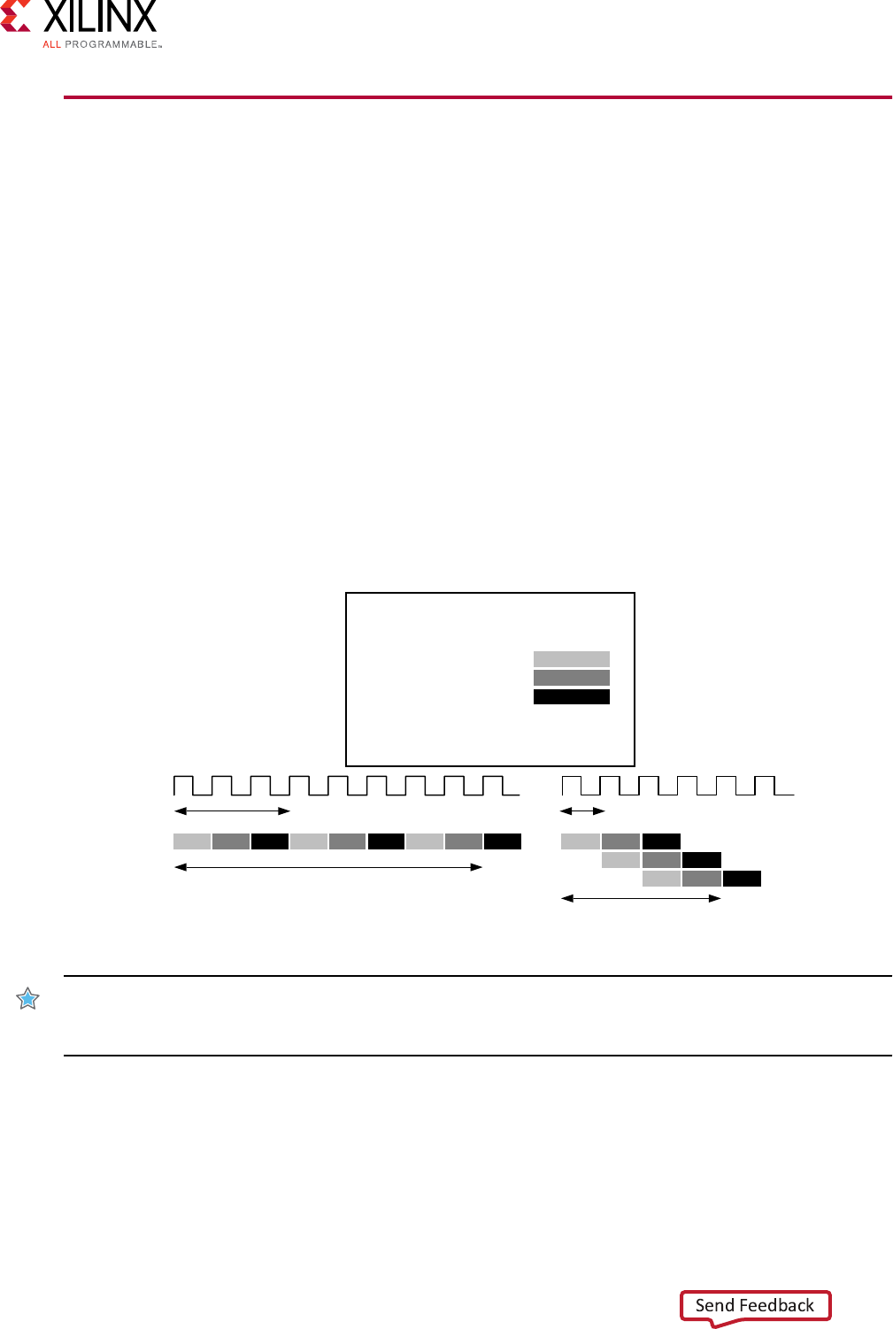
pragma HLS pipeline
Description
The PIPELINE pragma reduces the iniaon interval for a funcon or loop by allowing the
concurrent execuon of operaons.
A pipelined funcon or loop can process new inputs every N clock cycles, where N is the
iniaon interval (II) of the loop or funcon. The default iniaon interval for the PIPELINE
pragma is 1, which processes a new input every clock cycle. You can also specify the iniaon
interval through the use of the II opon for the pragma.
Pipelining a loop allows the operaons of the loop to be implemented in a concurrent manner as
shown in the following gure. In this gure, (A) shows the default sequenal operaon where
there are 3 clock cycles between each input read (II=3), and it requires 8 clock cycles before the
last output write is performed.
Figure 4: Loop Pipeline
void func(m,n,o) {
for (i=2;i>=0;i--) {
op_Read;
op_Compute;
op_Write;
}
}
4 cycles
RD
3 cycles
8 cycles
1 cycle
RD CMP WR
RD CMP WR
RD CMP WR
(A) Without Loop Pipelining (B) With Loop Pipelining
X14277-110217
CMP WR RD CMP WR RD CMP WR
IMPORTANT!: Loop pipelining can be prevented by loop carry dependencies. You can use the
DEPENDENCE
pragma to provide addional informaon that can overcome loop-carry dependencies
and allow loops to be pipelined (or pipelined with lower intervals).
If Vivado HLS cannot create a design with the specied II, it:
• Issues a warning.
• Creates a design with the lowest possible II.
Appendix B: HLS Pragmas
Vivado HLS Optimization Methodology Guide 120
UG1270 (v2017.4) December 20, 2017 www.xilinx.com [placeholder text]
You can then analyze this design with the warning message to determine what steps must be
taken to create a design that sases the required iniaon interval.
Syntax
Place the pragma in the C source within the body of the funcon or loop.
#pragma HLS pipeline II=
<int>
enable_flush rewind
Where:
•II=
<int>
: Species the desired iniaon interval for the pipeline. Vivado HLS tries to meet
this request. Based on data dependencies, the actual result might have a larger iniaon
interval. The default II is 1.
•enable_flush: An oponal keyword which implements a pipeline that will ush and empty
if the data valid at the input of the pipeline goes inacve.
TIP: This feature is only supported for pipelined funcons: it is not supported for pipelined loops.
•rewind: An oponal keyword that enables rewinding, or connuous loop pipelining with no
pause between one loop iteraon ending and the next iteraon starng. Rewinding is
eecve only if there is one single loop (or a perfect loop nest) inside the top-level funcon.
The code segment before the loop:
○Is considered as inializaon.
○Is executed only once in the pipeline.
○Cannot contain any condional operaons (if-else).
TIP: This feature is only supported for pipelined loops: it is not supported for pipelined funcons.
Example 1
In this example funcon foo is pipelined with an iniaon interval of 1:
void foo { a, b, c, d} {
#pragma HLS pipeline II=1
...
}
Note: The default value for II is 1, so II=1 is not required in this example.
See Also
•pragma HLS dependence
•Vivado Design Suite User Guide: High-Level Synthesis (UG902)
•xcl_pipeline_loop
Appendix B: HLS Pragmas
Vivado HLS Optimization Methodology Guide 121
UG1270 (v2017.4) December 20, 2017 www.xilinx.com [placeholder text]

•SDAccel Environment Opmizaon Guide (UG1207)
pragma HLS protocol
Description
The PROTOCOL pragma species a region of the code to be a protocol region, in which no clock
operaons are inserted by Vivado HLS unless explicitly specied in the code. A protocol region
can be used to manually specify an interface protocol to ensure the nal design can be
connected to other hardware blocks with the same I/O protocol.
Note: See "Specifying Manual Interface"in the Vivado Design Suite User Guide: High-Level Synthesis (UG902)
for more informaon.
Vivado HLS does not insert any clocks between the operaons, including those that read from, or
write to, funcon arguments, unless explicitly specied in the code. The order of read and writes
are therefore obeyed in the RTL.
A clock operaon may be specied:
• In C by using an ap_wait() statement (include ap_utils.h).
• In C++ and SystemC designs by using the wait() statement (include systemc.h).
The ap_wait and wait statements have no eect on the simulaon of C and C++ designs
respecvely. They are only interpreted by Vivado HLS.
To create a region of C code:
1. Enclose the region in braces, {},
2. Oponally name it to provide an idener.
For example, the following denes a region called io_section:
io_section:{
...
}
Syntax
Place the pragma inside the boundaries of a region to dene the protocol for the region.
#pragma HLS protocol <floating | fixed>
Appendix B: HLS Pragmas
Vivado HLS Optimization Methodology Guide 122
UG1270 (v2017.4) December 20, 2017 www.xilinx.com [placeholder text]

Where:
•floating: Protocol mode that allows statements outside the protocol region to overlap with
the statements inside the protocol region in the nal RTL. The code within the protocol region
remains cycle accurate, but other operaons can occur at the same me. This is the default
protocol mode.
•fixed: Protocol mode that ensures that there is no overlap of statements inside or outside
the protocol region.
IMPORTANT!: If no protocol mode is specied, the default of oang is assumed.
Example 1
This example denes region io_section as a xed protocol region. Place the pragma inside
region:
io_section:{
#pragma HLS protocol fixed
...
}
See Also
•pragma HLS array_map
•pragma HLS array_reshape
•Vivado Design Suite User Guide: High-Level Synthesis (UG902)
•xcl_array_paron
•SDAccel Environment Opmizaon Guide (UG1207)
pragma HLS reset
Description
Adds or removes resets for specic state variables (global or stac).
The reset port is used in an FPGA to restore the registers and block RAM connected to the reset
port to an inial value any me the reset signal is applied. The presence and behavior of the RTL
reset port is controlled using the config_rtl conguraon le. The reset sengs include the
ability to set the polarity of the reset, and specify whether the reset is synchronous or
asynchronous, but more importantly it controls, through the reset opon, which registers are
reset when the reset signal is applied. See Clock, Reset, and RTL Output in the Vivado Design
Suite User Guide: High-Level Synthesis (UG902) for more informaon.
Appendix B: HLS Pragmas
Vivado HLS Optimization Methodology Guide 123
UG1270 (v2017.4) December 20, 2017 www.xilinx.com [placeholder text]

Greater control over reset is provided through the RESET pragma. If a variable is a stac or
global, the RESET pragma is used to explicitly add a reset, or the variable can be removed from
the reset by turning off the pragma. This can be parcularly useful when stac or global arrays
are present in the design.
Syntax
Place the pragma in the C source within the boundaries of the variable life cycle.
#pragma HLS reset variable=
<a>
off
Where:
•variable=
<a>
: Species the variable to which the pragma is applied.
•off: Indicates that reset is not generated for the specied variable.
Example 1
This example adds reset to the variable a in funcon foo even when the global reset seng is
none or control:
void foo(int in[3], char a, char b, char c, int out[3]) {
#pragma HLS reset variable=a
Example 2
Removes reset from variable a in funcon foo even when the global reset seng is state or
all.
void foo(int in[3], char a, char b, char c, int out[3]) {
#pragma HLS reset variable=a off
See Also
•Vivado Design Suite User Guide: High-Level Synthesis (UG902)
pragma HLS resource
Description
Specify that a specic library resource (core) is used to implement a variable (array, arithmec
operaon or funcon argument) in the RTL. If the RESOURCE pragma is not specied, Vivado
HLS determines the resource to use.
Appendix B: HLS Pragmas
Vivado HLS Optimization Methodology Guide 124
UG1270 (v2017.4) December 20, 2017 www.xilinx.com [placeholder text]

Vivado HLS implements the operaons in the code using hardware cores. When mulple cores in
the library can implement the operaon, you can specify which core to use with the RESOURCE
pragma. To generate a list of available cores, use the list_core command.
TIP: The
list_core
command is used to obtain details on the cores available in the library. The
list_core
can only be used in the Vivado HLS Tcl command interface, and a Xilinx device must be
specied using the
set_part
command. If a device has not been selected, the
list_core
command does not have any eect.
For example, to specify which memory element in the library to use to implement an array, use
the RESOURCE pragma. This lets you control whether the array is implemented as a single or a
dual-port RAM. This usage is important for arrays on the top-level funcon interface, because
the memory type associated with the array determines the ports needed in the RTL.
You can use the latency= opon to specify the latency of the core. For block RAMs on the
interface, the latency= opon allows you to model o-chip, non-standard SRAMs at the
interface, for example supporng an SRAM with a latency of 2 or 3. See Arrays on the Interface
in the Vivado Design Suite User Guide: High-Level Synthesis (UG902) for more informaon. For
internal operaons, the latency= opon allows the operaon to be implemented using more
pipelined stages. These addional pipeline stages can help resolve ming issues during RTL
synthesis.
IMPORTANT!: To use the
latency=
opon, the operaon must have an available mul-stage core.
Vivado HLS provides a mul-stage core for all basic arithmec operaons (add, subtract, mulply and
divide), all oang-point operaons, and all block RAMs.
For best results, Xilinx recommends that you use -std=c99 for C and -fno-builtin for C and
C++. To specify the C compile opons, such as -std=c99, use the Tcl command add_files
with the -cflags opon. Alternavely, use the Edit CFLAGs buon in the Project Sengs
dialog box. See Creang a New Synthesis Project in the Vivado Design Suite User Guide: High-Level
Synthesis (UG902).
Syntax
Place the pragma in the C source within the body of the funcon where the variable is dened.
#pragma HLS resource variable=
<variable>
core=
<core>
\
latency=
<int>
Where:
•variable=
<variable>
: A required argument that species the array, arithmec operaon,
or funcon argument to assign the RESOURCE pragma to.
•core=
<core>
: A required argument that species the core, as dened in the technology
library.
Appendix B: HLS Pragmas
Vivado HLS Optimization Methodology Guide 125
UG1270 (v2017.4) December 20, 2017 www.xilinx.com [placeholder text]

•latency=
<int>
: Species the latency of the core.
Example 1
In the following example, a 2-stage pipelined mulplier is specied to implement the
mulplicaon for variable c of the funcon foo. It is le to Vivado HLS which core to use for
variable d.
int foo (int a, int b) {
int c, d;
#pragma HLS RESOURCE variable=c latency=2
c = a*b;
d = a*c;
return d;
}
Example 2
In the following example, the variable coeffs[128] is an argument to the top-level funcon
foo_top. This example species that coeffs be implemented with core RAM_1P from the
library:
#pragma HLS resource variable=coeffs core=RAM_1P
TIP: The ports created in the RTL to access the values of
coeffs
are dened in the RAM_1P core.
See Also
•Vivado Design Suite User Guide: High-Level Synthesis (UG902)
pragma HLS stream
Description
By default, array variables are implemented as RAM:
• Top-level funcon array parameters are implemented as a RAM interface port.
• General arrays are implemented as RAMs for read-write access.
• In sub-funcons involved in DATAFLOW opmizaons, the array arguments are implemented
using a RAM pingpong buer channel.
• Arrays involved in loop-based DATAFLOW opmizaons are implemented as a RAM
pingpong buer channel
Appendix B: HLS Pragmas
Vivado HLS Optimization Methodology Guide 126
UG1270 (v2017.4) December 20, 2017 www.xilinx.com [placeholder text]

If the data stored in the array is consumed or produced in a sequenal manner, a more ecient
communicaon mechanism is to use streaming data as specied by the STREAM pragma, where
FIFOs are used instead of RAMs.
IMPORTANT!: When an argument of the top-level funcon is specied as INTERFACE type
ap_fifo
, the array is automacally implemented as streaming.
Syntax
Place the pragma in the C source within the boundaries of the required locaon.
#pragma HLS stream variable=
<variable>
depth=
<int>
dim=
<int>
off
Where:
•variable=
<variable>
: Species the name of the array to implement as a streaming
interface.
•depth=
<int>
: Relevant only for array streaming in DATAFLOW channels. By default, the
depth of the FIFO implemented in the RTL is the same size as the array specied in the C
code. This opons lets you modify the size of the FIFO and specify a dierent depth.
When the array is implemented in a DATAFLOW region, it is common to the use the depth=
opon to reduce the size of the FIFO. For example, in a DATAFLOW region when all loops and
funcons are processing data at a rate of II=1, there is no need for a large FIFO because data
is produced and consumed in each clock cycle. In this case, the depth= opon may be used
to reduce the FIFO size to 1 to substanally reduce the area of the RTL design.
TIP: The
config_dataflow -depth
command provides the ability to stream all arrays in a
DATAFLOW region. The
depth=
opon specied here overrides the
config_dataflow
command
for the assigned variable.
•dim=
<int>
: Species the dimension of the array to be streamed. The default is dimension 1.
Specied as an integer from 0 to N, for an array with N dimensions.
•off: Disables streaming data. Relevant only for array streaming in dataow channels.
TIP: The
config_dataflow -default_channel fifo
command globally implies a
STREAM
pragma on all arrays in the design. The
off
opon specied here overrides the
config_dataflow
command for the assigned variable, and restores the default of using a RAM pingpong buer based
channel.
Example 1
The following example species array A[10] to be streaming, and implemented as a FIFO:
#pragma HLS STREAM variable=A
Appendix B: HLS Pragmas
Vivado HLS Optimization Methodology Guide 127
UG1270 (v2017.4) December 20, 2017 www.xilinx.com [placeholder text]

Example 2
In this example array B is set to streaming with a FIFO depth of 12:
#pragma HLS STREAM variable=B depth=12
Example 3
Array C has streaming disabled. It is assumed to be enabled by config_dataflow in this
example:
#pragma HLS STREAM variable=C off
See Also
•Vivado Design Suite User Guide: High-Level Synthesis (UG902)
pragma HLS top
Description
Aaches a name to a funcon, which can then be used with the set_top command to
synthesize the funcon and any funcons called from the specied top-level. This is typically
used to synthesize member funcons of a class in C/C++.
Specify the pragma in an acve soluon, and then use the set_top command with the new
name.
Syntax
Place the pragma in the C source within the boundaries of the required locaon.
#pragma HLS top name=
<string>
Where:
•name=
<string>
: Species the name to be used by the set_top command.
Appendix B: HLS Pragmas
Vivado HLS Optimization Methodology Guide 128
UG1270 (v2017.4) December 20, 2017 www.xilinx.com [placeholder text]

Examples
Funcon foo_long_name is designated the top-level funcon, and renamed to DESIGN_TOP.
Aer the pragma is placed in the code, the set_top command must sll be issued from the Tcl
command line, or from the top-level specied in the GUI project sengs.
void foo_long_name () {
#pragma HLS top name=DESIGN_TOP
...
}
set_top DESIGN_TOP
See Also
•Vivado Design Suite User Guide: High-Level Synthesis (UG902)
pragma HLS unroll
Description
Unroll loops to create mulple independent operaons rather than a single collecon of
operaons. The UNROLL pragma transforms loops by creang mulples copies of the loop body
in the RTL design, which allows some or all loop iteraons to occur in parallel.
Loops in the C/C++ funcons are kept rolled by default. When loops are rolled, synthesis creates
the logic for one iteraon of the loop, and the RTL design executes this logic for each iteraon of
the loop in sequence. A loop is executed for the number of iteraons specied by the loop
inducon variable. The number of iteraons might also be impacted by logic inside the loop body
(for example, break condions or modicaons to a loop exit variable). Using the UNROLL
pragma you can unroll loops to increase data access and throughput.
The UNROLL pragma allows the loop to be fully or parally unrolled. Fully unrolling the loop
creates a copy of the loop body in the RTL for each loop iteraon, so the enre loop can be run
concurrently. Parally unrolling a loop lets you specify a factor N, to create N copies of the loop
body and reduce the loop iteraons accordingly. To unroll a loop completely, the loop bounds
must be known at compile me. This is not required for paral unrolling.
Paral loop unrolling does not require N to be an integer factor of the maximum loop iteraon
count. Vivado HLS adds an exit check to ensure that parally unrolled loops are funconally
idencal to the original loop. For example, given the following code:
for(int i = 0; i < X; i++) {
pragma HLS unroll factor=2
a[i] = b[i] + c[i];
}
Appendix B: HLS Pragmas
Vivado HLS Optimization Methodology Guide 129
UG1270 (v2017.4) December 20, 2017 www.xilinx.com [placeholder text]

Loop unrolling by a factor of 2 eecvely transforms the code to look like the following code
where the break construct is used to ensure the funconality remains the same, and the loop
exits at the appropriate point:
for(int i = 0; i < X; i += 2) {
a[i] = b[i] + c[i];
if (i+1 >= X) break;
a[i+1] = b[i+1] + c[i+1];
}
Because the maximum iteraon count X is a variable, Vivado HLS may not be able to determine
its value and so adds an exit check and control logic to parally unrolled loops. However, if you
know that the specied unrolling factor, 2 in this example, is an integer factor of the maximum
iteraon count X, the skip_exit_check opon lets you remove the exit check and associated
logic. This helps minimize the area and simplify the control logic.
TIP: When the use of pragmas like DATA_PACK, ARRAY_PARTITION, or ARRAY_RESHAPE, let more
data be accessed in a single clock cycle, Vivado HLS automacally unrolls any loops consuming this
data, if doing so improves the throughput. The loop can be fully or parally unrolled to create enough
hardware to consume the addional data in a single clock cycle. This feature is controlled using the
config_unroll
command. See
config_unroll
in the Vivado Design Suite User Guide: High-
Level Synthesis (UG902) for more informaon.
Syntax
Place the pragma in the C/C++ source within the body of the loop to unroll.
#pragma HLS unroll factor=<N> region skip_exit_check
Where:
•factor=
<N>
: Species a non-zero integer indicang that paral unrolling is requested. The
loop body is repeated the specied number of mes, and the iteraon informaon is adjusted
accordingly. If factor= is not specied, the loop is fully unrolled.
•region: An oponal keyword that unrolls all loops within the body (region) of the specied
loop, without unrolling the enclosing loop itself.
•skip_exit_check: An oponal keyword that applies only if paral unrolling is specied
with factor=. The eliminaon of the exit check is dependent on whether the loop iteraon
count is known or unknown:
○Fixed (known) bounds: No exit condion check is performed if the iteraon count is a
mulple of the factor. If the iteraon count is not an integer mulple of the factor, the tool:
1. Prevents unrolling.
2. Issues a warning that the exit check must be performed to proceed.
○Variable (unknown) bounds: The exit condion check is removed as requested. You must
ensure that:
Appendix B: HLS Pragmas
Vivado HLS Optimization Methodology Guide 130
UG1270 (v2017.4) December 20, 2017 www.xilinx.com [placeholder text]

1. The variable bounds is an integer mulple of the specied unroll factor.
2. No exit check is in fact required.
Example 1
The following example fully unrolls loop_1 in funcon foo. Place the pragma in the body of
loop_1 as shown:
loop_1: for(int i = 0; i < N; i++) {
#pragma HLS unroll
a[i] = b[i] + c[i];
}
Example 2
This example species an unroll factor of 4 to parally unroll loop_2 of funcon foo, and
removes the exit check:
void foo (...) {
int8 array1[M];
int12 array2[N];
...
loop_2: for(i=0;i<M;i++) {
#pragma HLS unroll skip_exit_check factor=4
array1[i] = ...;
array2[i] = ...;
...
}
...
}
Example 3
The following example fully unrolls all loops inside loop_1 in funcon foo, but not loop_1
itself due to the presence of the region keyword:
void foo(int data_in[N], int scale, int data_out1[N], int data_out2[N]) {
int temp1[N];
loop_1: for(int i = 0; i < N; i++) {
#pragma HLS unroll region
temp1[i] = data_in[i] * scale;
loop_2: for(int j = 0; j < N; j++) {
data_out1[j] = temp1[j] * 123;
}
loop_3: for(int k = 0; k < N; k++) {
data_out2[k] = temp1[k] * 456;
}
}
}
See Also
•pragma HLS loop_aen
•pragma HLS loop_merge
Appendix B: HLS Pragmas
Vivado HLS Optimization Methodology Guide 131
UG1270 (v2017.4) December 20, 2017 www.xilinx.com [placeholder text]


Appendix C
Additional Resources and Legal
Notices
Xilinx Resources
For support resources such as Answers, Documentaon, Downloads, and Forums, see Xilinx
Support.
Solution Centers
See the Xilinx Soluon Centers for support on devices, soware tools, and intellectual property
at all stages of the design cycle. Topics include design assistance, advisories, and troubleshoong
ps
References
These documents provide supplemental material useful with this webhelp:
1. SDx Environments Release Notes, Installaon, and Licensing Guide (UG1238)
2. SDSoC Environment User Guide (UG1027)
3. SDSoC Environment Opmizaon Guide (UG1235)
4. SDSoC Environment Tutorial: Introducon (UG1028)
5. SDSoC Environment Plaorm Development Guide (UG1146)
6. SDSoC Development Environment web page
7. UltraFast Embedded Design Methodology Guide (UG1046)
8. Zynq-7000 All Programmable SoC Soware Developers Guide (UG821)
9. Zynq UltraScale+ MPSoC Soware Developer Guide (UG1137)
10. ZC702 Evaluaon Board for the Zynq-7000 XC7Z020 All Programmable SoC User Guide (UG850)
11. ZCU102 Evaluaon Board User Guide (UG1182)
12. PetaLinux Tools Documentaon: Workow Tutorial (UG1156)
13. Vivado Design Suite User Guide: High-Level Synthesis (UG902)
Vivado HLS Optimization Methodology Guide 133
UG1270 (v2017.4) December 20, 2017 www.xilinx.com [placeholder text]

14. Vivado Design Suite User Guide: Creang and Packaging Custom IP (UG1118)
15. Vivado® Design Suite Documentaon
Please Read: Important Legal Notices
The informaon disclosed to you hereunder (the “Materials”) is provided solely for the selecon
and use of Xilinx products. To the maximum extent permied by applicable law: (1) Materials are
made available "AS IS" and with all faults, Xilinx hereby DISCLAIMS ALL WARRANTIES AND
CONDITIONS, EXPRESS, IMPLIED, OR STATUTORY, INCLUDING BUT NOT LIMITED TO
WARRANTIES OF MERCHANTABILITY, NON-INFRINGEMENT, OR FITNESS FOR ANY
PARTICULAR PURPOSE; and (2) Xilinx shall not be liable (whether in contract or tort, including
negligence, or under any other theory of liability) for any loss or damage of any kind or nature
related to, arising under, or in connecon with, the Materials (including your use of the
Materials), including for any direct, indirect, special, incidental, or consequenal loss or damage
(including loss of data, prots, goodwill, or any type of loss or damage suered as a result of any
acon brought by a third party) even if such damage or loss was reasonably foreseeable or Xilinx
had been advised of the possibility of the same. Xilinx assumes no obligaon to correct any
errors contained in the Materials or to nofy you of updates to the Materials or to product
specicaons. You may not reproduce, modify, distribute, or publicly display the Materials
without prior wrien consent. Certain products are subject to the terms and condions of
Xilinx’s limited warranty, please refer to Xilinx’s Terms of Sale which can be viewed at
www.xilinx.com/legal.htm#tos; IP cores may be subject to warranty and support terms contained
in a license issued to you by Xilinx. Xilinx products are not designed or intended to be fail-safe or
for use in any applicaon requiring fail-safe performance; you assume sole risk and liability for
use of Xilinx products in such crical applicaons, please refer to Xilinx’s Terms of Sale which can
be viewed at www.xilinx.com/legal.htm#tos.
AUTOMOTIVE APPLICATIONS DISCLAIMER
AUTOMOTIVE PRODUCTS (IDENTIFIED AS “XA” IN THE PART NUMBER) ARE NOT
WARRANTED FOR USE IN THE DEPLOYMENT OF AIRBAGS OR FOR USE IN APPLICATIONS
THAT AFFECT CONTROL OF A VEHICLE (“SAFETY APPLICATION”) UNLESS THERE IS A
SAFETY CONCEPT OR REDUNDANCY FEATURE CONSISTENT WITH THE ISO 26262
AUTOMOTIVE SAFETY STANDARD (“SAFETY DESIGN”). CUSTOMER SHALL, PRIOR TO
USING OR DISTRIBUTING ANY SYSTEMS THAT INCORPORATE PRODUCTS, THOROUGHLY
TEST SUCH SYSTEMS FOR SAFETY PURPOSES. USE OF PRODUCTS IN A SAFETY
APPLICATION WITHOUT A SAFETY DESIGN IS FULLY AT THE RISK OF CUSTOMER, SUBJECT
ONLY TO APPLICABLE LAWS AND REGULATIONS GOVERNING LIMITATIONS ON PRODUCT
LIABILITY.
Appendix C: Additional Resources and Legal Notices
Vivado HLS Optimization Methodology Guide 134
UG1270 (v2017.4) December 20, 2017 www.xilinx.com [placeholder text]

© Copyright 2017 Xilinx, Inc. Xilinx, the Xilinx logo, Arx, ISE, Kintex, Spartan, Virtex, Vivado,
Zynq, and other designated brands included herein are trademarks of Xilinx in the United States
and other countries. OpenCL and the OpenCL logo are trademarks of Apple Inc. used by
permission by Khronos. PCI, PCIe and PCI Express are trademarks of PCI-SIG and used under
license. All other trademarks are the property of their respecve owners.
Appendix C: Additional Resources and Legal Notices
Vivado HLS Optimization Methodology Guide 135
UG1270 (v2017.4) December 20, 2017 www.xilinx.com [placeholder text]

