UsingR Using R
User Manual: usingR
Open the PDF directly: View PDF ![]() .
.
Page Count: 96
Using R for Data Analysis and Graphics
Introduction, Code and Commentary
J H Maindonald
Centre for Mathematics and Its Applications,
Australian National University.
©J. H. Maindonald 2000, 2004, 2008. A licence is granted for personal study and classroom use.
Redistribution in any other form is prohibited.
Languages shape the way we think, and determine what we can think about (Benjamin Whorf.).
This latest revision has corrected several errors. I plan, in due course, to post a new document that will largely
replace this now somewhat dated document, taking more adequate account of recent changes and enhancements
to the R system and its associated packages since 2002.
19 January 2008
ii
ii
t a i l
le n gt h
6 0 6 5 7 0 7 5
3 2
34 36 38 40 42
60 65 70 75
f o o t
le n gt h
3 2 3 6 4 0
e ar co n c h
le n gt h
4 0
45 50 55
4 0
4 5 5 0 5 5
C a m ba r v ille
B e llbir d
W h ia n W h ia n
B y ra n ge r y
C o n o n da le
A lly n R iv e r
B ulbu rin
f e m a le m ale
Lindenmayer, D. B., Viggers, K. L., Cunningham, R. B., and Donnelly, C. F. : Morphological variation
among populations of the mountain brushtail possum, trichosurus caninus Ogibly
(Phalangeridae:Marsupialia). Australian Journal of Zoology 43: 449-459, 1995.
possum n. 1 Any of many chiefly herbivorous, long-tailed, tree-dwelling, mainly Australian marsupials, some
of which are gliding animals (e.g. brush-tailed possum, flying possum). 2 a mildly scornful term for a person. 3
an affectionate mode of address.
From the Australian Oxford Paperback Dictionary, 2nd ed, 1996.
Introduction...........................................................................................................................................................1
The R System..................................................................................................................................................1
The Look and Feel of R ..................................................................................................................................1
The Use of these Notes ...................................................................................................................................2
The R Project ..................................................................................................................................................2
Web Pages and Email Lists.............................................................................................................................2
Datasets that relate to these notes....................................................................................................................2
_________________________________________________________________________ .......................2
1. Starting Up ........................................................................................................................................................3
1.1 Getting started under Windows.................................................................................................................3
1.2 Use of an Editor Script Window................................................................................................................4
1.3 A Short R Session .....................................................................................................................................5
1.3.1 Entry of Data at the Command Line...................................................................................................6
1.3.2 Entry and/or editing of data in an editor window...................................................................................6
1.3.3 Options for read.table() ..........................................................................................................................6
1.3.4 Options for plot() and allied functions ...................................................................................................7
1.4 Further Notational Details.......................................................................................................................7
1.5 On-line Help.............................................................................................................................................7
1.6 The Loading or Attaching of Datasets......................................................................................................7
1.7 Exercises ..................................................................................................................................................8
2. An Overview of R..............................................................................................................................................9
2.1 The Uses of R ................................................................................................................................................9
2.1.1 R may be used as a calculator. ...............................................................................................................9
2.1.2 R will provide numerical or graphical summaries of data .....................................................................9
2.1.3 R has extensive graphical abilities .......................................................................................................10
2.1.4 R will handle a variety of specific analyses .........................................................................................10
2.1.5 R is an Interactive Programming Language.........................................................................................11
2.2 R Objects.....................................................................................................................................................11
*2.3 Looping .....................................................................................................................................................12
2.3.1 More on looping...................................................................................................................................12
2.4 Vectors ........................................................................................................................................................12
2.4.1 Joining (concatenating) vectors............................................................................................................13
2.4.2 Subsets of Vectors................................................................................................................................13
2.4.3 The Use of NA in Vector Subscripts....................................................................................................13
2.4.4 Factors..................................................................................................................................................14
2.5 Data Frames ...............................................................................................................................................15
2.5.1 Data frames as lists ..............................................................................................................................15
2.5.2 Inclusion of character string vectors in data frames.............................................................................15
2.5.3 Built-in data sets ..................................................................................................................................15

iv
iv
2.6 Common Useful Functions..........................................................................................................................16
2.6.1 Applying a function to all columns of a data frame .............................................................................16
2.7 Making Tables.............................................................................................................................................17
2.7.1 Numbers of NAs in subgroups of the data ...........................................................................................17
2.8 The Search List ...........................................................................................................................................17
2.9 Functions in R .............................................................................................................................................18
2.9.1 An Approximate Miles to Kilometers Conversion...............................................................................18
2.9.2 A Plotting function...............................................................................................................................18
2.10 More Detailed Information .......................................................................................................................19
2.11 Exercises ...................................................................................................................................................19
3. Plotting.............................................................................................................................................................21
3.1 plot () and allied functions ..........................................................................................................................21
3.1.1 Plot methods for other classes of object...............................................................................................21
3.2 Fine control – Parameter settings...............................................................................................................21
3.2.1 Multiple plots on the one page .............................................................................................................22
3.2.2 The shape of the graph sheet................................................................................................................22
3.3 Adding points, lines and text .......................................................................................................................22
3.3.1 Size, colour and choice of plotting symbol ..........................................................................................23
3.3.2 Adding Text in the Margin...................................................................................................................24
3.4 Identification and Location on the Figure Region ......................................................................................24
3.4.1 identify() ..............................................................................................................................................24
3.4.2 locator()................................................................................................................................................25
3.5 Plots that show the distribution of data values ...........................................................................................25
3.5.1 Histograms and density plots ...............................................................................................................25
3.5.3 Boxplots ...............................................................................................................................................26
3.5.4 Normal probability plots ......................................................................................................................26
3.6 Other Useful Plotting Functions .................................................................................................................27
3.6.1 Scatterplot smoothing ..........................................................................................................................27
3.6.2 Adding lines to plots ............................................................................................................................28
3.6.3 Rugplots ...............................................................................................................................................28
3.6.4 Scatterplot matrices..............................................................................................................................28
3.6.5 Dotcharts ..............................................................................................................................................28
3.7 Plotting Mathematical Symbols ..................................................................................................................29
3.8 Guidelines for Graphs.................................................................................................................................29
3.9 Exercises .....................................................................................................................................................29
3.10 References .................................................................................................................................................30
4. Lattice graphics...............................................................................................................................................31
4.1 Examples that Present Panels of Scatterplots – Using xyplot() ...........................................................31
4.2 Some further examples of lattice plots ........................................................................................................32
4.2.1 Plotting columns in parallel .................................................................................................................32

v
v
4.2.2 Fixed, sliced and free scales.................................................................................................................33
4.3 An incomplete list of lattice Functions........................................................................................................33
4.4 Exercises .....................................................................................................................................................33
5. Linear (Multiple Regression) Models and Analysis of Variance ................................................................35
5.1 The Model Formula in Straight Line Regression........................................................................................35
5.2 Regression Objects......................................................................................................................................35
5.3 Model Formulae, and the X Matrix.............................................................................................................36
5.3.1 Model Formulae in General .................................................................................................................37
*5.3.2 Manipulating Model Formulae ..........................................................................................................38
5.4 Multiple Linear Regression Models ............................................................................................................38
5.4.1 The data frame Rubber.........................................................................................................................38
5.4.2 Weights of Books.................................................................................................................................40
5.5 Polynomial and Spline Regression..............................................................................................................41
5.5.1 Polynomial Terms in Linear Models....................................................................................................41
5.5.2 What order of polynomial? ..................................................................................................................42
5.5.3 Pointwise confidence bounds for the fitted curve ................................................................................43
5.5.4 Spline Terms in Linear Models............................................................................................................43
5.6 Using Factors in R Models .........................................................................................................................43
5.6.1 The Model Matrix ................................................................................................................................44
*5.6.2 Other Choices of Contrasts ................................................................................................................45
5.7 Multiple Lines – Different Regression Lines for Different Species .............................................................46
5.8 aov models (Analysis of Variance)..............................................................................................................47
5.8.1 Plant Growth Example .........................................................................................................................47
*5.8.2 Shading of Kiwifruit Vines ................................................................................................................48
5.9 Exercises .....................................................................................................................................................49
5.10 References .................................................................................................................................................50
6. Multivariate and Tree-based Methods..........................................................................................................51
6.1 Multivariate EDA, and Principal Components Analysis.............................................................................51
6.2 Cluster Analysis ..........................................................................................................................................52
6.3 Discriminant Analysis .................................................................................................................................52
6.4 Decision Tree models (Tree-based models) ................................................................................................53
6.5 Exercises .....................................................................................................................................................54
6.6 References ...................................................................................................................................................54
*7. R Data Structures .........................................................................................................................................55
7.1 Vectors ........................................................................................................................................................55
7.1.1 Subsets of Vectors................................................................................................................................55
7.1.2 Patterned Data......................................................................................................................................55
7.2 Missing Values ............................................................................................................................................55
7.3 Data frames.................................................................................................................................................56
7.3.1 Extraction of Component Parts of Data frames....................................................................................56

vi
vi
7.3.2 Data Sets that Accompany R Packages................................................................................................56
7.4 Data Entry Issues........................................................................................................................................57
7.4.1 Idiosyncrasies.......................................................................................................................................57
7.4.2 Missing values when using read.table()................................................................................57
7.4.3 Separators when using read.table()............................................................................................57
7.5 Factors and Ordered Factors .....................................................................................................................57
7.6 Ordered Factors..........................................................................................................................................58
7.7 Lists.............................................................................................................................................................59
*7.8 Matrices and Arrays..................................................................................................................................59
7.8.1 Arrays...................................................................................................................................................60
7.8.2 Conversion of Numeric Data frames into Matrices..............................................................................61
7.9 Exercises .....................................................................................................................................................61
8. Functions..........................................................................................................................................................62
8.1 Functions for Confidence Intervals and Tests.............................................................................................62
8.1.1 The t-test and associated confidence interval.......................................................................................62
8.1.2 Chi-Square tests for two-way tables.....................................................................................................62
8.2 Matching and Ordering ..............................................................................................................................62
8.3 String Functions..........................................................................................................................................62
*8.3.1 Operations with Vectors of Text Strings – A Further Example .........................................................62
8.4 Application of a Function to the Columns of an Array or Data Frame ......................................................63
8.4.1 apply() ..................................................................................................................................................63
8.4.2 sapply() ................................................................................................................................................63
*8.5 aggregate() and tapply() ...........................................................................................................................63
*8.6 Merging Data Frames...............................................................................................................................64
8.7 Dates ...........................................................................................................................................................64
8.8. Writing Functions and other Code.............................................................................................................65
8.8.1 Syntax and Semantics ..........................................................................................................................65
8.8.2 A Function that gives Data Frame Details ...........................................................................................66
8.8.3 Compare Working Directory Data Sets with a Reference Set..............................................................66
8.8.4 Issues for the Writing and Use of Functions ........................................................................................66
8.8.5 Functions as aids to Data Management................................................................................................67
8.8.6 Graphs ..................................................................................................................................................67
8.8.7 A Simulation Example .........................................................................................................................67
8.8.8 Poisson Random Numbers ...................................................................................................................68
8.9 Exercises .....................................................................................................................................................68
*9. GLM, and General Non-linear Models .......................................................................................................70
9.1 A Taxonomy of Extensions to the Linear Model .........................................................................................70
9.2 Logistic Regression.....................................................................................................................................71
9.2.1 Anesthetic Depth Example...................................................................................................................72
9.3 glm models (Generalized Linear Regression Modelling)............................................................................74

vii
vii
9.3.2 Data in the form of counts....................................................................................................................74
9.3.3 The gaussian family .............................................................................................................................74
9.4 Models that Include Smooth Spline Terms..................................................................................................74
9.4.1 Dewpoint Data .....................................................................................................................................74
9.5 Survival Analysis.........................................................................................................................................74
9.6 Non-linear Models ......................................................................................................................................75
9.7 Model Summaries........................................................................................................................................75
9.8 Further Elaborations ..................................................................................................................................75
9.9 Exercises .....................................................................................................................................................75
9.10 References .................................................................................................................................................75
*10. Multi-level Models, Repeated Measures and Time Series .......................................................................76
10.1 Multi-Level Models, Including Repeated Measures Models .....................................................................76
10.1.1 The Kiwifruit Shading Data, Again ...................................................................................................76
10.1.2 The Tinting of Car Windows .............................................................................................................78
10.1.3 The Michelson Speed of Light Data .................................................................................................79
10.2 Time Series Models ...................................................................................................................................80
10.3 Exercises ...................................................................................................................................................80
10.4 References .................................................................................................................................................81
*11. Advanced Programming Topics ................................................................................................................82
11.1. Methods....................................................................................................................................................82
11.2 Extracting Arguments to Functions ..........................................................................................................82
11.3 Parsing and Evaluation of Expressions ....................................................................................................83
11.4 Plotting a mathematical expression ..........................................................................................................84
11.5 Searching R functions for a specified token. .............................................................................................85
12. Appendix 1.....................................................................................................................................................86
12.1 R Packages for Windows...........................................................................................................................86
12.2 Contributed Documents and Published Literature ...................................................................................86
12.3 Data Sets Referred to in these Notes.........................................................................................................86
12.4 Answers to Selected Exercises ..................................................................................................................87
Section 1.6 ....................................................................................................................................................87
Section 2.7 ....................................................................................................................................................87
Section 3.9 ....................................................................................................................................................87
Section 7.9 ....................................................................................................................................................87

viii
viii

1
Introduction
These notes are designed to allow individuals who have a basic grounding in statistical methodology to work
through examples that demonstrate the use of R for a range of types of data manipulation, graphical presentation
and statistical analysis. Books that provide a more extended commentary on the methods illustrated in these
examples include Maindonald and Braun (2003).
The R System
R implements a dialect of the S language that was developed at AT&T Bell Laboratories by Rick Becker, John
Chambers and Allan Wilks. Versions of R are available, at no cost, for 32-bit versions of Microsoft Windows
for Linux, for Unix and for Macintosh OS X. (There are are older versions of R that support 8.6 and 9.) It is
available through the Comprehensive R Archive Network (CRAN). Web addresses are given below.
The citation for John Chambers’ 1998 Association for Computing Machinery Software award stated that S has
“forever altered how people analyze, visualize and manipulate data.” The R project enlarges on the ideas and
insights that generated the S language.
Here are points that potential users might note:
R has extensive and powerful graphics abilities, that are tightly linked with its analytic abilities.
The R system is developing rapidly. New features and abilities appear every few months.
Simple calculations and analyses can be handled straightforwardly. Chapters 1 and 2 indicate the range of
abilities that are immediately available to novice users. If simple methods prove inadequate, there can be
recourse to the huge range of more advanced abilities that R offers. Adaptation of available abilities allows
even greater flexibility.
The R community is widely drawn, from application area specialists as well as statistical specialists. It is a
community that is sensitive to the potential for misuse of statistical techniques and suspicious of what might
appear to be mindless use. Expect scepticism of the use of models that are not susceptible to some minimal
form of data-based validation.
Because R is free, users have no right to expect attention, on the R-help list or elsewhere, to queries. Be
grateful for whatever help is given.
Users who want a point and click interface should investigate the R Commander (Rcmdr package) interface.
While R is as reliable as any statistical software that is available, and exposed to higher standards of
scrutiny than most other systems, there are traps that call for special care. Some of the model fitting
routines are leading edge, with a limited tradition of experience of the limitations and pitfalls. Whatever the
statistical system, and especially when there is some element of complication, check each step with care.
The skills needed for the computing are not on their own enough. Neither R nor any other statistical system
will give the statistical expertise needed to use sophisticated abilities, or to know when naïve methods are
inadequate. Anyone with a contrary view may care to consider whether a butcher’s meat-cleaving skills are
likely to be adequate for effective animal (or maybe human!) surgery. Experience with the use of R is
however, more than with most systems, likely to be an educational experience.
Hurrah for the R development team!
The Look and Feel of R
R is a functional language.1 There is a language core that uses standard forms of algebraic notation, allowing
the calculations such as 2+3, or 3^11. Beyond this, most computation is handled using functions. The action of
quitting from an R session uses the function call q().
It is often possible and desirable to operate on objects – vectors, arrays, lists and so on – as a whole. This
largely avoids the need for explicit loops, leading to clearer code. Section 2.1.5 has an example.
1 The structure of an R program has similarities with programs that are written in C or in its successors C++ and Java.
Important differences are that R has no header files, most declarations are implicit, there are no pointers, and vectors of text
strings can be defined and manipulated directly. The implementation of R uses a computing model that is based on the
Scheme dialect of the LISP language.

2
The Use of these Notes
The notes are designed so that users can run the examples in the script files (ch1-2.R, ch3-4.R, etc.) using the
notes as commentary. Under Windows an alternative to typing the commands at the console is, as demonstrated
in Section 1.2, to open a display file window and transfer the commands across from the that window.
Readers of these notes may find it helpful to have available for reference the document: “An Introduction to R”,
written by the R Development Core Team, supplied with R distributions and available from CRAN sites.
The R Project
The initial version of R was developed by Ross Ihaka and Robert Gentleman, both from the University of
Auckland. Development of R is now overseen by a `core team’ of about a dozen people, widely drawn from
different institutions worldwide.
Like Linux, R is an “open source” system. Source-code is available for inspection, or for adaptation to other
systems. Exposing code to the critical scrutiny of highly expert users has proved an extremely effective way to
identify bugs and other inadequacies, and to elicit ideas for enhancement. Reported bugs are commonly fixed in
the next minor-minor release, which will usually appear within a matter of weeks.
Novice users will notice small but occasionally important differences between the S dialect that R implements
and the commercial S-PLUS implementation of S. Those who write substantial functions and (more
importantly) packages will find large differences.
The R language environment is designed to facilitate the development of new scientific computational tools.
The packages give access to up-to-date methodology from leading statistical and other researchers. Computer-
intensive components can, if computational efficiency demands, be handled by a call to a function that is written
in the C or Fortran language.
With the very large address spaces now possible, and as a result of continuing improvements in the efficiency of
R’s coding and memory management, R’s routines can readily process data sets that by historical standards
seem large – e.g., on a Unix machine with 2GB of memory, a regression with 500,000 cases and 100 variables is
feasible. With very large datasets, the main issue is often manipulation of data, and systems that are specifically
designed for such manipulation may be preferable.
Note that data structure is, typically, an even more important issue for large data sets than for small data sets.
Additionally, repeated smaller analyses with subsets of the total data may give insight that is not available from
a single global analysis.
Web Pages and Email Lists
For a variety of official and contributed documentation, for copies of various versions of R, and for other
information, go to http://cran.r-project.org and find the nearest CRAN (Comprehensive R Archive Network)
mirror site. Australian users may wish to go directly to http://mirror.aarnet.edu.au/pub/CRAN
There is no official support for R. The r-help email list gives access to an informal support network that can be
highly effective. Details of the R-help list, and of other lists that serve the R community, are available from the
web site for the R project at http://www.R-project.org/ Note also the Australian and New Zealand list, hosted at
http://www.stat.auckland.ac.nz/r-downunder, Email archives can be searched for questions that may have been
previously answered.
Datasets that relate to these notes
Copy down the R image file usingR.RData from http://wwwmaths.anu.edu.au/~johnm/r/dsets/
Section 1.6 explains how to access the datasets. Datasets are also available individually; go to
http://wwwmaths.anu.edu.au/~johnm/r/dsets/individual-dsets/ A number of the datasets are now available from
the DAAG or DAAGxtras packages.
_________________________________________________________________________
Jeff Wood (CMIS, CSIRO), Andreas Ruckstuhl (Technikum Winterthur Ingenieurschule, Switzerland) and John
Braun (University of Western Ontario) gave me exemplary help in getting the earlier S-PLUS version of this
document somewhere near shipshape form. John Braun gave valuable help with proofreading, and provided
several of the data sets and a number of the exercises. I take full responsibility for the errors that remain. I am
grateful, also, to various scientists named in the notes who have allowed me to use their data.
3
1. Starting Up
R must be installed on your system! If it is not, follow the installation instructions appropriate to the operating
system. Installation is now especially straightforward for Windows users. Copy down the latest SetupR.exe
from the relevant base directory on the nearest CRAN site, click on its icon to start installation, and follow
instructions. Packages that do not come with the base distribution must be downloaded and installed separately.
It pays to have a separate working directory for each major project. For more details. see the README file that
is included with the R distribution. Users of Microsoft Windows may wish to create a separate icon for each
such working directory. First create the directory. Then right click|copy2 to copy an existing R icon, it, right
click|paste to place a copy on the desktop, right click|rename on the copy to rename it3, and then finally go to
right click|properties to set the Start in directory to be the working directory that was set up earlier.
1.1 Getting started under Windows
Click on the R icon. Or if there is more than one icon, choose the icon that corresponds to the project that is in
hand. For this demonstration I will click on my r-notes icon.
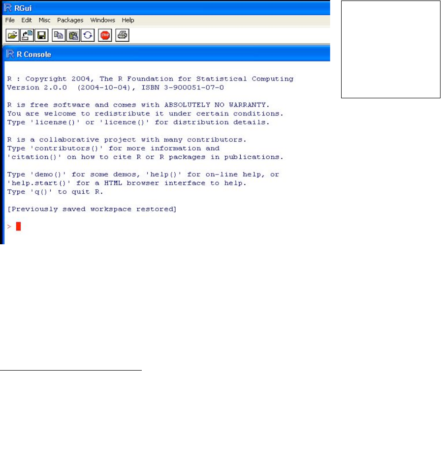
In interactive use under Microsoft Windows there are several ways to input commands to R. Figures 1 and 2
demonstrate two of the possibilities. Either or both of the following may be used at the user’s discretion.
This document mostly assumes that users will type commands into the command window, at the command line
prompt. Figure 1 shows the command window as it appears when version 2.0.0 of R has just been started.
The command line prompt, i.e. the >, is an invitation to start typing in your commands. For example, type 2+2
and press the Enter key. Here is what appears on the screen:
> 2+2
[1] 4
>
Here the result is 4. The[1] says, a little strangely, “first requested element will follow”. Here, there is just one
element. The > indicates that R is ready for another command.
2 This is a shortcut for “right click, then left click on the copy menu item”.
3 Enter the name of your choice into the name field. For ease of remembering, choose a name that closely matches the name
of the workspace directory, perhaps the name itself.
Fig. 1: The upper
left portion of the R
console (command
line) window, for
version 2.0.0 of R,
immediately after
starting up.
4
For later reference, note that the exit or quit command is
> q()
Alternatives to the use of q() are to click on the File menu and then on Exit, or to click on the in the top right
hand corner of the R window. There will be a message asking whether to save the workspace image. Clicking
Yes (the safe option) will save all the objects that remain in the workspace – any that were there at the start of
the session and any that have been added since.
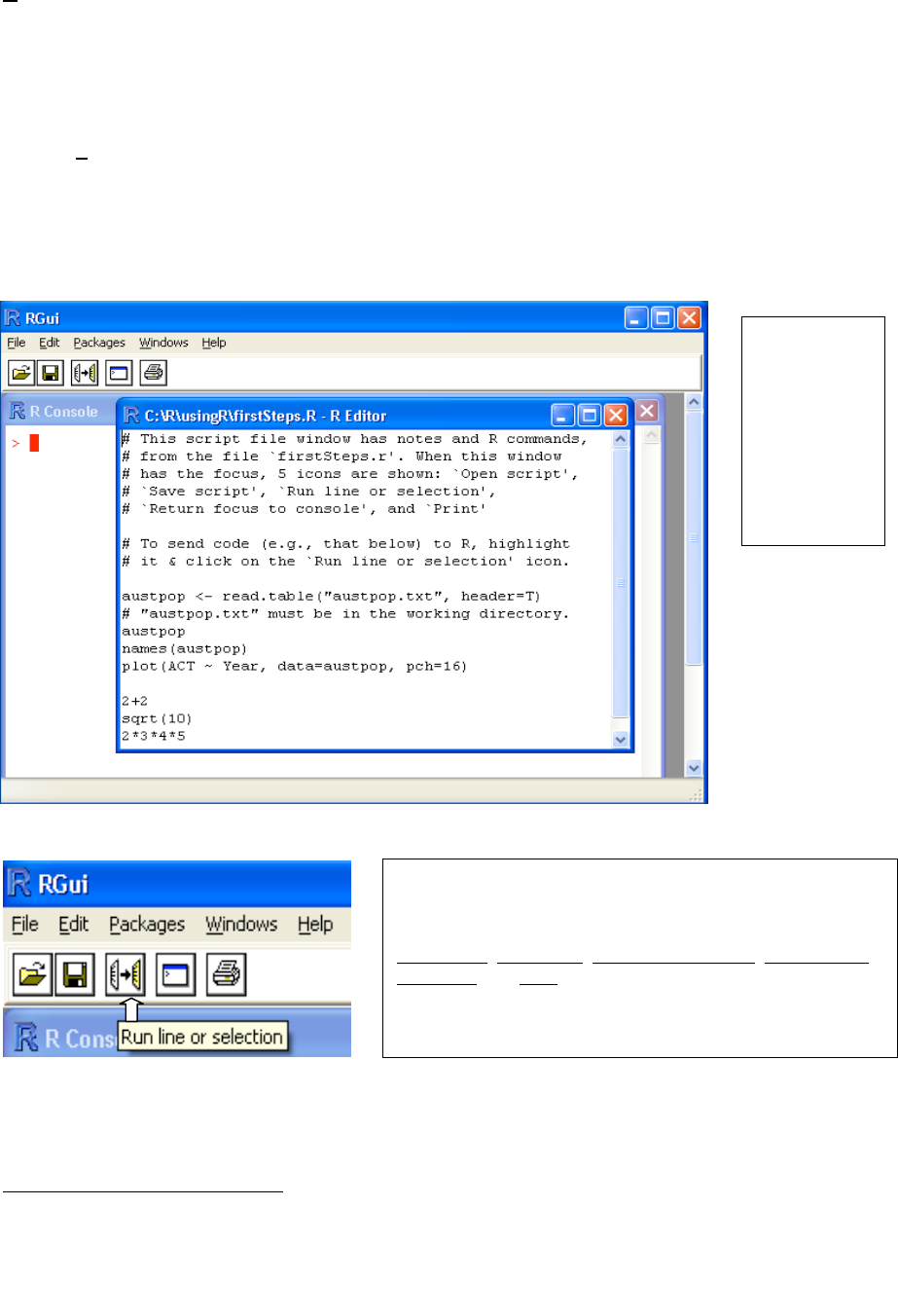
1.2 Use of an Editor Script Window
The screen snapshot in Figure2 shows a script file window. This allows input to R of statements from a file
that has been set up in advance, or that have been typed or copied into the window. To get a script file window,
go to the File menu. If a new blank window is required, click on New script. To load an existing file, click on
Open script…; you will be asked for the name of a file whose contents are then displayed in the window. In
Figure 2 the file was firstSteps.R.
Highlight the commands that are intended for input to R. Click on the `Run line or selection’ icon, which is the
middle icon of the script file editor toolbar in Figs. 2 and 3, to send commands to R.
Under Unix, the standard form of input is the command line interface. Under both Microsoft Windows and
Linux (or Unix), a further possibility is to run R from within the emacs editor4. Under Microsoft Windows,
4This requires emacs, and ESS which runs under emacs. Both are free. Look under Software|Other on the CRAN page.
Fig. 2: The
focus is on an
R display file
window, with
the console
window in the
background.
Fig. 3: This shows the five icons that appear when the focus
is on a script file window. The icons are, starting from the
left:
Open script, Save script, Run line or selection, Return focus
to console, and Print. The text in a script file window can be
edited, or new text added. Display file windows, which have
a somewhat similar set of icons but do not allow editing, are
another possibility.
5
attractive options are to use either the R-WinEdt utility that is designed for use with the shareware WinEdt
editor, or to use the free tinn-R editor5.
1.3 A Short R Session
We will read into R a file that holds population figures for Australian states and territories, and total population,
at various times since 1917, then using this file to create a graph. The data in the file are:
Year NSW Vic. Qld SA WA Tas. NT ACT Aust.
1917 1904 1409 683 440 306 193 5 3 4941
1927 2402 1727 873 565 392 211 4 8 6182
1937 2693 1853 993 589 457 233 6 11 6836
1947 2985 2055 1106 646 502 257 11 17 7579
1957 3625 2656 1413 873 688 326 21 38 9640
1967 4295 3274 1700 1110 879 375 62 103 11799
1977 5002 3837 2130 1286 1204 415 104 214 14192
1987 5617 4210 2675 1393 1496 449 158 265 16264
1997 6274 4605 3401 1480 1798 474 187 310 18532
The following reads in the data from the file austpop.txt on a disk in drive d:
> austpop <- read.table(“d:/austpop.txt”, header=TRUE)
The <- is a left diamond bracket (<) followed by a minus sign (-). It means “is assigned to”. Use of
header=TRUE causes R to use= the first line to get header information for the columns. If column headings are
not included in the file, the argument can be omitted.
Now type in austpop at the command line prompt, displaying the object on the screen:
> austpop
Year NSW Vic. Qld SA WA Tas. NT ACT Aust.
1 1917 1904 1409 683 440 306 193 5 3 4941
2 1927 2402 1727 873 565 392 211 4 8 6182
. . .
The object austpop is, in R parlance, a data frame. Data frames that consist entirely of numeric data have the
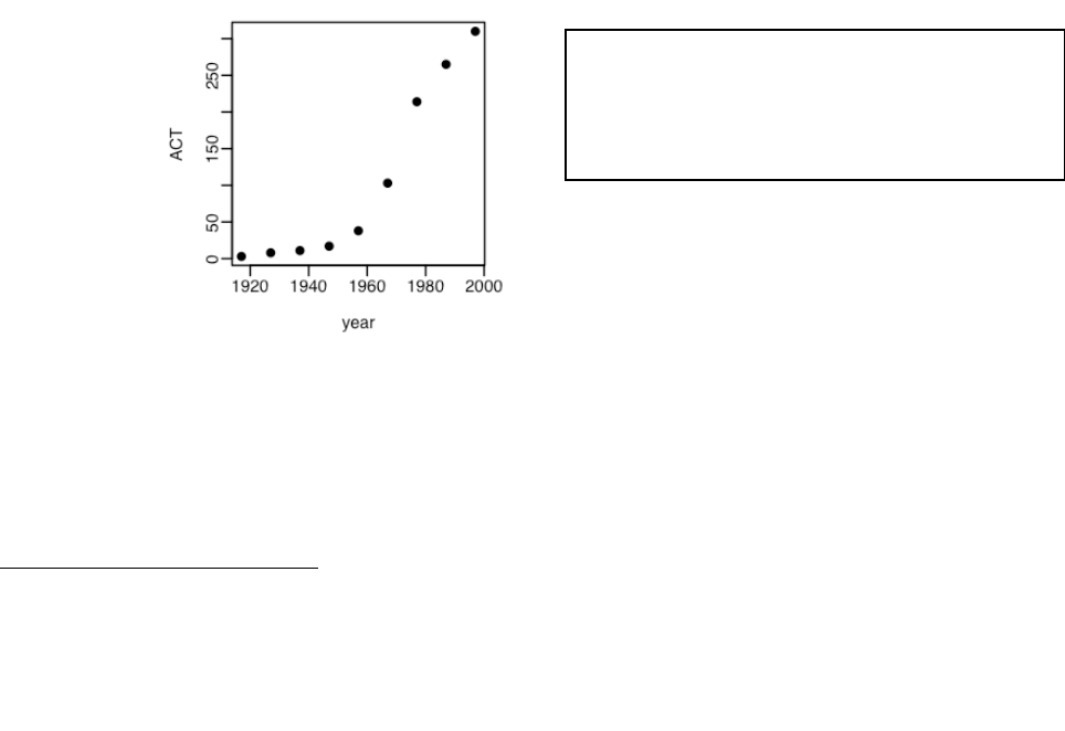
same form of rectangular layout as numeric matrices. Here is a plot (Figure 4) of the Australian Capital
Territory (ACT) population between 1917 and 1997 (Figure 4).
We first of all remind ourselves of the column names:
> names(austpop)
[1] "Year" "NSW" "Vic." "Qld" "SA" "WA" "Tas." "NT"
[9] "ACT" "Aust."
Note that in the version of the dataset that is in the DAAG package, year has a lower case y.
5 The R-WinEdt utility, which is free, is a “plugin” for WinEdt. For links to the relevant web pages, for WinEdt R-WinEdt
and various other editors that work with R, look under Software|Other on the CRAN web page.
Figure 4: Population of Australian Capital Territory,
at various times between 1917 and 1997. Code to
plot the graph is:
plot(ACT ~ Year, data=austpop, pch=16)
6
A simple way to get the plot is:
> plot(ACT ~ Year, data=austpop, pch=16) # For the DAAG version, replace ‘Year’ by ‘year’
The option pch=16 sets the plotting character to a solid black dot.
This plot can be improved greatly. We can specify more informative axis labels, change size of the text and of
the plotting symbol, and so on.
1.3.1 Entry of Data at the Command Line
A data frame is a rectangular array of columns of data. Here we will have two columns, and both columns will
be numeric. The following data gives, for each amount by which an elastic band is stretched over the end of a
ruler, the distance that the band moved when released:
stretch
46
54
48
50
44
42
52
distance
148
182
173
166
109
141
166
The function data.frame() can be used to input these (or other) data directly at the command line. We will
give the data frame the name elasticband:
elasticband <- data.frame(stretch=c(46,54,48,50,44,42,52),
distance=c(148,182,173,166,109,141,166))
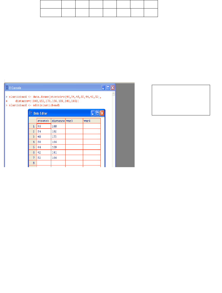
1.3.2 Entry and/or editing of data in an editor window
To edit the data frame elasticband in a spreadsheet-like format, type
elasticband <- edit(elasticband)
1.3.3 Options for read.table()
The function read.table() takes, optionally various parameters additional to the file name that holds the
data. Specify header=TRUE if there is an initial row of header names. The default is header=FALSE. In
addition users can specify the separator character or characters. Command alternatives to the default use of a
space are sep="," and sep="\t". This last choice makes tabs separators. Similarly, users can control over
the choice of missing value character or characters, which by default is NA. If the missing value character is a
period (“.”), specify na.strings=".".
There are several variants of read.table() that differ only in having different default parameter settings.
Note in particular read.csv(), which has settings that are suitable for comma delimited (csv) files that have
been generated from Excel spreadsheets.
If read.table() detects that lines in the input file have different numbers of fields, data input will fail, with
an error message that draws attention to the discrepancy. It is then often useful to use the function
count.fields() to report the number of fields that were identified on each separate line of the file.
Figure 5: Editor window,
showing the data frame
elasticband.

7
1.3.4 Options for plot() and allied functions
The function plot() and related functions accept parameters that control the plotting symbol, and the size and
colour of the plotting symbol. Details will be given in Section 3.3.
1.4 Further Notational Details
As noted earlier, the command line prompt is
>
R commands (expressions) are typed following this prompt6.
There is also a continuation prompt, used when, following a carriage return, the command is still not complete.
By default, the continuation prompt is
+
In these notes, we often continue commands over more than one line, but omit the + that will appear on the
commands window if the command is typed in as we show it.
For the names of R objects or commands, case is significant. Thus Austpop is different from austpop. For
file names however, the Microsoft Windows conventions apply, and case does not distinguish file names. On
Unix systems letters that have a different case are treated as different.
Anything that follows a # on the command line is taken as comment and ignored by R.
Note: Recall that, in order to quit from the R session we had to type q(). This is because q is a function.
Typing q on its own, without the parentheses, displays the text of the function on the screen. Try it!
1.5 On-line Help
To get a help window (under R for Windows) with a list of help topics, type:
> help()
In R for Windows, an alternative is to click on the help menu item, and then use key words to do a search. To
get help on a specific R function, e.g. plot(), type in
> help(plot)
The two search functions help.search() and apropos() can be a huge help in finding what one wants.
Examples of their use are:
> help.search("matrix")
(This lists all functions whose help pages have a title or alias in which the text string
“matrix” appears.)
> apropos(“matrix”)
(This lists all function names that include the text “matrix”.)
The function help.start() opens a browser window that gives access to the full range of documentation for
syntax, packages and functions.
Experimentation often helps clarify the precise action of an R function.
1.6 The Loading or Attaching of Datasets
The recommended way to access datasets that are supplied for use with these notes is to attach the file
usingR.RData., available from the author's web page. Place this file in the working directory and,
from within the R session, type:
> attach("usingR.RData")
Files that are mentioned in these notes, and that are not supplied with R (e.g., from the datasets or
MASS packages) should then be available without need for any further action.
6 Multiple commands may appear on the one line, with the semicolon (;) as the separator.

8
Users can also load (use load()) or attach (use attach()) specific files. These have a similar
effect, the difference being that with attach() datasets are loaded into memory only when required
for use.
Distinguish between the attaching of image files and the attaching of data frames. The attaching of
data frames will be discussed later in these notes.
1.7 Exercises
1. In the data frame elasticband from section 1.3.1, plot distance against stretch.
2. The following ten observations, taken during the years 1970-79, are on October snow cover for Eurasia.
(Snow cover is in millions of square kilometers):
year snow.cover
1970 6.5
1971 12.0
1972 14.9
1973 10.0
1974 10.7
1975 7.9
1976 21.9
1977 12.5
1978 14.5
1979 9.2
i. Enter the data into R. [Section 1.3.1 showed one way to do this. To save keystrokes, enter the successive
years as 1970:1979]
ii. Plot snow.cover versus year.
iii Use the hist() command to plot a histogram of the snow cover values.
iv. Repeat ii and iii after taking logarithms of snow cover.
3. Input the following data, on damage that had occurred in space shuttle launches prior to the disastrous launch
of Jan 28 1986. These are the data, for 6 launches out of 24, that were included in the pre-launch charts that
were used in deciding whether to proceed with the launch. (Data for the 23 launches where information is
available is in the data set orings, from the DAAG package.)
Temperature Erosion Blowby Total
(F) incidents incidents incidents
53 3 2 5
57 1 0 1
63 1 0 1
70 1 0 1
70 1 0 1
75 0 2 1
Enter these data into a data frame, with (for example) column names temperature, erosion, blowby and
total. (Refer back to Section 1.3.1). Plot total incidents against temperature.

9
2. An Overview of R
2.1 The Uses of R
2.1.1 R may be used as a calculator.
R evaluates and prints out the result of any expression that one types in at the command line in the console
window. Expressions are typed following the prompt (>) on the screen. The result, if any, appears on
subsequent lines
> 2+2
[1] 4
> sqrt(10)
[1] 3.162278
> 2*3*4*5
[1] 120
> 1000*(1+0.075)^5 - 1000 # Interest on $1000, compounded annually
[1] 435.6293
> # at 7.5% p.a. for five years
> pi # R knows about pi
[1] 3.141593
> 2*pi*6378 #Circumference of Earth at Equator, in km; radius is 6378 km
[1] 40074.16
> sin(c(30,60,90)*pi/180) # Convert angles to radians, then take sin()
[1] 0.5000000 0.8660254 1.0000000
2.1.2 R will provide numerical or graphical summaries of data
A special class of object, called a data frame, stores rectangular arrays in which the columns may be vectors of
numbers or factors or text strings. Data frames are central to the way that all the more recent R routines process
data. For now, think of data frames as matrices, where the rows are observations and the columns are variables.
As a first example, consider the data frame hills that accompanies these notes7. This has three columns
(variables), with the names distance, climb, and time. Typing in summary(hills)gives summary
information on these variables. There is one column for each variable, thus:
> load("hills.Rdata") # Assumes hills.Rdata is in the working directory
> summary(hills)
distance climb time
Min.: 2.000 Min.: 300 Min.: 15.95
1st Qu.: 4.500 1st Qu.: 725 1st Qu.: 28.00
Median: 6.000 Median:1000 Median: 39.75
Mean: 7.529 Mean:1815 Mean: 57.88
3rd Qu.: 8.000 3rd Qu.:2200 3rd Qu.: 68.62
Max.:28.000 Max.:7500 Max.:204.60
We may for example require information on ranges of variables. Thus the range of distances (first column) is
from 2 miles to 28 miles, while the range of times (third column) is from 15.95 (minutes) to 204.6 minutes.
We will discuss graphical summaries in the next section.
7 There are also versions in the DAAG package and in the Venables and Ripley MASS package.
10
2.1.3 R has extensive graphical abilities
The main R graphics function is plot(). In addition to plot() there are functions for adding points and lines
to existing graphs, for placing text at specified positions, for specifying tick marks and tick labels, for labelling
axes, and so on.
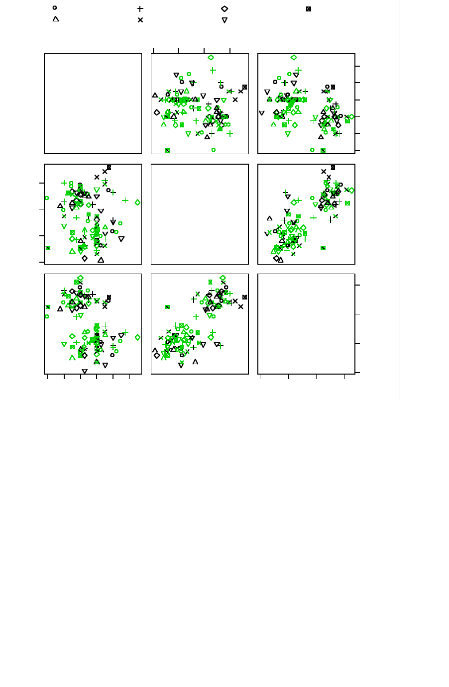
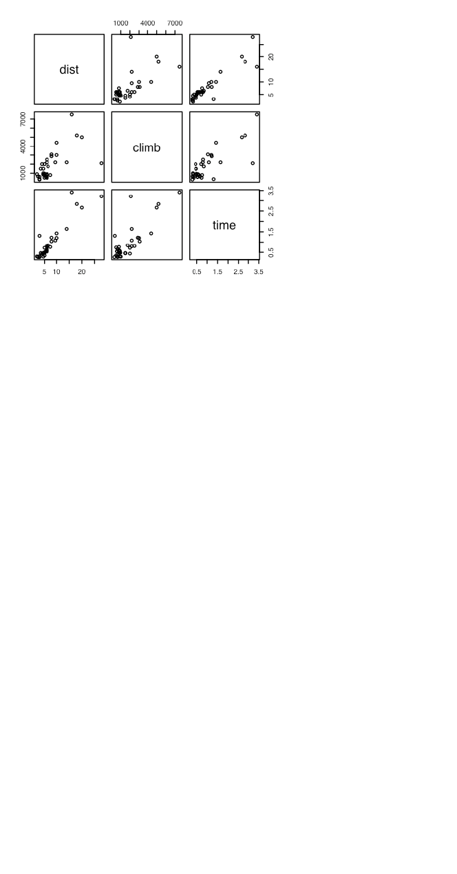
There are various other alternative helpful forms of graphical summary. A helpful graphical summary for the
hills data frame is the scatterplot matrix, shown in Figure 5. For this, type:
> pairs(hills)
Figure 5: Scatterplot matrix for the Scottish hill race data
2.1.4 R will handle a variety of specific analyses
The examples that will be given are correlation and regression.
Correlation:
We calculate the correlation matrix for the hills data:
> options(digits=3)
> cor(hills)
distance climb time
distance 1.000 0.652 0.920
climb 0.652 1.000 0.805
time 0.920 0.805 1.000
Suppose we wish to calculate logarithms, and then calculate correlations. We can do all this in one step, thus:
> cor(log(hills))
distance climb time
distance 1.00 0.700 0.890
climb 0.70 1.000 0.724
time 0.89 0.724 1.000
Unfortunately R was not clever enough to relabel distance as log(distance), climb as log(climb), and time as
log(time). Notice that the correlations between time and distance, and between time and climb, have reduced.
Why has this happened?
Straight Line Regression:
Here is a straight line regression calculation. The data are stored in the data frame elasticband (DAAG
package). The variable names are the names of columns in that data frame. The formula that is supplied to the
lm() command asks for the regression of distance travelled by the elastic band (distance) on the amount by
which it is stretched (stretch).

11
> plot(distance ~ stretch,data=elasticband, pch=16)
> elastic.lm <- lm(distance~stretch,data=elasticband)
> lm(distance ~stretch,data=elasticband)
Call:
lm(formula = distance ~ stretch, data = elasticband)
Coefficients:
(Intercept) stretch
-63.571 4.554
More complete information is available by typing
> summary(lm(distance~stretch,data=elasticband))
Try it!
2.1.5 R is an Interactive Programming Language
We calculate the Fahrenheit temperatures that correspond to Celsius temperatures 25, 26, …, 30:
> celsius <- 25:30
> fahrenheit <- 9/5*celsius+32
> conversion <- data.frame(Celsius=celsius, Fahrenheit=fahrenheit)
> print(conversion)
Celsius Fahrenheit
1 25 77.0
2 26 78.8
3 27 80.6
4 28 82.4
5 29 84.2
6 30 86.0
2.2 R Objects
All R entities, including functions and data structures, exist as objects. They can all be operated on as data.
Type in ls() to see the names of all objects in your workspace. An alternative to ls() is objects(). In both
cases there is provision to specify a particular pattern, e.g. starting with the letter `p’8.
Typing the name of an object causes the printing of its contents. Try typing q, mean, etc.
In a long session, it makes sense to save the contents of the working directory from time to time. It is also
possible to save individual objects, or collections of objects into a named image file. Some possibilities are:
save.image() # Save contents of workspace, into the file .RData
save.image(file="archive.RData") # Save into the file archive.RData
save(celsius, fahrenheit, file="tempscales.RData")
Image files, from the working directory or (with the path specified) from another directory, can be attached, thus
making objects in the file available on request. For example
attach("tempscales.RData")
ls(pos=2) # Check the contents of the file that has been attached
The parameter pos gives the position on the search list. (The search list is discussed later in this chapter, in
Section 2.9.)
Important: On quitting, R offers the option of saving the workspace image, by default in the file .RData in the
working directory. This allows the retention, for use in the next session in the same workspace, any objects that
were created in the current session. Careful housekeeping may be needed to distinguish between objects that are
8 Type in help(ls) and help(grep) to get details. The pattern matching conventions are those used for grep(),
which is modelled on the Unix grep command.

12
to be kept and objects that will not be used again. Before typing q() to quit, use rm() to remove objects that
are no longer required. Saving the workspace image will then save everything remains. The workspace image
will be automatically loaded upon starting another session in that directory.
*92.3 Looping
A simple example of a for loop is10
for (i in 1:10) print(i)
Here is another example of a for loop, to do in a complicated way what we did very simply in section 2.1.5:
> # Celsius to Fahrenheit
> for (celsius in 25:30)
+ print(c(celsius, 9/5*celsius + 32))
[1] 25 77
[1] 26.0 78.8
[1] 27.0 80.6
[1] 28.0 82.4
[1] 29.0 84.2
[1] 30 86
2.3.1 More on looping
Here is a long-winded way to sum the three numbers 31, 51 and 91:
> answer <- 0
> for (j in c(31,51,91)){answer <- j+answer}
> answer
[1] 173
The calculation iteratively builds up the object answer, using the successive values of j listed in the vector
(31,51,91). i.e. Initially, j=31, and answer is assigned the value 31 + 0 = 31. Then j=51, and answer is
assigned the value 51 + 31 = 82. Finally, j=91, and answer is assigned the value 91 + 81 = 173. Then the
procedure ends, and the contents of answer can be examined by typing in answer and pressing the Enter key.
There is a more straightforward way to do this calculation:
> sum(c(31,51,91))
[1] 173
Skilled R users have limited recourse to loops. There are often, as in this and earlier examples, better
alternatives.
2.4 Vectors
Examples of vectors are
c(2,3,5,2,7,1)
3:10 # The numbers 3, 4, .., 10
c(TRUE,FALSE,FALSE,FALSE,TRUE,TRUE,FALSE)
c(”Canberra”,”Sydney”,”Newcastle”,”Darwin”)
Vectors may have mode logical, numeric or character11. The first two vectors above are numeric, the third is
logical (i.e. a vector with elements of mode logical), and the fourth is a string vector (i.e. a vector with elements
of mode character).
9 Asterisks (*) identify sections that are more technical and might be omitted at a first reading
10 Other looping constructs are:
repeat <expression> ## break must appear somewhere inside the loop
while (x>0) <expression>
Here <expression> is an R statement, or a sequence of statements that are enclosed within braces

13
The missing value symbol, which is NA, can be included as an element of a vector.
2.4.1 Joining (concatenating) vectors
The c in c(2, 3, 5, 7, 1) above is an acronym for “concatenate”, i.e. the meaning is: “Join these numbers
together in to a vector. Existing vectors may be included among the elements that are to be concatenated. In the
following we form vectors x and y, which we then concatenate to form a vector z:
> x <- c(2,3,5,2,7,1)
> x
[1] 2 3 5 2 7 1
> y <- c(10,15,12)
> y
[1] 10 15 12
> z <- c(x, y)
> z
[1] 2 3 5 2 7 1 10 15 12
The concatenate function c() may also be used to join lists.
2.4.2 Subsets of Vectors
There are two common ways to extract subsets of vectors12.
1. Specify the numbers of the elements that are to be extracted, e.g.
> x <- c(3,11,8,15,12) # Assign to x the values 3, 11, 8, 15, 12
> x[c(2,4)] # Extract elements (rows) 2 and 4
[1] 11 15
One can use negative numbers to omit elements:
> x <- c(3,11,8,15,12)
> x[-c(2,3)]
[1] 3 15 12
2. Specify a vector of logical values. The elements that are extracted are those for which the logical value is T.
Thus suppose we want to extract values of x that are greater than 10.
> x>10 # This generates a vector of logical (T or F)
[1] F T F T T
> x[x>10]
[1] 11 15 12
Arithmetic relations that may be used in the extraction of subsets of vectors are <, <=, >, >=, ==, and !=. The
first four compare magnitudes, == tests for equality, and != tests for inequality.
2.4.3 The Use of NA in Vector Subscripts
Note that any arithmetic operation or relation that involves NA generates an NA. Set
y <- c(1, NA, 3, 0, NA)
11 It will, later in these notes, be important to know the “class” of such objects. This determines how the
method used by such generic functions as print(), plot() and summary(). Use the function class()
to determine the class of an object.
12 A third more subtle method is available when vectors have named elements. One can then use a vector of
names to extract the elements, thus:
> c(Andreas=178, John=185, Jeff=183)[c("John","Jeff")]
John Jeff
185 183

14
Be warned that y[y==NA] <- 0 leaves y unchanged. The reason is that all elements of y==NA evaluate to NA.
This does not select an element of y, and there is no assignment.
To replace all NAs by 0, use
y[is.na(y)] <- 0
2.4.4 Factors
A factor is stored internally as a numeric vector with values 1, 2, 3, k, where k is the number of levels. An
attributes table gives the ‘level’ for each integer value13. Factors provide a compact way to store character
strings. They are crucial in the representation of categorical effects in model and graphics formulae. The class
attribute of a factor has, not surprisingly, the value “factor”.
Consider a survey that has data on 691 females and 692 males. If the first 691 are females and the next 692
males, we can create a vector of strings that that holds the values thus:
gender <- c(rep(“female”,691), rep(“male”,692))
(The usage is that rep(“female”, 691) creates 691 copies of the character string “female”, and similarly for
the creation of 692 copies of “male”.)
We can change the vector to a factor, by entering:
gender <- factor(gender)
Internally the factor gender is stored as 691 1’s, followed by 692 2’s. It has stored with it the table:
1
female
2
male
Once stored as a factor, the space required for storage is reduced.
In most cases where the context seems to demand a character string, the 1 is translated into “female” and the 2
into “male”. The values “female” and “male” are the levels of the factor. By default, the levels are in
alphanumeric order, so that “female” precedes “male”. Hence:
> levels(gender) # Assumes gender is a factor, created as above
[1] "female" "male"
The order of the levels in a factor determines the order in which the levels appear in graphs that use this
information, and in tables. To cause “male” to come before “female”, use
gender <- relevel(gender, ref=“male”)
An alternative is
gender <- factor(gender, levels=c(“male”, “female”))
This last syntax is available both when the factor is first created, or later when one wishes to change the order of
levels in an existing factor. Incorrect spelling of the level names will generate an error message. Try
gender <- factor(c(rep(“female”,691), rep(“male”,692)))
table(gender)
gender <- factor(gender, levels=c(“male”, “female”))
table(gender)
gender <- factor(gender, levels=c(“Male”, “female”))
# Erroneous - "male" rows now hold missing values
table(gender)
rm(gender) # Remove gender
13 The attributes() function makes it possible to inspect attributes. For example
attributes(factor(1:3))
The function levels() gives a better way to inspect factor levels.

15
2.5 Data Frames
Data frames are fundamental to the use of the R modelling and graphics functions. A data frame is a
generalisation of a matrix, in which different columns may have different modes. All elements of any column
must however have the same mode, i.e. all numeric or all factor, or all character.
Among the data sets in the DAAG package is Cars93.summary, created from information in the Cars93 data
set in the Venables and Ripley MASS package. Here it is:
> Cars93.summary
Min.passengers Max.passengers No.of.cars abbrev
Compact 4 6 16 C
Large 6 6 11 L
Midsize 4 6 22 M
Small 4 5 21 Sm
Sporty 2 4 14 Sp
Van 7 8 9 V
The data frame has row labels (access with row.names(Cars93.summary)) Compact, Large, . . . The column
names (access with names(Cars93.summary)) are Min.passengers (i.e. the minimum number of
passengers for cars in this category), Max.passengers, No.of.cars., and abbrev. The first three columns
have mode numeric, and the fourth has mode character. Columns can be vectors of any mode. The column
abbrev could equally well be stored as a factor.
Any of the following14 will pick out the fourth column of the data frame Cars93.summary, then storing it in
the vector type.
type <- Cars93.summary$abbrev
type <- Cars93.summary[,4]
type <- Cars93.summary[,”abbrev”]
type <- Cars93.summary[[4]] # Take the object that is stored
# in the fourth list element.
2.5.1 Data frames as lists
A data frame is a list15 of column vectors, all of equal length. Just as with any other list, subscripting extracts a
list. Thus Cars93.summary[4] is a data frame with a single column, which is the fourth column vector of
Cars93.summary. As noted above, use Cars93.summary[[4]] or Cars93.summary[,4] to extract the
column vector.
The use of matrix-like subscripting, e.g. Cars93.summary[,4] or Cars93.summary[1, 4], takes advantage
of the rectangular structure of data frames.
2.5.2 Inclusion of character string vectors in data frames
When data are input using read.table(), or when the data.frame() function is used to create data frames,
vectors of character strings are by default turned into factors. The parameter setting
stringsAsFactors=TRUE, available both with read.table() and with data.frame(), will if needed
ensure that character strings are input without such conversion. For read.table(), an alternative is
as.is=TRUE.
2.5.3 Built-in data sets
We will often use data sets that accompany one of the R packages, usually stored as data frames. One such data
frame, in the datasets package, is trees, which gives girth, height and volume for 31 Black Cherry Trees.
Here is summary information on this data frame
14 Also legal is Cars93.summary[2]. This gives a data frame with the single column Type.
15 In general forms of list, elements that are of arbitrary type. They may be any mixture of scalars, vectors, functions, etc.

16
> summary(trees)
Girth Height Volume
Min. : 8.30 Min. :63 Min. :10.20
1st Qu.:11.05 1st Qu.:72 1st Qu.:19.40
Median :12.90 Median :76 Median :24.20
Mean :13.25 Mean :76 Mean :30.17
3rd Qu.:15.25 3rd Qu.:80 3rd Qu.:37.30
Max. :20.60 Max. :87 Max. :77.00
Type data() to get a list of built-in data sets in the packages that have been attached16.
2.6 Common Useful Functions
print() # Prints a single R object
cat() # Prints multiple objects, one after the other
length() # Number of elements in a vector or of a list
mean()
median()
range()
unique() # Gives the vector of distinct values
diff() # Replace a vector by the vector of first differences
# N. B. diff(x) has one less element than x
sort() # Sort elements into order, but omitting NAs
order() # x[order(x)] orders elements of x, with NAs last
cumsum()
cumprod()
rev() # reverse the order of vector elements
The functions mean(), median(), range(), and a number of other functions, take the argument na.rm=T;
i.e. remove NAs, then proceed with the calculation.
By default, sort() omits any NAs. The function order() places NAs last. Hence:ƒ
> x <- c(1, 20, 2, NA, 22)
> order(x)
[1] 1 3 2 5 4
> x[order(x)]
[1] 1 2 20 22 NA
> sort(x)
[1] 1 2 20 22
2.6.1 Applying a function to all columns of a data frame
The function sapply() takes as arguments the the data frame, and the function that is to be applied. The
following applies the function is.factor() to all columns of the supplied data frame rainforest17.
> sapply(rainforest, is.factor)
dbh wood bark root rootsk branch species
FALSE FALSE FALSE FALSE FALSE FALSE TRUE
> sapply(rainforest[,-7], range) # The final column (7) is a factor
dbh wood bark root rootsk branch
[1,] 4 NA NA NA NA NA
[2,] 56 NA NA NA NA NA
16 The list include all packages that are in the current environment.
17 Source: Ash, J. and Southern, W. 1982: Forest biomass at Butler’s Creek, Edith & Joy London Foundation, New South
Wales, Unpublished manuscript. See also Ash, J. and Helman, C. 1990: Floristics and vegetation biomass of a forest
catchment, Kioloa, south coastal N.S.W. Cunninghamia, 2(2): 167-182.

17
The functions mean() and range(), and a number of other functions, take the parameter na.rm. For example
> range(rainforest$branch, na.rm=TRUE) # Omit NAs, then determine the range
[1] 4 120
One can specify na.rm=TRUE as a third argument to the function sapply. This argument is then automatically
passed to the function that is specified in the second argument position. For example:
> sapply(rainforest[,-7], range, na.rm=TRUE)
dbh wood bark root rootsk branch
[1,] 4 3 8 2 0.3 4
[2,] 56 1530 105 135 24.0 120
Chapter 8 has further details on the use of sapply(). There is an example that shows how to use it to count the
number of missing values in each column of data.
2.7 Making Tables
table() makes a table of counts. Specify one vector of values (often a factor) for each table margin that is
required. For example:
> library(lattice) # The data frame barley accompanies lattice
> table(barley$year, barley$site)
Grand Rapids Duluth University Farm Morris Crookston Waseca
1932 10 10 10 10 10 10
1931 10 10 10 10 10 10
WARNING: NAs are by default ignored. The action needed to get NAs tabulated under a separate NA category
depends, annoyingly, on whether or not the vector is a factor. If the vector is not a factor, specify
exclude=NULL. If the vector is a factor then it is necessary to generate a new factor that includes “NA” as a
level. Specify x <- factor(x,exclude=NULL)
> x <- c(1,5,NA,8)
> x <- factor(x)
> x
[1] 1 5 NA 8
Levels: 1 5 8
> factor(x,exclude=NULL)
[1] 1 5 NA 8
Levels: 1 5 8 NA
2.7.1 Numbers of NAs in subgroups of the data
The following gives information on the number of NAs in subgroups of the data:
> table(rainforest$species, !is.na(rainforest$branch))
FALSE TRUE
Acacia mabellae 6 10
C. fraseri 0 12
Acmena smithii 15 11
B. myrtifolia 1 10
Thus for Acacia mabellae there are 6 NAs for the variable branch (i.e. number of branches over 2cm in
diameter), out of a total of 16 data values.
2.8 The Search List
R has a search list where it looks for objects. This can be changed in the course of a session. To get a full list of
these directories, called databases, type:
> search()
[1] ".GlobalEnv" "package:methods" "package:stats"

18
[4] "package:graphics" "package:grDevices" "package:utils"
[7] "package:datasets" "Autoloads" "package:base"
Notice that the loading of a new package extends the search list.
> library(MASS)
> search()
[1] ".GlobalEnv" "package:MASS" "package:methods"
[4] "package:stats" "package:graphics" "package:grDevices"
[7] "package:utils" "package:datasets" "Autoloads"
[10] "package:base"
Use of attach() likewise extends the search list. This function can be used to attach data frames or lists (use the
name, without quotes) or image (.RData) files (the file name is placed in quotes).
The following demonstrates the attaching of the data frame primates:
> names(primates)
[1] "Bodywt" "Brainwt"
> Bodywt
Error: Object "Bodywt" not found
> attach(primates) # R will now know where to find Bodywt
> Bodywt
[1] 10.0 207.0 62.0 6.8 52.2
Once the data frame primates has been attached, its columns can be accessed by giving their names, without
further reference to the name of the data frame. In technical terms, the data frame becomes a database, which is
searched as required for objects that the user may specify. Remember to detach an attached data frame, e.g.,
detach(primates), when it is no longer required.
Note also the function with(), which attaches the data frame that is given as its first argument for the duration
of the calculation that is specified by its second argument. For example:
> av <- with(primates, mean(Bodywt))
2.9 Functions in R
We give two simple examples of R functions.
2.9.1 An Approximate Miles to Kilometers Conversion
miles.to.km <- function(miles)miles*8/5
The return value is the value of the final (and in this instance only) expression that appears in the function
body18. Use the function thus
> miles.to.km(175) # Approximate distance to Sydney, in miles
[1] 280
The function will do the conversion for several distances all at once. To convert a vector of the three distances
100, 200 and 300 miles to distances in kilometers, specify:
> miles.to.km(c(100,200,300))
[1] 160 320 480
2.9.2 A Plotting function
The data set florida has the votes in the 2000 election for the various US Presidential candidates, county by
county in the state of Florida. The following plots the vote for Buchanan against the vote for Bush.
attach(florida)
plot(BUSH, BUCHANAN, xlab="Bush", ylab="Buchanan")
detach(florida) # In S-PLUS, specify detach("florida")
18 Alternatively a return value may be given using an explicit return() statement. This is however an uncommon
construction
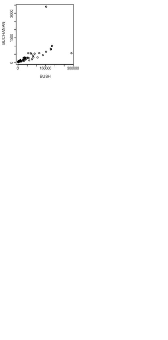
19
Here is a function that makes it possible to plot the figures for any pair of candidates.
plot.florida <- function(xvar=”BUSH”, yvar=”BUCHANAN”){
x <- florida[,xvar]
y <- florida[,yvar]
plot(x, y, xlab=xvar,ylab=yvar)
mtext(side=3, line=1.75,
“Votes in Florida, by county, in \nthe 2000 US Presidential election”)
}
Note that the function body is enclosed in braces ({ }).
Figure 6 shows the graph produced by plot.florida(), i.e. parameter settings are left at their defaults.
Figure 6: Election night count of votes received, by county,
in the US 2000 Presidential election.
As well as plot.florida(), the function allows, e.g.
plot.florida(yvar=”NADER”) # yvar=”NADER” over-rides the default
plot.florida(xvar=”GORE”, yvar=”NADER”)
2.10 More Detailed Information
Chapters 7 and 8 have a more detailed coverage of the topics in this chapter. It may pay, at this point, to glance
through chapters 7 and 8. Remember also to use R’s help pages and functions.
Topics from chapter 7, additional to those covered above, that may be important for relatively elementary uses
of R include:
The entry of patterned data (7.1.3)
The handling of missing values in subscripts when vectors are assigned (7.2)
Unexpected consequences (e.g. conversion of columns of numeric data into factors) from errors in data
(7.4.1).
2.11 Exercises
1. For each of the following code sequences, predict the result. Then do the computation:
a) answer <- 0
for (j in 3:5){ answer <- j+answer }
b) answer<- 10
for (j in 3:5){ answer <- j+answer }
c) answer <- 10
for (j in 3:5){ answer <- j*answer }
2. Look up the help for the function prod(), and use prod() to do the calculation in 1(c) above. Alternatively,
how would you expect prod() to work? Try it!
3. Add up all the numbers from 1 to 100 in two different ways: using for and using sum. Now apply the
function to the sequence 1:100. What is its action?

20
4. Multiply all the numbers from 1 to 50 in two different ways: using for and using prod.
5. The volume of a sphere of radius r is given by 4r3/3. For spheres having radii 3, 4, 5, …, 20 find the
corresponding volumes and print the results out in a table. Use the technique of section 2.1.5 to construct a data
frame with columns radius and volume.
6. Use sapply() to apply the function is.factor to each column of the supplied data frame tinting. For
each of the columns that are identified as factors, determine the levels. Which columns are ordered factors?
[Use is.ordered()].

21
3. Plotting
The functions plot(), points(), lines(), text(), mtext(), axis(), identify() etc. form a suite
that plots points, lines and text. To see some of the possibilities that R offers, enter
demo(graphics)
Press the Enter key to move to each new graph.
3.1 plot () and allied functions
The following both plot y against x:
plot(y ~ x) # Use a formula to specify the graph
plot(x, y) #
Obviously x and y must be the same length.
Try
plot((0:20)*pi/10, sin((0:20)*pi/10))
plot((1:30)*0.92, sin((1:30)*0.92))
Comment on the appearance that these graphs present. Is it obvious that these points lie on a sine curve? How
can one make it obvious? (Place the cursor over the lower border of the graph sheet, until it becomes a double-
sided arror. Drag the border in towards the top border, making the graph sheet short and wide.)
Here are two further examples.
attach(elasticband) # R now knows where to find distance & stretch
plot(distance ~ stretch)
plot(ACT ~ Year, data=austpop, type="l")
plot(ACT ~ Year, data=austpop, type="b")
The points() function adds points to a plot. The lines() function adds lines to a plot19. The text()
function adds text at specified locations. The mtext() function places text in one of the margins. The axis()
function gives fine control over axis ticks and labels.
Here is a further possibility
attach(austpop)
plot(spline(Year, ACT), type="l") # Fit smooth curve through points
detach(austpop) # In S-PLUS, specify detach(“austpop”)
3.1.1 Plot methods for other classes of object
The plot function is a generic function that has special methods for “plotting” various different classes of object.
For example, plotting a data frame gives, for each numeric variable, a normal probability plot. Plotting the lm
object that is created by the use of the lm() modelling function gives diagnostic and other information that is
intended to help in the interpretation of regression results.
Try
plot(hills) # Has the same effect as pairs(hills)
3.2 Fine control – Parameter settings
The default settings of parameters, such as character size, are often adequate. When it is necessary to change
parameter settings for a subsequent plot, the par() function does this. For example,
par(cex=1.25) # character expansion
increases the text and plot symbol size 25% above the default.
19 Actually these functions differ only in the default setting for the parameter type. The default setting for
points() is type = "p", and for lines() is type = "l". Explicitly setting type = "p" causes either
function to plot points, type = "l" gives lines.

22
On the first use of par() to make changes to the current device, it is often useful to store existing settings, so
that they can be restored later. For this, specify
oldpar <- par(cex=1.25, mex=1.25) # mex=1.25 expands the margin by 25%
This stores the existing settings in oldpar, then changes parameters (here cex and mex) as requested. To
restore the original parameter settings at some later time, enter par(oldpar). Here is an example:
attach(elasticband)
oldpar <- par(cex=1.5)
plot(distance ~ stretch)
par(oldpar) # Restores the earlier settings
detach(elasticband)
Inside a function specify, e.g.
oldpar <- par(cex=1.25)
on.exit(par(oldpar))
Type in help(par) to get details of all the parameter settings that are available with par().
3.2.1 Multiple plots on the one page
The parameter mfrow can be used to configure the graphics sheet so that subsequent plots appear row by row,
one after the other in a rectangular layout, on the one page. For a column by column layout, use mfcol
instead. In the example below we present four different transformations of the primates data, in a two by two
layout:
par(mfrow=c(2,2), pch=16)
attach(Animals) # This dataset is in the MASS package, which must be attached
plot(body, brain)
plot(sqrt(body), sqrt(brain))
plot((body)^0.1, (brain)^0.1)
plot(log(body),log(brain))
detach(Animals)
par(mfrow=c(1,1), pch=1) # Restore to 1 figure per page
3.2.2 The shape of the graph sheet
Often it is desirable to exercise control over the shape of the graph page, e.g. so that the individual plots are
rectangular rather than square. The R for Windows functions win.graph() or x11() that set up the Windows
screen take the parameters width (in inches), height (in inches) and pointsize (in 1/72 of an inch). The
setting of pointsize (default =12) determines character heights. It is the relative sizes of these parameters that
matter for screen display or for incorporation into Word and similar programs. Graphs can be enlarged or
shrunk by pointing at one corner, holding down the left mouse button, and pulling.
3.3 Adding points, lines and text
Here is a simple example that shows how to use the function text() to add text labels to the points on a plot.
> primates
Bodywt Brainwt
Potar monkey 10.0 115
Gorilla 207.0 406
Human 62.0 1320
Rhesus monkey 6.8 179
Chimp 52.2 440
Observe that the row names store labels for each row20.
20 Row names can be created in several different ways. They can be assigned directly, e.g.
row.names(primates) <- c("Potar monkey","Gorilla","Human", "Rhesus monkey","Chimp")

23
attach(primates) # Needed if primates is not already attached.
plot(Bodywt, Brainwt)
text(x=Bodywt, y=Brainwt, labels=row.names(primates), pos=4)
# pos=4 positions text to the right of the point
Figure 7A shows the result.
Figure 7: Plot of the primates data, with labels on points. Figure 8B improves on Figure 8A.
Figure 7A would be adequate for identifying points, but is not a presentation quality graph. We now show how
to improve it. Figure 7B uses the xlab (x-axis) and ylab (y-axis) parameters to specify meaningful axis titles.
It uses the parameter setting pos=4 to move the labelling to the right of the points. It sets pch=16 to make the
plot character a heavy black dot. This helps make the points stand out against the labelling.
Here is the R code for Figure 7B:
plot(x=Bodywt, y=Brainwt, pch=16,
xlab="Body weight (kg)", ylab="Brain weight (g)",
xlim=c(0,280), ylim=c(0,1350))
# Specify xlim so that there is room for the labels
text(x=Bodywt, y=Brainwt, labels=row.names(primates), pos=4)
detach(primates)
To place the text to the left of the points, specify
text(x=Bodywt, y=Brainwt, labels=row.names(primates), pos=2)
3.3.1 Size, colour and choice of plotting symbol
For plot() and points() the parameter cex (“character expansion”) controls the size, while col (“colour”)
controls the colour of the plotting symbol. The parameter pch controls the choice of plotting symbol.
The parameters cex and col may be used in a similar way with text(). Try
plot(1, 1, xlim=c(1, 7.5), ylim=c(1.75,5), type="n", axes=F, xlab="",
ylab="") # Do not plot points
box()
points(1:7, rep(4.5, 7), cex=1:7, col=1:7, pch=0:6)
text(1:7,rep(3.5, 7), labels=paste(0:6), cex=1:7, col=1:7)
The following, added to the plot that results from the above three statements, demonstrates other choices of pch.
points(1:7,rep(2.5,7), pch=(0:6)+7) # Plot symbols 7 to 13
text((1:7), rep(2.5,7), paste((0:6)+7), pos=4) # Label with symbol number
points(1:7,rep(2,7), pch=(0:6)+14) # Plot symbols 14 to 20
text((1:7), rep(2,7), paste((0:6)+14), pos=4) # Labels with symbol number
When using read.table() to input data, the parameter row.names is available to specify, by number or
name, a column that holds the row names.

24
Note the use of pos=4 to position the text to the right of the point (1=below, 2=left, 3=top, 4=right). Here
(Figure 8) is the plot:
Figure 8: Different plot symbols, colours and sizes
A variety of color palettes are available. Here is a function that displays some of the possibilities:
view.colours <- function(){
plot(1, 1, xlim=c(0,14), ylim=c(0,3), type="n", axes=F,
xlab="",ylab="")
text(1:6, rep(2.5,6), paste(1:6), col=palette()[1:6], cex=2.5)
text(10, 2.5, "Default palette", adj=0)
rainchars <- c("R","O","Y","G","B","I","V")
text(1:7, rep(1.5,7), rainchars, col=rainbow(7), cex=2.5)
text(10, 1.5, "rainbow(7)", adj=0)
cmtxt <- substring("cm.colors", 1:9,1:9)
# Split “cm.colors” into its 9 characters
text(1:9, rep(0.5,9), cmtxt, col=cm.colors(9), cex=3)
text(10, 0.5, "cm.colors(9)", adj=0)
}
To run the function, enter
view.colours()
3.3.2 Adding Text in the Margin
mtext(side, line, text, ..) adds text in the margin of the current plot. The sides are numbered 1(x-
axis), 2(y-axis), 3(top) and 4.
3.4 Identification and Location on the Figure Region
Two functions are available for this purpose. Draw the graph first, then call one or other of these functions.
identify() labels points. One positions the cursor near the point that is to be identified, and clicks the left mouse
button.
locator() prints out the co-ordinates of points. One positions the cursor at the location for which coordinates are
required, and clicks the left mouse button.
A click with the right mouse button signifies that the identification or location task is complete, unless the
setting of the parameter n is reached first. For identify() the default setting of n is the number of data
points, while for locator() the default setting is n = 500.
3.4.1 identify()
This function requires specification of a vector x, a vector y, and a vector of text strings that are available for
use a labels. The data set florida has the votes for the various Presidential candidates, county by county in
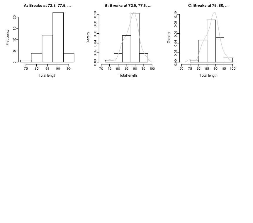
25
the state of Florida. We plot the vote for Buchanan against the vote for Bush, then invoking identify() so
that we can label selected points on the plot.
attach(florida)
plot(BUSH, BUCHANAN, xlab=”Bush”, ylab=”Buchanan”)
identify(BUSH, BUCHANAN, County)
detach(florida)
Click to the left or right, and slightly above or below a point, depending on the preferred positioning of the
label. When labelling is terminated (click with the right mouse button), the row numbers of the observations that
have been labelled are printed on the screen, in order.
3.4.2 locator()
Left click at the locations whose coordinates are required
attach(florida) # if not already attached
plot(BUSH, BUCHANAN, xlab=”Bush”, ylab=”Buchanan”)
locator()
detach(florida)
The function can be used to mark new points (specify type=”p”) or lines (specify type=”l”) or both points
and lines (specify type=”b”).
3.5 Plots that show the distribution of data values
We discuss histograms, density plots, boxplots and normal probability plots.
3.5.1 Histograms and density plots
The shapes of histograms depend on the placement of the breaks, as Figure 9 illustrates:
Figure 9: Panel A shows a histogram with a frequency scale. Panel B is drawn with a density
scale, so that a density curve can be readily superimposed. Panel C has a different choice of
breakpoints, so that the histogram gives a rather different impression of the distribution of the
data. The density curve is, again, superimposed.
Here is the code used to plot the histogram in Figure 10A.
attach(possum)
here <- sex == "f"
hist(totlngth[here], breaks = 72.5 + (0:5) * 5, ylim = c(0, 22),
xlab="Total length", main ="A: Breaks at 72.5, 77.5, ...")
detach(possum)
Density plots, now that they are available, are often a preferred alternative to a histogram. A histogarm is, in
fact, a very crude form of density plot.
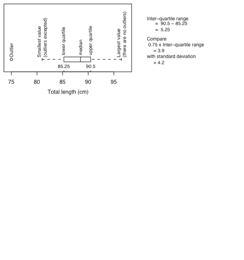
26
Density plots do not depend on a choice of breakpoints. The choice of width and type of window, controlling
the nature and amount of smoothing, does affect the appearance of the plot. The main effect is to make it more
or less smooth.
The following will give a density plot:
attach(possum)
plot(density(totlngth[here]),type="l")
detach(possum)
In Figure 9B the y-axis for the histogram is labelled so that the area of a rectangle is the density for that
rectangle, i.e., the frequency for the rectangle is divided by the width of the rectangle. This gives a scale that is
appropriate for superimposing a density curve estimate. The only difference between Figure 9C and Figure 9B
is that a different choice of breakpoints is used for the histogram, so that the histogram gives a rather different
impression of the distribution of the data. The code for Figure 9B is:
attach(possum)
here <- sex == "f"
dens <- density(totlngth[here])
xlim <- range(dens$x)
ylim <- range(dens$y)
hist(totlngth[here], breaks = 72.5 + (0:5) * 5, probability = TRUE,
xlim = xlim, ylim = ylim, xlab="Total length", main="")
lines(dens)
detach(possum)
3.5.3 Boxplots
We now (Figure 10) make a boxplot of the above data:
Figure 10: Boxplot of female possum lengths, with additional labelling
information.
The code for the boxplot is
attach(possum)
boxplot(totlngth[here], horizontal=TRUE)
rug(totlngth[here], side=1)
detach(possum)
Figure 12 adds information that is intended to assist in the interpretation of boxplots.
3.5.4 Normal probability plots
qqnorm(y) gives a normal probability plot of the elements of y. The points of this plot will lie approximately
on a straight line if the distribution is Normal. In order to calibrate the eye to recognise plots that indicate non-
normal variation, it is helpful to do several normal probability plots for random samples of the relevant size
from a normal distribution.
x11(width=8, height=6) # This is a better shape for this plot
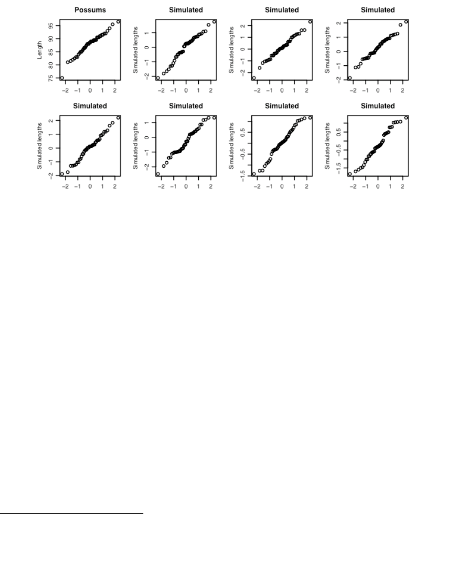
27
attach(possum)
here <- sex == "f"
par(mfrow=c(2,4)) # A 2 by 4 layout of plots
y <- totlngth[here]
qqnorm(y,xlab="", ylab="Length", main="Possums")
for(i in 1:7)qqnorm(rnorm(43),xlab="", ylab="Simulated lengths",
main="Simulated")
detach(possum)
# Before continuing, type dev.off()
Figure 11 shows the plots. There is one unusually small value. Otherwise the points for the female possum
lengths are as close to a straight line as in many of the plots for random normal data.
Figure 11: Normal probability plots. If data are from a normal distribution then points should
fall, approximately, along a line. The plot in the top left hand corner shows the 43 lengths of
female possums. The other plots are for independent normal random samples of size 43.
The idea is an important one. In order to judge whether data are normally distributed, examine a number of
randomly generated samples of the same size from a normal distribution. It is a way to train the eye.
By default, rnorm() generates random samples from a distribution with mean 0 and standard deviation 1.
3.6 Other Useful Plotting Functions
For the functions demonstrated here, we use data on the heights of 100 female athletes21.
3.6.1 Scatterplot smoothing
panel.smooth() plots points, then adds a smooth curve through the points. For example:
attach(ais)
here<- sex=="f"
plot(pcBfat[here]~ht[here], xlab = “Height”, ylab = “% Body fat”)
panel.smooth(ht[here],pcBfat[here])
detach(ais)
21 Data relate to the paper: Telford, R.D. and Cunningham, R.B. 1991: Sex, sport and body-size dependency of hematology
in highly trained athletes. Medicine and Science in Sports and Exercise 23: 788-794.
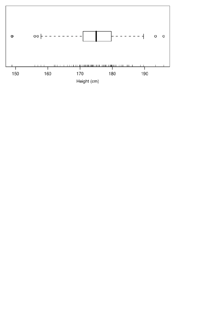
28
3.6.2 Adding lines to plots
Use the function abline() for this. The parameters may be an intercept and slope, or a vector that holds the
intercept and slope, or an lm object. Alternatively it is possible to draw a horizontal line (h = <height>), or a
vertical line (v = <ordinate>).
attach(ais)
here<- sex=="f"
plot(pcBfat[here] ~ ht[here], xlab = “Height”, ylab = “% Body fat”)
abline(lm(pcBfat[here] ~ ht[here]))
detach(ais)
3.6.3 Rugplots
By default rug(x) adds, along the x-axis of the current plot, vertical bars showing the distribution of values of
x. It can however be particularly useful for showing the actual values along the side of a boxplot. Figure 12
shows a boxplot of the distribution of height of female athletes, with a rugplot added on the y-axis.
Figure 12: Distribution of heights of female athletes.
The bars on the left plot show actual data values.
Here is the code
attach(ais)
here <- sex == "f"
oldpar <- par(mar=c(4.1,1.1,1.1, 1.1), mgp=c(2.25, 0.75,0))
boxplot(ht[here], boxwex = 0.35, ylab = "Height", horizontal=TRUE)
rug(ht[here], side = 1)
par(oldpar)
detach(ais)
The parameter boxwex controls the width of the boxplot.
3.6.4 Scatterplot matrices
Section 2.1.3 demonstrated the use of the pairs() function.
3.6.5 Dotcharts
These can be a good alternative to barcharts. They have a much higher information to ink ratio! Try
dotchart(islands) # vector of named numeric values, in the datasets base package
Unfortunately there are many names, and there is substantial overlap. The following is better, but shrinks the
sizes of the points so that they almost disappear:
dotchart(islands, cex=0.5)
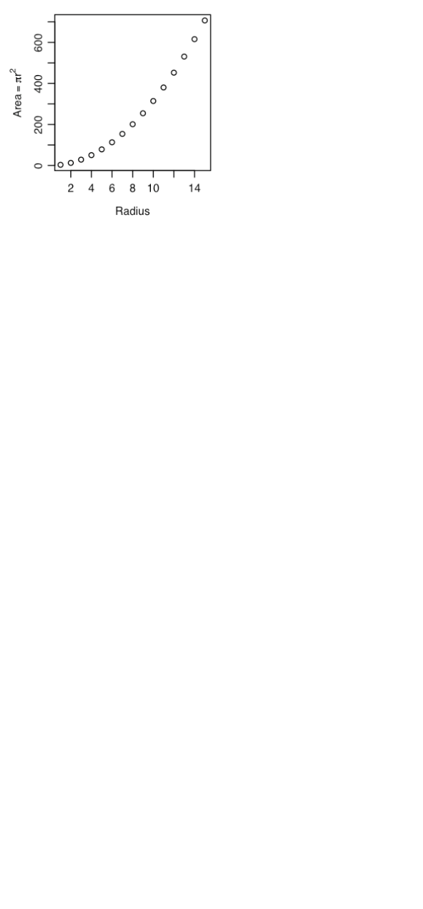
29
3.7 Plotting Mathematical Symbols
Both text() and mtext() will take an expression rather than a text string. In plot(), either or both of
xlab and ylab can be an expression. Figure 13 was produced with
x <- 1:15
plot(x, y, xlab="Radius", ylab=expression(Area == pi*r^2))
Figure 13: The y-axis label is a mathematical expression.
Notice that in expression(Area == pi*r^2), there is a double equals sign (“==”), although what will
appear on the plot is Area = pi*r^2, with a single equals sign.
See help(plotmath) for detailed information on the plotting of mathematical expressions. There is a further
example in chapter 12.
The final plot from
demo(graphics)
shows some of the possibilities for plotting mathematical symbols.
3.8 Guidelines for Graphs
Design graphs to make their point tersely and clearly, with a minimum waste of ink. Label as necessary to
identify important features. In scatterplots the graph should attract the eye’s attention to the points that are
plotted, and to important grouping in the data. Use solid points, large enough to stand out relative to other
features, when there is little or no overlap.
When there is extensive overlap of plotting symbols, use open plotting symbols. Where points are dense,
overlapping points will give a high ink density, which is exactly what one wants.
Use scatterplots in preference to bar or related graphs whenever the horizontal axis represents a quantitative
effect.
Use graphs from which information can be read directly and easily in preference to those that rely on visual
impression and perspective. Thus in scientific papers contour plots are much preferable to surface plots or two-
dimensional bar graphs.
Draw graphs so that reduction and reproduction will not interfere with visual clarity.
Explain clearly how error bars should be interpreted — SE limits, 95% confidence interval, SD limits, or
whatever. Explain what source of `error(s)’ is represented. It is pointless to present information on a source of
error that is of little or no interest, for example analytical error when the relevant source of `error’ for
comparison of treatments is between fruit.
Use colour or different plotting symbols to distinguish different groups. Take care to use colours that contrast.
3.9 Exercises
1. The data set huron that accompanies these notes has mean July average water surface elevations, in feet,

30
IGLD (1955) for Harbor Beach, Michigan, on Lake Huron, Station 5014, for 1860-198622. (Alternatively work
with the vector LakeHuron from the datasets package, that has mean heights for 1875-1772 only.)
a) Plot mean.height against year.
b) Use the identify function to label points for the years that correspond to the lowest and highest mean levels.
That is, type
identify(huron$year,huron$mean.height,labels=huron$year)
and use the left mouse button to click on the lowest point and highest point on the plot. To quit, press both
mouse buttons simultaneously.
c) As in the case of many time series, the mean levels are correlated from year to year. To see how each year's
mean level is related to the previous year's mean level, use
lag.plot(huron$mean.height)
This plots the mean level at year i against the mean level at year i-1.
2. Plot the graph of brain weight (brain) versus body weight (body) for the data set Animals from the
MASS package. Label the axes appropriately. Alongside on the same graphics page, log(brain weight) versus
log(body weight). Use the row labels to label the points with the three largest body weight values. Label the
axes in untransformed units. [To access this data frame, specify library(MASS)]
3. Check the distributions of head lengths (hdlngth) in the possum23 data set that accompanies these notes.
Compare the following forms of display:
a) a histogram (hist(possum$hdlngth));
b) a stem and leaf plot (stem(qqnorm(possum$hdlngth));
c) a normal probability plot (qqnorm(possum$hdlngth)); and
d) a density plot (plot(density(possum$hdlngth)).
What are the advantages and disadvantages of these different forms of display?
4. Try x <- rnorm(10). Print out the numbers that you get. Look up the help for rnorm. Now generate a
sample of size 10 from a normal distribution with mean 170 and standard deviation 4.
5. Use mfrow() to set up the layout for a 3 by 4 array of plots. In the top 4 rows, show normal probability plots
(section 3.4.2) for four separate `random’ samples of size 10, all from a normal distribution. In the middle 4
rows, display plots for samples of size 100. In the bottom four rows, display plots for samples of size 1000.
Comment on how the appearance of the plots changes as the sample size changes.
6. The function runif() generates a sample from a uniform distribution, by default on the interval 0 to 1. Try
x <- runif(10), and print out the numbers you get. Then repeat exercise 6 above, but taking samples from a
uniform distribution rather than from a normal distribution. What shape do the points follow?
*7. If you find exercise 6 interesting, you might like to try it for some further distributions. For example x <-
rchisq(10,1) will generate 10 random values from a chi-squared distribution with degrees of freedom 1. The
statement x <- rt(10,1) will generate 10 random values from a t distribution with degrees of freedom one.
Make normal probability plots for samples of various sizes from these distributions.
8. For the first two columns of the data frame hills, examine the distribution using: (a) histogram; (b) density
plots; (c) normal probability plots.
Repeat (a), (b) and (c), now working with the logarithms of the data values.
3.10 References
The web page http://www.math.yorku.ca/SCS/StatResource.html#DataVis has links to many
different collections of information on statistical graphics.
22 Source: Great Lakes Water Levels, 1860-1986. U.S. Dept. of Commerce, National Oceanic and
AtmosphericAdministration, National Ocean Survey.
23 Data relate to the paper: Lindenmayer, D. B., Viggers, K. L., Cunningham, R. B., and Donnelly, C. F. 1995.
Morphological variation among populations of the mountain brush tail possum, Trichosurus caninus Ogilby (Phalangeridae:
Marsupialia). Australian Journal of Zoology 43: 449-458.
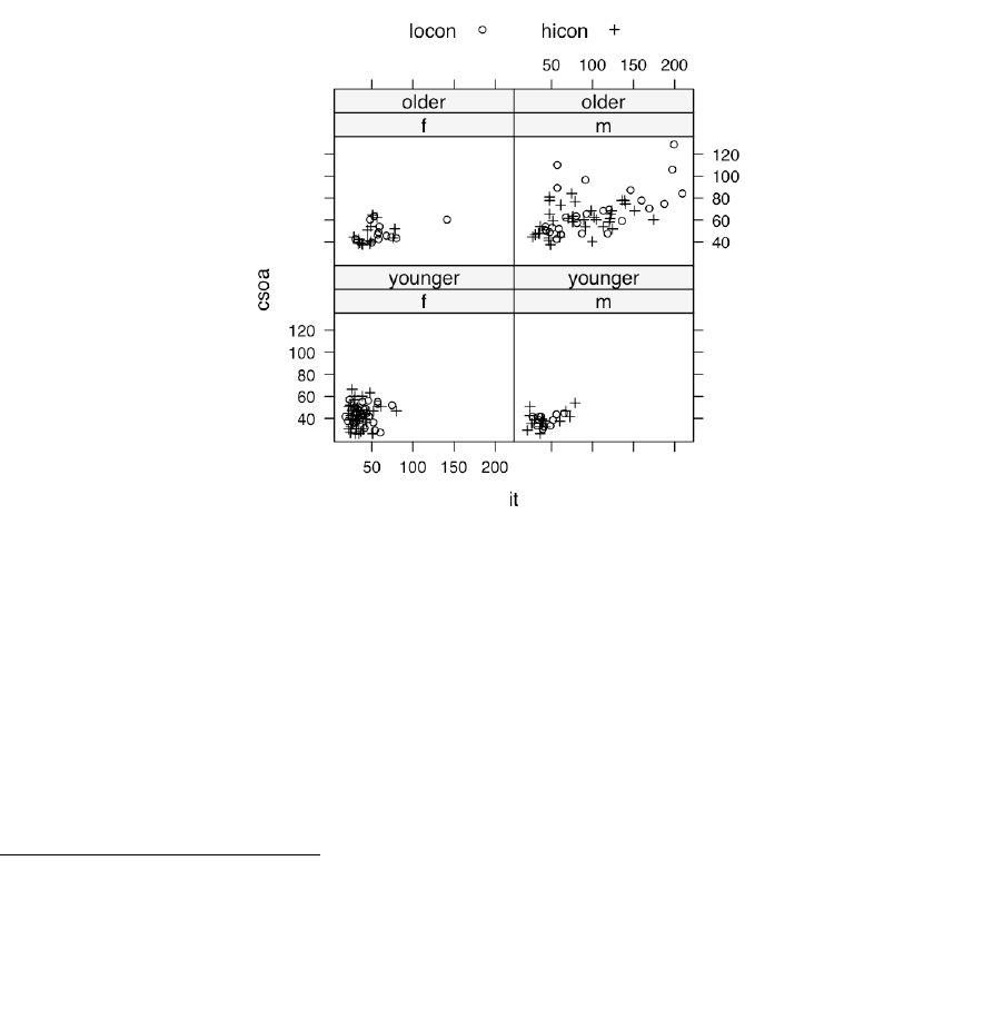
31
4. Lattice graphics
Lattice plots allow the use of the layout on the page to reflect meaningful aspects of data structure. They offer
abilities similar to those in the S-PLUS trellis library.
The lattice package sits on top of the grid package. To use lattice graphics, both these packages must be
installed. Providing it is installed, the grid package will be loaded automatically when lattice is loaded.
The older coplot() function that is in the base package has some of same abilities as xyplot( ), but with a
limitation to two conditioning factors or variables only.
4.1 Examples that Present Panels of Scatterplots – Using xyplot()
The basic function for drawing panels of scatterplots is xyplot(). We will use the data frame tinting
(supplied) to demonstrate the use of xyplot(). These data are from an experiment that investigated the effects
of tinting of car windows on visual performance24. The authors were mainly interested in visual recognition
tasks that would be performed when looking through side windows.
In this data frame, csoa (critical stimulus onset asynchrony, i.e. the time in milliseconds required to recognise
an alphanumeric target), it (inspection time, i. e. the time required for a simple discrimination task) and age
are variables, tint (level of tinting: no, lo, hi) and target (contrast: locon, hicon) are ordered factors, sex (1
= male, 2 = female) and agegp (1 = young, in the early 20s; 2 = an older participant, in the early 70s) are
factors. Figure 14 shows the style of graph that one can get from xyplot(). The different symbols are different
contrasts.
Figure 14: csoa versus it, for each combination of females/males and elderly/young.
The two targets (low, + = high contrast) are shown with different symbols.
In a simplified version of Figure 16 above, we might plot csoa against it for each combination of sex and
agegp. For this simplified version, it would be enough to type:
xyplot(csoa ~ it | sex * agegp, data=tinting) # Simple use of xyplot()
Here is the statement used to get Figure 16. The two different symbols distinguish between low contrast and
high contrast targets.
24 Data relate to the paper: Burns, N. R., Nettlebeck, T., White, M. and Willson, J. 1999. Effects of car window tinting on
visual performance: a comparison of elderly and young drivers. Ergonomics 42: 428-443.
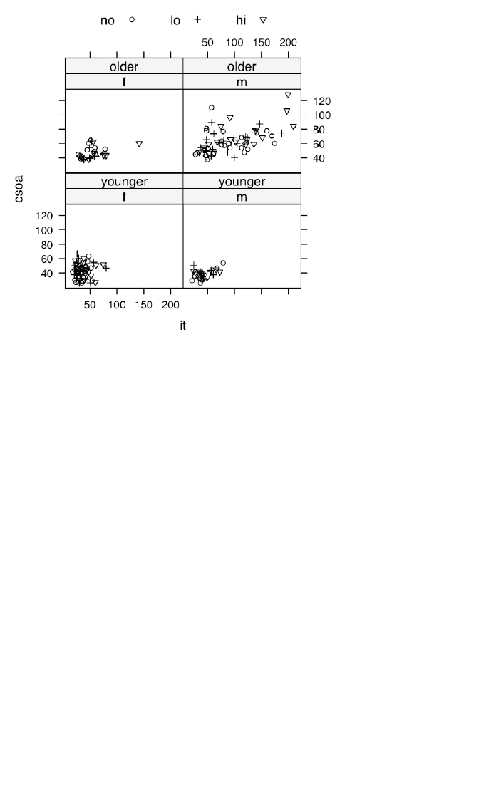
32
xyplot(csoa~it|sex*agegp, data=tinting,
groups=target, auto.key=list(columns=2))
If colour is available, different colours will be used for the different groups.
A striking feature is that the very high values, for both csoa and it, occur only for elderly males. It is apparent
that the long response times for some of the elderly males occur, as we might have expected, with the low
contrast target. The following puts smooth curves through the data, separately for the two target types:
xyplot(csoa~it|sex*agegp, data=tinting, panel=panel.superpose,
groups=target, type=c("p","smooth")
The relationship between csoa and it seems much the same for both levels of contrast.
Finally, we do a plot (Figure 15) that uses different symbols (in black and white) for different levels of tinting.
The longest times are for the high level of tinting.
xyplot(csoa~it|sex*agegp, data=tinting, groups=tint,
auto.key=list(columns=3))
Figure 15: csoa versus it, for each combination of females/males and elderly/young.
The different levels of tinting (no, +=low, >=high) are shown with different symbols.
4.2 Some further examples of lattice plots
These are given with a minimum of explanation.
4.2.1 Plotting columns in parallel
Use the parameter outer to control whether the columns appear on the same or separate panels. If on
the same panel, it is desirable to use auto.key to give a simple key. The following use the dataset
grog from the DAAGxtras package:
library(DAAGxtras)
xyplot(Beer+Spirit+Wine ~ Year | Country, outer=TRUE,
data=grog)
xyplot(Beer+Spirit+Wine ~ Year, groups=Country, outer=TRUE,
data=grog)
xyplot(Beer+Spirit+Wine ~ Year | Country, outer=FALSE,
data=grog, auto.key=list(columns=3),
par.settings=simpleTheme(pch=16, cex=2) )

33
In the final plot, note the use of simpleTheme() as a simple mechanism for controlling common
parameter settings. Use of the parameter par.settings makes the change for the current plot only.
Use trellis.par.set() to make the changes for the duration of the current device, unless reset.
4.2.2 Fixed, sliced and free scales
library(DAAG)
## scale="fixed"
xyplot(BC+Alberta ~ Date, data=jobs, outer=TRUE)
## scale="sliced" - different slices of same scale
xyplot(BC+Alberta ~ Date, data=jobs, outer=TRUE,
scales=list(y=list(relation="sliced")) )
## scale="free" - independent scales
xyplot(BC+Alberta ~ Date, data=jobs, outer=TRUE,
scales=list(y=list(relation="free")) )
4.3 An incomplete list of lattice Functions
splom( ~ data.frame) # Scatterplot matrix
bwplot(factor ~ numeric , . .) # Box and whisker plot
qqnorm(numeric , . .) # normal probability plots
dotplot(factor ~ numeric , . .) # 1-dim. Display
stripplot(factor ~ numeric , . .) # 1-dim. Display
barchart(character ~ numeric , . .)
histogram( ~ numeric , . .)
densityplot( ~ numeric , . .) # Smoothed version of histogram
qqmath(numeric ~ numeric , . .) # QQ plot
splom( ~ dataframe, . .) # Scatterplot matrix
parallel( ~ dataframe, . .) # Parallel coordinate plots
cloud(numeric ~ numeric * numeric, . .) # 3-D plot
contourplot(numeric ~ numeric * numeric, . .) # Contour plot
levelplot(numeric ~ numeric * numeric, . .) # Variation on a contour plot
In each instance, conditioning variables can be added. In most cases, a groups parameter can be specified, i.e.,
the plot is repeated for the groupings within the one panel.
4.4 Exercises
1. The following data gives milk volume (g/day) for smoking and nonsmoking mothers25:
Smoking Mothers: 621, 793, 593, 545, 753, 655, 895, 767, 714, 598, 693
Nonsmoking Mothers: 947, 945, 1086, 1202, 973, 981, 930, 745, 903, 899, 961
Present the data (i) in side by side boxplots (use bwplot()); (ii) using a dotplot form of display (use
dotplot()).
2. For the possum data set, generate the following plots:
a) histograms of hdlngth – use histogram();
b) normal probability plots of hdlngth – use qqmath();
c) density plots of hdlngth – use densityplot(). Investigate the effect of varying the density bandwidth
(bw).
12. The following exercises relate to the data frame possum that accompanies these notes:
(a) Using the xyplot function, explore the relation between hdlngth and totlngth, taking into account sex
and Pop.
25 Data are from the paper ``Smoking During Pregnancy and Lactation and Its Effects on Breast Milk Volume'' (Amer. J. of
Clinical Nutrition).

34
(b) Construct a contour plot of chest versus belly and totlngth – use levelplot() or contourplot().
(c) Construct box and whisker plots for hdlngth, using site as a factor.
(d) Use qqmath() to construct normal probability plots for hdlgth, for each separate level of sex and Pop. Is
there evidence that the distribution of hdlgth varies with the level of these other factors.
13. The frame airquality that is in the datasets package has columns Ozone, Solar.R, Wind, Temp, Month
and Day. Plot Ozone against Solar.R for each of three temperature ranges, and each of three wind ranges.
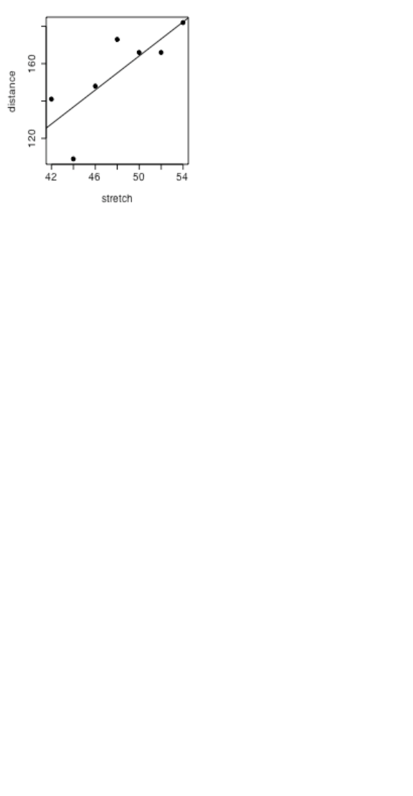
35
5. Linear (Multiple Regression) Models and Analysis of Variance
5.1 The Model Formula in Straight Line Regression
We begin with the straight line regression example that appeared earlier, in section 2.1.4. First, plot the data:
plot(distance ~ stretch, data=elasticband)
The code for the regression calculation is:
elastic.lm <- lm(distance ~ stretch, data=elasticband)
Here distance ~ stretch is a model formula. Other model formulae will appear in the course of this
chapter. Figure 16 shows the plot:
Figure 16: Plot of distance versus stretch for the elastic
band data, with fitted least squares line
The output from the regression is an lm object, which we have called elastic.lm . Now examine a summary
of the regression results. Notice that the output documents the model formula that was used:
> options(digits=4)
> summary(elastic.lm)
Call:
lm(formula = distance ~ stretch, data = elasticband)
Residuals:
1 2 3 4 5 6 7
2.107 -0.321 18.000 1.893 -27.786 13.321 -7.214
Coefficients:
Estimate Std. Error t value Pr(>|t|)
(Intercept) -63.57 74.33 -0.86 0.431
stretch 4.55 1.54 2.95 0.032
Residual standard error: 16.3 on 5 degrees of freedom
Multiple R-Squared: 0.635, Adjusted R-squared: 0.562
F-statistic: 8.71 on 1 and 5 degrees of freedom, p-value: 0.0319
5.2 Regression Objects
An lm object is a list of named elements. Above, we created the object elastic.lm . Here are the names of its
elements:
> names(elastic.lm)
[1] "coefficients" "residuals" "effects" "rank"
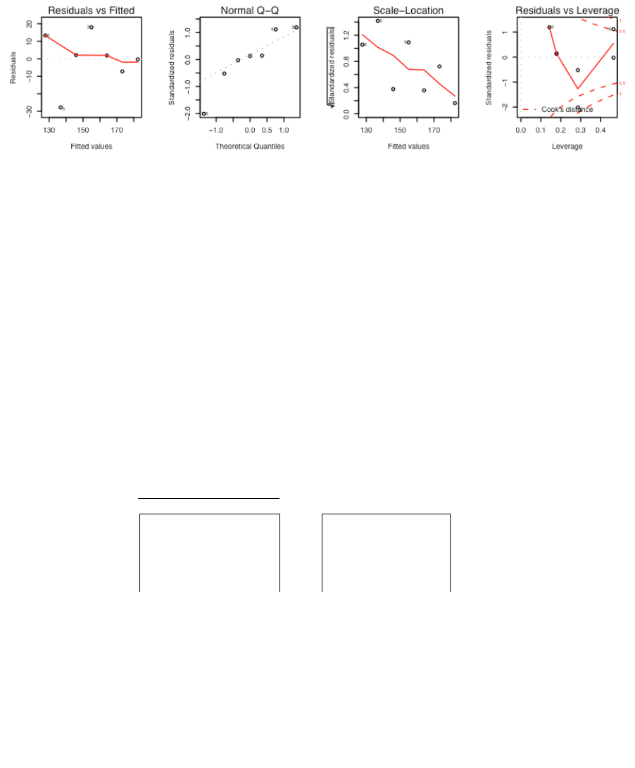
36
[5] "fitted.values" "assign" "qr" "df.residual"
[9] "xlevels" "call" "terms" "model"
Various functions are available for extracting information that you might want from the list. This is better than
manipulating the list directly. Examples are:
> coef(elastic.lm)
(Intercept) stretch
-63.571 4.554
> resid(elastic.lm)
1 2 3 4 5 6 7
2.1071 -0.3214 18.0000 1.8929 -27.7857 13.3214 -7.2143
The function most often used to inspect regression output is summary(). It extracts the information that users
are most likely to want. For example, in section 5.1, we had
summary(elastic.lm)
There is a plot method for lm objects that gives the diagnostic information shown in Figure 17.
Figure 17: Diagnostic plot of lm object, obtained by plot(elastic.lm).
To get Figure 17, type:
x11(width=7, height=2, pointsize=10)
par(mfrow = c(1, 4), mar=c(5.1,4.1,2.1,1.1))
plot(elastic.lm)
par(mfrow=c(1,1))
By default the first, second and fourth plot use the row names to identify the three most extreme residuals. [If
explicit row names are not given for the data frame, then the row numbers are used.]
5.3 Model Formulae, and the X Matrix
The model formula for the elastic band example was distance ~ stretch . The model formula is a recipe
for setting up the calculations. All the calculations described in this chapter require the use of an model matrix
or X matrix, and a vector y of values of the dependent variable. For some of the examples we discuss later, it
helps to know what the X matrix looks like. Details for the elastic band example follow.
The first 4 rows of the X matrix, with the y-vector alongside, is:
X
y
Stretch (mm)
Distance (cm)
1
46
148
1
54
182
1
48
173
1
50
166
…
…
...
The model matrix relates to the part of the model that appears to the right of the equals sign. The straight line
model is
y = a + b x + residual
which we write as
y = 1 a + x b + residual

37
The parameters that are to be estimated are a and b. Fitted values are given by multiplying each column of the
model matrix by its corresponding parameter, i.e. the first column by a and the second column by b, and adding.
Another name is predicted values. The aim is to reproduce, as closely as possible, the values in the y-column.
The residuals are the differences between the values in the y-column and the fitted values. Least squares
regression, which is the form of regression that we describe in this course, chooses a and b so that the sum of
squares of the residuals is as small as possible.
The function model.matrix() prints out the model matrix. Thus:
> model.matrix(distance ~ stretch, data=elasticband)
(Intercept) stretch
1 1 46
2 1 54
3 1 48
4 1 50
. . .
attr(,”assign”)
[1] 0 1
Another possibility, with elastic.lm as in section 5.1, is:
model.matrix(elastic.lm)
The following are the fitted values and residuals that we get with the estimates of a (= -63.6) and b ( = 4.55)
that result from least squares regression
X
!
ˆ
y
y
!
y"ˆ
y
Stretch (mm)
(Fitted)
(Observed)
(Residual)
-63.6
4.55
-63.6 + 4.55 Stretch
Distance
(mm)
Observed –
Fitted
1
46
-63.6 + 4.55 46 = 145.7
148
148-145.7 = 2.3
1
54
-63.6 + 4.55 54 = 182.1
182
182-182.1 = -0.1
1
48
-63.6 + 4.55 48 = 154.8
173
173-154.8 = 18.2
1
50
-63.6 + 4.55 50 = 163.9
166
166-163.9 = 2.1
…
…
…
…
…
Note the use of the symbol
!
ˆ
y
[pronounced y-hat] for predicted values.
We might alternatively fit the simpler (no intercept) model. For this we have
y = x b + e
where e is a random variable with mean 0. The X matrix then consists of a single column, the x’s.
5.3.1 Model Formulae in General
Model formulae take a form such as:
y~x+z : lm, glm,, etc.
y~x + fac + fac:x : lm, glm, aov, etc. (If fac is a factor and x is a variable, fac:x allows a different
slope for each different level of fac.)
Model formulae are widely used to set up most of the model calculations in R.
Notice the similarity between model formulae and the formulae that are used for specifying coplots. Thus,
recall that the graph formula for a coplot that gives a plot of y against x for each different combination of levels
of fac1 (across the page) and fac2 (up the page) is:
y ~ x | fac1+fac2
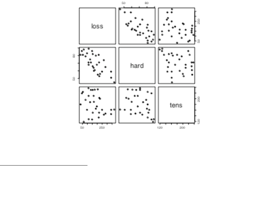
38
*5.3.2 Manipulating Model Formulae
Model formulae can be assigned, e.g.
formyxz <- formula(y~x+z)
or
formyxz <- formula(“y~x+z”)
The argument to formula() can, as just demonstrated, be a text string. This makes it straightforward to paste
the argument together from components that are stored in text strings. For example
> names(elasticband)
[1] "stretch" "distance"
> nam <- names(elasticband)
> formds <- formula(paste(nam[1],"~",nam[2]))
> lm(formds, data=elasticband)
Call:
lm(formula = formds, data = elasticband)
Coefficients:
(Intercept) distance
26.3780 0.1395
Note that graphics formulae can be manipulated in exactly the same way as model formulae.
5.4 Multiple Linear Regression Models
5.4.1 The data frame Rubber
The data set Rubber from the MASS package is from the accelerated testing of tyre rubber26. The variables are
loss (the abrasion loss in gm/hr), hard (hardness in `Shore’ units), and tens (tensile strength in kg/sq m).
We first obtain a scatterplot matrix (Figure 18) :
Figure 18: Scatterplot matrix for the Rubber data frame from the
MASS package.
26 The original source is O.L. Davies (1947) Statistical Methods in Research and Production. Oliver and Boyd,
Table 6.1 p. 119.
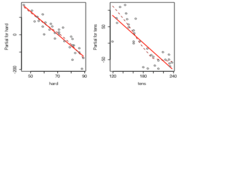
39
The code is
library(MASS) # if needed (the dataset Rubber is in the MASS package)
pairs(Rubber)
There is a negative correlation between loss and hardness. We proceed to regress loss on hard and tens.
Rubber.lm <- lm(loss~hard+tens, data=Rubber)
> options(digits=3)
> summary(Rubber.lm)
Call:
lm(formula = loss ~ hard + tens, data = Rubber)
Residuals:
Min 1Q Median 3Q Max
-79.38 -14.61 3.82 19.75 65.98
Coefficients:
Estimate Std. Error t value Pr(>|t|)
(Intercept) 885.161 61.752 14.33 3.8e-14
hard -6.571 0.583 -11.27 1.0e-11
tens -1.374 0.194 -7.07 1.3e-07
Residual standard error: 36.5 on 27 degrees of freedom
Multiple R-Squared: 0.84, Adjusted R-squared: 0.828
F-statistic: 71 on 2 and 27 degrees of freedom, p-value: 1.77e-011
In addition to the use of plot.lm(), note the use of termplot(). Figure 19) used the following code:
par(mfrow=c(1,2))
termplot(Rubber.lm, partial=TRUE, smooth=panel.smooth)
par(mfrow=c(1,1))
This plot raises interesting questions.
Figure 19: Plot, obtained with termplot(), showing the contribution of each of the two terms in
the model, at the mean of the contributions for the other term. A smooth curve has, in each
panel, been fitted through the partial residuals. There is a clear suggestion that, at the upper
end of the range, the response is not linear with tensile strength.

40
5.4.2 Weights of Books
The books to which the data in the data set oddbooks (accompanying these notes) refer were chosen to cover a
wide range of weight to height ratios. Here are the data:
> oddbooks
thick height width weight
1 14 30.5 23.0 1075
2 15 29.1 20.5 940
3 18 27.5 18.5 625
4 23 23.2 15.2 400
5 24 21.6 14.0 550
6 25 23.5 15.5 600
7 28 19.7 12.6 450
8 28 19.8 12.6 450
9 29 17.3 10.5 300
10 30 22.8 15.4 690
11 36 17.8 11.0 400
12 44 13.5 9.2 250
Notice that as thickness increases, weight reduces.
> logbooks <- log(oddbooks) # We might expect weight to be
> # proportional to thick * height * width
> logbooks.lm1<-lm(weight~thick,data=logbooks)
> summary(logbooks.lm1)$coef
Estimate Std. Error t value Pr(>|t|)
(Intercept) 9.69 0.708 13.7 8.35e-08
thick -1.07 0.219 -4.9 6.26e-04
> logbooks.lm2<-lm(weight~thick+height,data=logbooks)
> summary(logbooks.lm2)$coef
Estimate Std. Error t value Pr(>|t|)
(Intercept) -1.263 3.552 -0.356 0.7303
thick 0.313 0.472 0.662 0.5243
height 2.114 0.678 3.117 0.0124
> logbooks.lm3<-lm(weight~thick+height+width,data=logbooks)
> summary(logbooks.lm3)$coef
Estimate Std. Error t value Pr(>|t|)
(Intercept) -0.719 3.216 -0.224 0.829
thick 0.465 0.434 1.070 0.316
height 0.154 1.273 0.121 0.907
width 1.877 1.070 1.755 0.117
So is weight proportional to thick * height * width?
The correlations between thick, height and width are so strong that if one tries to use more than one of
them as a explanatory variables, the coefficients are ill-determined. They contain very similar information, as is
evident from the scatterplot matrix. The regressions on height and width give plausible results, while the
coefficient of the regression on thick is entirely an artefact of the way that the books were selected.
The design of the data collection really is important for the interpretation of coefficients from a regression
equation. Even though regression equations from observational data may work quite well for predictive
purposes, the individual coefficients may be misleading. This is more than an academic issue, as the analyses in
Lalonde (1986) demonstrate. They had data from experimental “treatment” and “control” groups, and also from
two comparable non-experimental “controls”. The regression estimate of the treatment effect, when comparison
was with one of the non-experimental controls, was statistically significant but with the wrong sign! The
regression should be fitted only to that part of the data where values of the covariates overlap substantially.
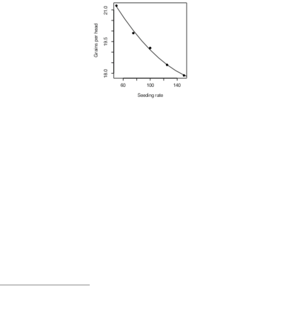
41
Dehejia and Wahba demonstrate the use of scores (“propensities”) to identify subsets that are defensibly
comparable. The propensity is then the only covariate in the equation that estimates the treatment effect. It is
impossible to be sure that any method is giving the right answer.
5.5 Polynomial and Spline Regression
Calculations that have the same structure as multiple linear regression are able to model a curvilinear response.
Curves are constructed from linear combinations of transformed values. Note that polynomial curves of high
degree are in general unsatisfactory. Spline curves, constructed by joining low order polynomial curves
(typically cubics) in such a way that the slope changes smoothly, are in general preferable.
5.5.1 Polynomial Terms in Linear Models
The data frame seedrates27 (DAAG package) gvies, for each of a number of different seeding rates, the
number of barley grain per head.
plot(grain ~ rate, data=seedrates) # Plot the data
Figure 20 shows the data, with fitted quadratic curve:
Figure 20: Number of grain per head versus seeding rate,
for the barley seeding rate data, with fitted quadratic curve.
We will need an X-matrix with a column of ones, a column of values of rate, and a column of values of
rate2. For this, both rate and I(rate^2) must be included in the model formula.
> seedrates.lm2 <- lm(grain ~ rate+I(rate^2), data=seedrates)
> summary(seedrates.lm2)
Call:
lm(formula = grain ~ rate + I(rate^2), data = seedrates)
Residuals:
1 2 3 4 5
0.04571 -0.12286 0.09429 -0.00286 -0.01429
Coefficients:
Estimate Std. Error t value Pr(>|t|)
(Intercept) 24.060000 0.455694 52.80 0.00036
rate -0.066686 0.009911 -6.73 0.02138
I(rate^2) 0.000171 0.000049 3.50 0.07294
27 Data are from McLeod, C. C. (1982) Effect of rates of seeding on barley grown for grain. New Zealand Journal of
Agriculture 10: 133-136. Summary details are in Maindonald, J. H. (1992).

42
Residual standard error: 0.115 on 2 degrees of freedom
Multiple R-Squared: 0.996, Adjusted R-squared: 0.992
F-statistic: 256 on 2 and 2 degrees of freedom, p-value: 0.0039
> hat <- predict(seedrates.lm2)
> lines(spline(seedrates$rate, hat))
> # Placing the spline fit through the fitted points allows a smooth curve.
> # For this to work the values of seedrates$rate must be ordered.
Again, check the form of the model matrix. Type:
> model.matrix(grain~rate+I(rate^2),data=seedrates)
(Intercept) rate I(rate^2)
1 1 50 2500
2 1 75 5625
3 1 100 10000
4 1 125 15625
5 1 150 22500
attr(,"assign")
[1] 0 1 2
This was a (small) extension of linear models, to handle a specific form of non-linear relationship. Any
transformation can be used to form columns of the model matrix. Thus, an x3 column might be added.
Once the model matrix has been formed, we are limited to taking linear combinations of columns.
5.5.2 What order of polynomial?
A polynomial of degree 2, i.e. a quadratic curve, looked about right for the above data. How does one check?
One way is to fit polynomials, e.g. of each of degrees 1 and 2, and compare them thus:
> seedrates.lm1<-lm(grain~rate,data=seedrates)
> seedrates.lm2<-lm(grain~rate+I(rate^2),data=seedrates)
> anova(seedrates.lm2,seedrates.lm1)
Analysis of Variance Table
Model 1: grain ~ rate + I(rate^2)
Model 2: grain ~ rate
Res.Df Res.Sum Sq Df Sum Sq F value Pr(>F)
1 2 0.026286
2 3 0.187000 -1 -0.160714 12.228 0.07294
The F-value is large, but on this evidence there are too few degrees of freedom to make a totally convincing
case for preferring a quadratic to a line. However the paper from which these data come gives an independent
estimate of the error mean square (0.17 on 35 d.f.) based on 8 replicate results that were averaged to give each
value for number of grains per head. If we compare the change in the sum of squares (0.1607, on 1 df) with a
mean square of 0.172 (35 df), the F-value is now 5.4 on 1 and 35 degrees of freedom, and we have p=0.024 .
The increase in the number of degrees of freedom more than compensates for the reduction in the F-statistic.
> # However we have an independent estimate of the error mean
> # square. The estimate is 0.17^2, on 35 df.
> 1-pf(0.16/0.17^2, 1, 35)
[1] 0.0244
Finally note that R2 was 0.972 for the straight line model. This may seem good, but given the accuracy of these
data it was not good enough! The statistic is an inadequate guide to whether a model is adequate. Even for any
one context, R2 will in general increase as the range of the values of the dependent variable increases. (R2 is
larger when there is more variation to be explained.) A predictive model is adequate when the standard errors of
predicted values are acceptably small, not when R2 achieves some magic threshold.

43
5.5.3 Pointwise confidence bounds for the fitted curve
Here is code that gives pointwise 95% confidence bounds. Note that these do not combine to give a confidence
region for the total curve! The construction of such a region is a much more complicated task!
plot(grain ~ rate, data = seedrates, pch = 16, xlim = c(50, 175), ylim
= c(15.5, 22),xlab="Seeding rate",ylab="Grains per head")
new.df <- data.frame(rate = c((4:14) * 12.5))
seedrates.lm2 <- lm(grain ~ rate + I(rate^2), data = seedrates)
pred2 <- predict(seedrates.lm2, newdata = new.df, interval="confidence")
hat2 <- data.frame(fit=pred2[,"fit"],lower=pred2[,"lwr"], upper=pred2[,"upr"])
attach(new.df)
lines(rate, hat2$fit)
lines(rate,hat2$lower,lty=2)
lines(rate, hat2$upper,lty=2)
detach(new.df)
The extrapolation has deliberately been taken beyond the range of the data, in order to show how the confidence
bounds spread out. Confidence bounds for a fitted line spread out more slowly, but are even less believable!
5.5.4 Spline Terms in Linear Models
By now, readers of this document will be used to the idea that it is possible to use linear models to fit terms that
may be highly nonlinear functions of one or more of the variables. The fitting of polynomial functions was a
simple example of this. Spline functions variables extend this idea further. The splines that I demonstrate are
constructed by joining together cubic curves, in such a way the joins are smooth. The places where the cubics
join are known as `knots’. It turns out that, once the knots are fixed, and depending on the class of spline curves
that are used, spline functions of a variable can be constructed as a linear combination of basis functions, where
each basis function is a transformation of the variable.
The data frame cars is in the datasets package.
> plot(dist~speed,data=cars)
> library(splines)
> cars.lm<-lm(dist~bs(speed),data=cars) # By default, there are no knots
> hat<-predict(cars.lm)
> lines(cars$speed,hat,lty=3) # NB assumes values of speed are sorted
> cars.lm5 <- lm(dist~bs(speed,5),data=cars) # try for a closer fit (1 knot)
> ci5<-predict(cars.lm5,interval="confidence",se.fit=TRUE)
> names(ci5)
[1] "fit" "se.fit" "df" "residual.scale"
> lines(cars$speed,ci5$fit[,"fit"])
> lines(cars$speed,ci5$fit[,"lwr"],lty=2)
> lines(cars$speed,ci5$fit[,"upr"],lty=2)
5.6 Using Factors in R Models
Factors are crucial for specifying R models that include categorical or “factor” variables,. Consider data from
an experiment that compared houses with and without cavity insulation28. While one would not usually handle
these calculations using an lm model, it makes a simple example to illustrate the choice of a baseline level, and
a set of contrasts. Different choices, although they fit equivalent models, give output in which some of the
numbers are different and must be interpreted differently.
28 Data are from Hand, D. J.; Daly, F.; Lunn, A. D.; Ostrowski, E., eds. (1994). A Handbook of Small Data Sets. Chapman
and Hall.

44
We begin by entering the data from the command line:
insulation <- factor(c(rep("without", 8), rep("with", 7)))
# 8 without, then 7 with
# `with’ precedes `without’ in alphanumeric order, & is the baseline
kWh <- c(10225, 10689, 14683, 6584, 8541, 12086, 12467,
12669, 9708, 6700, 4307, 10315, 8017, 8162, 8022)
To formulate this as a regression model, we take kWh as the dependent variable, and the factor insulation as the
explanatory variable.
> insulation <- factor(c(rep("without", 8), rep("with", 7)))
> # 8 without, then 7 with
> kWh <- c(10225, 10689, 14683, 6584, 8541, 12086, 12467,
+ 12669, 9708, 6700, 4307, 10315, 8017, 8162, 8022)
> insulation.lm <- lm(kWh ~ insulation)
> summary(insulation.lm, corr=F)
Call:
lm(formula = kWh ~ insulation)
Residuals:
Min 1Q Median 3Q Max
-4409 -979 132 1575 3690
Coefficients:
Estimate Std. Error t value Pr(>|t|)
(Intercept) 7890 874 9.03 5.8e-07
insulation 3103 1196 2.59 0.022
Residual standard error: 2310 on 13 degrees of freedom
Multiple R-Squared: 0.341, Adjusted R-squared: 0.29
F-statistic: 6.73 on 1 and 13 degrees of freedom, p-value: 0.0223
The p-value is 0.022, which may be taken to indicate (p < 0.05) that we can distinguish between the two types
of houses. But what does the “intercept” of 7890 mean, and what does the value for “insulation” of 3103 mean?
To interpret this, we need to know that the factor levels are, by default, taken in alphabetical order, and that the
initial level is taken as the baseline. So with comes before without, and with is the baseline. Hence:
Average for Insulated Houses = 7980
To get the estimate for uninsulated houses take 7980 + 3103 = 10993.
The standard error of the difference is 1196.
5.6.1 The Model Matrix
It often helps to keep in mind the model matrix or X matrix. Here are the X and the y that are used for the
calculations. Note that the first eight data values were all withouts:
Contrast
kWh
7980
3103
Add to get
Compare with
Residual
1
1
7980+3103=10993
10225
10225-10993
1
1
7980+3103=10993
10689
10689-10993
. . . .
. . . .
. . . .
. . . .
1
0
7980+0
9708
9708-7980
1
0
7980+0
6700
6700-7980
. . . .
. . . .
. . . .
. . . .

45
Type
model.matrix(kWh~insulation)
and check that it gives the above model matrix.
*5.6.2 Other Choices of Contrasts
There are other ways to set up the X matrix. In technical jargon, there are other choices of contrasts. One
obvious alternative is to make without the first factor level, so that it becomes the baseline. For this, specify:
insulation <- relevel(insulation, baseline="without")
# Make `without’ the baseline
Another possibility is to use what are called the “sum” contrasts. With the “sum” contrasts the baseline is the
mean over all factor levels. The effect for the first level is omitted; the user has to calculate it as minus the sum
of the remaining effects. Here is the output from use of the `sum’ contrasts29:
> options(contrasts = c("contr.sum", "contr.poly"), digits = 2)
# Try the `sum’ contrasts
> insulation <- factor(insulation, levels=c("without", "with"))
# Make `without' the baseline
> insulation.lm <- lm(kWh ~ insulation)
> summary(insulation.lm, corr=F)
Call:
lm(formula = kWh ~ insulation)
Residuals:
Min 1Q Median 3Q Max
-4409 -979 132 1575 3690
Coefficients:
Estimate Std. Error t value Pr(>|t|)
(Intercept) 9442 598 15.78 7.4e-10
insulation 1551 598 2.59 0.022
Residual standard error: 2310 on 13 degrees of freedom
Multiple R-Squared: 0.341, Adjusted R-squared: 0.29
F-statistic: 6.73 on 1 and 13 degrees of freedom, p-value: 0.0223
Here is the interpretation:
average of (mean for “without”, “mean for with”) = 9442
To get the estimate for uninsulated houses (the first level), take 9442 + 1551 = 10993
The `effects’ sum to one. So the effect for the second level (`with’) is -1551. Thus
to get the estimate for insulated houses (the first level), take 9442 - 1551 = 7980.
The sum contrasts are sometimes called “analysis of variance” contrasts.
It is possible to set the choice of contrasts for each factor separately, with a statement
such as:
insulation <- C(insulation, contr=treatment)
Also available are the helmert contrasts. These are not at all intuitive and rarely helpful, even though S-PLUS
uses them as the default. Novices should avoid them30.
29 The second string element, i.e. "contr.poly", is the default setting for factors with ordered levels. [Use the function
ordered() to create ordered factors.]
30 In general, use either the treatment contrasts or the sum contrasts. With the sum contrasts the baseline is the overall
mean.

46
5.7 Multiple Lines – Different Regression Lines for Different Species
The terms that appear on the right of the model formula may be variables or factors, or interactions between
variables and factors, or interactions between factors. Here we take advantage of this to fit different lines to
different subsets of the data.
In the example that follows, we had weights for a porpoise species (Stellena styx) and for a dolphin species
(Delphinus delphis). We take x1 to be a variable that has the value 0 for Delphinus delphis, and 1 for Stellena
styx. We take x2 to be body weight. Then possibilities we may want to consider are:
A: A single line: y = a + b x2
B: Two parallel lines: y = a1 + a2 x1 + b x2
[For the first group (Stellena styx; x1 = 0) the constant term is a1, while for the second group (Delphinus
delphis; x1 = 1) the constant term is a1 + a2.]
C: Two separate lines: y = a1 + a2 x1 + b1 x2 + b2 x1 x2
[For the first group (Delphinus delphis; x1 = 0) the constant term is a1 and the slope is b1. For the second group
(Stellena styx; x1 = 1) the constant term is a1 + a2, and the slope is b1 + b2.]
We show results from fitting the first two of these models, i.e. A and B:
> plot(logheart ~ logweight, data=dolphins) # Plot the data
> options(digits=4)
> cet.lm1 <- lm(logheart ~ logweight, data = dolphins)
> summary(cet.lm1, corr=F)
Call:
lm(formula = logheart ~ logweight, data = dolphins)
Residuals:
Min 1Q Median 3Q Max
-0.15874 -0.08249 0.00274 0.04981 0.21858
Coefficients:
Estimate Std. Error t value Pr(>|t|)
(Intercept) 1.325 0.522 2.54 0.024
logweight 1.133 0.133 8.52 6.5e-07
Residual standard error: 0.111 on 14 degrees of freedom
Multiple R-Squared: 0.838, Adjusted R-squared: 0.827
F-statistic: 72.6 on 1 and 14 degrees of freedom, p-value: 6.51e-007
For model B (parallel lines) we have
> cet.lm2 <- lm(logheart ~ factor(species) + logweight, data=dolphins)
Check the model matrix:
> model.matrix(cet.lm2)
(Intercept) factor(species) logweight
1 1 1 3.555
2 1 1 3.738
. . . .
8 1 0 3.989
. . . .
16 1 0 3.951
attr(,"assign")
[1] 0 1 2
attr(,"contrasts")
[1] "contr.treatment"

47
Enter summary(cet.lm2) to get an output summary, and plot(cet.lm2) to plot diagnostic information for
this model.
For model C, the statement is:
> cet.lm3 <- lm(logheart ~ factor(species) + logweight +
factor(species):logweight, data=dolphins)
Check what the model matrix looks like:
> model.matrix(cet.lm3)
(Intercept) factor(species) logweight factor(species).logweight
1 1 1 3.555 3.555
. . . .
8 1 0 3.989 0.000
. . . .
16 1 0 3.951 0.000
attr(,"assign")
[1] 0 1 2 3
attr(,"contrasts")$"factor(species)"
[1] "contr.treatment"
Now see why one should not waste time on model C.
> anova(cet.lm1,cet.lm2,cet.lm3)
Analysis of Variance Table
Model 1: logheart ~ logweight
Model 2: logheart ~ factor(species) + logweight
Model 3: logheart ~ factor(species) + logweight + factor(species):logweight
Res.Df Res.Sum Sq Df Sum Sq F value Pr(>F)
1 14 0.1717
2 13 0.0959 1 0.0758 10.28 0.0069
3 12 0.0949 1 0.0010 0.12 0.7346
5.8 aov models (Analysis of Variance)
The class of models that can be directly fitted as aov models is quite limited. In essence, aov provides, for data
where all combinations of factor levels have the same number of observations, another view of an lm model.
One can however specify the error term that is to be used in testing for treatment effects. See section 5.8.2
below.
By default, R uses the treatment contrasts for factors, i.e. the first level is taken as the baseline or reference
level. A useful function is relevel(). The parameter ref can be used to set the level that you want as the
reference level.
5.8.1 Plant Growth Example
Here is a simple randomised block design:
> attach(PlantGrowth) # PlantGrowth is from the base datasets package
> boxplot(split(weight,group)) # Looks OK
> PlantGrowth.aov <- aov(weight~group)
> summary(PlantGrowth.aov)
Df Sum Sq Mean Sq F value Pr(>F)
group 2 3.7663 1.8832 4.8461 0.01591
Residuals 27 10.4921 0.3886
> summary.lm(PlantGrowth.aov)
Call:
aov(formula = weight ~ group)

48
Residuals:
Min 1Q Median 3Q Max
-1.0710 -0.4180 -0.0060 0.2627 1.3690
Coefficients:
Estimate Std. Error t value Pr(>|t|)
(Intercept) 5.0320 0.1971 25.527 <2e-16
grouptrt1 -0.3710 0.2788 -1.331 0.1944
grouptrt2 0.4940 0.2788 1.772 0.0877
Residual standard error: 0.6234 on 27 degrees of freedom
Multiple R-Squared: 0.2641, Adjusted R-squared: 0.2096
F-statistic: 4.846 on 2 and 27 degrees of freedom, p-value: 0.01591
> help(cabbages) # cabbages is from the MASS package
> names(cabbages)
[1] "Cult" "Date" "HeadWt" "VitC"
> coplot(HeadWt~VitC|Cult+Date,data=cabbages)
Examination of the plot suggests that cultivars differ greatly in the variability in head weight. Variation in the
vitamin C levels seems relatively consistent between cultivars.
> VitC.aov<-aov(VitC~Cult+Date,data=cabbages)
> summary(VitC.aov)
Df Sum Sq Mean Sq F value Pr(>F)
Cult 1 2496.15 2496.15 53.0411 1.179e-09
Date 2 909.30 454.65 9.6609 0.0002486
Residuals 56 2635.40 47.06
*5.8.2 Shading of Kiwifruit Vines
These data (yields in kilograms) are in the data frame kiwishade that accompanies these notes. They are from
an experiment31 where there were four treatments - no shading, shading from August to December, shading
from December to February, and shading from February to May. Each treatment appeared once in each of the
three blocks. The northernmost plots were grouped in one block because they were similarly affected by
shading from the sun. For the remaining two blocks shelter effects, in one case from the east and in the other
case from the west, were thought more important. Results are given for each of the four vines in each plot. In
experimental design parlance, the four vines within a plot constitute subplots.
The block:shade mean square (sum of squares divided by degrees of freedom) provides the error term. (If
this is not specified, one still gets a correct analysis of variance breakdown. But the F-statistics and p-values
will be wrong.)
> kiwishade$shade <- relevel(kiwishade$shade, ref="none")
> ## Make sure that the level “none” (no shade) is used as reference
> kiwishade.aov<-aov(yield~block+shade+Error(block:shade),data=kiwishade)
> summary(kiwishade.aov)
Error: block:shade
Df Sum Sq Mean Sq F value Pr(>F)
block 2 172.35 86.17 4.1176 0.074879
shade 3 1394.51 464.84 22.2112 0.001194
Residuals 6 125.57 20.93
31 Data relate to the paper: Snelgar, W.P., Manson. P.J., Martin, P.J. 1992. Influence of time of shading on flowering and
yield of kiwifruit vines. Journal of Horticultural Science 67: 481-487.
Further details, including a diagram showing the layout of plots and vines and details of shelter, are in Maindonald (1992).
The two papers have different shorthands (e.g. Sept-Nov versus Aug-Dec) for describing the time periods for which the
shading was applied.

49
Error: Within
Df Sum Sq Mean Sq F value Pr(>F)
Residuals 36 438.58 12.18
> coef(kiwishade.aov)
(Intercept) :
(Intercept)
96.5327
block:shade :
blocknorth blockwest shadeAug2Dec shadeDec2Feb shadeFeb2May
0.993125 -3.430000 3.030833 -10.281667 -7.428333
Within :
numeric(0)
5.9 Exercises
1. Here are two sets of data that were obtained the same apparatus, including the same rubber band, as the data
frame elasticband. For the data set elastic1, the values are:
stretch (mm): 46, 54, 48, 50, 44, 42, 52
distance (cm): 183, 217, 189, 208, 178, 150, 249.
For the data set elastic2, the values are:
stretch (mm): 25, 45, 35, 40, 55, 50 30, 50, 60
distance (cm): 71, 196, 127, 187, 249, 217, 114, 228, 291.
Using a different symbol and/or a different colour, plot the data from the two data frames elastic1 and
elastic2 on the same graph. Do the two sets of results appear consistent.
For each of the data sets elastic1 and elastic2, determine the regression of stretch on distance. In each
case determine (i) fitted values and standard errors of fitted values and (ii) the R2 statistic. Compare the two sets
of results. What is the key difference between the two sets of data?
Using the data frame beams (in the data sets accompanying these notes), carry out a regression of strength on
SpecificGravity and Moisture. Carefully examine the regression diagnostic plot, obtained by supplying
the name of the lm object as the first parameter to plot(). What does this indicate?
Using the data frame cars (in the datasets package), plot distance (i.e. stopping distance) versus speed. Fit
a line to this relationship, and plot the line. Then try fitting and plotting a quadratic curve. Does the quadratic
curve give a useful improvement to the fit? If you have studied the dynamics of particles, can you find a theory
that would tell you how stopping distance might change with speed?5. Using the data frame hills (in package
MASS), regress time on distance and climb. What can you learn from the diagnostic plots that you get
when you plot the lm object? Try also regressing log(time) on log(distance) and log(climb). Which
of these regression equations would you prefer?
Use the method of section 5.7 to determine, formally, whether one needs different regression lines for the two
data frames elastic1 and elastic2.
In section 5.7 check the form of the model matrix (i) for fitting two parallel lines and (ii) for fitting two arbitrary
lines when one uses the sum contrasts. Repeat the exercise for the helmert contrasts.
6. Type
hosp<-rep(c(”RNC”,”Hunter”,”Mater”),2)
hosp
fhosp<-factor(hosp)
levels(fhosp)
Now repeat the steps involved in forming the factor fhosp, this time keeping the factor levels in the order RNC,
Hunter, Mater.
Use contrasts(fhosp) to form and print out the matrix of contrasts. Do this using helmert contrasts,
treatment contrasts, and sum contrasts. Using an outcome variable
y <- c(2,5,8,10,3,9)

50
fit the model lm(y~fhosp), repeating the fit for each of the three different choices of contrasts. Comment on
what you get.
For which choice(s) of contrasts do the parameter estimates change when you re-order the factor levels?
In the data set cement (MASS package), examine the dependence of y (amount of heat produced) on x1, x2, x3
and x4 (which are proportions of four constituents). Begin by examining the scatterplot matrix. As the
explanatory variables are proportions, do they require transformation, perhaps by taking log(x/(100-x))? What
alternative strategies one might use to find an effective prediction equation?
In the data set pressure (datasets package), examine the dependence of pressure on temperature.
[Transformation of temperature makes sense only if one first converts to degrees Kelvin. Consider
transformation of pressure. A logarithmic transformation is too extreme; the direction of the curvature changes.
What family of transformations might one try?
Modify the code in section 5.5.3 to fit: (a) a line, with accompanying 95% confidence bounds, and (b) a cubic
curve, with accompanying 95% pointwise confidence bounds. Which of the three possibilities (line, quadratic,
curve) is most plausible? Can any of them be trusted?
*Repeat the analysis of the kiwishade data (section 5.8.2), but replacing Error(block:shade) with
block:shade. Comment on the output that you get from summary(). To what extent is it potentially
misleading? Also do the analysis where the block:shade term is omitted altogether. Comment on that
analysis.
5.10 References
Atkinson, A. C. 1986. Comment: Aspects of diagnostic regression analysis. Statistical Science 1, 397–402.
Atkinson, A. C. 1988. Transformations Unmasked. Technometrics 30: 311-318.
Cook, R. D. and Weisberg, S. 1999. Applied Regression including Computing and Graphics. Wiley.
Dalgaard, P 2002. Introductory Statistics with R. Springer, New York.
Dehejia, R.H. and Wahba, S. 1999. Causal effects in non-experimental studies: re-evaluating the evaluation of training
programs. Journal of the American Statistical Association 94: 1053-1062.
Fox, J 2002. An R and S-PLUS Companion to Applied Regression. Sage Books.
Harrell, F. E., Lee, K. L., and Mark, D. B. 1996. Tutorial in Biostatistics. Multivariable Prognostic Models: Issues in
Developing Models, Evaluating Assumptions and Adequacy, and Measuring and Reducing Errors. Statistics in Medicine
15: 361-387.
Lalonde, R. 1986. Evaluating the economic evaluations of training programs. American Economic Review 76: 604-620.
Maindonald J H 1992. Statistical design, analysis and presentation issues. New Zealand Journal of Agricultural
Research 35: 121-141.
Maindonald J H and Braun W J 2007. Data Analysis and Graphics Using R – An Example-Based Approach, 2nd
edn. Cambridge University Press.
Venables, W. N. and Ripley, B. D., 4th edn 2002. Modern Applied Statistics with S. Springer, New York.
Weisberg, S., 2nd edn, 1985. Applied Linear Regression. Wiley.
Williams, G. P. 1983. Improper use of regression equations in the earth sciences. Geology 11: 195-1976.
Multivariate and Tree-Based Methods

51
6. Multivariate and Tree-based Methods
6.1 Multivariate EDA, and Principal Components Analysis
Principal components analysis is often a useful exploratory tool for multivariate data. The idea is to replace the
initial set of variables by a small number of “principal components” that together may explain most of the
variation in the data. The first principal component is the component (linear combination of the initial
variables) that explains the greatest part of the variation. The second principal component is the component
that, among linear combinations of the variables that are uncorrelated with the first principal component,
explains the greatest part of the remaining variation, and so on.
The measure of variation used is the sum of the variances of variables, perhaps after scaling so that they each
have variance one. An analysis that works with the unscaled variables, and hence with the variance-covariance
matrix, gives a greater weight to variables that have a large variance. The common alternative –scaling
variables so that they each have variance equal to one – is equivalent to working with the correlation matrix.
With biological measurement data, it is usually desirable to begin by taking logarithms. The standard deviations
then measure the logarithm of relative change. Because all variables measure much the same quantity (i.e.
relative variability), and because the standard deviations are typically fairly comparable, scaling to give equal
variances is unnecessary.
The data set possum has nine morphometric measurements on each of 102 mountain brushtail possums, trapped
at seven sites from southern Victoria to central Queensland32. It is good practice to begin by examining relevant
scatterplot matrices. This may draw attention to gross errors in the data. A plot in which the sites and/or the
sexes are identified will draw attention to any very strong structure in the data. For example one site may be
quite different from the others, for some or all of the variables.
Taking logarithms of these data does not make much difference to the appearance of the plots. This is because
the ratio of largest to smallest value is relatively small, never more than 1.6, for all variables.
Here are some of the scatterplot matrix possibilities:
pairs(possum[,6:14], col=palette()[as.integer(possum$sex)])
pairs(possum[,6:14], col=palette()[as.integer(possum$site)])
here<-!is.na(possum$footlgth) # We need to exclude missing values
print(sum(!here)) # Check how many values are missing
We now look (Figure 21) at particular views of the data that we get from a principal components analysis:
possum.prc <- princomp(log(possum[here,6:14])) # Principal components
# Print scores on second pc versus scores on first pc,
# by populations and sex, identified by site
xyplot(possum.prc$scores[,2] ~
possum.prc$scores[,1]|possum$Pop[here]+possum$sex[here], groups=possum$site,
auto.key=list(columns=3))
32 Data relate to the paper: Lindenmayer, D. B., Viggers, K. L., Cunningham, R. B., and Donnelly, C. F. 1995.
Morphological variation among columns of the mountain brushtail possum, Trichosurus caninus Ogilby
(Phalangeridae: Marsupiala). Australian Journal of Zoology 43: 449-458.

52
Figure 21: Second principal component versus first principal component,
by population and by sex, for the possum data.
6.2 Cluster Analysis
In the language of Ripley (1996)33, cluster analysis is a form of unsupervised classification. It is “unsupervised”
because the clusters are not known in advance. There are two types of algorithms – algorithms based on
hierachical agglomeration, and algorithms based on iterative relocation.
In hierarchical agglomeration each observation starts as a separate group. Groups that are “close” to one
another are then successively merged. The output yields a hierarchical clustering tree that shows the
relationships between observations and between the clusters into which they are successively merged. A
judgement is then needed on the point at which further merging is unwarranted.
In iterative relocation, the algorithm starts with an initial classification, that it then tries to improve. How does
one get the initial classification? Typically, by a prior use of a hierarchical agglomeration algorithm.
The mva package has the cluster analysis routines. The function dist() calculates distances. The function
hclust() does hierarchical agglomerative clustering, with a choice of methods available. The function kmeans()
(k-means clustering) implements iterative relocation.
6.3 Discriminant Analysis
We start with data that are classified into several groups, and want a rule that will allow us to predict the group
to which a new data value will belong. In the language of Ripley (1996), our interest is in supervised
classification. For example, we may wish to predict, based on prognostic measurements and outcome
information for previous patients, which future patients will remain free of disease symptoms for twelve months
or more.
Here are calculations for the possum data frame, using the lda() function from the Venables & Ripley MASS
package. Our interest is in whether it is possible, on the basis of morphometric measurements, to distinguish
animals from different sites. A cruder distinction is between populations, i.e. sites in Victoria (an Australian
state) as opposed to sites in other states (New South Wales or Queensland). Because it has little on the
distribution of variable values, I have not thought it necessary to take logarithms. I discuss this further below.
> library(MASS) # Only if not already attached.
> here<- !is.na(possum$footlgth)
> possum.lda <- lda(site ~ hdlngth+skullw+totlngth+
33 References are at the end of the chapter.
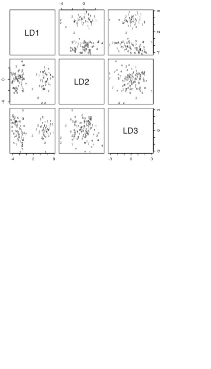
53
+ taillgth+footlgth+earconch+eye+chest+belly,data=possum, subset=here)
> options(digits=4)
> possum.lda$svd # Examine the singular values
[1] 15.7578 3.9372 3.1860 1.5078 1.1420 0.7772
>
> plot(possum.lda, dimen=3)
> # Scatterplot matrix for scores on 1st 3 canonical variates, as in Figure22
Figure 22: Scatterplot matrix of first three canonical variates.
The singular values are the ratio of between to within group sums of squares, for the canonical variates in turn.
Clearly canonical variates after the third will have little if any discriminatory power. One can use
predict.lda() to get (among other information) scores on the first few canonical variates.
Note that there may be interpretative advantages in taking logarithms of biological measurement data. The
standard against which patterns of measurement are commonly compared is that of allometric growth, which
implies a linear relationship between the logarithms of the measurements. Differences between different sites
are then indicative of different patterns of allometric growth. The reader may wish to repeat the above analysis,
but working with the logarithms of measurements.
6.4 Decision Tree models (Tree-based models)
We include tree-based classification here because it is a multivariate supervised classification, or discrimination,
method. A tree-based regression approach is available for use for regression problems. Tree-based methods
seem more suited to binary regression and classification than to regression with an ordinal or continuous
dependent variable.
Tree-based models, also known as “Classification and Regression Trees” (CART), may be suitable for
regression and classification problems when there are extensive data. One advantage of such methods is that
they automatically handle non-linearity and interactions. Output includes a “decision tree” that is immediately
useful for prediction.
library(rpart)
# Use fgl: Forensic glass fragment data; from MASS package
glass.tree <- rpart(type ~ RI+Na+Mg+Al+Si+K+Ca+Ba+Fe, data=fgl)
plot(glass.tree); text(glass.tree)

54
summary(glass.tree)
To use these models effectively, you also need to know about approaches to pruning trees, and about cross-
validation. Methods for reduction of tree complexity that are based on significance tests at each individual node
(i.e. branching point) typically choose trees that over-predict.
The Atkinson and Therneau rpart (recursive partitioning) package is closer to CART than is the S-PLUS tree
library. It integrates cross-validation with the algorithm for forming trees.
6.5 Exercises
1. Using the data set painters (MASS package), apply principal components analysis to the scores for
Composition, Drawing, Colour, and Expression. Examine the loadings on the first three principal
components. Plot a scatterplot matrix of the first three principal components, using different colours or symbols
to identify the different schools.
2. The data set Cars93 is in the MASS package. Using the columns of continuous or ordinal data, determine
scores on the first and second principal components. Investigate the comparison between (i) USA and non-USA
cars, and (ii) the six different types (Type) of car. Now create a new data set in which binary factors become
columns of 0/1 data, and include these in the principal components analysis.
3. Repeat the calculations of exercises 1 and 2, but this time using the function lda() from the MASS package
to derive canonical discriminant scores, as in section 6.3.
4. The MASS package has the Aids2 data set, containing de-identified data on the survival status of patients
diagnosed with AIDS before July 1 1991. Use tree-based classification (rpart()) to identify major influences
on survival.
5. Investigate discrimination between plagiotropic and orthotropic species in the data set leafshape34.
6.6 References
Chambers, J. M. and Hastie, T. J. 1992. Statistical Models in S. Wadsworth and Brooks Cole Advanced Books and
Software, Pacific Grove CA.
Friedman, J., Hastie, T. and Tibshirani, R. (1998). Additive logistic regression: A statistical view of boosting. Available
from the internet.
Maindonald J H and Braun W J 2008. Data Analysis and Graphics Using R – An Example-Based Approach, 2nd edn.
Cambridge University Press.
Ripley, B. D. 1996. Pattern Recognition and Neural Networks. Cambridge University Press, Cambridge UK.
Therneau, T. M. and Atkinson, E. J. 1997. An Introduction to Recursive Partitioning Using the RPART Routines. This is
one of two documents included in: http://www.stats.ox.ac.uk/pub/SWin/rpartdoc.zip
Venables, W. N. and Ripley, B. D., 2nd edn 1997. Modern Applied Statistics with S-Plus. Springer, New York.
34 Data relate to the paper: King. D.A. and Maindonald, J.H. 1999. Tree architecture in relation to leaf
dimensions and tree stature in temperate and tropical rain forests. Journal of Ecology 87: 1012-1024.

55
*7. R Data Structures
7.1 Vectors
Recall that vectors may have mode logical, numeric or character.
7.1.1 Subsets of Vectors
Recall (section 2.6.2) two common ways to extract subsets of vectors:
Specify the numbers of the elements that are to be extracted. One can use negative numbers to omit elements.
Specify a vector of logical values. The elements that are extracted are those for which the logical value is T.
Thus suppose we want to extract values of x that are greater than 10.
The following demonstrates a third possibility, for vectors that have named elements:
> c(Andreas=178, John=185, Jeff=183)[c("John","Jeff")]
John Jeff
185 183
A vector of names has been used to extract the elements.
7.1.2 Patterned Data
Use 5:15 to generate the numbers 5, 6, …, 15. Entering 15:5 will generate the sequence in the reverse order.
To repeat the sequence (2, 3, 5) four times over, enter rep(c(2,3,5), 4) thus:
> rep(c(2,3,5),4)
[1] 2 3 5 2 3 5 2 3 5 2 3 5
>
If instead one wants four 2s, then four 3s, then four 5s, enter rep(c(2,3,5), c(4,4,4)).
> rep(c(2,3,5),c(4,4,4)) # An alternative is rep(c(2,3,5), each=4)
[1] 2 2 2 2 3 3 3 3 5 5 5 5
Note further that, in place of c(4,4,4) we could write rep(4,3). So a further possibility is that in place of
rep(c(2,3,5), c(4,4,4)) we could enter rep(c(2,3,5), rep(4,3)).
In addition to the above, note that the function rep() has an argument length.out, meaning “keep on
repeating the sequence until the length is length.out.”
7.2 Missing Values
In R, the missing value symbol is NA. Any arithmetic operation or relation that involves NA generates an NA.
This applies also to the relations <, <=, >, >=, ==, !=. The first four compare magnitudes, == tests for equality,
and != tests for inequality. Users who do not carefully consider implications for expressions that include Nas
may be puzzled by the results. Specifically, note that x==NA generates NA.
Be sure to use is.na(x) to test which values of x are NA. As x==NA gives a vector of NAs, you get no
information at all about x. For example
> x <- c(1,6,2,NA)
> is.na(x) # TRUE for when NA appears, and otherwise FALSE
[1] FALSE FALSE FALSE TRUE
> x==NA # All elements are set to NA
[1] NA NA NA NA
> NA==NA
[1] NA
Missing values in subscripts: In R
y[x>2] <- x[x>2]
generates the error message “NAs are not allowed in subscripted assignments".

56
Users are advised to use !is.na(x) to limit the selection, on one or both sides as necessary, to those elements
of x that are not NAs. We will have more to say on missing values in the section on data frames that now
follows.
7.3 Data frames
The concept of a data frame is fundamental to the use of most of the R modelling and graphics functions. A
data frame is a generalisation of a matrix, in which different columns may have different modes. All elements
of any column must however have the same mode, i.e. all numeric or all factor, or all character.
Data frames where all columns hold numeric data have some, but not all, of the properties of matrices. There
are important differences that arise because data frames are implemented as lists. To turn a data frame of
numeric data into a matrix of numeric data, use as.matrix().
Lists are discussed below, in section 7.6.
7.3.1 Extraction of Component Parts of Data frames
Consider the data frame barley that accompanies the lattice package:
> names(barley)
[1] "yield" "variety" "year" "site"
> levels(barley$site)
[1] "Grand Rapids" "Duluth" "University Farm" "Morris"
[5] "Crookston" "Waseca"
We will extract the data for 1932, at the Duluth site.
> Duluth1932 <- barley[barley$year=="1932" & barley$site=="Duluth",
+ c("variety","yield")]
variety yield
66 Manchuria 22.56667
72 Glabron 25.86667
78 Svansota 22.23333
84 Velvet 22.46667
90 Trebi 30.60000
96 No. 457 22.70000
102 No. 462 22.50000
108 Peatland 31.36667
114 No. 475 27.36667
120 Wisconsin No. 38 29.33333
The first column holds the row labels, which in this case are the numbers of the rows that have been extracted.
In place of c("variety","yield") we could have written, more simply, c(2,4).
7.3.2 Data Sets that Accompany R Packages
Type in data() to get a list of data sets (mostly data frames) associated with all packages that are in the current
search path. To get information on the data sets that are included in the datasets package, specify
data(package="datasets")
and similarly for any other package.
In most packages, data from an attached package are automatically available; use of e.g., data(airquality)
to load the data set airquality (datasets package) is unnecessary
The out-of-the-box Windows and other binary distributions include many commonly required packages. Other
packages must be explicitly installed. For remaining sections of these notes, the MASS package, which comes
with the default distribution, will be used from time to time.
The base package, and several other packages, are automatically attached at the beginning of the session. To
attach any other installed package, use the library() command.

57
7.4 Data Entry Issues
7.4.1 Idiosyncrasies
The function read.table() is straightforward for reading in rectangular arrays of data that are entirely
numeric. When, as in the above example, one of the columns contains text strings, the column is by default
stored as a factor with as many different levels as there are unique text strings35.
Problems may arise when small mistakes in the data cause R to interpret a column of supposedly numeric data
as character strings, which are automatically turned into factors. For example there may be an O (oh)
somewhere where there should be a 0 (zero), or an el (l) where there should be a one (1). If you use any missing
value symbols other than the default (NA), you need to make this explicit see section 7.3.2 below. Otherwise
any appearance of such symbols as *, period(.) and blank (in a case where the separator is something other than
a space) will cause to whole column to be treated as character data.
Users who find this default behaviour of read.table() confusing may wish to use the parameter setting
as.is = TRUE. 36 If the column is later required for use as a factor in a model or graphics formula, it may be
necessary to make it into a factor at that time. Some functions do this conversion automatically.
7.4.2 Missing values when using read.table()
The function read.table() expects missing values to be coded as NA, unless you set na.strings to
recognise other characters as missing value indicators. If you have a text file that has been output from SAS,
you will probably want to set na.strings=c(".").
There may be multiple missing value indicators, e.g. na.strings=c(“NA”,".",”*”,""). The "" will
ensure that empty cells are entered as NAs.
7.4.3 Separators when using read.table()
With data from spreadsheets37, it is sometimes necessary to use tab (“\t”) or comma as the separator. The
default separator is white space. To set tab as the separator, specify sep="\t".
7.5 Factors and Ordered Factors
We discussed factors in section 2.6.4. They provide an economical way to store vectors of character strings in
which there are many multiple occurrences of the same strings. More crucially, they have a central role in the
incorporation of qualitative effects into model and graphics formulae.
Factors have a dual identity. They are stored as integer vectors, with each of the values interpreted according to
the information that is in the table of levels38.
The data frame islandcities that accompanies these notes holds the populations of the 19 island nation cities
with a 1995 urban centre population of 1.4 million or more. The row names are the city names, the first column
(country) has the name of the country, and the second column (population) has the urban centre population,
in millions. Here is a table that gives the number of times each country occurs
Australia Cuba Indonesia Japan Philippines Taiwan United Kingdom
3 1 4 6 2 1 2
35 Storage of columns of character strings as factors is efficient when a small number of distinct strings that are of modest
length are each repeated a large number of times.
36 Specifying as.is = T prevents columns of (intended or unintended) character strings from being converted into
factors.
37 One way to get mixed text and numeric data across from Excel is to save the worksheet in a .csv text file with comma
as the separator. If for example file name is myfile.csv and is on drive a:, use
read.table("a:/myfile.csv", sep=",") to read the data into R. This copes with any spaces which may appear
in text strings. [But watch that none of the cell entries include commas.]
38 Factors are column objects that have mode numeric and class “factor”. They have an attribute levels that holds the level
names.

58
[There are 19 cities in all.]
Printing the contents of the column with the name country gives the names, not the integer values. As in most
operations with factors, R does the translation invisibly. There are though annoying exceptions that can make
the use of factors tricky. To be sure of getting the country names, specify
as.character(islandcities$country)
To get the integer values, specify
unclass(islandcities$country)
By default, R sorts the level names in alphabetical order. If we form a table that has the number of times that
each country appears, this is the order that is used:
> table(islandcities$country)
Australia Cuba Indonesia Japan Philippines Taiwan United Kingdom
3 1 4 6 2 1 2
This order of the level names is purely a convenience. We might prefer countries to appear in order of latitude,
from North to South. We can change the order of the level names to reflect this desired order:
> lev <- levels(islandcities$country)
> lev[c(7,4,6,2,5,3,1)]
[1] "United Kingdom" "Japan" "Taiwan" "Cuba"
[5] "Philippines" "Indonesia" "Australia"
> country <- factor(islandcities$country, levels=lev[c(7,4,6,2,5,3,1)])
> table(country)
United Kingdom Japan Taiwan Cuba Philippines Indonesia Australia
2 6 1 1 2 4 3
In ordered factors, i.e. factors with ordered levels, there are inequalities that relate factor levels.
Factors have the potential to cause a few surprises, so be careful! Here are two points to note:
When a vector of character strings becomes a column of a data frame, R by default turns it into a factor.
Enclose the vector of character strings in the wrapper function I() if it is to remain character.
There are some contexts in which factors become numeric vectors. To be sure of getting the vector of text
strings, specify e.g. as.character(country).
To extract the numeric levels 1, 2, 3, …, specify as.numeric(country).
7.6 Ordered Factors
Actually, it is their levels that are ordered. To create an ordered factor, or to turn a factor into an ordered factor,
use the function ordered(). The levels of an ordered factor are assumed to specify positions on an ordinal
scale. Try
> stress.level<-rep(c("low","medium","high"),2)
> ordf.stress<-ordered(stress.level, levels=c("low","medium","high"))
> ordf.stress
[1] low medium high low medium high
Levels: low < medium < high
> ordf.stress<"medium"
[1] TRUE FALSE FALSE TRUE FALSE FALSE
> ordf.stress>="medium"
[1] FALSE TRUE TRUE FALSE TRUE TRUE
Later we will meet the notion of inheritance. Ordered factors inherit the attributes of factors, and have a further
ordering attribute. When you ask for the class of an object, you get details both of the class of the object, and of
any classes from which it inherits. Thus:
> class(ordf.stress)
[1] "ordered" "factor"

59
7.7 Lists
Lists make it possible to collect an arbitrary set of R objects together under a single name. You might for
example collect together vectors of several different modes and lengths, scalars, matrices or more general
arrays, functions, etc. Lists can be, and often are, a rag-tag of different objects. We will use for illustration the
list object that R creates as output from an lm calculation.
For example, consider the linear model (lm) object elastic.lm (c. f. sections 1.1.4 and 2.1.4) created thus:
elastic.lm <- lm(distance~stretch, data=elasticband)
It is readily verified that elastic.lm consists of a variety of different kinds of objects, stored as a list. You
can get the names of these objects by typing in
> names(elastic.lm)
[1] "coefficients" "residuals" "effects" "rank"
[5] "fitted.values" "assign" "qr" "df.residual"
[9] "xlevels" "call" "terms" "model"
The first list element is:
> elastic.lm$coefficients
(Intercept) stretch
-63.571429 4.553571
Alternative ways to extract this first list element are:
elastic.lm[["coefficients"]]
elastic.lm[[1]]
We can alternatively ask for the sublist whose only element is the vector elastic.lm$coefficients. For
this, specify elastic.lm[“coefficients”] or elastic.lm[1]. There is a subtle difference in the result
that is printed out. The information is preceded by $coefficients, meaning “list element with name
coefficients”.
> elastic.lm[1]
$coefficients
(Intercept) stretch
-63.571429 4.553571
The second list element is a vector of length 7
> options(digits=3)
> elastic.lm$residuals
1 2 3 4 5 6 7
2.107 -0.321 18.000 1.893 -27.786 13.321 -7.214
The tenth list element documents the function call:
> elastic.lm$call
lm(formula = distance ~ stretch, data = elasticband)
> mode(elastic.lm$call)
[1] "call"
*7.8 Matrices and Arrays
All elements of a matrix have the same mode, i.e. all numeric, or all character. Thus a matrix is a more
restricted structure than a data frame. One reason for numeric matrices is that they allow a variety of
mathematical operations that are not available for data frames. Matrices are likely to be important for those
users who wish to implement new regression and multivariate methods. The matrix construct generalises to
array, which may have more than two dimensions.
Note that matrices are stored columnwise. Thus consider
> xx <- matrix(1:6,ncol=3) # Equivalently, enter matrix(1:6,nrow=2)
> xx
[,1] [,2] [,3]
[1,] 1 3 5
[2,] 2 4 6

60
If xx is any matrix, the assignment
x <- as.vector(xx)
places columns of xx, in order, into the vector x. In the example above, we get back the elements 1, 2, . . . , 6.
Matrices have the attribute “dimension”. Thus
> dim(xx)
[1] 2 3
In fact a matrix is a vector (numeric or character) whose dimension attribute has length 2.
Now set
> x34 <- matrix(1:12,ncol=4)
> x34
[,1] [,2] [,3] [,4]
[1,] 1 4 7 10
[2,] 2 5 8 11
[3,] 3 6 9 12
Here are examples of the extraction of columns or rows or submatrices
x34[2:3,c(1,4)] # Extract rows 2 & 3 & columns 1 & 4
x34[2,] # Extract the second row
x34[-2,] # Extract all rows except the second
x34[-2,-3] # Extract the matrix obtained by omitting row 2 & column 3
The dimnames() function assigns and/or extracts matrix row and column names. The dimnames() function
gives a list, in which the first list element is the vector of row names, and the second list element is the vector of
column names. This generalises in the obvious way for use with arrays, which we now discuss.
7.8.1 Arrays
The generalisation from a matrix (2 dimensions) to allow > 2 dimensions gives an array. A matrix is a 2-
dimensional array.
Consider a numeric vector of length 24. So that we can easily keep track of the elements, we will make them 1,
2, .., 24. Thus
x <- 1:24
Then
dim(x) <- c(2,12)
turns this into a 2 x 12 matrix.
> x
[,1] [,2] [,3] [,4] [,5] [,6] [,7] [,8] [,9] [,10] [,11] [,12]
[1,] 1 3 5 7 9 11 13 15 17 19 21 23
[2,] 2 4 6 8 10 12 14 16 18 20 22 24
Now try
> dim(x) <-c(3,4,2)
> x
, , 1
[,1] [,2] [,3] [,4]
[1,] 1 4 7 10
[2,] 2 5 8 11
[3,] 3 6 9 12
, , 2
[,1] [,2] [,3] [,4]
[1,] 13 16 19 22
[2,] 14 17 20 23

61
[3,] 15 18 21 24
7.8.2 Conversion of Numeric Data frames into Matrices
There are various manipulations that are available for matrices, but not for data frames. Use as.matrix() to
handle any conversion that may be necessary.
7.9 Exercises
Generate the numbers 101, 102, …, 112, and store the result in the vector x.
Generate four repeats of the sequence of numbers (4, 6, 3).
Generate the sequence consisting of eight 4s, then seven 6s, and finally nine 3s. Store the numbers obtained , in
order, in the columns of a 6 by 4 matrix.
Create a vector consisting of one 1, then two 2’s, three 3’s, etc., and ending with nine 9’s.
For each of the following calculations, what you would expect? Check to see if you were right!
a)
answer <- c(2, 7, 1, 5, 12, 3, 4)
for (j in 2:length(answer)){ answer[j] <- max(answer[j],answer[j-1])}
b)
answer <- c(2, 7, 1, 5, 12, 3, 4)
for (j in 2:length(answer)){ answer[j] <- sum(answer[j],answer[j-1])}
In the built-in data frame airquality (datasets package): (a) Determine, for each of the columns of the data
frame airquality (datasets package), the median, mean, upper and lower quartiles, and range; (b) Extract the
row or rows for which Ozone has its maximum value; (c) extract the vector of values of Wind for values of
Ozone that are above the upper quartile.
Refer to the Eurasian snow data that is given in Exercise 1.6 . Find the mean of the snow cover (a) for the odd-
numbered years and (b) for the even-numbered years.
Determine which columns of the data frame Cars93 (MASS package) are factors. For each of these factor
columns, print out the levels vector. Which of these are ordered factors?
Use summary() to get information about data in the data frames attitude (both in the datasets
package), and cpus (MASS package). Write brief notes, for each of these data sets, on what this reveals.
From the data frame mtcars (MASS package) extract a data frame mtcars6 that holds only the information for
cars with 6 cylinders.
From the data frame Cars93 (MASS package), extract a data frame which holds only information for small and
sporty cars.

62
8. Functions
8.1 Functions for Confidence Intervals and Tests
Use the help to get complete information. Below, I note two of the simpler functions.
8.1.1 The t-test and associated confidence interval
Use t.test(). This allows both a one-sample and a two-sample test.
8.1.2 Chi-Square tests for two-way tables
Use chisq.test() for a test for no association between rows and columns in the output from table().
Alternatively, the argument may be a matrix. This test assumes that counts enter independently into the cells of
a table. For example, the test is invalid if there is clustering in the data.
8.2 Matching and Ordering
> match(<vec1>, <vec2>) ## For each element of <vec1>, returns the
## position of the first occurrence in <vec2>
> order(<vector>) ## Returns the vector of subscripts giving
## the order in which elements must be taken
## so that <vector> will be sorted.
> rank(<vector>) ## Returns the ranks of the successive elements.
Numeric vectors will be sorted in numerical order. Character vectors will be sorted in alphanumeric order.
The operator %in% can be highly useful in picking out subsets of data. For example:
> x <- rep(1:5,rep(3,5))
> x
[1] 1 1 1 2 2 2 3 3 3 4 4 4 5 5 5
> two4 <- x %in% c(2,4)
> two4
[1] FALSE FALSE FALSE TRUE TRUE TRUE FALSE FALSE FALSE TRUE
[11] TRUE TRUE FALSE FALSE FALSE
> # Now pick out the 2s and the 4s
> x[two4]
[1] 2 2 2 4 4 4
8.3 String Functions
substring(<vector of text strings>, <first position>, <last position>)
nchar(<vector of text strings>)
## Returns vector of number of characters in each element.
*8.3.1 Operations with Vectors of Text Strings – A Further Example
We will work with the column Make in the dataset Cars93 from the MASS package.
library(MASS) # if needed
To find the position at which the first space appears in the information on make of car, we might do the
following:
> car.brandnames <- sapply(strsplit(as.character(Cars93$Make), " ", fixed=TRUE),
+ function(x)x[1])
> car.brandnames[1:5]
[1] "Acura" "Acura" "Audi" "Audi" "BMW"

63
8.4 Application of a Function to the Columns of an Array or Data Frame
apply(<array>, <dimension>, <function>)
lapply(<list>, <function>)
## N. B. A dataframe is a list. Output is a list.
sapply(<list>, <function>)
## As lapply(), but simplify (e.g. to a vector
## or matrix), if possible.
8.4.1 apply()
The function apply() can be used on data frames as well as matrices. Here is an example:
> apply(airquality,2,mean) # All elements must be numeric!
Ozone Solar.R Wind Temp Month Day
NA NA 9.96 77.88 6.99 15.80
> apply(airquality,2,mean,na.rm=TRUE)
Ozone Solar.R Wind Temp Month Day
42.13 185.93 9.96 77.88 6.99 15.80
The use of apply(airquality,1,mean) will give means for each row. These are not, for these data, useful
information!
8.4.2 sapply()
The function sapply() can be useful for getting information about the columns of a data frame. Here we use it
to count that number of missing values in each column of the built-in data frame airquality.
> sapply(airquality, function(x)sum(is.na(x)))
Ozone Solar.R Wind Temp Month Day
37 7 0 0 0 0
Here are several further examples that use the data frame moths that accompanies these notes:
> sapply(moths,is.factor) # Determine which columns are factors
meters A P habitat
FALSE FALSE FALSE TRUE
> # How many levels does each factor have?
> sapply(moths, function(x)if(!is.factor(x))return(0) else length(levels(x)))
meters A P habitat
0 0 0 8
*8.5 aggregate() and tapply()
The arguments are in each case a variable, a list of factors, and a function that operates on a vector to return a
single value. For each combination of factor levels, the function is applied to corresponding values of the
variable. The function aggregate() returns a data frame. For example:
> str(cabbages)
`data.frame': 60 obs. of 4 variables:
$ Cult : Factor w/ 2 levels "c39","c52": 1 1 1 1 1 1 1 1 1 1 ...
$ Date : Factor w/ 3 levels "d16","d20","d21": 1 1 1 1 1 1 1 1 1 1 ...
$ HeadWt: num 2.5 2.2 3.1 4.3 2.5 4.3 3.8 4.3 1.7 3.1 ...
$ VitC : int 51 55 45 42 53 50 50 52 56 49 ...
> attach(cabbages)
> aggregate(HeadWt, by=list(Cult=Cult, Date=Date), FUN=mean)
Cult Date x
1 c39 d16 3.18
2 c52 d16 2.26
3 c39 d20 2.80
4 c52 d20 3.11

64
5 c39 d21 2.74
6 c52 d21 1.47
The syntax for tapply() is similar, except that the name of the second argument is INDEX rather than by.
The output is an array with as many dimensions as there are factors. Where there are no data values for a
particular combination of factor levels, NA is returned.
*8.6 Merging Data Frames
The data frame Cars93 (MASS package) holds extensive information on data from 93 cars on sale in the USA
in 1993. One of the variables, stored as a factor, is Type. I have created a data frame Cars93.summary, in
which the row names are the distinct values of Type, while a later column holds two character abbreviations of
each of the car types, suitable for use in plotting.
> Cars93.summary
Min.passengers Max.passengers No.of.cars abbrev
Compact 4 6 16 C
Large 6 6 11 L
Midsize 4 6 22 M
Small 4 5 21 Sm
Sporty 2 4 14 Sp
Van 7 8 9 V
We proceed thus to add a column that has the abbreviations to the data frame. Here however our demands are
simple, and we can proceed thus:
new.Cars93 <- merge(x=Cars93,y=Cars93.summary[,4,drop=F],
by.x="Type",by.y="row.names")
This creates a data frame that has the abbreviations in the additional column with name “abbrev”.
If there had been rows with missing values of Type, these would have been omitted from the new data frame.
This can be avoided by making sure that Type has NA as one of its levels, in both data frames.
8.7 Dates
Since version 1.9.0, the date package has been superseded by functions for working with dates that are in R
base. See help(Dates), help(as.Date) and help(format.Date) for detailed information.
Use as.Date() to convert text strings into dates. The default is that the year comes first, then the month, and
then the day of the month, thus:
> # Electricity Billing Dates
> dd <- as.Date(c("2003/08/24","2003/11/23","2004/02/22","2004/05/23"))
> diff(dd)
Time differences of 91, 91, 91 days
Use format() to set or change the way that a date is formatted. The following are a selection of the symbols
used:
%d: day, as number
%a: abbreviated weekday name (%A: unabbreviated)
%m: month (00-12)
%b: month abbreviated name (%B: unabbreviated)
%y: final two digits of year (%Y: all four digits)
The default format is "%Y-%m-%d".
The function as.Date() will take a vector of character strings that has an appropriate format, and convert it
into a dates object. By default, dates are stored using January 1 1970 as origin. This becomes apparent when
as.integer() is used to convert a date into an integer value. Here are examples:
> as.Date("1/1/1960", format="%d/%m/%Y")

65
[1] "1960-01-01"
> as.Date("1:12:1960",format="%d:%m:%Y")
[1] "1960-12-01"
> as.Date("1960-12-1")-as.Date("1960-1-1")
Time difference of 335 days
> as.Date("31/12/1960","%d/%m/%Y")
[1] "1960-12-31"
> as.integer(as.Date("1/1/1970","%d/%m/%Y")
[1] 0
> as.integer(as.Date("1/1/2000","%d/%m/%Y"))
[1] 10957
The function format() allows control of the formatting of dates. See help(format.Date).
> dec1 <- as.Date("2004-12-1")
> format(dec1, format="%b %d %Y")
[1] "Dec 01 2004"
> format(dec1, format="%a %b %d %Y")
[1] "Wed Dec 01 2004"
8.8. Writing Functions and other Code
We have already met several functions. Here is a function to convert Fahrenheit to Celsius:
> fahrenheit2celsius <- function(fahrenheit=32:40)(fahrenheit-32)*5/9
> # Now invoke the function
> fahrenheit2celsius(c(40,50,60))
[1] 4.444444 10.000000 15.555556
The function returns the value (fahrenheit-32)*5/9. More generally, a function returns the value of the
last statement of the function. Unless the result from the function is assigned to a name, the result is printed.
Here is a function that prints out the mean and standard deviation of a set of numbers:
> mean.and.sd <- function(x=1:10){
+ av <- mean(x)
+ sd <- sqrt(var(x))
+ c(mean=av, SD=sd)
+ }
>
> # Now invoke the function
> mean.and.sd()
mean SD
5.500000 3.027650
> mean.and.sd(hills$climb)
mean SD
1815.314 1619.151
8.8.1 Syntax and Semantics
A function is created using an assignment. On the right hand side, the parameters appear within round brackets.
You can, if you wish, give a default. In the example above the default was x = 1:10, so that users can run the
function without specifying a parameter, just to see what it does.
Following the closing “)” the function body appears. Except where the function body consists of just one
statement, this is enclosed between curly braces ({ }). The return value usually appears on the final line of the
function body. In the example above, this was the vector consisting of the two named elements mean and sd.

66
8.8.2 A Function that gives Data Frame Details
First we will define a function that accepts a vector x as its only argument. It will allow us to determine
whether x is a factor, and if a factor, how many levels it has. The built-in function is.factor() will return T
if x is a factor, and otherwise F. The following function faclev() uses is.factor() to test whether x is a
factor. It prints out 0 if x is not a factor, and otherwise the number of levels of x.
> faclev <- function(x)if(!is.factor(x))return(0) else
length(levels(x))
Earlier, we encountered the function sapply() that can be used to repeat a calculation on all columns of a
data frame. [More generally, the first argument of sapply() may be a list.] To apply faclev() to all
columns of the data frame moths we can specify
> sapply(moths, faclev)
We can alternatively give the definition of faclev directly as the second argument of sapply, thus
> sapply(moths, function(x)if(!is.factor(x))return(0)
else length(levels(x)))
Finally, we may want to do similar calculations on a number of different data frames. So we create a function
check.df() that encapsulates the calculations. Here is the definition of check.df().
check.df <- function(df=moths)
sapply(df, function(x)if(!is.factor(x))return(0) else
length(levels(x)))
8.8.3 Compare Working Directory Data Sets with a Reference Set
At the beginning of a new session, we might store the names of the objects in the working directory in the
vector dsetnames, thus:
dsetnames <- objects()
Now suppose that we have a function additions(), defined thus:
additions <- function(objnames = dsetnames)
{
newnames <- objects(pos=1)
existing <- as.logical(match(newnames, objnames, nomatch = 0))
newnames[!existing]
}
At some later point in the session, we can enter
additions(dsetnames)
to get the names of objects that have been added since the start of the session.
8.8.4 Issues for the Writing and Use of Functions
There can be many functions. Choose their names carefully, so that they are meaningful.
Choose meaningful names for arguments, even if this means that they are longer than one would like.
Remember that they can be abbreviated in actual use.
As far as possible, make code self-documenting. Use meaningful names for R objects. Ensure that the names
used reflect the hierarchies of files, data structures and code.
R allows the use of names for elements of vectors and lists, and for rows and columns of arrays and dataframes.
Consider the use of names rather than numbers when you pull out individual elements, columns etc. Thus
dead.tot[,"dead"] is more meaningful and safer than dead.tot[,2].
Settings that may need to change in later use of the function should appear as default settings for parameters.
Use lists, where this seems appropriate, to group together parameters that belong together conceptually.
Where appropriate, provide a demonstration mode for functions. Such a mode will print out summary
information on the data and/or on the results of manipulations prior to analysis, with appropriate labelling. The
code needed to implement this feature has the side-effect of showing by example what the function does, and
may be useful for debugging.

67
Break functions up into a small number of sub-functions or “primitives”. Re-use existing functions wherever
possible. Write any new “primitives” so that they can be re-used. This helps ensure that functions contain well-
tested and well-understood components. Watch the r-help electronic mail list (section 13.3) for useful functions
for routine tasks.
Wherever possible, give parameters sensible defaults. Often a good strategy is to use as defaults parameters that
will serve for a demonstration run of the function.
NULL is a useful default where the parameter mostly is not required, but where the parameter if it appears may
be any one of several types of data structure. The test if(!is.null()) then determines whether one needs to
investigate that parameter further.
Structure computations so that it is easy to retrace them. For this reason substantial chunks of code should be
incorporated into functions sooner rather than later.
Structure code to avoid multiple entry of information.
8.8.5 Functions as aids to Data Management
Where data, labelling etc must be pulled together from a number of sources, and especially where you may want
to retrace your steps some months later, take the same care over structuring data as over structuring code. Thus
if there is a factorial structure to the data files, choose file names that reflect it. You can then generate the file
names automatically, using paste() to glue the separate portions of the name together.
Lists are a useful mechanism for grouping together all data and labelling information that one may wish to bring
together in a single set of computations. Use as the name of the list a unique and meaningful identification
code. Consider whether you should include objects as list items, or whether identification by name is
preferable. Bear in mind, also, the use of switch(), with the identification code used to determine what
switch() should pick out, to pull out specific information and data that is required for a particular run.
Concentrate in one function the task of pulling together data and labelling information, perhaps with some
subsequent manipulation, from a number of separate files. This structures the code, and makes the function a
source of documentation for the data.
Use user-defined data frame attributes to document data. For example, given the data frame elasticband
giving the amount of stretch and resulting distance of movement of a rubber band, one might specify
attributes(elasticband)$title <-
“Extent of stretch of band, and Resulting Distance”
8.8.6 Graphs
Use graphs freely to shed light both on computations and on data. One of R’s big pluses is its tight integration
of computation and graphics.
8.8.7 A Simulation Example
We would like to know how well such a student might do by random guessing, on a multiple choice test
consisting of 100 questions each with five alternatives. We can get an idea by using simulation. Each question
corresponds to an independent Bernoulli trial with probability of success equal to 0.2. We can simulate the
correctness of the student for each question by generating an independent uniform random number. If this
number is less than .2, we say that the student guessed correctly; otherwise, we say that the student guessed
incorrectly.
This will work, because the probability that a uniform random variable is less than .2 is exactly .2, while the
probability that a uniform random variable exceeds .2 is exactly .8, which is the same as the probability that the
student guesses incorrectly. Thus, the uniform random number generator is simulating the student. R can do
this as follows:
guesses <- runif(100)
correct.answers <- 1*(guesses < .2)
correct.answers
The multiplication by 1 causes (guesses<.2), which is calculated as TRUE or FALSE, to be coerced to 1
(TRUE) or 0 (FALSE). The vector correct.answers thus contains the results of the student's guesses. A 1 is
recorded each time the student correctly guesses the answer, while a 0 is recorded each time the student is
wrong.

68
One can thus write an R function that simulates a student guessing at a True-False test consisting of some
arbitrary number of questions. We leave this as an exercise.
8.8.8 Poisson Random Numbers
One can think of the Poisson distribution as the distribution of the total for occurrences of rare events. For
example, an accident at an intersection on any one day should be a rare event. The total number of accidents
over the course of a year may well follow a distribution that is close to Poisson. [However the total number of
people injured is unlikely to follow a Poisson distribution. Why?] The function using rpois() generates
Poisson random numbers. Suppose for example traffic accidents occur at an intersection with a Poisson
distribution that has a mean rate of 3.7 per year. To simulate the annual number of accidents for a 10-year
period, we can specify rpois(10,3.7). We pursue the Poisson distribution in an exercise below.
8.9 Exercises
1. Use the round function together with runif() to generate 100 random integers between 0 and 99. Now
look up the help for sample(), and use it for the same purpose.
2. Write a function that will take as its arguments a list of response variables, a list of factors, a data frame, and
a function such as mean or median. It will return a data frame in which each value for each combination of
factor levels is summarised in a single statistic, for example the mean or the median.
3. Determine the number of days, according to R, between the following dates:
January 1 in the year 1700, and January 1 in the year 1800
January 1 in the year 1998, and January 1 in the year 2000
4. The supplied data frame milk has columns four and one. Seventeen people rated the sweetness of each of
two samples of a milk product on a continuous scale from 1 to 7, one sample with four units of additive and the
other with one unit of additive. Here is a function that plots, for each patient, the four result against the one
result, but insisting on the same range for the x and y axes.
plot.one <- function(){
xyrange <- range(milk) # Calculates the range of all values in the data frame
par(pin=c(6.75, 6.75)) # Set plotting area = 6.75 in. by 6.75 in.
plot(four, one, data=milk, xlim=xyrange, ylim=xyrange, pch=16)
abline(0,1) # Line where four = one
}
Rewrite this function so that, given the name of a data frame and of any two of its columns, it will plot the
second named column against the first named column, showing also the line y=x.
5. Write a function that prints, with their row and column labels, only those elements of a correlation matrix for
which abs(correlation) >= 0.9.
6. Write your own wrapper function for one-way analysis of variance that provides a side by side boxplot of the
distribution of values by groups. If no response variable is specified, the function will generate random normal
data (no difference between groups) and provide the analysis of variance and boxplot information for that.
7. Write a function that computes a moving average of order 2 of the values in a given vector. Apply the
function to the data (in the data set huron that accompanies these notes) for the levels of Lake Huron. Repeat
for a moving average of order 3.
9. Find a way of computing the moving averages in exercise 3 that does not involve the use of a for loop.
10. Create a function to compute the average, variance and standard deviation of 1000 randomly generated
uniform random numbers, on [0,1]. (Compare your results with the theoretical results: the expected value of a
uniform random variable on [0,1] is 0.5, and the variance of such a random variable is 0.0833.)
11. Write a function that generates 100 independent observations on a uniformly distributed random variable on
the interval [3.7, 5.8]. Find the mean, variance and standard deviation of such a uniform random variable. Now
modify the function so that you can specify an arbitrary interval.
12. Look up the help for the sample() function. Use it to generate 50 random integers between 0 and 99,
sampled without replacement. (This means that we do not allow any number to be sampled a second time.)
Now, generate 50 random integers between 0 and 9, with replacement.

69
13. Write an R function that simulates a student guessing at a True-False test consisting of 40 questions. Find
the mean and variance of the student's answers. Compare with the theoretical values of .5 and .25.
14. Write an R function that simulates a student guessing at a multiple choice test consisting of 40 questions,
where there is chance of 1 in 5 of getting the right answer to each question. Find the mean and variance of the
student's answers. Compare with the theoretical values of .2 and .16.
15. Write an R function that simulates the number of working light bulbs out of 500, where each bulb has a
probability .99 of working. Using simulation, estimate the expected value and variance of the random variable
X, which is 1 if the light bulb works and 0 if the light bulb does not work. What are the theoretical values?
16. Write a function that does an arbitrary number n of repeated simulations of the number of accidents in a
year, plotting the result in a suitable way. Assume that the number of accidents in a year follows a Poisson
distribution. Run the function assuming an average rate of 2.8 accidents per year.
17. Write a function that simulates the repeated calculation of the coefficient of variation (= the ratio of the
mean to the standard deviation), for independent random samples from a normal distribution.
18. Write a function that, for any sample, calculates the median of the absolute values of the deviations from the
sample median.
*19. Generate random samples from normal, exponential, t (2 d. f.), and t (1 d. f.), thus:
a) xn<-rnorm(100) b) xe<-rexp(100)
c) xt2<-rt(100, df=2) d) xt2<-rt(100, df=1)
Apply the function from exercise 17 to each sample. Compare with the standard deviation in each case.
*20. The vector x consists of the frequencies
5, 3, 1, 4, 6
The first element is the number of occurrences of level 1, the second is the number of occurrences of level 2,
and so on. Write a function that takes any such vector x as its input, and outputs the vector of factor levels, here
1 1 1 1 1 2 2 2 3 . . .
[You’ll need the information that is provided by cumsum(x). Form a vector in which 1’s appear whenever the
factor level is incremented, and is otherwise zero. . . .]
*21. Write a function that calculates the minimum of a quadratic, and the value of the function at the minimum.
*22. A “between times” correlation matrix, has been calculated from data on heights of trees at times 1, 2, 3, 4, .
. . Write a function that calculates the average of the correlations for any given lag.
*23. Given data on trees at times 1, 2, 3, 4, . . ., write a function that calculates the matrix of “average” relative
growth rates over the several intervals.
[The relative growth rate may be defined as
!
1
w
dw
dt =dlog w
dt
. Hence it is reasonable to calculate the average
over the interval from t1 to t2 as
!
log w2"log w1
t2"t1
.]

70
*9. GLM, and General Non-linear Models
GLM models are Generalized Linear Models. They extend the multiple regression model. The GAM
(Generalized Additive Model) model is a further extension.
9.1 A Taxonomy of Extensions to the Linear Model
R allows a variety of extensions to the multiple linear regression model. In this chapter we describe the
alternative functional forms.
The basic model formulation39 is:
Observed value = Model Prediction + Statistical Error
Often it is assumed that the statistical error values (values of in the discussion below) are independently and
identically distributed as Normal. Generalized Linear Models, and the other extensions we describe, allow a
variety of non-normal distributions. In the discussion of this section, our focus is on the form of the model
prediction, and we leave until later sections the discussion of different possibilities for the “error” distribution.
Multiple regression model
y = + 1x1 + 2x2 + . . . +pxp +
Use lm() to fit multiple regression models. The various other models we describe are, in essence,
generalizations of this model.
Generalized Linear Model (e.g. logit model)
y = g(a + b1x1) +
Here g(.) is selected from one of a small number of options.
For logit models,
!
y=
"
+
#
, where
!
log(
"
1#
"
)=a+b
1x1
Here is an expected proportion, and
!
log(
"
1#
"
) =logit(
"
) is log(odds).
We can turn this model around, and write
!
y=g(a+b
1x1)+
"
=exp(a+b1x1)
1+exp(a+b1x1)+
"
Here g(.) undoes the logit transformation.
We can add more explanatory variables: a + b1x1 + . . . + bpxp.
Use glm() to fit generalized linear models.
Additive Model
!
y=
"
1(x1)+
"
2(x2)+....+
"
p(xp)+
#
Additive models are a generalization of lm models. In 1 dimension
!
y=
"
1(x1)+
#
Some of
!
z1=
"
1(x1),z2=
"
2(x2),...,zp=
"
p(xp)
may be smoothing functions, while others may be the
usual linear model terms. The constant term gets absorbed into one or more of the
!
"
s.
Generalized Additive Model
39 There are various generalizations. Models which have this form may be nested within other models which have this basic
form. Thus there may be `predictions’ and `errors’ at different levels within the total model.
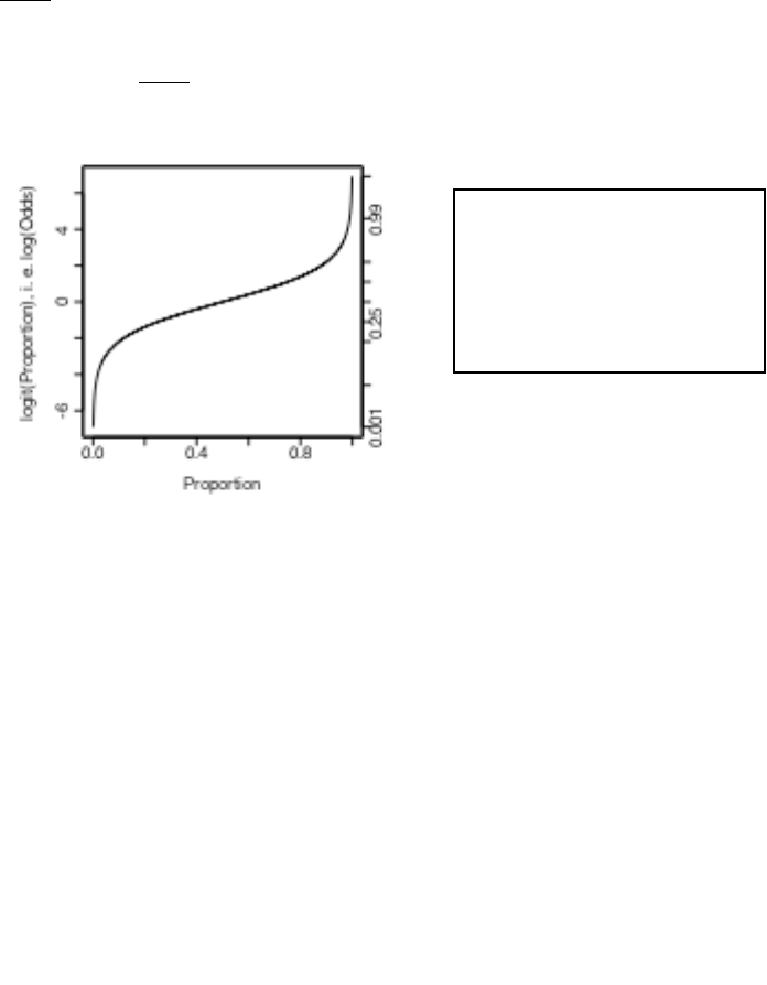
71
!
y=g(
"
1(x1)+
"
2(x2)+....+
"
p(xp)) +
#
Generalized Additive Models are a generalisation of Generalized Linear Models. For example, g(.) may be the
function that undoes the logit transformation, as in a logistic regression model.
Some of
!
z1=
"
1(x1),z2=
"
2(x2),...,zp=
"
p(xp)
may be smoothing functions, while others may be the
usual linear model terms.
We can transform to get the model
!
y=g(z1+z2+...+zp)+
"
Notice that even if p = 1, we may still want to retain both
!
"
1
(.) and g(.), i.e.
!
y=g(
"
1(x1)) +
#
.
The reason is that g(.) is a specific function, such as the inverse of the logit function. The function g(.) does as
much as it can of the task of transformation, with
!
"
1(.)
doing anything more that seems necessary.
The fitting of spline (bs() or ns()) terms in a linear model or a generalized linear model can be a good
alternative to the use of a full generalized additive model.
9.2 Logistic Regression
We will use a logistic regression model as a starting point for discussing Generalized Linear Models.
With proportions that range from less than 0.1 to 0.99, it is not reasonable to expect that the expected proportion
will be a linear function of x. Some such transformation (`link’ function) as the logit is required. A good way
to think about logit models is that they work on a log(odds) scale. If p is a probability (e.g. that horse A will
win the race), then the corresponding odds are p/(1-p), and
log(odds) = log(
!
p
1"p
) = log(p) -log(1-p)
The linear model predicts, not p, but log(
!
p
1"p
). Figure 23 shows the logit transformation.
The logit or log(odds) function turns expected proportions into values that may range from - to +. It is not
satisfactory to use a linear model to predict proportions. The values from the linear model may well lie outside
the range from 0 to 1. It is however in order to use a linear model to predict logit(proportion). The logit
function is an example of a link function.
There are various other link functions that we can use with proportions. One of the commonest is the
complementary log-log function.
Figure 23: The logit or
log(odds) transformation.
Shown here is a plot of
log(odds) versus proportion.
Notice how the range is
stretched out at both ends.
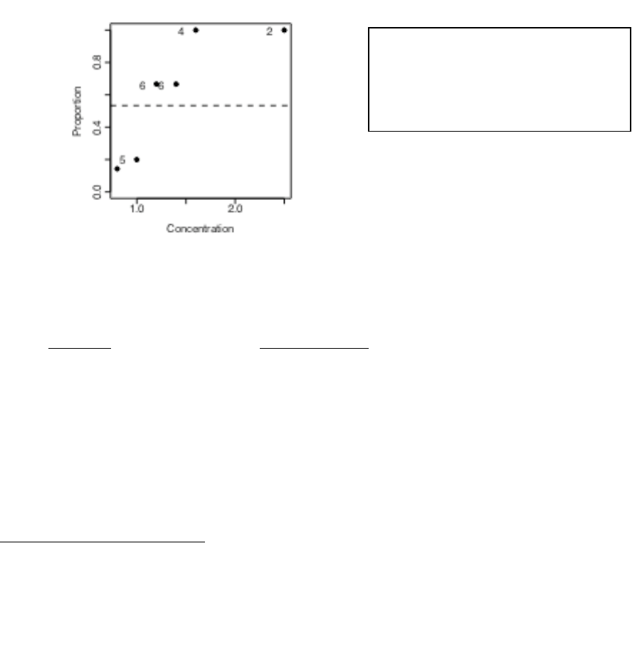
72
9.2.1 Anesthetic Depth Example
Thirty patients were given an anesthetic agent that was maintained at a pre-determined [alveolar] concentration
for 15 minutes before making an incision40. It was then noted whether the patient moved, i.e. jerked or twisted.
The interest is in estimating how the probability of jerking or twisting varies with increasing concentration of
the anesthetic agent.
The response is best taken as nomove, for reasons that will emerge later. There is a small number of
concentrations; so we begin by tabulating proportion that have the nomove outcome against concentration.
Alveolar Concentration
Nomove
0.8
1
1.2
1.4
1.6
2.5
0
6
4
2
2
0
0
1
1
1
4
4
4
2
Total
7
5
6
6
4
2
_____________________________________________
Table 1: Patients moving (0) and not moving (1), for each of
six different alveolar concentrations.
Figure 24 then displays a plot of these proportions.
We fit two models, the logit model and the complementary log-log model. We can fit the models either directly
to the 0/1 data, or to the proportions in Table 1. To understand the output, you need to know about “deviances”.
A deviance has a role very similar to a sum of squares in regression. Thus we have:
Regression
Logistic regression
degrees of freedom
degrees of freedom
sum of squares
deviance
mean sum of squares
(divide by d.f.)
mean deviance
(divide by d.f.)
We prefer models with a small
mean residual sum of squares.
We prefer models with a small
mean deviance.
40 I am grateful to John Erickson (Anesthesia and Critical Care, University of Chicago) and to Alan Welsh (Centre for
Mathematics & its Applications, Australian National University) for allowing me use of these data.
Figure 24: Plot, versus concentration,
of proportion of patients not moving.
The horizontal line estimates the
expected proportion of nomoves if the
concentration had no effect.
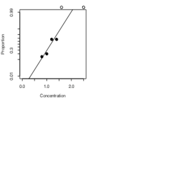
73
If individuals respond independently, with the same probability, then we have Bernoulli trials. Justification for
assuming the same probability will arise from the way in which individuals are sampled. While individuals will
certainly be different in their response the notion is that, each time a new individual is taken, they are drawn at
random from some larger population. Here is the R code:
> anaes.logit <- glm(nomove ~ conc, family = binomial(link = logit),
+ data = anesthetic)
The output summary is:
> summary(anaes.logit)
Call: glm(formula = nomove ~ conc, family = binomial(link = logit),
data = anesthetic)
Deviance Residuals:
Min 1Q Median 3Q Max
-1.77 -0.744 0.0341 0.687 2.07
Coefficients:
Value Std. Error t value
(Intercept) -6.47 2.42 -2.68
conc 5.57 2.04 2.72
(Dispersion Parameter for Binomial family taken to be 1 )
Null Deviance: 41.5 on 29 degrees of freedom
Residual Deviance: 27.8 on 28 degrees of freedom
Number of Fisher Scoring Iterations: 5
Correlation of Coefficients:
(Intercept)
conc -0.981
Fig. 25 is a graphical summary of the results:
Figure 25: Plot, versus concentration, of log(odds) [= logit(proportion)]
of patients not moving. The line is the estimate of the proportion of
moves, based on the fitted logit model.
With such a small sample size it is impossible to do much that is useful to check the adequacy of the model.
Try also plot(anaes.logit).

74
9.3 glm models (Generalized Linear Regression Modelling)
In the above we had
anaes.logit <- glm(nomove ~ conc, family = binomial(link = logit),
data=anesthetic)
The family parameter specifies the distribution for the dependent variable. There is an optional argument that
allows us to specify the link function. Below we give further examples.
9.3.2 Data in the form of counts
Data that are in the form of counts can often be analysed quite effectively assuming the poisson family. The
link that is commonly used here is log. The log link transforms from positive numbers to numbers in the
range - to + that a linear model may predict.
9.3.3 The gaussian family
If no family is specified, then the family is taken to be gaussian. The default link is then the identity, as
for an lm model. This way of formulating an lm type model does however have the advantage that one is not
restricted to the identity link.
# Dataset airquality, from datasets package
air.glm<-glm(Ozone^(1/3) ~ Solar.R + Wind + Temp, data = airquality)
# Assumes gaussian family, i.e. normal errors model
summary(air.glm)
9.4 Models that Include Smooth Spline Terms
These make it possible to fit spline and other smooth transformations of explanatory variables. One can request
a `smooth’ b-spline or n-spline transformation of a column of the X matrix. In place of x one specifies bs(x)or
ns(x). One can control the smoothness of the curve, but often the default works quite well. You need to install
the splines package. R does not at present have a facility for plots that show the contribution of each term to the
model.
9.4.1 Dewpoint Data
The data set dewpoint41 has columns mintemp, maxtemp and dewpoint. The dewpoint values are averages,
for each combination of mintemp and maxtemp, of monthly data from a number of different times and locations.
We fit the model:
dewpoint = mean of dewpoint + smooth(mintemp) + smooth(maxtemp)
Taking out the mean is a computational convenience. Also it provides a more helpful form of output. Here are
details of the calculations:
dewpoint.lm <- lm(dewpoint ~ bs(mintemp) + bs(maxtemp),
data = dewpoint)
options(digits=3)
summary(dewpoint.lm)
9.5 Survival Analysis
For example times at which subjects were either lost to the study or died (“failed”) may be recorded for
individuals in each of several treatment groups. Engineering or business failures can be modelled using this
same methodology. The R survival package has state of the art abilities for survival analysis.
41 I am grateful to Dr Edward Linacre, Visiting Fellow, Geography Department, Australian National University, for making
these data available.

75
9.6 Non-linear Models
You can use nls() (non-linear least squares) to obtain a least squares fit to a non-linear function.
9.7 Model Summaries
Type in
methods(summary)
to get a list of the summary methods that are available. You may want to mix and match, e.g. summary.lm()
on an aov or glm object. The output may not be what you might expect. So be careful!
9.8 Further Elaborations
Generalised Linear Models were developed in the 1970s. They unified a huge range of diverse methodology.
They have now become a stock-in-trade of statistical analysts. Their practical implementation built on the
powerful computational abilities that, by the 1970s, had been developed for handling linear model calculations.
Practical data analysis demands further elaborations. An important elaboration is to the incorporation of more
than one term in the error structure. The R nlme package implements such extensions, both for linear models
and for a wide class of nonlinear models.
Each such new development builds on the theoretical and computational tools that have arisen from earlier
developments. Exciting new analysis tools will continue to appear for a long time yet. This is fortunate. Most
professional users of R will regularly encounter data where the methodology that the data ideally demands is not
yet available.
9.9 Exercises
1. Fit a Poisson regression model to the data in the data frame moths that Accompanies these notes. Allow
different intercepts for different habitats. Use log(meters) as a covariate.
9.10 References
Dobson, A. J. 1983. An Introduction to Statistical Modelling. Chapman and Hall, London.
Hastie, T. J. and Tibshirani, R. J. 1990. Generalized Additive Models. Chapman and Hall, London.
Maindonald J H and Braun W J 2003. Data Analysis and Graphics Using R – An Example-Based Approach.
Cambridge University Press.
McCullagh, P. and Nelder, J. A., 2nd edn., 1989. Generalized Linear Models. Chapman and Hall.
Venables, W. N. and Ripley, B. D., 2nd edn 1997. Modern Applied Statistics with S-Plus. Springer, New York.

76
*10. Multi-level Models, Repeated Measures and Time Series
10.1 Multi-Level Models, Including Repeated Measures Models
Models have both a fixed effects structure and an error structure. For example, in an inter-laboratory comparison
there may be variation between laboratories, between observers within laboratories, and between multiple
determinations made by the same observer on different samples. If we treat laboratories and observers as
random, the only fixed effect is the mean.
The functions lme() and nlme(), from the Pinheiro and Bates nlme package, handle models in which a
repeated measures error structure is superimposed on a linear (lme) or non-linear (nlme) model. Version 3 of
lme is broadly comparable to Proc Mixed in the widely used SAS statistical package. The function lme has
associated with it highly useful abilities for diagnostic checking and for various insightful plots.
There is a strong link between a wide class of repeated measures models and time series models. In the time
series context there is usually just one realisation of the series, which may however be observed at a large
number of time points. In the repeated measures context there may be a large number of realisations of a series
that is typically quite short.
10.1.1 The Kiwifruit Shading Data, Again
Refer back to section 5.8.2 for details of these data. The fixed effects are block and treatment (shade). The
random effects are block (though making block a random effect is optional, for purposes of comparing
treatments), plot within block, and units within each block/plot combination. Here is the analysis:
> library(nlme)
Loading required package: nls
> kiwishade$plot<-factor(paste(kiwishade$block, kiwishade$shade,
sep="."))
> kiwishade.lme<-lme(yield~shade,random=~1|block/plot, data=kiwishade)
> summary(kiwishade.lme)
Linear mixed-effects model fit by REML
Data: kiwishade
AIC BIC logLik
265.9663 278.4556 -125.9831
Random effects:
Formula: ~1 | block
(Intercept)
StdDev: 2.019373
Formula: ~1 | plot %in% block
(Intercept) Residual
StdDev: 1.478639 3.490378
Fixed effects: yield ~ shade
Value Std.Error DF t-value p-value
(Intercept) 100.20250 1.761621 36 56.88086 <.0001
shadeAug2Dec 3.03083 1.867629 6 1.62282 0.1558
shadeDec2Feb -10.28167 1.867629 6 -5.50520 0.0015
shadeFeb2May -7.42833 1.867629 6 -3.97741 0.0073
Correlation:
(Intr) shdA2D shdD2F
shadeAug2Dec -0.53
shadeDec2Feb -0.53 0.50
shadeFeb2May -0.53 0.50 0.50
Standardized Within-Group Residuals:
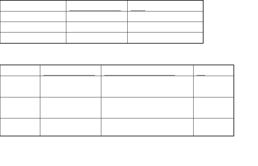
77
Min Q1 Med Q3 Max
-2.4153887 -0.5981415 -0.0689948 0.7804597 1.5890938
Number of Observations: 48
Number of Groups:
block plot %in% block
3 12
> anova(kiwishade.lme)
numDF denDF F-value p-value
(Intercept) 1 36 5190.552 <.0001
shade 3 6 22.211 0.0012
This was a balanced design, which is why section 5.8.2 could use aov(). We can get an output summary that is
helpful for showing how the error mean squares match up with standard deviation information given above thus:
> intervals(kiwishade.lme)
Approximate 95% confidence intervals
Fixed effects:
lower est. upper
(Intercept) 96.62977 100.202500 103.775232
shadeAug2Dec -1.53909 3.030833 7.600757
shadeDec2Feb -14.85159 -10.281667 -5.711743
shadeFeb2May -11.99826 -7.428333 -2.858410
Random Effects:
Level: block
lower est. upper
sd((Intercept)) 0.5473014 2.019373 7.45086
Level: plot
lower est. upper
sd((Intercept)) 0.3702555 1.478639 5.905037
Within-group standard error:
lower est. upper
2.770678 3.490378 4.397024
We are interested in the three sd estimates. By squaring the standard deviations and converting them to
variances we get the information in the following table:
Variance component
Notes
block
2.0192 = 4.076
Three blocks
plot
1.4792= 2.186
4 plots per block
residual (within group)
3.4902=12.180
4 vines (subplots) per plot
The above gives the information for an analysis of variance table. We have:
Variance component
Mean square for anova table
d.f.
block
4.076
12.180 + 4 2.186 + 16 4.076
= 86.14
2
(3-1)
plot
2.186
12.180 + 4 2.186
= 20.92
6
(3-1) (2-1)
residual
(within gp)
12.180
12.18
34(4-1)

78
Now fsee where these same pieces of information appeared in the analysis of variance table of section 5.8.2:
> kiwishade.aov<-aov(yield~block+shade+Error(block:shade),data=kiwishade)
> summary(kiwishade.aov)
Error: block:shade
Df Sum Sq Mean Sq F value Pr(>F)
block 2 172.35 86.17 4.1176 0.074879
shade 3 1394.51 464.84 22.2112 0.001194
Residuals 6 125.57 20.93
Error: Within
Df Sum Sq Mean Sq F value Pr(>F)
Residuals 36 438.58 12.18
10.1.2 The Tinting of Car Windows
In section 4.1 we encountered data from an experiment that aimed to model the effects of the tinting of car
windows on visual performance42. The authors are mainly interested in effects on side window vision, and
hence in visual recognition tasks that would be performed when looking through side windows.
Data are in the data frame tinting. In this data frame, csoa (critical stimulus onset asynchrony, i.e. the time
in milliseconds required to recognise an alphanumeric target), it (inspection time, i.e. the time required for a
simple discrimination task) and age are variables, while tint (3 levels) and target (2 levels) are ordered
factors. The variable sex is coded 1 for males and 2 for females, while the variable agegp is coded 1 for young
people (all in their early 20s) and 2 for older participants (all in the early 70s).
We have two levels of variation – within individuals (who were each tested on each combination of tint and
target), and between individuals. So we need to specify id (identifying the individual) as a random effect.
Plots such as we examined in section 4.1 make it clear that, to get variances that are approximately
homogeneous, we need to work with log(csoa) and log(it). Here we examine the analysis for log(it). We
start with a model that is likely to be more complex than we need (it has all possible interactions):
itstar.lme<-lme(log(it)~tint*target*agegp*sex,
random=~1|id, data=tinting,method="ML")
A reasonable guess is that first order interactions may be all we need, i.e.
it2.lme<-lme(log(it)~(tint+target+agegp+sex)^2,
random=~1|id, data=tinting,method="ML")
Finally, there is the very simple model, allowing only for main effects:
it1.lme<-lme(log(it)~(tint+target+agegp+sex),
random=~1|id, data=tinting,method="ML")
Note that we have fitted all these models by maximum likelihood. This is so that we can do the equivalent of an
analysis of variance comparison. Here is what we get:
> anova(itstar.lme,it2.lme,it1.lme)
Model df AIC BIC logLik Test L.Ratio p-value
itstar.lme 1 26 8.146187 91.45036 21.926906
it2.lme 2 17 -3.742883 50.72523 18.871441 1 vs 2 6.11093 0.7288
it1.lme 3 8 1.138171 26.77022 7.430915 2 vs 3 22.88105 0.0065
42 Data relate to the paper: Burns, N. R., Nettlebeck, T., White, M. and Willson, J. 1999. Effects of car window tinting on
visual performance: a comparison of elderly and young drivers. Ergonomics 42: 428-443.

79
The model that limits attention to first order interactions is adequate. We will need to examine the first order
interactions individually. For this we re-fit the model used for it2.lme, but now with method="REML".
it2.reml<-update(it2.lme,method="REML")
We now examine the estimated effects:
> options(digits=3)
> summary(it2.reml)$tTable
Value Std.Error DF t-value p-value
(Intercept) 6.05231 0.7589 145 7.975 4.17e-13
tint.L 0.22658 0.0890 145 2.547 1.19e-02
tint.Q 0.17126 0.0933 145 1.836 6.84e-02
targethicon -0.24012 0.1010 145 -2.378 1.87e-02
agegp -1.13449 0.5167 22 -2.196 3.90e-02
sex -0.74542 0.5167 22 -1.443 1.63e-01
tint.L.targethicon -0.09193 0.0461 145 -1.996 4.78e-02
tint.Q.targethicon -0.00722 0.0482 145 -0.150 8.81e-01
tint.L.agegp -0.13075 0.0492 145 -2.658 8.74e-03
tint.Q.agegp -0.06972 0.0520 145 -1.341 1.82e-01
tint.L.sex 0.09794 0.0492 145 1.991 4.83e-02
tint.Q.sex -0.00542 0.0520 145 -0.104 9.17e-01
targethicon.agegp 0.13887 0.0584 145 2.376 1.88e-02
targethicon.sex -0.07785 0.0584 145 -1.332 1.85e-01
agegp.sex 0.33164 0.3261 22 1.017 3.20e-01
Because tint is an ordered factor, polynomial contrasts are used.
10.1.3 The Michelson Speed of Light Data
Here is an example, using the Michelson speed of light data from the Venables and Ripley MASS package. The
model allows the determination to vary linearly with Run (from 1 to 20), with the slope varying randomly
between the five experiments of 20 runs each. We assume an autoregressive dependence structure of order 1.
We allow the variance to change from one experiment to another. Maximum likelihood tests suggest that one
needs at least this complexity in the variance and dependence structure to represent the data accurately. A model
that has neither fixed nor random Run effects seems all that is justified statistically. To test this, one needs to fit
models with and without these effects, setting method=”ML” in each case, and compare the likelihoods. (I
leave this as an exercise!) For purposes of doing this test, a first order autoregressive model would probably be
adequate. A model that ignores the sequential dependence entirely does give misleading results.
> library(MASS) # if needed
> michelson$Run <- as.numeric(michelson$Run) # Ensure Run is a variable
> mich.lme1 <- lme(fixed = Speed ~ Run, data = michelson,
random = ~ Run| Expt, correlation = corAR1(form = ~ 1 | Expt),
weights = varIdent(form = ~ 1 | Expt))
> summary(mich.lme1)
Linear mixed-effects model fit by REML
Data: michelson
AIC BIC logLik
1113 1142 -546
Random effects:
Formula: ~Run | Expt
Structure: General positive-definite
StdDev Corr
(Intercept) 46.49 (Intr)

80
Run 3.62 -1
Residual 121.29
Correlation Structure: AR(1)
Formula: ~1 | Expt
Parameter estimate(s):
Phi
0.527
Variance function:
Structure: Different standard deviations per stratum
Formula: ~1 | Expt
Parameter estimates:
1 2 3 4 5
1.000 0.340 0.646 0.543 0.501
Fixed effects: Speed ~ Run
Value Std.Error DF t-value p-value
(Intercept) 868 30.51 94 28.46 <.0001
Run -2 2.42 94 -0.88 0.381
Correlation:
(Intr)
Run -0.934
Standardized Within-Group Residuals:
Min Q1 Med Q3 Max
-2.912 -0.606 0.109 0.740 1.810
Number of Observations: 100
Number of Groups: 5
10.2 Time Series Models
The R stats package has a number of functions for manipulating and plotting time series, and for calculating the
autocorrelation function.
There are (at least) two types of method – time domain methods and frequency domain methods. In the time
domain models may be conventional “short memory” models where the autocorrelation function decays quite
rapidly to zero, or the relatively recently developed “long memory” time series models where the
autocorrelation function decays very slowly as observations move apart in time. A characteristic of “long
memory” models is that there is variation at all temporal scales. Thus in a study of wind speeds it may be
possible to characterise windy days, windy weeks, windy months, windy years, windy decades, and perhaps
even windy centuries. R does not yet have functions for fitting the more recently developed long memory
models.
The function stl() decomposes a times series into a trend and seasonal components, etc. The functions ar()
(for “autoregressive” models) and associated functions, and arima0() ( “autoregressive integrated moving
average models”) fit standard types of time domain short memory models. Note also the function gls() in the
nlme package, which can fit relatively complex models that may have autoregressive, arima and various other
types of dependence structure.
The function spectrum() and related functions is designed for frequency domain or “spectral” analysis.
10.3 Exercises
1. Use the function acf() to plot the autocorrelation function of lake levels in successive years in the data set
huron. Do the plots both with type=”correlation” and with type=”partial”.

81
10.4 References
Chambers, J. M. and Hastie, T. J. 1992. Statistical Models in S. Wadsworth and Brooks Cole Advanced Books
and Software, Pacific Grove CA.
Diggle, Liang & Zeger 1996. Analysis of Longitudinal Data. Clarendon Press, Oxford.
Everitt, B. S. and Dunn, G. 1992. Applied Multivariate Data Analysis. Arnold, London.
Hand, D. J. & Crowder, M. J. 1996. Practical longitudinal data analysis. Chapman and Hall, London.
Little, R. C., Milliken, G. A., Stroup, W. W. and Wolfinger, R. D. (1996). SAS Systems for Mixed Models. SAS Institute
Inc., Cary, New Carolina.
Maindonald J H and Braun W J 2003. Data Analysis and Graphics Using R – An Example-Based Approach.
Cambridge University Press.
Pinheiro, J. C. and Bates, D. M. 2000. Mixed effects models in S and S-PLUS. Springer, New York.
Venables, W. N. and Ripley, B. D., 2nd edn 1997. Modern Applied Statistics with S-Plus. Springer, New York.

82
*11. Advanced Programming Topics
11.1. Methods
R is an object-oriented language. Objects may have a “class”. For functions such as print(), summary(),
etc., the class of the object determines what action will be taken. Thus in response to print(x), R determines
the class attribute of x, if one exists. If for example the class attribute is “factor”, then the function which
finally handles the printing is print.factor(). The function print.default() is used to print objects that
have not been assigned a class.
More generally, the class attribute of an object may be a vector of strings. If there are “ancestor” classes –
parent, grandparent, . . ., these are specified in order in subsequent elements of the class vector. For example,
ordered factors have the class “ordered”, which inherits from the class “factor”. Thus:
> fac<-ordered(1:3)
> class(fac)
[1] "ordered" "factor"
Here fac has the class “ordered”, which inherits from the parent class “factor”.
The function print.ordered(), which is the function that is called when you invoke print() with an
ordered factor, could be rewritten to use the fact that “ordered” inherits from “factor”, thus:
> print.ordered
function (x, quote = FALSE)
{
if (length(x) <= 0)
cat("ordered(0)\n")
else NextMethod(“print”)
cat("Levels: ", paste(levels(x), collapse = " < "), "\n")
invisible(x)
}
The system version of print.ordered() does not use print.factor(). The function print.glm() does
not call print.lm(), even though glm objects inherit from lm objects. The mechanism is avaialble for use if
required.
11.2 Extracting Arguments to Functions
How, inside a function, can one extract the value assigned to a parameter when the function was called? Below
there is a function extract.arg(). When it is called as extract.arg(a=xx), we want it to return “xx”.
When it is called as extract.arg(a=xy), we want it to return “xy”. Here is how it is done.
extract.arg <-
function (a)
{
s <- substitute(a)
as.character(s)
}
> extract.arg(a=xy)
[1] “xy”
If the argument is a function, we may want to get at the arguments to the function. Here is how one can do it
deparse.args <-
function (a)
{
s <- substitute (a)
if(mode(s) == "call"){

83
# the first element of a 'call' is the function called
# so we don't deparse that, just the arguments.
print(paste(“The function is: “, s[1],”()”, collapse=””))
lapply (s[-1], function (x)
paste (deparse(x), collapse = "\n"))
}
else stop ("argument is not a function call")
}
For example:
> deparse.args(list(x+y, foo(bar)))
[1] "The function is: list ()"
[[1]]
[1] "x + y"
[[2]]
[1] "foo(bar)"
11.3 Parsing and Evaluation of Expressions
When R encounters an expression such as mean(x+y) or cbind(x,y), there are two steps:
The text string is parsed and turned into an expression, i.e. the syntax is checked and it is turned into code that
the R computing engine can more immediately evaluate.
The expression is evaluated.
Upon typing in
expression(mean(x+y))
the output is the unevaluated expression expression(mean(x+y)). Setting
my.exp <- expression(mean(x+y))
stores this unevaluated expression in my.exp . The actual contents of my.exp are a little different from what is
printed out. R gives you as much information as it thinks helpful.
Note that expression(mean(x+y)) is different from expression(“mean(x+y)”), as is obvious when the
expression is evaluated. A text string is a text string is a text string, unless one explicitly changes it into an
expression or part of an expression.
Let’s see how this works in practice
> x <- 101:110
> y <- 21:30
> my.exp <- expression(mean(x+y))
> my.txt <- expression("mean(x+y)")
> eval(my.exp)
[1] 131
> eval(my.txt)
[1] "mean(x+y)"
What if we already have “mean(x+y)” stored in a text string, and want to turn it into an expression? The
answer is to use the function parse(), but indicate that the parameter is text rather than a file name. Thus
> parse(text="mean(x+y)")
expression(mean(x + y))
We store the expression in my.exp2, and then evaluate it
> my.exp2 <- parse(text="mean(x+y)")
> eval(my.exp2)
[1] 131

84
Here is a function that creates a new data frame from an arbitrary set of columns of an existing data frame.
Once in the function, we attach the data frame so that we can leave off the name of the data frame, and use only
the column names
make.new.df <- function(old.df = austpop, colnames = c("NSW", "ACT"))
{
attach(old.df)
on.exit(detach(old.df))
argtxt <- paste(colnames, collapse = ",")
exprtxt <- paste("data.frame(", argtxt, ")", sep = "")
expr <- parse(text = exprtxt)
df <- eval(expr)
names(df) <- colnames
df
}
To verify that the function does what it should, type in
> make.new.df()
NSW ACT
1 1904 3
. . . .
The function do.call() makes it possible to supply the function name and the argument list in separate text
strings. When do.call is used it is only necessary to use parse() in generating the argument list.
For example
make.new.df <-
function(old.df = austpop, colnames = c("NSW", "ACT"))
{
attach(old.df)
on.exit(detach(old.df))
argtxt <- paste(colnames, collapse = ",")
listexpr <- parse(text=paste("list(", argtxt, ")", sep = ""))
df <- do.call(“data.frame”, eval(listexpr))
names(df) <- colnames
df
}
11.4 Plotting a mathematical expression
The following, given without explanation, illustrates some of the possibilities. It needs better error checking
than it has at present:
plotcurve <-
function(equation = "y = sqrt(1/(1+x^2))", ...){
leftright <- strsplit(equation, split = "=")[[1]]
left <- leftright[1] # The part to the left of the "="
right <- leftright[2] # The part to the right of the "="
expr <- parse(text=right)
xname <- all.vars(expr)
if(length(xname) > 1)stop(paste("There are multiple variables, i.e.",paste(xname,
collapse=" & "),
"on the right of the equation"))
if(length(list(...))==0)assign(xname, 1:10)
else {
nam <- names(list(...))
if(nam!=xname)stop("Clash of variable names")

85
assign("x", list(...)[[1]])
assign(xname, x)
}
y <- eval(expr)
yexpr <- parse(text=left)[[1]]
xexpr <- parse(text=xname)[[1]]
plot(x, y, ylab = yexpr, xlab = xexpr, type="n")
lines(spline(x,y))
mainexpr <- parse(text=paste(left, "==", right))
title(main = mainexpr)
}
Try
plotcurve()
plotcurve("ang=asin(sqrt(p))", p=(1:49)/50)
11.5 Searching R functions for a specified token.
A token is a syntactic entity; for example function names are tokens. For example, we search all functions in the
working directory. The purpose of using unlist() in the code below is to change myfunc from a list into a
vector of character strings.
mygrep <-
function(str)
{
## Assign the names of all objects in current R
## working directory to the string vector tempobj
##
tempobj <- ls(envir=sys.frame(-1))
objstring <- character(0)
for(i in tempobj) {
myfunc <- get(i)
if(is.function(myfunc))
if(length(grep(str,
deparse(myfunc))))
objstring <- c(objstring, i)
}
return(objstring)
}
mygrep(“for”) # Find all functions that include a for loop

86
12. Appendix 1
12.1 R Packages for Windows
To get information on R packages, go to:
http://cran.r-project.org
The Australian link (accessible only to users in Australia) is:
http://mirror.aarnet.edu.au/pub/CRAN/
For Windows 95 etc binaries, look in
http://mirror.aarnet.edu.au/pub/CRAN/windows/windows-9x/
Look in the directory contrib for packages.
New packages are being added all the time. So it pays to check the CRAN site from time to time. Also, watch
for announcements on the electronic mailing lists r-help and r-announce.
12.2 Contributed Documents and Published Literature
Dalgaard, P. 2002. Introductory Statistics with R. Springer, New York.
[This is an R-based introductory text, with a biostatistical emphasis.]
Maindonald J H and Braun W J 2008. Data Analysis and Graphics Using R – An Example-Based Approach, 2nd
edn. Cambridge University Press.
[This is an intermediate level text.]
Venables, W. N. and Ripley, B. D., 4th edn 2002. Modern Applied Statistics with S. Springer, NY.
[This has become a text book for the use of S-PLUS and R for applied statistical analysis. It assumes a fair level of
statistical sophistication. Explanation is careful, but often terse. Together with the ‘Complements’ it gives brief
introductions to extensive packages of functions that have been written or adapted by Ripley, Venables, and a number of
other statisticians.
For other books and literature, see
http://www.r-project.org/doc/bib/R-books.html
http://www.r-project.org/doc/bib/R-other.html
12.3 Data Sets Referred to in these Notes
Data sets included in the image file usingR.RData
Cars93.summary
ais
anesthetic
austpop
beams
dewpoint
dolphins
elasticband
florida
hills
huron
islandcities
kiwishade
leafshape
milk
moths
oddbooks
orings
possum
primates
rainforest
seedrates
tinting
All of these datasets, except beams, florida, huron and islandcities, are in the DAAG package. The units
of time for hills are however hours (not minutes) in DAAG.
Data Sets from Package datasets
airquality
attitude
cars
Islands
LakeHuron
Data Sets from Package MASS
Aids2
Animals
Cars93
PlantGrowth
Rubber
cement
cpus
fgl
michelson
mtcars

87
painters
pressure
ships
Data Set from Package lattice
barley
12.4 Answers to Selected Exercises
Section 1.6
1. plot(distance~stretch,data=elasticband)
2. (ii), (iii), (iv)
plot(snow.cover ~ year, data = snow)
hist(snow$snow.cover)
hist(log(snow$snow.cover))
Section 2.7
1. The value of answer is (a) 12, (b) 22, (c) 600.
2. prod(c(10,3:5))
3(i) bigsum <- 0; for (i in 1:100) {bigsum <- bigsum+i }; bigsum
3(ii) sum(1:100)
4(i) bigprod <- 1; for (i in 1:50) {bigprod <- bigprod*i }; bigprod
4(ii) prod(1:50)
5. radius <- 3:20; volume <- 4*pi*radius^3/3
sphere.data <- data.frame(radius=radius, volume=volume)
6. sapply(tinting, is.factor)
sapply(tinting[, 4:6], levels)
sapply(tinting[, 4:6], is.ordered)
Section 3.9
2. par(mfrow = c(1,2))
plot(Animals$body, Animals$brain, pch=1,
xlab="Body weight (kg)",ylab="Brain weight (g)")
plot(log(Animals$body),log(Animals$brain),pch=1,
xlab="Body weight (kg)", ylab="Brain weight (g)", axes=F)
brainaxis <- 10^seq(-1,4)
bodyaxis <-10^seq(-2,4)
axis(1, at=log(bodyaxis), lab=bodyaxis)
axis(2, at=log(brainaxis), lab=brainaxis)
box()
identify(log(Animals$body), log(Animals$brain), labels=row.names(Animals))
Section 7.9
1. x <- seq(101,112) or x <- 101:112
2. rep(c(4,6,3),4)
3. c(rep(4,8),rep(6,7),rep(3,9)) or rep(c(4,6,3),c(8,7,9))
mat64 <- matrix(c(rep(4,8),rep(6,7),rep(3,9)), nrow=6, ncol=4)

88
4. rep(seq(1,9),seq(1,9)) or rep(1:9, 1:9)
6. (a) Use summary(airquality) to get this information.
(b) airquality[airquality$Ozone == max(airquality$Ozone),]
(c) airquality$Wind[airquality$Ozone > quantile(airquality$Ozone, .75)]
7. mean(snow$snow.cover[seq(2,10,2)])
mean(snow$snow.cover[seq(1,9,2)])
9. summary(attitude); summary(cpus)
Comment on ranges of values, whether distributions seem skew, etc.
10. mtcars6<-mtcars[mtcars$cyl==6,]
11. Cars93[Cars93$Type==”Small”|Cars93$Type==”Sporty”,]
