Ensight 10.2 Advanced Training September 2017 Presentation User Manual En Sight
2017-09-26
User Manual: Ensight Ensight 10.2 Advanced Training - September 2017 EnSight 10.2 Advanced Training - September 2017 EnSight 10.2 Training CEI Detroit www3.ensight.com 3:
Open the PDF directly: View PDF ![]() .
.
Page Count: 213 [warning: Documents this large are best viewed by clicking the View PDF Link!]
EnSight 10.2 Advanced Training
Martin J. Faber –Sr. Account Manager, North America

EnSight 10 Advanced Training Overview 1 2
More EnSight Basics
Client-Server architecture, EnSight processes,
global shading and hidden lines overlay, 4 icons on the
right (display information, variable legend visibility,
record animation, fast display), EnSight modes
Parts and the Quick Edit Menu
Line width, visibility per viewport, element
representations, displacements, visual symmetry,
element labeling, parts filter elements, element
blanking, shaded and hidden line mode, auxiliary
clipping, fast display representation
Solution Time and Flipbook
Time and advanced tab, discrete or continuous,
record an animation, flipbook load and run tab,
objects and images, 4 types of data, record a flipbook
Pathlines (Transient Streamlines)
Pathlines introduction, creating pathlines, displaying
pathlines, displaying pathline particle traces
Copy, Clone and Tag
Part duplicating, when to use each one, create a part
copy, create a part clone, part tagging, how to

EnSight 10 Advanced Training Overview 2 3
Plots
Curve/graph visibility, show graph in separate
window, graph attributes, axis attributes, curve
attributes, select/delete graphs
More Part Creation
Contours, vector arrows, elevated surface, separation
& attachment lines, vortex cores
Create/Edit Viewports
Viewport overview, linking viewports, exchange with
largest viewport, background color, border and
location, bounds visibility, special attributes, viewport
layouts, new viewport, pop/push viewports
Texture Mapping and Skybox
Background of texture mapping, using decals, loading
and Z-axis projection, repeat mode, texture mode,
update the plane tool, using patterns, modulate,
background of a skybox, box tool, skybox picture
layout
The Keyframe Animator
Keyframe animation basics, quick animations,
keyframe animation examples, run attributes,
animating a clip plane, recording a KF animation, tips
and tricks, examples

EnSight 10 Advanced Training Overview 3 4
Using Predefined Materials
Materials library overview, materials assignment
example, lighting and shading per material, style
feature to copy materials, notes about the materials
library, using materials on the Chevy Traverse, Chevy
Traverse animation
Using Multiple Light Sources
Multiple light sources overview, types of light, notes
about light sources, example of using multiple light
sources, default light vs 3 light sources
Ray Tracing
Ray Tracing basics, creating a Ray Traced image,
creating auxiliary geometry, wheel - Whitted quality
3, wheel - Ambient Occlusion quality 3, Ray Traced
images comparison, Chevy Traverse –Whitted quality
3, Chevy Traverse –Ambient Occlusion quality 3
The Transformation Editor
Global transformation, Z-clipping, tools: cursor, line,
plane & quadratic, center of transform

EnSight 10 Advanced Training Overview 3 5
Create & Edit Attributes (Parts)
Several categories of attributes, full control
of all features
Case Linking
How to, operation, viewport capabilities, toggle full
view, viewport exchange, case linking off, notes
Annotations
Text strings, lines, 2D shapes, 3D arrow with text,
dials, bar gauges, logos, legends, select, delete
Actions that will Slow Down your
System
Hidden line display, opacity, element representation,
keyframe animation, anti-aliasing, high resolution,
label display
6
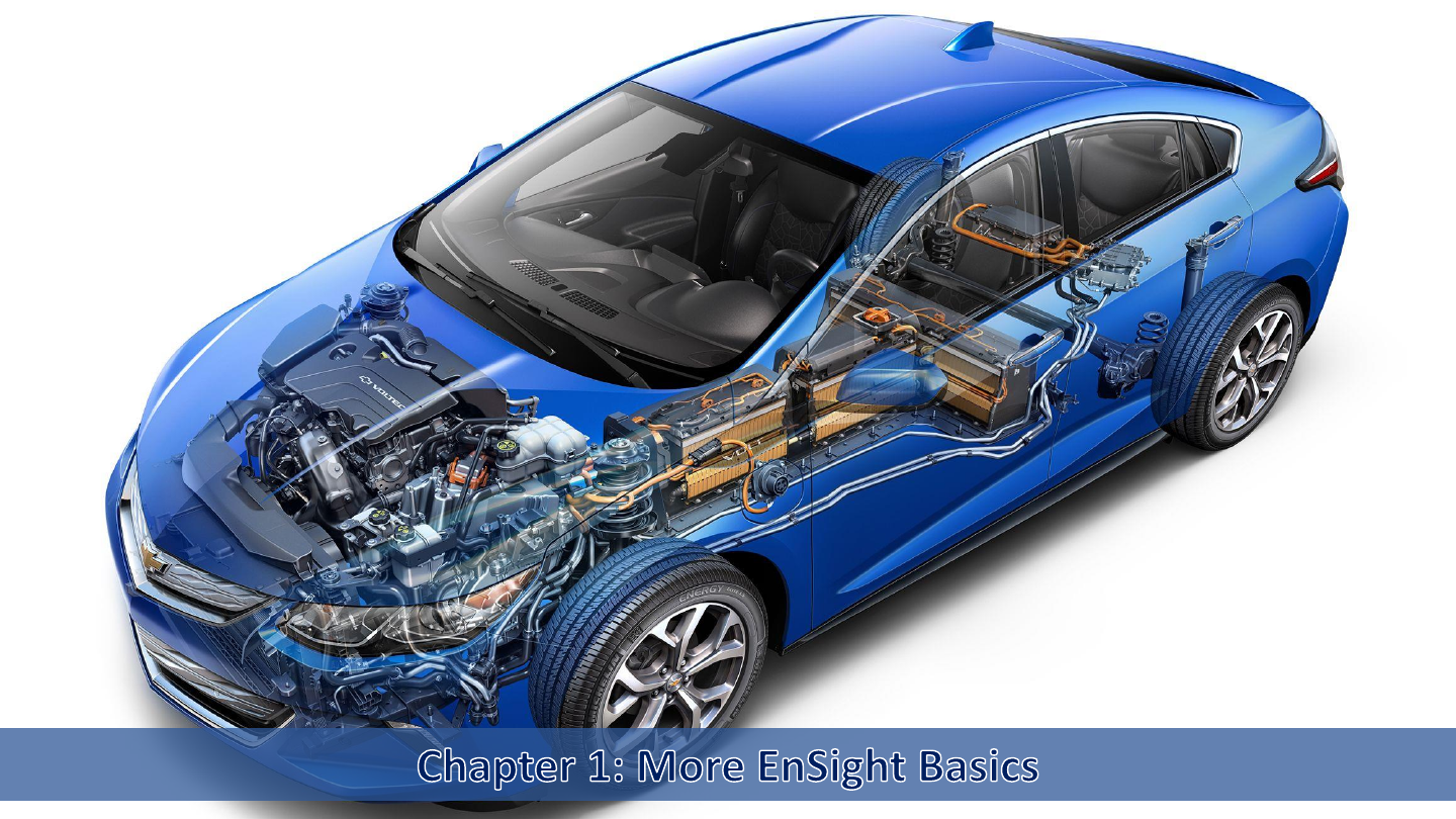
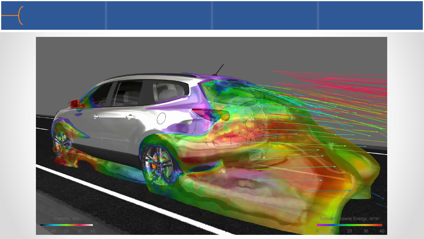
2017 Chevrolet Volt Cutaway Drawing
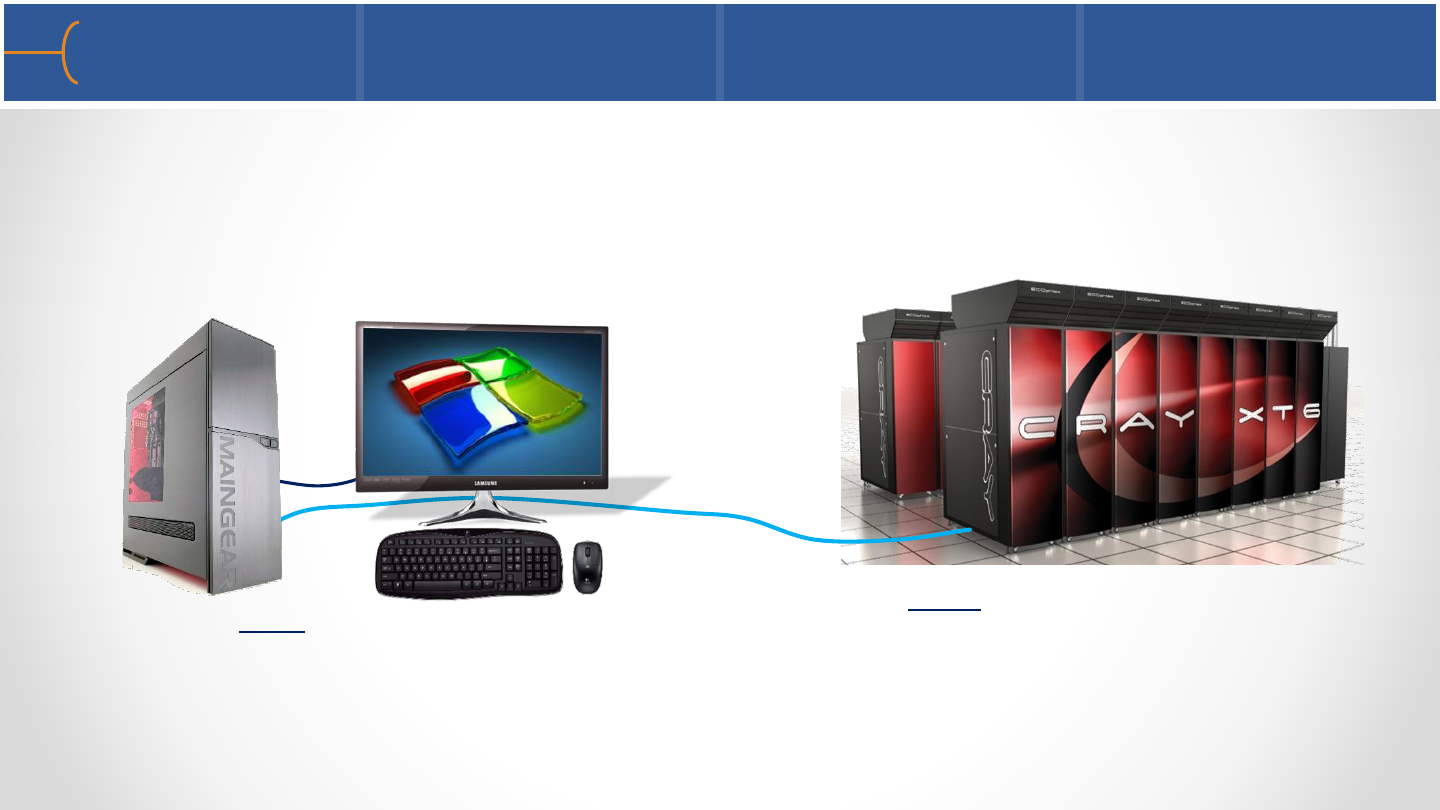
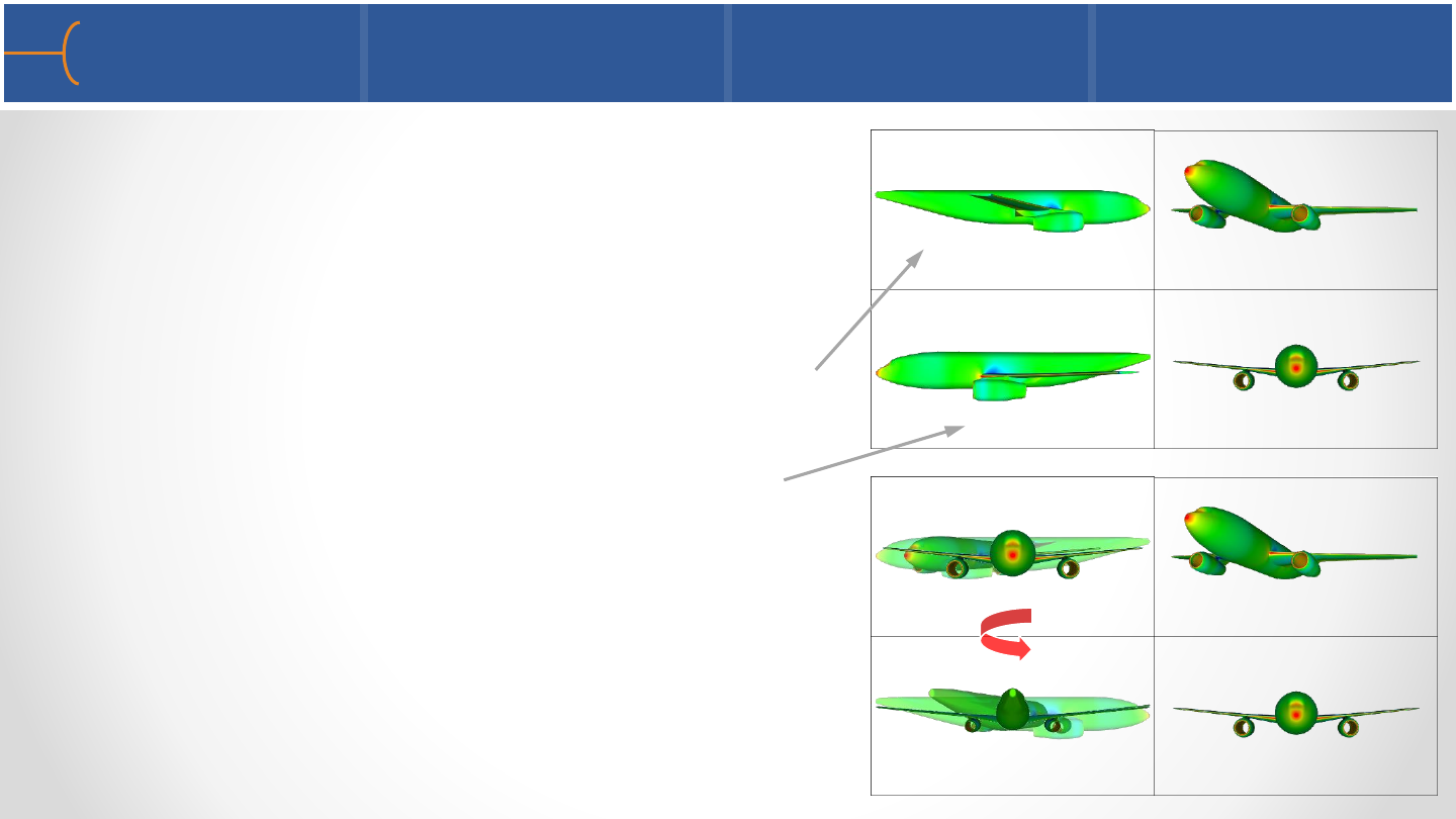
Client Server Architecture 1 7
•EnSight works on a client-server architecture that distributes the workloads
between the client and one or more servers –this architecture leaves the data
where it was computed; if EnSight is run on a single computer, both client and
server are run on that machine
•The GUI (Graphical User Interface) and graphics are handled by the Client; the
Server takes care of all data and the data extraction algorithms; the Server can be
local or remote
Server (cluster): all data, extraction
algorithms; local or remote
Client (GUI & all graphics)
network cable

•When an icon is clicked on the Feature Icon Bar, for instance to create streamlines,
the Client sends a request to the Server to calculate streamlines
•The Server responds by calculating the streamlines and sends back the 3D objects;
the Client then updates the display
Client Server Architecture 2 8
network cable
Requests
3D Objects
Client Server
Client Server Architecture 3 9
•When an icon is selected on the EnSight Feature Toolbar, an action is triggered
mainly on the Server
•When an icon is selected on the Quick Edit Menu, an action is triggered on the
Client
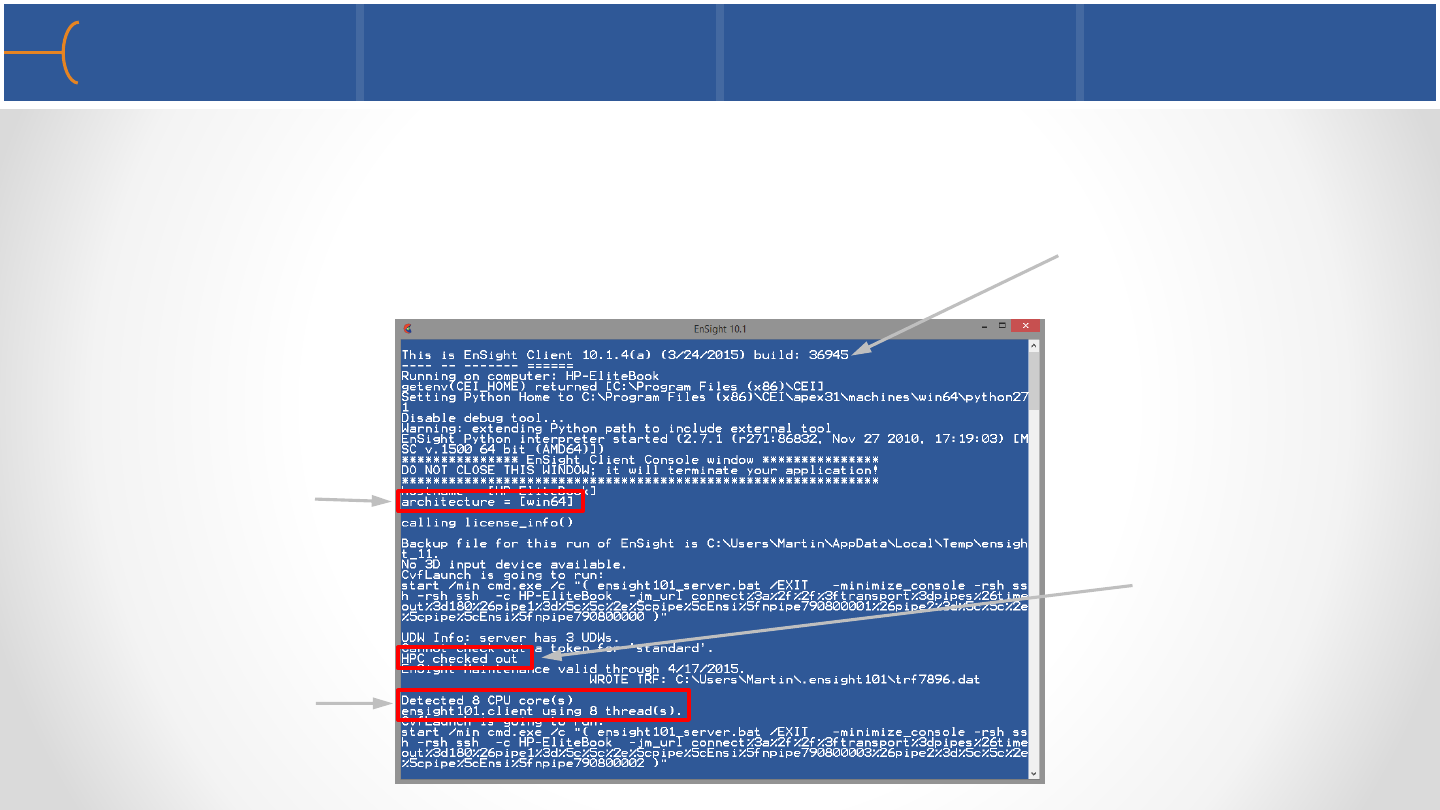
EnSight Processes 1 10
•When EnSight is started in Windows, an EnSight Client Console window is opened
that starts the Client process; as soon as the Client process is running and the
EnSight window with the GUI appears, the EnSight Client Console window is
minimized (it can be opened though)
Number of CPU’s
detected and number of
threads that are being
used
Runs in 64-bit mode
EnSight HPC
license checked
out
EnSight Processes 2 11
•As soon as the Client process is running, EnSight will start another Console window
for the Server process, similar to the EnSight Client Console window; this window
will also automatically be minimized (it can be opened as well)
•During normal operation, EnSight will use 1 Client process and 1 Server process;
when a second model (case) is loaded, EnSight will start a second Server process
for the second case; this means EnSight can connect a single Client to multiple
Servers at the same time, with each Server maintaining a unique dataset
Server Server
Client
Two
Cases
Server
Client
One
Case
•Should the client cease to work (in case of a crash), one or more server processes
are most likely still running; by closing the EnSight Console Server window, the
EnSight Server process will also be shut down
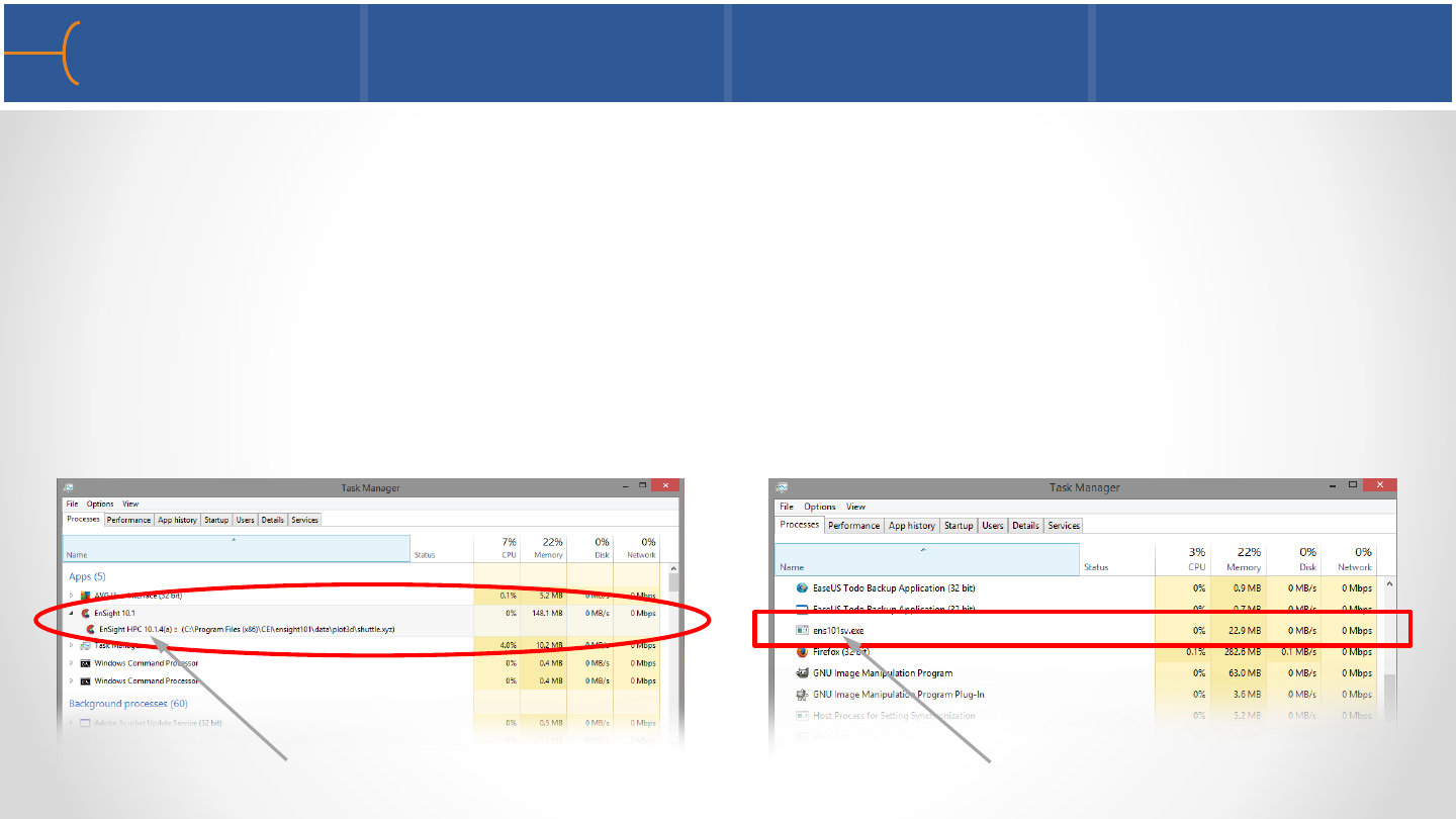
•When EnSight is running, the Task Manager (Ctrl-Shift-Esc) in Windows (ps
command in Linux) will show both Client and Server processes running at the
same time (the Task Manager of Windows 8.1 is shown below)
EnSight Processes 3 12
EnSight Server Process: ens101sv.exeEnSight Client Process: ens101cl.exe
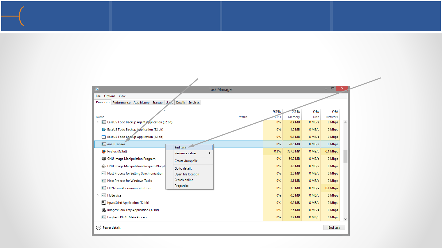
•The Task Manager in Windows (the kill command in Linux) can also be used to end
a lone EnSight Server process because it can slow down the system: Task Manager
-> Processes and left-click ens101sv.exe, then right-click and select End Task
EnSight Processes 4 13
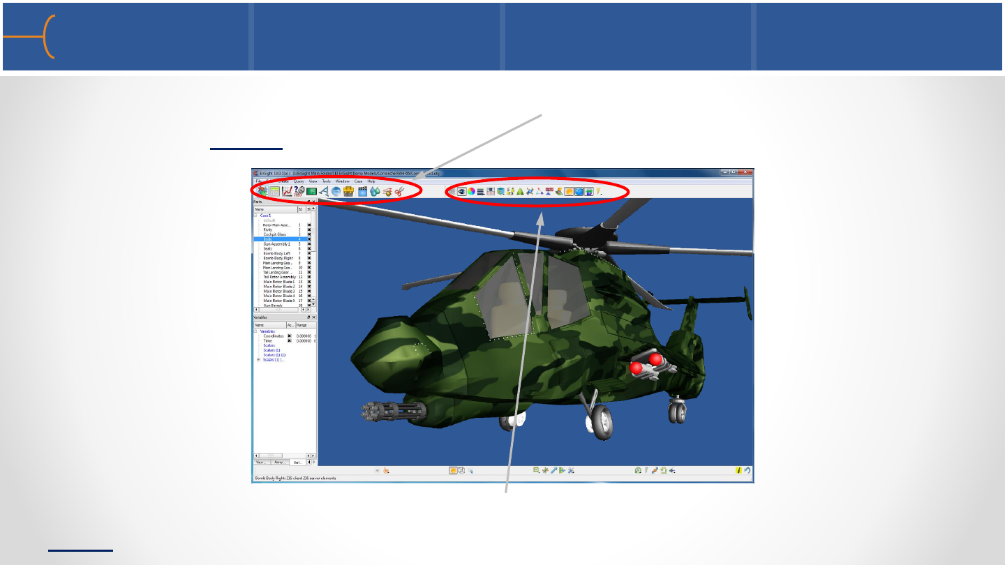
Global Shading and Hidden Lines 1 14
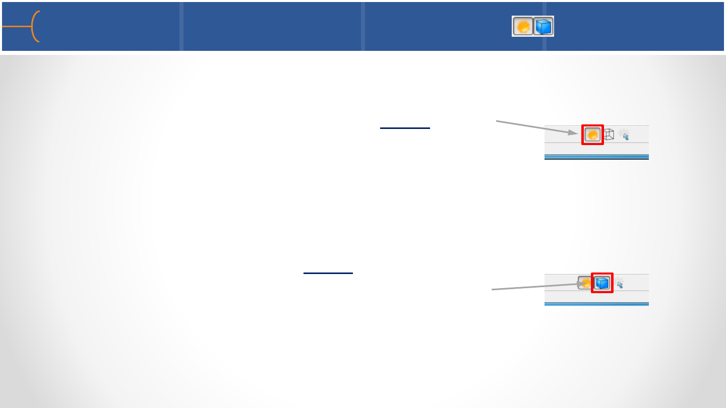
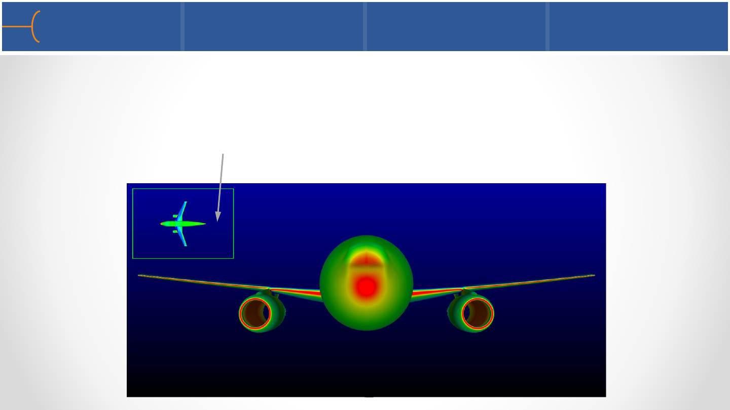
•On the Quick Settings Menu are 2 important icons:
oThe one with the icon of the sun is the global Display
Shaded Surfaces; this button is on by default and
when it is switched off there will be no shaded
surfaces displayed in EnSight, just wireframe; this
can also be toggled through View -> Shaded
oTo the right of this icon is the global Overlay Hidden
Lines icon that is switched off by default; this toggle
enables or disables hidden line mode; this can also
be toggled through View -> Hidden line
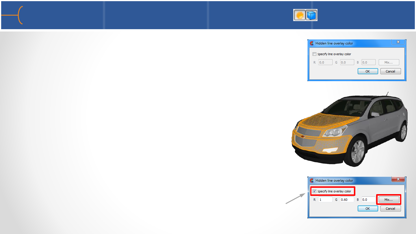
Global Shading and Hidden Lines 2 15
•If the current mode is Shaded when Overlay Hidden Lines
icon is toggled on, the Hidden Line Overlay dialog is
displayed; on this dialog a color for the overlay edges can
be specified
•If the Specify Line Overlay Color toggle is not enabled,
the overlay color will be set to the native color of each
part; if it is enabled, the color can be specified either by
entering red, green or blue color values or by clicking the
Mix... button and selecting a color from the palette
Delphi 3D Digital Instrument Cluster
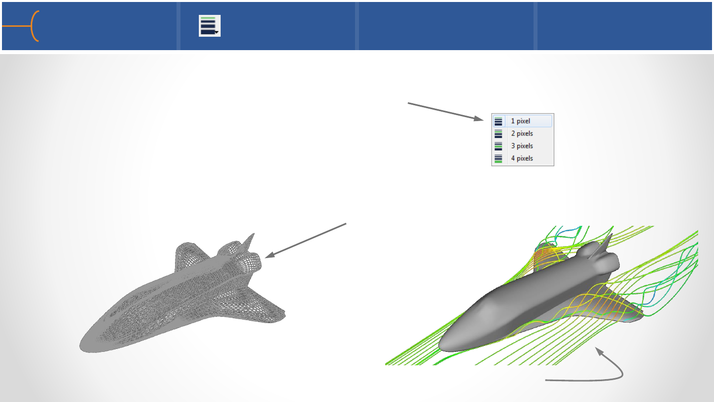
•The Line Width icon on the Quick Edit Menu controls the line width (in pixels) of
any part; by default it is set to a width of 1 pixel; this icon will update to reflect
attribute changes
•When displaying for instance the Shuttle model in wireframe, the width of the
wireframe can be adjusted; in this example from 1 to 3 pixels
•In this example the streamlines are adjusted from 1 to 4 pixels
Line Width 17
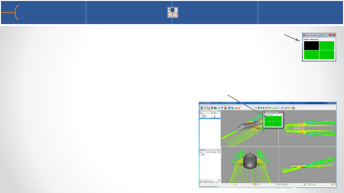
Visibility per Viewport 18
•The Visibility per Viewport icon controls whether a part is visible in
a certain viewport or not; black means the selected part is not visible
•When multiple viewports are used this feature will display a thumbnail of the
viewports; click on the thumbnails to make a part visible or invisible in a particular
viewport
•In this example the streamlines in the top
left viewport are not displayed; by selecting
the thumbnail on the menu the streamlines
can be displayed
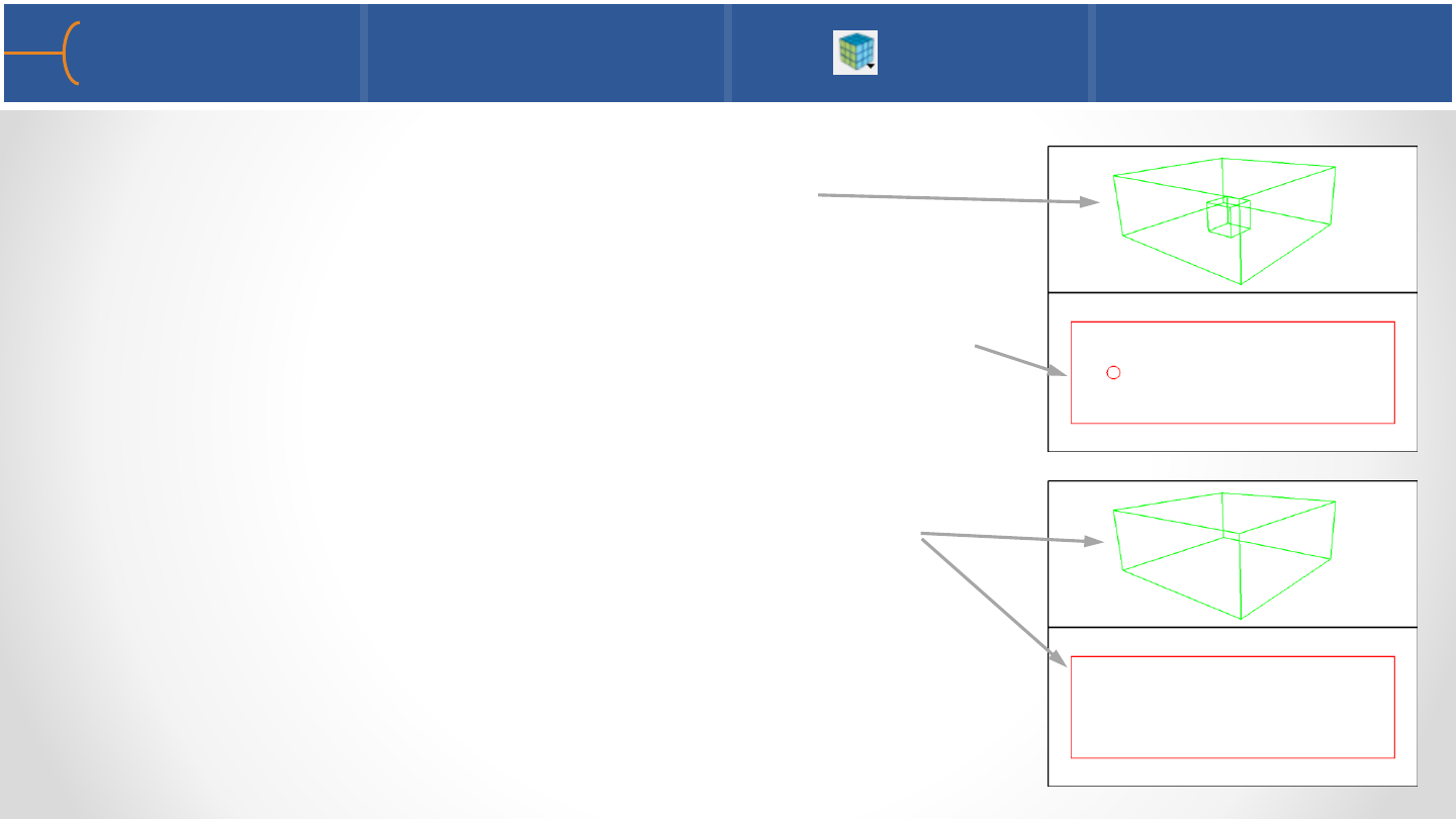
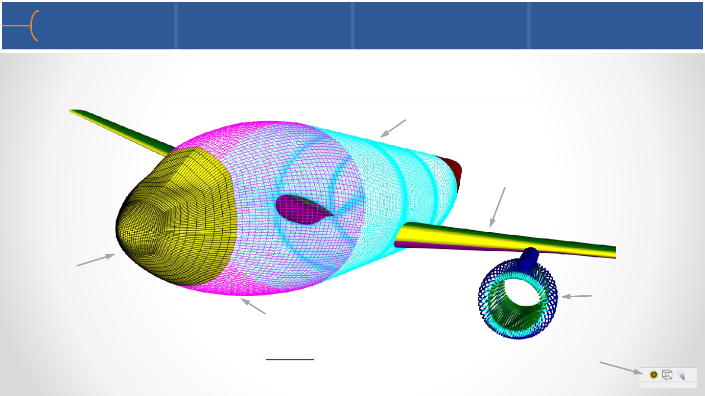
Element Representations 1 19
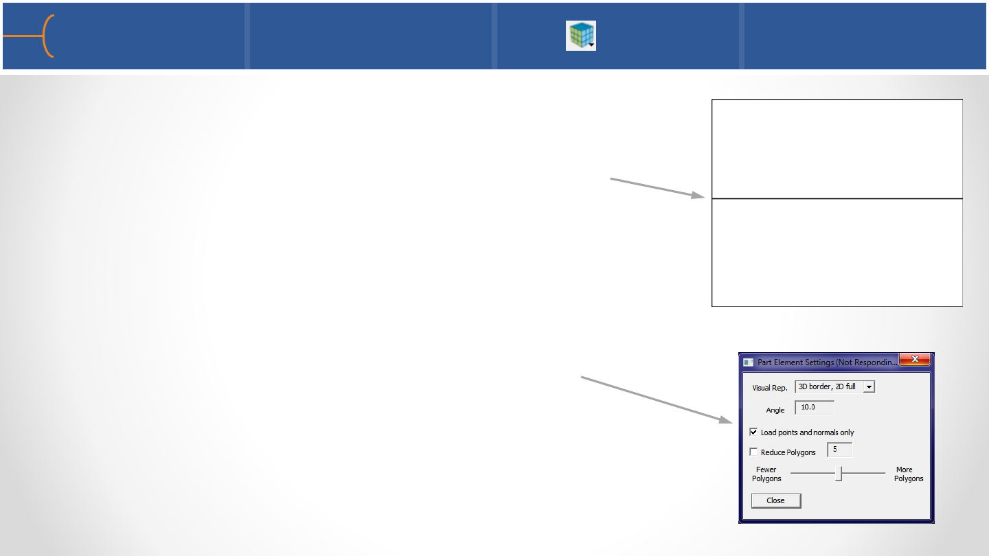
•Click the Part Element Settings icon to change the way a part is displayed; the
following menu appears:
•The default setting is 3D border, 2D full; this means a 3D element will only be
displayed by its border lines (no internal element lines will be shown) and a 2D
element will be fully displayed
•This does not modify a part’s geometry, just how it is displayed on the screen
•3D Border, 2D Full (default)
o3D elements are displayed in border mode
o2D elements are displayed in full representation
mode
•3D Feature, 2D Full
o3D elements are displayed in feature mode
o2D elements are displayed in full representation
mode
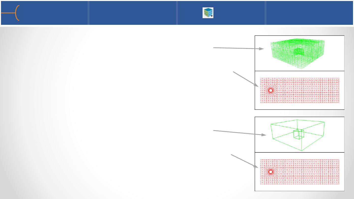
Element Representations 2 20
3D elements
2D elements
3D elements
2D elements
•3D NonVisual, 2D
oFull 3D elements are not loaded
o2D elements are displayed in full representation
mode
•Border
oShared faces (3D elements) are removed
oShared edges (2D elements) are removed
Element Representations 3 21
3D elements
2D elements
3D elements
2D elements
Element Representations 4 22
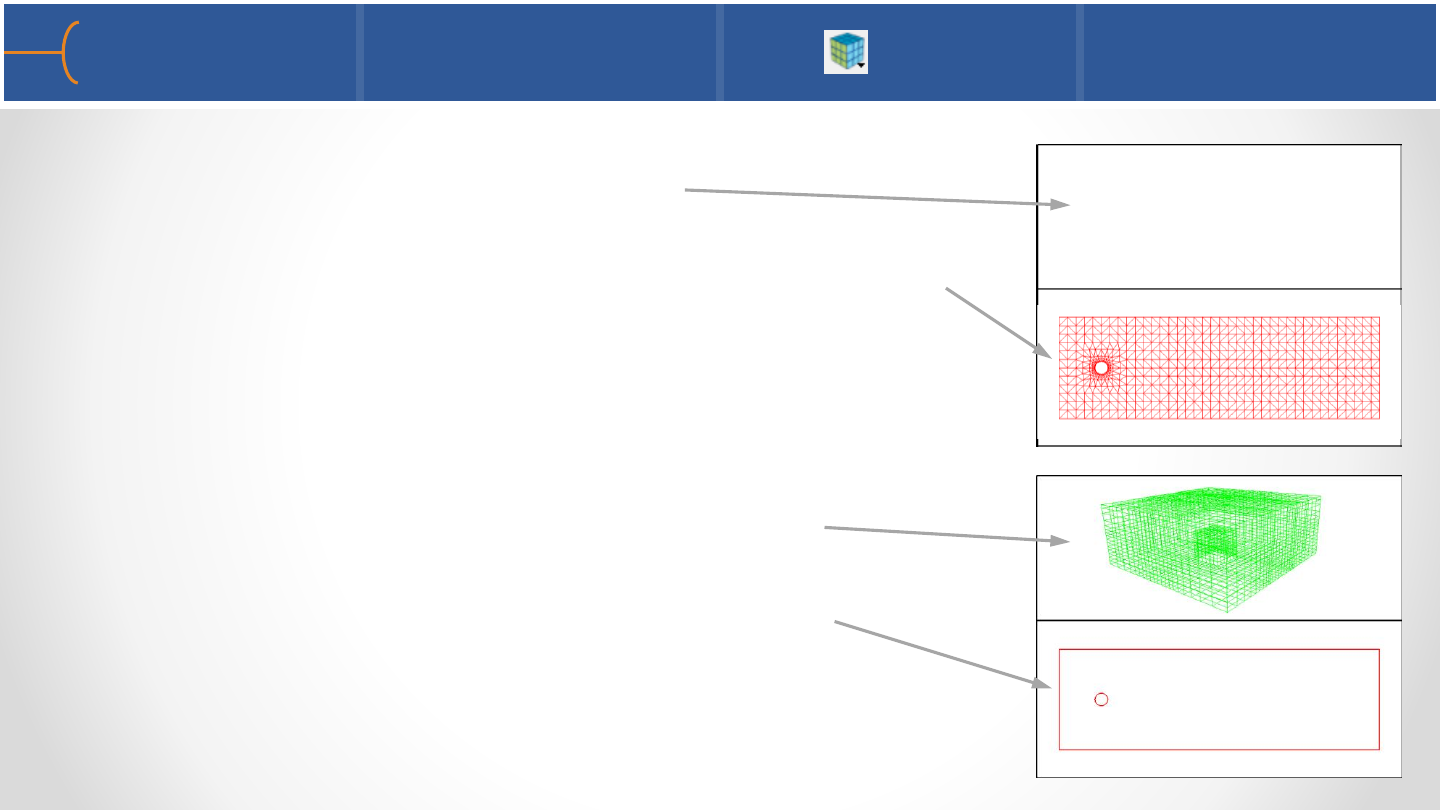
•Feature Angle
oFor 3D, operates off of Border elements
oLooks at 2D element normals –the edge between
2D elements are removed if the angle is less than
what the user has specified
•Bounding Box
oDisplays a bounding box around the geometry
3D elements
2D elements
3D elements
2D elements
•Full
oEvery face (3D elements) is visible
oEvery edge (2D elements) is visible
•Volume
o3D elements are rendered as volumes, including
alpha values (transparencies)
o2D elements become nonvisual
Element Representations 5 23
3D elements
2D elements
3D elements
2D elements
•NonVisual
oThe part is kept only on the EnSight server; it’s
geometry is not displayed on the EnSight client -
useful for external flowfields
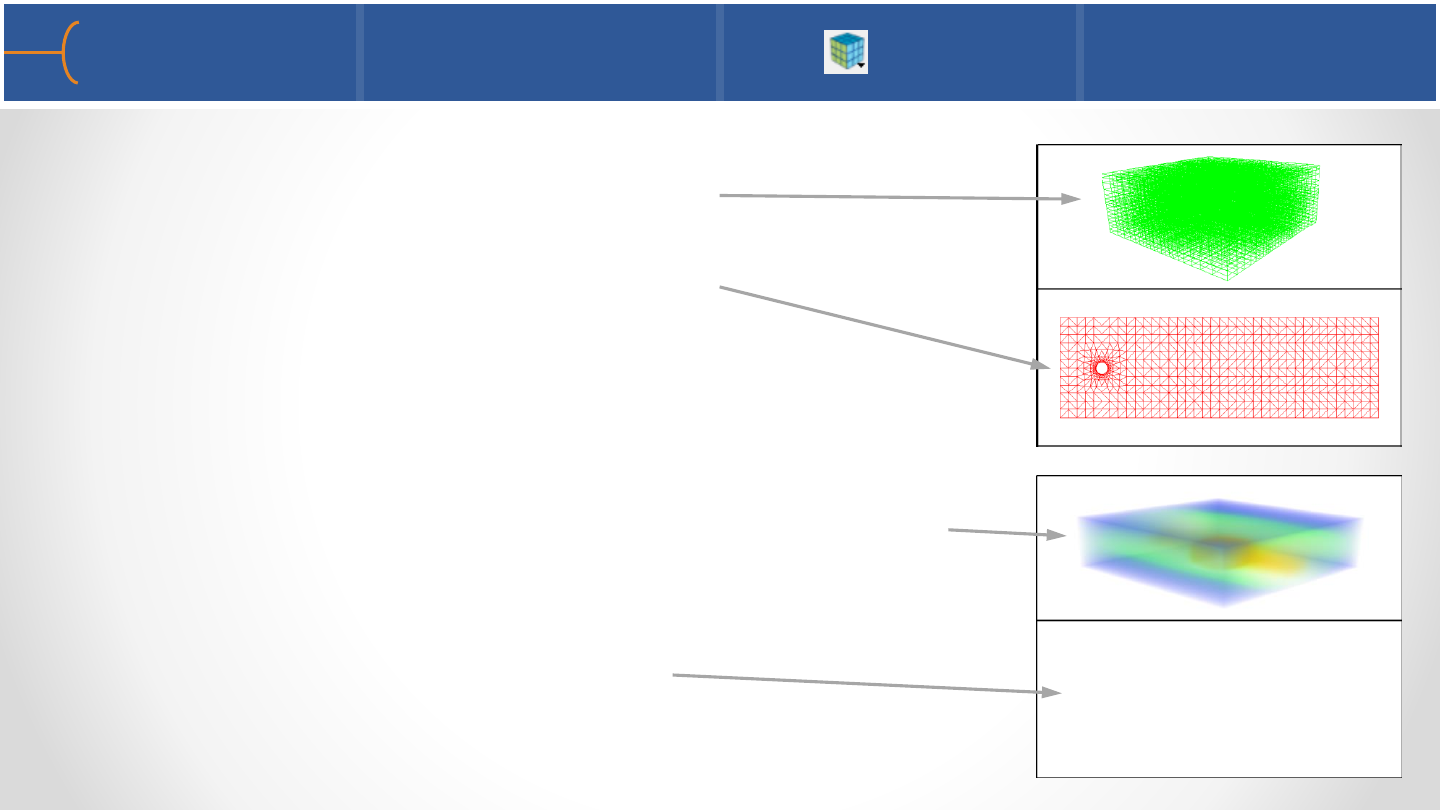
•Click the toggle Load Points and Normals Only to display
only the element centers of the model
Element Representations 6 24
3D elements
2D elements
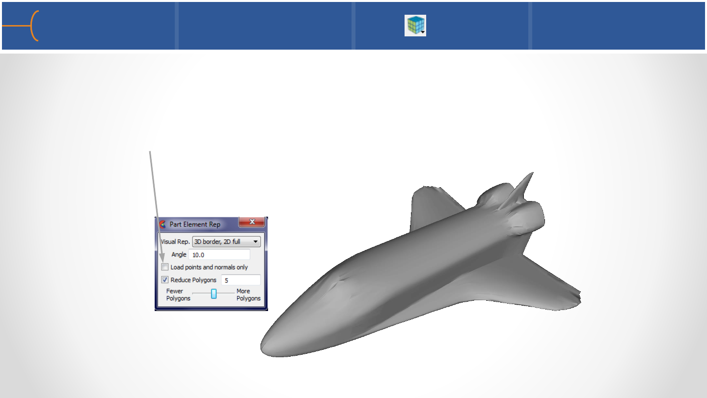
•Reduce Polygons speeds up visualization processing by thinning out the number
of polygons that are rendered; the trade off is in image quality and speed; the
model is not changed though, just the visual representation of it on the display
•Toggle Reduce Polygons to activate and use the slider for more or fewer polygons
Element Representations 7 25
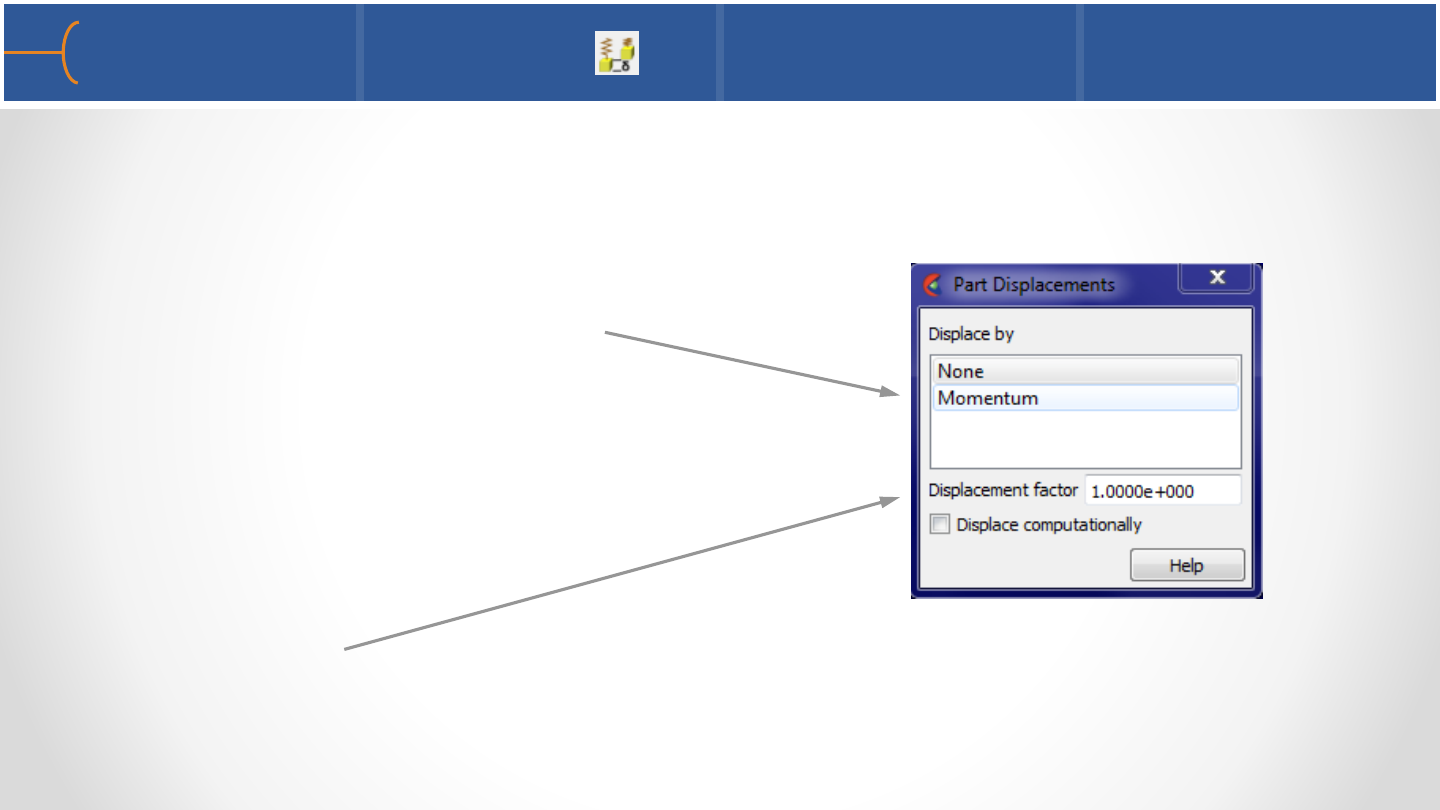
•For structural mechanics simulations, EnSight can display and animate
displacements to visualize the relative motion of the geometry
•Select the nodal variable to use
Please note the following restriction:
displacements can only use nodal
vector variables
•The Displacement Factor is a scalar that scales the vectors and exaggerates the
displacements; a value of 1.0 will give ‘true’ displacements
Part Displacement 26
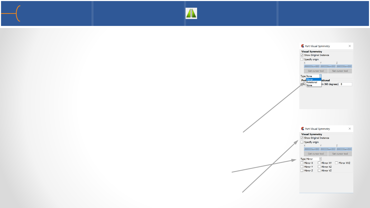
•Visual symmetry is done on the client so it’s a copy of the
original; the symmetry is performed with respect to the
reference frame of the part (see the Frame chapter)
•This feature is useful if there is symmetry in a model and only
part of the model has been analyzed
•There are 2 options: Mirror and Rotational symmetry
•Click on Mirror and select the mirror plane or axis
•There’s a toggle to show or hide the original instance
Part Visual Symmetry 1 27
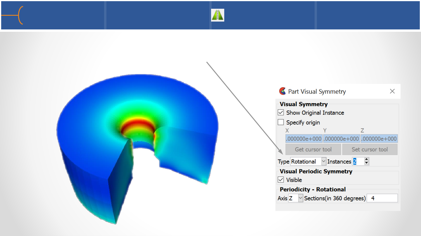
•For rotational symmetry, click on Rotational, select the Axis, the number of
Sections in 360 degrees and the number of Instances
Part Visual Symmetry 2 28
Exercise 1 –EnSight Processes & Element Rep 29
•See the EnSight 10 Advanced Training Exercises handout and do Exercise 1

Be careful with this feature because it can cause your system to slow down
significantly if used improperly
•Sometimes it is useful to identify specific nodes or elements within a model;
EnSight can display node and element labels in the Graphics Window
•Select the desired part and click the Element
Labeling icon and the labeling menu is displayed;
start by selecting a filter in the Thresholds box;
this has 5 filters to display only selected ranges
of labels:
None - show all labels
Low - remove all labels < the Low value
Band - remove all labels >= Low and <= High
Element Labeling 1 30
WARNING
WARNING

High - remove all labels > the High value
Low/High - remove all labels < the Low value as
well as those > the High value
•Click on the Node Label Visibility toggle to display
the labels
•The example shows the Space Shuttle model with a
Low/High filter on the nodes of < 475 and > 500
•The Mix button controls the color of the labels
Element Labeling 2 31
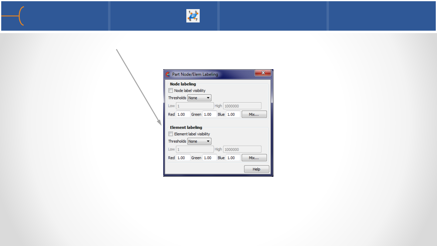
•The menus for Element Label Visibility are identical to the Node Label Visibility
menus
Element Labeling 3 32
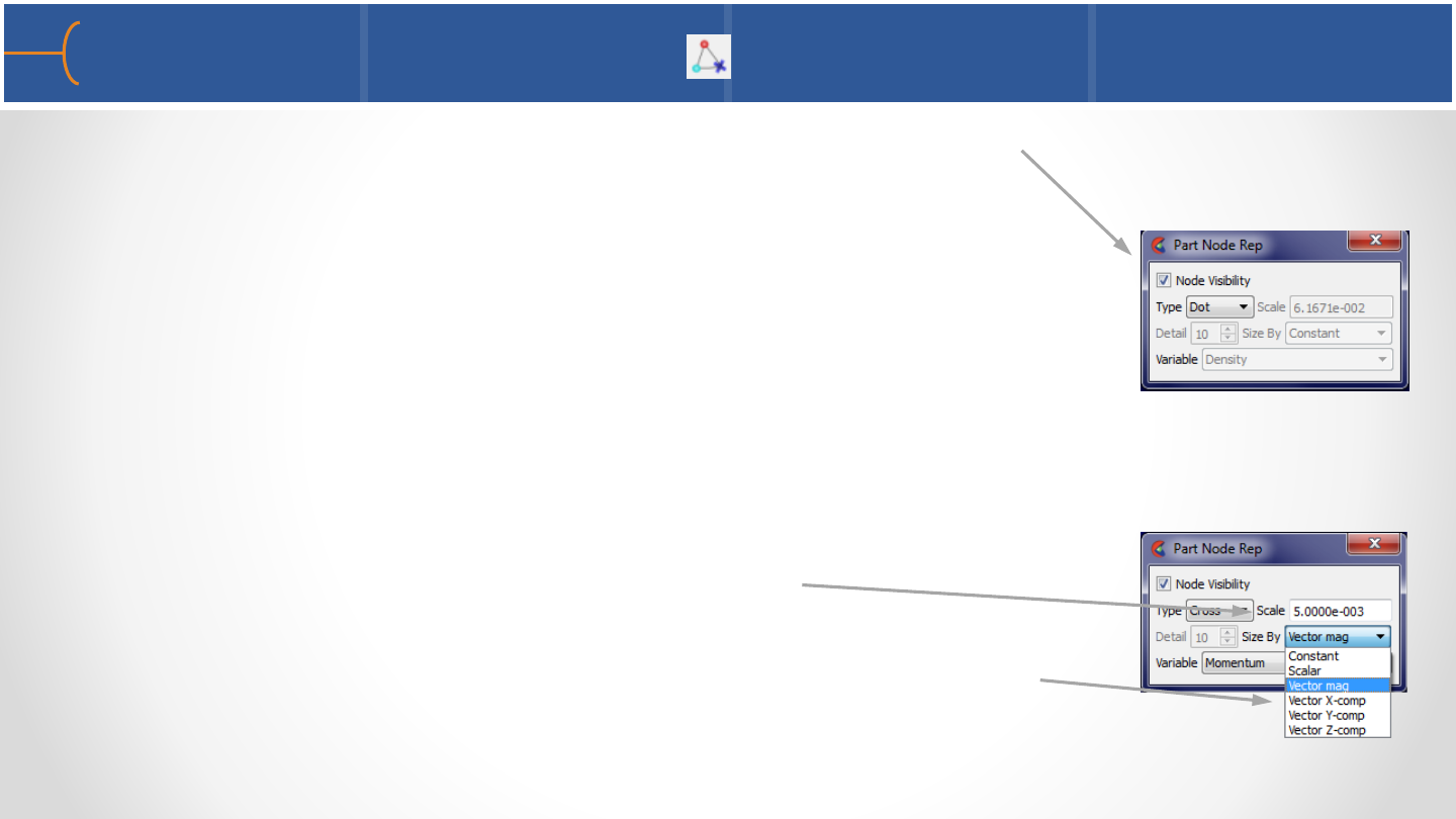
•EnSight can display the nodes of a model in the Graphics
Window
•There are 3 display types: Dot, Cross and Sphere
oDot: nodes are displayed as points
oCross: nodes are displayed as crosses and can be fixed
size or sized based on a variable
oSphere: nodes are displayed as spheres and can be fixed
size or sized based on a variable
•Scale changes the display size of the nodes
•Crosses and Spheres can be scaled by a variable (scalar or
vector)
Node Representation 33
Part Filter Elements 1 34
•In EnSight filters can be used to remove certain elements; the filter criteria can be
one or two variables or it can be a variable (such as a Von Mises stress/strain)
threshold for which limiting values and conditions are entered as a filter
•Elements are not just visually removed of the client, but are also removed for all
calculations of the server; if elements need to be removed for visual purposes
only, consider Element Blanking
•The variable used must be an Elemental Variable, not a nodal one; use the
NodeToElem function in the Variable Calculator to convert variables if needed
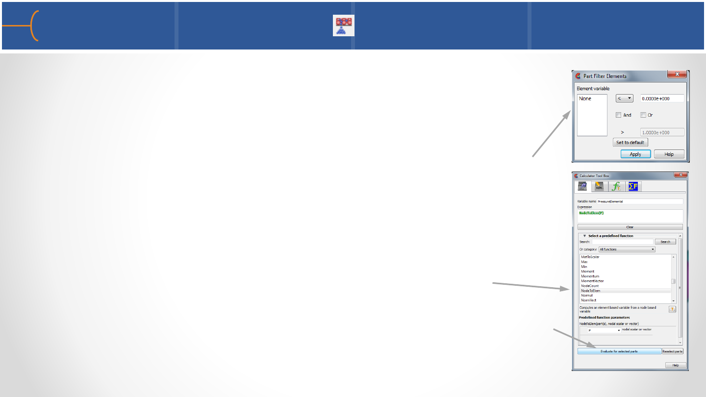
•To use Part Filter Elements, do the following:
oSelect the part(s) to use
oClick the Part Filter Elements icon; the is displayed and the
available Element Variable(s) are listed (they may have to be
calculated from Nodal Values)
oTo calculate Elemental Variables from Nodal Values, open
the Variable Calculator and select the NodeToElem
function; then type in a new variable name and select the
variable, in this case P; click the Evaluate for Selected Parts
button to create the new variable
Part Filter Elements 2 35
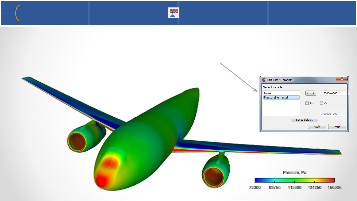
•The Part Filter Element Settings menu now displays the new PressureElemental
variable that was just calculated; type for example < 130,000 (Pa) as the filter
criteria, click Apply and only elements with a pressure higher than that number
are displayed
Part Filter Elements 3 36
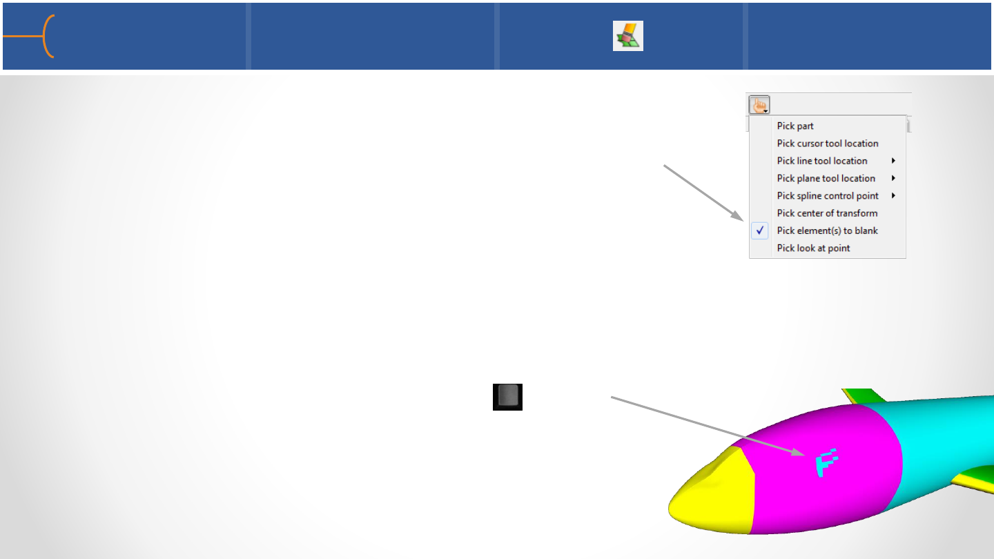
•Elements can be blanked; this can be useful to peek
inside of certain parts or remove only portions of a part;
element blanking is just a visual removal on the client
•Do the following to blank elements:
oSet the pick action to Pick Element(s) to Blank
oSelect one or more parts in the part list that needs
elements blanked
oPlace the mouse pointer over an element that needs
to be blanked and press the P-key on the
keyboard or click the middle mouse button to
blank the element
Element Blanking/Visibility 1 37
P
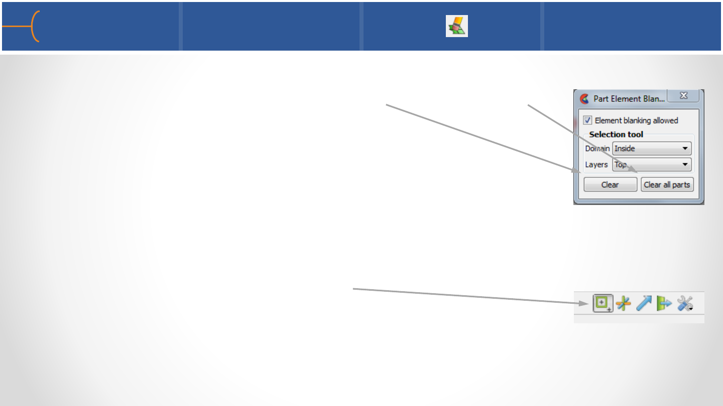
•To make the element(s) visible again, click the Element
Blanking/Visibility icon and click the Clear button or the Clear
All Parts button
•The Selection Tool can also be used to blank elements on a
larger scale
•Do the following to blank elements using the Selection Tool:
oSelect the part(s) on which to blank elements
oToggle the Selection Tool icon on
oPosition the tool and adjust its size if needed
Element Blanking/Visibility 2 38
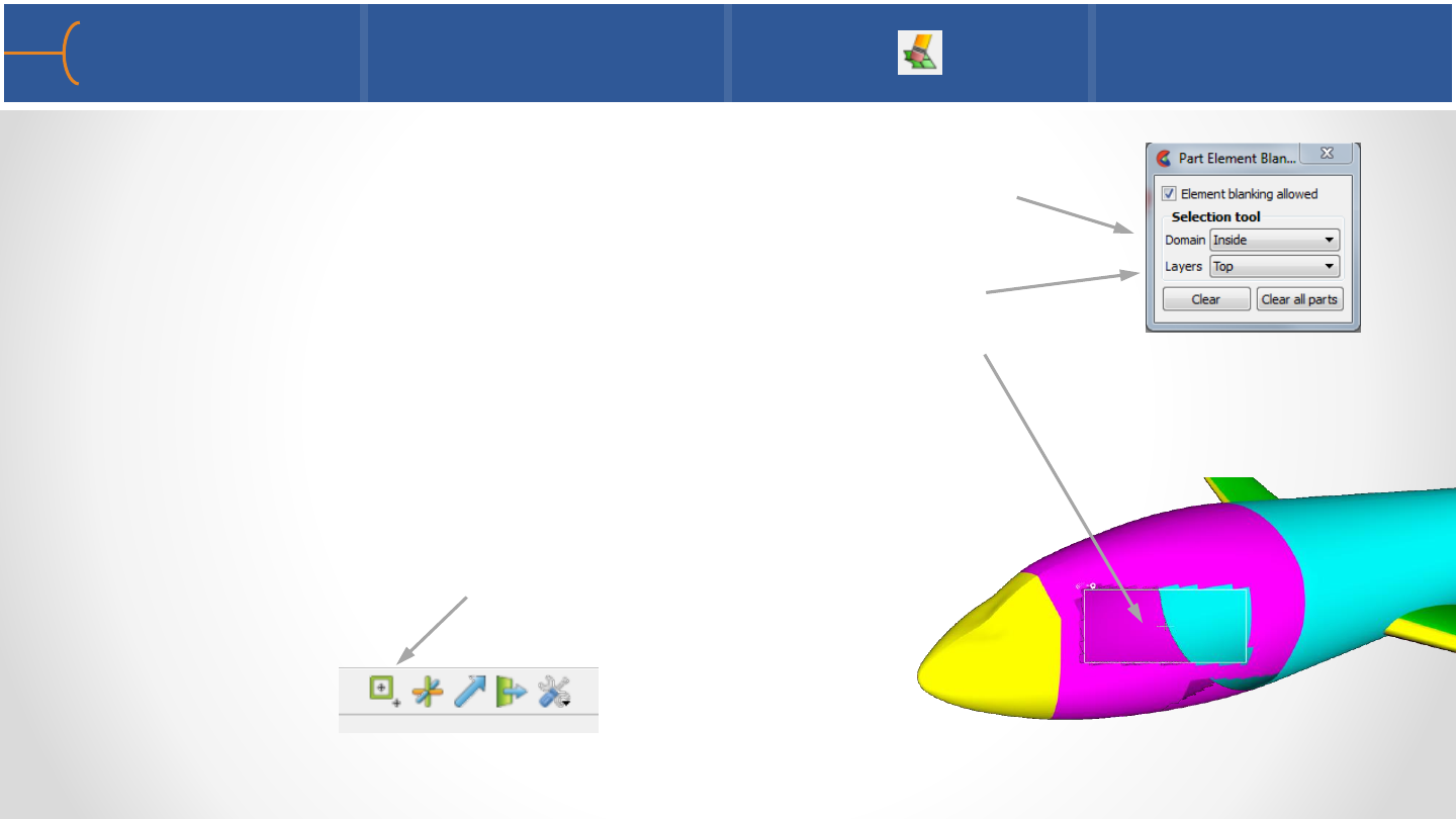
oClick the Element Blanking/Visibility icon and select
the Domain (Inside or Outside) and which Layers to
blank (Top or All); Inside blanks the elements inside
of the Selection Tool -Outside does the opposite;
Top only blanks the top visible layer while All blanks
all layers with a single click
oClick the Eraser Symbol on the top left corner of the
tool and the first layer of elements is removed; click
it again and the next layer is removed
oToggle the Selection Tool icon off when finished
Element Blanking/Visibility 3 39
•Part Shading and Hidden Line display can both be switched on and off per part;
this means that wireframe, shaded and hidden line views can be mixed in a model
•Remember to switch on the global Display Shaded Surfaces and Overlay Hidden
Lines to see these features
Part Shading and Part Hidden Line 40
Shaded
Shaded with
hidden line overlay
Wireframe
Hidden Line
Element centers
•Auxiliary Clipping can be set per part; by default it is set to on but it can be
switched on or off per part
•In the example below, the body parts of the car are the only parts that have
Auxiliary Clipping set to on; when the Plane Tool is moved, it seems like the outer
skin of the car is peeled away
•Auxiliary Clipping can be toggled on and off by clicking on View -> Auxiliary
Clipping
Part Auxiliary Clipping 41
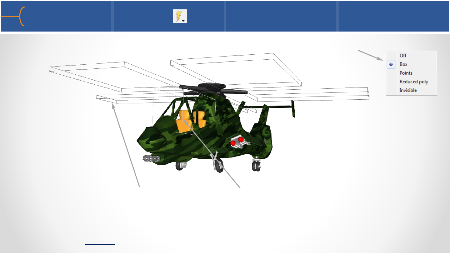
•Fast Display can be set per part; by default it is set to display a Box
•In this example the main rotor and the cockpit glass are set to a Box display while
the other parts are set to Off
•To make the lines more visible, the Line Width is set to 2
•To activate global Fast Display, click on View -> Fast Display
Part Fast Display 42
Procter & Gamble Pantene Products
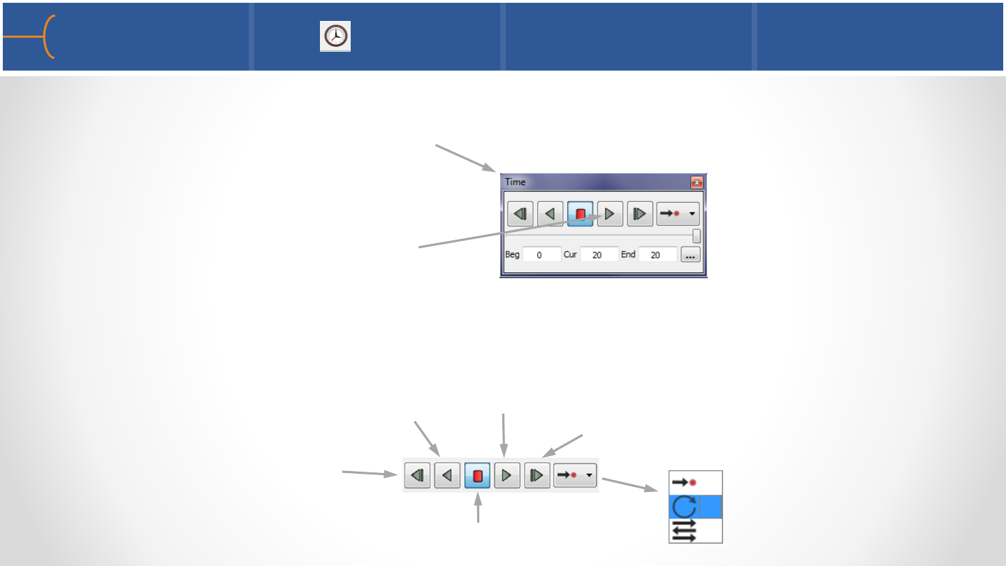
Time Menu 1 44
•EnSight can handle both steady state and transient data; when a transient model
is loaded the Time menu will appear on the screen (by default above the Parts
List)
•Click the Play button to run the
model through the time steps
•The DVR like buttons have the following functions:
Play (forward)
Play (in reverse) Step (forward)
Stop
Step (in reverse) Play Once
Loop
Swing
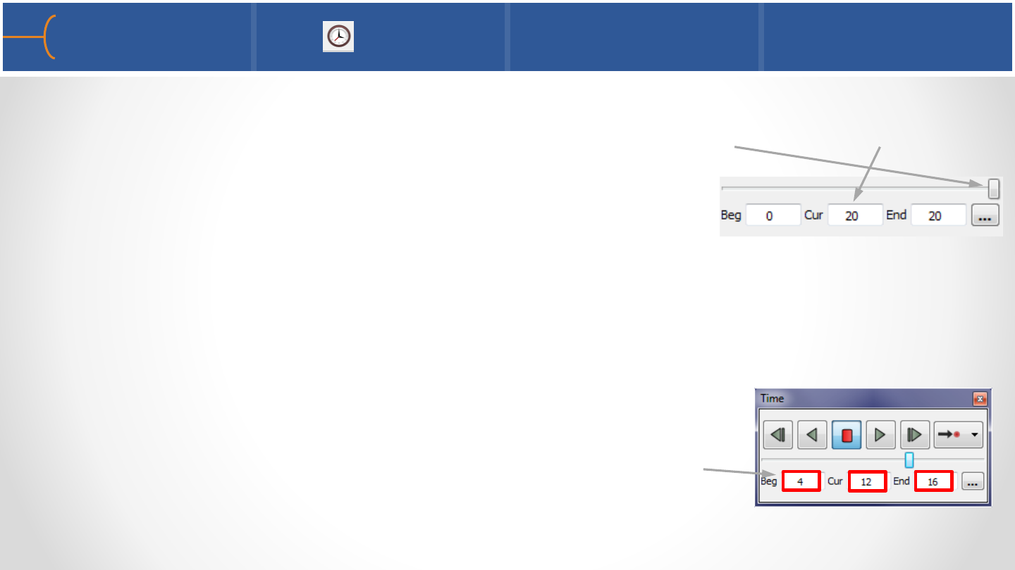
•When a transient data set is loaded, by default the last time step is displayed; this
can be seen by the slider that’s at the end of the time range or by the Cur(rent)
field that has the last time step in it (20 in this example)
Note: The user can select whether the last or first step is
displayed by default by clicking on Edit -> Preferences ->
Data -> If Starting Time Step is Not Specified, Load: select
First Step for instance
•The slider can be dragged to any specific time step; in this
example the slider has been dragged to time step 12, the
Beg(inning) has been changed to step 4 and the End has
been modified to 16 by just typing in these values
Time Menu 2 45
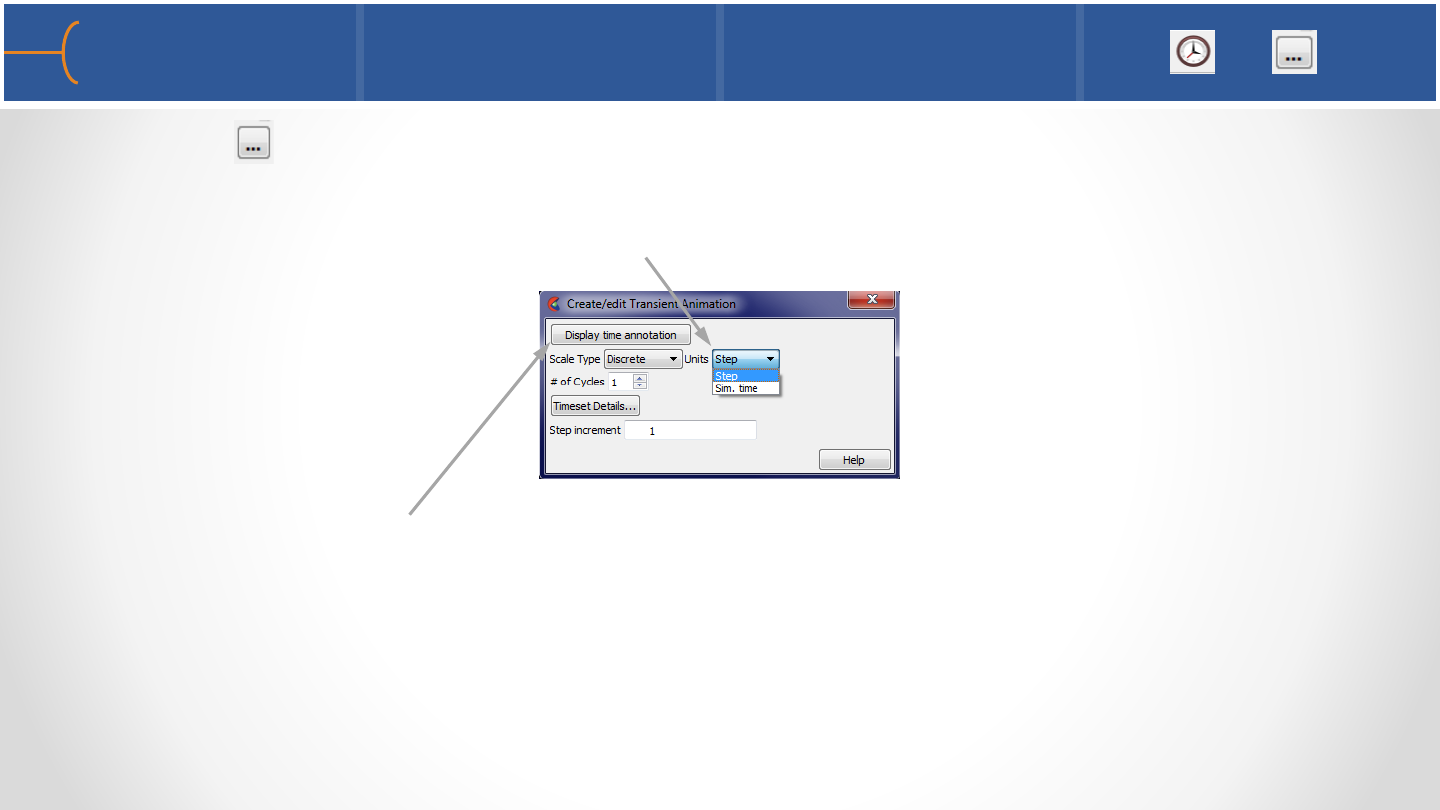
Create/Edit Transient Animation menu 1 + 46
•Click the icon for some advanced features; the time Units can be set as either
discrete Step(s), running from zero to the total number of steps minus one or the
actual simulation time values found in the results data set
•Click the Display Time Annotation to display the time in the Graphics Window;
this is a toggle and the time display can be moved and resized by dragging the
touch-n-go handles
•The time annotation can of course also be displayed by dragging and dropping the
Time variable in the Variable List onto the background of the graphics window
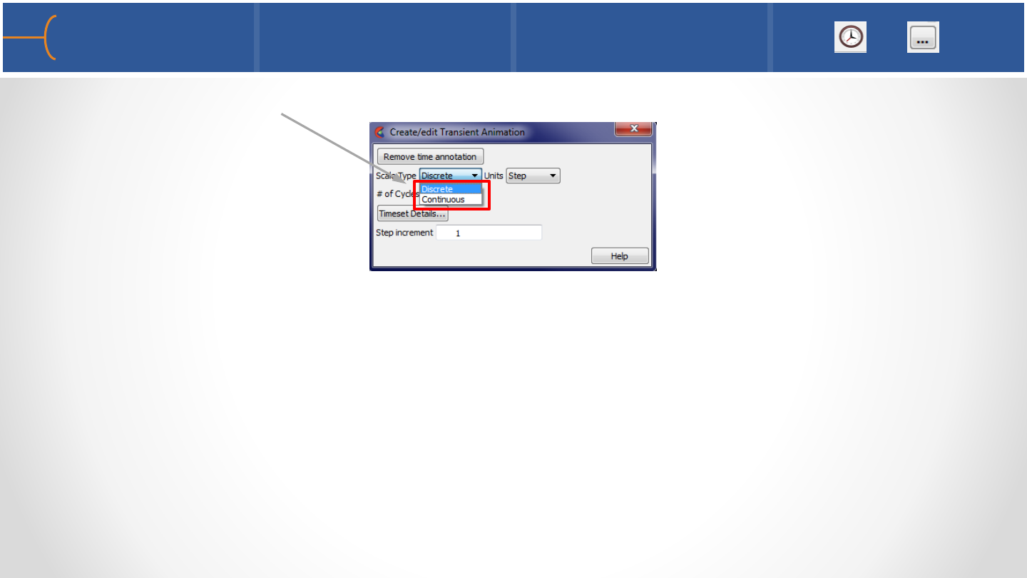
•The time Scale Type can either be Discrete or Continuous:
oIf the Scale Type is set to Discrete, only actual time steps that are listed in the
results data set can be displayed
oIf the Scale Type is Continuous, results can be displayed between actual output
time steps; all variable values are linearly interpolated between the two time
steps
Note: if the mesh is changing over time, results can’t be displayed continuously
•The Timeset Details button controls how multiple timelines of several datasets
can be synchronized and played simultaneously
Create/Edit Transient Animation menu 2 + 47
•Record a transient animation for instance by clicking on
the Record Current Graphics Window Animation icon
on the Quick Settings menu and select the options on
the Save Animation menu such as movie format, window
size, number of passes etc (some of these options are
under the Advanced tab); select the Play and Reset
toggles
•The # of Cycles field determines the number of times
the solution time is played when an animation is
recorded
Record Current Graphics Window Animation 48
•A flipbook is a quick and easy way to make an animation by playing back a series
of images; for each step, a graphical ‘page’ is created and stored in RAM memory;
when the flipbook is played, the pages are sequentially displayed as fast as the
graphics card allows; click the flipbook icon
•A flipbook can be created as Objects or Images; if the flipbook is created using
Objects, during playback of the animation the model can still be rotated or
zoomed but for bigger models the RAM on the client that is needed can be
substantial; in that case Images (pixel data only) is a
better choice due to lower RAM requirements but the
animation can not be rotated or zoomed during playback
Flipbook 1 49
•Most EnSight users use a flipbook to animate and record transient data but a
flipbook can animate 4 types of data:
•Once a flipbook is loaded, the Flipbook menu uses DVR like buttons just like the
Solution Time panel to play an animation
Flipbook 2 50
Display Speed can
slow down the
animation
Cycle can play the
flipbook forward
and in reverse
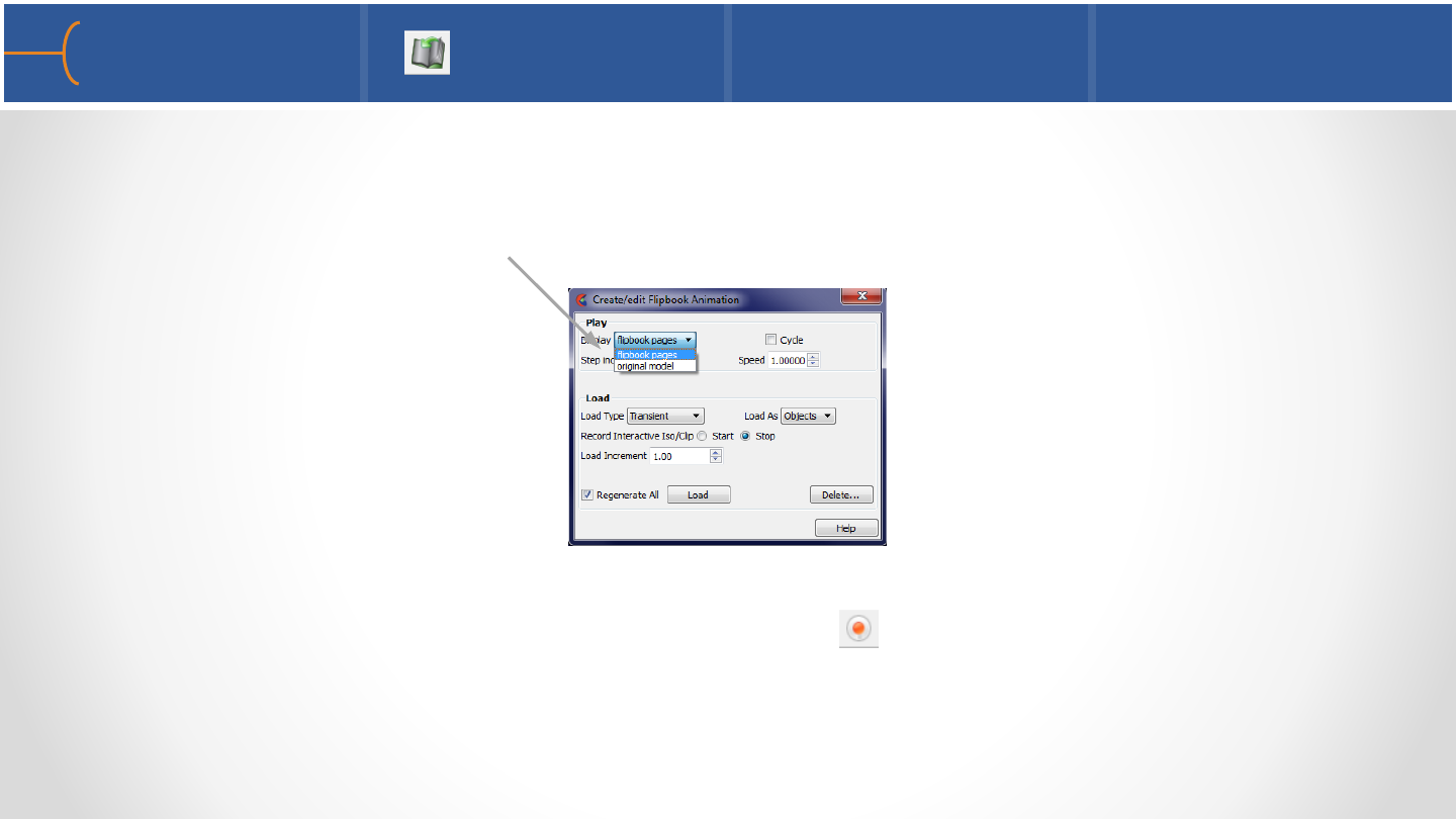
•If the flipbook pages were created using Images, don’t forget to set the Display
back to Original Model otherwise rotate, pan and zoom will not work (because
the display is still set to Flipbook Pages)
•When a flipbook has been created it can be recorded to a movie file using the
Record Current Graphics Window Animation icon on the Quick Settings menu
•For more complex and sophisticated animations, use the Keyframe Animator and
not a flipbook
Flipbook 3 51
•See the EnSight 10 Advanced Training Exercises handout and do Exercise 2
Solution Time and Flipbook Exercise 52
2017 Cadillac CTS-V Sedan
Pathlines Introduction 54
•The path calculated using a transient flowfield that is updated as the calculation
proceeds is known as a pathline
•By default, pathlines will start at the first time step of the simulation and
terminate at the last step (unless stopped earlier)
•A delta value can be specified for an emitter that will cause additional particles to
be emitted into the flow at regular intervals (Multiple Pulses); this type of pathline
is also called a streakline or smoke trace
•Pathlines can be animated just like streamlines with the same options on the
Particle Trace -> Animate menu
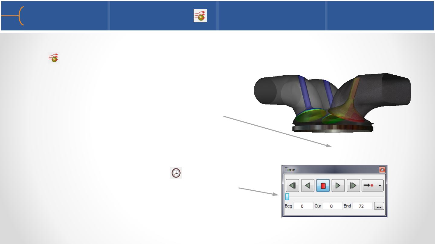
•A pathline is created with the same icon as a streamline, so click the Particle Trace
icon and in the Type selection box select Pathline
•Select the flowfield and click the Create
button and the pathlines part will be created;
however most likely no pathlines will be
displayed on the screen
•This is caused by the settings of 2 menus:
1.The Solution Time menu should be set
to the first time step (usually Start =0)
Creating Pathlines 1 55
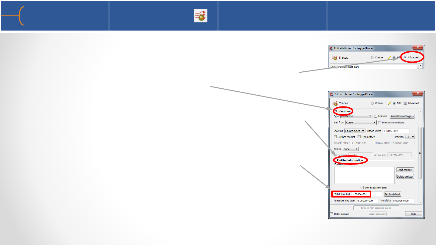
2.Double click the Particle Trace Part in the Parts List; this
brings up the Edit Attributes menu for that part; click
the Advanced toggle on; this opens up many more
options under the Creation label
The Emitter Information fields must have values that
are appropriate for the data set; these values can be
found in the results data set: First the Total Time Limit,
(the end time minus the start time) - for this model it
is .1
Creating Pathlines 2 56
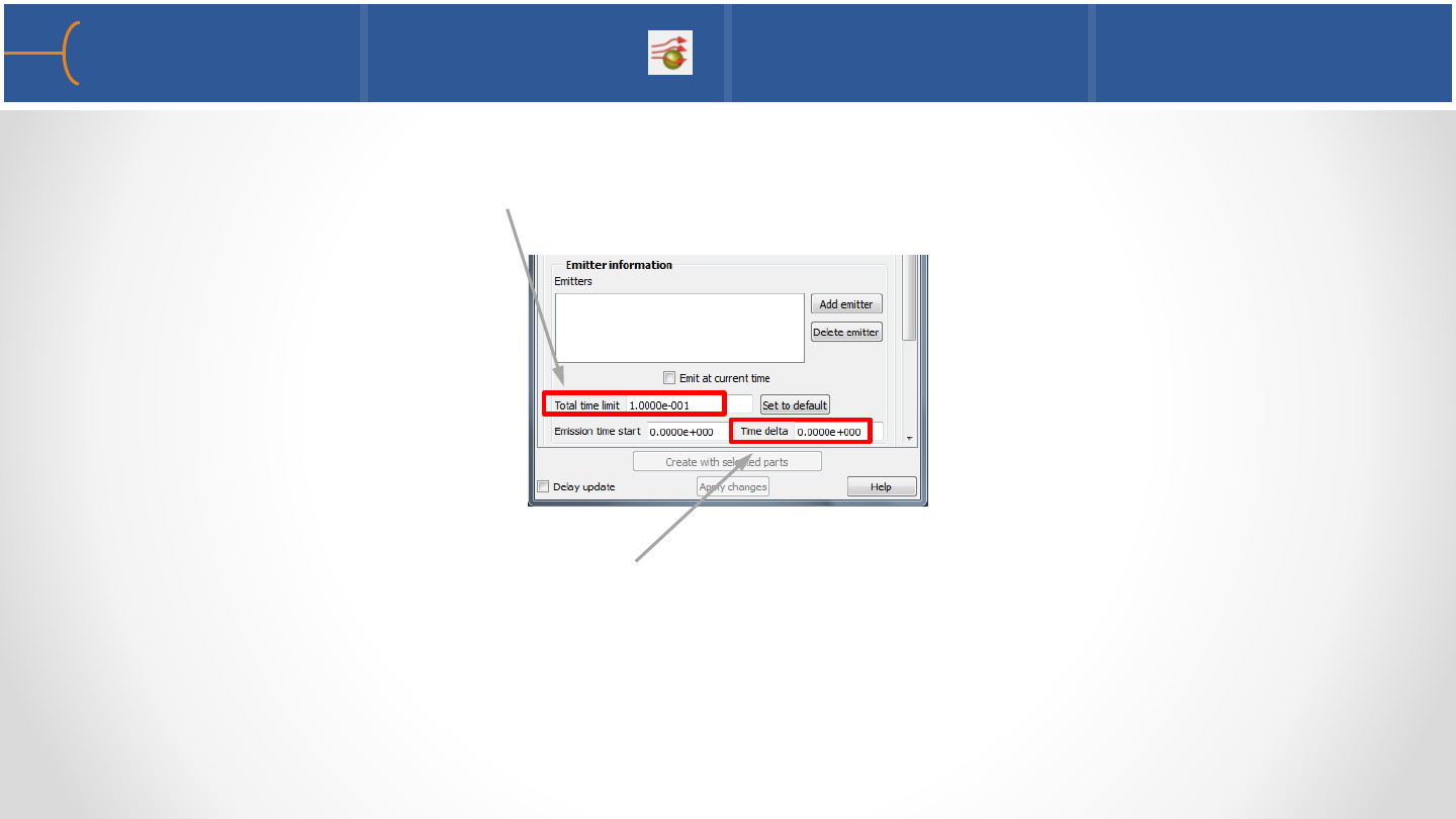
Then the Emission Time Start (the time when the analysis starts); for many
models this is at time = 0)
3.The Time Delta is set by default to 0 and this value doesn’t need to be
changed unless more particle traces are needed; if a value is typed in, a new
set of traces will be emitted at S, S+D, S+2D etc into the flow field (S is the
start time and D is the delta value)
Creating Pathlines 3 57

•After the adjustments using the Emitter settings, the pathlines are displayed
Displaying Pathlines 58
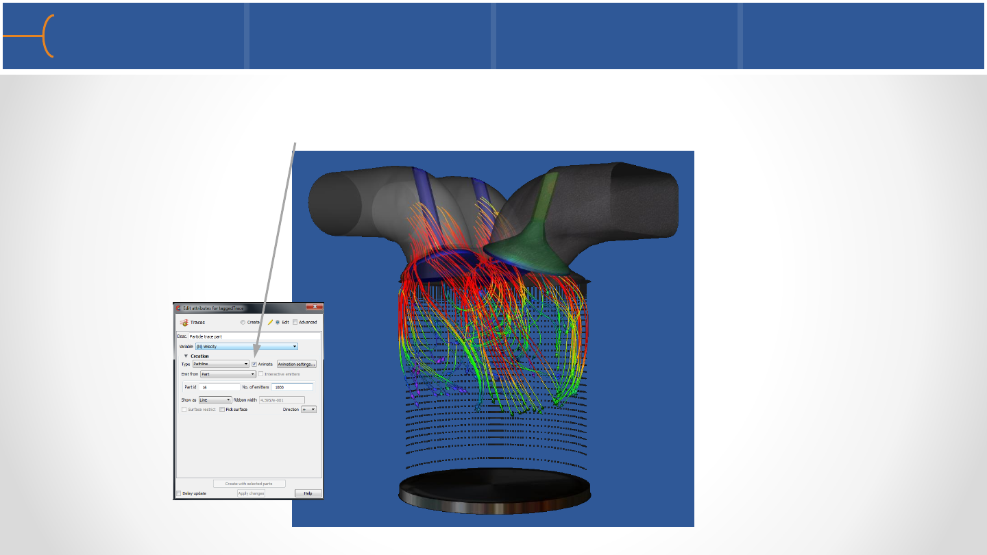
•Pathline particle traces are displayed by double clicking the Particle Trace Part in
the Parts List and selecting the Animate toggle
Animating Pathline Particle Traces 59

Part Duplicating 61
•There are two main methods to duplicate parts in EnSight*
•(1) Part Copy
oCreates a ‘linked’ copy of the parent part
▪Users may change color of the copy, display attributes
▪Updates to parent are reflected in the copy
Move the parent, and the copy moves as well
•(2) Part Clone
oCreates a ‘separate’ clone of the parent
▪Initially the clone will have all of the same attributes (color,
position, display, etc)
▪All attributes of the clone are independent from the parent
▪The Clone is a completely separate from the parent
*(You can re-load model parts from dataset to duplicate model parts only)

When to use each one 62
•(1) Part Copy
•When you want to color the SAME part by a different variable
•The Location of the Parent and Copy remain the same
•It is really a ‘linked’ copy
•Not a independent part
•(2) Part Clone
•You have created/setup a part (location, color, style), but now want another
one just like it (to start with)
•Initially it has all the same attributes, but you want the ability to change
anything
•Completely Independent
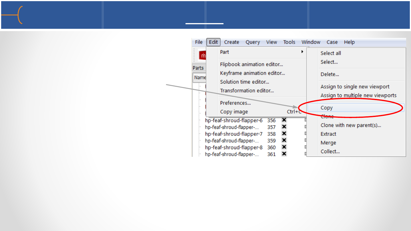
How to Create a Part Copy 63
•(1) Part Copy
oSelect the part(s)
oTop Pull Down Menu
▪Edit -> Part -> Copy
•The new Part can have only its
visual properties changed (color,
reflection, viewport assignment)

How to Create a Part Clone 64
•(2) Part Clone
oSelect the part(s)
oTop Pull Down Menu
▪Edit -> Part -> Clone
•Alternatively, you can use the Right
Click:
oSelect the part(s)
oRight Click -> Clone
Creating and Using Part Clone 65
•Example of quickly
creating similar part via
‘Clone’ Method
Part Tagging 66
•Part Selection can be tagged (new for EnSight 10.1)
oAbility to Save and Recall Part Selection - up to 10 saved/recalled selections
•Part Selection Tagging is handled via:
oSaved using Alt + [0-9]
oRecalled using Ctrl + [0-9]
•‘Groups’ are not created - simply an ability to save & recall part selection
•Meant for quick save/recall of complex part selections
•Parts can exist in multiple selections (Part #4 can be in both Alt-0 and Alt-4)
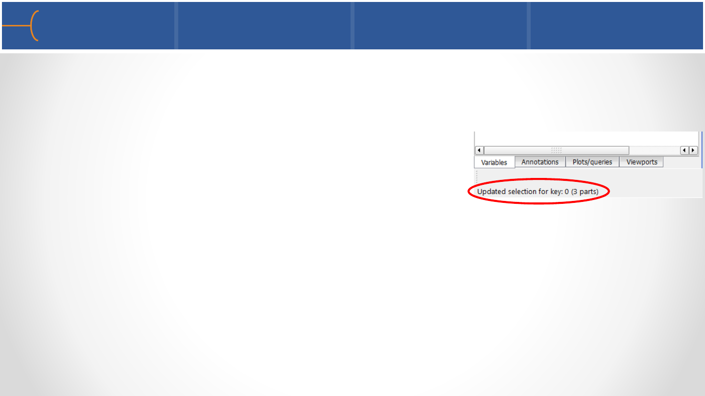
Part Tagging –How To 67
•Select the Part(s) you wish to save the selection
oPress Alt + [0-9] to save the selection to one of 10 selections
oPress Ctrl + [0-9] to recall that selection
•Each Selection Creation is noted in the output area
•Part Tagging selections are saved and restorable from Context, Session, and
Archive files
•Part Tagging is not saved or restored in Journal files (no command
equivalent)
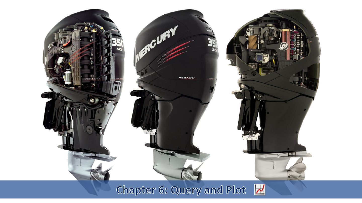
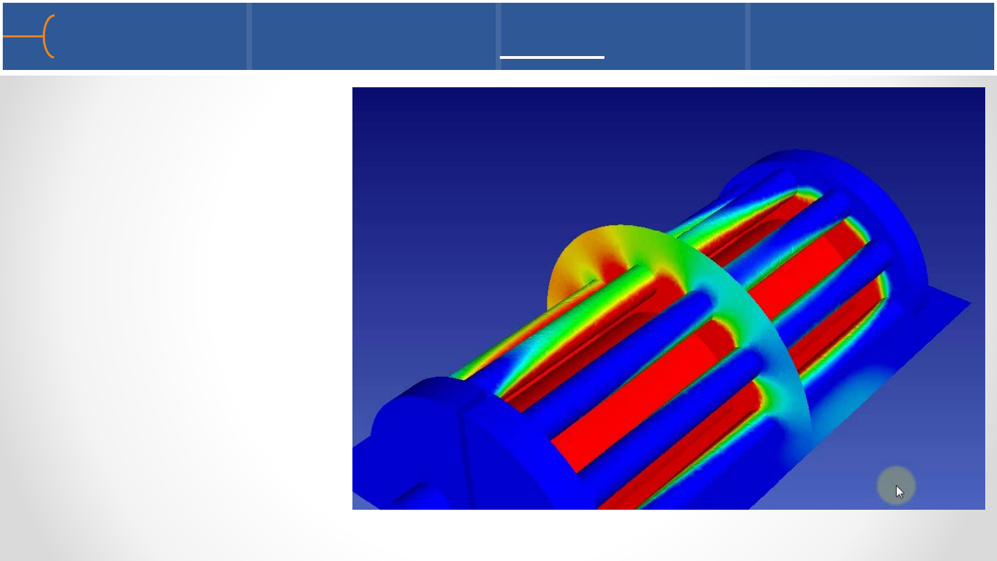
Mercury Marine Verado
350 SCi outboard engine
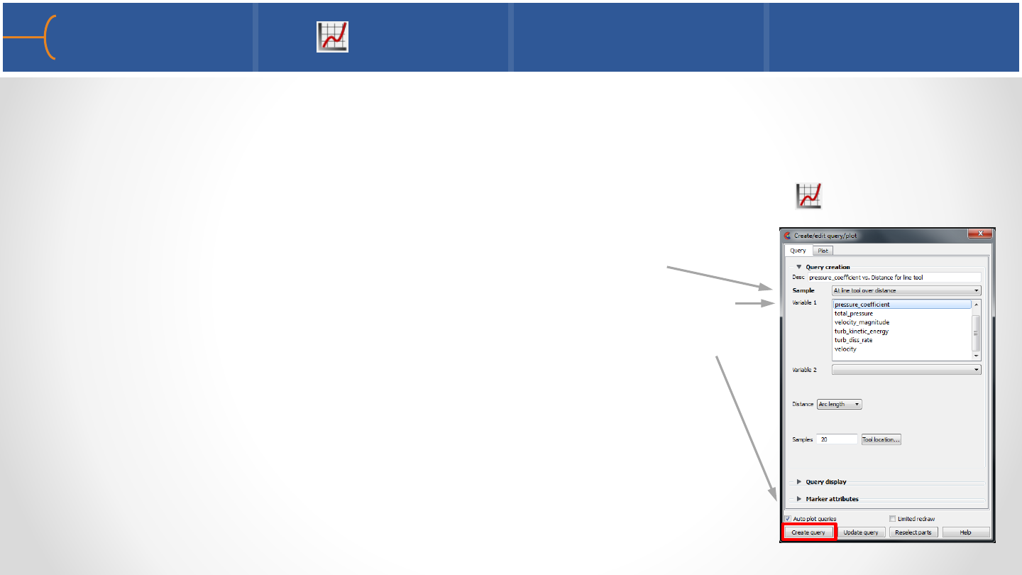
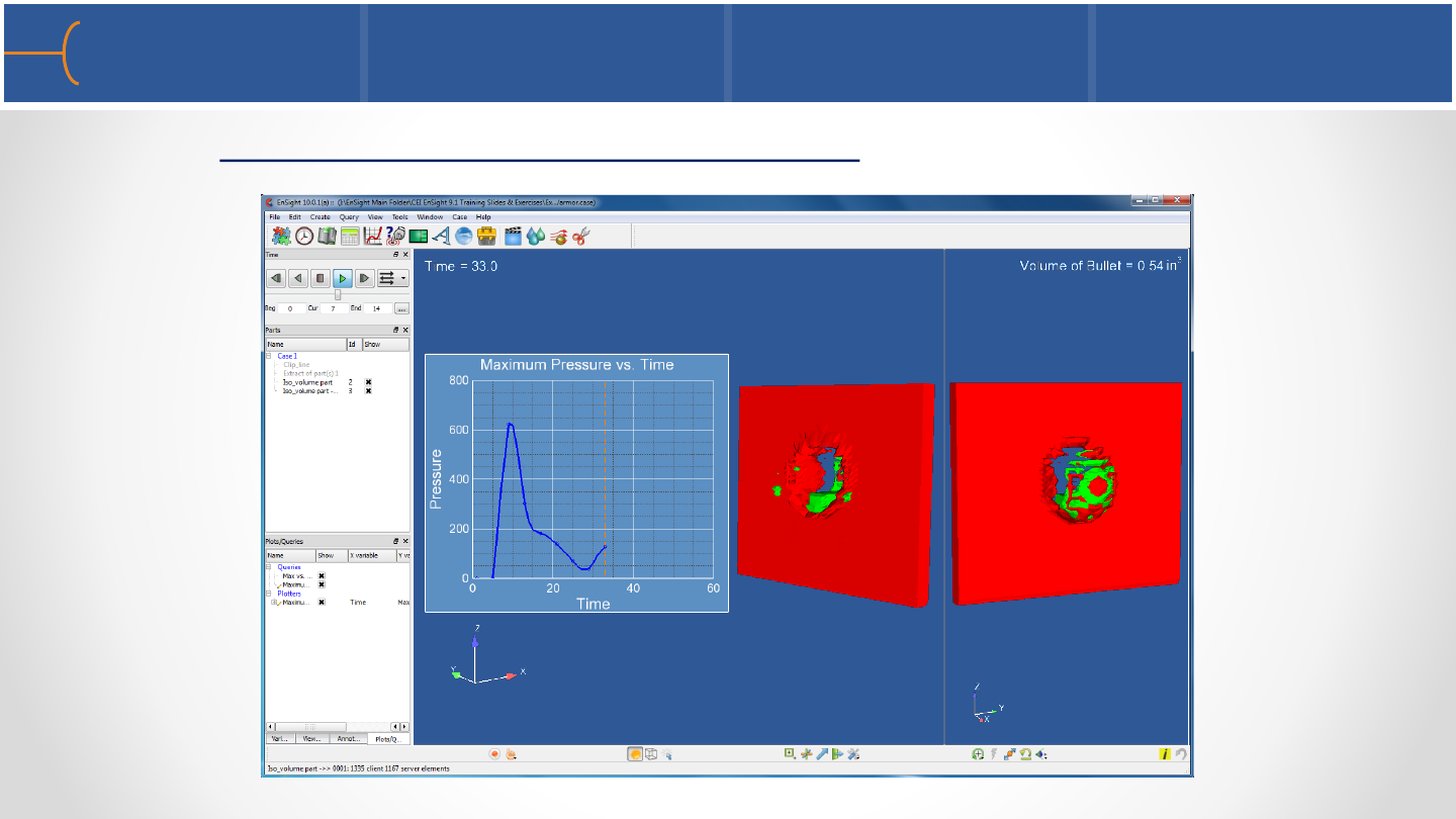
•Queries and plots can be generated by right clicking the Line Tool or right clicking
a clip part and selecting Query (Variable) as described in the EnSight Basic
Training
•A query and plot can also be created by clicking the Query icon on the Feature
Toolbar; the Create/Edit Query/Plot menu is displayed
•On this menu select the Sample, in this example the
Line Tool, Variable 1, for instance the pressure_coefficient
then select the appropriate part(s) and click on the Create
Query button
•Since the Auto Plot Queries is toggled on, the query will
be immediately plotted as well
Query/Plot 1 69
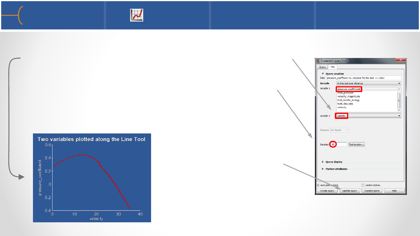
•If Variable 2 is clicked and a second variable is selected, the result is a scatter
query and plot of two different variables along the line tool
•The number of Samples controls the number of points
along the sample tool (the Line Tool in this example)
•Click the Update Query
button if the number of
Samples is changed for
an existing plot
Query/Plot 2 70
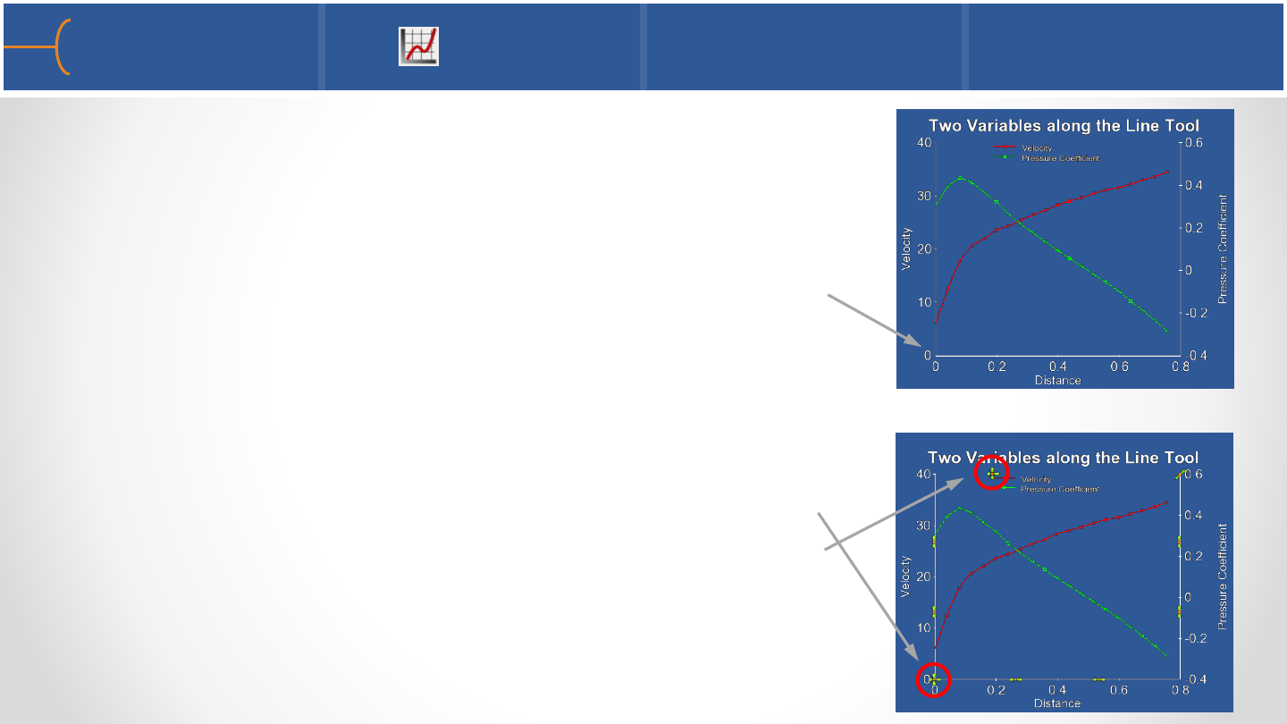
•Of course it’s also possible to create a plot with the
distance along the Line Tool on the X-axis and the 2
variables on the Y and Y2 (right) axes; to do this, create
the first query and plot, then create the second query
and drag-and-drop it onto the origin or one of the axes
of the existing plot
•Move the Query Description by double clicking the
origin of the plot; new handles will appear to move
the description
Query/Plot 3 71
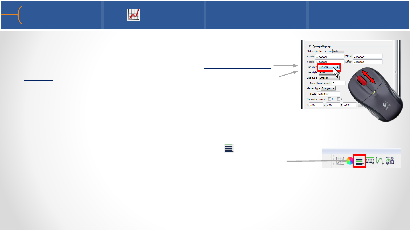
•Toggle the Query Display to change the Line Width of the
graph; as mentioned in the EnSight Basic Training, just put
the cursor over the drop down list and roll the mouse
wheel; this will change the Line Width without actually
having to go into the drop down list
•Please note that the Curve Line Width icon on the Quick
Edit Menu is dynamically updated as the mouse wheel is
rolled
Query/Plot 4 72
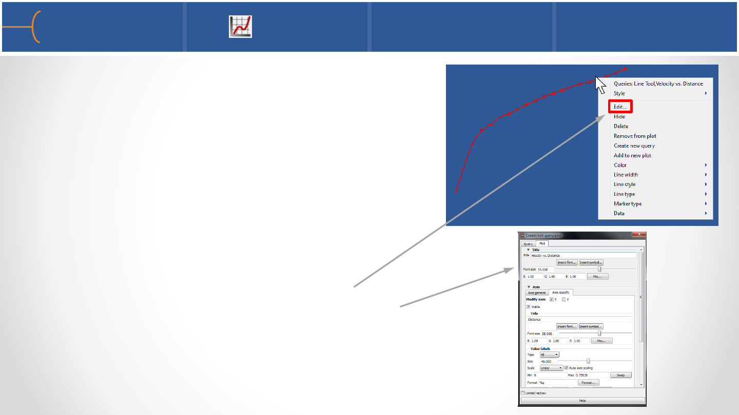
•Right click on a curve to get instant access to
many parameters of the curve
•Select Edit to display the Create/Edit
Query/Plot menu which enables complete
control over both the query and the plot
Query/Plot 5 73
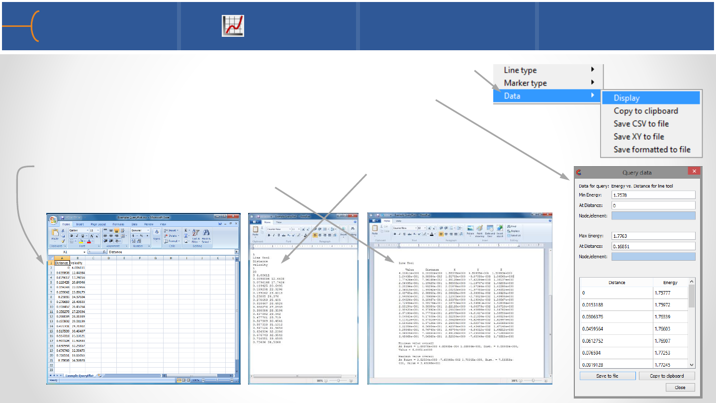
•The last option on this menu is Data and it provides a
way to Display the data for the current Query/Plot
•The information can also be saved to the clipboard, a
CSV file which can be read by Excel, an XY plain text file
or a formatted plain text file
Query/Plot 6 74
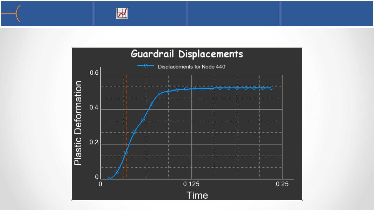
•This is an example of a finished graph
Query/Plot 7 75
Lockheed Martin
F-22 Raptor
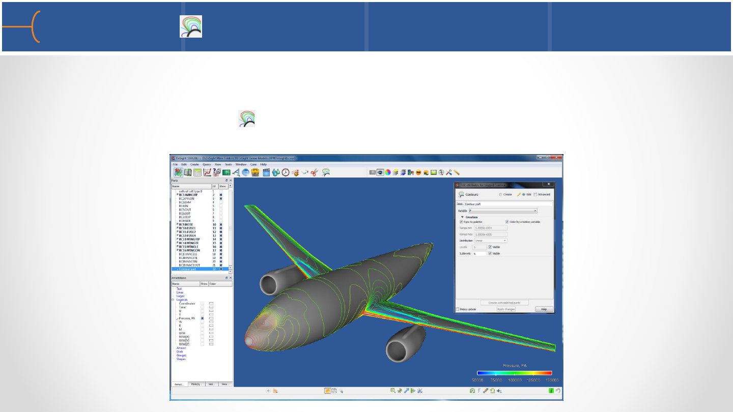
•A contour is a line of constant value on a 2D surface
•Select the parts the contours should be displayed on
•Click the Contours icon , select a variable and click the Create with Selected
Parts button
Contours 77

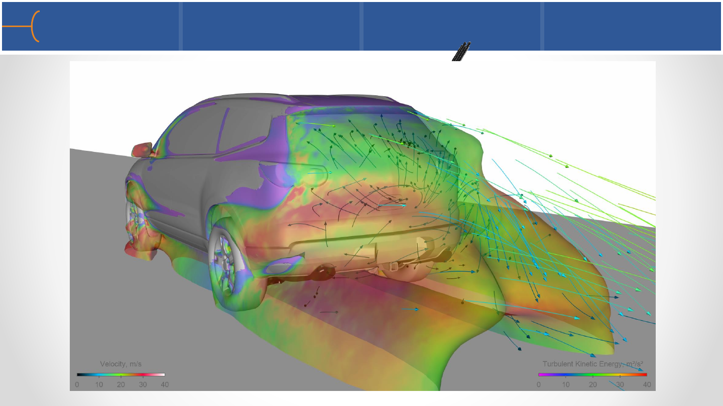
•Represents the direction and magnitude of a vector field
•Create a Clip plane in a fluid domain for instance and select the Clip Part
•Click the Vector Arrows icon , select a variable and click the Create with
Selected Parts button
•The Scale Factor controls the size of the vector arrows
•Vector arrows can be Straight or Curved
•The Density field controls the number of arrows
Vector Arrows 1 78

Vector Arrows 2 79
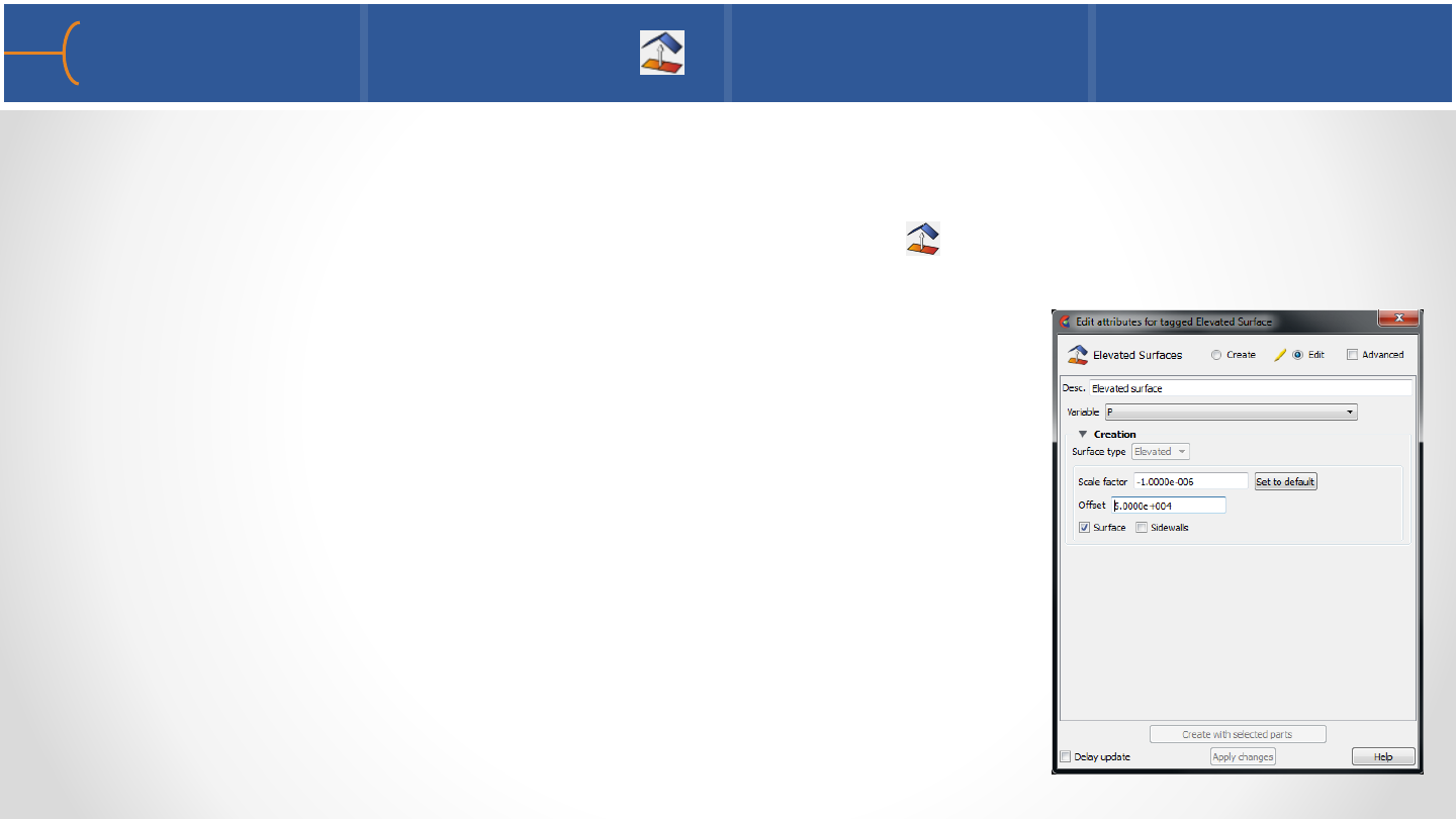
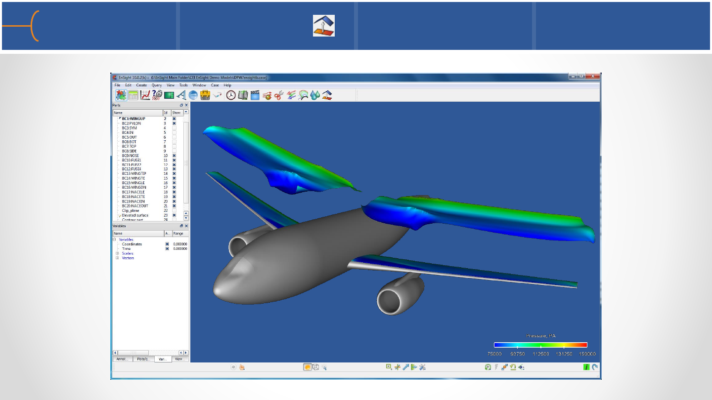
•Represents an offset surface of a scalar variable
•Select a part then click the Elevated Surfaces icon , select a variable and
click the Create with Selected Parts button
•The Surface Type can be Elevated or Offset
•The Scale Factor controls the size of the elevated surface
•The Offset field allows to shift the elevated surface
away from the parent, but does not affect the shape
•An Elevated Surface can have Sidewalls
Elevated Surfaces 1 80
Elevated Surfaces 1 81
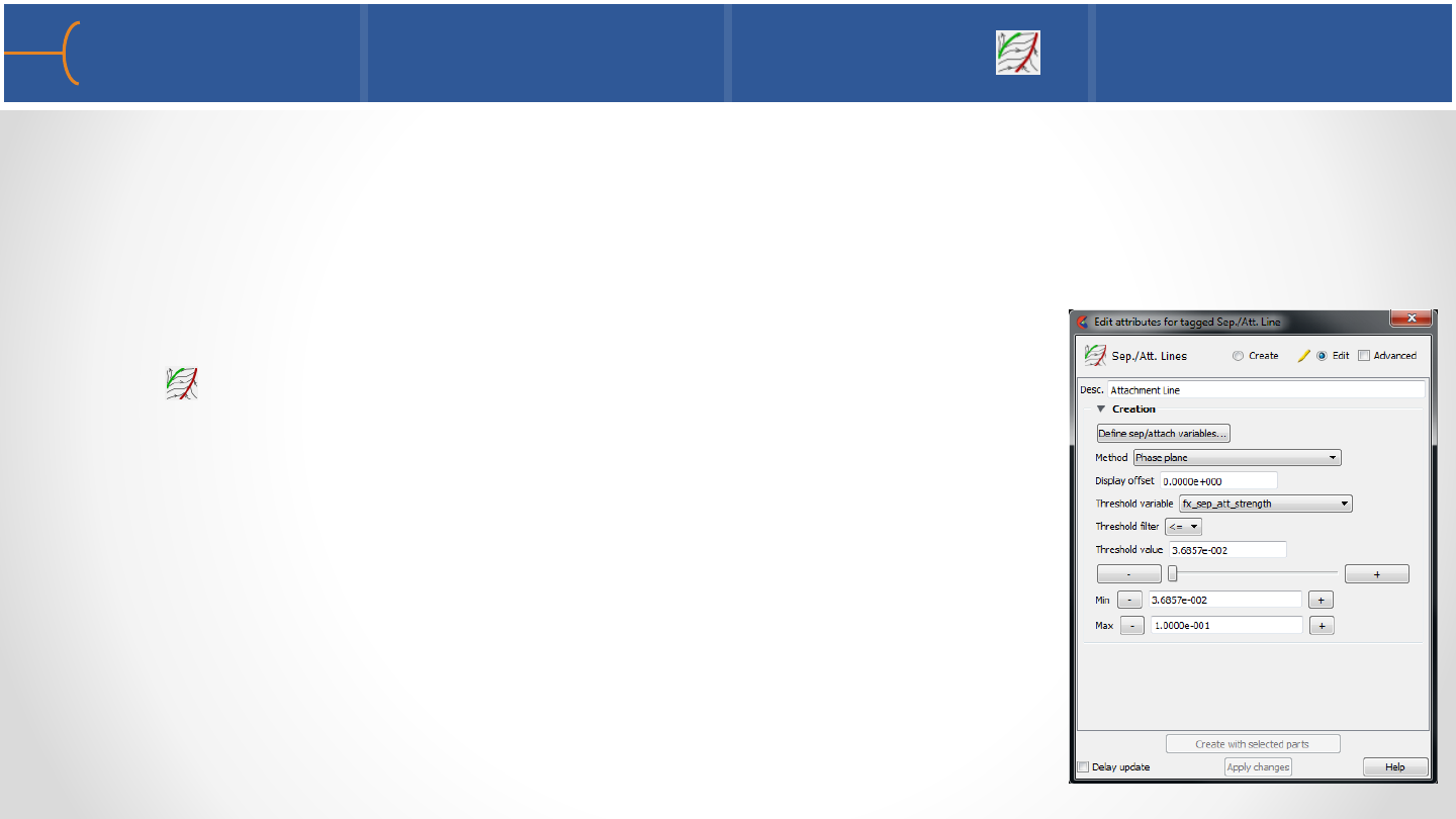
•Separation and attachment lines are created on any 2D surface and show
interfaces where flow abruptly leaves (separates) or returns (attaches) to the
surface
•Select a part then click the Separation & Attachment Lines
icon , select a variable and click the Create with Selected
Parts button
•The separation lines are green and the attachment lines
are pink
•There are various menus to define the Method that is
used and tweak the separation & attachment lines
Separation & Attachment Lines 1 82
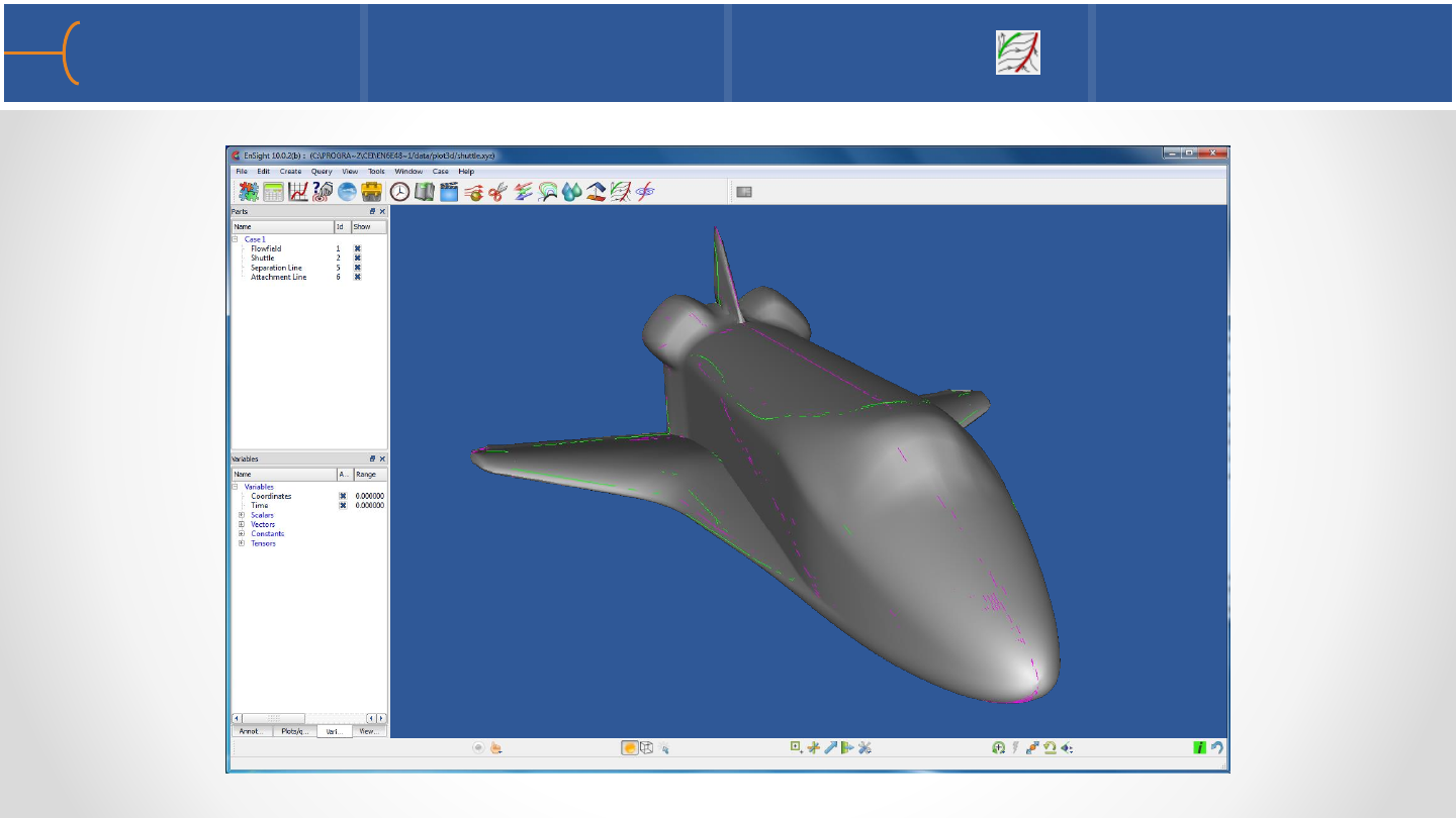
Separation & Attachment Lines 2 83
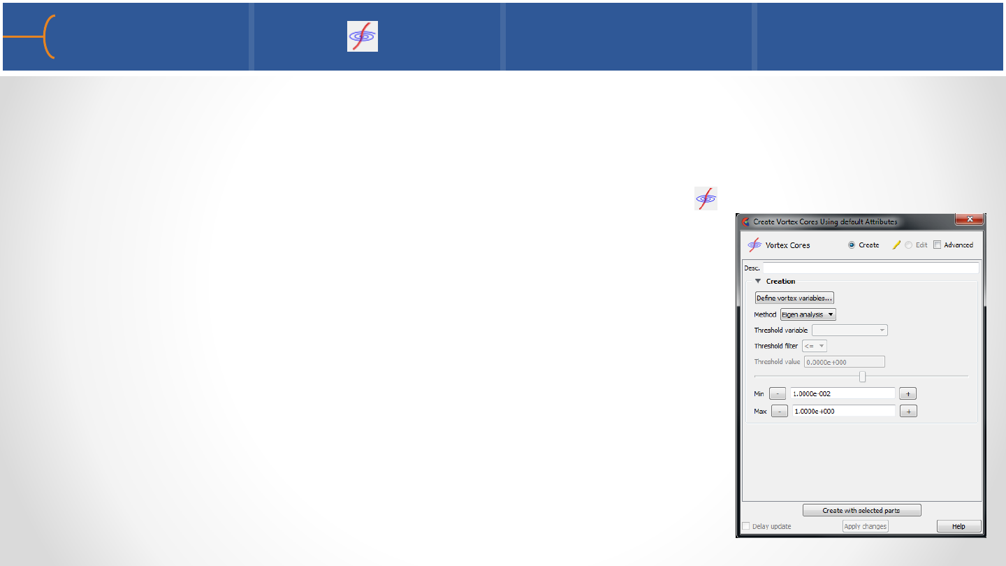
•Vortex cores are centers of swirling flow where the velocity is parallel to the
vorticity
•Select the fluid domain then click the Vortex Cores icon
•There are various menus to define The vortex variables
and the Method that is used
•Click the Create with Selected Parts Button
•Some CFD users like to use vortex cores to generate
streamlines from
Vortex Cores 1 84
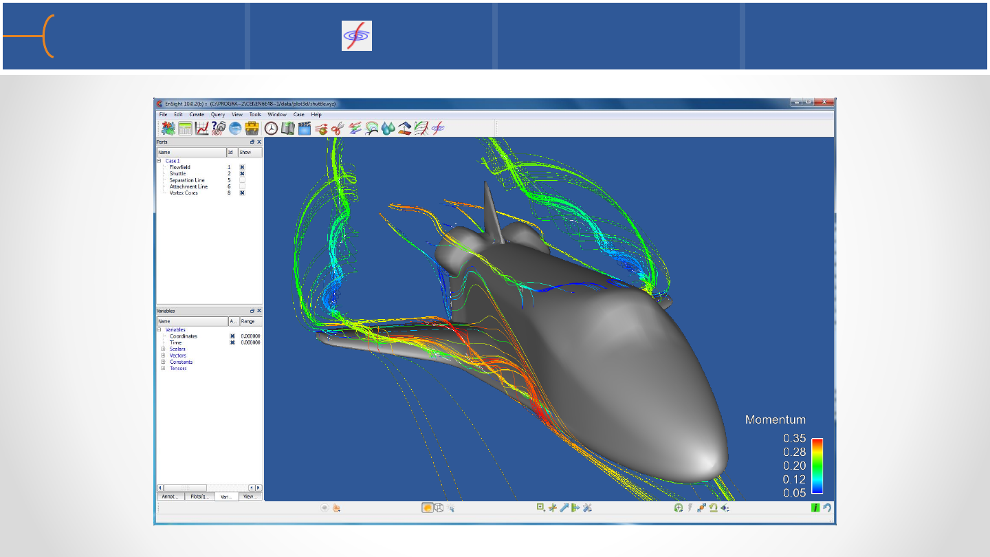
Vortex Cores 2 85
More Part Creation Exercise 86
•See the EnSight 10 Advanced Training Exercises handout and do Exercise 3
Polaris Snowmobile
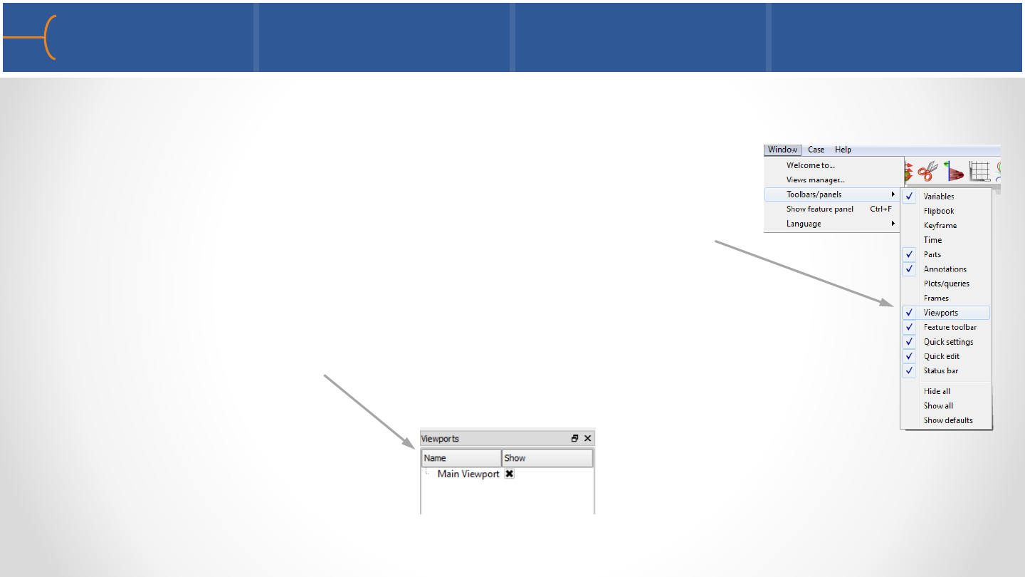
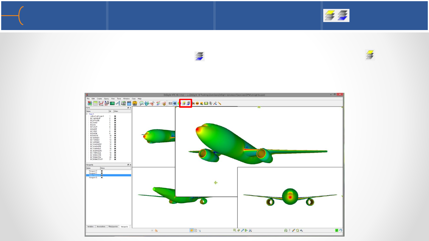
•Advanced control over one or multiple viewports can be achieved through the
Viewport tab in the Objects List
•If the Viewports tab is not displayed in the Objects List,
click on Window -> Toolbars/Panels -> Viewports and it
will be toggled on; this is also how it can be toggled off
•Click the Viewports tab in the Objects List and the Main
Viewport will be listed
Viewport Overview 1 88
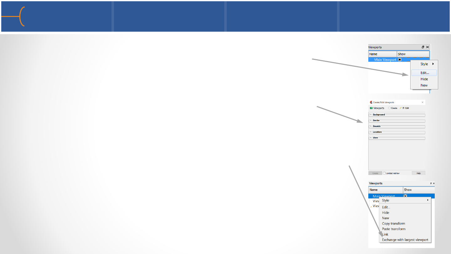
•Right click in the background of the the Main Viewport - since
there is only 1 viewport in this example there are only 3
options: Edit, Hide and New
•When Edit is selected the Create/Edit Viewports menu is
displayed with 5 options; these options are explained in the
following slides
•When there are 2 or more viewports, a right click has 4
additional options: Copy Transform, Paste Transform, Link and
Exchange with Largest Viewport
•Copy Transform and Paste Transform can be used to copy the
view from one viewport to another; use Copy Transform in one
viewport and Paste Transform in another to copy the view from
the first viewport to the second
Viewport Overview 2 89
•The Link option can link 2 or more viewports
that have the same or totally different views in
them
•To link 2 viewports, for instance the right and
left views of the airplane, right click in the first
viewport and select Link –then perform the
same action in the second viewport; the 2
viewports are now linked; more viewports can
be linked in the same way
•To unlink the viewports, right click and select
Unlink in each of the viewports that was
linked
Linking Viewports 90
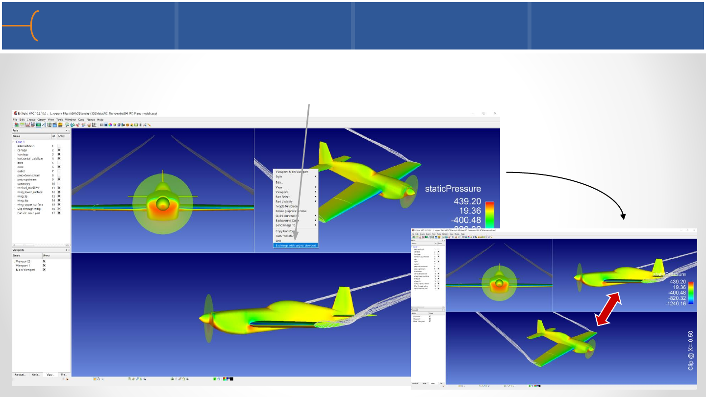
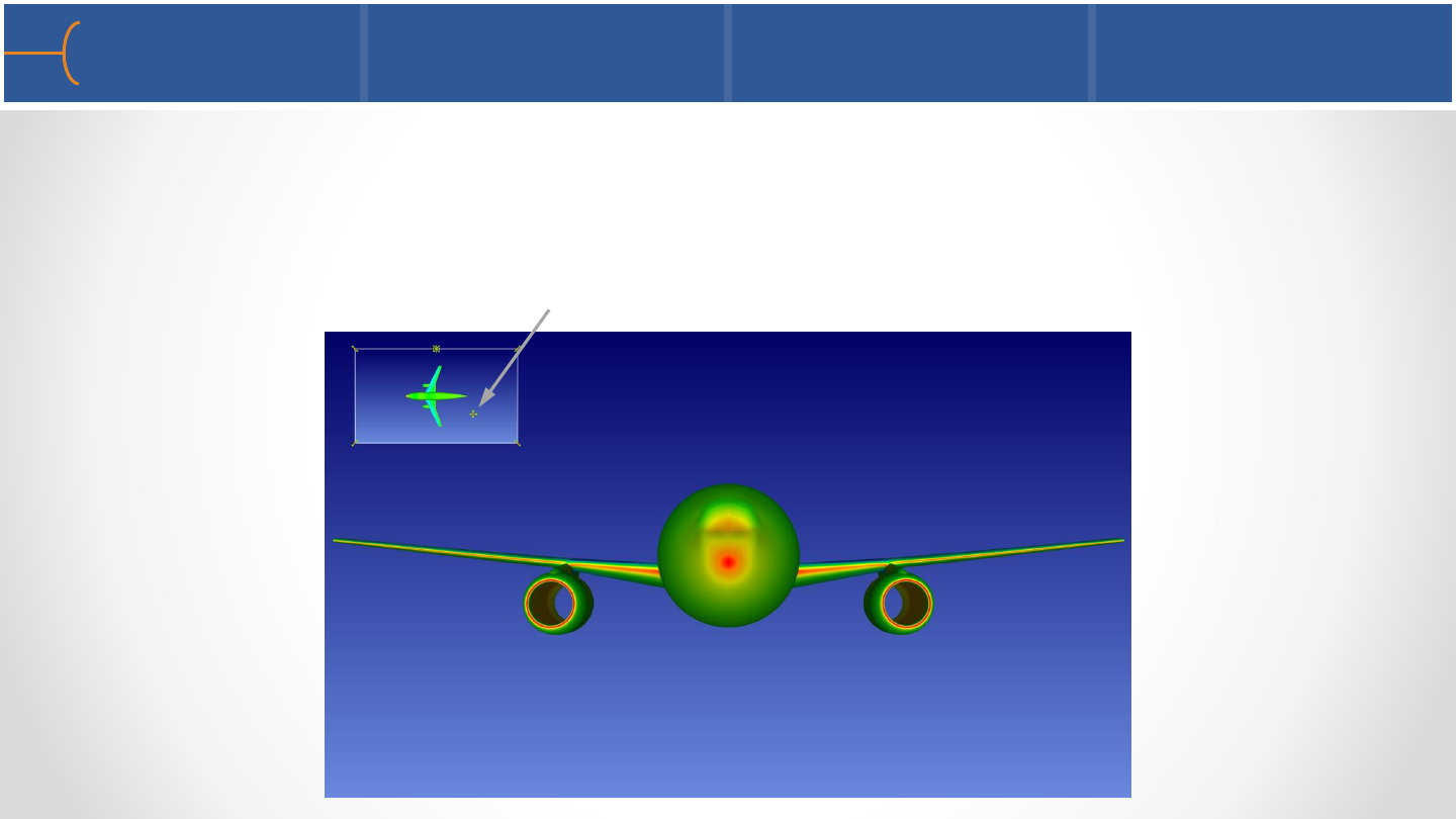
Exchange with Largest Viewport 91
•The Exchange with Largest Viewport option exchanges the view of a smaller
viewport with the one in the largest viewport
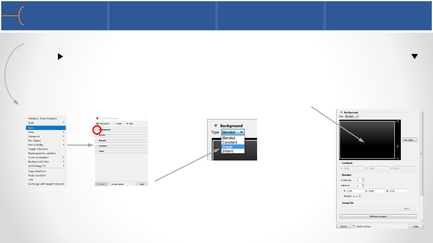
•Select a viewport and right click to edit the viewport; click the Background expand
arrow to display the options - the expand button is now pointing downwards
to indicate that the menu has expanded; the viewport background colors can be
constant, blended or inherited from the default viewport; the default color is a
blended color that changes from black at the bottom to gray at the top in 3 levels
•The background of a viewport can also be an image; select
Image under the Type Selection box and the system will ask
for an image file name to display in the background
Viewport Background Color 1 92
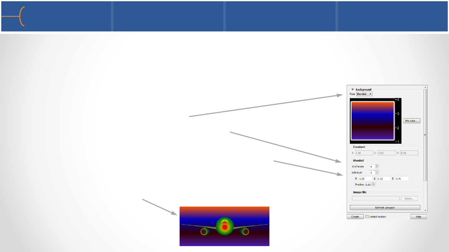
•For a Blended background, up to 5 horizontal level colors can be specified with
blending between each level
•To create a new blended background color,
do the following:
oSelect Blended under Type
oEnter the # of Levels, for example 4
oSet Edit Level to 1 and enter the RGB values,
for instance .3, .1 & .7 or click on Mix Color…
oDo the same for the other levels and a new
Blended background has been created
Viewport Background Color 2 93
•Use the Inherit option so the selected viewport(s) inherit the background type
and color from the Main viewport
•In this example the new viewport (# 1) has the default Blended colors and when
that is changed to Inherit, it takes the local color of the default viewport
Viewport Background Color 3 94

•The border of a viewport can be made visible by clicking the Border arrow; the
border visibility can be toggled and the color of the border can be selected as well
•The position and size of a viewport can be
entered by clicking the Location arrow
Viewport Border and Location 95
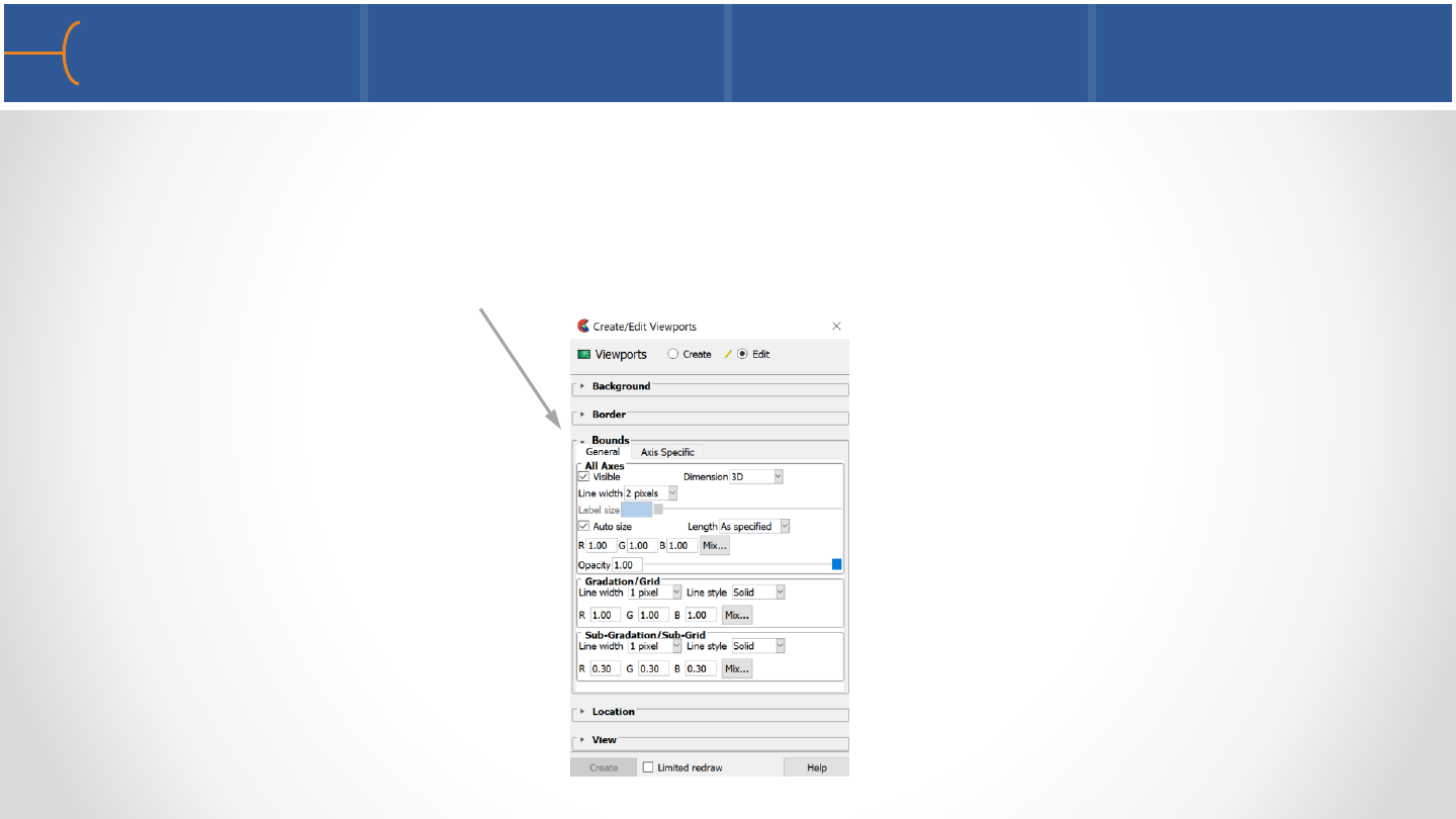
•Part bounds can be displayed per viewport; click on View -> Bounds Visibility
from the Main Menu to toggle this feature on; right click in a viewport and click on
the Bounds expand arrow
•The attributes of the Bounds Visibility feature can be modified with this panel
Viewport Bounds Visibility 96
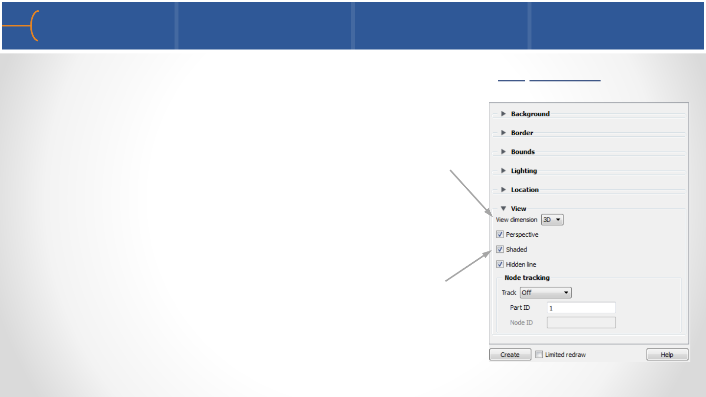
•Click the View arrow to see more options that can be set per viewport
•A viewport can be set to either a 2D or 3D View
Dimension; if the viewport is set to 2D, only planar
parts will be displayed in the viewport and the
rotations in that viewport can be only around the
screen Z-axis
•Each viewport has it’s own toggles for Perspective,
Shaded and Hidden Line display modes
Selected Viewport Special Attributes 1 97
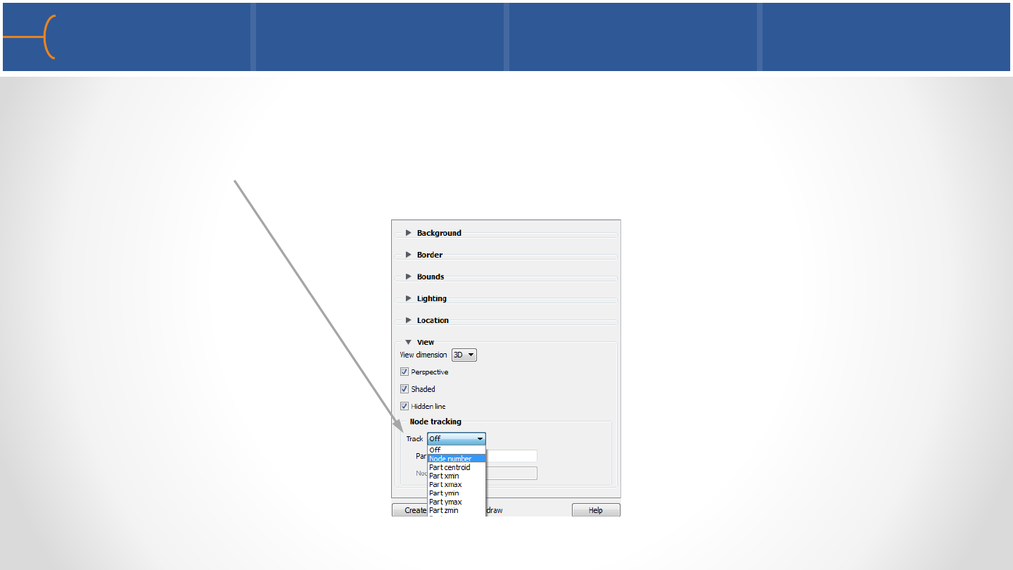
•A viewport can track a Node Number, a Part Centroid or the Part XYZ Min or Max
values; as a model changes over time the viewport will remain centered on that
location; this can be very useful for transient datasets
Selected Viewport Special Attributes 2 98
•When EnSight is started, it creates a single default viewport (labeled Main
Viewport) that fills the entire Graphics Window
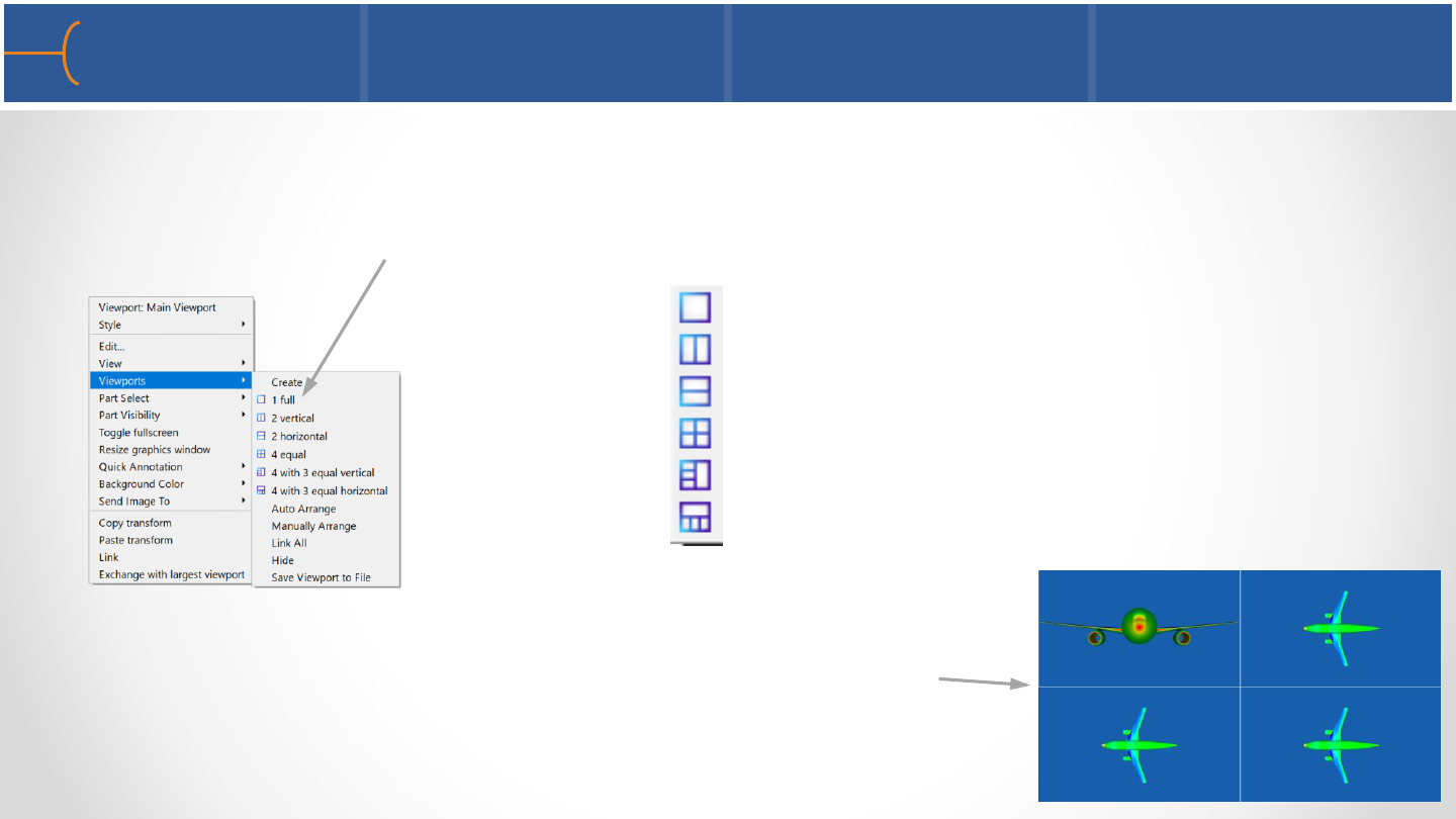
•Right click in the viewport and 6 viewport layouts are displayed:
•Click the layout that is desired; in this example the
4 equal viewports layout is selected and the system
resets the views in the new viewports
Viewport Layouts 99
1 single full viewport
2 vertical viewports, side by side
2 horizontal viewports, top and bottom
4 equal viewports
4 viewports with 3 equal vertical
4 viewports with 3 equal horizontal
•Right click in the viewport and select Viewports -> Create; this will create a new
viewport in the top left corner of the Graphics Window
•The new viewport can be resized by dragging the borders and moved by clicking
and dragging in the new viewport
New Viewport 100
•EnSight allows overlapping viewports; the viewport order can be controlled with
the Pop Viewport(s) Forward icon and Push Viewport(s) Back icon ; click in a
viewport and click either the Pop or Push icons
•The Main Viewport can also be popped forward or pushed backwards
Pop/Push Viewport(s) Forward/Back 101
Cummins 6.7L Diesel Engine with
Variable Valve Actuation

•Texture Mapping is a technique whereby a 2D picture is projected onto a 3D
object or even wrapped around a 3D object
•The easiest way to use Texture Mapping is to take a picture and use it as a decal (a
sticker) and place it somewhere on a 3D object; Texture Mapping can also be used
to display a pattern over part of the 3D object or the entire 3D object
•To access the Texture Mapping panel, select a
part, click the Surface Property Editor and click the
Texture arrow; click the Edit
Textures button to display the
Textures menu
Texture Mapping Overview 103
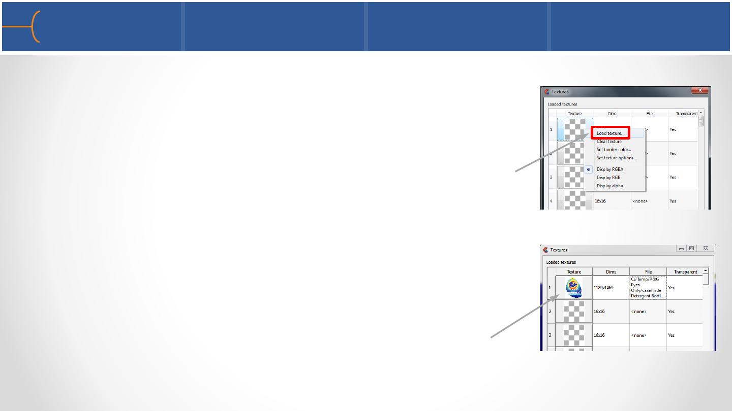
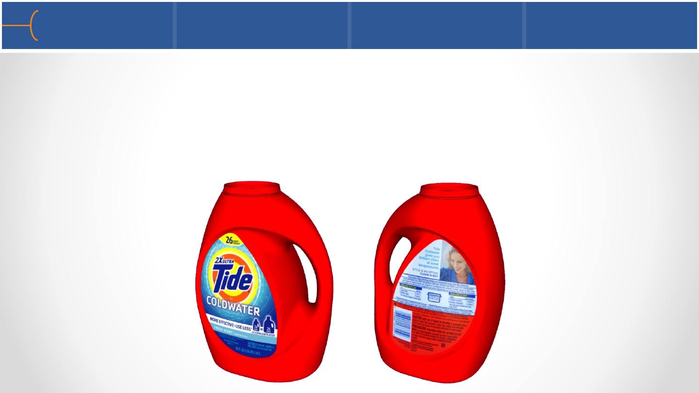
•The following example projects the front label of a Tide
detergent bottle onto the front of a 3D model of that
bottle
•On the Textures menu, load a picture by right clicking on
the first texture and selecting Load Texture; this will
display a file browser where a picture file can be selected
(.png, .jpg, .bmp etc); a high resolution image will give
best results
•As soon as a picture is selected, a thumbnail will be
displayed on the Textures menu; in this case the front
label of the Tide detergent bottle
Texture Mapping –1st Method - 1 104
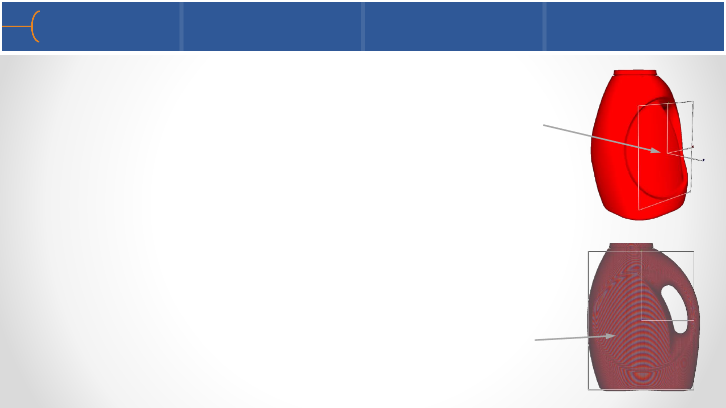
•The fastest way to apply a texture map is to use the Plane Tool;
in this example the XY-plane of the tool is parallel to the front
of the Tide bottle with the Z-axis sticking out the front of the
display
•It’s easiest to look at it from the front view with View ->
Perspective switched off
•Select the bottle in the Parts List and left click on the first
texture with the Tide front label; this will project the texture
along the Z-axis onto the bottle; the strange pattern on the
bottle is caused by the Repeat Mode on the Textures menu
Texture Mapping –1st Method - 2 105
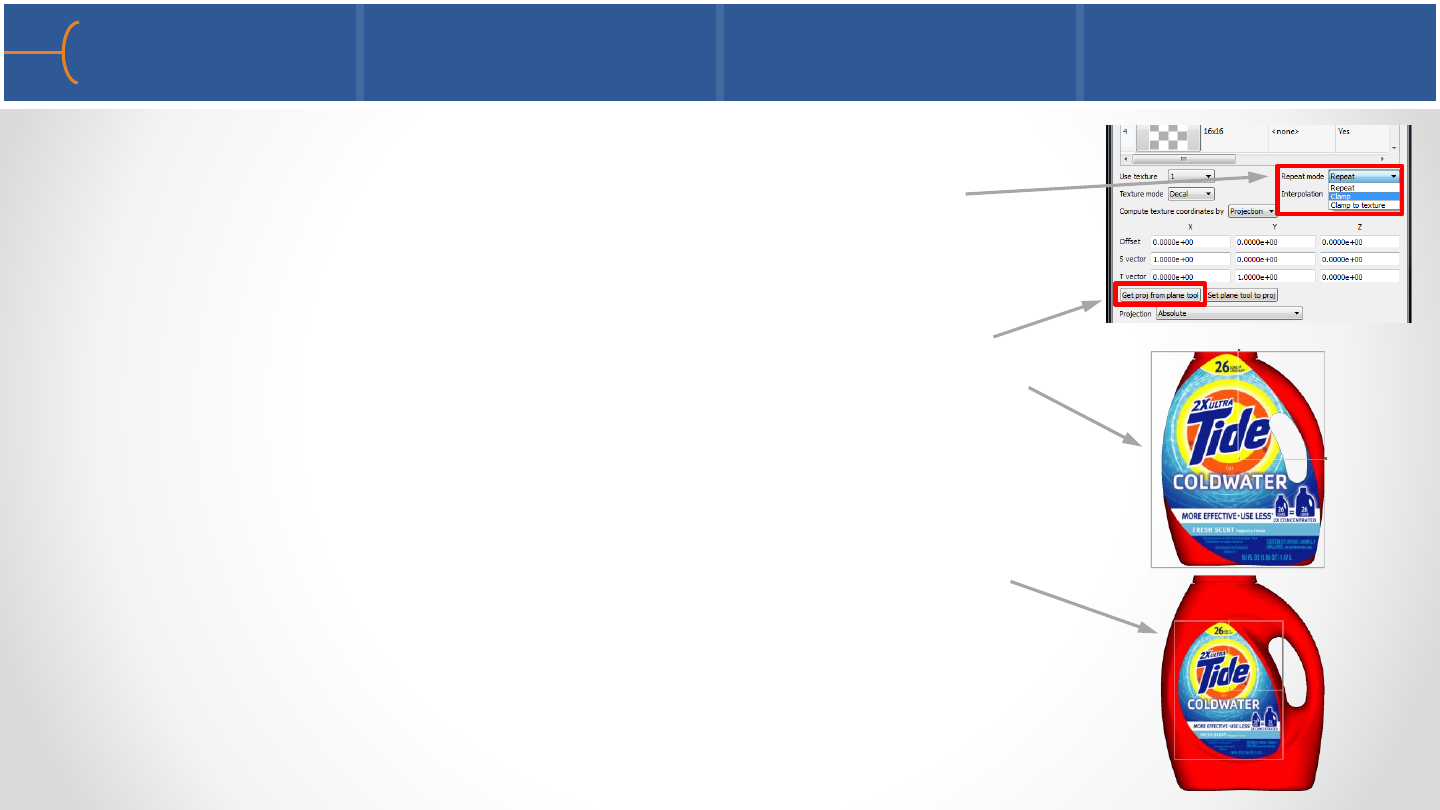
•Repeat Mode is set by default to Repeat which is typically
used for patterns; for this example change it to Clamp
•To make the system use the current size, position and
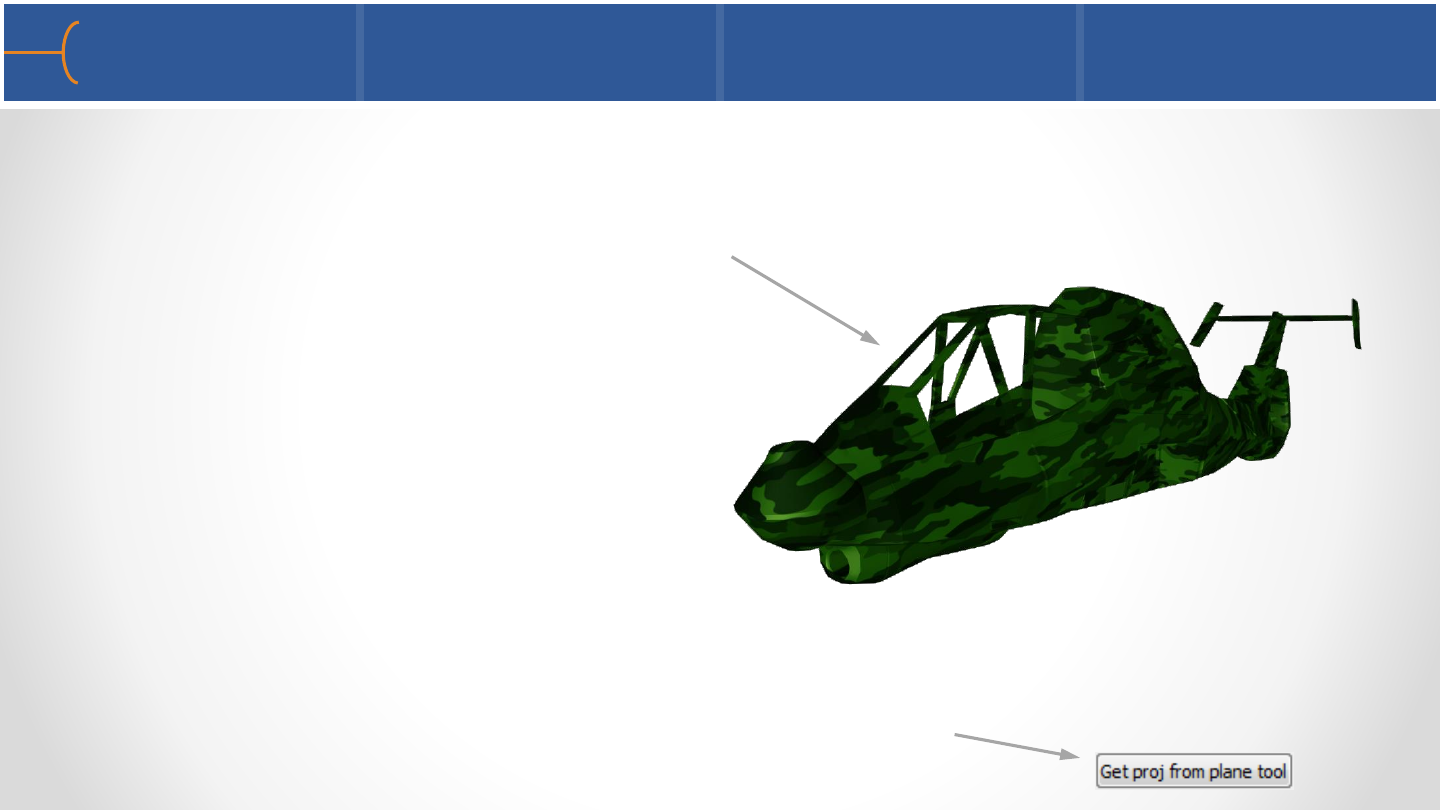
orientation of the Plane Tool, click on the Get Proj from
Plane Tool button; this will update the texture map to use
the current Plane Tool
•Adjust the size and position of the Plane Tool and click the
Get Proj from Plane Tool button after each change; after
several changes the fit will be near perfect
Texture Mapping –1st Method - 3 106
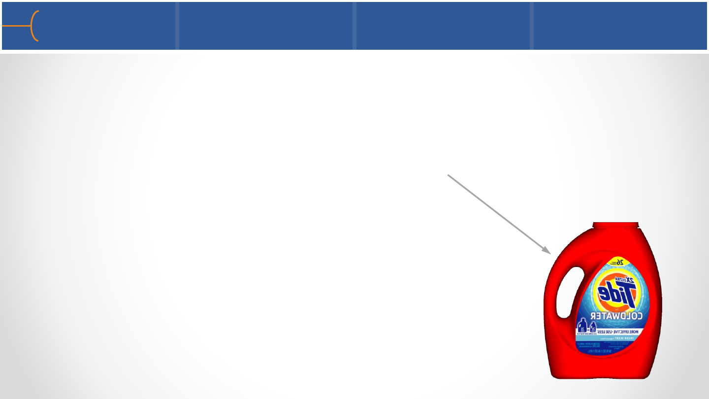
•Rotate and zoom in on the model (watch it full screen for instance by hitting F9)
and see that the texture map adds a great amount of realism to the model
•When the model is rotated to the back of the bottle it will be clear there’s a
problem; the front label is also mapped on the back of the bottle and because of
the Z-axis projection, it’s in mirror image
•This can be fixed by cutting the bottle in 2 halves; click
the Tools button on the top Main Menu and select Box;
position the box in the middle of the bottle and make
sure it covers the entire half of the bottle; click the Clip
icon and select Box as the Use Tool
Texture Mapping –1st Method - 4 107
•The model looks like this with the Box tool covering half the
model; the Box tool’s axis can be resized and the entire tool can
be moved by dragging the origin point of the 3 axes
•With the bottle still selected in the Parts List, cut the bottle with
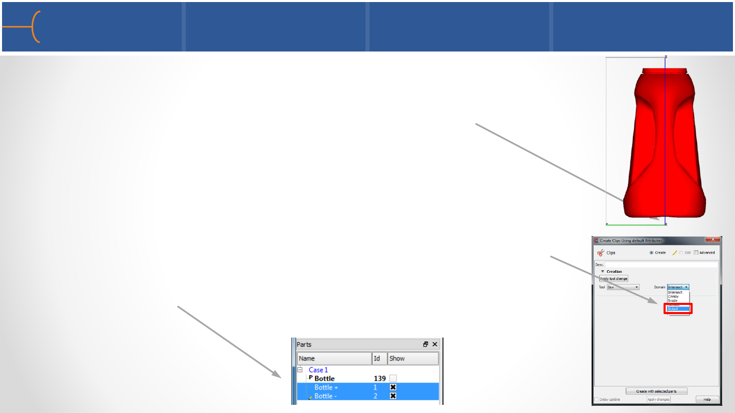
the Box tool using the Clip feature; select In/Out as the Domain,
this will create 2 new bottle halves in the parts list, named
Bottle + and Bottle - ; at the same time it will hide the original
Bottle part
Texture Mapping –1st Method - 5 108

•Now there are 2 bottle halves that can be texture
mapped individually using the same Z-axis
projection method as described before to texture
both the front and the back label onto the Tide
bottle
•Under Interpolation select Nearest or Linear, whichever looks best
•On the Textures panel, set Texture
Mode to Decal
Texture Mapping –1st Method - 6 109
•Load bottle.case and cut the bottle so the front and back labels can be texture
mapped on it
•Texture map both labels onto the bottle
•Create 2 viewports side by side and show the front and back view at the same
time; link the viewports and make the viewport borders invisible
Texture Mapping Exercise 110

•The second method of using Texture Mapping is to use an image as a pattern over
the entire 3D model or a portion of it; patterns like wood, brick, fabric etc can be
used to give a 3D object more realism
•The Plane Tool is again used to specify the Z-axis that will define the way the
pattern is projected onto the 3D object
•The Comanche helicopter body will be used to texture map a pattern onto; the
color of the body of the helicopter is military green
Texture Mapping –2nd Method - 1 111
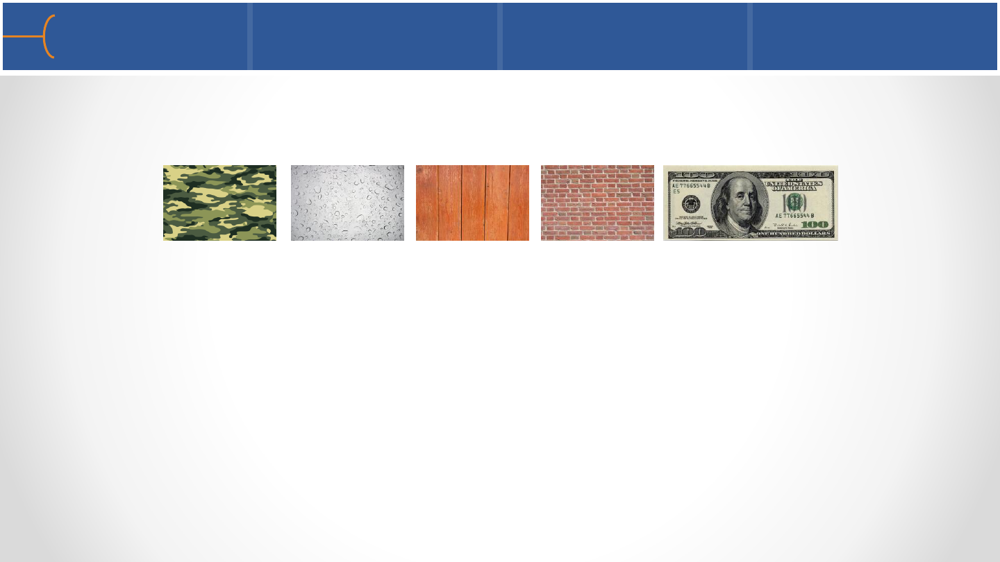
•The following patterns are textures that were found on the internet and will be
used to texture map the Comanche body
•To use one of the above textures, do the following:
oLoad the Comanche model, select the Comanche body (Part ID 4) and open
the Textures menu
oToggle the Plane Tool Visibility icon on
oRight click the first texture field and select Load Texture… and load the
camouflage image from the file browser
oLeft click the thumbnail that just appeared on the Textures menu and the
texture will appear on the body of the Comanche
Texture Mapping –2nd Method - 2 112
camouflage water drops wood bricks $100 bill
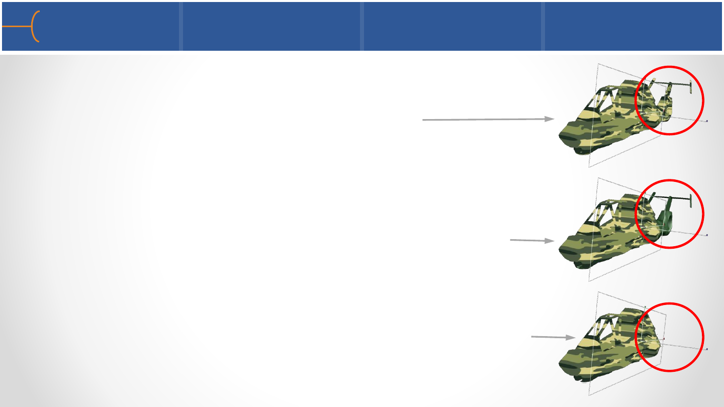
•On the Textures menu the Texture Mode is by default set to
Decal; the Repeat Mode is by default set to Repeat; the
Comanche model will look something like this
•Set Repeat Mode to Clamp and only the portion of the
object that is under the Z-axis projection will be textured
•Set Texture Mode to Replace and only the textured portion
of the object will be displayed
Texture Mapping –2nd Method - 3 113
•Still on the Textures menu, set the Texture Mode to Modulate and the color of
the object (military green in this example) will shine through the texture and it will
preserve the shading of the model underneath the texture map; the Repeat Mode
has been set back to Repeat
•By changing the color of the Comanche body and by modifying the size and
orientation of the Plane Tool, the texture map will be influenced; after every
change to the Plane Tool, click the Get Proj from Plane Tool button to update the
image
Texture Mapping –2nd Method - 4 114
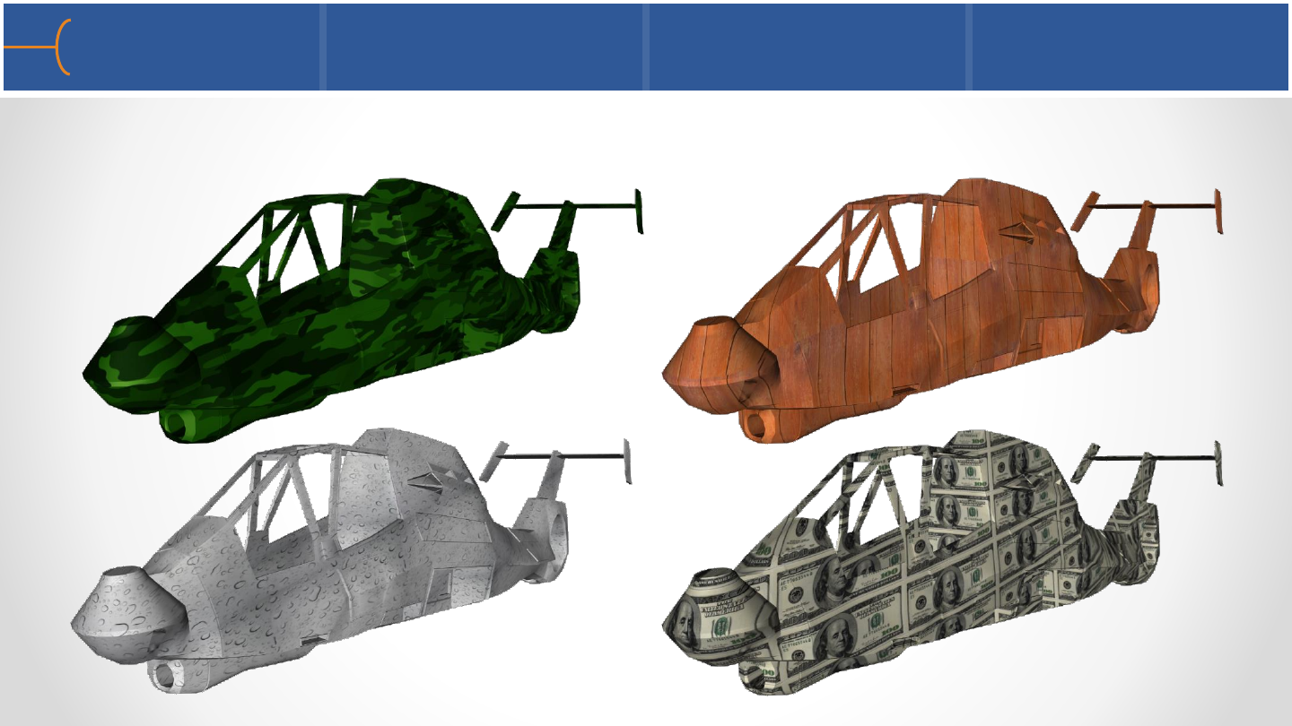
•Here are some examples of texture maps on the Comanche
Texture Mapping –2nd Method - 5 115
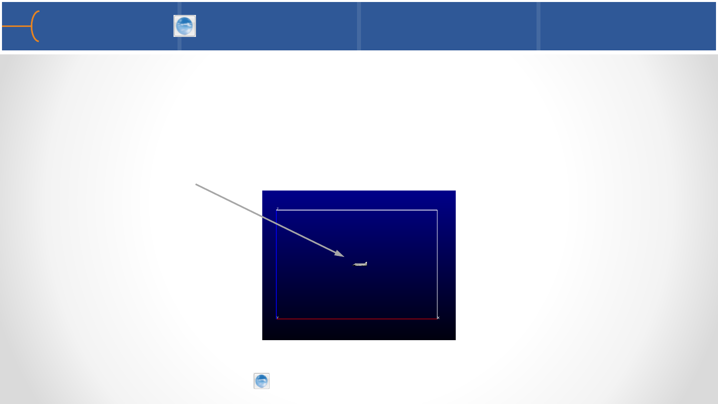
•A Skybox is a cube that is placed around the entire model and the 6 sides of the
box are texture mapped with 6 images that are continuous at the seams; this
creates the illusion of a 3D world around the model that rotates as the model is
being rotated
•The cube has to be significantly bigger than the limits of the model, so the user
can zoom in to the model and see the 3D world in the background
Skybox Overview 116
Click the movie to play
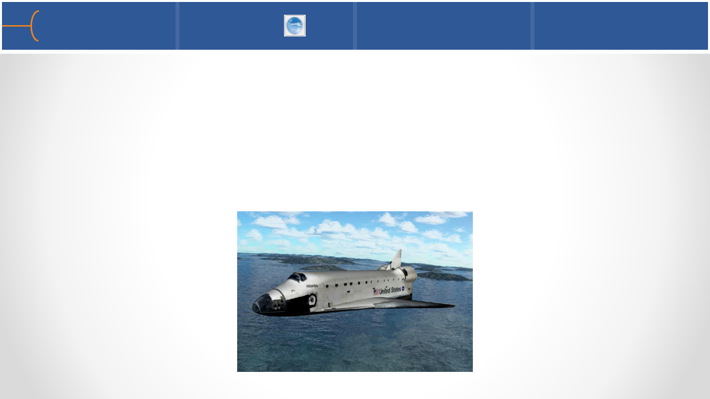
•To create a Skybox around the Space Shuttle model, do the following:
oLoad the model and texture map the shuttle for even more realism (set View
-> Perspective to off to make it easier)
oZoom out so the model is relatively small at the center of the screen and click
Tools -> Box (resize the box if needed)
oSelect the Space Shuttle (Part ID 2) in the Parts List
oClick the Skybox icon and click Ok
Skybox 1 117
oSelect a Skybox picture in the file browser; a
Skybox picture has the following layout
oSwitch of the Box tool and switch Perspective
back on
oZoom into the Skybox so the model can be seen;
switch on any particle traces, clip planes,
isosurfaces etc
oClick F9 and rotate and zoom the model full
screen
oA Skybox will be recorded in an animation
Skybox 2 118
Texture Mapping Exercise 119
•See the EnSight 10 Advanced Training Exercises handout and do Exercise 4

Embraer Legacy 600 Business Jet

Keyframe Animation Basics 1 121
•EnSight can create smooth and complex animations using a process called
Keyframe Animation
•In a keyframe animation, a particular start view and a different end view (called
keyframes) are defined and EnSight can automatically generate frames to
interpolate between the two views creating a smooth animation
•A keyframe animation will record not only all rotations, pans and zooms that are
used but also changes in transparency, auxiliary clipping, particle traces,
isosurfaces, clip planes, plots, texture maps, a skybox etc
•The length of the animation is determined by the number of frames generated
between the two keyframes
•A keyframe animation can also be used to record a transient model; the time line
of the dataset can be controlled
•The results of a keyframe animation can be written to various movie formats such
as MPEG, AVI, QuickTime, Flash etc
•The resolution of the animation can be controlled from NTSC, PAL, DVD, HD 720p,
HD 1080p up to User Defined; anti-aliasing can be used to get the highest possible
quality for the frames used in the animation
•Once EnSight is starting to generate frames, the process can be aborted by placing
the cursor in the Graphics Window and pressing the key on the keyboard (
for abort)
Keyframe Animation Basics 2 122
A A
•A fast way of generating a keyframe animation is to click
the Keyframe Animation -> Quick Predefined Animations
toggle; this displays a panel where 3 predefined options
can be selected
•Enter the total number of frames, one or more of the
predefined options (Fly Around, Rotate Objects and
Explode Views) and type in the desired parameters for
each option
•Click the Create Predefined Keyframe button and the
keyframe sequence will be created
Quick Animations 123
•The Space Shuttle model with the particle traces will be
used as example
•Once the model is loaded, select the -Y view and
press the ‘Fit Geometry’ icon so the Shuttle is
facing left
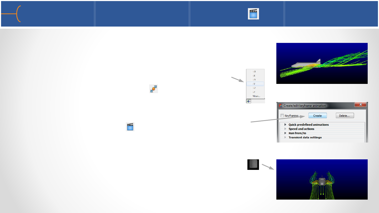
•Click the Keyframe icon ; on the menu click the Create
button –this will create the first keyframe
•Then rotate the model to the front view by pressing
twice and click Create again - this will create the second
keyframe
Keyframe Animation Creation 1 124
Keyframe 1
Keyframe 2
F2
•EnSight just created a keyframe animation and it can be
played back; click on the Run button and the animation
will be played
•This animation is not very useful because the playback
time is less than a second; this is controlled by the Speed
and Actions button; clicking this toggle will display a menu
where the number of Sub-frames to the Next Keyframe
can be entered; this number controls the speed of an
animation
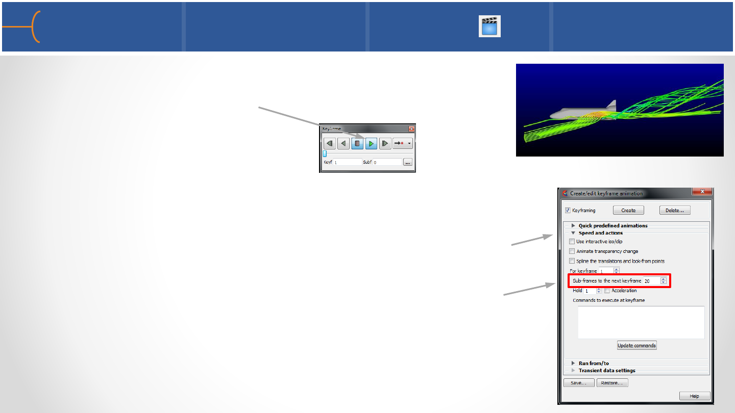
Keyframe Animation Creation 2 125
Click the movie to play
•In this next movie the number of subframes has been
set to 88; the animation now takes exactly 3 seconds
to play - why 3 seconds? Well, an animation has a
default frame rate of 30 frames per second and since
there are 2 keyframes that were created (the start
view and the end view) plus 88 sub-frames, there are
a total of 90 frames - at 30 frames per second, that’s
exactly 3 seconds
Keyframe Animation Creation 3 126
Click the movie to play
Keyframe 1 Keyframe 2
Frame #1 #90
Sub-frame 1…………………………………………………………………….88

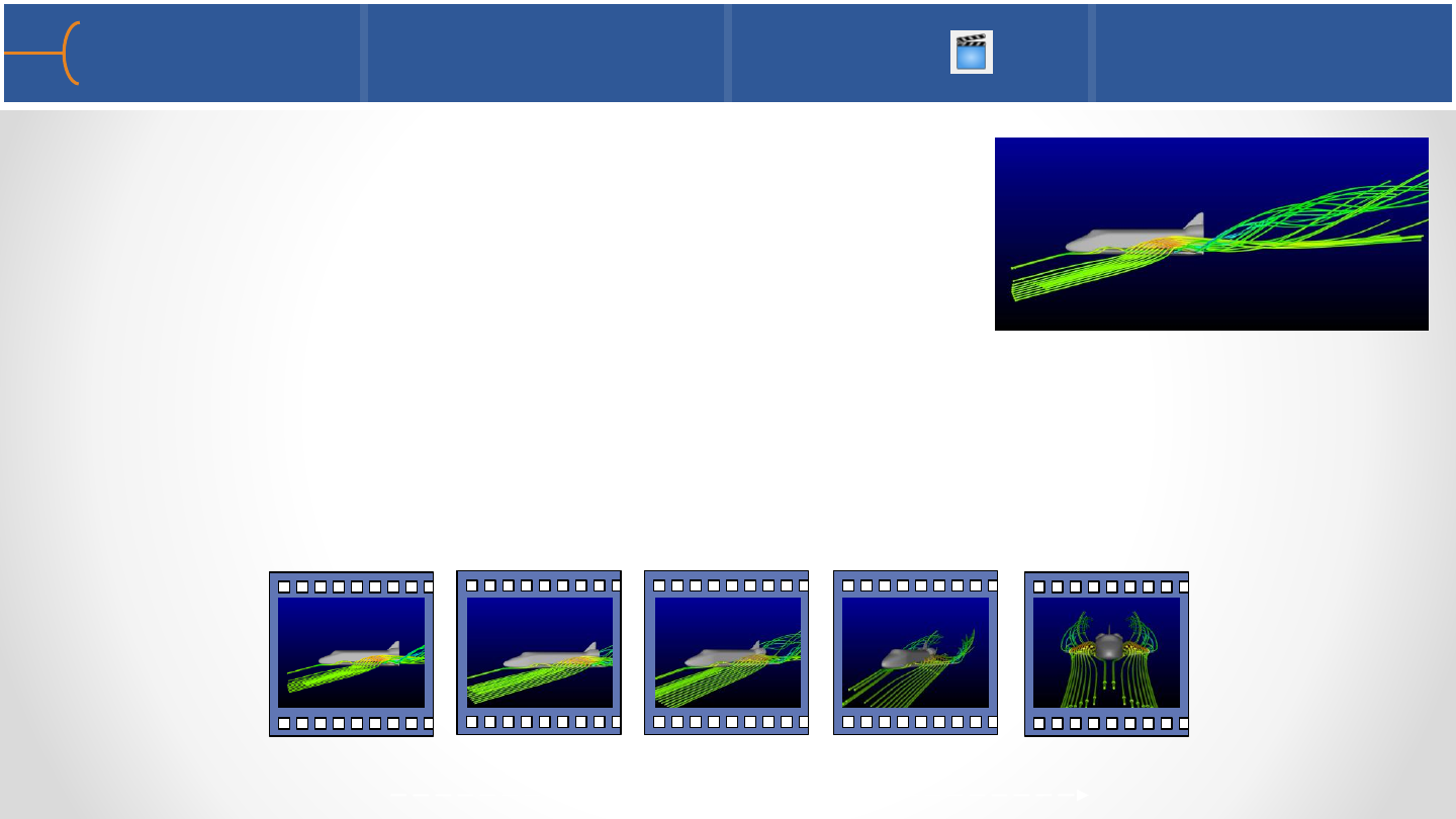
•After the first 2 keyframes, more keyframes can be created; press two more
times and zoom in on the Space Shuttle, then click Create again; there are now 3
keyframes and 2 sets of sub-frames; to make the segment from the second
keyframe to the third keyframe also 3 seconds long, the number of sub-frames
have to be 89 - here’s why:
•Note that the animation between keyframes 2 and 3
not only rotates but also zooms at the same time
(noticed the animated particles?)
Keyframe Animation Creation 4 127
KF 1
Frame #1 #180
88 Sub-frames KF 2 KF 3
89 Sub-frames
Click the movie to play
F2
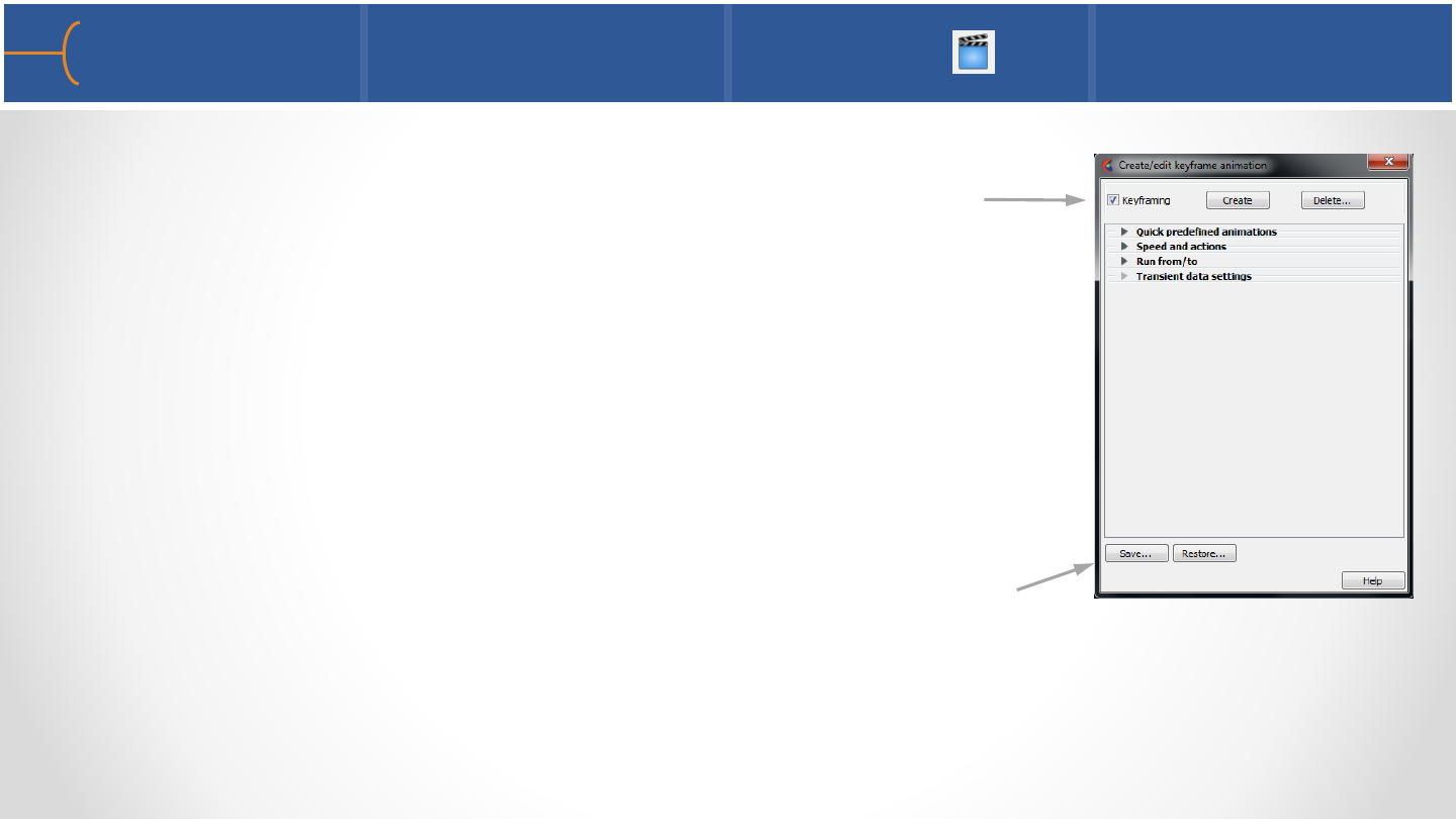
•As soon as 1 or more keyframes are defined, the
Keyframing toggle will be checked; when this toggle is
checked, it means there are 1 or more keyframes
defined
•When the toggle is unchecked, the entire keyframe
sequence is deleted; click on Save to file a keyframe
sequence and press Restore to read it back in from a file
Keyframe Animation Creation 5 128
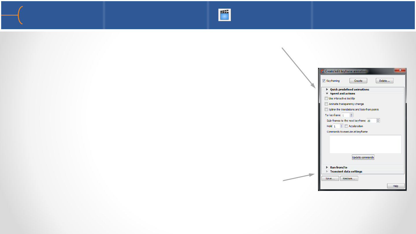
•After 2 or more keyframes have been created, the Speed
and Actions panel will become available; on this panel
besides the number of sub-frames, options to animate
Isosurfaces, Clips and Transparency changes can be
toggled on
•Click the Transient Data Settings toggle if the dataset is
transient and the motion should be included in the
animation (if the dataset is not transient this feature is
grayed out)
Keyframe Run Attributes 129
•Create another Space Shuttle keyframe animation
starting with the shuttle facing left with a clip plane in X
•Click the Create button then rotate the model 180° so it’s
facing right; left click the clip plane and drag it so it’s just
behind the Space Shuttle; now click the Create button
again
•The animation now rotates and moves the clip plane at
the same time
Animating a Clip Plane 130
Click the movie to play
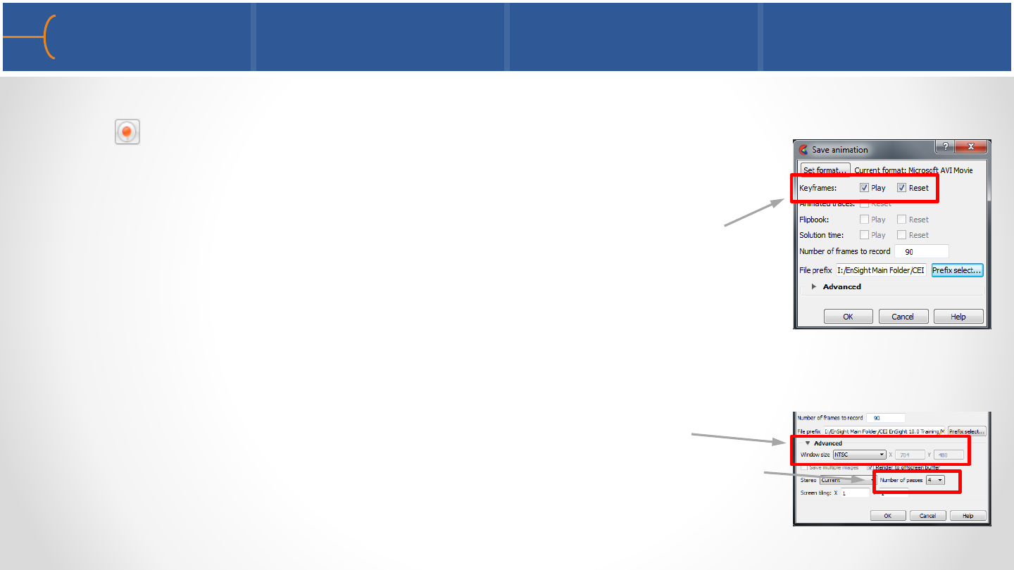
•To make a movie from a keyframe animation, click the record
icon or click File -> Export -> Animation; the Save
Animation menu is displayed
•Make sure to select the toggles for Keyframes Play and Reset
•Enter the name for the movie
•Click the Advanced toggle to display a menu where the
Window Size and anti-aliasing (Number of Passes) can be set
Recording a Keyframe Animation 1 131
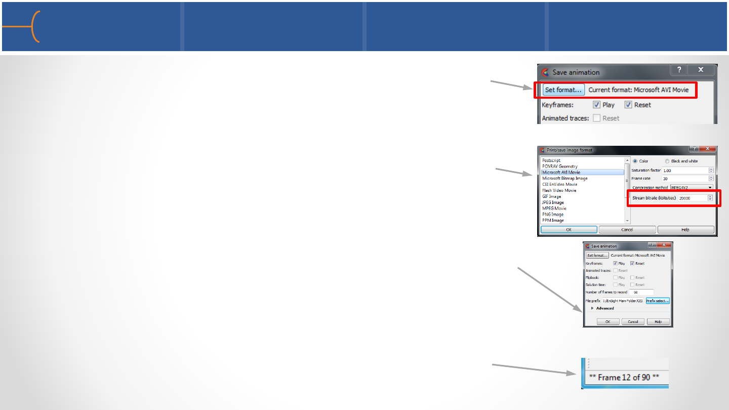
•The Set Format button displays a variety of movie formats
that can be selected; choose a format, in this example AVI,
and see the options for that format
•The Stream Bitrate controls the quality of the movie; a
higher number results in a higher quality but at the cost of
a bigger file size
•Click the OK button on the Save Animation menu and the
movie will be created
•The Message Area in the lower left corner of the EnSight
window will display the frame numbers that are being
generated
Recording a Keyframe Animation 2 132
•Creating many keyframes does have its drawbacks; for instance if a certain
keyframe sequence has to be modified, there’s no way to just go back to that one
sequence and modify it; for this reason it’s better to create a keyframe sequence
between only 2 keyframes and then write it as an animation file
•After all the individual movie segments have
been created, a free program supplied by CEI
called EnVe is used to create one complete
movie from all these segments
Keyframe Animation Tips 1 133

Keyframe Animation Tips 2 134
•If an animation is needed that can be continuously looped, make sure the start
frame and the last frame are the same
•Remember that the graphics on a workstation run at a different frame rate
(normally slower) than a movie (30 frames per second); this means that an
animation that looks fine on a workstation could be too fast when played back as
a movie
•When an animation is created using a large window size (resolution) and/or anti-
aliasing, the generation time of the movie file will be significantly longer
•Creating a keyframe animation is pretty easy; however, creating a great movie
using keyframe animation takes skills, creativity, a plan of what the movie should
look like and experience

Keyframe Animation Examples 135
HCCI Engine In-cylinder Contact Lens Packaging
Boeing C-17 Ground Vortex
Keyframe Animation Exercise 136
•See the EnSight 10 Advanced Training Exercises handout and do Exercise 5

137
Boeing 787-10 Dreamliner
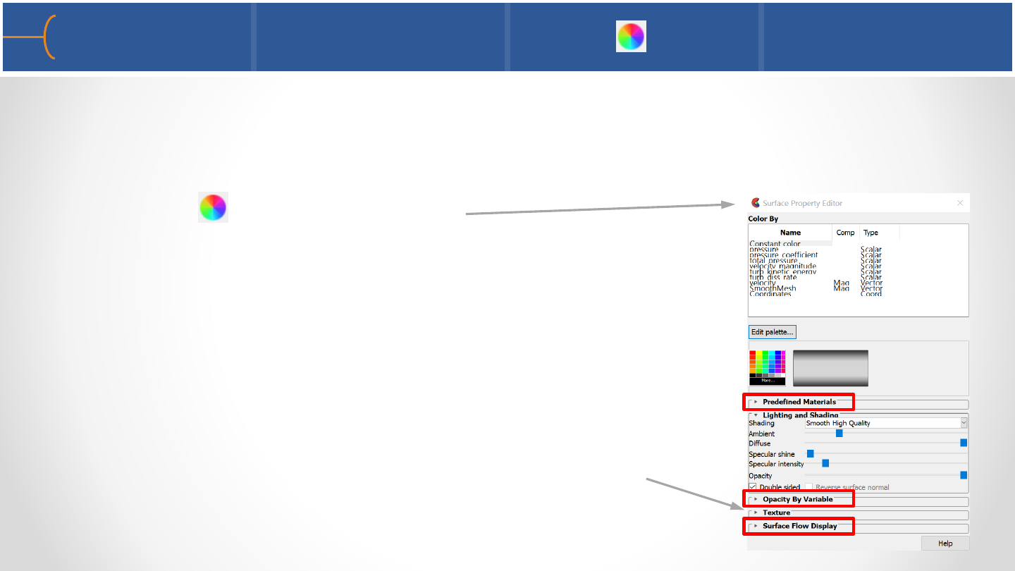
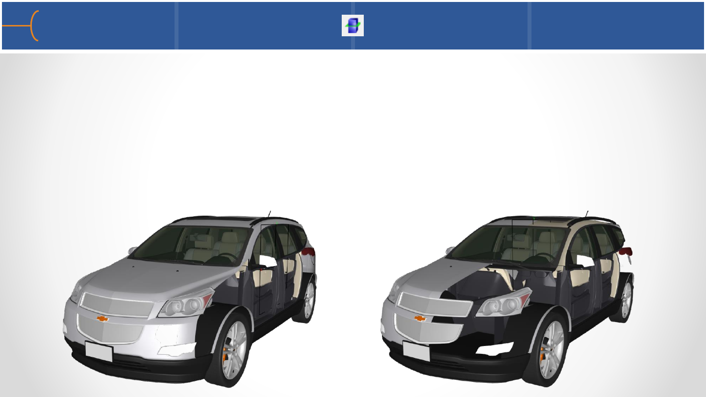
Materials Library Overview 1 138
•EnSight 10.2 introduces a predefined materials library that can be used to
enhance the realism of parts
•The Surface Property Editor is used to assign a material to a part –click the Color
Wheel icon to display the menu
•The Surface Property Editor menu is similar to the
previous Color Editor menu but it has more lighting
controls and it contains several new menus as well:
oPredefined Materials
oOpacity By Variable
oSurface Flow Display
•The Texture menu is now directly accessible on the
Surface Property Editor menu
Materials Library Overview 2 139
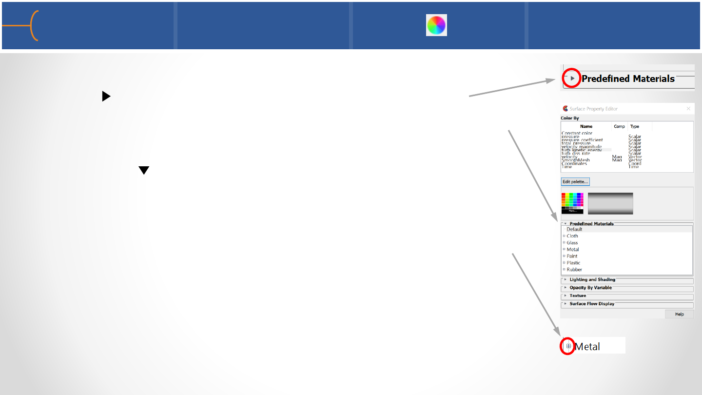
•The materials library is accessible by clicking the expand
button to the left of the Predefined Materials label
•When clicked, the materials library opens up and displays 6
types of materials - the expand button is now pointing
downwards to indicate that the menu has expanded
•By default, parts are not assigned a material when they are
created or read in from a dataset
•To see the available metal materials for instance, click the +
sign to the left of the Metal label; this will open the Metal
group and it will display several metals
•Select a part in the Parts List and select a material, for instance
Metal -> Chrome –this assigns the metal chrome to the part
that is selected

Materials Assignment Example 140
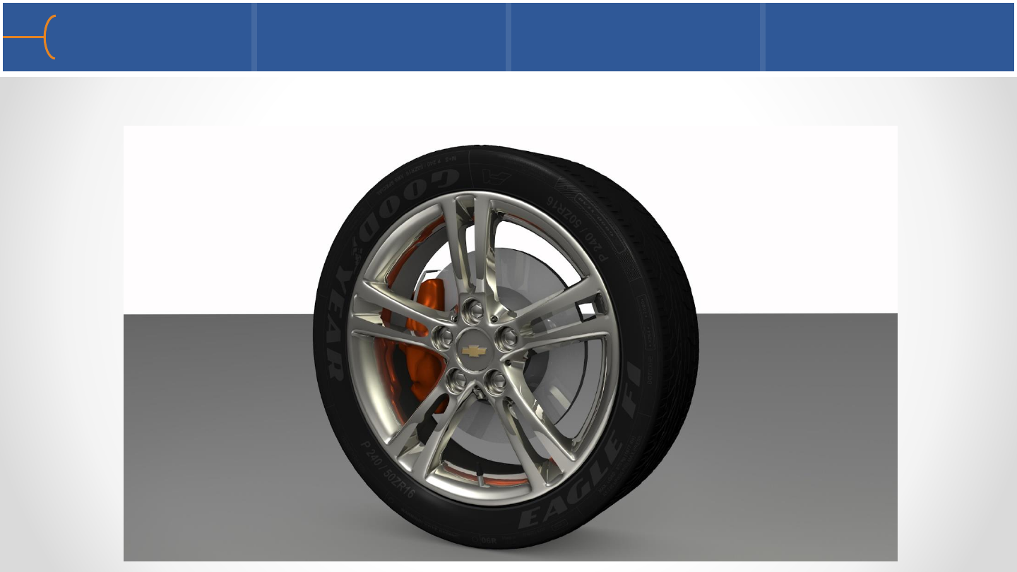
•Use the ‘Chevy Traverse Wheel.case’ dataset as example
•Assign Chrome as the material for the rim, rim center logo edge and rim center,
Rubber -> Hard for the tire, use Paint -> High-gloss for the caliper, Aluminum for
the rotor, brake line and the valve stem, Iron for the brake housing, Gold for the
GM logo and Plastic -> Hard for the valve cap –modify some of the slider settings
and see what the effects are; adjust colors as needed
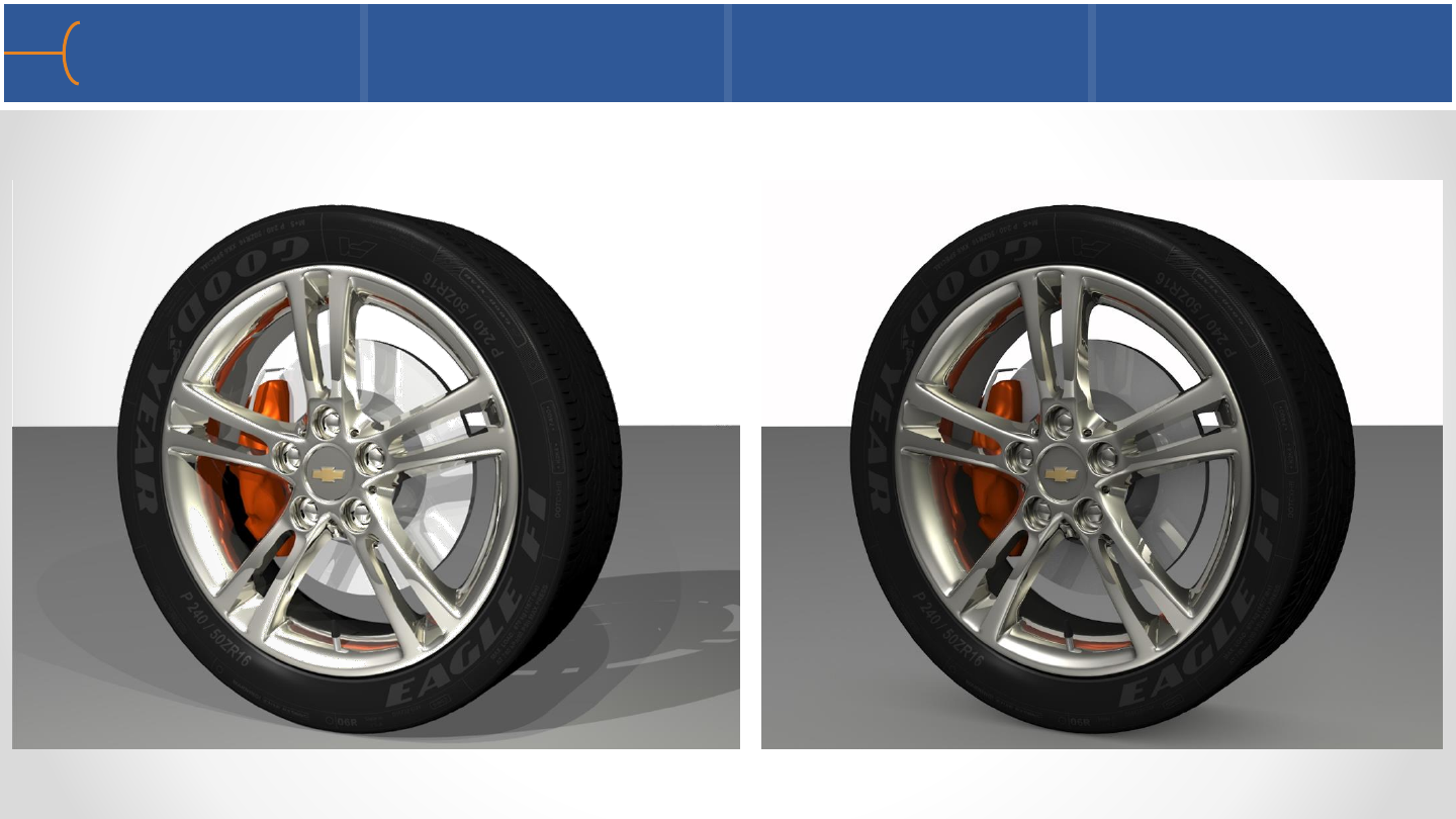
Without Materials With Materials With Materials, texture map & road
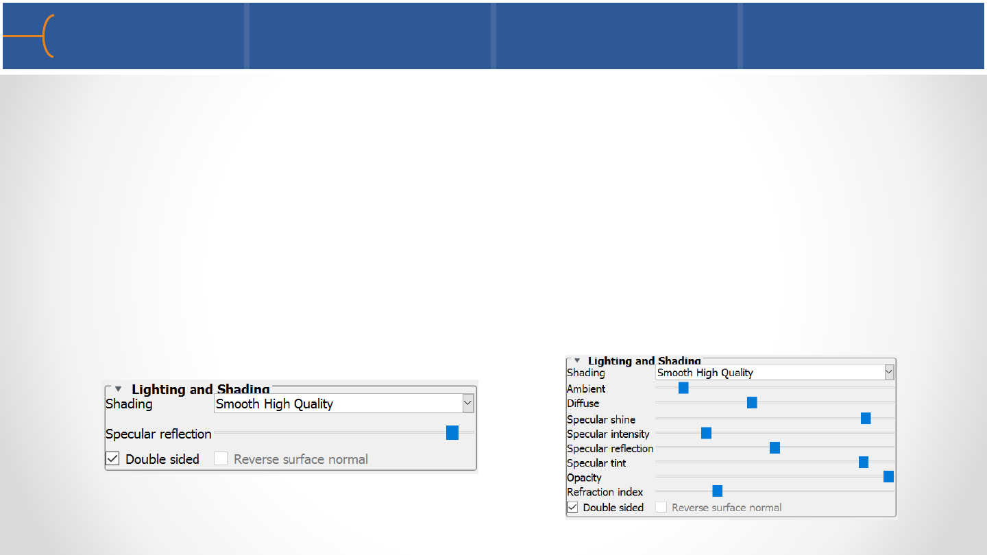
Lighting and Shading per Material 141
•The sliders in the Lighting and Shading menu have different options depending on
the material that is selected
•The Metal and Glass group and the Paint –> High-gloss and Semi-gloss have
reflections –on the Lighting and Shading menu there’s an additional slider for
Specular Reflections for these materials –some of the Glass and the Gloss Paints
have a Refraction Index as well; all other materials are matte and do not have
reflections
•Depending on the selected material, the Lighting and Shading menu can have
from 1 to 8 sliders that control how the materials look
Lighting and Shading menu for High-gloss & Semi-gloss paint
Lighting and Shading menu for Glass -> Mirror
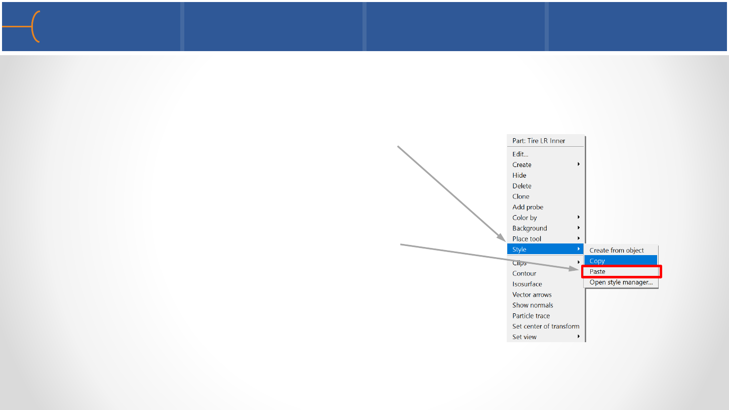
Style Feature to Copy Materials 142
•The color and material settings of a certain part can be copied to other parts by
using the Style feature in the right-click menu
•Put the cursor on the part with the color and material that needs to be copied and
right-click; then select Style and click Copy
•Now put the cursor on the part that needs
the new color and material settings and
right-click; then select Style and click Paste
•Style -> Paste can be used for multiple parts
and groups as well
•Please note that the Shading Type is not
copied from one part to another
Notes About the Materials Library 143
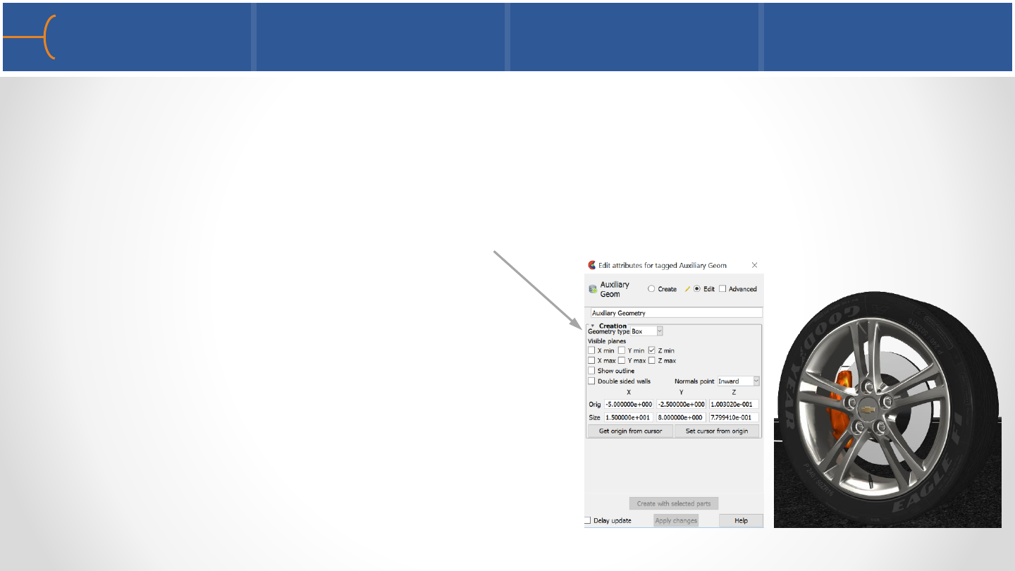
•Some notes about using materials:
oFor Glass -> Mirror, there is only 1 slider for Specular Reflection in the Lighting
and Shading menu; there is no color assigned to a mirror
oAuxiliary geometry can serve as reference geometry to increase the realism of
the scene; click on Create -> Auxiliary Geometry to select the plane that’s
needed; the road surface in the
image on the right was created using
Auxiliary Geometry with a texture map
oTo create even more realistic scenes, use
multiple light sources and Ray Tracing; this
is discussed in the next 2 chapters
oFor high quality output, use antialiasing
and make sure the Shading is at least
set to Smooth; switch off the Model Triad
Using Materials on the Chevy Traverse 144
CFD modelCFD model with some materialsCFD model with CAD model
CFD & CAD model with correct colors
CFD CAD colors materials CFD CAD colors materials texture maps
CFD CAD colors materials texture maps lights CFD CAD colors materials texture maps lights auxiliary geometry
Chevy Traverse Animation 145
146
Boeing 787 Dreamliner
without any seats
Multiple Light Sources Overview 147
•EnSight 10.2 Has 7 additional light sources besides the standard light
•Using multiple light sources has a significant effect on the realism and overall
visual quality of the model, particularly when Ray Tracing will be used
•There are 3 different types of lights: Directional, Spot and Point
•Each light source can be placed anywhere in 3D space
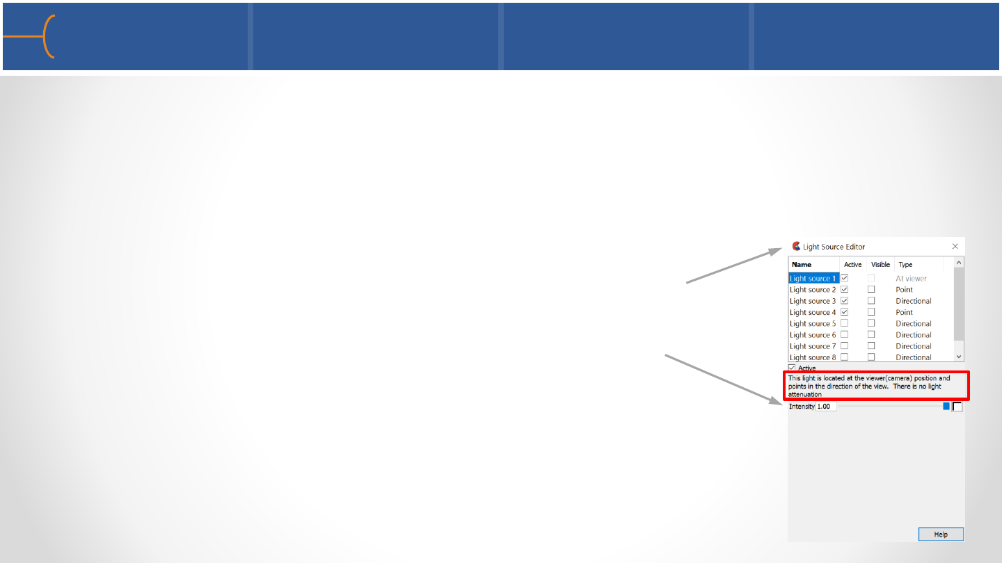
•Click View -> Lighting to display the Light Source Editor
menu
•The intensity and color of the lights can be controlled
•The first light source is the original light source that has
always been present in EnSight; the light is from the user
in the direction of the –Z screen axis, towards the model;
there is no light attenuation (gradual loss in light intensity)
and the type of light can not be modified
Types of Light 1 148
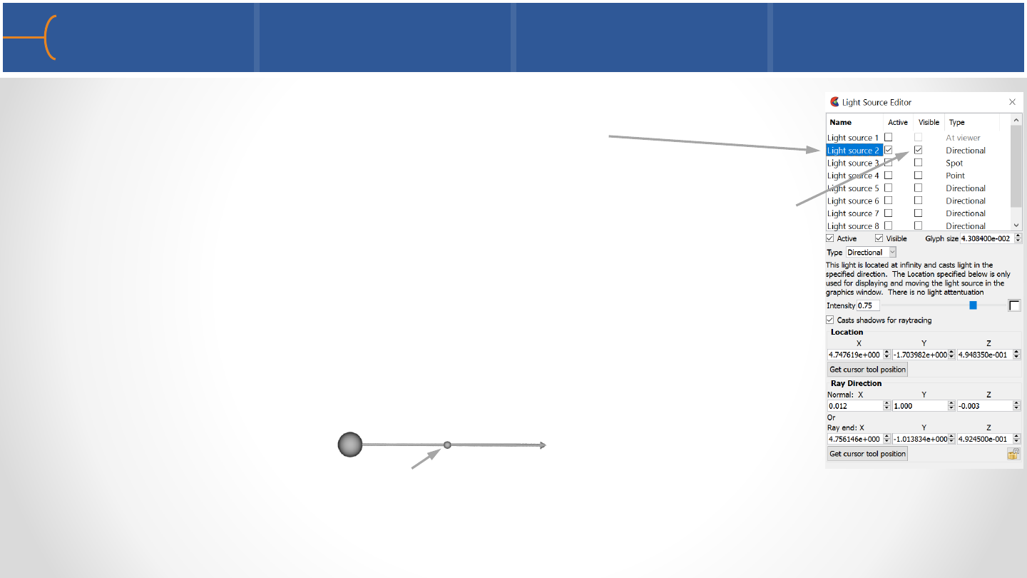
•Each of the 7 additional light sources can be active or inactive –
use the toggle to switch a light source on or off
•Each light source, except light source 1, has a Glyph (an icon) in
the graphics window that indicates its position and orientation;
the visibility of a glyph can be toggled on or off; a glyph has 3
hot points: at both ends and at its center
•There are 3 types of light:
oDirectional - the light is located at infinity and points towards
its end; there is no light attenuation; the glyph and hot point
locations for this light are:
Moving the glyph at its center has no effect on the lighting of
the model; only moving its end points changes the lighting
effects
++
+

Types of Light 2 149
oSpot - the light shines towards its point; this light has attenuation; this light type
also has a spot angle as well as a falloff angle which defines how blurry the light
cone will be; the glyph and hot point locations for this light are:
Moving any of the hot points has an immediate effect on the lighting of the
model; use the Falloff % slider to control the blurriness of the light; use the
Intensity slider and the length of the arrow to control the light intensity
oPoint - the light shines in all directions and is located at the specified point; this
light type has light attenuation; the glyph and hot point locations for this light
are:
+++
+++
Ray End
Types of Light 3 150
Moving any of the hot points has an immediate effect on the lighting of the
model; moving the Ray End (the small sphere at the end of the glyph) towards
the light source will dim the light –moving it away from the light source will
increase the intensity of the light until at a certain distance it’s not noticeable
anymore; the direction of the light source has no effect on this type of light

Notes About Light Sources 151
•Using multiple light sources of various types can greatly enhance the overall visual
quality of a scene
•Start by switching off all available light sources
•Add the first light source and don’t use the first default light since this is often
overpowering and it will make the scene look flat
•Use Light Source 2 as the first light source to light the overall scene; experiment
with the position, color and intensity –click and drag the glyph to various
positions to see the effect
•Use additional light sources to fill or back light objects you want to focus on
•When multiple light sources are used, make sure not to oversaturate the scene
with too much light –experiment with the intensity slider
•Lighting a scene properly is as much art as it is science; the more experience
someone has in lighting, the better the scene will look
Example of Using Multiple Light Sources 152
No light sources Add 1 Directional light Add 1 Spot light
Add 1 Point light
Default Light vs 3 Light Sources 153
Default light 3 Light sources, no default light
154
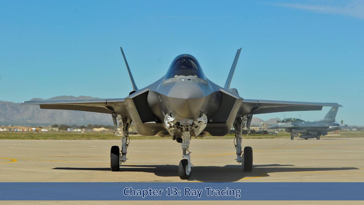
Lockheed Martin F-35
Joint Strike Fighter with
F-16 in the background

Raytracing Basics 155
•Raytracing is an advanced rendering technique that traces the path of light and
simulates the effects of its encounters with virtual objects
•This technique is capable of creating highly realistic images; however these types
of images have to be calculated by the system and this takes time
•Raytracing can accurately create a wide variety of optical effects including
multiple lights, shadows and reflections
•EnSight uses a build in raytracer called enRay –this Raytracer can be accessed
directly from within EnSight
•The implementation of the Raytracer in terms of the GUI has been kept to a
minimum to ensure ease of use
•Depending on the quality of the output and the complexity of the scene,
Raytraced images can take several seconds to several minutes to calculate
Creating a Raytraced Image 1 156
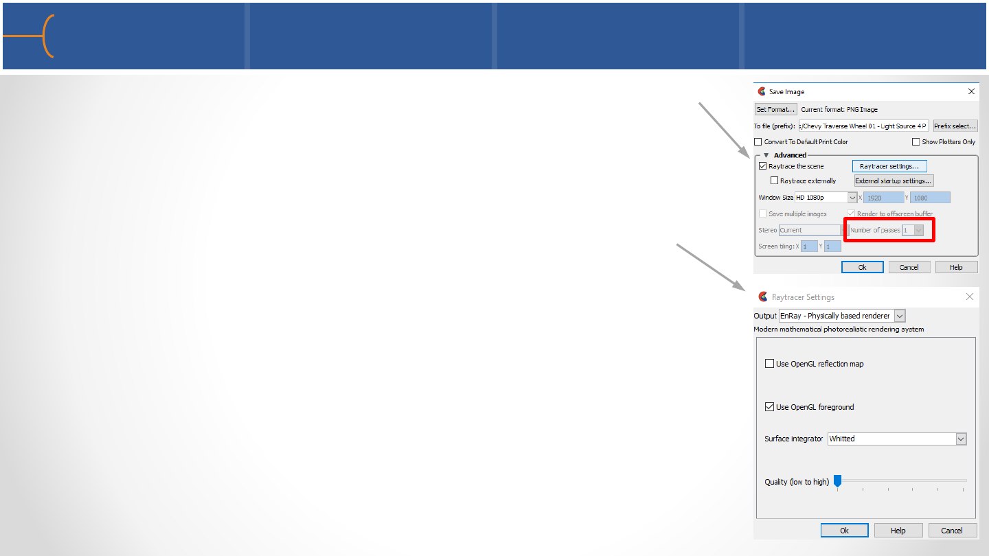
•Click on File -> Export -> Image and click on the Raytrace
The Scene toggle; this informs EnSight to use the Raytracer
to create the image; the anti-aliasing options are disabled
since they are automatically set in the Raytracer
•Click the Raytracer Settings button to see the available
options for the Raytracing process
•The Surface Integrator has 2 options: Whitted or Ambient
Occlusion
oWhitted will produce images with sharp shadow edges
that typically occur on a sunny day without any clouds
oAmbient Occlusion will create much softer, blurry
shadows that occur on a sunny but slightly cloudy day
Creating a Raytraced Image 2 157
•There are 6 Quality settings for both Surface Integrators; on setting 1 (the lowest
quality setting) the image on the left takes about 7 seconds to create on a Dell
Precision 7710 laptop; the image to the right on quality setting 6 (the highest
quality setting) takes about 160 seconds to create using the same laptop
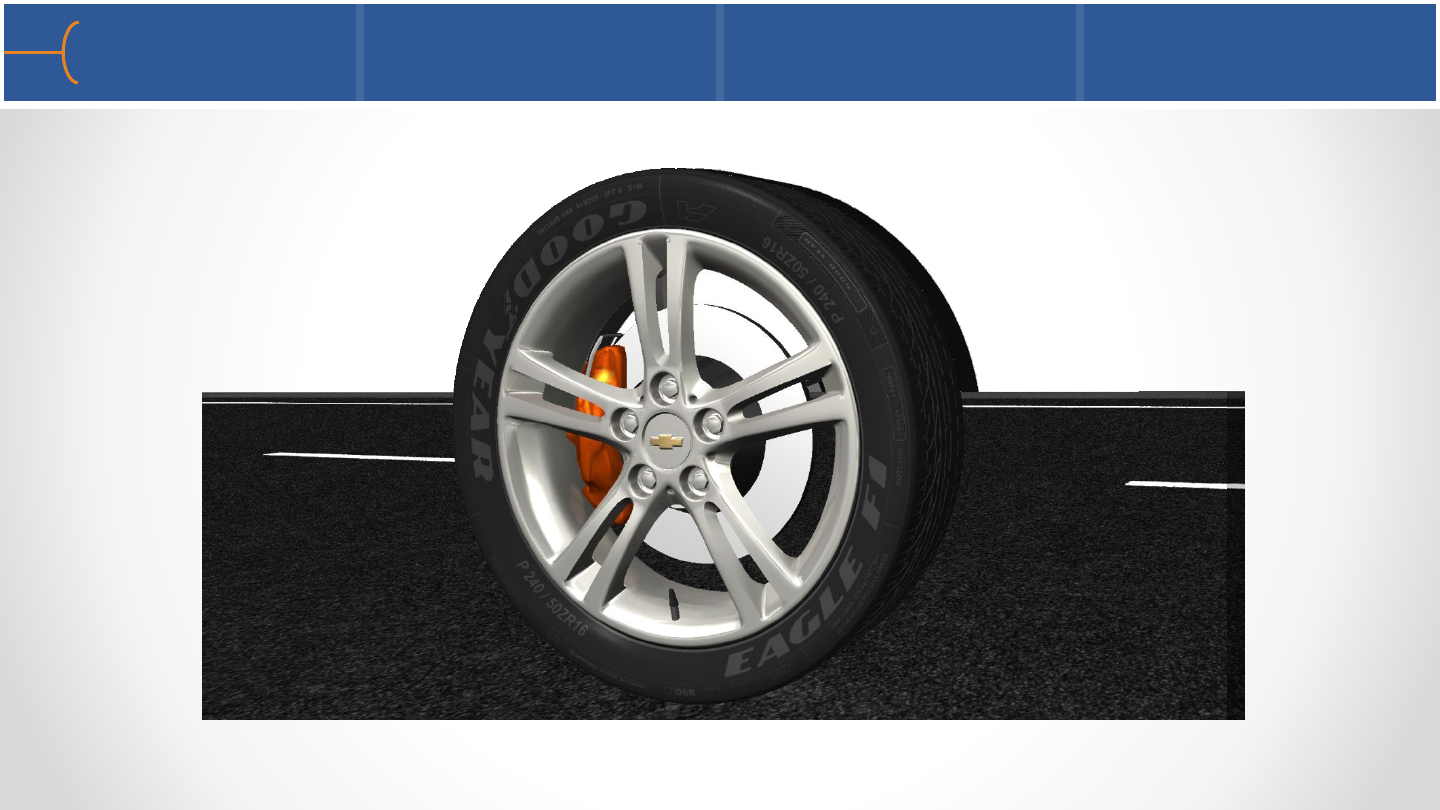
Create Auxiliary Geometry 158
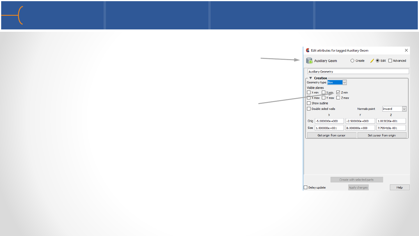
•Click on Create -> Auxiliary Geometry to create the road
surface for the Chevy Traverse model for instance
•This uses the sides of the bounding box of the model to
create up to 6 sides; in this case only the bottom Z-plane
of the bounding box is needed so that is selected
•This plane can be used to texture map or to assign a
material for instance
•Shadows from the Raytracer will be cast onto the
Auxiliary Geometry
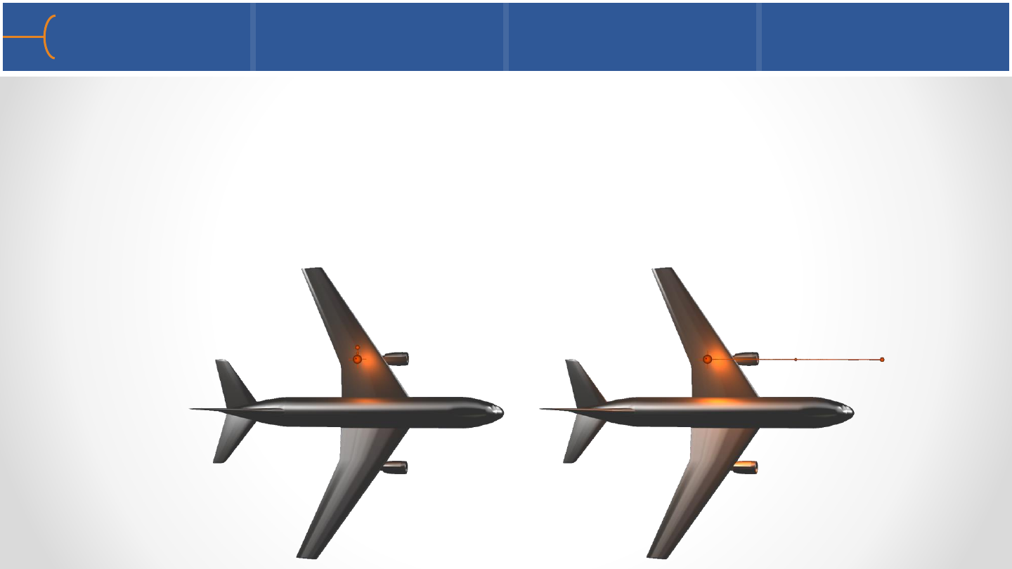
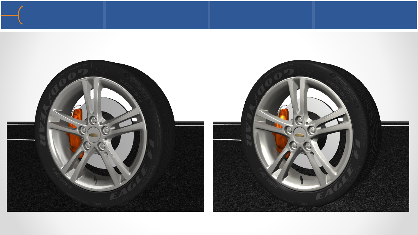
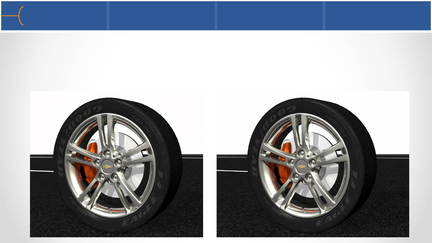
Wheel - Whitted Quality 3 159
•The following image, using Whitted on Quality 3, takes about 20 seconds to
generate
Wheel - Ambient Occlusion Quality 3 160
•Here’s the same image with Ambient Occlusion on Quality Setting 3 (70 seconds)
Ray Traced Images Comparison 161
Whitted, Quality 3 Ambient Occlusion, Quality 3
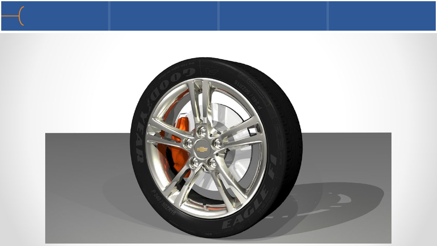
Chevy Traverse - Whitted Quality 3 162
Chevy Traverse –Ambient Occlusion Quality 3 163
NASA’s Space Shuttle Atlantis Launch

•The Transformation Editor can do transformations with exact values; it can also
perform several other useful tasks
•Click on Edit -> Transformation Editor and a panel is
displayed that has Transformation Editor in the title bar
and then in brackets Global Transform; the phrase in
brackets indicates the current function the Transformation
Editor is executing, so in this case it is a global
transformation
•There are 4 transformations that can be done: Rotate,
Translate, Zoom and Scale around any of the axes
The Transformation Editor 1 165

•To do a global transformation with exact values, use either
the slider, the forward and backward increments or type in
a number in the Increment or Limit field
•For instance, if a rotation is needed around the X-axis with
an angle of 34.95°, type in 34.95 in the Increment field and
click the forward or backward button or type in 34.95 in
the Limit field and move the slider to its limit in either
positive or negative direction; the total angle will be + or -
34.95°
The Transformation Editor 2 166
•When parts are zoomed in very closely, the model can progressively disappear;
this is called Z-clipping; there are 2 Z-clip planes: the front and back planes and
they are in the Z-axes of the display so coming out and going into the screen
•The Z-clipping in EnSight can be controlled by clicking on Editor Functions -> Z-Clip
to display a panel that shows the Front and Back Z-clip planes (the red lines); the
white box represents a bounding box of the geometry
•By default the Z-clip buffers float with any transformation;
however, if Z-clipping occurs anyway, the user can modify
the Minimum Z-Value by making it smaller or larger
The Transformation Editor 3 167

•The tools in EnSight (Cursor, Line and Plane) can also be
manipulated using the Transformation Editor; click on
Editor Functions -> Tools -> Line and the following panel is
displayed; please note that the title bar displays Line Tool
in brackets
•The transformation tools on this panel can be used to
Rotate, Translate and Scale the Line Tool by exact values
•For the Line Tool, this panel lists the start and end points
•The Line Tool can also be positioned using 2 Node ID’s
The Transformation Editor 4 168
•A similar panel is available for all other tools (Cursor, Plane, Box and the quadratic
tools as well)
•Click on Editor Function -> Center of Transform to display or set the coordinates
of the center around which the model transforms; this can also be done by
clicking the Pick icon and selecting ‘Pick Center of Transform’ and then
selecting a node of a part using the cursor and the key on the keyboard
The Transformation Editor 5 169
P
•Click the Tool Location Settings icon and then Reset to display a
menu that allows tools and viewports to be reset
•When the Reinitialize button is clicked, the center of transform is
modified to the geometric center of the visible parts on the
screen
•Clicking the Tool Location Settings icon and then Tool Location
Editor brings up the Transformation Editor displaying one of the
Tool menus
The Transformation Editor 6 170

•Another method of displaying the Transformation Editor is to click the Graphics
Window Transforms icon and then select Transformation Editor; the system will
display the Transformation Editor in the Global Transform mode
The Transformation Editor 7 171

2017 Chevrolet Volt Interior
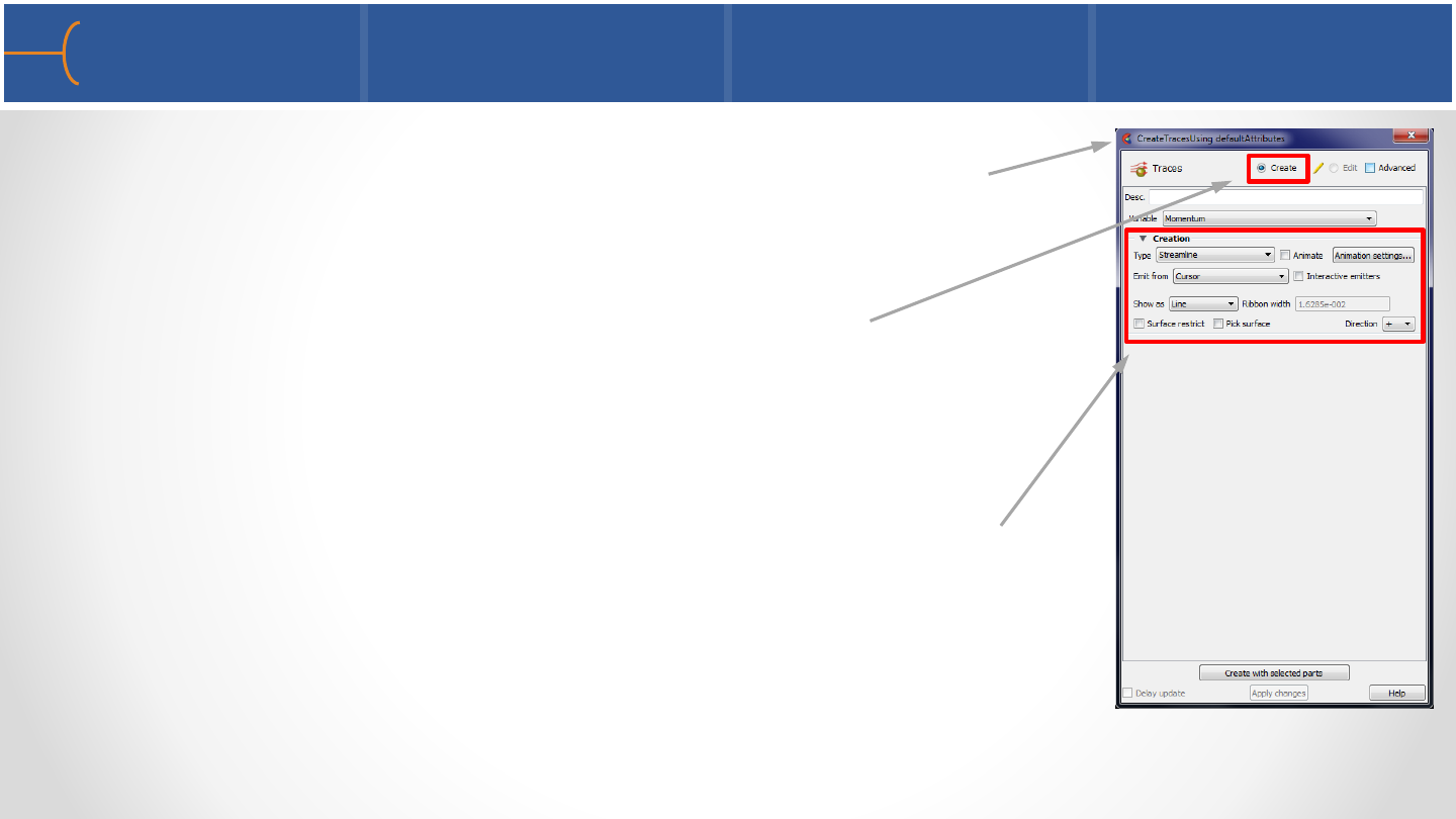
•When a function on the Feature Toolbar is clicked, for
instance Particle Traces in this example, EnSight will display
the basic Create Traces menu
•Please note this menu is to create a new particle trace part as
can be seen by the Create selection box
•This menu displays the basic creation features that are
available for this operation and are displayed under the
Creation toggle
Create Attributes (Parts) 1 173

•For more advanced features, click on the Advanced toggle
•The system displays several more options to create particle
traces
•For instance, for Surface Restricted particles, a Variable
Offset and a Display Offset can be specified
•For pathlines the Total Time Limit, Emission Time Start
and Time Delta can be entered on this menu
•At the bottom of this panel there’s a toggle called Massed
Particles; when this toggle is switched on, a new panel will
be displayed that allows particle traces to have a mass
(regular particle traces are massless)
Create Attributes (Parts) 2 174
•The Massed Particle Attributes panel has several tabs that
specify how to define the massed particles; see the User
Manual for more information about the mathematical
background of massed particles
•Scroll down on the Edit Attributes menu and click the other
toggles on the Edit Attributes menu to modify General
Attributes, Node, Element & Line Attributes and
Displacement Attributes; for some parts it will also display IJK
Axis Display Attributes
Create Attributes (Parts) 3 175
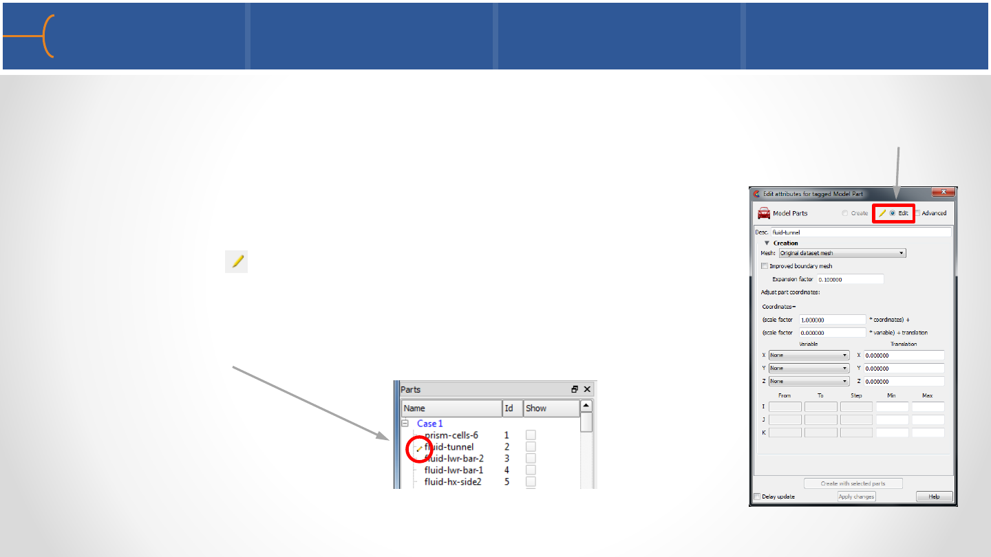
•When a part in the Parts List is double clicked, the Edit Attributes menu is
displayed; this menu is very similar to the Create Attributes menu but on this
menu the Edit selection box is active
•Please note that in the Parts List the part that is being
edited has the icon in front of the name to indicate
this is the part that is being edited; even if another part
is selected, the icon will stay in front of the part that
was edited last
Edit Attributes (Parts) 1 176

•Toggle the Advanced button and EnSight will display several
more options
•Click for instance on the Displacement toggle to display
several options for this feature; check out the others as well
(General, Node & IJK)
•The Edit Attributes menu can also be displayed by right
clicking on a part in the Parts List and selecting Edit
Edit Attributes (Parts) 2 177

Ferrari FXX-K

Case Linking 179
•As an extension to EnSight’s ability to Load Multiple Datasets at once, Case Linking
attempts to provide an easier manipulation of the analysis of multiple datasets
oOperations performed on one case are automatically done on all other open
datasets
oSynchronization of part creation, coloring, queries across all of the cases
oEnSight 10.1 has introduced this capability (version 1)
•Make Comparisons between cases easier

Case Linking Requirements and Caveats 180
•Current Case Linking Requirements:
oThe Parts List for all cases must be identical in number and order
oThe Variable list for all cases must be identical and comparable
oMust be turned on when you load 2nd case
•Caveats:
oOnly 4 datasets can be case linked
oOnce turned Off, case linking cannot be turned back on (no catch up)
oUses context capability –whatever limitations on context files will apply to
case linking
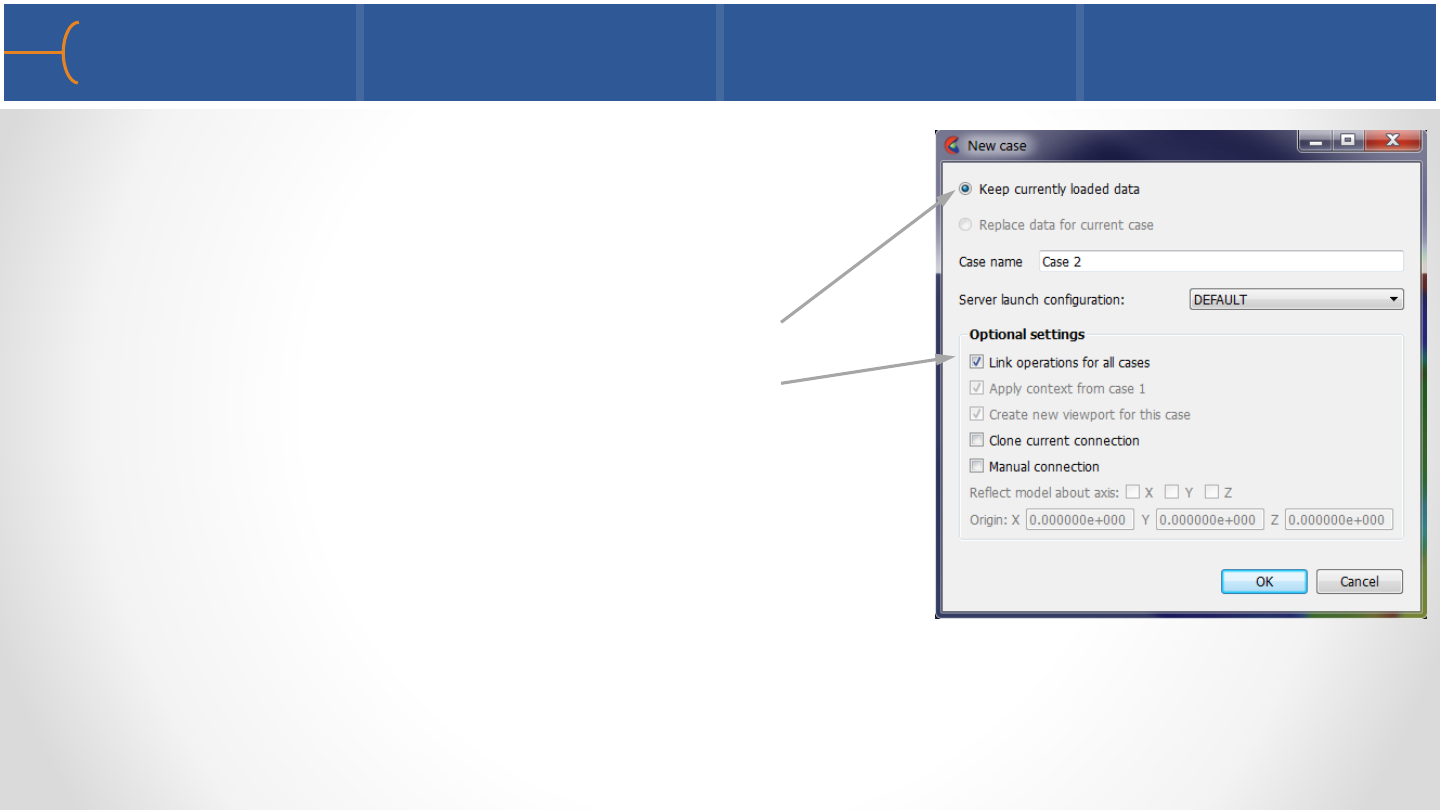
Case Linking –How To 181
•Load up for first dataset, and perform as
many operations as you’d like
•Upon Loading the 2nd case
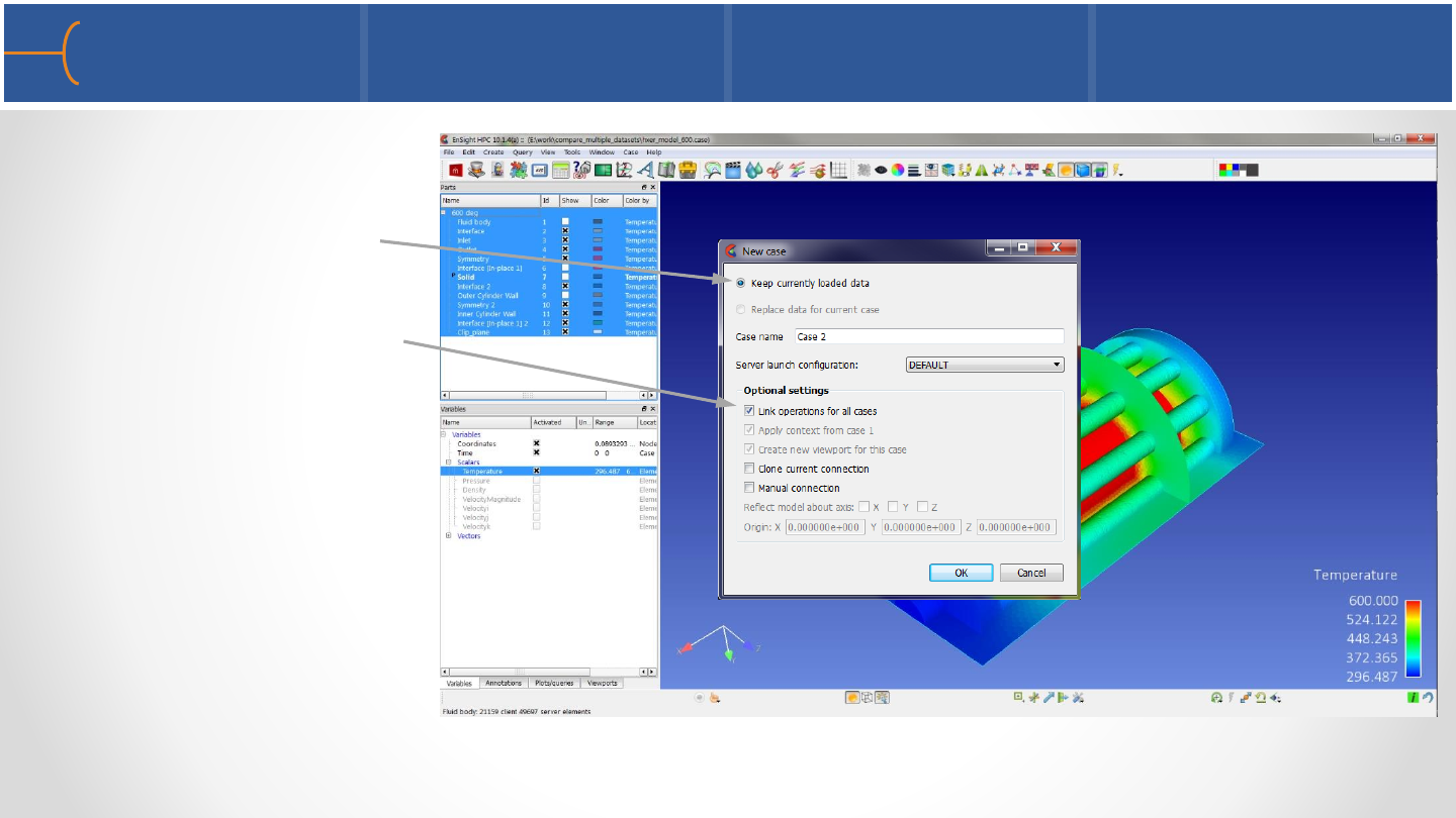
oSelect to Keep currently loaded data
oSelect Link Operations for All Cases
•The new case is loaded and all subsequent
operations are linked to the other datasets
•All else is take care of by EnSight - there is no
other user involvement in Case Linking

Case Linking –Operation 1 182
•In Case Linking mode:
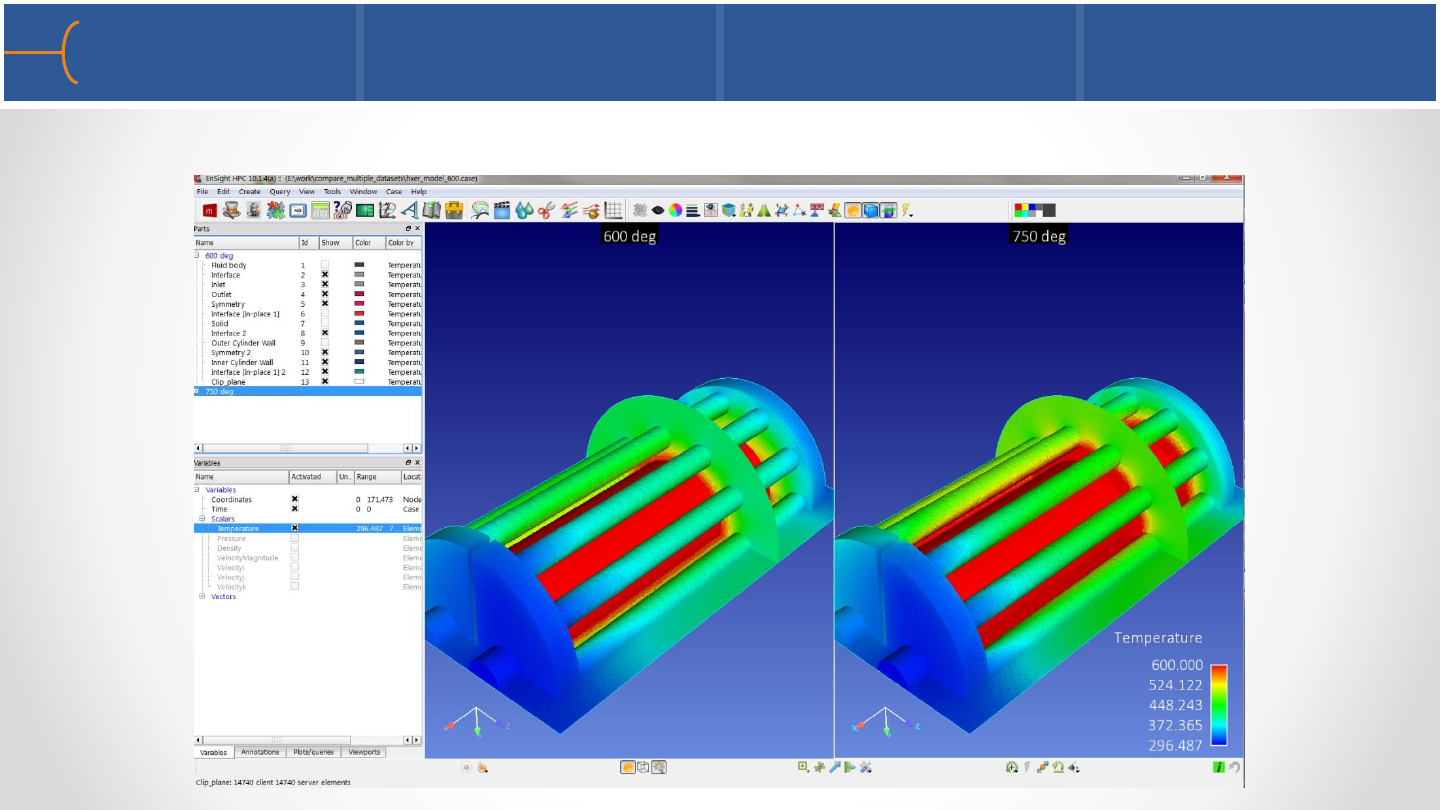
oSeparate Viewports for each case are made
▪Viewports are linked for transformations
oPart Edits and creations are done across all cases
oVariables are created across all cases
▪Constants are created for each case as well
oQueries are created across all cases
oInteractive Probes are performed across all cases
Case Linking –Operation 2 183
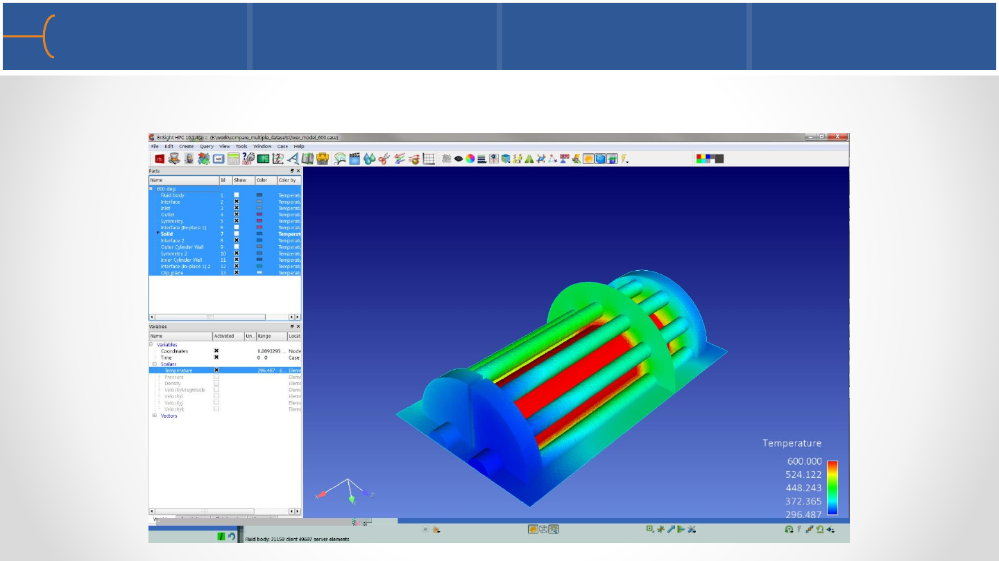
•Load the first model, and perform the operations you desire
Case Linking –Operation 3 184
•Load the second
case, choosing to
(a) keep currently
loaded data, and
(b) Link operations
Case Linking –Operation 4 185
•Second Case is loaded, and all operations are automatically performed
Case Linking –Operation 5 186
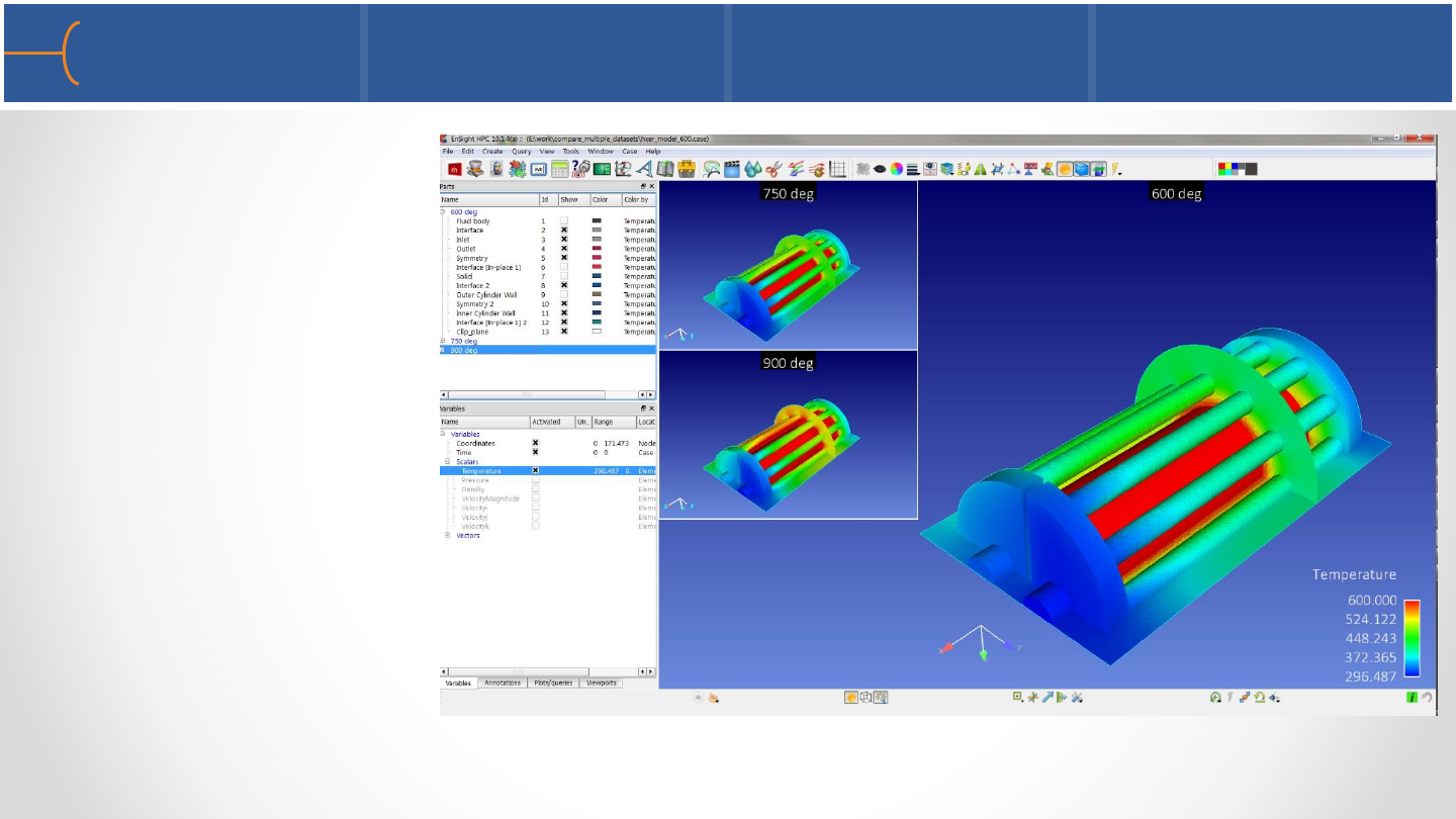
•As subsequent
cases are loaded,
operations are
automatically
performed

Case Linking –Operation 6 187
•Now, as you create
new parts in a
single case, that
operation is
automatically done
on all other cases
•The second clip
plane is
automatically
created & colored
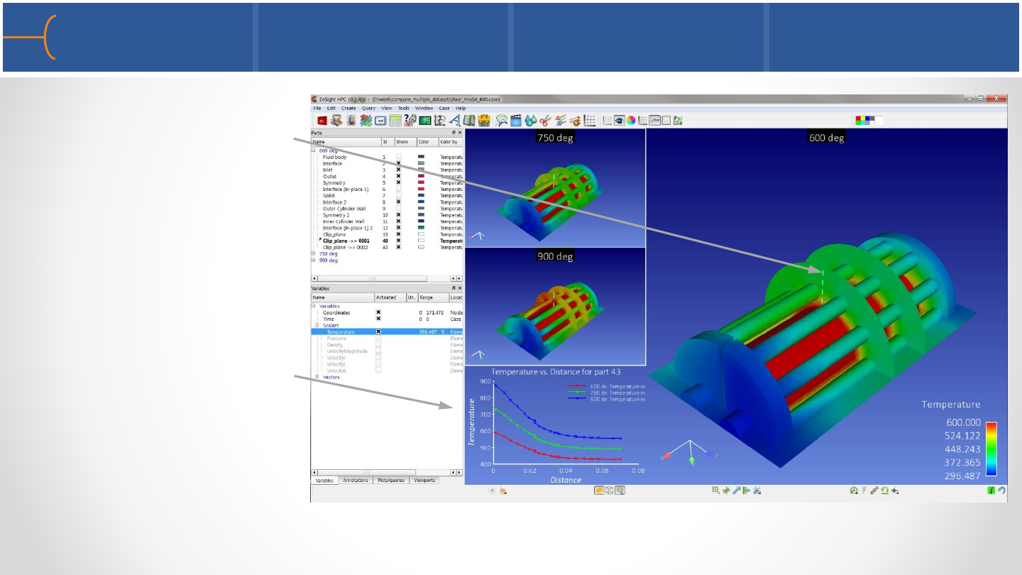
Case Linking –Operation 7 188
•Creating a single
Query in one model
•The queries are
automatically
created in the other
models, and added
together into the
graph automatically
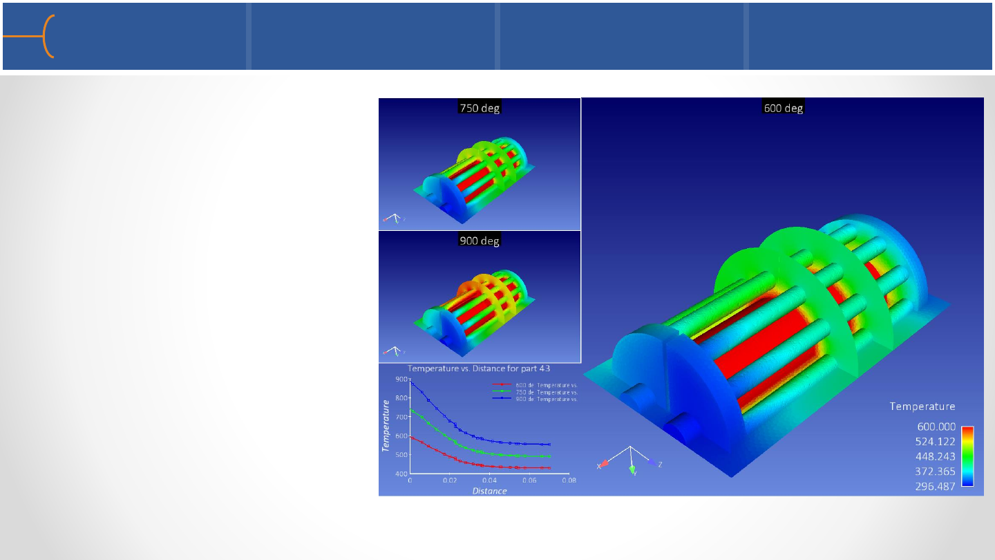
Case Linking –Viewport Capabilities 189
•While in Case Linking
mode, there is a ‘master
viewport’ and ‘slave
viewports’
•There are two new
functions with regards to
viewport operation while
in Case Linking Mode
Master Viewport
Slave Viewports
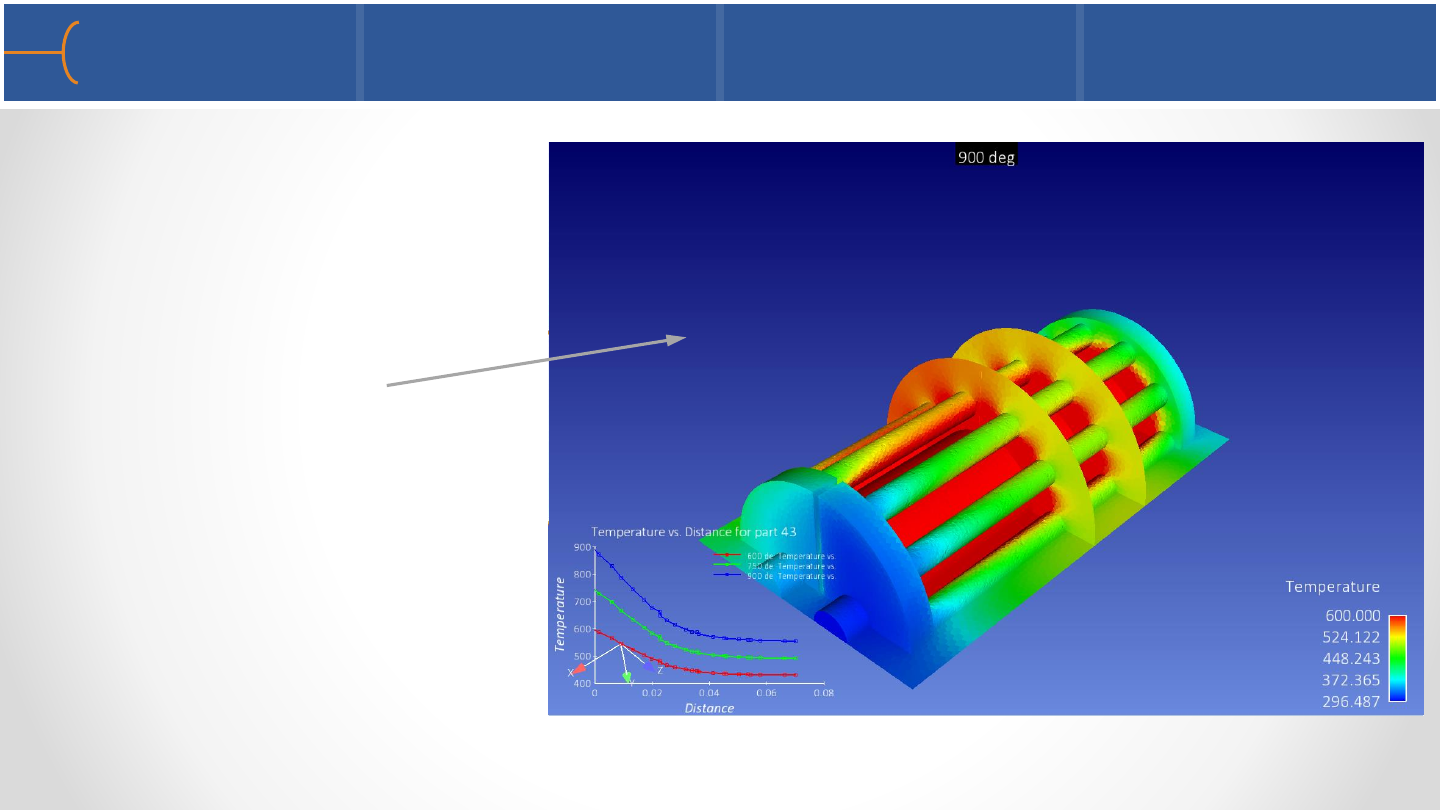
Case Linking –Viewport Toggle Full View 190
•Left Click in the viewport
to bring up the selection
handles
•Click on the handle at the
top/middle of the
viewport
•This toggles this viewport
to be Full View
•Same operation to return
to its original position

Case Linking –Viewport Exchange 191
•You can Exchange the
current viewport with the
largest viewport
•Right Click in a Viewport
•Choose Exchange with
Largest Viewport
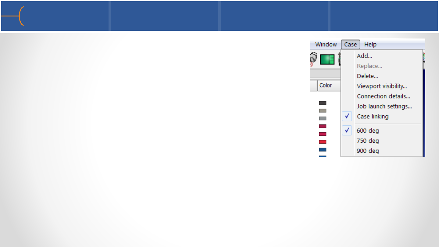
Case Linking - Off 192
•To turn OFF Case Linking, simple toggle off under the
main menu: Case -- > Case Linking
•Once you have turned it Off, you cannot re-activate it

Case Linking - Notes 193
•Saving Journal Files, Context Files, Session Files, should all work* with Case Linking
•Restoring from these files will also maintain Case Linking
•Improvements in Case Linking, expansion of capability, and removal of limitations
is planned for future work
* Context and Session Files do not always restore, but this is independent of Case
Linking
Caterpillar 797F Mining Truck
•EnSight can create any annotation by right clicking in the Annotations Objects List
and selecting any of the 7 annotations that are listed
•EnSight will create the selected annotation immediately; please note that 2D
annotations overlay the graphics window and are not associated with any
viewport
•When a new text is created, the Create/Edit Annotation (Text) menu is displayed
as well
Create/Edit Annotations 195

•Text strings can be created in 2 ways:
1.By right clicking in the background of the graphics window and selecting
Quick Text (see the ‘Annotations’ chapter in the EnSight 10 Basic Training)
2.By right clicking the Text keyword in the Annotations
Tab of the Object Lists and selecting Create -> Text
By double clicking the Text keyword in the Annotations
Tab of the Object Lists, the Create/Edit Annotations (Text)
menu is displayed; click the Create button to create a text
•Dynamic text that changes over time can be created as well
Create/Edit Text Strings 1 196
•In all text creation methods, the Create/Edit Annotation (text) menu is displayed
and a ‘New Text’ annotation is created in the location of the mouse when the right
mouse button was clicked or in the center of the graphics window; this menu is
used to both create and edit text annotations
•Text annotations can also be edited by
right clicking on an annotation in the
graphics window or in the text in the
Annotation Tab of the Object Lists
Create/Edit Text Strings 2 197
•Lines can be created in 2 ways:
1. By right clicking in the background of the graphics window
and selecting Quick Line (see the ‘Annotations’ chapter in
the EnSight 10 Basic Training)
2. By right clicking one of the Annotations keywords in the
Annotations Tab of the Object Lists and selecting Create >
Line
3. By double clicking the Line keyword in the Annotations Tab
of the Object Lists, the Create/Edit Annotations (Lines)
menu is displayed; click the Create button to create a text
Create/Edit Lines 1 198
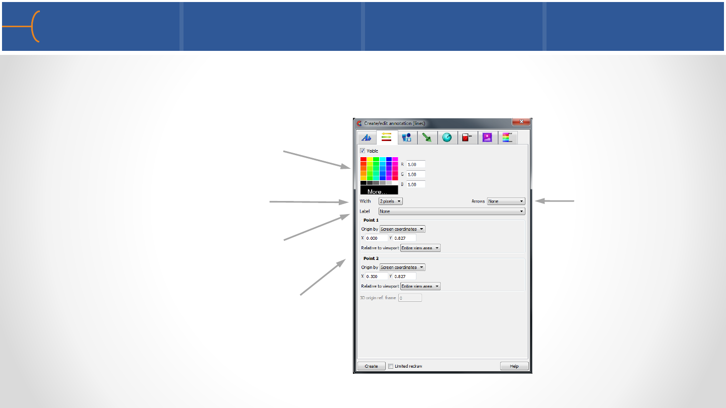
•EnSight can display annotation lines that can either be specified in 2D screen
space or in 3D world space
Create/Edit Lines 2 199
Select a color for the line
Select Width
Attach a previously made
text to the line
Select Origin settings for Point 1
and Point 2 in either Screen
Coordinates or 3D Coordinates
Select Arrows
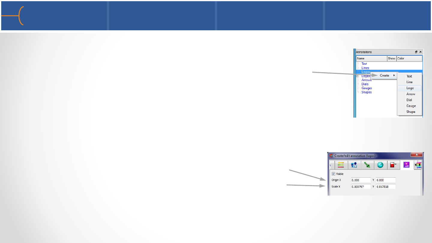
•EnSight can display a bitmap file such as a logo Display a logo
on the screen by right clicking one of the Annotations keywords
in the Annotations Tab of the Object Lists and click Create
-> Logos, then select a logo bitmap file
•Right click on the logo and select Edit to display the Create/Edit
Annotation (Logo) menu or right click the Logos keyword in the
Annotations Objects List or double click the Logos keyword
•A logo has move and resize handles just like any annotation
•Bitmaps are drawn over all geometric objects in the Graphics Window but under
all other annotation entities
Create/Edit Logos 200
Specify the Origin of the logo
Specify the Scale of the logo
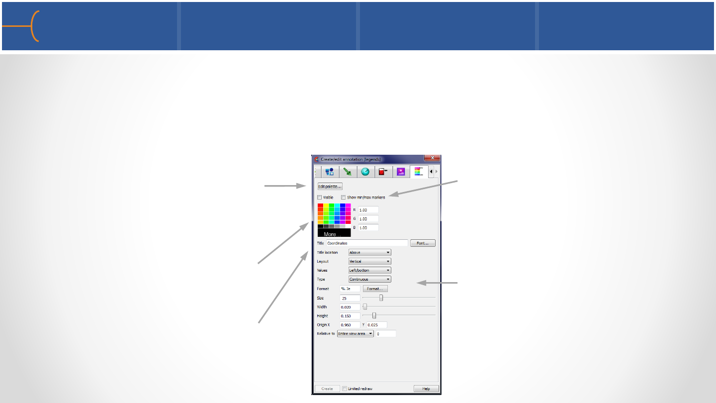
•Right click the Legends keyword in the Annotations Objects List or double click the
Legends keyword
•The size and position of the color legend can be changed and the legend itself can
be edited as well
Create/Edit Legends 201
Toggle Show Min/Max
Markers on or off
Edit the Title of the legend
Select the color of the legend Edit many details of the legend
such as Layout, Title, Values,
Value Format, Type, Font Size,
Font, Origin, Width and Height
Click Edit Palette to modify
the colors and range of the
legend
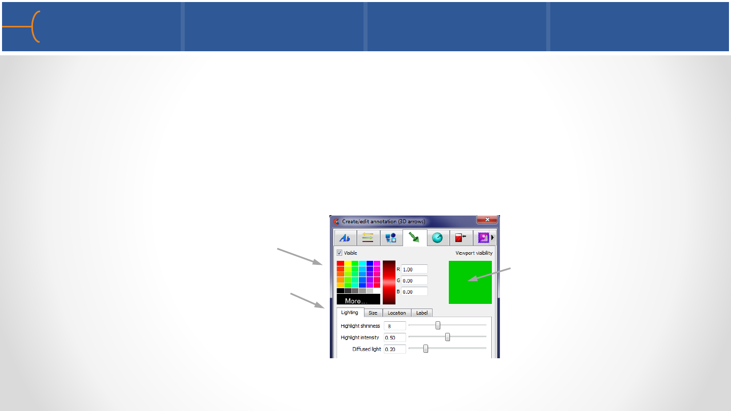
•The 3D arrow is defined in model space and transforms with the scene
•Display an arrow on the screen by right clicking one of the Annotations keywords
in the Annotations Tab of the Object Lists and clicking Create -> Arrow
•Right click on the shape to display the Create/Edit Annotation (Shapes) menu or
right click the Shapes keyword in the Annotations Objects List or double click the
Shapes keyword
Create/Edit 3D Arrows with Text 202
Select color of the 3D Arrow
Click the 4 tabs (Lighting, Size,
Location and Label) to specify
more details of the 3D Arrow
and text
The 3D arrow is visible in
the specified viewport(s)
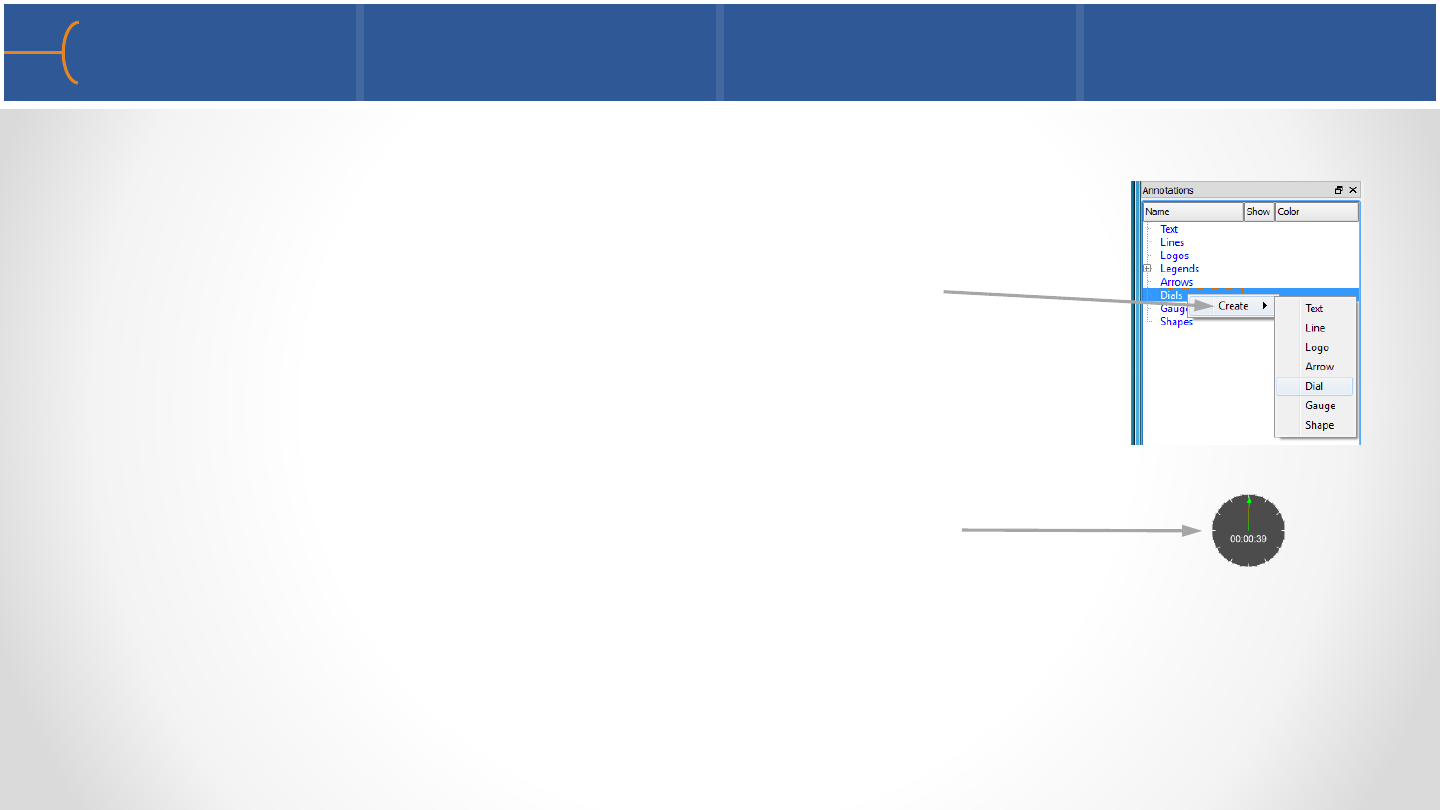
•EnSight can display a 2D dial (such as a clock to measure time) tied to a constant
variable
•Create a dial by right clicking one of the Annotations
keywords in the Annotations Tab of the Object Lists and
selecting Create -> Dial
•A dial is created in the center of the screen by default
•Right click on the dial and select Edit to display the Create/Edit Annotation (Dials)
menu or right click the Dials keyword and select Edit in the Annotations Objects
List or double click the Dials keyword
Create/Edit Dials 1 203
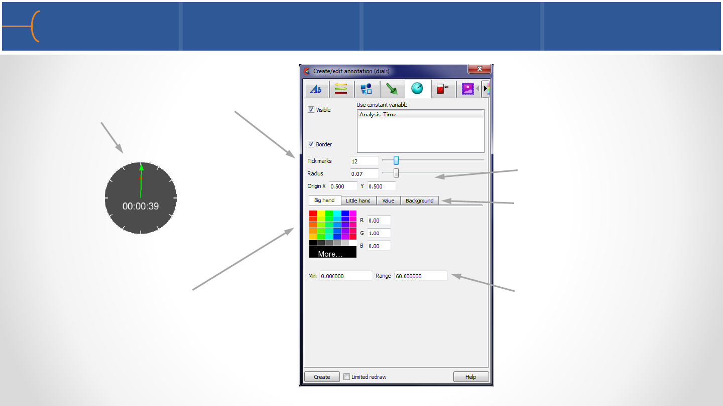
Create/Edit Dials 2 204
Enter the number of Tick Marks
for the dial; in this example there
are 12
Click the 4 options (Big Hand,
Little Hand, Value and
Background) to specify more
details of the dial
Select color of the dial
Specify the Radius and Origin
Enter the Minimum value and the
Range of the dial
12
7
12
3
4
5
6
8
9
10
11
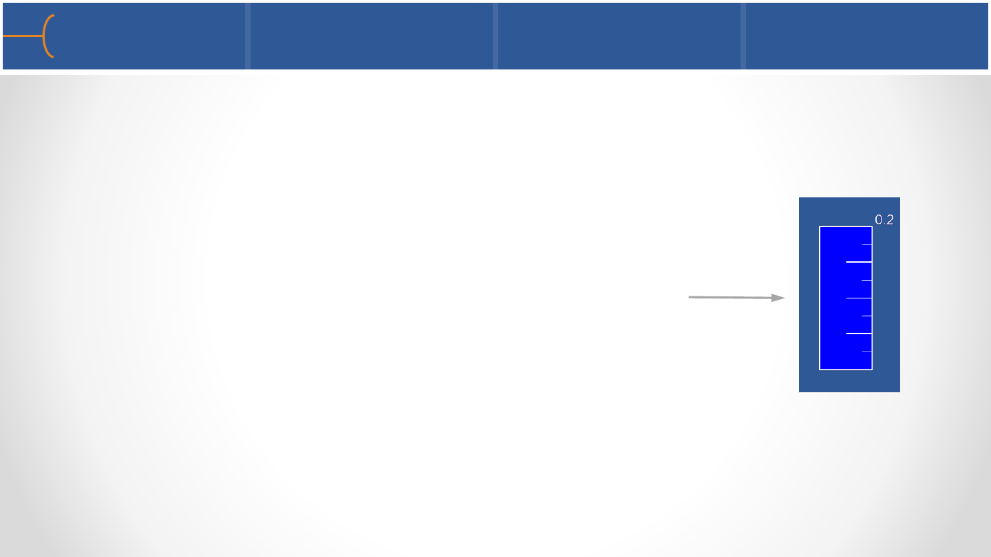
•Similar to a dial, EnSight can display a 2D gauge tied to a constant variable
•Create a gauge by right clicking one of the Annotations keywords in the
Annotations Tab of the Object Lists and selecting Create -> Gauge
•A gauge is created in the center of the screen by default
•Right click on the gauge and select Edit to display the Create/Edit Annotation
(Gauges) menu or right click the Gauges keyword and select Edit in the
Annotations Objects List or double click the Gauges keyword
Create/Edit Bar Gauges 1 205
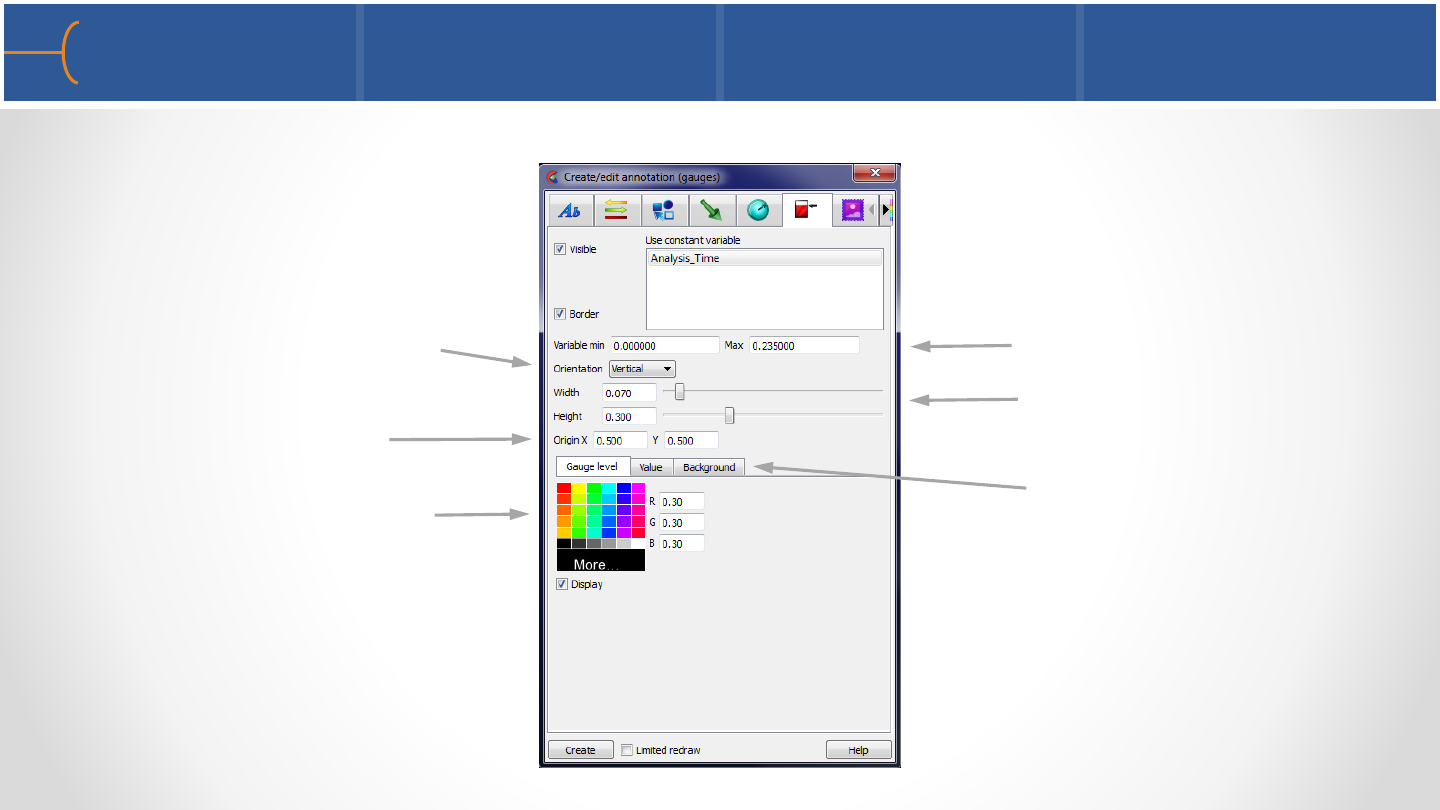
Create/Edit Bar Gauges 2 206
Select the Orientation of the
gauge
Click the 3 options (Gauge Level,
Value and Background) to specify
more details of the gauge
Select the color of the gauge
Specify the Width and
Height
Specify the Variable Min and
Max
Specify the Origin point
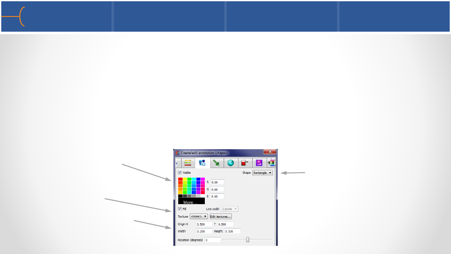
•EnSight can create 2D shapes (2D arrow, circle and rectangle)
•Create a 2 D shape by right clicking one of the Annotations keywords in the
Annotations Tab of the Object Lists and selecting Create -> Shape
•A rectangle is created in the center of the screen by default
•Right click on the shape and select Edit to display the Create/Edit Annotation
(Shapes) menu or right click the Shapes keyword in the Annotations Objects List
or double click the Shapes keyword
Create/Edit 2D Shapes 207
Select color of the shape Select a Shape (2D arrow, circle
or rectangle)
Select Origin, Width, Height
and Rotation
Select Fill or Texture
Buzz Aldrin walking on the moon in
1969 during the Apollo 11 mission –
photo taken by Neil Armstrong
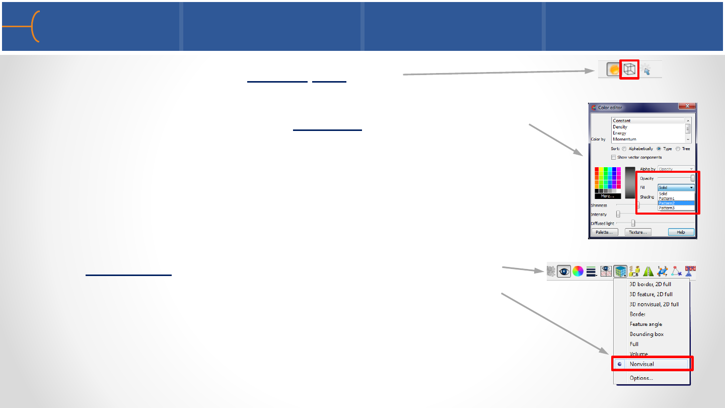
•Displaying many parts in Hidden Line mode
•Displaying many parts with an Opacity setting smaller than
1.0 when the graphics card is not powerful enough to do so -
instead use Fill Patterns 1, 2or 3
•Making the Element Representation of a big part on the
server such as the flowfield of a CFD model, anything other
than NonVisual - hiding it using the Visibility icon is not
going to do any good because it’s still using RAM on the
Client side
Actions that will slow down your system 1 209
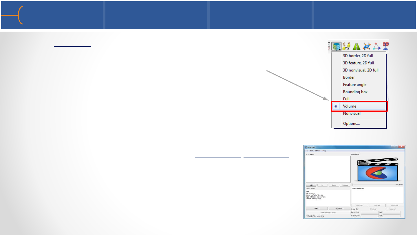
•Using Volume rendering on too many parts; this will take
a lot of power from the graphics card - instead make sure
the graphics card is powerful enough to do volume
rendering
•Creating too many keyframes in the Keyframe Animator
with many subframes while using transient data - instead
make movie segments between 2 keyframes and create
the complete movie using EnVe
Actions that will slow down your system 2 210

•Using the maximum number of anti-aliasing (Number of
Passes = 16) when pictures or movies are created -
instead start by using Number of Passes = 1and when a
test picture or movie is ok, crank up the quality
•Using a large resolution when creating a picture or
movie - instead start by using a smaller size resolution
(for instance NTSC or PAL) and when a test picture or
movie is ok, use the desired higher resolution
Actions that will slow down your system 3 211
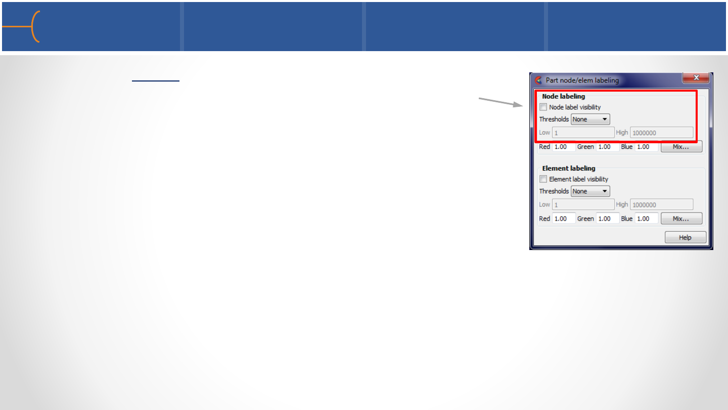
•Displaying labels on parts with thousands or millions of
nodes or elements can degrade display performance
significantly as well as obscure both the geometry and
the labels of interest - instead use a small range of nodes
and element labels of interest then toggle the Node or
Element Label Visibility on
Actions that will slow down your system 4 212
Enjoy working with EnSight 10.2! 213
