Ensight Howto User Manual How To
2017-12-05
User Manual: Ensight Howto HowTo EnSight10_Docs www3.ensight.com 3:
Open the PDF directly: View PDF ![]() .
.
Page Count: 546 [warning: Documents this large are best viewed by clicking the View PDF Link!]
- Introduction
- Read and Load Data
- Save or Output
- Manipulate Viewing Parameters
- Rotate, Zoom, Translate, Scale
- Set Drawing Mode
- Set Global Viewing Parameters
- Set Z Clipping
- Set LookFrom / LookAt
- Set Auxiliary Clipping
- Define and Change Viewports
- Set Light Sources
- Display Remotely
- Save & Restore Viewing Parameters
- Create and Manipulate Frames
- Reset Tools and Viewports
- Use the Color Selector
- Enable Stereo Viewing
- Pick Center of Transformation
- Set Model Axis/Extent Bounds
- Do Viewport Tracking
- View a Viewport Through a Camera
- Manage Views
- Manipulate Tools
- Miscellaneous
- Visualize Data
- Introduction to Part Creation
- Create Auxiliary Geometry
- Create Contours
- Create Isosurfaces
- Create Particle Traces
- Create Clips
- Create Clip Lines
- Create Clip Planes
- Create Box Clips
- Create Quadric Clips
- Create IJK Clips
- Create XYZ Clips
- Create RTZ Clips
- Create Revolution Tool Clips
- Create Revolution of 1D Part Clips
- Create General Quadric Clips
- Create Clip Splines
- Create Vector Arrows
- Create Elevated Surfaces
- Extrude Parts
- Create Profile Plots
- Create Developed (Unrolled) Surfaces
- Create Subset Parts
- Create Tensor Glyphs
- Display Displacements
- Display Discrete or Experimental Data
- Change Time Steps
- Extract Vortex Cores
- Extract Separation & Attachment Lines
- Extract Shock Surfaces
- Create Material Parts
- Filter Part Elements
- Do Element Blanking
- Use Point Parts
- Use Raytrace Rendering
- Create and Manipulate Variables
- Query, Probe, Plot
- Manipulate Parts
- Animate
- Annotate
- Configure EnSight

Page 1
HOW TO TABLE OF CONTENTS
Introduction
Use the Online Documentation
Use The How To Manual
EnSight Overview
Command Line Start-up Options
Use Environment Variables
Connect EnSight Client & Server
Read and Load Data
Read Data
Use ens_checker
Load Multiple Datasets (Cases)
Compare Cases
Load Transient Data
Use Server of Servers
Load Spatially Decomposed Case Files
Read User Defined
Do Structured Extraction
Use Resource Management
Use Root Level Server of Servers
Save or Output
Save or Restore an Archive
Record and Play Command Files
Print/Save an Image
Save Geometric Entities
Save/Restore Context
Save Scenario
Save/Restore Session
Manipulate Viewing Parameters
Rotate, Zoom, Translate, Scale
Set Drawing Mode
Set Global Viewing Parameters
Set Z Clipping
Set LookFrom / LookAt
Set Auxiliary Clipping
Define and Change Viewports
Set Light Sources
Display Remotely
Save & Restore Viewing Parameters
Create and Manipulate Frames
Reset Tools and Viewports
Use the Color Selector
Enable Stereo Viewing
Pick Center of Transformation
Set Model Axis/Extent Bounds
Do Viewport Tracking
View a Viewport Through a Camera
Manage Views
Manipulate Tools
Use the Cursor (Point) Tool
Use the Line Tool
Use the Plane Tool
Use the Box Tool
Use the Cylinder Tool
Use the Sphere Tool
Use the Cone Tool
Use Surface of Revolution Tool
Use the Selection Tool
Use the Spline Tool
Miscellaneous
Use Batch
Use Keyboard Shortcuts
Use Rigid Body Motion
Select Files
Use EnSight with Workbench
Visualize Data
Introduction to Part Creation
Create Auxiliary Geometry
Create Contours
Create Isosurfaces
Create Particle Traces
Create Clips
Create Clip Lines
Create Clip Planes
Create Box Clips
Create Quadric Clips
Create IJK Clips
Create XYZ Clips
Create RTZ Clips
Create Revolution Tool Clips
Create Revolution of 1D Part Clips
Create General Quadric Clips
Create Clip Splines
Create Vector Arrows
Create Elevated Surfaces
Extrude Parts
Create Profile Plots
Create Developed (Unrolled) Surfaces
Create Subset Parts
Create Tensor Glyphs
Display Displacements
Display Discrete or Experimental Data
Change Time Steps
Extract Vortex Cores
Extract Separation & Attachment Lines
Extract Shock Surfaces
Create Material Parts
Filter Part Elements
Do Element Blanking
Use Point Parts
Use Raytrace Rendering
Create and Manipulate Variables
Activate Variables
Create New Variables
Extract Boundary Layer Variables
Edit Color Palettes
Use Volume Rendering

Page 2
HOW TO TABLE OF CONTENTS
Query, Probe, Plot
Get Point, Node, Element, & Part Info
Probe Interactively
Query/Plot
Change Plot
Query Datasets
Manipulate Parts
Change Color
Set Surface Properties
Use Quick Color Settings
Clone a Part
Copy Parts
Group Parts
Merge Parts
Extract Part Representations
Cut Parts
Delete a Part
Change the Visual Representation
Set
Display Labels
Set Transparency
Select Parts
Set Symmetry
Map Textures
Animate
Animate Transient Data
Create a Flipbook Animation
Create a Keyframe Animation
Animate Particle Traces
Annotate
Create Text Annotation
Create Lines
Create 2D Shapes
Create 3D Arrows
Create Dials
Create Gauges
Load Custom Logos
Create Color Legends
Manipulate Fonts
Configure EnSight
Customize Icon Bars and Panels
Customize Mouse Button Actions
Save Settings
Define and Use Macros
Set or Modify Preferences
Enable User Defined Input Devices
Produce Customized Pop-Up Menus
Produce Customized Access to Tools & Features
Setup For Parallel Computation
Setup For Parallel Rendering

Page 3
HOW TO USE THE ONLINE DOCUMENTATION
Introduction
Use the Online Documentation
INTRODUCTION
The EnSight online documentation consists of:
WHERE TO START?
If you are new to EnSight you should read the EnSight Overview article. Chapter 1 and Chapter 5 in the User
Manual also provide overview information. The Introduction to Part Creation provides fundamental information on
EnSight’s part concept.
PDF READER
The EnSight online documentation is in pdf format. EnSight uses a pdf reader such as the Acrobat® Reader software
from Adobe Systems, Inc., Xpdf, or Apple’s Preview. Any of these readers provide similar capabilities. For the
purposes of this documentation, the Acrobat Reader will be pictured. A pdf reader provides much the same
functionality as a World Wide Web browser while providing greater control over document content quality. To use a
different reader (from the default), simply set the environment variable CEI_PDFREADER to a different reader
application. See How To Use the How To Manual for more information on using a pdf reader.
Installation Guide Consists of a .pdf file in the doc directory (as well as being available for easy reading
from the web install page). Also goes out as hardcopy with an EnSight CD.
Getting Started
Manual
The Getting Started Manual contains basic Graphical User Interface overview
information and several tutorials. This manual is not cross-referenced with any of the
other manuals.
How To Manual The How To documentation consists of relatively short articles that describe how to
perform a specific operation in EnSight, such as change the color of an object or
create an isosurface. Step-by-step instructions and pictures of relevant dialogs are
included. In addition, each How To article typically contains numerous hyperlinks
(colored blue) to other related articles (and relevant sections of the User Manual).
How To Use the How To Manual
How To Table of Contents
User Manual The User Manual is a more traditional document providing a detailed reference for
EnSight. The User Manual contains blue hyperlinks as well. The User Manual table of
contents is hotlinked as well as cross-reference entries within chapters (which
typically start with “See Section ...” or “See How To ...”).
User Manual Table of Contents
Interface Manual The Interface Manual contains the information needed for creating user-defined
readers, creating user-defined writers, creating user-defined math functions,
interacting with EnSight through the external command driver, and using the EnSight
python interpreter.

Page 4
HOW TO USE THE ONLINE DOCUMENTATION
HOW TO PRINT THE DOCUMENTATION
Printing Topics From a PDF Reader
You can easily print any topic in the How To manual or any pages from the other documentation from within the pdf
reader. The documents have been optimized for screen manipulation, but will still produce decent hardcopy printouts.
To print a topic:
1. Navigate to the topic you want to print.
2. Choose Print... from the File menu.
3. Be sure the Printer Command setting is correct for your environment and then click OK. Your document should
print to the selected (or default) printer. If you do not have a printer available on your network or you wish to save
the PostScript file to disk, you can do so: click the File button, enter a filename, and click OK.
Printing EnSight Manuals
You can print (all or portions of) the EnSight manuals from provided .pdf files. These files have been print optimized
and should produce reasonably high quality hardcopy. They have all been formatted for letter size paper. These files
are located in the doc/Manuals directory of the EnSight installation.
$CEI_HOME/ensight102/doc/Manuals/GettingStarted.pdf
$CEI_HOME/ensight102/doc/Manuals/HowTo.pdf
$CEI_HOME/ensight102/doc/Manuals/UserManual.pdf
$CEI_HOME/ensight102/doc/Manuals/InterfaceManual.pdf
You can open these manuals in the pdf reader and print any or all pages, or send them to an outside source for
printing, or order printed copies from our website.
CONTACTING CEI
If you have questions or problems, please contact CEI:
Computational Engineering International, Inc.
2166 N. Salem Street, Suite 101
Apex, NC 27523 USA
Email: support@ceisoftware.com
Hotline: 800-551-4448 (U.S.)
919-363-0883 (Non-U.S.)
Phone: 919-363-0883
FAX: 919-363-0833
WWW: http://www.ceisoftware.com

Page 5
HOW TO USE THE HOW TO MANUAL
Use The How To Manual
INTRODUCTION
The “How To” documentation provides quick access to various topics of interest. The topics provide basic and some
advanced usage information about a specific tool or feature of EnSight. Each topic will provide links to the
appropriate section of the EnSight User Manual as well as links to other applicable How To articles. When you hit a
Help button within the various dialogs in EnSight, you will generally be taken to one of the topics in the “How To”
manual.
Topics typically contain the following sections:
(See below for how to quickly jump to a specific section using document navigation.)
The header and footer of each article page provides simple navigation controls:
In addition, links to other documents are displayed as highlighted text. Note that all links and navigation controls are
colored blue.
Historically, an index was provided for this document. However, since the document is intended to be used online, the
index has been removed in favor of the more efficient “search” capabilities provided in pdf readers.
PDF READER
The EnSight online documentation is in .pdf format. EnSight uses a pdf reader such as the Acrobat® Reader software
from Adobe Systems, Inc., Xpdf, or Apple’s Preview. Any of these readers provide similar capabilities. For the
purposes of this documentation, the Acrobat Reader is pictured. A pdf reader provides much the same functionality
as a World Wide Web browser while providing greater control over document content quality. To use a different pdf
reader, simply set the environment variable CEI_PDFREADER to a different reader application.
The user interface for the various pdf readers is very simple and provides intuitive navigation controls. Keep in mind
that the pages were designed to be viewed at 100% magnification. Although you can use other magnification
settings, the quality of the dialog images may be degraded.
Introduction Introduction to the topic
Basic Operation Quick steps for simple usage
Advanced Usage Detailed information on topic
Other Notes Other items of interest
See Also Links to related topics and documentation
Return to How To
Topics List
Access this page
First page of
current topic Last page of
current topic
Previous page Next page
Page 6
HOW TO USE THE HOW TO MANUAL
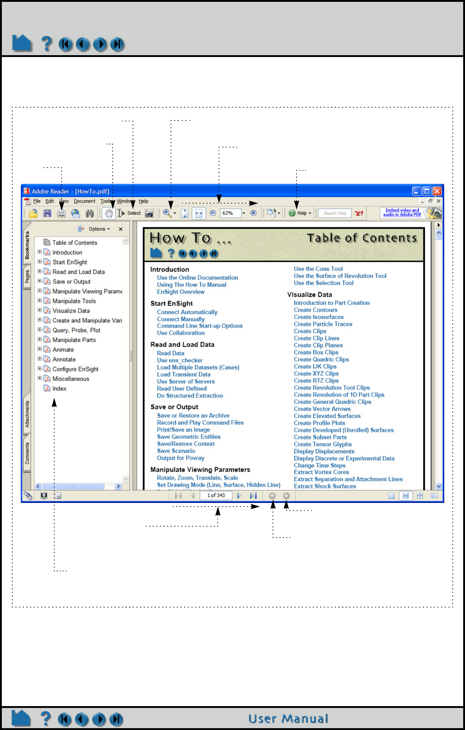
Thus, in addition to the navigation controls within the document itself which are described above, a pdf reader
(Acrobat for example) provides quick access to various display options and navigation controls. A few of them are
pointed out for the Acrobat Reader below. Please use the Help option for your reader for a more comprehensive
description of its options.
The “Go back/forward” buttons are particularly useful – they operate somewhat like the “Back” and “Forward” buttons
on standard Web browsers. If your previously viewed page was in a different document, the pdf reader will
automatically reload the appropriate file and jump to the correct page. Note that most pdf readers also consider a
change of view (e.g. scrolling) or magnification as an event to remember in the back/forward list.
Grab and move page
Click and zoom in
(Ctl-click to zoom out)
Standard page
navigation
Standard page
magnification controls
Go back to last
viewed page
Go forward to previously
viewed page
Select Tool
Print For additional help
Each How To topic provides a set of bookmarks that match the standard
section titles. You can quickly navigate to one of these sections by using
the bookmark list in pdf reader.

Page 8
HOW TO ENSIGHT OVERVIEW
EnSight Overview
ENSIGHT OVERVIEW
EnSight is a powerful software package for the postprocessing, visualization, and animation of complex datasets.
Although EnSight is designed primarily for use with the results of computational analyses, it can also be used for
other types of data.
This document provides a very brief overview of EnSight. Consult Chapter 1 in the User Manual for additional
overview information. This article is divided into the following sections:
Graphical User Interface
Client / Server Architecture
EnSight’s Parts Concept
Online Documentation
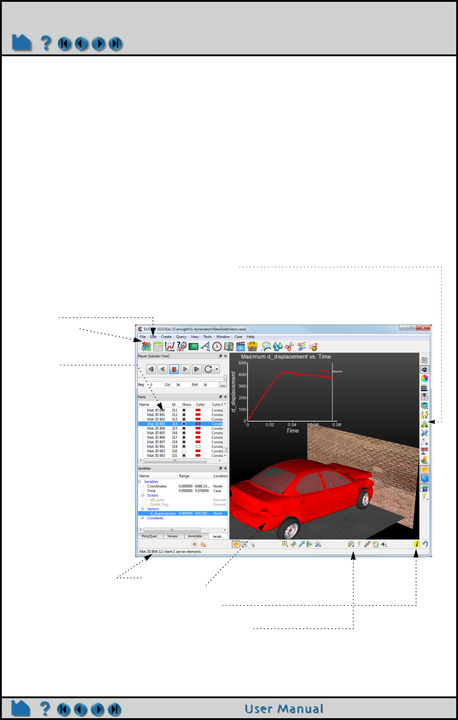
Graphical User Interface
The graphical user interface () of EnSight contains the following major components:
Chapter 1 in the User Manual provides additional overview information on the user interface.
Main Menu
Feature Icon Bar
Sets the current feature and opens
the Feature Panel.
Parts List
All parts from your model as well as
created parts (e.g. clips, isosurfaces)
are listed here. Click an item to
select part(s) to operate on.
Quick Action Icon Bar
Features and Actions relevant to the last selected object
Message Area
Graphics Window showing inset plot and viewport
Information Button
Click to see information dialog.
Transformation Control Area
Buttons that control the current transformation operation (e.g.
rotate or translate) associated with mouse action in the Graphics
Window.
Note: This whole upper level of the is
referred to as the “Desktop”
Page 9
HOW TO ENSIGHT OVERVIEW
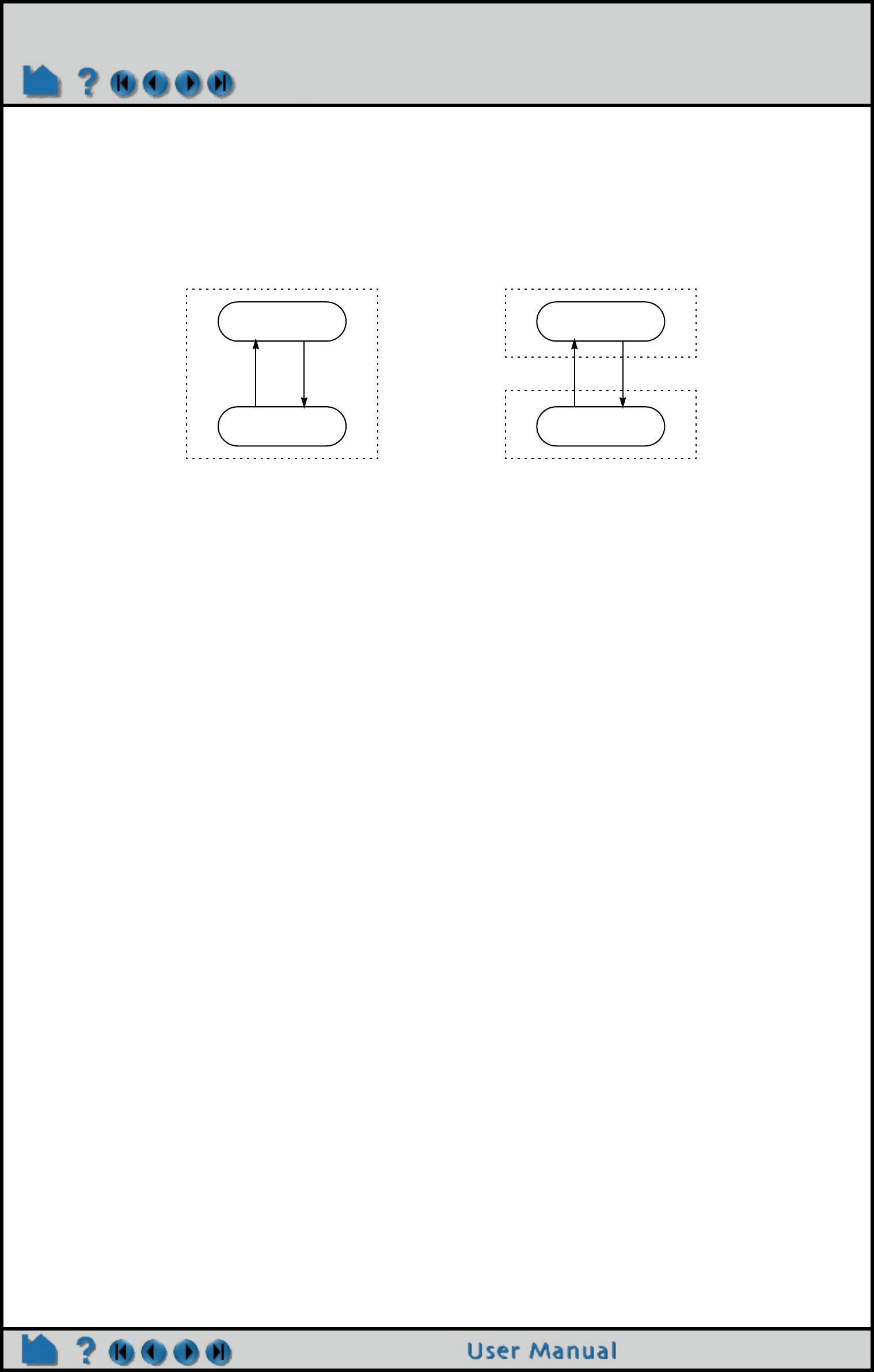
Client / Server Architecture
To facilitate the handling of large datasets and efficiently use networked resources, EnSight was designed to
distribute the postprocessing workload. Data I/O and all compute intensive functions are performed by a server
process. The server transmits 3D geometry (and other information) to a client running on a graphics workstation.
The client handles all user interface interaction and graphic rendering using the workstation’s built-in graphics
hardware.
The client and server each run as separate processes on one or more computers. When distributed between a
compute server and a graphics workstation, EnSight leverages the strengths of both machines. When both tasks
reside on the same machine, a stand-alone capability is achieved. The client–server architecture allows EnSight to
be used effectively, even on systems widely separated geographically.
Before EnSight can be used, the client and server must be connected. For standalone operation, you simply run the
“ensight102” script and the client and server are started and connected for you. For distributed operation (as well as
for standalone operation when more control is desired), there are two methods of achieving a connection: a manual
connection (described in the Getting Started manual) or an automatic connection (described in How To Connect
EnSight Client and Server).
EnSight’s cases feature allows you to postprocess multiple datasets simultaneously. Cases is implemented by
having a single client connected to multiple servers running on the same or different machines.
EnSight’s Parts Concept
One of the central concepts of EnSight is that of the part. A part is a named collection of elements (or cells) and
associated nodes. The nodes and/or elements may have zero or more variables (such as pressure or stress). All
components of a part share the same set of attributes (such as color or line width).
Parts are either built during the loading process (based on your computational mesh and associated surfaces) or
created during an EnSight session. Parts created during loading are called model parts.
All other parts are created during an EnSight session and are called created or derived parts. Created parts are built
using one or more other parts as the parent parts. The created parts are said to depend on the parent parts. If one or
more of the parent parts change, all parts depending on those parent parts are automatically recalculated and
redisplayed to reflect the change. As an example, consider the following case. A clipping plane is created through
some 3D computational domain and a contour is created on the clipping plane. The contour’s parent is the clipping
plane, and the clipping plane’s parent is the 3D domain. If the 3D domain is changed (e.g. the time step changes),
the clipping plane will first be recalculated, followed by the contour. In this way, part coherence is maintained.
Since operating on parts is integral to the operations you will perform in EnSight, it is important that you are aware of
the different ways this can be done. See How To Select Parts.
See the Introduction to Part Creation for more information on parts.
Online Documentation
Documentation for EnSight is available online. See How To Use the Online Documentation for more information as
well as hyperlinks to the main documents. Online documentation is accessed from the Main Help menu in the user
interface. In addition, major dialog windows contain Help buttons that will open a relevant “How To” article.
Server
Client
Stand-alone Operation
host1
Requests 3D objects
Server
Client
Distributed Operation
host2
host1
Page 10
HOW TO COMMAND LINE START-UP OPTIONS
Command Line Start-up Options
INTRODUCTION
There are a number of options that can be included on the command line when starting EnSight. The following tables
indicate the commands that can be issued for the EnSight script (ensight102), the EnSight client (ensight102.client),
the EnSight server (ensight102.server), or the EnSight server-of-servers (ensight102.sos). To see the most current
listing for any of these, issue one or more of the following:
Linux/Unix/Mac Windows
ensight102 -help
ensight102.client -help ensight102_client -help
ensight102.server -help ensight102_server -help
ensight102.sos -help ensight102_sos -help
BASIC USAGE
ensight102 [options]
or
ensight102.client [options]
Section 1. EnSight Startup/Client-Server Options
-ar <f> Restore from specified archive file “f”
-c [<host>[:<exe>]] Do an auto connection, with optional “host” machine and executable. If only -c is used, the
auto connection will be according to the values set in your ensight_conn_settings file (which is
created in your EnSight Defaults directory (located at
%HOMEDRIVE%%HOMEPATH%\(username)\.ensight102 commonly located at
C:\Users\username\ on Vista and Win7, C:\Documents and Settings\yourusername\ on older
Windows, ~/.ensight102 on Linux, and in ~/Library/Application Support/EnSight102 on the Mac)
if you connect via the Connect dialog). EnSight server will run on “host” if you include it after
the -c. And you can also optionally specify the server executable to run on said “host”.
-case <f> Read EnSight casefile name ”f” and display part loader
-ceishell [URL] Start up EnSight and connect with URL, default URL is as follows:
- connect://localhost?port=1109&timeout=60
-cierr Connect auto and ignore errors
-cip Send client’s IP address to the server for auto connect. The IP address will be used
instead of the internet hostname. This can be useful for clients which use dynamic IP
address assignment (i.e. dhcp). (However, it may not send the correct address if the
client computer has multiple network interfaces (e.g. WiFi and wired ethernet).)
-cm Do a manual connection of server
-ctx <f> Applies context file “f” as soon as connection is made
-custom Force the license manager to look for a custom token
-cwd <p> Sets the client working directory to the path specified by ‘p’
-d #
-display #
With multiple displays, enter a number and EnSight will start up on that display.
ensight102 -d :0.1 will start up on display 1
-delay_refresh Graphics window is not updated during command file playback, until finished
-extcfd Extended CFD variables automatically placed in variable list
-externalcmdport Specify the port on which to receive external commands. See -externalcmds.
-externalcmds Has EnSight start listening for a connection on port 1104 (or the port specified with the
-externalcmdport) for an external command stream. Once connected, all commands
must then come from the external source - as the commands will be ignored.
-gold Force the license manager to look for a hpc (formerly gold) token (while this still works,
please use -hpc)
-hpc Force the license manager to look for a hpc (formerly gold) token
-hide_console (Windows only) hides console on startup
-homecwd (Windows only) Sets the client working directory to HOME
-lite Start EnSight in Lite mode
-localhostname <host> Host name to force server(s) to use to connect to client
-no_delay_refresh Graphics window is updated during command file playback, until finished
Page 11
HOW TO COMMAND LINE START-UP OPTIONS
-p <f> Plays playfile “f” as soon as connection is made
-part_loader If a file is specified on the command line, this command will bring up the part loader to
allow for part selection. If a file is specified on the command line without this command,
all parts will be loaded.
-ports # Allows user specification of socket communication port. (passed on to server or sos)
-prdist # Specify a parallel rendering config file.
-pyargv . . . [-endpyargv] Anything on the command line between these two options will appear as ‘sys.argv’ in
Python. sys.argv[0] = “ensight” except if a python startup file is specified via -qtguipy, in
which case, that filename becomes sys.argv[0]. Note, -pyargv will swallow arguments
up to the end of the argument list or -endpyargv, whichever comes first.
-rsh <cmd> Remote shell program to use for automatic connection. (passed on to server or sos)
-security [#] Forces a handshake between the client and server using the # provided or a random
number
-slim_on_server Tells EnSight to look for the license key on the server.
-sos Set up to connect to the Server-of-Servers (ensight102.sos) instead of normal server.
-soshostname <host> Host name to force server(s) to use to connect to Server-of-Servers
-standard Force the license manager to look for a standard token
-timeout <#> Number of seconds to wait for server connection; default = 60, infinite = -1
-token_try_again <#> If can’t obtain a license token, try again in # minutes. where # is a float value. If neither
-token_wait_for nor -token_wait_until is specified, will try for 1 hour.
-token_wait_for # If can’t obtain a license token, try again for # minutes, where # is a float value.
If -token_try_again is not specified, sets -token_try_again to 10.
Supersedes -token_wait_until.
-token_wait_until # If can’t obtain a license token, try again until the time is hour:minute. If -token_try_again
is not specified, sets -token_try_again to 10.
-usage_feedback_always EnSight will ask if certain usage and message data can be forwarded back to CEI in
order to enhance our support. This will force EnSight to always send user data
regardless of the option that the user chooses. See the 10.2 Release Notes for more
details.
-usage_feedback_never EnSight will ask if certain usage and message data can be forwarded back to CEI in
order to enhance our support. This will force EnSight to never send user data regardless
of the option that the user chooses. See the 10.2 Release Notes for more details.
-v # Output verbosity 0 to 9, none, normal, medium, high, debug, and full, respectively
-version Prints out EnSight’s version number. (Does not start EnSight)
Section 2. EnSight Client Options
-E<extension_name> Call a method on a registered user-defined extension (see EnSight extension
mechanism and How to Produce Customized Access to Tools & Features) using
the name of the extension. There must be no space between the -E and the extension
name and the option can be used repeatedly in the same command line (the order of
execution matches the order on the command line). These calls are made just prior to
playing command files or python files after EnSight starts up. By default, the method
‘cmdLine()’ is invoked, but options exist to specify the method as well as parameters to
the method. The whole option may need to be enclosed in quotes if some of these latter
features are used.
For example, suppose you have a registered extension named ‘foo’. The following
usages are permitted.
‘-Efoo’ will call foo.cmdLine().
‘-Efoo.run()’ will call foo.run(), a specific object method.
‘-Efoo=5.7’ will call foo.cmdLine(5.7), the default method with a parameter.
‘-Efoo.bar(5.7,”hello”)’ will call foo.bar(5.7, “hello”), a specific object method with multiple
parameters.
-iconlblf <#> Icon label font size
-ignorexerr Ignore X window errors
-jumboicons Adds support for high resolution displays such as IBM Big Bertha (linux/unix) (see -mag)
-largeicons Uses larger feature icons in EnSight (non-Windows only)
Page 12
HOW TO COMMAND LINE START-UP OPTIONS
-mag # Magnification factor of menus, titlebars, icons using a float number that is greater than
1.0 on high resolution displays or power wall (Windows only).
-ni Will use text in place of icons
-smallscreen Sets window based on the screen size of 1024x768 (non-Windows only)
-smallicons Uses smaller feature icons in EnSight (default)
Section 3. EnSight Server Specific Options
-buffer_size <#> Set element buffer size for Unstructured Auto Distribute (passed from client down)
-gdbg Print some debugging info for EnSight format geometries (passed from client to server)
-iwd Ignore the working directory in the ensight.connect.default file
-maxoff Turns off maxsize checking (passed from client to server)
-no_ghosts Don’t produce ghosts in Unstructured Auto Distribute (passed from client down).
-use_ghosts Produce ghosts in Unstructured Auto Distribute (passed from client down). This action
can also be turned on by setting the environment variable:
UNSTRUCT_AUTODISTRIBUTE_USE_GHOSTS to 1.
-no_metric Don’t print metric for Unstructured Auto Distribute (passed from client down).
-use_metric Print metric for Unstructured Auto Distribute (passed from client down). This action can
also be turned on by setting the environment variable:
UNSTRUCT_AUTODISTRIBUTE_USE_METRIC to 1.
-readerdbg Prints user-defined-reader library loading information in shell window upon startup of
server (passed from client to server)
-scaleg <#> Provide scale factor to scale geometry by (passed from client to server)
-scalev <#> Provide scale factor to scale all vectors by (passed from client to server)
-swd <dir> Set the server working directory
-time Prints out timing information (passed from client to server)
-writerdbg Prints user-defined-writer library loading information in shell window upon startup of
server (passed from client to server)
Section 4. Miscellaneous Options
-h, -help, -Z Prints the usage list
-inputdbg Prints user-defined input device information
-nb No automatic backup recording
-no_file_locking Turns off file locking (lock()). Some systems don’t support this properly
-no_prefs Do not load saved user preferences (uses original defaults except for mouse button
settings)
-pal_tex Use 1D textures for color palettes.
-pal_rgb Use rgb colors for color palettes
-range10 Use palette ranges which are 10% in from the extremes
-silent Causes all stdout and stderr messages to be thrown away
-slimtimeout Allow slimd token to expire if idle.
-stderr <f> Cause all stderr messages to be written to the file.
-stdout <f> Causes all stdout messages to be written to the file.
Section 5. Rendering Options
-batch <width>< height> Batch mode with optional width and height.
-bbox Render only bounding boxes in the window (useful for detached displays with
-prsd2 option). (See How To Setup For Parallel Rendering)
-box_resolution <#> Resolution of bounding boxes for part culling (max 9). Implies -no_display_list
-ctarget <#> Set the number of chunks per server for parallel rendering (passed from client to
server(s)).
-dconfig Specify a display configuration file
-display_list Use OpenGL display lists
Page 13
HOW TO COMMAND LINE START-UP OPTIONS
Client Examples:
ensight102 -cm -p myplayfile
This will allow the user to do a manual connection, after which the “myplayfile” will be run.
ensight102 -c -gold -ports 1310 -case myfile.case
This will do an automatic connection (according to information in the user’s ensight.connect.default file) on port 1310,
using a gold seat. After the connection is made, the “myfile.case” casefile will be run.
ensight102 -rsh ssh (or ensight102.client -c -rsh ssh )
-egl Use embedded OpenGL which directly calls the graphics card and no longer needs
access to an X-server, nor uses the DISPLAY environmental variable. This option is only
available on Linux using nVidia cards with driver 3.58.16 or later when using batch or
when using parallel compositing.
-frustrum_cull Use frustrum culling where possible
-glconfig Prints current OpenGL configuration parameter defaults to screen
-glsw Forces use of software implementation of OpenGL, bypassing the hardware graphics
card (same as -X)
-gl Sets line drawing mode to draw polygons
-ogl Sets line drawing mode to draw lines
-no_display_list Force EnSight to use immediate mode graphics
-no_frustrum_cull Do not use frustrum culling
-norm_per_vert Use one normal per vertex for flat-shading
-norm_per_poly Use one normal per polygon for flat-shading
-multi_sampling Turns MultiSampling on
-multi_sampling_sw Use software MultiSampling
-no_multi_sampling Do not use MultiSampling
-no_start_screen Ignore the start screen image (Good for HP using TGS OpenGL)
-num_samples <#> Specify number of samples for software multi-sampling
-num_samples_st <#> Specify number of samples for hardware stereo multi-sampling
-occlusion_test Use the HP occlusion extension if available
-no_occlusion_test Do not use the HP occlusion extension
-stencil_buff Use the OpenGL stencil buffer (even if not enabled by default)
-no_stencil_buff Assumes there is not a working stencil buffer (some Windows video cards)
-double_buffer Use double-buffering for the graphics window (default)
-single_buffer Do not use double-buffering
-sort_first Sets the default parallel rendering sorting method to be the sort first method
-sort_last Sets the default parallel rendering sorting method to be the sort last method
-unmapdd Don’t map the detached display on startup
-vcount <#> Specifies the maximum number of vertices between begin/end pairs in a OpenGL
display list object. This option is useful for certain graphics cards (most modern Nvidia
based) when dealing with large display objects - it will usually impact the performance of
creating the display list objects. Every graphics card/driver will be optimal at a different
vcount value so testing is necessary to achieve maximum performance.
-X Starts the X version of EnSight (uses Mesa OpenGL instead of native OpenGL,
bypassing the hardware graphics card. This is the same as -glsw)
Section 6. Resource Options
-chres <f> Collab hub resource filename
-res <f> Resource filename
Section 7. Distributed Rendering (HPC & DR) Specific Options
-offscreen Batch offscreen rendering
-onscreen Batch onscreen rendering
-pc Compositing mode
Page 14
HOW TO COMMAND LINE START-UP OPTIONS
This will use ssh as the remote shell for an automatic connection.
Server Examples (when started manually):
ensight102.server -c clientmachine -readerdbg
Specifies “clientmachine” as the machine on which the client is running, and that information on user-defined-reader
library loading should be printed out.
ensight102.server -ports 1310 -scaleg 3.7 -scalev 3.7
Specifies that communication is to occur on port 1310, and that the geometry and all vectors are to be scaled by a
factor of 3.7.
ensight102.server [options]
-buffer_size <#> Set element buffer size for Unstructured Auto Distribute
-c <host> “host” indicates where the client is running
-ctarget <#> Set the number of chunks per server for parallel rendering.
-ctries <#> The number of times (1 second per try) to try to connect client and server.
-ether Ethernet device name such as ln0
-gdbg Print some debugging info for EnSight format geometries
-h, -help Prints the usage list
-maxoff Turns off maxsize checking
-no_ghosts Don’t produce ghosts in Unstructured Auto Distribute
-no_metric Don’t print metric for Unstructured Auto Distribute
-pipe Forces the server to use a named pipe connection (must be on same machine)
-ports <#> Allows user specification of socket communication port.
-readerdbg Prints user-defined-reader lib loading information in shell window upon startup of server
-scaleg <#> Provide scale factor to scale geometry by
-scalev <#> Provide scale factor to scale all vectors by
-security <#> Provide number for client to server security check or else random token is generated
-sock Forces the server to use a socket connection
-soshostname <host> Allows different name for servers to connect back to Server-of-Servers with
-time Prints out timing information
-writerdbg Prints user-defined-reader lib loading information in shell window upon startup of server
ensight102.sos [options]
-buffer_size <#> Set element buffer size for Unstructured Auto Distribute (passes on to servers)
-c <host> “host” indicates where the client is running
-cports Allows specification of socket communication port to the client.
See also -ports, -sports.
-ctarget <#> Set the number of chunks per server for parallel rendering (passes on to servers).
-ctries <#> The number of times (1 second per try) to try to connect client and server.
-ether Ethernet device name such as ln0
-gdbg Print some debugging info for EnSight format geometries (passes on to servers)
-h, -help Prints the usage list
-maxoff Turns off maxsize checking (passes on to servers)
-no_ghosts Don’t produce ghosts in Unstructured Auto Distribute (passes on to servers)
-no_metric Don’t print metric for Unstructured Auto Distribute (passes on to servers)
-pipe Forces the server to use a named pipe connection (must be on same machine) (passes
on to servers)
-ports <#> Allows user specification of socket communication port. (passes on to servers)
Has the effect of setting -cports and -sports to be the same.
-readerdbg Prints user-defined-reader library loading information in shell window upon startup of
server (passes on to servers)
-rsh <cmd> Remote shell program to use for automatic connection of servers. (passes on to servers)
Page 15
HOW TO COMMAND LINE START-UP OPTIONS
SOS (Server-of-Servers) Examples (when started manually):
ensight102.sos -c clientmachinename -soshostname sosmachinename
Specifies “clientmachinename” as the machine on which the client is running, and that the individual servers should
connect back to “sosmachinename”.
ensight102.sos -readerdbg -gdbg
Specifies that the sos and any servers print out user-defined-reader library loading information, and that the servers
print out EnSight data format geometry loading information.
-scaleg <#> Provide scale factor to scale geometry by (passes on to servers)
-scalev <#> Provide scale factor to scale all vectors by (passes on to server)
-security <#> Provide number for client to server security check (passes on to servers)
-slog <f> Create SOS log file ‘f’
-sock Forces the server to use a socket connection
-soshostname <host> Allows different name for servers to connect back to Server-of-Servers with (passes on
to servers)
-sports Allows specification of socket communication port to the servers.
See also -ports, -cports.
-time Prints out timing information (passes on to servers)
-writerdbg Prints user-defined-reader library loading information in shell window upon startup of
server (passes on to servers)
Page 16
HOW TO USE ENVIRONMENT VARIABLES
Use Environment Variables
INTRODUCTION
There are a number of environment variables that can be set to control and modify aspects of EnSight. These are
generally described in sections of the documentation where they apply. However, for convenience, a summary of
them is indicated below. All, except those indicated otherwise, are optional.
Note: None of the environment variables associated with specific user defined readers and writers are included here.
See the appropriate README files or other documentation for each reader/writer.
BASIC USAGE
List sorted by Category:
Name Location Category Description
CEI_FONT_GLYPHCACHESIZE Client Font Number of font characters to keep in memory at a given
time (default 500). Increasing this number will use more
memory but may increase rendering speed if many
different characters are in use.
CEI_FONT_NOSYSTEMFONTS Client Font Disable the loading of fonts from the system directories,
and use only the fonts provided by CEI.
CEI_FONTPATH Client Font A list of ":" separated directories (";" on Windows) where
EnSight looks for .ttf and .ttc font files.
ENSIGHT_FONT_DEFAULT_ANNOT Client Font Specify family to be used for annotation defaults
ENSIGHT_FONT_DEFAULT_ANNOT_STYLE Client Font Specify style to be used for annotation defaults
ENSIGHT_FONT_DEFAULT_OUTLINE Client Font Specify family to be used for ID and axis defaults
ENSIGHT_FONT_DEFAULT_OUTLINE_SCALE Client Font Specify the relative scale for the outline font. (The value
100.0 is the default, 200.0 is 2x larger, 50.0 is 1/2 size).
ENSIGHT_FONT_DEFAULT_OUTLINE_STYLE Client Font Specify style to be used for ID and axis defaults
ENSIGHT_FONT_DEFAULT_SYMBOL Client Font Specify family to be used instead of the symbol font
ENSIGHT_FONT_DEFAULT_SYMBOL_STYLE Client Font Specify style to be used with the symbol font
ENSIGHT10_FIXED_FONT_SIZE Client Font defines font size - expecting range between 10 and 100
(old)
CEI_ENABLE_PBUF Client Graphics Enable/disable the use of pbuffers for off-screen rendering
CEI_ENABLE_PMAP Client Graphics Enable/disable the use of pixmaps for off-screen rendering
CEI_PIXELFORMAT Client Graphics Specify pixel format for mono rendering
CEI_PIXELFORMAT_ST Client Graphics Specify pixel format for stereo rendering
CVF_NO_WM_OVERRIDE Client Graphics Change the behavior of detached displays so that the
'OverrideRedirect' attribute is not used on the Windows.
ENSIGHT_PICK_SCALE Client Graphics If > 1, modifies the scaling of the GL viewport
CEI_RSH Client/
SoS
Networking Alternative to default ssh command
CVF_COMM2_NAGLE Client/
Server
Networking Enable Nagle (RFC896) network feature (on by default).
ENSIGHT10_SOCKBUF Client/
SoS/
Server
Networking Sets socket buffer size (can be different between client and
server)
DISPLAY Client Other Do not remote the display from a different machine as this
is inefficient and prone to problems. Run the client on your
local machine and the server remotely and connect them
as EnSight is optimized for this configuration.
ENSIGHT10_MAX_CTHREADS Client Parallel The maximum number of threads to use for each EnSight
client. Threads in the client are used to accelerate sorting
of transparent surfaces. If not defined, then the EnSight
client chooses the number of threads based on the number
of processors available and license limitations.
Page 17
HOW TO USE ENVIRONMENT VARIABLES
ENSIGHT10_MAX_SOSTHREADS SoS Parallel The maximum number of threads to use on the server of
server in order to start up server processes in parallel
rather than serially. If not defined, then EnSight chooses
the number of threads based on the number of processors
available and license limitations.
ENSIGHT10_MAX_THREADS Server Parallel The maximum number of threads to use for each EnSight
server. Threads are used to accelerate the computation of
streamlines, clips, isosurfaces, and other compute-
intensive operations. If not defined, then the EnSight
server chooses the number of threads based on the
number of processors available and license limitations.
ENSIGHT10_RES Client/
SoS/
Collab
Resources Specify a resource file name that the client reads
ENSIGHT10_SERVER_HOSTS Client/
SoS
Resources Specify quoted strings of space delimited host names (e.g.
“host1 host2 host1 host3”) to be used for EnSight servers.
The host names are used in the order they occur. A host
name may occur multiple times
LSB_MCPU_HOSTS Client/
SoS
Resources If either the ‘-use_lsf_for_servers’ or ‘-
use_lsf_for_renderers’ command line options are
specified, then the client will evaluate this environment
variable for resources. The environment variable specifies
a quoted string such as “host1 5 host2 4 host3 1”
which indicates 5 CPUs should be used on host1, 4 CPUs
should be used on host2, and 1 CPU should be used on
host3. The hosts will be used in a round-robin fashion.
CEI_ARCH All Path Description of hardware & OS (set automatically on
EnSight startup)
CEI_HOME All Path Location of EnSight installation (required)
CEI_PDFREADER Client Path Application for reading EnSight .pdf help files
CEI_PYTHONHOME Client Path Point to a different Python runtime library. Default is
CEI_HOME/apex31/machines/CEI_ARCH/python271
CEI_UDILPATH Client Path A list of ":" separated directories (";" on Windows) where
EnSight looks for user-defined image libraries.
ENSIGHT_PATHREPLACE Client Path Replaces the data path with the path found in this
environment variable
PATH Client Path Must include $CEI_HOME/bin
TMPDIR Server Path Location for temporary files. Default is usually /tmp or /usr/
tmp
CEI_CONTROLLER_KEY Client Tracking See CEI_INPUT
CEI_INPUT Client Tracking To specify the tracking library. To select trackd, use:
setenv CEI_INPUT trackd (for csh or equivalent users)
The value of CEI_INPUT can either be a fully-qualified
path and filename or simply the name of the driver, in
which case EnSight will load the library libuserd_input.so
from directory:
$CEI_HOME/apex31/machines/$CEI_ARCH/udi/
$CEI_INPUT/
For the trackd interface you will also need to set:
CEI_TRACKER_KEY <num>
CEI_CONTROLLER_KEY <num>
CEI_TRACKD_DEBUG Client Tracking Turn on debug information from the trackD user defined
input library.
CEI_TRACKER_KEY Client Tracking See CEI_INPUT
ENSIGHT10_INPUT Client Tracking Input device to use for EnSight (same as CEI_INPUT)
ENSIGHT10_READER Server User Path to the location of additional user-defined readers
ENSIGHT10_READER_ Server User Set to 0 in order to not load user-defined extra. Any other
setting (or unset) loads extra.
ENSIGHT10_UDMF Server User Sets directory location of user defined math functions to be
loaded by EnSight at startup
Name Location Category Description
Page 18
HOW TO USE ENVIRONMENT VARIABLES
ENSIGHT10_UDW Server User Sets directory location of user defined writers to be loaded
by Ensight at startup
UNSTRUCT_AUTODISTRIBUTE_USE_GHOSTS
Server Autodistribute Sets unstructured server autodistribution to use ghost
processing. (Same effect as, and takes precedence over,
using -use_ghosts command line argument)
UNSTRUCT_AUTODISTRIBUTE_USE_METRIC
Server Autodistribute Sets unstructured server autodistribution to calculate the
ghost metric. (Same effect as, and takes precedence over,
using -use_metric command line argument)
ENSIGHT_FORCE_POLYHEDRAL_CLIPCUT n
Server Part Creation EnSight can clip or cut with the traditional algorithm that
tesselates the element faces with additional face elements
or the polyhedral algorithm that shows the clipped/cut
faces with the exact representation of the element face. If
you always want to see a clip or cut face without additional
tesselation, then use option 2.
n = 0, 3D Zoo elements clipped or cut with traditional
algorithm.
n=1, Treat 3D Zoo elements as polyhedral only if there are
polyhedral elements in the part when it is clipped or cut.
n=2, Treat 3D Zoo elements as polyhedra.
SLIMD8_SERVERS
Server License EnSight can set slimd8 server hostname(s) and port.
setenv SLIMD8_SERVERS “huey:7790”
setenv SLIMD8_SERVERS “huey:7790; dewey:8890”
Name Location Category Description
Page 19
HOW TO CONNECT ENSIGHT CLIENT & SERVER
Connect EnSight Client & Server
INTRODUCTION
EnSight is a distributed application with a client that manages the user interface and graphics, and a server that reads
data and performs compute-intensive calculations. The client and server each run as separate processes on one or
more computers. Before EnSight can do anything useful, the client process must be connected to the server process.
For a simple operation on the same machine (standalone), the client and server processes will be started and
connected for you. If you desire more control over the standalone operation or want to take advantage of a
distributed operation, you have the options described below.
Necessary Prerequisites
EnSight must have been installed and the CEI_HOME and the command search path set properly. If you successfully
performed the installation as described in the Installation Guide, then these settings should be correct.
(See $CEI_HOME/ensight102/doc/Manuals/Installation.pdf if you need this manual.)
SIMPLE STANDALONE OPERATION (CONNECTION OCCURS AUTOMATICALLY)
If you want to run Ensight client and server (or SOS) on the same machine (standalone), and you have not changed
the default automatic connections to be elsewhere, you can simply do the following:
To Start Ensight:
Non Windows:
At the prompt In a shell window, type:
ensight102
Windows:
To Start Ensight in SOS mode: (reminder that you need a gold license key for this)
Non Windows:
At the prompt in a shell window, type:
ensight102 -sos
Windows:
Note: To add another dataset or replace the existing dataset (which EnSight refers to as another case), see Adding Another Case
below
$ ensight102
Either double click the EnSight
10.2 icon on the desktop,
or
Start > CEI > EnSight 10.2
$ ensight102 -sos
Start > CEI > EnSight 10.2 SOS
Page 20
HOW TO CONNECT ENSIGHT CLIENT & SERVER
CONNECTING MANUALLY
ensight102.client -cm will start a client that expects a manual connection and will prompt the user to start the
server/SOS manually. You can do something like the following:
The Server should now make the connection. To see if the connection is successful, you can click on the Information
button in the Tools Icon Bar on the Desktop. You should see “Connection accepted” in the EnSight Message Window
Note: the machine you are running the client on will be referred to as CLIENT_HOST.
the machine you desire to run the server on will be referred to as SERVER_HOST
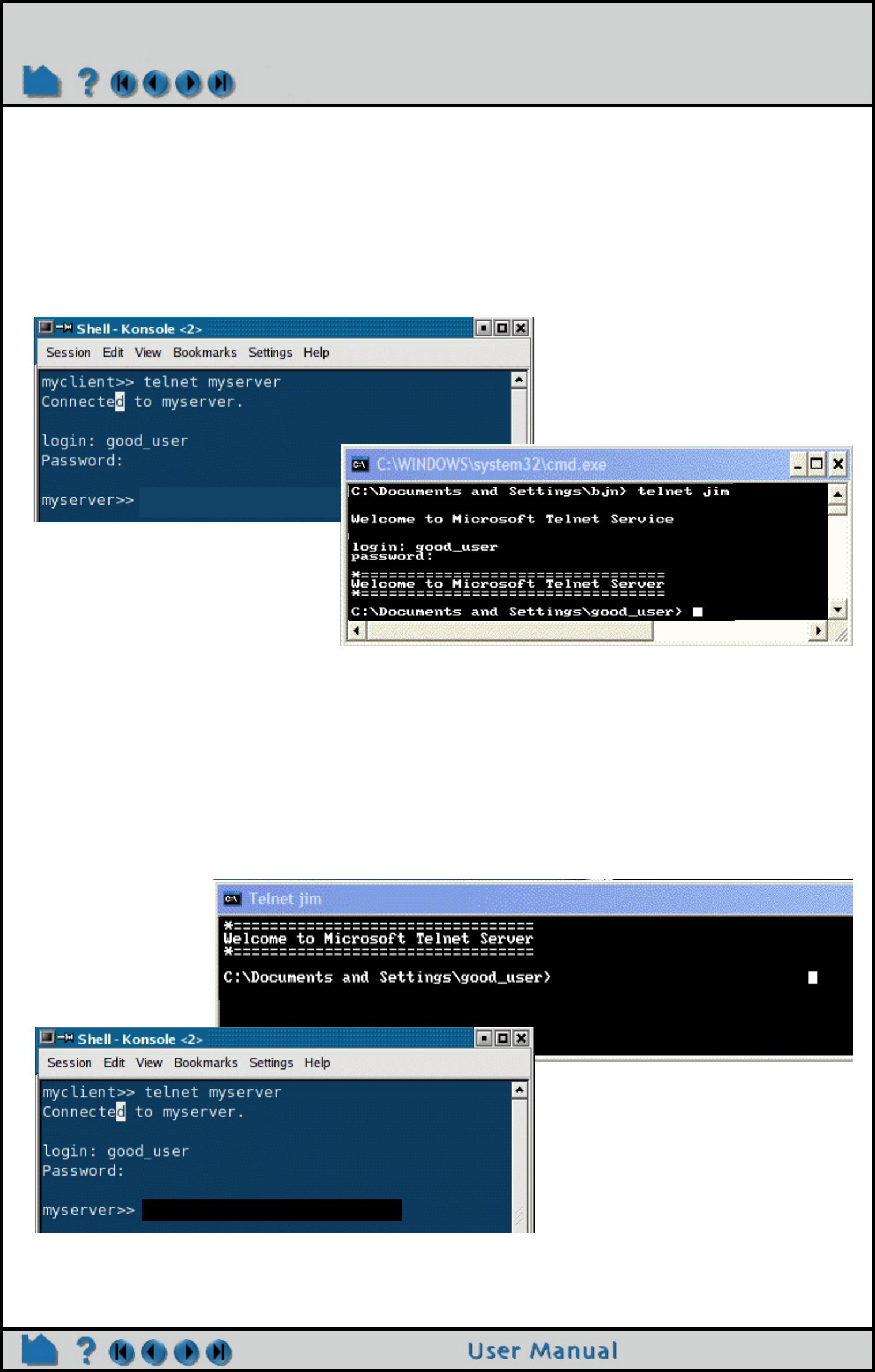
In a second window, log onto the SERVER_HOST machine using telnet (or ssh or equivalent).
The SERVER_HOST does not have to be of the same operating system as the CLIENT_HOST.
Start the ensight server on the SERVER_HOST machine, using the appropriate script and the -c option.
ensight102.server -c CLIENT_HOST
or for SOS
ensight102.sos -c CLIENT_HOST
The -c CLIENT_HOST option tells the EnSight Server to connect to the EnSight Client listening on CLIENT_HOST.
Example if doing a
telnet into a
SERVER_HOST which is a
windows machine
Example if doing a telnet into a
SERVER_HOST which is a linux machine.
Example of doing a telnet from a
linux machine to a unix machine.
Example of doing a telnet
from a windows machine to
a windows machine.
ensight10_server -c wclient
ensight10.server -c myclient
Page 21
HOW TO CONNECT ENSIGHT CLIENT & SERVER
which comes up. You can also check the Connection Details under the Case menu. Licensing information should also
appear in the Graphics Window. If the connection failed, please consult Manual Connection Troubleshooting below
and Troubleshooting the Connection in the Installation Guide before contacting CEI support.
Manual Connection Troubleshooting
A manual connection can fail for any of several reasons. Because of the complexity of networking and customized
computing environments, we recommend that you consult your local system administrator and/or CEI support if the
following remedies fail to resolve the problem.
ADVANCED USAGE
Command Line Options
Command line options can be used to streamline many of the connection processes.
.
Problem Probable Causes Solutions
For Unix Systems:
Unable to telnet into the
SERVER_HOST machine
Telnet service not allowed or not
running on the SERVER_HOST
machine.
Get system administration help to be able to perform this
operation. It may be that your site requires the use of ssh
or some other equivalent.
Ensight server does not start on
SERVER_HOST machine.
EnSight is not properly installed on
the SERVER_HOST
Verify the installation on the SERVER_HOST as described
in the Installation Guide. Making sure that the proper
environment variables and command path have been set.
Startup Command Description
ensight102
ensight102.client -c Starts up client and autoconnects to localhost.*
ensight102 -sos
ensight102.client -c -sos Starts up client and auto connects to sos on localhost. This requires a gold key.*
ensight102.client Starts up client with no connection.*
ensight102.client -c hostname Starts up client and auto connects to the hostname. The host localhost is are used is used if
hostname is not listed.*
ensight102.client -c hostname -sos Starts up client and auto connects the sos to the host specified.*
ensight102.client -cm Starts up a client, and prompts for a manual connection.*
* Note that if you are starting from a PC in a command window, change the period to an underscore: ensight102.client becomes
ensight102_client. Also if you specify a resource file to use in the start up, it takes precedence over connection settings.
Page 22
HOW TO CONNECT ENSIGHT CLIENT & SERVER
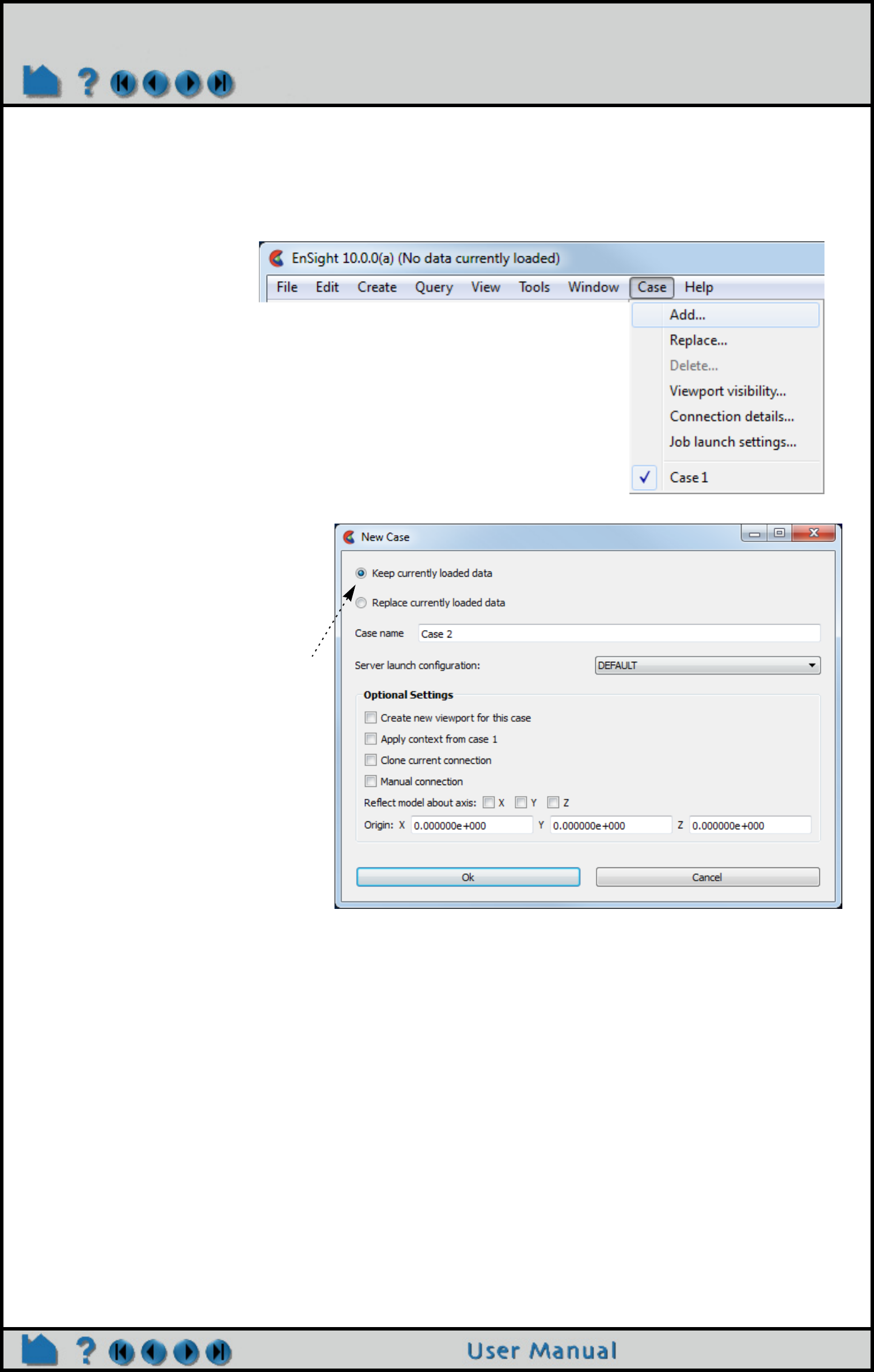
Adding Another Case
You would add another case when you want to add an additional dataset (called a “case”) to your EnSight session.
This is often used for things like A-B comparisons or for assembling components that have been analyzed in different
solvers. You can also use the process described below to replace the current case with a new one without having to
restart EnSight.
You can add or replace cases
directly from the Case menu,
From either option, this dialog will appear
when adding a case.
If you keep the current case the optional
settings are available and will be applied
to the new added case.
Create viewport - If checked the added
case will appear in a new viewport.
Apply Context - The context from the first
case is applied to the new case.
Clone current connection - Use the same
server connection as the first case.
Manual connection - Add the new case
using a manual connection even if the
first connection was auto connected.
Reflect model - Reflect the new case
about an axis using the Origin specified.
For more information on Cases, see How To Load Multiple Datasets (Cases)

Page 23
HOW TO CONNECT ENSIGHT CLIENT & SERVER
Other Auto connection requirements
The auto-connect mechanism requires that certain conditions exist in your computing environment for auto
connections to work when running the EnSight server or SOS process on a different computer. Specifically, EnSight
depends on a correctly working 'ssh' command that doesn't require passwords. The notes below assume using the
default 'ssh' command.
Alternatively, EnSight can use a replacement command for 'ssh' as long as that replacement command follows 'ssh'
syntax or ‘rsh’ syntax
(i.e. rsh [-l username] hostname command)
Should you wish to use an alternative command for 'ssh', you may specify this command on the EnSight command
line with the '-ssh alternative_command_name' command line option where 'alternative_command_name' is the
replacement command. Typically, one of these mechanisms is used in computing environments that use either 'ssh'
or 'k5rsh'.
On Unix Systems:
1. You have a .cshrc file (even if you are running some other command shell such as /bin/sh) in your home
directory on the EnSight server host that contains valid settings for CEI_HOME, and that your path variable
includes the bin directory of CEI_HOME. For example, if your EnSight is installed in /usr/local/CEI and you
are running EnSight on an Linux or Unix system (other architectures use a different library path variable), your
.cshrc should contain:
setenv CEI_HOME /usr/local/CEI
set path = ( $path $CEI_HOME/bin )
To verify the settings, simply try to start the server.
2. Your .cshrc file (or files sourced or executed from there) has no commands that cause output to be written (e.g.
date or pwd). Any output can interfere with EnSight server startup.
3. You can successfully execute a remote shell command from the client host system to the server host system. The
name of the remote shell command varies from system to system. While logged on to the client host system,
execute one of the following (where serverhost is the name of your server host system):
ssh serverhost date
If successful, the command should print the current date.
If any of these conditions are not met, you will be unable to establish a connection automatically and will have to use
the manual connection mechanism. Note that it is not uncommon for system administrators to disable operation of all
remote commands for security reasons. Consult your local system administrator for help or more information.
Note that if you wish to use ‘rsh’ instead of ‘ssh’, then you need to have a valid .rhosts file in your home directory
on all systems on which you wish to run the EnSight server. The file permission for this file must be such that only the
owner (you) has write permission (e.g. chmod 600 ~/.rhosts). A .rhosts file grants permission for certain
commands (e.g. rsh or rlogin) originating on a remote host to execute on the system containing the .rhosts file.
For example, the following line grants permission for remote commands from host clienthost executed by user
username to execute on the system containing the .rhosts file:
clienthost username
There should be one line like this for every client host system that you wish to be able issue remote commands from.
It is sometimes necessary to add an additional line for each client host of the form clienthost.domain.com
username (where domain.com should be changed to the full Internet domain name of the client host system). To
verify this, simply try to rsh to the remote machine.
On Windows Systems:
1. You have the EnSight server (ensight102_server) installed on the same system as your EnSight client (if you plan
to connect to the same system)
---- OR ----
2. You can successfully execute a remote shell command from the client host system to the server host system.
Page 24
HOW TO CONNECT ENSIGHT CLIENT & SERVER
Note: By default EnSight will use the ‘ssh’ command. ssh is not a default component on Windows
workstations and must be installed by the user from one of many third party sources. However, Windows
does include a rsh command which EnSight can optionally use. Note, however, only systems running
Windows Server have the RSH service and can respond by executing the EnSight server.
The name of the remote shell command varies from system to system. While logged on to the client host system,
execute one of the following (where serverhost is the name of your server host system):
ssh serverhost date
rsh serverhost date
If successful, the command should print the current date.
If condition 1. or 2. is not met, you will be unable to establish a connection automatically and will have to use the
manual connection mechanism. Note that it is not uncommon for system administrators to disable operation of all
remote commands for security reasons. Consult your local system administrator for help or more information.
Manual connection Troubleshooting
An automatic connection can fail for any of several reasons. Because of the complexity of networking and customized
computing environments, we recommend that you consult your local system administrator and/or CEI support if the
following remedies fail to resolve the problem.
Problem Probable Causes Solutions
For Unix Systems:
Automatic connection fails or is
refused
Server (remote) host name is
incorrect for some reason.
Is the server host entered correctly in the Hostname
field? Try running telnet serverhost from the client
machine.
Incorrect or missing .rhosts file
in your home directory on the
server host.
Follow the instructions on .rhosts files (as described in
the Basic Operation section, step 1 above). If you cannot
successfully execute a remote command (such rlogin
or rsh) from the client host to the server host, you will not
be able to connect automatically.
The user account (i.e. login name)
on the client host does not exist on
the server host.
Enter your login name on the server host in the Login
name field.
The server executable is not found
on the server system
Is the entry in the Executable [path/]name field correct? If
the server executable is NOT in your default command
search path on the server, you must include the full path
name to the executable. For example, /usr/local/
CEI/ensight102/bin/ensight102.server.
Your .cshrc does not contain a
valid setting for CEI_HOME.
Add the appropriate line as described in the Basic
Operation section, step 2 above.
Your .cshrc file (or files executed
by it) causes output to be written.
This is interpreted as a server
startup error.
Remove the offending commands from your .cshrc file.
As a test, do the following:
% cd
% mv .cshrc .cshrc-SAVE
Create a new .cshrc file that contains only the lines to set
CEI_HOME and path as described in the Basic
Operation section, step 2 above. If that test works, you
will need to examine your .cshrc to find and remove the
offending lines.
For Windows Systems:
Automatic connection fails or is
refused (trying to connect to
same host system)
Server not installed or not
executable.
You should be able to locate the server executable
(ensight102_server) using Windows Explorer. Double
click on it and see if a console window opens with “This is
EnSight Server 10.2” etc. If this doesn’t happen, refer to
“Troubleshooting the Installation” in the Getting Started
Manual.
Page 25
HOW TO CONNECT ENSIGHT CLIENT & SERVER
Other Notes
Connection Name - Hostname flexibility
When you specify '-c hostname' on the command line, EnSight will start up a server on the hostname.
Users with complex computing environments should migrate to using ceishell (see the demo by typing ceistart102).
Network ports used by EnSight and SLiM
Client/Server Mode
The EnSight client connects to the slimd8 license manager via TCP port 7790 typically. This actual port used is
defined in $CEI_HOME/license8/slim8.key and appears on the 'slimd' line as the number after 'slimd'.
The client listens for connections from the EnSight server on TCP port 1106. It also communicates with the
collaborative hub on TCP port 1107. If the client is listening for external commands, it will use TCP port 1104.
If port 1106 is used by another process, EnSight will give you an error "Address already in use", and there are two
possible solutions:
1: use another port with command line option "-ports ####" for both client and server (inconvenient)
2: kill (or have root kill) the process that has the port locked.
For example, determine the process:
/sbin/fuser 1106/tcp
the result comes back....
1106/tcp: 314159o
in this case you(or root, if necessary) would kill it...
kill -9 314159
Note that the specific commands to use will vary depending on operating system.
Path to the server is incorrect If using the EnSight Connect dialog, check that the
correct path is specified in the “Executable” field.
If running from the ensight102 command, first ensure that
your PATH environment variable contains the paths for
the ensight102 “client” and “server” directories. You can
check and correct the value of PATH in the Start
>Settings >ControlPanel >System_Environment dialog.
Incorrect hostname entered in the
“Hostname” field of the Connection
settings dialog.
Make sure that the hostname is correct, including the
case of all letters. The ONLY way to confidently see the
hostname (in the correct case) from Windows is to open
a Command Prompt window and type:
> ipconfig /all
The Host Name will be one of the first things listed.
Automatic connection fails or is
refused (trying to connect to a
remote server)
Same causes as for a Unix system See “For Unix Systems” portion of this table above.
Problem Probable Causes Solutions

Page 26
HOW TO CONNECT ENSIGHT CLIENT & SERVER
Server of Server Mode
When running in Server of Server mode (SOS), the SOS is threaded and will start up server processes in parallel
(subject to CPU availability and license restrictions) using ports 1110 through 1117. To limit the number of threads,
set the environmental variable ENSIGHT10_MAX_SOSTHREADS to the maximum number of threads (max is 8).
Distributed Renderer - used by parallel compositor
Ports 8739 to 8789 must be available to EnSight for its own internal TCP/IP connections when running the parallel
compositor in EnSight DR.
SEE ALSO
Chapter 2 of the Getting Started Manual
How To Load Multiple Datasets (Cases)
Page 27
HOW TO READ DATA
Read and Load Data
Read Data
INTRODUCTION
EnSight supports a number of file formats common in computational analysis. In addition, CEI has defined generic
data formats (in both ASCII and binary versions) that can be used for both structured and unstructured data. In many
cases analysis codes output this data directly (i.e. FLUENT, STAR-CD, KIVA, etc.)
BASIC OPERATION
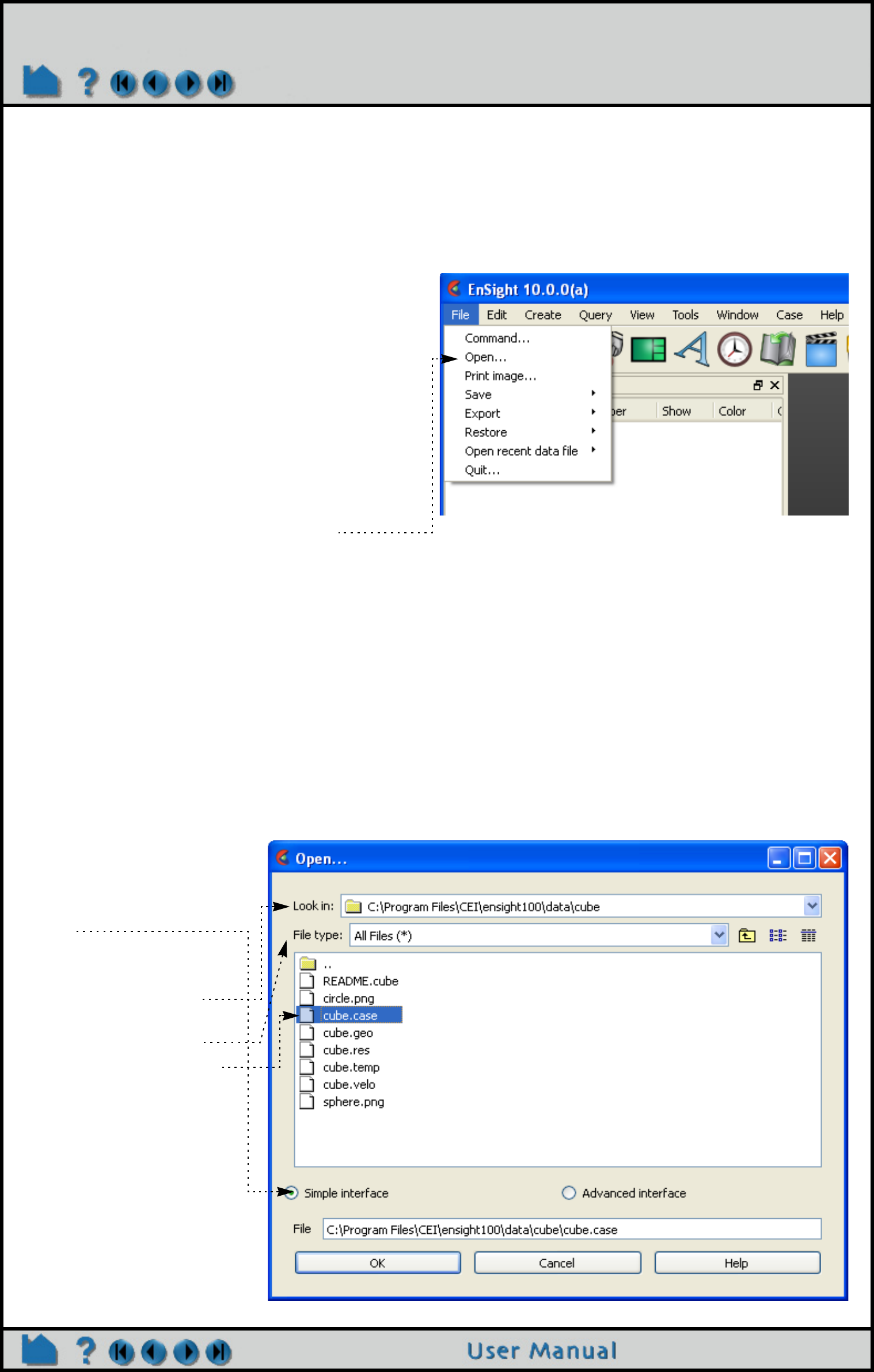
Simple Interface
Reading data into Ensight can be accomplished with a
“simple interface” if an association is known for the data
format type and you wish to load all parts.
Otherwise, the more traditional method for loading data
into EnSight can be accomplished with the “advanced
interface”. It provides more control over the reading of
data files and the part creation process. The first step is
the selection of appropriate files. The second step is the
loading of parts. Both steps have many similarities
regardless of the data format. These basic steps are
described below. Variations from the methods shown will
be described in Chapter 2 (Reader Basics) of the User
Manual for the various formats. Both of these methods
are accessed under File->Open...
1. Select File > Open...
2. If not already selected,
toggle Simple Interface
on.
3. Navigate to the desired
directory using typical
navigation methods.
4. Filter the list using the
File type, if desired.
5. Select the desired file.
This file’s extension is what
will be mapped to a reader
in the
ensight_reader_extension.
map.
6. Click Okay
(Double clicking the file in
step 4. is also allowed.)
The simple interface method of reading data into EnSight works for most formats and requires a file extension-to-
reader mapping file (ensight_reader_extension.map). This file can reside in the site_preferences directory and/or
each user can have his own personal one in his personal EnSight defaults directory (located at
%HOMEDRIVE%%HOMEPATH%\(username)\.ensight102 commonly located at C:\Users\username\.ensight102 on Vista
and Win7 and newer, C:\Documents and Settings\yourusername\.ensight102 on older Windows, and ~/.ensight102 on
Linux, and in ~/Library/Application Support/EnSight102 on the Mac). A sample of this file is shown below. The mapping
file associates file extensions to readers. If this file is not provided or an association is not known, or the format
doesn’t allow it due to required intermediate information (such as Plot3D currently), the simple interface method
cannot be used and the OK button will not be active. One is then required to use the advanced Interface method
Page 28
HOW TO READ DATA
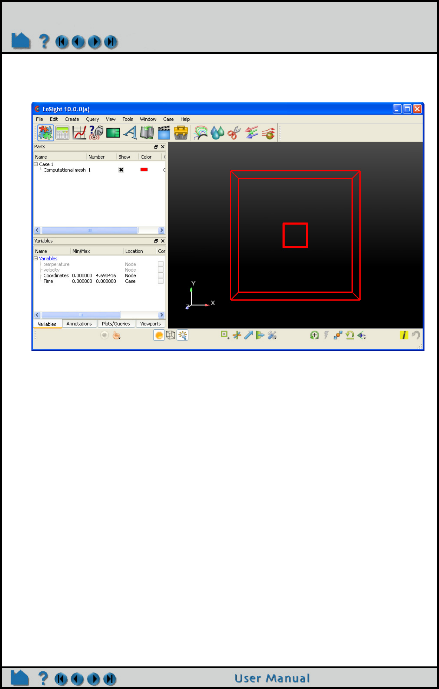
At this point (provided the association is successful and the data is readable) all parts of the model will be loaded into
EnSight and will appear in the graphics screen and in the Parts List. If the association is not successful, an error
message will result.
Note that variables in the data are also listed at this point. They have not yet been activated. The process for doing so
will be discussed in How To Activate Variables.
Ensight_reader_extension.map file example:
The following is a sample containing associations for EnSight Case, EnSight5, STL and MSC/Dytran:
EnSight file extension to format association file
Version 1.0
#
# Comment lines start with a #
#
#
# The format of this file is as follows:
#
# READER_NAME: reader name as it appears in the Format chooser in the EnSight Data Reader dialog
# NUM_FILE_1: the number of file_1_ext lines to follow
# FILE_1_EXT: the extension that follows a file name minus the “.”, i.e., “geo”, “case”, etc.
# There should be one definition after the :. Multiple FILE_1_EXT lines may exist
# NUM_FILE_2: the number of file_2_ext lines to follow
# FILE_2_EXT: the extension of a second file that will act as the result file. This is only used
# for formats that require two file names. As with FILE_1_EXT, there may be multiple
# FILE_2_EXT lines.
# ELEMENT_REP: A key word that describes how the parts will be loaded (all parts will be loaded the
# same way). One of the following:
# “3D border, 2D full”
# “3D feature, 2D full”
# “3D nonvisual, 2D full”
# “Border”
# “Feature angle”
# “Bounding Box”
# “Full”
# “Non Visual”
# If option is not set then 3D border, 2D full is used
# READ_BEFORE: (optional) The name of a command file to play before reading the file(s)

Page 29
HOW TO READ DATA
# READ_AFTER: (optional) The name of a command file to read after loading the parts
# Definition for Case files
READER_NAME: Case
NUM_FILE_1: 2
FILE_1_EXT: case
FILE_1_EXT: encas
ELEMENT_REP: 3D feature, 2D full
# Definition for EnSight5 files
READER_NAME: EnSight 5
NUM_FILE_1: 2
FILE_1_EXT: geo
FILE_1_EXT: GEOM
NUM_FILE_2: 2
FILE_2_EXT: res
FILE_2_EXT: RESULTS
ELEMENT_REP: 3D feature, 2D full
# Definition for STL files
READER_NAME: STL
NUM_FILE_1: 4
FILE_1_EXT: stl
FILE_1_EXT: STL
FILE_1_EXT: xct
FILE_1_EXT: XCT
ELEMENT_REP: 3D feature, 2D full
# Definition for Dytran files
READER_NAME: MSC/Dytran
NUM_FILE_1: 2
FILE_1_EXT: dat
FILE_1_EXT: ARC
ELEMENT_REP: 3D border, 2D full
READ_AFTER: read_after_dytran.enc
Page 30
HOW TO READ DATA
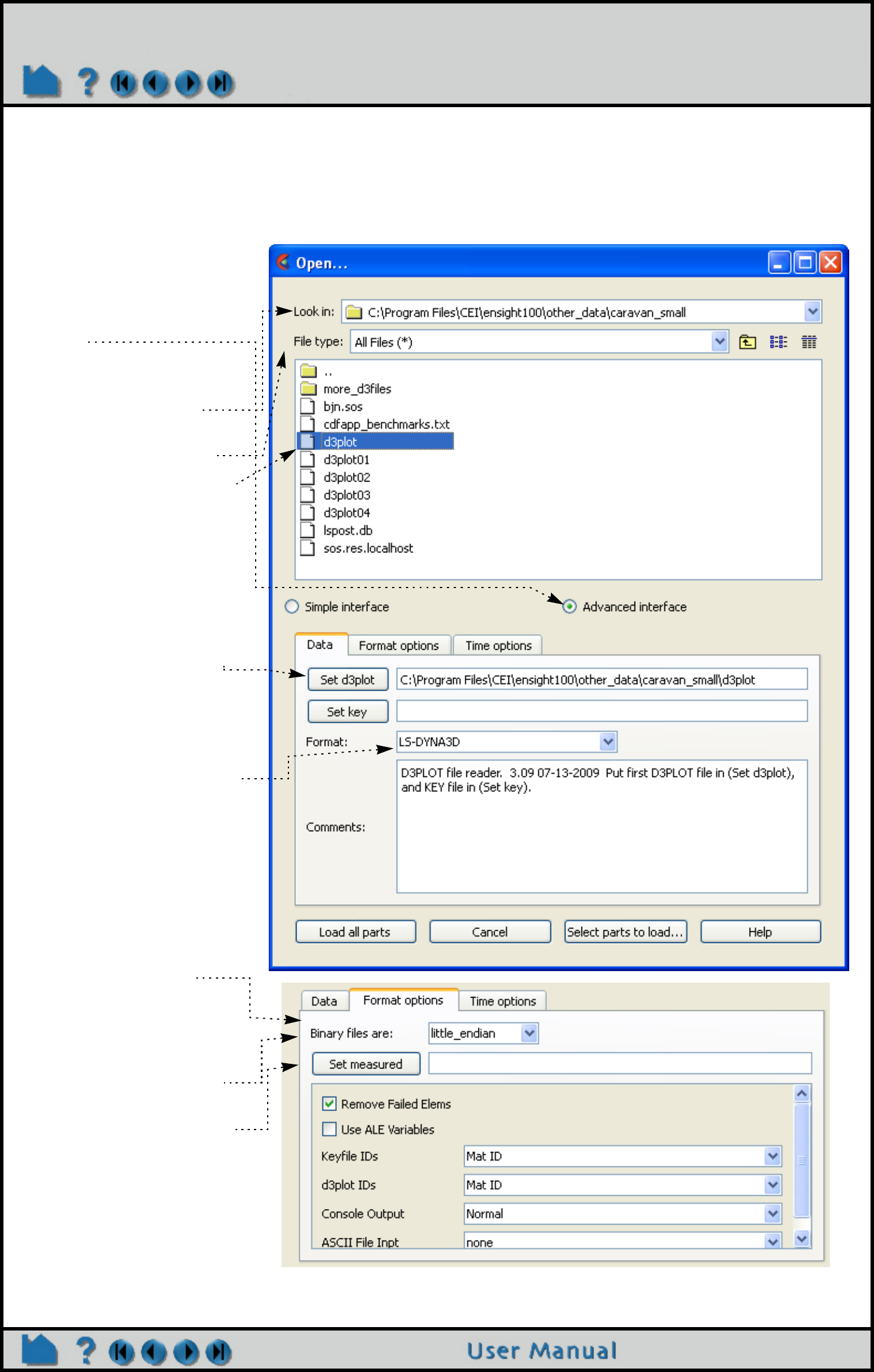
Advanced Interface
When using the advanced method, the user similarly specifies the files, but can also specify the format, and other
format and time options. He then has control over whether all parts will be loaded into EnSight, or whether EnSight
will be informed of their existence, but not actually be loaded yet.
1. Select File > Open...
2. Toggle Advanced
Interface, if not already
set.
3. Navigate to the desired
directory using typical
navigation methods.
4. Filter the list using the
File type, if desired.
5. Select the desired file.
This file’s extension is what will
be mapped to a reader in the
ensight_reader_extension.map.
6. Click the applicable Set
Button(s) (in this case, the
Set d3plot button)
If a mapping is known, the
correct Format will be
automatically chosen for you.
7. Select the correct Format
- if not already correct.
The list shown is dependent on
the presence of internal and
user-defined readers at your
site, and in your preference
settings. For the list of
available readers please see
Native EnSight Format
Readers or Other Readers.
8. Optionally set any
Format options.
Note the options presented will
vary according to the data
format.
Big-Endian is only necessary for
legacy binary case gold files
written on Unix platforms.
All but the Casefile format will
allow input of measured point
data. See EnSight5 Measured/
Particle File Format. Plot3d,
Casefile, and Special HDF5
structured formats will provide a
field for a boundary file. See
EnSight Boundary File
Format
(Continued on next page)
Page 31
HOW TO READ DATA
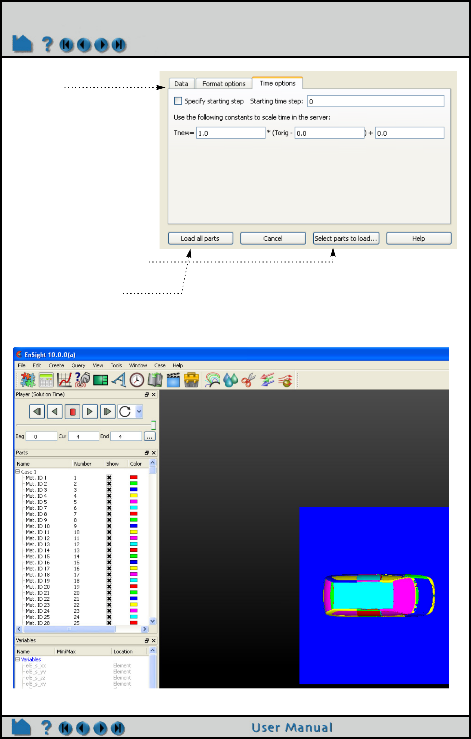
The parts in the model will now appear in the Parts list in EnSight. If you did a Load all parts, the parts will be loaded
and active and will also be visible in the Graphics window.
9. Optionally set any Time
options.
.
10. Click Select parts to load...
If you want to pick and choose which
parts get loaded.
or click Load all parts
If you want to have all parts loaded.
Page 33
HOW TO READ DATA
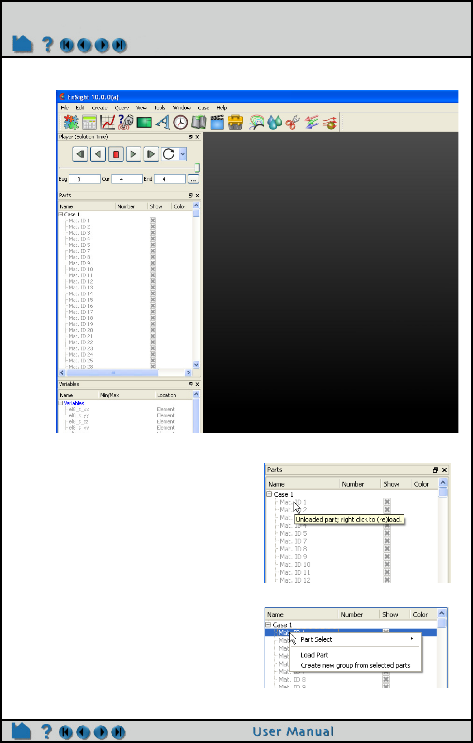
Note that all parts in the case can be loaded by right clicking on the parent Case 1, instead of individual parts.
If there are any exceptions to this general process, please see the details for specific readers in Chapter 2 (Other
Readers) of the User Manual
SEE ALSO
How To Use ens_checker
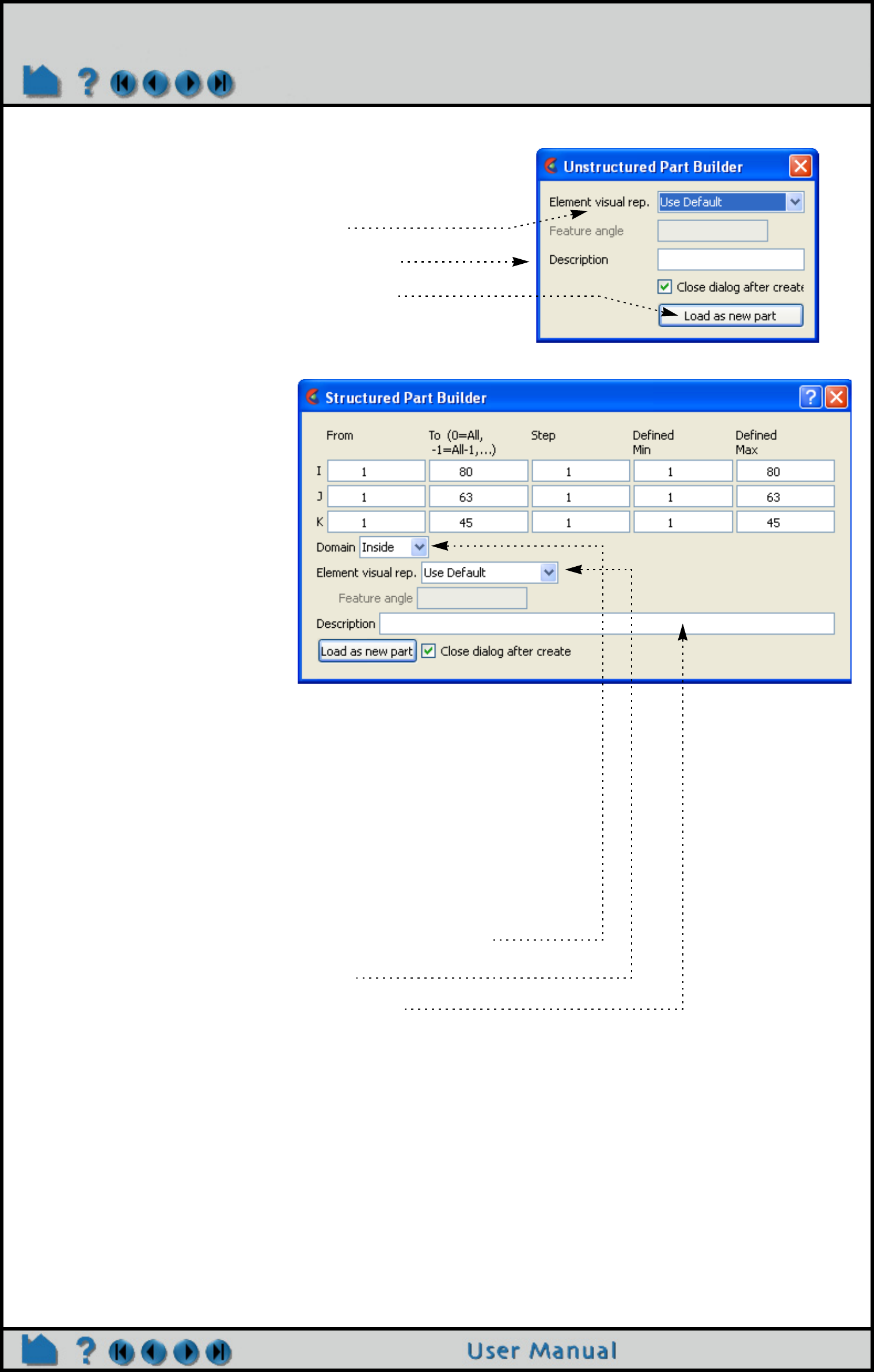
And if your data is unstructured, when you click on Load
part, you will see a dialog like that to the right, wherein
you can set:
1. The initial Visual Representation to use
2 A description other than the default, if desired.
And click Load as new part to get the part created.
If the data is structured, then you will
see a dialog like the one to the right,
wherein you can set:
1. From, To, and Step IJK values
for the selected part(s).
The From and To values are
inclusive.
Valid values in the From and To
fields are numbers advancing from
1(the min for each part), or
numbers decreasing from 0(the
max for each part):
1,2,3,... ---> <---...-3,-2,-1,0
|---------------------------------------|
min max
(always 1) (varies per part)
If you specify values that will be outside of the range of an
individual part, the proper min or max values for the given part will
be used.
The Defined Min and Defined Max fields are for reference only.
2. If the selected part has Iblanking, you can build based on
the value (Inside selects cells where Iblank=1, Outside
selects Iblank=0, All selects all cells ignoring Iblanking).
3. The initial Visual Representation to use
4. A description other than the default, if desired.
If you leave the Description field blank, it will default to what is
shown in the Parts list.
And click Load as new part to get the part created.


Page 35
HOW TO USE ENS_CHECKER
Use ens_checker
INTRODUCTION
This program attempts to check the integrity of the EnSight Gold (or EnSight6) file formats. Most files that pass this
check will be able to be read by EnSight (see Other Notes below). If EnSight Gold (or EnSight6) data fails to read into
Ensight, one should run it through this checker to see if any problems are found.
Ens_checker makes no attempt to check the validity of floating point values, such as coordinates, results, etc. It is
just checking the existence and format of such. Invoke ens_checker using the version of EnSight that you are using.
For example, for EnSight 10.2, use ens_checker102.
BASIC OPERATION
Program invocation:
If you invoke the program without any arguments, it will prompt you for the casefile to read. For example:
> ens_checker102
*****************************************************************
* EnSight Data Format Checker *
* =========================== *
* Currently, *
* 1. Must be run from directory in which casefile is located. *
* 2. Handles EnSight6 and EnSight Gold formats only. *
* 3. Does not process SOS casefiles. *
*****************************************************************
<Enter casefile name (must be in directory containing it!) > mydata.case
You can alternatively invoke the program with the casefile on the command line.
> ens_checker102 mydata.case
Sample runs:
As ens_checker works it will be providing feedback. This feedback is important in interpreting what is wrong in the
files. Here is a sample run, which was successful:
> ens_checker102 3by3.case
*****************************************************************
* EnSight Data Format Checker *
* =========================== *
* Currently, *
* 1. Must be run from directory in which casefile is located. *
* 2. Handles EnSight6 and EnSight Gold formats only. *
* 3. Does not process SOS casefiles. *
*****************************************************************
<Enter casefile name (must be in directory containing it!) > 3by3.case
Casefile to Process:
--------------------
3by3.case (Opened successfully)
---------------------
Major Sections Found:
---------------------
Required FORMAT section (at line 1)
Required GEOMETRY section (at line 4)
Optional VARIABLE section (at line 7)
Optional TIME section (at line 11)
---------------
FORMAT Section:
---------------

Page 36
HOW TO USE ENS_CHECKER
EnSight 6 Format (set at line 2)
-------------
TIME section:
-------------
Info for timeset number: 1
----------------------------
Time set: 1 (at line 12)
No description provided
Number of steps: 1 (at line 13)
Time values: (starting on line 14)
time values[1] = 0
>-------------------<
> TIME section OKAY <
>-------------------<
-----------------
GEOMETRY Section:
-----------------
--------
Model filename is: 3by3.geo (at line 5)
Static geometry
--------
Opened 3by3.geo successfully
File type is: ASCII
Description 1: EnSight test geometry file
Description 2: ==========================
node ids: assign
element ids: assign
Global section:
Number of nodes: 64
Coordinates for (64) nodes found
Part 1:
Description is: 3 x 3 xy
Unstructured Part
Number of quad4 elements is: 9
Connectivities for (9) quad4 elements found
Part 2:
Description is: 3 x 3 yz
Unstructured Part
Number of quad4 elements is: 9
Connectivities for (9) quad4 elements found
Part 3:
Description is: 3 x 3 xz
Unstructured Part
Number of quad4 elements is: 9
Connectivities for (9) quad4 elements found
Part 4:
Description is: 3 x 3 45
Unstructured Part
Number of quad4 elements is: 9
Connectivities for (9) quad4 elements found
>-----------------------<
> GEOMETRY section OKAY <
>-----------------------<
-----------------
VARIABLE Section:
-----------------
scalar per node: scalar (at line 8)
Filename is: 3by3.scl

Page 37
HOW TO USE ENS_CHECKER
Non transient variable
--------
Opened 3by3.scl successfully
Description: 3by3 scalar variable
Global section:
(64) Nodal scalar values for unstructured nodes found
vector per node: vector (at line 9)
Filename is: 3by3.vct
Non transient variable
--------
Opened 3by3.vct successfully
Description: 3by3 vector variable
Global section:
(192) Nodal vector values for unstructured nodes found
>-----------------------<
> VARIABLE section OKAY <
>-----------------------<
>----------- Hooray! ----------<
> <
> Data verification SUCCESSFUL <
> <
> with No Warnings <
> <
>------------------------------<
And here is a sample run, with a problem, namely a ‘block’ line is missing:
> ens_checker102 3by3s.case
*****************************************************************
* EnSight Data Format Checker *
* =========================== *
* Currently, *
* 1. Must be run from directory in which casefile is located. *
* 2. Handles EnSight6 and EnSight Gold formats only. *
* 3. Does not process SOS casefiles. *
*****************************************************************
Casefile to Process:
--------------------
3by3s.case (Opened successfully)
---------------------
Major Sections Found:
---------------------
Required FORMAT section (at line 1)
Required GEOMETRY section (at line 4)
Optional VARIABLE section (at line 7)
Optional TIME section (at line 11)
---------------
FORMAT Section:
---------------
EnSight 6 Format (set at line 2)
-------------
TIME section:
-------------
Info for timeset number: 1

Page 38
HOW TO USE ENS_CHECKER
----------------------------
Time set: 1 (at line 12)
No description provided
Number of steps: 1 (at line 13)
Time values: (starting on line 14)
time values[1] = 0
>-------------------<
> TIME section OKAY <
>-------------------<
-----------------
GEOMETRY Section:
-----------------
--------
Model filename is: 3by3s.geo (at line 5)
Static geometry
--------
Opened 3by3s.geo successfully
File type is: ASCII
Description 1: EnSight test geometry file
Description 2: ==========================
node ids: assign
element ids: assign
Global section:
Number of nodes: 0
Part 1:
Description is: 3 x 3 xy block
Structured Part
Not iblanked
i j k = 4 4 1
Number of nodes: 16
Number of cells: 9
Block X coordinates for (16) nodes found
Block Y coordinates for (16) nodes found
Block Z coordinates for (16) nodes found
Part 2:
Description is: 3 x 3 yz block
===> Problem:
-------------
Looking for one of the following valid line types:
element type (unstructured types, any of the following:
point tria6 tetra10 penta15
bar2 quad4 pyramid5 hexa8
bar3 quad8 pyramid13 hexa20
tria3 tetra4 penta6
block (structured block)
part (the next part)
but found the following:
4 4 1
>-------------------------<
> GEOMETRY section FAILED <
>-------------------------<
>-*-*-*-*-*-* bummer! *-*-*-*-*-*-<
> <
> Verification of the data FAILED <
> <
>-*-*-*-*-*-*-*-*-*-*-*-*-*-*-*-*-<

Page 39
HOW TO USE ENS_CHECKER
After fixing the ‘block’ line and running the program again, another problem is encountered - namely, an extra space
at the end of the second line of x coordinates for the block that is part 2.
> ens_checker102 3by3s.case
*****************************************************************
* EnSight Data Format Checker *
* =========================== *
* Currently, *
* 1. Must be run from directory in which casefile is located. *
* 2. Handles EnSight6 and EnSight Gold formats only. *
* 3. Does not process SOS casefiles. *
*****************************************************************
Casefile to Process:
--------------------
3by3s.case (Opened successfully)
---------------------
Major Sections Found:
---------------------
Required FORMAT section (at line 1)
Required GEOMETRY section (at line 4)
Optional VARIABLE section (at line 7)
Optional TIME section (at line 11)
---------------
FORMAT Section:
---------------
EnSight 6 Format (set at line 2)
-------------
TIME section:
-------------
Info for timeset number: 1
----------------------------
Time set: 1 (at line 12)
No description provided
Number of steps: 1 (at line 13)
Time values: (starting on line 14)
time values[1] = 0
>-------------------<
> TIME section OKAY <
>-------------------<
-----------------
GEOMETRY Section:
-----------------
--------
Model filename is: 3by3s.geo (at line 5)
Static geometry
--------
Opened 3by3s.geo successfully
File type is: ASCII
Description 1: EnSight test geometry file
Description 2: ==========================
node ids: assign
element ids: assign
Global section:
Number of nodes: 0
Part 1:
Description is: 3 x 3 xy block
Structured Part
Not iblanked

Page 40
HOW TO USE ENS_CHECKER
i j k = 4 4 1
Number of nodes: 16
Number of cells: 9
Block X coordinates for (16) nodes found
Block Y coordinates for (16) nodes found
Block Z coordinates for (16) nodes found
Part 2:
Description is: 3 x 3 yz block
Structured Part
Not iblanked
i j k = 4 4 1
Number of nodes: 16
Number of cells: 9
===> Problem:
-------------
Previous lines end with 1 extra chars on the line,
but line 2 has 2 extra chars. The lines must be consistent
or EnSight will have trouble reading it.
===> Problem:
-------------
Not successful reading 16 X block coordinates
>-------------------------<
> GEOMETRY section FAILED <
>-------------------------<
>-*-*-*-*-*-* bummer! *-*-*-*-*-*-<
> <
> Verification of the data FAILED <
> <
>-*-*-*-*-*-*-*-*-*-*-*-*-*-*-*-*-<
After eliminating the extra space, the file then checked out fine.
ADVANCED USAGE
Redirecting Output to a File:
ens_checker is writing to stderr, so if you want to redirect output to a file, you need to use “>&”. For example, the
following will place the output of the run into a file called output.file:
> ens_checker102 3by3.case >& output.file
OTHER NOTES
The word “most” is used above because one of the things that could pass the checker, but fail in EnSight is element
connectivity of EnSight6 files with node ids. The ens_checker checks that node ids used in the element connectivities
lie within the min and max range of the node ids, but does not verify that there is actually a node with each individual
id.
The validity of model extents, presence of nan’s, etc. are currently checked to some degree in ens_checker, but
again, this is a format checker - not a model integrity checker.
SEE ALSO
User Manual:
EnSight Gold Casefile Format
EnSight6 Casefile Format
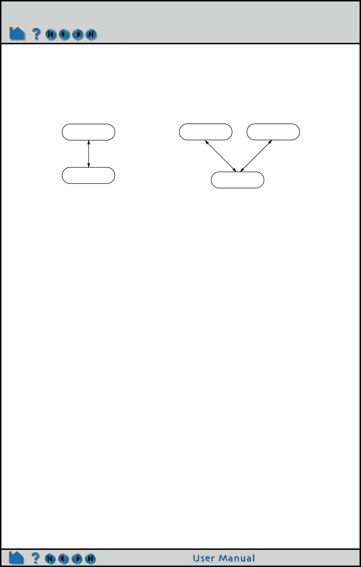
Page 41
HOW TO LOAD MULTIPLE DATASETS (CASES)
Load Multiple Datasets (Cases)
INTRODUCTION
Normal operation of EnSight involves one client process (the graphics and user interface) interfacing with one server
process (data I/O and computation) to postprocess your data. There are however several other configurations
possible. One of these is the ability to connect a single client to multiple servers at the same time, with each server
maintaining a unique dataset. Each of these servers can potentially run on different machines.
The main use of this capability is to visualize multiple datasets simultaneously. Each dataset is loaded into a separate
case and can be viewed in the same window or in separate viewports. You can perform before and after comparisons
of the same problem or compare experimental with simulated results. The same operation (such as a clip or a particle
trace) can be performed in both cases simultaneously. Created parts always belong to the same case as the parent
from which the part was created. As a consequence, you cannot perform operations that combine parts (such as a
merge) from multiple cases.
When EnSight reads a new case, it searches the current list of variables for matches with the variables from the new
case. If it finds a match (based on an exact match of the variable name), it will not enter the new variable in the list.
Rather, the matched name will be used for both. This behavior is based on the assumption that the identical variable
names represent the same physical entity and should therefore be treated the same. If the new variable name does
not match any existing name, the new variable is added to the list as usual.
Up to 32 cases can be active at one time. You can add a new case or replace an existing case to a running session
by using the File->Open... process (if you want to load all parts and don’t need to control other options available when
loading cases) or the File->Data (reader)... process (which provides greater control). Adding a case starts a new
server process, connects it to the client, and either loads all the parts (if you used Open...) or allows you to specify the
data format and files as well as which parts to load into the new server and what optional settings to use as the case
is created. One of the helpful uses of the replace case option is to load a new dataset into EnSight without re-starting
the client. You can of course also delete cases you no longer need.
It is possible to allow EnSight to link cases together in which operations performed on one case are performed on all
cases. See the Release Notes for a list of limitations and for details on linking cases see How To Compare Cases.
Server
Client
Server
Client
Server
Normal Operation Two Cases
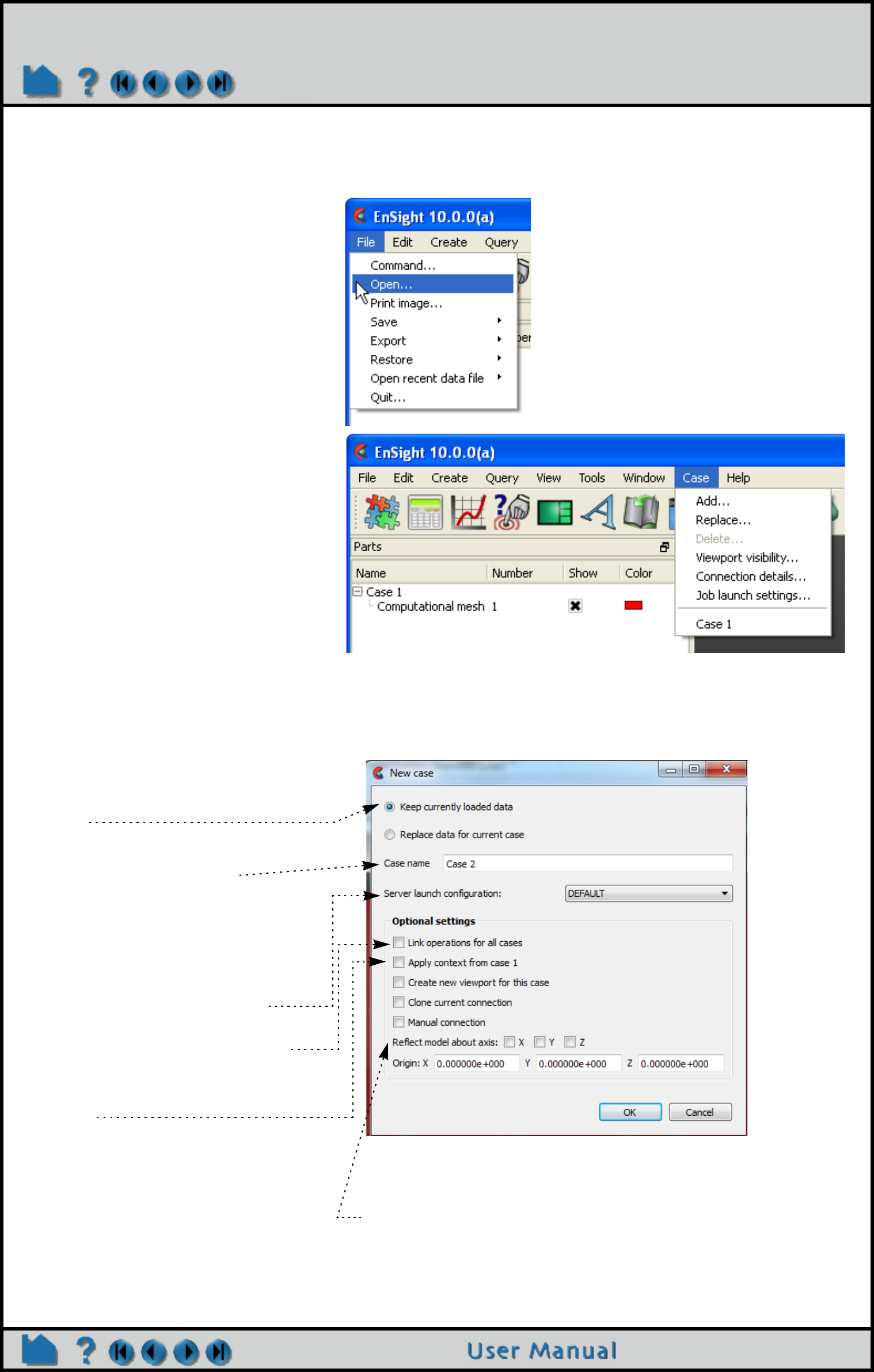
Page 42
HOW TO LOAD MULTIPLE DATASETS (CASES)
BASIC OPERATION
Once an existing case has been loaded in the normal manner, further case operations can be accessed through:
Add a Case
To add a case to a running EnSight session
File->Open...
or through:
Case->Add..., Replace..., Delete,,.
Do File->Open..., or Case->Add...
1. Select Keep currently loaded data
This will add, rather than replace, the
case
2. If desired, enter a name for the case
(other than the default).
The name will be displayed in the Case
menu.
3. Set other optional settings.
Select Server launch configuration if you
have a predefined configuration.
Link operations for all cases see How To
Compare Cases.
Apply Context From Case 1 will cause the
new case to inherit positioning etc. from
case 1.
Create new viewport for this case will
place the new case in a new viewport.
Clone current connection will cause the
same connection method as current one.
Manual connection will cause a manual
connection to be used - even if current
connection(s) were automatic.
Reflect Model About Axis allows the model to be reflected as
it is read in. Pick the axis and specify the origin location.
4. Click Okay.

Page 43
HOW TO LOAD MULTIPLE DATASETS (CASES)
The EnSight client will now start the connection process for the new server. Depending on the launch or connection
settings chosen, the new server will be started automatically or you will have to manually start another server. The
default is to start a new server automatically if your original connection was automatic, or to cause you to start
another server manually if your original connection was manual. You can follow the progress of the connection in the
Message area. See the EnSight Getting Started Manual or How To Connect EnSight Client and Server for more
information. Once connected, EnSight will also load all parts of this new case if you use this method.
You will then be presented
with the Open... dialog.
Navigate to and select your
data, and use the Simple
interface to load all parts.
(Note that the file type must be
recognized for this method to
work.)
Or, use the Advanced
interface, and control the
Format and other options.
As well as being able to
Select parts to load, etc.
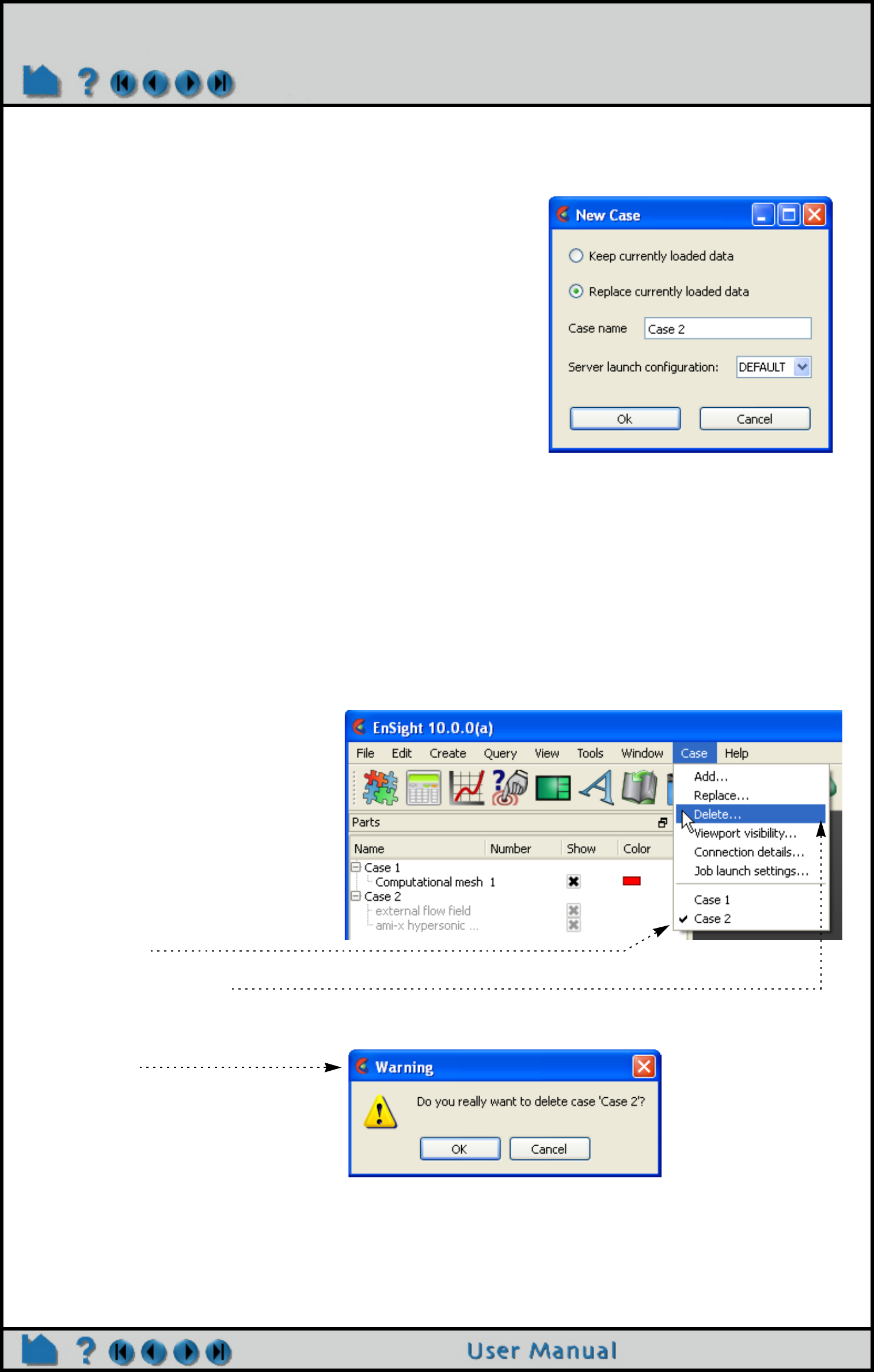
Page 44
HOW TO LOAD MULTIPLE DATASETS (CASES)
Replace a Case
You can replace an existing case. This is most useful when you wish to load a new dataset without having to stop and
re-start the client. To replace a case:
You will now be presented with the Open... dialog, just as shown in Add Case above. You can use the Simple
Interface and load all parts, or control the options and part loading by using the Advanced interface. The server
associated with the selected case is terminated and the EnSight client will now start the connection process for the
new server. Again, depending on the launch configuration chosen, the new server will be started automatically or you
will have to manually start another server. The default is to start a new server automatically if your original connection
was automatic, or to cause you to start another server manually if your original connection was manual. You can
follow the progress of the connection in the Message area. See How To Connect EnSight Client and Server for
more information.
Delete a Case
To delete a case:
Do File->Open... and select Replace currently loaded data, or
Case->Replace...
This will open the dialog shown. You can optionally set a case
name or choose a predefined launch configuration, or just use
the default.
Click Okay
1. Select the case you wish to
delete in the Case menu (Case >
casename).
2. Select Case > Delete...
You will be asked to confirm the
deletion. If confirmed, the server
associated with the selected case is
terminated.

Page 45
HOW TO LOAD MULTIPLE DATASETS (CASES)
Displaying Parts by Case
By default all parts from all cases are displayed in the Main Parts list and they are displayed in a hierarchical manner
by case. See How To... Introduction to Part Creation for more details on viewing the parts list.
Case Viewport Display
One of the chief advantages of the case feature is the ability to perform side-by-side comparisons of different
datasets. One way to do this is to display each case in a separate viewport. To do this:
1. Create as many additional
viewports as you need to display
your cases. See How To Define
and Change Viewports for more
information.
2. Select the case whose parts you
wish to display only in certain
viewports in the Case menu
(Case > casename).
3. Select Case > Viewport Visibility...
4. Click in the desired viewport to
enable or disable display of the
selected case. Black means the
selected case is not displayed in
the viewport, green means that it
is displayed.
Page 46
HOW TO LOAD MULTIPLE DATASETS (CASES)
ADVANCED USAGE
EnSight’s cases capability has also been used to achieve coarse-grained parallelism for very large datasets by
partitioning a mesh into blocks and reading each block into a different case. Each case can run on different machines
or on different CPUs of a multiprocessor host. Since the EnSight client places the geometry from the different cases
in the same coordinate system, the blocks are effectively “stitched” back together for viewing. Operations such as
clipping and isosurface calculation are then automatically performed in parallel. However, since there is no
communication between the servers (in the current release) you cannot trace particles originating in one block and
expect them to cross a block boundary into a different block. (It should be noted that EnSight’s server-of-server
capability is an alternate, and usually better way to do parallel operations on a model.)
OTHER NOTES
When you perform an archive operation, a binary dump file is produced for each active server (case). The archive
information file contains details about the cases and can be used to restart the EnSight client as well as all servers
active when the archive was performed. See How To Save and Restore an Archive for more information.
SEE ALSO
User Manual: Case Menu Functions
How To Manual: Compare Cases

Page 47
HOW TO COMPARE CASES
Compare Cases
INTRODUCTION
EnSight has long had the ability to load multiple datasets and included tools to help compare them. Each of these
datasets is loaded as a separate EnSight Case. But no functionality or capability existed to try to make case
comparison easy or automated for the user.
The first step instructions on using multiple EnSight cases, is to see How to Load Multiple Datasets (Cases) which
will explain how multiple cases are loaded in EnSight. All of this functionality for reading and comparing multiple
cases is available to the user in a somewhat tedious step-by-step process. This “How To” was written to document a
new and more automated case compare capability named “case linking” which is intended to provide easy case
comparison functionality.
The goal of linking all the cases is to quickly and uniformly perform the same operation over all of the cases. So
transformations, part attribute changes, part and variable creation and query operations are performed automatically
and uniformly across all of the loaded cases. When one case is changed, all are changed in the same way.
To use case linking, first load a dataset and perhaps set up what you want to visualize. Then load the next case and
toggle on "Link operations for all cases". This will read in the new case, apply the context file from the first case and
automatically place the new case in its own linked viewport. Subsequent cases loaded will also be linked together
and each appear in their own linked viewport.
Case linking remains on until you turn it off (either right click on a case in the parts dialog or turn it off via the Case
pulldown). Once turned off, the case linking can not be turned back on in the current session.
Limitations
Every dataset must contain the same number of parts.
Case linking does not use part id nor part name, but rather part order in the part list to match up the parts. Therefore
the parts must match up in the same order in the part list.
Same model variables must exist with same names across the cases. Load all cases prior to doing calculations.
The geometry must be in roughly the same dimensions.
What are linked?
Once turned on, case linking applies all of the previous and subsequent operations that have been and will be applied
to any case and applies them to all of the cases as follows:
Any case added will apply the context file from the first case and place the new case in a new, linked viewport.
The second case will automatically split the screen into a left/right viewport. Other cases added will produce
“thumbnail” viewports down the left side.
Once the number of cases added is greater than the number of viewports that can be viewed, a scroll bar is added.
All transformations in all viewports are linked.
Any part attribute modified will be applied to the corresponding parts of the other cases.
Any part created (e.g. a clip part) will be created through the same parts of the other cases.
Any variable created will be duplicated across all loaded cases. Constant variables will have the case number
appended to their name (e.g. “variable_02”). Scalar and vector variables will appear only once in the variable list.
Queries will be performed through all cases and plotted on the same plotter.
Interactive probe queries will be performed at the same screen position in the linked viewports.
Rotational and mirrored symmetry will be applied to all the cases.
Caveat
This is a capability that is evolving. For the most current conditions and limitations please refer to the Release Notes.

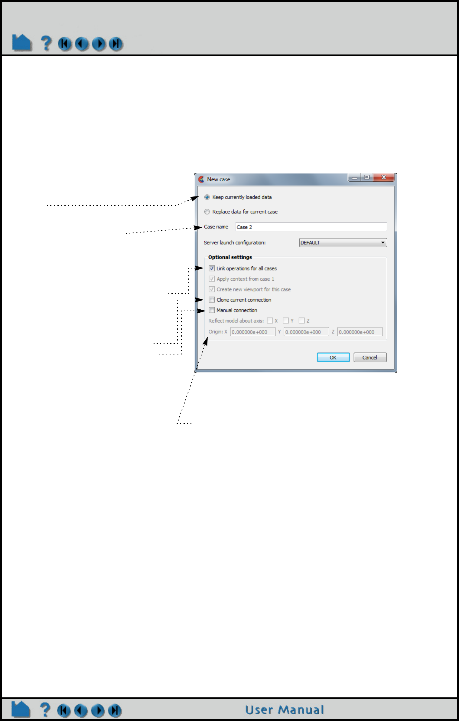
Page 49
HOW TO COMPARE CASES
BASIC OPERATION
Add a Case
To add a case to a running EnSight session. First verify that your datasets all fall within the limitations described
above. Then read in the first dataset in the normal manner. Next, load subsequent linked datasets. Finally do any
calculations, manipulations, part creations etc.
Do File->Open..., or Case->Add...
1. Select Keep currently loaded data
This will add, rather than replace, the
case
2. If desired, enter a name for the case
(other than the default).
The name will be displayed in the Case
menu.
3. Set other optional settings.
Link operations for all cases to compare
this newly added case to the existing one.
Toggle this on. When this is toggled on
other options become unavailable.
Server connection options are still
available with the Link option.
Note: The case linking toggle is only
available on the addition of the second
case. All subsequent cases adopt the
Link setting of the second case. If the Link
toggle is on for the second case, the
dialog will no longer even appear for
subsequent cases.
Grayed out options are no longer necessary if you Link
operations for all cases as they now automatically happen.
4. Click Okay.
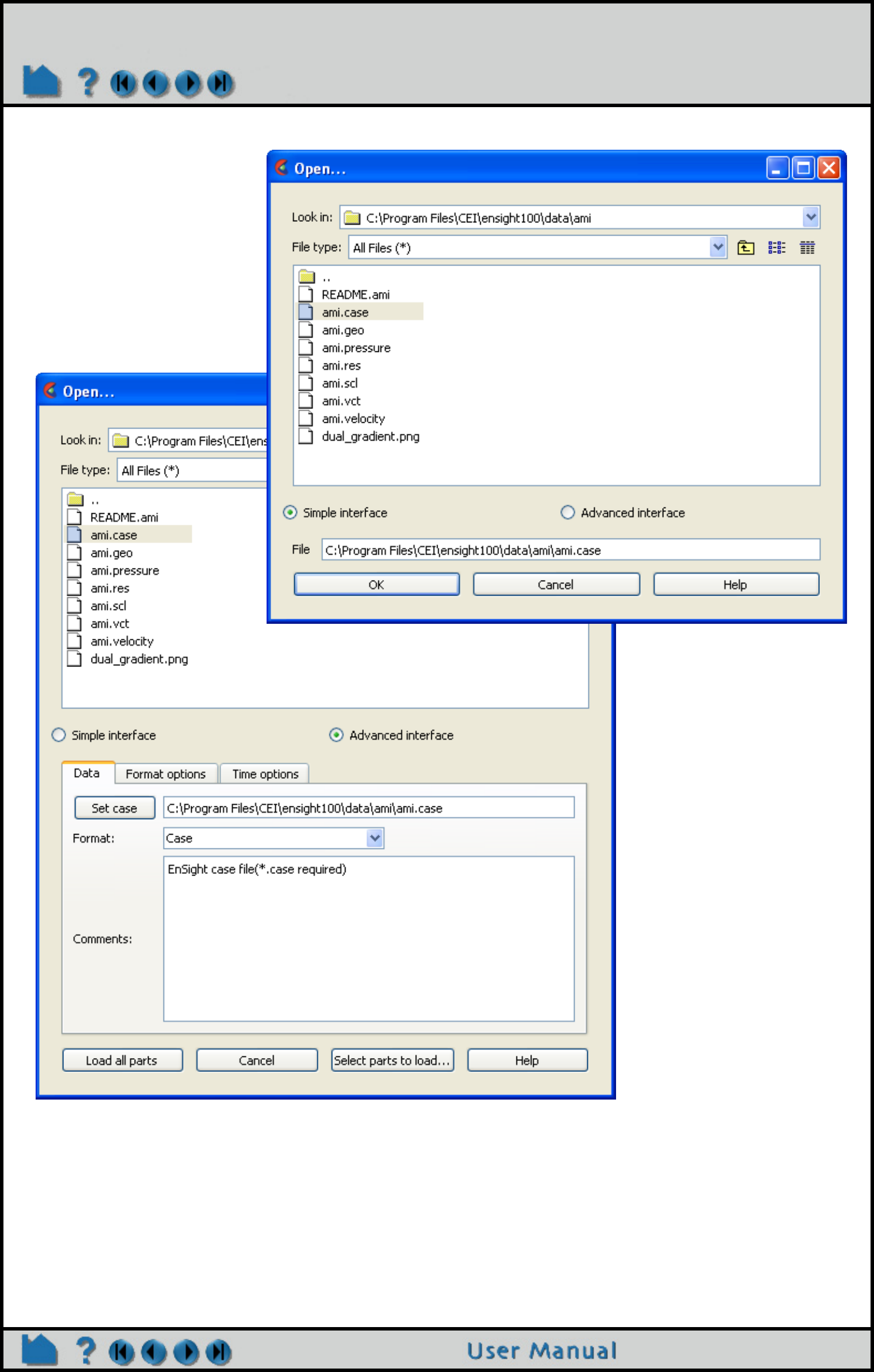
Page 50
HOW TO COMPARE CASES
The EnSight client will now start the connection process for the new server. Depending on the launch or connection
settings chosen, the new server will be started automatically or you will have to manually start another server. The
default is to start a new server automatically if your original connection was automatic, or to cause you to start
another server manually if your original connection was manual. You can follow the progress of the connection in the
Message area. See the EnSight Getting Started Manual or How To Connect EnSight Client and Server for more
information. Once connected, EnSight will also load all parts of this new case if you use this method, and, if the “Link
operations for all cases” toggle is on, a new linked viewport labeled with the case will be created for the data. Load all
of your cases prior to doing calculator functions.
You will then be presented
with the Open... dialog.
Navigate to and select your
data, and use the Simple
interface to load all parts.
(Note that the file type must be
recognized for this method to
work.)
Or, use the Advanced
interface, and control the
Format and other options.
As well as being able to
Select parts to load, etc.
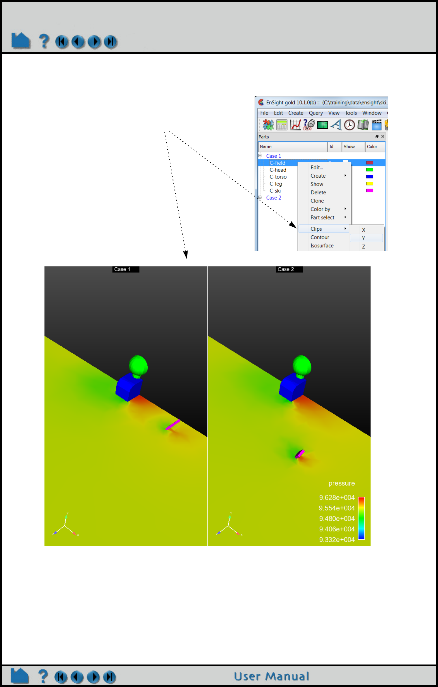
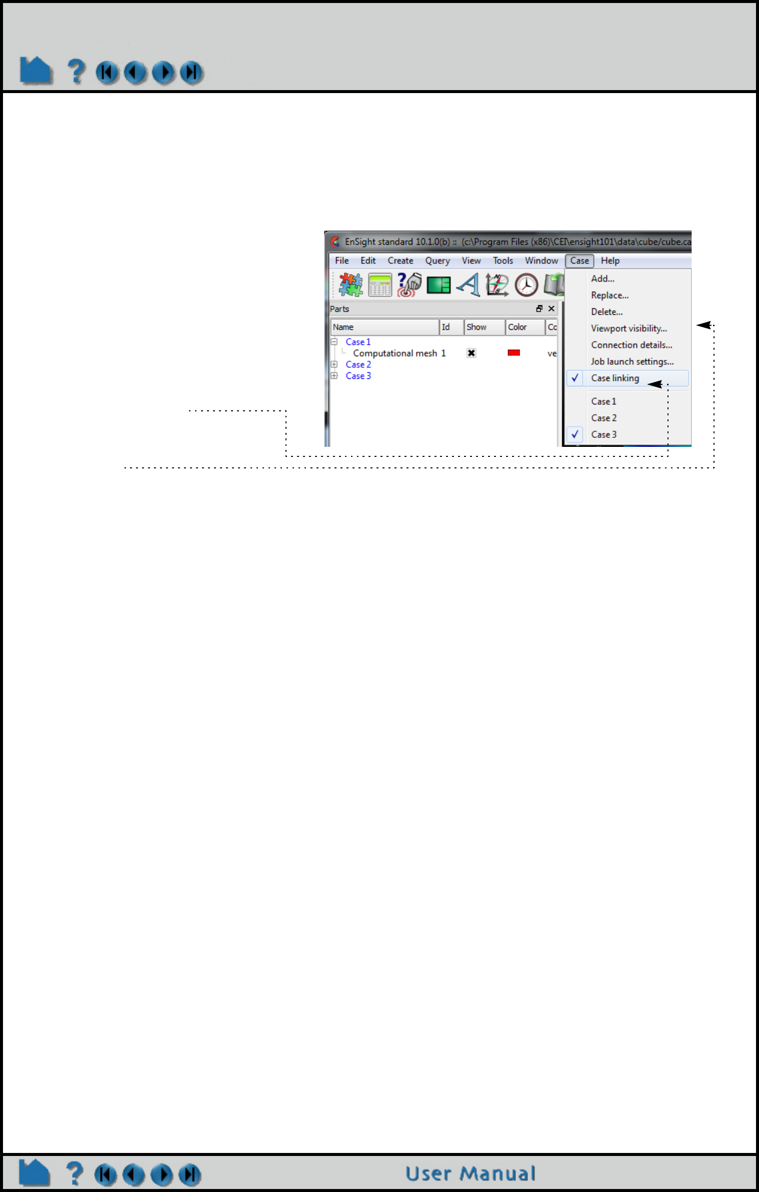
Page 52
HOW TO COMPARE CASES
How to end case linking
Toggle off Case Linking using the top menu entry under Case. Do Case>Case Linking to toggle it off. And once you
turn it off you can continue working with the unlinked cases, but you cannot turn linking back on during the remainder
of the EnSight session.
:
1. When you are finished with the
portion of your analysis
facilitated by Case Linking,
simply toggle off Case>Case
linking and the cases will no
longer be linked.
2. Warning: once you end case
linking you can no longer case
link in this EnSight Session.
3. When Case Linking is turned off
you can now change features in
one viewport and they will no
longer change in the other
viewports. You can calculate
variables in one case that will no
longer be calculated in the other
cases.
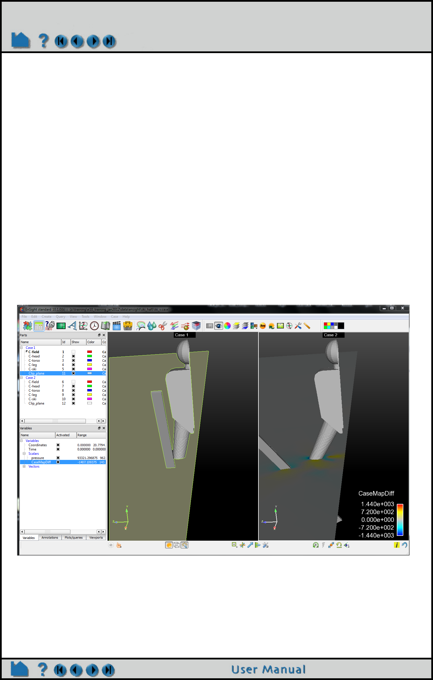
Page 53
HOW TO COMPARE CASES
Case linked Calculations
If you are going to do calculations with multiple cases, it is recommended that you load all the cases first, then do the
calculations.
Calculation of a variable such as vsq = velocity*velocity on a certain part, such as a clip plane, in one of the cases will
cause that same variable to be calculated on the corresponding clip plane in all the other cases when case linking is
on. The variable vsq will show up once in the variable list if it is a vector or scalar as always. If the variable is a
constant such as that returned by the EnSight Flow function then there will be a constant variable for each case in the
variable list calculated on the corresponding cases. Constant variables from cases besides the first, will have the
case number appended to their name (e.g. “flow_02” for the case 2 flow).
To compare a variable across cases, use the new CaseMapDiff calculator function. This will give you a variable that
results from the subtraction of that variable from the CaseMap of that variable from the chosen case. See the
example below for an illustration of using this function to compare the pressure across cases.
Case Mapping Tips
The searching algorithm in CaseMap and CaseMapDiff slows dramatically as the size of the model grows. Consider
starting EnSight with the -hpc (formerly -gold) option if you have an hpc (formerly gold) license, to maximize your use
of Threading. At your first attempt at casemapping, use the faster ‘search only’ (option 0) flag, which will result in an
undefined value if the local search fails, and will not resort to the slower global search used by the ‘nearest value’
search option. When case mapping finishes, check your results by right clicking on the variable and edit the palette
and, under the Options tab in the Palette dialog, change the ‘Display Undefined’ as Invisible. This will remove the
CaseMapDiff Calculator function example:
Select the Field part in Case 2, calculate CaseMapDiff of the
variable pressure from Case 1 using the nearest value. Now
create a Y clip of the field and color by the variable. See that
the CaseDiff variable is zero everywhere at Case 1 and has a
non-zero value of CaseDiff at Case 2 because it equals (Case2
pressure - Case 1 pressure).

Page 54
HOW TO COMPARE CASES
undefined value as a ‘hole’ in your mesh to give you a sense of the number of failures in your case mapping. If you
have holes in your mesh, and if the case map was relatively quick, and the variable that you are mapping is
elemental, then consider creating a nodal variable and rerunning using search option 0 flag. Nodal variables tend to
succeed in the searching algorithm better. Or if you are using a nodal variable and still getting undefined values, try
using ‘nearest value’ (search option 1) flag, which, if the local search fails, will ‘look around’ using a slower, global
search.
You can restrict the search using the ‘parts to map from’ pulldown. If both cases have matching part numbers, use the
‘Part number match’ and the search will be restricted to matching part(s) in the same list position in the Part List. Or I
can use ‘Parts selected for case to map from’ and select the parts in each case to use for searching. Or if I’m mapping
to parts that are all the same dimension (say 2D) then I can select ‘Dimensionality match’ to only use parts in the
‘case to map from’ that are the same dimension as my selected parts. Warning, if you use the default search option
‘Global search’, then EnSight will search the 3D, 2D, 1D, and 0D parts in the ‘case to map from’, which may slow
performance dramatically.
ADVANCED USAGE
A common usage scenario is to load all your cases with case linking turned on, do your common calculations and
perform the operations that case linking takes care of most easily. Then turn it off to complete the post processing.
OTHER NOTES
When calculator functions are executed and then subsequent cases are loaded, this sometimes works, however this
is not recommended. It is recommended that you load all your cases first and then do your calculations so that they
can all occur on the existing cases at once.
SEE ALSO
User Manual: Case Menu Functions
How to Manual: Load Multiple Datasets (Cases)
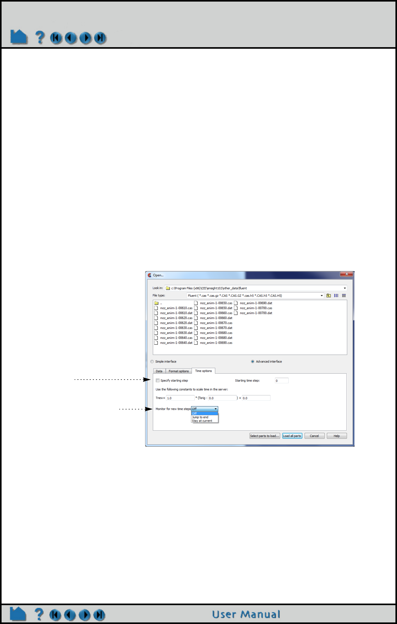
Page 55
HOW TO LOAD TRANSIENT DATA
Load Transient Data
INTRODUCTION
From its inception, EnSight has been used extensively to postprocess time-varying or transient data. In many cases,
dynamic phenomena can only be understood through interactive exploration as a transient case is animated. EnSight
handles all types of transient data. All variables as well as mesh coordinates and connectivity can vary over time. The
rate at which variables (or the mesh) change can differ (supported through the EnSight Gold and EnSight6 Case data
format only).
EnSight can postprocess transient data in many ways. The Player (Solution Time) area lets you easily set the
current time step, step through time (manually or automatically), or restrict the range of time to a region of interest.
You can perform query operations to extract information over time. You can use the flipbook capability to create an
on-screen animation of your data changing over time and continue to interact with it during animation playback.
EnSight’s keyframe animation capability can be used to create high-quality video animations of transient data.
This article covers reading transient data into EnSight.
BASIC OPERATION
Reading transient data into EnSight is essentially the same as reading static data (see How To Read Data for more
information). By default, the last time step will become the current time step. This behavior is based on the
assumption that the last step will contain the largest dynamic range of the variable data so that variable palettes will
be initialized properly.
For many data formats, some type of “results” file supplies the necessary time information, including number of
steps, actual solution time at each step, and how to access the dynamic variable and geometry files. However, some
formats supported by EnSight include this information in the same file that contains other geometry or variable data.
EnSight 6 and EnSight Gold formats have a casefile which contains solution time information and how this is tied to
each variable and the geometry. The manner for each format can vary widely enough that we refer you to User
Manual 2.1 Reader Basics, User Manual 2.1 Native EnSight Format Readers, and User Manual 2.1 Other
Readers
However, you can override this
by clicking the Specify Starting
step toggle and entering the
desired time step under the
Time options tab in the File >
Open dialog.
Note, for some data formats,
you can also monitor the
dataset for new timesteps as
described in User Manual 5.1
Solution Time.
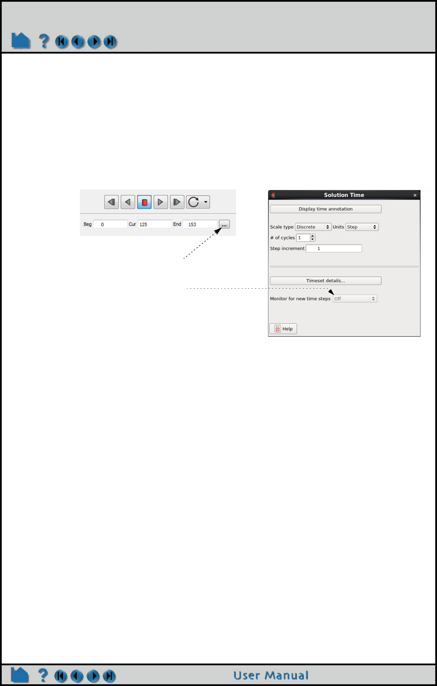
Page 56
HOW TO LOAD TRANSIENT DATA
ADVANCED
If you wish to read transient data that is being updated (that is, perhaps the solver is in the process of writing the data
and you are looking at it as the solution proceeds: coprocessing) then you will need to get your solver to write out the
maximum number of steps keyword if the data is PLOT3D Results File Format or EnSight Gold Casefile Format.
Or, if you are using another format and have a custom user-defined reader, then you will need to add a routine called
USERD_get_max_time_steps that cues the EnSight Server that the number of time steps can be updated (and pro-
vides a maximum never-to-exceed number of time steps that can be loaded). Currently the EXODUS II Reader has
this capability.
The user chooses the action which will occur when a new timestep becomes available. Either the timestep will
automatically update to the last timestep available or you can stay at the current timestep. For the latter, the End time
value for the solution time dialog will update to reflect the new timestep availability, but the time will not be modified.
SEE ALSO
How To Change Time Steps, How To Animate Transient Data, How To Query/Plot
User Manual: Flipbook Animation, Query/Plotter
Click on the advanced button to pop up the
“Solution time” dialog. If the current dataset is set
for timestep monitoring, the pulldown options for
Monitor for new time steps will be available.
Click this pulldown to decide what action will be
taken when new timesteps are available.
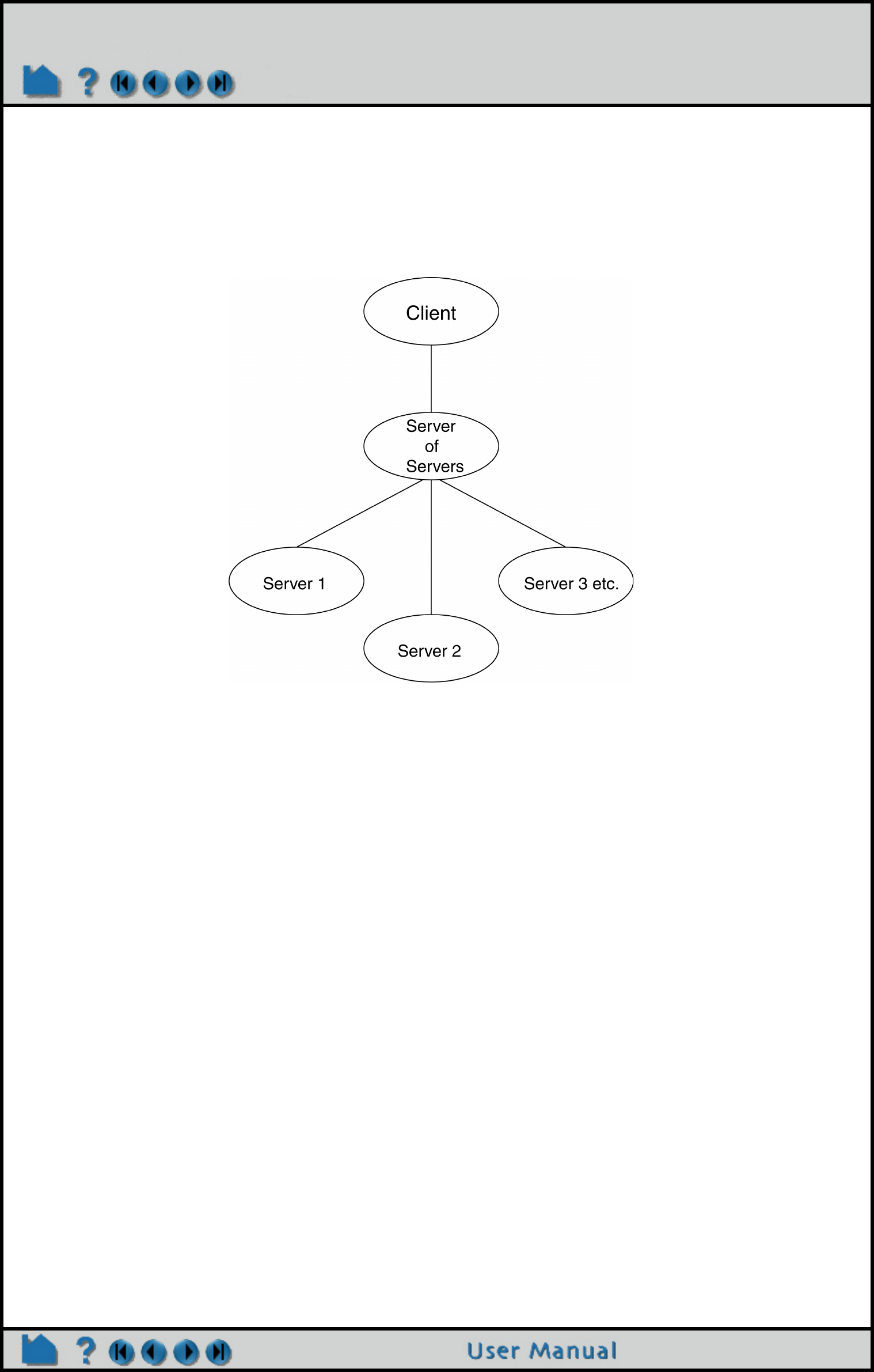
Page 57
HOW TO USE SERVER OF SERVERS
Use Server of Servers
INTRODUCTION
EnSight102, using an hpc (formerly gold) license key has the capability of dealing with spatially partitioned data or
temporally decomposition in an efficient distributed manner by utilizing what we call a server-of-servers (SOS for
short). An SOS server resides between a normal client and a number of normal servers. Thus, it appears as a normal
server to the client, and as a normal client to the various normal servers.
When reading spatially decomposed data (or when the decomposition is done on the fly), each server is responsible
for only a portion of the geometry for all time. This is useful, for example, when the entire geometry for a single
timestep simply cannot fit into one server on one machine. When the data is temporally decomposed, each server is
responsible for all of the geometry but only at one timestep. This is useful, for example, when the entire geometry at
one timestep fits on one server, and the user desires to precache (read ahead) to other timesteps to speed up time
changes.
This arrangement allows for distributed parallel processing of the various portions of a model or different portions of
time, and has been shown to scale quite well.
Currently, EnSight SOS spatially decomposed capability is only available for EnSight5, EnSight6, EnSight Gold,
Plot3d, and some EnSight User-Defined Reader data formats. All data formats permit temporal decomposition.
For spatial decomposition, please recognize that your data must be spatially partitioned in some manner (hopefully in
a way that will be reasonably load-balanced) in order for this approach to be useful. This partitioning can be done
externally, be done by a reader internally, or be auto_distributed by the EnSight servers. Each of these options for
spatial decomposition will now be discussed, because they have limitations. Temporal decomposition will be
discussed at the very end of this document.
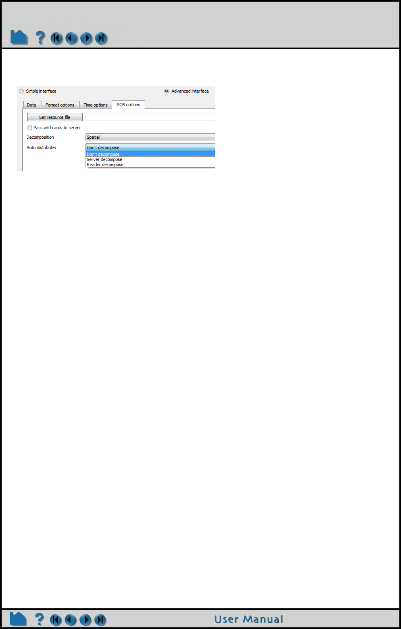
Page 58
HOW TO USE SERVER OF SERVERS
SPATIAL PARTITIONING OF DATA DONE OUTSIDE ENSIGHT
Choose “Don’t decompose” in the SOS options tab if the data is already partioned outiside of EnSight and you don’t
want EnSight to do the decomposition. This option requires that each portion of the model be prepared as a stand-
alone partitioned dataset, that can be read as such by an EnSight server. For example, if it were EnSight gold format,
there will be a casefile (.case) and associated gold geometry and variable results file(s) for each partitioned dataset.
There will also need to be an SOS casefile (.sos), which is a simple ascii file which informs the SOS about pertinent
information needed to run a server on each of the machines that will compute the various portions and what case file
partition it is to read. The SOS will read the sos casefile (.sos), and each server will read one of these pre-partitioned
(.case) datasets. The SOS will conglomerate geometry together so that the client sees the whole model. The EnSight
formats, PLOT3D, and any user-defined readers using our 1.0 or 2.0 APIs can be used
The advantage of external partitioning is that once the data has been partitioned once, the partitioning is done.
EnSight’s SOS and servers can then operate without expending any effort on partitioning. The disadvantage is that it
is not easily changed. Some formats require that the number of servers be the same as the number of partitioned
datasets. However, for EnSight Gold format, EnSight now has the capability of running more than one of these
datasets on a given server - so it is possible to run the model on fewer servers than the number of partitioned
datasets. And the number of those servers is easily changed. See How To Load Spatially Decomposed Case
Files.
Data can be partitioned prior to reading in EnSight, for example, by a solver, or by an external partitioning utility as
described below.
Partitioning with a Solver, or Self-Partitioning
Note: If you do your own partitioning, please be aware that, as of EnSight 10.2, each dataset is no longer required to
have all parts present in all of the partitioned data files. EnSight now uses the part name as the unique identifier, so, if
the part is present in the dataset, it must be consistently named everywhere: in all partitioned datasets over all
timesteps. Thus one can fairly easily partition as desired, whether that be with decomposed parts across several
datasets, or with parts empty (or even nonexistent) in all but one of the datasets, etc. Note that in EnSight Case Gold
format, an empty part need only have the “part” line, the part number, and a consistent “description” line (or, now, it
can be left out altogether).
EnSight’s Partition102 Utility
Included in the EnSight distribution is a command-line Partition Utility that will take EnSight Case Gold multi-file
format, C-binary unstructured datasets and partition them for you using geometric partitioning (thick slicing the
geometry along it’s longest edge into chunks). This utility will work for static, changing coordinate or changing
geometry datasets. It will not work for ascii files, for single file format, measured/particle data, or datasets with
multiple timesets (i.e. all variables must be on same timeset). It will also not work for structured data (which must be
server decomposed, see below).
Simply type partition102 at the command prompt to begin. This command line program will prompt you for the
name of the input case file and the number of partitions in the x, y, and z and whether or not to use ghost elements,
etc. and will create (in a directory of your choosing) a case sos file (.sos) pointing to the partitioned case files ready
for loading into EnSight server of server mode.
You should place each partitioned portion of the model on the machine that will compute that portion. On the machine
where the EnSight SOS will be run, you will need to place the sos casefile. If you move the case files around to
different locations and/or different machines, you will need to edit the sos file (.sos) to properly indicate the machines
and directories where the case files are located. Once you load the data into EnSight Server of Server mode,
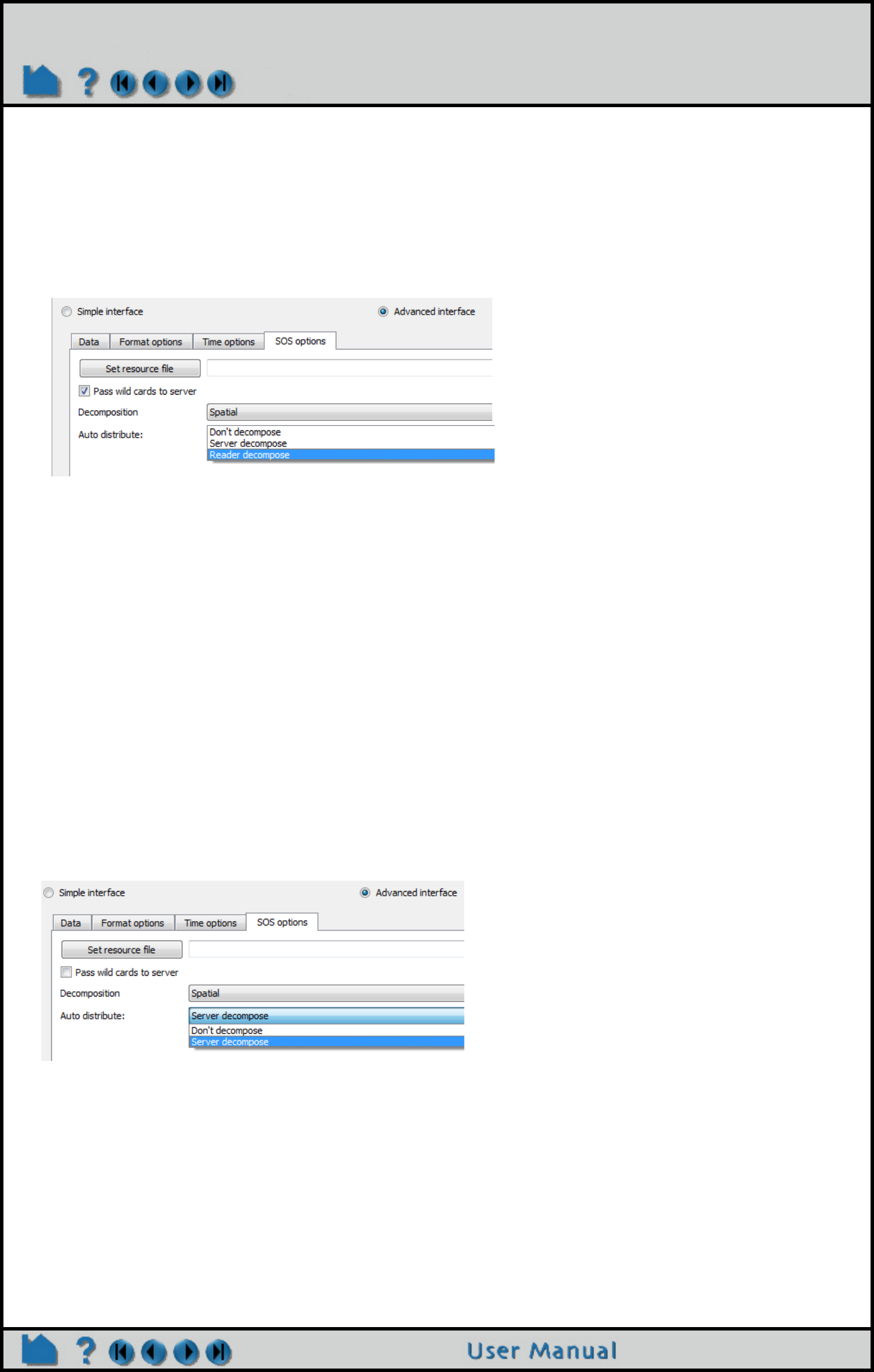
Page 59
HOW TO USE SERVER OF SERVERS
calculate the variable ServerNumber in the EnSight calculator and color your geometry by this variable to visualize
the spatial distribution chosen by the partition utility. The partition utility simply takes the bounding box of the data and
divides it into a grid according to the number of partitions in the x, y, and z-directions so works best on data that is
cubic in shape.
SPATIAL PARTITIONING DONE BY A READER, “READER DECOMPOSE”
If the “Reader decompose” option is available, then the reader for your chosen format is SOS aware. You would
choose “Reader decompose” in the SOS options tab to read the data in partitions on each server. If this option is
available, then you will usually choose it because the reader knows how to best decompose the data. This method
requires that the reader be based on our 2.0 or later User-defined reader API, which is “server-aware”, and that it
does its own determination of what data goes to each server. Some “multiblock” formats for example, can easily
distribute certain blocks to certain servers. And they can do so based on the number of servers that are being used at
the time. There is still the requirement that each server be informed of the same number of total parts. But the reader
can return different portions of a given part based on which server is querying. And yes, a given part can be empty for
some servers.
This type of partitioning reader has the advantage of being adaptable to the number of servers used. It does require
the development of such a reader. Examples of that allow reader decompose are as follows: CGNS-XML, CTH,
xdmf2, Exodus, Flow3d, Silo and VTK readers. In the data reader dialog (File>Open...) under the SOS options tab,
are the SoS options for the selected data reader. One option is to pass wildcards to the server, for example if the data
file refers to a set of files (file*.vtm).
PARTITIONING DONE BY ENSIGHT SERVERS, “SERVER DECOMPOSE”
If your data is not already decomposed nor is the Reader decompose option available, then EnSight has the final
option of using the EnSight server to decompose (also called auto-distribute, since the EnSight server automatically
does the distribution). Some formats/readers allow for an spatial auto-distribute capability that occurs within each
server. Pre-partitioning is not required. Each server will determine its portion using a connectivity-based partitioning
algorithm (selecting N elements in the connectivity order), and will read and act just on that portion. Note that this
connectivity based algorithm is different than the partition utility described above.
Currently this capability is available to Plot3d and EnSight Case gold format.
It can be implement in User-defined readers (at level 2.08 or greater), which have implemented the “*_in_buffers”
routines.

Page 60
HOW TO USE SERVER OF SERVERS
So, since none of the user-defined readers distributed by EnSight have currently implemented the needed *_in_buffer
routines or structured reader cinching capability to take advantage of this option, only the internal EnSight Gold and
Plot3d readers can be used with Server decompose (auto_distribute). However if you have on-site user defined
readers, these may include this capability.
Use of SOS with our native, Case Gold format can use an ASCII SOS Casefile which is a map for how data is to be
distributed to the Servers using auto-distribute.
FORMAT OF THE SOS CASEFILE:
The format for this file is as follows: (Note that [ ] indicates optional information, and a blank line or a line with # in the
first column are comments.)
FORMAT (Required)
type: master_server datatype (Required)
where: datatype is required and is one of the formats of EnSight’s internal readers (which
use the Part builder), namely:
gold ensight6 ensight5 plot3d
or it can be the string used to name any of the user-defined readers.
Note: For user-defined readers, the string must be exactly that which is defined in the
USERD_get_name_of_reader routine of the reader (which is what is presented in the Format
pulldown of the Data Reader dialog).
If datatype is blank, it will default to EnSight6 data type.
[auto_distribute: on/off] (Optional for structured or unstructured data)
EnSight server will automatically distribute data to the servers (also called Server decompose)
specified below if this option is present and set to “on”. This will require that each of the servers
have access to the same data (or identical copies of it). For structured data: use only if the
datatype is gold, plot3d or a 2.06 or greater user-defined reader (which has implemented
structured cinching). For unstructured data: use only if the datatype is gold, or a 2.08 (or
greater) user-defined reader. Additionally, be aware that 2.* user-defined readers should
implement the special functions defined in README_USERD_IN_BUFFERS file if memory is to
be used efficiently in the unstructured auto-distribute process.
[use_resources: on/off] (Optional, to allow specification of server machines to come from the “resource file”)
[do_ghosts: on/off] (Optional for unstructured auto_distribute - default is on (before version 10.1.4(a)),
and is off for later versions)
Allows user to control whether ghost cells will be produced between the distributed portions.
Please note that this could alternatively be set with the -use_ghosts command line argument, or
by setting the UNSTRUCT_AUTODISTRIBUTE_USE_GHOSTS environment variable to 1.
[buffer_size: n](Optional for unstructured auto_distribute and do_ghosts - default is 100000)
Allows user to modify the default buffer size that is used when reading node and element
information of the model when producing ghost cells.
[want_metric: on/off](Optional for unstructured auto_distribute and do_ghosts - default is on (before version
10.1.4(a), and is off for later versions.)
If set on, a simple metric will be printed in the shell window that can indicate the quality of the
auto_. The unstructured auto_distribute method relies on some coherence in the element
connectivity - namely, that elements that lie next to each other are generally listed close to each
other in the data format.
The metric is simply the (#total_nodes / #nodes_needed_if_no_ghosts).
When no ghosts, the value will be 1.0. The more ghosts you must have, the higher this metric
will be. If the number gets much more than 2.0, you may want to consider partitioning yourself.
Please note that this could alternatively be set with the -use_metric command line argument, or
by setting the UNSTRUCT_AUTODISTRIBUTE_USE_METRIC environment variable to 1.
NETWORK_INTERFACES (Note: This whole section is optional. It is needed only when more than one network
interface to the sos host is available and it is desired to use them. Thus, distributing the servers
to sos communication over more than one network interface)
number of network interfaces: num(Required - if section used)
where: num is the number of network interfaces to be used for the sos host.
network interface: sos_network_interface_name_1(Required - if section used)

Page 61
HOW TO USE SERVER OF SERVERS
network interface: sos_network_interface_name_2(Required - if section used)
.
.
network interface: sos_network_interface_name_num(Required - if section used)
SERVERS (Required)
number of servers: num [repeat](Required)
where: num is the number of servers that will be started and run concurrently.
repeat indicates that the first server specification should be repeated num times for use
with resources. Other server specifications will be ignored.
#Server 1 (Comment only)
machine id: mid (Required)
where: mid is the machine id of the server.
executable: /.../ensight92.server(Linux/Unix/Apple Required, must use full path)
or ensight92_server.bat (Windows only Required, must use .bat extension)
[directory: wd](Optional)
where: wd is the working directory from which ensight92.server will be run
[login id: id](Optional)
where: id is the login id. Only needed if it is different on this machine.
[data_path: /.../dd](Optional)
where: dd is the directory where the data resides. (Full path must be provided if you use this).
casefile: yourfile.case (Required, but depending on format, may vary as to whether it is a casefile, geometry file,
neutral file, universal file, etc. Relates to the first data field of the Data Reader Dialog.)
[resfile: yourfile.res](Depends on format as to whether required or not. Relates to the second data field of the Data
Reader Dialog.)
[measfile: yourfile.mea](Depends on format as to whether required or not. Relates to the third data field of the Data
Reader Dialog.)
[bndfile: yourfile.bnd](Depends on format as to whether required or not. Relates to the fourth data field of the Data
Reader Dialog.)
--- Repeat pertinent lines for as many servers as declared to be in this file ---
BASIC OPERATION
To use Server of Servers, depending on the method of spatial partitioning (Externally partitioned, Reader partitioned,
or Server partitioned) described above, you do the following:
External partitioning
1. Partition your data, and distribute it (or make it available) to the various machines on which you will run servers.
2. Create the sos casefile, which defines the data format to use, the server machines, the location of server
executables on those machines, and the name and location of the [partitioned] data for the servers. Each server in
the casefile will reference different data. Examples will be shown below.
3. Run EnSight with the -sos command line option(or use ensight102.sos in place of ensight102.server if connecting
manually) and provide it with the sos casefile. You can run EnSight like:
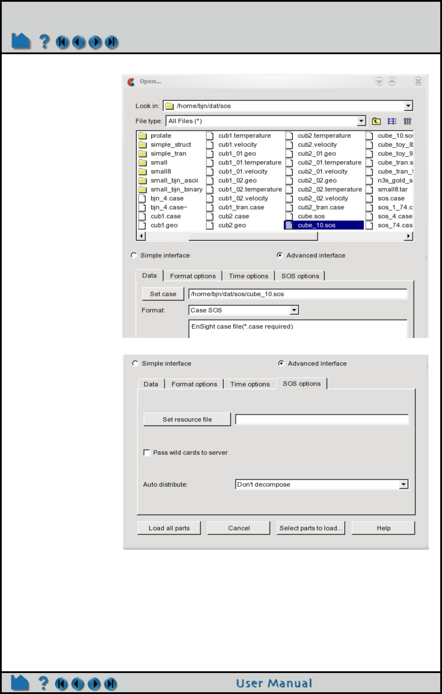
Page 62
HOW TO USE SERVER OF SERVERS
ensight102 -sos
Using the command in this way runs the SOS on the same machine as the client. If you want to control where the
SOS runs, connect manually instead (a manual example will be shown later in this article). Also note that if you want
to load all parts, you could have simply included the sos casefile on the command line, like:
ensight102 -sos /home/bjn/dat/sos/cube_10.sos
Additionally, you can use resources in combination with a sos casefile if desired. See How To Use Resource
Management for an example.
Spatial partitioning done by a reader, “Auto distribute Reader decompose”
If you use a reader that can do its own partitioning, you can use an sos casefile in which each server references the
Then under File->Open,
set the sos casefile under
the data tab, with a format
of Case SOS.
Under the SOS options tab,
you can verify that Auto
distribute is set to Don’t
decompose (because the
data is already
decomposed).
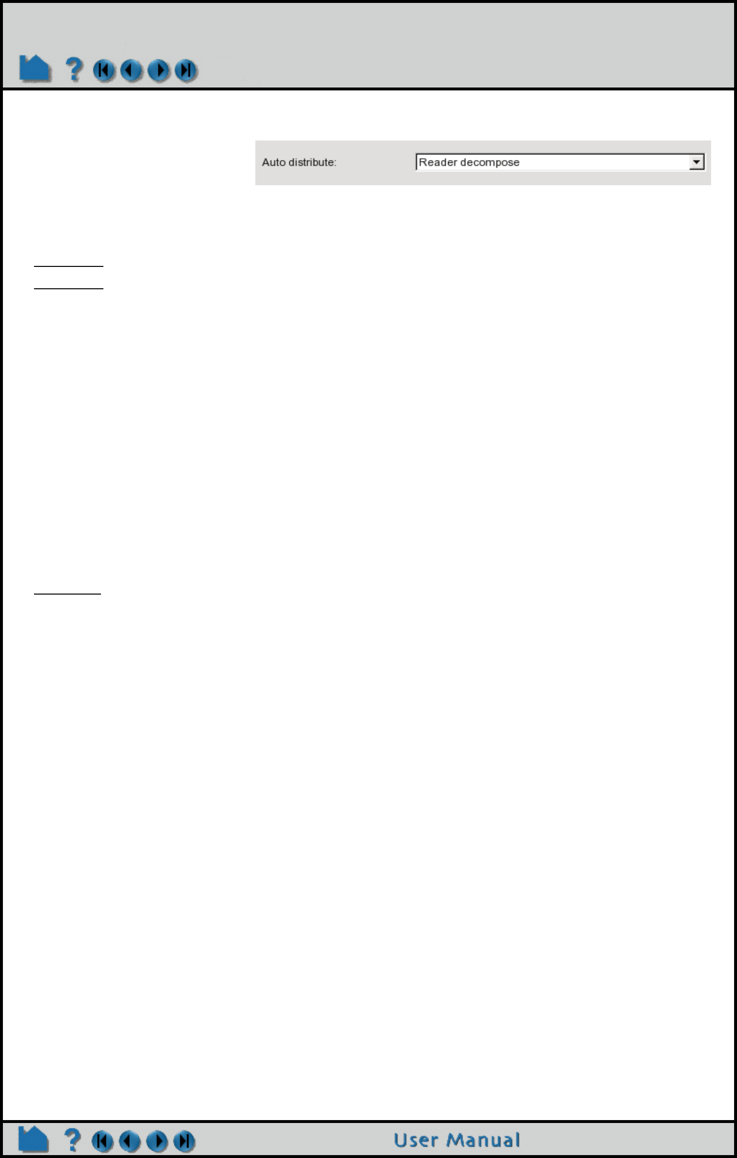
Page 63
HOW TO USE SERVER OF SERVERS
same data, OR take advantage of a resource file and not have to create an sos casefile. Note that for this method,
under the SOS options tab in the File->Open dialog, you will see that Auto distribute is set to Reader Decompose.
It is probably easiest to describe the usage based on an example. So using the Exodus reader, lets run an Exodus
model on two servers (computer1 and computer2), first using the .sos case file and then the .res file (you don’t use
them both at the same time). The files we will reference are:
sample.exo (the Exodus data file)
servers.sos (the SOS casefile)
FORMAT
type: master_server MultiExodusII
SERVERS
number of servers: 2
#Server 1
#------------
machine id: computer1
executable: ensight102.server
data_path: /home/user/exodus
casefile: sample.exo
#Server 2
#------------
machine id: computer2
executable: ensight102.server
data_path: /home/user/exodus
casefile: sample.exo
servers.res (the resource file, see How To Use Resource Management for more details)
#!CEIResourceFile 1.0
SOS:
host: localhost
SERVER:
host: computer1
host: computer2
Flow3D SOS Case file example which uses two computers (computer1 and computer2), and 4 servers, with 4 files
(flsgrf1.dat, flsgrf2.dat, flsgrf3.dat and flsgrf4.dat) located on a common file system that both computers can read: /
scratch/data/lowres and perhaps name it servers.sos. It will also be necessary that the machine where you start up
your server of server has the Flow3d reader (must be either a linux or windows machine) and it is able to start up
servers using passwordless ssh.
FORMAT
type: master_server Flow3D-Multiblock
SERVERS
number of servers: 4
#Server 1
#------------
machine id: computer1
# for same machine use
#machine id: localhost
executable: ensight102.server
# for windows use
#executable: ensight102_server
data_path: /scratch/data/lowres/
casefile: flsgrf*.dat
#Server 2
#------------
machine id: computer1
Page 64
HOW TO USE SERVER OF SERVERS
executable: ensight102.server
data_path: /scratch/data/lowres/
casefile: flsgrf*.dat
#Server 3
#------------
machine id: computer2
executable: ensight102.server
data_path: /scratch/data/lowres/
casefile: flsgrf*.dat
#Server 4
#------------
machine id: computer2
executable: ensight102.server
data_path: /scratch/data/lowres/
casefile: flsgrf*.dat
Your servers.res file will be the same as above except it will have four servers, and perhaps named four_servers.res.
#!CEIResourceFile 1.0
SOS:
host: localhost
SERVER:
host: computer1
host: computer1
host: computer2
host: computer2
1. For the exodus example above, make sure your sample.exo data file is available to the various computers on
which you will run servers. For the Flow3d example above, make sure all four flsgrf*.dat files are in the same
directory and available to all the computers.
2. Create the sos casefile, Or the resource file appropriate for your format above (use one or the other). You can
copy/paste from the examples above.
3. Run EnSight using one of the following (not both):
ensight102 -sos
Then set the servers.sos file in the File->Open dialog (format Case SOS). This will let you load all parts, or
select the ones to be loaded. Or use ensight102 -sos servers.sos on the command line if you want to load all
parts.
-- OR if you want to use the resource (.res) file --
Choose the sample.exo file or the flsgrf*.dat in the File->Open dialog (format MultExodusII, format Flow3d-
Multiblock respectively), and place the appropriate .res file in the Set resource file field under the SOS options
tab. For Flow3d data, toggle ON the Pass wild cards to server option, which will allow the asterisk in flsgrf*.dat
to pass down to the servers to handle appropriately. This will let you then load all parts, or select the ones to be
loaded. Or use ensight102 -sos -res servers.res on the command line and set sample.exo (or flsgrf*.dat) file
in the File->Open dialog (format MultExodusII, Flow3D-Multiblock, respectively). Or, for exodus format, use
ensight102 -sos -res servers.res sample.exo on the command line if you want to load all parts. You cannot
use the command line for Flow3D format because you must tell EnSight to pass the asterisk to the servers and
this appears to only work from the dialog.
There are several other variations that could be used, including the use of a manual connection with the SOS. They
all have similar corresponding options.
Spatial partitioning by EnSight Servers “Auto_distribute, e.g. Server decompose”
If you use EnSight Gold, Plot3d, or a User-defined reader that is capable (as described above), you can let EnSight
do the partitioning. You can use an sos casefile in which each server references the same data, or take advantage of
a resource file and not have to create an sos casefile. Note that for this method, under the SOS options tab in the
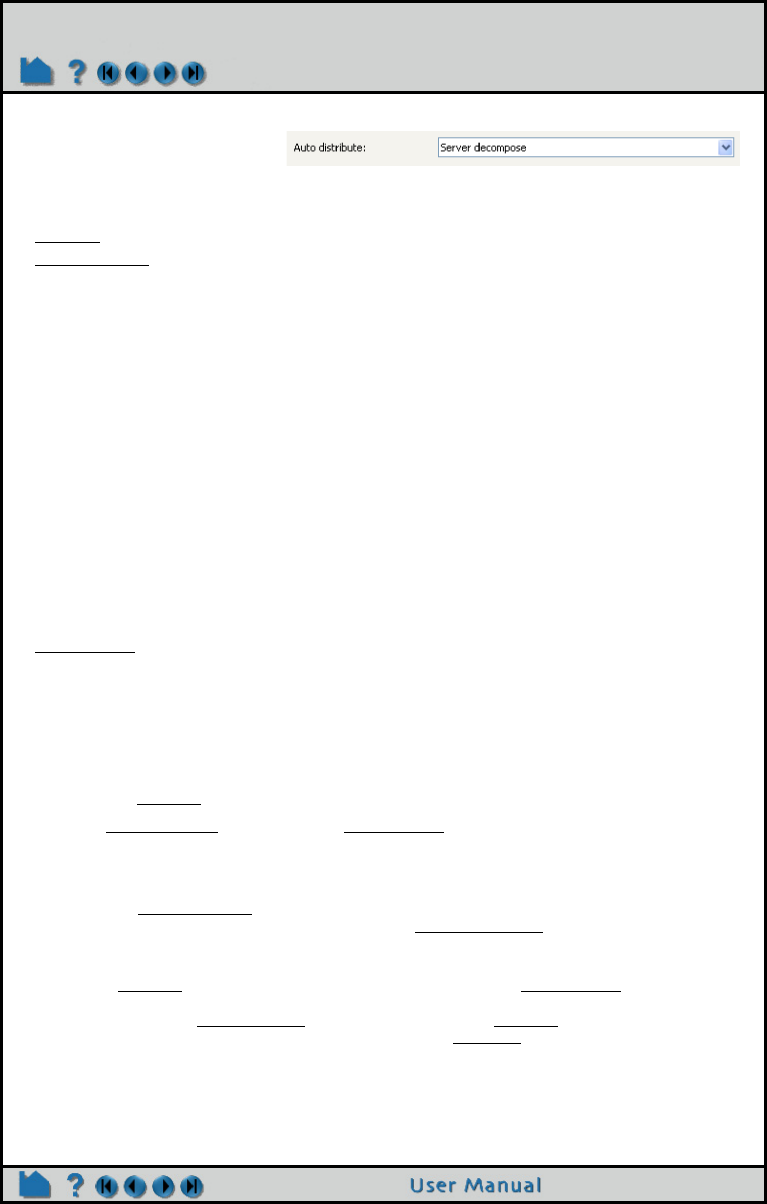
Page 65
HOW TO USE SERVER OF SERVERS
File->Open dialog, you will see that Auto distribute is set to Server Decompose.
It is probably easiest to describe the usage based on an example. So using the EnSight Gold format, lets run a simple
model on two servers (computer1 and computer2). The files we will reference are:
cube.case (the EnSight Gold data file)
two_partitions.sos (the SOS casefile)
FORMAT
type: master_server gold
auto_distribute: on
do_ghosts: on
SERVERS
number of servers: 2
#Server 1
#------------
machine id: computer1
executable: ensight102.server
data_path: /home/user/exodus
casefile: cube.case
#Server 2
#------------
machine id: computer1
executable: ensight102.server
data_path: /home/user/exodus
casefile: cube.case
two_servers.res (the resource file, see How To Use Resource Management for more details)
#!CEIResourceFile 1.0
SOS:
host: localhost
SERVER:
host: computer1
host: computer2
1. Make sure your cube.case data is available to the various machines on which you will run servers.
2. Create the two_partitions.sos sos casefile, or the two_servers.res resource file
3. Run EnSight like:
ensight102 -sos
Then set the two_partitions.sos file in the File->Open dialog (format Case SOS). This will let you load all parts,
or select the ones to be loaded. Or use ensight102 -sos two_partitions.sos on the command line if you want
to load all parts.
-- or --
Open the cube.case file in the File->Open dialog (format Case), and place two_servers.res in the Set resource
file field under the SOS options tab. This will let you then load all parts, or select the ones to be loaded. Or use
ensight102 -sos -res two_servers.res on the command line and set cube.case file in the File->Open dialog
(format Case). Or use ensight102 -sos -res two_servers.res cube.case on the command line if you want to
load all parts.
There are several other variations that could be used, including the use of a manual connection with the SOS. They
all have similar corresponding options.
Page 66
HOW TO USE SERVER OF SERVERS
Example SOS Casefile
This example deals with a EnSight Gold dataset that has been partitioned into 3 portions, each running on a different
machine. The machines are named joe, sally, and bill. The data is not in the same location on all machines. Note that
the optional data_path line is used on two of the servers, but not the third.
FORMAT
type: master_server gold
SERVERS
number of servers: 3
#Server 1
machine id: joe
executable: ensight102.server
data_path: /usr/people/john/data
casefile: portion_1.case
#Server 2 is a Windows machine (notice .bat extension)
machine id: sally
executable: ensight102_server.bat
data_path: D:\john\data
casefile: portion_2.case
#Server 3
machine id: bill
executable: ensight102.server
casefile: /scratch/temp/john/portion_3.case
If we name this example sos casefile - “all.sos”, and we run it on yet another machine - one named george, you would
want the data distributed as follows:
On george: all.sos
On joe (in /usr/people/john/data): portion_1.case, and all files referenced by it.
On sally (in /scratch/sally/john/data): portion_2.case, and all files referenced by it.
On bill (in /scratch/temp/john): portion_3.case, and all file referenced by it.
By starting EnSight with the -sos command line option (which will autoconnect using ensight102.sos instead of
ensight102.server), or by manually running ensight102.sos in place of ensight102.server, and providing all.sos as the
casefile to read in the Data Reader dialog - EnSight will actually start three servers and compute the respective
portions on them in parallel.
So, one could do the following (after preparing the all.sos file):
On “george”, run the client and the sos by invoking the ensight102 script in a shell window (non-windows) or
Command Prompt window (windows), like:
george>> ensight102 -sos
Or one could run the client on the “myclient” machine, telnet (or equivalent) into the “george” machine and run the sos
there, by using the following commands:
:
If “myclient” is a non-windows machine:
In a window on “myclient”: In a window that is telneted into the “george” machine:
myclient>> ensight102.client -cm If “george: is a non-windows machine:
george>> ensight102.sos -c myclient
If “george is a windows machine:
george>> ensight102_sos -c myclient
If “myclient” is a windows machine:
In a Command Prompt window on “myclient”: In a Command Prompt window that is telneted into the
“george” machine:
myclient>> ensight102_client -cm If “george: is a non-windows machine:
george>> ensight102.sos -c myclient

Page 67
HOW TO USE SERVER OF SERVERS
In either case, you would enter the all.sos command as the file to read in the Data Reader dialog once EnSight is up
and connected. And the servers on “joe”, “sally”, and “bill” would be started and used automatically.
ENVIRONMENT Variables
The following Environment variables will directly affect the SOS performance, see How To Setup for Parallel
Computation.
ENSIGHT10_MAX_THREADS
ENSIGHT10_MAX_SOSTHREADS
Additionally, rather than specifying whether unstructured ghost processing and metric calculations will be done in an
sos casefile, you can specify this via command-line argument (-use_ghosts and -use_metric), or via the following
environment variables. Remember that the ghost processing and metric calculation is defaulted off.
UNSTRUCT_AUTODISTRIBUTE_USE GHOSTS 1 will set ghost processing on.
UNSTRUCT_AUTODISTRIBUTE_USE_METRIC 1 will set metric on.
The environment variable settings will take precedence over the command line arguments.
Optional NETWORK_INTERFACES section notes
If the machine named george had more than one network interface (say it had its main one named george, but also
had one named george2), we could add the section shown below to our casefile example:
NETWORK_INTERFACES
number of network interfaces: 2
network interface: george
network interface: george2
This would cause machine joe to connect back to george, machine sally to connect back to george2, and machine bill
to connect back to george. This is because the sos will cycle through its available network interfaces as it connects
the servers. Remember that this is an optional section, and most users will probably not use it. Also, the contents of
this section will be ignored if the -soshostname command line option is used.
Example SOS Casefile for PLOT3D, Using structured auto_distribute
This example shows a plot3d dataset (post.x and post.q) that has not been partitioned, but is on an nfs mounted disk
available to each server machine. EnSight will distribute the data to the 3 servers defined. IO will not necessarily be
great since each server will be reading from the same file, but execution will be enhanced by the partitioning. We will
use the same machines used in the previous example.
FORMAT
type: master_server plot3d
auto_distribute: on
SERVERS
number of servers: 3
#Server 1
machine id: joe
executable: ensight102.server
data_path: /scratch/data
casefile: post.x
resfile: post.q
#Server 2
machine id: sally
executable: ensight102.server
data_path: /scratch/data
casefile: post.x
resfile: post.q
#Server 3
If “george is a windows machine:
george>> ensight102_sos -c myclient
Page 68
HOW TO USE SERVER OF SERVERS
machine id: bill
executable: ensight102.server
data_path: /scratch/data
casefile: post.x
resfile: post.q
Example SOS Casefile for EnSight Gold, Using unstructured auto_distribute
This example shows an EnSight Gold dataset (trial.case) that has not been partitioned, but is on an nfs mounted disk
available to each server machine. EnSight will distribute the data to the 3 servers defined. IO will not necessarily be
great since each server will be reading from the same file, but execution will be enhanced by the partitioning. We will
use the same machines used in the previous examples.
FORMAT
type: master_server gold
auto_distribute: on
do_ghosts: on
buffer_size: 10000
want_metric: on
SERVERS
number of servers: 3
#Server 1
machine id: joe
executable: ensight102.server
data_path: /scratch/data/gold
casefile: trial.case
#Server 2
machine id: sally
executable: ensight102.server
data_path: /scratch/data/gold
casefile: trial.case
#Server 3
machine id: bill
executable: ensight102.server
data_path: /scratch/data/gold
casefile: trial.case
Special Case:
If using auto_distribute (and thus each server will be accessing the same data files), and the servers will all be run on
the same machine, then one can add the word “repeat” to the end of the “number of servers: num” line and then only
define one set of Server info. For example:
FORMAT
type: master_server gold
auto_distribute: on
SERVERS
number of servers: 3 repeat
#Server 1
machine id: joe
executable: ensight102.server
data_path: /scratch/data/gold
casefile: trial.case
Structured Auto Distribute Note:
If using structured auto_distribute, the default decomposition scheme is to do so in the i, j, or k direction that has the
largest dimension. This may not always be the best direction for a given analysis. Thus, through the use of an
environment variable, the user can set the axis to use. The chosen axis will be used unless the dimension in that
direction will not allow for all servers to contain data (namely, as long as the dimension in the chosen direction is

Page 69
HOW TO USE SERVER OF SERVERS
greater than the total number of servers used). To use the this option, set the following to 0, 1, 2, or -1:
setenv SAD_DECOMPOSE_AXIS 0 (for the i axis)
1 (for the j axis)
2 (for the k axis)
-1 (to use the default largest dimension scheme,
same as not setting the variable)
PROBLEMS
If you load your data using SOS and it does not run any faster, or it appears to be using more total memory than you thought, or
you are missing geometry, then consider the following tips.
1. The Server of Server (SOS) Console will tell you where the output is logged. For example:
Server output logged to file </tmp/enssoLOzqmV>
and should echo the servers that get started as follows:
CvfLaunch is going to run:
( ensight102.server -c steve -ports 1110 -sosid 0 -auto_distribute -jm_url
connect%3a%2f%2fsteve%3ftransport%3dsocket%26port%3d1110%26sockbufsize%3d2097152%26timeout%3d60%26nc
onnections%3d4%26connect%5fdirection%3djoin ) >>/tmp/enssoamE7ZE 2>&1 &
CvfLaunch is going to run:
( ensight102.server -c steve -ports 1110 -sosid 1 -auto_distribute -jm_url
connect%3a%2f%2fsteve%3ftransport%3dsocket%26port%3d1110%26sockbufsize%3d2097152%26timeout%3d60%26nc
onnections%3d4%26connect%5fdirection%3djoin ) >>/tmp/enssoamE7ZE 2>&1 &
2. Is all of your geometry showing? If not then some of the servers may not be reading their portion of the geometry correctly, or
they may not have started properly, or they may be hung up and frozen. Check and make sure you have all of your server processes still
running.
3. Each reader behaves differently. Some readers require that you enter an asterisk (*) to load multiple spatially decomposed files
( for example spcth* in the Data Reader dialog Data tab set name field). In the SOS Options tab of the data reader dialog, make sure you
check the toggle to allow asterisks to be passed to the Servers if the filename has an asterisk, verify that your autodistribute pulldown
choice is correct, and verify that you have chosen a valid resource file in the resource file field. Finally, each reader has a unique set of
format options that may or may not impact SOS operation. Please look up individual reader functionality in the User Manual.
4. If you know how many elements are in a given part, then when you are running SOS do a Query>Show Information>Part and
verify that it has the proper number of elements. You can also do a Query>Dataset to find the total number of elements. If it has a
multiple number of elements equal to the number of servers, then you have the problem that all servers are loading all of the data. For
example, with 4 Servers, your part has a multiple of four of all the element types. If you don’t remember how many elements you have, try
loading your data without SOS, and write down how many elements you have, then repeat with SOS and compare.
A multiple number of elements, can be an indication that you’ve chosen the external decompose option above and every Server
thinks that it is supposed to be reading all of the data that it encounters. Another sign of this is that each server process still consumes
the same amount of memory as a single server process without SOS. All servers are loading all of the data. Another sign of this problem
is that SOS runs slower. All Servers are busy with all your data AND with communications. You may want to try Reader Decompose if
the reader allows this option, or Auto Decompose to allow the Servers to decompose your data, and recount your number of elements.
5. The calculator includes a function, ServerNumber, that Calculates the server number. Simply select all your parts and calculate
this value and color your geometry by ServerNumber. Now you can visualize what servers are responsible for what portion of the
domain. If you color your geometry by ServerNumber variable, and the ServerNumber legend does not have the same range as the
number of servers that you are using, then something is wrong. For example, with 4 servers, the ServerNumber legend should have a
range of 1 to 4 and you should see colors on your geometry ranging from 1 to 4. If the range is from 1 to 1, then your servers may not
have started up and you are just running client and server or Server number 1 has all of your data and servers 2-4 have none.. If the
range is from 3 to 3, then Server number 3 has all of your data and servers number 1, 2, and 4 do not have data for some reason. If the
range is from 1-4 (indicating that there are 4 Servers), but you only see your geometry colored all one color, then it may be that you are
experiencing the problem discussed in item 2 above: each Server is loading all of the data and you have 4 times the geometry
overlapping on the client display, and only the last color shows up.
6. EnSight does include the capability to trick client and server into thinking they are in SOS for isolating problems. Simply set the
following environmental variables as follows:
setenv AUTODISTRIBUTE_DEBUG_TOTAL_SERVERS 50
setenv AUTODISTRIBUTE_DEBUG_CURRENT_SERVER 13
setenv AUTODISTRIBUTE_DEBUG_N_OF_M 1
The first and second make the server think it is server 13 out of 50, and the last one turns this all on when set to 1. This will enable
you to run EnSight in normal client and server mode, but the server will behave as if it is server 13 out of 50, thus allowing you to isolate
problems and validate behavior, while only using memory of one server.
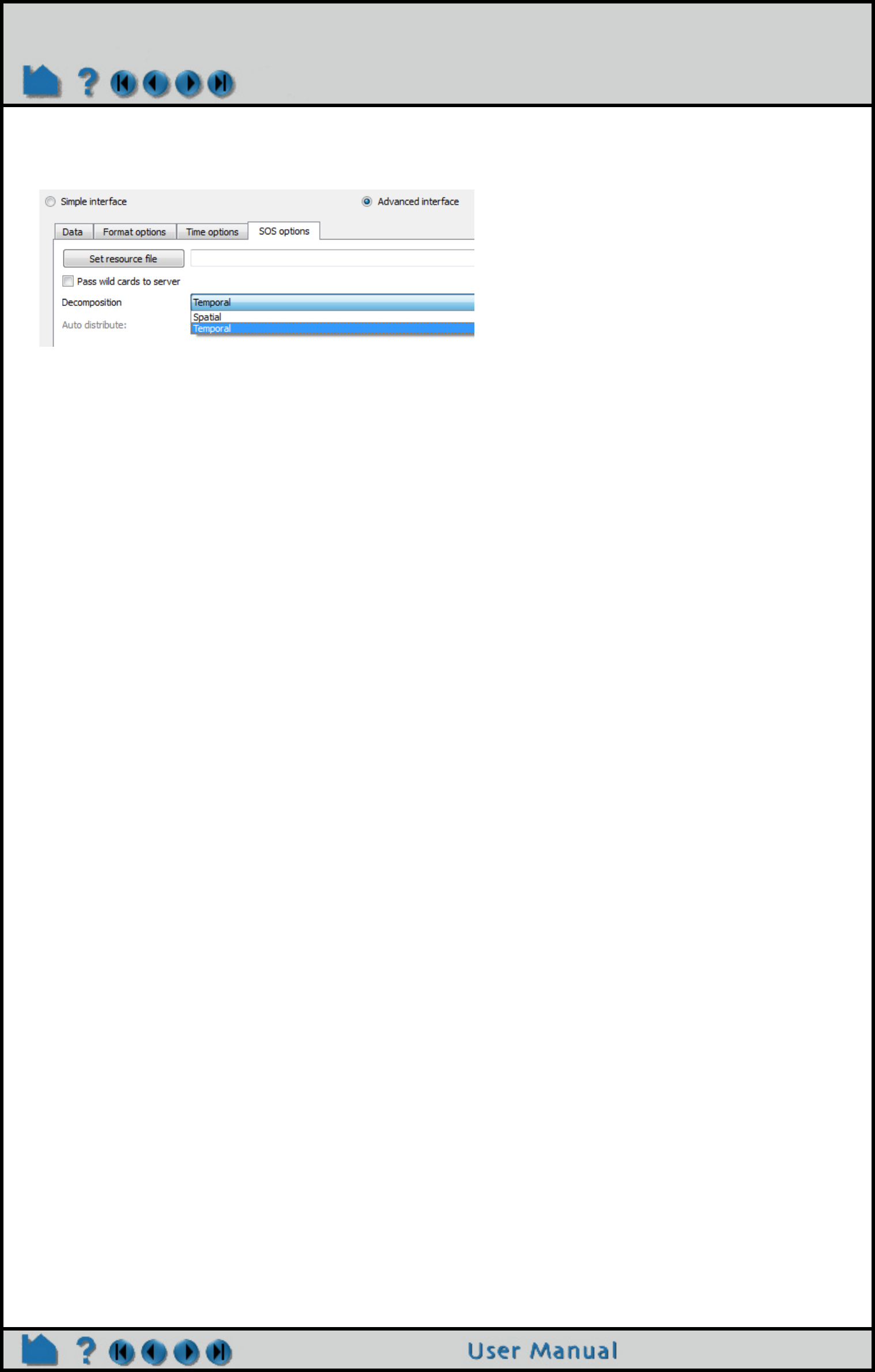
Page 70
HOW TO USE SERVER OF SERVERS
TEMPORAL DECOMPOSITION
All of the previous discussion was spatial. This section will cover temporal decomposition. All formats should be
able to use temporal decomposition as long as there is sufficient room on your servers so that each server can load
the geometry and variables for one full timestep. Temporal decomposition is really just temporal caching of the
timesteps before and after the current timestep. Each server reads one timestep and calculates all variables and
creates all parts that you have created in your analysis on the current timestep. Therefore, changing timestep to the
next (or previous) timestep occurs much more rapidly because the server that has responsibility that step has it pre-
cached does not need to do I/O nor calculations nor part creation, and must simply pass its data up to the client. Note
that the caching is for timesteps right around the current timestep: five servers and the current timestep is 6, might
mean that one server is responsible for timestep 6 and the others are responsible for timesteps 4, 5, 7, and 8.
Changing to timestep 12 will not benefit from the cached timesteps, and will, in fact, slow EnSight down: all five
servers now will load five new timesteps simultaneously: 10, 11, 12, 13, and 14.
SEE ALSO
How To Read Data
How To Read User Defined
How To Setup for Parallel Computation
How To Use Resource Managament
How To Use Root Level Server of Servers
User Manual: Server-of-Server Casefile Format

Page 71
HOW TO LOAD SPATIALLY DECOMPOSED CASE FILES
Load Spatially Decomposed Case Files
INTRODUCTION
If one has multiple EnSight gold casefiles (each of which contain a spatially decomposed portion of the same model),
they can be read using one or more servers (as long as the number of servers is less than or equal to the number of
casefiles). In other words, when it is desired to read N casefiles with M servers (M<=N), an additional section can be
added to the SOS casefile to accomplish this. Note that the following important restrictions/limitations will apply:
1. M (number of servers) must be less than or equal to N (number of casefiles).
2. Unstructured data only. (Note: a similar capability exists for structured data. See How to Use Block Continuation)
3. Auto distribute may not be specified in the SOS casefile.
4. None of the following can be specified in the partition casefiles:
GEOMETRY
measured:
match:
boundary:
rigid_body:
Vector_glyphs:
BLOCK_CONTINUATION
<any of the options>
MATERIAL
<any of the options>
Note: that some of the restrictions (such as measured) may eventually be lifted. But currently all of the above are
in effect.
5. All of the normal SOS requirements still apply.
a) All parts must be present in all cases. (Empty parts are allowed)
b) The same variables must exist in all cases.
c) The same timesets must be used in all cases.
Note: If the desired number of servers is equal to the number of casefiles, one can either use the procedure
described in this How To, or could use the normal SOS procedures (see How To Use Server of Servers).
BASIC OPERATION
To postprocess your partitioned EnSight Gold unstructured data on fewer servers than casefiles, run SOS using an
SOS casefile that has a MULTIPLE_CASEFILES section.
Three possible methods are available for your convenience. They all accomplish the same thing in slightly different
ways. So use whichever is easiest for your situation.
Note: in using one of the 3 the methods below, one should determine something about how the data resides, or is
available to EnSight. Namely, how will one need to specify the path to the data.
Since the whole idea is that the number of servers may vary, and Ensight will determine which casefiles go
to which servers, there are really only two possibilities for paths.
A) There is a global path for all of the data. And thus each server needs to know this global path (which it
will prepend to each casefile).
B) Each casefile has its own path. And each server needs to know the path for each.
Page 72
HOW TO LOAD SPATIALLY DECOMPOSED CASE FILES
Example
Method 1
Specify the number of and the actual files in the sos casefile
A) Using global path:
MULTIPLE_CASEFILES
total number of cfiles: 3
cfiles global path: /home/bjn/data
cfiles: file1.case
file_b.case
bruce.case
B) Using path per casefile:
MULTIPLE_CASEFILES
total number of cfiles: 3
cfiles: /home/bjn/data1/file1.case
/home/bjn/data2/file_b.case
/home/bjn/data3/bruce.case
Method 2
Specify the number of, the pattern, and the start and increment
A) Using global path:
MULTIPLE_CASEFILES
total number of cfiles: 3
cfiles global path: /home/bjn/data
cfiles pattern: file**.case
cfiles start number: 0
cfiles increment: 1
OR
MULTIPLE_CASEFILES
total number of cfiles: 3
cfiles pattern: /home/bjn/data/file**.case
cfiles start number: 0
cfiles increment: 1
Available Section lines: Comments
MULTIPLE_CASEFILES Required for all methods
total number of cfiles: n Used for method 1 and 2
cfiles global path: global_path Optional, used for methods 1 and 2
cfiles: partition_1.case Used for method 1
partition_2.case
.
.
partition_n.case
cfiles pattern: partition_*.case Used for method 2
cfiles start number: # Used for method 2
cfiles increment: # Used for method 2
cfiles file: filename Used for method 3

Page 73
HOW TO LOAD SPATIALLY DECOMPOSED CASE FILES
B) Using path per casefile:
Note: method 2 does not have a way to have a separate path for each casefile.
Method 3
Similar to 1., but place the info in a separate file
A) Using global path:
MULTIPLE_CASEFILES
cfiles file: all_together_cfiles.txt
and in all_together_cfiles.txt, (first line contains number of, second line contains the optional global path, then
filenames come 1 per line on the following lines). Like:
3
/home/bjn/data
file1.case
file_b.case
bruce.case
B) Using path per casefile:
MULTIPLE_CASEFILES
cfiles file: separated_cfiles.txt
and in separated_cfiles.txt, (first line contains number of, second line must be the word “none” - indicating no global
path specified, then filenames come 1 per line on the following lines). Like:
3
none
/home/bjn/data1/file1.case
/home/bjn/data2/file_b.case
/home/bjn/data3/bruce.case
Another Example
An EnSight Gold unstructured transient geometry model with a couple of variables, in 4 partitions, like:
Using Method 1:
If they all reside in the same directory (/home/bjn), a method 1 SOS casefile that will use just 2 servers (perhaps
named bjn_4x2.sos) should look like:
FORMAT
type: master_server gold
MULTIPLE_CASEFILES
total number of cfiles: 4
cfiles global path: /home/bjn
cfiles: bjn1.case
bjn2.case
bjn3.case
bjn4.case
SERVERS
number of servers: 2 repeat
bjn1.case bjn2.case bjn3.case bjn4.case
bjn1.geo0000 bjn2.geo0000 bjn3.geo0000 bjn4.geo0000
bjn1.geo0001 bjn2.geo0001 bjn3.geo0001 bjn4.geo0001
bjn1.scalar0000 bjn2.scalar0000 bjn3.scalar0000 bjn4.scalar0000
bjn1.scalar0001 bjn2.scalar0001 bjn3.scalar0001 bjn4.scalar0001
bjn1.evector0000 bjn2.evector0000 bjn3.evector0000 bjn4.evector0000
bjn1.evector0001 bjn2.evector0001 bjn3.evector0001 bjn4.evector0001
Page 74
HOW TO LOAD SPATIALLY DECOMPOSED CASE FILES
machine id: gun
executable: ensight102.server
Using Method 2:
If they all reside in the same directory (/home/bjn), a method 2 SOS casefile that will use just 2 servers should look
like:
FORMAT
type: master_server gold
MULTIPLE_CASEFILES
total number of cfiles: 4
cfiles global path: /home/bjn
cfiles pattern: bjn*.case
cfiles start number: 1
cfiles increment: 1
SERVERS
number of servers: 2 repeat
machine id: gun
executable: ensight102.server
Using Method 3:
For this one, lets change things and say that they reside in separate directories, like:
the SOS casefile could look like:
FORMAT
type: master_server gold
MULTIPLE_CASEFILES
cfiles file: /scratch/bjn.txt
SERVERS
number of servers: 2 repeat
machine id: gun
executable: ensight102.server
and the /scratch/bjn.txt file could look like:
4
none
/scratch/portion1/bjn1.case
/scratch/portion2/bjn2.case
/scratch/portion3/bjn3.case
/scratch/portion4/bjn4.case
or could look like: (See the Other Notes below)
4
/scratch
portion1/bjn1.case
portion2/bjn2.case
portion3/bjn3.case
portion4/bjn4.case
/scratch/portion1 /scratch/portion2 /scratch/portion3 /scratch/portion4
bjn1.case bjn2.case bjn3.case bjn4.case
bjn1.geo0000 bjn2.geo0000 bjn3.geo0000 bjn4.geo0000
bjn1.geo0001 bjn2.geo0001 bjn3.geo0001 bjn4.geo0001
bjn1.scalar0000 bjn2.scalar0000 bjn3.scalar0000 bjn4.scalar0000
bjn1.scalar0001 bjn2.scalar0001 bjn3.scalar0001 bjn4.scalar0001
bjn1.evector0000 bjn2.evector0000 bjn3.evector0000 bjn4.evector0000
bjn1.evector0001 bjn2.evector0001 bjn3.evector0001 bjn4.evector0001

Page 75
HOW TO LOAD SPATIALLY DECOMPOSED CASE FILES
OTHER NOTES:
When your casefile data resides in separate directories below a parent, such as:
/home/bjn
/home/bjn/data1
/home/bjn/data2
/home/bjn/data3
it is valid to use the global path to specify the parent directory, and the individual files to give the path on down. Such
as:
cfiles global path: /home/bjn
cfiles: data1/file1.case
data2/file_b.case
data3/bruce.case
This will result internally as the same thing as if you had done:
cfiles: /home/bjn/data1/file1.case
/home/bjn/data2/file_b.case
/home/bjn/data3/bruce.case
APPENDED_CASEFILES Variation:
If you desire to use all casefiles on one server, you can obviously do so with the above option by using the SOS with
one server. However, there is a variation on this option that can be used without using the SOS. It can be used with
a client and server alone.
It is very similar to the MULTIPLE_CASEFILES option in an SOS casefile, except that it is placed in the first regular
casefile of the series - the one that you will read. It uses APPENDED_CASEFILES as the section header, and lists
just the additional casefiles (not the one that this is placed in).
So instead of using the SOS with an SOS casefile like:
FORMAT
type: master_server gold
MULTIPLE_CASEFILES
total number of cfiles: 4
cfiles global path: /home/bjn
cfiles: bjn1.case
bjn2.case
bjn3.case
bjn4.case
SERVERS
number of servers: 1
machine id: gun
executable: ensight102.server
You could place the following in bjn1.case:
FORMAT
type: ensight gold
GEOMETRY
model: bjn1.geo
VARIABLE
scalar per node: scalar bjn1.scl
APPENDED_CASEFILES
total number of cfiles: 3
cfiles global path: /home/bjn
cfiles: bjn2.case
bjn3.case
bjn4.case
Note that all current limitations for the MULTIPLE_CASEFILES option (which were enumerated above) also
apply to the APPENDED_CASEFILES option. The two options cannot be used in combination. It is an either
or situation.


Page 77
HOW TO READ USER DEFINED
Read User Defined
INTRODUCTION
EnSight provides a mechanism for users to write their own readers and have the code automatically link and execute
at run-time (using a shared library).This capability is documented in the EnSight Interface Manual. As indicated in
that manual, sample readers, as well as the code for several actual readers are provided below the following
directory: $CEI_HOME/ensight102/src/readers/. In subdirectories underneath, there may exist other
README files that contain additional information on using existing user defined readers.
Also, as explained in that manual, be aware that a udr_checker.c file is provided in $CEI_HOME/ensight102/src/
readers/checker directory. This can be used to debug your User-defined reader before using it with EnSight.
OTHER NOTES
When starting EnSight (ensight102 or ensight102.server), you can use the command line option “-readerdbg” to echo
user defined reader loading status. This will allow you to see what readers are actually being loaded.
Set the environment variable ENSIGHT10_READER to point to the path where additional user defined readers exist
and then start up with the -readerdbg option described above to verify that you are loading the reader(s) of interest.
SEE ALSO
The EnSight Interface Manual, as well as:
How To Read Data
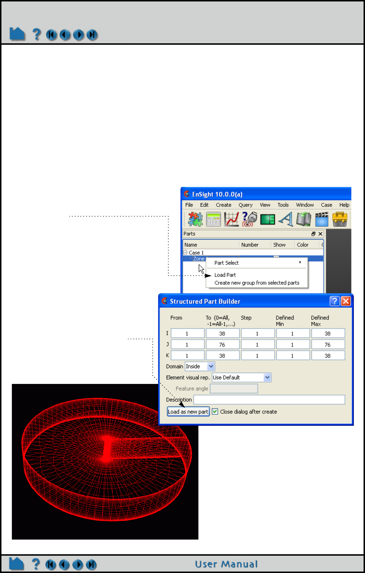
Page 78
HOW TO DO STRUCTURED EXTRACTION
Do Structured Extraction
INTRODUCTION
When loading structured parts (normally by right clicking on a part in the Parts list that has not yet been loaded), there
is some flexibility in what is actually extracted. If the model contains iblanking, then you have control over which
iblanking domain to use, namely Inside, Outside (blanked out), or All (which ignores the iblanking). If no iblanking in
the model, the domain is All by default. You can do things like extracting all or portions of zones at original or coarser
resolutions or doing the extractions on single or multiple zones.
BASIC OPERATION
When extracting the domain parts, whether iblanked or not, some (but definitely not all combinations) of the options
include:
Extracting a complete zone at original resolution,
1. Right click on the desired zone, and
click Load Part.
Optionally you can change the iblank
domain, choose the element
representation, and provide a part
description.
2. Hit the Load as new part button.
The part will be created and shown in the
graphics window. In the example below, it
is shown in border representation mode.
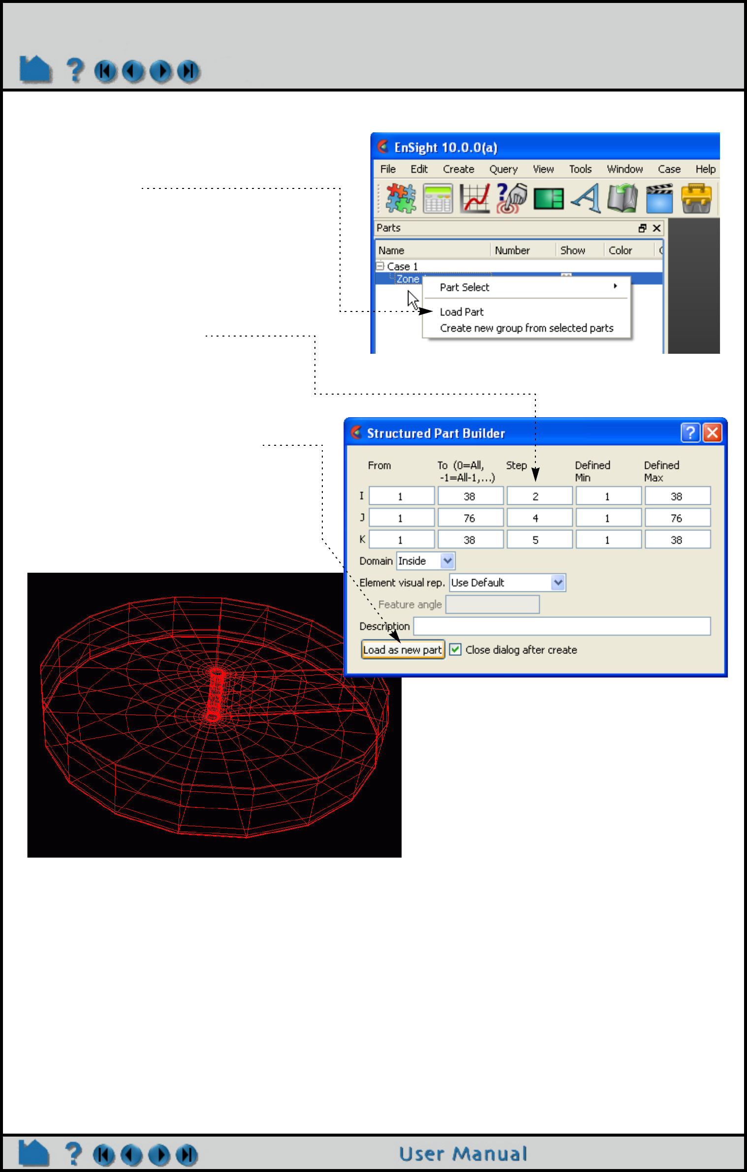
Page 79
HOW TO DO STRUCTURED EXTRACTION
Extracting a complete zone at coarser resolution,
1. Right click on the desired zone, and
click Load Part.
Optionally you can change the iblank
domain, choose the element representation,
and provide a part description.
2. Modify the Step values.
These should be positive integer values. A
step of two means to deal with every other
plane, a step of four means every fourth
plane, etc.
3. Hit the Load as new part button.
The part will be created and shown in the
graphics window. In the example below, it is
shown in border representation mode. Note
that it is considerably coarser than the
previous because step values of 2, 4, and 5
were used in the ijk directions respectively.
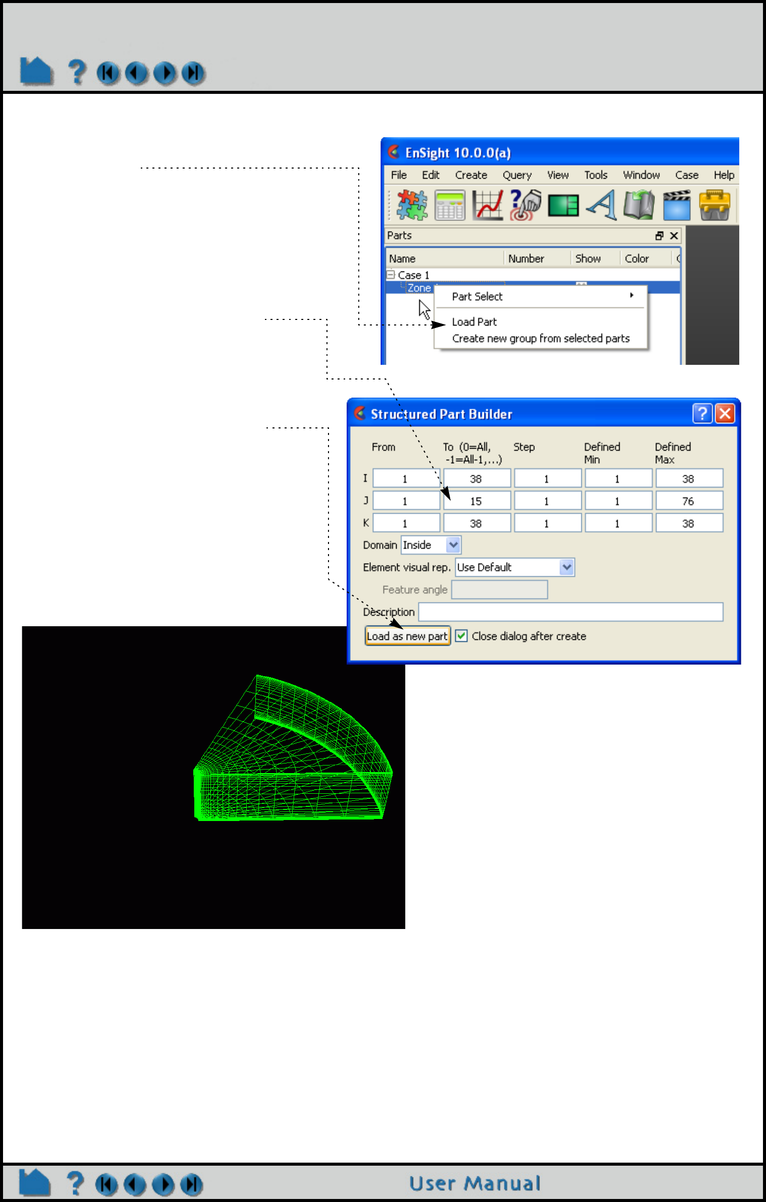
Page 80
HOW TO DO STRUCTURED EXTRACTION
Extracting portions of a zone,
1. Right click on the desired zone, and
click Load Part.
Optionally you can change the iblank
domain, choose the element representation,
and provide a part description.
2. Modify the From and To values.
These can be anything between the ranges
shown in the Min and Max columns. By
default they will be the entire range, but you
can modify them.
3. Hit the Load as new part button.
The part will be created and shown in the
graphics window. In the example below, it is
shown in border representation mode. Note
that you now get a portion instead of the
whole. Note also that we got original
resolution because we set step values back
to one. The step values can be other than
one, and your portion will be at the coarser
resolution.
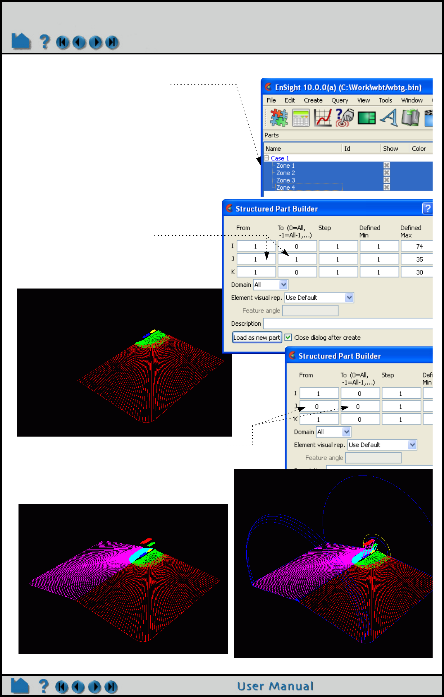
Page 81
HOW TO DO STRUCTURED EXTRACTION
Extracting the same portions over multiple parts,
1. Select the structured zones desired.
Optionally you can change the domain
2. Modify the From and To values.
These can be anything between the ranges shown in the Min
and Max columns (which will now be the min and max of all
parts selected). By default the From and To will be the entire
range, but you can modify them. Additionally, “-1” is a valid
entry, indicating the last plane. Minus numbers are ways to
specify the plane from the max back toward the min, thus -2
equals the next to last plane. (Note: Zero is treated the same
as -1)
3. Hit the Load as new part button.
In this example, 4 parts will be created, and they will
each be the full extent IK plane at J = 1 for each of the
four zones. Note that the IK ranges can actually vary
per part because the max is specified, but each zone
may be less than the max.
In our example, we then changed From and To to be “0”, thus
extracting the last plane in each zone. Note the image below.
The image at the right includes complete zones that were
extracted, but shown in feature angle representation so
you get the feel of the complete zone.

Page 82
HOW TO DO STRUCTURED EXTRACTION
Note: Prior to EnSight10, one could also extract multiple planes within the same zone while loading the part, through
the use of a delta column. This has been discontinued, but the same effect can be achieved by using the delta field
within an ijk clip.
SEE ALSO
How To Read Data
User Manual: Using Node Ranges:

Page 83
HOW TO USE RESOURCE MANAGEMENT
Use Resource Management
INTRODUCTION
Resources are used to specify which computers are used for running the various EnSight components, specifically
the Server (ensight102.server), the SOS (ensight102.sos), the CollabHub (ensight102.collabhub), and the distributed
renderers (ensight102.client). If you are running a single client and server on a single computer, you may skip this
document.
Resources are an alternative way to specify these computers compared to SOS case files, PRDIST files, Connection
Settings, and command line options. While these other ways are still valid and take precedence for backwards
compatibility, resources greatly simplify specifying computers in a dynamic network environment. For example, SOS
Case files and PRDIST files no longer need to be edited to reflect the current node allocation from cluster batch
schedulers. Resources coupled with native reader support in the SOS even make SOS Case files unnecessary.
Resources can be specified via command line arguments and environment variables. Resources can be specified
multiple times; precedence rules determine which resources ultimately get used. This allows sites to specify defaults
while allowing those to be overridden.
NOTE: While resources can still be specified according to this document, the entire resource management
support is moving to the newer technology called “cei-shell”.
BASIC OPERATION
Resource Files
Resources can be specified via a resource file. Here is an example of a resource file:
#!CEIResourceFile 1.0
SOS:
host: localhost
SERVER:
prologue: “setup_job”
epilogue: “cleanup_job”
host: server1
host: server2
host: server3
host: server4
COLLABHUB:
host: pc0
RENDERER:
prologue: “setenv DISPLAY :0.0”
# epilogue:
host: pc1
host: pc2
host: pc2
Resource files must begin with the ‘#!CEIResourceFile 1.0’ line. Afterwards, they may have up to four optional
sections: SOS, SERVER, COLLABHUB, and RENDERER. Each of the four sections contains one or more ‘host:
hostname’ lines. These lines specify which computers to use for the corresponding section. ‘hostname’ must be an
Internet/intranet routable host name or IP address. A given host name may appear on multiple lines within a section
or in different sections. If it appears multiple times within a section, then that host will run multiple instances of the
corresponding EnSight component if needed.
Additionally, each section may have an optional ‘prologue: cmd’ line and/or an optional ‘epilogue: cmd’ line.
These specify a command to execute on each host before and after the corresponding EnSight component. Note that
the cmd string must be quoted, and may include appropriate job backgrounding symbols (e.g. ‘&’).
At version 2.0, the resource file can accept an optional ‘shell:’ line, like:
#!CEIResourceFile 2.0
SOS:
host: bunker
shell: "/usr/local/bin/ssh"

Page 84
HOW TO USE RESOURCE MANAGEMENT
Note the new version number (2.0) and that the shell line string must be double quoted.
How to specify resources
Resources can be specified via resource files, environment variables, and command line options. Precedence rules
determine which resources will be used. Basically, the last occurrence of a resource section (e.g. SERVER) will be
used in its entirety. For example, if multiple SERVER resource sections are found, only one will be used as determined
by the precedence rules.
Since the EnSight Client, SOS, and CollabHub start other EnSight processes, they can use resources. The EnSight
Server and distributed renderers do not start other EnSight processes that require resources.
While many ways exist to specify resources, in practice only one or two will be used given the particular user’s
computational environment.
Client Resources
The EnSight client supports the following ways for specifying resources:
1. the ENSIGHT10_RES environment variable;
2. the ENSIGHT10_SERVER_HOSTS environment variable;
3. the ENSIGHT10_RENDERER_HOSTS environment variable;
4. the ‘-use_lsf_for_servers’ command line option;
5. the ‘-use_lsf_for_renderers’ command line option;
6. the ‘-use_pbs_for_servers’ command line option;
7. the ‘-use_pbs_for_renderers’ command line option;
8. the ‘-sosres file_name’ command line option;
9. the ‘-chres file_name’ command line option; and
10.the ‘-res file_name’ command line option.
If multiple resources are specified to the client, then they will be evaluated in the order indicated above with the later
methods taking higher precedence for a given section.
The ENSIGHT10_RES environment variable specifies a resource file name that the client reads.
ENSIGHT10_SERVER_HOSTS and ENSIGHT10_RENDERER_HOSTS specify quoted strings of space delimited host
names (e.g. “host1 host2 host1 host3”) to be used for EnSight servers and distributed renderers, respectively.
The host names are used in the order they occur. A host name may occur multiple times.
If either the ‘-use_lsf_for_servers’ or ‘-use_lsf_for_renderers’ command line options are specified, then
the client will evaluate the environment variable LSB_MCPU_HOSTS for the resources. The environment variable
specifies a quoted string such as “host1 5 host2 4 host3 1” which indicates 5 CPUs should be used on host1,
4 CPUs should be used on host2, and 1 CPU should be used on host3. The hosts will be used in a round-robin
fashion.
If either of the ‘-use_pbs_for_servers’ or ‘-use_pbs_for_renderers’ command line options are specified,
then the client will evaluate the environment variable PBS_NODEFILE for the resources. The environment variable
specifies a filename in which the file contains list of line delimited host names that were allocated by the PBS
scheduler.
The ‘-sosres file_name’ command line option specifies the pathname to a resource file. This file name is passed
to the SOS and processed by it; thus the file name must be accessible and readable by the ensight102.sos process.
If multiple ‘-sosres’ options are specified, only the last will be used.
The ‘-chres file_name’ command line option specifies the pathname to a resource file. This file name is passed
to the CollabHub and processed by it; thus the file name must be accessible and readable by the
ensight102.collabhub process. If multiple ‘-chres’ options are specified, only the last will be used.
The ‘-res file_name’ command line option specifies the pathname to a resource file. This command line option
can be specified multiple times. This might be useful when generating resource files dynamically: a single file might
specify only a particular type of resource (e.g. SERVER or RENDERER). The last occurrence of a particular section
takes precedence when multiple ‘-res’ options are given.
Finally, a resource file may be selected in the File->Open dialog for the SOS to use.

Page 85
HOW TO USE RESOURCE MANAGEMENT
SOS Resources
The EnSight SOS supports the following ways for specifying resources:
1. resources gathered and sent from the client;
2. the ‘-sosres file_name’ command line option;
3. the ENSIGHT10_RES environment variable;
4. the ENSIGHT10_SERVER_HOSTS environment variable;
5. the ‘-use_lsf_for_servers’ command line option;
6. the ‘-use_pbs_for_servers’ command line option;
7. the ‘-res file_name’ command line option; and,
8. a resource file specified via the File->Open dialog.
If multiple resources are specified to the SOS, then they will be evaluated in the order indicated above with the later
methods taking higher precedence for a given section. However, the SOS only uses SERVER section resources; the
other sections are ignored.
The ‘-sosres file_name’ command line option specifies the pathname to a resource file. If multiple ‘-sosres’
options are specified, only the last will be used.
The ENSIGHT10_RES environment variable specifies a resource file name that the SOS reads.
ENSIGHT10_SERVER_HOSTS specifies a quoted string of space delimited host names (e.g. “host1 host2 host1
host3”) to be used for EnSight servers.
If the ‘-use_lsf_for_servers’ command line option is specified, then the SOS will evaluate the environment
variable LSB_MCPU_HOSTS for the resources. The environment variable specifies a quoted string such as “host1 5
host2 4 host3 1” which indicates 5 CPUs should be used on host1, 4 CPUs should be used on host2, and 1 CPU
should be used on host3. The hosts will be used in a round-robin fashion.
If the ‘-use_pbs_for_servers’ command line option is specified, then the SOS will evaluate the environment
variable PBS_NODEFILE for the resources. The environment variable specifies a filename in which the file contains
list of line delimited host names that were allocated by the PBS scheduler.
The ‘-res file_name’ command line option specifies the pathname to a resource file. This command line option
can be specified multiple times. The last occurrence of a particular section takes precedence when multiple ‘-res’
options are given.
Finally, a resource file may be selected in the File->Open dialog for the SOS to use.
CollabHub Resources
The EnSight CollabHub supports the following ways for specifying resources:
1. resources gathered and sent from the client;
2. the ‘-chres file_name’ command line option;
3. the ENSIGHT10_RES environment variable;
4. the ENSIGHT10_RENDERER_HOSTS environment variable;
5. the ‘-use_lsf_for_renderers‘ command line option;
6. the ‘-use_pbs_for_renderers’ command line option; and,
7. the ‘-res file_name’ command line option.
If multiple resources are specified to the CollabHub, then they will be evaluated in the order indicated above with the
later methods taking higher precedence for a given section. However, the CollabHub only uses RENDERER section
resources; the other sections are ignored.
The ‘-chres file_name’ command line option specifies the pathname to a resource file. If multiple ‘-chres’
options are specified, only the last will be used.
The ENSIGHT10_RES environment variable specifies a resource file name that the CollabHub reads.
ENSIGHT10_RENDERER_HOSTS specifies a quoted string of space delimited host names (e.g. “host1 host2
host1 host3”) to be used for EnSight distributed renderers.
If the ‘-use_lsf_for_renderers‘ command line option is specified, then the CollabHub will evaluate the
environment variable LSB_MCPU_HOSTS for the resources. The environment variable specifies a quoted string such

Page 86
HOW TO USE RESOURCE MANAGEMENT
as “host1 5 host2 4 host3 1” which indicates 5 CPUs should be used on host1, 4 CPUs should be used on
host2, and 1 CPU should be used on host3. The hosts will be used in a round-robin fashion.
If the ‘-use_pbs_for_renderers’ command line option is specified, then the CollabHub will evaluate the
environment variable PBS_NODEFILE for the resources. The environment variable specifies a filename in which the
file contains list of line delimited host names that were allocated by the PBS scheduler.
The ‘-res file_name’ command line option specifies the pathname to a resource file. This command line option
can be specified multiple times. The last occurrence of a particular section takes precedence when multiple ‘-res’
options are given.
When using distributed rendering, any hosts specified via a prdist file are used instead of those given by RENDERER
resources. Additionally, any prdist file specified directly to the collabhub, will override one specified to the client.
A Client/Server Example
Resources are not used to specify where a server runs when it is part of a normal client/server session. The default
server connection in the Connection Setting dialog determines on which computer the server runs unless the Client
command line option ‘-c connection_name’ is specified.
A Simple SOS Example
The SOS can read any of the supported file formats in addition to the SOS Case file format. When a SOS Case file is
not used, then the number of EnSight Servers used is equal to the number of hosts specified in the SERVER resource
section.
1. The following resource file ‘my_hosts.res’ is created:
#!CEIResourceFile 1.0
SOS:
host: borg
SERVER:
host: drone1
host: drone2
host: drone3
host: drone1
2. EnSight is started with this command line:
ensight102 -res my_hosts.res -sos
The EnSight Client will automatically check out a gold key and will run on the local workstation, the SOS
(ensight102.sos) will be automatically started on computer ‘borg’ and will connect back to the client. Borg will need to
recognize the name of the computer that the client is running on.
3. In the File->Open dialog the LS-Dyna file ‘d3plot’ is selected and the ‘Load All’ button is clicked.
The SOS will start four EnSight Servers on computers ‘drone1’, ‘drone2’, ‘drone3’, and ‘drone1’ (presumably,
‘drone1’ might be a SMP). The ‘drone’ computers need to recognize the hostname borg in order to connect back to
the sos running on this computer.
Each of the servers will read 1/4 of the data set since the ‘Auto Distribute’ flag (on the SOS tab of the File->Open
dialog) is on by default for the LS-Dyna reader.
Another SOS Example
1. EnSight is started with this command line:
ensight102
2. The Case->Connection Settings dialog is opened. On the ‘SOS’ tab, an entry for host ‘borg’ is created. For
that entry, ‘Executable:’ is set to the name of command file ‘my_sos’, ‘Use default rsh cmd’ is
deselected, and ‘Alt rsh cmd:’ is set to ‘ssh’. The entry is saved and EnSight is terminated.
3. The following resource file ‘my_hosts.res’ is created:

Page 87
HOW TO USE RESOURCE MANAGEMENT
#!CEIResourceFile 1.0
SOS:
host: borg
SERVER:
host: drone1
host: drone2
host: drone3
host: drone1
4. On computer borg (assuming it is running Unix or Linux), the file ‘my_sos’ is created:
#!/bin/csh
setenv ENSIGHT10_SERVER_HOSTS ‘cat $PBS_NODEFILE‘
ensight102.sos $*
The file must be in the user’s default path and must be executable.
5. EnSight is started with this command line:
ensight102 -res my_hosts.res -sos
The EnSight Client will check out an hpc (formerly gold) license key and run on the local workstation, the command
file ‘my_sos’ will run on computer ‘borg’ which must be able to connect back to the local workstation by hostname.
The client will start up ‘my_sos’ via ssh. ‘my_sos’ sets the environment variable ENSIGHT10_SERVER_HOSTS to
be the contents of the file specified by the environment variable PBS_NODEFILE (OpenPBS’ dynamic list of
allocated nodes).
6. In the File->Open dialog the LS-Dyna file ‘d3plot’ is selected and the ‘Load All’ button is clicked.
The SOS will start EnSight Servers on computers specified in file $PBS_NODEFILE. Hosts specified in the SERVER
section of my_hosts.res are ignored since ENSIGHT10_SERVER_HOSTS takes precedence.
Each of the servers will read 1/N of the data set since the ‘Auto Distribute’ flag (on the SOS tab of the File-
>Open dialog) is on by default for the LS-Dyna reader.
A SOS Case File Example
When a SOS Case file is used with resources, it needs to be modified otherwise the resources will be ignored for the
EnSight Servers. This is done for backwards compatibility.
1. The file SOS case file ‘big_data.sos’ is modified. Two lines are added to the FORMAT section:
‘use_resources: on’ and ‘auto_distribute: on’. The ‘casefile: ‘ line for each server is brought to
the beginning of each subsection.
FORMAT type: master_server LS-DYNA3D
use_resources: on
auto_distribute: on
SERVERS
number of servers: 2
#Server 1
#---------
casefile: d3plot
machine id:
executable: ensight102.server
directory: /tmp
login id:
data_path: /tmp
#Server 2
#---------
casefile: d3plot
machine id:
executable: ensight102.server
directory: /tmp
login id:

Page 88
HOW TO USE RESOURCE MANAGEMENT
data_path: /tmp
Note that the ‘casefile:’ line must appear before the other lines for that server
when using resources.
2. The following resource file ‘my_hosts.res’ is created:
#!CEIResourceFile 1.0
SOS:
host: borg
SERVER:
host: drone1
host: drone2
host: drone3
host: drone1
2. EnSight is started with this command line:
ensight102 -res my_hosts.res -sos
The EnSight Client will run on the local workstation, the SOS (ensight102.sos) will run on computer ‘borg’.
3. In the File->Open dialog the SOS Case file ‘big_data.sos’ is selected and the ‘Load All’ button is clicked.
The SOS will start two EnSight Servers on computers ‘drone1’ and ‘drone2’. Only two servers are used since two
‘casefile: ‘ lines occur in the SOS Case file. The ‘number of servers: 2’ line is ignored as are the
‘machine id:’ lines.
Each of the servers will read half of the data set due to the line ‘auto_distribute: on’ in ‘big_data.sos’.
Another SOS Case File Example
1. The file SOS case file ‘big_data.sos’ is modified. Two lines are added to the FORMAT section:
‘use_resources: on’ and ‘auto_distribute: on’. The ‘number of servers:’ line is modified. One
server subsection is specified.
FORMAT
type: master_server LS-DYNA3D
use_resources: on
auto_distribute: on
SERVERS
number of servers: 4 repeat
#Server 1
#---------
casefile: d3plot
machine id:
executable: ensight102.server
directory: /tmp
login id:
data_path: /tmp
2. The following resource file ‘my_hosts.res’ is created:
#!CEIResourceFile 1.0
SOS:
host: borg
SERVER:
host: drone1
host: drone2
host: drone3
host: drone1

Page 89
HOW TO USE RESOURCE MANAGEMENT
2. EnSight is started with this command line:
ensight102 -res my_hosts.res -sos
The EnSight Client will run on the local workstation, the SOS (ensight102.sos) will run on computer ‘borg’.
3. In the File->Open dialog the SOS Case file ‘big_data.sos’ is selected and the ‘Load All’ button is clicked.
The SOS will start four EnSight Servers on computers ‘drone1’, ‘drone2’, ‘drone3’, and ‘drone1’. Since the
‘number of servers:’ line has the word ‘repeat’, the servers specified in the SERVERS resource is used to
determine the number of servers used and their host names. All server subsections after the first in
‘big_data.sos’ are ignored due to ‘number of servers: 4 repeat’.
Each of the servers will read 1/4 of the data set since the ‘Auto Distribute’ flag (on the SOS tab of the File-
>Open dialog) is on by default for the LS-Dyna reader.
A PRDIST Example
1. The following resource file ‘my_hosts.res’ is created:
#!CEIResourceFile 1.0
SOS:
host: borg
SERVER:
host: drone1
host: drone2
host: drone3
host: drone1
COLLABHUB:
host: curly
RENDERER:
prologue: “xhost +”
host: larry
host: moe
2. The following prdist resource file ‘my_conf_with_res.prdist’ is also created:
#ParallelRender EnSight 1.0
router
pc
client
3. EnSight is started with this command line:
ensight102 -res my_hosts.res -prdist my_config_with_res.prdist
The EnSight Client will run on the local workstation, the SOS (ensight102.sos) will run on computer ‘borg’.
The EnSight CollabHub will run on computer ‘curly’. Two distributed renderers will start on hosts ‘larry’ and
‘moe’.
The my_conf_with_res.prdist file here specifies both "router" and "client" followed by blank names which indicate to
use the 'my_hosts.res' file. The "pc" option indicates to use parallel compositing which removes the from the
composited display
NOTE: if "pc" is not specified, then a will wrap the composited display - which is a testing and debug mode. In
addition, no display sync will be used during interactive transformations, producing a lag effect which is quite
annoying.
4. In the File->Open dialog the LS-Dyna file ‘d3plot’ is selected and the ‘Load All’ button is clicked.
The SOS will start four EnSight Servers on computers ‘drone1’, ‘drone2’, ‘drone3’, and ‘drone1’ (presumably,
‘drone1’ might be a SMP).

Page 90
HOW TO USE RESOURCE MANAGEMENT
Each of the servers will read 1/4 of the data set since the ‘Auto Distribute’ flag (on the SOS tab of the File-
>Open dialog) is on by default for the LS-Dyna reader.
Note that a prdist file can be specified as an option to the ‘-prdist’ command line option. However, if the defaults
are adequate or overridden with command line options, then a prdist file is no longer needed. Furthermore, specifying
the command line option ‘-prdist’ automatically implies the command line option ‘-sos’; previous versions
required the user to specify it. Chapter 11 Parallel Compositing of the User Manual for prdist file documentation,
including default values and manual connect support.
OTHER NOTES
Chapter 8 Resource File Format of the User Manual for details on the resource file syntax.
See the EnSight User’s Guide for details on relevant SOS Case file modifications as they pertain to resources. Also,
see that section regarding details on which file formats support auto . Note that not all Case files (i.e. non-gold) can
be auto distributed.
The default SOS and server entries in the Connections Setting dialog will be used as the template for SOS and
server computers not specifically listed in the dialog. This is useful for specifying defaults such as to use ‘ssh’ in place
of ‘rsh’ or to specify a default path.
SEE ALSO
How To Read Data
How To Read User Defined
How To Setup for Parallel Computation
User Manual:
Resource File Format
Parallel Compositing
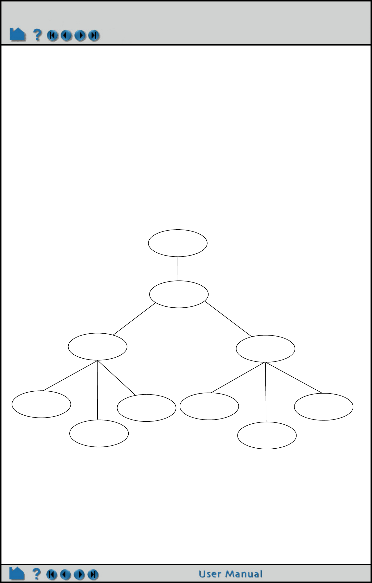
Page 91
HOW TO USE ROOT LEVEL SERVER OF SERVERS
Use Root Level Server of Servers
INTRODUCTION
EnSight 10.2, using an hpc (formerly gold) license key has the capability of using multiple EnSight Servers to process
a dataset in an efficient distributed manner by using what's called Server-of-Servers (SOS for short). See How To
Use Server of Servers for details. The SOS process acts as a router between the EnSight Client and one or more
EnSight Servers. It broadcasts commands from the Client to the multiple Servers and gathers and aggregates
response data from the Servers to send back to the Client. If the dataset size is sufficiently large, a single SOS may
become a bottleneck. In such situations, multiple SOS processes coordinated by a parent, or root level, SOS may be
warranted to increase scalability. EnSight 10.2 adds the ability to use multiple SOS processes to distribute the load,
and adds a single Root Level SOS (RLSOS) that communicates between the EnSight Client and multiple SOS
processes. Each of the additional SOS processes in turn communicates with one or more Servers (see Figure 1).
Root Level SOS (RLSOS) enables EnSight to scale to much larger problem sizes.
Just as the EnSight SOS acts as router for multiple EnSight Servers, the RLSOS acts as a router for multiple EnSight
SOSes. In theory, the RLSOS should provide the same degree of scalability for multiple SOSes as a single SOS
provides for multiple Servers. It is anticipated, but not yet tested, that the RLSOS could enable EnSight to scale into
the tens of thousands of EnSight Servers. To take advantage of this potential, the data set must be sufficiently large
to keep all Servers busy and to warrant the overhead of the additional communication. It is anticipated that data sets
should be on the order of millions of elements/nodes per Server to obtain reasonable scalable performance..
BASIC OPERATION
Start Up
Starting EnSight RLSOS requires the use of CEIShell to launch all processes and properly configure them. Please
review the CEIShell documentation for configuration instructions. Typically, someone at a site configures one or
more CEIShell networks for the site while most EnSight users simply use these locally configured CEIShell networks.
Server
Server Server
Server
Server
Server
SOS SOS
RLSOS
Client
Figure 1 Simple RLSOS Connectivity
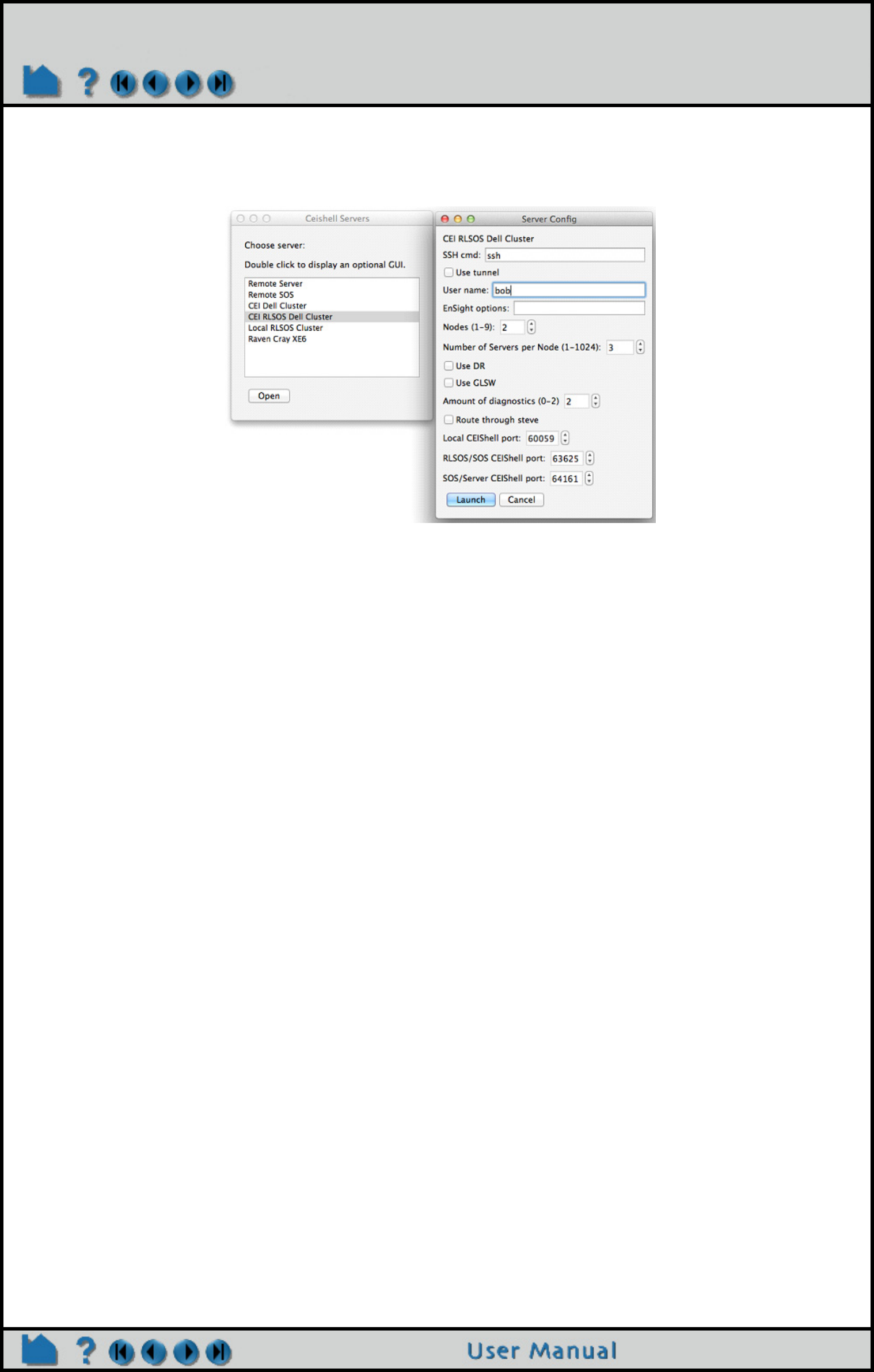
Page 92
HOW TO USE ROOT LEVEL SERVER OF SERVERS
End-users typically access the CEIShell networks and launch EnSight via the -based program ‘ceistart102’ (see
Figure 2 below for an example configuration).
In terms of configuring a CEIShell network for use with RLSOS and optionally EnSight HPC+, the concepts are
exactly the same as with configuring any CEIShell network. The sole exceptions are specifying the CEIShell “role”
tags “RLSOS” and multiple “SOS” roles to the appropriate CEIShells. Figure 1 shows a typical CEIShell network
layout. One CEIShell has the role “RLSOS”, one or more child CEIShells have the role “SOS”, and each of the SOS
CEIShells have one or more child CEIShells with the role “SOS_SERVERS”. In the example represented by the
figure, EnSight will start and use via this CEIShell network one RLSOS, two SOSes, and six Servers.
If EnSight HPC+ is to be used with RLSOS, then the computer executing the RLSOS must be able to open a network
connection to the computer(s) running the EnSight CollabHub as well as the EnSight master Client. Additionally, the
EnSight HPC+ Clients must be able to open network connections to the EnSight CollabHub and master Client. A
future version of EnSight and CEIShell may provide for network tunneling via CEIShell.
Operation
To the end-user of EnSight, once RLSOS is running, there is no other difference from using RLSOS compared to
using EnSight with just SOS -- all user interaction is the same as it is with SOS use.
Limitations
Currently, the only known limitation when using RLSOS concerns the use of legacy EnSight SOS Case files (not
normal Case files). If a legacy SOS Case file is used, then it must not contain ‘machine id:’ nor ‘executable:’ lines.
Additionally, the ‘number of servers:’ in the SOS Case file must match the total number of EnSight Servers started by
the CEIShell network. Lastly, the underlying data files specified in the SOS Case file must be accessible by all
Servers since it is not known apriori which Server will read which data file.
PROBLEMS
Start up issues
As with any CEIShell use, if there is a problem launching EnSight, be sure to see if the CEIShell network is starting
correctly before invoking EnSight. Typically, the person who set up CEIShell for a site can determine this. If a
CEIShell network is running, use the command ‘ceishell31 -cmd show_net’ to display the running network, hosts
running the CEIShells, and the various CEIShell roles assigned to each CEIShell. This command is executed on the
same computer running the CEIShell that has the ‘-app’ option. See the CEIShell documentation for further details.
In terms of RLSOS specifically, one CEIShell must have the role “RLSOS”. One or more CEIShells one level below
Figure 2 Simple RLSOS Configuration

Page 93
HOW TO USE ROOT LEVEL SERVER OF SERVERS
this CEIShell must have the role “SOS”. Finally, CEIShells below these CEIShells must have the role
“SOS_SERVERS” (see Figure 1).
While EnSight HPC+ may be used with RLSOS, it still has limitations affecting how the DRClients and CollabHub
connect back to the Master Client and RLSOS. While CEIShell is used to launch the DRClients and CollabHub, the
DRClients and CollabHub do NOT use CEIShell for establishing network communication to the Master Client nor
RLSOS. This can lead to problems especially if firewalls or restrictive routers are used or when hosts have multiple
network interfaces with varying hostnames. CEI Support can advise.
Output
Due to the potential of running thousands to tens of thousands of EnSight Servers, output from the Servers (or
DRClients) can be overwhelming. More importantly, this magnitude of output can actually throttle overall
performance. To remedy this problem, CEIShell was enhanced for use with EnSight RLSOS to address this issue.
CEIShell adds a command line option ‘-app_output_buffering true|false’ that controls output buffering for any
processes started by the CEIShell.
If CEIShell output buffering is turned on, output from its child processes (e.g. the EnSight Server) is buffered until the
process exits or until an error is detected in the output. Should an error be detected in the output, the buffer will be
released for display. Furthermore, once the buffer is release, no additional buffering occurs until the process
terminates.
The example CEIShell network configurations provided with ceistart102 use this option to provide output buffering in
a reasonable way along with three selectable levels. The user can choose to turn off all output buffering; this means
that all output from EnSight processes is displayed. Turning on output buffering means that no output from EnSight
processes is displayed (except for error conditions). The third option ‘default’ shows all output from the EnSight
RLSOS and CollabHub processes but buffers the output from the Servers, DRClients, and child SOS processes.
This option tends to give reasonable feedback without adversely affecting performance. Turning output buffering ‘off’
may be useful for debugging purposes but the user should be mindful that the amount of output can be exceedingly
large. Also note that -app_output_buffering option is independent from the ‘-v #’ option which affects the amount of
verbosity from the EnSight components (Client, Server, SOS, etc.). For maximum output, use ‘-app_output_buffering
false -v 3’. For minimum output, use ‘-app_output_buffering true -v 0’.
For any questions or problems with using CEIShell and/or RLSOS, please contact CEI Support
(support@ceisoftware.com).
SEE ALSO
How To Read Data
How To Read User Defined
How To Setup for Parallel Computation
How To Use Resource Managament
How To Use Server of Servers
User Manual: Server-of-Server Casefile Format
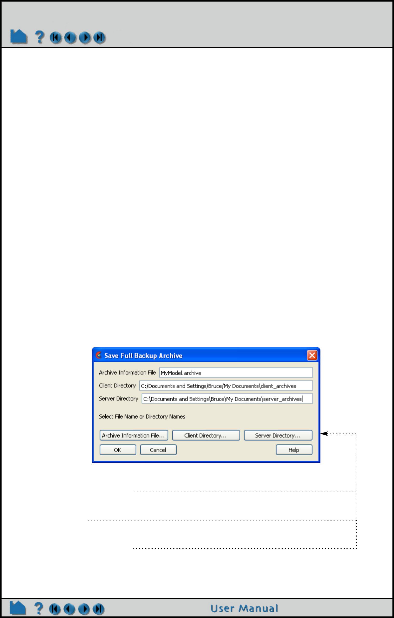
Page 94
HOW TO SAVE OR RESTORE AN ARCHIVE
Save or Output
Save or Restore an Archive
INTRODUCTION
EnSight command files are useful for restoring the system to a state reached in a previous session. However,
restoring a long session dealing with large files can take a long time. Fortunately, EnSight provides an archiving
mechanism that saves only the current state of the system, rather than the entire history of a session.
This capability is useful not only for large data files with several active variables, but also for saving a standard
starting point for sessions. In the initial session, geometry can be loaded, variables activated, a good viewpoint
selected, and an archive written. Subsequent sessions take advantage of this investment by merely loading the
archive (which can be done as you start EnSight from the command line).
The client and server each write separate binary files containing the complete current state of the respective
processes. Since these files are binary, they can be quickly written and restored. Note that an archive only contains
information resident in either client or server memory at the time of the archive. No information is available for
variables that were inactive or time steps other than the current. For this reason, you should never remove the
original dataset and attempt to use the archive as a substitute (unless you know what you’re doing).
BASIC OPERATION
An EnSight archive consists of three files:
1. The Archive Information File. This file provides pointers to the client and server archive files as well as additional
information required to load the archive. An example is given in the Advanced Usage section below.
2. The Client Archive file. This is the client’s binary dump file.
3. The Server Archive file. This is the server’s binary dump file.
(Note that for Server-of Servers, there will be an SOS archive file and then a server archive file per server)
Although each file has a default location, you can override the default during the archiving process.
Saving an Archive
1. Close all open EnSight windows except the main window.
2. Select File > Save > Full Backup... to open the Save Full Backup Archive dialog.
2. If desired, enter a new name for the Archive Information file. You can set the directory for
the Archive Information File by clicking the Archive Information File... button to open a
standard File Selection dialog.
3. If desired, select a directory for the client’s binary dump file by either entering the directory
in the Client Directory field or clicking the Client Directory... button to open a standard File
Selection dialog.
4. If desired, select a directory for the server’s binary dump file by either entering the
directory in the Server Directory field or clicking the Server Directory... button to open a
standard File Selection dialog.
5. Click Okay.
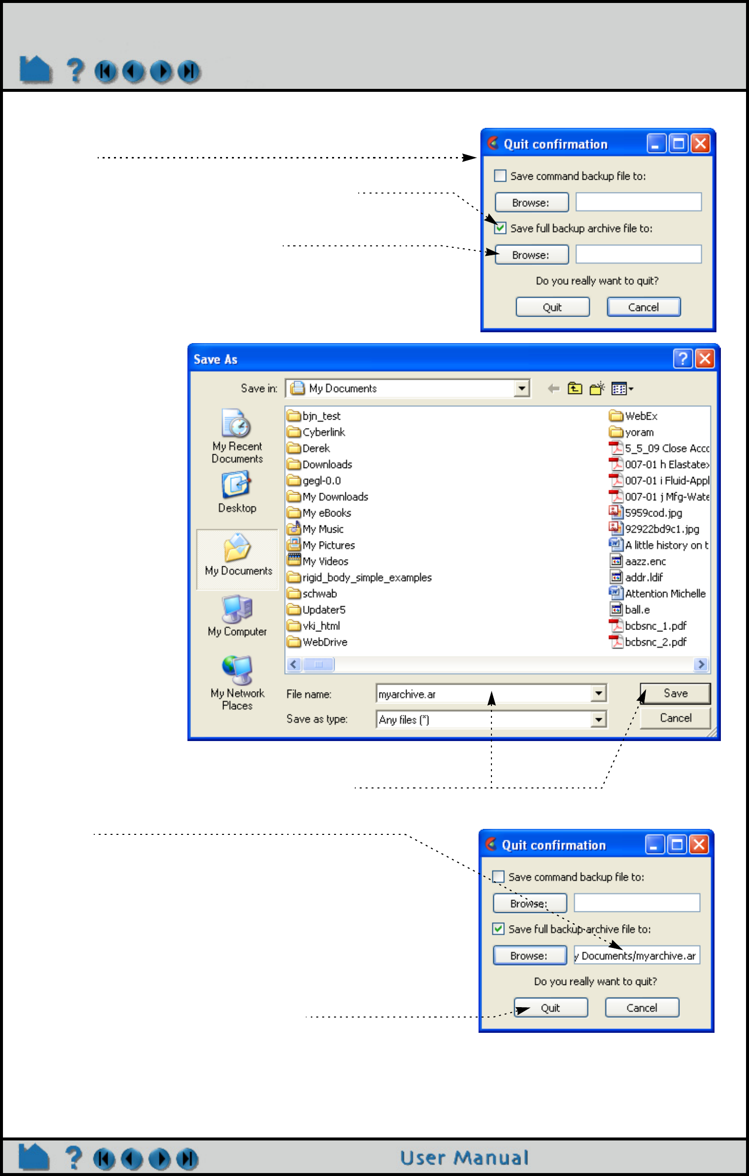
Page 95
HOW TO SAVE OR RESTORE AN ARCHIVE
You also have the option of saving an archive as you exit EnSight.
1. Select File > Quit... to open the Quit Confirmation
dialog.
2. Click the “Save full backup archive to:” toggle,
and either enter a new name for the Archive
information file or browse to the desired location/
file by clicking the Browse: button.
3. If you browsed to the file, click Save once you
have selected or entered the desired filename.
This will place the filename in the Quit confirmation
dialog.
3. Click Quit to save the archive and exit.

Page 96
HOW TO SAVE OR RESTORE AN ARCHIVE
Restoring an Archive
You can restore an archive either as part of EnSight startup or during an active session. To load an archive on
startup:
1. Use the “-ar archive_info_file” option when you start EnSight. For example,
% ensight102 -ar load.ar
where load.ar is an Archive Information file saved in a previous session.
To restore an archive during an active session:
1. Select File > Restore > Full Backup... to open the File Selection dialog.
2. Select the desired Archive Information file and click Okay.
3. If the original connection (when the archive was saved) was manual, you will need to manually restart the
server.
ADVANCED USAGE
There are times when you may want to modify the contents of the Archive Information file. If you wish to use the
archive on a different machine or change the location of the binary dump files, you can simply edit the file with a text
editor. The following example shows the contents:
OTHER NOTES
Important note! Archives are typically not upwardly compatible with new major – and some minor – releases of
EnSight. For this reason, the complete current command file is also saved as part of the client’s binary dump. If you
attempt to restore an archive and EnSight determines that the archive is not compatible with the current release, the
command file will be restored to a default location, and you can get back to your state by playing that command file.
SEE ALSO
User Manual: Saving and Restoring a Full backup
Wed Apr 2 15:31:51 1997
client ./ensight0402_153151.clientbkup
# server for Case ‘Case 1’. **Warning Don’t Modify The Internal Number**.
case_internal_number 0
case_name Case 1
case_connect_type auto
case_connect_machine indigo2
case_connect_executable /usr/local/bin/ensight/server/ensight.server
case_connect_directory /usr/people/joe/data
case_connect_login_id
server ./ensight_c1_0402_153151.serverbkup
Date saved
Path to client’s binary file
comment
Case internal number
Case name
Connect type (auto or manual)
Server host machine
Server executable
Server data directory
Alternate server login ID
Path to server’s binary file
Note that there will be a section for all the case_ variables for each current case in the EnSight session. See How
To Load Multiple Datasets for more information on cases.
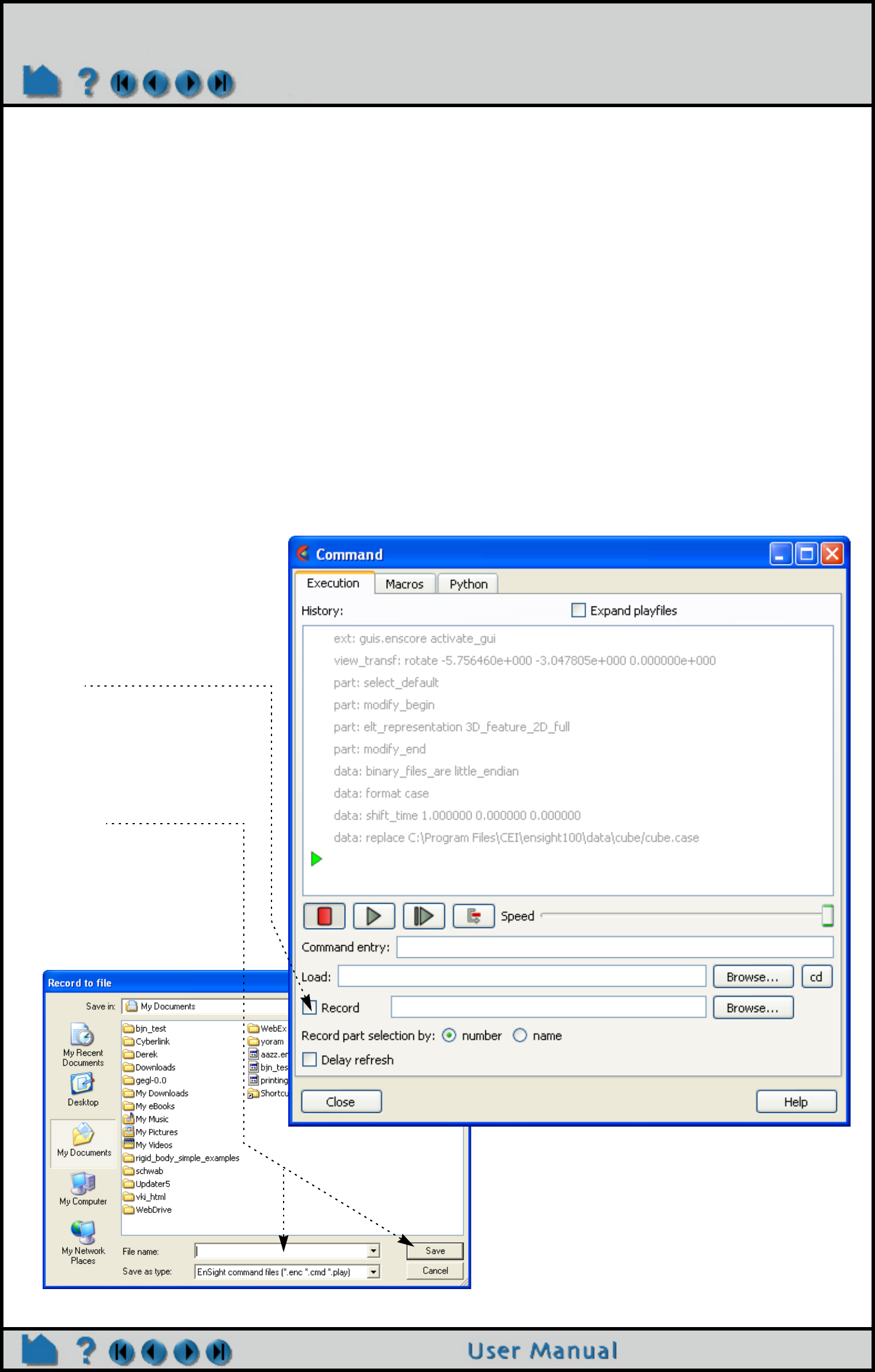
Page 97
HOW TO RECORD AND PLAY COMMAND FILES
Record and Play Command Files
INTRODUCTION
Most powerful software systems have a built-in language that provides additional levels of power and functionality to
complement and enhance a graphical user interface. EnSight is no exception. Any action that you can perform with
the mouse or keyboard has a counterpart in the EnSight command language. A sequence of commands can be
saved during a session to automate repetitive or tedious tasks. Command files can be automatically executed on
EnSight startup to initialize the system to a desired state. Execution of command files can also be bound to keyboard
keys for user-defined macros.
BASIC OPERATION
During an EnSight session, all actions are recorded and saved to a file known as the default command file. This file
name typically starts with “ensight_” and is saved in /usr/tmp on UNIX systems or C:\Documents and
Settings\<user>\Local Settings\temp on Windows systems (unless you have redefined your TMPDIR environment
variable). The default command file can be saved (and renamed) when exiting EnSight.
Recording Commands
To record a series of commands:
1. Select File > Command...
to open the Command
dialog.
2. Toggle the Record button
on.
3. A File Selection dialog
opens. Select or enter the
desired file to save
commands to and click
Save.
4. When you wish to stop
recording, toggle the
Record button off.
Note: As long as the record filename stays the
same, the record button may be toggled on and
off at any time, appending more commands to the
file.
When a new record file is selected, any existing
commands in that file will be overwritten.
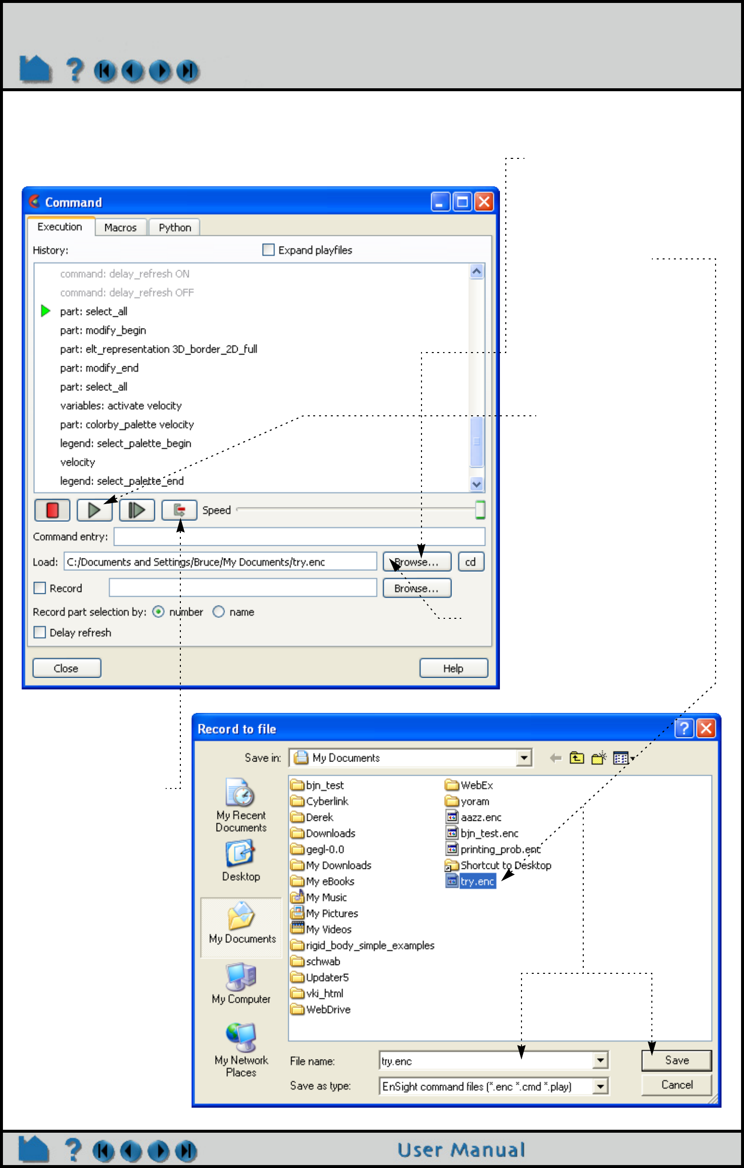
Page 98
HOW TO RECORD AND PLAY COMMAND FILES
Playing a Command File
To replay a command file:
2. Click on the Browse
button for load field.
3. A File Selection dialog
opens. Select the
desired command file
and click Save.
The command file will be
loaded and the commands
to be executed will be shown
in black below the green
current line indicator in the
History window.
4. Toggle the Play button
on.
As commands are executed,
they will be shown in gray
above the current line.
You can control command
execution by pressing the
VCR style buttons to:
stop,
start,
and single step playback
.
Once playback is
stopped, you can
use the “Skip” button
to skip commands.
Playback speed can
be controlled using
the “Speed” slider.
1. Select File > Command... to open the Command dialog.

Page 99
HOW TO RECORD AND PLAY COMMAND FILES
Playing a Command File on Startup
You can execute a command file as part of EnSight startup using the “-p command_file” option when you start
EnSight. For example,
% ensight102 -p redo.enc
where redo.enc is a command file saved in a previous session.
ADVANCED USAGE
Command files are simple ASCII text and can be edited with any text editor. To easily determine the command for a
given action, open the Command dialog and watch the list above the current line as you perform various operations.
Keep in mind that the successful execution of some commands depends on the proper state existing at the time of
execution. For example, creating a part when the parent part (as referenced by the part number) does not exist will
cause an error.
Command files can be nested: if you have a file that performs a certain task, you can “call” that command file from
another file with the “play: filename” command. When a play: command is executed, the command file being
played will be expanded in the History window, in a different color below the current line. Check the "Expand playfiles"
box to expand all played files ahead of time. When played files are nested, their commands will be shown in red,
yellow, green, blue and black respectively.
An “exit:” command will cause EnSight to quit. An “interrupt:” command will cause the command file to pause
execution and open the command dialog.
You can save the command file for the current session when you exit EnSight, or you can use File > Save >
Command from this session... to save the commands up to that point
Command language can be used to generate macros. See How To Define and Use Macros.
In addition to command files and macros, you also access the python interface through this dialog. This is explained
in detail in the Interface Manual. (see Chapter 7.1, Python EnSight module interface)
OTHER NOTES
Command files provide an excellent method of documenting problems or potential bugs encountered during your use
of EnSight. The command file can be transmitted to CEI electronically to help determine the nature of the problem.
SEE ALSO
How To Define and Use Macros
User Manual: Command Files
Interface Manual: Python EnSight module interface

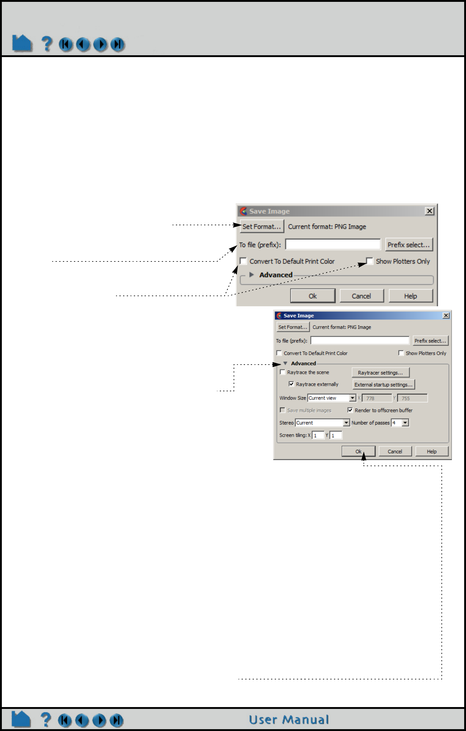
Page 101
HOW TO PRINT/SAVE AN IMAGE
Print/Save an Image
INTRODUCTION
The image displayed in the Graphics Window can be saved to disk or printed in a variety of formats. Note JPEG,
TIFF, RGB (SGI), XPM, PNG, and Postscript store single images in each file, and Apple QuickTime, EnVideo,
MPEG1, MPEG4, AVI, Macromedia Flash Video, Macromedia Flash and Animated GIF all support video streams.
See below for Saving Animations
BASIC OPERATION
Basic Still Image Operation
1. Select File > Export > Image....
2. Select Set Format... to choose the desired
output format and format options.
(See Changing the Save File Format below)
3. Set the base filename to save the image to
disk.
The Prefix select... option will allow a standard file
save dialog to be used to fill in this field.
4. Set various options:
The 'Convert to Default Print Color' option will invert
the color of the display. For example, the background
can be changed from black to white.
The 'Show Plotters Only' option will print only the
plots in the display. See the shortcut section below to
save an individual plot to a file.
5. Select any advanced options.
The 'Advanced' turndown opens the following options:
Raytrace the scene.
Retracing is an advanced rendering technique in computer graphics,
where simulation of the light transport is performed between the image
pixels, objects in the scene, and the light sources. This technique is
capable of generating high realism images, but at a much higher cost
than that of typical rasterization-based techniques. Raytracing is
suitable for rendering a wide variety of optical effects, such as reflection,
refraction, soft, shadows, etc.
Ensight offers a built-in raytracing renderer entitled Enray.
EnSight also offer both immediate and external (postpone to a specified data/time)
raytracing.
Window size: The 'Normal' option picks a window the same size as the current window. 'Full'
picks a full screen window. Other options select various NTSC and DVD standards. The
'User defined' option allows the user to select any size output image. Note: there are no
limits to the size of the image that can be rendered. Some formats cannot handle extremely
large images. EnSight may need to render the scene in multiple passes to render at larger
sizes, which can slow rendering down.
Render to offscreen buffer: EnSight can use off-screen OpenGL 'p-buffers' on graphics
cards that support them. This avoids artifacts that can show up with on-screen rendering.
Save multiple images: This option causes EnSight to save MTM files based on detached
displays.
Number of passes: sets the amount of multi-pass anti-aliasing to use: higher is better quality.
Stereo: The current scene can be rendered in stereo, even if the target system is not capable
of displaying it. 'Current' is the default and picks stereo or mono display, depending on the
current display mode. Mono and Interleaved select mono or traditional dual-image stereo.
The remaining options allow for the saving of anaglyph stereo images (seen through red/
cyan or other glasses).
Screen tiling: if these are set to values other than 1, the image will be saved as an MTM file.
The numbers specify the number of tiles in X and Y that the saved image will be subdivided
into.
7. Select OK (or Print) to save and/or print the image.
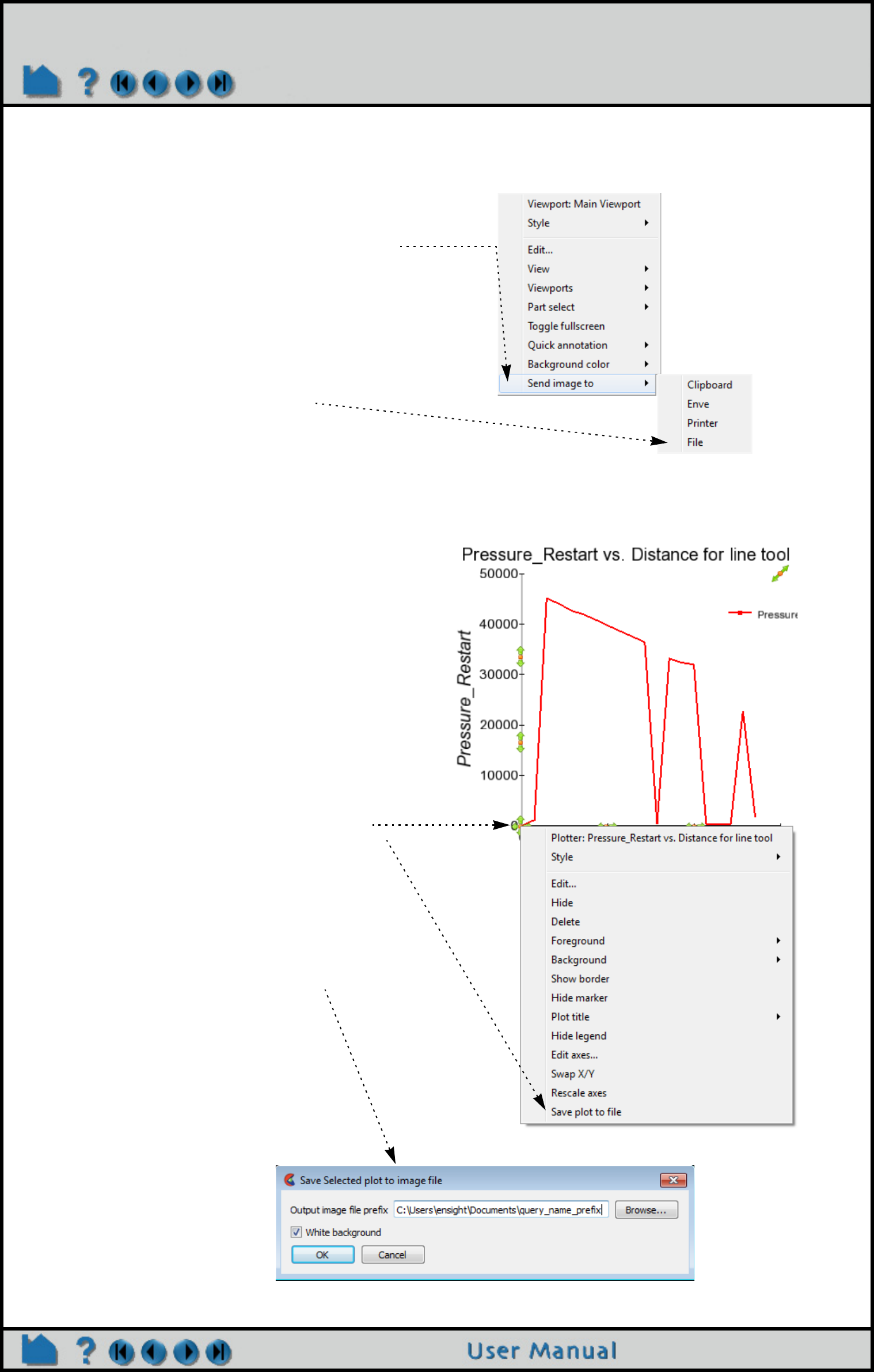
Page 102
HOW TO PRINT/SAVE AN IMAGE
SHORTCUT
1. To print or save the graphics window, right-
click on the main viewport.
In the pop up menu, choose “Send image to” and
then send it to the clipboard, to EnVe the video editor,
to your printer, or to a File.
The file option will pop up a browser to name the file
and then save it in the png format.
2. To save just a single plot, right-click on the
plot origin. If you have selected the plot
correctly then the first line of the pop up menu
will read Plotter: Name of the Plotter.
In the pop up menu choose “Save plot to file”.
This will pop up a browser to name the file and give
you the option for a white background. When you
click OK, All other items on the screen will become
temporarily invisible, and the plot will be made full
screen and saved at the pixel resolution of your
graphics screen in the png format.
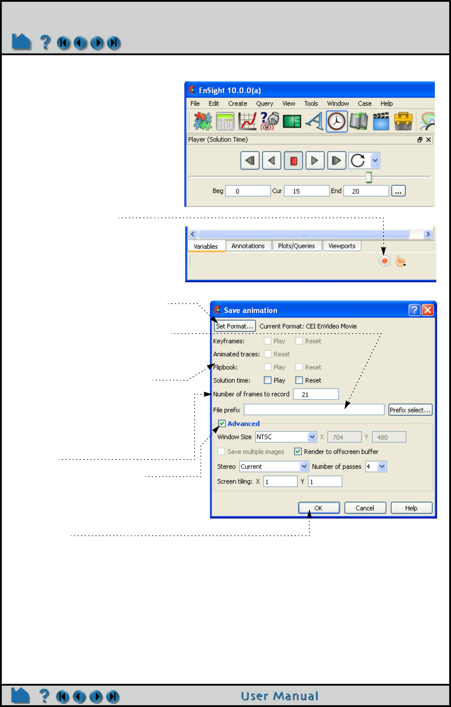
Page 103
HOW TO PRINT/SAVE AN IMAGE
Saving Animations
The current keyframe, flipbook, animated
trace, or solution time animation can be
saved to disk by following these steps:
1) Use the record button to bring up the
Save animation dialog
2) Select the format of the file to save
(See Changing the Save File Format below)
3) Set the base filename for the image.
The 'Prefix select…' option will allow a
standard file save dialog to be used to fill this
field in.
4) For various types of animations
(flipbooks, solution times and animated
traces), select if these will be animated
during the saving operation and if they
should be reset to their initial values
before beginning the save operation.
5) Set the number of frames of the animation
to save
6) Select any advanced options.
The 'Advanced' toggle brings up the following
options. These are described in detail in the
Image file saving section.
7) Selecting 'Ok' will begin recording the
animation.
Progress is displayed in the information text in
the main window. The recording can be
aborted by pressing the 'a' key while it is
progressing.
For more information, see EnSight’s keyframe animation and Flipbook animation facilities.
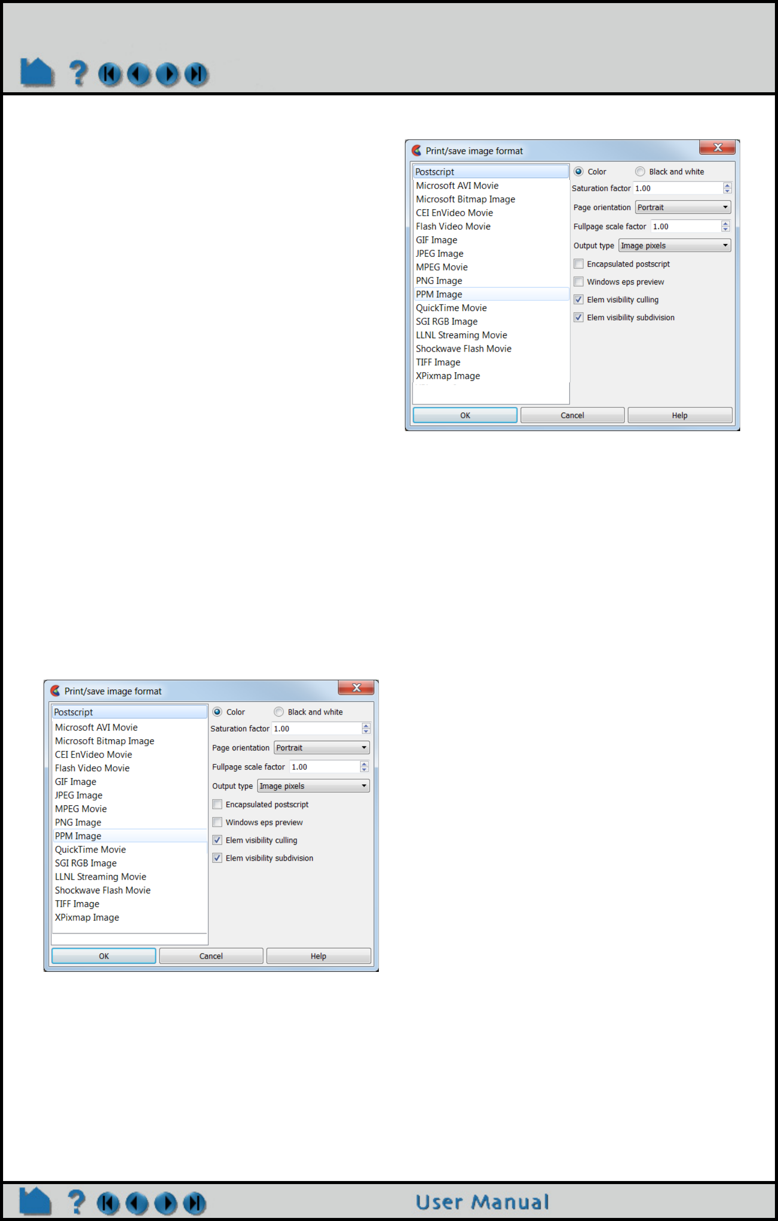
Page 104
HOW TO PRINT/SAVE AN IMAGE
Changing the Save File Format
Options for PostScript Format
The PostScript format handles primitives as sampled images (pixel data). Move/Draw and encapsulated PostScript
are no longer available as output.
Portrait or Landscape output orientation may be selected.
The page can be scaled by an arbitrary page scale factor.
This dialog is presented to the user when any of the 'Set
Format...' buttons are clicked. It allows for options
according to a specific file format. The subsequent
operations will utilize this format. The basic dialog is shown
here. The options specific to the selected format are
displayed on the right side of the dialog. Pressing the 'Ok'
button selects the new format.
The file formats are actually provided via plug-in modules
known as UDILs. It is possible for users to provide their own
formats, but the options for ones shipped with EnSight are
documented here.
Common options
There are a number of common options used by many (but not all) of the formats. These are at the top of the dialog on
the right and include:
· Color/Black and White: Selects between RGB and Grayscale output
· Saturation Factor: Set the saturation factor for color images. Full saturation is 1.0, no saturation (i.e. white) is 0.0.
· Framerate: Most animation formats allow for the rate of the frames (in frames per second, fps) to be set for the
animation to be recorded. Generally, the default is 30fps.
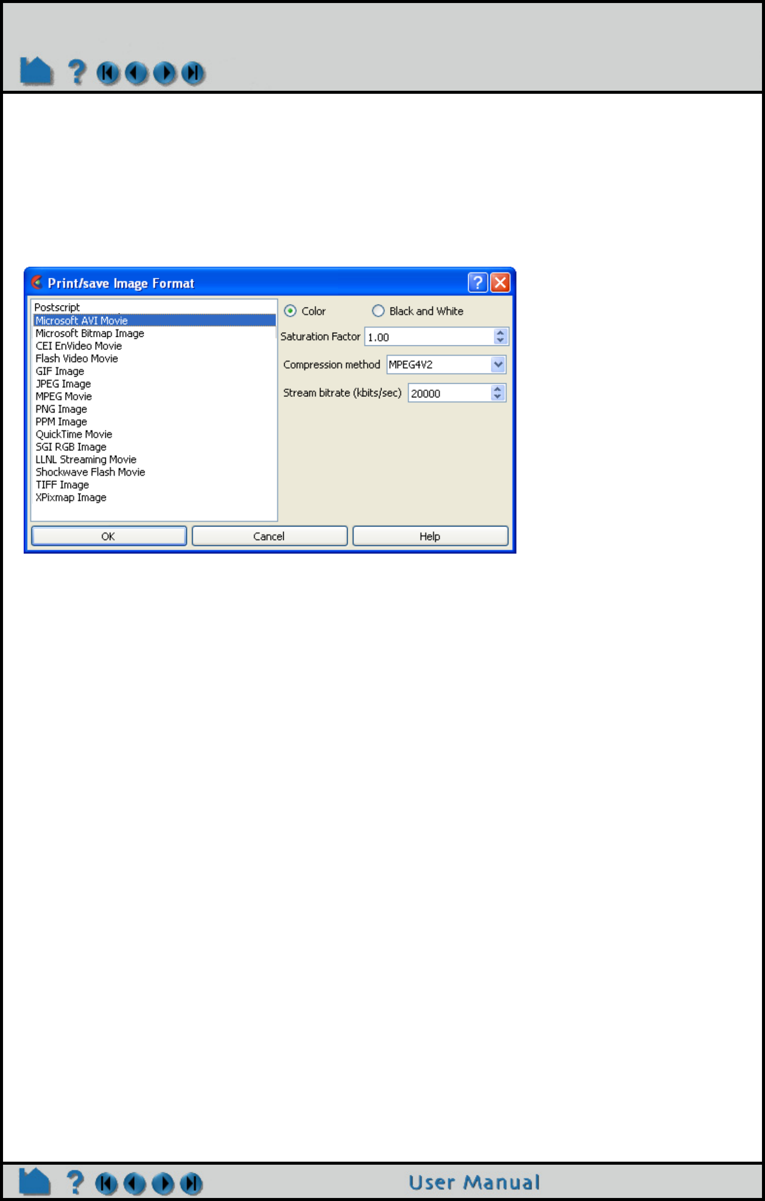
Page 105
HOW TO PRINT/SAVE AN IMAGE
Options for Microsoft AVI Format
Note: AVI files are a Microsoft standard format for movies, audio, icons, and other data types and are based on the
'RIFF' core file format.
The options for this format are a little different for Unix and 32bit Windows. For Unix and Windows 64, the only
Compression options are 'MJPEG', 'RAW' and 'MPEG4'. The only other option is the ability to set the maximum
bitrate for the MJPEG4 compression scheme. On Win32, the system installed AVI codecs will be listed as
compression options, along with options to specify the rate of keyframing, a general quality factor (0-100) and the
desired bit-rate in kilobits/second.
Uncompressed AVI files can be quite large for even small animations. You can compress these files on your Windows
PC using the EnVe utility. It is capable of reading an AVI file (or any other animation file written by EnSight) and
translating it to another format, including recompressing any AVI files.
The AVI file format can have problems porting from platform to platform as the compression schemes are not always
supported on all platforms. The MJPEG scheme is fairly well supported (Windows users need to install the latest
DirectX runtime for it) and the RAW format has size limitation for 640x480 on some platforms. In general, the Indeo
Video formats (e.g. IV41) and cvid are fairly portable and can be played by Apple's QuickTime player as well.
Options for Windows BMP Format
There are no special options (other than the Common options) for this format.
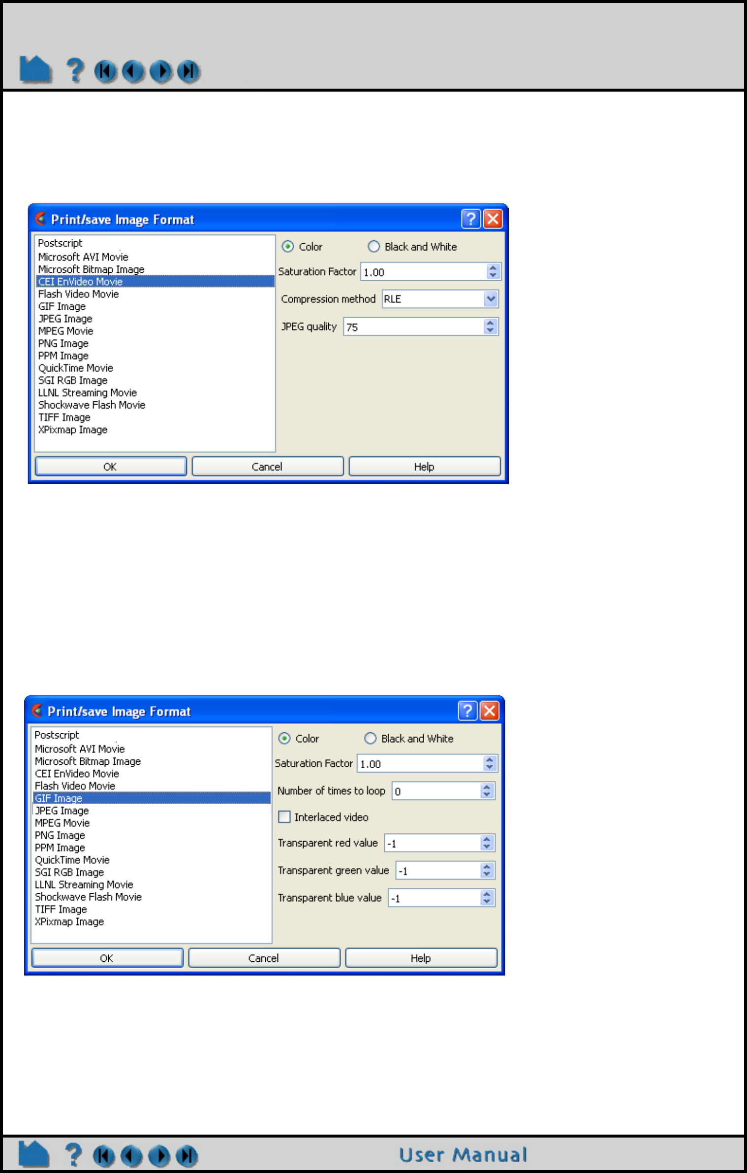
Page 106
HOW TO PRINT/SAVE AN IMAGE
Options for EnVideo Format
This format has the advantage of being one of the few that natively supports stereo image streams. It also has a
number lossless compression options and is recommended by CEI for archival/original animation output. EVO files
can be converted to any other supported format using the EnVe tool without loss of quality. This cannot be said for
other formats.
There are four compression options:
Raw - lossless, no compression, very large files.
RLE - lossless, run-length encoded imagery.
GZ - lossless, uses the 'zlib' compression scheme, good balance for machines with faster processors.
JPEG - lossy compression that uses the 'quality' option (0-100). Best compression ratio, but sacrifices some
quality.
Options for GIF Format
This format is intended for simple, low-quality output for Web pages. Most browsers will automatically playback .gif
animations without the need of any plug-in modules. The format is limited to 256color images, so the quality of the
images is poor, especially for smooth shaded images. The compression ratio can be quite high.
Options include:
Number of times to loop: sets the number of times the animation should loop before stopping
Interlaced video: optimizes for slow web connection incremental display
Transparent values: The R,G,B values (0-255) of a pixel color that should be set to "transparent" in the image.
For example, setting these to (0,0,0) will cause all black pixels in the animation to be made
transparent on playback. -1 values select that no pixel is transparent.
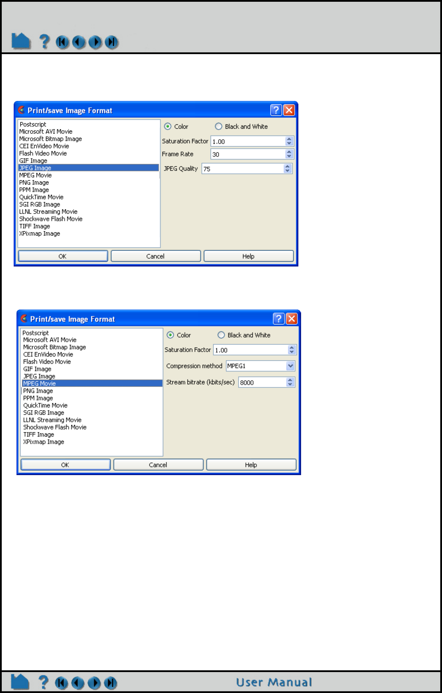
Page 107
HOW TO PRINT/SAVE AN IMAGE
Options for JPEG Format
This is a very portable, but lossy compressed format. The only option is a notional "Quality" setting that controls the
compression rate (0-100).
Options for MPEG Format
MPEG1 is a very portable but lossy standard for animations.
Two options exist for MPEG. The specific sub-type of MPEG (1/2/4) can be selected as well as a target bitrate in
kilobits per second.
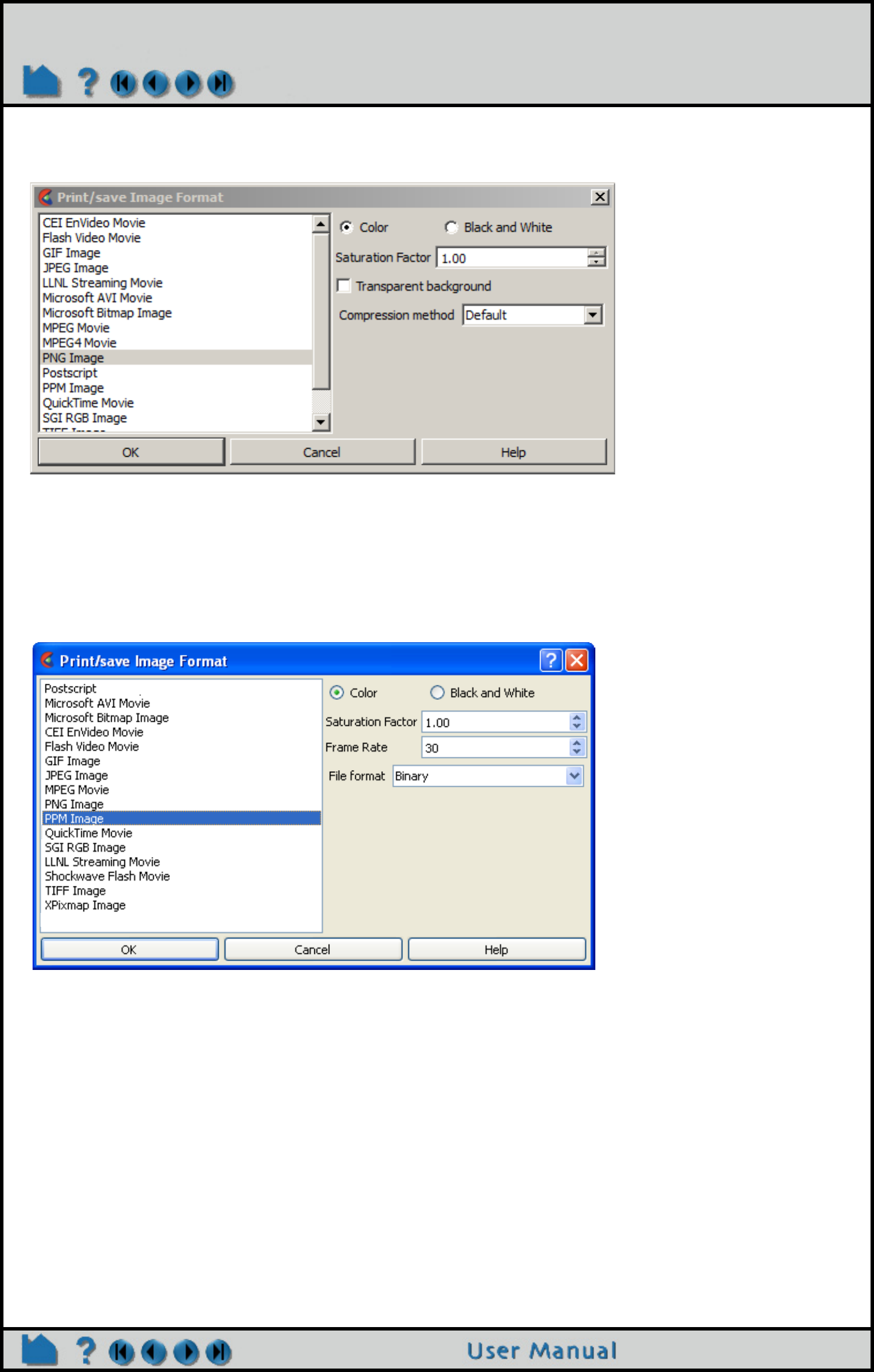
Page 108
HOW TO PRINT/SAVE AN IMAGE
Options for PNG Format
The PNG format is a lossless image format supported by many platforms and most web browsers.
There is an option to have the background be Transparent, and the option for the method for compression - which
trades off computational complexity for overall compression rates.
Options for PPM Format
The PPM format is a common lossless Unix image format that includes full color pixmaps (PPM), grayscale images
(PGM) and bitmaps (PBM).
The options allow for the selection of Binary or ASCII forms of these files.
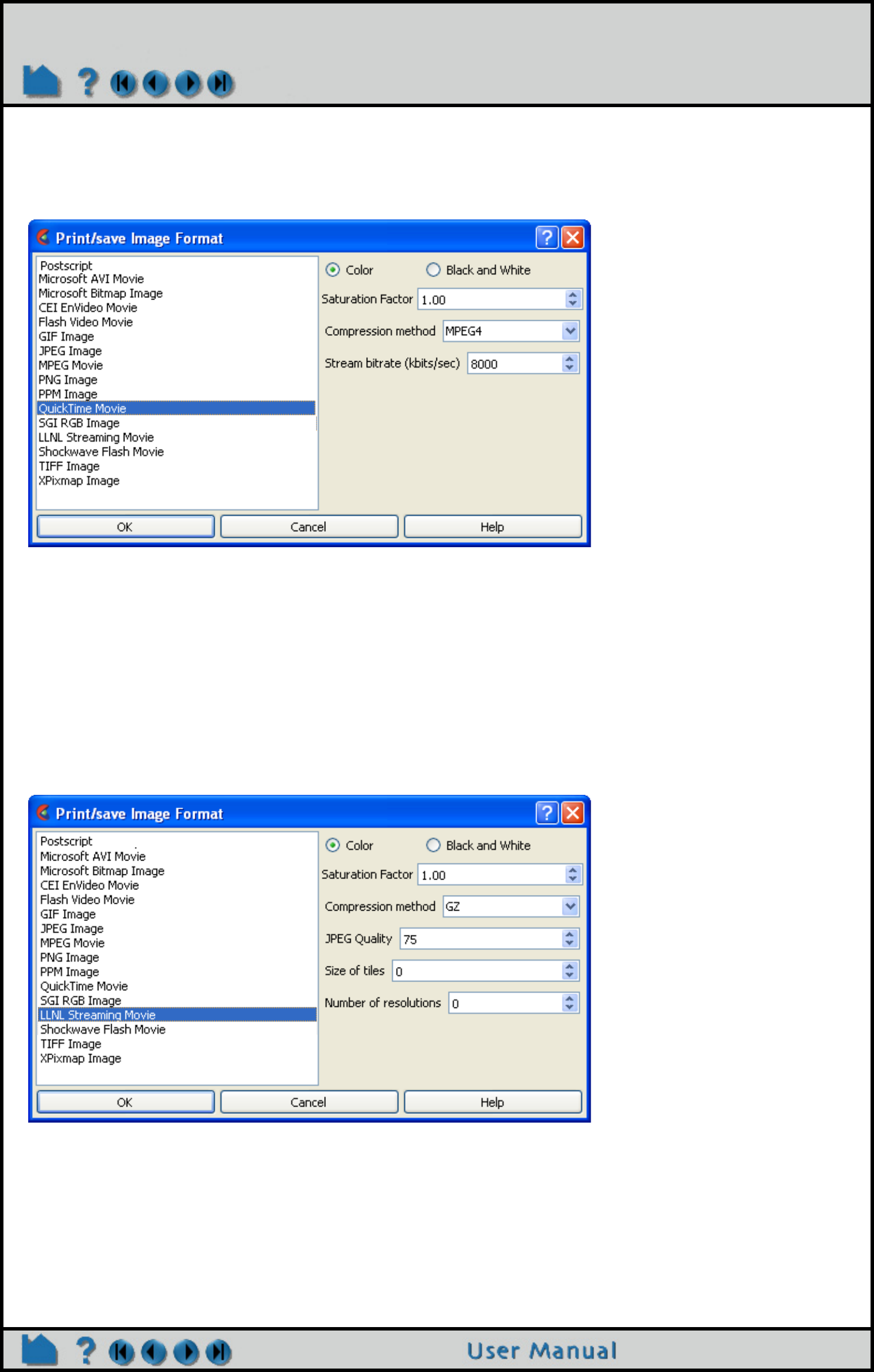
Page 109
HOW TO PRINT/SAVE AN IMAGE
Options for Quicktime Format
This is a popular animation format on the Apple Macintosh computers and Windows systems. The player can be
downloaded as part of the iTunes package from www.quicktime.com. EnSight does not support all the codecs that
QuickTime does, only the MPEG4-based compression.
The bitrate option selects the target stream rate in kilobits per second. There is a compression method option, but the
only possible value at this time is MPEG4.
Options for SGI RGB Format
There are no special options (other than the Common options) for this format.
Options for LLNL SM Format
This format was developed by Lawrence Livermore National Labs specifically for support of large, tiled displays with
dynamic pan/zoom playback. Players for the format include xmovie and blockbuster (blockbuster.sourceforge.net).
The format is internally tiled and includes multiple resolutions of the animation in the same file.
Options include:
Compression: Raw, GZ, JPEG and RLE Similar to the CEI EVO format
Quality: JPEG quality setting
Tilesize: the size of the edge of one tile. 256 uses 256x256 tiles, while 0 specifies no tiling
Resolutions: the number of lower resolution movies to include. If the original animation is 640x480 and the
number of resolutions is 2, the file will contain animations at: 640x480, 320x240 and 160x120.
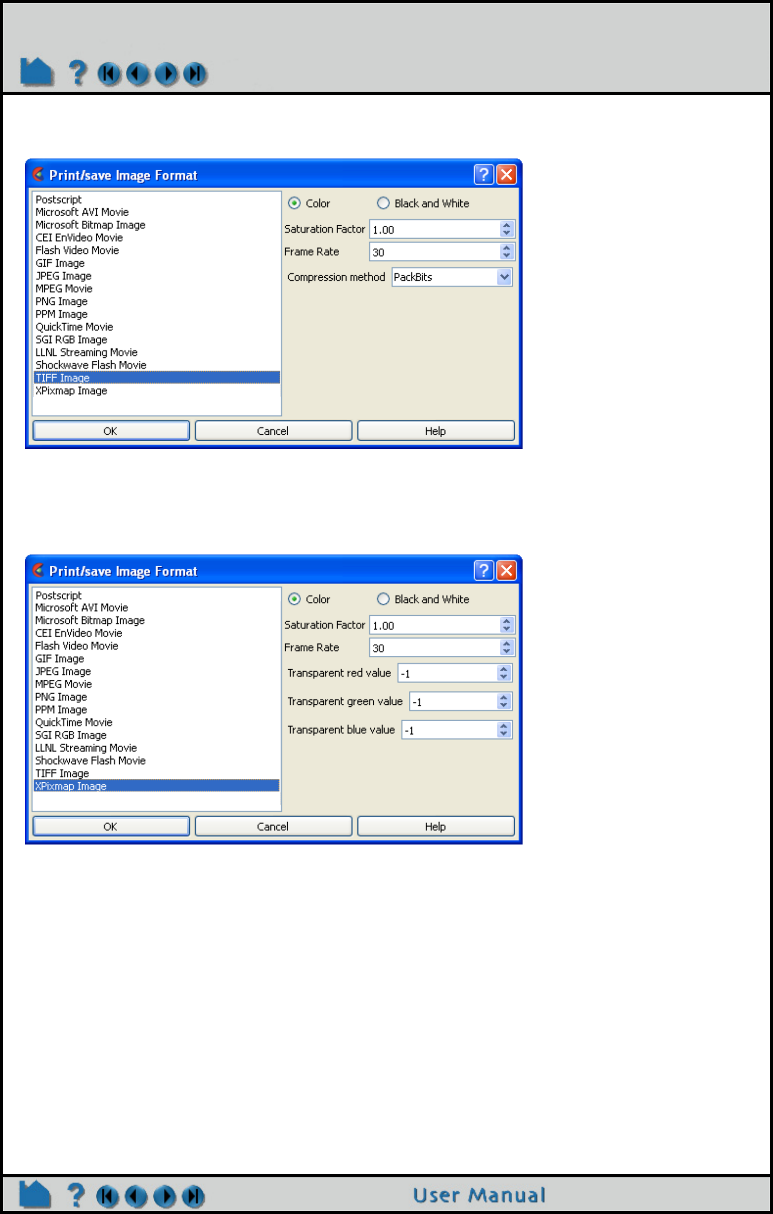
Page 110
HOW TO PRINT/SAVE AN IMAGE
Options for TIFF Format
Tiff is a very portable, lossless image file format.
The format has one option and that is the compression method. All the supported methods are lossless.
Options for XPM Format
This format is popular on Unix platforms and is generally used for icons, but can be used for any image.
The transparent options allow for the specification of R,G,B values (0-255) of a pixel color that should be set to
"transparent" in the image. For example, setting these to (0,0,0) will cause all black pixels in the image to be made
transparent. -1 values select that no pixel is transparent.
ADVANCED USAGE
There are also some excellent public domain (i.e. free) tools for manipulating images. ImageMagick is a public
domain, X-windows based program for displaying both images and animations (loaded as sequences of images) on a
wide variety of platforms. Visit the Web site
http://www.wizards.dupont.com/cristy/ImageMagick.html for more information.
One of the most popular, cross platform tools is the GIMP. This tool has nearly the full functionality of Photoshop and
can read/write all the image formats EnSight can. It is often installed by default on Linux platforms, but OSX, Windows
and other platforms are supported as well: www.gimp.org.
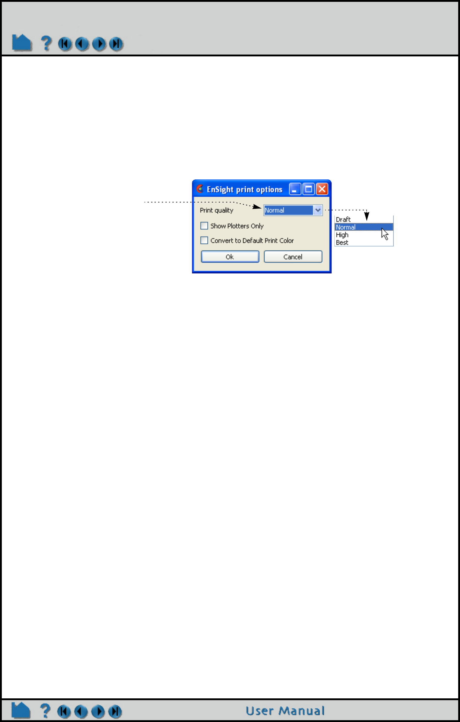
Page 111
HOW TO PRINT/SAVE AN IMAGE
OTHER NOTES
1. The file is saved or printed from the EnSight client machine - not the server.
2. The printer command should not include the file name. For example, if you normally print with "lpr -Plaser1 file.ps"
then enter "lpr -Plaser1" in the To Printer Using Command field.
3. If you toggle on Convert to default print colors, all viewport background colors are changed to white and any object
(part, viewport border, annotation, etc.) currently colored pure white (RGB = 1,1,1) will be changed to black.
Print Quality Control - Available in Print Dialog of Windows Version
SEE ALSO
User Manual: Saving Graphic Images
Note the pulldown allowing print
quality to be changed. Increases here
can greatly improve the resulting
printed image, but will cause a
slowdown in printing time.
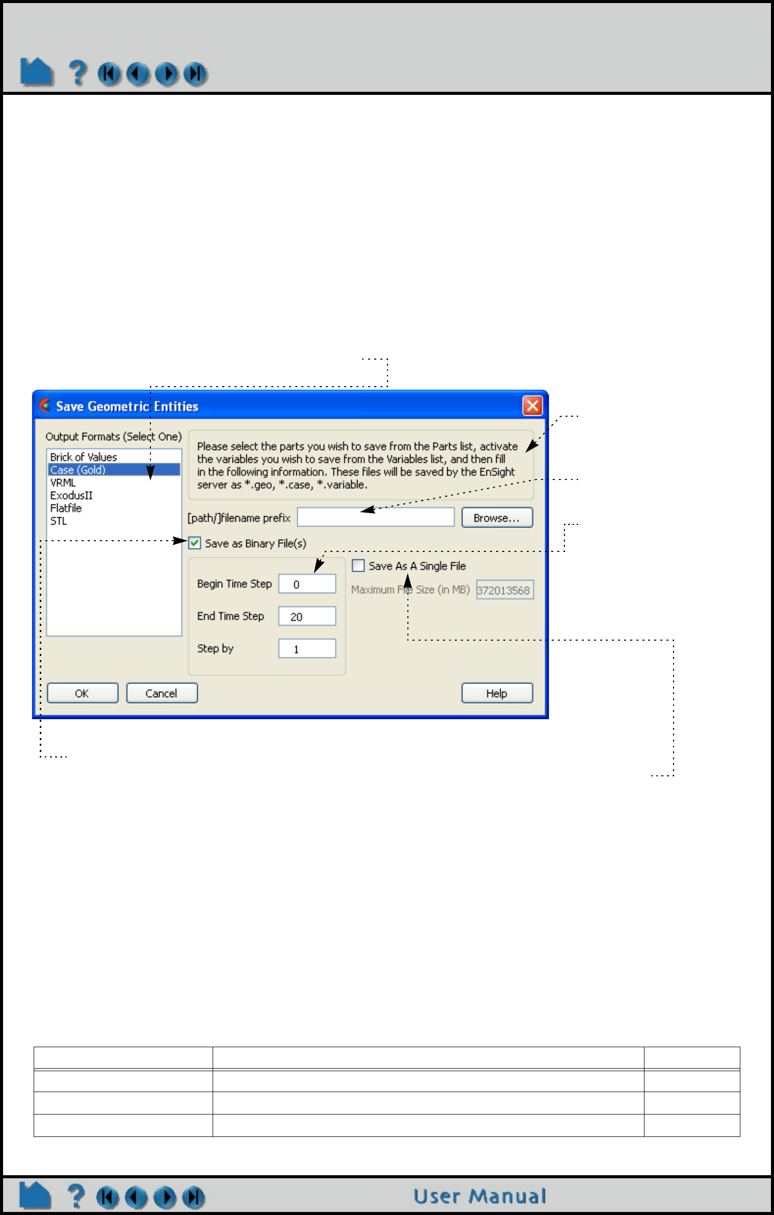
Page 112
HOW TO SAVE GEOMETRIC ENTITIES
Save Geometric Entities
INTRODUCTION
EnSight has the exporting geometric data and variable values in various formats. Several are provided by EnSight
(such as Brick of Values, Case (EnSight Gold), VRML, Flatfile, etc.). EnSight also allows the user to create their own
writer as a dynamic shared library that is loaded at runtime.
BASIC OPERATION
Saving Parts in EnSight Gold or VRML Formats
Writers have access only to the geometry of selected parts and each of their active variables. For all writers except
VRML, only parts located on the server can be saved. This includes all original model parts, as well as many of the
created parts (such as 2D-clips, Elevated Surfaces, Developed Surfaces, and Isosurfaces).
The VRML writer saves all the visible parts on the client in their current visible state except for Parts which have limit
fringes set to transparent. The VRML file will be saved on the client.
Output in the EnSight formats is intended to provide a method to save both model and created parts (with active
variables) for subsequent reuse with EnSight. VRML output is intended for export to other systems.
Most World Wide Web browsers come with either built-in or plug-in support for VRML file viewing.
There are some important differences in how EnSight saves parts according to format chosen.
Case (EnSight Gold) VRML
Which parts are saved? All parts currently selected in the Main Parts List (except those indicated below) All visible parts
Saved from where? EnSight server EnSight client
Which parts cannot be saved? Any client-based parts: contours, vector arrows, particle traces, profiles.
1. Select the Part(s) that you wish to export in
the main part list.
2. Select File > Export > Geometric Entities...
3. Be sure the desired output format is selected.
For EnSight Gold only:
7. Toggle to save as binary files or not.
8. If the dataset is transient you can choose to save the multiple timesteps in one file
(one file per variable). If you choose this option, you can also specify the maximum
file size.
9. Click Ok.
4. Follow the
instructions given.
5. Enter a file root name.
6. If the dataset is
transient, specify the
beginning, ending,
and step values.
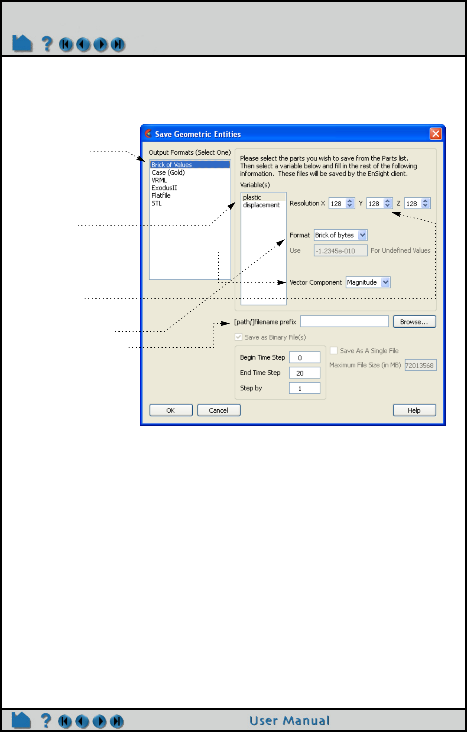
Page 113
HOW TO SAVE GEOMETRIC ENTITIES
Saving Data in Brick of Values Format
Brick of Bytes and Brick of Floats is intended to give you an interface mechanism to volume rendering codes for your
3D Part(s).
When you click the Okay button the selected 3D parts are discritized to the resolution indicated using the box tool as
the bounds and orientation (x/y/z resolution refers to the x/y/z directions for the box tool).
For Brick of Bytes (BoB) format a value of 0 is reserved for undefined (i.e., the discritized point found no variable
information). The value of 1 is tied to all variable values less than or equal to the minimum palette value tied to the
variable chosen while 255 is tied to all values greater to or equal to the maximum palette value.
For Brick of Floats (BoF) format undefined values are assigned the undefined value indicated in dialog.
Both BoB and BoF files are written out without any metadata - only the values for the discritized points is written. The
order of the data is according to the following pseudo code:
num_values = 0
for(z=0; z<z_resolution; ++z) {
for(y=0; y<y_resolution; ++y) {
for(x=0; x<x_resolution; ++x) {
value_array[num_values] = value_at_this_location
}
}
}
write(file_name,value_array)
3. Be sure Brick of Values
is selected as the
Format type.
4. Follow the instructions
given.
5. Select the desired
variable.
6. If the variable is a
vector, select the
component desired.
7. Select the sampling
resolution.
8. Select the sampling
format, Brick of Bytes
or Brick of Floats.
9. Enter a file root name.
10. Click OK.
1. Select the 3D Part(s) (only 3D) to export
2. Select File > Export > Geometric Entities...
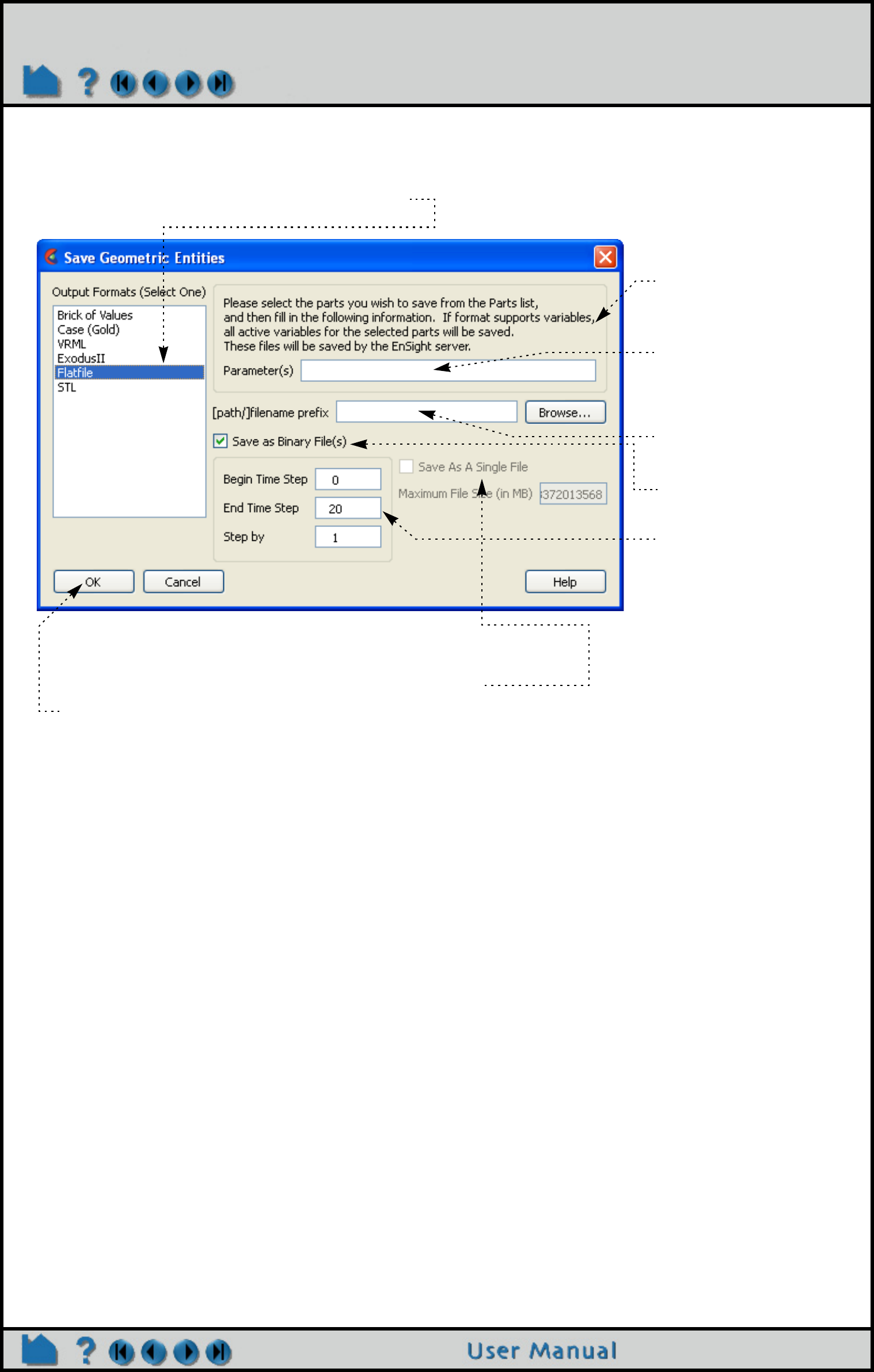
Page 114
HOW TO SAVE GEOMETRIC ENTITIES
Saving Data in User Defined Writer Formats
The user-defined writers can call the routines of an EnSight API to retrieve, for example, nodal coordinates, node ids,
element ids of parts selected in the Parts window, to be passed by value to be used, manipulated and/or written out in
any format desired. The User-defined writer dialog includes a Parameter field that allows the passing of text into the
writer from the. This text could contain extra options which the writer understands.
Several example writers (including source code header files, Makefile and the corresponding shared library) are
included to demonstrate this capability.
The Case (Gold) Lite writer is included to demonstrate how to exercise most of the API and output a subset of the
Case (Gold) format. Complex numbers and custom Gold format are not supported with this writer. The Case (Gold)
writer ignores the Parameter field. While the writer is not compiled, the source code of this writer, the required header
files, and the Makefile are included.
The Flatfile user-defined writer is designed to demonstrate the output of selected part nodal data (coordinates & IDs)
as well as active variable values (scalar and/or vector only) in a comma delimited format easily imported into other
applications. If any of the keywords ‘ANSYS’ or ‘force’ or ‘body’ is entered into the Parameter field, then Flatfile will
output an ANSYS body force file.
The STL user-defined writer is designed to write out the border geometry in the form of triangular 2D elements of the
selected part(s) at the beginning timestep. The end time and the step time are ignored. The STL format does not sup-
port multiple parts in a single binary file, but does support multiple parts in a single ASCII file. Therefore, if multiple
parts are selected and ascii is checked, the STL writer outputs an ascii file with the border of each of the parts. If mul-
tiple parts are selected and binary is checked, the STL writer outputs a binary file containing a single border of the
multiple parts. The STL writer only saves the beginning timestep and ignores the End Timestep and Step By fields.
The STL writer ignores the Parameter field.
1. Select File > Export > Geometric Entities...
2. Be sure the desired output format is selected.
7. If the dataset is transient you can choose to save the multiple
timesteps in one file (one file per variable). If you choose this
option, you can also specify the maximum file size.
8. Click Okay.
3. Follow the
instructions given.
4. If the writer accepts
parameters, enter any
desired ones in the
Parameter(s) field.
5. Enter a file root name.
6. Toggle to save as
binary files or not.
7. If the dataset is
transient, specify the
beginning, ending,
and step values.
Page 115
HOW TO SAVE GEOMETRIC ENTITIES
There are some important differences in how EnSight saves parts according to format chosen.
More user-defined writers may be distributed with EnSight in the future.
ADVANCED USAGE
Created Parts
Created parts are saved as changing connectivity. One situation where this might become important is if you choose
to save some very large model parts that happen to be static and some created parts that are changing connectivity
parts together into one case gold file. All of the parts must be saved as changing connectivity (because the changing
geometry attribute is global). Thus you will find that the combined geometry file for all parts is saved for every
timestep, even though the large static model parts don’t really change. Also when this saved file is reloaded, every
model part is reconstructed at every timestep as if it were changing connectivity, greatly increasing the disk space,
the I/O, and the geometry reassembly, and limiting functionality (e.g. cannot interpolate between the timesteps). A
better solution to this situation is to save the changing connectivity created parts separately as a case gold file, and
then the model parts as a separate case gold file and then load them as two separate cases into EnSight.
Rigid Body Transformations Present
Since EnSight does something special with the model timeset when rigid body information is read (via the rigid_body
option in the casefile, or from a user-defined reader with rigid_body reading capability), you need to be aware of a few
important issues. EnSight assumes that the rigid body timeset encompasses the normal geometry timeset, and it
replaces the normal geometry timeset with the rigid body timeset - thus the following occurs when using this option.
1. If any created parts are in the list to be saved, EnSight will save as true changing coordinates. Namely, a geometry
file containing the coordinates for each part will be saved at each time. Upon re-reading this model, you will be able to
duplicate all actions, but it will be done as a true changing coordinate model. In other words, the original rigid_body
file nature will not be duplicated.
2. If the original model had static geometry and rigid body file information - and you do not have any created parts in
the list to be saved - saving will preserve the single static geometry and rigid_body file nature of the model. However,
if the original model had changing geometry, or if variables have been activated - the number of geometry/variable
files saved will be according to the rigid body timeset. This timeset often has many more steps than the original time-
sets - so be wise about the number of steps you write. It is often important to use the “Step by” option to control this.
3. Because of the things mentioned in 1 and 2 above - if you want to use the save geometric entities option in EnSight
to “translate” a rigid body model from a different format into the EnSight format, you may want to consider the follow-
ing process. First, read in the model without the rigid body transformations, activate the desired variables, and save
the model. Second, read in the model with the rigid body transformations, do not activate any variables, and save the
model (with a different name). Edit the Casefile of the first model to use the model: and rigid_body: lines of the
second casefile instead of the first casefile.
SEE ALSO
User Manual: Saving Geometric Entities
Readme file is $CEI_HOME/ensight102/src/writers/README.txt
User Defined Writers (UDW)
Which parts are available to the UDW? All parts currently selected in the Main Parts List (except those indicated below)
Where are the available parts located? EnSight server
Which parts are unavailable to the UDW? Any client-based part: contours, vector arrows, particle traces, profiles
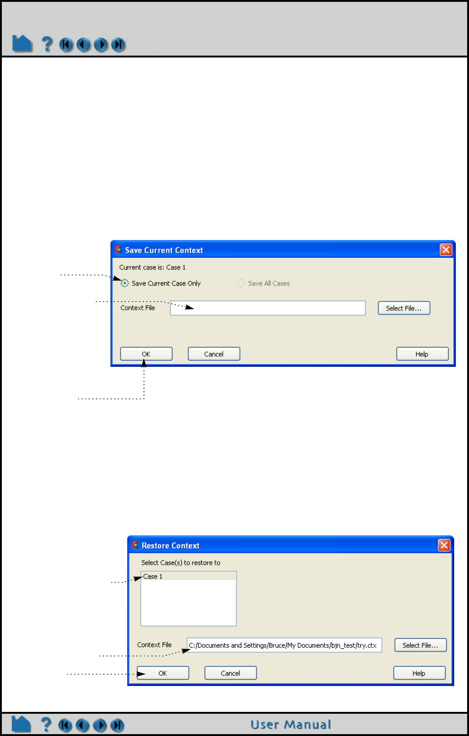
Page 116
HOW TO SAVE/RESTORE CONTEXT
Save/Restore Context
INTRODUCTION
EnSight context files can be used to duplicate the current EnSight state with the same or a different, but similar,
dataset. The context file works best if the dataset it is being applied to contains the same variable names and parts,
but can also be used when this is not the case.
BASIC OPERATION
An EnSight context consists of a set of files: the context file itself as well as associated palette, view, and keyframe
animation files. The names of the associated files will be that of the context file with a standard extension.
Saving a Context
Restoring a Context
Three options:
1) Start EnSight and restore a context as described below. This will recreate the parts of the original dataset
and restore them to their saved condition.
2) Start EnSight, read a new dataset, cancel the part loader without creating parts, and restore a context as
described below. This will create the parts of the new dataset (mapping as directed) and restore the
context of the original dataset.
3) Start EnSight, read a new dataset, create the desired parts, and restore a context as described below. This
will do the mapping (as directed) of parts and restore the context of the original dataset.
1. Select File > Save > Context... to open the Save Current Context dialog.
2. Toggle Save
Current Case
Only or Save All
Cases.
3. Enter a name for
the Context File.
You can set the
directory for the
Context File by
clicking the Select
File... button to
open a standard
File Selection
dialog.
4. Click Okay.
1. Select File > Restore >
Context...
2. Select the case to
restore the context to.
Note: If the context file
contains information for
multiple cases, ignores the
selection
3. Enter or select the
desired context file
4. Click OK.

Page 117
HOW TO SAVE/RESTORE CONTEXT
OTHER NOTES
The same part names (and variable names) do not have to exist in the new case. If this situation arises, a pop-up
dialog will appear where you will be asked to match the part names (or variable names) from the context file with the
parts (or variables) from the new case. This dialog is not available in batch mode. Therefore, you can’t use a context
file that needs matching in batch mode. If the number of parts between the two datasets match, then no mapping of
parts occurs and the parts will end up renamed to match the original case.
When restoring context files with multiple cases, the needed cases will be started, if needed, according to the
connection scheme of the current run of EnSight.
Flipbook animations are not restored using the context file because it is unknown at the time the context file is
created what state existed when the flipbook was saved.
If data is not read before restoring the context file, the data that was used when the context file was saved will be
loaded.
Context files use EnSight’s command language and other state files (such as palette, view, and keyframe animation)
to recreate the parts, variables, and view state.
SEE ALSO
User Manual: File Menu Functions
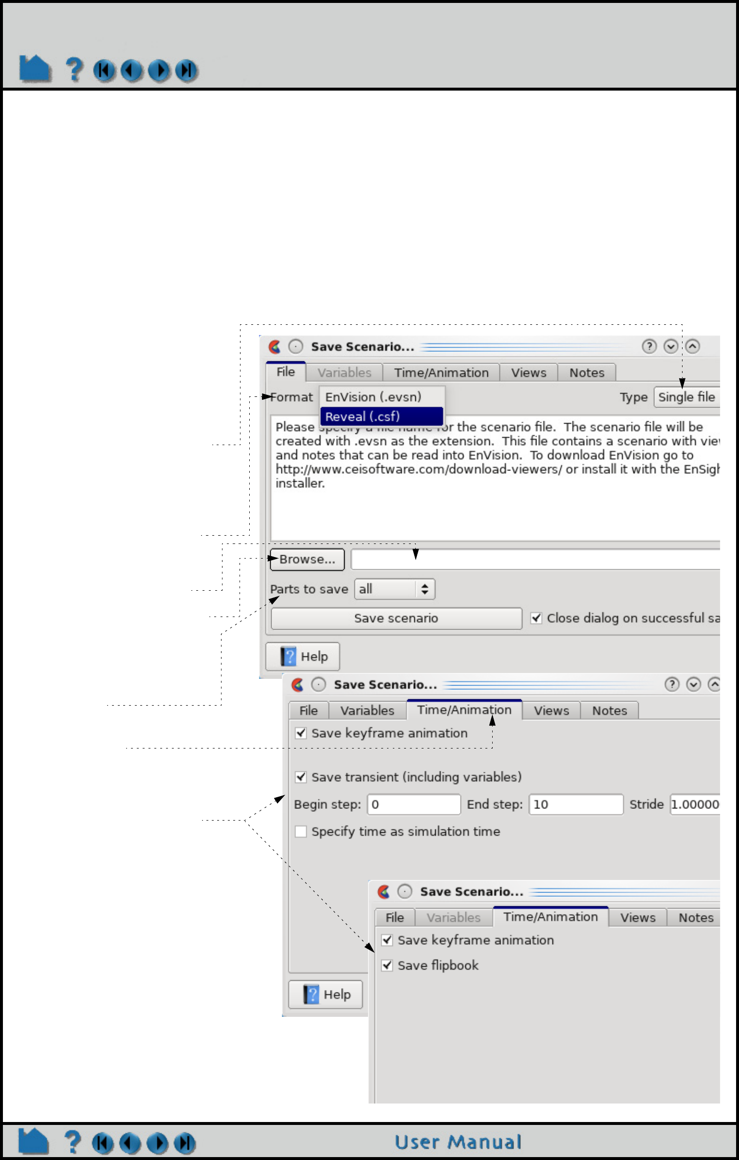
Page 118
HOW TO SAVE SCENARIO
Save Scenario
INTRODUCTION
Scenario files are used by CEI’s viewer products which are capable of viewing all geometry (such as parts,
annotation, plots, etc.) that EnSight can display, including flipbook, keyframe, and particle trace animations.
A “scenario” defines all visible entities you wish to view with EnVision or Reveal and includes any saved views and
notes that you want to make available to the viewer user.
BASIC OPERATION
1. Create the display you want to
share with the EnVision or
Reveal user.
2. Select File > Export >
Scenario... to open the
Save Scenario dialog.
3. Select Single File to save a
scenario file only, or
Project to save the
scenario, jpg image file,
and EnSight context file.
4. Choose EnVision(.evsn)
or Reveal (.csf) format.
5. Enter a name for the
Scenario file/directory.
Click the Browse... button
to open a standard File
Selection dialog.
6. Select whether all, visible
or selected parts will be
included.
7. Select the Time/Animation
Options tab
and select the flipbook,
keyframe, transient and/or
particle trace animations.
Available options depends
on output format chosen
under the File tab.
8. Save the scenario.
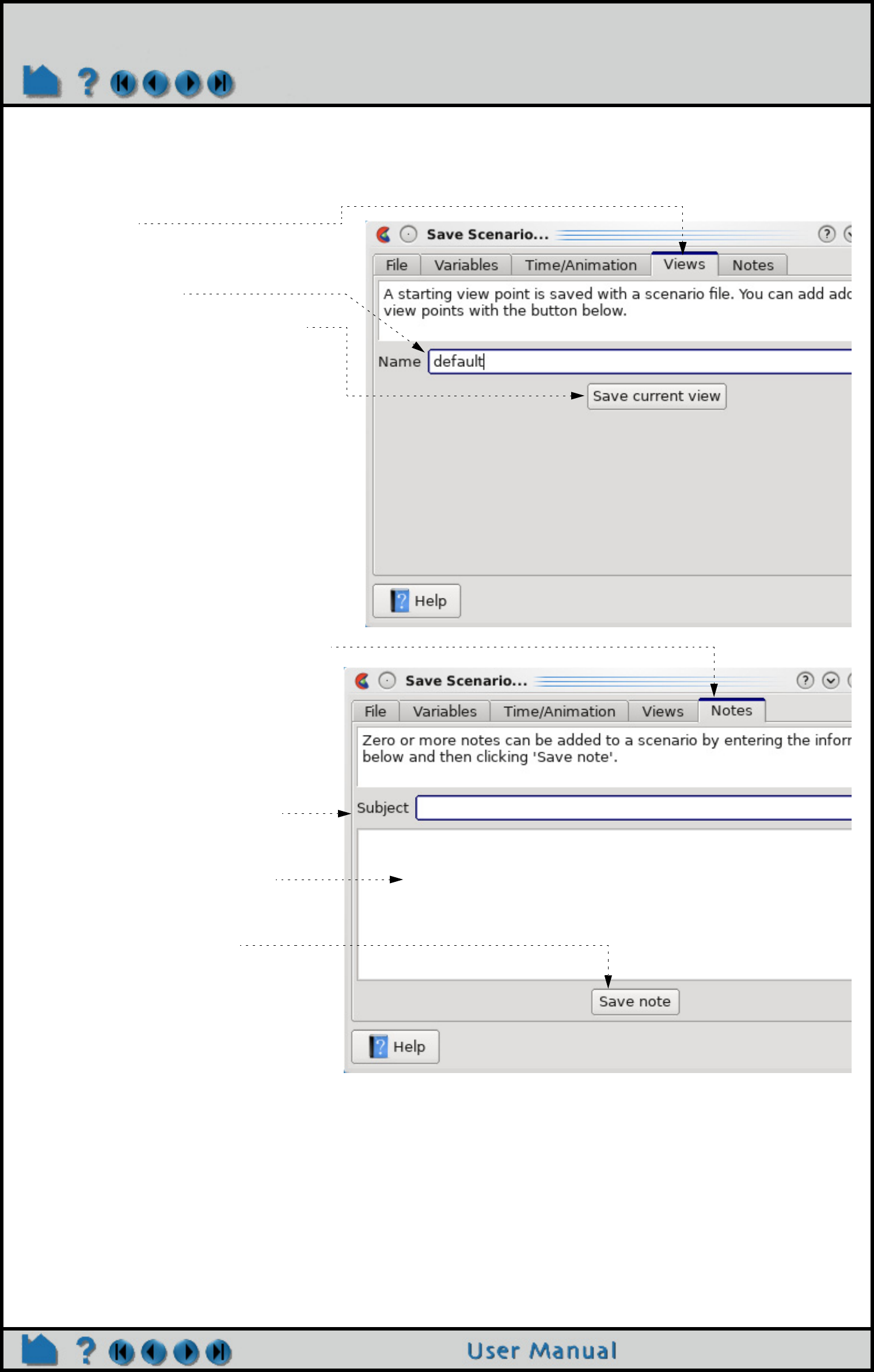
Page 119
HOW TO SAVE SCENARIO
ADVANCED USAGE
After the scenario has been saved, you may add additional views, as well as notes.
9. To Save additional views, click the Views
tab.
10. Manipulate the view as desired.
11. Name the view.
12. Click Save current view button.
You can repeat steps 10 through 12 as
desired.
13. To save notes, click the Notes tab.
14. Enter a subject for the note.
15. Type in the text of the note.
16. Click Save note button.
You can repeat steps 14 through 16 as
desired.
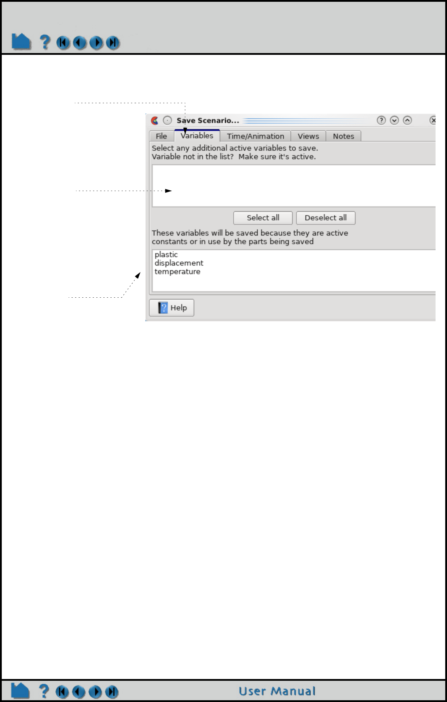
Page 120
HOW TO SAVE SCENARIO
OTHER NOTES
The Reveal format (.csf) as of EnSight 10.2 is on life support only and will be phased out entirely by the next major
release. The Reveal code is not distributed with EnSight. EnVision and Reveal are geometry viewers only. As such
they are not capable of creating any new variables nor parts. In addition, EnVision Standard does not support
changing timesteps - consider the flipbook capability instead. However, EnVision Pro can change timesteps
(assuming transient data has been saved to the scenario file).
Note: Users without an EnSight license may download EnVision separately as a free product.
SEE ALSO
User Manual: Scenario Files
17. Variables can be saved in the scenario
file, under the Variables tab.
Any variables not already used by
the parts being saved, will show up
here.
Select any desired.
Those variables already being
used, will show up here, and will
be saved.
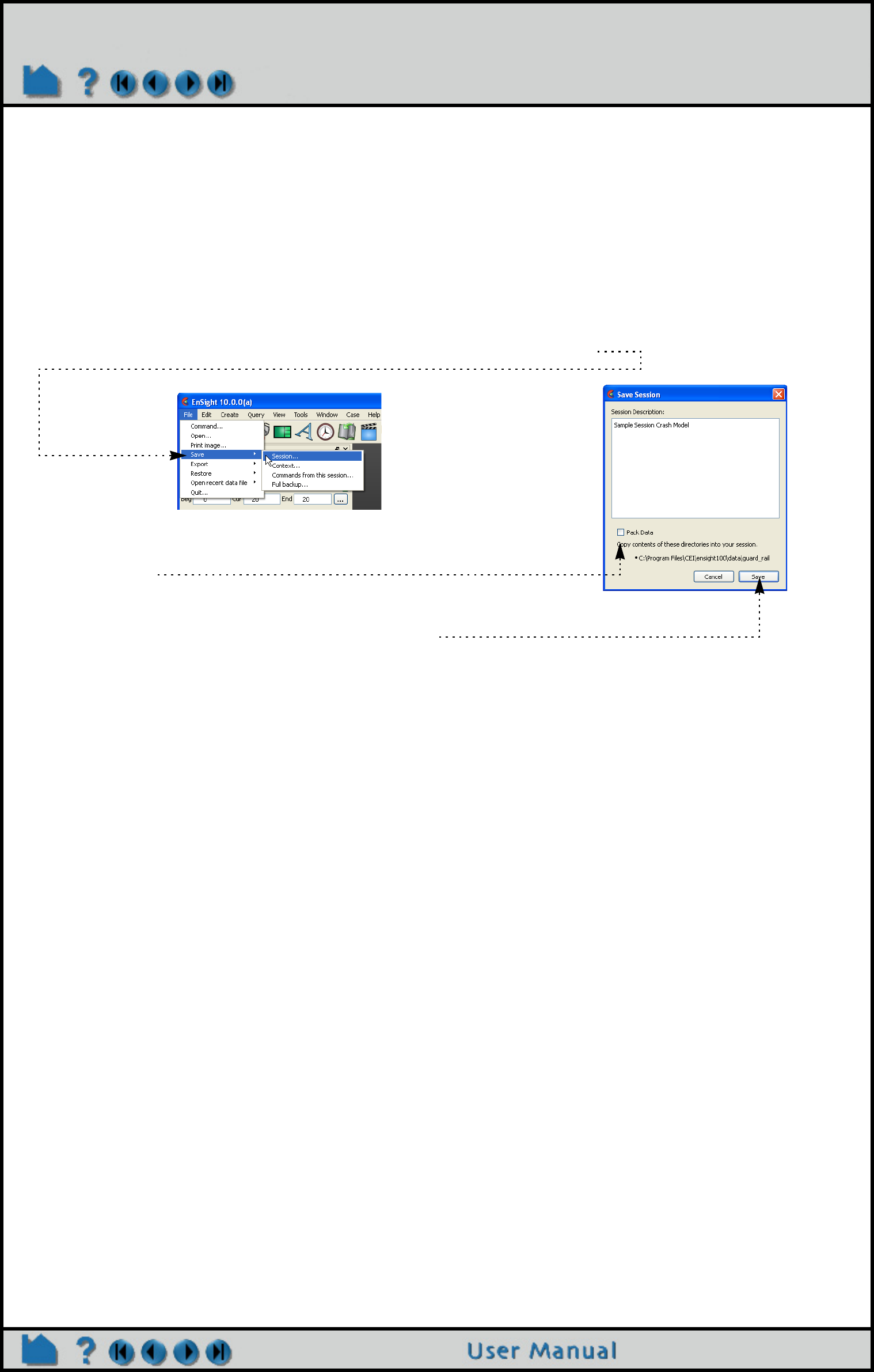
Page 121
HOW TO SAVE/RESTORE SESSION
Save/Restore Session
INTRODUCTION
EnSight session file is a single file used to restore an EnSight state. When a session file is restored, the current
case(s) are deleted, and new case(s) from the session file are loaded and restored to the saved state.
BASIC OPERATION
Saving a Session
Restoring a Session
Three options:
1) The 'Welcome to EnSight' screen on startup displays your most recent Sessions. Just double click on the
desired session to load the data and restore it.
2) Mac and Windows users can double click any EnSight session file (ending in .ens) and the file will restore.
3) Any time during your EnSight session you can browse for a session file from the EnSight main menu as
follows: File > Restore > Session.... and just located the session file using the standard file access
window.
OTHER NOTES
If you already have data loaded and restore a session, EnSight will delete all the cases, start anew and then restore
the session.
If you are restoring a session file containing information for multiple cases, then all of the cases will be restored.
When restoring session files with multiple cases, the needed cases will be started, if needed, according to the
connection scheme of the current run of EnSight.
Flipbook animations are not restored using the session file because it is unknown at the time the session file is
created what state existed when the flipbook was saved.
All Session files are machine and operating system independent. However the data file(s) used in a non-packed
session file must remain in same directory in order to find the data file(s). In contrast, Packed Session files include all
the data files therefore can be moved to a different directory. The tradeoff is that Packed Session files can become
quite large.
Also, the restoring platform must include all the data readers necessary to read the data format(s) contained in the
session.
SEE ALSO
User Manual: File Menu Functions
1. Select File > Save > Session... to open the Save Session dialog.
2. Toggle ‘Pack Data’ if you wish to include contents from listed
directories (including the data itself) in the session file (for
portability).
3. Click ‘Save’ button to open a file save browser and name
the session file (use .ens suffix) and click ‘Save’.
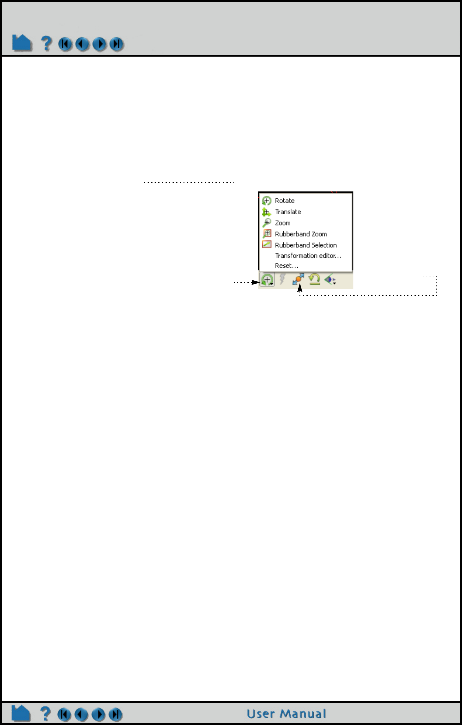
Page 122
HOW TO ROTATE, ZOOM, TRANSLATE, SCALE
Manipulate Viewing Parameters
Rotate, Zoom, Translate, Scale
INTRODUCTION
EnSight provides visual only (only the visual elements on the client are changed) global transformations (rotation,
translation, and zooming) to permit user manipulation of all parts simultaneously in the Graphics Window. The
transformations can either be performed interactively with the mouse, or precisely by entering explicit values. The
mouse buttons can be user-programmed to perform different transformations.
BASIC OPERATION
To rotate:
1. Click the rotate icon.
2. Move the mouse pointer into the Graphics
Window.
3. Click and hold the left mouse button and:
• move the mouse left and right to rotate
about the screen Y (vertical) axis, or
• move the mouse up and down to rotate
about the screen X (horizontal) axis, or
• hold down the Control key and move the
mouse left and right to rotate about the
screen Z axis.
4. Press the F1, F2 or F3 keys for 45 degree
rotation about the X, Y, or Z axis,
respectively. Hold the Control key down for -
45 degree rotation. (Note: cursor must be in
the EnSight window for F keys to work)
5. To put the geometry in free rotation mode,
put the cursor in the EnSight graphics
window Press the F4 key, and left click in the
graphics window and drag the mouse to set
the view in motion and then let the left
mouse button up. The geometry will
continue to freely rotate according to the
speed of your drag. Press F4 to stop the free
rotation.
To translate:
1. Click the translate icon (or use the middle
mouse button in steps 2 and 3 (default)).
2. Move the mouse pointer into the Graphics
Window.
3. Click and hold the left mouse button and:
• move the mouse left and right to translate
in the screen X (horizontal) direction, or
• move the mouse up and down to translate
about the screen Y (vertical) direction, or
• hold down the Control key and move the
mouse left and right to translate in the
screen Z direction.
Note that you can open the Transformation
Editor dialog and the Reset Tools and
Viewport(s) dialog here as well.
The Graphics window transforms icon on the Tools Icon Bar controls the operation of the left mouse button (by
default) in the Graphics Window:
To zoom:
1. Click the zoom icon (or use the middle mouse
button in steps 2 through 5 (default)).
2. Move the mouse pointer into the Graphics
Window.
3. Click and hold the left mouse button.
4. Drag down to zoom in or drag up to zoom out.
5. Hold down the Control key and move the mouse to
pan.
To rubber-band zoom:
1. Click the rubber-band zoom icon.
2. Move the mouse pointer into the Graphics
Window and position it at one corner of the
desired viewing region.
3. Click and hold the left mouse button.
4. Drag to include the desired viewing region. An
outline of the region will appear as you drag.
To rubber-band zoom using the selection tool:
1. Click the Selection Tool Rubber-band Positioning
icon.
2. Move the mouse pointer into the Graphics
Window and position it approximately at one
corner of the desired viewing region.
3. Click and hold the left mouse button.
4. Drag to include the desired viewing region. An
outline of the region will appear as you drag.
5. Manipulate the tool as desired, by clicking at the
center and dragging to a new position or clicking
on any corner and resizing. (Note that the aspect
ratio will be preserved as indicated by the dotted
lines within the tool.)
6. Click the zoom (magnifying glass) indicator at the
top left of the tool.
Fit the geometry to
the viewport
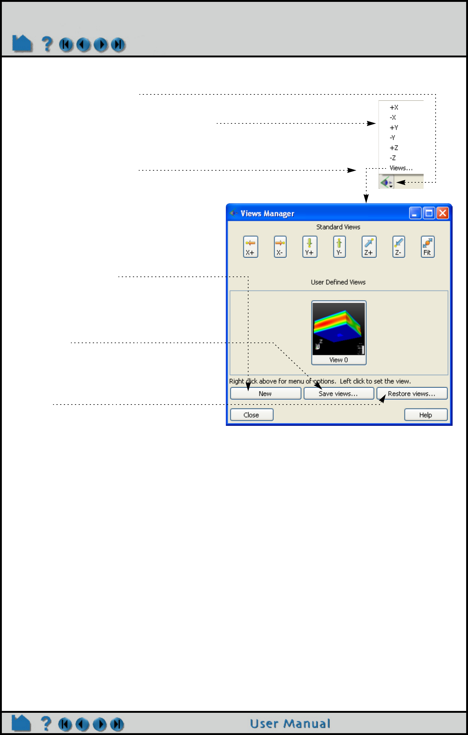
Page 123
HOW TO ROTATE, ZOOM, TRANSLATE, SCALE
Note that zooming actually changes the location of EnSight’s virtual “camera” or “look-from” point. Zooming in moves
the camera closer to the object; zooming out moves it farther away. The look-from/look-at points can also be edited
explicitly.
If you have multiple viewports visible, each one can be manipulated independently. To transform in a different
viewport, place the mouse pointer within the bounds of that viewport before you click the left mouse button.
You can reset transformation parameters (as well as tool and frame transforms) by clicking the Reset.... See How
To Reset Tools and Viewports for more information.
The Fit button is useful in causing the currently visible parts to be centered and zoomed to fit within the selected
viewport.
The Graphics window view orientation icon can be used to quickly view the scene
from the global axes directions.
Press +X to view the scene from the positive X axis (looking toward the
origin). The +Y, +Z, -X, -Y, -Z buttons are similar.
It also provides quick access to the Views manager that will allow you to save and
restore your own custom views.
Note that you also have the + and - axes buttons available in the Views Manager.
To save your own custom views:
1. Orient the scene as desired.
2. Click the New button.
And the view will be shown.
3. Repeat steps 1. and 2. until you have all
the views you desire.
4. Click the Save views... button, and
specify the folder in the dialog that
comes up.
This will save all of the views you defined.
To restore your custom views:
1. Click the Restore views... button, and
specify the folder containing your
views.
This will restore them to the dialog.
To apply any views in the dialog, simply left click on them.
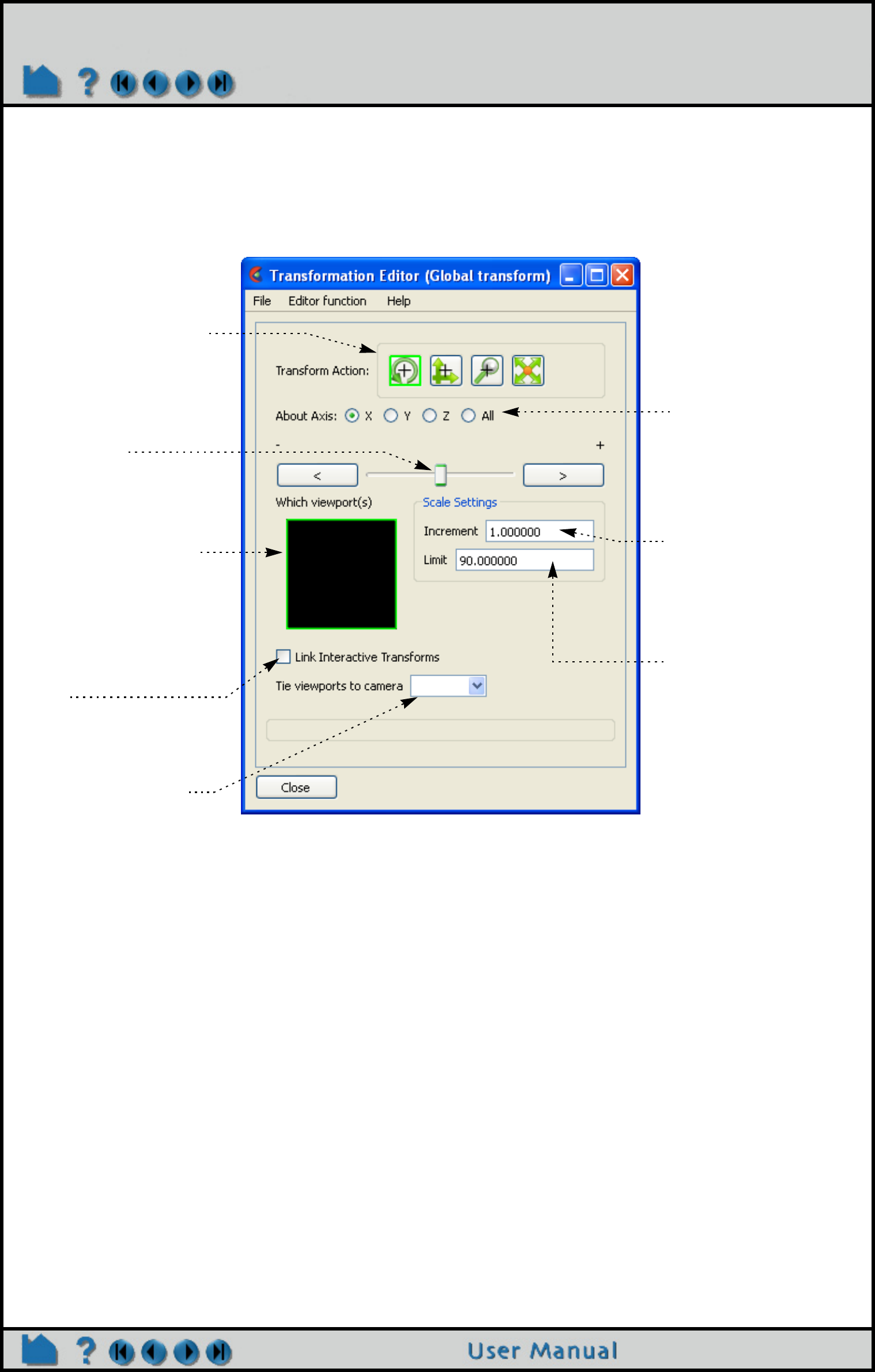
Page 124
HOW TO ROTATE, ZOOM, TRANSLATE, SCALE
ADVANCED USAGE
All EnSight transformations can be controlled precisely by specifying explicit transforms in the Transformations Editor
dialog. To open the dialog, click the Tools Icon Bar -> Graphics window transforms icon -> Transformations editor...
The slider performs the requested transformation (based on the selected transformation action) in the selected
viewport(s).
You can also perform scaling in any or all dimensions (to, for example, magnify subtle differences in a surface).
Although you cannot perform the scaling operation with the mouse, you can scale using the Transformations dialog.
Click the Scale icon in the Transformation Action area and specify the scaling as described above.
You can copy the transformations from one viewport to another. First select the viewport you wish to copy, select
Editor Function->Copy Transformation State, then select the viewport(s) you wish to modify and select Editor
Function->Paste Transformation State.
OTHER NOTES
By default, EnSight uses the left mouse button for performing the selected transformations. You can, however,
program the transformation action attached to each mouse button. See Customize Mouse Button Actions for more
information.
The transformation operations described here also apply to frame transformations. If additional frames have been
created and if operating on frames, then any transform will apply to the currently selected frame. See Create and
Manipulate Frames for more information.
Pressing the F5, F6, or F7 keys while the mouse is within the EnSight graphics window or desktop area will transform
the scene to show a standard right, top, or front view, respectively. Pressing the F8 key will return the scene to that
which existed prior to F5, F6, or F7 being pressed. Further, holding the Control key down while pressing F5, F6, or F7
will store the current view to the selected Fx button.
Pressing F9 while the mouse is in the Graphics Window or the desktop area will zoom the display to full screen.
Press F9 again to return to the normal display.
Slider to specify
transform.
Set (by clicking within
the desired region) the
viewport that the
transform applies to.
Specify axis to which
the transform applies
Limit controls the
sensitivity and limit of
the slider action.
Increment controls the
step size for the slider
end arrows.
Enter explicit values in
the Increment field
(and press return) to
transform by a precise
amount.
To interactively perform
transformations on
multiple viewports,
Control click on multiple
viewports, then toggle
on.
Select the desired
transformation action.
If you have defined
cameras, you can tie
selected viewports to
particular cameras.

Page 125
HOW TO ROTATE, ZOOM, TRANSLATE, SCALE
OTHER OPTIONS FOR PART TRANSLATION, ROTATION AND/OR SCALING
All of the above transformations are visual only and are much like moving the position of a camera or visually
changing the geometry only. That is, they occur only on the client and don’t change the actual geometry values in
EnSight. There are several other different methods for transforming coordinates described below as follows.
If you want to “deep” scale model parts with a scale factor or translate using a variable with “server-side” scaling and
displacement (where the actual coordinates are changed, both visually AND calculational) then look for Adjust Part
Coordinates under Model Parts. This is different from the rotate, zoom, and translate in that it is part by part and the
modification will be reflected in calculations, for example, calculated length, area, and volume will change.
If you want to displace by a vector, for example a Displacement Variable Vector, then click on the displacement icon
at the top. The resulting displacement is updated each timestep using the chosen vector variable and can be visual
only (on the client) or computational (on the server) and can be scaled (see How To Display Displacements). This
is different from the rotate, zoom, and translate in that coordinates are changed using a scalable vector and they can
be changed visually on the client or for use in deep on the server and used in further calculations.
If you want to scale, translate, or rotate a number of parts visually only consider grouping them and doing a group
transform. Also if you have coincident geometry in two parts and need to offset them slightly from each other use a
group transform (see Part Group Visual Transformations). This differs from rotate, zoom, and translate in that you
can do it only for a select group and not for all parts globally. This method is very similar to Frames discussed below
except it operates on a group.
If you need to define the rotation or translation of a part over time at a deep (computational) level, then consider rigid
body translations (see EnSight Rigid Body File Format). This is different from rotate, zoom, and translate in that
you can defined precise translations and rotations over time, and they are deep on the server for use in
computations.
If you need precise control of the visual (client only) rotation and translation of parts separately for animation
purposes, consider attaching a separate coordinate frame to each part and manipulating them separately (see How
To Create and Manipulate Frames). This is different from rotate, zoom and translate in that you can do these
transformations on a part by part basis rather than globally.
SEE ALSO
Other viewing operations:
How To Set LookFrom/LookAt
How To Set Z Clipping
How To Create and Manipulate Frames
How To Reset Tools and Viewports
How To Use the Selection Tool
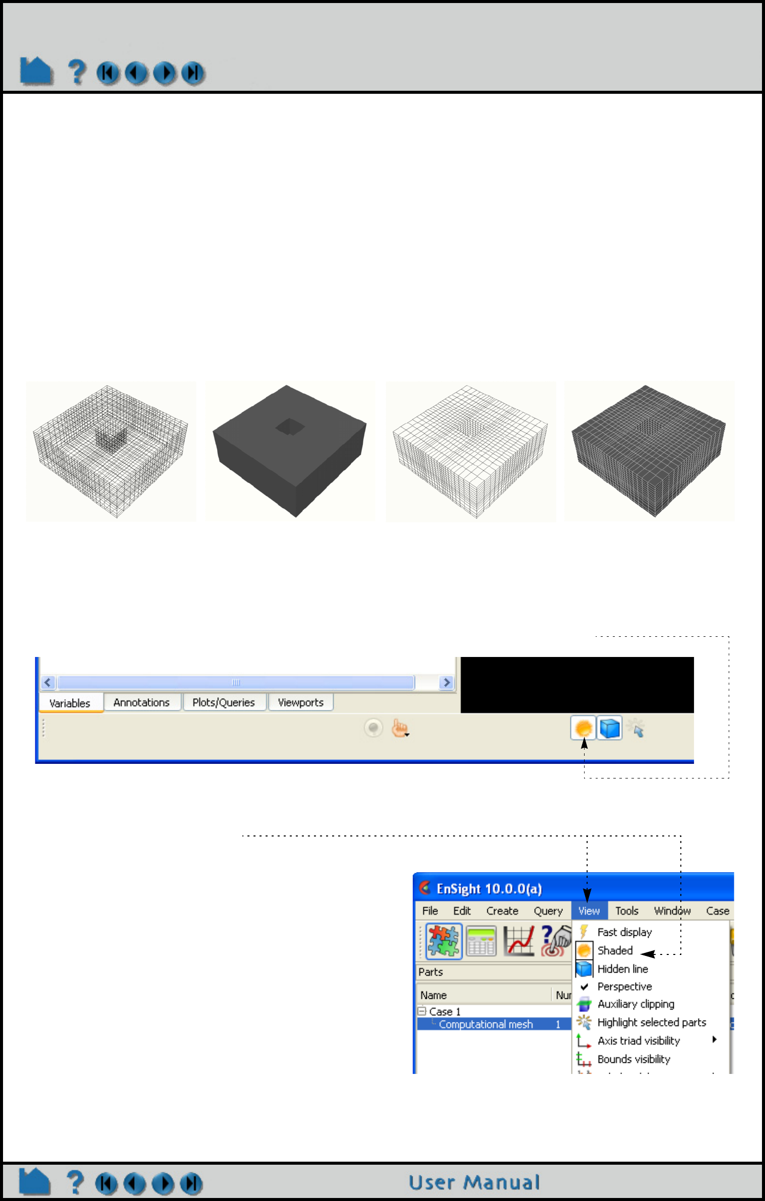
Page 126
HOW TO SET DRAWING MODE
Set Drawing Mode
INTRODUCTION
EnSight provides two basic drawing styles for graphics objects: line or shaded. Line mode draws only the line
segments of an object – regardless of the whether the lines are polygon edges or not. Shaded mode displays all
objects consisting of polygons (e.g. element or cell faces) as solid filled regions with light source shading enabled.
These drawing styles can be enhanced by enabling hidden-line mode. If the current mode is line, hidden-line will
eliminate all those lines that would be invisible if the object were a solid surface. If the current mode is shaded,
hidden-line mode will draw lines overlaying face edges. In shaded mode, hidden-line overlays are particularly useful
for visualizing computational grids.
The setting of line or shaded mode is a global toggle. You can also set the mode on a per part basis so that some
parts are displayed as lines and others as shaded surfaces. Each viewport also provides individual controls so that
the drawing mode can differ from viewport to viewport.
BASIC OPERATION
:
Line mode Shaded mode Hidden-line mode Hidden-line overlay mode
The global toggles for shaded and hidden-line mode are available from the Tools Icon Bar.
You can also enable these modes by selecting View >
Shaded or View > Hidden Line.
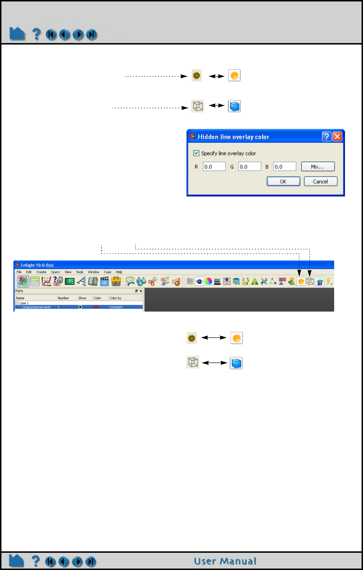
Page 127
HOW TO SET DRAWING MODE
To use the global Tools Icon Bar toggles
Note that enabling shaded mode for a part has no effect unless the global shading toggle is also enabled (on the
Tools Icon Bar or under the View menu). The same is true for hidden-line: unless the global hidden-line toggle is
enabled, the part will be drawn without hidden lines.
1. Click the Shaded toggle to switch from line to
shaded mode (or vice-versa).
2. Click the Hidden Line toggle to enable or
disable hidden-line mode.
If the current mode is Shaded when you toggle on
Hidden Line, the Hidden Line Overlay dialog is
displayed. This dialog allows you to specify a color for
the overlay edges. If Specify Line Overlay Color is not
enabled, overlay color will be set to the native color of
each part. If it is enabled, the color can be specified
either by entering red, green, blue color values, or by
clicking the Mix... button and picking a color with the
standard Color Selector dialog.
Line Shaded
Unhidden Hidden
1. Select Part in the Part List.
2. Click the Shaded toggle to switch from line to
shaded (or vice-versa).
3. Click the Hidden Line toggle to enable or
disable hidden-line mode.
Line Shaded
Unhidden Hidden
The per-part toggles for shaded and hidden-line mode are available in the Quick Action Icon Bar when part(s)
are selected in the Part List.
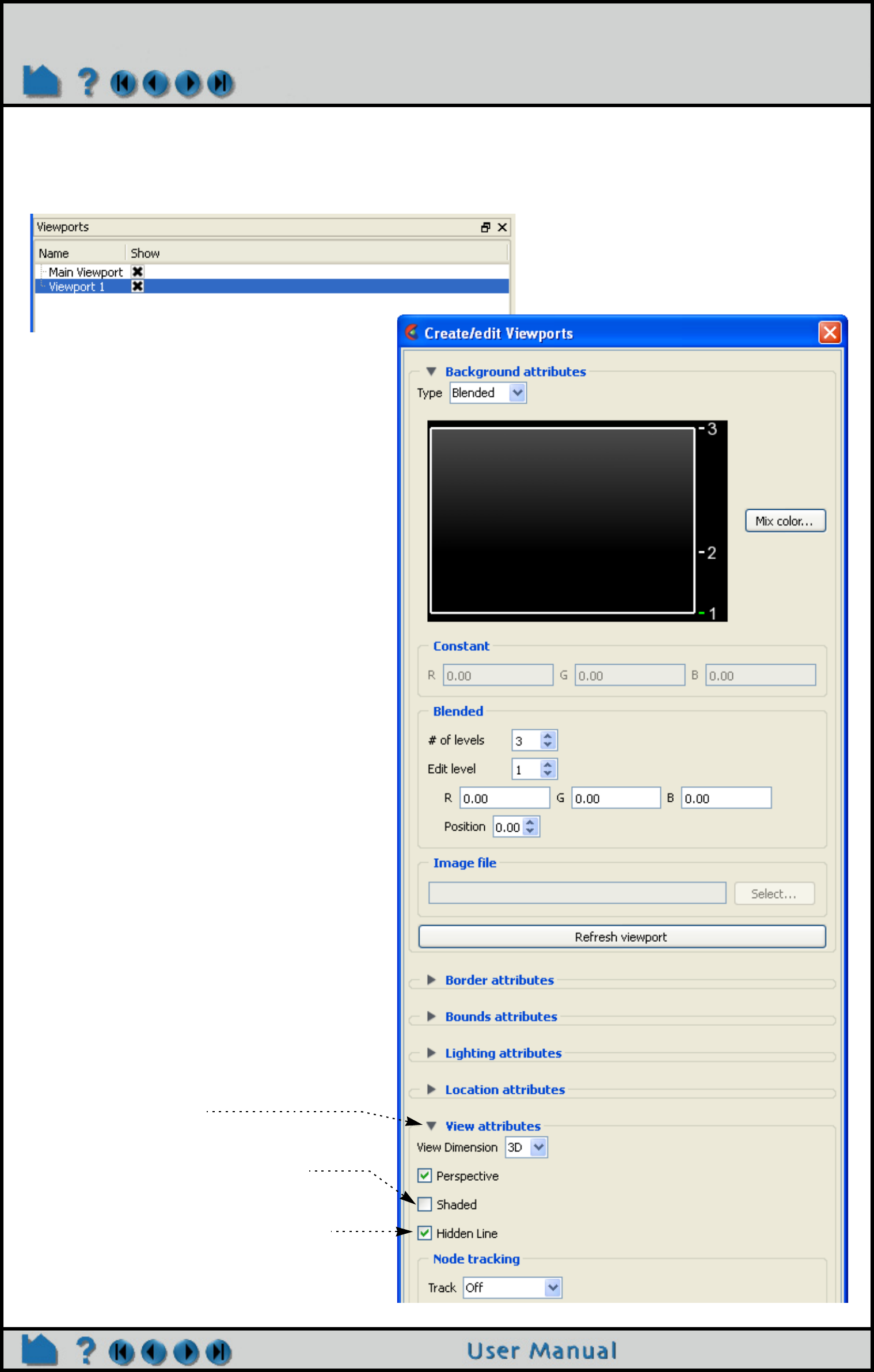
Page 128
HOW TO SET DRAWING MODE
ADVANCED USAGE
Drawing modes can also be set on a per-viewport basis. As with per-part settings, these toggles require that the
corresponding global toggle is also set to have any effect.
1. Double click (or right-click -> Edit...) the
desired viewport in Viewport list panel.
This will open the Viewport Feature Panel.
2. Open the Viewport turndown if it isn’t
already open.
3. Click the Shaded button to disable
shading in the current viewport.
4. Click the Hidden Line button to disable
hidden-line in the current viewport.

Page 129
HOW TO SET DRAWING MODE
OTHER NOTES
When a part is drawn in shaded mode (with or without hidden-line overlay) the surface is displayed with light source
shading enabled. EnSight uses two pre-defined light sources: one at the look-from point (the camera) and one on the
opposite side of the model (for back-lighting). The location of one of the light sources can be changed, see How To
Control Lighting.
In computer graphics, the appearance of a shaded surface is governed by a lighting model controlled by various
parameters. In EnSight, these parameters are part of the part’s and can be changed on a per-part basis. See How
To Set for more information.
SEE ALSO
How To Control Lighting
User Manual: Global Shaded, Global Hidden Line
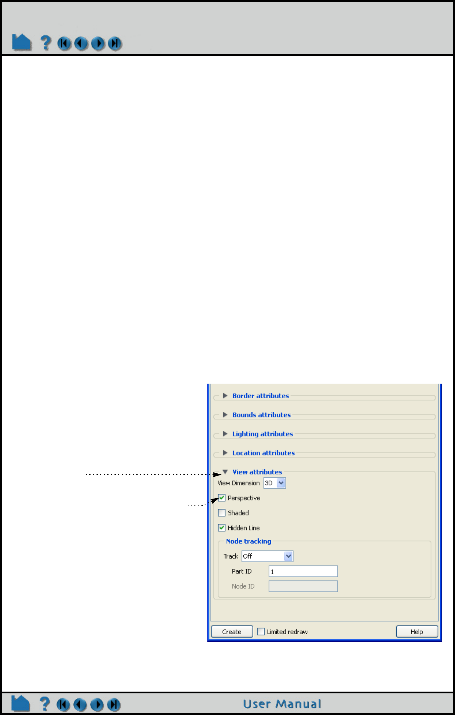
Page 130
HOW TO SET GLOBAL VIEWING PARAMETERS
Set Global Viewing Parameters
INTRODUCTION
EnSight provides various modes that control global viewing behavior. Three of these modes are discussed here:
perspective/orthographic projection, bounding box display modes, and static lighting.
EnSight can display viewports in either perspective or orthographic projection. A perspective projection is how we
normally view the world: objects that are farther away appear smaller. An orthographic projection removes this effect:
objects appear the same size regardless of distance. The projection setting can be specified on a per-viewport basis.
By default EnSight draws every point, line, and polygon for every visible part each time the Graphics Window
updates. For very large models (or slow graphics hardware), this behavior leads to unresponsive manipulations since
the update lags behind the corresponding mouse motion. Fortunately, EnSight provides other display modes that
improve responsiveness. Fast Display mode displays all visible parts in a reduced fashion during interactive
manipulation. This can be a bounding box representation, a point cloud representation, a reduced polygon
representation, an invisible representation, or if using immediate mode - a percentage of each part’s elements. When
the mouse button is released, parts are drawn normally. The Fast Display mode can also be set such that the
bounding display is used until the mode is changed - even when the mouse is released. (Edit->Preferences...
Performance - Static Fast Display)
Surface shading operations are expensive for very large models. Since the shading is dependent on the orientation of
the model with respect to the light sources, the surface colors must be recalculated each time the model moves.
Static lighting mode precalculates surface colors for a given orientation and then uses these colors during
subsequent transformations, resulting in improved interactive response.
BASIC OPERATION
Perspective/Orthographic Projection
The projection mode can be toggled either from a menu (View > Perspective) or in the Viewport editor. To set the
projection from the Viewport editor:
1. Double click (or right click->Edit...) the
desired viewport in the Viewport list panel.
This will bring up the Viewport Feature Panel.
2. Open the View turndown if it isn’t already
open.
3. Click the Perspective button to toggle the
projection type in the current viewport.
Note that a viewport will only display a perspective
projection if the global toggle (as set with View >
Perspective) is on as well.
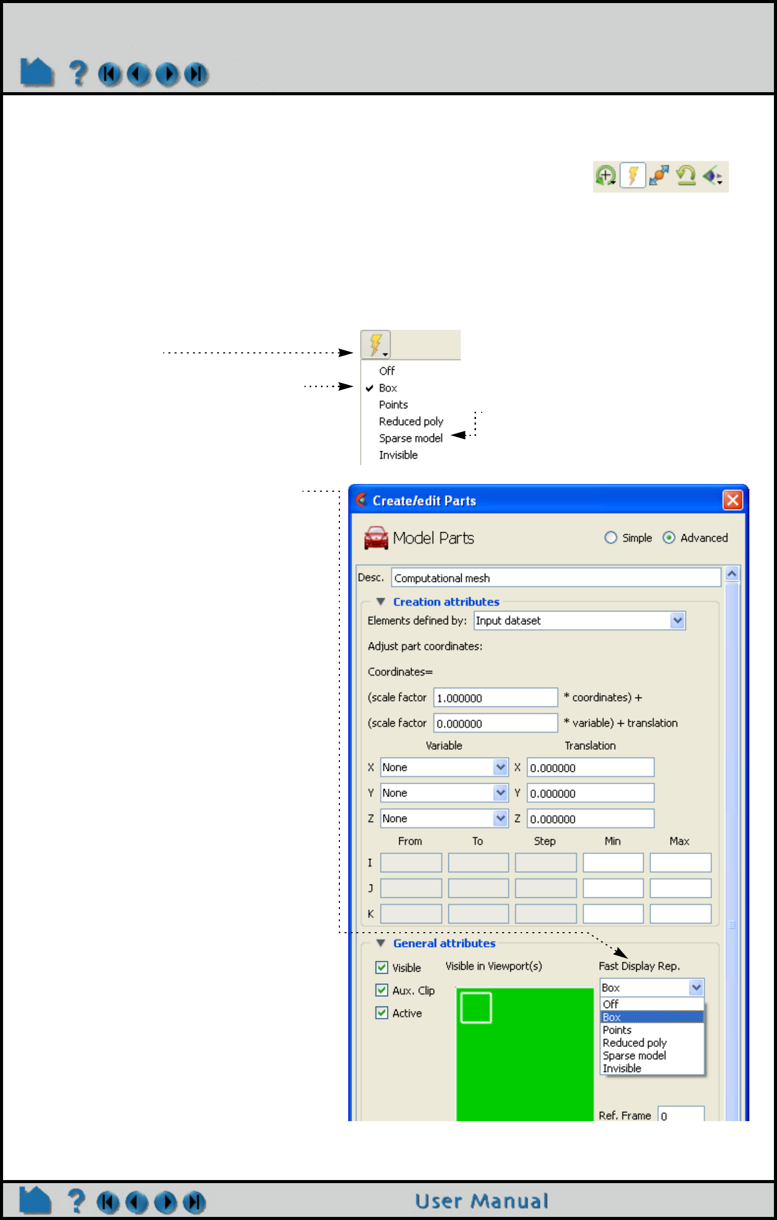
Page 131
HOW TO SET GLOBAL VIEWING PARAMETERS
Fast Display Mode
1. Select the part(s) in the part list.
2. Click the Fast Display Representation pull-
down icon.
3. Select the desired fast display mode.
Select Off to return to standard display
mode.
Note that this can also be done in the General
section of the Part Feature Panel.
Note, if not using immediate mode, this
Sparse Model option will not be
available here.
The global Fast Display Mode can be set either from a menu (View > Fast Display
> ) or by the Fast Display toggle on the Tools Icon Bar.
To change between the Dynamic or Static operation of this mode, go to Edit-
>Preferences... Performance.
To change the part representation for Fast Display Mode:

Page 132
HOW TO SET GLOBAL VIEWING PARAMETERS
ADVANCED USAGE
If using immediate mode, and you desire to use the Sparse Model option for Fast Display, you can control the
percentage of the model that is displayed. See Fast Display Mode. This mode is intended for large models. It
generally will not be pleasing (nor should it be needed) for small models.
SEE ALSO
User Manual: Fast Display Rep.
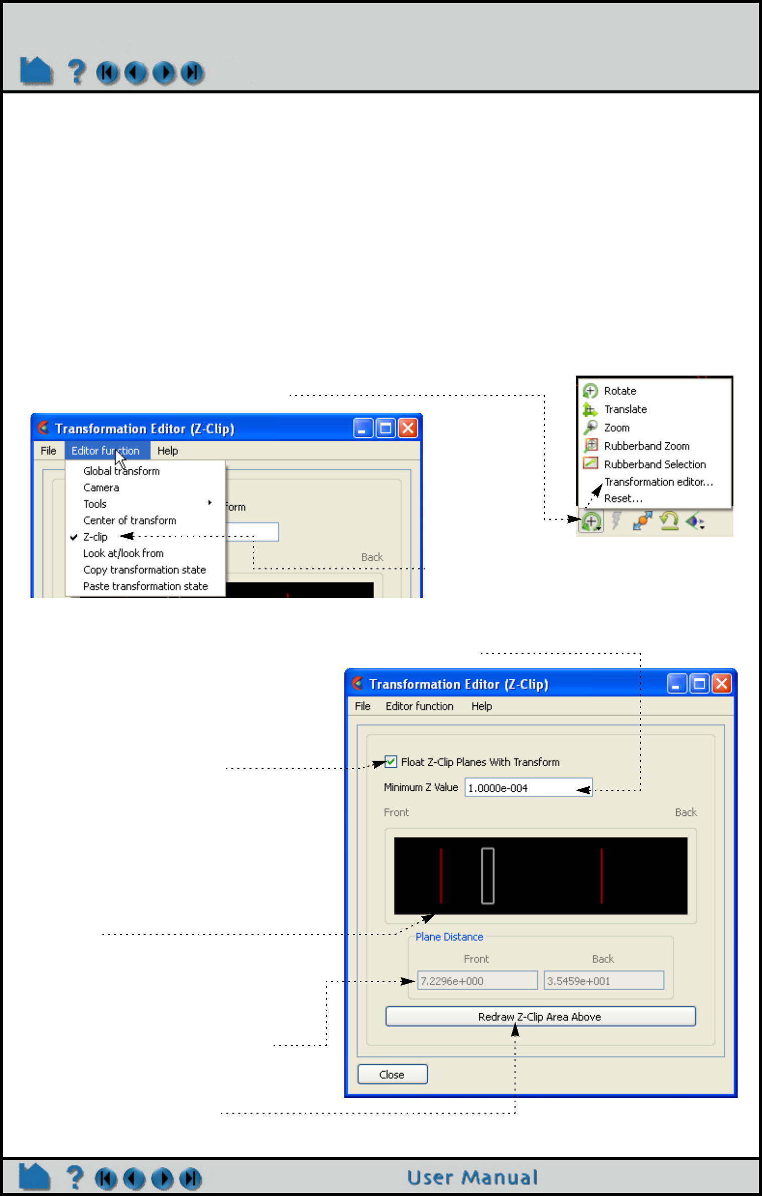
Page 133
HOW TO SET Z CLIPPING
Set Z Clipping
INTRODUCTION
As you apply zoom transformations in EnSight, you may have noticed that the model begins to progressively
disappear as you move close to the model. This happens when the visible model parts intersect the front Z clipping
planes. The Z-clip planes (which are always perpendicular to your line of sight) are specified as distances from the
look-from point (the camera position). The Z clipping plane positions can be set by the user and can be used to
remove unneeded geometry from the display. Each viewport has its own set of Z clipping planes. By default, the Z-
clip planes adjust (float) with the model - thus stay out of the way if possible.
BASIC OPERATION
The initial position of the Z clipping planes is set based on the Z (depth) extent of the visible geometry – plus quite a
bit extra to leave room for transformations. The plane positions can only be set via the Transformation Editor dialog.
1. Click the graphics window transform icon on the Tools Icon Bar
and select Transformation editor...
2. Select Editor Function -> Z-clip
The graphics display shows the relative
positions of the front and back clipping planes
(left and right vertical red lines) to the Z extent of
all currently visible objects (white box).
2. Toggle the Float Z-Clip Planes option on to
have the Z-clip planes automatically
adjust. OR
Toggle the option off to manually adjust
the Z-clip plane locations.
If the Float Z-Clip option is off, you can edit the
plane positions either by dragging the red lines
or by entering explicit values in the Front and
Back text fields. Recall that the values represent
the distance from the look-from point to the
plane.
3. Place the mouse pointer over the desired
plane marker and click the left mouse
button.
4. Drag the marker left or right to the desired
location. The Graphics Window will
update as the marker is moved.
– OR –
3. Enter explicit values in the Front and/or
Back text fields and press return.
If the markers become difficult to manipulate due
to changes, click the Redraw Z-Clip Area Above
button to rescale the markers.
If the Float Z-clip Planes With Transform option is on,
you can specify the minimum Z value that the Front clip
plane can float to.
Page 134
HOW TO SET Z CLIPPING
Each viewport maintains its own independent Z clipping planes. The operation described above will change the
planes for the current viewport (as set by clicking in the desired viewport in the Graphics Window).
You can also reset by clicking the Graphics window transforms icon and clicking Reset... to open the Reset Tools and
Viewports dialog. Then click the Reinitialize button.
OTHER NOTES
EnSight uses your workstation’s graphics hardware to implement Z clipping. The same hardware is used for Z-
buffering – determining which objects are visible based on Z (depth) values. The Z buffer typically provides 24 bits of
resolution. EnSight attempts to make the best use of this limited resolution by setting the front and back clipping
planes reasonably close together. If the planes are too far apart, relative Z resolution is reduced and the hardware
may not be able to accurately determine surface visibility. If you see artifacts like this, move the clipping planes closer
together.
EnSight also provides an additional clipping plane: the auxiliary clipping plane. Unlike the Z clipping planes which are
always perpendicular to your line of sight, the auxiliary clipping plane can be placed at any location in any orientation.
The Plane Tool specifies the location of the auxiliary clipping plane. By default, all geometry on the negative Z side of
the Plane Tool is removed. However, you can specify auxiliary clipping on a per part basis – some parts are clipped
while others are not. See How To Set Auxiliary Clipping for more information.
SEE ALSO
How To Define and Change Viewports, How To Set Auxiliary Clipping
Note that clicking the Reinitialize transforms icon on the Tools Icon Bar will reset the Z
clipping planes of the current viewport based on the Z extent of all objects currently
visible in that viewport
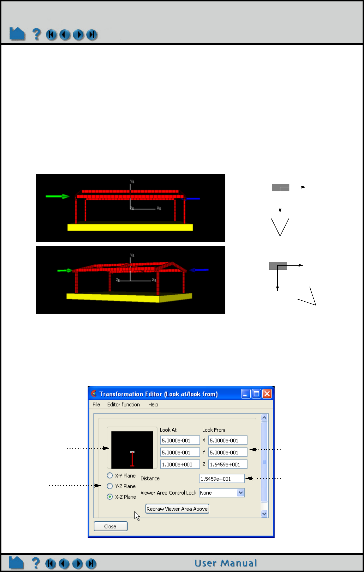
Page 135
HOW TO SET LOOKFROM / LOOKAT
Set LookFrom / LookAt
INTRODUCTION
In addition to providing control over model manipulations, EnSight also provides control over the virtual camera used
to view the scene in the Graphics Window while in Global Transform Mode. If a viewport is being viewed through a
camera, this section is not applicable. The two control parameters are the look-from point (the position of the camera)
and the look-at point (a point on the camera’s line-of-sight vector). The Global Axis is positioned at the look-at point
and is always in the center of the Graphics Window.
Initially, the look-at point is set to the geometric center of all visible objects and the look-from point is set to a point on
the positive Z axis such that all visible objects fit in the Graphics Window (as shown in the top image below). The
white axis triad is the Global Axis and can be displayed by selecting View > Axis triad visibility > Global. The bottom
image shows the view after the look-from point has been repositioned between the X and Z axes. The diagrams to
the right of each image show a top-down schematic of each viewing case.
BASIC OPERATION
The look-from, look-at points are controlled via the Transformation Editor dialog.
1. Click the Graphics window transforms icon on the Tools Icon Bar, and select Transformation editor...
2. Select Editor Function > Look At/Look From.
x
z
x
z
Text fields for
entering numeric
values
Viewer Area for
interactive
manipulation
Viewer Area plane
toggles
Text field for
moving look-from
by setting an
explicit distance
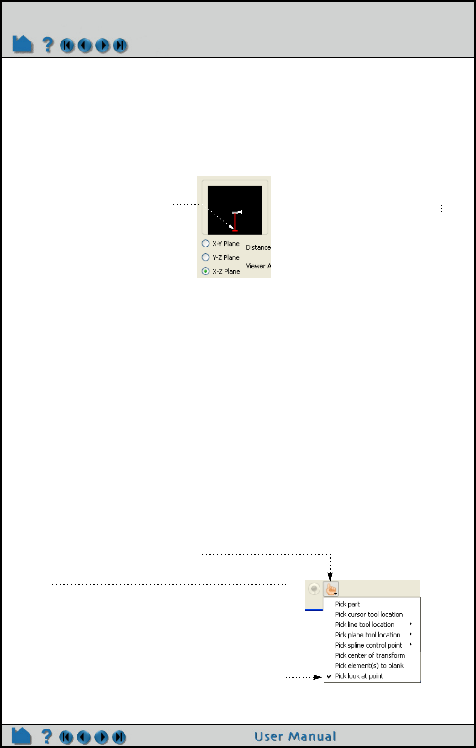
Page 136
HOW TO SET LOOKFROM / LOOKAT
The Transformation Editor dialog provides two methods for setting the look-at and look-from points. Numeric values
can be entered directly into the X,Y,Z Look At, Look From text fields (remember to press return). You can also enter a
value in the Distance field to explicitly move the look-from point a certain distance away from the look-at point.
Alternately, the Viewer Area can be used to interactively manipulate the points. The presentation of the Viewer Area
depends on the which plane toggle is set: X-Y (view from the positive Z axis), Y-Z (view from the positive X axis), or
X-Z (view from the positive Y axis – the default). In each case, the gray box represents the extent of all visible parts.
The intersection of the two red lines is the look-from point. The opposite end of the long red line is the look-at point
(which is initially near the center of the gray box). The example below shows the X-Z Plane presentation, the others
behave analogously.
During your manipulation, the display in the View Area may become difficult to use. Click the “Redraw Viewer Area
Above” button to rescale the display.
The Viewer Area Control Lock pull-down menu effects interactive operation in the Viewer Area as follows:
None No constraints are placed on movement of either the look-from point or the look-at point.
Distance Movement of the look-from (look-at) point is restricted to a circle whose radius is the current Distance
value and whose center is the look-at (look-from) point.
Together The movement of both points is locked such that movements applied to one are applied to the other.
You can easily reset the look-from and look-at points such that all currently visible parts are displayed. Click the
Graphics window transforms icon and Click Reset... to open the Reset Tools and Viewports dialog. Click the
Reinitialize button to reset the currently selected viewports.
OTHER NOTES
You can also set the look-at point by picking an object with the mouse in the Graphics Window:
To change the look-from point:
1. Place the mouse pointer over the
intersection of the two red lines.
2. Click and drag to the desired
location. Note that the Graphics
Window updates as the look-from
point is moved.
To change the look-at point:
1. Place the mouse pointer over the free
end-point of the long red line.
2. Click and drag to the desired location.
Note that the Graphics Window
updates as the look-from point is
moved.
1. Click Reinitialize in the Reset Tools and Viewport(s)
dialog to clear all global transformations.
2. Click the Pick icon on the Tools Icon Bar.
3. Select Pick Look/At Point from the Pick Pull-down
icon.
4. Move the mouse into the Graphics Window. Place the
mouse pointer over the point you wish to set to the
look-at point and press the ‘p’ key (or whatever
mouse button you have set for “Selected Pick
Action” in Edit > Preferences > Mouse and
Keyboard).

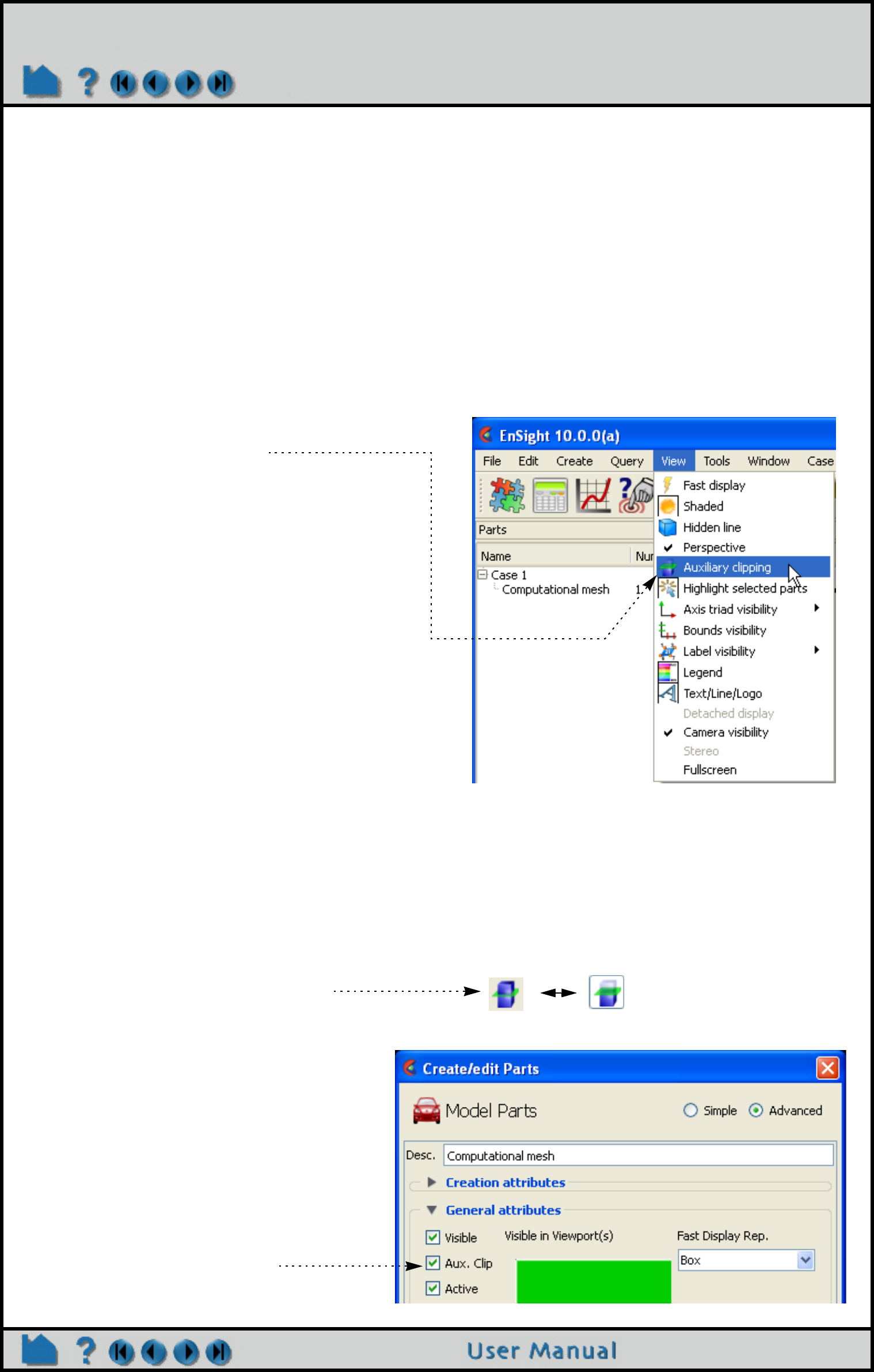
Page 138
HOW TO SET AUXILIARY CLIPPING
Set Auxiliary Clipping
INTRODUCTION
Unlike standard Z clipping where the front and back planes are always perpendicular to your line of sight, auxiliary
clipping lets you clip parts against a plane with arbitrary position and orientation. In addition, the auxiliary clip attribute
can be set on a per-part basis. This permits selective clipping to reveal objects of interest.
EnSight’s Plane Tool is used to provide the location for auxiliary clips. As the Plane Tool is manipulated (either
interactively with the mouse or via the Transformations dialog), the display in the Graphics Window updates to reflect
the new location of the plane.
BASIC OPERATION
The Plane Tool will become visible and all objects on the negative Z side of the plane will be clipped (assuming the
plane currently intersects some visible part). You can now manipulate the Plane Tool to achieve the desired display
effect (see How To Use the Plane Tool for details). Note that Auxiliary Clipping always uses the infinite extent of the
plane specified by the Plane Tool – there is no way to restrict it to the rectangular bounds of the tool.
Each part has an attribute that controls whether it is clipped by the Auxiliary Clipping plane or not. To toggle this
setting:
Auxiliary clipping can be globally enabled by
selecting it in the View menu:
1. Select the desired part (see How To Select Parts).
2. Click the Auxiliary Clipping toggle.
(This attribute can also be toggled in the Feature
Panel for the part. See How to Set for more
information.)
Off On

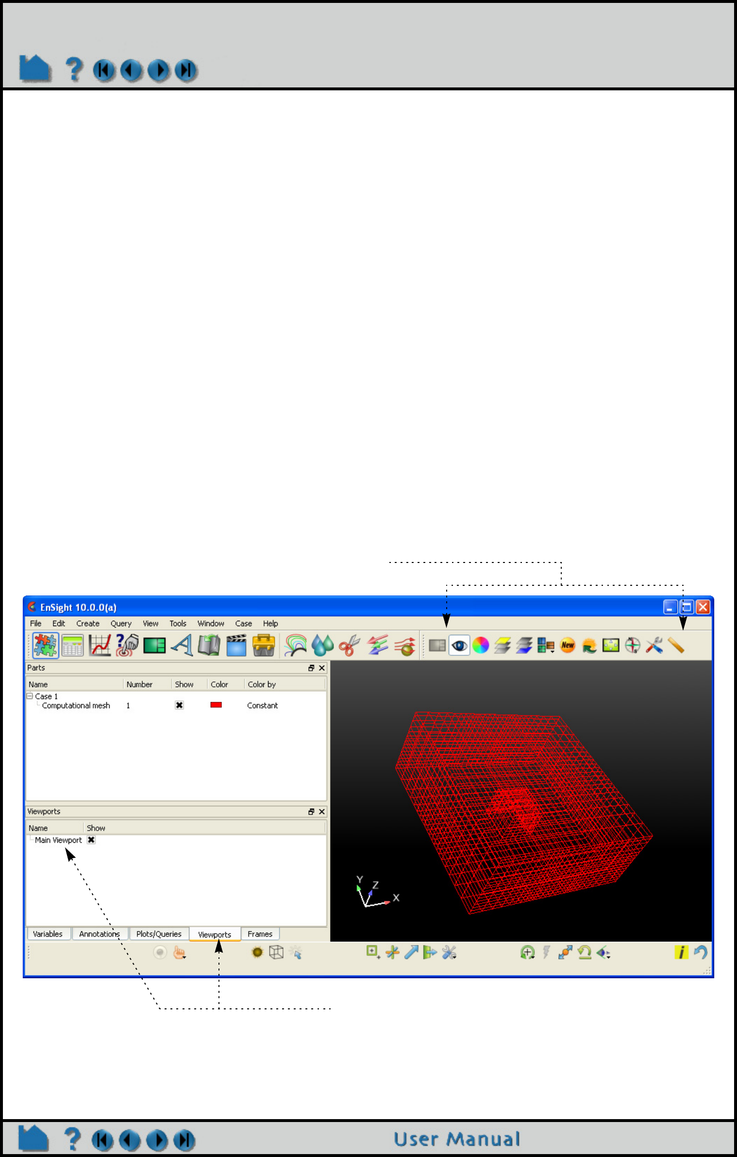
Page 140
HOW TO DEFINE AND CHANGE VIEWPORTS
Define and Change Viewports
INTRODUCTION
EnSight provides up to sixteen user-defined viewports in the Graphics Window. Each viewport is a rectangular region
of the screen (with or without a border) displaying some or all of the currently visible parts. Each viewport can be
transformed (e.g. rotated or zoomed), sized, and positioned independently. Viewports have several display including
background and border color. Viewports provide a very flexible environment for data display.
This article is divided into the following sections:
Create a New Viewport
Select Viewports
Move and Resize Viewports
Set Viewport Background Color or Image
Set Viewport
Display Selected Parts in Viewports
Set Case Visibility Per Viewport
Perform Transformations in Viewports
Reset Viewport Transformations
Delete Viewports
BASIC OPERATION
Viewport areas on the Desktop
Viewport Quick Action Icons
Viewports Panel
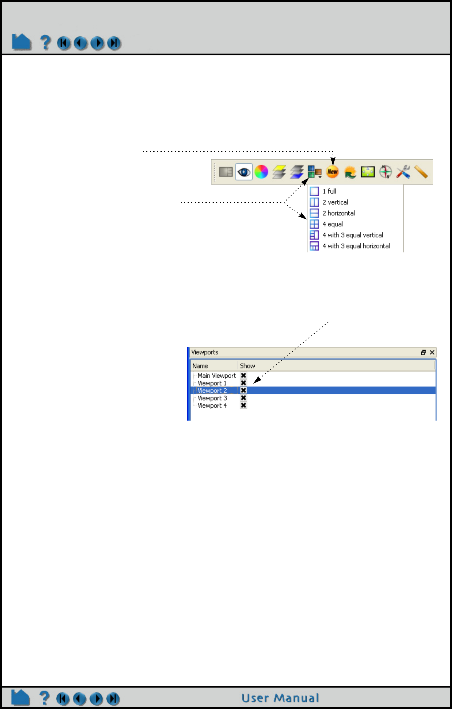
Page 141
HOW TO DEFINE AND CHANGE VIEWPORTS
Create a New Viewport
On startup, EnSight creates a single viewport that fills the Graphics Window. To create a new viewport:
Select Viewports
When you create a new viewport, it automatically becomes the currently selected viewport. Any action to change
viewport always operates on the currently selected viewport(s). To select viewports:
1. Click Viewports tab and select a viewport in the list
panel to make Viewport Quick Action Icons available.
You can alternatively click in the background of one of the
viewports.
2. Click the New Viewport icon.
OR
2. Click the Viewports Layout pull-down icon to select
any of the standard viewport layouts.
Note: you can also right click in the viewport list and
select New.
1. Click Viewports tab and select the desired viewport(s) in the Viewports list panel.
You can alternatively click in the background of the desired viewport.
Note: that the typical multiple selection
techniques can be used. Control
click to append additional
viewports to the selection. Shift
click to select a range of viewports.
Note that the selected viewport is also changed in other modes (such as View) any time you perform some action
in a viewport (such as rotation). There is however, no visual feedback of this change unless or until you have the
Viewport list visible.
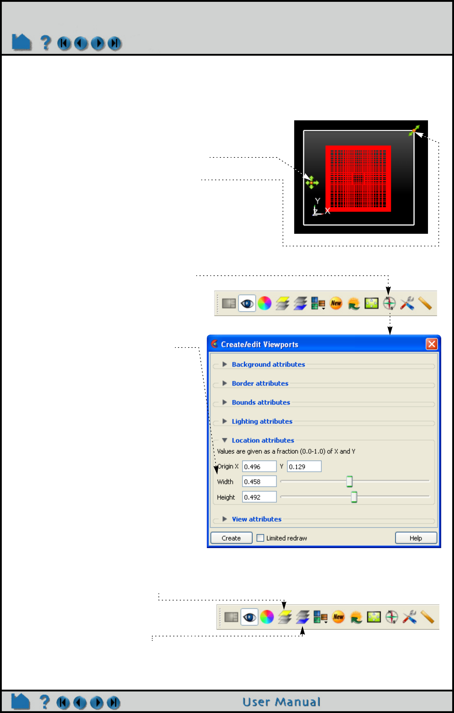
Page 142
HOW TO DEFINE AND CHANGE VIEWPORTS
Move and Resize Viewports
Viewports can be easily moved and resized. You can either reposition a viewport with the mouse in the Graphics
Window, or precisely by entering exact values. To move or resize a viewport:
1. Get the move and resize hotpoints to appear by clicking in the
background or hovering the mouse over the border of the
desired viewport.
2. To move a viewport, click and hold on the move hotpoint as
you drag the viewport to the desired location.
3. To resize a viewport, click and hold on the resize hotpoint as
you drag the corner to the desired location.
EnSight permits overlapping viewports. You can control the ordering (from front to back):
Click the Pop viewport(s) forward icon to bring the selected viewports to the top.
Click the Push viewport(s) back icon to send the selected viewports to the bottom.
Note: Viewport 0 is always displayed first, thus it cannot be pushed or popped with these icons.
To precisely reposition a viewport:
5. Click the Selected viewport(s) position
icon to open the Create/edit Viewports dialog.
Alternatively you can double click (or right click
and select Edit...) on the viewport in the list.
Then open the Location Attributed area.
6. Enter new values in the Origin X,Y, Width,
or Height fields (and press return).
You can alternatively use the sliders to change
the Width and Height.
The origin (at 0,0) is the lower left corner of the
Graphics Window. Note that the values are
normalized to the width and height of the default
viewport (i.e. the Graphics Window).
7. To quickly or to automatically arrange a
number of viewports right-click on the
viewport and choose Viewports>Manually
arrange which will prompt you to create a
single large viewport and a grid arrangement
of the remaining viewports.
Right click and choose Viewports>Automatically
arrange to have your viewports quickly
automatically arranged in a pre-defined fashion.
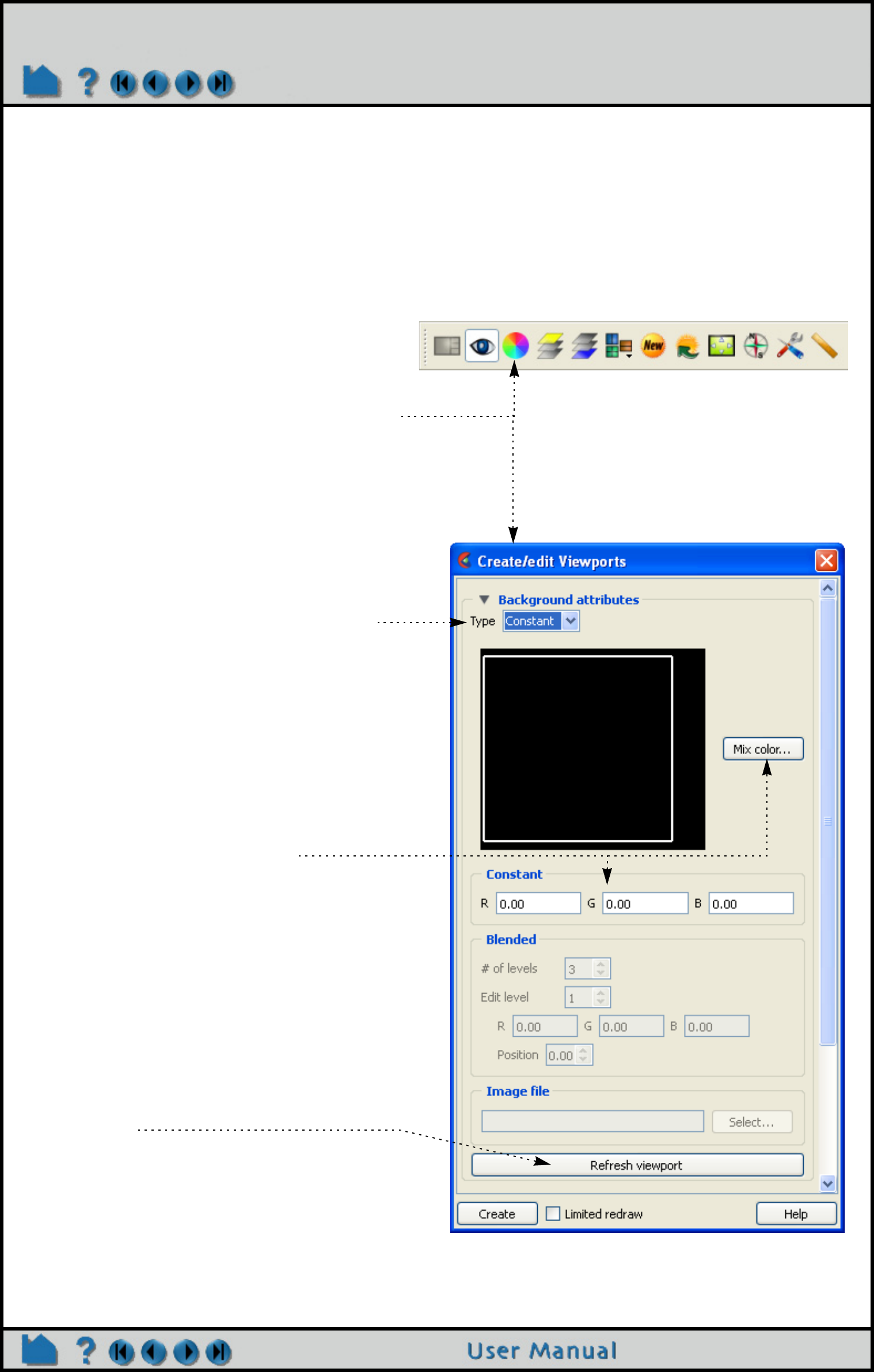
Page 143
HOW TO DEFINE AND CHANGE VIEWPORTS
Set Viewport Background Color or Image
Viewport background colors can be constant, blended, or inherited from the default viewport. To set viewport
background color:
1. Click Viewports tab and select a viewport in the
list to bring up the Viewport Quick Action
icons.
You can alternatively click in the background of
one of the viewports.
2. Select the desired viewport(s) by any of the
methods described above.
3. Click the Selected viewport(s) background
color icon to open the Create/edit Viewports
dialog, in the Background section.
The Type pull-down controls the type of background
coloring used. There are four types: Constant,
blended, inherit, and image.
Constant
A constant color will be used for the entire
background. To set a constant color:
4. Select Constant from the Type pull-down.
5. Either enter values in the RGB color fields (and
press return OR click the Mix Color... button to
open the Color Selector dialog.
6. The viewport should be refreshed
automatically, but if not you can click Refresh
viewport.
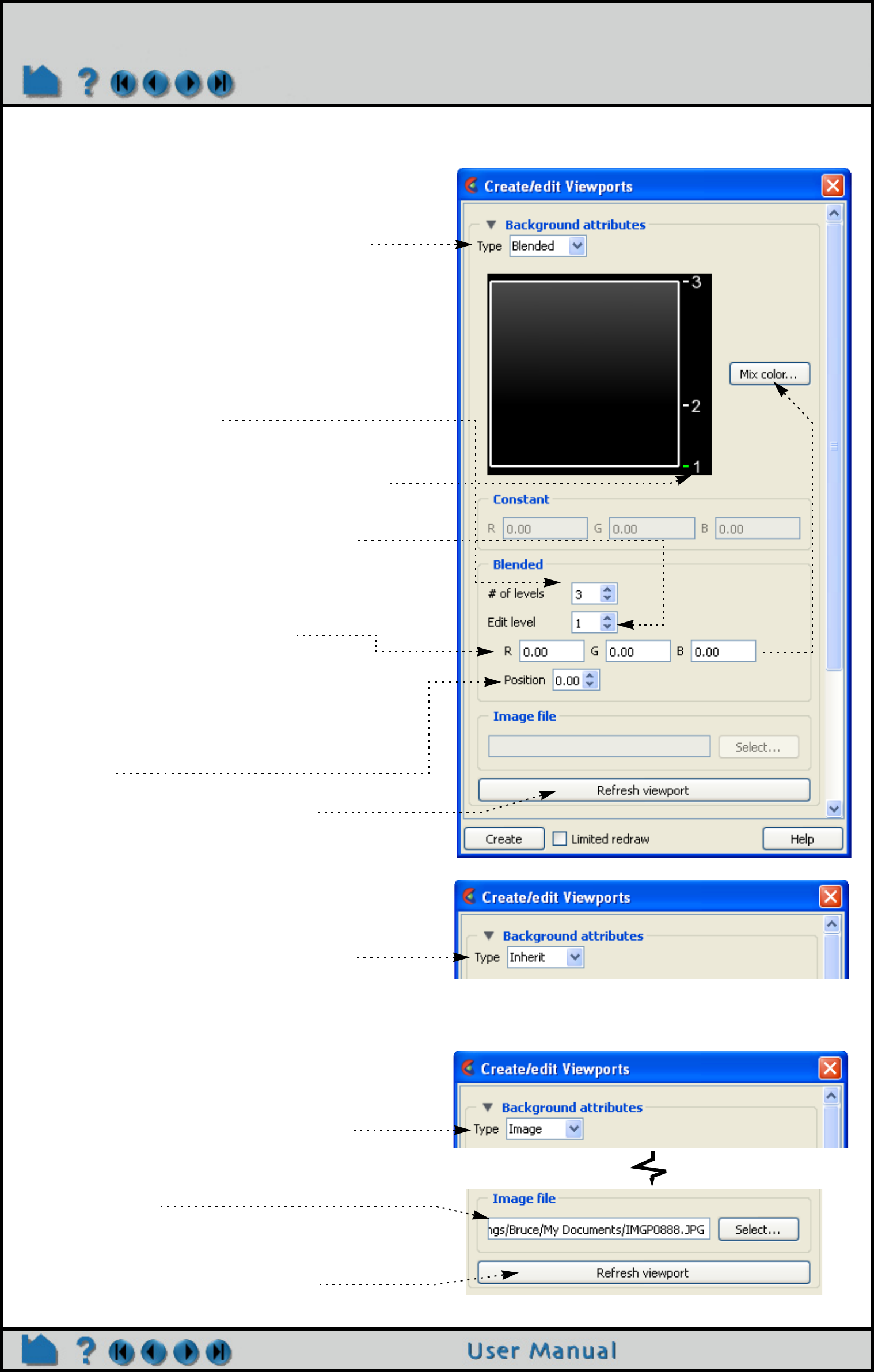
Page 144
HOW TO DEFINE AND CHANGE VIEWPORTS
Blended
Up to 5 horizontal level colors can be specified with
interpolation between levels. To set a blended
background:
1. Select Blended from the Type pull-down.
2. Enter the desired number of levels in the # of
Levels field (and press return). Up to five
levels are supported.
3. To edit a color, first select it by clicking on the
number label in the Viewport Color window.
As shown, level 1 is currently selected.
Alternately, you can enter a value in the Edit
Level field or click the up/down arrows.
4. Change the selected color by either entering
new values in the RGB fields (and pressing
return) or clicking the Mix Color... button to
open the Color Selector dialog.
5. You can also change the relative vertical
position of a level by either clicking on the
level number with the left mouse button and
dragging up or down OR by entering a new
value in the Position field (and pressing
return).
6. Click Refresh viewport, if needed.
Inherit
The selected viewports inherit the background type
and color from the default viewport. To set an
inherited background:
1. Select Inherit from the Type pull-down.
2. Click Refresh Viewport, if needed.
Image
The image specified will be used as the background
for the selected viewports. To set an image
background:
1. Select Image from the Type pull-down.
2. Enter the filename for the background image
to use or click the Select... button and
navigate to it.
Note, that the image must be a format that is
recognized, but most common image formats are.
2. Click Refresh Viewport, if needed.
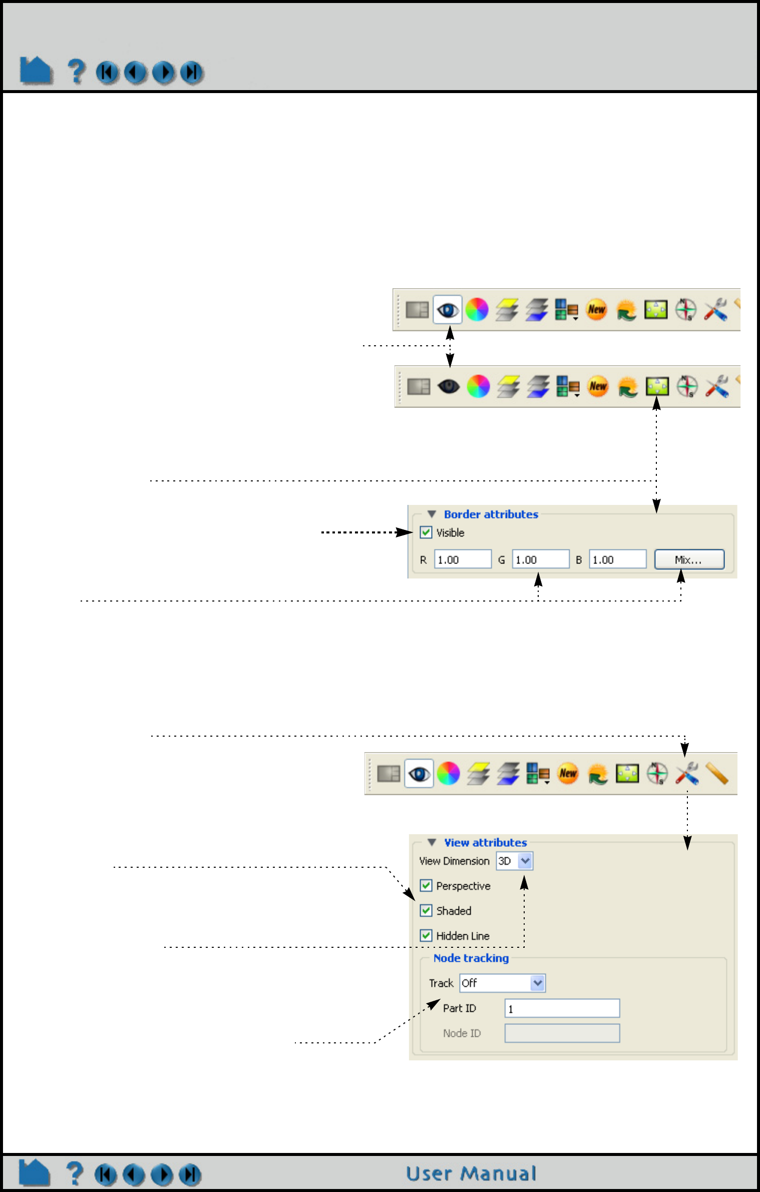
Page 145
HOW TO DEFINE AND CHANGE VIEWPORTS
Set Viewport
Viewports can be displayed with a variety of options:
1. Click Viewports tab and select a viewport in the list
to bring up the Viewport Quick Action icons.
You can alternatively click in the background of one of
the viewports.
2. Select the desired viewport(s) by any of the
methods described above.
3. Set the desired attribute as described below:
Click the Selected viewport(s) visibility icon to
toggle display of the selected viewports on or off.
Click the Selected viewport(s) border icon to open
the Border section of the Create/edit Viewports
dialog.
Click the Visible toggle to display a border.
Enter values in the RGB fields (and press return) or
click the Mix... button to open a Color Selector
dialog.
Click the Select viewport(s) special icon to open the
View section of the Create/edit Viewports dialog.
Each viewport has its own toggles for perspective,
hidden surface, and hidden line drawing styles.
These controls will toggle the respective attribute for
the selected viewports. See How To Set Drawing Style
and/or How To Set Global Viewing for more
information.
In addition, a viewport can be 3D or 2D in nature. If the
viewport is designated as 2D, only planar parts may be
displayed in the viewport and transformations will
become 2D limited.
A viewport can be set such that it will track a node
number, a part centroid, or one of the part min or max
values. Thus as a model changes in time, the viewport
will stay centered on that location. See How To Do
Viewport Tracking for more information.
Off
On
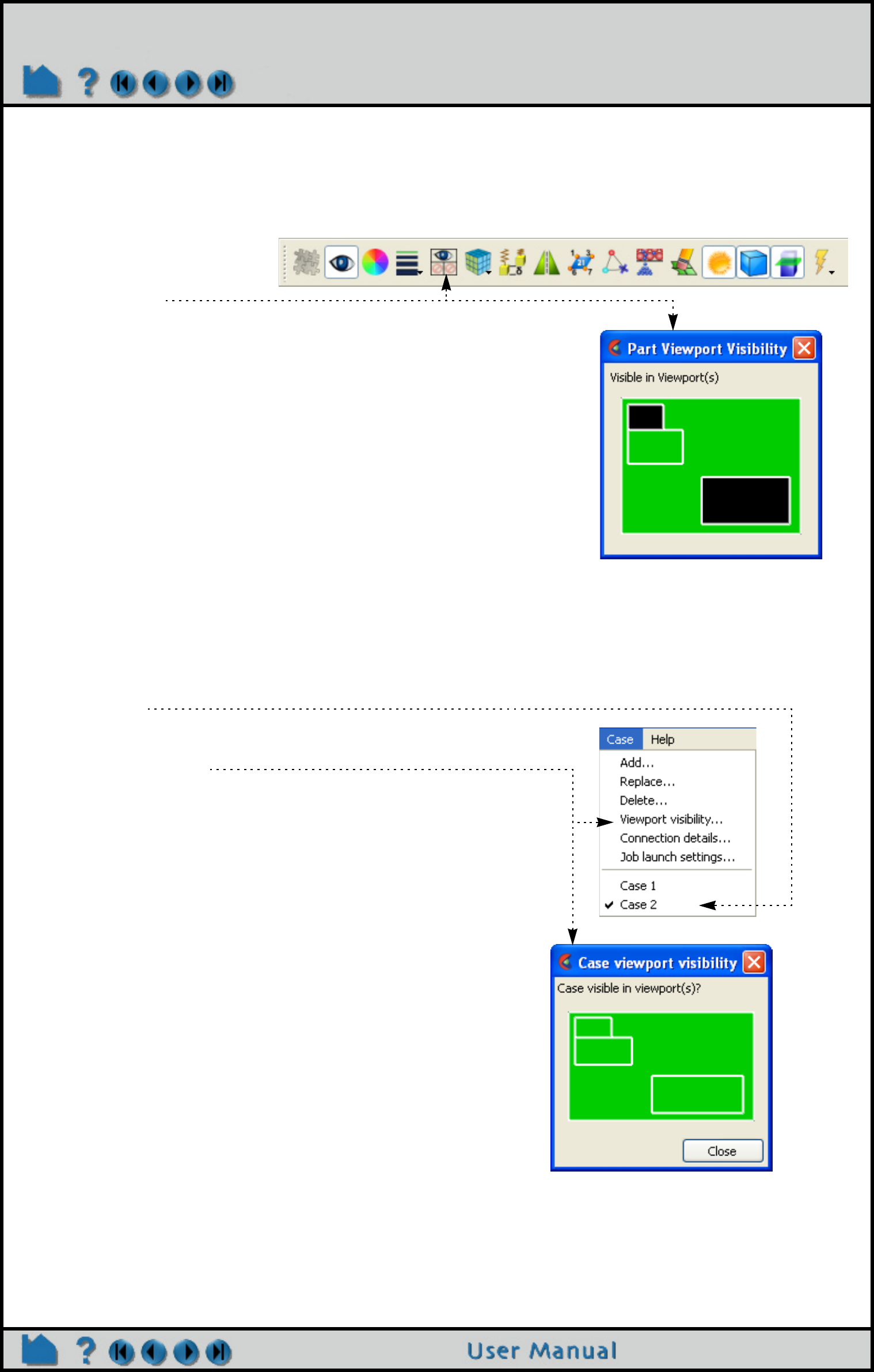
Page 146
HOW TO DEFINE AND CHANGE VIEWPORTS
Display Selected Parts in Viewports
Part visibility can be a set on a per-viewport basis such that some parts are visible in some viewports but not in
others. To set part visibility per viewport:
Set Case Visibility Per Viewport
If you have multiple cases in your session of EnSight, you can set viewport visibility for all parts associated with a
case. This makes it easy to display one case per viewport. To set case visibility per viewport:
1. Select the desired part(s) in the Main Parts list.
2. Click the Visibility per
viewport icon.
The Part Viewport Visibility dialog displays a schematic of the
current viewports. The part is currently visible in the green
viewports but invisible in the black viewports.
3. Click in a green viewport to disable display of the selected
part(s) in that viewport OR click in a black viewport to
enable display of the selected part(s) in that viewport.
Note that a similar interface for setting this attribute appears in the
General section of the Create/edit Parts dialog.
1. Select the desired case from the Case menu (Case >
casename).
2. Select Case > Viewport Visibility to open the Case visible in
viewport(s)? dialog.
3. Click in a green viewport to disable display of the selected case
in that viewport OR click in a red viewport to enable display of
the case in that viewport.
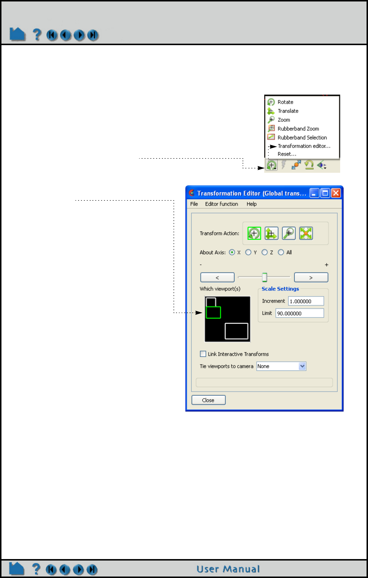
Page 147
HOW TO DEFINE AND CHANGE VIEWPORTS
Perform Transformations in Viewports
You can transform objects in a user-created viewport as easily as in the default viewport (See How To Rotate, Zoom,
Translate, Scale for details). For precise viewport transformations, you can use the Transformations Editor on a per
viewport basis:
1. Click the Graphics window transforms icon,
then select Transformation editor...
2. To perform precise transformations in a
viewport, click the desired viewport in the
Which viewport(s) window and perform the
transformation.
To select more than one viewport,
simultaneously hold down the control key
and click on additional viewports.
Note that this action will change the currently
selected viewport(s).
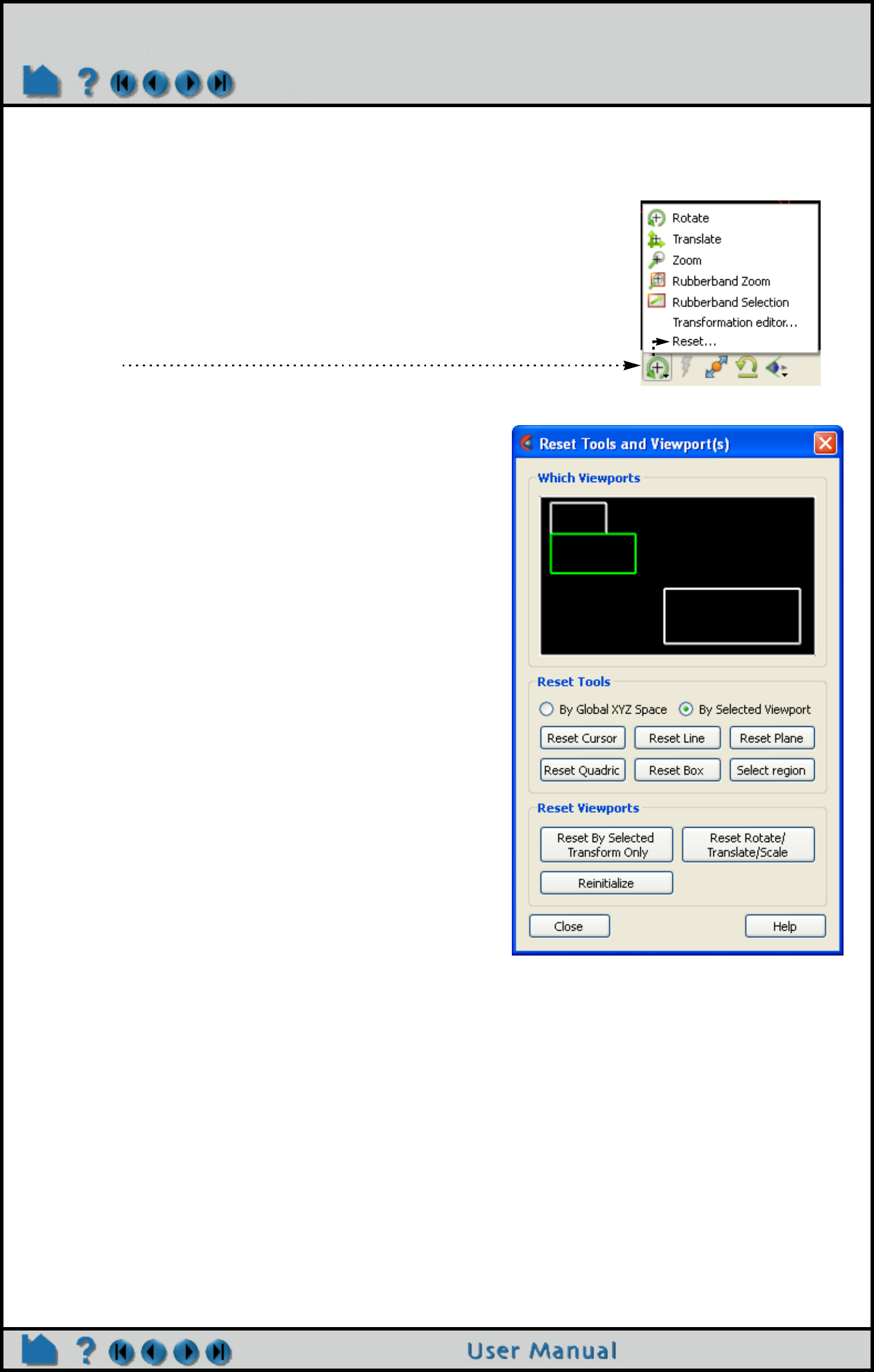
Page 148
HOW TO DEFINE AND CHANGE VIEWPORTS
Reset Viewport Transformations
The transformations for one or more viewports can be reset at any time in the Reset Tools and Viewport(s) dialog.
1. Click the Graphics window transforms icon, then select
Reset...
2. Select the viewport(s) on which the reset will act.
3. Click on the appropriate button to perform the reset
action desired.
You can reset the selected action only, all rotates translates
and scales at once, or do a complete reinitialization of the
viewport.
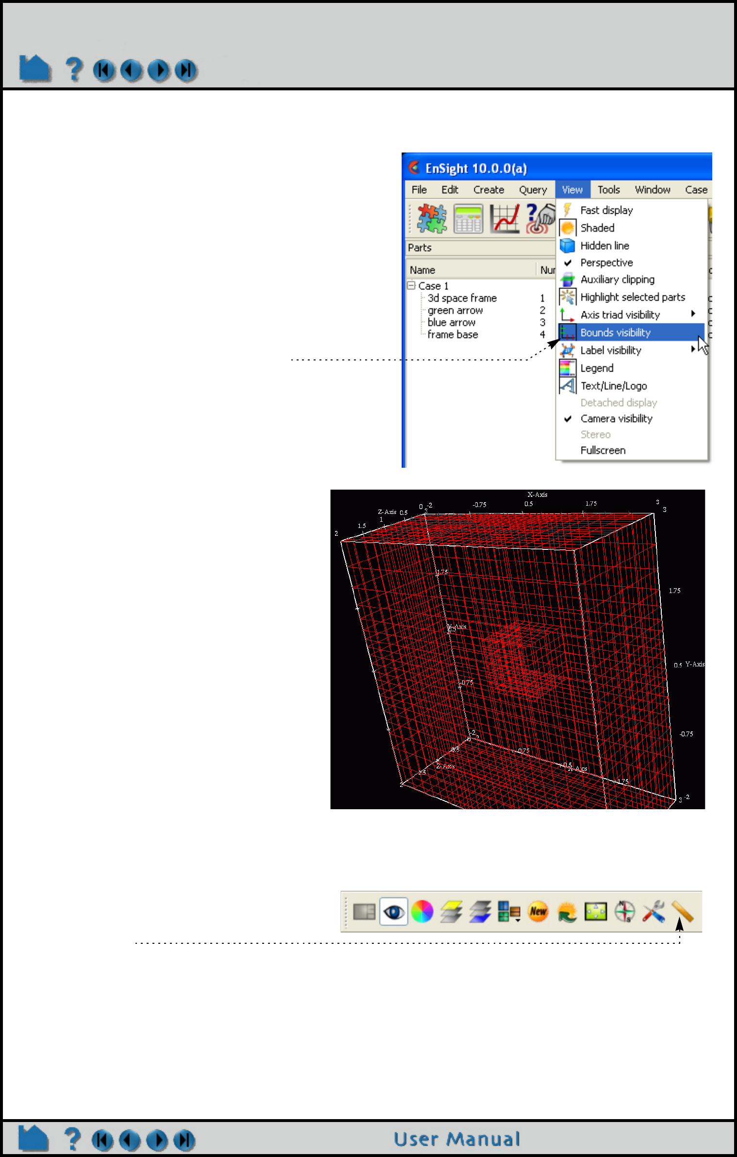
Page 149
HOW TO DEFINE AND CHANGE VIEWPORTS
Setting/Changing Viewport Part Bounds
Part bounds can be displayed within a viewport. This is useful for understanding the size of the model domain.
1. To turn on part bounds globally, toggle the
Bounds visibility under the View menu.
This will display the bounds around the parts
in the viewports.
2. To control the of these bounds, click the
Selected viewport(s) part bounds icon.
Which will open the Bounds section of the
Viewports Feature Panel (see next page).
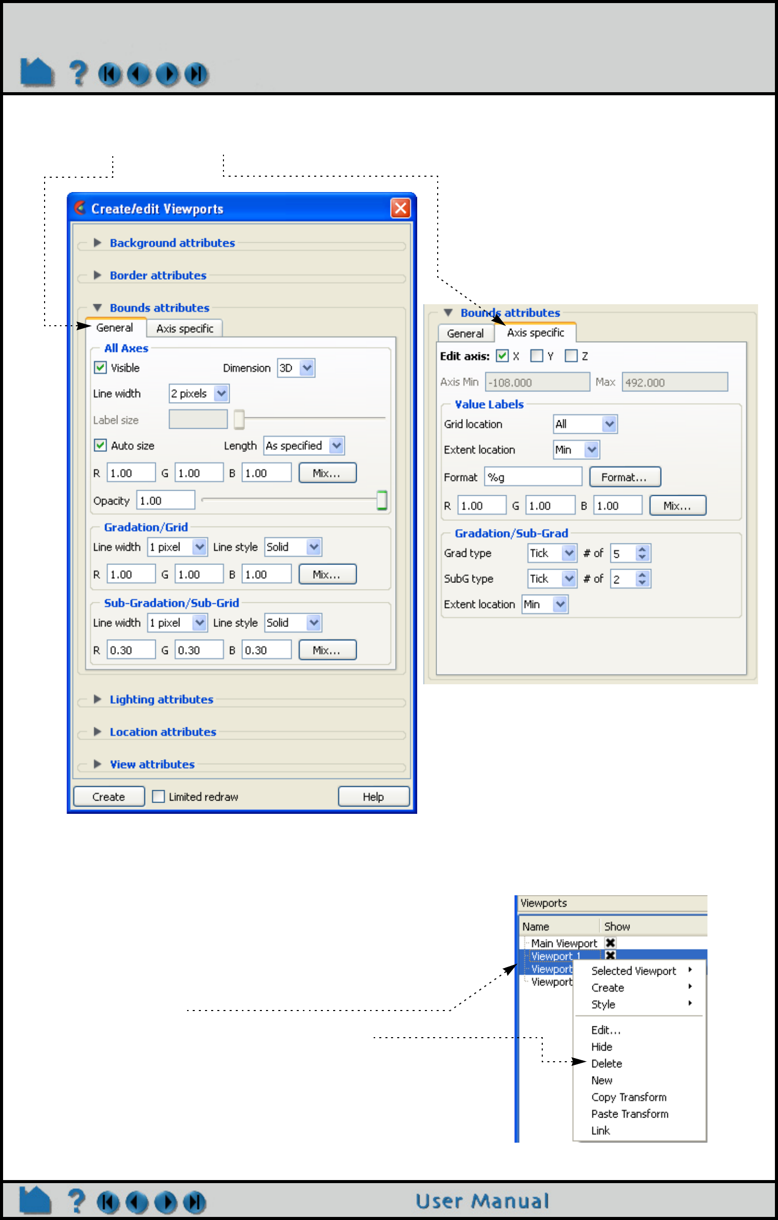
Page 150
HOW TO DEFINE AND CHANGE VIEWPORTS
Delete Viewports
A created viewport can be deleted at any time:
3. Select General or the Axis specific tabs.
4. Modify any desired.
Including the visibility toggle if you
don’t desire to see the bounds in the
selected viewports.
1. Right click on the desired viewport in the Viewport list
panel and select Delete.
OR, if multiple desired:
1. Select the desired viewports in the list by any of the
typical methods. (Hold down the control key to select
multiple viewports)
3. Right click on the selection and choose Delete.

Page 151
HOW TO DEFINE AND CHANGE VIEWPORTS
Other Notes
Border visibility and color, and lighting for the viewports can also be controlled in the Create/edit Viewports dialog.
You can interactively transform multiple viewports simultaneously by selecting the viewports you want to link together
and turning on the Link Interactive Transforms toggle in the Transformation Editor dialog. Those viewports that are
highlighted in green will now transform together for any transformations performed in the Transformation dialog.
Linking does not apply to transformations performed by the mouse in the graphics window.
You can copy the transformations from one viewport to another. First select the viewport you wish to copy, then select
Editor Function->Copy Transformation State. Next select the viewport(s) you wish to modify and select
Editor Function->Paste Transformation State.
SEE ALSO
How To Rotate, Zoom, Translate, Scale, How To Control Lighting
User Manual: Viewports List Panel
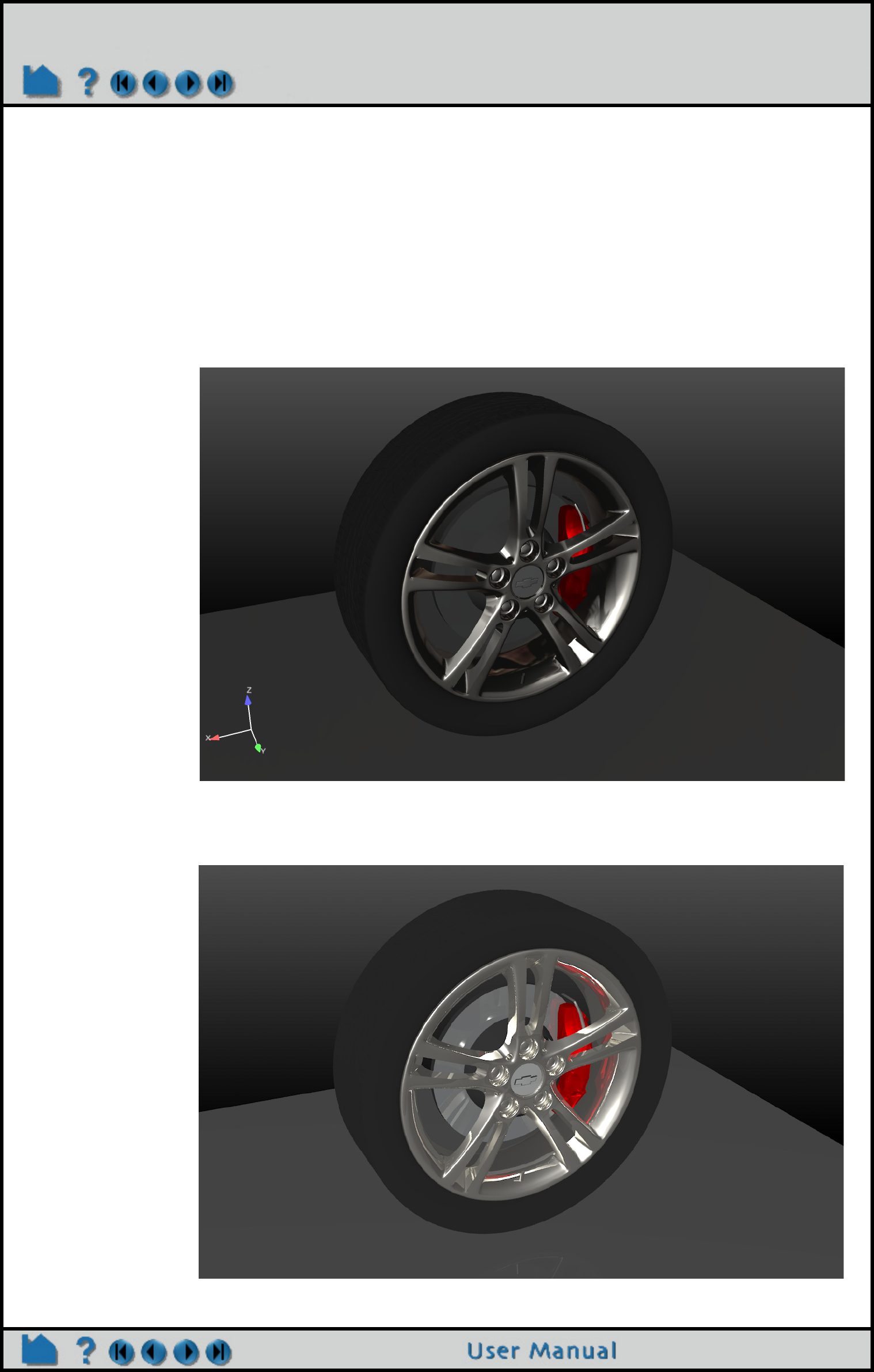
Page 152
HOW TO SET LIGHT SOURCES
Set Light Sources
INTRODUCTION
The surfaces of parts are rendered using surface properties (such as color and highlight properties) interacting with
one or more light sources. But default there is a directional light located along the line of sight. This “at the viewer”
light source can’t be modified, i.e., it is always a directional light pointing in the camera view direction. However, you
can turn it off or adjust it’s color or light intensity. In addition to this first light source, there can be up to seven
additional lights of various types and positions. These lights are taken into account in the graphics window and for
ray traced images.
There are various reasons to define additional light sources. However, the primary and most common use is to
define lights for the ray tracer, such that shadows and reflectivity can be shown in the scene.
Here is a scene showing the image produced in the graphics window. It has a single default light source, i.e., the
light is at the camera position shining in the camera view direction. If we ray trace this, you get the following
image:
As you can see, you
have no shadows in
the scene because
the light and viewer
directions are co-
aligned.
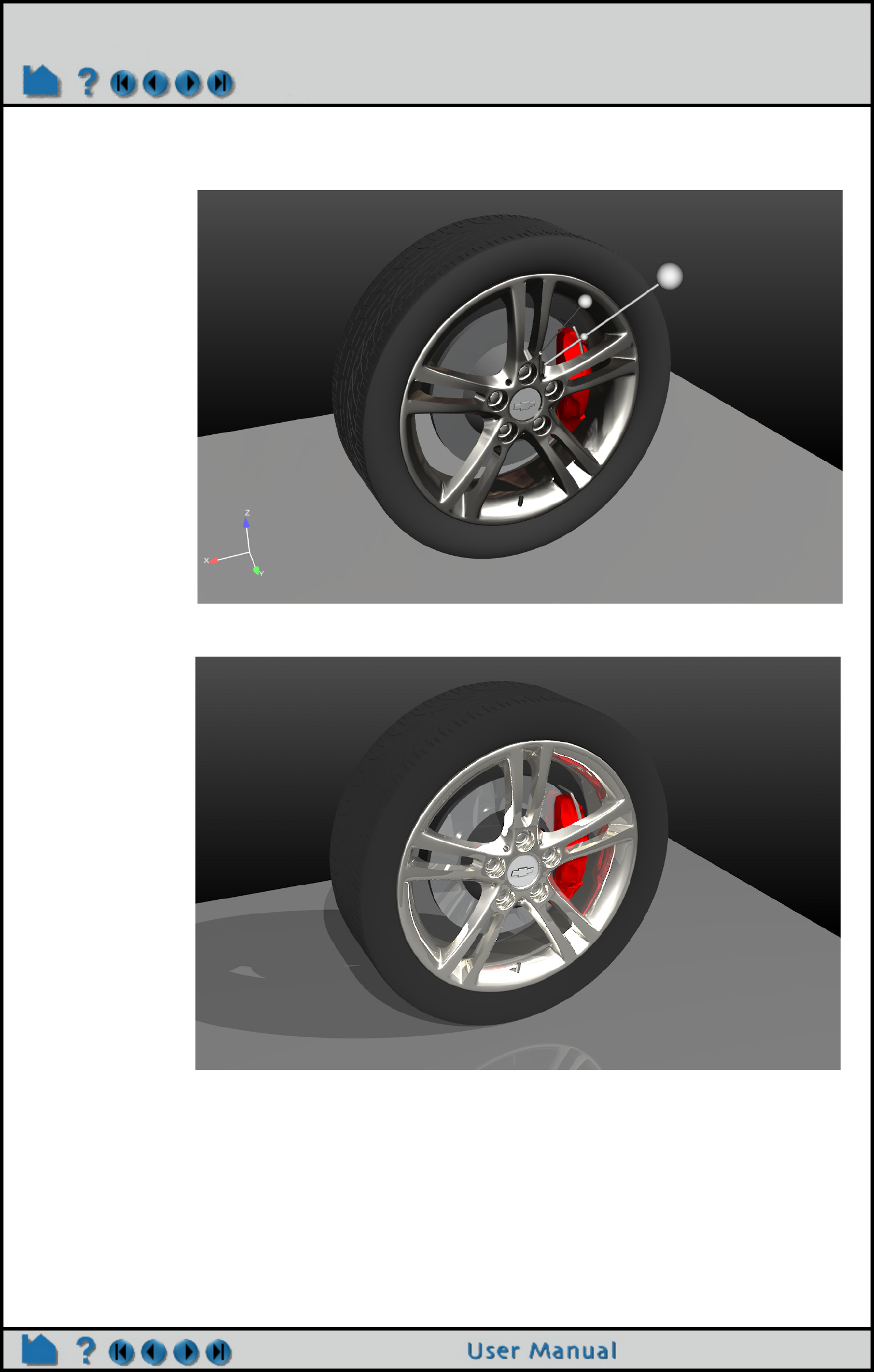
Page 153
HOW TO SET LIGHT SOURCES
If we introduce two more directional light sources at locations and in the directions shown in this image:
And now ray trace the scene, we get the following image:
As you can see, we now have shadows, better reflections, and better lighting in the tread part of the tire.
However, the chrome is also fully saturated in some areas of the wheel. We might consider using a less intense
light for one or more of the lights to make this a better image.
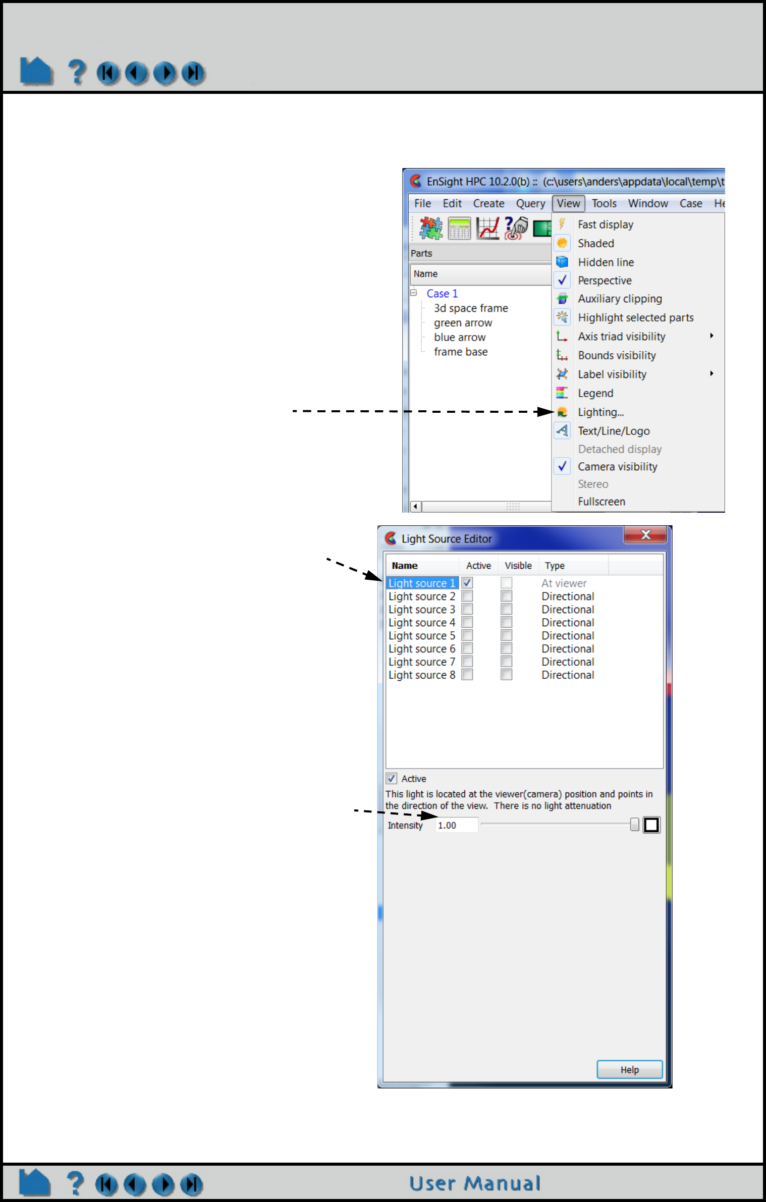
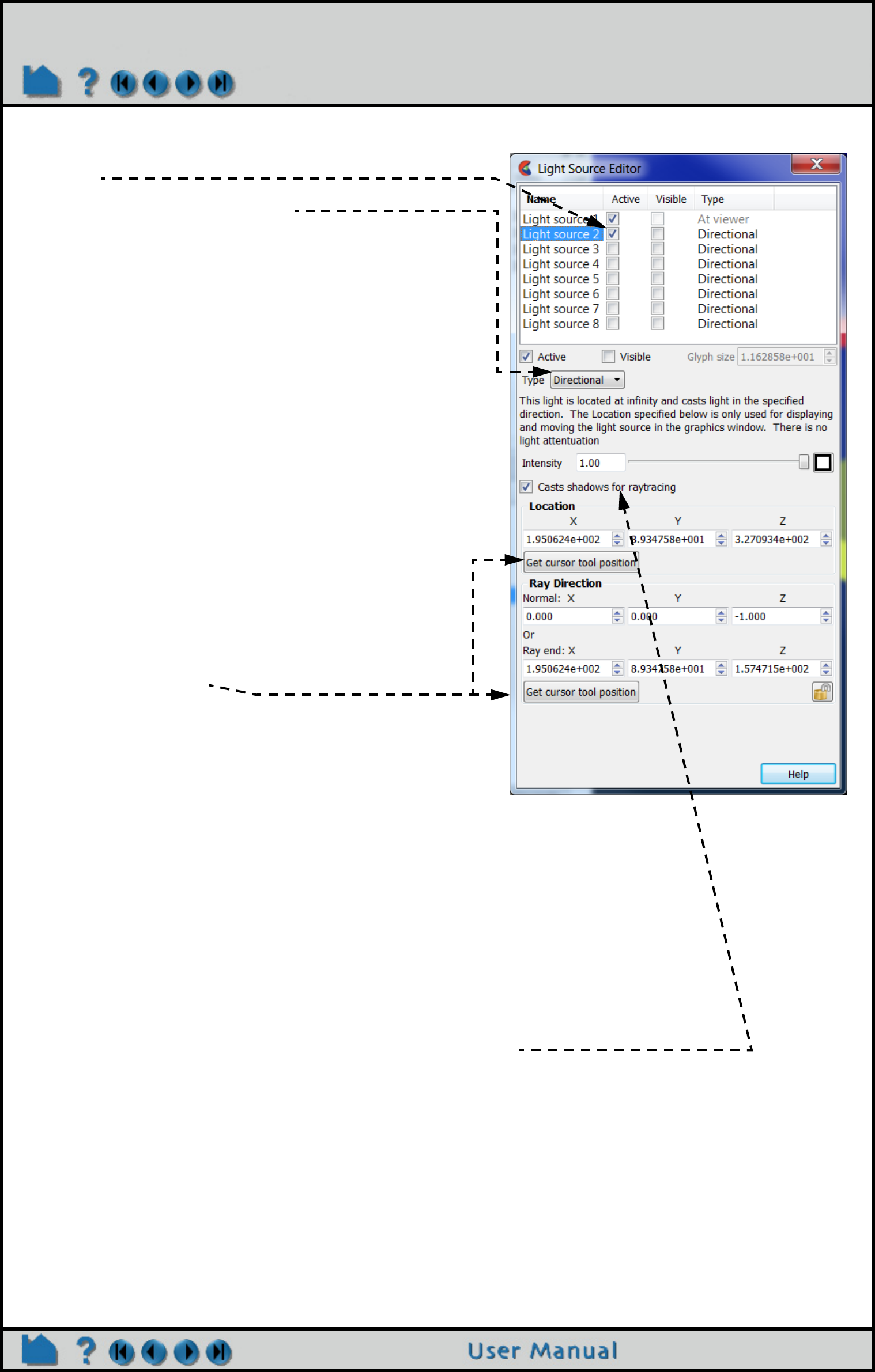
Page 155
HOW TO SET LIGHT SOURCES
ADVANCED USAGE
You have the option to cast shadows from a light source when producing ray traced images.
Toggle on “Casts shadows for raytracing” in the Light Source Editor.
SEE ALSO
How To Use Raytrace Rendering
How To Use the Cursor (Point) Tool
3. To activate a new light source, toggle it’s “Active”
toggle.
4. The Type can be set to one of:
Directional - the light is located at infinity and points in the
direction (or towards the point) defined. There is no light
attenuation for this light type.
Point - the light shines in all directions and is located at
the point specified. This light type has light attenuation and
uses the distance from the light source to the ray end as the
light radius.
Spot - the light shines in the direction (or towards the
point) defined. This light type has light attenuation and uses
the distance from the light source to the ray end as the light
radius. This light type also has a spot angle as well as a falloff
angle which defines how “blurry” the light cone will be.
5. The easiest way to modify the light source location or
light source direction is either:
a) Move the mouse over the light glyph hot points,
which is one of:
(i) the light location,
(ii) the mid point of the ray, or
(iii) the light ray end location.
Then click and drag the location.
b) Or use one of the many tools to specify the cursor
tool location. Once the cursor tool is in location, use the
“Get cursor tool” button to define the light or ray end
locations.
6. If you want to move the light origin or light ray end
location along the ray direction, you can toggle on the
lock icon. Once the icon is locked, you can grab any of
the three hot points for the light glyph with the mouse in
the graphics window and adjust by
(i) moving the light location, which will move the light
location along the ray direction, or by
(ii) moving the ray end location, which will move the
ray end along the ray direction, or by
(iii) moving the mid point, which will move the light
location and ray end together.

Page 156
HOW TO DISPLAY REMOTELY
Display Remotely
INTRODUCTION
EnSight does not support the running of the client on one machine and setting the system display environment back
to a different machine. Not all of the features of OpenGL are supported on all platforms in this mode which can
conflict with EnSight’s graphics. It is intended that you actually run the client from the console of the client
machine.
If you run the client on a remote machine and display back, you will see the following warning displayed on the
console machine:
--------------------------------------------------------------------------
Warning: EnSight has detected indirect OpenGL rendering. This could be
caused by remote display using X11, by an incorrect setting of the DISPLAY
environment variable, or by a bad driver installation.
When running using indirect OpenGL, you will notice a performance degradation
and loss of some rendering features. If you are running over a network we
strongly recommend that you install EnSight directly on the client machine.
EnSight is a client/server application, and you can run the EnSight server
on your remote machine.
--------------------------------------------------------------------------
One way is to run the client on your local machine with a manual connection:
ensight102.client -cm (Linux)
ensight102_client -cm (Windows)
and on the remote machine:
ensight102.server -c clienthostname (Linux)
ensight102_server -c clienthostname (Windows)
Another way is to run your client and to tell it to open a connection on a remote machine (default is ssh) as follows
ensight102.client -c remotehostname (Linux)
ensight102_client -c remotehostname (Windows)
Running one or multiple servers remotely incurs no cost as only the EnSight client requires a license key.
And, of course the various VR combinations of display are valid.
SEE ALSO
How To Use Server of Servers
How To Setup for Parallel Rendering
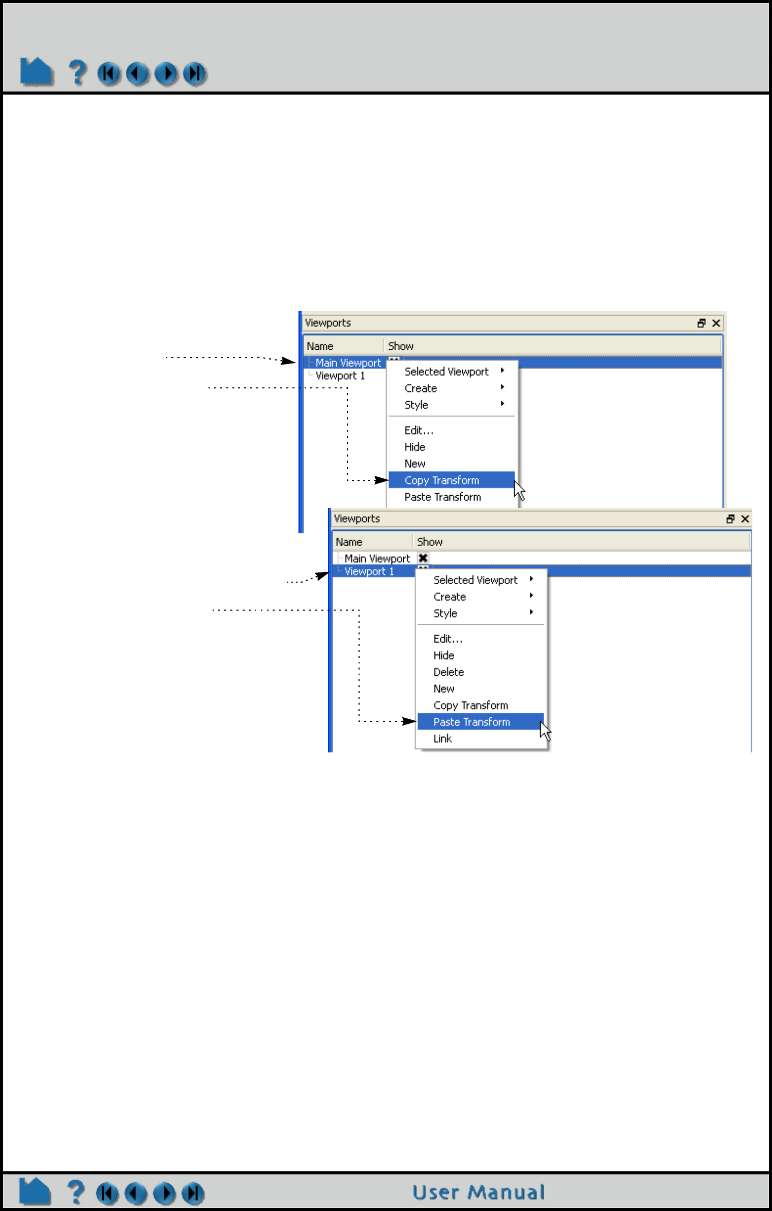
Page 157
HOW TO SAVE & RESTORE VIEWING PARAMETERS
Save & Restore Viewing Parameters
INTRODUCTION
EnSight’s viewports provide a great deal of flexibility in how objects are displayed in the Graphics Window. Given the
complicated transformations that can be performed, it is imperative that users be able to save and restore
accumulated viewport transforms.
BASIC OPERATION
Copying Viewing Parameters from one Viewport to another.
This is most easily done by using right click operations.
1. In the Viewports list panel, right
click the viewport which contains
the desired view.
2. Select Copy Transform.
3. In the Viewports list, right click the
viewport which is to receive the view.
4. Select Paste Transform.
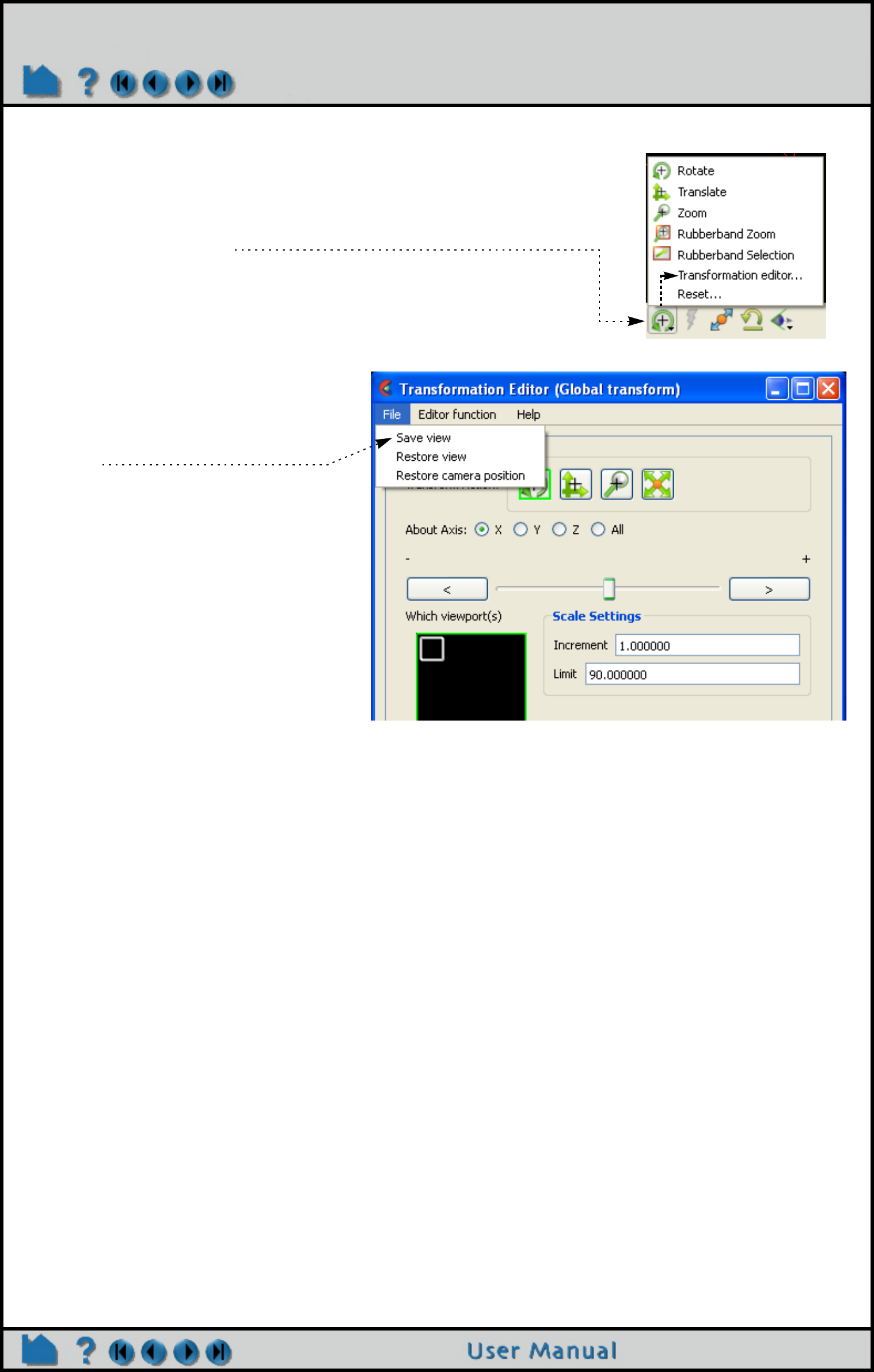
Page 158
HOW TO SAVE & RESTORE VIEWING PARAMETERS
Saving Viewing Parameters to a file
EnSight provides a maximum of 16 viewports: the main viewport (which you cannot change) and 15 additional
viewports. When EnSight saves one or more viewports, it also includes the viewport number (which is equal to the
creation order) as a tag. When you request that one or more viewports be restored, EnSight looks in the saved file
and searches for tag numbers corresponding to the currently selected viewports. If it finds a match, it restores that
viewport. If there is no match for a selected viewport, it is left unchanged.
Restoring Viewing Parameters
Click the Graphics window transforms icon in the Transformations Control area of the Tools Icon Bar and
select Transformation editor... to open the Transformations dialog.
1. Select the viewports you want to restore.
2. Select Restore View... from the File menu. Select a file name in the file browser and click OK.
What is Saved
Only global and local (frame) transformations are stored in a view parameters file. No information is stored for
viewport, look-from/look-at points, or Z clipping.
Other Notes
By default, the F5, F6, or F7 buttons restore a standard right, top, or front view (respectively) of the selected viewport.
However, by holding down the Control key while pressing one of these keys, the current view will be saved to that
key. Subsequent pressing of that key will restore the saved view. Only Global transforms are saved / restored by
these operations, not Frame transforms.
SEE ALSO
How to Define and Change Viewports, How to Create and Manipulate Frames.
Click the Graphics window transforms
icon in the Transformations Control area
of the Tools Icon Bar and select
Transformation editor... to open the
Transformations dialog.
1. Select the viewports you want to save.
Click within a viewport to select it.
Hold down the control key as you
click to select additional viewports. Or
select them similarly in the Viewport
list.
2. Select Save View... from the File
menu.
3. Select a directory and enter a file
name in the file browser and click OK.

Page 159
HOW TO CREATE AND MANIPULATE FRAMES
Create and Manipulate Frames
INTRODUCTION
A coordinate frame can be created for calculator functions or for parts.
The two calculator functions VectorCylProjection and VectorRectProjection use a Frame to designate the projection
coordinate system.
The remaining use of frames is for parts. By default, all parts are assigned to the same frame of reference. You can,
however, create additional coordinate frames and assign parts to them. These frames (and the parts assigned to
them) can be manipulated (rotated, translated, scaled) independently of other frames. Some examples of frame
usage:
1. You wish to create a copy of a part and display a different variable on the copy. When you create the copy, a new
frame is automatically created and the copy is assigned to it. The new frame can be translated away from the
original to visualize both variables simultaneously.
2. You wish to create an animation of parts moving independently (e.g. for an exploding view or to “open” a closed
object with a “hinged door”). Each dynamic part is assigned to a new frame. During keyframe animation, the
frames are manipulated independently to achieve the desired motion.
3. You have a dataset with rotational periodicity but the symmetry axis is not aligned with a major axis. A new
frame is created and positioned such that one of its axes is aligned with the symmetry axis.
4. You have a dataset that makes correct positioning of EnSight tools difficult, e.g. a duct not aligned with a major
axis. Create a new frame and align one of the axes with the duct. Since tool positions are always specified with
respect to the current frame, you can now use the Transformation Editor to accurately position tools along the axis
of the duct.
In addition to position and orientation, frames have a number of display such as visibility, line width, and color. You
can also specify the length of each axis separately and display a series of evenly spaced labels to use as a 3D
measuring tool.
Frames are a powerful but complex feature of EnSight. Understanding the basics of frames is essential for proper
use. This article is divided into the following sections:
Introduction
Create a New Frame
Select Frames
Assign Parts to Frames
Move and Rotate Frames
Reset Frame Transform
Set Frame
Determine What Frame a Part is Assigned To
Delete Frames
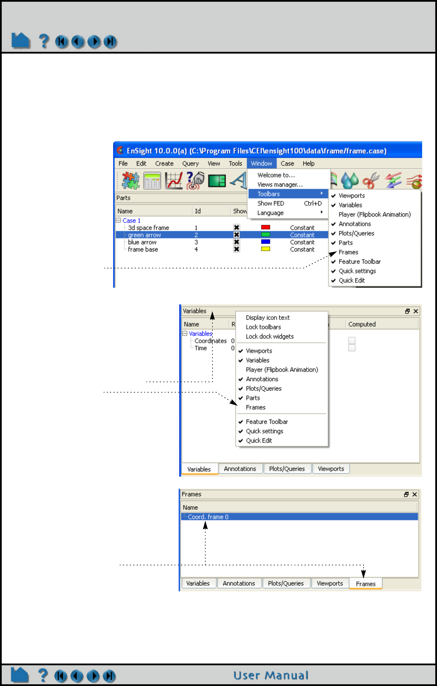
Page 160
HOW TO CREATE AND MANIPULATE FRAMES
BASIC OPERATION
Introduction
On startup, EnSight creates a default frame – frame 0 – located at 0,0,0 of the right-handed “world” or model
coordinate system and aligned with the X, Y, Z axes. All parts (model and newly created) are assigned to frame 0
initially. Frame 0 is special in that it cannot be repositioned or deleted.
Frames are selected either by clicking a visible frame axis triad in the Graphics Window (implying that the frame triad
had to previously been set to be visible) or by selecting the desired frame in the Frames list panel. Any frame
operation (such as setting) acts on the currently selected frame(s).
Note: Frame operations
are reserved for the
expert user. By default,
the Frame Feature Icon
is not enabled. To
enable it, go to Window-
>Toolbars, and toggle
Frames on.
Alternatively, one can right click on
the head of the List Panel section,
and toggle Frames on.
After which, the Frames List Panel will
be available, default Coord. frame 0 is
listed, and the operations described
below can be performed.
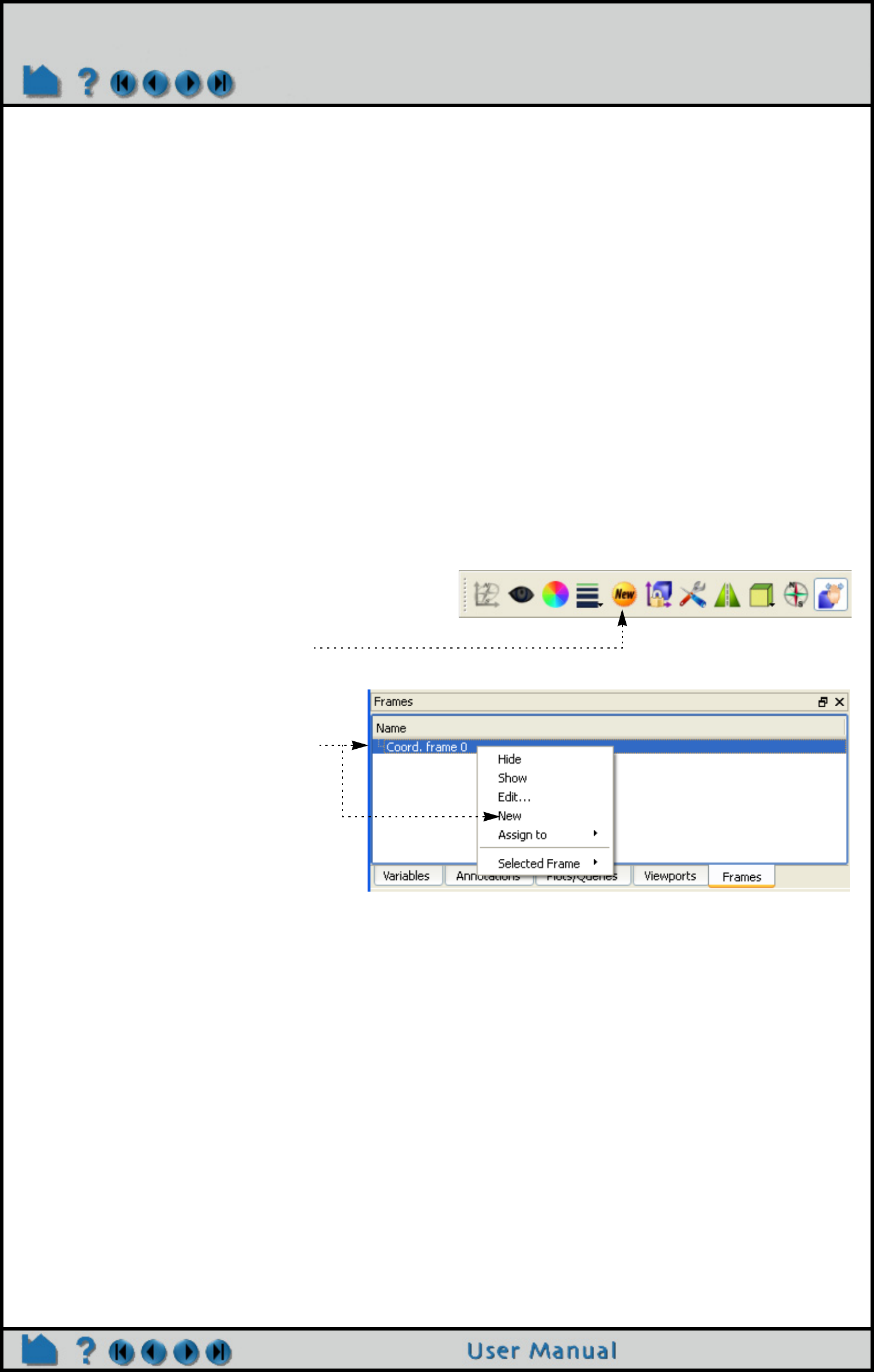
Page 161
HOW TO CREATE AND MANIPULATE FRAMES
The EnSight positioning tools (Cursor, Line, Plane, and Quadric tools) are always positioned with respect to the
currently selected frame. If more than one frame is selected, frame 0 is the reference frame for tools. If you have tools
visible, you will notice them changing position as the selected frame is changed.
EnSight implements computational periodicity (such as rotational symmetry) as an attribute of frames. If a frame has
symmetry enabled, all parts assigned to the frame will be duplicated as specified by the particular type of symmetry.
A frame axis triad consists of three lines representing the X, Y, and Z orientation vectors plus labels. Selected frames
are highlighted in the Frames list.
EnSight does not support hierarchical frames: you cannot assign a frame to another frame to implement nested
transformations. All frames are embedded in the same world coordinate system (i.e. frame 0).
Create a New Frame
In general, you have to explicitly create new frames. However, EnSight will automatically create a new frame each
time you create a copy of a part and assign the copy to the frame.
To create a frame:
1. Decide if you want the new frame to be set to the default 0,0,0
position (same as the model coordinates), or whether you would
like to have it centered on some selected part(s). If the former,
make sure no parts are selected in the Parts list. If the latter, select
the desired part(s) in the Parts list.
2. Either select an existing frame in the Frames list
panel and hit the New Frame icon.
OR
Right click on an existing frame in the
Frames list panel, and select New.
The new frame also becomes the currently
selected frame.
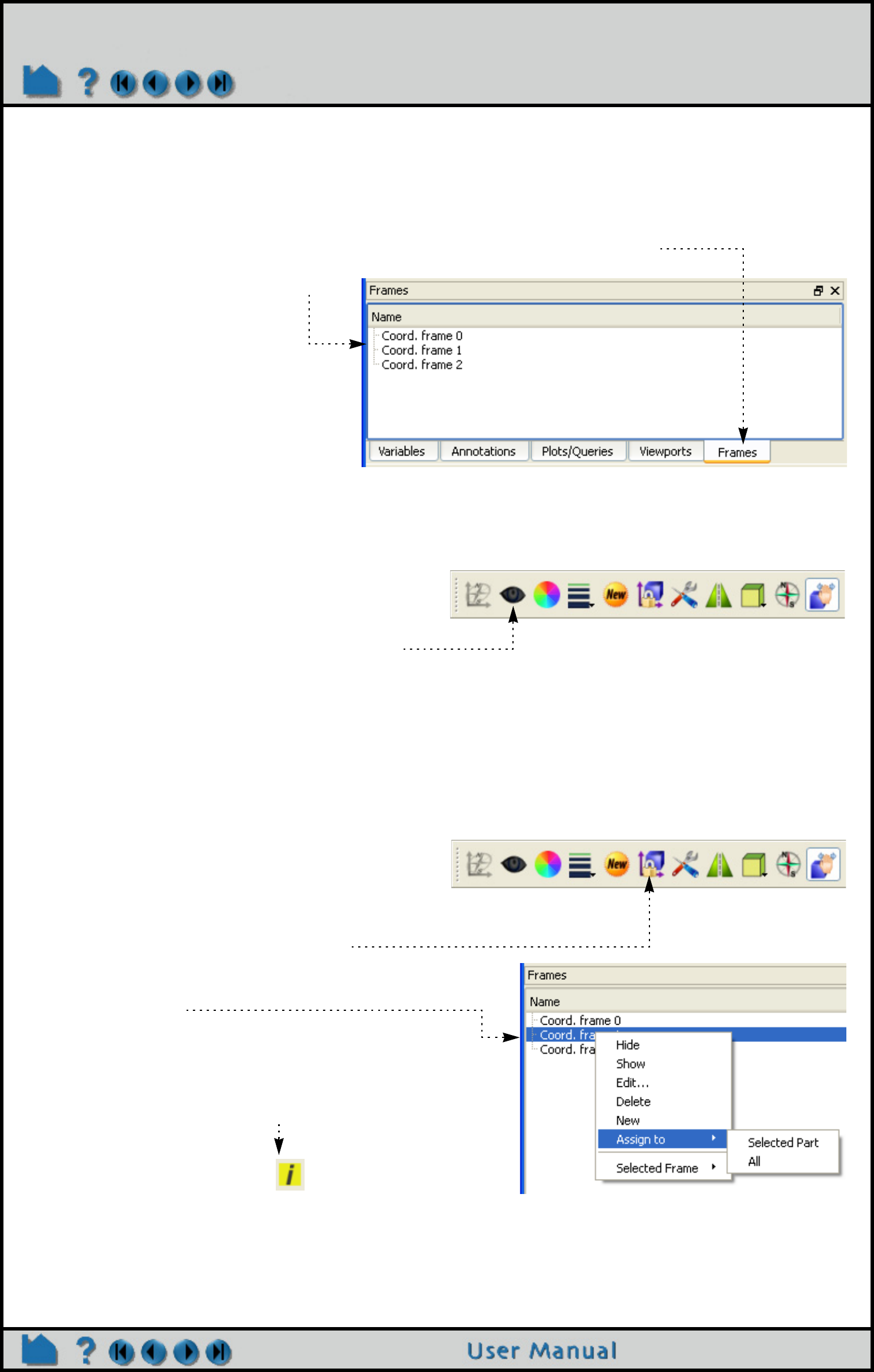
Page 162
HOW TO CREATE AND MANIPULATE FRAMES
Select Frames
There are two ways to select frames. You can select frames in the Frames list panel, or click on the frame axis triad in
the Graphics Window (if the triad is visible).
To select frames using the Frames list:
To select frames in the Graphics Window:
Assign Parts to Frames
To assign a part to a frame:
1. Click the Frames tab, to show the Frames list panel, if it is not already shown.
2. Select the desired frames in the list.
You can use standard techniques, such as
shift-click to extend a selection or control-
click to add to the list (or de-select an item if
already selected).
Note that this implies that the frame triad(s) are
already visible. If they are not, you will need to do
your first selection using the Frames list as
described above. Then make the frame triad(s)
visible by toggling on the Axis visibility icon.
You can now:
1. Position the mouse pointer over the frame axis triad (the lines – not the XYZ labels) and click the left
mouse button.
You can extend a selection of frames by holding down the Control key as you click on frames.
1. Select the desired part(s) in the Main Parts list.
2. Select the desired frame (as described above).
4. Click the Assign selected part(s) to selected frame
icon to assign the part(s) to the frame.
OR
Right click on the desired frame and select Assign to,
then Selected Part.
Note that you can easily assign all parts to a frame using
the latter method
A message is printed to the EnSight Message Window
(found under the Information display icon), confirming the
assignment.
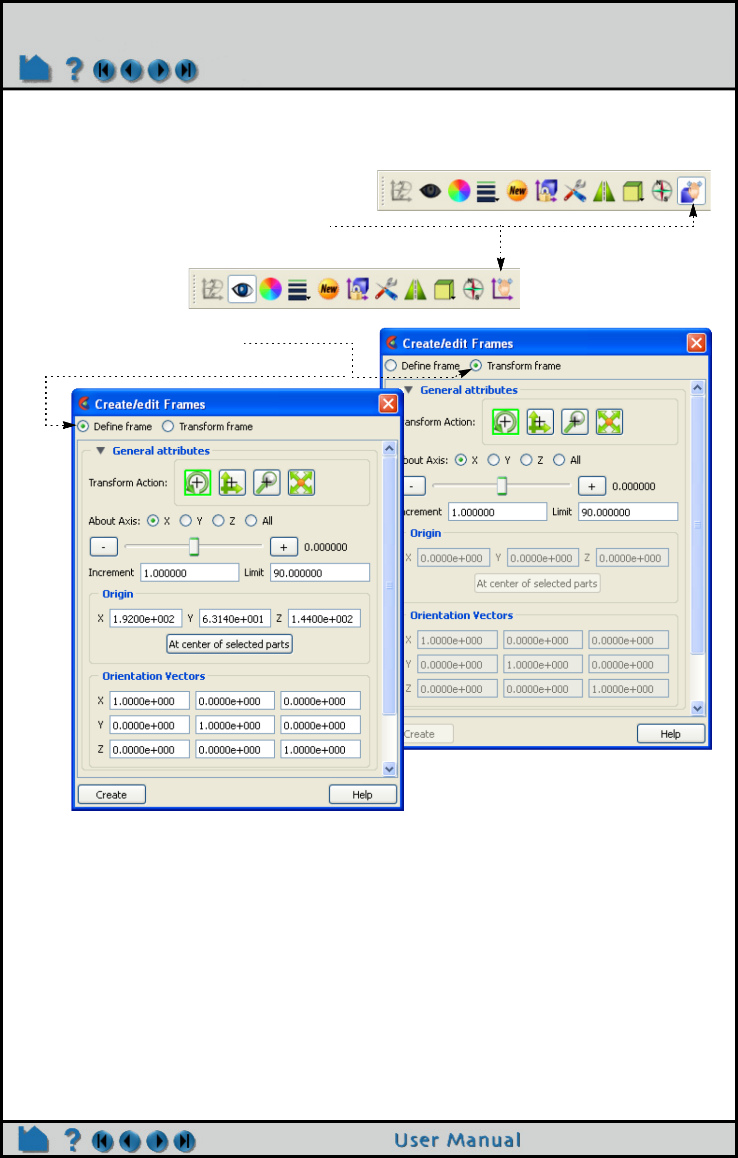
Page 163
HOW TO CREATE AND MANIPULATE FRAMES
Move and Rotate Frames
You transform a frame (and all parts assigned to it) when you perform any transformation while in Frame Transform
mode. Frame Transform mode is set by default.
You toggle between it and Frame definition mode
for the selected frame(s) using the Transform/
Define frame(s) icon on the Quick Action Icon Bar.
or in the Create/edit Frames dialog.
Transform
Mode
Define
Mode
IMPORTANT: Generally one should only use the Define mode while first creating and orienting the
frame. Thus before any parts are assigned to it. Thereafter one should ensure that he is using Transform
mode. If you do this, you will avoid error and confusion in the use of frames.
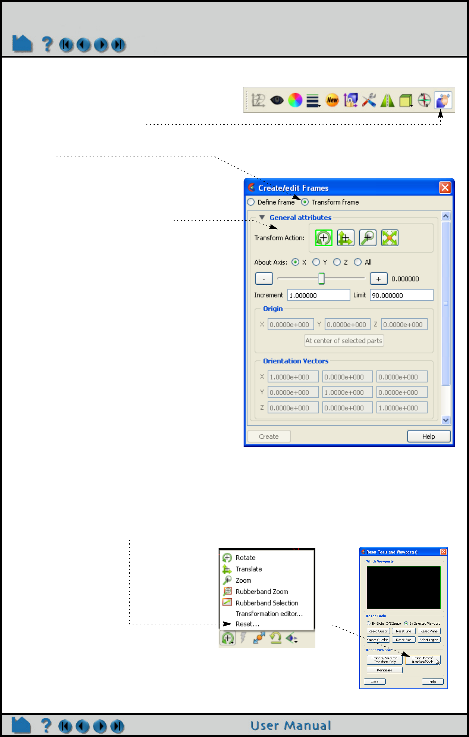
Page 164
HOW TO CREATE AND MANIPULATE FRAMES
To transform in Frame Transform mode:
Frame transforms are implemented as a transformation applied with respect to the frame’s position and orientation.
At times you will need to modify the position and orientation of the frame independent of the parts assigned to it. This
is done while in Frame Definition mode. You have been shown how to enter Frame Definition mode above.
Important! You cannot change the frame definition if you have performed any frame transformations (if you attempt
to do so, a dialog will remind you). Any frame definition must be applied prior to a frame transformation. If you have
already made frame transforms you can clear them by returning to frame transform mode and using the Reset Tools
and Viewports dialog (click Reset... to open).
1. Select the desired frame(s) (as described above).
2. Ensure that the Transform/Define frame(s) icon is
set to the Transform mode.
This can alternatively be done in the Create/edit
Frames dialog, where radio buttons show the
state.
3. Perform the desired transformation either
interactively (using the Transformations Control
icons and the mouse in the Graphics Window) or
via the Transform Actions in the General section
in the Create/edit Frames dialog.
See How To Rotate, Zoom, Translate, and Scale
for more information.
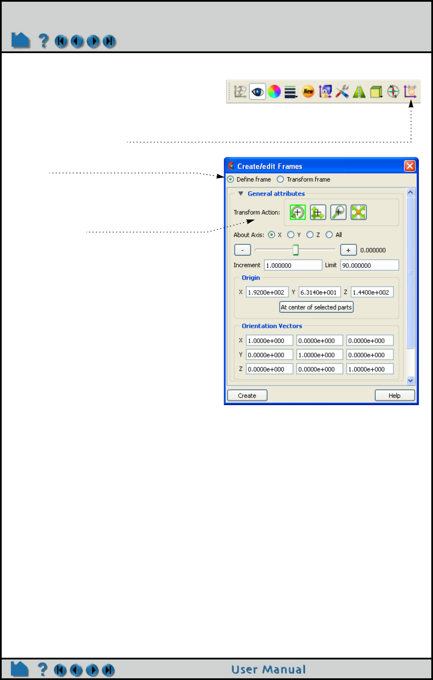
Page 165
HOW TO CREATE AND MANIPULATE FRAMES
To transform the Frame Definition:
1. Select the desired frame(s) (as described
above).
2. Ensure that the Transform/Define frame(s) icon
is set to the Define mode.
This can alternatively be done in the Create/edit
Frames dialog, where radio buttons show the
state.
3. Perform the desired transformation either
interactively (with the mouse in the Graphics
Window) or via the Transform Actions in the
General section in the Create/edit Frames
dialog.
To translate the frame interactively, move the
mouse pointer into the Graphics Window and
click and drag the left mouse button. To rotate
the frame interactively, click and hold the left
mouse button on one of the frame axes and
drag the mouse. Clicking on the X axis will
rotate the frame about its Y axis. Clicking on the
Y axis will rotate the frame about its X axis.
Clicking the Z axis will rotate about both X and
Y.
(Use the Transform Action in the General
section to rotate about the Z axis only.)

Page 166
HOW TO CREATE AND MANIPULATE FRAMES
You can also edit the frame’s definition explicitly using the Transformation Editor dialog:
Reset Frame Transform
The frame transform can be reset back to the default position and orientation by using the Reset Tools and Viewports
dialog. To clear the frame transform:
1. Click the Frame Location icon.
This opens the Create/edit Frames dialog in Frame Definition mode.
2. Select the desired frame(s).
4. If desired, enter new value(s) in the XYZ
fields to change the frame’s origin
(remember to press return).
5. If desired, enter new value(s) for the
orientation vectors (remember to press
return).
Note that the orientation vectors are
normalized afresh when you press return.
1. Select the desired frame(s) (as described above).
2. Make sure the Transform/Definition Icon is set to transform
3. Click the Reset... button in the Transformation Control area to open the
Reset Tools and Viewports dialog.
4. In the Reset Tools and Viewports dialog, click the desired button:
Reset By Selected Transform Only: clear only the transformation component
currently selected (e.g. rotate or translate) in the Transformation Control area
Reset Rotate/Translate/Scale: clear all transformation components
See How To Reset Tools and Viewports for more information.
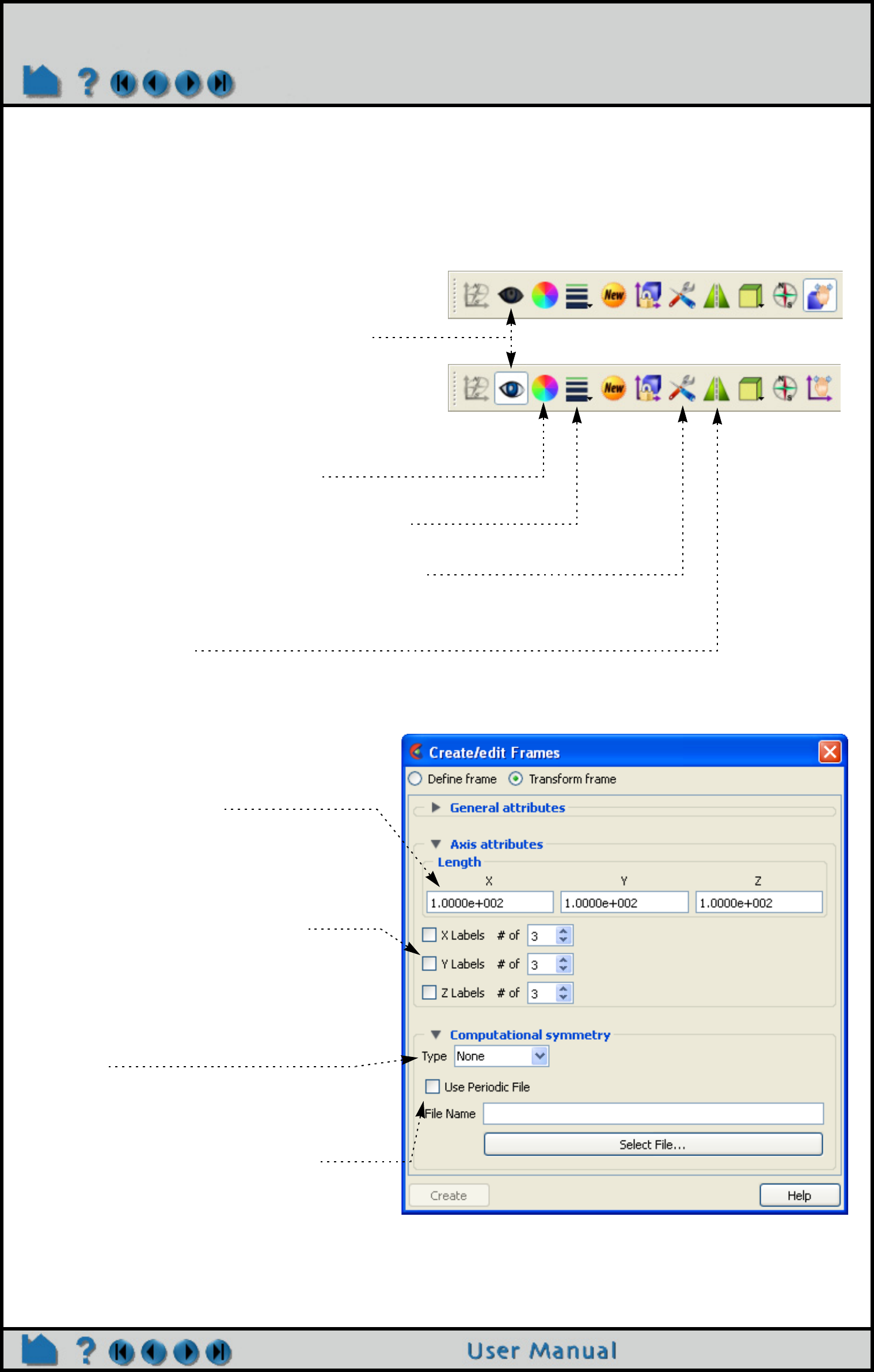
Page 167
HOW TO CREATE AND MANIPULATE FRAMES
Set Frame
Frames can be displayed with a variety of options:
1. Select the desired frame(s) (as described above).
2. Set the desired attribute as described below:
Click the Axis Visibility Toggle to toggle display of
the axis triad of selected frames on or off.
Click (opens the Color Selector) to set the color
for the axis triad of selected frames.
Click the Frame Line Width pull-down to set the
line width for the axis triad of selected frames.
Click the Axis icon to set axis (described below).
Click Computational symmetry icon to set
translational, rotational, or mirror symmetry
(described below)
To adjust the length of the frame axes,
enter new values in the X, Y, and Z Length
fields and press return.
To display a series of evenly spaced labels
along an axis (showing distance from the
axis origin), toggle on the applicable Label
button, enter the desired number of labels
in the # of field, and press return.
To choose the type of computational
symmetry (translatational, rotational,
mirror).
Once the type is chosen, appropriate
controls will open for that type.
If your data is not Case Gold format then
you can interactively chose to use a
Periodic File. If it is Case Gold then you
must enter the matchfile name in the Case
file
Off
On
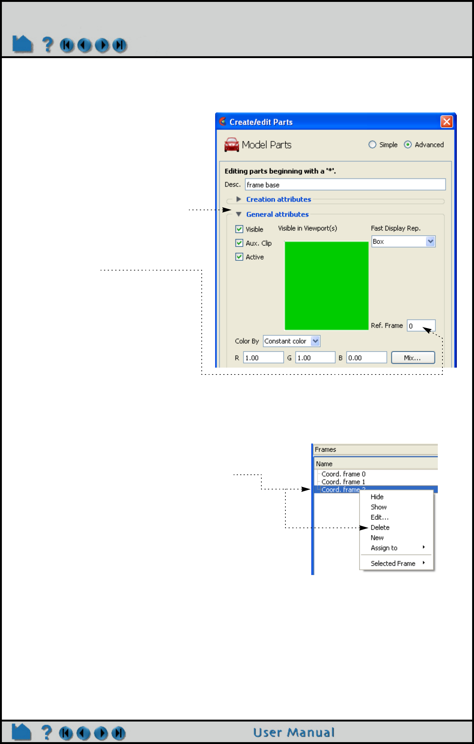
Page 168
HOW TO CREATE AND MANIPULATE FRAMES
Determine What Frame a Part is Assigned To
You can determine what frame a part is assigned to (and change it) by opening the Parts Feature Editor:
Delete Frames
Selected frames can be deleted. Note that a frame cannot be deleted if any parts are currently assigned to it. All parts
assigned to the frame must be assigned to other frames prior to deletion.
SEE ALSO
How To Set Symmetry, How To Rotate, Zoom, Translate, and Scale, How To Reset Tools and Viewports
User Manual: Frames List Panel
1. Open Create/edit Parts by double
clicking on the desired part.
or
Right click on the part in the Parts list,
and select Edit...
3. Open the General turndown.
The part’s current frame number is shown in
the Ref. Frame field. You can reassign a part to
a different frame by entering a new value and
pressing return.
1. Select the desired frame(s) (as described above).
2. Right click on your selection and choose Delete.
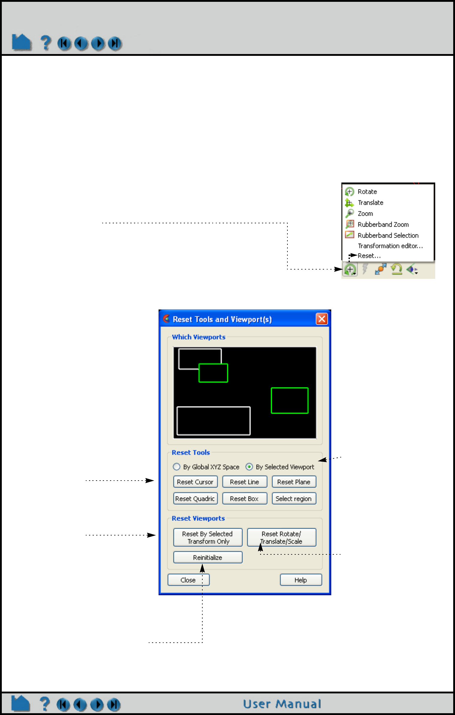
Page 169
HOW TO RESET TOOLS AND VIEWPORTS
Reset Tools and Viewports
INTRODUCTION
EnSight provides support for complex transformations of various entities (e.g. the scene, tools, frames). It is often
necessary to clear all or part of the transformation associated with an entity; the Reset Tools and Viewports dialog
provides this capability.
BASIC OPERATION
To clear global transformations or tool positions:
1. Click the Graphics windows transform icon in the
Transformation Control area of the Tools Icon Bar
and select Reset... to open the Reset Tools and
Viewports dialog.
2. Perform the desired operation as described
below.
3. Click Close.
Transformations will only be reset for the
current viewport(s). Click in a viewport to
select it (turns green). Control-click to
extend the selection or de-select a
selected item.
Click the applicable button to reset the
corresponding tool.
Click to clear only the transformation
component currently selected in the
Transformation Control area (e.g. Rotate
or Translate).
Click to clear all transformations as well
as reset the camera look-from/look-at
points so that all currently visible parts
are centered in the selected viewport(s).
This also resets the center of transform
to the geometric center of the visible
parts.
Click to clear all
transformations in the
selected viewport(s). Note
that zoom is not a scene
transformation and is not
cleared. Zoom is
implemented by moving the
look-from point (the camera
position). To clear zoom, click
Reinitialize.
Toggle selects whether tool is
reset based on the global XYZ
space or reset based only on
the selected viewport.
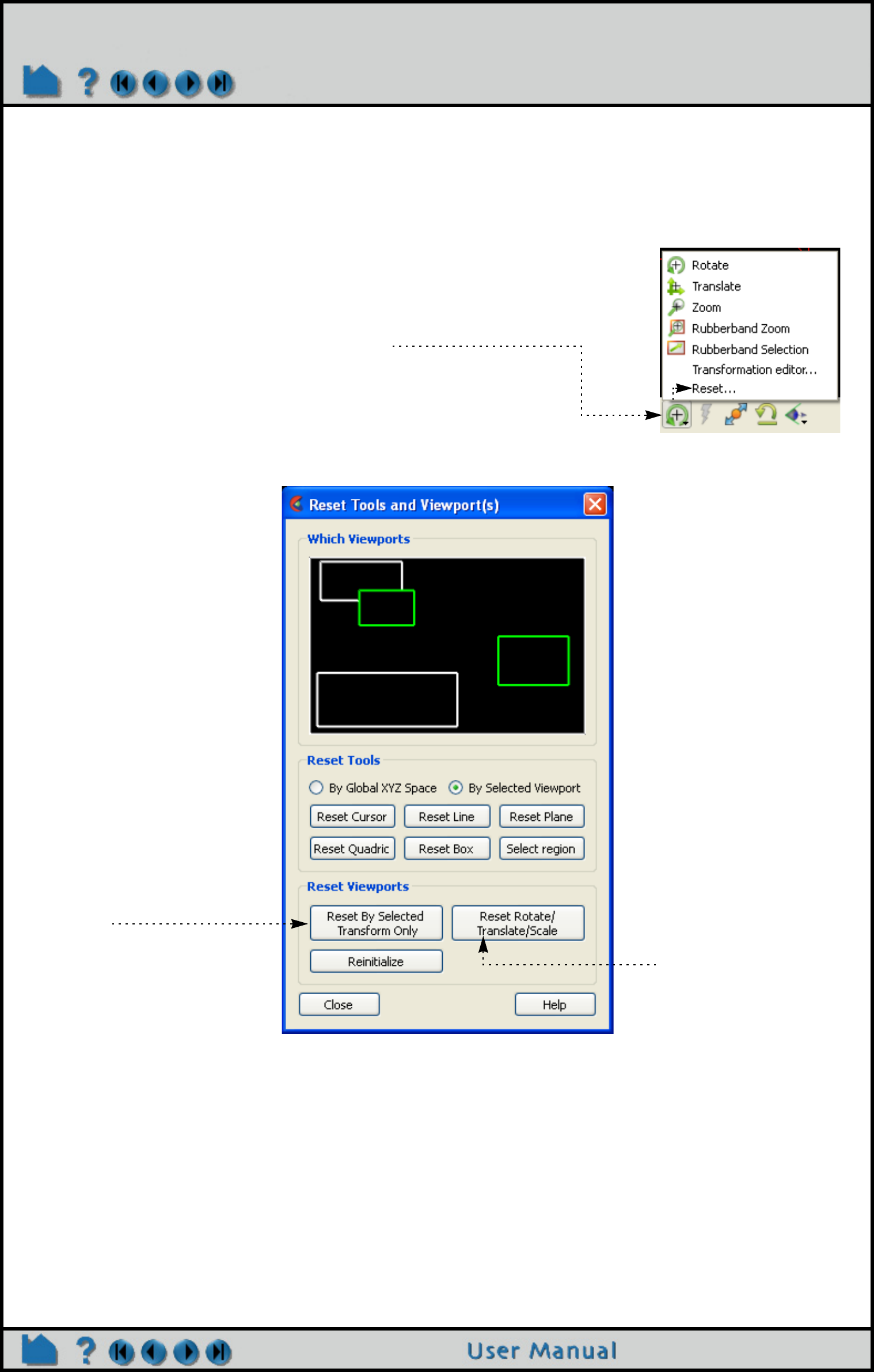
Page 170
HOW TO RESET TOOLS AND VIEWPORTS
ADVANCED USAGE
The Reset Tools and Viewports dialog is also used to clear Frame transformations. See How To Create and
Manipulate Frames for more information on frames and frame transforms.
To clear frame transformations:
SEE ALSO
How To Rotate, Zoom, Translate, Scale, How To Define and Change Viewports, How To Create and Manipulate
Frames
1. Select the desired frame(s) in the Frame list.
2. Click the Graphics windows transform icon in the
Transformation Control area and select Reset... to
open the Reset Tools and Viewports dialog.
3. Perform the desired operation as described
below.
4. Click Close.
Frame transformations will only be reset
for the current viewport(s). Click in a
viewport to select it. Control-click to
extend the selection or de-select a
selected item.
Click to clear only the frame
transformation component currently
selected in the Transformation Control
area (e.g. Rotate or Translate) for the
selected frame(s) in the selected
viewport(s).
Click to clear all frame
transformations for the
selected frame(s) in the
selected viewport(s).
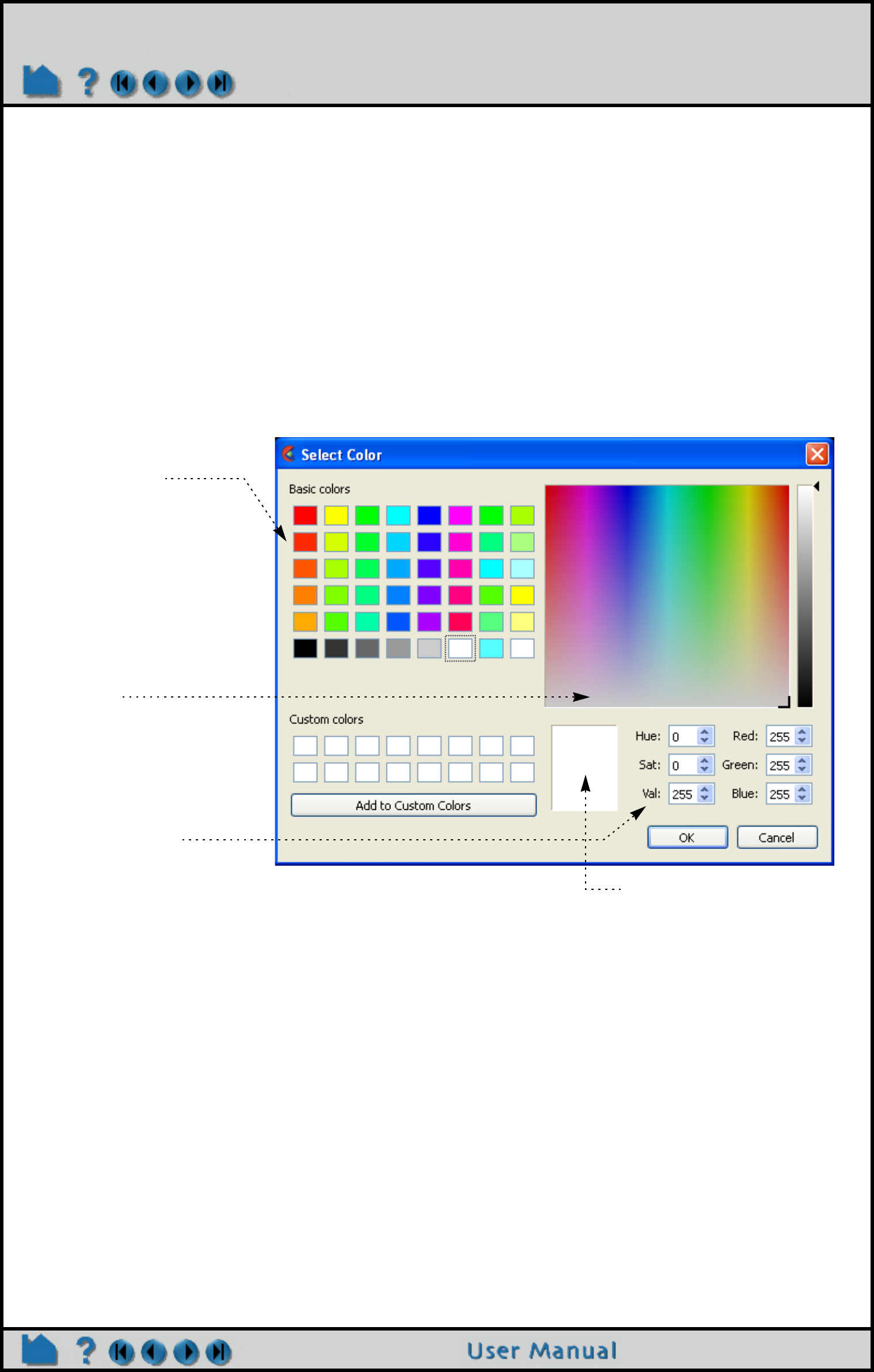
Page 171
HOW TO USE THE COLOR SELECTOR
Use the Color Selector
INTRODUCTION
Several operations in EnSight require that you select a color. The Color Selector dialog is used throughout the user
interface to provide a powerful and easy-to-use color selection mechanism.
BASIC OPERATION
The selector operates using one of two basic color models: RGB or HSV. The RGB color model specifies color by the
percentage of red, green, and blue and closely mimics the way computers deal with color. The HVS color model
specifies colors as percentages of hue (the actual color with red equal to both 0.0 and 1.0, green equal to 0.33, and
blue equal to 0.66), saturation (the “amount” of color, where 0.0 is white and 1.0 is full), and the value (the brightness,
where 0.0 is black and 1.0 is full). The HSV model is often more intuitive for mixing custom colors.
The dialog provides three basic methods of selecting colors:
When you have selected a color, click the OK button to have the selected color applied to the object being edited (e.g.
part, color map level, text, etc.).
Specify Custom Colors
If you have colors that you use frequently that are not represented in the color grid, you can save them to one of the
Custom colors grids by clicking Add to Custom Colors button. Your custom colors are automatically saved for future
sessions. To set custom colors:
The color information is saved in EnSight defaults directory (located at
%HOMEDRIVE%%HOMEPATH%\(username)\.ensight102 commonly located at C:\Users\username\.ensight102 on
Vista and Win7, C:\Documents and Settings\yourusername\.ensight102 on older Windows, and ~/.ensight102 on
Linux, and in ~/Library/Application Support/EnSight102 on the Mac) with the following filename:
ensight.colpal.default.
SEE ALSO
User Manual: Quick Color Widget Panel, Part Color/Surface Property Icon
1. By picking one of the
predefined colors from the
grid of color cells.
2. By grabbing the marker in the
color cube and moving it with
the mouse.
3. By entering values for HSV
(or RGB, depending on
mode) directly in the fields
and pressing return.
Color square always displays
the current color selection.
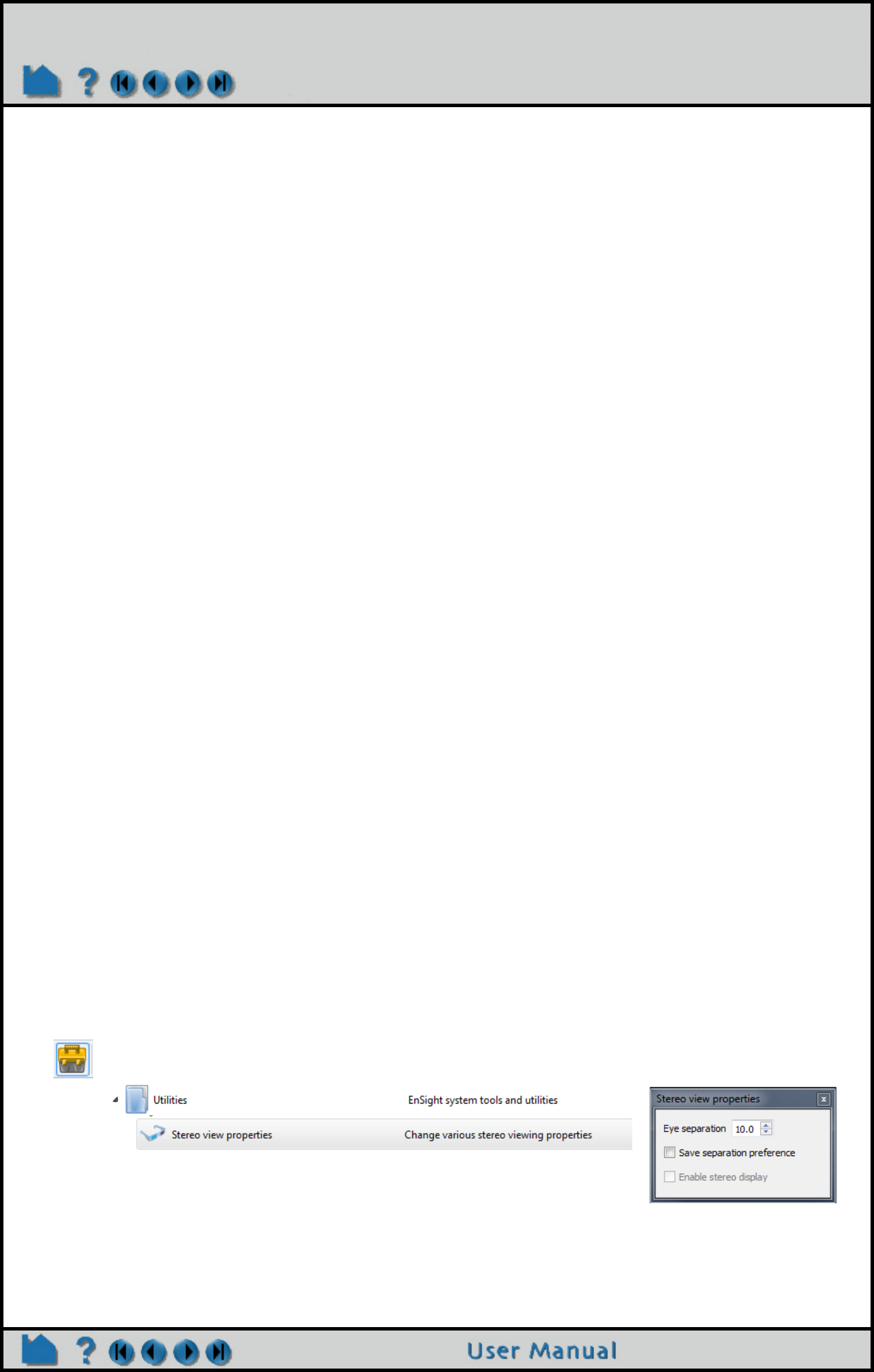
Page 172
HOW TO ENABLE STEREO VIEWING
Enable Stereo Viewing
INTRODUCTION
EnSight supports active stereo display on workstations with quad-buffered OpenGL stereo capability, in addition to
passive (polarized) stereo support for detached displays (see How To Setup Parallel Rendering). Active stereo
works by rapidly displaying alternating left and right eye views on the screen. An emitter (which sits on top of your
display monitor) sends an infrared signal to special glasses worn by the viewer(s). The glasses contain liquid crystal
shutters that alternately open and close the left and right eye lenses in response to the signal from the emitter in sync
with the monitor display. The update frequency is such that the viewer effectively fuses the left and right views into a
single stereo image.
Stereo is useful for viewing any type of visually complex geometry. It is especially helpful for visualizing amorphous
objects such as animating particle traces, trace ribbons, or discrete particles. It has also been noted that
management and customers are typically quite impressed by stereo display.
BASIC OPERATION
In EnSight, stereo display is enabled by pressing the F12 key on your keyboard. Pressing the F12 key again will
return to normal display. The stereo separation angle can be controlled by pressing the F10 and F11 keys. F10
decreases the angle and F11 increases the angle. Pressing Ctrl-F12 will swap the left and right eyes in order to
correct for stereo displays which have the left and right eyes reversed. When EnSight is configured to use a
detached display (see How To Setup Parallel Rendering), these commands affect only the detached display. The
window remains monoscopic.
The stereo model used by EnSight to generate stereo imagery is one of two physical cameras. These cameras are
located some distance from the screen and they are some distance apart. We render the right and left eye views
using those two cameras. This will look (completely) correct, if your eyes are located at these two camera points.
Unfortunately, we are not head-tracking in the case of desktop stereo, so it is very difficult to be perfectly aligned.
Fortunately, the brain is very adept at compensating for the differences in projection and can tolerate an amazing
level of inaccuracy in the projections (witness the fixed projection at your local 3D theater).
However, as geometry gets closer and closer to the eye, the compensation tends to fail. It also tends to fail when
geometry near the border of the screen gets clipped. In those cases, the brain refuses to 'fuse' the imagery into a
single 3D image. To compensate for this, EnSight allows you to vary the eye separation. You can use the function
keys (F10 and F11) to adjust the stereo separation, or, you can adjust the number directly. Or you can use a tool
included in the EnSight tools as shown further below. The command:
ensight.objs.core.STEREO_SEPARATION = 5.0
either in the Python command window or the command language command window (File>Command) or even in a
command file (.enc file) or python file (.py file) adjusts the current value. These numbers are not in units of any
specific distance (we would need to know the screen DPI for that) and are larger for eyes closer together and smaller
for when they are further apart. Think of them as the distance the viewer is away from the screen, given a fixed
intraocular distance. Thus, head position is implied. It is directly in the center of the imagery, as some distance back
from the screen.
Configuring your display
On most platforms the display is not initialized by default in a mode which enables stereo viewing. In general quad-
buffered stereo requires a refresh rate of 96Hz or higher. On some monitors it may be necessary to decrease the
Double click on the tools icon, and in the tools dialog,
Open the Utilities folder, double click the Stereo tool to enable stereo and set eye separation

Page 173
HOW TO ENABLE STEREO VIEWING
display resolution in order to accommodate this higher refresh rate. Check your monitor documentation before
attempting to change the refresh rate.
There is a utility distributed with EnSight which can be used to determine if your display has stereo capability. Run
‘cei_apex31_glinfo’ from a command line and look for OpenGL visuals with a ‘y’ the column ‘st’ or ‘stro’. If none exist,
then the current display parameters do not allow for stereo viewing.
Below are example instructions for various platform configurations which have been tested and confirmed to work
with EnSight. When in doubt, refer to your system documentation for OpenGL as well as the X server (Unix) or video
adapter device driver (Windows).
Linux
Professional graphics cards generally support stereo OpenGL under Linux. Documentation is included with the
drivers, which may be downloaded from the card vendors web sites.
MS Windows
Configuration of stereo under Microsoft Windows is dependent upon the graphics card driver which is installed.
Right-click on the background and choose “Properties” to open to Display Properties dialog. Look for a tab which
such as “OpenGL Properties” or “Advanced” and search for a stereo option. In many cases there is a toggle button
for enabling stereo display.
The nVidia stereo-enabled graphics cards have a number of ‘gotchas’. Firsts, when you upgrade your graphics
card software driver from the manufacturer’s web site, your stereo may no longer work because it may be turned
off as a result of the upgrade. And you may turn on stereo in the driver and find that the stereo test app works, but
EnSight still fails. This is because the nVidia test app uses DirectX, but EnSight uses OpenGL. So while the nVidia
test app is working in stereo because you have turned on DirectX stereo, EnSight may not be working because
OpenGL is still turned off. In nVidia, the critical setting that allows OpenGL stereo is not under the “Stereoscopic
3D” settings, but is rather under “Manage 3D Settings”. Set “Stereo Enable” to “On”.
You will usually need to restart the machine in order for changes to take effect. If stereo still does not work, try
changing the display resolution, as stereo may not be available at higher resolutions. Also, if you lowered the
refresh rate below 120 Hz, put it back to 120 Hz.
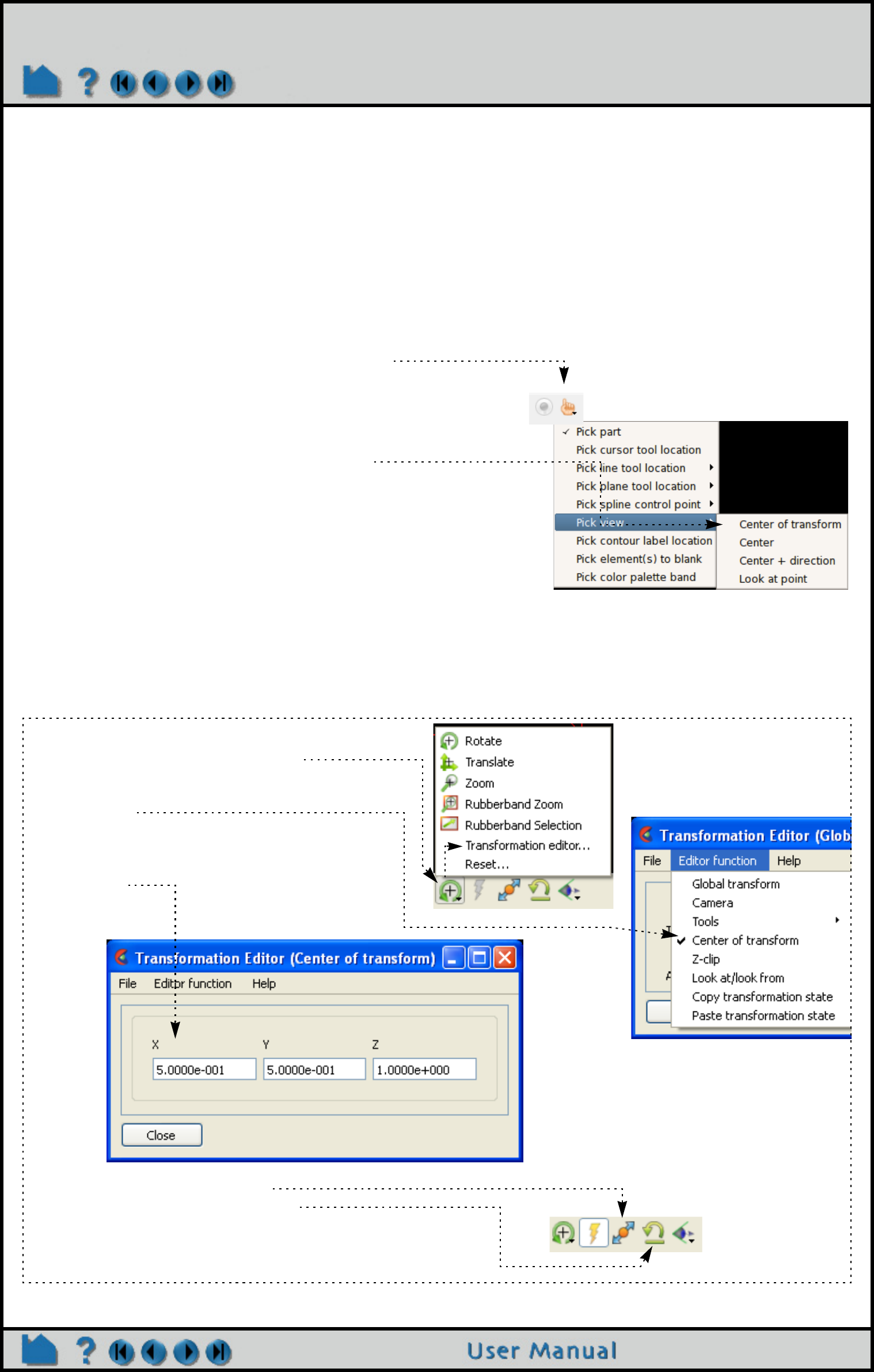
Page 174
HOW TO PICK CENTER OF TRANSFORMATION
Pick Center of Transformation
INTRODUCTION
EnSight allows you to define the model center of transformation as well as useful options for orienting the model.
FAST OPERATION
Simply right click on a part in the graphics window and choose Set Center of Transform and the center of transform
will be set to the selected part at the location of your cursor.
BASIC OPERATION
You can also set or change the exact location of the center of transform by using the Transformation Editor.
1. Click the Pick button on the Tools Icon Bar.
2. Toggle on Pick Center of Transformation.
3. Position the mouse cursor on your model at the
desired location for the center of transformation.
4. Press the “p-key” (or the default, middle mouse
button click, or whatever mouse button you have set for
“Selected Pick Action” in Edit > Preferences > Mouse
and Keyboard).
Your model will now rotate about the position on the model
that you just picked.
1. Click Graphics window transforms icon
and select the Transformation editor...
2. Under “Editor Function”, select “Center of
Transform”.
3. Set of modify the x,y,z coordinate location
of the center of transform in the dialog which
comes up.
Note: clicking on the ‘Fit’ icon
or the Reinitialize transforms icon
will reset the center of transform to the
geometric center of the visible parts.
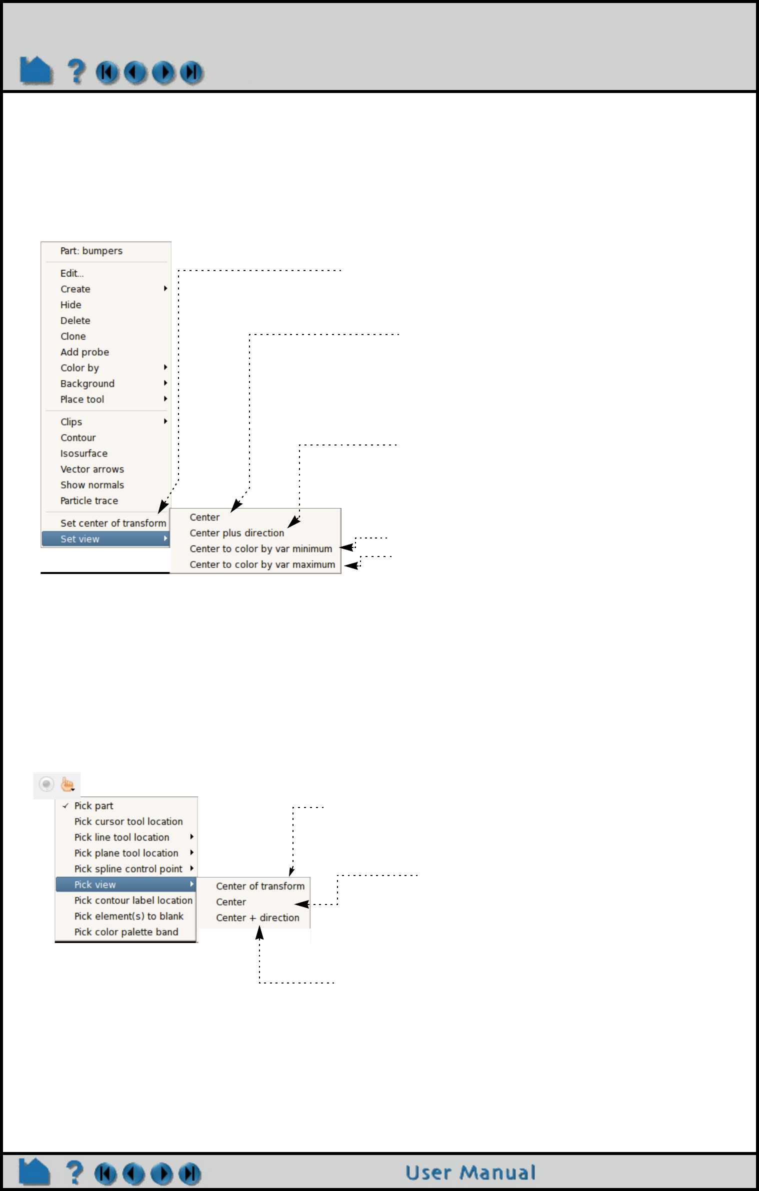
Page 175
HOW TO PICK CENTER OF TRANSFORMATION
ADVANCED
A number of other useful options exist for setting both the center of transformation and the orientation to locations of
interest.
The first is to simply right click on a part location in the graphics window, and choose one of the following options.
The second set of options are useful if you wish to repeatedly redefine the Center of transform, or to repeatedly
Center, or repeatedly perform a Center plus direction; These involve redefining the Pick operation. Then you can
repeatedly execute the pick operation on a location on a part in the graphics window.
The third option for setting the center of transform is done using the maximum or the minimum value of a variable in
the variable list. Right click on a variable and do one of the following:
When this option is chosen, the center of
global transformation is positioned at the
mouse location on the part.
When this option is chosen, the mouse
location on the part is centered in the
graphics window and the center of
transform is set to this mouse location
on the part.
When this option is chosen, the mouse location
on the part is centered in the graphics window
and then rotated so the surface normal is parallel
to the screen normal. The center of transform is
also set to this mouse location on the part.
When one of these options is chosen, and the part is
colored by a variable, the location of the variable
minimum or maximum on this part is centered in the
graphics window and the center of global
transformation is positioned at this part location.
When this Pick operation is chosen and the Pick
operation is performed, the center of global
transformation is positioned at the Picked point.
When this Pick operation is chosen and then the
Pick option is performed, the Picked point is
centered in the graphics window and the center
of transform is set to the Picked point.
When this Pick operation is chosen and the Pick operation is
performed, the Picked point is centered in the graphics
window and then rotated so the surface normal is parallel to
the screen normal. The center of transform is also set to the
Picked point
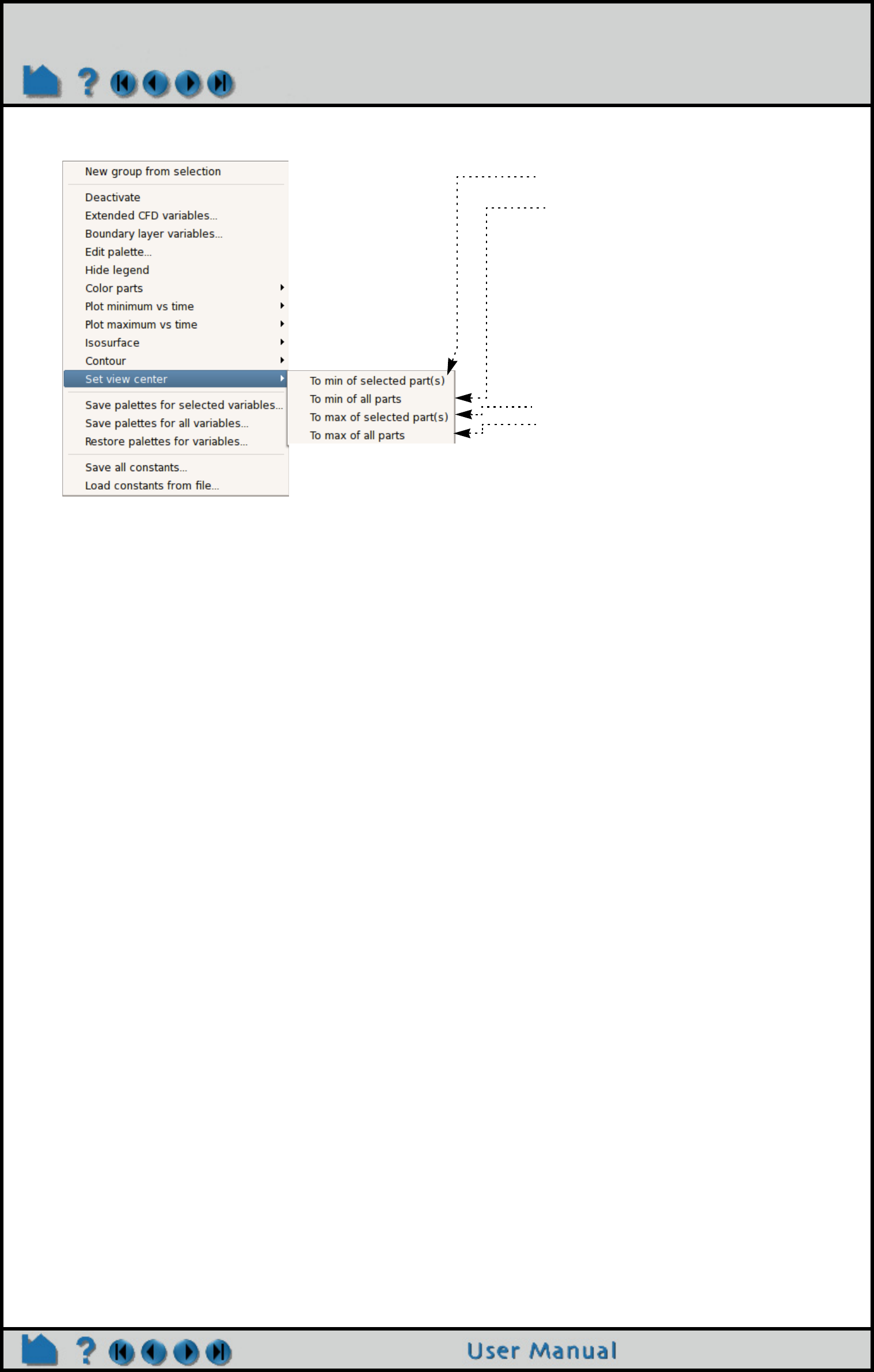
Page 176
HOW TO PICK CENTER OF TRANSFORMATION
When one of these options is chosen,
the location of the variable minimum on
the selected or all part(s), respectively,
is centered in the graphics window and
the center of global transformation is
positioned at this location.
When one of these options is chosen,
the location of the variable maximum on
the selected or all part(s), respectively,
is centered in the graphics window and
the center of global transformation is
positioned at this location.
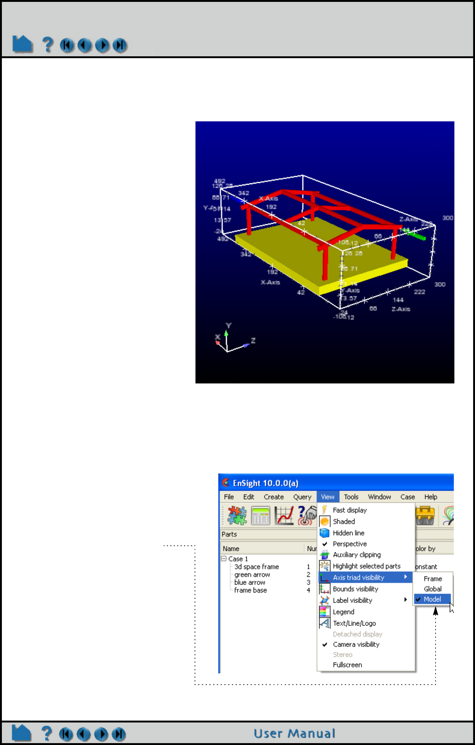
Page 177
HOW TO SET MODEL AXIS/EXTENT BOUNDS
Set Model Axis/Extent Bounds
INTRODUCTION
EnSight provides model axes and extent bounds to help in orienting your model.
BASIC OPERATION
Model Directional Triad
The model axes help maintain awareness of the principal directions of the reference frame of the model. This is
especially helpful during model transformations. It is on by default, but can be toggled on/off by:
View > Axis triad visibility > Model
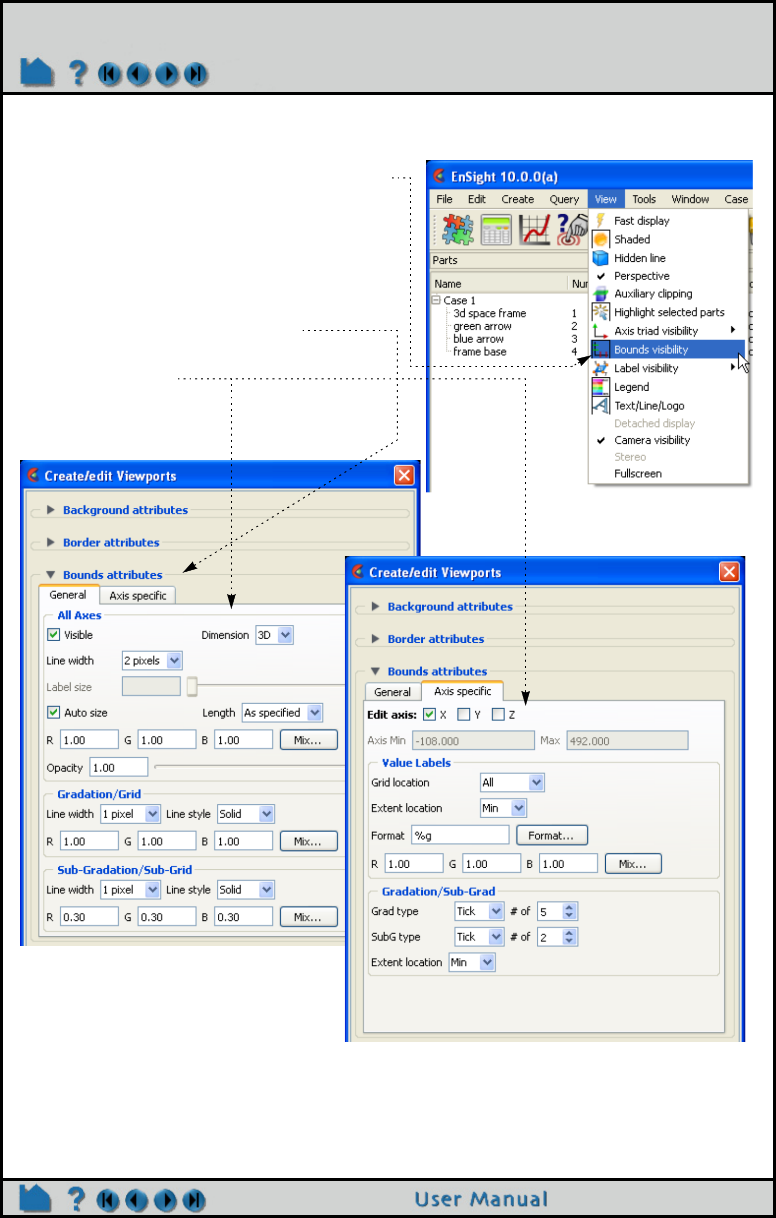
Page 178
HOW TO SET MODEL AXIS/EXTENT BOUNDS
Model Extent Bounds
The model extent bounds also help maintain dimensional information pertaining to the extents of the model.
SEE ALSO
User Manual: Part Bounds Attributes
View > Bounds visibility to display the model extents
To control the various associated with the model extents:
1. Double click on the desired viewport in the
Viewports list panel.
2. Open the Bounds turndown.
3. Modify the various general and/or Axis specific as
desired.
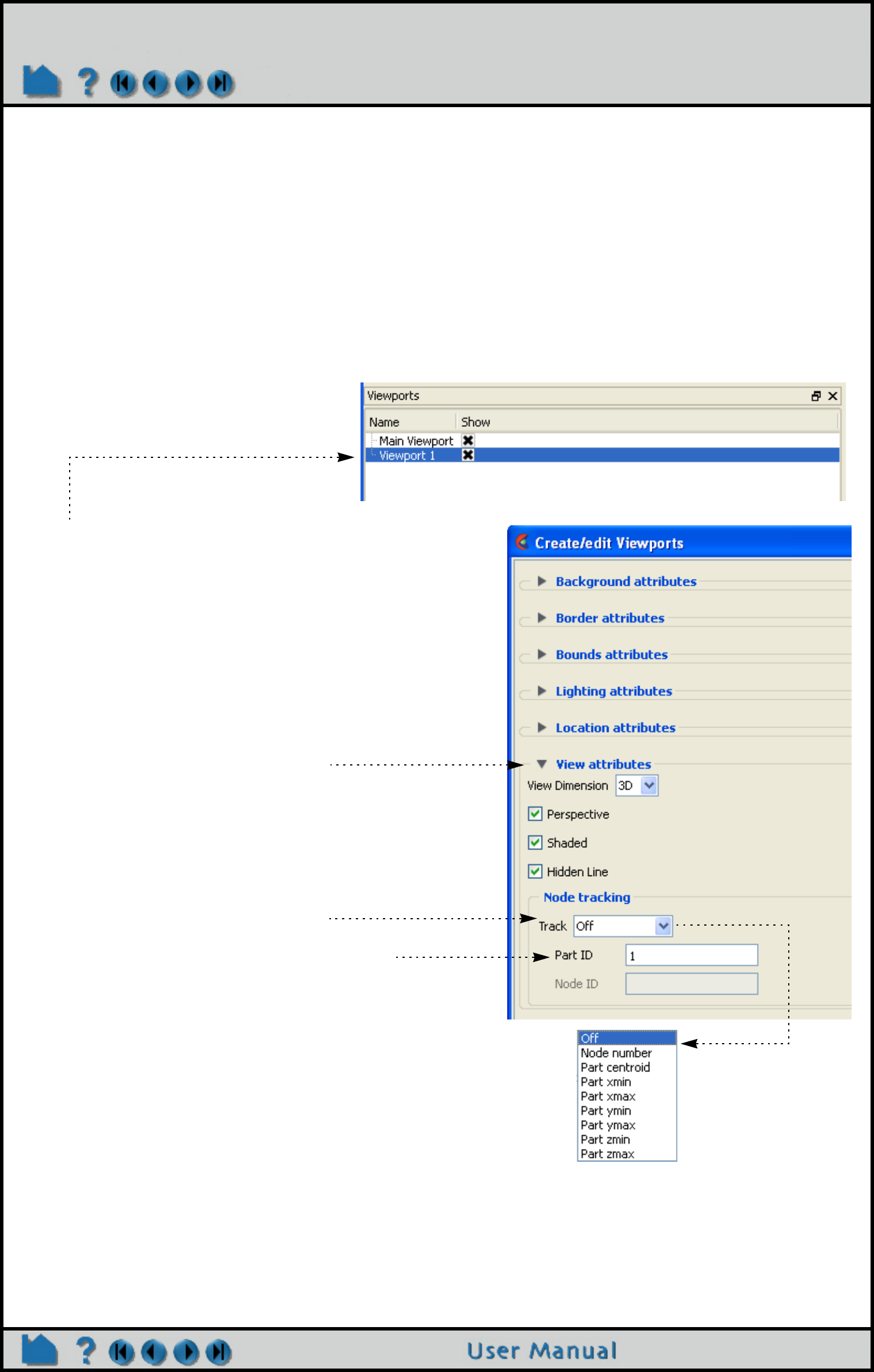
Page 179
HOW TO DO VIEWPORT TRACKING
Do Viewport Tracking
INTRODUCTION
EnSight provides the capability to “track” a particular location on the model parts displayed in a viewport. Tracking
means that the viewport will be caused to center on the chosen location as time is changed. This is particularly useful
for models with changing geometry or applied displacements - allowing one to stay focused on the moving bodies
during an animation.
BASIC OPERATION
Viewports can be displayed with a variety of options:
SEE ALSO
How To Define and Change Viewports
User Manual: Viewports List Panel
1. Double click on the desired viewport, (or
select the desired viewport(s) and right click
-> Edit...
2. Open the View if needed.
3. Select the Tracking option desired,
5. And supply the node or part id appropriately.
6. Change time step, load a transient flipbook,
or the like and note that the viewport will stay
centered on the location chosen.
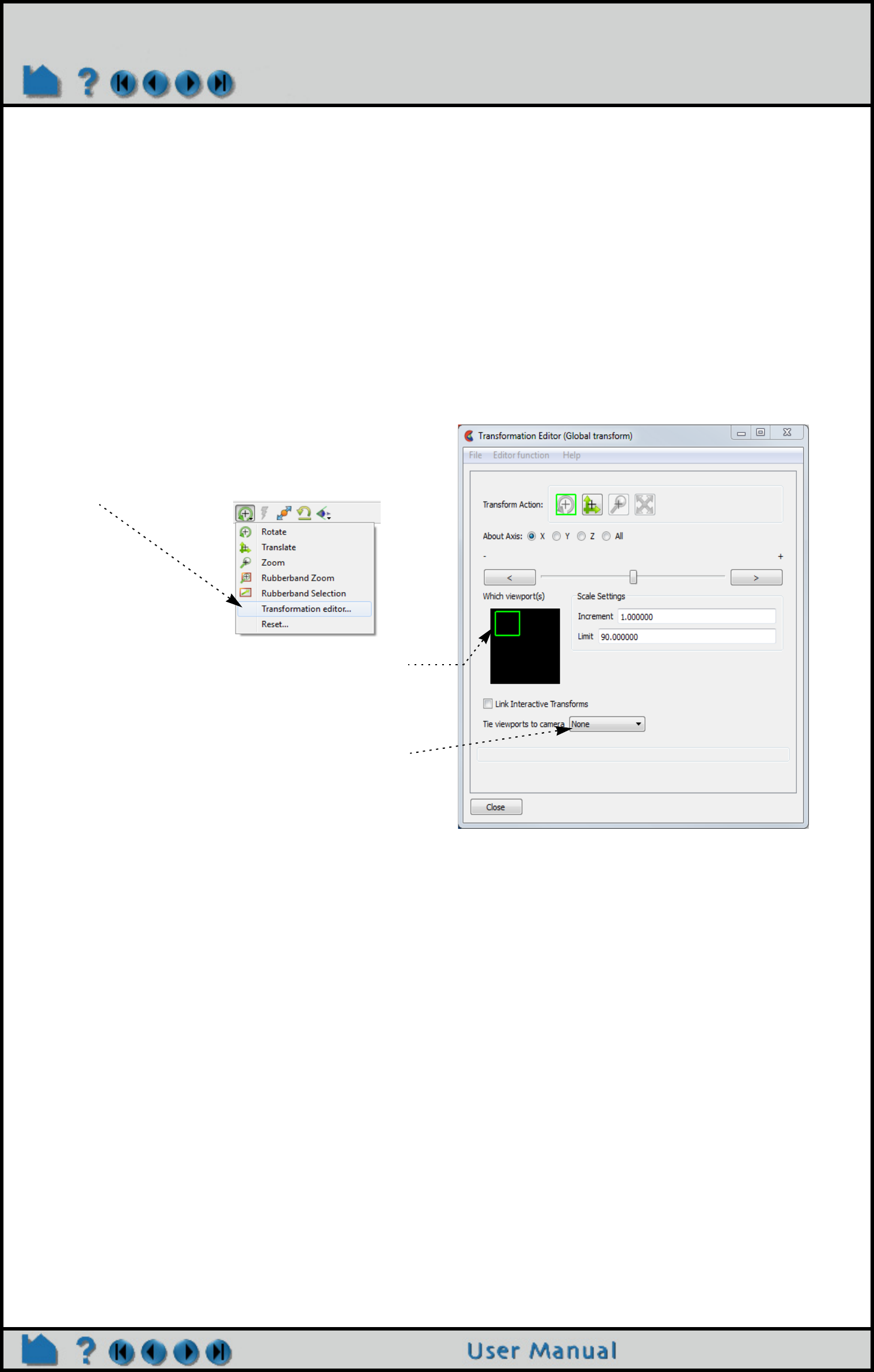
Page 180
HOW TO VIEW A VIEWPORT THROUGH A CAMERA
View a Viewport Through a Camera
INTRODUCTION
Global transform mode defines a viewing position and then allows you to transform (translate and rotate) the scene.
Camera mode behaves a little differently. In this mode the scene remains as defined and does not move. Instead the
scene is viewed through a camera which can be positioned at any location and oriented to look in a specific direction
and have a specified "tilt".
A viewport can either be in Global transform mode (default) or it can be defined to be viewed through the camera.
Local transforms are valid in either mode. In order to view a viewport through a camera (a) the camera position and
orientation must be defined, and (b) the viewport must be tied to a camera.
BASIC OPERATION
If a viewport is being viewed through a camera the interactive transformations (when you click and drag the mouse
buttons in the viewport) affect the camera position and orientation. By default the visibility of the cameras are off.
There are eight total cameras available that can be manipulated. By default they are positioned at the +/- XYZ axis
locations plus two more cameras showing a view of -1 -1 -1 and 1 -1 -1.
To position/orient a camera interactively:
1. If you click-drag for a transform in a viewport being tracked by a camera the camera will transform
OR
1. In viewports that are not being viewed through a camera you will see a camera icon (if camera visibility is on). You
can click-drag the center of the camera to drag the camera to a new position. Clicking/dragging the axis of the
camera rotate the camera.
OR
1. You can set the Pick option on the tool ribbon to position/orient the camera
2. Place the mouse pointer over the desired location on a part in any of the viewports in the graphics window and
press the 'p' key (or whatever mouse button you have set for the "Selected Pick Action" in Edit->Preferences->Mouse
and Keyboard). Depending on which pick action was chosen the camera will be positioned or oriented according to
the pick.
You may pick a spline control point for the Camera origin in which case the camera will position and orient itself
according to the spline.
Any viewport can be viewed through a camera by
1. From the Transformation icon on the Tools Icon
Bar, click Transformation
editor...
2. In the resulting
Transformation editor
(Global Transform) select
the viewport you want to view through a camera
3. Select the camera from the Tie viewport(s) to
camera pulldown. When set to None the camera
model is not used and the Global transformation
model is active.
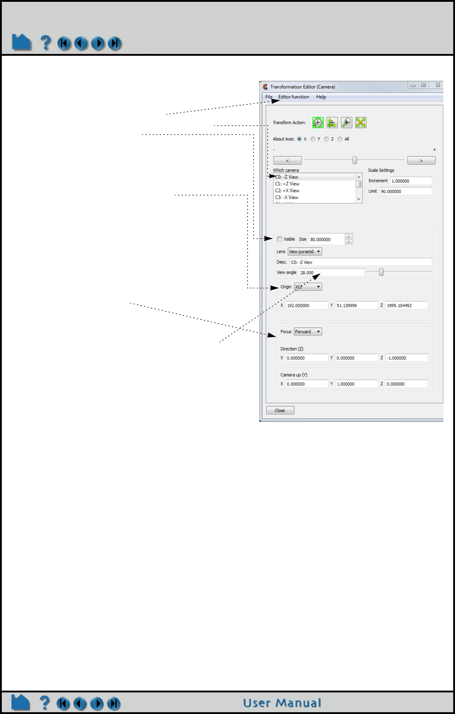
Page 181
HOW TO VIEW A VIEWPORT THROUGH A CAMERA
ADVANCED USAGE
1. If the camera origin is on a spline, zoom operations will move the camera along the spline
2. If the origin or Focus is set to a node number the camera will update if the node changes position.
SEE ALSO
How To Use the Spline Tool
To turn on camera visibility:
1. Open the Transformation Editor as described in
previous section.
2. Select Editor function > Camera
3. Select the camera(s) you want to turn visible
4. Turn on the Visible toggle.
To position/orient a camera interactively from the
Camera Transformation editor
1. If the Origin is set to XYZ then the camera is located
at the X, Y, Z locations shown here
If the Origin is set to Spline then the camera origin
will be located on the defined spline
If the Origin is set to Node then the camera origin will
be located at a specified node id.
2. The camera orientation is controlled by the Camera
Z direction and the Camera Up vector. If the Focus is
set to Node or XYZ then the Z vector is defined by the
Node/XYZ location.
To set other camera:
1. The view angle controls the field of view through the
camera. A small value simulates a telephoto lens
while a large value simulates a wide angle lens
2. The Size sets the size of the camera glyph. Use the
up/down arrows to increase/decrease the glyph size
by a factor of 2.
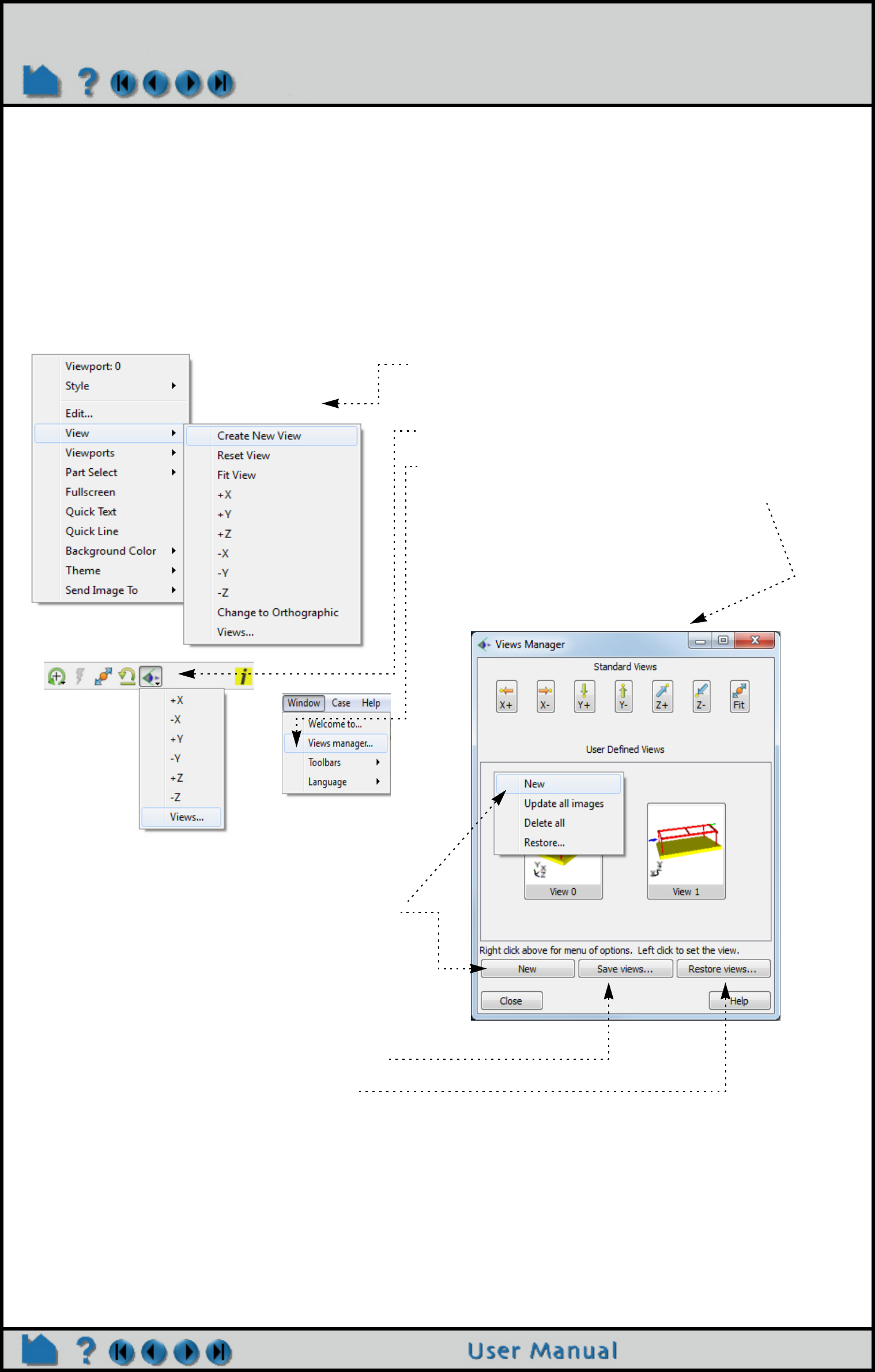
Page 182
HOW TO MANAGE VIEWS
Manage Views
INTRODUCTION
EnSight provides a capability to save and restore viewing parameters for the data model and all viewports.
Collectively, this state is known as a View. This dialog portrays Views graphically as buttons with a small picture
("thumbnail") of the currently displayed data rendered with the underlying viewing parameters of that View.
With the Views Manager the user can create, save, restore, and apply viewing parameters in a simple point-and-click
interaction.
BASIC OPERATION
The Views Manager dialog is displayed by right clicking on
the EnSight graphics area background and choosing
View>Create New View
OR by selecting the 'Views…' icon on the Tools Icon Bar
OR in the main menu Windows>Views Manager...
The dialog will look similar to that shown here.
(Initially, the Views Manager will not contain
any thumbnails of Views.)
Click on the ‘New’ Button (or right-click on an empty
area of the User Defined Views and select ‘New’) to
create a new view using the current orientation and
viewing parameters in the main graphics window.
The 'Save views' button will display a file browser in
which the user can select a directory. The manager
will then write each View into a separate EnSight
view file (named sequentially 'view0', 'view1',
'view2'...) A maximum of 16 Views can be used.
The button 'Restore views' will display a file
browser. Select a directory which contains EnSight
View files and click the ‘Choose’ button. Any Views
found in that directory will be loaded and displayed
as a thumbnail button with the currently loaded
data. Note that the 'Restore views' button will only
look for views created by EnSight 8.2.1(e) or newer.
Older Views must be loaded individually via the
right-click menu explained later.
Note: when restoring, the file browser has a toggle
button “Use stored images for thumbnails’ which when
set causes the originally stored image in the view to be
displayed on the thumbnail instead of the currently
loaded image. This can be useful if the current image
takes a long time to render.
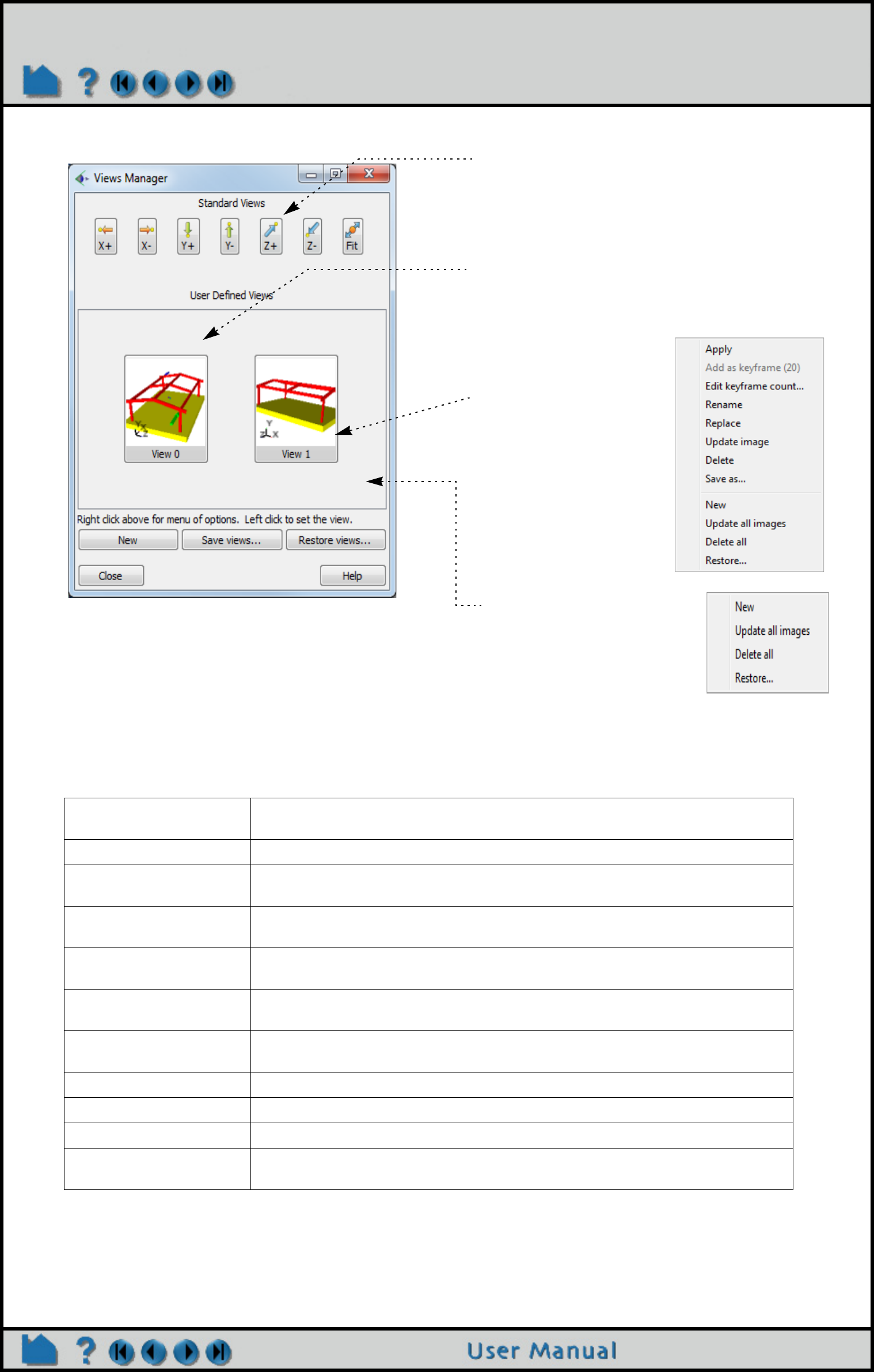
Page 183
HOW TO MANAGE VIEWS
The menu options perform the following actions:
SEE ALSO
See the User Manual: Window Functions
Apply Performs the same action as clicking the left mouse button on the selected thumbnail
button.
Add as keyframe (20) Adds a keyframe with this view with 20 Sub-Frames.
Edit keyframe count Pops up a window to query enter number of SubFrames, then adds a keyframe with this
view.
Replace Replaces the thumbnail button's viewing parameters and image with the currently
displayed state of the EnSight graphics window.
Update image Replaces the thumbnail button's image with the button's viewing parameters while using
the currently loaded data.
Delete Deletes the selected thumbnail button and associated viewing parameters. Note that if
the View is associated with an EnSight View file, the file will not be deleted.
Save as... Displays a file browser where the user can specify both a directory and an alternative
file name for the View.
New Creates a new View button using the currently displayed model data and all viewports.
Update all images Performs the same action as 'Update image' but for all thumbnail buttons.
Delete all Performs the same action as 'Delete' but for all thumbnail buttons
Restore... Displays a file browser where the user can select an EnSight View file to load. Note that
this option allows the user to load all versions of View files.
Clicking on a standard view will put the main
graphics window in that view. It does not create a
view in the User Defined Views.
Clicking a thumbnail button with the left mouse
button will apply that View to the EnSight graphics
window.
Clicking the mouse's right button will display one
of two pop-up menus.
If the right mouse button is
clicked on top of a
thumbnail image, then the
menu to the right will be
displayed.
Clicking the mouse’s right
button in the background of
the thumbnail drawing area
will display this menu.
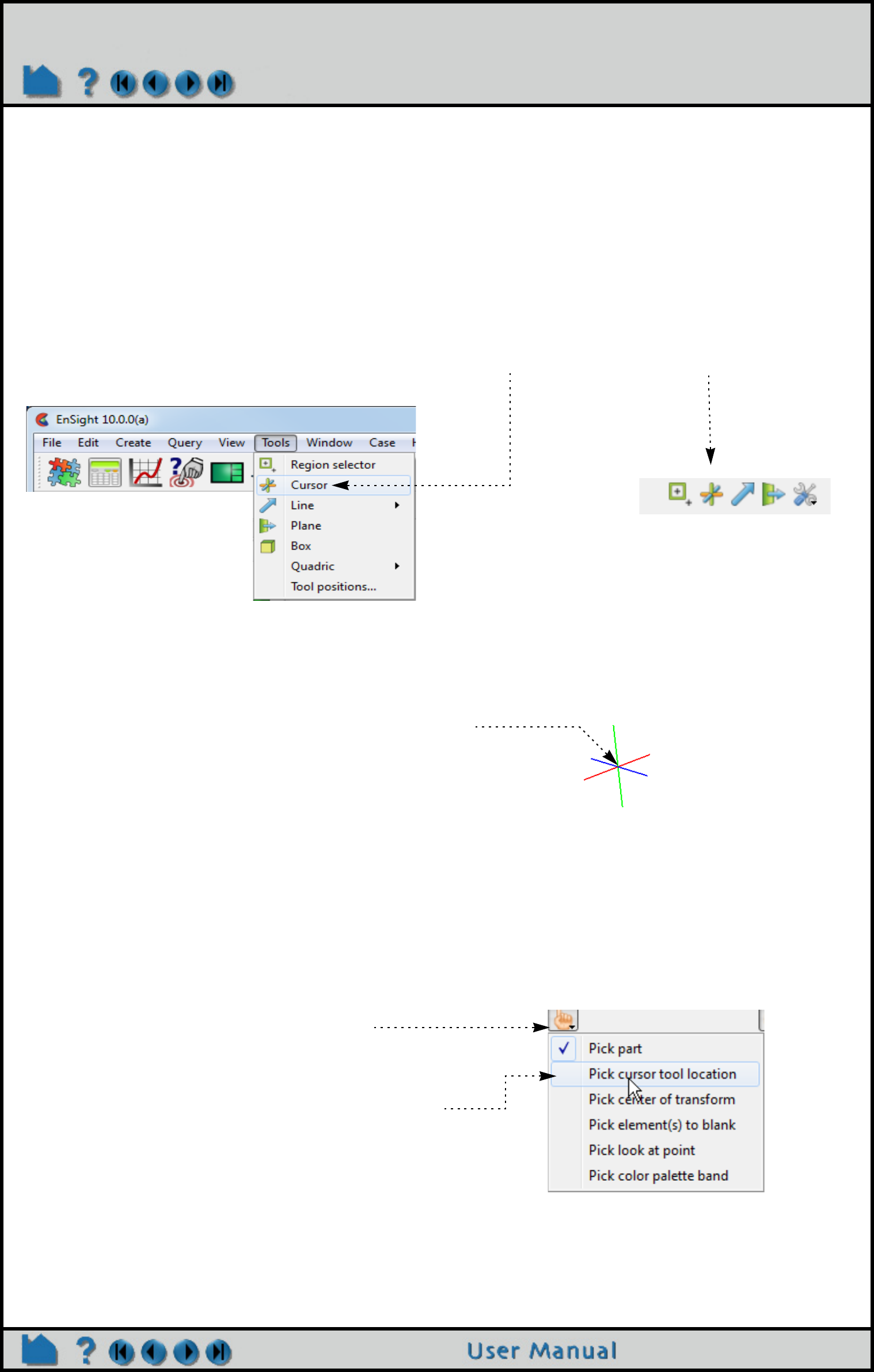
Page 184
HOW TO USE THE CURSOR (POINT) TOOL
Manipulate Tools
Use the Cursor (Point) Tool
INTRODUCTION
EnSight provides a 3D point specification tool called the “Cursor” tool. When visible, the Cursor appears as a 3D
cross colored red (X axis), green (Y axis), and blue (Z axis). The Cursor tool is used to supply EnSight with point
information, for example to specify the location for a query or the starting point for a particle trace.
BASIC OPERATION
In many cases, the Cursor tool will automatically turn on when performing some function that requires it. You can also
turn the tool on and off manually by toggling the Cursor entry in the Tools menu or by clicking the Cursor toggle on the
Tools Icon Bar.
The Cursor tool can be placed in three ways: interactively through direct manipulation with the mouse, by positioning
the mouse pointer over a part and pressing the ‘p’ key, or precisely positioned by typing coordinates into a dialog.
To position the Cursor with the mouse:
Cursor translation is restricted to the plane perpendicular to your line of sight. If you need to move the cursor in
another plane, rotate the model such that the desired translation plane is perpendicular to your new line of sight.
(Note that the Cursor may not exactly track the location of the mouse pointer.)
To position the Cursor on a part with the ‘p’ key:
1. Place the mouse pointer over the center of the tool.
Note that the mouse cursor will change when over the center
of the cursor tool.
2. Click (and hold) the left mouse button.
3. Drag the Cursor to the desired location.
4. Release the mouse button.
(Undo/Redo button at the bottom of screen can be used to undo/redo the
tool transformation)
1. Turn on the Cursor tool as specified above. Then
Click the Pick button on the tool ribbon.
2. Select “Pick cursor tool location” from the pop-up
menu.
3. Place the mouse pointer over the desired location on
a part in the graphics window and press the ‘p’ key
(or whatever mouse button you have set for the
“Selected Pick Action” in Edit > Preferences > Mouse
and Keyboard). The middle mouse button is usually
defaulted to perform the pick action as well.
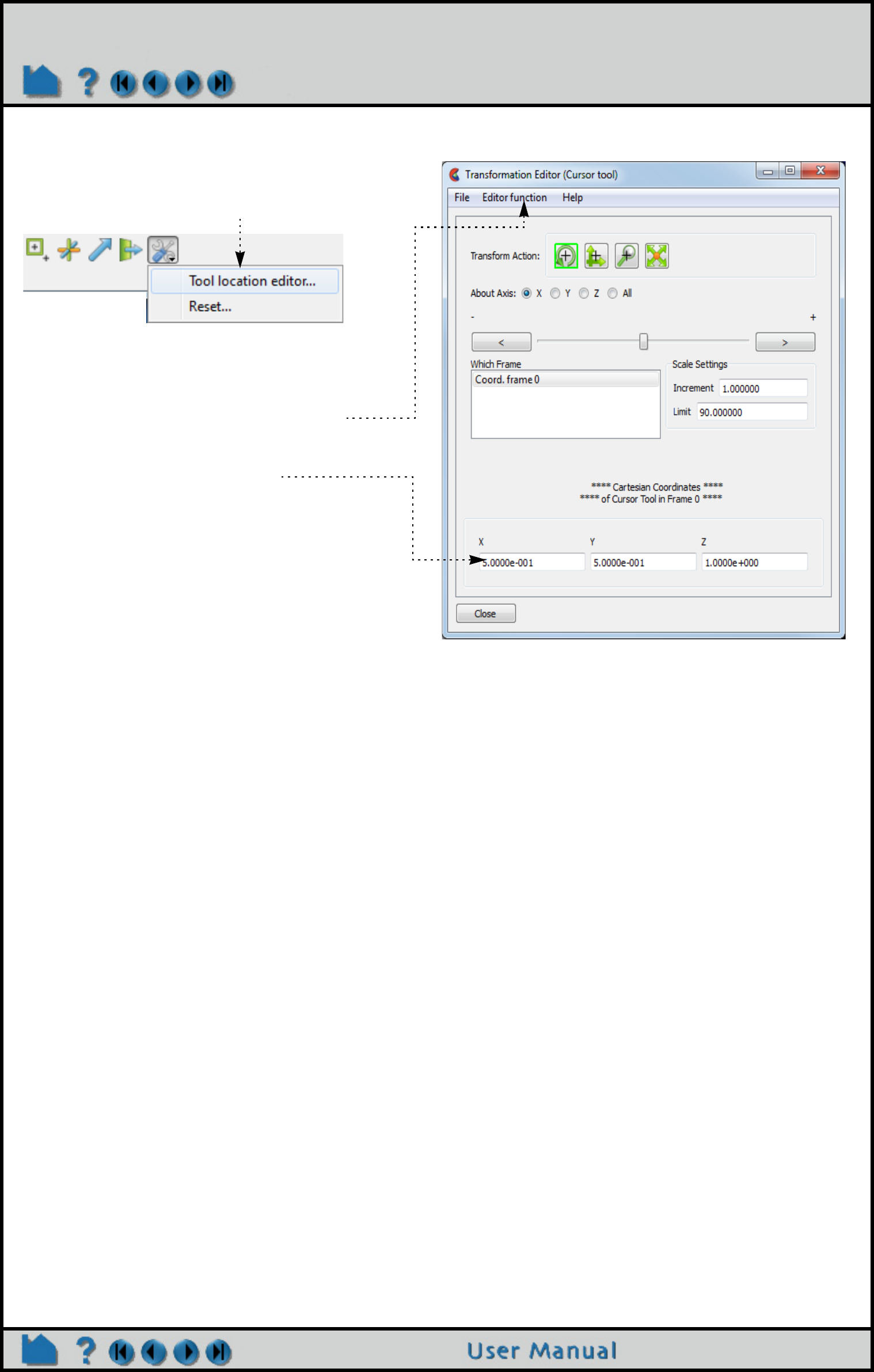
Page 185
HOW TO USE THE CURSOR (POINT) TOOL
To set the Cursor by specifying coordinates:
You can also move the Cursor by setting the desired axis of translation in the About Axis field and manipulating the
slider bar. In this case, the values in the “Scale Settings” section control the sensitivity and limit of the slider action.
Note that you can also use this dialog to view (rather than set) the position of the Cursor since the X,Y,Z numeric
values always update to reflect the current location. If you are positioning the Cursor interactively with the mouse, the
values will update when the mouse button is released.
Shortcut
While Part Quick Action icons are available (indicating that one is dealing with parts), right click on the cursor tool.
You can hide the tool (make it invisible), edit it (open the Transformation Editor), or use the tool to quickly do
something such as query a variable over time, or emit a particle streamline trace.
ADVANCED USAGE
After a model has been loaded, the initial location of the Cursor is set to the “look-at” point – the geometric center of
all visible geometry. The coordinates of the Cursor are specified with respect to the default frame: frame 0. However,
if you have created additional frames, you can position the Cursor relative to the origin of a different frame. This is
accomplished by selecting the desired frame in the “Which Frame” list in the Transformation Editor dialog.
You can easily reset the position of the Cursor tool to the default. See How To Reset Tools and Viewports for more
information.
Positioning a 3D tool with a 2D device (the mouse) can be difficult. Multiple viewports are sometimes helpful in
positioning tools since you can see the tool simultaneously from multiple vantage points.
SEE ALSO
Other tools: Line, Plane, Box, Cylinder, Sphere, Cone, Surface of Revolution. See the How To article on Frames
for additional information on how frames effect tools.
User Manual: Tools Menu Functions
1. Open the Transformation Editor dialog by
clicking Tool location editor... from the
Tool Locations settings icon.
2. If the Transformation Editor is not set to
Cursor Tool, set it by Editor function->
Tools.
3. Enter the desired coordinates into the X, Y,
and Z type-ins and hit return.
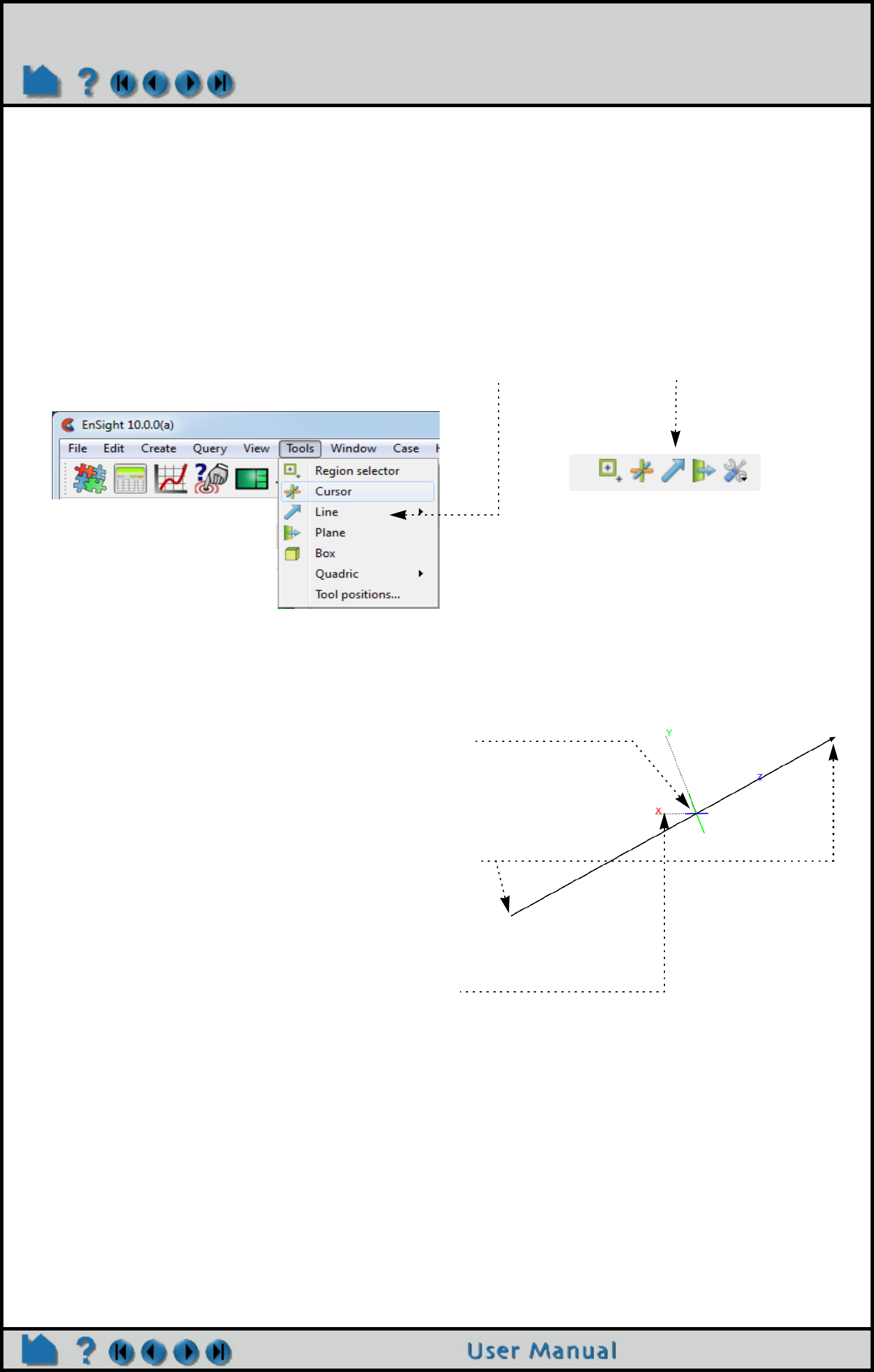
Page 186
HOW TO USE THE LINE TOOL
Use the Line Tool
INTRODUCTION
EnSight provides a 3D linear specification tool called the “Line” tool. When visible, the Line tool appears as a
(typically white) line with an axis system at the center point and an arrow head on one end. The Line tool is used to
supply EnSight with a linear specification, for example to specify the location for a line clip or a “rake” for a particle
trace.
BASIC OPERATION
In many cases, the Line tool will automatically turn on when performing some function that requires it. You can also
turn the tool on and off manually by toggling the Line entry in the Tools menu or by clicking the Line toggle on the
Tools Icon Bar.
The Line tool can be placed or manipulated in three ways: interactively through direct manipulation of tool “hotpoints”
with the mouse, by positioning the mouse pointer over a part and typing the ‘p’ key, or precisely positioned by typing
coordinates into a dialog and/or rotating the tool about its axis. With surface normal options the line remains normal.
Line moving and stretching is restricted to the plane perpendicular to your line of sight. If you need to move the Line
in another plane, rotate the model such that the desired translation plane is perpendicular to your new line of sight.
(Note that the Line will not exactly track the location of the mouse pointer.)
To move the Line with the mouse:
1. Place the mouse pointer over the center of the tool.
2. Click (and hold) the left mouse button.
3. Drag the Line to the desired location.
4. Release the mouse button.
To stretch the Line with the mouse:
1. Place the mouse pointer over one of the Line endpoints.
2. Click (and hold) the left mouse button.
3. Drag the endpoint to the desired location.
4. Release the mouse button.
To rotate the line with the mouse:
1. Place the mouse over the end of one of the tool axes.
2. Click (and hold) the left mouse button.
3. Drag the axis endpoint until the line has rotated as desired.
4. Release the mouse button.
Note selecting the X axis endpoint will rotate about the Y axis, selecting the Y axis endpoint will rotate
about the X axis, and selecting the Z axis endpoint will rotate in a general fashion about the centerpoint.
Note that the mouse pointer will change when it is over a hotpoint.
(Undo/Redo button can be used to undo/redo the tool transformation)
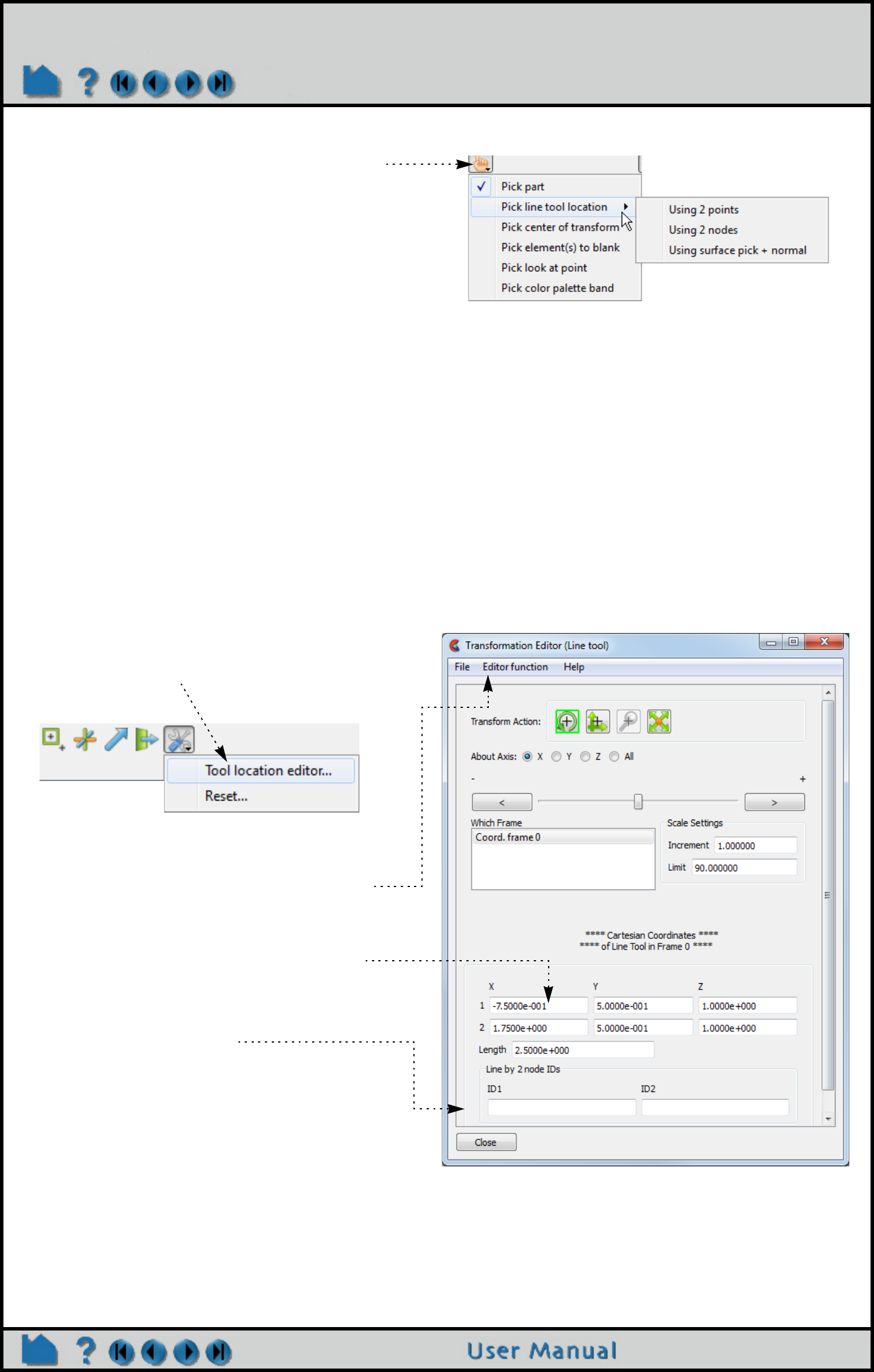
Page 187
HOW TO USE THE LINE TOOL
To position the Line on a part with the ‘p’ key:
To set the Line by specifying coordinates:
Rotation, translation or scaling of the tool can also be accomplished by selecting the appropriate transform action
icon and the desired axis, and then manipulating the slider. In this case, the values in the “Scale Settings” section
control the sensitivity and limit of the slider action.
Note that you can also use this dialog to view (rather than set) the position of the Line since the X,Y,Z numeric values
always update to reflect the current location. If you are positioning the Line interactively with the mouse, the values
will update when the mouse button is released.
1. Click the Pick button on the Tools Icon Bar.
2. Select “Pick line tool location” from the pop-up menu.
(Then pick either by 2 points or 2nodes.)
3. In the Graphics Window, place the mouse pointer on
a part over the desired location for the first Line
endpoint and press the ‘p’ key (or whatever mouse button
you have set for the “Selected Pick Action” in Edit >
Preferences > Mouse and Keyboard). The middle mouse
button is usually defaulted to perform the pick action as
well
4. Move the mouse pointer to the desired location for the
second Line endpoint and again press the ‘p’ or middle
mouse key/button.
When “Using 2 points” the endpoints will be place at the pick location.
When “Using 2 nodes”, the endpoints will be placed at the nearest
node and the ids of those nodes will be saved, such that the line tool
will continue to be attached to these nodes - even if they move.
1. Open the Transformation Editor dialog by clicking
Tool location editor... from the Tool Locations
settings icon..
2. If the Transformation Editor is not set to
Line Tool, set it by Editor function-> Tools..
3. Enter the desired coordinates for the
endpoints into the X, Y, and Z fields and
press return.
3. Alternatively, you can enter the node ids for
two nodes in the model.
This has the effect of keeping the line tool tied
to the two nodes - even if they move over time.
Note the Length field - which is discussed in
Advanced Usage below.

Page 188
HOW TO USE THE LINE TOOL
Shortcut
Right click on a part in the graphics window and choose Place Tool, and then choose to place the line tool normal to
a surface, or tangential to a surface at the location of the mouse pointer.
Right click on center selection point of the line tool (while Part Quick Action icons are available indicating that parts
can be edited),. You can do quick x or y rotates, hide the tool, or open the transformation editor. You can also use this
right click to quickly create a line clip, query a variable, or do a particle streamline trace with the line tool as the
emitter.
ADVANCED USAGE
After a model has been loaded, the initial location of the Line center is set to the “look-at” point – the geometric center
of all visible geometry and parallel to the X axis. The coordinates of the Line are specified with respect to the default
frame: frame 0. However, if you have created additional frames, you can position the Line relative to the origin of a
different frame. This is accomplished by selecting the desired frame in the “Which Frame” list in the Transformation
Editor dialog.
You can easily reset the position and orientation of the Line tool to the default. See How To Reset Tools and
Viewports for more information.
Positioning a 3D tool with a 2D device (the mouse) can be difficult. Multiple viewports are sometimes helpful in
positioning tools since you can see the tool simultaneously from multiple vantage points.
To find the distance between two nodes that have IDs, you can use the calculator function Dist2Nodes. However, to
find the distance between two nodes on different parts, or between two nodes if one or both don’t have IDs, use the
line tool. Use the Pick Line Tool Location-> Using 2 nodes option as shown above, then move the cursor near the first
node location, hit ‘p’ key, move to the second node location and hit the ‘p’ key, then open up the transformation editor
and in the transformation editor menu, Edit>Tools>Line you’ll find the length of the line tool which is the distance
between those two points.
SEE ALSO
Other tools: Cursor, Plane, Box, Cylinder, Sphere, Cone, Surface of Revolution. See the How To article on
Frames for additional information on how frames effect tools.
User Manual: Tools Menu Functions
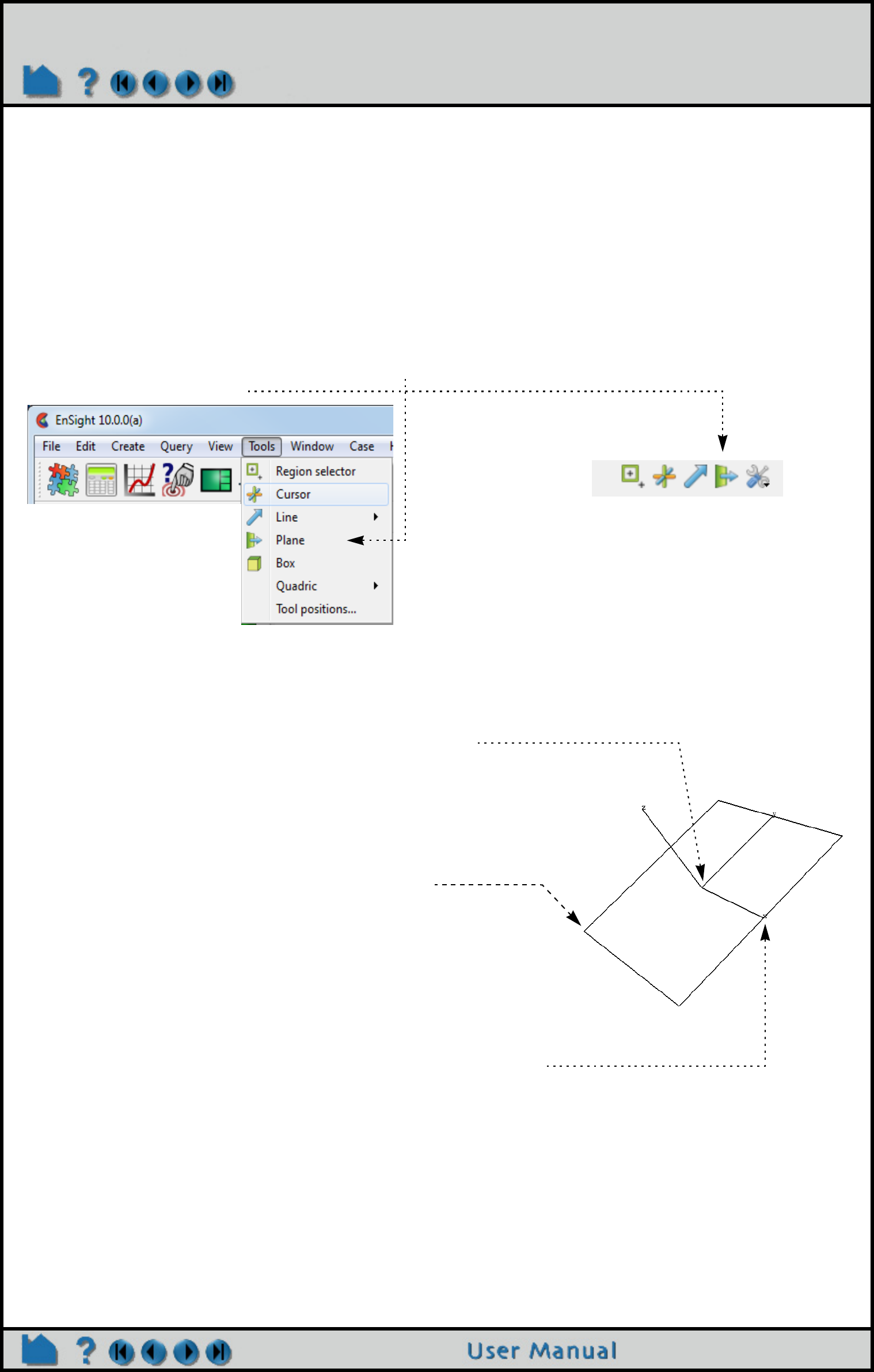
Page 189
HOW TO USE THE PLANE TOOL
Use the Plane Tool
INTRODUCTION
EnSight provides a plane specification tool called the “Plane” tool. When visible, the Plane tool appears as a
(typically white) rectangular region with an axis located at the center point. The Plane can also have a semi-
transparent “filled” center that enhances visibility of the region. The Plane tool is used to supply EnSight with a
planar specification, for example to specify the location for a planar clip or a “net” for a particle trace.
BASIC OPERATION
In many cases, the Plane tool will automatically turn on when performing some function that requires it. You can also
turn the tool on and off manually by toggling the Plane entry in the Tools menu (e.g. Tools > Plane) or by clicking the
Plane toggle on the Tools Icon Bar.
The Plane tool can be placed in three ways: interactively through direct manipulation of tool “hotpoints” with the
mouse, by positioning the mouse pointer over a part and typing the ‘p’ key, or precisely positioned by typing
coordinates into a dialog.
Plane moving is restricted to the plane perpendicular to your line of sight. If you need to move the Plane in another
plane, rotate the model such that the desired translation plane is perpendicular to your new line of sight. (Note that
the Plane will not exactly track the location of the mouse pointer.)
To move the Plane with the mouse:
1. Place the mouse pointer over the center of the tool.
2. Click (and hold) the left mouse button.
3. Drag the Plane to the desired location.
4. Release the mouse button.
To stretch (or scale) the Plane about the plane’s center with the
mouse:
1. Place the mouse pointer over any of the corners.
2. Click (and hold) the left mouse button.
3. Drag the corner to the desired location.
4. Release the mouse button.
To rubber-band a corner of the plane tool (while the opposite corner
stays fixed), do the same as above, but hold the Ctrl key down as you
click and drag a corner.
To rotate the Plane tool with the mouse:
1. Place the mouse pointer over one of the axis labels (X, Y, or Z).
2. Click and drag to the desired orientation. Grabbing the X (Y) label
will rotate around the plane’s Y (X) axis. Grabbing the Z label
enables free rotation about the Plane’s center point.
Note that the mouse pointer will change when it is over a hotpoint.
(Undo/Redo button at the bottom of screen can be used to undo/redo the tool
transformation)
X
Y
Z
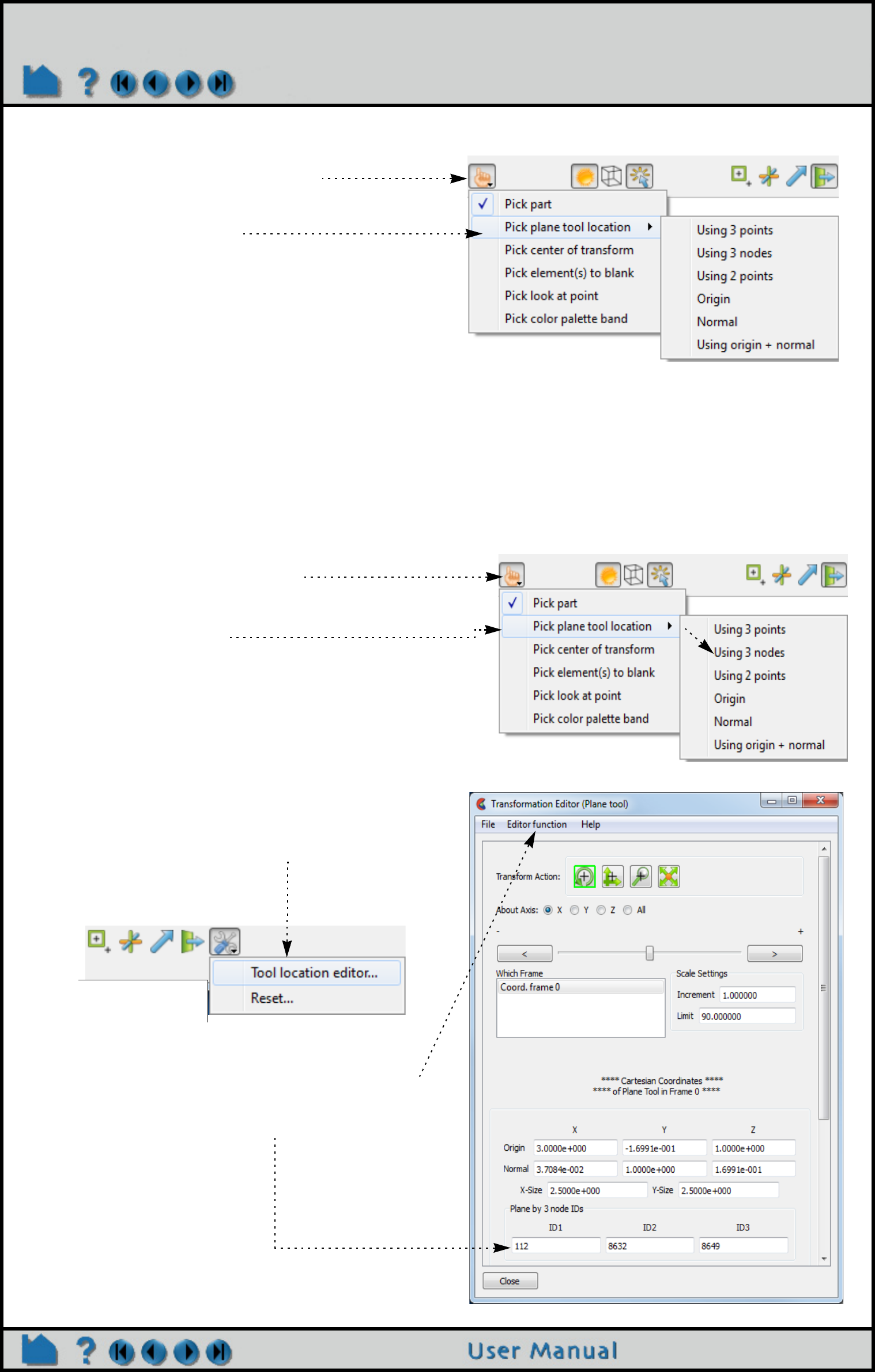
Page 190
HOW TO USE THE PLANE TOOL
To position the Plane on a part (by specifying three points) with the ‘p’ key:
You can also position the Plane Tool by picking three nodes (this differs from the above where 3 points in space are
used - in that the node ids of the three closest nodes are found and saved). The Plane orientation will be changed
such that it lies in the plane of the three nodes chosen, and will continue to lie in the plane of these three nodes, even
if they change location.
To position the Plane (by specifying three nodes):
1. Turn on the Plane tool as noted above. Then Click
the Pick button on the tool ribbon.
2. Select “Pick plane tool location > Using 3 points”
from the pop-up menu.
3. In the Graphics Window, place the mouse pointer on
a part and press the ‘p’ key (or whatever mouse
button you have set for the “Selected Pick Action” in
Edit > Preferences > Mouse and Keyboard).
4. Repeat two more times. Note that you are not
specifying corner points – just three unique points.
1. Turn on the Plane tool as noted above, then click the
Pick button on the tool ribbon.
2. Select “Pick plane tool location > Using 3 nodes”
from the pop-up menu.
3. In the Graphics Window, place the mouse pointer on
a part, near a desired node and press the ‘p’ key (or
whatever mouse button you have set for the
“Selected Pick Action” in Edit > Preferences > Mouse
and Keyboard).
4. Repeat two more times. Note that you are not
specifying corner points – just three unique nodes.
If you open the Transformation Editor,
it should open in Plane Tool mode assuming you just
performed the operations above. If not, change the
Editor function to Tools->Plane. You can see the id of the
three nodes that you have chosen.
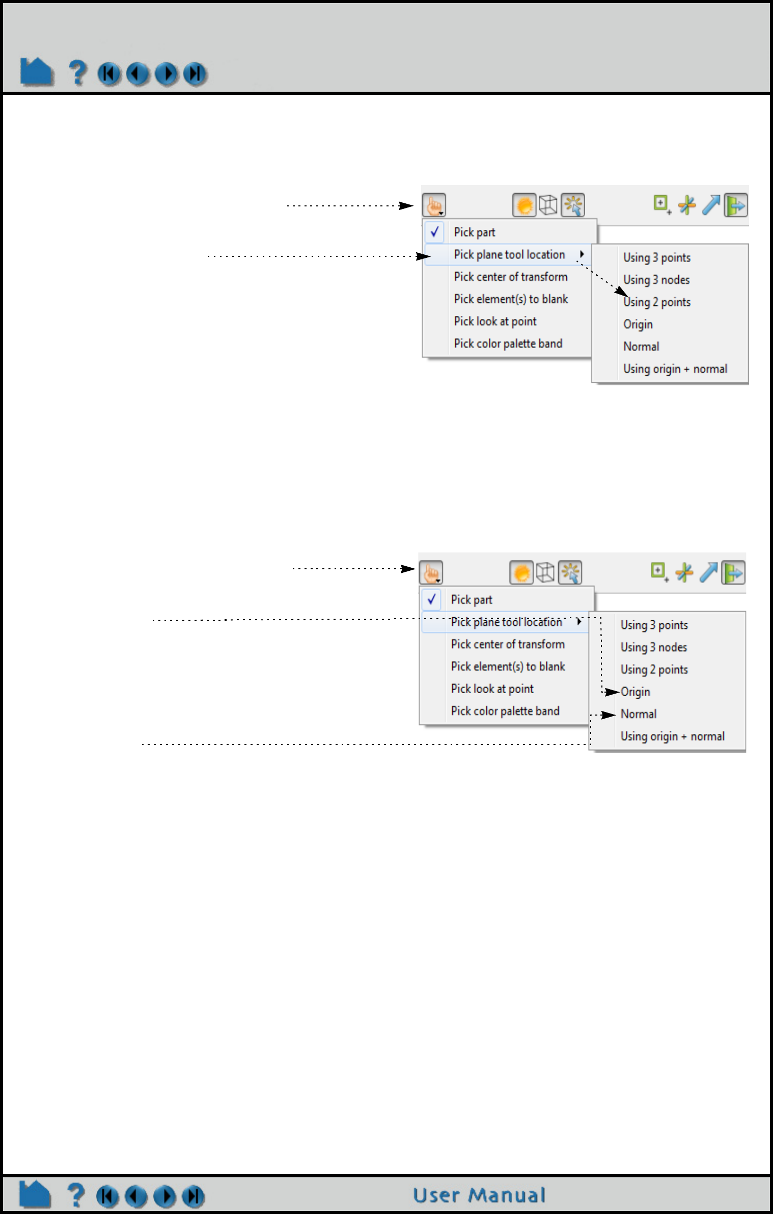
Page 191
HOW TO USE THE PLANE TOOL
You can also position the Plane Tool by tracing out a line on the screen. The Plane orientation will be changed such
that it is both parallel to the specified line and perpendicular to the screen.
To position the Plane (by specifying a line):
You can also position the Plane Tool by picking an origin, then a point out on the normal. This takes two picking
operations to accomplish.
To position the Plane (by picking origin, then point on normal):
1. Turn on the Plane tool as indicated earlier, then Click
the Pick button on the tool ribbon.
2. Select “Pick plane tool location > Using 2 points”
from the pop-up menu.
3. Move the mouse pointer into the Graphics Window
and press the ‘p’ key. Place the pointer over the
desired starting point. Click and hold the left mouse
button as you trace out the desired line.
4. Release the mouse button.
1. Turn on the Plane tool as indicated earlier, then Click
the Pick button on the tool ribbon.
2. Select “Pick plane tool location > Origin” from the
pop-up menu.
3. Move the mouse pointer into the Graphics Window
and place the pointer over the desired origin of the
plane tool - then press the ‘p’ key.
4. Select “Pick plane tool location > Normal” from the
pop-up menu.
5. Place the pointer over a point along the normal
vector (from the origin of the plane tool) - then press
the ‘p’ key.

Page 192
HOW TO USE THE PLANE TOOL
To set the Plane by specifying parameters exactly:
You can also rotate, translate, or scale the Plane by selecting the desired transform action, setting the desired axis
and manipulating the slider bar. In this case, the values in the “Scale Settings” section control the sensitivity and limit
of the slider action.
Note that you can also use this dialog to view (rather than set) the position of the Plane since the X,Y,Z numeric
values always update to reflect the current location. If you are positioning the Plane interactively with the mouse, the
values will update when the mouse button is released.
The Undo/Redo button at the bottom of screen can be used to undo/redo the tool transformation.
Shortcut
If you right click on center selection point of the line tool you can do quick x or y rotates, increase or decrease the size
of the tool, hide the tool, or open the transformation editor. You can also use this right click to quickly create a plane
clip, or do a particle streamline trace with the plane tool as the emitter.
ADVANCED USAGE
After a model has been loaded, the initial location of the Plane center is set to the “look-at” point – the geometric
center of all visible geometry and parallel to the X-Y plane. The coordinates of the Plane are specified with respect to
the default frame: frame 0. However, if you have created additional frames, you can position the Plane relative to the
1. Turn on the Plane tool, then open the
Transformation Editor from the tools ribbon.
2. If necessary, set the editor to Plane mode
by Editor Function > Tools > Plane.
3. Enter the desired coordinates for the origin,
the components of the normal vector, and
the x and y size, and press return.
– OR –
3. Enter the id of three nodes and press
return.
– OR –
3. Enter the plane equation parameters (Ax +
By + Cz = D) and press return.
– OR –
3. Enter the desired coordinates for three
corner points into the X, Y, and Z fields and
press return.

Page 193
HOW TO USE THE PLANE TOOL
origin of a different frame. This is accomplished by selecting the desired frame in the “Which Frame” list in the
Transformation Editor dialog.
You can easily reset the position and orientation of the Plane tool to the default. See How To Reset Tools and
Viewports for more information.
By default the plane tool will be displayed in line mode. You can display the tool as a transparent plane by changing
the setting for Edit > Preferences... View - Plane Tool Filled.
Positioning a 3D tool with a 2D device (the mouse) can be difficult. Multiple viewports are sometimes helpful in
positioning tools since you can see the tool simultaneously from multiple vantage points.
SEE ALSO
Other tools: Cursor, Line, Box, Cylinder, Sphere, Cone, Surface of Revolution. See the How To article on
Frames for additional information on how frames effect tools.
The Plane Tool is also used to specify the location of the clip plane for Auxiliary Clipping.
User Manual: Tools Menu Functions
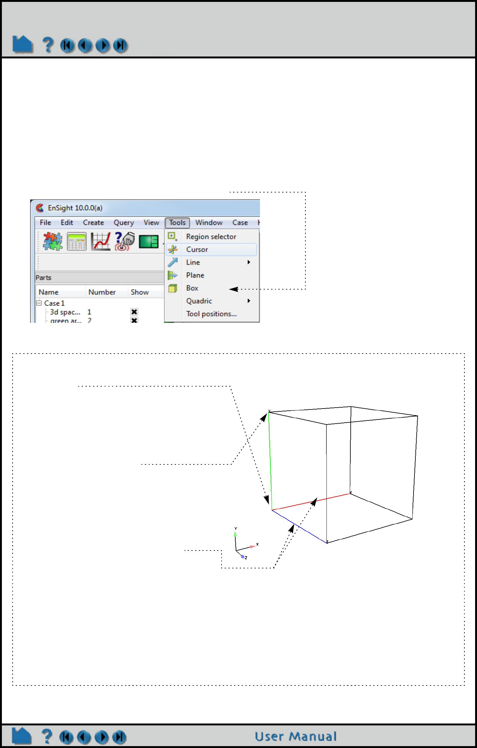
Page 194
HOW TO USE THE BOX TOOL
Use the Box Tool
INTRODUCTION
EnSight provides a hexahedron shaped specification tool called the “Box” tool. When visible, the Box tool appears as
a (typically white) wireframe box icon with a triad at one corner. The Box tool is used to supply EnSight with a 3D
volume specification, for example to specify the location for a box clip or cut.
BASIC OPERATION
In many cases, the Box tool will automatically turn on when performing some function that requires it. You can also
turn the tool on and off manually by toggling Tools > Box.
The Box tool can be placed in two ways: interactively through direct manipulation of tool “hotpoints” with the mouse or
precisely positioned by typing coordinates into a dialog.
Box tool moving and stretching is in 3 space. (Note the Box may not exactly track the location of the mouse pointer.)
To move the Box Tool with the mouse:
1. Place the mouse pointer over the origin corner
of the tool.
2. Click (and hold) the left mouse button.
3. Drag the Box to the desired location.
4. Release the mouse button.
To stretch the Box Tool with the mouse:
1. Place the mouse pointer over any of the corner
points (except the origin).
2. Click (and hold) the left mouse button.
3. Drag the endpoint to produce the desired
stretched size.
4. Release the mouse button.
To rotate the Box Tool with the mouse:
1. Place the mouse pointer over the center of the
x, y, or z edge (not at the endpoints).
2. Click and drag to rotate.
Note: Selection of the X axis edge will rotate the
box about the Y axis edge. Selection of the Y
axis edge will rotate about the X axis edge.
Selection about the Z axis edge will rotate
about the origin.
Note that the mouse pointer will change when it is over a
hotpoint (if you are in Part or Frame mode).
(Undo/Redo button at the bottom of screen can be used
to undo/redo the tool transformation)
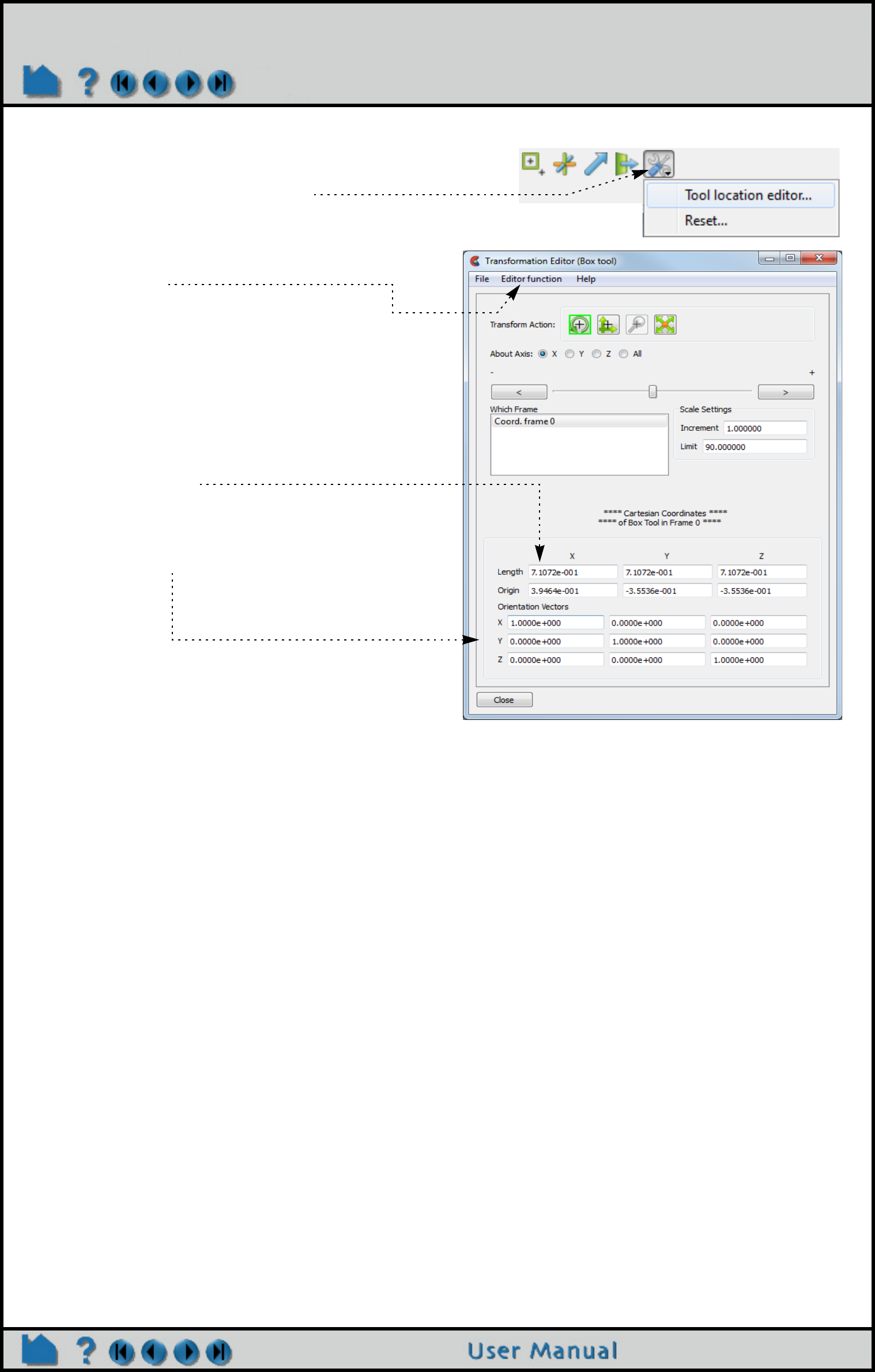
Page 195
HOW TO USE THE BOX TOOL
To set the Box Tool by specifying coordinates:
You can also rotate, translate or stretch the Box Tool by selecting the desired Transform Action, setting the desired
axis, and then manipulating the slider bar. For these tool actions, the values in the “Scale Settings” section control the
sensitivity and limit of the slider action.
Note that you can also use this dialog to view (rather than set) the position of the Box Tool since the numeric values
always update to reflect the current location, size, and orientation. If you are positioning the Box Tool interactively with
the mouse, the values will update when the mouse button is released.
Shortcut
While Part Quick Action icons are available (indicating that parts can be edited), right click on center selection point of
the Box tool. You can do quick hide the tool, or open the transformation editor.
ADVANCED USAGE
After a model has been loaded, the initial location of the Box Tool is centered about the “look-at” point – the geometric
center of all visible geometry - and is aligned with the model axis system. The coordinates of the Box are specified
with respect to the default frame: frame 0. However, if you have created additional frames, you can position the Box
Tool relative to the origin of a different frame. This is accomplished by selecting the desired frame in the “Which
Frame” list in the Transformation Editor dialog.
You can easily reset the position and orientation of the Box tool to the default. See How To Reset Tools and
Viewports for more information.
Positioning a 3D tool with a 2D device (the mouse) can be difficult. Multiple viewports are sometimes helpful in
positioning tools since you can see the tool simultaneously from multiple vantage points.
1. Open the Transformation Editor dialog by
clicking on the Tools icon then selecting
the Tool location editor.... option.
2. If the dialog is not set for Box tool (look at
the title of the dialog) then switch the
dialog to the Box tool by Editor Function
> Tools > Box.
3. To place and size, enter the desired
coordinates for the Origin corner and
the length in each of the directions,
and press return.
4. To orient, enter the components of the
orthogonal axis orientation vectors

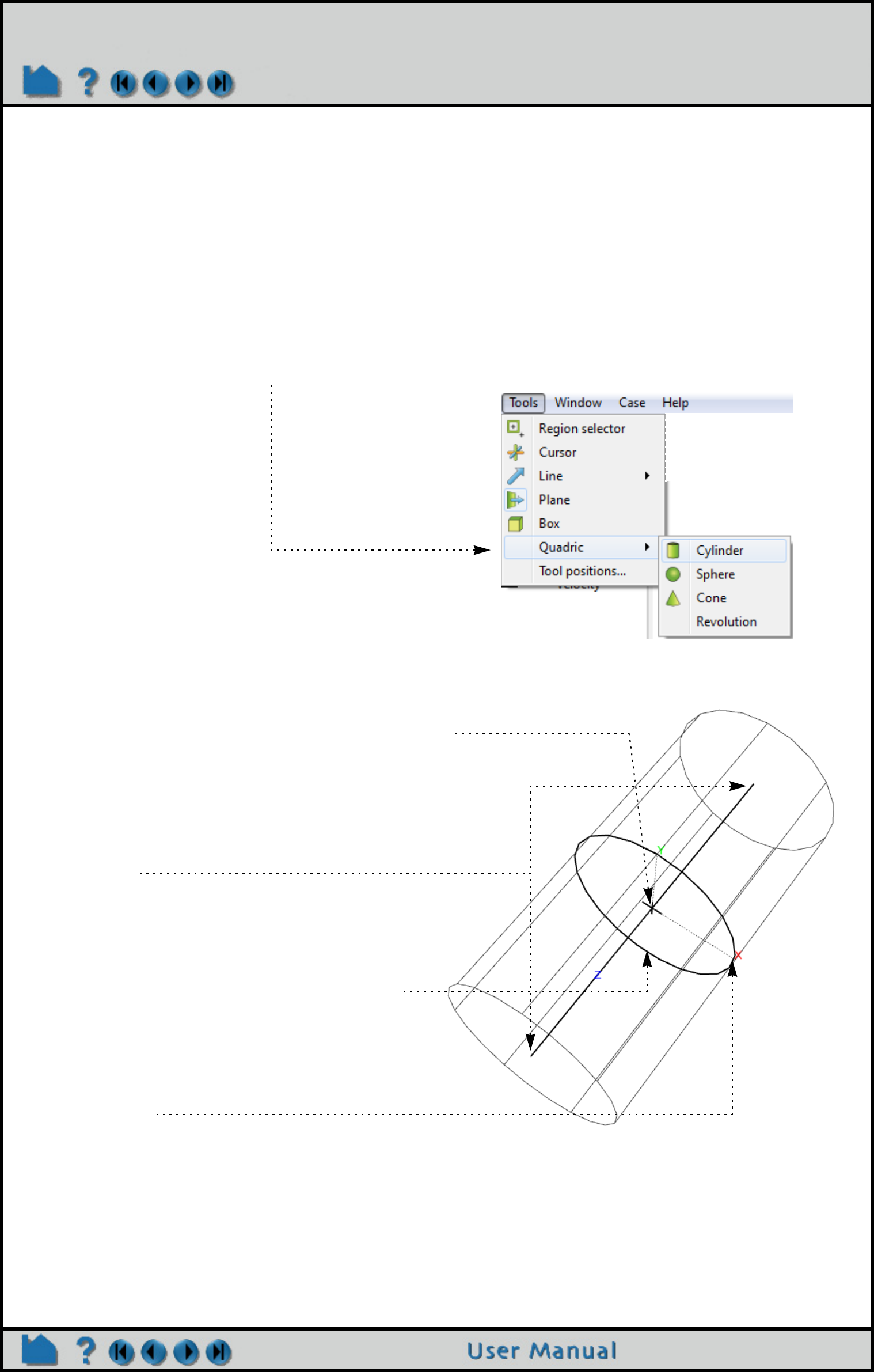
Page 197
HOW TO USE THE CYLINDER TOOL
Use the Cylinder Tool
INTRODUCTION
EnSight provides a cylindrical specification tool called the “Cylinder” tool. When visible, the Cylinder tool appears as a
(typically white) cylinder icon with a line running down the central axis. An axis triad will be at the center of the central
axis line. The Cylinder tool is used to supply EnSight with a cylindrical specification, for example to specify the
location for a cylinder clip or cut.
BASIC OPERATION
In many cases, the Cylinder tool will automatically turn on when performing some function that requires it. You can
also turn the tool on and off manually by toggling Tools > Quadric > Cylinder.
The Cylinder tool can be placed in two ways: interactively through direct manipulation of tool “hotpoints” with the
mouse or precisely positioned by typing coordinates into a dialog.
To move the Cylinder with the mouse:
1. Place the mouse pointer over the center of the tool.
2. Click (and hold) the left mouse button.
3. Drag the Cylinder to the desired location.
4. Release the mouse button.
To stretch the Cylinder with the mouse:
1. Place the mouse pointer over either of the center line’s
endpoints.
2. Click (and hold) the left mouse button.
3. Drag the endpoint to the desired location.
4. Release the mouse button.
To change the Cylinder radius with the mouse:
1. Place the mouse pointer over the center ring.
2. Click and drag to the desired radius.
3. Release the mouse button.
To rotate the Cylinder with the mouse:
1. Place the mouse pointer over the end of one of the
central axes.
2. Click and drag until desired rotation is accomplished.
3. Release the mouse button.
Note:
Selecting the x axis will rotate about the Y axis.
Selecting the y axis will rotate about the X axis.
Selecting the z axis will rotate in general about the axis
origin.
Note that the mouse pointer will change when it is
over a hotpoint (if in Part or Frame mode).
(Undo/Redo button at the bottom of screen can be
used to undo/redo the tool transformation)
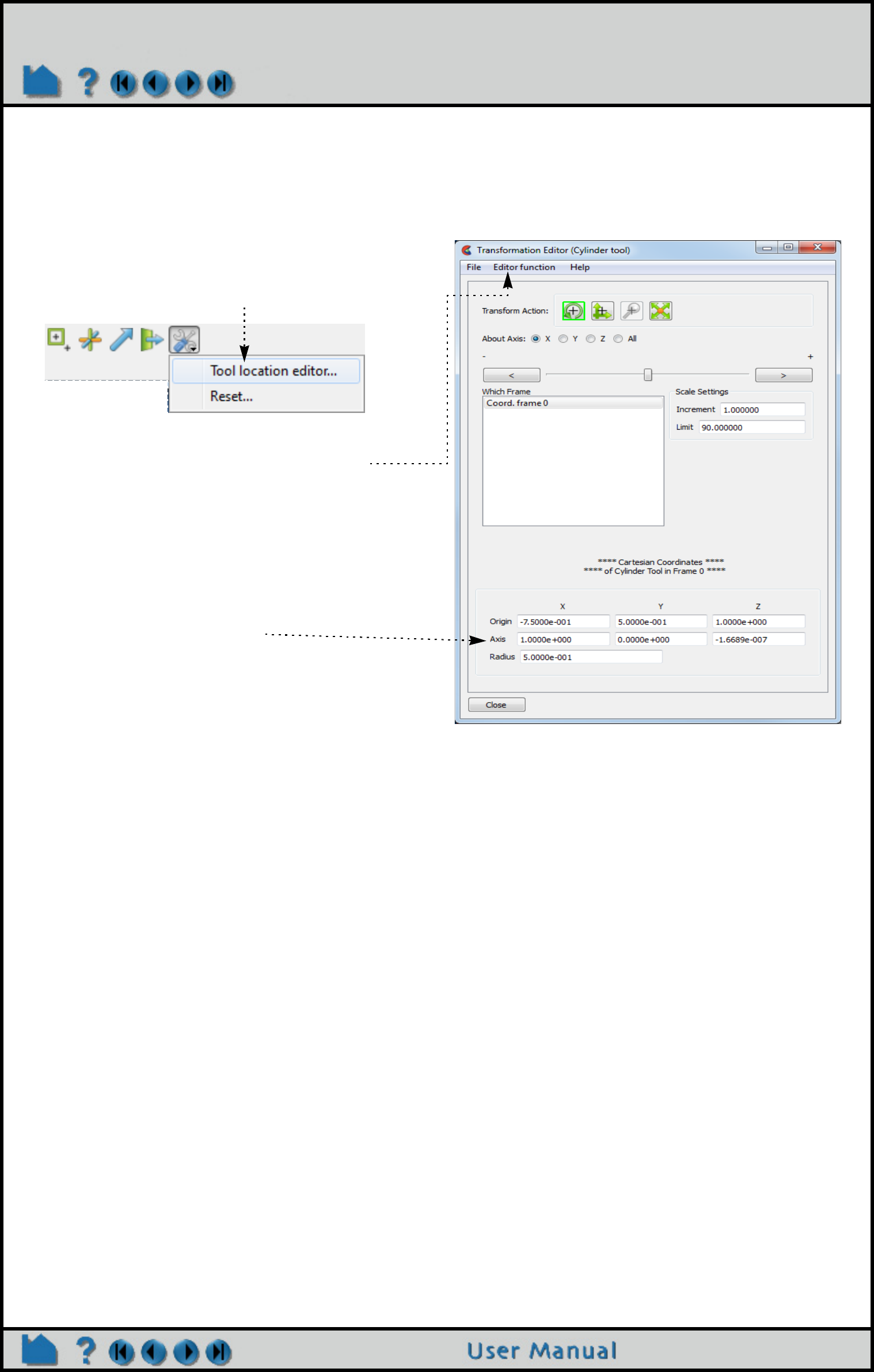
Page 198
HOW TO USE THE CYLINDER TOOL
Cylinder moving and stretching with the mouse is restricted to the plane perpendicular to your line of sight. If you
need to move the Cylinder in another plane, either rotate the model such that the desired translation plane is
perpendicular to your new line of sight or use the other modes for manipulating the tool. (Note that the Cylinder will
not exactly track the location of the mouse pointer.)
To set the Cylinder by specifying coordinates:
You can also rotate, translate, or scale the Cylinder by setting the desired transform action and axis and manipulating
the slider bar. In this case, the values in the “Scale Settings” section control the sensitivity and limit of the slider
action.
Note that you can also use this dialog to view (rather than set) the position of the Cylinder since the numeric values
always update to reflect the current location. If you are positioning the Cylinder interactively with the mouse, the
values will update when the mouse button is released.
ADVANCED USAGE
After a model has been loaded, the initial location of the Cylinder center is set to the “look-at” point – the geometric
center of all visible geometry and aligned with the X axis. The coordinates of the Cylinder are specified with respect
to the default frame: frame 0. However, if you have created additional frames, you can position the Cylinder relative
to the origin of a different frame. This is accomplished by selecting the desired frame in the “Which Frame” list in the
Transformation Editor dialog.
You can easily reset the position and orientation of the Cylinder tool to the default. See How To Reset Tools and
Viewports for more information.
Positioning a 3D tool with a 2D device (the mouse) can be difficult. Multiple viewports are sometimes helpful in
positioning tools since you can see the tool simultaneously from multiple vantage points.
SEE ALSO
Other tools: Cursor, Line, Plane, Box, Sphere, Cone, Surface of Revolution. See the How To article on Frames
for additional information on how frames effect tools.
User Manual: Tools Menu Functions
1. Open the Transformation Editor dialog by
clicking Tool location editor... from the
Tool Locations settings icon.
2. Select Editor Function > Tools > Cylinder
if the panel is not set to Cylinder Tool.
3. Enter the desired coordinates for the
Origin (location of the center point),
the Axis (direction vector), and the
Radius and press return.
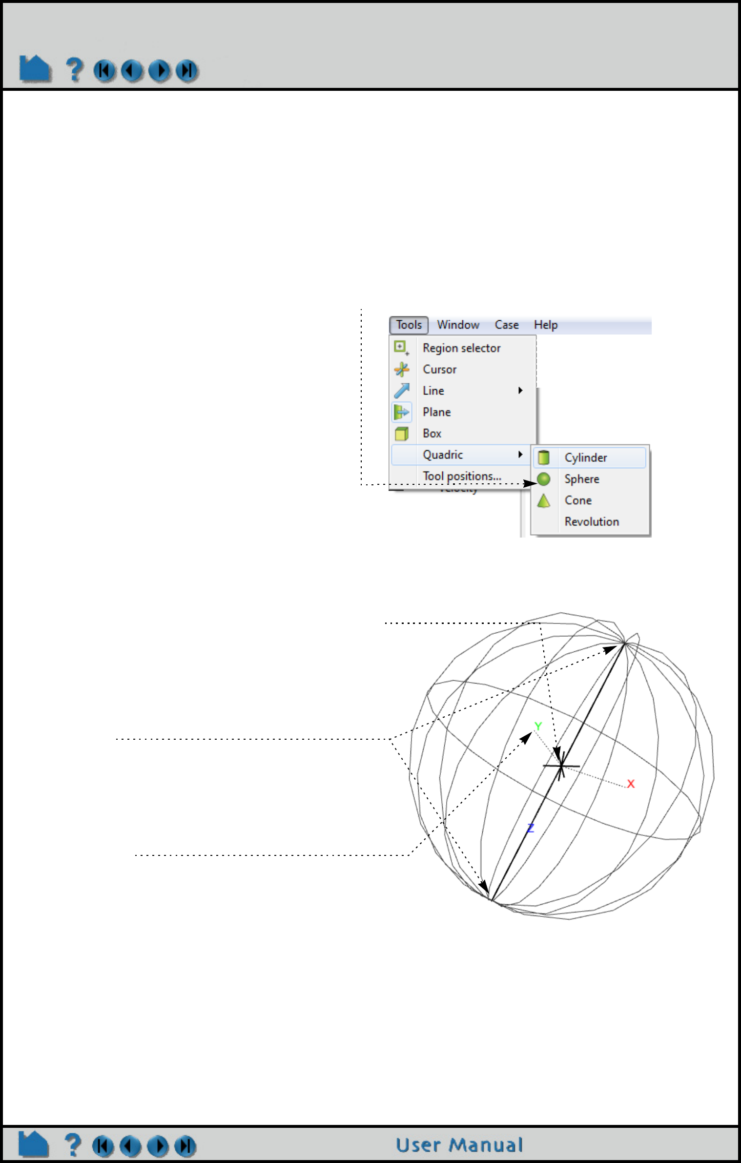
Page 199
HOW TO USE THE SPHERE TOOL
Use the Sphere Tool
INTRODUCTION
EnSight provides a spherical specification tool called the “Sphere” tool. When visible, the Sphere tool appears as a
(typically white) sphere icon with a line running down the central axis. An axis triad will be at the center of the central
axis line. The Sphere tool is used to supply EnSight with a spherical specification, for example to specify the location
for a sphere clip or cut.
BASIC OPERATION
In many cases, the Sphere tool will automatically turn on when performing some function that requires it. You can
also turn the tool on and off manually by toggling Tools > Quadric > Sphere.
The Sphere tool can be placed in two ways: interactively through direct manipulation of tool “hotpoints” with the
mouse or precisely positioned by typing coordinates into a dialog.
Sphere moving and stretching is restricted to the plane perpendicular to your line of sight. If you need to move the
Sphere in another plane, either rotate the model such that the desired translation plane is perpendicular to your new
line of sight or use the other modes for manipulating the tool. (Note that the Sphere will not exactly track the location
of the mouse pointer.)
To move the Sphere with the mouse:
1. Place the mouse pointer over the center of the tool.
2. Click (and hold) the left mouse button.
3. Drag the Sphere to the desired location.
4. Release the mouse button.
To stretch the Sphere with the mouse:
1. Place the mouse pointer over either of the center line’s
endpoints.
2. Click (and hold) the left mouse button.
3. Drag the endpoint to the desired location.
4. Release the mouse button.
To rotate the sphere with the mouse:
1. Place the mouse pointer over the end of one of the
central axes.
2. Click and drag until desired rotation is accomplished.
3. Release the mouse button.
Note:
Selecting the x axis will rotate about the Y axis.
Selecting the y axis will rotate about the X axis.
Selecting the z axis will rotate in general about the axis origin.
Note that the mouse pointer will change when it is over a hotpoint.
(Undo/Redo button at the bottom of screen can be used to undo/redo the tool
transformation)
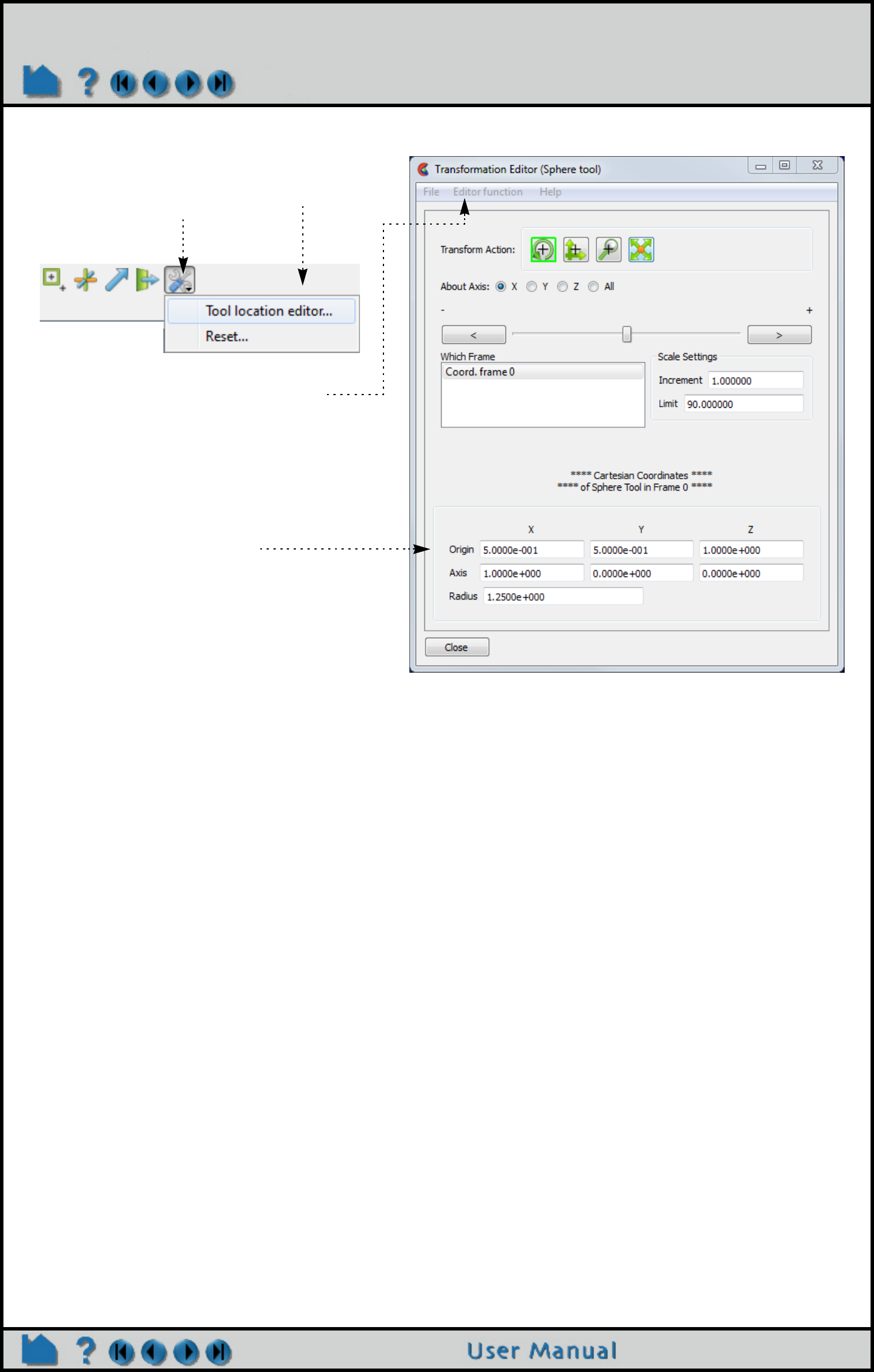
Page 200
HOW TO USE THE SPHERE TOOL
To set the Sphere by specifying coordinates:
You can also rotate, translate or scale the Sphere by setting the desired transform action and axis and manipulating
the slider bar. In this case, the values in the “Scale Settings” section control the sensitivity and limit of the slider
action.
Note that you can also use this dialog to view (rather than set) the position of the Sphere since the numeric values
always update to reflect the current location. If you are positioning the Sphere interactively with the mouse, the
values will update when the mouse button is released.
ADVANCED USAGE
After a model has been loaded, the initial location of the Sphere center is set to the “look-at” point – the geometric
center of all visible geometry and aligned with the X axis. The coordinates of the Sphere are specified with respect to
the default frame: frame 0. However, if you have created additional frames, you can position the Sphere relative to
the origin of a different frame. This is accomplished by selecting the desired frame in the “Which Frame” list in the
Transformation Editor dialog.
You can easily reset the position and orientation of the Sphere tool to the default. See How To Reset Tools and
Viewports for more information.
Positioning a 3D tool with a 2D device (the mouse) can be difficult. Multiple viewports are sometimes helpful in
positioning tools since you can see the tool simultaneously from multiple vantage points.
SEE ALSO
Other tools: Cursor, Line, Plane, Box, Cylinder, Cone, Surface of Revolution. See the How To article on Frames
for additional information on how frames effect tools.
User Manual: Tools Menu Functions
1. Open the Transformation Editor dialog by
clicking Tool location editor... from the
Tool Locations settings icon.
3. Enter the desired coordinates for the
Origin (location of the center point),
the Axis (direction vector), and/or the
Radius.
if you are going to create a developed surface from
a spherical clip, you need to be aware of how the
spherical axis orientation affects this operation.
(See How To Create a Developed Surface)
2. Select Editor Function > Tools > Sphere if
the panel is not set to Sphere tool.
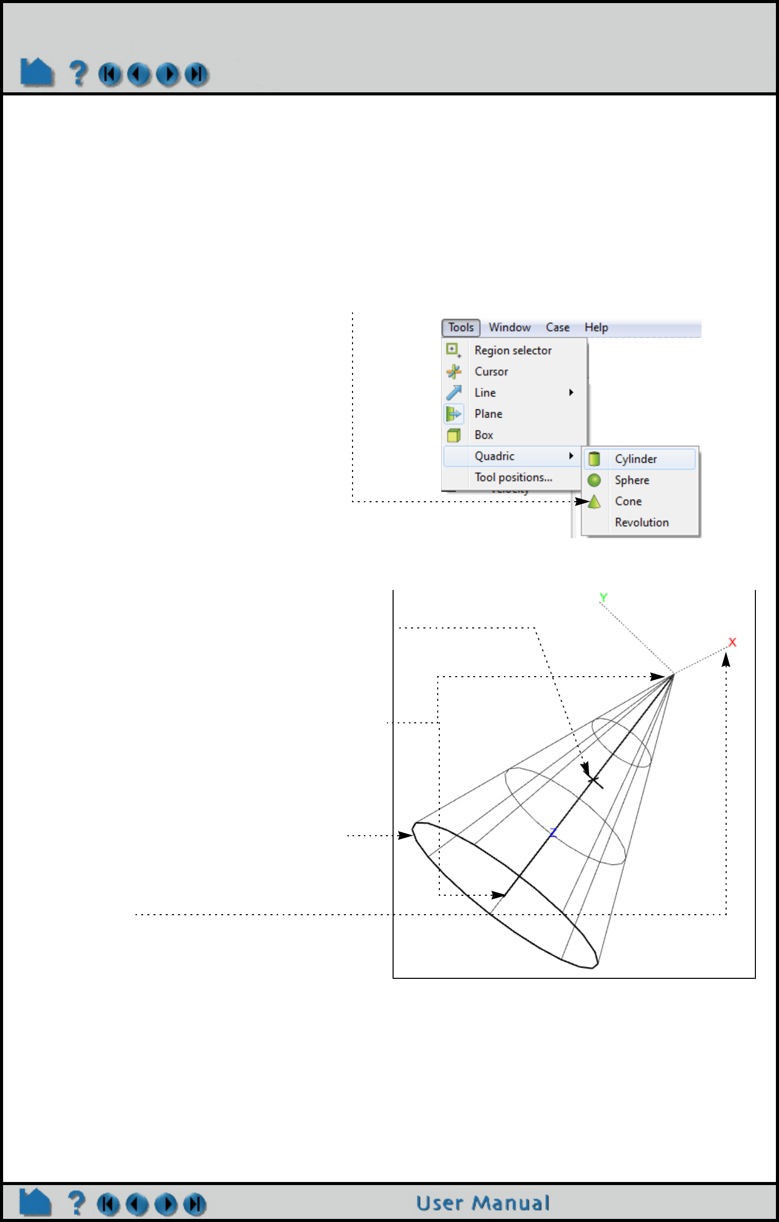
Page 201
HOW TO USE THE CONE TOOL
Use the Cone Tool
INTRODUCTION
EnSight provides a conical specification tool called the “Cone” tool. When visible, the Cone tool appears as a
(typically white) cone icon with a line running down the center axis. The Cone tool is used to supply EnSight with a
conical specification, for example to specify the location for a conical clip or cut.
BASIC OPERATION
In many cases, the Cone tool will automatically turn on when performing some function that requires it. You can also
turn the tool on and off manually by toggling Tools > Quadric > Cone.
The Cone tool can be placed in two ways: interactively through direct manipulation of tool “hotpoints” with the mouse
or precisely positioned by typing coordinates into a dialog.
Cone moving and stretching is restricted to the plane perpendicular to your line of sight. If you need to move the Cone
in another plane, either rotate the model such that the desired translation plane is perpendicular to your new line of
sight or use the other modes for manipulating the tool. (Note that the Cone will not exactly track the location of the
mouse pointer.)
To move the Cone with the mouse:
1. Place the mouse pointer over the center of the tool.
2. Click (and hold) the left mouse button.
3. Drag the Cone to the desired location.
4. Release the mouse button.
To stretch the Cone with the mouse:
1. Place the mouse pointer over either of the center
line’s endpoints.
2. Click (and hold) the left mouse button.
3. Drag the endpoint to the desired location.
4. Release the mouse button.
To change the Cone radius with the mouse:
1. Place the mouse pointer over the base ring.
2. Click and drag to the desired radius.
To rotate the Cone with the mouse:
1. Place the mouse pointer over the end of one of the
central axes.
2. Click and drag until desired rotation is
accomplished.
3. Release the mouse button.
Note:
Selecting the x axis will rotate about the Y axis.
Selecting the y axis will rotate about the X axis.
Selecting the z axis will rotate in general about the
axis origin.
Note that the mouse pointer will change when it is over
a hotpoint.
(Undo/Redo button at the bottom of screen can be used
to undo/redo the tool transformation)
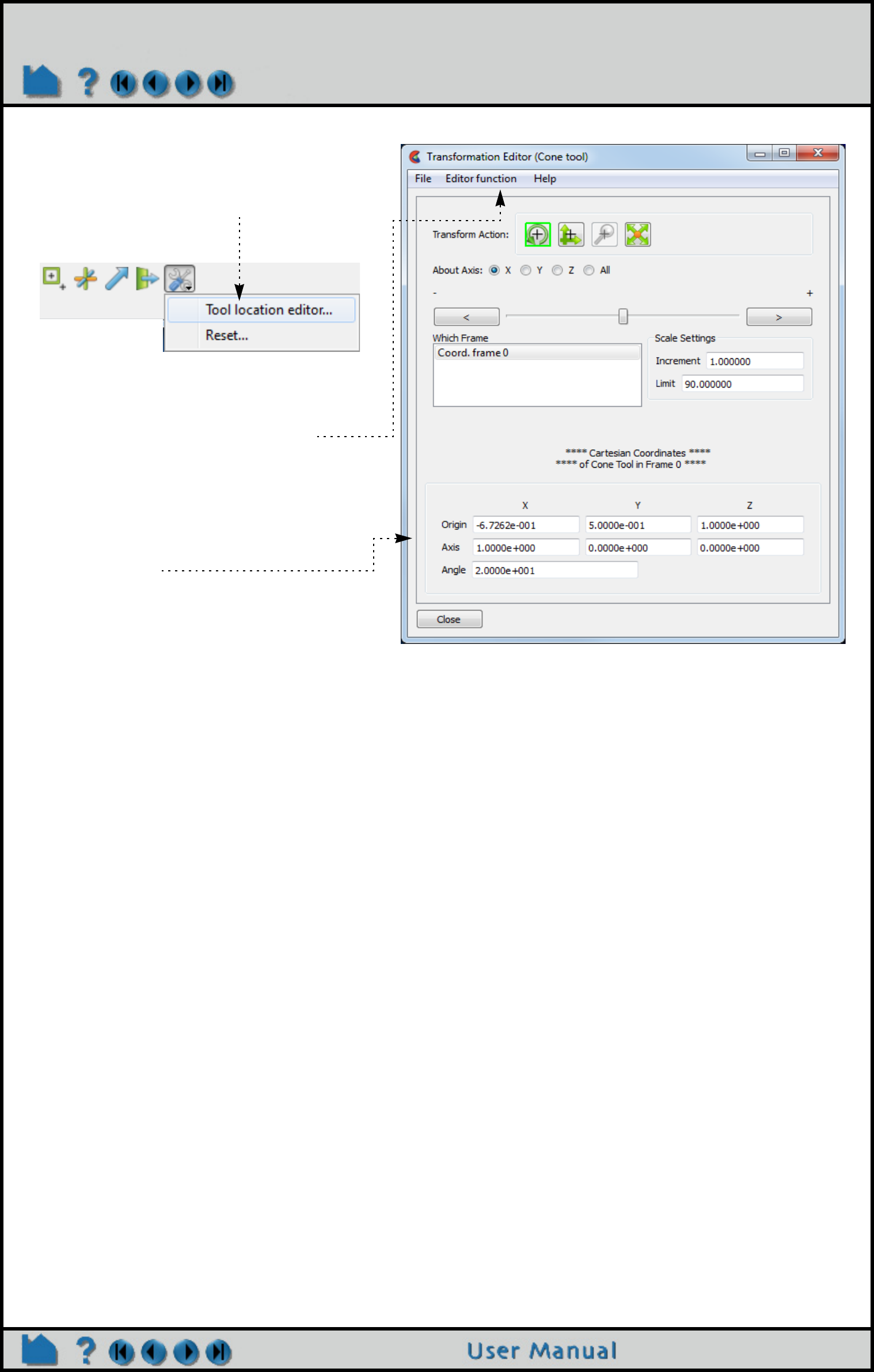
Page 202
HOW TO USE THE CONE TOOL
To set the Cone by specifying coordinates:
You can also rotate, translate or scale the Cone by setting the desired transform action and axis and manipulating the
slider bar. In this case, the values in the “Scale Settings” section control the sensitivity and limit of the slider action.
Note that you can also use this dialog to view (rather than set) the position of the Cone since the numeric values
always update to reflect the current location. If you are positioning the Cone interactively with the mouse, the values
will update when the mouse button is released.
The clip/cut from the cone tool will extend infinitely from the tip outwards unless you choose Extent>Finite in the
pulldown.
ADVANCED USAGE
After a model has been loaded, the initial location of the Cone center is set to the “look-at” point – the geometric
center of all visible geometry and aligned with the X axis. The coordinates of the Cone are specified with respect to
the default frame: frame 0. However, if you have created additional frames, you can position the Cone relative to the
origin of a different frame. This is accomplished by selecting the desired frame in the “Which Frame” list in the
Transformation Editor dialog.
You can easily reset the position and orientation of the Cone tool to the default. See How To Reset Tools and
Viewports for more information.
Positioning a 3D tool with a 2D device (the mouse) can be difficult. Multiple viewports are sometimes helpful in
positioning tools since you can see the tool simultaneously from multiple vantage points.
SEE ALSO
Other tools: Cursor, Line, Plane, Box, Cylinder, Sphere, Surface of Revolution. See the How To article on
Frames for additional information on how frames effect tools.
User Manual: Tools Menu Functions
1. Open the Transformation Editor dialog by
clicking Tool location editor... from the
Tool Locations settings icon.
2. Select Editor Function > Tools > Cone if
the panel is not set to Cone tool.
3. Enter the desired coordinates for the
Origin (location of the cone tip), the
Axis (direction vector), and the
conical half angle (in degrees) and
press return.
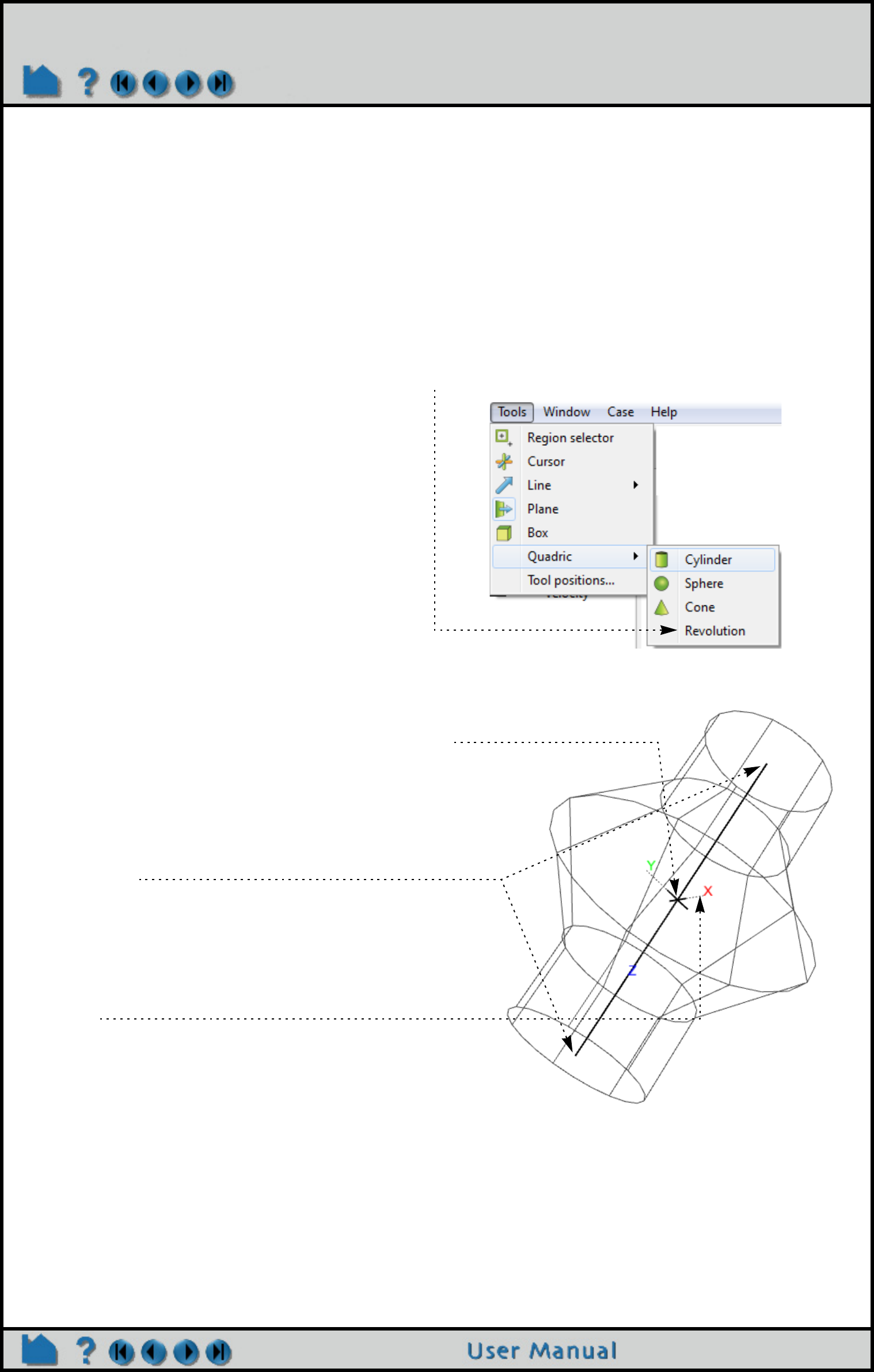
Page 203
HOW TO USE SURFACE OF REVOLUTION TOOL
Use Surface of Revolution Tool
INTRODUCTION
EnSight provides a surface of revolution specification tool called the “Revolution” tool. When visible, the Revolution
tool appears as a (typically white) icon with a line running down the center axis. By default, the distance of five
planar points from the central axis defines the profile curve of the revolution surface (although you can add points up
to a maximum of ten). The Revolution tool is used to supply EnSight with a surface of revolution specification, for
example to specify the location for a revolution clip or cut.
BASIC OPERATION
In many cases, the Revolution tool will automatically turn on when performing some function that requires it. You can
also turn the tool on and off manually by toggling Tools > Quadric > Revolution.
The Revolution tool can be placed in two ways: interactively through direct manipulation of tool “hotpoints” with the
mouse or precisely positioned by typing coordinates into a dialog.
Revolution tool moving and stretching is restricted to the plane perpendicular to your line of sight. If you need to move
the Revolution tool in another plane, either rotate the model such that the desired translation plane is perpendicular to
your new line of sight or use the other modes to manipulate the tool. (Note that the Revolution tool will not exactly
track the location of the mouse pointer.)
To move the Revolution tool with the mouse:
1. Place the mouse pointer over the center of the tool.
2. Click (and hold) the left mouse button.
3. Drag the tool to the desired location.
4. Release the mouse button.
To reorient the Revolution tool with the mouse:
1. Place the mouse pointer over either of the center line’s
endpoints.
2. Click (and hold) the left mouse button.
3. Drag the endpoint to achieve the desired orientation.
4. Release the mouse button.
To rotate the Revolution tool with the mouse:
1. Place the mouse pointer over the end of one of the
central axes.
2. Click and drag until desired rotation is accomplished.
3. Release the mouse button.
Note:
Selecting the x axis will rotate about the Y axis.
Selecting the y axis will rotate about the X axis.
Selecting the z axis will rotate in general about the axis
origin.
Note that the mouse pointer will change when it is
over a hotpoint.
(Undo/Redo button at the bottom of screen can be
used to undo/redo the tool transformation)
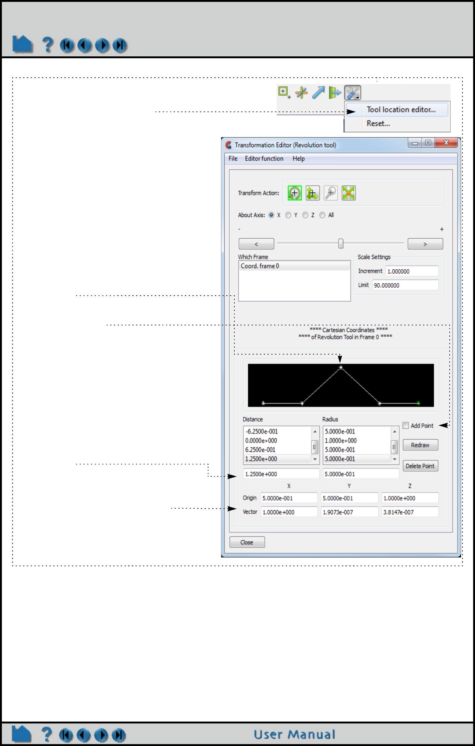
Page 204
HOW TO USE SURFACE OF REVOLUTION TOOL
To set the Revolution tool by specifying coordinates:
You can also rotate, translate, and scale the Revolution tool by setting the desired transform action and axis and
manipulating the slider bar. In this case, the values in the “Scale Settings” section control the sensitivity and limit of
the slider action.
Note that you can also use this dialog to view (rather than set) the position of the Revolution tool since the numeric
values always update to reflect the current location. If you are positioning the Revolution tool interactively with the
mouse, the values will update when the mouse button is released.
1. Open the Transformation Editor dialog by
clicking Tool location editor... from the
Tool Locations settings icon.
2. If the dialog is not set to Revolution Tool,
Select Editor Function > Tools >
Revolution.
The dialog displays the profile curve as a series
of connected line segments with stars
positioned at the curve points. You can edit the
curve by clicking and dragging the points or by
manually entering distance-radius pairs. You
can also add or delete points. As you make
changes, the tool in the graphics window
updates interactively.
To edit points with the mouse:
1. Click on the point and drag to the desired
location.
To add points (up to a maximum of 10):
1. Click Add Point.
2. Move the mouse pointer into the curve
window and click the left mouse button in
the location of the desired new point.
Clicking Delete Point will remove the
currently selected point.
To manually edit a point:
1. Click the point (to select it) in the curve
window or click the desired point in
either the Distance or Radius lists.
2. The distance and radius of the selected
point are shown in the text fields below
each list.
3. Edit the point’s distance and/or radius
value and press return.
To edit the position or orientation:
1. Enter the desired coordinates for the
Origin (location of the axis center point)
or Axis (direction vector) and press
return.

Page 205
HOW TO USE SURFACE OF REVOLUTION TOOL
ADVANCED USAGE
After a model has been loaded, the initial location of the Revolution tool center is set to the “look-at” point – the
geometric center of all visible geometry and aligned with the X axis. The coordinates of the Revolution tool are
specified with respect to the default frame: frame 0. However, if you have created additional frames, you can position
the Revolution tool relative to the origin of a different frame. This is accomplished by selecting the desired frame in
the “Which Frame” list in the Transformations dialog.
You can easily reset the position and orientation of the Revolution tool to the default. See How To Reset Tools and
Viewports for more information.
Positioning a 3D tool with a 2D device (the mouse) can be difficult. Multiple viewports are sometimes helpful in
positioning tools since you can see the tool simultaneously from multiple vantage points.
SEE ALSO
Other tools: Cursor, Line, Plane, Box, Cylinder, Sphere, Cone. See the How To article on Frames for additional
information on how frames effect tools.
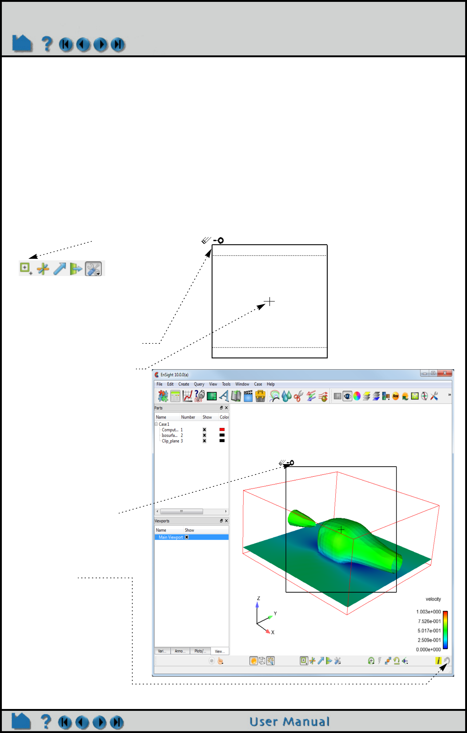
Page 206
HOW TO USE THE SELECTION TOOL
Use the Selection Tool
INTRODUCTION
EnSight provides a 2D screen selection tool called the “Selection” tool or “Region Selector”. It is different than most of
the other tools - in that it is not used to create other parts. It is basically used for selection purposes. For example, it
can be used to select a screen region to zoom in to. It can be used in the part selection process. And it can be used
for the element blanking operation.
BASIC OPERATION
Zoom to Region
To use the selection tool to perform a zoom operation:
1. Turn on the Selection Tool via
the icon on the Tools Icon Bar.
You manipulate the tool by:
- clicking and dragging on any
corner to rubberband the tool.
- clicking and dragging on the
center of the tool to move it.
Note: the dotted box indicates the
aspect ratio of the graphics window
and is used for zoom operations.
2. Click the Zoom symbol, at the
upper left of the tool, to cause
the zoom to occur.
Note: the Undo button is useful if
you want to undo the last
transformation.
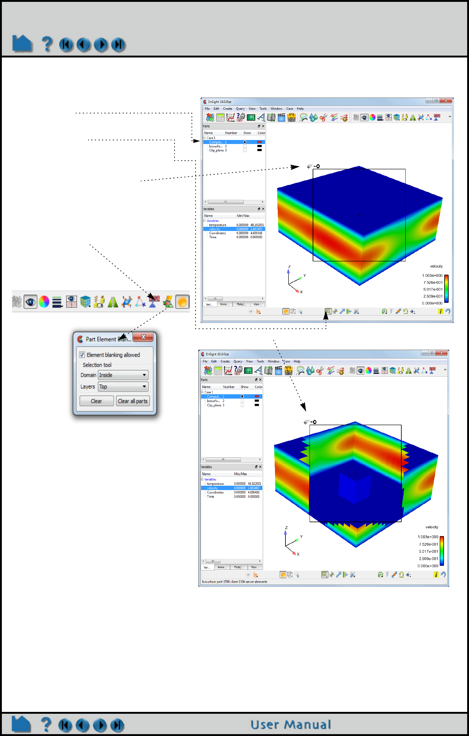
Page 207
HOW TO USE THE SELECTION TOOL
Element Blanking
The selection tool can be used in the element blanking operation.:
1. Select the part(s) on which to do element
blanking.
2. Click on the Selection tool icon to turn on
the tool.
3. Position the tool as desired.
4. Click on the element blanking symbol at
the upper left of the tool.
Note, in order for this to work, the Element
blanking allowed toggle needs to be on (the
default).
To undo the blanking, click the Clear or Clear
all parts button.
Results in the following:
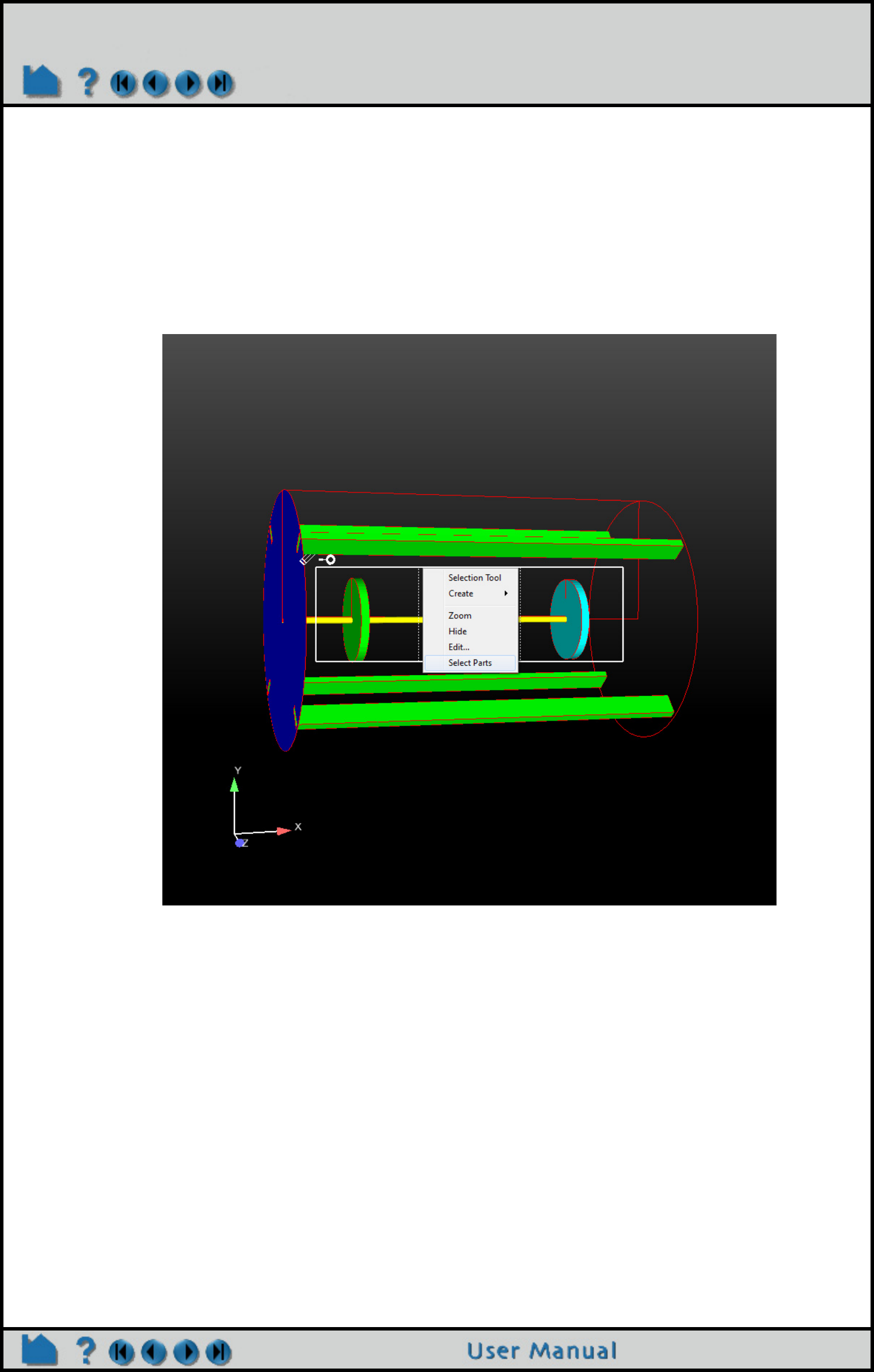
Page 208
HOW TO USE THE SELECTION TOOL
Part Selection
To use the tool in the part selection process:
SEE ALSO
How To Do Element Blanking
How To Rotate, Zoom, Translate, Scale
User Manual: Tools Menu Functions
1. Turn on the selection tool and manipulate its location/size until it
overlaps the parts you whish to select.
2. Right click the selection tool and “Select Parts”
Note that the selected parts will now be highlighted in the parts list.
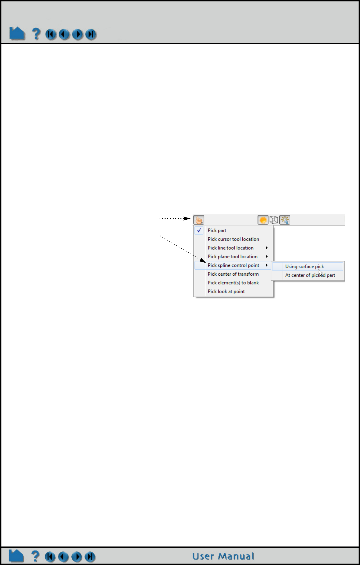
Page 209
HOW TO USE THE SPLINE TOOL
Use the Spline Tool
INTRODUCTION
Splines can be used for (a) the path of a camera, (b) the path of a clip plane, and (c) the input to a distance vs.
variable query. Splines can be defined and edited as well as saved and restored from disk. Further, the splines have
such as visibility, line width, and color in order to more easily select and manipulate them.
The splines are defined as piece-wise cubic. The spline is thus always guaranteed to pass through the control points
which you define. The definition of the control points can come from a part (such as a particle trace perhaps), be
picked in the graphics window, be input via x/y/z coordinates, or from the position of the cursor tool.
BASIC OPERATION
There are several ways to define a spline and its control points:
To create a spline via picking on surfaces:
1. Click the Pick button on the Tools Icon Bar
2. Select "Pick spline control point" from the
pop-up menu and select the required option.
3. In the Graphics Window, place the mouse
pointer on a part near a desired location and
press the "p" key (or whatever mouse button you
have set for the "Selected Pick Action" in Edit-
>Preferences->Mouse and Keyboard). A spline
control point marker will appear where you
pressed the "p" key (if you chose “Using surface
pick” or at the center of the part if you chose “At
center of picked part”). If more than one control
point has been created you will also see the
spline being constructed.
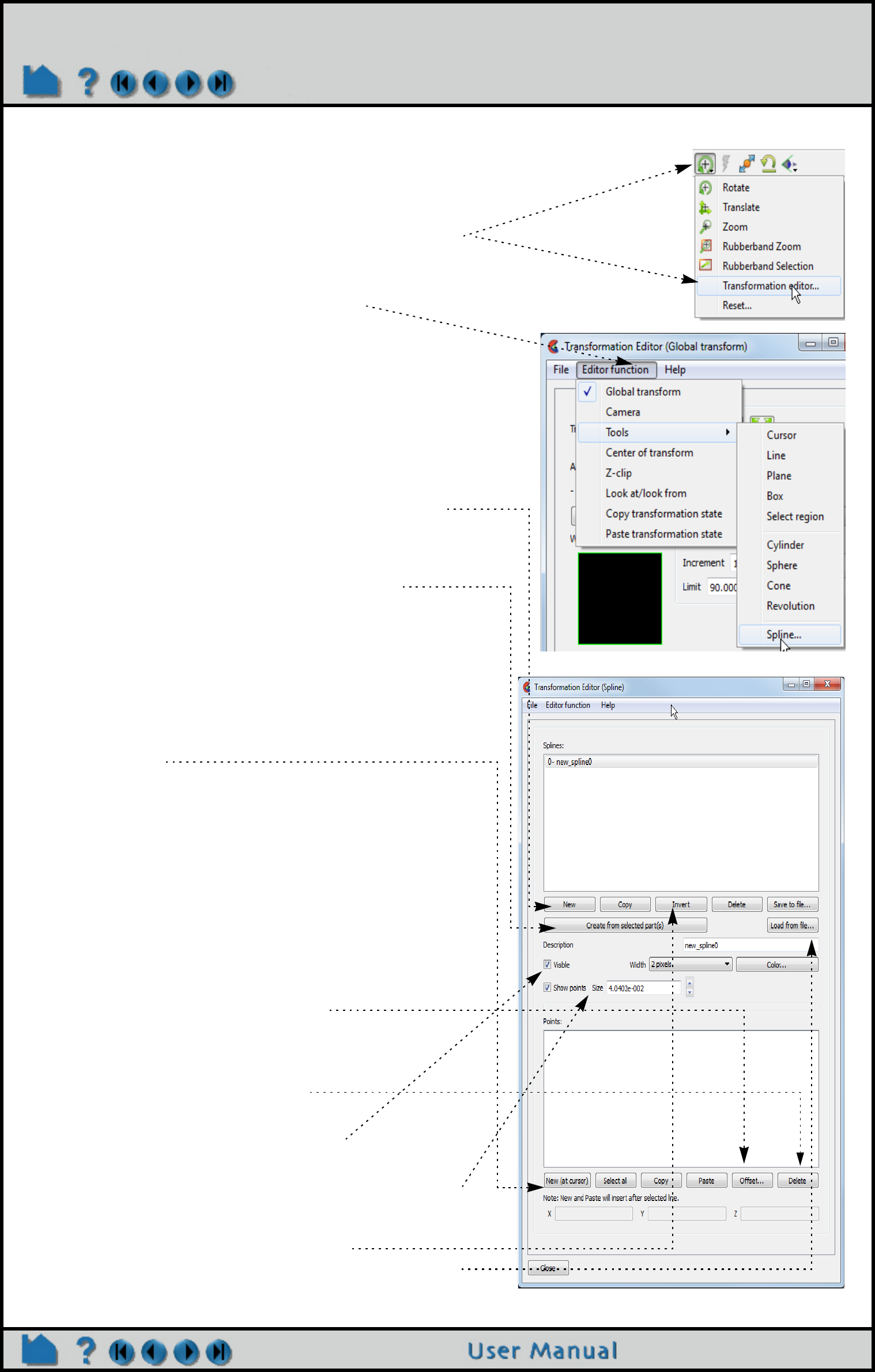
Page 210
HOW TO USE THE SPLINE TOOL
To create a spline via the Transformation editor dialog
1. Open the Transformation Editor dialog from the Tools
Icon Bar by selecting “Transformation editor...” from the
transform icon pulldown.
2. Select Editor Function > Tools > Spline
3. Select New to create a new spline and if you wish,
rename it by editing the Description
4. If you want to create control points from all of the
coordinates of a 1D part, select the part in the part list
and then select Create from selected part(s).
OR
4. If you know the exact location for the control point
select New (at cursor) then edit the X/Y/Z fields to reflect
the correct control point location.
OR
4. Select an existing control point in the Points list. Select
the Copy button. Then select the line in the Points list
after which you want to insert a new point and select the
Paste button.
To edit the control points of a spline:
1. Move the mouse pointer to a control point you wish to
move in the Graphics Window. Click and drag the
control point.
OR
1. Select the point from the Points list and edit it via the
XY/Z fields
OR
1. Select the point(s) you wish to edit and select the
Offset.. button
2. In the resulting pop-up enter a delta x/y/z value to add
to all of the selected points.
Control point(s) can be deleted by:
1. Select one or more points in the Points list
2. Select the Delete button
To edit the spline
1. The Visible toggle will turn the spline on/off in all
viewports (there are no per-viewport controls)
2. You may choose to show the control points. If visible
then the size of the control point glyph is controlled
here.
3. Adjust the Line width and Color here
4. Invert the spline (to use it in reverse).
5. Load from file (see Spline Control Point File Format)

Page 211
HOW TO USE THE SPLINE TOOL
ADVANCED USAGE
The spline by definition starts at the first control point (spline value of 0.) and ends at the last control point (spline
value of 1). If the spline is used for camera, clip plane path, or distance vs. variable query the direction along the
spline is always in the positive direction. If you wish to use the spline in reverse you simply Invert the spline.
SEE ALSO
Create Clip Splines
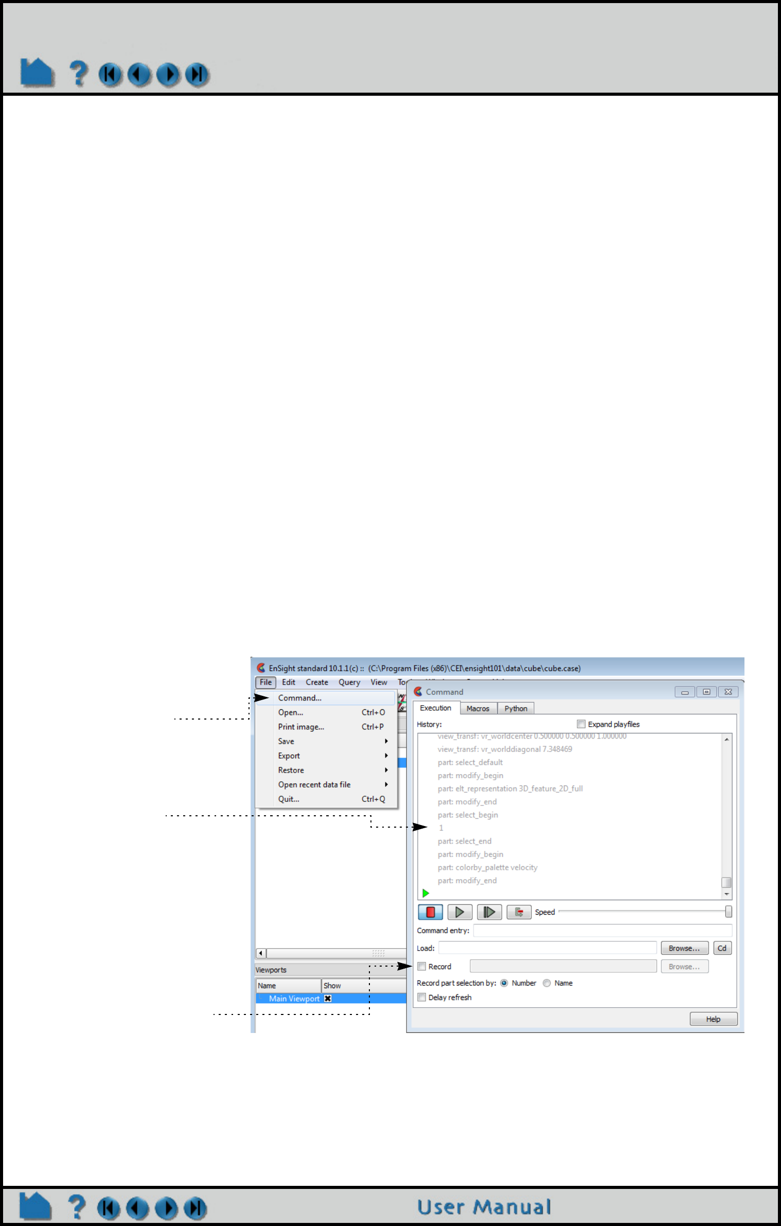
Page 212
HOW TO USE BATCH
MiscellaneousUse Batch
INTRODUCTION
EnSight can be run three ways.
1. First it can be run interactively by entering values into the various input fields and/or clicking on various icons in the
graphical user interface (GUI). Each of the user actions, such as reading data, creating parts, and saving images and
movies, is sequentially stored in EnSight in the form of journaling commands. The user can save these commands
into a command file (.enc file).
2. The second way to run EnSight is to start run the command file saved in #1. This can be done from the command
line such as (the last parameter is the name of the file you saved):
ensight102 -p file.enc
or you can play the command file from within EnSight by choosing File>Command from the top menu, then click the
play button and select the file.enc file you wish to execute. EnSight will perform the actions (reading data, creating
parts, saving images and movies) in your current EnSight session, sequentially in the order journaled in the
command file. If specified, the same images and movies that were generated interactively will be rewritten in the
folder specified in the command file.
3.The third way to run EnSight is to execute the commands in the command file without a GUI and without a graphics
screen, i.e., running in “batch”. All of the actions still happen in EnSight (without a GUI and without visible graphics)
and images and movies appear in the folder exactly as specified in the command file. In fact, to be useful, the
command file must save something that you can later take a look at.
The command to execute EnSight in batch is:
ensight102 -batch -p file.enc
Which will execute the graphics using the hardware graphics resources if available. Please see the Basic Operation
section on instructions on how to run in software rendering mode.
When you interact with EnSight,
commands are generated for
each action. To see these
commands, do a
File>Command as shown in the
image to the right.
The command window dialog
will pop up and the Execution
Tab will be active and the latest
commands will show up in the
command window.
File>Save>Commands from the
Session will save all the
commands from the start of
EnSight.
Or, click on the Record Toggle
and start saving commands to a
command file. All subsequent
commands are saved to the
designated command file.

Page 213
HOW TO USE BATCH
BASIC OPERATION
Keep in mind that command files are created by interactively executing EnSight and then saving the command
language to a file. To apply your commands to a new dataset, you would edit the command file in a text editor and
change the name of the input dataset and the output files (such as images) and then execute the modified command
file in batch.
Command language is not flexible: it does not allow programming or looping or decision making. It is, however,
possible to convert the command language file to a Python file to add programming constructs if necessary.
Command language processing does not always handle errors gracefully. Usually the command file processing will
simply stop when an error is found. But it is possible to issue commands to EnSight that can cause terminal errors. d
Example
Suppose you have 5 similar solver runs. Suppose that you wish to do the same postprocessing to each dataset and
run them overnight and show up in the morning and look at images and movies.
The first step is to create the command file. Load one of the solver runs into an interactive session of EnSight and
create the visuals and outputs you desire. Then save the commands to a file. Next, make four copies of the
command file and edit each one for input and output files.
Now run each of your jobs in batch as described above. Note that if your batch job is expected to run overnight on
your remote Linux system you might consider using the linux nohup command.
If you don’t have computing resources to handle all the jobs simultaneously then submit them sequentially. If you are
on a shared resource and licenses are limited, your EnSight batch process will fail if it is unable to acquire a license
token. To work around this, consider using one of the following EnSight startup modifiers: -token_try_again, -
token_wait_for, or -token_wait_until which will allow your batch EnSight processes to wait for an available
EnSight license token to become available (see Command Line Start-up Options).
Direct OpenGL, bypass X-Server
If the your machine has X-server issues (e.g. problems starting up the X-server) or issues with the DISPLAY
environmental variable, and you have an nVidia graphics card with driver 358.16 or later, and are on Linux, you can
start EnSight up with the -egl option. EnSight will use embedded OpenGL (which bypasses the X-server and makes
direct calls to the graphics card, which must be present) as follows.
ensight102 -egl -batch -p file.py
In a multi-GPU system the first GPU will be used by default. To choose a GPU, set the environment variable
CEI_EGL_GPU to a value between 0 and the number of GPUs minus 1.
Software Rendering
If the batch machine has inadequate or lacks a graphics card you can execute EnSight in a software mode which will
utilize the CPU to generate the graphics. The execution will be significantly slower but assuming you save only a few
images may have little impact on the overall run time. To use software rendering in batch, run EnSight with a -X as
follows:
ensight102 -X -batch -p file.enc
Alternatively -glsw is interpreted the same as -X
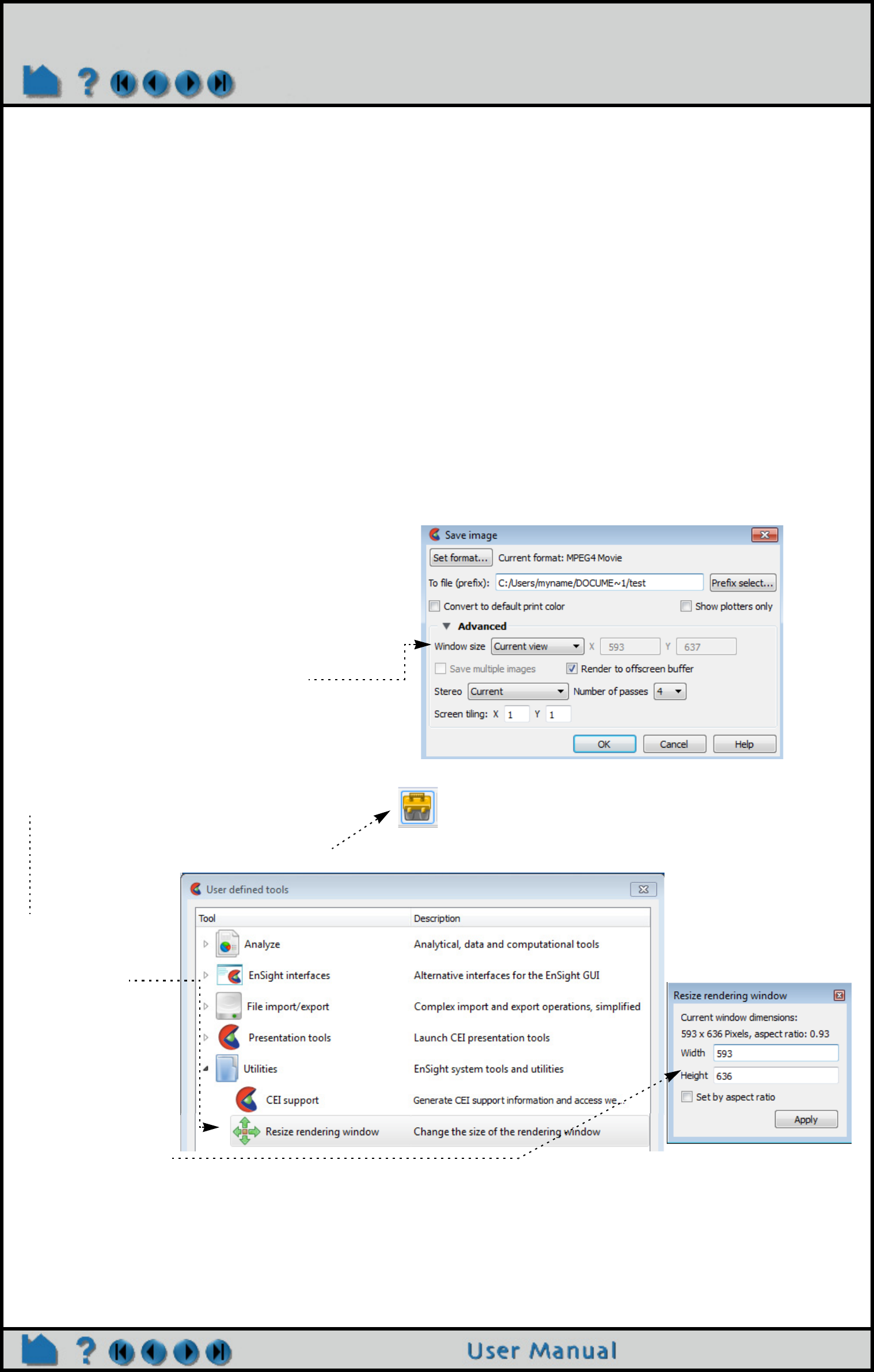
Page 214
HOW TO USE BATCH
Advanced Concepts
Image Size
There are two resolutions you need to keep in mind when setting up a batch run of EnSight. First is the window size
when you are running EnSight. Second is the size of any images that you save. In order for the images saved in
your batch run to capture the same imagery it is important that the image be the same aspect ratio (width vs. height)
as the image generated when you created the command file interactively in EnSight. Lacking the same aspect ratio
it is possible that the images saved in batch mode may cut off some portion of your scene.
When saving an image in EnSight you can specify the “Window Size”. If this is set to “Current View” the image will be
saved at the current resolution of the graphics window. By default, the “current” window size when you execute in
batch mode is 1280x720 (width x height). The “current” window size when you execute EnSight interactively is
variable, i.e., the window can be resized. See below for instructions on determining the current window size and
aspect ratio. The “current” window size in batch can be specified by setting the size on the start line such as:
ensight102 -batch 1024 768 -p file.enc
It it much better to save images by specifying the resolution of the images, i.e., either setting the “Window Size” to a
user defined size or using one of the predetermined resolutions such as “HD 1080p”. This prevents the issue of
trying to match the window size and forcing the user to both (a) know the resolution, and (b) specify it on the start line.
If you set “Window size” to Current view you
must specify the resolution when you start
EnSight in batch mode if you are going to
match the images you saved interactively.
The resolution is not required to be the
same, but keeping the aspect ratio is
important. It is better to save images using
an option other than Current view.
If you wish to know what the current
resolution and aspect ratio you can pull up a
user defined tool as follows:
To precisely control the graphics screen
size during your interactive session,
1. Click on the tool box icon at the top,
2. Open the
utilities folder, and
double click on
the Resize
rendering window
tool,
3. Adjust or note
the window size
and aspect ratio.

Page 215
HOW TO USE BATCH
Python
EnSight can also run EnSight Python scripts in batch exactly the same as command files.
ensight102 -p file.py
EnSight Python has all of the advantages of the Python programming language (variables, looping, if/then, and a
number of python modules) as well as the capabilities of the EnSight journaling language in the ensight Python
module.
For example, instead of editing five command files, which are custom edited for each solution dataset, you can create
a single EnSight python file which loops through a list of the dataset filenames and executes the desired commands
and auto creates the output image and animations.
LIMITATIONS
EnSight cannot be run in batch mode using context files (.ctx). Batch mode can only be run using command files
(.enc) or EnSight Python files (.py). However, a command file may restore a context file.
SEE ALSO
Record and Play Command Files
Python EnSight module interface
Command Line Start-up Options

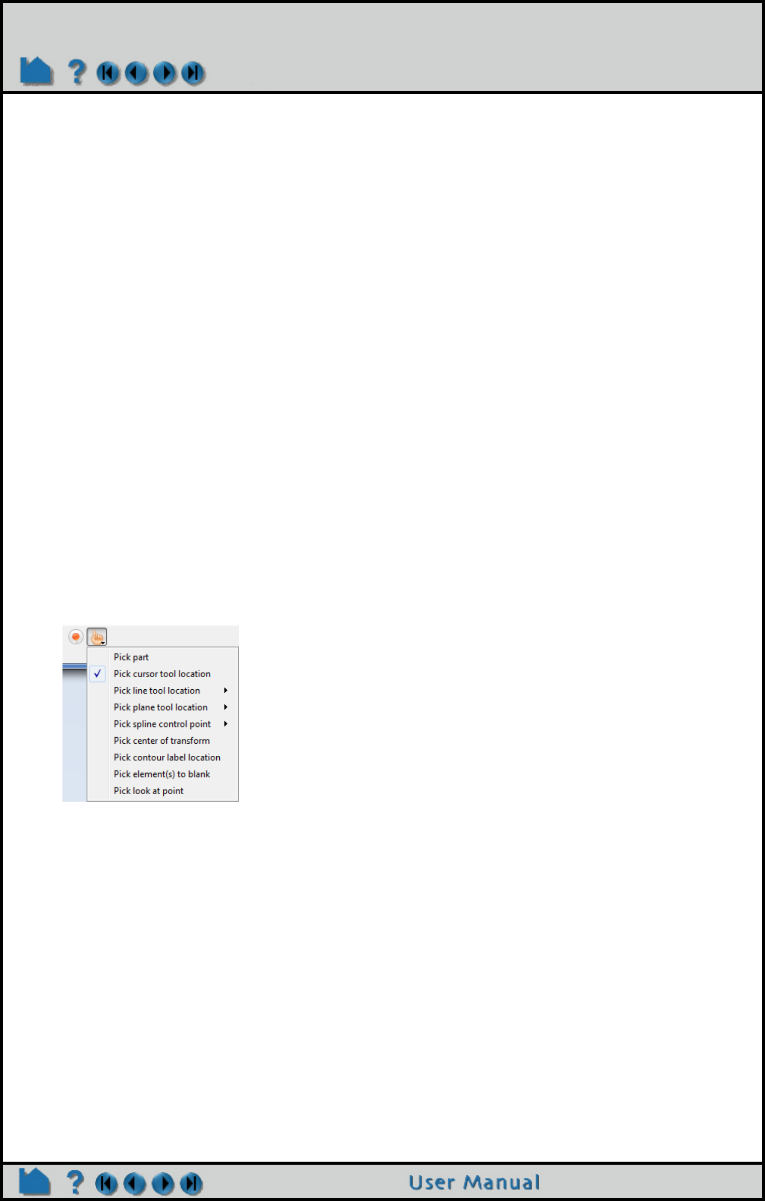
Page 217
HOW TO USE KEYBOARD SHORTCUTS
Use Keyboard Shortcuts
INTRODUCTION
EnSight has a number of keyboard shortcuts that are documented in the User Manual and in this Manual. But they
are scattered all over the Manuals. This is a consolidation of all the commands in one reference location. Note below
that the alphanumeric keys are capitalized for emphasis, but that the actual key is the lower case key. You do not
need to press the shift key when it says ‘P’. Simply press the ‘p’ key.
BASIC OPERATION
Macros (default - can be edited by users)
Advanced users of EnSight often find themselves performing repetitive tasks. EnSight’s macro facility lets you save a
sequence of commands and then assign a keyboard key to those commands such that they are executed when the
key is pressed. Macros are useful in full screen mode. Note: macros only work when the mouse cursor is in the
graphics window. (see How to Define and Use Macros).
V - toggle selected part visibility
S - toggle global part highlighting
Contextual keyboard keys
A - Press the ‘a’ key to cancel saving an animation (“abort”)
P - The pick key. Manually change what you are picking using the pick mode pulldown. The default is to pick a part.
Simply hover over a part and press the ‘p’ key and the part will be selected. Or, choose another pick mode. Change
the mode to Pick cursor tool location, and move the mouse over a location on a part and press the ‘p’ key and the
cursor will appear at that location on the part.
When Interactive Probe Query is set to ‘Surface pick’, the ‘p’ key will override the selected pick mode and will place
the query probe on the surface of a part. If Interactive Probe Query is not set to ‘Surface pick’ then the ‘p’ key will use
the pick mode.
Part tagging
Use this shortcut to quickly select parts. See the Advanced section of How to Select Parts
Alt-# (where # is any number from 0-9) - tag selected parts
Ctrl-# - select parts tagged with this number
Keyboard Ctrl-Mouse combinations
For the mac, these use the command button.
Ctrl-Left button - Rotation about the screen Z-axis
Ctrl-Middle click (or Right+Left buttons) - Zoom

Page 218
HOW TO USE KEYBOARD SHORTCUTS
Ctrl-Right button - Pan
Changing the view
See How to Rotate, Zoom, Translate, Scale for details on these shortcuts.
F1 - Rotate about screen X-axis by 45 degrees
F2 - Rotate about screen Y-axis by 45 degrees
F3 - Rotate about screen Z-axis by 45 degrees
Ctrl-F1/F2/F3 - Rotates -45 degrees
F4 - Spin the graphics window - with mouse motion
F5 - Front view
F6 - Side view
F7 - Top view
F8 - Return to previous view before F5/F6/F7 was pressed
F9 - Full screen (F9 or Esc to go back)
Ctrl-F5/F6/F7 - Save current view to this key
3D stereo commands
If you have a stereo graphics card and are running EnSight in stereo mode, there are some function key shortcuts
that are helpful. For more information see How to Enable Stereo Viewing.
F10 - Increase stereo separation angle
F11 - Decrease stereo separation angle
F12 - Toggle 3D stereo on/off
Ctrl-F12 - Swap 3D stereo left/right eyes
Menu Shortcuts (seen in top menu)
You can see this shortcuts in the menu drop downs. For example, see the File>Save menu has a Ctrl-S beside the
command, showing the shortcut. Some of the more useful menu short cuts are as follows.
Ctrl-O - Open results dialog
Ctrl-P - Print image dialog
Ctrl-Q - Quit EnSight
Ctrl-S - Save Session file
Ctrl-Shift-S - Save commands from this session
Ctrl-C - Copy image to clipboard
Ctrl-F - Open the Feature Edit Dialog

Page 219
HOW TO USE RIGID BODY MOTION
Use Rigid Body Motion
INTRODUCTION
If the geometry is not static then it must be updated every timestep. EnSight geometry can be updated either by
updating the entire geometry (the coordinates and the connectivity) every timestep, OR by updating only the
coordinates (connectivity is unchanged) every timestep. For either type of geometry, updating it every timestep by
reading the data from disk is time consuming. However, if the motion of the geometry can be characterized as rigid
body motion (where a single rotational axis, a single rotational angle, and a single translation describe the motion of
the entire part, with no connectivity changes) then the entire update of the coordinates can occur using CPU and
memory, which can be orders of magnitude faster than reading the coordinate updates from disk. Further, since the
orientation and location of every point on the geometry is an equation that is a function of time, the delta time
resolution can be as fine as needed for detailed calculations or as coarse as allowed for visualization.
EnSight implements rigid body motion on the EnSight Server on a per part basis in both Case Gold format and using
the EnSight User Defined Reader API. When rigid body motion is applied to a part, the part is then considered
transient geometry with it’s own timeline. Case Gold implements rigid body through two rigid body files, one of which
is referenced directly and the other indirectly from the .case file. For formats that have a custom reader, the User
Defined Reader API has it’s own routines for informing the Server and supplying the rigid body parameters. The
implementation and the use will be discussed below.
DETAILS
Case Gold
EnSight Case Gold uses two files for the rigid body implementation. The EnSight Case Gold file references a file
called the EnSight Rigid Body Rotation File (.erb) that contains per-part scaling, offsets, initial rotation as well as the
Euler Parameter file (.eet) filename (see EnSight Rigid Body File Format for details and for examples). The Euler
Parameter file contains center of gravity transformations as well as Euler parameters which fully describe the Euler
Rotation and Translation rigid body motion (see Euler Parameter File Format for details and for an examples).
Basically, at each timestep, each part is first translated then rotated using the offset and initial rotations found in the
EnSight Rigid Body File, then it is rotated according to the Euler angles about the Euler axis and finally it is translated
according to the translation parameters.
User Defined Reader
If the part by part rigid body transformation data exists within your solver data file, then simply read it in and supply
them to the appropriate EnSight user defined routines (see Quick Index of 2.0 Library Routines).
USERD_rigidbody_existence - Turns on the rigid body feature
USERD_rigidbody_values - Called part by part to get the initial translation and rotation parameters, as well as the
Euler rotation parameters and the final translation values. It is expected that these values are available from the
solver data file or that they can be calculated in the reader from the rigid body transforms found in the solver data file.
USAGE
Conversion
If your rigid body parameters do not match our Euler implementation then you will need to convert your format. This
can be done by converting your data files to our EnSight Rigid Body File format and our Euler Parameter File format
if you are using Case Gold. Or it can occur inside your reader if you are using a custom reader.
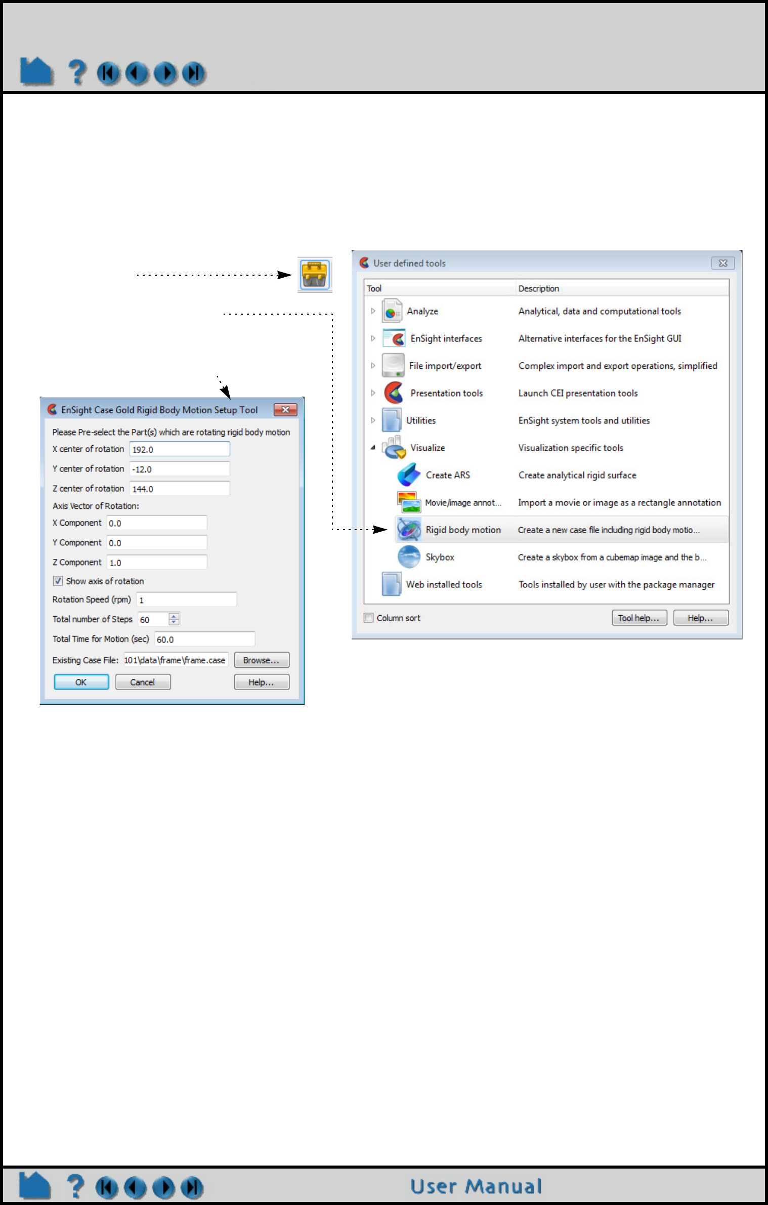
Page 220
HOW TO USE RIGID BODY MOTION
Example Rigid Body Tool
Use the EnSight Rigid body motion tool if you have data in the form of a Case Gold file and part(s) undergoing simple
rigid body rotational motion and/or you need an example of the EnSight Rigid Body File (.erb) and Euler Parameter
File (.eet) formats. This tool prompts you for rotational input values and will create the two rigid body motion files (.erb
and .eet), and a new case file by adding the .erb and .eet filenames to the case file. It then reloads your model using
this new case file to demonstrate the rigid body motion.
EXAMPLE IMPLEMENTATIONS
STL & OP2
Both the EnSight STL and Nastran OP2 formats, in addition to reading the native formats directly (.stl and .op2,
respectively), each include the ability to read a customized variant case file that contains a list of native format files
and the associated EnSight Euler format filename. The STL reader calls this an exec file (.xct), see the STL Reader
section for details. The Nastran OP2 calls this case file a MOP file (.mop). This "executive file" (.stl or .mop) allows
either reader to handle multiple native files simultaneously, as well as optionally allowing them to be transformed by
one or more rigid body Euler files. Note that the rigid body transformations in the Euler file must be created outside
the STL format, and outside of the Nastran solver.
Abaqus ODB analytical rigid surfaces
Abaqus has a concept of rigid surfaces that do not have elements and are modeled only analytically as extruded or
rotated surfaces (plates or cylinders) that move as rigid, non deformable bodies over time according to
transformations in the .odb data file. The Abaqus ODB reader creates these rigid entities first as lines using EnSight
line elements in the User Defined Reader API (which can be extruded in a separate operation in EnSight into
surfaces). These lines will translate and rotate according to the parameters in the odb file. The user can then
manually use the EnSight Extrude option or can use a python tool included with EnSight to properly extrude these
line parts into cylindrical or planar surfaces according to their design (for details, see the ABAQUS reader section).
Fluent and Star Export Case Gold
For data with part(s) rotating at a steady state, both Fluent and Star export this data as a steady state geometry with
an assigned rotational rate value. Their native postprocessors, which are aware of this, can then reproduce the
transient orientation of the fan at any given time. A pseudo transient state is created from steady state files. This
1. Click on the Tool icon at the top of the
EnSight Tools
2. In the Visualize folder, double click
the Rigid body motion tool.
3. Fill in the GUI, taking special note that
the speed is in rotations per minute and
the time is in seconds.
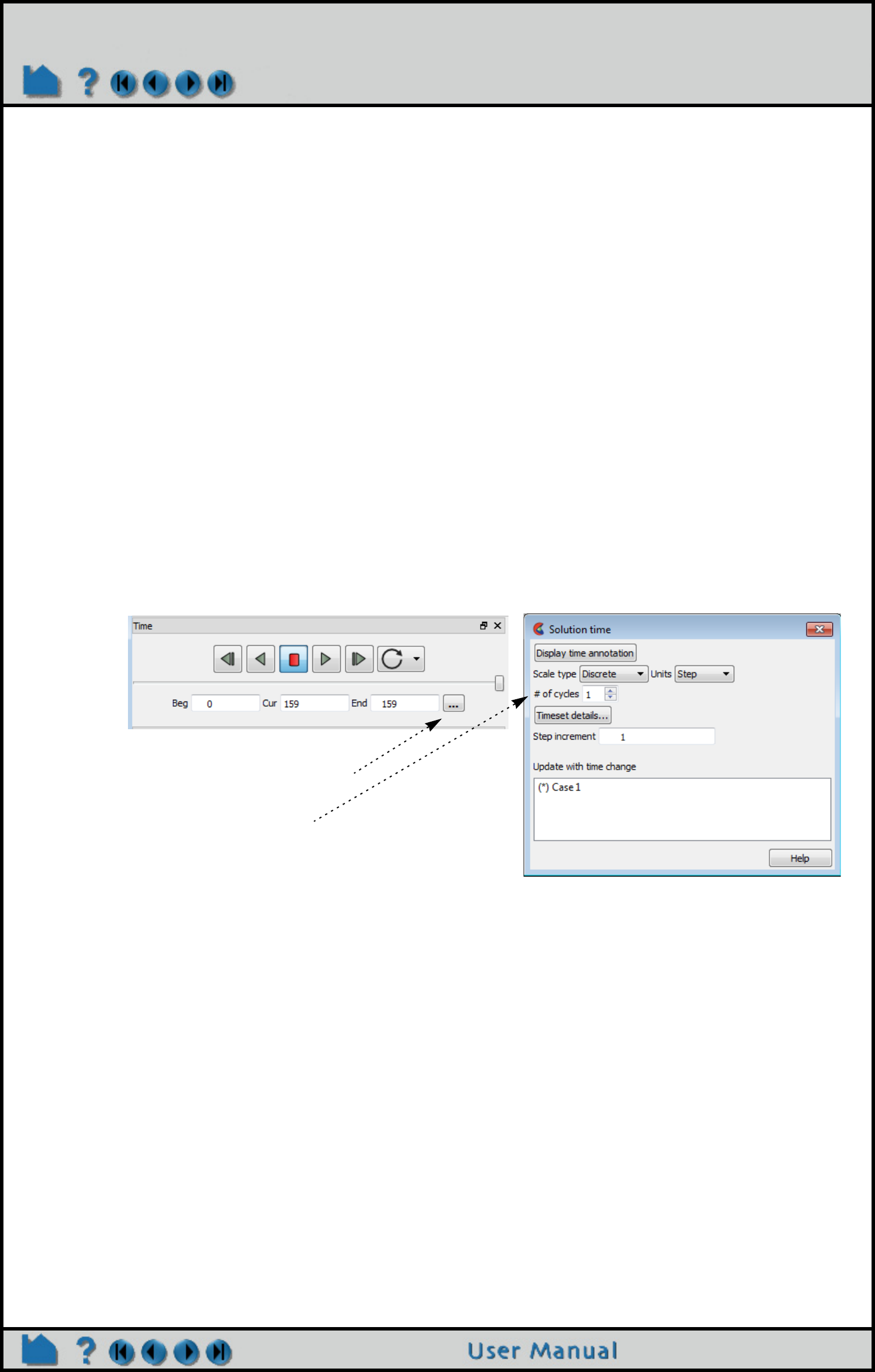
Page 221
HOW TO USE RIGID BODY MOTION
allows the geometry to be written out only once, but the transient orientation of the fan can be reproduced at any
arbitrary level of fineness of time in the native post-processor.
Unfortunately, when users export their data from the solver into EnSight Case Gold, this native awareness is lost. The
pseudo transient state does not exist to update the fan's transient orientation in time. Thus you can have effects like
streamline traces which impact the non-moving fan and just stop. Some effort is required to reproduce the effects of
the native solver postprocessor in this case. Basically, rigid body can be used. EnSight Rigid Body and Euler
Parameter files must be created and referenced in an updated Case Gold file, and the pathline trace option should be
used instead of streamline traces.
If your solution has been solved in an implicitly rotating reference frame, and you want to either visualize the motion,
or correctly produce particle traces through the domain, then you will need to utilize both EnSight Case Gold Format
files, as well as utilizing the Rigid Body Tool (Click on the toolbox icon at the top and open Visualize -- > Rigid Body
Motion). This will generate both of the two rigid body files as well as modify the case file to reference the new
information. Two critical decisions you must make when running the tool are a) number of steps, and b) total time to
rotate. The number of steps chosen should be small enough to reflect the courant number of the grid + velocity so
that the change between timesteps maintains reasonable changes in grid location and velocity values so that
continuous pathline integration is numerically accurate. Choosing too small of a timestep will slow the calculation and
animation time, while too large of a timestep will result in errors in pathline calculation. Models with either higher
rotational speeds, finer grids, or higher velocity regions should be setup with small timesteps. The Total Time should
be chosen so that you have rotated one repeatable sector, given the rotational speed (fixed, and specified), and the
number of steps.
Since the rotation is cyclical, only one repeatable increment in fan rotation is necessary, and then EnSight can
cyclically repeat that increment N number of times as below, to allow the relatively low speed upstream flow sufficient
number of fan blade cycles to reach to the relatively high speed fan blade and pass through successfully..
VARIABLES
Vector variables are rotated and translated with the geometry through time using the rigid body transformations.
There can be an exception to this rule for vector variables created in the EnSight calculator which are based purely
on scalar variables with no geometric influence. Known predefined functions in the calculator with this attribute, such
as MakeVect, are actually handled correctly. But if a user defines his own vector using the match capabilities of the
calculator, it may not be transformed.
PERIODICITY AND RIGID BODY MOTION COMBINED
When a model part is originally loaded, any rigid body transforms defined for that part’s geometry are applied. When
a model vector variable is first activated, the appropriate vector transforms for periodicity, and rigid body, are applied.
When periodicity is first turned on, the new instances get their geometry and vector variables transformed at that
time.
Commonly, neither or only one of these types of transformations will be defined and used in a model at the same
time. When that is the case, there is no issue with the order that the transformations are applied in EnSight.
However, when both types of transformations (periodic and rigid body) are defined, the order they are applied
becomes important. There is an example of such below.
To repeat a time series for N cycles:
1. Click on the more button on the time
controls
2. Change the number of cycles

Page 222
HOW TO USE RIGID BODY MOTION
The default order of application is periodic then rigid body - which is good for when rigid body is used to move any or
all of the parts throughout time.
If one instead needs to have a rigidbody then periodic order - which is good for when rigidbody is used to assemble a
model from different orientations or coordinate systems, then you can specify the order via one of the following
methods.
Case Gold
Simply add the “do_first” designator to the end of the rigid_body line in the GEOMETRY section of the casefile as
follows (See EnSight Gold Casefile Format ).
FORMAT
type: ensight gold
GEOMETRY
model: rbv.geo
rigid_body: rbv.erb do_first
. . .
User Defined Reader
For other readers then simply set the environment variable ENSIGHT_DO_RB_FIRST . On Linux,
setenv ENSIGHT_DO_RB_FIRST 1
Note, that the order specified will be honored when time is changed and the model geometry and vector variables are
updated. Namely, for default (periodic then rigidbody) order:
1st Any changing geometry will be loaded from the file or reader.
2nd Any model variables will be loaded from the files or reader.
3rd The periodic transformations will be applied to model geometry and model vector vars.
4th The rigidbody transformations will be applied to model geometry and vector variables.
5th Created parts and created variables will be recreated according to the dependency tree.
If you explicitly specify the rigidbody to be first, by one of the methods described above, the process is the same -
except that the 3rd and 4th steps are reversed.
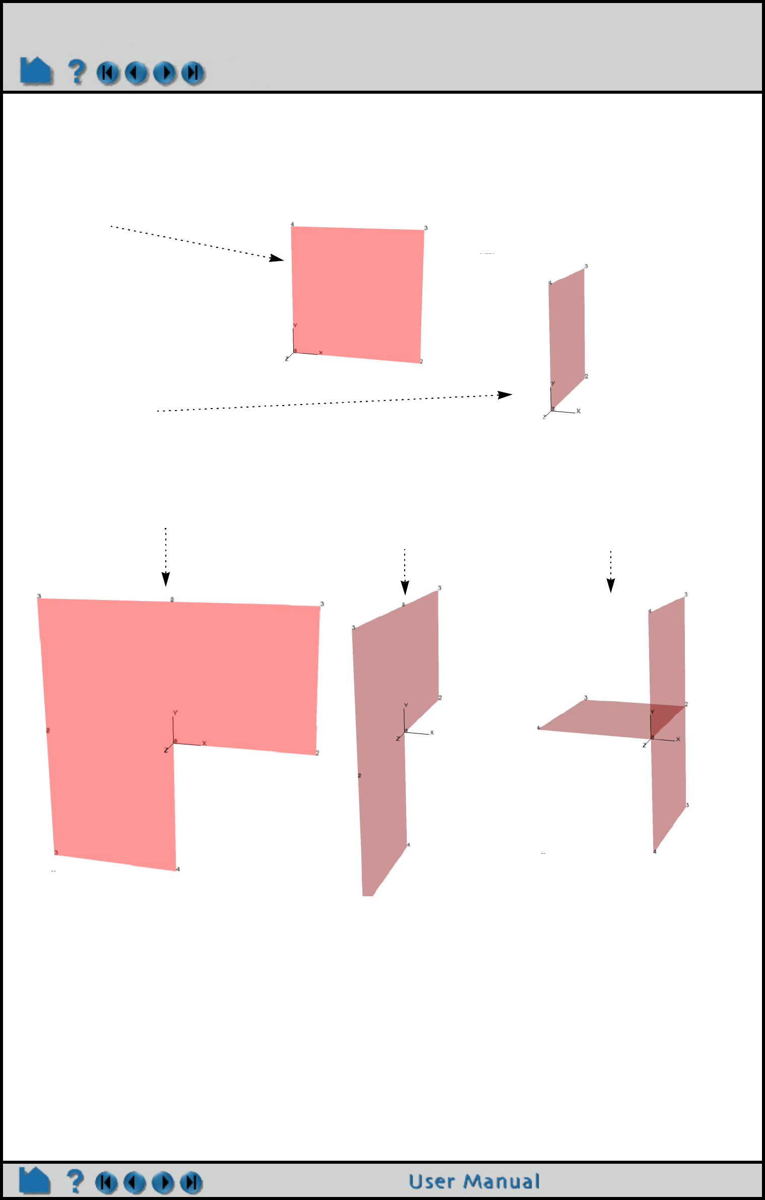
Page 223
HOW TO USE RIGID BODY MOTION
Illustration
Given a square in the xy plane as shown below, with a rigid body transformation defined as 90 degree rotation about
the y axis. And a periodic transform defined as 90 degree rotation about the z axis (3 instances):
ADVANCED
If you have static geometry that moves in a rigid body fashion, then rigid body motion will greatly speed up
the updating of the geometry. It has not yet been mentioned, but if you have transient geometry, you can also
implement EnSight rigid body motion. You will lose the speed-up because the transient geometry still needs
to update coordinates and/or connectivity using disk reads, but this is still possible.
SEE ALSO
1. Shown is the initial square
geometry.
2. Shown is the geometry with only
the rigid body transformation
described above.
3. Shown below is the geometry with only
the periodic transformation applied. 4. Shown below is the
geometry with periodic then
rigid body (default order).
5. Shown below is the
geometry with rigid body first,
then periodic.
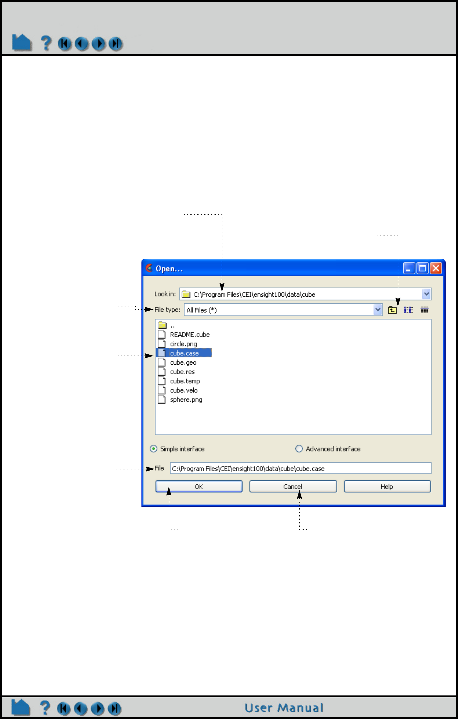
Page 224
HOW TO SELECT FILES
Select Files
INTRODUCTION
Many operations in EnSight (such as loading data) require that you specify a file. EnSight uses a standard file open
dialog that lets you quickly search through directories to find the desired file.
BASIC OPERATION
By default, the File Open dialog opens with the directory from which the EnSight client was started as the current
directory.
The following shows the basic components of the File Open dialog:
The File type pulldown controls
the listing of files in the Files list.
You can filter what is shown
based on the selection here
The Look in pulldown displays the current directory.
Note that the parent of the current directory is shown
ending with “..” (standard UNIX nomenclature).
To change to a directory, double-click it.
The File field contains the full
path name of the file currently
selected in the Files list. This is
the file that will be chosen if OK is
clicked.
Change the selection either by
clicking a file in the Files list or
editing the field directly.
Pressing return will accept the
Selection and close the dialog.
The Files list displays the list of
subdirectories and files contained
in the current directory (possibly
modified by the wildcard in the
File type filter field).
To make a file the current
Selection, click it.
To accept a file and close the
dialog, double-click it.
Click to accept the current
Selection and close the dialog. Click to cancel the selection and
close the dialog.
Standard up, and listing icons
can be used.
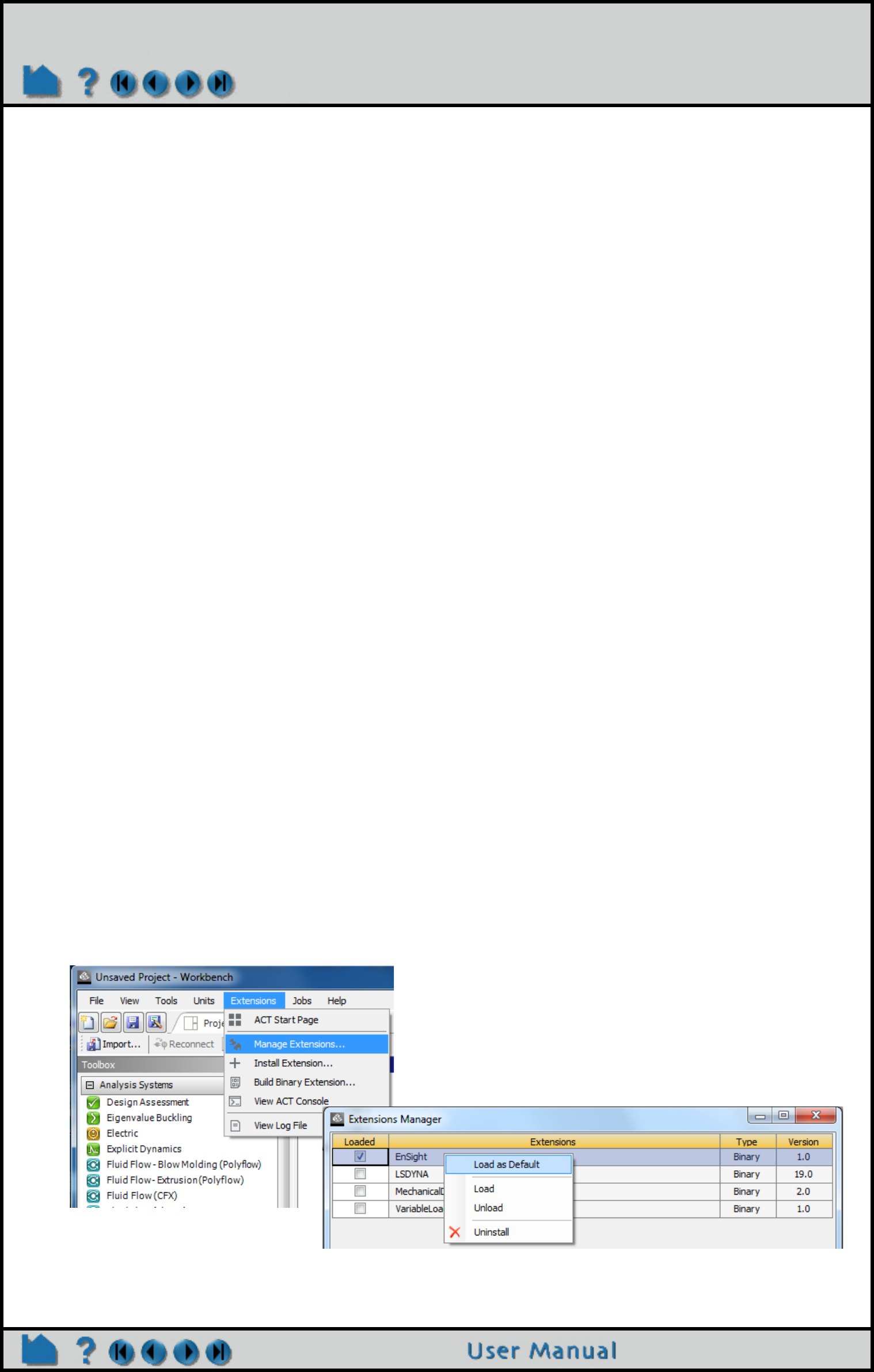
Page 225
HOW TO USE ENSIGHT WITH WORKBENCH
Use EnSight with Workbench
INTRODUCTION
EnSight can be run as a stand-alone application, or as a component from within ANSYS Workbench. This document
describes the use of EnSight from within the WorkBench environment. It covers activating the EnSight WorkBench
Extension, linking EnSight to WorkBench solutions and using EnSight to open the WorkBench solution. This
document assumes that Ansys Workbench has been installed on your Windows or Linux machine and that you wish
to use EnSight within this framework. It does not attempt to teach WorkBench, nor EnSight usage.
Quick Startup
Simple Example EnSight Session within ANSYS Workbench
Detailed view of the EnSight ANSYS Workbench Interface
File locations within WorkBench
EnSight Differences within ANSYS WorkBench
EnSight Limitations within ANSYS WorkBench
Advanced Usage: Design Point Session Using EnSight
QUICK STARTUP
Launch WorkBench
To launch ANSYS Workbench on Windows, click the Start menu, then select
All Programs > ANSYS 19.0 > Workbench 19.0
.
To launch ANSYS Workbench on Linux, open a command line interface, type the path to “runwb2” (for
example, “/ansys_inc/v190/Framework/bin/Linux64/runwb2”), then press Enter.
The ANSYS Workbench interface has a Toolbox list on the left side to make it easy to choose the tool set that will
enable you to solve particular types of problems. Tools are chosen from the Toolbox list and dragged onto the Project
Schematic in order to use them. Tools are then linked together in a workflow to accomplish tasks. Supporting features
such as Properties and Messages provide orienting information. These features and the status indicators in the
system cells guide you through the completion of your workflow. In order to see EnSight in the Toolbox, the EnSight
WorkBench extension must be activated.
Activating EnSight as a WorkBench Extension
If the EnSight extension is not in the list of Component Systems in the Toolbox Workspace, choose, from the
WorkBench top menu, Extensions>Manage Extensions... which will pop up the Extensions Manager dialog
(see below). Toggle on the EnSight Extension, and then right click on EnSight and choose Load as Default
(as shown below). This will load the EnSight application extension when you start up WorkBench in the future.
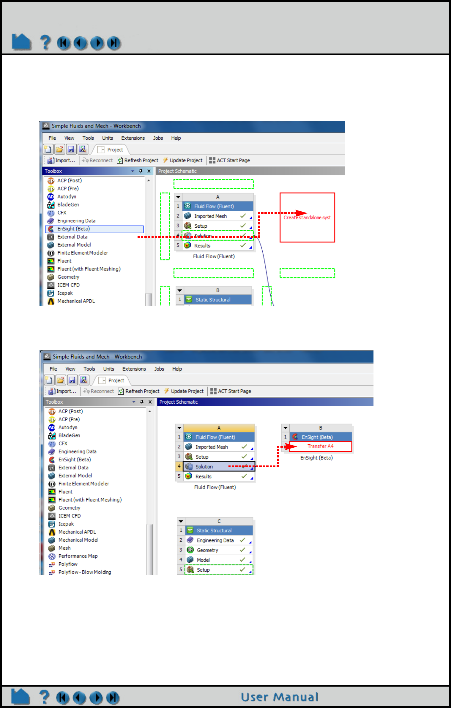
Page 226
HOW TO USE ENSIGHT WITH WORKBENCH
Linking EnSight to WorkBench solutions
To link the EnSight Extension to a solution result, drag the EnSight extension from the Component Systems list onto
the Project Schematic. A red, square landing pad will appear in the WorkBench Project Schematic space to give you
guidance.
Now drag the Solution onto the Results under EnSight to link the Solver Solution to EnSight’s Results. Once the link
is created, right click on the EnSight Results and choose Update.

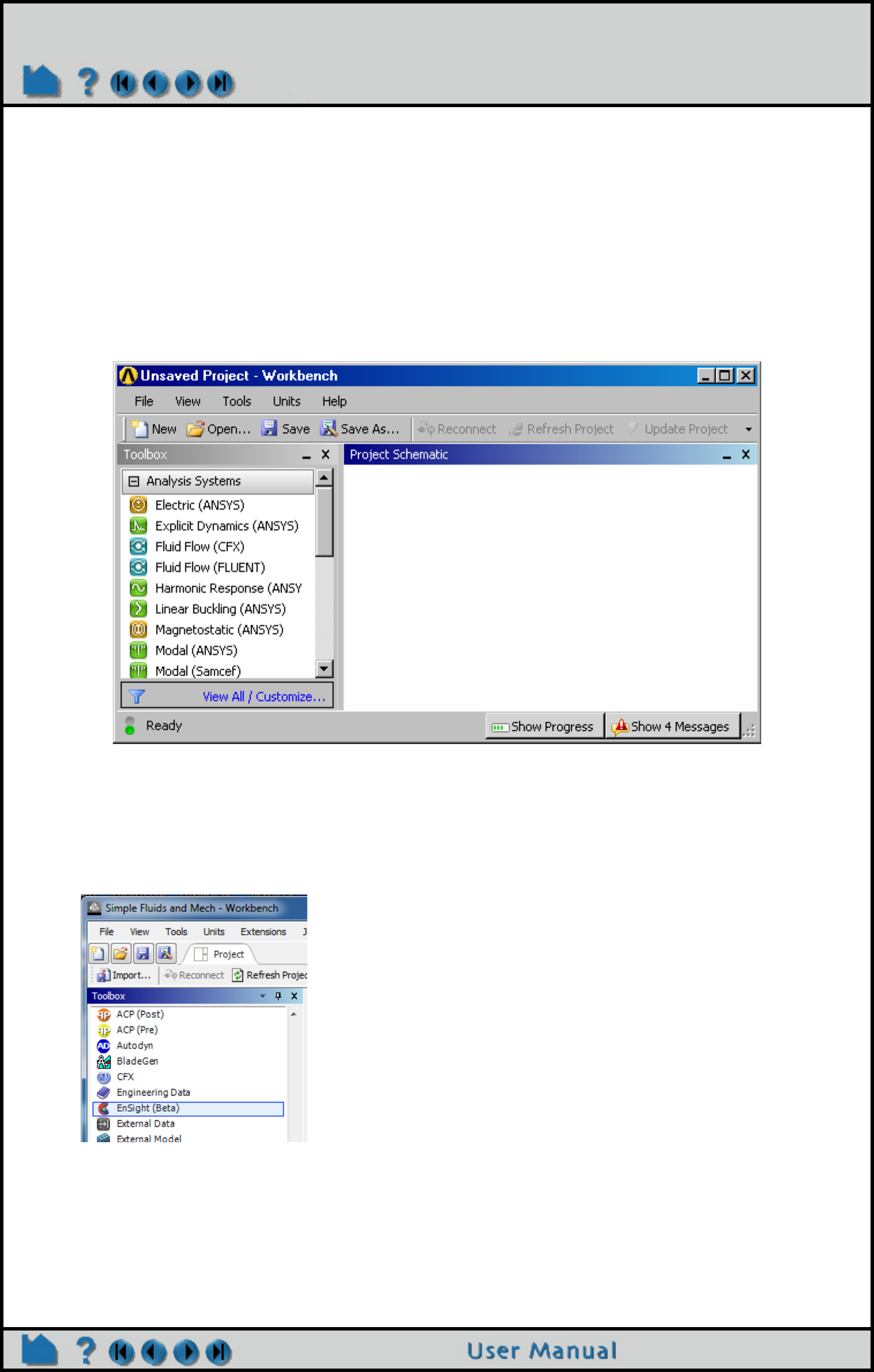
Page 228
HOW TO USE ENSIGHT WITH WORKBENCH
SIMPLE EXAMPLE ENSIGHT SESSION WITHIN ANSYS WORKBENCH
This walkthrough loads a simple, sample ANSYS Workbench analysis (creating the analysis is beyond the scope of
this document) and then adds the ANSYS EnSight extension and attaches the mechanical and fluid analysis
workflow to EnSight and then opens the solutions using EnSight.
This example uses the EnSight FLUENT Direct Reader to load the Fluent fluid flow analysis and the EnSight
ANSYS Reader to load the Ansys Mechanical analysis results, in order to demonstrate, step by step, an EnSight
WorkBench workflow using multiple, simultaneous, heterogeneous solutions.
1. Now, Launch WorkBench, then open a project containing both fluid and structural solutions.
2. If you have not already done this, Activating EnSight as a WorkBench Extension must be done here so that you
can see EnSight in the Toolbox. Then, restart WorkBench.
3. Upon restarting WorkBench, you should see the EnSight extension under the Component Systems pulldown in
the Toolbox Workspace on the left side.
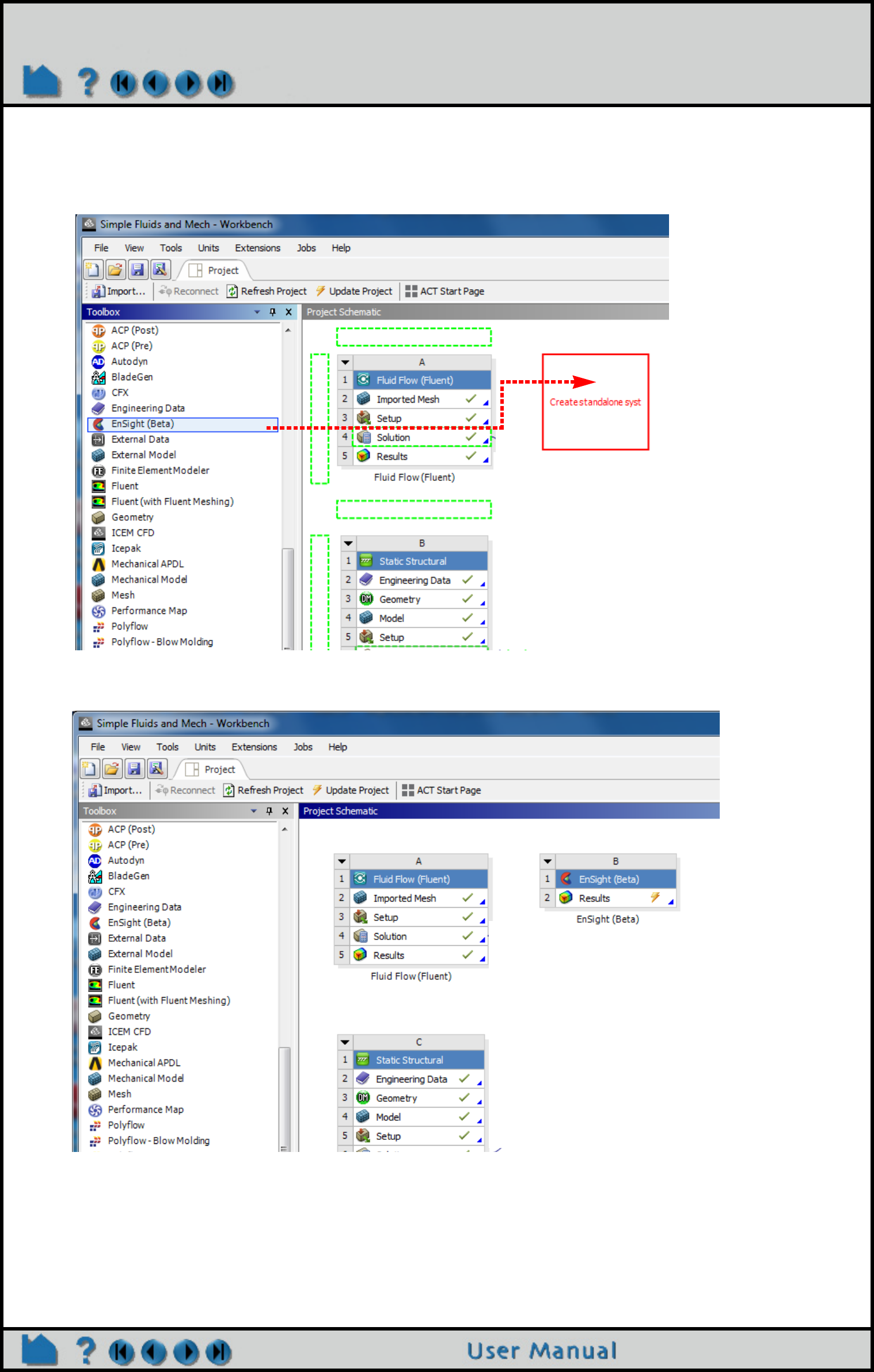
Page 229
HOW TO USE ENSIGHT WITH WORKBENCH
4. Load the WorkBench project using File>Open. Now drag the EnSight extension from the Component Systems
list onto the Project Schematic. A red, square landing pad will appear in the WorkBench Project Schematic space to
give you guidance.
5. Now an EnSight system is established in your Project Schematic and ready to be linked up.
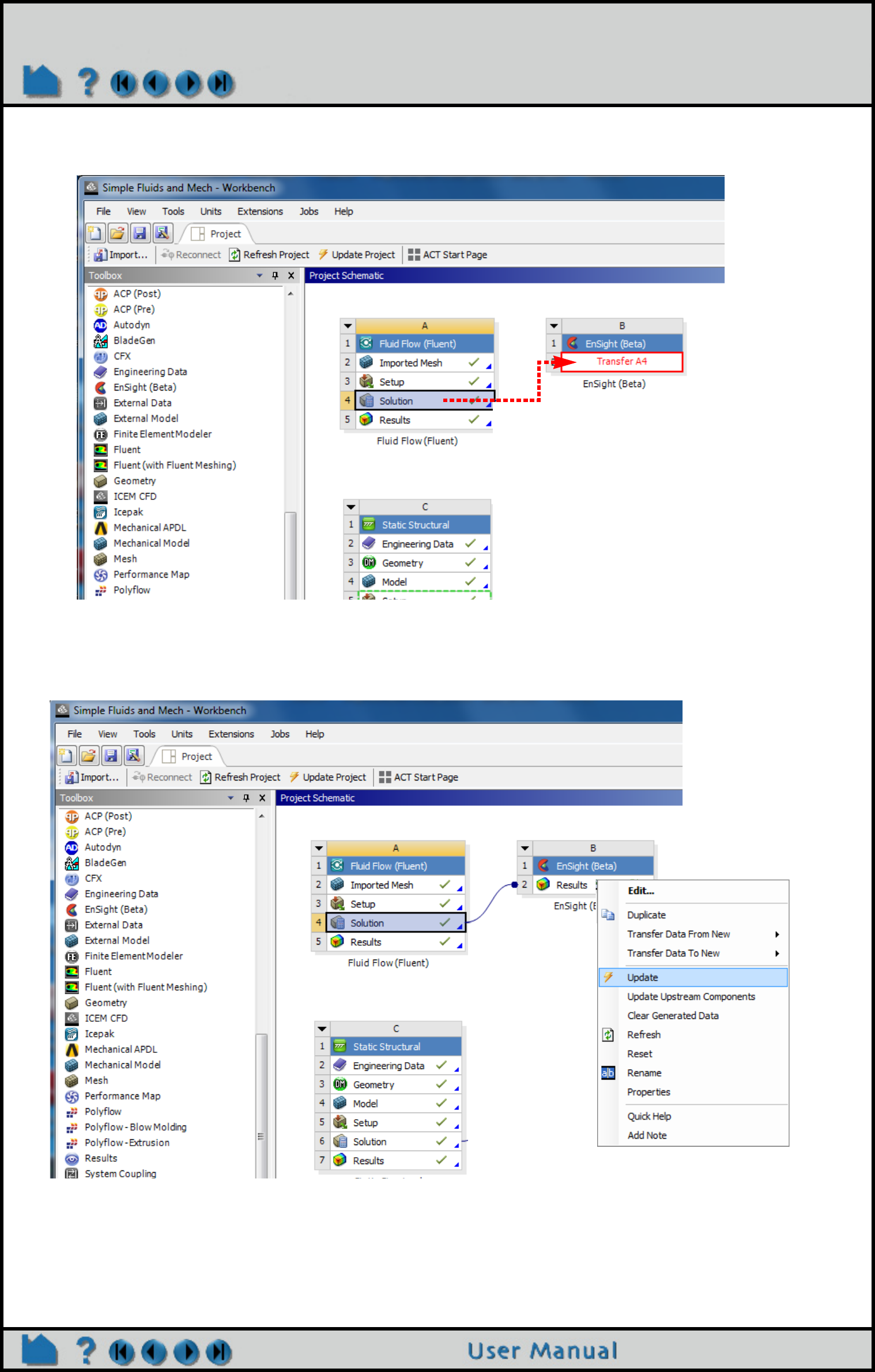
Page 230
HOW TO USE ENSIGHT WITH WORKBENCH
6. Now drag the Fluid Flow Solution on to the Results under EnSight to link the Solver output to EnSight’s input.
7. Now, EnSight is linked to the solution. Right click on the green arrows in the EnSight Results to update the link.
Important: Any time your result has the double arrows, then it needs to be updated. A check box means your
results are current. Updating EnSight Results prepares the data to be loaded.
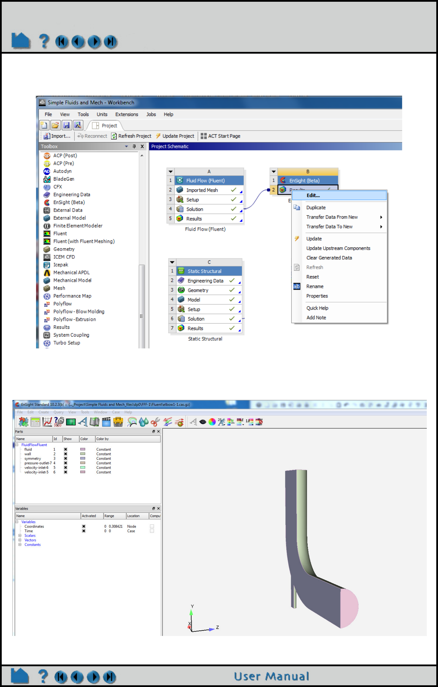
Page 231
HOW TO USE ENSIGHT WITH WORKBENCH
8. The EnSight results will show a check box when they are properly updated. Now double-click on the EnSight
Results or Right-click > Edit... which will startup EnSight and load the Solver Solution for interactive use.
9. The EnSight session will start up with only the Fluent solution loaded as shown below. Note that only the Fluent
results were linked up to EnSight, so only the Fluent results are loaded. This portion of the manual assumes that you
know how to use EnSight from here. If not, from the top menu of EnSight, Help> Getting Started Manual.
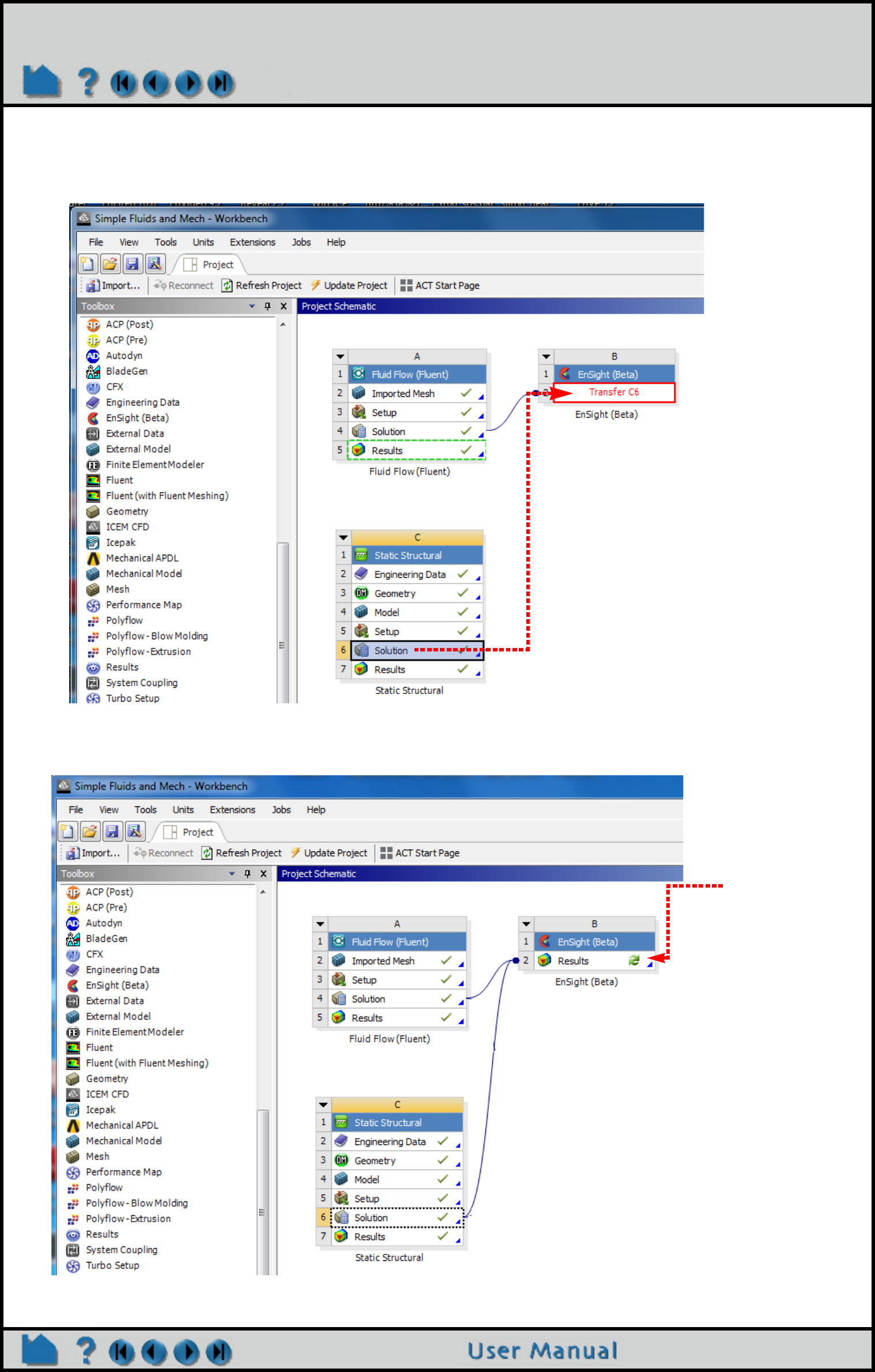
Page 232
HOW TO USE ENSIGHT WITH WORKBENCH
10. Within EnSight’s menu, File>Quit to exit EnSight. Now, back in the WorkBench environment, in the Project
Schematic area, let’s also add the structural solution to the EnSight process. Drag the structural solution onto the
EnSight results section as shown below.
11. Note that you now have two links into the EnSight results section, as shown below but EnSight’s Results show the
double arrow indicating they need to be updated.
Double arrows
indicate that this
needs updating
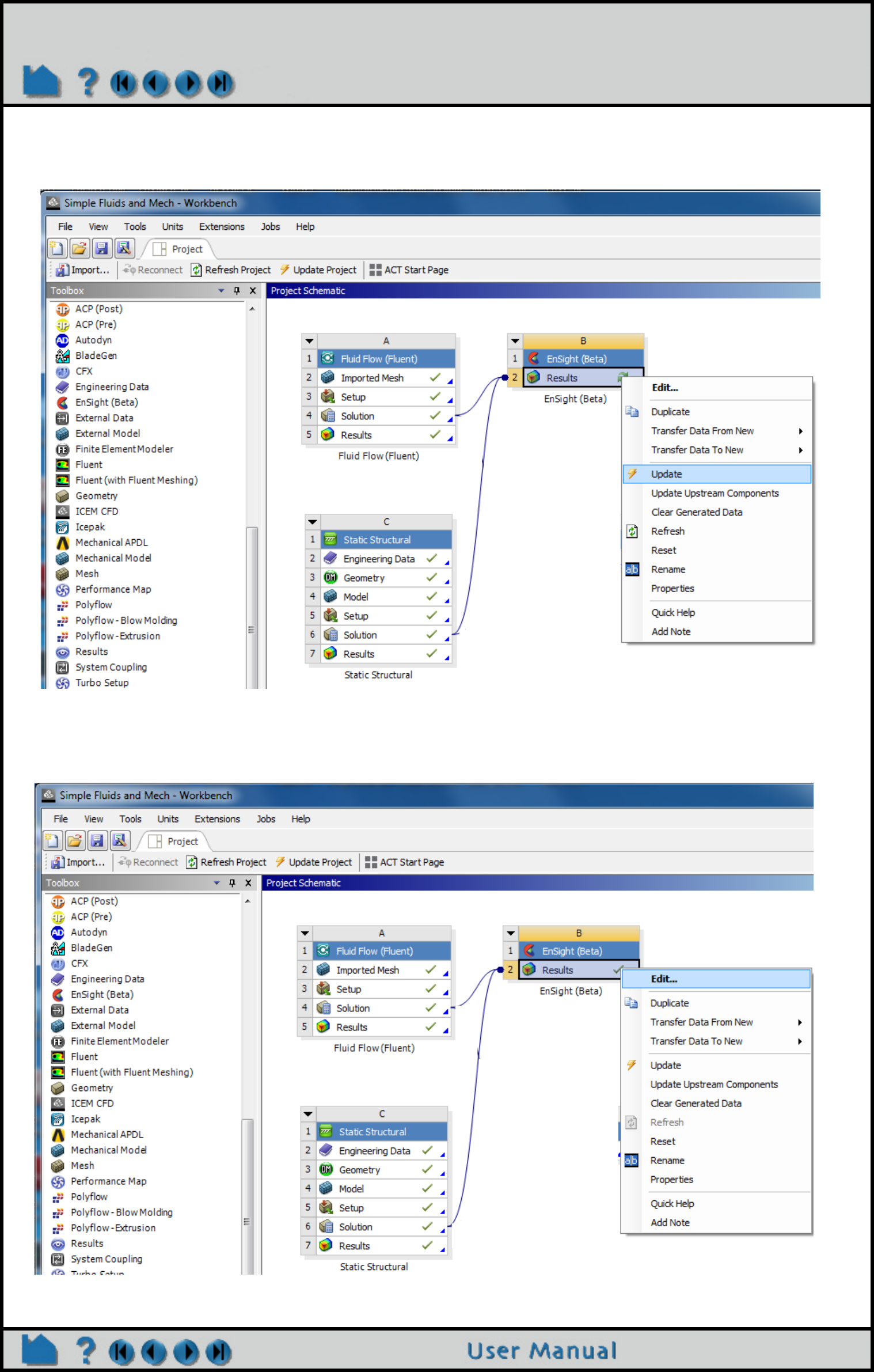
Page 233
HOW TO USE ENSIGHT WITH WORKBENCH
12. Now, with the new link, again, notice that there is no longer a check box on the EnSight results. We need to
update the EnSight results. On the EnSight Results, Right-click > Update.
13. Now let’s open EnSight and load the Fluid Solution and the Structural Solution. Right-click > Edit or
double-click on the EnSight Results section as shown below to start up EnSight and load the solution data:
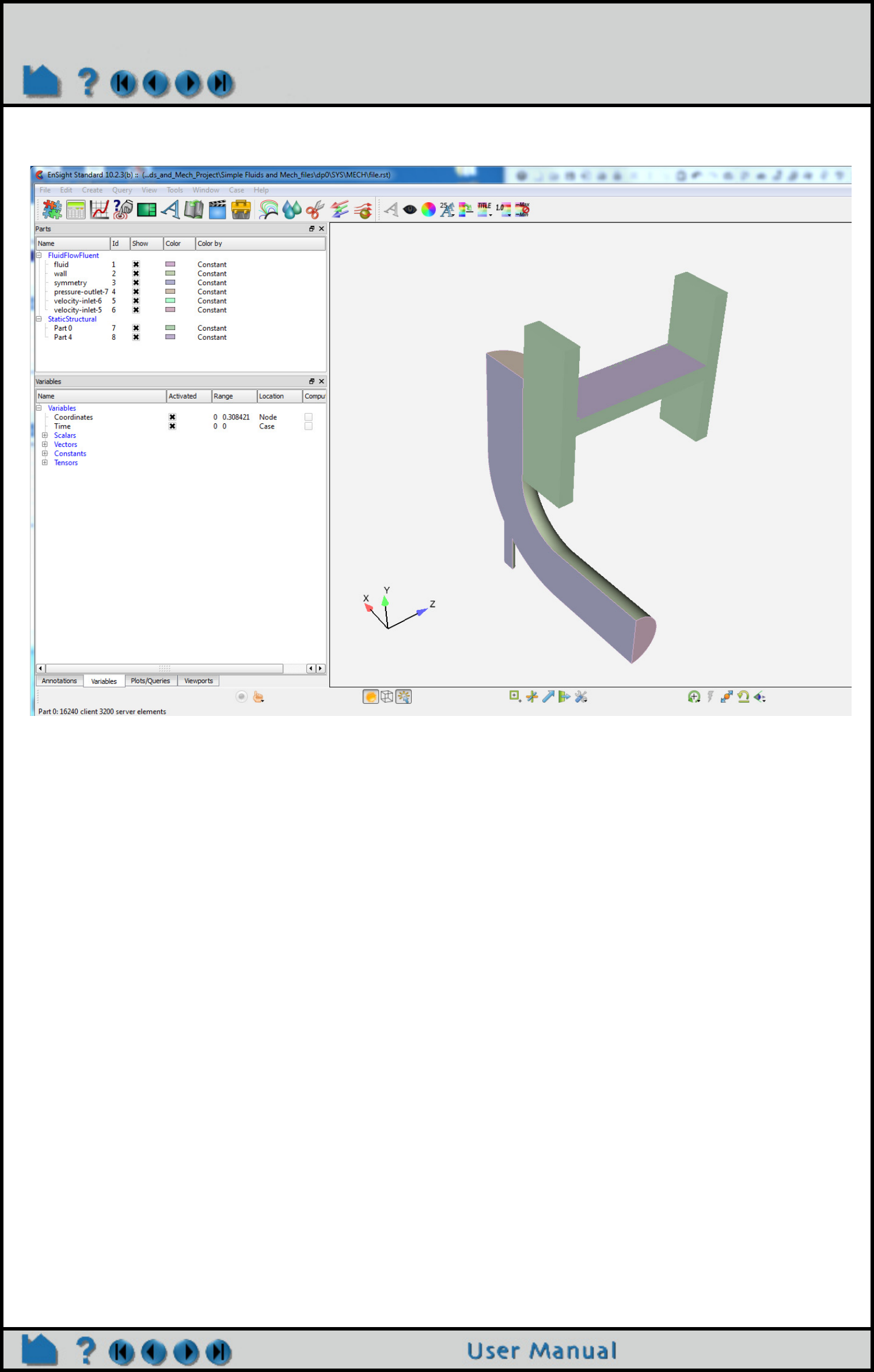
Page 234
HOW TO USE ENSIGHT WITH WORKBENCH
14. EnSight now opens with both Fluid and Structural solution results (see Load Multiple Datasets (Cases)).
15. Now, set the EnSight properties in the WorkBench Properties View to enable the Beta feature in EnSight to see
Units (units are labels only, more details are discussed later in the Properties View). To adjust EnSight properties,
select the EnSight Results (click on the EnSight Results) and in the top menu, View>Properties. Toggle on
Advanced EnSight Features; now adjust the EnSight Advanced properties (shown below) as described. Close the
properties view by right-clicking on the Title Bar, and choosing Close. If EnSight is running, quit EnSight and then
double click on the EnSight Results to reload the Solution with EnSight using the Beta features that you have toggled
on.
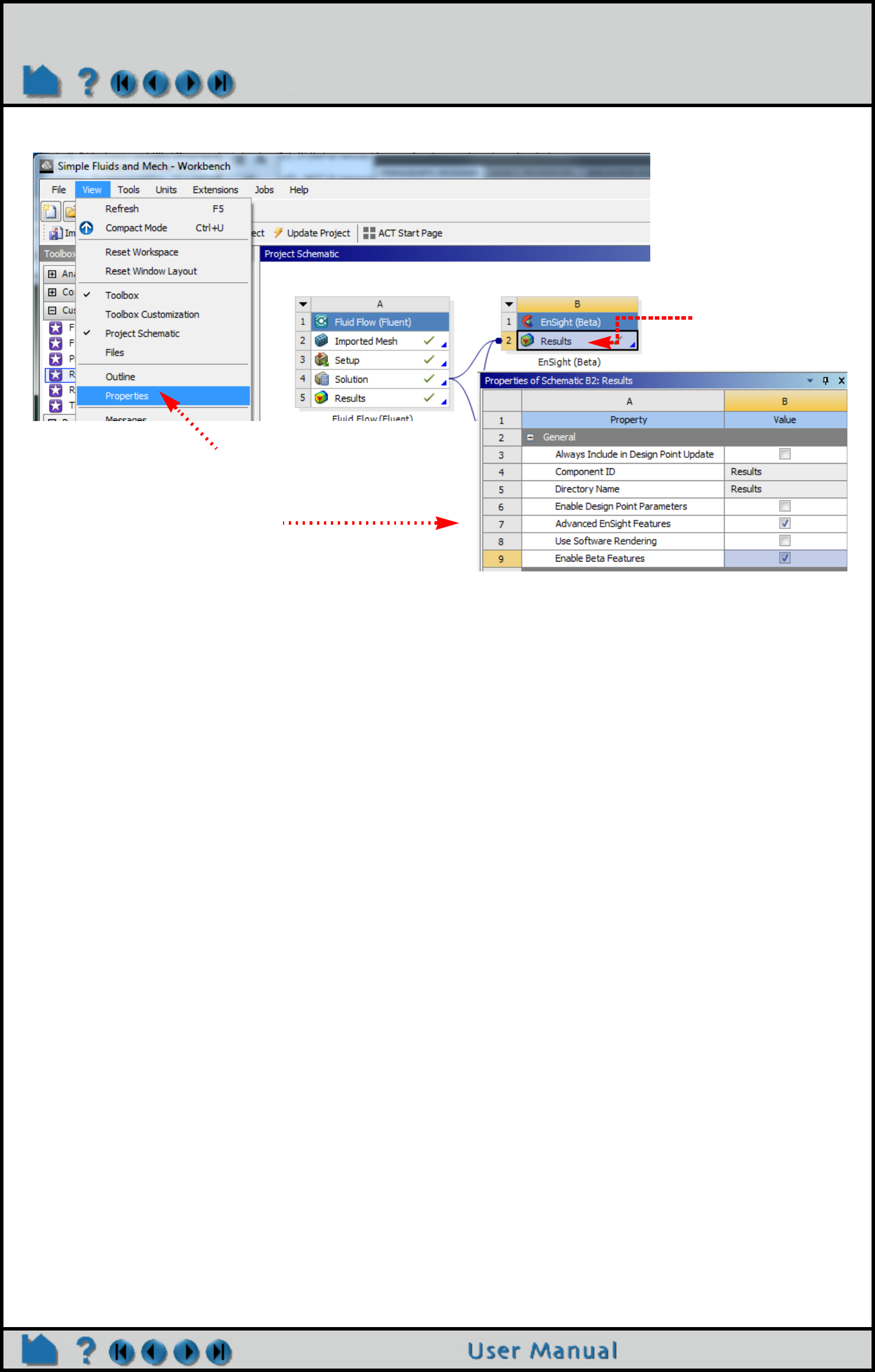
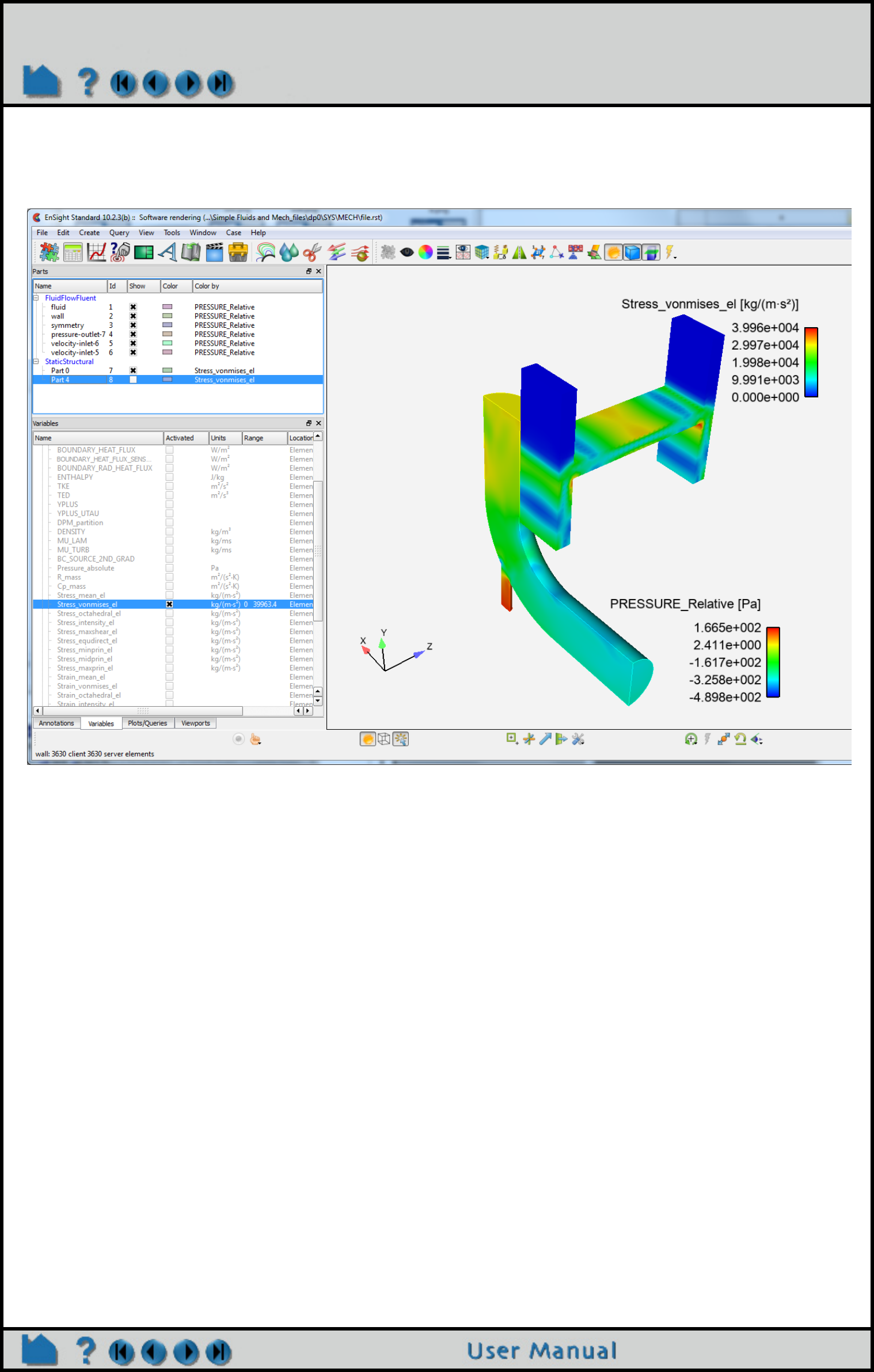
Page 236
HOW TO USE ENSIGHT WITH WORKBENCH
16. Color by variables from each of the two solutions simultaneously. This is the view below (with units shown in the
legend titles), that you will see if you have enabled Beta features. If you don’t see units in the legend bar, go back to
step 15 and then make sure you have quit and restarted EnSight after you enable the Beta features.
17. Quit EnSight when you are done with your simultaneous postprocessing of the two solutions.
18. Consider saving your updated Workbench project, and then exit Workbench.
Important
Saving a WorkBench project enables you to re-open the project on the machine that originally created it. To make the
project available on another machine, you need to use File > Archive to create a project archive. To open the
project on a different machine, run File > Restore Archive on that machine.
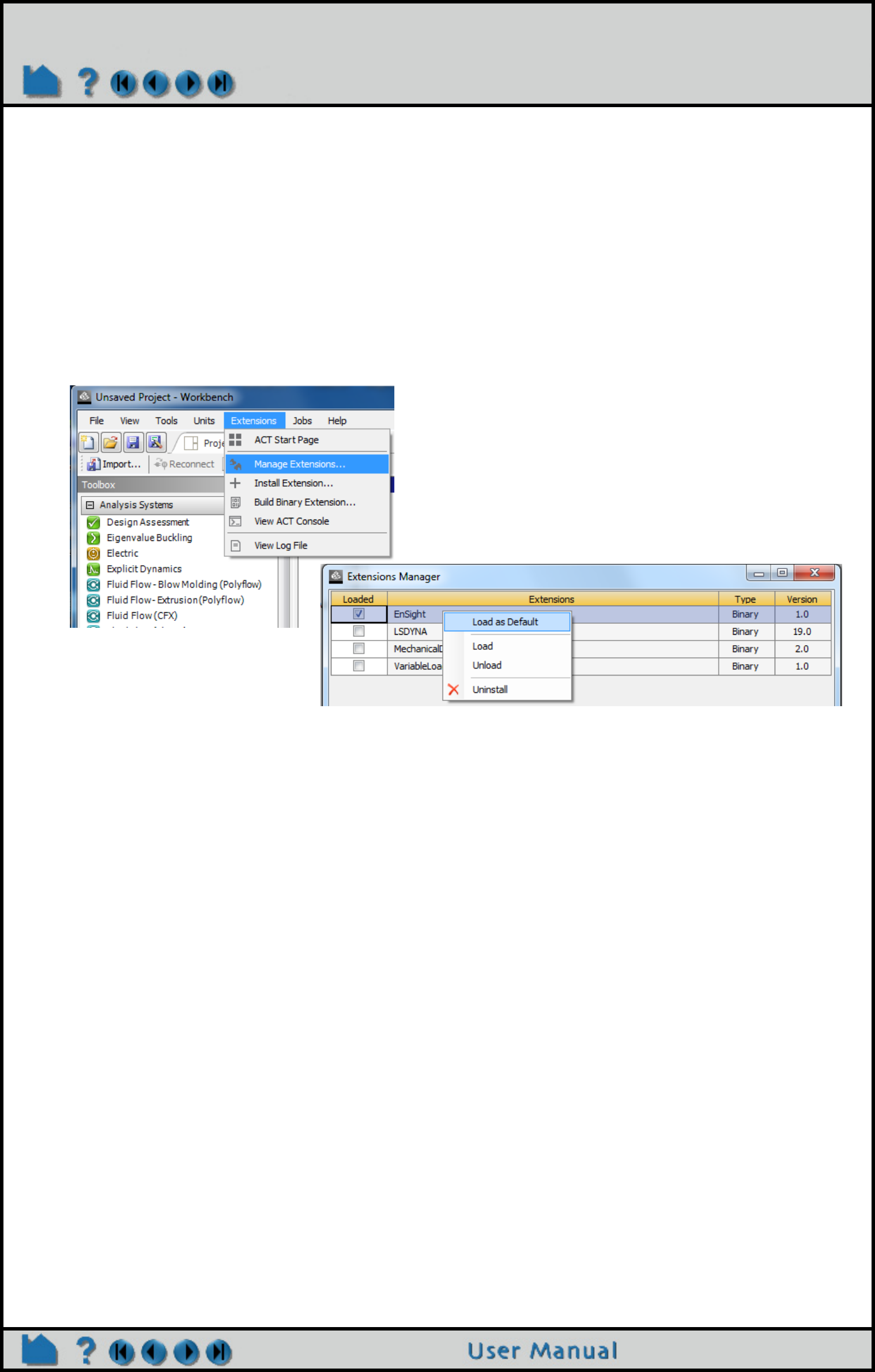
Page 237
HOW TO USE ENSIGHT WITH WORKBENCH
DETAILED VIEW OF THE ENSIGHT ANSYS WORKBENCH INTERFACE
The previous section stepped through a sample analysis and provided a broad overview of using EnSight within the
WorkBench workflow. What follows is a more detailed look at the WorkBench GUI as it relates to EnSight. Some of
the content is repeated for the advanced WorkBench user who skips the sample analysis and wants to dive into the
details.
Reminder, if the EnSight extension is not shown in the list of Component Systems in the Toolbox Workspace then
it must be loaded as a WorkBench extension as follows. Choose, from the WorkBench menu, Extensions>Manage
Extensions... which will pop up the Extensions Manager dialog. Toggle on the EnSight Extension, and then
right click on EnSight and choose Load as Default. Now, quit WorkBench. Restart WorkBench and verify that
EnSight appears in the Toolbox under the Component Systems pulldown.
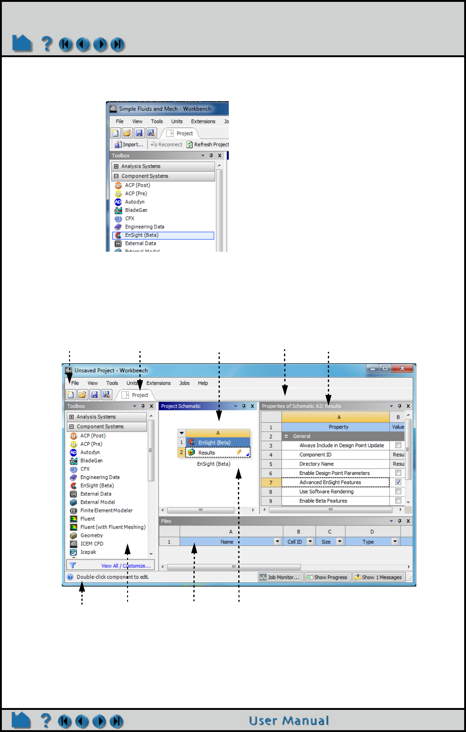
Page 238
HOW TO USE ENSIGHT WITH WORKBENCH
After choosing to Load as Default, the EnSight as a WorkBench extension, and then restarting WorkBench, you
should now see EnSight in the Component Systems pulldown in the Toolbox Workspace as follows:
Now let’s look at the WorkBench GUI in more detail. Shown below are the components of WorkBench. WorkBench
has a top-level Menu Bar, and a lower Status Bar and one or more Project Tabs. Each Project Tab has a Toolbar, with
a number of Workspace Views, some of which are shown below: the Toolbox Workspace, Properties View, Files
View and the Project Schematic Workspace. The Project Schematic is where Systems from the ToolBox are
assembled together into a Workflow. Some of this will be discussed in this section as it pertains to EnSight.
Menu Bar Workspace Tab(s) Project Schematic Toolbar Properties
Status Bar Toolbox Files View System
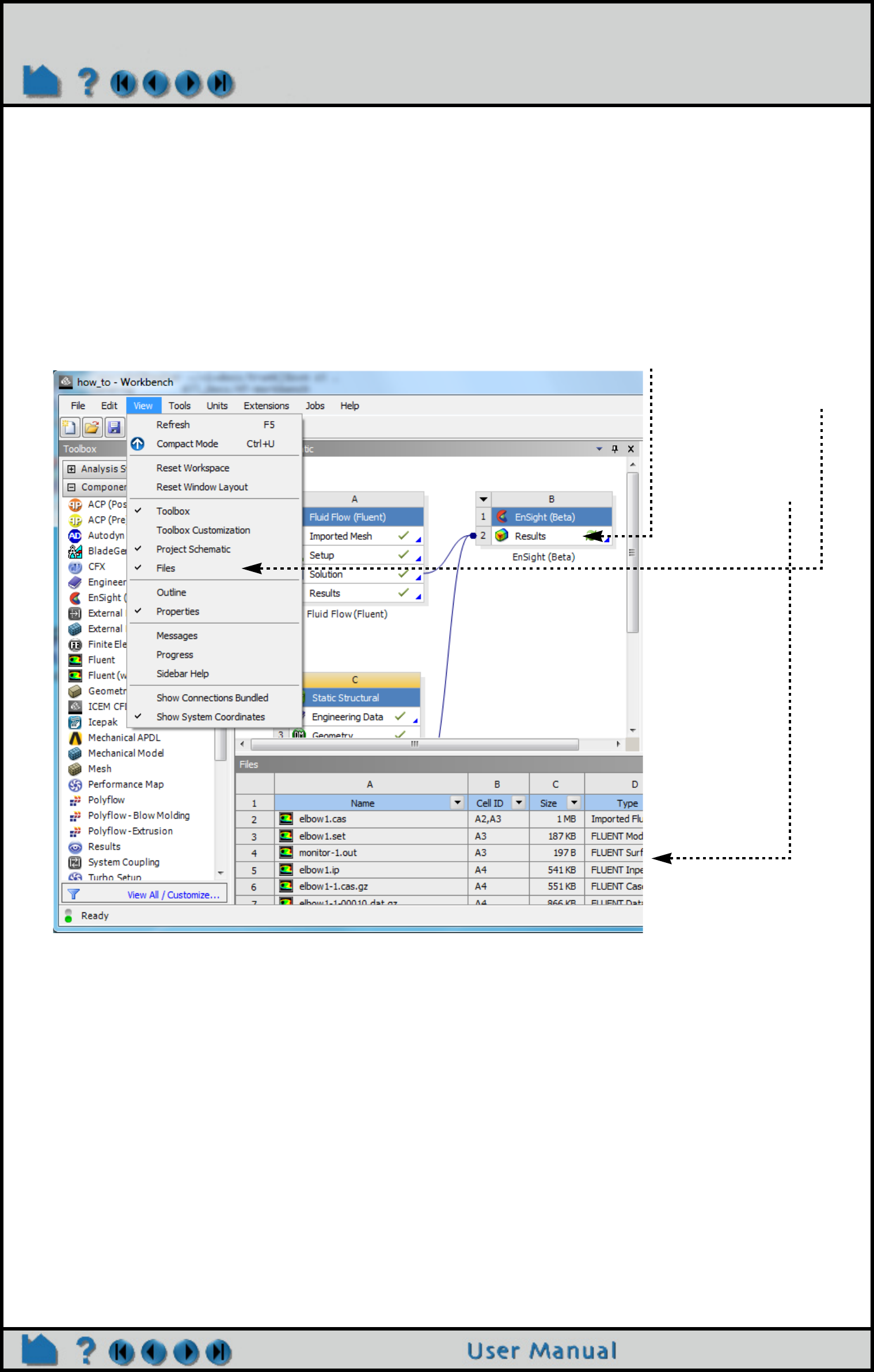
Page 239
HOW TO USE ENSIGHT WITH WORKBENCH
Views
You control which views are displayed by choosing View from the top menu and choosing the view you want to
display. Note that the Toolbox and the Project Schematic are displayed by default. For the following View, first select
a cell, then choose one of the following other views from the top level View Menu, and the workspace corresponding
to the selected cell will appear: Toolbox Customization, Files View, Properties View, Messages View, Progress
View, Sidebar Help View. If you minimize a view (on the Title Bar, Right-click>Minimize), it appears as a tab
in the View Bar and the check box is cleared from the View menu. For more details on workspaces and tabs, see
Tabs within Workbench in the Workbench User's Guide and Views within Tabs in the Workbench User's Guide. Now,
let’s look at several Workspaces and Views.
1. Select the EnSight
Results,
2. From the top menu
bar, View>Files
3. Pops up the
dockable/undockable
Files Workspace.
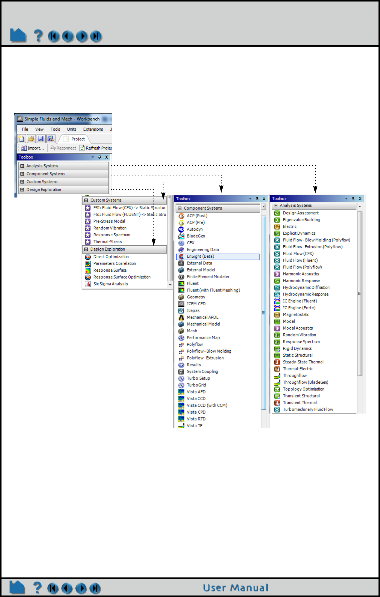
Page 240
HOW TO USE ENSIGHT WITH WORKBENCH
Toolbox Workspace
The list on the left is the Toolbox; by default viewing is toggled on for the Toolbox. The Toolbox contains four
pulldowns containing systems available to you: Analysis Systems, Component Systems, Custom Systems, and
Design Exploration, which are discussed below.
1. Analysis Systems
The Analysis Systems pulldown contains applications that transform input and solve particular types of problems,
often resulting in transformed output. These systems can be thought of as of the kind of solution that is desired
packaged with the Solver. For example Eigenvalue Buckling system is a modeling, a meshing, a modal
frequency buckling analysis and a visualization process packaged with Ansys Mechanical. Similarly, the Fluid
Flow (Fluent) system contains tools for creating the geometry, performing the meshing, setting up the solver,
using the solver to derive the solution, and viewing the fluid flow results.
2. Component Systems
The Component Systems pulldown contains extensions that are loaded into WorkBench that also solve particular
types of problems similar to the Analysis Systems. In particular, you will see the EnSight Extension under this
pulldown. EnSight is available to input solution results and to interactively Analyze, Visualize and Communicate these
solution results and create postprocessing output such as tables, movies, images, or data files.
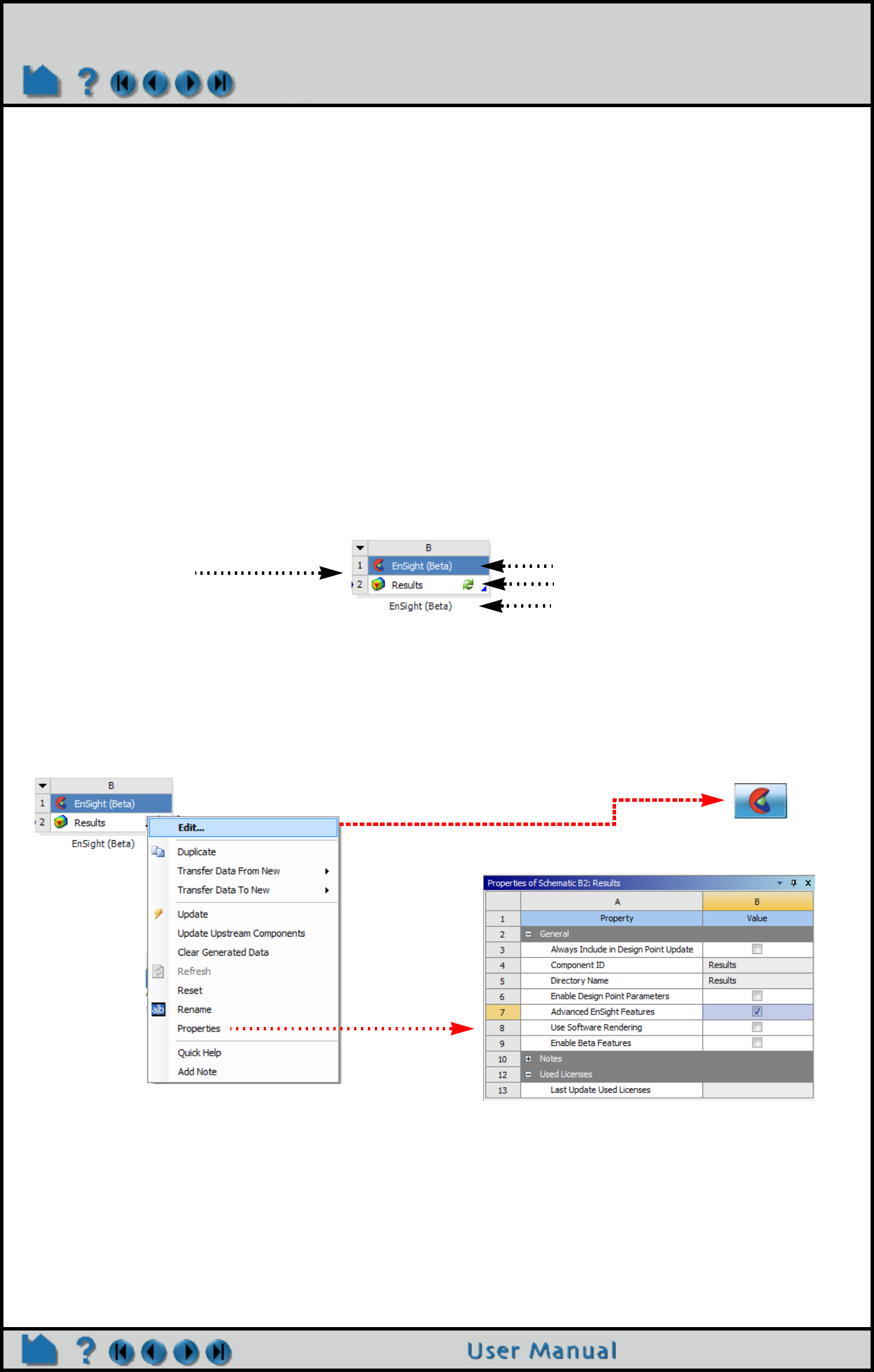
Page 241
HOW TO USE ENSIGHT WITH WORKBENCH
3. Custom Systems
The Custom Systems pulldown contains customized applications that combine multiple analysis systems. For
example, the FSI: Fluid Flow (Fluent) > Static Structural system combines ANSYS Fluent and the Mechanical
application to perform a Fluid Structure Interaction (FSI) analysis.
4. Design Exploration
The Design Exploration pulldown contains systems that enable you to see how changes to parameters affect the
performance of the system.
Note: Which systems are shown in the Toolbox depends on the licenses that exist on your system. You can
hide systems by enabling View > Toolbox Customization and clearing the check box beside the name of the
system you want to hide. To begin using a system, drag it into the Project Schematic area.
Project Schematic Workspace
The Project Schematic enables you to manage the process of your work flow; by default viewing of the Project
Schematic is on. It keeps track of your files and shows the actions available as you work on a project. At each step
you can select the operations that process or modify the case you are solving.
When you move a system from the Component Systems toolbox to the Project Schematic, you will see a system
similar to the following:
Each white cell represents a step in solving a problem. Right-click the cell to see what options are available for you to
complete a step. For example, you would select Edit in the example above on an EnSight Results cell to launch
EnSight and load solution data, or Properties to open the EnSight Properties table to enable optional EnSight
capabilities.
System Type
Cell State
System Name
System
Coordinates
Load Results using EnSight
Toggle on
Advanced
EnSight
Features to
expose other
options.
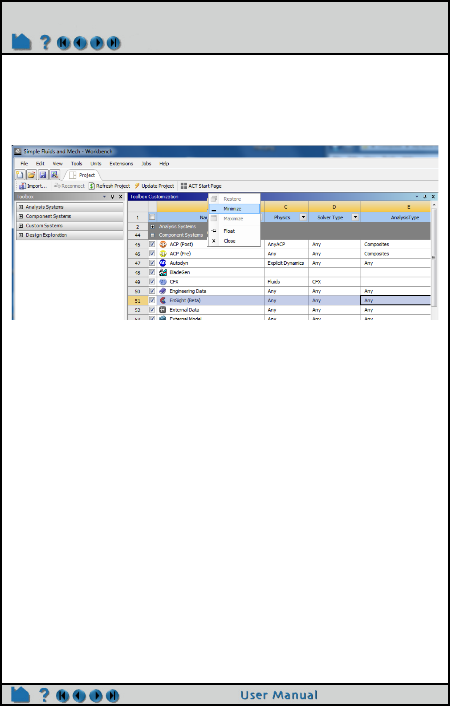
Page 242
HOW TO USE ENSIGHT WITH WORKBENCH
Toolbox Customization
View>Toolbox Customization will view the Tool Customization Workspace in a tabular form, as shown below.
This allows you to customize the Physics, Solver Type and Analysis Type of the particular application or extension
according to your workflow needs as shown below. Right-click>Minimize on the Toolbox Customization title
bar, to reduce the workspace table down to a tab below the Toolbox list. Right-Click>Close to close the Toolbox
Customization workspace.
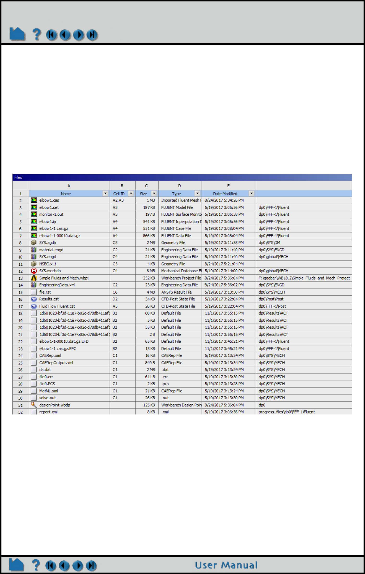
Page 243
HOW TO USE ENSIGHT WITH WORKBENCH
Files View
The Files view (View>Files) shows the files that are in the selected cell of a given System. The project files are
updated constantly, and any “save” operation from a component will save all files associated with the project.
ANSYS Workbench associates data with system cells. This data may be stored in different ways, including as part of
the ANSYS Workbench project file or as separate files.When files are generated, they appear in the Files view. This
view can be used to identify which files are associated with each cell.
On the title bar, Right-click>Minimize or Right-click>Close to minimize this file Workspace to a tab or to
close it, respectively.
Important
Although the Files View reveals the data files that make up a project, you should not attempt to manipulate these files
directly, as project data management will proceed unaware of your changes and with unpredictable results.
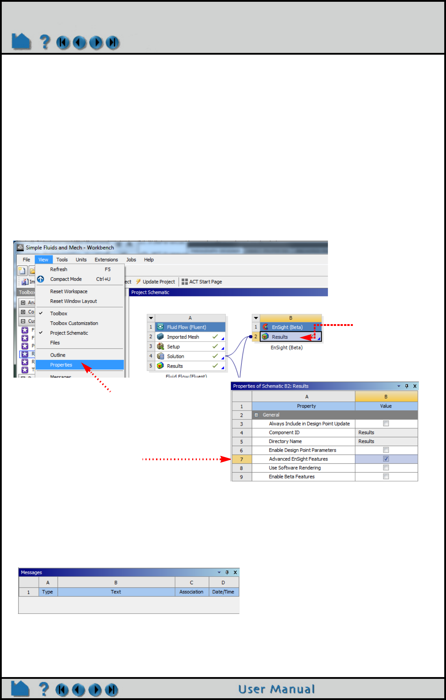
Page 244
HOW TO USE ENSIGHT WITH WORKBENCH
Properties View
The Properties view is a table whose entries describe the status of a system. These entries vary between system
cells and are affected by the status of the cell. Some entries in the Properties area are changeable; others are for
information only. To display the Properties for a particular cell, right-click the cell and select Properties, or click on the
cell to select it, and in the top menu, View>Properties. Note, once the Properties view is open, simply selecting
another cell in the Project Schematic will display its properties. Right click on the Toolbar and choose Close to close
the window, or minimize to reduce it to a tab.
EnSight Example
For example to adjust EnSight properties, select the EnSight Results (click on the EnSight Results) and in the top
menu, View>Properties. Toggle on the Advanced EnSight Features toggle to see the available properties
and their settings. The Use Software Rendering toggle is available in the rare instance that EnSight is unable to
adjust its rendering mode due to graphics incompatibilities; toggle this on to force EnSight to use internal software
rendering in order to manually bypass hardware or software graphics card rendering problems. The Enable Beta
Features toggle exposes two features under development: units labeling (for details, see EnSight Limitations within
ANSYS WorkBench) and the Nexus report interface.
Messages View
The Messages view shows the messages to the user. For example, click on the EnSight Results in the Project
Schematic to select it, and in the top menu, View>Messages.
On the title bar, Right-click>Close to Close the Message view workspace.
1. Select EnSight
Results
2. From the top menu,
View>Properies
Toggle
3. Toggle on Advanced
EnSight Features to
expose other toggles.
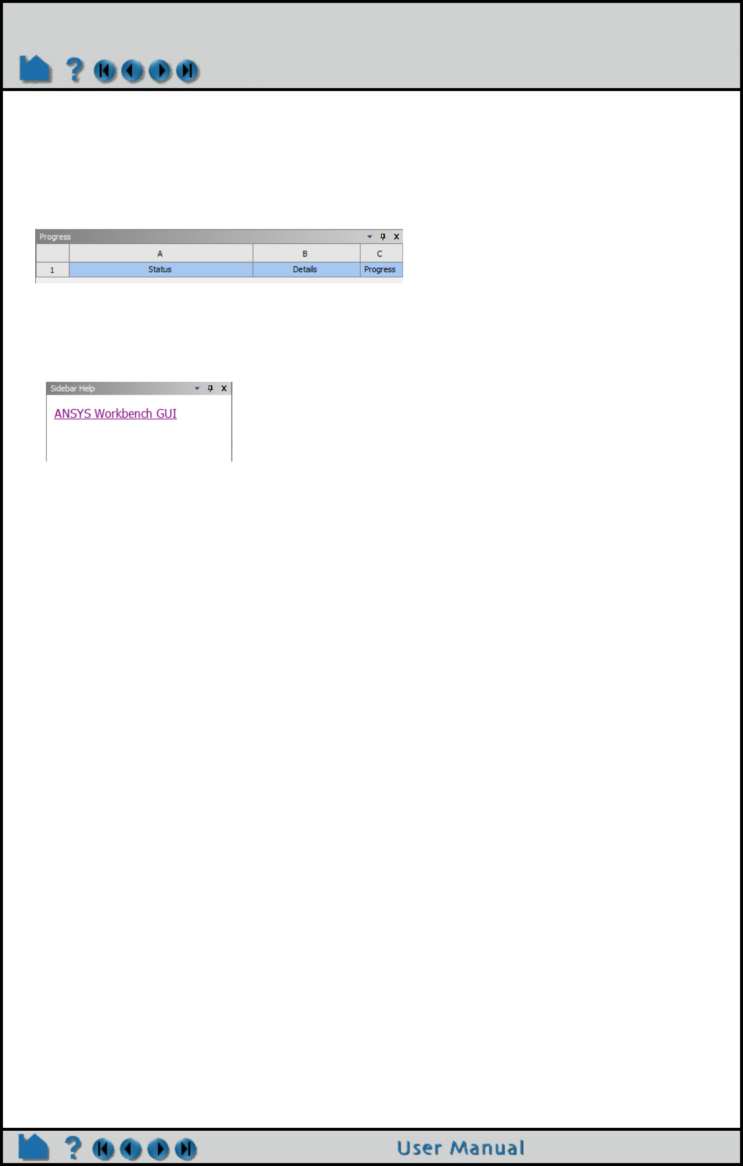
Page 245
HOW TO USE ENSIGHT WITH WORKBENCH
Progress View
The Progress view shows the progress to the user. For example, click on the EnSight Results in the Project
Schematic to select it, and in the top menu, View>Progress.
On the title bar, Right-click>Close to Close the Message view workspace.
Sidebar Help View
In the top menu, View>Sidebar Help. Click on this link.
In addition to having a visual layout that guides you through completing your project, you can also access Sidebar
Help by pressing F1 while the mouse focus is anywhere on ANSYS Workbench. Sidebar Help is a dynamically
generated set of links to information appropriate for helping you with questions you have about any of the tools and
systems you currently have open.
Shortcuts (Context Menu Options)
You can access commonly used commands by right-clicking in most areas of ANSYS Workbench. These commands
are described in Context Menus in the Workbench User's Guide.

Page 246
HOW TO USE ENSIGHT WITH WORKBENCH
FILE LOCATIONS WITHIN WORKBENCH
EnSight has default locations for file operations within the ANSYS Workbench environment. To view a file within your
OS, simply select the Results cell of interest, View>Files to see the Files View, and then Right-click>Open
Containing Folder . Warning: Do not move WorkBench files around!
ENSIGHT DIFFERENCES WITHIN ANSYS WORKBENCH
Note that EnSight behaves somewhat differently in a WorkBench session than when run stand-alone. Many of these
changes are largely cosmetic, but that can be confusing initially.
• The default part colors are different. EnSight in WorkBench utilizes a more muted color palette with an improved
default lighting configuration.
• The mouse button graphics view manipulations have been modified to align better with the other Ansys application
defaults. Specifically, the middle mouse is used to manipulate the view (with control and shift modifiers), the left
mouse is used to select entities and the right mouse is used to bring up context sensitive menus.
• All interactive operations in an EnSight WorkBench session are saved in an EnSight context file automatically.
When you reopen EnSight, this context file will be used to restore the session to its last saved state. Whenever
EnSight is closed, the context file is updated. You will not be prompted to save the EnSight state when exiting
EnSight when it is launched from WorkBench.
• The default license manager for EnSight, when run from within an Ansys installation (including via WorkBench) is
the Ansys license manager. EnSight will use a SLiM license if an appropriate license cannot be obtained from the
Ansys license manager.
ENSIGHT LIMITATIONS WITHIN ANSYS WORKBENCH
There are several EnSight limitations within the WorkBench environment.
• When launched from WorkBench, EnSight always opens using an EnSight Standard license; you cannot do parallel
processing from within Workbench.
• Workbench cannot effectively use the EnSight native, Case Gold data format due to Workbench limitations in the
handling of large numbers of files.
• Care must be taken when using EnSight Python and command language files from within WorkBench. The
WorkBench interface relies on specific ordering of cases in the EnSight session and any Python or command
language operations that modify case attributes (e.g. names, etc) will conflict with WorkBench conventions.
• EnSight cannot be run in script-driven, batch mode using Workbench. WorkBench will evaluate design points in
batch mode if an EnSight session is not open, but there is no mechanism to run a specific script in batch mode.
• Currently in EnSight units are labels only. EnSight-standalone displays units by default. In contrast, EnSight within
the WorkBench environment does not display units by default. Display of units is a EnSight WorkBench Property
controlled by the Enable Beta Features toggle, which is off within the WorkBench environment by default. This is
because EnSight lacks a mechanism to convert common variables to common unit systems prior to display. Thus, it
is possible when using EnSight through WorkBench to view “temperature” related variables (with different names)
from different data sources (e.g. Fluent and Mechanical) in different units (e.g. K, C). The individual variables will be
properly labeled with ‘K’ and ‘C’ denoting that the variables are in different unit systems. It was decided to limit the
units exposure as a beta feature until this shortcoming is addressed.
• When using design point parameter in the current release, WorkBench is not automatically made aware of any
EnSight constants that are created/activated. The list of design point parameters is updated when the EnSight task
‘Enable Design Point Parameters’ property changes state. Thus, if you have a running EnSight session and use the
calculator to create a new constant that you wish to appear in the current WorkBench design point variables, one
may need to uncheck and recheck the “Enable Design Point Parameters” property.
• The current EnSight session state is explicitly linked to the collection of solutions marked as inputs into the EnSight
Results task in WorkBench. If one changes the inputs (e.g. adds an additional solution or removes one), the state of
the EnSight session will be reset to the default (the EnSight context file will be reset). It is strongly recommended

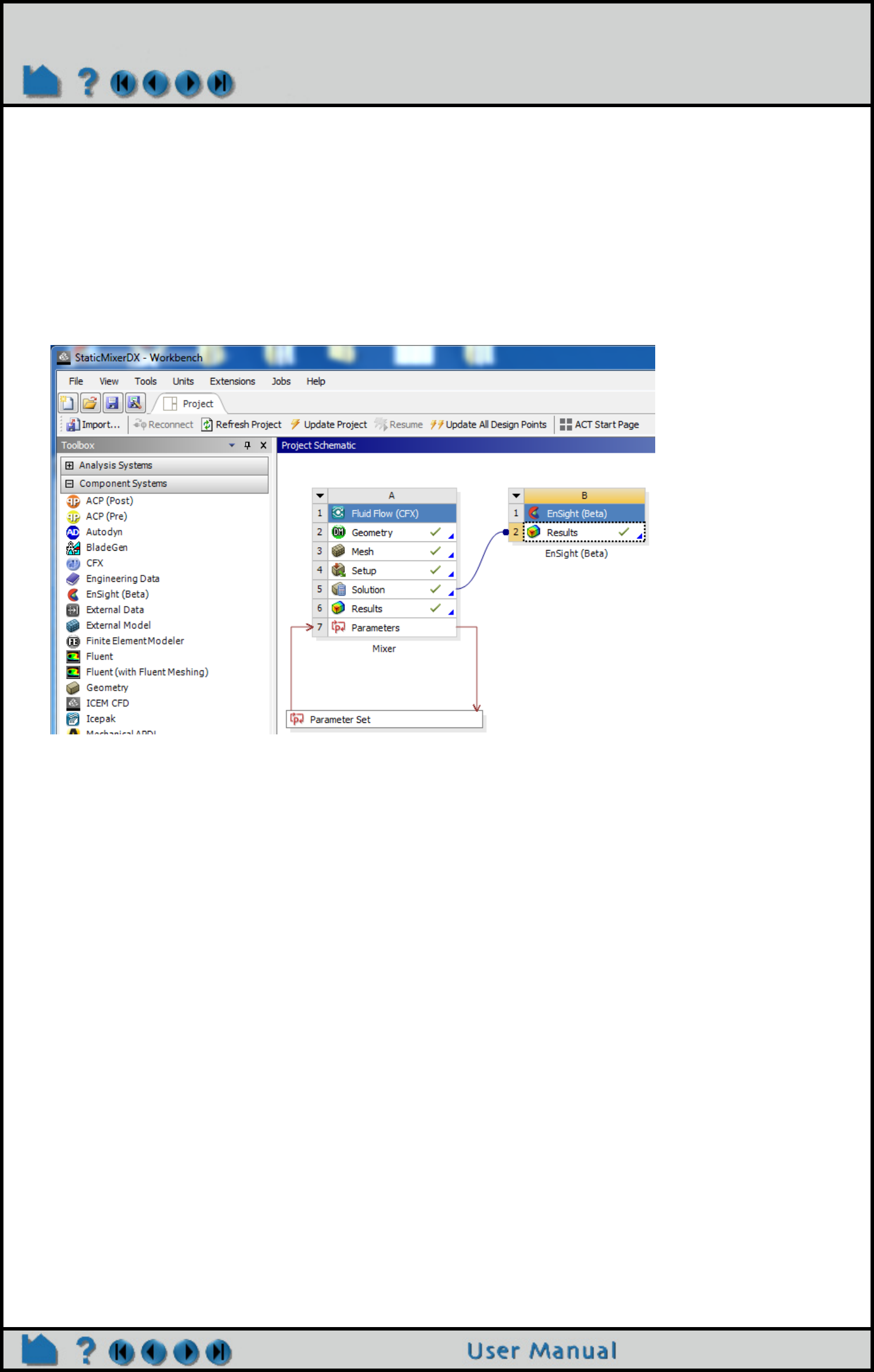
Page 248
HOW TO USE ENSIGHT WITH WORKBENCH
ADVANCED USAGE: DESIGN POINT SESSION USING ENSIGHT
This example will take you step by step through a WorkBench Design Points EnSight example session. You might, for
example, use Design Points if you wanted to optimize a design based on some figures of merit. This section assumes
you have successfully worked through the previous simple, example session: Simple Example EnSight Session
within ANSYS Workbench so some intermediate steps will be skipped in the interest of brevity.
1. Load a WorkBench dataset, drag the EnSight system from the WorkBench Toolbox onto the Project Schematic and
link the Solver Solution to the EnSight Results cell. Right click the EnSight Results and choose Update if your
EnSight Results cell has arrows rather than a check mark. If the update takes a while, in order to see the progress,
from the WorkBench top menu, View>Progress. You should see the following.
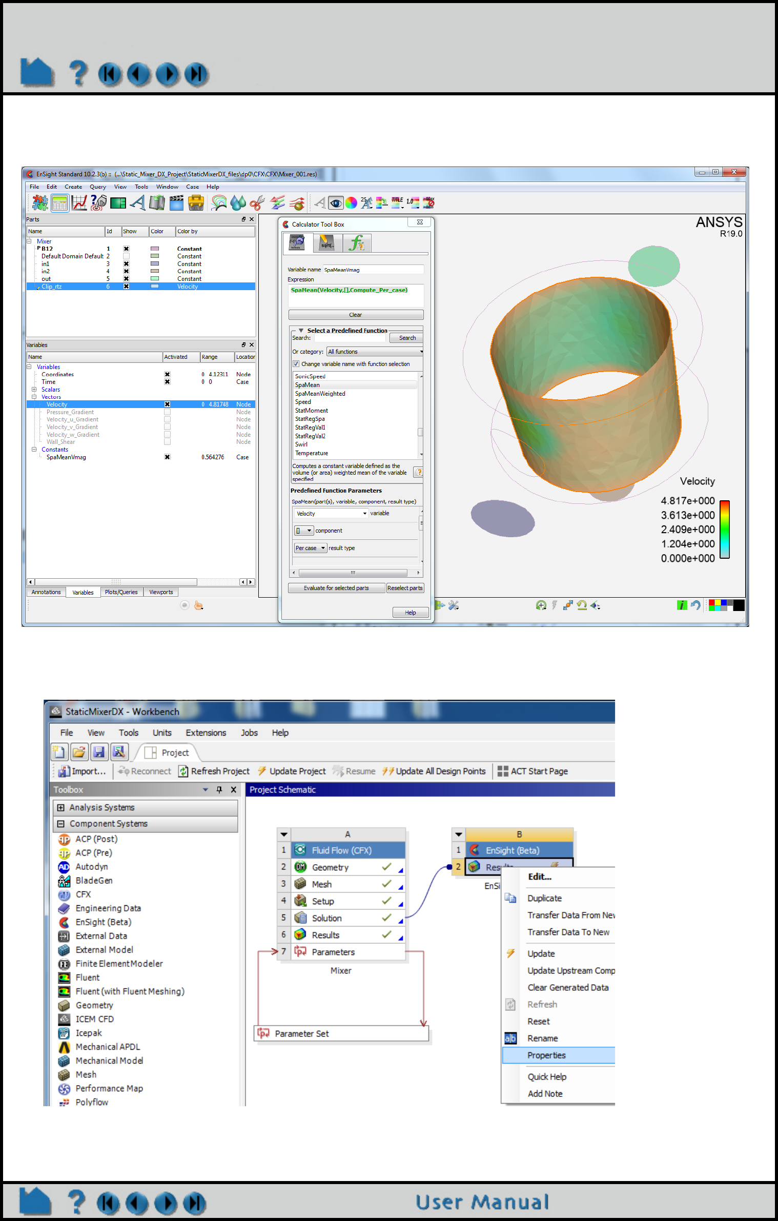
Page 249
HOW TO USE ENSIGHT WITH WORKBENCH
2. Now double-click EnSight Results to start up an interactive EnSight session. Do something and calculate a Case
Constant that you wish to use as a design value. In this EnSight example, we have created a new part, a radial clip
and calculated the Spatial Mean of the Velocity vector magnitude.
3. Now we want to import the EnSight Case Constant into WorkBench as a Design Point. On the EnSight Results
Right-click>Properties.
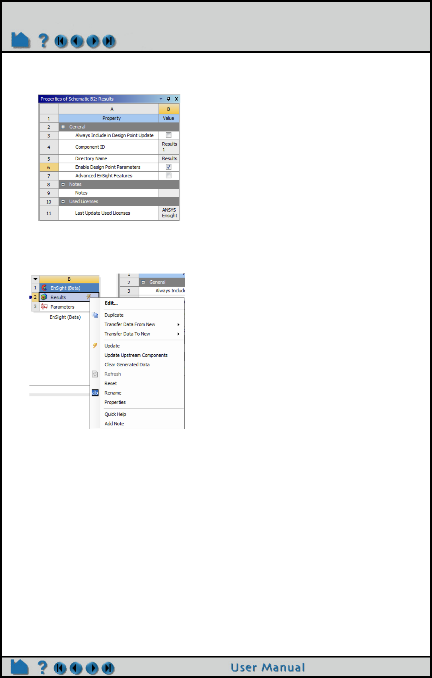
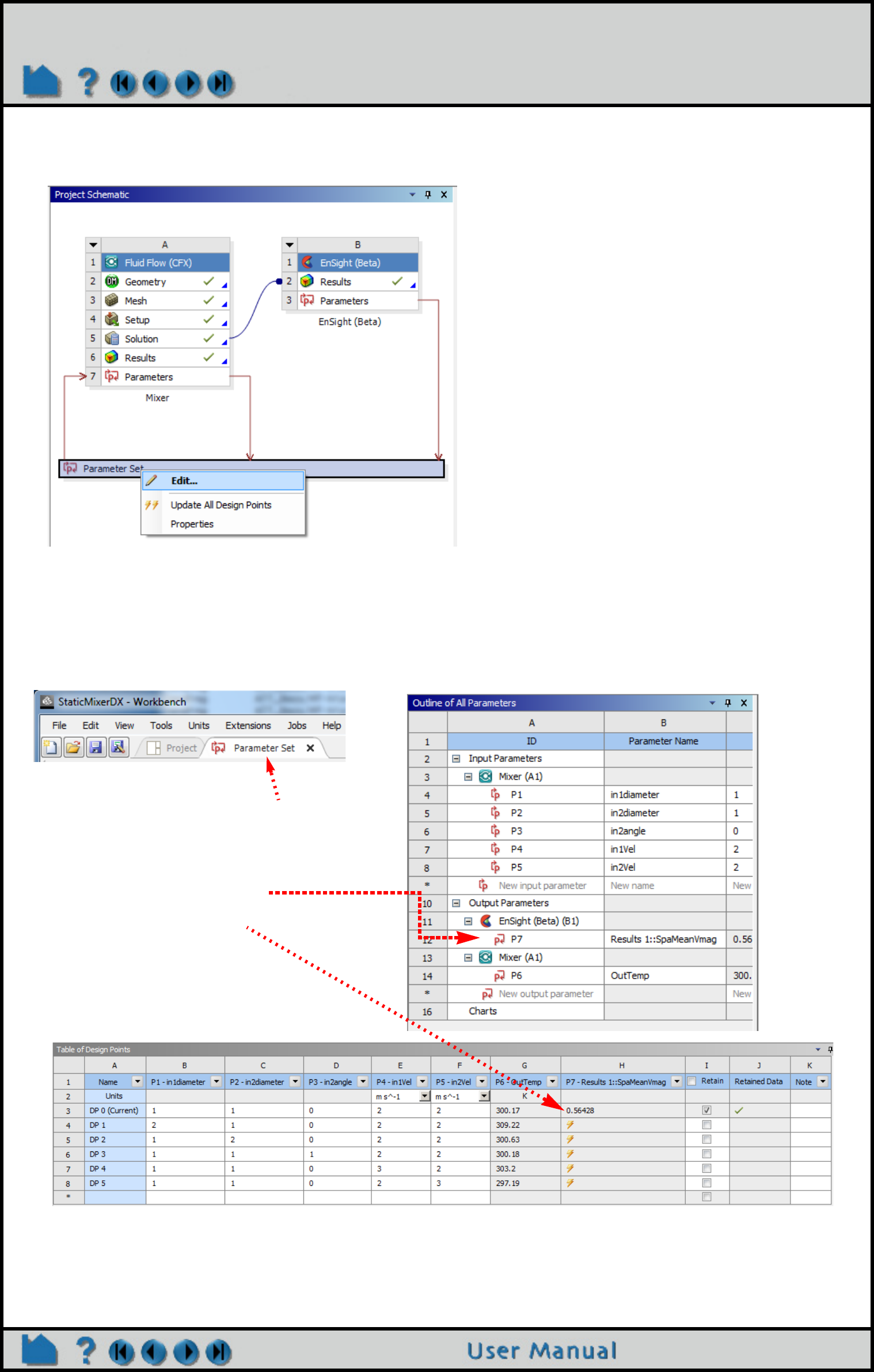
Page 251
HOW TO USE ENSIGHT WITH WORKBENCH
6. Once the EnSight Results are updated, now, on the Parameter Set, Right-click>Edit
8. Now you will see that you are in the Parameter Set tab rather than the Project Tab. The Outline of All Parameters
table below. Now do a View>Table and see the Table of Design points shown below. Notice the constant calculated
in EnSight on the Radial Clip Plane part in EnSight, SpaMeanVelMag has been imported into WorkBench as a Design
Point.
EnSight variable shows up
in the Parameters, and as a
WorkBench Design Point
Note you are in the Parameter Set View
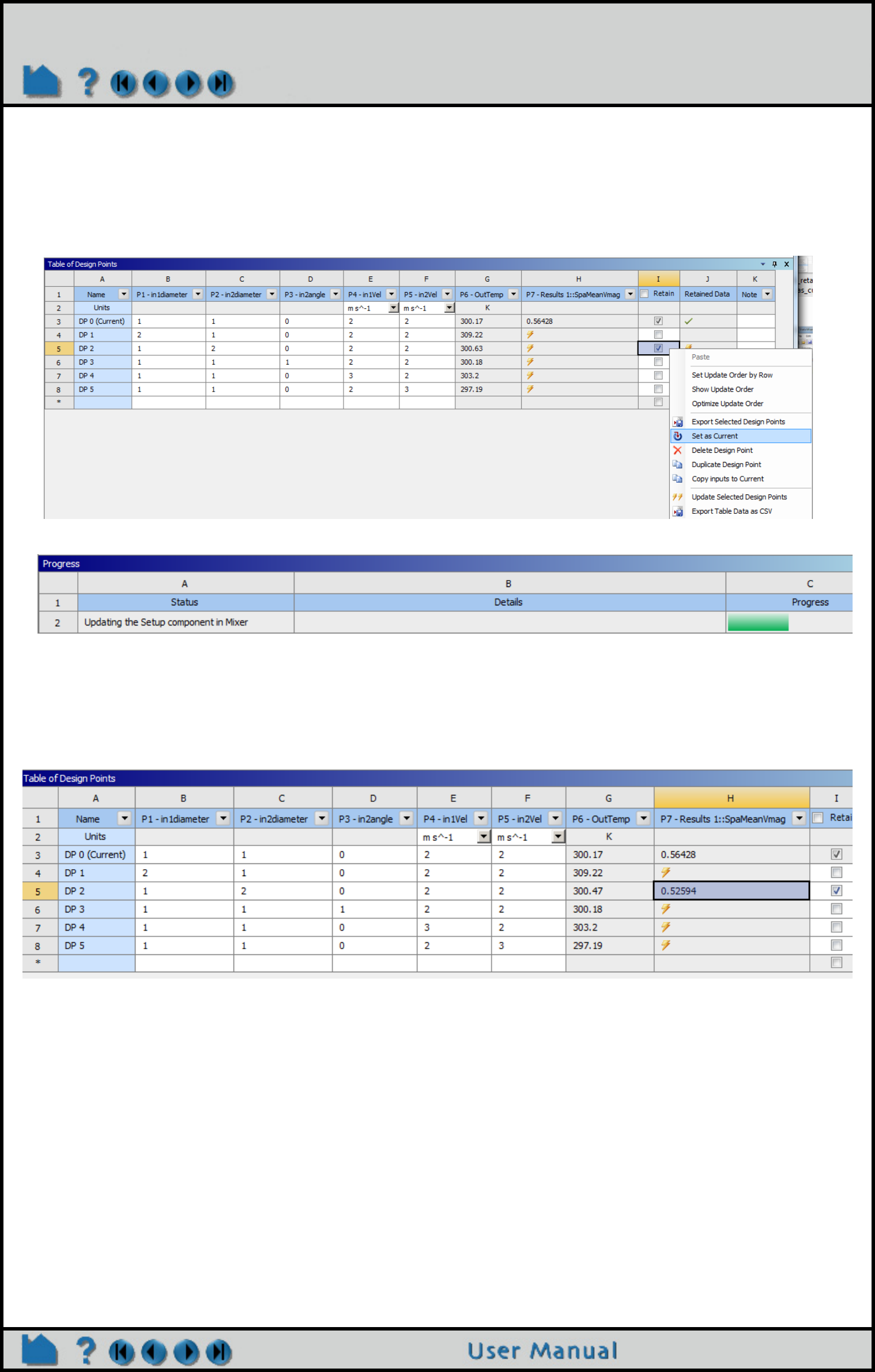
Page 252
HOW TO USE ENSIGHT WITH WORKBENCH
8. In the Table of Design Points, Toggle on one of the Retain toggles for DP2. Now right click on the row and choose
Set as Current. This will make DP 2 as the current Design Point. Now to update to Design Point 2 as the input, to
solve the flow and to use EnSight to Calculate the Spatial Mean of the Velocity Magnitude on the Radial Clip, Right-
click> Update Selected Design Points.
9. Now take a closer look at your updated Table of Design Points. Two of the SpaMeanVmag EnSight Constants /
WorkBench Design Points (see P7 Results in Column H below) are have been calculated. You now can see that
Design point 0 has a higher average velocity at the EnSight Radial clip part.
Choose View>Progress to see what is happening
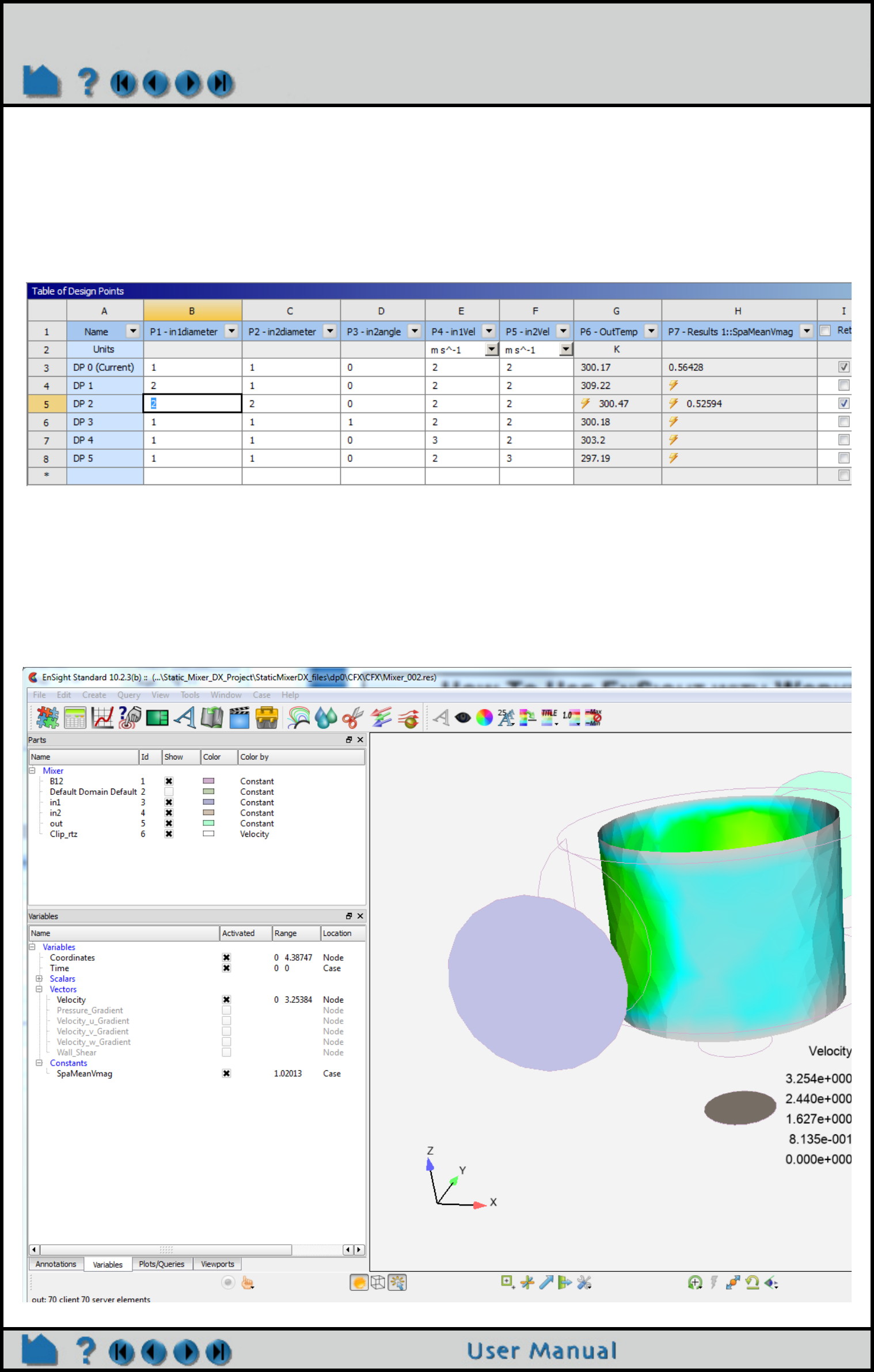
Page 253
HOW TO USE ENSIGHT WITH WORKBENCH
10. Notice the cells in the Table of Design Points that are White. These are editable. The columns that are gray are
the Design Point output from the Solver or from EnSight; they are not editable. They are the input values for the
Solver. Edit the diameter of DP2, part in1 and change it to 2. Notice that the corresponding Design Points now need
updating. Right-click>Update Selected Design Points on row 5. Now the solver re-runs with the new
value for the in1 diameter, and then the solution data is fed to EnSight to create a radial clip and calculate the
average velocity magnitude.
9. When the update of DP2 is finished, click on the EnSight Window and notice the increased diameter of part in1, the
input part..
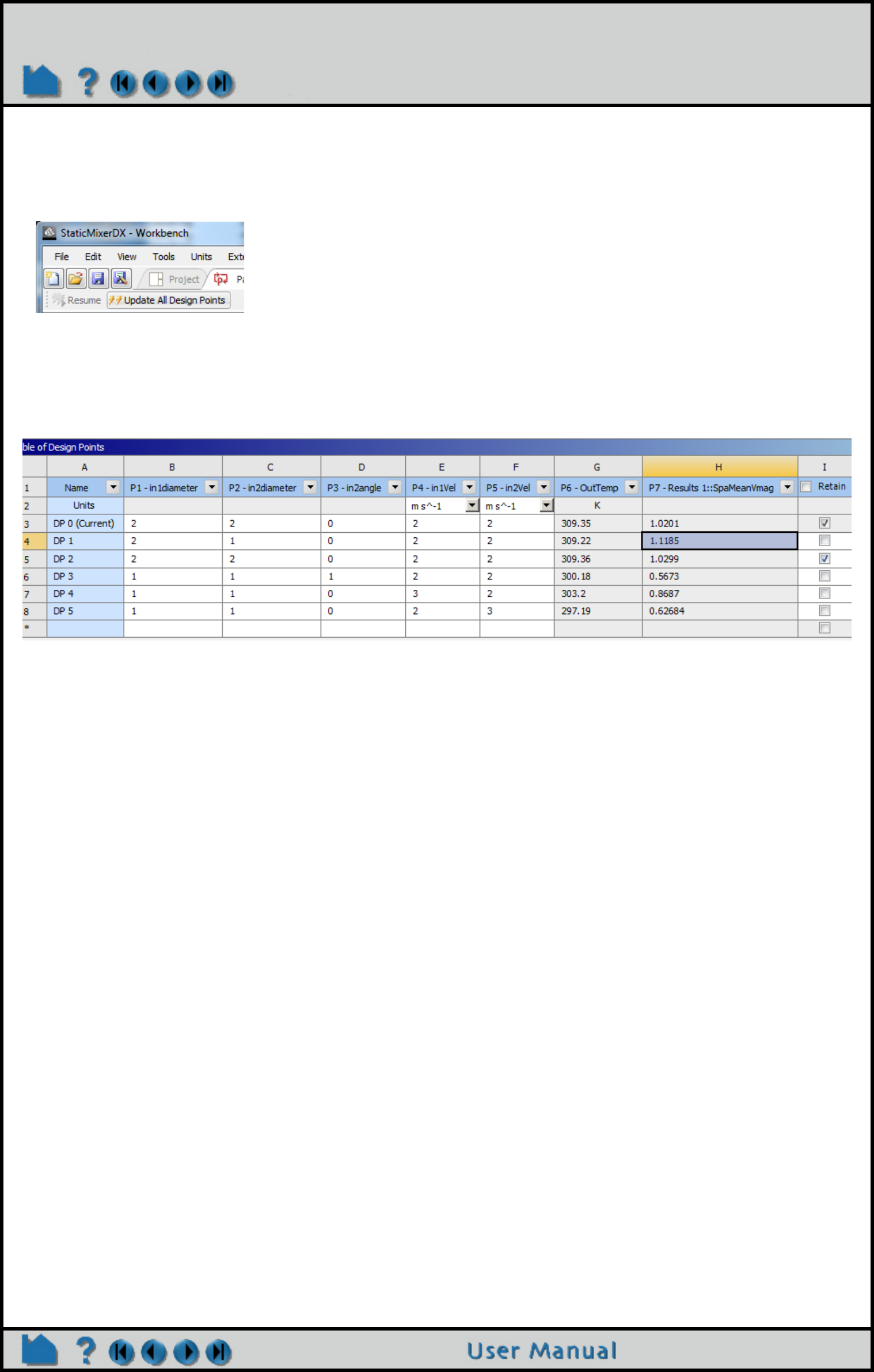
Page 254
HOW TO USE ENSIGHT WITH WORKBENCH
10. Now, update all design points. Note that EnSight does not launch multiple EnSight processes. It works through
each of the design points one by one using one EnSight process and one EnSight license. This may take a while
depending on your number of design points: View>Progress.
11. Now look at your Table of Design Points. It is fully populated. Now you can decide which Spatial Mean of the
Velocity magnitude satisfies your criteria and answer your hypothetical design problem: DP1 has the maximum value.
12. Exit WorkBench.

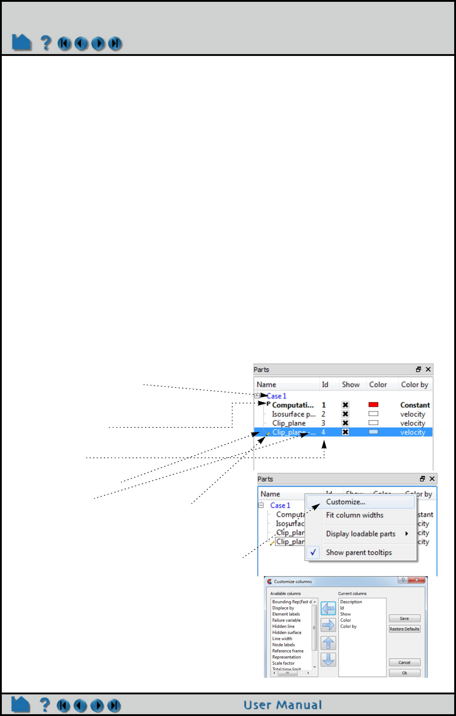
Page 256
HOW TO INTRODUCTION TO PART CREATION
Visualize Data
Introduction to Part Creation
INTRODUCTION
Much of the strength of EnSight derives from its flexible and powerful part creation mechanism. Since virtually every
task you perform in EnSight will involve some form of part manipulation, it is vital to understand these concepts.
In EnSight, a part is a named collection of elements (or cells) and associated nodes. The nodes may have zero or
more variables (such as pressure or stress) currently defined at the node positions. All components of a part share
the same set of (such as color or line width).
Parts are either built during the loading process (based on your computational mesh and associated surfaces) or
created during an EnSight session. Parts created during loading are called model parts. Model parts can also be
created during an EnSight session by performing a copy on other model parts or performing a load operation on the
part.
All other parts are created during an EnSight session and are called created or derived parts. Created parts are built
using one or more other parts as the parent parts. The created parts are said to depend on the parent parts. If one or
more of the parent parts change, all parts depending on those parent parts are automatically recalculated and
redisplayed to reflect the change. As an example, consider the following case. A clipping plane is created through
some 3D computational domain and a contour is created on the clipping plane. The contour’s parent is the clipping
plane, and the clipping plane’s parent is the 3D domain. If the 3D domain is changed (e.g. the time step changes),
the clipping plane will first be recalculated, followed by the contour. In this way, part coherence is maintained.
This article is divided into the following sections:
The Parts List Creating Parts Part Types Part Operations
Part Where Parts Are Created and Maintained Hints and Tips
The Parts List
Both model parts as well as all derived parts are displayed as items in the Parts List. There are several ways that the
Parts list can be displayed, the default looks something like:
Part numbers
Case number (important when
multiple datasets have been
loaded)
Part description
P indicates Parent of
currently selected part
Currently selected part
If you right click on any of the columns of the Parts list you
can Customize which columns of data will be shown in the
list. In the resulting pop-up dialog you can select from
either the left or right columns and use the left/right arrow
buttons to add or remove the column to the Parts list. You
can also change the order of the columns in the Parts list
by selecting the attribute in the right panel and using the
up/down arrows to change the order.
Save will keep the settings for the next time you run
EnSight while OK will apply the changes but not save
them.
Part being edited in the
Feature Panel is marked
with a pencil icon
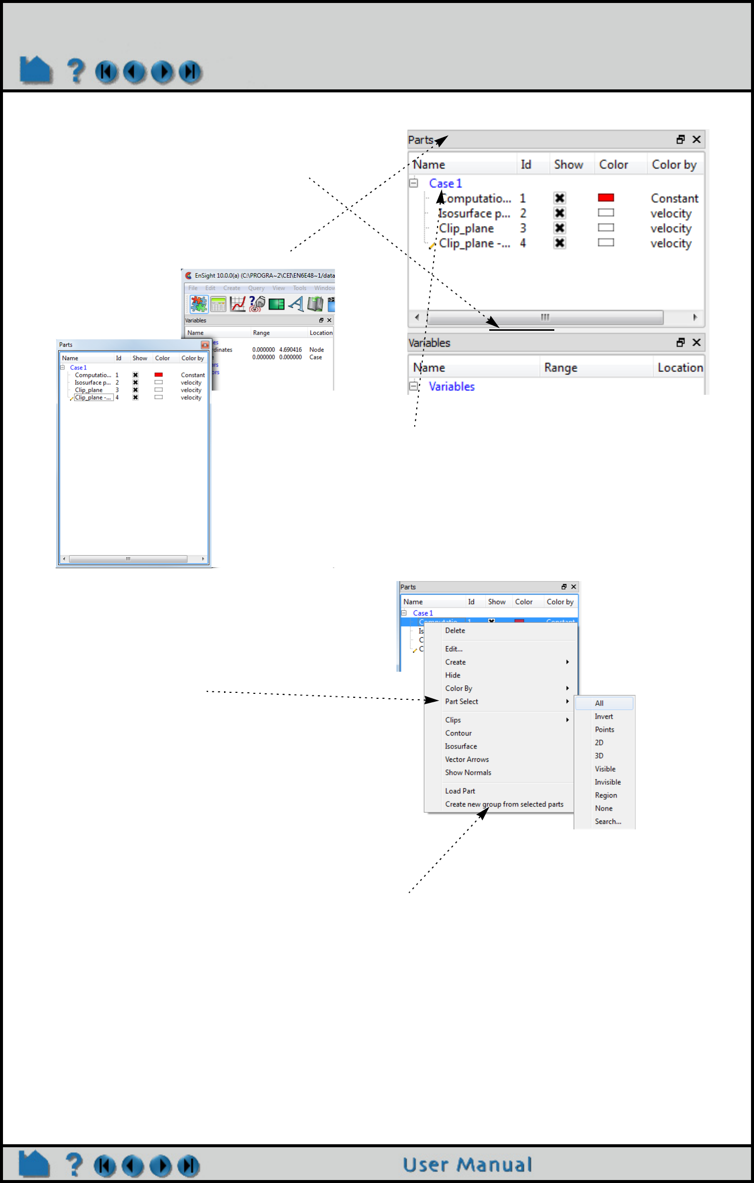
Page 257
HOW TO INTRODUCTION TO PART CREATION
There are a number of right click
capabilities for a part. The right click
works in both the Parts list as well as
in the graphics window. Shown at
right is that you can perform various
Part selection operations.
You delete a part by either utilizing
the right click pulldown, or you can
select the part and hit the Delete
keyboard button in either the Parts
list or in the graphics window.
There are several ways to easily select multiple
parts. If you wish to select all parts in a Case (which
is really just a group) you select the blue Case line
in the Parts list. You can also perform part selection
operations via the right click pulldown menu.
You can create part groupings by selecting one or more parts
and creating a group from the right click pulldown.
Once a part group has been created you can drag and drop
parts into/out of the group.
The part list can be resized by grabbing the
boundary between the panels (the mouse
cursor will change to show a resize handle if
you’re in the right spot)
You can also grab the Parts panel by the title
bar and drag the entire panel out from its user
interface dock location.
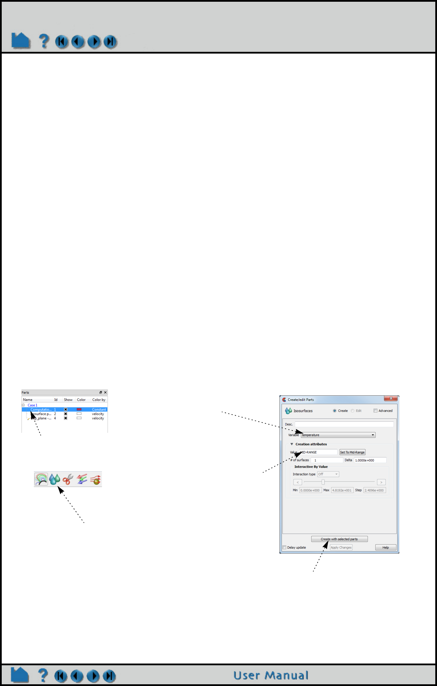
Page 258
HOW TO INTRODUCTION TO PART CREATION
Also, Items in the Parts List can be selected using standard selection methods:
Creating Parts
The mechanism for creating derived parts is largely the same regardless of part type:
1. In the Parts List, select the part(s) to use as parents.
2. Select the desired creation feature. This can be done via the Feature Icon Bar if the required creation feature is
visible or can be selected via the Create pulldown from the main interface or from the right click on the part (either
in the Parts list or in the graphics window). Any one of these will bring up the Feature Panel for the part type in
question in create mode.
3. Set any desired in the Feature Panel.
4. Click the “Create with selected parts” button to create the part.
There are also right click methods to create parts. These go through the same steps as above but may make some
assumptions to quickly create a part.
The example below shows Isosurface part creation:
To ... Do this ... Details ...
Select an item Select
(or single-click)
Place the mouse pointer over the item and click the left mouse button. The item is
highlighted to reflect the “selected” state.
Extend a (possibly long)
contiguous selection
Shift-click Select the first item. Place the mouse pointer over the last item in the list to be
selected. Press the shift key and click the left mouse button. This action will
extend a selection to include all those items sequentially listed between the first
selection and this one.
Extend a non-contiguous
selection
Control-click Place the mouse pointer over the item. Press the control key and click the left
mouse button. This action will extend a selection by adding the new item, but not
those in-between any previously selected items.
De-select an item Control-click Place the mouse pointer over the selected item. Press the control key and click the
left mouse button. This action will de-select the item.
Edit the part via the
Feature Panel area for
parts
Double-click Place the mouse pointer over the item and click the left mouse button twice in rapid
succession.
3. Select the variable to use.
5. Click “Create with selected parts”.
1. Select the parent part(s).
4. Select an appropriate isovalue.
(Often there is a sensible default)
2. Select the Isosurface Feature
Icon.
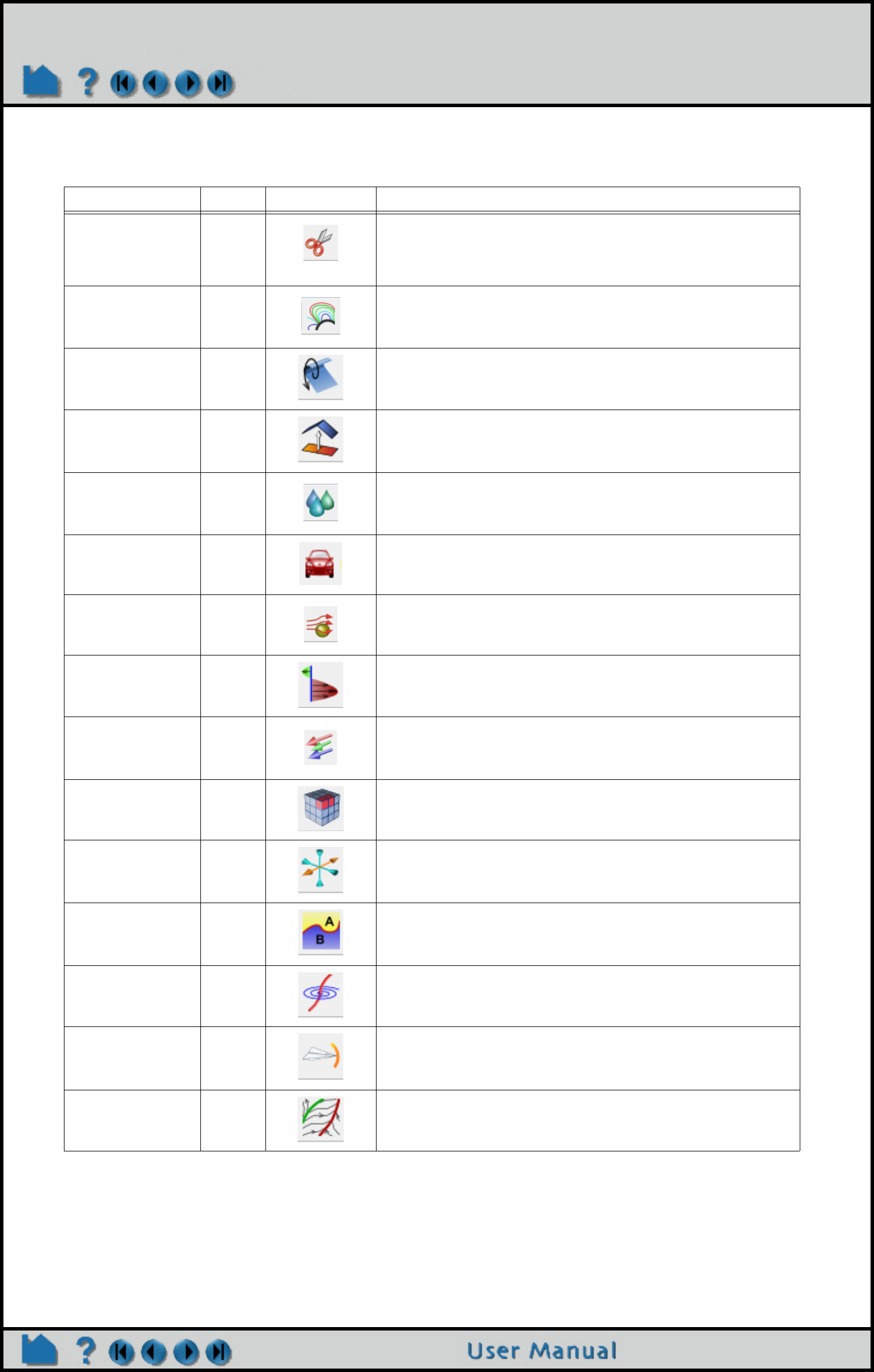
Page 259
HOW TO INTRODUCTION TO PART CREATION
Part Types
The following table provides information on the available part types in EnSight:
Part Type Symbol Feature Icon Description
Clip 2 A surface or line resulting from a clip of parts using an IJK, XYZ, or
RTZ surface of the parts; or a clip of other parts using the Line,
Plane, Box, Cylinder, Sphere, Cone, or Surface of Revolution tool;
or a clip of other parts by revolving an existing 1D part.
Contour C Lines of constant value on 2D elements.
Developed
Surface
D A planar surface derived by unrolling a surface of revolution (e.g.
unrolling a clip created with the Cylinder tool).
Elevated Surface E A part created by scaling a 2D part (in the direction of the local
surface normal) based on the value of a variable.
Isosurface I A surface of constant value through 3D elements.
Model M An original part (i.e.loaded from a disk file) or created through some
operation (e.g. copy or extract) on a model part.
Particle Trace T A part consisting of the paths taken by one or more massless
particles as integrated through a vector (typically velocity) field.
Profile P Plot of a variable along a line (the 2D counterpart to an elevated
surface).
Vector Arrow V A part consisting of a set of arrows showing direction and
magnitude of a vector variable.
Subset S A part created by node and/or element label range(s) from model
part(s).
Tensor Glyph G A part consisting of tensor glyphs showing direction and relative
magnitude of the eigenvectors of a tensor variable.
Material Part A A part created according to the intersection of or domains of
material values.
Vortex Core X A part consisting of line segments down the center of flow vortices.
Shock Surface/
Region
K A part consisting of the surface or volume elements where shock is
higher than a threshold.
Separation/
Attachment Line
L A part consisting of line segments on a surface where flow
separation and attachment is occurring.

Page 260
HOW TO INTRODUCTION TO PART CREATION
Part Operations
EnSight provides several powerful part operators. These operations are accessible from the Edit > Part submenu or
from right click on a part.
Part
All parts have numerous that control behavior and display. Although many can be controlled either through the Part
Quick Access Icons or the right mouse button options, complete access is provided by the Feature Panel. Part and
the Feature Panel are covered in detail in How To Set .
Copy The copy operation creates a dependent copy of another part. The part is created on the client and
is not known to the server. The new part has its own set of (except for representation), but shares
geometric and variable data with the original.
One of the best reasons to create a copy is to show multiple variables on one part at the same time
in a side-by-side configuration. The copies can be moved independently since each new copy is
automatically assigned a new frame.
See How To Copy a Part for more information.
Clone This operation will create a new part identical to the one(s) being cloned. They are not dependent on
the part cloned for model parts but are dependent on the same parent parts in the case of created
parts.
See Clone a Part for more information.
Group This operation will collapse the selected parts into a new “umbrella” part. Grouping is most often
used to combine a series of parts into a single entity for ease in handling. No new part is created -
only a hierarchy in the Parts list. The operation is reversible through the Ungroup command.
See How To Group Parts for more information.
Delete The delete operation completely removes not only the currently selected parts, but also any parts
derived from the selected parts.
See How To Delete a Part for more information.
Extract The extract operation is closely tied to part representations. Extract creates a new dependent part
using only the geometry of the current representation of the part. For example, if the current
representation of a part consisting of 3D elements is Border, the result of extraction will be a part
consisting of all unshared 2D elements (the surface).
Extract is most often used to reduce the amount of information for a part (e.g. for faster display or for
geometry output) or to create a surface shell part – perhaps for subsequent cutting – of a 3D
computational domain.
See How To Extract Part Representations for more information.
Merge Merge creates one new dependent part from one or more selected parts. The original parts are
unchanged. If only a single part is selected for the operation, merge will create a “true” copy of the
part (as opposed to the “shallow” copy that the Copy operation creates).
Merging is most often used to combine a series of parts into a single part for ease in handling (such
as attribute setting).
See How To Merge Parts for more information.
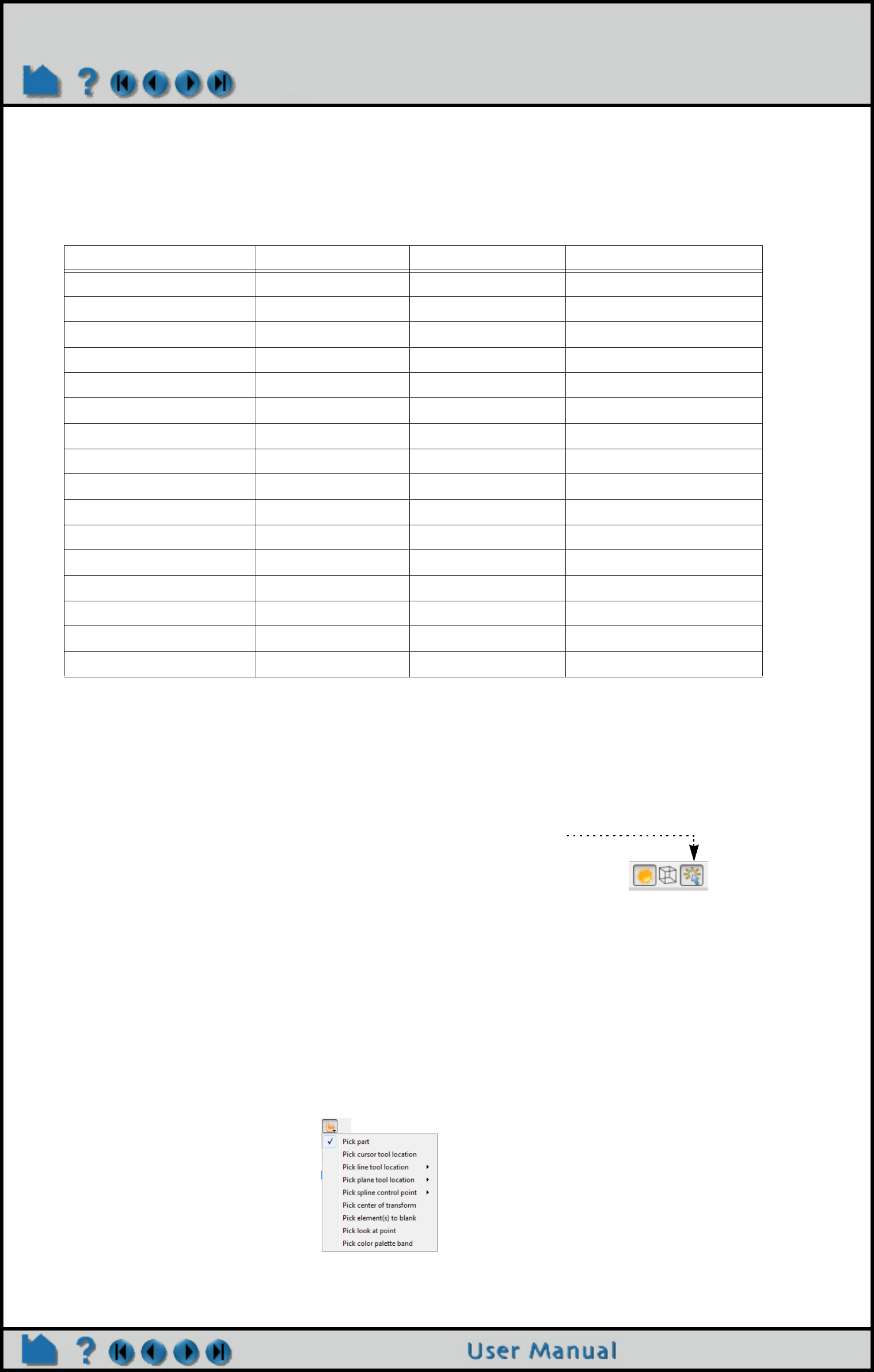
Page 261
HOW TO INTRODUCTION TO PART CREATION
Where Parts Are Created and Maintained
Part creation occurs on either the EnSight client or the server. Since the data that is available on the client and server
are different, it is useful to understand where parts are created and where the data is stored. For example, you can
only perform a query operation for parts that are stored on the server. The following table provides this information
for each part type:
In the last column, “depending on representation” means the current visual representation for the part. For
example, if the part’s visual representation is “Not Loaded”, then no data is currently present on the client.
Hints and Tips
With some datasets that contain many parts, it is important to maintain the connection between a part as displayed in
the Graphics Window and the corresponding item in the Parts List. EnSight shows the selected parts as highlighted.
To toggle this feature on or off, click on the Highlight Selected Parts toggle.
You can rapidly cycle through items in the Parts List using the up/down arrow keys on your keyboard. Select any item
in the list and then press the up arrow (to move to previous entries) or down arrow (to move to subsequent entries).
This is particularly helpful when used in conjunction with the Part(s) Selected Highlighting (as described above) to
quickly locate a part of interest.
You can select parts in the Parts List using a single left click on the part in the graphics window. This should work
unless your single-click settings has been changed from the default Pick Part. To change it back to Pick Part,
Edit>Preferences and click on Mouse and Keyboard. You can also select parts in the Graphics Window by picking
using the ‘p’ key. Select Pick Part from the Pick pull-down. In the Graphics Window, place the mouse pointer over any
portion of the desired part and press the ‘p’ key. If you hold down the control key at the same time, the part is added
to the list of currently selected parts.
Part Type Where Created Data on Server? Data on Client?
Clip server yes depending on representation
Contour client no yes
Developed Surface server yes depending on representation
Discrete Particle N/A yes depending on representation
Elevated Surface server yes depending on representation
Isosurface server yes depending on representation
Model N/A yes depending on representation
Particle Trace server no yes
Profile client no yes
Vector Arrow client no yes
Subset server yes depending on representation
Tensor Glyph client no yes
Vortex Core server yes depending on representation
Shock Surface/Region server yes depending on representation
Separation/Attachment Line server yes depending on representation
Material server yes depending on representation

Page 262
HOW TO INTRODUCTION TO PART CREATION
A quick way to create parts using the default settings is to right click on a part in the graphics window. A pulldown
selection will appear that will give you the option to create a Contour, Isosurface or Vector Arrow part using the default
settings using the parent as the part you right clicked.
Selected parts can be written to disk and loaded in a future session. Select File > Save > Geometric Entities ... You
have the option of saving either in EnSight format, VRML format, STL format, or other user-defined formats. See How
To Save Geometric Entities for more information.
SEE ALSO
User Manual: Features, Parts
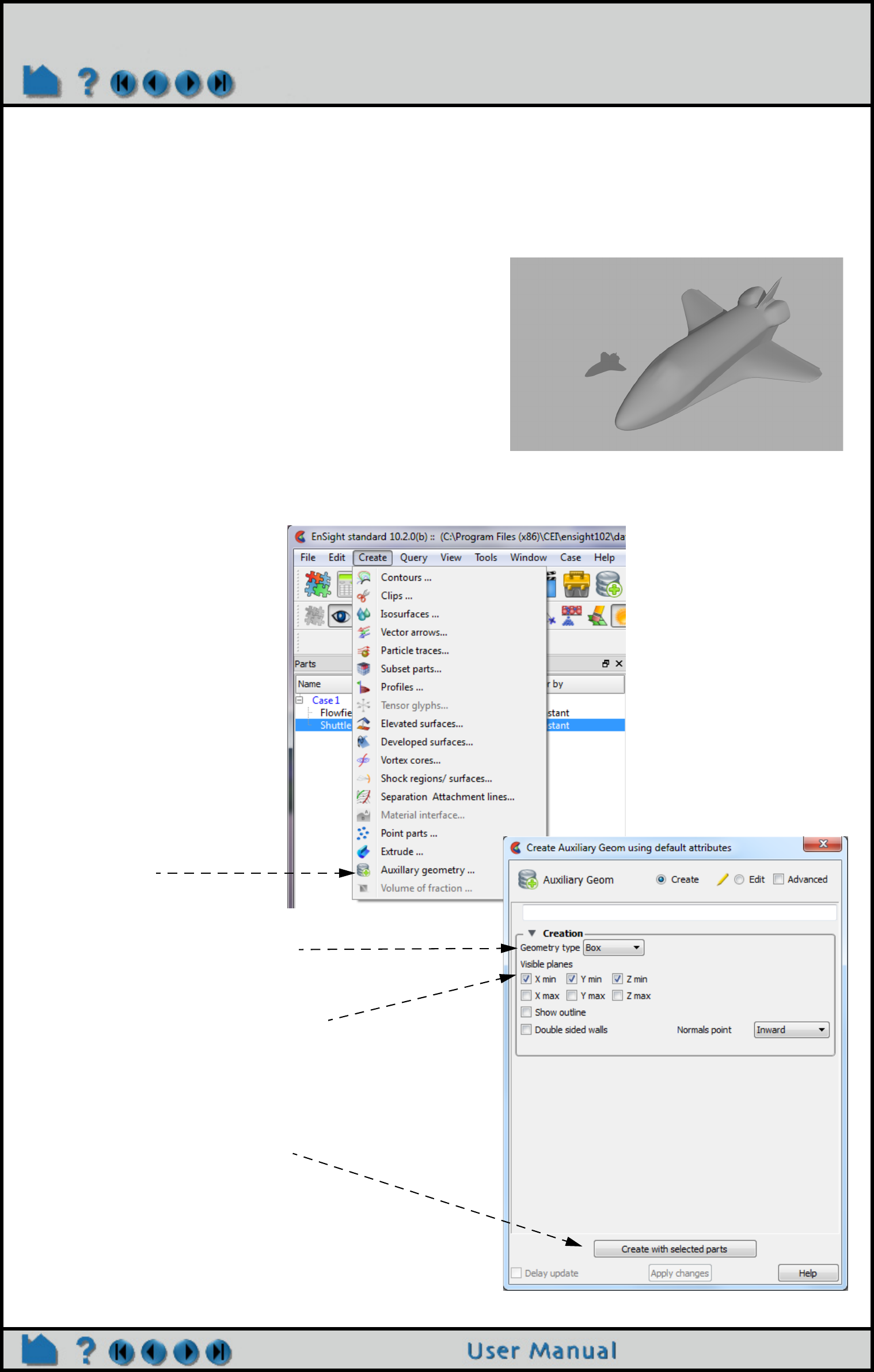
Page 263
HOW TO CREATE AUXILIARY GEOMETRY
Create Auxiliary Geometry
INTRODUCTION
Auxiliary geometry can serve as reference geometry to augment visual settings for parts. It can be used for things like
mapping textures upon, or to cast shadows from model part(s) upon. Auxiliary geometry quickly bounds your
specified part(s), and is interactively extended about the vicinity of the part(s).
BASIC OPERATION
Shadow of the shuttle is being cast on
auxiliary geometry part.
1. Select the parent part(s) in
the part list
2. Select Create->Auxiliary
geometry...
5. Click “Create with selected
parts”.
Note you can click on each of the the
walls and drag it to a desired
location.
3. Select the Geometry type box.
Currently ‘Box’ is the only option but it is
a pulldown because more may be
added in the future.
4. Choose which wall(s) of the box to
show.
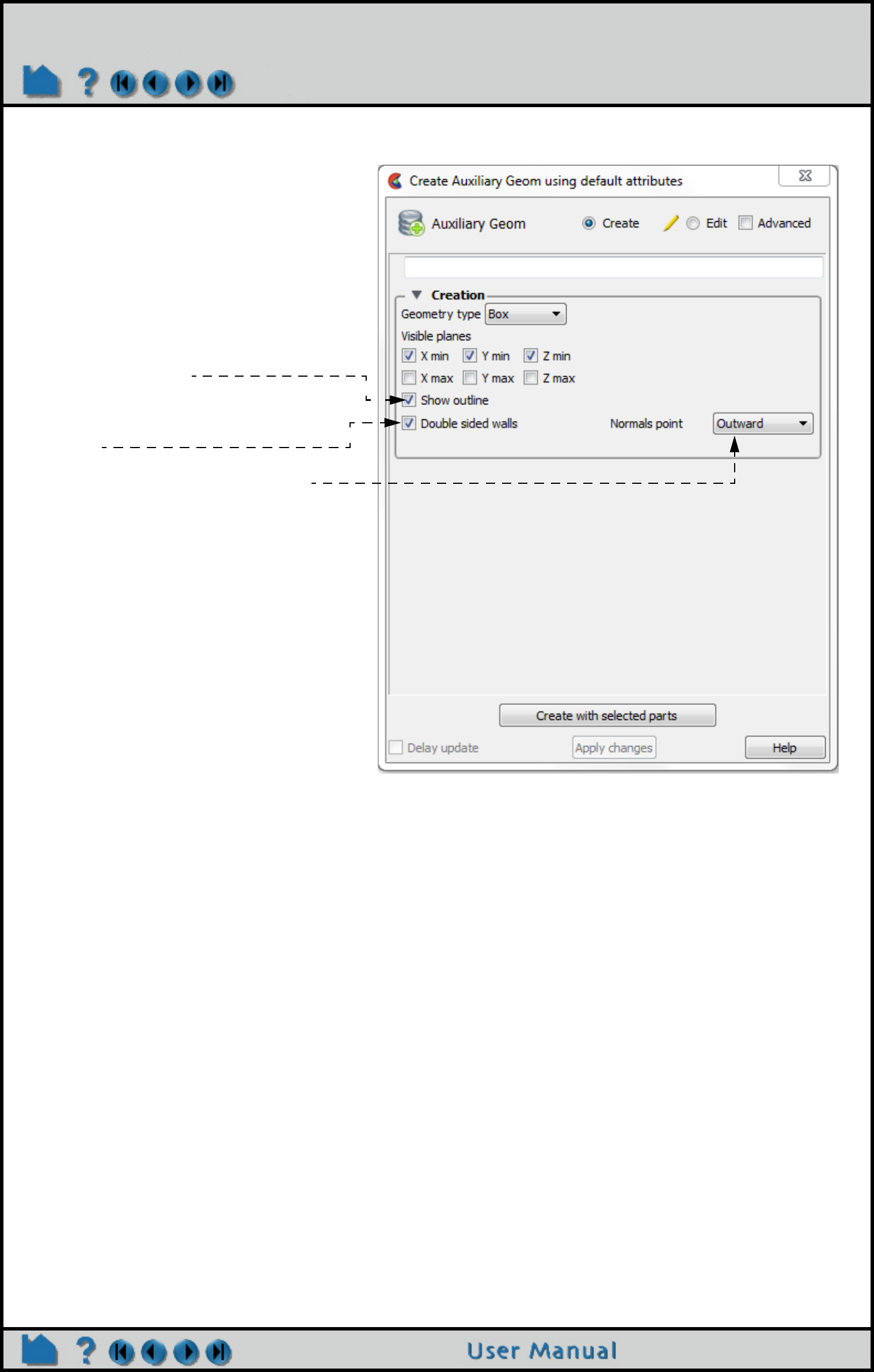
Page 264
HOW TO CREATE AUXILIARY GEOMETRY
ADVANCED USAGE
OTHER NOTES
Auxiliary geometry can be used in conjunction with directional lighting and ray traced images to display cast shadows
of the specified parts.
SEE ALSO
User Manual: Auxiliary Geometry
How To Set LIght Sources
How To Use Raytrace Rendering
Other options can be specified to fine tune
the geometry.
1. Show the bounding box outline of the
auxiliary geometry.
2. Produce double-sided walls to
resolve corner issues for ray-traced
images.
3. Control surface normal direction.

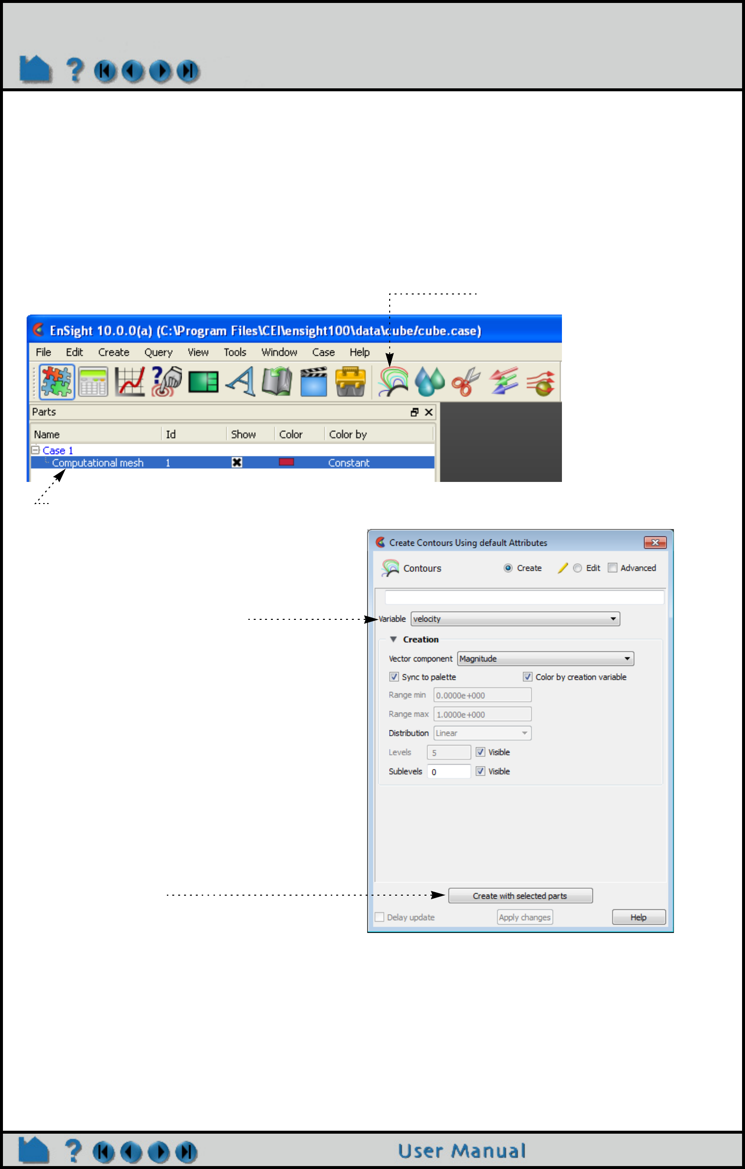
Page 266
HOW TO CREATE CONTOURS
Create Contours
INTRODUCTION
A contour is a line of constant value on a two-dimensional (though not necessarily planar) surface. The region on one
side of the line is larger than the isovalue; the region on the other side is less than the isovalue. EnSight creates
contour lines in groups where the isovalues either correspond to the levels in the palette defined for the contour
variable, or a user specified range and. The contour lines can also be labeled with the corresponding palette value.
BASIC OPERATION
1. Select the parent part.
3. Select the variable to use.
2. Click the Contours icon.
4. Click the Create with selected
parts button.
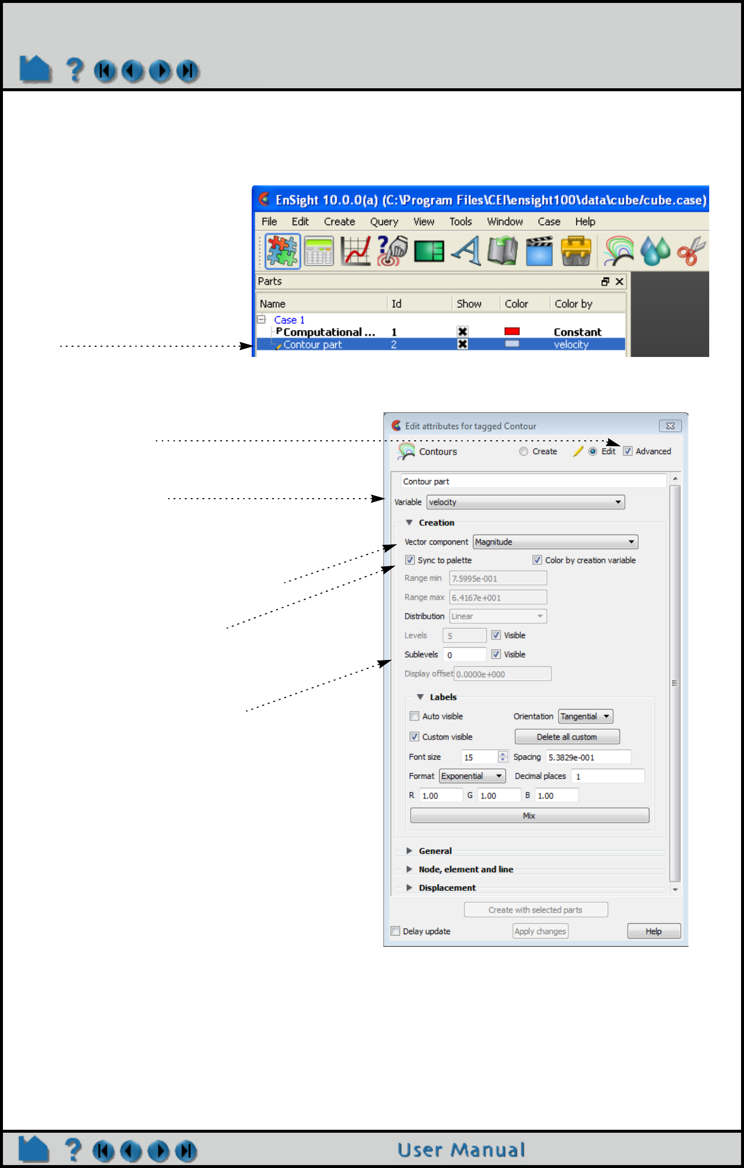
Page 267
HOW TO CREATE CONTOURS
The Contour Feature Panel lets you set the number of contour levels (and sublevels) as well as attach labels to the
contour lines. Contour lines can be synced to the palette levels or can be chosen manually.
In the parts list, double-click
the contour part you wish to
edit.
If you want contour lines for each level of the palette:
1. Select Advanced.
2. Select the Variable.
And the component or magnitude if a
vector.
3. Toggle on Sync To Palette.
4. Select the number of sublevels
desired (if any). And make sure Visible
toggles are set as desired.
See How To Edit Color Maps for how to
set the color palette levels.

Page 268
HOW TO CREATE CONTOURS
If you want to set the contour line ranges:
In the parts list, double-click
the contour part you wish to
edit.
1. Select Advanced.
2. Select the Variable.
And the component or magnitude if a
vector.
3. Toggle off Sync To Palette.
4. Specify the Min and Max Range.
5. Specify the method for the Range.
6. Specify the
number of Levels and sublevels.
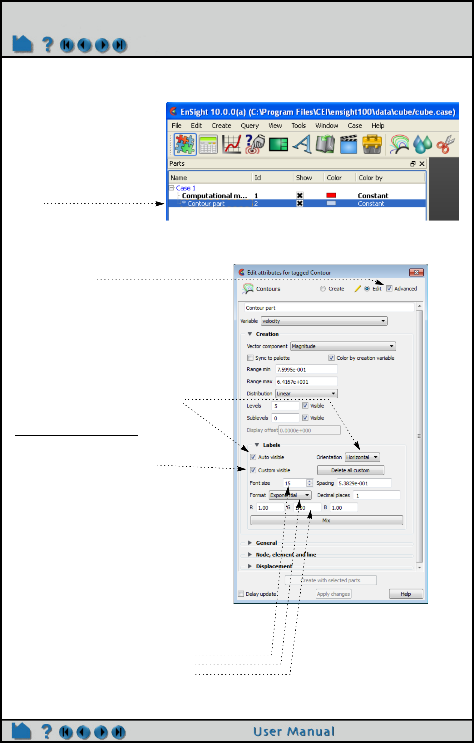
Page 269
HOW TO CREATE CONTOURS
If you want to place labels on the contour lines:
In the parts list, double-click
the contour part you wish to
edit.
1. Select Advanced.
2. Auto labels will create a label on each
main contour loop with a spacing as
specified.
Custom labels: Right-clicking
3. Toggle on or off the visibility of the
custom created contour labels.
4. Custom labels can be created by right
clicking on a contour loop and choosing
Label>Add to Add a label.
5. You can also remove any label by right
mouse clicking on the label and choosing
the Label>"Delete this one" option.
Label formatting
6. You can control the label orientation,
format (linear, log, or quadratic), size, and
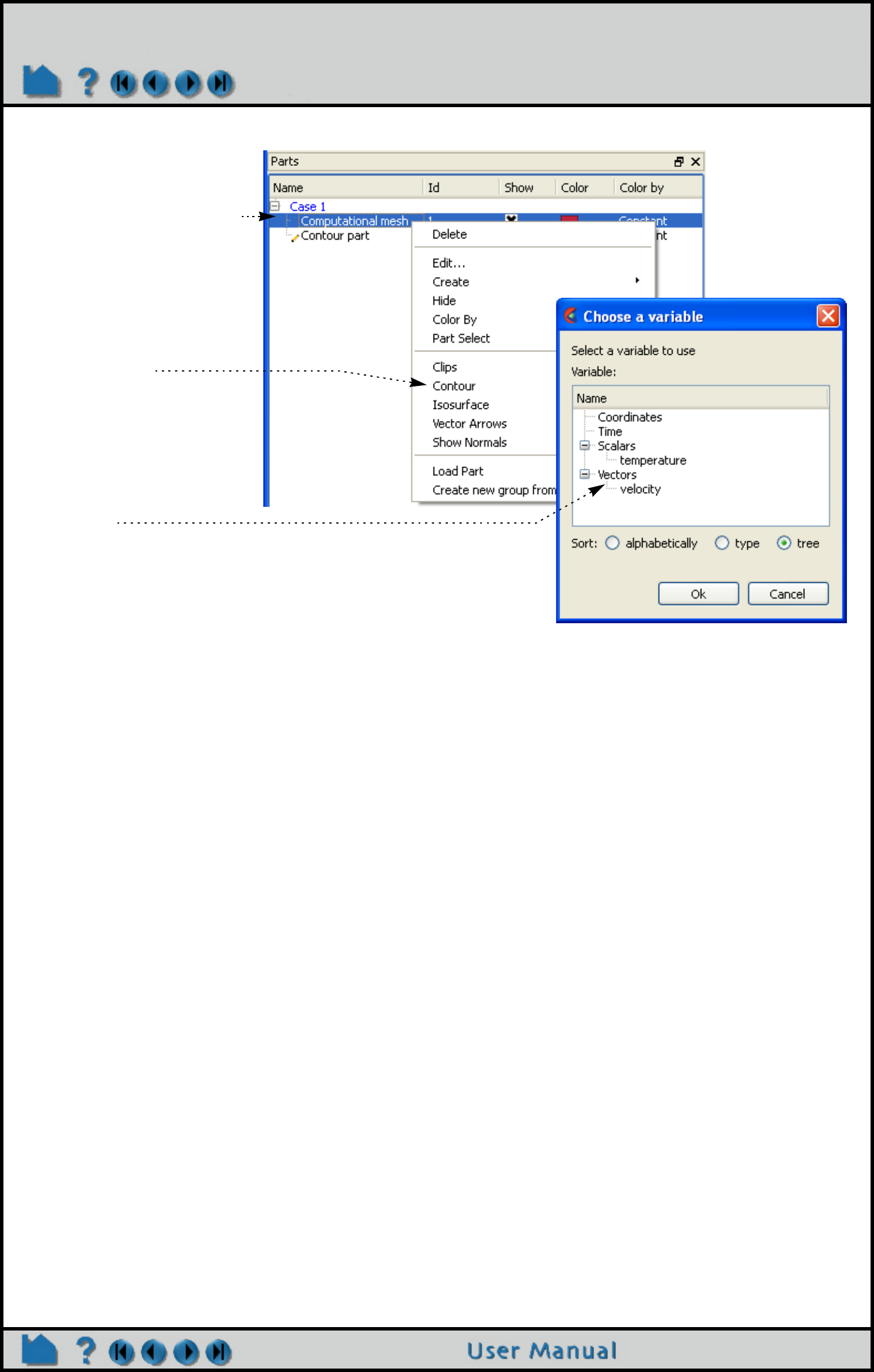
Page 270
HOW TO CREATE CONTOURS
Shortcut
ADVANCED USAGE
When Sync To Palette is specified, the levels of the variable palette are used as the contour levels. You must edit the
palette using the Feature Panel for Variables to modify the number of levels, etc. See How To Edit Color Maps for
guidance.
OTHER NOTES
The default behavior is to color the contour part by the creation variable. If you toggle this off, the contour part will not
be colored by a variable automatically, but will be white.
Unlike most part creation operators, contours are created from the client’s representation of the part – not the
server’s. If the parent part of the contour consists of one-dimensional elements or has no client-side visual
representation at all, the resulting contour will be empty. This would be the case if the parent part was currently
displayed as feature angle, border representation, or not loaded. The 3D border, 2D full representation is typically
used for contour part parents. See How to Change Visual Representation for more information.
SEE ALSO
Introduction to Part Creation, How To Edit Color Maps.
User Manual: Contour Parts
Right click on a part in the Parts
list or in the graphics window.
In the resulting pulldown,
choose Contour.
A window will pop up to choose
a variable.
This then automatically creates
a contour part with the default
settings using the selected
variable and using the right-
clicked part as the parent part.
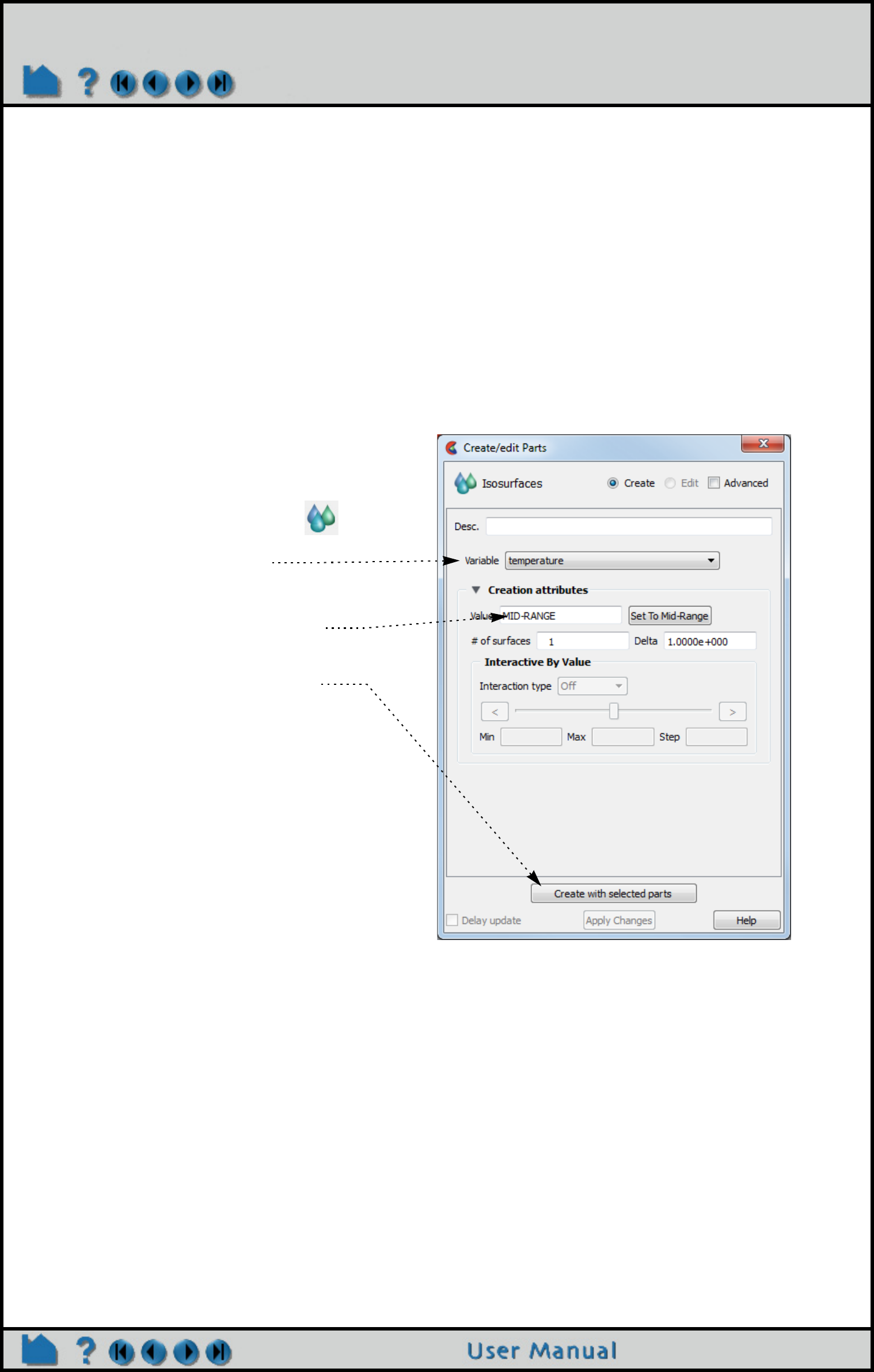
Page 271
HOW TO CREATE ISOSURFACES
Create Isosurfaces
INTRODUCTION
An isosurface is a surface of constant value in a three-dimensional field. It is the 3D counterpart to the contour loop:
the region on one side of the isosurface has values greater than the isovalue; the region on the other side has values
less than the isovalue. In EnSight, an isosurface can be generated from a scalar variable, a component or magnitude
of a vector variable, or a component of the model coordinates.
An isosurface of a scalar or vector variable is typically a complex surface reflecting the of the underlying variable.
Isosurfaces of coordinates, however, are typically regular geometric shapes such as planes, cylinders, cones or
spheres.
BASIC OPERATION
Shortcut
Right click on a part in the graphics window. In the resulting pulldown, choose Isosurface. A window will pop up to
choose a variable. This then automatically creates an isosurface part with the default settings using the selected
variable and using the right-clicked part as the parent part.
1. Select the parent part.
3. Select the variable to use.
2. Click the Isosurface
Feature icon.
4. Select an appropriate isovalue.
(the default will be a mid-range value)
5. Click “Create with selected parts”
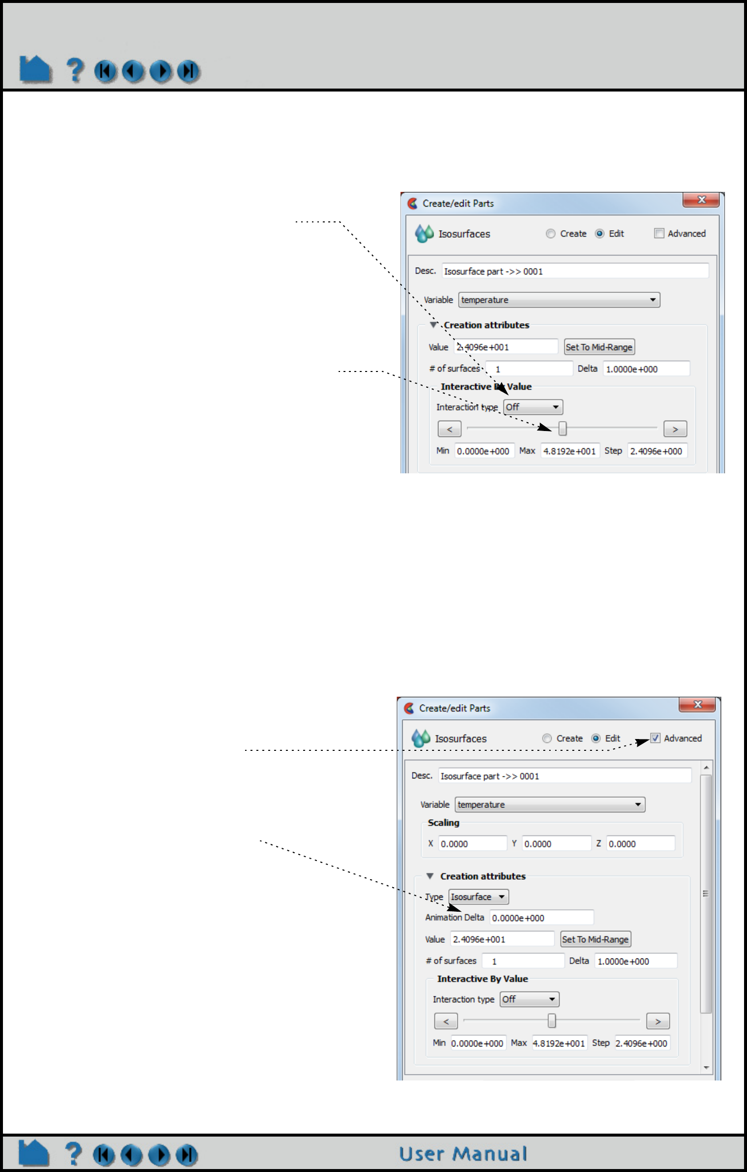
Page 272
HOW TO CREATE ISOSURFACES
ADVANCED USAGE
Interactive Isosurfaces
You can have EnSight automatically generate and display isosurfaces as you adjust a slider with the mouse.
You can also set the Interactive mode to Auto and EnSight will automatically sweep from Range Min to Max with step
size equal to Increment.
Shortcut
In the graphics window, left click on the isosurface and you will see a green handle appear. Drag the handle to
change the value of the isosurface and see a printout on the screen of the actual value as you drag the isosurface.
Isosurface Animation
A range of isosurfaces can be automatically generated and viewed in a flipbook. Flipbooks provide on-screen
animation of various dynamic events and (in the default setting) permit graphic manipulation (e.g. rotation or zoom)
while the animation runs.
1. Set the Interactive mode to Manual.
2. Adjust the slider to the desired location.
1. Double click on the Isosurface part.
2. Click on the Advanced button.
3. In the Creation section, set the Animation Delta
to an appropriate value. For each page (frame)
of the flipbook, this value will be added to the
current value to yield the new isovalue.
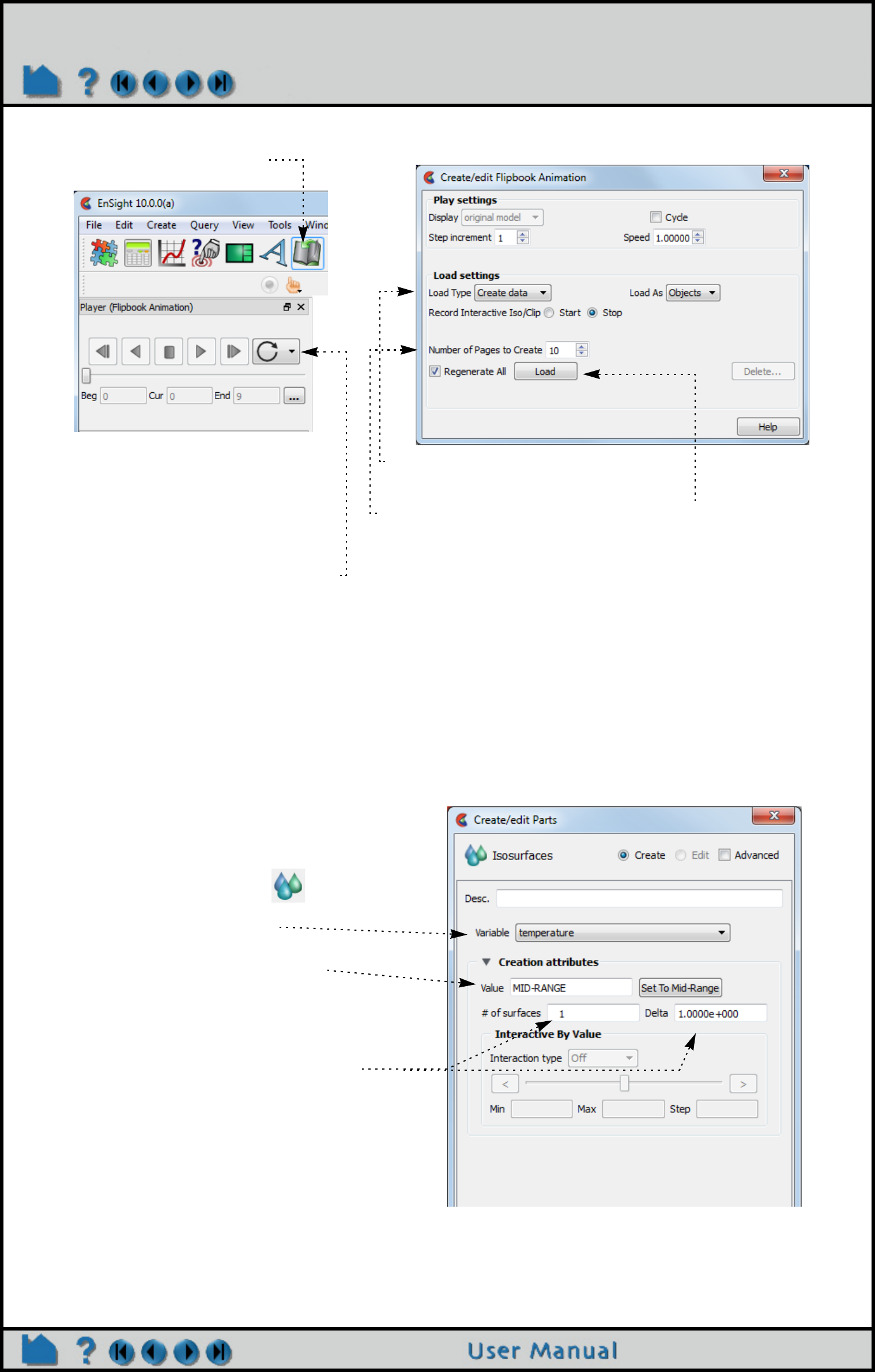
Page 273
HOW TO CREATE ISOSURFACES
Alternatively you can put the isosurface in interactive manual mode, and then click on the flipbook icon, click on the
more detail icon, choose Load Type Create Data, then click on the Start button, move the isosurface, then click on the
stop button and choose your number of pages and click Load.
Creating Multiple Offset Isosurfaces:
You can have EnSight create multiple isosurfaces at a specified delta value. The results is a group of isosurfaces:
Isovolume Creation
An isovolume is a volume whose constituents (e.g. nodes and elements) are constrained to a constant interval range
in a scalar field. In EnSight, you can constrain the isovolume to ranges less than an interval minimum, greater than an
4. Click the Flipbook icon.
6. Set the number of pages
to an appropriate value.
7. Click Load.
8. When loading is complete use the
controls to play the flipbook
5. Choose Create Data.
1. Select the parent part.
3. Select the variable to use.
2. Click the Isosurface
Feature icon.
4. Select an appropriate isovalue.
(the default will be a mid-range value)
6. Click “Create with selected parts”
5. Set the number of surfaces and the
delta between them. Note that you can
only change the number of surfaces at
creation.
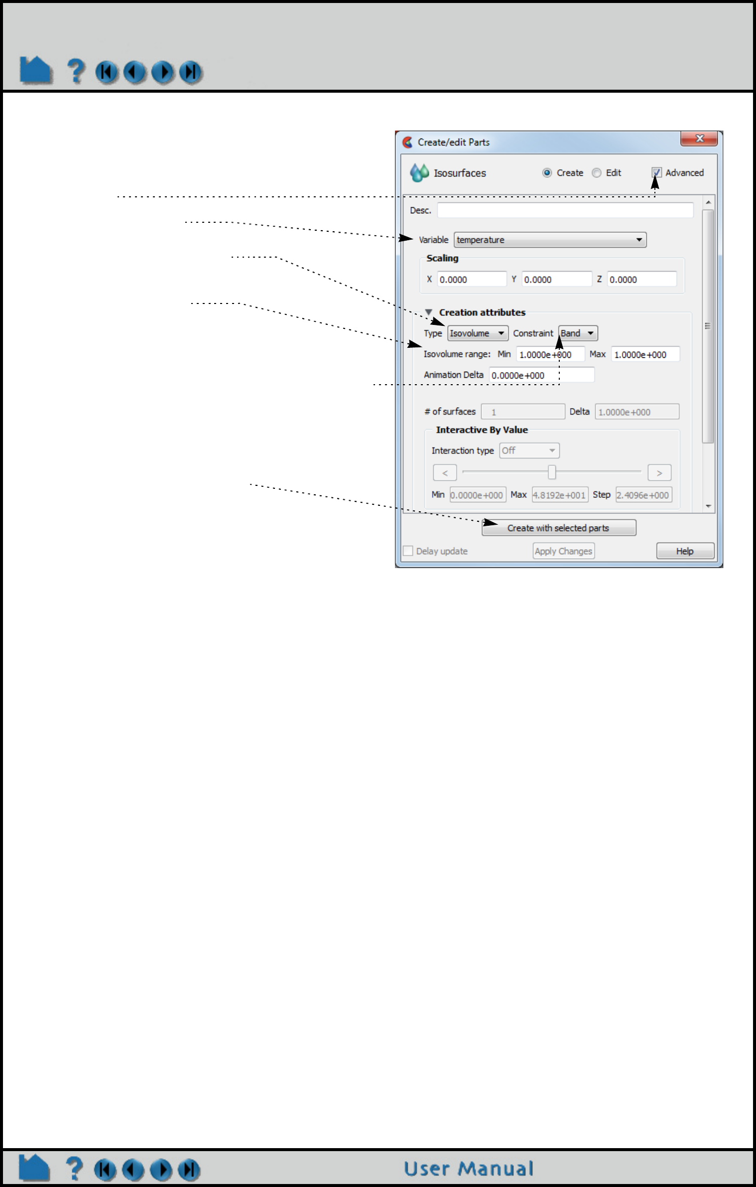
Page 274
HOW TO CREATE ISOSURFACES
interval maximum, or between the interval minimum and maximum.
OTHER NOTES
Effective display of more than two nested isosurfaces is difficult. Set transparency on the outermost isosurface(s) to
reveal the inner surfaces. To avoid confusion, don’t try to display isosurfaces of more than one variable
simultaneously, or multiple isosurfaces of the same variable colored by different variables.
SEE ALSO
How-To Create a Flipbook Animation, How-To Create a Keyframe Animation
User Manual: Isosurface Parts
1. In the Isosurface Feature Panel, toggle on
Advanced
3. Set the type to Isovolume.
5. Set the Constraint to Band to constrain the
isovolume within an appropriate Min and Max
range of the scalar variable. Min will create an
isovolume constrained to be <= o the value given
while Max will create an isovolume >= to the value
given.
4. Set the Min and Max.
2. Choose a variable.
6. “Create with selected parts”

Page 275
HOW TO CREATE PARTICLE TRACES
Create Particle Traces
INTRODUCTION
Streamline and Pathline Traces:
A particle trace represents the path a particle would take if released in a flow field. From an initial seed point (the
emitter), a path is formed by integrating through the velocity field over time. The path is therefore everywhere parallel
to the flow. For models with rotational periodic geometry, streamlines and pathlines can exit a symmetry face and re-
enter the corresponding symmetry face and continue. Traces calculated using a single time step in a flow field are
called streamlines. The path calculated using a transient flowfield that is updated as the calculation proceeds is
known as a pathline.
EnSight provides a great deal of control over emitter definition and trace appearance:
• Emitters can be defined using one of the built-in tools (Cursor, Line, or Plane) or by clicking on any
surface in the Graphics Window. The nodes of an arbitrary part can be used as an emitter, or the emitter
time and locations can be read from a file (see EnSight Particle Emitter File Format in the Chapter 11 of
the User Manual).
• The streamline path can be generated in the positive, negative, or positive and negative time directions.
• Traces can be restricted to lie on any surface to search for flow topology and separation features.
• For transient cases, an emitter can have a delta time that controls the periodic release of additional
particles into the dynamic flow.
• Emitters can be interactive: as you move the emitter with the mouse, the associated traces
automatically recalculate and redisplay (This option is not available for surface-restricted Particle
traces, traces emitted from a Part, in Server of Server mode, or for Pathlines).
• Trace paths can be displayed as lines, ribbons, tubes, or as square tubes, where ribbon or tube twist
follows the local flow rotation around the path.
• Right-click on an individual trace and select “Hide this trace emission” to hide it and select “Show all
trace emissions” to reset the traces to visible. This is useful for making uninteresting traces invisible
while retaining the interesting ones.
• If the particle trace part is colored by a constant color: then the following options are available:
- Right-click and select "Set trace emission to random colors" to assign a random color automatically to
each emission of the particle trace part. This is useful for distinguishing between traces.
- Right click on an individual trace and select "Set trace emission to constant color..." to assign a color
to the individual emission selected. The standard color widget will appear to allow you to select a color.
- To reset the color of the trace colors back to a uniform color, simply color the traces by a constant.
• Particle traces can be easily animated to provide intuitive comprehension of the flow field. Complete
control over all aspects of the animating tracers is provided, including length, speed, and release
interval for multiple pulses.
Node Tracks:
Another form of trace that is available in EnSight is entitled node tracking. This trace is constructed by connecting the
locations of nodes through time. It is useful for changing geometry or transient displacement models (including
measured particles) which have node ids.
Min/Max Variable Tracks:
A further type of trace that is available is a min or max variable track. This trace is constructed by connecting the min
or max of a chosen variable (for the selected parts) though time. Thus, on transient models one can follow where the
min or max variable location occurs.
Both the node tracking and the min/max variable tracking options are like a connect-the-dots through time trace.
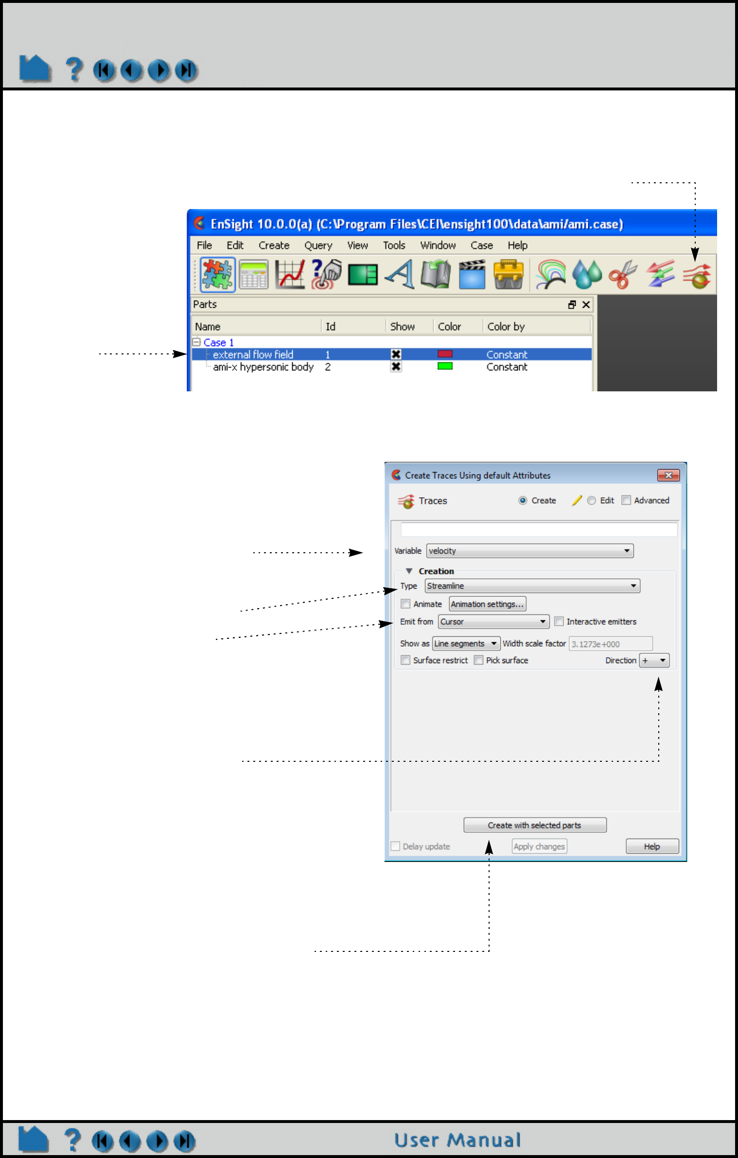
Page 276
HOW TO CREATE PARTICLE TRACES
BASIC OPERATION
To trace particles through a steady-state flow field (streamline):
1. Select the flow field
mesh part(s) to trace
through.
3. Select the vector variable to use.
2. Click the Particle Traces icon.
5. Select the desired emitter.
If the emitter is a tool (Cursor, Line, Plane),
position the tool at the desired emitter
location. If the chosen emitter is Part, then
enter the part number in the Part ID field and
press return.
4. Select Streamline as the type.
7. Click Create with selected parts buttons.
The particle traces will be created from the desired emitter. Their maximum time duration is
controlled via the Total Time Limit found under the Emitter Information when Advanced is
chosen instead of Simple.
6. Click to set the trace direction:
+: forwards in time (positive velocity
direction) from the emission point(s)
-: backwards in time (negative velocity
direction) from the emission point(s)
towards the entering flow boundary
(Streamlines only)
+/-: both forwards and backwards
(Streamlines only)
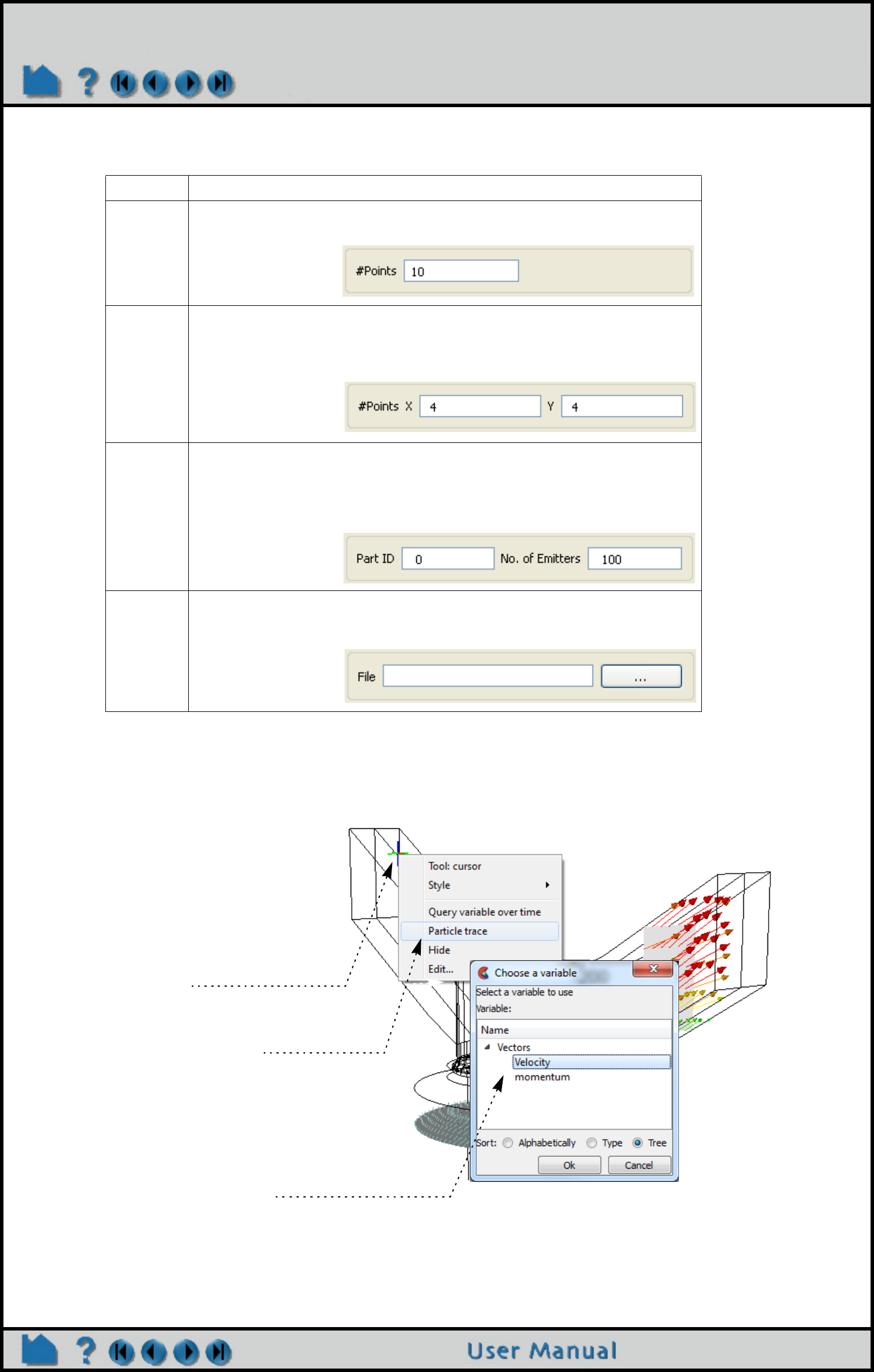
Page 277
HOW TO CREATE PARTICLE TRACES
The following are the available Emit From options. Note that traces will only be generated for those emitter points that
actually lie within an element of the selected flow field part(s).
Shortcut
.
Cursor A single trace will be emitted from the Cursor tool.
Line Multiple traces will be emitted from evenly spaced points along the Line tool.
Enter the desired number of traces in the # Points field and press return.
Plane Multiple traces will be emitted from evenly spaced points in a grid pattern over the
Plane tool. Enter the desired number of traces in the X and Y direction (with
respect to the Plane tool’s axis) in the # Points X/Y fields and press return. The
total number of traces will be the product of X and Y.
Part One trace will be emitted from the number of nodes of the part you specify. This
number of nodes will be randomly selected. Enter the Part ID number (from the
Main Parts list) of the part you wish to use as an emitter, and the number of nodes.
Limitation: if you create a particle trace from a Part ID, you cannot later change the
ID nor can you change the emitter type to something else (such as Cursor).
File Traces will be emitted from the locations, and at the times, specified in an EnSight
Particle Emitter file. See EnSight Particle Emitter File Format in Chapter 11 of the
User Manual.
To quickly create a particle trace:
1. Select the parent part(s).
2. Right click on a tool (cursor, line
or plane).
3. and choose Particle Trace.
If you have no parts selected then a
dialog will pop up to ask you to select
part(s).
If there are more than one vector
variables, then a pop up will ask you
to choose your vector variable.
This will create streamline trace(s)
using default settings and the tool as
the emitter
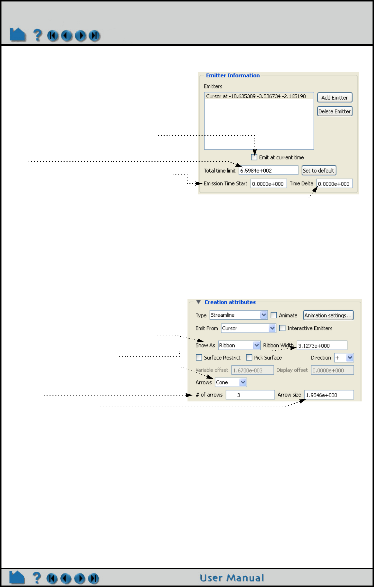
Page 278
HOW TO CREATE PARTICLE TRACES
The complete set of particle trace can be edited in the Create/edit dialog for Traces, when in Advanced mode. For
example, the emitter can be changed under the Emitter Information in the Creation section:
Display Traces as Ribbons, Tubes or Square Tubes, and control Arrowheads
Streamline and Pathline Particle paths can be displayed as lines, ribbons, tubes or square tubes, where ribbon or
tube twist follows the local flow rotation. To enable ribbon or tube display, and change trace arrowheads:
Animate Particles
Any type of particle trace can be animated. See How To Animate Particle Traces for more information.
Toggle on to have start time be the current time,
otherwise specify the start time (Streamlines only).
Set the total amount of time a trace will last (it may terminate
for other reasons as well). An intelligent default will be set for
you.
Solution time at which to begin pathline trace (Pathlines only).
Delta emission time for pathlines.
If not zero, a new set of traces will be emitted at S, S+D, S+2D, etc. into the changing flow field (where S is the Start time and
D is the delta value). Used to create streaklines or smoke traces. Animated streaklines are one of the most powerful methods
for visualizing transient flow (Pathlines only)
2. Set Show As to Ribbon, Tubes or Square Tubes.
3. If desired, change the default ribbon or tube width
and press return.
4. Select the Arrowhead representation desired.
(Cone, Normal, or Triangles)
5. Set the number of arrowheads to display along a
trace.
6. Set the arrowhead size.
Note that node tracks and min/max variable tracks can only be displayed as lines. Trace arrowheads can
be used for tracks, but this must be done from the Particle Trace Feature Panel.
1. Double-click the desired particle trace part in the Parts list (or right click on it in the list or in the
graphics window and select Edit...). This will open the Create/edit Parts dialog. If necessary, toggle on
Advanced mode, and open the Creation section.
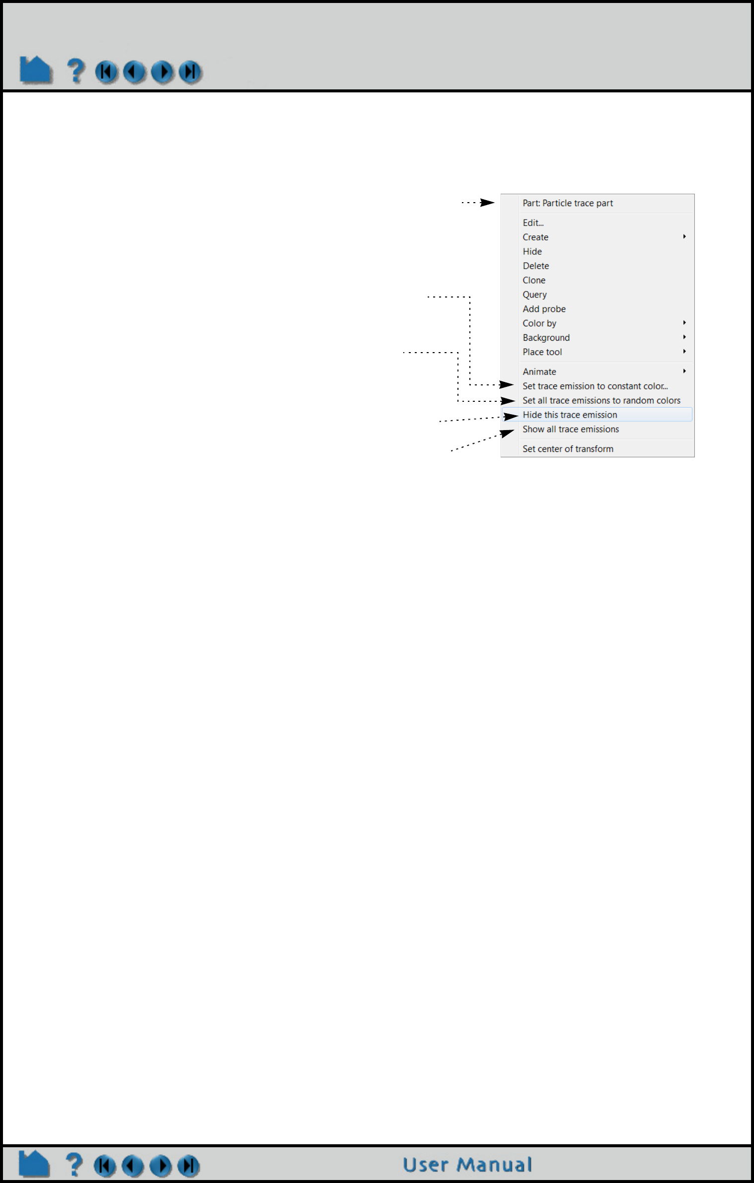
Page 279
HOW TO CREATE PARTICLE TRACES
Individual emission visibility and color
Each individual particle trace visibility status and color can be controlled via a right mouse button selection of the
particle trace in the graphics window. Note that coloring individual traces only works if the trace part is a constant
color.
1. Right click on an individual trace to see the following menu:
2. If the particle trace part is colored by a constant color (this
won’t work if the particle trace is colored by a variable).
a. Select "Set trace emission to constant color..." to choose a
color to set the selected emission. The standard color widget
will appear to allow you to select a color.
b. Select "Set trace emission to random colors" and EnSight
will automatically assign a random color to each emission of
the particle trace part.
c. To clear the per trace color simply color the part by a
constant color (see Change Color)
3. Each individual trace can be turned invisible by selecting
"Hide this trace emission"
4. Reset all traces to visible using "Show all trace emissions"
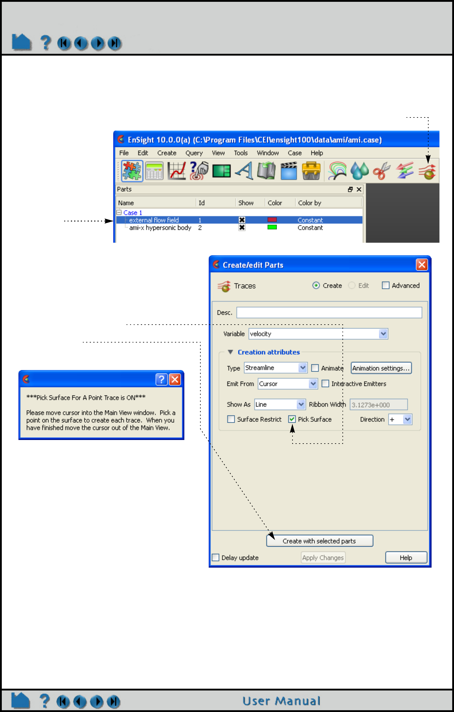
Page 280
HOW TO CREATE PARTICLE TRACES
Pick a Surface to Trace a Particle
Rather than emit from a tool or a part, you can also interactively pick points on a surface in the Graphics Window to
define emitter locations. To do this:
Note that you can also specify a rake (line) or net (plane) emitter by picking on a surface. Just set the emitter to Line
or Plane prior to clicking Create. Then follow in the instructions in the pop-up window.
3. Toggle on Pick Surface
4. Click Create.
And the following dialog will appear:
5. Do as instructed, move the mouse into the
Graphics Window and click the left mouse
button when the cursor is over the
desired location. The clicked point must be
found within some element of the selected
3D part to result in a trace.
6. You can click to create as many point
emitters as you like. When done, move
the mouse out of the Graphics Window.
7. Click off Pick Surface.
2. Click the Particle Traces icon.
1. Select the flow field
mesh part to trace
through.
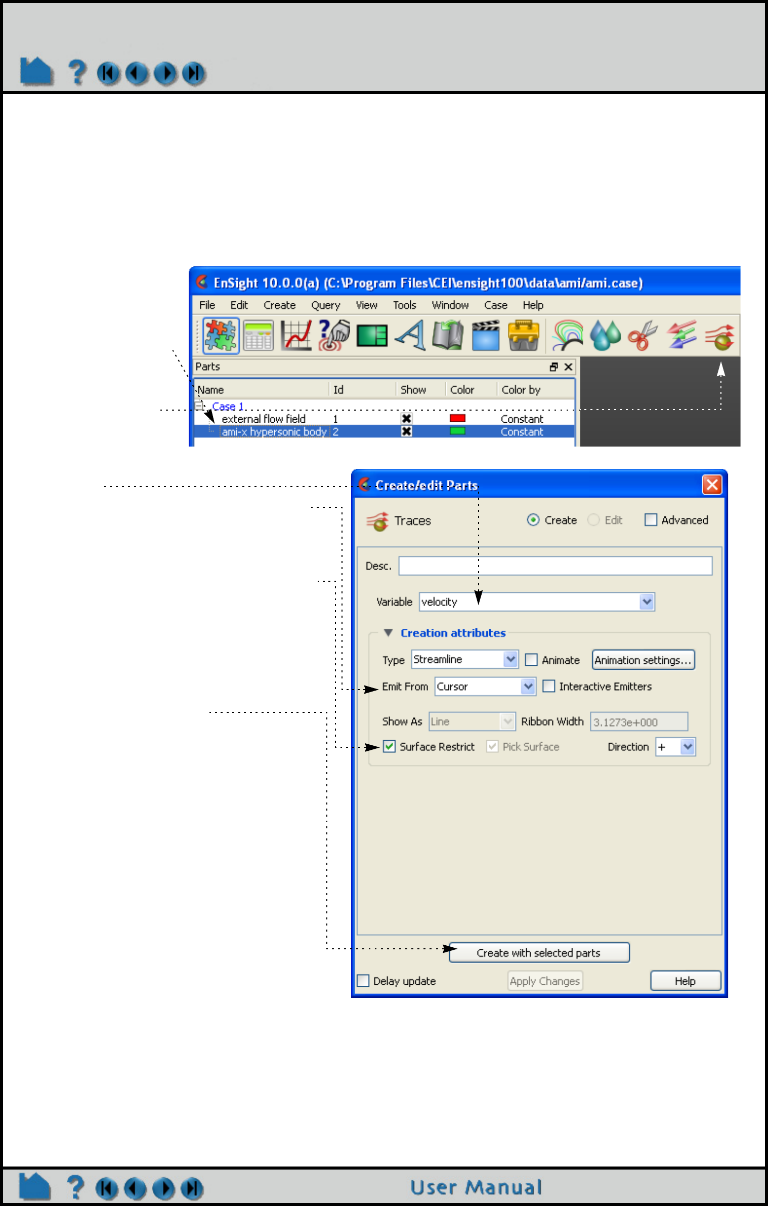
Page 281
HOW TO CREATE PARTICLE TRACES
Trace Surface-Restricted Particles
EnSight can trace particles such that they are constrained to lie on a (not necessarily planar) 2D surface – even if the
velocity is zero at the surface. The trace is calculated by projecting a short distance off the surface into the 3D flow
field and using the velocity value found there. Both the projection distance (variable offset) and a display offset are
user definable and are in the surface normal direction.
Surface-restricted trace emitters are defined by mouse action in the Graphics Window. When you click and drag over
the desired surface, the emitter is defined by projecting the mouse path onto the surface. To trace surface-restricted
particle traces:
3. Set the desired vector variable to use for
tracing.
4. Select the desired emitter type (Cursor,
Line, or Plane). Note that the applicable
tool will not actually be used in this
operation (a pick action will be used).
5. Toggle on the Surface Restricted button.
Note that all subsequent tracing will be
assumed to be surface restricted until
this is toggled off.
6. If the Emit From is set to Line or Plane,
enter the desired number of points (Line)
or X and Y points (Plane).
7. Click the Create button.
8. Move the mouse pointer into the
Graphics Window and:
for a Cursor emitter: click the left mouse
button on the desired location.
for a Line emitter: click and hold the left
mouse button on one endpoint of the
desired line. Drag to the other endpoint
(a white line will provide feedback).
for a Plane emitter: click and hold the left
mouse button on one corner of the
desired region. Drag to the opposite
corner (a white rectangle will provide
feedback).
9. You can continue to specify emitters of
the selected type as long as the mouse
pointer remains in the Graphics Window.
When the pointer exits the window, the
trace part will be created.
10. When done, toggle off both Surface
Restricted, and then Pick Surface.
Note that in Advanced mode, you have control over the various other of the trace - including variable offset,
display offset, trace direction, etc.
1. Select the desired
surface part(s) in
the Parts list. This
should be the
surface you wish to
trace on.
2. Click the Particle
Traces icon.
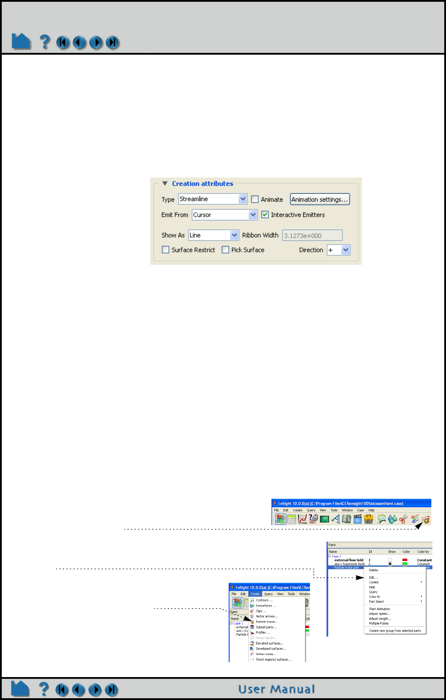
Page 282
HOW TO CREATE PARTICLE TRACES
Interactive Particle Tracing
If a particle trace was created from one of the tool emitters (Cursor, Line, or Plane) and the trace is a streamline trace,
the emitter can be made interactive. When interactive, the tool that created the particle trace part can be moved with
the mouse. As the tool is moved, new particle traces are automatically recalculated and redisplayed (This option is
not available for surface-restricted Particle traces, traces emitted from a Part, in Server of Server mode, or to
Pathlines). To trace interactively:
1. Either create a particle trace part as described above (based on a tool) or double-click an existing particle
trace part to open the Parts Feature Panel, and turndown the Creation .
2. Toggle on Interactive Emitter.
If the tool that originally defined the emitter is not visible, it will be turned on by this operation.
3. Move the mouse into the Graphics Window and manipulate the tool as desired. See the article on the
applicable tool for information on tool manipulation (Cursor, Line, or Plane).
4. When done, toggle off Interactive Emitters.
Trace Pathlines
EnSight provides complete control over transient particle tracing. Both the start time and the stop time can be
specified. In addition, you can specify a delta value for an emitter that will cause additional particles to be emitted into
the flow at regular intervals. This type of pathline is also called a streakline or smoke trace.
You create a pathline trace by setting the Type to Pathline (rather than Streamline) prior to clicking Create. By default,
the pathlines will start at the first time step of your simulation and terminate at the last step (unless stopped earlier).
You can change these defaults within the Emitter Information in the Creation section of the Create/edit dialog as
described above.
Edit Emitter
Complete control over all creation attributes is found in the Advanced mode of the Create/edit Parts dialog for particle
trace parts. There are many ways to get to these, some are:
1. Double click on the desired Particle trace part in the Parts list
or select the desired Particle trace part in the Parts list and click
the Particle traces icon.
or right click on the desired Particle trace part in the Parts list and select
Edit...
or select Create->Particle traces...,
then select the desired Particle trace part in the
Parts list.
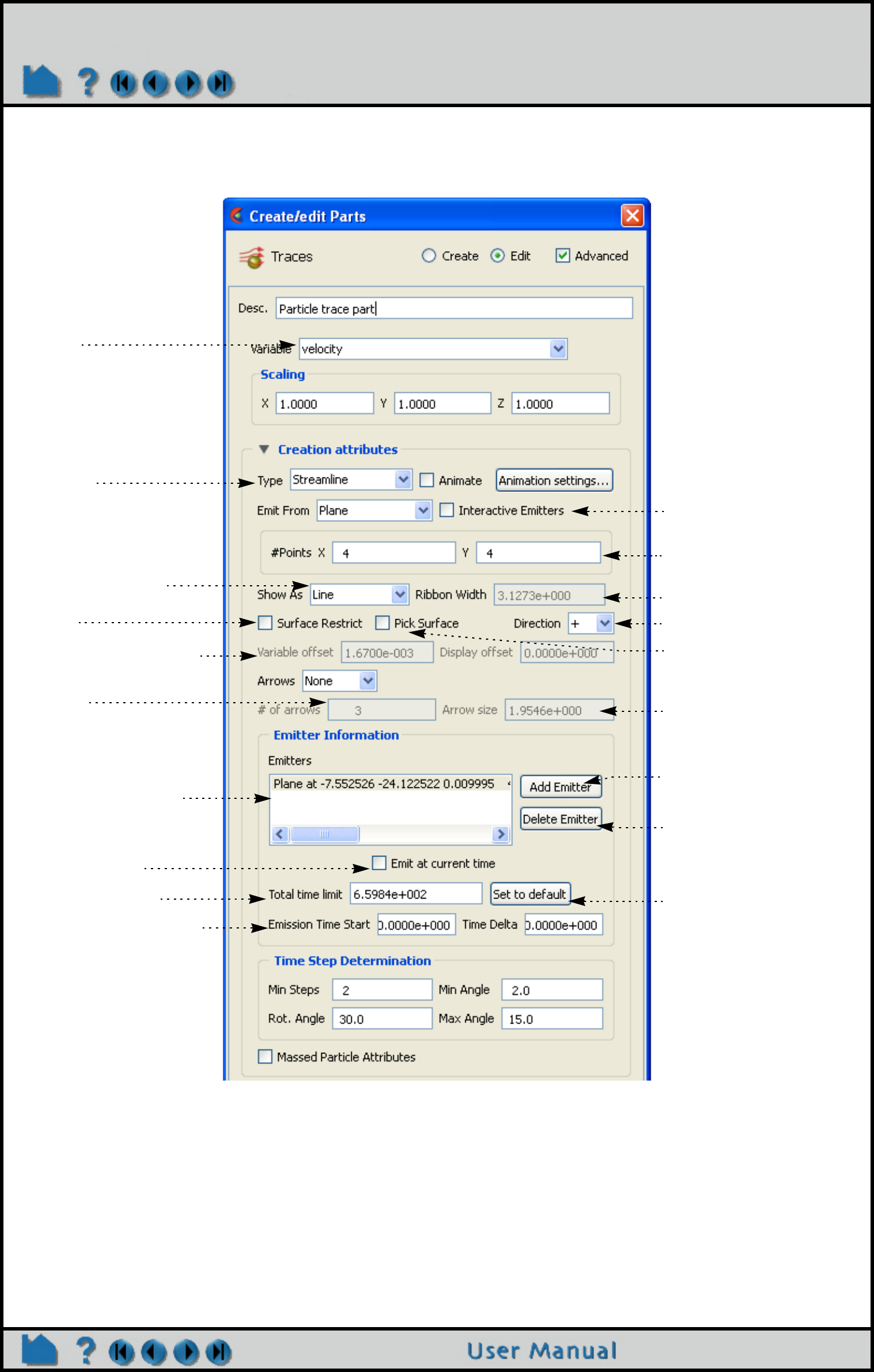
Page 283
HOW TO CREATE PARTICLE TRACES
2. Make sure you are in Advanced mode.
Set the desired flow field
variable
Trace type
Line or ribbon display
Toggle on Surface Restricted
tracing
Set surface restricted
variable and display offsets.
Number of arrowheads along
the trace.
List of the emitters belonging
to the selected trace part
Set to emit at current time, or
set emission time.
Set emitter total time
Set emission start and delta
Set interactive emitter
Number of points (If Line or
Plane emitter)
Set ribbon width
Set Emitter direction
Toggle on surface picking for
emitter definition
Set Arrowhead size.
Emission tool for currently
selected emitter
Add Emit: add a new emitter
to the selected part based on
the current.
Delete Emit: delete the
selected emitter.
Set Total Time to the default.
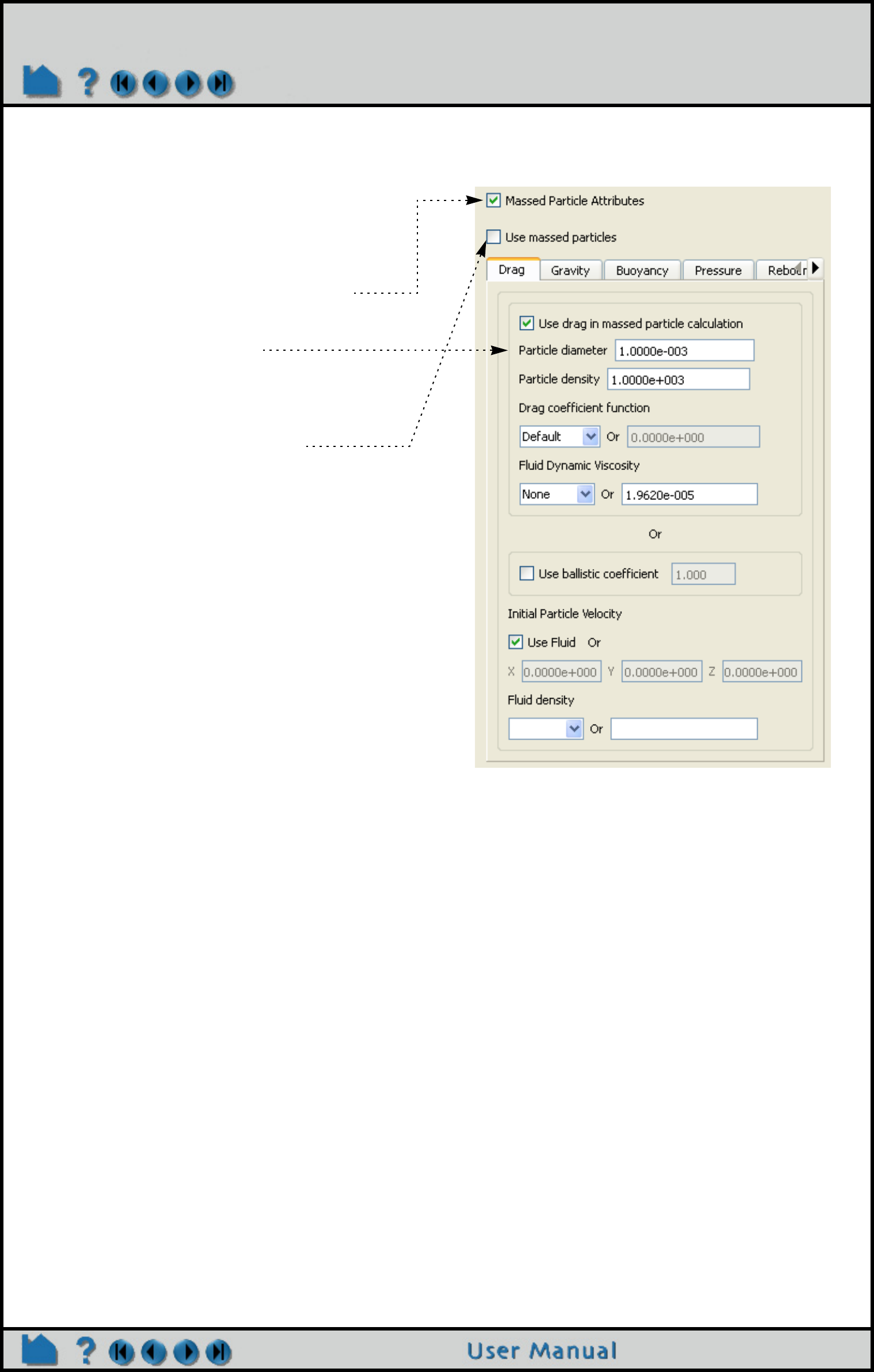
Page 284
HOW TO CREATE PARTICLE TRACES
Massed Particle Traces
Ensight also provides massed particle traces via the Advanced mode in the Feature Panel for Traces.
1. Open the Parts Feature Panel for the desired
particle trace part by one of the several
methods shown above.
2. Click the Massed Particle toggle to reveal the
massed particle parameters.
3. Modify the massed particle parameters
according to your dataset.
Each term in the momentum balance equation
has a separate tab containing the parameters
which pertain.
4. Toggle on Use massed particles.
The selected particle trace part will update to a
massed particle trace(s) taking into consideration
the parameters you specified.
For the theory used in massed particle traces, see
the User Manual: Particle Trace Parts
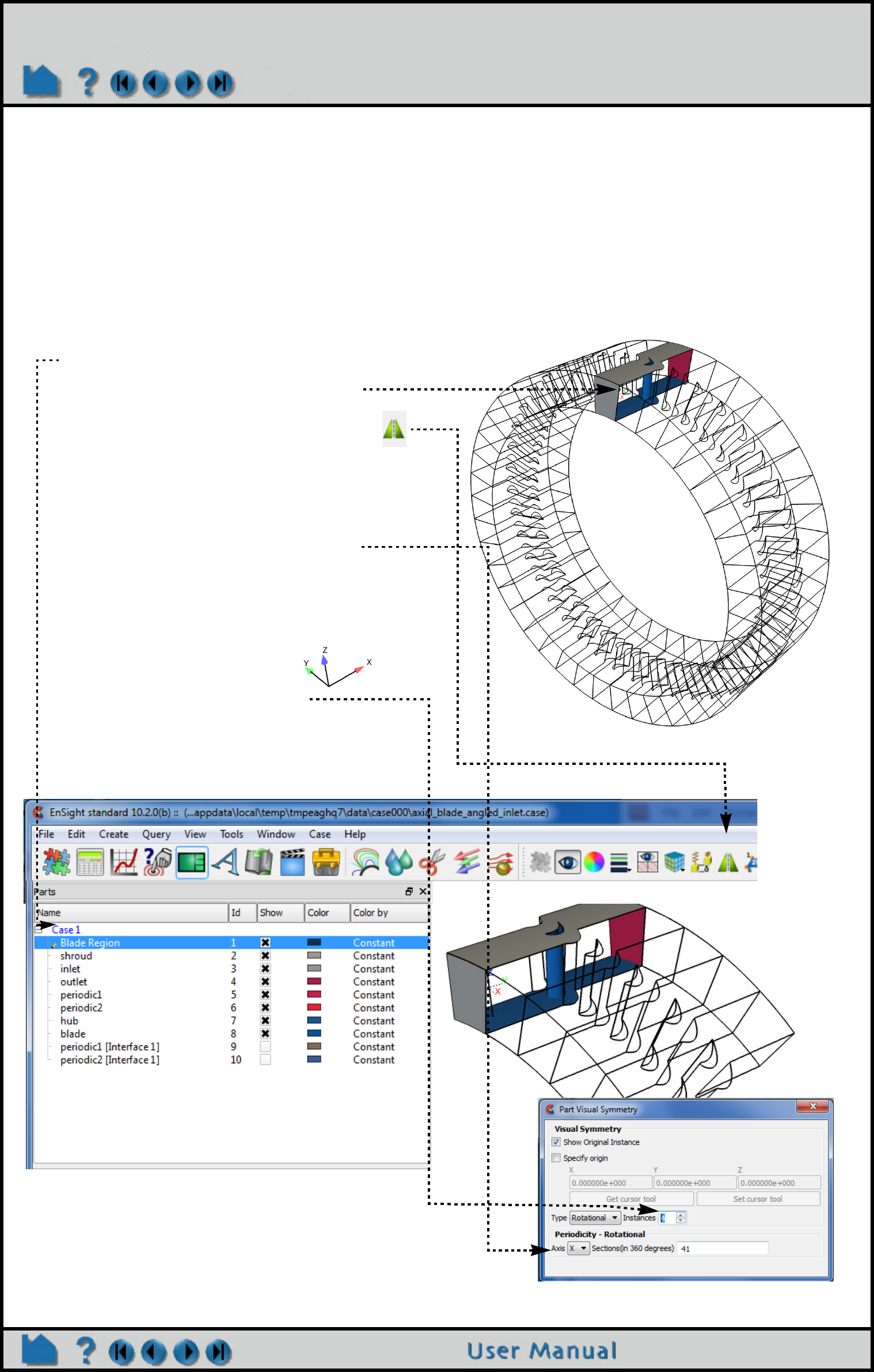
Page 285
HOW TO CREATE PARTICLE TRACES
Periodic Particle Traces
Ensight also provides a special option for rotational periodic geometry. Both streamlines and pathlines, which exit a
symmetry face of a part, can re-enter the part at the corresponding symmetry face and continue. As will be illustrated
below, one must first specify the correct symmetry for the periodic geometric parts, and toggle on the periodic option.
See below for an example model of the flow field and surfaces of an axial blade with angled inlet – periodic faces are
set as non-visual and, the top view has the original and all of the remaining 40 instances, while the bottom view has
the original as well as four instances as shown below.
1. Select the periodic field parts that share
the same symmetry attributes. In this
case, the field part is the Blade Region.
2. Place your emitter tool in the original
instance prior to making instances. You
cannot emit within in the symmetry
instances as they are graphical only!
3. Click the Visual Symmetry icon to open
up the Part Visual Symmetry dialog.
4. Choose rotational symmetry, the axis of
rotation (here X), set the number of
instances for full 360 degree rotation (in
this case 41).
Note in this case each slice is 360/41 degrees.
5. Toggle to show the original
instance, and the number of
instances to show (in this
case shown below, show 4).
If you show the original instance, then 40 will
show the entire 360 rotation. If not showing
the original instance then 41 will show all (see
the image to the right).

Page 286
HOW TO CREATE PARTICLE TRACES
6. Click on the Particle Traces icon, to open
the Create Traces dialog. And click the
Advanced toggle – to open the full
dialog.
7. Set your desired options as explained in
other sections of this How To
(streamline or pathline, emit from, etc.).
8. Toggle on “Compute using periodicity”.
Note this will use the information from the
parent visual symmetry dialog.
9. Click the Create with selected parts
button.
If you only have one instance of the parent
flow field part showing, streamlines will be
shown entering and exiting the flow field part
and can be confusing. It is helpful to display
several instances in the visual symmetry
dialog.
10. With the newly created particle trace
part selected, click on the visual
symmetry icon
11. In the resulting Part Visual Symmetry
dialog, choose rotational symmetry.
Show the same number of instances of the
particle trace part as the parent flow field part.
Turning on Visual Periodic Symmetry with
multiple parent instances will give you a sense
of the flow between the instances as shown
below.
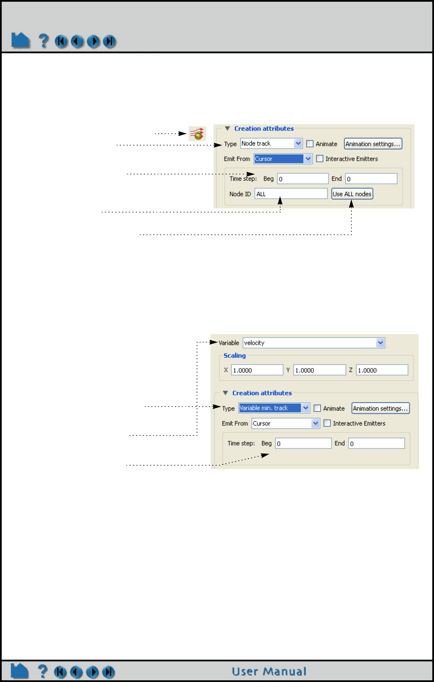
Page 287
HOW TO CREATE PARTICLE TRACES
Node Tracks
Ensight provides the capability to track the location of node(s) through time. As one would expect, node ids are
required, and this only makes sense for nodes that change location over time - whether by changing geometry or by
transient displacement. Measured particle parts are often a particularly good choice for this option.
Min/Max Variable Tracks
Ensight provides the capability to track the location of the minimum or maximum of a chosen variable through time.
This of course only makes sense for transient models.
1. Select the part(s) containing the nodes you
wish to track in the Part list.
2. Click on the Particle Traces Icon
3. Set Type to Node track.
4. Optionally you can modify the begin and end
times to use for the track.
The default will be all time steps.
5. Specify the particular node id you wish to
track, or do “ALL”.
You can use the ‘Use ALL nodes” button to select
all if you have modified the field.
1. Select the part(s) containing the variable, for
which you wish to track the min or max.
2. Set Type to Variable min. track
(Or Variable max. track)
3. Select the desired variable.
4. Optionally you can modify the begin and end
times to use for the track.
The default will be all time steps.
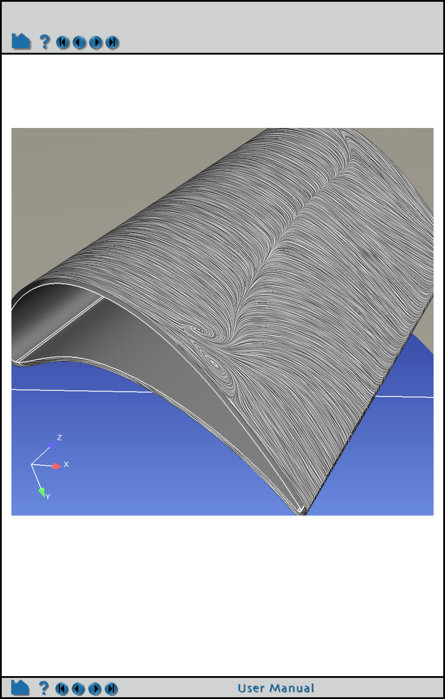
Page 288
HOW TO CREATE PARTICLE TRACES
Surface Flow Visualization
Ensight provides the capability to visualize the flow over a surface part, similar to tufts in a wind tunnel. This
visualization is not interactive, nor is it animated; it is a graphical texture of the flow tufts calculated on the part surface
using surface velocity (or velocity in the flow just above the surface) using the Line Integral Convolution algorithm. It
is designed to provide a uniform visualization of the flow of a vector over a surface. This will update when time is
changed for transient data. See Surface Flow Display for details.

Page 289
HOW TO CREATE PARTICLE TRACES
ADVANCED
Reverse Pathlines
From time to time we have users that wish to trace pathlines backward in time. This can be accomplished fairly easily
using the EnSight casefile format. (Note, if your data is in a different format, you can use File->Export->Geometric
Entities to convert it into casefile format).
1. Reverse the order for the timeset files, by using a negative filename increment.
Example:
TIME
time set: 1
filename start number: 1
filename increment: 1
time values: 0.0 2.0 4.0 6.0 8.0
change to:
TIME
time set: 1
filename start number: 5
filename increment: -1
time values: 0.0 2.0 4.0 6.0 8.0
2. Create a vector variable that is the negative of the normal vector field. Simply use the variable calculator to create
a new vector variable (neg_vector = - vector).
3. Create pathlines using the neg_vector variable.
Limiting Pathlines
If your geometry is much larger than your region of interest, you can try setting the total time limit value in the particle
trace dialog (with the Advanced toggle turned on). This will stop traces after a given time and avoid wasted
computational time outside your region of interest. You can estimate the total time as follows. Determine the total
distance of your region of interest, and divide it by an average velocity to get a time (making sure all units are
consistent in this calculation and within EnSight. Then try the run with a few pathlines. If you have significant
recirculation within sections of your flow, this method will stop particles long before they exit your region of interest. In
this case, you may want to consider using spatial limits on your flowfield.
If your geometry is much larger than your region of interest and temporal limits stop some of the traces too soon, then
you can set spatial limits for your particle trace. There are two ways to limit the volume in which your pathline is
traced. The first is to create a new part of limited volume and use this part as the trace parent; you can do this by
using the box tool to define the region of interest and do an interior cut of your model volume (and then select the cut
part as your parent part for your pathline trace). The trace will stop when it reaches the box tool volume limits. The
second is to set six environmental variables before you start up EnSight to limit the x, y, or z max and/or min:
ENSIGHT10_MIN_TRACE_X, ENSIGHT10_MAX_TRACE_X, ENSIGHT10_MIN_TRACE_Y,
ENSIGHT10_MAX_TRACE_Y, ENSIGHT10_MIN_TRACE_Z, or ENSIGHT10_MAX_TRACE_Z. The trace will stop
when it falls outside the bounds set by the environmental variables. The downside of using the box tool is that it costs
memory to create a new part (which can be substantial on a large dataset). The downside of setting environmental
variables is that you must do this before you start EnSight.
OTHER NOTES
Particle trace calculation can be expensive for large or transient datasets and/or a large number of particles. Be
careful when you initiate a trace operation – there is currently no way to abort it. If you are calculating pathlines, you
should specify as many particles as possible at one time. Much of the pathline execution time is in reading the
transient data from disk and this operation has to be performed regardless of how many traces were specified.
The EnSight particle trace algorithm integrates the vector flow field over time using a 4th-order Runge-Kutta method

Page 290
HOW TO CREATE PARTICLE TRACES
with a time varying integration step. Several of the integration parameters can be changed by the user. See Particle
Trace Parts in the User Manual for more information.
If you have trace data for other types of particles (e.g. for multi-phase flow simulations) you can use the discrete/
measured data facility to load the particle path positions and animate them over time.
SEE ALSO
How To Animate Particle Traces
User Manual: Particle Trace Parts

Page 292
HOW TO CREATE CLIPS
Create Clips
INTRODUCTION
EnSight provides a powerful set of clipping operators. See the following How To articles for more information:
Create Line Clips Clip lines are linear clips through 2D or 3D models (using the Line Tool) with samples taken at
evenly spaced intervals (grid), or at intersections of element boundaries of the parent parts
(mesh). Clip line values can be visualized using profiles or queried and sent to a plotter.
Create Plane Clips A clipping plane is a planar slice through a 3D mesh using the Plane Tool. EnSight’s clipping
operation can take arbitrary cuts through either structured or unstructured meshes. The clip
can be infinite in extent (at least to the bounds of the parts it is created from) or restricted to
the bounds of the Plane tool. The nodes of the resulting clipping plane can be based on the
topology and resolution of the underlying mesh or sampled on a regular grid.
You can also create a clip that contains all the elements that intersect the plane value via the
crinkly domain specification. These clips help view the integrity of the mesh at these values.
Create Box Clips A Box clip is a 3D volumetric hexahedral-shaped clip or cut. This clip uses the box tool (which
can be manipulated anywhere in space), and the result can be the surface intersection of the
box tool walls and the model, the volume portion of the model inside the tool, the volume
portion of the model outside the tool, or the crinkly surface elements of the intersection. Be
aware that due to the algorithm used, this clip can (and most often does) have chamfered
edges, the size of which depends on the coarseness of the model elements.
Create Quadric Clips In addition to standard clipping planes, EnSight also provides clipping against quadric shapes.
These clips use the corresponding quadric tool (Cylinder, Sphere, Cone, Surface of
Revolution) to specify the location of the clip.
You can also create a clip that contains all the elements that intersect the quadric value via the
crinkly domain specification. These clips help view the integrity of the mesh at these values.
Create IJK Clips An IJK clip is a 1D or 2D slice through a structured mesh. The resulting clip is a 1D line or 2D
surface where one dimension (e.g. I) is held fixed while the other one or two dimensions (e.g.
J and K) vary. The minimum and maximum range of the free dimensions can be set by the
user, as well as the step size. IJK clips can be interactively animated throughout the range of
the fixed dimension by manipulating a slider.
Although planar clips can still be created through structured meshes, it is often preferable to
create IJK clips since they are faster to calculate and use less memory. In addition, IJK clips
are often more intuitive for the user (who typically built the mesh).
Create XYZ Clips An XYZ clip is a 1D or 2D slice through a 2D or 3D mesh (structured or unstructured). The
resulting clip is a 1D or 2D mesh slice where one of the dimensions (e.g. X) is held constant
(or fixed) while the other two dimensions (e.g. Y and Z) vary in reference to the local frame of
the mesh. XYZ clips can be interactively animated throughout the range of the fixed
dimension by manipulating a slider. The minimum, maximum, and step size of the range of the
fixed dimension can be set by the user.
Although plane clips can still be created through meshes, it is often preferable to create XYZ
clips since they are constrained to the local frame of the meshed part. To quickly create an
XYZ clip, simply right-click on a part and choose Clip and then choose the direction.
Create RTZ Clips An RTZ clip is a 1D or 2D slice through 2D or 3D meshes (structured or unstructured). The
resulting clip is a 1D or 2D mesh slice where one of the dimensions (e.g. R,”radial
component”) is held constant (or fixed) while the other one or two dimensions (e.g. T, ”theta
component” and Z, “z axis component”) vary in reference to the local frame of the mesh. RTZ
clips can be interactively animated throughout the range of the fixed dimension by
manipulating a slider. The minimum, maximum, and step size of the range of the interactive
fixed dimension can be set by the user. To quickly create an RTZ clip, simply right-click on a
part and choose Clip and then choose the direction.
Revolution Tool Clips A Revolution Tool clip can be made using the surface of revolution tool. It can be the surface
created by the intersection of the surface of revolution tool and the model, the elements
intersected by the surface of revolution tool (crinkly), or the volume of the inside and/or the
outside domain swept by the revolution tool. This clip cannot be interactively manipulated.
Revolve 1D Part Clips A Revolution of 1D Part clip can be made using a 1D part and a user specified axis. It can be
the surface created by the intersection of the 1D part about the axis and the model, the
elements intersected by the 1D part about the axis(crinkly), or the volume of the inside and/or
the outside domain swept by the 1D part about the axis. This clip is always infinite. This clip
does not have interactive manipulation capability, with a slider or by dragging the tool with the
mouse. However, if the 1D part is capable of being moved, you can move it and the revolution
clip will update.
Create Clip Splines Spline clips will sample a defined spline on evenly spaced intervals along the spline. Values
along a spline clip can be visualized using profiles or queried and sent to a plotter, or used in
subsequent computations such as computations of a line integral.
Create General
Quadric Clips A general quadric clip AX2+BY2+CZ2+DXY+EYZ+FXZ+GX+HY+IZ=J can be created. This is
only available from the Clip Feature Panel.
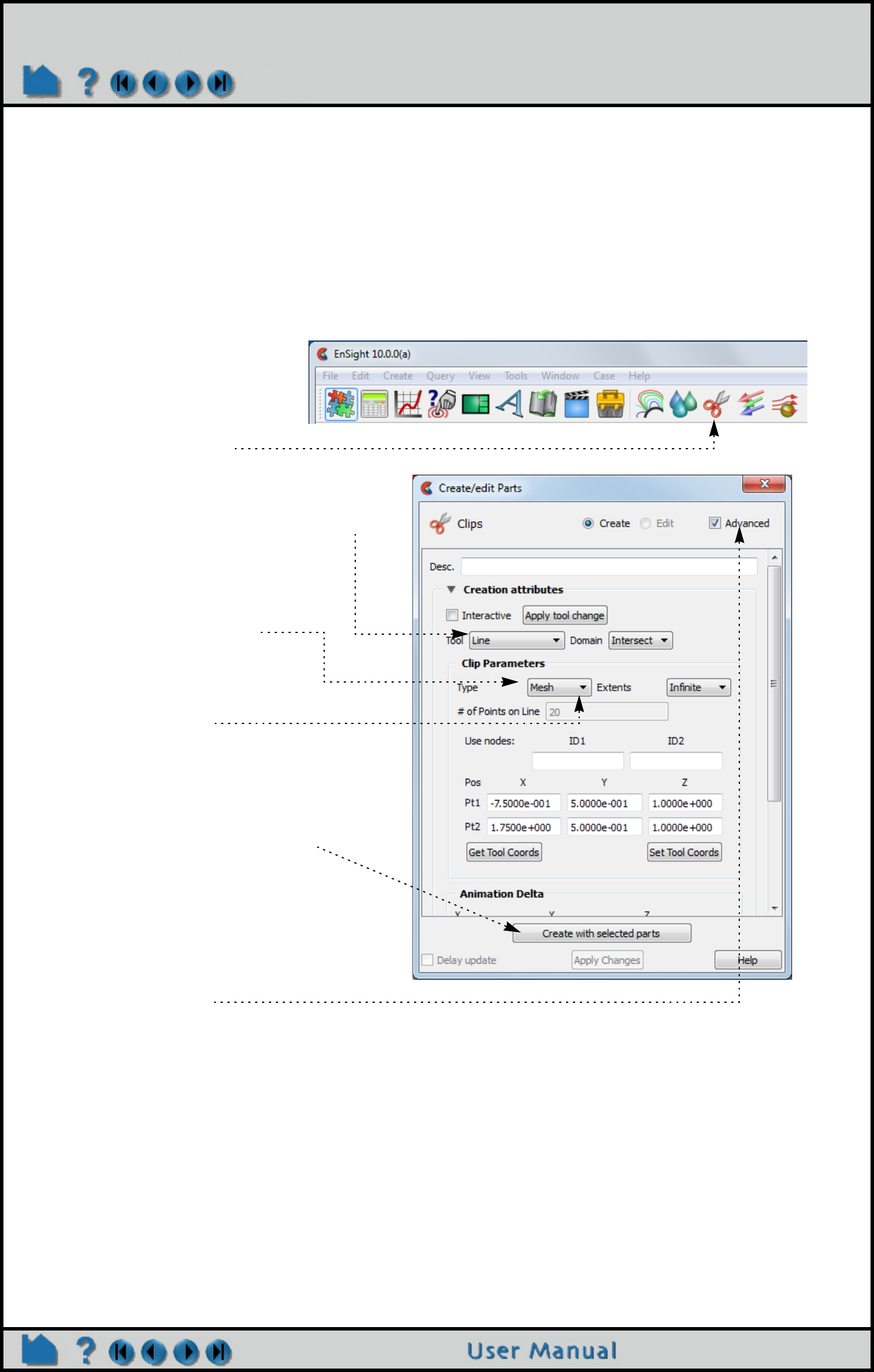
Page 293
HOW TO CREATE CLIP LINES
Create Clip Lines
INTRODUCTION
In addition to standard clipping planes, EnSight also provides one dimensional clipping. Clip lines are linear clips
through 2D or 3D models with either samples taken at evenly spaced intervals (grid) or true intersections at the faces
of the parent part’s elements (mesh). Values along a clip line can be visualized using profiles or queried and sent to
a plotter.
BASIC OPERATION
1. Select the parent part.
2. Click the Clip icon.
7. Click “Create with selected parts”
3. Select Line from the Use Tool pull-down.
4. Select Mesh or Grid type.
6. Position the Line tool as
desired (see How To Use the
Line Tool).
5. If Mesh, select Finite or Infinite
If Grid, set the number of evenly spaced
points on the line
Note: To quickly create a line clip, right click on the line tool and choose Clip. This will create a
line clip using the default settings.
8. Click on the Advanced toggle
to see more options
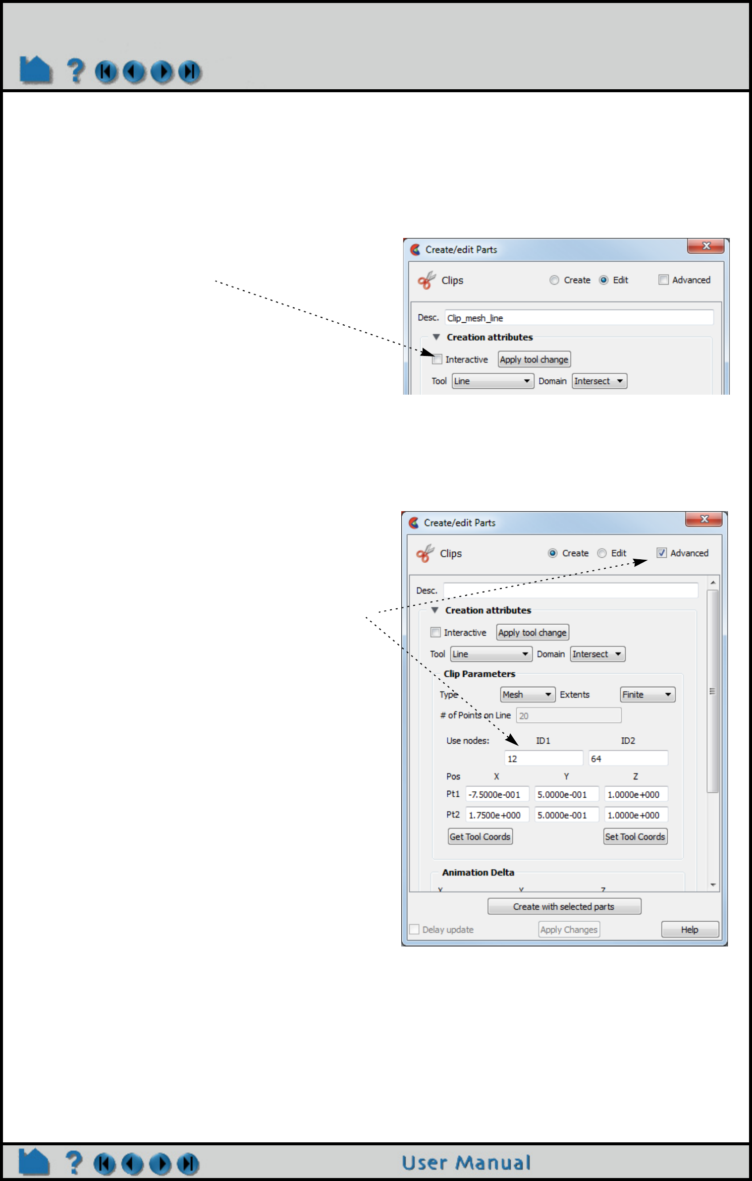
Page 294
HOW TO CREATE CLIP LINES
ADVANCED USAGE
Like the other clipping tools in EnSight, clip lines can be interactive: as you drag, rotate, or stretch the Line tool with
the mouse, the clip line is automatically recalculated and re-displayed. If a query has been created from the clip line,
the plotted curve will automatically re-display as well. To perform interactive line clips:
.
OTHER NOTES
It is sometimes useful to display just the nodes of a line clip. Click Node, elements and line pulldown lower in the
Create/edit Parts dialog in the advanced mode and you can change the display such that only nodes (not lines or
elements) are displayed. The nodes can be dots, crosses, or spheres. If displayed as crosses or spheres, the size
(radius) can be constant or scaled by the value of a variable. See How to Set for more information.
1. Double-click the desired clip line part in the parts list.
2. Toggle on Interactive Tool in the Feature Panel.
3. Move the mouse into the Graphics Window. Click on
one of the Line tool hotpoints (either endpoint or
center axis origin or axes) and drag the tool to the
desired location.
Note that the line tool itself will be made invisible while moving the tool interactively, so as not to obscure the
clip. It will reappear when the mouse is released.
A line clip can be specified by identifying two nodes as
points on the line.
This requires that node ids be available and that the Feature
Panel be in advanced mode.
The effect of this method is that the line clip remains
tied to the two nodes, even if their location moves over
time.
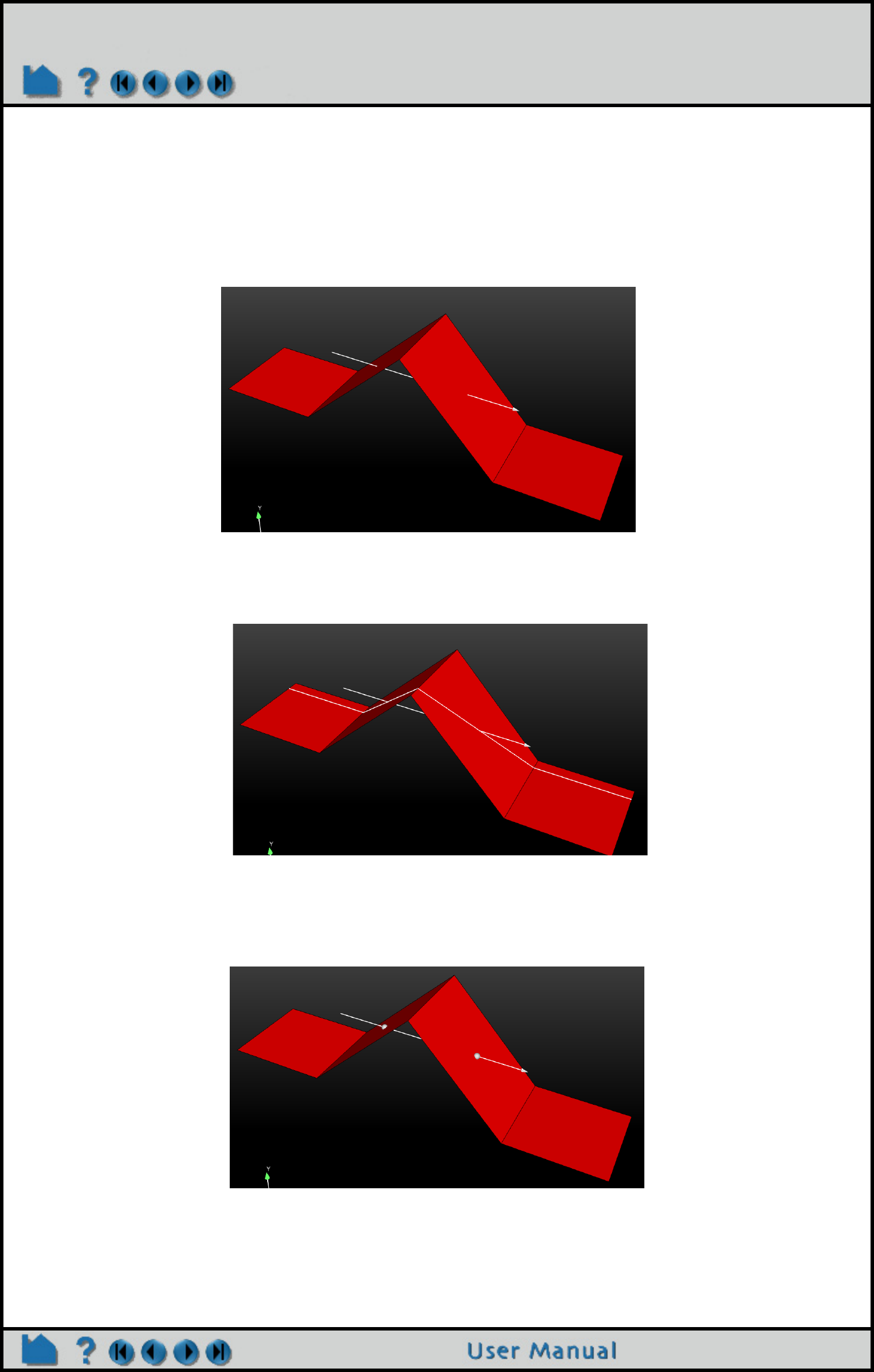
Page 295
HOW TO CREATE CLIP LINES
Clip of a 2D part using the line tool
A Clip of a 2D part using a line tool that is perpendicular to the 2D part surface will give you an empty part. The
reason is as follows. In the past, EnSight would sometimes fail to clip a 2D part due to numerical tolerance errors
when the line tool wasn’t numerically exactly on the surface. To work around this numerical issue, the line tool is now
projected onto the 2D part, which results in a line clip projected onto the surface except for a perpendicular line tool.
For example, suppose you have a geometry shown below with the line tool positioned as indicated.
If you create a clip using the line tool, you will get the following line clip, which is a projection of the line tool onto the
surface of the part. Note that the clip is at one of the infinitely many possible projection planes through the line tool. If
you want to control the projection plane, clip with the plane tool rather than doing a line clip.
The algorithm used to decide which projection plane to use may not be to your liking, and you may wish to only have
the points where the line tool intersects the part. To do this, set an environmental variable which will give the point
intersection of the line tool and redo the clip that results in a clip part with two points, as shown below.
setenv ENSIGHT_2D_MESH_LINECLIP_POINT_OPTION 1
SEE ALSO
Introduction to Part Creation
How To Use the Line Tool

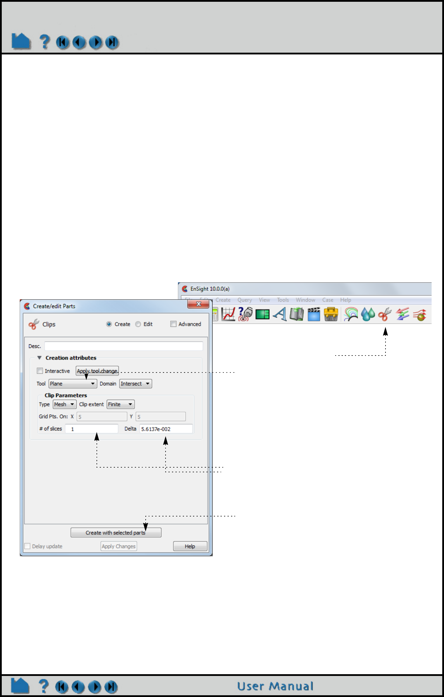
Page 297
HOW TO CREATE CLIP PLANES
Create Clip Planes
INTRODUCTION
A clipping plane is a planar slice through a 3D mesh. EnSight’s clipping operation can take arbitrary cuts through
either structured or unstructured meshes. The clip can be based on EnSight’s plane tool, and as such can be infinite
in extent (at least to the bounds of the parts it is created from) or restricted to the bounds of the Plane tool. The nodes
of the resulting clipping plane can be based on the topology and resolution of the underlying mesh or sampled on a
regular grid according to the plane tool.
A clip can also be created by specifying the node id of three nodes. When node ids are used, the plane will be infinite
in extent and will stay tied to those three nodes - even if they move in a changing geometry model.
Besides creating the intersection of a plane through a domain, which is the normal mode for clipping, a clipping plane
can also be used to create parts which are what would result from a cut of its parent domain into “front” (inside) and or
“back” (outside) parts. These parts contain valid elements of the same order as the original domain parts.
Like other clip tools, clipping planes can be interactively manipulated with the mouse providing a powerful volume
visualization capability. Clipping planes can also be automatically animated to display results throughout a region of
space or over time.
BASIC OPERATION
1. Select the parent part(s).
2. Click the Clip icon.
5. Click “Create with selected parts”
3. Select Plane from the Tool pull-down.
4. Position the Plane tool as desired (see
How To Use the Plane Tool).
Note: Multiple plane clips with a delta in the normal
direction can be created easily by setting these values.
Note: To quickly create a plane clip,
right click on the plane tool and
choose Clip. This will create a
plane clip using the default
settings.
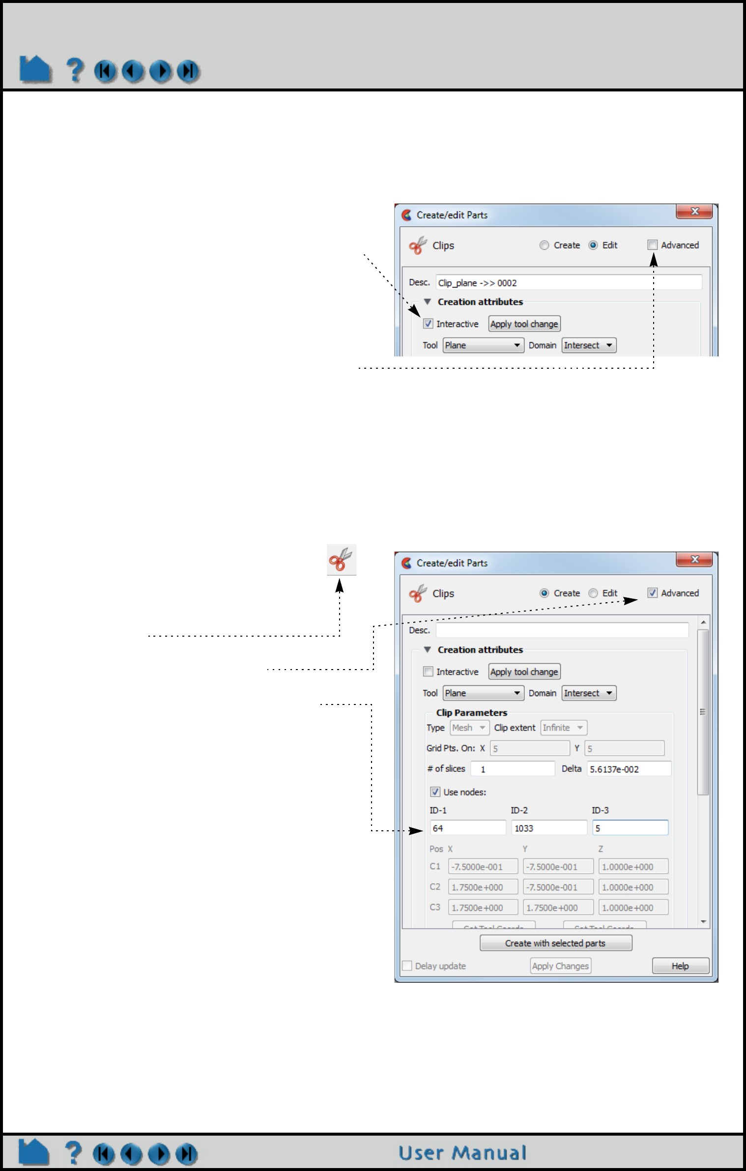
Page 298
HOW TO CREATE CLIP PLANES
Interactive Clipping Planes
Like the other clipping tools in EnSight, intersection clip planes (based on the plane tool) can be interactive: as you
drag the Plane tool with the mouse, the clipping plane is automatically recalculated and re-displayed. To perform
interactive plane clips:
ADVANCED USAGE
Using 3 Node Ids
You can specify three nodes on a plane (using their node ids) and clip in an infinite manner. This method of produc-
ing a plane clip has the added benefit that the plane will stay tied to those three nodes even if it is a changing geom-
etry model. This method requires the use of the Clips Feature panel
1. Double-click the desired clip plane part in the parts
list.
2. Toggle on Interactive Tool in the Feature Panel.
3. Move the mouse into the Graphics Window. Click on
one of the Plane tool hotpoints (centerpoint or axis
labels) and drag the tool to the desired location.
4. Click on the advanced toggle for more options
1. Select the parent part in the Parts list.
2. Click on the Clip icon to bring up the
Feature Panel.
3. Click on the Advanced toggle.
3. Enter the id for three nodes that lie on the
desired plane.
4. Click “Create with selected parts”
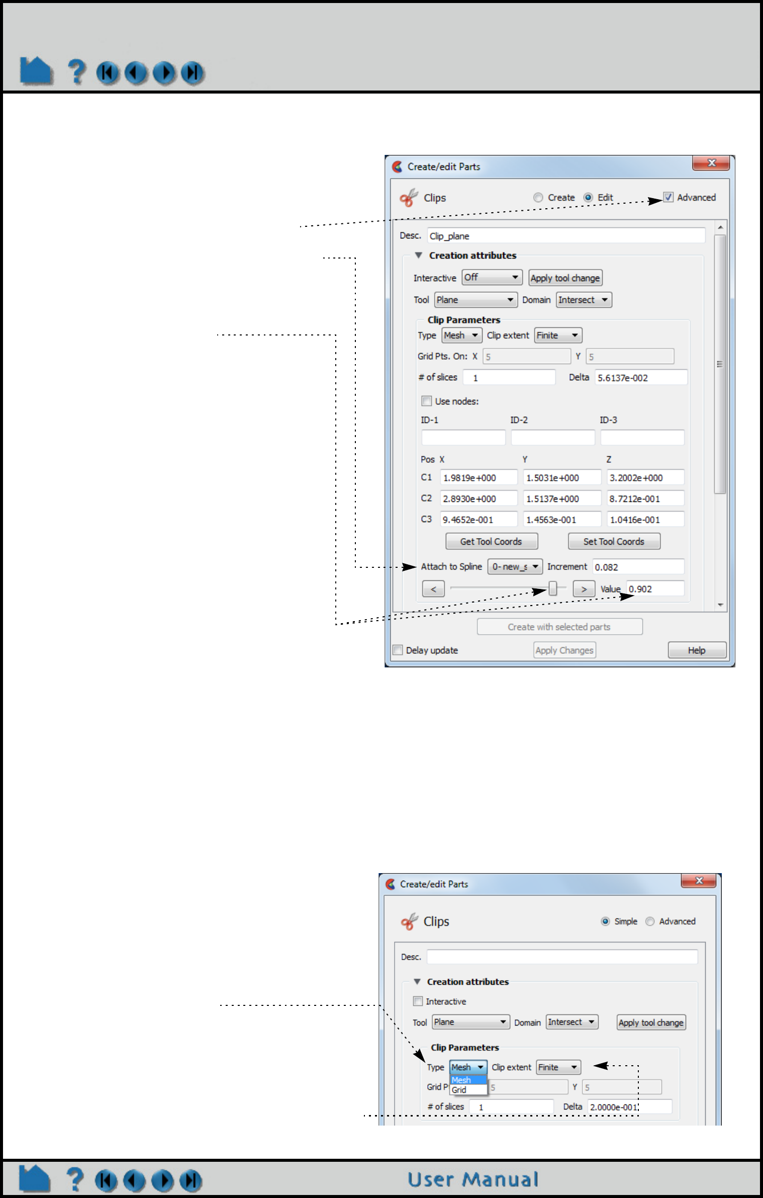
Page 299
HOW TO CREATE CLIP PLANES
Attaching a Plane Clip to a Spline
A Clip created with the Plane tool may be attached to a defined spline.
Grid Clips and Finite Clips
By default, clipping planes (based on the plane tool) are calculated based on the resolution and topology of the
underlying mesh (parent part(s)). Clipping planes can also be calculated using a regular sampling of the mesh. Such
a clip is called a grid clip and is typically used for clipping unstructured meshes where element volumes vary widely.
Creating vector arrows on a grid clip typically yields a more useful visualization than on a standard mesh clip.
By default, clipping planes extend to the bounds of the parent part. A clipping plane can also be restricted to the
bounds of the Plane tool.
To change an existing clipping plane to a grid clip or to have finite extent:
1. Create a spline (How To Use the Spline
Tool)
2. Now, create a clip plane as previously
indicated then open the Advanced section.
3. Attach the plane clip to a spline by selecting
the desired spline from the pulldown in the Clip
Plane Feature Panel.
4. Adjust the plane clip location (0 to 1) via the
Value input field or the slider.
1. Double-click the desired clipping plane part in
the Parts list.
2. To change to a grid clip, select Grid from the
Plane Type pull-down.
3. To change to a finite-extent clipping plane,
select Finite from the Plane Extents pull-down.
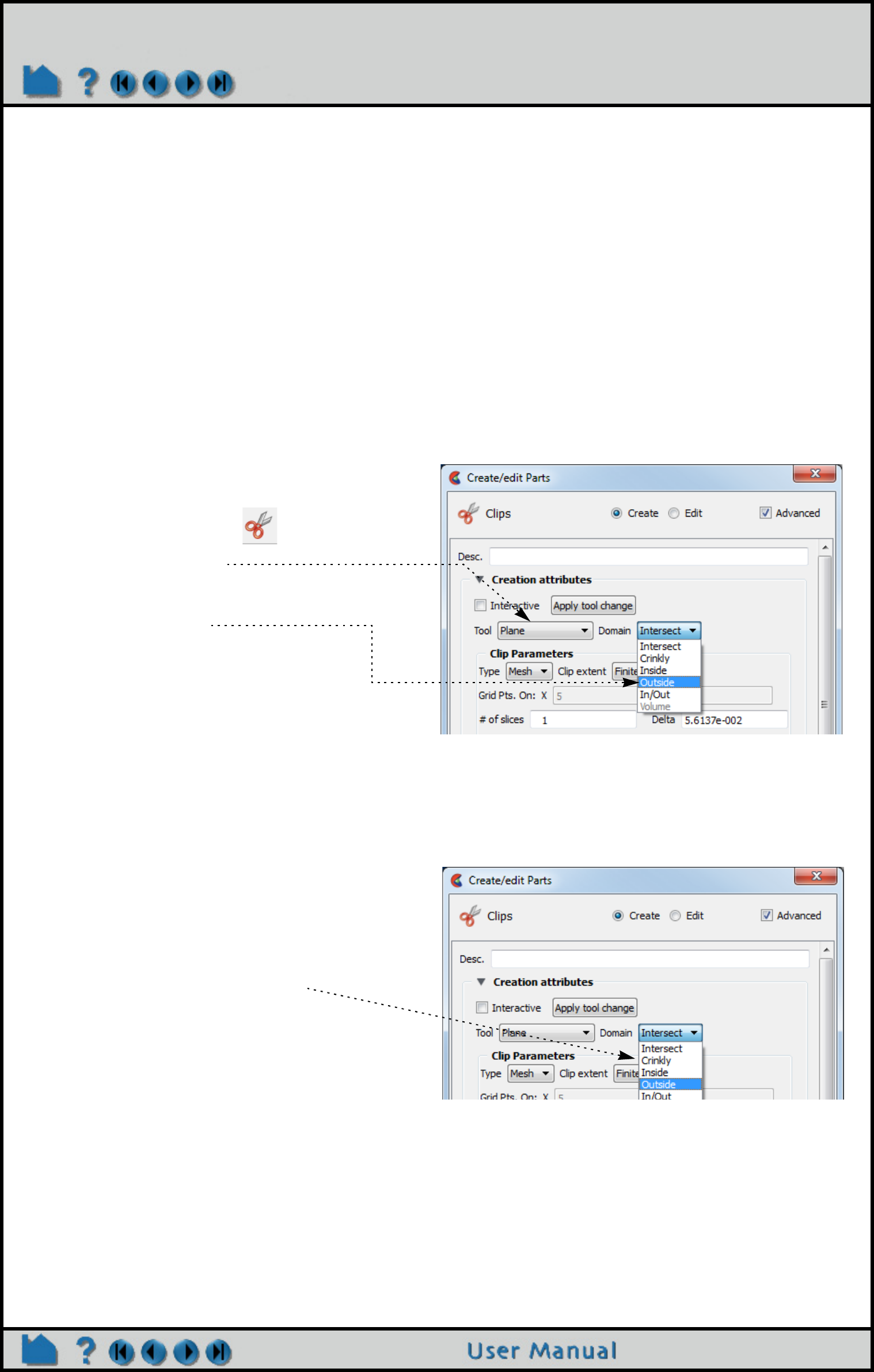
Page 300
HOW TO CREATE CLIP PLANES
Clipping Plane Animation
Although you can interactively sweep a clipping plane (based on the plane tool) through a volume, it is sometimes
desirable to have EnSight automatically calculate a series of clipping planes for you. These can then be replayed (as
fast as your graphics hardware will permit) using EnSight’s Flipbook Animation facility. The flipbook can animate a
series of clipping planes using a starting and ending position for the Plane tool. You can also use the Keyframe
Animation facility to animate clipping planes.
For a description of calculating a series of clipping planes with the Flipbook, see How To Create a Flipbook
Animation. For more information on keyframing, see How to Create a Keyframe Animation.
Cutting with Planes
A plane can be used to create parts which are the result of a cut of its parent domain into “front” (inside) and or “back”
(outside) parts. These parts contain valid elements of the same order as the original domain parts. For example, a
plane front cut of a 3D cube model part will include all of the 3D elements in front of the plane tool. Cutting can be
used to slice away portions of a model that are not needed or to create animation effects such as “opening” closed
regions to view the interior. Note that the parent part is made invisible so that you can see your cut part.
Crinkly Plane Clips
You can also check the integrity of your mesh by clipping with a crinkly intersection. Specifying a Crinkly Domain
results in a part composed of all the mesh elements that intersect the plane tool.
OTHER NOTES
If you have a clip defined by three node ids and you attempt to use the interactive mode (which makes no sense for
the 3 node option), the interactive movement of the clip will occur according to the plane tool - but will go back to the
3 node representation when you release the mouse button.
Use clipping planes to create planar clips through arbitrary meshes. If you have a structured mesh (such as those in
PLOT3D format), you may wish to use IJK clips instead. An IJK clip displays a “plane” of constant I, J, or K. An
interactive IJK clip will sweep through the range of (for example) I displaying the JK plane at each I value. See How
1. Select the desired parent parts in the Parts list.
2. Click the Clip icon.
3. Select the Plane Tool.
4. Set the Domain to Inside, Outside, or In/Out (both
inside and outside).
5. Hit the Create button.
The parent part will be made invisible and your cut
part will appear.
1. Change the Domain to Crinkly.

Page 301
HOW TO CREATE CLIP PLANES
to Create IJK Clips for more information.
SEE ALSO
Introduction to Part Creation
How To Use the Plane Tool
How To Create a Flipbook Animation.
Other clips:
How To Create Clip Lines
How To Create IJK Clips
How To Create Quadric Clips
How To Create XYZ Clips
How To Create RTZ Clips
How To Create Box Clips.
How To Use the Spline Tool
User Manual: Clip Parts
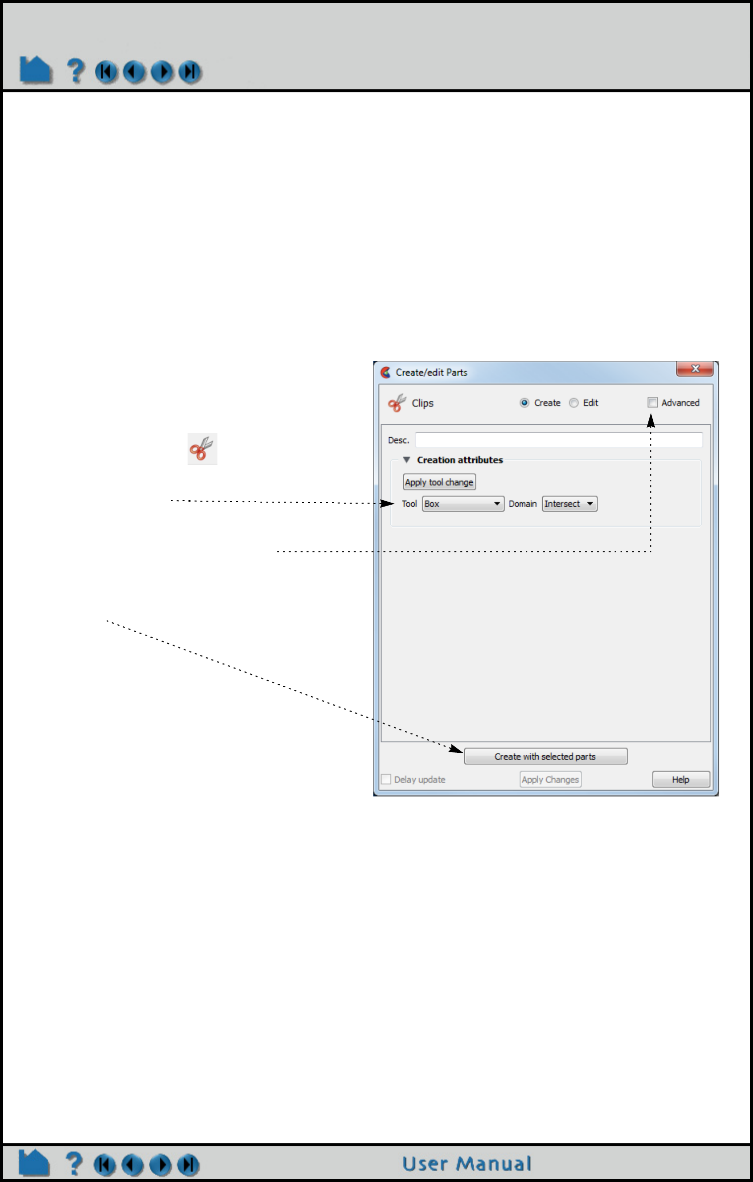
Page 302
HOW TO CREATE BOX CLIPS
Create Box Clips
INTRODUCTION
A Box clip is a 3D volumetric hexahedral-shaped clip or cut. This clip uses the box tool (which can be manipulated
anywhere in space), and the result can be the surface intersection of the box tool walls and the model, the volume
portion of the model inside the tool, the volume portion of the model outside the tool, or the crinkly surface elements
of the intersection.
Be aware that due to the algorithm used, this clip can (and most often does) have
chamfered edges, the size of which depends on the coarseness of the model
elements.
BASIC OPERATION
SEE ALSO
Introduction to Part Creation
How To Use Box Tool
Other clips:
How to Create Clip Lines
How to Create Clip Planes
How to Create Quadric Clips
How to Create IJK Clips
How to Create XYZ Clips
How to Create RTZ Clips.
User Manual: Clip Parts
1. Select the parent part(s) in the part list
2. Click the Clip Icon
4. Position the Box Tool as desired.
Toggle advanced to enter precise
box tool coordinates.
5. Click “Create with selected
parts”.
3. Select Box tool.
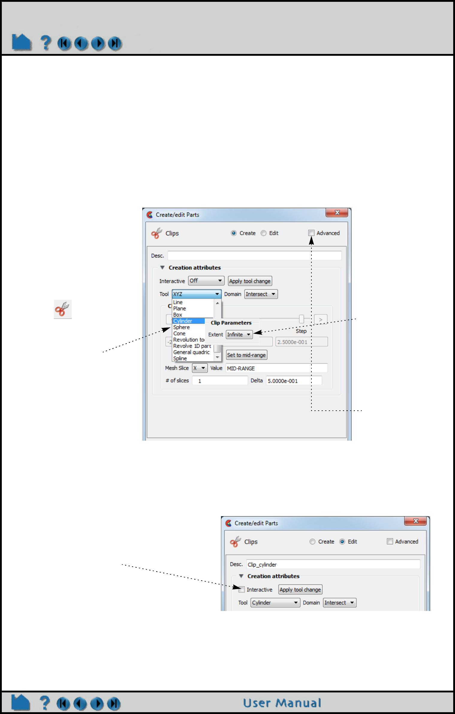
Page 303
HOW TO CREATE QUADRIC CLIPS
Create Quadric Clips
INTRODUCTION
In addition to standard clipping planes, EnSight also provides clipping against quadric shapes. These clips use the
corresponding quadric tool Cylinder, Sphere, Cone, Surface of Revolution) to specify the location of the clip.
As with clip planes, these tools can also be used to perform cut operations, creating parts which are the “inside” or
“outside” of the parent domain.
As with intersection clip planes, quadric clips can be changed interactively by manipulating the corresponding tool
with the mouse.
BASIC OPERATION
ADVANCED USAGE
Like the other clipping tools in EnSight, intersection quadric clips (except those created with the revolution tool) can
be interactive: as you drag the applicable tool with the mouse, the clip is automatically recalculated and redisplayed.
To perform interactive quadric clips:
1. Select the parent
part(s) in the EnSight
Part list.
2. Click the Clip icon.
6. Click “Create with
selected parts” at the
bottom of the dialog.
3. Select the desired
quadric tool from the
Tool pulldown. 5. Position the tool
as desired (see
the How to for
the applicable
tool). Toggle
advanced to
enter precise
tool coordinates.
4. Select Finite or
Infinite clip
extents
1. Double-click the desired quadric clip
part in the Parts list.
2. Toggle on Interactive Tool in the
Feature Panel.
3. Move the mouse into the Graphics
Window. Click on one of the tool
hotpoints (see the How to for the
applicable tool) and drag the tool to
the desired location.
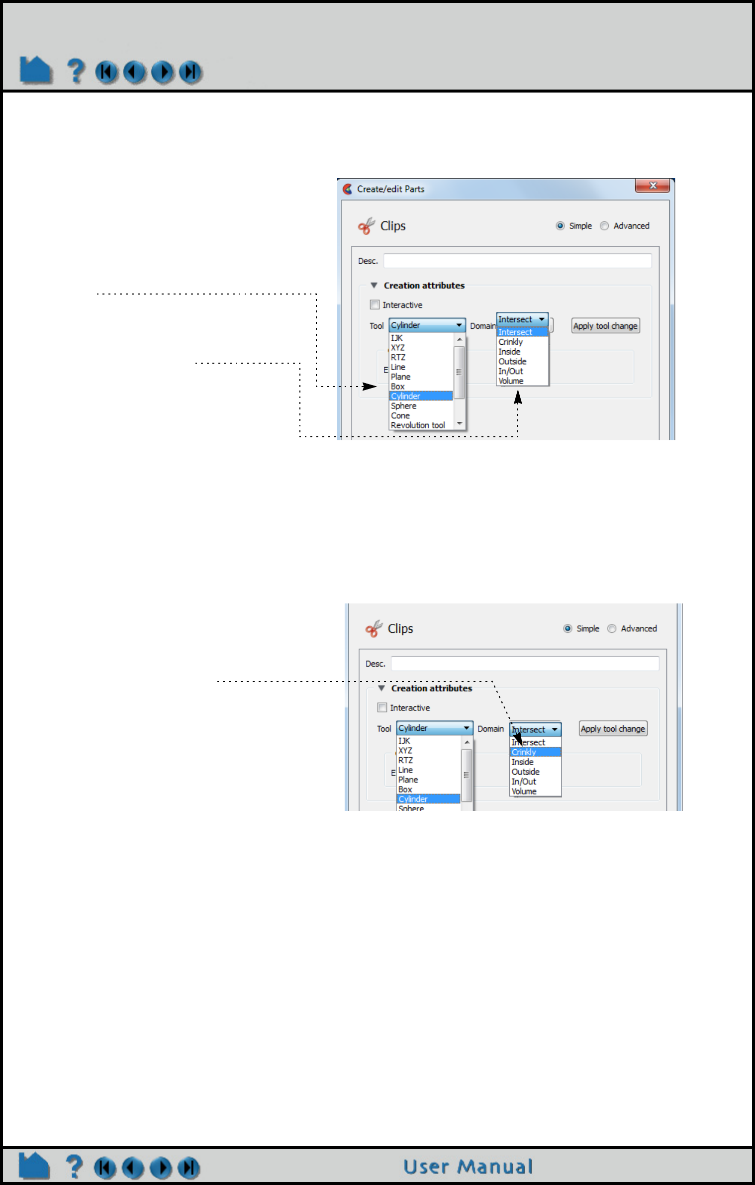
Page 304
HOW TO CREATE QUADRIC CLIPS
Cutting with Quadric Tools
A quadric tool can be used to create parts which are the result of a cut of its parent domain into “inside” and or
“outside” parts. These parts contain valid elements of the same order as the original domain parts.
Crinkly Quadric Clips
You can check the integrity of your mesh by clipping with a crinkly intersection. Specifying a Crinkly Domain results in
a part composed of all the elements of the mesh that intersect the quadric tool.
SEE ALSO
Introduction to Part Creation
How To Use the {Cylinder, Sphere, Cone, Surface of Revolution} Tool.
Other clips:
How to Create Clip Planes
How to Create Clip Lines
How to Create IJK Clips
How to Create XYZ Clips
How to Create RTZ Clips
How to Create Box Clips.
User Manual: Clip Parts
1. Select the desired parent
parts in the Parts list.
2. Click the Clip feature icon.
3. Select the desired Quadric
Tool.
4. Set the Domain to Inside,
Outside, or In/Out (both
inside and outside).
5. Click “Create with selected
parts” at the bottom of the
dialog.
4. Change the Domain to Crinkly
and clip is automatically
updated.
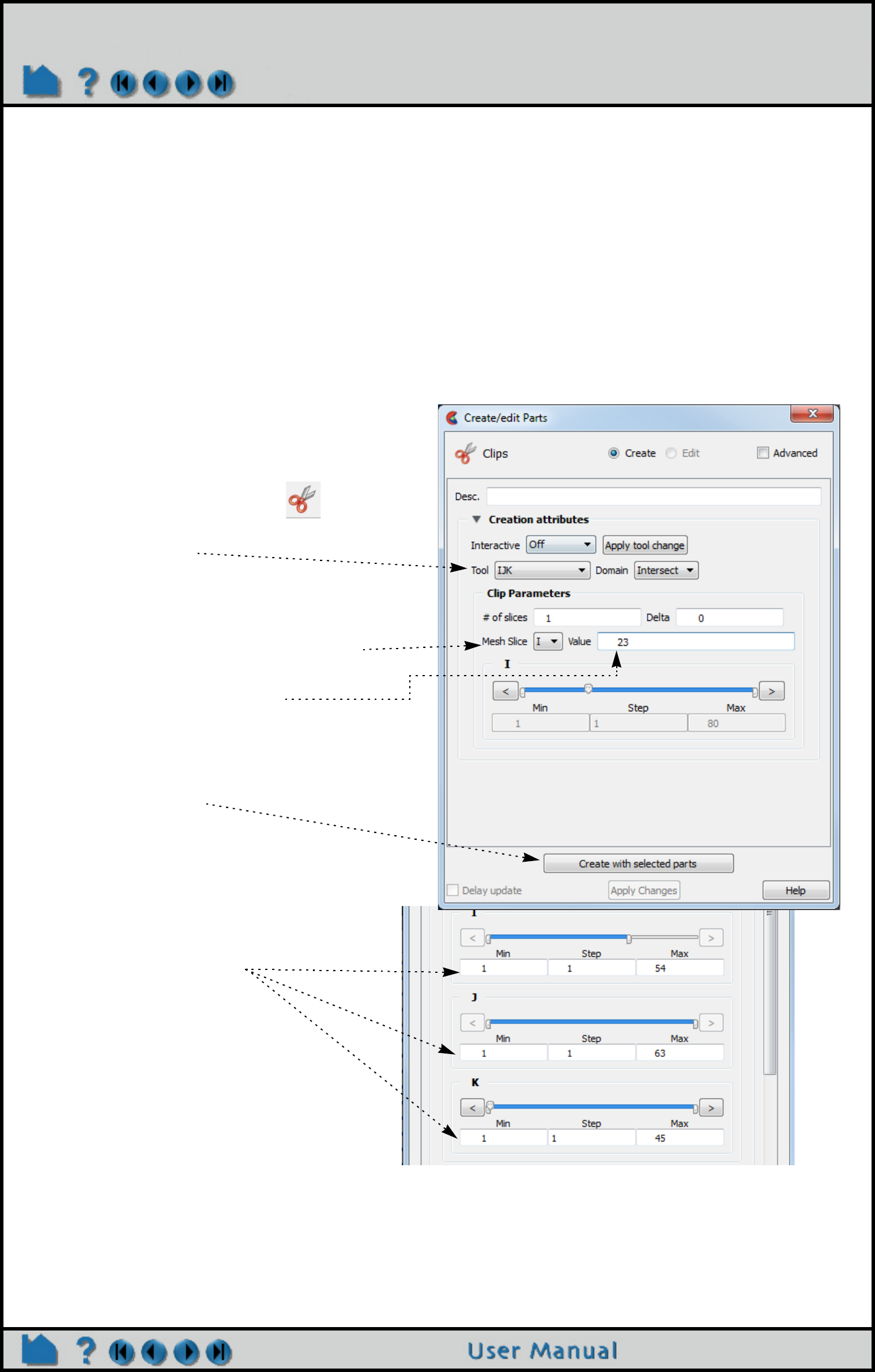
Page 305
HOW TO CREATE IJK CLIPS
Create IJK Clips
INTRODUCTION
An IJK clip is a 1D or 2D slice through a structured mesh. The resulting clip is a 1D line or 2D surface where one
dimension (e.g. I) is held fixed while the other one or two dimensions (e.g. J and K) vary. The minimum and
maximum range of the free dimensions can be set by the user, as well as the step size. IJK clips can be animated
throughout the range of the fixed dimension by manipulating a slider.
Although planar clips can still be created through structured meshes, it is often preferable to create IJK clips since
they are faster to calculate and use less memory. In addition, IJK clips are often more intuitive for the user (who
typically built the mesh).
BASIC OPERATION
Note that you can change the fixed dimension of an IJK clip at any time (with the Mesh Slice pulldown).
1. Select the parent part(s) in the EnSight
main part list.
5. Enter the value for the fixed
dimension in the Value text field and
press return.
4. Select the desired fixed dimension from
the Mesh Slice pulldown.
7. If you desire to modify values for the Min,
Max, and Step for all dimensions, toggle
Advanced and the dialog will expand to
allow detailed editing.
2. Click on the clip icon.
6. Click “Create with
selected parts”.
3. Set Tool to IJK.
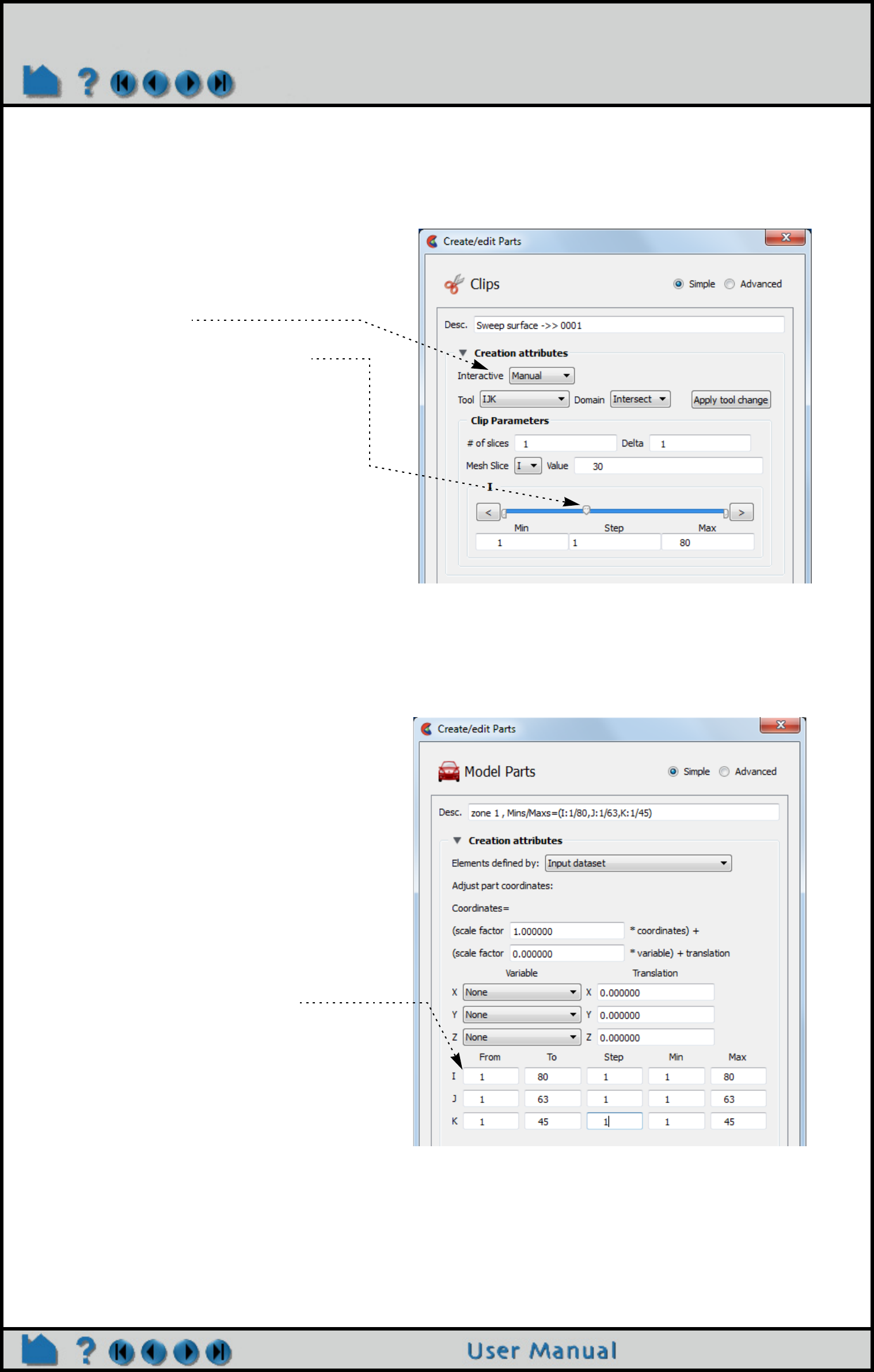
Page 306
HOW TO CREATE IJK CLIPS
ADVANCED USAGE
Interactive IJK Clipping
You can interactively sweep through the range of the fixed dimension by adjusting a slider with the mouse.
Changing IJK Step Refinement
You can modify block-structured model parts to any level of IJK step refinement with proper updating of all dependent
parts and variables.
Clipping Plane Animation
Although you can interactively sweep an IJK clip through a mesh, it is sometimes desirable to have EnSight
automatically calculate a series of IJK clips for you. These can then be replayed (as fast as your graphics hardware
will permit) using EnSight’s Flipbook Animation facility. See How To Create a Flipbook Animation for more
information.
1. Double-click the desired IJK clip part
in the Parts list.
2. Change Interactive to Manual, to
enable sweeping.
3. Adjust the slider with the mouse.
1. Double-click on a model part. This
will bring up the Model Parts Feature
Panel. Note that his is no longer a
clip dialog.
3. Simply enter values into the From,
To, and Step fields based on their
Min and Max limits to update the
refinement of the respective I, J, and/
or K mesh component directions.
When you press return or move to a
new field, the part is updated. All
dependent parts and variables will
also be updated.

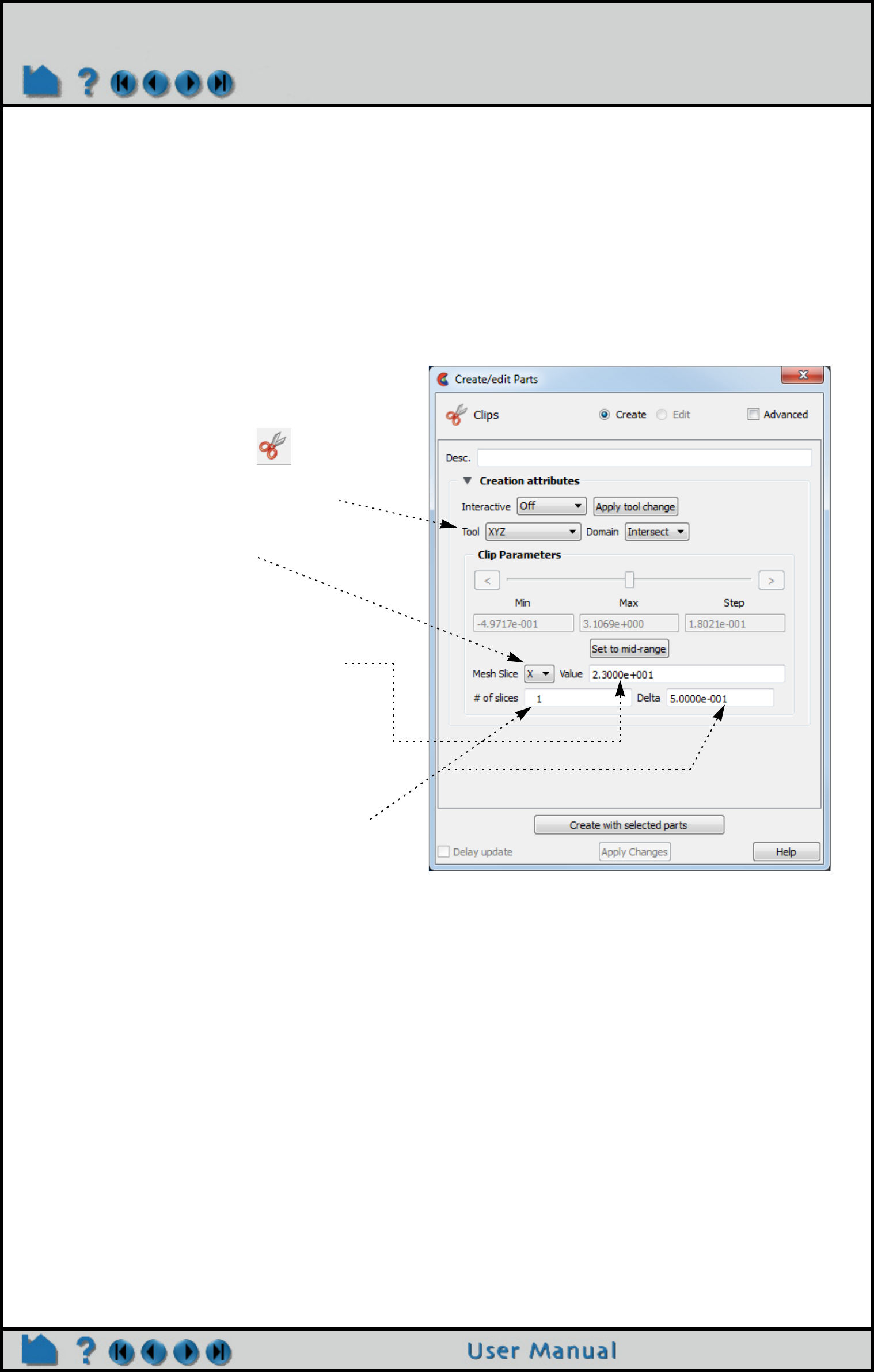
Page 308
HOW TO CREATE XYZ CLIPS
Create XYZ Clips
INTRODUCTION
An XYZ clip is a 1D or 2D slice through 2D or 3D meshes (structured or unstructured). The resulting clip is a 1D or
2D mesh slice where one of the dimensions (e.g. X) is held constant (or fixed) while the other one or two dimensions
(e.g. Y and Z) vary in reference to the local frame of the mesh. XYZ clips can be interactively animated throughout
the range of the fixed dimension by manipulating a slider. The minimum, maximum, and step size of the range of the
interactive fixed dimension can be set by the user.
BASIC OPERATION
Note that you can change the fixed dimension of an XYZ clip at any time (with the Mesh Slice pulldown).
Shortcut
Right click on a part in the graphics window. In the resulting pulldown, choose Clip and in the further pulldown,
choose X, Y, or Z. This then automatically creates an X, Y, or Z clip part with the default settings using the right-
clicked part as the parent part and location indicated by the right click.
1. Select the parent part(s) in the
Parts list..
2. Click the Clip icon.
3. Select XYZ from the Tool pulldown.
4. Select the desired fixed dimension from
the Mesh Slice pulldown.
5. Enter the value for the fixed dimension in
the Value text field and press return.
6. Click the “Create with selected parts”
button.
Note: Multiple slices with a delta in the normal direction
can be created easily by setting these values.
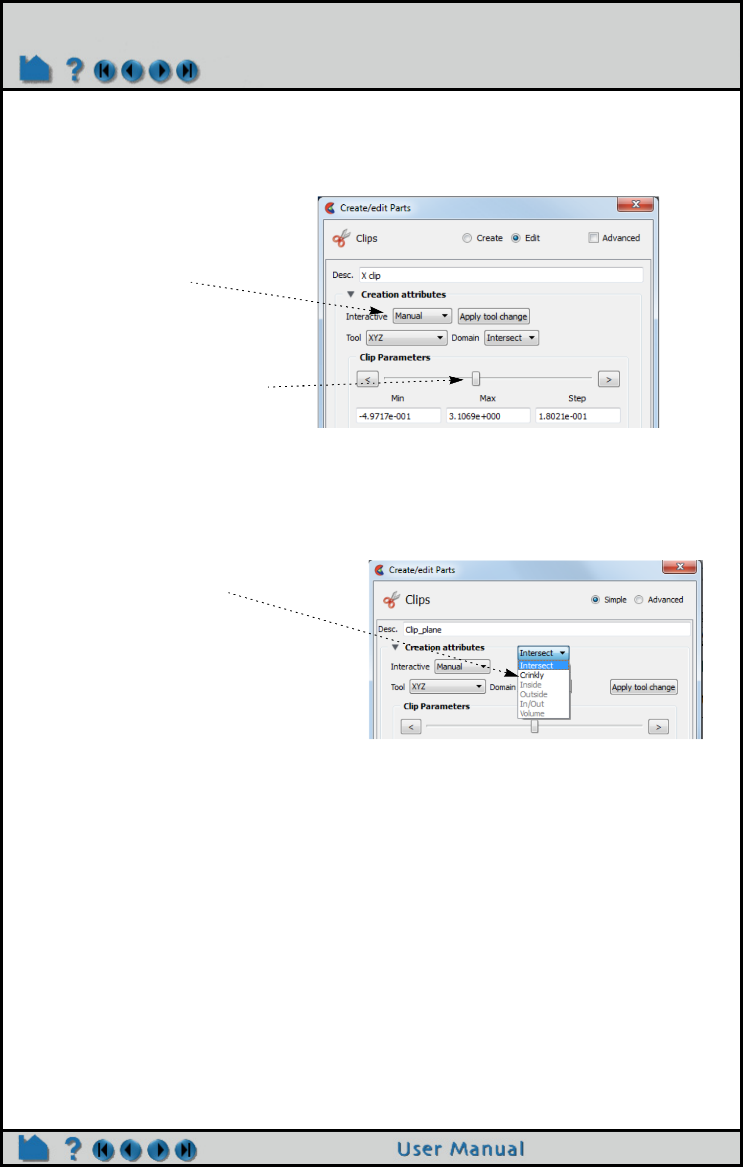
Page 309
HOW TO CREATE XYZ CLIPS
ADVANCED USAGE
Interactive XYZ Clipping
You can interactively sweep through the range of the fixed dimension by adjusting a slider with the mouse.
Crinkly XYZ Clipping
You can check the integrity of your mesh by clipping with a crinkly intersection. Specifying a crinkly domain results in
a part composed of all the elements that intersect the mesh slice value.
Clipping Plane Animation
Although you can interactively sweep an XYZ clip through a mesh, it is sometimes desirable to have EnSight
automatically calculate a series of XYZ clips for you. These can then be replayed (as fast as your graphics hardware
will permit) using EnSight’s Flipbook Animation facility. See How To Create a Flipbook Animation for more
information.
SEE ALSO
Introduction to Part Creation
How To Create a Flipbook Animation
Other clips:
How to Create Clip Lines
How to Create Clip Planes
How to Create Quadric Clips
How to Create IJK Clips
How to Create RTZ Clips
How to Create Box Clips.
User Manual: Clip Parts
1. Double-click the desired XYZ clip
part in the Parts list.
2. Change Interactive to Manual to
enable sweeping.
3. If desired, enter values for the Min,
Max, and Step to override the
defaults.
4. Adjust the slider with the mouse.
1. Change the Domain to Crinkly
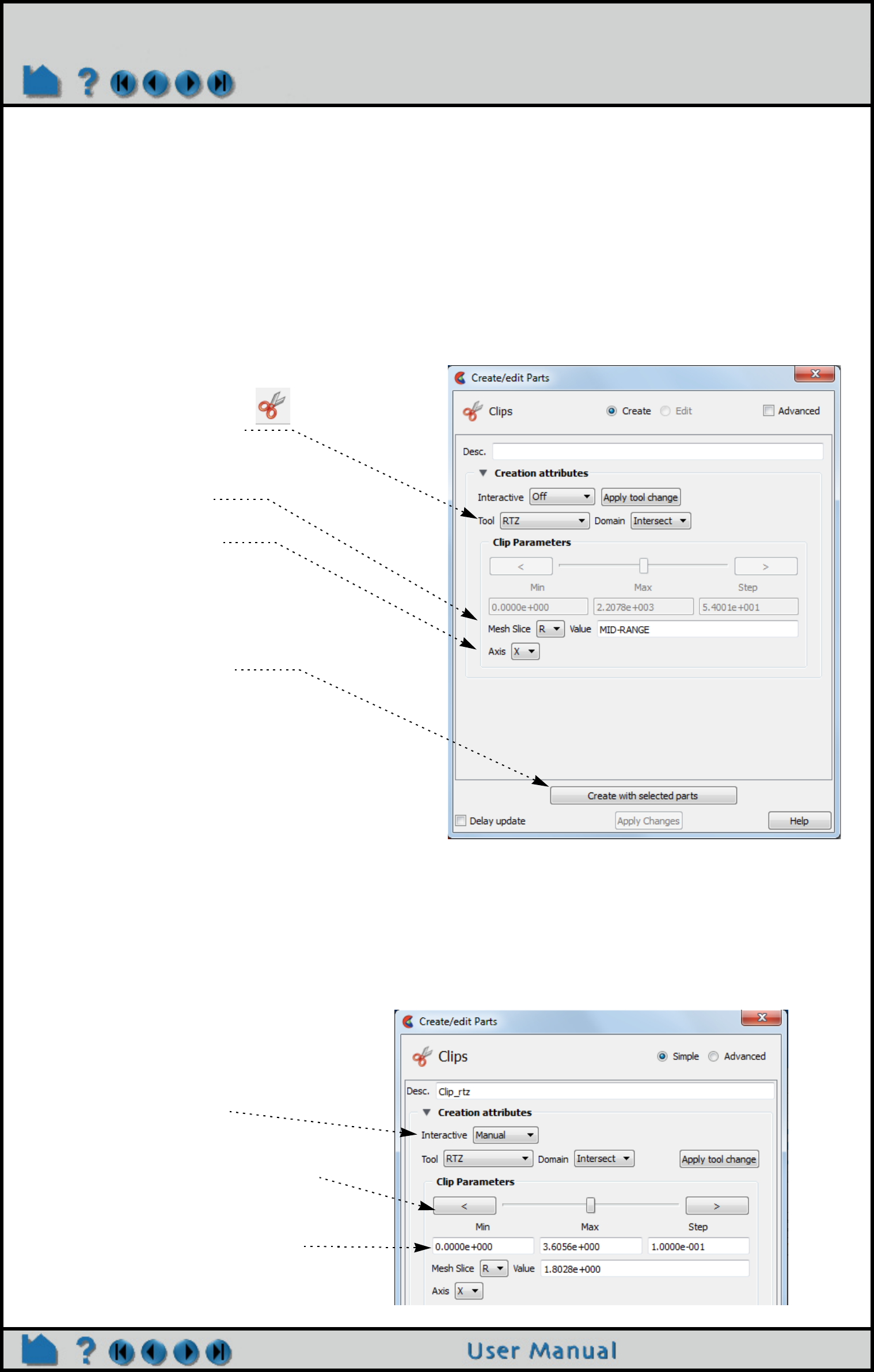
Page 310
HOW TO CREATE RTZ CLIPS
Create RTZ Clips
INTRODUCTION
An RTZ clip is a 1D or 2D slice through 2D or 3D meshes (structured or unstructured). The resulting clip is a 1D or 2D
mesh slice where one of the dimensions (e.g. R,”radial component”) is held constant (or fixed) while the other one or
two dimensions (e.g. T, ”theta component” and Z, “z axis component”) vary in reference to the local frame of the
mesh. RTZ clips can be interactively animated throughout the range of the fixed dimension by manipulating a slider.
The minimum, maximum, and step size of the range of the interactive fixed dimension can be set by the user.
BASIC OPERATION
Note that you can change the fixed dimension of an RTZ clip at any time (with the Slice pulldown). If you change the
numeric value, remember to press return for the change to take effect.
ADVANCED USAGE
Interactive RTZ Clipping
You can interactively sweep through the range of the fixed dimension by adjusting a slider with the mouse.
1. Select the parent part.
2. Click the Clip icon.
3. Select RTZ from the Tool
pulldown
4. Select the desired fixed dimension of
the slice (R, T, or Z).
5. Select the Axis that describes the
cylindrical length.
6. Enter the value for the slice (the value
of R, T, or Z), or leave MID-RANGE and
press return.
7. Create using selected
parts or select parts to use.
1. Double-click the desired RTZ clip
part in the main parts list.
2. Change Interactive to Manual to
enable sweeping.
3. Adjust the slider with the mouse.
4. If desired, enter values for the Min,
Max, and Increment to override the
defaults.
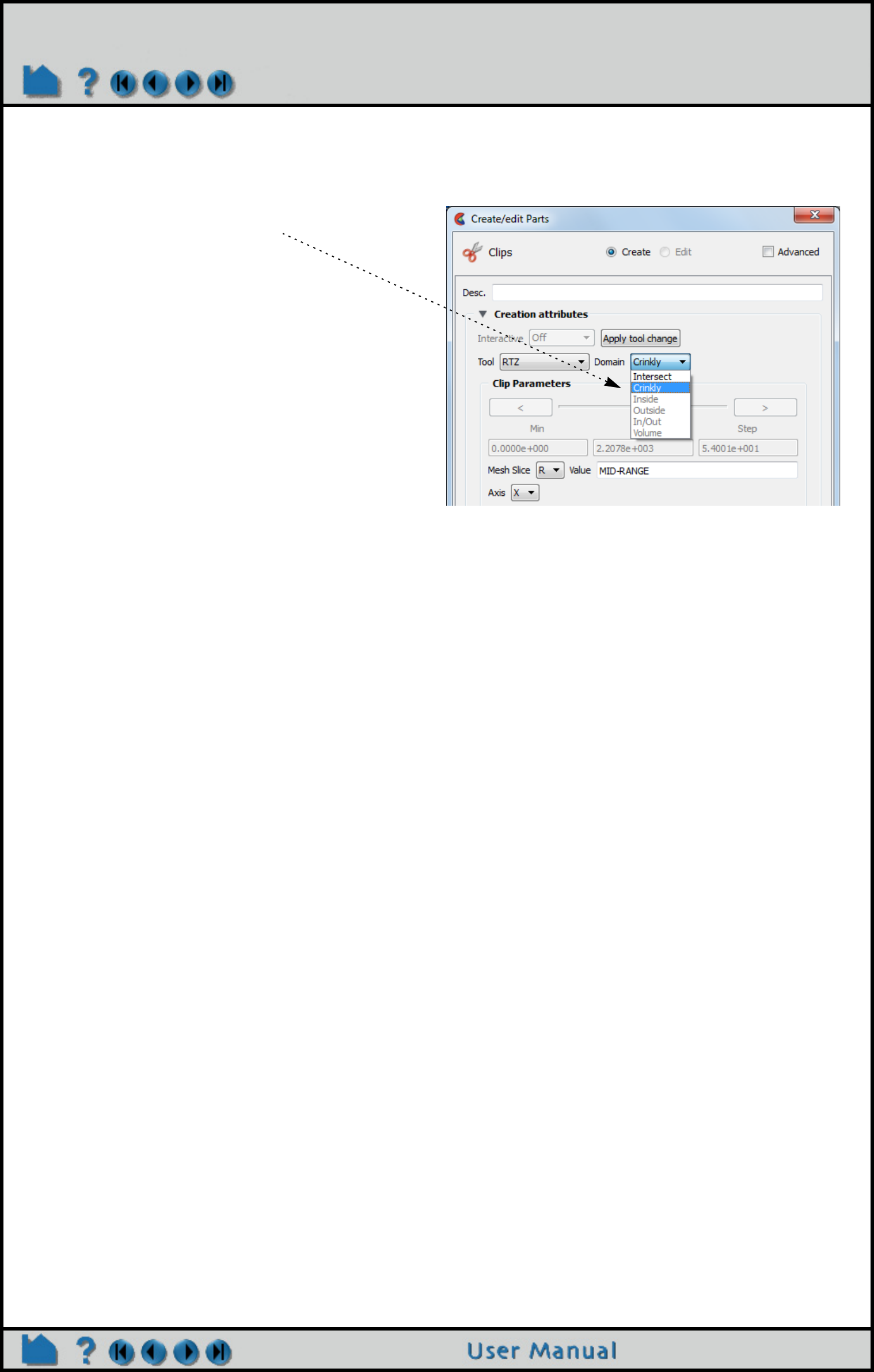
Page 311
HOW TO CREATE RTZ CLIPS
Crinkly RTZ Clipping
You can check the integrity of your mesh by clipping with a crinkly intersection. Specifying a crinkly domain results in
a part composed of all the elements that intersect the mesh slice value. Crinkly clipping cannot be done interactively.
Clipping Plane Animation
Although you can interactively sweep an RTZ clip through a mesh, it is sometimes desirable to have EnSight
automatically calculate a series of RTZ clips for you. These can then be replayed (as fast as your graphics hardware
will permit) using EnSight’s Flipbook Animation facility. See How To Create a Flipbook Animation for more
information.
OTHER NOTES
Inside, Outside, and In/Out cutting are disabled for this clipping type because it has no meaning for T. And if you
desire this effect for Z or R, you can use a plane clip or cylindrical clip instead.
SEE ALSO
Introduction to Part Creation
How To Create a Flipbook Animation
Other clips:
How to Create Clip Lines
How to Create Clip Planes
How to Create Quadric Clips
How to Create IJK Clips
How to Create XYZ Clips
How to Create Box Clips.
User Manual: Clip Parts
1. Change the Domain to Crinkly
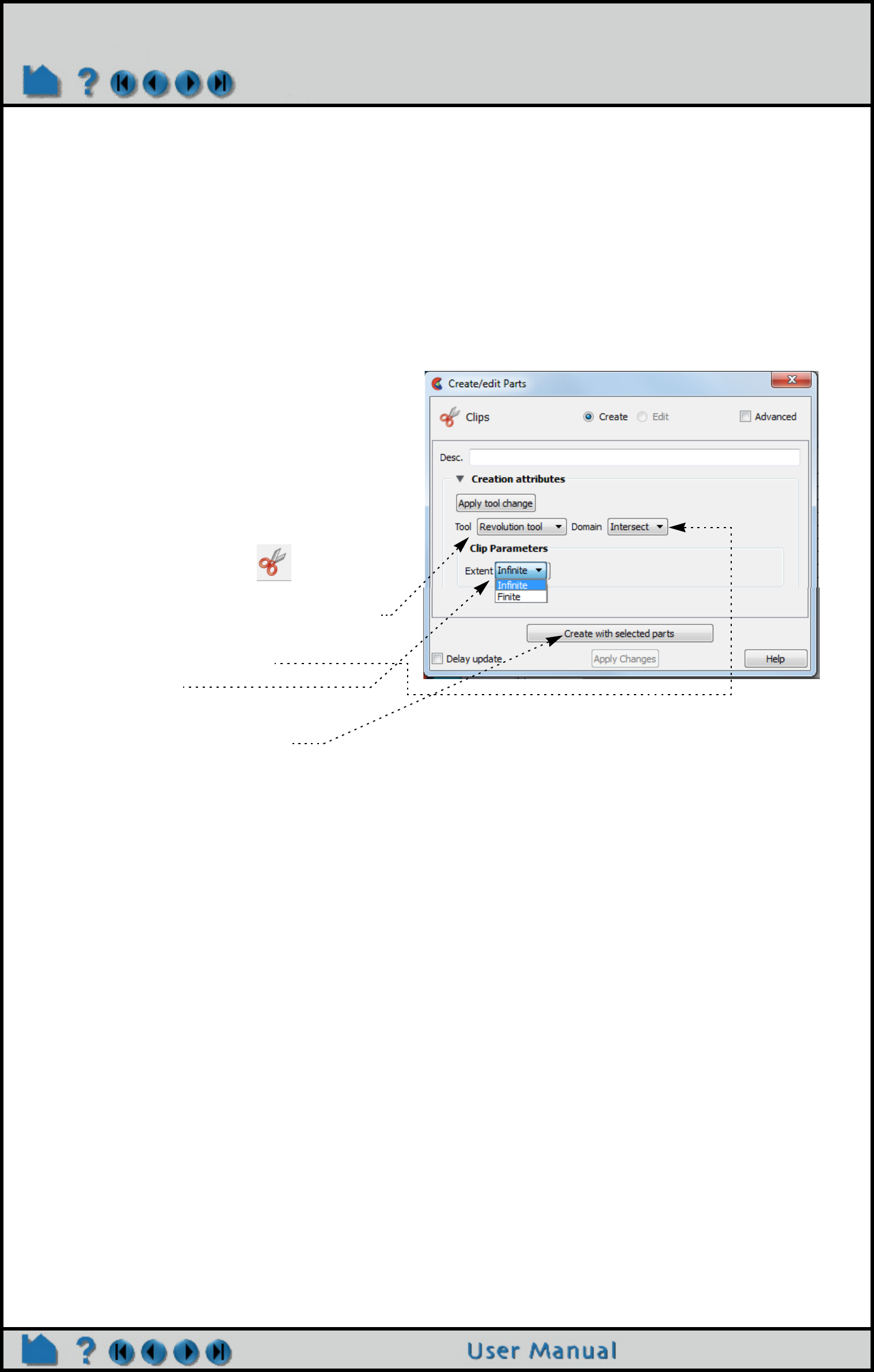
Page 312
HOW TO CREATE REVOLUTION TOOL CLIPS
Create Revolution Tool Clips
INTRODUCTION
A Revolution Tool clip can be made using the surface of revolution tool. It can be the surface created by the
intersection of the surface of revolution tool and the model, the elements intersected by the surface of revolution tool
(crinkly), or the volume of the inside and/or the outside domain swept by the revolution tool. This clip does not have
interactive manipulation capability, with a slider or by dragging the tool with the mouse. However, the tool can be
manipulated and the clip updated.
BASIC OPERATION
SEE ALSO
Introduction to Part Creation
Other clips:
How to Create Clip Lines
How to Create Clip Planes
How to Create Quadric Clips
How to Create XYZ Clips
How to Create RTZ Clips
How to Create Box Clips
How to Create IJK Clips
How to Create Revolution of 1D Part Clips.
User Manual: Clip Parts
1. Place the Surface of Revolution Tool at the
desired location. See How To Use the
Surface of Revolution Tool.
2. Select the parent part from the EnSight
main part list.
3. Click the Clip icon.
4. Select Revolution Tool from the Use Tool
pulldown.
5. Select the desired Domain.
6. Select extents
7. Create using selected parts. Note that you can manipulate the Surface
of Revolution tool and update your clip by
clicking Apply Tool Change.
You can also change the domain, and the
clip will change.
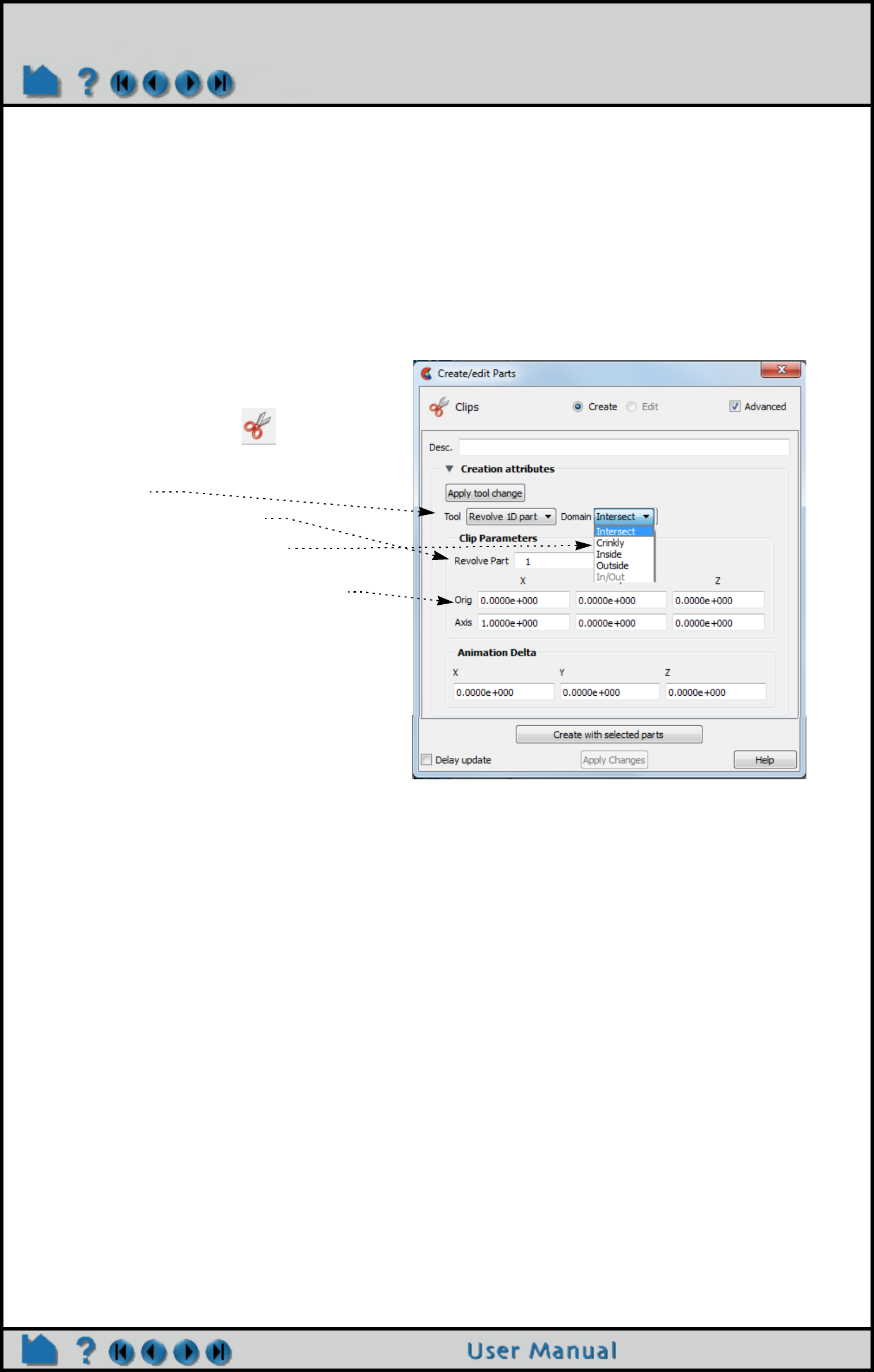
Page 313
HOW TO CREATE REVOLUTION OF 1D PART
Create Revolution of 1D Part Clips
INTRODUCTION
A Revolution of 1D Part clip can be made using a 1D part and a user specified axis. It can be the surface created by
the intersection of the 1D part about the axis and the model, the elements intersected by the 1D part about the
axis(crinkly), or the volume of the inside and/or the outside domain swept by the 1D part about the axis. This clip is
always infinite. This clip does not have interactive manipulation capability, with a slider or by dragging the tool with the
mouse. However, if the 1D part is capable of being moved, you can move it and the revolution clip will update.
BASIC OPERATION
SEE ALSO
Introduction to Part Creation
Other clips:
How to Create Clip Lines
How to Create Clip Planes
How to Create Quadric Clips
How to Create XYZ Clips
How to Create RTZ Clips
How to Create Box Clips
How to Create IJK Clips
How to Create Revolution Tool Clips.
User Manual: Clip Parts
1. Select the parent part(s) in the main
EnSight part list.
2. Click the Clip Icon.
3. Select Revolve 1D Part from the Tool
pulldown.
4. Enter the 1D part to use.
5. Select the desired Domain.
6. Set the desired origin and axis of the
revolution.
7. Click create.
Note that you can manipulate the 1D part or the
origin and axis and the clip will update.
You can also change the domain, and the clip will
change.
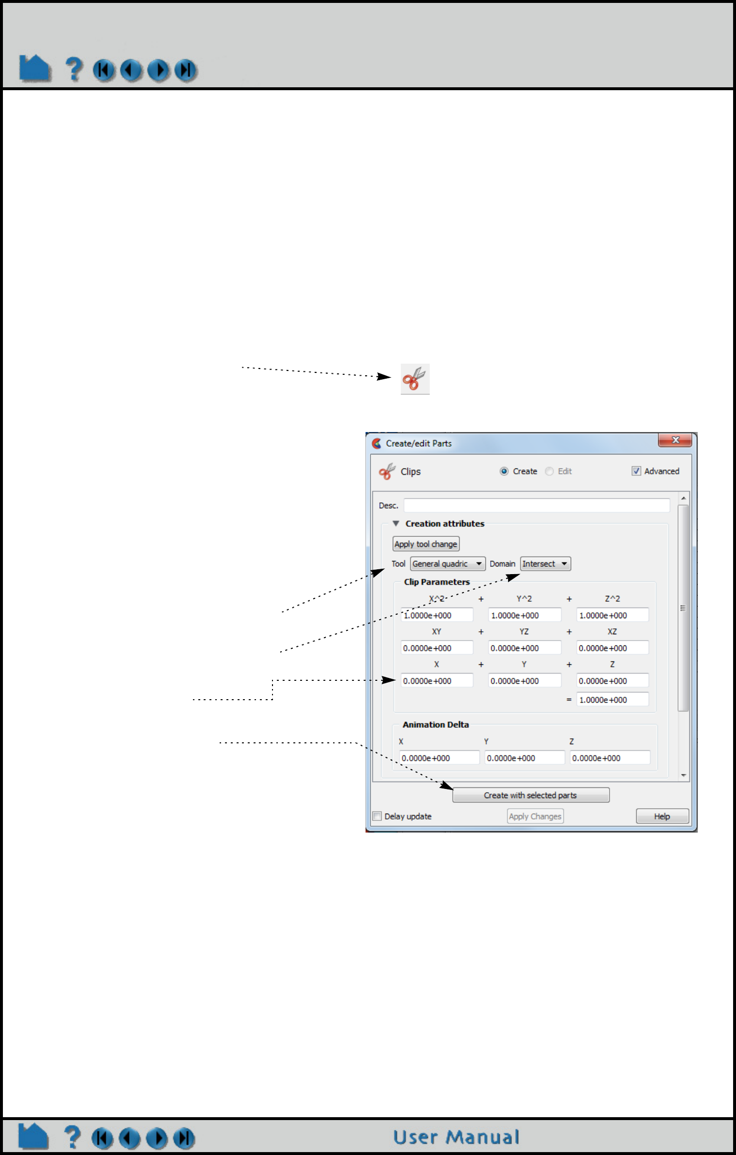
Page 314
HOW TO CREATE GENERAL QUADRIC CLIPS
Create General Quadric Clips
INTRODUCTION
Clicking on the Clips Icon brings up the Clips Feature Panel, the Creation section of which offers access to a General
quadric clip type. It is possible to create a 3D Quadric clip using the General Quadric option by directly specifying the
coefficients of a general quadric equation.
These coefficient values represent the general equation of a Quadric surface. They can be changed by modifying the
coefficient values. No tool exists corresponding to this equation.
AX2+BY2+CZ2+DXY+EYZ+FXZ+GX+HY+IZ=J
BASIC OPERATION
SEE ALSO
Introduction to Part Creation
Other clips:
How to Create Clip Lines
How to Create Clip Planes
How to Create Quadric Clips
How to Create XYZ Clips
How to Create RTZ Clips
How to Create Box Clips
How to Create IJK Clips
How to Create Revolution Tool Clips.
User Manual: Clip Parts
1. Click the Clip Feature Icon.
2. Select the parent part(s) in the Parts list.
3. Choose the General Quadric Tool.
4. Choose the desired Domain (Intersect,
Crinkly, Inside, Outside, or In/Out)
5. Edit the coefficients.
3. Click the Create button.
Note: The Animation Delta is not available for
general quadric clips.
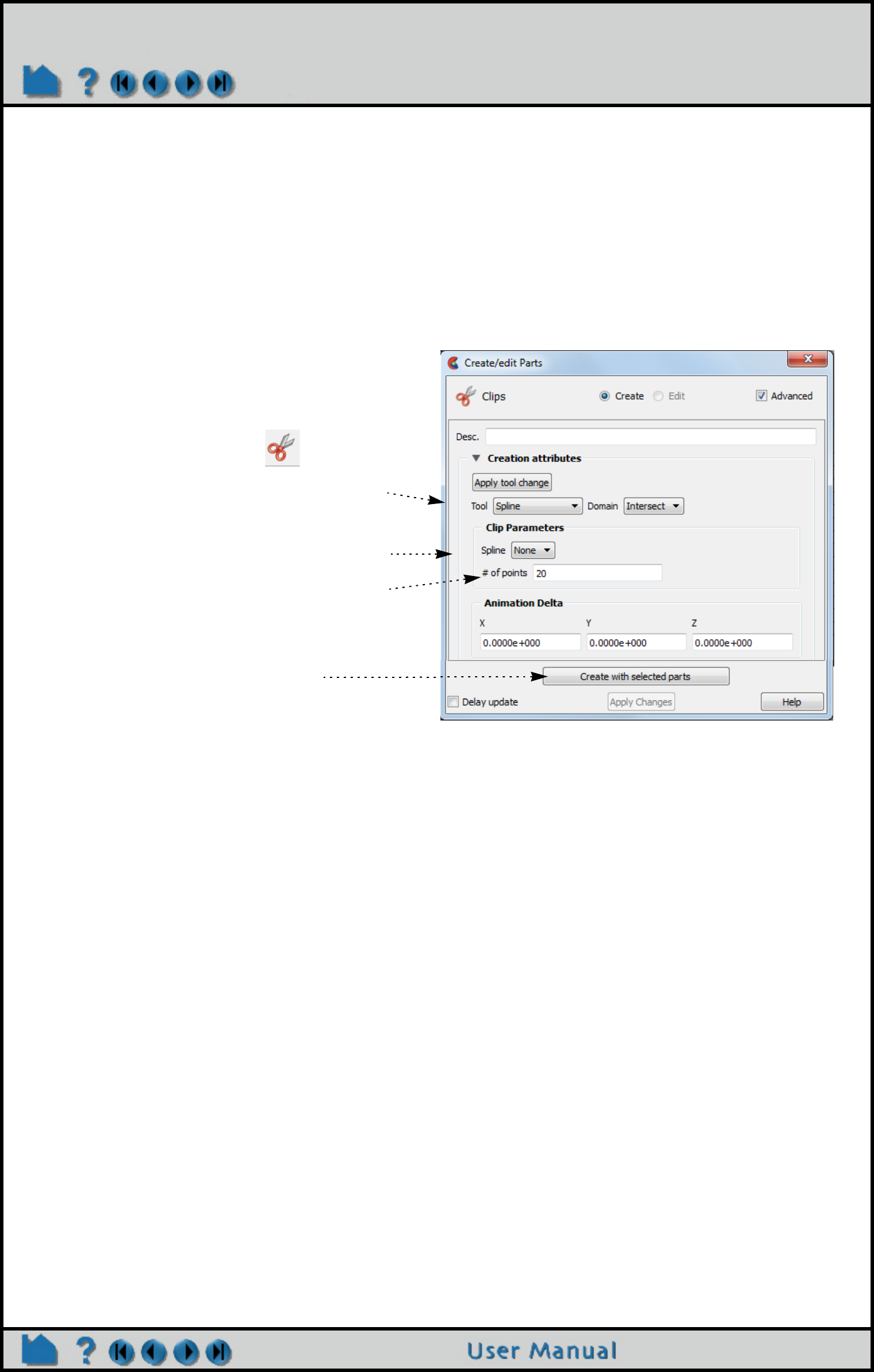
Page 315
HOW TO CREATE CLIP SPLINES
Create Clip Splines
INTRODUCTION
In addition to clipping along a line, EnSight also provides clipping along a defined spline. Spline clips will query the 2D
or 3D parent parts at samples taken along the spline at evenly spaced intervals. Values along a spline clip can be
visualized using profiles, queried and sent to a plotter, or used in further computations (for example a line integral).
BASIC OPERATION
OTHER NOTES
It is sometimes useful to display just the nodes of a spline clip. Using the Feature Panel you can change the display
such that only nodes (not lines) are displayed. The nodes can be shown as dots, crosses, or spheres. If displayed as
crosses or spheres, the size (radius) can be constant or scaled by the value of a variable. See How to Set for more
information.
SEE ALSO
Introduction to Part Creation
How To Use the Spline Tool
How to Create Profile Plots
How to Query/Plot.
Other clips:
How to Create Clip Planes
How to Create Clip Lines
How to Create Quadric Clips
How to Create Box Clips
How to Create IJK Clips
How to Create XYZ Clips
How to Create RTZ Clips.
User Manual: Clip Parts
1. Select the parent part.
2. Click the Clip icon.
6. Create using selected parts.
3. Select Spline from the Tool pull-down.
4. Select the desired Spline (to create a
Spline see How To Use the Spline Tool)
5. Set the number of evenly spaced points
on the line
Note: To adjust the clip you can grab the spline knot points and adjust. The clip will update.
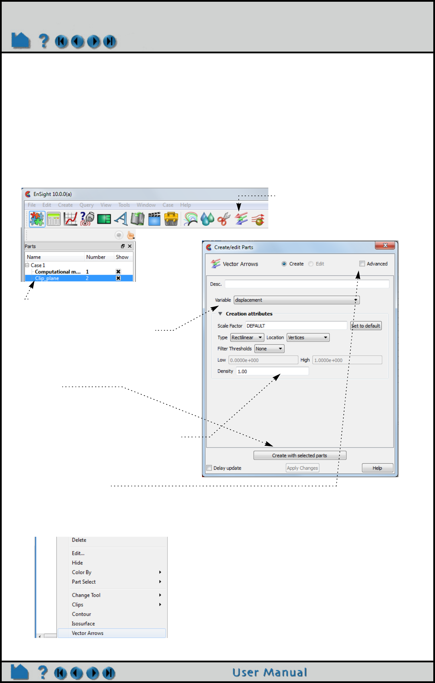
Page 316
HOW TO CREATE VECTOR ARROWS
Create Vector Arrows
INTRODUCTION
Vector arrows display the direction and magnitude of a vector at discrete locations in a model. Although vector
magnitude can be visualized with other methods (e.g. color), important directional information is provided by the
arrows.
Vector arrows have numerous including length scale, tip style and size, projection, origin location, and display filters
based on vector magnitude.
BASIC OPERATION
Instant Arrows Shortcut
To quickly create vector arrows on a part, right click in the part list or in the graphics area and choose Vector Arrows
1. Select the parent.
part.
3. Select the vector variable to use.
2. Click the Vector Arrows icon.
4. Leave it Default to load a suitable Scale
Factor and change it later as desired.
5. Create
6. Select the desired density (0.0 to 1.0).
The density of the arrows will vary from no arrows (0.0)
to arrows at every location (1.0). At intermediate
densities the arrows are placed randomly with no user
control of their locations.
7. More options are available by clicking on
the Advanced toggle
1. User will be presented with a list of vector variables and
then vector arrows will be instantly created on the part
using all the defaults.
2. If only one vector variable is in the dataset, then vector
arrows will be created using that variable on the selected
part.
3. Vector arrows are then colored by the vector.
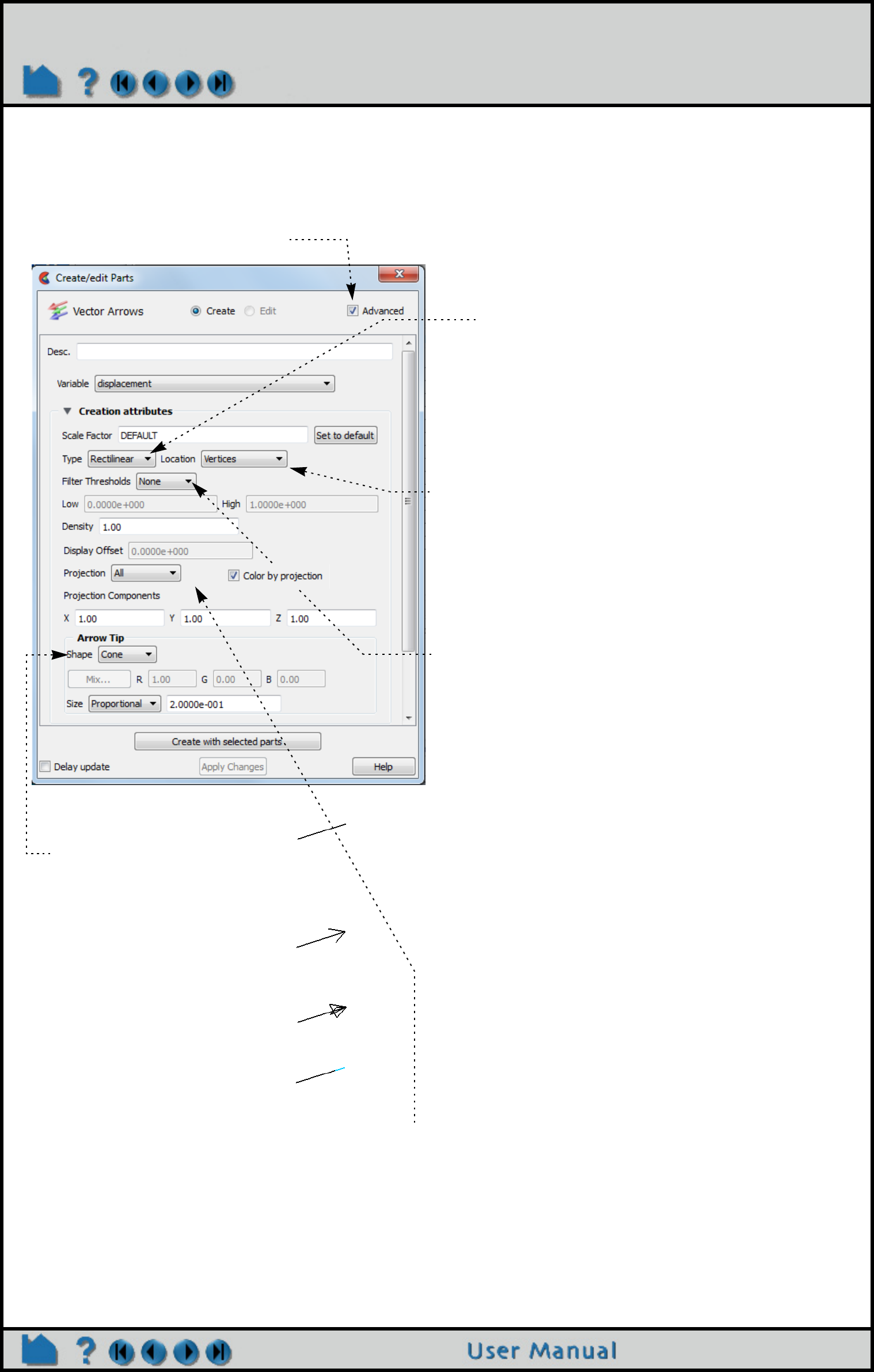
Page 317
HOW TO CREATE VECTOR ARROWS
Advanced Vector Arrow
Other vector arrow control the type of arrow, the location of the arrow origin, and arrow filtering options.
1. To change vector arrow at any time, simply double-click
the desired vector arrow part in the parts list.
2. Click on the Advanced Toggle
3. Select the desired type from the Type pulldown.
Choices are:
Rectilinear Standard vector arrows: shaft points in local vector
direction with length equal to vector magnitude
scaled by Scale Factor Value.
Rect. Fixed Same as Rectilinear except that length is set by
Scale Factor value independent of vector magnitude.
Curved Arrow shaft is the path of a particle trace in the local
flow field. Scale Factor becomes “Time” and controls
the duration (stopping criteria) for each trace.
WARNING! This can take a great deal of time for
large numbers of vector arrows and/or long Time
values!
5. Select the desired filter type from the Filter
pulldown.
Choices are:
None No filtering – all vector arrows appear.
Low Display only those arrows with magnitude above the
value in the Low text field.
Band Display only those arrows with magnitude below
Low and above High (opposite of Low/High).
High Display only those arrows with magnitude below the
value in the High text field.
Low/High Display only those arrows with magnitude between
Low and High (opposite of Band).
4. Select the desired arrow Location of the origin.
Choices are:
Node Arrows originate from each node of the parent
part(s).
Vertices Arrows originate only from those nodes that are also
vertices of the parent part(s).
Element Center Arrows originate from the geometric center of all
elements of the parent part(s).
6. Select the desired tip shape.
None No tip (default).
Cone Solid cone shape
Normal Single wedge. Good for 2D
problems. Plane of the
wedge is based on the
relative magnitudes of the
components.
Triangles Two intersecting triangles.
Good for 2D/3D problems.
Tipped End of the shaft colored in a
different color. Good where
other shapes yield too much
visual clutter.
7. Set the desired display offset.
Note: this is rarely necessary because by default, Display offset is
set automatically using the graphics hardware. The display offset
moves the vector arrows a short distance away from the surface on
which they are defined (typically for hardcopy or animation
purposes) in the direction of the surface normal. This is used when
a tangential projection is used and the arrows are coincident with
the parent part’s surface. Note that a negative offset may be
appropriate (depending on orientation). You must turn off the
hardware display offset in Preferences in order to manually set it
here. To turn if off, Edit>Preferences, View.
8. Select the desired projection component.
Choices are modified by the Projection component field. Scale the x, y, and/or z in the Projection component field.
Values less than 1 diminish the contribution, more than 1 exaggerate the contribution. Zero means that the component
is not considered and confine arrows to the plane perpendicular to this component. If you choose Tangential or Normal,
and turn ON the Color by Projection Toggle then the part will be colored by the Tangential or Normal
All Display arrows in the vector direction.
Tangential Display component parallel to surface element.
Normal Display component normal to surface element.

Page 318
HOW TO CREATE VECTOR ARROWS
OTHER NOTES
Vector arrows can be animated by animating the parent part (e.g. a clip plane) over space or time using flipbook or
keyframe animation. See How To Create a Flipbook Animation or How to Create a Keyframe Animation for
more information.
If vector arrows are created on a clip through an unstructured mesh, the resulting arrows can be difficult to visualize if
the resolution of the underlying mesh varies substantially or is highly irregular. One solution is to create the vector
arrows on a grid clip rather than the default mesh clip. See How to Create Clip Planes for more information.
Unlike most part creation operators, vector arrows are created from the client’s representation of the part – not the
server’s. For example, if you have a clip plane that is displayed using a feature-angle or border representation, only
those elements comprising the reduced display will yield vector arrows – even though all elements of the clip plane
reside on the server. See How to Change Visual Representation for more information.
Vector arrows with a tangential projection can sometimes by occluded by the surface on which the arrows are
defined. To solve this problem, use the Display Offset field to add a small displacement to move the arrows away
from the surface in the direction of the surface normal. This is most useful for presentation (e.g. hardcopy or
animation) output.
SEE ALSO
Introduction to Part Creation.
User Manual: Vector Arrow Parts
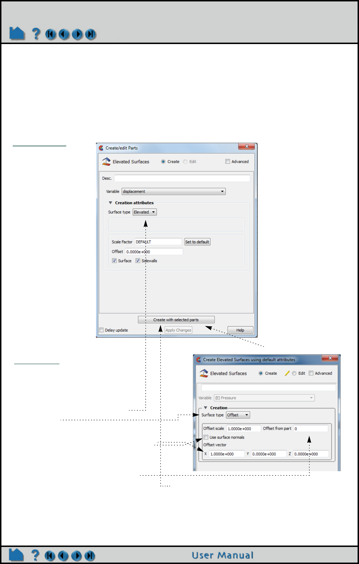
Page 319
HOW TO CREATE ELEVATED SURFACES
Create Elevated Surfaces
INTRODUCTION
An Elevated Surface is a 2D surface scaled (in the local surface normal direction of the parent) based on a variable
value. Elevated surfaces resemble topographic maps and are useful for accentuating relative differences in the value
of a variable. An Offset Surface uses a rigid-body translated origin part translated within a 3D parent part, to create a
new part using the geometry of the origin part, while getting variable information from the parent part. In other words,
an Offset Part results from using a translated origin part to clip a 3D volume parent part.
BASIC OPERATION
SEE ALSO
User Manual: Elevated Surface Parts
1. Select the parent part.
4. Select Surface type
Elevated.
2. In the top EnSight
menu, Create >
Elevated Surfaces.
5. If desired, enter an
appropriate scale factor
(or leave it DEFAULT).
8. Create using selected
parts
6. If desired, enter an
Offset value.
The Offset allows you to
“shift” the elevated
surface away from the
parent, but does not affect
the shape.
7. If desired, toggle
Surface or Sidewalls
off.
The Surface is the actual
elevated surface. Sidewalls
stretch from the border of
the parent to the border of
the Surface to enclose the
created part.
Elevated Surface
3. Select the variable.
2. Change Surface type pulldown
to Offset.
3. Choose the surface normal translation OR
vector direction and scale. The rigid-body
translation=offset_scale * offset_vector
4. Choose the origin part number which
will be used to clip the parent part at a
location specified by the surface
normal or rigid-body translation in the
offset vector direction.
Offset Surface
An offset surface can be thought of as
clip of a 3D field using a 2D part
translated into the field.
1. Do items 1-3 above.
5. Create using selected parts.

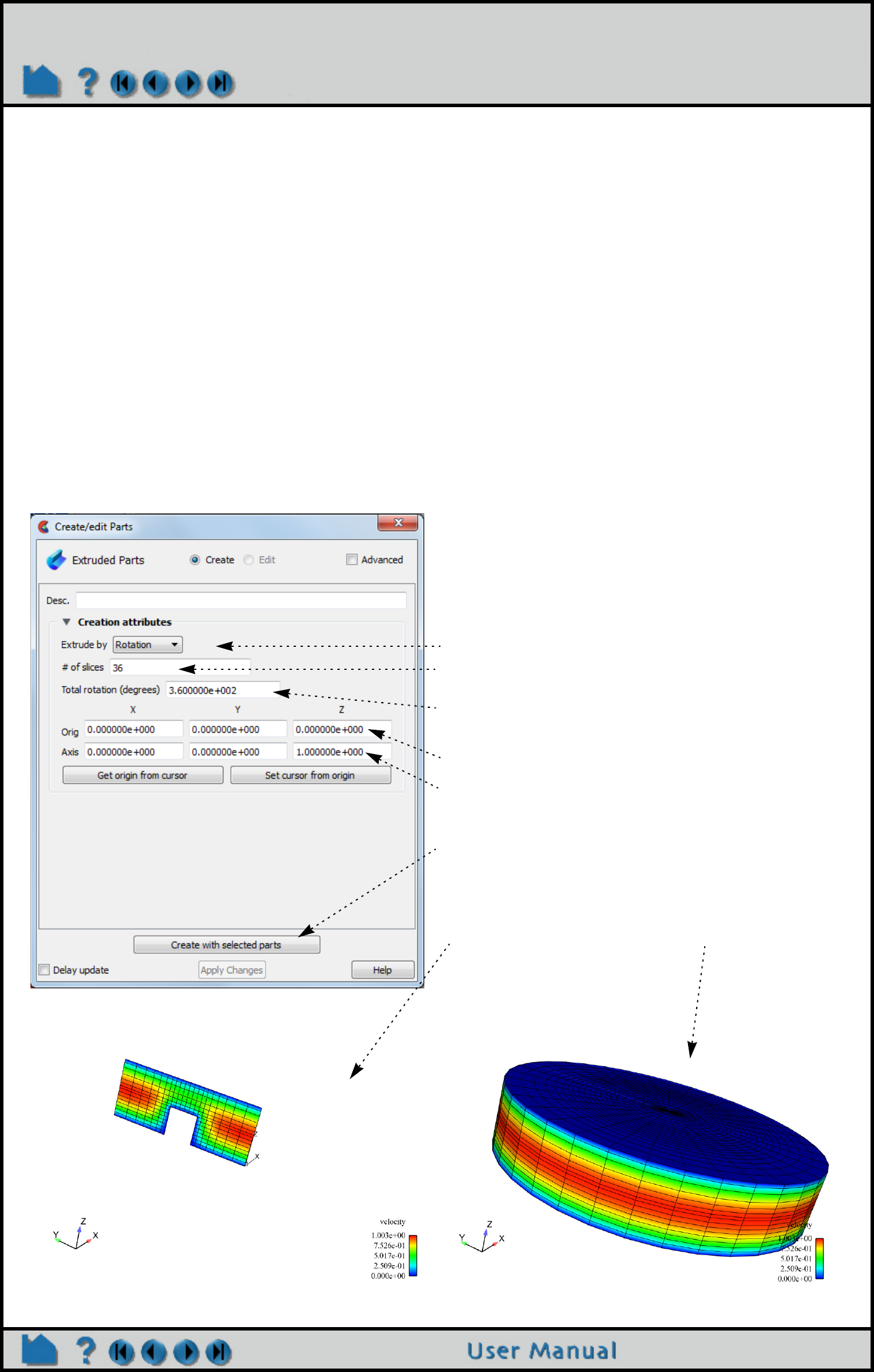
Page 321
HOW TO EXTRUDE PARTS
Extrude Parts
INTRODUCTION
A part or parts can be “extruded” to the next higher ordered part using the Extrusion feature. Namely, a 1d line can
become a plane, a 2D surface can become a volume, etc. This “extrusion” can occur in a rotational way (making the
whole pie from a thin slice) such as would be needed for reconstruction of a model from an axi-symmetric slice. Or it
can be done in a translational manner - as if the part were glued in place, but could be stretched in one direction.
For rotation extrusions, you must define an origin and axis vector in the global coordinate system, about which the
rotational extrusion will occur, as well as the number of slices and the total rotation angle to sweep through. For
translation extrusions, you define a direction vector in the global coordinate system, as well as the number of slices
and the total distance to stretch.
BASIC OPERATION
1. Select the parent part in the part list. 2. In the top EnSight menu, Create > Extrude
8. Create
6. Set the origin of the rotation axis
5. Set the total rotation to extrude.
(Needs to be between -360 and 360)
4. Set the number of “slices” that will be created.
3. Select Rotation type
7. Set the components (direction cosines) of the
rotation general axis.
This will cause a 2D slice to become a 3D volume.
Rotational Extrusion:
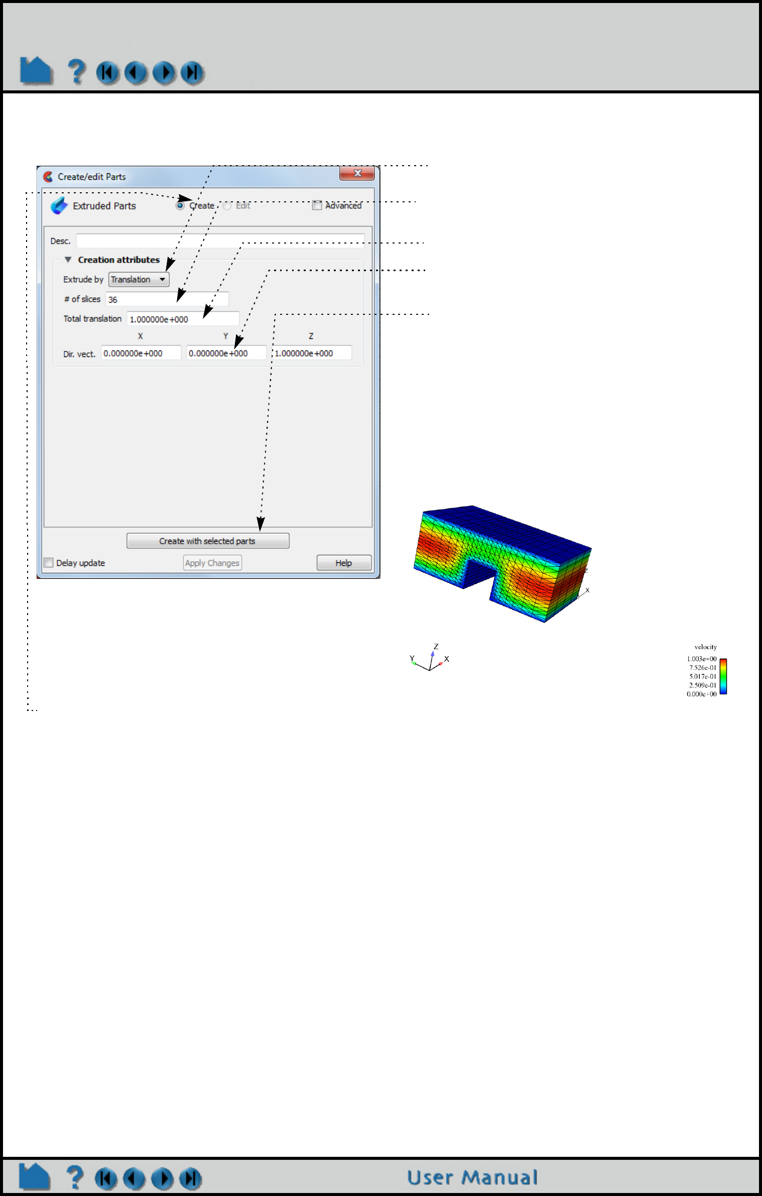
Page 322
HOW TO EXTRUDE PARTS
SEE ALSO
User Manual: Extruded Parts
Translational Extrusion: 1. and 2. as above
3. Select Translation type.
4. Set the number of slices in the translation
direction.
5. Set the total translation distance.
6. Set the components of the direction vector.
And the slice will now become something like the
following:
7. Create
Advanced: Click on the Advanced Toggle for
more options
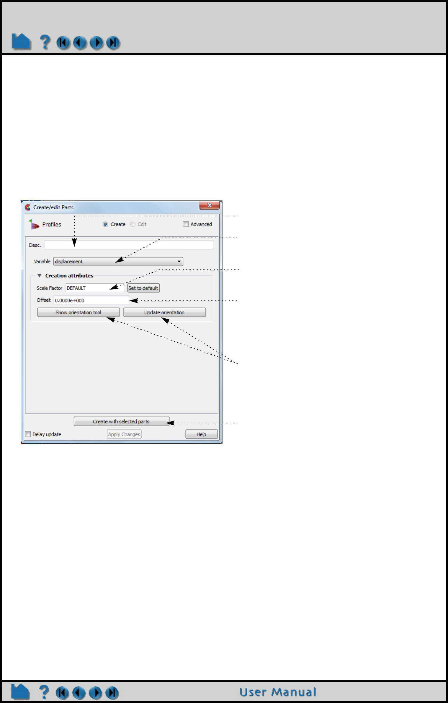
Page 323
HOW TO CREATE PROFILE PLOTS
Create Profile Plots
INTRODUCTION
A profile plot is the 2D counterpart to an elevated surface: a projection away from a 1D part based on the value of a
variable. Profile plots can be created on any 1D part: clip lines, contours, particle traces, or model parts consisting
of 1D elements.
BASIC OPERATION
For each node of the parent part, the corresponding node on the profile curve is determined by adding the value of
the Offset to the selected variable value and then multiplying the sum by the Scale Factor. The projectors of the
profile are the lines that connect the nodes of the parent part to the nodes of the profile curve. The Plane tool is used
to specify the orientation and direction of the projectors. The projectors are created parallel to the Plane tool
projecting away from the center of the Plane tool (at least where the value of the selected variable plus the Offset is
positive).
Although the parent part of a profile plot must be 1D, the nodes that make up the part do not have to be linear. For
curved parents, the projectors of the resulting profile plot are still parallel, but they do not all lie in the same plane.
ADVANCED
Click on the advanced toggle to see more scale options and plane tool orientation options.
SEE ALSO
User Manual: Profile Parts
1. Select the parent part in the Part list.
2. In the main menu, Create>Profiles
5. Select an appropriate Scale
Factor (or leave as Default).
8. Create
6. If desired, enter an Offset value.
The Offset allows you to “shift” the profile away
from the parent, but does not affect the shape.
7. If desired, adjust the orientation of the Plane
tool.
The Plane Tool is used to specify the orientation
and direction of the profile plot. See below for
details.
3. Name the new part.
4. Select the variable to use.
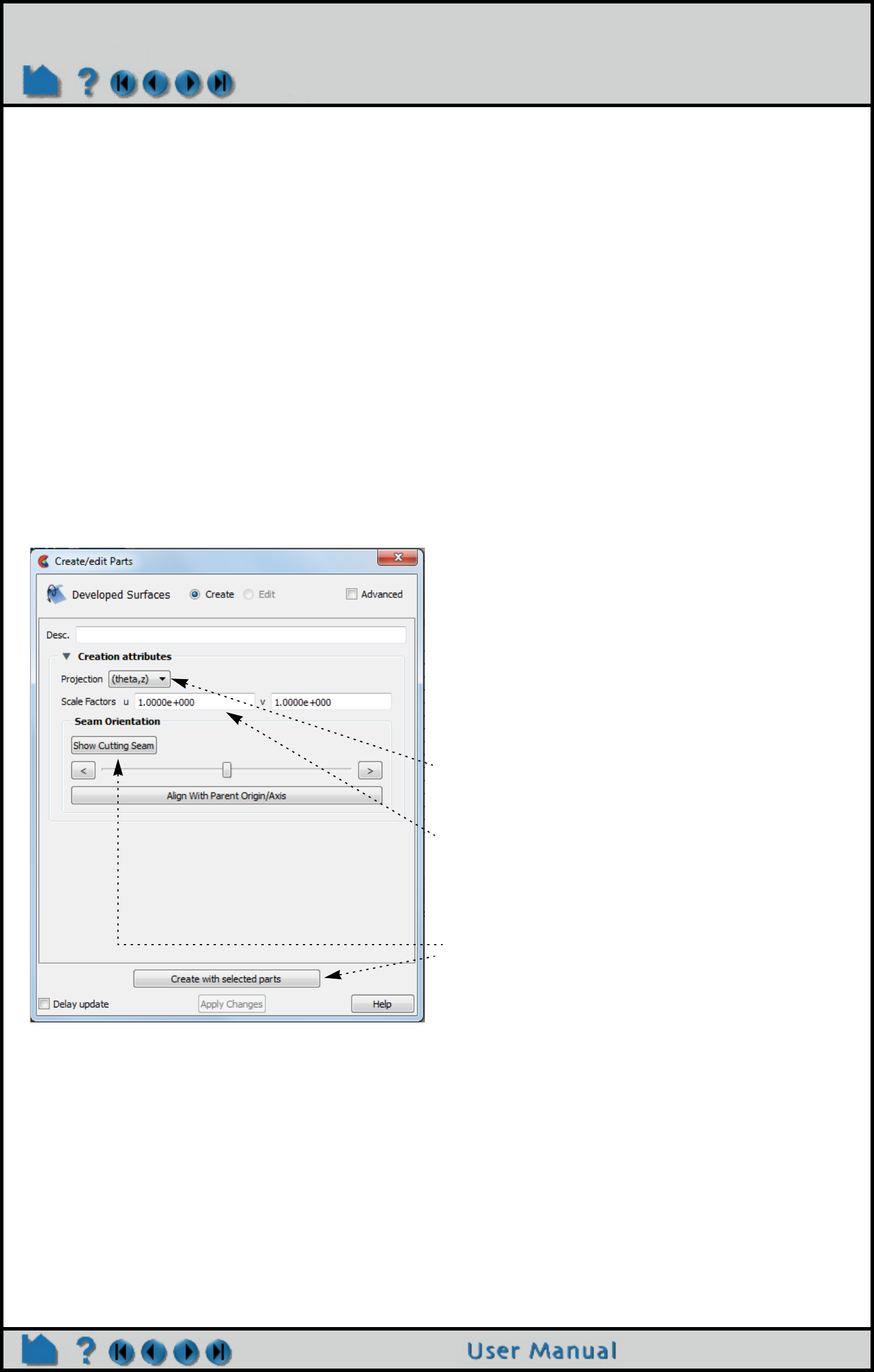
Page 324
HOW TO CREATE DEVELOPED (UNROLLED) SURFACES
Create Developed (Unrolled) Surfaces
INTRODUCTION
EnSight provides several sophisticated tools for extracting computational surfaces from meshes. For model parts or
clipped surfaces with a defined axis of rotation (such as those created with the quadric clipping tools), the surface can
“developed” or unrolled onto a plane. All variables defined on the clip are properly interpolated onto to the developed
surface.
A clip can be developed based on curvilinear (radius, z), (theta, z), or (meridian, theta) coordinate projections. The
“seam” of the clip can be specified interactively.
A model part must have its seam, its longitudinal axis and origin defined appropriately in the Feature Detailed Editor
(developed surface settings). To do this, right click on the part, choose ‘Edit’ and then pick the developed surface icon
in the top of the window that pops up and define the entities appropriately.
BASIC OPERATION
To create a developed surface:
A part is developed by specifying one of three curvilinear mappings called developed projections. The projections are
based on the curvilinear coordinates r (radius), z, (theta), and m (meridian or longitude). These coordinates are
defined relative to the local origin and axis of the tool that created the parent part (e.g. the Cylinder tool). The
projections are (r,z), (, z), and (m, ). The u, v scale factors (only for (, z) or (m, ) projections) provide scaling for
the coordinates in the listed order. For example, if the projection is (, z) then u scales and v scales z.
Toggle Advanced to edit seam origin and axis coordinates
SEE ALSO
How To Create Quadric Clips
User Manual: Developed Surface Parts
1. First, create the desired quadric clip (cylinder, sphere, or cone), or skip this step if your quadric model
part already exists.
3. In the main menu, choose
Create > Developed surfaces.
4. Select the desired projection type (see
below for details on the types).
5. If applicable for the projection type (and desired)
enter u,v scaling factors and press return).
6. To display and change the cutting seam, click the
Show Cutting Seam button, and adjust the slider.
7. Create
2. In the Part list, select the parent part for the
developed surface (i.e. the part you created in step 1).
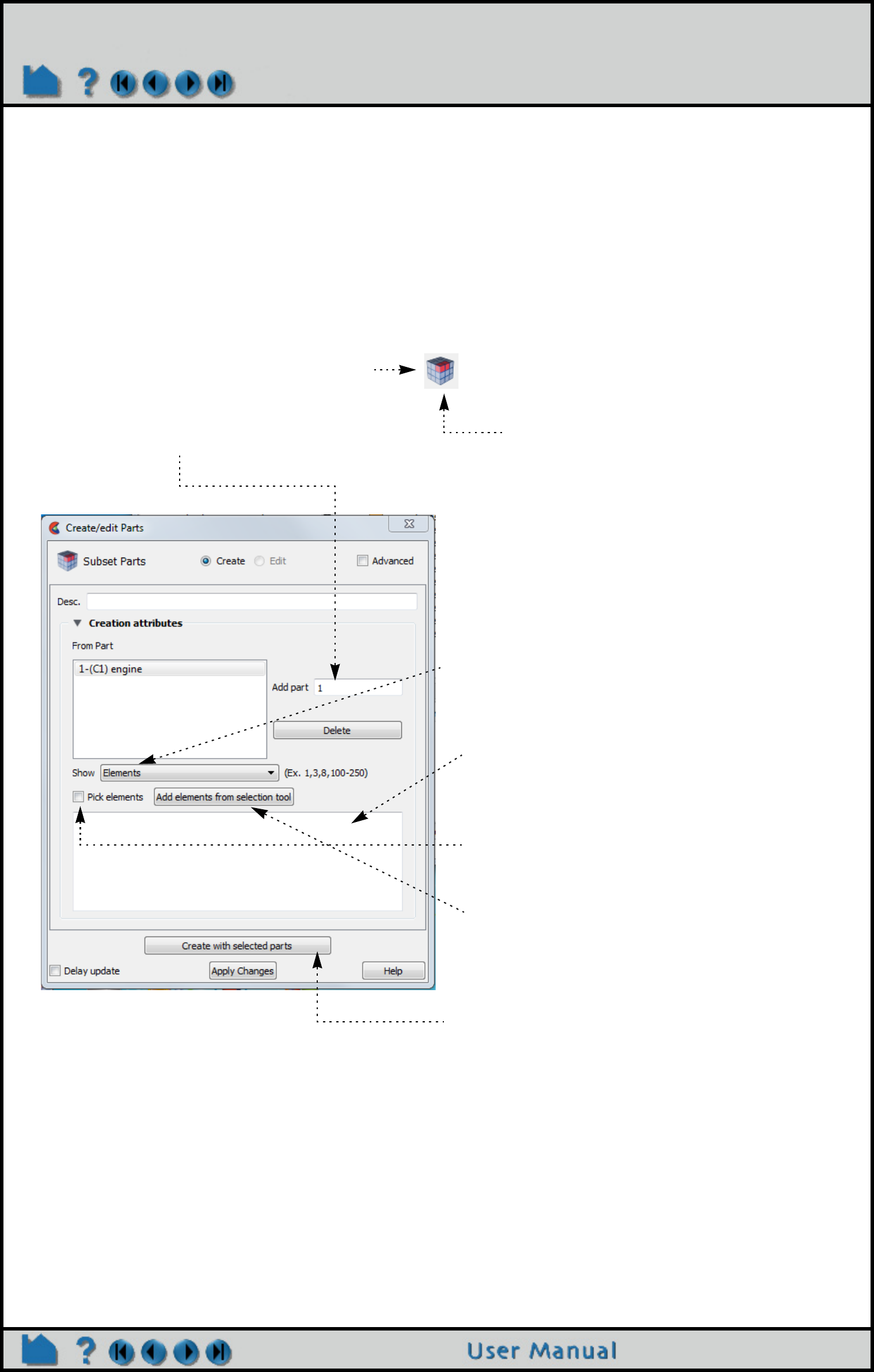
Page 325
HOW TO CREATE SUBSET PARTS
Create Subset Parts
INTRODUCTION
A Subset Part can be created by specifying node and/or element label ranges of a model part. Subset Parts can only
be created from model parts that have node and/or element labels. The Subset Part feature can be used to isolate
specified nodal and element regions of interest in large data sets.
BASIC OPERATION
SEE ALSO
How To Probe Interactively
User Manual: Subset Parts
1. First, click the Subset Parts Feature icon.
3. Now, for each parent model part,
enter the part number of the desired parent
part in the Add field, and press return.
3. Select Elements (or Nodes) to Show.
4. Enter the element (or node) label range(s)
in the Show List text field (ranges are
separated by commas).
OR
Toggle on “Pick elements” and select
elements using pick selection, which by
default is the “p” keyboard key.
OR
Turn on the selection tool and place it
where desired, then click “Add elements
from selection tool” to pick all the elements
within the tool.
5. Create to use selected parts in step 3.
2. Can’t find the icon in your Quick Action
Icon Bar? Right click on the icon bar
and choose Customize Feature
Toolbar. Use the left right arrows to
add the subset part icon, and the up-
down arrows to slide its location along
the icon bar.
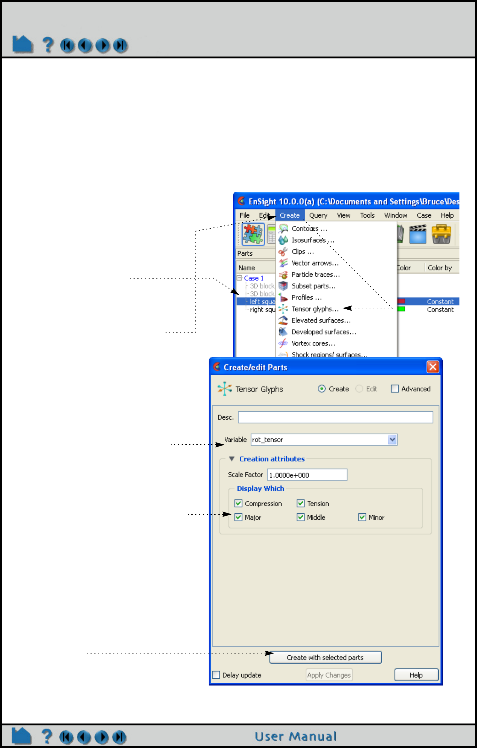
Page 326
HOW TO CREATE TENSOR GLYPHS
Create Tensor Glyphs
INTRODUCTION
Tensor glyphs display the direction of the eigenvectors for a tensor variable. Controls exist to show just the
compressive or tensile eigenvectors, and to selectively show the minor, middle, or major vectors.
Tensor glyphs have numerous including length scale, tips, color, and line width which can be used to indicate
compression or tension.
BASIC OPERATION
1. Select the parent parts.
2. Click Create -> Tensor glyphs...
(By default there is not an icon for this option
in the Feature Icon Bar.)
3. Select the tensor variable to use.
4. Select which eigenvectors to display.
5. Click Create.
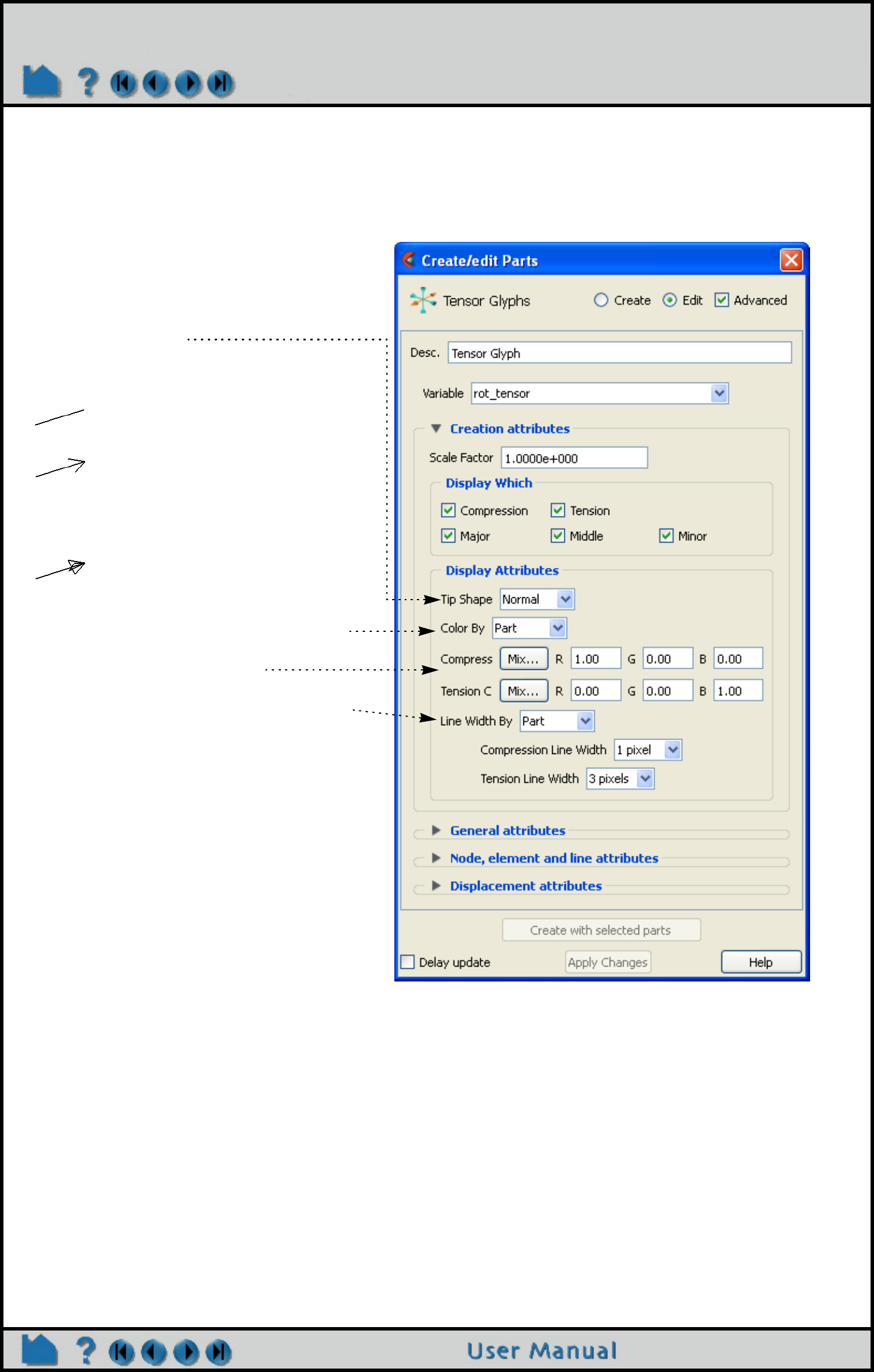
Page 327
HOW TO CREATE TENSOR GLYPHS
OTHER NOTES
Tensor glyphs can be animated by animating the parent part (e.g. a clip plane) over space or time using flipbook or
keyframe animation. See How To Create Flipbook Animation or How to Create a Keyframe Animation for more
information.
Unlike most part creation operators, tensor glyphs are created from the client’s representation of the part - not the
server’s. For example, if you have a clip plane that is displayed using a feature angle or border representation, only
those elements comprising the reduced display will yield tensor glyphs - even though all elements of the clip plane
reside on the server. See How to Change Visual Representation for more information.
SEE ALSO
Introduction to Part Creation.
User Manual: Tensor Glyph Parts
Display
The glyph’s to indicate tension or compression can be modified in several ways. Put the Tensor Glyph Feature
Panel into Advanced mode to open the Tensor Display:
2. The glyph can either be colored by the
part color, or show a specified color for
compressions and tension.
1. Select the desired tip shape from the Tip
Shape pulldown.
Tip Shape Choices:
None No tip (default)
Normal Single wedge. Good for 2D
problems. Plane of the
wedge is based on the
relative magnitudes of the
components.
Triangles Two intersecting triangles.
Good for 2D/3D problems.
3. The glyph can either be shown with the
line width attribute of the glyph, or show
a different line width for tension and
compression.

Page 328
HOW TO DISPLAY DISPLACEMENTS
Display Displacements
INTRODUCTION
In structural mechanics simulations, a common output variable is a set of vectors representing the movement or
displacement of geometry. Each displacement vector specifies a translation of a node from its original position (an
offset). EnSight can display and animate these displacements to help visualize the relative motion of geometry.
In many cases, the magnitude of the actual displacements is extremely small relative to the size of the model.
EnSight provides a displacement factor to scale the vectors and exaggerate the displacement.
For Model Parts
Displacements can be applied deeply on the server (in which the displacement vector is actually added to the
coordinates) or on the client (in which the graphical entities on the client are displaced visually only using the graphics
card). Server-side applied displacements (Displace computationally toggle ON, default) will apply the displacement
on the server coordinate prior to a calculation or operation. Client-side (Displace computationally toggle OFF)
displacement occurs after calculations and operations. Thus, for example, toggle on the Displace computationally
toggle to see the calculated volume change, and toggle this off to see the volume remain unchanged. And, for
example, if you wish to make a cutaway down the centerline of your model then show the cutaway displaced, turn off
Displace Computationally, make your cut, and then pick your variable to use in displacement, so that your cut occurs
before the displacement.
For Created Parts
Created parts can only be visually displaced.
A part created using a parent model part that has been computationally displaced on the server will apply the
displaced coordinates to the parent then create the part. This created part will show up with part displacements
turned off, yet will be displaced because it used the changed coordinates of the parent when it was created. Warning:
if you then turn on visual displacements on this newly created part, then it becomes twice displaced: once from the
changed model part coordinates, and once from visual displacement on the client.
And a part created using a parent model part that has been visually displaced will use the original, undisplaced
coordinates to create the part. This created part will also show up with part displacements turned of and will not be
displaced because it used the original, undisplaced coordinates of the parent when it was created. if you then turn on
visual displacements on this newly created part, then it becomes once displaced: once from visual displacement on
the client.
A simple summary of cutting a model part is as follows. Cutting a visually displaced part does a cut then move.
Cutting a computationally displaced model part does a move then a cut.
So if you create a plane cutaway on a model part that is computationally displaced, the cutaway will appear to grow
through the fixed plane as more of it displaces through the plane because it is using the displaced coordinates prior to
making the cutaway. If you create a plane cutaway on a model part that is only visually displaced, the displaced
cutaway part will remain of fixed size and not move. If you turn on visual displacements, the cutaway will remain the
same size and then start to move because the cutaway occurs on the undisplaced part and then that cutaway moves
visually.
Note: If you select parts that are heterogeneous (some model parts, some created parts), the dialog will always show
the computational displacements unchecked and greyed out (unchangeable) so that the displacement is visual only.
This is because created parts can only be visually displaced, and model parts can be either computationally or
visually displaced so the dialog chooses the only possible displacement common to both: visual.
Caution: A common mistake is to make cutaway part using undisplaced model parts and then to select all and turn on
displacements. This will turn on visual displacements only.
Other
Warning: you cannot turn on displacement when using Rigid Body Motion. See How to Use Rigid Body Motion.
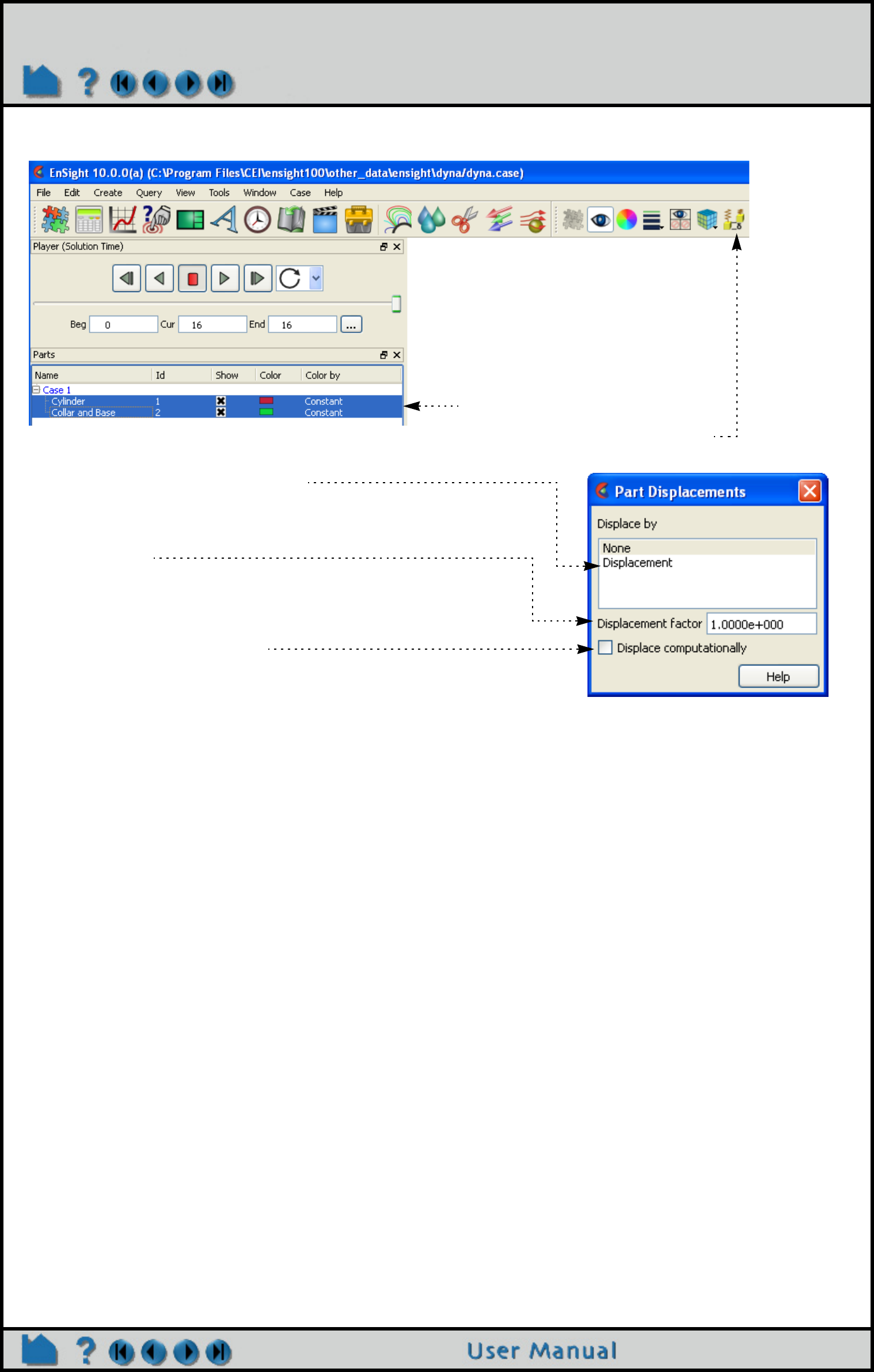
Page 329
HOW TO DISPLAY DISPLACEMENTS
BASIC OPERATION
Note that your changes made are immediate. Specifying a displacement does not create a new part, it merely sets
the displacement for the selected parts.
1. Select the parent parts.
2. Click the Displacements icon.
3. Select the nodal variable to use.
Limitation: can only use nodal vector variables.
4. If desired, enter a value for the Displacement Factor and
press return.
5. For speed and memory, default is visual displacement only.
If you desire to use the displacement in any calculations
then toggle on Displace computationally, which will do
server-side displacements.
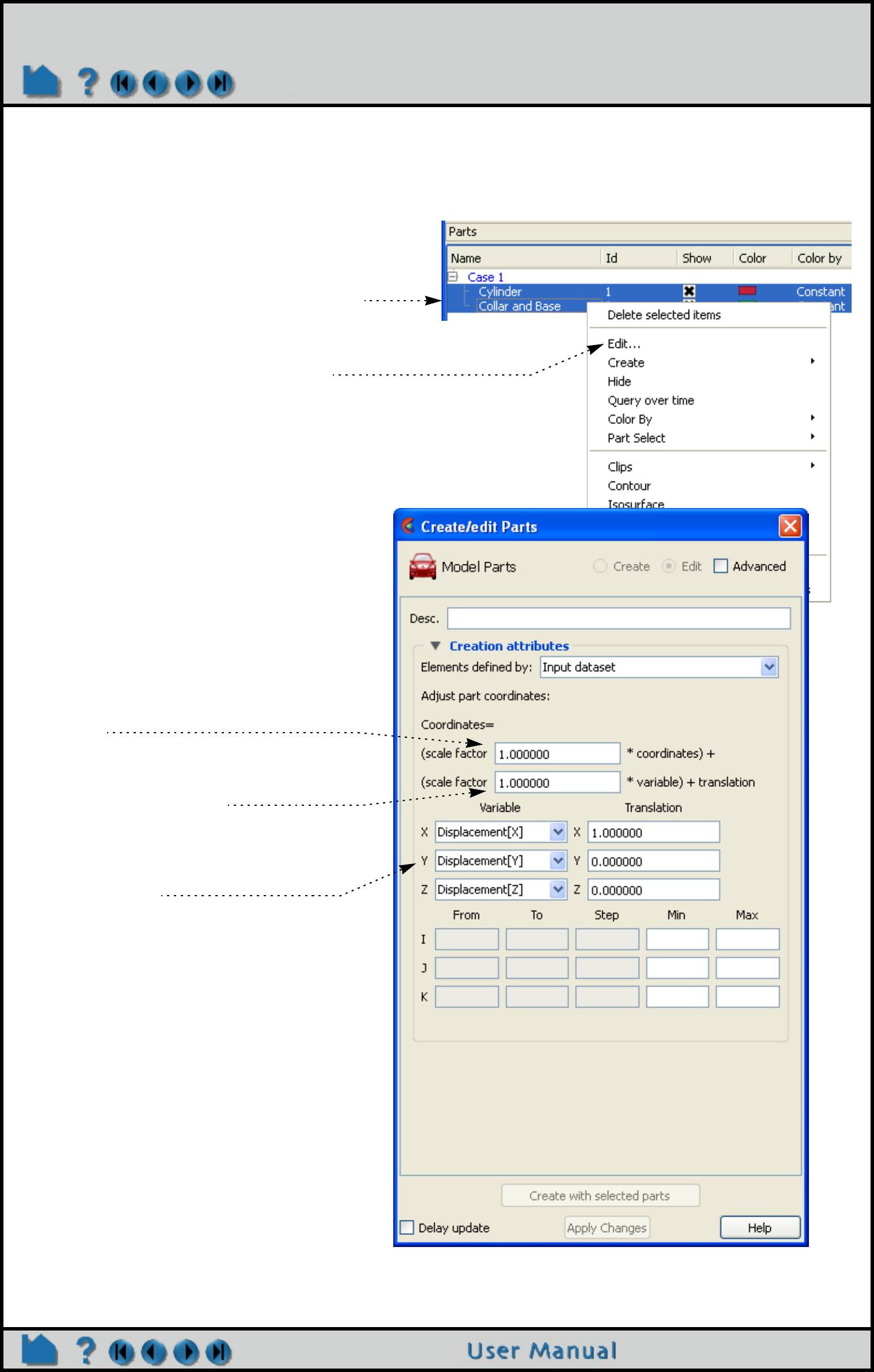
Page 330
HOW TO DISPLAY DISPLACEMENTS
Server Side Displacements
Server side displacements have more detailed found in
the Create/edit dialog.
1. First read in your model, build the desired parts,
and activate the model variable (not computed
variables) representing displacement.
2. Select the desired parts in the Parts list.
3. Right click on them and select Edit...
4. Set any desired entire geometry scale
factor.
Hit a carriage return.
5. Set the scale factor for any desired
displacement variable.
Hit a carriage return.
6. Set the nodal displacement model variable
and any desired translation for each
component.
Hit a carriage return.
Note that it is possible to displace in each
component direction by a different variable and to
translate by a single value in each direction. It is
also possible to scale the entire geometry by a
factor.
Displacements applied in this manner actually
modifies the geometry on the server (not just the
visual representation on the client). Any queries or
computations will reflect this modified geometry.
For example an area or volume calculation will
now use the displaced values.
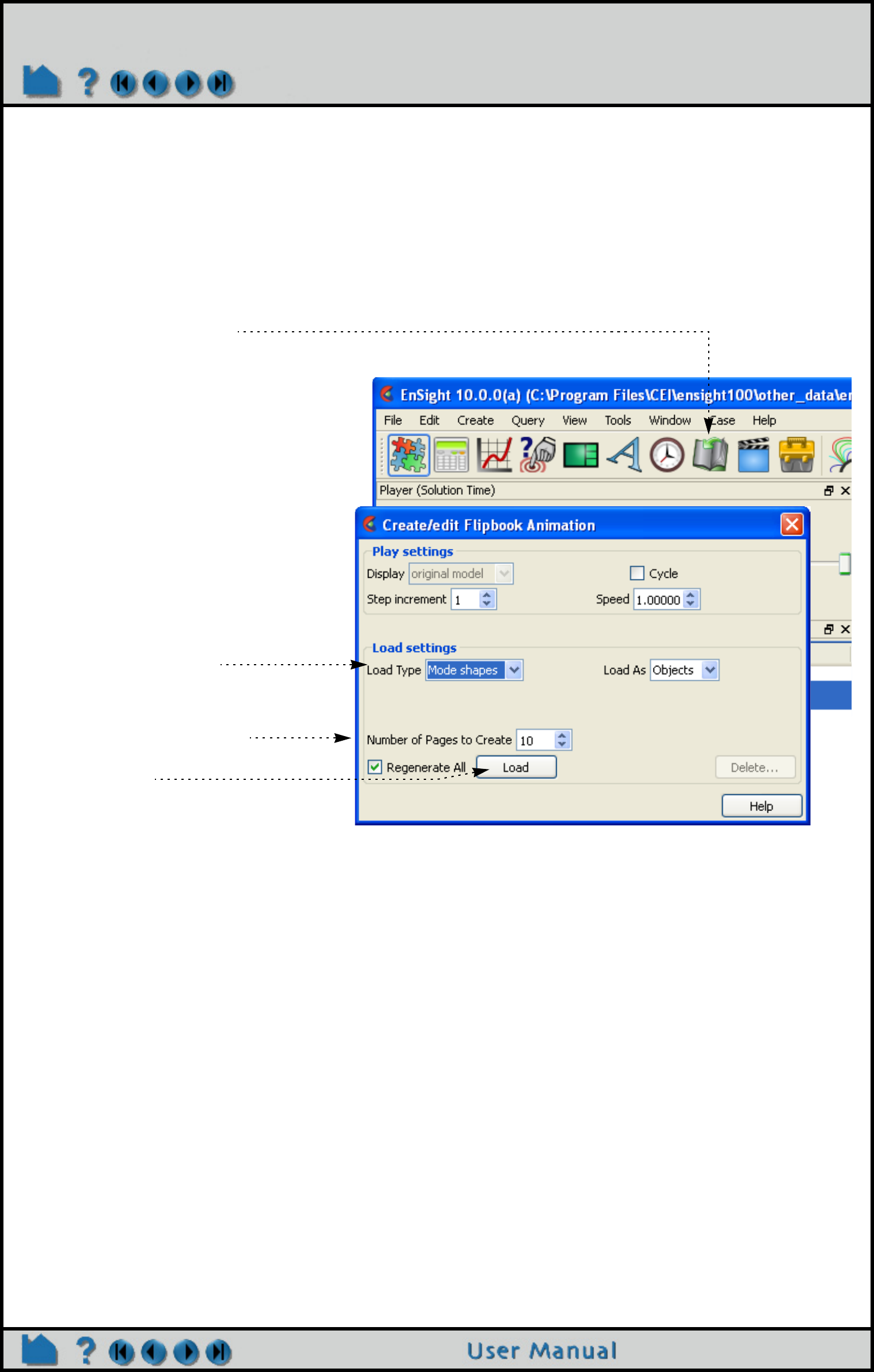
Page 331
HOW TO DISPLAY DISPLACEMENTS
ADVANCED USAGE
Vibrational analysis typically produces eigenvectors. EnSight can animate these vectors as mode shapes to visualize
selected vibration modes (each represented by a different displacement vector). The EnSight Flipbook is used to
build and load the animation. Once loaded, the animation can be replayed while still providing viewing control. To
create a mode shape flipbook:
The first page of the animation shows the full displacement (as it is shown in the Graphics Window without the
Flipbook) while the last page shows full displacement in the opposite direction. Intermediate pages show
displacements as driven by the cosine function.
Note that you can create copies or extracts of parts and simultaneously display them with different mode shape
variables or to show the initial static state along with the mode shape animation.
SEE ALSO
See How To Create a Flipbook Animation for more information on Flipbooks.
User Manual: Flipbook Animation
1. Be sure displacements are active and the
Displacement Factor is set to a suitable value
(as described above).
2. Click the Flipbook icon.
3. Select Mode Shapes from the
Load Type pulldown.
4. Enter the desired number of
Flipbook pages to create.
5. Click “Load”.
6. Once loading is complete it will
automatically start running.
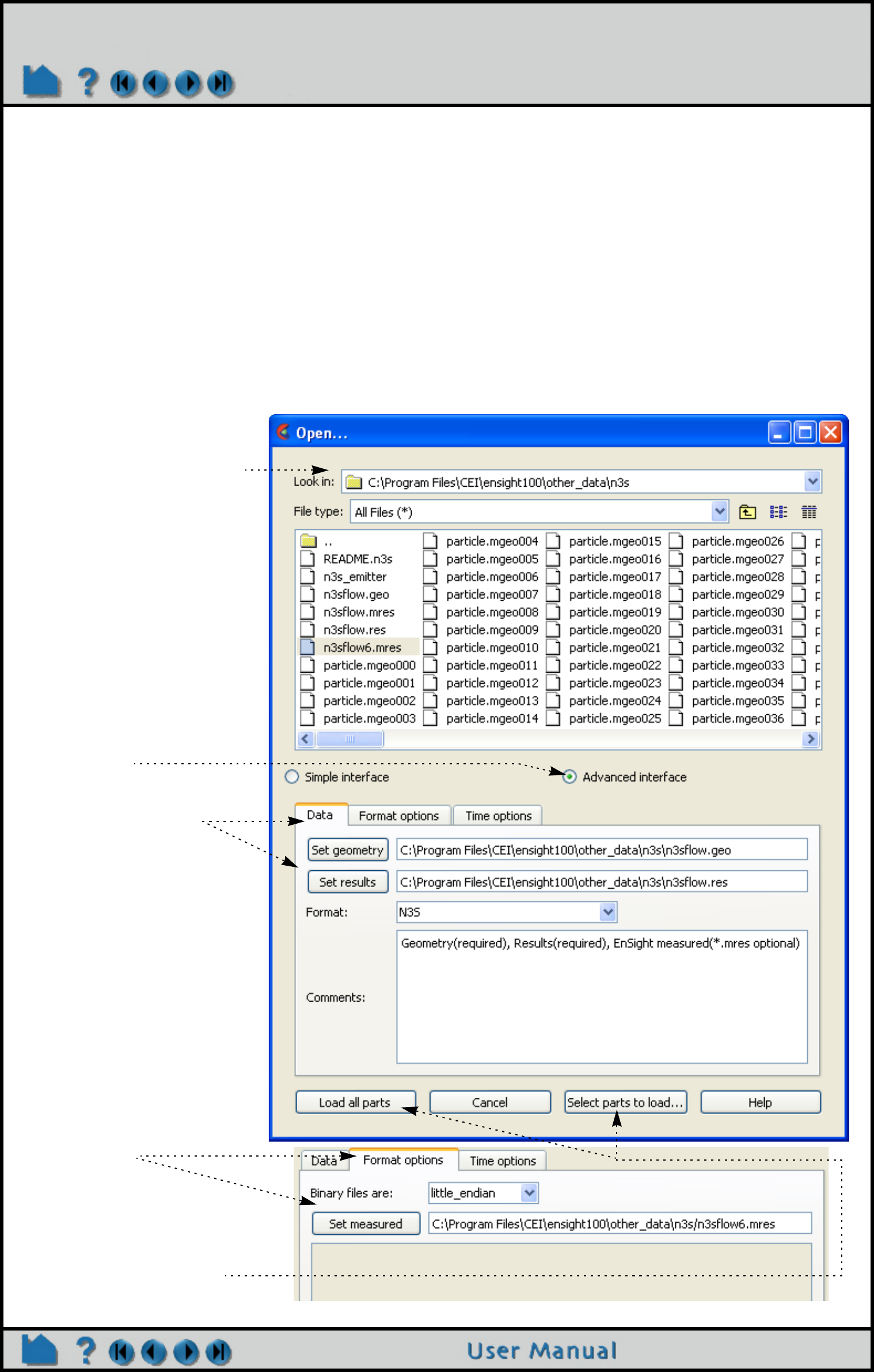
Page 332
HOW TO DISPLAY DISCRETE OR EXPERIMENTAL DATA
Display Discrete or Experimental Data
INTRODUCTION
In addition to meshed data consisting of nodes and elements, EnSight also supports discrete or measured data. A
measured dataset consists of a series of arbitrary points in space with no connectivity. Measured data can have
associated variable data and can vary over time. Examples of measured data include fuel sprays, multi-phase flows,
and experimental data.
Measured data cannot be loaded by itself – you must also specify a regular geometric mesh.
BASIC OPERATION
Measured data is read into EnSight naturally via the casefile (for EnSight6 and Ensight Gold formats) or can be read
with other mesh formats via the Format options tab in the Open... dialog, as shown below:
1. Select File > Open... to open the dialog for data file selection.
2. Find the directory
containing the data (see
How To Read Data for
more information on
using File Selection).
3. Click Advanced
interface.
4. In the Data tab, select
and set the needed
information for the
(meshed) geometry,
including the Format,
geometry file, and if
applicable, the result
file.
5. Open the Format
options tab and select
and set the measured
result file.
9. Now you can continue
the normal process of
either Load all parts, or
Select parts to load...
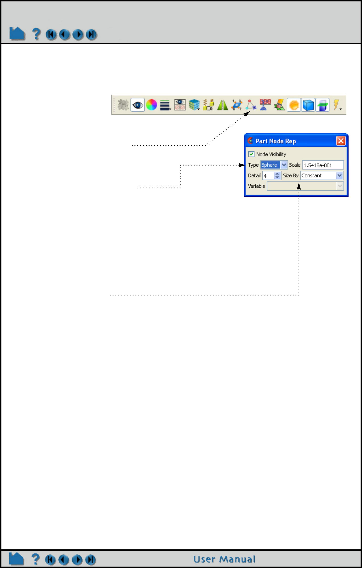
Page 333
HOW TO DISPLAY DISCRETE OR EXPERIMENTAL DATA
Measured data is represented as a single part. In the Main Parts list you should see a part named “Measured/
Particle” after loading.
Measured data is represented as a set of unconnected nodes. You can use EnSight’s ability to display nodes in
various ways to accentuate measured data visualization. To change node display:
OTHER NOTES
The file formats for measured data and the measured results file are detailed in EnSight Gold Measured/Particle
File Format.
Transient measured data can be animated using either the flipbook or keyframe animation capability.
You can load multiple measured datasets simultaneously by using EnSight’s cases capability.
SEE ALSO
User Manual: EnSight Gold Measured/Particle File Format
1. Select the desired measured data part in the
Parts list.
2. Click the Node representation icon
Which opens the Part Node Rep dialog. Node
Visibility will be on by default for measured data
parts.
3. Select the desired node display type
• Dot: nodes are displayed as points.
• Cross: nodes are displayed as crosses and can
be fixed sized (size set by the Scale value) or
sized based on a Variable (and scaled by the
Scale value).
• Sphere: nodes are displayed as spheres and
can be fixed sized (size set by the Scale value)
or sized based on a Variable (and scaled by the
Scale value). Sphere detail controlled by Detail
value.
4. If applicable, set desired values for Scale,
Detail, Size By, and Variable.
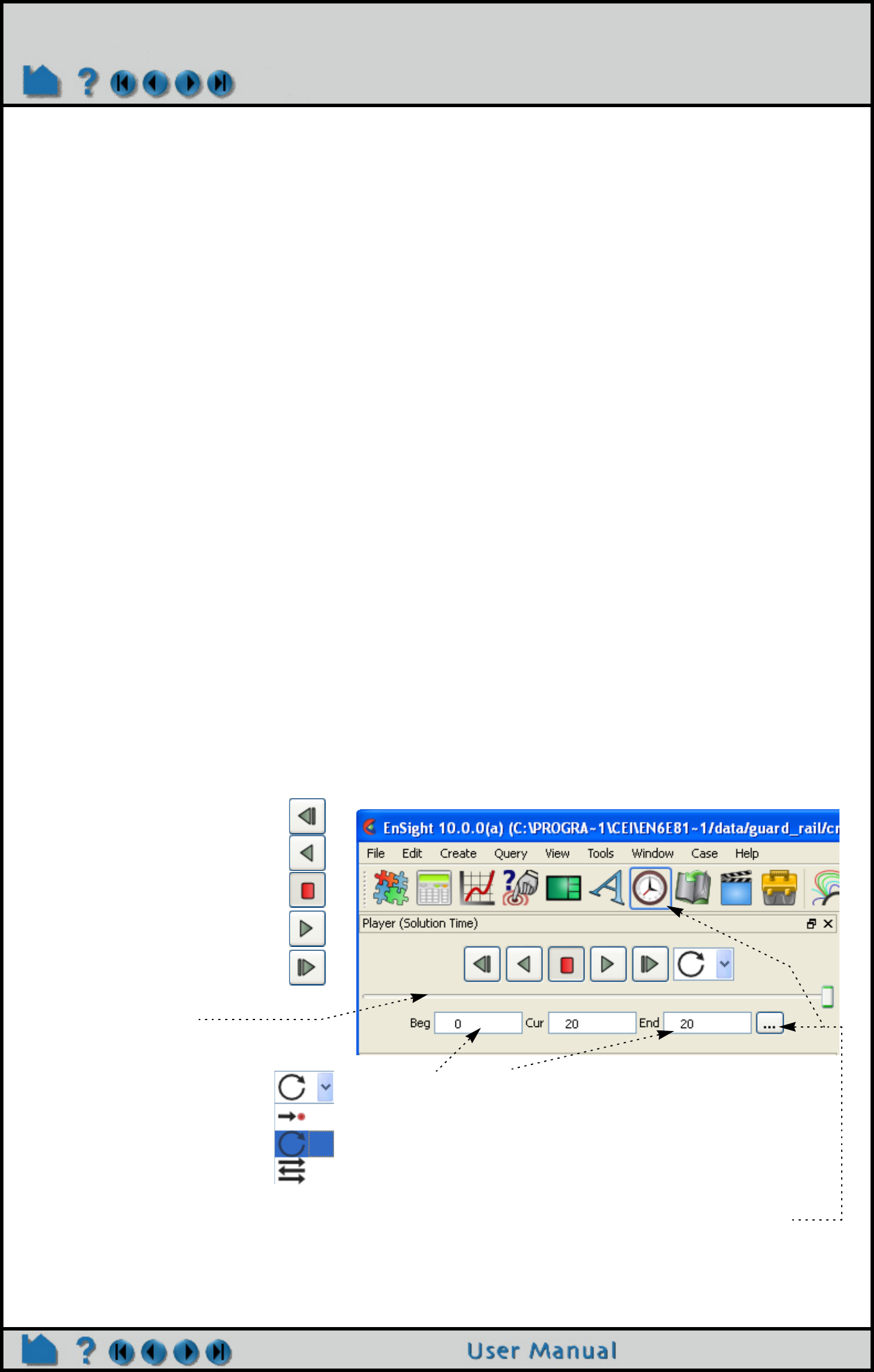
Page 334
HOW TO CHANGE TIME STEPS
Change Time Steps
INTRODUCTION
From its inception, EnSight has been used extensively to postprocess time-varying or transient data. In many cases, dynamic
phenomena can only be understood through interactive exploration. One can easily change time with vcr-type controls in the
Solution Time Player (which comes up by default for transient models). Further control for transient data time handling is provided
in the Create/edit Transient Animation dialog, accessed via the Solution time icon.
EnSight provides two ways to work with transient data. By default, time is presented as a series of discrete steps running from zero
to the total number of steps minus one. However, you can also present time based on the actual simulation time values found in
your results data. The presentation mode is controlled by the Units pulldown which will be shown below. shown below.
The current time range is displayed in the Beg and End fields with the current time step shown in the Cur field. You can modify the
time range controlled by the slider by editing the Beg and/or End fields (remember to press return). You can change the current
time step by editing the Cur field (press return), manipulating the slider, or clicking the left/right vcr buttons. Setting the Beg to any
number less than the min, and End to any number larger than the max will Reset Time Range to its full range.
Time scaling and stepping (as manipulated through the slider bar and Beg, Cur, and End fields) can either be Discrete or
Continuous. If scaling is Discrete, only your actual time steps as written in the results data can be visualized. In addition, the Beg,
Cur, and End fields can only be set to integer values (if Units is set to Step and Scale Type is Discrete) or actual simulation times
represented in your results data (if Units is set to Sim. Time). If scaling is Continuous, you can display results between your actual
output time steps (all variable values are linearly interpolated between the two surrounding time steps). Note that if your mesh
connectivity is changing over time you cannot display results continuously.
When you load multiple cases it is possible that the composite master timeline is inappropriate. You can specify a master timeline
from any one of the cases you have loaded and decide how the other cases will sync up to changes in time. You can even create
your own master timeline.
When you manipulate the slider or change the Cur field, EnSight will perform all tasks necessary to correctly display the new time
step in the Graphics Window. Depending on the size of the dataset and the number of additional parts you have created, this may
take a significant amount of time. If you wish to create an on-screen animation of your results, use the VCR run icon or go use the
Flipbook
facility.
BASIC OPERATION
To use the Solution Time Player (which comes up by default for transient models):
To change one step lower.
To play steps in reverse order.
To stop a running play.
To play steps in forward order.
To change one step higher.
The slider can also be used to
manually change time.
To control what happens when playing and
the limit is reached.
To stop when it reaches the limit.
To cycle, starting at the first again.
To reverse order and continue.
(bounce back and forth)
The Beg and End fields control the available time range (and
also the range of the slider action). You can enter new values
into the fields and press return.
The Cur field sets the current time step. Either move the
center slider or enter a new value in the field and press
return.
To open the Create/edit Transient Animation dialog for
additional controls. (Same as hitting the Solution time icon).
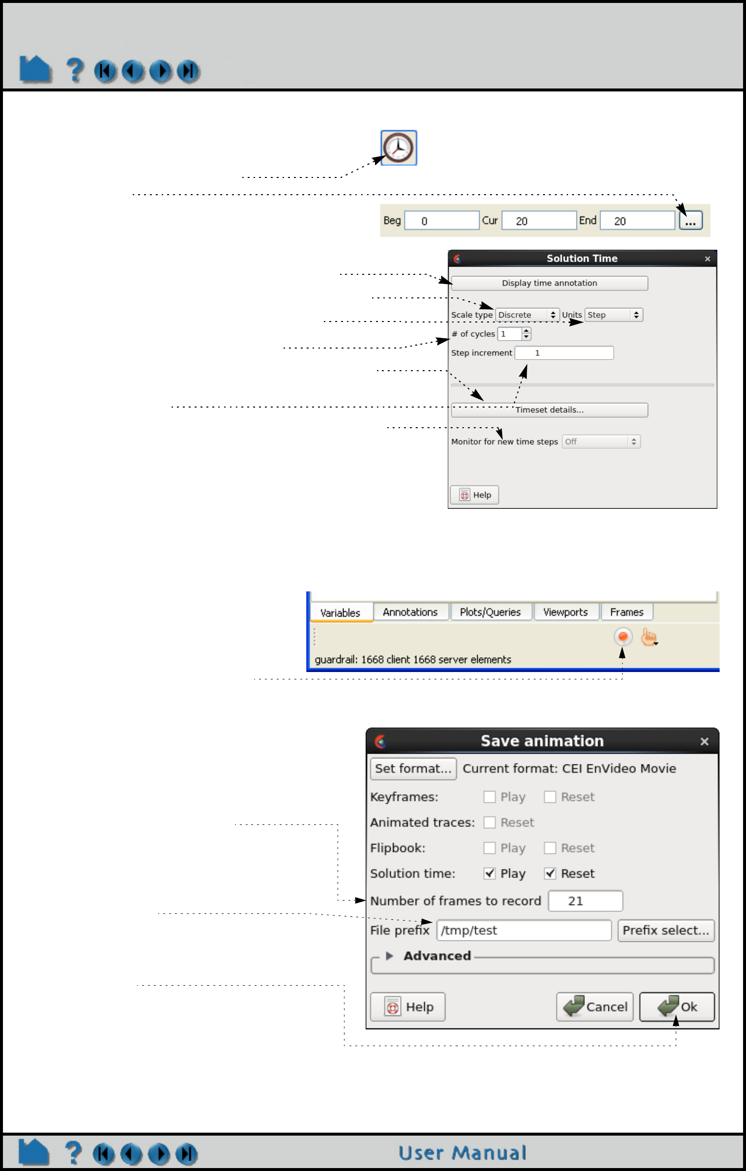
Page 335
HOW TO CHANGE TIME STEPS
:
You control more by opening the Create/edit
Transient Animation dialog.
Click either the Solution time icon
or the ... button.
Make changes as desired.
Click to display time as annotation in the graphics window.
Set Scale Type to Discrete or Continuous (see above for details).
Set Units to Step or Sim. Time (see above for details).
Set the number of time cycles in the time range.
Click to view/modify timeset details (see Advanced Usage below).
Set the step increment size for the slider arrows. Must be an integer
if Scale Type is Discrete.
If the Monitor for new time steps button is available, you may choose
an update method for monitoring the availability of new time steps.
This is only available if your data reader supports this feature (for
more details see the advanced feature in User Manual 5.1 Solution
Time
Recording an Animation of your data:
You can record the timesteps to images or
animation formats by clicking the Record
current graphics window animation icon to
bring up the Save animation dialog.
Set the transient data settings and set the number
of frames to record (by default this will be the
number of available time steps).
Specify a file name
The images or movie file will be created after you
click the Ok icon.
The options for this dialog are explained in How
To Print/Save an Image
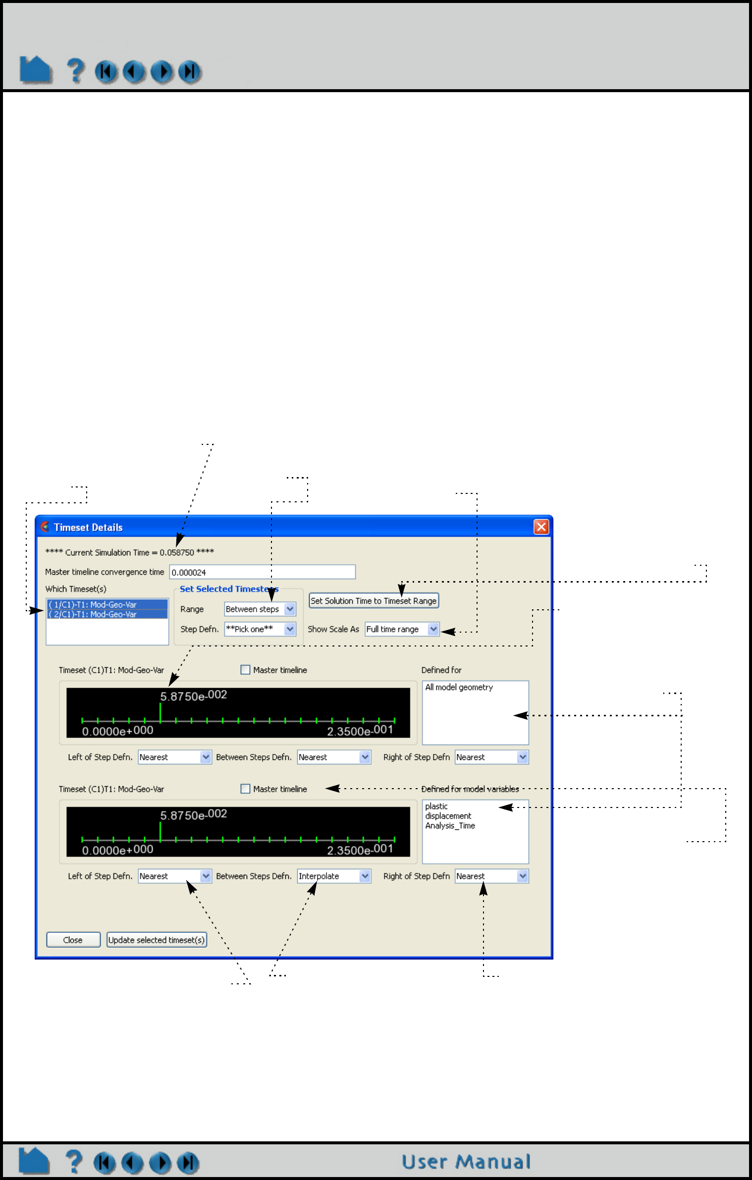
Page 336
HOW TO CHANGE TIME STEPS
ADVANCED USAGE
Timeset Details
EnSight allows geometry and variables to behave in a transient manner on different timelines, i.e., a variable called
Temperature can be defined at t = 0., 3., and 6. while a variable called Pressure can be defined at t = 0., 2., and 5.5.
The Timeset Details button will bring up the Timeset Details dialog which allows the user to view the various
timelines as well as specify how the variables will behave when they are not defined.
The EnSight case file defines the timesets (name and associated time values) and associates a timeset with each of
the variables and geometry.
By default the Solution Time player will show a composite of all of the timesteps that exist across all of the timesets.
This can, however be changed to show just the time values associated with a particular timeset.
In the Timeset Details dialog shown below, multiple timesets exists. Two timesets (from the Which Timeset(s) list) are
selected and are thus shown in detail. The graphics for each timeset shows (a) the minimum and maximum overall
time value, (b) green tick marks indicating the time values defined for the timeset, (c) the current time value (indicated
with the long green line) associated with the timeset. (See Timeset Details... Tim sets Tab in UserManual 5.10 for more
info.)
The current solution time (as
set in the Solution Time dialog.
Select the timeline to be
viewed.
To modify all the timelines to
behave the same way, select
which range is to be modified,
then select how they will be
displayed.
The timeset can either be
shown having a time range
over the total number of time
values or can be shown
according to the timeset’s
range.
By default the Solution
Time dialog shows the
composite timeline.
This button will modify
the Solution Time
dialog’s Beg and End
values to those of the
selected timeset.
Shows the time value being
used at the current time.
The timeset is used by the
variables (or geometry)
shown in this list.
When the current time (from the
Solution Time dialog and indicated
in the upper left corner of this
dialog) is set to a value less than
what is available for this timeline,
use the Nearest value or make the
variable Undefined.
When the current time (from the
Solution Time dialog and indicated
in the upper left corner of this
dialog) is set to a value that does
not exist for this timeline,
Interpolate between defined time
values, use the Left, Right, or
Nearest value, or make the
variable Undefined.
When the current time (from the
Solution Time dialog and indicated in
the upper left corner of this dialog) is
set to a value greater than what is
available for this timeline, use the
Nearest value or make the variable
Undefined.
Toggle ON the Master
timeline toggle, then click
on the Update selected
timeset button to use only
the timesteps in this
timeline
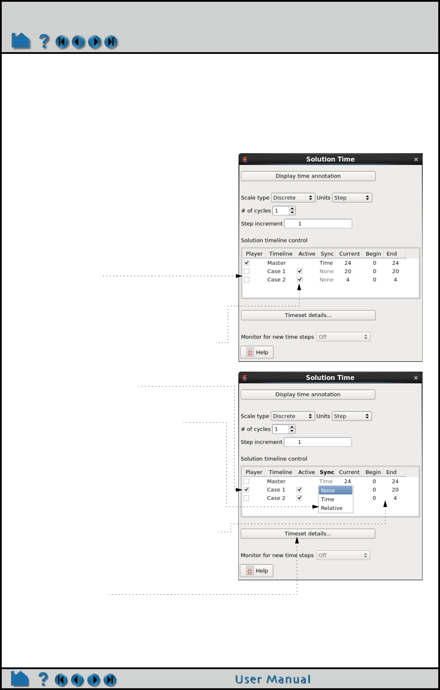
Page 337
HOW TO CHANGE TIME STEPS
Master Timelines
When multiple transient cases are loaded it is entirely possible that the number of time values as well as the time
values themselves do not match up between the cases. By default EnSight creates a master timeline which is the
composite timeline across all the cases, i.e., it finds all of the unique time values and places these on the master
timeline.
It is often desirable to define a master timeline. This can be done by either redefining the master timeline or by
allowing the master timeline for any case to become the master timeline for EnSight and occupy the VCR controls for
time.
As soon as you read more than one case into EnSight the
Solution Time dialog will show an extra section where you
can control not only which timeline might become the VCR
player controls but also indicate how the various cases will
behave when time is changed.
In the image shown here there are two cases. The first
case has 21 timesteps and the second has 5 timesteps.
The only time value that overlaps between the cases is
the first with t=0. and thus the Master timeline has 25
timesteps. You can see that the current timestep for Case
1 is the last time step (20) and Case 2 is also currently at
the last timestep (4).
Any one of the timelines can be shown as the transient
data controls in the EnSight Time panel (the VCR
controls).
When time is changed the Case will be updated to the
new time value only if the Active toggle is set. You can
use this to "freeze" a case at a specific time value.
In this dialog we have changed the Player toggle to
indicate that Case 1 is in control.
Once you choose a case to have control you can set how
a change to time for the controlling case will modify the
other cases. Three options are available:
None - indicates that when a time change is made the
other active cases will not be affected.
Time - indicates that the other active cases will attempt
to change to the same time value.
Relative - means that the other active cases will be
modified to have a time value offset by the
current difference, i.e., if the time is stepped
forward by one step the other active cases
will also be stepped forward by one step.
The Current, Begin, and End columns are shown for
informational purposes to help you see where each case
timeline is currently located.
If you want to create your own Master timeline, click the
Timeset details... button.
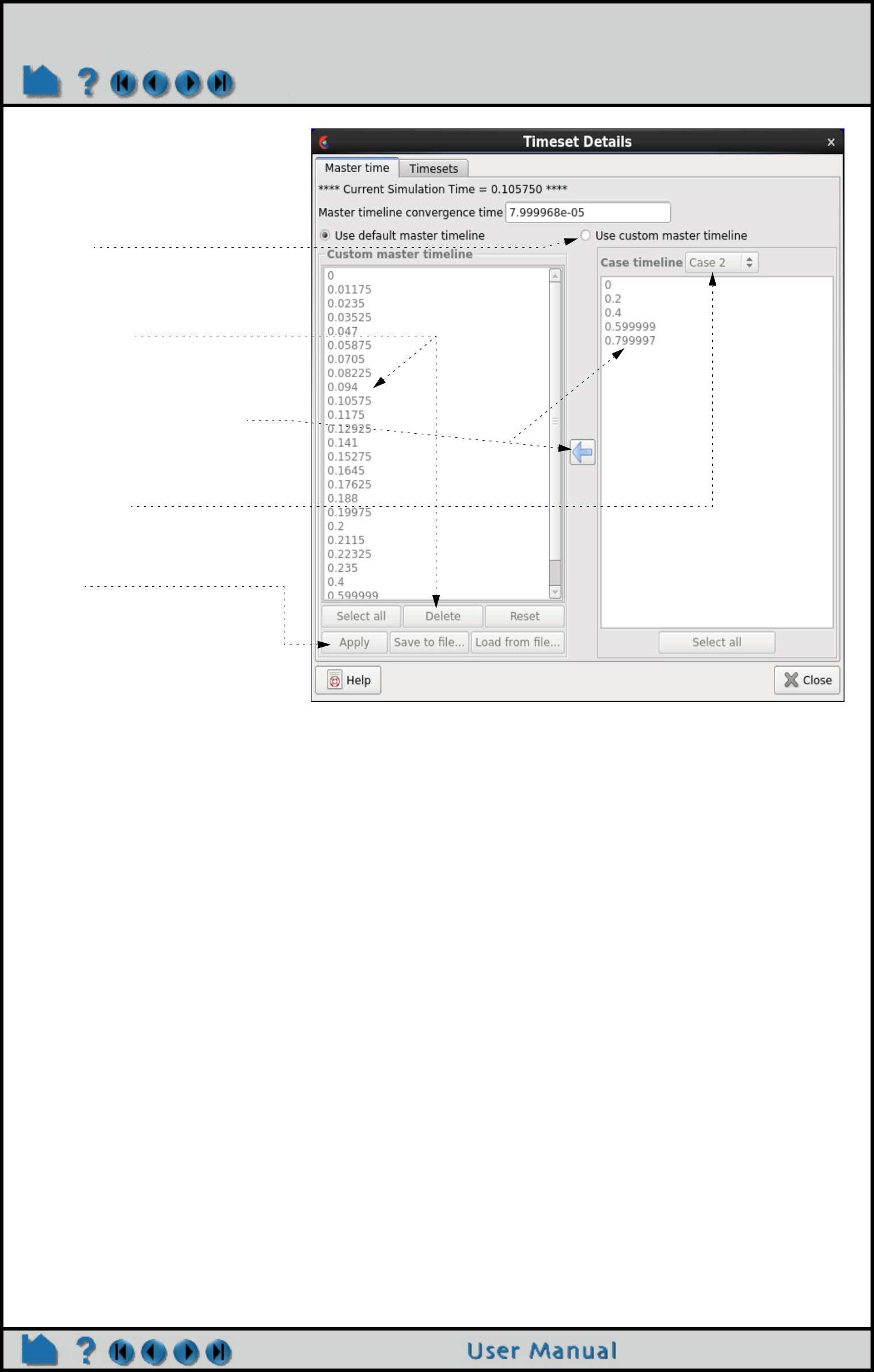
Page 338
HOW TO CHANGE TIME STEPS
SEE ALSO
How To Load Transient Data, How To Animate Transient Data
User Manual: Flipbook Animation
This dialog shows the time values
for the composite master timeline.
Toggle on "Use custom master
timeline" to create a new master
timeline
You can select time values in the left
column and remove them with the
Delete button
You can select time values in the
right column and push them into the
left column via the arrow icon
Change the Case timeline pulldown
to see time values for the various
loaded cases
When completed, click the Apply
button
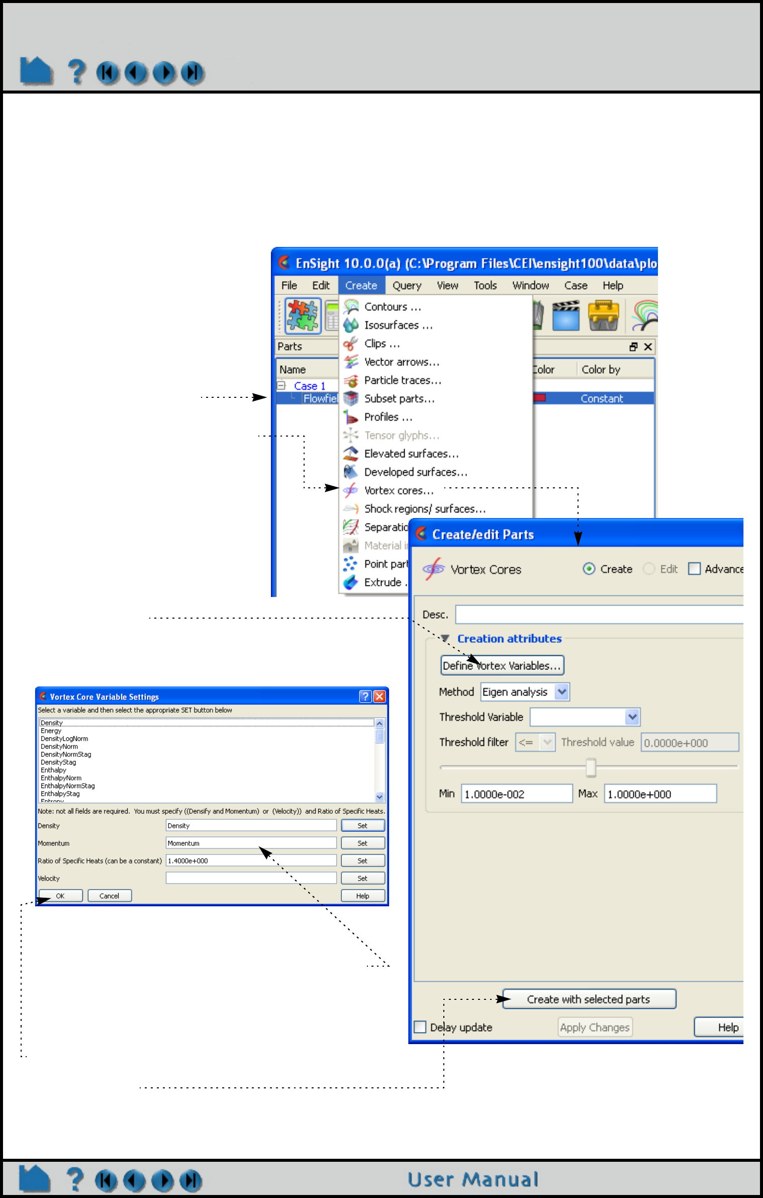
Page 339
HOW TO EXTRACT VORTEX CORES
Extract Vortex Cores
INTRODUCTION
Vortex cores are centers of swirling flow where the velocity is parallel to the vorticity. For a more complete description
refer to the User Manual section below.
BASIC OPERATION
1. Select the parent part.
2. Select Create -> Vortex cores...
3. Bring up the Vortex Core
Variable Settings dialog by
clicking here.
4. Define either (Density and Momentum) or
Velocity, as well as the Ratio of Specific Heats.
The variables can be set by either typing them
into the fields, or selecting them from the list
above and clicking the Set button.
5. Click Okay to finish the variable setup.
6. Click Create.
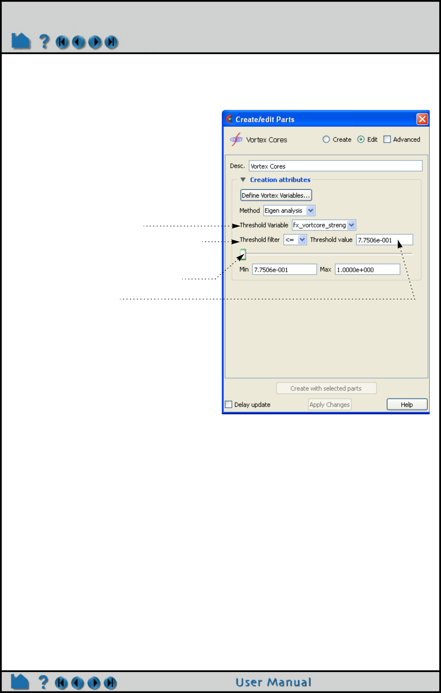
Page 340
HOW TO EXTRACT VORTEX CORES
ADVANCED USAGE
The resulting vortex core lines can be filtered by the vortex core strength or by any other active variable.
OTHER NOTES
Extract Vortex Cores does not work with more than one case.
SEE ALSO
User Manual: Vortex Core Parts
1. Select the variable to filter by.
2. Set the Threshold filter to remove the portion
of the vortex core that is larger or less than the
specified threshold value.
3. Slide the slider to a new threshold value.
- or -
3. Enter a threshold value
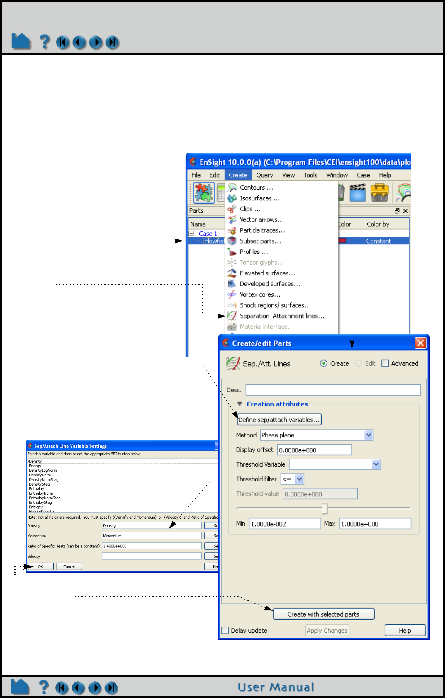
Page 341
HOW TO EXTRACT SEPARATION & ATTACHMENT LINES
Extract Separation & Attachment Lines
INTRODUCTION
Separation and attachment lines are created on any 2D surface and show interfaces where flow abruptly leaves
(separates) or returns (attaches) to the surface. For a more complete description refer to the User Manual section
below.
BASIC OPERATION
1. Select the 2D parent part.
2. Select Create -> Separation Attachment
lines...
3. Bring up the dialog defining the
necessary variables by clicking here.
4. Define either Density and Momentum or
velocity, as well as the Ratio of Specific Heats.
The variables can be set by either typing them into
the fields or be selecting them from the list above
and clicking the Set button.
5. Click Okay to finish the variable setup
6. Click Create
This will create two parts - one each for the
separation and attachment lines. You can modify
the visual of these parts separately, but when you
change any creation attribute, both parts will be
modified.
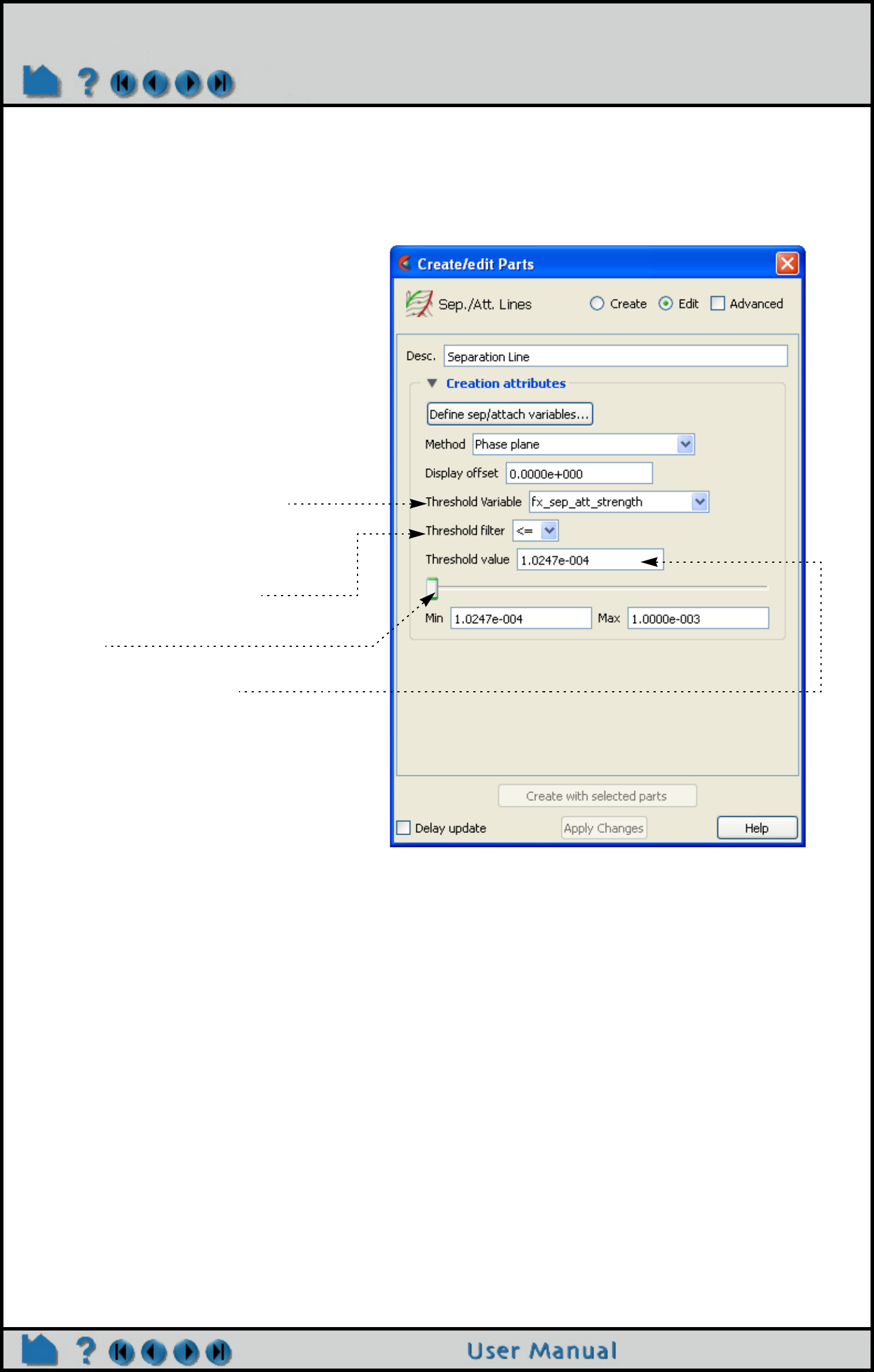
Page 342
HOW TO EXTRACT SEPARATION & ATTACHMENT LINES
ADVANCED USAGE
The resulting separation/attachment parts can be filtered by the fx_sep_att_strength variable or by any other active
variable.
OTHER NOTES
The separation and attachment parts are linked together with regard to their creation, i.e. when one is modified the
other is also. Further, when one is deleted the other is also deleted.
Separation and Attachment feature extraction only works with one case.
The separation and attachment line parts should generally not interfere visually with the 2D parent parts they lie on
(as long as the preference for graphics hardware offset is on - see View Preferences), but they may interfere if
printed. In either case you can apply a display offset manually to avoid the interference in the Feature Panel for the
part. The display offset will be in the direction of the parent surface normal.
SEE ALSO
User Manual: Separation/Attachment Line Parts
1. Select the variable to filter by.
2. Set the Threshold filter to remove the
portion of the separation/attachment
line that is larger or smaller than the
specified threshold value.
3. Slide the slider to a new threshold
value
- or -
3. Enter a threshold value.
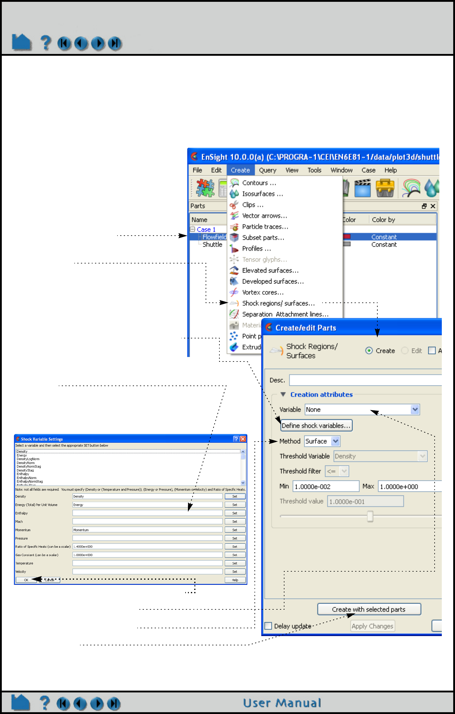
Page 343
HOW TO EXTRACT SHOCK SURFACES
Extract Shock Surfaces
INTRODUCTION
Shock surfaces and regions help visualize shock waves in 3D (trans/super-sonic) flow. For a more complete
description, refer to the User Manual section below.
BASIC OPERATION
1. Select the parent part.
2. Select Create -> Shock regions/
surfaces...
3. Bring up the dialog defining the
necessary variables by clicking here.
4. Define either Density or (Temperature
and Pressure), (Energy or Pressure),
(Momentum or Velocity), and Ratio of Specific
Heats.
The variables can be set by either typing them
into the fields, or selecting them from the list and
clicking the Set button.
5. Click Okay to finish the variable setup.
6. Choose the Variable to use.
7. Choose Region or Surface.
8. Click Create.
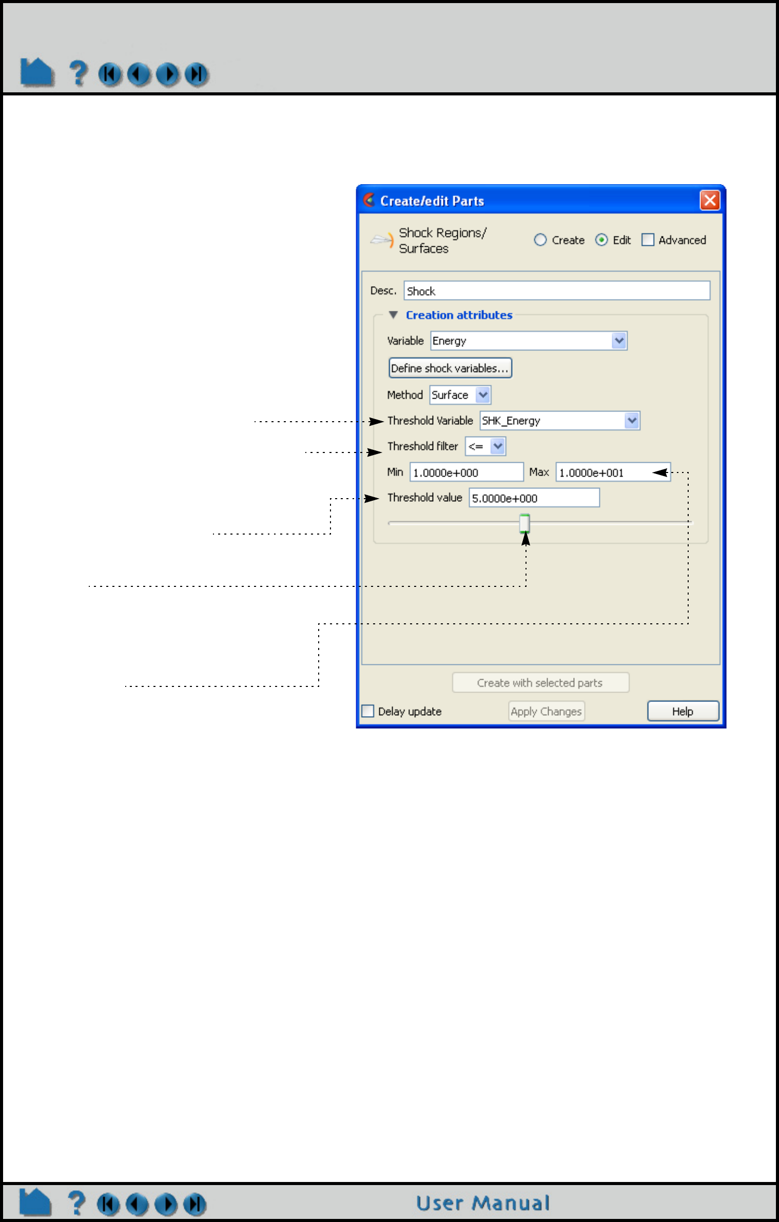
Page 344
HOW TO EXTRACT SHOCK SURFACES
ADVANCED USAGE
The resulting shock can be filtered by any of the threshold variables
OTHER NOTES
See Other Notes in the Shock Surface/Region Create/Update section of the User Manual for options on how to pre-
filter flow field regions, and/or post-filter shock regions via a specified mach number. Also to apply the transient
correction term for moving shocks when using the shock Region method.
Shock Surface feature extraction does not work with multiple cases.
SEE ALSO
User Manual: Shock Regions/Surfaces Parts
1. Select the variable to filter by.
2. Set the Threshold filter to remove the
portion of the shock surface or region
that is greater or less than the
specified threshold value.
3. Enter a threshold value
- or -
3. Slide the slider to a new threshold
value
4. The shock is usually defined in a very
narrow band, so the slider min/max
values may need to be adjusted by
either entering new values in the min/
max fields.
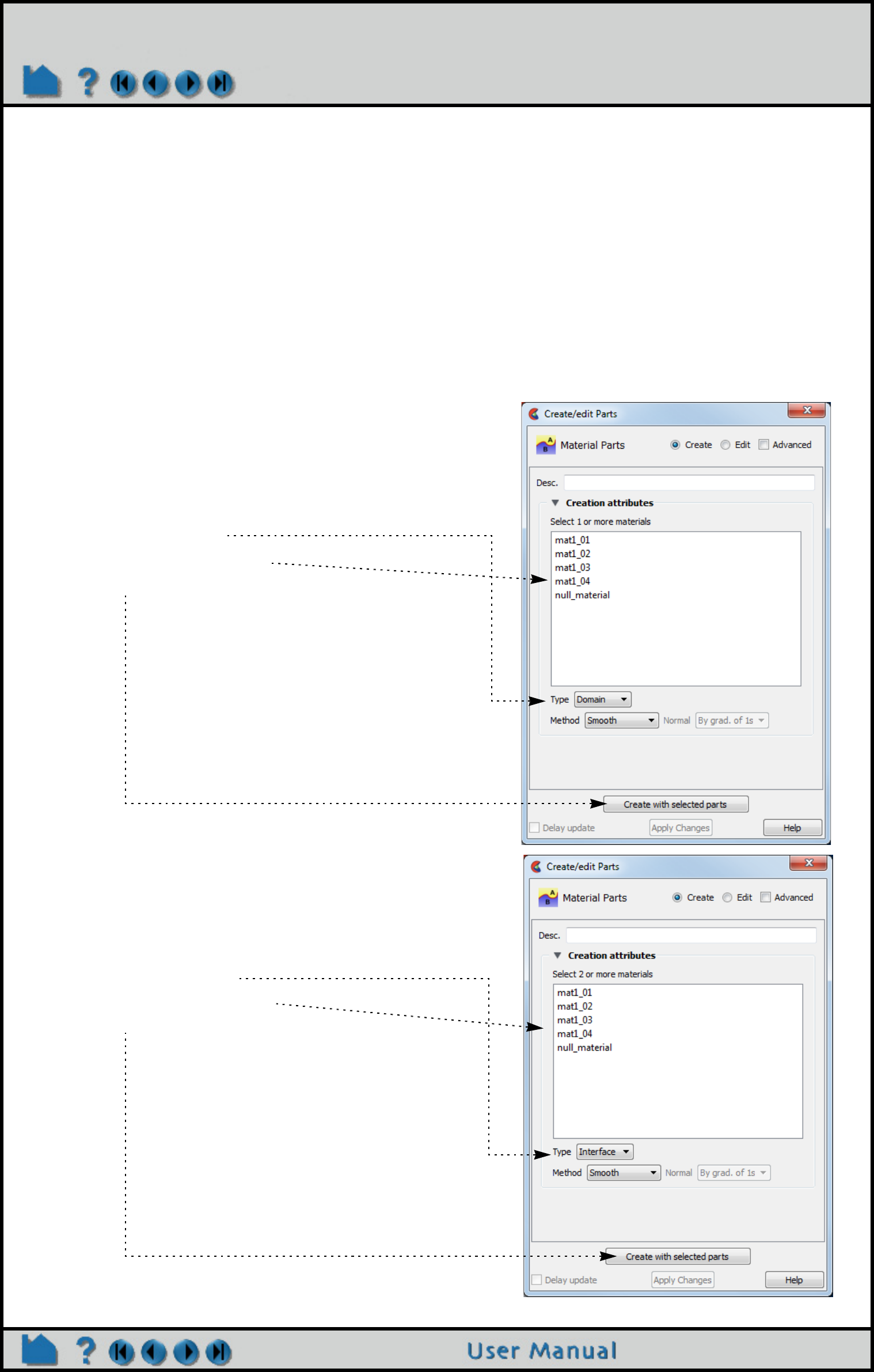
Page 345
HOW TO CREATE MATERIAL PARTS
Create Material Parts
INTRODUCTION
A Material Part can be created as either a domain or an interface.
A material Domain is a solid region (or regions) composed of one or more specified materials. Parts with 2D
elements yield 2D material elements, and parts with 3D elements yield 3D material elements.
A material Interface is a boundary region (or regions) between adjacent materials composed of at least two or more
specified materials. Parts with 2D elements yield 1D material elements, and parts with 3D elements yield 2D material
elements.
The Material Part feature can be used to isolate specified elemental regions of interest in data sets with material
fractions.
BASIC OPERATION
For Material Domain (for Smooth Method):
1. Bring up the Feature Panel for Material Parts. For
example, choose Material Parts from the Create
pulldown.
2. Select the parent model part(s).
3. Set Type to Domain.
4. Select 1 or more materials.
5. Click Create.
For Material Interface (for Smooth Method):
1. Bring up the Feature Edit Dialog for Material Parts.
For example, choose Material Parts from the Create
pulldown.
2. Select the parent model part(s).
3. Set Type to Interface.
4. Select 2 or more materials.
5. Click Create.


Page 347
HOW TO FILTER PART ELEMENTS
Filter Part Elements
INTRODUCTION
One or more variables can be used within EnSight as a means of filtering out elements in model parts. In the simplest
form a single "failure" variable might be specified which will remove elements that are beyond a threshold and thus no
longer viable. The element filtering is a "deep" filter in that elements are not just visually removed on the client, but
are also removed for all calculations on the server. For example, the volume of a part calculated using the calculator
will only include the non-filtered elements. If you only need to visually remove elements consider Element Blanking.
The filter criteria can be something as simple as a variable with two states (one state to indicate the element is failed,
and the other state to indicate that the element is not failed), or it can be a variable (such as a Von Mises stress/
strain) threshold for which you specify limiting values and conditions for element removal. The filter variable would
ideally be a per-element variable. But you can also use a per-node variable in which case the nodal values are
averaged on the element.
Note: element filtering can only be performed on model parts. So if its effect is desired on created parts, such as clip
planes or isosurfaces, one should apply this operation to the model parent parts of the desired created parts and the
children will inhered the element filtering.
Six filters are available. Each filter can specify a variable to use in the filtering process which can be compared
against another variable or a constant value. The filters are combined with "and" or "or" operators. The filtering occurs
sequentially through the filters, i.e., it is not possible, for example, to specify a filter operation of "variable1 < 0.5 OR
(variable2 > 1.0 AND variable 3 < 0.0)"
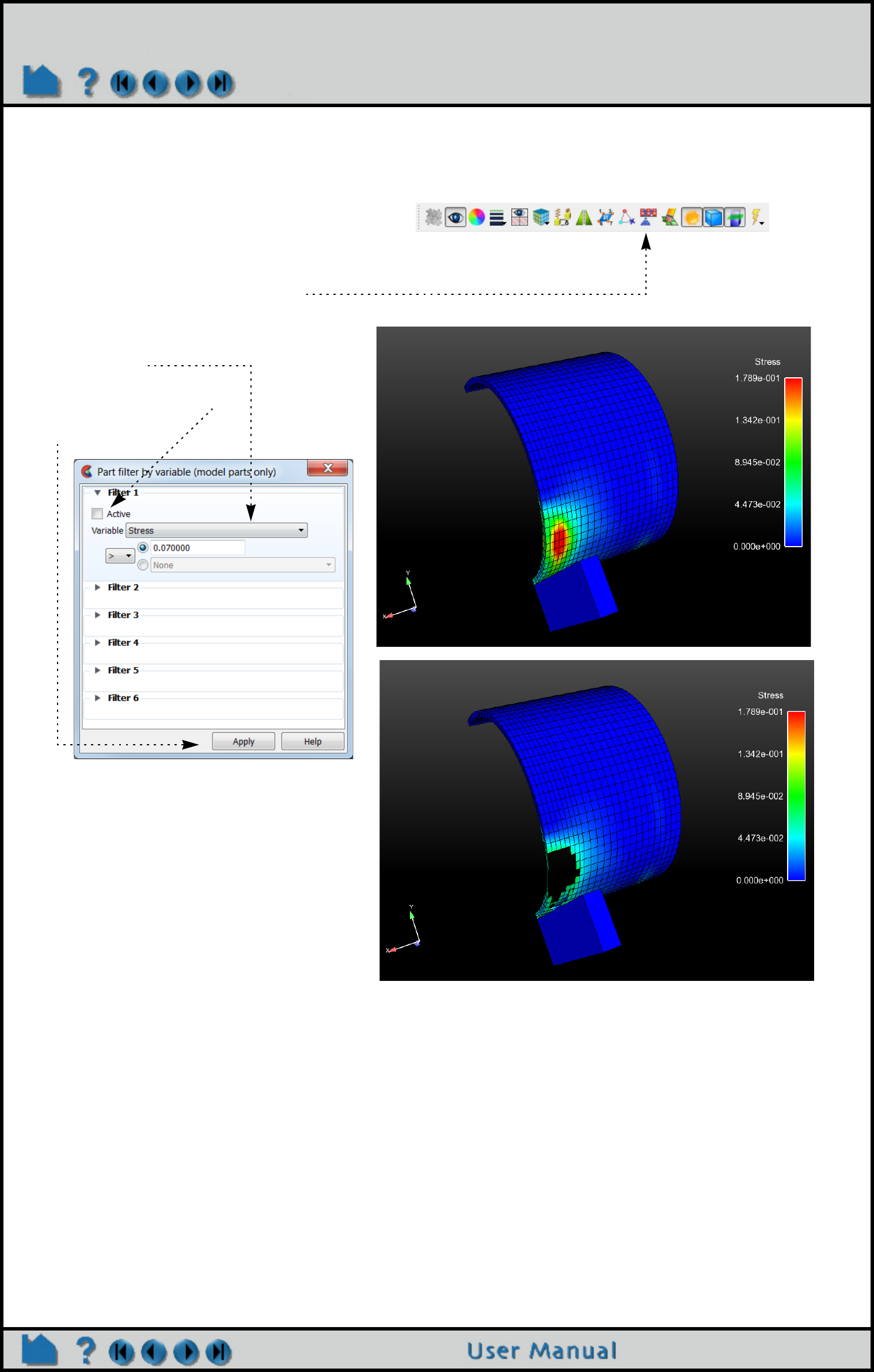
Page 348
HOW TO FILTER PART ELEMENTS
BASIC OPERATION
1. Select the model part(s) to use.
2. Click on the Filter Elements icon.
3. Select the variable you wish to use for
filtering (In this example we use Stress
> 0.07).
4. Turn the filter "active"
5. Click Apply
Those elements which satisfy the element
filter criteria will be removed from the model.
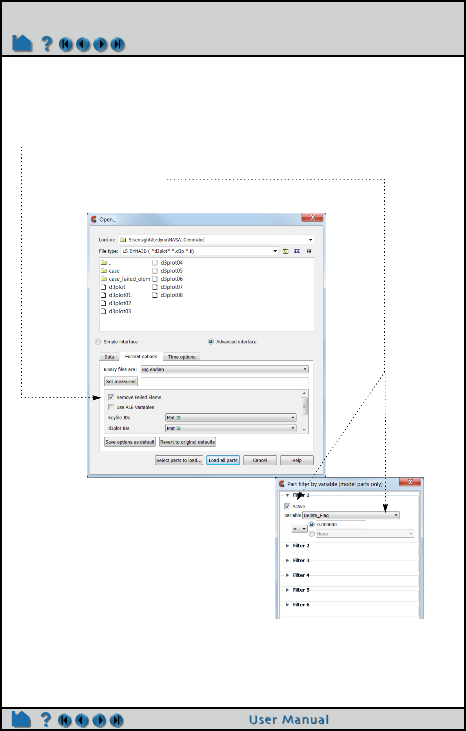
Page 349
HOW TO FILTER PART ELEMENTS
ADVANCED USAGE
EnSight’s User-defined reader API is capable of dealing with designated failure variables and the failure values and
conditions. Thus, a reader can be set up to use failure conditions that solvers provide and automatically apply the
element filtering operations for you. An example of this is the LS-DYNA3D reader provided with EnSight.
.
SEE ALSO
How-To Read User Defined
Do Element Blanking
Note the Format option provided by this reader, entitled: “Remove Failed Elems”. By checking
this option, a “Delete_Flag” variable is created, and the element filter feature of EnSight will
be automatically on - with the conditions and values set that will filter the failed elements that
the solver flagged
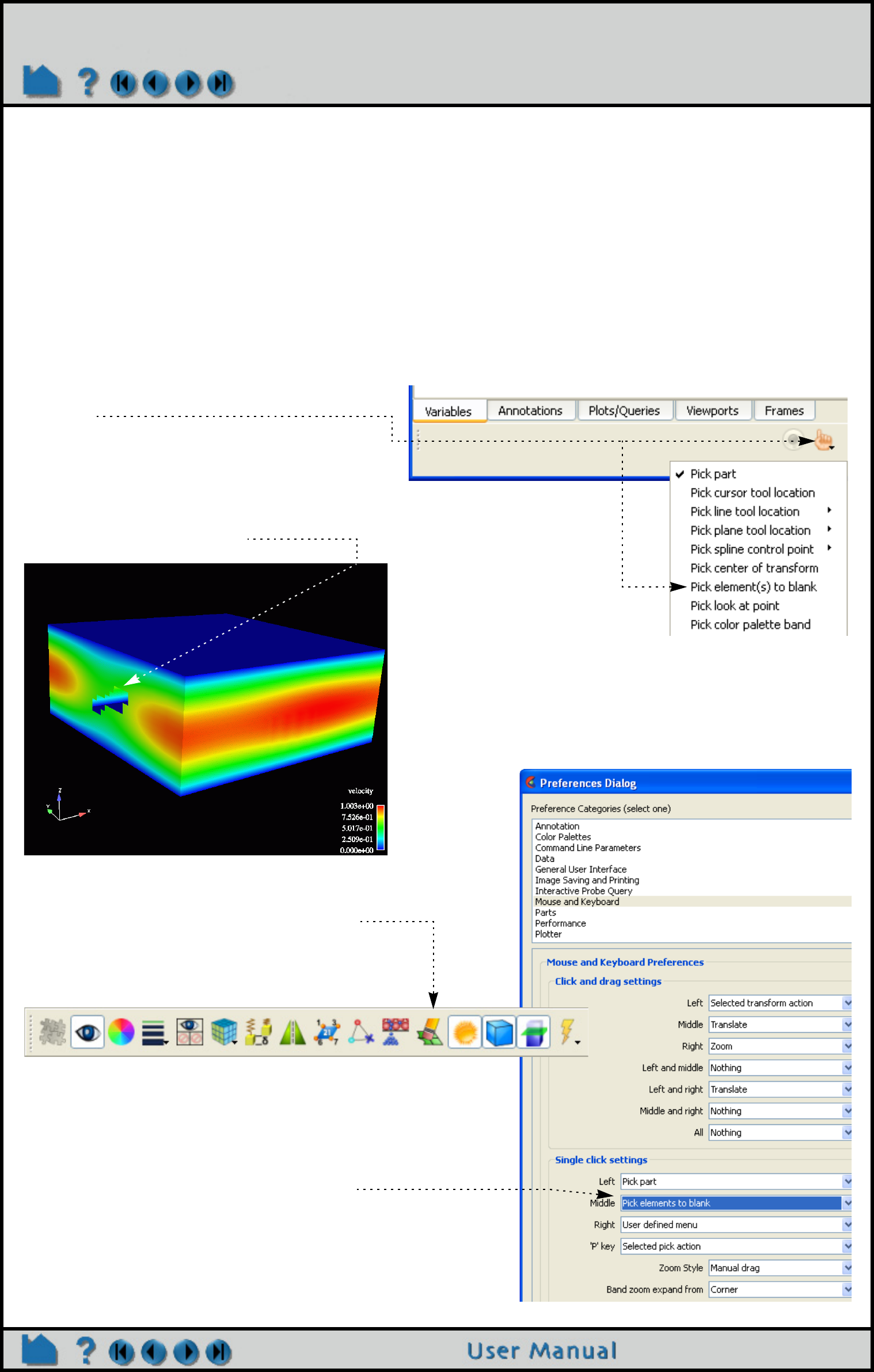
Page 350
HOW TO DO ELEMENT BLANKING
Do Element Blanking
INTRODUCTION
EnSight allows you to pick elements in the model and make them disappear - “blank them out”. This may be desirable
if you want to peek inside of certain parts or remove portions of a part (without making the entire part invisible or
transparent). Element blanking is only visual removal on the client. For example the calculated volume does not
change if some elements are blanked. Element blanking is a temporary state that can easily be “cleared” - making the
elements visible again.
BASIC OPERATION
Using picking to do element blanking:
1. Set the pick action to “Pick element(s) to
blank”.
2. Select part(s) in the part list that you wish
to operate on.
3. Place the mouse pointer over the element
you wish to blank out and press the “p”
key to blank the element.
You will see the element under the mouse
disappear as you do the picking.
4. To cause the elements to reappear, click
the Element blanking/visibility icon and
click the clear button in the dialog which
comes up.
Note that blanking can be done directly using the
mouse if you change the mouse and keyboard
settings. For example, the preferences can be
set to blank using a middle mouse button click
on the part. Edit > Preferences > Mouse and
Keyboard.
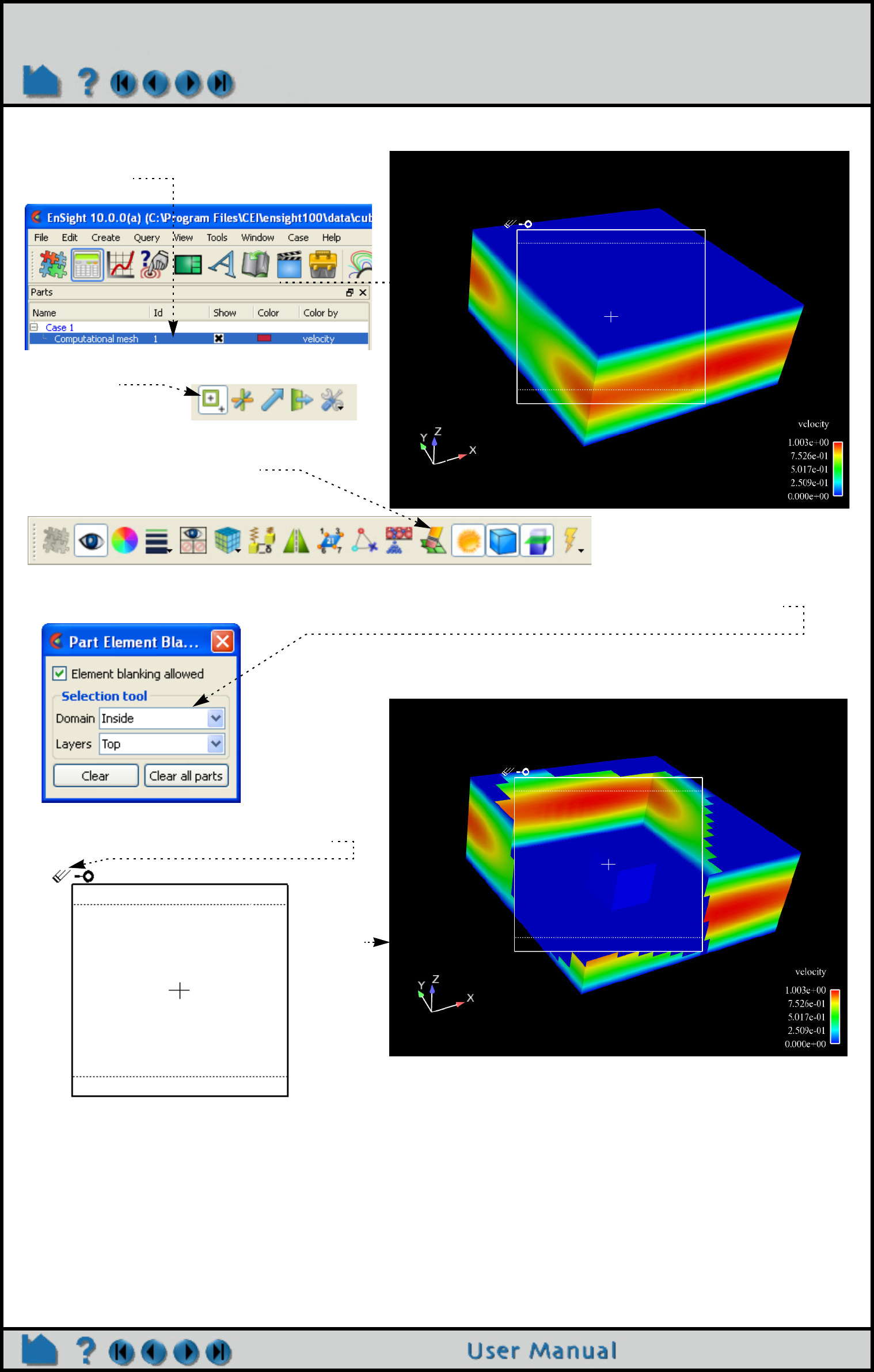
Page 351
HOW TO DO ELEMENT BLANKING
Also, the selection tool can be used to do element blanking on a larger scale:
Note
The element IDs are used to tag visibility. These tags are preserved through timestep changes. If the elements
change IDs (perhaps changing connectivity) then EnSight will continue to use those same IDs which may result in
invisible elements at different locations.
SEE ALSO
How To Use Selection Tool
1. Select the part(s) on which to do element
blanking.
2. Click on the Selection tool icon to turn on
the tool.
3. Position the tool as desired.
4. Click on the blanking icon.
5. Choose the criteria to use for blanking: inside or outside (inside or outside the box) and top or all
(top is just the first visible layer, all is to blank all elements in a direction perpendicular to box.
Results
in this.
To undo the blanking, click the Clear or Clear all parts button.
6. Click on the element blanking eraser
symbol at the upper left of the tool.
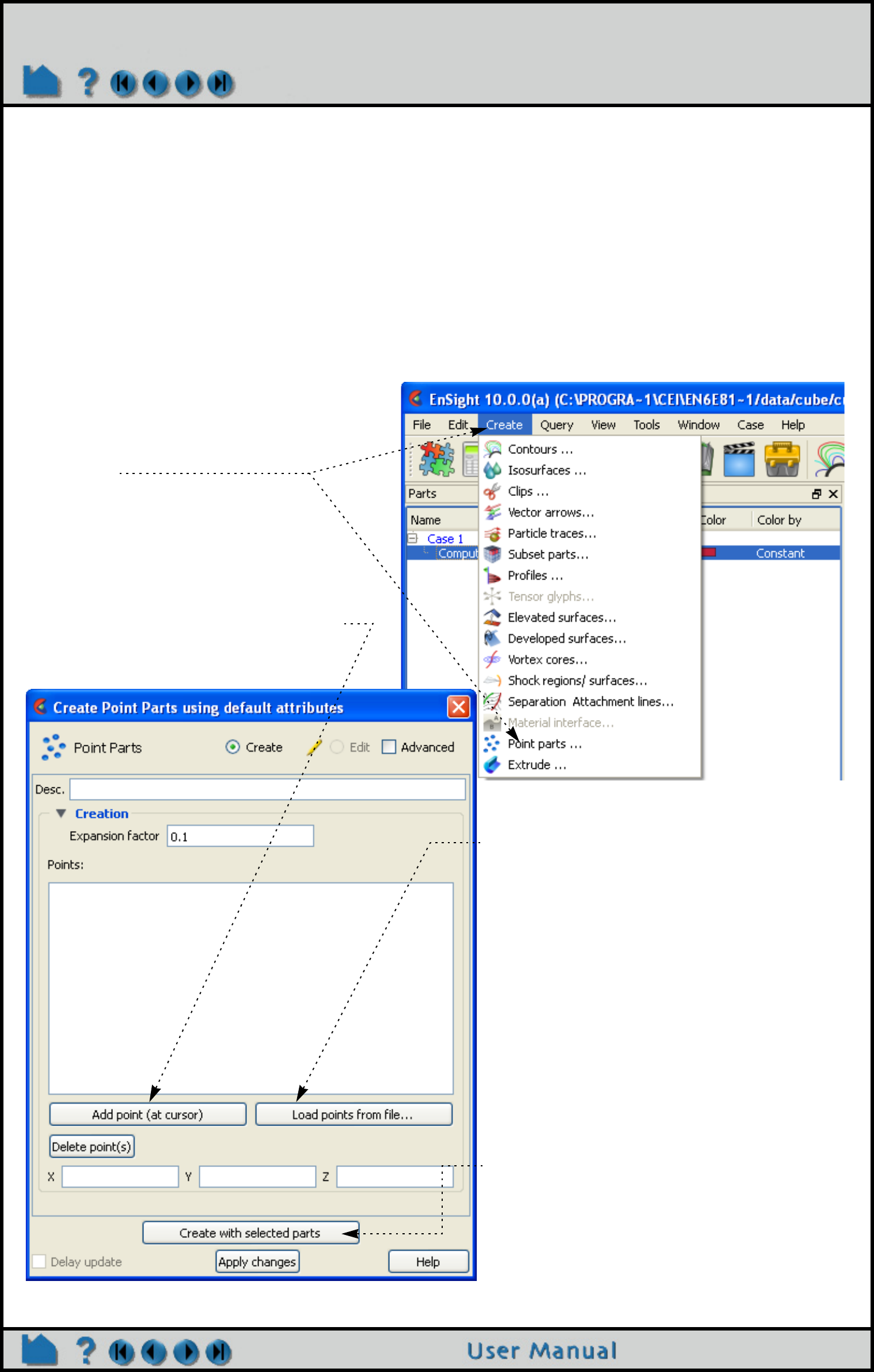
Page 352
HOW TO USE POINT PARTS
Use Point Parts
INTRODUCTION
A point part is a part composed only of nodes. It can be read in as a model part or can be created through the use of
the Point Part feature. In order to create the part, a series of point locations must be defined. The point locations can
be read from an external file, or can be created by placing the cursor tool at desired locations and adding points. You
can later edit the locations of, or delete any of the points. When you select a parent part and click Create, a new part
with only nodes is created. This type of part can represent probes in the data, or lends itself well to meshing into a 2D
or 3D part. As the per-node variables of the model parts are mapped to the point part locations, it is also a great way
to write out nodal variable information (using File->Save->Geometric Entities) for further calculations. Note if a parent
part has per element variables then they must be moved to the nodes using the calculator function ElemToNode.
BASIC OPERATION
1. Select the parent part.
2. Click Create -> Point parts ...
To open the Feature Panel for Point
Parts.
5. Click Create.
OR
4. Click the Load points from file... button.
(Which will bring up the file select dialog)
and select a file that contains the desired
points.
(See Section 9.17 Point Part File Format in the User
Manual)
A simple sample of a Point Part file:
#Version 1.0
#EnSight Point Format
-.5, -.5, .5
-.5, .5, .6
.5, -.5, .7
.5, .5, .4
-1.5, -1.5, .5
1.5, 1.5, .3
2.25, 2.1, 1.5
4. Move the cursor to the desired spot.
(Interactively or by using the Transformation
Editor.)
and
Click the Add Point (at cursor) button.
(Repeat as many times as needed)
3. Make the cursor tool visible.
6. To create a mesh from a point part, click on
the Advanced button.

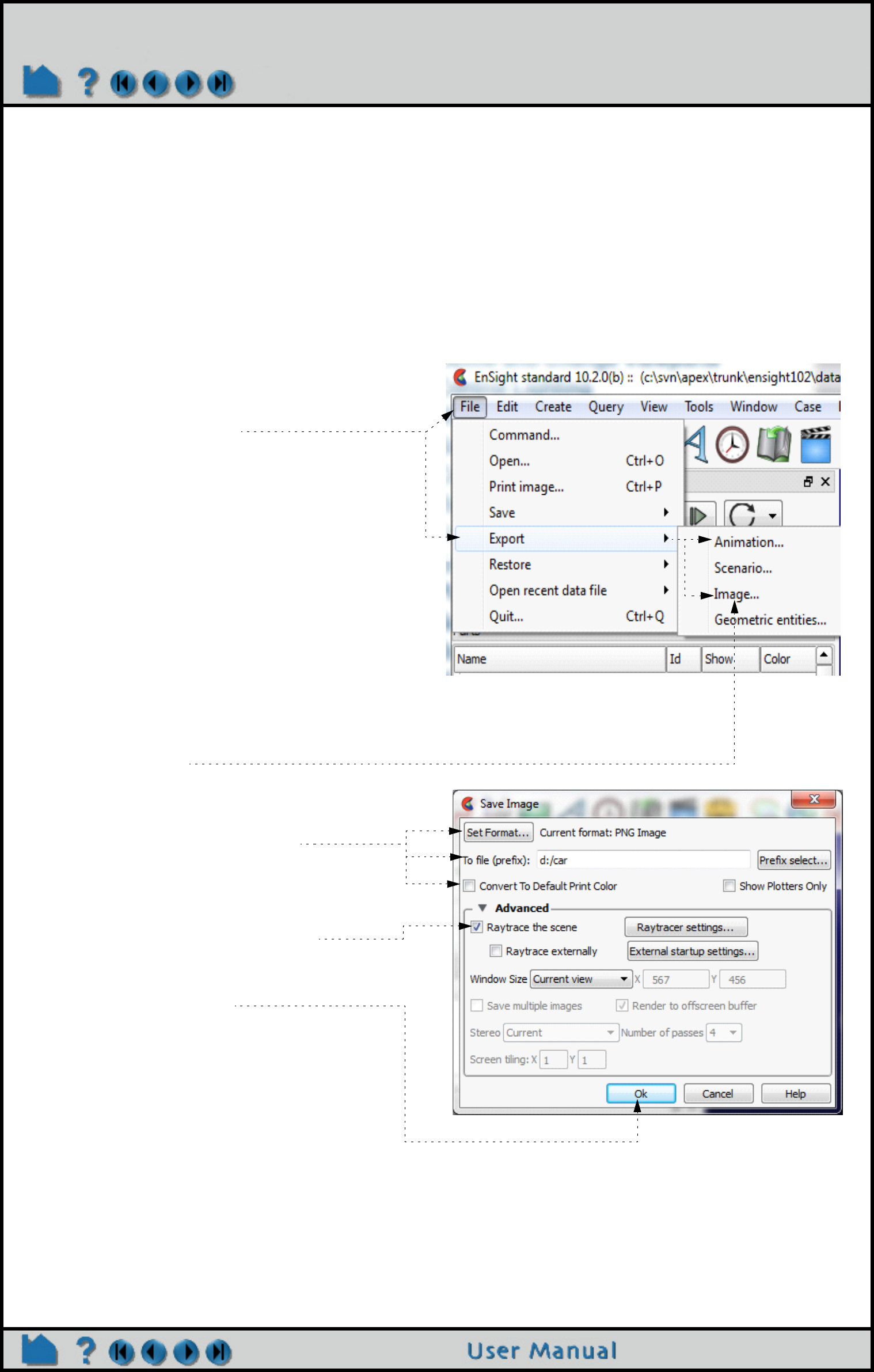
Page 354
HOW TO USE RAYTRACE RENDERING
Use Raytrace Rendering
INTRODUCTION
Raytracing is an advanced rendering technique in computer graphics, where simulation of the light transport is
performed between the image pixels, objects in the scene, and the light sources. This technique is capable of
generating high realism images, but at a much higher cost than that of typical rasterization-based techniques. It is
usually implemented in software while the rasterization-based techniques are in hardware. Raytracing is suitable for
rendering a wide variety of optical effects, such as reflection, refraction, soft shadow, etc.
BASIC OPERATION
1. Choose File->Export.
There are two export types which support
raytracing.
Exporting an Image:
2. Select Image...
The save Image dialog will appear.
3. In this dialog, we first set up the normal
image output options, such as file path,
image format, image size, etc.
4. Open the Advanced frame box.
Here we will see the raytracing settings.
5. For a quick start, simply check the
“Raytrace the scene” checkbox
and leave all the rest of the settings
untouched.
6. Press the Ok button.
The data will be rendered using the
raytracing rendering engine and exported as
specified after the rendering is finished.
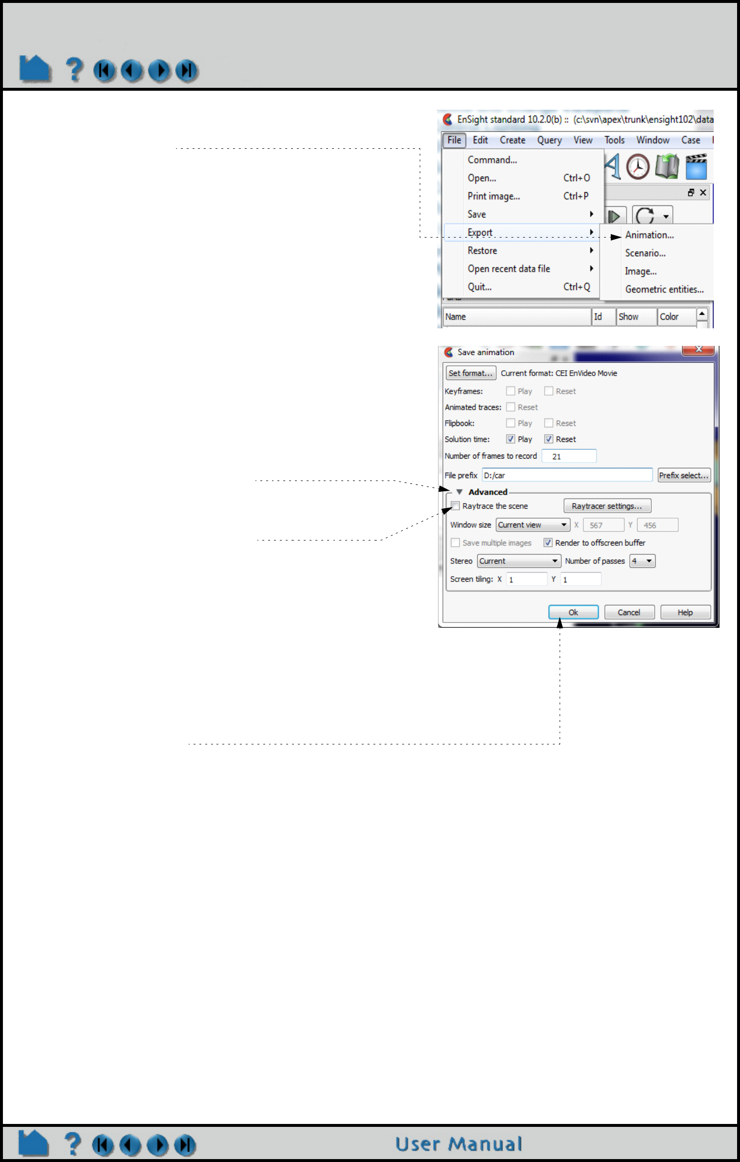
Page 355
HOW TO USE RAYTRACE RENDERING
Exporting a video (Animation):
2. Select Animation...
The Save animation dialog box will come up.
If you see that the Animation menu item is
grayed out, then the data set does not contain
transient data. You will need to create some
transient data such as a flipbook or keyframe
animation.
3. Open the Advanced frame box.
Here we will see the raytracing settings.
4. For a quick start, simply check the
“Raytrace the scene” checkbox
and the raytracing rendering engine will be
used for rendering each frame of the
animation. This dialog differs from the one with
image export. Namely, the “Raytrace
externally” option does not exist here. The
reason is that we automatically let a backend
task manager take charge of the time
consuming work involved. You can let this
happen in the background and continue your
interactive wor, and leave all the rest of the
settings untouched.
5. Press the Ok button.
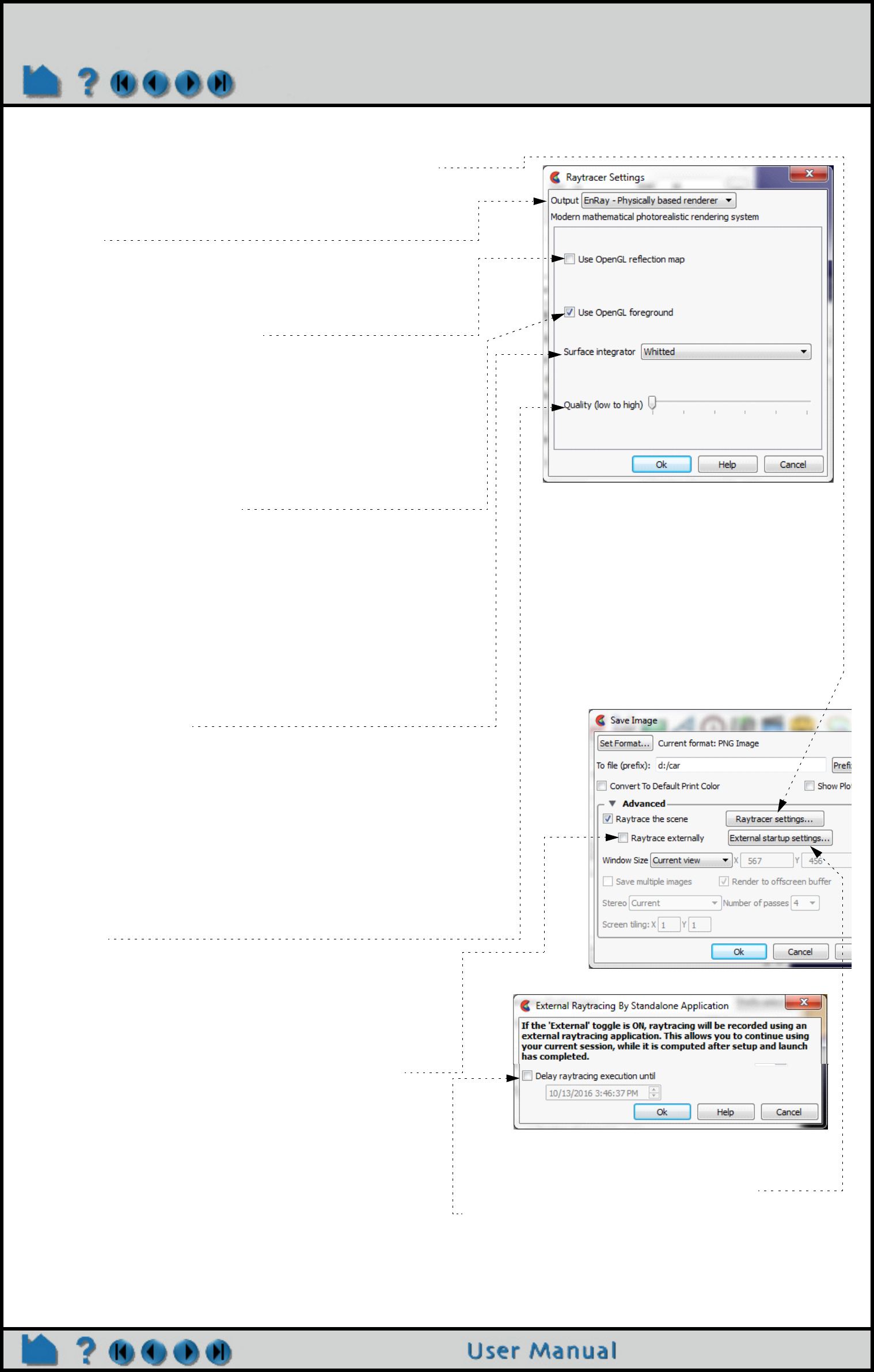
Page 356
HOW TO USE RAYTRACE RENDERING
RAYTRACING OPTIONS
When you click on the “Raytracer settings” button in the
previous dialog, the settings dialog box will come up. and
you can control several options.
Output
A user can choose which output to use. The default choice
is EnRay - which is EnSight’s built-in renderer. POV-Ray
will generate files suitable for the POV-Ray application.
Use OpenGL reflection map
EnSight provides a default material library, where there are
some reflection maps used for reflective materials when
the graphics hardware rendering engine is used. If a user
prefers to use these reflection images in the raytracer, he
can inform the raytracer to use them here. But, doing so
will disable the real inter-reflection computation between
scene objects.
Use OpenGL foreground
Whether output of 2D overlay of the graphics hardware
rendered result is sent to the raytracer or not. Usually,
EnSight’s graphics window contains not only rendering
results from 3D geometry, but also 2D illustrations such as
palettes, plots, tables, etc. The raytracer does not have the
capability to render the 2D layer. Therefore, when this
option is set, the system will output the hardware rendered
2D layer as an image and composite it with the raytracing
result.
Surface integrator
Choose from different raytracing algorithms. Currently the
raytracer has two options. The Whitted style, which traces
three types of rays: reflection, refraction, and shadow. It is
an efficient rendering algorithm for rendering highly
reflective scenes. It is not good at rendering diffusely
reflective scenes. And the ambient occlusion technique,
which is suitable for scenes which are dominated by
ambient lights. It uses the local occlusion ratio to modulate
the shading results.
Quality
Specify the image quality of the raytracing result. In the
current implementation we set 6 levels, where 0 is the
lowest and 5 is the highest quality. The detailed raytracing
parameters are hidden from the user, such as number of
samples per pixel, recursive depth, etc.
Raytrace externally (when doing Image output)
EnSight can use both the internal EnRay raytracer or the
external command line EnRay raytracer to perform the
raytracing task. By checking the option “Raytrace
externally” for image output, EnSight will use the external
one. The benefit of doing so is that a user will not be
blocked by the time-consuming raytracing computation,
and will be able to continue his interactive session.
External Raytracing startup settings
Delay raytracing execution until
Allows you to specify the date and time to start the
jobs, in place of having them start as soon as
submitted.


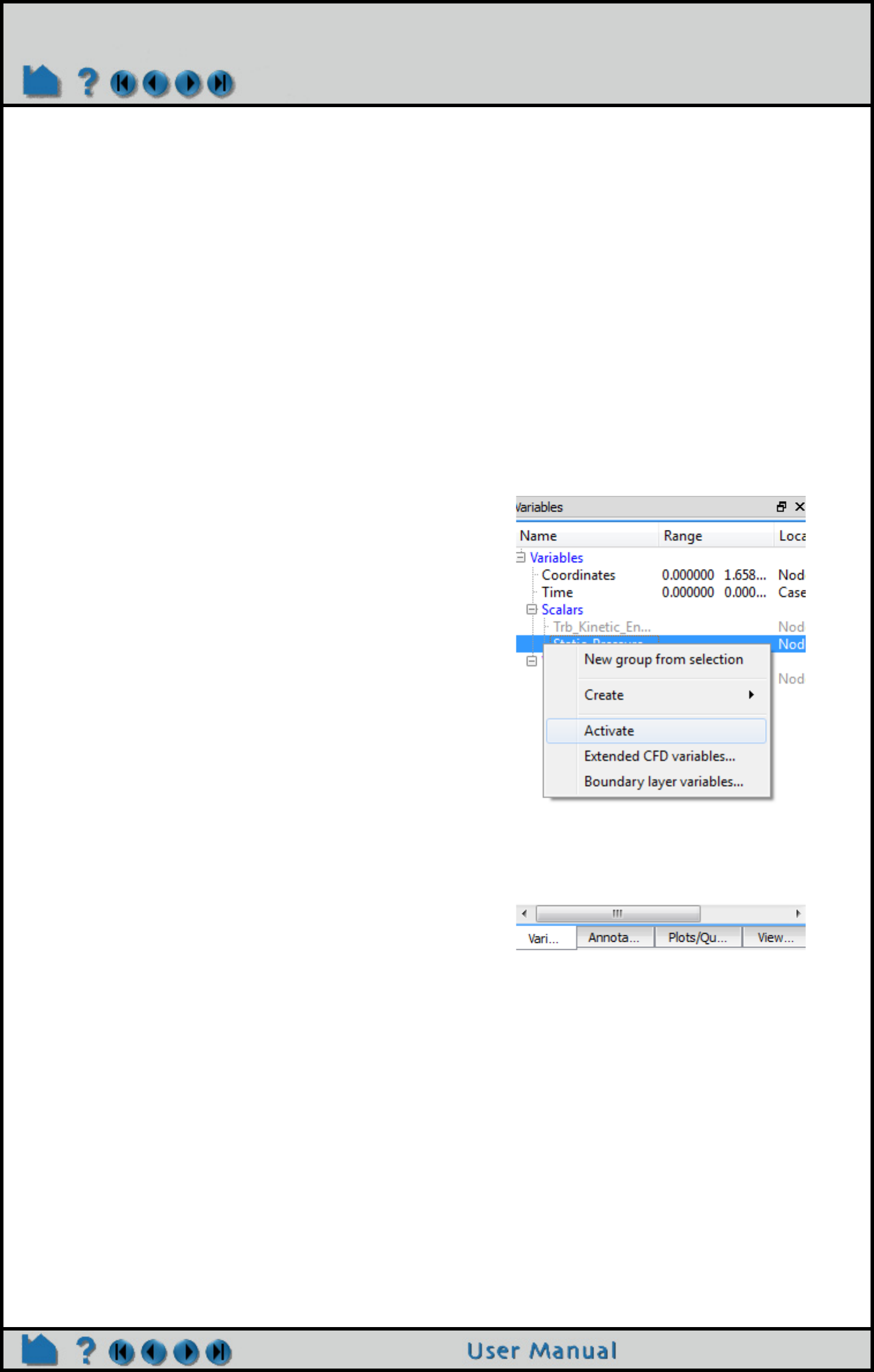
Page 359
HOW TO ACTIVATE VARIABLES
Create and Manipulate Variables
Activate Variables
INTRODUCTION
When a results dataset is read into EnSight, associated variables are noted and listed in the Variables List Panel.
However, a variable will remain deactivated (not loaded into memory) until some operation requires it or it is explicitly
activated (read into memory).
If an active variable is no longer required, you can deactivate it and free the associated memory.
BASIC OPERATION
Variable Activation and Deactivation
In most instances, variables are automatically activated as required. For example, if you create a contour using a
deactivated variable, EnSight will automatically activate the variable prior to creating the contour.
You can also activate and deactivate variables explicitly via right clicking on the variables in the Variable list.
SEE ALSO
How To Edit Color Palettes, How To Create New Variables
User Manual: Variable Selection and Activation
1. Right click on the variable(s) you wish to
activate or deactivate. Grayed out variables
are currently deactivated.
2. From the resulting right click pull down select
Activate (or Deactivate if the variable is
already active)

Page 360
HOW TO CREATE NEW VARIABLES
Create New Variables
INTRODUCTION
EnSight provides a powerful capability to derive new variables from existing variables and parts. For example, in a
fluids dynamics problem, if you have momentum, density, and stagnation energy you can calculate temperature,
Mach number, pressure, or velocity. In addition to the built-in functions, you can also compose your own functions
using the equation editor in conjunction with previously defined variables.
This article is divided into the following sections:
Introduction
Variable Creation
Examples of Expressions
Extended CFD Variables
BASIC OPERATION
Introduction
EnSight provides six distinct types of variables:
Variables are either given (read from the dataset or automatically provided by EnSight) or computed (derived from
existing variables during an EnSight session). The variable type and whether it is given or computed are shown in the
Variables list panel by looking at the Computed column. The Location column will tell you if a variable is node or
element based.
Every non-constant variable (both given as well as computed) has an associated color palette that defines the
mapping from variable values to color. These palettes can be edited to change the mapping (see How To Edit Color
Maps for details). The value of a constant variable can be displayed as a text string in the Graphics Window (see
How To Create Text Annotation for details).
For time-dependent data, calculated variables will automatically recalculate when the current time step is changed.
Constant A constant variable is a single value. Constants do not vary across a part
although a constant can vary over time. Examples include Analysis_Time,
Temperature[123] (the value of temperature at node 123), Stress{3}[321]
(the value of stress at node 321 at time step 3), or the value of a function
that produces a constant (e.g. Area).
Constant per
part
A constant per part is a single value per part. Thus the value does not vary
within a given part, but can be different for each part. Examples include
things like area, volume, max of a scalar, etc.
Scalar A scalar variable is a set of values: one for each node or element of the
applicable part(s). Examples include Pressure, Velocity[Z] (the Z component
of velocity), Stress{3} (the value of stress at time step 3), or the value of a
function that produces a scalar (e.g. Flow)
Vector A vector variable is a set of values: three (the X,Y,Z components) for each
node or element of the applicable part(s). Examples include Velocity,
Velocity{3} (the value of velocity at time step 3), Coordinates (a given
variable equal to the XYZ coordinate at a node), or the value of a function
that produces a vector (e.g. Vorticity).
Tensor A tensor variable is a set of values: six (if symmetric) or nine (if asymmetric),
for each node or element of the applicable part(s). Tensor variables can be
represented by Tensor Glyphs directly, and within the variable calculator
eigenvalues, eigenvectors, determinant, VonMises or Tresca, etc. can be
computed.
Complex A complex variable, which within Ensight can be either scalar or vector,
includes the real and imaginary portions of the values. The variable
calculator allows the user to compute things like modulus, argument,
transient response, etc.
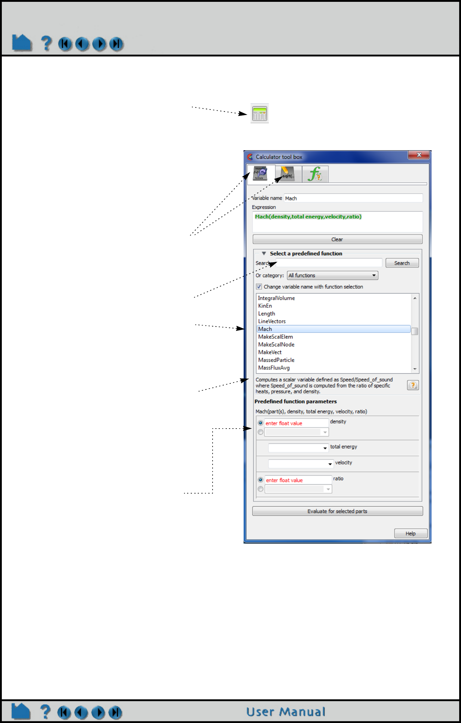
Page 361
HOW TO CREATE NEW VARIABLES
Variable Creation
Derived variables are easily created using the Variable Calculator. To create new variables:
1. Click the Variable Calculator icon in the
Feature Icon bar to open the Calculator Tool
Box. There are by default three tabs (and
usually a fourth as you can see). The left
mouse icon is for Predefined functions, the
icon with the pencil is for Defining your own,
the third tab is used for modal variable
feedback. Then multiple other user defined
tabs might exist with various functions. The
Sum of F tab is a user defined tool distributed
by default. It finds the summation of forces
and moments.
2. Select the desired tab to either use predefined
functions or define your own equation using
math operators and functions.
Predefined functions Tab:
You can search for a function name or find the
function in the list.
When you select a function, the Variable Name
field (at the top of the section) is loaded with the
name of the function. This will be the name of
the variable as seen in the Variables list. You
can change this name by entering a new name
(and pressing return).
A description of the function parameters appears
directly below the function list.
In the Predefined function parameters section
you are presented with the required inputs to the
expression.
For each required input you are presented with
the valid choices. For example, in the function in
the figure at right, density can be either a floating
point value or it can be a scalar. If you wish to
specify a scalar you would click on the radio
button and find the required scalar in the
pulldown list (which will only be showing you
scalar variables). If you wish to enter a floating
point value you would enter it into the field that
currently indicates “enter float value” by double
clicking and overwriting it with the appropriate
value.
3. When all of the parameters have been set
make sure you have the correct parts
selected in the Parts list then click on the
“Evaluate for selected parts” button.
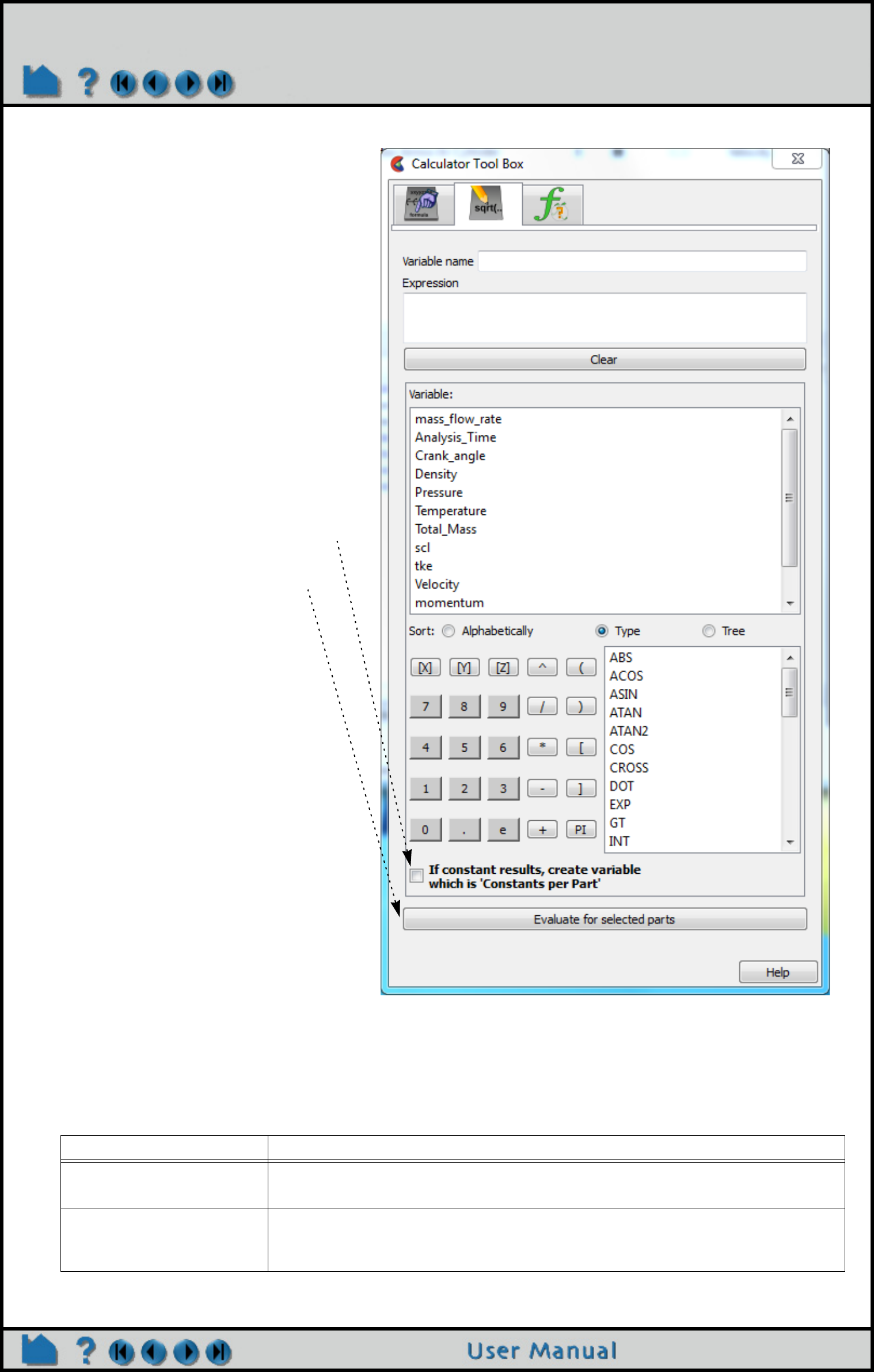
Page 362
HOW TO CREATE NEW VARIABLES
Examples of Expressions
The following examples demonstrate usage of the variable calculator. In each case, first enter a name in the Variable
Name field then click on the interface buttons or list entries or type directly into the Expression area. The examples
below assume that Analysis_Time (a given constant variable if the dataset is transient), pressure, density, and
velocity are all existing, active variables.
Expression Description and How to Build
-13.5/3.5 A simple constant.
To build, either type the text on the keyboard or click in the Calculator keypad.
Analysis_Time/60.0 A constant variable. Assuming the solution time was given in seconds, this expression will
provide a variable giving the time in minutes.
To build, select Analysis_Time from the Active Variable list and either type or click /60.0
Define equation Tab:
Alternatively, you can build your own equation
by selecting variables, math functions,
operators, and numbers as desired.
Once you have the desired equation in the
Expression field, and a name in the Variable
name field - make sure you have
1. the correct parts selected then
2. toggled on the Constants per Part if your
result will be a constant and you want a
value defined on each part. The default is
off, which is a single case constant.
3. click “Evaluate for selected parts”.
Page 363
HOW TO CREATE NEW VARIABLES
Since EnSight can compute only one variable at a time, one must break down involved equations into multiple
smaller ones, using temporary or intermediate variables.
Calculator limitations include the following:
1. The variable name cannot be used in the expression. The following is invalid:
temperature = temperature + 100
Instead use:
temperature2 = temperature + 100
2. The result of a function cannot be used in an expression.
(pressure / MAX(plist,pressure) )^2
Instead use two steps. Define p_max as:
MAX(plist,pressure)
then define norm_press_sqr as:
(pressure / p_max)^2
3. Created parts (or changing geometry model parts) cannot be used with a time calculation (using { }).
4. Calculations occur only on server-based parts. Client-based parts are ignored, and variable values may be
undefined.
For information on the arguments (and equations), see General Functions or Math Functions in the User Manual.
velocity*density Momemtum – a vector variable.
To build, select velocity from the Active Variable list, click or type *, and select density
from the Active Variable list.
SQRT(pressure[73]*2.5)
+ velocity[X][73]
Square root of (pressure at node 73 * 2.5 + the X component of velocity at node 73)
To build, select SQRT from the Math function list, select pressure from the Active Variable
list, click or type [73]*2.5)+, select velocity from the Active Variable list, and click or
type [X][73].
velocity^2 You have to be careful here. velocity^2 is NOT equal to DOT(velocity,velocity). A vector *
vector in EnSight is performed component-wise (x-component * x-component, y-
component*y-component, and z-component*z-component). The magnitude of this
expression is SQRT(x-component^4 + y-component^4 + z-component^4) which is NOT the
square of the magnitudes. If you are looking for a scalar result for the square of the velocity,
use DOT(velocity,velocity), or, for velocity magnitude, use RMS(velocity) or
SQRT(DOT(velocity,velocity)), or SQRT(velocity[x]*velocity[x] +
velocity[y]*velocity[y]+velocity[z]*velocity[z]).
pressure{19} Scalar variable equal to pressure at time 19. This variable will not change if the current
time step is changed.
To build, select pressure from the Active Variable list and click or type {19}.
MAX(plist, pressure) Constant variable equal to the maximum value for pressure over all nodes of all parts in
plist.
To build, select MAX from the General function list and follow the instructions in the Feedback
area.
(pressure/max_pres)^2 Scalar variable equal to squared normalized pressure.
To build, first calculate the MAX constant variable as described in the preceding example
(here named max_pres). Click or type (, select pressure from the Active Variable list, click
or type /, select max_pres from the Active Variable list, and click or type)^2.
Expression Description and How to Build

Page 364
HOW TO CREATE NEW VARIABLES
Extended CFD Variables
Rather than having to individually create the various common CFD variables, EnSight can automatically make them
available for use if the appropriate basis variables and constants have been provided. This can be accomplished
after loading the model with the Extended CFD Variable Settings Dialog:
2. Select the variable name in the list and then
click the appropriate SET button.
For example, select Density in the list and then
click the SET button to right of the Density field.
3. After all variables and constants have been
specified, click Show Extended CFD
Variables.
4. Click Okay.
The common CFD variables will now be listed in
the main variables list. Note that they will NOT
actually be computed until activated.
If you have a “standard” PLOT3D Q file, Extended
CFD variables will be shown by default when you
read your data.
1. Right click on any variable in the Variable list
then choose “Extended CFD variables...”
from the pulldown.

Page 365
HOW TO CREATE NEW VARIABLES
ADVANCED
Rules for inheriting Constant Per Part variables
Note that constants per part, that are in model files and exist with the same value in all parent parts of a created part
- are inherited by said created parts. If the value differs, the constant per part will become undefined in the created
part. However, computed constants per part are not automatically inherited by created parts (even if the values
are the same), and become undefined in the created parts. If a value for the computed constant per part is desired in
the created part(s), one should include the created part as one of the parent parts for the computed constant per part.
Example: If part 1 of a model has the constant per part variable rpm (of value 60), and an isovolume (which becomes
part 2) is created with part 1 as the parent, part 2 will inherit the rpm constant per part and its value of 60.
If however, part 1 is used as the parent of the computation of constant per part volume (which results in a value of
135.4), and an isovolume (which becomes part 2) is created with part 1 as the parent, volume in part 2 will be
undefined. It will not be inherited. One could, however, then go and add part 2 to the list of parent parts for the
volume constant per part - and update the variable. This would result in part 2 having volume computed on its
elements(and it would be something less than or equal to 135.4).
Plug in Variables
EnSight has the ability to display and create custom plug in variables. These variables appear in the various variable
lists when variables they depend on are present. A plug in variable is linked to a command or python file which is
executed when the user activates the variable. In short, a plug in variable appears and behaves to the user exactly
like any other variable.
Plug in variables are defined in a text file named ensight_user_def_vars.dat. This file contains the name of
the plug in variable along with a list of variables needed to compute it as well as the name of an EnSight command or
python file to execute on activation. If the variables that a plug in variable needs are present, the plug in variable will
be added to the variable lists. Any time a new variable is created the plug in variables are re-examined and added to
the variable lists if the new variable satisfies the presentation of a plug in variable.
On activation a plug in variable will execute a command file. The command file (or python file) must create the new
variable named the same as the plug in variable definition. If the plug in variable has been defined to be dependent
on variables using multiple spellings the python file that creates the variable must check on the variable spellings
during the variable creation.
To enable plug in variables, the ensight_user_def_vars.dat file must be located in a subdirectory called
"variables" and can be defined in the site-wide preference file or in the local preference file location. The site
preferences location is $CEI_HOME/ensight102/site_preferences/ while the local location is
%HOMEDRIVE%%HOMEPATH%\(username)\.ensight102\ for Windows, ~/.ensight102/ for Linux, or ~/
Library/Application Support/EnSight102/ on the Mac.
All files for the plug in variables must be in the same "variables" subdirectory (or "folder" if you prefer). This includes
not only the ensight_user_def_vars.dat file but also any command or python file needed to compute the variables.
User Defined variables ensight_user_def_vars.dat file format description
EnSight Variable Extension File
Version 1.0
#
################################################################
# The first two lines of this file are shown above. They MUST always exist
# A ‘#’ on the first column is a comment and is ignored
#
# This file is organized by keywords. The keywords are not case sensitive
# depend: and DEPEND: are the same.
#The following keywords are valid with the following meaning:
#
# BEGIN VARIABLE: new_var_name
# Starts a new variable and names it. The name of the variable that will show up in the variable
object list
#

Page 366
HOW TO CREATE NEW VARIABLES
# VARIABLE TYPE: One of "scalar", "vector", "tensor", or "constant".
# This is an optional keyword and if missing the variable is assumed to be of type scalar.
# This is used to display the variable in the correct var object group
#
# DEPEND: variable_name
# The computation of new_var_name depends on this variable. If new_var_name is dependent on a
variable that does
# not exist the variable will not be shown in the var object list.
# This is an optional keyword
# A DEPEND line, if it exists, must be defined after a VARIABLE NAME line
# There can be multiple DEPEND lines. If they exist the meaning is that new_var_name depends on
variable_name1 AND variable_name2.
# And only if both of these variables exist will new_var_name be shown in the var object list.
# There can be an unlimited number of DEPEND lines.
# This version of the DEPEND line is case senstive, i.e., it will match the case exactly of
variable_name.
#
# DEPEND NOCASE: variable_name
# Same as the DEPEND definition except case will be ignored for the variable_name
#
# OR DEPEND: or_variable_name
# This is an optional keyword and if it is defined it must be defined after a DEPEND or OR DEPEND
line.
# This keyword defines optional variable names for the variable defined on the DEOEND line.
# For example, assume "new_var_name = Temperature*2".
# But for some solvers maybe Temperature is actually output as "degrees",
# i.e., new_var_name could be defined
# with "Temperature" OR "degrees"
# This keyword uses the exact case for the or_variable_name
#
# OR DEPEND NOCASE: or_variable_name
# This is the case insenstive version
#
# EXECUTE: play_file_name
# Defines the command file that will be played when the variable is activated.
# The play file can be any file that can be executed via "play: play_file_name", thus
# EnSight commands file or python file should work. The play file must be located in the
# same directory as this definition file.
# You should not specify a path to the file - only the filename.
# This keyword is required.
# This playfile should select the parts of interest to calculate the variable and
# should create a variable with the same name as the definition: new_var_name.
# Note that a user defined variable will not appear if an existing model variable
# has that same name
# Note that the playfile can create multiple variables as well
#
# RECOMPUTE ON NEW MODEL PARTS: <YES | NO >
# Is an optional keyword. If missing NO is implied
# If YES, the variables created when play_file_name is executed are recomputed
# to include any new model parts that are
# loaded. Thus for example is a new case is loaded the variable(s) would get
# recomputed on the parts loaded from the new case
#
# END VARIABLE:
# Is a required keyword. It simply closes the variable definition
Example ensight_user_def_vars.dat file is shown below:
#####################################################################################
EnSight Variable Extension File
Version 1.0
# Example 1: This will compute a scalar named "Pressure_psi"
# by executing a command filed called "pres_Pa_to_psi.py"
# It will be shown in the variable lists if it finds a variable called

Page 367
HOW TO CREATE NEW VARIABLES
# "pressure" (case insensitive).
#
BEGIN VARIABLE: Pressure_psi
VARIABLE TYPE: scalar
DEPEND NOCASE: pressure
EXECUTE: pres_Pa_to_psi.py
END VARIABLE:
#
# Example 2: Create a Stress Tensor variable from the six symmetric stress components
# Stress Tensor: This will compute a tensor variable named "Stress_Tensor"
# by executing a command file called "Stress_Tensor.py"
# It will appear in the variable list if it finds
# all of the stress variable components
# After it has executed it will update to include any new model parts created
#
BEGIN VARIABLE: Stress_Tensor
VARIABLE TYPE: tensor
RECOMPUTE ON NEW MODEL PARTS: YES
DEPEND NOCASE: S11
DEPEND NOCASE: S12
DEPEND NOCASE: S13
DEPEND NOCASE: S22
DEPEND NOCASE: S23
DEPEND NOCASE: S33
EXECUTE: Stress_Tensor.py
END VARIABLE:
# Example 3: Create a Velocity vector from the components
#
BEGIN VARIABLE: Velocity
VARIABLE TYPE: vector
DEPEND: velx
DEPEND: vely
DEPEND: velz
EXECUTE: vel_vec.enc
END VARIABLE:
#####################################################################################
Example EnSight Command/Python files for the above ensight_user_def_vars.dat file:
#####################################################################################
Example 1 EnSight Python File, above: pres_Pa_to_psi.py
# Convert Pressure from Pa to PSI
# psi = Pa / 6894.757
#
# import an EnSight utilities module
#
import ens_utils as eu
# For details on the functions available:
# print dir(eu)
#
# Get a list of variables exactly matching ‘pressure’
# which should be only one
# (must use a case independent search)
# for details do the following:
# print help(eu.get_vars_by_name)
#
pvars = eu.get_vars_by_name('pressure', flag='all', case_sensitive=False)
if pvars:
# should only be one
ensight.variables.activate(pvars[0].DESCRIPTION)
ensight.part.select_all()
ensight.variables.evaluate("Pressure_psi = " + pvars[0].DESCRIPTION + " / 6894.757")
#####################################################################################
#####################################################################################

Page 368
HOW TO CREATE NEW VARIABLES
Example 2: EnSight Python File: Stress_Tensor.py
#
# Create a Stress Tensor using the components (exact match)
#
ensight.sendmesgoptions(version="10.16 (b)")
ensight.sendmesgoptions(version=0)
ensight.part.select_all()
ensight.variables.activate("S11")
ensight.variables.activate("S22")
ensight.variables.activate("S33")
ensight.variables.activate("S12")
ensight.variables.activate("S13")
ensight.variables.activate("S23")
ensight.variables.evaluate("Stress_Tensor = TensorMake(plist,S11,S22,S33,S12,S13,S23)")
#####################################################################################
#####################################################################################
Example 3: EnSight Command File: Make a velocity vector from the component scalars
vel_vec.enc
#
#
#
part: select_all
variables: activate velx
variables: activate vely
variables: activate velz
variables: evaluate Velocity = MakeVect(plist,velx,vely,velz)
EXPORTING CONSTANT VARIABLES
Right click on one or more constant or a per part constant variable(s) and choose export to .csv. The values of the
variables will be exported to comma separated value (csv) format as follows. The header will be time step, then time
value, followed by variable name(s). The second row will include part names (for the per part constant(s)). The
remaining rows will be the value of the constant(s) at each timestep. Note this data can be loaded into a spreadsheet
program and transposed if you wish to have the data in a transposed format.
SEE ALSO
How to Edit Color Maps
User Manual: Variable Creation, General Functions and Math Functions.

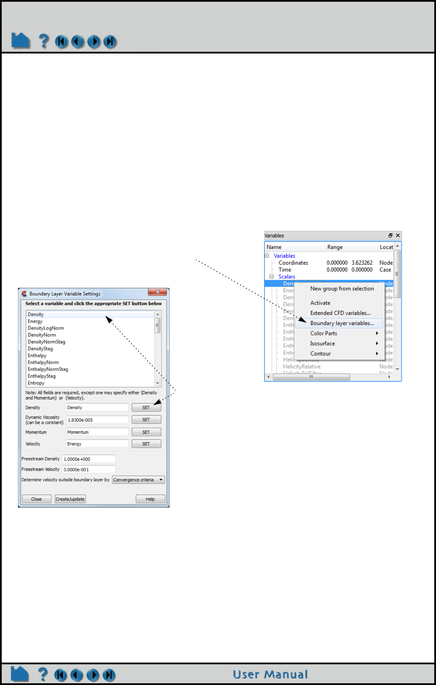
Page 370
HOW TO EXTRACT BOUNDARY LAYER VARIABLES
Extract Boundary Layer Variables
INTRODUCTION
EnSight can compute many boundary layer variables via the variable calculator. It can also compute the following
variables in bulk (at essentially the same compute costs):
boundary layer thickness named: (bl_thickness)
displacement thickness (bl_displ_thickness)
momentum thickness (bl_momen_thickness)
shape parameter (bl_shape_parameter)
skin friction coefficient (bl_skin_friction)
You must have a 2D surface in a 3D field and specify the 2D surface as the parent part(s).
For a complete description of these variables, refer to the User Manual section below.
BASIC OPERATION
OTHER NOTES
These variables and more are also individually available in the Variable calculator. See the Boundary Layer
Variables section of Chapter 4 in the User Manual
Note that the Freestream Density, and Freestream Velocity fields are for constant ‘upstream’ density and velocity
magnitude values (near flow inlet). They are only used for skin-friction coefficient, Cf.
Boundary Layer variables do not work with multiple cases.
1. Select the 2D parent part(s).
2. Right click on any variable in the Variables
list and choose “Boundary Layer variables”
from the pulldown.
3. Define the required variables by selecting them in the list
and clicking the Set button.
4. Define either (Density and Momentum) or velocity.
The variables can be set by either typing them into the fields, or
selecting them from the list and clicking on the Set button.
5. Click Okay to finish the variable setup.
6. Choose the method that will be used to determine the
velocity outside the boundary layer.
7. Click Create/Update.
This will create the five new variables, which can be used for further operations - such as part coloring and
queries.

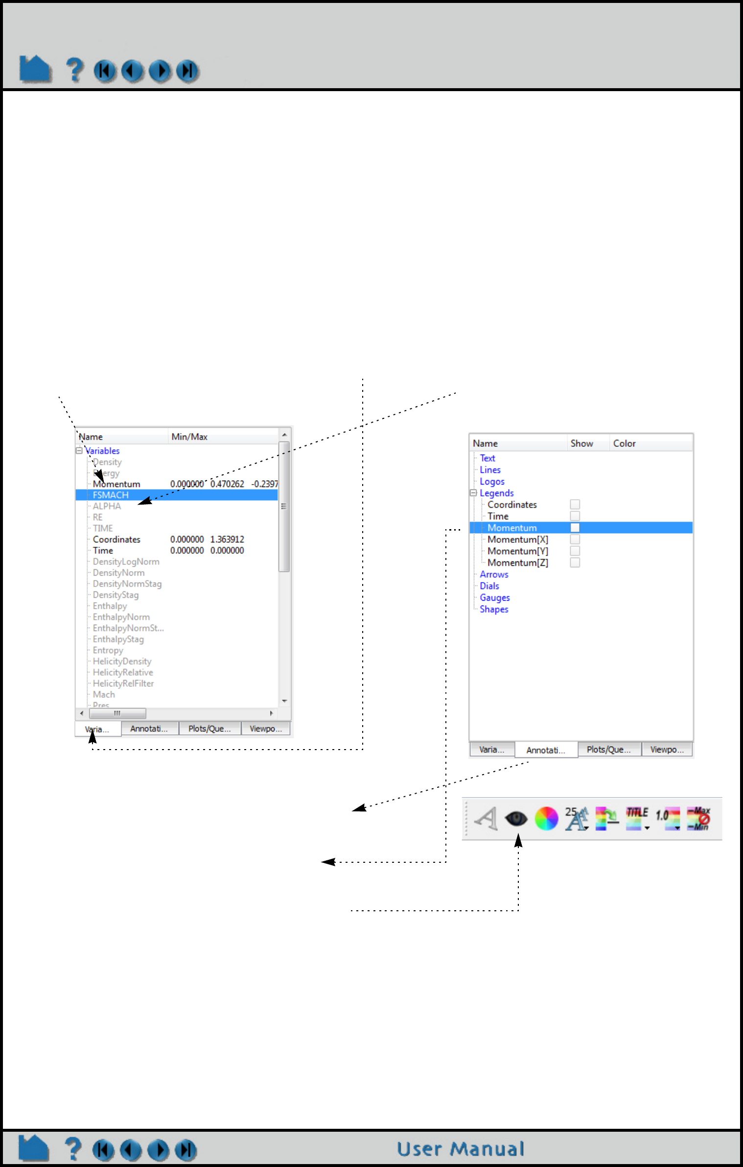
Page 372
HOW TO EDIT COLOR PALETTES
Edit Color Palettes
INTRODUCTION
All scalar, vector, and constant per part variables have an associated color palette that defines the mapping from
variable values to colors. These palettes can be easily edited to customize the mapping. Color palettes can also be
saved to disk and restored during a subsequent session.
BASIC OPERATION
The default color palette created for each variable has five Levels (with the minimum and maximum set to the range
of the variable at the time step selected when the variable was activated). The color ramp is a standard spectrum with
the five Levels set to (from min to max) blue, cyan, green, yellow, and red.
Active scalars and vectors have color palettes that are initialized to the variable range for the currently loaded parts.
An active variable has a solid color in the Variables List Panel while an inactive variable (not yet read by EnSight) is
grayed out. To activate an inactive variable you can right click on the item in the list and Activate it.
EnSight can display multiple color legends in the Graphics Window:
Color legends have a number of display attributes including size, position, and how/where the variable labels are
formatted. See How To Create Color Legends for details.
1. Click the Annotation tab and open the Legend group.
2. Select the desired variable(s) or variable
components in the list.
3. Turn on visibility via the Quick Action Icon Bar
To remove a legend repeat the procedure or you can remove
the legend by right clicking and performing a “Hide” operation.
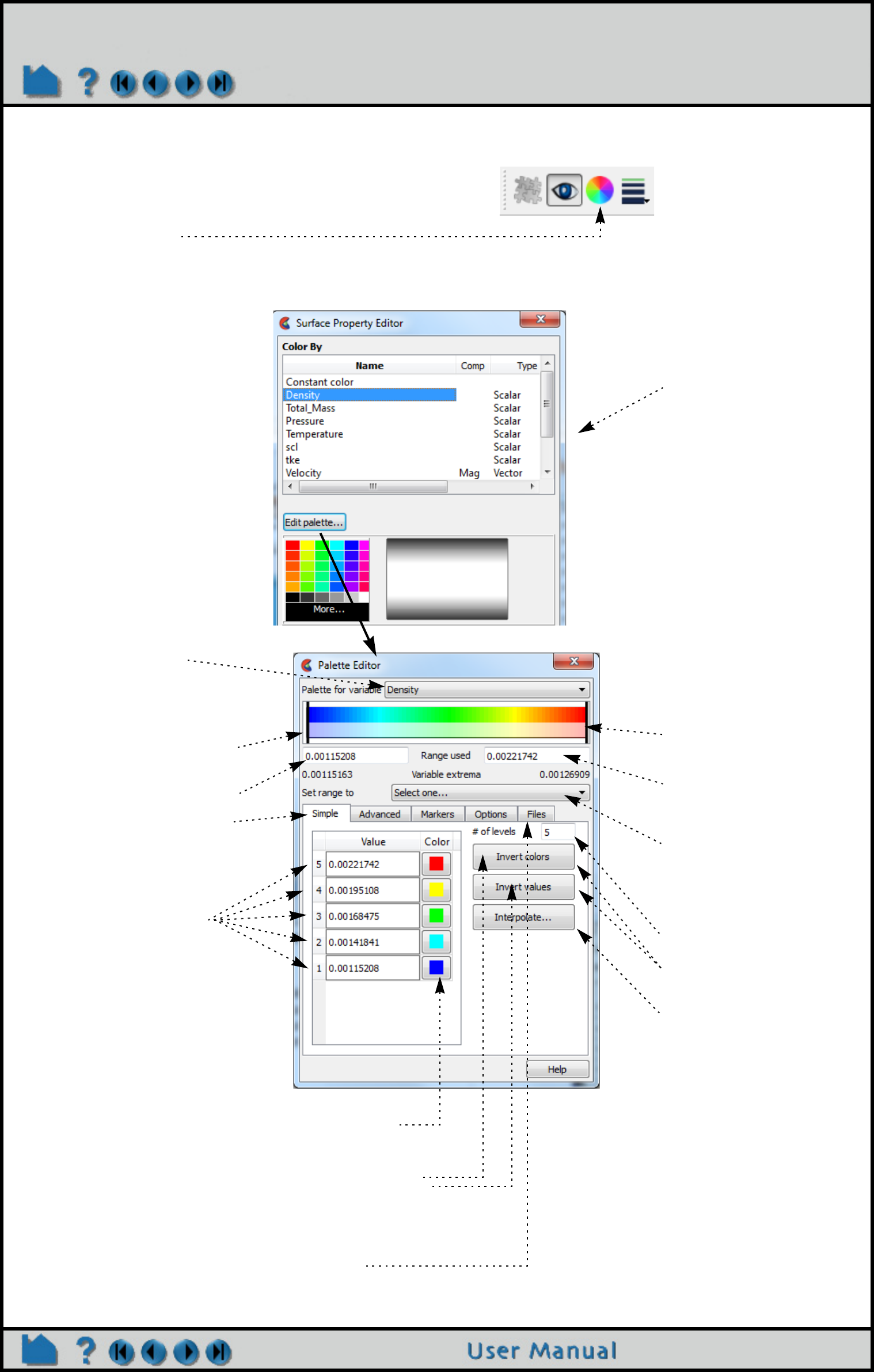
Page 373
HOW TO EDIT COLOR PALETTES
The Palette Editor provides access to all aspects of variables including min/max information, histogram, and variable
value mapping to color and transparency:
3. Select the palette to be
edited from the
pulldown
Grab the Minimum Palette Value
Slider
Type in a Minimum Palette Value
Opens by default in Simple Tab
Palette Levels (and variable
values). Enter a new value if
desired. Click on Color to
change.
Notice that if you have
chosen to color by a variable
(here Density)
Grab the Maximum Palette
Value Slider
Enter a Maximum Palette
Value
Update variable range using
a) extrema, b) selected
part(s) (note element
representation of part(s)
matters), c) currently visible
part(s) in selected viewport.
Enter desired number of
Levels in the palette (2 to 21)
Reverse colors/levels
Interpolate between two
levels. Enter the upper and
lower levels and click
interpolate to create the
intermediate levels.
1. Select the part you want to edit, then Click the
Color icon in the Quick Action Icon Bar to open
the Color Editor.
2. Click the Palette... button to bring up the Palette
Editor
To change the colors associated with
the levels
4. Click on the color for the level you wish to modify
and select a new color in the pop up dialog.
OR
5. Click the Invert colors button to invert the color
order, or Invert values to invert the values order.
OR
6. Click on the Files Tab and choose a new palette
and click Restore to load a new palette.
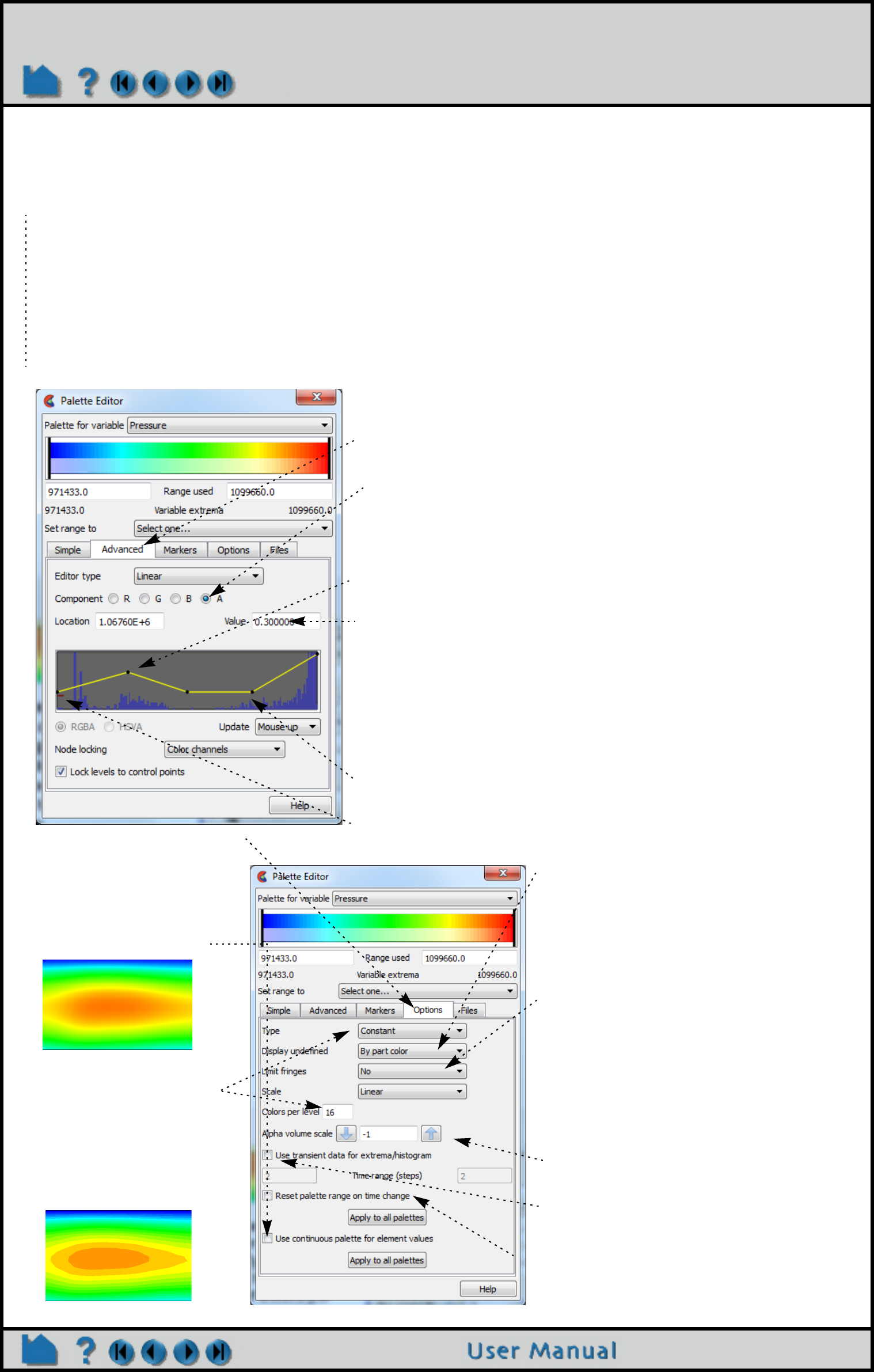
Page 374
HOW TO EDIT COLOR PALETTES
ADVANCED USAGE
A color palette is composed of color and Alpha (opacity) information at a set number of control points.
The uniform opacity can be controlled under the Lighting and Shading turndown in the Part Color/Surface
Opacity dialog. The part opacity can also be a function of a variable value in the Opacity by variable
turndown in the Part Color/Surface Opacity dialog. Finally you can choose to modify the scaling of the
opacity by its color value in the Palette Editor. By default, EnSight creates the control points to be
uniformly spaced and to have the same number as the number of levels in the palette. You can decouple
the control points from the levels by changing the Node Locking option at the bottom of the dialog.
The background of the control point graphic contains a histogram for the variable which is tied to the
palette. The small horizontal handle at the left of the image will scale the histogram information.
1. Bring up the Color Editor, then click on the Edit Palettes...
button.
2. Select Advanced Tab - and now manipulate the Control Points
3. Select which component (Red, Green, Blue, or Alpha) to
manipulate.
Change the value of the Control Points. Warning: you must change to
Alpha by Variable in the Color editor dialog (see previous page) in order to
change the Alpha for a variable here in the Palette Editor dialog.
4. Click on a Control Point and type in a value in the Value:
field,
5. OR Click on the Control Point and drag it to a new value. By
default the movement of the control point is limited such
that only the value can be changed. If you wish to move the
control points location you must unlock it by untoggling the
Node Locking option in the Options tab
To Add or Delete a Control Point
6. Right click on a control point to choose to add or delete a
control point. If adding a control point, it will be added to
the right of the selected point.
7. Click on the red handle to scale the histogram
11. You can specify how to handle
Undefined variable values. The default
is to display the Undefined value as
the part color. You can change this
such that Undefined values will be
invisible or the zero index value.
12. Limit fringes: The default behavior is
for variable values outside the min/
max range to be clamped to the color/
opacity defined at the bottom and top
of the palette. You change this
behavior so that out of bound values
are colored by the part color or are set
to invisible.
13. Change the alpha volume scale to
affect volume rendering
14. For transient data, toggle on and fill in
time range to use to rescale variable
extrema and recreate the histogram
over time.
15. Toggle ON to reset the palette range
when a timestep is changed.
8. Click on the ‘Options’ Tab
9. Default is Type Constant
for elemental variables.
For a smoother image
use a continuous palette
for elemental values
10. To create a color band
for each color in the
texture, change ‘Type’ to
‘Banded’. Reduce the
number of Colors per
level to coarsen the
bands
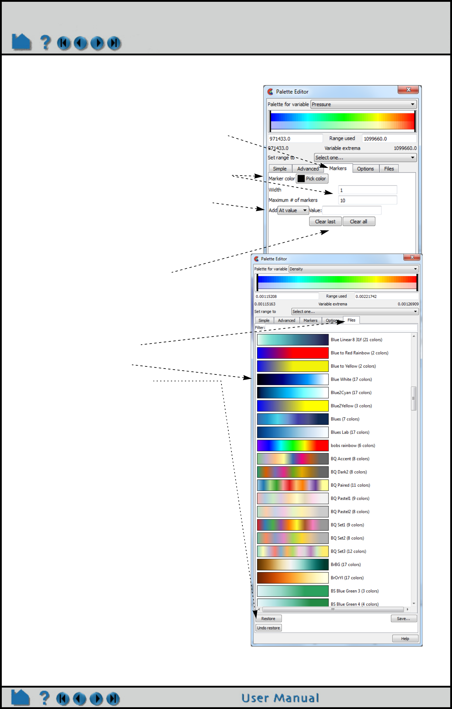
Page 375
HOW TO EDIT COLOR PALETTES
Markers are single-colored level(s) overlaid on top of the
color palette designed to emphasize the distinction
between levels.
16. Click on the Markers Tab. Markers are divider
bands drawn in the color specified at the
specified variable value. They serve to divide your
coloration similar to isocontours.
17. Choose the color, the width and the maximum
number of markers
18. At the Add: pulldown, choose one of the
following to add markers at At levels (adds a
marker at each level value), At value (adds a
single marker at the value indicated), or Uniformly
(adds marker uniformly if you enter a value into
the How Many field that appears.
19. Markers remain until cleared.
EnSight includes a number of predefined palettes
available for loading.
20. Click on the Files Tab.
21. Choose a palette.
22. Click restore to load it.
If the new number of levels does not match the
current number of levels a dialog will pop up to ask
whether you want the new number of levels or the
current.
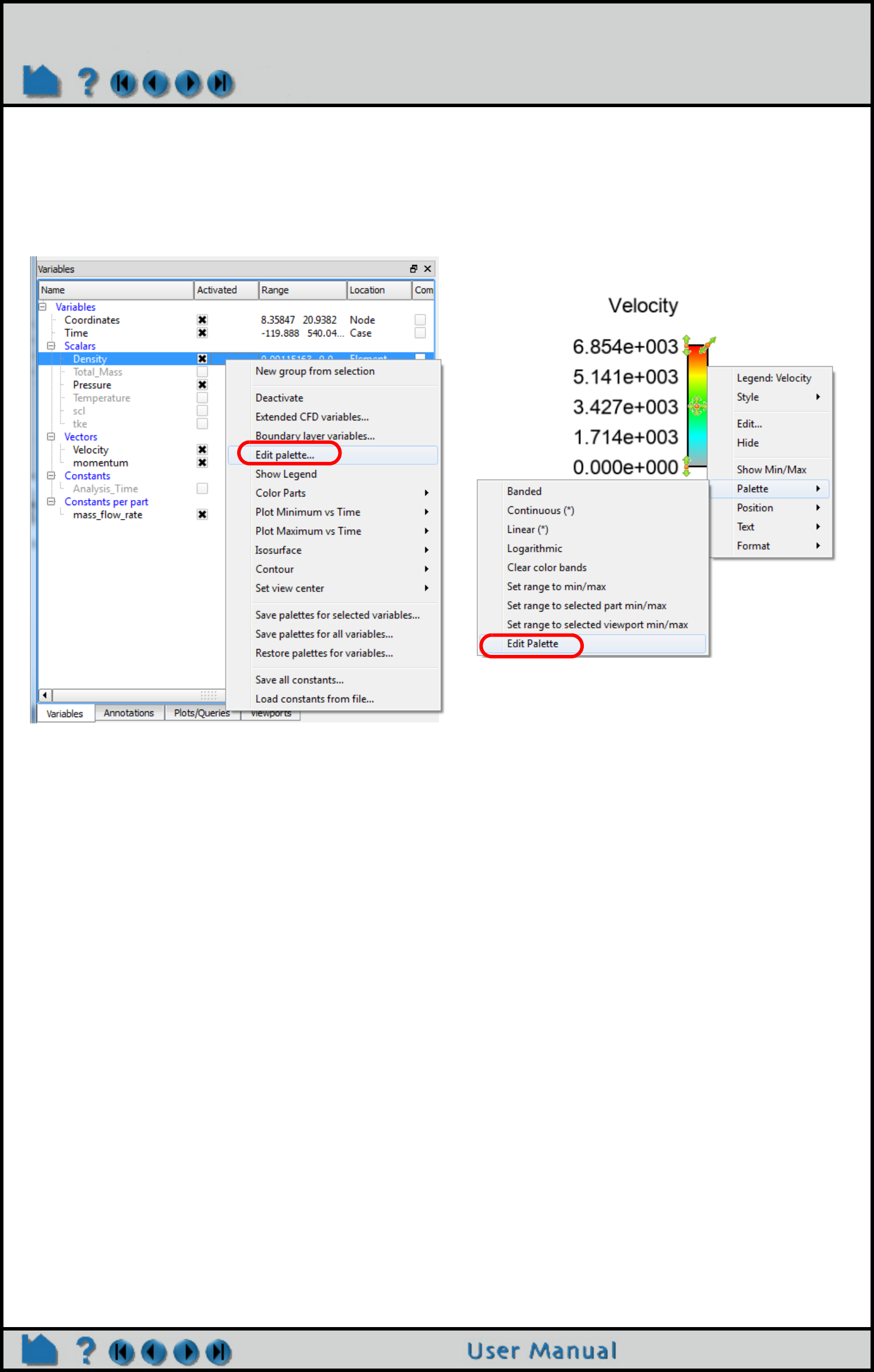
Page 376
HOW TO EDIT COLOR PALETTES
SHORTCUTS
You can open the Palette Editor from either right-clicking on the variable list or on a variable legend that is visible in
the graphics area.
SEE ALSO
How To Create Color Legends, How To Create New Variables, How To Create Contours
User Manual: Variable Summary & Palette
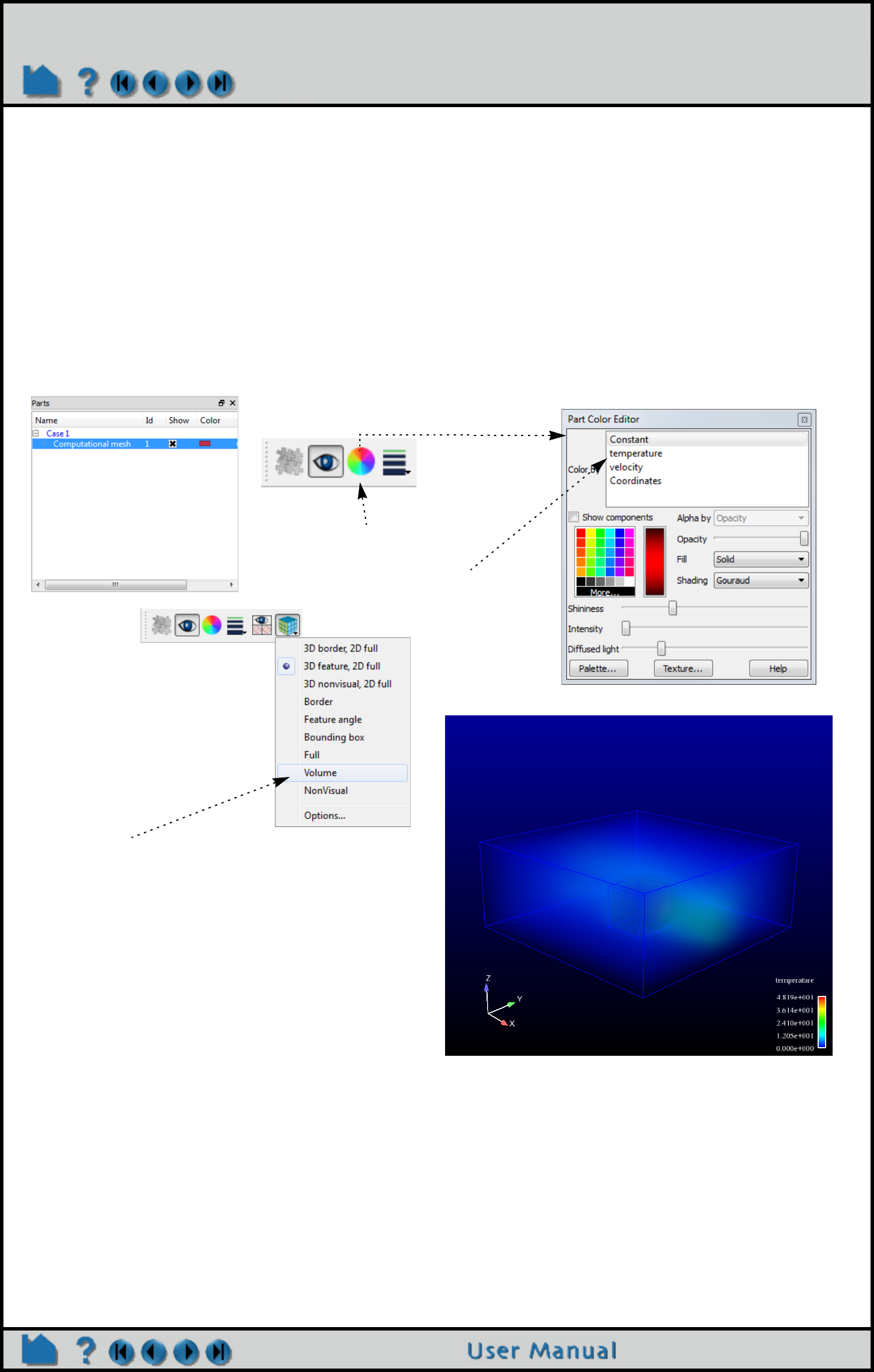
Page 377
HOW TO USE VOLUME RENDERING
Use Volume Rendering
INTRODUCTION
Most of the visualization techniques in EnSight use points, lines, and surfaces to represent data, requiring volumetric
data to be subsampled in some way. Volume rendering is a visualization technique that allows the user to view an
entire volume of data at once, without having to slice the data in any way. The process involves finding all cells that
overlap each pixel and accumulating a color for that pixel from the color and transparency of each cell. Volumes can
be constant colored, but more often you will color the volume using a palette corresponding to a variable or a variable
component. Color palettes include transparency ("alpha") values, allowing control of transparency based on variable
value.
BASIC OPERATION
Volume rendering is one of several "element representations" for a part. Results are generally loaded into EnSight by
default in Border, Feature Angle, or Full representation. These representations include only point, line, or surface
data. The "volume" element representation will activate volume rendering for a part. Just as for surfaces, the part
color dialog can be used to control the color and opacity of the volume. You can color the volume by a scalar, vector,
or vector component, and the colors will be assigned based on the palette. For large unstructured parts please see
the Advanced Usage which describes how to utilize block structured volume rendering for significantly smaller
memory and higher performance.
4. Set the Element Representation to
Volume.
1. Select the 3D parent part.
2. Open the color dialog.
3. Color the part by a variable
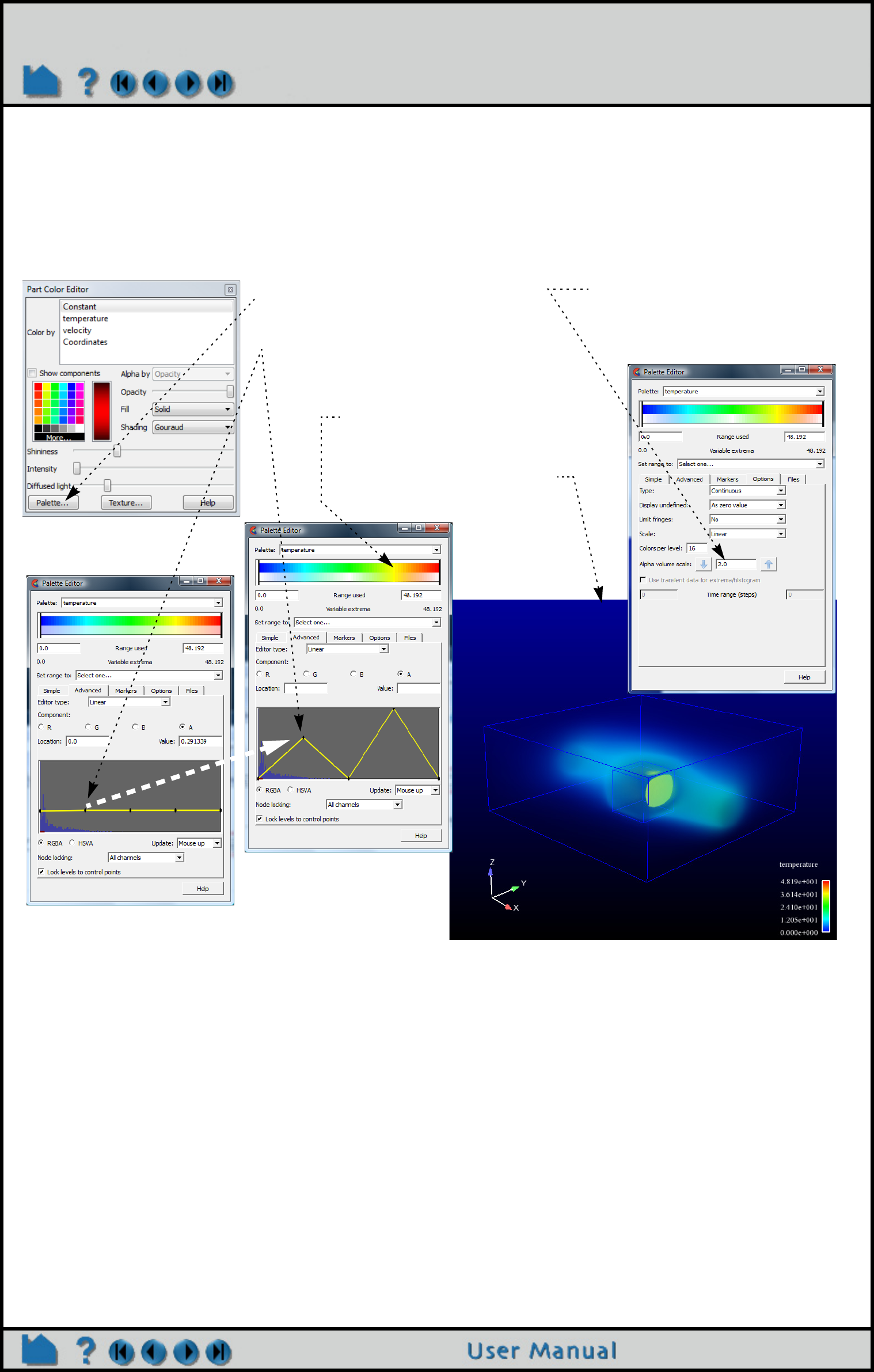
Page 378
HOW TO USE VOLUME RENDERING
ADVANCED USAGE
EnSight provides advanced control of volume rendering. You can control the volume rendering magnitude of each
level of the variable palette by adjusting the alpha value (shown as an A in the Palette Editor). The alpha value is the
opacity/intensity of the particular level when volume rendered. This means that you can emphasize select variable
levels in your volume rendering coloration by specifically increasing the alpha magnitude of these select levels. You
can also scale up the entire alpha by adjusting a multiplier value.
8. If the volume looks nearly
invisible then increase the
alpha scale uniformly to raise
the opacity level.
7. Notice the opacity of the
variable values at these levels
is scaled upward creating
emphasis in the graphics
screen and in the legend
5. Click on the Palette button.
6. Click on the control points
with the left mouse button
and drag them upward.
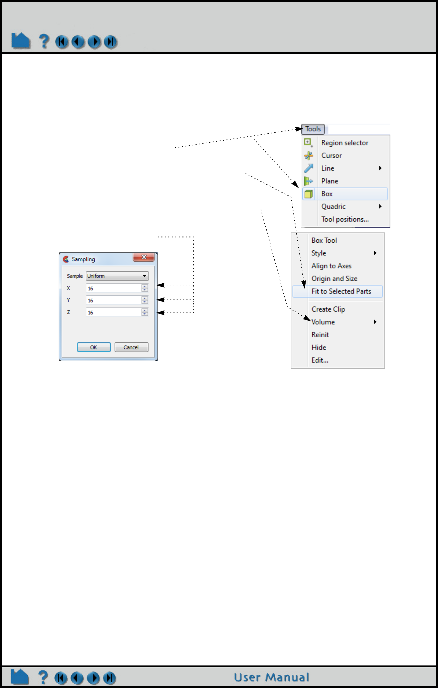
Page 379
HOW TO USE VOLUME RENDERING
Structured Volume Rendering
Unstructured volume rendering - used above - utilizes a large amount of memory on the desktop system and
significantly taxes the graphics hardware. Another option is to use structured volume rendering. In this technique a
box clip will be created using uniform spacing through the parent parts. You control the number of samples that will be
taken. In this technique your solution will be sampled onto a regular grid - something to be aware of.
OTHER NOTES
Volume rendering requires a DirectX 10 capable graphics card. Newer cards with more memory and up-to-date
software drivers will perform best. Volume rendering will use roughly 1GB of graphics memory per 10M tetrahedra.
Other cells will be decomposed into multiple tetrahedra. EnSight will disable volume rendering when it encounters
archaic graphics card hardware. Because volume rendering exercises a large amount of the OpenGL functionality
remote rendering problems are very likely, therefore this remote rendering is not supported.
SEE ALSO
See How to Change Visual Representation, How To Edit Color Maps for more information.
1. Select the 3D parent part(s)
2. Turn on the visibility of the Box tool
3. Move the mouse pointer on top of the box tool and right click
to get the box tool pulldown. Then select “Fit to Selected
Parts”. This will make the box tool fit the parts you selected
in step #1.
4. Right click again on the box tool and choose Volume->Create.
5. In the resulting pop-up dialog set the number of samples in
the box tool’s X, Y, and Z direction
6. Color the resulting Volume Clip part using the palette
instructions given above.
7. The Volume clip just created is a Box Clip. It can be edited (or
initially created) via the Part Feature Panel for clips.
Page 380
HOW TO GET POINT, NODE, ELEMENT, & PART INFO
Query, Probe, Plot
Get Point, Node, Element, & Part Info
INTRODUCTION
EnSight provides many methods for extracting exact quantitative data from your results. Specific information about
nodes, elements, parts, IJK locations, or arbitrary points can be displayed.
BASIC OPERATION
Show Point Information
To show information about an arbitrary point:
Show Node Information
To show information about a specific node, you must have either given or automatically assigned node labels for your
data. You must also know the number of the node of interest. If you do not know the number, you can display node
labels for the part or, if you know an element that contains the node, you can display element information for the
element (as described in the next section). All active variables for the node specified will be shown. To show node
information:
1. If your data is transient, set the desired time in the Solution Time Panel.
2. If you have multiple Cases, select the desired case using Case > casename.
3. Position the Cursor Tool to the desired location.
4. Select the desired part(s) in the Part List. The query will only be successful if the Cursor Tool is
found within an element of a selected part.
5. Select Query > Show Information > Cursor.
The query results will be printed to the EnSight message window, which will pop up.
It can also be accessed from the Info icon.
The following shows sample output from a point query:
Point (6.19810e-01,2.77589e-01,2.41451e-01)(In Frame 0) Query Information.
Found in structured part # 2.
Found in element # 168379.
Closest node # 1782 (within the element)
Value for Variable density is 9.96230e-01.
Values for Variable momentum are:
x=3.03989e-01,y=-1.42727e-02,z=8.51241e-02,mag=3.16005e-01.
1. If your data is transient, set the desired time in the Solution Time Panel.
2. If you have multiple Cases, select the desired case using Case > casename.
3. Select the desired part(s) in the Part List. The query will only be successful if the specified node is
found in a selected part.
4. Select Query > Show Information > Node. The Query Prompt dialog opens. Enter the ID number of the
desired node in the text field and click Okay.
The query results will be printed to the EnSight message window, which will pop up.
It can also be accessed from the Info icon.
The following shows sample output from a node query:
Node 123 Query Information.
Coordinates (In Frame 0) are: (-2.00000e+00,0.00000e+00,1.19320e+00)
Found in unstructured part # 1.
Values for Variable velocity are:
x=5.82290e-01,y=3.70160e-02,z=-1.82780e-03,mag=5.83468e-01.
Page 381
HOW TO GET POINT, NODE, ELEMENT, & PART INFO
Show IJK Information
To show information about a specific IJK location for structured models:
Show Element Information
To show information about a specific element, you must have either given or automatically assigned element labels
for your data. You must also know the number of the element of interest. If you do not know the number, you can
display element labels for the part. To show element information:
1. If your data is transient, set the desired time in the Solution Time Panel.
2. If you have multiple Cases, select the desired case using Case > casename.
3. Select the desired part (one only) in the Part List. The query will only be successful if the specified
IJK is found in the selected part.
4. Select Query > Show Information > IJK. The Query Prompt dialog opens. Enter the values for the
desired IJK location in the text fields and click Okay.
The query results will be printed to the EnSight message window, which will pop up. It can also be accessed
from the Info icon on the tools ribbon. All active variables at the IJK location specified
will be displayed.
The following shows sample output from an IJK query:
IJK 2 5 10 Query Information.
Node Id is: 26146
Found in iblanked structured part # 1.
Coordinates (In Frame 0) are: (4.72982e-01,1.64710e-01,6.50679e-02)
No variables active to show values at the IJK location.
1. If your data is transient, set the desired time in the Solution Time Panel.
2. If you have multiple Cases, select the desired case using Case > casename.
3. Select the desired part(s) in the Part List. The query will only be successful if the specified element is
found in a selected part.
4. Select Query > Show Information > Element. The Query Prompt dialog opens. Enter the ID number of
the desired element in the text field and click Okay.
The query results will be printed to the EnSight message window, which will pop up.
It can also be accessed from the Info icon. All active per element variables found on the element will be
displayed.
The following shows sample output from an element query:
Element 321 Query Information.
Found in unstructured part # 2.
Type of element is 6 Noded triangle
Number of nodes is 6
Node IDs are: 1050 910 1054 1052 1053 1055
Neighboring Element Information is:
Element neighbor 318 is of type 6 Noded triangle
Element neighbor 322 is of type 6 Noded triangle
Page 382
HOW TO GET POINT, NODE, ELEMENT, & PART INFO
Show Part Information
To show information about a part:
Note: In general client side parts (particle traces, profiles, vector arrows, contours) can’t be queried in this manner.
You will receive and error message like the following:
ERROR: The query of the part specified could not be completed.
Particle trace parts will give one bit of information - namely how many traces there are in the part. And a note will be
given informing you how to get a “dump” of the trace into the message window. Something like:
Part 2 Query Information
This part is a particle trace part
Part has 10 traces
Note:
For full trace dump into this window,
issue the following command in the command dialog:
test: full trace query ON
Then repeat this query.
SEE ALSO
How To Query/Plot, How To Probe Interactively.
User Manual: Show Information
1. If your data is transient, set the desired time in the Solution Time Panel.
2. Select the desired part in the Part List.
3. Select Query > Show Information > Part.
The query results will be printed to the EnSight message window, which will pop up.
It can also be accessed from the Info icon.
The following shows sample output from a part query:
Part 2 Query Information.
Unstructured part.
Number of nodes 2380
Minimum coordinate (In Frame 0) is (0.00000e+00,0.00000e+00,0.00000e+00)
Maximum coordinate (In Frame 0) is (3.80000e+01,1.20000e+01,0.00000e+00)
Min node label in part is (1)
Max node label in part is (2380)
Element Information is:
Element type: 6 Noded triangle, count = 1128.
Min element label in part is (1)
Max element label in part is (1128)
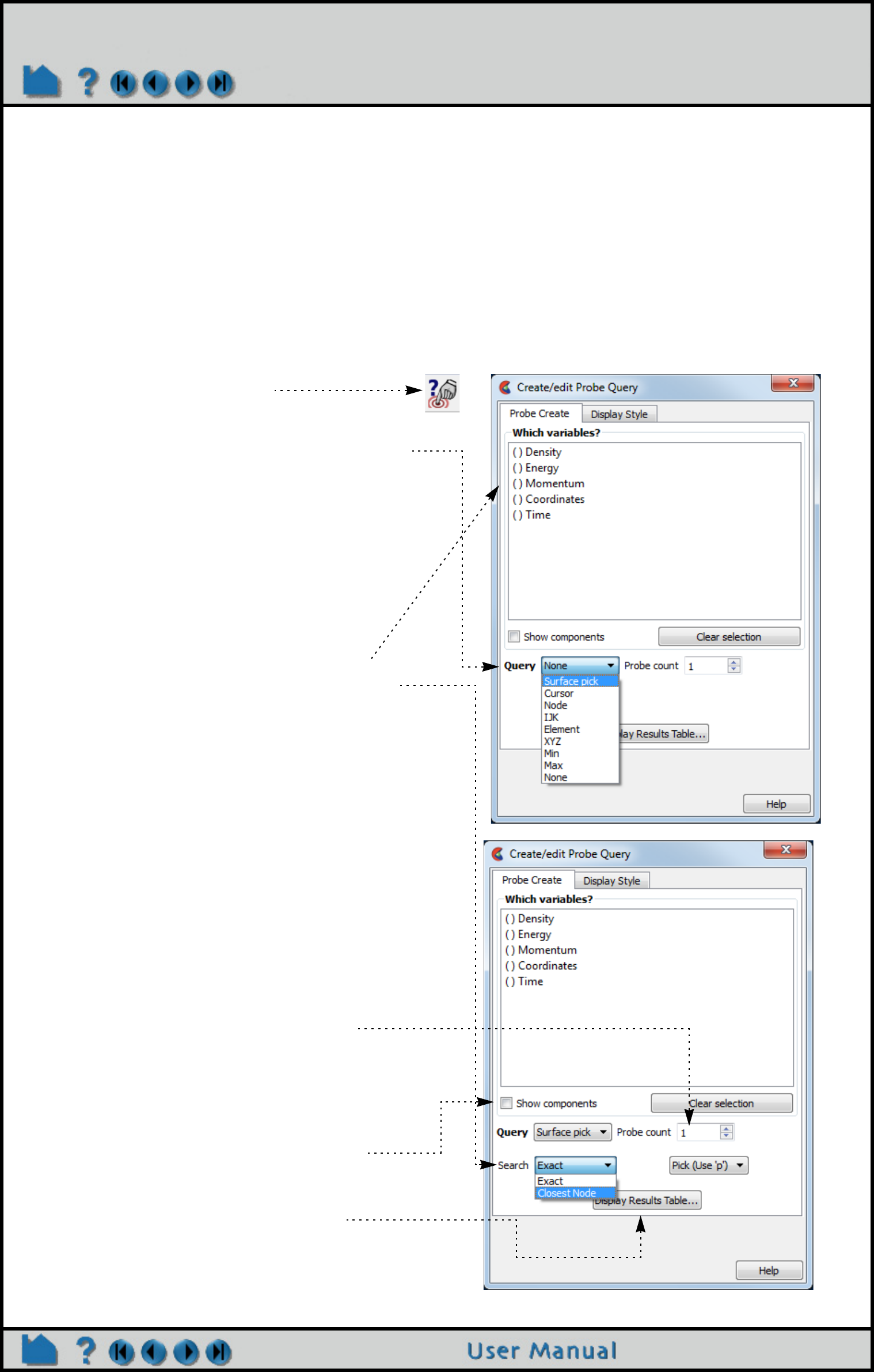
Page 383
HOW TO PROBE INTERACTIVELY
Probe Interactively
INTRODUCTION
EnSight provides an interactive query capability that displays variable data in the Graphics Window as you move the
mouse pointer over geometry, as you move the cursor tool within the model, or at specified node, element, ijk or xyz
locations. The probe can display the value directly under the mouse pointer (by interpolating the nodal values of the
applicable element) or search for and display the value at the node closest to the mouse pointer.
BASIC OPERATION
To probe interactively:
1. Click the Probe Feature Icon
(or select Query > Interactive Probe...).
2. Set the Query pulldown to desired operation.
Surface Pick: Interpolate to any picked position on the
surface of the model.
Cursor: Interpolate to location of cursor tool within the
model.
Node: At a specific node number.
IJK: At a specific IJK location.
Element: At a specific element number.
XYZ: At a specific XYZ location.
3. Select the desired variable(s) to display.
4. If Query is set to Surface Pick, you can select:
a) whether the probe will snap to closest node
(which will show node id).
or
b) use exact location (which will show nearest
element ID).
And whether the information will be sampled:
c) when you click the “p” keyboard key or
d) continuously as you move the mouse.
If Query is set to Node, Element, IJK, or XYZ,
enter ID or values needed followed by Enter.
If Query is set to Cursor, move the cursor tool to
desired location and press the “p” keyboard key
(while the mouse is in the graphics window).
5. Enter a value controlling the number of
simultaneous probe markers displayed. Once
this number has been reached, the oldest
marker is replaced by each new marker.
6. If the selected variable is a vector variable,
you can specify which component (or the
magnitude) of the variable is displayed.
7. In addition to having the results displayed on
the model in the graphics window, you can
open a table that displays the results
8. When done, change the Query to None to
disable interactive probing.
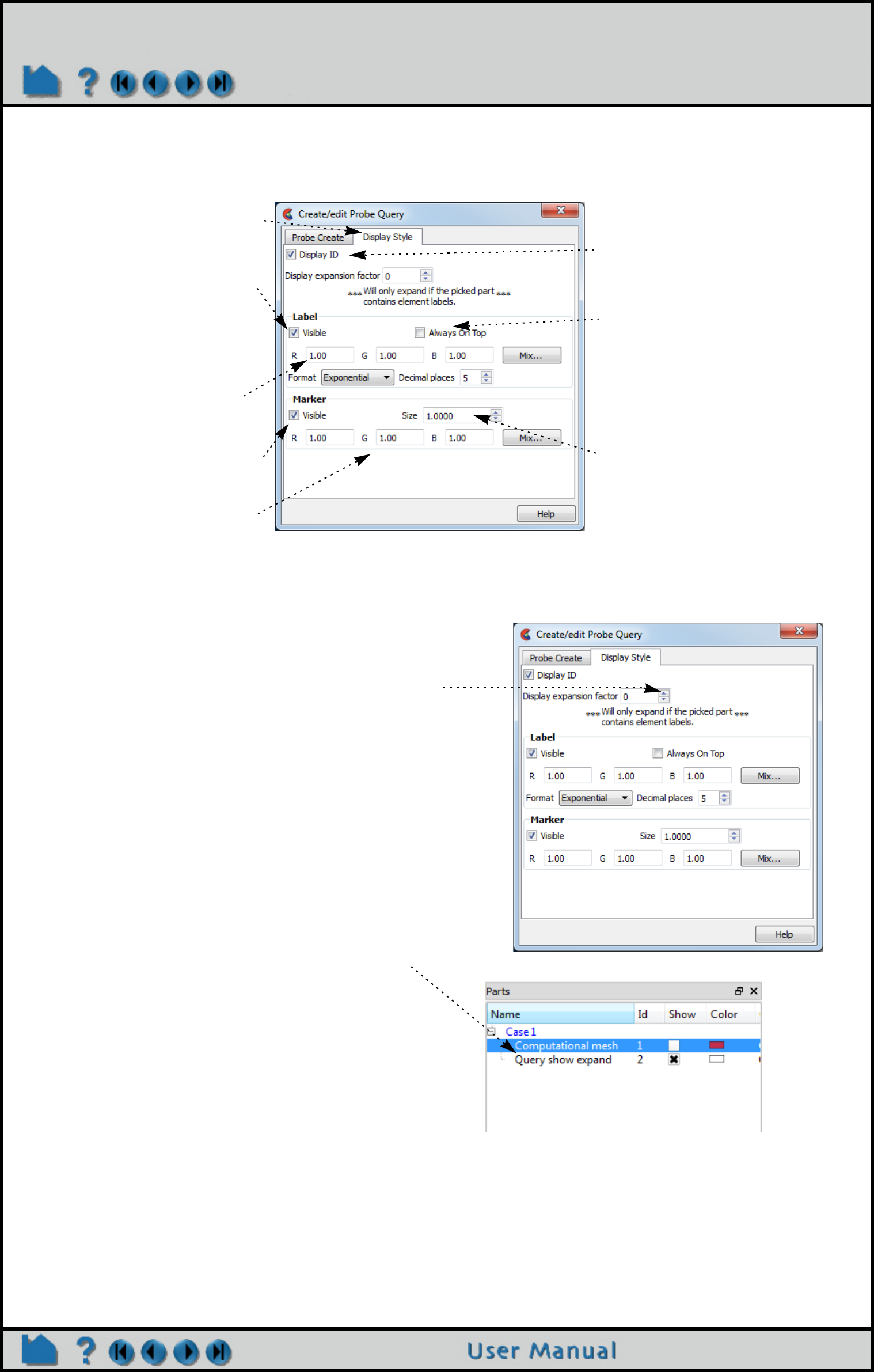
Page 384
HOW TO PROBE INTERACTIVELY
Probe Display
Probes are displayed as a marker (sphere) and the query text label. The appearance of the marker and label can be
changed:
See the Elements surrounding the query
Toggle visibility for the query
text label. Label size is set in
the annotation preferences
(see Setting Annotation
Defaults).
Set the color of the label.
Toggle visibility for the probe
marker.
Set the color of the marker.
Set the radius of all probe
markers.
Toggle whether query text
labels are “always on top”
(never hidden by geometry) or
occluded by geometry that is
closer.
1. Click the Display Style tab Toggle visibility for the id label.
(Node id, element id, etc.)
It is possible to extract the elements that contain the query
locations, if element ids exist:
1. After creating a query open the Display Style tab.
2. Click the up arrow for the Display expansion factor.
An expansion factor of 1 indicates that the elements that
contains the query will be extracted and shown.
3. Click the up arrow again.
An expansion factor of 2 indicates that the elements
from the step 2 will be shown along with the elements
that neighbor these elements.
Since the expansion factor feature uses a subset part, if
you wish to display the subset part differently (such as
turn on node labels) this can easily be done through the
subset part attribute editing. The name of the subset
part in the part list will be "Query show expand".
4. If you wish to keep the subset part that was the
result of the display expansion factor setting, you
may do so when you turn off the interactive query.
A pop-up dialog will ask you if you wish to keep or
delete the expansion factor subset part.

Page 385
HOW TO PROBE INTERACTIVELY
OTHER NOTES
Note that interactive query actions do not generate corresponding command language!
While doing queries and using the ‘p’ key to pick a query location, other picking options that use the ‘p’ key are
disabled (such as Part, Cursor, Line, Plane, and LookAt Point).
Even though it is not shown in the dialogs above, the “Time” variable is also available. This time variable is the
integration time for particle traces. Thus, it is only defined and useful when probing particle traces. For other part
types it will be undefined.
SEE ALSO
How To Query/Plot
User Manual: Interactive Probe Query
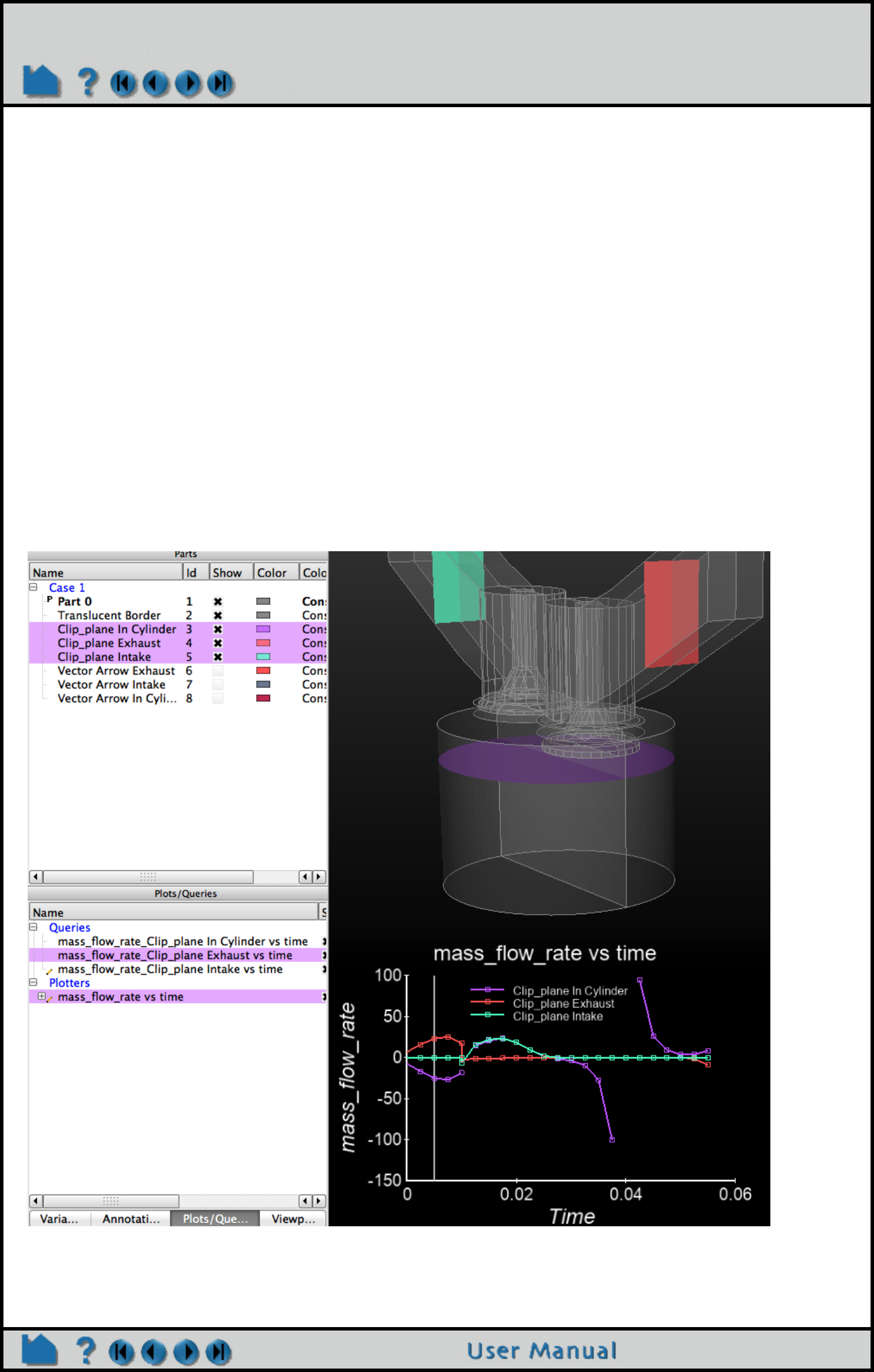
Page 386
HOW TO QUERY/PLOT
Query/Plot
INTRODUCTION
EnSight can perform a number of different kinds of queries over time or space. The result is a Query Entity that can
be plotted using EnSight’s built-in Plotting facility or that can be printed as a table or written to a disk file.
BASIC OPERATION
Shortcut for plotting transient data over time
Select variable(s) in the variable list and then right click on vector or scalar variable(s) in the variable list and choose
Plot Maximum (or Minimum) vs Time. EnSight will step through all timesteps, calculating the maximum (or minimum)
of scalar variable(s) or vector magnitude variable(s) and create a query for each selected variable and put each new
query curve into a new plot.
Select per part constant(s) in the variable list and then right click on one of the selected constant variable(s), choose
Plot Maximum, Plot Minimum to get a single plot which is the maximum of all parts or selected parts (depending on
the sub-menu). Choose Plot vs Time to get the value of each of the selected per part constants in a separate plot with
each curve colored the same color as its corresponding part (if the part is not colored by a variable and the parts are
different colors). Each query will be named by its corresponding part and var with the legend the part name.
Select one or more Case Constant variable(s) and all three Plot options will produce the same result for each Case
Constant variable.
Long Methodology
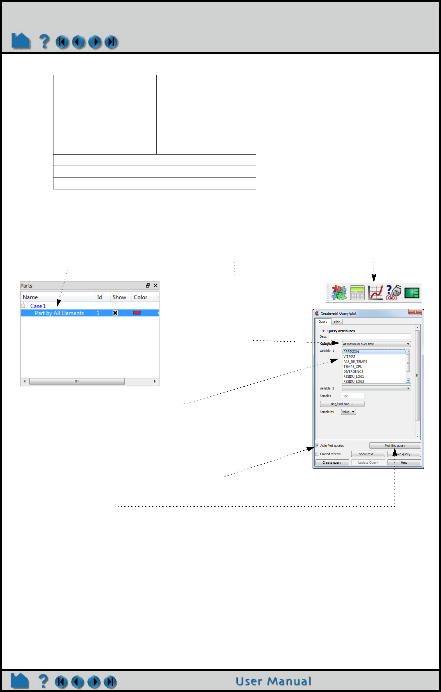
Page 387
HOW TO QUERY/PLOT
One first must create query items, which can be any of the following types:
As one of these is selected, the Feature Panel changes to reflect the information needed (such as variable to use) for
the selected type. One can control whether the query entity will be a curve or a scatter plot by the choice for Variable
1 and 2.
Query entities can be printed to the Status History Area, saved to a file, deleted, or plotted.
Sample Query Creation and Plot (At Maximum Over time)
Managing Query Entities
The Feature Panel combined with the Plots/Query lists provides various controls for managing existing Query
At Line Tool Over Distance.
At 1D Part Over Distance.
On a Spline Over Distance
At Node Over Time
At Element Over Time
At IJK Over Time
At XYZ Over Time
Over Time Queries
By Scalar Value (integer
match)
By Constant on Part Sweep
By Operating on Existing Queries
Read From An External File
Read from server file
1. Select the part to query.
3. Select the Sample type for the
query.
2. Click the Query/Plot icon (or select
Query > Over Time/Distance...).
4. Select the variable(s) for Variable: 1.
Note: for max or min over time you can select multiple variables to query
simultaneously over time for efficiency.
Leave Variable: 2 as None and it will default to Time, because of sample
type.
5. Click “Create query”
6. The query is created and plotted because the “Auto Plot curves”
toggle is on. Had it been off the query would have been created and
you could then plot it.
For more information on plotting, see the Plotting section towards the
end of this How To.
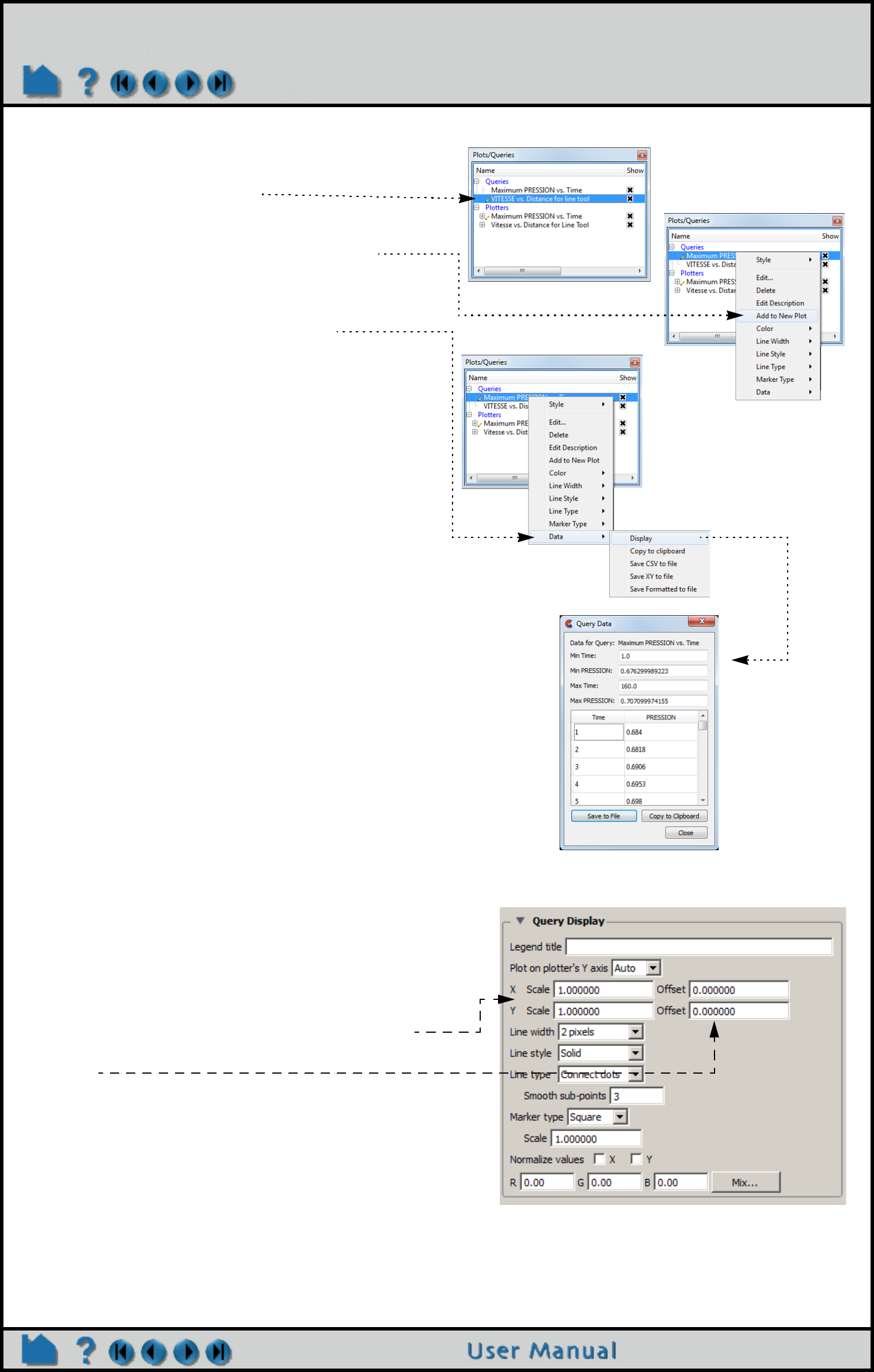
Page 388
HOW TO QUERY/PLOT
Entities:
List of Query Entities. The tagged (pencil marker)
items are edited in the Feature Panel.
Any query can be plotted by a right click on the query
via the “Add to new plot” on the pulldown.
There are several ways to view and use the query data
by right clicking on the query in the Query list and
choosing “Data” from the pulldown.
“Display” will show a table of values.
“Copy to clipboard” will allow the query to be pasted
into other applications as columns of data - perfect for
Excel for example.
“Save CSV to file” will save a file with comma
separated values.
“Save XY to file” saves a file that can be read back
into EnSight as an “Read from an external file”.
“Save Formatted to file” gives you a file that is
formatted like a report.
Delete a query by right clicking and choosing “Delete”
from the pulldown.
How to Scale the X and Y axis (for example to use
different units).
Right click on the query in the query list and choose
Edit.
Open the Query Display pulldown and change the X
scale and Y scale to change the query multiplier,
and the X and Y Offset to change the query additive
values.
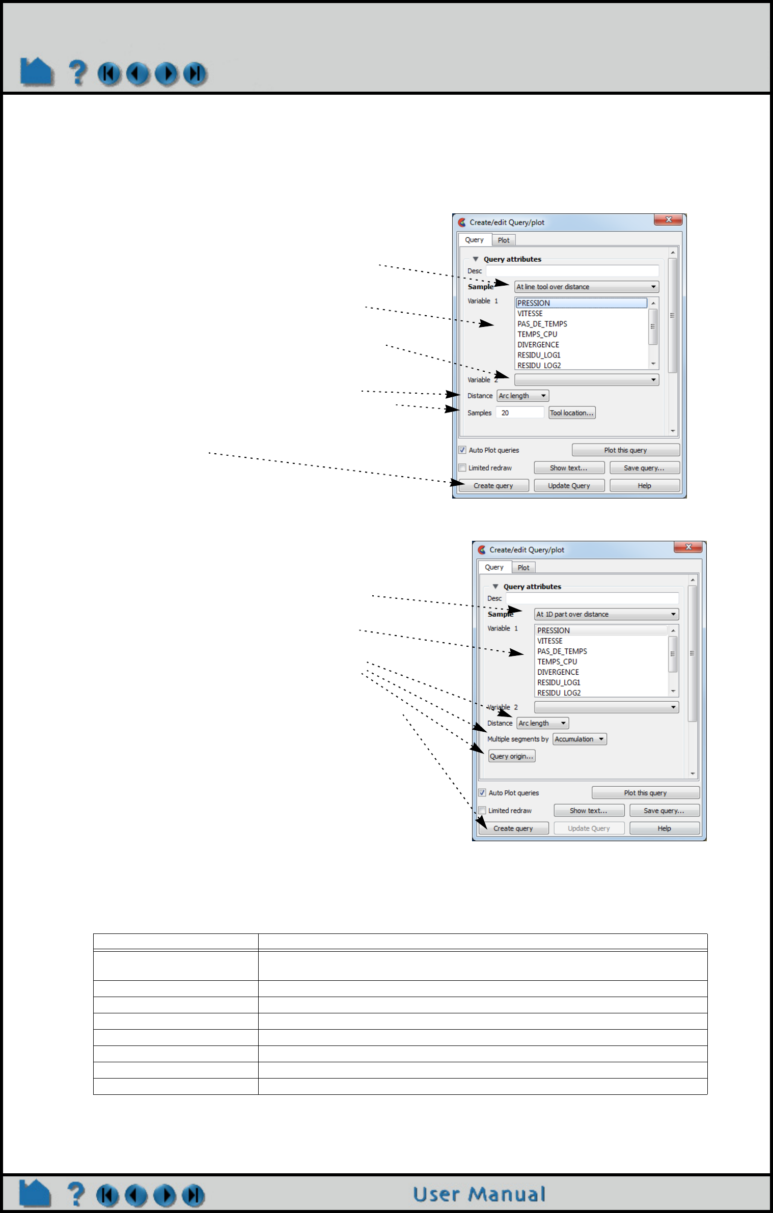
Page 389
HOW TO QUERY/PLOT
Over Distance Queries
EnSight can perform queries at uniform points along the line tool, at nodes along a 1D part, or at uniform points along
a spline. One-dimensional parts include model parts consisting of bar elements, 1D (Line) Clips, and particle traces.
At Line Tool Over Distance.
At 1D Part Over Distance.
For the two over distance query types, the variable is plotted against the selected “Distance” metric. The node with
the lowest node ID number (or nearest the selected origin) is queried first. The query then proceeds automatically
from the first to the last according to the 1D part connectivity (this order cannot be changed). Since the nodes for 1D
part over distance are not necessarily evenly spaced, the reported distance is one of the following:
If the 1D part contains more than one set of contiguous 1D elements (such as a particle trace from a Line emitter), the
resulting query will contain one plot entity for each set.
Distance In Setting Reported Distance
Arc Length The distance along the part from the first node to each subsequent node (i.e. the
sum of the 1D element lengths)
X Arc Length The X coordinate value of each node accumulated from the start
Y Arc Length The Y coordinate value of each node accumulated from the start
Z Arc Length The Z coordinate value of each node accumulated from the start
From Origin The distance from the origin
X From Origin The X distance from the origin
Y From Origin The Y distance from the origin
Z From Origin The Z distance from the origin
After selecting the part to query in the Parts list and clicking
the Query/Plot icon
1. Select Sample as “At Line Tool Over Distance”
2. Select the variable to query over the distance in
“Variable: 1”.
Leave “Variable: 2” as None unless you want a scatter
query of two different variables along the line tool.
3. Optionally, select the Distance option desired,
number of points along the line, and modify the tool
location if needed.
4. Click “Create query”
After selecting the part containing 1D elements in the Parts list
and clicking the Query/Plot icon
1. Select Sample as “At 1D Part Over Distance”
2. Select one variable to query in “Variable: 1”.
3. Optionally modify Distance, origin and multiple
segment.
4. Click “Create query”.
The query will be created starting at the origin (or the lowest
node ID number, or the first node in the connectivity list) and
will automatically proceed by following the connectivity order.
The order of the query cannot be changed, but it can be
reversed in the plotter, if desired.
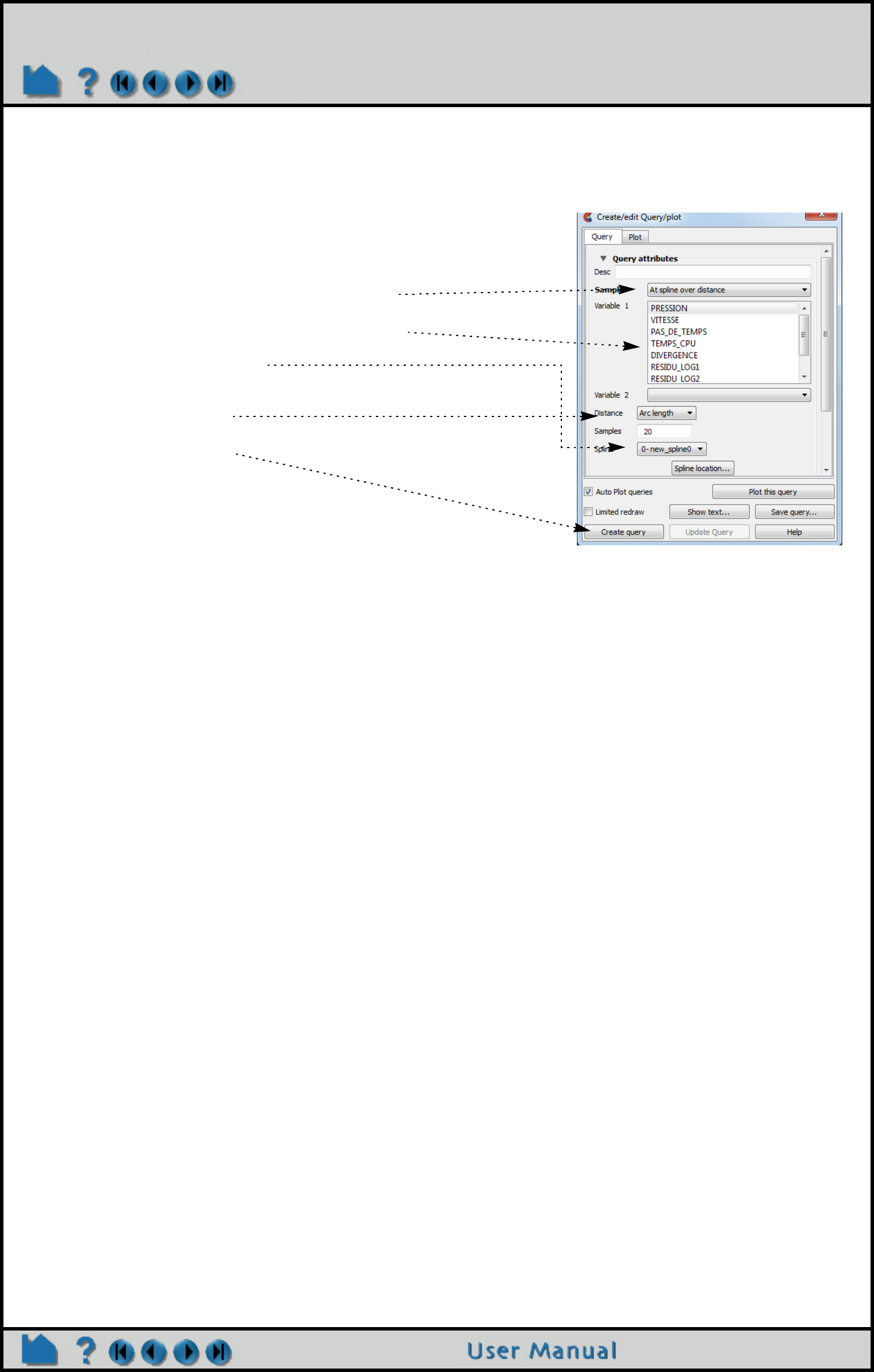
Page 390
HOW TO QUERY/PLOT
On a Spline Over Distance
After selecting the part to query in the Parts list and clicking the Query/
Plot icon
1. Select Sample as "At spline over distance"
2. Select the variable to query along the spline
3. Select the spline to query
4. Optionally, select the Distance option desired and the number of
points along the spline.
5. Click “Create query”
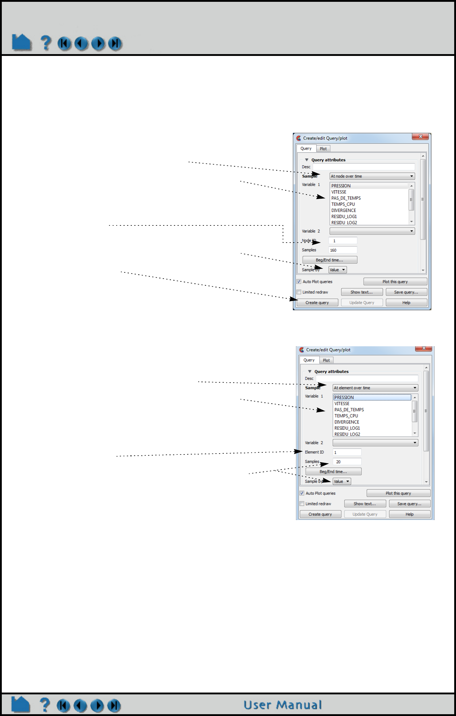
Page 391
HOW TO QUERY/PLOT
Over Time Queries
For transient dataset, EnSight can query the variable values over a range of time at a particular node, element (or
specific IJK coordinate for structured data) or an arbitrary point. You can also search the minimum or maximum of a
variable over all nodes over a time range.
At Node Over Time
At Element Over Time
After selecting the part to query in the Parts list and clicking the Query/
Plot icon
1. Select Sample as “At Node Over Time”
2. Select one variable to query over time in “Variable: 1”.
Leave “Variable: 2” as None unless you want a scatter query of two
different variables over time.
3. Enter the Node ID.
4. Optionally, change the number of Samples (defaults to number
of time steps), and whether to sample by Value of FFT.
5. Click “Create query”
After selecting the part in the Parts list to query and clicking the
Query/Plot icon
1. Select Sample as “At Element Over Time”
2. Select one per-element variable to query over time in
“Variable: 1”.
Leave “Variable: 2” as None unless you want a scatter query of two
different variables over time.
3. Enter the Element ID.
4. Optionally, change the number of Samples (defaults to
number of time steps), and whether to sample by Value of FFT.
5. Click “Create query”
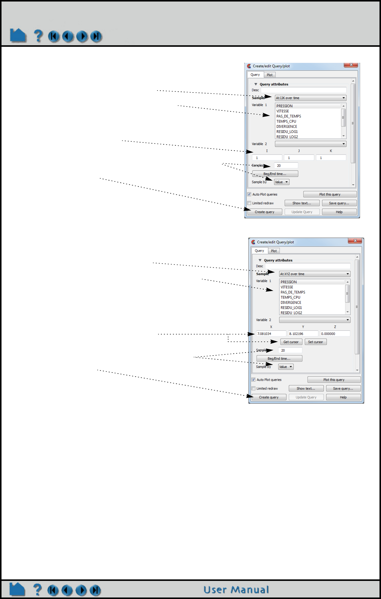
Page 392
HOW TO QUERY/PLOT
At IJK Over Time
At XYZ Over Time
After selecting the part in the Parts list to query and clicking the
Query/Plot icon
1. Select Sample as “At IJK Over Time”
2. Select one variable to query in “Variable: 1”.
Leave “Variable: 2” as None unless you want a scatter query of two
different variables over time.
3. Enter IJK for the point.
4. Optionally, change the number of Samples (defaults to
number of time steps), and whether to sample by Value of FFT.
5. Click “Create query”
After selecting the part in the Parts list to query and clicking the Query/Plot
icon
1. Select Sample as “At XYZ Over Time”
2. Select one variable to query over time in “Variable: 1”.
Leave “Variable: 2” as None unless you want a scatter query of two
different variables over time.
3. Either type in the desired xyz location or place the cursor where
desired in the model, either through picking, or other transformation
methods and click the cursor Get button.
4. Optionally, change the number of Samples (defaults to number of
time steps), and whether to sample by Value of FFT.
5. Click “Create query”
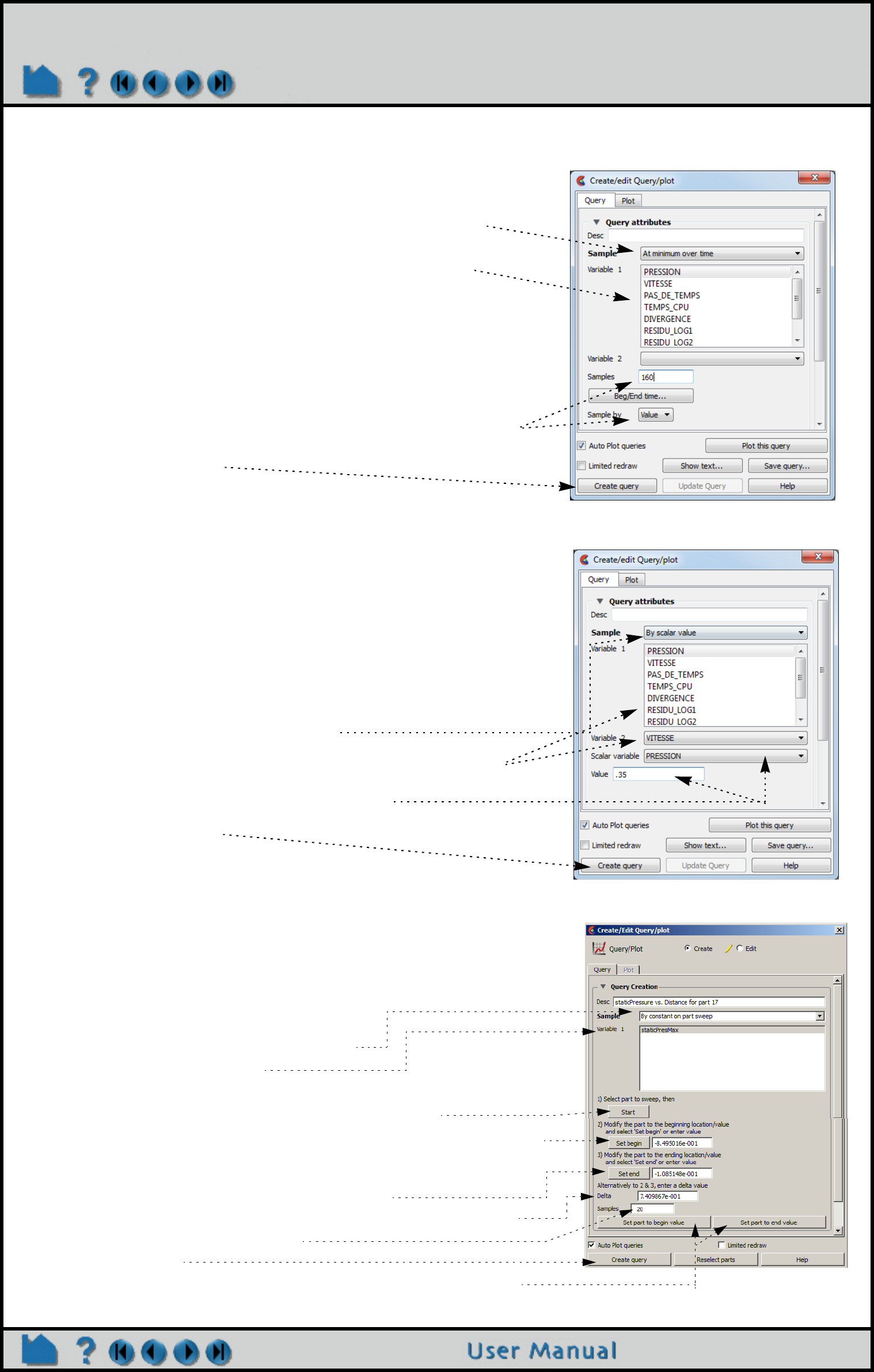
Page 393
HOW TO QUERY/PLOT
At Minimum/Maximum Over Time
By Scalar Value (integer match)
By Constant on Part Sweep
After selecting the part to query in the Parts list and clicking the Query/Plot
icon
1. Select Sample as “At Minimum Over Time” or “At Maximum Over
Time”
2. Select variable(s) to query over time in “Variable: 1”.
Note: for max or min over time you can select multiple variables to query
simultaneously over time for efficiency.
Leave “Variable: 2” as None unless you want a scatter query of two different
variables over time.
3. Optionally, change the number of Samples (defaults to number of
time steps), and whether to sample by Value of FFT.
4. Click “Create query”
This query you select two variables - the first will be plotted on the y axis
and the second is plotted on the x axis. Further, you specify another
variable (can be the same as one of the two previous variables) and a
value. The x and y variables will be extracted for all nodes/elements that
integer match the value indicated (such that the int(value) exactly equals
the int(value you enter)). It is best to view the results as a scatter plot.
After selecting the part in the Parts list to query and clicking the Query/Plot
icon
1. Select Sample as “By Scalar Value”
2. Select the two variables you wish to form the query from.
3. Select the desired scalar variable and value
4. Click “Create query”
You can perform a query of a constant variable along a moving part at
sampled locations.
After selecting the part in the Parts list to query and clicking the Query/Plot
icon
1. Select Sample as “By constant on part sweep”
2. Select a listed constant variable.
3. Select a part to sweep. (in the main part list)
4. Select “Start” (At this point the dialog will become as shown)
5. Click-and-drag the part to the beginning location, and select “Set begin”, or
just enter the beginning part location value.
6. Now interactively click-and-drag the part to the ending location, and select
“Set end”, or just enter the ending part location value.
7. Alternatively, you can just enter the Delta in place of the last two steps.
8. Enter the number of sample locations.
9. Select Create query
Note that you can update the part to the beginning or ending values here.

Page 394
HOW TO QUERY/PLOT
Scatter Query Example
By Operating on Existing Queries
You can perform a scaling of an existing query, or a scaling and algebraic addition of two queries, or an integration or
differentiation of a query.
Queries From External Sources
You can import previously created and saved (or externally generated) EnSight queries or Dytran time history (.ths)
files.
Read From An External File
A scatter query is a query of one variable
against another.
Everything is done like a regular query
except you select another variable in the
Variable: 2 field, instead of leaving it as
None.
1. Select Sample as “By Operating On Existing Queries”
2. Select the operation.
(Combine/Scale, Integrate or Differentiate).
For Combine/Scale (shown):
3. Select the Query Item and the set the Scale Factor if you want
to scale a single query - or - Select both Query Items and set
both Scale Factors if you want to scale and add algebraically.
3. Click “Create query”
Note, if integrate or differentiate is chosen, you will only need to
choose the query to operate on.
1. Select Sample as “Read From An External File”.
2. Click the “Load XY Data From File ...” button to open
the File Selection dialog, and select any previously saved
EnSight XY data file or a Dytran .ths file.
Note: Depending on the version of the Dytran reader you
are using (reader version 2.05 or later is needed), the
Dytran xy data may be loaded automatically for you,
making this option unnecessary for Dytran data.
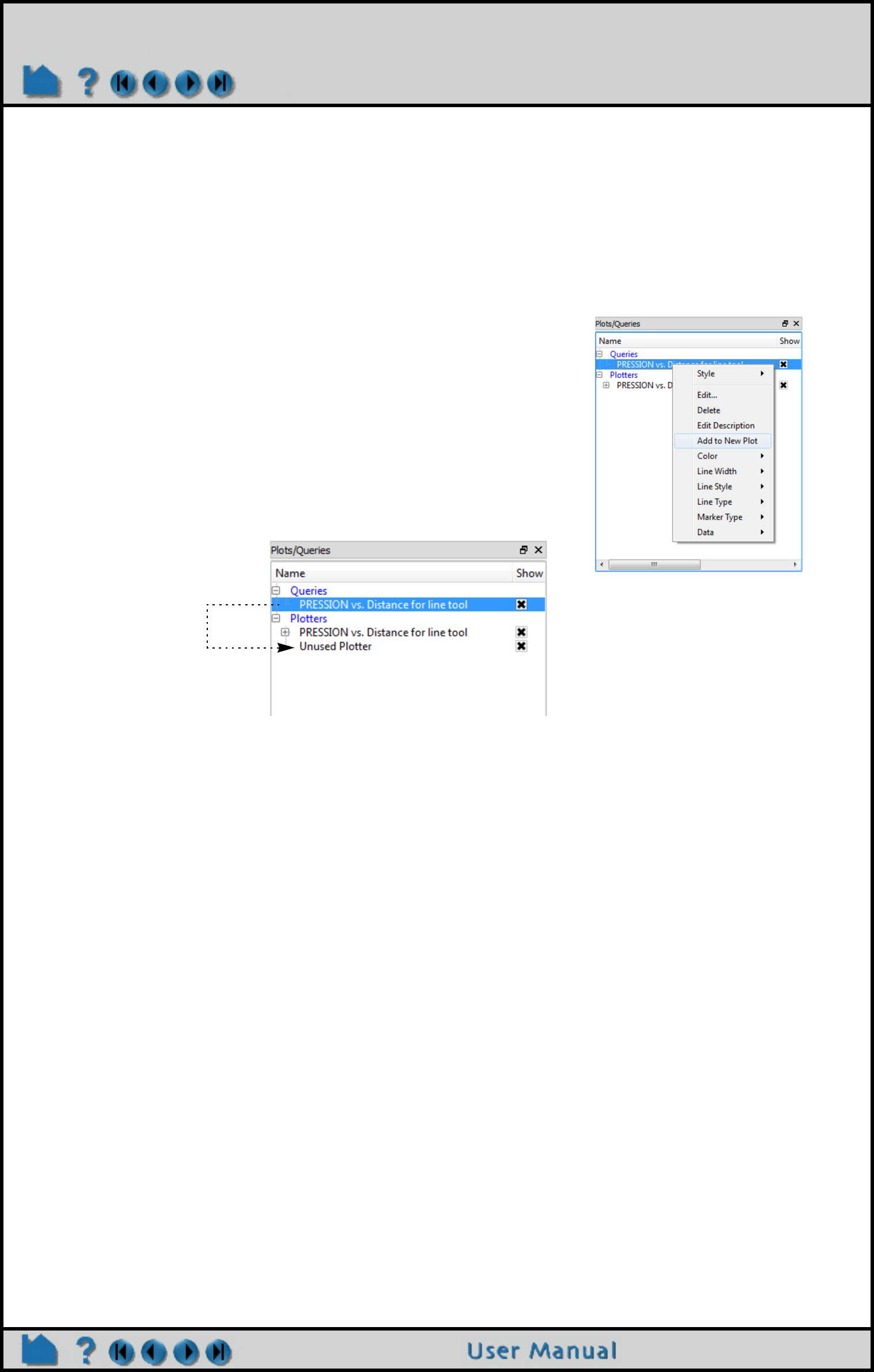
Page 395
HOW TO QUERY/PLOT
Read from server file
Traditionally, you could ask the server for any queries that it knows about. Some data formats (accessed by user-
defined readers) have such. If any are available, they would show up in the list of Queries. In version 10, such
queries get loaded automatically, so this option is not really needed and may do nothing.
Plotting
Once Queries exist, they can be easily plotted in a new plotter in EnSight, or if an existing plotter of the correct type
exists, they can be added to the existing plotter.
OTHER NOTES
See XY Plot Data Format in the User Manual for a description of the plot file format.
SEE ALSO
How To Probe Interactively
How To Change Plot
User Manual: Query/Plotter
1. Right click on the query to be plotted.
2. Select “Add to New Plot” from the pulldown to create a new plotter
showing the selected query.
If you want to plot the query on an existing plotter:
1. Click and drag the query over the plotter and release the mouse
button. Similarly, you can click and drag the query to the graphics
window and release the mouse button on top of the axis system of an
existing plotter.
Drag the query and
drop it onto the
plotter

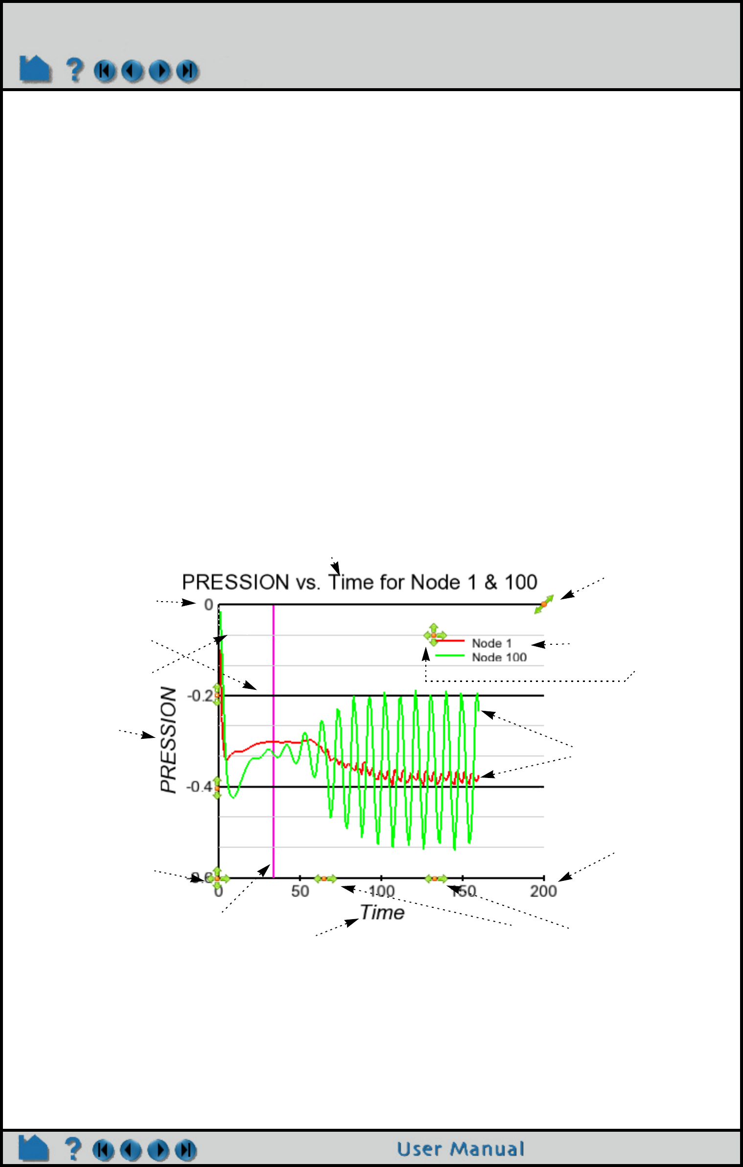
Page 397
HOW TO CHANGE PLOT
Change Plot
INTRODUCTION
EnSight provides a full-featured X-Y plotting system fully integrated with the query and transient data handling
capabilities. Query entities (see How To Query/Plot) are assigned to plotters. Plotters display one or more curves
where each curve is based on the data from a single query entity. If the query entity is changed, the corresponding
curve will automatically update. Plotter (controlling aspects of appearance such as color of curves and titles, axis
labeling, gradation and tick marks, and border/background color) can be edited through the Quick Action icon bar or
the Feature Panel.
This article is divided into the following sections:
Anatomy of a Plotter
Create Plotters
Select Plotters and Curves
Move and Resize Plotters
Plotter Quick Action icons
Set Title, Background, Legend, Border, Position, Marker
Set Axis
Set Curve
Delete Plotters
Operations on all curves on a Plotter
Anatomy of a Plotter
Plotters are composed of the following fundamental components:
Plot Title
Legend
Curves
X Axis Title
Y Axis Title
Legend Position Handle
X Axis Value Labels
Y Axis Value Labels
Plot Scale Handle.
Y Axis Gradation
Y Axis Subgradation
X Axis Title
Current time marker
Origin click-n-go handle
Adjust min and max X axis click-n-go handles
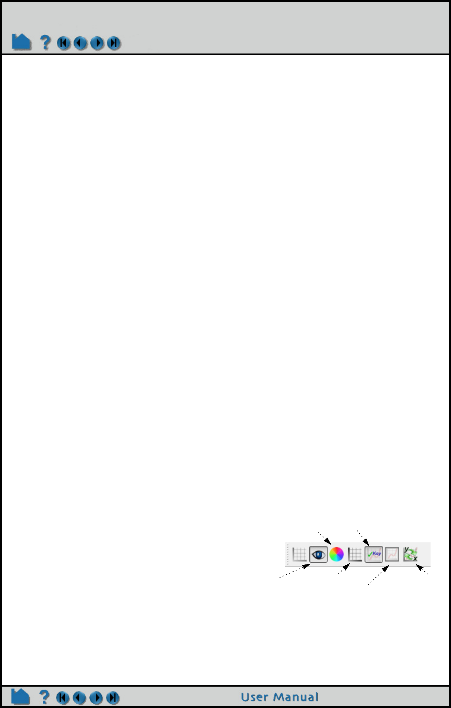
Page 398
HOW TO CHANGE PLOT
Create Plotters
Plotters are automatically created when you assign a query entity to a new plotter (see How To Query/Plot for
details). Also, by default when you create a query it is automatically plotted.
Select Plotters and Curves
Any action to change plotter always operates on the currently selected plotter(s) (or the plotter defaults if none are
selected). To select plotters:
Curves have one set of attributes even though they may be plotted on multiple plotters. To select curves:
Move and Resize Plotters
Plotters can be easily moved and resized. You can either reposition a plotter with the mouse in the Graphics Window,
or precisely by entering exact values. To move or resize a plotter interactively:
A plotter can also be positioned precisely. See below for details.
Plotter Quick Action icons
Plotters that are currently invisible are displayed dimmed if Limited redraw is enabled.
1. Left click on the plotter in the Plotters list.
OR
2. Move the mouse pointer into the Graphics Window and click the left mouse button anywhere on the
plotter axis or titles
1. Left click on the query in the Queries list.
OR
2. Move the mouse pointer into the Graphics window and click the left mouse button on the desired
curve. You can add to an existing selection by holding down the Control key as you click on additional
curves.
1. Move the mouse pointer over the plotter. The touch-n-go handles will appear.
2. Click and drag anywhere on the plotter to move it.
3. To resize the plotter move the click and drag the resize handle in the upper right corner.
Shortcut
Right-click at the plot origin and choose ‘Auto Arrange Plots’. All of the visible plots (up to 16 plots) will
be automatically arranged into a grid of plots (of dimension row x column) which is 2x2 for 2-4 plots,
3x2 for 5-6 plots, 3x3 for 7-9 plots, 4x3 for 10-12 visible plots, 4x4 for more than 12 visible plots. If
more than 16 plots, this will only automatically arrange the first 16 into a 4x4 grid of plots.
1. Click to select a plotter. The Quick Action icon bar
configures to display plotter which may be modified.
Visibility
Foreground color
Axis settings
Legend visibility
Border visibility
Swap x/y axis
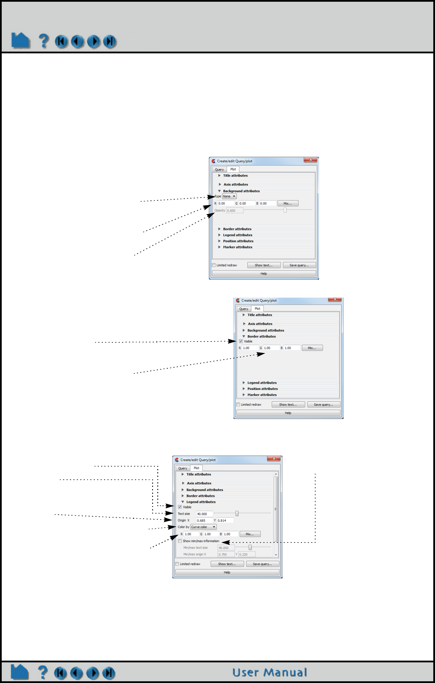
Page 399
HOW TO CHANGE PLOT
Set Title, Background, Legend, Border, Position, Marker
Overall of plotters are controlled through the Plotter Feature Panel:
The Plotter Specific dialog contains six sections: Background, Border, Legend, Position, Marker, and Title. Open the
turn-down section for the required function.
The Background section controls the type and color of the plotter background:
The Border section controls the visibility and color of the plotter border:
The Legend section controls the plotter legend text. The actual text in the legend is the name of the individual curves
in the plotter. See Set Curve below.
Double click on a plotter in the Plotter list (or right click to Edit) to bring up the Feature Panel.
Set background type to either None or Solid.
A solid background is opaque.
If the background type is Solid, set the color
(either enter new values in the RGB fields or
click the Mix... button to open the Color
Selector dialog).
You can also control the background
opacity.
Toggle border visibility
Set border color (either enter new values in
the RGB fields or click the Mix... button to
open the Color Selector dialog)
Toggle legend visibility
Set text size
Set origin (with respect to lower left corner
of plotter)
The legend text can be constant colored or
the color of the curves. If set to constant
color set text color (either enter new values
in the RGB fields or click the Mix... button to
open the Color Selector dialog)
You can display the curve min/max and
average information
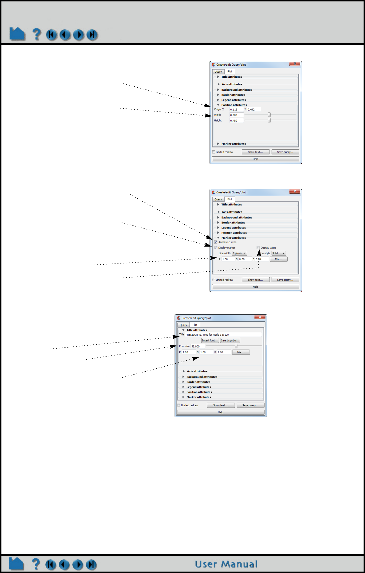
Page 400
HOW TO CHANGE PLOT
The Position section controls the size and position of the plotter:
The Marker section controls whether the curves will animate and whether the plot will be swept out during the
animation or whether a time marker will sweep along the curve in the plotter:
The Title section controls the main title at the top of the plotter:
Set the origin of the plotter (with respect to
the lower left corner of the Graphics
Window).
Set the plotter width/height (0-1 normalized
to the width and height of the Graphics
WIndow)
Select Animate curves if you want the curve
to be swept out or a time marker to be swept
along the curve during animation.
Toggle Display marker if you want a vertical
line to show time/distance value
corresponding to the query marker in the
graphics window. For time queries the
marker will sweep as time updates.
You can control the line width, style, and
color of a time marker.
Display value will show the value of the x
and y axis of where the marker intersects
the curves on the plotter.
Set title text
Set the size of the title text
Set the text color (either enter new values in
the RGB fields or click the Mix... button to
open the Color Selector dialog)
If you desire special symbols, click Insert
Symbol, pick the symbol(s) and pick the
symbol out of the pop-up window.
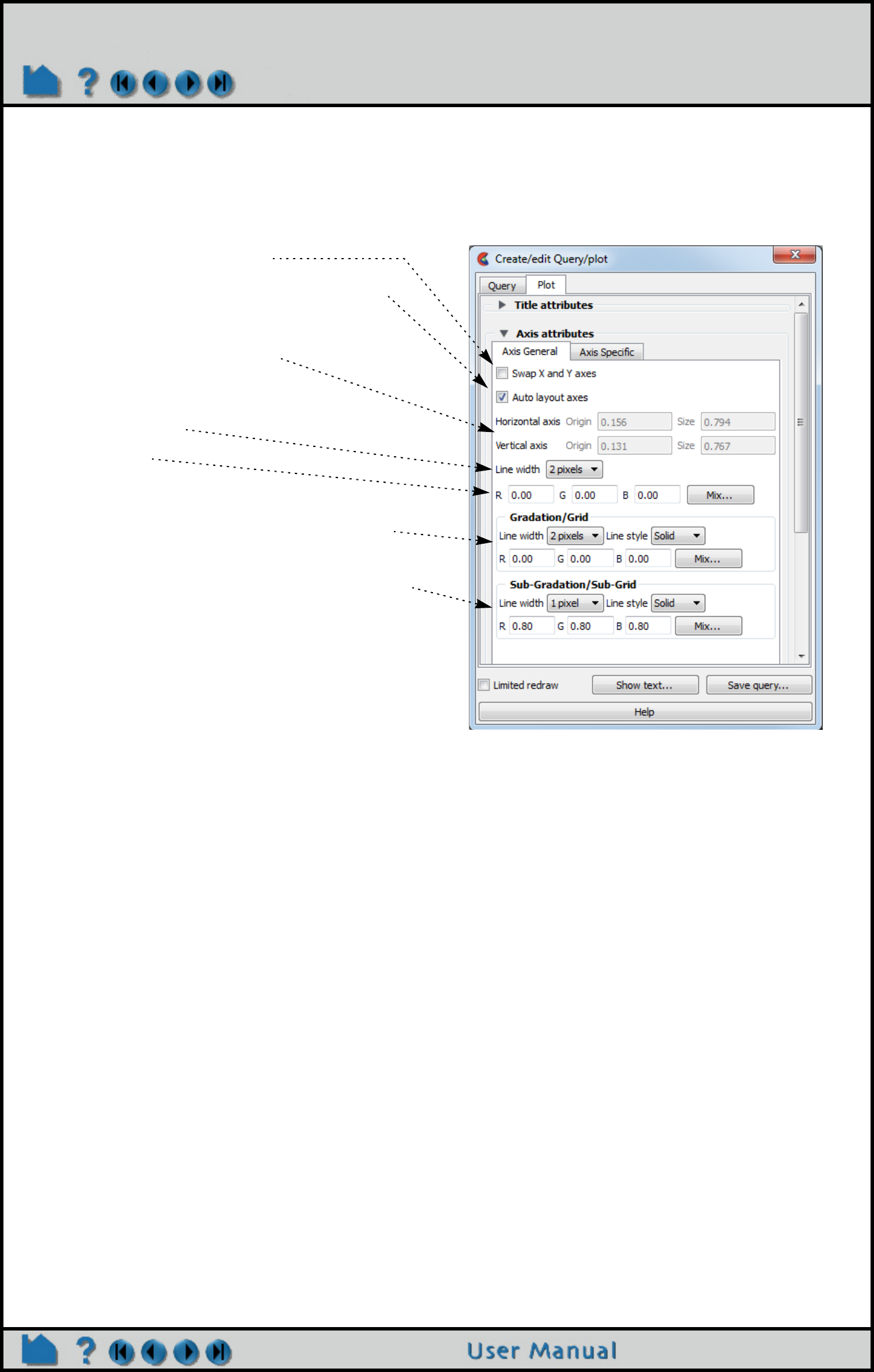
Page 401
HOW TO CHANGE PLOT
Set Axis
Axis of a plotters are controlled through the Axis section of the Plotter Feature Panel.
The Axis turndown contains two sections: General and Specific. Select the tab to display the corresponding section.
The General section controls axis width, color, and scaling as well as Gradation and Subgradation marks.
Swap the X and Y axis on the plotter
Auto layout will insure that the various components of the
plotter (title, axis description, values, etc.) don’t overlap.
Specify the axis origin (vertical and horizontal) within the plotter
area. These will be grayed out if “Auto layout axes” is enabled.
Set line width of axes
Set color of axes
Set line width, style, and color for major gradations (gradations
are enabled on a per-axis basis in the X-Axis and Y-Axis
sections)
Set line width, style, and color for subgradations
(subgradations are enabled on a per-axis basis in the X-Axis
and Y-Axis sections)
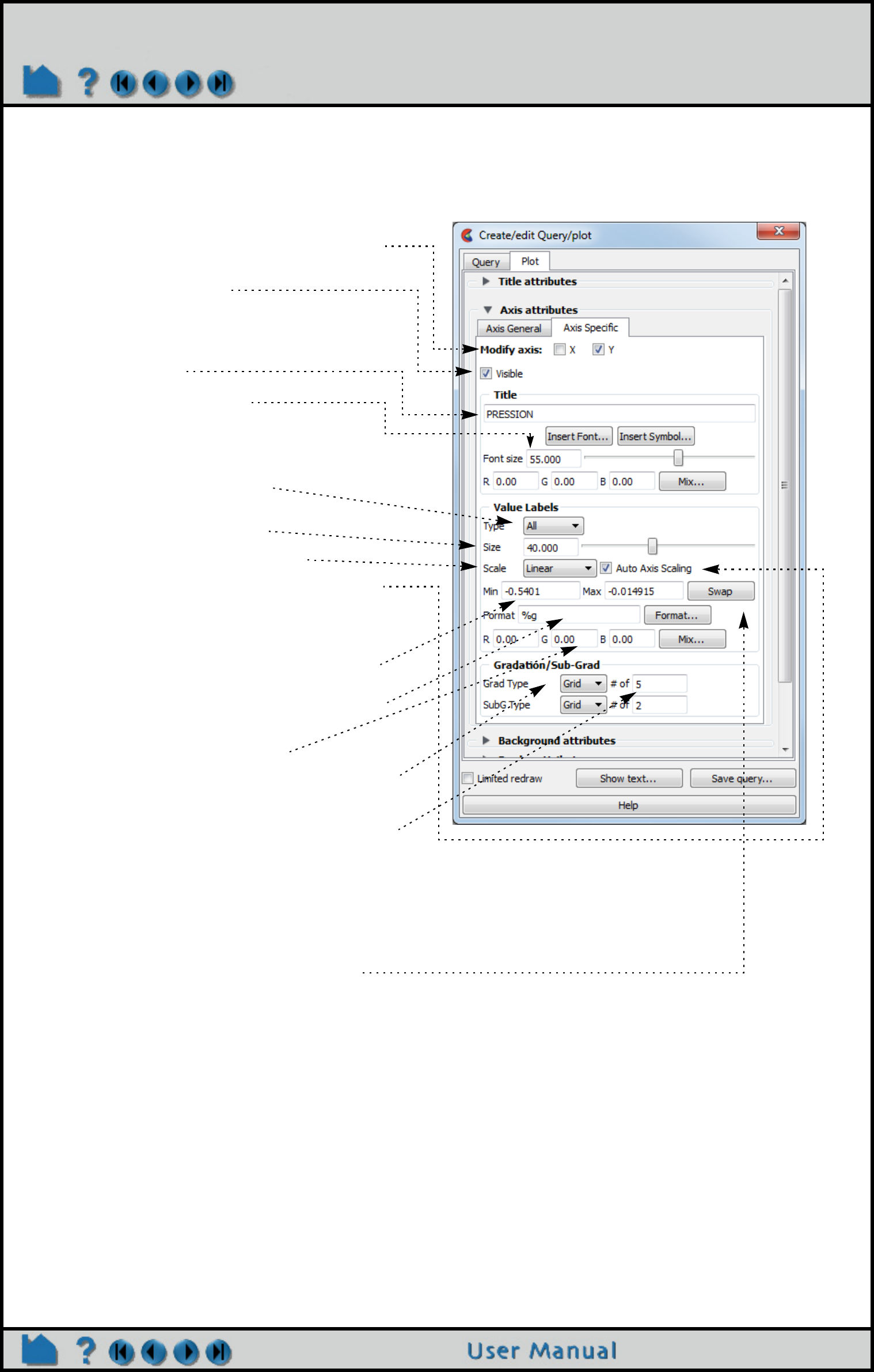
Page 402
HOW TO CHANGE PLOT
The Specific section controls the title, value labels, and gradation marks for the X or Y axis.
Choose which axis to deal with - you can select x or y or
both.
Toggle visibility of the axis line
Set the title of the axis
Set the size of the title of the axis
Set the color of the title of the axis
Set the type of axis label: None (show no value labels), All
(show value labels at each gradation), or Beg/End (show
only the first and last value labels)
Set the size of the axis value labels
Set the scale to linear or logarithmic(log10)
Set auto scaling - when on, the Min/Max values and the
number of gradations will be used as suggested values to
arrive at pleasing numbers for the axis labels.
Set the min/max range of the variable displayed on the axis
(Note: will be used as exact values only if the Auto Axis
Scaling toggle is off.)
Set the display format of the value labels (or click Format...
to select common formats from a list)
Set the color of the axis value labels
Set the type of gradation: None (no gradation marker), Grid
(a vertical line), or Tick (a mark on the axis at the value label
positions)
Set the approximate number of gradations (also depends on
the min/max range)
Set the type of subgradation: None (no subgradation
marker), Grid (a vertical line), or Tick (marks on the axis
between the value label positions)
Set the number of subgradations between each value label
By swapping the min and max can swap the positive
direction.
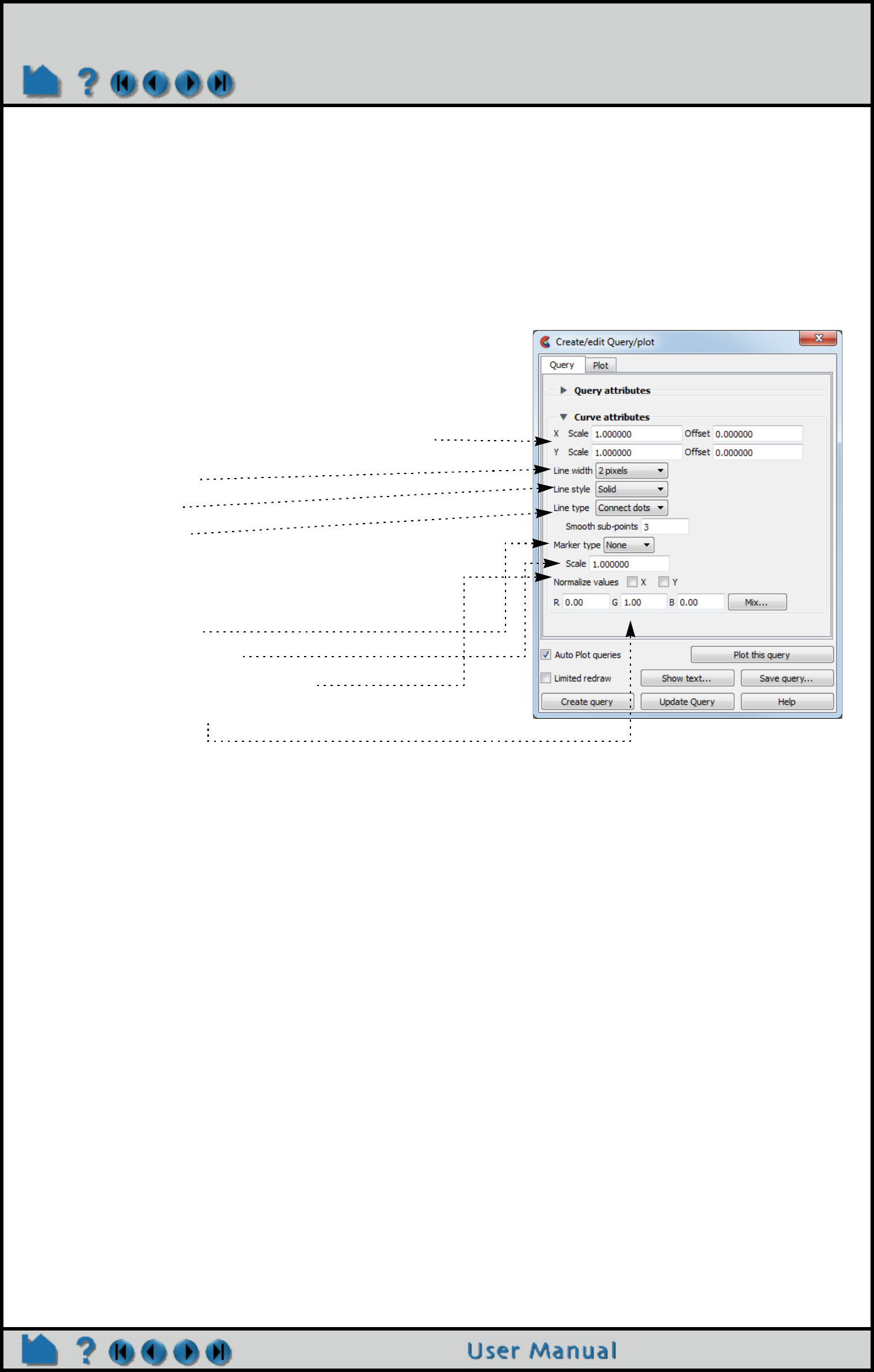
Page 403
HOW TO CHANGE PLOT
Set Curve
Curve and marker are controlled through the Query tab of the Query/plot Feature Panel:
Delete Plotters
Existing plotters can be deleted:
1. Select the desired curve(s) by clicking on them in the
Graphics Window or selecting them in the Query list
(control-click to select multiple curves).
2. Right click in the Query list to Edit
OR
1. Double click on a query in the Query list
To bring up the Query tab of the Feature Panel
If desired, you can apply an offset and scale factors to your x
and/or y data. The offset value is added to the query value
then the sum is scaled by the Scale factor.
Set the line width
Set the line style
Set the line type:
None (only curve markers are drawn),
Connect Dots (data points are connected by straight lines),
Smooth (a piece wise spline is fit to the data points using the
number of points specified in the Smooth Sub-points field)
Set the marker type
Set the size of the markers
Normalize x and/or y values, if desired.
Set the color of the curve
1. Select the plotters
2. Right click on the Plotters list to Delete. Note that deleting a plotter
has no effect on any query
entities that were attached
to the plotter
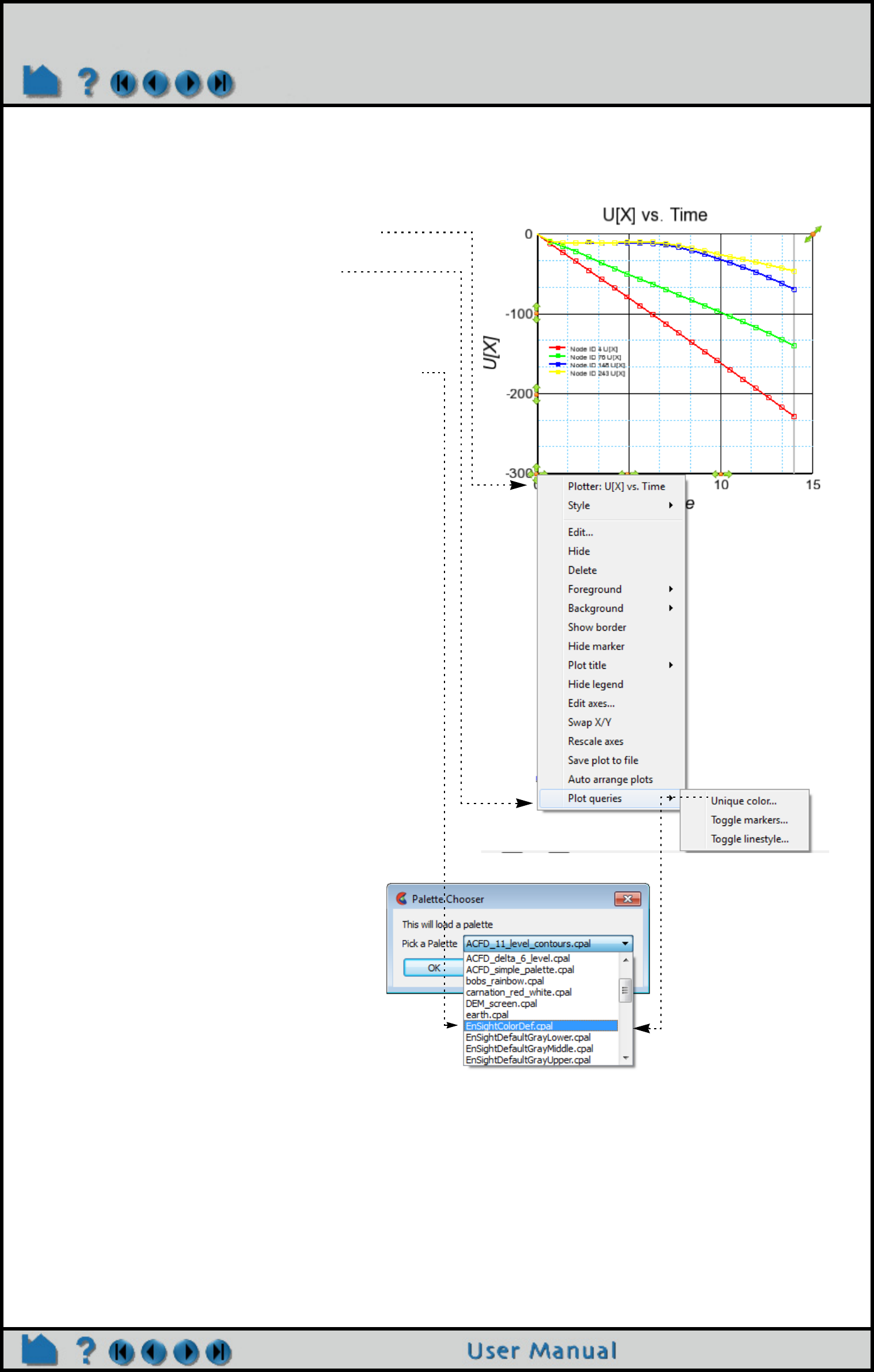
Page 404
HOW TO CHANGE PLOT
Operations on all curves on a Plotter
If a plotter has many curves, it is nice to be able to change all the curves.
SEE ALSO
How To Query/Plot
1. Right click on the plotter origin. You should see the
name of the plotter at the top of the pulldown if you
have right-clicked directly on the origin.
2. Choose Plot queries
a) Unique Color - This will pop up a dialog with a
pulldown list of available palettes available in
EnSight and then assign the color of the curves
using the palettes. These are the same palettes
files available in EnSight to color variables,
allowing some level of creativity. For more
information on palette files, see Palette Editor Files
Tab
b) Toggle markers will toggle all markers off if any are
on. It will toggle all markers on if any are off, and
will round-robin assign the markers a shape.
c) Toggle linestyle will toggle all lines to solid if any
are not solid. If all are solid it will round-robin
assign the markers a line style.
Plot queries > Unique color
dialog
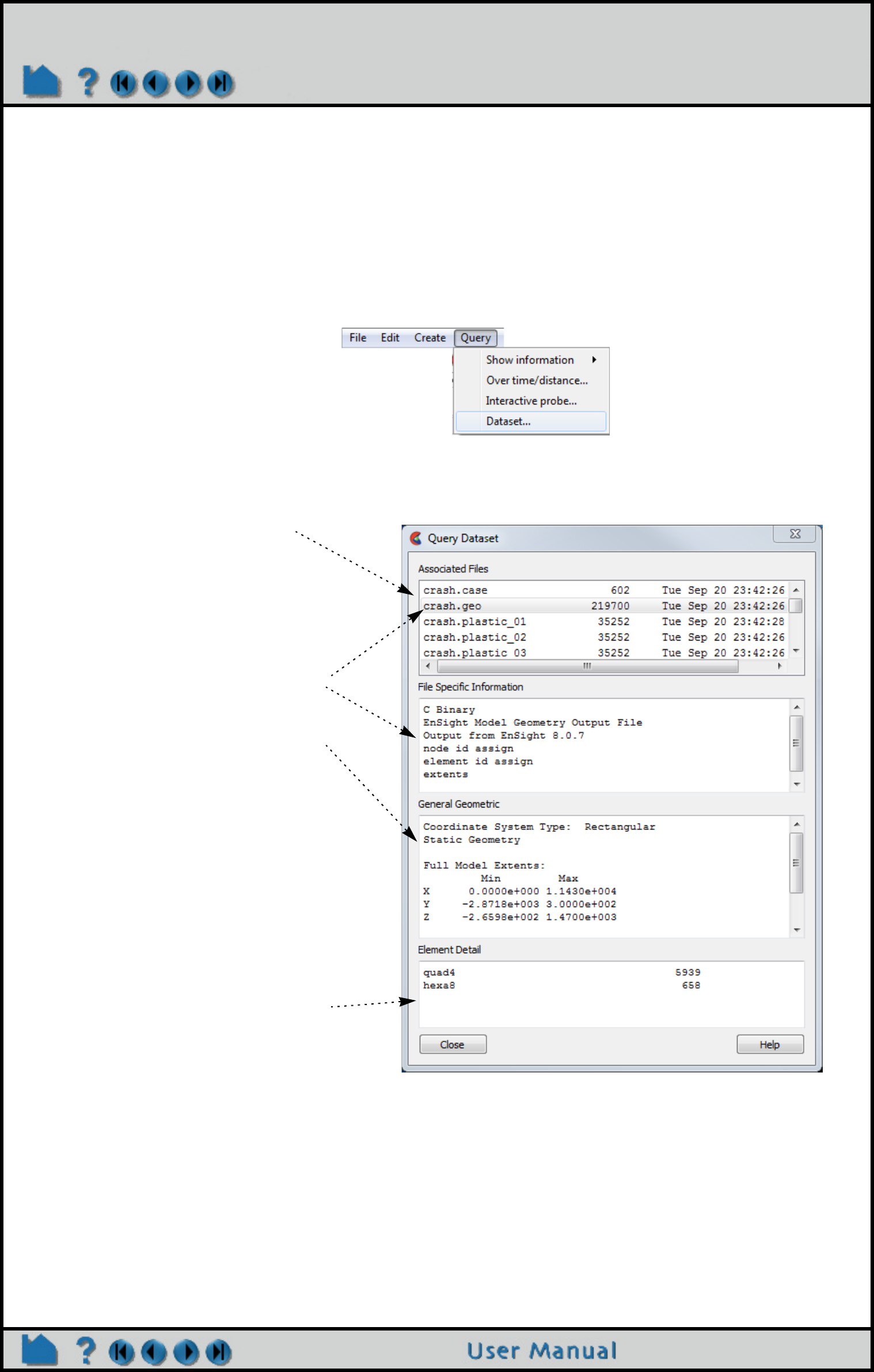
Page 405
HOW TO QUERY DATASETS
Query Datasets
INTRODUCTION
Results datasets often consist of multiple files. EnSight provides a mechanism to quickly ascertain basic information
about dataset files.
BASIC OPERATION
To display dataset information:
SEE ALSO
User Manual: Query Dataset
1. Select Query > Dataset...
The Associated Files section displays all
dataset files giving the size in bytes and
last modification date.
The File Specific Information section
displays information about the file
currently selected in the Associated Files
list. The information presented varies
based on the file type and format.
The General Geometric section displays
whether the geometry is static (time
invariant), changing coordinates (nodal
coordinates update each timestep), or
changing connectivity (coordinates plus
connectivity update every timestep).
Further the 3D extent of all geometry as
well as the number of nodes and elements
is displayed.
The Element Detail section shows the
type and number of all unique element
types in the dataset.
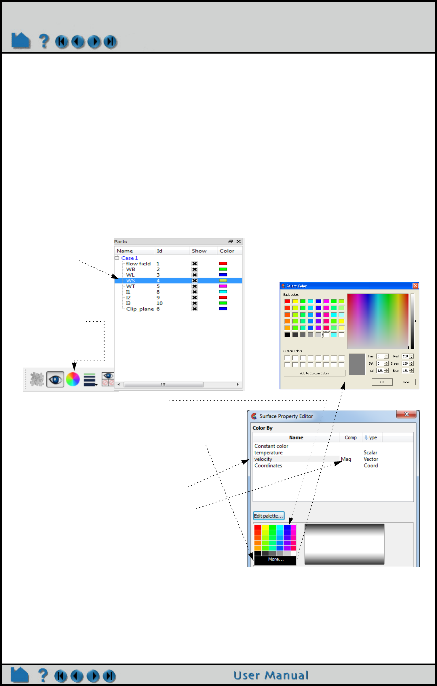
Page 406
HOW TO CHANGE COLOR
Manipulate Parts
Change Color
INTRODUCTION
In EnSight, parts can be colored either by a constant color or based on the value of a variable. Coloring geometry by
variables is one of the simplest and most effective means of visualizing a variable along the surface of a part.
You can also set a “default” color – all parts subsequently created will automatically be colored by the default color
(described in the Other Notes section below).
This article covers changing the color of a part. See How To Edit Color Maps for information on changing the
mapping from variable values to color.
BASIC OPERATION
To change a part’s color:
1. Select the desired
part(s) in the Main
Parts List.
3. Select the variable in the ‘Color by’ list.
4. If coloring by a vector component, click on
the default component ‘Mag’ to change to a
pulldown and choose a component.
- OR you can utilize the click-drag capabilities
to color by the variable described below:
2. Click the Color
icon on the Part
Quick Action
Icon Bar.
This will open the
Surface Property
Editor dialog.
3. Select a color from the color matrix.
- OR -
4. click the More... area to open the Color Selector
dialog
- OR if coloring by a variable -
3. Click and drag the variable from the Variable list to the part in the part list or to the part in the
graphics window you wish to color by the variable. You can drop the variable on the background
in the graphics window to color all parts in the viewport by the variable or you can drop the
variable on the Case heading in the part list to color all parts in the case.
4. OR Simply choose a list of parts and right-click and choose “Color by” as described in the
Shortcut section below.
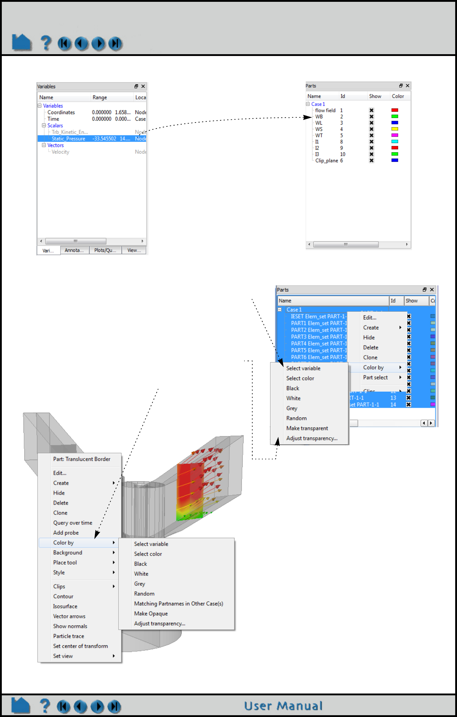
Page 407
HOW TO CHANGE COLOR
SHORTCUTS
Drag the variable from the
variable list and let go of it on
top of the part you wish to color.
Drop in either the part list or
drop in the graphics window.
Select your parts of interest in the part list. Right click and
choose “Color by”. The list will allow you to color by a variable,
or to pop up the color selector to select a single color, or to
quickly color by Black, White, or Grey. “Random” will color each
of the selected parts by a color chosen randomly from a
relatively unsaturated color palette. “Make transparent” will give
the part(s) a moderate level of transparency, and “Adjust
transparency” will allow you to choose the transparency.
Note that you can also right click on a part in the graphics
screen and have access to this “Color by” menu as well for an
individual part
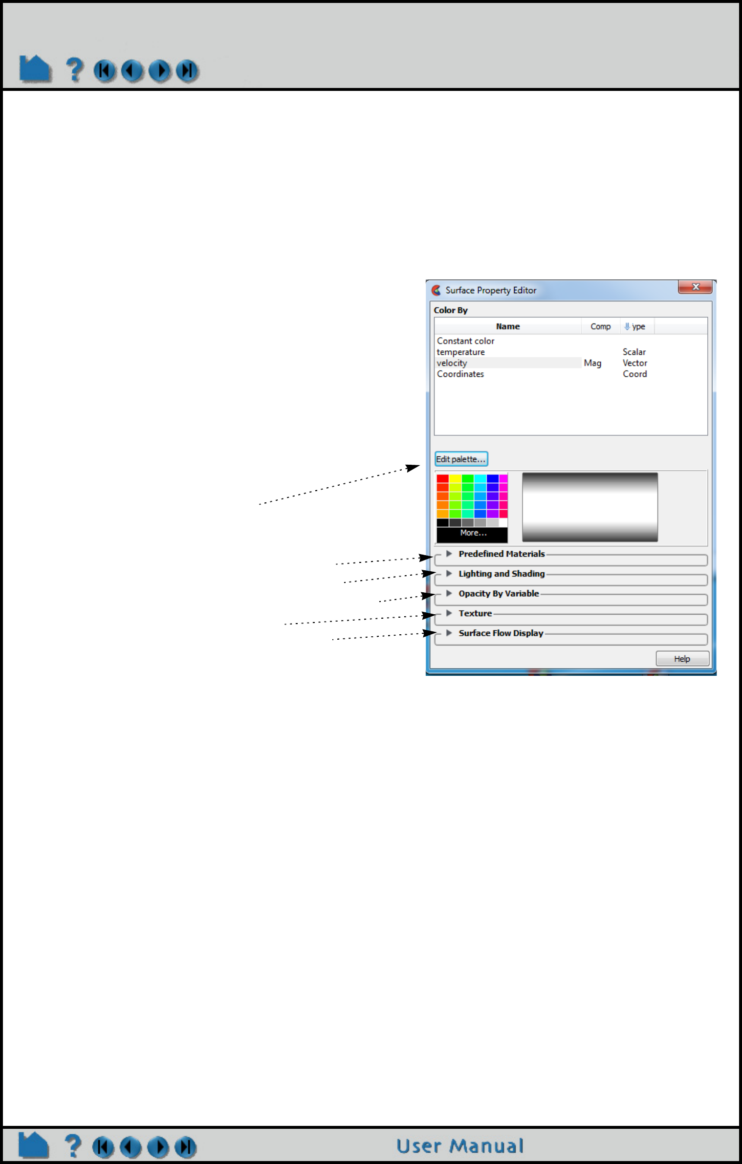
Page 408
HOW TO CHANGE COLOR
OTHER NOTES
If coloring by a nodal variable, the default coloring will be continuously varying - even within a given element. If you
are coloring by a per-element variable, the coloring will not vary within a given element. If you desire to see per-
element variables in a continuously varying manner, you can toggle on “Use continuous palette for per element vars”
under Edit->Preferences... Color Palettes.
Also consider using the Quick Color Settings Widget (see Use Quick Color Settings) to color parts.
ADVANCED
SEE ALSO
How To Edit Color Maps.
How To Set Surface Properties
You can set a default variable that will be used to color all
subsequently created parts. To do this, be sure no parts are
selected in the Main Parts list. (To de-select a part, hold down the
control key as you click on the selected item.)
Select the desired default variable in the Variables list of the
Color Editor.
Any part created subsequently will automatically be colored by
the default variable.
Advanced Options:
See also How to Edit Color Palettes
There are also a number of additional sections at the bottom of
this dialog.
Predefined Materials, see Predefined Materials
Lighting and Shading, see Lighting and Shading
Transparency, see Opacity by Variable (Transparency)
Textures, see How To Map Textures
Surface Flow Display, see Surface Flow Display
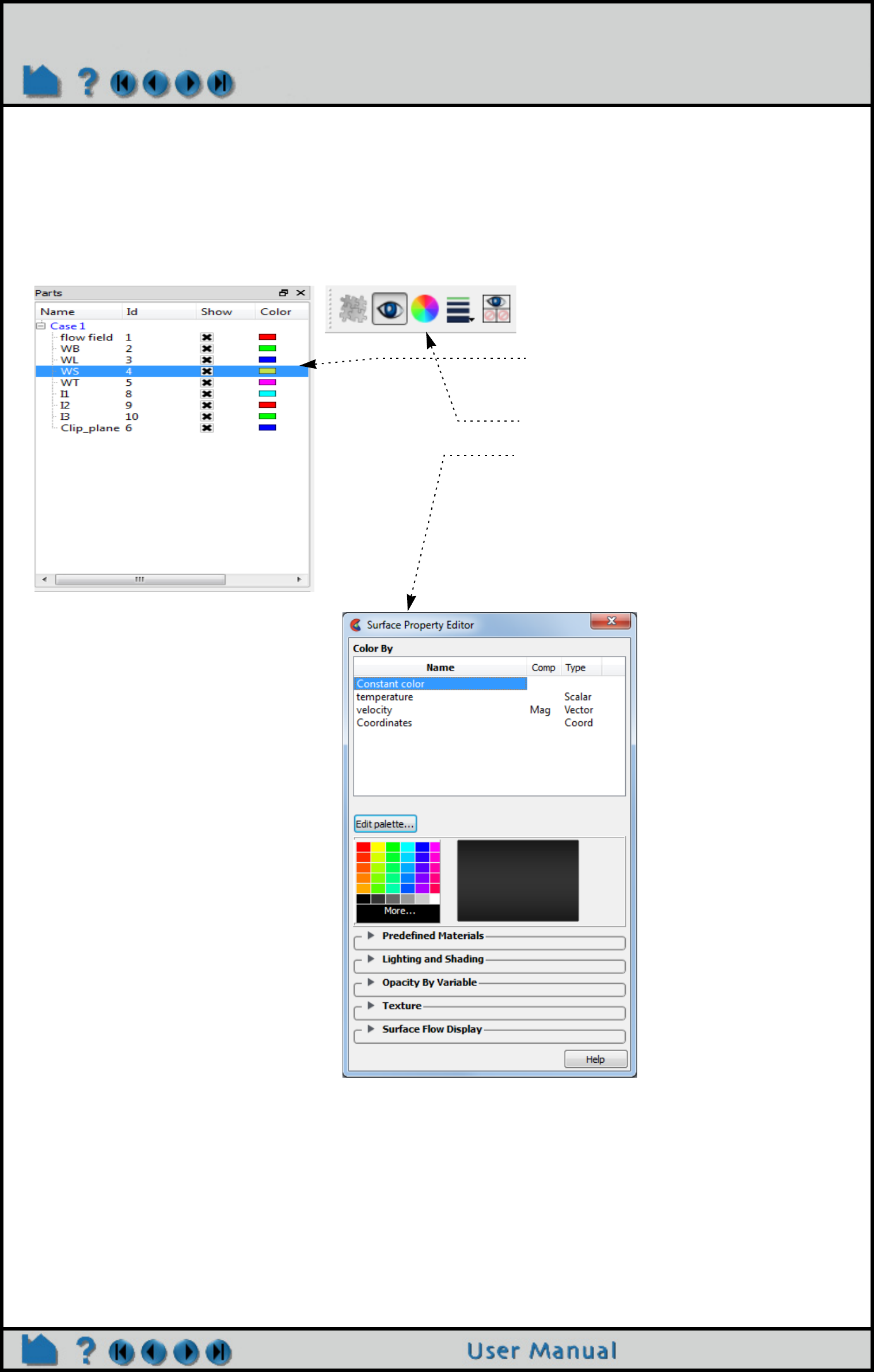
Page 409
HOW TO SET SURFACE PROPERTIES
Set Surface Properties
INTRODUCTION
Use this editor to Control Lighting and Shading values, to adjust Opacity by Variable, to apply Textures to part
surface, or to simply pick from Predefined Materials, or to show Surface Flow Display (see also How to Change
Color). You open the surface property editor as follows:
1. Select the desired part(s) in the Main
Parts List.
2. Click on the color wheel icon at the
top to open the Surface Property Editor
dialog.
3. This will open up the Part Color/
Surface Property Editor
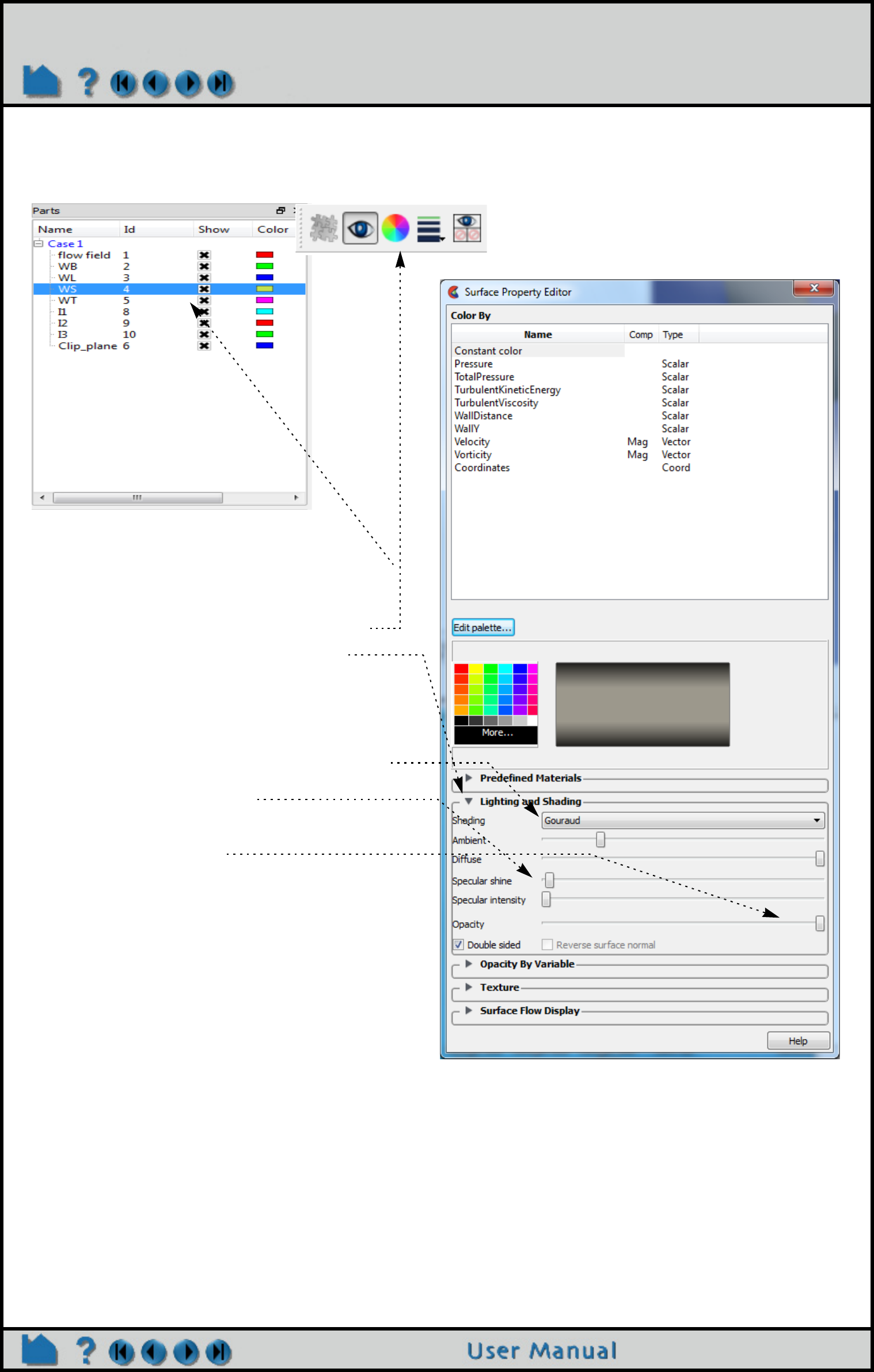
Page 410
HOW TO SET SURFACE PROPERTIES
LIGHTING AND SHADING
The Surface Property Editor allows a great deal of control of the part surface lighting properties.
Part Lighting and surface characteristics
1. Select the desired part(s) in the Main Parts
List.
2. Click on the color wheel icon at the top to
open the Surface Property Editor dialog.
3. Pulldown the Lighting and Shading.
4. Change part properties (see the User Manual
for descriptions of the options: Lighting and
Shading).
Change the Shading to a higher quality smoothing
algorithm to reduce surface tesselation artifacts
Make the surface shiny
Adjust the opacity to make the surface transparent
to see through the part
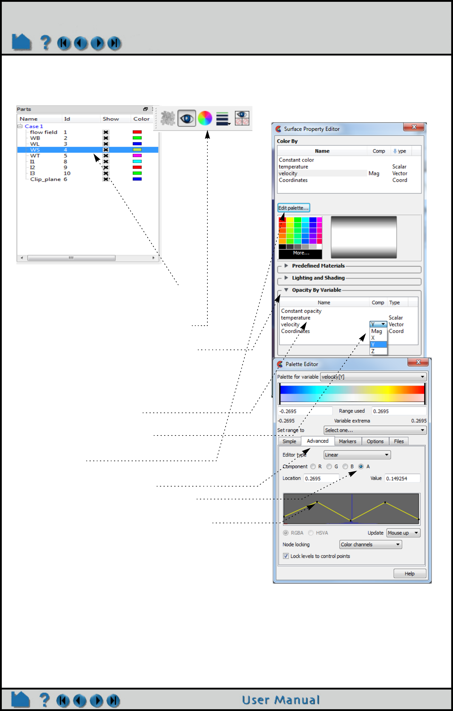
Page 411
HOW TO SET SURFACE PROPERTIES
OPACITY BY VARIABLE (TRANSPARENCY)
The Surface Property Editor allows you to render surface transparency according to variable value as follows.
Variable Transparency on Parts
1. Select the desired part(s) in the Main Parts
List.
2. Click on the color wheel icon at the top to
open the Surface Property Editor dialog.
3. Pulldown the Opacity By Variable to change
the part surface opacity using the variable
value.
Note: this turns off the constant opacity in the
Lighting and Shading turndown. You cannot do
both.
4. Click to choose a variable.
Click on the Comp value if the variable is a vector
and choose the component
5. Click on Edit Palette to control opacity
behavior.
6. In the Palette Editor, choose the Advanced
Tab to edit the opacity settings.
7. Select ‘A’ for alpha mode (transparency)
8. Move the ‘knots’ around to increase and
decrease transparency at each of the values.
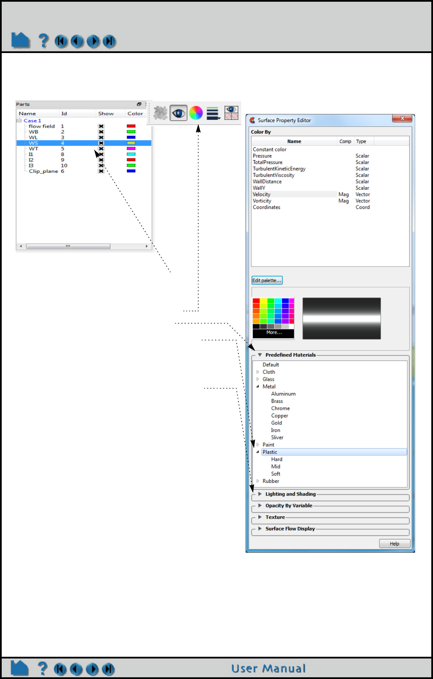
Page 412
HOW TO SET SURFACE PROPERTIES
PREDEFINED MATERIALS
There is a quick methodology in the Surface Property Editor to quickly achieve more realistic looking parts.
More realistic looking Parts
1. Select the desired part(s) in the Main Parts
List.
2. Click on the color wheel icon at the top to
open the Surface Property Editor dialog.
3. Pull down the Predefined Materials.
4. Click to open a category and pick a material.
This will, in some cases, automatically chose an
appropriate color and set the proper lighting and
shading values to approximate the material on the
selected part(s), see Understanding EnSight’s
Materials in the User Manual.
5. Pull down the Lighting and Shading if
additional changes are desired after picking a
material.
Note that the Lighting and Shading entries are
context sensitive to the material type chosen.
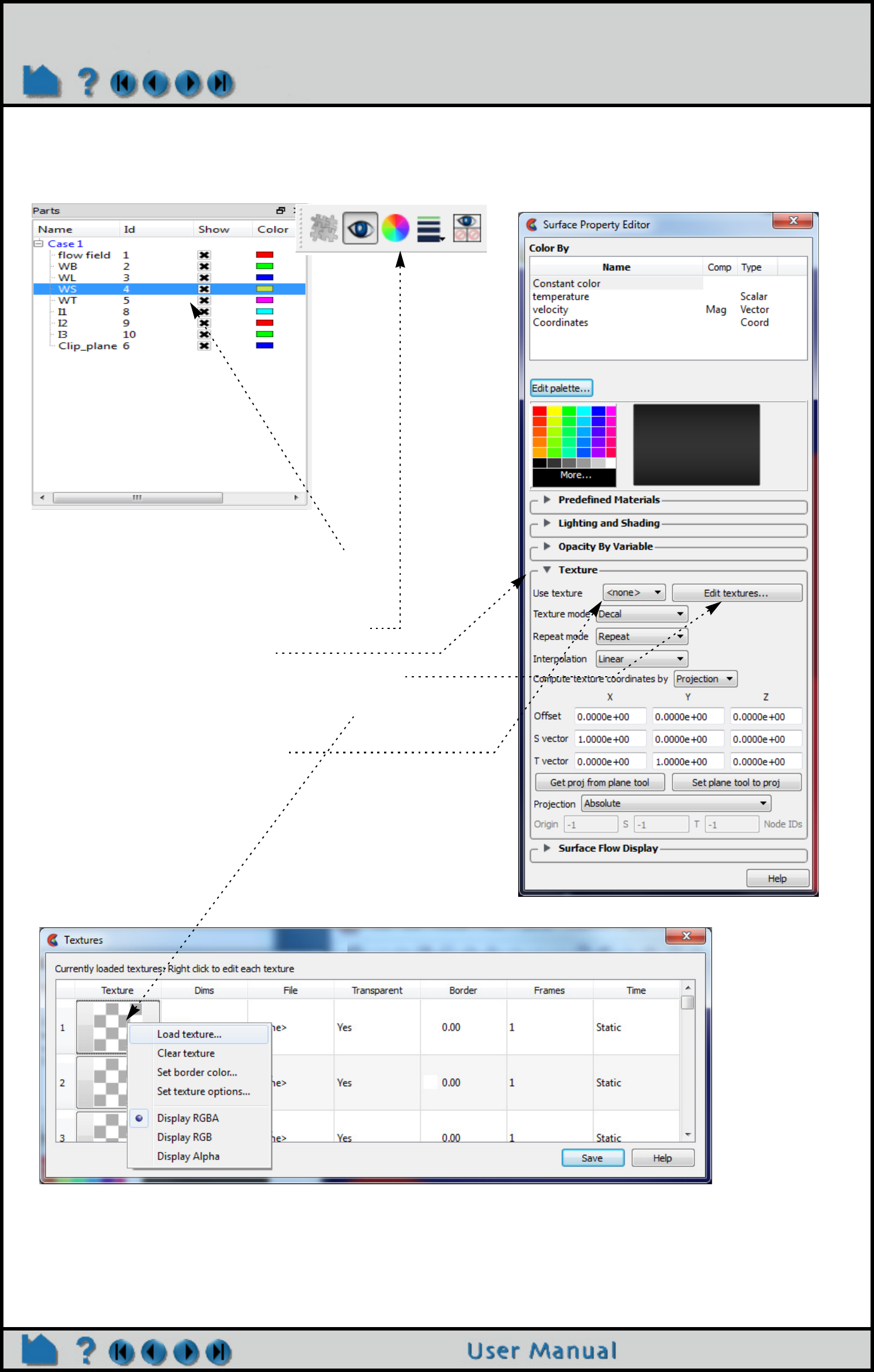
Page 413
HOW TO SET SURFACE PROPERTIES
TEXTURE
There is a quick methodology in the Surface Property Editor to add a texture to part(s).
Putting a logo or image on Part(s)
1. Select the desired part(s) in the Main Parts
List.
2. Click on the color wheel icon at the top to
open the Surface Property Editor dialog.
3. Pulldown the Texture.
4. Click on Edit textures and load some images.
5. Right click on Texture and load an image from
file, to be used as a texture
6. Pick a loaded texture to use
see How to Map Textures
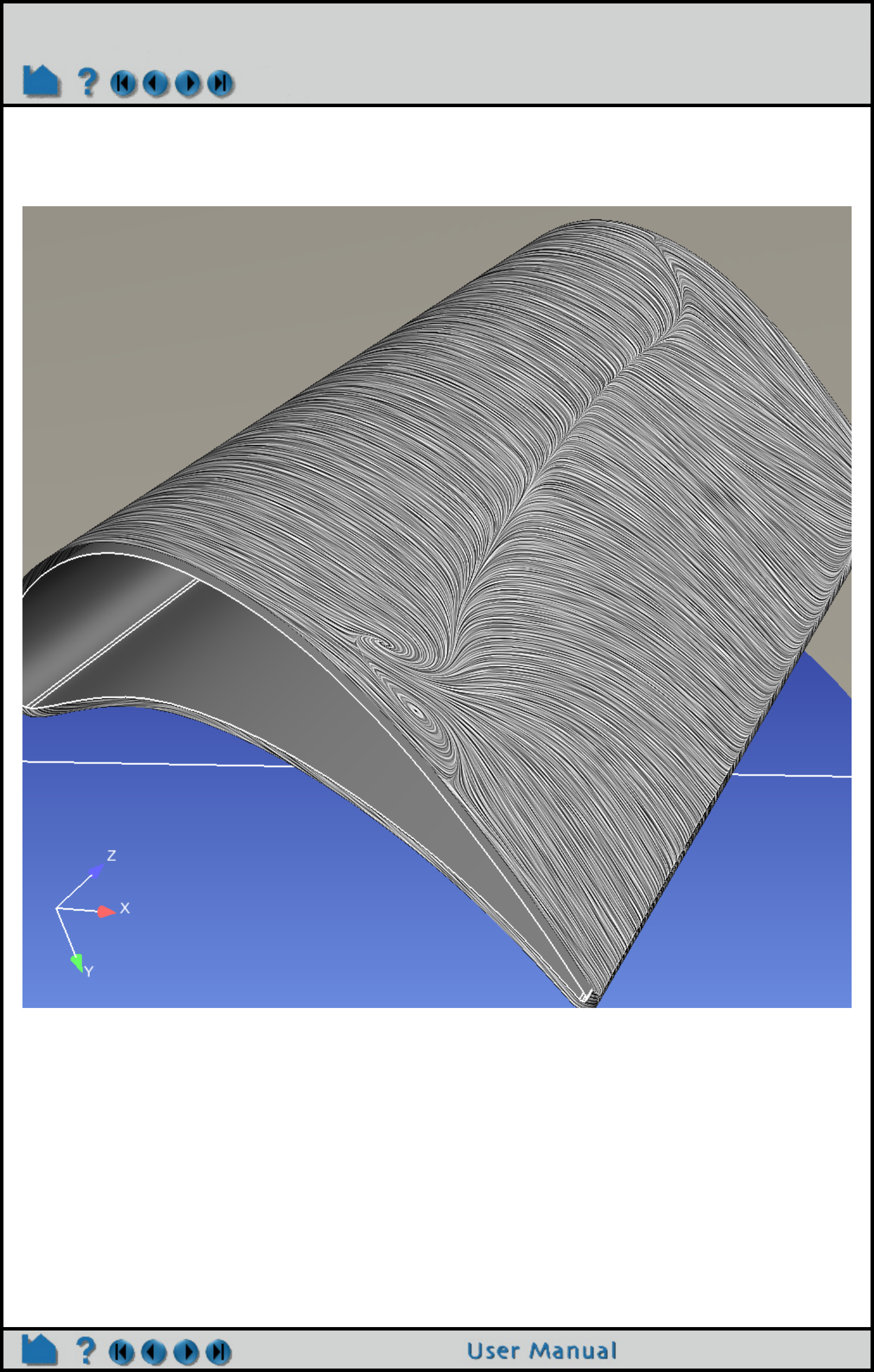
Page 414
HOW TO SET SURFACE PROPERTIES
SURFACE FLOW DISPLAY
Ensight provides the capability to visualize a vector (typically velocity) over a surface part, similar to tufts in a wind
tunnel. This is not the same as a particle trace part. It is a texture over the entire surface.
This visualization is not capable of being animated; it is a graphical texture of the flow tufts calculated on the part
surface using surface vector (or the vector in the 3D field just above the surface) using the Line Integral Convolution
algorithm. It is designed to provide a uniform visualization of the flow of a vector over a surface. This texture will
update when time is changed for transient data.
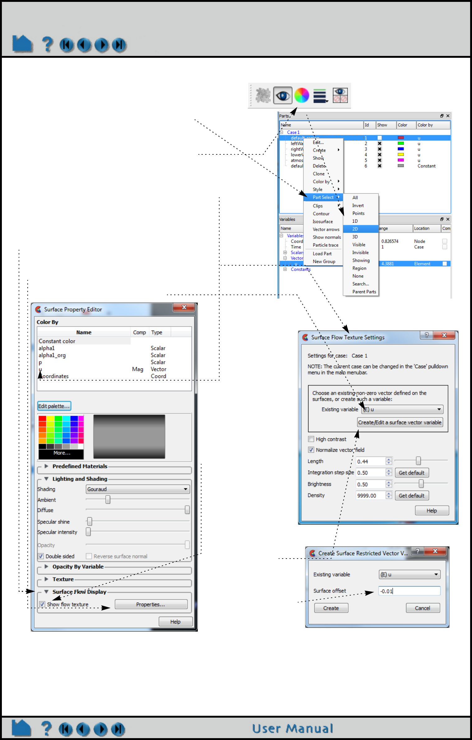
Page 415
HOW TO SET SURFACE PROPERTIES
Note that nodal variables give a more pleasing and smooth rendering.
Show flow tufts on 2D part or 3D Border part
1. Select the desired 2D surface part(s) in the
Main Parts List. A quick way to select all 2D
parts is to right click on the part list, Part
Select>2D.
2. Click on the color wheel icon at the top to
open the Surface Property Editor dialog.
Recommended: determine if the vector is defined
on the selected part(s); in this example, by coloring
by the vector ‘u’, in order to determine if your part(s)
have velocity defined on the surface. After you
determine this, right click on the selected part(s)
and choose Color by>Gray to choose a neutral
surface coloration.
3. Pulldown the Surface Flow Display.
Click on the Properties button and the Surface Flow
Texture Settings dialog will appear.
4. Choose a vector to visualize
5. If your 2D part(s)
have a non-zero
velocity on their
surface, activate the
creation of the flow
texture: Toggle on the
Show flow texture.
6. If your 2D part(s)
have an undefined or
zero surface velocity,
then you need to get
the velocity using an
offset into the
flowfield by clicking
on the Create/Edit a
surface variable
In the resulting dialog,
choose your surface
offset into the flow. Use
a negative value if your
normals are reversed.
Note: one interesting visualization methodology is to create
a surface part progressively offset from your original part into
the flow and to turn on this Surface flow visualization. See the
Offset section in How to Create Elevated Surfaces
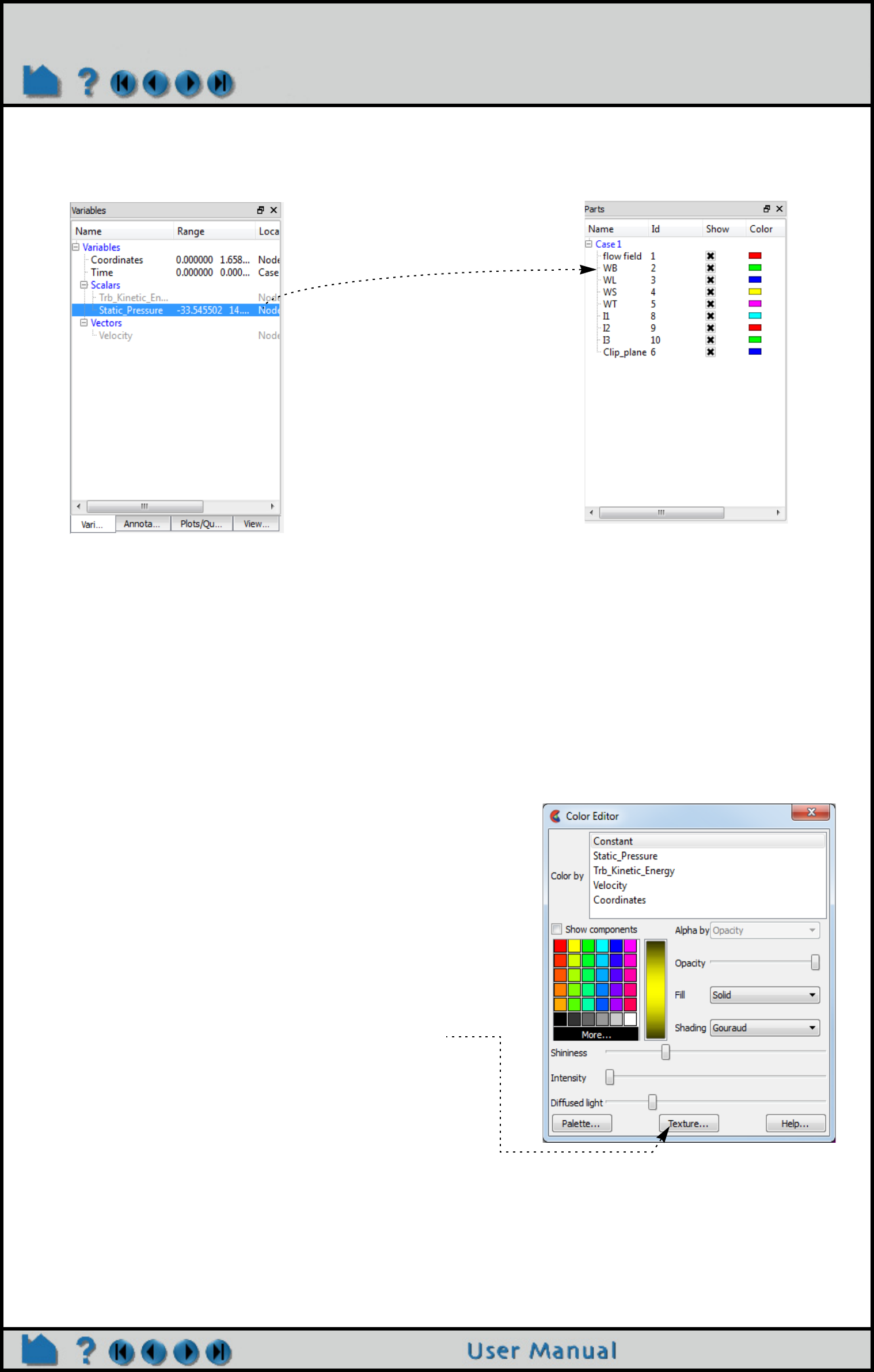
Page 416
HOW TO SET SURFACE PROPERTIES
DRAG N DROP
To change a part’s color quickly, simply click on the variable and drag it to the part name:
OTHER NOTES
If coloring by a nodal variable, the default coloring will be continuously varying - even within a given element. If you
are coloring by a per-element variable, the coloring will not vary within a given element. If you desire to see per-
element variables in a continuously varying manner, you can open the Palette Editor (see How to Edit Color
Palettes) and, under the Options tab, toggle on ‘Use continuous palette for element values’ for this variable for this
session. Or to make continuous the default for all per-element variables, toggle on “Use continuous palette for per
element vars” under Edit->Preferences... Color Palettes.
Also consider using the Quick Color Settings Widget (see Use Quick Color Settings) to color parts.
Drag the variable from the
variable list and let go of it on
top of the part you wish to color.
Drop in either the part list or
drop in the graphics window.
You can set a default variable that will be used to color all
subsequently created parts. To do this, be sure no parts are
selected in the Main Parts list. (To de-select a part, hold down
the control key as you click on the selected item.)
Select the desired default variable in the Variables list of the
Color Editor.
Any part created subsequently will automatically be colored by
the default variable.
Applying 2D Textures:
You can also apply 2D textures to a part, by clicking the
Texture.. button here. The Textures dialog will be opened.
See How To Map Textures
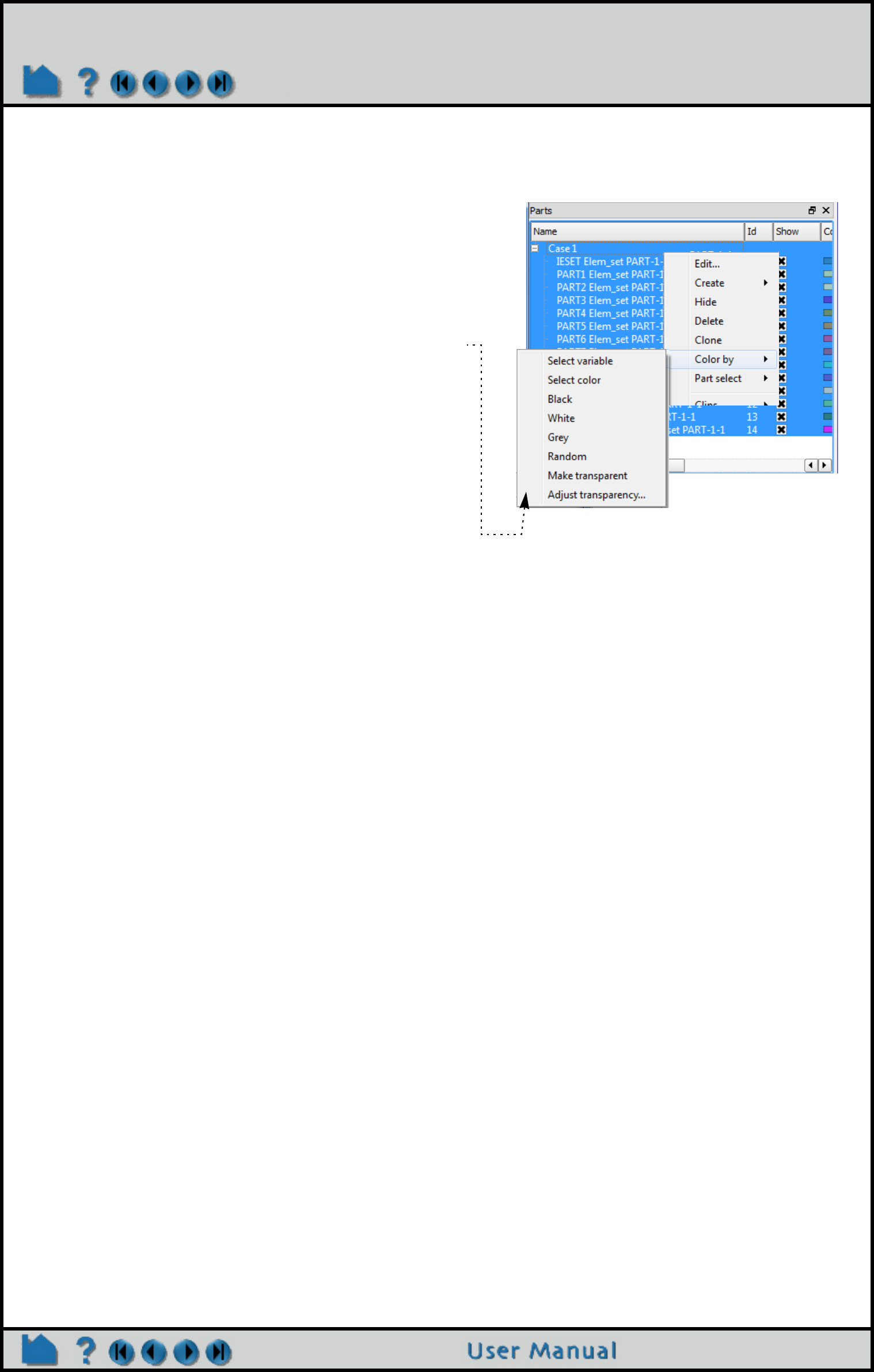
Page 417
HOW TO SET SURFACE PROPERTIES
SHORTCUT
SEE ALSO
How To Edit Color Maps.
How To Map Textures
Select your parts of interest in the part list. Right click and
choose “Color by>”. The list will allow you to color by a variable,
or to pop up the color selector to select a single color, or to
quickly color by Black, White, or Grey. “Random” will color each
of the selected parts by a color chosen randomly from a
relatively unsaturated color palette. “Make transparent” will give
the part(s) a moderate level of transparency, and “Adjust
transparency” will allow you to choose the transparency.
Note that you can also right click on a part in the graphics
screen and have access to this “Color by>” menu as well for an
individual part
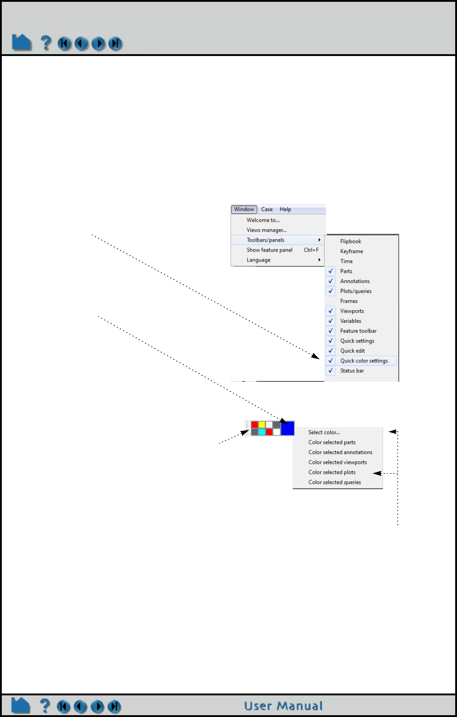
Page 418
HOW TO USE QUICK COLOR SETTINGS
Use Quick Color Settings
INTRODUCTION
The Quick Color Settings widget allows you to store your favorite colors and drag/drop them onto objects that have a
color attribute. Currently parts, plotters, queries, and all annotation types will accept a drag/drop color operation from
the widget.
Colors on the Quick Color Settings widget are stored as part of the user's preferences and thus the colors on the
widget are available between EnSight sessions.
BASIC OPERATION
To use quick color settings:
OTHER NOTES
Color changes performed via the widget are part of the Undo/Redo infrastructure.
1. Toggle the setting from
Window>Toolbars/panels>Quick
color settings
2. When any object that
has a constant color
attribute is selected, the
color will be reflected in
the larger color patch
on the widget
3. Drag a color from any color patch on the widget
to any other color patch on the widget.
4. Drag any color from the widget to an object in
either the user interface or in the graphics
window (assuming your graphics hardware
handles drag and drop operations). The drop is
limited to a single object.
5. Load a color into a color patch by right clicking
on the patch and choosing Select Color... which
will bring up standard Select Color dialog.
6. Right click on the color patch in the widget to
color multiple selected objects.

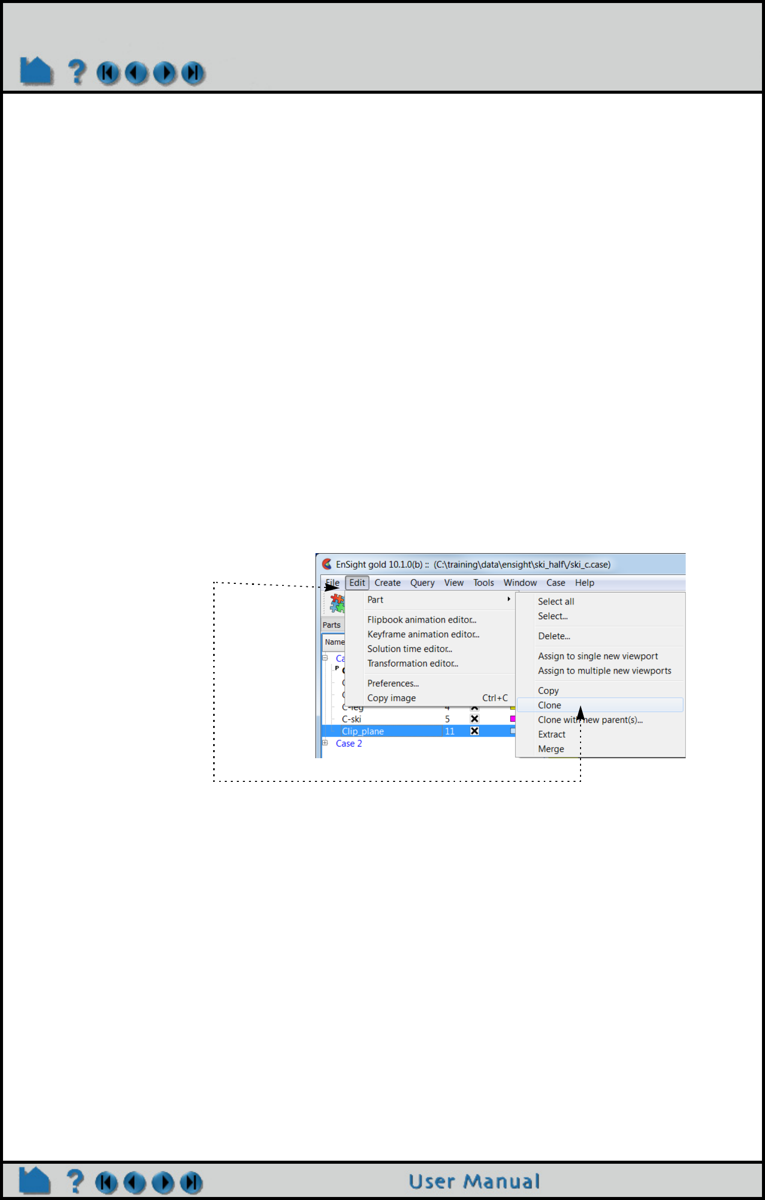
Page 420
HOW TO CLONE A PART
Clone a Part
INTRODUCTION
The clone operation creates a independent deep (on client, and if applicable on server) copy of either a model or a
created part including all of its attributes. A cloned model part is a reloaded model part with its attributes updated to
match the original. Note: a cloned model part has no parent as it remains an independent model part. A cloned
created part recreates the created part with all of the attributes updated to match the original. Note: a cloned created
part retains the same parentage as the original. Remember that a cloned part uses the same amount of memory on
both the client and server as the original part.
A cloned part will recreate a new part identical to the selected part. The cloned part will inherit all of the model
variables available to it as a model part or from the parents if the clone is a created part. The clone will not, however,
inherit calculated variables from the part that is being cloned. If you wish to have calculated variables extended to
include the cloned part you must recalculate these variables.
In contrast, a part copy (see Copy Parts) is a shallow operation, existing only on the client (visual only). Shallow
copying of a part is useful to save memory on the server, and is best used if all that is needed is to color the part by
two different variables, perhaps in two different viewports. A shallow copy is cheaper in terms of memory usage but
limited to visual operations only.
BASIC OPERATION
To create clone(s) of a part or parts:
1. Select the desired part(s) in the Parts List. A separate clone will be created for each selected part.
ADVANCED USAGE
If you need to do more than just color a duplicate part, then cloning is the way to go. One of the best reasons to clone
a model part, rather than just reload it, is because the act of cloning both reloads the part plus updates the of the
cloned model part to match the original. One of the best reasons to clone a created part is to avoid all of the hassles
of creation: reselecting the parents and setting all of the creation parameters, creating it and then updating its
attributes (e.g. display and coloration). You might slide an X clip colored by velocity to an interesting location, create
a clone and continue sliding it to another interesting location and create another clone, thereby leaving behind a ‘trail’
of clips at interesting locations all colored by velocity.
It is also possible to create a clone of a created part and assign it new parents using the “Edit>Part>Clone with new
parent(s)...” option which is described as follows.
2. Select Edit > Part > Clone.
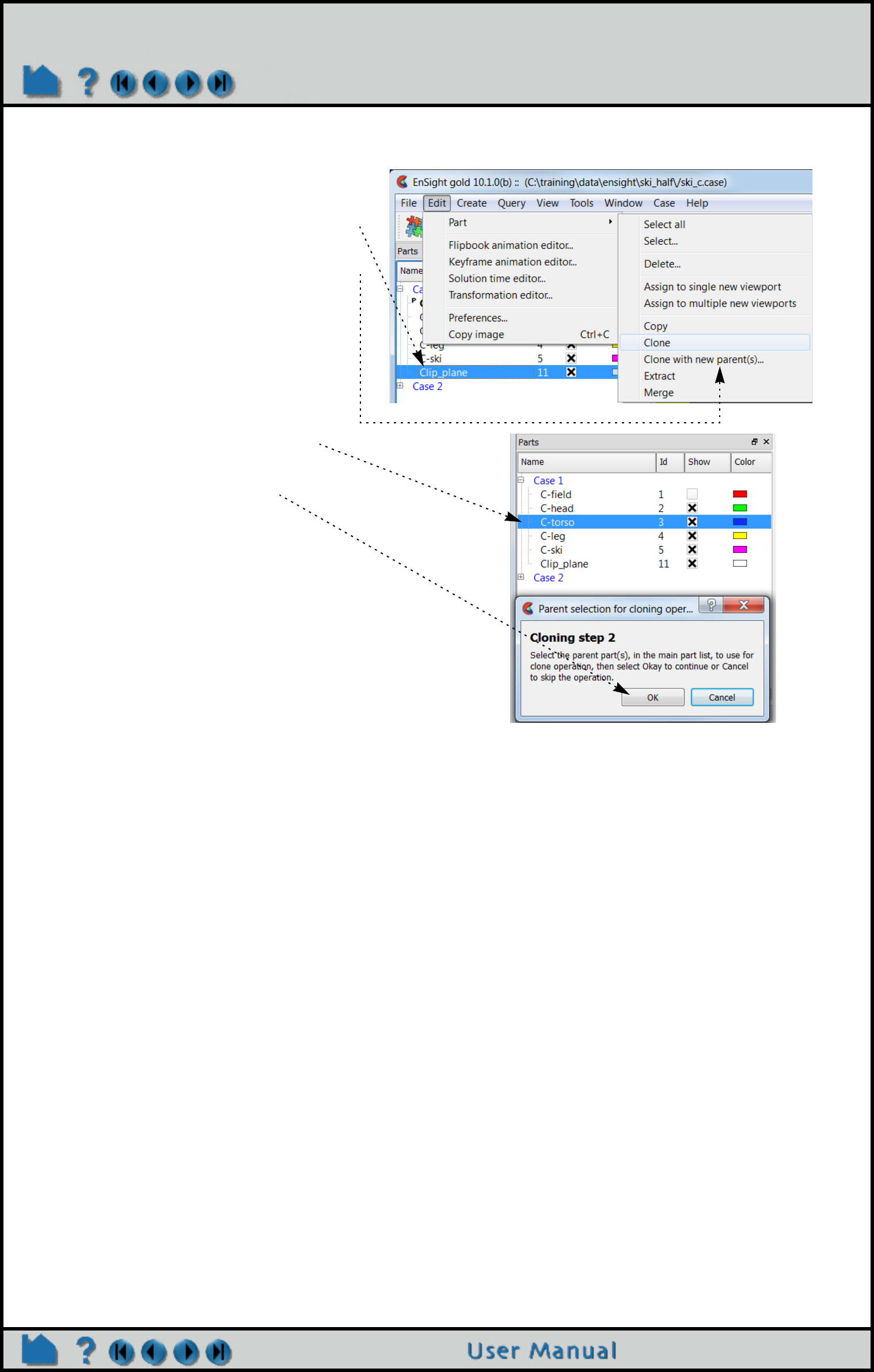
Page 421
HOW TO CLONE A PART
OTHER NOTES
EnSight offers several options for duplicating parts. As discussed above, copying (see Copy Parts) is shallow and
exists only visually on the client. Merging (see Merge Parts) allows the combining of one or more parts into one,
created (dependent), deep, child part. Right clicking on an existing model part and choosing Load Part (reloading a
model part) does create an independent new part from scratch. Extracting a part makes a deep copy of just the visual
components of the part. And now finally, cloning which makes a deep copy of the part including its attributes.
SEE ALSO
User Manual: Part Operations
How To Manual: Introduction
How To Manual: Merge Parts
How To Manual: Extract Part Representations
Clone with new parents
1. Select the part(s) in the part list that
you wish to clone.
2. Select Edit > Part > Clone with new
parents...
3. When the dialog pops up, choose
the new parent(s) in the part list.
4. Click OK and the part(s) will be
cloned with new parent(s)
Caveat:
Keep in mind that the new part(s) have
the exact same as their duplicate, but
applied on a new part. This can cause
confusion, for example, when a Y clip
on one part is cloned with another
parent and the Y clip disappears
because the max and min and Y value
are from the first part and the Y clip
falls off the edge of the second part
and becomes empty.
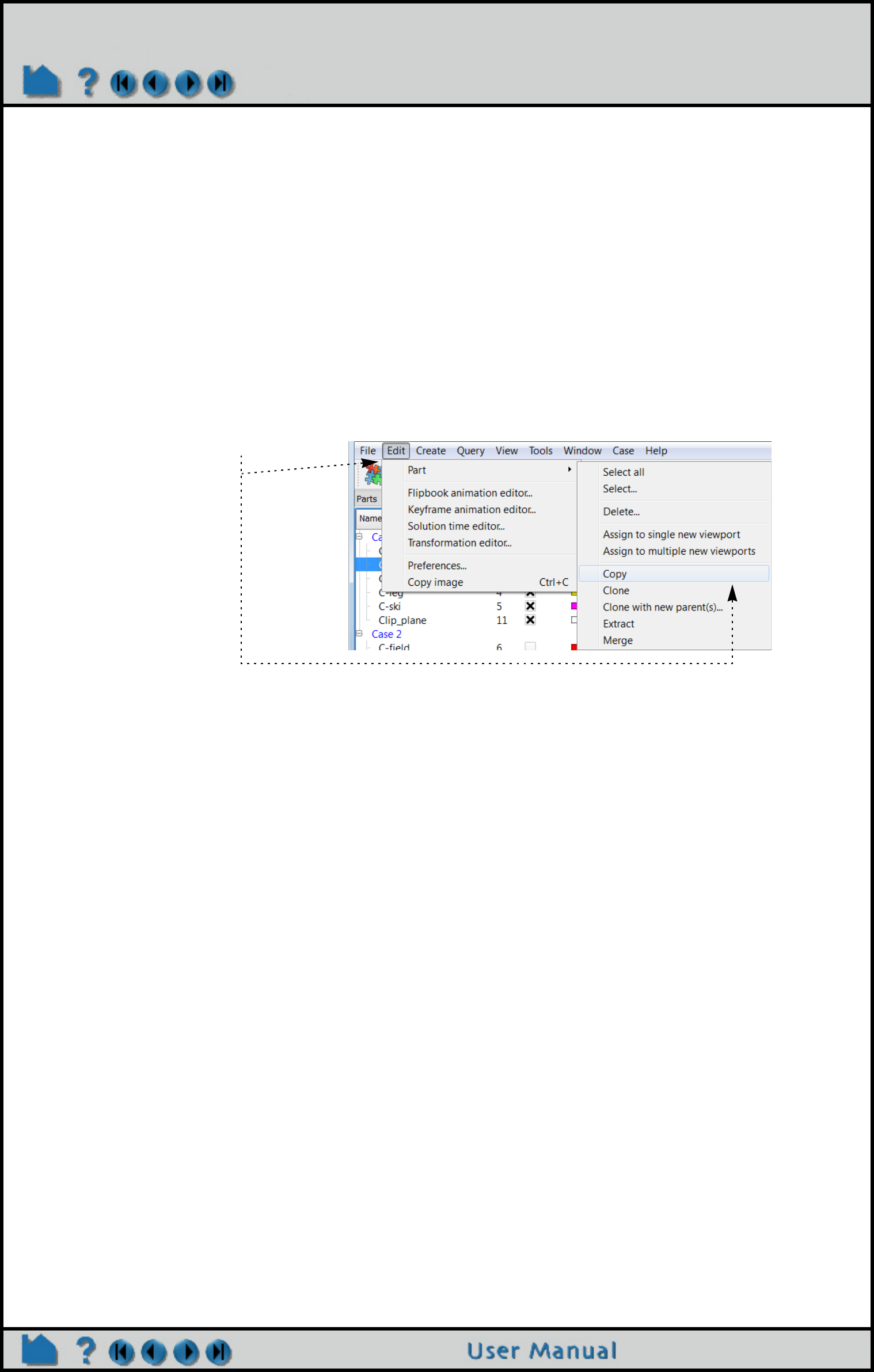
Page 422
HOW TO COPY PARTS
Copy Parts
INTRODUCTION
The copy operation creates a dependent shallow (only on client) copy of another part. The new part has its own set of
attributes (except for representation), but shares geometric and variable data with the original. One of the best
reasons to create a copy is to show multiple variables on one part at the same time in a side-by-side configuration.
The copy can be moved independently since new copies are automatically assigned a new frame. If you need to do
more than this to the new part, then consider reloading the part or cloning the part (see Clone a Part).
BASIC OPERATION
To create a copy of a part or parts:
1. Select the desired part(s) in the Parts List. A separate copy will be created for each selected part.
The new copies will be added to the end of the Parts List with “– COPY” appended to the part description.
ADVANCED USAGE
The most common reason for needing a copy of a part is to display multiple variables on the same geometry
simultaneously. When you create a copy, a new Frame is also created and the copy is assigned to it (when you create
multiple copies at the same time, a new frame is created for each new copy). Using the Frame feature, frames can be
manipulated (e.g. translated or rotated) independently. See How To Create and Manipulate Frames for more
information.
Consider a part clone (see Clone a Part) instead of a part copy if memory is not an issue.
OTHER NOTES
The dependence of the copy on the original has some important consequences:
1. If you change the visual representation of the original, the representation of the copy will change as well.
2. You cannot delete the original until the copy has also been deleted.
3. Since the part copy only exists on the client, you cannot save a part copy to disk.
If you want to create a dependent, non-shallow copy of a part, you can perform a merge operation on a single part.
This type of copy does now have the same consequences: the resulting “copy” is basically independent except that it
cannot exist without its parent. Or you can simply reload the part to create another “copy” of it.
2. Select Edit > Part > Copy.

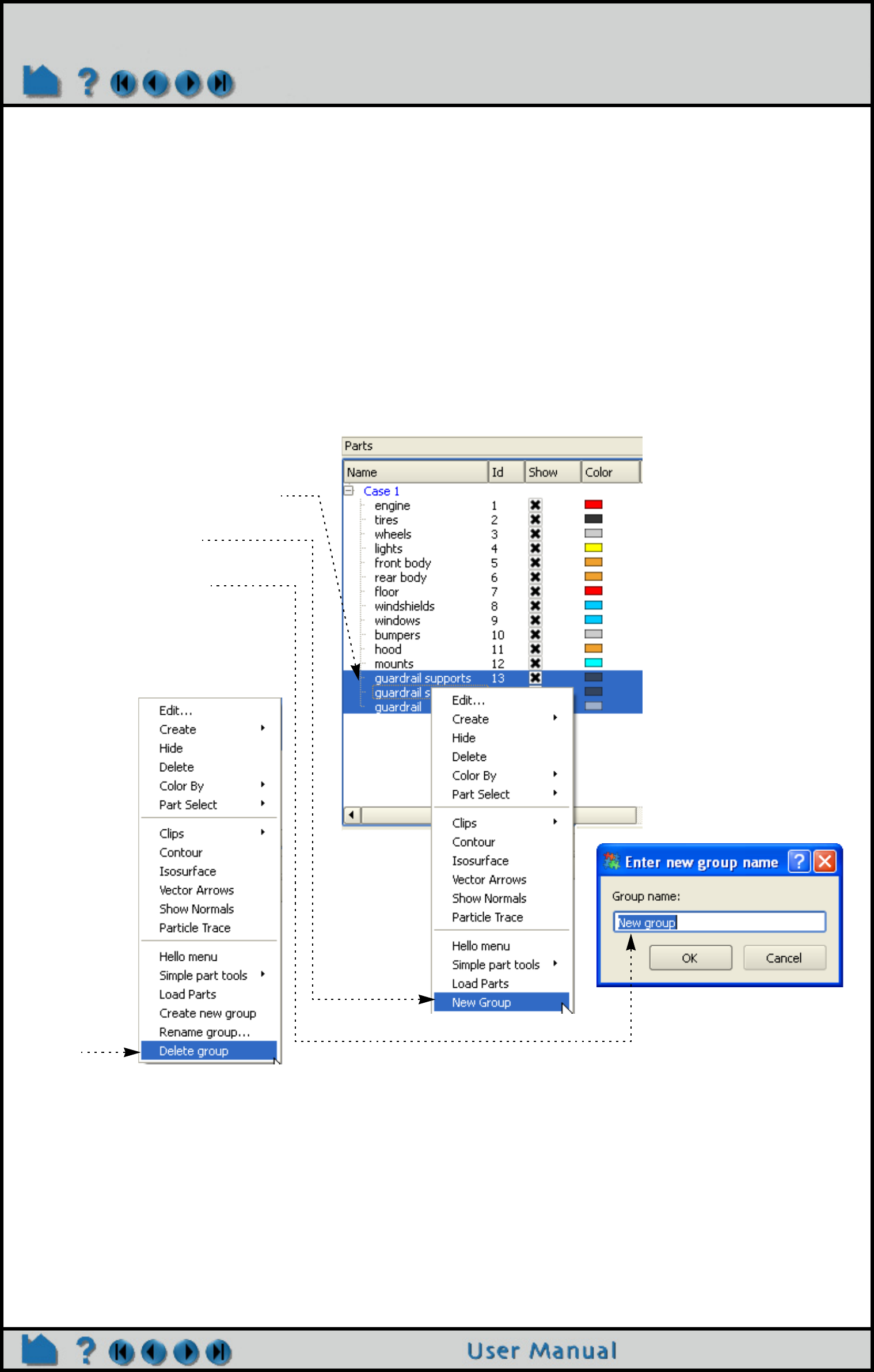
Page 424
HOW TO GROUP PARTS
Group Parts
INTRODUCTION
In many types of analysis, multiple parts are used to distinguish between various components or material types. To
the extent allowed by the particular data format, EnSight maintains this distinction by assigning these entities to
separate model parts. In many cases however, this distinction is no longer useful for postprocessing. When
manipulating parts, you often need to apply the same set of to all of them. If the number of parts to be treated
identically is large, this process can become unwieldy. EnSight provides a group operator to combine multiple parts of
the same type and case into a single part. The selected parts for the group can be hidden inside the group and are
thus effectively removed from the user interface, leaving only the newly formed group part. The operation can be
reversed by removing the group.
BASIC OPERATION
The selected parts for the group are placed under the new group entity. The group can be opened or closed to hide/
expose the parts in the group.
OTHER NOTES
Grouped parts can contain other grouped parts.
A part can only exist in one group.
SEE ALSO
User Manual: Part Groups
1. Select the desired part(s) in the
Parts List.
2. Right click on your selection.
3. Select the “New group” option
from the pulldown.
4. Give the group a name in the
dialog that pops up.
Note: A group can be deleted by
right clicking on a group and
using the Delete group option
from the right click pulldown.
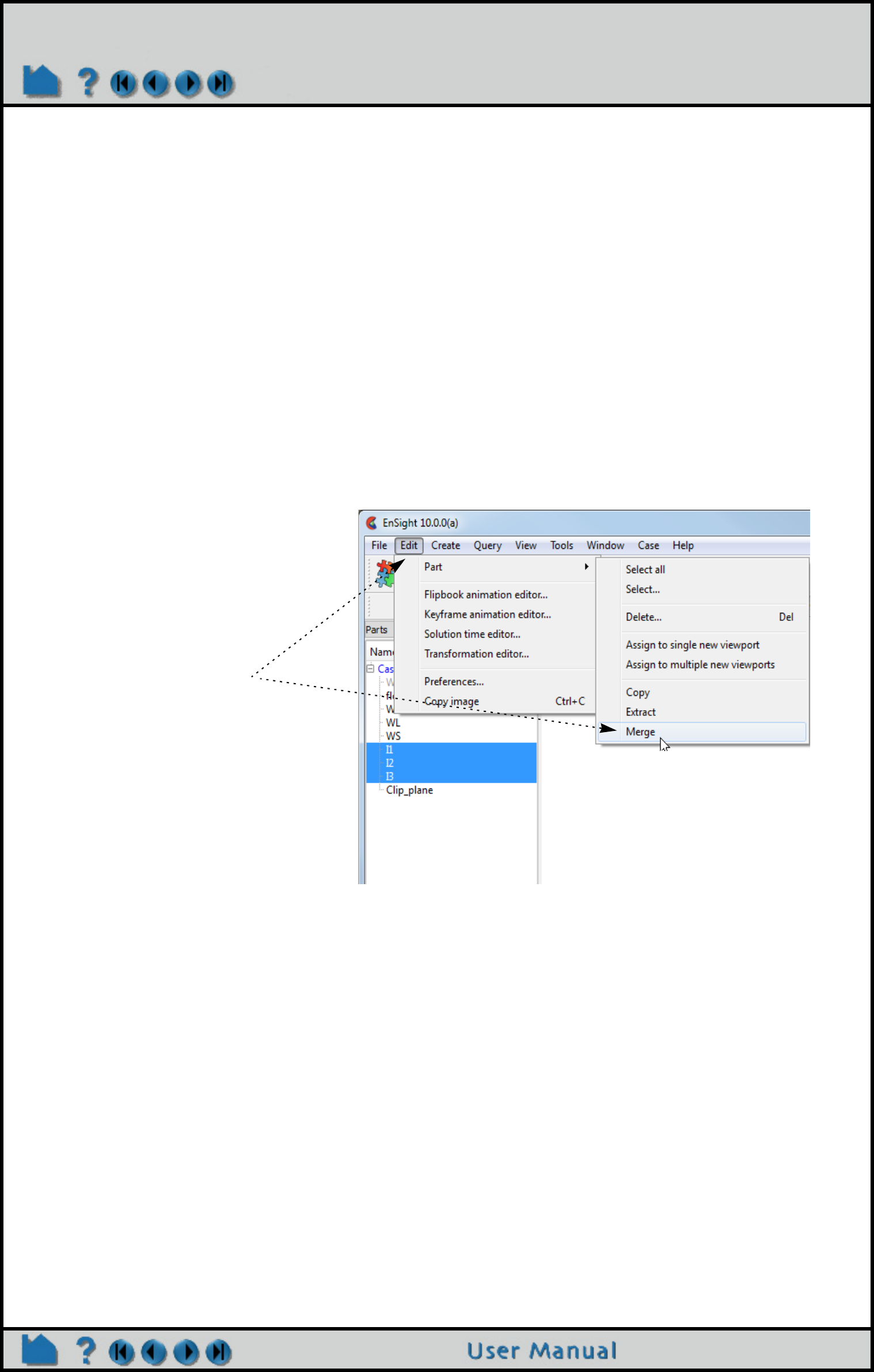
Page 425
HOW TO MERGE PARTS
Merge Parts
INTRODUCTION
In many types of analysis, multiple parts are used to distinguish between various components or material types. To
the extent allowed by the particular data format, EnSight maintains this distinction by assigning these entities to
separate model parts. In many cases however, this distinction is no longer useful for postprocessing. When
manipulating parts, you often need to apply the same set of to all of them. If the number of parts to be treated
identically is large, this process can become unwieldy. EnSight provides a merge operator to combine multiple parts
into a single part.
The merge operation creates one new part from one or more selected parent parts. The original parts are
unchanged. If only a single part is selected for the operation, merge will create a “true” copy of the part (as opposed
to the shallow copy that the Copy operation creates), with the only dependence being that the parent must exist.
If you delete any of the original parts after the merge, these components will be deleted from the merged part as well.
BASIC OPERATION
1. Select the desired part(s) in the Parts List.
The new merged part is added to the end of the Parts List with the description “Merge of parts #,#,#” where # are the
part numbers of the originally selected parts.
OTHER NOTES
Unlike Copy, merge creates true, server-based parts. Unlike Extract, merge creates parts based on the full, server-
based representation of the part.
If you merge a structured (IJK) part, the resulting part will be unstructured.
SEE ALSO
How To Group Parts.
User Manual: Part Groups
2. Select Edit > Part > Merge
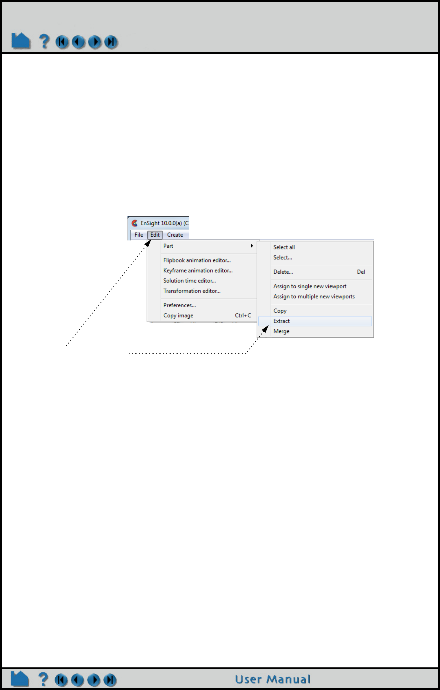
Page 426
HOW TO EXTRACT PART REPRESENTATIONS
Extract Part Representations
INTRODUCTION
The extract operation is closely tied to part representations. Extract creates a single new part using only the
geometry of the current representation of the selected part(s). For example, if the current representation of a part
consisting of 3D elements is Border, the result of extraction will be a part consisting of all unshared 2D elements (the
surface).
Extract is most often used to reduce the amount of information for a part (e.g. for faster display or for geometry
output) or to create a surface shell part – perhaps for subsequent cutting – of a 3D computational domain.
BASIC OPERATION
1. Select the desired part(s) in the Parts List.
The new part is added to the end of the Parts List with the description “Extract of parts #,#,#” where # are the part
numbers of the originally selected parts.
SEE ALSO
See How To Change Visual Representation.
User Manual: Part Operations
2. Select Edit > Part > Extract
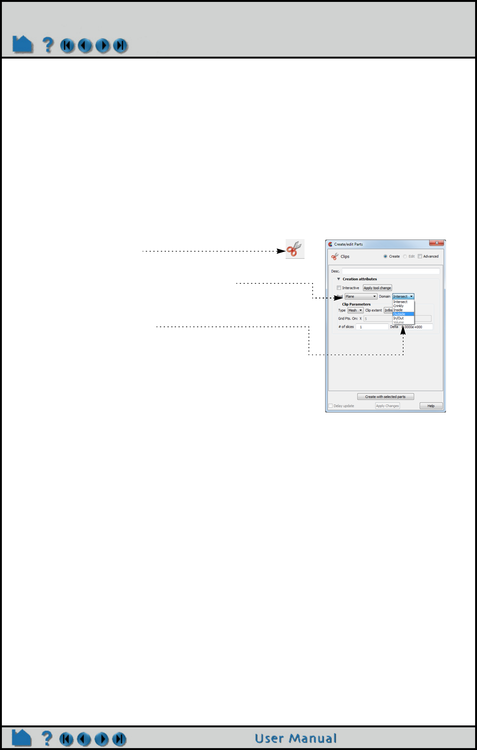
Page 427
HOW TO CUT PARTS
Cut Parts
INTRODUCTION
It is sometimes desirable to cut parts to, for example, reveal the interior of a solid or remove unwanted or unneeded
portions of a model. EnSight can cut any server-based part and either keep both “sides” or discard one. Any of the 3D
tools (Plane, Quadric, or Box) can be used as the cutting surface.
The cut operation produces dependent copies of the parent part. The part(s) resulting from a cut are completely valid
parts consisting of standard element types. These parts can be used for any operation – including further cuts.
BASIC OPERATION
To cut a part:
1. Select the part(s) in the Parts list.
For the Plane tool, the inside is the positive Z side of the tool. For the quadric tools, the inside and outside are
intuitive. In the Parts list, the original part remains and cannot be deleted without also deleting the cut parts (but can
easily be made invisible if desired). If In/Out was used, two new parts are added to the end of the Main Parts list with
the same name as the original part with “+” added to the name of the Inside part and “–” appended to the name of the
Outside part. If Inside or Outside was used, one new part is created with “+” added to the beginning of the name.
OTHER NOTES
A part copy cannot be cut. However, if the parent of the copy is cut, the copy will be cut as well (since part copies
share geometry with the parent).
The cut operation maintains the order of the elements, e.g. 3D elements yield 3D elements and 3D quadric elements
yield 3D quadric elements.
The cut algorithm breaks elements intersecting the cutting surface into tetrahedrons. Since there is no transition
zone created between these tetrahedrons and their non-cut neighbors, non-shared element faces are possible.
These non-shared faces can result in undesired lines and/or elements during border and/or feature angle
representations.
If you cut a structured (IJK) part the resulting parts will be unstructured.
Cuts with the Box are not true cuts, but simply a division of all elements that fall completely within the box or not.
SEE ALSO
User Manual: Clip Parts
2. Click the Clip Feature icon.
3. Select the desired cutting tool (Plane, Box, Cylinder, Sphere,
Cone, Surface of Revolution or Revolve 1D Part).
4. Position the desired cutting tool in the desired location.
5. Select which “sides” to keep.
Inside: Keeps inside of quadrics or box and “front” of plane.
Outside: Keeps outside of quadrics or box and “back” of plane.
In/Out: Keeps both sides
Crinkly: Keeps all elements that intersect the plane.
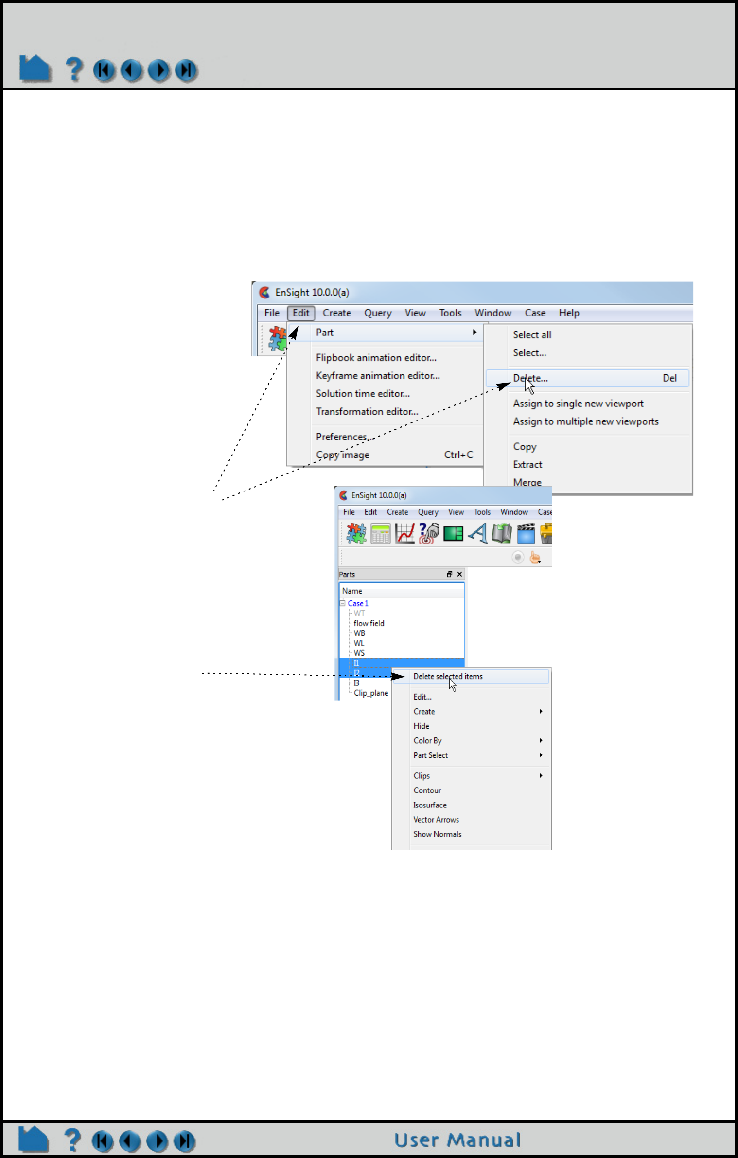
Page 428
HOW TO DELETE A PART
Delete a Part
INTRODUCTION
The delete operation removes selected parts and any parts dependent on them. All information associated with the
parts on both the client and server is removed. Deletion cannot be undone.
BASIC OPERATION
1. Select the desired part(s) in the Parts List.
OTHER NOTES
In some cases, variables that depend on a deleted part may have to be updated. For example, if you have a variable
such as Area calculated on a set of parts and one of the parts is deleted, the Area variable will automatically be
recalculated.
If you delete a grouped part, all parts in the group will be deleted.
SEE ALSO
User Manual: Part Operations
2. Select Edit > Part > Delete
or click the Delete key on your
keyboard while the mouse is
in the EnSight window
or right click and select Delete
(or Delete selected items, if
more than one item is
selected)

Page 429
HOW TO CHANGE THE VISUAL REPRESENTATION
Change the Visual Representation
INTRODUCTION
The part visual representation (part element settings) controls how you see the elements that you have loaded on the
server in the graphics window on the client. To be clear, the full part and all the elements are loaded and maintained
on the server, but the part visual representation exists on the client. For example, you can make a clip plane of a flow
field that is set to non-visual because the clip happens on the server. Part element settings are per part, that is, the
child clip can be shown in full representation, showing all elements, while the parent flow field is set to non-visual. The
ability to change part representations is a powerful management tool in EnSight. This allows you to see the border
elements, just an outline of the part, or to make the part entirely non visual. Not only can you select the visual
representation that best meets your needs, you can also manage graphics memory and performance more
effectively. Using simpler representations both reduces your client memory consumption as well as improves
graphics display speed. EnSight provides six representation modes for parts (as well as three modes that are a
combination of the six depending on the dimensional order of parts):
Full Every face and edge of every element is displayed. Warning: do not use
this for a 3D part with a large number of elements because it moves every
face of every element from the server to the client and can overwhelm
your client memory and your graphics card’s ability to process the data.
Conversely, this is often a useful choice for 2D parts.
Border Displays the outside surface of your part. Only unshared faces (for 3D
parts) or unshared edges (for 2D parts) are displayed. This is often a
useful choice for 3D parts.
Feature Angle Only those edges joining faces in the Border representation for which the
angle between the faces is less than some threshold are displayed.
Feature Angle typically extracts the topological features of interest in a
model. This is often a useful choice for 3D parts.
Non Visual No visual representation exists on the client. Note: this is different than
just turning off the visibility. Choosing this option means that NO 2D
surface elements are moved to the client for this part and no client
memory is allocated for the part. Turning off the visibility simply makes the
exising polygons in client memory invisible. It is often useful to use Non
Visual as the representation for 3D CFD flow field parts to save memory –
especially if you also have shell border part(s) to display the outer
surface.
3D Border, 2D Full Display 3D parts in Border representation; display 2D parts in Full
representation. This is useful in a structural model to show the outside
border of a 3D object, and to show all the elements of the shell border
parts.
3D Feature, 2D Full Display 3D parts in Feature representation; display 2D parts in Full
representation. This is useful for a CFD model to show the outside
features of the 3D flow field and to show all the elements of the 2D border
parts such as inlet, and wall and boundary condition part(s).
3D nonvisual, 2D Full Display 3D parts in Non Visual representation; display 2D parts in Full
representation. This is useful for a CFD model to avoid loading any of the
element surfaces of a high-resolution 3D flow field (to preserve client
graphics memory and performance) and to still show all the elements of
the 2D border parts such as inlet, and wall and boundary part(s).
Bounding Box Only a wireframe box representing the XYZ extents is displayed.
Volume Every element is displayed with a controllable level of transparency. Use
this with caution as this can require a large amount of client memory on
your hardware graphics card: for unstructured rendering, 100MB/ million
Tets, and structured rendering 2bytes/cell + 72 bytes / pixel.
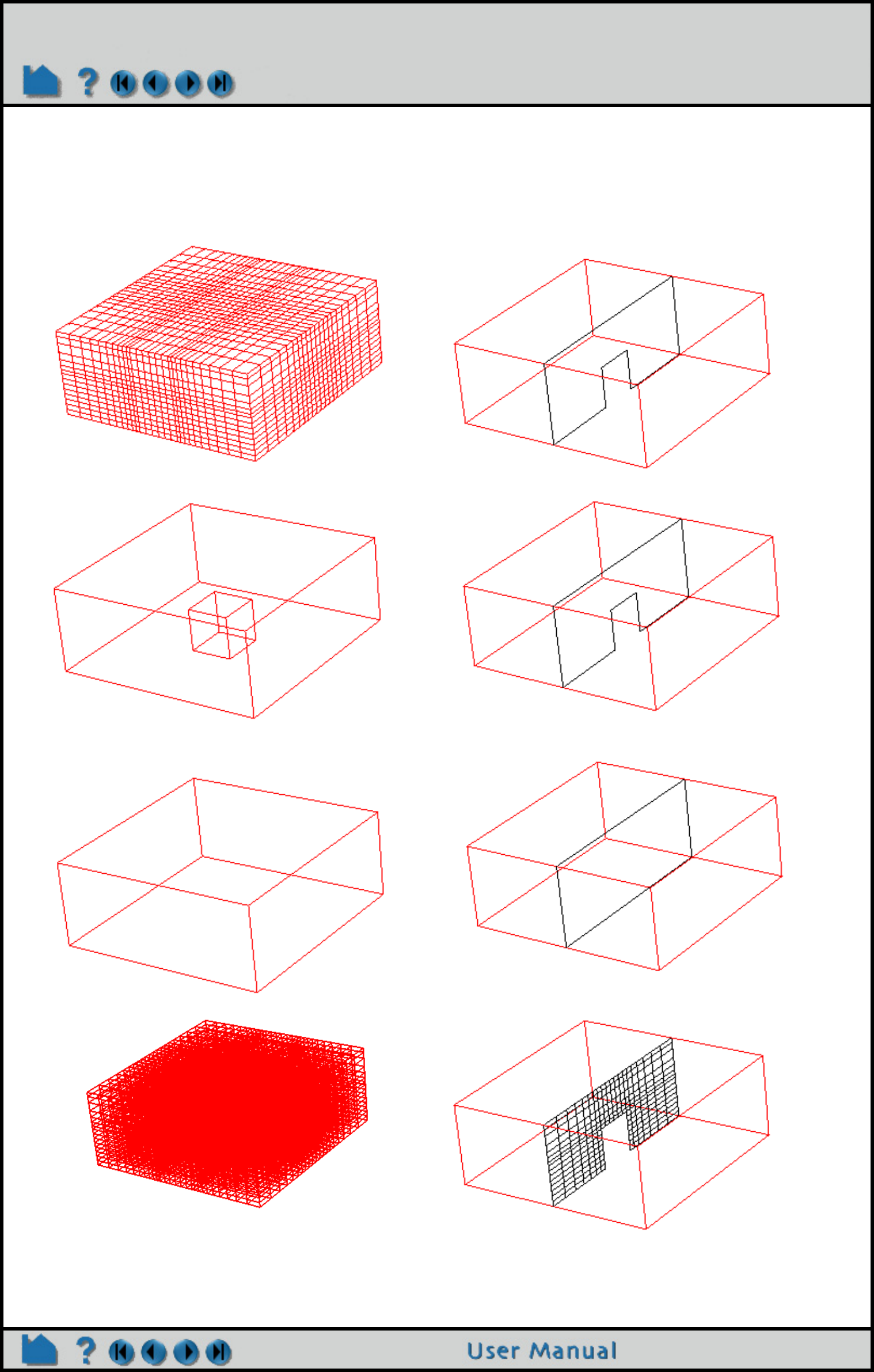
Page 430
HOW TO CHANGE THE VISUAL REPRESENTATION
Additionally, one can specify the use of only a point and normal (instead of the element connectivity) for the specified
part representation to be loaded. This reduces the number of entities to visualize and thus, is most useful for very
dense models. Double click on the part, and choose advanced, and under the node, element and line turndown, turn
on the Load points and normals only toggle.
3D 2D
Border
Feature
Angle
Bounding
Box
Full
As you can see from the part element settings above, that 3D parts are best shown in Border or Feature Angle,
and 2D parts are best shown in Full. Hence the hybrid 3D Border 2D Full and 3D Feature 2D Full settings.
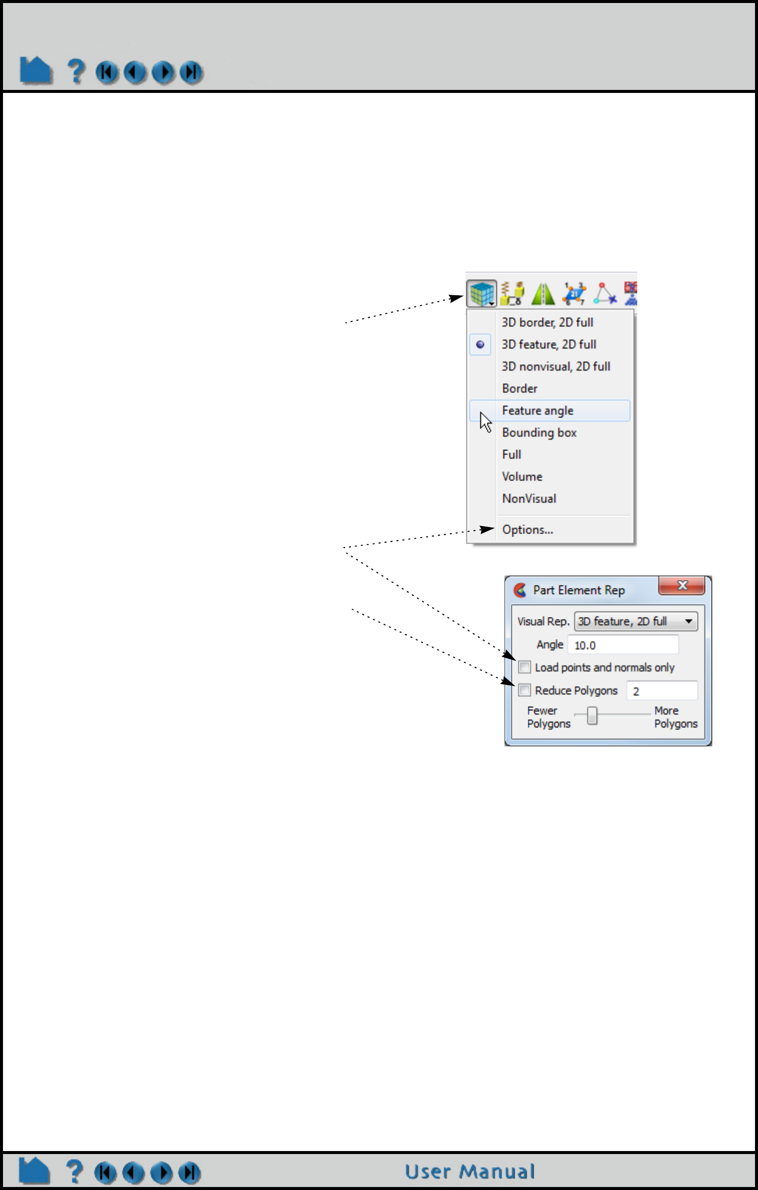
Page 431
HOW TO CHANGE THE VISUAL REPRESENTATION
The sitewide default visual representation (as well as extension mapping) is individually specified for data formats in
the $CEI_HOME/ensight102/site_preferences/ensight_reader_extension.map file. For example
.case files always open with the EnSight Case gold reader and parts are always in 3D Feature, 2D Full mode.
Custom visual representation can be specified in the user’s local ensight_reader_extension.map file located in
the users local EnSight Defaults directory.
BASIC OPERATION
OTHER NOTES
Note that some derived parts (such as contours or vector arrows) are based on the client’s representation of the
parent part. If the parent’s representation changes, the derived parts will change as well.
You cannot change the representation of a copied part. A copy always exhibits the current representation of the
original part.
A part’s representation can be made “permanent” by creating a new part based on the current representation. See
How to Extract Part Representations for more information.
1. Select the desired part(s) in the Parts List.
2. Click the Element Representation icon on the
Part Quick Action Icon Bar.
3. Select the desired visual representation.
4. If desired, you can have each element
connectivity of your element representation be
replaced by a point and normal only. Click
Options, then set the option for points and
normals only.
5. And if desired, you can apply polygon reduction.
Polygon reduction is designed to speed up visualization
processing by thinning out the number of polygons that are
rendered. There is naturally a trade off in image quality and
speed. Note that the original model is not modified, just its
rendered image.

Page 432
HOW TO CHANGE THE VISUAL REPRESENTATION
ADVANCED
Face Culling
If you have a 2D part in a ‘full’ representation showing the elements, and you color by a variable, and you experience
a ‘flimmering’ effect caused by coincident 2D elements with different variable values (perhaps representing the other
side of a 2D surface), there is an option to visually cull the faces whose normals face away or towards the viewer.
This culling only works if the front side 2D elements and the back side 2D elements have normals facing in the
opposite direction. And this is only a visual culling, it does not affect, for example, the Area calculated on the 2D part.
SEE ALSO
User Manual: Part Element Settings Icon
Page 433
HOW TO SET
Set
INTRODUCTION
Part control the appearance and behavior of parts. Much of the power of EnSight derives from the broad range of
available and the ease with which they can be changed. are grouped into several classes:
The Creation for non-model parts can be edited in the Feature Panel by double-clicking on the part in the Parts list.
Most display (such as color and visibility) can be controlled via the icons on the Quick Action icon bar.
Since Creation are specific to each (non-model) part type, they are not covered here. Look in the How To article for
the specific part type for details on those particular Creation.
Server side displacement capability is available in the Creation Attribute area for model parts. See How To Display
Displacements for a description of this capability.
This article is divided into the following sections:
Part Quick Action Icons
Creation
General
Node, Element, and Line
Displacement
IJK Axis Display
Creation Creation are unique for each (non-model) part type (e.g. the isovalue of an isosurface). The creation for
a part are accessible in the Feature Panel after double-clicking the part in the Main Parts List, or by the
main menu structure Create->Isosurfaces (for example).
However, model parts have a consistent set of in this dialog including ability to remesh the model part,
scaling and translating the model part, filtering the elements of a model part or resetting the I/J/K ranges
of a structured model part.
General Visibility
Susceptibility to auxiliary clipping
Reference Frame
Response to change in time (active or frozen)
Symmetry options
Viewport visibility
Coloration (by variable or constant color)
Hidden surface toggle
Hidden line toggle
Shading type (flat, Gouraud, smooth)
Transparency
Lighting (diffuse, shininess, highlight intensity)
Visual symmetry
Volume Rendering
Node, Element,
and Line
Node, line, element visibility toggles
Node type (dot, cross, sphere)
Node scale (constant or variable)
Node detail (for spheres)
Node and element label toggle
Element-line width
Element-line style (solid, dotted, or dot-dash)
Element representation on client (full, border, 3D border/2D full, 3D feature/2D full, 3D nonvisual/2d full,
feature angle, bounding box, nonvisual)
Element shrink factor
Polygon reduction factor
Displacement Displacement variable
Displacement scaling factor
IJK Axis Display IJK Axis visibility
IJK Axis scale value
Page 434
HOW TO SET
BASIC OPERATION
Part Quick Action Icons
The Part Quick Action Icons can be used to quickly set for parts. To use these controls:
1. Select the desired part(s) in the Parts list.
2. Click appropriate icon to set the desired attribute:
Part Visibility
Color, Lighting, & transparency
Line Width
Visibility Per Viewport
Element Visual Representation
Displacement
Visual Symmetry
Node and Element Labeling
Node Representation
Filter Elements
Element Blanking
Shading Type
Hidden Line
Auxiliary Clipping
Fast Display Representation
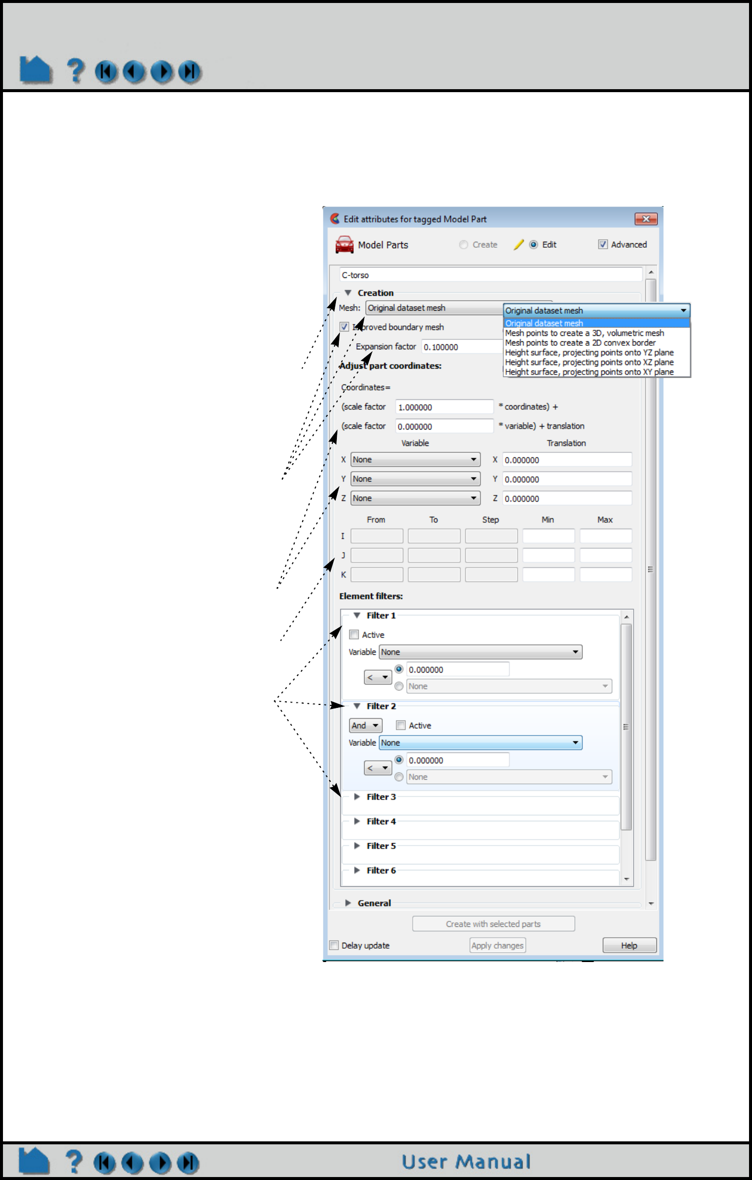
Page 435
HOW TO SET
Creation
For model parts, the Creation section in the Feature Edit Dialog allows improved boundary mesh option, scaling, and
filtering of elements. For structured model parts, you can change the model part I/J/K range.
1. Right click on the model part name in the Parts list and choose ‘Edit’ or right click on the
model part in the graphics window and
choose ‘Edit’, or double click the model
part in the Parts list.
By default, any changes you make to will take
effect immediately. If you wish to “batch” a
series of changes turn on the “Delay update
toggle at the bottom of the dialog. When you
are ready to apply a set of changes click the
“Apply Changes” button.
2. Open the “Creation” turndown, then set
the desired attribute(s):
A Model Part can be remeshed in
2D or in 3D or projected onto
one of 3 orthogonal planes using
an improved boundary mesh
option and a variable expansion
factor. See the Model Parts
section in the User Manual.
A Model Part can be rescaled and
translated independently in the
X, Y and Z directions.
A Structured Model Part can have
the I/J/K Range changed.
A Model Part’s elements can be
filtered (up to six filters) by a
variable or a value. See Filter
Part Elements in the How To
Manual.
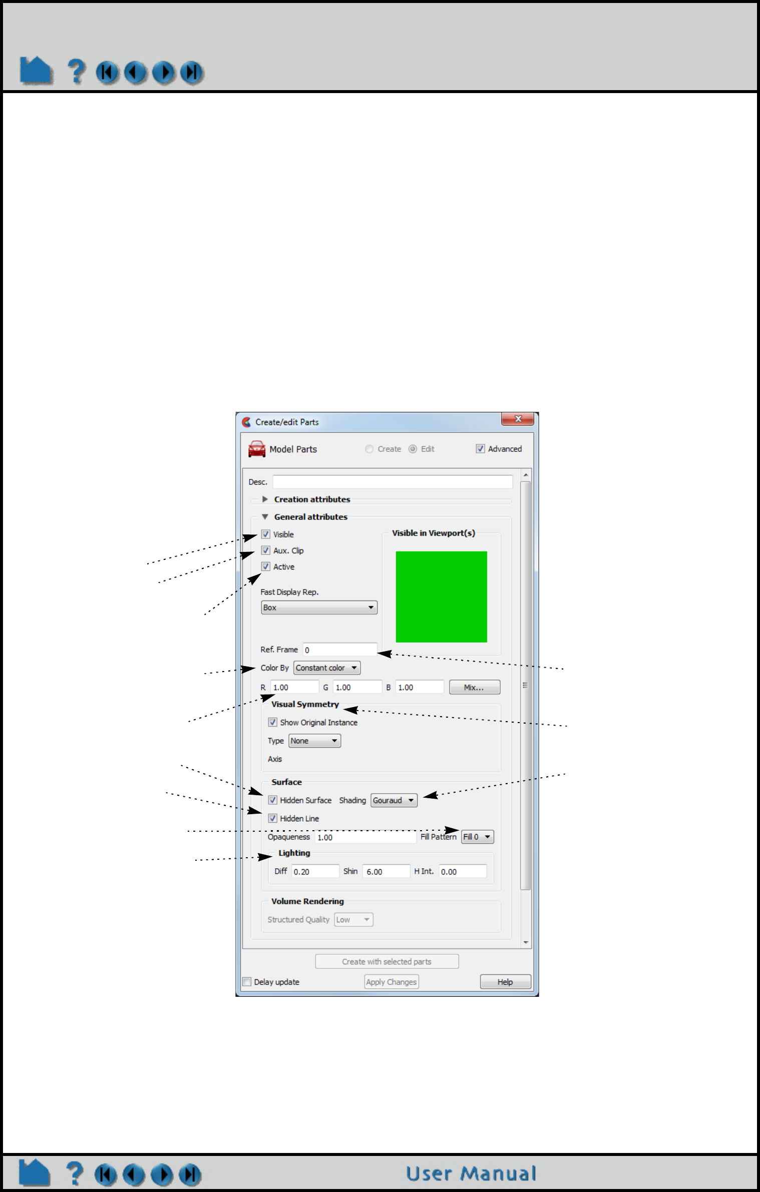
Page 436
HOW TO SET
General
The General section in the Feature Edit Dialog duplicates many of the controls available in the part Quick Action icon
bar. To set using the General section:
See Also
Set Global Viewing Parameters
1. Right click on the part name in the Parts list and choose ‘Edit’ or right click on the part in
the graphics window and choose ‘Edit’, or double click the part in the Parts list.
1. OR Select Create > part type.
By default, any changes you make to will take effect immediately. If you wish to “batch” a series of
changes turn on the “Delay update toggle at the bottom of the dialog. When you are ready to apply
a set of changes click the “Apply Changes” button.
2. Toggle the Advanced Toggle in the top right corner of the dialog to see the additional
turndowns besides Creation.
3. Open the “General” turndown, then set the desired attribute(s):
Set part Fast display
representation (according to
Global Viewing Detail
Mode):
• Box: part is represented as
bounding box.
• Elements: part is represented
according to Element
Representation
• Points: part is represented as
a point cloud
Set part reference frame
Set part graphical symmetry
Set shading type:
• Flat: color and shading are
constant across elements
• Gouraud: color and shading
vary linearly across elements
• Smooth: color and shading
calculated based on surface
normal interpolated across
elements to simulate a
smooth surface.
• Smooth High Quality:
Smoothing that attempts to
retain subtle features.
Toggle part visibility
Toggle auxiliary clipping on/off
Toggle whether the client’s portion
of the part changes if the current
time step changes
Set color by constant or color by
variable
Set the part color if constant
Toggle part hidden surface
Toggle part hidden line
Set part transparency fill pattern
Set part shading parameters:
• Diff: diffuse shading – the
amount of light that a surface
reflects. 0 is none and 1 is full.
• Shin: Degree of shininess – 0 is
dull and 100 is very shiny.
• H Int: Degree of highlight
intensity – 0 is none and 1 is full.
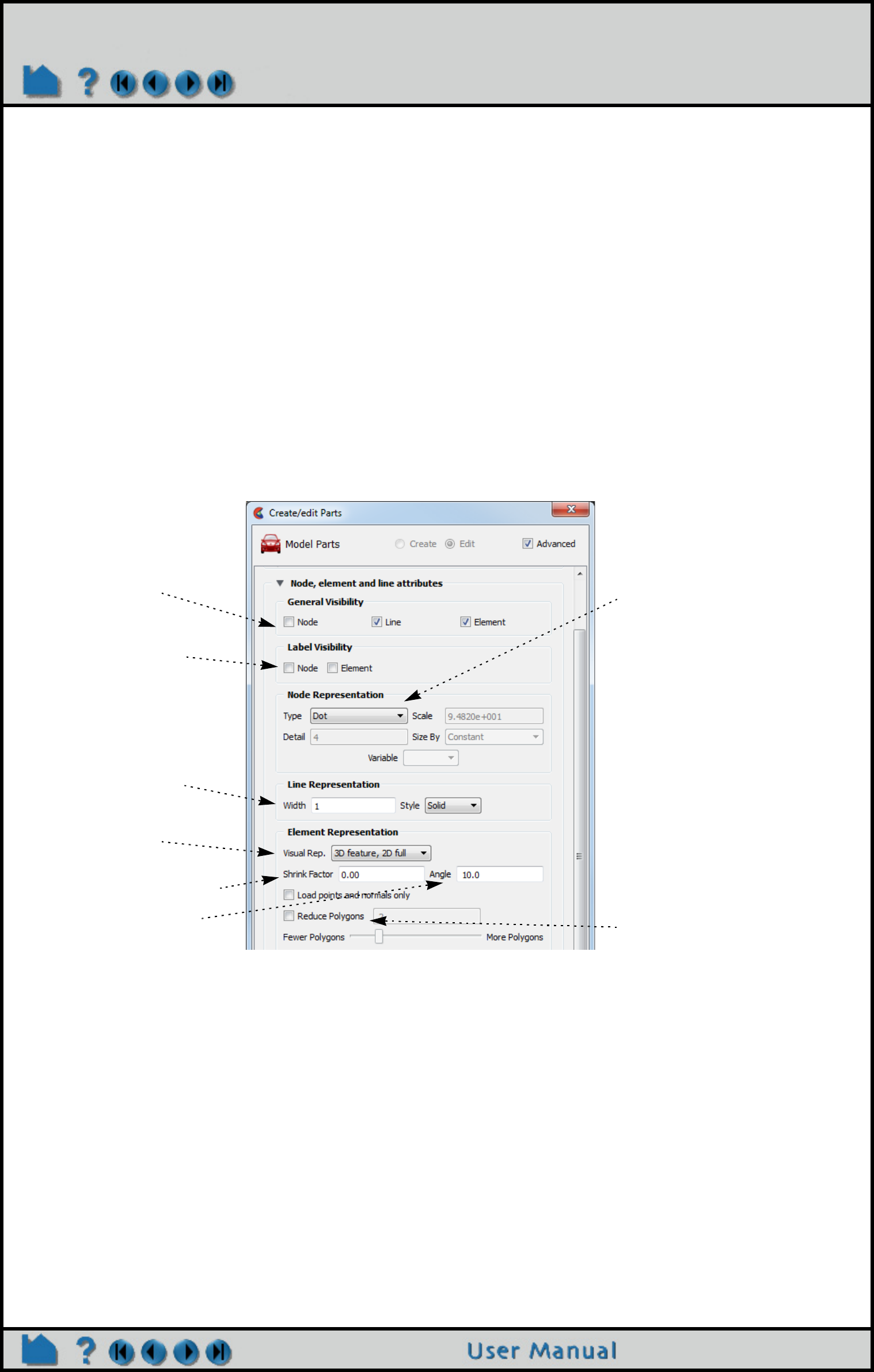
Page 437
HOW TO SET
Node, Element, and Line
Node, element, and line control how a part’s nodes and elements are displayed. Nodes can be displayed as dots,
crosses, or spheres. If displayed as crosses or spheres, the radius can be set by the value of a variable at that node.
To set using the Node, Element, and Line section:
EnSight provides five representation modes (and three combination modes) for parts (see also How To Change
Visual Representation):
Full Every face and edge of every element is displayed.
Border Only unshared faces (for 3D parts) or unshared edges (for 2D parts) are displayed.
3D Border, 2D Full Display 3D parts in Border representation; display 2D parts in Full representation. This is the
default representation for all parts.
3D Feature, 2D Full Display 3D parts in Feature representation; display 2D parts in Full representation.
3D nonvisual, 2D Full Display 3D parts in Non Visual representation; display 2D parts in Full representation.
Feature Angle Only those edges joining faces in the Border representation for which the angle between the
faces is less than some threshold are displayed. Feature Angle typically extracts the
topological features of interest in a model.
Non Visual No visual representation exists on the client. It is often useful to use Non Visual as the
representation for 3D computational domain parts – provided you also have some sort of shell
part to display the outer surface.
Bounding Box Displays a bounding box surrounding (and in place of) the nodes and elements.
Set visibility of nodes, lines,
elements
Set node/element label visibility
Set Line width and Style (Solid,
Dotted, or Dot-dashed)
Set element representation
(described below)
Set element shrink factor (shrink
elements toward the centroid)
Set angle for Feature Angle
representation
Set node representation
• Dot: nodes are displayed as
points.
• Cross: nodes are displayed as
crosses and can be fixed size
(size set by the Scale value) or
sized based on a variable (and
scaled by the Scale value).
• Sphere: nodes are displayed as
spheres and can be fixed size
(size set by the Scale value) or
sized based on a variable (and
scaled by the Scale value).
Sphere detail controlled by Detail
value. To avoid hanging up your
graphics card, first set your scale
using crosses, then turn on
spheres.
Set polygon reduction. Same
model, but simpler representation.
Trade-off of visual fidelity and
rendering speed.
1. Right click on the part name in the Parts list and choose ‘Edit’ or right click on the part in
the graphics window and choose ‘Edit’, or double click the part in the Parts list.
1. OR Select Create > part type.
By default, any changes you make to will take effect immediately. If you wish to “batch” a series of
changes turn on the “Delay update toggle at the bottom of the dialog. When you are ready to apply
a set of changes click the “Apply Changes” button.
2. Toggle the Advanced Toggle in the top right corner of the dialog.
3. Open the “Node, element, and line” turndown, then set the desired attribute(s):
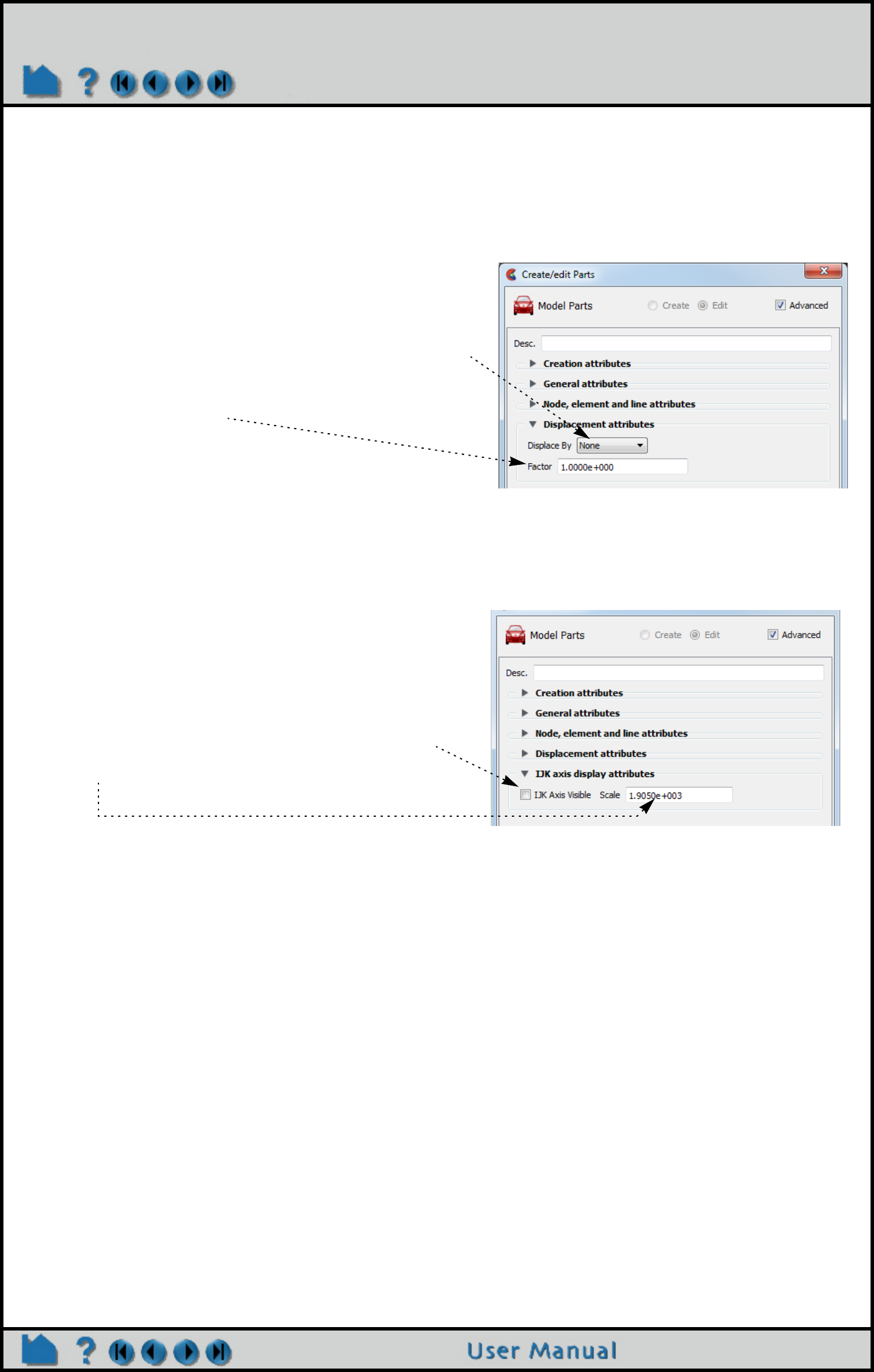
Page 438
HOW TO SET
Displacement
In structural mechanics simulations, a common output variable is a set of vectors representing the movement or
displacement of geometry. Each displacement vector specifies a translation of a node from its original position (an
offset). EnSight can display and animate these displacements to help visualize the relative motion of geometry. To set
Displacement (see also How To Display Displacements):
IJK Axis Display
Model Parts and clips (because they can be structured parts) will have these available. These will only be applicable
to structured parts.
SEE ALSO
Introduction to Part Creation
User Manual: Parts Quick Action Icons
1. Toggle the Advanced Toggle in the top right corner of the
dialog.
2. Open the “Displacement” turndown.
Set Displace By to either None (no displacement) or the vector variable to
use for displacement.
Set nodal displacement factor to reduce or exaggerate a displacement
1. Toggle the Advanced Toggle in the top right corner of the
dialog.
2. Open the “IJK axis display” turndown.
Toggle IJK Axis Visible to display an IJK axis for the part.
The scale factor for the IJK Axis triad can be modified in this field.
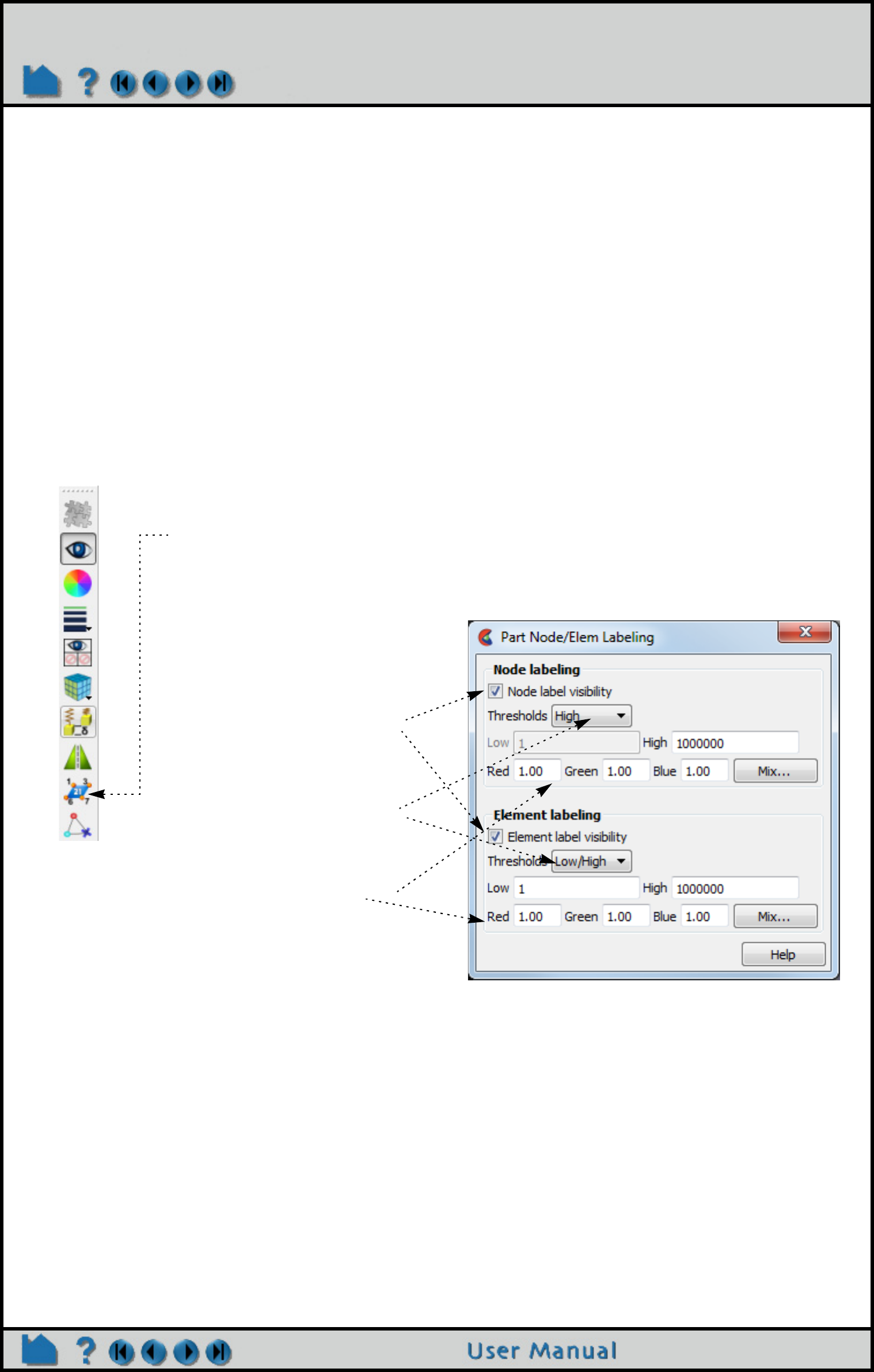
Page 439
HOW TO DISPLAY LABELS
Display Labels
INTRODUCTION
It is often useful to be able to identify specific nodes or elements within your model. EnSight can display node and
element labels in the Graphics Window. If your data provides explicit node or element labels (or you are using
EnSight data formats and have asked EnSight to assign ids), EnSight will be able to display those values. Only model
parts and clips through model parts can have labels.
Displaying labels on parts with thousands of nodes or elements can obscure both the geometry as well as the labels
of interest (as well as degrading display performance). EnSight provides a filtering mechanism to display only
selected ranges of labels.
BASIC OPERATION
Displaying Node and/or Element Labels
To display labels (and to control filtering and coloring):
1. Select the desired part(s) in the Parts list.
2. Click the Node/Element Label icon to display the Node/Element
labeling dialog.
3. Click the appropriate
toggle(s) to turn on/off node
and/or element labels.
4. To set filters for node/
element labels, select the
desired filter and enter the
appropriate values in the
Low and/or High fields.
5. Set the node/element label
color.
The label filters operate as follows:
None Display all labels.
Low Remove all labels < the Low value
Band Remove all labels >= Low and <= High
High Remove all labels > the High value
Low/High Remove all labels < the Low value as well as those > the High value.
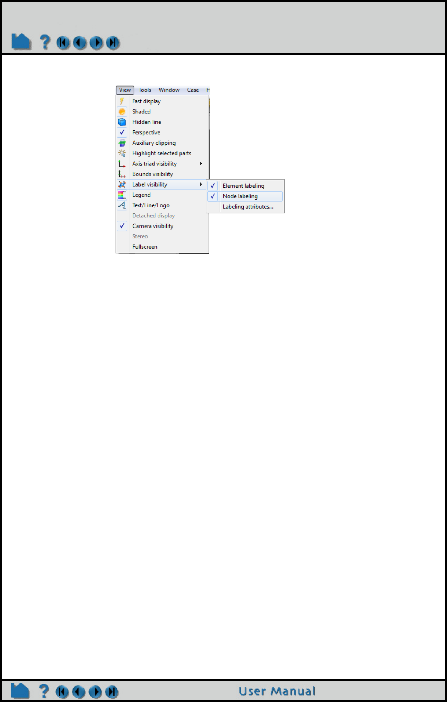
Page 440
HOW TO DISPLAY LABELS
Note that the Node and Element Label toggles also have counterpart toggles in the View Menu. These act as global
toggles that enable or disable any per-part node or element labels.
OTHER NOTES
Note that created parts (except clips through model parts) do not have node or element labels.
Note: The font size of the node and element labels can be modified under Edit > Preferences > Annotation. Simply
change the value in the 3D label size field and hit a return. If desired, this change can be made permanent for future
EnSight sessions by hitting the Save to preference file button.
Another useful technique for reducing label clutter is to use the front and back Z clipping planes to display only a thin
slice of interest. See How To Set Z Clipping for more information.
SEE ALSO
User Manual: Label Visibility
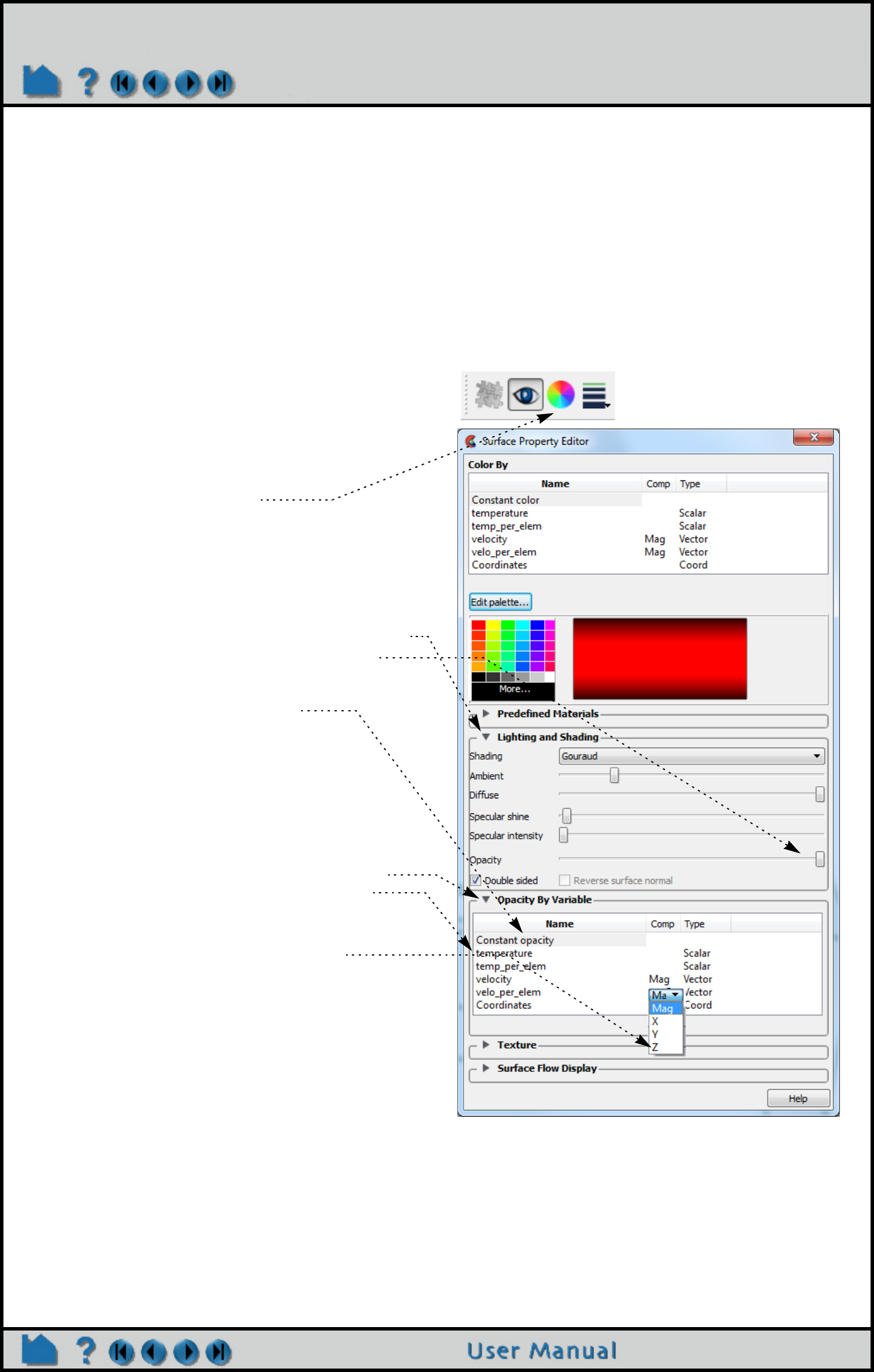
Page 441
HOW TO SET TRANSPARENCY
Set Transparency
INTRODUCTION
Transparency/Opacity can be turned on with one or other of the following methods:
BASIC OPERATION
SEE ALSO
User Manual: Part Transparency
How to Manual: Opacity by Variable (Transparency)
How to Manual: Lighting and Shading
Constant
(alpha)
Transparency is a single value applied over the entire part.
Variable Transparency (Opacity, or Alpha) varies according to a variable value.
1. Select the desired part(s) in the Parts List.
2. Click the Part color/surface property icon from
the Part Quick Action Icon Bar to open the
corresponding dialog.
For constant transparency:
3. Open the Lighting and Shading turndown and
move the Opacity slider (see Lighting and
Shading). If the opacity option is not shown,
then you must change the Opacity by Variable
to Constant Opacity.
The Part Opacity in the Graphics Window will dynamically
update as the slider is adjusted.
OR
For transparency that varies over the part surface
using variable values:
3. Open the Opacity By Variable pulldown and
select the variable of interest (see How to
Opacity by Variable (Transparency)).
For vector component, click on the comp column
“Mag” pulldown and select the component.
SHORTCUT
Right click on the part of interest in the graphics window
and select ‘Color by’ then choose ‘Make Transparent’ for a
quick 50% constant transparency, or choose “Adjust
transparency... to control percentage with a slider.
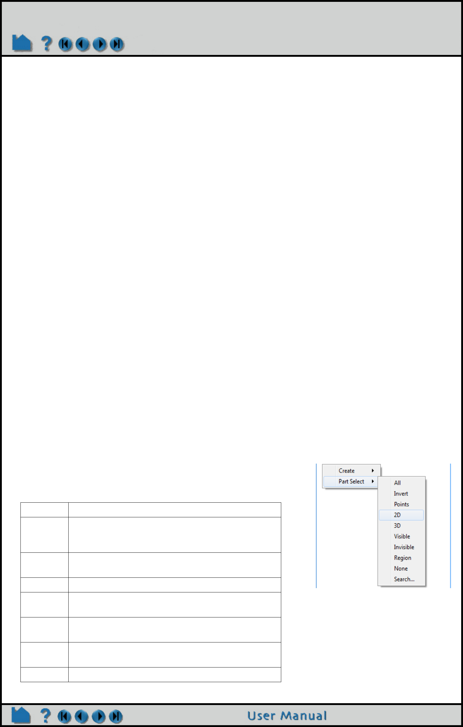
Page 442
HOW TO SELECT PARTS
Select Parts
INTRODUCTION
Manipulating parts is one of the fundamental operations in EnSight. Before you operate on parts, they must be
selected. Parts can either be selected through standard mouse interaction with the items in the Parts list or selected
by picking parts in the Graphics window.
BASIC OPERATION
Selecting Parts in the Graphics Area
Left click on the part in the graphics window to select it. Use control key to select multiple parts.
Selecting Parts using the Parts List
Items in the Parts List itself are selected using standard selection methods:
Selecting Parts using the Right click Select... Options
There are several other useful options for selecting parts available from right clicking in the part list or the graphics
window.:
To ... Do this ... Details ...
Select an item Select (or single-click) Place the mouse pointer over the item and click the left mouse
button. The item is highlighted to reflect the “selected” state.
Extend a selection Shift-click Select the first item. Place the mouse pointer over the last item in
the list to be selected. Press the shift key and click the left mouse
button. This action will extend a selection to include all those
items sequentially listed between the first selection and this one.
Extend a non-contiguous
selection
Control-click Place the mouse pointer over the item. Press the control key and
click the left mouse button. This action will extend a selection by
adding the new item, but not those in-between any previously
selected items.
De-select an item Control-click Place the mouse pointer over the selected item. Press the control
key and click the left mouse button. This action will de-select the
item.
Open the Feature Panel Double-click Place the mouse pointer over the item and click the left mouse
button twice in rapid succession.
1. Right click in the part list or the graphics window and select
Part Select from the list.
2. Select the desired option.
All Selects all parts in the list.
Invert Inverts the selection. Namely, all parts currently
selected become unselected and all unselected
become selected.
Visible/
Invisible
Selects all visible/Invisible parts.
2D/3D Selects parts that contain 2d or 3d elements
Region Selects all parts that are within the selection tool.
(Requires that the selection tool be on)
Showing Selects all visible parts which are showing in the
graphics window.
Search... Opens a dialog which allows for selections using
keywords and regular expressions.
None Unselects all parts.
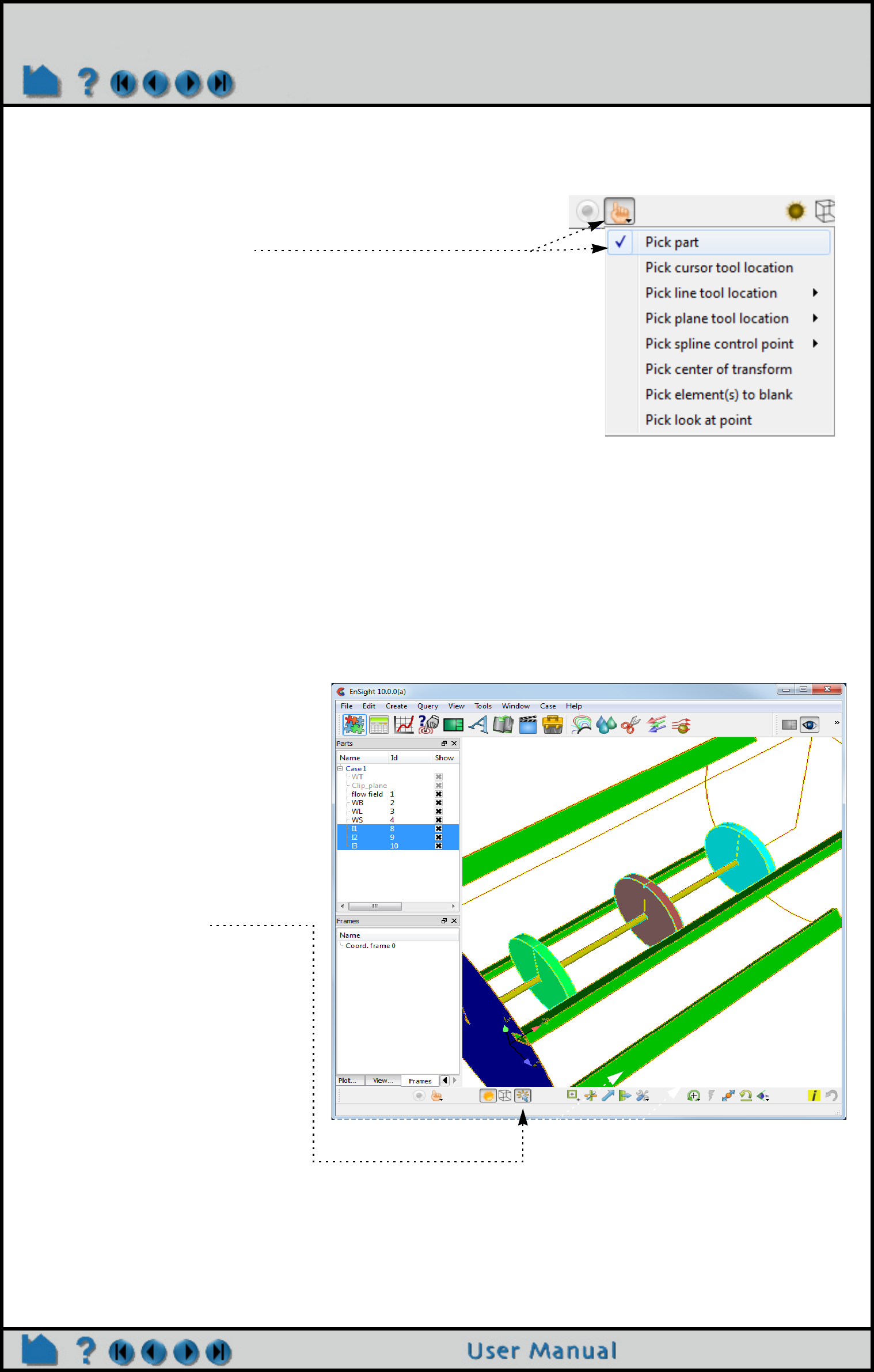
Page 443
HOW TO SELECT PARTS
Selecting Parts by Picking
Parts can also be selected by “picking” them in the Graphics window. To select parts by picking:
You must pick a part on a visible surface/line/point. Picking a part where the background is showing through (for
example, you are in line mode and you pick on the center of an element) will not pick the part.
By default, when you press the ‘p’ key any previously selected parts are de-selected. Holding down the Control key
as you hit ‘p’ modifies this behavior: if the picked part is not currently selected, it will be added to the existing selection
(so you can select multiple parts by picking), otherwise the picked part is de-selected.
OTHER NOTES
1. From the Pick pulldown icon on the Tools Icon Bar, select
Pick Part. (Note that this is the default, and this setting will
be retained until explicitly changed.)
2. Position the mouse pointer over the desired part in the
Graphics Window and press the ‘p’ key (or perform the
mouse action which has been set to “Selected pick action”
in Edit > Preferences > Mouse and Keyboard).
See below regarding how parts are identified.
Note that the picked part is now selected in the Part list.
1. By default, parts selected in the
part list are shown highlighted
by the highlight color and
transparency.
2. A global toggle turns this on
(default) and off
To modify the select/unselect
highlighting preferences open
Edit->Preferences->View and
set new settings.
3. Unselected parts are also
modified according to the
unselected color and
transparency.

Page 444
HOW TO SELECT PARTS
ADVANCED USAGE
Part tagging and selection
EnSight supports the concept of part 'tagging'. A tag defines a collection of parts, which can be useful for large
numbers of parts. One part can be a member of more than one tag. The current selection can be used to create a tag
and a tag can be used to set the current selection. This allows the user to quickly store and recall selections of
arbitrary complexity. EnSight pre-defines a set of ten tags. These correspond to the number keys: 0-9. By default, no
parts are members of any tags and any part can have multiple tags (e.g. a part can be a member of tags 0, 4 and 5).
Part tags are saved in context, session and archive files. They are not stored in command language files, although
command language does exist to specify membership in a tag.
Defining a tag from the current part selection
EnSight uses 'Alt' and the number keys (0-9) to define a tag from the current selection. To tag a collection of parts
(marking that selection for easy recall later) do the following:
1) Select any part(s)
2) Press Alt# where '#' is a number key from 0-9
First, the tag is cleared for all parts and then the selected parts are tagged with that key. On Windows and Linux, the
details of the new tag are displayed in the status bar.
Using a tag to recall a stored part selection
EnSight uses 'Ctrl' (Window/Linux) or (OSX) and the number keys (0-9) to reset the current selection to the set of
parts with the matching tag. To recall a tag and set the current part selection to the parts with that tag:
1) Press 'Ctrl'# or #, where '#' is a number key from 0-9.
The previous part selection is cleared and the all of the parts tagged with the matching key are selected. This allows
one to very rapidly recall a previously tagged selection.
EnSight Python Implementation details
Tagging is stored on each part through the Python METADATA attribute on the part objects. The pre-defined
METADATA keys are 'ENS_PLIST_KEY_SEL_#', where # is a digit from the set '0-9'. Check on the membership in
the tag using code as follows:
test = ensight.objs.core.PARTS[0].METADATA.get('ENS_PLIST_KEY_SEL_1',0)
The above will return whether the first part in the partlist is a member of tag '1'. Likewise, one can set/unset
membership in the tag using the following:
ensight.objs.core.PARTS[0].setmetatag('ENS_PLIST_KEY_SEL_1',1)
and the following to unset:
ensight.objs.core.PARTS[0].setmetatag('ENS_PLIST_KEY_SEL_1',0)
(see EnSight Python Interpreter).
Note that these last two examples are also valid command language and can be placed in command (.enc) files as
well.
Finally, since the tagging system is based on the part metadata infrastructure, one can also set the tag membership
directly from a reader using the metadata schema (see https://sites.google.com/a/ensight.com/ensight-python-api/
metadata for more details).
SEE ALSO
User Manual: Part List Panel
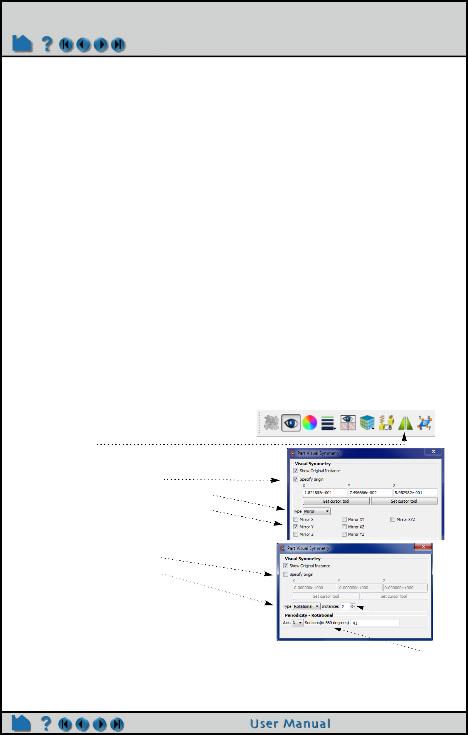
Page 445
HOW TO SET SYMMETRY
Set Symmetry
INTRODUCTION
In many instances, a modeler can take advantage of symmetry present in a problem to reduce the computational
complexity of a subsequent analysis. EnSight can impart visual realism to such models by mirroring parts around any
or all axes of the part’s reference frame or performing rotational symmetry about any of the axes. Although the
mirrored or rotated portions appear identical to the source part (except for the reflection or rotation), they are only
visual (client-based) and cannot be used for calculation. For example, you cannot start a particle trace in one half of
a mirrored model and expect the trace to cross the plane of symmetry into the other half (although you can make the
particle trace part symmetric as well).
EnSight also provides “true” or “computational” symmetry operations (mirror, rotational, translational) as an attribute
of the part’s reference frame. This option creates the symmetry instances as actual data on the server. Thus, with
computational symmetry, you can trace particles across a periodic boundary.
There now exists an option for rotational periodicity, where one can have particle traces exit a symmetry surface and
re-enter on the corresponding symmetry surface and continue. This does not require the creation of additional
geometry on the server (like computational symmetry does), but does require some additional information to be
included in the Part Visual Symmetry dialog (see below) - along with the setting of a toggle in the Trace creation
dialog. See the Periodic Trace section in the How To Create Particle Traces.
Both types of symmetry (visual or computational) are based on the part’s reference frame. Although you can use
simple visual or computational symmetry without having to manipulate the frame, more advanced usage of symmetry
could require a working knowledge of frames. See How To Create and Manipulate Frames for more information.
BASIC OPERATION
Visual Symmetry
Visual symmetry is an attribute of parts. You can enable display of a mirrored copy of a part into one or more of the
seven octants of the part’s reference frame. You can also enable display of a number of rotational instances about the
x, y, or z axes of the part’s reference frame. You can specify an origin for the symmetry. To display visual symmetry:
3. Specify the origin, if necessary.
4. Select Mirror from the Type pulldown menu.
5. Select the desired octant(s) from the menu.
Visual Mirror Symmetry:
Visual Rotational Symmetry:
3. Specify the origin, if necessary.
4. Select Rotational from the Type
pulldown menu.
5. Set the number of instances to
display.
1. Select the desired part(s) in the Main Parts list.
2. Click the Visual Symmetry icon from the Part Quick
Action Icon Bar.
Note that for rotational periodicity only, the additional section
entitled “Periodicity - Rotational” will be shown. Some additional
per part information is required if you are using periodic traces. Here you will specify the rotational
periodic axis and the number of sections (instances) which will make 360 degrees. Follow the link to
the traces How To that is specified above (or in the See Also section below).
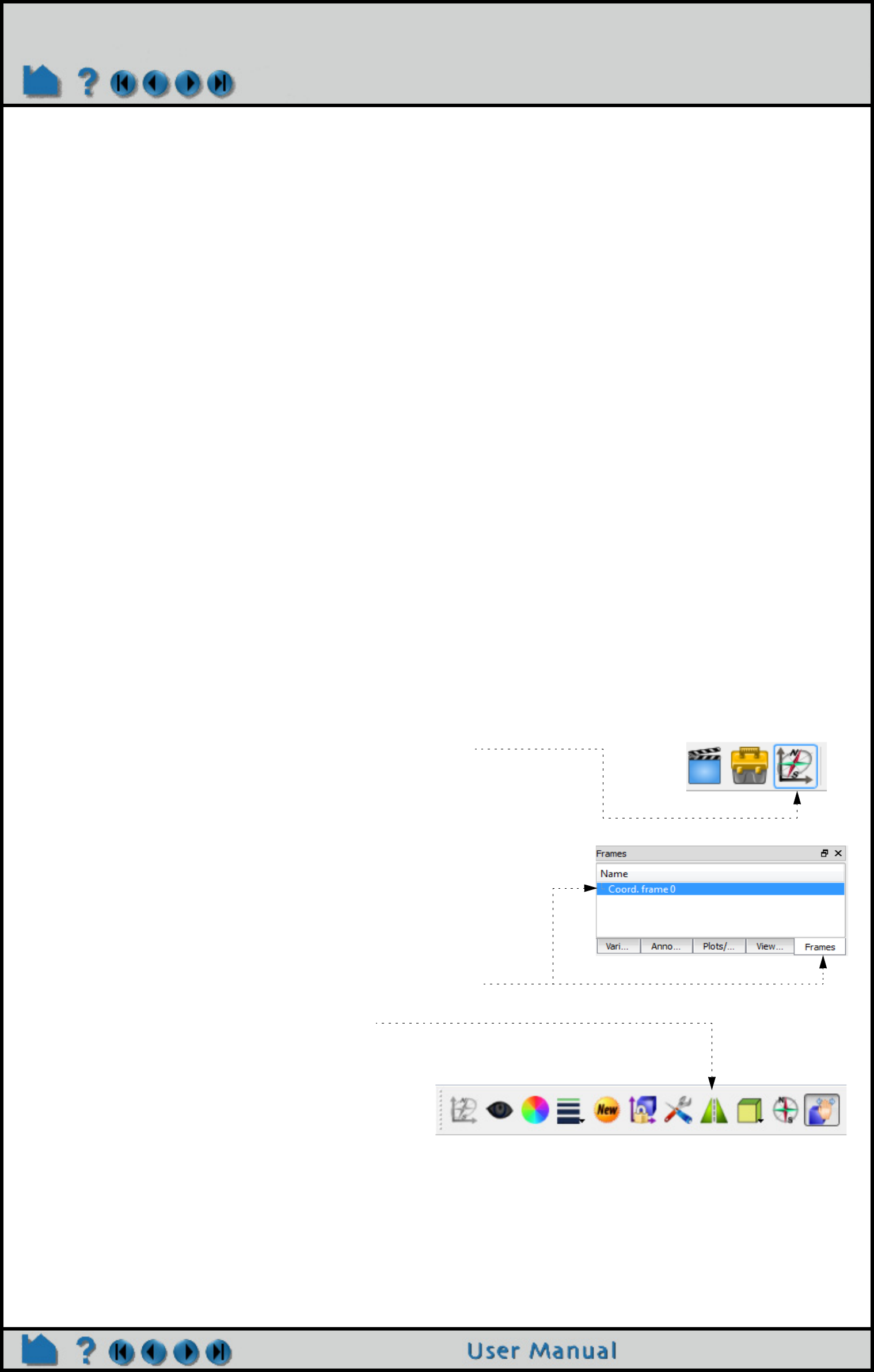
Page 446
HOW TO SET SYMMETRY
Recall that symmetry is performed with respect to the reference frame of the part. The frame’s origin and axes define
the partitioning of space into the octants that attached parts are mirrored into, or the rotational axis. If the symmetry
operation did not produce the desired effect, it is probably due to the fact that the part’s frame is not located/aligned
on/with the plane of symmetry, or the rotational symmetry axis, as designed for the model. The solution is to create a
new frame, assign the part(s) to the new frame, and position the frame such that two of its axes lie in the plane of
symmetry, or one of its axes align with the rotational axis. There operations are discussed in How To Create and
Manipulate Frames.
Visual Symmetry Specify Origin
If the Specify Origin toggle is off, then the origin of your rotation axes is the part reference frame origin. However, If
you toggle on the Specify Origin, then this is the origin that will be used (instead of the reference frame origin), and
the reference frame of the part will only be used for the direction of the axes. Note that the origin is specified here in
global coordinates. Specifying the origin in this manner is useful if your axes are aligned properly with your model, but
you just need the origin to be moved and don’t want to go to the trouble of creating, moving and then assigning a new
frame to your part(s).
Computational Symmetry
Computational symmetry can be used for unstructured and structured model parts with periodic boundary conditions.
(Note, it does not work for created parts.) Computational symmetry can handle rotational, translational, and mirror
symmetry. Unlike visual symmetry, computational symmetry actually produces the symmetric geometry and variables
on the server - allowing for more than just visual symmetry.
You enable computational symmetry by selecting the frame, specifying the type (Mirror, Translational, Rotational),
and setting type specific (such as the rotation angle and the number of instances to create). Each part assigned to
the frame will be updated on the server to reflect the specified symmetry.
Note that each new instance of a part created through computational symmetry creates a new part on the server.
To use computational symmetry, you will need to enable the Frame feature if it isn’t already enabled. Then:
1. Window>Toolbars/Panels>Frames OR Click the Frame
feature from the Feature Icon Bar. If you do not see this
option you will need to turn it on by right clicking in the
Feature Icon Bar to Customize the ribbon to show the
Frame feature.
2. If the default frame (frame 0) is not correctly positioned
for the desired symmetry operation, create a new frame,
position the frame in the proper location and
orientation, and assign the part(s) to the new frame.
(See How To Create and Manipulate Frames for details.)
3. Click the Frame tab then select the desired frame to edit.
4. Click the Computational Symmetry Icon.
The remaining steps depend on the type of symmetry
desired.
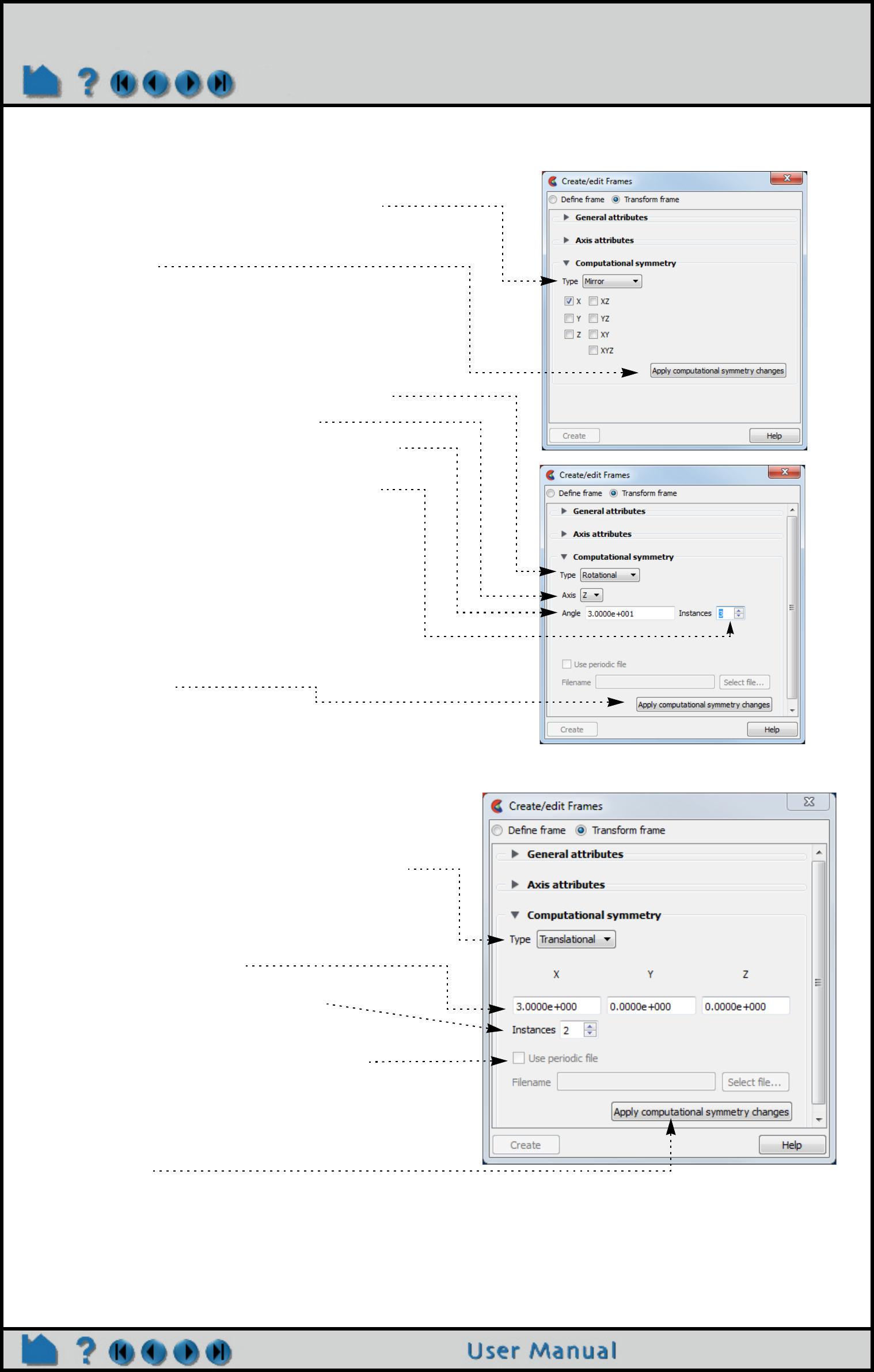
Page 447
HOW TO SET SYMMETRY
Mirror Symmetry is similar to graphical symmetry as
described above.
5. Set the Type to Mirror and set the desired
octant(s).
6. Click Apply.
Rotational Symmetry creates instances by rotating,
around the selected axis of the frame, the specified
number of degrees. The selected frame’s axis must
be aligned with the desired symmetry axis.
5. Select Rotational from the Type pulldown.
6. Select the frame rotational axis.
7. Set the desired rotation angle (in degrees) in
the Angle field.
8. Set the desired number of instances in the
Instances field (number 1 is the original, set
Instances to 2 to yield one copy).
9. If a periodic match file is available, toggle Use
Periodic File and enter the file name.
Periodic match files are discussed below. Note that
this toggle will be grayed out and unavailable for
Case and Case Gold formats because the periodic
match file name is entered into the Case file.
10. Click Apply.
Translational Symmetry creates instances in the
direction of the specified translation vector (using the
frame to get the x, y, z directions).
5. Select Translational from the Type pulldown.
6. Enter the desired translation vector in the XYZ
fields and press return.
7. Set the desired number of instances in the
Instances field (number 1 is the original, set
Instances to 2 to yield one copy).
8. If a periodic match file is available, toggle Use
Periodic File and enter the file name.
Periodic match files are discussed below.
9. Click Apply.
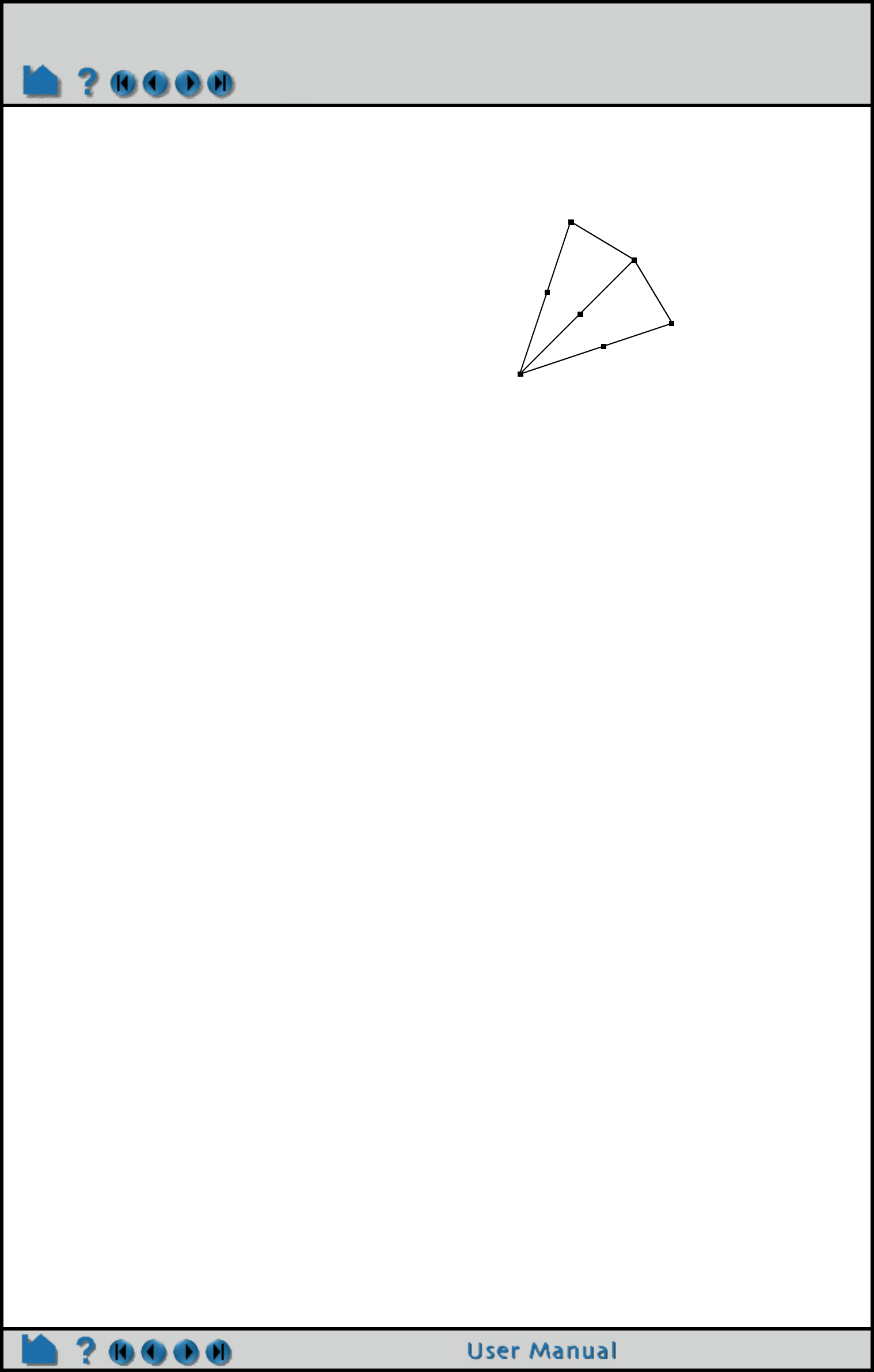
Page 448
HOW TO SET SYMMETRY
Periodic Matching for Computational Symmetry
When a model is created with periodic boundary conditions, there is typically a built-in correspondence or “match”
between certain nodes and elements. For example:
When instances are added to a part, it is desirable to eliminate these duplicate nodes. Without a match file, EnSight
will attempt to find and remove them using a hashing scheme. This method works quite well, but may not find all
duplicates. (Remaining duplicates are usually noticed when the part is in feature angle representation since EnSight
treats elements with duplicate nodes as separate – even if they are coincident.)
Note that if you have a periodic match file you do not need to specify the rotation axis and angle in the Frame
Computational Symmetry dialog – the value is provided in the file.
A user-supplied matching file can be used to quickly find and remove all duplicates. The match file is a simple ASCII
text file. The file for the example above would be (the text in italics is not part of the file):
rotate_z specifies rotational symmetry and the applicable axis
52.34 the angle of rotation (in degrees)
3the number of node pairs to follow
1 1 first node pair
2 6 second node pair...
3 7
See Periodic Match File for more information on periodic match files.
SEE ALSO
How To Create and Manipulate Frames
How To Create Particle Traces
1
2
3
4
5
6
7
The elements defined by nodes 1,2,3 and nodes 1,6,7 should
match when rotated about an axis passing through node 1
(perpendicular to the screen). When another instance is
created, node 2 matches with 6 and node 3 matches with 7.
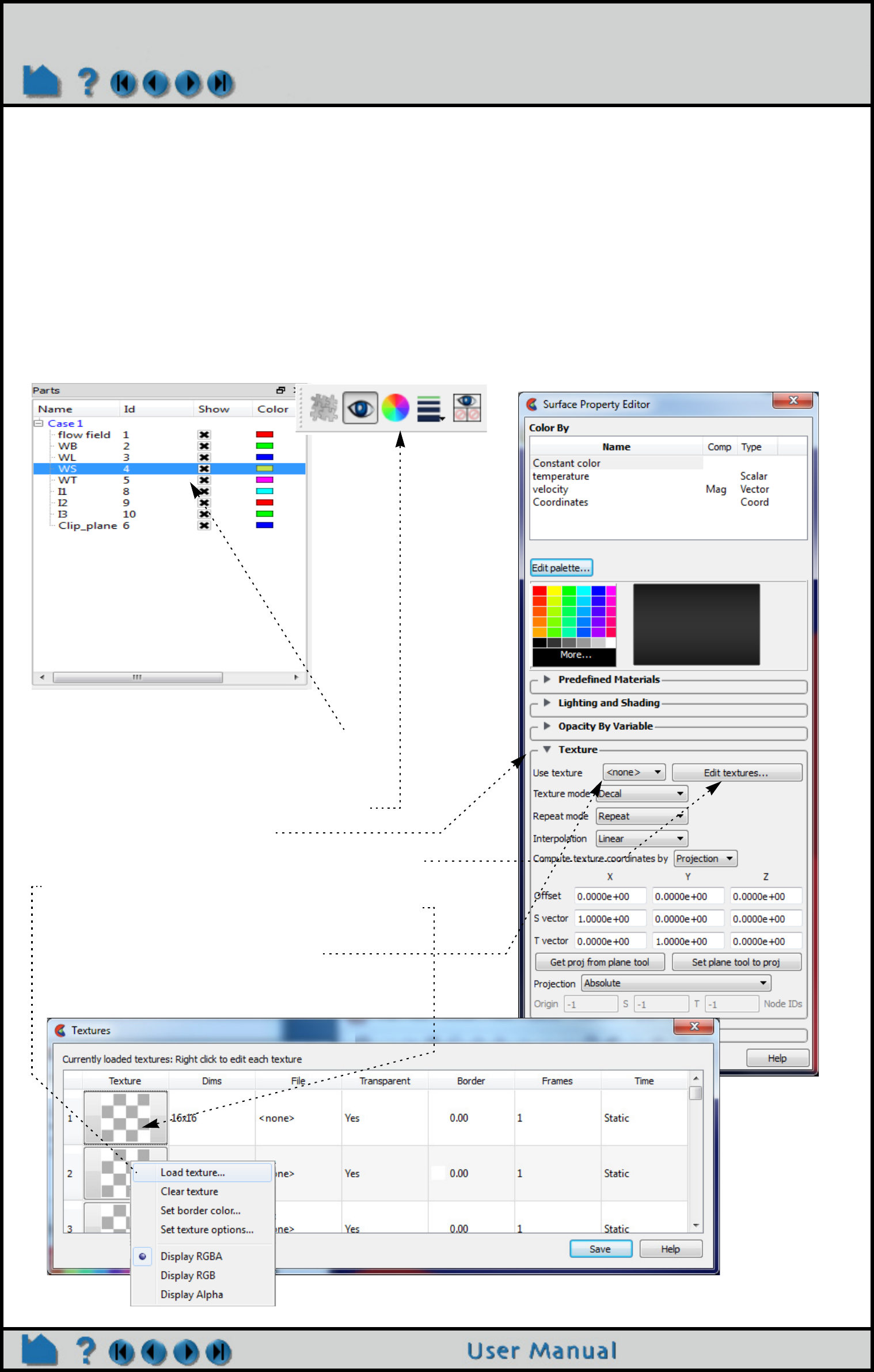
Page 449
HOW TO MAP TEXTURES
Map Textures
INTRODUCTION
Texture mapping is a mechanism for placing an image on a surface or modulating the colors of a surface by various
manipulations of the pixels via a texture map image. EnSight supports the application of a texture onto a part and the
combining of texture effects with the normal EnSight coloring schemes. This can include animated textures(e.g. EVO
or MPEG files), which can be used to texture parts and 2D annotations.
The simplest use is to place a "decal"/logo or photograph on the surface of a part. Texturing can also be used to add
repeated patterns, provide custom transparency and lighting, color a part by multiple variables and clip parts to
arbitrary boundaries. A texture operation in EnSight consists of a texture map image, a collection of interpolation and
blending options and a mechanism for projecting the texture map image onto a part. Each of these items is described
in the following sections. Shown below is a quick overview from the Surface Property Editor to add a texture.
Putting a logo or image on Part(s)
1. Select the desired part(s) in the Main Parts
List.
2. Click on the color wheel icon at the top to open
the Surface Property Editor dialog.
3. Pulldown the Texture.
4. Click on Edit textures to open Textures dialog.
5. In the Textures dialog, right click on Texture
and choose Load texture... to load an image from
file, to be used as a texture.
6. Pick a texture number to apply.
see How to Set Surface Properties
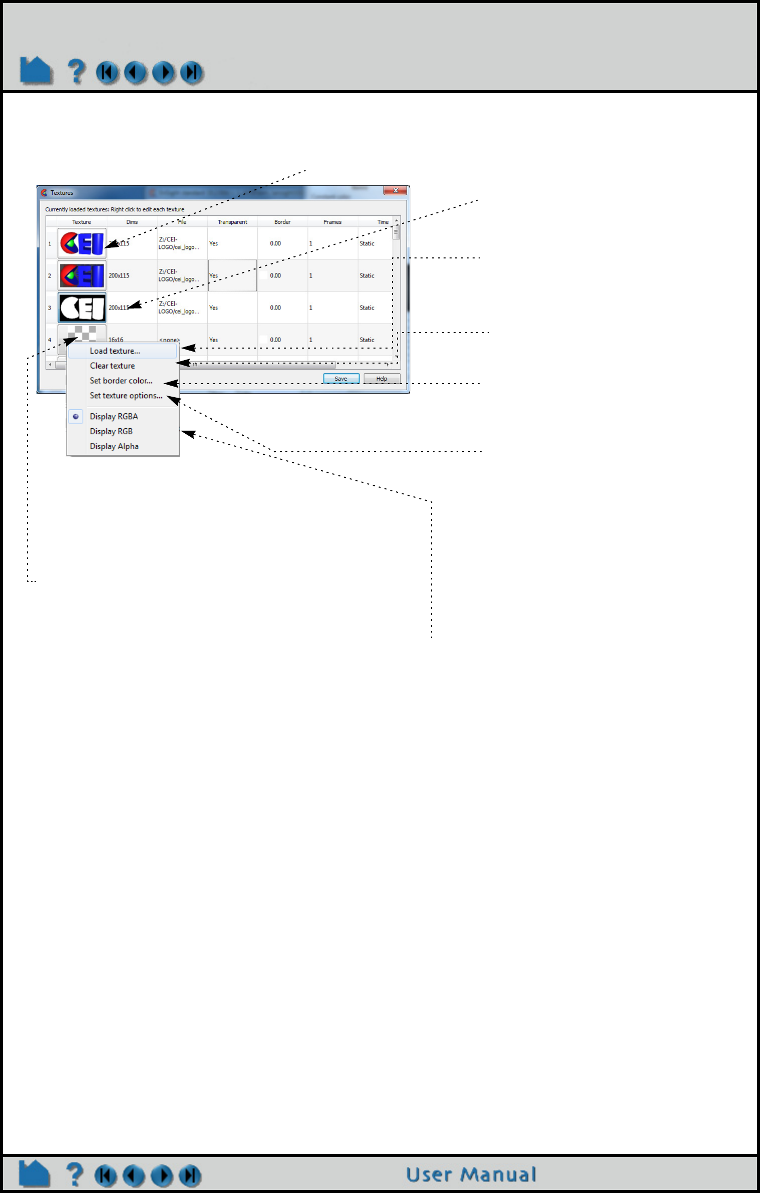
Page 450
HOW TO MAP TEXTURES
Setting the texture map image
A number of operations can be
performed on the textures by right-
clicking on the thumbnail image and
selecting from the menu.
A new image or movie (e.g. EVO,
MPEG, etc.) can be set for the texture
using the 'Load texture file…' option.
A texture can be reverted back to the
16x16 transparent checkerboard
default pattern using the 'Clear texture'
menu.
Each texture has a border color that is
used for colors outside of the texture
bounds. This color (RGB and opacity)
can be set explicitly using the 'Set
border color…' menu.
Advanced options for loaded texture
images and animations can be set
using the ‘Set texture options...’ menu
(see Texture options section below).
The basic information for the currently
selected texture is displayed in the text
field below the thumbnails. The size of
the texture, its source, border color and
the nature of its transparency (A channel
and border color) is displayed.
All textures have both a color (RGB) and an opacity (A) component. By default, the thumbnail
is drawn using the full RGBA pixel value. Options at the bottom of the right click menu allow the user
to select which channels to draw: Display RGBA, RGB, or Alpha. The first three images in the
example dialog above are all the same texture, but drawn with a different function.
The the first image is the full RGBA image,
the second one is just the RGB part of the image
and the third one is just the A part of the image.
Notice how the A channel masks out the black and white pixels in the RGB image. This masking can
be used to place non-rectangular images/icons on EnSight parts.
Users often make use of a common set of textures for many different analyses (e.g. company logos,
standard palettes, etc). The 'Save' button allows the user to save the currently loaded selection of
textures and their display mode into the user's preferences directory. These will be automatically
loaded every time EnSight is launched.
EnSight supports up to 32 different textures, which are displayed as
thumbnails down the Texture column in Textures dialog.
The 32 textures are numbered one
through 32. Each part in EnSight can
have one of the 32 texture associated
with it. This can be done by selecting
the part(s) and either clicking on the
appropriate button thumbnail or
selecting the number from the 'Use
texture' option menu.
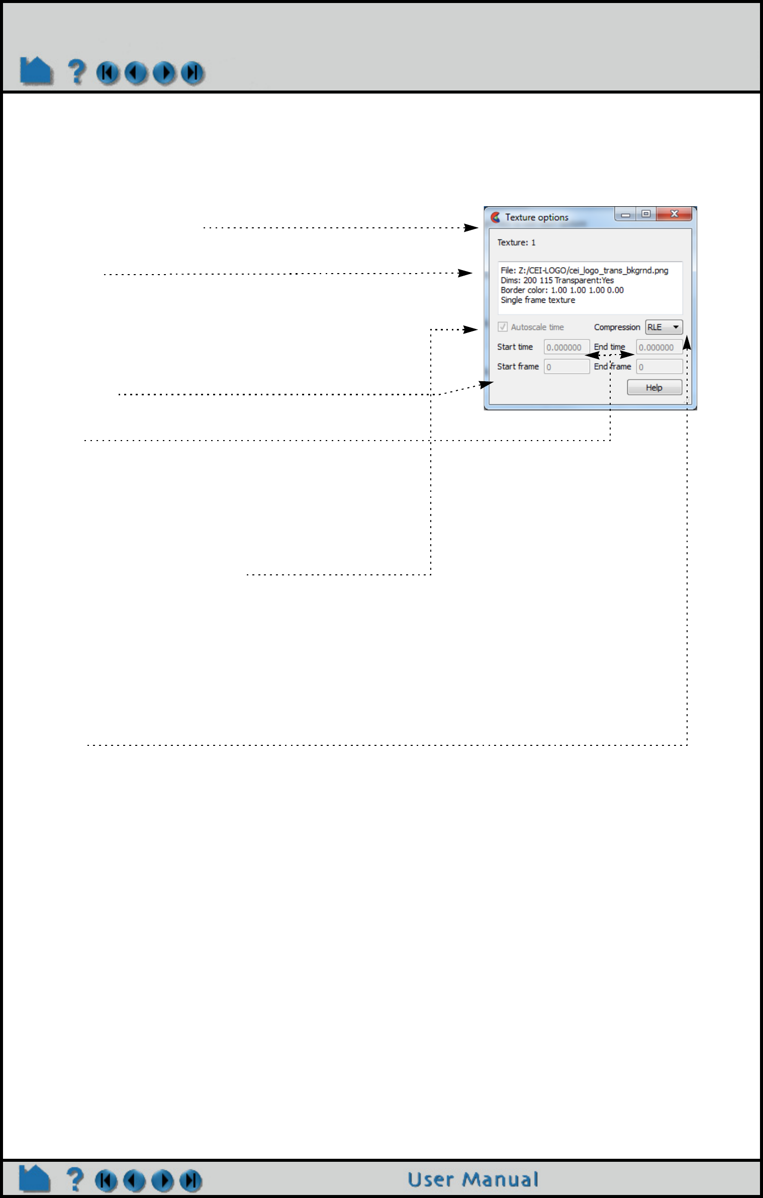
Page 451
HOW TO MAP TEXTURES
Setting Texture Options
In Ensight, animated textures (e.g. EVO or MPEG files)
can be used to texture parts and 2D annotations. Each
animated texture is linked to the current solution time in
EnSight. This temporal mapping can be set by right-
clicking on the logo, choosing “Set texture options” to see
the Texture options dialog.
Basic information about the texture is presented in the
upper pane.
This includes the filename, border color, dimensions, and
number of frames in the texture. It also includes temporal
reference information for animated textures.
Animated textures have a start and ending frame number.
These can be used to “crop” the texture to some subset of
the animation.
There is also a starting and ending solution time for the
texture.
The frame from the texture is selected such that the
starting frame number is used when the current EnSight
solution time is at or before the texture start time and the
ending frame is used when the current solution time is at
or after the ending time. The temporal mapping is linear
in-between.
There is also an “Autoscale” option.
If this option is set, the starting and ending time for that
texture will always be set to the dynamic range of currently
loaded EnSight solution times.
Note: EnSight will read the entire animation into memory
when it is loaded. If the movie is large, it can use a
significant amount of memory. In memory, EnSight uses
lossless compression schemes for the data. The current
scheme can be changed using the ‘Compression’ options
pulldown.
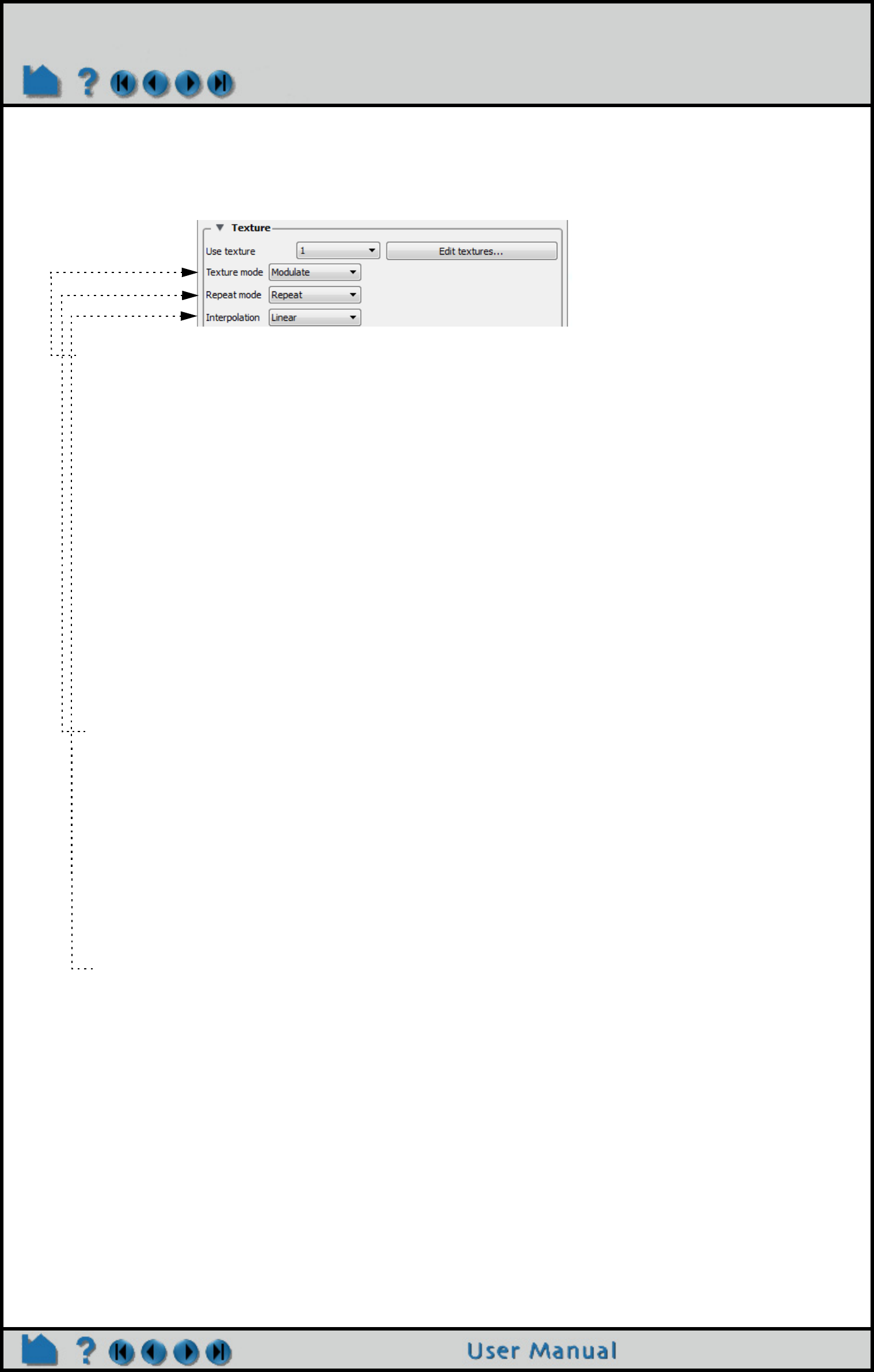
Page 452
HOW TO MAP TEXTURES
Texture operations and parameters
The Texture mode, Repeat mode and Interpolation scheme define how textures are accessed and how they are
integrated into the normal EnSight coloring scheme.
The Texture mode determines how a texture is combined with the natural coloring scheme in
EnSight. The pulldown has three options: Replace, Decal and Modulate.
In Replace mode, the base colors provided by EnSight are ignored and the
texture is used as the only source of color for the part (note, this has the side effect
of disabling any lighting).
In Decal mode, the alpha channel of the texture is used to select between the
texture color and the base color of the part. If the texture alpha value is 0, the base
color of the part is displayed, while locations where the texture alpha value is 255,
the texture color will be used exclusively. All alpha values in-between 0 and 255 will
result in an interpolation between the texture and base colors. Note that the default
texture uses an alpha channel with values 255 and 80.
In Modulate mode, the base color is multiplied by the texture color and the
resulting texture is used. Modulate mode is commonly used with a texture that has
a color of white and some pattern in the alpha channel. This allows the base color to
show through, but varies the transparency of the part. Arbitrary clipping operations
can be set up this way. Modulation of the color channels can be confusing as the
operation tends to suppress colors, but it can be used with a grayscale texture to
attenuate.
The Repeat mode allows the user to control how the texture repeats outside the texture
coordinates [0,1]. The pulldown has three options: Repeat, Clamp, or Clamp to texture.
In Repeat mode, the coordinates are repeated (e.g. a texture coordinate of
2.3 is mapped to 0.3) so that the texture repeats itself, and the border color is not
used.
In Clamp mode, coordinates outside of [0,1] are fixed to the border color of
the texture. If repeat mode is set to repeat, Clamping is often used for logos and
explicit texture coordinates (see Texture projections) that you wish to see only once.
In Clamp to texture mode, coordinates outside of [0,1] are fixed to the edge
value of the texture. The border color is not used.
The Interpolation scheme is applied when the graphics hardware needs to access a pixel in
the current texture. The pulldown has two options: Linear or Nearest.
Linear interpolation mode generally results in smoother looking displays, but
can result in "fringes" that are the result of interpolating to colors that might not exist
in the native texture. Linear can be slower, but in EnSight, this is often the result of
the fact that a part may be turned translucent and need to be sorted during
rendering (See Texture implementation limitations).
Nearest will result in the exact colors in a texture using the nearest neighbor
interpolation method. It is less smooth and has starker contrast.
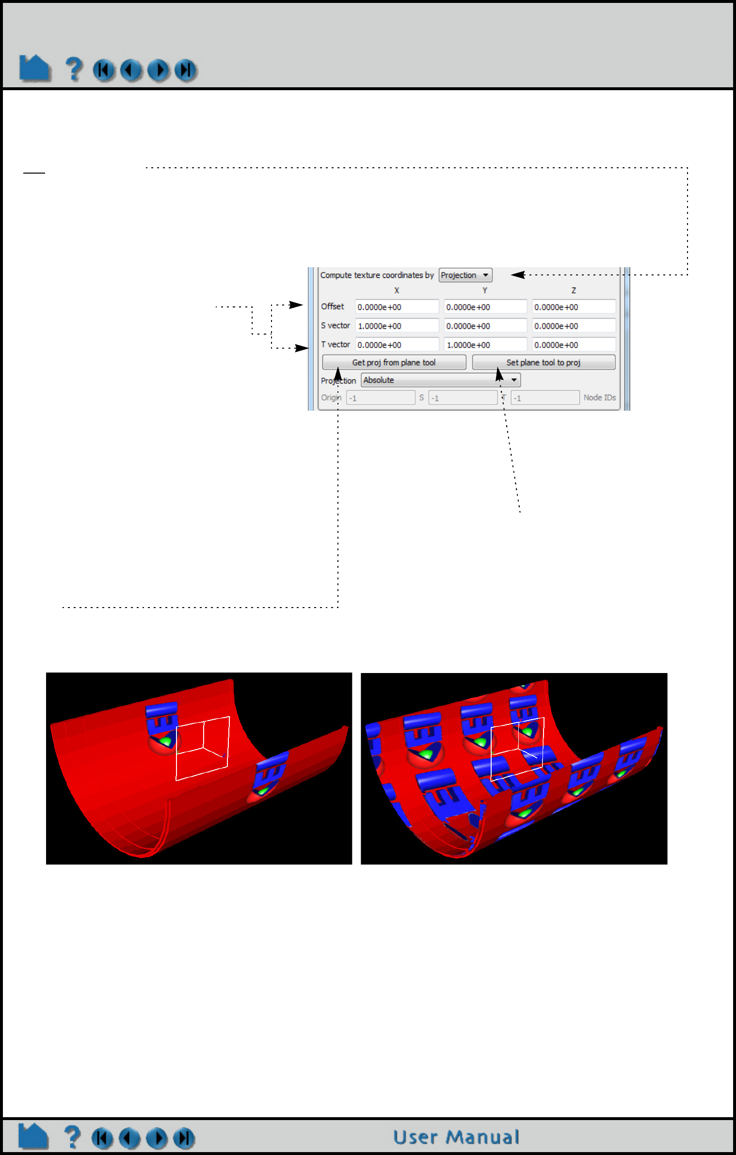
Page 453
HOW TO MAP TEXTURES
Texture projections
.
EnSight provides two mechanisms which may be used to define where a texture should appear on a part. The
first is by projection.
In this mode, it helps to think of the texture as a projected light-source, like a presentation projector, only
without divergence (i.e. the light lines are parallel). The user places the light source to shine through the
scene at some orientation centered at some point. Textures are not limited to the exposed surface in EnSight,
thus any surface that intersects the beam of light is textured.
The user can enter the values for this
projection in the "S vector", "T vector"
and "Offset" fields in the dialog..
These define a vector in the space of
the part that will correspond to the
directions of the X and Y axis of the
texture image as well as a point of
focus for the texture.
Perhaps the simplest method for setting
these values is to use the plane tool.
Place the plane tool in the view to
match the desired projection. The
texture will be scaled to fit in the
boundaries of the plane tool with the
texture axis aligned with the tool X and
Y axis. The texture itself is projected
along the Z axis of the tool. Once the
tool has been placed, click on 'Get proj
from plane tool' to fill in the dialog
fields.
The 'Set plane tool to proj' will move
the plane tool to the projection formed
by the current dialog values.
The example below illustrates the placement of a logo, in decal mode with clamp and repeat modes set. Notice
that the texture appears both in front of and behind the tool.
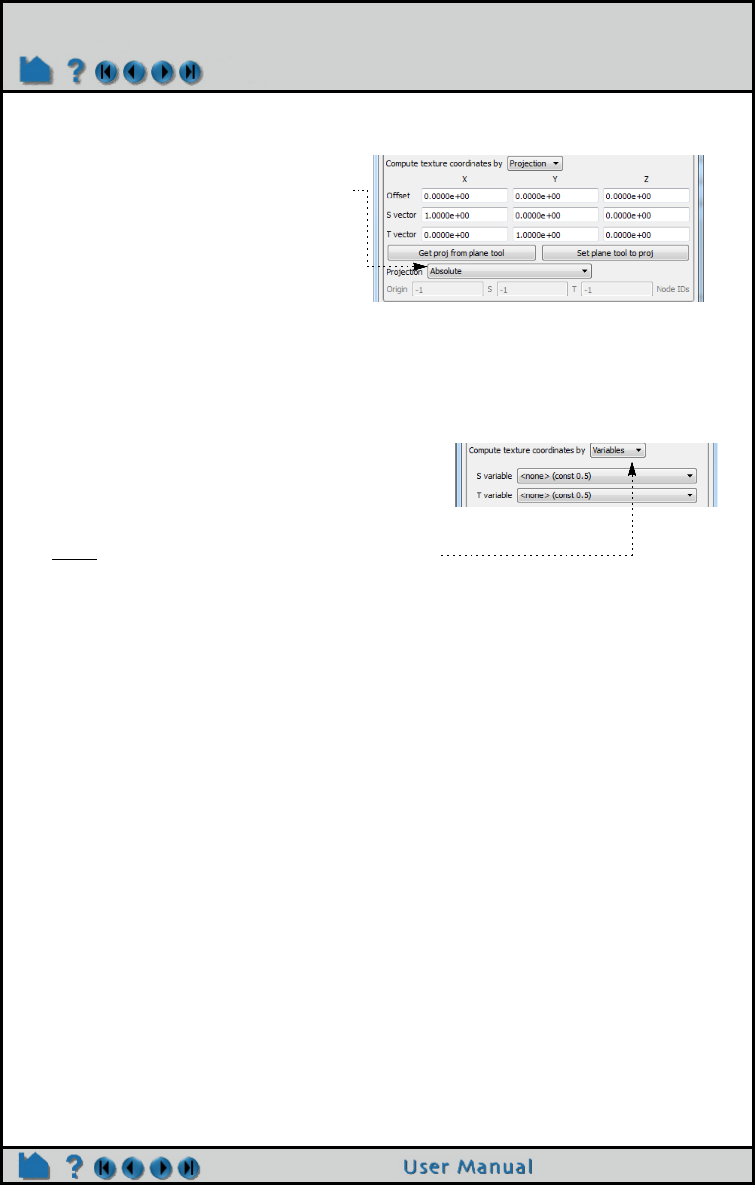
Page 454
HOW TO MAP TEXTURES
The texture projection can also be specified relative to a point or a
collection of points.
The Projection option menu in 'Absolute' mode will set
the texture projection to the current settings which
places the texture at an absolute position and attitude in
space. If the part geometry moves or deforms, the
texture remains fixed in the scene, thus it appears to
move on the part surface.
Choose Projection 'Offset relative to ID', to specify a
node ID in the 'Origin' field. The 'Offset' X,Y,Z values
are considered to be relative to this node ID. If it moves in time, the
texture projection will translate with this node.
Likewise, Projection 'Offset and S/T vecs relative to node Ids' allows
for three node Ids to be specified, causing the projection to rotate
and scale with the relative positions of those nodes.
If you turn on these relative modes, you may need to click 'Get proj
from plane tool' to set up the field values to match the plane tool
again (The get proj option always honors the current relative
projection and node IDs, if provided).
The second form of projection EnSight supports is via 'Variables'.
In this mode, one or two scalar variables are used to provide explicit S and T texture
coordinates for texturing. This is the most general mechanism for texturing. The S-variable
and T-variable option menus provide a list of possible scalar variables.
Users may also set the S and/or T value to the constant quantity 0.5. The variables are
generally in the range [0,1], which map to the edges of the texture map, just inside the border.
Values outside this range will either be mapped to the texture border color (in the case of
clamp mode) or will be warped back into the range of [0,1] by repeated subtraction/addition (in
repeat mode). This form of projection is capable of emulating the previous model. It also
makes it relatively easy to create two dimensional data palettes. Just like the existing palette
in EnSight, some function of a variable is used to select a color from a table. In this case, the
table is a 2D texture, so this can be done for two different variables at the same time, and the
opacity can be varied as a function of those variables.
All forms of EnSight part displays can be textured: surfaces, lines, points, etc. Of special note,
in "variable" mode, points are rendered with a single texture coordinate, regardless of the
form they are displayed as. Thus, a point displayed as a sphere can only use a single pixel
sample from a texture. Thus, to place a logo on a point rendered in sphere mode, one would
need to use 'projection' mode.
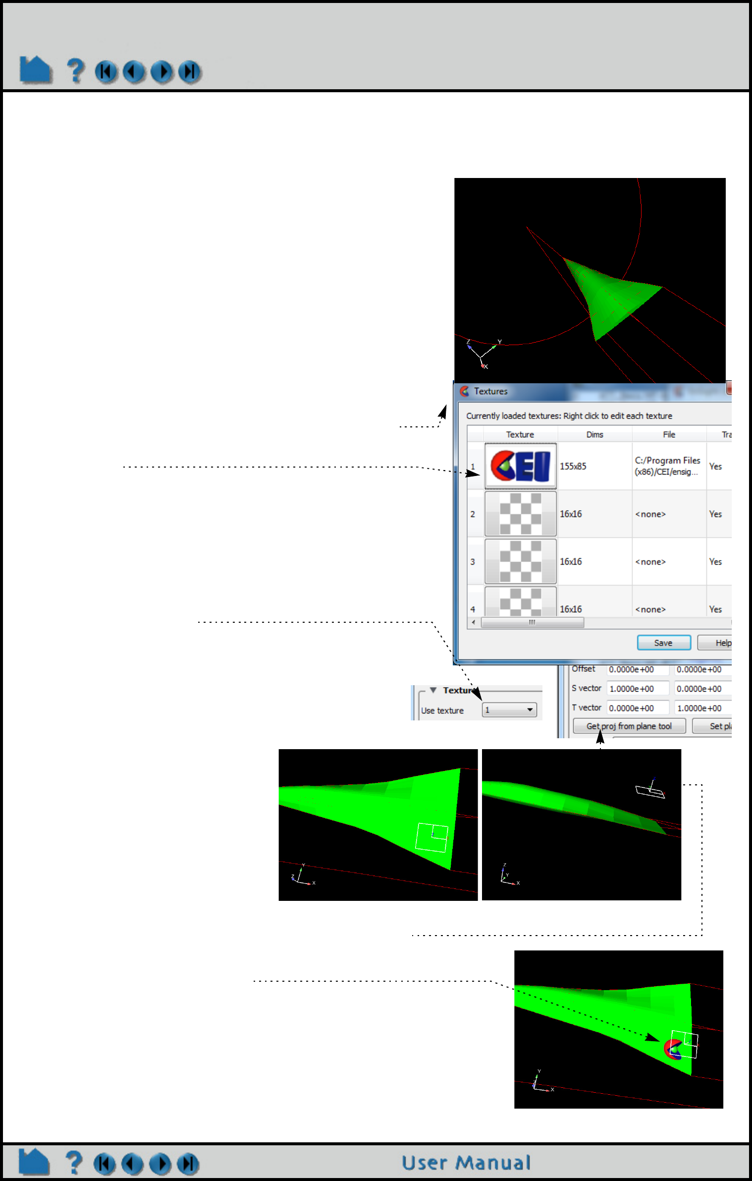
Page 455
HOW TO MAP TEXTURES
BASIC OPERATION
How to place a logo on a part
One common use of textures is to place a logo or "decal" onto
a part. This operation involves using a projected texture. This
is a simple three step process.
For this example we will use the AMI dataset which comes
with the EnSight.
1. Load the AMI dataset and set the display type to
shaded surface.
Orient the hypersonic body as shown and select it in the
part list.
2. Next we need to set up the texture map to use.
Select the color icon to bring up the Part Color/Surface
Property Editor dialog and turndown Textures, then click on
the Edit Textures… button to bring up the texture dialog.
Right click on the first texture button and select 'Load
texture file…'.
Browse to the image file containing your logo image.
A good example is the CEI logo found in CEI_HOME/
ensight102/doc/wiki.ensight.com/
cei_logo_png72.png. This image includes an alpha
channel that is zero outside of the logo pixels (the 'Display
Alpha' menu option will display only this channel').
Associate this texture with the part by selecting the part and
set Use Texture to 1.
The hypersonic body will get a tiling of CEI logos over it,
since we only want a single logo, change the Repeat mode
to 'Clamp' (the logos will likely disappear).
3. Finally, we need to set up the transform necessary to
place the logo.
Bring up the plane tool and size/
position it as illustrated:
The key here is to think of the plane
tool as a "flashlight" that shines down
the plane tool's Z axis and the light is
bounded by the plane rectangle.
Once you have the plane positioned, click on 'Get proj from
plane tool'.
The logo texture will now be displayed on the body at the
location specified by the plane tool.
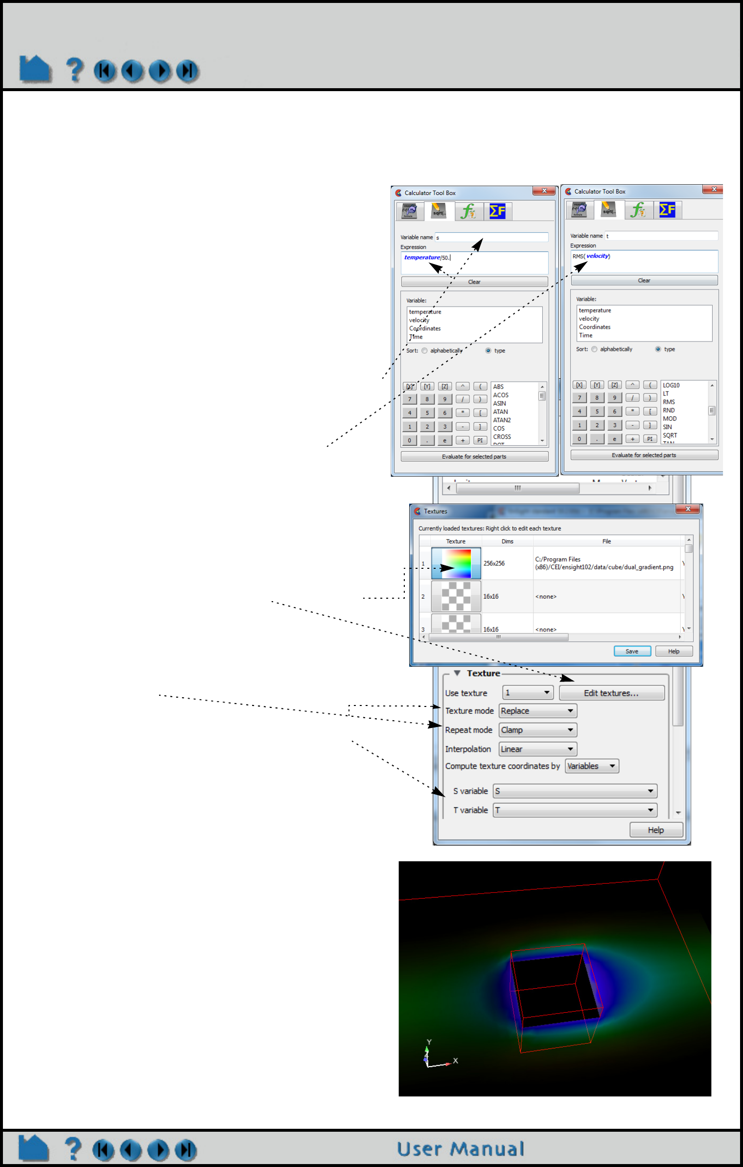
Page 456
HOW TO MAP TEXTURES
ADVANCED USAGE
How to use textures as palettes
EnSight textures can also be used as multi-dimensional
palettes to allow the user to control the color and opacity of
a part based on arbitrary functions of two variables. The key
to this technique is generating the appropriate texture map.
In the following example, we will use a texture map found in
the data directory with the "cube" model.
1. Load the cube model and bring up the variable
calculator.
We will need to create an "S" and a "T" variable that will
be used to access the texture.
2. In the calculator create a new variable named 'S' with
the expression 'temperature/50.0' (this puts 'S'
roughly in the range [0,1]).
3. Create a variable 'T' that is the expression
'RMS(velocity)'.
4. Create an xyz clip of the mesh as a 'Z' clip and turn
on shaded display.
5. With the clip_plane part selected, open the Part
Color/Surface Property Editor, Textures turndown,
and click on the Edit textures button. Load the file
'dual_gradient.png', included in the directory with the
cube dataset, into the first slot.
Notice that this texture is an opacity ramp along the X
axis and a color ramp along the Y axis.
6. Set the texture mode to 'Replace' and the repeat
mode to 'Clamp'.
7. Now, set the 'Compute texture coordinates by' option
to 'Variables' and pick 'S' and 'T' as the S and T
variable names.
The display will look like the image shown, depending on
the placement of the clip plane. The coloring is relative to
the Velocity of the field, while the opacity of the plane is
relative to the temperature of the plane. This type of
technique can be used with any two variables; the key is
generating a 2D texture map that is meaningful for
ranges of the two variables in question.
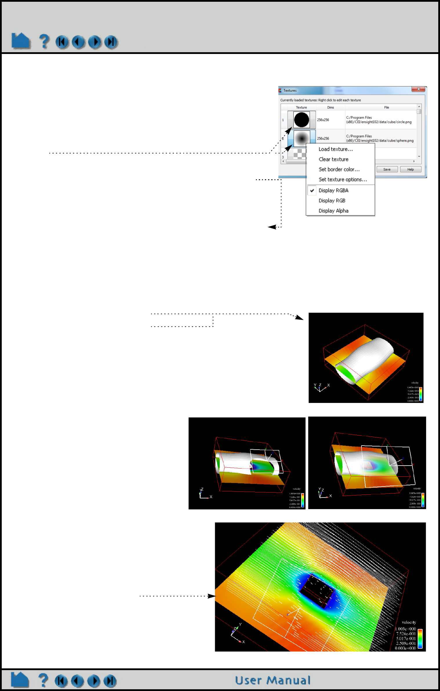
Page 457
HOW TO MAP TEXTURES
How to clip an object with a texture
Textures can also be used to manipulate the transparency of portions of
objects in interesting ways. In this example, a texture image with only an
alpha channel will be used to clip into a part to reveal parts inside of it.
1. Load the cube dataset again.
And as in the textures as palettes example:
2. Load the image files 'circle.png' and 'sphere.png' into two texture
slots.
In both cases:
3. Use the right mouse button menu to set the textures' border
color. Change the border color alpha channel value to 255 and
view only the alpha channel.
Notice that the RGB channels are white, but there is a dark region in
the alpha channel of the images.
4. Create an isosurface of temperature in the mesh as well as a 'Z'
plane clip.
5. Color the plane clip by velocity.
6. Now, select the isosurface part and much like the logo example,
use the plane tool to project the texture onto the isosurface.
In this case, use the circle texture and modulate texture mode and
set the repeat mode to clamp.
The texture will clip through the isosurface as
a projected circle (from the circle in the
texture) to view parts interior to it. The sphere
texture provides a smoother clip. Experiment
with other textures and repeat modes for
other effects. Remember that each part can
have its own texture, each with a different set
of projection settings for highly expressive
visual options.
Here is an example of a clipping texture applied to
dynamic particle traces. The tracer pulses are not
clipped, but the traces are clipped to a projected
circle texture as in the example.

Page 458
HOW TO MAP TEXTURES
OTHER NOTES
Texture implementation limitations
Texturing in EnSight is done using OpenGL and the multi-texture extension. If your graphics card/driver does not
support this extension, texturing will not be allowed in EnSight and the button used to bring up the Textures dialog will
be removed. OpenGL works best with textures that are powers of two in size and every graphics card has a different
limit on the maximum size of a texture. EnSight will internally scale any input texture (via bilinear interpolation) to fill
the nearest power of two sized rectangle. This can result in much larger textures being used than users might expect
and it can cause interpolated pixels to be used in textures. Also, if textures are too large, EnSight will down-sample
them to the resolution the driver supports. For maximum performance and efficiency, use natural power of two sized
textures where possible and avoid extremely large textures.
A common performance issue users encounter with textures in modulate or replace mode revolves around
transparency. If a texture includes transparent pixels (or transparent border pixels), it is possible that the part could
become transparent. In this case, EnSight is required to sort the polygons of the part to ensure proper occlusion. This
process can be very expensive and slows down rendering significantly. The user can avoid requiring the expensive
sorting, by using textures with solid (or no) alpha channel. If a texture uses only entirely opaque or transparent pixels
and the interpolation option is set to nearest neighbor, EnSight will recognize that it is not possible to have translucent
pixels and will not be required to sort the polygons. This can be used to improve interactive performance and further
enable the use of textures as selective clipping operations in modulate mode.
SEE ALSO
User Manual: Part Color/Surface Property Icon

Page 459
HOW TO ANIMATE TRANSIENT DATA
Animate
Animate Transient Data
INTRODUCTION
Transient data can be animated through EnSight’s flipbook capability. During the flipbook load process, all parts
(both model and created) are automatically rebuilt (if necessary) using the data from each time step in sequence. At
each step, a graphical “page” is created and stored in memory. When the flipbook is active, the pages are displayed
in order as rapidly as the hardware allows (although you can slow it down). You can also step through pages
manually.
The graphical pages can be one of two types: object or image. An object flipbook saves each page as 3D geometry
so you can continue to manipulate the model (e.g. rotate or zoom) during playback. However, for very large models
and/or long sequences, the memory requirements can be substantial. In this case, you can create image flipbooks
that save only the image pixels for each page. Although the size of each page is now fixed, you cannot change the
viewing parameters without reloading the flipbook.
This article covers using the flipbook capability for transient data (and assumes that you have successfully loaded
your transient data). See How To Create a Flipbook Animation for more details on flipbooks. EnSight’s keyframe
animation capability also works with transient data and provides a flexible mechanism for synchronizing your
available time steps with the output animation frames. See How To Create a Keyframe Animation for more
information.
BASIC OPERATION
Prior to loading the flipbook, you should create all parts of interest (e.g. clips, contours, isosurfaces, etc.). These parts
will automatically be recalculated for each time step. To load a transient flipbook:
3. Select the desired page type (Object or
Image).
4. Be aware that the begin to end time
values as defined in the solution time
settings will be used. If desired, edit the
begin/end time values before you load the
flipbook.
5. If desired, you can specify a time
increment for the load.
6. Click Load.
For example, using 0.5 would create pages
representing time steps 0, 0.5, 1, 1.5, 2, 2.5,
etc. The in-between steps are calculated by
linear interpolation.
1. Click the Flipbook Animation icon in
the Feature Icon bar.
2. Be sure the Load Type is set to
Transient.
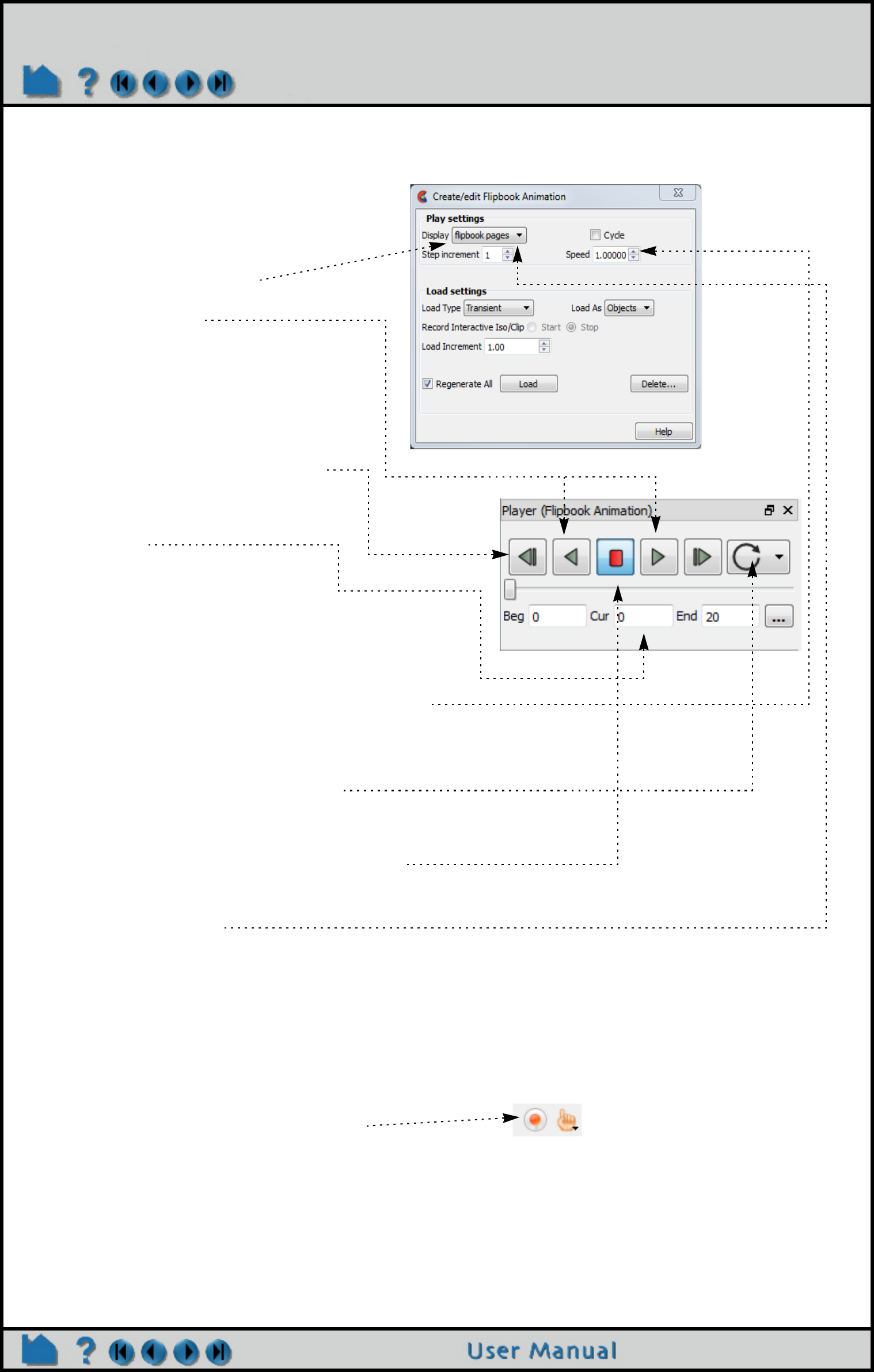
Page 460
HOW TO ANIMATE TRANSIENT DATA
The Load Flipbook Status dialog will open and show the progress of the load. You can cancel the load by clicking the
Cancel button and retain all the pages loaded to that point. Once the load is complete, you can run the flipbook using
VCR type controls:
Record
Once a flipbook is loaded, it can be recorded.
After a flipbook load, the next 3 steps will
generally be the default already.
1. Make sure the Display is set to
flipbook pages.
2. Click the run forward or backward
button.
The flipbook will begin to run.
OR
You can also step through the pages
manually:
2. Click the forward/backward single
step buttons (once for each page).
You can also enter values in the Current
Page field (and press return) to jump to a
specific page.
3. To change the range of displayed pages, enter new
values in the Begin Page and/or End Page fields.
4. To change the display speed, enter a new value in the
Display Speed field (and press return) or simply slide
the slider.
A speed of 1.00 represents “full” hardware speed with no
delays; a value of 0.5 is half of full speed.
5. To cycle the page display, click Cycle.
Cycle will replay the pages in reverse order when the last
page is reached.
6. To stop the animation, click the stop button.
7. When done, set the Display to “original model” instead
of “flipbook pages”.
Open the image and animation recorder by clicking
on the Record icon on the Tool ribbon.
This is explained in How To Print/Save an Image

Page 461
HOW TO ANIMATE TRANSIENT DATA
Delete
Any type of flipbook can be deleted:
1. Click Delete... in the Create/Edit Flipbook Animation dialog.
2. Confirm the deletion.
All memory associated with the flipbook is freed.
ADVANCED USAGE
If you have created transient particle traces (pathlines) and set up a particle trace animation, you can also load a
flipbook and show the particle trace animation synchronized with the flipbook. The trace animation will automatically
play through the time range of the flipbook and stay in sync with the flipbook pages. See How To Create Particle
Traces and How To Animate Particle Traces for more information.
OTHER NOTES
Since both object and image flipbooks build pages from the current set of parts based on their current, if you make a
change (such as color a part by a different variable or create a new part), you must reload the flipbook. There are
exceptions. With an object flipbook, you can make a part invisible while the flipbook is running.
SEE ALSO
How To Load Transient Data
How To Print/Save an Image
How To Create a Flipbook Animation
User Manual: Flipbook Animation
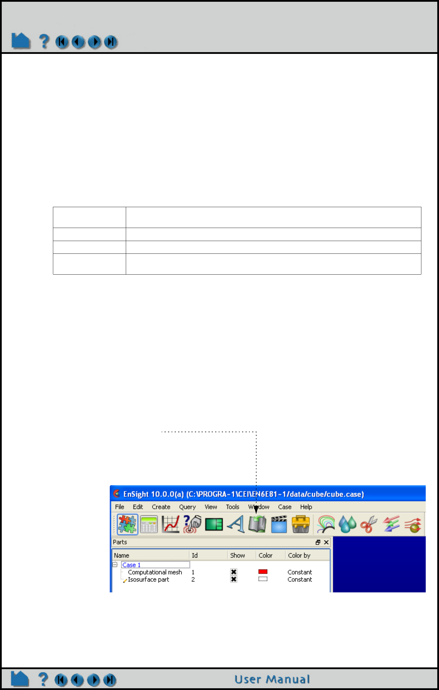
Page 462
HOW TO CREATE A FLIPBOOK ANIMATION
Create a Flipbook Animation
INTRODUCTION
Various types of data can be animated through EnSight’s flipbook capability. During the flipbook load process,
selected parts are automatically rebuilt based on some criteria (such as a delta for a clipping plane). For each step, a
graphical “page” is created and stored in memory. When the flipbook is active, the pages are displayed in order as
rapidly as the hardware allows (although you can slow it down). You can also step through pages manually.
The graphical pages can be one of two types: object or image. An object flipbook saves each page as 3D geometry
so you can continue to manipulate the model (e.g. rotate or zoom) during playback. However, for very large models
and/or long sequences, the memory requirements can be substantial. In this case, you can create image flipbooks
that save only the image pixels for each page. Although the size of each page is now fixed, you cannot change the
viewing parameters without reloading the flipbook.
There are four distinct types of flipbooks:
This article covers only the “Create Data” type of flipbook. See How To Animate Transient Data for details on
transient flipbooks. See How To Display Displacements for details on mode shape flipbooks.
For more sophisticated animations, use EnSight’s keyframe animation capability.
BASIC OPERATION
For each page of the flipbook, a delta value will be applied to all active clip parts and isosurfaces. For clips, the delta
represents a translation vector; for isosurfaces it is an increment to the isovalue. There are two ways to specify these
delta values: either through interactive manipulation or via the applicable Feature Panel for the part. The former
method is discussed below, the latter in the Other Notes section at the end.
Prior to loading the flipbook, you should create all parts that you wish to animate (clips and/or isosurfaces) and
manipulate the part so that it is in the desired location for the start of the flipbook. To load the flipbook:
Transient Pages are constructed by stepping from the current beginning to ending time range and
rebuilding all time-dependent parts based on each time step in sequence.
Mode Shapes Pages are constructed by applying a cosine-driven scaling factor to a displacement variable.
Create Data Pages are constructed by applying a delta to either a clip part or an isosurface.
Linear Load Pages are constructed by applying linear interpolation ranging from zero to the maximum
(displacement) vector field value.
1. Click the Flipbook Animation icon.
Which will open the Flipbook Animation Feature
Panel.
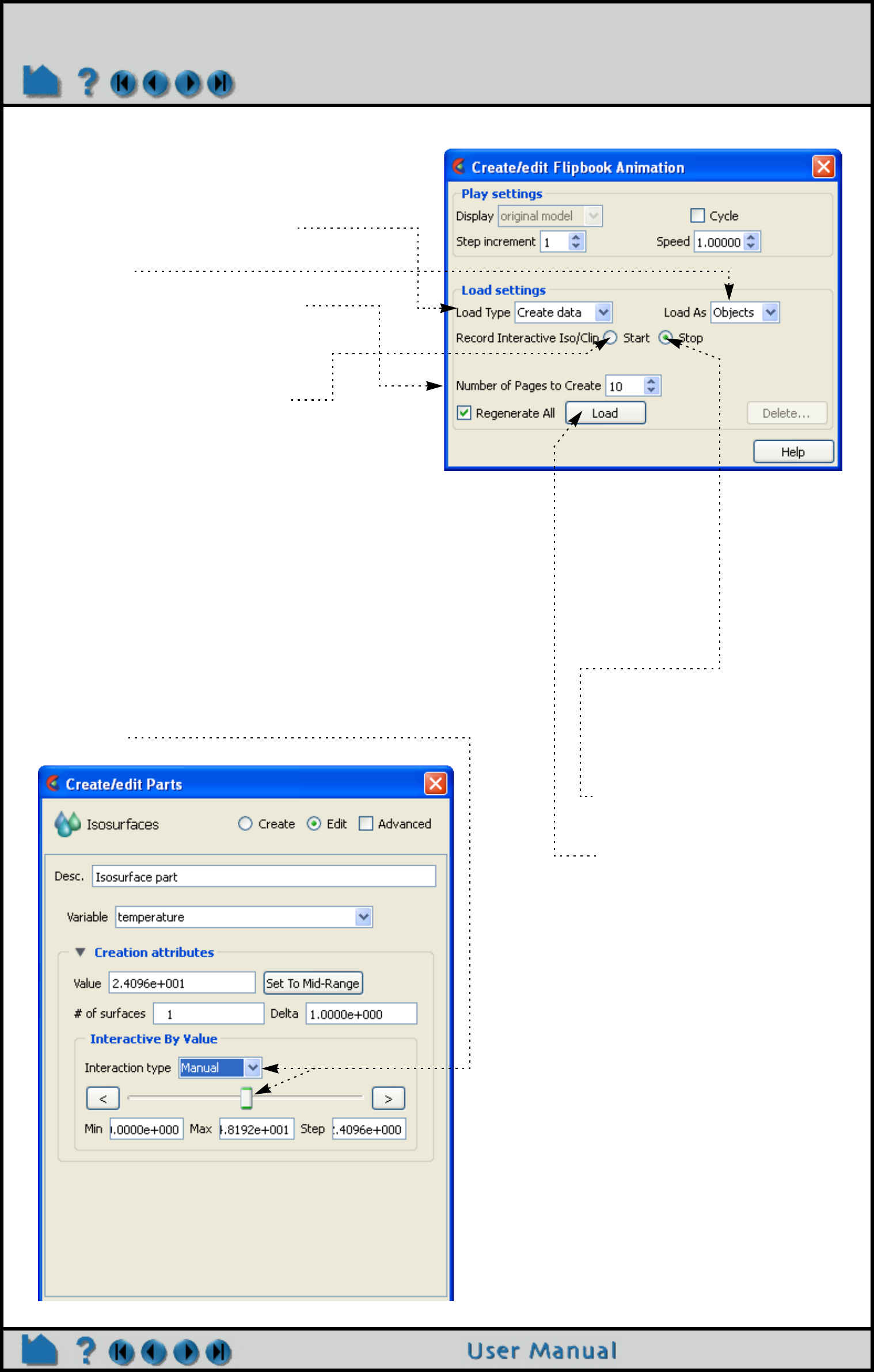
Page 463
HOW TO CREATE A FLIPBOOK ANIMATION
2. Under the Load settings, Be sure the
Load Type is set to Create data.
3. Select the desired page type (Object
or Image).
4. Set the desired number of pages.
The delta value will be added to the
appropriate entities for each page
5. Click Start to begin recording
interactive part manipulations.
6a. For clipping plane parts, return to the Create/edit Parts
dialog for clips (double-click on the part in the Main Parts
list).
6b. Toggle on Interactive Tool, move the mouse into the
Graphics Window and interactively position the tool to the
desired location for the end of the flipbook.
6a. For isosurface parts, return to the Create/edit Parts dialog
for isosurfaces (double-click on the part in the Main Parts
list).
6b. Change the Interactive Pulldown to Manual and adjust
the slider until the isovalue is as desired for the end of the
flipbook.
7. Return to the Create/edit
Flipbook Animation dialog (i.e.
perform step 1 again).
8. Click Stop to end recording
interactive Iso/Clip.
9. Click Load.
10. Save playing animation to file
(must be playing to save)

Page 464
HOW TO CREATE A FLIPBOOK ANIMATION
The Load Flipbook Status dialog will open and show the progress of the load. You can cancel the load by clicking the
Cancel button and retain all the pages loaded to that point. Once the load is complete, you can run the flipbook using
VCR type controls:
Record
Once a flipbook is loaded, it can be recorded.
After a flipbook load, the Player (Flipbook
Animation) will open, and the next steps will
generally be the default already.
1. Click the run forward or backward
button.
The flipbook will begin to run.
OR
You can also step through the pages
manually:
2. Click the forward/backward single step
buttons (once for each page).
You can also enter values in the Current Page
field (and press return) to jump to a specific
page.
3. Choose Once, Cycle or Bounce for
playback.
4. To change the range of displayed pages,
enter new values in the Begin Page and/
or End Page fields (and press return) or
move the slider range markers.
5. To change the display speed, enter a
new value in the Display Speed field (and
press return).
A speed of 1.00 represents “full” hardware
speed with no delays; a value of 0.5 is half of
full speed.
6. To cycle the page display, click Cycle.
Cycle will replay the pages in reverse order
when the last page is reached.
7. To stop the animation, click the stop
button.
8. When done, delete the “flipbook pages”
and click on the Time tab to view the
original data. Note that the EnSight client
retains the memory allocated to the
flipbook in case it is needed later.
The “Record current graphics window animation”
icon will be on.
Click it to open the Save Animation dialog.
This is explained in How To Print/Save an Image
Off On

Page 465
HOW TO CREATE A FLIPBOOK ANIMATION
Delete
Any type of flipbook can be deleted:
1. Click Delete... in the Create/edit Flipbook Animation dialog.
2. Confirm the deletion.
All memory associated with the flipbook is freed.
OTHER NOTES
Rather than specify the part delta values through interactive part manipulation as described above, you can set the
values explicitly in Advanced mode in the Create/edit Parts dialog for the part. For clip parts:
1. Double click on the part in the Parts list (or right-click and choose Edit...) to open the Create/edit Parts
dialog (Clips).
2. In the Animation Delta section, enter the desired values in the X, Y, and Z fields and press return.
For isosurfaces:
1. Double click on the part in the Parts list (or right-click and choose Edit...) to open the Create/edit Parts
dialog (Isosurfaces).
2. In the Animation Delta field, enter the desired isovalue delta value and press return.
When a flipbook is subsequently loaded, active clips and/or isosurfaces will update based on these animation delta
values.
Since both object and image flipbooks build pages from the current set of parts based on their current attributes, if
you make a change (such as color a part by a different variable or create a new part), you must reload the flipbook.
There are exceptions. With an object flipbook, you can make a part invisible while the flipbook is running.
SEE ALSO
User Manual: Flipbook Animation
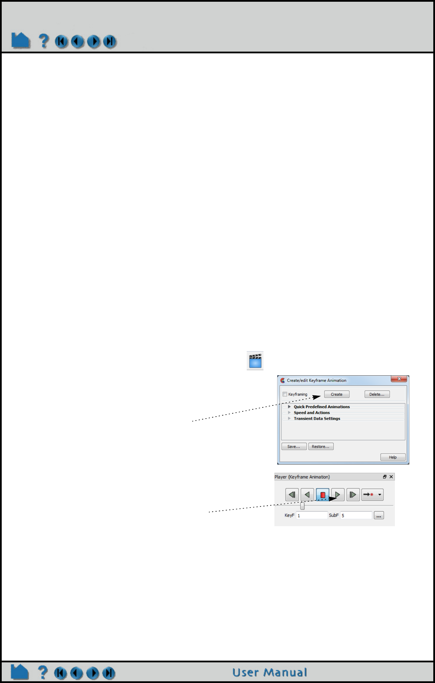
Page 466
HOW TO CREATE A KEYFRAME ANIMATION
Create a Keyframe Animation
INTRODUCTION
EnSight’s ability to handle large, transient datasets has led to its use in the production of many video animations of
engineering and scientific data. EnSight uses a keyframe animation system. A keyframe is a set of viewing
parameters that specify a particular view of the scene in the Graphics Window. The view may be notable because of
what is visible, or because the view represents the transition point from one scene to another. Once a set of
keyframes has been selected, EnSight can automatically generate frames to interpolate the viewing parameters
between keyframes for a smooth animation.
The changes to viewing parameters between keyframes are not limited to simple rotations, translations, or zoom
operations. You can also use EnSight’s frames capability to move parts independently, e.g. to animate an exploded
view of a complex assembly. You can also animate the global look-from and look-at points for “fly-by” style
animations.
While refining your animation, you can display it directly in the Graphics Window. When complete, you can specify
the output resolution and set the recording device (e.g. to a disk file).
Although the production of adequate animation is easy, good animation takes experience. A sequence that looks
good on your high resolution workstation screen may look less than acceptable when transferred to analog DVD. An
object rotating in ten degree increments may be an appropriate speed for your workstation graphics. At thirty frames
per second, however, the rotation will complete in just over a second – too fast for normal viewing. See the Other
Notes section for some additional hints and tips.
BASIC OPERATION
All keyframe animation functions are controlled through the Feature Panel. You can define the transformations
between keyframes, or you can create standard animations
To define your own keyframes:
1. Click the Keyframe icon Animation icon in the Feature
Icon bar.
2. Set all viewing parameters to the desired location for
keyframe 1.
Important Note!
If you toggle-off the Keyframing button, any
keyframes currently defined will be deleted.
If you wish to save a set of keyframes, click
the Save... button.
3. Click “Create” to save the first keyframe.
Note that the Keyframing toggle is automatically switched on
when you begin saving keyframes.
4. Change the viewing parameters to the desired location for
keyframe 2.
5. Click “Create” again to save keyframe 2.
You can play your animation at any time to check your results.
6. Click the Play button on the Keyframe Animation Player to
play the animation.
7. Continue to change viewing parameters and click Create
keyframe until you have saved all desired keyframes.
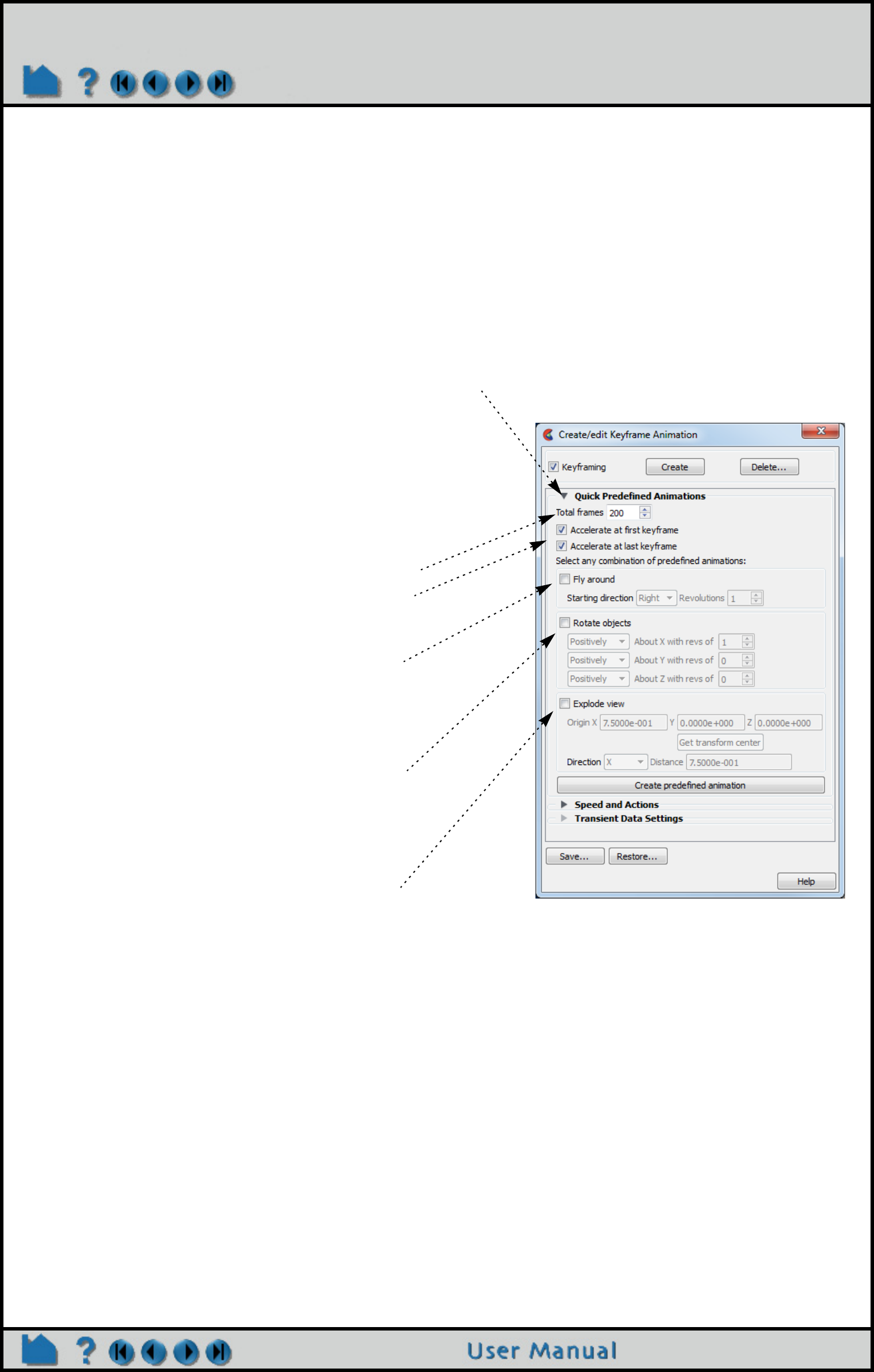
Page 467
HOW TO CREATE A KEYFRAME ANIMATION
There are many ways to specify the desired transformations between keyframes. See the following articles for more
information:
How To Rotate, Zoom, Translate, Scale
How To Create and Manipulate Frames
How To Set LookFrom/LookAt
How To Define and Change Viewports
To Create Keyframes using Predefined Animations:
1. Click the Keyframe Animation icon in the Feature Icon bar.
2. Set all viewing parameters to the desired location for
keyframe 1.
3. Turn down the Quick Predefined Animations to view the
Keyframe Quick Animations settings.
In this turndown area you will be able to create keyframes which
define transformations which will (a) fly the viewer around your
model, (b) rotate your model, or (c) create exploded views of your
parts. Any one of these, or a combination may be used.
4. Set the number of frames which will be created
5. Acceleration at the first and last keyframes that
will be created is on by default. If you do not
want to accelerate/decelerate toggle these off.
6. Toggle Fly Around on if you wish to move the
viewer (camera) in a circle.
(a) You can choose Right (start the viewer moving
to the right) or Left.
(b) Specify the number of revolutions.
7. Toggle Rotate Objects if you wish to rotate the
scene.
You can rotate positively or negatively about all
three axis. For each axis you set the number of
revolutions.
8. Toggle Explode View if you want your parts to
be translated in reference to an origin.
You can specify the origin or set the origin to the
transformation center.
Direction sets the explode direction and can be one
of:
X,Y,Z - translate in the coordinate direction
XYZ - translate in the dominant coordinate direction
Radial - translate in the direction from the origin specified
through the part centroid
The part that is farthest from the origin specified will
be transformed Distance units
9. Click “Create predefined animation” to
create the keyframes which will transform
according to the selections made.
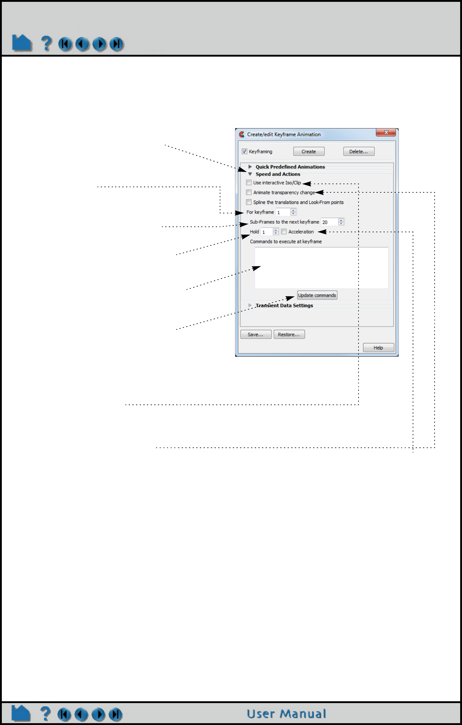
Page 468
HOW TO CREATE A KEYFRAME ANIMATION
The following sections provide details on the animation control turndowns in the Keyframe Animation Feature Panel.
Speed/Actions
The Speed/Actions turn down exposes allowing you to set the number of sub-frames between each pair of
consecutive keyframes as well as specify run such as acceleration and commands to execute:
The number of sub-frames controls the speed with which objects transform between keyframes. More sub-frames
yields slower motion.
You can insert any valid EnSight command to be executed at a keyframe. If your command sequence is more than a
few lines, it is best to save the sequence in a file and just enter the command play: filename. There is a special
case of executing a command at a keyframe. If you insert the command shell: filename, The file filename
(which is assumed to be a UNIX executable command) will be executed after each sub-frame and each surrounding
keyframe. In addition, if you are saving animation frames to disk files, the name of the image file just written is
passed to the executable as the first argument. This capability can be used to postprocess the image files, for
example to resize and re-sample an image or copy it to a different location. If this capability is used, the shell:
filename command must be the only command specified.
1. Click on the “Speed and Actions”
turndown to open the section.
2. Select the desired keyframe to edit:
either enter the value or use the up/
down buttons.
3. Enter the desired number of sub-frames
between the keyframe selected in step 1
and the next (the default is 20).
4. If desired, set the number of frames to
hold for the keyframe (default is 1).
5. If desired, enter EnSight commands to
execute when the selected keyframe is
reached. The command(s) will be
executed before the frame is displayed.
6. If you added or changed the commands
to be executed at a keyframe, click
Update Commands.
7. If you want the transformation to accelerate out
(or into) the keyframe, toggle Acceleration on.
8. Continue by selecting a new keyframe to edit
and click Close when done.
Use Interactive IsoClip
By turning this toggle on, any clip or isosurface
interactively moved during the keyframe will animate.
Animate Transparency Change
By turning this toggle on, transparency changes to
parts during the definition of the keyframes will be
part of the animation.
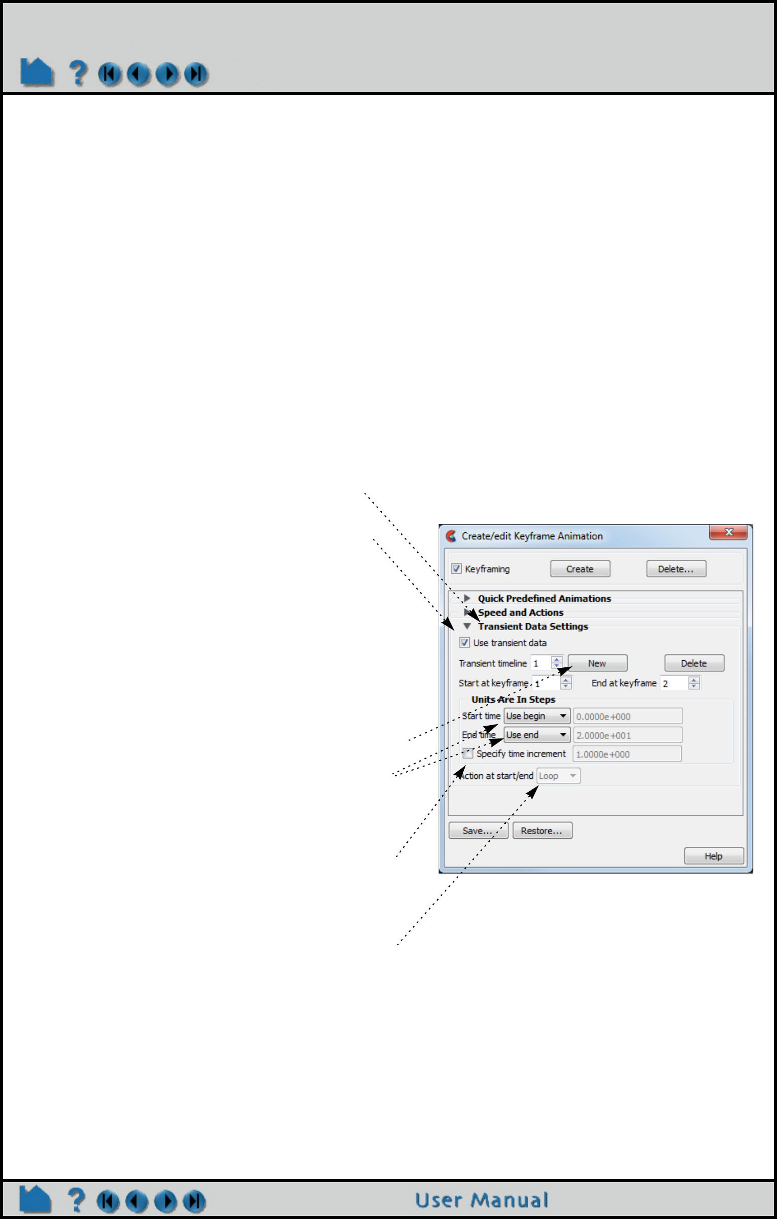
Page 469
HOW TO CREATE A KEYFRAME ANIMATION
Run From/To
The Run From/To turndown allows you to specify the range of keyframes to play.
Transient
If you have transient data you can specify how it will be used during the keyframe animation.
1. Click on the Run From/To turndown to open the
section.
2. If you wish to limit the animation playback to certain
keyframes set the Run From and To fields. By
default they are set to cover all of the keyframes you
have created.
1. Click on the “Transient Data Settings” turndown to
open the section.
2. Toggle Use Transient Data on if you want to use
transient data during the animation.
Transient data does NOT have to be on (and should not)
to play back a flipbook animation during the keyframe
animation.
3. Timelines allow you to use transient data during
each defined timeline.
If the timelines do not cover all of the keyframes you will
have a portion of your animation with no transient data.
By default a single timeline exists which covers all of the
defined keyframes. To create more timelines click New
4. For each timeline you can specify the begin and
ending time value (either step or simulation time -
See Solution Time dialog).
5. Time will be interpolated such that the Start Time
occurs at the Start At Keyframe and the End Time
will occur at the End At Keyframe unless the Specify
Time Increment is toggled on. If the Specify Time
Increment is on each frame during the timeline is
incremented by the time indicated.
If the Start Time or End Time is encountered before the
Start At or End At Keyframes the transient data will either
Loop (go back to the Start Time) or Swing (play in
reverse).

Page 470
HOW TO CREATE A KEYFRAME ANIMATION
Recording your animation
See How To Print/Save an Image for instructions on how to record the animation.
Save and Restore
A set of keyframes and related information can be saved to disk and later restored. To save keyframes:
1. Click Save... in the Feature Edit Dialog.
2. Enter the desired file name in the File Selection dialog and click Okay.
To restore previously saved keyframes:
1. Click Restore... in the Feature Edit Dialog.
2. Enter the desired file name in the File Selection dialog and click Okay.
OTHER NOTES
As pointed out in the introduction to this article, high-quality animation takes time and experience. CEI has produced
a great deal of animation over the years and has learned a variety of lessons. In the hope that EnSight users can
avoid many of the pitfalls inherent in the process, many of these lessons and rules of thumb are presented here.
EnSight’s keyframe animation methodology is borrowed from the animated film industry. In making animated films,
the master animator defines how the scene will look at certain points in time (the keyframes) and then hands the work
off to an “in-betweener”, with instructions on how many frames to add between each pair of keyframes. The in-
betweener then draws the missing frames. EnSight’s approach is similar with the user as the master animator and
EnSight as the in-betweener. Some of the strengths of this approach include:
1. When keyframing is on, EnSight is not only recording the viewing parameters when you click Create Keyframe, it
also records the actions taken to get from the last keyframe to the current one. This approach permits certain
operations to be performed without ambiguity (such as rotating by 180 degrees or more).
2. Each Viewport can be animated independently.
3. Flipbooks can be played during an animation.
4. Animated particle traces can be played during an animation.
5. Transient data is easily synchronized with the generated frames. When the animation is run, EnSight will
automatically step through time and recalculate all time-dependent entities.
6. Output can go directly to disk files for later recording, manipulation, or conversion to other formats (e.g. MPEG or
QuickTime).
7. Additional power and flexibility can be achieved since EnSight command language statements can be issued at
keyframes.
The keyframe capability was designed to enable engineers and scientists to produce quality animation. As such, it
lacks most of the more elaborate controls available in commercial animation packages (which typically cost 2-3 times
more than EnSight). Some limitations:
1. Only transformation parameters (global, frame and camera transforms) are saved through the keyframing
process. Other parameters and part are not interpolated between keyframes.
2. Light sources are fixed in EnSight – they cannot move during the animation.
3. The shading and lighting model used by EnSight is fairly simplistic.

Page 471
HOW TO CREATE A KEYFRAME ANIMATION
Tips for Video Recording
Animation Holds
Whenever an animation is started or stopped use a “hold” to allow your viewers to establish the visual context of the
scene. A hold of 3 seconds at the beginning and 2 seconds at the end usually works well. For complex imagery,
longer holds may be required. Note that a hold can typically be performed at the recording level – it is not necessary
to have EnSight compute multiple frames for a hold.
Rate Control
The speed at which events occur during an animation is one of the most difficult aspects to master. Viewers become
confused and disoriented if motion is too fast; too slow and your viewer may lose interest. The frame rate for NTSC
(the video format used in North America) is 30 frames per second. Although there is a great deal of variation
(depending on graphics hardware speed and model size), your workstation will typically have a much slower frame
rate. Therefore, what appears to be good speed on your workstation may be much too fast when recorded to video
at 30 frames per second.
Trial and error is one method to determine proper rates. Although you may end up doing some “line test” video
recording to refine your rates, use the method described here to derive good starting values:
1. Define all the keyframes.
2. Set up the animation to play back at full screen.
3. Set up the animation to play only from the first to the second keyframe.
4. Set the number of sub-frames between keyframes 1 and 2 to be 300.
5. Select View > Bounding Box > Static Box.
6. Using a watch with a second hand, time how long it takes to play the animation. Call this time “T”. We know that
it will take 10 seconds to play 300 frames on video. Compute the following:
factor = T/10.
For example, if you find T to be about 12 seconds, then factor is 1.2, which means that the rate you see on the screen
is 1.2 times slower than what you will see on video.
7. Iteratively adjust the number of sub-frames between keyframe 1 and 2 (running the animation after each
adjustment) until you like the rate you see on the screen.
8. Finally, adjust the number of sub-frames by the factor found in step 6. For example, if 150 sub-frames were
required for a good rate of speed, then change the number of sub-frames to 150*factor to see the same rate on
video.
9. Perform steps 3 through 8 for the next set of keyframes.
Transient Data
Animation is particular useful for presenting transient data. However, since both viewing parameters and time can
change simultaneously, the potential for confusing viewers is very high. In general, you should never change both
viewing parameters and time simultaneously. It is typically much better to use transformations in an opening scene to
present the model to the viewer. The transformations should end at a vantage point suitable for viewing the transient
phenomena. At that point, the time-dependent data can be displayed. If you must alter the scene during transient
display, do so with great care to avoid disorienting viewers.
Note that you can animate time-dependent information without transformations by merely creating two keyframes
without performing any transformations between them.
In many instances, there will not be enough time steps in the simulation to produce an animation of adequate
duration. If the simulation does not involve changing geometries, EnSight can interpolate between time steps
(linearly) to yield additional frames. However, keep in mind that your simulated phenomena is almost certainly not
linear in nature. If you have EnSight generate more than a few interpolating frames between each actual time step,
the resulting discontinuity at keyframes (from the piece-wise linear interpolation) is quite visible in the resulting video.

Page 472
HOW TO CREATE A KEYFRAME ANIMATION
Frame count
The total number of frames that EnSight will produce during the animation is the sum of all sub-frames plus the
number of keyframes. This is especially important to keep in mind when synchronizing transient data with animation
frames.
Animated Traces
If you display animating particle traces during keyframe animation, you may have noticed that the trace animation
always resets at the beginning of the keyframe animation. However, in most cases it is desirable to have the trace
animation fully in progress when the animation begins. This can be accomplished by creating an additional keyframe
at the beginning of the animation. Set the number of sub-frames between keyframes 1 and 2 to a value high enough
to yield the desired tracer saturation. When you run the animation, set the Run From field to 2 so that the animation
begins generating frames with keyframe 2. At that point, the tracer animation process will have executed once for
each sub-frame between keyframes 1 and 2.
Color
The color gamut (the range of colors a device is capable of displaying) of video (especially NTSC) is significantly less
than that of your workstation monitor. The result is that certain colors that look fine on your workstation cannot be
reproduced on video. Fully saturated colors (especially red and blue which “bleed” across the screen) are particularly
troublesome. However, it is quite easy to de-saturate your images prior to recording. There are actually three ways
to do this:
1. Modify all of the colors in use to de-saturate them. For example, if a color is pure red (1., 0., 0.), change it to be a
more pastel red (.85, .1, .1).
2. Modify the saturation factor in the Image Format Options. A factor of 0.85 is usually good.
3. Create your animation, then de-saturate the images using an image tool such as the one available from the San
Diego Supercomputing Center (it is free). This will only work, of course, if you are saving animation images to disk
files.
Dark backgrounds work much better than light backgrounds. Black is often the best choice.
Lines
Moving single-width lines have a tendency to “crawl” on video. Use a minimum line width of 2.
Anti-aliasing
Without correction, computer-generated imagery exhibits aliasing artifacts that typically show up as jagged edges.
For our purposes it is sufficient to say that aliasing results from sampling at a resolution too low to capture the “signal”
represented by the underlying geometry. We can only sample our geometry at the available pixels. Since the
effective number of pixels in the NTSC video signal is only one quarter the number of your workstation screen, what
looks fine on your workstation may be less than acceptable on video. EnSight provides direct anti-aliasing support
through its multipass capability. There are also some other ways to mitigate this problem.
If you are recording images to disk files, record them at full screen resolution and then use an image re-scaling tool
(such as EnVe) to down-sample the images to the desired video resolution. This down-sampling averages several
pixels to yield one output pixel, effectively preserving much of the resolution contained in the original full screen
image.
Annotation
The smallest annotation text that can be clearly read on video has a font size of 40. For title sequences, use a size of
about 65.
If you display parts colored by variables, you should always include the applicable color legend so viewers
understand what the coloration represents. For color legends, it is often sufficient to display just one value at the top
(the maximum) and one at the bottom (the minimum) in addition to the name of the variable. In fact, sometimes just
using “High” and “Low” are sufficient if only the relative magnitudes of the variable are important.

Page 473
HOW TO CREATE A KEYFRAME ANIMATION
Screen Space
The region of a video display that is “safe” for viewing is typically smaller than your animation display window. You
should plan your scenes such that objects of interest (especially annotation entities) do not come “too close” to the
edge. If you keep these objects within the range (in EnSight viewport coordinates) .06 to .94 for X (width) and .05 to
.95 for Y (height) you should be safe.
Introductory Sequence
Your animation should begin with some title slides explaining the problem domain to your viewers. Try not to put too
many words on any one slide and display each one for at least four seconds.
Next, before displaying your results, provide a sequence that introduces viewers to your model. This sequence
should be long enough and complete enough to orient the average target viewer to your problem. It is difficult to
overestimate the need for this sequence. Without it, viewers are often confused and disoriented for the entire
animation.
Credits
You should always include proper credits on any animation you produce. Even animations initially intended only for
internal consumption often end up shown to broader audiences.
SEE ALSO
User Manual: Keyframe Animation
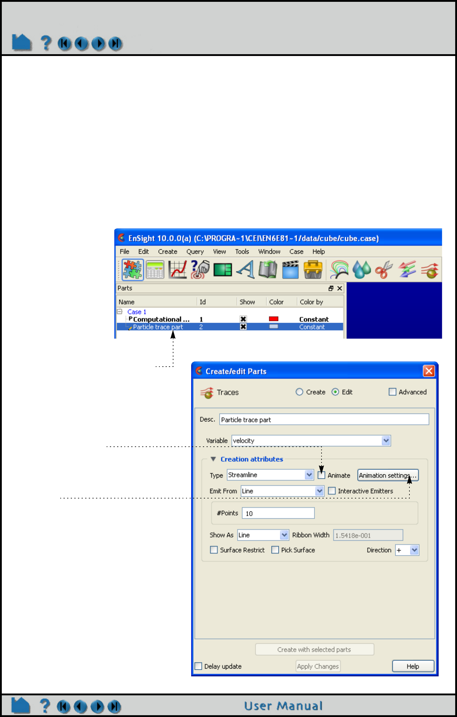
Page 474
HOW TO ANIMATE PARTICLE TRACES
Animate Particle Traces
INTRODUCTION
EnSight’s powerful particle tracing facility can trace particles (either steady-state or transient) through flow fields.
Animating the resulting traces often promotes intuitive comprehension of the characteristics of the underlying flow
field. Traces are animated by displaying one or more tracers on all traces of the trace part. A tracer moves along the
path of a trace with length proportional to the local velocity. EnSight provides complete control over all aspects of the
tracers including length, speed, and release interval for multiple pulses.
This article covers particle trace animation and assumes that you have already created one or more particle trace
parts. See How To Create Particle Traces for more information.
BASIC OPERATION
To enable particle trace animation and adjust the animation parameters:
1. Double-click the desired particle
trace part in the Main Parts list.
Which will bring up the Parts
Feature Panel.
2. Toggle on Animate.
3. Click Animation settings... to open
the Trace Animation Settings dialog.
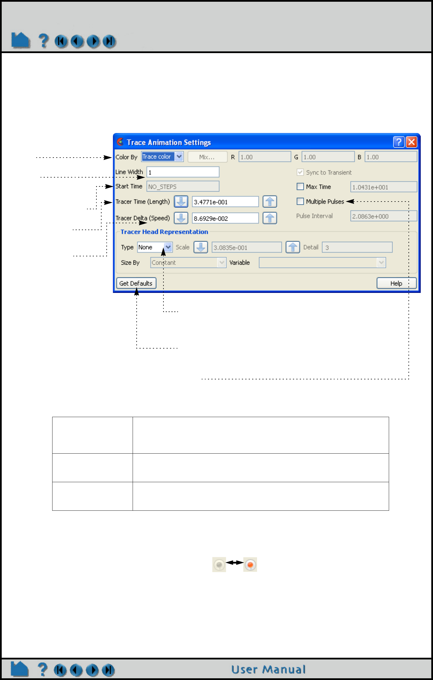
Page 475
HOW TO ANIMATE PARTICLE TRACES
Tracer Parameter Descriptions:
Record
Once animated traces are computed, they can be recorded.
Tracer Time (Length) The Tracer Time (Length) parameter acts as a scaling factor for all tracer lengths
(the higher the value the longer the tracer). Tracer length varies as the local
velocity changes along the trace. For example, the tracer will lengthen as the
leading edge of the tracer moves into a higher velocity region.
Tracer Delta (Speed) The Tracer Delta (Speed) parameter acts as a scaling factor for the tracer speed
(the higher the value the faster the tracer). The speed of the leading and trailing
tracer edges varies as the local velocity changes along the trace.
Pulse Interval The interval between successive tracer emissions when in multiple pulse mode
(the higher the value the longer the interval between pulses). Note that the
distance between tracers will increase when the local velocity increases.
Set the color of the tracers
to either Trace Color (i.e.
the same color as the
parent trace part) or
Constant (and set the
desired color using the
Mix... button or the RGB
fields.
Set the line width of the
tracers.
If transient traces
(pathlines), set the Start
Time and/or Max Time.
Set the tracers length
factor (see below).
Set the tracers speed
factor (see below).
Make changes as desired (remember to press return for changes to text fields).
Set tracers head representation. Either None or Spheres. If Spheres,
the radius can be Constant (set by the Scale value) or sized by a
variable and scaled by the Scale value. Sphere detail set via Detail
field.
Click to load good default values to the Tracer Time, Tracer Delta, and
Pulse Intervals fields.
Toggle on Multiple pulses and set the interval between pulses (see
below).
The “Record current graphics window animation”
icon will be on.
Click it to open the Save Animation dialog.
This is explained in How To Print/Save an Image
Off On

Page 476
HOW TO ANIMATE PARTICLE TRACES
ADVANCED USAGE
If you have time-dependent data and have calculated transient particle traces (pathlines), you can enable trace
animation, load a transient flipbook, and view the animating pathlines simultaneously with the dynamic flipbook. See
How To Create Particle Traces and How To Animate Transient Data for more information.
OTHER NOTES
The parameters in the Trace Animation Settings dialog are not specific to the currently selected particle trace part –
the settings apply to all currently animating particle trace parts.
SEE ALSO
User Manual: Particle Trace Animation
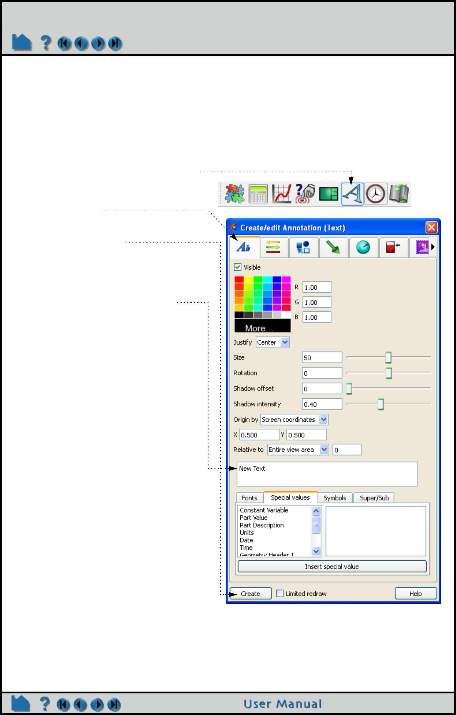
Page 477
HOW TO CREATE TEXT ANNOTATION
Annotate
Create Text Annotation
INTRODUCTION
EnSight has comprehensive features for text annotation. Not only can you display and position user-specified text,
you can also display text contained in the description lines of some data formats as well as dynamic text that changes
over time.
BASIC OPERATION
1. Click Text icon from the Feature Icon Bar to
open the Annotation Feature Panel.
2. Click the Text tab
3. Click the Create button, which will create a
“New Text” annotation.
4. Click on the text string and modify it.
If you hit the “Enter” keyboard key you will
insert a line return into the annotation.
While entering text, you can easily change the
script to super, sub, or normal by clicking the
Superscript, Subscript, or Normal buttons found
in the Super/Sub tab. These buttons will insert
<up>, <dn>, or <no> into the string.
Other Special Coded Items, including changing
the font, which can be inserted into a string (by
selecting and hitting Insert special item) are
discussed below.
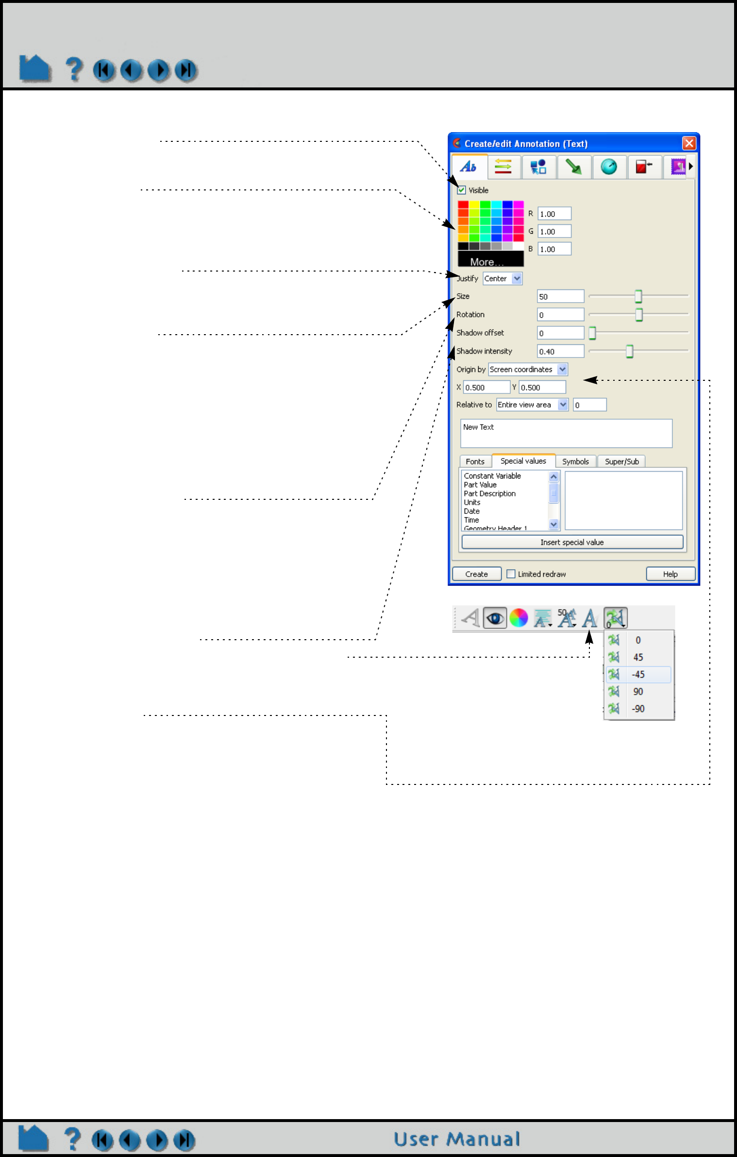
Page 478
HOW TO CREATE TEXT ANNOTATION
To manipulate text string, first select the string(s) of interest in the list then:
To change visibility:
Toggle Visible off or on.
To change color:
Select the desired color from the matrix, enter RGB
values in the fields, or click More... to open the Color
Selector dialog.
To change justification:
Select the desired Left, Right, or Center justification from
the Justify pulldown.
To change text size:
Either resize the text interactively by grabbing the touch-
n-go resize handle and dragging, or by precisely
specifying the font size in the Size field of the dialog (or
using the slider to change the font size).
Important Note! The text size specified is relative to the
size of the Graphics Window. If you increase the size of
the Graphics Window, all text will also rescale to
maintain the same relative size.
To change text rotation:
The orientation of text about the text justification point
may be specified by specifying the rotation angle (in
degrees) in the Rotation field (or using the slider to
change rotation angle). You can also specify a rotation
angle from the Quick Action icon bar.
To add shadow text effect:
Enter offset and intensity or use sliders. You can also
use the Quick Action Icon Bar.
To change location of the justification point in the
graphics window:
Either interactively drag the text to the desired location
using the touch-and-go handles, or precisely specify the
location in the Origin XY fields.
You can also specify the viewport that the text is to be
positioned relative to. If 0, the position is relative to the
graphics window.
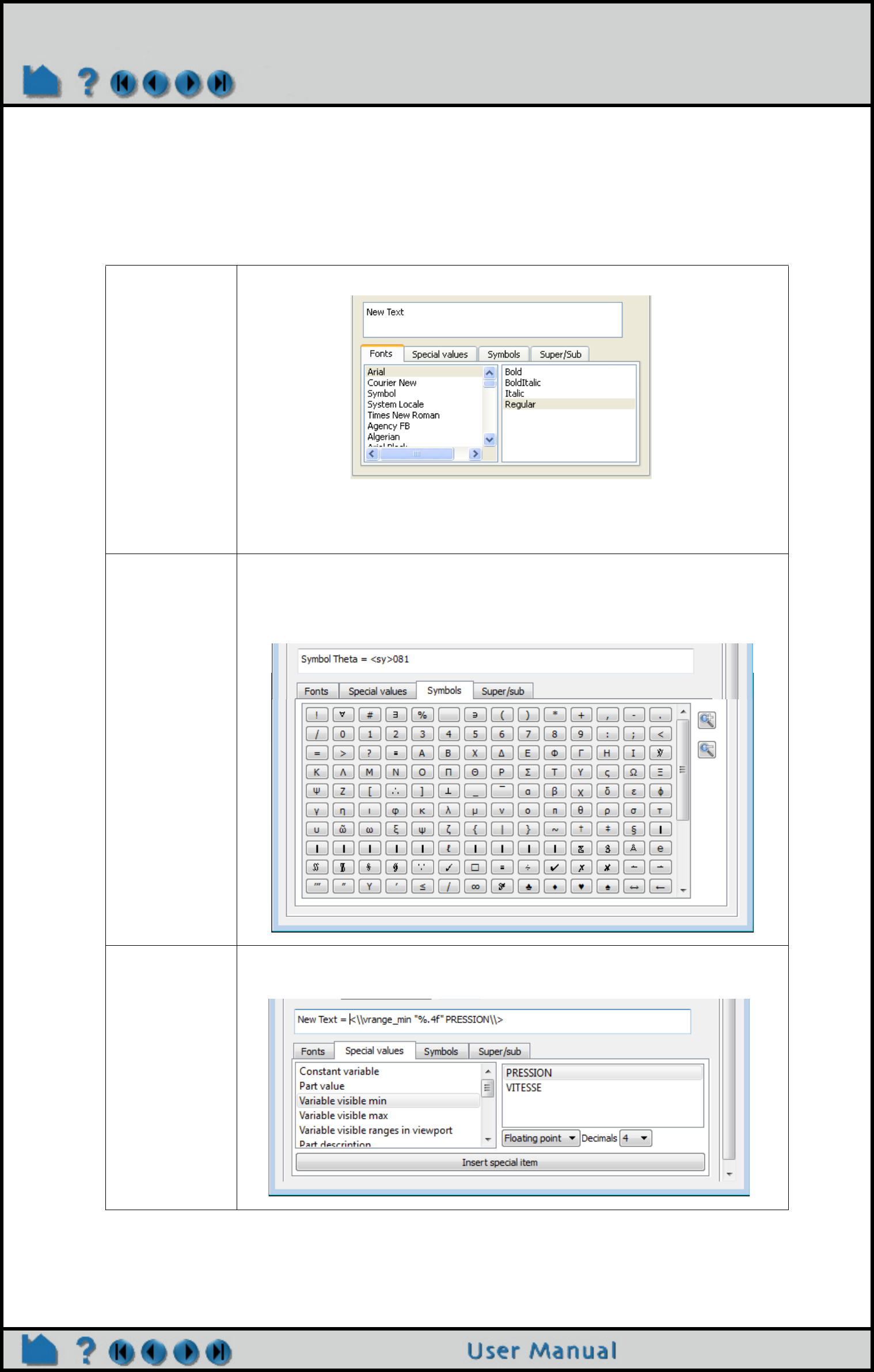
Page 479
HOW TO CREATE TEXT ANNOTATION
Special Coded Items
EnSight can automatically build text strings based on information from various sources. To use one of these special
strings, select the desired item from the Special String list, select any required options, and click Insert Special Item.
A code will be inserted into the Text field.
The following special strings are available. If multiple cases are loaded, any reference to parts or variables applies to
the currently selected case (select Case > casename to changes cases)
Fonts Brings up the TrueType font selection dialog, allowing a new font to be selected
Symbols Brings up a symbol dialog. Click on any symbol to insert it at the current character
insertion point of the string. The symbol will be inserted in to the string via a <sy>xxx,
where xxx is the ASCII number for the selected symbol.
Special values Values from the operating system, the geometry and the variables.
Information on manipulating fonts, including additional text font formatting codes
that can be used, are described in How To Manipulate Fonts
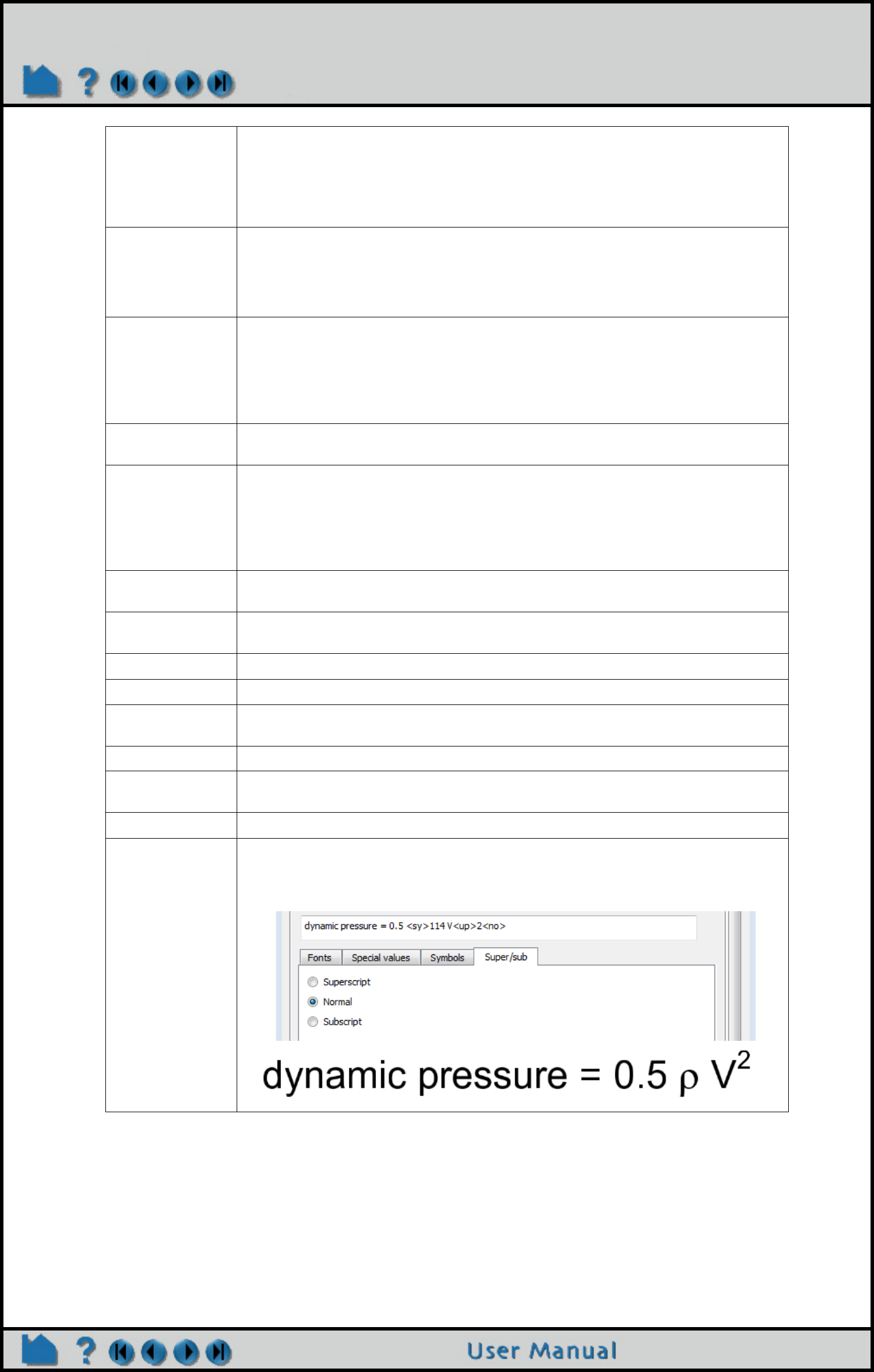
Page 480
HOW TO CREATE TEXT ANNOTATION
EnSight command language variables can also be inserted into annotation strings via a special item coding option.
This coding item does not have an associated, but can be typed directly into the annotation text edit field. The coding
has the form:
<\\ensv “format“ var_name\\>
The format string is the “C” printf specification for the item formatting. var_name is the actual name of the variable
value to be inserted. If the following lines of EnSight command language were executed:
$globalstring example
Constant Variable The value of a constant variable (such as Time or Length). Select the variable from the
Constant Variables list and select the desired numeric display format from the Number
Format list.
If the constant variable changes, the corresponding text will automatically update. This
is very useful for displaying the current solution time during a transient animation.
Part Value The “value” of a part. Currently works for isosurface and some (ijk, xyz, rtz, plane
aligned with axis, or attached to spline) clip parts where the value is the corresponding
isovalue or clip location or value. Parts that have a value will appear in the part selection
list. Select the part in the Part(s) list and select the desired numeric display format from
the Number Format list.
Variable visible min The minimum value of the variable on the visible elements in the visible geometry on the
client at the current time. This is, therefore, different from the min function in the
calculator, in the query/probe minimum, or the query/plot minimum. The value of this
annotation can change when visible parts are made invisible, when the element
representation of the part is changed, and when new parts are made visible in the
viewport.
Variable visible
max
The same as the min value only using the maximum values of the variable existing on
the visible elements of the part(s) in the graphics window.
Variable visible
ranges in viewport
Display the min/max variable information for all parts visible (taking into account element
blanking) in a specified viewport. If parts are colored by multiple variables then multiple
annotation strings will be created - one for each variable in use in the viewport. If you
change the color by variable(s) the text string will update to reflect the new color change.
If you change the part element representation, the text string will update to reflect the
visible elements.
Part Description The description of the part as displayed in the Main Parts list. (Note that you can change
this text by editing the Desc field in the applicable Feature Panel for the part.)
Units This will display the variable units for the selected variable. If the variable selection list is
empty then this dataset does not have units.
Date Current date. Example: January 1, 2012
Time Current time. Example: 14:19:12
Geometry Header The first or second text line of the geometry file of the current case. Select Line 1 or Line
2.
Measured Header The first line of the measured (discrete) data file of the current case.
Variable Header The first line (typically the description line) from a variable file. Select the desired
variable from the variable selection list.
Version The name and current version number. Example: EnSight Version 10.2.
Super/Sub Select the text that you want to be superscripted or subscripted, click on the Super/Sub
tab and toggle the appropriate value.

Page 481
HOW TO CREATE TEXT ANNOTATION
$example = Hello from EnSight
The annotation string:
The value is: <\\ensv “%s“ example\\>
would result in the annotation containing the string “The value is: Hello from EnSight”. If the variable is updated, the
following command language will update the annotation:
text: update
Another example uses the built-in EnSight frames per second counter which stores the current rendering rate in
frames per second in the ensight variable “ensight_fps”. This annotation string, containing embedded ensight
variable formatting, will display the current rendering rate dynamically in EnSight:
Frames per second: <\\ensv “%.2f“ ensight_fps\\>
It is also possible to embed the value of an interactive query into an annotation string. The first value of the
interactive query results is always used. The format for this is the keyword "iqval", followed by a format statement
and a interactive query id number (zero based). For example:
Temperature = <\\iqval "%.2f" 0\\>
will display an annotation string with the value of interactive query 0 displayed to two places of precision after the
equal sign in the annotation.
Delete Annotations
SEE ALSO
How To Manipulate Fonts
User Manual: Text Annotation
Existing annotations can be deleted by selecting them in the
Annotations list and performing a right click to “Delete”.
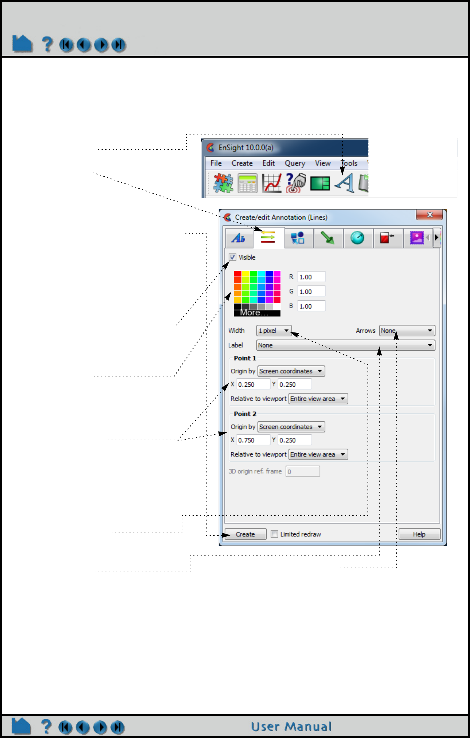
Page 482
HOW TO CREATE LINES
Create Lines
INTRODUCTION
EnSight can display annotation lines that can either be specified in 2D screen space or in 3D world space.
BASIC OPERATION
SEE ALSO
User Manual: Line Annotation
2. Click Line icon.
To manipulate a line’s, first select
the line(s) of interest in the
Annotation list panel, then:
To change visibility:
Toggle Visible on or off. Note that if the
Limited redraw toggle is on invisible
lines are drawn in a subdued color.
To change color:
Select the desired color from the
matrix, enter RGB values in the fields,
or click More... to open the Color
Selector dialog
To change location:
Set the ‘Origin by’ to Screen
coordinates or 3D coordinates. You
can drag the endpoints specified by
screen coordinates in the graphics
window. You can also specify the X, Y
(and Z if 3D coordinates) by typing into
the fields.
To change line width:
Click the Width Pulldown and select the
desired line width.
To label the line:
Specify Text Annotation from the
pulldown to align it with line annotation.
3. Create a new line in the Graphics
Window by clicking the Create button.
1. Click the Annotation
feature icon.
To change Arrowhead status:
Click the Arrows Pulldown and select the desired state.
To delete a line, Select the item in the list and right click to
Delete.
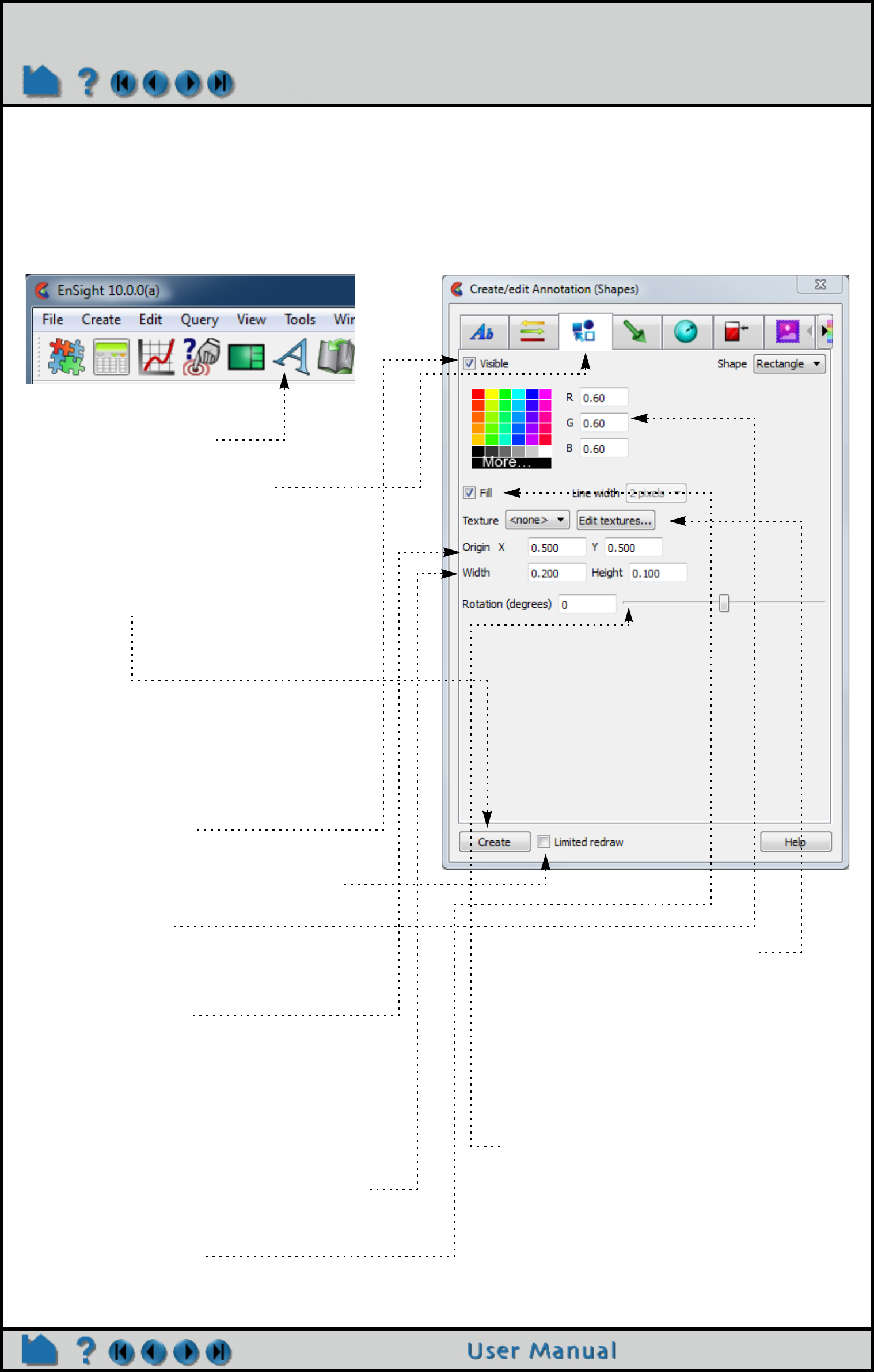
Page 483
HOW TO CREATE 2D SHAPES
Create 2D Shapes
INTRODUCTION
EnSight can display 2D shapes (arrow, rectangle, and circle in present release). These 2D shapes overlay the
Graphics window and are not associated with any viewport.
BASIC OPERATION
To manipulate a shape’s, first select the
shape(s) of interest in the list panel (or pick
them in the graphics window), then:
To change visibility:
Toggle Visible on or off. Note that if you turn on
Limited redraw invisible shapes are drawn in a
subdued color.
To change color:
Select the desired color from the matrix, enter
RGB values in the fields, or click More... to open
the Color Selector dialog.
To change location:
Either select the shape and drag it to the desired
location, or type appropriate coordinates into the
Origin X/Y fields. The origin of a 2D arrow is the
point of the arrow. The origin of a rectangle or
circle is the center of the object.
To change size:
Either select the shape by the resize handle and
drag it to the desired size, or type appropriate
Width/Length (or Height or Diameter) values into
the fields. Units are 0 to 1.
To change fill mode:
You can draw the shape in filled mode or in outline
mode.
1. Click the Annotation
feature icon.
To Apply textures to the shape:
These are the same textures used by the
parts and the ‘Edit textures...’ button will
open the part texture dialog, where textures
or animations can be loaded and other set.
Note that 2D shape textures always replace the
current shape color and modes like “modulate”
and “decal” as well as custom projections and
repeat behavior are not supported.
Other: To Rotate the shape:
According to the selected shape, other may
exist, such as rotation, arrowhead, etc.
To delete a shape, Right click the shape in
the Annotations object panel and Delete.
2. Click 2D Shape icon in the
Create/edit Annotation dialog.
3. Create a new shape in the
Graphics Window by setting
the Shape type and then
clicking the Create button.

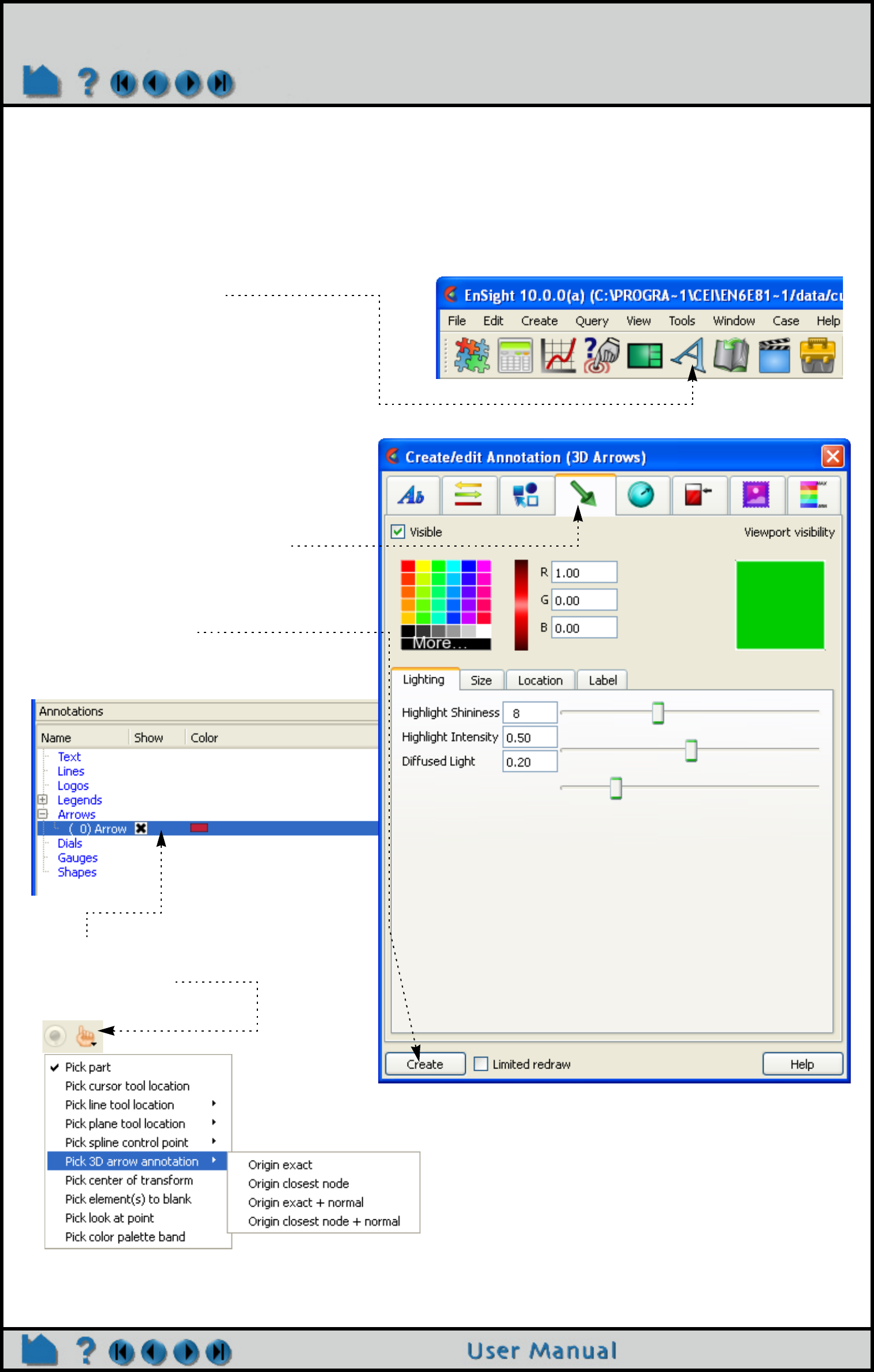
Page 485
HOW TO CREATE 3D ARROWS
Create 3D Arrows
INTRODUCTION
EnSight can display 3D arrows. The 3D arrow is defined in model space and transforms with the scene. The 3D arrow
is visible in the viewport(s) specified.
BASIC OPERATION
1. Click Annotation icon.
2. Click 3D Annotation Arrow tab in the
Create/edit Annotation dialog.
3. Create a new 3D annotation arrow in
the Graphics Window (and in the
Arrows Annotations list) by clicking
the Create button.
5. Position the mouse and press the ‘p’ key.
4. Select this Arrow in the list, then Pick
the arrow tip location option in the
Pick pulldown.
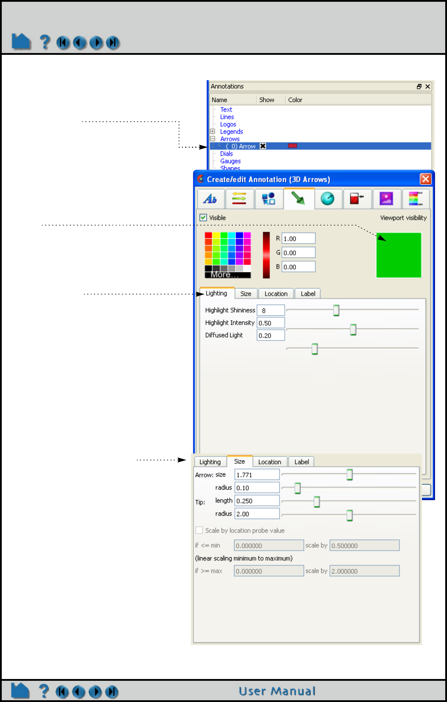
Page 486
HOW TO CREATE 3D ARROWS
To manipulate 3D annotation, first select
the item(s) of interest in the list panel (or
pick them in the graphics window), then:
To change viewport visibility:
Click on the viewport region to toggle the
visibility in the viewport. Green means visibility
is on.
Under Lighting Tab, change surface
characteristics:
Shininess is surface smoothness, intensity is
how much white light in reflected color, and
diffusivity is amount of ambient light reflected.
Under Size Tab, change size:
Arrow size is in global coordinates. Arrow
radius, tip length and tip radius are all in
percent of arrow size.
Note that scaling of the arrows can also be
controlled below and above given value
ranges.
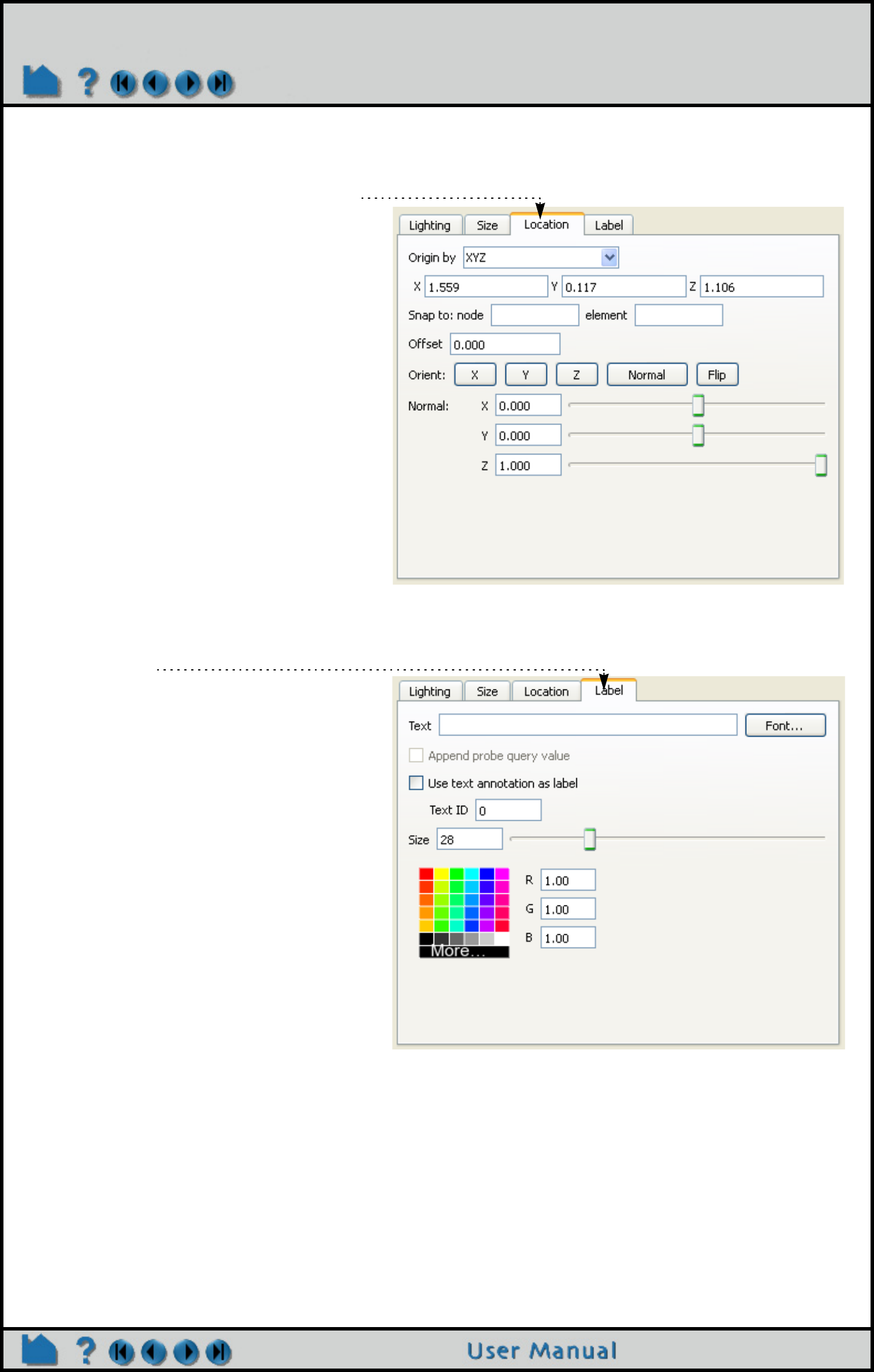
Page 487
HOW TO CREATE 3D ARROWS
SEE ALSO
User Manual: 3D Arrow Annotation
Under the Label Tab, change Label
characteristics:
Type in the arrow label, size it, and color it here.
If the 3D arrow Location was defined as the
location for an interactive query you can
append the interactive query value.
The arrow label can also be defined as an
existing text annotation id. Specify the ID here
and set the text size and color.
Under the Location Tab, change location:
The origin can be set by interactive query
probe locations, xyz coordinate, or external
force or moment vector glyphs. For example,
for xyz location - either type appropriate
coordinates in the X, Y, and Z fields or enter a
node ID or an element ID. Offset value moves
the arrow backwards.
and orientation:
Buttons: The X, Y, Z orient the arrow parallel to
the axis, Flip reverses 180 degrees, and
Normal is normal to a surface (active only if a
surface).
Sliders: Also you can rotate the normal about
the X, Y, or Z. it here.
For the other “Origin by” options appropriate
are presented.
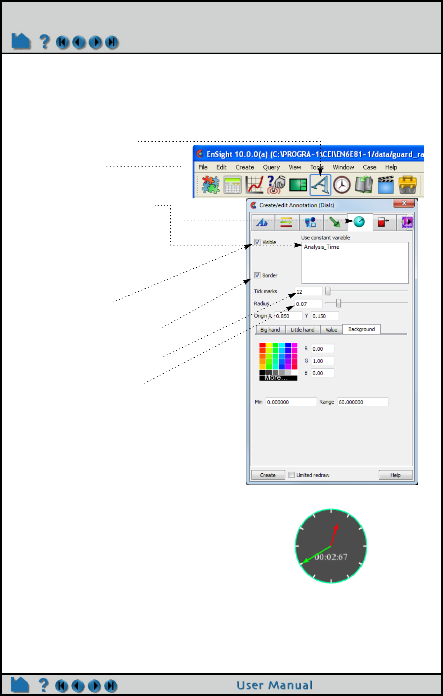
Page 488
HOW TO CREATE DIALS
Create Dials
INTRODUCTION
EnSight can display A 2D dial (such as a clock to measure time) tied to a constant variable. These 2D dials overlay
the Graphics window and are not associated with any viewport.
BASIC OPERATION
To change visibility:
Toggle Visible on or off.
To change whether border is drawn:
Toggle Border on or off.
To change the number of tick marks:
Enter the number of tick marks.
To change the size of the dial:
Enter a value for the dial radius or use the slider.
Values are 0 to 1.
To change location:
Either select the dial and drag it to the desired
location, or type appropriate coordinates into the
Origin X/Y fields. The origin of a dial is the center.
To delete a dial, Right click the dial in the
Annotations list and select “Delete” from the
pulldown.
The Big hand, Little Hand, Value and Background
area is explained on the next page.
Example:
1. Click the Annotations icon.
2. Click the Dial icon in the Create/edit
Annotation dialog.
3. Create a new dial in the Graphics
Window by selecting a variable in
the Use constant variable list and
then clicking the Create button.
To manipulate dial, first select the
gauge(s) of interest in the list, then:
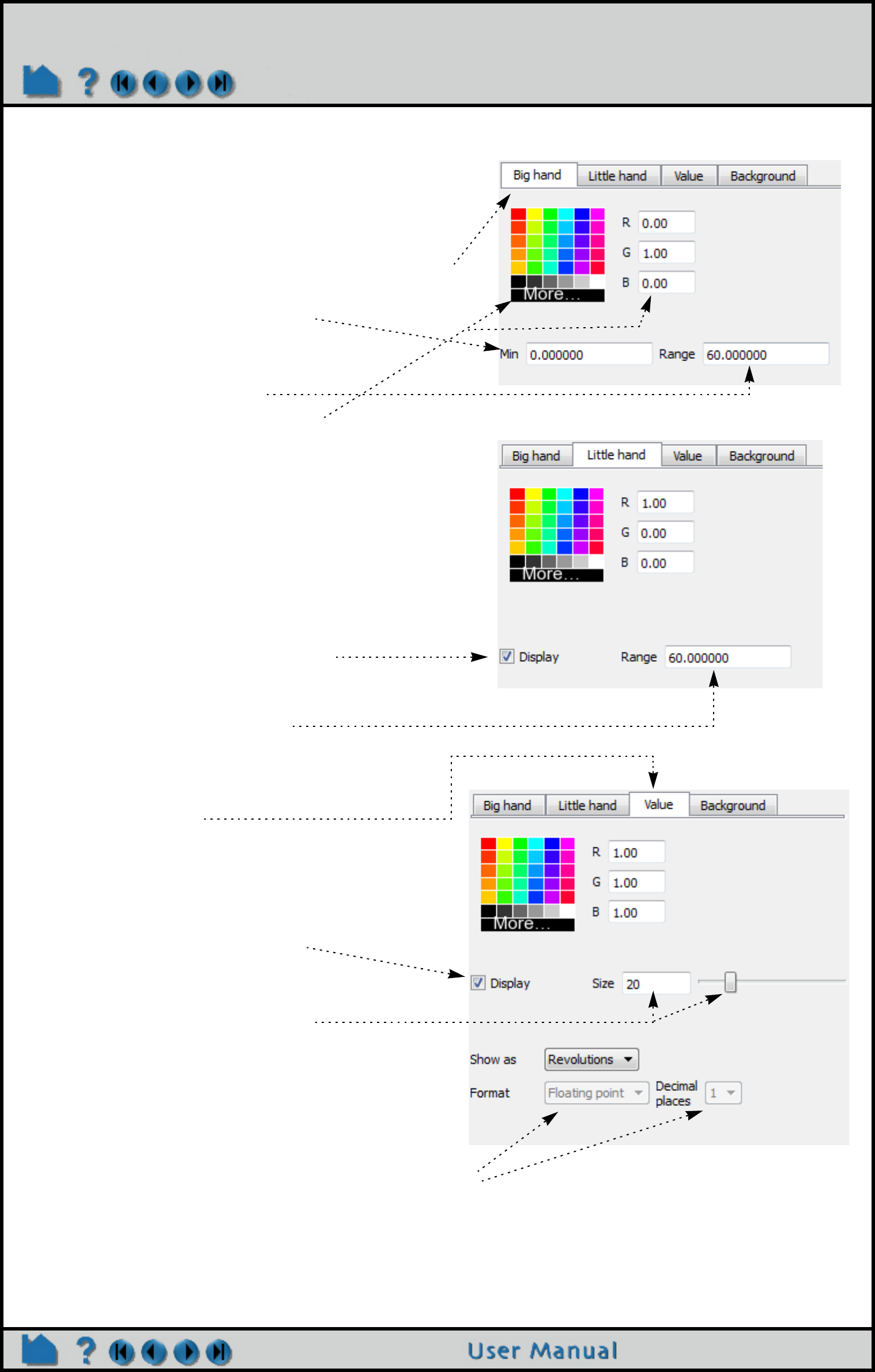
Page 489
HOW TO CREATE DIALS
for the Big hand
The dial "big hand" points straight up at the minimum value
and has a range specified. If the variable being tracked
exceeds the range the modulus of the variable and the range
is shown.
To change any of the Big hand click the "Big hand" tab.
To change the minimum value:
Enter the minimum value in the field.
To change the range:
Enter the range in the field.
To change color for the big hand:
Select the desired color from the matrix, enter RGB values
in the fields, or click More... to open the Color Selector
dialog.
for the Little hand
The dial "little hand" may be visible or not. If visible it is simply
the count of how many rotations the big hand has made. A
value of 0 is straight up and can not be changed.
To change any of the Little hand click on the "Little hand"
tab.
To change the little hand visibility:
Click on the Display toggle.
To modify the Little hand range:
Enter a new range value.
To change color for the little hand:
See instructions under Big hand.
for Value
The dial may display a value on the dial representing the
variable value or the number of rotations the little hand has
made.
To change any of the value display on the dial click on
the "Value" tab.
To change the value visibility:
Click on the Display toggle.
To change the size of the font:
Enter a font size or slide the slider.
To change the display type:
Set Show as to Revolutions if you wish the value to
indicate the number of revolutions that the Big hand has
made or set to Value if you want to display the variable
value.
If you set the Show as to Value you can also set the format
being used by modifying the Format type and the number of
Decimal places.
To change color for the value display:
See instructions under Big hand.
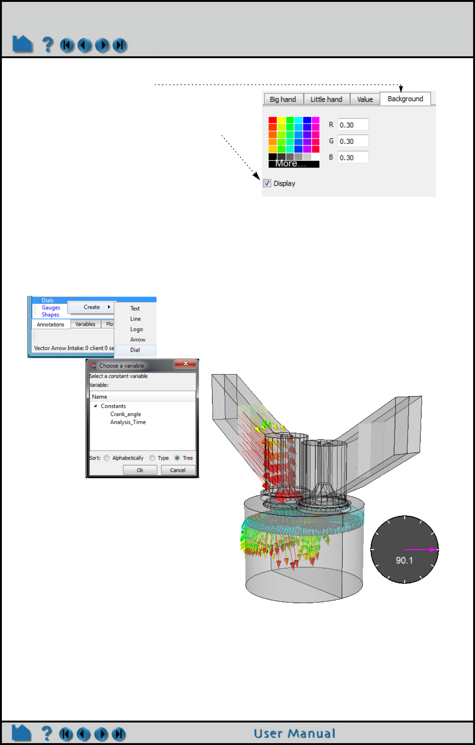
Page 490
HOW TO CREATE DIALS
QUICK CREATION
Right click on the Annotation list under the Annotation Tab and choose Create Dial. This will pop up a dialog to select
a constant. If the constant has ‘angle in it then the dial will be scaled from 0 to 360 (which is useful, for example, for
showing crank angle as seen below). Otherwise the min, max and current timestep will be loaded to determine the
scaling for the dial. .
SEE ALSO
User Manual: Dial Annotation
for the Background
Controls the shading and color of the dial.
To remove the dial background:
Click on the Display toggle. When off no dial background
will be displayed (the dial will be in "wireframe").
To change color for the background:
See instructions under Big hand.
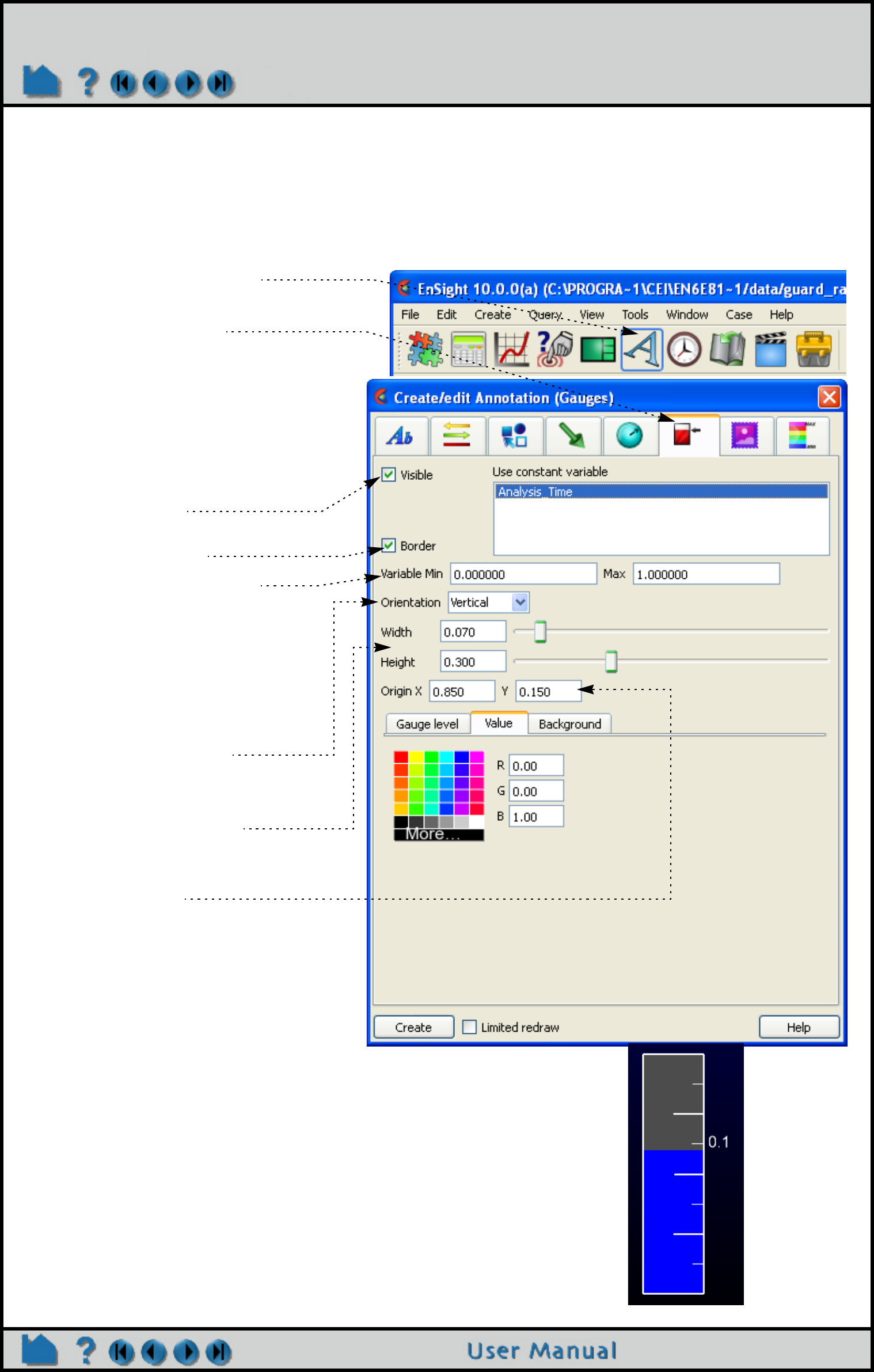
Page 491
HOW TO CREATE GAUGES
Create Gauges
INTRODUCTION
EnSight can display a 2D gauge tied to a constant variable. These 2D gauges overlay the Graphics window and are
not associated with any viewport.
BASIC OPERATION
1. Click the Annotations icon.
2. Click the Gauge icon in the Create/
edit Annotation dialog.
3. Create a new gauge in the Graphics
Window by selecting a variable in
the Use constant variable list and
then clicking the Create button.
To manipulate gauge, first select the
gauge(s) of interest in the list, then:
To change visibility:
To change whether border is drawn:
Toggle Border on or off.
To change the variable range:
Adjust the min and max values. If the
variable value being tracked is greater
than or equal to the maximum value, the
gauge will be “full”. Similarly, if the
variable value is less than or equal to the
minimum value, the gauge will be
“empty”.
To change the orientation:
Set the orientation to Vertical or
Horizontal.
To change the width/height:
Enter a new width/height value or use the
sliders. Values are 0 to 1.
To change location:
Either select the gauge and drag it to the
desired location, or type appropriate
coordinates into the Origin X/Y fields.
The origin of a gauge is the lower left
corner.
To delete a gauge, right click on it in the
graphics window and select Delete.
Example:
The Gauge level, Value and
Background area is explained
on the next page.
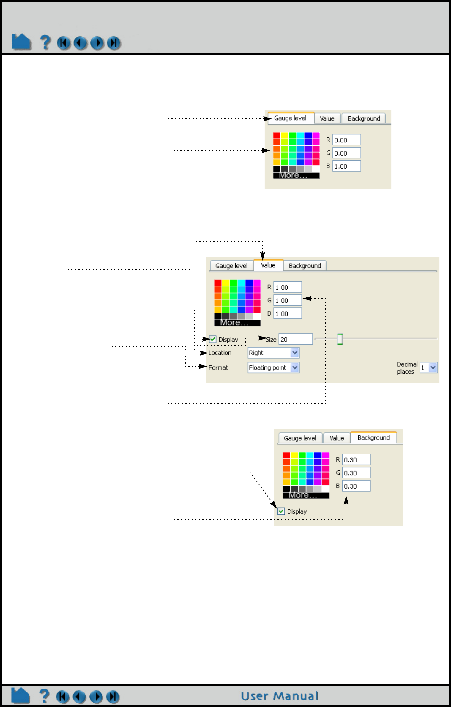
Page 492
HOW TO CREATE GAUGES
for the Gauge level
You can modify the gauge foreground color
(the color tracking the variable value) by:
Click on the Gauge level tab/button.
Select the desired color from the matrix,
enter RGB values in the fields, or click
More... to open the Color Selector dialog.
for Value
A label may be placed on the gauge to
indicate the current value of the tracked
variable.
To change any of the value display on
the gauge click on the "Value" tab.
To change the value label visibility:
Click on the Display toggle.
To change the size and location:
Set the font size and the location for the
label.
To change the format:
You can set the format to floating or
exponential format. For both formats you
can specify the number of decimal places
to display.
To change color for the value label:
See instructions under Gauge level.
for the Background
Controls the shading and color of the gauge.
To remove the gauge background:
Click on the Display toggle. When off no
gauge background will be displayed (the
gauge will be in "wireframe").
To change color for the background:
See instructions under Gauge level.
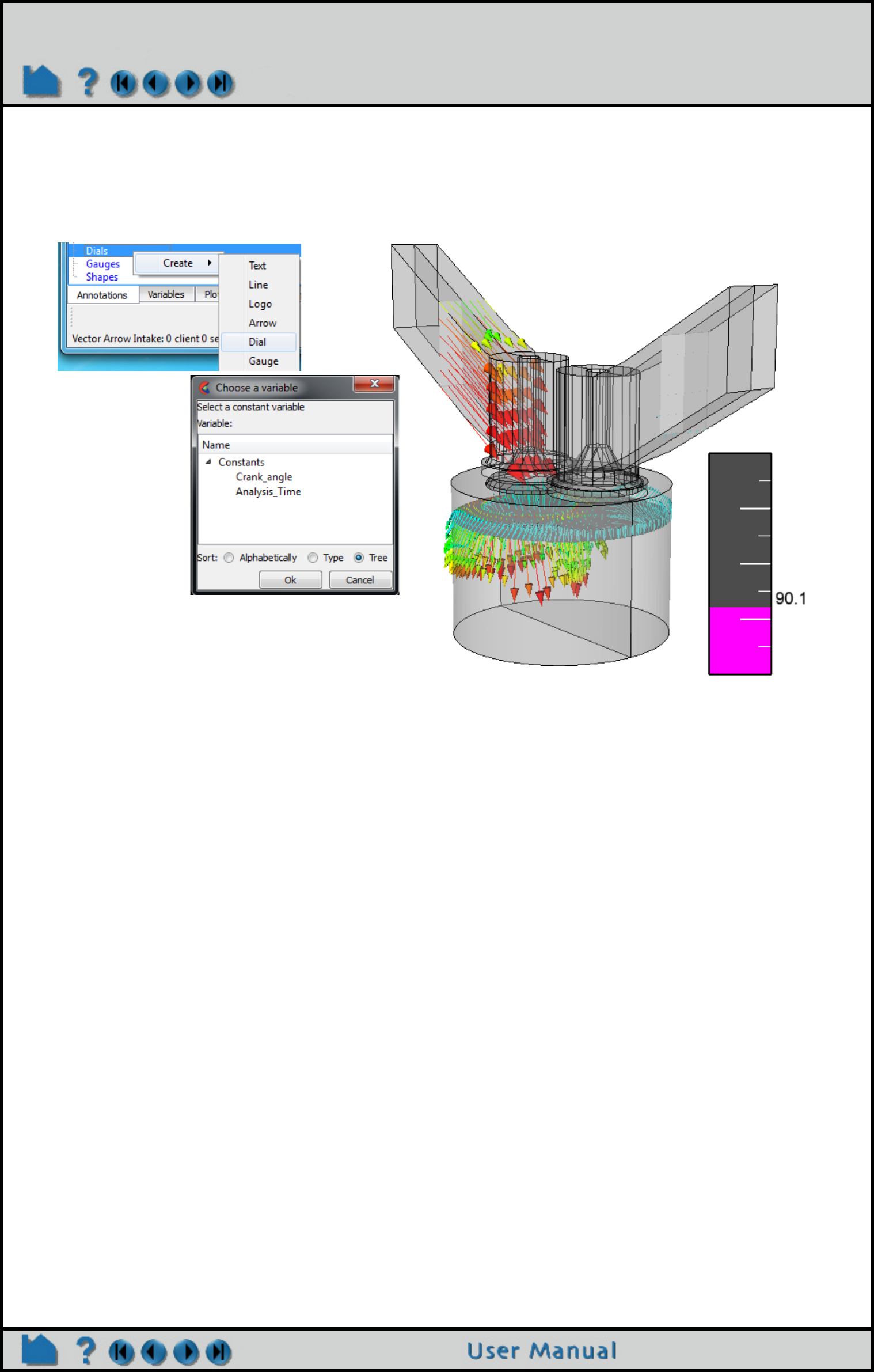
Page 493
HOW TO CREATE GAUGES
QUICK GAUGE
Right click on the Gauges folder in the Annotations tab, and choose Create>Gauge. A dialog will pop up to select a
constant to use for the dial. Select a constant and the value of the constant at the current, the min and the max
timesteps will be used to scale the newly created gauge.
SEE ALSO
User Manual: Gauge Annotation
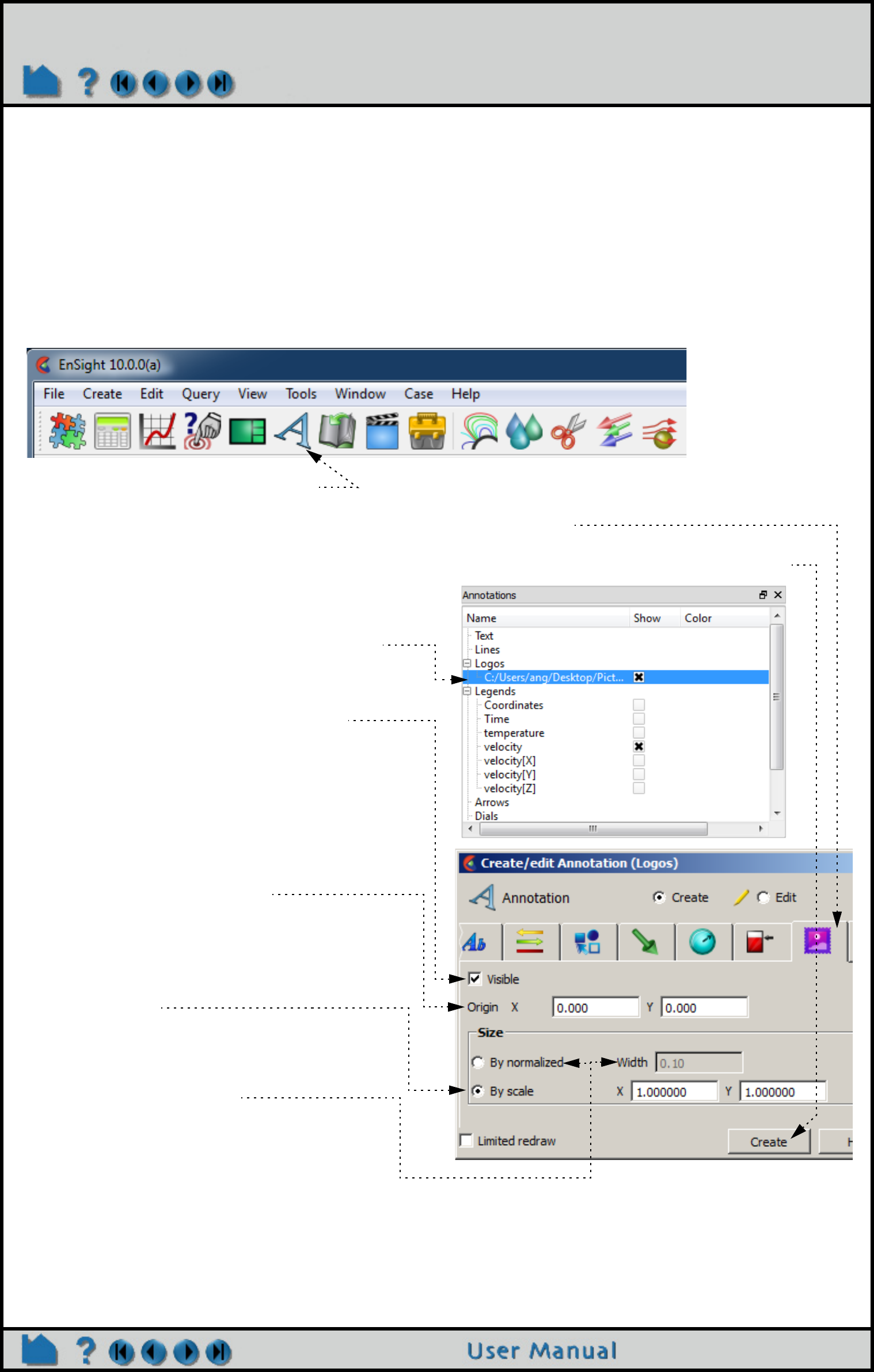
Page 494
HOW TO LOAD CUSTOM LOGOS
Load Custom Logos
INTRODUCTION
EnSight can display bit mapped graphics loaded from disk files. A bitmap can be any image, however, the most
common use is to include a logo or other signature graphic to identify the source of images or animations. Bitmaps
are drawn over all geometric objects in the Graphics Window (at least where the bitmap is opaque), but under all
other annotation entities.
BASIC OPERATION
To load a logo:
SEE ALSO
User Manual: Logo Annotation
To manipulate logo, first select the logo(s) of
interest in the list (or in the graphics window),
then:
To change visibility:
Toggle Visible off or on. Note that if “Limited redraw”
is turned on, the logo will not be completely invisible
but will be displayed in a subdued color.
To change location in the graphics window:
Either position the logo interactively by selecting the
desired logo in the Graphics Window and dragging
it to the desired location, or specify the precise
coordinates in the X and Y fields.
To change size:
Type the desired scaling factors into the “By scale”
X & Y fields and pressing return rescales the logo to
remain at a constant size no matter the size of the
graphics window.
Or selecting “By normalized” and changing the
Width value between 0.0 and 1.0 will automatically
rescale the logo proportional to the size and aspect
ratio of the graphics window.
Note that the size of a logo cannot be adjusted
interactively.
1. Select the Annotation Feature icon.
2. Click the Logo icon at the top of the Create/Edit Annotations dialog.
3. Click the Create button and select the supported image format file using the File selection dialog
which comes up, and click Open.
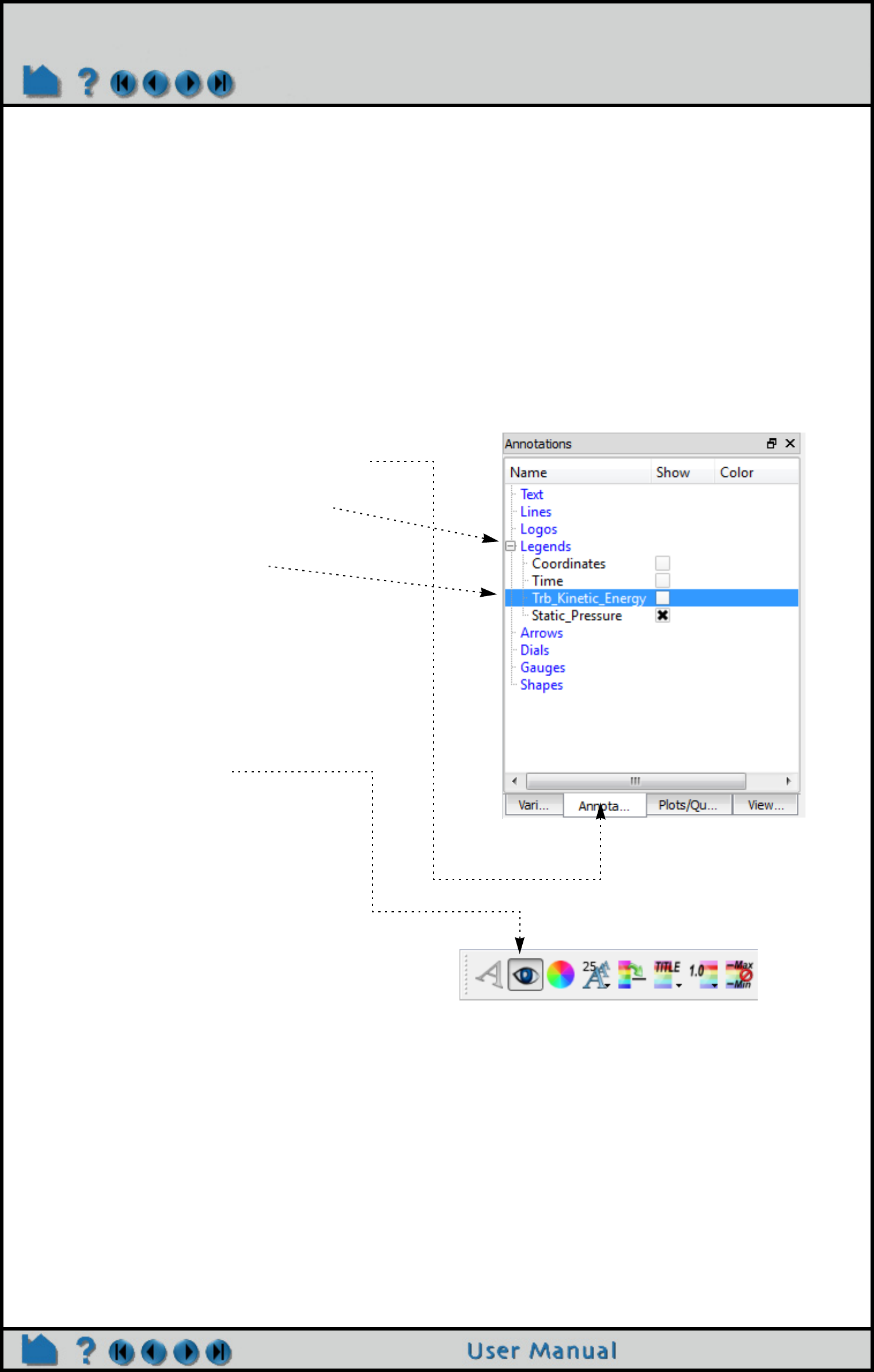
Page 495
HOW TO CREATE COLOR LEGENDS
Create Color Legends
INTRODUCTION
Every currently active variable has an associated color legend that can be displayed in the Graphics Window. Color
legends provide essential information about images that use parts colored by variable values (color fringes).
Legends are particularly important if the image is to be viewed by others.
Legends are drawn as a vertical or horizontal color bar with associated variable values. The size and position of the
color legend can be changed. This article discusses changing the appearance of color legends by modifying
Annotation. To edit the color palette itself (change colors or change the mapping from variable values to colors) see
How To Edit Color Palettes.
BASIC OPERATION
To display a color legend:
1. Click on the Annotation tab in the object list
area.
2. Turn down the Legends group so you can
see the legends that are available.
3. Click the variable legend(s) you wish to
show or hide.
The list contains legends for scalar variables and
for magnitude and components of vector
variables.
4. Right click to Hide or Show the legend
- OR -
4. Click on the visibility icon in the Legends
Quick Action Icon Bar.
If you wish to turn all of the legends off you can
click on the Legends group (which selects all
legends) then right click to hide.

Page 496
HOW TO CREATE COLOR LEGENDS
Resize or Reposition Color Legends in Graphics Window
Color legends can be selected in the graphics window and then scaled or moved:
Manipulating Other Legend
1. Move the mouse on top of the legend you wish to move or scale. The touch-
n-go handles appear
.
2. Click and drag the center point to move the legend.
3. Click and drag the resize handle (upper right) to modify the width and height
of the legend.
The other two resize handles will modify the min and max values attached to
the palette.
1. Double click on the legend you wish
to modify or select it and right click
to Edit. This will bring up the Feature
Panel.
2. Click Legend icon tab if not already
active, then:
To change visibility:
Toggle Visible on or off.
To change color of text and colorbar
outline:
Select the desired color from the matrix,
enter RGB values in the fields, or click
More... to open the Color Selector dialog.
To change title position:
Click the Title Pulldown and select either
Above (the default), Below, or None.
To change legend orientation:
Click the desired Layout (Vertical or
Horizontal).
To change text position:
Click the Values Pulldown and select either
Left/Bottom (the default), Right/Top, or None.
To change legend type:
Click the Type Pulldown and select either Continuous
(the default) or Discrete.
To change text size:
Enter the desired text size or slide the slider.
To change Value label format:
Either select a pre-defined format from the Value format List or enter a new format
string in the Text Format field.
To change location:
Enter values for X & Y (lower left corner) and width and height.

Page 498
HOW TO MANIPULATE FONTS
Manipulate Fonts
INTRODUCTION
EnSight draws all of its text in the graphics window using TrueType fonts. It is capable of reading and drawing most
TrueType fonts and font collections. Under Windows, it is also capable of rendering internationalized multi-byte text in
annotations, provided an appropriate font containing the necessary glyphs is selected.
To ensure portability between platforms, EnSight includes a collection of cross-platform fonts embedded into EnSight.
These include the typefaces: Arial, Courier New, Symbol, and Times New Roman. If a user restricts font usage to
these font families, resulting .els and other files will be portable. If other font families are used, EnSight may substitute
one of these (or other) fonts if it cannot find a match on the target system. EnSight will also read the installed system
fonts on Windows and Power PC-based Macs. The environmental variable CEI_FONTPATH may be set to a list of ':'
(';' on Windows) separated directory names in which EnSight should also look for .ttf and .ttc files. This allows
the user to use their own fonts in EnSight on any platform.
Fonts are always specified in EnSight as a family name and an optional style with a ':' separator. For example,
'Arial:BoldItalic' specifies the Arial family with the styles Bold and Italic applied. Style names of 'Roman', 'Italic',
'Bold' and 'Oblique' (and combinations) are all recognized by EnSight and are mapped against the internal flags in the
TrueType files themselves. The default fonts, styles and sizes used by EnSight can also be set through a collection of
environmental variables:
The ENSIGHT_FONT_DEFAULT_*_STYLE environmental variables use a numbering scheme for the styles. The
following values may be added together to form the style: BOLD 1
ITALIC 2
OBLIQUE 4
ROMAN 8
For example, if the user wanted annotations to default to Arial:BoldItalic, the following environmental variables should
be set (Windows syntax):
set ENSIGHT_FONT_DEFAULT_ANNOT=Arial
set ENSIGHT_FONT_DEFAULT_ANNOT_STYLE=3
This selects Arial and BOLD+ITALIC=3. The default font is not recorded in scenario files. Thus, if a scenario file is
generated with these defaults, for the EnLiten user to see the exact same annotations, they would need to set the
same environmental variables and have the same fonts installed on their system. Font changes made with the <fo=>
formatting codes (see below) are embedded into the scenario files and do not require the environmental variable
changes for proper display (but do require the same fonts be installed).
Note: under Windows, EnSight uses Times New Roman as the default font for annotations. This font does not contain
a large selection of multi-lingual characters. For users running internationalized versions of Windows, we suggest
that they set ENSIGHT_FONT_DEFAULT_ANNOT to the name of the typeface that best matches their locale. This
allows for natural internationalized text input.
ENSIGHT_FONT_DEFAULT_SYMBOL family to be used instead of the symbol font - default = “symbol”
ENSIGHT_FONT_DEFAULT_OUTLINE family to be used for ID/axis labeling - default = “Arial”
ENSIGHT_FONT_DEFAULT_ANNOT family to be used for annotations - default = “Times New Roman”
ENSIGHT_FONT_DEFAULT_SYMBOL_STYLE style to be used with the symbol font
ENSIGHT_FONT_DEFAULT_OUTLINE_STYLE style to be used with the outline font
ENSIGHT_FONT_DEFAULT_ANNOT_STYLE style to be used with the annotation font
ENSIGHT_FONT_DEFAULT_OUTLINE_SCALE specifies the relative scale for the outline font. The value 100.0 is
the default 200.0 is 2x larger, 50.0 is ½ size
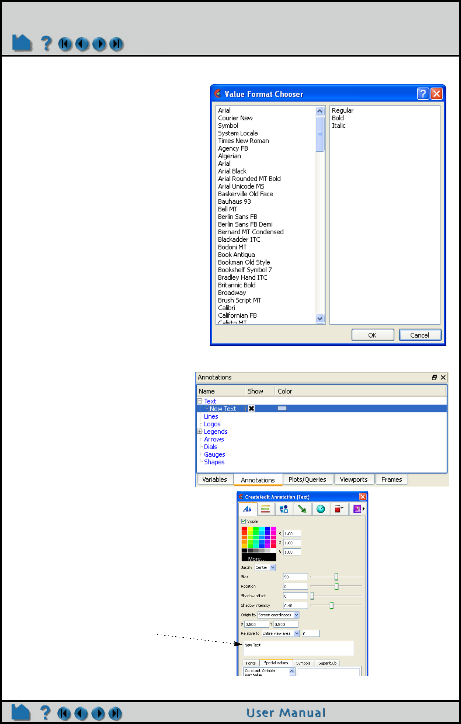
Page 499
HOW TO MANIPULATE FONTS
BASIC OPERATION
Font selection dialog
In nearly every location where EnSight allows the
user to enter a text string to be used for display
(e.g. text annotations, plot titles, axis titles, etc), it
is possible to change the font. It is also possible to
change the font repeatedly in a string. This is done
by inserting a special code into the string that
contains the font name (See Text formatting codes
for details). In several locations in EnSight, this
operation is simplified via the Value Format
Chooser dialog (or something similar) which lists
all the available font family/style combinations and
allows the user to change fonts in the text field
currently being edited
The current font (possibly the default) is selected
in the list when the dialog is opened. The user
may change this font to any other by selecting
from this list and clicking OK.
To illustrate the use of font capabilities,
Text Annotation will be used:
Double click, or right click and select Edit...
to open the Create/edit Annotation (Text)
dialog.
The text can be modified in the field.
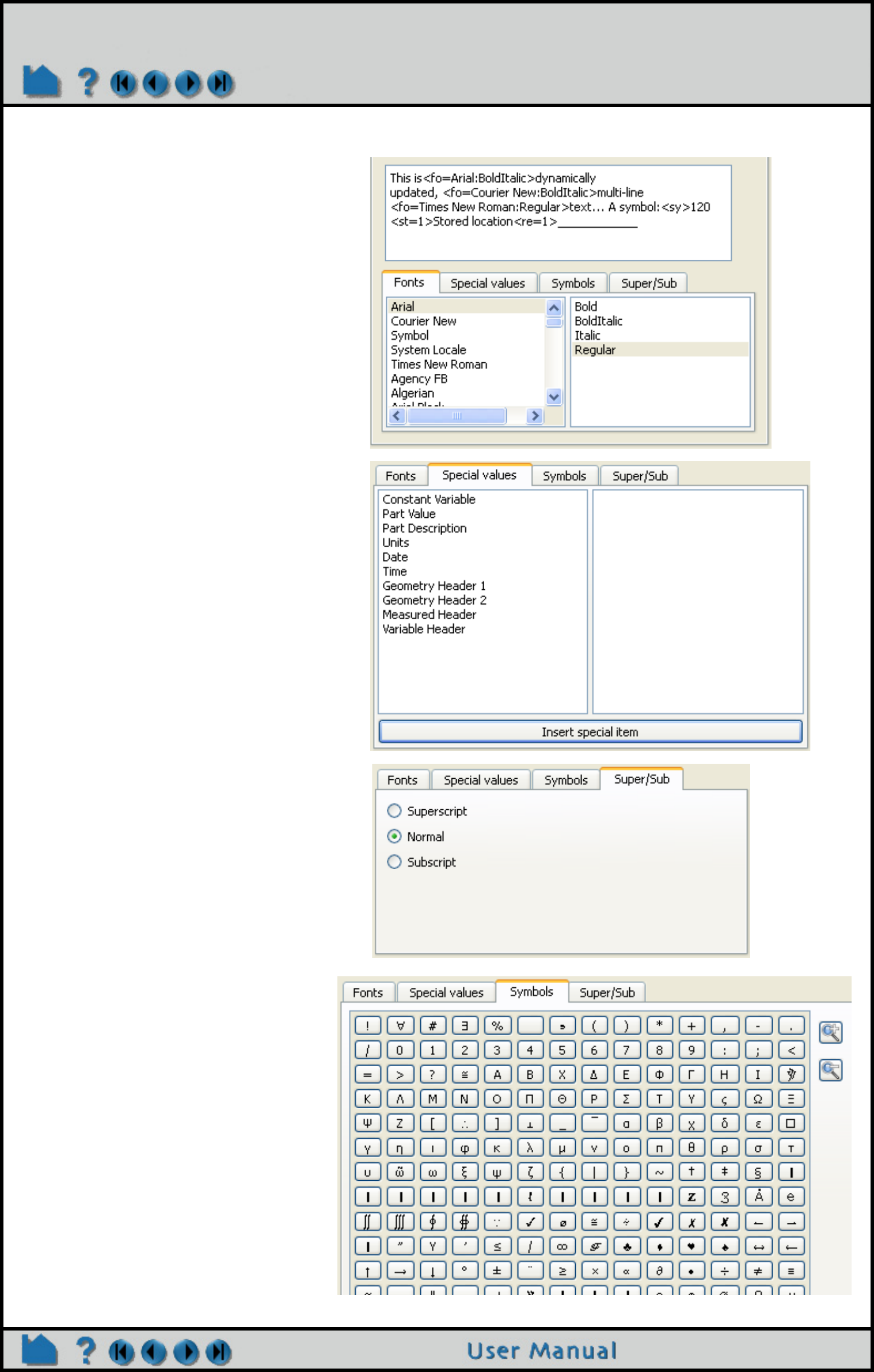
Page 500
HOW TO MANIPULATE FONTS
The text to be edited is typed into the
scrolling text field. Note that pressing 'enter'
inserts a new line into the annotation.
The results of the edit are dynamically
redrawn in the graphics window as you make
changes.
The Fonts and their weights can be inserted
by selecting them under the Fonts tab.
Special EnSight values can be inserted
under the Special values tab.
Under the Super/Sub tab, the Normal,
Subscript and Superscript radio buttons
allow the user to mark sections of the text to
be in super or subscript form by inserting the
special codes <no> <up> and <dn> into the
text stream.
Symbols can be selected under the
Symbols tab.
Any of the codes (shown in the Font
Formatting Codes on the next page) can
be typed in manually as well, if desired.
Page 501
HOW TO MANIPULATE FONTS
Font formatting codes
The TrueType rendering system supports a number of special embedded codes. These can generally be placed in
most any string displayed in the EnSight graphics window (e.g. plot titles, axis titles, etc). When the text string is
drawn, these special codes are parsed out of the string and they affect any text to the right of the code. In general, the
effects are additive and to turn an effect off, insert another code that sets the feature back to its default value. The
codes are:
<no> The text is drawn in "normal" mode.
<up> The text is drawn in superscript mode.
<dn> The text is drawn in subscript mode.
<fo=[family|*][:style]> Change the current font family and/or style. To change just the font family, use
<fo=newfamily>. To change the style only, use <fo=*:newstyle>. The
special case of <fo=> resets the text family and style to the default.
<so=[scale][:voff]> Change the current scaling and/or vertical line offset. To change only the relative
fontsize, use <so=scale>, where 1.0 is the default size of the text. To change
only the vertical offset of the next text, use <so=:offset>. For example,
<so=0.5:0.5> simulates superscript. The special case of <so=> resets the scale
and vertical offset to 1.0 and 0.0 respectively.
<st=X> Store the current text position into slot X (x is an integer from 1 to 9).
<re=X> Recall the current text position from slot X (x is an integer from 1 to 9).
The store/recall mechanism in conjunction with <so=> allows for accurate
repositioning of text. For example, it allows overstrike of text and for the generation
of simultaneous super and subscripts as well as formatted fractions. Note that slot
0 is reserved for the first character in the current line of text.
<sy>XXX Insert a single glyph from the "Symbol" font at this position. Note that 3 decimal
digits must follow the <sy> text.
<uc=num> An arbitrary glyph from a font using its Unicode number. The number must be
specified as four hexadecimal digits. For example, <uc=00A9> will produce the
copyright symbol (©) if it is available in the current font.
<co=R[:G:B[:A]]> Set the color of the subsequent text. The user may supply up to 4 floating point
values in the range [0.0,1.0] for the Red, Green, Blue and Alpha (opacity) of the
text. The alpha value defaults to 1.0, while other values default to the value to their
left. Note: <co=:::0.5> changes just the opacity of the text.
<cr> Explicitly move to the next line. This is the same as pressing 'enter' in the textfield.
Note that text shown in the Annotation dialog list for text annotations is displayed
with <cr> in place of all new lines.
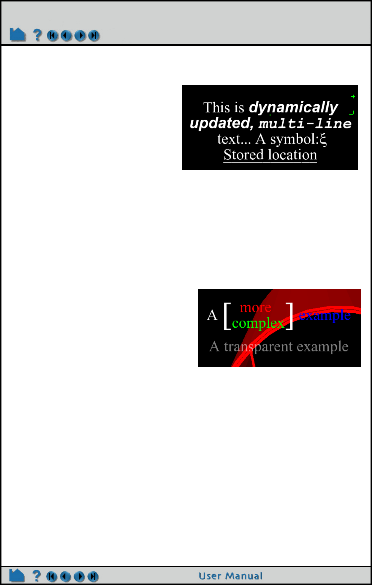
Page 502
HOW TO MANIPULATE FONTS
A simple example
The following is an example of a text annotation that utilizes multiple fonts, multiple lines of text, symbols and the
store/recall feature.
The first few words are in normal text, followed by a font change and a new line. Midway through the second line, the
font changes again and at the end of that line, it changes back to the default font and style. The third line ends with a
glyph from the symbol font. The last line starts by storing the location of the 'S' character in slot '1'. It then draws
'Stored location' before the <re=1> command recalls current output to the 'S' location. Finally, a row of underscores
are drawn that overstrike the words "Stored location".
A more complex example
The following text annotation example illustrates the use of text colors and some scaling and offset options.
This example begins by drawing an 'A', then scaling up the text while dropping it a bit below the line before drawing a
left brace '['. It then stores off that location and sets up drawing at the original size, but above the baseline. The color
is changed to red and the word 'more' is drawn. The stored location is recalled and a similar operation is done for the
word 'complex' below the baseline. The scale is set to the same as the first brace, the color is reset to white and the
right brace ']' is drawn. To end the line, the scale and offset are reset and 'example' is drawn in blue. The second line
is a blank line. The final line is a simple example of how to make a piece of text partially transparent. Note that the red
object behind the text can been seen through the text.
SEE ALSO
How To Create Text Annotation
User Manual: Annotations List Panel
The string entered into the View Text Create/Edit
Dialog to create this annotation is:
This is <fo=Arial:BoldItalic>dynamically
updated, <fo=Courier New:BoldItalic>multi-line
<fo=>text... A symbol:<sy>120
<st=1>Stored location<re=1>____________
The string entered into the View Text Create/Edit Dialog to
create this annotation is shown below (note that this is
actually three lines of text, the first is a single, very long line):
A<so=2:-0.25><sy>091<st=1><so=1:0.5><co=1:0:0> more<re=1><so=:-
0.25><co=0:1:0>complex<so=2:-0.25><co=><sy>093<so=> <co=0:0:1>example
<co=1:1:1:0.5>A transparent example
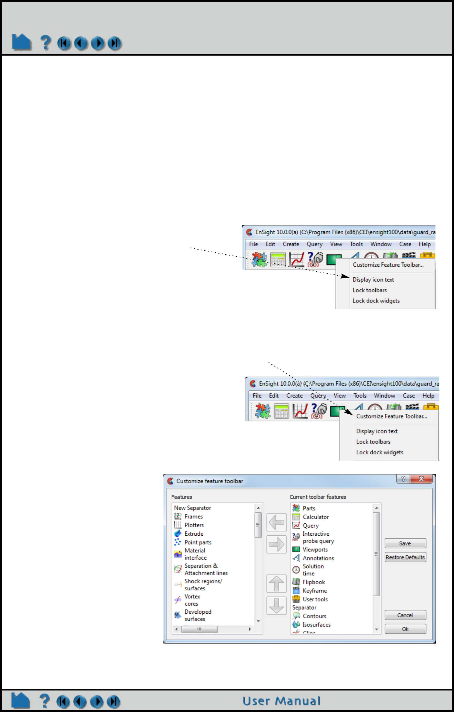
Page 503
HOW TO CUSTOMIZE ICON BARS AND PANELS
Configure EnSight
Customize Icon Bars and Panels
INTRODUCTION
EnSight uses several sets of icons to group functionality. The Feature Icon bar can be customized in terms of which
features are available and what order they will be presented. All of the icon bars can be moved and docked or
undocked. In addition, all of the list panels (part, variable, viewports, annotations, query/plots, and frames) can
customize the columns of data displayed in the panel.
The icons can have text “sub titles” under the icon. Many users find it useful to turn this text one while they learn the
system and turn it back off once mastered.
BASIC OPERATION
To turn on Icon text:
To customize the Feature Icon Bar:
1. Right click in the Feature Icon bar then select
“Display icon text” from the pulldown.
1. Right click in the Feature Icon bar then select “Customize Feature Toolbar” from the pulldown.
2. In the resulting dialog you can:
(a) Select features from the “available” list on the
left and use the right arrow button to place it on the
Feature Icon bar.
(b) Similar, if you select a feature in the right
column you can click the left
mouse button which will remove it
from the Feature Icon bar.
(c) Any feature in the right column
can be moved up and down to
modify its order on the icon bar via
use of the up/down arrows.
3. The Save button will retain the
settings next time you run EnSight.
4. While the OK button will make
the modifications for the current
session only.l
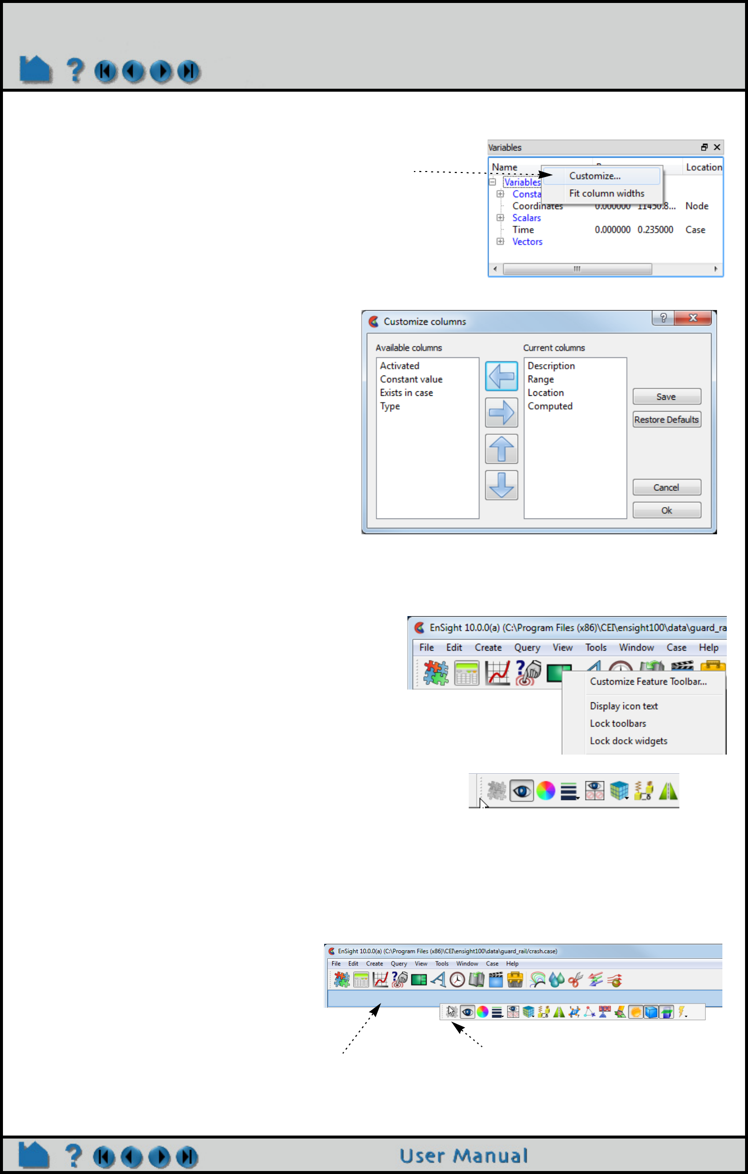
Page 504
HOW TO CUSTOMIZE ICON BARS AND PANELS
To customize the columns in the list panels:
1. Right click on the column header in the list you wish to
customize. In the figure shown the right click was performed
on the “Name” portion of the list.
2. Each list panel will have a different set of that can be shown.
The figure at right shows the choices for the Variables list.
Similar to the Feature Bar discussion above you can add or
remove new columns and modify the order of the columns
using the left/right and up/down arrows.
To move the Icon bars:
1. Right click on any icon bar. In the resulting pulldown
the “Lock toolbars” should be unchecked, i.e., toolbars
are allowed to be moved.
2. The icon bars have a “handle”. Click and drag the
handle and the icon bar will come out of the user
interface and will follow the mouse as you move it.
3. If you release the mouse button outside of the user interface
the icon bar will be free floating.
OR
3. As you drag the icon bar to the various docking locations in
the user interface you will see a space open up where the bar
could dock itself. Release the mouse button and the icon bar
will doc in the space provided.
The blue rectangle indicates
where the bar could be
docked.
This bar is being dragged
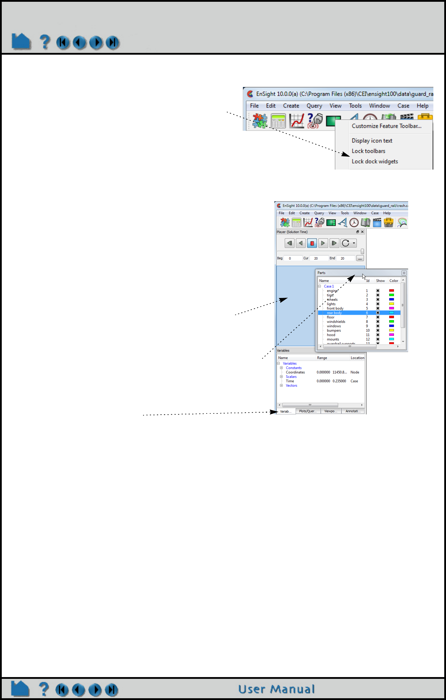
Page 505
HOW TO CUSTOMIZE ICON BARS AND PANELS
ADVANCED USAGE
The layout and position of the icon bars and panels are saved and will be restored next time you run EnSight. The
easiest way to restore the default configuration is to start EnSight with a “-no_prefs” start parameter.
SEE ALSO
User Manual: Icon Bars
To move the panels:
1. Right click on any icon bar or the header of any panel.
In the resulting pulldown the “Lock dock widgets”
should be unchecked, i.e., “widgets” are allowed to be
moved.
2. The panels can be dragged by their header. Click and
drag the header and the panel will come out of the user
interface and will follow the mouse as you move it.
3. If you release the mouse button outside of the user interface
the panel will be free floating.
OR
3. As you drag the panel to the various docking locations in the
user interface you will see a space open up where the panel
could dock itself. Release the mouse button and the panel
will doc in the space provided.
The blue rectangle indicates
where the panel could be
docked.
This panel is being dragged
4. Panels can be stacked on top
of each other. In which case you
will get a tab for each panel
occupying the same space. By
default for example, the Variables,
Plots/Queries, Annotations, and
Viewports panels are stacked.
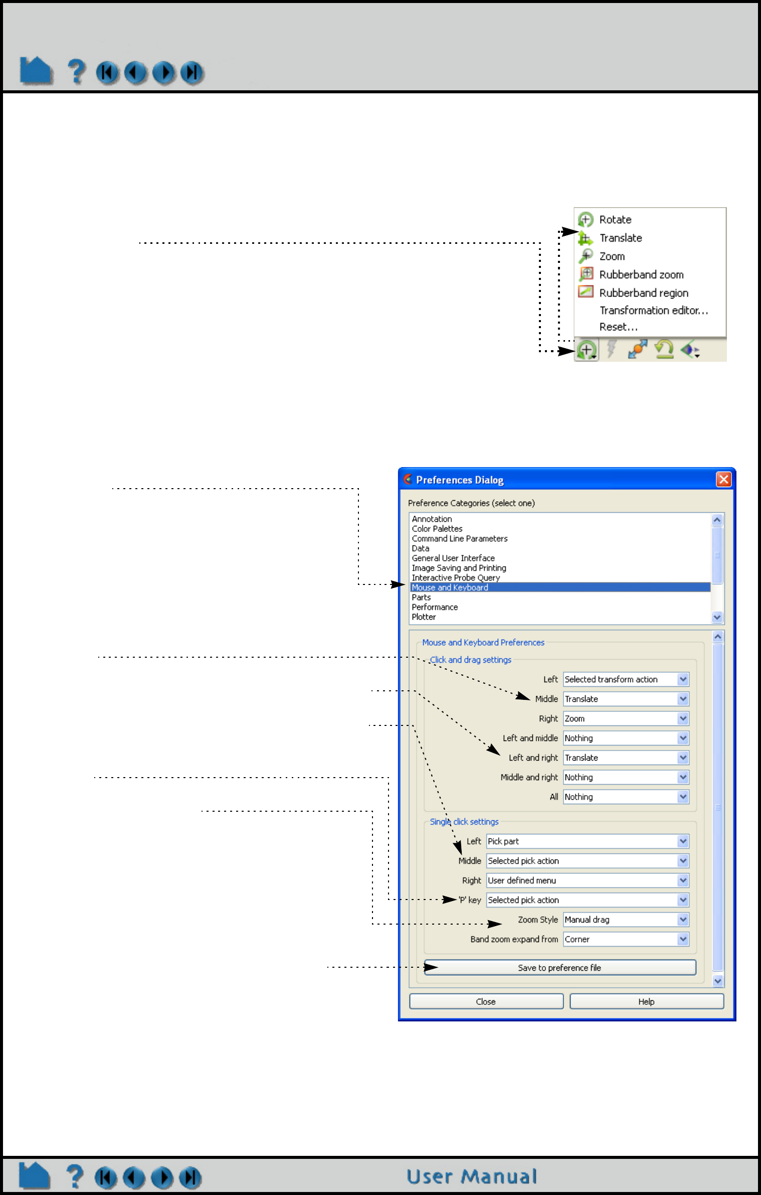
Page 506
HOW TO CUSTOMIZE MOUSE BUTTON ACTIONS
Customize Mouse Button Actions
INTRODUCTION
When the mouse pointer is in the Graphics Window, clicking and holding the left mouse button as you drag will
perform the current transformation (e.g. rotate or zoom) as selected under the Graphics window transforms icon in
the Transformation Control area.
BASIC OPERATION
To change the behavior of mouse buttons in the Graphics Window:
To perform a different transformation, you have to click on this icon and select
the new operation.
To avoid this, you can redefine how the left mouse works as well as map
additional transformation operations onto the middle and right mouse buttons,
combinations of mouse buttons, and double-clicking of mouse buttons.
This customization only effects the mouse usage while in the Graphics Window.
The left button is still used for other user-interface actions.
1. Select Edit > Preferences..., then click on Mouse and
Keyboard
2. Set each click and drag mouse button pulldown
(Left, Middle, Right and combinations of such) as
desired.
3. Set the two button click and drag for each mouse.
4. Set the single click action for each mouse button.
5. Set the action for the keyboard ‘P’ key (see
below).
5. Set desired Zoom Style.
Automatic slide will zoom based on the direction and
distance the mouse is moved. To the right or up zooms
away, while to the left or down zooms towards. The
distance the mouse is dragged determines the rate of
continuous zoom.
Manual drag zooms in the same directions, but only a
distance relative to the distance the mouse is dragged.
6. Click Save To Preference File to save your
changes (if you want these changes to be the
default for future sessions of EnSight) and Close
to exit the dialog.
The new settings will take effect as soon as you hit the
close button. If you clicked Save To Preference Files,
your changes are also written to a file and automatically
loaded during future EnSight sessions.

Page 507
HOW TO CUSTOMIZE MOUSE BUTTON ACTIONS
Each mouse button (or combination of mouse buttons) can have one of the following associated behaviors:
Note that at least one of the mouse buttons (or combinations) must be set to “Selected transform action”!
Each double-click mouse action or the keyboard ‘P’ key can be set to the following:
Note that at least one of the mouse buttons, double-click options or the “P” key must be set to “Selected pick
action”!
SEE ALSO
User Manual: Mouse and Keyboard Preferences
Selected
transform action
When this mouse button is clicked and dragged, the operation performed will be the currently
selected function in the Transformation Control area.
Rotate When this mouse button is clicked and dragged, the operation performed will be rotate.
Translate When this mouse button is clicked and dragged, the operation performed will be translate.
Zoom When this mouse button is clicked and dragged, if Zoom Style is Manual Drag then a zoom
displacement will occur, and if Zoom Style is Automatic Slide then a zoom velocity will occur
Rubberband
zoom
When this mouse button is clicked and dragged, the operation performed will be a rubberband
zoom.
Rubberband
selection tool
When this mouse button is clicked and dragged, the operation performed will be a rubberband
selection tool manipulation.
Selected pick
action
When this mouse button is clicked, the currently selected pick action (as previously selected
under the pick icon) will be performed.
Pick part When this mouse button is clicked, the pick part action will be performed - causing the part under
the mouse to be selected in the main parts list.
Pick cursor tool
location
When this mouse button is clicked, the pick cursor tool action will be performed - causing the
cursor tool to move to the picked location.
Pick transf. center When this mouse button is clicked, the pick transformation center action will be performed -
causing the center of transformation to move to the picked location.
Pick elements to
blank
When this mouse button is clicked, the element blanking action will be performed - causing the
element under the mouse to be removed.
Nothing When this mouse button is clicked, no action will be performed.

Page 508
HOW TO SAVE SETTINGS
Save Settings
INTRODUCTION
The default size and position of the EnSight user interface windows was chosen to try to minimize window overlap.
When you move and resize windows EnSight saves this information such that the next time you start EnSight the
layout should be the same as when you left it last.
ADVANCED USAGE
If you want to get back to the default layout for the windows, start EnSight with the “-no_prefs” start parameter.
SEE ALSO
See User Manual: GUI Overview
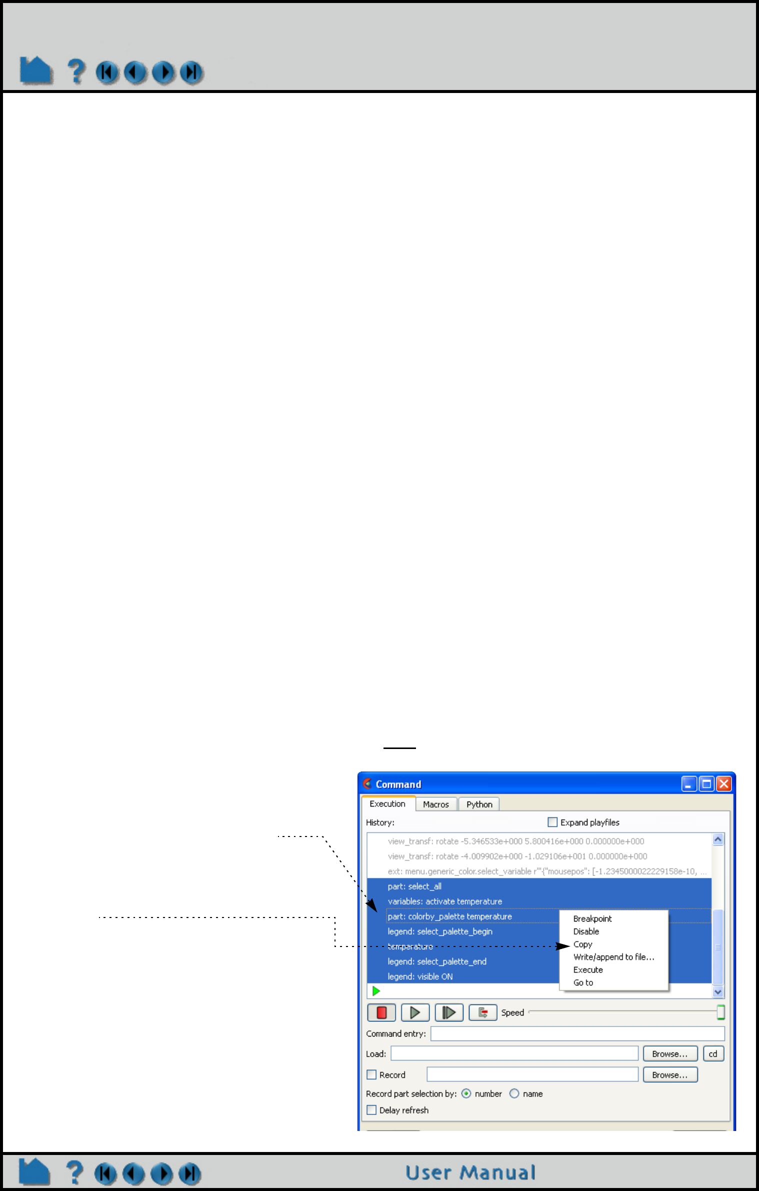
Page 509
HOW TO DEFINE AND USE MACROS
Define and Use Macros
INTRODUCTION
Advanced users of EnSight often find themselves performing repetitive tasks. EnSight’s macro facility lets you save a
sequence of commands and then assign a keyboard key to those commands such that they are executed when the
key is pressed. Note: macros only work when the mouse cursor is in the graphics window.
Pressing a key assigned to a macro causes the associated command file to be read and executed. Depending on
how it is set up, a macro can execute its file in one of three ways:
1. The command file is executed once for each key press. This mode is useful for one-time operations such as cut-
ting flipbook animation on/off or saving an image.
2. The command file repeatedly executes as long as the key is held down. This is useful for operations that are con-
tinuous in nature, such as rotating around the Y axis by 5 degrees.
3. Multiple command files execute in a cycle for each keystroke.
Keystroke macros are defined in a text file, macro.define. Macros can be defined at a site or local level, with local
macros overriding site macros that might be defined for the same key. The macro.define file (if any) that resides
in the %CEI_HOME%/ensight102/site_preferences/macros directory defines site-level macros, while the
macro.define file (if any) under the user’s EnSight defaults directory (located at
%HOMEDRIVE%%HOMEPATH%\(username)\.ensight102 commonly located at C:\Users\username\.ensight102 on
Vista and Win7, C:\Documents and Settings\yourusername\.ensight102 on older Windows, and ~/.ensight102 on
Linux, and in ~/Library/Application Support/EnSight102 on the Mac) will define that user’s local macros. Any
command files referenced by macros must be located in these directories as well.
Most of the functions needed to define and edit macros can be found under the Macros tab of the Command Dialog
(File > Command from the Main Menu). Open this dialog to view the default, system macros in the default install.
BASIC OPERATION
Creating Macro Command Files
The first step in creating macros is to save the various command sequences that perform the desired actions. This
can be done in several ways.
One way to save commands for a macro is to save off a command file from an Ensight session. See How To Record
and Play Command Files for more information. Be careful as you perform the operations that are saved to the
command file. Superfluous or errant commands will slow down macro operation or cause errors. You may wish to
view the resulting command files with a text editor and possibly make changes.
A second way to create the command file for a macro is to copy commands from the Command Dialog history
window:
1. Mark the desired commands by clicking
and dragging in the history window, or by
any combination of clicking and dragging
while holding down the CTRL key.
2. With the cursor over the marked
commands, click the right mouse button to
bring up the action menu, then select
"Copy".
This will copy the commands to the system
clipboard.
3. Bring up a text editor and insert the
commands using "Paste".
4. When you are finished building your
macro command file, be sure you save it in
the site or local macros directory (see
above).
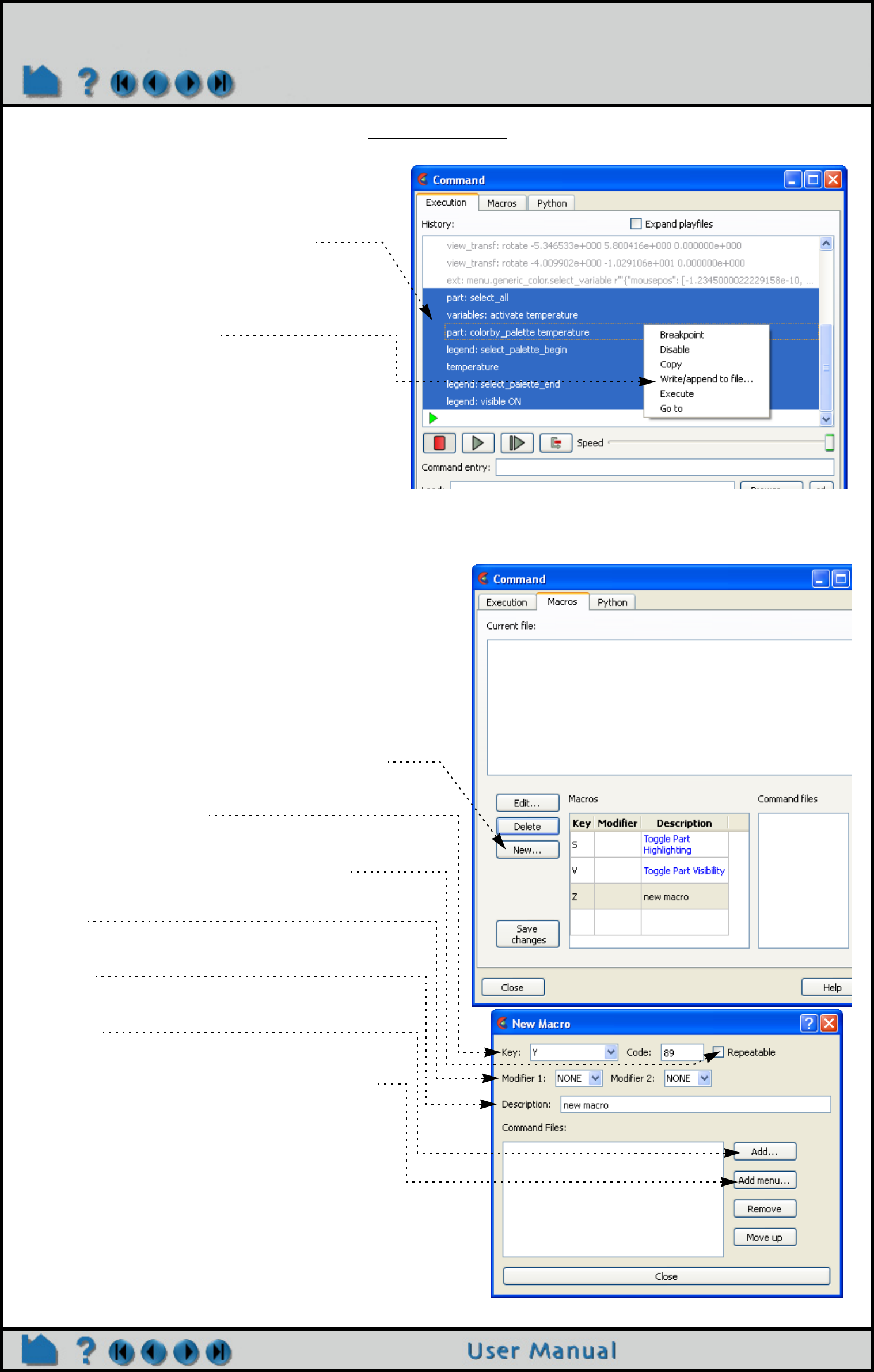
Page 510
HOW TO DEFINE AND USE MACROS
A third way to create a macro command file is by writing/appending them directly to a file from the Command Dialog
history window:
Linking macro command files to keys
To link a command file in the macros directory to a key or mouse button:
1. Mark the desired commands by clicking
and dragging in the history window, or by
any combination of clicking and dragging
while holding down the CTRL key.
2. With the cursor over the marked
commands, click the right mouse button
to bring up the action menu, then select
"Write/append" to file.
3. A File Selection dialog opens. Select or
enter the desired file to save commands
to and click Save. If the file already exists,
the selected commands will be appended,
if it does not, it will be created with the
selected commands.
1. In the Command Dialog "Macros" tab (File >
Command from the Main Menu), click "New".
The New Macro dialog opens.
2. Select or type a key,
3. Check "Repeatable" if you want the macro to
be repeated while the key is held down.
4. Select any modifier keys such as CTRL or
ALT.
5. Enter a brief description of what the macro
does.
6. Click "Add" to add a command file for the
macro.
6. OR click “Add Menu” to add the functionality
from an existing EnSight menu to the macro.
A File Selection dialog opens.
7. Select the desired file and click Save.
Note: you can select a file anywhere on your
system, and if it is not already in the local .macros
directory, it will be copied there.
8. Repeat steps 6 and 7 for macros with
multiple command files.
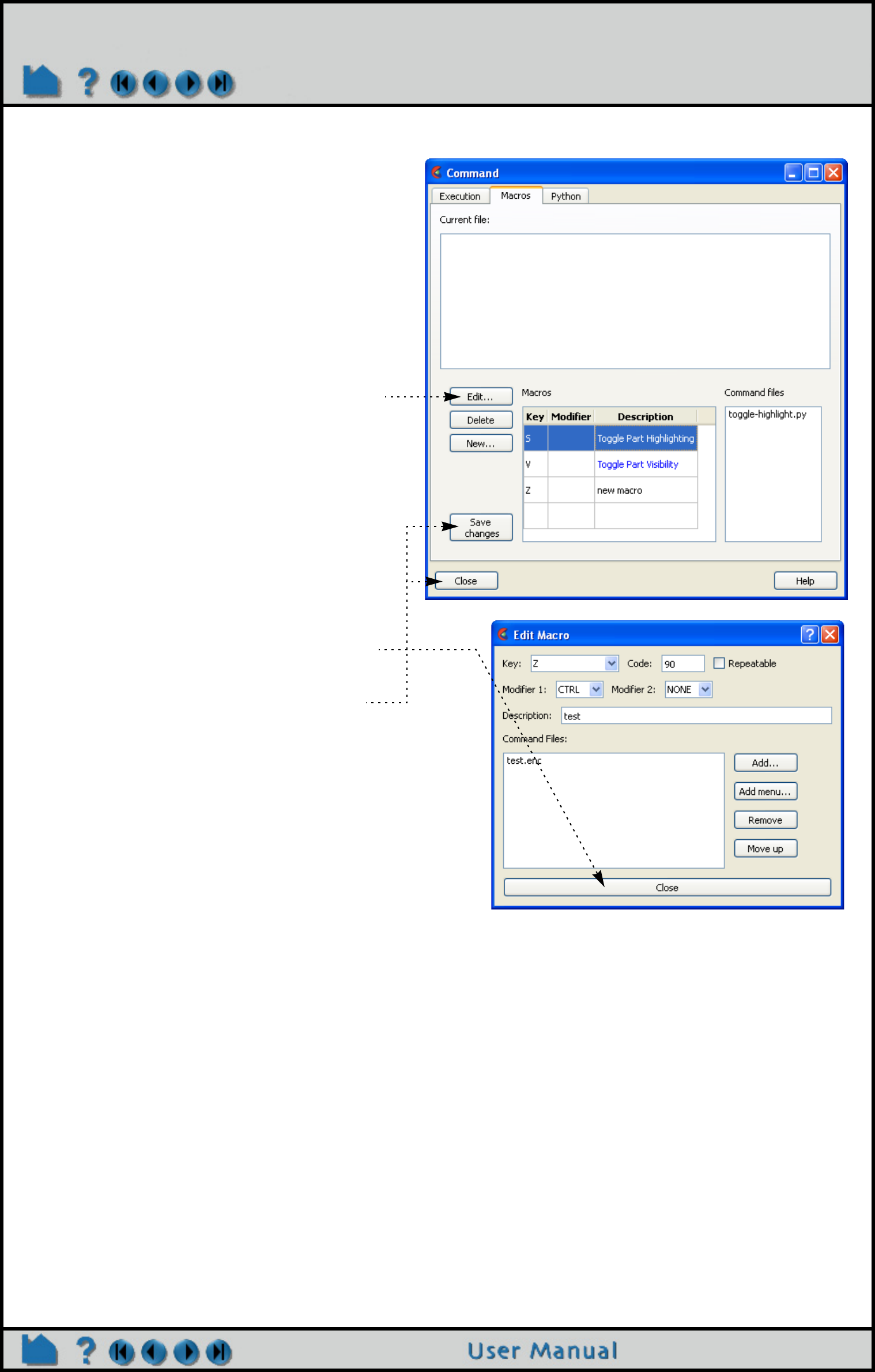
Page 511
HOW TO DEFINE AND USE MACROS
To change an existing macro definition:
OTHER NOTES
A common use of tying more than one command file to the same key is to create a toggle. Make the first command
file turn the option on, and the second command file turn the option off. Then tie both of these to the same key. You
will now cycle through the two command files, effectively creating a toggle situation.
SEE ALSO
How To Record and Play Command Files
User Manual: Macros Tab
1. In the Command Dialog "Macros" tab (File >
Command from the Main Menu), click "Edit".
2. The Edit Macro dialog opens. Change any of
the values in this dialog, then click "Close".
Your changes will not be written to the
macro.define file until you either click "Save
Changes" in the Command dialog Macros tab, or
close the command dialog and answer "Yes" to the
Save Changes query message.

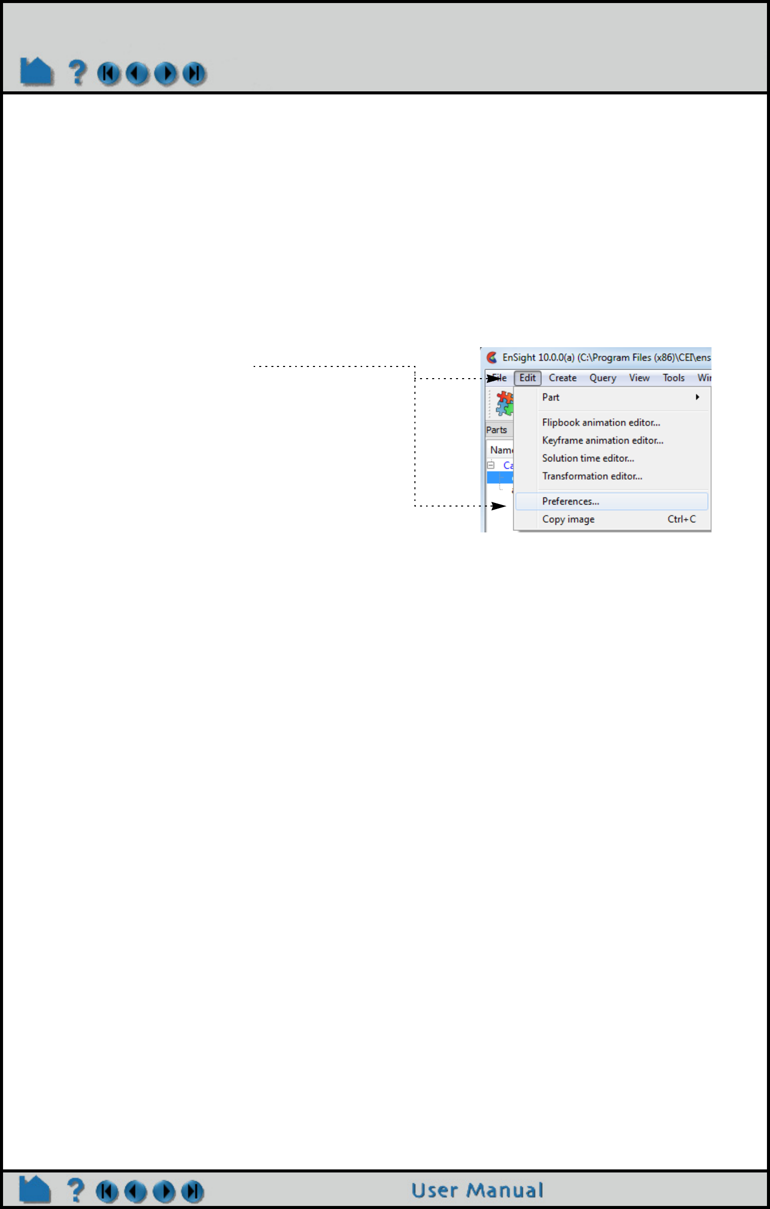
Page 513
HOW TO SET OR MODIFY PREFERENCES
Set or Modify Preferences
INTRODUCTION
Nearly every operation and function in EnSight is initially set to a default value. Preferences allow you to set these
initial values as well as set some default behaviors such as which time step to initially load for transient data, how the
mouse buttons are defined, etc. When EnSight starts, the preference settings are read from the $CEI_HOME/
ensight102/site_preferences directory and then overlaid by the preference settings found in your EnSight defaults
directory (located at %HOMEDRIVE%%HOMEPATH%\(username)\.ensight102 commonly located at
C:\Users\username\.ensight102 on Vista and Win7, C:\Documents and Settings\yourusername\.ensight102 on older
Windows, and ~/.ensight102 on Linux, and in ~/Library/Application Support/EnSight102 on the Mac).
BASIC OPERATION
The following preference categories are available in the Preferences dialog (and will be explained below):
Setting Annotation Defaults
To Set Color Palette Defaults:
To Set Data Preferences:
To Set Image Saving and Printing Preferences:
To Set Mouse and Keyboard Preferences:
To Set Performance Preferences:
To Set User Defined Input Preferences:
To Set Variable Preferences:
To Set View Preferences:
To Set Viewports Preferences:
1. Bring up the Preferences dialog by selecting Preferences
from the Edit pull-down menu.
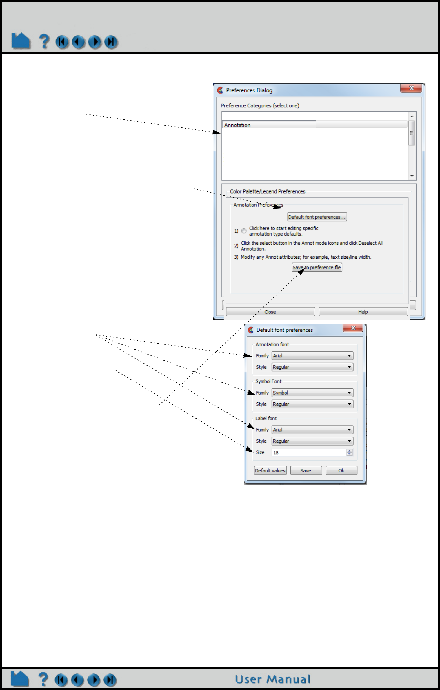
Page 514
HOW TO SET OR MODIFY PREFERENCES
Setting Annotation Defaults
Need to make the font bigger everywhere in
EnSight?
1. Select Annotation from the Preference
Categories list.
2. Click on the Default font preferences button
6. Change the annotation, symbol and label fonts
individually
7. Change the size
8. Click here to save the preferences.
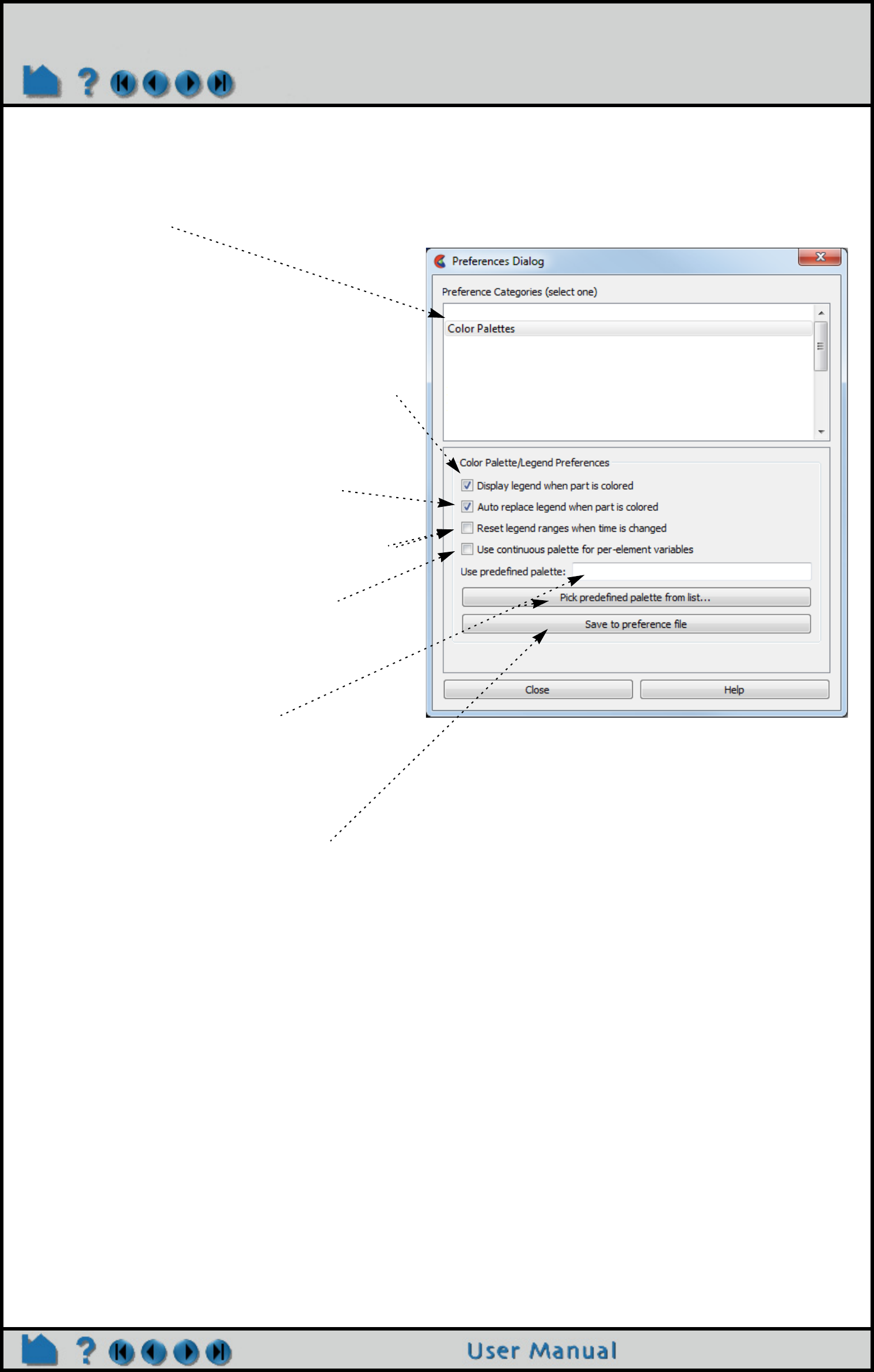
Page 515
HOW TO SET OR MODIFY PREFERENCES
To Set Color Palette Defaults:
1. Select Color Palettes from the Preference
Categories list.
2. Toggle on if you want the color legend to
automatically appear when you color a part by
a variable.
3. Toggle on if you want color legends to be
replaced when the current legend is no longer
in use (i.e., no parts are colored by the
variable) and a new variable is in use.
4. Toggle on if you wish the legend ranges to be
updated when time is changed, thus based on
values of variable at the current time.
5. Set the default legend for per element
variables to be constant over the element or to
vary continuously over the element (averages
with neighbors).
6. If you have predefined color palettes, you can
set one of them to be the default by entering
the name or picking one from the list of
defined palettes.
8. Click here to save the preferences.
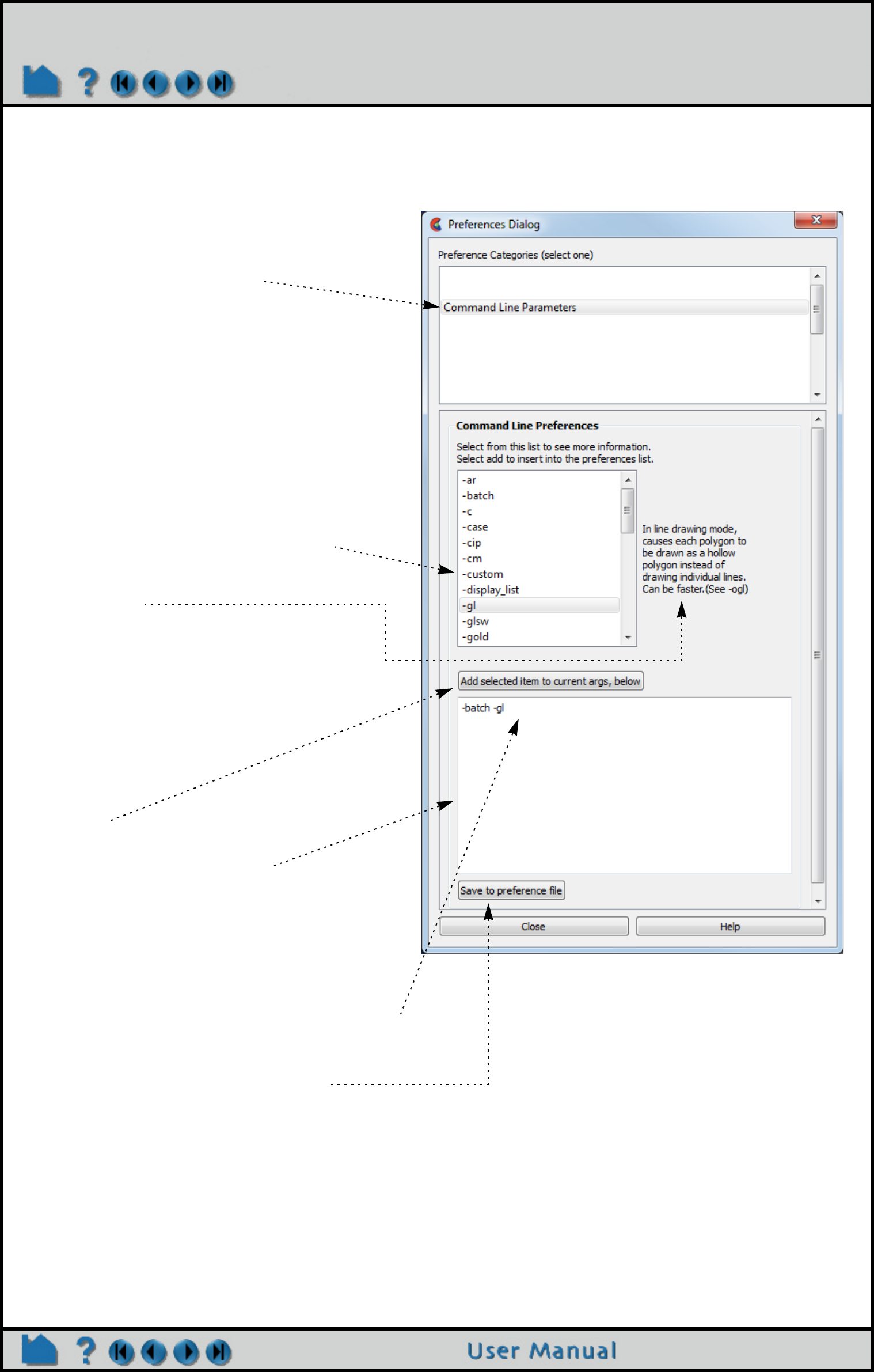
Page 516
HOW TO SET OR MODIFY PREFERENCES
To Set Command Line Preferences:
A number of command line parameters exist for
EnSight. These parameters can be set in your
preference file so you do not have to specify them on
the start line each time you use EnSight.
1. Select Command Line Parameters from the
Preference Categories list.
2. Select a command line argument.
An explanation of the selected argument will appear
in the dialog.
3. Click here to add the parameter.
It will be placed in the edit area.
If you make a mistake and add an unwanted
parameter, simply highlight it in the feedback area and
delete it.
If additional information is required, a note will be
posted here to help you.
4. If you need to add additional information, add
any text needed into the edit area.
5. Click here to save the preferences.
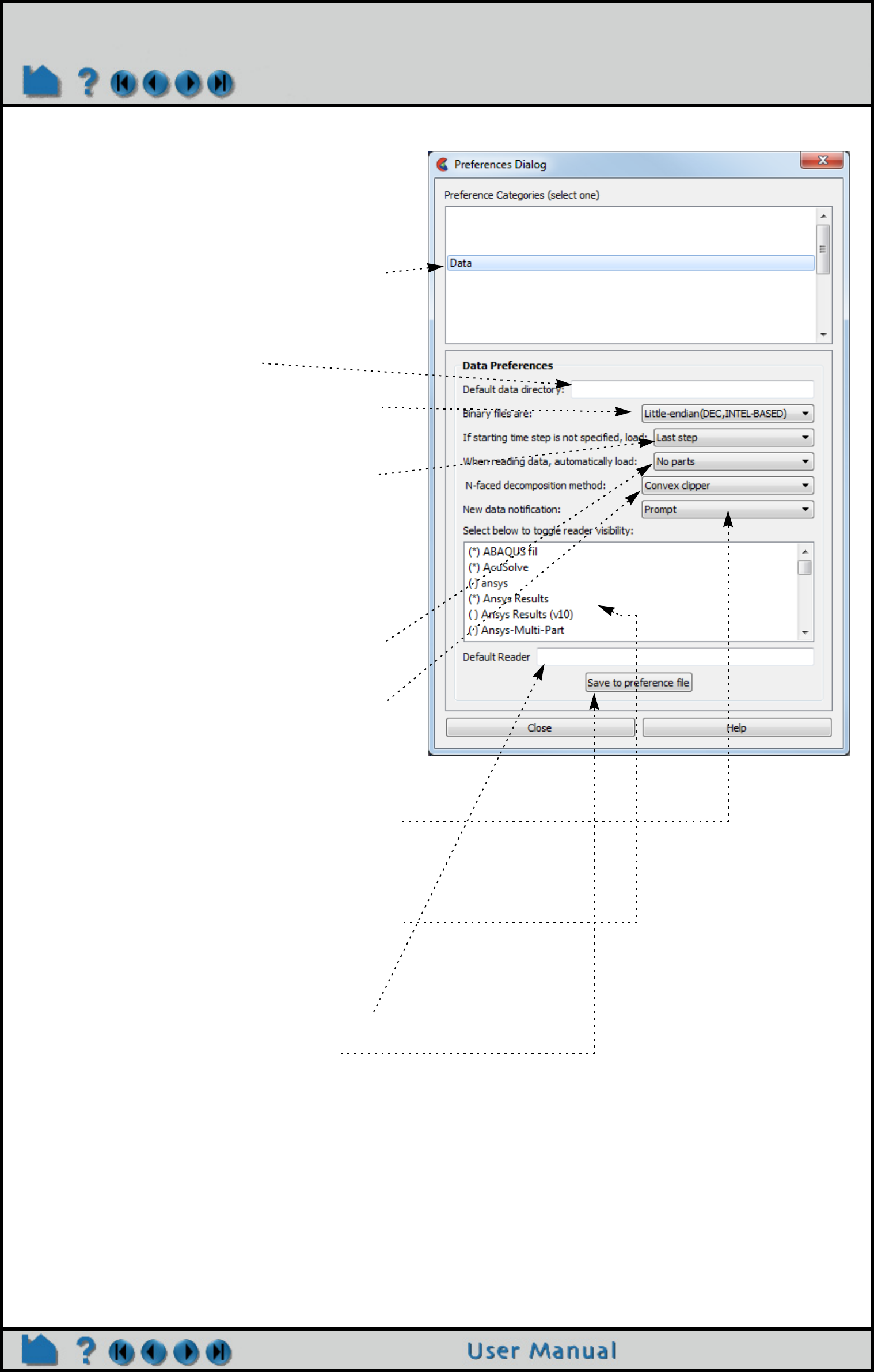
Page 517
HOW TO SET OR MODIFY PREFERENCES
To Set Data Preferences:
1. Select Data from the Preference Categories
list.
2. If you want to specify a path to look for data,
specify it here.
3. You can specify the default binary file type
here.
4. When transient data is loaded into EnSight
you can choose to specify a beginning time
step. If you do not specify a beginning time
step, either the first or the last time step will
be loaded depending on this preference.
5. After successfully reading data into EnSight
you are presented (for most data formats) with
a part loader if this attribute is set to No Parts.
If set to any other attribute the parts specified
will be loaded and displayed without
intervention from the part loader.
6. Sets the n-faced polyhedron decomposition
algorithm (for detailed description, see User
Manual Edit Menu Functions)
7. When solver solution is proceeding and new
timestep files appear this will prompt you to
include the new files as additional timesteps -
only for Case Gold format. Please Contact CEI
Support regarding this option.
8. The readers shown with a * will show up in the
pull-down for data format in the EnSight data
reader dialog. You can take readers off of the
pull-down list if you toggle the * off (select the
reader in the list).
9. You can specify the default data type by
typing in the exact name of the reader.
10. Click here to save the preferences.
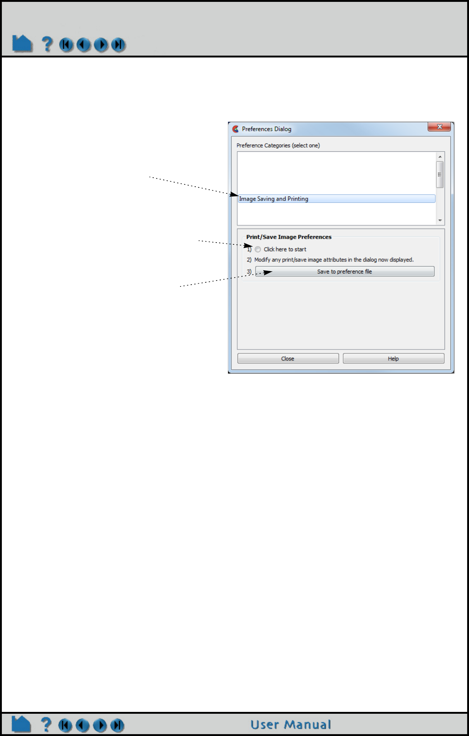
Page 518
HOW TO SET OR MODIFY PREFERENCES
To Set Image Saving and Printing Preferences:
1. Select Image Saving and Printing from the
Preference Categories list.
2. Click the “Click Here To Start” button. This
will bring up the Print/Save Image dialog.
3. Modify the you want for your preference
such as the image format.
4. Click here to save the preferences.
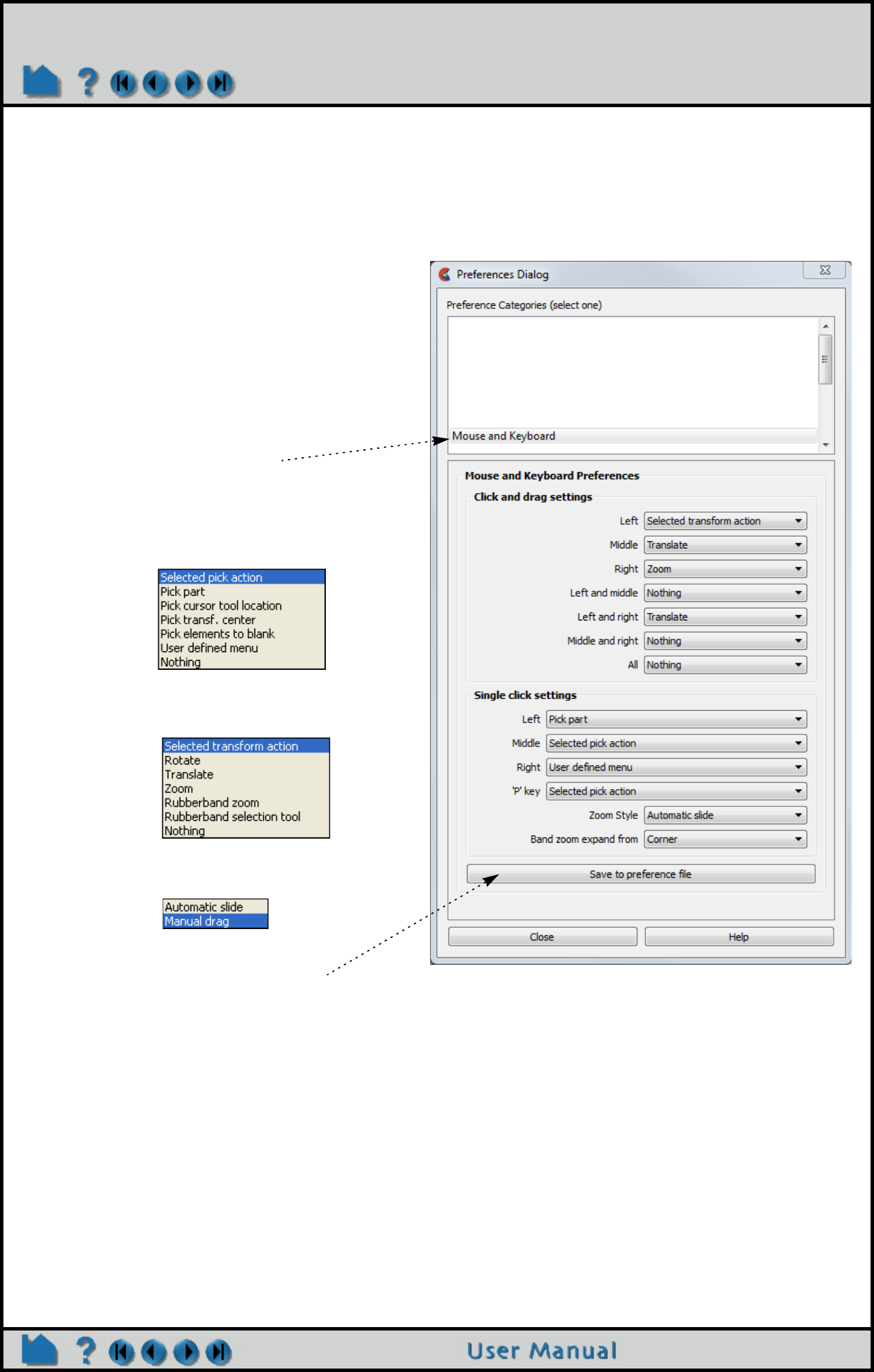
Page 519
HOW TO SET OR MODIFY PREFERENCES
To Set Mouse and Keyboard Preferences:
This preference allows you to modify the behavior
of the mouse buttons used during EnSight
transformations. Several different actions are
available for the various single click, multiple-
button single click, and double click options. Note,
it is required to set at least one button to “Selected
transform action” (which means that the button is
set to the action as shown in transformation icons
at the bottom of the EnSight dialog - set to rotate
by default). Also, one mouse or the “p” keyboard
key must be set to “Selected pick action”.
1. Select Mouse and Keyboard from the
Preference Categories list.
2. Modify the preference for each of the mouse
buttons (and keyboard ‘P’ key).
Single click actions available are:
Click and drag options are:
And the possible zoom styles are:
3. Click here to save the preferences.
See How To Produce Customized Pop-Up
Menus for a description of what “User defined
menu” is.
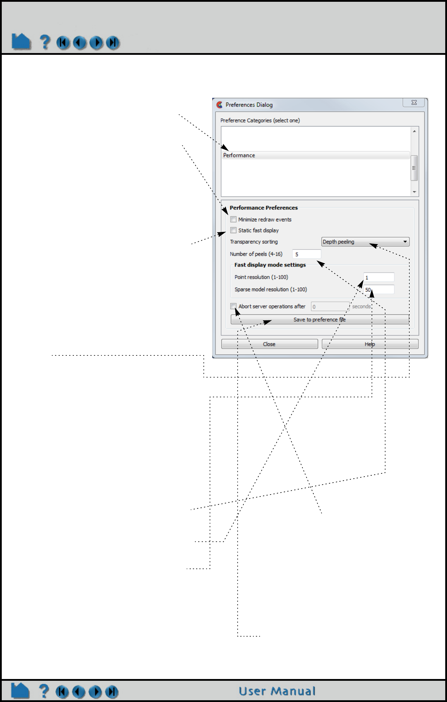
Page 520
HOW TO SET OR MODIFY PREFERENCES
To Set Performance Preferences:
1. Select Performance from the Preferences
Categories list.
2. To take advantage of pixel saving when
redrawing a window movement, set this
toggle. (Graphics card speed for reading/
writing of pixels needs to be reasonable to
use.)
4. To set fast mode to static, toggle on. The
default is off meaning that the fast display
(i.e., bounding box) is only active during
transformations such that the image returns
back to full graphics display when the
mouse buttons are not depressed. In static
mode the fast representation is
continuously displayed.
5. To ensure proper display of transparent
geometry, EnSight must sort all the
transparent polygons in the display. This
can be an expensive operation, particularly
if multiple transparent parts are visible. This
option controls when and how surfaces are
sorted.
In “Interactive” mode, sorting is performed
between every redraw of the view. In “Delayed”
mode, sorting is not performed while the user is
interacting with the view (while the mouse button
is held down). NOTE: Hidden line overlay does
not work with either “Interactive” or “Delayed”. In
“Depth peeling” mode (which is only available on
graphics cards that support the OpenGL Shading
Language) sorting is done by the graphics card on
a per-pixel basis by rendering the view repeatedly.
This mode scales better as the number of
polygons increases and it does not suffer a
performance hit when multiple parts are
transparent. The number of peels (and hence the
number of surfaces to order properly) is controlled
by the “Number of peels” field.
5. If using point display for fast display mode,
set the point resolution here.
6. If using sparse geometry display for fast
display mode, set the percent of the model
to show here.
(Only used if immediate mode is being used.)
7. EnSight is a client-server architecture
with the possibility that the two
processes are executing on different
and possibly remote machines. Due to
this, a general abort function is not
possible. Instead a timer abort function
is available that will terminate many
server operations after a set amount of
time has passed. If you wish to set this
time-out value turn the toggle on and
set the time-out amount (in seconds).
8. Click here to save the preferences.
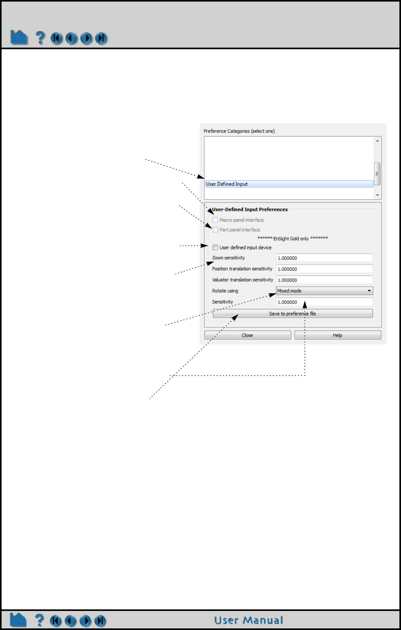
Page 521
HOW TO SET OR MODIFY PREFERENCES
To Set User Defined Input Preferences:
1. Select User Defined Input from the
Preferences Categories list.
2. Turn this on to show the macro panel display
3. Toggle to select the default to display a part
list in the graphics window. This is especially
helpful in full screen mode or a VR
environment.
4. Turn this on to activate the user defined input
device (ENSIGHT10_INPUT must be set to the
proper device).
5. Sets the sensitivity for the zoom operation.
The values for zoom are scaled by this
setting, so values larger than 1.0 will make
the inputs larger while less than 1.0 will make
them smaller.
6. Mixed mode will use the input devices z
rotate directly but use x and y translation
values for x/y rotations. Direct mode will use
the rotation angles from the input device
directly for all three axis.
7. Sensitivity will set a scaling factor for the
rotation values.
8. Click here to save the preferences.
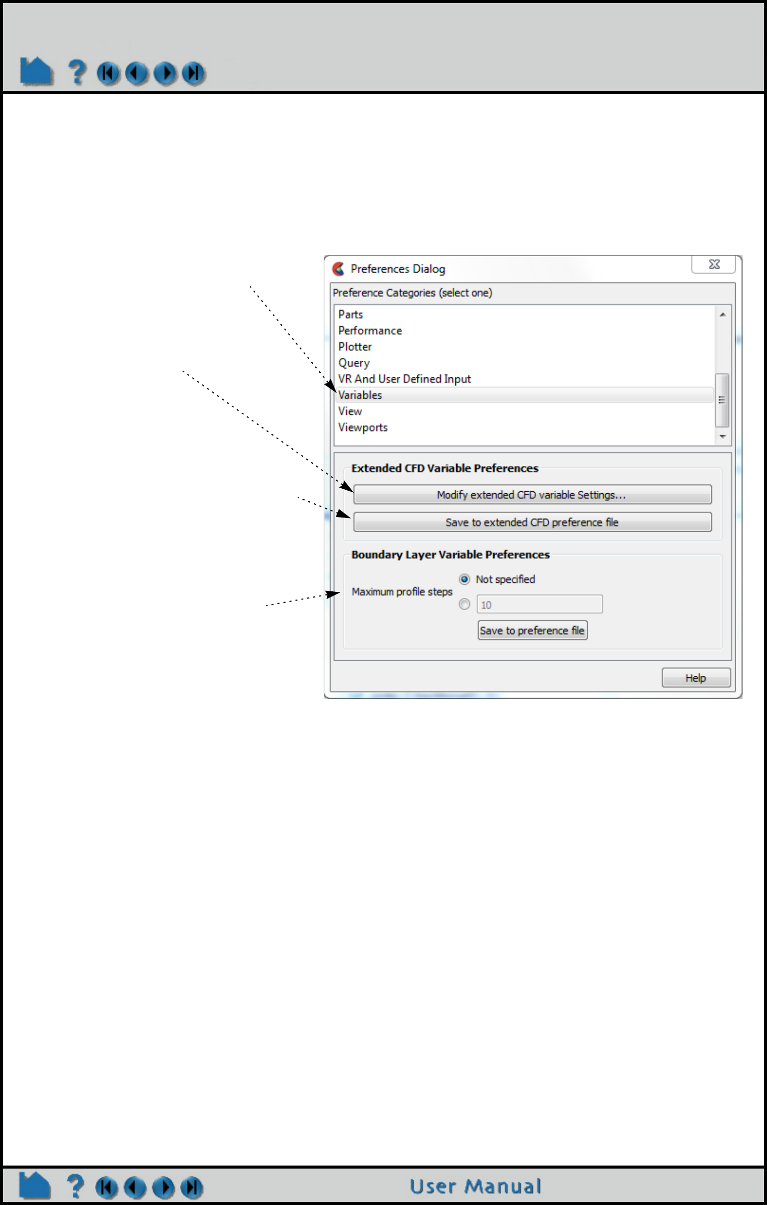
Page 522
HOW TO SET OR MODIFY PREFERENCES
To Set Variable Preferences:
1. Select Variables from the Preferences
Categories list.
2. Brings up the dialog for setting extended
CFD settings.
Save these settings by clicking here.
3. Boundary Layer calculation
Recommendation: let EnSight determine
the maximum number of profile values from
the surface to the edge of the boundary
layer.
Manually changing this value allows
clamping of the number of sample points in
the profile off the wall into the flow field.
Since each sample point is approximately
equivalent to the center of each cell in the
boundary layer sub-mesh, if the number of
cell layers in the boundary layer sub-mesh is
known, this would be a good value so the
profile does not exceed this limit. Warning:
Setting this value too low can cause the
sampling to terminate before the edge of the
boundarylayer is reached, thus wrongly
predicting the values of interest.
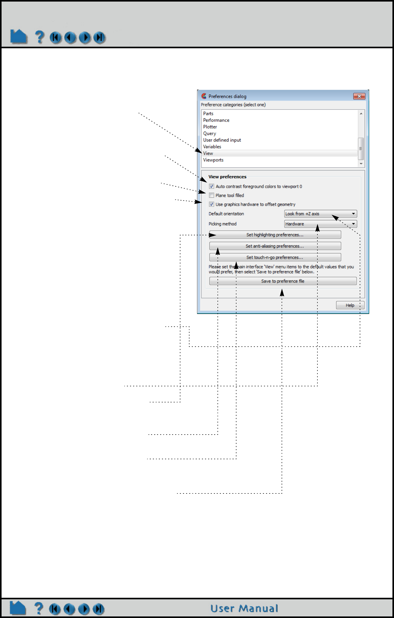
Page 523
HOW TO SET OR MODIFY PREFERENCES
To Set View Preferences:
1. Select View from the Preferences
Categories list.
2. Switches white and black foreground
colors for maximum contrast with Constant
and Blended backgrounds for viewport 0.
3. Turn on if you want the plane tool to be
shown as a transparent plane, or off if you
want it shown in line drawing mode.
4. There are two offsets employed in EnSight.
This one, hardware offset, is perpendicular to
the monitor screen, and done in hardware if
this toggle is on. This will allow, for example
contour lines to appear closer to the viewer
than their parent part so they are visible no
matter what orientation the part is viewed
from.
The second offset is the display offset. The display offset
can be set in the feature panel for line parts such as
contour lines, particle trace lines, vector arrows, and
separation/attachment lines. The display offset is the
distance in the direction of the element normal
(perpendicular to the surface).
5. Select the default viewing orientation.
6. For newer graphics cards leave as
‘hardware’ and EnSight will attempt to use
hardware picking, and if not available will
use software picking. For older graphics
cards with sluggish performance, choose
software picking.
7. Click to bring up dialog controlling
selection feedback in the graphics window
8. Click to bring up dialog controlling the anti-
aliasing parameters.
9. Click to bring up dialog controlling the
click-n-go preferences.
10. Click here to save the preferences.
Caution: if you save software picking and
later change to a newer graphics card you
must change this back to ‘hardware’ to take
advantage of the new card.
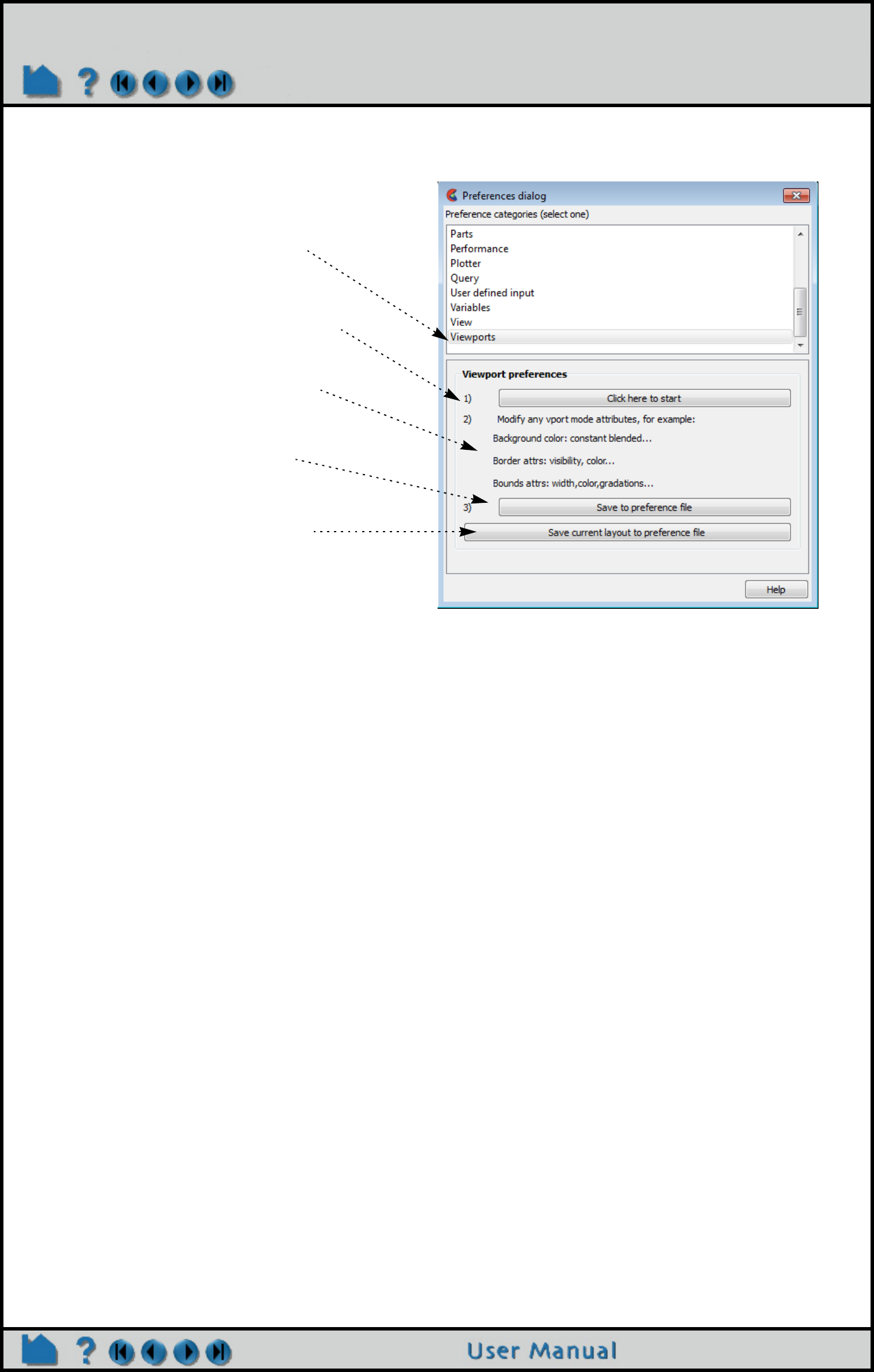
Page 524
HOW TO SET OR MODIFY PREFERENCES
To Set Viewports Preferences:
SEE ALSO
User Manual: Edit Menu Functions
1. Select Viewports from the Preferences
Categories list.
2. Click here to start. This will bring up the
Viewports dialog with all the viewport items
selected.
3. Set any viewport attribute (for example,
background color to blended).
4. Click here to save the attributes set in
above in item #2 to the preference file as
defaults for future sessions.
5. Click here to save the current viewport
layout to the preference file.
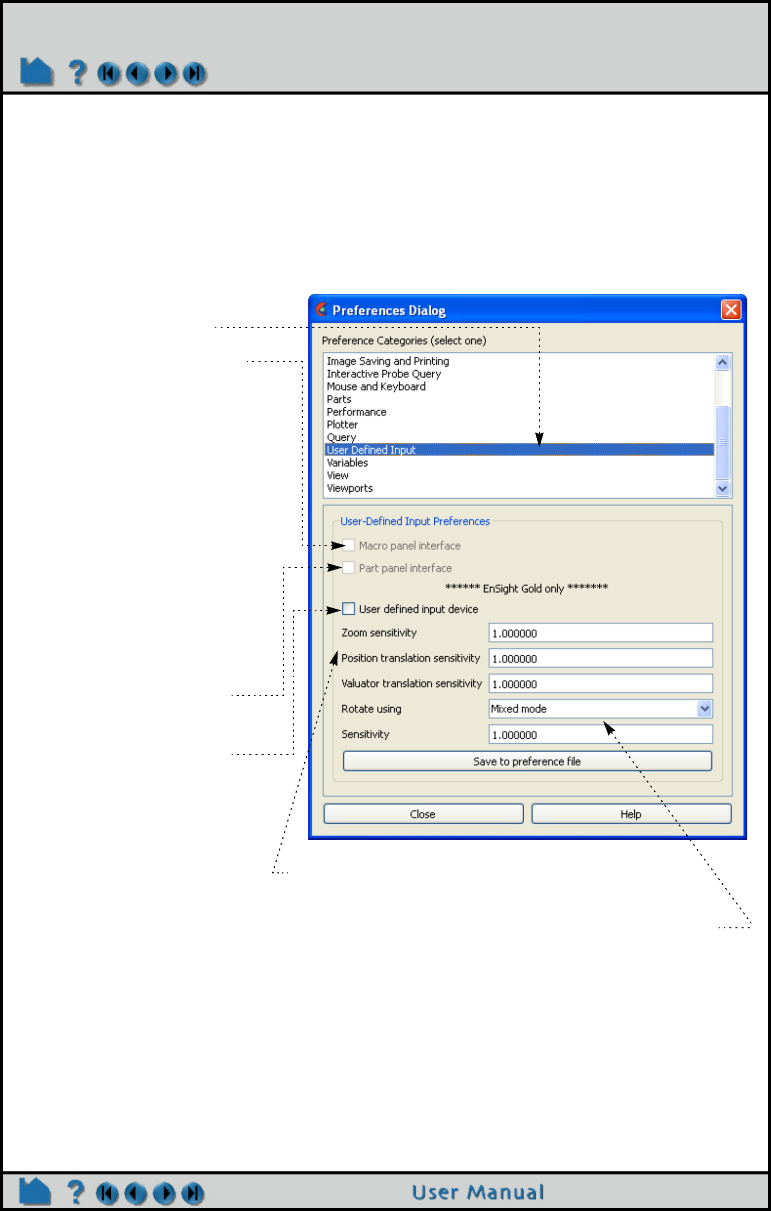
Page 525
HOW TO ENABLE USER DEFINED INPUT DEVICES
Enable User Defined Input Devices
INTRODUCTION
EnSight offers user defined input devices that have been specifically designed for (but not limited to) typical input
devices used in VR environments. Implementation of these input devices requires adherence to the instructions
outlined in the respective reference files listed below.
BASIC OPERATION
Manual Panel Interface:
SEE ALSO
User Manual: VR and user defined input Preferences
1. Select Edit > Preferences..., and
click User Defined Input.
2. Toggle Macro Panel Interface
The Main Graphics window updates the
Macro Panel as defined in the EnSight
Defaults Directory (located at
%HOMEDRIVE%%HOMEPATH%\(usernam
e)\.ensight102 commonly located at
C:\Users\username\.ensight102 on Vista
and Win7, C:\Documents and
Settings\yourusername\.ensight102 on
older Windows, and ~/.ensight102 on
Linux, and in ~/Library/Application
Support/EnSight102 on the Mac) as the
following file:
hum.define
(If you have not created this file, an
example is provided in:
$CEI_HOME/ensight102/src/cvf/udi/
HUM/hum.define
on your EnSight Client host system.)
3. Toggle Part Panel Interface
(if you desire a part list in the
graphics window).
4. Toggle User Defined Input.
(Detailed steps to implement the User
Defined Input Device are outlined in the
file:
$CEI_HOME/ensight102/src/udi/cvf/
README.v3
on your EnSight Client host system.)
5. Set Zoom Using to the appropriate type of input device you
are using to record zoom transformations, adjusting the
Sensitivity as needed (i.e., 0 < slower < 1 faster).
6. Set Rotate Using to the appropriate type of input device you
are using to record rotation transformations, adjusting the
Sensitivity as needed (i.e., 0 < slower < 1 faster).
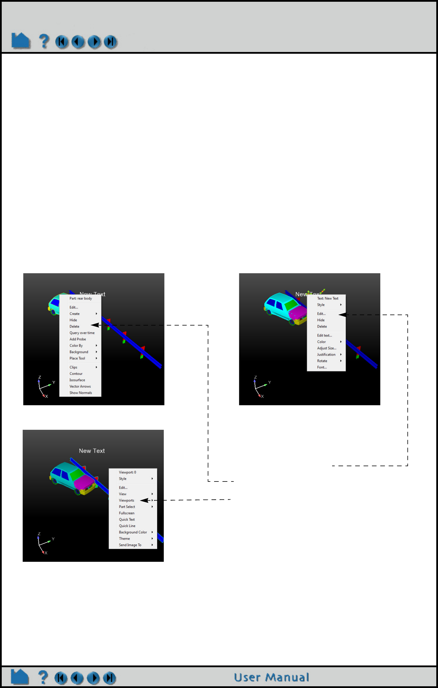
Page 526
HOW TO PRODUCE CUSTOMIZED POP-UP MENUS
Produce Customized Pop-Up Menus
INTRODUCTION
EnSight includes pop-up menus invoked via the right mouse button. The menus are specific to each object (part,
annotation, plot, etc.). They are written as Python objects that are dynamically loaded when EnSight starts up. Menus
can implement any function that can be built on top of command language or Python. Most menus use Python to
query EnSight state and perform customized actions based on that state.
There is a formal mechanism through which EnSight users may add additional, customized menus to the existing
pop-up menus with all of the same capabilities. The mechanism opens up EnSight to specific customization to meet a
particular site or individual user’s needs.
BASIC OPERATION
This section describes the default EnSight menu usage with no additional customization. To use the capability
included with EnSight, simply right click on a part, on some text, or on the background as shown below. By default,
the pop-up menus are tied to the right mouse button single click. This can be changed using options outlined in: To
Set Mouse and Keyboard Preferences:. The menus can also be accessed by assigning them to a particular
keystroke as a macro using as outlined in Define and Use Macros. The specific menu that is displayed depends on
what object was clicked on. Some examples are shown here:
Menu targets
In general, the target of the operation is listed at the top of the menu. A special modifier key (‘ctrl’) is used to control
object/part selection. When the menu click is made, a pick operation is performed under the mouse pointer. This pick
returns the selected part or object. If that object is part of the current selection, the selection is not changed and the
entire selection is the target of the menu operation. If the object is not part of the current selection, the object
becomes the current selection and the menu operation is performed on this new selection. The ‘ctrl’ key can be used
to modify this behavior. In normal left mouse button picking, the ctrl key tells EnSight that the picked object should be
Clicking on an annotation
Clicking on a selected part
Clicking on the viewport background

Page 527
HOW TO PRODUCE CUSTOMIZED POP-UP MENUS
added to the current selection. When right clicking to open a menu, holding the ctrl key tells EnSight not to change
the current selection and to target the current selection, even if the pick operation did not include a selected object.
This can be used to more easily bring up the popup menu operations for objects that are not easily clicked on, or
even visible.
ADVANCED USAGE
This section describes how to create custom user-defined menus as explained by EnSight extension mechanism in
the Interface Manual. This section assumes familiarity with the Python language, as well as object-oriented
programming. Both custom and built-in menus have the same capabilities because they are built on the same
interface. Also, customized menus allow the user to display options, including cascading menus. By default, your
custom menus will appear below EnSight’s default list of options that appear when you right click. The user may also
define a key (using the macro facility) to invoke the operation as noted above.
EnSight includes two well-documented, example Python files to demonstrate the process of creating custom, user-
defined pop-up menus. As an exercise to show how to customize EnSight, these two files can be moved from their
existing location to a directory where they will automatically load into EnSight at startup and change EnSight’s
menus.
How menus get loaded
By default EnSight scans the Python files found in subdirectories of the site-specific $CEI_HOME/ensight102/
site_preferences/extensions/user_defined directory and in the user specific extensions/
user_defined subdirectory, under the EnSight Defaults Directory. The EnSight Defaults Directory varies per
platform:
Linux: ~/.ensight102/extensions/user_defined/Menus
Mac: ~/Library/Application Support/EnSight102/extensions/user_defined/Menus
Windows Vista, Windows 7: C:\Users\username\.ensight102\extensions\user_defined\Menus
Windows XP: %HOMEDRIVE%%HOMEPATH%\(username)\.ensight102\extensions\user_defined\Menus
Specific details of this process are covered in EnSight extension mechanism. When EnSight finds a Python file, it
calls a “factory” function specified in the file. The factory function returns a list of objects that are registered with
EnSight. The objects can be user-defined menus, tools and s, based on the extension class they subclass from.
Whenever a pop-up menu is invoked by the user (normally though the right-mouse button), EnSight will filter the list
of registered menu objects, display them as a pop-up menu and will invoke the run method when selected by the
user.
In the next two sections, we walk thought two simple examples of writing custom EnSight user-defined menus.
“Hello world” menu
Shown below is a simple example menu extension. It can serve as a template for more useful menus. This example
Python file is included with your EnSight installation in the following folder $CEI_HOME/ensight102/src/
user_defined_ext/. Copy the entire directory to the extensions/user_defined/examples subdirectory
under your user EnSight Defaults Directory (see above) and restart EnSight. The figure that follows shows the new
menu item generated from this Python code, as well as the console output which is found in the Python window
(File>Command, and click on the Python tab in the resulting window). It also illustrates the directory structure for
placing the files into the user specific EnSight startup path.
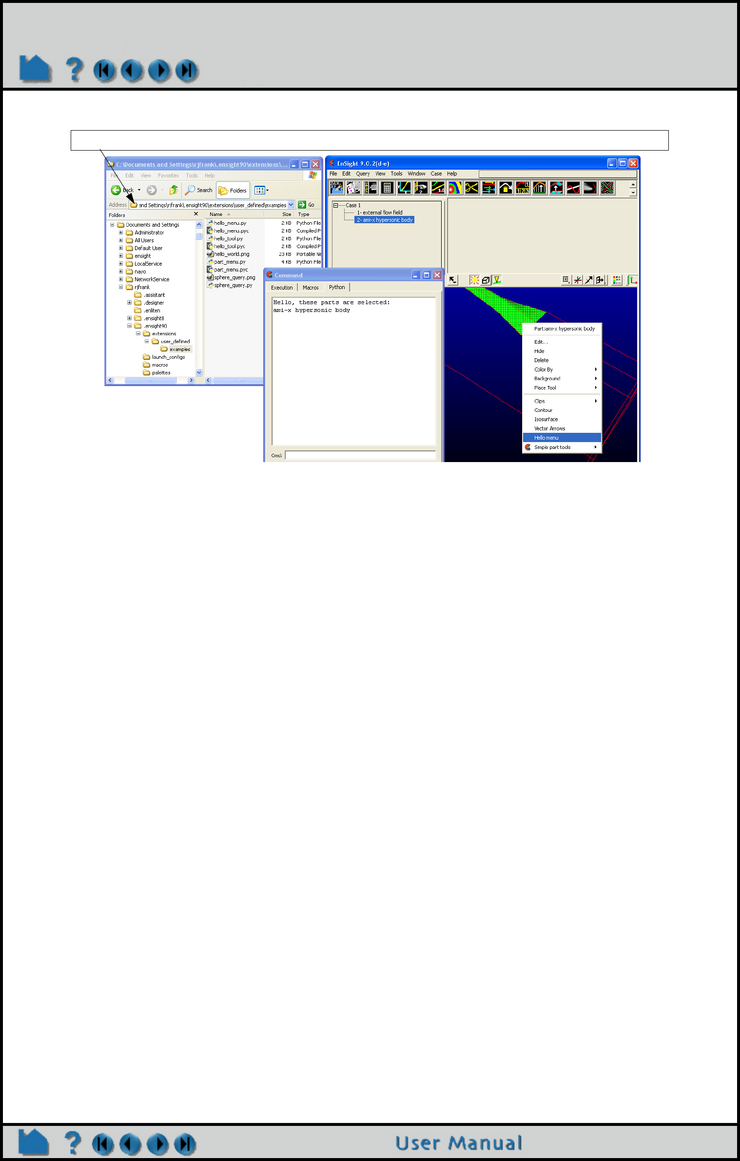
Page 528
HOW TO PRODUCE CUSTOMIZED POP-UP MENUS
Shown below is the commented Python code. Notice in particular the block of comment lines starting with
#ENSIGHT_USER_DEFINED_BEGIN and ending with #ENSIGHT_USER_DEFINED_END. These specially formatted
Python comments are what EnSight looks for at startup. They specify the name of the function to call when this file is
loaded. That “factory” function is responsible for creating instances of the menu object and returning them to EnSight.
#
# This comment block is required to identify the file for loading at
# startup by EnSight. The function named by FACTORY= (in this case
# 'ctor' is called by EnSight on startup. Note: the file is loaded
# as a module in EnSight and the path to this file is added to sys.path.
#
#ENSIGHT_USER_DEFINED_BEGIN
#FACTORY=ctor
#ENSIGHT_USER_DEFINED_END
#
# Import the parent class for all user-defined menus and the ensight module
#
import ensight
from ensight.core.menu_extension import menu_extension
#
# Define a menu class, a subclass of the menu_extension class
#
class hello_menu(menu_extension):
#
# Construct the menu with reasonable defaults
#
def __init__(self,name,parent,text="",tooltip="",desc="",icon=None):
menu_extension.__init__(self,name,__file__,1.0)
if (parent): parent.addChild(self)
if (icon): self.setIcon(icon)
self.setText(text)
self.setDesc(text)
self.setTooltip(text)
#
# Method that is called when the menu is selected
#
def run(self):
#
C:\Users\username\.ensight102\extensions\user_defined\examples
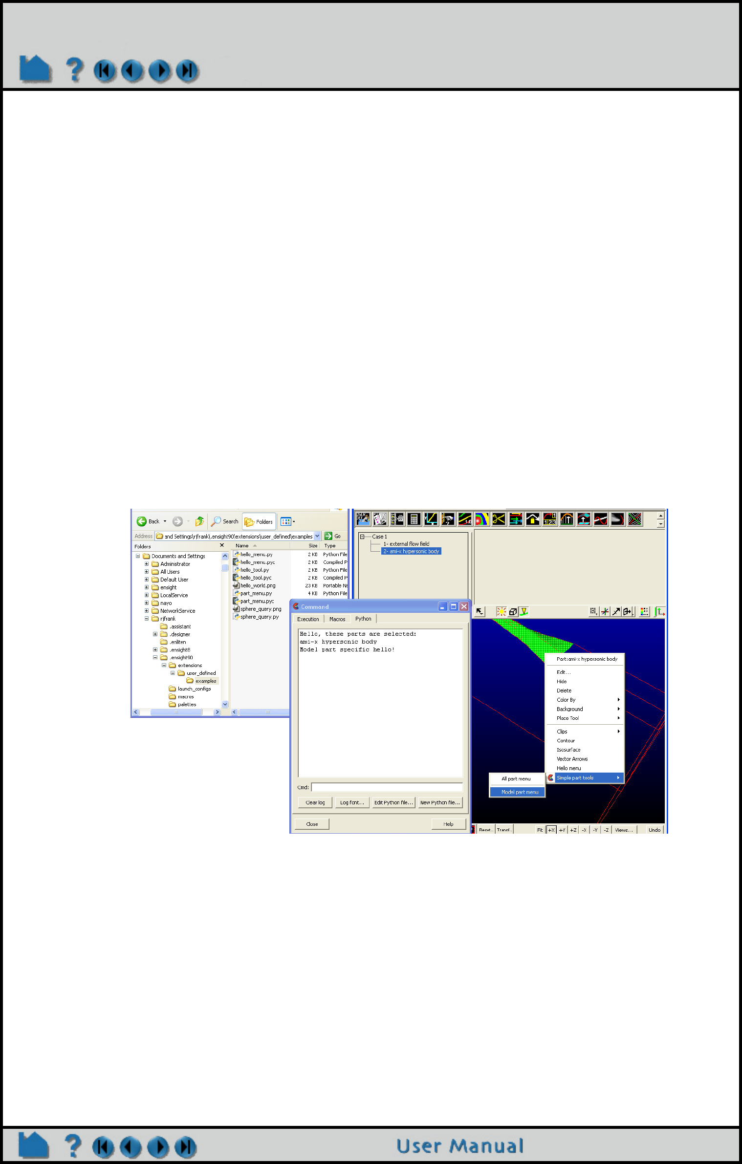
Page 529
HOW TO PRODUCE CUSTOMIZED POP-UP MENUS
# Do whatever operation this menu should do, replace with your own code
#
print "Hello, these parts are selected:"
for part in ensight.query_parts(client=1):
print part[3]
#
# Construct a list of menu objects to be added to the global list of
# user-defined menus
#
def ctor(parent):
list = []
#
# Create the actual menu object, giving it a unique name an
# onscreen name and a text description
#
p = hello_menu("hello_menu",parent,"Hello menu","Menu description")
list.append(p)
return list
Context-sensitive, Hierarchial Menus
Shown below is a more complex menu example. Again, it can be installed in the same manner as described above
and the resulting menus are illustrated in the following image.
This example builds on the previous one. First, it demonstrates that a single Python file can generate as many menus
as it wants. It also demonstrates the ability to define a hierarchy out of those menus. In this example, the menus
themselves have expressed the desire to only be displayed in specific contexts, e.g. when a specific type of part has
been selected. Finally, several other menu options are set, the name of the “vendor” for the menu and an icon are
specified. More options are documented in the Interface Manual.
The basic file structure is the same as before. There is a header block followed by the various class definitions
followed by the factory function.

Page 530
HOW TO PRODUCE CUSTOMIZED POP-UP MENUS
#
# This comment block is required to identify the file for loading at
# startup by EnSight. The function named by FACTORY= (in this case
# 'ctor' is called by EnSight on startup. Note: the file is loaded
# as a module in EnSight and the path to this file is added to sys.path.
#
#ENSIGHT_USER_DEFINED_BEGIN
#FACTORY=ctor
#ENSIGHT_USER_DEFINED_END
#
# Import the parent class for all user-defined menus and the ensight module
#
import ensight
from ensight.core.menu_extension import menu_extension
#
# Define a "separator" menu class used to put a dividing line between menus
#
class sep_menu(menu_extension):
def __init__(self,name,parent):
menu_extension.__init__(self,name,__file__,1.0)
self.setSeparator(True)
if (parent): parent.addChild(self)
#
# Define a menu class, a subclass of the menu_extension class
#
class part_menu(menu_extension):
#
# Construct the menu with reasonable defaults
#
def __init__(self,name,parent,text="",tooltip="",desc="",icon=None):
menu_extension.__init__(self,name,__file__,1.0)
if (parent): parent.addChild(self)
if (icon): self.setIcon(icon)
self.setText(text)
self.setDesc(text)
self.setTooltip(text)
self.setVendor("John Q. Public")
#
# Method that is called when the menu is selected
#
def run(self):
#
# We are constructing two instances of this class. They differ by
# name. We use the name to perform different operations for each
# of the instances. This could also be done with any other class
# data, including user defined data members.
#
if (self._name == "allpart_menu"):
print "All parts hello!"
else:
print "Model part specific hello!"
#
# Construct a hierarchy of menus. A parent "roll-over" menu and two
# children with a separator between them. These menus use context
# sensitive filtering. The parent is only displayed in EnSight "Part" mode.
# One child is always display and the other is only displayed when the
# currently selected part is a "Model" part. Note: this filtering could
# also be performed by overriding the "validFilter()" method on the menu
# object to perform any custom filtering operation.
#

Page 531
HOW TO PRODUCE CUSTOMIZED POP-UP MENUS
def ctor(parent):
#
# The factory method always returns a list of object to be added.
# In this example, we only return menu_extension subclass instances,
# but the list can include any combination of object subclassed from
# the core_extension class.
#
list = []
#
# Create the parent roll-over menu
#
p = menu_extension("placeholder",None)
#
# Create an icon for the menu (this is optional). In this case, we
# access one of the icons embedded in EnSight itself. See the Qt
# resource management documentation for details.
#
p.setIcon(":/ensight/ens_icn_small")
#
# Set the EnSight mode filter to only display in "Part" mode.
#
p.setMode("Part")
#
p.setText("Simple part tools")
p.setTooltip("Example part tools")
if (parent): parent.addChild(p)
list.append(p)
#
# Create the instance of the part_menu class that should be displayed
# for any part that is selected.
#
m = part_menu("allpart_menu",p,"All part menu","Menu description")
list.append(m)
#
# Add a horizontal separator line between the child menus.
#
m = sep_menu("sep1",p)
list.append(m)
#
# Create an instance of the part_menu class that is only displayed
# when a "Model" part is selected.
#
m = part_menu("modelpart_menu",p,"Model part menu","Menu description")
#
# Set the EnSight part type filter to "Model" parts.
#
m.setPartType("Model")
list.append(m)
return list
Other examples
The example source code shown here is included in the $CEI_HOME/ensight102/src/user_defined_ext/
examples directory, but many other examples exist. The source code to all of the built-in menus is included in the
$CEI_HOME/ensight102/site_preferences/extensions/user_defined directory. Some other example
objects are included in $CEI_HOME/ensight102/site_preferences/extensions/user_defined/Tools/
QuickTools/Examples. While these are user-defined tools instead of menus, the extension mechanisms for both
share a large number of common features and techniques that work in both. There are a pair of tools examples

Page 532
HOW TO PRODUCE CUSTOMIZED POP-UP MENUS
located in the user-defined tool Advanced Usage that demonstrate the ability of all user-defined extensions to
generate and execute custom command language and make use of external icon files.
To get the most out of this mechanism, menu developers are encouraged to utilize Python scripts and convert
command language scripts into Python using the provided tools. The Python interface is largely documented in the
Interface manual Python EnSight module interface.
SEE ALSO
EnSight Interface Manual
Mouse and Keyboard Preferences
Produce Customized Access to Tools & Features
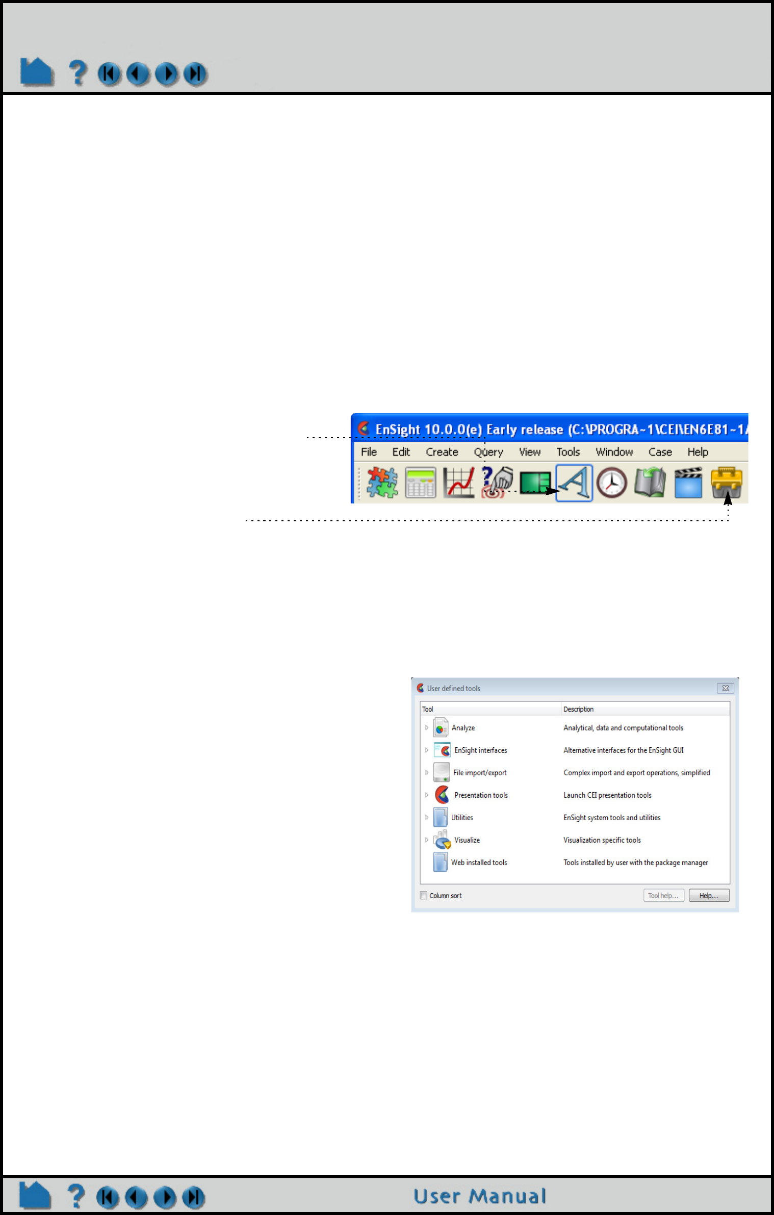
Page 533
HOW TO PRODUCE CUSTOMIZED ACCESS TO TOOLS & FEATURES
Produce Customized Access to Tools & Features
INTRODUCTION
EnSight allows users to define toolbox items, that are accessed by selecting the "User Defined" toolbox feature icon.
These items are collections of custom Python code that perform common operations. These tools can include full
interfaces and can interact with all of EnSight’s core features. The mechanism opens up EnSight to specific
customization to meet a particular site or individual user’s needs.
Tool are written as Python objects that are dynamically loaded from when EnSight starts up. There is a formal
mechanism (EnSight extension mechanism) through which EnSight users may add their own, custom tools.
BASIC OPERATION
The user defined tool icon should be displayed by default. If it is not, it can be turned ON by right clicking on the
Feature Icon Bar and selecting Customize Feature Toolbar... To access the user-defined tools, click the icon to bring
up the dialog and make a selection from the dialog by double clicking.
1. Click on the User Tools Icon.
2. The User Defined Tools Window appears.
The EnSight QuickTools are a collection of common
operations that would normally take many steps to
complete in EnSight, packaged in a simpler form.
There are six folders, each with a collection of related
tools:
a) Analyze - Tools designed to perform multi-step
Engineering Analysis
b) EnSight interfaces - Tools that demonstrate
alternative EnSight Front-end s.
c) File import/export - Import or Export data to/from
the EnSight client in various formats
d) Presentation tools - Export visualizations or Run
the current visualization in one of EnSight’s free post-
postprocessing tools.
e) Utilities - Support, development, raw core object
access, development tools and Python
documentation.
f) Visualize - Tools that animate, move, enhance
visualization, or create visualization entities.
g) Web installed tools - Customized tools installed by
EnSight’s package manager from external sources.
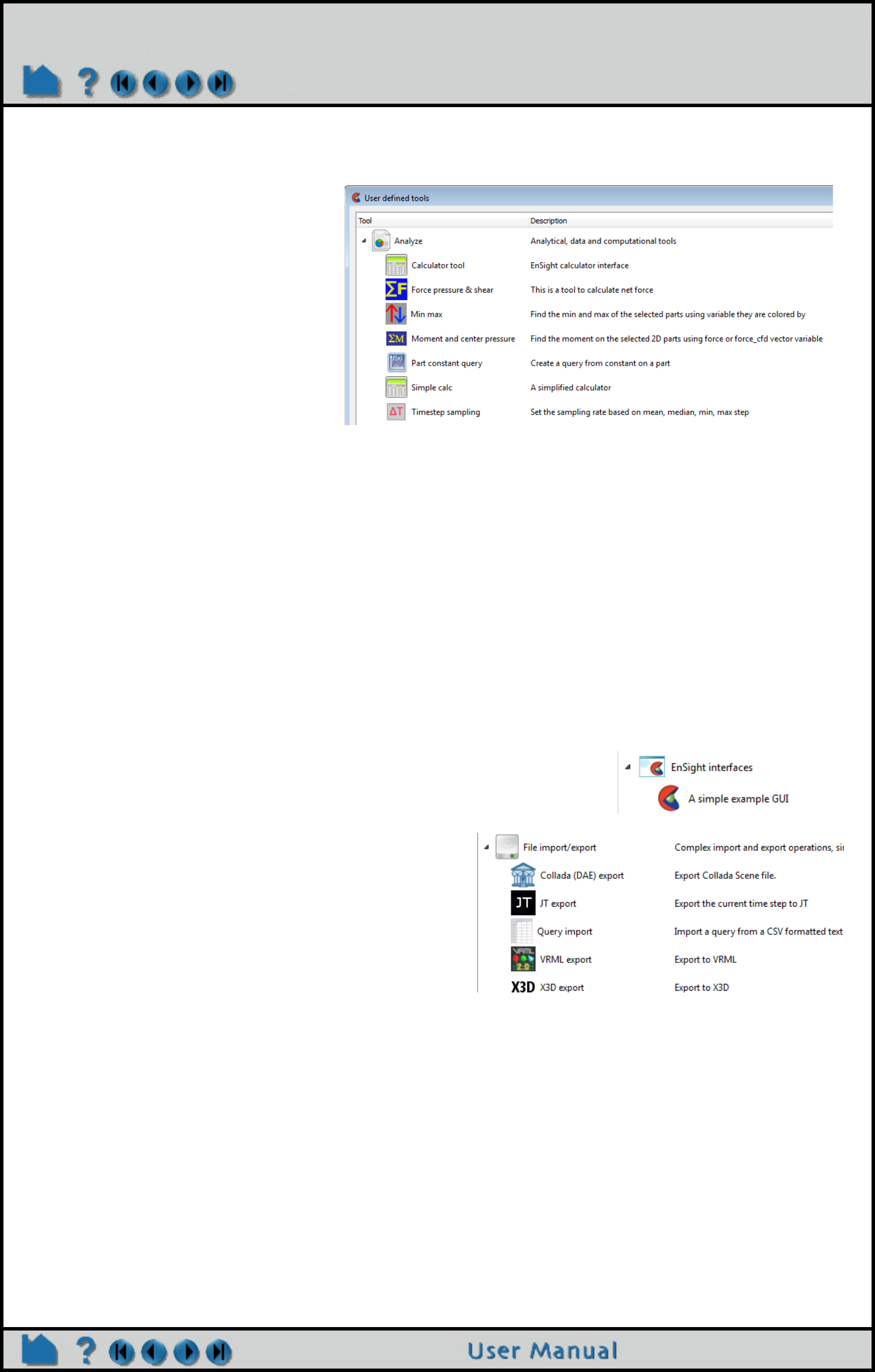
Page 534
HOW TO PRODUCE CUSTOMIZED ACCESS TO TOOLS & FEATURES
1. Click on the User Tools Icon.
2. Open the Analyze folder.
a) Calculator tool. Use a python
calculator
b) Force tool. Sum the net force
(either part by part or total) from
pressure, force vectors, or
shear. All variables are stored in
a Force folder in the variables
area. Optionally a .csv
spreadsheet file can be written
out which contains the net force components, force coefficients, etc. per part.
c) Min max tool. Find the min/max of the selected parts of the colored variable
d) Moment tool. Using the Force variables calculated in the Force tool above,
calculate the moment about a single point entered by the user.
e) Part constant query tool. Create a query (and optionally plot it) from a constant
calculated on a clip, isosurface, or isovolume as the clip/isosurface/isovolume
is swept from min to max. For example, calculate the mean, min, or max
temperature on a X-clip and plot the value vs. x-location as the clip is swept
from xmin to xmax.
f) Simple calc tool. Calculates constants from a subset of the calculator
functions.
g) Timestep tool. Resample transient data to a uniform timestep
3. Open the View alternative EnSight Graphical User Interfaces.
4. Open the File import/export folder.
a) Export Collada (DAE) format. This is a 3D XML
geometry format exported from the EnSight client.
b) Export data to a Reveal .csf file and then
translates to OpenJT format.
c) Import a CSV text file as an EnSight Query
d) Export VRML format.
e) Export X3D format. X3D is an open-source XML 3D geometry format which is a
follow on to VRML. This tool exports surface geometry and coloration from the
client simultaneously into two files: a Reveal file and an x3d geometry file. See
Web3D Consortium for more details.
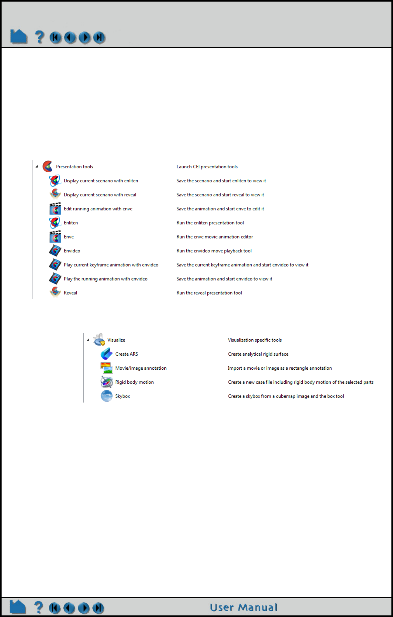
Page 535
HOW TO PRODUCE CUSTOMIZED ACCESS TO TOOLS & FEATURES
5. Open the Presentation tools folder. Note that each of the tools is designed to
export the current visualization to one of EnSight’s free, post-post processing
application: This would bypass the step of saving a file then starting up the
appropriate application as follows:
a) EnLiten or Reveal to view 3D geometry with results,
b) EnVe to perform simple video editing on a running animation,
c) EnVideo to play a movie animation.
6. Utilities - EnSight Advanced and Python programmer tools. For example, there
is a support tool, a ceishell logger, a graphics window resize tool, a stereo tool, a
graphics performance testing tool, and an EnSight Python Developer subfolder.
7. Visualize
a) Create Analytical Rigid Body surfaces by automatically extruding or rotating
line parts read in from ABAQUS ODB data. You must check the box in the format
options of the ABAQUS ODB data reader dialog to read in this type of part in order
to then use this tool to make these parts.
b) Movie tool. This will import a movie as a texture that is placed on a rectangular
annotation box. The movie will interpolate with the transient steps of your data, so
if the beginning and ending times are the same, the playback will roughly synch.
c) Rigid body motion tool. This was intended to be a demonstration of the Rigid
Body Motion capability of EnSight. Read in an EnSight Case Gold file, select the
parts of interest, then run this tool and choose the rigid body rotation parameters
and it will create a case gold file containing those parts with the appropriate
transient rigid body files (See EnSight Rigid Body File Format and See Euler
Parameter File Format).
d) Skybox - Using a specially formatted image, called a cubemap image (which is a
panoramic background scene containing the five interior sides of a cube) a
background skybox is automatically created using the box tool for placement.

Page 536
HOW TO PRODUCE CUSTOMIZED ACCESS TO TOOLS & FEATURES
ADVANCED USAGE
This section describes how to create custom user-defined tools as explained by EnSight extension mechanism in
the Interface Manual. This section assumes familiarity with the Python language, as well as object-oriented
programming. Custom tools have the same capabilities as the built-in tools because both are built on the same
interface. By default, your custom tools will appear below EnSight’s built-in list of tools in the user-defined toolbox.
EnSight includes two well-documented, example Python files to demonstrate the process of creating custom, user-
defined tools. As an exercise to show how to customize EnSight, these two files can be moved from their existing
location to a directory where they will automatically load into EnSight at startup and change EnSight’s tool list.
How EnSight Loads Menus
System directory - CEI installed tools
EnSight scans for Python tools in the
$CEI_HOME/ensight102/site_preferences/extensions/user_defined/Tools
directory. Note that because EnSight caches the files in this directory in order to speed up the start up process, new
tools put in this directory may not be recognized and loaded when you restart EnSight. In that situation, simply restart
EnSight from the command line with no preferences and it will reload and recache the python files from this directory.
ensight102 -no_prefs
$CEI_HOME - python files developed by your company for all your users
EnSight scans the $CEI_HOME directory for subdirectories containing a file named product.xml. Python files are
loaded in this directory according to the product.xml and internal parentage coding. Contact CEI support for more
details.
Local directory - python files for your own personal use
EnSight then looks in the user specific EnSight Defaults Directory. This directory differs on each platform:
Linux: ~/.ensight102/extensions/user_defined/Tools
Mac: ~/Library/Application Support/EnSight102/extensions/user_defined/Tools
Windows Vista, Windows 7: C:\Users\username\.ensight102\extensions\user_defined\Tools
Windows XP: %HOMEDRIVE%%HOMEPATH%\(username)\.ensight102\extensions\user_defined\Tools
To find out your %HOMEDRIVE%%HOMEPATH% do Help>Online Support, click the System Into tab, and look at the
Prefs Dir. This is where EnSight looks for user defined tools.
When EnSight finds a candidate Python file, it loads it into a private Python module and calls a “factory” function
specified in the file. The factory function returns a list of objects that are registered with EnSight. The objects can be
user-defined tools, menus and s, based on the extension class they subclass from. A registry of user-defined tools is
maintained by EnSight. It is normally displayed as a tree-list in the noted in the previous section. Applications are
free however to invoke any tool using its run method and tools that implement custom command language may be
called directly from the command parser, even in batch mode.
In the next two sections, we walk through two simple examples of writing custom EnSight user-defined tools.
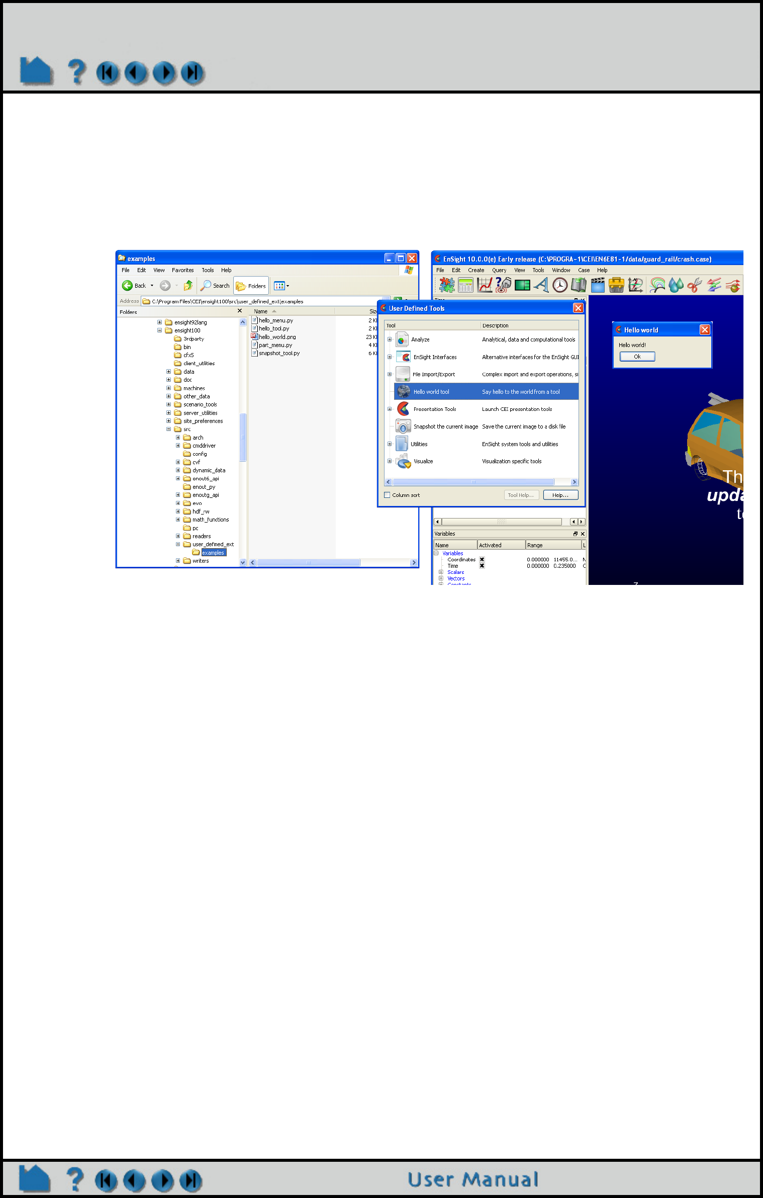
Page 537
HOW TO PRODUCE CUSTOMIZED ACCESS TO TOOLS & FEATURES
“Hello world” tool
Shown below is perhaps the simplest example tool extension implementation. It can serve as a template for more
useful tools. This example Python file is included with your EnSight installation in the following folder $CEI_HOME/
ensight102/src/user_defined_ext/examples. Copy the entire folder to the extensions/user_defined
subfolder under your user specific EnSight Defaults Directory (see above) and restart EnSight. The figure that follows
shows the new tool item generated from this Python code, as well as the dialog it generates. It also illustrates the
directory structure for placing the files into the user specific EnSight startup path.
Shown below is the commented Python code. Notice in particular the block of comment lines starting with
#ENSIGHT_USER_DEFINED_BEGIN and ending with #ENSIGHT_USER_DEFINED_END. These specially formatted
Python comments are what EnSight looks for while scanning for extensions at startup. They specify the name of the
function to call when this file is loaded. That “factory” function is responsible for creating instances of the tool objects
and returning them to EnSight.
#
# This comment block is required to identify the file for loading at
# startup by EnSight. The function named by FACTORY= (in this case
# 'ctor' is called by EnSight on startup. Note: the file is loaded
# as a module in EnSight and the path to this file is added to sys.path.
#
#ENSIGHT_USER_DEFINED_BEGIN
#FACTORY=ctor
#ENSIGHT_USER_DEFINED_END
#
# Import the parent class for all user-defined tools and the generic dialog
#
from cei.qtgenericdlg import *
from ensight.core.tool_extension import tool_extension
#
# Define a tool class, a subclass of the tool_extension class
#
class hello_tool(tool_extension):
#
# Construct the menu and set up common information
#
def __init__(self,parent=None):
tool_extension.__init__(self,"hello_tool",__file__,1.0)
self.setText("Hello world tool")
self.setDesc("Say hello to the world from a tool")
self.setTooltip("Say hello to the world from a tool")

Page 538
HOW TO PRODUCE CUSTOMIZED ACCESS TO TOOLS & FEATURES
if (parent): parent.addChild(self)
#
# We have a PNG icon in the same directory as this file
#
dir = os.path.dirname(__file__)
self.setIcon(os.path.join(dir,"hello_world.png"))
#
# Method that is called when the tool is selected
#
def run(self):
#
# Do whatever operation this menu should do, replace with your own code
# In the example, we use the "generic" dialog to display "Hello world!"
#
items = []
items.append(['textval',ITEM_TEXT,"Hello world!","A tooltip..."])
dlg = CeiQtGenericDialog(items,None,"Hello world","Ok",cancel=None)
ret = dlg.doit()
if (ret > 0):
#
# If the user pressed ok, do something...
#
pass
#
# Construct a list of menu objects to be added to the global list of
# user-defined tools
#
def ctor(parent):
list = []
obj = hello_tool()
list.append(obj)
return list
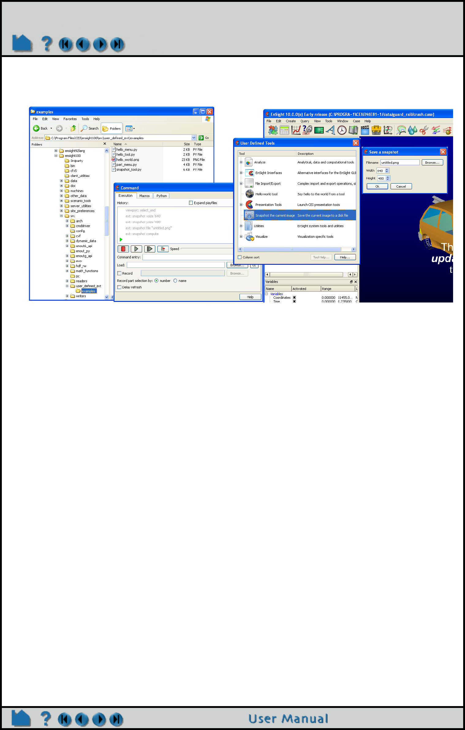
Page 539
HOW TO PRODUCE CUSTOMIZED ACCESS TO TOOLS & FEATURES
Batch-aware tool with custom command language
Shown below is a more complex tool example. Again, it can be installed in the same manner as described above and
the resulting tool is illustrated in the following image.
This example builds on the previous one. When the tool is invoked, it brings up a more complex dialog that prompts
the user for information including integer parameters and a filename. If the ‘Ok’ button is clicked, it creates a snapshot
of the current rendering and saves it to disk. More importantly, it generates custom command language (shown in the
Command dialog window) that when executed in batch mode will perform the same operation. All user-defined
extensions (tools, menus, and even “core”) automatically extend EnSight command language in this fashion. The
super-classes provide a scaffolding that makes it easy to enforce the separation between interface and function. For
example, the tool Python file could easily be extended to provide an interface to the same functionality as a user-
defined menu by adding a menu_extension subclass to the same file. The example uses an icon from the built-in
EnSight icon resources. Finally, this example is “persistent”, that is it stores state (in the case the values entered in
the dialog) and uses it to repopulate the dialog. A major advantage of EnSight extensions is that they can store state
and have both private data and method members.
The basic file structure is the same as before. There is a header block followed by the various class definitions
followed by the factory function.
#
# This comment block is required to identify the file for loading at
# startup by EnSight. The function named by FACTORY= (in this case
# 'ctor' is called by EnSight on startup. Note: the file is loaded
# as a module in EnSight and the path to this file is added to sys.path.
#
#ENSIGHT_USER_DEFINED_BEGIN
#FACTORY=ctor
#ENSIGHT_USER_DEFINED_END
#
#
# Import the parent class for all user-defined tools, the ensight module
# and the generic dialog
#
from cei.qtgenericdlg import *
from ensight.core.tool_extension import *
import ensight
#
# Define a tool class, a subclass of the tool_extension class
#
class snapshot_tool(tool_extension):
#

Page 540
HOW TO PRODUCE CUSTOMIZED ACCESS TO TOOLS & FEATURES
# Construct the tool and set up common information
#
def __init__(self,parent=None):
tool_extension.__init__(self,"snapshot",__file__,1.0)
self.setText("Snapshot the current image")
self.setDesc("Save the current image to a disk file")
self.setTooltip("Save the current image to a disk file")
if (parent): parent.addChild(obj)
#
# Create an icon for the menu (this is optional). In this case, we
# access one of the icons embedded in EnSight itself. See the Qt
# resource management documentation for details.
#
self.setIcon(":/ensight/image")
#
# This is where we store the current command language parameters
# We start with some defaults...
#
self._params = {'file':'untitled.png','xsize':640,'ysize':480}
#
# A user-defined method that performs the desired operation taking its
# parameters from a Python dictionary. This method can be called from
# interactive operation or in batch, so it should not display anything.
#
def compute(self,params):
#
# Render and save an image to disk. This is only an example.
# A deeper example can be found in the ensight.core.qtimageutils
# module found in:
# $CEI_HOME/ensight92/site_preferences/extensions/core/qtimageutils.py
#
img = ensight.render(x=params['xsize'],y=params['ysize'])
fname = params['file']
#
# The render method returns an EnVe image object, simplifying saving.
#
if (img.save(fname) == 0):
return True
if (img.errstr().find("Unknown file format") >= 0):
fname += ".png"
if (img.save(fname) == 0):
return True
return False
#
# Method that is called when the tool is selected interactively
#
def run(self):
#
# Do whatever operation this tool should do, replace with your own code
# In the example, we use the "generic" dialog to prompt the user for
# and image size and a filename.
#
items = []
items.append(['file',ITEM_FILE,"Filename",
"Name of file to save",self._params['file'],OPT_FILE_SAVE])
items.append(['xsize',ITEM_INT,"Width",
"Width of the image in pixels",self._params['xsize'],10,2048])
items.append(['ysize',ITEM_INT,"Height",
"Height of the image in pixels",self._params['ysize'],10,1536])
dlg = CeiQtGenericDialog(items,None,"Save a snapshot")

Page 541
HOW TO PRODUCE CUSTOMIZED ACCESS TO TOOLS & FEATURES
ret = dlg.doit()
#
# If the user pressed ok, we will continue.
#
if (ret > 0):
#
# Build a dictionary of output values
#
for key in self._params:
self._params[key] = dlg.getValue(key)
#
# Try to perform the operation
#
if (self.compute(self._params)):
#
# The operation succeeded, so we need to record custom
# command language to place the operation into the journaled
# output.
#
self.cmdRecord("xsize '%d'" % self._params['xsize'])
self.cmdRecord("ysize '%d'" % self._params['ysize'])
self.cmdRecord("file '\""+self._params['file']+"\"'")
self.cmdRecord("compute")
#
# All extensions include the ability to record custom command language
# and play it back. Remember that extensions should be able to play
# back their operations in batch mode. This mechanism allows for an
# extension developer to break interaction and the actual operation
# into two parts.
#
# The cmdExec() method is passed all of the custom command language for
# this tool. Here we use a trick where we assume that the recorded
# command language takes the form of actual Python assignment statements.
# We break up the passed line and use the Python 'exec()' method to
# recover the information back into a dictionary.
#
def cmdExec(self,str):
p = str.split("'")
try:
key = p[0].strip()
if (key == 'compute'):
self.compute(self._params)
else:
exec("d = "+p[1])
self._params[key] = d
except Exception, e:
print "Error handling the command:",str,e
#
# Construct a list of tool objects to be added to the global list of
# user-defined tools
#
def ctor(parent):
list = []
obj = snapshot_tool()
list.append(obj)
return list

Page 542
HOW TO PRODUCE CUSTOMIZED ACCESS TO TOOLS & FEATURES
Other examples
The example source code shown here is included in the $CEI_HOME/ensight102/src/user_defined_ext/
examples directory, but many other examples exist. The source code to all of the built-in tools is included in the
$CEI_HOME/ensight102/site_preferences/extensions/user_defined directory (perhaps most notably
the QuickTools subdirectory). Other example objects are included in $CEI_HOME/ensight102/
site_preferences/extensions/user_defined/Tools/QuickTools/Examples. There are a number of
user-defined menu examples included as well. While these may not be tools, the extension mechanisms for both
tools and menus share a large number of common features and techniques often work in both. There are a pair of
worked tools examples located in the user-defined tool Advanced Usage that demonstrate the ability of all user-
defined extensions to be able to create object hierarchies and to include multiple objects inside of a single Python
module.
To get the most out of this mechanism, menu developers are encouraged to utilize Python scripts and convert
command language scripts into Python using the provided tools. The Python interface is documented in the Interface
manual Python EnSight module interface.
SEE ALSO
Command Language Manual
EnSight Interface Manual
Produce Customized Pop-Up Menus

Page 543
HOW TO SETUP FOR PARALLEL COMPUTATION
Setup For Parallel Computation
INTRODUCTION
Ensight supports shared-memory parallel computation via POSIX threads on all of our supported platforms.
BASIC OPERATION
Configuration
Each executable of EnSight can be configured individually to control the number of threads used.
The following environment variables are used to specify the maximum number of threads that the
executable can use for computation.
ENSIGHT10_MAX_THREADS
The maximum number of threads to use for each EnSight server. Threads are used to
accelerate the computation of streamlines, clips, isosurfaces, and other compute-intensive
operations.
ENSIGHT10_MAX_CTHREADS
The maximum number of threads to use for each EnSight client. Threads in the client are
used to accelerate sorting of transparent surfaces.
ENSIGHT10_MAX_SOSTHREADS
The maximum number of threads to use on the server of server in order to start up server pro-
cesses in parallel rather than serially.
OTHER NOTES
The number of threads is limited to 2 (per client or server) with a Lite license and 8 (per client or server) with a
Standard license, while the upper limit for an HPC (formerly Gold) license is 128. EnSight, by default, uses threading
according to the license and the number of processors available and will echo this information out to the console at
startup.
....
Detected 2 CPU(s)
ensight102.client using 2 threads.
....
Detected 2 CPU(s)
ensight102.server using 2 threads.
When manually setting these parameters it is a good idea to take into account the number of processors on the
system. In general, you will not see benefit from setting the parameters higher than the number of total processors.
Because the server, server-of-servers and client operate in a pipelined fashion, it is not necessary to limit one in order
to apply more threads to another.
Compute intensive server operations that make use of shared memory parallel computations include isosurface,
clipping, and particle trace computations as well as most calculator functions. Client threaded operations include
transparency resort and display list creation.

Page 544
HOW TO SETUP FOR PARALLEL RENDERING
Setup For Parallel Rendering
INTRODUCTION
EnSight Gold now supports general parallel rendering for increased performance, increased display resolution, and
arbitrary screen orientations. The configuration file format and several examples are described in the User Manual.
Just click the link below to see this information.
SEE ALSO
User Manual: Remote Display and Parallel Compositing
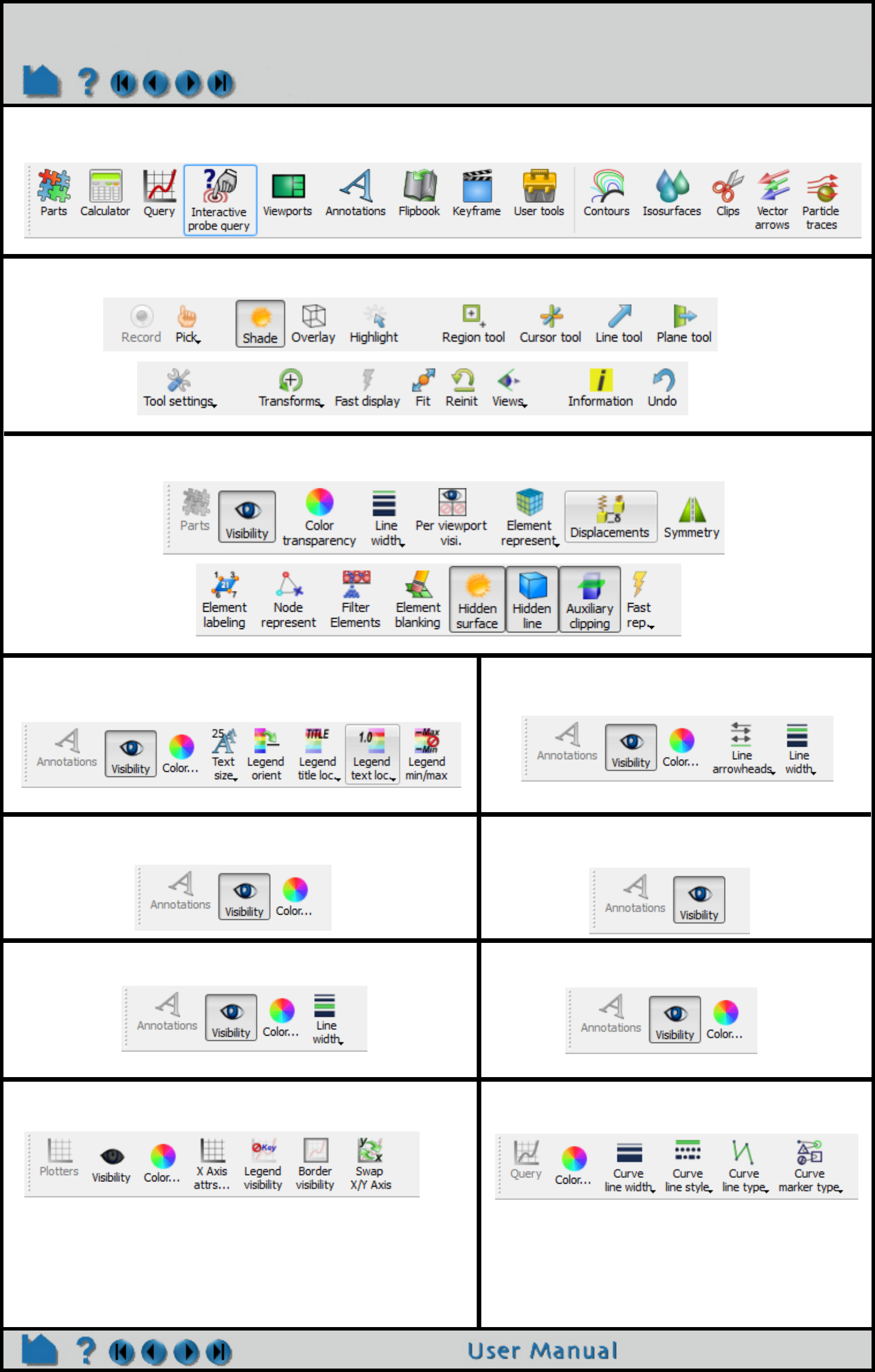
Page 545
QUICK ICON REFERENCE
Feature Icon Bar
Part Quick Action
Annotate Legend Quick Action Annotate Line Quick Action
Annotate Dial/Gauge Quick Action Annotate Logo Quick Action
Annotate Shape Quick ActionAnnotate Shape Quick Action Annotate Arrow Quick Action
Plotters Quick Action Query (curve) Quick Action
Tools Icon Bar