SIMULIA EPU Oil Gas Ebook
2015-10-19
: Ensight Simulia-Epu-Oilgas-Ebook SIMULIA-EPU-OilGas-ebook AbaqusRUM_2015 CEI Houston
Open the PDF directly: View PDF ![]() .
.
Page Count: 50

ENABLING SAFE AND EFFICIENT
OIL & GAS OPERATIONS

2
www.3ds.com/simulia
Oil and Gas
Content
Strategy Overview: Supplying Realistic Simulation to Meet Global Demands 3
Advanced Engineering Simulation: Allowing Technip to Take it Further
Technip Keynote Presentation Video, 2012 SIMULIA Community Conference
4
Realistic Simulation Drills Deeper into Oil and Gas Reservoir Sustainability
Eni develops full-scale geomechanical models with automated workflow in Abaqus
SIMULIA Community News
5
Co-simulation of Two-phase Flow in an M-shaped Subsea Piping Component
College of Technology, University of Houston
SIMULIA Community News
8
Jumping the Iteration Train: Using Isight to Advance Downhole Seal Design
Baker Hughes
SIMULIA Community Conference, Providence, Rhode Island, USA
10
Large Scale Prototyping in the Oil & Gas Industry: The Use of FEA in the Structural Capacity
Rating of a Deep Sea Pipeline Clamping System
Freudenberg Oil & Gas Technologies Ltd.
Strategic Simulation and Analysis Ltd.
SIMULIA Community Conference, Providence, Rhode Island, USA
14
Finite Element Analysis of Casing and Casing Connections for Shale Gas Wells
C-FER Technologies
SIMULIA Community Conference, Providence, Rhode Island, USA
25
Integrating Business and Technical Workflows to Achieve Asset-Level Production Optimization
Halliburton Landmark Graphics
SIMULIA Community Conference, Providence, Rhode Island, USA
33
Abaqus/Standard Simulation of Ground Subsidence due to Oil and Gas Extraction
Abaqus Technology Brief
42
Pipeline Rupture in Abaqus/Standard with Ductile Failure Initiation
Abaqus Technology Brief
46
Explore, Develop, and Produce—Safely and Efficiently
with Realistic Simulation

3
www.3ds.com/simulia
Oil and Gas
STRATEGY OVERVIEW
Supplying Realistic Simulation
to Meet Global Demands
Energy demand throughout the world is increasing. Yet the economic, financial, and
environmental challenges facing society and the energy industry are more demanding
than ever. There is an urgent need to balance sustained economic growth with
longer-term environmental sustainability, especially when it is clear that oil & gas
will continue to be the world’s dominant energy sources. Realistic simulation is an
increasingly valuable enabler along the path to a sustainable future.
Over the past few years, the energy industry has been through events both unimaginable
and predictable. The Deepwater Horizon accident in the Gulf of Mexico in 2010 illustrated the
equipment, environmental, and operational challenges facing offshore oil production. In 2011,
the earthquake and tsunami that struck Japan caused a terrible nuclear crisis at Fukushima and
shook global confidence in nuclear energy and its renaissance. In more predictable circumstances,
global automobile fuel efficiency is increasing and the introduction of hybrid and all-electric cars
is accelerating. Investments in “green” energy sources such as wind and solar and associated
technologies for energy storage continue to be strong. Even with all these occurrences, one fact
remains clear – the world will continue to rely on hydrocarbons as the primary energy source for
the foreseeable future, with oil and especially natural gas being key sources of energy.
In order to sustain the world’s energy demand and related economic growth, it is critical that we
continue to discover, develop, and produce from new sources of oil & gas and do so safely and
efficiently. For example, in the United States the extraction of shale gas is contributing to a switch
to natural gas for electricity production, thereby helping reduce CO2 emissions and reliance on
imported energy, and providing a boost to the overall economy. At the same time, there continues
to be concerns about the environmental impact of “fracking” – a concern that will need to be
addressed with effective engineering assessments and communication. Similar opportunities and
challenges are being confronted by other world regions as well, whether it involves developing
new oil & gas sources, ensuring continued efficient operations of existing fields, or even attempts
to maximize recovery from older oil & gas fields, all without compromising on safety.
Realistic simulation has been a key enabler in the oil & gas industry for several decades and is
poised to play an even more vital role throughout the value chain, from exploration to eventual
distribution to end-users. The articles presented in this e-book illustrate the critical value of
the realistic simulation solutions from the SIMULIA brand of Dassault Systèmes for various
applications in upstream oil & gas. Topics covered include optimal equipment design, well designs,
reservoir simulations, and optimized production operations.
Realistic simulation has
been a key enabler in
the oil & gas industry
for several decades and
is poised to play an even
more vital role throughout
the value chain, from
exploration to eventual
distribution to end users.
Next
Previous
Contents
4
www.3ds.com/simulia
Oil and Gas
Customer Video
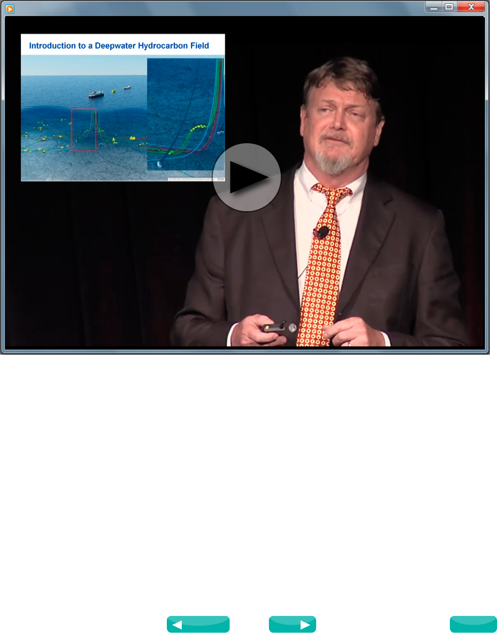
Advanced Engineering Simulation:
Allowing Technip to Take it Further
Watch Jim O’Sullivan, VP Offshore Technology at Technip present the 2012 SIMULIA Community Conference keynote address.
Abstract: Energy, along with food and shelter, is an essential need of each of us. Strong growth of the global economy is
fundamentally tied to the availability of accessibly and reliable sources of energy in all forms: hydrocarbon based, renewable, and
nuclear. For over 50 years, Technip and its subsidiaries have provided innovative products and engineering solutions to meet the
needs of the Energy industry. Technip is active from the most challenging offshore, deepwater hydrocarbon plays, where the billions
of dollars of infrastructure are required for safe and reliable operations, to the massive, and equally capital intensive, refineries and
LNG plants that needed to convert those hydrocarbons into useful products to fuel our global economy. As the technical challenges
facing the Energy industry have grown over the years, advanced engineering simulations have allowed Technip to overcome these
challenges by taking its products and designs further.
For More Information
www.technip.com
Source: SIMULIA Community Conference, 2012
Next
Previous
Contents
5
www.3ds.com/simulia
Oil and Gas
Realistic Simulation Drills
Deeper into Oil and Gas
Reservoir Sustainability
Eni develops full-scale geomechanical
models with automated workflow in Abaqus
Managing the lifespan of an oil or gas field is an ongoing, big-
picture concern for energy companies. With huge investments
needed just to start the flow of hydrocarbons from a well,
keeping production levels at optimum rates for as long as
possible is a necessity: the world still relies heavily on petroleum.
The challenge of such reservoir “sustainability” has been
partially met with flow-predicting software and on-site
monitoring tools. When flow rates drop, the injection of
fluids can boost production higher again. But there is more
to the puzzle than how fast the oil or gas will come out,
and for how long. As petroleum is pumped from its original
bed, subsidence and compaction of the soils surrounding
the reservoir can affect rock permeability, the integrity of
boreholes, equipment function, and even the geology of the
land around the production sites.
This happens because the extraction of petroleum from
underground reservoirs leads to a reduction in pore fluid
pressure within the reservoir, which results in a redistribution
of stress in the rock formation. Since rock deformations are
often plastic, this produces subsidence of the ground around
the reservoir that expands over time as extraction continues. As
the rock deforms, the permeability of the rock itself changes,
which then affects the flow of fluid within the reservoir. The
phenomena of fluid flow and mechanical deformations are thus
inexorably coupled to each other (see Figure 1).
Subsidence challenges petroleum industry
both on and offshore
Reservoir compaction has been extensively investigated to
determine its impact on both hydrocarbon field production and
environmental stability, onshore or offshore. The effects can
be cumulative. For example, in the Netherlands, subsidence at
the large Groningen gas field, though only on the order of tens
of centimeters to date, poses significant long-term challenges
since large portions of the Netherlands are below sea level
and protected by dikes. Some important, much-documented
lessons from the past clearly demonstrate the negative impact
of the phenomenon over time. The city of Long Beach,
California, experienced subsidence of some 20 square miles
of land, with a surface dip of 29 feet near the center, due to
extraction from the huge Wilmington oilfield. Subsidence from
the Goose Creek oilfield in Texas affected over four square
miles, with up to five feet of surface drop. Remediation in
both cases cost millions of dollars. Offshore, the Ekofisk field
in the North Sea suffered seafloor subsidence that required
highly expensive interventions to re-establish the safety of the
producing platforms.
While the majority of oil and gas projects don’t encounter
challenges at such a large scale, petroleum engineers now
clearly understand the value of starting with deeper knowledge
of the terrain at the earliest stages of reservoir development.
A more realistic view of what lies beneath
As an integrated energy company operating in engineering,
construction, and drilling both off- and onshore for customers
around the world, Italy’s Eni S.p.A. devotes considerable
manpower and resources to research into reservoir management.
Their work helps clients close to home as well: Gas fields in the
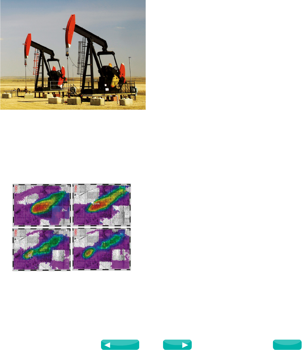
Figure 1. The NASA images above show the rapid rate of subsidence (in
red) of over 3 cm/month during active production in the Lost Hills area
of California. Note that production occurs over several years and so
easily results in several feet of subsidence.
Source: SIMULIA Community News, 2012
Next
Previous
Contents

6
www.3ds.com/simulia
Oil and Gas
Adriatic Sea have become a major source of energy for the
country. Due to the particular morphology of theshoreline in
that area, it is of paramount importance for Eni to be able to
correctly predict the land subsidence that may be induced by
hydrocarbon production in order to guarantee the sustainable
development of the offshore fields.
Eni has for some time been developing advanced methodologies
for studying the problem of reservoir subsidence and
compaction with the help of Abaqus finite element analysis
(FEA). “Abaqus is our main stress/strain simulator for studying
the geomechanical behavior of reservoirs at both field and well
scale,” says Silvia Monaco, geomechanical engineer in the
petroleum engineering department of Eni E&P headquarters in
San Donato, Milan, Italy.
The ability of Abaqus Unified FEA to realistically simulate
complex structural and material behavior makes it well suited to
the task. Although the study of subsidence in petroleum fields
has been slowly advancing since the 1950s, earlier approaches
were based on an assumption of homogeneity of the whole
system, i.e. they described the side-, over-, and under-burdens
of rock and soil with mechanical properties identical to those
of the reservoir. But soil and rock are in fact very non-
homogeneous and show highly nonlinear behavior that is
strongly influenced by previous stress paths. Incorporating
FEA into a computer model of a reservoir provides a much
more realistic simulation of this truth. Different types of finite
elements, a large variety of material properties, coarser or finer
element meshes, and data-based boundary conditions can all
be woven into a prediction that much more accurately reflects
the full effects of the geomechanical complexities unfolding
beneath the surface.
Coupling Abaqus with the leading flow simulator
Of course it’s the start of oil or gas flow out of the reservoir
that gives rise to the effects that FEA models anticipate. So the
Eni group links their Abaqus FEA models to the leading flow
simulator ECLIPSE (from Schlumberger). “Fluid-flow analysis
is essential in order to forecast production and manage field
development,” says Monaco. “But the geomechanical processes
at work in the rock and the fluid contained in its pore space are
also of primary interest since they can affect the behavior of
the reservoir itself. By transferring pore pressure depletion data
from ECLIPSE into Abaqus, we can more fully understand the
mechanisms involved in surface subsidence in order to forecast
and prevent well failures and adverse environmental impact.”
(see Figure 2)
Running a computer model of the large-scale dynamics of
an entire oilfield is becoming much more efficient these
days, thanks to huge leaps in parallel processing and high-
performance computing that can handle FEA models with
millions of degrees of freedom (DOF). And for Eni, creating
those kind of models in the first place has recently become
much easier.
When the Eni team first began coupling Abaqus with their
ECLIPSE models several years ago, there was still considerable
effort involved in creating the complex workflow needed to
produce simulations that behaved realistically and correlated
well with real-world measurements. “Previously, we had a
number of non-automated procedures as well as simplifications
related to the geometry description, such as the smearing
of faults and simplified treatment of collapsing layers,” says
Monaco. “It used to take almost two months to complete a
single model suitable for running.”
With the goal of streamlining this process, Eni teamed with
SIMULIA in a two-year R&D collaboration, the results of which
were presented at the 2011 SIMULIA Customer Conference in
Barcelona, Spain. “SIMULIA worked closely with us to develop
new features in Abaqus that definitely change the approach to
geomechanical reservoir simulation by allowing a completely
automated workflow,” says Monaco. “Now we can build a
geomechanical model in only four weeks: We obtained an
improved efficiency compared to the previous process in terms
of elapsed time needed to set up an analysis. Moreover, the
new iterative solver implementation provides a strong reduction
in computational times and memory usage that further speeds
up the execution of the study.”
The new workflow (see Figure 3) automates the transfer of
data from ECLIPSE into Abaqus and speeds the subsequent FEA
model set-up, expanding the flow-centric view of a field-scale
reservoir into a much richer 3D profile of flow-plus-subsidence
over time. This involves the following steps:
• A translator establishes a link between ECLIPSE and Abaqus.
All the information from the reservoir model (grid, properties,
and pressure) is automatically populated into the FEA model
in the form of data that can be used for the geomechanical
Figure 2. (Left) Active region generated from the flow simulation solution.
(Right) Abaqus mesh showing the active region within a reservoir. Linking
ECLIPSE with Abaqus incorporates the geomechanical effects of extraction
for a more realistic simulation of full-site development over time.
Source: SIMULIA Community News, 2012
Next
Previous
Contents
7
www.3ds.com/simulia
Oil and Gas
analysis. For example, ECLIPSE cells are designated either
as gas, oil, or water according to the percentage of fluid
saturation they hold; in the Abaqus model the elements that
are automatically derived from these cells can be assigned
as many as 300 different material property definitions.
ECLIPSE pressure history descriptions are also translated into
Abaqus pore pressure values. These values are essential for
calculating the change in the effective stress in the reservoir.
Abaqus meshing tools automatically adjust the elements
and nodes as needed and perform upscaling, a process that
condenses the size of the FEA model by merging horizontal
rows of elements while maintaining the vertical zones
(where drill data has already been collected), which are more
relevant to subsidence prediction.
• Burden regions over, under, and to the sides of the oil
reservoir are created in Abaqus to extend the analysis to the
terrain beyond the reservoir as the petroleum is pumped out.
• Once the model is set up, results from an initial elastic run
are used to update the plasticity values (since rock behavior
is elasto-plastic) to make the models more realistic. The
simulations are then run over time increments so predictions
can extend over many years (from the year 2018 to 2020 to
2024 to 2028, as seen in Figure 4).
New geomechanical models
provide greater predictability
“We now have a logical scheme for easily and automatically
executing all the steps required for creating and running
our geomechanical models,” says Monaco. “This significantly
improves our efficiency in terms of user time in the preprocessing
stage. Our analyses are now measurably more precise.”
Such precision is helping Eni better serve their energy customers
in developing strategies for ensuring sustainable oil and gas
production for the long term.
“The increased quality of the results we’ve obtained with the
new Abaqus implementations allows for a highly accurate and
predictive environmental analysis,” says Monaco. “This is a
key point for a sustainable development of Italy’s hydrocarbon
reservoirs. Moreover, as a result of the cutback in computational
times, a larger number of studies can also be performed
internally, thus strengthening the link between geomechanical
engineers and the team in charge of the geological and
reservoir model construction.”
In the near future, the Eni team plans to turn its attention
to a comprehensive integration of the huge quantities of
deformation measurements they’ve acquired at different
scales and through different methodologies. “The automatic
Eclipse
Output
Eclipse
Translation
Eclipse
ODB File
CAE:
Element Validity
Upscaling
CAE:
Reorder Ids
CAE:
Model
Import
CAE:
Add over/under
and side burden
CAE:
Material
Assignment
Standard:
Elastic
Geostatic
Standard:
Complete
Reservoir
CAE:
Material
Assignment for
Plasticity
ODB File
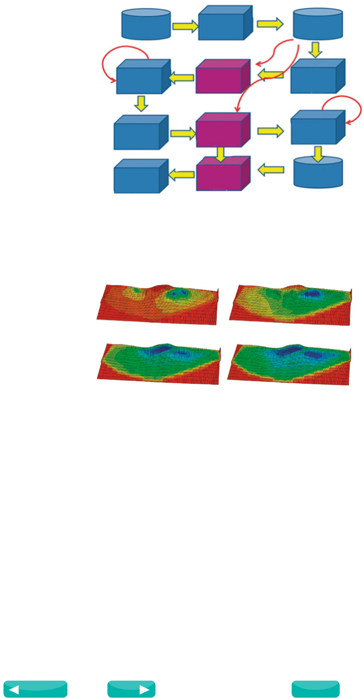
Figure 3. Reservoir geomechanics workflow. An output database file
(ODB) is created from ECLIPSE and imported into Abaqus/CAE for
creation of an FEA geomechanical model from which the stress
distribution over a reservoir can be derived. A plastic analysis then
predicts the geomechanical deformations (subsidence) in the
surrounding terrain that will result from this stress.
2018 2020
2024 2028
Figure 4. Four increments in an Abaqus FEA simulation of subsidence in a
hypothetical oilfield, displayed over ten years. Blue areas denote greatest
downward displacement of the surface. This particular example from Eni
contains just 300,000 degrees of freedom; enhancements in model setup
and automation now allow the running of huge full-scale models with
millions of DOF in just a few hours. Rock faults (not pictured here) can be
included in simulations.
calibration of the rock properties of a geomechanical model will
allow for this,” says Monaco. “Isight process automation and
optimization software from SIMULIA could be a proper tool for
obtaining results.”
For More Information
www.eni.com
www.3ds.com/SCN-June2012
Source: SIMULIA Community News, 2012
Next
Previous
Contents
8
www.3ds.com/simulia
Oil and Gas
Co-simulation of Two-phase
Flow in an M-shaped Subsea
Piping Component
Components in a subsea production system require different
types of pipelines, such as a jumper (a short U-shaped section
of pipe to connect one pipeline to another), to transport fluids.
The internal flow in pipes involves an interaction between fluid
and structure, which is important to understand since their
interaction can generate high amplitude vibrations, also known
as “flow-induced vibration.” Consequently, these vibrations can
result in fatigue damage of the structure. This phenomenon has
become a great concern in the oil & gas industry where subsea
jumpers are exposed to this type of vibration when transporting
production fluid. The industry is currently putting a lot of effort
into investigating vibration-induced fatigue cases to prevent
negative effects on revenue, production, environmental safety
and health.
Production fluid flowing through subsea components is usually
a mixture of oil, gas, and water. When a gas and liquid
flow through a pipe, a potential slug flow is formed, and
consequently this generates vibration issues in the structure.
A slug is an intermittent flow in which long gas bubbles
are separated by chunks of liquid causing large pressure
fluctuations and corrosion. The amplitude of the vibrations
increases and creates a potential risk of failure of the pipe when
the natural frequency of the structure is close to the frequency
of the slugs as they are transported along the pipeline.
To assess the impact of this type of flow in the structure,
Leonardo Chica, a researcher at the College of Technology,
University of Houston, conducted an analysis of the fluctuation
of stress with time to predict the number of cycles that the
jumper can withstand without failure. The best option to
represent this fluid-structure interaction problem is to perform
a two-way coupling simulation or co-simulation between
Abaqus and a computational fluid dynamics (CFD) program,
such as CD-adapco’s Star-CCM+. In this process, the pressure
fluctuations are exported from the CFD tool into Abaqus, and
then Abaqus computes the stresses and displacements. These
displacements are exported back to the CFD program and the
cycle starts again. Both programs run simultaneously and
exchange data at each time step.
To set up the analysis, we imported the CAD model and
then extracted the natural frequencies in Abaqus. Next, the
simulation was set up in the CFD program with the appropriate
mesh and physics, and the co-simulation was initiated to
communicate the CFD code to Abaqus. After initializing the
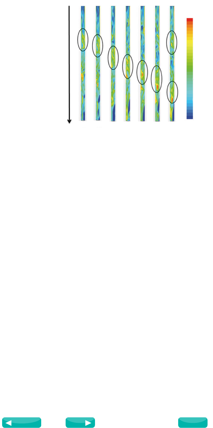
solution with 50% air and 50% water, the results showed that
irregular slugs are developed at the vertical section of a two-
bend model. Slug frequency was determined to be 1.0417
Hz (see Figure 1), which is close to the fundamental natural
frequency (1.079 Hz), so amplitude of the vibrations could be
intensified and the fatigue life of the jumper might be reduced.
In this case, the co-simulation results of the von Mises stress
vs. time graph obtained in Abaqus show a sinusoidal pattern
with a response frequency of 0.167 Hz. Based on the material’s
S-N curve, fatigue life is infinite (below the fatigue limit curve),
due to the small stress range, and the two-bend structure can
withstand cyclic loading from the pressure fluctuations of the
two-phase flow.
In this initial investigation, only water-air mixture was
simulated to understand the behavior of this two-phase flow
and to determine the response in the jumper. For future work,
oil-gas-water flow will be simulated and analyzed to compare
with experimental results. The Fluid-Structure Interaction (FSI)
analysis should also be extended to include the entire jumper
model in order to draw solid conclusions about fatigue damage.
This type of FSI co-simulation is becoming more valuable in
subsea engineering to understand how the internal or external
flow affects the fatigue life of subsea components. The Abaqus
co-simulation capability for FSI allows the user to perform
a co-simulation between Abaqus and third party software,
such as Star-CCM+. One of the advanced features of Abaqus
is to perform either a one-way coupling or two-way coupling
simulation depending on the magnitude of the displacements.
This selection would be made on a case-by-case basis to
achieve a balance between computational cost and accuracy
Figure 1. Slug travelling in vertical section of two-bend model.
Two-bend subsea pipe model
Volume fraction
of water
1.0000
0.80000
0.60000
0.40000
0.20000
0.00000
6.64s 6.72s 6.96s 7.12s 7.28s 7.44s 7.6s
Direction of flow
Source: SIMULIA Community News, 2012
Next
Previous
Contents

9
www.3ds.com/simulia
Oil and Gas
of the results. Either way, co-simulation for FSI is rapidly
becoming a requirement in the subsea industry to provide
greater reliability, safety, and performance in complex subsea
systems.
For More Information
www.tech.uh.edu
www.3ds.com/SCN-June2012
Two-bend subsea pipe model
Source: SIMULIA Community News, 2012
Next
Previous
Contents
10
www.3ds.com/simulia
Oil and Gas
Jumping the Iteration Train: Using Isight
to Advance Downhole Seal Design
Jeff Williams (Baker Hughes Incorporated)
Abstract: In the oilfield, market segments are driven by the next profound “unreachable” payzone. In the last few decades, we have
gone through various design levels attempting to reach the operators latest requests. The common term to designate these extreme
conditions is High Pressure/High Temperature (HP/HT). Under the HP moniker, there are multiple Tiers: Tier 1 up to 15,000 psi,
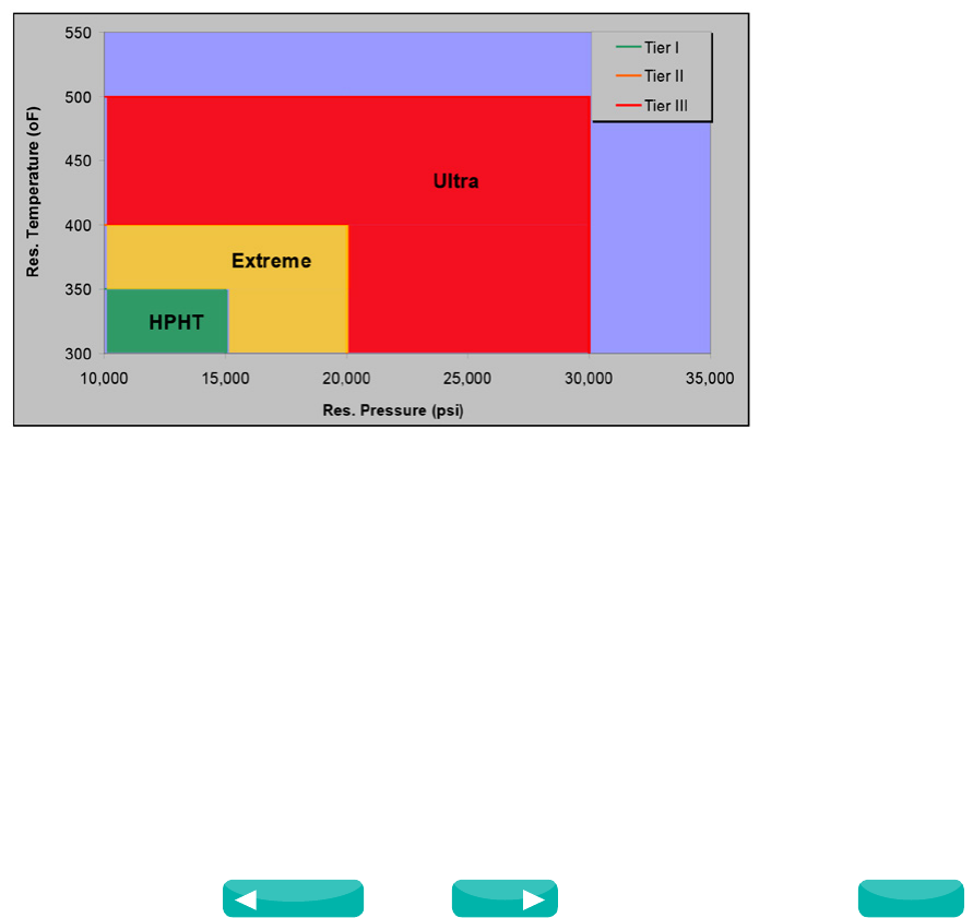
Tier 2 up to 20,000 psi, Tier 3 up to 30,000 psi, and Tier 4 beyond 35,000 psi. BHI currently has a Liner Top Packer that covers
Tier 1 rated for 15,000 psi. This paper will show the path we took with Isight and Abaqus to conceptually achieve higher Tiers for
a Liner Top Packer, and will show how we “jumped the iteration train” with surprising results.
Keywords: Oilfield High Pressure/High Temperature Completions, HP/HT, Liner Hanger Packer, Optimization, FEA
1. Going Deep
With the ever-increasing global demand for hydrocarbons, the oil and gas industry is being challenged to explore and develop
deeper and hotter reservoirs, pushing the boundaries of equipment capability further into higher pressures and higher temperature
(HP/HT) wells. The criteria for designating fields as HP/HT have changed over the years. In the past, they were fields with pressure
greater than 10,000 psi and temperature higher than 300°F (Tier 1). Currently, the “extreme” HP/HT designation tends to be
at 15,000 psi and 350°F (Tier 2), an environment where technical operational challenges have been mostly overcome. The term
“ultra HP/HT” is used to define well environments that are above 20,000 psi and 450°F (Tier 3). High gas prices and the search for
hydrocarbons in deeper and more extreme formations are key drivers of the development of HP/HT completion technologies. Figure
1 shows how the oil industry has categorized different Tiers for defining the technological boundaries.
Figure 1: Chart of Oilfield Reservoir Tiers for HP/HT
2. Downhole Seal Design 101
We set out to investigate how far our existing seal technology would go into these realms. All our proprietary seal technology was
investigated. Some fared very well, while others fell off early. Our attention turned to our existing expandable “zero-extrusion”
seal (Figure 2) arraignment, which is the focus of this paper.
Source: SIMULIA Community Conference, 2014
Next
Previous
Contents
11
www.3ds.com/simulia
Oil and Gas
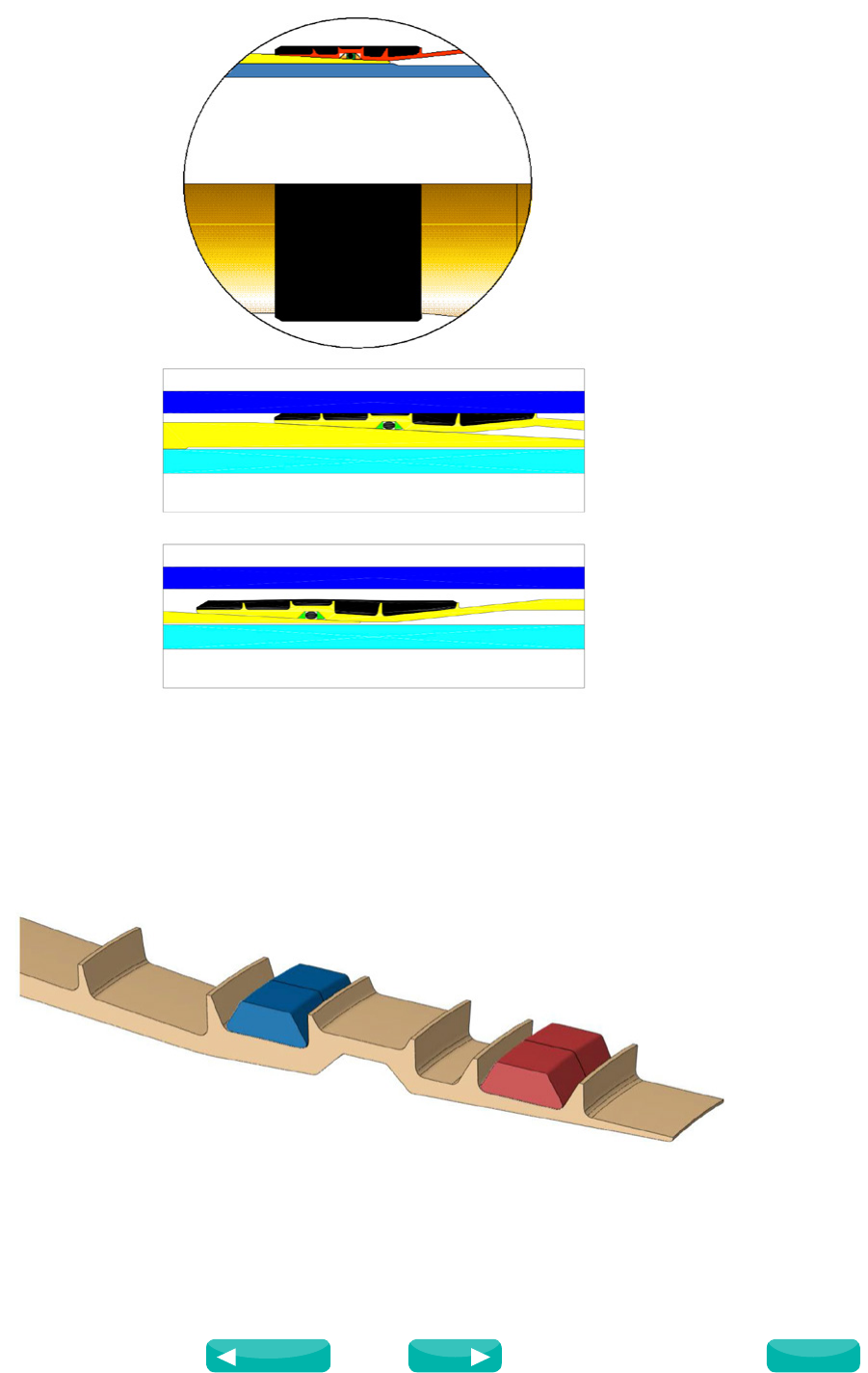
Figure 2: Typical Baker Hughes “Zero-Extrusion” Seal
The term “zero-extrusion” refers to the gap after the seal comes into contact inside a bore; in this case the ID of a parent well casing.
To pass a gas-tight test, the seal needs to have a zero-extrusion gap. We had developed a new feature on the existing technology
in another project to limit the radial travel of the seal using split-rings. While studying the metal-to-metal interactions of that seal,
we determined that this new feature could aid in protecting the seal and boosting performance. Figure 3 shows a generic form of
this configuration (minus the elastomer) where we had packaged the new rings with the existing seal.
Figure 3: Existing Seal with New Feature(s)
Source: SIMULIA Community Conference, 2014
Next
Previous
Contents
12
www.3ds.com/simulia
Oil and Gas
3. Surprise: Tier 2!
This new seal configuration showed surprising promise. Early analysis showed positive results for high differential pressures.
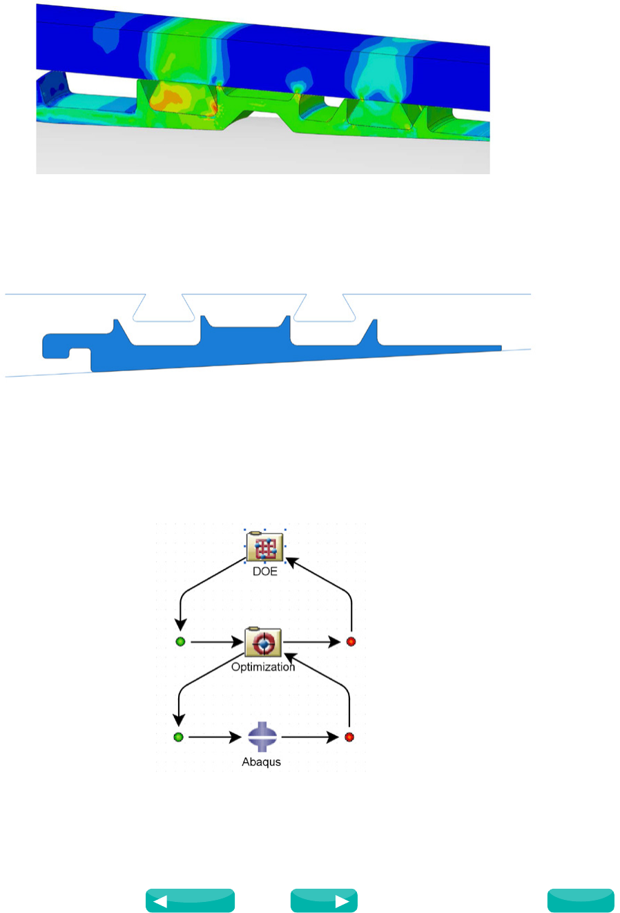
Figure 4 shows an early iteration: with very little adjustment the new design could achieve Tier 2.
Figure 4: New seal concept shown with 20,000 psi differential (Tier 2)
4. Jumping the Iteration Train: Optimization at its Best
With the idea to eventually use Isight and Abaqus to optimize the seal, there was a problem: The model was too big! A typical 3D
version of this model would take days on multiple cores on a compute cluster. A replica was created in 2D to perform much quicker
runs with an axisymmetric model. Figure 5 shows an example of the new simulated version.
Figure 5: Axisymetric Representation of the Seal Before Expansion
Since the split-rings were non-circumferential, they did not need to be part of the expansion of the tubular metal seal. By making
them a rigid body in a final expanded state, a simplified axisymmetric model was enabled. This model was much more streamlined
for time and would run on a local PC in under 5 minutes. Now a local Isight model was usable. Isight 5.7, along with Abaqus 6.12,
was utilized on a 4-core processor. A combination of design of experiments (DOE) and optimization techniques were used to cycle
through hundreds of iterations. Figure 6 shows the Isight Sim flow path.
Figure 6: Isight Sim Flow Path Utilized
Source: SIMULIA Community Conference, 2014
Next
Previous
Contents
13
www.3ds.com/simulia
Oil and Gas
The DOE loop utilized an optimal latin hypercube algorithm with 100 points, while the optimization loop utilized a sequential
quadratic (NLPQL) algorithm with 40 maximum iterations. The combination of the two methods resulted in much more trustworthy
final output that avoids getting stuck in any false solutions from plateaus or valleys.
5. Results: Defining New Thresholds
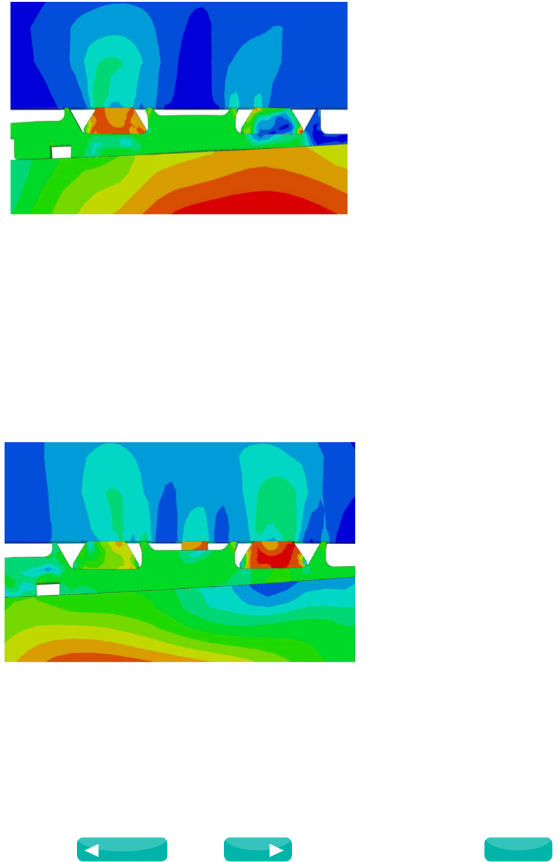
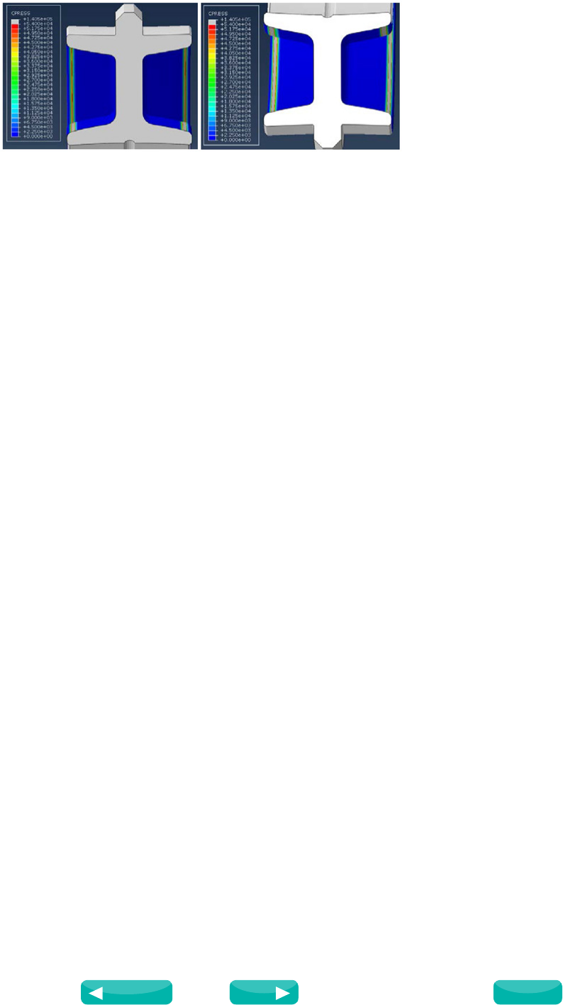
The results were astonishing. We were now plunging into the 30Ksi realm (Tier 3). Figure 7 shows the optimized seal with 30,000
psi differential pressure applied across the seal.
Figure 7: Tier 3 Results: 30,000 psi across the seal
With these types of pressures, it was a slight shift in strategy and non-elastomeric seals were next being considered. We focused
on optimizing the contact pressures of the metal contact points and our goal was to retain a proprietary threshold to maintain a
reliable seal. To keep pushing the boundary of what could be achieved with this concept, some assumptions needed to be defined:
1. The parent casing would be rated for the equivalent pressures.
2. The operators would be willing to use “non-standard” dimensions for OD/ID
3. Expense of high grade materials would not be the limiting factor
With these assumptions, we extended the seal design to structurally withstand 40,000 psi. A third ring was added for structural
support and the Isight procedure from before was repeated. Figure 8 shows the final configuration which helped define a new Tier
4 threshold.
Figure 8: 40,000 psi Conceptual Design
6. Summation: Why a Simple Seal Optimization Will Change our Business
• Downhole seal design had reached an impasse, HP/HT seals were thought to be the limiting agent of well exploration.
• By taking some pre-existing designs and putting a new spin on them, a fresh perspective was achieved.
• Using Isight, optimization has extended new seal limits that previously seemed unreachable in the deep well completion world.
Source: SIMULIA Community Conference, 2014
Next
Previous
Contents

14
www.3ds.com/simulia
Oil and Gas
Large Scale Prototyping in the Oil & Gas Industry: The Use of
FEA in the Structural Capacity Rating of a Deep Sea Pipeline
Clamping System
Dr. David Winfield1, Laurence Marks2, John Stobbart1 and Nick Long1
1Freudenberg Oil & Gas Technologies Ltd, Unit 18, Baglan Industrial Estate, Baglan, Port Talbot, SA12 7BY, United Kingdom
2Strategic Simulation and Analysis Ltd, Southill Barn, Southill Business Park, Cornbury Park, Charlbury, Oxfordshire, OX7 3EW,
United Kingdom
Abstract: Freudenberg Oil & Gas Technologies (FO>) in Port Talbot, UK, provides complex metal to metal sealing solutions for the
oil & gas and energy industries. FO> is supplying two of its largest Optima® subsea connectors for use just inside the Arctic Circle.
These will be the deepest of their kind anywhere in the world.
Weighing some 10 tons, the Optima® is a high precision, multi-piece clamping system using a FO> Duoseal® metallic seal,
tensioned by multiple leadscrew(s), activated via integral drive buckets. The resulting leadscrew tension positions the clamp
segments on the hubs; as the tension increases, the opposing hubs are pulled together overcoming external forces and moments.
Pressure energisation and plastic deformation ensure a high integrity double seal between the inner pipeline and the deep water
environment.
Multi-body elasto-plastic finite element analysis (FEA) is used to simulate the interaction and contact between all parts of the
Optima®, with focus on the stress and plastic strain of individual components during make-up and operation.
Fluctuating in-service loadings such as temperature, pressure and bending moment are also analyzed to qualify the clamp segments,
together with capacity analysis for the clamps and Duoseal®, where contact analysis is used to verify Duoseal® compliance. The
Optima® is also required to overcome a range of hub misalignments, resulting from installation tolerances, friction and pipeline
flexibility.
The FEA simulation results of the Optima® will be used to support experimental test data obtained during factory trials, prequalifying
these components to the most extreme subsea loading conditions.
Keywords: Subsea, Clamping, Plasticity, Dynamic Implicit, Multi-Body Dynamics, Connectors, Coupled Analysis, Design
Optimization, Interface Friction, Oil & Gas, Pipeline, Sealing, Metallic Seals, Abaqus/CAE.
1. Introduction
Freudenberg Oil & Gas Technologies Ltd (FO>) specializes in a range of high precision metal to metal sealing solutions, including
seal rings, pipe connectors and flanges, as well as full assemblies of a range of high capacity Optima subsea connectors. Oil and gas
pipeline operation requires high integrity sealing solutions to cope with the fluctuating demands of transport media, pressure and
temperature to match the campaign life required by the customer. With oil and gas resources becoming increasingly more difficult
to find and extract, pipeline components must be designed to cope with the increased demands of deeper and rougher waters.
As well as the analysis of specialist subsea equipment, FO> have used Abaqus/CAE to undertake coupled thermal-structural FEA
simulations for ultra-high temperature applications (1600 F) utilizing custom flange and connector designs, together with bespoke
kammprofile gaskets, producing highly reliable sealing solutions whilst subjected to severe in-service loadings. FO> has also
analyzed, bespoke sealing solutions for harsh environment chemical mixing and reaction vessels up to 65,000 Psi.
FO> has been approached to design and specify a pair of No.36 Optima subsea connectors for an application in the Norwegian
Sea, just inside the Arctic Circle. The No.36 Optima that FO> are analyzing and supplying, will be both the largest and deepest of
its kind installed anywhere in the world; it is expected that the Optima will be subjected to operating depths of nearly 4,000 feet,
in some of the harshest deep sea conditions. Due to the simple design of the Optima and the use of a FO> DuoSeal®, complex
multi-body finite element analysis (FEA) is required to be undertaken with Abaqus/CAE to qualify the components of interest.
The design of the No.36 Optima is based on a similar qualified clamp size for a previous customer request. The design challenges
look to incorporate a new clamping and leadscrew arrangement, being subjected to a pressure depth FO> have never supplied
to before. Previous FEA work undertaken on the earlier customer design was done externally, but with FO> now undertaking
Source: SIMULIA Community Conference, 2014
Next
Previous
Contents
15
www.3ds.com/simulia
Oil and Gas
FEA simulation work completely in-house, the modeling methodology has been extensively fine-tuned, and the results generated
through the FEA can be checked periodically with theory, ensuring the accuracy of the settings used to predict the resultant
solution.
FEA simulation has been undertaken on a range of similar individual components and principles, such as lip seals (Chun-Ying Lee,
2006), (Chung Kyun Kim, 1997), clamping pressure distribution (Alex Bates, 2013), together with general analysis of pressure
vessels (Sanal, 2000).
This paper addresses the problem of analyzing an optimized FO> design which has been tailored to provide a high capacity
sealing solution to the customer, whilst remaining light-weight and easy to manufacture. FEA simulation provides a robust, cost
effective and non-invasive method of structural interrogation, especially when components and systems must be taken to the point
of failure and structural collapse. The paper also documents how the Optima’s are assessed from an FEA perspective, presenting
results on the optimized No.36 Optima, designed to meet customer specification. Rated capacity procedures for the No.36 Optima
are detailed, together with how the FEA results and proposed factory testing validate one another. A summary of the function
and location within the pipeline system of the No.36 Optima is followed by an overview of the problems encountered during the
modeling process causing inconsistent, or, very little convergence is discussed. Contact stabilization, mass effects and time step
lengths, together with the processes and settings required to overcome some of the more complex convergence problems are
reviewed, that finally generate a repeatable and reliable solution.
2. Deep Sea Pipeline/Clamping System Layout and No.36 Optima
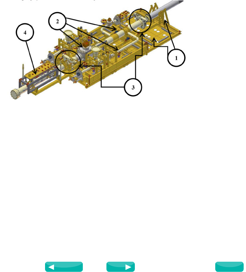
The pipeline/clamping system is illustrated in Figure 1;
Figure 1: Illustration of the deep sea pipeline/clamping system with the four major structures identified.
The system constitutes four major elements; the frame support platform (FSP) complete with ‘cow horns’ to support the main gas
pipeline (1), the pipeline module (PLEM), which is pre-constructed and lowered onto a set of friction pads incorporated into the FSP
(2), a pair of No.36 FO> Optima’s (3), and the pig launcher which is connected to the rear end of the PLEM (4).
2.1 No.36 Optima; Principles of Operation
The No.36 Optima (see Figure 2) is a high precision, multi-piece clamping system using a FO> DuoSeal metallic seal between
opposing male and female hubs. The clamping segments are locked around the hubs using the tension generated by threaded
leadscrew(s) and trunnion(s), actuated via a suitable subsea tooling interface. Resulting leadscrew tension aligns and positions the
clamp segments over the hubs. As leadscrew tension increases, opposing hubs are displaced towards each other, overcoming large
external forces and moments.
Inward displacement of opposing hubs generates elasto-plastic deformation in the DuoSeal, creating the initial seal on the inner/
outer heel regions. When subjected to internal pressure, pressure energisation together with plastic deformation ensures a high
integrity double seal between the inner pipeline and external deep water environment. Movement of the trunnion(s) and link-pin
is directed via guide slots cut into the supporting enclosure. Once assembled the Optima is freely supported by the enclosure alone
Source: SIMULIA Community Conference, 2014
Next
Previous
Contents
16
www.3ds.com/simulia
Oil and Gas
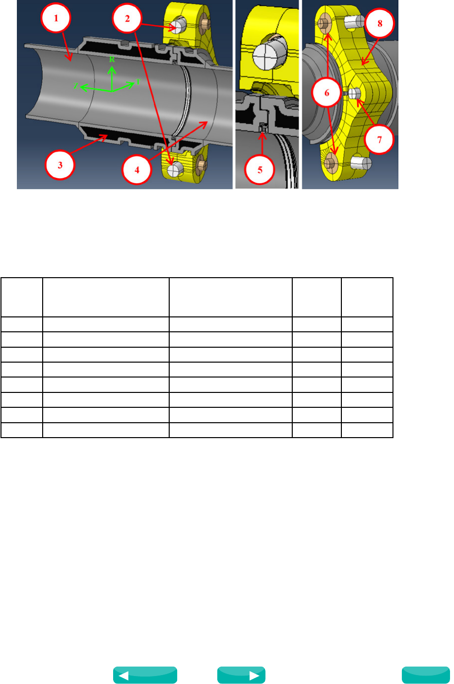
Figure 2: Left to right: schematic symmetry plan view of the No.36 Optima and cylindrical co-ordinate system, close-up of hub, seal and clamp
geometry detail, external view of clamp segments.
The Optima enclosure is nominally 96 inches square, by 25 inches deep. The No.36 Optima has an internal bore of 34 inches and
an external hub diameter of 50 inches. The whole assembly weighs approximately 22x103 Lbs (10 tons). Component materials are
identified in Table 1;
Table 1: No.36 Optima components and materials.
Region Optima Component Material Specification
Young’s
Modulus
(Psi)
Yield
Stress
(Psi)
1Male Hub and Pipe ASTM A694 F65 30.5x10⁶ 71.4x10³
2Leadscrew(s) Inconel 725 (UNS N07725) 30.3x106116.0x103
3Inner forging (black regions) ASTM A694 F65 30.5x10665.7x103
4Female Hub and Pipe ASTM A694 F65 30.5x10671.4x103
5DuoSeal Inconel 725 (UNS N07725) 30.3x106116.0x103
6Trunnion(s) Hiduron 130 20.2x106100.8x103
7Link-pin Inconel 725 (UNS N07725) 30.3x106116.0x103
8Clamp Segments AISI 4140 30.5x10675.0x103
The geometry model utilizes inner forging regions (see Figure 2) specified by FO>. These inner regions have a slightly lower yield
point than the outer portion of the hub(s) due to the manufacturing process associated with the forging (heat treatment, water
quench and tempered).
3. Outline of the FEA Model
3.1 FEA Sub-Modeling
The FEA modeling methodology began life with a series of less complex sub models of different interacting parts of the Optima. This
included hub-on-DuoSeal contact, clamp-on-hub contact, clamp-on-clamp-on-link-pin contact, leadscrew/trunnion contact within
the clamp and constraints for applied bending moment and pipe flexure during hub misalignment analysis.
Early in the modeling process it was determined that static-general analysis was not robust enough to attain a stable solution.
Dynamic-implicit was therefore chosen to attain a robust and reliable converged solution during the clamp-up and leadscrew
pretension phase of the simulation, over-coming initial contact stabilization and convergence problems.
Source: SIMULIA Community Conference, 2014
Next
Previous
Contents
17
www.3ds.com/simulia
Oil and Gas
3.2 Mesh Density and Structure
To satisfy contractual obligations, two separate Optima models were created. The first Optima model (parent) would consider the
detailed aspects of DuoSeal and clamp contact performance through the in-service load case to qualify the design. As such, the
mesh discretization on this parent model from which multiple load cases would be run, was optimized in the contact regions.
The mesh density in the DuoSeal where contact is made on the hub seat area(s) was set to 0.03 inches as a result of a thorough
mesh sensitivity analysis. It was found that below this 0.03 inch mesh size, the Von Mises (V.M.) and contact stress profiles in the
DuoSeal proved to be largely mesh independent, with deviation from the smallest mesh size considered in the analysis, to the 0.03
inch threshold, of <5 %.
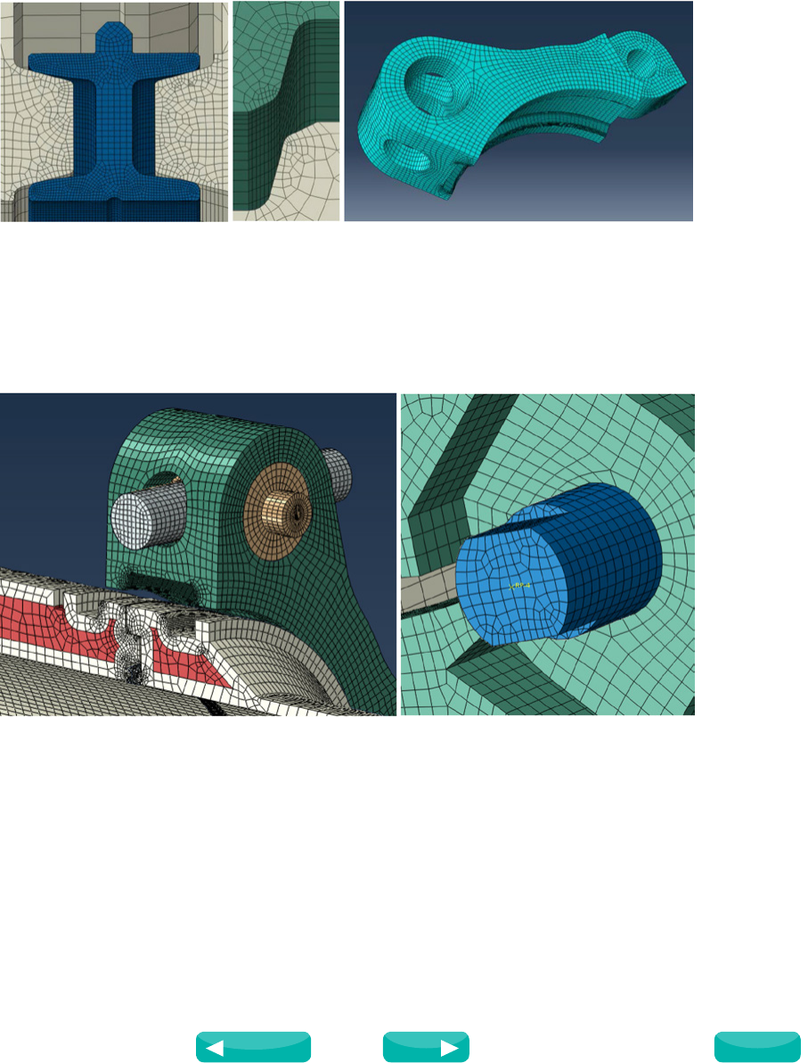
Figure 3: Left to right; mesh density in the DuoSeal and surrounding seat area, mesh density in the contacting
clamp and hub region, overview of mesh structure in the lower clamping segment.
The second Optima model considered for the analysis was required to simulate two hub misalignment load cases, where the
central axis of the male and female hub(s) was offset by 0.5° and 1°, equally about the central plane through the clamp segments.
In this model, a lower mesh density was used in the DuoSeal and other relevant contact areas, with minimal additional elements
concentrated in these contact regions. Figure 3 illustrates the optimized mesh structure for sections of the parent model;
Figure 4: Left to right; General view of parent model global mesh of the No.36 Optima, detailed view of link-pin within upper clamp lug.
In all load cases considered to satisfy customer requirements, the same global mesh density was used containing around 93
% C3D8R hexahedral elements, with the remaining 7% using C3D4 tetrahedral elements. The misalignment models utilized
approximately 380x103 elements with 410x103 nodes. The parent model run with multiple load cases used approximately 445x103
elements with 600x103 nodes, where approximately 1x10⁶ degrees of freedom (DOF) are located in the DuoSeal alone.
Source: SIMULIA Community Conference, 2014
Next
Previous
Contents
18
www.3ds.com/simulia
Oil and Gas
3.3 In-service Boundary Conditions
In order to complete the comprehensive structural assessment required for the No.36 Optima, stress profiles of individual
components, through the clamp segments ability to pull-in against bending moments and withstand internal pressures must be
quantified. The range of individual structural loads are detailed below and documented in Table 2;
1. Internal design pressure of 3,379 Psi (plus internal pressure to yielding).
2. Leadscrew pretension of 787,730 lbf.
3. Axial pipe thrust due to internal pressure 20,013 Psi.
4. Axial pipe thrust due to mass of the pig launcher of 38,532 Psi.
5. Global bending moment of 4.13x10⁶ lb·ft (plus global bending moment to yielding).
6. 1° hub misalignment with 7.38x10⁶ lb·ft of pull-in bending moment.
7. 0.5° hub misalignment with 2.29x10⁶ lb·ft of pull-in bending moment.
Individual components are given a bespoke thermal profile at specified points during all simulations. Throughout all simulations, a
friction co-efficient of 0.15 is used on all contacting surfaces, except for those surfaces where the clamps come into contact with
the male and female hubs; this value is increased to 0.25.
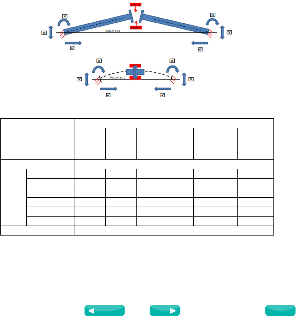
Figure 5: Bending moment schematic for generated hub misalignment.
Table 2: Boundary conditions and temperatures for in-service load case.
Load Case: In-service Hub Alignment Status: Aligned
Analysis Step No.
No.1 –
Initial
Contact
No.2 –
Clamp-up
& Pull-in
No.3 –
Pressurization
No.4 – Hub
& DuoSeal
Temperature
Variation
No.5 –
Bending
Moment
Temperature Specification (°C)
System
Component
DuoSeal -2 -2 -2 +60 +60
Clamp(s) -2 -2 -2 -2 -2
Hub(s) -2 -2 -2 +60 +60
Link-pin -2 -2 -2 -2 -2
Leadscrew(s) -2 -2 -2 -2 -2
Trunnion(s) -2 -2 -2 -2 -2
Loading Value (units)
Source: SIMULIA Community Conference, 2014
Next
Previous
Contents

19
www.3ds.com/simulia
Oil and Gas
System Loading
Bending
Moment/Axial
Thrust due to
Pull-in
-
0 lb·ft /
38,532
Psi
0 lb·ft / 38,532 Psi 0 lb·ft / 38,532
Psi
0 lb·ft /
38,532 Psi
Leadscrew
Pretension -787,730
lbf 787,730 lbf 787,730 lbf 787,730 lbf
Pressurization - - 3,379 Psi 3,379 Psi 3,379 Psi
Axial Pipe
Thrust (applied
as pressure)
- - 20,013 Psi 20,013 Psi 20,013 Psi
Global bending
Moment - - - - 4.13x10⁶
lb·ft
The modeling of hub misalignment (see Figure 5) is considered as an additional capacity check by the customer. Hub misalignment
is taken out of the system through the action of the clamping segments wrapping themselves around the male and female hub
shoulders. As more contact is made at the primary hub shoulders, hub faces become increasingly parallel, to the point where the
clamps are fully positioned and hub misalignment in the system is zero (with hub faces touching).
During this process, the respective male and female hub pipe ends are fixed to the original misalignment angle, but allowed to move
freely along the global central axis of the model (see Figure 5). As the misalignment is taken out of the hub end, pipe stresses are
generated due to induced bending moment. The length of pipes for the 0.5° and 1° alignment simulations are calculated so that
hub faces become parallel when maximum pipe bending moment is generated.
3.4 Model Stability Issues and Limitations
Considering the hub misalignment simulations documented in Section 3.3, initial problems were encountered with the contact force
generated between the secondary shoulders of the clamp segment(s) and hub(s). Point load contact generated early in the clamp-up
phase from the leading edges of the upper clamp segment, caused local mesh distortion at the point of contact. Initial modeling for
the parallel hub load cases used node-to-surface contact to establish contact stabilization. It was found that as contact force became
higher (especially during misalignment load cases), it was better to revert to the surface-to-surface contact algorithm, with a larger
time step size used to compensate for the more complex surface contact algorithm.
Local mesh distortion was found to affect the initial movement of the upper clamp(s) around the hub(s), creating local deformations/
discontinuities; in the worst instances, the formation of mesh ‘spikes’ were seen. This dramatically increased solution time, with
some trial runs causing a complete lack of solution convergence. Increases in the time step length were employed to reduce these
meshing problems.
An initial time step length of 1 was used to monitor solution convergence. Solution convergence was found to be slow, partly
down to the meshing ‘spikes’ mentioned previously, making it harder for primary contact surfaces to move relative to one another.
Increasing the time step length from 1 to 10, improved this, and with another increase from 10 to 100, solution convergence
became easier, with a reduction in the amount of visible mesh deformation seen on the FEA model. A time step length of 100 was
maintained for each of the subsequent load steps, reducing model instabilities, where overheads associated with dynamic implicit,
utilizing quasi-static damping effects, are negligible due to the stability achieved through the first load step of the analysis.
Further increases in local radial mesh density of the hub(s) allowed these problems to be reduced to much more manageable levels.
A relatively easy fix for the local mesh deformation would have been to increase the mesh density on the affected areas significantly
over that originally specified in initial models. The mesh structure in the pipe sections adjoining to the male and female hubs is
generally of little interest compared to the DuoSeal and clamps. Consequently, the mesh is coarsened in these areas to improve
overall solution speed.
Initial troubleshooting highlighted element distortion in the end of the pipe sections, when specified with the continuum coupling
feature for the applied global bending moment. In order to eliminate these convergence problems, full element integration was
selected in the mesh of the pipe sections, creating more gauss points, improving the resolution of the element stiffness matrix.
The quest for a sufficiently accurate and detailed FEA model, whilst maintaining sensible speed to solution times due to customer
Source: SIMULIA Community Conference, 2014
Next
Previous
Contents
20
www.3ds.com/simulia
Oil and Gas
timescales, meant that overall high mesh densities were not a viable option. Intelligent use of increased element density in
important areas, together with reductions in element numbers in other less critical parts of the FEA model, ensured that global
element numbers and DOF did not alter significantly.
4. FEA Validation
In order to justify the simulation techniques and methodology used for analysis of the FEA results generated from the two worst
load case requirements; 0.5° and 1° hub misalignment, comparison has been made of the bending stresses induced in the pipes
joined to the male and female hubs. A 4.2 % and 2.1 % discrepancy is recorded between hand calculations (for pipe bending
under flexure and applied moment) and Abaqus/CAE for the 0.5° and 1° misalignment load case respectively. Similar comparisons
have been made between the in-service load case and theory, with discrepancies between theory and Abaqus/CAE being almost
negligible.
5. Simulation Results
5.1 Von Mises Stress Results of In-service Analysis
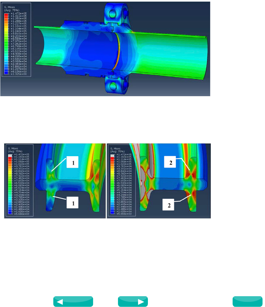
Figure 6 shows the overall FEA stress profile of the No.36 Optima, generated at the end of the general operation (in-service) load
case documented in Table 2;
Figure 6: Global V.M. Stress plot (Psi) for the No.36 Optima.
Figure 6 shows that most stresses in the Optima (DuoSeal excluded) are relatively low, with high stress regions present around the
primary contact shoulders between the male and female hubs, and the corresponding contact regions with respective clamps. The
higher stress found along the lengths of the pipe work is the result of applied bending moment together with internal pressure.
Figure 7: Left to right; V.M. Stress plot (Psi) of the upper DuoSeal region in the No. 36 Optima DuoSeal showing local regions of plastic deformation
(grey), V.M. Stress plot (Psi) of the lower DuoSeal region in the No.36 Optima DuoSeal showing local regions of plastic deformation (grey).
Figure 7 illustrates the V.M stresses in the DuoSeal, generated at the end of the application of global bending moment on the FEA
model. The inner portions of the DuoSeal are highly stressed, but significantly lower stresses (compared to the respective inner
regions) are seen on the outer heel sections of the DuoSeal (see inset Figure 7; labels (1) and (2)).
Source: SIMULIA Community Conference, 2014
Next
Previous
Contents
21
www.3ds.com/simulia
Oil and Gas
As is expected from the application of bending moment, the left hand image of Figure 7 shows a variation of stress that reduces
both outward through the radius, and anticlockwise through the bending angle. This generates increased compressive stresses in
the lower portion of the DuoSeal (see right hand side image of Figure 7), both on the upper and lower heel sections of this portion
of the DuoSeal. In this particular scenario, the inner heel regions deform plastically. This enables the DuoSeal to generate a larger
sealing area when excessively stressed, promoting better sealing performance when subjected to the in-service operational loadings.
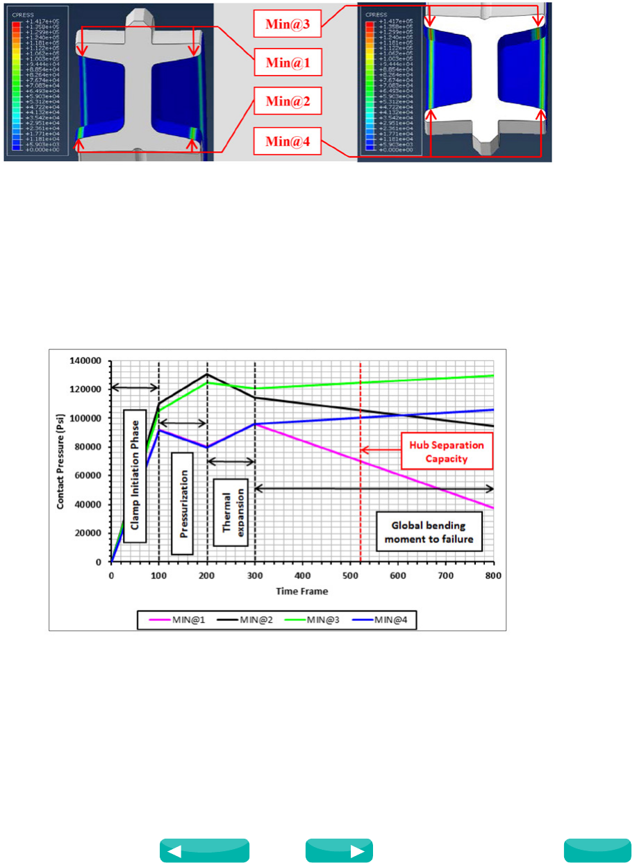
5.2 DuoSeal Contact Pressure Results of In-service Analysis
Figure 8: Left to right; Illustration of seat contact pressure (Psi) on the top portion of the DuoSeal at the end of analysis step No. 5
and on the bottom portion of the DuoSeal at the end of analysis step No.5 (see Table 2).
In Figure 8, Min@1, Min@2, Min@3 and Min@4 are representative of the maximum contact stresses recorded at the four individual
sealing points on the upper and lower sections of the DuoSeal, as in the FEA model shown in Figure 2. Of these contact stresses,
the minimum of the maximum values of the four data sets are plotted in the contact pressure graph (see Figure 9).
Very good sealing performance is illustrated in Figure 8 whereby the inner portions of both the upper and lower regions of the
DuoSeal have a much wider contact area than the outer portions, with the right hand side image of Figure 8 showing distinctive high
banding contact stresses, consistent with the V.M. stress patterns shown in Figure 7. Figure 9 illustrates the variation in DuoSeal
contact stress through the complete range of operation
Figure 9: Graph of DuoSeal contact pressure during the stages of the simulation for the general operational in-service load case of Table 2.
Figure 9 shows the contact pressure profile on the DuoSeal through to the end of the global bending moment capacity test, where
the bending moment capacity was run to 7.08x10⁶ lb·ft. Once the clamp-up phase is complete, subsequent system loadings
generate contact stresses on the important inner heel areas of the DuoSeal that never drop below approximately 80,000 Psi,
higher than customer requirements for contact stress. The global bending moment to cause loss of hub face contact pressure, and
subsequent hub face separation is approximately 4.96x10⁶ lb·ft.
Source: SIMULIA Community Conference, 2014
Next
Previous
Contents
22
www.3ds.com/simulia
Oil and Gas
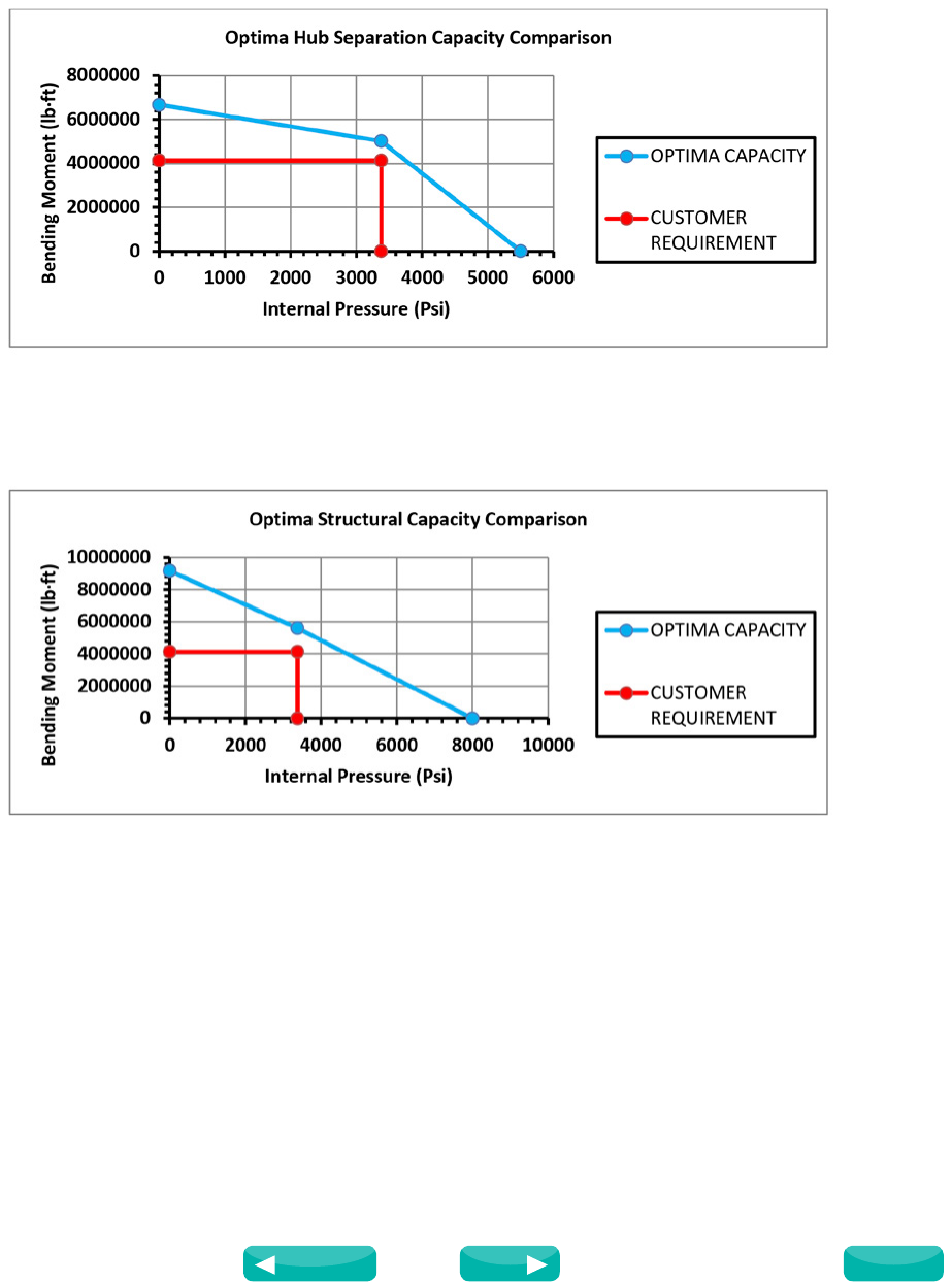
5.3 Structural Capacity Analysis
In order to generate an official structural rating for the No.36 Optima under the specific loading conditions of Table 2, it must exceed
both the pressure and bending moment design criteria imposed by the customer. The bending moment and pressure capacity tests
(each undertaken in isolation) are subjected to 1.67x10⁷ lb·ft and 10,000 Psi respectively. In these tests, the clamp-up phase of
the Optima is simulated, then either the bending moment or pressure capacity is applied to the Optima until hub separation or
yielding occurs.
Figure 10: Graph of hub separation capacity for the No.36 Optima subsea connector.
Figure 10 shows the No.36 Optima can withstand 61.4 % more bending moment and 62.7 % more internal pressure than required
by the customer. Adequate sealing contact pressure is still maintained even after the separation of hub faces (see Figure 9).
Figure 11: Graph of structural capacity for the No.36 Optima subsea connector.
Figure 11 shows the structural capacity of the No.36 Optima, based on local plastic strain within the components. The graph shows
that the Optima can withstand 121.9 % more bending moment and 195.7 % more internal pressure than required before the onset
of plastic strain.
During the analysis required to determine the data for Figure 11, it was noted that plastic strain is always present within the DuoSeal
and is therefore eliminated from the predictions of Figure 11. It is also noted that the trailing and leading edges of the clamp
segments cause very small localized areas of plastic strain, but these strains are present only at the surface of the components.
Therefore, plastic strain generated as a result of the trailing and leading edges of the clamp segments is also eliminated from these
predictions.
Source: SIMULIA Community Conference, 2014
Next
Previous
Contents
23
www.3ds.com/simulia
Oil and Gas
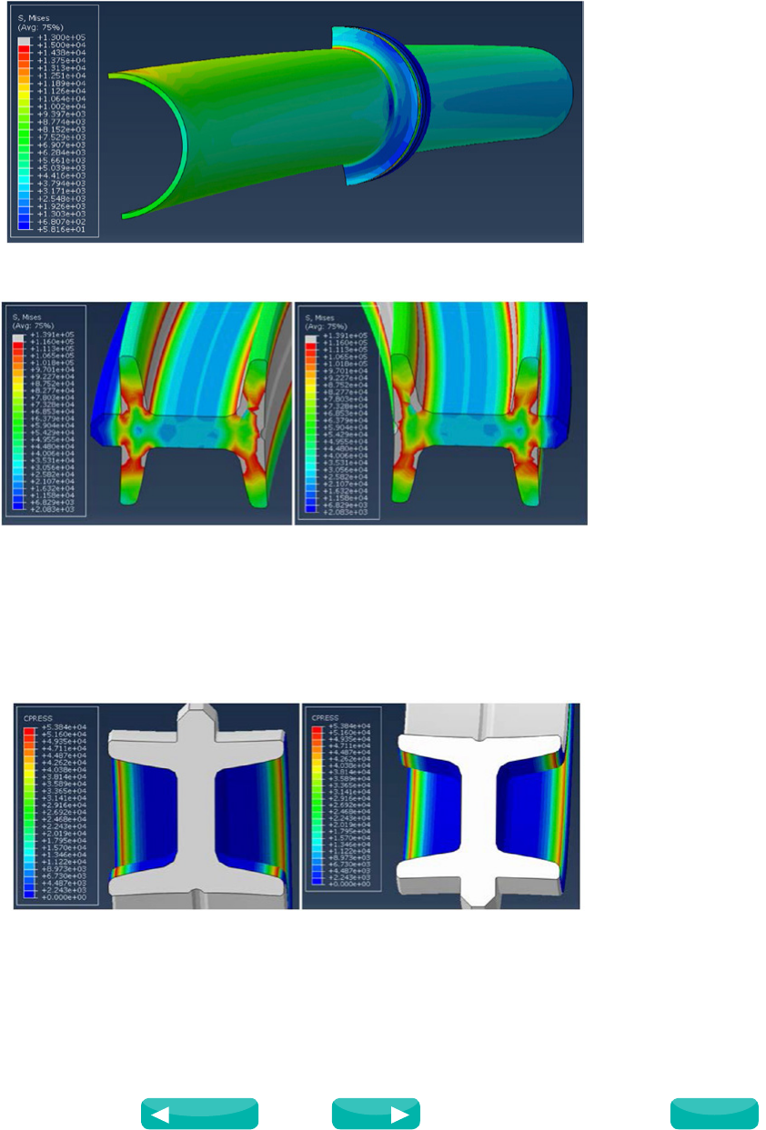
5.4 Hub Misalignment Analysis
Clamp qualification through reduction in hub misalignment is in fulfillment of a scenario where the pipeline and No.36 Optima are
not able to be brought parallel for initial clamp-up and mechanical energisation of the DuoSeal. For the hub misalignment load case,
there is no internal pressure or external global bending moment requirements for the simulation. Figure 12 illustrates the stress
profile through the 1° hub misalignment load case, and shows an expected difference in stress levels in the two pipes as a result of
the difference in their respective lengths and pipe wall thicknesses;
Figure 12: V.M. Stress plot (Psi) in the pipework and male and female hub components after reduction from 1° to 0° of hub misalignment.
Figure 13: Left to right; V.M. Stress plot (Psi) of the upper DuoSeal region in the No.36 Optima DuoSeal showing local regions of plastic deformation
(grey), V.M. Stress plot (Psi) of the lower DuoSeal region in the No.36 Optima DuoSeal showing local regions of plastic deformation (grey).
Figure 13 shows that the V.M. stresses generated from clamp-up show large areas of plastic deformation in both the upper and
lower portions of the DuoSeal. This acts as a sanity check for the hub misalignment load cases, indicating that the male and female
hubs have been brought together properly by the action of the clamp segments, showing that the clamp segments are generating
equal load through the hubs, reacting onto the DuoSeal.
Figure 14: Left to right; Illustration of seat contact pressure (Psi) on the top portion of the DuoSeal at the end of the FEA simulation, Illustration of seat
contact pressure (Psi) on the bottom portion of the DuoSeal at the end of the simulation.
Source: SIMULIA Community Conference, 2014
Next
Previous
Contents
24
www.3ds.com/simulia
Oil and Gas
Figure 15: Left to right; Illustration of seat contact pressure (Psi) on the top portion of the DuoSeal during in-service clamp-up, Illustration of seat
contact pressure (Psi) on the bottom portion of the DuoSeal during in-service clamp-up.
Discrepancies between Figure 14 and Figure 15 can be attributed to the mesh density used within the DuoSeal. Both load cases
illustrate that the stress banding is consistent around the whole diameter of both the upper and lower, inner and outer sealing
regions of the DuoSeal. Therefore, the comparative analysis shows that the modeling assumptions that have been used are correct,
even if the magnitude of values generated through the FEA simulations are dissimilar.
6. Conclusion and Future Work
This paper has documented the detailed set-up required to produce the simulation load cases required for the No.36 Optima. FEA
simulation results indicate that the collective design of all components meets the bending moment and internal pressure capacity
criteria set out by the customer. The simulation results have demonstrated the ability of the No.36 Optima to successfully pull-in
against the static weight of the pig launcher, together with a range of hub misalignments up to 1°, representing discrepancies in
pipeline global positioning. It has been shown that the integrity of the DuoSeal is maintained throughout the required load cases,
producing contact stresses that exceed requirements. Fatigue analysis for component life cycles has not been required due to the
in-service steady state loadings on the No.36 Optima.
The analysis has allowed FO> to make predictions where important areas of large elastic/plastic strain may occur during the
factory qualification process. Validation of the FEA results will help to further improve the analysis process for future applications.
Strain gauging equipment can be positioned during the factory qualification process to accurately monitor plastic deformation.
Rigorous checking of factory performance figures against the analysis predictions in this report will ensure that areas/results/data
that agree/disagree with simulation reference data are identified, with subsequent steps taken to rectify the correlations obtained.
7. References
8. Acknowledgements
I would like to thank all individuals and companies involved in the creation of this paper. I would especially like to thank my
co-author Mr. Laurence Marks for his support and guidance with the simulation aspects of this project. I would also like to thank Mr.
John Stobbart (Technical Director) and Mr. Nick Long (Subsea Technical Authority) for their expertise in the design of the DuoSeal
and No.36 Optima.
1. Bates A., Mukherjee S., Hwang S., Lee S.C., Kwon O., Choi G.H., Park S. “Simulation and Experimental Analysis of the Clamping
Pressure Distribution in a PEM Fuel Cell Stack”, International Journal of Hydrogen Energy 38, pp. 6481-6493, 2013.
2. Dassault Systems Abaqus 6.12, Abaqus/CAE User’s Guide, Providence: [s.n.], 2013.
3. Hilber H.M., Hughes T.J.R., “Collocation, Dissipation and ‘Overshoot’ for Time Integration Schemes in Structural Dynamics”,
Earthquake Eng. Struct. Dyn. 6, pp. 99-117, 1978.
4. Kyun C. Woo K., Shim J., “Analysis of Contact Force and Thermal Behaviour of Lip Seals”, Tribology International 30, pp. 113-119,
1997.
5. Lee C.Y., Lin C.S., Jian R.Q., Wen C.Y., ”Simulation and Experimentation on the Contact Width and Pressure Distribution of Lip
Seals”, Tribology International 39, pp. 915-920, 2006.
6. Rebelo N., Nagtegaal J.C., Taylor L.M., “Comparison of Implicit and Explicit Finite Element Methods in the Simulation of Metal
Forming Processes: Numerical Methods in Industrial Forming Processes”, Chenot, Wood, Zienkiewicz, 1992.
7. Sanal Z., “Nonlinear Analysis of Pressure Vessels: Some Examples” International Journal of Pressure Vessels and Piping 77, pp.
705-709, 2000.
8. Sun J.S., Lee K.H., Lee H.P., “Comparison of Implicit and explicit Finite Element Methods for Dynamic Problems”, Journal of
Materials Processing Technology. 105, pp. 110-118, 2000.
Source: SIMULIA Community Conference, 2014
Next
Previous
Contents
25
www.3ds.com/simulia
Oil and Gas
Finite Element Analysis of Casing and
Casing Connections for Shale Gas Wells
Jueren Xie (C-FER Technologies, Canada)
Abstract: The application of horizontal drilling and hydraulic fracturing has enabled operators to rapidly develop shale gas production
from deep shale formations over the past decade. It has, however, presented significant challenges to casing and casing connection
designs due to the complicated and extreme load conditions within these wells. Advanced Finite Element Analysis (FEA) is therefore
required to understand casing deformation mechanisms and to assist well designs. This paper presents FEA models developed
using Abaqus for analyzing casing and casing connections under shale gas well load scenarios, such as horizontal well installation,
perforating and hydraulic fracturing pressures, and formation shear movement. Analysis examples are provided.
Keywords: Bending, Buckling, Casing, Connections, Constitutive Model, Damage, Deformation, Design Optimization, Drilling,
Dynamics, Explosive, Failure, Fatigue, Formation Shear, Fracture, Geomechanics, Hydraulic Fracture, Optimization, Perforation,
Plasticity, Seal, Soils, Soil-Structure Interaction, Structural Integrity, Wellbore, and Well Installation.
1. Introduction
Shale gas is an unconventional resource which requires an enhanced extraction method to facilitate its production from low
permeable rocks. Over the past decade, the application of horizontal drilling and hydraulic fracturing has enabled operators to
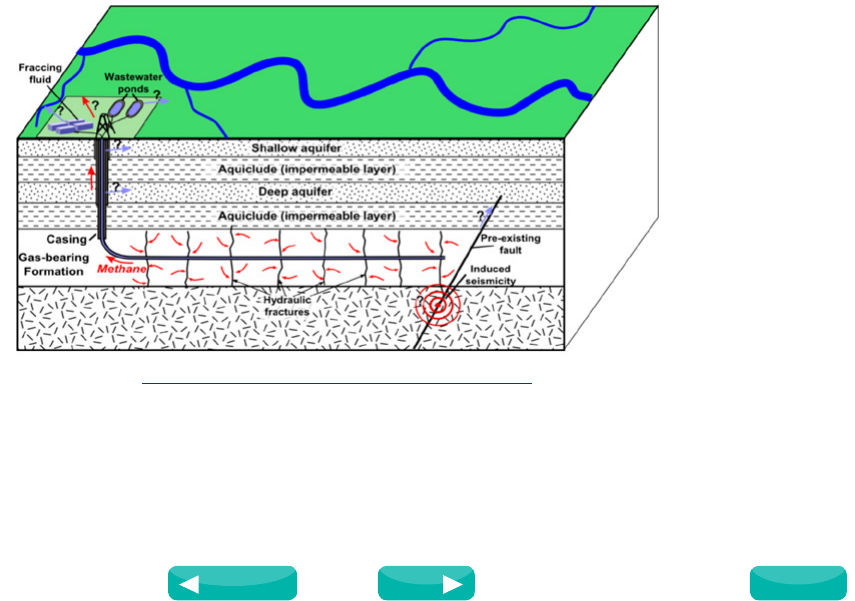
rapidly develop shale gas production from deep shale formations. Figure1 shows a schematic representation of a horizontal shale
gas well undergoing hydraulic fracturing.
The use of horizontal drilling and hydraulic fracturing has, however, presented significant challenges to well completion designs.
One of the key failure modes for a well is leakage. When leakage occurs, the well function of isolating gases from the aquifer layers
can be compromised. Nikiforuk (2013) noted that 5% to 7% of all new oil and gas wells leak, and as wells age the percentage of
wells which leak can increase to a startling 30% to 50%. Wittmeyer (2013) suggested that the high casing pressure from fracturing
operations and the lack of a pressure relief system are the primary failure modes for shale gas wells. Ghassemi (2011) pointed
out that shale stimulation causes a combination of tensile and shear failure. This can occur as shear slippage is induced by the
intense stresses near the tip of the fractures, as well as by the increased pore pressure in response to leak-off. Casing failure due to
formation shear movement is also considered one of the key failure modes in shale gas wells.
Due to the complicated and extreme load conditions in installation, stimulation and production, casing and casing connection
designs for shale gas wells require the use of advanced FEA models. This paper presents FEA models developed using Abaqus for
analyzing casing and casing connections under shale gas well load scenarios, such as horizontal well installation, perforating and
hydraulic fracturing pressures, and formation shear movement. Analysis examples are provided.
http://en.wikipedia.org/wiki/File:HydroFrac.pen
Figure 1. Schematic depiction of hydraulic fracturing for shale gas.
Source: SIMULIA Community Conference, 2014
Next
Previous
Contents
26
www.3ds.com/simulia
Oil and Gas
2. Well Completion Design Considerations
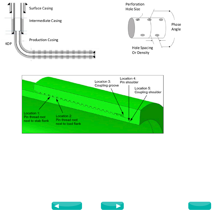
Figure 2 shows a schematic representation of a horizontal well construction. Wellbore construction typically includes conductor
casing, surface casing, intermediate casing and production casing. Casing designs are defined by size (i.e. OD), weight, grade (i.e.
material strength), and connections. Premium connections are typically used to join casing strings (e.g.13m long) in shale gas
wells. The horizontal portion of the well is often perforated. The perforation is defined by the perforation hole size, hole density,
and phase angle.
Casing connection is a critical element in well completion design. Payne and Schwind (1999) noted that, based on industry
estimates, connection failures account for 85% to 95% of all oilfield tubular failures. Connection failures can include structural
failure and/or leakage. In the FEA models, the structural failures are defined as parting and/or fatigues at critical locations such as
the thread roots, coupling groove and shoulder (see Figure3). The connection sealing capacity is described by the contact stress
profile in the seal region. Various design criteria have been established for assessing connection structural and sealing performance
(Xie et al. 2011, and Xie 2013).
Casing and casing connection designs for shale gas wells should consider the following load scenarios:
• Phase 1 – Installation: impact of well depth and build angle on casing structural integrity
• Phase 2 – Stimulation: impact of perforating and fracturing pressure on casing structural integrity
• Phase3–Operation: impact of formation shear movement on casing connection structural and sealing integrities
The following sections present FEA models for analyzing casing and casing connections under the above load scenarios. Analysis
examples presented in this paper consider a 7inch, 23lb/ftL80 casing and connection, with L80 material which is modeled using
elastic-plastic constitutive relationships, a Young’s modulus of 30,000ksi, and yield strength of 80ksi.
Figure 2. Schematic depiction of well completion design (left) and perforation (right).
Figure 3. Critical locations for fatigue damage and structural failure within a premium casing connection.
3. Analysis of Casing Connection under Installation Loads
The first example is for casing installation in horizontal wells. Casing connections may be subjected to structural fatigue damage
during installation and/or cementing operations. Horizontal wellbore designs often have a target curvature of 6°/100 ft to 20°/100
ft. The rotation of the casing strings during cementing operations within directional or horizontal wells will inherently give rise to
Source: SIMULIA Community Conference, 2014
Next
Previous
Contents
27
www.3ds.com/simulia
Oil and Gas
fatigue loading conditions within the connections. This is due to the cyclic bending that occurs within the portion of the string
positioned within the build section of such wells. As a result, the connections will experience different levels of strain variation
(e.g.between axial tension and compression) which produces a severe elastic or plastic cyclic deformation.
Xie (2007) presented methodologies for analyzing casing connection under curvature loading. The connection can be modeled
using axisymmetric solid elements with non-linear, asymmetric deformation. As noted in the Abaqus documentation (2013), these
elements are intended for the nonlinear analysis of structures which are initially axisymmetric, but which undergo non-linear,
nonaxisymmetric deformation. Contact between the pin and coupling elements was modeled using slide-lines.
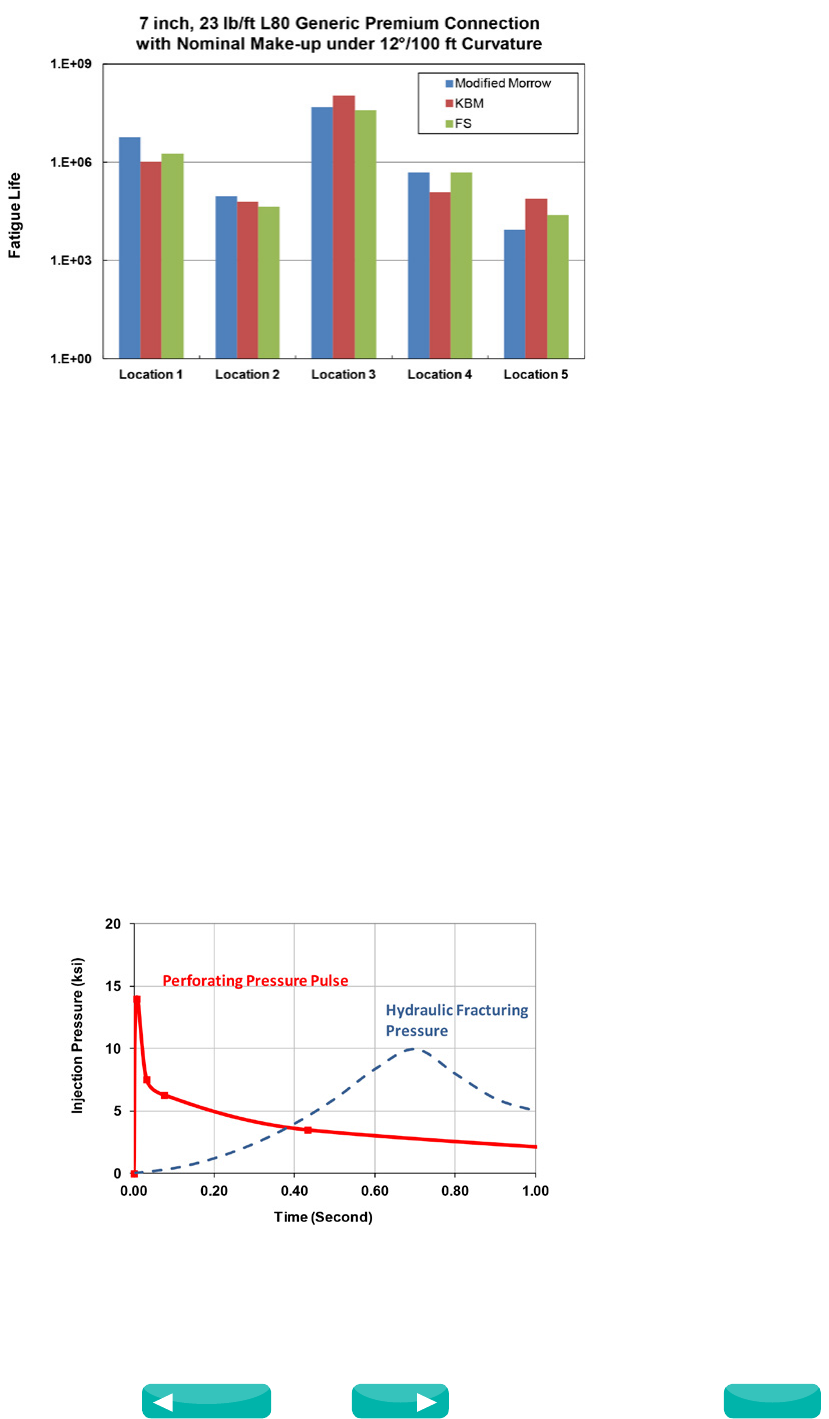
As an example case, a generic 7 inch, 23 lb/ft L80 premium casing connection was analyzed under 12°/100 ft curvature loading
following a nominal torque make-up. The generic connection model captured the basic features common to the premium
connections currently used in shale gas well applications (e.g. buttress threads, torque shoulder, metal-metal radial seal) to ensure
that the analysis produces results that are illustrative.
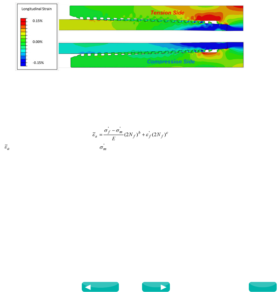
Figure4 presents the axial strain distribution within the connection. The high compressive axial strains are represented in blue,
while the high tensile axial strains are in red. The figure shows the significant variations that exist in the axial strain values at the
same locations on the tension and compression sides of the connection. It is these variations in axial strain around the circumference
that create the potential for fatigue damage during casing rotation.
Figure 4. Longitudinal strain for a generic premium connection subjected to 12º/100 ft curvature loading.
Since the strain in the critical locations (e.g. as shown in Figure3) may exceed the elastic limit, strain-based criteria should be used
to assess the fatigue life of connections. Xie et al.(2011) proposed the use of several criteria, such as a modified Morrow approach
(Dowling 1998), KBM approach (Kandil et al. 1982), and FS approach (Fatemi et al. 1988). The key features of these approaches
are described in the following.
The modified Marrow approach takes the mean stress effect into account, and can be expressed in the following equation (Dowling 1998):
where is the equivalent strain amplitude and is the effective mean stress. According to this modified Morrow criteria, the
effect of mean stress declines with increasing strain amplitude.
The KBM approach considers the effect of critical plane, and FS approach takes the normal stress on the critical plane into account.
Equations for these two criteria can be found in Xie et al.(2011).
Based on analysis results as shown in Figure4, the fatigue life predictions at the five critical locations (see Figure3) derived using
these respective criterion are presented in Figure5 for the nominal make-up condition.
Source: SIMULIA Community Conference, 2014
Next
Previous
Contents
28
www.3ds.com/simulia
Oil and Gas
Figure 5. Fatigue life prediction for a generic premium connection with nominal make-up subjected to 12º/100 ft cyclic curvature loading.
As shown in Figure5, Location2 (i.e. thread root next to the load flank of the fourth pin thread from the coupling face) had a higher
strain range and therefore a much lower fatigue life (i.e. as low as 4.4×10⁴ based on the FS criteria). Location5 (coupling shoulder
region) also shows low fatigue life but the shoulder is not considered to be the primary failure location.
Typical well installation may have casing rotation at 20RPM for 1.5hours during cementing operations, giving a total of 1800
revolutions. The above analysis suggests that the generic premium connection should have fatigue life which is greater than the
anticipated casing rotations during the installation for the horizontal well with the build section at 12°/100 ft.
4. Analysis of Casing under Stimulation Loads
The horizontal portion of the well is often completed with perforated casing. The perforations on the casing can be drilled prior to
installation, or generated by perforating after installation.
Hydraulic fracturing may involve significantly high pressure in a short time period. According to Love (2005), injection pressure
rates for hydraulic fracturing can reach up to 100 MPa (14.5ksi) and 265 liters per second. During perforating, the explosion pulse
pressure can be reached in a much short time period. Figure6 shows the pressure pulses for perforating and hydraulic fracturing
which are representative of shale gas wells.
The peak pressure during perforating or hydraulic fracturing is often much higher than the static yield pressure capacity of casing
(e.g. 7.2ksi for 7inch, 23lb/ft L80 casing). As such, dynamic FEA of the casing string should be used for perforating and hydraulic
pressure loading. This allows for consideration of the effect of strain rate on material yield and tensile strengths.
Figure 6. Assumed pressure pulses for perforating and hydraulic fracturing.
Source: SIMULIA Community Conference, 2014
Next
Previous
Contents
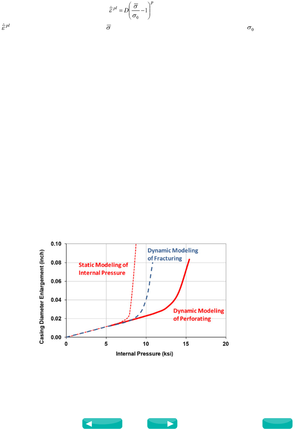
29
www.3ds.com/simulia
Oil and Gas
The effect of strain rate on the elastic-plastic response of the material can be considered using the following overstress power law
(Ting 1961):
in which is the equivalent plastic strain rate; is the yield stress at a non-zero plastic strain rate; is the static
yield stress; and D and p are material parameters defining the overstress power law, which were set as D = 20 and p = 6 based on
the experimental results of mild steel by Manjoine (1944).
Abaqus provides the capability to model the above equation for strain-rate effect; described as the hardening dependencies with an
overstress power law (Abaqus 2013).
The analysis example considers a 7inch, 23lb/ftL80 perforated casing. The perforation is defined by a shot density of 8shots/ft,
phase angle of 135°/45°, and perforation diameter of 20.3mm. The perforated casing string is modeled using three-dimensional
solid elements for an interval with a few rows of perforations. The perforation pattern is modeled in detail so that the localized
stress and strain concentrations at individual perforations can be investigated. Three loading models are analyzed: a static pressure,
a dynamic pressure with the loading rate similar to hydraulic fracturing, and a dynamic pressure with the loading rate similar to
perforating. The analyses are performed with pressure loading increased monotonically until casing deformation is significant.
Figure7 presents the analysis results of casing diameter enlargement due to applied pressures for the three analysis models. The
response of diameter enlargement is basically similar for these three models prior to the static yield pressure (i.e. 7.2ksi); however,
beyond the static yield pressure, the static modeling shows rapid expansion of the casing diameter leading, eventually, to casing
rupture. On the other hand, dynamic modeling with consideration of strain rate impact predicts much higher pressure loading
capacities for hydraulic fracturing and perforating. The pressures corresponding to 0.1inch diameter enlargement are 8.7, 11.3 and
16.0 ksi for the static, hydraulic fracturing and perforating pressures.
The diameter enlargement results in high tensile strain at the perforations. When considering the initiation of casing material
fracture at the perforations, the tensile strain is significantly higher than the elastic limit, and therefore can be represented by the
plastic strain. Figure 8 presents the maximum plastic strain values in the perforated casing for the three models analyzed. The
distribution of residual plastic strain resulting from a static pressure of 8.0ksi is also shown in Figure 8. The plastic strain is highly
localized at the both sides of each perforation, indicating that the casing would likely split axially if the strain at the holes exceeds
the tensile limit of the casing material. Assuming 10% as the strain limit for the casing material, the corresponding pressure values
are 8.3, 10.6, and 14.8ksi for the static, hydraulic fracturing and perforating pressures, respectively.
This example demonstrates that the dynamic analysis model, with consideration of strain rate on material yield and tensile
strengths, should be used for the prediction of allowable pressures for hydraulic fracturing and perforating.
Figure 7. Casing diameter enlargement vs. internal pressure.
Source: SIMULIA Community Conference, 2014
Next
Previous
Contents
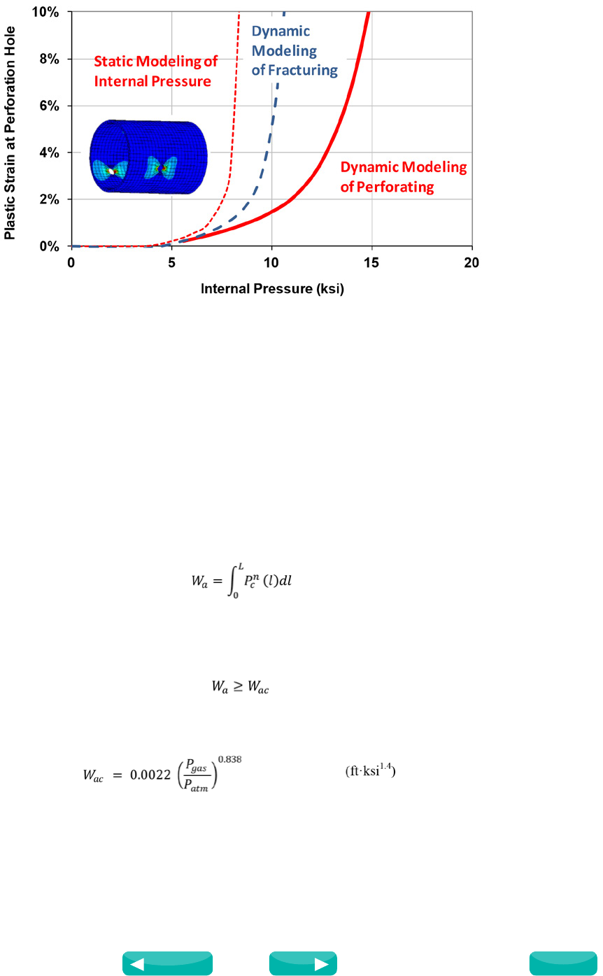
30
www.3ds.com/simulia
Oil and Gas
Figure 8. Plastic strain at perforation vs. internal pressure.
5. Analysis of Casing Connections under Shear Loads
Formation fractures resulting from the hydraulic fracturing process may inevitably cause formation movement. The formation
shear movements refer to the opposite displacements about a plane which is angled with respect to the well axis. The formation
shear movement is considered to be one of most severe loading scenarios in terms of structural integrity and sealability of casing
connections (Xie et al. 2011).
One of the critical scenarios which must be examined is the leakage resistance of casing connections when they are positioned at
the shear center plane, as shown on the left of Figure9. On the right side of Figure9 is a schematic representation of contact stress
in the seal region which can be used to assess the sealability of a premium connection.
Published research papers have described empirical relationships for the sealability of premium tubular connections as a function
of seal contact stress and seal length. In one such study, Murtagian et al. (2004) performed physical tests and numerical modeling
to investigate the relationship between the sealability of stationary metal-to-metal seals and the seal contact profile, both with and
without thread compounds. They proposed a weighted area of seal contact stress, Wa, as a means to evaluate the sealability of a
connection, which was defined by:
where Pc(l) is the seal contact pressure, L is the seal length, and n is a correlation exponent. Based on test results, Murtagian et
al. (2004) proposed values of 1.2 and 1.4 for the exponent n, for connections with and without sealing compounds, respectively.
A premium connection might be considered to provide acceptable seepage resistance when the weighted area of seal contact stress
(Wa) was greater than some critical value Wac:
Based on review of the available data and the incorporation of the ISO 13679 leakage rate limit, Xie (2013) proposed the following
equation for calculating the critical value of Wac for tubular connections for stimulated applications (e.g. HPHT):
Assuming that the required containment pressure for the hydraulic fracturing application is 14.5ksi, the critical value of Wac would
be 0.72ft·ksi1.4.
Source: SIMULIA Community Conference, 2014
Next
Previous
Contents
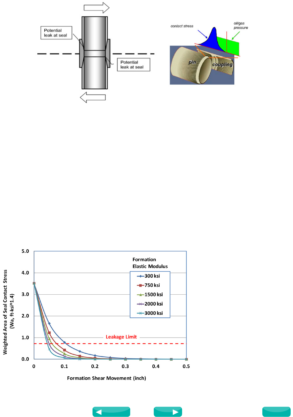
31
www.3ds.com/simulia
Oil and Gas
Figure 9. Schematic representation of connection model under shear (left) and contact stress distribution on the seal (right).
An example case with a 7 inch, 23 lb/ft L80 generic connection is presented here. The FEA of the impact of formation shear
movement on connection sealing capacity is carried out in two steps. First, to determine the shear force to be applied to the
connection model, analysis is performed with a casing string modeled as beam elements subjected to formation shear loading,
where casing formation interaction is represented by a series of spring elements distributed along the axis of the model (Xie 2008).
Note that the shear force determined here varies with the formation elastic modulus. In the second step, the shear force determined
from the beam model is applied to a casing connection model constructed using axisymmetric-asymmetric solid elements. The
connection model considers a relatively short interval with both ends clamped to allow the resultant bending moments to be
generated. Shear forces are applied at both ends.
Figure 10 presents the analysis results of the weighted area of seal contact stress versus formation shear movement for the
formation elastic modulus values of 300, 750, 1500, 2000 and 3000ksi. As shown in the figure, the weighted area starts with
3.52ft·ksi1.4 for all cases prior to the application of shear movement. The weighted area decreases with formation shear movement
and formation elastic modulus. As the shear movement increases further, the weighted area of contact stress decreases below
the sealing limit established for containing 14 ksi hydraulic fracturing pressure. The critical values of formation movements
corresponding to the leakage limit are 0.108, 0.082, 0.067, 0.050 and 0.046inch for the formation elastic modulus of 300, 750,
1500, 2000 and 3000ksi, respectively.
This example demonstrates that the sealing capacity of a premium connection can decrease significantly under the formation shear
movement. It should be considered a critical load case in the casing design for shale gas wells.
Figure 10. Analysis results of the weighted
area of seal contact stress vs. formation
shear movement.
Source: SIMULIA Community Conference, 2014
Next
Previous
Contents

32
www.3ds.com/simulia
Oil and Gas
6. Conclusions
This paper presents several considerations for FEA modeling of casing and casing connections for the shale gas well application.
Based on the analysis of example cases, the following conclusions are made:
• A methodology is presented for assessing well fatigue life during installation (as the casing string is rotated over the build section)
using FEA of casing connections under bending. The critical locations for connection fatigue failure are found to be in the thread
roots near the coupling entry plane.
• The dynamic analysis model with consideration of strain rate on material yield and tensile strengths is presented for the
prediction of allowable pressures for hydraulic fracturing and perforating.
• FEA of connection under formation shear loading shows that the sealing capacity of a premium connection can decrease
significantly. The formation shear movement should be considered to be a critical load case in the casing design for shale gas
wells.
7. References
1. Abaqus, “User Manual,” Version 6.13, 2013.
2. Dowling, N. E., “Mechanical Behavior of Materials – Engineering Methods for Deformation, Fracture, and Fatigue,” 2nd edition,
Prentice Hall, New Jersey, 1998.
3. Fatemi, A. and Socie, D.F., “A Critical Plane Approach to Multi-axial Fatigue Damage Including Outof-Phase Bending,” Fatigue and
Fracture of Engineering Materials and Structures, 11, pp.149165, 1988.
4. Ghassemi, A., “A Geomechanical Analysis of Gas Shale Fracturing and Its Containment,” A Technology Status Report, Texas A&M
University, March 2011.
5. Kandil, F.A., Brown, M.W. and Miller, K.J., “Biaxial Low Cycle Fatigue Fracture of 316 Stainless Steel at Elevated Temperature,”
Met. Soc. London, 280, pp.203-210, 1982.
6. Love, A. H., “Fracking: The Controversy Over its Safety for Environment,” Johnson Wright Inc. December 2005.
7. Manjoine, M. J., “Influence of Rate of Strain and Temperature on Yield Stresses of Mild Steel,” Journal of Applied Mechanics, 11,
A-211. 1944.
8. Murtagian G R, Fanelli V, Villasante J. A, et al., “Sealability of Stationary Metal-to-Metal Seals,” Journal of Tribology, Vol. 126, No.
3.: 591. 2004.
9. Nikiforuk, A., “Shale Gas: How Often Do Fracked Wells Leak?” The Tyee, January 9, 2013.
10. Payne, M.L., Schwind, B.E., “A New International Standard for Casing/Tubing Connection Testing,” SPE/IADC 52846, Presented
at the SPE/IADC Drilling Conference, Amsterdam, Holland, March 9-11, 1999.
11. Wittmeyer, H., “Fracking and Well Casing Failures,” Fracwire, June 27, 2013.
12. Xie, J., “Analysis of Oil Well Casing Connections Subjected to Non-axisymmetric Loads,” Abaqus Users’ Conference, Paris, France,
May 22-24: 634–646. 2007.
13. Xie, J. and Liu, Y., “Analysis of Casing Deformation in Thermal Wells,” Abaqus Users’ Conference, RI. 2008.
14. Xie, J., Fan, C., Tao, G. and Matthews, C. M., “Impact of Casing Rotation on Premium Connection Service Life in Horizontal
Thermal Wells,” World Heavy Oil Congress, Edmonton, Alberta, Canada, 2011.
15. Xie, J., “Numerical Evaluation of Tubular Connections for HPHT Applications,” Baosteel Conference, Shanghai, China, 2013.
8. Acknowledgement
The work presented in this paper was supported by CFER Technologies, Canada. The author would like to sincerely acknowledge Dr.
Nader Yoosef-Ghodsi, Senior Research Engineer, for his technical advice and assistance in reviewing this paper.
Source: SIMULIA Community Conference, 2014
Next
Previous
Contents

33
www.3ds.com/simulia
Oil and Gas
Integrating Business and Technical Workflows to Achieve
Asset-Level Production Optimization
Michael Szatny and Mark Lochmann
Halliburton Landmark Graphics
Abstract: The pressure on the oil and gas industry to meet the growing demand for energy when faced with fewer technical
professionals, more complex reservoirs, and increased global competition is making it more critical than ever before for operators
to make quick, accurate, and informed field development decisions that efficiently leverage the expertise of seasoned technical
professionals. With experienced, technical professionals in short supply, the industry is looking for information technologies that
can extend the reach of technical experts and better ground high-level business decisions in the scientific evaluation of the asset.
Flexible workflow automation systems can now take technical production applications at the engineering level and put them in a
computing environment where they can be integrated with business process management (BPM) systems to create automated
asset-level workflows. In initial implementations, the results have included more efficient production operations, less personnel
time required to complete repeatable production tasks, better incorporation of uncertainties into business level decisions, and most
importantly, increased reservoir production.
Halliburton has partnered with SIMULIA to deliver advanced technologies that have traditionally been used for complex
manufacturing and design applications to the O&G industry. Halliburton has adapted the iSight® and FIPER® software into the
normal day-to-day operations routine of an O&G production engineer and allowed him/her to become much more efficient.
Halliburton commercially markets the SIMULIA iSight and FIPER technologies into the O&G industry re-branded as AssetConnect™
and part of Landmark’s DecisionSpace® for Production™ technology suite.
1. Introduction
The oil and gas industry faces manpower, equipment, and service shortages as it tries to cope with a world energy demand that
is projected to grow from 230 million barrel of oil equivalents per day (boe/d) today to 335 million boe/d in 2030. As such, it will
rely heavily on technological advances to meet future energy demands, which means ever more complex operating environments
and, consequently, the need for applying more rigorous solutions. Additionally, the most experienced engineering staff will retire in
the next 5–10 years. Therefore, significant workforce productivity gains will have to be realized through digital oilfield automation
initiatives to manage future levels of E&P activity.
Industry Issues
• Data volumes and data size
• Advanced acquisition techniques
• Advancements in HW allow large volume analysis
• Advancements in seismic data acquisition
• Industry “crew change”
• Past knowledge hemorrhaging
• New generation entering workforce
• No more easy oil
• Rising costs
• Complex workflows
• Global collaboration
• Increasing customer focus on operational efficiency
Source: SIMULIA Community Conference, 2010
Next
Previous
Contents

34
www.3ds.com/simulia
Oil and Gas
Many production workflows require engineers to coordinate data flows between disparate numbers of applications. Studies
have shown that about 70% of an engineer’s time is spent gathering, formatting, and translating data for use in these different
applications. For standard production activities (i.e., workflows), this time can be drastically reduced by creating an automated
system to execute the prescribed workflow. The automated workflow not only reduces the engineers’ valuable time performing
these repetitive tasks, but also ensures consistency in methods, reduces the likelihood of input errors, and creates a repository for
“best practices” that can be maintained long term as personnel (and their knowledge) is moved into, and out of, the production
asset.
For many years, automated workflows have been a part of the design and production cycles in other industries, including aerospace,
automotive, and industrial manufacturing. These industries have been tying together applications and data sources along with using
stochastic analysis methods and optimization to improve their overall productivity.
Within the O&G production space, some common workflows may include:
Well-Test Validation
Long-Term Work Plan
Subsurface / Surface Production Forecasting
Production History Match
Well Shut-in Testing & Analysis
Mid-Term Work Plan
Daily Production Optimization
Well-Restart Monitoring
Production Allocation
Glycol Monitoring
Pressure History Match
Data Statistics and Visualization
Production-Decline Analysis
Process Material Balance
Candidate Recognition & Production Prediction
SAGD Integrated Forecast
KPI Monitoring
Reliability Monitoring
Stochastic Production Forecasting
Subsea and Surface Pipeline Network Performance Analysis
Flow Assurance
LPG Monitoring
Pump/Motor Performance
Production Economics
Well-Test Prioritization
Compression-System Monitoring
Chargeable Fired Hours Tracking
Pipeline Monitoring
Virtual Metering
Well Production Surveillance and Optimization
Model Update
Facility Monitoring
BHP Correction
Real-Time Asset Optimization
Reserves Tracking
Loss Management
Flux Monitoring
Well Monitoring
Real-time Closed-loop Well Optimization
Production Stimulation Design Optimization
Zonal-Split Calculation
Methanol Injection Optimization
Non-Operator Reporting
Pipeline Network Deliverability
Production-Performance Analysis
Model based Production Optimization
Equipment Surveillance by Exception
Reservoir Performance Analysis
Short-Term Work Plan
Maintenance (KPIs and root cause)
Reservoir Surveillance
Source: SIMULIA Community Conference, 2010
Next
Previous
Contents
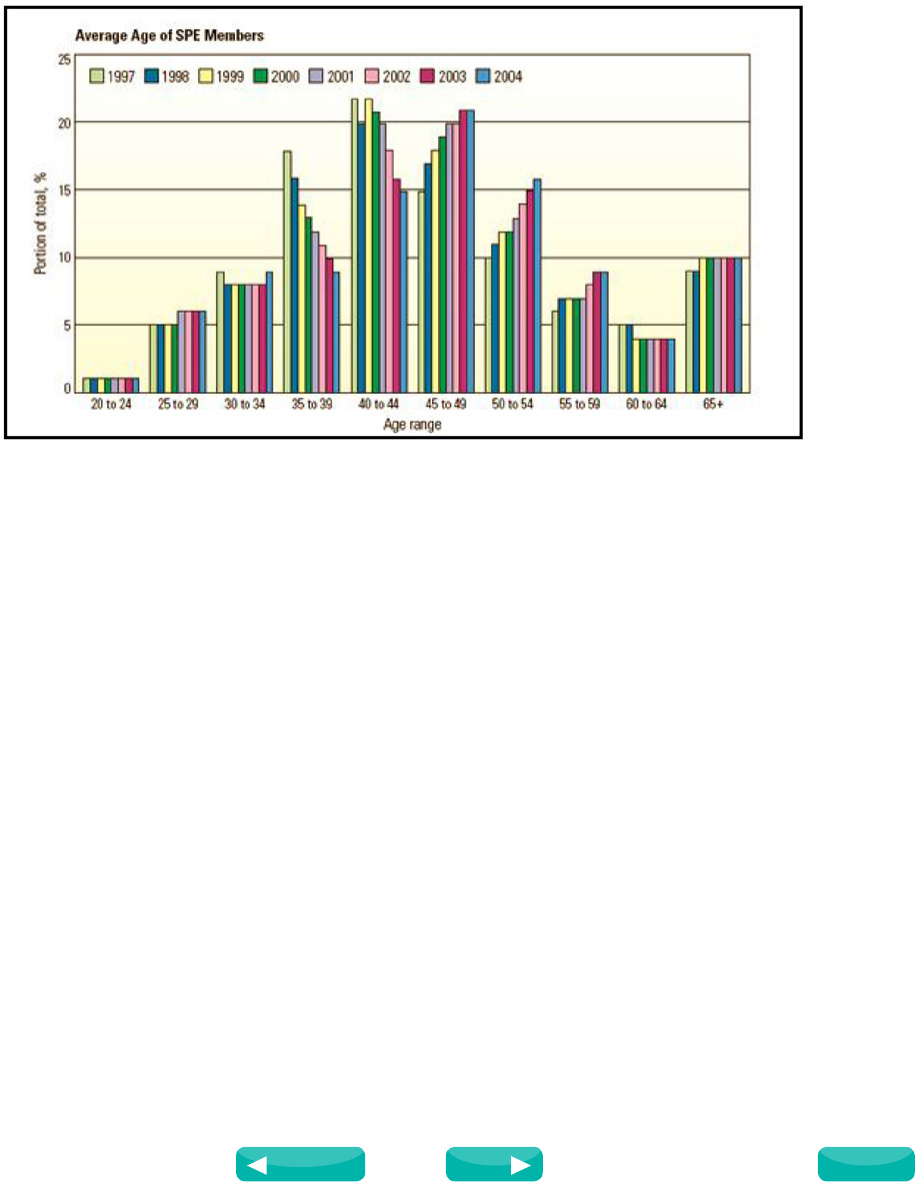
35
www.3ds.com/simulia
Oil and Gas
2. Upstream Oil and Gas Business Needs
The O&G production domain software ecosystem has for many years been highly fragmented. Individual operating assets had been
given the autonomy to select their own preferred software and data solutions based on the specific needs unique to their own
operating conditions. As a result, the O&G companies’ IT infrastructure became quite burdened with the large number of individual
engineering applications and data systems it was asked to support. For years, this inefficiency was tolerated because of the
relatively high operating margins that could be achieved. However, times have indeed changed. The higher costs of producing from
more challenging reservoirs and the diminishing numbers of O&G professionals graduating from university to replace the estimated
40% of the workforce that will retire within the next 15 years have placed a sense of urgency within the industry.
Figure 1: Age distribution of Society of Petroleum Engineers (SPE) members from 1997 to 2004. The SPE is an
international network of Petroleum Engineers with more than 60,000 members.
The problem has been aggravated owing to the loss of in-house training programs in many large oil companies and the loss of
research centers in many major oil companies. This loss was a response to the lower oil prices, which caused overall contraction in
the industry after the oil crises.
Over the past 5 years, O&G companies have recognized the need to make their production operations more efficient by using digital
technologies. These initiatives go by different names, such as “iField™” (Chevron), “SmartField™” (Shell), “Digital Oil Field” (BP),
and the “Digital Asset®” workflow (Halliburton). While results have yet to be quantified precisely, the results are expected to be in
line with the Cambridge Energy Research Associates (CERA) expectations for operators implementing digital oilfield initiatives. With
a production increase of approximately 4%, the reservoir recovery factor improved by as much as 3%, and costs reduced by 9%.
Source: SIMULIA Community Conference, 2010
Next
Previous
Contents
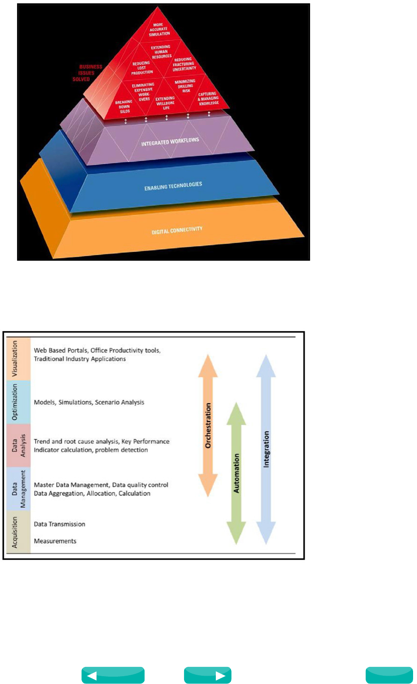
36
www.3ds.com/simulia
Oil and Gas
Figure 2: Halliburton Digital Asset®—A Real-Time Collaborative Environmentto Model, Measure, and Optimize the Asset.
These digital initiatives all have common elements of orchestration, automation, and integration, as shown in this upstream
business activity diagram recently presented by Microsoft.
Figure 3: Upstream O&G Business Activities.
Source: SIMULIA Community Conference, 2010
Next
Previous
Contents

37
www.3ds.com/simulia
Oil and Gas
3. Approaches to Achieving the Digital Asset® Workflow
While most agree on the individual elements required for achieving the Digital Asset® workflow, the people, process, and technology
approach is often very different. Originally, some companies have tried to connect software systems and data together using
custom programming or via Excel spreadsheets and macros. While this may seem to be a valid solution at the outset, many have
experienced serious problems with maintaining these systems in the long term. Another methodology for creating complex
automated workflows is to replace existing systems and software with an “All-in-One” solution that provides the required
functionality within a single environment from a single technology provider. This method sounds like an attractive alternative to
building custom solutions. However, it must be realized that companies have significant investment in the existing systems and
software that is currently used to make critical business decisions. Replacing the existing reliable systems and software is very risky
and often comes with unforeseen compromises in performance and capability.
Halliburton has taken a third approach by allowing O&G companies to retain their existing software technologies and data sources
while at the same time providing a common platform for software integration and automation. This combination of flexibility
and maintainability will increase the efficiency of production operations while significantly lowering the cost of overall systems
maintenance. Furthermore, Halliburton recognized that such technologies already existed in other manufacturing-related and
process industries. Currently, Halliburton is leveraging technologies from the following companies:
• Rockwell Automation (formerly Incuity) – Federated Data Model
• Rockwell Automation (formerly Pavilion) – Data Modeling / Real-time control and optimization.
• SIMULIA (formerly Engineous) – Production Workflow Automation
By smartly leveraging these existing technologies, Halliburton has been able to leapfrog competitors and become the leader in the
industry for delivering Integrated Production Operations (IPO) Systems.
4. SIMULIA iSight and FIPER Technologies
The SIMULIA iSight and FIPER technologies play a very key role for Halliburton. Over the past 3 years, Halliburton has extended the
iSight platform to support upstream modeling software for reservoirs, wells, networks, and facilities. In addition, Halliburton has
pushed the limits of iSight and FIPER applications into areas that traditionally were not common. For example, while Halliburton’s
use of iSight software for design focused on workflows, such as Well Stimulation Design or Reservoir Uncertainty Analysis,
workflows were reasonably aligned with the traditional CAD/CAE workflows, other workflows, including Well Test Analysis and
Pressure Transient Analysis, required elements, such as continuous condition monitoring, interactive human approval processes,
and portal workflow visualization. Such elements are typically found in Enterprise level Business Process Management (BPM)
software. Traditional BPM software, however, is incapable of integrating the required level of technical software.
The iSight and FIPER suite of SIMULIA software gives Halliburton the right level of application integration, workflow system
management, and architectural flexibility to implement a series of 30+ inter-dependant business critical workflows for a single
customer at a single producing asset. Many of these 30+ workflows are running 24/7 and constantly being used by operations
personnel to make real-time operating decisions. An example of one of these real-time workflows is well-test validation.
5. Halliburton Well-Test Validation Workflow
Production from oil & gas reservoirs is a dynamically changing process. Not only are the exact characteristics of the producing
reservoir not completely known, it is often very difficult to acquire accurate flow and compositional data (over time) for a well’s
production. This may be due to the remote location of the well or maybe a lack of measurement instrumentation on a particular
well. Of course, a well’s production over time is a very important piece of information when you are trying to “optimize” fluid
production from the system. The reality is that wells are typically only tested on a monthly or quarterly basis. During this testing
process, the individual well is isolated from other wells within its network so its flow characteristics can be measured independently.
Well testing often involves the “shut in” of certain wells, so that others may be tested. As a result, well testing frequency is often
minimized so as to not disrupt overall production.
The results from a well test are used for revenue allocation across the ownership entities, production history matching of reservoir
models, and calibration of well models. The calibration of the well models is an important part of overall understanding of a well
operating health. When a well test does not match the results of a predictive hydraulic software model (PROSPER for example),
the engineer must decide if the reservoir characteristics need to be adjusted (ie. Lowered bottom hole pressure) or if the well model
itself needs adjustment (ie. Skin factor). This well test validation process is a prime candidate for automation.
Source: SIMULIA Community Conference, 2010
Next
Previous
Contents
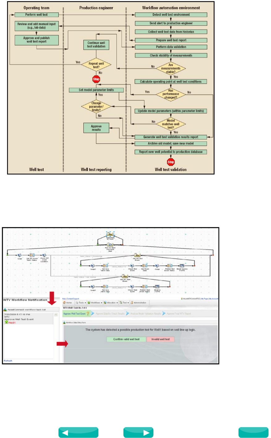
38
www.3ds.com/simulia
Oil and Gas
Figure 4: Well-Test Validation Automated Workflow.
Using the iSight integration technology, the Halliburton team was able to automate many of the simple, yet time-consuming,
manual steps of the well-test process. This process can be described in 4 basic steps:
Step 1. Detect the well test event through continuous monitoring of well-valve positions from a real-time data collection system.
The engineer is alerted of the event and prompted for confirmation of the valid well test.
Figure 5: Detect Well Test Event.
Source: SIMULIA Community Conference, 2010
Next
Previous
Contents
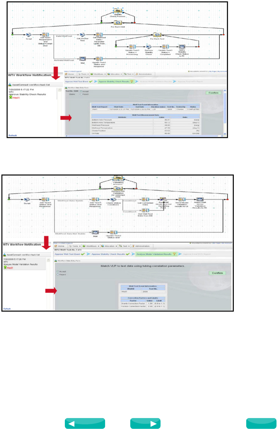
39
www.3ds.com/simulia
Oil and Gas
Step 2. Perform a stability check to ensure proper test-data quality. The engineer can accept or reject the test data.
Figure 6: Perform Stability Check.
Step 3. Perform data validation against the well model (i.e., PROSPER used in the case). The engineer can accept or reject the
validation results.
Figure 7: Model Validation.
Source: SIMULIA Community Conference, 2010
Next
Previous
Contents
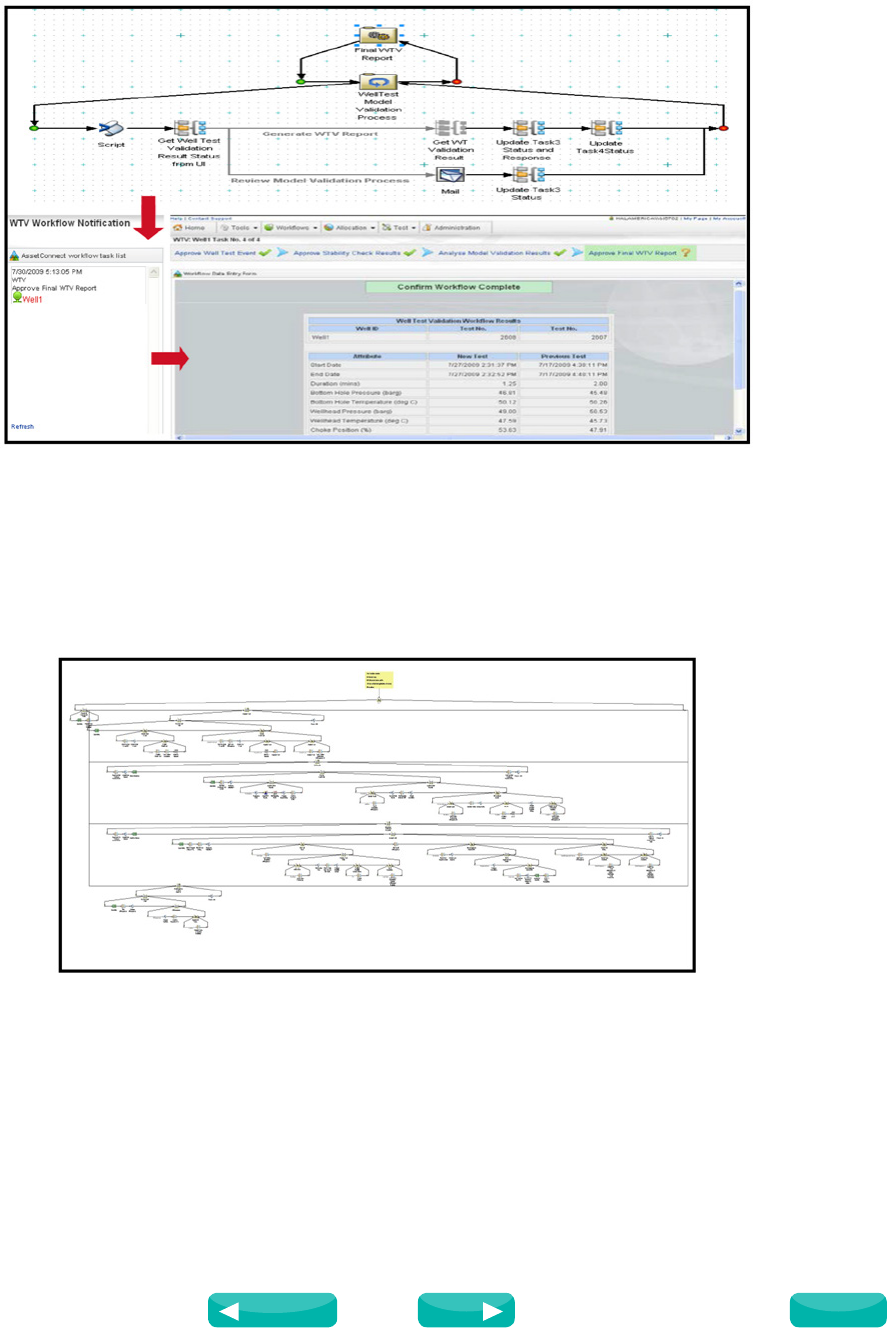
40
www.3ds.com/simulia
Oil and Gas
Step 4. Generate the well-test validation report from the test data stored in the production database.
Figure 8: Generate Well-Test Validation Report.
By using the iSight technology, Halliburton was able to cut the time required to validate a well test from one day to a mere 15
minutes.
While the above example of a well-test validation represents a somewhat simplistic and streamlined view of the process for
demonstration purposes, the actual implementation of this workflow within a world-class, state-of-the-art production operating
environment may look something like Figure 9.
Figure 9: Realistic iSight workflow model representing well-test validation.
Source: SIMULIA Community Conference, 2010
Next
Previous
Contents

41
www.3ds.com/simulia
Oil and Gas
7. Benefits
Halliburton recently implemented the iSight and FIPER technologies (including AssetConnect along with data management and
portal visualization software from the Landmark DecisionSpace for Production suite) into a deepwater greenfield FPSO (Floating
Production, Storage, and Off-loading). The documented benefits realized to date include:
• Optimization of well rates resulting in 50,000 BOPD gain
• Availability of the Landmark DecisionSpace for Production system by first oil enabled availability of key field information in
“relevant time” to asset personnel at both offshore and onshore locations and remote access to field data for experts outside the
production asset to support flawless startup operations. Well availability and facilities uptime were significantly greater (about
95% compared to 50-65% projection) for the first 6 months of production.
• Avoidance of lost production opportunity as a result of timely access and analysis of data directly results in significant savings. A
conservative estimate of actual savings resulting from LPO avoidance (despite variations in oil price) is predicted at over $10MM
for the first year alone. The value delivery is still on going and relies on system sustenance for continuous future benefits.
• Automation of interdependent and repetitive work processes enabled a 98% reduction in engineers’ non-productive time
associated with data gathering, sorting, analysis, and reporting.
• The Landmark DecisionSpace for Production system incorporates best practices and asset team know-how in workflows through
automation. This system helps to capture knowledge and reduce attrition of expertise when asset team members are relocated.
Further, workflows provide a structured method to induct new employees into asset business processes.
• What Landmark delivered to the customer in this engagement was a complete technical workflow solution consisting of data
access from multiple sources, data visualization and monitoring, and workflow execution and orchestration. The system currently
supports over 30 different workflows many of which run on a constant 24/7 basis. The SIMULIA FIPER technology now called
Simulation Engine Environment (SEE) was critical to managing the large number of workflows being executed and maintained.
8. Conclusion
SIMULIA has helped Halliburton maintain a significant technology lead over its competitors in delivering digital oil field solutions.
Halliburton is continuously looking for other technologies from outside our industry to leverage into our valuable Integrated
Production Operations systems.
9. References
1. Sankaran, S., Olise, M., Meinert, D., Awasthi, A., ”Realizing Value from Implementing i-Field(tm) in a Deepwater Greenfield in
Offshore Nigeria Development”. SPE Paper No. 127691. Presented at the SPE Intelligent Energy Conference and Exhibition, The
Netherlands, March 2010.
2. Microsoft Global Energy Forum, January 21, 2010, Houston, Texas
3. O.S. Adeyemi, S.G. Shryock, S. Sankaran, O. Hostad, J. Gontijo, “Implementing “I-Field” Initiatives in a Deepwater Green Field,
Offshore Nigeria”. SPE Paper No. 115367. Presented at the Annual Technical Conference and Exhibition, Denver, 2008.
4. Szatny, M. “Integrating business and technical workflows helps achieve asset-level production optimization” World Oil Magazine,
Nov. 2008.
5. Peries, C. “SOA Removes Traditional E&P Barriers to Production Optimization” Zeus Technology Magazine, October 2008.
6. Szatny, M. “Enabling Automated Workflows for Production” SPE 109859 Presented at 2007 ATCE Conference in Anaheim,
California, Nov. 2007.
Source: SIMULIA Community Conference, 2010
Next
Previous
Contents

42
www.3ds.com/simulia
Oil and Gas
Abaqus/Standard Simulation
of Ground Subsidence
due to Oil and Gas Extraction
Deepak Datye (Dassault Systèmes)
Summary
Extraction of oil and gas from an underground reservoir
alters the pore pressure distribution in the reservoir strata.
Modifications in pore pressure can lead to plastic deformation
in the strata, which can in turn modify the pore fluid flow and
lead to ground subsidence.
Since subsidence can affect the operability of equipment on
the ground as well as the safety of buildings and structures, it
needs to be accurately predicted and kept within limits. In this
Technology Brief, we present a method for predicting the rock
deformation and ground subsidence resulting from oil and gas
extraction.
Background
The oil and gas fluids in an underground reservoir are under
pressure, and this pressure is released or altered when the
fluids are extracted. The fluid pressure can be affected by
the permeability and compaction properties of the rock, the
locations of the bore holes, and the specific extraction and
recovery procedures employed.
As the fluids are extracted, the reservoir rock deforms and
undergoes a change in its porosity, which then leads to
modifications in the permeability. The phenomena of fluid
flow and rock deformation are thus coupled; the fluid flow
leads to deformations, which in turn can affect the fluid flow.
Simulation of a coupled reservoir geomechanics system would
therefore require one to take into account the movement of the
different fluids as well as the inelastic deformations in the rock.
The simulation of the flow of different fluids within the
reservoir is itself a complex problem, and sophisticated tools
that are specifically designed to address flow complexities
such as phase changes and miscibility are available. However,
these tools may not directly include deformations in the rock
and their effect on the fluid flow. Abaqus, on the other hand,
is well suited for modeling inelastic deformations in the rock,
but is not able to simulate the multiphase complexities in the
fluid flow regime.
We can, however, combine the strengths of different tools.
For example, using a reservoir flow simulation code, the flow
problem can be solved to compute the pore pressure depletion
history; Abaqus can then be used to compute the inelastic
deformation in the reservoir rock. A methodology based on
this approach is described in [1], wherein the flow simulation is
performed using ECLIPSE (available from Schlumberger, Ltd.),
and the geomechanics simulation is performed using Abaqus/
Standard.
The approach taken in [1] involves considerable manual effort
to create and modify the finite element mesh and transfer the
pore pressures from ECLIPSE to Abaqus. However, as explained
in [2], it is now possible to automate several of these tasks using
more recent capabilities available in Abaqus. In this Technology
Brief we describe a representative reservoir geomechanics
application that uses these new capabilities.
Key Abaqus Features and Benefits
• Fully coupled displacement-pore fluid flow solution method
in Abaqus/Standard
• Geomechanics material models
• Submodeling technique to drive detailed local models from
global model results
• Python scripting for automation of modeling and job
submission tasks
Finite Element Model
We assume that a flow simulation has been performed using
ECLIPSE and the pore pressure depletion history is available.
For this Technology Brief we use the data for the PUNQ
reservoir [1]. Using a translator, an Abaqus output database is
created from the ECLIPSE flow simulation results. This output
database contains the finite element mesh data, the initial
values of porosity and void ratio, as well as the pore pressure
history.
Abaqus can represent only a single fluid within each finite
element. Therefore, even though multiple fluids exist in each
flow simulation grid cell, the appropriate fluid to be used for
Figure 1: A representative oil and gas reservoir model. The reservoir
region is shown in red and the surrounding geological layers are shown
with independent colors.
Source: Technology Brief, 2013
Next
Previous
Contents
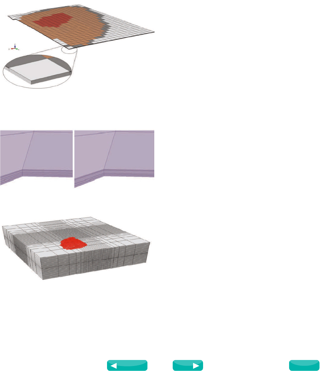
43
www.3ds.com/simulia
Oil and Gas
each finite element must be selected. Using the fluid saturation
values and the grid cell volume data, the translator automatically
locates and designates regions that are principally gas-bearing,
oil-bearing, or water-bearing for each reservoir layer. The
specific weight values of the fluid are also derived and written
to the output database. The output database is then imported
into Abaqus/CAE. Figure 2 shows the finite element mesh
output by the translator, highlighting the regions determined
to contain gas, oil, and water.
A script is used in Abaqus/CAE to manage the sequence of
operations used to modify the mesh and to specify density,
specific weight, material properties, initial conditions, and
boundary conditions. The mesh is first edited, mainly to merge
extremely thin layers in the reservoir. For example, layer 2,
which is the second layer from the top of the reservoir, is found
to be very thin in some regions and is hence merged with layer
3. Figure3 shows a zoomed view of the unedited mesh on the
left and the edited mesh on the right.
Layers of elements are then added below, on the sides, and
on top of the reservoir mesh to represent the under, side, and
over burden regions, respectively. The grid for these regions is
not present in the original flow simulation model and hence
no corresponding mesh is present in the output database
created by the translator. Figure 4 shows the mesh after adding
elements to represent the burden regions. The burden regions
are added such that the top surface of the model is located
at ground level and the bottom surface at a depth of 5.0 km.
The final dimensions of the model then become 15.0 km x
13.5 km in the horizontal plane. Material density is specified
using distributions that are created by the script based on an
analytical function. Gravity loading is then applied.
Initial and Boundary Conditions
Initial stress, pore pressure, and void ratio conditions are
specified. The initial void ratios and pore pressures are read
directly from the output database created by the translator.
Initial stresses are specified as a piece-wise linear distribution
through the model depth.
Displacements normal to the side and bottom boundary
surfaces are specified as zero. The submodeling technique
is used to specify pore pressure boundary conditions in the
reservoir region. Pore pressure values within the reservoir are
driven by the values computed from the flow simulation; these
are available in the output database created by the translator.
As pore pressures are specified at all nodes that have pore
pressure degrees of freedom, the permeability values used for
the analysis are inconsequential.
Material Properties and Analysis
The geomechanics simulation involves two distinct analyses.
An elastic geostatic analysis is first performed to obtain
the vertical stress distribution. For this analysis the porous
reservoir rock is modeled as porous elastic. Non-porous
regions, including the under, side, and over burden regions are
modeled as linear elastic. The analysis is allowed to iterate until
the displacements obtained for the applied gravity load are
nearly zero. This analysis thus provides the stress distribution
that equilibrates the applied loading and boundary conditions.
Figure 2: Finite element mesh of the PUNQ reservoir obtained from the
flow simulation grid. Gas-filled regions are colored red, oil-filled regions
brown, and water-filled regions dark grey. The reservoir consists of five
layers, as shown in the zoomed view.
Figure 3: Zoomed views of the finite element mesh before editing (left)
and after layers 2 and 3 from the top are merged (right).
Figure 4: Finite element mesh after the addition of elements
representing the under, side, and over burden regions. The fluid-
containing region of the reservoir is colored red.
Source: Technology Brief, 2013
Next
Previous
Contents
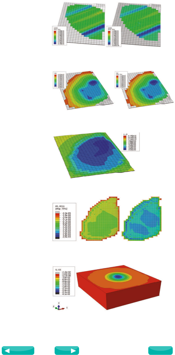
44
www.3ds.com/simulia
Oil and Gas
For the subsequent analysis the reservoir rock is modeled as
elastoplastic, using the clay plasticity material model with
exponential hardening. The vertical stress values obtained from
the elastic analysis are used to compute the compressibility
values of the reservoir rock; these values are then used to
compute the logarithmic plastic bulk modulus, and also update
the logarithmic elastic bulk modulus for the porous region. The
compressibility values are also used to update the linear elastic
properties of the nonporous regions including those of the
under, side, and over burden regions. A steady-state coupled
pore fluid flow displacement analysis using these elastoplastic
material properties is then performed for 30 time increments
representing 30 time-history pore pressure depletion data sets
obtained from the flow simulation. Displacements and plastic
strain values for the reservoir and the surrounding burden
regions are obtained from this analysis.
Results and Discussion
The mesh used for the geomechanics analysis is different from
the mesh derived from the flow simulation grid. In particular,
layers 2 and 3 in the flow simulation grid have been merged
in the mesh used for the geomechanics analysis. Variables,
including pore pressures and initial void ratios, hence, need to
be accurately transferred from one mesh to the other. Mapping
functionalities available in Abaqus can be used to transfer these
data values. Figure 5 shows a comparison of the initial void
ratio distribution in the two meshes. The void ratio values are
consistently mapped from one mesh to the other.
Figure 6 shows contours of pore pressure at the end of the flow
simulation and at the end of the elastoplastic geomechanics
analysis. The pore pressure values in the geomechanics
simulation are consistent with the submodeling-driven
boundary conditions used for the analysis.
Figure 7 shows contours of displacement in the vertical
direction in the reservoir region at the end of the analysis.
The top surface of the reservoir settles downwards and the
maximum value is about 4 cm.
Figure 8 shows the contours of plastic strain in the vertical
direction at two time instances, at 50% of the total depletion
time, and at the end of depletion. These are plotted on plan
views of the fluid-containing region of the reservoir. The plastic
strain magnitude increases with time, indicating that the fluid-
containing region of the reservoir gets compacted as fluids are
extracted.
Figure 9 shows the contours of vertical displacement of the
ground. A maximum subsidence of about 2.5 cm is obtained
just above the reservoir. The subsidence values decrease with
distance away from this location.
Figure 10 shows contours of vertical displacement of the ground
displayed on the model in plan view. The fluid-containing
region of the reservoir is colored red. Displacement contour
Figure 5: Initial values of void ratio from flow simulation (left) and after
mapping onto the finite element mesh (right)
Figure 6: Pore pressure (Pa) at the end of the flow simulation (left) and
at the end of the elastoplastic geomechanics analysis (right)
Figure 7: Vertical displacement (m) in the reservoir region
Figure 8: Plastic strain in the vertical direction at 50% depletion (left),
and at the end of depletion (right)
Figure 9: Vertical displacement of the ground (m)
Source: Technology Brief, 2013
Next
Previous
Contents
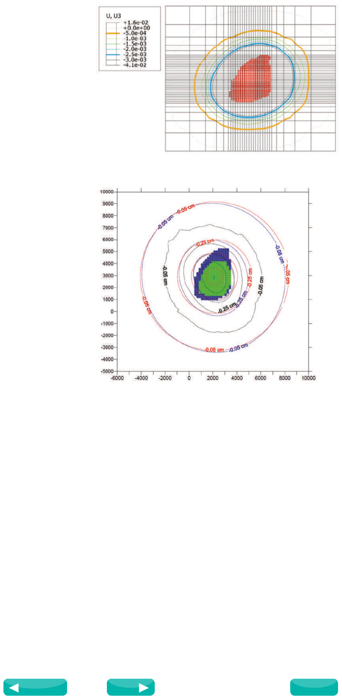
45
www.3ds.com/simulia
Oil and Gas
lines of -0.5 mm and -2.5 mm have been highlighted in this
figure. The ground subsidence decreases rapidly with distance
away from its maximum location just above the reservoir. The
subsidence is less than a millimeter at a horizontal distance
of approximately the horizontal span of the fluid-containing
region of the reservoir.
Figure 11 shows contours of vertical displacement of the
ground surface from the analysis presented in [1]. The results
show a strong correlation to the displacements in Figure 10.
The methodology presented in this Technology Brief can be
used to compute reservoir compaction and surface subsidence
of the ground. Additionally, the geomechanics model can
be used as a global model to drive submodels for smaller
scale applications such as bore-hole stability. The method
presented in this Technology Brief can also be used as one
of the components of an iteratively coupled technique for
reservoir geomechanics simulation. In such a technique the
modifications in void ratios arising from reservoir compaction
are transferred to the flow simulation code, which would
then be able to modify the flow permeability values for an
incremental flow simulation.
Acknowledgements
DS SIMULIA is thankful to Eni, SpA for providing the flow
simulation data and results files for the PUNQ model.
References
1. “Numerical Simulation of Compaction and Subsidence using
Abaqus,” G. Capasso and S. Mantica, Abaqus Users’
Conference, 2006, Boston, USA.
2. “Field Scale Geomechanical Modelling using a New
Automated Workflow,” S. Monaco, G. Capasso, S. Mantica,
D. Datye, and R. Vitali, International Petroleum Technology
Conference, 7-9 February 2012, Bangkok, Thailand.
Figure 10: Vertical displacement of the ground (m)
Figure 11: Vertical displacement of the ground from the analysis
presented in [1]
Source: Technology Brief, 2013
Next
Previous
Contents
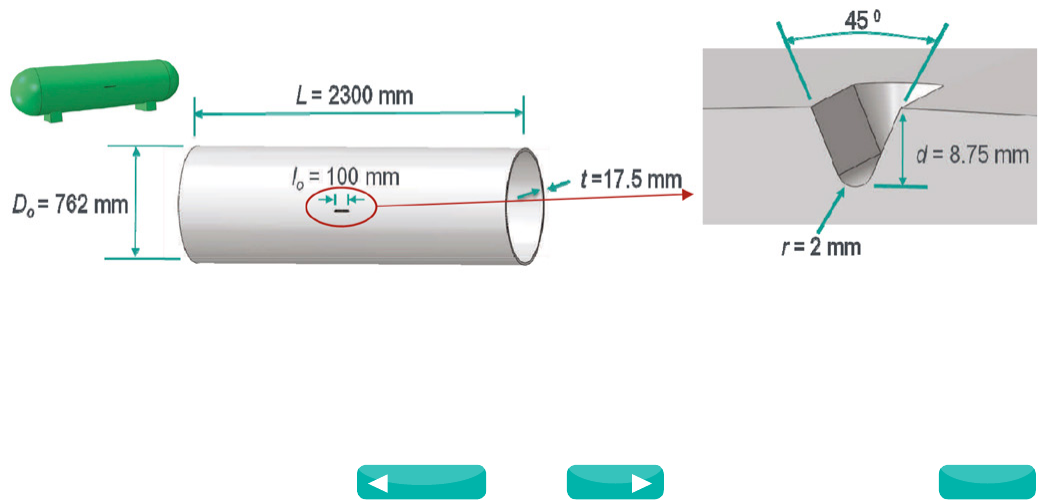
46
www.3ds.com/simulia
Oil and Gas
Pipeline Rupture in
Abaqus/Standard with
Ductile Failure Initiation
Lance Hill (Dassault Systèmes)
Summary
Defects may be introduced in metal pipelines during
construction, repair, or by accident. A common example is
a gouge from a backhoe bucket or other heavy equipment.
At the site of a local defect operating stresses may become
sufficiently concentrated to induce plastic deformation and
material damage, possibly resulting in eventual failure of the
pipeline.
Historically, methods for assessing the structural integrity of
a damaged pipe have been based on experimental tests. The
Abaqus finite element suite includes the ability to simulate
the initiation and evolution of damage in metals, providing
a low-cost alternative to laboratory structural testing. In this
Technology Brief, Abaqus/Standard will be used to predict
the burst pressure of a steel pipeline with a notch-type defect.
A ductile damage initiation criterion is used, and favorable
comparison with available experimental data will be shown.
Key Abaqus Features and Benefits
• Damage initiation and failure modeling for ductile metals
• Ductile and shear initiation criteria allow for the modeling of
two primary fracture mechanisms: coalescence of voids and
shear banding
• Can be used for bulk or sheet metal analyses
• Available for all mechanical elements and allows for element
removal
Background
Pipelines are a critical component of industrial infrastructure
and are used world-wide to transport liquids and gases.
During the course of its lifetime, a metal pipeline may sustain
mechanical damage in such forms as dents, gouges, or weld
defects. When damage is detected, a decision to monitor,
repair, or replace is necessary.
A body of assessment guidelines for determining the fitness-
for-purpose of a damaged pipeline has been built over the past
several decades. As discussed in [1], many of these methods
rely on experimental results and semi-empirical procedures; as
such, their validity may be limited when considering loadings,
materials, or specific damage configurations that are outside
the scope of their assumptions.
With the ability to include the effects of damage initiation and
evolution in the analysis of a ductile metal pipeline, the Abaqus
finite element suite can complement existing methodologies
by adding a more general predictive capability. Specifically,
two types of damage initiation criterion are offered: ductile,
based on the nucleation, growth, and coalescence of voids, and
shear, based on shear band localization. We will focus on the
use of the ductile criterion. The present analysis will consider
an internally pressurized pipe of API X65 steel with a gouge
defect.
Finite Element Analysis Approach
The geometry of the model under consideration is shown in
Figure 1. A simulated gouge, 100mm long, was introduced
into the pipeline. A quarter-symmetric mesh of second order
hex elements was generated, and internal pressure loading
was applied. End forces were applied to simulate experimental
closed end conditions, and the loads were increased linearly
with time. In general, the specification of damage initiation
is included in the material definition and must be used in
conjunction with a plasticity model. In this analysis we use the
Mises plasticity formulation. The mesh is shown in Figure 2.
Figure 1: Geometry of damaged pipe model, with detail of simulated gouge
Source: Technology Brief, 2012
Next
Previous
Contents
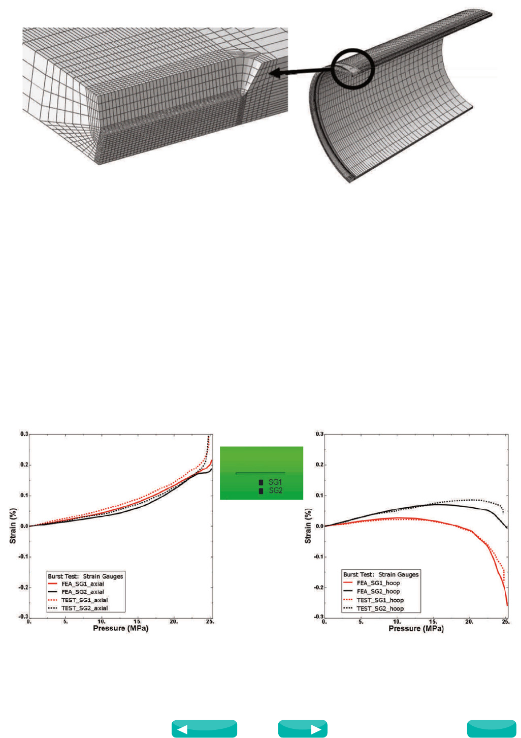
47
www.3ds.com/simulia
Oil and Gas
The ductile damage initiation criterion is a phenomenological
model. It is included in the analysis by specifying the equivalent
plastic strain at damage initiation as a function of stress
triaxiality and equivalent plastic strain rate. Stress triaxiality is
defined as h = -p/q (where p is the pressure stress and q is the
Mises equivalent stress), and is known to play a role in damage
growth. The procedure for calibrating the model used here is
outlined in Appendix A.
Results
We compare the Abaqus/Standard results to the full scale
experimental burst test data collected by Oh et al [2]. Axial
and hoop strain measurements from two gauges are plotted
against the analytical result in Figure 3. The gauges are located
adjacent to the gouge, at circumferential distances of 24.9 and
54.9 mm. Favorable comparison with the experimental data is
achieved.
Figure 2: Quarter symmetric mesh of the pipe, with close-up of detailed mesh at the gouge
A contour plot of the damage initiation output variable
DUCTCRT is shown in Figure 4. Damage has initiated when
this variable is greater than 1.0. From the contour, we see that
the critical element in the structure is in the root of the notch
at the intersection of the symmetry planes. By X-Y plotting
the initiation criterion in the critical element, a more precise
determination of the failure pressure can be determined. In
Figure 5, DUCTCRT at the centroid of the critical element is
plotted against the applied internal pressure, and the threshold
of 1.0 is crossed at a pressure of 24.97 MPa. The experimentally
determined burst pressure 24.68 MPa.
The Abaqus prediction is compared to several other commonly
used failure criteria in Table 1. The relatively good performance
of the peak criteria is attributed to the same relative triaxiality
of the smooth round tensile bar (~0.65) used to determine
material properties as compared to that of the actual application
(~0.6).
Figure 3: Experimental and analytical strain results near the notch and location of strain gauges
Source: Technology Brief, 2012
Next
Previous
Contents
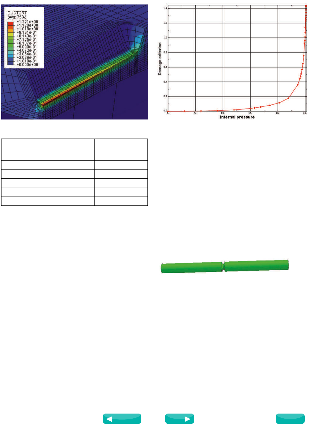
48
www.3ds.com/simulia
Oil and Gas
Figure 4: Damage initiation criterion in the pipe gouge
Conclusions
In this Technology Brief we have demonstrated the utility
of the Abaqus/Standard ductile failure initiation criterion for
predicting the burst pressure of pipes with notch-type defects.
Good correlation with available full scale experimental data
has been shown. The Abaqus damage initiation and evolution
capability for metals provides a general numerical tool that can
supplement existing failure prediction methods that are based
on empirical data.
References
1. Cosham, A. and Hopkins, P., “An overview of the pipeline
defect assessment manual (PDAM),” 4th International
Pipeline Technology Conference, 2004.
2. Oh, C.-K., Kim, Y.-J., Baek, J.-H., Kim, Y.-P., and Kim, W.-S.,
“Ductile failure analysis of API X65 pipes with notch-type
defects using a local fracture criterion,” International Journal
of Pressure Vessels and Piping, Vol. 84, pp. 512-525.
Abaqus References
For additional information on the Abaqus capabilities referred
to in this document please see the following Abaqus 6.13
documentation references:
• Analysis User’s Guide
—“Damage and failure for ductile metals,” Section 24.2.1
Figure 5: Damage criterion v. internal pressure load in critical element
Criterion Burst Pressure
Predicted/
Experimental
Abaqus Ductile Failure 1.01
Net Section Collapse 1.04
Peak Max Principal Stress 1.01
Peak Equivalent Plastic Strain 1.01
Axial Crack (ASME B&PV Code Sec. XI) 0.86
Appendix A - Determination of the Ductile Failure
Initiation Parameters
To use the ductile failure initiation criterion in Abaqus/
Standard, one must specify the equivalent plastic strain at
damage initiation as a function of stress triaxiality and strain
rate. As outlined in [2] this requires an experimental program,
a finite element analysis of each test, and the construction of
a failure loci.
Experimental tests were performed on round, notched bars.
The notched specimens were used to capture the effect of
stress triaxiality on yield and tensile strength. A schematic
diagram of the bar geometry is shown in Figure A1. The bars
had an outer diameter of 17.5 mm and length of 130 mm.
Smooth bars and those with three different notch radii were
tested: 1.5, 3 and 6 mm. The bars were loaded in tension until
complete fracture was achieved.
Each test had a corresponding axisymmetric finite element
analysis. Second order, reduced integration elements (CAX8R)
were used in a half-symmetric mesh. In the critical location,
an element size of 0.15 mm x 0.15 mm was used. The Mises
plasticity model was employed, and nonlinear geometric effects
were included. A comparison of the computed stress-strain
response and the experimental measurements is shown in
Figure A2. The Abaqus/Standard analyses were run until crack
initiation occurred in the experiment and good correlation was
obtained. It can be seen that as notch radius decreased, yield
and tensile strengths increased, but strain to failure decreased.
This behavior is consistent with the increasing triaxiality of the
stress state with decreasing notch radius.
Figure A1: Schematic geometry of round, notched tensile test specimen
Source: Technology Brief, 2012
Next
Previous
Contents
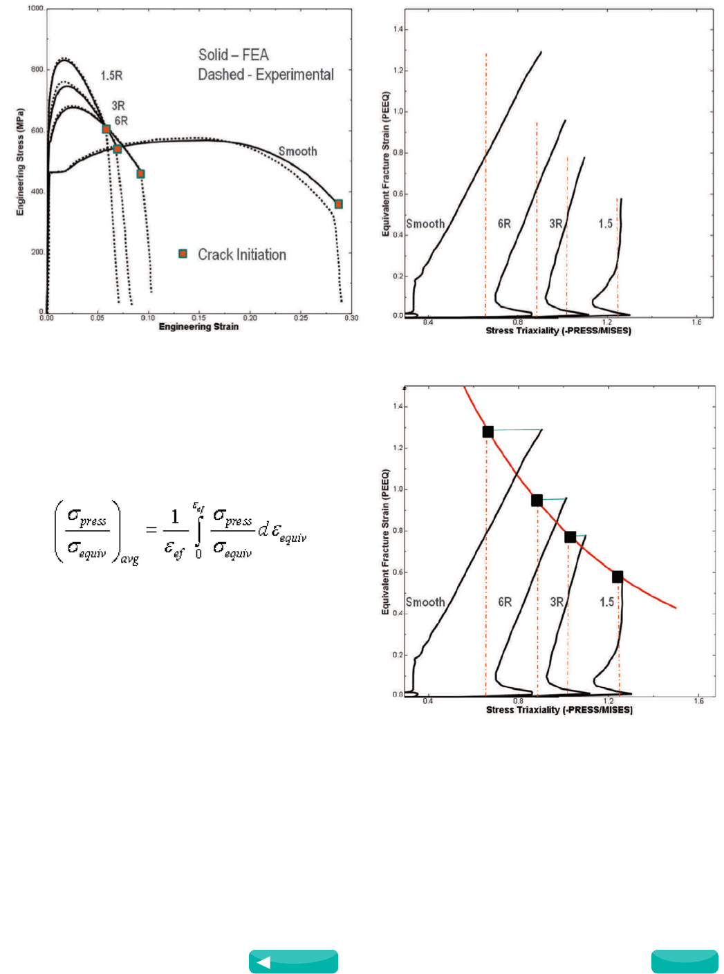
49
www.3ds.com/simulia
Oil and Gas
Figure A2: Experimental and Abaqus results for smooth and notched
bar tensile tests
Figure A4: Equivalent strain—stress triaxiality pairings (black squares)
used in the Abaqus ductile failure initiation criterion
Figure A3: Equivalent strain vs. stress triaxiality, with values of average
stress triaxiality
The critical location for each of the test specimens is at the
center point of the bar. From the analysis results, the equivalent
plastic strain as a function of the stress triaxiality at that
location is plotted in Figure A3.
Included in Figure A3, shown by red dotted lines, is the average
stress triaxiality for each specimen, defined as where
εef is the equivalent strain at failure initiation. Each equivalent
strain trace in Figure A3 ends at its corresponding value of
εef. The points located by the black squares in Figure A4 are
the equivalent stain—stress triaxiality data points used in the
Abaqus ductile failure initiation definition. The red curve is the
loci fitted by Oh et al. [2].
Source: Technology Brief, 2012
Previous
Contents

Our 3DEXPERIENCE Platform powers our brand applications, serving 12 industries, and provides arich
portfolio of industry solution experiences.
Dassault Systèmes, the 3DEXPERIENCE Company, provides business and people with virtual universes to imagine sustainable innovations. Its world-leading
solutions transform the way products are designed, produced, and supported. Dassault Systèmes’ collaborative solutions foster social innovation, expanding
possibilities for the virtual world to improve the real world. The group brings value to over 170,000 customers of all sizes in all industries in more than 140
countries. For more information, visit www.3ds.com.
Europe/Middle East/Africa
Dassault Systèmes
10, rue Marcel Dassault
CS 40501
78946 Vélizy-Villacoublay Cedex
France
Americas
Dassault Systèmes
175 Wyman Street
Waltham, Massachusetts
02451-1223
USA
Asia-Pacific
Dassault Systèmes K.K.
ThinkPark Tower
2-1-1 Osaki, Shinagawa-ku,
Tokyo 141-6020
Japan
©2014 Dassault Systèmes. All rights reserved. 3DEXPERIENCE, the Compass icon and the 3DS logo, CATIA, SOLIDWORKS, ENOVIA, DELMIA, SIMULIA, GEOVIA, EXALEAD, 3D VIA, BIOVIA, NETVIBES, and 3DXCITE are commercial trademarks
or registered trademarks of Dassault Systèmes or its subsidiaries in the U.S. and/or other countries. All other trademarks are owned by their respective owners. Use of any Dassault Systèmes or its subsidiaries trademarks is subject to their express written approval.
